the assessment of queuing performance for access to health

155

COOU Journal of Physical Sciences 4 (1), 2021

Website:www.coou.edu.ng

THE ASSESSMENT OF QUEUING PERFORMANCE FOR ACCESS TO HEALTH

CARE AT THE GENERAL HOSPITAL, OZORO, DELTA STATE, NIGERIA

F. E. Itiveh1, G. E. Nworuh2, and C. O. Aronu3* 1Delta State Polytechnic, Ozoro, Delta State, Nigeria

2Federal University of Technology Owerri (FUTO), Imo State, Nigeria 3Chukwuemeka Odumegwu Ojukwu University, Anambra State.

*Corresponding Author’s Email: [email protected]

Abstract

This study considered the performance of the queuing system for access to health care at the

General Hospital Ozoro, Delta State, Nigeria. The objectives of the study include: to determine

the mean number of arrivals per hour in the health care service provider; to determine the

mean number of patients served per hour; to determine the traffic intensity; and to determine

the average mean time a patient spends in the system. The General Hospital, Ozoro, Delta

State was randomly selected from the frame of all public health care service provider in Isoko

Nation by simple random sampling using lottery- method. A special data collection sheet was

designed to capture all the necessary data element-patient arrival and leave time, start and

end times of all the patient flow steps in the hospital 9.45 am - 1.02 pm, using a time clock,

from the triage and consulting sections in an efficient and organized manner. The resulting

database was then used as the basis for the simulation model input distribution. The simulation

model (M/M/s) developed using MySQL database depicts real-life events, and possesses

generalization features with well- designed experiments; if any quantity in simulation is

random, the simulation results must also be random. Thirty-seven (37) data were simulated for

the history/ triage and consulting sections. Simulation results from application shows mean

client on the system as 37clients, meantime on the system was 26.1540 minutes, the queue wait

time was 15.4648 minutes, and wait time before service was 10.6265 minutes. However, using

the simulated data and computing manually shows the mean arrival rate of 10 patients per

hour. Servers in the history/triage sections were busy 64.46% of the time and idle 7.522% of

the time, mean service rate was 3.878 patients per hour, mean waiting time per patient in the

queue was 10.941 minutes and mean waiting time in the system per patient was 16.941 minutes.

Also, the mean service rate in the consulting room was 15.976 patients per hour, the average

time a patient spends in the queue was 3.7596 minutes and the average time a patient spends

in the system was 9.7596 minutes. Combined manually computed meantime on the system was

26.701 minutes and the queue wait time was 14.701 minutes which is in tandem with the

simulation results.

Keyword: Health care, Queuing, Patients, Simulation.

1. Introduction

A queue is a waiting line, whether of people, signals or things (Udom, 2010). Queuing time is

the amount of time a person, signal or a thing spends before being attended to for services.

Queuing theory is the mathematical study of waiting lines. Queuing theory is generally

considered as a branch of operations research because its results are often used when making

156



business decisions about the resources needed to provide services. The theory seeks to

determine how best to design and operate a system usually under conditions requiring the

allocation of scarce resources.

Queuing models are those models where a facility performs a service. A queuing problem arises

when the current service rate of a facility falls short of the current flow rate of customers. If

the size of the queue happens to be a large one, then at times it discourages customers who may

leave the queue and if that happens, then a sale is lost by the concerned business unit. Hence,

the queuing theory is concerned with the decision-making process of the business unit which

confronts with queue questions and makes decisions relative to the numbers of service facilities

which are operating action (Iserson and Moskop, 2007). Queues are formed because of limited

resources and they are experienced almost every day. Thus queuing theory calculates the

average time a customer spends in a system, the average time a customer spends in a line, and

the average time a customer spends in service. Queuing theory applies to intelligent

transportation systems, call centres, advanced telecommunications.

Queuing Theory tries to answer questions like e.g. the mean waiting time in the queue, the

mean system response time (waiting time in the queue plus service times), mean utilization of

the service facility, distribution of the number of customers in the queue, distribution of the

number of customers in the system and so forth. These questions are mainly investigated in a

stochastic scenario, where e.g. the inter-arrival times of the customers or the service times are

assumed to be random.

A hospital is an integral part of a social and medical organization, the function of which is to

provide for the population complete healthcare services, both curative and preventive, and

whose out-patient services reach out to the family and its home environment. The out-patient

department in the General Hospital, Ozoro, was considered to be the shop window of the

hospital and it is the most important service provided by all hospitals, as it is the point of contact

between the hospital and the community.

Nowadays, Out-Patient Department (OPD) services of the majority of hospitals are having

queue and waiting time problems. Patients’ waiting time refers to the time from the registration

of the patient for an appointment with a doctor until they enter the doctors’ chamber. The main

objective of the out-patient department of a hospital should include the reduction of patients’

time in the system, improvement on customer service, better resource utilization and reduction

of operating costs. Waiting time in out-patient departments is a problem throughout the world.

One consistent feature of patient dissatisfaction has been expressed with the lengths of waiting

time in the out-patient department.

The aim of this study was to apply queuing model to healthcare provider services using

simulation of data. In order to achieve the aim the following specific objectives has been set:

i. to determine the number of arrivals per hour ( ) in the healthcare service

provider.

ii. to determine the mean number of patients served per hour (

)

iii. to compare the mean number of arrivals and mean number of patients served

per hour ( and

)

iv. to determine the average time a patient spends waiting in the queue before being

seen by a doctor or physician

157



v. to determine the average time a patient spends in the system.

2. Review of related Literature

Adeleke et al. (2009) conducted a study on the application of queueing theory to the waiting

time of outpatients in hospitals. The study took the arrival times and service times of 100

patients of the University of Ado-Ekiti Health centre for 14 days. The total waiting times were

945 minutes, total service times were 798 minutes, mean arrival rate was 0.1058, mean service

rate µ was 0.1253, traffic intensity P was 0.8444, an average number of patients per queue was

6 patients, an average number of patients in the system was 5 minutes and average service time

was 8 minutes. The study revealed that the service rate of the health centre was not 100%

efficient which was supported by the fact that there will always be queue because the average

time of service of 8 minutes was greater than 6, the average service time (that is the average

time in the queue system for both queues receiving service is greater than the average time in

queue before service is numbered.

Olorunsola et al. (2004) analyzed the queueing pattern of patients flow in the hospital. Using a

tertiary hospital in South-Western Nigeria, the admissions of Accident victims into the

emergency department to the intensive care unit and medical and surgery ward. The results of

the research show that when the number of available bed spaces is 24, there was no waiting at

the Intensive care unit since an urgent patient who is in need of urgent care are brought in

through it. When the number of available bed spaces is 132, an approximate value of 85.46%

efficient utilization and minimum waiting time in queue was established. Kembe et al. (2012)

in their study of waiting and service time costs of a multiserver queuing model, collected data

from Riverside specialist clinic at Federal Medical Centre, Makurdi. The data was collected

for a period of 4 weeks using direct observations, personal interviews and questionnaires. The

study revealed that optimal server level at the clinic is achieved when the number of

servers/doctors is 12 with (a minimum cost of N13,174.84 per hour as against 10

servers/doctors which has a total cost of N14,50908 per hour. Again, the patients average

waiting time and congestion in the server was also less than the optimal service level. The study

by Mwangi and Ombuni (2015) compared M/M/1, M/M/2 and M/M/3 models on the services

rendered to students at Jkut students finance office. It shows that M/M/2 and M/M/3 reduced

the system utilization and length of the queues. Waiting time and service time for the customers

reduced from 3.5 and9.5 minutes to 3.23 and 2.83 minutes. The probability that there are no

students in the queue as the number of servers is increased was 0.0705 for M/M/1, 0.3913 for

M/M/2 and 0.3654 for M/M/3. This shows that M/M/1 which is the model in use is not effective

at all time especially during the beginning of the semester as students will need the services of

the finance department for registration and examinations. Bahadori et al., (2017) took a study

of optimization of the performance of Magnetic Resonance Imaging (MRI) using a queueing

system and simulation to increase productivity and patients satisfaction. In their results, it was

revealed that the highest average patients waiting time were related to taking turn till admission

(56 days) while the average time spent from admission to leaving the MRI department was 124

minutes. The department productivity on the average was 52.5% indicating high system

capacity which had not been utilized. There was a sharp reduction in waiting time in the fourth

case considered indicating that the waiting time could be significantly reduced by making small

158



changes in human resources, that is changes in the working hours and the number of personnel

and the numbers of machines (addition of MRI machines).

3. Material and Method

3.1 Data Collection

The population of the study consists of five (5) public healthcare facilities in Isoko Nation that

houses the Isoko - South Local Government Area and Isoko -North Local Government Area.

They are the Central Hospital, Oleh, General Hospital, Olomoro situated in Isoko -South L.

G. A., and the General Hospital, Ozoro, General Hospital, Owhelogbo and General Hospital,

Ofagbe situated in Isoko -North L.G.A. respectively. A representative sample was randomly

selected from the frame using simple random sampling for the purpose of this study, by

employing the lottery-method. The General Hospital, Ozoro was selected at the end of the

experiment. A special data collection sheet was designed to capture all the necessary data

elements, that is arrival interval, patients arrival, begin service, service duration and service

completion times between the hours of 9.45 am -1.02 pm. The resulting database was then used

as a basis for the simulation model inputs distribution M/M/s where the inter-arrival/ service

times follows the exponential distribution and s = 4 servers were stationed at both the triage

and consulting sections by nurses and doctors respectively.

3.2 Pure Death Model

In the pure death model, the system starts with N patients at time 0 and no new arrivals are

allowed. Departures occur at the rate 𝜇 patients per unit time. To develop the difference-

differential equations for the probability 𝑝𝑛(𝑡) of 𝑛 customers remaining after 𝑡 time units, we

follow the arguments used with the pure birth model.

Thus,

𝑝𝑁(𝑡 + ℎ) = 𝑝𝑁(𝑡)(1 − 𝜇ℎ) (1)

𝑝𝑛(𝑡 + ℎ) = 𝑝𝑛(𝑡)(1 − 𝜇ℎ) + 𝑝𝑛+1(𝑡)𝜇ℎ, 0 < 𝑛 < 𝑁

Also, as ℎ → 0 , we have

𝑝𝑁1(𝑡) = −𝜇𝑝𝑁(𝑡) (2)

𝑝𝑛1(𝑡) = −𝜇𝑝𝑛(𝑡) + 𝜇𝑝𝑛+1(𝑡), 0 < 𝑛 < 𝑁

𝑃01(𝑡) = 𝜇𝑝1(𝑡)

The solution of these equations yields the following truncated Poisson distribution:

𝑝𝑛(𝑡) = (𝜇𝑡)𝑁−𝑛𝑒−𝜇𝑡

(𝑁−𝑛)ǃ , 𝑛 = 1,2, …𝑁 (3)

𝑝0(𝑡) = 1 − ∑ 𝑝𝑛𝑁𝑛−1 (𝑡) (Taha, 2007)

3.3 The Traffic intensity (𝝆) An important parameter in any queuing system is the traffic intensity also called the load or the

utilization, defined as the ratio of the mean service time

𝐸[𝑋]=1

𝜇 over the mean inter-arrival time 𝐸[𝜏]=

1

𝜆

𝜌=𝐸[𝑋]

𝐸[𝜏]=𝜆

𝜇 (4)

Where 𝜆 and 𝜇 are the mean inter-arrival and service rate respectively. Clearly, if 𝜌 > 1 or

𝐸[𝑋] > 𝐸[𝜏], which mean that the mean service time is longer than the mean inter-arrival time,

then the queue will grow indefinitely long for large 𝑡, because packets are arriving faster on

159



average than they could be served. In this case(𝜌 > 1), the queuing system is unstable or will

never reach a steady-state. The case where 𝜌=1 is critical. In practice, therefore, most situations

where 𝜌 < 1 are of interest.

If 𝜌 < 1, a steady-state can be reached. These considerations are a direct consequence of the

law of conservation of packets in the system.

3.4 Generalized Stationary Queuing Model

Queue can be seen as a form of the birth and death process where arrival can be likened to birth

and departure likened to death. For the purpose of this work we consider stationary or

equilibrium queuing models in which the following assumptions are made:

(i) 𝑃𝑛(𝑡) = 𝑃𝑛

(5)

(ii) 𝑃𝑛1(𝑡) = 0

(6)

That is, as 𝑡 increases, 𝑃𝑛(𝑡) approaches a limit 𝑃𝑛 which is independent of 𝑡 and in this case,

𝑃𝑛1(𝑡) approaches zero. We note here that in the general birth and death process where the birth

and death parameters are 𝜆𝑛 and µ𝑛 respectively, the differential – difference equation is

𝑃𝑛1(𝑡) = −(𝜆𝑛 + µ𝑛)𝑃𝑛(𝑡) + 𝜆𝑛−1 𝑃𝑛−1(𝑡) + µ𝑛+1𝑃𝑛+1(𝑡).

(7)

Let {𝑁(𝑡)𝑡 ≥ 0} be a queue, under the above assumptions the differential-difference equation

of the generalized birth and death process becomes.

0 = −(𝜆𝑛 + µ𝑛)𝑃𝑛 + 𝜆𝑛−1𝑃𝑛−1 + µ𝑛+1𝑃𝑛+1

⇒ (𝜆𝑛 + µ𝑛)𝑃𝑛 = 𝜆𝑛−1𝑃𝑛−1 + µ𝑛+1𝑃𝑛+1

We solve the above equation recursively, 𝑓𝑜𝑟 𝑛 = 0, 𝜆−1and µ0 are not defined, so we have

𝜆0𝑃0 = µ1𝑃1 ⇒ 𝑃1 =𝜆0

µ1𝑃0 (8)

For 𝑛 = 1,we have (𝜆1 + µ1)𝑃1 = 𝜆0𝑃0 + µ2𝑃2

⇒ 𝜆1𝑃1 = 𝜆1𝑃1 = µ2𝑃2 ⇒ 𝑃2 =𝜆1

µ2𝑃1 =

𝜆1𝜆0

µ2µ1𝑃0 (9)

In general 𝑃𝑛 = 𝜆𝑛−1𝜆𝑛−2…𝜆0

µ𝑛µ𝑛−1…µ1𝑃𝑜 (10)

= 𝑃𝑛𝑃0where𝑃0 = 1

𝑃𝑛 = 𝜆𝑛−1𝜆𝑛−2…𝜆0

µ𝑛µ𝑛−1…µ1 = ∏

𝜆𝑖−1

µ𝑖; 𝑛 ≥ 1𝑛

𝑖=1

To obtain 𝑃𝑜, we use the normalizing equation

∑𝑃𝑛𝑃0 = 1

∞

𝑛=0

⇒𝑃0 + 𝜆0

µ1𝑃0 +

𝜆1𝜆0

µ2µ1𝑃0+⋯ = 1 ⇒ 𝑃0 + 𝑃1 + 𝑃2 +⋯ = 1

𝑃0 ⌈1 +𝜆0

µ0+𝜆1𝜆0

µ2µ2+⋯⌉ = 1

𝑃0 [1 +𝜆0

µ1+𝜆1𝜆0

µ2µ2+⋯]

−1

(11)

160



Thus the general distribution of 𝑁(𝑡) = 𝑛 is thus

𝑃𝑛 = 𝜆𝑛−1𝜆𝑛−2…𝜆0

µ𝑛µ𝑛−1…µ1𝑃𝑜 𝑛 = 1,2, …

3.5 M/M/I Queue

This is a single server queue with Poisson arrivals and exponenntial service times. Customers

are served according to first come first served discipline and there is an infinite capacity waiting

room. Let 𝑁(𝑡) be the number of customers in the system (those who are waiting plus any in

service) at time t. This is a stationary birth and death process with parameters.

𝜆𝑛 = 𝜆

µ𝑛 = µ

Then, substituting these parameters in the general distribution (2) and (3) we have the

following:

𝑃𝑛 = (𝜆

µ)𝑛

𝑃𝑜 = 𝑃𝑛𝑃0

𝑃𝑛 = 𝜆 x 𝜆 x…x𝜆

µ x µ x…x µ= (

𝜆

µ)𝑛

(12)

Where 𝑝 =𝜆

µ the parameter is called the traffic intensity and represents the ratio of the mean

service time to the mean inter-arrival time. The mean number of arrivals during the mean

service time.

∑ 𝑃𝑛 = {11−𝑝∞

∞𝑛=0

Thus, the stability condition is p<1 and

𝑃𝑜 = (∑ 𝑃𝑛∞𝑛=0 )−1 = 1 − 𝑝

(13)

𝑃𝑛 = 𝑃𝑛𝑃0 = 𝑃

𝑛(1 − 𝑝) 𝑛 ≥ 0

The expected number of customers in the system and variance are:

𝐸[𝑁(𝑡)] = ∑ 𝑛𝑃𝑛 = 𝑃

1−𝑝∞𝑛=0 (14)

𝑉𝑎𝑟 [𝑁(𝑡)] = 𝑃

(1−𝑃)2 (15)

We note that the stability condition p < 1 is in order; because if p is greater than Unity, then it

means that customers are on the average arriving faster than the rate of service: a queue is

bound to build on continuously and we cannot expect to achieve equilibrium.

3.6 The Distribution of Waiting Time in M/M/I

For a queuing system, interest may be on how long one is likely to wait on the queue for service

or in the system. Here we derive the distribution of the time a customer waits in the system (the

time he waits on the queue plus his own service time) and the distribution of waiting time on

the queue. Notice that waiting is only meaningful if the queue is not empty; if there is no

customer on queue, an arriving customer receives service immediately on arrival. The

probability of an arriving customer getting service immediately on arrival (that is, time on

queue is zero) is equivalent to the probability of meeting the queue empty, suppose a customer

comes and finds n persons before him, he becomes the (n+1)th customers.

Let W = time taken to serve n persons before him,

𝑖𝑓 𝑝 < 1

𝑖𝑓 𝑝 ≥ 1

161



V = his own service time.

Then, P(W≤ 0) = P(W=0)

P(Systems is empty on arrival)

𝑃0 = 1 − 𝑝 (16)

3.7 The Distribution of Waiting Time in the System

The waiting time in the system, is the time taken to service n persons before him plus his own

service time. Let 𝑋𝑖be the service time of the ith customer before him, then W + V is total

waiting time or total delay of the customer in the system.

W+ V = 𝑋1 + 𝑋2 +⋯+ 𝑋𝑛+1, the sum of n +1 independent exponential service times with

parameter µ therefore, has the gamma distribution 𝛤(𝑛 + 1) The conditional probability of 𝑊 + 𝑉 ≤ 𝑡 given that there are n persons before him is

𝑃[𝑊 + 𝑉 ≤ 𝑡| 𝑛 𝑝𝑒𝑟𝑠𝑜𝑛𝑠 𝑏𝑒𝑓𝑜𝑟𝑒 ℎ𝑖𝑚] = ∫µ(µ𝑥)𝑛𝑒−µ𝑥

𝑛!𝑑𝑥

1

0

The conditional probability of W+V≤ 𝑡 𝑖𝑠

𝑃[𝑊 + 𝑉 ≤ 𝑡] = ∑𝑃[𝑤 + 𝑣 ≤ 𝑡 |𝑛]𝑃[𝑋(𝑡) = 𝑛]

𝑛

=∑∫µ(µ𝑥)𝑛𝑒−µ𝑥

𝑛!𝑃𝑛(1 − 𝑝)𝑑𝑥

1

0𝑛

= ∫ µ(∑(µ𝑝𝑥)𝑛

𝑛!𝑛

) (1 − 𝑝)𝑒µ𝑥𝑑𝑥1

0

= ∫ µ𝑒µ𝑝𝑥(1 − 𝑝)𝑒−µ𝑥𝑑𝑥1

0

= ∫ µ(1 − 𝑝)𝑒−µ𝑥(1−𝑝)𝑑𝑥1

0

𝑒−µ𝑥(1−𝑝)|0𝑡

1 − 𝑒−µ𝑥(1−𝑝)𝑡 The probability density function of W + V is therefore 𝑑

𝑑𝑡 𝑃(𝑊 + 𝑉 ≤ 𝑡] = 𝑓(𝑡)

µ (1 − 𝑝)𝑒−µ(1−𝑝)𝑡 the mean waiting time in the system is

𝐸(𝑊 + 𝑉) = 𝐸(𝑇)

= 1

µ(1−𝑃)= 𝑚𝑒𝑎𝑛 𝑡𝑜𝑡𝑎𝑙 𝑑𝑒𝑙𝑎𝑦 (17)

3.8 The Distribution of Waiting Time in the Queue

Now, consider a customer who arrives when there are n units (customers) in the system, the

time he waits on the queue for service is the time taken to serve the n customers before him.

Because of the memoryless property of the expeonential (service) distribution, the distribution

of time required for n service completion is independent of the current arrival and is a

convolution of n exponential random variable, which is the Erlang distribution (a special form

of the gamma distribution).

The conditional distribution of W given n persons before him is

162



𝑃[𝑊 ≤ 𝑡|𝑛 𝑝𝑒𝑟𝑠𝑜𝑛𝑠 𝑖𝑛 𝑡ℎ𝑒 𝑠𝑦𝑠𝑡𝑒𝑚] = ∫µ(µ𝑥)𝑛−1

(𝑛 − 1)!

𝑡

0

𝑒−µ𝑥𝑑𝑥

Therefore, the probability of a customer waiting in the queue, a time less than or equal to t for

service is

𝑃(𝑊 ≤ 𝑡) = ∑𝑃(𝑊 ≤ 𝑡|𝑛)𝑃(𝑁(𝑡) = 𝑛)

∞

𝑛=1

= ∑∫µ(µ𝑥)𝑛−1

(𝑛 − 1)!

𝑡

0

𝑒−µ𝑥∞

𝑛=1

𝑃𝑛(1 − 𝑝)𝑑𝑥

= (1 − 𝑝)∑𝑃𝑛∞

𝑛=1

∫µ(µ𝑥)𝑛−1

(𝑛 − 1)!

𝑡

0

𝑒−µ𝑥𝑑𝑥

= (1 − 𝑝)𝑃∫µ−µ𝑥∑µ(µ𝑥)𝑛−1

(𝑛 − 1)! 𝑑𝑥

∞

𝑛=1

𝑡

0

= 𝑝 − 𝑝𝑒−µ(1−𝑝)𝑡 𝑡 > 0

(18)

The probability density of the waiting time in the queue is therefore 𝑑𝑝(𝑊≤𝑡)

𝑑𝑡= µ𝑝(1 − 𝑝)𝑒−µ(1−𝑝)𝑡 (19)

The expected waiting time in the queue is

𝐸(𝑊) = ∫ 𝑡𝑑𝑃(𝑊 ≤ 𝑡)

∞

0

= ∫ 𝑡µ𝑃(1 − 𝑝)𝑒−µ(1−𝑝)𝑡 = 𝑝

µ(1−𝑝)

∞

0 (20)

The expected waiting time in the queue can also be obtained in the following way;

𝐸(𝑊) = 𝐸(𝑊 + 𝑉) − 𝐸(𝑉) = 1

µ(1 − 𝑝)−𝑝

µ=

𝑝

µ(1 − 𝑝)

The time a fictitious customer would have to wait, were he is to arrive at an arbitrary point in

time is called the virtual waiting time. The stationary distribution of this virtual waiting time is

identical to that of the actual waiting time of an arriving customer, for all queues with poisson

arrival.

3.9 M/M/I/K Queue

This is the same as M/M/I queue, expect that the system has a capacity to add at most k

customers. In this case a customer, who arrives and finds that the system has k customers in it

has to leave because there is no waiting vacancy for him.

Let N(t) be the number of customers in the system at time t, then the {𝑁(𝑡), 𝑡 ≥ 0} is a

stationary birth and death process with parameters.

𝜆𝑛 = {𝜆 𝑖𝑓 0 ≤ 𝑛 𝑘0 𝑖𝑓 𝑛 ≥ 𝑘

(since the system can only carry k customers)

µ𝑛 = µ 𝑓𝑜𝑟 𝑛 ≥ 1

163



Let 𝑝 = 𝜆

µ

𝑃𝑛 = 𝑃𝑛 𝑖𝑓 0 ≤ 𝑛 ≤ 𝑘

Then

∑𝑃𝑛∞

𝑛=0

= ∑𝑃𝑛∞

𝑛=0

= ∑𝑃𝑛∞

𝑛=0

− ∑ 𝑃𝑛∞

𝑛=𝑘+1

′

= 1

1 − 𝑝 −𝑃𝑘+1

1 − 𝑝= 1 − 𝑃𝑘+1

1 − 𝑃

𝑃𝑜 + 𝑃1 + 𝑃2 +⋯+ 𝑃𝑘 = 1 (𝑠𝑖𝑛𝑐𝑒 𝑡ℎ𝑒 𝑐𝑎𝑝𝑎𝑐𝑖𝑡𝑦 𝑜𝑓 𝑡ℎ𝑒 𝑠𝑦𝑠𝑡𝑒𝑚 𝑖𝑠 𝑘)

𝑃0(1 + 𝑝 + 𝑝2 +⋯+ 𝑝𝑘) = 1 ⇒ 𝑝0 (∑𝑝𝑛

𝑘

𝑛=0

) = 1

𝑃0 = 1−𝑝

1−𝑝𝑘+1 (21)

Using (2.22) we have

𝑃𝑛 = 𝑝𝑛 (1 − 𝑝

1 − 𝑝𝑘+1) 𝑛 = 0,1, … , 𝑘 𝑖𝑓 𝑝 ≠ 1

The expected number of customers in the system (𝑖𝑓 𝑝 ≠ 1) is

𝐸(𝑁(𝑡) = ∑𝑛𝑃𝑛

𝑘

𝑛=0

=1 − 𝑝

1 − 𝑝𝑘+1∑𝑛𝑃𝑛𝑘

𝑛=0

= 1 − 𝑝

1 − 𝑝𝑘+1𝑝𝑑

𝑑𝑝∑𝑛𝑃𝑛𝑘

𝑛=0

(𝑆𝑖𝑛𝑐𝑒 𝑝𝑑

𝑑𝑝∑𝑛𝑃𝑛𝑘

𝑛=0

=∑𝑛𝑃𝑛𝑘

𝑛=0

)

1 − 𝑝

1 − 𝑝𝑘+1𝑝𝑑

𝑑𝑝(1 − 𝑝𝑘+1

1 − 𝑝)

Thus 𝐸(𝑁(𝑡) = 𝑝⌊1−(𝑘+1)𝑝𝑘+𝑘𝑝𝑘+1⌋

(1−𝑝𝑘+1)(1−𝑝) (22)

However, if p =1, 𝑃𝑛 = 1

𝑘+1 𝑎𝑛𝑑 𝐸(𝑁(𝑡) =

𝑘

2

Note here that the value of 𝑝 =𝜆

µ need not be less than 1 because arrivals at the system are

controlled by the system capacity k.

3.10 M/M/s Queue

This is a queue with exponential inter-arrival and service times in which there are s number of

servers. Here customers form a single queue and the customer at the head of the queue is served

by the next available server. If an incoming customer finds more than one server idle, he joins

any one of them for service. Let 𝑁(𝑡) be the number of customers in the system. Then {𝑁(𝑡), 𝑡 ≥ 0} is a stationary birth and death process with parameters;

𝜆𝑛 = 𝜆 𝑛 ≥ 0

µ𝑛 {𝑖𝑓 0 ≤ 𝑛 < 𝑠 (𝑎𝑙𝑙 𝑐𝑢𝑠𝑡𝑜𝑚𝑒𝑟𝑠 𝑐𝑎𝑛 𝑏𝑒 𝑎𝑡𝑡𝑒𝑛𝑒𝑑 𝑡𝑜 𝑠𝑖𝑚𝑢𝑙𝑡𝑎𝑛𝑒𝑜𝑢𝑠𝑙𝑦

(𝑖𝑓𝑛 ≥ 𝑠 (𝑠 𝑐𝑎𝑛 𝑏𝑒 𝑠𝑒𝑟𝑣𝑒𝑑 𝑎𝑡 𝑡ℎ𝑒 𝑠𝑎𝑚𝑒 𝑡𝑖𝑚𝑒, 𝑡ℎ𝑒 𝑟𝑒𝑚𝑎𝑖𝑛𝑖𝑛𝑔 𝑛 − 𝑠 𝑤𝑖𝑙𝑙 𝑤𝑎𝑖𝑡𝑠µ

𝑛µ

164



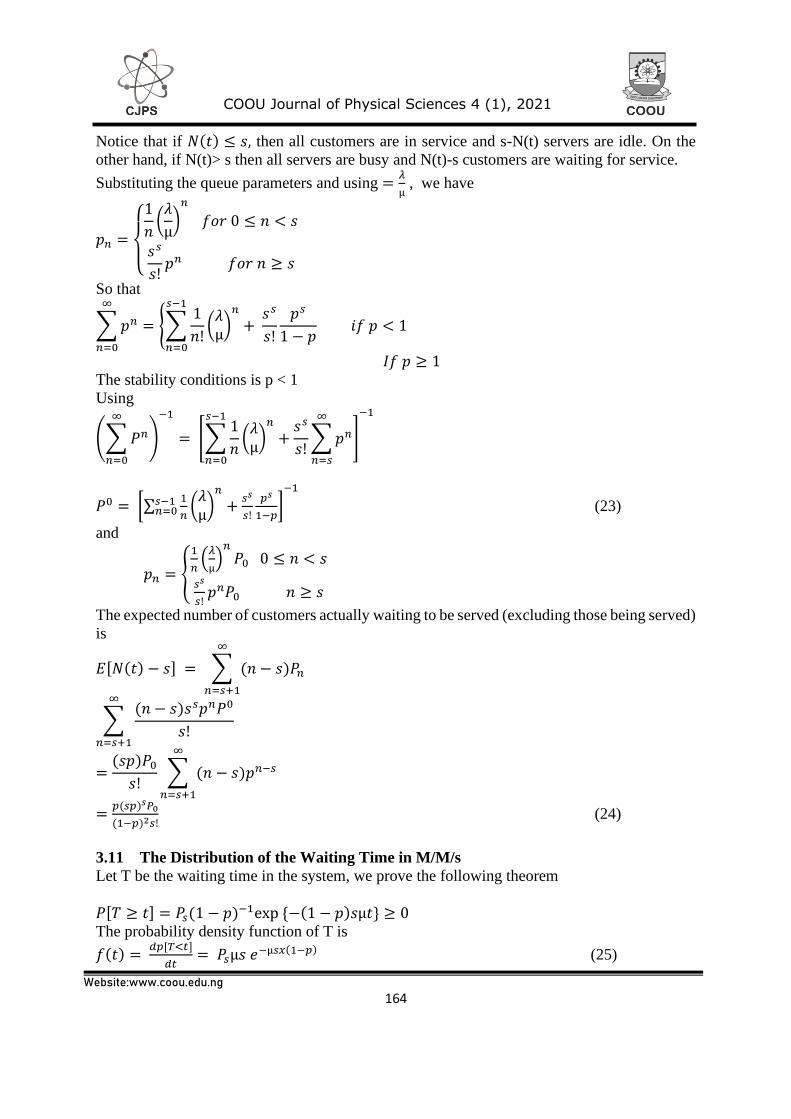
Notice that if 𝑁(𝑡) ≤ 𝑠, then all customers are in service and s-N(t) servers are idle. On the

other hand, if N(t)> s then all servers are busy and N(t)-s customers are waiting for service.

Substituting the queue parameters and using =𝜆

µ , we have

𝑝𝑛 =

{

1

𝑛(𝜆

µ)𝑛

𝑓𝑜𝑟 0 ≤ 𝑛 < 𝑠

𝑠𝑠

𝑠!𝑝𝑛 𝑓𝑜𝑟 𝑛 ≥ 𝑠

So that

∑𝑝𝑛∞

𝑛=0

= {∑1

𝑛!

𝑠−1

𝑛=0

(𝜆µ)𝑛

+ 𝑠𝑠

𝑠!

𝑝𝑠

1 − 𝑝 𝑖𝑓 𝑝 < 1

𝐼𝑓 𝑝 ≥ 1

The stability conditions is p < 1

Using

(∑𝑃𝑛∞

𝑛=0

)

−1

= [∑1

𝑛

𝑠−1

𝑛=0

(𝜆µ)𝑛

+𝑠𝑠

𝑠!∑𝑝𝑛∞

𝑛=𝑠

]

−1

𝑃0 = [∑1

𝑛

𝑠−1𝑛=0 (

𝜆µ)𝑛

+𝑠𝑠

𝑠!

𝑝𝑠

1−𝑝]−1

(23)

and

𝑝𝑛 = {

1

𝑛(𝜆

µ)𝑛

𝑃0 0 ≤ 𝑛 < 𝑠

𝑠𝑠

𝑠!𝑝𝑛𝑃0 𝑛 ≥ 𝑠

The expected number of customers actually waiting to be served (excluding those being served)

is

𝐸[𝑁(𝑡) − 𝑠] = ∑ (𝑛 − 𝑠)𝑃𝑛

∞

𝑛=𝑠+1

∑(𝑛 − 𝑠)𝑠𝑠𝑝𝑛𝑃0

𝑠!

∞

𝑛=𝑠+1

=(𝑠𝑝)𝑃0𝑠!

∑ (𝑛 − 𝑠)𝑝𝑛−𝑠∞

𝑛=𝑠+1

=𝑝(𝑠𝑝)𝑠𝑃0

(1−𝑝)2𝑠! (24)

3.11 The Distribution of the Waiting Time in M/M/s

Let T be the waiting time in the system, we prove the following theorem

𝑃[𝑇 ≥ 𝑡] = 𝑃𝑠(1 − 𝑝)−1exp {−(1 − 𝑝)𝑠µ𝑡} ≥ 0

The probability density function of T is

𝑓(𝑡) = 𝑑𝑝[𝑇<𝑡]

𝑑𝑡= 𝑃𝑠µ𝑠 𝑒

−µ𝑠𝑥(1−𝑝) (25)

165



3.12 The Mean waiting Time in the System

The mean waiting time of a customer can also be obtained by noting that; if a 𝑛 ≤ 𝑠 −1, an incoming customer finds a free server and is immediately served. But if 𝑛 ≥𝑠, an incoming customer must wait until 𝑛 − 𝑠 + 1 other customers have departed taking an

average (n-s+1)/sµ units. The mean waiting time 𝜛 is therefore

𝜛 = ∑𝑛 − 𝑠 + 1

𝑠µ𝑃𝑛

∞

𝑛=𝑠

= (𝑠𝑝)𝑠𝑃0𝑠µ(𝑠!)

∑(𝑛 − 𝑠 + 1)𝑝𝑛−𝑠∞

𝑛=𝑠

= (𝑠𝑝)𝑠𝑃0

(1−𝑝)𝑠µ(𝑠!)

(26)

The limiting probability that all servers are busy is

∑ 𝑃𝑛∞𝑛=𝑠 =

𝑠𝑠

𝑠!

𝑃𝑠

1−𝑝𝑃0 =

𝑃𝑠

1−𝑝 (27)

3.13 M/M/∞ 𝑸𝒖𝒆𝒖𝒆

This is a special type of M/M/s queue in which all the customers at any time are in service.

Notice that in the strict sense of the word, no queue is actually formed, since all customers in

this case are in service. Here the parameters are

𝜆𝑛 = 𝜆 𝑛 ≥ 0

µ𝑛 = 𝑛µ 𝑛 ≥ 0

Substituting the parameters in (3) we have

𝑝𝑛 = 1

𝑛!(𝜆

µ)𝑛

𝑛 ≥ 0

𝑎𝑛𝑑 ℎ𝑒𝑛𝑐𝑒 ∑ 𝑝𝑛 = 𝑒𝜆µ, 𝑠𝑜 𝑡ℎ𝑎𝑡 𝑃0

∞

𝑛=0

= (∑𝑝𝑛∞

𝑛=0

)

−1

= 𝑒−𝜆µ

𝑝𝑛 = 𝑝𝑛𝑃0 =𝑒−𝜆µ(𝜆

µ)𝑛

𝑛! (28)

Let N(t) be the number of customers in the system, then

𝐸{𝑁(𝑡) =𝜆

µ (29)

3.14 M/M/s/k(s ≤ 𝒌) 𝑸𝒖𝒆𝒖𝒆

This queue differs from M/M/s queue in that the system capacity is finite and equal to k, which

means that the maximum queue is k –s. Here, both the inter-arrival time and the service time

are exponentially distributed; there are s servers and the system has capacity to hold at most k

customers. Let N(t) be the number of customers in the system, then this is a stationary queue

with parameters

𝜆𝑛 = 𝜆 𝑓𝑜𝑟 0 ≤ 𝑛 < 𝑘 (30)

µ𝑛 = {𝑛µ 0 ≤ 𝑛 < 𝑠𝑠µ 𝑠 ≤ 𝑛 ≤ 𝑘

(31)

166



Substituting the parameters in the general expression for 𝑝𝑛 and noting that 𝑝 = 𝜆

µ we have

𝑃𝑛 = {

𝑝𝑛

𝑛!𝑃0 0 ≤ 𝑛 < 𝑠

𝑝𝑛

𝑠! 𝑠𝑛−𝑠𝑃0 𝑠 ≤ 𝑛 ≤ 𝑘

𝑊ℎ𝑒𝑟𝑒 𝑃0 =∑𝑝𝑛

𝑛!+ 𝑝𝑠 [

1 − (𝑝𝑠)

𝑘−𝑠+1

𝑠! (1 −𝑝𝑠)

]

−1

𝑖𝑓 𝑝

𝑠≠ 1.

𝑠−1

𝑛=0

𝐼𝑓 𝑝

𝑠= 1 𝑡ℎ𝑒𝑛 𝑃0 = (∑

𝑝𝑛

𝑛!

𝑠−1

𝑛=0

+𝑃𝑠

𝑠!(𝑘 − 𝑠 + 1))

−1

The expected size of the queue if 𝑝

𝑠≠ 1 𝑖𝑠

𝐸(𝑁(𝑡) − 𝑠) = ∑(𝑛 − 𝑠)𝑃𝑛

𝑘

𝑛=𝑠

= ∑𝑖𝑃𝑖+𝑠 = 𝑝𝑠𝑝

𝑠! 𝑠∑(

𝑝

𝑠)𝑖−1

𝑃0

𝑘−𝑠

𝑖=0

𝑘−𝑠

𝑖−0

= 𝑝𝑠+1

𝑠𝑠!

𝑑

𝑑 (𝑝𝑠)∑(

𝑝

𝑠)𝑖

𝑘−𝑠

𝑖−1

𝑃0

= 𝑝𝑠+1

(𝑠 − 1)! (𝑠 − 𝑃)2[1 − (

𝑝

𝑠)𝑘−𝑠+1

− (𝑘 + 𝑠 + 1) (1 −𝑝

𝑠) (𝑝

𝑠)𝑘−𝑠

] 𝑃0

However, if 𝑝

𝑠= 1, 𝑡ℎ𝑒𝑛 𝐸(𝑁(𝑡) − 𝑠) =

𝑝𝑠(𝑘−𝑠)(𝑘−𝑠+1)

2𝑠!𝑃0

Note again here that the value of 𝑝

𝑠 need not be less than 1 because arrivals at the system are

controlled by the system capacity k.

3.15 Operating Characteristics of a Multiple Server Model-Infinite Population

(M/M/S/∞)

The model is based on the following assumptions;

(i)The arrival of customers follows Poisson probability distribution

(ii)The service time has an exponential distribution

(iii)There are S-servers, each of which provides identical services

(iv) A single waiting line is formed

(v)The input population is infinite

(vi)The service is on first- come, first served basis

(vii)The arrival rate is smaller than the combined service rate of all S-service facilities

3.16 The Operating Characteristics of Multiple Server Model with Infinite

Population

Average rate of arrivals = 𝜆

Number of Servers = 𝑆

167



Mean combined rate of all servers = 𝑠𝜇 (32)

Utilization factor of the entire system =𝑝 =𝜆

𝑠𝜇 (33)

Probability that the system shall be idle

(1) 𝑝𝑜=[∑(𝜇

𝜆)𝑖

𝑖!

𝑠−1𝑖=0 +

(𝜆

𝜇)𝑠

𝑠!(1−𝑝)]

−1

(34)

The Probability that there would be exactly n-customers in the system

(2) 𝑝𝑛=𝑝𝑜(𝜆

𝜇)

𝑛!, when 𝑛 ≤ 𝑠 and

𝑝𝑛=𝑝𝑜 [(𝜆

𝜇)𝑛

𝑠!𝑠𝑛−1], when 𝑛 > 𝑠

(3) The expected number of customers in the waiting line

𝐿𝑞=(𝜆

𝜇)𝑠

𝑠!(1−𝑝)2(𝑝𝑜) (35)

(4) The expected number of customers in the system

𝐿𝑠=𝐿𝑘+𝜆

𝜇 (36)

(5)The expected waiting time in the queue

𝑊𝑞=𝐿𝑞

𝜆 (37)

(6)The expected time a customer spends in the system

𝑊𝑠=𝐿𝑞+1

𝜇 (38)

3.17 Simulating the Hospital Patient Flow

A process-oriented simulation model using MySQL Database of PHP programming language

is developed with the patient flow pattern through the hospital system. Iconic representations

of the MySQL Database simulation block model the hospital clinic system. It is usually difficult

to construct an analytic model to represent such complex environments (Fishwick, 1995).

MySQL Database is a discrete event simulation model that changes its state each time a new

event occurs (Delancy and Vaccuri, 1989). The simulation approach is based on the description

of the series of events that occur in sequence, in order to replicate the system behaviour. To

understand the system and determine the control variables that will improve the hospital

preferences and determine policies, it is necessary to set up a number of defined and

appropriately designed experiments. It is also necessary to understand the kinds of control

variables, which represent the critical resources and performance measures that would have a

significant influence on the overall system performance.

This study considered the patient arrival in the General hospital, Ozoro, as discrete elements.

The events that trigger the clinic to respond to patient’s needs are modelled as a sequence of

discrete events connected logically in order to construct the overall simulation model. The

patients flow through the system at a different location and interact with the resources that are

necessary to facilitate their care. The resources are the clinic premises, waiting room,

administrative staff, nurses, doctors, emergency equipment and other necessary inventories. In

addition, the system is governed by other important system parameters. Some of these

168



parameters can be listed as total time a patient is spending in the clinic to go through the

healthcare phases, the waiting time, the idle time of the resources, and the busy time of the

parameters and doctors including nurses. Essentially, the simulation should run for a long

period of time to avert the unbiased estimate of the system. MySQL Database is powerful

enough to keep track of the system behaviour and generates statistics and other data that can

be used later for detailed analysis. Furthermore, MySQL Database allows a modeller to

incorporate priority processing, and allocate different resources when necessary at any stage of

the treatment process.

4.0 Data Analysis and Result

This section will deal with the analysis of data simulated from all the two sections (history and

consulting room) of the out-patient department of the General Hospital, Ozoro. The

distribution of the models(M/M/s)where inter-arrival/service times follows the exponential

distribution with s=4 servers at both triage and consulting sections and its properties will be

calculated manually from the data simulated and their results will be used to measure the

performance of the entire system.

4.1 Computation of parameters of the simulated data

Let λ be the mean arrival rate and let n be the number of patients that entered the system

between 9.45 am - 1.02 pm. Also, let h be the number of hours between 9.45 am-1.02 pm.

Then, the mean arrival rate is given by the formula, the mean arrival rate = 𝜆 =𝑛

ℎ

= 37

3.57

= 10 patients/hour

Table 1: Service times of patients at Triage section

Patient number Service time (minutes) at triage section

Nurse 1 Nurse 2 Nurse 3 Nurse 4

1 – 4 1.03 1.65 1.92 2.00

5 – 8 1.9 3.6 12.9 14.2

9 – 12 14.7 16.4 18.5 18.3

13 – 16 18.2 18.4 18.5 18.7

17 – 20 18.7 18.7 18.7 18.5

21 – 24 18.7 18.5 17.8 18.2

25 – 28 18.2 18.4 18.4 18.5

29 – 32 19.3 18.7 19.00 18.8

33 – 36 18.8 18.9 18.9 19.4

37 – 40 18.8

Source: Simulated Data

The mean service rate was computed from the data presented in Table 1:

µ = 𝑛𝑢𝑚𝑏𝑒𝑟 𝑜𝑓 𝑓𝑜𝑙𝑑𝑒𝑟𝑠 (𝑝𝑎𝑡𝑖𝑒𝑛𝑡𝑠)

𝑡𝑜𝑡𝑎𝑙 𝑛𝑢𝑚𝑏𝑒𝑟 𝑜𝑓 ℎ𝑜𝑢𝑟 𝑠𝑝𝑒𝑛𝑡

Total number of minutes = = 572.4 𝑚𝑖𝑛𝑢𝑡𝑒𝑠

= 9.54 hours

Hence, µ = 37

9.54

169



= 3.878 𝑝𝑎𝑡𝑖𝑒𝑛𝑡 /ℎ𝑜𝑢𝑟

1. The utilization factor of the entire system was obtained as:

p = 10

4(3.878)

= 0.6446

2. The probability that the system would be idle was obtained as:

𝑝𝑜 = [∑(10

3.878)𝑖

𝑖!+

(10/3.878)4

4!(1−0.6446)4−1𝑖=0 ]

−1

= ∑(10/3.878)𝑖𝑖

𝑖!

30 = (

2.5786

0!)0

+ (2.5786

1!)1

+ (2.5786

2!)2

+ (2.5786

3!)3

= 8.1101

Also solving the second part inside the bracket, we have it as

(10 3.878⁄ )4

4!(1−0.6446) = 5.1833 , Therefore

𝑝𝑜 = (8.1101 + 5.1833)−1

= (13.2934)−1

= 0.07522

3. The expected number of patients waiting in the queue was computed as:

= (10/3.878)4𝑥 0.6446

4!(1−0.6446)2× 0.07522

= 0.7072

4. The expected number of patients waiting in the system was found to be:

= 0.7072 +10

3.878

= 1.8235

5. The expected waiting time of a patient in the queue was found to be:

= 1.8235

10

= 0.18235 hrs = 10.941 minutes

6 . The expected time a patient spends in the system was found as:

= 0.18235 +1

10

= 0.28235 hrs = 16.941minutes

The results show that the server would be busy 64.46% of the time and idle 7.522% of the

time. Also, the average time a patient waits in the queue is 10.941 minutes and the average

time a patient spends in the system is 16.941 minutes at the triage section.

Table 2: Service time of patients at the Consulting section

Patient number Service time (minutes)

Doctor 1 Doctors 2 Doctor 3 Doctor 4

1 – 4 2 3 5 1

5 – 8 9 2 3 9

9 – 12 4 3 2 2

13 – 16 4 7 3 2

17 – 20 1 1 2 6

21 – 24 2 1 4 1

25 – 28 2 4 2 8

170



29 – 32 5 1 3 10

33 – 36 4 1 18 1

37 – 40 1

Source: Culled from Simulated Data

From Table 2, the mean service rate was found as:

µ = 37

2.316

= 15.976 𝑝𝑎𝑡𝑖𝑒𝑛𝑡𝑠/ℎ𝑜𝑢𝑟

Number of servers (s) = 4

1 Utilization factor of the entire system was;

𝑝 = 10

4(15.976)

= 0.1563

2 The probability that the system would be idle was;

𝑝𝑜= [∑(

10

15.976)𝑡

𝑖!+

(10 15.976⁄ )4

4!(1−0.1563)3𝑖=0 ]

−1

𝑝𝑜= (1.8627 + 0.0409)−1

= 0.5253

3 The expected number of patients waiting in the queue was;

𝐿𝑞= (10 15.976⁄ )

4×0.1563

4!(1−0.1563)2× 0.5253

= 0.0007

4 The expected number of patients waiting in the system was;

𝐿𝑠= 0.0007 +10

15.976

= 0.6266

5 The expected waiting time of a patient in the queue was;

𝑊𝑞 = 06266

10

= 0.06266hrs = 3.760 minutes

6 From equation (3.41), the expected time a patient spends in the system was;

𝑊𝑠 = 0.06266 +1

10

= 0.16266 hrs = 9.760 minutes

The results show that the average time a patient spends in the queue is 3.7596 minutes and the

average time a patient spends in the system is 9.7596 minutes at the consulting section.

Table 3: The operating characteristics of simulated data at the sections

Operating Characteristics History/

Triage

Consulting

Room

The mean arrival rate (𝜆)[patient/hour] 10 10

The mean service rate (µ) [patient/hour] 3.878 15.976

171



Utilization factor of the system (𝑝) in percentage 64.46 15.63

The probability that the system will be idle (𝑝0) in

percentage

7.522 52.53

The expected number of patients in the queue (𝐿𝑞) 26.1664 0.0259

The expected number of patients in the system (𝐿𝑠) 1.8235 0.6266

The average time a patient spends in the queue (𝑊𝑞)in

minutes

10.941 3.760

The average time a patient spends in the system (𝑊𝑠) in

minutes

16.941 9.760

Source: Culled from Simulated Data

The result presented in Table 3 showed able to show the busiest of all the sections is the history

section. Its utilization factor is 64.46%. However, the table also revealed that the consulting

room section has less patients waiting in the queue than the history Also, the number of minutes

a person spends before doctor attends to him or she is far lower in the consulting section than

the history/ triage section. On the average, a patient spends about 16.941 minutes in the entire

system of the history section and 9.760 minutes in the consulting room.

5. Conclusion

Patients’ satisfaction is very important to hospital management because the patients are the

people who sell the good image of the hospital to others which help to increase the revenue

base of the hospital. The objective of every hospital is to help reduce patients’ waiting time,

increase revenue and improve upon the patient services and care.

The study looked at the queuing system at the history/triage and consulting sections of the

General hospital, Ozoro, outpatient department using a simulation model of M/M/s. It looked

at patients’ arrival rates, service rates and utilization factor of the whole system. These three

parameters were then used to measure the waiting time of patients in the available queues and

the entire system. They were also used to find the number of patients in the queue and the

whole system.

It was also found out from the study that doctors-to-patients’ ratio is very small. This tends to

put the doctors under stress and tension and hence make the doctors dispose of patients without

in-depth probing or treatment, which often leads to patients’ dissatisfaction.

In total, it was found that patients had to wait for - more than twice- long in the queues of the

history than the consulting room sections of the hospital understudy.

References

Adeleke, R.A.; Ogunwale, O.G and Halid, O.Y (2009): Application of queuing theory to

waitng time of out-patients in hospitals. The pacific journal of science and

technology.10(2), 270-274. Also available at

http://www.akamaiuniversity.us/PJST.htm

Bahadori,M; Teymourzadeh,E; Hosseini,S.H and Ravangard,R (2017).Optimizing the

performance of magnetic resonance imaging department using queuing theory and

simulation. Shiraz.E-Med.J. 18(1), 1-9

http://www.akamaiuniversity.us/PJST.htm

172



Delaney, W. and Vaccari, E. (1989). Dynamic worlds and discrete event simulation.

Marcel Dekker.

Fishwicker, P.A. (1995). Simulation model design and execution:Building digital

worlds. Prentice-Hall

Iserson,V.P. and Moskop, J.C. (2007).Triage in medicine, part 1:concept,history and

types. Annals of Emergency Medicine. 49(3),275-281

Kembe, M.M nah, E.S and Lorkegh, S.A (2012). A study of waiting and service time

costs of a multi-server queuing model in a specialist hospital. International

journal of scientific and technological research, 1(18), 19-23

Mwangi, S.K and Ombimi, T.M (2015) An empirical analysis of queueing model and

queueing behaviour in relation to customer satisfaction at Jkuat students finance

office. American journal of theoretical and applied statistics. 4(4), 233-246. Also available at

doi: 10.11648/s.ajtas. 20150404.12

Taha, H.A. (2007). Operations Research: An introduction.8th editions.Pearson Prentice-

Hall, New Jersey

Udom, A.U.(2010). Element of Applied Mathematical Statistics. ICIDR Publishing House ,

Ikot Ekpene, Akwa Ibom State.

the assessment of queuing performance for access to health

Documents

Transcript of the assessment of queuing performance for access to health