The Art and Practice of Electrochemistry

The Art and Practice of Electrochemistry

Monash UniversityFebruary & March 2008

Stephen W. [email protected]

To those of you who might be perusing these notes on your own:

These notes have been updated to include just the material of the lectures already presented. There will likely be a few changes from the original presentations (significantly in the case of Lecture I)

Please note that some of the slides are animated and will display properly only when viewed in the Slide Show mode.

Comments, questions and/or corrections are welcome – during the lecture or any other time.

Lectures V and VI will be heavily focused on simulation results using DigiSim (for CV) and, DigiElch (for chronoamp, band and disk). The DigiSim and DigiElch files will be made available and named as follows: **DS.cvs (for DigiSim files); **DE.cvs (for DigiElch CV files); and **DE.cas (for DigiElch chonoamp files). DigiElch is available (at some annual cost)- please see: http://www.elchsoft.com/DigiElch/Default.aspx

Mar. 20 will be my last day at Monash this visit – so if there’s anything you’d like to discuss with me please do so sooner rather than later.

Thanks.swf

My thanks to Alan for giving me the opportunity to discuss the Art and Practice of Electrochemistry. There is obviously a lot more to be said about that subject than can possibly be touched upon in 6 sessions, so my objective will be to focus on issues that I think are more likely to be (or ought to be!) of interest to the Bond group.

Questions are welcome – please feel free to interrupt. Any questions that cannot be adequately addressed during a lecture can be pursued at another time – the door to office 135 is always “open”. Email address: [email protected]

These lectures are a work in progress and I expect/hope that your questions and comments will lead to some interesting detours, as well as additions and corrections. The Power Point notes will be updated and made available after each lecture.

swfFebruary 24, 2008

Some suggested electrochemistry texts:• Electrochemical Methods: Fundamentals and Applications

John Wiley & Sons, 2001 Allen J. Bard and Larry R. Faulkner__________________________________• Modern Polarographic Methods in Analytical Chemistry Marcel Dekker 1980

Alan M. Bond____________________________________________________• Broadening Electrochemical Horizons

Oxford University Press 2002 Alan M. Bond____________________________________________________• Fundamentals of Electrochemical Science Academic Press 1994

Keith B. Oldham and Jan C. Myland__________________________________• Elements of Molecular and Biomolecular Electrochemistry: An Electrochemical Approach to Electron Transfer Chemistry

John Wiley & SonsJean-Michel Savéant______________________________________________

• Investigations on the Theory of Brownian Movement Dover Publications, Inc. A. Einstein, (R. Fürth, ed.)

Some (but hardly all) papers that deserve attention

(available through Monash Library’s electronic journals unless otherwise noted)

A. Hickling, Studies in electrode polarisation part IV. The automatic control of the potential of a working electrode. Trans. Faraday Soc., 38 (1942) 27

Nicholson & Shain, Theory of stationary electrode polarography: Single scan and cyclic methods applied to reversible, irreversible and kinetic systems. Analytical Chemistry 36 (1964) 706-723

Marcus, On the theory of electron-transfer reactions VI: unified treatment for homogeneous and electrode reactions. J. Chem. Phys. 43 (1965) 679

Chidsey, Free energy and temperature dependence of electron transfer at the metal- electrolyte interface, Science 251 (1991) 919-922

Rudolph, Reddy & Feldberg, A simulator for cyclic voltammetric responses. Analytical Chemistry 66 (1994) 589A (contact swf for a reprint)

Forster, Loughman & Keyes, Effect of electrode density of states on the heterogeneous electron-transfer dynamics of osmium-containing monolayers, JACS 122 (2000) 11948

Analytical Chemistry 36 (1964) 706-723

Probably one of the most cited electrochemical papers!We’ll be discussing this work in more detail later.

and a classic paper:

Topics to be discussed:1. Where does the electrochemical potential come from?2. Reference Electrodes3. The 3-electrode system4. The Potentiostat and the Op-amp revolution5. The double layer6. Redox couples, emf and reduction potentials.7. The Nernst equation8. Cell design9. Butler-Volmer and Marcus theory10. Mass transport11. Homogeneous kinetics12. Cyclic voltammetric responses13. DigiSim as an educational tool as well as research aid.

Where does the electrochemical

potential come from?

Charge Separation and Potential:

The universe is electro-neutral (or at least assumed to be)

Local charge separation electric field (V cm–1)

Potential = integral of the electric field

11

oc020

oc

0fieldoc

0field

mCV85.8);mfarads(

;

-

VaqC

aqEV

aqE

The Capacitor: basic concepts of charge separation and potential

Sign Convention:Positive charge moves in a positive direction in a positive electric field.

0

00 ;

aqV

VaVCaqC

The capacitor (cont’d):

Abutting conductors at a given temperature:

What happens when two different metals are brought into contact?

Work to move a test charge from any point in the system to infinity must be independent of path.

Note that there are electric fields outside the metal.

Abutting conductors at a given T:

1

e,1e,221

mole C 96485/

FF

The difference in the partial molar free energies, e,1and e,2, of the electrons in phases 1 and 2 produces charge separation and an electrical potential, 21, between phases 1 and 2:

Can the potential between points 1 and 2 be measured?If so, how?

Abutting conductors (cont’d):

0)()(

)()(

e,2e,3

e,1e,2

e,3e,1

322113

FFV

So this isn’t going to work.Any other ideas?

Abutting conductors (cont’d):

Adjust the value of V so that:

2112

Cap

and0

then

0dd

V

V

i

This is the basis of the Kelvin Probe, see, e.g.: Janata and Josowisz: Analytical Chemistry 69 (1997) 293A-296A

Better- but not perfect.Why?

Those pesky dipoles.

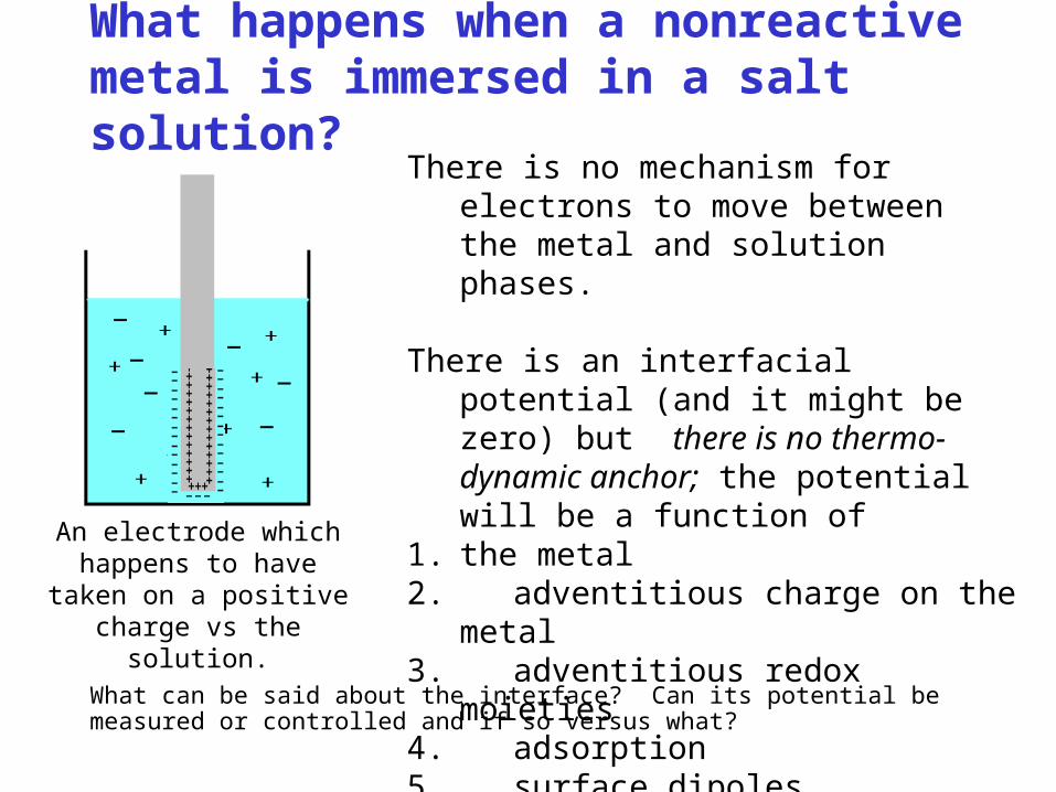
What happens when a nonreactive metal is immersed in a salt solution?

What can be said about the interface? Can its potential be measured or controlled and if so versus what?

There is no mechanism for electrons to move between the metal and solution phases.

There is an interfacial potential (and it might be zero) but there is no thermo-dynamic anchor; the potential will be a function of

1. the metal2. adventitious charge on the

metal3. adventitious redox

moieties4. adsorption5. surface dipoles

The potential will likely be irreproducible.

An electrode which happens to have

taken on a positive charge vs the solution.

We just caught our first glimpse of the infamous “double layer”. Let’s take a closer look.

What can be said about the interface? Can its potential be measured and if so versus what?

Let’s assume that an inert metal in solution is initially uncharged (center panel) and that charge can be added (right panel) or removed (left panel) in a controlled manner.

What happens when a nonreactive metal is immersed in a salt solution which also contains a redox couple: ox + e = red

Now, there is a mechanism for moving electrons between the metal and the solution, i.e., there is a thermodynamic mechanism for establishing a well defined interfacial potential.

The interfacial charge separation will be exactly that required to produce the potential required for equilibration with the redox system. .

F/electrrodee,redoxe,redoxelectrode

redoxelectrode Charge on an

electrode when positive vs the

solution

Two different noble metal electrodes immersed in a salt solution containing a redox couple: ox + e = red

What is V? Note:

0)()()()(

)(

e,1e,3redoxe,e,1

e,2redoxe,e,3e,2

1,3redox1,2redox,3,2

FFV

)()( e,1redoxe,e,2redoxe,

does not mean that V 0!!

There is no free lunch. Perpetual motion the perpetual notion! The quintessential test. What if V 0?

One could then

• connect the two electrodes through a resistor and perpetually generate heat (I could save thousands in house- heating costs!!) OR

• connect the two electrodes through a motor and produce an electric car that goes forever.

Man indicted for violating the laws of thermodynamics!

Judge tosses case for lack of evidence.

Two noble metal electrodes with two different redox systems.

Now, legitimately, FV 0:

)()(Δ)()(

)(

e,1e,3redox1e,e,1

junctione,2redox2e,e,3e,2

1,3redox11,junctionredox2,23,2

FFV

If junction 0

FV /)( redoxe,redoxe,

These are the concepts underlying the battery and reference electrode.

Question: Why should junction 0?

Answer: The junction barrier is not permselective to electrons, i.e., other charged species (ions) can also pass through the junction.

However- suppose that the junction is replaced by a barrier that transports only electrons (e.g., a noble metal foil, e.g., M1), then:

redox2redox11redox1

redox21junction

)()(Δ

and therefore: V = 0

The Nernst Equation

The Nernst EquationThe Nernst equation indicates the ability of a redox coupleto donate and accept electrons – this is directly related to e,redox. It is expressed as a potential (of the electrode) vs some reference potential (e.g., E0

H+/H2 = 0):

0/redox

red

ox

red

ox0/redox

red0oxe,ox

0oxe,

red

ox0redox

exp

or

ln

or

/]ln[]ln[ln

EERTnF

cc

cc

nFRTEE

nFaRTuaRTuaa

nFRTEE

The electrochemical sign convention: the lower the electrode potential the more readily it will donate electrons to a redox couple.

The Reference Electrode

The Reference Electrode (RE): purposeThe purpose of a true reference electrode is• to ensure that any perturbation or measurement of the

potential of the working electrode (WE) is based on a stable and known potential of the reference electrode (RE)

• to allow one to determine an accurate value of the formal potential, E0/, of a target couple– the E0/ is an identifying characteristic if not a fingerprint for a given redox couple

RE examples: AgCl/Ag; HgCl2/Hg, Ag/Ag+, Pt/H+/H2

The purpose of a quasi-reference electrode isto ensure that any perturbation or measurement of the WE potential is based on a RE potential that may be only approximately known but is invariant at least over the course of a single measurement. May be used in conjunction with an internal reference.

examples: Pt, Au, Ag wires

The Reference Electrode:properties to be considered1. ease of preparation*2. known and reproducible potential3. stability (short term? long term?)*4. no chemical interference with systems of

interest5. impedance**6.

* Considerations for using a quasi-reference electrode** Impedance may be very high for a chemically isolated electrode while low impedance may be required for certain

types of measurements, e.g., FFT

What is an “Internal Reference”? • An internal reference is a redox couple that is added to the analyte solution.

• It is usually used in conjunction with a quasi-reference electrode (in principle it is not needed when a true reference is available).

The Internal Reference:properties to be considered1. chemically stable in potential range of

interest

2. known E0/

3. No interaction with analytes of interest:If then start with Redref and Oxanalyte i.e.:

If then start with Oxref and Redanalyte i.e.:

/0analyte

/0ref EE

/0analyte

/0ref EE

analyterefanalyteref RedOxOxRed

analyterefanalyteref OxRedRedOx

The Paradigm Change: Hickling’s potentiostat (Trans. Faraday Soc., 38, p. 27 (1942)) and the 3-electrode systemHickling’s invention of device he dubbed “potentiostat” effected a paradigm change in the design of electrochemical methodologies as well as in the fabrication of reference electrodes.

The key element of the potentiostat (as well as of many electronic control systems) is the operational amplifier (op-amp). The change was catalyzed by the transition to solid-state devices which rapidly evolved post-WWII.

The Potentiostat

The two electrode system: electrochemistry the old fashioned way

Voltage of working electrode (WE) controlled and/or measured vs reference electrode (RE)

Note: Current passes through the RE.

The three electrode system and the do-it-yourself potentiostat

The do-it-yourself potentiostat:

1. Visually monitor the potential between the working and reference electrodes.

2. “Set” the potential between the WE and RE to a desired value by adjusting the sign and magnitude of the current passed between the WE and auxiliary electrode (AE).

This is a tedious, boring and inherently slow approach but it can be automated using Hickling’s potentiostat.

Key elements of the potentiostat:The Operational Amplifier (op-amp) Thanks to Darrell Elton for comments and insights!

Op-amp properties:• E denotes the “inverting” input• E+ denotes the non-inverting input• E out is maximum when E E+ < 0 • E out is minimum when E E+ > 0

Op-amp configuration:The voltage follower:

Voltage follower:Eout = V

The current amplifier:

Current follower:Eout = iRout

Note: E_ = virtual

ground

Potentiostat* #1: Single op-amp configuration

* HICKLING. Trans. Faraday Soc., 38, p. 27 (1942)

Potentiostat #2: dual op-amp configuration

Ei = iRi

Impact of potentiostats (and ultimately of computers) and the 3-electrode configuration• Reference electrodes could be small and have high impedance

– they could be more effectively isolated using high resistance frits

– reference electrode redox couples did not have to be exquisitely reversible

• Working electrodes could be subjected to a variety of perturbations – and with computers, an infinite variety.

Design of System (cell & electronics): things to think about (too often ignored)

• Uncompensated iRu which becomes increasingly problematic with:

larger currentslarger electrodeshigher solution resistanceshorter measurement timespoor cell configuration

• Stray capacitance problems become increasingly problematic with: smaller currents (of interest)

smaller electrodes higher solution resistance

reference electrode resistanceshorter measurement times

• Background currents, electrical noise, mechanical vibration, effective electrode shape and position

System design: things to think about (cont’d)

• Electrical noise from mains and other generators (lasers, motors, computers) • Mechanical noise (hood fans, human movement, air movement, temperature gradients, concentration gradients)• Effective electrode shape Life is simpler when electrode geometry can be dealt with using simple theory (i.e., planar diffusion). For example, a

band, disk, hemisphere or hemicylinder electrode can be treated as a linear system if

• Background currents

1/or 1or 1/000

r

fDrD

rFvDRT

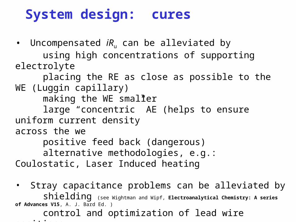
System design: cures

• Uncompensated iRu can be alleviated byusing high concentrations of supporting

electrolyteplacing the RE as close as possible to the

WE (Luggin capillary)making the WE smallerlarge “concentric” AE (helps to ensure

uniform current density across the we

positive feed back (dangerous)alternative methodologies, e.g.:

Coulostatic, Laser Induced heating

• Stray capacitance problems can be alleviated by shielding (see Wightman and Wipf, Electroanalytical Chemistry: A series of Advances V15, A. J. Bard Ed. )

control and optimization of lead wire positions

tight electronic designbetter cell design proximity of electronics the cell

System design: cures (cont’d)

• Electrical noise can be alleviated by:eliminating or turning off noise sourcesshielding cell and/or whole roomavoiding frequencies associated with the

noise (e.g., 50 Hz)

• Mechanical noise can be alleviated byeliminating, turning off, or distancing from

sourcesmechanical isolationorientation of electrodes temperature control (too often ignored)

• Electrode geometry can be optimized byimproved fabrication methodsimproved computer modeling to deal with

weird geometries

• Background currents can be diminished bypurifying ingredients; changing

ingredients; changing electrode material

Junction Potentials

• Systems at equilibrium.• System in steady state.

Junction Potentials: systems at equilibrium

The potential across the membrane selective for Cl only is

VF

RTF

T06.0]01.0ln[]1.0ln[

/C25

0.10.01mem

V1 is the measured potential between a pair of identical AgCl/Ag electrodes. V1 is the membrane potential if the junction potentials across the frits are identical. Why is this a valid assumption? Hint: it would not be a valid assumption if the salt were NaCl.

Junction Potentials: systems at steady state

Steady state theory for a concentration involving only two ions is independent of the shape of the barrier.

KCl is favored because DCl– = DK+ .

When more than two ions are involved the system is considerably more complicated and barrier size and shape matter

]1.0/01.0ln[])01./1.0ln[]1.0/1.0(ln[

]/ln[

memM

memX

memM

memX

fritM

fritX

fritM

fritX

1

12mem/fritM

mem/fritX

mem/fritM

mem/fritX

12mem/frit

FRT

DDDD

FRT

DDDD

V

ccF

RTDDDD

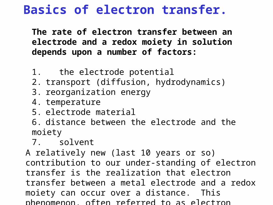
Basics of electron transfer.

The rate of electron transfer between an electrode and a redox moiety in solution depends upon a number of factors:

1. the electrode potential2. transport (diffusion, hydrodynamics)3. reorganization energy 4. temperature5. electrode material6. distance between the electrode and the moiety7. solvent

A relatively new (last 10 years or so) contribution to our under-standing of electron transfer is the realization that electron transfer between a metal electrode and a redox moiety can occur over a distance. This phenomenon, often referred to as electron tunneling, clarifies a number of aspects of heterogeneous ET.

Potentiostatic measurements

A true potentiostatic measurement is an equilibrium measurement. The classic example is the glass pH electrode:

]/ln[ inoutoutin aaF

RT

The glass electrode is effectively a mem-brane that is permselective for H+ ions:

What happens when a nonreactive metal is immersed in a salt solution?

What can be said about the interface? Can its potential be measured or controlled and if so versus what?

There is no mechanism for electrons to move between the metal and solution phases.

There is an interfacial potential (and it might be zero) but there is no thermo-dynamic anchor; the potential will be a function of

1. the metal2. adventitious charge on the

metal3. adventitious redox

moieties4. adsorption5. surface dipoles

The potential will likely be irreproducible.

An electrode which happens to have

taken on a positive charge vs the solution.

The Art and Practice of

Electrochemistry

Lecture II

In Lecture I we caught our first glimpse of the infamous “double layer”. Let’s take a closer look:

What can be said about the interface? Its potential can be measured vs a RE but there is no thermodynamic anchor.

Let’s assume that an inert metal is immersed in a solution containing ions but no redox species:

The potential of the electrode, measured vs some reference electrode can, in principle, can be any value- depending upon the amount of charge injected.

And, also in principle, since there is no mechanism for electrons to move directly between the metal and the solution the potential that is initially set should be stable. However, that is never the case. Why? Because there are a not a lot of charges on the electrode and trace amounts of adventitious electroactive material can react.

What happens when a noble metal electrode is immersed in a salt solution which also contains a redox couple: ox + e = red?

Now, there is a mechanism for moving electrons between the metal and the solution, i.e., there is a thermodynamic mechanism for establishing a well defined interfacial potential.

The interfacial charge separation will produce the potential which exactly balances the difference .

F/electrrodee,redoxe,redoxelectrode

redoxelectrode

Charge on an electrode when positive vs the

solution

redoxe,electrodee,

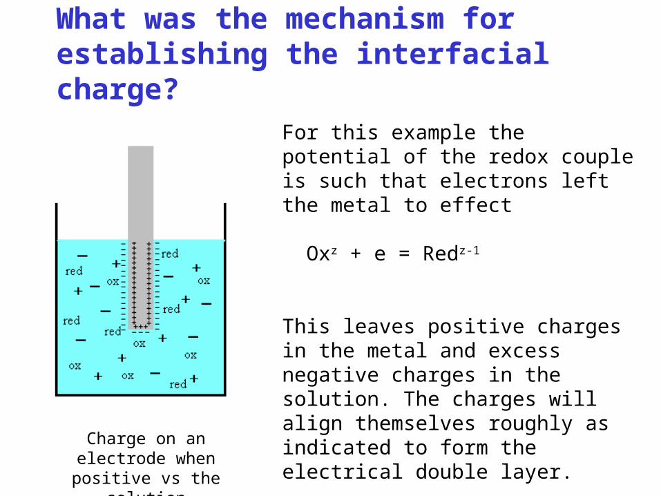
What was the mechanism for establishing the interfacial charge?

For this example the potential of the redox couple is such that electrons left the metal to effect

Oxz + e = Redz-1

This leaves positive charges in the metal and excess negative charges in the solution. The charges will align themselves roughly as indicated to form the electrical double layer.

No external current was required to achieve this condition! So how did it happen?


solution

The equilibrium potential of a WE vs a RE will be defined by the Nernst equation:


solution

0/redox

red

ox

red

ox0/redox

red

ox0redox

exp

or

ln

or

ln

EERTnF

cc

cc

nFRTEE

aa

nFRTEE

What would be different about this system if the metal were different?

0/

red

ox

red

ox0/

exp

or

ln

EERTnF

cc

cc

nFRTEE

Applying a potential will instantaneously change the redox concentrations at the electrode surface, but a current may have to be passed to maintain the proper values of cox and cred.Why?

Thus the electrode potential can be set by adjusting the redox concentrations or by adjusting electrode potential:

A bit more detail about the double layer

1. What is a double layer and why do we care?

2. What differences might there be between a double layer in aqeous solution and in an ionic liquid?

1a. What is the double layer? See discussion in: Bard and Faulkner, Electrochemical Methods,

Fundamentals and Applications, 2nd Edition, WileyLet’s take a closer look at the interface of a positively charged noble metal (e.g., Pt or Au) in a solution containing non-reacting, non-adsorbing ions (e.g., Hg in KF (why?):

)(;

2ddl

M2

i

M1

CC

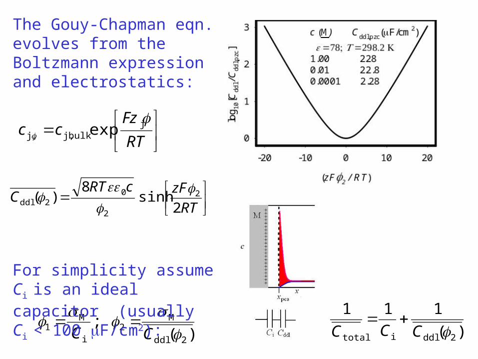
RTzFcRTC 2sinh8)( 2

2

02ddl

)(111

2ddlitotal CCC

The Gouy-Chapman eqn. evolves from the Boltzmann expression and electrostatics:

For simplicity assume Ci is an ideal capacitor (usually Ci < 100 F/cm2):

RTFz

cc

j

bulkj,j, exp

The theory as presented here is highly simplistic: an implicit assumption is that there is no adsorption of any electrolyte ions or of any adventitious materials which could greatly confound the analysis.

Typical values of Ctotal are of the order of

10-5 to 10–4 farads cm–2

The amount of charge required to change the interfacial potential can be significant when compared to the amount of charge that is passed which is associated with the faradaic processes – the reaction of interest.

Just how serious a problem this is (or is not) will depend on the experimental protocol and on many aspects of the experimental conditions. This will be examined in greater detail subsequent lectures.

So: Why do we care about the Double Layer?

Most electrochemical processes cannot occur without it!! Why?

s cm

: to x

)s( and cm 10where

)](exp[

pcaet,10et

pca

1et,

18

pcapcaet,et,

x

x

xx

kk

x

k

xxkk

Note: integrating from

Short and sweet answer: The double layer provides a mechanism to establish a large potential difference across a very small distance (a few angstroms). If that distance is too large (a few nanometers) the electron transfer rate will be too slow to do anything useful or the potential difference will be too small to do anything useful.

What might the diffuse double layer look like in an ionic liquid? Now, consider what happens when a noble metal (e.g., Pt) is placed in an ionic liquid comprising nonreacting, nonadsorbing ions. If the partial molar volume is ~same for both components:

constant:constraintwith

cc

See Kornyshev J. Phys. Chem. B, 111 (207)5545-5557

M

0

2

MddlIL,

0

20

02

00

22)d(

)(d

C

dxx-d

dxxE

x

dx

x

dxx

2pzcGC,ddl,

ddlIL,

2

0

2

0ddlIL,

20M

2

422

FRT

CC

czFC

See Kornyshev J. Phys. Chem.. B, May 2007

There remains, I believe, a dearth of capacitive measurements on ILs. A maximum in the capacitance at the pzc has not been seen. In most ILs the partial molar volumes are not equal (Kornyshev considers that possibility). It is possible that the potential dependence of the inner layer may dominate.

So- what are the implications for actual electrochemical measurement.

One important feature of many electrochemical measurements of interest (to us) is that changing the potential of an electrode changes the concentration at or near the surface of the electrode (remember that the distance dependence for ET falls off exponentially approximately as exp[-108 x]) This is true even if the conditions near the electrode surface are described by the Nernst equation. The result is that mass transport will play a critical role in understanding electrochemical responses.

It is also true that the rate constants for ET are finite and therefore Nernstian equilibrium may not obtain.

The Ubiquitous Junction PotentialWhen a frit separates two solutions of a fully ionized salt M+X– having concentrations c1 and c2 the potential across the frit is

]/ln[ 12fritM

fritX

fritM

fritX

12frit ccF

RTDDDD

As long as the D values within the frit for both ions are finiteboth ions pass through the frit and there will be a net flow of salt from the high concentration solution to the low concentration solution.

However, if either the frit then becomes permselective for one ion or the other and once electrostatic equilibrium has been established there will be no net flow of ions across the frit.

0 or fritX

fritM DD

Junction Potentials (cont’d)

The potential across the membrane selective for Cl only is

This is an equilibrium potential.

VF

RTF

T06.0]01.0ln[]1.0ln[

/C25

0.10.01mem

V1 is the measured potential between a pair of identical AgCl/Ag electrodes. V1 is the membrane potential if the junction potentials across the frits are identical. Why is this a valid assumption? Hint: it would not be a valid assumption if the salt were NaCl.

Junction Potentials (cont’d)

For the simple binary electrolyte the potential will be independent of the size and shape of the frit and of time if the relative D values are the same in solution and within the frit.

When there are different ions on each side of the frit the analysis is much more complicated and frit shape and size and timie do matter.

Thus there can be instabilities in the potential of a reference electrode which may be isolated by one or more frits separating solutions of vastly different composition and possibly involving different solvents.


ElectrochemistryLecture III

Paradigms for Heterogeneous Electron

Transfer: Butler-Volmer and

Marcus-Hush

A. Surface and bulk concentrations are identical (i.e., no concentration polarization):

E – E0/

redox moietydistance from the

electrode electrode materialreorganization energyreactant concentrationselectrode areasolventtemperaturesurface modification

(intentional, incidental and accidental)others?

Rates of electron transfer.The rate of electron transfer (ET) between an electrode and electroactive species in solution depends upon a number of factors:

B. In real systems surface and bulk concentrations are rarely identical and the

following additional factors must also be considered:transport (diffusion,

migration, convection/hydrodynamics)geometric effectscoupled homogeneous

kineticsGroup A will be the focus of lecture III and group B of lecture IV. In lectures V and VI we’ll explore how all these phenomena couple to control electrochemical responses.

The Butler-Volmer* description of interfacial electron transfer

0/

red

ox exp EERTnF

cc

The Butler-Volmer expression describing the rate constants for heterogeneous electron transfer is an empirical expression that is adequate for many electrochemical applications:

0/0

ox0/0

reds exp)1(exp EERTFcEE

RTFcFki xx

where i is the current density (A/cm2), ks (or k0) is the standard heterogeneous rate constant (cm/s). The eqn. is consistent with the IUPAC convention: anodic currents are positive; catodic are negative; the voltage scale is negative to positive from left to right.

Note: when ks the equation reduces to the Nernst expression:

__________________________________________________* J. A. V. Butler, Trans. Faraday Soc., 19 (1924) 729, 734 T. Erdey-Grúz & M. Volmer. Phyzik. Chem., B150A (1930) 203

The Butler-Volmer (BV) (cont’d):It is convenient to express the BV expression as:

where

The relationship between koxBV or kredBV, and E – E0/ is graphically depicted by a plot of ln[koxBV /ks ] or [kredBV / ks ] vs (F/RT)(E – E0/). For = 0.5 this will look like:

0oxBVred

0red

BVox

xx ckckFi

0/s

BVred

0/s

BVox

exp

)1(exp

EERTFkk

EERTFkk

For the sake of generality the plot is presented in terms of dimensionlessparameters. When T = 298.2 K, F/RT ~ 40.

Marcus-Hush Theory (MH) OR how intuition can lead you astray

Intuition suggests that the larger the driving force for a process the faster the process should go: • when the wind blows harder the sailboat goes faster• when the water pressure is higher the water flows faster:

And this might lead you to conclude that........

........... if the free energy driving force for a chemical reaction is increased the reaction rate should also increase.

Right?

Only up to a point!

Marcus-Hush Theory (MH) with seminal contributions of Levich and Gerisher

We’ve already seen thatButler-Volmer (BV) theorypredicts that the electron transfer rate increases withdriving force.

Let’s look at the implications of free-energy-vs-reaction-coordinate parabolas. First, consider how one might describe a homogeneous outer sphere electron transfer reaction: A + Q = B + P reactants products

MH: Quick and DirtyOuter sphere electron transfer: A + Q = B + P reactants products

When G0 = 0 some trivial algebra describing a pair of identically shaped intersecting parabolas tells us that :then

4/ΔΔ ‡b

‡f GG

bf

‡b

b

‡f

f

thereforeand

Δexp

Δexp

kk

RTGAk

RTGAk

(solvent reorganization energy) is a descriptor of the location of the two parabolas on the rc and in this case represents AB + PQ.

20‡b

20‡f

Δ14Δ

Δ14Δ

GG

GG

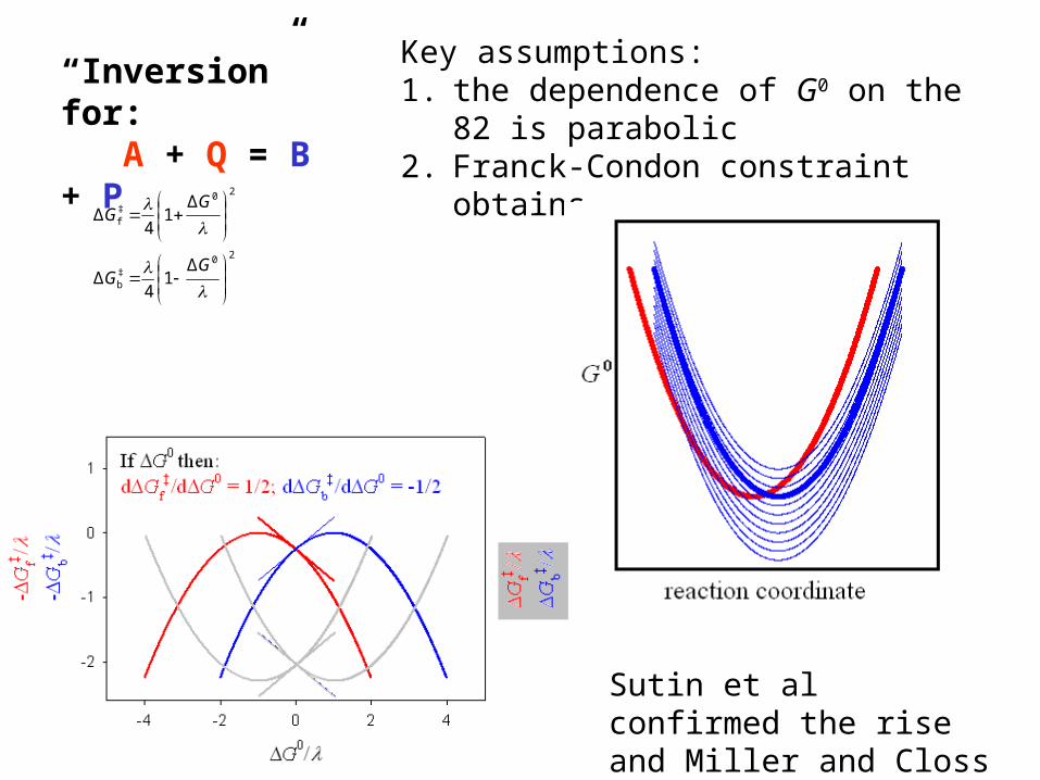
“Inversion” for: A + Q = B + P

Key assumptions:1. the dependence of G0 on the

82 is parabolic 2. Franck-Condon constraint

obtains

Sutin et al confirmed the rise and Miller and Closs the fall.

The Franck-Condon Dance:

Instead of A + Q = B + Pconsider now A + e = B

Key assumptions:Chidsey: Science 251 (1991)

919-9221.the dependence of G0 on the

rc is parabolic 2.Franck-Condon constraint

obtains3.there is a uniform

distribution of electronic states in the metal

4. an electron in the kth state has energy k.

5.For any given value of G0

one must consider the ET between A and B and all the states; Fermi-Dirac probabilities that state k is occupied or vacant are po and pv :

1

B

Fkv

1

B

Fko

exp1

exp1

Tkp

Tkp

The MH description forheterogeneous ET:

Chidsey’s 1991 theoretical clarification and experimental confirmation that MH is significantly better than BVChristopher Chidsey: Science 251 (1991) 919-922

Chidsey cont’d:

Tk

Tk

Tk

EETk

eTk

EETk

e

Tk

TkPkB

B

B

2/0

BB

/0

B

B

BMHred d

2cosh2

4exp

2exp4

4exp

)(exp2 02DA

xxHP

Tk

Tk

Tk

EETk

eTk

EETk

e

Tk

TkPkB

B

B

2/0

BB

/0

B

B

BMHox d

2cosh2

4exp

2exp4

4exp

dependence distance thezescharacteri at constant coupling electronic theis

metal in the states electronic ofdensity theis where0

2DA

xxH

Assuming that there is virtually acontinuum of electronic states:

Tk

Tk

Tk

EETk

eTk

EETk

e

Tk

TkPk

B

B

B

2/0

BB

/0

B

B

BMHred d

2cosh2

4exp

2exp4

4exp

Tk

Tk

Tk

EETk

eTk

EETk

e

Tk

TkPk

B

B

B

2/0

BB

/0

B

B

BMHox d

2cosh2

4exp

2exp4

4exp

Key features of these equations:1. Nernst condition obtains (obvious from equations), i.e.:

)(exp/ /0

B

MHred

MHox EE

Tkekk

Tk

Tk

Tk

EETk

eTk

EETk

e

Tk

TkPk

B

B

B

2/0

BB

/0

B

B

BMHred d

2cosh2

4exp

2exp4

4exp

Tk

Tk

Tk

EETk

eTk

EETk

e

Tk

TkPk

B

B

B

2/0

BB

/0

B

B

BMHox d

2cosh2

4exp

2exp4

4exp

Key features of these equations:1. Nernst condition obtains (obvious from

equations), i.e.:

2. Maximum value of koxMH /P and kredMH /P is 1.000 (not obvious)

3. Computation shows that for any given value of :

koxMH /P = 0.5 when e(E – E0/) = kredMH /P = 0.5 when – e(E – E0/) =

)(exp/ /0

B

MHred

MHox EE

Tkekk


equations), i.e.:

2. Maximum value of koxMH /P and kredMH /P is 1.0003. Computation shows that for any given value

of : koxMH /P = 0.5 when e(E – E0/) = kredMH /P = 0.5 when – e(E – E0/) =

)(exp/ /0

B

MHred

MHox EE

Tkekk

Tk

Tk

Tk

Tk

Tk

TkPkkk

B

B

B

2

B

B

BBVs

MHss d

2cosh2

4exp

4

4exp

When E – E0/ = 0 the MH expression gives the standard rate constant ksMH which must equal ksBV:

Then, it is straight forward to obtain koxMH/ks and koxMH/ks :

Tk

Tk

Tk

EETk

eTk

EETk

e

Tk

TkPk

B

B

B

2/0

BB

/0

B

B

BMHred d

2cosh2

4exp

2exp4

4exp

TkTk

Tk

Tk

TkTk

Tk

EETk

eTk

EETk

e

kk

B

B

B

2

B

B

B

B

20

BB

0

B

s

MHred

d

2cosh2

4exp

d

2cosh2

4exp

2exp

TkTk

Tk

Tk

TkTk

Tk

EETk

eTk

EETk

e

kk

B

B

B

2

B

B

B

B

20

BB

0

B

s

MHox

d

2cosh2

4exp

d

2cosh2

4exp

2exp


equations), i.e.:

2. Maximum value of koxMH /P and kredMH /P is 1.000 (not obvious)

3. Computation shows that for any given value of :

koxMH /P = 0.5 when e(E – E0/) = kredMH /P = 0.5 when – e(E – E0/) =

4. Comparison to BV? There is a small zone where

there is reasonable agreementbetween MH and BV- the larger the value of the better the agreement. Expanding thezone of interest close to E0/........

)(exp/ /0

B

MHred

MHox EE

Tkekk

Chidsey: Science 251 (1991) 919-922 Forster et al: JACS 122 (2000) 11948

Both Chidsey and Forster et al present strong evidence for significant deviation from BV-behavior. Forster work also indicates “flattening” but not inversion – more easily accomplished since ~ 0.28 eV for osmium system compared to 0.85 eV for the ferrocene system.


ElectrochemistryLecture IV

Transport and homogeneous kinetics

and (perhaps) more about diffusion than you really

want to know

A. Surface and bulk concentrations are identical (i.e., no concentration polarization):

E – E0/

redox moietydistance from the

electrode electrode materialreorganization energyreactant concentrationselectrode areasolventtemperaturesurface modification

(intentional, incidental and accidental)others?

Rates of electron transfer.The rate of electron transfer (ET) between an electrode and electroactive species in solution depends upon a number of factors:

B. In real systems surface and bulk concentrations are rarely identical and the

following additional factors must also be considered:transport (diffusion,

migration, convection/hydrodynamics)geometric effectscoupled homogeneous

kinetics

Group A was the focus of lecture III; group B is the focus of lecture IV. In lectures V and VI we’ll explore how all these phenomena couple to control electrochemical responses.

xRTcD

f dd jjj

j

DiffusionThe phenomenological diffusion equation (for linear diffusion) is

where fj is the flux of the jth particle (moles cm-2

s-1)Dj is the diffusion coefficient of the jth

particle (cm2 s-1)cj is the concentration of the of the jth

particle (moles cm-3)

j is the partial molar free energy of the jth particle (J mole-1)

RT has its usual significance (J mole-1)

xRTcD

f dd jjj

j

Diffusion cont’d:

The sign convention here is chosen so that the flux direction is positive when the free energy gradient is negative, i.e., the particle will go “downhill”.

Implicit in the phenomenological expression is the assumption that the speed of the particle (vj = fj /cj (cm s-1)) is proportional to the force dj /dx acting upon it.

Whoa!!!! Something’s fishy here! Didn’t we all learn that a force acting on a particle will cause the particle to accelerate rather than simply attain a constant speed?

xRTcD

f dd jjj

j

Diffusion cont’d:

What I forgot to mention is that the particle is in a viscous medium and that the frictional force is assumed to be proportional to the velocity. That is a reasonable assumption if the velocity is not too big (the need for that assumption is why they call this equation “phenomenological”).j

jj

jjjj

jjj :. ;d

d1 :. ;0dd

DRTr

xrvrv

xam

whereaj is the acceleration of the jth particle

(cm s–2) vj is the velocity of the jth particle (cm

s–1)rj is a frictional coefficient of the jth

particle (J s cm–2)

The time required to accelerate a particle to its steady-state velocity is too short to be of concern.

xRTcD

f dd jjj

j

Diffusion cont’d:

How do we get from this equation to Fick’s law or beyond?

where aj is now the activity and zj is the charge. If, and only if, the activity coefficient, j, is constant:

/dxd field electric theis whered]ln[d d

d]ln[]ln[

jjjj

jjj0jjj

0jj

VzFx

cRT

x

FVzcRTFVzaRT

jjjj

jjjj

j

jj

jj

jjj

RTdd

dd

RT

:equationPlanck -Nernst obtain the weuncleyour sBob' anddd d

]ln[d dd

zcDFxc

Dx

cDf

zFxc

cRTzF

xc

RTx

Diffusion cont’d:

The Nernst-Planck expression allows us to compute the effect of an electric field on ions

in solution (migration). When = 0 or zj = 0 the Nernst-Planck expression reduces to the Fick equation, familiar to most of you:

But there is still a subtle ambiguity here- it is easy to envision how an electric filed can create a force on a charged particle but how can a concentration gradient comprising randomly walking non-interacting particles create a force? It doesn’t really but it can be describe that way.

jjjj

jj RTdd

zcDFxc

Df

xc

Df dd j

jj

Diffusion cont’d (the random walk):

Consider a particle that can move a step to the right or to the left during the time increment t.

Now consider a large number N of those particles initially located at a starting point on a line, say x =0, and at t = 0 begin their random right-or-left motion.

After time increments of 0.1t let’s see how the particles redistribute as they relocate at , 2, 3, etc. In any 0.1t 5% of the particles at n will relocate at (n+1) and 5% at (n-1). What will the distribution look like as a function of time?

Run QB Diff#1.bas

tmtnxt

D

Dtx

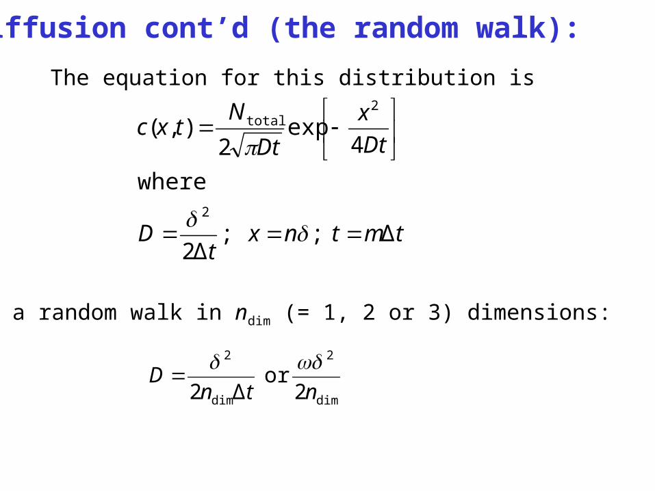
DtNtxc

Δ ; ;Δ2

where4exp

2),(

2

2total

The equation for this distribution is


For a random walk in ndim (= 1, 2 or 3) dimensions:

2or Δ2 dim

2

dim

2

ntnD

14 s cm 103 MRTv

One of Einstein’s many seminal contributions to science was his elucidation of Brownian motion. He postulated that a particle’s velocity in a viscous medium is the same as its velocity in a gas:

Diffusion cont’d (the random walk):Investigations on the Theory of Brownian Movement, Dover Publications, Inc. A. Einstein, (R. Fürth, ed.)

Seems amazing – until you realize that the mean free paths of particles in a gas phase and in a condensed phase are dramatically different. We also know that in many condensed phases D ~10–5 cm2 s–1 so we can now estimate the values of and : 125

214 s cm 106 ;s cm 103

DMRTv

and therefore112

5

829

4

5s 101.7 106

106 and cm 10 610

1066

D

vvD

What about the assumption that the random walk step is exactly or that the frequency, , is metronomically constant?Chandresekahr showed that the exact equation for D is:


2 dim

2

nD

However it does mean that the implicit assumption made to estimate the values of and ,

could be quite inaccurate unless the range of is narrow.

2

Diffusion cont’d (Fick’s 2nd law):Fick’s equation

xc

Df dd j

jj

can be differentiated to give:

2j

2

jj

dd

dd

xc

Dxf

For linear diffusion it is easy to show that

This equation is sometimes referred to as Fick’s second law.2j

2

jjj

dd

dd

dd

xc

Dxf

tc

Diffusion cont’d (Fick’s 2nd law):

With the Nernst-Planck expression the corresponding equation is:

xc

xczD

RTF

xc

Dtc

dd

dd

dd

dd j

jjj2j

2

jj

Incorporating hydrodynamics gives:

xc

vxc

xczD

RTF

xc

Dtc

x dd

dd

dd

dd

dd jj

jjj2j

2

jj

Tossing in some homogeneous kinetics, say, for the first-order disappearance of cj, gives:

jfjj

jjj2j

2

jj

dd

dd

dd

dd

dd

ckxc

vxc

xczD

RTF

xc

Dtc

x

Diffusion cont’dIn principle, we have the tools to describe a lot of the solution-based phenomena that will control the rate at which species get to an electrode surface or leave an electrode surface.

Once upon a time we were concerned about getting electroactive species to and from the plane of closest approach. Now we know that they can be consumed or produced at some distance (many angstroms) from the electrode.

In some cases the electroactive species are [permanently] attached to the electrode surface thereby eliminating transport as a factor (we touched on that briefly in our discussions of the Chidsey and Forster papers).

In other cases (best avoided!!) species in solution also adsorb on the electrode and in doing so create a virtually intractable computational challenge.

Some basics of diffusion-controlled transport Let’s consider a simple example of diffusion controlled electro-chemistry. The redox couple of interest is A + e = B with E0/ = 0:

1. The solution contains only 0.001 M A and 1 M KCl (why?)2. The open-circuit potential of the Pt working electrode (1.0 cm2)

is +0.300V and T = 298.2. (what does that tell you?) 4. The potentiostat is turned on and the potential of the WE is adjusted to 0.300 V 5. The electrode potential is then stepped “instantaneously” to – 0.300 V and the current observed as a function of time.

Assuming that the interfacial concentrations of A and B are governed by the Nernst equation what will happen to those concentrations at the electrode surface (or to be more precise,

within a few angstroms of the electrode surface)?

What will the current be? What will the concentration profiles look

like and how will they depend upon time and upon the values of DA and DB .

What would the results look like if the potential were –0.5 V?

Diffusion-controlled transport (cont’d)The equation describing the current as a function of time is the Cottrell equation:

tDFciAbulk

A

The equation describing the concentration profile of A is:

t2xerfc),(

dexp2zerf wheret2

xerf),(

BB

AbulkAB

B

A

0A

B

0

2

A

bulkAA

DDDctxc

DD

cc

yyD

ctxc

x

z

Some basics of diffusion-controlled transport Let’s consider a simple example of diffusion controlled electro-chemistry. The redox couple of interest is A + e = B with E0/ = 0:

1. The solution contains only 0.001 M A and 1 M KCl (why?)2. The open-circuit potential of the Pt working electrode (1.0 cm2)

is +0.300V and T = 298.2. (what does that tell you?) 4. The potentiostat is turned on and the potential of the WE is adjusted to 0.300 V 5. The electrode potential is then stepped “instantaneously” to – 0.300 V and the current observed as a function of time.

Assuming that the interfacial concentrations of A and B are governed by the Nernst equation what will happen to those concentrations at the electrode surface (or to be more precise,

within a few angstroms of the electrode surface)?

What will the current be? What will the concentration profiles look

like and how will they depend upon time and upon the values of DA and DB .

What would the results look like if the potential were –0.5 V?

Diffusion-controlled transport (cont’d)The equation describing the current as a function of time is the Cottrell equation:

tDFciAbulk

A

The equation describing the concentration profile of A is:

t2xerfc),(

dexp2zerf wheret2

xerf),(

BB

AbulkAB

B

A

0A

B

0

2

A

bulkAA

DDDctxc

DD

cc

yyD

ctxc

x

z


ElectrochemistryLecture V

Honing our intuition for the interpretation of cyclic voltammetric

responses:easy steps first

Comment (stimulated by a couple of questions asked after Lecture IV):I’d like to continue the discussion of c-amp. Why c-amp?

not because it is widely used (it is not) and not because it might be the technique of choice for certain types of measurements.

Rather:because the diffusional, kinetic and

geometric phenomena that are likely to be operative in many electroanalytical systems of interest (certainly to the Bond group) are more easily understood in the context of c-amp. Hopefully it will all come together when we discuss CV in Lecture VI.

I’ll be using DigiElch for C-amp simulations. With a bit of trickery one can also do c-amp using DigiSim (check the help file or see me).

Chronoamperometry (cont’d): the simplest versionGiven:• an electroactive species, e.g., A, in solution

(the [reversible] redox couple is A + e = B)• supporting electrolyte Ru ~ 0• 3-electrode system with potentiostatic control• current follower with an infinite bandwidth and dynamic range• semi-infinite linear geometry

There are two basic requirements for the execution of the c-amp experiment in its simplest form:1. An initial potential chosen so that there is no oxidation or reduction of the electroactive species that is initially present (and therefore – ideally – no current flow) 2. An instantaneous step in the potential of the working electrode to effect a Dirichlet boundary condition at the electrode surface which means that the concentrations of A and B are fixed at x = 0.

Chronoamperometry (cont’d):

[VCA(simple_c-amp)DE.cas]

For a solution initially containing A (and virtually no B) this is most easily and definitively achieved by stepping from E0/ + ~0.3 V to E0/ – ~0.3 V which effectively sets [A]x=0 = 0: why? How do you know the value of E0/?

For a measurement of i vs t, the relevant experimental parameters here are:• i = current density = F x flux (units: A cm–2) • DA = diffusion coefficient of A (units: cm2 s–1)• cAbulk = bulk concentration of A (units: moles cm–3)• t = time after the potential step (units: s)• F = Faraday’s constant (units: 96485 C mole–1 of electrons)

Dimensional Analysis. Buckingham’s theorem- only one dimensionless grouping that can be formed from the parameters i, DA, cA, t, F:

AbulkA DFc

tiBuckingham’s theorem: given a physically meaningful equation involving a certain number, n, of physical variables, and these variables are expressible in terms of k independent fundamental physical quantities, then the original expression is equivalent to an equation involving a set of p = n−k dimensionless variables constructed from the original variables. .: 5 physical variables (i,D,cA,t,F) and 4 fundamental physical quantities (cm, s, C, mole) 1 dimensionless parameter.


AbulkA DFc

ti

tDFc

iDFc

ti AbulkA

AbulkA

constant thereforeandconstant

Thus, dimensional analysis alone, with no mathematical analsysis, can predict a useful functional relationship between i and t.

The full analytic solution of the PDEs describing the diffusion problem (see, e.g., Bard and Faulkner p162) tells us that the value of the constant is –1/2 thus revealing the familiar Cottrell expression:

Because this parameter is the only dimensionless parameter that can be formed from the five parameters

i, D, coxbulk ,t & F it must be the case that.

tDFc

i

AbulkA


The complete solution also describes the concentration profiles of the A and B species:

B

AbulkAB

BB

AbulkAB

0

2

A

bulkAA

),0(

t2xerfc),(

dexp2zerf wheret2

xerf),(

DDctc

DDDctxc

yyD

ctxcz

Note that the characteristic thickness of the diffusion layer is . tJD

t2/ JDx

Chronoamperometry (cont’d): What happens when we......1. set DA DB?

2. change the Dirichlet boundary condition, e.g. by stepping from E0/ + ~0.3 V to E0/ ?

3. decrease the heterogeneous rate constant?

4. introduce homogeneous kinetics, e.g., A + e = B; B = C (show

reaction layer) or S = A; A + e = B

5. change the geometry from semi-infinite linear (planar) to hemispherical or disk geometry?

6. introduce uncompensated resistance and double layer capacitance?

Chronoamperometry (cont’d): What happens when we......

1. set DA DB? DA/DB > 1 or DA/DB < 1

[VCA(Dratio)DE.cas]

B

AbulkAB

BB

AbulkAB

0

2

A

bulkAA

),0(

t2xerfc),(

dexp2zerf wheret2

xerf),(

DDctc

DDDctxc

yyD

ctxcz

Chronoamperometry (cont’d): What happens when we......

2. change the Dirichlet boundary condition, e.g. by stepping from E0/ + ~0.3 V to E0/ ?

[VCA(Dirichlet)DE.cas]

/0

A

B

bulkA

B exp where),0( EERTF

DDctc

An obvious (??) prerequisite here is that is that the electron transfer be reversible. If that condition is not met the Dirichlet boundary condition will not be met.

Maybe it’s not obvious.

Chronoamperometry (cont’d): What happens when we......3. decrease the heterogeneous rate

constant?

We eliminate the mathematical discontinuities associated with dealing with a perfect voltage step.

No more infinite current at t = 0!

Remember the Butler-Volmer equation:

[VCA(ks)DE.cas]

0/

A0/

Bs exp)0()1(exp)0( EERTFxcEE

RTFxcFki

Chronoamperometry (cont’d): What happens when we......4. introduce homogeneous kinetics, e.g., “EC”: A + e = B; B = C or “CE”: Y = A; A + e = B or “ECE”: A + e = B; B = C; C +

e = D; B + C = A + D

Old (but useful) concept:reaction layer

New concepts:pre-equilibration

TSR (Thermodynamically Superfluous Reaction)

[VCA(EC)DE.cas][VCA(CE)DE.cas][VCA(ECE)DE.cas]

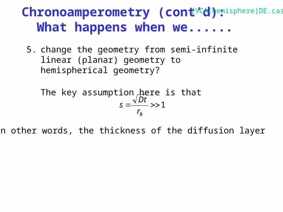
Chronoamperometry (cont’d): What happens when we......5. change the geometry from semi-infinite

linear (planar) geometry to hemispherical geometry?

The key assumption here is that1

0

rDts

In other words, the thickness of the diffusion layer

[VCA(hemisphere)DE.cas]

Chronoamperometry (cont’d): What happens when we......6. introduce uncompensated resistance and

double layer capacitance?

Of course, they were always there.

Another realistic way in which mathematical discontinuity is eliminated.

Thus far both uncompensated resistance and and double layer capacitance have been ignored. A serious flaw because of the high currents associated with the c-amp method.

[VCA(RuCdl)DE.cas]


ElectrochemistryLecture VI

Putting it together for Cyclic Voltammetry

DigiSim at Work

Analytical Chemistry 36 (1964) 706-723

Probably one of the most cited electrochemical papers!We’ll be discussing this work in more detail later.

and a classic paper:

A cyclic voltammogram is a spectrum: a response (current) is examined as a function of energy (voltage).

(an approximate quote)

Jurgen Heinze

CV: The basicsGiven:• an electroactive species, e.g., A, in solution

(the [reversible] redox couple is A + e = B)• supporting electrolyte Ru ~ 0• 3-electrode system, potentiostat and a triangular

wave form generator•• No longer require a current follower with an

infinite bandwidth and dynamic range• semi-infinite linear geometry

Then:1. Choose an initial potential, Estart so that there is no oxidation or reduction of the electroactive species that is initially present (and therefore – ideally – no current flow) 2. Scan the potential at a constant ± dV/dt between Estart and Erev:

Estart ( Erev Estart)n where n = 1 in common practice and good practice often deems n > 2!! Show ECE.

CV: The basics

Consider the simplest redox process: A + e = B

We’ll initiate the CV scan at E0/ + ~0.3 V and scan at – 1 V/s to

E0/ – ~0.3

What happens when1. the reaction is reversible with DA = DB? 2. the scan rate, |v| (= |dV/dt|), is changed

3. the reaction is reversible with DA DB? 4. the reaction is quasi-reversible because of slow

BV interfacial kinetics?5. the reaction appears to be quasireversible

because of uncompensated resistance?6. there are double-layer effects? 7. when MH rather than BV controls ET?

CV: The basics

For the simplest redox process A + e = B

what happens when1. the reaction is reversible with DA = DB? [VI-CV(E)DS.cvs]

3. the reaction is reversible with DA DB?

ox

red/0

ox

redpapcavg ln2ln22 D

DF

RTEDD

FRTEE

E

2. the scan rate, |v| (= |dV/dt|), is changed? What happens to Epeak?

4463.0||Abulk

A

pf

RTvFDFc

i This equation (save for the value of the constant) can also be deduced using dimensional analysis.

The variable “t” is replaced by RT/(F|v|)

CV: The basics

for the simplest redox process: A + e = B

what happens when4. the reaction is quasi-reversible because of slow BV interfacial kinetics?

What happens to ipeak and Epeak when |v| is increased or decreased?

RTvFD

kP||A

s so peak separation should be the same for ks = 0.001 cm/s and |v| = 1.0 V/s and ks = 0.01 cm/s and |v| = 100 V/s

5. the reaction appears to be quasi-reversible because of uncompensated resistance? What happens to the peak separation if the concentrations are changed when BV or Ru controls?

CV: The basics

For the simplest redox process: A + e = B

What happens when6. there are double-layer effects?

bulkAdl

bulkA

bulkAdl

bulkA

total

faradaic

bulkAdlfaradaicCdltotal

bulkAfaradaic

dlCdl

||||||

i

||i)(abs/ where||

bcCvbc

vsbcvCvsbci

vsbcvCiivvsvsbci

vCi

CV: The basics

for the simplest redox process: A + e = B

what happens when7. ET kinetics are controlled by Marcus-Hush rather

than Butler-Volmer?When do the differences become important? How sensitive to these differences is the FFT

approach?

CV: unusual and amusing behavior

What will the CV for this system look like ( is the starting species).

5eq

35

46

45

36

/02

45

35

5eq

/01

46

36

10 CrOH(CN)Cr(CN)CrOH(CN)Cr(CN)

CN

3.0 CrOH(CN)CrOH(CN)10 ||

0 Cr(CN) Cr(CN)

OH

K

EeK

Ee

36Cr(CN)

CV: unusual and amusing behavior

What will the CVs for these systems look like?

or

5eq

/02

/01

10 2B C A 15.0 C e B15.0 B e A

KEE

5eq

/02

/01

10 2B C A 15.0 C e B15.0 B e A

KEE

CV: in films and thin layers

What happens when the electrochemistry is constrained to a thin layer or film?

If we ensure that the the diffusion layer thickness,(D RT/Fv) is much larger than the the thickness of the film, , there will be no concentration polarization with in the film.

The operative CV equation is then:

filmfilmA,A2

/0

/0

A2

whereexp1

exp

cEE

RTF

EERTF

RTvFi

Some concluding remarks:Computer simulation is a powerful tool for unraveling the electrochemistry of complicated systems. However, there is a long way to go before we have an inverse algorithm which can digest the experimental data and spit back the correct mechanism with values for all its operative parameters.

Until then the experimentalist must do the inversion: making initial conjectures, choosing a model that is chemically sensible, and then, with the aid of computational tools, optimizing parameter values and ultimately deciding if the model is “correct”.

I hope that some of the discussions we’ve had over the past few weeks will help you do that.

Thank you.

swf

Postscript:It is possible to simulate single step chroamperometric experiments using DigiSim (see DigiSim help file; search for “chronoamperometry”). If you have questions please contact me: [email protected]

Much of the last two lectures was based on simulations using DigiElch and/or DigiSim. I did not attempt to include all the various simulated CVs in this collection – however, the programs used to generate the simulations are included. Files named “*DE.cas” are DigiElch files and can only be read using DigiElch; files named “*DS.cvs” are DigiSim files and can only be read using DigiSim. Again, please contact me if you have any questions.

Thank you.

swfMarch 16, 2008

mailto:[email protected]

mailto:[email protected]

The Art and Practice of Electrochemistry

Documents

Transcript of The Art and Practice of Electrochemistry