The accuracy of grid digital elevation models linearly constructed from scattered sample data

Research Article

The accuracy of grid digital elevation models linearly constructed fromscattered sample data

FERNANDO J. AGUILAR*, MANUEL A. AGUILAR, FRANCISCO

AGUERA and JAIME SANCHEZ

Department of Agricultural Engineering, University of Almeria, Spain, Ctra. de

Sacramento s/n. La Canada de San Urbano, 04120 Almerıa, Spain

(Received 28 March 2005; in final form 7 September 2005 )

In this paper, a theoretical-empirical model is developed for modelling the

accuracy of a grid digital elevation model (DEM) linearly constructed from

scattered sample data. The theoretical component integrates sample data

accuracy in the model by means of the error-propagation theory. The empirical

component seeks to model what is known as information loss, i.e. the sum of the

error due purely to sampling the continuous terrain surface with a finite grid

interval and the interpolation error. For this purpose, randomly spaced data

points, supposed to be free of error, were converted into regularly gridded data

points using triangulation with linear interpolation. Original sample data were

collected with a 262 m sampling interval from eight different morphologies,

from flat terrain to highly rugged terrain, applying digital photogrammetric

methods to large-scale aerial stereo imagery (1 : 5000). The DEM root mean

square error was calculated by the true validation method over several sets of

check points, obtaining the different sampling densities tested in this work.

Several empirical models are calibrated and validated with the experimental data

set by modelling the DEM accuracy by combining two variables such as sampling

density and a descriptive attribute of terrain morphology. These empirical models

presented a morphology based on the product of two potential functions, one

related to the terrain roughness and another related to the sampling density. The

terrain descriptors tested were average terrain slope, standard deviation of terrain

slope, standard deviation of unitary vectors perpendicular to the topographic

surface (SDUV), standard deviation of the difference in height between adjacent

samples in the grid DEM (SDHD), and roughness estimation by first-, second-,

or third-degree surface fitting error. The values obtained for those terrain

descriptors were reasonably independent from the number and spatial distribu-

tion of the sample data. The models based on descriptors SDHD, SDUV, and

standard deviation of slope provided a good fitting to the data observed

(R2.0.94) in the calibration phase, model SDHD being the one that yielded the

best results in validation. Therefore, it would be possible to establish a priori the

optimum grid size required to generate or store a DEM of a particular accuracy,

with the saving in computing time and file size that this would mean for the

digital flow of the mapping information in GIS.

Keywords: Grid digital elevation models; Interpolation; Quality assessment of

spatial data; Digital elevation model accuracy; Modelling

*Corresponding author. Email: [email protected]

International Journal of Geographical Information Science

Vol. 20, No. 2, February 2006, 169–192

International Journal of Geographical Information ScienceISSN 1365-8816 print/ISSN 1362-3087 online # 2006 Taylor & Francis

http://www.tandf.co.uk/journalsDOI: 10.1080/13658810500399670

1. Introduction

Digital elevation models (DEMs) have become one of the most important covers for

Geographical Information Systems (GIS) in many disciplines, which highlight the

need to assess DEM accuracy. If GIS users are not aware of the DEM accuracy,

perfectly logical GIS analysis techniques can lead to incorrect results. In other

words, the data may not be fit for use in a certain context (Fisher 1998).

The awareness of the GIS user community of this problem is shown by the vast

number of studies published in the last few years on error detection, both

quantitative methods based on statistical-mathematical algorithms (e.g. Felicısimo

1994, Lopez 1997, Briese et al. 2002) and qualitative methods based on visualization

techniques (Wood and Fisher 1993, Wood 1996, Yang and Hodler 2000).

It must be borne in mind that the DEM data-acquisition phase has reached a

remarkable degree of development with the introduction of new technologies, such as

the laser scanner (LIDAR) and InSAR (Smith 2004), which allow a high degree of

automation and density sensing. Thus, the US Geological Survey scientists are now

finding new methods for the use and representation of high-resolution LIDAR data

(Queija et al. 2005). Therefore, the problem nowadays is not obtaining data from a

DEM, but handling and maintaining such an amount of information using structures,

which will allow its efficient integration and exploitation in GIS or CAD areas. In the

majority of cases, it is preferable to have an optimized DEM adapted to our needs, i.e.

without excess information, rather than to have a vast amount of data, which will be

more difficult for us to handle (Aguilar et al. 2005). Thus, optimum sampling strategies

are clear favourites to guarantee the quality requirements of a DEM with the lowest

possible number of points (Balce 1987).

It seems obvious that the user and the producer of DEMs need to agree on the

accuracy and the grid interval of the product, among other specifications (Huang

2000). To this end, they should speak the same language and have models at their

disposal that will allow them to predict the grid DEM accuracy in terms of the main

factors that intervene in its definition: accuracy and density of the data source,

characteristics of the terrain surface and the method used for the construction of the

DEM surface (Li 1992, Gong et al. 2000). The work presented in this paper is

focused on this last point.

Most of the models developed in the last few years for modelling the global error

of a DEM can be classified as empirical or theoretical. Within the empirical models,

based on experience, the works of Ackermann (1980), Ayeni (1982), Li (1992), Gao

(1997) and Davis et al. (2001) can be referred to. In these empirical models

regression techniques are used to adjust the different parameters of the model to the

experimental results obtained, generally on vast terrain databases. As an example of

a classical methodology in the development of this type of model, we can highlight

Gao’s work (1997), where the accuracy (root mean square error (RMSE)) of the

DEMs extracted from topographic maps was regressed against contour density

(km km22) and DEM resolution at six resolution levels. More recent studies like that

of Davis et al. (2001) use characteristics which are typical of the Digital

Photogrammetric Workstations (DPWs) for modelling the accuracy of grid

DEMs. It is an interesting empirical model capable of estimating both the global

error of the DEM (RMSE) and the vertical accuracy of the elevation value for every

grid point in the DEM (spatial variation of elevation error). For this purpose, they

use parameters derived from the automated DEM extraction, called figure of merit

(FOM), as independent variables in the regression analysis. An FOM value is

170 F. J. Aguilar et al.

produced for each DEM point by the stereo-correlation software used in the DEM

generation process. Obviously, this model is highly dependent upon the methods

used for computing FOM values and would only be suitable when the stereo-

matching method is being utilized to obtain the DEM.

In the case of theoretical models, the first relevant contributions were based on

relatively complex mathematical formulations such as the Fourier analysis

(Makarovic 1972) and autocovariance and variogram analysis (Kubik and

Botman 1976). In the first case, no suitable mathematical expressions were derived

for practical application, whilst in the second, it should be stressed that it is difficult

to have good approximate co-variance values as a terrain descriptor, and therefore

the final prediction would not be very reliable (Li 1993a).

Since the 1990s, it has been possible to observe a certain tendency to develop

theoretical models based on the error-propagation theory, segmenting the problem

and calculating separately the error contributed by the different uncertainty sources.

In the case of Weng’s proposal (2002), the total DEM uncertainty is determined

from cartographic digitising, as the square root of the sum of the RMSE squares

related to three sources of error: topographic map source, sampling and

measurement error, and interpolation process. Likewise, Filin and Doytsher’s work

(1998) can be quoted, where a thorough and mathematically complex theoretical

model is developed based on the propagation error of the photogrammetric solution

process.

A special mention is made of the studies carried out by Li (1993a, b), as they have

provided the basis for the theoretical development of the model presented in this

paper. In these studies, theoretical models are based on the distinction between the

error ascribable to measuring the sample data points, which from now on will be

referred to as s2SDE or sample data error, and the sum of the interpolation error and

the error due purely to sampling the continuous terrain surface with a finite grid

interval (s2IL). The latter is sometimes referred to as information loss (Huang 2000).

It is important to note that both terms are expressed as error variance.

Of the two terms mentioned, s2SDE is relatively easy to obtain from empirical

observations. For example, in photogrammetric DEM generation, the photographic

scale is the main determinant of DEM accuracy given that all other specifications

are logically consistent. In this case, s2SDE can be estimated with reasonable

approximation from the Flying Height above Mean Terrain (H). Torlegard et al.

(1986) evaluating the sampling error as 0.2–0.4% (per mill) of the flight height H for

flat terrain and 1–2% H for mountainous terrain. In the case of DEM generation

using DPWs, a high precision of sSDE,0.1% H can be achieved for manual

measurement (Karras et al. 1998). For elevations collected automatically with a

cursor kept on the terrain by digital correlation, the precision obtained could be

sSDE,0.2% H (Karras et al. 1998). The typical specification for vertical error is a

sSDE of H/9000 and a maximum error of three times sSDE (Daniel and Tennant

2001).

Likewise, theoretical approximations based on space resection projective

geometry can be used, obtaining equations like the following (Saleh and Scarpace

2000):

sSDE~GrspH

f

H

Bð1Þ

Gr being the geometric resolution of the digital image (mm pixel21), f the camera

Accuracy of grid digital elevation models 171

focal length (mm), sp the parallax precision (pixels) and H/B the base-to-distance

ratio of the photogrammetric flight. Values of sp between 0.4 and 0.7 pixels are

frequent in DPW automatic DEM generation (Karras et al. 1998).

Nonetheless, the estimation of sIL presents greater problems because terrain

shape varies from place to place, i.e. ‘terrain is highly capricious’. Therefore, it is

impossible to find an analytical method to compute the standard deviation for all

the height differences (dh) between the terrain surface and the DEM surface (sIL). Li

(1993b) proposes the use of statistical methods where the random variable is dh.

However, the model proposed by Li (1993b) requires the estimation of a series of

parameters which depend to a great extent on the morphology of the terrain, a

circumstance which is not resolved in the above-mentioned study.

One alternative to theoretical or empirical models for modelling information loss

could be that pointed out in Huang’s (2000) paper. This study proposes the

utilization of the possibilities offered by powerful DPWs to generate an extremely

dense set of points derived directly from stereo-correlation. This DEM can be as

dense as one point every few pixels. Therefore, the DEM can be treated as a

representation of the terrain free from information loss, i.e. it could be considered as

a very good reference surface for assessing the information loss in a less dense DEM.

This is a practical, simple, and interesting methodology that can only be applied if

we have a DPW. Moreover, to estimate the accuracy of a grid DEM with a certain

spacing, it would be necessary to obtain previously an extremely dense DEM of the

same terrain.

In this paper, the estimation of sIL was approached by an empirical

approximation, where the most important factors that intervene in the vertical

accuracy of a grid DEM are taken into account, such as sampling interval and

terrain complexity (Li 1992, Gong et al. 2000, Aguilar et al. 2005). Previously, the

modelling method was fixed as triangulation with linear interpolation, and the error

variance of the data source (s2SDE) was included in the theoretical model.

2. Methodology

2.1 Study sites and data sets

The two study areas are located in Almerıa, south-eastern Spain. The first is situated

in what is known as the ‘Comarca del Marmol’, specifically in the municipal area of

Macael. It is a zone with marble quarries and a high level of extraction activity

which has formed a terraced and artificial relief; hence the predominance of steep

slopes and even vertical walls that are found there. The second study area is situated

in the ‘Comarca del Campo de Nıjar’, bordering on the ‘Cabo de Gata’ Nature

Reserve. This is an area with a smooth relief sculpted by natural agents. For the

development of this study, eight topographic surfaces were selected, measuring

1986198 m (approximately 3.92 ha), two situated in Macael, and six in Nıjar. The

morphological characteristics of these surfaces can be observed in table 1. It is

interesting to observe the great diversity of the morphologies utilized, in terms of

their roughness and their average slope. As a roughness descriptor, we used the

Standard Deviation of Unitary Vectors perpendicular to the topographic surface

(SDUV), calculated as detailed in section 2.4.

The DEM of each topographic surface was obtained automatically by stereo-

image matching. Later on, a revision and a manual edition of the DEM were carried

out. The photogrammetric flight presented an approximate scale of 1 : 5000 and was


carried out with a Zeiss RMK TOP 15 metric camera using a wide-angle lens with a

focal length of 153.33 mm. The negatives were digitalized with a Vexcel 5000

photogrammetric scanner with a geometric resolution of 20 mm and a radiometric

resolution of 24 bits (8 bits per RGB channel). In the case of the Nıjar study area,

the DEM was constructed using the module Automatic Terrain Extraction of the

digital photogrammetric system LH Systems SOCET SET NT 4.3.1H. For the study

area of Macael, the DEM was constructed using the modules ImageStation

Automatic Elevations and ImageStation DTM Collection of the digital photogram-

metric system Z/I Imaging ImageStation SSKH. In both cases, we obtained a final

DEM in grid format with a spacing of 262 m, orthometric elevations, map

projection UTM zone 30 North and European Datum 1950.

2.2 Theoretical approach

The theoretical development presented is similar to that proposed by Li (1993b) and

used by other authors like Huang (2000). In Li’s paper (1993b), the error made when

modelling the terrain surface is determined using contiguous bilinear facets

supported by square grid sample data. In our case, randomly spaced data points

are converted into regularly gridded data points using triangulation with linear

interpolation, i.e. we use contiguous triangular facets to obtain regular grid DEMs.

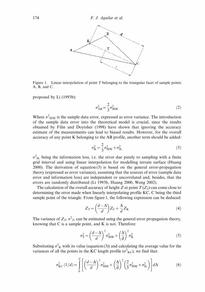
In figure 1, a facet can be observed from the triangular grid established with the use

of the optimal Delaunay triangulation (Guibas and Stolfi 1985). This algorithm

creates triangles by drawing lines between data points. The original points are

connected in such a way that no triangle edges are intersected by other triangles. The

result is a patchwork of triangular facets over the extension of the grid.

The overall average value of error variances for all the points along the whole AB

(s2AB) profile, where A and B are sample data, can be modelled by the equation

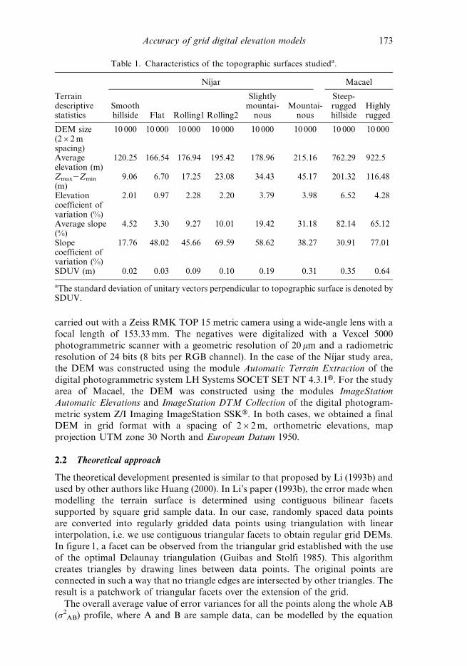
Table 1. Characteristics of the topographic surfaces studieda.

Terraindescriptivestatistics

Nıjar Macael

Smoothhillside Flat Rolling1 Rolling2

Slightlymountai-

nousMountai-

nous

Steep-ruggedhillside

Highlyrugged

DEM size(262 mspacing)

10 000 10 000 10 000 10 000 10 000 10 000 10 000 10 000

Averageelevation (m)

120.25 166.54 176.94 195.42 178.96 215.16 762.29 922.5

Zmax2Zmin

(m)9.06 6.70 17.25 23.08 34.43 45.17 201.32 116.48

Elevationcoefficient ofvariation (%)

2.01 0.97 2.28 2.20 3.79 3.98 6.52 4.28

Average slope(%)

4.52 3.30 9.27 10.01 19.42 31.18 82.14 65.12

Slopecoefficient ofvariation (%)

17.76 48.02 45.66 69.59 58.62 38.27 30.91 77.01

SDUV (m) 0.02 0.03 0.09 0.10 0.19 0.31 0.35 0.64

aThe standard deviation of unitary vectors perpendicular to topographic surface is denoted bySDUV.


proposed by Li (1993b):

s2AB~

2

3s2

SDE ð2Þ

Where s2SDE is the sample data error, expressed as error variance. The introduction

of the sample data error into the theoretical model is crucial, since the results

obtained by Filin and Doytsher (1998) have shown that ignoring the accuracy

estimate of the measurements can lead to biased results. However, for the overall

accuracy of any point K belonging to the AB profile, another term should be added:

s2K~

2

3s2

SDEzs2IL ð3Þ

s2IL being the information loss, i.e. the error due purely to sampling with a finite

grid interval and using linear interpolation for modelling terrain surface (Huang

2000). The derivation of equation (3) is based on the general error-propagation

theory (expressed as error variance), assuming that the sources of error (sample data

error and information loss) are independent or uncorrelated and, besides, that the

errors are randomly distributed (Li 1993b, Huang 2000, Weng 2002).

The calculation of the overall accuracy of height Z at point T (ZT) can come close to

determining the error made when linearly interpolating profile KC, C being the third

sample point of the triangle. From figure 1, the following expression can be deduced:

ZT~d{D

d

� �ZCz

D

dZK ð4Þ

The variance of ZT, s2T, can be estimated using the general error propagation theory,

knowing that C is a sample point, and K is not. Therefore:

s2T~

d{D

d

� �2

s2SDEz

D

d

� �2

s2K ð5Þ

Substituting s2K with its value (equation (3)) and calculating the average value for the

variances of all the points in the KC length profile (s2KC), we find that:

s2KC 1=dð Þ~

ðd0

d{D

d

� �2

s2SDEz

D

d

� �22

3s2

SDEzs2IL

� �" #dD ð6Þ

Figure 1. Linear interpolation of point T belonging to the triangular facet of sample pointsA, B, and C.


Solving the integral proposal, we obtain:

s2KC~

5

9s2

SDEz1

3s2

IL ð7Þ

Notice that the term s2IL must be added again to obtain the overall accuracy of the

points along profile KC, an expression that allows us to determine the average value

for the error of the points on a triangulated surface given as error variance, s2surf.

s2surf~

5

9s2

SDEz4

3s2

IL ð8Þ

The sample data error, s2SDE, evidently depends on the method employed to obtain

sample points.

2.3 Evaluation of the grid DEM accuracy

As we discussed in the previous section, we only need to estimate the value of sIL toevaluate the grid DEM error, ssurf, because sSDE can be obtained from empirical

observations depending on the method used to measure the sample data points. If the

sample data points are considered free of error, the following expression is deduced:

s2surf~

4

3s2

IL ð9Þ

Because the most widely used global accuracy measure for evaluating the performance

of DEMs is the RMSE (Li 1988, Wood 1996, Yang and Hodler 2000), and bearing in

mind that the RMSE is close to the value of ssurf when the mean of residuals tends to be

zero (unbiased residuals), we can write the following equation:

RMSEsurf~2ffiffiffi3

p RMSEIL[RMSEIL~

ffiffiffi3

p

2RMSEsurf ð10Þ

That is to say, estimating RMSEsurf when the sample data points are considered free of

error (sSDE50), we obtain an indirect measure of the value of the information loss

(RMSEIL<sIL).

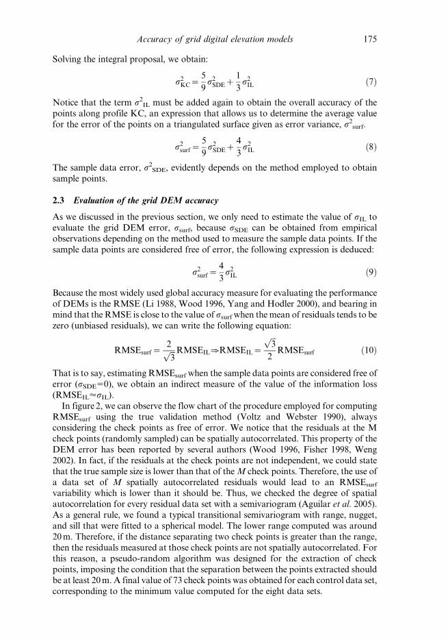
In figure 2, we can observe the flow chart of the procedure employed for computing

RMSEsurf using the true validation method (Voltz and Webster 1990), always

considering the check points as free of error. We notice that the residuals at the M

check points (randomly sampled) can be spatially autocorrelated. This property of the

DEM error has been reported by several authors (Wood 1996, Fisher 1998, Weng

2002). In fact, if the residuals at the check points are not independent, we could state

that the true sample size is lower than that of the M check points. Therefore, the use of

a data set of M spatially autocorrelated residuals would lead to an RMSEsurf

variability which is lower than it should be. Thus, we checked the degree of spatial

autocorrelation for every residual data set with a semivariogram (Aguilar et al. 2005).

As a general rule, we found a typical transitional semivariogram with range, nugget,

and sill that were fitted to a spherical model. The lower range computed was around

20 m. Therefore, if the distance separating two check points is greater than the range,

then the residuals measured at those check points are not spatially autocorrelated. For

this reason, a pseudo-random algorithm was designed for the extraction of check

points, imposing the condition that the separation between the points extracted shouldbe at least 20 m. A final value of 73 check points was obtained for each control data set,

corresponding to the minimum value computed for the eight data sets.


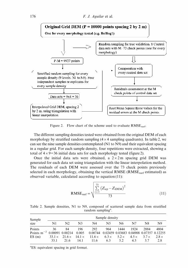
The different sampling densities tested were obtained from the original DEM of each

morphology by stratified random sampling (464 sampling quadrants). In table 2, we

can see the nine sample densities contemplated (N1 to N9) and their equivalent spacing

in a regular grid. For each sample density, four repetitions were extracted, showing a

total of 469536 initial data sets for each morphology tested (figure 2).

Once the initial data sets were obtained, a 262 m spacing grid DEM was

generated for each data set using triangulation with the linear interpolation method.

The residuals of each DEM were assessed over the 73 check points previously

selected in each morphology, obtaining the vertical RMSE (RMSEsurf estimated) as

observed variable, calculated according to equation (11):

RMSEsurf~

ffiffiffiffiffiffiffiffiffiffiffiffiffiffiffiffiffiffiffiffiffiffiffiffiffiffiffiffiffiffiffiffiffiffiffiffiffiffiffiP73

i~1

Zicp{ZiDEM

� �2

73

vuuutð11Þ

Figure 2. Flow chart of the scheme used to evaluate RMSEsurf.

Table 2. Sample densities, N1 to N9, composed of scattered sample data from stratifiedrandom samplinga.

Samplesize

Sample density

N1 N2 N3 N4 N5 N6 N7 N8 N9

Points 36 84 196 292 964 1444 1924 2884 4804Points m22 0.00091 0.00214 0.005 0.00744 0.02459 0.03683 0.04908 0.07357 0.12255ES (m) 33.16

33.121.6621.6

14.1614.1

11.6611.6

6.366.3

5.265.2

4.564.5

3.763.7

2.862.8

aES: equivalent spacing in grid format.


where Zicp is the check point elevation, and ZiDEM is the interpolated grid DEM

elevation.

2.4 Definition and processing of terrain roughness descriptors

As variables that are representative of the topographic surface morphology,

the following descriptors were selected: average terrain slope (AS), standard

deviation of terrain slope (SDS), standard deviation of unitary vectors perpendi-

cular to the topographic surface (SDUV), standard deviation of the height

difference between adjacent samples in the DEM (SDHD), and finally the

roughness estimation by first, second, and third degree surface fitting error

(SFE1, SFE2, and SFE3). The processing and detailed calculation of each one of

these are described below.

First, we proceeded to fill in the grid using triangulation with linear interpolation

from the original sample points (N1 to N9 sampling densities). The appropriate

triangulated irregular network was obtained by the optimal algorithm Delaunay

triangulation (Guibas and Stolfi 1985). A final grid DEM with a spacing of 262 m

was obtained for each original data set, to be considered as input for computing the

descriptors AS, SDS, SDUV, and SDHD. The calculation of descriptors SFE1,

SFE2, and SFE3 was carried out over the original sample data, i.e. without

interpolation.

2.4.1 Average Terrain Slope (AS). Starting from the 262 m spacing grid DEM,

the slope (Sij) was determined in each node of the grid using the gradient calculation:

Sij~

ffiffiffiffiffiffiffiffiffiffiffiffiffiffiffiffiffiffiffiffiffiffiffiffiffiffiffiffiffiffiffiffiffiLzLx

� �2

zLzLy

� �2s

ð12Þ

The third-order finite difference method shown in equation (12) is more accurate

than some of the others (Skidmore 1989) and was therefore chosen for this study.

Using the compass-based grid notation difference, equation (12) yields:

Sij&

ffiffiffiffiffiffiffiffiffiffiffiffiffiffiffiffiffiffiffiffiffiffiffiffiffiffiffiffiffiffiffiffiffiffiffiffiffiffiffiffiffiffiffiffiffiffiffiffiffiffiffiffiffiffiffiffiffiffiZE{ZW

2Dx

� �2

zZN{ZS

2Dy

� �2s

ð13Þ

where ZE, ZW, ZN, and ZS are the elevations of the four cardinal points (east, west,

north and south) neighbours in each node in the grid DEM. Dx and Dy represent the

spacing of the grid DEM, 2 m in our case.

The value of the average terrain slope descriptor would be the arithmetical mean

of the slopes calculated in every node in the grid, excluding the edge values (first and

last rows, first and last columns).

2.4.2 Standard deviation of terrain slope (SDS). The standard terrain slope

deviation was computed in radians from the slope values on each node of the

grid DEM obtained in the previous section:

SDS~

ffiffiffiffiffiffiffiffiffiffiffiffiffiffiffiffiffiffiffiffiffiffiffiffiffiffiffiffiffiffiffiPVi,Vj

Sij{AS� �2

N

vuutð14Þ

with N being the number of points in the grid DEM, Sij the terrain slope at the point

located in row i and column j, and AS the average terrain slope.


2.4.3 Standard deviation of unitary vectors perpendicular to the topographic surface

(SDUV). Once the slope had been determined at each point in the grid DEM, its

aspect was calculated. The algorithm for computing terrain aspect calculates the

downhill direction of the steepest slope at each grid node. The aspect at each grid

node was calculated as angle hij, expressed in degrees, which exists between direction

north and the projection on the horizontal plane of the slope vector normal to the

surface. That is to say, 0u points to the north and 90u points to the east:

hij&270{ tan{1

ZN{ZS

2Dy

ZE{ZW

2Dx

!ð15Þ

The SDUV was computed determining the variance of the unitary vectors which are

perpendicular to the surface in each node (i,j) in the grid DEM (adapted from

Hobson 1972). The Cartesian components xi,j, yi,j, and zi,j of each unitary vector can

be expressed in terms of slope Sij and aspect hij in this node through the following

expressions:

xij~ sin (cij) sin (hij)

yij~ sin (cij) cos (hij)

zij~ cos (cij)

cij~ tan{1 (sij)

ð16Þ

This way, we were able to find the variance of the unitary vectors for each co-

ordinate x, y, z, and determine the total standard deviation (SDUV) using the

following expression:

SDUV~ffiffiffiffiffiffiffiffiffiffiffiffiffiffiffiffiffiffiffiffiffiffiffiffiffiffiffiffiffiffiffiffiffiffiffiffiffiffiffiffiffiffiffiffiffiffiffiffiffiffiffiffiffiffiffiffiffiffiffiffiffiffiffiffiffiffiffiffiffiffiffiffiffiffiffiffiffiffiffiffiffiffivariance (x)zvariance (y)zvariance (z)

pð17Þ

2.4.4 Standard deviation of the height difference between adjacent grid points in the

DEM (SDHD). The standard deviation of the height difference between adjacent

grid points in the DEM has been used as terrain roughness descriptor by some

authors (Evans 1972, Rees 2000). The algorithm used in our case starts from the

interpolated grid DEM with a 262 m spacing. A 363 node mobile window was

shifted over the whole of the interpolated grid DEM. Then, the average height

difference between the central node of the window and the rest of the nodes (eight

closest neighbours) was calculated according to the following expression:

DZP~

P8k~1

ZP{Zkj j

8ð18Þ

Where ZP is the elevation at the central point of the window (node P) and Zk is the

elevation of each of the eight points surrounding node P. Thus, a mean value of the

height differences around each node of the grid DEM was obtained. The SDHD is

defined as the standard deviation of the set of values DZP.

2.4.5 Roughness estimation by first-, second-, and third-degree surface-fitting error

(SFE1, SFE2, and SFE3, respectively). The fitting of a first-, second- or third-degree

surface to the irregular sample point grid of the original DEM can be an indicator of


the terrain roughness (Hobson 1972). In fact, if the regression coefficient R2 is

determined for each fitting, a non-dimensional indicator of the terrain roughness

could be generated using the simple expression SFE512R2. This indicator will be

included between values 0 (optimal fitting of the surface)less roughness) and 1

(worst fitting)maximum roughness).

All the procedures described above were programmed with the SCRIPTERHmodule, included in the SURFER 8.01H (Golden Software Inc. 2002), which allows

the use of the tool Active X Automation to work with the SURFER modelling

engine in an environment that is compatible with Visual BasicH.

3. Relationships between DEM accuracy, sampling density, and terrain roughness

First, and foremost, we shall examine the relationships between DEM error,

sampling density, and terrain roughness to explore the morphology that our

empirical model should have. For this purpose, six morphologies were selected from

the eight that were available, in order to establish and calibrate the different

empirical models tested to estimate the RMSEsurf considering the sample points as

free of error. The morphologies chosen were the following: smooth hillside, rolling1,

slightly mountainous, mountainous, highly rugged, and steep-rugged hillside

(table 1). The two remaining morphologies, flat and rolling2, would be used to

carry out the validation of the empirical models developed.

3.1 DEM error and sampling density

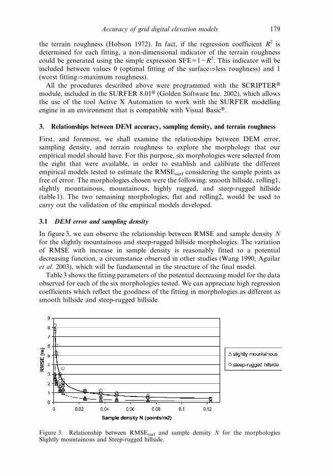
In figure 3, we can observe the relationship between RMSE and sample density N

for the slightly mountainous and steep-rugged hillside morphologies. The variation

of RMSE with increase in sample density is reasonably fitted to a potential

decreasing function, a circumstance observed in other studies (Wang 1990, Aguilar

et al. 2003), which will be fundamental in the structure of the final model.

Table 3 shows the fitting parameters of the potential decreasing model for the data

observed for each of the six morphologies tested. We can appreciate high regression

coefficients which reflect the goodness of the fitting in morphologies as different as

smooth hillside and steep-rugged hillside.

Figure 3. Relationship between RMSEsurf and sample density N for the morphologiesSlightly mountainous and Steep-rugged hillside.


In sections 3.2 and 3.3, the most suitable terrain roughness descriptors to explain

the relief effect on the DEM error will be selected to be included in the model.

3.2 Terrain roughness and sampling density

In the first place, it seems reasonable to request a certain independence from the

terrain descriptor with regard to the spatial distribution and number of original

sample points in the dataset. Thus, the final user of the model can determine the

approximate value of the appropriate descriptor using data previously extracted

from topographic maps (Gao 1995) or DEMs (e.g. in USA: National Elevation

Dataset at the USGS Earth Resources Observation Systems Data Centre; Gesch et

al. 2002). In table 4, one can verify how the descriptors presenting a lower variability

with regard to the number and distribution of sample points are Average Slope and

SDUV. The value calculated for descriptor SDHD is shown as relatively sensitive to

the number and distribution of sample points, especially in the case of mountainous

and slightly mountainous morphologies with coefficients of variation higher than

28%.

In any case, the coefficients of variation calculated show promising results,

especially bearing in mind the range of sample densities employed (from

N150.00091 points m22 to N950.12255 points m22). In figure 4, we can observe

how the variability in determining descriptors SDUV and SDHD is high, above all

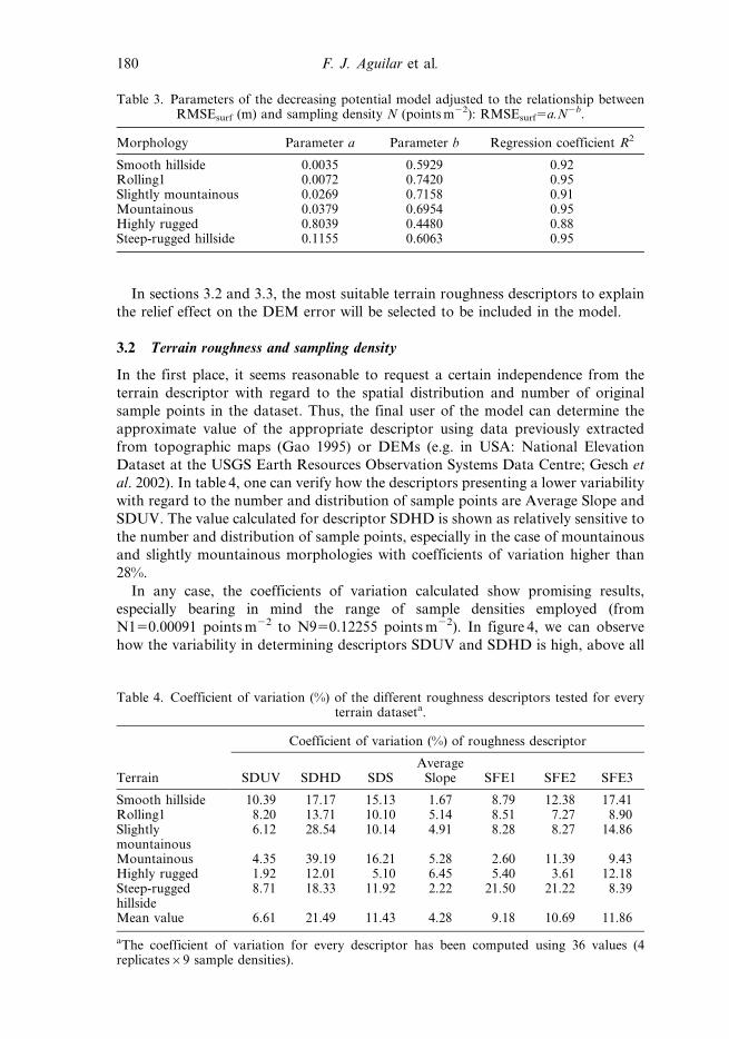
Table 3. Parameters of the decreasing potential model adjusted to the relationship betweenRMSEsurf (m) and sampling density N (points m22): RMSEsurf5a.N2b.

Morphology Parameter a Parameter b Regression coefficient R2

Smooth hillside 0.0035 0.5929 0.92Rolling1 0.0072 0.7420 0.95Slightly mountainous 0.0269 0.7158 0.91Mountainous 0.0379 0.6954 0.95Highly rugged 0.8039 0.4480 0.88Steep-rugged hillside 0.1155 0.6063 0.95

Table 4. Coefficient of variation (%) of the different roughness descriptors tested for everyterrain dataseta.

Terrain

Coefficient of variation (%) of roughness descriptor

SDUV SDHD SDSAverage

Slope SFE1 SFE2 SFE3

Smooth hillside 10.39 17.17 15.13 1.67 8.79 12.38 17.41Rolling1 8.20 13.71 10.10 5.14 8.51 7.27 8.90Slightlymountainous

6.12 28.54 10.14 4.91 8.28 8.27 14.86

Mountainous 4.35 39.19 16.21 5.28 2.60 11.39 9.43Highly rugged 1.92 12.01 5.10 6.45 5.40 3.61 12.18Steep-ruggedhillside

8.71 18.33 11.92 2.22 21.50 21.22 8.39

Mean value 6.61 21.49 11.43 4.28 9.18 10.69 11.86

aThe coefficient of variation for every descriptor has been computed using 36 values (4replicates69 sample densities).


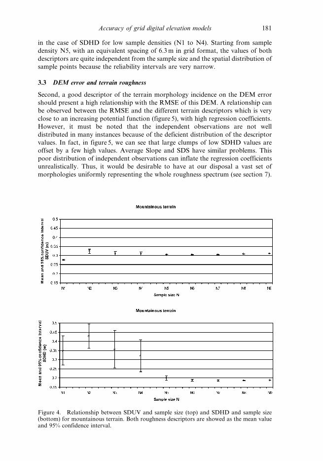
in the case of SDHD for low sample densities (N1 to N4). Starting from sample

density N5, with an equivalent spacing of 6.3 m in grid format, the values of both

descriptors are quite independent from the sample size and the spatial distribution of

sample points because the reliability intervals are very narrow.

3.3 DEM error and terrain roughness

Second, a good descriptor of the terrain morphology incidence on the DEM error

should present a high relationship with the RMSE of this DEM. A relationship can

be observed between the RMSE and the different terrain descriptors which is very

close to an increasing potential function (figure 5), with high regression coefficients.

However, it must be noted that the independent observations are not well

distributed in many instances because of the deficient distribution of the descriptor

values. In fact, in figure 5, we can see that large clumps of low SDHD values are

offset by a few high values. Average Slope and SDS have similar problems. This

poor distribution of independent observations can inflate the regression coefficients

unrealistically. Thus, it would be desirable to have at our disposal a vast set of

morphologies uniformly representing the whole roughness spectrum (see section 7).

Figure 4. Relationship between SDUV and sample size (top) and SDHD and sample size(bottom) for mountainous terrain. Both roughness descriptors are showed as the mean valueand 95% confidence interval.


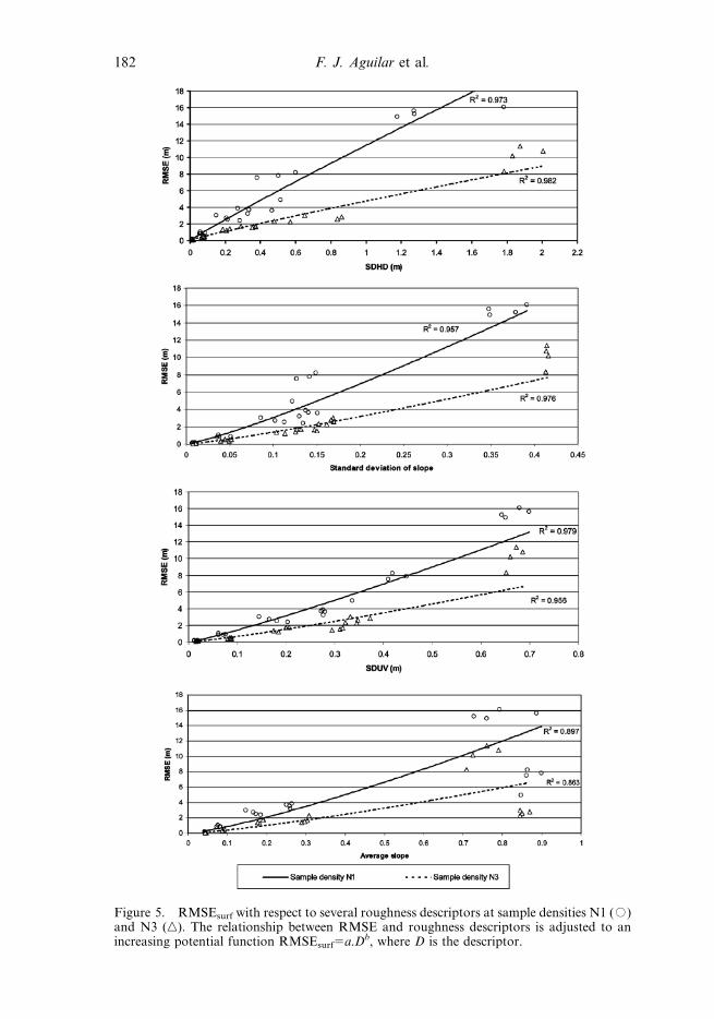
Figure 5. RMSEsurf with respect to several roughness descriptors at sample densities N1 (#)and N3 (n). The relationship between RMSE and roughness descriptors is adjusted to anincreasing potential function RMSEsurf5a.Db, where D is the descriptor.


In any case, using only the Average Slope terrain descriptor R2, values lower than

0.90 were obtained, due to a defective fitting of the model to the morphologies in the

Macael site. Let us recall that these morphologies are constituted by quarry terrains

with a terraced and anthropic relief, where steep slopes and even vertical walls are

predominant (table 1).

On the other hand, the group of descriptors SFE1, SFE2, and SFE3 showed very

low regression coefficients, lower than 0.50 in each case. The inefficiency shown by

the terrain descriptor Surface Fitting Error for the modelling of the DEM error is

due to the fact that it presents a high dependence on the morphological analysis

scale. When we seek to fit a first-, second-, or third-degree surface to terrain with

homogenous behaviour on a large scale, a hillside for example (steep-rugged

hillside), excessively low SFE values are obtained. That is to say, the local roughness

is underestimated. Conversely, let us suppose we wish to fit a first-degree surface, a

flat surface, to the triangular transversal section of a riverbed. In this case, the fitting

will be deficient, and therefore SFE1 will adopt a very high value, although the local

roughness of the riverbed is actually very low.

4. Development of empirical models

Once the relationships between the variables involved in grid DEM error modelling

have been described, we can conclude that the structure of the empirical model

should conform starting from the product of two potential functions, increasing in

the case of the terrain descriptor and decreasing in the case of the sampling density.

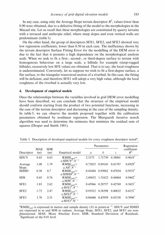
In table 5, we can observe the models proposed together with the calibration

parameters obtained by nonlinear regression. The Marquardt iterative search

algorithm was used to determine the estimates that minimize the residual sum of

squares (Draper and Smith 1981).

Table 5. Description of developed empirical models for every roughness descriptor testeda.

DescriptorMAE(m)

SDR(m) Empirical model

Parameters Regressioncoefficient

R2a b c

SDUV 0.43 0.63 RMSEsurf5a.SDUVb.N2c

2.3175 1.71739 0.38001 0.9618*

AverageSlope

1.08 1.79 RMSEsurf5a.ASb.N2c

0.73825 0.89145 0.41707 0.6929*

SDHD 0.38 0.7 RMSEsurf5a.SDHDb.N2c

0.41684 0.95062 0.47034 0.9533*

SDS 0.45 0.76 RMSEsurf5a.SDSb.N2c

2.69652 1.31622 0.44464 0.9442*

SFE1 1.83 2.62 RMSEsurf5a.SFE1b.N2c

0.45966 0.28757 0.42769 0.3421*


0.91912 0.56598 0.40632 0.4151*


0.86444 0.43959 0.43158 0.3996*

aRMSEsurf is expressed in metres and sample density (N) in points m22. SDUV and SDHDare expressed in m and SDS in radians. Average Slope, SFE1, SFE2, and SFE3 are non-dimensional. MAE: Mean Absolute Error. SDR: Standard Deviation of Residuals.*Significant at the 0.01 level.


One can verify how parameter ‘c’ of the potential decreasing function presents

similar values in every model developed, indicating that the variation of the RMSE

with sampling density N is independent of the type of terrain descriptor employed.

On the other hand, one can see how the models containing descriptors SDUV,

SDHD, and SDS present very acceptable results with R2 regression coefficients

higher than 0.94. However, in the case of the SFE group of descriptors, low R2

values have been obtained, thus confirming their inefficacy to model DEM error for

the reasons stated in section 3.3.

Equally, the model that employs Average Slope as descriptor offered a mediocre

fitting to the data observed, as also pointed out in section 3.3 (figure 5). No doubt,

the inclusion of extremely rugged terrain such as that situated in the marble quarries

of Macael, with very steep slopes and terraced and anthropic morphology, has

decreased the efficacy of Average Slope to model the RMSE of the grid DEM

generated.

Based on experimental tests, Ackermann (1980) established that the relationship

between DEM error and sampling interval is linear. Likewise, he obtained linear

relationships between the mean slope of an area and the error of a DEM. Both

findings led him to formulate the following model.

s2DEM~K1s

2rawzK2(Dxtana)2 ð19Þ

where Dx denotes the sampling interval, tana is the mean slope of the area, s2raw is

the error variance of raw data (error of sample data measurements), and s2DEM is

the error variance of the final DEM. Parameters K1 and K2 were later added by Li

(1993a). If the sample data points are supposed to be free of error (s2raw50), we

have a very similar model to the empirical one proposed in this study where Average

Slope is used as descriptor. In fact, applying the equation (19) model to our data, an

R2 value of 0.68 is obtained, a similar value to that presented in table 5. When the

data from the two Macael morphologies (steep-rugged hillside and highly rugged)

are removed in the regression analysis, the value of R2 increases to 0.92. Thus, it can

be concluded that the Average Slope can be a good roughness descriptor for terrain

with geomorphology modelled by natural processes and where slopes are neither

extreme nor too variable, at least on a local scale.

The Mean Absolute Error (MAE) and Standard Deviation of Residuals (SDR)

values shown in table 5 confirm what has been stated above. Those models based on

descriptors SDUV, SDHD, and Standard Deviation of Slope show a lower MAE

and SDR than those based on the Average Slope and SFE. That is to say, all the

differences between the RMSE values observed and fitted by the model are lower

and present moreover a lower dispersion with regard to the mean value. The

quantitative differences in the data fitting observed in models SDUV, SDHD, and

Standard Deviation of Slope are unimportant, judging by the R2, MAE, and SDR

values. In any case, it must be stressed that although the SDHD model shows a

slightly higher dispersion of residuals than model SDUV, the MAE value is lower,

which indicates the existence of a series of point residuals with a high absolute value

which artificially increases the value of the SDR, hence the decrease in the regression

coefficient (see figure 6).

Figure 6 shows the plots of the differences between the observed and the fitted

RMSEs for terrain descriptors SDHD, SDUV, Average Slope, and Standard

Deviation of Slope. We can highlight how the majority of the empirical models show

problems for modelling the RMSEs computed in the steep-rugged hillside and


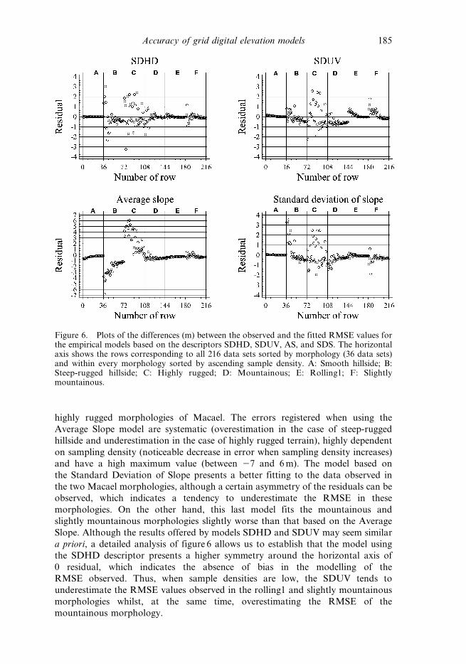
highly rugged morphologies of Macael. The errors registered when using the

Average Slope model are systematic (overestimation in the case of steep-rugged

hillside and underestimation in the case of highly rugged terrain), highly dependent

on sampling density (noticeable decrease in error when sampling density increases)

and have a high maximum value (between 27 and 6 m). The model based on

the Standard Deviation of Slope presents a better fitting to the data observed in

the two Macael morphologies, although a certain asymmetry of the residuals can be

observed, which indicates a tendency to underestimate the RMSE in these

morphologies. On the other hand, this last model fits the mountainous and

slightly mountainous morphologies slightly worse than that based on the Average

Slope. Although the results offered by models SDHD and SDUV may seem similar

a priori, a detailed analysis of figure 6 allows us to establish that the model using

the SDHD descriptor presents a higher symmetry around the horizontal axis of

0 residual, which indicates the absence of bias in the modelling of the

RMSE observed. Thus, when sample densities are low, the SDUV tends to

underestimate the RMSE values observed in the rolling1 and slightly mountainous

morphologies whilst, at the same time, overestimating the RMSE of the

mountainous morphology.

Figure 6. Plots of the differences (m) between the observed and the fitted RMSE values forthe empirical models based on the descriptors SDHD, SDUV, AS, and SDS. The horizontalaxis shows the rows corresponding to all 216 data sets sorted by morphology (36 data sets)and within every morphology sorted by ascending sample density. A: Smooth hillside; B:Steep-rugged hillside; C: Highly rugged; D: Mountainous; E: Rolling1; F: Slightlymountainous.


Another aspect to be considered in the empirical models developed is the

variability of the predicted RMSE with regard to the configuration of the original

sample points. All the models developed have shown a mean variability, expressed

as coefficient of variation, lower than 10% (table 6), which can be considered

acceptable. We must highlight that the relative variability with regard to the sample

density shown by the SDHD descriptor (table 4) has been smoothed by the value of

parameters ‘a’ and ‘b’ obtained in the empirical model fitting (table 5).

Finally, the use of global terrain variability measures only makes sense in

calculating the global error of a grid DEM working over the same area where the

terrain descriptor has been calculated, i.e. there is an implicit assumption that

descriptor variability is stationary across the study area. Obviously, it would be

desirable for DEM accuracy to be a local variability function rather than a single,

possibly quite misleading, global average. However, it is difficult and sometimes

unapproachable, at least in practice, in the mapping production environment. Note

that although Slope has been found to be the most important terrain-surface

descriptor and is widely used in surveying and mapping (Balce 1987, Li 1993b), it

presents a remarkable dependency on the characterization scale. In fact, since the

scale is arbitrarily defined and not necessarily related to the scale of characterization

required, the derived results may not always be appropriate (Wood 1996). Indeed,

Slope is considered scarcely useful to estimate local roughness or to detect variation

at a finer scale than DEM. For instance, let us consider two surfaces: one is a plain

tilted at 10u. The other is a moderately varying field with an Average Slope of 10u.The two surfaces present the same Average Slope, but their corresponding grid

DEMs will probably present a different global error because the local roughness can

be remarkably different.

Thus, terrain descriptors more sensitive to changes in local roughness (e.g.

SDHD, SDS or SDUV) can perform better than those more centred to describe the

roughness variation on a coarser scale (e.g. Average Slope or SFE).

5. Validation of empirical models

Although the observations discussed in the previous section point to the model

based on terrain descriptor SDHD as the most appropriate, the results had to be

validated on morphologies not used in the calibration of empirical models. This

validation was carried out on the flat and rolling2 morphologies (table 1). In

Table 6. Coefficient of variation (CV) of predicted RMSEsurf for every morphology androughness descriptors, computed as CV5(CVN1+CVN2 +…+CVN9)/9, CVNi being the

coefficient of variation for the sample density Ni (four data or replicates).

Terrain

Coefficient of variation (%) of predicted RMSEsurf

SDUV SDHD Average slopeStandard

deviation of slope

Smooth hillside 10.62 9.41 0.70 11.50Rolling1 5.71 7.29 1.39 8.26Slightly mountainous 7.14 12.83 1.91 8.38Mountainous 2.46 11.41 1.32 5.25Highly rugged 1.66 5.71 2.06 1.67Steep-rugged hillside 5.48 10.45 0.83 3.75Mean value 5.51 9.52 1.37 6.47


figure 7, we can see the plots of the maximum and minimum RMSE (by means of the

95% confidence interval) versus the sampling density for predicted and observed

data on flat terrain. The empirical models based on terrain descriptors SDHD,

Standard Deviation of Slope, SDUV, and Average Slope were tested. As we stated

previously, the model that best reproduced the data observed on flat terrain was

based on the SDHD descriptor, closely followed by the one based on the Standard

Deviation of Slope. The SDUV model underestimated the observed RMSE, whereas

the Average Slope did the opposite, probably because it was calibrated with a very

high Average Slope.

In figure 8, the validation carried out on the rolling2 morphology is shown. The

behaviour of the four models developed is similar to that observed on flat terrain,

although in this case the SDHD model showed itself as clearly superior to the

others. In every model, we can observe a slight overestimation of the observed

RMSE at high-level densities. Once more the Average Slope model presented a

tendency to overestimate the observed data, a circumstance that in this case can also

be seen in the Standard Deviation of Slope.

6. Conclusions

In this study, a theoretical-empirical model has been developed which determines

the error that occurs when modelling the terrain surface from randomly spaced data

points that are converted into regularly gridded data points using triangulation with

linear interpolation. The model consists of a theoretical part based on the error

propagation theory, and of an empirical part which attempts to determine the value

of what is known as Information Loss (RMSEIL), i.e. the error due purely to

sampling with a finite grid interval and to using linear interpolation of the terrain

surface (Huang 2000). The empirical models developed present a morphology based

on the product of two potential functions, an increasing one related to terrain

roughness, and a decreasing one related to sample density. Some of the bi-variant

empirical models developed explain with reasonable accuracy (R2.0.94) the global

error of a grid DEM in terms of Root Mean Square Error. To be specific, the results

obtained in this study allow us to highlight the empirical model based on the SDHD

terrain descriptor as the one that best reproduces, both on a calibration level and on

a validation level, the observed grid DEM error in the majority of the morphologies

studied, considering that the sample data points are free of error. Thus, bearing in

mind the theoretical development shown in sections 2.2 and 2.3, the average value

for the error of a grid DEM linearly constructed from scattered sample data,

RMSEsurf (m), can be expressed by means of the following equation:

RMSEsurf~

ffiffiffiffiffiffiffiffiffiffiffiffiffiffiffiffiffiffiffiffiffiffiffiffiffiffiffiffiffiffiffiffiffiffiffiffiffiffiffiffiffiffiffiffiffiffiffiffiffiffiffiffiffiffiffiffiffiffiffiffiffiffiffiffiffiffiffiffiffiffiffiffiffiffiffiffiffiffiffiffiffiffiffiffiffiffiffiffiffiffi5

9RMSE2

SDEz 0:4168SDHD0:9506N{0:4703� �2

rð20Þ

where RMSESDE is the sample data error, expressed as root mean square error (m),

SDHD is the standard deviation of the height difference between adjacent grid

points in the DEM (m), and N is the sampling density (points m22).

Equally, RMSEIL (m) can be determined using the following expression:

RMSEIL~

ffiffiffi3

p

20:4168 SDHD0:9506N{0:4703 ð21Þ

The findings obtained in this work could be used as a guide for the selection of


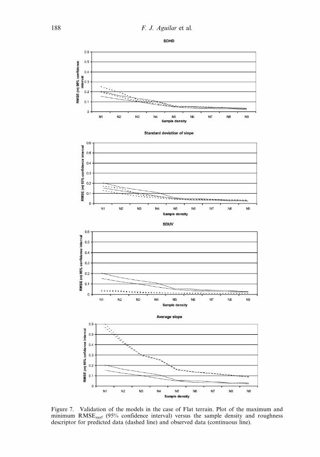
Figure 7. Validation of the models in the case of Flat terrain. Plot of the maximum andminimum RMSEsurf (95% confidence interval) versus the sample density and roughnessdescriptor for predicted data (dashed line) and observed data (continuous line).


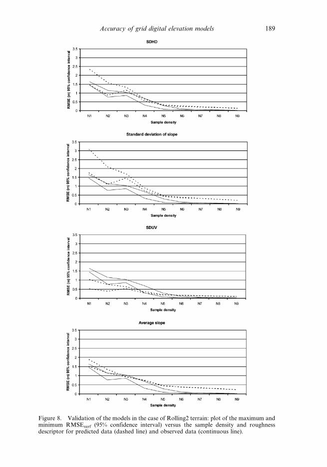
Figure 8. Validation of the models in the case of Rolling2 terrain: plot of the maximum andminimum RMSEsurf (95% confidence interval) versus the sample density and roughnessdescriptor for predicted data (dashed line) and observed data (continuous line).


appropriate resolutions in linearly constructed DEMs from scattered sample data,

given the accuracy required and the terrain roughness.

7. Further works

Apart from the descriptors based on the Surface Fitting Error (SFE), which have

been proved totally inefficient for modelling the grid DEM error, the rest of the

terrain descriptors tested have shown certain advantages and disadvantages. In our

case, the SDHD model has proved to be the one that best reproduced the RMSE

observed in the eight morphologies studied. We must point out that these

morphologies presented a very broad range of slopes and ruggedness, due basically

to the inclusion of the quarry soils located in Macael. On the other hand, terrain

descriptors Average Slope and SDUV have shown a lower variability than SDHD

with regard to the number and distribution of the sample points, which can be

considered as favourable elements. In short, it is likely that a single ideal terrain

descriptor does not exist for all morphology types that can be found in practice.

Each one represents an optimal application range. Thus, we would recommend the

inclusion in the empirical model of a particular descriptor with regard to the

objective parameters of each terrain, such as its mean slope or its roughness

(measured with the SDUV indicator, for example). For the ‘a la carte’ development

of these models we should have at our disposal a vast set of morphologies uniformly

representing the whole roughness spectrum. This terrain dataset could be implemented

generating synthetic self-similar surfaces with, for example, a fractional Brownian

process using a range of values for the fractal dimension (Goodchild and Mark 1987).

An infinitely rugged surface should have a limiting fractal dimension of 3, whereas a

smooth surface should have a fractal dimension of 2.

Acknowledgements

The authors are grateful to the Consejerıa de Agricultura y Pesca of the Andalusia

Government for financing this work through the Project: ‘Cartografıa basica para la

redaccion del proyecto de red de riego del Campo de Nıjar (Almerıa)’ (Basic

Cartography for the design of the Campo de Nıjar irrigation network project).

Thanks are also due to Prof. J. Delgado and Prof. J. Cardenal from the University

of Jaen (Spain).

ReferencesACKERMANN, F., 1980, The accuracy of digital terrain models. In Proceedings of 37th

Photogrammetric Week (Stuttgart: University of Stuttgart), pp. 113–143.

AGUILAR, F.J., AGUERA, F., AGUILAR, M.A. and CARVAJAL, F., 2005, Effects of terrain

morphology, sampling density and interpolation methods on grid DEM accuracy.

Photogrammetric Engineering and Remote Sensing, 71(7), pp. 805–816.

AGUILAR, F.J., AGUERA, F., AGUILAR, M.A., CARVAJAL, F. and SANCHEZ, P.L., 2003, Grid

digital elevation models accuracy. Analysis and modelling. In Proceedings of the 13th

ADM and 15th INGEGRAF International Conference on Tools and Methods Evolution

in Engineering Design (Naples: Universita degli studi di Napoli Federico II), CD

ROM Proceedings.

AYENI, O.O., 1982, Optimum sampling for digital terrain models: a trend towards automation.

Photogrammetric Engineering and Remote Sensing, 48(11), pp. 1687–1694.

BALCE, A.E., 1987, Determination of optimum sampling interval in grid digital elevation

models (DEM) data acquisition. Photogrammetric Engineering and Remote Sensing,

53(3), pp. 323–330.


BRIESE, C., PFEIFER, N. and DORNINGER, P., 2002, Applications of the robust interpolation

method from DTM determination. International Archives of Photogrammetry and

Remote Sensing, 34(3A), pp. 55–61.

DANIEL, C. and TENNANT, K., 2001, DEM quality assessment. In Digital Elevation Models

and Applications: The DEM Users Manual, D.F. Maune (Ed.), pp. 395–440 (Bethesda,

MD: ASPRS).

DAVIS, C.H., JIANG, H. and WANG, X., 2001, Modeling and estimation of the spatial variation

of elevation error in high resolution DEMs from stereo-image processing. IEEE

Transactions on Geoscience and Remote Sensing, 39(11), pp. 2483–2489.

DRAPER, N.R. and SMITH, H., 1981, Applied regression analysis, 2nd edition (New York:

Wiley).

EVANS, I.S., 1972, General geomorphometry, derivatives of altitude and descriptive statistics.

In Spatial Analysis in Geomorphology, R.J. Chorley (Ed.), pp. 17–91 (London:

Methuen).

FELICISIMO, A., 1994, Parametric statistical method for error detection in digital elevation

models. ISPRS Journal of Photogrammetry and Remote Sensing, 49(4), pp. 29–33.

FILIN, S. and DOYTSHER, Y., 1998, Estimating accuracy of photogrammetric data.

Mechanism and implementation. Journal of Surveying Engineering, 124(4), pp.

156–170.

FISHER, P., 1998, Improved modeling of elevation error with geostatistics. GeoInformatica,

2(3), pp. 215–233.

GAO, J., 1995, Comparison of sampling schemes in constructing DTMs from topographic

maps. ITC Journal, 1, pp. 18–22.

GAO, J., 1997, Resolution and accuracy of terrain representation by grid DEMs at a micro-

scale. International Journal of Geographical Information Systems, 11(2), pp. 199–212.

GESCH, D., OIMOEN, M., GREENLEE, S., NELSON, C., STEUCK, M. and TYLER, D., 2002, The

National Elevation Dataset. Photogrammetric Engineering and Remote Sensing, 68(1),

pp. 5–11.

GOLDEN SOFTWARE INC. 2002, Surfer 8 Users’ Guide (Golden, CO: Golden Software).

GONG, J., LI, Z., ZHU, Q., SUI, H. and ZHOU, Y., 2000, Effects of various factors on the

accuracy of DEMs: an intensive experimental investigation. Photogrammetric

Engineering and Remote Sensing, 66(9), pp. 1113–1117.

GOODCHILD, M.F. and MARK, D.M., 1987, The fractal nature of geographic phenomena.

Annals of the Association of American Geographers, 77(2), pp. 265–278.

GUIBAS, L. and STOLFI, J., 1985, Primitives for the manipulation of general subdivisions and

the computation of Voronoi diagrams. ACM Transactions on Graphics, 4(2), pp.

74–123.

HOBSON, R.D., 1972, Surface roughness in topography: quantitative approach. In Spatial

Analysis in Geomorphology, R.J. Chorley (Ed.), pp. 221–245 (London: Methuen).

HUANG, Y.D., 2000, Evaluation of information loss in digital elevation models with digital

photogrammetric systems. Photogrammetric Record, 16(95), pp. 781–791.

KARRAS, G.E., MAVROGENNEAS, N., MAVROMMATI, D. and TSIKONIS, N., 1998, Tests on

automatic DEM generation in a digital photogrammetric workstation. International

Archives of Photogrammetry and Remote Sensing, 32(2), pp. 136–139.

KUBIK, K. and BOTMAN, A.G., 1976, Interpolation accuracy for topographic and geological

surfaces. ITC Journal, 2, pp. 236–274.

LI, Z., 1988, On the measure of digital terrain model accuracy. Photogrammetric Record,

12(72), pp. 873–877.

LI, Z., 1992, Variation of the accuracy of digital terrain models with sampling interval.

Photogrammetric Record, 14(79), pp. 113–128.

LI, Z., 1993a, Theoretical models of the accuracy of digital terrain models: an evaluation and

some observations. Photogrammetric Record, 14(82), pp. 651–660.

LI, Z., 1993b, Mathematical models of the accuracy of digital terrain model surfaces linearly

constructed from square gridded data. Photogrammetric Record, 14(82), pp. 661–674.


LOPEZ, C., 1997, Locating some types of random errors in digital terrain models. International

Journal of Geographical Information Science, 11(7), pp. 677–698.

MAKAROVIC, B., 1972, Information transfer in reconstruction of data from sampled points.

Photogrammetria, 28(4), pp. 111–130.

QUEIJA, V.R., STOKER, J.M. and KOSOVICH, J.J., 2005, Recent US Geological Survey

applications of Lidar. Photogrammetric Engineering and Remote Sensing, 71(1), pp.

5–9.

REES, W.G., 2000, The accuracy of digital elevation models interpolated to higher resolutions.

International Journal of Remote Sensing, 21(1), pp. 7–20.

SALEH, R. and SCARPACE, F., 2000, Image scanning resolution and surface accuracy;

experimental results. International Archives of Photogrammetry and Remote Sensing,

33(part B), pp. 482–485.

SKIDMORE, A.K., 1989, A comparison of techniques for calculating gradient and aspect from

a gridded digital elevation model. International Journal of Geographical Information

Systems, 3(4), pp. 323–334.

SMITH, S.L., 2004, ISPRS Workshop on 3D reconstruction from laser scanner and InSAR

data. Photogrammetric Record, 19(105), pp. 74–76.

TORLEGARD, K., OSTMAN, A. and LINDGREN, R., 1986, A comparative test of photo-

grammetrically sampled digital elevation model. Photogrammetria, 41(1), pp. 1–16.

VOLTZ, M. and WEBSTER, R.A., 1990, A comparison of kriging cubic splines and classification

for predicting soil properties from sample information. Journal of Soil Science, 41(3),

pp. 473–490.

WANG, L., 1990, Comparative studies of spatial interpolation accuracy, Master thesis,

Department of Geography, University of Georgia, USA.

WENG, Q., 2002, Quantifying uncertainty of digital elevation models derived from

topographic maps. In Advances in Spatial Data Handling, D. Richardson and P.

van Oosterom (Eds), pp. 403–418 (New York: Springer).

WOOD, J.D., 1996, The geomorphological characterisation of digital elevation models. PhD

thesis, University of Leicester, UK.

WOOD, J.D. and FISHER, P.F., 1993, Assessing interpolation accuracy in elevation models.

IEEE Computer Graphics & Applications, 13(2), pp. 48–56.

YANG, X. and HODLER, T., 2000, Visual and statistical comparisons of surface modelling

techniques for point-based environmental data. Cartography and Geographic

Information Science, 27(2), pp. 165–175.

192 Accuracy of grid digital elevation models

The accuracy of grid digital elevation models linearly constructed from scattered sample data

Documents

Transcript of The accuracy of grid digital elevation models linearly constructed from scattered sample data