
Active error detection and resolution for speech-to-speech ...
Upload
khangminh22Category
view
0download
0
Text-to-Speech Synthesis
Paul Taylor
University of Cambridge


Summary of Contents1 Introduction . . . . . . . . . . . . . . . . . . . . . . . . . . . . . . . . . . . . . .. . . . . . . . . . . . . . . . . . . . . . . . . 12 Communication and Language . . . . . . . . . . . . . . . . . . . . . . . . . .. . . . . . . . . . . . . . . . . . . 83 The Text-to-Speech Problem . . . . . . . . . . . . . . . . . . . . . . . . . .. . . . . . . . . . . . . . . . . . . . . . 264 Text Segmentation and Organisation . . . . . . . . . . . . . . . . . . .. . . . . . . . . . . . . . . . . . . . . 525 Text Decoding. . . . . . . . . . . . . . . . . . . . . . . . . . . . . . . . . . . . . .. . . . . . . . . . . . . . . . . . . . . . . . 796 Prosody Prediction from Text . . . . . . . . . . . . . . . . . . . . . . . . .. . . . . . . . . . . . . . . . . . . . . . 1127 Phonetics and Phonology . . . . . . . . . . . . . . . . . . . . . . . . . . . . .. . . . . . . . . . . . . . . . . . . . . . 1478 Pronunciation . . . . . . . . . . . . . . . . . . . . . . . . . . . . . . . . . . . . .. . . . . . . . . . . . . . . . . . . . . . . . . 1939 Synthesis of Prosody . . . . . . . . . . . . . . . . . . . . . . . . . . . . . . . .. . . . . . . . . . . . . . . . . . . . . . . 22710 Signals and Filters . . . . . . . . . . . . . . . . . . . . . . . . . . . . . . . .. . . . . . . . . . . . . . . . . . . . . . . . . 26511 Acoustic Models of Speech Production . . . . . . . . . . . . . . . . .. . . . . . . . . . . . . . . . . . . . . 31612 Analysis of Speech Signals . . . . . . . . . . . . . . . . . . . . . . . . . .. . . . . . . . . . . . . . . . . . . . . . . . 34913 Synthesis Techniques based on Vocal Tract Models . . . . . . .. . . . . . . . . . . . . . . . . . . 39614 Synthesis by Concatenation and Signal Processing Modification . . . . . . . . . . . . . . 42215 Hidden Markov Model Synthesis. . . . . . . . . . . . . . . . . . . . . . .. . . . . . . . . . . . . . . . . . . . . 44616 Unit Selection Synthesis . . . . . . . . . . . . . . . . . . . . . . . . . . .. . . . . . . . . . . . . . . . . . . . . . . . . 48417 Further Issues . . . . . . . . . . . . . . . . . . . . . . . . . . . . . . . . . . . .. . . . . . . . . . . . . . . . . . . . . . . . . 52818 Conclusions . . . . . . . . . . . . . . . . . . . . . . . . . . . . . . . . . . . . . .. . . . . . . . . . . . . . . . . . . . . . . . . . 545
iii


Summary of Contents v
Preface. . . . . . . . . . . . . . . . . . . . . . . . . . . . . . . . . . . . . . . . . . . .. . . . . . . . . . . . . . . . . . . . . . . . . . . . xix1 Introduction . . . . . . . . . . . . . . . . . . . . . . . . . . . . . . . . . . . . . .. . . . . . . . . . . . . . . . . . . . . . . . . 1
1.1 What are text-to-speech systems for? . . . . . . . . . . . . . . . .. . . . . . . 21.2 What should the goals of text-to-speech system development be? . . . . . . . . 31.3 The Engineering Approach . . . . . . . . . . . . . . . . . . . . . . . . . .. . 41.4 Overview of the book . . . . . . . . . . . . . . . . . . . . . . . . . . . . . . . 5
1.4.1 Viewpoints within the book . . . . . . . . . . . . . . . . . . . . . . . 51.4.2 Readers’ backgrounds . . . . . . . . . . . . . . . . . . . . . . . . . . 61.4.3 Background and specialist sections . . . . . . . . . . . . . . .. . . . 7
2 Communication and Language . . . . . . . . . . . . . . . . . . . . . . . . . .. . . . . . . . . . . . . . . . . . . 82.1 Types of communication . . . . . . . . . . . . . . . . . . . . . . . . . . . .. . 8
2.1.1 Affective communication . . . . . . . . . . . . . . . . . . . . . . . .. 82.1.2 Iconic communication . . . . . . . . . . . . . . . . . . . . . . . . . . 92.1.3 Symbolic communication . . . . . . . . . . . . . . . . . . . . . . . . 102.1.4 Combinations of symbols . . . . . . . . . . . . . . . . . . . . . . . . 112.1.5 Meaning, form and signal . . . . . . . . . . . . . . . . . . . . . . . . 12
2.2 Human Communication . . . . . . . . . . . . . . . . . . . . . . . . . . . . . .132.2.1 Verbal communication . . . . . . . . . . . . . . . . . . . . . . . . . . 142.2.2 Linguistic levels . . . . . . . . . . . . . . . . . . . . . . . . . . . . . 162.2.3 Affective Prosody . . . . . . . . . . . . . . . . . . . . . . . . . . . . 172.2.4 Augmentative Prosody . . . . . . . . . . . . . . . . . . . . . . . . . . 18
2.3 Communication processes . . . . . . . . . . . . . . . . . . . . . . . . . .. . . 182.3.1 Communication factors . . . . . . . . . . . . . . . . . . . . . . . . . .192.3.2 Generation . . . . . . . . . . . . . . . . . . . . . . . . . . . . . . . . 202.3.3 Encoding . . . . . . . . . . . . . . . . . . . . . . . . . . . . . . . . . 212.3.4 Decoding . . . . . . . . . . . . . . . . . . . . . . . . . . . . . . . . . 222.3.5 Understanding . . . . . . . . . . . . . . . . . . . . . . . . . . . . . . 23
2.4 Discussion . . . . . . . . . . . . . . . . . . . . . . . . . . . . . . . . . . . . . 232.5 Summary . . . . . . . . . . . . . . . . . . . . . . . . . . . . . . . . . . . . . . 24
3 The Text-to-Speech Problem . . . . . . . . . . . . . . . . . . . . . . . . . .. . . . . . . . . . . . . . . . . . . . . . 263.1 Speech and Writing . . . . . . . . . . . . . . . . . . . . . . . . . . . . . . . .26
3.1.1 Physical nature . . . . . . . . . . . . . . . . . . . . . . . . . . . . . . 273.1.2 Spoken form and written form . . . . . . . . . . . . . . . . . . . . . .283.1.3 Use . . . . . . . . . . . . . . . . . . . . . . . . . . . . . . . . . . . . 293.1.4 Prosodic and verbal content . . . . . . . . . . . . . . . . . . . . . .. 313.1.5 Component balance . . . . . . . . . . . . . . . . . . . . . . . . . . . 313.1.6 Non-linguistic content . . . . . . . . . . . . . . . . . . . . . . . . .. 323.1.7 Semiotic systems . . . . . . . . . . . . . . . . . . . . . . . . . . . . . 333.1.8 Writing Systems . . . . . . . . . . . . . . . . . . . . . . . . . . . . . 34
3.2 Reading aloud . . . . . . . . . . . . . . . . . . . . . . . . . . . . . . . . . . . 35

vi Summary of Contents
3.2.1 Reading silently and reading aloud . . . . . . . . . . . . . . . .. . . . 353.2.2 Prosody in reading aloud . . . . . . . . . . . . . . . . . . . . . . . . .363.2.3 Verbal content and style in reading aloud . . . . . . . . . . .. . . . . 37
3.3 Text-to-speech system organisation . . . . . . . . . . . . . . . .. . . . . . . . 383.3.1 The Common Form model . . . . . . . . . . . . . . . . . . . . . . . . 383.3.2 Other models . . . . . . . . . . . . . . . . . . . . . . . . . . . . . . . 393.3.3 Comparison . . . . . . . . . . . . . . . . . . . . . . . . . . . . . . . . 40
3.4 Systems . . . . . . . . . . . . . . . . . . . . . . . . . . . . . . . . . . . . . . 413.4.1 A Simple text-to-speech system . . . . . . . . . . . . . . . . . . .. . 413.4.2 Concept to speech . . . . . . . . . . . . . . . . . . . . . . . . . . . . 423.4.3 Canned Speech and Limited Domain Synthesis . . . . . . . . .. . . . 43
3.5 Key problems in Text-to-speech . . . . . . . . . . . . . . . . . . . . .. . . . . 443.5.1 Text classification with respect to semiotic systems .. . . . . . . . . . 443.5.2 Decoding natural language text . . . . . . . . . . . . . . . . . . .. . 463.5.3 Naturalness . . . . . . . . . . . . . . . . . . . . . . . . . . . . . . . . 473.5.4 Intelligibility: encoding the message in signal . . . .. . . . . . . . . . 483.5.5 Auxiliary generation for prosody . . . . . . . . . . . . . . . . .. . . . 493.5.6 Adapting the system to the situation . . . . . . . . . . . . . . .. . . . 50
3.6 Summary . . . . . . . . . . . . . . . . . . . . . . . . . . . . . . . . . . . . . . 504 Text Segmentation and Organisation . . . . . . . . . . . . . . . . . . .. . . . . . . . . . . . . . . . . . . . . 52
4.1 Overview of the problem . . . . . . . . . . . . . . . . . . . . . . . . . . . .. 524.2 Words and Sentences . . . . . . . . . . . . . . . . . . . . . . . . . . . . . . .53
4.2.1 What is a word? . . . . . . . . . . . . . . . . . . . . . . . . . . . . . 544.2.2 Defining words in text-to-speech . . . . . . . . . . . . . . . . . .. . . 554.2.3 Scope and morphology . . . . . . . . . . . . . . . . . . . . . . . . . . 594.2.4 Contractions and Clitics . . . . . . . . . . . . . . . . . . . . . . . .. 604.2.5 Slang forms . . . . . . . . . . . . . . . . . . . . . . . . . . . . . . . . 614.2.6 Hyphenated forms . . . . . . . . . . . . . . . . . . . . . . . . . . . . 624.2.7 What is a sentence? . . . . . . . . . . . . . . . . . . . . . . . . . . . . 634.2.8 The lexicon . . . . . . . . . . . . . . . . . . . . . . . . . . . . . . . . 64
4.3 Text Segmentation . . . . . . . . . . . . . . . . . . . . . . . . . . . . . . . .. 644.3.1 Tokenisation . . . . . . . . . . . . . . . . . . . . . . . . . . . . . . . 644.3.2 Tokenisation and Punctuation . . . . . . . . . . . . . . . . . . . .. . 654.3.3 Tokenisation Algorithms . . . . . . . . . . . . . . . . . . . . . . . .. 664.3.4 Sentence Splitting . . . . . . . . . . . . . . . . . . . . . . . . . . . . 67
4.4 Processing Documents . . . . . . . . . . . . . . . . . . . . . . . . . . . . .. . 694.4.1 Markup Languages . . . . . . . . . . . . . . . . . . . . . . . . . . . . 694.4.2 Interpreting characters . . . . . . . . . . . . . . . . . . . . . . . .. . 70
4.5 Text-to-Speech Architectures . . . . . . . . . . . . . . . . . . . . .. . . . . . 714.6 Discussion . . . . . . . . . . . . . . . . . . . . . . . . . . . . . . . . . . . . . 76

Summary of Contents vii
4.6.1 Further Reading . . . . . . . . . . . . . . . . . . . . . . . . . . . . . 764.6.2 Summary . . . . . . . . . . . . . . . . . . . . . . . . . . . . . . . . . 77
5 Text Decoding: Finding the words from the text . . . . . . . . . . .. . . . . . . . . . . . . . . . . . 795.1 Overview of Text Decoding . . . . . . . . . . . . . . . . . . . . . . . . . .. . 795.2 Text Classification Algorithms . . . . . . . . . . . . . . . . . . . . .. . . . . 80
5.2.1 Features and algorithms . . . . . . . . . . . . . . . . . . . . . . . . .805.2.2 Tagging and word sense disambiguation . . . . . . . . . . . . .. . . . 835.2.3 Ad-hoc approaches . . . . . . . . . . . . . . . . . . . . . . . . . . . . 845.2.4 Deterministic rule approaches . . . . . . . . . . . . . . . . . . .. . . 845.2.5 Decision lists . . . . . . . . . . . . . . . . . . . . . . . . . . . . . . . 865.2.6 Naive Bayes Classifier . . . . . . . . . . . . . . . . . . . . . . . . . . 875.2.7 Decision trees . . . . . . . . . . . . . . . . . . . . . . . . . . . . . . . 885.2.8 Part-of-speech Tagging . . . . . . . . . . . . . . . . . . . . . . . . .. 89
5.3 Non-Natural Language Text . . . . . . . . . . . . . . . . . . . . . . . . .. . . 935.3.1 Semiotic Classification . . . . . . . . . . . . . . . . . . . . . . . . .. 935.3.2 Semiotic Decoding . . . . . . . . . . . . . . . . . . . . . . . . . . . . 965.3.3 Verbalisation . . . . . . . . . . . . . . . . . . . . . . . . . . . . . . . 96
5.4 Natural Language Text . . . . . . . . . . . . . . . . . . . . . . . . . . . . .. . 995.4.1 Acronyms and letter sequences . . . . . . . . . . . . . . . . . . . .. 1005.4.2 Homograph disambiguation . . . . . . . . . . . . . . . . . . . . . . .1015.4.3 Non-homographs . . . . . . . . . . . . . . . . . . . . . . . . . . . . . 102
5.5 Natural Language Parsing . . . . . . . . . . . . . . . . . . . . . . . . . .. . . 1035.5.1 Context Free Grammars . . . . . . . . . . . . . . . . . . . . . . . . . 1035.5.2 Statistical Parsing . . . . . . . . . . . . . . . . . . . . . . . . . . . .. 105
5.6 Discussion . . . . . . . . . . . . . . . . . . . . . . . . . . . . . . . . . . . . . 1065.6.1 Further reading . . . . . . . . . . . . . . . . . . . . . . . . . . . . . . 1095.6.2 Summary . . . . . . . . . . . . . . . . . . . . . . . . . . . . . . . . . 110
6 Prosody Prediction from Text . . . . . . . . . . . . . . . . . . . . . . . . .. . . . . . . . . . . . . . . . . . . . . . 1126.1 Prosodic Form . . . . . . . . . . . . . . . . . . . . . . . . . . . . . . . . . . . 1126.2 Phrasing . . . . . . . . . . . . . . . . . . . . . . . . . . . . . . . . . . . . . . 113
6.2.1 Phrasing Phenomena . . . . . . . . . . . . . . . . . . . . . . . . . . . 1136.2.2 Models of Phrasing . . . . . . . . . . . . . . . . . . . . . . . . . . . . 114
6.3 Prominence . . . . . . . . . . . . . . . . . . . . . . . . . . . . . . . . . . . . 1176.3.1 Syntactic prominence patterns . . . . . . . . . . . . . . . . . . .. . . 1176.3.2 Discourse prominence patterns . . . . . . . . . . . . . . . . . . .. . . 1196.3.3 Prominence systems, data and labelling . . . . . . . . . . . .. . . . . 120
6.4 Intonation and tune . . . . . . . . . . . . . . . . . . . . . . . . . . . . . . .. 1226.5 Prosodic Meaning and Function . . . . . . . . . . . . . . . . . . . . . .. . . . 123
6.5.1 Affective Prosody . . . . . . . . . . . . . . . . . . . . . . . . . . . . 1236.5.2 Suprasegmental . . . . . . . . . . . . . . . . . . . . . . . . . . . . . . 124

viii Summary of Contents
6.5.3 Augmentative Prosody . . . . . . . . . . . . . . . . . . . . . . . . . . 1256.5.4 Symbolic communication and prosodic style . . . . . . . . .. . . . . 127
6.6 Determining Prosody from the Text . . . . . . . . . . . . . . . . . . .. . . . . 1286.6.1 Prosody and human reading . . . . . . . . . . . . . . . . . . . . . . . 1286.6.2 Controlling the degree of augmentative prosody . . . . .. . . . . . . . 1296.6.3 Prosody and synthesis techniques . . . . . . . . . . . . . . . . .. . . 129
6.7 Phrasing prediction . . . . . . . . . . . . . . . . . . . . . . . . . . . . . .. . 1306.7.1 Experimental formulation . . . . . . . . . . . . . . . . . . . . . . .. 1306.7.2 Deterministic approaches . . . . . . . . . . . . . . . . . . . . . . .. . 1316.7.3 Classifier approaches . . . . . . . . . . . . . . . . . . . . . . . . . . .1336.7.4 HMM approaches . . . . . . . . . . . . . . . . . . . . . . . . . . . . 1346.7.5 Hybrid approaches . . . . . . . . . . . . . . . . . . . . . . . . . . . . 137
6.8 Prominence Prediction . . . . . . . . . . . . . . . . . . . . . . . . . . . .. . . 1376.8.1 Compound noun phrases . . . . . . . . . . . . . . . . . . . . . . . . . 1376.8.2 Function word prominence . . . . . . . . . . . . . . . . . . . . . . . .1396.8.3 Data driven approaches . . . . . . . . . . . . . . . . . . . . . . . . . .139
6.9 Intonational Tune Prediction . . . . . . . . . . . . . . . . . . . . . .. . . . . 1406.10 Discussion . . . . . . . . . . . . . . . . . . . . . . . . . . . . . . . . . . . . .140
6.10.1 Labelling schemes and labelling accuracy . . . . . . . . .. . . . . . . 1406.10.2 Linguistic theories and prosody . . . . . . . . . . . . . . . . .. . . . 1426.10.3 Synthesising suprasegmental and true prosody . . . . .. . . . . . . . 1436.10.4 Prosody in real dialogues . . . . . . . . . . . . . . . . . . . . . . .. . 1446.10.5 Conclusion . . . . . . . . . . . . . . . . . . . . . . . . . . . . . . . . 1456.10.6 Summary . . . . . . . . . . . . . . . . . . . . . . . . . . . . . . . . . 145
7 Phonetics and Phonology . . . . . . . . . . . . . . . . . . . . . . . . . . . . .. . . . . . . . . . . . . . . . . . . . . . 1477.1 Articulatory phonetics and speech production . . . . . . . .. . . . . . . . . . 147
7.1.1 The vocal organs . . . . . . . . . . . . . . . . . . . . . . . . . . . . . 1487.1.2 Sound sources . . . . . . . . . . . . . . . . . . . . . . . . . . . . . . 1487.1.3 Sound output . . . . . . . . . . . . . . . . . . . . . . . . . . . . . . . 1517.1.4 The vocal tract filter . . . . . . . . . . . . . . . . . . . . . . . . . . . 1537.1.5 Vowels . . . . . . . . . . . . . . . . . . . . . . . . . . . . . . . . . . 1537.1.6 Consonants . . . . . . . . . . . . . . . . . . . . . . . . . . . . . . . . 1557.1.7 Examining speech production . . . . . . . . . . . . . . . . . . . . .. 157
7.2 Acoustics phonetics and speech perception . . . . . . . . . . .. . . . . . . . . 1587.2.1 Acoustic representations . . . . . . . . . . . . . . . . . . . . . . .. . 1597.2.2 Acoustic characteristics . . . . . . . . . . . . . . . . . . . . . . .. . 161
7.3 The communicative use of speech . . . . . . . . . . . . . . . . . . . . .. . . . 1627.3.1 Communicating discrete information with a continuous channel . . . . 1627.3.2 Phonemes, phones and allophones . . . . . . . . . . . . . . . . . .. . 1647.3.3 Allophonic variation and phonetic context . . . . . . . . .. . . . . . . 168

Summary of Contents ix
7.3.4 Coarticulation, targets and transients . . . . . . . . . . .. . . . . . . . 1697.3.5 The continuous nature of speech . . . . . . . . . . . . . . . . . . .. . 1707.3.6 Transcription . . . . . . . . . . . . . . . . . . . . . . . . . . . . . . . 1717.3.7 The distinctiveness of speech in communication . . . . .. . . . . . . 173
7.4 Phonology: the linguistic organisation of speech . . . . .. . . . . . . . . . . . 1737.4.1 Phonotactics . . . . . . . . . . . . . . . . . . . . . . . . . . . . . . . 1747.4.2 Word formation . . . . . . . . . . . . . . . . . . . . . . . . . . . . . . 1807.4.3 Distinctive Features and Phonological Theories . . . .. . . . . . . . . 1827.4.4 Syllables . . . . . . . . . . . . . . . . . . . . . . . . . . . . . . . . . 1857.4.5 Lexical Stress . . . . . . . . . . . . . . . . . . . . . . . . . . . . . . . 187
7.5 Discussion . . . . . . . . . . . . . . . . . . . . . . . . . . . . . . . . . . . . . 1907.5.1 Further reading . . . . . . . . . . . . . . . . . . . . . . . . . . . . . . 1907.5.2 Summary . . . . . . . . . . . . . . . . . . . . . . . . . . . . . . . . . 191
8 Pronunciation . . . . . . . . . . . . . . . . . . . . . . . . . . . . . . . . . . . . .. . . . . . . . . . . . . . . . . . . . . . . . . 1938.1 Pronunciation representations . . . . . . . . . . . . . . . . . . . .. . . . . . . 193
8.1.1 Why bother? . . . . . . . . . . . . . . . . . . . . . . . . . . . . . . . 1938.1.2 Phonemic and phonetic input . . . . . . . . . . . . . . . . . . . . . .. 1948.1.3 Difficulties in deriving phonetic input . . . . . . . . . . . .. . . . . . 1958.1.4 A Structured approach to pronunciation . . . . . . . . . . . .. . . . . 1968.1.5 Abstract phonological representations . . . . . . . . . . .. . . . . . . 197
8.2 Formulating a phonological representation system . . . .. . . . . . . . . . . . 1988.2.1 Simple consonants and vowels . . . . . . . . . . . . . . . . . . . . .. 1988.2.2 Difficult consonants . . . . . . . . . . . . . . . . . . . . . . . . . . . 2008.2.3 Diphthongs and affricates . . . . . . . . . . . . . . . . . . . . . . .. 2018.2.4 Approximant-vowel combinations . . . . . . . . . . . . . . . . .. . . 2028.2.5 Defining the full inventory . . . . . . . . . . . . . . . . . . . . . . .. 2038.2.6 Phoneme names . . . . . . . . . . . . . . . . . . . . . . . . . . . . . 2058.2.7 Syllabic issues . . . . . . . . . . . . . . . . . . . . . . . . . . . . . . 207
8.3 The Lexicon . . . . . . . . . . . . . . . . . . . . . . . . . . . . . . . . . . . . 2088.3.1 Lexicon and Rules . . . . . . . . . . . . . . . . . . . . . . . . . . . . 2098.3.2 Lexicon formats . . . . . . . . . . . . . . . . . . . . . . . . . . . . . 2118.3.3 The offline lexicon . . . . . . . . . . . . . . . . . . . . . . . . . . . . 2148.3.4 The system lexicon . . . . . . . . . . . . . . . . . . . . . . . . . . . . 2158.3.5 Lexicon quality . . . . . . . . . . . . . . . . . . . . . . . . . . . . . . 2168.3.6 Determining the pronunciation of unknown words . . . . .. . . . . . 217
8.4 Grapheme-to-Phoneme Conversion . . . . . . . . . . . . . . . . . . .. . . . . 2198.4.1 Rule based techniques . . . . . . . . . . . . . . . . . . . . . . . . . . 2198.4.2 Grapheme to phoneme alignment . . . . . . . . . . . . . . . . . . . .2208.4.3 Neural networks . . . . . . . . . . . . . . . . . . . . . . . . . . . . . 2208.4.4 Pronunciation by analogy . . . . . . . . . . . . . . . . . . . . . . . .221
x Summary of Contents
8.4.5 Other data driven techniques . . . . . . . . . . . . . . . . . . . . .. . 2228.4.6 Statistical Techniques . . . . . . . . . . . . . . . . . . . . . . . . .. 222
8.5 Further Issues . . . . . . . . . . . . . . . . . . . . . . . . . . . . . . . . . . .2238.5.1 Morphology . . . . . . . . . . . . . . . . . . . . . . . . . . . . . . . 2238.5.2 Language origin and names . . . . . . . . . . . . . . . . . . . . . . . 2248.5.3 Post-lexical processing . . . . . . . . . . . . . . . . . . . . . . . .. . 224
8.6 Summary . . . . . . . . . . . . . . . . . . . . . . . . . . . . . . . . . . . . . . 2259 Synthesis of Prosody . . . . . . . . . . . . . . . . . . . . . . . . . . . . . . . .. . . . . . . . . . . . . . . . . . . . . . . 227
9.1 Intonation Overview . . . . . . . . . . . . . . . . . . . . . . . . . . . . . .. . 2279.1.1 F0 and pitch . . . . . . . . . . . . . . . . . . . . . . . . . . . . . . . 2289.1.2 Intonational form . . . . . . . . . . . . . . . . . . . . . . . . . . . . . 2289.1.3 Models of F0 contours . . . . . . . . . . . . . . . . . . . . . . . . . . 2309.1.4 Micro-prosody . . . . . . . . . . . . . . . . . . . . . . . . . . . . . . 231
9.2 Intonational Behaviour . . . . . . . . . . . . . . . . . . . . . . . . . . .. . . 2319.2.1 Intonational tune . . . . . . . . . . . . . . . . . . . . . . . . . . . . . 2329.2.2 Downdrift . . . . . . . . . . . . . . . . . . . . . . . . . . . . . . . . . 2339.2.3 Pitch Range . . . . . . . . . . . . . . . . . . . . . . . . . . . . . . . . 2359.2.4 Pitch Accents and Boundary tones . . . . . . . . . . . . . . . . . .. . 237
9.3 Intonation Theories and Models . . . . . . . . . . . . . . . . . . . . .. . . . . 2399.3.1 Traditional models and the British school . . . . . . . . . .. . . . . . 2399.3.2 The Dutch school . . . . . . . . . . . . . . . . . . . . . . . . . . . . . 2399.3.3 Autosegmental-Metrical and ToBI models . . . . . . . . . . .. . . . . 2409.3.4 The INTSINT Model . . . . . . . . . . . . . . . . . . . . . . . . . . . 2419.3.5 The Fujisaki model and Superimpositional Models . . . .. . . . . . . 2429.3.6 The Tilt model . . . . . . . . . . . . . . . . . . . . . . . . . . . . . . 2449.3.7 Comparison . . . . . . . . . . . . . . . . . . . . . . . . . . . . . . . . 246
9.4 Intonation Synthesis with AM models . . . . . . . . . . . . . . . . .. . . . . 2489.4.1 Prediction of AM labels from text . . . . . . . . . . . . . . . . . .. . 2489.4.2 Deterministic synthesis methods . . . . . . . . . . . . . . . . .. . . . 2499.4.3 Data Driven synthesis methods . . . . . . . . . . . . . . . . . . . .. . 2509.4.4 Analysis with Autosegmental models . . . . . . . . . . . . . . .. . . 250
9.5 Intonation Synthesis with Deterministic Acoustic Models . . . . . . . . . . . . 2519.5.1 Synthesis with superimpositional models . . . . . . . . . .. . . . . . 2519.5.2 Synthesis with the Tilt model . . . . . . . . . . . . . . . . . . . . .. 2529.5.3 Analysis with Fujisaki and Tilt models . . . . . . . . . . . . .. . . . 252
9.6 Data Driven Intonation Models . . . . . . . . . . . . . . . . . . . . . .. . . . 2529.6.1 Unit selection style approaches . . . . . . . . . . . . . . . . . .. . . 2539.6.2 Dynamic System Models . . . . . . . . . . . . . . . . . . . . . . . . . 2549.6.3 Hidden Markov models . . . . . . . . . . . . . . . . . . . . . . . . . 2559.6.4 Functional models . . . . . . . . . . . . . . . . . . . . . . . . . . . . 256

Summary of Contents xi
9.7 Timing . . . . . . . . . . . . . . . . . . . . . . . . . . . . . . . . . . . . . . . 2579.7.1 Formulation of the timing problem . . . . . . . . . . . . . . . . .. . . 2579.7.2 The nature of timing . . . . . . . . . . . . . . . . . . . . . . . . . . . 2589.7.3 Klatt rules . . . . . . . . . . . . . . . . . . . . . . . . . . . . . . . . . 2599.7.4 Sums of products model . . . . . . . . . . . . . . . . . . . . . . . . . 2609.7.5 The Campbell model . . . . . . . . . . . . . . . . . . . . . . . . . . . 2609.7.6 Other regression techniques . . . . . . . . . . . . . . . . . . . . .. . 261
9.8 Discussion . . . . . . . . . . . . . . . . . . . . . . . . . . . . . . . . . . . . . 2619.8.1 Further Reading . . . . . . . . . . . . . . . . . . . . . . . . . . . . . 2629.8.2 Summary . . . . . . . . . . . . . . . . . . . . . . . . . . . . . . . . . 263
10 Signals and Filters . . . . . . . . . . . . . . . . . . . . . . . . . . . . . . . .. . . . . . . . . . . . . . . . . . . . . . . . . 26510.1 Analogue signals . . . . . . . . . . . . . . . . . . . . . . . . . . . . . . . .. . 265
10.1.1 Simple periodic signals: sinusoids . . . . . . . . . . . . . .. . . . . . 26610.1.2 General periodic signals . . . . . . . . . . . . . . . . . . . . . . .. . 26810.1.3 Sinusoids as complex exponentials . . . . . . . . . . . . . . .. . . . . 27010.1.4 Fourier Analysis . . . . . . . . . . . . . . . . . . . . . . . . . . . . . 27210.1.5 Frequency domain . . . . . . . . . . . . . . . . . . . . . . . . . . . . 27510.1.6 The Fourier transform . . . . . . . . . . . . . . . . . . . . . . . . . .278
10.2 Digital signals . . . . . . . . . . . . . . . . . . . . . . . . . . . . . . . . .. . 28310.2.1 Digital waveforms . . . . . . . . . . . . . . . . . . . . . . . . . . . . 28310.2.2 Digital representations . . . . . . . . . . . . . . . . . . . . . . .. . . 28410.2.3 The discrete-time Fourier transform . . . . . . . . . . . . .. . . . . . 28410.2.4 The discrete Fourier transform . . . . . . . . . . . . . . . . . .. . . . 28510.2.5 The z-Transform . . . . . . . . . . . . . . . . . . . . . . . . . . . . . 28610.2.6 The frequency domain for digital signals . . . . . . . . . .. . . . . . 288
10.3 Properties of Transforms . . . . . . . . . . . . . . . . . . . . . . . . .. . . . 28810.3.1 Linearity . . . . . . . . . . . . . . . . . . . . . . . . . . . . . . . . . 28810.3.2 Time and Frequency Duality . . . . . . . . . . . . . . . . . . . . . .. 28910.3.3 Scaling . . . . . . . . . . . . . . . . . . . . . . . . . . . . . . . . . . 28910.3.4 Impulse Properties . . . . . . . . . . . . . . . . . . . . . . . . . . . .28910.3.5 Time delay . . . . . . . . . . . . . . . . . . . . . . . . . . . . . . . . 29010.3.6 Frequency shift . . . . . . . . . . . . . . . . . . . . . . . . . . . . . . 29110.3.7 Convolution . . . . . . . . . . . . . . . . . . . . . . . . . . . . . . . . 29110.3.8 Analytical and Numerical Analysis . . . . . . . . . . . . . . .. . . . 29210.3.9 Stochastic Signals . . . . . . . . . . . . . . . . . . . . . . . . . . . .292
10.4 Digital Filters . . . . . . . . . . . . . . . . . . . . . . . . . . . . . . . . .. . 29210.4.1 Difference Equations . . . . . . . . . . . . . . . . . . . . . . . . . .. 29310.4.2 The impulse response . . . . . . . . . . . . . . . . . . . . . . . . . . 29410.4.3 Filter convolution sum . . . . . . . . . . . . . . . . . . . . . . . . .. 29610.4.4 Filter transfer function . . . . . . . . . . . . . . . . . . . . . . .. . . 297
xii Summary of Contents
10.4.5 The transfer function and the impulse response . . . . .. . . . . . . . 29810.5 Digital filter analysis and design . . . . . . . . . . . . . . . . . .. . . . . . . . 299
10.5.1 Polynomial analysis: poles and zeros . . . . . . . . . . . . .. . . . . 29910.5.2 Frequency Interpretation of z-domain transfer function . . . . . . . . . 30210.5.3 Filter characteristics . . . . . . . . . . . . . . . . . . . . . . . .. . . 30410.5.4 Putting it all together . . . . . . . . . . . . . . . . . . . . . . . . .. . 310
10.6 Summary . . . . . . . . . . . . . . . . . . . . . . . . . . . . . . . . . . . . . . 31311 Acoustic Models of Speech Production . . . . . . . . . . . . . . . . .. . . . . . . . . . . . . . . . . . . . . 316
11.1 Acoustic Theory of Speech Production . . . . . . . . . . . . . . .. . . . . . . 31611.1.1 Components in the model . . . . . . . . . . . . . . . . . . . . . . . . 317
11.2 The physics of sound . . . . . . . . . . . . . . . . . . . . . . . . . . . . . .. 31811.2.1 Resonant systems . . . . . . . . . . . . . . . . . . . . . . . . . . . . . 31811.2.2 Travelling waves . . . . . . . . . . . . . . . . . . . . . . . . . . . . . 32111.2.3 Acoustic waves . . . . . . . . . . . . . . . . . . . . . . . . . . . . . . 32311.2.4 Acoustic reflection . . . . . . . . . . . . . . . . . . . . . . . . . . . .325
11.3 Vowel Tube Model . . . . . . . . . . . . . . . . . . . . . . . . . . . . . . . . .32611.3.1 Discrete time and distance . . . . . . . . . . . . . . . . . . . . . .. . 32711.3.2 Junction of two tubes . . . . . . . . . . . . . . . . . . . . . . . . . . .32811.3.3 Special cases of junction . . . . . . . . . . . . . . . . . . . . . . .. . 33011.3.4 Two tube vocal tract model . . . . . . . . . . . . . . . . . . . . . . .. 33111.3.5 Single tube model . . . . . . . . . . . . . . . . . . . . . . . . . . . . 33311.3.6 Multi-tube vocal tract model . . . . . . . . . . . . . . . . . . . .. . . 33511.3.7 The all pole resonator model . . . . . . . . . . . . . . . . . . . . .. . 337
11.4 Source and radiation models . . . . . . . . . . . . . . . . . . . . . . .. . . . . 33811.4.1 Radiation . . . . . . . . . . . . . . . . . . . . . . . . . . . . . . . . . 33811.4.2 Glottal source . . . . . . . . . . . . . . . . . . . . . . . . . . . . . . . 338
11.5 Model refinements . . . . . . . . . . . . . . . . . . . . . . . . . . . . . . . .. 34111.5.1 Modelling the nasal Cavity . . . . . . . . . . . . . . . . . . . . . .. . 34111.5.2 Source positions in the oral cavity . . . . . . . . . . . . . . .. . . . . 34311.5.3 Models with Vocal Tract Losses . . . . . . . . . . . . . . . . . . .. . 34411.5.4 Source and radiation effects . . . . . . . . . . . . . . . . . . . .. . . 344
11.6 Discussion . . . . . . . . . . . . . . . . . . . . . . . . . . . . . . . . . . . . .34511.6.1 Further reading . . . . . . . . . . . . . . . . . . . . . . . . . . . . . . 34711.6.2 Summary . . . . . . . . . . . . . . . . . . . . . . . . . . . . . . . . . 347
12 Analysis of Speech Signals . . . . . . . . . . . . . . . . . . . . . . . . . .. . . . . . . . . . . . . . . . . . . . . . . . 34912.1 Short term speech analysis . . . . . . . . . . . . . . . . . . . . . . . .. . . . . 350
12.1.1 Windowing . . . . . . . . . . . . . . . . . . . . . . . . . . . . . . . . 35012.1.2 Short term spectral representations . . . . . . . . . . . . .. . . . . . . 35112.1.3 Frame lengths and shifts . . . . . . . . . . . . . . . . . . . . . . . .. 35312.1.4 The spectrogram . . . . . . . . . . . . . . . . . . . . . . . . . . . . . 358
Summary of Contents xiii
12.1.5 Auditory scales . . . . . . . . . . . . . . . . . . . . . . . . . . . . . . 35812.2 Filter bank analysis . . . . . . . . . . . . . . . . . . . . . . . . . . . . .. . . 35912.3 The Cepstrum . . . . . . . . . . . . . . . . . . . . . . . . . . . . . . . . . . . 360
12.3.1 Cepstrum definition . . . . . . . . . . . . . . . . . . . . . . . . . . . 36012.3.2 Treating the magnitude spectrum as a signal . . . . . . . .. . . . . . . 36112.3.3 Cepstral analysis as deconvolution . . . . . . . . . . . . . .. . . . . . 36212.3.4 Cepstral analysis discussion . . . . . . . . . . . . . . . . . . .. . . . 363
12.4 Linear prediction analysis . . . . . . . . . . . . . . . . . . . . . . .. . . . . . 36412.4.1 Finding the coefficients: the covariance method . . . .. . . . . . . . . 36512.4.2 Autocorrelation Method . . . . . . . . . . . . . . . . . . . . . . . .. 36712.4.3 Levinson Durbin Recursion . . . . . . . . . . . . . . . . . . . . . .. 369
12.5 Spectral envelope and vocal tract representations . . .. . . . . . . . . . . . . . 37012.5.1 Linear prediction spectra . . . . . . . . . . . . . . . . . . . . . .. . . 37012.5.2 Transfer function poles . . . . . . . . . . . . . . . . . . . . . . . .. . 37212.5.3 Reflection coefficients . . . . . . . . . . . . . . . . . . . . . . . . .. 37212.5.4 Log area ratios . . . . . . . . . . . . . . . . . . . . . . . . . . . . . . 37512.5.5 Line spectrum frequencies . . . . . . . . . . . . . . . . . . . . . .. . 37512.5.6 Linear prediction cepstrum . . . . . . . . . . . . . . . . . . . . .. . . 37712.5.7 Mel-scaled cepstrum . . . . . . . . . . . . . . . . . . . . . . . . . . .37812.5.8 Perceptual linear prediction . . . . . . . . . . . . . . . . . . .. . . . 37812.5.9 Formant tracking . . . . . . . . . . . . . . . . . . . . . . . . . . . . . 378
12.6 Source representations . . . . . . . . . . . . . . . . . . . . . . . . . .. . . . . 38012.6.1 Residual signals . . . . . . . . . . . . . . . . . . . . . . . . . . . . . 38012.6.2 Closed-phase analysis . . . . . . . . . . . . . . . . . . . . . . . . .. 38312.6.3 Open-phase analysis . . . . . . . . . . . . . . . . . . . . . . . . . . .38512.6.4 Impulse/noise models . . . . . . . . . . . . . . . . . . . . . . . . . .38612.6.5 Parameterisation of glottal flow signal . . . . . . . . . . .. . . . . . . 387
12.7 Pitch and epoch detection . . . . . . . . . . . . . . . . . . . . . . . . .. . . . 38812.7.1 Pitch detection . . . . . . . . . . . . . . . . . . . . . . . . . . . . . . 38812.7.2 Epoch detection: finding the instant of glottal closure . . . . . . . . . . 390
12.8 Discussion . . . . . . . . . . . . . . . . . . . . . . . . . . . . . . . . . . . . .39312.8.1 Further reading . . . . . . . . . . . . . . . . . . . . . . . . . . . . . . 39412.8.2 Summary . . . . . . . . . . . . . . . . . . . . . . . . . . . . . . . . . 394
13 Synthesis Techniques Based on Vocal Tract Models . . . . . . .. . . . . . . . . . . . . . . . . . . 39613.1 Synthesis specification: the input to the synthesiser .. . . . . . . . . . . . . . . 39613.2 Formant Synthesis . . . . . . . . . . . . . . . . . . . . . . . . . . . . . . .. . 397
13.2.1 Sound sources . . . . . . . . . . . . . . . . . . . . . . . . . . . . . . 39813.2.2 Synthesising a single formant . . . . . . . . . . . . . . . . . . .. . . 39913.2.3 Resonators in series and parallel . . . . . . . . . . . . . . . .. . . . . 40013.2.4 Synthesising consonants . . . . . . . . . . . . . . . . . . . . . . .. . 402

xiv Summary of Contents
13.2.5 Complete synthesiser . . . . . . . . . . . . . . . . . . . . . . . . . .. 40313.2.6 The phonetic input to the synthesiser . . . . . . . . . . . . .. . . . . 40513.2.7 Formant synthesis quality . . . . . . . . . . . . . . . . . . . . . .. . 407
13.3 Classical Linear Prediction Synthesis . . . . . . . . . . . . .. . . . . . . . . . 40813.3.1 Comparison with formant synthesis . . . . . . . . . . . . . . .. . . . 40913.3.2 Impulse/noise source model . . . . . . . . . . . . . . . . . . . . .. . 41013.3.3 Linear prediction diphone concatenative synthesis. . . . . . . . . . . 41113.3.4 Complete synthesiser . . . . . . . . . . . . . . . . . . . . . . . . . .. 41313.3.5 Problems with the source . . . . . . . . . . . . . . . . . . . . . . . .. 414
13.4 Articulatory synthesis . . . . . . . . . . . . . . . . . . . . . . . . . .. . . . . 41513.5 Discussion . . . . . . . . . . . . . . . . . . . . . . . . . . . . . . . . . . . . .417
13.5.1 Further reading . . . . . . . . . . . . . . . . . . . . . . . . . . . . . . 41913.5.2 Summary . . . . . . . . . . . . . . . . . . . . . . . . . . . . . . . . . 420
14 Synthesis by Concatenation and Signal Processing Modification . . . . . . . . . . . . . . 42214.1 Speech units in second generation systems . . . . . . . . . . .. . . . . . . . . 423
14.1.1 Creating a diphone inventory . . . . . . . . . . . . . . . . . . . .. . . 42414.1.2 Obtaining diphones from speech . . . . . . . . . . . . . . . . . .. . . 425
14.2 Pitch synchronous overlap and add (PSOLA) . . . . . . . . . . .. . . . . . . . 42614.2.1 Time domain PSOLA . . . . . . . . . . . . . . . . . . . . . . . . . . 42614.2.2 Epoch manipulation . . . . . . . . . . . . . . . . . . . . . . . . . . . 42714.2.3 How does PSOLA work? . . . . . . . . . . . . . . . . . . . . . . . . . 430
14.3 Residual excited linear prediction . . . . . . . . . . . . . . . .. . . . . . . . . 43314.3.1 Residual manipulation . . . . . . . . . . . . . . . . . . . . . . . . .. 43414.3.2 Linear Prediction PSOLA . . . . . . . . . . . . . . . . . . . . . . . .434
14.4 Sinusoidal models . . . . . . . . . . . . . . . . . . . . . . . . . . . . . . .. . 43514.4.1 Pure sinusoidal models . . . . . . . . . . . . . . . . . . . . . . . . .. 43514.4.2 Harmonic/Noise Models . . . . . . . . . . . . . . . . . . . . . . . . .437
14.5 MBROLA . . . . . . . . . . . . . . . . . . . . . . . . . . . . . . . . . . . . . 44014.6 Synthesis from Cepstral Coefficients . . . . . . . . . . . . . . .. . . . . . . . 44014.7 Concatenation Issues . . . . . . . . . . . . . . . . . . . . . . . . . . . .. . . 44214.8 Discussion . . . . . . . . . . . . . . . . . . . . . . . . . . . . . . . . . . . . .444
14.8.1 Further Reading . . . . . . . . . . . . . . . . . . . . . . . . . . . . . 44414.8.2 Summary . . . . . . . . . . . . . . . . . . . . . . . . . . . . . . . . . 444
15 Hidden Markov Model Synthesis. . . . . . . . . . . . . . . . . . . . . . .. . . . . . . . . . . . . . . . . . . . . 44615.1 The HMM formalism . . . . . . . . . . . . . . . . . . . . . . . . . . . . . . . 447
15.1.1 Observation probabilities . . . . . . . . . . . . . . . . . . . . .. . . . 44715.1.2 Delta coefficients . . . . . . . . . . . . . . . . . . . . . . . . . . . . .45015.1.3 Acoustic representations and covariance . . . . . . . . .. . . . . . . . 45015.1.4 States and transitions . . . . . . . . . . . . . . . . . . . . . . . . .. . 45215.1.5 Recognising with HMMs . . . . . . . . . . . . . . . . . . . . . . . . . 452
Summary of Contents xv
15.1.6 Language models . . . . . . . . . . . . . . . . . . . . . . . . . . . . . 45515.1.7 The Viterbi algorithm . . . . . . . . . . . . . . . . . . . . . . . . . .45615.1.8 Training HMMS . . . . . . . . . . . . . . . . . . . . . . . . . . . . . 45915.1.9 Context-sensitive modelling . . . . . . . . . . . . . . . . . . .. . . . 46315.1.10 Are HMMs a good model of speech? . . . . . . . . . . . . . . . . . .467
15.2 Synthesis from hidden Markov models . . . . . . . . . . . . . . . .. . . . . . 46815.2.1 Finding the most likely observations given the statesequence . . . . . 46915.2.2 Finding the most likely observations and state sequence . . . . . . . . 47115.2.3 Acoustic representations . . . . . . . . . . . . . . . . . . . . . .. . . 47415.2.4 Context sensitive synthesis models . . . . . . . . . . . . . .. . . . . . 47515.2.5 Duration modelling . . . . . . . . . . . . . . . . . . . . . . . . . . . .47615.2.6 HMM synthesis systems . . . . . . . . . . . . . . . . . . . . . . . . . 476
15.3 Labelling databases with HMMs . . . . . . . . . . . . . . . . . . . . .. . . . 47715.3.1 Determining the word sequence . . . . . . . . . . . . . . . . . . .. . 47715.3.2 Determining the phone sequence . . . . . . . . . . . . . . . . . .. . . 47815.3.3 Determining the phone boundaries . . . . . . . . . . . . . . . .. . . . 47815.3.4 Measuring the quality of the alignments . . . . . . . . . . .. . . . . . 480
15.4 Other data driven synthesis techniques . . . . . . . . . . . . .. . . . . . . . . 48115.5 Discussion . . . . . . . . . . . . . . . . . . . . . . . . . . . . . . . . . . . . .481
15.5.1 Further Reading . . . . . . . . . . . . . . . . . . . . . . . . . . . . . 48115.5.2 Summary . . . . . . . . . . . . . . . . . . . . . . . . . . . . . . . . . 482
16 Unit Selection Synthesis . . . . . . . . . . . . . . . . . . . . . . . . . . .. . . . . . . . . . . . . . . . . . . . . . . . . 48416.1 From Concatenative Synthesis to Unit Selection . . . . . .. . . . . . . . . . . 484
16.1.1 Extending concatenative synthesis . . . . . . . . . . . . . .. . . . . . 48516.1.2 The Hunt and Black Algorithm . . . . . . . . . . . . . . . . . . . . .488
16.2 Features . . . . . . . . . . . . . . . . . . . . . . . . . . . . . . . . . . . . . . 48916.2.1 Base Types . . . . . . . . . . . . . . . . . . . . . . . . . . . . . . . . 48916.2.2 Linguistic and Acoustic features . . . . . . . . . . . . . . . .. . . . . 49116.2.3 Choice of features . . . . . . . . . . . . . . . . . . . . . . . . . . . . 49216.2.4 Types of features . . . . . . . . . . . . . . . . . . . . . . . . . . . . . 493
16.3 The Independent Feature Target Function Formulation .. . . . . . . . . . . . . 49416.3.1 The purpose of the target function . . . . . . . . . . . . . . . .. . . . 49416.3.2 Defining a perceptual space . . . . . . . . . . . . . . . . . . . . . .. 49616.3.3 Perceptual spaces defined by independent features . .. . . . . . . . . 49616.3.4 Setting the target weights using acoustic distances. . . . . . . . . . . 49816.3.5 Limitations of the independent feature formulation. . . . . . . . . . . 502
16.4 The Acoustic Space Target Function Formulation . . . . . .. . . . . . . . . . 50316.4.1 Decision tree clustering . . . . . . . . . . . . . . . . . . . . . . .. . 50416.4.2 General partial-synthesis functions . . . . . . . . . . . .. . . . . . . . 506
16.5 Join functions . . . . . . . . . . . . . . . . . . . . . . . . . . . . . . . . . .. 508

xvi Summary of Contents
16.5.1 Basic issues in joining units . . . . . . . . . . . . . . . . . . . .. . . 50816.5.2 Phone class join costs . . . . . . . . . . . . . . . . . . . . . . . . . .50916.5.3 Acoustic distance join costs . . . . . . . . . . . . . . . . . . . .. . . 51016.5.4 Combining categorical and and acoustic join costs . .. . . . . . . . . 51116.5.5 Probabilistic and sequence join costs . . . . . . . . . . . .. . . . . . 51216.5.6 Join classifiers . . . . . . . . . . . . . . . . . . . . . . . . . . . . . . 514
16.6 Search . . . . . . . . . . . . . . . . . . . . . . . . . . . . . . . . . . . . . . . 51516.6.1 Base Types and Search . . . . . . . . . . . . . . . . . . . . . . . . . . 51616.6.2 Pruning . . . . . . . . . . . . . . . . . . . . . . . . . . . . . . . . . . 51916.6.3 Pre-selection . . . . . . . . . . . . . . . . . . . . . . . . . . . . . . . 52016.6.4 Beam Pruning . . . . . . . . . . . . . . . . . . . . . . . . . . . . . . 52016.6.5 Multi-pass search . . . . . . . . . . . . . . . . . . . . . . . . . . . . .520
16.7 Discussion . . . . . . . . . . . . . . . . . . . . . . . . . . . . . . . . . . . . .52116.7.1 Unit selection and signal processing . . . . . . . . . . . . .. . . . . . 52216.7.2 Features, costs and perception . . . . . . . . . . . . . . . . . .. . . . 52316.7.3 Example unit selection systems . . . . . . . . . . . . . . . . . .. . . 52416.7.4 Further Reading . . . . . . . . . . . . . . . . . . . . . . . . . . . . . 52616.7.5 Summary . . . . . . . . . . . . . . . . . . . . . . . . . . . . . . . . . 526
17 Further Issues . . . . . . . . . . . . . . . . . . . . . . . . . . . . . . . . . . . .. . . . . . . . . . . . . . . . . . . . . . . . . 52817.1 Databases . . . . . . . . . . . . . . . . . . . . . . . . . . . . . . . . . . . . . 528
17.1.1 Unit Selection Databases . . . . . . . . . . . . . . . . . . . . . . .. . 52817.1.2 Text materials . . . . . . . . . . . . . . . . . . . . . . . . . . . . . . . 52917.1.3 Prosody databases . . . . . . . . . . . . . . . . . . . . . . . . . . . . 53017.1.4 Labelling . . . . . . . . . . . . . . . . . . . . . . . . . . . . . . . . . 53017.1.5 What exactly is hand labelling? . . . . . . . . . . . . . . . . . .. . . 53117.1.6 Automatic labelling . . . . . . . . . . . . . . . . . . . . . . . . . . .53217.1.7 Avoiding explicit labels . . . . . . . . . . . . . . . . . . . . . . .. . 532
17.2 Evaluation . . . . . . . . . . . . . . . . . . . . . . . . . . . . . . . . . . . . .53317.2.1 System Testing: Intelligibility and Naturalness . .. . . . . . . . . . . 53417.2.2 Word recognition tests . . . . . . . . . . . . . . . . . . . . . . . . .. 53417.2.3 Naturalness tests . . . . . . . . . . . . . . . . . . . . . . . . . . . . .53517.2.4 Test data . . . . . . . . . . . . . . . . . . . . . . . . . . . . . . . . . 53617.2.5 Unit or Component testing . . . . . . . . . . . . . . . . . . . . . . .. 53617.2.6 Competitive evaluations . . . . . . . . . . . . . . . . . . . . . . .. . 538
17.3 Audiovisual Speech Synthesis . . . . . . . . . . . . . . . . . . . . .. . . . . . 53817.3.1 Speech Control . . . . . . . . . . . . . . . . . . . . . . . . . . . . . . 539
17.4 Synthesis of Emotional and Expressive Speech . . . . . . . .. . . . . . . . . . 54017.4.1 Describing Emotion . . . . . . . . . . . . . . . . . . . . . . . . . . . 54017.4.2 Synthesizing emotion with prosody control . . . . . . . .. . . . . . . 54117.4.3 Synthesizing emotion with voice transformation . . .. . . . . . . . . 542

Summary of Contents xvii
17.4.4 Unit selection and HMM techniques . . . . . . . . . . . . . . . .. . . 54217.5 Summary . . . . . . . . . . . . . . . . . . . . . . . . . . . . . . . . . . . . . . 543
18 Conclusion . . . . . . . . . . . . . . . . . . . . . . . . . . . . . . . . . . . . . . .. . . . . . . . . . . . . . . . . . . . . . . . . . 54518.1 Speech Technology and Linguistics . . . . . . . . . . . . . . . . .. . . . . . . 54518.2 Future Directions . . . . . . . . . . . . . . . . . . . . . . . . . . . . . . .. . 54818.3 Conclusion . . . . . . . . . . . . . . . . . . . . . . . . . . . . . . . . . . . . .550
Appendix 552A Probability. . . . . . . . . . . . . . . . . . . . . . . . . . . . . . . . . . . . . . .. . . . . . . . . . . . . . . . . . . . . . . . . . 552
A.1 Discrete Probabilities . . . . . . . . . . . . . . . . . . . . . . . . . . .. . . . 552A.1.1 Discrete Random Variables . . . . . . . . . . . . . . . . . . . . . . .. 552A.1.2 Probability Mass Function . . . . . . . . . . . . . . . . . . . . . . .. 553A.1.3 Expected Values . . . . . . . . . . . . . . . . . . . . . . . . . . . . . 553A.1.4 Moments of a PMF . . . . . . . . . . . . . . . . . . . . . . . . . . . . 554
A.2 Pairs of discrete random variables . . . . . . . . . . . . . . . . . .. . . . . . . 554A.2.1 Marginal Distributions . . . . . . . . . . . . . . . . . . . . . . . . .. 555A.2.2 Independence . . . . . . . . . . . . . . . . . . . . . . . . . . . . . . . 555A.2.3 Expected Values . . . . . . . . . . . . . . . . . . . . . . . . . . . . . 556A.2.4 Moments of a joint distribution . . . . . . . . . . . . . . . . . . .. . 556A.2.5 Higher-Order Moments and covariance . . . . . . . . . . . . . .. . . 556A.2.6 Correlation . . . . . . . . . . . . . . . . . . . . . . . . . . . . . . . . 557A.2.7 Conditional Probability . . . . . . . . . . . . . . . . . . . . . . . .. . 557A.2.8 Bayes’ Rule . . . . . . . . . . . . . . . . . . . . . . . . . . . . . . . . 558A.2.9 Sum of Random Variables . . . . . . . . . . . . . . . . . . . . . . . . 558A.2.10 The chain rule . . . . . . . . . . . . . . . . . . . . . . . . . . . . . . 559A.2.11 Entropy . . . . . . . . . . . . . . . . . . . . . . . . . . . . . . . . . . 559
A.3 Continuous Random Variables . . . . . . . . . . . . . . . . . . . . . . .. . . 560A.3.1 Continuous Random Variables . . . . . . . . . . . . . . . . . . . . .. 560A.3.2 Expected Values . . . . . . . . . . . . . . . . . . . . . . . . . . . . . 562A.3.3 Gaussian Distribution . . . . . . . . . . . . . . . . . . . . . . . . . .562A.3.4 Uniform Distribution . . . . . . . . . . . . . . . . . . . . . . . . . . .562A.3.5 Cumulative Density Functions . . . . . . . . . . . . . . . . . . . .. . 563
A.4 Pairs of Continuous Random Variables . . . . . . . . . . . . . . . .. . . . . . 563A.4.1 Independence vs Uncorrelated . . . . . . . . . . . . . . . . . . . .. . 564A.4.2 Sum of Two Random Variables . . . . . . . . . . . . . . . . . . . . . 565A.4.3 Entropy . . . . . . . . . . . . . . . . . . . . . . . . . . . . . . . . . . 565A.4.4 Kullback-Leibler Distance . . . . . . . . . . . . . . . . . . . . . .. . 565
B Phone Definitions . . . . . . . . . . . . . . . . . . . . . . . . . . . . . . . . . . .. . . . . . . . . . . . . . . . . . . . . . . 567

This book is dedicated to the technical team at Rhetorical Systsms.

ForewardSpeech processing technology has been a mainstream area of research for more than 50
years. The ultimate goal of speech research is to build systems that mimic (or potentially surpass)human capabilities in understanding, generating and coding speech for a range of human-to-humanand human-to-machine interactions.
In the area of speech coding a great deal of success has been achieved in creating systems thatsignificantly reduce the overall bit rate of the speech signal (from order of 100 kilobits per second,to rates on the order of 8 kilobits per second or less), while maintaining speech intelligibilityand quality at levels appropriate for the intended applications. The heart of the modern cellularindustry is the 8 kilobit per second speech coder, embedded in VLSI logic on the more than 2billion cellphones in use worldwide at the end of 2007.
In the area of speech recognition and understanding by machines, steady progress has en-abled systems to become part of everyday life in the form of call centers for the airlines, financial,medical and banking industries, help desks for large businesses, form and report generation forthe legal and medical communities, and dictation machines that enable individuals to enter textinto machines without having to explicitly type the text. Such speech recognition systems weremade available to the general public as long as 15 years ago (in 1992 AT&T introduced the VoiceRecognition Call Processing system which automated operator-assisted calls, handling more than1.2 billion requests each year with error rates below 0.5penetrated almost every major industrysince that time. Simple speech understanding systems have also been introduced into the mar-ketplace and have had varying degrees of success for help desks (e.g., the How May I Help Yousystem introduced by AT&T for customer care applications) and for stock trading applications(IBM system), among others.
It has been the area of speech generation that has been the hardest speech technology area toobtain any viable degree of success. For more than 50 years researchers have struggled with theproblem of trying to mimic the physical processes of speech generation via articulatory models ofthe human vocal tract, or via terminal analog synthesis models of the time-varying spectral andtemporal properties of speech. In spite of the best efforts of some outstanding speech researchers,the quality of synthetic speech generated by machine was unnatural most of the time and has beenunacceptable for human use in most real world applications.In the late 1970s the idea of gener-ating speech by concatenating basic speech units (in most cases diphone units which representedpieces of pairs of phonemes) was investigated and shown to bepractical once researchers learnedhow to reliably excise diphones from human speech. After more than a decade of investigation asto how to optimally concatenate diphones, the resulting synthetic speech was often highly intelli-gible (a big improvement over earlier systems) but regrettably remained highly unnatural. Henceconcatenative speech synthesis systems remained lab curiosities but were not employed in realworld applications such as reading email, user interactions in dialogue systems, etc. The really bigbreakthrough in speech synthesis came in the late 1980s whenYoshinori Sagisaka at ATR in Japanmade the leap from single diphone tokens as the basic unit setfor speech synthesis, to multiple di-
xix

xx Preface
phone tokens, extracted from carefully designed and read speech databases. Sagisaka realized thatin the limiting case, where you had thousands of tokens of each possible diphone of the Englishlanguage, you could literally concatenate the “correct” sequence of diphones and produce naturalsounding human speech. The new problem that arose was deciding exactly which of the thousandsof diphones should be used at each diphone position in the speech being generated. History hasshown that, like most large scale computing problems, thereare solutions that make the search forthe optimum sequence of diphones (from a large, virtually infinite database) possible in reasonabletime and memory. The rest is now history as a new generation ofspeech researchers investigatedvirtually every aspect of the so-called “unit selection” method of concatenative speech synthesis,showing that high quality (both intelligibility and naturalness) synthetic speech could be obtainedfrom such systems for virtually any task application.
Once the problem of generating natural sounding speech froma sequence of diphones wassolved (in the sense that a practical demonstration of the feasibility of such high quality synthesiswas made with unit selection synthesis systems), the remaining long-standing problem was theconversion from ordinary printed text to the proper sequence of diphones, along with associatedprosodic information about sound duration, loudness, emphasis, pitch, pauses, and other so-calledsuprasegmental aspects of speech. The problem of converting from text to a complete linguisticdescription of associated sound was one that has been studied almost as long as synthesis itself;much progress had been made in almost every aspect of the linguistic description of speech as inthe acoustic generation of high quality sounds.
It is the success of unit selection speech synthesis systemsthat has motivated the research ofPaul Taylor, the author of this book on text-to-speech synthesis systems. Paul Taylor has been inthe thick of the research in speech synthesis systems for more than 15 years, having worked at ATRin Japan on the CHATR synthesizer (the system that actually demonstrated near perfect speechquality on some subset of the sentences that were input), at the Centre for Speech Technologyresearch at the University of Edinburgh on the Festival synthesis system, and as Chief TechnicalOfficer of Rhetorical Systems, also in Edinburgh.
Based on decades of research and the extraordinary progressover the past decade, Taylor hasput together a book which attempts to tie it all together and to document and explain the processesinvolved in a complete text-to-speech synthesis system. The first nine chapters of the book ad-dress the problem of converting printed text to a sequence ofsound units (which characterize theacoustic properties of the resulting synthetic sentence),and an accompanying description of theassociated prosody which is most appropriate for the sentence being spoken. The remaining eightchapters (not including the conclusion) provide a review ofthe associated signal processing tech-niques for representing speech units and for seamlessly tying them together to form intelligibleand natural speech sounds. This is followed by a discussion of the three generations of synthesismethods, namely articulatory and terminal analog synthesis methods, simple concatenative meth-ods using a single representation for each diphone unit, andthe unit selection method based onmultiple representations for each diphone unit. There is a single chapter devoted to a promisingnew synthesis approach, namely a statistical method based on the popular Hidden Markov Model

Preface xxi
(HMM) formulation used in speech recognition systems.According to the author, “Speech synthesis has progressed remarkably in recent years, and it
is no longer the case that state-of-the-art systems sound overtly mechanical and robotic”. Althoughthis statement is true, there remains a great deal more to be accomplished before speech synthesissystems are indistinguishable from a human speaker. Perhaps the most glaring need is expressivesynthesis that not only imparts the message corresponding to the printed text input, but impartsthe emotion associated with the way a human might speak the same sentence in the context of adialogue with another human being. We are still a long way from such emotional or expressivespeech synthesis systems.
This book is a wonderful addition to the literature in speechprocessing and will be a must-read for anyone wanting to understand the blossoming field oftext-to-speech synthesis.
Lawrence Rabiner August 2007


PrefaceI’d like to say thatText-to-Speech Synthesiswas years in the planning but nothing could be
further from the truth. In mid 2004, as Rhetorical Systems was nearing its end, I suddenly foundmyself with spare time on my hands for the first time since...,well, ever to be honest. I had noclear idea of what to do next and thought it might “serve the community well” to jot down a fewthoughts on TTS. The initial idea was a slim “hardcore” technical book explaining the state ofthe art, but as writing continued I realised that more and more background material was needed.Eventually the initial idea was dropped and the more comprehensive volume that you now see waswritten.
Some early notes were made in Edinburgh, but the book mainly started during a summer Ispent in Boulder Colorado. I was freelancing at that point but am grateful to Ron Cole and hisgroup for accomodating me in such a friendly fashion at that point. A good deal of work wascompleted outside the office and I am enternally grateful to Laura Michalis for putting me up,putting up with me and generally being there and supportive during that phase.
While the book was in effect written entirely by myself, I should pay particular thanks toSteve Young and Mark Gales as I used the HTK book and lecture notes directly in Chapter 15 andthe appendix. Many have helped by reading earlier drafts, especially Bob Ladd, Keiichi Tokuda,Rochard Sproat, Dan Jurafsky, Ian Hodson, Ant Tomlinson, Matthew Aylett and Rob Clark.
From October 2004 to August 2006 I was a visitor at the Cambridge University Engineeringdepertment, and it was there that the bulk of the book was written. I am very grateful to SteveYoung in particular for taking me in and making me feel part ofwhat was a very well establishedgroup. Without Steve’s help Cambridge wouldn’t have happended for me and the book probablywould have not been written. Within the department the otherfaculty staff made me feel verywelcome. Phil Woodland and Mark Gales always showed an interest and were of great help onmany issues. Finally, Bill Byrne arrived at Cambridge at thesame time as me, and proved agreat comrade in our quest to understand how on all earth Cambridge University actually worked.Since, he has become a good friend and was a great encouragment in the writing of this book. Allthese and the other members of the Machine Intelligence lab have become good friends as wellas respected colleagues. To my long suffering room mate GabeBrostow I simply say thanks forbeing a good friend. Because of the strength of our friendship I know he won’t mind me havingthe last word in a long running argument and saying that Ireland really is a better place than Texas.
It is customary in acknowlegdments such as these to thank one’s wife and family; unfortu-natley while I may have some skill in TTS, this has (strangely) not transfered into skill in holdingdown a relationship. None the less, no man is an island and I’dlike to thank Laura, Kirstin,and Kayleigh for being there while I wrote the book. Final andspecial thanks must go to MariaFounda, who has a generosity of spirit second to none.
For most of my career I have worked in Edinburgh, first at the University’s Centre for SpeechTechnology Research (CSTR) and laterly at Rhetorical Systems. The book reflects the climate inboth those organisations which, to my mind, had a healthy balance between eclectic knowledge
xxiii

xxiv Preface
of engineering, computer science and linguistics on one hand and robust system building on theother. There are far too many individuals there to thank personally, but I should mention Bob Ladd,Alan Wrench and Steve Isard as being particular influential,especially in the early days. The laterdays in the university were mainly spent on Festival and the various sub-projects it included. Mylong term partner in crime Alan Black deserves particular thanks for all the long conversationsabout virtually everything that helped form that system andgave me a better understanding on somany issues in computational linguistics and computer science in general. The other main authorin Festival, Richard Caley, made an enormous and often unrecognised contribution to Festival.Tragically Richard died in 2005 before his time. I would of course like to thanks everyone else inCSTR and the general Edinburgh University speech and language community for making it sucha great place to work.
Following CSTR, I co-founded Rhetorical Systems in 2000 andfor 4 years had a great time.I think the team we assembled there was world class and for quite a while we had (as far as our testsshowed) the highest quality TTS system at that time. I thought the technical environment therewas first class and helped finalise my attitudes towards a no-nonsense approach to TTS system.All the techical team there were outstanding but I would likein particular to thank the R& D teamwho most clearly impacted my thoughts and knowled on TTS. They were Kathrine Hammervold,Wojciech Skut, David McKelvie, Matthew Aylett, Justin Fackrell, Peter Rutten and David Talkin.In recognition of the great years at Rhetorical and to thank all those who had to have me as a boss,this book is dedicated to the entire Rhetorical technical team.
Paul TaylorCambridge
November 19, 2007

1 INTRODUCTION
This is a book about getting computers to read out loud. It is therefore about three things: theprocess of reading, the process of speaking, and the issues involved in getting computers (asopposed to humans) to do this. This field of study is known bothasspeech synthesis, that is the“synthetic” (computer) generation of speech, andtext-to-speechor TTS; the process of convertingwritten text into speech. As such it compliments other language technologies such asspeechrecognition, which aims to convert speech into text,machine translation which converts writingor speech in one language into writing or speech in another.
I am assuming that most readers have heard some synthetic speech in their life. We experi-ence this in a number of situations; some telephone information systems have automated speechresponse, speech synthesis is often used as an aid to the disabled, and Professor Stephen Hawkinghas probably contributed more than anyone else to the directexposure of (one particular type of)synthetic speech. Theidea of artificially generated speech has of course been around for a longtime - hardly any science fiction film is complete without a talking computer of some sort. In factscience fiction has had an interesting effect on the field and our impressions of it. Sometimes (lesstechnically aware) people believe that perfect speech synthesis exists because they “heard it onStar Trek”1. Often makers of science fiction films fake the synthesis by using an actor, althoughusually some processing is added to the voice to make it sound“computerised”. Some actuallyuse real speech synthesis systems, but interestingly theseare usually not state of the art systems,as these sound too natural, and may mislead the viewer2 One of the films that actually makes agenuine attempt to predict how synthetic voices will sound is the computer HAL in the film 2001:A Space Odyssey [265]. The fact that this computer spoke witha calm and near humanlike voicegave rise to the sense of genuine intelligence in the machine. While many parts of this film werewide of the mark (especially, the ability of HAL to understand, rather than just recognise humanspeech), the makers of the film just about got it right in predicting how good computer voiceswould be in the year in question.
1 Younger readers please substitute the in-vogue science-fiction series of the day2 In much the same way, when someone types the wrong password ona computer, the screen starts flashing and saying“access denied”. Some even go so far as to have a siren sounding. Those of us who use computers know this neverhappens, but in a sense we go along with the exaggeration as itadds to the drama.
1

2 Chapter 1. Introduction
Speech synthesis has progressed remarkably in recent years, and it is no longer the casethat state-of-the-art systems sound overtly mechanical and robotic. That said, it is normally fairlyeasy to tell that it is a computer talking rather than a human,and so substantial progress is still tobe made. When assessing a computer’s ability to speak, one fluctuates between two judgments.On the one hand, it is tempting to paraphrase Dr Johnson’s famous remark [61] “Sir, a talkingcomputer is like a dog’s walking on his hind legs. It is not done well; but you are surprised tofind it done at all.” And indeed, even as an experienced text-to-speech researcher who has listenedto more synthetic speech than could be healthy in one life, I find that sometimes I am genuinelysurprised and thrilled in a naive way that here we have a talking computer: “like wow! it talks!”.On the other hand it is also possible to have the impression that computers are quite dreadful atthe job of speaking; they make frequent mistakes, drone on, and just sound plainwrong in manycases. These impressions are all part of the mysteries and complexities of speech.
1.1 WHAT ARE TEXT-TO-SPEECH SYSTEMS FOR?
Text-to-speech systems have an enormous range of applications. Their first real use was in readingsystems for the blind, where a system would read some text from a book and convert it into speech.These early systems of course sounded very mechanical, but their adoption by blind people washardly surprising as the other options of reading braille orhaving a real person do the readingwere often not possible. Today, quite sophisticated systems exist that facilitate human computerinteraction for the blind, in which the TTS can help the user navigate around a windows system.
The mainstream adoption of TTS has been severely limited by its quality. Apart from userswho have little choice (as in the case with blind people), people’s reaction to old style TTS isnot particularly positive. While people may be somewhat impressed and quite happy to listen toa few sentences, in general the novelty of this soon wears off. In recent years, the considerableadvances in quality have changed the situation such that TTSsystems are more common in anumber of applications. Probably the main use of TTS today isin call-centre automation, where auser calls to pay an electricity bill or book some travel and conducts the entire transaction throughan automatic dialogue system Beyond this, TTS systems have been used for reading news stories,weather reports, travel directions and a wide variety of other applications.
While this book concentrates on the practical, engineeringaspects of text-to-speech, it isworth commenting that research in this field has contributedan enormous amount to our generalunderstanding of language. Often this has been in the form of“negative” evidence, meaning thatwhen a theory thought to be true was implemented in a TTS system it was shown to be false; infact as we shall see, many linguistic theories have fallen when rigorously tested in speech systems.More positively, TTS systems have made a good testing grounds for many models and theories,and TTS systems are certainly interesting in their own terms, without reference to application oruse.

Section 1.2. What should the goals of text-to-speech systemdevelopment be? 3
1.2 WHAT SHOULD THE GOALS OF TEXT-TO-SPEECH SYSTEM DEVELOPMENT
BE?
One can legitimately ask, regardless of what application wewant a talking computer for, is itreally necessary that the quality needs to be high and that the voice needs to sound like a human?Wouldn’t a mechanical sounding voice suffice? Experience has shown that people are in factvery sensitive, not just to the words that are spoken, but to the way they are spoken. After onlya short while, most people find highly mechanical voices irritating and discomforting to listento. Furthermore tests have shown that user satisfaction increases dramatically the more “natural”sounding the voice is. Experience (and particularly commercial experience) shows that usersclearly want natural sounding (that is human-like) systems.
Hence our goals in building a computer system capable of speaking are to first build a systemthat clearly gets across the message, and secondly does thisusing a human-like voice. Within theresearch community, these goals are referred to asintelligibility andnaturalness.
A further goal is that the system should be able to take any written input; that is, if we buildan English text-to-speech system, it should be capable of reading any English sentence given toit. With this in mind, it is worth making a few distinctions about computer speech in general. Itis of course possible to simply record some speech, store it on a computer and play it back. Wedo this all the time; our answer machine replays a message we have recorded, the radio playsinterviews that were previously recorded and so on. This is of course simply a process of playingback what was originally recorded. The idea behind text-to-speech is to “play back” messagesthat weren’t originally recorded. One step away from simpleplayback is to record a number ofcommon words or phrases and recombine them, and this technique is frequently used in telephonedialogue services. Sometimes the result is acceptable, sometimes not, as often the artificiallyjoined speech sounded stilted and jumpy. This allows a certain degree of flexibility, but falls shortof open ended flexibility. Text-to-speech on the other hand,has the goal of being able to speakanything, regardless of whether the desired message was originally spoken or not.
As we shall see in Chapter 13, there are a number of techniquesfor actually generating thespeech. These generally fall into two camps, which we can call bottom-up and concatenative.In the bottom-up approach, we generate a speech signal “fromscratch”, using our knowledge ofhow the speech production system works. We artificially create a basic signal and then modify it,much the same way that the larynx produces a basic signal which is then modified by the mouthin real human speech. In the concatenative approach, there is no bottom-up signal creation perse; rather we record some real speech, cut this up into small pieces, and then recombine these toform “new” speech. Sometimes one hears the comment that concatenative techniques aren’t “real”speech synthesis in that we aren’t generating the signal from scratch. This point may or may not berelevant, but it turns out that at present concatenative techniques far out perform other techniques,and for this reason concatenative techniques currently dominate.

4 Chapter 1. Introduction
1.3 THE ENGINEERING APPROACH
In this book, we take what is known as anengineering approachto the text-to-speech problem.The term “engineering” is often used to mean that systems aresimply bolted together, with nounderlying theory or methodology. Engineering is of coursemuch more than this, and it should beclear that great feats of engineering, such as the Brooklyn bridge were not simply the result of someengineers waking up one morning and banging some bolts together. So by “engineering”, we meanthat we are tackling this problem in the best traditions of other engineering; these include, workingwith the materials available and building a practical system that doesn’t for instance take days toproduce a single sentence. Furthermore, we don’t use the term engineering to mean that this fieldis only relevant or accessible to those with (traditional) engineering backgrounds or education. Aswe explain below, TTS is a field relevant to people from many different backgrounds.
One point of note is that we can contrast the engineering approach with the scientific ap-proach. Our task is to build the best possible text-to-speech system, and in doing so, we will useany model, mathematics, data, theory or tool that serves ourpurpose. Our main job is to build anartefactand we will use any means possible to do so. All artefact creation can be called engineer-ing, butgoodengineering involves more: often we wish to make good use of our resources (wedon’t want to use a hammer to crack a nut); we also in general want to base our system on solidprinciples. This is for several reasons. First, using solid(say mathematical) principles assures uswe are on well tested ground; we can trust these principles and don’t have to experimentally verifyevery step we do. Second, we are of course not building the last ever text-to-speech system; oursystem is one step in a continual development; by basing our system on solid principles we hopeto help others to improve and build on our work. Finally, using solid principles has the advantageof helping us diagnose the system, for instance to help us findwhy some components do perhapsbetter than expected, and allow the principles of which these components are based to be used forother problems.
Speech synthesis has also been approached from a more scientific aspect. Researchers whopursue this approach are not interested in building systemsfor their own sake, but rather as modelswhich will shine light on human speech and language abilities. As such, the goals are different,and for example, it is important in this approach to use techniques which are at least plausiblepossibilities for how humans would handle this task. A good example of the difference is in theconcatenative waveform techniques which we will use predominantly; recording large numbers ofaudio waveforms, chopping them up and gluing them back together can produce very high qualityspeech. It is of course absurd to think that this is how humansdo it. We bring this point upbecause speech synthesis is often used (or was certainly used in the past) as a testing ground formany theories of speech and language. As a leading proponentof the scientific viewpoint states,so long as the two approaches are not confused, no harm shouldarise (Huckvale [225]).

Section 1.4. Overview of the book 5
1.4 OVERVIEW OF THE BOOK
I must confess to generally hating sections entitled “how toread this book” and so on. I feel thatif I bought it, I should be able to read it any way I damn well please! Nevertheless, I feel someguidelines may be useful.
This book is what one might call anextended text book. A normal text book has the job ofexplaining a field or subject to outsiders and this book certainly has that goal. I qualify this byusing the term “extended” for two reasons. Firstly the book contains some original work, and isnot simply a summary, collection or retelling of existing ideas. Secondly, the book aims to takethe reader right up to the current state of the art. In realitythis can never be fully achieved, butthe book is genuinely intended to be an “all you ever need to know”. More modestly, it can bethought of as “all that I know and can explain”. In other words: this is it: I certainly couldn’t writea second book which dealt with more advanced topics.
Despite these original sections, the book is certainly not amonograph. This point is worthreinforcing: because of my personal involvement in many aspects of TTS research over the last 15years, and specifically because of my involvement in the development of many well-known TTSsystems, including Chatr [53], Festival [55], and rVoice, many friends and colleagues have askedme whether this is a book about those systems or the techniques behind those systems. Let meclearly state that this is not the case;Text-to-Speech Synthesisis not a system book that describesone particular system; rather I aim for a general account that describes current techniques withoutreference to any particular single system or theory.
1.4.1 Viewpoints within the book
That said, this book aims to provide a single, coherent picture of text-to-speech, rather than simplya list of available techniques. And while not being a book centred on any one system, it is certainlyheavily influenced by the general philosophy that I have beenusing (and evolving) over the pastyears, and I think it is proper at this stage to say something about what this philosophy is andhow it may differ from other views. In the broadest sense, I adopt what is probably the currentmainstream view in TTS, that this is an engineering problem,that should be approached with theaim of producing the best possible system, rather than with the aim of investigating any particularlinguistic or other theory.
Within the engineering view, I again have taken a more specialist view in posing the text-to-speech problem as one where we have a single integrated text analysis component followed by asingle integrated speech synthesis component. I have called this thecommon form model (thisand other models are explained in Chapter 3.) While the common form model differs significantlyfrom the usual “pipelined” models, most work that has been carried out in one framework can beused in the other without too much difficulty.
In addition to this, there are many parts which can be considered as original (at least tomy knowledge) and in this sense, the book diverges from beinga pure text book at these points.

6 Chapter 1. Introduction
Specifically, these parts are
1. the common form model itself
2. the formulation of text analysis as a decoding problem,
3. the idea that text analysis should be seen as a semiotic classification and verbalisation prob-lem,
4. the model of reading aloud,
5. the general unit selection framework.
6. the view that prosody is composed of the functionally separate systems of affective, aug-mentative and suprasegmental prosody.
With regard to this last topic, I should point out that my views on prosody diverge consid-erably from the mainstream. My view is that mainstream linguistics, and as a consequence muchof speech technology has simply got this area of language badly wrong. There is a vast, confus-ing and usually contradictory literature on prosody, and ithas bothered me for years why severalcontradictory competing theories (of say intonation) exist, why no-one has been able to make useof prosody in speech recognition and understanding systems, and why all prosodic models thatI have tested fall far short of the results their creators saywe should expect. This has led me topropose a completely new model of prosody, which is explained in Chapters 3 and 6.
1.4.2 Readers’ backgrounds
This book is intended for both an academic and commercial audience. Text-to-speech or speechsynthesis does not fall neatly into any one traditional academic discipline, and so the level andamount of background knowledge will vary greatly dependingon a particular reader’s background.Most TTS researchers I know come from an electrical engineering, computer science or linguisticsbackground. I have aimed the book at being directly accessible to readers with these backgrounds,but the book should in general be accessible to those from other fields.
I assume that all readers are computer literate and have someexperience in programming.To this extent, concepts such as algorithm, variable, loop and so on are assumed. Some areasof TTS are mathematical, and here I have assumed that the entry level is that of an advancedhigh school or first year university course in maths. While some of the mathematical conceptsare quite advanced, these are explained in full starting with the entry level knowledge. For thosereaders with little mathematical knowledge (or inclination!) don’t worry; many areas of TTS donot require much maths. Even for those areas which do, I believe a significant understanding canstill be achieved by reading about the general principles, studying the graphs, and above all, tryingthe algorithms in practice. Digital filters can seem like a complicated and abstract subject to many;but I have seen few people fail to grasp its basics when give the opportunity to play around withfilters in a GUI package.
My commercial experience made it clear that it was difficult to find software developers withany knowledge of TTS. It was seen as too specialist a topic andeven for those who were interested
Section 1.4. Overview of the book 7
in the field, there was no satisfactory introduction. I hope this book will help solve this problem,and I have aimed it at being accessible to software engineers(regardless of academic background)who wish to learn more about this area. While this book does not give a step by step recipe forbuilding a TTS system, it does go significantly beyond the theory, and tries to impart a feel for thesubject and tries to pass on some of the “folklore” that is necessary for successful development.I believe the book covers enough ground such that a good software engineer should not have toomuch difficulty with implementation.
1.4.3 Background and specialist sections
The book contains a significant amount of background material. This is included for two reasons.Firstly, as just explained, I wanted to make the book seem complete to any reader outside thefield of speech technology. I believe it is to the readers’ benefit to have introductory sections onphonology or signal processing in a single book, than have toresort to the alternative of pointingthe reader to other works.
There is a second reason however, which is that I believe thatthe traditional approach toexplaining TTS is too disjointed. Of course TTS draws upon many other disciplines, but the dif-ferences between these to me are often overstated. Too often, it is believed that only “an engineer”(that is someone who has a degree in engineering) can understand the signal processing, only “alinguist” (again, degree in linguistics) can understand the phonetics and so on. I believe that thisview is very unhelpful; it is ridiculous to believe that someone with the ability to master signalprocessing isn’t able to understand phonetics and vice versa. I have attempted to bridge these gapsby providing a significant amount of background material, but in doing so have tried to make thisfirstly genuinely accessible and secondly focused on the area of text to speech. I have thereforecovered topics found in introductory texts in engineering and linguistics, but tried to do so in anovel way that makes the subject matter more accessible to readers with different backgrounds. Itis difficult to judge potential readers’ exposure to the fundamentals of probability as this is nowtaught quite extensively. For this reason, I have assumed a knowledge of this in the body of thebook, and have included an reference section on this topic inthe appendix.
The book is written in English and mostly uses English examples. I decided to write thebook and focus on one language rather than make constant references to the specific techniquesor variations that would be required for every language of interest to us. Many newcomers (andindeed many in the field who don’t subscribe to the data-driven view) believe that the differencesbetween languages are quite substantial, and that what works for English, is unlikely to work forFrench, Finnish, or Chinese. While languages obviously do differ, in today’s modern synthesisersthese differences can nearly all be modelled by training andusing appropriate data; the same coreengine suffices in all cases. Hence concentrating on Englishdoes not mean we are building asystem that will only work on one language.

2COMMUNICATION ANDLANGUAGE
Before delving into the details of how to perform text-to-speech conversion, we will first examinesome of the fundamentals of communication in general. This chapter looks at the various waysin which people communicate and how communication varies depending on the situation and themeans which are used. From this we can develop a general modelwhich will then help us specifythe text-to-speech problem more exactly in the following chapter.
2.1 TYPES OF COMMUNICATION
We experience the world though our senses and we can think of this as a process of gaininginformation . We share this ability with most other animals; if an animal hears running water itcan infer that there is a stream nearby; if it sees a ripe fruitit can infer there is food available. Thisability to extract information from the world via the sensesis a great advantage in the survival ofany species. Animals can however cause information to be created: many animals make noises,such as barks or roars, or gestures such as flapping or head nodding, which are intended to beinterpreted by other animals. We call the process ofdeliberate creationof information with theintention that it be interpretedascommunication.
The prerequisites for communication are an ability to create information in one being, anability to transmit this information, and an ability to perceive the created information by anotherbeing. All three of these pre-requisites strongly influencethe nature of communication; for exam-ple, animals that live in darkness or are blind would be unlikely to use a visual system. But despitethese restrictions, it is clear that they are still many possible ways to make use of the possibilitiesof creation, medium and perception to communicate. We will now examine the three fundamentalcommunication techniques that form the basis for human communication.
2.1.1 Affective communication
The most basic and common type of communication isaffective communication, where we ex-press a primary emotional state with external means. A good example of this is the expressionof pain, where we might let out a yell or cry upon hurting ourselves. A defining characteristic of
8
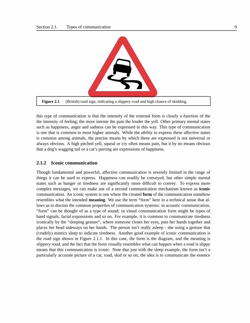
Section 2.1. Types of communication 9
Figure 2.1 (British) road sign, indicating a slippery road and high chance of skidding.
this type of communication is that the intensity of the external form is clearly a function of thethe intensity of feeling; the more intense the pain the louder the yell. Other primary mental statessuch as happiness, anger and sadness can be expressed in thisway. This type of communicationis one that is common to most higher animals. While theability to express these affective statesis common among animals, the precise means by which these areexpressed is not universal oralways obvious. A high pitched yell, squeal or cry often means pain, but it by no means obviousthat a dog’s wagging tail or a cat’s purring are expressions of happiness.
2.1.2 Iconic communication
Though fundamental and powerful, affective communicationis severely limited in the range ofthings it can be used to express. Happiness can readily be conveyed, but other simple mentalstates such as hunger or tiredness are significantly more difficult to convey. To express morecomplex messages, we can make use of a second communication mechanism known asiconiccommunication. An iconic system is one where the createdform of the communication somehowresembles what the intendedmeaning. We use the term “form” here in a technical sense that al-lows us to discuss the common properties of communication systems: in acoustic communication,“form” can be thought of as a type of sound; in visual communication form might be types ofhand signals, facial expressions and so on. For example, it is common to communicate tirednessiconically by the “sleeping gesture”, where someone closesher eyes, puts her hands together andplaces her head sideways on her hands. The person isn’t really asleep - she using a gesture that(crudely) mimics sleep to indicate tiredness. Another goodexample of iconic communication isthe road sign shown in Figure 2.1.1. In this case, the form is the diagram, and the meaning isslippery road, and the fact that the form visually resembles what can happen when a road is slippymeans that this communication is iconic. Note that just withthe sleep example, the form isn’t aparticularly accurate picture of a car, road, skid or so on; the idea is to communicate the essence

10 Chapter 2. Communication and Language
of the meaning and little else.Anecdotally, we sometimes think of pre-human communication also working like this, and
in such a system, the presence of a saber tooth tiger might be communicated by imitating its growl,or by acting like a tiger and so on. Such systems have a certainadvantage of transparency, in thatif the intended recipient does not know what you mean, a certain amount of mimicry or actingmay get the point across. In essence, this is just like the road sign example, in that the form andmeaning have a certain direct connection. When travelling in a country where we don’t speak thelanguage, we often resort to miming some action with the hopethat the meaning will be conveyed.
Iconic systems though have several drawbacks. One is that while it may be easy to imitate atiger, it is less easy to imitate more abstract notions such as “nervous” or “idea”. More importantlythough, iconic systems can suffer from a lack of precision: when a first caveman imitates the tiger,a second caveman may not get this reference exactly - he mightbe sitting there thinking, “well, itcould be a tiger, or perhaps a lion. Or maybe a large dog”. And by the time the first caveman hasmimed his way through this and the action of “creeping up behind”, both have probably departedto the great cave in the sky. While useful and important, iconic communication clearly has itslimits.
2.1.3 Symbolic communication
In contrast to iconic and affective communication, we also havesymboliccommunication in whichwe give up the idea that the form must indicate the meaning. Rather we use a series of correspon-dences between form and meaning, in which the relationship is not direct. In symbolic systems,a tiger might be indicated by waving the left hand, a lion by waving the right. There is no reasonwhy these forms should indicate what they do, it is merely a matter of convention. The advantageis that it is easier to devise a system where the forms are clear and distinct from one another - lessconfusion will arise. The disadvantage is that the fact thatleft-arm-wave means tiger, and right-arm-wave means lion has to belearned, if you don’t know, seeing the movement in isolation won’tgive clue to the meaning. Despite the disadvantage in needing to learn, using conventions ratherthan icons can be hugely advantageous in that the conventions can be relatively brief; one noiseor gesture may represent the tiger and this need not be acted our carefully each time. This brevityand clarity of form leads to a swiftness and precision seldompossible with iconic communication.
Once a convention-based communication system is used, it soon becomes clear that it is thenotion ofcontrast in form that is the key to success. To put it another way, once the form no longerneeds to resemble the meaning, the communication system gains benefit from making the formsas distinct from one another as possible. To show this point,consider the following experiment.
We grouped eight subjects into pairs, and in isolation, asked each pair to design a commu-nication system based on colour cards. The premise was that the pair were in a noisy pub, oneindividual was at the bar while the other was sitting down at atable. We said there were four basicconcepts to communicate: “I would like a drink of water”, “I would like some food”, “I wouldlike a beer” and “I would like to listen to some music”. Each pair was given a set of 100 different

Section 2.1. Types of communication 11
Figure 2.2 With three symbols in isolation only three meanings are possible. When we combine thesymbols in sequences the number of meanings exponentially increases, while the ability to uniquelyperceive the symbols is unaffected.
coloured cards arranged across the spectrum, and asked to pick one card for each concept andmemorise which colour was associated with which concept. Ina simple test, it was clear that thepairs could remember the colours and their meanings, and could effectively communicate thesesimple concepts with this system. The real purpose of the experiment was different though. Whilethree of the groups chose a blue colour for the concept “I wanta drink of water”, for the other cat-egories there was no commonality in the choice. So “I want a beer” had two pairs chose green, oneyellow and one black. Interestingly most gave some justification as to why each colour was chosen(green means “yes, lets have another”) and so on; but it is clear that this justification was fairlysuperficial in that each group choose quite different colours. This demonstrates one of the mainprinciples of symbolic communication system, namely that the relationship between the form ofthe symbol (in this case the colour) and its meaning is in general arbitrary . These form/meaningpairs must be learned, but as we shall see, in many cases the “cost” of learning the pairing to anindividual is less than the “cost” of potential confusion and imprecision that can arise from havingthe form resemble the meaning. This simple study demonstrates another vital point. In each case,the pairs chose quite different colours; so group A chose a blue, a red, a yellow and a green, whilegroup B chose a red, a yellow, a light blue and a black. In no case did a group choose say a green,a light blue, a medium blue and a dark blue for instance. In other words, the groups chose a set ofcolours that had clear contrast with each other. In a way thismakes obvious sense; picking coloursthat are significantly different from one another lessens the possibility that they will be confused,but it does demonstrate a crucial point in symbolic systems,namely that the systems are based onthe notion of contrast between forms rather than the absolute “value” of each form.
2.1.4 Combinations of symbols
This simple communication system works well because we onlyhave four concepts we wish toconvey. What happens when we need to communicate more concepts? We can see that the simple
12 Chapter 2. Communication and Language
colour contrast will eventually reach its limits. If say 20 concepts are required, it soon becomesa difficult task to associate each with just one colour. Setting aside the issue of whether theindividuals can remember the colours (let us assume they have a crib sheet to remind them), amajor problem arises because as more concepts get added, a new colour is associated with eachone, and as the range of colours is fixed, each new added concept increases the likelihood that itwill get confused with another concept which has a similar colour. While it may be possible for anindividual to distinguish 20 colours, asking them to do so for 1000 colours seems unlikely to meetwith success. We therefore need a separate solution. The obvious thing to do is usecombinationsof colour cards. For instance, we could associate the colourblack with the conceptnot, pink withlarge, and then use these and one of the original colours to indicate a much larger range of concepts(so holding a black card, pink card and blue card would say “I don’t want a large drink of water”).Note that this is different from holding a single card that isa mixed combination of black pinkand blue (which might be a murky brown). The reason why the combination system works is thateach colour card on its own is clear, distinct and unconfusable, but by combining them, we cangenerate a large number of concepts from a small number of form/meaning pairs. The power ofcombination is considerable; in the limit, the number of complex forms exponentially multiples,so that if we haveN simple forms andM instances of them, we have a total ofNM complex forms;so 10 forms combined in 10 different ways would produce over 10 billion different complex forms.
We call communication systems that use a fixed number of simple forms which can be com-bined into a much larger number of forms asymbolic language. Here we use the term “language”in both a very precise and general sense. Precise, in that it we use it only to mean this principle ofcombination, but general in the sense that all human languages make use of this principle in thissense, as are other systems, such as written numbers (we can create any number from a combina-tion of the 10 digits), mathematics and even email addresses. Human language often goes underthe description ofnatural language and we shall use that term here to distinguish it from theprinciple of languages in general. One of the main distinctive properties of natural language is thesheer scale of things that it can express. While we can talk ofother animals having sophisticatedcommunication systems (bee dancing etc), none has anythinglike the scale of natural language,where a person might know say 10,000 words, and be able to combine these into trillions andtrillions of sentences.
2.1.5 Meaning, form and signal
In our discussion so far, we have been somewhat vague and a little informal about what we reallymean by “meaning” and “form”. The study of meaning (often called semantics), is notoriouslydifficult, and has been the subject of debate since the earliest philosophy. It is an inherently trickysubject, because firstly it requires an understanding of theworld (what the world contains, how thethings in the world relate to one another and so on), and secondly, from a cognitive perspective,it is exceedingly difficult to peer inside someone’s brain and find out exactly how they representthe concept of “warm” or “drink” and so on. As we shall see, developing a precise model of
Section 2.2. Human Communication 13
semantics does not seem to be necessary for text-to-speech,and so we shall largely bypass thistopic in a formal sense.
Our notion of “form” also needs some elaboration. A proper understanding of this part ofcommunicationisvital for our purposes, but thankfully we can rely on an established framework tohelp us. The main issue when discussing form is to distinguish the general nature of the form fromany specific instantiation it may have. Going back to our simple colour example; it is important torealise that when one individual holds up a red card, it isn’tthe red card itself that is the importantpoint, rather that red was used rather than the other choicesof green, blue and yellow. So forexample, a different red card could be used successfully, and probably any red card would do, as itis not the particular red card itself which is the form, but rather that the card has the property “red”and it is this property and its contrasting values that is thebasis of the communication system. Insome accounts, the termmessageis used instead of form.
We use the termsignal to refer to the physical manifestation of the form. Here signal isagain used in a specific technical sense: it can be thought of as the thing which is stored or thething which is transmitted during communication. The idea of “red” (and the idea that it contrastswith other colours) is the form; the physical light waves that travel are the signal. The aboveexample also demonstrates that the same form (red) can have anumber of quite different signals,each dependent on the actual mode of transmission.
It is important to see that the relationship between meaningand form, and form and signalare quite separate. For instance, in our example we have associated the colours red, yellow, blueand green each with a concept. Imagine now the sender holds upan orange card. Most likely thereceiver will see this signal and correctly interpret the physical light-waves into a form “orange”.After this however she is stuck because she can’t determine what concept is matched with this or-ange form. The signal/form relationship has worked well, but it has not been possible to determinethe correct concept. This situation is similar to that when we read a new word - while are quitecapable of using our eyes to read the physical pattern from the page and create an idea of the lettersin our head, if we don’t know the form/meaning mapping of the word, we can not understand it.
Finally, we use the termchannelor medium to refer to the means by which we the messageis converted and transmitted as a signal. In this book, we deal mainly with thespoken channeland thewritten channel.
2.2 HUMAN COMMUNICATION
The above examination of communication in the abstract has of course been leading us to anexplanation of how human communication operates. Taking spoken communication first, let usmake a primary distinction between the two main aspects of this, which we shall call theverbalcomponent and theprosodic component. We use the term “verbal” to mean the part of humancommunication to withwords. In some books, the term “verbal” and “language” are synonymous,but because “language” has so many other, potentially confusable meanings, we will stick with the

14 Chapter 2. Communication and Language
terms “verbal” or “verbal component” throughout. The verbal component is a symbolic systemin that we have a discrete set of words which can be arranged insequences to form a very largenumber of sentences.
In contrast, the prosodic component (often just calledprosody) is different in that it is notprimarily symbolic. We use prosody for many purposes: to express emotion or surprise, to em-phasise a word, to indicate where a sentence ends and so on. Itis fundamentally different in thatit is not purely discrete, does not generally have units which combine in sequences and so has amuch more limited range of meanings that can be expressed. That said, prosody should not betaken as a poor relative of the verbal component; if we say “its wonderful” with words, but use atone of voice that indicates disgust; the listener will guess we are being sarcastic. If the prosodicand verbal component disagree, the prosodic information wins. To a certain extent, these systemscan be studied separately; in fact nearly all work in the fieldof linguistics is solely interested inthe verbal component. The two do interact though; first in theobvious sense that they share thesame signal (speech), but also in more complex ways in that prosody can be used to emphasiseone particular word in a sentence.
2.2.1 Verbal communication
The symbolic model of the verbal component states that the principle unit of form is thephoneme.Phonemes operate in a contrastive system of sounds, in whicha fixed number of phonemes cancombine to a much larger number ofwords (a vocabulary of more than 10,000 words is common,but many millions of words are possible). Next, these words are taken as the basic units, andthey further combine intosentences. Verbal language is therefore seen as a combination of twosystems; one that makes words from phonemes, and another that makes sentences from words.As the word/sentence system has quite a large set of basic units to start with, the number ofcombined units is vast. The two systems have different properties with regard to meaning. In thefirst system, the basic building blocks, the phonemes, have no direct (arbitrary, iconic or other)meaning, they are simply building blocks. These are combined to form words, and these dohave meaning. The relation between a word’s meaning and the phonemes which comprise it iscompletely arbitrary and so the meaning and pronunciation of each word has to be learned. Thesecond system operates differently, in that the basic building blocks (the words) do have inherentmeaning, and the meaning of the sentence is related to the meaning of the components. Exactlyhow the sentence meaning relates to the word meaning is stillan issue of considerable debate;one the one hand there is considerable evidence that it is a function, in the sense that if we haveJOHN KICKED MARY1 we can substitute different people forJOHN andMARY (e.g. ANN KICKED
GEORGE), or different verbs (e.g.JOHN KISSED MARY) and predict the sentence meaning fromthe parts. On the other hand, there is also considerable evidence that sentence meaning is not asimple function, in thatJOHN KICKED THE BUCKET means John has died, and has nothing to do
1 From here we will use a small caps typeface when we refer to form/message such asJOHN and a courier typefacefor the written signal, e.g.john.
Section 2.2. Human Communication 15
with kicking or buckets.From this basic model, we can now explore some of the fundamental features of language. In
doing so, we follow Hockett [214], who stated the principle defining properties of verbal language.Among these are:
Arbitrary
Phonemes do not have inherent meaning but words do; a word is in effect a form/meaning pair inwhich the correspondence between the meaning and the form (ie. the sequence of phonemes) isarbitrary. Because of this, there is no way to guess the meaning of a word if it is not learned, so asa reader, you won’t know the meaning of the wordPANDICULATION unless you are informed of itsmeaning. From this, it follows that words of similar form canhave complete different meanings,soBIT andPIT mean quite different things despite only having a slight sound difference, whereasDOG andWOLF are similar in meaning, but share no sounds.
Duality
The duality principle states that verbal language is not onesystem but two; the first system uses asmall inventory of forms, phonemes, which sequentially combine to form a much larger inventoryof words. The phonemes don’t carry meaning but the words do, and this association is arbitrary.The second system combines the large number of words into an effectively limitless number ofsentences.
Productive
The productive property means that there is an effectively unlimited number of things that onecan say in a verbal language. It is not the case that we have a fixed number of messages and incommunication simply choose one from this selection; rather many of the sentences we produceare unique, that is, the particular combination of words we use have never been used before. Ofcourse many of the sentences we say are conventionalised (“How do you do?” etc), but most areunique. It might seem questionable if this is really the caseas most people don’t feel they are beingparticularly “original” when the speak. However, a simple examination of the combinatorics ofcombining even a modest vocabulary of 10,000 words shows that a vast number of possibilitiesexist (certainly larger that the number of atoms in the universe).
Discrete
Both the basic types of linguistic unit, the phoneme and the word, arediscrete. Phonemes are dis-tinct from one another and form a finite and fixed set. The set ofwords is less fixed (we can createnew words), but nevertheless all words are distinct from oneanother and are countable. Whatis remarkable about the discreteness property of language is that the primary signal of language,speech, is not discrete and hence there is a mismatch betweenform and signal. Speech signalsare continuous functions of pressure over time (see Chapter10) and so speaking is a process of

16 Chapter 2. Communication and Language
converting a discrete phoneme representation into a continuous acoustic one. This process is re-versed during listening, where we recover a discrete representation from the continuous signal. Aswe shall see, this is a remarkably complex process, and is oneof the main reasons why automaticspeech synthesis and speech recognition are difficult.
2.2.2 Linguistic levels
Another common way to look at verbal language is as a series ofso-called linguisticlevels. Sofar we have talked about the duality of form such that we have aphonemes which combine toform words which combine to form sentences. In our model, sentences, words and phonemesare considered the primary units of form, and suffice to describe the basic properties of verballanguage. It is however extremely useful to make use of a number of secondary units, whichwe shall now introduce.Morphemes are units used to describe word formation or the internalstructure of words. This describes for instance the connection between the three English wordsBIG, BIGGER, BIGGEST, and the study of this is calledmorphology. Next we havesyntax, oftendefined as the study of the patterns of words within a sentence. Syntax describes the process ofhow nouns, verbs, prepositions and so on interact, and why some sequences of words occur butnot others. The fundamental units of syntax are thesyntactic phraseand sentence. With theselevels, we can for a given sentence describe asyntactic hierarchy where a sentence comprises anumber of phrases, each of these comprises a number of words,which then comprise morphemes,which then comprise phonemes.
We can also consider thephonological hierarchy, which is a different, parallel hierarchywhich focuses on the sound patterns in a sentence. In this, wehave the additional units ofsyllables,which are a structural sound unit used to group phonemes together; andphonological phrases,another structural sound unit that groups words together within the sentence. Representationsusing these units can also be expressed in a hierarchy of sentences, prosodic phrases, words,syllables and phonemes.
The difference between the two hierarchies is that the phonological one concentrates on thesound patterns alone, and is not concerned with any aspect ofmeaning, while the syntactic oneignores the sound patters, and concentrates on the grammatical and semantic relationships betweenthe units.
Next we consider levels between the form and the signal, which in spoken communication isan acoustic waveform. Here we havespeech acousticswhich involves working with the acousticspeech sound signal. Next we havephonetics, which is often described as the study of the physicalspeech sounds in a language. Phonetics is often studied independently of other linguistic areas, asit is seen as part of the system which links form and signal rather than as part of the meaning/formverbal linguistic system.Phonologyis the study of sound patterns as they relate to linguistic use;in contrast to phonetics, thisis considered part of the core linguistic system as phonology describesthe form in the meaning/form system. That said, phonology and phonetics are closely related andphonology is sometimes described as the organisational system of phonetic units.
Section 2.2. Human Communication 17
Semanticsis sometimes given a broad definition as the study of “meaning” in the generalsense, but is sometimes given a much narrower definition, andis concerned only with certain as-pects of meaning, such as analytic truth, reference, and logic. Finallypragmaticsconcerns a num-ber of related areas including the aspects of meaning not covered by semantics, the interaction oflanguage, a speaker’s knowledge and the environment and theuse of language in conversations anddiscourses. Sometimes pragmatics is described as being “parallel” to semantics/syntax/phonologyetc as it is the study of how language is used.
It is important to realise that these terms are used both to refer to the linguistic level and thearea of study. In traditional linguistics these terms are often taken as absolute levels that exist inlanguage, such that one sometimes sees “turf wars” between phoneticians and phonologists aboutwho best should describe a particular phenomenon. From our engineering perspective, we will findit more convenient to adopt these terms, but not worry too much about the division between each;rather it is best to view these levels as salient points in a continuum stretching from pragmatics toacoustics.
2.2.3 Affective Prosody
We now turn to a different component of human communication.Broadly speaking, we can statethat prosody has two main communicative purposes, termedaffective andaugmentative. Theaffective use of prosody can be used to convey a variety of meanings: perhaps the most straight-forward case is when is is used to indicate primary emotions such as anger or pain. Prosody isparticularly good at this; when we hurt ourselves and want totell someone we usually let out ayell rather than say “look, I’ve cut off my fingers” in a calm measured tone. The use of prosodyto convey primary emotion is also largely universal; when listening to someone who speaks a dif-ferent language we find they use more or less the same form to indicate the same meanings. Infact this extends to animals too; we are often in little doubtas to what an animal snarl or growl istrying to convey. Beyond primary emotions we can consider a whole range of meanings that areexpressible via prosody. These include secondary emotionssuch as angst or distrust, speech actssuch as question, statement and imperative; modes of expression such as sarcasm or hesitancy andso on.
Many of these phenomena are language specific (in contrast toprimary emotion), and have aconventional or arbitrary character such that a speaker of that language has to learn the appropriateprosodic pattern in the same way that they learn the form/meaning correspondences for words inverbal language. In fact we can see these effects as lying on ascale with universal systems lyingat one end and conventional arbitrary systems lying at the other. In many languages, a rising pitchpattern at the end of a sentence indicates a question; but this is not universally so. Ladd [269]shows that the pattern is reversed in Hungarian such that certain questions are indicate by a fallingpitch.
One of the central debates in the field of prosodic linguistics is just how far this scale extends.Crudely speaking, the argument concerns whether prosody ismainly a universal, non-arbitrary
18 Chapter 2. Communication and Language
system, with a few strange effects such as Hungarian question intonation; or whether it is in factmuch more like verbal language in that it ismainlyarbitrary, and has rules of syntax and so on.
2.2.4 Augmentative Prosody
The second aspect of prosody is calledaugmentative prosody. The basic purpose of this is toaugmentthe verbal component. Taking a simple example first, we see that many sentences arehighly confusable with respect to syntactic structure. In sentences such as
(1) BILL DOESN’ T DRINK BECAUSE HE’ S UNHAPPY
we see that there are two completely different interpretations which depend on which syn-tactic structure is used. The speaker can choose to insert a pause, and if she does so, she willbias the listener’s choice as to which interpretation is intended, and hence facilitate understanding.In addition to helping with phrasing structure, this component of prosody is also used to drawattention to words by emphasising them.
This use of prosody is called augmentative because it augments the verbal component andtherefore helps the listener to find the intended form and meaning from the signal. In contrast toaffective prosody, the use of augmentative prosody here does not add any new meaning or extraaspect to the existing meaning, it is simply there to help findthe verbal content. One of the mostinteresting aspects of augmentative prosody is that speakers show considerable variation in howand when they use it. While one speaker may pause at a certain point, another speaker will speakstraight on, and we even find that the same speaker will quite happily use a pause on one occasionand not on another. We can explain this variation by considering the range of conversationalsituations where augmentative prosody might be used.
In general, when a speaker generates a message that is potentially ambiguous, it is oftenentirely obvious from the form of words used, the backgroundknowledge and the situation whatinterpretation is intended, and in such cases no or little augmentative prosody is used. In othercases however, we may find that the speaker suspects the listener may have difficulty in interpre-tation, we find that here the speaker does indeed make use of prosody. In other words, prosodyis usually only used when it is needed. Hence if we consider a sentence in isolation, it is nearlyimpossible to predict what prosody a speaker will use. A consequence of this is that it is clearlypossible to use more or use less prosody for any given sentence. We can think of this as a scaleof prosodic intensity, and this applies to both affective and augmentative prosody. In many cases,speakers utter sentences at the lower end of this scale, in which case we say they are speaking withnull prosody or neutral prosody to indicate that there is no true prosody being used.
2.3 COMMUNICATION PROCESSES
In this section, we will build a general model of communication that will serve as a framework inwhich to analyse the various communicative processes involved in spoken and written language.

Section 2.3. Communication processes 19
generation
encoding
understanding
meaning
message
signal
message
meaning
signal
speaker listener
transmission
decoding
Figure 2.3 Processes involved in communication between two speakers.
For illustration, let us consider a dialogue between two participants, A and B. In a normal con-versation, A and B take it in turns to speak, and these are known asdialogue turns. Suppose, Adecides to say something to B. To do this, A firstlygeneratesa linguistic form, which we shall callthemessage. He thenencodesthis as aspeech signal, which is a form which can betransmittedto B (lets assume they are in the same room). On receiving the signal, B firstdecodesthe signaland creates her own message as linguistic form. Next she attempts tounderstand this messageand so find the meaning.
In line with our model of language explained before, we have three types of representation:the meaning, the form and the signal. In communicating, A andB use 4 separate systems to movefrom one to the other; these are:
generation : meaning to form
encoding : form to signal
decoding : signal to form
understanding : form to meaning
This model works equally well for written language; A converts his thought into a message,then encodes this as writing and sends this to B (in this case the “sending” can be quite general,for example an author writing a novel and a reader subsequently picking it up). Once received,B attempts to decode the writing into a message, and then finally understand this message. Adiagram of this is shown in Figure 2.3.
2.3.1 Communication factors
We start our discussion by simply asking, why do the participants say the things they do? While“free-will” plays a part in this, it it is a mistake to think that “free-will” is the sole governing factor
20 Chapter 2. Communication and Language
in how conversations happen. In fact there are a number of guiding principles involved, which weshall now explore.
The first concerns the understood conventions of communication. In human conversation,participants don’t just say everything on their mind; to do so would swamp the conversation.Rather, they only say what they need to in order to get their point across. We can state thisas a case ofeffectivenessand efficiency; we wish to effectively communicate our message sothat it is understood, but also to do so efficiently so that we don’t waste energy. In fact it isclear that conversation works by adopting a set of understood conventions that govern or guidethe conversation. The most famous exposition of these principles was by Grice, who definedfour main principles, of conversation which are now commonly known asGrice’s maxims [184].These principles state for instance that it is expected thatone participant should not be overly longor overly short in what is said; one should say just the right amount to make the thought clear.Grice’s maxims are not meant as prescriptive guides as to howconversation should progress,or even statements about how they do progress, but rather a set of tacit conventions, which wenormally adhere to, and which we notice when they are broken.
The second factor concerns thecommon groundthat the participants share. This is a generalterm which covers the background knowledge, situation and mutual understand that the conver-sational participants share. When in the same room, they canpoint to objects or refer to objects,actions and so on, in a different way to how such things can be referred to if they are more distant.If one says “have a seat” and there is a chair in the room, this means something straightforward.The situation can significantly alter the intended meaning of an utterance. Take for instance thesentence “my car has broken down”. Now this can be taken as a simple statement of fact, but ifsomeone says this upon entering a mechanic’s workshop, the implication is that the person’s carhas broken down and he’d like the mechanic to fix it. If by contrast, this is the first thing someonesays when arriving for dinner, the intention might be to apologise for being late because an un-forseen travel delay occurred. To take another example, if two experts in the same research fieldare talking, they can talk assuming that the other has a detailed knowledge of the subject matter.This is different to when an expert talks to a lay person.
Finally, the knowledge of thechannelhelps form the message. Participants don’t generatemessages and then decided whether to speak them or write themdown; they know what mediumis going to be used before they start. This allows the participants to best exploit the strengthsof each form of communication; in spoken language extensiveuse may be made of prosody; inwritten language the author may take the liberty of explaining something in a complicated fashionknowing that the reader can go back and read this several times.
2.3.2 Generation
In our model, the process of converting a meaning into a message is calledmessage generation(elsewhere the termlanguage generationis often used, but this is too potentially confusing forour purposes). To demonstrate how generation works, let us use the above mentioned communi-
Section 2.3. Communication processes 21
cation factors to consider situation where a participant ina conversation wants to know the scorein a particular football game. We should realise that the participant has considerablechoice inconverting this thought into a message. For example, the participant can make a statement “I wantto know the score” or a question “what is the score”; the participant has choices over mood, andmay choose to say “can you tell me the score?”, may choose between active and passive “whohas scored?” vs “have any goals been scored?”. The participant has choices over vocabulary, maywell qualify the message, may decide on a casual, formal, polite, demanding tone and so on. Inaddition the participant can choose to emphasise words, pick different intonational tunes, perhapsmake a pointing gesture and so on. The important point is thatthe participant have a wide rangeof options in turning the thought into the message. The result is the message, and a perfectlytransparent communication system would send this to the receiver will all this detail and with nochance of error.
It is sometimes assumed that messages themselves convey or represent the communicatedmeaning. While in certain cases this may be possible, we havejust demonstrated that in mostconversations, to extract (understand) the correct meaning one must know the situation and sharedknowledge.
2.3.3 Encoding
Encoding is the process of creating a signal from a message. When dealing with speech, we talkof speech encodingand when dealing with writing we talk ofwriting encoding. Speech encodingby computer is more commonly known asspeech synthesis, which is of course the topic of thisbook.
The most significant aspect of speech encoding is that the nature of the two representations,the message and the speech signal, are dramatically different. A word (e.g. HELLO) may becomposed of four phonemes, /h eh l ow/, but the speech signal is a continuously varying acousticwaveform, with no discrete components or even four easily distinguishable parts. If one considersthe message, we can store each phoneme in about 4-5 bits, so wewould need say 2 bytes to store/h eh l ow/. By contrast, a reasonably high fidelity speech waveform2 would need about 20,000bytes, assuming that the word took 0.6 seconds to speak. Where has all this extra content comefrom, what is it for and how should we view it?
Of course, the speech signal is significantly moreredundant than the message: by variouscompression techniques it is possible to reduce its size by afactor of 10 without noticeably affect-ing it. Even so, this still leaves about three orders of magnitude difference. The explanation forthis is that the speech waveform contains a substantial amount of information that is not directlyrelated to the message. First we have the fact that not all speakers sound the same. This maybe a fairly obvious thing to say, but consider that all English speakers can say exactly the samemessage, but they all do so in subtly different ways. Some of these effects are not controllable by
2 Say 16 bits dynamic range and 16,000Hz sampling rate. (See Chapter 10 for an explanation)

22 Chapter 2. Communication and Language
the speaker and and determined by purely physiological means. Some are due to prosody, wherefor instance, the speaker can have different moods, can affect the signal by smiling when talking,can indicate different emotional states and so on. This factis hugely significant for speech synthe-sis, as it demonstrates that encoding the message is really only part of the problem; the encodingsystem must do several other tasks too if the speech signal isto sound genuinely human-like to thereceiver.
2.3.4 Decoding
Decoding is the opposite of encoding; its job is to take a signal and create a message.Speechdecoding is the task of creating a message from the signal; the technology that does this is mostcommonly known asspeech recognition. The challenges for speech decoding (speech recogni-tion) systems are just the converse of speech encoding; froma continuous signal, which containsenormous amounts of information, the system must extract the small amount of content that is themessage. Speech recognition is difficult because of the problem of ambiguity. For each part ofa message, a word or a phoneme, if one studies the speech patterns produced from that one seesthat there is an enormous amount of variability. This is partly caused by the factors we describedabove, namely speaker physiology, emotional state and so on, and partly from the encoding pro-cess itself, where a phonemes characteristics are heavily influenced by the other phonemes aroundit. This variability wouldn’t be a problemper se, but it turns out that the patterns for each phonemeoverlap with one another, such that given a section of speech, it is very hard to determine whichphoneme it belonged to. These aspects make speech recognition a difficult problem.
Text decoding, also calledtext analysis, is a similar task where we have to decode thewritten signal to create a message. If the writing is on paper, we face many of the same problems aswith speech recognition; namely ambiguity that arises fromvariability, and this is particularly trueif we are dealing with hand writing. Computerised writing issignificantly easier as we are dealingwith a much cleaner representation in which the representation is discrete and each character isuniquely identified.
For many types of message, the text decoding problem is fairly trivial. For instance, forsimple text such asthe man walked down the street, it should by possible for a simplesystem to take this and generate the correct message all the time. Significant problems do arisefrom a number of sources. First, ambiguity exists even in computerised written signals. One typeis homograph ambiguity, where two different words have the same sequenceof characters (e.g.polish can mean “from Poland” or “to clean”,console can mean “to comfort” or “a part of amachine”).
One final point should be made when comparing text and speech decoding. In speech recog-nition, the problem is understood as being difficult, and so error rates of say 10% are often seenas good system performance on difficult tasks. As we have seentext decoding is fundamentallyeasier, but along with this so are expectations. So while forsome tasks the vast majority of wordsmay be decoded successfully, the expectation is also high and so error rates of 0.1% may be seen
Section 2.4. Discussion 23
as too hight.
2.3.5 Understanding
Understanding is the process of creating a thought from the message. Understanding can bethought of as the reverse of generation and also bears similarity to decoding in the sense that we aretrying to recover a thought from a representation (the message), which also includes informationgenerated from other sources such as the background, situation and so on.
In understanding, we also have an ambiguity problem, but this is quite different from theambiguity problem in decoding. For example, it is perfectlypossible when hearing a speechsignal to decode it into the correct message, but then fail tounderstand it because of ambiguity.For instance, if someone says “did you see the game last night”, it is quite possible to correctlyidentify all the words, but fail to determine which game is being referred to.
2.4 DISCUSSION
This chapter has introduced a model of communication and language that will serve as the basis forthe next chapter, which looks at text-to-speech conversionin detail, and the subsequent chapters,which explore the various problems that occur and the techniques that have been developed tosolve them. We should stress that what we have presented hereis very much amodel; that is auseful engineering framework in which to formulate, test and design text-to-speech systems.
In building this model, we have drawn from a number of fields, including semiotics, informa-tion theory, psychology, linguistics and language evolution. These fields have overlapping spheresof subject matter, but unfortunately are often studied in isolation such that none really gives ascomplete and detailed a model of communication as we might wish for. Each of these separatedisciplines is a vast field in itself, so we have only touched on each area in the briefest possibleway.
Considering semiotics first, we should look at the works of Ferdinand de Saussure, whois widely acknowledged to have invented the field of semiotics and is considered by many asthe first modern linguist. Saussure was the first to emphasisethe significance of the arbitrarynature of form and meaning in communication and proposed that the study of the relationshipbetween the two should be the central topic in linguistics [391], [392]. The philosopher CharlesSanders Pierce also pioneered early work in semiotics and semantics, and gave us the frameworkof iconic and symbolic semiotics which is used here [350]. The second main area we draw fromis communication theory or information theory, and from this we have the principles of encoding,decoding, channels, messages and signals. The pioneering work in this field was produced byClaude Shannon [400], who was originally interested in the problem of accurate transmission ofinformation along telephone wires (he worked for the telephone company AT&T). It soon becameclear that the implications of this work were much broader (Weaver [401]) and it has been widely
24 Chapter 2. Communication and Language
adopted as an approach to the analysis of signals arising from linguistic sources, such that thisinformation theoretic approach is now dominant in speech recognition and many other fields.Saussure did not in general deal much with signals, and Shannon and Weaver did not deal muchwith meaning, but their work clearly intersects regarding the issue of form and message (the termform is used in linguistics and semiotics and message in information theory, but they both refer tothe same thing.)
The field of linguistics is often described as the science of language, but in the main thisfield focuses very much on just the meaning/form verbal part of language, as opposed to theentire process which includes participants, conversations, signals and so on. Linguistics generallyapproaches language without reference to use; the idea is that a language is an entity and it canbe studied independently of any purpose to which it is put3. This approach is part tradition andpart pragmatic; as linguistics can trace its lineage back tothe philosophical musings of ancientGreek philosophers. In addition there is the practical justification that by isolating effects it makesthem easier to study. In modern times, the field of linguistics has been dominated by NoamChomsky[89], [90], [88], who in addition to many other innovations has championed the idea thatthe primary function of language is not communication at all, but rather forms the basis of thehuman mind; it evolved for this reason and its communicativepurpose was a useful by product.Despite this mismatch between linguistics and our more practical needs, this field does provide thebasics of a significant chunk of the overall picture of human communication, including the modelsof phonetics, phonology, words, syntax and so on that are central to our problem. Many linguisticstext books tend to be heavily skewed towards one of the many incompatible theories within thediscipline, so care needs to be taken when reading any book onthe subject. A good introductorybook which explains the “hard issues”, which is accessible to those with a scientific backgroundand which doesn’t follow any particular theory is Lyons [290].
The study of human communication in terms of participants, conversations, backgroundknowledge and so on is often performed outside the field of mainstream linguistics by psycholo-gists and philosophers. Good books on human conversation and language use include Clark [95]and Clark and Clark [96], Searle [395], Grice [184] and Power[361].
2.5 SUMMARY
Communication
• A semiotic system has three levels of representation; meaning, form, and signal.
• in affective communication, the meaning, form and signal are continuous and simply related.
• in iconic communication, the form resembles the meaning in some way. Iconic systems canbe either discrete or continuous
3 In fact in surveying more than twenty introductory text books in linguistics found in the Cambridge University bookshop, I did not find even one that mentioned that language is used for communication!

Section 2.5. Summary 25
• in symbolic communication, the form does not resemble the meaning and the correspon-dences between these have to be learned.
• Symbolic systems are discrete, and this and the arbitrary meaning/form relationship meanthat communication of complex meanings can occur more effectively than with the othertypes.
• Human language operates as a discrete symbolic system.
Components of language
• Human communication can be divided into two main components:
– The verbal component describes the system of phonemes, words and sentences. It is adiscrete symbolic system in which a finite number of units canbe arranged to generatean enormous number of messages.
– The prosodic component is by contrast mostly continuous, and in general expressesmore basic meanings in a more direct
• Affective prosody is when a speaker uses prosody to express emotion, speech act or otherinformation which is conveyed sentence by sentence
• Augmentative prosody is used to disambiguate and reinforcethe verbal component.
• Both types of prosody are optional, in that speakers can choose to use no prosody if they wishand just communicate via the verbal component. Writing in fact uses just this component.
Communication
• We can break communication into four processes in spoken communication:
1. generation is the conversion of meaning into form by the speaker2. encoding is the conversion of form into signal by the speaker3. decoding is the conversion of signal into form by the listener4. understanding is the conversion of form into meaning by the listener
• The equivalent processes exist for written communication also, where we have a writer andreader instead of a speaker and listener.
3THE TEXT-TO-SPEECHPROBLEM
We now turn to an examination of just what is involved in performing text-to-speech (TTS) syn-thesis. In the previous chapter, we described some of the basic properties of language, the natureof signal, form and meaning, and the four main processes of generation, encoding, decoding andunderstanding. We will now use this framework to explain howtext-to-speech can be performed.
In TTS, the input is writing and the output speech. While it issomewhat unconventional toregard it as such, here we consider writing as a signal, in just the same way as speech. Normal read-ing then is a process of decoding the signal into the message,and then understanding the messageto create meaning. We stress this, because too often no distinction is made at all between signaland form in writing; we here about “the words on the page”. More often an informal distinction ismade in that it is admitted that real writing requires some “tidying up” to find the linguistic form,for instance by “text normalisation” which removes capitalletters, spells out numbers or separatespunctuation. Here we take a more structured view in that we see linguistic form as clean, abstractand unambiguous, and written form as a noisy signal that has been encoded from this form.
The process of reading aloud then is one of taking a signal of one type, writing, and con-verting it into a signal in another type, speech. The questions we will explore in this chapterare:
• How do we decode the written signal?
• Does the message that we extract from the written signal contain enough information togenerate the speech we require?
• When someone is reading aloud, what are the relationships between the author, reader andlistener?
• What do listeners want from a synthetic voice?
3.1 SPEECH ANDWRITING
It is clear that natural (human) language developed first using sound as its medium. While humansclearly also communicate with facial and hand gestures and so on, these systems are not ableto express the same wide range of expressions as natural language. Quitewhy human language
26
Section 3.1. Speech and Writing 27
evolved using sound as its medium is not clear, perhaps it wasdown to an ability to make distinctpatterns more easily with the mouth, than say by waving hands. It is important to realise that thischoice of sound may well have been a complete accident of evolution, today we communicate inmany different ways with vision either by reading or by interpreting sign language. For most ofhuman history, speech was the only (sophisticated) means ofcommunication, but a second keyinvention, perhaps 10,000 years ago, was that of writing.
To begin with, we need to look at the nature of speech and writing in more depth. We willdo this from a number of angles, looking first at the physical differences between these signals,before moving on to look at how these differences influence communication.
3.1.1 Physical nature
The speech signal is a continuous, acoustic waveform. It is created by the operation of the vocalorgans in response to motor control commands from the brain.We only have a partial understand-ing of how this process works, but it is clear that the coordinated movement of the vocal organs toproduce speech is extremely complicated. One of the main reasons why the relationship betweenthe speech signal and the message it encodes is that speech iscontinuous and the form is discrete.In addition to this, speech is highly variable with respect to the discrete message as many otherfactors, including prosody, speaker physiology, a speaker’s regional accent and so on all affect thesignal. A single message can generate many potential signals. Finally, speech is not permanent;unless a recording device is present, once something is spoken, it is lost for ever and if no listeneris present or a listener does not hear the speech then the message that the speech encodes willnever be decoded.
Writing is fundamentally different from speech in a number of ways. Firstly writing isprimarily seen asvisual: traditionally, writing always took the form of visible marks on a pageor other material, and today we are quite used to seeing writing on computer and other screens.This is not however a complete defining property; we considerbraille a form of writing and its keybenefit is of course that one does not need to be able to see to read it. It has been argued [199] thatthe main defining feature of writing is that it ispermanent in a way that speech is not. Whetherthe writing is created with a pen on ink or impressions on a page, the key point is that once writtenit does not disappear. We can of course destroy what we have done, but this is not the point; theidea is that with writing we can record information, either so that we can access it at a later date,or send it over some distance (as a letter for instance).
What then does writing record? Writing can be used to record natural language, but in sayingthis we should make it clear that writing attempts to record the linguistic form of a message, ratherthan the actual signal. That is, if we write down what someonesays, we do not attempt to recordall the information in the speech, such that a reader could exactly mimic the original; rather wedecode the speech into a linguistic message, and then encodethat. Of course quite often themessage we wish to write has never been spoken, and so when writing we generate a linguisticform from our thoughts, and then encode this as writing without ever considering speech.

28 Chapter 3. The Text-to-Speech Problem
We explained in Chapter 2 that spoken language had a dual structure of sentences made ofwords, and words comprised of phonemes. We have a similar dual structure in written communi-cation, where sentences are made of words (as before), but where words are made ofgraphemes.Graphemes are in many ways analogous to phonemes, but differin that they vary much more fromlanguage to language. In alphabetic languages like Englishand French, graphemes can be thoughtof as letters or characters (we will define these terms later); in syllabic writing like Japanese hira-gana, each grapheme represents a syllable or mora, and in languages like Chinese each graphemerepresents a full word or part of a word.
It should be clear that even apart from the visual and permanency aspects writing signalsand speech signals are very different in nature. The most important differences is that writing isdiscrete and “close to the message”, while speaking is continuous, more complex, and does notencode the message in any trivial way. The complexities of the speech encoding and decodingarise because we are using an apparatus (the vocal organs) for a purpose quite different fromtheir original one. In fact, one can state that it is a marvel that speech can be used at all forcommunication messages. In contrast, writing is a culturalinvention, and was designed explicitlyand solely for the purposes of communicating form. If we consider it a “good” invention, itshould not be surprising that the encoding mechanism between linguistic form and writing is muchsimpler. This is not to say that the reading and writing process are trivial; it takes considerableskill for the brain to interpret the shapes of letters and decode messages from them; but this skill isone shared with other visual processing tasks, and not something specific to writing. The difficultyof decoding a written signal depends very much on the specificmessage. Often the relationshipbetween the writing on the page and the words is obvious and transparent; but often it is complexenough for the decoding and encoding processes to be non-trivial, such that we have to resort tosophisticated and principled techniques to perform these operations.
3.1.2 Spoken form and written form
We have just explained the differences between spoken and written signals. Turning now to form,we can ask how (if at all) do the spoken and written form differ? One way of looking at this isto consider the combined generation/encoding process of converting meaning into a signal. Ingeneral we can convert the same meaning into either a spoken signal or a written one, so we seethat speech and writing (in general) share the same meaning representation but different signalrepresentations. The question now is, how much of the overall language system do the two share?It is difficult to answer this conclusively, as to do so (in humans at least) would require a muchmore thorough understanding of the processes than we currently have. It is however possible toconsider a model where the meaning to form systems for both spoken and written language sharea common system from meaning to the second level of form. In other words, the meaning-to-wordsystem is the same for both. The divergence occurs when we consider the primary level of form;in spoken language words are comprise of phonemes, in written language, they are comprisedof graphemes. From this point until the signal, the two systems are separate. Depending on the

Section 3.1. Speech and Writing 29
language, the primary forms may be broadly similar (for instance in Spanish) such that one candeduce the pronunciation from the spelling and vice versa, or quite different, (for example inChinese).
While a few problems certainly occur, this model seems to fit the facts very well. Whetherwe write or say the sentenceTHE MAN WALKED DOWN THE STREET, there are six words and theyoccur in the same order in the spoken and written versions. This fact may be so obvious as to seemsuperfluous, but it is in fact vital to our discussion. One would find it difficult for instance to teachsomeone to read French text and speak English words: even if we learned that the pronunciationfor chien was /d ao g/, we would find it difficult to understand why the written French sentencehas different numbers of words in different orders from the spoken English version.
The main point in this realisation of the commonality between the first level of form inwritten and spoken language is that it shows that if we can decode the form from the written signal,then that we have virtually all the information we require togenerate a spoken signal. Importantly,it is notnecessary to go all the way and uncover the meaning from the written signal; we only haveto perform the job of text decoding and not text understanding. There are two qualifications weneed to add to this. Firstly, some understanding may be required, or may make the job easier whenwe are resolving ambiguity in the written signal. For example, when encountering the homographpolish it may help in our disambiguation to know that the topic of thesentence is above peoplefrom Poland. Secondly, we may need to generate prosody when speaking, and this may not beobtainable from the writing. This issue is dealt with below (Section 3.5.5).
This conclusion is so important for our system that it is worth restating again; by and large,the identity and order of the words to be spoken is all we require to synthesise speech; no higherorder analysis or understanding is necessary.
3.1.3 Use
Speech and writing are used for different purposes. When do we use one instead of the other? Incertain cases we have no real choice; in face to face communication it is normal to speak: while wecould write something down and pass it to our friend to read, this is in general cumbersome. Whenwriting a book, or an article we normally use writing; that isthe standard way in which material isstored, copied and distributed. Before the computer era it was fairly clear which communicationmode was used for what purpose.
Modern technology certainly gives us more choices; with telephones we can communicateover distance, whereas in the past this was only possible by letter. We can also now quickly sendwritten messages electronically, by email, phone messaging, computer messaging and by othermeans. Computer or “instant” messaging is particularly interesting in that it assumes many ofthe characteristics of speech, but exists as a written signal. When phone messaging (“texting” or“sms”) first arrived, many though the idea absurd; why would you ever want to send a message inwriting with a phone when you could simply call the person directly? In fact, many “functional”uses have been found; a common one is for someone to send an address as a text message as this

30 Chapter 3. The Text-to-Speech Problem
is easier for the receiver than having to listen and write theaddress down in case it is forgotten.Uses go beyond this though, and today we see “texting” as particularly popular among teenagers.Anecdotally, we believe that by using text, teenagers can think about, plan and edit their messagesso as to seem more confident, funny and so on; this saves the embarrassment that may ensue fromhaving to actuallytalk to someone.
One major difference is that speech is in generalspontaneous. During a normal conversa-tion, we usually speak with little planning or forethought;we can’t simply suspend the conver-sation until we have thought of the best possible way to say something. This accounts for thedisfluenciesin speech, such as hesitations, pauses and restarts. Writing is usually free of theseeffects, but it is important to realise that this is not because of any property of writing itself, butmore because the writer can spend time over difficult sections, or can go back and correct whathas been written.
Another significant difference is that in spoken communication the speaker can often seeor interact with the listeners. In face to face communication the speaker can see the listener andsee how they react to what is being spoken; in addition to the listener responding directly (“Yes,I agree”), they may nod their head, give an acknowledgment orshow confusion and so on. Inresponse, the speaker can alter or modify their behaviour accordingly. This also happens over thephone, where verbal cues (“uh-huh”, “yeah...”) are given bythe listener to help show the speakertheir level of comprehension and agreement. This is less effective than with the visual cues; anyonewho has taken part in a multi-person call can attest to the difficulty involved in sensing everyonesunderstanding and participation in the conversation.
If we compare this to a typical situation where written communication is involved, we seesome important differences. For example, imagine someone is reading a newspaper on a train.Here the author of a particular column will not personally know the reader, in fact the author willprobably know only a handful of people who read the column. The author and reader are separatedin time and space and the communication is one way only (the reader may comment on the articleto someone else, but this will not reach the author). Becauseof these factors, the situation withrespect to common ground is very different. First, the author is writing for many readers, and allwill have somewhat different degrees and types of background knowledge. Secondly, as no feed-back is possible, it is necessary for the author to “get it right first time”, there is no possibility ofstarting an article and then checking to see if the reader is following. These situational distinctionsaccount for many of the differences in content between spoken and written language; for example,because the level of background information can not be known, writing is often more explicit indefining references, times and places and so on. Informally,we can describe the writing as being“more exact” or “less ambiguous”. Of course, these terms only make sense when considering thespeech or writing in isolation; as explained above, most ambiguity is instantly resolved when thesituation is taken into account.

Section 3.1. Speech and Writing 31
3.1.4 Prosodic and verbal content
One of the most notable features of writing is that it nearly exclusively encodes the verbal compo-nent of the message alone: the prosody is ignored. This feature seems to be true of all the writingsystems known around the world. Because of this it is sometimes said that written language isimpoverishedwith respect to spoken language as it can only express part ofthe message. It is ofcourse possible to represent effects such as emotion in written language, (one can simply write “Iam sad”) but this is done by adding information in the verbal component and is different from thesystematic use of prosody to indicate this emotion. Quite why prosody is not encoded in writingis not well understood. Possible explanations include the fact that it is often continuous, whichcreates difficulties if we are using a discrete coding system. Prosody is most powerful for emotivelanguage; and while this is an important part of literature,the ability to express emotion directlyis not needed so much for legal documents, newspapers, technical manuals and so on.
We do however have a limited prosodic component in written language. Punctuation can beused to show structure; and underlined, italicised or bold text is used to show emphasis. Theseare clearly encoding augmentative prosody in that the punctuation and italics are there to help thereader uncover the correct verbal form from the writing. Affective prosody on the other hand isnearly entirely absent; there is no conventional way to shown anger, pain or sarcasm. The onlyaspect that is present is the ability to express sentence types such as question, statement and imper-atives with punctuation at the end of a sentence. It is interesting to note that in most early writingsystems (e.g. Ancient Greek) no punctuation was used at all,but as writing evolved punctuationappeared and more recently italics and other font effects have become commonplace due to thewide availability of computer word processing. In the last few years, a system of “emotions” hasbecome common in email and other electronic communication,in which punctuation is used toindicate happy faces :-) and other effects, which attempt toencode affective prosody. Quite whythis trend is present is again not clear; while we can ascribethe rise of smiley faces to writingbeing used for more informal purposes, this doesn’t explainthe trend from classical Greek to theEnglish of 200 years ago with its commas, semi-colons and full stops.
3.1.5 Component balance
From the outset, a person knows whether a message should be spoken or written: it is not thecase that the person first generates the message and then decides what channel it should be sent in.This principle gives rise to another set of differences between spoken and written signals. Becausehe knows that a certain message is to be written, the person will, from the outset, structure themessage so as to take account of the component balance available in that signal. So if for instance,if a writer wishes to convey something happy, he is quite likely to express this happiness in theverbal component, as the ability to encode affective prosody is not available. So he might say “I’mthrilled that you got that place” instead of perhaps “well done that you got that place”, which couldgive the impression of being somewhat unmoved. With appropriate expression, the “well done...”
32 Chapter 3. The Text-to-Speech Problem
version may sound very enthusiastic if spoken. The different use of components in written andspoken language is calledcomponent balance.
Simply put, a speaker has a open choice of how much prosody or how much verbal contentto put in a message; they will balance these against each other, to create a final signal that conveysthe message they wish in a way that is balanced between efficiency and effectiveness. A writeron the other hand has only a very limited ability to use prosody; and so has to rely on the verbalcomponent more. Because of this, he is likely to “beef-up” the verbal component, so that it is lessambiguous and more explicit than the spoken equivalent. In addition, the writer will “verbalise”any emotion if that is required (that is, explicitly explainthe emotion by using words).
It is this awareness of the prosodic deficiencies of written language and the ability to getaround them that enables good writers to make themselves understood. It should be noted that themajority of people don’t really write anything more than theodd note or shopping list in their dayto day lives. While we all learn to read and write at school, itis readingthat is the essential skillto cope with modern life; only a few of us regularly write. This point is worth making becausewriting well, that is so that one communicates effectively,is actually quite difficult. One of themain aspects of this is that the ability to encode emotions, make writing unambiguous, and have agood picture of a potential reader in mind while writing, areall skills that require some mastering.We have seen this with the advent of email - many new users of emails send messages which arefar too brief (e.g. “yes” in reply to something that was askeddays ago) or that come across asbeing quite rude - the writer has written the words that he would normally use if he were speakingface to face, but without the prosody, the emotion (which could be humour or politeness) is lostand the words themselves seem very abrupt.
3.1.6 Non-linguistic content
In our discussion so far we have equated speech as being the signal used to communicate linguisticmessages acoustically and writing as the signal used to communicate linguistic visually or overtime. This in fact simplifies the picture too much because we can use our speaking/listening andreading/writing apparatus for types of communication which don’t involve natural language. Justas we can use our vocal organs for whistling, burping, coughing, laughing and of course eating,breathing and kissing, we find a similar story in writing, in that we can use writing for many otherpurposes than just to encode natural language.
This is a significant concern for us, in that we have to accurately analyse and decode text, andto do so we need to identify any non-linguistic content that is present. When considering “non-linguistic” writing, it helps again to look at the evolutionof writing. The key feature of writingis that it is more permanent than speech it can be used to record information. Even the earliestforms of Egyptian and Sumerian are known to have recorded numerical information relating toquantities of grain, livestock and other “accounting” typeinformation. Furthermore, there areseveral cultures who developed methods for recording and communicating accounting informationwithout developing a system for encoding their language: the most famous of these is the Inca

Section 3.1. Speech and Writing 33
quipu system, in which numbers could be stored and arithmetic performed. This ability for writingsystems to encode non-linguistic information is thereforean ancient invention, and it continuestoday in printed mathematics, balance sheets, computer programs and so on.[64], [19], [6]
Consider for a moment numbers and mathematics. Without getting to far into the debateabout what numbers and mathematics actually are, it is worthdiscussing a few basic points aboutthese areas. Firstly, in most primitive cultures, there is only a very limited number system presentin the language; one might find a word for one, two and three, then a word for a few and a wordfor lots.
More sophisticated number communication systems (as opposed to numbers themselves) area cultural invention, such that in Western society, we thinkof numbers quite differently, and havedeveloped a complex system for talking and describing them.Most scientifically and mathemati-cally minded people believe that numbers and mathematics exist beyond our experience and thatadvancing mathematics is a process of discovery rather thaninvention. In other words, if we metan alien civilisation, we would find that they had calculus too, and it would work in exactly thesame way as ours. Whatis a cultural invention is our system of numerical and mathematical no-tation. This is to some extent arbitrary; while we can all easily understand the mathematics ofclassical Greece, this is usually only after their notational systems have been translated into themodern system: Pythagoras certainly never wrotex2+y2 = z2. Today, we have a single commonlyused mathematical framework, such that everyone knows thatone number raised above another(e.g. x2) indicates the power. The important point for our discussion is to realise that when wewrite x2+y2 this isnotencoding natural language; it is encoding mathematics. Now, it so happensthat we cantranslate x2+y2 into a language such as English and we would read this as somethinglike “x to the power of two plus y to the power of two”. It is vital to realise thatx2 + y2 is notan abbreviated, or shorthand form of the English sentence that describes it. Furthermore, we canargue that while mathematics can be described as a (non-natural) language, in that it has symbols,a grammar, a semantics and so on; it is primarily expressed asa meaning and awritten form only;the spoken form of mathematical expressions is derivative.We can see this from the ease at whichwe can write mathematics and the relative difficulties we canget in when trying to speak morecomplex expressions; we can also see this from the simple fact that every mathematically literateperson in the western word knows whatx2 + y2 means, can write this, but when speaking has totranslate into words in their own language first (e.g.EKS SQUARED PLUS Y SQUAREDin EnglishIX QUADRAT PLUS YPSILON QUADRAT in German).
3.1.7 Semiotic systems
A semiotic systemis a means of relating meaning to form. Natural language is a semiotic system,and probably has by far the most complicated form to meaning relationship, and as we have justseen mathematics is another. Most semiotic systems are muchsimpler than natural language asthey are cultural inventions rather than biological processes (recall that while mathematics itselfmay be a property of the universe, the mechanism we use for itsform and encoding are cultural

34 Chapter 3. The Text-to-Speech Problem
inventions). In addition to these examples, we also have computer languages, email addresses,dates, times, telephone numbers, postal addresses and so on. Just as with mathematics, a telephonenumber is not part of natural language, it is a complete meaning/form/signal system in its ownright.
If it were just a case of each semiotic system having its own writing system, we could designa separate system to process each. The problem arises because frequently we mix these systemsin the same signal and using the same characters to do so. For example, in the above text, we sawthe sentence
(2) Pythagoras certainly never wrote x2 +y2 = z2.
in which we clearly mixed natural language text with mathematical text. There are many othercases too; while the mathematics example uses different fonts and so on, many systems share thesame characters as natural language writing, so that we get:
(3) a. I was born on 10/12/67
b. It weighed 23Kg
c. I’ll send it to [email protected]
and so on. The point is that these numbers, dates and email addresses are encoded using the samesignal as natural language writing. To be able to process this type of writing, we have to identifywhich parts of the text relate to which semiotic systems.
3.1.8 Writing Systems
To the best of our knowledge1, the first writing system was that of Sumer which developed intoCuneiform. Perhaps the best known early writing system is the hieroglyphic writing of the AncientEgyptians, although it is not entirely clear whether these two systems are related.
Initially these systems werelogographic in nature, meaning that one symbol usually rep-resented one word or one morpheme. Furthermore, the scriptswerepictographic meaning andthat the symbols were often iconic, ie pictorial representations of the entity the word stood for. Asthese systems developed, the iconic nature became less obvious, developing into a more abstractlogographic script. Additionallyalphabeticelements were developed in the language that allowedwriters to “spell out” words. These developments should come as no surprise; in Section 2.1 wesaw that it is quite natural for a communication system to start highly iconic and then progress toa state when the relation between meaning and form is more arbitrary as this general allows forexperienced users to communicate more quickly and more accurately.
Most writing systems can be described as belonging to one of the following groups, butin some cases, e.g. Japanese, the complete writing system uses more than one of these types.Logographic systems, as we have just seen use one symbols to represent words or morphemes.Syllabic systems use one symbol per syllable, such as in Japanese hiragana.Alphabetic systems
1 If only someone had taken the trouble to write down this key discovery!

Section 3.2. Reading aloud 35
generation
transmission
encoding decodingtexttext
signalwritten
writtensignal
message
meaning
spokensignal
Author Reader Listener
meaning
verbal message
spokensignal
verbalmessage
speechencoding
Figure 3.1 Basic model of reading aloud, which shows in the informationflow between the author,reader and listener.
use a small list of symbols which roughly correspond to the phonemes of a language. The latinalphabet is of course the most widely used, but its relation to phonemes varies greatly from lan-guage to language.Abjad systems are ones primarily based on consonants, vowels are usuallynot written. It is a basic fact of human language that most information that discriminates wordsis carried by the consonants, and so ignoring these in written language is possible (this is why theabbreviation forDOCTOR is dr and notoo). The semitic family of languages, including Hebrewand Arabic are abjads.
Writing systems are an important consideration in TTS as in general we have to be able todesign a system for any language, and this means being able tohandle all writing systems. Prob-lems that have to be solved include, identifying the language, identifying the writing system (forexample Japanese uses a logographic and a syllabic system),identifying the computer encodingused, the writing direction and many other issues specific toeach language.
3.2 READING ALOUD
We now turn to the problem ofreading aloud, that is, how to read text and then speak what wehave read.
3.2.1 Reading silently and reading aloud
The process of reading, as we normally understand it, is one of taking some text, decoding it intoa message, and then understanding it. For clarity, we call this processreading silently. By and
36 Chapter 3. The Text-to-Speech Problem
large, the process of decoding the text is relatively straightforward for us, and in say a newspaper,we can often successfully decode all the text without error.Understanding is more difficult, inthat we may not completely understand an article, and we can perhaps think of various degrees ofunderstanding that we might achieve with respect to a text.
The other participant in this process is the author, and exactly the same factors govern theway she generates a message as with our conversation exampleof section 2; she assumes somebackground knowledge on behalf of the reader, makes an assumption about the reader’s situation,and is guided by the conversational principles outlined before.
In addition to all these though, she generally assumes that the reader will be reading in theway just described; that is, decoding the writing into the message and then understanding this.This last point is highly significant because this carries with it an assumption that the spoken partof the communication process is not relevant to the task of normal, silent, reading. Examplesof the effect of this include a situation where a journalist may include the name of a foreignperson or place, but not have to explain how this should be pronounced. The word structure of thesentences can be different, because unlike speaking, thereis no need to limit the length of phraseor sentences to chunks that are possible to say with one breath. Far more significantly though,there is little or no specification of prosodic information;it is assumed that the verbal content isenough to create the correct understanding, and emotional or other thoughts are communicated viathe verbal component. These problems cause no problem for normal reading, as this speech isn’tinvolved in this process.
Now consider the act ofreading aloud, that is, reading the text and simultaneously speakingit. This is considerably more complicated in that it involves three agents; an author, a reader anda listener, and two types of signal, text and speech. A diagram of this process is shown in Figure3.1. This type of reading of coursedoesinvolve speech; and herein lies the problem, because inthe majority of cases, the text that has been written has onlybeen written to be read silently; itwas never intended to be read aloud. The problem is that as we explained in Section 3.1.5, thecomponent balance is now wrong; a message that was intended to be communicated by writingis now being communicated by speech. While sometimes this isunproblematic, often difficultiescan arise from this mismatch, and we can class these difficulties into those to do with prosody andthose to do with the verbal content and style. We now investigate these in detail.
3.2.2 Prosody in reading aloud
We have seen already that the written signal contains littleor no prosodic information, and whenthis is decoded, it is decoded into a message that has verbal content only; the prosodic content isgenerally missing. This is not a problem for reading silently, the reader can understand the thoughtwithout needing the prosodic information, and the assumption is that the author has made stronguse of the verbal component to compensate for the lack of prosody. If the message is to be spokenaloud we face the issue of what and how much prosody to use. Formessages which have littleemotion and/or are highly propositional in content, there should not be much of a problem. We

Section 3.2. Reading aloud 37
decide to use neutral prosody, and the suprasegmental effects that need to be synthesised can befound from the verbal part of the message. For more emotive messages, or in cases where wethink we need significant use of augmentative prosody, we have a fairly serious problem. Thisis because we have no means of knowing what prosody the speechshould be encoded with; themessage that we found from the text has no explicit clues as towhat the prosody should be.
The only solution is for the reader to generate their own prosody. This is very different fromwhat they are doing with the verbal content; there they are simply decoding from one mediumand encoding in another, no imagination, creativity or understanding is required. With prosodygeneration however, the message does not contain the necessary content, and so the speaker mustgenerate this themselves. We don’t really know exactly how people perform this task, but it isplausible that some understanding of the message is undertaken, and from this an attempt is madeto generate prosody that the speaker believes is appropriate for the verbal content. Another way oflooking at this, is that they in some sense attempt to reproduce the prosody that the author woulduse if they had decided to speak the message rather than writeit.
It is crucial to realise the difference between the process of finding the message by decodingthe writing, and the process of prosody generation. In the first, there is a clear right and wrong;the source generated this partial representation, it was clear and specific, and it is our job to find it.Any difficulties that may arise are solely because some distinctions in the structured representationare lost when the message is encoded in the signal (they are ambiguous). In the case of prosodygeneration, there can be no right or wrong; this informationnever existed in the first place and sowe cannot recover it.
3.2.3 Verbal content and style in reading aloud
Another issue concerns the situation where the reading process is taking place. In our canonicalexample, the author is writing with the intent that the reader silently reads the text. If the text is thenread aloud, we face a potential problem in that the communication convention assumptions usedto generate the message have been violated, and we are now converting the message into a signalthat it wasn’t intended for. A simple example will demonstrate this. Many written documents arequite long; simplisticly we can say that this is necessary because the author has a lot to say and itmay not be easy to get this across except in a long document (say a book). The author of courseassumes that the reader will read this at a time that is convenient and at his own rate. Furthermore,while the author may not explicitly desire this, it is understood that the reader can skip ahead,glance through sections, or reread sections again.
If we now consider the situation of a human or computer reading this document out loud, wesee that many of these assumptions no longer apply; the speech progresses linearly from the startof the book, the rate of reading is more or less constant, and that the reader doesn’t directly decidewhen the reading should start and stop. Potentially, this can cause severe problems and we mayfind that although the system is reading and speaking the textperfectly adequately, the user is notsatisfied with the experience because of these violations ofcommunicative norms.

38 Chapter 3. The Text-to-Speech Problem
signalwritten spoken
signal
words
decodingtext
encodingspeech
graphemes phonemes
Figure 3.2 The common-form model showing the two processes of text decoding, which finds thewords, and speech encoding from those words. For illustration we have shown the different primarylevels of form for speech and writing as graphemes and phonemes to show that these are not directlyconnected.
3.3 TEXT-TO-SPEECH SYSTEM ORGANISATION
The above discussion shed light on some of the issues of spoken and written communication, andthe particular process of reading aloud. From our understanding of these processes, we can nowdefine a model of how text-to-speech conversion by computer can be carried out. The next sectiondescribes the model we adopt throughout the book, and the sections after that describe alternativemodels and how these compare.
3.3.1 The Common Form model
In the common form model, there are essentially two components; a text analysis systemwhich decodes the text signal and uncovers the form, and a speech synthesis system which encodesthis form as speech. The first system is one of resolving ambiguity from a noisy signal so as tofind a clean, unambiguous message; the second system is one where we take this message andencode it as a different, noisy, ambiguous and redundant signal. The core idea is that writing andspeech share a “common form” and that that, and that alone is the single and correct intermediaterepresentation between the two types of signals. A diagram of this is shown in Figure 3.2.
For purposes of basic explanation, we should take the word “form” here to mean “the words”.Hence, in analysis phase, we are trying to find the unambiguous, underlying words from the text;and in the synthesis phase we are attempting to create a speech signal from these words. In thebasic common form model, we always read the words as they are encoded in the text; every wordis read in the same order we encounter it. No understanding orother higher level analysis isperformed, and as such everything is read with a neutral prosody.
The key features of this model are;
• There are two fundamental processes; text analysis and speech synthesis.

Section 3.3. Text-to-speech system organisation 39
• The task of analysis is to find the form, ie. the words, from thetext.
• The task of synthesis is to generate the signal from this form.
• No understanding is required, an accurate decoding of the text into a linguistic form is suffi-cient.
• Prosodic information can not in general be decoded from the text, and so everything is spo-ken with neutral prosody.
3.3.2 Other models
A number of different models are found in TTS systems and we will briefly examine these now.These models are not mutually exclusive and many real life systems are a combination of two ormore models.
Signal-to-signal model In this model, the process is seen as one of converting the written signalinto a spoken one directly. In such models, the process is notseen as one of uncovering alinguistic message from a written signal, and then synthesising from this, but as a processwhere we try and directly convert the text into speech. In particular, the system is not dividedinto explicit analysis and synthesis stages.
Pipelined modelsQuite often the signal-to-signal model is implemented as a pipelined modelwere the process is seen as one of passing representations from one module to the next.Each module performs one specific task such as part-of-speech tagging, or pause insertionand so on. No explicit distinction is made between analysis and synthesis tasks. Thesesystems are often highly modular, such that each module’s job is defined as reading one typeof information and producing another. Often the modules arenot explicitly linked so thatdifferent theories and techniques can co-exist in the same overall system.
Text as language modelsIn this model, the process is seen as basically one of synthesis alone.The text itself is taken as the linguistic message, and synthesis is performed from this. As thetext is rarely clean or unambiguous enough for this to happendirectly, atext normalisationprocess is normally added, as a sort of pre-processor to the synthesis process itself. The ideahear is that the text requires “tidying-up” before it can be used as the input to the synthesiser.
Grapheme and phoneme form modelsThis approach is in many ways similar to the commonform model in that first a grapheme form of the text input is found, and this in then convertedto a phoneme form for synthesis. Words are not central to the representation as is the casein the common form model. This approach is particularly attractive in languages wherethe grapheme-phoneme correspondence is relatively direct; in such languages finding thegraphemes often means the phonemes and hence pronunciationcan accurately be found. Forother languages such as English, this is more difficult, and for languages such as Chinesethis approach is probably impossible. If it can be performed, a significant advantage of thegrapheme/phoneme form model is that, an exhaustive knowledge of the words in a language

40 Chapter 3. The Text-to-Speech Problem
is not necessary; little or no use is needed for a lexicon. This fact makes this approach stillattractive for small footprint systems.
Full linguistic analysis models The common form model is based on the idea that all we need touncover from the text is primarily the identity of the words;we don’t make heavy use of anyother linguistic form or meaning representations. Some systems go much further in terms oflinguistic analysis and perform morphological analysis, part-of-speech tagging and syntacticparsing. To some extent, all these are useful for finding the words; the issue is really whetherthese should be performed as separate stand-alone tasks whose output feeds in to the wordfinding system, or whether we can find the words with a single, integrated approach. Thisissue is addressed in detail in Chapter 5. In addition to wordidentity detection, parsing andother types of linguistic analysis are often seen as being useful for helping with prosody.
Complete prosody generationThe common form model allows us to describe the three types ofprosody independently. Suprasegmental “prosody” is modelled by the verbal component,and for utterances which have little affective prosody. This means that only augmentativeprosody has to be explicitly generated. This contrasts withmany systems which state that theF0, phrasing, stress and so on in an utterance are all directly determined by prosody, and soto generate speech we have to generate all these quantities with an explicit prosodic model.If this is the case, then the prosodic part of the system playsa much bigger role.
Prosody from the text Following from the assumptions of the complete prosody model, we findthat if every utterance requires a detailed prosodic specification, then this must somehow begenerated. A common assumption is that the text does in fact contain enough information todetermine prosody, and so many TTS systems have modules which try and predict prosodicrepresentations directly from the text, often with the assumption that this is an analysis pro-cess with a right and wrong answer.
3.3.3 Comparison
While some of the above systems may seem quite different fromthe common form model that weadopt, it should be realised that in many cases the differences can be somewhat superficial andthat “under-the-hood” many of the same underlying operations are being performed. It formulatestext analysis as a decoding problem, and this allows us to bring many of the powerful statisticaltext processing techniques to bear on the problem. This is a more powerful approach than thealternatives of either treating text as the synthesis input, which in some way must be normalised;or the approach of performing a full traditional linguisticanalysis, which can often be errorfulwhile the reason why we have chosen the common form model is that it simplifies the overalldesign of the system. The text decoding approach allows us tofocus on a single well definedproblem such that we are often able to perform this in a single, optimised system. Secondly, byavoiding the “complete prosody” assumption, we bypass manyof the difficulties (and we believeimpossibilities) that arise from trying to determine the prosodic content from the text.
The common form approach is what one can also term anintegratedapproach. In many

Section 3.4. Systems 41
TTS systems, one often finds a huge list of modules arranged ina pipeline; a typical systemof this kind might include modules for preprocessing, tokenisation, text normalisation, part-of-speech tagging, parsing, morphological analysis, lexicon, post-lexical rules, intonation, phrasing,duration, F0 generation, unit selection and signal processing. The problem with this approach isthat if each module operates independently, it may only be marginally contributing to the overallprocess. Each module will have to make “hard decisions” to generate its output, and this canlead to a propagation of errors through the system. Furthermore, from an analysis of errors andperformance, it may in fact be clear that many of these modules (e.g. a parser) would only be ofmarginal benefit even if their output was always correct. An integrated approach on the other handaims to avoid these problems by optimising the system performance on a single metric. In the caseof text decoding, the idea is to go from raw text to a word list in a single step. While some ofthe tasks performed by modules in a pipelined system may still be performed, they will be doneimplicitly, with few hard decisions until the final output isrequired.
3.4 SYSTEMS
3.4.1 A Simple text-to-speech system
To demonstrate the common form model, let us now sketch how a text-to-speech system actuallyworks. The input text arrives as a sequence of ascii characters, which can be of any length. Tomake the processing more manageable, we break input text into separate sentences using a sen-tence splitting algorithm. The input may only have one sentence, but we don’t know this so wealways attempt to find sentence boundaries. For each sentence, we then further divide the inputinto a sequence of tokens, based on the presence of whitespace, punctuation and so on. Oftentokens are just the written encodings of individual words, but can also be encodings of numbers,dates and other types. Next we find the semiotic class of each token. For non-natural languagetokens, we use a separate system for each type to decode the text into he underlying form, and thenusing rules, we translate this form into a natural language form with words. For natural languagetokens, we attempt to resolve any ambiguity and so find the words. We attempt a basic prosodicanalysis of the text. Although much of the information we might ideally like is missing from thetext, we do the best we can and use algorithms to determining the phrasing, prominence patternsand intonational tune of the utterance. This concludes the text and prosodic analysis phase.
The first stage in the synthesis phase is to take the words we have just found and encodethem as phonemes. We do this, because this provides a more compact representation for furthersynthesis processes to work on. The words, phonemes and phrasing form an input specification tothe unit selection module. Actual synthesis is performed byaccessing a database of pre-recordedspeech so as to find units contained there that match the inputspecification as closely as possible.The pre-recorded speech can take the form of a database of waveform fragments and when aparticular sequence of these are chosen, signal processingis used to stich them together to form a

42 Chapter 3. The Text-to-Speech Problem
single continuous output speech waveform.This is essentially how (one type) of modern TTS works. One may well ask why it takes
an entire book to explain this then, but as we shall see, each stage of this process can be quitecomplicated, and so we give extensive background and justification for the approaches taken.Additionally, while it is certainly possible to produce a system that speakssomethingwith theabove recipe, it is considerably more difficult to create a system that consistently produces highquality speech no matter what the input is.
3.4.2 Concept to speech
It is not strictly speaking necessary to start with text as input in creating synthetic speech. As wehave clearly stated, our TTS model is really two processes, an analysis one followed by a synthesisone, and these are quite different in nature. As the analysissystem will never be perfect, it is quitereasonable to ask whether there are situations where we can do away with this component andgenerate speech “directly”. Often this way of doing things is calledconcept-to-speechin contrastto text-to-speech. We shall stick with the generally used term “Concept-to-speech”, but we shouldpoint out that this can however mean a number of different things which we will now explain.
Clearly, in our model, if we do away with text analysis, then the input to the system mustbe the input to the synthesiser itself, that is, the word-based form or message. We could call this“message-to-speech” or “form-to-speech” synthesis. The idea is that a message-to-speech systemwould be a component in a larger computer natural language system, and that the message wouldbe generated by a natural language generation system. As this system knows whether it saidPROJECT-NOUN or PROJECT-VERB, it can pass this directly into the synthesiser and so bypassanyerrors the text analysis system may make here. While this would certainly bypass any inadequaciesof text analysis, it does suffer from a significant problem inthat we don’t have a standard definitionof what form actually is. Even with systems that conform to the common-form model, each mayhave a slightly different idea of what this form should take;one system may just use words, anothermay use syntax as well. We therefore face a situation of each system potentially exposing a quitedifferent interface to an external system developer. A standard interface could be designed, butstandardisations of systems often progress along a lowest common denominator strategy and mayend up being somewhat ineffective.
An alternative strategy is to propose a “meaning-to-speech” system, in which semantic rep-resentations are the input. Here the message generation andspeech encoding parts would becombined into a single system. While this bypasses the nature of how the message should look,it opens up an even thornier problem in that we have even less agreement about how semanticrepresentations should look. Such a system would have a significant advantage in that it couldsolve the prosody generation problem. As we are synthesising directly from meaning, it would inprinciple be possible to generate prosody in the signal directly, and so bypass problems of prosodicimpoverishment in the text, or problems with how to represent prosodic form.
A final solution is that we use a TTS system as before, but augment the input so as to reduce
Section 3.4. Systems 43
ambiguity and explicitly show the system where to generate prosodic effects. This can be done bya number of means, including the use of XML or other markup (explained in Chapter 17). Whilethis will inevitably lack the power and fine control of the twoabove methods, it has the advantagein that the input is in a more standard form, such that a systemdeveloper should be able to get thisworking and switch from one system to another. It also has theadvantage in that one can easilyvary how close the system is to “raw” text or “clean” text.
The message-to-form and augmented-text approaches are well covered in this book in thesense that they can be adapted from our main common-form TTS system. Meaning-to-speechis considerably more difficult and has only been researched in a very tentative manner to date.Mainly for this reason, we do not cover this approach in any detail here.
3.4.3 Canned Speech and Limited Domain Synthesis
Today, most applications which use speech output do not use text-to-speech. Rather they makeuse of a set of recordings which are simply played back when required. These are calledcannedspeechor pre-recorded promptsdepending on the application. A typical way these are deployedis that a designer creates an exhaustive list of the utterances that are needed for an application.Quite often these utterances are specific to that application and a new set will be created andrecorded for a different application. Once the utterances have been designed, a speaker is askedto read these, they are recorded and then stored as waveform files. The application then playsback the required file at the required time. A typical system of this kind might be deployed in atrain station announcement system or an automated credit card booking system, where the usersinteracts with the system by speech recognition and automated dialogue control.
Such systems initially compare unfavorably with TTS in thatthey require a new set of ut-terances for each application, compared to a TTS system which would just be deployed once andcan be used for any application. Furthermore, the canned speech approach can only say a veryfixed number of things, which can limit the scope of the application (for instance it would be verydifficult to speak a user’s name). Finally, if the application has to be updated in some way andnew utterances added, this requires additional recordingswhich may incur considerable difficultyif say the original speaker is unobtainable. Despite these apparent disadvantages, canned speechis nearly always deployed in commercial systems in place of TTS. Part of the reason behind thisis technical, part cultural. Technically canned speech is perfectly natural and as users show ex-treme sensitivity to the naturalness of all speech output this factor can outweigh all others. Inrecent years, TTS systems have improved considerably in terms of naturalness, and so it is morecommon to find TTS systems in these applications. There are other non-technical reasons; cannedspeech is seen as a simple, low-tech solution whereas TTS is seen as complex and hi-tech. Theupshot is that most system designers feel that they know where they stand with canned speech,whereas TTS requires some leap of faith. There may be purely business reasons also; while thecanned speech approach incurs up front cost in an application, it is a one off cost, and does notincrease with the size of deployment. TTS systems by contrast can often be sold like normal soft-

44 Chapter 3. The Text-to-Speech Problem
ware where extra licences (and hence cost) is required when the size of the deployment increases.The main technical drawback of canned speech is that it can only say a fixed number of
things. This can be a severe drawback in even simple applications where for example a telephonenumber is to be read in an answer machine application. A common solution is to attempt to splicetogether recordings of individual words or phrases so as to create new utterances. The result ofsuch operations varies greatly from acceptable (but clearly spliced) to comically awful. That said,even the resultant poor naturalness of this is often chosen over TTS in commercial situations.
Faced with the choice between fully natural but inflexible canned speech, and somewhat un-natural but fully flexible TTS, some researchers have proposed limited domain synthesissystemswhich aim to combine the benefits of both. There are as many different approaches to this. Somesystems attempt to mix canned speech and TTS. Black and Lenzo[52] proposed a system for clev-erly joining words and carrier phrases, for use in applications such as a talking clock. Thephrasesplicing approach of Donovan et al [139] used recorded carrier phrases and cleverly spliced withunit selection synthesis from recordings of the same speaker. A somewhat different approach isto use what is basically the same system as for normal unit selection synthesis but to load thedatabase of recordings with words and phrases from the required domain [440], [436], [394], [9].
3.5 KEY PROBLEMS INTEXT-TO-SPEECH
In this section we identify the main challenges in high quality text-to-speech. First we describefour areas which we believe are the key problems that have been recognised as the main goals ofTTS system building (but note, the problems are not always described in this way). Then we goon to describe two additional problems, which are starting to attract more attention and which webelieve will be central to TTS research in the future.
3.5.1 Text classification with respect to semiotic systems
As we explained, it is a mistake to think that text is simply oralways an encoding of naturallanguage. Rather, we should see text as a common physical signal that can be used to encodemany different semiotic systems, of which natural languageis just one (rather special) case.
There are two main ways to deal with this problem. The first is the text-normalisationapproach, which sees the text as the input to the synthesiserand tries to rewrite any “non-standard”text as proper “linguistic” text. The second is to classify each section of text according to one ofthe known semiotic classes. From there, a parser specific to each classes is used to analyse thatsection of text and uncover the underlying form. For naturallanguage the text analysis job isnow done; but for the other systems an additional stage is needed, where the underlying form istranslated into words.
Let us consider the semiotic class approach. Assume for a moment that we can divide aninput sentence into a sequence of text tokens, such that the input sentence

Section 3.5. Key problems in Text-to-speech 45
(4) Tuesday September 27, 10:33 am ET
would be tokenised as
(5) TuesdaySeptember27,10:33amET
Semiotic classification is therefore a question of assigning the correct class to each of these tokens.This can be done based on the patterns within the tokens themselves (e.g. three numbers dividedby slashes (e.g.10/12/67) is indicative of a date) and optionally the tokens surrounding the onein question (so that if we find “1967” preceded by “in” there is a good chance that this is a year).
Once the class has been identified, it is normally quite straightforward for classes otherthan natural language to analyse this token to find its underlying form. In dealing with times forinstance, the text token might say10:45am and from this we would find a form something like(hours=10, minutes=45, timeof day=morning). Finally, we cantranslate this into words. In onesense this is often straightforward as there are often simple well-accepted rules which describethis. In our time example, the word version could be read asTEN FORTY FIVE A M, and it is fairlyeasy to see how the form-to-words rules would be written for this example. Two issues complicatethe matter however. Firstly, often there are many differentlegitimate ways to translate the sameform; with our time example we could have
(6) a. A QUARTER TO ELEVEN
B. A QUARTER OF ELEVEN
C. A QUARTER TO ELEVEN IN THE MORNING
D. TEN FORTY FIVE IN THE MORNING
E. TEN FORTY FIVE
F. TEN FORTY FIVE A M
and so on. All are legitimate, but as the system can read only one, we have to be sensitive to whichone this should be. Sometimes preferences depend on the user; in particular a British Englishspeaker may prefer one, an American speaker another. In addition, the context and genre of thetext may have an effect; in an airline reservation system it would be useful to make absolutely surethe user knows the time is in the morning, in a business appointment system this may be obvious.

46 Chapter 3. The Text-to-Speech Problem
The important point to realise is that there is often no single correct answer to the translation issue,and so systems need to be sensitive to the user expectations.
A further difficulty with translation is that for some content there is no commonly agreedrendering in words. While times, dates and currencies normally present no problem, classes suchas email addresses, computer programs and other technical information has no agreed reading. Forexample, taking the email address:
We can easily parse this into
user = pat40top level domain = uksecondary domain= aclocal domain = cam
In effect as all email programs do just this. The problem is how should we read this? Shouldpat40 be readP A T FOUR ZERO, P A T FORTY, or PAT FORTY?
In summary then, there are three tasks involved here.
1. Identify which semiotic class a token belongs to. This is often the most difficult task.
2. Analyse each token to find its underlying form. Apart from the case of natural language, thisis often quite easy as the semiotic systems are cultural inventions and have been designed tobe easy to understand.
3. Translate into natural language. It is often quite easy togenerate at leastone legitimatetranslation but sometimes difficult to generate the particular version that a user expects.
3.5.2 Decoding natural language text
While most semiotic systems have a fairly simple and direct signal-to-form mapping, this in gen-eral is not so for natural language. Once the text has been properly classified in terms of itssemiotic class, the general level of ambiguity with respectto form is greatly reduced; it is only inthe area of natural language where significant ambiguity still remains.
Ambiguity occurs in many different guises. The most basic ishomographambiguity, wheretwo words share the same form. In cases such as
(8) lets now project the image
and
(9) the project was running behind schedule
we see that two separate wordsPROJECT-VERB and PROJECT-NOUN both share the same lettersequence, but have different meanings and different pronunciations. In addition to homographambiguity,syntactic ambiguity is also reasonably common. In the example (from [363])
Section 3.5. Key problems in Text-to-speech 47
(10) Police help dog bite victim
we (at least) two different possible syntactic patterns that could give rise to these tokens:
(11) a. (POLICE HELP DOG) BITE VICTIM
b. POLICE HELP(DOG BITE VICTIM)
The question when building a TTS system is just how much of this ambiguity we actuallyneed to resolve. A comprehensive approach would attempt to resolve all the ambiguity in the textand create a rich, structure for the form. In recognition that the more we attempt the more likelywe are to make an error, and also in recognition of the basic engineering principle of efficiency,we could also take a minimalist approach, which would adopt the principle that we should onlyresolve those ambiguities that affect pronunciation. The word SET is used in many different waysin English, but it is always spelt the same and always pronounced the same, and so we can ignorethe multitude of meanings and uses. If we know that some text could be two or more underlyingforms, but realise that all these forms are spoken the same way, then we shouldn’t bother resolvingthe ambiguity.
3.5.3 Naturalness
We take the view that a major goal of TTS research is to make thesystem asnatural sounding aspossible. By natural we mean that the system should sound just like a human; and so eventuallywe would like our TTS system to be able to create the full rangeof human speech.
Sometimes the question is raised as to whether we really wanta TTS system to sound like ahuman at all. The concern is raised that if the system sounds too much like a human listeners willget confused and mistake it for a person. We think that in reality this is highly unlikely. All thetime we hear “perfect” recordings of people’s voices, view photographs, watch films and so on,and are rarely confused. In fact, most of us are used to hearing recorded voices on the telephonein the form of people’s answering machines, introductory messages or recorded prompts in IVRsystems. Rarely do these confuse us. So no matter how good a system is, it will rarely be mistakenfor a real person, and we believe this concern can be ignored.
We still have to ask however whether people reallywantnatural sounding voices: wouldn’tthey be happy with a “robotic” sounding one instead? (which would after all be much easier forus to produce). This is really an empirical question that needs to be resolved from user trials.From what we know however, the answer is over whelming in thatpeople give much highersatisfaction and acceptance ratings to natural sounding systems. In fact we can go so far as tosay that most listeners are extremely intolerant of unnaturalness to the extent that they will refuseto use non-natural sounding systems regardless of what other benefits are provided. Quite whythis should be so is somewhat of a mystery; after all in many situations we are quite happy withvisual caricatures of people as evidenced by cartoons and animation. Somehow we don’t considera drawing of Homer Simpson a pathetic rendition of reality, but we are insistent on him having anatural voice, such that in the Simpsons (and all other cartoons) a real actor is used for his voice.
48 Chapter 3. The Text-to-Speech Problem
What then makes one voice sound more natural than another? Again, this is a question thatwe are not in a position to answer fully, but we can provide a sketch of the factors involved. Firstly,any system that produces obviously non-human artefacts in the speech will readily be judged asunnatural. It is all too easy to generate speech with pops, clicks, buzzes and an endless varietyof other mechanical sounds. Even speech that is absent from any of these “error” type of soundscan readily sound unnatural. While speech exhibits considerable variability in the realisation of aparticular phoneme, this is controlled by a number of factors including phonemic context, positionin sentence, supra-segmental influence and so on. Getting this variation just right is a key task.Beyond this, we can consider a number of issues which are related to individuality. In normalspeech, any given instance of speech is obviously speechfrom someone; there is no such thinkas speaker-neutral speech. So in a sense, we are completely conditioned to the fact that speechcomes from people, all of whom sound slightly different. So when listening to a synthesiser, onenaturally thinks that it is from someone, and to sound natural, this someone must have a believablesounding voice. This aspect of naturalness has virtually nothing to do with the message beingspoken, it is entirely a property of the system that encoded the speech. Hence we must make thesynthesiser sound like someone, either a copy of a real person’s voice, or the creation of a newvoice that could pass for a real person unproblematically.
3.5.4 Intelligibility: encoding the message in signal
The final central task isintelligibility . For our purposes, we define intelligibility as the ability ofa listener to decode the message from the speech. As such, this does not include any measure ofcomprehension directly, but the idea is that if the listenercan decode the message properly theyshould be able to understand it with the same ability as they could the same message spoken by ahuman. Because of that we can sometimes measure intelligibility with comprehension tests; thisis usually done with content that may be hard to decode, but isoften not difficult to understand(e.g. a simple sentence address or telephone number).
Of all the TTS problems, intelligibility is probably the easiest to solve. In fact, it is possibleto argue that this problem was solved some time ago, as was possible to generate fairly intelligiblesounding speech in TTS systems from the late 1970s onwards. In fact, it can be shown in teststhat the intelligibility of a modern TTS system is often onlymarginally better than much oldersystems such as MITalk [10], once any text errors have been dealt with2. From this it is wrongto conclude that little progress has been made on this issue.Crudely speaking, the story is thatwhile the intelligibility of older systems was reasonably good, research focused on improvingnaturalness which was uniformly rated as being very poor with these systems. Hence the idea inthe research community (though rarely stated as such) was toimprove naturalness without makingintelligibility any worse.
2 Today’s systems are massively more accurate with respect totext analysis, and so any text processing errors insystems such as MITalk have to be eliminated if a comparison of synthesis encoding with respect to intelligibility is tobe performed.

Section 3.5. Key problems in Text-to-speech 49
The relationship is by no means deterministic or simple, butit is possible to see that in manysynthesis paradigms there is an inverse correlation between naturalness and intelligibility. Toachieve high intelligibility, formant systems and early diphone systems used very “safe” speech,which was well articulated and close to the average realisation for the message in question. In asense, this speech was too safe, and containing none of the fluency, slurring, rhythm and heavycoarticulation found in real speech. As these effects are added, there is a chance that they willbe added inappropriately, and in so doing will actually cause a loss of intelligibility. The tricktherefore is to add in extra naturalness by synthesising variation more appropriately, but to do soin a way that does not cause unnatural variation to occur.
3.5.5 Auxiliary generation for prosody
We now consider the first of the more advanced problems; specifically how to create speech thatencodes the full range of prosodic effects and not just the neutral prosody of most of today’ssystems. Recall that this is difficult because while the textencodes the verbal message that the au-thor generated, it does not do the equivalent with prosody. The author of course (subconsciously)knows this. As such, it is not the case that he generates a message with verbal and prosodic contentas he would do if speaking, rather he generates a message thatonly contains verbal content; theprosody was neither generated or encoded, and so it we can never recover this from the writing.How then are we to generate prosodic content if we can’t uncover it from the text?
Firstly, let us separate the issue of generating a signal which contains a particular prosodiceffect (for example surprise, or accentuation of a particular word) from the issue of deciding howto do this automatically from the text. The issue of the realisation of a particular prosodic formis by no means easy, but it is certainly more tractable than the second issue. In essence it is nodifferent from other parts of the synthesis problem in that we can collect data with this effect,study how supra-segmental features vary with respect to this effect and so on.
It is really the second issue; that of how to determine automatically which prosodic effectsto use from the text that is the more difficult problem. We termthis processauxiliary generationto show that it is a generation (and not text decoding) issue,and that this is done as a separate,auxiliary task to the process of verbal decoding and encoding. How then are we to approach thisproblem of auxiliary generation? First let us state that just because there is no definite right orwrong, this doesn’t imply an “anything goes” policy. One would not think highly of a systemthat read a message “we are regret to inform you of the sad demise of Mr...” with a humorous orflippant paralinguistic tone. Furthermore, we probably wouldn’t think too highly of a system thatplaced emphasis as follows “THE share price is AT and all TIMEhigh because of uncertaintiescaused BY the forecast of PROFESSOR Merton...” and so on. Nowthere is nearly always somecontext which we can construct that makes the emphasis of anyparticular word seem reasonable.However, using the same knowledge and context that we used todecode the writing, we can seethat some emphasis patterns seem more appropriate than others. This leads us to the proposalthat the approach to prosody generation should be one ofassumed intent, which means that we
50 Chapter 3. The Text-to-Speech Problem
have to make aguessas to what the authormight have specified in the structured representationif he had intended to speak rather than write the message. This is by no means a certain or easytask but it does give us a reasonable basis on which to solve this problem. We should make twofinal points about this. Firstly, as we are making an assumption as to what the author might havedone, there is no clear right or wrong about this task. Secondly, we have to from the outset buildthe notion of generation choice into our model of auxiliary completion: just as the author canchoose to represent a thought in a number of different ways, we have to assume that he could haveexercised choice over the prosodic and paralinguistic components. Therefore, as well as beinguncertain because we are making an assumption, it is also perfectly valid to assume that there area number of equally valid choices.
3.5.6 Adapting the system to the situation
The issue here is that unlike the “normal” communicative situations of reading silently or havinga conversation; in the case of reading aloud we have three agents; the author, the listener and thereader (i.e. the TTS system). Most text was never written with the intention that it be read aloud,and because of this, problems can occur in that faithful readings of the text can lead to situationswhere the reader is speaking something that the listener cannot understand, has no knowledge ofor is not interested in hearing. When people take on the role of the reader, they often stray fromthe literal text, using explanatory asides, paraphrasing,synonyms and other devices to make theauthor’s message understood. Just how faithful the reader is to the text depends very much on thesituation; we sometimes describe a good reader as someone who has a good awareness of both thelistener and the intent of the author and as such can steer a good compromise between faithfulnessand acceptability.
Very few TTS systems themselves make any serious attempt at solving this issue; it is nor-mally seen as a problem for the application to resolve such issues. Even so, it is possible for theTTS to facilitate better control; this can be done by providing natural and easy to control ways tochange the speed of the speaking, to have a phrase repeated, aphrase skipped and so on.
3.6 SUMMARY
Speech and writing
• We can consider both speech and writing/text as signals which encode a linguistic, or other,message.
• The primary functional difference is that writing is an invention used to record messages; assuch it is significantly “closer” to the message than is the case with speech.
• Most writing is written with the intention that the reader reads it silently. This can presentdifficulties if this writing is then read aloud.

Section 3.6. Summary 51
• Not all writing encodes linguistic messages, it is used to encode messages in many othersemiotic systems also.
Reading aloud
• To a large extent, we can perform the task of reading aloud, bydecoding a written signal intoa message, and the re-encode this into a speech signal.
• In many cases, no prosody is required, but in others a more sophisticate approach is toattempt to generate prosody that is appropriate for the message. This can not however bydecoded from the text as that information was never encoded there in the first place.
• These observations lead us to build our system within the framework of the common formmodel. This has two fundamental processes.
1. Text analysis; a decoding process that finds the message from the text2. Speech synthesis; a encoding processes that creates a signal from the message.
Text to Speech Key Challenges
• We can identify four main challenges for any builder of a TTS system:
1. Semiotic classification of text2. Decoding natural language text3. Creating natural, human sounding speech4. Creating intelligible speech
• We can also identify two current and future main challenges
1. Generating affective and augmentative prosody2. Speaking in a way that takes the listeners situation and needs into account.

4TEXT SEGMENTATIONAND ORGANISATION
The next three chapters of the book deal with how to extract linguistic information from the textinput. This chapter can covers various pre-processing issues, such as how to find whole sentencesin running text or how to handle text various markup or control information in the text. Chapter 5describes the main processes of text analysis itself, such as how to resolve homograph ambiguity.Finally, Chapter 6 describes how to predict prosody information from an often impoverished textinput. In many ways, this subject shares similarities with text analysis. There is an importantdifference however in that while we can view text analysis asa decoding problem with a clear rightand wrong, prosody prediction has no strict right and wrong as we are attempting to determiningprosody from an underspecified input.
4.1 OVERVIEW OF THE PROBLEM
The job of the text analysis system is to take arbitrary text as input and convert this to a form moresuitable to subsequent linguistic processing. This can be thought of as an operation where we tryto bring a sense of order to the often quite daunting range of effects present in raw text. If weconsider
(12) Write a cheque from acc 3949293 (code 84-15-56), for $114.34, signit and take it down to 1134 St Andrews Dr, or else!!!!
we can see that this is full of characters, symbols and numbers all of which have to be interpretedand spoken correctly.
In view of our communication model (Chapter 2), we can more precisely define the job ofthe text analysis system to take arbitrary text and perform the task of classifying the written signalwith respect to its semiotic type (natural language or other, e.g. a date),decoding the writtensignal into an unambiguous, structured, representation, and in the case of non-natural language,verbalising this representation to generate words. Importantly, the text analysis process onlyinvolves finding an underlying word form from the input, it does not attempt any understandingor further analysis. A simple overview of the processes involved in text analysis and prosodyprediction is given below;
52
Section 4.2. Words and Sentences 53
1. Pre-processing: possible identification of text genre, character encodingissues, possiblemulti-lingual issues.
2. Sentence splitting: segmentation of the document into a list of sentences.
3. Tokenisation: segmentation of each sentence into a number of tokens, possible processingof XML.
4. Text analysis
(a) Semiotic classification: classification of each token as one of the semiotic classes ofnatural language, abbreviation, quantity, date, time etc.
(b) Decoding/parsing: finding the underlying identities of tokens using a decoderor parserthat is specific to the semiotic class.
(c) Verbalisation: Conversion of non-natural language semiotic classes intowords.
5. Homograph resolution Determination of the correct underlying word for any ambiguousnatural language token.
6. Parsing Assigning a syntactic structure to the sentence
7. Prosody prediction Attempting to predict a prosodic form for each utterance from the text.This includes
(a) Prosodic phrase break prediction
(b) Prominence prediction
(c) Intonational tune prediction
In this chapter, we concentrate on a number of preliminary, document processing and archi-tectural issues. Firstly we attempt to define the precise goal of most of these operations, which isto uncover the underlying linguistic form. Mostly, this involves defining a precise notion of whatwe mean by a word and a sentence and how it relates to its spokenand written form. Secondly, weexamine many of the initial tasks mentioned above, specifically those of classifying documents,handling markup, splitting documents into sentences and splitting sentences into tokens. The to-kens which are an end result of this are then used as the input to the further text analysis modules.Finally, we discuss how to store and communicate information within a TTS system.
4.2 WORDS AND SENTENCES
This section examines the notion of just what we mean by aword and asentence. We may thinkwe are so familiar with these entities that we don’t have to consider it further but as we saw inChapter 2 we nearly all make one basic confusion which is to confuse words with their writtenform. The next sections therefore attempt to define the notions of words and sentences with somerigour.

54 Chapter 4. Text Segmentation and Organisation
4.2.1 What is a word?
In the model of text analysis used in this book, we always maintain a clear distinction between aword and its written form. The basic idea is that each word is aunique linguistic entity, which canbe expressed in either speech or writing. To do so, it must be expressed as aform , and so we talkof the spoken and written form of a word. People rarely confuse a word with its pronunciation,but often the identity of a word and its written form are confused, so we will take extra care toexplicitly show the difference. This is highly beneficial because we can then see text analysis as aprocess of determining words from text, rather than a process of say assuming that there are wordsactually in the text, such that all text analysis essentially becomes a process of tidying up thesewords (e.g. expanding abbreviations). Making text analysis a process of uncovering words fromsuperficial text is a cleaner and more powerful formulation.
The idea behind our use of underlying words is to try to define some notion of word thatcaptures the essential essence of the linguistic unit of word, but is free from distinctions thatare not directly linked to word identity itself. Hence whilethe capitalisation difference betweenCaptain andcaptain may provide some useful information, in essence, these are writtenvariants of the same word. We use the concept of word to reflectthis, and so we state that theCAPTAIN is the underlying word ofCaptain andcaptain.
Next, we use this concept to help us with the ambiguity problem, namely that sometimesdifference words have the same written form. If we consider the text formDr we see that this ishighly ambiguous as it can meanDOCTORor DRIVE, or less commonlyDOOR (4Dr car). Dr isanabbreviation, ie anorthographiclyshortened form of a written word. Abbreviations are oftencreated by leaving characters out (usually vowels) of the original word, and the omission of thesecharacters can create the ambiguity. So the full written form of the wordsDOCTORandDRIVE arenot confusable, but the abbreviated forms are and so we term theseabbreviation homographs.Note that the abbreviation only happens in the written form of the language: when people speakthey say /d aa k t er/ and /d r ay iv/ in its full form, and not /d r/.
We also have words such aspolishwhich is ambiguous (someone from Poland and some-thing to shine your shoes with), but not because of a short cut: there is no other way to write thisword. Such words are calledtrue homographs as the ambiguity is not caused by writing styleor abbreviation, but rather due to the defined spelling of theword. There are two ways in whichtrue homographs come into a language. First, there are many words such aspolish in whichit is a pure coincidence that the two words have the same written form. These are calledacci-dental homographs. Secondly, we have words which are related, such asrecord in I wantto record this andjust for the record. These words are clearly related and forma verb/noun pair and such homographs are calledPart-of-speech homographs.
We finish this section with a note on the definitions and terminology we will use for theremainder of the book. The termword will always be used for the unambiguous, underlyingidentity of a word, and never used to indicate its written or spoken form. Words will alwaysbe marked in aSMALL CAPS FONT. The termswriting , orthography and text are used more
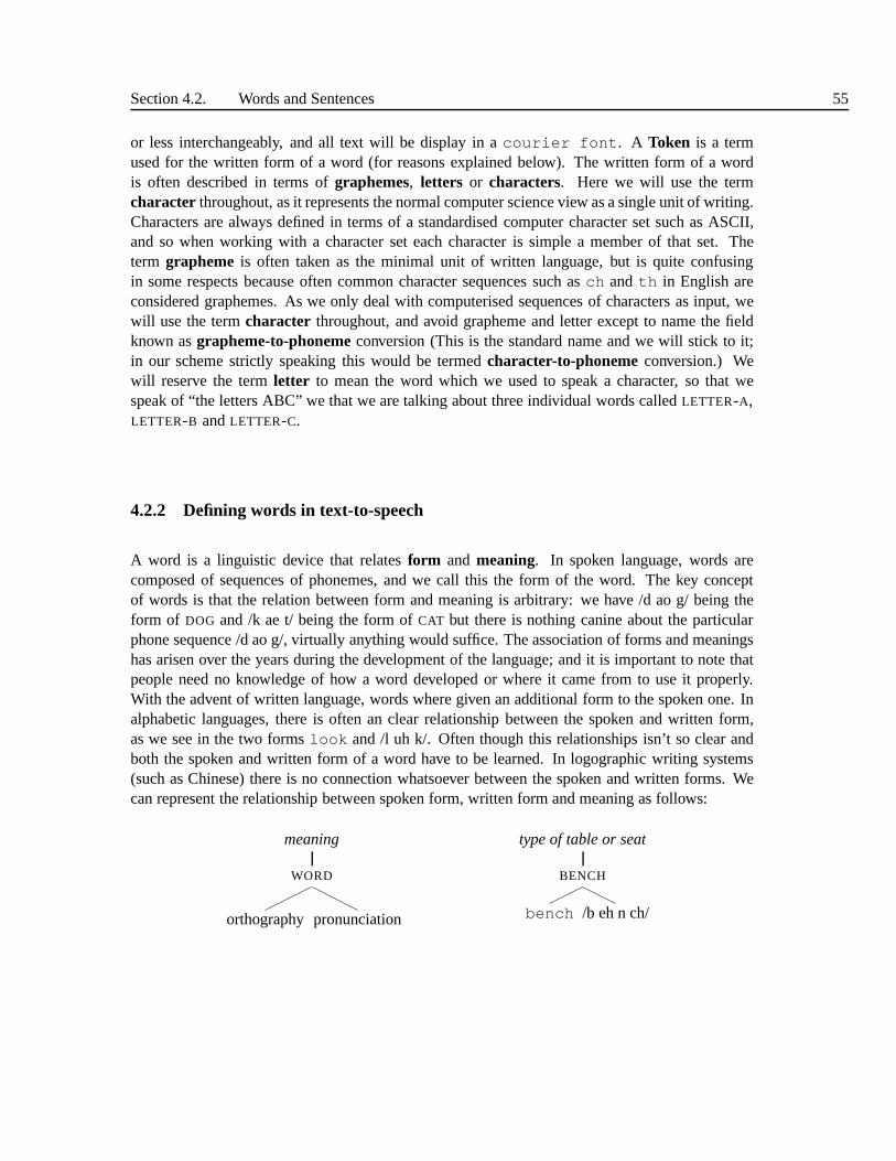
Section 4.2. Words and Sentences 55
or less interchangeably, and all text will be display in acourier font. A Token is a termused for the written form of a word (for reasons explained below). The written form of a wordis often described in terms ofgraphemes, letters or characters. Here we will use the termcharacter throughout, as it represents the normal computer science view as a single unit of writing.Characters are always defined in terms of a standardised computer character set such as ASCII,and so when working with a character set each character is simple a member of that set. Theterm grapheme is often taken as the minimal unit of written language, but isquite confusingin some respects because often common character sequences such asch andth in English areconsidered graphemes. As we only deal with computerised sequences of characters as input, wewill use the termcharacter throughout, and avoid grapheme and letter except to name thefieldknown asgrapheme-to-phonemeconversion (This is the standard name and we will stick to it;in our scheme strictly speaking this would be termedcharacter-to-phonemeconversion.) Wewill reserve the termletter to mean the word which we used to speak a character, so that wespeak of “the letters ABC” we that we are talking about three individual words calledLETTER-A,LETTER-B andLETTER-C.
4.2.2 Defining words in text-to-speech
A word is a linguistic device that relatesform and meaning. In spoken language, words arecomposed of sequences of phonemes, and we call this the form of the word. The key conceptof words is that the relation between form and meaning is arbitrary: we have /d ao g/ being theform of DOG and /k ae t/ being the form ofCAT but there is nothing canine about the particularphone sequence /d ao g/, virtually anything would suffice. The association of forms and meaningshas arisen over the years during the development of the language; and it is important to note thatpeople need no knowledge of how a word developed or where it came from to use it properly.With the advent of written language, words where given an additional form to the spoken one. Inalphabetic languages, there is often an clear relationshipbetween the spoken and written form,as we see in the two formslook and /l uh k/. Often though this relationships isn’t so clear andboth the spoken and written form of a word have to be learned. In logographic writing systems(such as Chinese) there is no connection whatsoever betweenthe spoken and written forms. Wecan represent the relationship between spoken form, written form and meaning as follows:
meaning
WORD
orthography pronunciation
type of table or seat
BENCH
bench /b eh n ch/
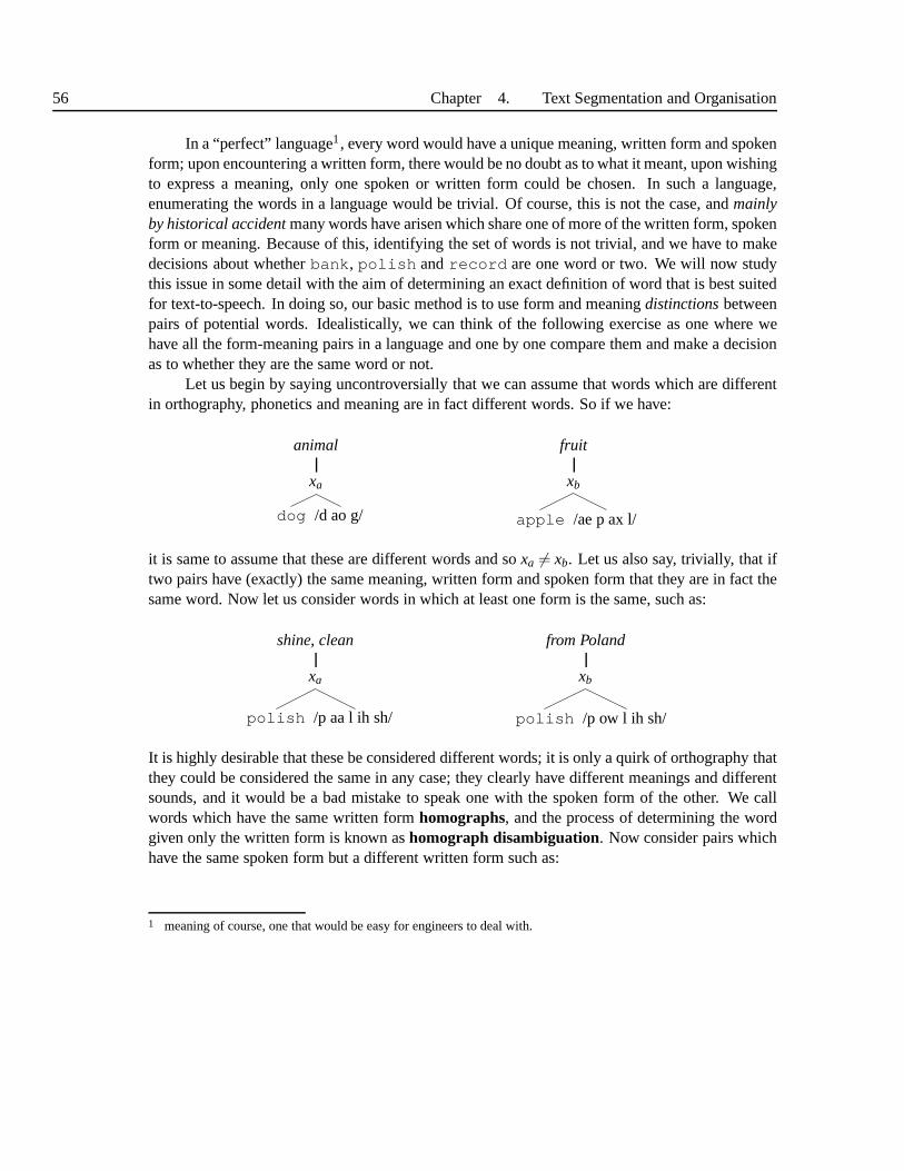
56 Chapter 4. Text Segmentation and Organisation
In a “perfect” language1, every word would have a unique meaning, written form and spokenform; upon encountering a written form, there would be no doubt as to what it meant, upon wishingto express a meaning, only one spoken or written form could bechosen. In such a language,enumerating the words in a language would be trivial. Of course, this is not the case, andmainlyby historical accidentmany words have arisen which share one of more of the written form, spokenform or meaning. Because of this, identifying the set of words is not trivial, and we have to makedecisions about whetherbank, polish andrecord are one word or two. We will now studythis issue in some detail with the aim of determining an exactdefinition of word that is best suitedfor text-to-speech. In doing so, our basic method is to use form and meaningdistinctionsbetweenpairs of potential words. Idealistically, we can think of the following exercise as one where wehave all the form-meaning pairs in a language and one by one compare them and make a decisionas to whether they are the same word or not.
Let us begin by saying uncontroversially that we can assume that words which are differentin orthography, phonetics and meaning are in fact differentwords. So if we have:
animal
xa
dog /d ao g/
fruit
xb
apple /ae p ax l/
it is same to assume that these are different words and soxa 6= xb. Let us also say, trivially, that iftwo pairs have (exactly) the same meaning, written form and spoken form that they are in fact thesame word. Now let us consider words in which at least one formis the same, such as:
shine, clean
xa
polish /p aa l ih sh/
from Poland
xb
polish /p ow l ih sh/
It is highly desirable that these be considered different words; it is only a quirk of orthography thatthey could be considered the same in any case; they clearly have different meanings and differentsounds, and it would be a bad mistake to speak one with the spoken form of the other. We callwords which have the same written formhomographs, and the process of determining the wordgiven only the written form is known ashomograph disambiguation. Now consider pairs whichhave the same spoken form but a different written form such as:
1 meaning of course, one that would be easy for engineers to deal with.
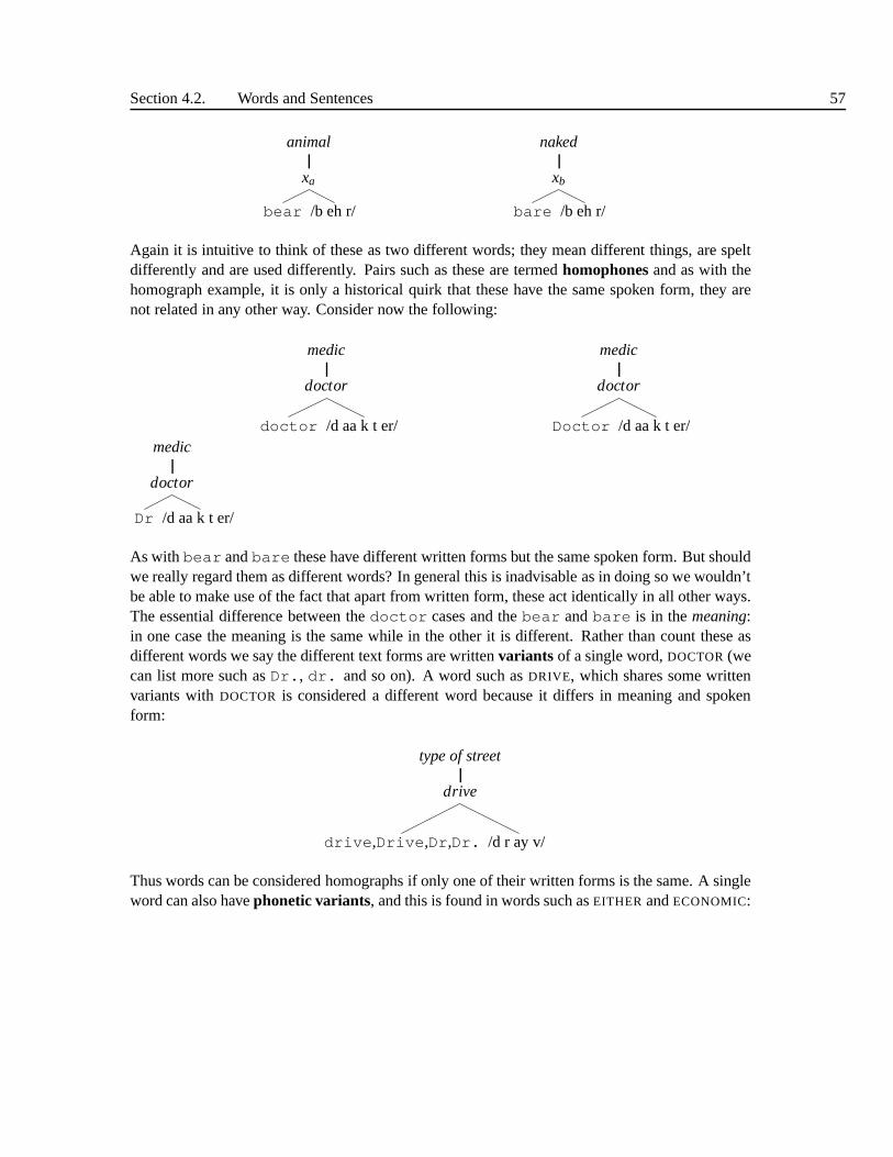
Section 4.2. Words and Sentences 57
animal
xa
bear /b eh r/
naked
xb
bare /b eh r/
Again it is intuitive to think of these as two different words; they mean different things, are speltdifferently and are used differently. Pairs such as these are termedhomophonesand as with thehomograph example, it is only a historical quirk that these have the same spoken form, they arenot related in any other way. Consider now the following:
medic
doctor
doctor /d aa k t er/
medic
doctor
Doctor /d aa k t er/medic
doctor
Dr /d aa k t er/
As withbear andbare these have different written forms but the same spoken form.But shouldwe really regard them as different words? In general this is inadvisable as in doing so we wouldn’tbe able to make use of the fact that apart from written form, these act identically in all other ways.The essential difference between thedoctor cases and thebear andbare is in themeaning:in one case the meaning is the same while in the other it is different. Rather than count these asdifferent words we say the different text forms are writtenvariants of a single word,DOCTOR(wecan list more such asDr., dr. and so on). A word such asDRIVE, which shares some writtenvariants withDOCTOR is considered a different word because it differs in meaningand spokenform:
type of street
drive
drive,Drive,Dr,Dr. /d r ay v/
Thus words can be considered homographs if only one of their written forms is the same. A singleword can also havephonetic variants, and this is found in words such asEITHER andECONOMIC:
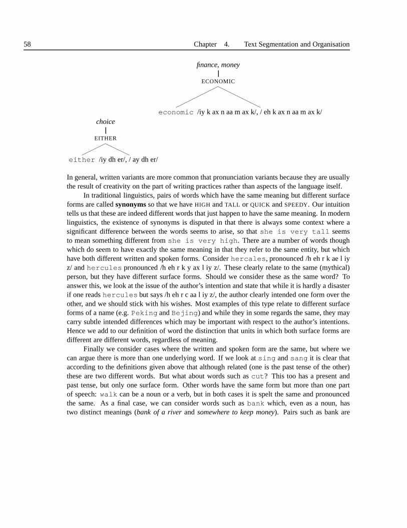
58 Chapter 4. Text Segmentation and Organisation
finance, money
ECONOMIC
economic /iy k ax n aa m ax k/, / eh k ax n aa m ax k/choice
EITHER
either /iy dh er/, / ay dh er/
In general, written variants are more common that pronunciation variants because they are usuallythe result of creativity on the part of writing practices rather than aspects of the language itself.
In traditional linguistics, pairs of words which have the same meaning but different surfaceforms are calledsynonymsso that we haveHIGH andTALL or QUICK andSPEEDY. Our intuitiontells us that these are indeed different words that just happen to have the same meaning. In modernlinguistics, the existence of synonyms is disputed in that there is always some context where asignificant difference between the words seems to arise, so that she is very tall seemsto mean something different fromshe is very high. There are a number of words thoughwhich do seem to have exactly the same meaning in that they refer to the same entity, but whichhave both different written and spoken forms. Considerhercales, pronounced /h eh r k ae l iyz/ andhercules pronounced /h eh r k y ax l iy z/. These clearly relate to the same (mythical)person, but they have different surface forms. Should we consider these as the same word? Toanswer this, we look at the issue of the author’s intention and state that while it is hardly a disasterif one readshercules but says /h eh r c aa l iy z/, the author clearly intended one form over theother, and we should stick with his wishes. Most examples of this type relate to different surfaceforms of a name (e.g.Peking andBejing) and while they in some regards the same, they maycarry subtle intended differences which may be important with respect to the author’s intentions.Hence we add to our definition of word the distinction that units in which both surface forms aredifferent are different words, regardless of meaning.
Finally we consider cases where the written and spoken form are the same, but where wecan argue there is more than one underlying word. If we look atsing andsang it is clear thataccording to the definitions given above that although related (one is the past tense of the other)these are two different words. But what about words such ascut? This too has a present andpast tense, but only one surface form. Other words have the same form but more than one partof speech:walk can be a noun or a verb, but in both cases it is spelt the same andpronouncedthe same. As a final case, we can consider words such asbank which, even as a noun, hastwo distinct meanings (bank of a riverandsomewhere to keep money). Pairs such as bank are
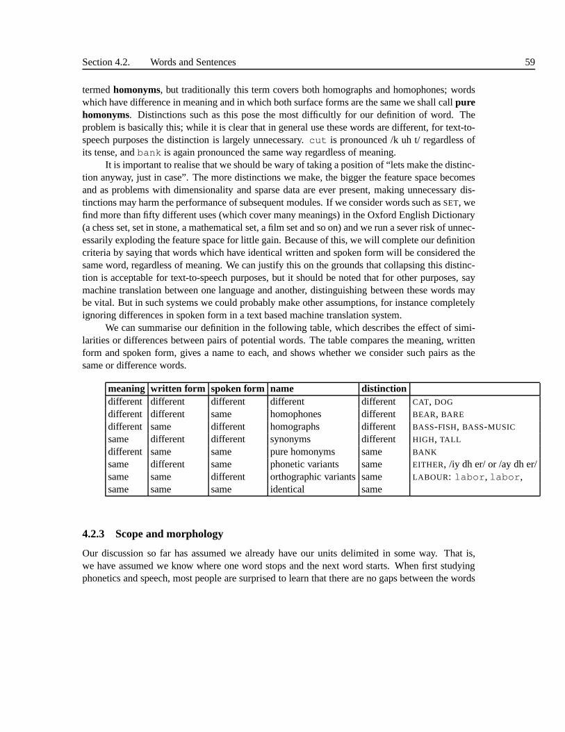
Section 4.2. Words and Sentences 59
termedhomonyms, but traditionally this term covers both homographs and homophones; wordswhich have difference in meaning and in which both surface forms are the same we shall callpurehomonyms. Distinctions such as this pose the most difficultly for our definition of word. Theproblem is basically this; while it is clear that in general use these words are different, for text-to-speech purposes the distinction is largely unnecessary.cut is pronounced /k uh t/ regardless ofits tense, andbank is again pronounced the same way regardless of meaning.
It is important to realise that we should be wary of taking a position of “lets make the distinc-tion anyway, just in case”. The more distinctions we make, the bigger the feature space becomesand as problems with dimensionality and sparse data are everpresent, making unnecessary dis-tinctions may harm the performance of subsequent modules. If we consider words such asSET, wefind more than fifty different uses (which cover many meanings) in the Oxford English Dictionary(a chess set, set in stone, a mathematical set, a film set and soon) and we run a sever risk of unnec-essarily exploding the feature space for little gain. Because of this, we will complete our definitioncriteria by saying that words which have identical written and spoken form will be considered thesame word, regardless of meaning. We can justify this on the grounds that collapsing this distinc-tion is acceptable for text-to-speech purposes, but it should be noted that for other purposes, saymachine translation between one language and another, distinguishing between these words maybe vital. But in such systems we could probably make other assumptions, for instance completelyignoring differences in spoken form in a text based machine translation system.
We can summarise our definition in the following table, whichdescribes the effect of simi-larities or differences between pairs of potential words. The table compares the meaning, writtenform and spoken form, gives a name to each, and shows whether we consider such pairs as thesame or difference words.
meaning written form spoken form name distinctiondifferent different different different different CAT, DOG
different different same homophones different BEAR, BARE
different same different homographs different BASS-FISH, BASS-MUSIC
same different different synonyms different HIGH, TALL
different same same pure homonyms same BANK
same different same phonetic variants same EITHER, /iy dh er/ or /ay dh er/same same different orthographic variantssame LABOUR: labor, labor,same same same identical same
4.2.3 Scope and morphology
Our discussion so far has assumed we already have our units delimited in some way. That is,we have assumed we know where one word stops and the next word starts. When first studyingphonetics and speech, most people are surprised to learn that there are no gaps between the words
60 Chapter 4. Text Segmentation and Organisation
in speech; we are naturally think that language is writing, so that we think of words as welldelimited units (at least for speakers of European languages). In normal speech however, the flowof speech is continuous with no acoustic boundaries marked.Furthermore, while some phonemesare more likely to occur near word beginnings and ends, therereally is no way to bottom-up findword boundaries from acoustic evidence. The sceptical observer might well then ask, do words,as distinct units in time, really exist, or are they simply a invention of linguists (both traditionaland modern)?
These problems ofscope(that is where one word stops and the next starts) can be seenas problems ofmorphology, the study of how words are composed. In practice, the main issueconcerns whether we should explicitly regard all theinflected forms of alexemeas words in theirown right, or whether we should only consider the as a true word. A lexeme (e.g.BIG) is definedas the most basic form of a word, and itsinflections are composed from this so that we haveBIG, BIGGER andBIGGEST. In addition we havederivational morphology, which explains howwords such asCREATION are formed fromCREATE. In earlier text-to-speech systems it was oftenconsidered wasteful to list all the forms, rather the lexemewas stored and the other forms werederived. This approach of course is more expensive computationally as processing has to be usedto derive the forms from the lexeme. Today it really is a matter of engineering expediency whichapproach is chosen as it is quite possible to store all the forms of a lexeme.
4.2.4 Contractions and Clitics
We will now turn to the issue of whether longer units form words in their own right. First letus considercontractions, which are written forms created from particular combinations of twowords. Common examples are:
(13) I’ve, can’t, won’t ,they’ll, he’d
Contractions arenot abbreviations. Abbreviations are words which have a shortened written formonly, such as (Dr 7→ DOCTOR). By contrast, contractions have shortened forms in both the writtenand spoken form, sothey’ll, formed from the contraction ofTHEY andWILL is pronounced/dh ey l/ and not /dh ey w ih l/. We can state more properly that contractions are shorted spokencombinations of words, whose properties are reflected in writing conventions. The question withcontractions is whether we should regard the contraction asone word or two. First note that thecontraction isn’t always simply a case of concatenating a first written form to a shortened secondwritten form. Whilethey’ll is created this way,won’t meaningWILL NOT is not formedthis way, and similarly withaint. While don’t can be formed from the concatenation ofdoandnot followed by the replacement ofo with ’, phonetically the process is different in that thevowel of DO, /uw/ changes to /ow/ indon’t. Furthermore, sometimes the apostrophe occurs atthe place where we would break the forms (e.g.they’ll) but sometimes not e.g.don’twouldbreak intodo andn’t, notdon and’t).
As with previous problems, we settle this issue by deciding what we think is best for TTS.While it is common in natural language parsing to expand contractions and regard them as two

Section 4.2. Words and Sentences 61
words, in TTS, they arespokenexactly as a single word would be, and for this reason we regardall these forms as single words. In further support of this wefind that contractions can be veryambiguous with respect to the second word, for examplehe’d can either beHE HAD or HE
WOULD. If we chose to expandhe’dwe would have to decide which word the’d was a form of.Luckily in text-to-speech, both forms are written the same and are pronounced the same (/h iy d/),so we don’t have to resolve the ambiguity. Contractions comeclose to forming a closed class, inthat they vast majority of contractions are formed from pronouns plus auxiliaries (I’ll, he’d)or with negationscan’t, won’t, but it is in fact possible to form contractions from normalnouns as in:
(14) The roads’ll be busy tonight
(15) The boy’s got to learn
(16) The team’ve really shown their strengths
which means the set is not truly closed.Clitics have similar written forms to contractions in that they use aapostrophe, and that the
written pattern follows through to the spoken form (unlike abbreviations). Clitics differ thoughin that they are not contractions of two words, but rather function more like an affix joined to anormal word. There is only one use of a clitic in English, which is the genitive’s, as used inPaul’s book. Other languages have much richer use for clitics. In this sense, clitics can bethought of as affixes; indeed some argue that it is only a historical quirk of English printing thatthe generative apostrophe is used at all; there is no structural linguistic reason why we shouldn’twrite Pauls book. As with contractions, we view a form with a clitic as a singleword.
A final type of modified word is theshortened form where a normal word has been short-ened in some way. Examples includelab (from laboratory),phone from telephone andso on. These are distinct from abbreviations in that both thewritten and spoken form are short-ened. This is an important distinction because we assume that when an author writeslab he doesin fact mean just this and if he were to speak it aloud he would say /l ae b/ not /l ax b ao r ax tao r ii/. Despite the commonality in meaning, we therefore regardLAB andLABORATORY as twoseparate words.
4.2.5 Slang forms
An additional type of contraction is what we termslang forms which include forms such asgonna, wanna, gotcha and so on. Despite the lack of the apostrophe that we find with theother contractions, these are similar to contractions in that the written form clearly represents thecombination of two words as a single word. The issue here is again whether to representgonnaas two words (GOING andTO) or one. At first glance, the answer to this may seem to be the sameas with the other contractions we looked at, such asI’ve etc, and that they should be regarded asa single word. Recall however that our definition of a contraction was one of two words becominga single surface form inboth the written and spoken form. The problem withgonna is that it is
62 Chapter 4. Text Segmentation and Organisation
not clear exactly what the status of the spoken form is. In reality, the sequence<GOING, TO> isrealised in a wide variety of fine spoken forms, and it is only an accident that two (going to andgonna) have become standard in the orthography. Whilegonnamay be a genuine case, there areactually quite a number of less standard forms such asgotcha (GOT YOU), (whadaya WHAT
DO YOU) and so on. If it wasn’t for the fact that these forms span two words, we would describethem as orthographic variants of the same word, in the way we would withnite andthru andso on. Weighing up these competing arguments and the discussion on pronunciation variation thatwe will have in Chapter 8, we decide thatgonna and other similar forms should be representedby two words and should not be regarded as bona fide contractions.
4.2.6 Hyphenated forms
So far our discussion has centred on whether forms which we normally delimit by whitespaceshould be considered as full words or further broken down, and we have seen that apart from afew exceptions, whitespace in conventional writing is actually a quite reliable guide as to wordboundaries. But there are certain cases where we can argue that forms separated by whitespaceshould in fact be treated as a single word. Most of this involves issues to do with hyphens andcompounding. Consider the following examples:
(17) a. last ditch, last-ditch
b. spokes woman, spokes-woman, spokeswoman
c. web site, web-site, website
d. new line, new-line, newline
e. steam boat, steam-boat, steamboat
f. vice chancellor, vice-chancellor
g. lock nut, lock-nut, locknut
Here we have a different set of words in which we can have the same two words combined to formup to three written forms; either as separate written forms separated by whitespace, as forms sepa-rated by a colon, or as a single written form. These patterns raise a number of issues. Firstly, therecan be a huge number of forms such asSPOKESWOMAN, in which two relatively common wordscombine to form a single token. While we could again put everyform of this type in the lexiconas is, there are likely to be several unknown forms. Secondly, words likespokeswoman act likeseparate words for the purposes of inflection; the plural ofspokeswoman is spokeswomenand notspokeswomans, and so the orthographic form uses the irregular plural formof one ofits constituents. Thirdly, as shown in the list of examples,the written conventions actually usedvary considerably, and one finds that theweb site, web-site andwebsite forms are allcommon, when it is clear that they are all just written variant forms of the same word. Finally,many of these words act like a single phonological word. Of course, in all cases, there is nosilence between the words in when spoken fluently, but there is also the problem of stress. Innormal adjective noun patterns (e.g.large site) the stress normally goes on the second word,

Section 4.2. Words and Sentences 63
but in cases such asweb site it goes on the first, as would be the case in single words suchasPARASITE. This helps show the reason over the variability and behavior of the written form; inspeaker’s minds this acts like a single word. There is no realway to resolve this issue as we feel wemust allow words likeblackbird to be represented by a single word, but it is also impossibleto know where to draw the line.
In summary, we use the following guidelines and rules to delimit words:
• Words include free stems and all inflected and derived forms of a stem
• Contractions and forms containing clitics are single words
• Slang forms created from two words are not single words
• Compounds, hyphenated words and multi words are consideredsingle words on a case bycase basis.
• In conventional writing, whitespace and is quite a good guide to word boundaries.
4.2.7 What is a sentence?
As with our discussion with words, we find that there are many possible definitions of a sentence,and we need to investigate this a little further before discussing any algorithms which processsentences. It is frequently asked whether people really “speak in sentences” at all. When listeningto politicians being interviewed, they have an uncanny ability to avoid ever ending a sentence; ifthey did they could be interrupted. As they wish to hog the floor, they avoid ending a sentence at allcosts (to the extent thateven morerubbish is spoken). In spontaneous dialogue, it is again uncertainwhether sentences are the main unit. Thankfully this is one area where our cross-over betweenwritten and spoken language does actually help. While it is unclear whether people engaged ininterviews or dialogues use sentences, it is clear that the vast majority of conventional writing isindeed clearly written in sentences. Furthermore, when people read aloud, they effortlessly findthe sentence boundaries and adopt the appropriate sentence-final prosody, such that the boundariesare preserved in the spoken signal. For our purposes, the situation is complicated somewhat by theuse of non-natural language writing. In an email header, there are no sentences explicitly marked,and it is part of the verbalisation process that we find suitable sentence boundaries. Again, thisproblem is one we share with a human reader - when they are given an email header and told toread it, they also suffer from not knowing exactly how to go about this. Nonetheless, our task insentence splitting is therefore to find the written sentenceboundaries in conventional and all othertypes of writing.
In the linguistic literature, many different ways of defining what a sentence is have beenproposed. One approach is what we can term the discourse approach, which states something like,a sentence is the smallest possible answer to a question, or that it is the smallest unit that canbear functional meaning and so on. Another approach is to define sentences using more formalmechanisms; this can take the form of saying that a sentence is a linguistic unit with a subject-predicate structure, or even more formally, a sentence is the full expansion of any formal grammar

64 Chapter 4. Text Segmentation and Organisation
(this final point of course doesn’t attempt to define sentences “in nature” but just says that theyare a logical by product of a formal grammar). A third definition based on writing, which woulddefine a sentence as something like “the words between two full stops” or, “it starts with a capitalletter and ends with a full stop”. With certain caveats (see below) we will adopt this definition aswe can’t rely on using any deeper linguistic analysis to assess the internal coherence of a sentence.
4.2.8 The lexicon
In all modern TTS systems we make extensive use of alexicon. The issue of lexicons is in factquite complicated, and we discuss this in full in Chapter 8 when we start to talk about pronunci-ation in detail. For our current purpose, its main use is thatit lists the words that are known tothe system, and that it defines their written form. A word may have more than one written form(labour andlabor) and two words may share the same written formpolish etc. It is byusing a lexicon as a place to define what is a possible word and what its written forms may be, thatwe can use the decoding model we are adopting in this book.
4.3 TEXT SEGMENTATION
Now that we know what we are looking for (underlying words) wecan turn our attention to theproblem of how to extract these from text. While in principlethis could be achieved in a singleprocess, it is common in TTS to perform this in a number of steps. In this section and the next wedeal with the initial steps oftokenisation andsentence splittingwhich aim to split the input se-quence of characters into units which are more easily processed by other processes which attemptto determine the word identity. subsequent
4.3.1 Tokenisation
Formally, we can think of the input as a sequence of characters which encode a sequence of words:
< w1,w2,w3, ...wN > 7→< c1,c2,c3, ...cM >
and so our problem in text analysis is simply one of reversingthis process so that we can uncoverthe word sequence from the character sequence, as in the following:
(18) The old lady pulled her spectacles down→< THE, OLD, LADY , PULLED,HER, SPECTACLES, DOWN >
In most cases of conventional writing, the words don’t overlap with respect to the characters, sowe can also represent this relationship as:
(19)
THE︷︸︸︷
The
OLD︷︸︸︷
old
LADY︷ ︸︸ ︷
lady
PULLED︷ ︸︸ ︷
pulled
HER︷︸︸︷
her
SPECTACLES︷ ︸︸ ︷
spectacles
DOWN︷ ︸︸ ︷
down

Section 4.3. Text Segmentation 65
We can clearly see that the written sentence is easily segmented by using whitespace as a delimiter.This is only possible in this because the incidence of whitespace in the input always indicates thepresence of a word boundary. There are numerous cases however where this simplistic approachfails. In a sentence such as:
(20) In 1997, IBM opened a Polish lab
problems occur because a section of the text may be ambiguousas to its word:
(21) polish→ POLISH COUNTRY or POLISH SHINE
problems where whitespace is insufficient to act as the only guide to segmentation:
(22) IBM→< LETTER I, LETTER B, LETTER >
cases where the token does not map to an word:
(23) ,→ NULL
and cases where both ambiguity and segmentation problems exist:
(24)
a. 1997→< NINETEEN, NINETY, SEVEN >
b. or< ONE, THOUSAND, NINE, HUNDRED, AND, NINETY, SEVEN >
c. or< ONE, NINE, NINE, SEVEN >
so we see in this last example that the process of converting sentences into words is one of bothsegmentation and classification of the written form of the sentence. As the classification and seg-mentation interact, it is not possible to do one then the other. Rather, our approach is to firstperform aprovisionalsegmentation into potential written forms calledtokens, followed by a sec-ond step whereby we examine each token in turn and resolve anyambiguity. This first processis called tokenisation; the step which then generates the words from the tokens is called textanalysisand is the subject of the next chapter
So in our first example, the tokenisation process would perform the following mapping:
(25) The old lady pulled her spectacles down→< the,old,lady,pulled,her, spectacles,down >
The advantage of dividing the problem this way is that it makes it much easier to performthe text analysis step. By tokenising (segmenting) the text, we are making it possible for the textanalysis algorithms to focus on one token at a time: while theanalysis algorithms may examinethe tokens on either side of the one in question, only a few areusually consulted, and this makesthe writing of rules and the training of algorithms quite a bit easier.
4.3.2 Tokenisation and Punctuation
In languages like English, it is obvious that the presence ofwhitespace in the input is a very goodguide to tokenisation. In most conventional writing, splitting on whitespace will often leave a

66 Chapter 4. Text Segmentation and Organisation
one-to-one mapping between tokens and words. The difficulties soon arise however: when weencounter sequences of capital characters such asIBM we could guess that this will be a lettersequence and therefore go someway towards the classification and rewrite process by splitting thisinto three tokens. But there are several forms such asNATO andUNICEF which don’t follow thisconvention; furthermore, sometimes normal words are put into upper case for effect:lets GO!.
Dealing with punctuation properly is one of the main issues in tokenisation. In sentencessuch as
(26) So, he went all that way (at considerable cost) and found no-onethere
we see the classic uses of punctuation. Firstly it creates a boundary between two tokens whichmight otherwise be assumed to be linked, or it creates a link between two tokens which mightotherwise be assumed to be separate. So a full stop ends a sentence, a comma ends a clause andboth create a boundary between the tokens that precede and follow them. Within this use, we havestatus markers, so that while., ? and! all indicate the end of a sentence, they each assigna different status to that sentence. Hyphens and apostrophes link tokens that might otherwise beassumed to be more separate (assuming that whitespace wouldbe used if there were no hyphen orapostrophe).
More difficult problems arise with technical language. First the rules of using whitespace inconjunction with punctuation are often different; so that in a time we find10:34am in which thereis no whitespace after the colon. Furthermore, some of the verbalisations of technical languagespeak the punctuation as words, so that the words foryahoo.com are<YAHOO, DOT, COM>,where the. is spoken asDOT. It helps in cases like these to make some distinctions. Firstwe need to distinguishunderlying punctuation from text punctuation. Underlying punctuationis the abstract notion of what we normally think of as punctuation in conventional writing, andtext punctuation is its written form. These are clearly the punctuation equivalent of words andtokens. So, while we may have two types of underlying punctuation DASH and HYPHEN theremay in fact be only one written form in our character set. Thisuse of one character for twounderlying punctuation marks causes ambiguity and this must be resolved. In addition, as wehave just mentioned, punctuation is sometimesspokenin technical language. We deal with thisphenomenon by using our model of verbalisation, so that inyahoo.com the sequence is analysedfirstly as an email address, then verbalised into natural language and then spoken. In such cases,we will represent the word that the punctuation is spoken asWORD COMMA, WORD COLON andso on, to distinguish from the silent form ofCOMMA andCOLON.
4.3.3 Tokenisation Algorithms
We will now describe a basic tokenisation algorithm:
1. Create an empty list for the tokens to be placed in.
2. Define a start point before the first character of the sentence.

Section 4.3. Text Segmentation 67
3. Move forwards through the sentence, examine each character and the character following it,and decide whether there should be a token boundary at this point
4. If yes, append an entry to the token list and copy (without modification) the characters fromthe start point to the boundary point.
5. Reset the start point to be at the boundary point6. If at the end of the sentence stop, otherwise go to step 3.
The heart of the algorithm is therefore the part which decides whether a boundary should beplaced between two characters of the input. This works on thefollowing criteria:
1. Split on whitespace, but don’t include the whitespace itself in any token.2. Split on punctuation, create a separate token for each punctuation character.3. Split when a contiguous non-whitespace sequence changesfrom one character grouping to
another (e.g.10cm→ 10 cm).4. Don’t split in any other cases.
Sometimes more complex (or more accurate) tokenisation algorithms are used. The amountof resource put into tokenisation to some extent depends on the sophistication of the process thatfollows it. If this can handle errors or noise in the tokenisation, then a fairly simple algorithmshould suffice. If however the subsequent algorithms require more accurate tokenisation a numberof approaches can be applied. The deterministic approach can be extended by considering greaternumbers of cases and writing rules by hand which deal with each case in turn (e.g. email addresses,times, dates and so on). Alternatively, a data-driven approach can be taken where we label a corpuswith token boundaries and train an algorithm to learn the correspondence. Such an approach is aclassic use of a data-driven technique in speech and language processing, and discussion of thiswill be deferred until the general discussion of this in Section 5.2.1.
4.3.4 Sentence Splitting
Many of the algorithms in TTS work a sentence at a time. This isbecause most linguistic unitssmaller than this (words, syllables) etc are heavily influenced by their neighbours which makesautonomous processing difficult. Sentences on the other hand don’t interact with each other much,and apart from some specific phenomena, we can by and large process each sentence indepen-dently without problem. The input to the TTS system is not necessarily in sentence form however,and in many cases we are presented with a document which contains several sentences. The taskof sentence splittingthen is to take the raw document and segment it into a list of sentences.
While sentence splitting is not the most complex of tasks in TTS, it is important to get rightand this is mainly due to the fact thatsentence-final prosodyis one of the phenomena that listenersare most sensitive to. Generating the high quality sentence-final prosody is hard enough in its ownright, but if the sentence boundary is in the wrong place, then the system has no chance.
For conventional writing we make use of the fact that in most cases the writer has clearlymarked the sentence boundaries; and so our job is simply to recover these from the text. Perhaps

68 Chapter 4. Text Segmentation and Organisation
ironically then, our algorithm is based on the lay notion of finding upper case characters at begin-nings of sentences and period characters at the end, and marking sentences as what lies between.The situation is not quite that simple; as we know the period character can be used for a variety ofpurposes, as can upper case characters. The task is therefore one of finding instances periods andrelated characters, and classifying them as to whether theyindicate sentence boundaries or not.
A basic sentence splitting algorithm for conventional writing can be defined as follows:
1. Start a new sentence at the beginning of the input2. Search forwards through the input to find instances of the possible end of sentence characters
., ! and?.3. Using the immediate context of these characters, determine whether a sentence boundary
exists; if so complete the current sentence and start a new one.4. End the current sentence at the end of the document (regardless of whether the last characters
are., ! or ?.)
The heart of the algorithm is the decision as to whether an instance of an text form of.,! or ? constitutes a sentence of not. The most difficult case is. as this can be used as part ofan abbreviation, a number an email address and so on. In conventional writing, a space alwaysfollows the full stops at a sentence end, and the next sentence always starts with an upper caseletter. In fact the onlyconventionalother use of. is in abbreviations, so that we might find:
(27) Dr. Jones lives in St. James Road
In fact, in most modern writing, the use of. in this sort of abbreviation is not common. Profes-sional publishers make use ofstyle manualsto help authors with various issues in writing andlayout. Conventions differ, but instructions from one academic journal include:
• Do not use periods in titles, henceDr Jones, Mr Mark Johnson Jr
• Do not use periods in letter sequences, henceUSA, IBM• Do use periods for abbreviations in personal names, henceJ. R. R. Tolkein (note
that a space follows the period)• Do use periods for latin letter sequences, hencee.g. andet. al.
These guidelines show that the incidence of periods in abbreviations is probably less com-mon that expected, but there are still potentially confusing situations. Remarkably, many styleguides are aware of this and even advise writers “do not starta sentence with an abbreviation”. Ofcourse, real life is never so simple, and even in conventional writing, one sees frequent variationson the above guidelines, such that we must in principle allowfor a period after any abbreviation(For example, one seesJRR Tolkein, J.R.R. Tolkein, J R R Tolkein andJ. R.R. Tolkein all on writing from the Tolkein Society alone). Usage patterns are potentially sig-nificant, in that while we may allow a period after any abbreviation, a probabilistic algorithm couldmake use of the fact that they are rarely found in some cases. And of course, if these really wereuniversal conventions they wouldn’t have to be spelled out in a style guide, authors would simplyknow.

Section 4.4. Processing Documents 69
For less casual conventional writing, the situation can be more difficult. In email messages,one finds that some writers do not use an upper cases characters at the start of a sentence, or thatnew-lines are used as sentence boundaries and no ending punctuation is found. We also comeacross the problem in email that the form of the headers is intended for email programs to parseand process and not for reading aloud. So the notion of “sentence” is unclear here. To get aroundthis, we simply have to decide in what form we will read this information and so what form thesentences will take in these genres. One approach is to have each line as a sentence, another is tosomehow process the header into a spoken list or other structure.
4.4 PROCESSINGDOCUMENTS
4.4.1 Markup Languages
It is useful to be able to control the behavior of the TTS system at run time. While global parame-ters can be set in a number of ways, often it is useful to have very precise instructions which affectspecified words. This is most effectively done by interleaving instructions to the TTS system withthe actual text to be spoken. In older TTS systems, it was common for each to have its own typeof markup. So for example in the Bell Labs system [411],, there are special sequences of escapecharacters that help the user specify what behaviour the system is to follow.
The disadvantage of this is that these special characters would mean nothing to a differentTTS system, so a document marked up for one TTS system would not work with another. Toget around this, Taylor and Isard [435], [444] proposed thespeech synthesis markup language(SSML) which aimed to provide a general set of markuptags which could in principle be usedby any TTS system. This was extended by a number of further projects including thespoken textmarkup language by Sproat et al [411], and thejava speech markup languagedeveloped byAndrew Hunt at Sun Microsystems. These served as the basis ofthe synthesis part of the W3CstandardVoiceXML (also called SSML, but not to be confused with the original).
All these schemes are based on the idea ofgeneralised markup, first developed in the type-setting industry. There, the idea ofmarkup had been around for a long time, where a typesetterwould mark some text to be printed in 12 point, or in italics orso on. The problem with suchmarkup is that instructions is that they arephysical, meaning that they are very specific to the typeof printing being used. If someone wished to print the document in a bigger font for instance, theinsistence on using 12 point (which may have seemed large in a10pt document) means that theintended effect is not achieved. Generalised markup attempts to get round this by splitting the typesetting into a two stage process. The author, or editor, addslogical markup to the text, for exampleby indicating that something is a heading, or requires emphasis. In the second stage, this is thenrendered by a process much more specific to the actual printing mechanism being employed. Asthe document itself only contains logical instructions, itis much more portable, and can be printedon a number of devices and in a number of styles.

70 Chapter 4. Text Segmentation and Organisation
The speech synthesis markup languages followed a similar philosophy, so instead of spec-ifying that a word should be spoken at 150Hz (which would havedifferent effects for differentspeakers), instead more abstract or “logical” instructions are used, which for instance state that aparticular word is to be emphasised. A few simple examples will now be explored.
tag Example Explanation<s> This tag can be used <s>
to override the decisionsof the <s> sentencesplitting algorithm.
This tag indicates that a sentence breakshould be placed at this point. It is agood way for the author to over rideany possible shortcomings in the sen-tence splitting algorithm.
<emphasis> Sometimes we<emphasis>need</emphasis>to give a word specialemphasis.
This is used to give particular empha-sis to a word or group of words. Notehow abstract or “logical” this tag is; noreference is made to the phonetics ofhow to render the emphasis as height-ened pitch, longer duration and so on.
<voice> <voice gender="female"age="20"> This is afemale voice </voice><voice name="mike">And this is a male one<break/> Hope you’re OK.</voice>
Many TTS systems have the capabil-ity of speaking in more than one voice.This tag can switch between voices inby specifying general attributes or spe-cific voice names:
In an SSML document, the tags are interleaved with the text tobe spoken. It is of courseimportant that the two are distinguished, and so the first stage in processing an SSML document isto perform an XML parsing step. There are a number of standardparsers which do this and whichsubsequently produce a structure in which the text and tags are clearly separated. From there, it isup to the TTS system itself to decide how to interpret each tag. The tags vary considerably in theirpurpose, and hence they require processing by different modules in the TTS system. The standardway of dealing with this is to do a partial processing of the XML initially, and then leave hooksin the tokens which tell subsequent modules what to do. As canbe seen with the<s> tag, XML,tokenisation and sentence splitting can interfere, and so it is often a good idea to perform all therequired processing in a single step.
4.4.2 Interpreting characters
Since computers have been around they have been used to storetext, but as computers only operatein ones and zeros, text can not be represented directly. Rather a character encodingschemeis used which maps internal computer numbers to characters.So long as the same convention

Section 4.5. Text-to-Speech Architectures 71
is maintained by the readers and writers, chunks of memory can be used to represent encodedtext. The issue for a TTS system is to identify the character encoding being used and processit appropriately. Partly due to the sheer diversity of the worlds writing systems and partly dueto historical issues in the development of character encoding schemes, there are several ways inwhich characters can be encoded.
One of the earliest and most common encodings wasASCII (the American Standard Codefor Information Interchange), which gave a character valueto the first 127 values in an 8-bit byteof memory (the final bit was left unused). Ascii is of course a standard that was developed in theUnited States, which could only represent the 26 charactersof the standard English alphabet. Mostof the worlds languages of course require different characters and so ascii alone will not sufficeto encode these. A series of extensions were developed primarily with use with other Europeancharacters, often by making use of the undefined eighth bit inascii.
The ISO 8859standard defines a number of encodings. For exampleISO 8859-1encodesenough extra characters for most western European languages such as French and German.ISO8859-2encodes eastern European languages, whileISO 8859-7encodes Greek characters. Theseare all 8-bit encodings are can be used without trouble so long as it is known which is in use. Allcontain ascii as a subset so have the advantage of backwards compatibility. Many languages, inparticular south east Asian languages have far more characters than can be included in 8 bits, andso cannot be accommodated in single byte encoding schemes. Anumber of incompatiblewidecharacter encodings were developed for these languages before a universal standardunicodewasdeveloped in the early 1990s. This provides an encoding for virtually all languages, although somecontrovosies (largely political rather than technical) still prevent its completely universal adoption.
Unicode simply defines a number for each character, it is not an encoding scheme in itself.For this, a number of different schemes have been proposed.UTF-8 is popular on Unix machinesand on the internet. Is is a variably width encoding, meaningthat normal ascii remains unchangedbut that wider character formats are used when necessary. BycontrastUTF-16 popular in Mi-crosoft products, uses a fixed size 2 byte format. More recentextensions to unicode mean that theoriginal 16 bit limitation has been surpassed, but this in itself is not a problem (specifically forencodings such as UTF-8 which are extensible).
4.5 TEXT-TO-SPEECHARCHITECTURES
The various algorithms described here all produce output, and this has to be passed to the nextmodule in the TTS system. As the next module will produce output too, it makes sense to have ageneral mechanism for storing and passing information in the system, This brings us to the issueof how to design our text-to-speecharchitecture.
Most TTS systems have adopted a solution whereby a single data structure is passed betweeneach module. Usually, this data structure represents a single sentence, so the TTS system works byfirst splitting the input into sentences by the sentence splitter, forming a data structure containing

72 Chapter 4. Text Segmentation and Organisation
the raw text for each sentence, and then passing this data structure through a series of modulesuntil a speech waveform is generated. We will term this theutterance structure.
In many early systems, the utterance structure was no more than a string that was passedbetween modules. In doing this systems could adopt either anoverwrite paradigm or aadditionparadigm. For instance in an overwrite system if the input text was
The man lived in Oak St.
The text normalisation module might produce output like:
the man lived in oak street
And the subsequent pronunciation module might then produceoutput like:
dh ax m a n l i v ax d ax n ou k s t r ii t
The point is, in each case, the module takes its input and onlyoutputs the particular results fromthat module. In an addition paradigm, each module adds its output to the output from the previousmodules. So in the above example, the output from the text normalisation module might producesomething like:
The|the man|man lived|lived in|in Oak|oak St|street .|null
And the subsequent pronunciation module might then produceoutput like:
The|the|/dh ax/ man|man|/m ae n/ lived|lived|/l ih v ax d/
in|in|/ax n/ Oak|oak|/ow k/ St|street|/s t r iy t/ .|null
The advantage of addition systems is that it is often hard to know in advance of developmentwhat each module requires as input, and if we delete information we run the risk of supplying amodule with impoverished input. For example, we might find that the phrasing module (whichis called after the text normalisation module) requires punctuation, which can clearly not be usedif the information has been deleted. The trouble with stringbased addition systems is that theycan become unwieldy rather quickly. Even in the example above, with a short sentence and theoperation of only two modules, we see that the string is rather difficult to read. Furthermore, eachmodule will have to parse this string, which becomes increasingly more complicated as the stringbecomes richer.
It is common therefore for modern systems to adopt an approach which follows the additionparadigm, but does so in a way that allows easier and clearer access to the information. Two of themost widely used formalisms are theheterogeneous relation graphor HRG formalism [441],
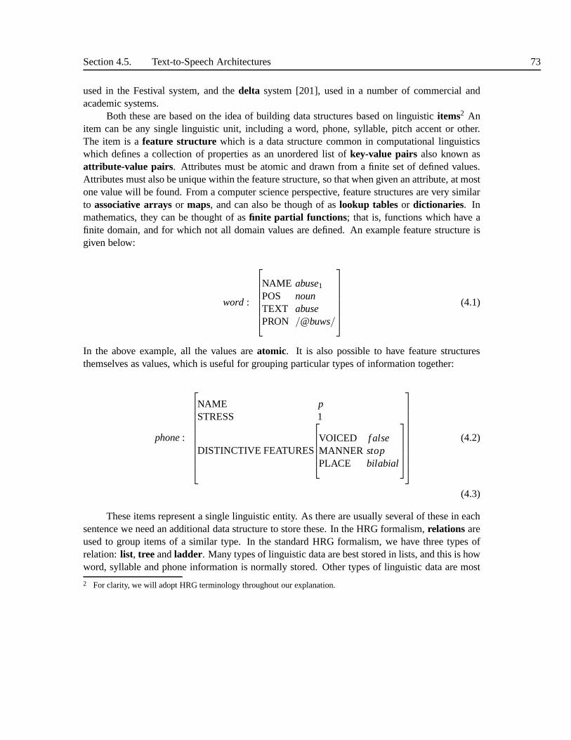
Section 4.5. Text-to-Speech Architectures 73
used in the Festival system, and thedelta system [201], used in a number of commercial andacademic systems.
Both these are based on the idea of building data structures based on linguisticitems2 Anitem can be any single linguistic unit, including a word, phone, syllable, pitch accent or other.The item is afeature structure which is a data structure common in computational linguisticswhich defines a collection of properties as an unordered listof key-value pairs also known asattribute-value pairs. Attributes must be atomic and drawn from a finite set of defined values.Attributes must also be unique within the feature structure, so that when given an attribute, at mostone value will be found. From a computer science perspective, feature structures are very similarto associative arraysor maps, and can also be though of aslookup tables or dictionaries. Inmathematics, they can be thought of asfinite partial functions ; that is, functions which have afinite domain, and for which not all domain values are defined.An example feature structure isgiven below:
word :
NAME abuse1POS nounTEXT abusePRON /@buws/
(4.1)
In the above example, all the values areatomic. It is also possible to have feature structuresthemselves as values, which is useful for grouping particular types of information together:
phone:
NAME pSTRESS 1
DISTINCTIVE FEATURES
VOICED f alseMANNER stopPLACE bilabial
(4.2)
(4.3)
These items represent a single linguistic entity. As there are usually several of these in eachsentence we need an additional data structure to store these. In the HRG formalism,relations areused to group items of a similar type. In the standard HRG formalism, we have three types ofrelation: list, tree andladder. Many types of linguistic data are best stored in lists, and this is howword, syllable and phone information is normally stored. Other types of linguistic data are most
2 For clarity, we will adopt HRG terminology throughout our explanation.

74 Chapter 4. Text Segmentation and Organisation
(c)(b)(a)
Figure 4.1 The three types of relation: a) list relation, b) tree relation and c) ladder relation
S
VP
NP
(a)
(b)
this is
parent
daughter1
daughter2
parent
daughter2
an example
daughter1
this is
next
previous
next next
previous previous
an example
daughter2
Figure 4.2 a) list relation containing word items. b) syntax relation containing syntax items.
suited to trees, and this is how syntax, prosodic phrasing and syllable structure can be stored. Lesscommon is the use of ladders, which are used to represent connections between linguistic datathat is not organised hierarchically, as in a tree. The ladder structure can be used to implementthe data structures ofautosegmental phonology[179], which is used for instance to represent therelationship between syllables and intonation accents. The three types of structure are shown inFigure 4.1.
One way of configuring the data structures is to have a separate relation for the output of each

Section 4.5. Text-to-Speech Architectures 75
321
69
5
8
7
4
this is
Syntax
Word
an example
NP
VP
S
Figure 4.3 Example of a word and syntax relation in which the items in theword relation are alsoin the syntax relation.
module, and so overwriting the output of previous modules isavoided. While straightforward, thisconfiguration can makes the utterance structure very dependent on the particular TTS setup, so thata module that performs pronunciation in one step would generate one relation, whereas one thatperforms lexical lookup, letter-to-sound rules and post-lexical processing as three separate mod-ules would generate three relations. An alternative is to separate relations from particular modulesand instead use relations to store information for each linguistic type, so we can have a “phone” re-lation which comprises a list of phone items, a syllable relation, word relation, intonation relationand so on.
The relations are graphs of nodes arranged in the form of lists, trees and ladders. Each nodecan be linked to an item, and in this way the relation can show the contents of the items and therelationship between them. Named links such asnext(), previous(), daughter() andparent() andso on are used to navigate through the relation. Examples of alist and tree relation are shown inFigure 4.2.
One of the key features of the HRG architecture is that items can be in more than one relationat once. For example, word items can be be in both the word relation and the syntax relation. Thisis useful because often we wish to process the words left to right as a list: the word relation isused for this. Sometimes, however, we want to access the syntax relation, which is a tree in whichthe words form the terminal nodes. Having the same information in the two different places isunappealing as an update to one item requires an update to theother, and this is often awkwardto achieve. Figure 4.3 shows the syntax and word stream together. This ability to include itemsin multiple relations means that usually any information inthe utterance structure can be accessed
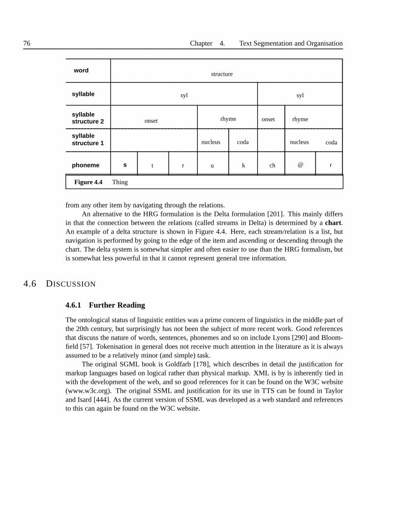
76 Chapter 4. Text Segmentation and Organisation
s
word
phoneme
structure 1syllable
structure 2syllable
syllable
nucleus
rhyme
coda
onset
ch r@
coda
kurt
onset rhyme
nucleus
syl
structure
syl
Figure 4.4 Thing
from any other item by navigating through the relations.An alternative to the HRG formulation is the Delta formulation [201]. This mainly differs
in that the connection between the relations (called streams in Delta) is determined by achart.An example of a delta structure is shown in Figure 4.4. Here, each stream/relation is a list, butnavigation is performed by going to the edge of the item and ascending or descending through thechart. The delta system is somewhat simpler and often easierto use than the HRG formalism, butis somewhat less powerful in that it cannot represent general tree information.
4.6 DISCUSSION
4.6.1 Further Reading
The ontological status of linguistic entities was a prime concern of linguistics in the middle part ofthe 20th century, but surprisingly has not been the subject of more recent work. Good referencesthat discuss the nature of words, sentences, phonemes and soon include Lyons [290] and Bloom-field [57]. Tokenisation in general does not receive much attention in the literature as it is alwaysassumed to be a relatively minor (and simple) task.
The original SGML book is Goldfarb [178], which describes indetail the justification formarkup languages based on logical rather than physical markup. XML is by is inherently tied inwith the development of the web, and so good references for itcan be found on the W3C website(www.w3c.org). The original SSML and justification for its use in TTS can be found in Taylorand Isard [444]. As the current version of SSML was developedas a web standard and referencesto this can again be found on the W3C website.

Section 4.6. Discussion 77
4.6.2 Summary
Words and sentences
• It is important to distinguishwords which are unique linguistic entities fromtokenswhichare their textural instantiation.
• The chapter attempts to provide a rigourous definition of thenotion of word so that theprocess of finding these from the text has a clear target.• Homographsare sets of words which share the same text form. There are three reasons why
homographs arise:
1. The samelexemebeing used as a noun or verb which have different pronunciation (e.g.project)
2. From abbreviated forms of two words producing the same written form (e.g.DOCTOR
andDRIVE producingDr).3. By historical accident (e.g.BASS-MUSIC andBASS-FISH).
• We use a series of tests to define our set of words by looking at distinctions in written form,spoken form and meaning.• Sentences have a number of possible valid definitions. We useone based on the writing as
this is most helpful to TTS.
Text Segmentation
• Top make subsequent processing easier we require that the input be segmented into sentencesand tokens.• It is hard to divide the input into sequences of characters which align one-to-one with the
words, hence tokenisation often produces a provisional segmentation of the text.
• Deterministic algorithms are often accurate enough to produce acceptable tokenisation andsentences.
Documents
• A number ofmarkup languagesexist for speech synthesis, based onXML the successor toXML .
• These markup languages can be used to give extra instructions to the TTS system to overridedefault behaviour.• In modern systems, this markup takes the form oflogical rather thanphysical instructions.
Text-to-speech Architectures
• All TTS systems are composed of a series of modules and all systems have to pass data fromone module to the next.• Early systems typically used strings for this purposes

78 Chapter 4. Text Segmentation and Organisation
• More modern systems use sophisticated structures where each type of linguistic information(e.g. words, syllables, phonemes) can be accessed separately.
• TheHRG system anddelta system are two popular systems for this purpose.

5TEXT DECODING:FINDING THE WORDSFROM THE TEXT
5.1 OVERVIEW OF TEXT DECODING
The task of text decoding is to take a tokenised sentence and determine the best sequence of words.In many situations this is a classical disambiguation problem: there is one, and only one correctsequence of words which gave rise to the text, and it is our jobto determine this. In other situations,especially where we are dealing with non-natural language text such as numbers and dates and soon, there may be a few different acceptable word sequences.
So in general, text decoding in TTS is a process of resolving ambiguity. The ambiguityarises because two or more underlying forms share the same surface form, and given the surfaceform (i.e. the writing), we need to find which of the underlying forms is the correct one. Thereare many types of linguistic ambiguity, including, word identity, grammatical and semantic, but inTTS we need only concentrate on the type of ambiguity which affects the actual sound produced.So while there are two words which share the orthographic form bank, they both sound the sameand so we can ignore this type of ambiguity for TTS purposes. Tokens such asrecord can bepronounced in two different ways, and so thisis the type of ambiguity we need to resolve.
’In this chapter, we concentrate on resolving ambiguity relating to the verbal component oflanguage. At its core, this means identifying the correct sequence of words for every sentence,but we shall also consider in brief the issue of resolving ambiguity in the syntactic structure of asentence also, as this is thought by some to have a lesser but still significant impact on speech. Inthe next chapter, we concentrate on the corresponding process for prosody, where we attempt tofind a suitable underlying prosodic representation from thetext.
This process boils down to the following tasks:
1. Determine the semiotic class (number, date, natural language etc) for each token.
2. For each sequence of tokens in the same semiotic class find resolve any ambiguity and findtheir underlying forms
3. For non-natural language classes, perform a verbalisation process, which converts their un-derlying forms into a sequence of words which can be spoken.
Generally, non-natural language tokens are quite easy to decode; the difficulty is not in
79

80 Chapter 5. Text Decoding: Finding the words from the text
knowing how to decode the token1997 once we know it is a year, but rather in determining it isa year in the first place. With natural language tokens, even once we have established that they areindeed natural language, we still can face considerable difficulty in determining their underlyingform as different words can share the same text form.
While there are many subtle issues involved in text decoding, in essence then it reduces totwo main problems;semiotic classification, i.e. the assignment of a semiotic class to each token,and homograph disambiguation where we determine the correct word for ambiguous naturallanguage tokens. Both these tasks involve assigning a category to a token, and as we shall see,both can be solved with very similar algorithms. Because of this, we now turn our attention to ageneral overview of text disambiguation.
5.2 TEXT CLASSIFICATION ALGORITHMS
5.2.1 Features and algorithms
In both semiotic classification and homograph disambiguation, our goal is to assign alabel to eachtoken, where the label is drawn from a pre-defined set. This process is one ofclassification, whichas we shall see, crops up all the time in TTS to the extent that we use a number of basic approachesagain and again for various TTS problems.
More formally, we say that for each unit (tokens in this case)we wish to assign a labell idrawn from a set of labelsL = l1, l2, ...lN. Our decision is based on analysing a number offeatures each of which has set of legalvalues. These serve as information as to which label isbest in each case. This process can be defined as a functionC
C : F 7→ L
which maps from a feature spaceF to a label spaceL.Let us consider a simple example where we wish to disambiguate the tokenreadwhich can
encode the past tense wordREAD-PAST, pronounced /r eh d/ or the present tense/infinitive wordREAD-PRESENT, pronounced /r iy d/. In this case, our label set comprises two labels such thatL = l1 = READ-PAST, l2 = READ-PRESENT. If we now consider some example sentences:
(28)
a. I was going to read it tomorrow.
b. I read it yesterday.
c. It is vital that young people learn to read at the correct stage.
d. It read him the riot act.
We see that the other words/tokens in the sentence, and the way they interact with the to-kenread gives us strong clues as to which word is correct in each case.These “clues” can beformulated as features, so in the above examples we might have features and values defined as:

Section 5.2. Text Classification Algorithms 81
Name Feature legal valuesF1 Time token TOMORROW, NOW, YESTERDAY
F2 Is the preceding wordTO ? yes, noF3 Is the sentence part of a narrativeyes, no
Hence a classification algorithm working on this is defined as
C(F1,F2,F3) 7→ l1 or l2
Below we describe a range of algorithms which operate in thisway. Some are explicitly formulatedby a human designer and by convention we call such algorithmshand written (although obviouslyit is the brain which really writes the rules). In these approaches, a human designer has consideredthe effect of the features and has by one means or another written a system which performs theabove mapping. The other common approach isdata driven where the mapping is learned byanalysis of a database of examples. Often this database islabelled, meaning that it comprises a setof pairs of feature values and labels, with the idea that an algorithm can be trained to reproducethis correspondence. Not all data driven algorithms work inthis way, some areunsupervisedmeaning that they look at the inherent patterns in the data and attempt to come up with a mappingthat way. An important sub-class of data-driven algorithmsarestatistical or probabilistic .
Regardless of which approach is taken, the goal is effectively the same, and all encounter thesame problems to be overcome. The difference between hand written and data driven is not as largea difference as it is often portrayed in that even if a human designs the rules, they presumably dothis based on experience of the problem, in which they have encountered data with these featuresand labels. Conversely, using an arbitrary data driven algorithm on data generally produces poorresults; better results are obtained by pre-processing thefeatures and constraining the model insome way, which of course requires knowledge of the problem.
The basic problem in all classification algorithms, no matter what type, comes from theissue of how features interact. In general, the features cannot be considered independent, suchthat we count the evidence from one feature, then the next andso on and then combine these tomake a final decision. If we could do this, then the design of classification algorithms would be asimple matter. Rather the features tend to interact, so in the above example, instead of examininga separate situation for each feature, we have to considerall combinations of feature values. If wehad say three values for the first feature (TOMORROW, NOW, YESTERDAY)), and yes/no values forthe second and third, this would give use a total of 3×2×2= 12 possible feature combinations.
The fundamental issue in classifier design is how to deal withthis feature combination issue.On the one hand, features hardly ever operate independently, so the effect of particular combina-tions needs to be taken into account. On the other, it is generally impossible to deal with everfeature combination uniquely as there are simply far too many. If one uses hand written rules thereare too many cases to deal with, if one uses a statistical algorithm the amount of data requiredis too large. The worst case is where the feature combinations are completely unpredictable, inwhich case the only answer is alookup table which lists every combination of feature values and

82 Chapter 5. Text Decoding: Finding the words from the text
specifies a label:
F1 F2 F3 LabelYESTERDAY yes yes READ-PRESENT
YESTERDAY yes no READ-PRESENT
YESTERDAY no yes READ-PAST
YESTERDAY no no READ-PAST
NOW yes yes READ-PRESENT
NOW yes no READ-PRESENT
NOW no yes READ-PAST
NOW no no READ-PRESENT
TOMORROW yes yes READ-PRESENT
TOMORROW yes no READ-PRESENT
TOMORROW no yes READ-PAST
TOMORROW no no READ-PRESENT
Our above example is quite small in fact, more realisticallywe might have 10 or 20 featuresthat we used and in such cases the number of feature combinations might be in the thousands oreven millions. In general of course, the more features we use, the more accurately we should beable to make our prediction. But as we add more features, the number of feature combinationsincreases and we become less likely to observe a full set. This problem is known in statistics asthecurse of dimensionalityand gives rise to the phenomenon known asdata sparsity meaningthe inability to obtain sufficient examples of each feature combination. While using fewer featureswill result in less data sparsity, it also runs the risk that the classifier will be too crude and missout on important distinctions. Thankfully, thepathological casewhere every feature combinationoperates differently is very rare; and in general while features rarely operate independently, theydo have well behaved effects, such that we can build models, or make assumptions about featureinteractions that allow us to avoid the lookup table case.
As we shall see, all the classification approaches below workby using some knowledge orassumptions about how the features interact in order to reduce the number of parameters thanneed to be specified. One common approach is totransform the original features into a newfeature space in which the new features do in fact operate independently. Another approach is todetermine which features interact most, model the dependencies between these and then assumethat the other features do in fact operate independently. Inour above example, we may decidefor instance that whileF1 andF3 often interact,F2 operates independently, which means we canreduce the size of the lookup table to six entries.
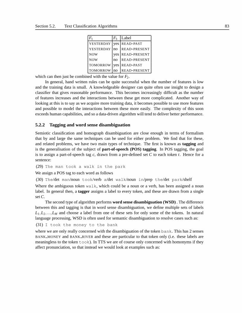
Section 5.2. Text Classification Algorithms 83
F1 F3 LabelYESTERDAY yes READ-PAST
YESTERDAY no READ-PRESENT
NOW yes READ-PRESENT
NOW no READ-PRESENT
TOMORROW yes READ-PAST
TOMORROW no READ-PRESENT
which can then just be combined with the value forF2.In general, hand written rules can be quite successful when the number of features is low
and the training data is small. A knowledgeable designer canquite often use insight to design aclassifier that gives reasonable performance. This becomesincreasingly difficult as the numberof features increases and the interactions between these get more complicated. Another way oflooking at this is to say as we acquire more training data, it becomes possible to use more featuresand possible to model the interactions between these more easily. The complexity of this soonexceeds human capabilities, and so a data-driven algorithmwill tend to deliver better performance.
5.2.2 Tagging and word sense disambiguation
Semiotic classification and homograph disambiguation are close enough in terms of formalismthat by and large the same techniques can be used for either problem. We find that for these,and related problems, we have two main types of technique. The first is known astagging andis the generalisation of the subject ofpart-of-speech (POS) tagging. In POS tagging, the goalis to assign a part-of-speech tagc, drawn from a pre-defined setC to each tokent. Hence for asentence:
(29) The man took a walk in the park
We assign a POS tag to each word as follows
(30) The/det man/noun took/verb a/det walk/noun in/prep the/det park/shelf
Where the ambiguous tokenwalk, which could be a noun or a verb, has been assigned a nounlabel. In general then, atagger assigns a label to every token, and these are drawn from a singlesetC.
The second type of algorithm performsword sense disambiguation (WSD). The differencebetween this and tagging is that in word sense disambiguation, we define multiple sets of labelsL1,L2, ...,LM and choose a label from one of these sets for only some of the tokens. In naturallanguage processing, WSD is often used for semantic disambiguation to resolve cases such as:
(31) I took the money to the bank
where we are only really concerned with the disambiguation of the tokenbank. This has 2 sensesBANK MONEY andBANK RIVER and these are particular to that token only (i.e. these labels aremeaningless to the tokentook). In TTS we are of course only concerned with homonyms if theyaffect pronunciation, so that instead we would look at examples such as:

84 Chapter 5. Text Decoding: Finding the words from the text
(32) He played bass guitar
with the aim of resolving it to
(33) He played bass/BASS-MUSIC guitar
Similar techniques can be used for both tagging and WSD; the reason these are consideredtwo different problems is that one is mainly concerned with syntactic ambiguity, the other withsemantic ambiguity. In the following sections, we example anumber of algorithms. In thesewe use homograph disambiguation for all the examples; but this is purely for reasons of exposi-tion. In general, all these techniques can be used for semiotic classification, and other types ofclassification described in Chapter 6.
5.2.3 Ad-hoc approaches
While we like to imagine that beautiful well constructed theories underly our algorithms, wefrequently find that when it comes to text classification manysystems in practice simply use ahodge-podge of rules to perform the task. This is particularly common in approaches to semioticclassification in genres where the amount of non-natural language text is very low, and so only afew special cases (say dealing with numbers) are required.
As these systems are by their very definition ad-hoc we can’t give a comprehensive guideto how these work, but often these are configured as a series ofregular expressions which try tofind a pattern (e.g. if the number is 4 digits long and has the form 19xx or 20xx is is a year).These rules are often ordered somewhat arbitrarily, in manycases with the most recently writtenrules last. Sometimes the output is directly rewritten overthe input and sometimes systems keepsrunning in a repeated fashion until no rules fire.
For text genres dominated by natural language text, and in situations where very little trainingdata is available, this approach may be adequate for semiotic classification. This is less likely towork for homographs, but again depending on the language, the level of errors may be acceptable.
5.2.4 Deterministic rule approaches
A more principled approach is to define a general rule format,a rule processor or engine and aclearly defined set of rules. This at least has the advantage of engine/rule separationmeaningthat the way the rules are processed and the rules themselvesare separate, which helps with systemmaintenance, optimisation, modularity and expansion to other languages. One common type ofrule is thecontext-sensitive rewrite rule, which takes the form
A→ B/d/C
meaning tokenA is converted (“rewrites to”)d when preceded by token(s)B and followed bytoken(s)C. In general, the contextsB andC can be any length. This rule has the disadvantage thatonly the very immediate context can be used, and so a second type of rule, called acollocationrule is also popular and takes the form:
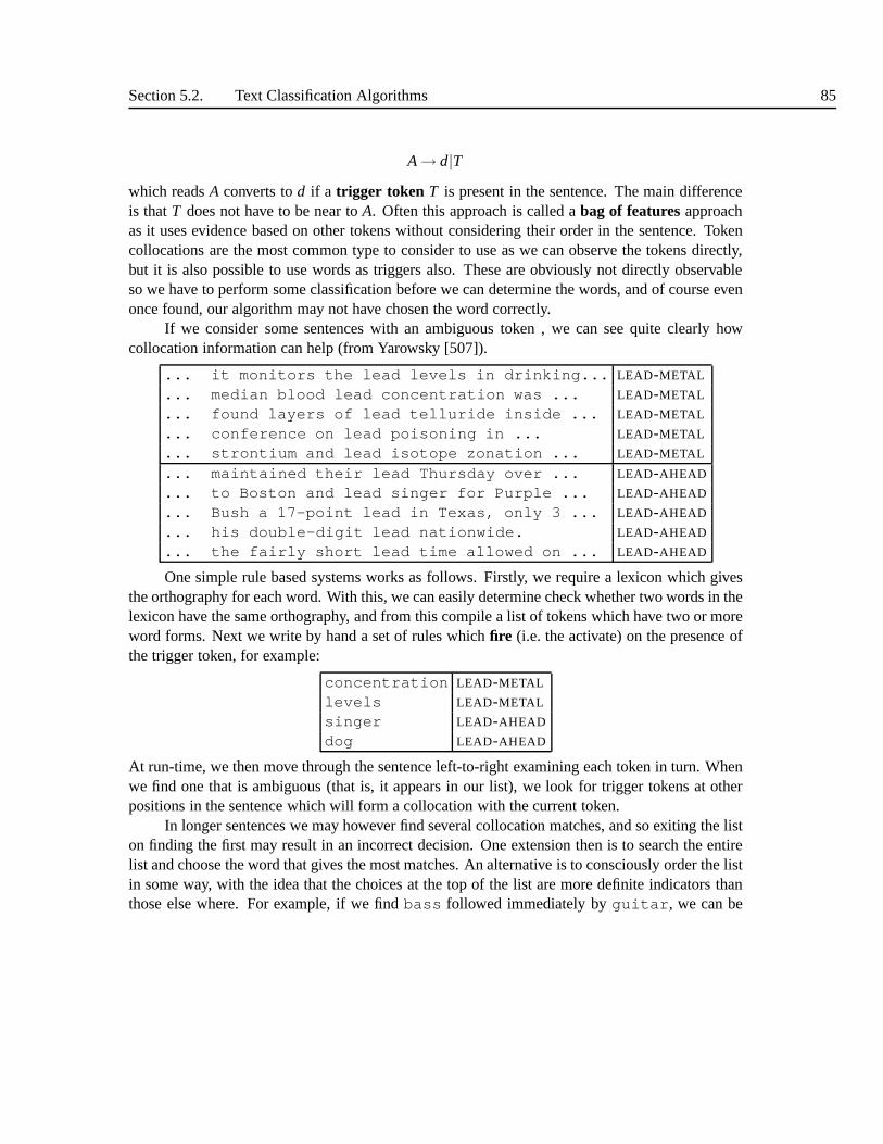
Section 5.2. Text Classification Algorithms 85
A→ d|T
which readsA converts tod if a trigger token T is present in the sentence. The main differenceis thatT does not have to be near toA. Often this approach is called abag of featuresapproachas it uses evidence based on other tokens without considering their order in the sentence. Tokencollocations are the most common type to consider to use as wecan observe the tokens directly,but it is also possible to use words as triggers also. These are obviously not directly observableso we have to perform some classification before we can determine the words, and of course evenonce found, our algorithm may not have chosen the word correctly.
If we consider some sentences with an ambiguous token , we cansee quite clearly howcollocation information can help (from Yarowsky [507]).
... it monitors the lead levels in drinking... LEAD-METAL
... median blood lead concentration was ... LEAD-METAL
... found layers of lead telluride inside ... LEAD-METAL
... conference on lead poisoning in ... LEAD-METAL
... strontium and lead isotope zonation ... LEAD-METAL
... maintained their lead Thursday over ... LEAD-AHEAD
... to Boston and lead singer for Purple ... LEAD-AHEAD
... Bush a 17-point lead in Texas, only 3 ... LEAD-AHEAD
... his double-digit lead nationwide. LEAD-AHEAD
... the fairly short lead time allowed on ... LEAD-AHEAD
One simple rule based systems works as follows. Firstly, we require a lexicon which givesthe orthography for each word. With this, we can easily determine check whether two words in thelexicon have the same orthography, and from this compile a list of tokens which have two or moreword forms. Next we write by hand a set of rules whichfire (i.e. the activate) on the presence ofthe trigger token, for example:
concentration LEAD-METAL
levels LEAD-METAL
singer LEAD-AHEAD
dog LEAD-AHEAD
At run-time, we then move through the sentence left-to-right examining each token in turn. Whenwe find one that is ambiguous (that is, it appears in our list),we look for trigger tokens at otherpositions in the sentence which will form a collocation withthe current token.
In longer sentences we may however find several collocation matches, and so exiting the liston finding the first may result in an incorrect decision. One extension then is to search the entirelist and choose the word that gives the most matches. An alternative is to consciously order the listin some way, with the idea that the choices at the top of the list are more definite indicators thanthose else where. For example, if we findbass followed immediately byguitar, we can be

86 Chapter 5. Text Decoding: Finding the words from the text
almost certain that this isBASS 1 (rhyming with “base”) and not the type of fish. Another way ofusing the rules is to run the mostspecificrules first, so if we have a rule which has several triggertokens, or a very rare trigger token (e.g.strontium) these fire before more general rules. Theidea here is that very specific rules are much more likely to beappropriate for that word only.
There are fundamental difficulties with regard to this and similar hand written rule ap-proaches. Firstly, it can be extremely laborious to write all these rules by hand. Secondly, weface situations where we have an ambiguous token but no trigger tokens that are present in ourcollocation list. Both these problems amount to the fact that the mapping from the feature spaceto the label is only partially defined. Finally, we face situations where say 2 rules match for eachword - which do we then pick? For these reasons, we now consider machine learning and statisticaltechniques.
5.2.5 Decision lists
One of the weaknesses of the simple collocation list is that it doesn’t tell given any indication ofhow strong a collocation might be. While we can use ordering (as in the case ofbass guitar),finding the correct ordering can be difficult and can still cause problems when contradictory rulesfire. An alternative is then to use statistics to give us an indication of how strong or how likely aparticular collocation is. One such method is to usedecision lists, introduced by Rivest [373], andused in TTS by Yarowsky [506], [507], Gale et al [169] [125] and Sproat [411].
The basic idea of decision lists is to determine the strengthof the link between a token andits trigger, and this is done by measuring the frequency of occurrence. In the following table (takenfrom [507]), we see the raw counts which have been found for the tokenbass:
Trigger BASS-FISH BASS-MUSIC
fish 0 142guitar 136 0violin 49 0river 0 48percussion 41 0salmon 0 38
from this it is clear that the trigger words are very strong disambiguation indicators, but alsothat some triggers occur more frequently that others. From these counts, we can calculate theconditional probability that of seeing a word given the collocation, e.g.
P(BASS-FISH|guitar,bass)P(BASS-MUSIC|guitar,bass)
We then compute the log-likelihood ratios for each collocation:
abs(
log( P(BASS-FISH|collocationi)
P(BASS-MUSIC|collocationi)
))

Section 5.2. Text Classification Algorithms 87
which then give us a sorted decision list:
Log likelihood Collocation tokenword10.98 fish BASS-FISH
10.92 stripped BASS-FISH
8.87 sea BASS-FISH
9.70 guitar BASS-MUSIC
9.20 player BASS-MUSIC
9.10 piano BASS-MUSIC
At run time, we simply start at the top of the list and progressdownwards until we find the colloca-tion which matches our input sentence. We then take the word that results from that as the answer.There are many subtle modifications, which for instance smooth the probability estimates, countall the evidence (not just the best case) and which consider the conditional probability of a wordbeing the answer when we have several triggers present. Yarowsky notes however that the simpleapproach is often good enough that many of these modifications don’t add any extra accuracy.
5.2.6 Naive Bayes Classifier
The naive Bayes classifieris a simple and popular approach in word sense disambiguation. Inthis, we attempt to estimate the probability that we have word wi is the correct one for a tokenbased on a number of features:
P(W = wi| f1, f2, ... fN) (5.1)
This is difficult to estimate directly so instead we make use of Bayes rulewhich gives us a moretractable formulation:
P(W = wi| f1, f2, ... fN) = P(W = wi)P( f1, f2, ... fN|wi) (5.2)
In this, the expressionP( f1, f2, ... fN|wi) is easier to calculate than the expression of Equation 5.1because all we need do now is find a word that gives rise to an ambiguous token and then countoccurrences of the featuresf1, f2, ... fN around this word. As we mentioned in Section 5.2.1, ingeneral the interactions between a set of featuresf1, f2, ... fN mean that calculatingP( f1, f2, ... fN)or P( f1, f2, ... fN|w) can be quite complicated because we have to consider every possible combi-nation of features. This approach is called thenaive Bayes classifier because it makes the hugesimplifying assumption that none of these features interact, such that the are statistically indepen-dent. This means that the expressionP( f1, f2, ... fN) can be simplified:
P( f1, f2, ... fN) = P( f1)P( f2), ...P( fN) =
=N
∏i=1
P( fi)

88 Chapter 5. Text Decoding: Finding the words from the text
which means that all we need find are the probabilities that a word is found with a each featureindividually.
P(W = wi| f1, f2, ... fN) = P(W = wi)N
∏i=1
P( fi)
When an ambiguous token is found, the classification is performed by calculating the above ex-pression for each word and choosing the answer as the one withthe highest probability. Thisalgorithm has the advantage that the features can be quite heterogeneous; for instance as well assimply the tokens themselves (as with the decision list case), we can also use POS tags, positionin sentence and any other features we think might help. Whilethe algorithm is obviously crude inthe sense that it ignores feature dependencies, it does at least give a defined mapping from pointin the feature space.
5.2.7 Decision trees
Given the simplicity of the naive Bayes classifier it performs surprisingly well. However, theassumption that the features are independent is in general too crude and better performance shouldbe obtainable by a system which models interaction between features. To see the problem offeature dependence we might see that the tokenMorgan is a strong indicator that we are havewith BANK MONEY and notBANK RIVER. We might also find that the tokenStanley is just asstrong an indicator. But it is clearly false to assume that these tokens operate independently of oneanother and that it is just coincidence that they appear in the same sentence.Morgan Stanleyis of course the name of a real bank and those two tokens very frequently co-occur. Once we haveused one feature, seeing the second adds very little extra information that we are dealing withBANK MONEY.
In general though, we have seen that it is intractable to assume that every combination offeatures is unique and needs to be calculated separately: wesimply never have enough trainingdata to estimate such models accurately. One popular solution to this is to usedecision trees.These model interactions between features but do so in a particular way so as to concentrateon learning the influence of the most important features first, such that rare or undiscriminatingfeature combinations can be ignored with some safety. We will explore decision trees in full inSection 15.1.9; for now we will give a quick overview and showhow they can be used for textclassification.
At run time, a decision tree asks a series of questions in order, and based on the outcomeof these delivers a label. In essence then, this is no more than series of nested “if then else”constructions in a computer program. For our cases, one set of questions might be “if the tokenis lead and the following token is contains the stringpoison and if the tokenpollution orheavy is also found in the sentence then mark this asLEAD METAL ”.
Any series of questions can be formulated as a tree, and in fact decision trees can be writtenby hand. We do however have a number of algorithms which automatically build trees and it is

Section 5.2. Text Classification Algorithms 89
because of these that the technique is popular. The decisiontree growing works as follows:
1. Create an initial group containing all the instances of one ambiguous token.
2. Design a set of questions based on our features which we think will help in the word identi-fication
3. For each question
(a) form two new groups based on the value of the feature(b) measure the combinedimpurity of the new groups
4. Find the question which gives the biggest reduction in impurity
5. Delete this question from the list of features to be examined.
6. Form two new groups based on this question.
7. Repeat steps 3 to 6 on each new group until the stopping criteria have been met.
The impurity of a cluster can be formulated in a number of ways as we shall see in Section15.1.9. Here even a simple measure will do, for example the ratio of word-1 over word-2. Thestopping criteria usually involves specifying a minimum decrease in impurity. The decision treegets round the problem of modelling all the feature combinations by effectively clustering certainfeature combinations together. This is not always ideal, but it certainly does allow for more accu-rate modelling than naive Bayes, as we can see that the same feature can appear in different partsof the tree and have a different affect on the outcome.
5.2.8 Part-of-speech Tagging
A somewhat different approach to the problem is to use atagging algorithm. This type of al-gorithm arose from the problem ofpart-of-speech (POS) taggingwhich was concerned withfinding the sequence of syntactic categories or parts of speech for each token in a sentence. Thesealgorithms are of interest to us in two ways. Firstly, many homographs arepart-of-speech homo-graphs. In English, these are often noun/verb pairs where the same token can be used as a nounor verb from the same semantic root. In fact a huge number of words in English have noun/verbpairs, so that can haveGO FOR A WALK and I LIKE TO WALK . In most cases these aresyntactichomonymsmeaning that while they may operate differently with regardto syntax, they are speltand pronounced the same way. A few however are spelt the same way but pronounced differ-ently and these are the cases which concern us. The idea of POS-tagging is that if we find thepart-of-speech from the text we will know which word we are dealing with.
A second interest in POS-tagging is that this technique can be used to assign any type oflabels to the tokens, not just parts-of-speech. Hence we could use a tagging algorithm for generaldisambiguation purposes.
POS-tagging has been a problem of concern in NLP for some time. There it is often used asa first required step before syntactic parsing is performed,but it is also used in other applicationsand seen as a problem in its own right. Many approaches have been tried but probably the most
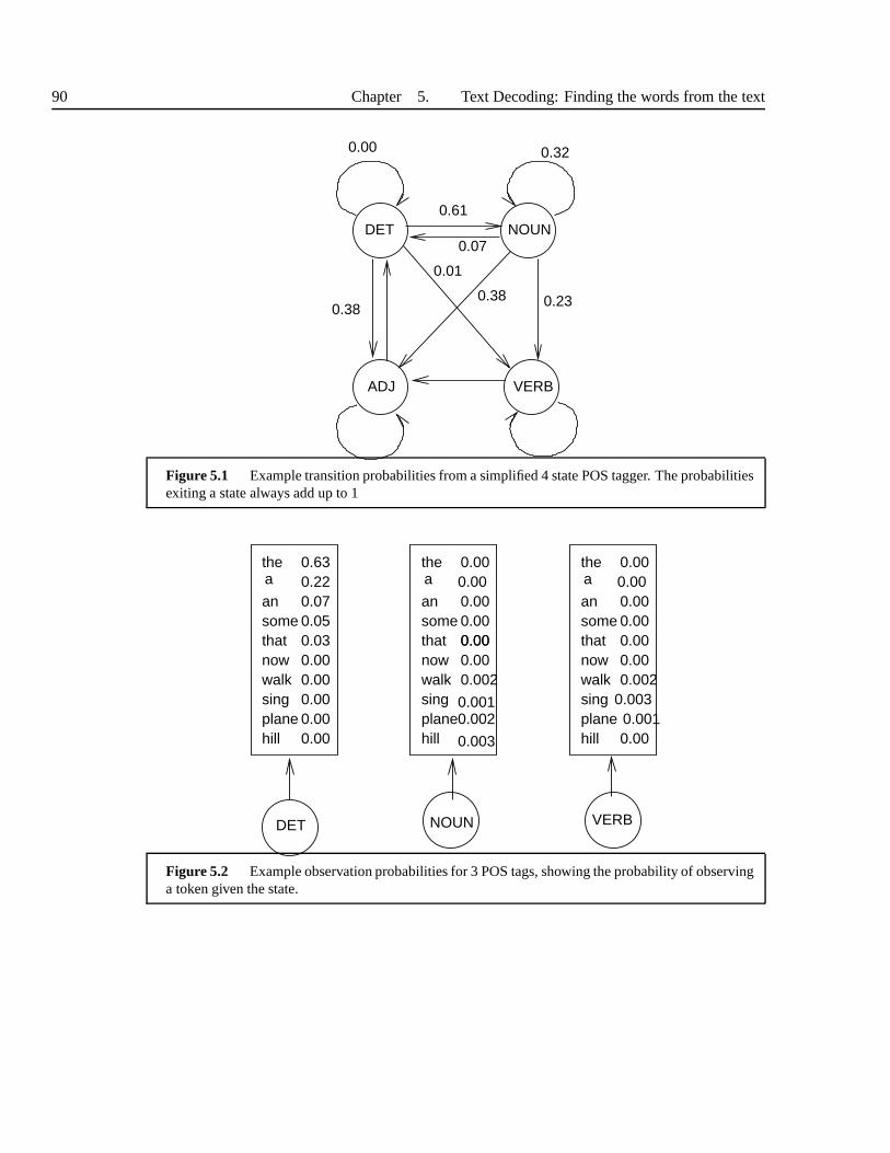
90 Chapter 5. Text Decoding: Finding the words from the text
NOUN
VERBADJ
DET
0.00
0.01
0.38
0.61
0.32
0.23
0.07
0.38
Figure 5.1 Example transition probabilities from a simplified 4 state POS tagger. The probabilitiesexiting a state always add up to 1
thea
ansomethatnowwalk
0.00
singplanehill 0.003
0.0010.002
0.000.000.000.000.000.00
0.002
DET NOUN
thea
ansomethatnowwalk
0.630.220.070.050.030.000.00
singplanehill
0.000.000.00
VERB
thea
ansomethatnowwalk
0.00
singplanehill
0.000.000.000.000.00
0.002
0.000.001
0.003
Figure 5.2 Example observation probabilities for 3 POS tags, showing the probability of observinga token given the state.

Section 5.2. Text Classification Algorithms 91
common approach is to use ahidden Markov model. These are dealt with fully in Chapter 15, butfor now we can give a quick overview explaining their use for tagging purposes. An HMM taggeroperates probabilistically to find the most likely sequenceof tags (labels as we have previouslycalled them)L for an input sequence of tokensT. We write this as
L = argmaxl
P(L|T)
Rather than compute the probability that a token generates atagP(l |t), an HMM is agenerativemodel which computesP(t|l), that is, the probability of seeing a token given the tag. We cancalculate one from the other by concatenating the HMM modelsto form sequences and then applyBayes rule:
P(L|T) =P(L)P(T|L)
P(T)
WhereP(L) is called theprior and is the probability of a particular sequence of tags occurring.P(T) is called theevidence, that is, what we actually see, andP(T|L) is called thelikelihood.An HMM can be viewed as a network of states, where each state represents one POS tag. Ina tagger, all the states are connected, and the connection between each pair of states is given atransition probability . This represents the probability of seeing one POS tag follow another. Asimple example of this is shown in Figure 5.1 and in this example we see that the probability ofa noun following a determiner is high, whereas the probability of a determiner following anotherdeterminer is very low. In addition, each state has a set ofobservation probabilities which givethe probability of that state generating each token. An example of this is seen in Figure 5.2 for thedeterminer POS tag. As we would expect, tokens such asthe have high probabilities, whereascontent tokens such aswalk have low probabilities meaning it is highly unlikely that this tagwould generate that token.
We will consider the full issue of how to train an HMM in Section 15.1.8. For now, let ussimply assume that we can calculate the transition probabilities and observation probabilities bysimply counting occurrences in a labelled database. To see how the tagging operates considerthe issue of resolving the classic POS homographrecord. This can be a noun or a verb, and atrained HMM would tell us for instance:
P(t = record|l = NOUN) = 0.00065
P(t = record|VERB) = 0.0045
Which basically states that in our training data one in every1538 nouns that we encountered wasthe tokenrecord, and one in every 220 verbs we encountered wasrecord.
In addition to this we have the prior model which gives us the probability that a sequence oftags will occur independent of any actual observations. In general this would take the form:

92 Chapter 5. Text Decoding: Finding the words from the text
P(L) = P(l1, l2, ..., lN)
that is, the probability of seeing all the tags in the sentence. We then wish to find the probabilityof a particular tag given all its predecessors:
P(l i|l1, l2, ..., l i−1)
We would never have enough data to count all these occurrences, so we make an assumptionbased on the chain rule of probability (see Appendix A). Thisstates that a sequence as above canbe approximated by considered only a fixed window of tags before the current one:
P(l i |l i−2, l i−1)
orP(l i |l i−1)
In this model we might find for instance that the probability of two particular tag sequencesare
P(NOUN|DET) = 0.019
P(VERB|DET) = 0.00001
which indicates that the chance of a verb following a determiner is much much smaller than thechance of a noun following a determiner. Given an input tokensequence which includes...the record ... we would be certain that the tokenthe would be classed as a determiner,and so when we can combine the two models and calculate the probability we see that the tokenrecord is a noun rather than verb.
In a real HMM tagger system, we have to determine these probabilities from data. In general,this data has to be labelled with a POS tag for each word, but incases where labelled data is scarce,we can use a pre-existing tagger to label more data, or use a bootstrapping technique where weuse one HMM tagger to help label the data for another iteration of training.
The prior probability is calculated by counting occurrences of sequences of tags. This ismodelled by ann-gram model which gives the probability of finding a tagti given a fixed lengthsequence of previous tagsti−1, ti−2.... The longer the tag sequence the more accurate the priormodel, but in general sparse data problems prevent us from having an n-gram of more that 3 or4 tags in length. We also have to build a likelihood model, andwe do this by defining a separatemodel for every tag. Each of these models then defines a probability distribution over the setof tokens, giving the probability of seeing any one token given the tag. At run-time, a search isconducted through all possible tag sequences to find the single most likely, and this is given asthe answer. Another advantage of the HMM approach is that it is amenable to computing every
Section 5.3. Non-Natural Language Text 93
possible sequence of tags and choosing the one with the highest probability. This is performedusing theViterbi algorithm, explained in Section 15.1.7. We will return to the entire subject ofHMMs in Chapter 15 where we discuss the general nature of the likelihood models, the priorn-gram models, the search algorithms, the training algorithms and other practical matters.
5.3 NON-NATURAL LANGUAGE TEXT
We now turn to the problem of dealing with text which does not directly encode natural language.In our model of communication we have a number of semiotic systems which are used to com-municate information. Natural language is the richest and often the most common of these, butwe also have numbers, dates, times, computer information, money, addresses and so on. Thesesystems are separate from natural language, but in TTS we arerequired to speak them, and thiscan only be done if we convert data in this form into natural language. This is a two stage problemwhere first we must analyse the text to determine its units andstructure; this is done by a processof semiotic decoding. Then we have to convert this into natural language, and thisprocess iscalledverbalisation. But we have an additional problem in that as these systems share the samecharacters as natural language and hence each other, the text forms of these systems often overlap,leading to considerable ambiguity. Hence before we attemptdecoding and translation, we firsthave to performsemiotic classificationto resolve this ambiguity and determine which systemeach token of the input belongs to.
5.3.1 Semiotic Classification
Semiotic classification can be performed by any of the techniques described in Section 5.2.1 above.First, we define which classes we believe our system will encounter. We can immediately identifysome which crop up regardless of text type and genre, and these include:
cardinal numbers 25, 1000ordinal numbers 1st, Henry VIIItelephone numbers0131 525 6800, 334-8895years 1997, 2006, 1066dates 10 July, 4th April 10/12/67money $56.87, 45p, Y3000, $34.9Mpercentages 100%, 45%measures 10cm, 12 inches
In addition, we have a number of classes which are more genre specific; for example we may havestreet addresses in a telephone directory application, computer programs in a screen reader for theblind and any number of systems in specialist areas such as medicine, engineering or construction:

94 Chapter 5. Text Decoding: Finding the words from the text
emails [email protected] http://mi.eng.cam.ac.uk/ pat40computer programsfor (i = 0; i < n; ++i)addresses 4318 East 43rd Streetreal estate CGH, sng whit fem
So it is important to have a good knowledge of the applicationarea in order to ensure a good andaccurate coverage of the type of semiotic systems that will be encountered.
It should be clear that a simple classifier based on token observations will only be sufficientin the simplest of cases. If we take the case of cardinal numbers, we see that it would be absurdto list the possible tokens that a cardinal class can give rise to; the list would literally be infinite.To handle this, we make use of specialistsub-classifierswhich use regular expression generatorsto identify likely tokens from a given class. One way of doingthis is to run regular expressionmatches on tokens and use the result of this as a feature in theclassifier itself. So we might have
(34) Match[0-9]+ ?
as a rule, which will return true if the token is composed entirely of an arbitrary number of digits.More specific regular expressions can also be used which handle numbers of a fixed length (e.g.years in the modern era being 4 digits long,) or for real numbers which contain a decimal point.In addition to theseopen classrules, we also see that semiotic classes form a hierarchy. Sothemoneyclass is composed of thenumber class and usually a currency symbol (e.g. $). A furtherissue is that often several tokens form a coherent semiotic group, such that if we have
(35) 8341 Belville Dr
we have three tokens that together form a single address. Hence we need an ability to group thetokens after or during classification.
The process of semiotic classification can therefore be summarised as:
1. Define the setS= s1, ...sN of semiotic classes2. For each decide if this is a closed or open class.3. Closed classes can be enumerated, open classes require regular expression matches.4. For each token:
(a) run the open class expressions and record the answer for each as a feature(b) Using the open class features and the normal features, run a classifier (e.g. the naive
Bayes classifier), record the most probable classsi for each token.
5. Group consecutive tokens of the same class together6. Perform class-specific decoding and verbalisation
To take a simple example, suppose we have the sentence:
(36) You should meet him at 3:30pm at 1994 Melville Drive
and we have the set of semiotic classes as just defined. For each open class we would have aregular expression as follows:

Section 5.3. Non-Natural Language Text 95
natural language [A-Za-z]+cardinal numbers [0-9]+telephone numbers0131 525 6800, 334-8895years 1[0-9][0-9][0-9] | 2[0-9][0-9][0-9]time hours : minutes part-of-dayhours [0-9] | 1[0-9] | 2[0-4]minutes [0-6][0-9]part-of-day am | pmaddresses cardinal number proper-name street-typeproper-name [A-Z][a-z]+street-type Dr| St| Rd| | Drive| Street | Road
For each token we run each regular expression and record its answer as a feature:
text natural languagecardinal year hours minutes part-of-day proper-nameYou 1 0 0 0 0 0 1should 1 0 0 0 0 0 0meet 1 0 0 0 0 0 0him 1 0 0 0 0 0 0at 1 0 0 0 0 0 03 0 1 0 1 0 0 0: 0 0 0 0 0 0 030 0 1 0 0 1 0 0pm 1 0 0 0 0 1 0at 1 0 0 0 0 0 01994 0 1 1 0 0 0 0Melville 1 0 0 0 0 0 1Dr 1 0 0 0 0 0 1
The results of these matches can now be used as features, along with general features such as “isthis the first word in the sentence” (which is useful for telling a normal natural language wordfrom a proper name). All the features are then given to the classifier which makes a final decisionon semiotic class.
With regard to the issue of grouping, we can use a combinationof the classifier and regularexpression matches to ensure that a sequence of tokens such as3, :, 30, pm are seen as a singletime. A more sophisticated approach is available if we make use of the HMM tagging algorithmas one of the features of an HMM is its ability to include multiple tokens in a single class, andalso, via the Viterbi search algorithm, ensure that the mostprobably global sequence of classes isfound, which helps resolves problems where two classes claim overlapping tokens.

96 Chapter 5. Text Decoding: Finding the words from the text
5.3.2 Semiotic Decoding
Once identified, each token or sequence of tokens must be decoded to determine its underlyingform. Luckily for nearly all classes except natural language, this is fairly straightforward issue.In fact many classes (e.g. email addresses or computer programs) have been specifically designedto ensure that the underlying form can be found quickly and deterministically. We have call thisprocessdecodingas it is seen as the process of reversing an encoding of the original form into text.This is often also be calledparsing in computer science, but we reserve this term for the specificproblem of uncovering syntactic structure in natural language. We require a separate decoder foreach semiotic class, but due to the simplicity of each, this in is general is not too difficult to designby hand. Let us take the example of dates to see how a decoder would work.
Let us take theGregorian calendersystem (i.e. the date system we nearly always use) asan example. This is particularly illustrative as a non-natural language semiotic class in that
1. It has a number of text forms, e.g. 10/12/67 or 10th December ’67
2. It is used nearly universally, regardless of which natural language is being used.
3. There are a number of ways to verbalise a date
Gregorian dates have a day a month and optionally a year and the task of the decoder is to deter-mine the values of each of these from the text. The same date can give rise to a number of differenttext encodings, for example:
(37) a. 10 December 1967
b. December 10 1967
c. 10th of December 1967
d. 10th of December ’67
e. 10/12/1967
f. 10/12/67
g. 12/10/67
In each of these cases, the date is exactly the same, and so here we see how a single date can giverises to multiple text encodings. Despite these possible differences, finding the day month andyear is normally possible with a little care (the only reallydifficult case being the handling of theconvention often found in the United States, where the pattern is month/day/year rather than themore common day/month/year). A typical way of actually performing the decoding a date is touse a list of rules, each of which decodes one particular dateformat. The rules are run in order,until a match is found.
5.3.3 Verbalisation
The final step in handling non-natural language text is to convert it into words and this process isoften calledverbalisation. If we take our decoded date example, we see that we have values for

Section 5.3. Non-Natural Language Text 97
the three fields of day month and year, and with these we cangeneratea sequence of words. Fordates we have a number of conventions, such that the date day=10, month=12, year=Decembercan be spoken in English as:
(38) a. TEN TWELVE SIXTY SEVEN
b. THE TENTH OFDECEMBER SIXTY SEVEN
c. THE TENTH OF DECEMBER NINETEEN SIXTY SEVEN
d. DECEMBER THE TENTH NINETEEN SIXTY SEVEN
e. DECEMBER TENTH NINETEEN SIXTY SEVEN
f. DECEMBER TENTH SIXTY SEVEN
g. DECEMBER THE TENTH IN THE YEAR OF OUR LORD NINETEEN SIXTY SEVEN
and so on. In this case the issue of verbalisation is not difficult per-se - a simpletemplateapproachcan be used to create the word sequence. First we define two functionsordinal() andcardinal()which convert a number into a word string representing the type of number. For example, forcardinal() we have:
1 → ONE
2 → TWO
3 → THREE
13 → THIRTEEN
32 → THIRTY TWO
101 → ONE HUNDRED AND ONE
1997 → ONE THOUSAND NINE HUNDRED AND NINETY SEVEN
and forordinal() :
1 → FIRST
2 → SECOND
3 → THIRD
13 → THIRTEENTH
32 → THIRTY SECOND
101 → ONE HUNDRED AND FIRST
1997 → ONE THOUSAND NINE HUNDRED AND NINETY SEVENTH
next we define a functionyear(). A simple version of this which covers all years between 1010and 1999 is:
(39) cardinal(y1y2) cardinal(y3y4)
which when give 1387 for instance will produce the stringTHIRTEEN EIGHTY SEVEN. For theyears immediately after the millennium the situation is more tricky, where we require a functionof the type:
(40) cardinal(y1000)AND cardinal(y4)

98 Chapter 5. Text Decoding: Finding the words from the text
which when given 2006 would generate
(41) TWO THOUSAND AND SIX
Here we start to see the first case of why verbalisation can be tricky as some people prefer this rulenot to have theAND so that the function should produce
(42) TWO THOUSAND SIX
and there is some debate over whether 2013 will be pronouncedTWENTY THIRTEEN or TWO
THOUSAND AND THIRTEEN. With theyear() function we can now define a template for verbalis-ing the full date. One template would then be:
(43) THE ordinal (day) ofmonth-name(month)year(year)
giving
(44) THE TENTH OF DECEMBER NINETEEN SIXTY SEVEN
In general, verbalisation functions for cases like these are not too difficult to construct, allthat is required is a careful and thorough evaluation of the possibilities. The main difficulty inthese cases is that there is no one correct expansion; from 38we see at least 7 ways of sayingthe date, so which should we pick? While sometimes the original text can be a guide (such that10/12/67would be verbalised asTEN TWELVE SIXTY SEVEN) we find that human readers oftendo not do this, but rather pick a verbalisation that they believe is appropriate. The problem for usas TTS system builders is that sometimes the verbalisation we use is not the one that the readerexpects or prefers, and this can be considered an error.
For some each semiotic classes, we can specify a degree ofconventionality with regardto verbalisation. We can state that ordinals and cardinals verbalisations are very conventional inthat nearly all readers verbalise a number the same way (although there may be slight differencesbetween American and other types of English.) With dates, wesee that these are again quiteconventional, but that there is quite a range of acceptable forms. We find that there is a significantproblem with some other semiotic forms in that the degree of convention can be quite low. If weconsider the email addresses
(45) [email protected]
we might find that any of the following are acceptable verbalisations:
(46) LETTER-P LETTER-A LETTER-T FORTY AT CAM DOT LETTER-A LETTER-C DOT LETTER-U LETTER-K
LETTER-P LETTER-A LETTER-T FOUR ZERO AT CAM DOT LETTER-A LETTER-C DOT
LETTER-U LETTER-K
PAT FORTY AT CAM DOT LETTER-A LETTER-C DOT LETTER-U LETTER-K
PAT FORTY AT CAM DOT AC DOT UK
The problem being, that the particular owner of this addressmay only consider one of these as“correct” and will be dissatisfied if an alternative versionis used.

Section 5.4. Natural Language Text 99
5.4 NATURAL LANGUAGE TEXT
Having dealt with non-natural language text, we now turn ourattention to the issue of how to findthe words from the text when that textdoesin fact encode natural language. For many words,this process is relatively straightforward; if we take a word such asWALK , we will have its textualform walk listed in the lexicon, and upon finding the a tokenwalk in the text we can be fairlysure that this is in fact a written representation ofWALK . At worst we might be presented with acapitalised versionWalk or an upper case versionWALK but these are not too difficult to deal witheither. If all words and all text behaved in this manner the problem would be solved, but of coursenot all cases are so simple, and we can identify the main reasons for this:
Alternative spellings A number of words have more than one spelling. Often in English this isrelated to American vs non-American conventions so that we havetyre andtire andhonour andhonor. In many cases these differences are systematic, for instance with thesuffix -ISE which can be encoded asorganise or organize. Often it is possible to listalternative spellings in the lexicon.
Abbreviations Many words occur in abbreviated form, so for instance we havedr for DOCTOR
andst for STREET. In many cases these are heavily conventionalised such thatthey can belisted as alternative spellings, but sometimes the writer has used a new abbreviation or onethat we may not have listed in the lexicon.
Unknown words There will always be words that are not in the lexicon and whenwe find thesewe have to deal with them somehow.
Homographs are cases where two words share the same text form. In cases where the wordsdiffer in pronunciation, we must find the correct word. In natural language homographsarise for three reasons:
1. Accidental homographsarise because completely words such asBASS-FISH andBASS-MUSIC just happen to share the same text formbass.
2. Part-of-speech homographsarise from words which have a similar sematic root, butwhere their use as a noun or verb gives them a different pronunciation. For instancePROJECT-NOUN andPROJECT-VERB both share the same text formproject but arepronounced differently.
3. Abbreviation homographs arise because as we use fewer characters in abbreviations,we are more likely to use the same text encoding as for anotherabbreviated word.Hence we find that whileDOOR, DOCTOR andDRIVE all have the quite separate fulltext forms ofdoor, doctor, DRIVE, but all share an abbreviated text formdr.
Mis-spellings Often if a text form of a word is misspelled a human reader is quite capable ofguessing what word was intended, e.gdiscovery and ideally a TTS system should beable to cope with such instances.
100 Chapter 5. Text Decoding: Finding the words from the text
This shows why we need a more sophisticated model than a simple isomorphic correspondencebetween words and their text encodings.
5.4.1 Acronyms and letter sequences
At this stage it is worth mentioning two other types of word/token relationships that are oftencited as problems for TTS.Acronyms are words formed from sequences of other words, usually(but not always) by taking the first letter of each. Examples includeNATO, UNICEF SCUBA andAIDS. In our approach, these are treated as normal words so that wehave a wordNATO in ourlexicon and this has a pronunciation /n ey t ow/; the fact thatthis was historically formed fromother words or is normally found written in upper case is of noreal concern. (In fact, with usemany acronyms really do become indistinguishable from normal words such thatRADAR is nearlyalways spelled in lower case and few people realise that it isan acronym, and fewer still what theoriginal words were).
In lay speak, the term acronym is also used for a different type of formation which we shallcall a letter sequence; examples of these includeIBM, HTML, HIV. The difference between theseand acronyms is that letter sequences don’t form new pronunciations; they are simply spoken asa sequence of letters, hence we haveIBM asLETTER-I LETTER-B LETTER-M giving a combinedpronunciation /ay b iy eh m/. It doesn’t really matter if we regardIBM as being a single wordwith pronunciation /ay b iy eh m/ or a token which represents three words (LETTER-I LETTER-B
LETTER-M). Potentially however, the productivity of letter sequences is very high, so regardlessof whether we keep them in the lexicon or not, we still need a means of identifying new onesand pronouncing them as letter sequences rather than as normal words (i.e. we don’t want toencounter a tokenRAF and think that this is just an upper case version of an unknownword, andthen pronounced it as /r ae f/).
A solid solution to the problem of upper case tokens is to assume that in a well developedsystem all genuine acronyms will appear in the lexicon. Uponencountering a capitalised token,we first check if it is in the lexicon and if so just treat it as a normal word. If not, we then splitthe token into a series of single character tokens and designate each as a letter. There is a possiblealternative, where we examine upper case tokens and attemptto classify them either as acronymsor letter sequences. Such a classification would be based on some notion of “pronouncability”such that if the token contains vowel characters in the certain places then this might lead us tothink that it is an acronym instead of a letter sequence. Experience has shown that this approachseldom works (at least in English) as there are plenty of potentially pronounceable tokens (e.g.USA or IRA that sound absurd if treat then as acronyms (e.g. /y uw s ax/ or/ay r ax/). If a mistakeis to be made, it is generally better to pronounce an acronym as a letter sequence rather than theway round.

Section 5.4. Natural Language Text 101
5.4.2 Homograph disambiguation
The main problem in natural language text decoding is dealing with homographs, whether they beaccidental, part-of-speech or abbreviation homographs. Many systems choose to handle each ofthese separately, and in particular abbreviation homographs are often with at the same time or inthe same module as semiotic classification. Typically this is done in systems which don’t have anexplicit semiotic classification stage. An alternative approach is to handle these in a single module.Regardless, the general approach is to use one of the token disambiguation techniques describedin Section 5.2.1. Here we discuss some of the specifics of homograph disambiguation.
Turning to POS homographs first, we see that the classic way toresolve these is to use a POS-tagger of the type described in Section 5.2.2. One problem with this approach is that unfortunatelyPOS-taggers only have a certain accuracy (96%-98% are commonly quoted figures [299]), andoften it is in the hard cases of resolving noun/verb pairs where the errors are made. Recall that thePOS tagger has two components, one which models sequences oftags and one which generatestokens given a tag. The tag sequence n-gram is a very powerfulconstraint and nearly always givesthe correct answer in cases such as:
(47) The/det project/noun was/aux behind/prep schedule/noun
(48) The/det problem/noun is/aux how/wrb to/inf project/verb the/noun missile/nounaccurately/adv
but in sentences such as
(49) The new images project well on to the wall
POS-taggers often struggle as the n-gram sequence of tags alone is not sufficient to disambiguate inthis case. Part of the problem with POS taggers is that they are often formulated as general purposeNLP tools, and as such are not focused on the goals of how they might be used in a particularapplication. One simple improvement then is to adapt the tagset so that the discriminative powerin the algorithm is geared towards the distinctions we really care about.
An alternative approach is to use one of the word sense disambiguation algorithms as thesecan be more easily focused for each homograph case. A furtheradvantage in using the WSDapproach is that we can use this single approach for all type of homograph, not just the POShomographs that the tagger deals with. To give an example, consider the abbreviation homographDr which can encodeDOCTORor DRIVE. Both of these are often collocated with a proper noun,but differ in their position relative to that proper noun. A simple feature that distinguishes manyexamples is then whether theDr occurs before or after the proper noun:
(50) Dr + proper-noun→ DOCTOR
(51) proper-noun +Dr→ DOCTOR
for example
(52) Dr Williams→ DOCTOR WILLIAMS

102 Chapter 5. Text Decoding: Finding the words from the text
(53) Williams Dr→ WILLIAMS DRIVE
In deterministic rule system this can be used as is, but as therule is not 100% accurate an alternativeis to use is as a feature in a WSD classifier.
We can summarise the procedure for building a homograph disambiguation system as fol-lows:
1. Build a lexicon which records all the text forms of each word
2. Compare text forms and construct a list of homograph tokens
3. For each form
(a) search for cases of these in a large text corpus(b) by hand mark the correct word(c) find collocation trigger tokens by finding the tokens which most frequently co-occur
with the word(d) write feature rules which may describe any more elaborate relationship between word
and trigger tokens
4. Train WSD classifier
5. Run over test corpus, examine errors and repeat training process based on findings.
5.4.3 Non-homographs
Most tokens are not in fact homographs, and we will now outline how these non-homograph tokensare processed.
1. Check whether the token is present in the lexicon as the text form of a known word.
2. If it is found, take that word as the correct answer and no further processing is conducted.
3. If in the lexicon and upper case, label it as a letter sequence.
Regarding this last rule, It is nearly impossible to sure whether an upper case token is anacronym or letter sequence, but analysis of data shows that unknown letter sequences are muchmore common than unknown acronyms and hence the most accurate strategy is to assign it as aletter sequence. Furthermore an acronym spoken as a letter sequence is deemed a lesser error thana letter sequence spoken as a single word.
If the token is not upper case and not in the lexicon we have thechoice, it could potentiallybe a normal unknown word, an abbreviation for a known word, a different spelling for a knownword or a misspelling of a known word. The probability of eachof these cases mainly depends onthe quality of our lexicon. If we have a very accurate comprehensive lexicon then it is less likelythat we have a missed a normal word or alternate spelling. This therefore increases the chanceof the token being a mis-spelling. If the system has a spell correction system, it should be runat this point. Assuming the spell corrector has a confidence score we can then decide whetherthe token is a mis-selling of a known word or an unknown word. The final case occurs when webelieve we have a token for a genuinely unknown word. This is assigned a new unique label (e.g.
Section 5.5. Natural Language Parsing 103
UNKNOWN-43), and the token and label are added to the run-time lexicon. The pronunciation isdetermined by the grapheme-to-phoneme convertor, which wewill describe in Section 8.4. Theseset of operations can be found in the right half of Figure 5.3.
5.5 NATURAL LANGUAGE PARSING
Our concern so far has been the task of identifying the word sequence from the token sequence,and to a large extent this is all the text decoding that we are required to do. Once we have un-ambiguously identified the word sequence, we can use the lexicon and grapheme-to-phonemeconversion to generate a sound representation which can then be input to the synthesiser itself.It can be argued however that the word sequence alone is not enough, and that in addition it isadvantageous to conduct further processing to determine the underlying structure of the sentence.Semantic analysis is generally thought too difficult and/orunnecessary, but a number of systemsperform asyntactic analysiswhich finds the correct or bestsyntactic tree for the input sentence.There are several justifications for wishing to perform thisadditional level of analysis.
1. Proper parsing can resolve part-of-speech ambiguity problems that finite state (ie HMMparsers) fail on, such as Example 49 above.
2. The syntax can help determine sentential prominence patterns (explained in Section 6.8).3. The syntax gives a basic grouping of words, and these groupings strongly influence the
prosodic phrase structure of the utterance (explained in Section 6.7).
5.5.1 Context Free Grammars
In Chomsky’s early work [88], he proposed that the syntax of natural languages like English couldbe described at a basic level by acontext free grammar (CFG). A CFG defines a number of rulesof the form
(54)S→ NP VPNP→ DET NPVP→ V NPVP→ PPPP→ P NP
The rules operategenerativelymeaning that they are applied by starting with a basic top node (Sstanding for “sentence”) and then applying rules in turn until a string of terminal nodes (ie words)are generated. Chomsky’s idea was that this finite set of these rules could generate the near infiniteset of sentences in natural language. In addition, the operation of the rules defined thestructurestructure of a sentence. The operation of context-free rules is easilyrepresented by a syntactictree:
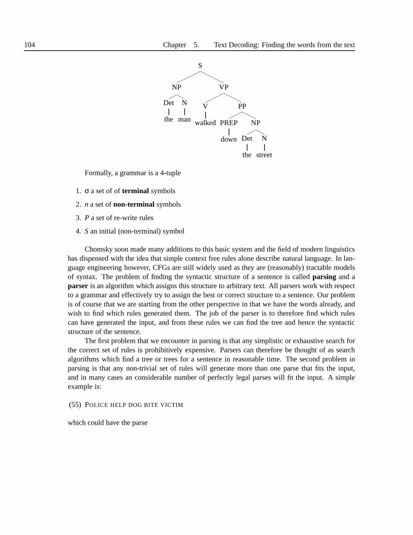
104 Chapter 5. Text Decoding: Finding the words from the text
S
NP
Det
the
N
man
VP
V
walked
PP
PREP
down
NP
Det
the
N
street
Formally, a grammar is a 4-tuple
1. σ a set of ofterminal symbols
2. n a set ofnon-terminal symbols
3. P a set of re-write rules
4. San initial (non-terminal) symbol
Chomsky soon made many additions to this basic system and thefield of modern linguisticshas dispensed with the idea that simple context free rules alone describe natural language. In lan-guage engineering however, CFGs are still widely used as they are (reasonably) tractable modelsof syntax. The problem of finding the syntactic structure of asentence is calledparsing and aparser is an algorithm which assigns this structure to arbitrary text. All parsers work with respectto a grammar and effectively try to assign the best or correctstructure to a sentence. Our problemis of course that we are starting from the other perspective in that we have the words already, andwish to find which rules generated them. The job of the parser is to therefore find which rulescan have generated the input, and from these rules we can find the tree and hence the syntacticstructure of the sentence.
The first problem that we encounter in parsing is that any simplistic or exhaustive search forthe correct set of rules is prohibitively expensive. Parsers can therefore be thought of as searchalgorithms which find a tree or trees for a sentence in reasonable time. The second problem inparsing is that any non-trivial set of rules will generate more than one parse that fits the input,and in many cases an considerable number of perfectly legal parses will fit the input. A simpleexample is:
(55) POLICE HELP DOG BITE VICTIM
which could have the parse

Section 5.5. Natural Language Parsing 105
S
NP
N
Police
VP
V
help
N
dog
VP
V
bite
N
victim
meaning the police were helping the dig to bite the victim, or S
NP
N
Police
VP
V
help
AP
AP
Adj
dog
Adj
bite
N
victim
meaning the police were helping a victim of a dog bite.TheCocke-Younger-Kasami (CYK) algorithm is one of the most widely used parsing al-
gorithms. It can (in general) efficiently parse text and is easily adaptable to probabilistic formula-tions. Its basic operation can be thought of as dynamic programming for context free grammars.
This algorithm considers every possible group of words and sets entries in a table to be trueif the sequence of words starting from i of length j can be generated from the grammar. Once ithas considered sequences of length 1, it goes on to ones of length 2, and so on. For the sequencesgreater than length length 1, it breaks the sequence into allpossible subdivisions, and again checksto see if a rule in the grammar can generate one of these subdivisions (this is why the grammar hasto be in Chomsky normal form). If a match is found, this is stored in the table also. This process iscontinued until the full set of rules (ie. parses) is found. Deterministic parsers have no real meansof choosing which parse is best, soprobabilistic parsers (explained below) are usually preferredas these at least show that one parse is more probable than another.
5.5.2 Statistical Parsing
The CYK algorithm as just explained will find the set of legal parses for a sentence, but the problemis in general that we wish to find justoneparse, not several. We of course want the “true” parseand by this we mean we want what the author originally intended when the sentence was written.

106 Chapter 5. Text Decoding: Finding the words from the text
The major weakness with this type of parsing is that it only considers syntactic factors, semanticsis completely ignored. That is why a parser often returns parses that are “correct” but seem silly.Some more advanced models of syntax do incorporate semanticinformation [78], [177], [312],but in general most syntax models, especially in engineering, only make use of syntactic rules.
A sensible alternative then is instead of trying to find the parse which the author intended, orwhich makes most sense, we can try and find themost likelyparse. That is, we build a probabilisticmodel of the grammar and use the parser to find the most likely parse. There are a number of waysthis can be done, but the most common is to assign probabilities to the rules themselves so thatwe say a non-terminal expands to each of its productions witha certain probability. When theparsing is complete, each set of rules has an associated probability and the highest can be chosenas the right answer. A number of specialist databases calledtree-banksare available for trainingPCFGs. These have trees and nodes labelled by hand, and from these a grammar can be trained andprobabilities assigned to each rule. For unlabelled data (that is sentences which we have no treesfor) the inside-outside algorithm can be used. This is the PCFG equivalent of the Baum-Welchalgorithm used to train hidden Markov models, and is explained in Section 15.1.8.
We can therefore identity three common approaches to parsing:
1. Define a CFG by hand and use a deterministic search algorithm (i.e. the parser) to find theparse or parses which best fit the input
2. Define a CFG by hand and use a probabilistic search algorithm to find the parse or parseswhich is most likely given the input
3. Learn the CFG from data and use this with a probabilistic search algorithm to find the parseor parses which is most likely given the input.
5.6 DISCUSSION
Figure 5.3 shows the flowchart for the text decoding system described in this chapter.At this stage, we will discuss a number of alternate formulations to the one presented here.
In the (distant) past, text forms such asDr were often see as abberations as far as text and lan-guage processing was concerned to the extent that these wereoften calledtext anomalies[276] .The “real job” of text/language processing was to perform syntactic and morphological process-ing. For instance in the MITalk book 6 pages are devoted to text anomalies and 48 to syntactic,morphological and phonological processing. As can be seen from this chapter, in modern systems,the opposite balance is seen. Another view is that this problem is one oftext normalisation inwhich the a form likeDr should beconvertedinto its truetext form doctor. In such systemsthere is often no formal distinction between the concept of words and tokens. A more recent ap-proach is to define such text forms asnon-standard words (NSWs)[413]. This approach takesthe notion of these text forms much more seriously, and for example notes that the text forms fora word are quite productive and can’t simple be listed. The NSW approach uses decision tress
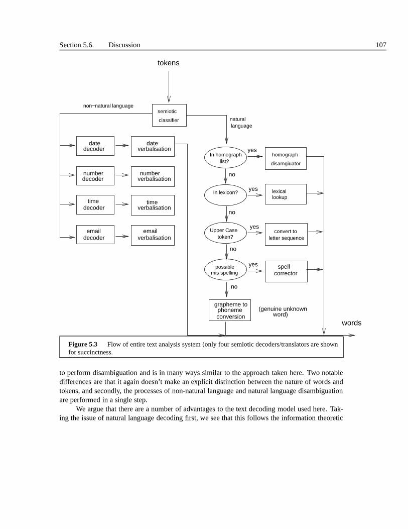
Section 5.6. Discussion 107
In homographlist?
In lexicon?
Upper Casetoken?
mis spellingpossible spell
corrector
convert toletter sequence
homograph
disamgiuator
lexicallookup
naturallanguage
verbalisation
verbalisation
verbalisation
verbalisationdecoder
decoder
decoder
decoder
time
number
date date
number
time
yes
yes
yes
yes
no
no
no
grapheme tophonemeconversion
words
no
(genuine unknownword)
classifier
semiotic
tokens
non−natural language
Figure 5.3 Flow of entire text analysis system (only four semiotic decoders/translators are shownfor succinctness.
to perform disambiguation and is in many ways similar to the approach taken here. Two notabledifferences are that it again doesn’t make an explicit distinction between the nature of words andtokens, and secondly, the processes of non-natural language and natural language disambiguationare performed in a single step.
We argue that there are a number of advantages to the text decoding model used here. Tak-ing the issue of natural language decoding first, we see that this follows the information theoretic

108 Chapter 5. Text Decoding: Finding the words from the text
source/channel paradigm where we have a clean, discrete underlying form that has generated thenoisy surface form that we observe. This is a very general andpowerful model and has been shownsuccessful in many speech and language applications. It facilitates the ability to have abbrevia-tions, misspellings and ambiguity all handled in a single unified powerful statistical framework.Probabilistic models can be built for the general process oftext encoding that will facilitate suc-cessful decoding. In addition, once the words are found in this model, all problems of ambiguityare resolved, which greatly simplifies the work of say the pronunciation module.
The model of semiotic systems described here makes explicitthe notion that text encodesother information that natural language information. Thisis well understood in the field of semi-otics but is nearly universally ignored or brushed over in speech and language processing. Thereare two main advantages we see in adopting this model. First,it makes explicit the differencebetween analysis and verbalisation. In analysing text tokens (for example the time 3:30pm) thereis one, and only one, correct answer which is hour=3, minutes=30, part-of-day=afternoon. Whenit comes to verbalisation however, there are many ways in which we can render this as words, e.g.THREE THIRTY, HALF PAST THREE, HALF THREE etc and different users will have different pref-erences depending on their dialectal preferences and system application. The upshot is that it issignificantly easier to build a system where we know that onlyone part suffers from this subjectiveproblem - the analysis/decoding part can be attempted with complete assuredness.
The second advantage comes when we consider language dependence. It may not be im-mediately apparent, but the text3:30 is nearly universally recognisable no matter which naturallanguage surrounds it so we can have
(56) THREE THIRTY
in English and
(57) TROIS HEURES TRENTE
in French. If we consider3:30 as simple a strange encoding of natural language, we would haveto build a separate analysis system for every language. Withthe semiotic model, one classifierand decoder suffices for all languages; all that is required is a language specific verbalisationcomponent1
We need to comment on the shift in emphasis in text analysis between older systems whichconcentrated on syntactic, morphological and phonological analysis and paid little attention totext decoding issues, and modern systems which perform little linguistic analysis but devote con-siderable attention to ambiguous text forms. The are three separate factors influencing this shift.Firstly, with the commercialisation of TTS, we have found that in real use, non-canonical wordencodings and non-natural language text is rife and any TTS system must deal with this compre-hensively and robustly if it is to be judged usable. Secondly, the simple length of time we havehad to collect data and particularly lexicons over the yearsmeans that we have very comprehensive
1 It is perhaps worth mentioning at this stage that books on teaching languages to non-native speakers are oftenparticularly good at explaining the rules as to how numbers,times and dates are verbalised in particular languages.

Section 5.6. Discussion 109
lists of words, their pronunciations and their text forms. This means that morphological analysisfor instance, is much less necessary than before and that data driven methods are quite practicalin terms of training (we have the data) and run time (we can perform searches or run algorithmswith large numbers of parameters/rules). Thirdly, and perhaps most profoundly, pure linguisticanalysis such as syntactic parsing has fallen out of favour for the simple reason that it has failed“to deliver”. Few doubt that a full, accurate and true description of a sentences linguistic structurewould be very useful, but what form exactly should this take?Modern linguistics has more theo-ries of syntax than even specialists can keep up with, and disagreements run to the very nature ofwhat syntax is and what it represents (and there are now plenty who see it as an epiphenomenon).From a more practical perspective, despite the use of tree-banks, there simply is no such thingas a theory-independent model of syntax which we can use for engineering purposes. All use agrammar and all such grammars make strong claims about the nature of language (such as whetherit is context free). Next, and maybe because of these problems, we find that even the best parsersare really quite inaccurate and relying on their output can cause quite noticeable errors in otherparts of the system. Finally, we find that even if we had a good model of syntax and an accurateparser, we still may not find syntactic analysis helpful. As we shall see in the next chapter, themain uses for syntactic structure are in determining prominence, intonation and phrasing; but evenif we knew the syntax it is far from certain how to derive theseother sorts of information. Therelationship between syntactic and prosodic structure is agreat void in linguistics.
Many regard these problems with syntax and other types of “deep” linguistic analysis as onesof expediency; with a more work in these fields we will gradually improve the theories, grammarsand parsers to the extent that accurate syntactic structures can be assigned to arbitrary text. Analternative viewpoint is that these difficulties are genuinely profound, and given the enormouswork that has been put into the area of theoretical and applied syntax with so little solid progress,that perhaps the nature of the problem itself is incorrectlyformulated and that a new approach tothe organisational properties of language is required.
5.6.1 Further reading
In commercial TTS, text analysis is seen as vitally important as any error can cause an enour-mous negative impression with a listener. Despite this, theproblem has only received sporadicattention amongst academic researchers. Notable exceptions include various works by RichardSproat [410], [411], [412], [413], who tackles nearly all the problems in text analysis (and manyin prosody, explained in the next chapter). The Bell Labs system that Sproat worked on is partic-ularly well known for its very high accuracy with regard to text processing. In a separate line ofwork Sproat et al investigated a number of machine learning approaches to semiotic classificationand verbalisation. David Yarowsky [506], [507], introduced an approach which showed the use ofthe WSD approach to homograph resolution. A more traditional view is given in the MITalk book[10].
Outside the field of TTS we find that a lot of the work in the field of natural language
110 Chapter 5. Text Decoding: Finding the words from the text
processing (NLP) is directly applicable to these problems.While researchers in those fields areoften attempting somewhat different tasks (e.g. homonym disambiguation rather than homographdisambiguation), the approaches are often essentially thesame. A particularly good book in thisarea is by Manning by Schutze, who give a thorough overview ofall aspects of statistical languageprocessing, including WSD, POS-tagging and parsing.
5.6.2 Summary
Classifiers
• Many tasks in text processing involved assigning a label to aunit; this is calledclassification.• Usually this is done by making use of a set offeatures that are found elsewhere in the
utterance.
• A classifier can be therefore be defined as a function which maps from afeature spaceto alabel space.• Treating evidence from features independently is often toocrude and inaccurate. Examining
every possible combination of features is nearly always impossible due to lack of data.
• All sophisticated classifiers therefore adopt an in betweensolution which gives an answerfor every feature combination, but does not necessarily have to have seen all of these duringtraining. The mapping for unobserved feature combinationsis inferred from observed ones.
• A basic distinction can be made betweentaggerswhich assign a label to every token drawnfrom a single set, andword sense disambiguators (WSD)which assign labels only to am-biguous tokens and do so from multiple label sets.
• Popular classifiers include context-sensitive rewrite rules, decision lists, decision trees, naiveBayes classifiers and HMM taggers.
Non-natural language text
• Text is often full of tokens which encode non-natural language systems such as dates, times,email addresses and so on.
• The first stage in text analysis is therefore to performsemiotic classificationwhich assignsa class to each token. This is performed by one of the above mentioned classification algo-rithms
• Once a token’s class is found, it is decoded into its underlying form and then translated intonatural language by a process ofverbalisation
Natural language text
• The main problem here is to resolvehomographswhich occur when two words share thesame text form. These occur because of accident, part-of-speech changes or abbreviations.
• POS-taggers can be used to resolve POS ambiguity

Section 5.6. Discussion 111
• In general WSD approaches are more focused and produce better results.
• In addition some systems use syntactic parsers which generate a syntactic tree for the utter-ance.

6PROSODY PREDICTIONFROM TEXT
Informally we can describe prosody as the part of human communication which expresses emo-tion, emphasises words, shows speaker attitude, breaks a sentence into phrases, governs sentencerhythm and controls the intonation, pitch or tune of the utterance. This chapter describes how topredict prosodic form from the text while Chapter 9 goes on todescribe how to synthesize theacoustics of prosodic from these form representations. In this chapter we first we introduce thevarious manifestations of prosody in terms of phrasing, prominence and intonation. Next we goon to describe how prosody is used in communication, and in particular explain why this has amuch more direct affect on the final speech patterns than withverbal communication. Finally wedescribe techniques for predicting what prosody should be generated from a text input.
6.1 PROSODICFORM
In our discussion of the verbal component of language, we sawthat while there were many dif-ficulties in pining down the exact nature of words and phonemes, broadly speaking words andphonemes were fairly easy to find, identify and demarcate. Furthermore, people can do this read-ily without much specialist linguistic training - given a simple sentence, most people can say whichwords were spoken, and with some guidance people have littledifficulty in identifying the basicsounds in that sentence.
The situation is nowhere near as clear for prosody, and it mayamaze newcomers to thistopic to discover that there are no widely agreed description or representation systems foranyaspect of prosody, be it to do with emotion, intonation, phrasing or rhythm. This is not to saythat description systems do not exist; the literature is full of them, but rather that none matchthe simplicity and robustness of the simple systems we use todescribe the verbal component oflanguage. There are many schools of prosodic theories, and within one school, everything mayhave the illusion of simplicity, but the very fact that thereare so many different theories often withcompletely conflicting accounts, leads us to the position ofextreme uncertainty with regard to howto describe, model, analyse and synthesise prosody. We mention this here, because firstly thesedifficulties prevent us from giving a single clean and simpleexplanation of prosodic phenomena,
112

Section 6.2. Phrasing 113
and secondly we wish to alert the reader to the very tenuous nature of the literature regardingprosody.
To some extent prosody can be seen as a parallel communication mechanism to verbal lan-guage. There we had meaning, form and signal, and broadly speaking we can use these termswhen talking about prosody. Hence we can have a meaning (say anger), which is manifested in aform (say raised pitch levels), which is common to all speakers of a group, which is then encodedacoustically in a joint process with verbal encoding.
At the semantic (meaning) level, prosody is no more difficultto describe than the semanticsof the verbal component (i.e. with great difficulty). It is when we get to prosodic form that we startto see more significant differences between prosody and verbal language. With verbal language,our basic units are words and phonemes, and while these unitshave some difficulties, they arecertainly coherent enough for the engineering purposes of text-to-speech. With prosody though,the situation is much more complex as it is very difficult to determine the basics of what prosodicform should be. We believe on the one hand that abstract prosodic form does exist (we all seem touse similar patterns when asking questions in particular ways), but on the other find it difficult todescribe how this should operate in practice. In the next sections then we attempt to give a theoryneutral1 account of some prosodic phenomena before describing some of the more well knownmodels.
6.2 PHRASING
We use the termprosodic phrasingor justphrasing to describe the phenomenon of where speak-ers groups certain words within the utterances they speak. As will all aspects of prosody, there isacknowledgment that this phenomenon exists, but no agreement as to how best to describe it.
6.2.1 Phrasing Phenomena
Many cases are clear cut, so that when we say
(58) IN TERMS OF THE NECESSARY POLITICAL EXPEDIENCY| THE RESULT WAS CLEARLY A
GOOD ONE FOR SHAW
there is a clear break in grouping between the words up to and including EXPEDIENCY and thewords that follow (here phrasing is marked with a| symbol). The above case may be unproblematicbut there are theories which state that many finer groupings exist, so that we would have:
(59) IN TERMS | OF THE NECESSARY| POLITICAL EXPEDIENCY | | THE RESULT|WAS CLEARLY
| A GOOD ONE | FOR SHAW
(where|| indicates a strong phrase break) and furthermore, some theories express this as a brack-eting to show that some groupings are stronger than others:
1 In reality, there is no such thing as theory neutral, we always make some assumptions when we describe anything.
114 Chapter 6. Prosody Prediction from Text
(60) ((IN TERMS) ((OF THE NECESSARY) (POLITICAL EXPEDIENCY))) (( THE RESULT) (( WAS
CLEARLY) (A GOOD ONE)) (FOR SHAW))
A question that has interested linguists for some time concerns the relationship between syn-tactic phrases (ie. the syntax tree) and prosodic phrasing.While there is clearly some relationship(easily seen in the above examples), finding the general nature of this is extremely difficult. Factorswhich complicate the relationship include:
1. Prosodic phrasing seems “flatter” in that while syntacticphrasing is inherently recursive andcan exhibit a large degree of nesting, if levels in prosodic phrasing exist there are only a few,and there is no sense in which the phrases within an utteranceseem to embed so strongly.
2. Prosodic phrasing is to some extent governed by purely phonological, phonetic or acousticfactors which can override the syntax. In the classic example, Chomsky [89] commented onthe fact that in
(61) THIS IS THE DOG THAT WORRIED THE CAT THAT KILLED THE RAT THAT ATE THE
MALT THAT LAY IN THE HOUSE THAT JACK BUILT
nearly every speaker says this with a flat prosodic phrasing like:
(62) THIS IS THE DOG | THAT WORRIED THE CAT | THAT KILLED THE RAT | THAT ATE
THE MALT | THAT LAY IN THE HOUSE | THAT JACK BUILT
whereas the syntactic phrasing is deeply recursive and embedded
(63) (THIS IS (THE DOG ( THAT WORRIED THE CAT (THAT KILLED THE RAT (THAT ATE
THE MALT (THAT LAY IN THE HOUSE (THAT JACK BUILT )))))))
The speech patterns of the utterance seem to override the syntactic patterns.
3. Phrasing is particularly prone to speaker choice, and while “rules” exist for where phrasebreaks may or may not occur, quite often it appears optional whether a phrase break will befound in a particular utterance. Hence all of the following are possible:
(64) JOHN AND SARAH WERE RUNNING VERY QUICKLY
(65) JOHN AND SARAH | WERE RUNNING VERY QUICKLY
(66) JOHN AND SARAH WERE RUNNING | VERY QUICKLY
So as we can see the relationship between syntactic and prosodic structure is complicated anda general theory which links syntax and prosody is yet to be developed. Some have even arguedthat the difficulty really lies with our models of syntax, andthat if we developed syntactic modelswhich took more account of the ways sentences were spoken some of these problems might beresolved [1].
6.2.2 Models of Phrasing
While there is no single accepted theoretical model of phrasing, all models can be encompassedwithin the idea that a sentence has aprosodic phrase structure. The main point of disagreement

Section 6.2. Phrasing 115
revolves around the details of this phrase structure, and inparticular how nested or deep it shouldbe.
Some have proposed that phrasing should be represented by a tree and that this should actas a parallel tree to the syntax tree. As such the prosodic tree can be generated by a CFG, and socan have recursion and arbitrary depth. Perhaps the most elegant model of this type is the modelof metrical phonology from Liberman [284], [286]. The central idea is that any sentence, orpart of sentence has a metrical tree which specifies its phrase and stress patterns. The lowest unitin the tree is the syllable, and so metrical phonology provides a unified theory of syllable, wordand phrasal patterns. Ignoring the syllable level for the moment we can see the general form of ametrical trees example below:
W
W
was
S
clearly
S
W
W
a
S
S
good
W
one
S
W
for
S
shaw
The S and W labels will be explained later, but for now simply note that the metrical treegroups words together. This model seems particularly good at explaining the patterns within com-pound noun phrases, which we will re-examine in Section 6.3.1. A major criticism though is thatthe theory implies unlimited depth in trees, which implies that a) there are many graded subtletiesin the actual production or perception of phrase breaks, or b) that this representation maps toanother surface representation that is flatter and has fewerlevels. Many solutions have been pro-posed, both as amendments to the original theory2 and as alternatives. The theory ofcompoundprosodic domainsproposed by Ladd [268] allows a more limited recursion with arbitrary depthbut not full recursion. Another variant, called thestrict layer hypothesis [398] is much moreconstrained and states that every word has a fixed number of prosodic constituents above it. Thisand many other theories can be seen as forming a model called theprosodic hierarchy. In this,we have a tree as before, but with a fixed number of levels, eachof which is its own type. A richversion of this might include the levels utterance, intonational phrase, phonological phrase, word,foot, syllable and segment. In thisintonational phrase means a large phrase with a clear intona-tional tune (see below), aphonological phraseis a smaller phrase that spans only a few words,
2 The field of metrical phonology still survives today, but unfortunately bears little resemblance to the elegance andpower of the original theory.
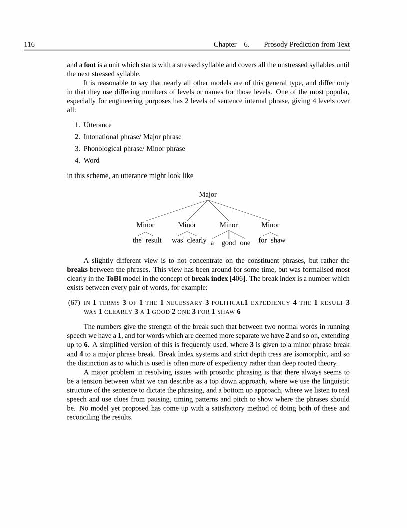
116 Chapter 6. Prosody Prediction from Text
and afoot is a unit which starts with a stressed syllable and covers allthe unstressed syllables untilthe next stressed syllable.
It is reasonable to say that nearly all other models are of this general type, and differ onlyin that they use differing numbers of levels or names for those levels. One of the most popular,especially for engineering purposes has 2 levels of sentence internal phrase, giving 4 levels overall:
1. Utterance
2. Intonational phrase/ Major phrase
3. Phonological phrase/ Minor phrase
4. Word
in this scheme, an utterance might look like
Major
Minor
the result
Minor
was clearly
Minor
a good one
Minor
for shaw
A slightly different view is to not concentrate on the constituent phrases, but rather thebreaks between the phrases. This view has been around for some time,but was formalised mostclearly in theToBI model in the concept ofbreak index [406]. The break index is a number whichexists between every pair of words, for example:
(67) IN 1 TERMS 3 OF 1 THE 1 NECESSARY 3 POLITICAL1 EXPEDIENCY 4 THE 1 RESULT 3WAS 1 CLEARLY 3 A 1 GOOD 2 ONE 3 FOR 1 SHAW 6
The numbers give the strength of the break such that between two normal words in runningspeech we have a1, and for words which are deemed more separate we have2 and so on, extendingup to6. A simplified version of this is frequently used, where3 is given to a minor phrase breakand4 to a major phrase break. Break index systems and strict depthtress are isomorphic, and sothe distinction as to which is used is often more of expediency rather than deep rooted theory.
A major problem in resolving issues with prosodic phrasing is that there always seems tobe a tension between what we can describe as a top down approach, where we use the linguisticstructure of the sentence to dictate the phrasing, and a bottom up approach, where we listen to realspeech and use clues from pausing, timing patterns and pitchto show where the phrases shouldbe. No model yet proposed has come up with a satisfactory method of doing both of these andreconciling the results.

Section 6.3. Prominence 117
6.3 PROMINENCE
Emphasis, prominence, accentandstressare all terms used to indicate the relative strength ofa unit in speech. These terms are used with a variety of definitions in the literature, so to avoidconfusion we will use these these terms as follows.Stressindicateslexical stress, which is aninherent property of words, and indicates for instance thatthe first syllable inTABLE is strongerthan the second, while the second syllable inMACHINE is stronger than the first. We discuss thistype of stress more fully in the section on phonology in Chapter 7.Prominenceis used to indicatethe strength of a word, syllable or phrase when it is used in a sentence. We will use the termaccentsolely to indicate intonational phenomena associated withpitch, andemphasisto indicatea specific use of prominence in discourse.
There are many different ways to formally describe prominence and stress, but for expositionpurposes we will use the termprominent to indicate a unit has more prominence than normal, andreduced to indicate that it has less prominence than normal.
6.3.1 Syntactic prominence patterns
Prominence is really a property of words, such that one word is given extra strength compared toits neighbours. This however is manifested in the lexicallystressed syllable of that word receivingthe extra strength, rather than all the syllables of the word. It is widely accepted that some, but notall, of the prominence pattern in a sentence is governed by the syntax within that sentence.
A first type of effect is that ofnuclear prominence3, which describes the particular promi-nence that often falls on the last content word in sentence. In the following examples, we havemarked this word in bold:
(68) THE MAN WALKED DOWN THE STREET.
(69) TELL ME WHERE YOU ARE GOING TO.
These examples are what are often termeddiscourse neutralrenderings, indicating the “normal”or canonical way these sentences are phrases are spoken, in contrast to some of the ways in whichthey may be spoken in particular discourse contexts.
Prominence patterns are particularly noticeable in sequences of adjectives and nouns whichare collectively calledcompound noun phrases. For example
(70) PARKING LOT
(71) CITY HALL
(72) THE UNION STRIKE COMMITTEE
The final main type of syntactic prominence concerns function words. A very simple rule isthat content words (nouns, verbs etc) can have normal or extra levels of prominence but functionwords are reduced. This certainly covers many simple cases so that in
3 This is often termed a nuclear accent in the literature.

118 Chapter 6. Prosody Prediction from Text
(73) THE MAN MADE THE OFFER ON THE BACK AN ENVELOPE.
we feel that the two instances ofTHE, ON and AN, carry the least prominence and are reduced.Function words are not always reduced however, and in cases like
(74) A BOOK LIKE THAT IS ALWAYS WORTH HOLDING ON TO
we see thatTHAT andTO are not reduced, and in some situations theTHAT would even be the mostprominent word in the sentence. It can be argued that linguistic items such asTHAT are reallyseveral distinct words that happen to carry the same form. This item can be used as a pronoun, anadjective a conjunction, or an adverb as in the following examples
(75) THAT IS MY HOUSE (pronoun)
(76) I WANTED THAT BOOK (adjective)
(77) HE SAID THAT HE WAS AFRAID (conjunction)
(78) HE DIDN’ T TAKE IT THAT SERIOUSLY (adverb)
where we see different degrees of prominence depending on use. Getting the prominence right inthese situations may therefore not be so much an issue of prominence prediction per se, but ratherof making the correct word definitions and finding these from the text.
A second type of prominence effect occurs when function words occur in sequences. Whenwe have sentences such as
(79) I WAS WALKING THE DOG
it seems quite natural to have more prominence onWALKING than onWAS, which follows our sim-ple content word prominent/function word unstressed rule.But when we have longer sequencessuch as
(80) WHAT WOULD YOU HAVE DONE IF IT HADN ’ T BEEN FOR ME?
we see a sentence made entirely of function words. If these are all spoken in reduced form thespeech sounds terrible, and so stresses must be placed on some words. A reasonable rendition ofthis with prominence might then be:
(81) WHAT WOULD YOU HAVE DONE IF IT HADN ’ T BEEN FORME ?
though many other patterns are possible. In fact the overalldegree of prominence in sentences likethis is no less than in “normal” sentences where there is a mixture of content and function words.This situation can be likened to the situation in phrasing where speakers feel the need to placephrase breaks at regular intervals somewhat independentlyof the top down linguistic structure.
Each type of prominence can be “overridden” by the next type,so while the normal promi-nence pattern forTHIRTEEN is
(82) THIRTEEN
in many compound noun phrases, the word undergoesprominence shiftand to give:
(83) THIR TEEN BOYS

Section 6.3. Prominence 119
This is often explained by the notion that the main stress onBOYS “repels” the stress on -TEEN sothat stressed syllables do not directly occur as neighbours.
6.3.2 Discourse prominence patterns
When sentences are spoken in discourses or dialogues, additional patterns can occur. One com-monly cited affect is the difference in prominence levels betweengivenandnew information. Thisidea says that when a word is first used in a discourse, it will often be quite strong, but on secondand subsequent mentions it is actually weaker, so we might have:
(84) FIRST MAKE SURE THAT PAUL ANSWERS THE PHONE.
(85) THEN TELL PAUL TO BRING THE BOOK OVER TONIGHT.
in which the first mention ofPAUL is prominent and the second is not. While this given/newdistinction has traditionally received considerable attention in the literature, many recent empiricalstudies on real speech have shown that this affect is not so common as traditionally though [328],[329], [23], [330]. First, it is far more common that the second sentence would have a pronouninstead of the original name
(86) THEN TELL HIM TO BRING THE BOOK OVER TONIGHT.
and secondly, as Aylett [24] points out, even when words are repeated in full form in dialogues,there is very little evidence of prominence patterns being governed by the given/new distinction.What does occur, is that the degree of prominence is heavily influenced by the redundancy in thedialogue, such that if the speaker feels the listener has a high probability of understanding then heor she may well give a word less prominence. Crucially, the word receiving less prominence doesnot have to be the same as the original word, hence
(87) THEN TELL THE IRISH GIT TO BRING THE BOOK OVER TONIGHT.
here as IRISH GIT is obviously related toPAUL it may receive less prominence. Prominencepatterns of these sort are clearly augmentative and will be explained further in Section 6.5.3.
We can identify a second type of discourse prominence effectwhich we shall termemphasis.This occurs when a speaker wants to draw attention to a particular word:
(88) IT WAS REALLY HUGE
(89) I DIDN ’ T BELIEVE A WORD HE SAID
(90) I’VE HEARD IT ALL BEFORE
(91) THATS JUST TOO BAD
(92) ITS IMPORTANT TO DO THAT BEFORE YOU ENTER THE ROOM
(93) NOT THAT ONE
and so on. In general, emphatic prominence is used for augmentation purposes (see below inSection 6.5.3) where the speaker wants to make particularlysure that the listener understandswhat is being said. A particularly salient example is contrastive prominence of the type:

120 Chapter 6. Prosody Prediction from Text
(94) THE PROFIT WAS$10M BEFORE TAX , NOT AFTER TAX
This however also extends into affective purposes, where for example the speaker knows thatthe listener will understand, but still uses extra emphasis. This could occur for example when thespeaker wishes to express frustration or imply that the listener is stupid and therefore has to haveeverything spoken slowly or clearly.
6.3.3 Prominence systems, data and labelling
As with phrasing, we have a number of models and theories which attempt to explain prominence.Again as with phrasing, the theories range from simple models to ones which posit a rich andembedded prominence structure. Broadly speaking, the phenomenon of lexical stress is fairlyuncontentious with good agreement between labellers as to where stress values lie. Prominenceand emphasis is more difficult to mark, as labellers often findit hard to distinguish between whatis “normal”, discourse neutral prominence and marked emphasis. The distinction here is relatedto the issue of augmentative prosody, discussed in Section 6.5.3.
As with phrasing, the basic distinction is between systems which have a fixed number ofprominence values or levels, and ones in which nesting and recursion can occur. And again,we see that the issue is the tradeoff between a system which seems to match linguistic structure,and one that is more bottom up and perceptually verifiable. Wehave already examined Liberman’smodel of metrical phonology for phrasing, but actually thiswas primarily developed for explainingprominence patterns. In this, we have binary trees in which each node is marked eitherstrong (S)or weak (W). Using this, we can then describe prominence patterns as follows:
W
city
S
Hall
S
James
W
street
S
parking
W
lot
The “clever bit” is that this model allows us to elegantly combine smaller groups of words intobigger groups by further use of the metrical trees:
W
S
James
W
street
S
S
parking
W
lot
in which case there is one and only one node that is dominated only by S, and this is how wespecify the most prominent or nuclear prominence of the sentence or phrase. Metrical phonology
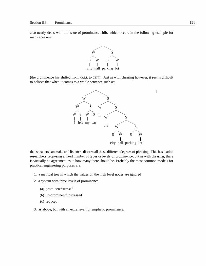
Section 6.3. Prominence 121
also neatly deals with the issue of prominence shift, which occurs in the following example formany speakers:
W
S
city
W
hall
S
S
parking
W
lot
(the prominence has shifted fromHALL to CITY). Just as with phrasing however, it seems difficultto believe that when it comes to a whole sentence such as:
W
W
W
I
S
left
S
W
my
S
car
S
W
in
S
W
the
S
W
S
city
W
hall
S
S
parking
W
lot
]
that speakers can make and listeners discern all these different degrees of phrasing. This has lead toresearchers proposing a fixed number of types or levels of prominence, but as with phrasing, thereis virtually no agreement as to how many there should be. Probably the most common models forpractical engineering purposes are:
1. a metrical tree in which the values on the high level nodes are ignored
2. a system with three levels of prominence
(a) prominent/stressed
(b) un-prominent/unstressed
(c) reduced
3. as above, but with an extra level for emphatic prominence.

122 Chapter 6. Prosody Prediction from Text
Figure 6.1 Example of F0 contour with pitch accents and boundary tones marked.
6.4 INTONATION AND TUNE
Intonation is sometimes used as a synonym for prosody, and as such includes prominence andphrasing as just described. Here we use a more narrow definition in which intonation is the sys-tematic use of pitch for communication. Often we describe intonation with reference to thepitchcontour or theF0 contour, which is the pattern of pitch/F0 variation over an utterance4
Most traditional accounts of intonation speak of intonational tuneswhich span the length ofthe sentence. In these accounts, we might have a question tune, an exclamation tune and so on.More modern accounts advocate a more compositional approach, where the global intonation tuneis composed of a number of discrete elements. Most importantof these is thepitch accent, whichcan be defined as a significant excursion (either positive or negative) in the F0 contour that lendsemphasis to a syllable. Pitch accents only occur on prominent syllables, and hence prominence canbe seen as defining the possible places where pitch accents can occur. Figure 6.1 shows a sentencewith two clearly visible pitch accents. In addition to this,it is common to haveboundary accentsor boundary toneswhich are pitch movements associated with the ends of phrases rather thansyllables. A classic example of a boundary tone is where we having rising pitch at the end of asentence to indicate a question, shown in Figure 6.1.
Beyond this, we again find that there is little agreement about how to describe pitch accentsand boundary tones. Some theories state there are a fixed inventory of these, while some describethem with continuous parameters. The nature of pitch accents and boundary tones is disputed, withsome theories describing them astones or levels while others say their characteristic propertyis pitch movement. One prominent theory states that we have anintonational phonology thatparallels normal phonology, and as such we have inventoriesof contrasting units (sometimes called
4 F0 is shorthand for fundamental frequency. Informally thiscan be thought of as being the same as pitch, the exactrelationship is described in Section 9.1.1.

Section 6.5. Prosodic Meaning and Function 123
tonemes) and grammars which state what can follow what.As with phrasing, we find there is a considerable degree of speaker choice with regard to
intonation, such that while it may be common to speak a question such as
(95) IS THIS THE WAY TO THE BANK?
quite often speakers speak this with the same intonation as anormal statement. Just why speakersdo this is addressed in Section 6.5.3.
It is difficult to discuss intonation further without reference to the phonetics and acousticsof this part of language, and for that reason we forgo a more thorough account of intonation untilChapter 9.
6.5 PROSODICMEANING AND FUNCTION
One of the reasons why good models of prosody have proved so hard to develop is that researchershave often tried to study prosody without reference to its communicative function. In verballinguistics it is quite common to study a particular sentence without reference to why a speakersaid this, and by and large this separation provides a usefulmodularity for research purposes. Sowhen we consider a sentence such as
(96) THE MAN WALKED DOWN THE STREET
We can say thatTHE MAN is the subject andWALKED is a verb and so on, and then perhapsgo on to study the phonetics of the sentence, without having to know why the speaker actuallysaid this sentence. It is common to follow a similar approachin prosody, but we believe this ismistaken, and that in fact, it is more or less impossible to study the nature of prosody withouttaking into account the dialogue, speaker situation and other functional factors. Hence we nowgive an account ofprosodic function which states the reasonswhy we use prosody, and as weshall see, this significantly simplifies the practical issues concerning how to generate prosody in atext-to-speech system.
6.5.1 Affective Prosody
Affective prosody is the most basic type of prosody and in a sense can be regardedas pureprosody. Affective prosody includes the expression of meaning related to emotion, mental stateand speaker attitude. Significantly, prosody is theprimarychannel for the communication of thesemeanings: if one is angry and wishes to express this, it is best done with a loud, shouting, growlingvoice, rather than a simple, natural statementI AM ANGRY . In fact simply saying that one is in anemotional state with words without any matching prosody is usually taken as a sign of insincerity(e.g.YES YOU LOOK NICE IN THAT DRESS), and if the words and prosody seem to contradict, thelistener usually takes prosody to be the true expression of the speaker’s meaning. (For example,
124 Chapter 6. Prosody Prediction from Text
if you ask a child whether they ate all the cookies, they find iteasy to sayNO but less hard to saythis convincingly).
Affective prosody has a certain degree of language universality. In all languages, raisingone’s voice and shouting are seen as expressions of angry or hostile states, while speaking in asofter voice is seen as conciliatory or calming. In fact the relationship is so direct that often wesay “she spoke in a calm voice” etc. Affective prosody is not completely universal however, and interms of primary emotion, there are significant differencesacross languages. Even within Englishit is common to find that one group of speakers are regarded as brash and another meek, whenin fact all that is different are the “settings” and “thresholds” with which the basic emotions areexpressed.
In general, affective prosody has a fairly direct meaning-to-form relationship and hence themore extreme the form the more extreme the emotion. This implies that, unlike verbal language,the affective prosody system is not arbitrary with regard tomeaning/form. A number of emotioncategorisation systems have been proposed. One common theory holds that there are six basicemotions (anger, happiness, sadness, disgust, fear and surprise) from which follow a number ofsecondary emotions such as puzzlement or intrigue [110], [113], [153]. Some however arguethat there is no fixed set of emotions and rather emotion is best expressed in a multi-dimensionalsystem. One such proposal advocates three independent axesof emotion calledactivation, evalu-ation andpower [393], [126].
In addition to emotion, affective prosody includes speakerattitude. The difference betweenemotion and attitude is that only emotion can exist independent of communication. As an illustra-tion; you can be happy on your own, but you need someone else tobe sarcastic with. Apart fromthis distinction, attitude functions similarly to emotionin that it is fairly direct, has a significantdegree of universality and does not have a arbitrary or dual nature.
One point of debate in the literature on both emotion and affective prosody concerns whetherthere is such a state as “no emotion” or “no affective prosody”. The argument is that if we are ableto increase the level of intensity of anger, then we should beable to decrease this to the pointwhere there is no anger. Similarly with the other emotions. This issue is important as it seemsthat the total affective content of an utterance can vary greatly and can be contrasted with the totalpropositional content of the verbal part of the utterance. These two effects seem to trade-off suchthat we can have sentences that are nearly purely affective “thats amazing” and others which arepurely propositional “the sum of the square of the opposite and adjacent sides...”. This later typeof sentence is what we have previously termed discourse neutral.
6.5.2 Suprasegmental
If a sentence is spoke with little or no affective content, ie. in a discourse neutral manner, we stillsee characteristic patterns in the phrasing, rhythm, pitch, voice quality and timing. Typical effectsinclude phones at the ends of sentences or phrases being lengthened, syntactically salient words(e.g. heads) having more emphasis, F0 levels being higher atthe starts of sentences and so on.

Section 6.5. Prosodic Meaning and Function 125
These effects are often called “prosodic” but according to the model we use here, these arenot real prosodic phenomena but just another aspect of the verbal component. We can see thisbecause speakers do not impart extra information by using these effects and they are as highlyformulaic as the use of say nasalization, voicing and tongueposition. These effects are oftencalled prosodic as they use much the same acoustic means as expression - anger is expressedthrough pitch and voice quality, which is also used to distinguish the middle and ends of a phrase.In the model used here, we do not include these effects under the umbrella of prosody, but insteadterm these thesuprasegmentalpart of verbal phonetics. The term suprasegmental here is usedto show that while these effects may be verbal in nature, theyare operate over the span of severalphones (segments). It is best to think of these as a by productin the production of the phoneticcontent.
While suprasegmental effects are rightly seen as the natural effect of phonetic production onF0, timing and voice quality, it is important to realise thatthe speaker still has conscious controlover these. That is, while it is normal for a particular voicequality to be used at the end of asentence, the speaker can override this if desired. However, while overriding default behaviouris possible, it is highly noticeable if this is done, and so a speaker who deviates from defaultbehaviour will be perceived as wanting to draw attention to the aspect of the utterance which haschanged. Another way of looking at suprasegmental is in terms of defaults, and deviation fromdefaults. The key to this is to realise that the default for a sentence is not connected to mathematicalsimplicity where we might have a constant duration for each phone, a flat F0 contour and a constantstate of vocal effort. Rather, the default behaviour exhibits considerable variation from these fixedvalues in ways dictated by verbal production. Deviations from the suprasegmental default areindications of real prosody, whether they be for affective or augmentative purposes (explainedbelow).
In tone languageslike Mandarin, pitch can be used to identify words. For example, liuspoken with one tone pattern means “flow”, but when spoken with a different tone pattern means“six”. In our model, this is a purely suprasegmental effect and treated in just the same way asnasalization is used to distinguish words in English. Mandarin of course has intonation also, whichis used for all the same affects as English. The fact that intonation and parts of word identityare expressed in the same acoustic variable, does of course complicate analysis and synthesissomewhat, but with modern synthesis techniques we can modelboth without difficulty.
6.5.3 Augmentative Prosody
Augmentative prosodyis used as an aid to ensure successful communication of the verbal com-ponent of a message. Unlike affective prosody, augmentative prosody does not contain or conveyany extra information, it is merely a means for the speaker toensure that a message is decodedand understood more clearly. Augmentative prosody can onlybe understood with reference to adialogue model of the type presented in Section 2.3. There wesaw that participants in a dialoguehave a mental image of each other and are constantly balancing the desire to beefficient in com-

126 Chapter 6. Prosody Prediction from Text
munication (whereby they would use the least effort in generating their utterances) with a desireto beeffective, whereby they wish to ensure the message is correctly decoded and understood.
In an ideal communicative setting, where the participants know each other, can see eachother and are able to converse without background noise or other distractions, it is nearly alwaysthe case that the verbal message can be communicated withoutneed for any augmentative prosody.Whether any prosody is used therefore is purely a matter of the affective nature of the utterance.Successful communication is possible because the verbal channel is highly redundant, to the extentthat the speaker should always be able to decode and understand the message. In other conditionswe face a different situation, so for example in noisy conditions we might see that the speakerspeaks with greater vocal effort and more slowly. Likewise we may see the same effect if thespeakers don’t know each other so well, or in more polite situations in which the speaker wants tobe seen to be making a clear effort to communicate effectively.
While it may be fairly obvious that increased articulation effort will lead to a higher prob-ability of a phoneme string being correctly recognised, it is with other aspects of augmentativeprosody that the situation becomes particularly interesting. For example, it is frequently assertedthatyes/no questionssuch as
(97) IS THIS THE WAY TO THE BANK?
having rising intonation in English. In fact empirical studies of data show that the most commonintonation for such sentences is exactly the same pattern used for statements. While speakerscanuse rising intonation, they often don’t. This behaviour is best explained with reference to thecommunicative model. In examples such as 97, it is usuallyobviousthat a yes/no question is beingasked, there really is little need for a speaker to use the additional cues that a rising intonationpattern would provide. However if the speaker believes she may be misunderstood, or if she istrying to sound polite, the rising intonation pattern may appear. By comparison, it is common toask “yes/no questions” that are have the same syntax as statements, but in which the speaker doesnow in fact use a rising intonation pattern to make sure theseare interpreted correctly:
(98) THIS IS THE WAY TO THE BANK?
We see this effect in all aspects of prosody. The given/new distinction, where it is often claimedthat subsequent mentions of an entity are less prominent than first mentions, is rarely observed inreal speech, partly because it is quite clear from the verbalcontent which in fact is intended [328],[24].
In classic example sentences such as
(99) BILL DOESN’ T DRINK BECAUSE HE’ S UNHAPPY
which are spoken without phrase breaks may potentially be ambiguous but in general the listenerwill know enough of the dialogue context to correctly decodethis. If however the speaker is lesssure of a correct decoding, phrase breaks may be inserted to aid communication, and likewise withevery other aspect of prosody.

Section 6.5. Prosodic Meaning and Function 127
In summary, augmentative prosody works by changing the default suprasegmental contentof an utterance in particular ways. It is used by the speaker solely to increase the chances of theverbal message being correctly decoded and understood. Significantly, unlike affective prosody, itimparts no extra information into the message.
6.5.4 Symbolic communication and prosodic style
It is useful at this stage to compare and contrast the verbal and prosodic components of language.Verbal language was defined in Section 2.2.1, and there we sawits defining properties as beingdiscrete anddual, in the sense that every message is composed of a sequence of discrete wordentities which in turn are composed of a sequence of phonemes. Verbal language isarbitrary inthe sense that one cannot infer the form of a word from its meaning or vice-versa. Verbal languageis productive in that completely new sentences can be created all the time.What if any of theseproperties does prosody have?
First of all, let us realise that in verbal language, to construct a message we must alwaysselect a unit (e.g. word) and place these in sequence. A word is either present or absent in anutterance and every utterance is composed of a sequence of words. With prosody the situationis different. Firstly, we need not always have a prosodic unit - it is completely acceptable andcommon to have an entire sentence with no particular emphasis, intonation or phrasing effects(recall, suprasegmental effects are considered part of verbal language, not prosody). Furthermore,if a prosodic effect is present, it can be there to a greater orlesser extent. So we can have a wordthat is somewhat emphasised to one which is heavily emphasised - this is unlike verbal languagewhere something is either present or not.
In verbal language, speakers really have very little choicein how they speak a particularword. So while speakers when saying the wordCAT may vary somewhat in their tongue positionsor degree of aspiration, only so much variation is allowed, otherwise a different word may be per-ceived. Hence verbal language is inherently restricted andformulaic. With prosody, the fact thatan utterance is not required to be “full” of prosody gives thespeaker much more choice. Augmen-tative prosody may be used to aid communication but often it doesn’t have to be; conversely incertain polite or formal situations a speaker may choose to use considerably more augmentativeprosody than is strictly required for successful communication. The degree of affective prosody isagain very variable - some conversations or messages (e.g. speech from a news reader) are nearlycompletely lacking in affective content while some are full(e.g. a chat between two friends).
An important consequence of the degree of choice in prosody is that it allows the speaker todeviate from the default patterns in certain ways without running the risk of changing the meaningof the sentence entirely. This then allows for the phenomenon termedprosodic style. This ismost marked in situations where particular speakers, oftenactors or comedians, use prosodic stylein a quite unconventional way. This use of prosody is not related to the communication of themessage or even emotion, but is intended to draw attention tothe speaker himself. Informally, wecan talk about the speaker “sounding cool” by the way they candeviate from the normal patterns
128 Chapter 6. Prosody Prediction from Text
of prosody and be creative in their usage. Stylistic use of prosodic is one significant factor inexplaining why some speakers seem more interesting to listen too than others.
6.6 DETERMINING PROSODY FROM THETEXT
6.6.1 Prosody and human reading
In text-to-speech, our interest is of course to generate prosody from text. This is problematic in thattext mostly encodes the verbal component of language; prosody is by and large ignored. Given thatprosody is such a vital part of spoken language, how then is itpossible that written communicationcan even work? We examined this in some detail in Section 3.2,and can summarise the situationas follows:
• Quite often text encodes sentences which are rich in propositional content rather than af-fective content. Text genres like newspapers, non-fiction books, histories, company reports,scientific articles and so on simply do not have much affective content in the first place.
• The writer knows that prosody is absent from the text that is being written, and thereforecompensatesfor this by using words in different ways that would be the case when speaking.For example in literature, we see phrases such as:
(100) ‘thats right’, he said angrily
where thehe said angrily is obviously written to help the reader understand how the‘thats right’ section should have sounded.
• The awareness that prosody is lacking often leads to the writer writing in a style that isinherently less ambiguous; in such cases we say the writer iswriting “clearly” and so on.
• Quite often, people who are reading aloud add their own prosody into the speech. By this wemean that when they read the words, they keep accurately to the word, but as the prosody isnot encoded in the text the reader “makes up” what they think is appropriate for this situation.It is if the reader is saying “if I were saying this myself, what prosody would I use?” andthen adding this into the speech.
• This requires considerable skill and is often based on an understanding of the text, ratherthan just a decoding as is the case for words. The reader is in effect adding in affective andaugmentative prosody in places she believes are appropriate.
From this we can conclude that in situations where the text genre is quite factual, it is usuallysufficient to generate speech from the verbal message only, and so all that is required is the gen-eration of the suprasegmental part of the signal; the affective part of prosody is ignored. In othertext genres the situation is significantly more difficult, and if say a dialogue from a play is readin this fashion (or more likely) responses from a computer dialogue system, the generated speechcan sound somewhat dull and removed. Finally, we see that mimicking a genuinely good humanreader is very difficult indeed, as they will be performing anactual comprehension of the text, and

Section 6.6. Determining Prosody from the Text 129
then generating their own prosody. In no way are they simply decoding the prosody from the textand then speaking it aloud, as they can do with the words. To date, no satisfactory solution hasbeen found to this problem, and so current text-to-speech systems are, unfortunately, lacking inthis regard.
6.6.2 Controlling the degree of augmentative prosody
We face a different situation with regard to augmentative prosody. When a person speaks, she usesa mental image of the likelihood of a listener decoding and understanding the message to decidehow much augmentative prosody to use and where to use it. We therefore face two problemsin TTS: guessing the state of the listener and knowing which parts of the utterance may needdisambiguating with prosody. Doing this properly is very difficult - even if we have a good ideaabout the likelihood of a message being misunderstood, knowing exactly where to place phrasebreaks and additional emphasis is extremely hard as often this can require a full and accuratesyntactic and sometimes semantic analysis of the sentence.But luckily, as with affective prosody,we have a “get-out” which enables us in many cases to bypass this problem.
Firstly, writers often use punctuation and fonts when they feel that the words in some wayneed disambiguation. So when we see a comma or semi-colon, itis often a safe bet to place aphrase boundary here as we know the author felt that the wordsbefore and after the break shouldbe separated. If a word is in italics or bold, it is again probably a safe bet to give this word ex-tra emphasis. A second strategy arises from the fact that augmentative prosody is indeed onlythere tohelp in the decoding and understanding of an utterance. If we simply don’t include anyaugmentative prosody, there is a good chance the utterance will still be decoded and understood,but perhaps just not with so much certainty. We can compensate for this specific lack of disam-biguation information by ensuring that other parts of the signal do aid decoding; for instance if wesynthesise the speech more clearly and slowly than normal the listener will have a better chanceof understanding.
6.6.3 Prosody and synthesis techniques
In the remainder of this chapter we shall concentrate onprosody prediction, the term given to thetask of generating the prosodic form from the text. In Chapter 9 we complete the task by consider-ing the issue ofprosody synthesis, the job of generating phonetic or acoustic information from theprosodic form. As we shall see, the degree to which prosody needs to be specified depends verymuch on the synthesis technique employed in waveform synthesis. Roughly speaking, in modernsystems suprasegmental prosody can be generated at the sametime as the verbal content, whereasin first and second generation synthesis systems, the suprasegmental content has to be generatedexplicitly. Most of the following sections can be read without too much emphasis being placed onthis distinction, it will however become more of an issue in Chapter 9.

130 Chapter 6. Prosody Prediction from Text
6.7 PHRASING PREDICTION
First we will examine the issue ofphrasing prediction which is how to generate a prosodicphrase structure for a sentence from the text. For purposes of illustration we will adopt the modeldescribed in Section 6.2.2 where we have a major phrase and a minor phrase and this is probablythe most commonly used in TTS.
6.7.1 Experimental formulation
To help in our exposition, we will formalise the problem in the manner suggested by Taylor andBlack [443]. In this, our input is a list of tokens:
T =< t1, t2, t3, ..., tn,>
and between every token is ajuncture , so that a full sentence is:
T =< t1, j1, t2, j2, t3, j3, ..., jn−1,wn,>
The job of the phrasing algorithm is to assign values to everyj i drawn from an inventory ofjuncture types, which we will define to be non-break, minor-break, major-break, sentence.About 1 in 5 junctures are of typenon-break (that is the gap between normal words) and so wehave to be careful in assessing the accuracy of any algorithm- if we use one which always assignsnon-break we will have achieved 80% accuracy on a simple junctures correct measure. Becauseof this, Taylor and Black proposed a number of measures, later extended by Busser et al [77].These are calculated from the following basic quantities:
Breaks B number of breaks in the corpusInsertions I a non-break has been incorrectly marked as a breakDeletion D a break has been incorrectly marked as a non-breakSubstitution S a break of one type has been incorrectly marked as a break of another typeNumber of junctures N total tokens in the corpus -1
These are then used to calculate the following scores:

Section 6.7. Phrasing prediction 131
Breaks correct= BC =B−D−S
B×100% (6.1)
Non-breaks correct= NC =N− I −S
N×100% (6.2)
Junctures correct= JC =N−D− I−S
N×100% (6.3)
Juncture insertions= JI =IN×100% (6.4)
Juncture deletions= BI =IB×100% (6.5)
(6.6)
An alternative scheme, more in line with that used in naturallanguage processing is based onprecision andrecall, which are specifically designed to give accuracy figures forproblems wherethe number of occurrences is much less than the number of non-occurrences.
Precision= P =number of breaks correct
number of breaks predicted=
BC− IBC
(6.7)
Recall= P =number of breaks correct
number of breaks in the test set=
BC− IB
(6.8)
These are often combined in afigure of merit , F:
Fβ =(β2 +1)PR
β2P+R(6.9)
whereβ is used to govern the relative importance of whether it is a worse error to falsely insert abreak or falsely miss one. If these are considered equal, then β = 1 and
F =2PRP+R
(6.10)
This is a commonly used measure of overall quality, but as we shall see, it is almost certainly nottrue that human perception believes an insertion and deletion cause the same gravity of error.
6.7.2 Deterministic approaches
There are two popular and very simple phrasing algorithms:
1. deterministic punctuation (DP): Place a phrase break at every punctuation mark

132 Chapter 6. Prosody Prediction from Text
2. deterministic content, function (DCF): Place a phrase break every time a function wordfollows a content word.
The first algorithm, DP, works very well in sentences of the type:
(101) The message is clear: if you want to go, you have to go now
For DP algorithm to work, we must have an accurate means of determining underlying punctua-tion. This is so that sentences like
(102) But really!? You can go -- but it won’t do you any good.
have the punctuation sequence!? and--mapped to a single underlying form because we don’twant to have an additional phrase break between the! and the?. The DCF algorithm works wellin sentences such as
(103) It was taking a long time to gather all the information
where we place a phrase break after every function word that follows a content word:
(104) it was taking | a long time | to gather |all the information
These can be combined into a single algorithm,deterministic content function punctuation(DCFP), which places a break after every content word that precedesa function word and also atpunctuation. The algorithms were tested on a large corpus ofread speech which had phrase breakslabelled by hand. The results for these algorithms given in Taylor and Black [443] are:
Algorithm breaks correctjunctures correctjuncture insertionsDeterministic Punctuation 54.274 90.758 0.052Deterministic Content Function Punctuation84.40 70.288 31.728
These figures basically show that that the DP algorithm massively under predicts and the DCFPalgorithm massively over predicts. The DP algorithm resultis worth examining further becauseit shows that placing a phrase break at a punctuation mark is in fact a very safe thing to do; thisnearly always coincides with a real break. The only problem is that many other breaks are missed.The DPCF algorithm over predicts far too much, which lead to the idea that if finer distinctionscould be made than just content word and function word, a moreaccurate algorithm would bepossible.
A number of more sophisticated deterministic systems have been proposed [26], [186], [10]which make of rules for specific cases. For example, theverb balancing rule of Bachenko andFitzpatrick [26] works through a sentence left to right and compares the number of words in apotential phrase formed with the verb and the syntactic constituents to the left, and the number ofwords in the constituent to the right. The potential phrase with the shortest number of words ischosen as the correct one.

Section 6.7. Phrasing prediction 133
6.7.3 Classifier approaches
The general historical trend in phrase break prediction is the same as with most problems we ex-amine: as more data has become available, researchers have moved away from rule based systemstowards trainable systems. This is partly because the new data showed how errorful rule basedsystems were, and partly because it allowed algorithms to have their parameters and rules auto-matically inferred from the data. We now turn to data-driventechniques, where interestingly wesee a similar pattern of algorithm type to that used in text classification. In this section we examinelocal classifieralgorithms, which share many features in common with WSD algorithms. In thenext section we examine HMM approaches, which are very similar to POS taggers.
Wang and Hirschberg [363] introduced the idea of using decision trees for phrase breakprediction. Decision trees allow a wide variety of heterogeneous features, examples of which aregiven below:
• total seconds in the utterance
• total words in the utterance
• speaking rate
• time from start of sentence to current word
• time to end of sentence from current word
• is the word before the juncture accented?
• is the word after the juncture accented?
• Part-of-speech
• syntactic category of constituent immediately dominatingthe word before the juncture
• syntactic category of constituent immediately dominatingthe word after the juncture
These features (and others) were used as question in the tree, which was grown in the normal way.Wang and Hirschberg trained and tested their system on 298 utterances from the ATIS corpus,giving the following results (the results aren’t availablein the formats we described above):
Boundaries correct 88.5%Non-Boundaries correct93.5%
It should be pointed out that this approach can’t strictly beused for TTS purposes as acousticfeatures (e.g. time in seconds) measured from the corpus waveforms were used in addition tofeatures that would be available at run time. Following thisinitial work, a number of studies haveused decision trees [264] [418], and a wide variety of other machine learning algorithms havebeen applied to the problem including memory based learning[77] [402], Bayesian classifiers[516], support vector machines [87] and neural networks [157]. Similar results are reported inmost cases, and it seems that the most important factors in the success of a system are the featuresused and the quality and quantity of data rather than the particular machine learning algorithmused.
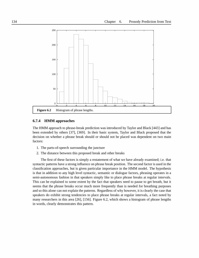
134 Chapter 6. Prosody Prediction from Text
0
50
100
150
200
250
0 2 4 6 8 10 12 14 16 18 20
Figure 6.2 Histogram of phrase lengths.
6.7.4 HMM approaches
The HMM approach to phrase-break prediction was introducedby Taylor and Black [443] and hasbeen extended by others [37], [369]. In their basic system, Taylor and Black proposed that thedecision on whether a phrase break should or should not be placed was dependent on two mainfactors:
1. The parts-of-speech surrounding the juncture
2. The distance between this proposed break and other breaks
The first of these factors is simply a restatement of what we have already examined; i.e. thatsyntactic patterns have a strong influence on phrase break position. The second factor is used in theclassification approaches, but is given particular importance in the HMM model. The hypothesisis that in addition to any high level syntactic, semantic or dialogue factors, phrasing operates in asemi-autonomous fashion in that speakers simply like to place phrase breaks at regular intervals.This can be explained to some extent by the fact that speakersneed to pause to get breath, but itseems that the phrase breaks occur much more frequently thanis needed for breathing purposesand so this alone can not explain the patterns. Regardless ofwhy however, it is clearly the case thatspeakers do exhibit strong tendencies to place phrase breaks at regular intervals, a fact noted bymany researchers in this area [26], [156]. Figure 6.2, whichshows a histogram of phrase lengthsin words, clearly demonstrates this pattern.

Section 6.7. Phrasing prediction 135
B N
NB0.2
0.8
0.8
0.2
NB
NB NN
BB
0.97
0.03
0.24
0.76
0.88
0.03
0.03
0.71
0.120.97
0.290.97
Figure 6.3 Finite state machine depictions of n-gram phrasing models.
The phrase break length histogram shows a preference for phrase lengths of about 3 - 6words, and shows that very long or very short phrases are highly unlikely. Alternatively, we canview this distribution cumulatively, meaning that the longer we have been since the previous phrase

136 Chapter 6. Prosody Prediction from Text
break the more likely it is that the next juncture will have a phrase break. While it is easy to addthis sort of information into a classifier, it is difficult to do so in an globally optimal way. Thebasic problem is, that say we are at a juncture that is six words away from the previous juncture.Our distribution may say that it is now quite likely that we will observe a break at this point. If theevidence from the POS sequence seems reasonable, then a break will be placed here. The problemis that the next juncture, seven words away from the last break may be an even better place toput a break, but we can’t do this now as the break at word six hasalready been assigned. Whatis required is a way to searchall possiblesequences of phrase breaks, and this, via the Viterbialgorithm, is exactly what the HMM approach can deliver.
In the HMM approach, we have a state for each type of juncture,so ignoring sentence breaks,we either have three states if we distinguish major and minorbreaks or two states if we don’t.Taking the second case first, we now have a state which gives:
P(C| j i)that is, the probability of a juncture after tokeni omitting a POS sequenceL. Ideally the POSsequenceL would be the tag sequence for the entire sentence, but as these distributions are non-parametric models which have to be learned by counting, the size of the window is quite limited interms of what can be estimated robustly. Hence we approximate the POS sequence of the wholesentence as a window of POS tags around the juncture. This canbe seen as a generalisation to theDCFP algorithm where we used one tag before and after the juncture. Taylor and Black howeverreported that a window of two tags before and one tag after thejuncture gave the best results givenlimited training data. Informally, we can see that we would expect the following to give relativelyhigh probabilities
P(ADJ NOUN AUX|break)
P(DET NOUN NOUN|non-break)
The juncture sequence model is given by an n-gram, which is calculated in the way explained inSection 5.2.2, that is by counting occurrences of sequences. An important difference to the n-gramin a POS tagger is that we now only have two or three types in then-gram rather than 40 or so.This means that the number of unique sequences is much less, which means that for the sameamount of data we can robustly compute longer n-grams. In these models we would see that
P(N,N,N,B,N)
would give a high probability and that
P(B,B,N,B)
would give a low probability. Taylor and Black report that the best results are found from whichuses a 6-gram language model, where there are two tags beforethe juncture and one after. Thisgave figures of 79.24% breaks correct, 91.597% junctures correct and 5.569% juncture insertions.

Section 6.8. Prominence Prediction 137
6.7.5 Hybrid approaches
More recently a number of approaches have been proposed which combine the advantages ofdecision tree approaches (use of heterogeneous features, robustness to curse of dimensionality)and the HMM approach (statistical, global optimal search ofsequences). In addition, there hasbeen somewhat of a re-awakening of use of syntactic featuresdue to the provision of more robustparsers. Rather than attempt an explicit model of prosodic phrasing based on trying to map fromthe syntax tree, most of these approaches use the syntax information as additional features in aclassifier [508], [209], [257].
While the pure HMM approach uses a discrete probability distribution over observations(in our case POS tags), in practice, all we need is a means of finding the likelihood of seeingthe observation given the juncture typeP(C|J). Many have therefore tried alternative ways ofgenerating this. One of the most popular is actually to use decision trees, as these can be used togiven probabilities as wall as simple decisions on classification. As it stands, a decision tree gives aposterior probability, not a likelihood, but a likelihood value can be obtained by either ensuring thatthe tree is trained on an equal amount of break and non-break data, or by normalizing the posteriorby the basic frequency of breaks and non-breaks. The advantage in this combined approach is thatwe can use any features that require, but also perform the global Viterbi search using n-grams tofind the best overall sequence of breaks [403], [369], [423].
6.8 PROMINENCE PREDICTION
Prominence prediction algorithms follow the same basic approaches as phrase break predictionwhere we have simple deterministic algorithms, sophisticated deterministic algorithms and datadriven algorithms.
6.8.1 Compound noun phrases
The simplest prominence prediction algorithm simply uses the concatenation of the lexical promi-nence patterns of the words. So for:
(105) IN TERMS OF THE NECESSARY POLITICAL EXPEDIENCY TO ENSURE SURVIVAL — THE
RESULT WAS A CLEARLY A GOOD ONE FORSHAW
we might generate a prominence pattern of:
(106) IN TERMS OF THE NECESSARY POLI TICAL EX PEDIENCY TO ENSURE SURVI VAL THE
RESULT WAS A CLEAR LY A GOOD ONE FOR SHAW
The main ways in which this rule fails (again ignoring affective and augmentative effects) arein compound noun phrases and certain function words uses. The prominence patterns in com-pound noun phrases in English are complex and can seem quite baffling. When we consider theprominence patterns in street names such as

138 Chapter 6. Prosody Prediction from Text
(107) WINDSOR AVENUE
(108) BEAUFORT DRIVE
(109) PARK LANE
it seems quite obvious what the pattern is, until we considerexamples with the wordSTREET
(110) W INDSOR STREET
(111) BEAUFORT STREET
(112) PARK STREET
in which the prominence pattern is reversed. Sproat [410] conducted a very thorough study intocompound noun phrasing patterns, and concluded that in general, there is no simple syntacticpattern which governs prominence. Instead he proposed an extensive set of rules based partly onsynactic and partly on semantic patterns. The most basic rule says that compound noun phraseswith two words assign their prominence according to whetherthe two words are taken as a singlecompound “word” or a phrase. In general in English, phrases receive their main prominence onthe last word in the phrase. English words, and particularlynouns, by contrast tend to have theirprominence on the first syllable. This can be seen in the difference between
(113) BLACK BIRD meaning the type of bird
(114) BLACK BIRD a bird which just happens to be black
This principle can then be generalised to cope with all two word cases, with the idea beingthat only conventionalised cases are treated as compound words which receive their prominenceon the first word. In addition to this, there are a number of semantically driven rules , which rangefrom the general to the more specific:
(115) Furniture + Room→ RIGHT, e.g. kitchentable
(116) Proper-name + street→ LEFT, e.g. Park street
For more compound noun phrases involving three or more words, a CYK parser (see Section5.5) is used to assign the internal structure to the noun phrase, after which prominence values canbe assigned. To resolve ambiguity, a set of heuristics is used to find the best parse. These are:
1. Prefer parses determined by semantic rather than syntactic means. (This partly works be-cause semantic parses are much more specific)
2. Choose phrase based parses over compound word bases parses3. Choose parses with right branching structure.
Additional rules are used to shift prominence in cases wherethe parses would produce twoprominent syllables side by side.We also find that many typesof non-natural language entitieshave characteristic patterns. For example, it is common place to find telephone numbers readwith a particular stress pattern (and indeed phrasing). Producing the correct stress patterns forthese is often fairly straight forward and the creation of these patterns can be integrated into theverbalisation process.

Section 6.8. Prominence Prediction 139
6.8.2 Function word prominence
Less work as been carried out on the second main problem of determining the prominence patternsin function word sequences. The most we can say about this is that not all function words are equalwhen it comes to propensity for reduction. At one extreme, wehave determiners (THE and A)which in their default form are always reduced, and at the other extreme closed class words suchasHOWEVER, WELL andSO can receive the most prominence in a sentence. Given a sequence ofcontent words, a reasonable approach is then to give each a score according to where it comes inthe strength list, and starting with the strongest, add prominence at regular intervals. A possiblehierarchy, from weakest to strongest, might be:
articles THE, A , AN
auxiliary verbs WAS, HAS, IS
prepositions TO, FROM, BY
particles IF, THEN, WELL
conjunctions THAT, AND , BUT
pronouns HE, HIM , SHE, ME, THEM
modals WOULD, COULD, SHOULD
Note that auxiliary verbs (e.g.HAVE) can function as main verbs also. We find a fairly clearpattern that when used as an auxiliary the word is often reduced, when used as a main verb it isoften unreduced or prominent. With this table, we can then use a rule which states that prominentsyllables should not occur side by side, and so in a sequence of function words we first assignprominence to the strongest word given in the table, ensure its neighbours and reduced and thenlook for the next strongest word. This then can give the stress pattern for the sentence we saw inSection 6.3.1:
(117) WHAT WOULD YOU HAVE DONE IF IT HADN ’ T BEEN FORME ?
6.8.3 Data driven approaches
Prominence prediction by deterministic means is actually one of the most successful uses of non-statistical methods in speech synthesis. This can be attributed to a number of factors, for examplethe fact that the rules often don’t interact or the fact that many of the rules are base on semanticfeatures (such that even if we did use a data driven techniquewe would still have to come upwith the semantic taxonomy by hand). Sproat notes [410] thatstatistical approaches have hadonly limited success as the issue (especially in compound noun phrases) is really one of breadthand not modelling; regardless of how the prominence algorithm actually works, what it requiresis a broad and exhaustive list of examples of compound nouns.Few complex generalisations arepresent (what machine learning algorithms are good at) and once presented with an example, therules are not difficult to write by hand.
That said, with the provision of larger, labelled corpora, the natural progression has stillbeen towards using machine learning techniques to predict prominence. We should probably not

140 Chapter 6. Prosody Prediction from Text
be surprised to find that these techniques follow the basic paradigm used for phrase break predic-tion, where we obtain a corpus of speech, label the prosodic content of this by hand (in this caseprominence levels) and train an algorithm to predict these values from features available to thesystem at run time. Approaches tried have included decisiontress [207], [378], [147], memorybased learning [303], transformation based learning [200]and neural networks [72], [323], [389].
6.9 INTONATIONAL TUNE PREDICTION
Here we have explicitly separated prominence from the tune part of intonation, and so for our pur-poses intonation prediction is specifically the predictionof intonational tune from text, rather thanthe broader definition of this problem that encompass predicting tune, accentuation and sometimesphrasing.
Of all the prosodic phenomena we have examined intonationaltune is the most heavily re-lated to augmentative and particularly affective content.In situations where these effects are ab-sent, we can say to a first approximation that all utterances have in fact the same intonational tune;the only differences occur as to where the pitch accents and boundary tones which make up thistune are positioned. Hence we can almost argue that for discourse neutral synthesis, there simplyisn’t any intonational tune prediction to be done. In other words, the real task is to predict a suitableF0 contour that expresses the prominence and phrasing patterns and encodes the suprasegmental,rather than true prosodic patterns of the utterance.
While we can describe prominence and phrasing in quite abstract high level terms, this issignificantly harder with intonation as all theories to a greater or lesser extent make explicit refer-ences to F0 patterns, levels and dynamics. Given this, and the fact that for the most part we aregenerating discourse neutral suprasegmental intonation,we will leave the entire topic of intonationuntil Chapter 9.
6.10 DISCUSSION
At first glance it may seem that predicting prosodic form fromtext is an impossible task. Twosignificant barriers stand in our way; first, the text is greatly under specified for the type of in-formation we require as textual encoding of prosody is more or less non-existent. Secondly, theuncertainty surrounding what prosodic form should be makesit hard to label data, train algorithmsand basically even know if we are headed in the right direction.
6.10.1 Labelling schemes and labelling accuracy
Taking the second issue first we see that in every area of prosody there is considerable disagree-ment as to how to represent prosodic form. The problem isn’t so much that researchers disagree

Section 6.10. Discussion 141
completely; there is wide spread agreement about how to label many utterances; in many cases itis quite clear that a particular utterance has a strongly prominent syllable, has a clear phrase breakand has a distinctive intonational tune. There are many “black and white” cases where all theoriesand all labellers agree. The problem is rather that there is asignificant grey area, where we can’ttell if this really sounds prominent, where we aren’t sure that there is a phrase break between twowords and where we can’t really decide on the intonational tune for an utterance.
There are of course grey areas in other aspects of linguistics. As we saw in Section 4.2, pin-ning down the exact definition of a word can be tricky, and we will come across similar difficultiesin Section 7.3.2 when we consider the definition of the phoneme. But in general the agreementamong researchers ismuch muchhigher with regard to these phenomena. Furthermore, so longaswe are aware of the difficulties, the definitions of word and phoneme which we use in this bookaregood enough, meaning that, as engineers, using these models does not seem to result in signif-icant loss of quality in synthesis. Studies that have examined inter-labeller reliability of prosodicschemes have shown the true extent of the problem; for instance in the original publication of theToBI system, Silverman et al reported that the agreement on phrase breaks was only 69% for fourlabellers, and 86% for whether a syllable is prominent (bears a pitch accent in their paper). Thesefigures might not seem too bad, but are about anorder of magnitudeworse than the equivalentresults for verbal, phonetic transcription, and up totwo or threeorders of magnitude worse for thetranscription used for text analysis in Chapter 5. Furthermore, when we consider that the numberof choices to be made in prosodic labelling is often small (say choose one break index value from5) we see just how difficult labellers find this task. These results for ToBI are not particularly un-usual, consistently similar figures have been reported for many other schemes [426], [488], [487].Furthermore it is misleading to blame poor labelling agreement on the labellers not being “expert”enough - non-experts can readily label many of the types of data we require in TTS, and so incomparing the figures for other types of labelling we are in fact comparing like with like.
Why does these problems arise?. Essentially we face two related issues;: which labellingscheme, model or theory to use; and how to assign the labels arising from this to a corpus ofspeech. Most researchers involved in both the scientific investigation and engineering implemen-tation are aware that there are a huge number of differing andoften incompatible theories and mod-els of prosody. The temptation then is therefore to seek a “theory-neutral”, “common-standard” or“engineering” system which we can use to label the data and soavoid having to nail our coloursto any one particular theoretical mast. We have to emphasiseat this point that such an approach isfolly; there is simply no such thing as a theory neutral scheme. If we take the break index schemefor instance, this explicitly states that there are a fixed number of types of breaks, that no recursionor limited recursion exists, that phrasing is not explicitly linked to prominence patterns and so on.
Furthermore, there is no sense in which we can just “label what we hear” in the data; alllabelling schemes are based on a model, the fundamentals of that model are implied when welabel speech, and if our scheme is wrong, inaccurate or at fault in some other way, we run a highrisk of enforcing inappropriate labels on our data. If we then use these labels as ground truth, weare running a severe risk of enforcing our training and run-time algorithms to make choices that

142 Chapter 6. Prosody Prediction from Text
are often meaningless.
6.10.2 Linguistic theories and prosody
Given these difficulties with labelling schemes and models,it is worth asking whether we need amodel of prosodic form at all; perhaps it would be possible tosimply define a mapping from thetext or semantics to the acoustics. This viewpoint certainly has some merit, but we should be waryof dismissing the idea of prosodic form entirely. A brief digression into the theoretical history ofprosody may help explain why.
It is probably fair to say that the field of linguistics has always had a troubled relationshipwith prosody. In fact many accounts of language completely ignore prosody (e.g. prosody ishardly ever mentioned in any work by Chomsky): whether this is because it is deemed to be quiteseparate from verbal language or simply too tricky to handleis hard to say. Ifwehowever want afull account of language and communication we have to include prosody.
Older linguistic accounts of prosody tended to treat it as quite a different system, and this toa degree was unproblematic. But with the rise of more formal theories of language, new theoriesof prosody were put forward that used the new techniques of formal language theory, featurestructures and so on. The problem facing these researchers was how closely should a formaltheory of prosody follow the formal theories of verbal language. Unfortunately (in my opinion)too much emphasis was placed on an insistence that prosodic phenomena could be explained withthe same mechanisms for verbal language, and hence we saw grammars of intonation, intonationalphonology and schemes for pitch accent description which were meant to be the direct equivalentof normal phonology. To be fair, external pressures pushed research in this direction; there wasa strong desire to move from the very impressionistic and informal models of the past towards amore rigorous model and in addition there was the idea that ifprosody could be explained withthe same mechanisms as verbal language this would somehow bemore parsimonious and wouldalso ensure prosody was taken seriously as a linguistic areaof study (instead of just being ignoredas mentioned above).
Ladd [269] points out that a major justification for the development of a phonology forprosody was to counter attempts in linguistics to correlatesay F0 values with syntax patterns.While correlations may exist, building such a model ignoresthe fact that different speakers havedifferent “parameters” in their F0 encoding model, for example that high pitched voices will pro-duce different patterns to low pitched ones. A better model is to posit a system of abstract prosodicform, where all speakers of an language/accent would share the same representations for similarsemantic and functional purposes. The actual acoustic encodings of these might vary with speakerphysiology, but the prosodic form would be the same for all speakers. In formal terms, all weare saying is that there are a number of levels, or interacting systems of prosody. In summary thephonological school of prosody is nearly certainly right inadvocating abstract description systemsfor prosodic form, but is perhaps less right in advocating that these should be formulated withthe same mechanisms as verbal language. Prosody has an abstract structure, but it operates in a

Section 6.10. Discussion 143
fundamentally different way to verbal language.
6.10.3 Synthesising suprasegmental and true prosody
Turning to the problem of predicting prosody from under-specified text, we find the situation isless bleak that it might appear. Let us consider the issue of prosody not being encoded in thetext. In many applications, we are not synthesising text with any particular emotive or attitudinalcontent, and so are therefore going for a discourse neutral reading. This simple fact saves us, andin such cases allows us to ignore the affective side of prosody. Many non-TTS synthesis systemsare of course required to synthesize this type of text, and ifemotive or attitude information isprovided in the input there is no reason that these effects can not be successfully synthesized.
When we consider augmentative prosody, we can again find waysaround the problem.Firstly, as we discussed in Section 3.1.4, authors do often use punctuation and sometimes useitalics and so on, and these are very good indicators that augmentative disambiguation is appro-priate at this point. As we saw from Table 104, placing a phrase break at a punctuation markis rarely wrong; human readers nearly always do this. However, recall that the whole point ofaugmentative prosody is that it acts as anaid to decoding and understanding and in many casesisn’t strictly necessary. Hence if weunder predictphrase breaks, the only risk is that we mayincrease the chance of mis-comprehension by the listener. Significantly, speech generated withless augmentative prosody may sound completely natural - its just the case that the listener mayhave to pay more attention. It is also important to realise that the most crucial phrase breaks areoften just those marked by commas in the text as it is here thatthe authors wants to be most cureof correct comprehension. While not ideal, under prediction is a safe strategy. Conversely how-ever, inserting a phrase break in a completely inappropriate position can sound terrible and oftencompletely throws the listener, resulting in loss of naturalness and intelligibility. Hence when de-veloping algorithms for phrase break prediction it is probably not sensible to balance insertionsand deletions as equally bad errors; insertions are in general far worse than deletions. In practicalterms, this means that the figure of merit scores which combine precision and recall should beweighted strongly in favour of precision rather than recall.
One area where augmentative prosody does however hurt us is in the data. While we canbypass the augmentative prosody problem at run time by underpredicting, when we come toconsider real data we effectively a priori have no idea what augmentative prosody the speaker willchoose to use. While we can measure the acoustic encoding of this (pause lengths and positionsand so on), this does not help us in determining the high levelfeatures required to predict these.We can imagine the speaker “inventing” these features and using them when speaking; they arenot available to us. This to a large extent explains the widely reported phenomenon of “speakerchoice” or “speaker variability” in prosody. Basically, when speaking or reading, because ofthe redundancy in the verbal component, the speaker has considerable choice where to place thephrase breaks; it all depends on their mental image of the listener. For practical purposes this hasthe effect of addingnoise into the data; the features we have access to (the ones we can derive

144 Chapter 6. Prosody Prediction from Text
from the text) explain the presence of phrasing to a certain degree. The other features explain therest of the behaviour, but as we don’t have access to these, they effectively appear as noise in ourdata and variance in our models.
The consequence of this, taken in conjunction wit the issue of very low level of transcribedagreement, may well mean that many prediction algorithms are as accurate as theoretically possi-ble; no amount of extra refinement in the techniques or extraction of alternative features will makemuch difference. The reason why the algorithms can not improve is due to noise in the data, fromeither or both or these sources.
6.10.4 Prosody in real dialogues
In Sections 6.8 and 6.7 we have seen how to predict prominenceand phrasing patterns from text.The techniques described though in general only operate on single sentences, which are usuallydeclarative in nature. Much of interest in prosody takes part at a different level, where many ofthe main phenomena occur in conversational, discourse, emotive or spontaneous communication.Hence most TTS systems only model a small range of the possible prosodic phenomena. We canhowever imagine systems which go beyond current capabilities. If speech synthesis were used inmore conversational applications, the discourse effects of prosody it would become important tomodel the discourse effects of prosody. In many current dialogue systems, the interaction feelsvery artificial because the system is only capable of simple questions and declarative sentences.The study of prosody in discourse in a rich topic of research in linguistics, but little has be donein terms of well adopted practices in TTS systems. Hirschberg [208] gives a review of manydiscourse and functional aspects of intonation and describes much of the work that has been donein discourse prosody in TTS.
We need to reiterate some points about the augmentative function of prosody and how thisaffects studies into prosodic phenomena. While it is widelyaccepted that prosody does undergomore variation, or undergoes more speaker choice than otherparts of language, it is our belief thatthedegreeto which this occurs is vastly underestimated in most studies. If we compare prosodicform to verbal form, we see that while speakers can indeed vary the articulation of a word such asHAT, they are very constrained in doing, and too much deviation from the canonical pronunciationruns the risk of the word being decoded incorrectly.
A key reason for the difference in degree of variation between verbal and prosodic languageis to do with their functional use in communication. To a large extent, we can study the verbal partof language without reference as towhya particular utterance is used in a discourse but the samesituation simply does not hold for prosody. The way in which prosody is used is primarily drivenby the discourse, and taking sentences out of their discourse and studying them without referenceto this, leads to problematic analyses. In verbal phoneticsa common practice is to carefully elicitsentences spoken under laboratory conditions. These conditions are artificial and can lead to dis-crepancies between the phonetic/acoustic patterns observed between “canonical” speech and real,spontaneous speech. In general though, a considerable amount can be learned from controlled

Section 6.10. Discussion 145
experiments in this way. The situation is radically different in prosody however, and eliciting indi-vidual sentences in laboratory conditions is extremely risky in that these bear virtually no relationto how prosody is used in real, spontaneous speech. Many studies unfortunately impose a strongdiscourse bias, so that when we examine utterances elicitedfor the purposes of studying say thegiven/new distinction, what we are doing is asking speakersto produce sentences in a very artifi-cial discourse context. The effect of this is to grossly exaggerate the way the prosody is generated,such that effects such as given/new or contrastive prominence can seem quite clear, distinct and or-derly. In real, spontaneous speech by contrast, the discourse situation and the speaker and listenersmental models of each other dictate how prosody is used. In these situations, the discourse contextand information content is often so obvious and redundant that prosody is simply not required forfurther disambiguation. This helps explain while earlier laboratory based studies of prosody claimclear patterns and effects, but when studies of real data areperformed [328], [24], these effects areoften far less clear.
6.10.5 Conclusion
The take home message from this discussion is that the theoretical difficulties with prosodic mod-els and the under specification of prosody in text mean that this is an inherently difficult problemand should be approached with a degree of caution. While it ispossible to continually drive downthe error rate with regard to semiotic classification, homograph disambiguation and so on, it isunrealistic to assume the same can be done with prosody.
6.10.6 Summary
Prosodic form
• It is usual to consider three basic components of prosodic form: phrasing, prominenceandintonation.
• Phrasing is used to group words together in the utterance, and is influenced by top downfactors such as syntax, and bottom up factors which place phrase breaks at roughly equalintervals.
• Prominence is used to give extra strength to certain words. It is partly determined by syntax,where in particular it governs stress patterns in compound noun phrases and function wordsequences.
• Intonation is the use of pitch to convey prosodic information.
• Very little agreement exists on how to represent prosodic form, which makes the design ofpractical algorithms more difficult than in other areas of TTS.
Prosodic function
• Affective prosody conveys emotion and attitude in communication.

146 Chapter 6. Prosody Prediction from Text
• Augmentative prosodyis used to help disambiguate the verbal component of communica-tion.
• Suprasegmental prosodyarises from the natural patterns of how words are joined togetherin utterances.
Prosody prediction from text
• This is inherently difficult as prosody is largely absent from text.
• In practice though, the genres that we often use in TTS are nothigh in affective content.
• Phrasing and prominence prediction can be performed by a variety of algorithms, includingsimple rules, sophisticated rules, data driven techniquesand statistical techniques.
• Most popular machine learning algorithms have been appliedto prosodic prediction. Theresults are often similar, and difficult to improve upon because of the inherent difficulties inrepresenting prosodic form and under specification in the text.
Prosodic labels and data
• In general prosodic labelling by hand has low levels of inter-labeller agreement compared toother labelling tasks in TTS.
• This may stem from the fact that we have yet to develop a robustsystem for describingprosody.
• Speakers change their prosody depending on the discourse context and so it is difficult toassociate one prosody with a particular sentence.
• As speakers naturally vary their prosody, and labels are often unreliable, the labelling ofprosodic databases is often very noisy.

7PHONETICS ANDPHONOLOGY
This chapter gives an outline of the related fields of phonetics and phonology. A good knowledgeof these subjects is essential in speech synthesis as they help bridge the gap between the discrete,linguistic, word-based message and the continuous speech signal. More traditional synthesis tech-niques relied heavily on phonetic and phonological knowledge, and often implemented theoriesand modules directly from these fields. Even in the more modern heavily data driven synthesissystems, we still find that phonetics and phonology have a vital role to play in determining howbest to implement representations and algorithms.
7.1 ARTICULATORY PHONETICS AND SPEECH PRODUCTION
The topic ofspeech productionexamines the processes by which humans convert linguistic mes-sages into speech. The converse process, whereby humans determine the message from the speechis calledspeech perception. Together these form the backbone of the field know asphonetics. Ingeneral,
Regarding speech production, we have what we can describe asacompletebut approximatemodel of this process. That is, in general we know how people use their articulators to producethe various sounds of speech. We emphasise however that our knowledge is very approximate; nomodel as yet can predict with any degree of accuracy how a speech waveform from a particularspeaker would look like given some pronunciation input. Thereason for this lack of precisionis that the specifics of the production process are in fact incredibly complex; while we can makesolid generalisations about how a [s] sound is pronounced for instance, it is another matter en-tirely to explain how this varies from speaker to speaker, how [s] is affected by speech rate, howsurrounding sounds influence it and how this is affected by prosodic interaction. The fact that thisknowledge is incomplete should of course not be a surprise toreaders of this book; if we fullyunderstood this process we could simply implement it in a computer and thereby solve the speechsynthesis problem. In fact, as we shall see, in the field of text-to-speech, our lack of knowledge hasled us to abandon (for the time being at least) the path of trying to mimic the human productionprocess directly. However, what knowledge we have can be putto good use, and hence a solid
147
148 Chapter 7. Phonetics and Phonology
grounding in what speech production and perception knowledge we do have is an essential part ofconstructing a high quality synthesiser.
Probably the main difficulty in discovering the mechanisms of human speech productionis that of measurement and data collection. Of course this isa problem common to all science;before telescopes only the simplest models of astronomy were possible; afterwards detailed andaccurate observations could be made which allowed the rapiddevelopment of theories. We see thesame in the scientific study of phonetics; in the early days there were no instruments available forexamining speech (phonetics even predates the invention ofsound recording). With the inventionfirst of sound recording, then spectrographic analysis, x-ray films and other techniques, speechscientists were able to examine the processes in more detail. Such instruments and more elemen-tary techniques (such as looking directly into a speaker’s mouth or simply trying to determine theposition of one’s own tongue) have led to the level of understanding we have today and which weshall briefly describe next.
Progress in speech perception has been significantly slower. The lack of progress can beexplained simply by the difficulty in extracting information about the process. While some tech-niques exist for examining the cochlea and analysing brain patterns when listening, in general itis very difficult to collect concrete data on the problem, andas a result scientists have little to goon when developing theories. What ever progress has been made is typically conducted withinwithin the framework of experimental psychology (e.g. [58]]. This significant imbalance betweenour knowledge of production and perception helps explain why phonetics is in general approachedfrom a speech production point of view; that is simply the area of the speech process that we bestunderstand.
7.1.1 The vocal organs
We generate speech by the coordinated use of various anatomical articulators known col-lectively as thevocal organs. Figure 7.1 shows a mid-sagittal section of the head showingthevocal organs. If we consider just the tongue in isolation fora moment, it should be clear that itcan move in all three dimensions, and can create a complex variety of movements and trajecto-ries. The movement and position of the tongue directly affects the speech produced and even amovement of a few millimeters can dramatically alter the speech sound produced. While the otherorgans are somewhat simpler, it should be clear that a substantial number of vocal organconfigu-rations are possible, and each gives rise to a different sound. This alone gives some insight intothe complexities of speech.
7.1.2 Sound sources
Nearly all sounds in English are created by by air moving fromthe lungs through the vocal organsto the lips and then outwards. This flow is called anegressive pulmonic air stream; egressive,because the air is flowing outwards, and pulmonic because thesource is the lungs. During the

Section 7.1. Articulatory phonetics and speech production 149
nasal cavity
oral cavity
tongue pharynx
glottis
larynx
vocal folds
hard palate soft palate
lips
nostril
alveolar ridge
teeth
velum
uvula
Figure 7.1 Diagram of the vocal organs or articulators
passage of the air flow, one or moreconstrictions is applied, the effect of which is to generate asound. We call constriction that causes the sound thesourceand the sound produced thesourcesound. We shall consider the types of source in turn.
The vocal folds are two folds of tissue which stretch across thelarynx . A speaker cancontrol the tension in his or her vocal folds (Figure 7.2) so that they can by fully closed, narrowor open. The gap between the vocal folds is called theglottis, and we usually refer to this type ofsound production as aglottal source. When the vocal folds form a narrow opening, the air streammoving through them causes them to vibrate, giving rise to aperiodic sound. We term the rateof vibration of the vocal folds thefundamental frequency, denotedF0. The termpitch is usedfor the rate of vibration that is perceived by the listener, and in general the pitch and fundamentalfrequency can be taken as the same thing. By varying the tension in the vocal folds, a speaker canchange the fundamental frequency of the sound being produced. When the vocal folds operate inthis way, they are said to be generating avoiced sound. A typical male speaker can vibrate hisvocal folds between 80 and 250 times a second, so using the standard terminology we say that hisfundamental frequency varies from 80 Hertz (Hz) to 250 Hertz. By comparison a female speakermight have a fundamental frequency range of 120Hz to 400 Hz. All vowels are voiced sounds -
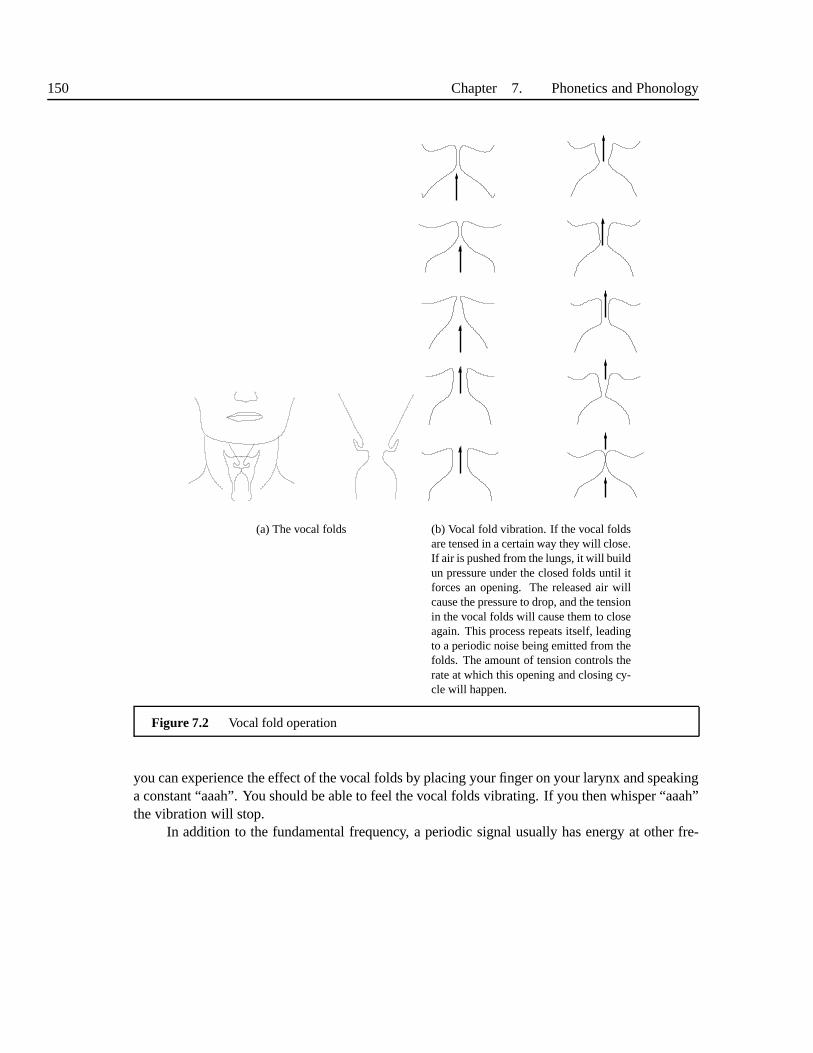
150 Chapter 7. Phonetics and Phonology
(a) The vocal folds (b) Vocal fold vibration. If the vocal foldsare tensed in a certain way they will close.If air is pushed from the lungs, it will buildun pressure under the closed folds until itforces an opening. The released air willcause the pressure to drop, and the tensionin the vocal folds will cause them to closeagain. This process repeats itself, leadingto a periodic noise being emitted from thefolds. The amount of tension controls therate at which this opening and closing cy-cle will happen.
Figure 7.2 Vocal fold operation
you can experience the effect of the vocal folds by placing your finger on your larynx and speakinga constant “aaah”. You should be able to feel the vocal folds vibrating. If you then whisper “aaah”the vibration will stop.
In addition to the fundamental frequency, a periodic signalusually has energy at other fre-

Section 7.1. Articulatory phonetics and speech production 151
quencies known asharmonics. These are found at multiples of the fundamental, so if we havea glottal sound with a fundamental of 100Hz, we will find harmonics at 200Hz, 300Hz, 400Hzand so on. In general the harmonics are weaker than the fundamental, but nonetheless are heardand can be thought of as giving the sound its basictimbre . A musical analogy might help here.One can create a sound of the same fundamental frequency by either bowing or plucking a violinstring. In both cases the fundamental frequency is the same,however the different in action cre-ates a different pattern of harmonics and this is why the timbre of bowing and plucking soundsdifferent.
If the glottis is opened slightly further, periodic vibration will cease. Instead a non-periodicturbulent air flow will be created, which generates a different type of sound, termednoise. Here theterm “noise” is used in the technical sense (as opposed to a general definition which is a synonymfor “sound”) to mean the random sound created, somewhat likean untuned analogue radio. Thisis the natural way to generate the [h] sound inHEDGE, but is also the way in which whisperingworks. If the vocal folds are brought together completely, the air stream stops and no sound isproduced. By carefully controlling the timing of this opening and closing, it is possible to produceaglottal stop, which is the normal way to realise the [t] in words such asBUTTER in some accentsof English (e.g. Glaswegian or Cockney).
Sound can be created from sources other than the glottis. If the glottis is open, it will notgenerate any sound, but will allow the air stream to flow through. It is then possible to use com-binations of the tongue, lips and teeth to form a constriction, and thereby generate a non-glottalsound source. The [s] sound inSIT is generated this way - by speaking this, and extending thelength of time the [s] is spoken for, you can feel that the glottis is not vibrating and that the tongueis very close to the roof of the mouth. Noisy sounds can also becreated by holding the teeth closeto the lips (as in the [f] sound inFALL ) or by placing the tongue near the teeth as in the [th] soundin THANK . Because there is no glottal periodic vibration in these sounds, they are calledunvoiced.It is possible to have sounds which are both voiced and noisy,such as the [z] sound inZOO. Inthese cases, the glottis operates as with vowels, but a further narrow constriction is created in themouth to generate a secondary, noisy, sound source.
Sounds such as [s], [f] and all vowels can be spoken as a continuous sound, and are thereforecalledcontinuants. By contraststopsare sounds which have a relatively short duration whichcan only be spoken as “events” and can not be spoke continuously. The [p] sound inPEN or [t]sound inTIN are stops. Stops are produced by creating aclosuresomewhere in the vocal tract sothat all air flow is blocked. This causes a build up of pressure, followed by areleasewhere theair suddenly escapes. Because the sound is produced in this way, the sound must have a finite,relatively short duration and hence these sounds cannot be produced continuously.
7.1.3 Sound output
For most speech sounds, the acoustic signal leaves via the mouth - such sounds are termedoral.For a few however, the sound leaves via the nose; such sounds are callednasal. In English the first

152 Chapter 7. Phonetics and Phonology
(a) oral output
(b) nasal output (c) nasal and oral output
Figure 7.3 Oral sounds are when the velum blocks the nasal cavity, and the sound escapes from theopen mouth. Nasal sounds are caused, first by blocking sound escape from the mouth and secondlyby lowering the velum so that sound can escape from the nose. Nasalised sounds have sound escapefrom both the mouth and nose.
sounds inNO andME are nasal, as are the last sounds inTHEM, THIN andTHING. As evidence thatthese sounds leave via the nose and not the mouth, say “mmmmm”and then pinch your nose soas to close it - the sound will stop. Sometimes sound exists through the both the nose and mouth.There are no canonical sounds in English which do this, but inFrench for instance for the lastsound inONT exits through both the nose and mouth. Such sounds are callednasalised.
Thevelum is a piece of skin at the back of the mouth. When it is raised, the nasal cavity isblocked off and the speech is completely oral. When the velumis lowered, the sound will be nasalor nasalised, depending on if the mouth is closed or open. It is important to note that in an oral

Section 7.1. Articulatory phonetics and speech production 153
sound, the velum blocks the entrance to the nasal cavity, andso this plays no part in determiningthe sound. In nasal sounds however, while the oral cavity is blocked, it is not blocked at theentrance, rather it is blocked at some other point (at the lips in an [m] sound and near the alveolarridge in an [n] sound). During the production of a nasal, air enters the oral cavity, is reflected andeventual escapes from the nose. The shape of the oral cavity plays an important part in determiningthe sound of the nasal, even though no air escapes from it directly. Figure 7.3 shows vocal tractconfigurations for these output types.
7.1.4 The vocal tract filter
The diversity of sound from the source and output are furtherenriched by the operation of thevocal tract. The vocal tract is collective term given to the pharynx, theoral cavity and the nasalcavity. These articulators can be used to modify the basic sound source and in doing so create awider variety of sounds than would be possible by the source alone. Recall that all voiced soundsfrom the glottis comprise a fundamental frequency and its harmonics. The vocal tract functionsby modifying these harmonics which has the effect of changing the timbre of the sound. That is, itdoes not alter the fundamental frequency, or even the frequency of the harmonics, but it does alterthe relative strengths of the harmonics.
In general it is the oral cavity which is responsible for the variation in sound. The pharynxand nasal cavity are relatively fixed, but the tongue, lips and jaw can all be used to change theshape of the oral cavity and hence modify the sound. The vocaltract can modify sounds fromother sources as well by the same principle.
This model, whereby we see speech as being generated by a basic sound source, and thenfurther modified by the vocal tract is known as thesource/filter model of speech. The separationinto source and filter not only adequately represents the mechanics of production, it also repre-sents a reasonable model of perception in that it is known that listeners separate their perceptionof the source in terms of its fundamental frequency from the modified pattern of its harmonics.Furthermore, we know that the main acoustic dimension of prosody is fundamental frequency,whereas the main dimensions of verbal distinction are made from a combination of the type ofsound source (but not its frequency), and the modification bythe vocal tract. The mathematics ofboth the source and the filter will be fully described in Chapter 10.
7.1.5 Vowels
All vowel sounds are voiced and hence have the same sound source (the glottis). What distin-guishes one vowel sound from another is the shape of the oral cavity and to a lesser extent theshape of the lips and duration with which the sound is spoken.The oral cavity and lips operateto create different shaped cavities through which the source sound must pass. By moving the jaw,lips and tongue, different filter effects can be created, which serve to modify the harmonics of theglottal sound source and produce the wide variety of vowel sounds. It is important to note that

154 Chapter 7. Phonetics and Phonology
(a) HEAT vowel
(b) HOOT vowel (c) HOT vowel
Figure 7.4 Vocal tract configurations for three vowels
the pitch of the speech is controlled entirely by the glottis, whereas the type of vowel is controlledentirely by the tongue, jaw and lips. As evidence of this, generate any vowel and keep the pitchconstant. Now vary the shape of your mouth in any way you wish -it is clear that the pitch remainsthe same, but the mouth alone is determining the quality of the vowel. Conversely, say an “aaah”sound and convince yourself that you can change the pitch without changing the vowel itself.
It helps to describe vowels if we define a number of dimensionsof oral cavity and lip config-uration. First, the height of the tongue combined with the position of the jaw defines a dimensioncalled height (sometimes calledopen/close). If one compares the position of the mouth whenspeakingHEAT andHOT one should be able to tell that the jaw is raised and the tongueis high inHEAT, whereas forHOT the jaw and tongue are lower. Secondly, the position of the raised part of

Section 7.1. Articulatory phonetics and speech production 155
the tongue with in relation to the front of the mouth defines another dimension, which we can callfront/back . Consider the difference in tongue position in the vowel inHEAT andHOOT - whilethis is slightly more difficult to feel or measure than in the case of height, it should at least be clearthat the tongue is in a different position and that the jaw remains relatively fixed. Figure 7.4 showsthe articulator positions forHEAT, HOOT andHOT. A third dimension is calledlip rounding orsimply rounding. This effect is caused when the lips are protruded from theirnormal position.Some vowels (e.g.HOOT) have noticeably rounded vowels, while others are noticeably unrounded(e.g.HEAT). A final basic dimension of vowel classification islength. This feature is very accentspecific, but in many accents the vowel inHEAT is considerably longer than the one inHIT.
In languages such as English, there is a particular vowel sound known asschwa. This isoften called theneutral vowel in that its position is neither front nor back, high nor low, roundednor unrounded. It is first vowel inABOUT, SEVILLE, COLLECT, and the second vowel inSARAH,CURRENCY, andDATA . Most other sounds are simply called by how they sound; schwais givenits special name because it is difficult to pronounce in isolation: if one attempts this, the sound thatcomes out is normally too strong sounding. Schwa is spoken with a tongue position which is closeto that when the tongue is in its rest position, and as such thetongue doesn’t create any particularcavities or shapes in the vocal tract; rather the vocal tractis in the shape of a fairly uniform tube.
Some vowels are characterised by a movement from one vocal tract position to another. InHEIGHT for instance, the vowel starts with a low front mouth shape and moves to a high position.Such vowels are termeddiphthongs. All other vowels are calledmonophthongs. As with length,whether or not a vowel can properly be considered a diphthongis heavily accent dependent. Inparticular the vowels in words such asHATE andSHOW vary considerably in their vowel qualityfrom accent to accent.
7.1.6 Consonants
Consonant sounds are more heterogeneous than vowels in thatthey are produced by a wider varietyof sound sources. While consonants share some inherent characteristics, it is not inappropriate todefine consonants as the set of speech sounds that are not vowels.
Consonants can be classified in terms ofvoicing, manner andplace of articulation. Aswe have mentioned, voicing describes whether the sound source is produced by the vibration ofthe glottis or by another means. Consonants such as [f] and [s] are unvoiced while [v] and [z] arevoiced. This can be seen by speaking a [v] continuously and turning it into an [f] - it should bepossible to do this without altering the shape of the vocal tract and simply changing the vibrationmode of the glottis.
The first important category of sounds are known asoral stops. In English, stops occur invoiced/unvoiced pairs, so that [b] and [p] use the same manner and place and of articulation, anddiffer only as to whether the glottis is vibrating or not. Thethree nasals (the last sounds inTHEM,THIN andTHING) are often also described asnasal stops. While it is possible to continuously utterthese three phones, they usually follow the pattern of the stop in normal speech, with a closure and

156 Chapter 7. Phonetics and Phonology
(a) Alveolar constriction (b) Labio-dental constric-tion
Figure 7.5 Place of articulation for alveolar and labio-dental fricatives
release. During the production of nasals, the mouth is closed, so the sound only escapes from thenose. The position of the tongue in the mouth is important however - the nasal tract is fixed andso does not distinguish the three nasals. The production of nasals can be thought of as the glottissending a periodic sound into the mouth which is modified (filtered) by the oral cavity and thenpassed out through the nose, which performs further modification.
Fricatives are generated by creating a narrow constriction in the vocaltract, by placing (say)the tongue near to the roof of the oral cavity, thus creating aturbulent, noisy sound. Fricatives canbe voiced (e.g. [v]) or unvoiced (e.g. [f]). In voiced fricatives, there aretwo sound sources, theglottis, which produces a periodic sound source, and the constriction which adds turbulence tothis. To demonstrate that this is indeed the case, try saying[v] and [f] with different pitches. Thisis possible with [v] but not with [f]. The final class of true consonants is theaffricates, such asthe first and last sound inCHURCH. These are spoken as a stop followed by further frication.
What then distinguishes the unvoiced fricatives such as [f]and [s]? The answer lies inwherethe constriction occurs. For [f] the teeth combines with thelips to form the constriction - this istermedlabiodental. In [s] the sound in generated by the tongue coming into closeproximity withthe roof of the mouth near the alveolar ridge and hence this sound is calledalveolar. There aremany other possible positions, and each will produce a slightly different sound. While in realitya continuum of constriction positions can occur, for convenience it is useful to identify and namea few key positions for constrictions. These includebilabial in which both lips combine to formthe restriction, anddental in which the tongue combines with the teeth. The alveolar position iswhere the tongue approaches the roof of the mouth in a forwardposition. The tongue can create aconstriction at positions further back, which are termedpost-alveolar, palatal, velar anduvular .The place of articulation can be described on a scale starting at the lips and moving to the near the

Section 7.1. Articulatory phonetics and speech production 157
back of the vocal tract. The important point is not so much which articulators (teeth, lips, tongue)are involved, but rather where the constriction occurs, as this governs the shape of the oral cavity.
One important point worth noting about fricative sounds is that the constrictionas a soundsourcedoes not define the difference between an [f] sound and a [s] sound. In fact the soundsource produced by all fricatives is the more or less the same. Rather, it is the fact that the con-striction gives rise to a vocal tract configuration, and it isthis acting as afilter which modifies thesound source and thereby produces the difference in sound. As we shall see in Chapter 11, it is notthe case that sound always moves forward in sound production. In dental fricatives, while someportion of the sound source is immediately propagated from the mouth, the remainder is propa-gated back into the vocal tract, where it is modified by the filter, after which it is then reflected andpropagated forward. It is by this mechanism that the vocal tract generates different sounds even ifthe sound source is near the mouth opening. The termobstruent is used as a collective term forfricatives, affricates and oral stops to indicate their noisy character.
Theapproximants are a class of sounds which are interesting in that they sharemany of theproperties of both vowels and consonants. All approximantsare voiced and all are produced inroughly the same manner as vowels, that is by varying tongue,lips and jaw position. [j] and [w]are know asglidesand have similar sounds and means of articulation to the vowels in HEAT andHOOT. In some analyses, diphthongs are described not as compoundvowels but as a combinationof a vowel and a glide, as the glide comes after the vowel it is termed anoff-glide. It is alsopossible to haveon-glides, soCURE is described as a [y] sound followed by a vowel. Glides alsofunction as proper consonants, for example as the first consonant in YELL , WIN and so on. Ifthese functioned as vowels rather than consonants, the perception would be that these words havetwo syllables rather than one. The approximants [r] and [l] are known asliquids and act more likenormal consonants, but still have many unusual properties (see Section 8.2.4).
7.1.7 Examining speech production
In traditional phonetics, the tools available to the phonetician were extremely limited and muchof what we have so far described was developed with virtuallyno equipment. Progress was madeby simply “feeling” the position of the articulators when speaking, or by looking down someone’sthroat as they spoke (which is not very helpful for examiningnasal stops). The ability of thesephoneticians to construct a model of speech production withsuch limited means is quite astonish-ing, and by and large, they got the basics of the model correct(or correct in terms of our currentunderstanding). One aspect which was not however realised at this time was the complexities ofthe syntagmatic dimension, meaning the influence that sounds had with one another when spokenas a sequence. Furthermore the role that “top-down” knowledge was playing in the phoneticians’examination was also largely unrecognised.
As recording and examination apparatus improved it became clear that what had seemedlike clearly identifiable distinct sounds of speech where infact quite hard to classify based on thearticulatory evidence alone. We will address this questionfully in Section 7.3.2, but for now let

158 Chapter 7. Phonetics and Phonology
us simply note that it was found that what were thought of as single sounds (e.g. [p]) in fact had ahuge range of possible articulatory realisations.
Over the years a number of analysis tools have been developedto examine the productionprocess. The first was the use of x-ray still photography, andthen x-ray motion pictures. Thesetechniques, especially the x-rays movies clearly showed the various articulators in motion. Unfor-tunately, the availability of x-ray movies is extremely limited due to the now understood harmfuleffects of x-ray exposure and hence this technique can not beused much. More recently a numberof techniques have been developed. These include:
electropalatography This takes the form of a plate fitted to the roof of the mouth which measurescontact between the tongue and palate.
electoglottograph or laryngograph This is a device which fits around the neck and measures theimpedance across the glottis. From this, a signal measuringglottal activity can be found.
airflow measurement A mask and measuring apparatus can be used for measuring air flow fromthe mouth and separately from the nose. This is particularlyuseful in that we can measurethe output from the nose and mouth separately, and we can do this in terms of air flow signalsrather that the pressure signals which microphones record.
magnetic resonance imaging (MRI)This technique, originally developed for medical use, cangenerate 3-D images of the head and so measure the position ofthe articulators.
electromagnetic articulograhpy (EMA) This is a device which works by attaching small elec-tronic coils to the tongue and other articulators. During speech, the movement of the coilscauses fluctuations in a surrounding magnetic field, which allows articulator movement tobe tracked.
A description of the operation of many of these devices can befound in Ladefoged [272].Examples of studies using EMA and MRI can be found in [498], [380], [332], [13], [331].
7.2 ACOUSTICS PHONETICS AND SPEECH PERCEPTION
We term output of the speech production process thespeech signal. This acoustic signal travelsthrough air to the listener, who can then decode this to uncover the message that the speakeruttered. Speech signals can be recorded by means of a microphone and other equipment, such thatwith a little care, we can store a perfect representation of what the speaker said and the listenerwill hear. The field ofacoustic phoneticsstudies speech by analysis of acoustic signals. The ideahere is that since this is what the speaker receives when listening, all the required information forperception should be present, and so by suitable analysis wecan discern the processes of humanspeech perception itself. That said, it must be emphasised that to date we have only a very limitedunderstanding of speech perception. We know some of the initial processes (which for instanceseparate pitch from other aspects of the signal), but virtually nothing about how people actuallydistinguish one sound from another. Hence speech analysis should be thought of as an independent

Section 7.2. Acoustics phonetics and speech perception 159
0
2
4
6
8
10
12
14
0 1000 2000 3000 4000 5000 6000 7000 8000
ampl
itude
normalise frequency
Figure 7.6 The log magnitude spectrum shows the pattern of harmonics asa series of evenly spacedspikes. The pattern of the amplitudes of the harmonics is called the spectral envelope, and an approx-imation of this is drawn on top of the spectrum.
study of the signal, in which we are trying to find the dimensions of variability, contrast anddistinctiveness from the signal itself, rather than as an actual study of perception.
The main tool for use in phonetics is thespectrogram, shown in Figure 7.7. The verticalaxis of the spectrogram represents frequency, the horizontal axis time and the level of darknessamplitude, such that a dark portion states that there is significant energy at that frequency at thattime. For illustration, the phones for this example utterance are written along the bottom. Somepatterns can be seen immediately. Firstly the fricatives and vowels contrast strongly - the vowelshave characteristic vertical streaks, and dark bands whichmove with time. To a certain extent thefricatives also have bands, but the important difference isthat the vertical streaks are completelyabsent. The vertical streaks in the spectrogram are caused by the vibration of the glottis - eachstreak represents one pitch period and by measuring the distance between streaks one can estimatethe pitch: if for example the glottis is vibrating at 100 Hz (100 vibrations per second) streaks willoccur once every 0.01seconds. With the fricative sounds, there is no voicing, hence no periodicityand no streaks.
7.2.1 Acoustic representations
The acoustic waveform itself is rarely studied directly. This is becausephasedifferences,which significantly affect the shape of the waveform, are in fact not relevant for speech perception.We will deal with phase properly in Chapter 10, but for now letus take for granted that unless we“normalise” the speech with respect to phase we will find it very difficult to discern the necessarypatterns. Luckily we have a well established technique for removing phase, known asspectral

160 Chapter 7. Phonetics and Phonology
Figure 7.7 Wide band spectrogram
analysisor frequency domain analysis. We can use analysis software to transform the signal tothe frequency domain and when this is done, it is a simple matter to remove the phase. Figure 7.6shows what is known as alog magnitude spectrumof a short section (about 20ms) of speech.
In this figure we can see the harmonics quite clearly; they areshown as the vertical spikeswhich occur at even intervals. In addition to this, we can discern aspectral envelope, which isthe pattern of amplitude of the harmonics. From our previoussections, we know that the positionof the harmonics is dependent on the fundamental frequency and the glottis, whereas the spectralenvelope is controlled by the vocal tract and hence containsthe information required for voweland consonant identity. By various other techniques, it is possible to further separate the harmon-ics from the envelope, so that we can determine the fundamental frequency (useful for prosodicanalysis) and envelope shape.
While useful, these spectral representations only show thespeech characteristics at one pointin time; a further representation called thespectrogram is commonly used to show how the(phase-free) speech representation evolves over time. Figure 7.7 shows an example, in whichthe vertical axis of the spectrogram represents frequency,the horizontal axis time and the levelof darkness amplitude, such that a dark portion states that there is significant energy at that fre-quency at that time. For illustration, the identities of thesounds for this example utterance arewritten along the bottom. Some patterns can be seen immediately. Firstly the fricatives and vow-els contrast strongly - the vowels have characteristic vertical streaks of the harmonics, and darkbands which move with time. To a certain extent the fricatives also have bands, but the importantdifference is that the vertical streaks are completely absent.
It is important to realise that the spectrogram is an artificial representation of the speech sig-nal that has been produced by software so as to highlight the salient features that a phonetician isinterested in. The software for generating spectrograms can be configured in different ways, for ex-ample to vary the contrast between the levels of darkness. A second way to vary the spectrogram isto emphasise either the time or frequency resolution of the speech (it is generally not possible to doboth at the same time). A spectrogram with high frequency resolution is known as anarrow-bandspectrogram (shown later in Figure 12.9), one with high timeresolution awide-bandspectrogram.

Section 7.2. Acoustics phonetics and speech perception 161
Wide-band spectrograms are actually more useful for examining the frequency patterns in speechbecause the lack of frequency resolution somewhat blurs thefrequency information and makes thepatterns within more visible. Finally, it is often useful to“zoom” with respect to the time domain,so that sometimes a full sentence is displayed, while at others only a few phones. These pointsillustrate some of the artifacts of spectrogram display so as to inform that two spectrograms ofthe same utterance can look quite different because of the particular settings being used. In mostmodern spectrogram software, these settings can easily be varied. With these and other acousticrepresentations it is possible to study speech from an acoustic (and pseudo-perceptual) point ofview.
7.2.2 Acoustic characteristics
At integer multiples of the fundamental frequency we have the harmonics. Speech with a lowfundamental frequency (say 100Hz) will have closely spacedharmonics (occurring at 200Hz,300Hz, 400Hz ...) while speech with a higher fundamental frequency (e.g. 200Hz) will havewidely spaced harmonics (400Hz, 600Hz, 800Hz etc). The tongue, jaw and lip positions createdifferent shaped cavities, the effect of which is to amplifycertain harmonics, while attenuatingothers. This gives some clue as to why we call this a vocal tract filter; here the vocal tractfiltersthe harmonics by changing the amplitudes of each.
An amplification caused by a filter is called aresonance, and in speech these resonancesare known asformants. The frequencies at which resonances occur are determined solely by theposition of the vocal tract: they are independent of the glottis. So no matter how the harmonics arespaced, for a certain vocal tract position the resonances will always occur at the same frequencies.Different mouth shapes give rise to different patterns of formants, and in this way, the productionmechanisms of height and loudness give rise to different characteristic acoustic patterns. As eachvowel has a different vocal tract shape, it will have different formant pattern, and it is these thatthe listener uses as the main cue to vowel identity. The relationship between mouth shapes andformant patterns is complicated, and is fully examined in Chapter 11.
By convention, formants are namedF1, F2, F3 and so on. Somewhat confusingly, funda-mental frequency is often calledF0. Note that fundamental frequency/F0 isnota formant, and hasnothing to do with formants - it is determined by the glottis alone. Studies have shown that not allformants are of equal perceptual importance; in fact, the identity of a vowel is nearly completelygoverned by the frequency of the first two formants (F1 and F2). Figure 7.8 shows aformantchart in which the axes represent F1 and F2 values. Typical positions of each vowel (determinedexperimentally) are shown on the graph. and from this we can see that each vowel occupies adifferent position on the graph, giving evidence to the ideathat it is in fact the first two formantsthat distinguish vowels.
Other speech sounds have characteristic spectrogram patterns also. Nasals are generallyweak and have a wide formant at around about 300Hz, caused by resonance in the nasal cavity.As the nasal cavity is fixed, the resonance will always occur at the same position. Each nasal has

162 Chapter 7. Phonetics and Phonology
i I ae
u
First Formant
400 800 1200
Sec
ond
For
man
t
500
1000
2000
3000
4000
Figure 7.8 Chart of measured mean positions of vowels plotted in terms of first and second formantpositions. The chart shows that to a large extent, the two formant positions separate most vowels. Thishas led to the general assumption that F1 and F2 positions areused to discriminate vowels. This chartis shown in the form standard in phonetics; note that the axeshave been specifically set up to makethis plot easier to interpret.
its own oral cavity shape however, and the resonances in thisare the main distinguishing featurebetween [m] and [n]. In stops, it is often possible to see the distinct phases of closure and thesubsequent burst. While subtle, it is possible to tell one stop from another from the resonantpatterns in the burst and in the immediately neighbouring vowel. Approximants look like weakvowels, which is what we would expect.
7.3 THE COMMUNICATIVE USE OF SPEECH
We have shown in the previous sections how the vocal organs can organise into a rich varietyof configurations which in turn can produce a rich variety of speech sounds. We have also seenthat the differences in vocal organ configurations can produce patterns which are discernible inthe acoustic signal and representations derived from it. Wenow turn to the question of how thiscapability can be used to communicate.
7.3.1 Communicating discrete information with a continuous channel
Recall that natural language is a discrete symbolic semiotic system. In this system we combinewords in different ways to produce a near limitless number ofsentences, each with a separate
Section 7.3. The communicative use of speech 163
meaning. One might imagine a system of speech communicationwhereby each word was rep-resented by a single unique speech sound, so thatDOG would have a high central vowel,CAT aalveolar fricative and so on. The problem with such a system would be one of distinctiveness: ifwe had 10,000 separate words we would need 10,000 different speech sounds. It is unlikely thatsuch a system would work simply because it would not be possible for listeners to accurately dis-tinguish all the separate sounds, nor would it be likely thatspeakers would have enough precisionto utter each sound exactly. To get round this problem, we canmake use of a much smaller setof sounds, but use multiple sounds in sequence for each word.As the set of fundamental soundsis small it should be easier to distinguish one from the other; and so long as we can “segment” aword into a sequence of separate sounds, we should be able to create a large number of distinctwords with a relatively short sequence for each.
This is of course how speech communication actually works; we have a small number ofunits which we can distinguish from one another and we use these in different sequences to createthe form of a large number of words. We call these unitsphonemes. The number of phonemesvaries from language to language, but all languages use a roughly similar set of units ranging insize from about 15 to about 50. There is clearly a tradeoff between the number of phonemes weuse and the length of words; languages with small numbers of phonemes will need on average touse longer sequences of these phonemes to produce distinct forms.
The question now is, out of all the possible vocal organ configurations, which do we usefor this process? First, let us say that the evidence shows that we do no simply pick a arbitraryset of 40 particular sounds from the entire set and make use ofthese alone. We know from ourprinciple of semiotic contractiveness that it makes sense to pick a set of sounds that are readilydistinguishable from one another; hence we don’t find languages which only have fricatives or onlyhave front vowels. Secondly we want sounds, or more precisely a system of sound sequencing,that produces sequences that are relatively easy to speak and relatively easy to “segment” whenlistening. (For example, we would not expect a language to have sequences of velar stops followedby bilabial nasals followed by oral stops, as these sequences are difficult to say). The choice ofphonemes in a language is therefore a tradeoff between picking a large number of sounds (shortwords) and a short number (easier to identify each), sounds which are distinctive from one another,sounds which are easy to speak in sequence and sounds which are easy to segment when heard insequence.
Even given a set of sounds that obey these criteria, it is not the case that each phoneme hasa unique articulatory position or acoustic pattern. To takean example, when speaking the wordSHOE, most speakers utter the first sound (represented by the symbol [M]) sound with a mouthposition in which the lips are pursed orrounded. Compare this with the lip position inSHINE
and we see that the lips are in another position, which is morespread and in a position somewhatsimilar to a smile. However, despite the fact that the acoustic and articulatory differences betweenthe initial sounds in these two words is quite big, they are perceived cognitively as a single sound.The reason why this variation occurs is quite obvious;SHOE has a rounded vowel, and so all thespeaker is doing is anticipating speaking the rounded vowelby already having the mouth in this

164 Chapter 7. Phonetics and Phonology
position before hand. This is therefore a consequence of wanting to produce a sequence whichrequires less effort to speak. This does not produce confusion because while the rounded [M] isdifferent from the normal [M], the rounded [M] is not confusable with any other phoneme, andhence the listener should not have difficulty in identifyingthe correct phoneme. Note that it isquite possible that the rounded and unrounded versions of [M] could be different phonemes inanother language; it is just a property of English that they are grouped together.
Hence the language system makes use of a set of contrasting sounds as its basic units, butwithin each unit a considerable degree of variability is allowed. These properties are entirelyto be expected from the semiotic principles of contrast and sequencing, and the communicativeprinciples of ease of production and ease of perception.
7.3.2 Phonemes, phones and allophones
We will now define four terms commonly used in phonetics. The term phonemeis used for themembers of the relatively small (between 15-50) set of unitswhich can be combined to producedistinct word forms. Phonemes can have a range of articulatory configurations, but in general therange for a single phoneme is relatively limited and occupies a contiguous region in the articulatoryor acoustic space. The termphoneis used to describe a single speech sound, spoken with a singlearticulatory configuration. The termallophone is used to link the phoneme and phone: differentways of realising a single phoneme are called allophones. Inour example, we identified a singlephoneme at the beginning of the two wordsSHOE and SHINE. As each of these has a differentarticulatory position, each is a separate phone, but as theyboth “belong” to the same phonemethey are termed allophones of this phoneme. Finally, we willuse the termsegmentas a generalterm to refer to phonemes, phones and allophones.
Phones can be thought of as units of basic speech production and perception whereas phonemesare specific to a particular language. The way phonemes and phones are connected varies fromlanguage to language and is not necessarily a simple relationship. The easiest way to demonstratethis for speakers of English involves demonstrating a case where two sounds are phonemes inEnglish but allophones in a different language. The classiccase of this is the [r] vs [l] distinctionin South East Asian languages; all English speakers readilytell these apart and usually have noidea they are even related phonetically. In Japanese, thereis no such distinction, and they are allo-phones of a single phoneme (by convention usually represented [r]), such that Japanese speakersspeaking English often seem to get [l] and [r] “wrong”. To many speakers of English, this seemsincredible that such a “basic” distinction can be missed, and this unfortunately becomes the sub-ject of many a lame comedy parody. In fact mastering the allophonic and phonemic distinctions isone of the most difficult tasks when learning a new language asour whole perceptual mechanismseems geared to treating all allophones in our native language as the same.
The above in fact shows the most accepted way of determining the phoneme inventory fora language. This is based on the principle of theminimal pair , and in effect says that if one canfind two distinct words (such asRUSH andLUSH) that differ only in one sound, then those sounds

Section 7.3. The communicative use of speech 165
are cognitively distinct in the language, and are classed asphonemes. If on the other we take aword and change the manner of articulation of one of the sounds, but in doing do don’t changeits meaning, or the cognitive impression of that word, then the original and modified sound donot form a minimal pair and are not distinct phonemes. Theoretically (and only theoretically) onecould randomly combine all the phones in various ways, perform tests on every change, and in sodoing cluster all phones into sets of allophones and sets of sounds which form phoneme contrastsfor the language in question.
In traditional phonetics, phones were seen as a set of distinct, discrete, separable units. Thisnotion is no longer defensible as we now know that in reality the phonetic space is a multi-dimensional continuum (describable either with articulatory or acoustic dimensions), and thereare no “bottom up” divisions within it. The concept of using phones should now be seen as anidealised division of phonetic space and this can be justifiable as a handy notational device; it iscumbersome to describe every sound in terms of continuous dimensions (of say tongue height). Itis important to realise however, that phones really are a discrete abstraction of a continuous space;no procedure or process can be given for objectively definingthese units.
One of the advantages of using phones is that we can easily compare sounds from differentspeakers, accents and languages with some degree of standardisation. In doing this, it is commonto make use of the standard International Phonetic Association symbol set (often call the IPAalphabet) to name each phone; having done so we can then transcribe a word to the extent thatanother person trained in this system can make a reasonable guess at determining the phonetics ofthe speech from this transcription alone. There are over 100basic IPA phone symbols and this setis further enhanced by a system of diacritics which adds detail, such as nasalisation, rounding andso on. The standard IPA vowel chart and consonant chart are shown in figures 7.9 and 7.10. Inthe IPA vowel chart, the vowels are arranged in a pattern thatreflects the position of each vowelin terms of height and front/back.
For comparison, we also show in Figure 7.11 a revised versionof the formant chart of Figure7.8. We see that the two charts bears a striking resemblance.We have of course arranged the axeshelp show this (e.g.F1 has its values going downwards), but even so the diagrams do show aclear similarity. The usefulness of this correspondence isarguable - while on the one hand itdemonstrates the distinctness of the vowels, it is important to realise that a vowel being high doesnot in itself cause a high F2. The relationship between mouthshape and formant patterns is verycomplicated - and is not a one to one relationship. In fact, aswe show in Chapter 10 and 11, manydifferent mouth positions can give rise to the same formant shapes.
Although it is rarely described this way, the IPA symbol set can be thought of defining a setof possible sounds based on the union of phonemic definitions. If we imagine each language asbeing a set of phonemes, each described by boundaries in phonetic space, then the set of phonesis the union of the sets of phonemes for all languages. This isof course how the IPA symbol setevolved historically; phoneticians started with a basic set of symbols, and as new languages werediscovered or analysed, new symbols so as to further divide the phonetic space. Hence the set ofphones should be thought of as a set of named regions in phonetic space, which are defined from

166 Chapter 7. Phonetics and Phonology
æ V* ••<••T•'• u•5•o• • =••••Œ•a•
œ••ø•e•
y•i •
Figure 7.9 IPA Vowel chart. The position of each vowel indicates the position of the tongue used toproduce that vowel. Front vowels are to the left, back vowelsto the right. Where a unrounded/roundedpair occurs, the unrounded version is on the left.
Bilabial Labiodental Dental Alveolar Post-alveolarRetroflex Palatal Velar Uvular Pharyngeal glottal
Plosive p b t d P c , k g q bNasal m 4 n 9 7 8 :Trill B r R
Tap/Flap D FFricative C f v S s z M ` L _ CX jX X [ K # h $
Lateral fricative / 1Approximant Y G H j 6
Lateral approximant l 0 \ L
Figure 7.10 IPA Consonant chart. Where there is a unvoiced/voiced contrast, the unvoiced symbolis shown on the left.
the union of all known phonemic boundaries.Yet another way of thinking of phones and phonemes is in termsof cognitive and physical
spaces. Cognitively, we represent all the instantiations of a particular phoneme as being the same;in our SHOE/SHINE example, the first sound is clearly the same in the sense that most people arecompletely unaware that there is even any difference until the differences are explicitly pointedout. By the same measure, although the physical difference between say [p] and [t] may be veryslight, people readily agree that they are different sounds. It is important to realise that we don’tgroup allophones together because we can’t tell the difference, but rather because they group viathe cognitive map of the phonetic space. To see this, we can again repeat the experiment where weuse an unroundedMat the start ofSHOEand a roundedMat the start ofSHINE. Most people can tellthe difference here, and while maybe not being able to attribute this difference to the articulationitself, can none the less hear the difference. So it is not thecase that somehow the ear or low levelperceptual hearing filters these changes, as we can hear themif we try.
It is now timely to comment on the practice of phonemic notation. Unlike the IPA there is

Section 7.3. The communicative use of speech 167
4000
3000
2000
1000
500
1200
400
800
Firs
t For
man
t
Second Formant
ae
I
i
u
Figure 7.11 Rearranged version of the formant chart of Figure 7.9. The similarity between theF1/F2 positions as shown here, and the height/front positions as shown on the IPA vowel chart canclearly be seen.
no universally agreed method of phonemic notation, but a fewconventions are common. The firstis to simply pick the IPA symbol for one of the allophones of that phoneme. Hence we wouldrepresent the first phoneme inSHONE asM. This has the advantage that we are drawing from anestablished symbol set, and also helps a newcomer to that language quickly grasp the basics of thephonemic system. This method does have its drawbacks however. If a phoneme has two or moreallophones only one symbol can be chosen, and this can be seenas unfairly biasing one allophoneover another. Secondly, when using a phonemic transcription using IPA symbols, it is sometimestempting to step outside the defined phoneme set and pick a symbol representing an allophone orother phone.
An alternative is to define a completely different set of symbols. A common approach inspeech technology is to use one or more ascii characters for each phoneme, so that the consonantat the start ofSHOE is /sh/, the vowel is /uw/ and so on. Note that the use of ascii characters isrelatively easy when our task is to represent 50 or less phonemes; coming up with a unique asciirepresentation for each hundreds phones is much more difficult. For now we will use themodifiedtimit ascii character set, defined for general American English: afull description and justificationof this will be given in Chapter 8. In addition to any practical, computer benefit, the use of a
168 Chapter 7. Phonetics and Phonology
different notation system for phonemes than phones helps emphasise the difference between thetwo. This is helpful for our purposes as it makes it clear thatphonemes are a set of contrastivelinguistic units, and not entities which are expected to have well defined or invariant physicalmanifestations. Notationally, it is conventional to use square brackets[ ] when describing phonesand segments, and slash “brackets”/ / when describing phonemes. Hence for the wordHELLO wehave a phone sequence [hl oV] and a phoneme sequence /h ax l ow/.
7.3.3 Allophonic variation and phonetic context
As has already been mentioned, phonemes do not represent a single point in phonetic space; ifthey did then each phoneme would have a unique acoustic pattern and the process of synthesisand recognition would largely be trivial. We have already touched on the subject ofallophonicvariation , which we define as the realisation of a phoneme as a range of possible phones. We havealready discussed anticipatory rounding forM, but other anticipatory affects are quite common. Forexample in the [k] ofCOT, /k aa t/ andKIT , /k ih k/ we see that inCOT the tongue positionfor [k] is in a back position, whereas inKIT it is much further forward. This can be explained bythe position that the tongue will be in during the following vowel.
The allophonic possibilities for a phoneme can depend on itsposition in relation to otherphonemes. For example, the [n] inNIT, /n ih t/ needs to sound different from the [m] inMIT ,/m ih t/, but the [n] inHAND, /h ae n d/ does not need to contrast with [m] as there is no word/h ae m d/ that it could be confused with. It does need to be distinct from say [r], [sh] and [v]otherwise it could be confused withHARD, HASHED andHALVED . This shows that the [n] needsto still be a nasal in that it still needs to be identified with respect to some other consonants; itdoesn’t need to be identified with respect to other nasals andso its distinctiveness with respectto [m] and [ng] need not be so precise as in other positions. Asthere are constraints on whatphoneme sequences occur; only distinctions between possible phonemes at a given point need tobe maintained. The variability mainly arises from the fact that it is physically easier for a speakerto produce a given phoneme one way in one position and a slightly different way in a differentposition.
It turns out that a great degree of verbal variability can be explained once we takephoneticcontext into account. By this we mean that if we consider the identityof the phonemes surround-ing the one we are interested in; the identity of those surrounding phonemes helps explain whywe see the variation in the speech. For example, we find in general that nasals before stops oftenshare the place of articulation with the stop; so we naturally get words such asHUNT, / h ah n t/andHUMP, / h ah m p/, where the [n] and [t] are both alveolar, and the [m] and [p] both bilabial;but we don’t get words /h ah m d/ and / h ah n p/, where the nasal has one place of articulation andthe following stop has another. This phenomenon is calledassimilation, reflecting the idea thatthe place of articulation of one phone assimilates to the other.
Another common effect is calledcolouring, where the identity of the phoneme in questionisn’t affected or limited, but where the phoneme takes on some characteristics of the a neighbour-

Section 7.3. The communicative use of speech 169
ing phoneme. A common type of colouring isnasalisation, in which a vowel followed by a nasalitself becomes somewhat nasalised (that is the velum is not completely closed during the produc-tion of the vowel). Colouring in vowels frequently happens when they are followed by nasals andalso to some extent [l] and [r] (in rhotic accents). In English, this is again usually anticipatory.Other effects includeelisionor deletion in which a sound is “deleted” andepenthesisor insertionis where an extra sound is inserted. For these phenomena, consider the wordsMINCE andMINTS;they sound indistinguishable and clearly a process of elision or epenthesis has occurred. Interest-ingly, it is not clear which has happened; either we could have elision, in which both would havethe phoneme sequence /m ih n s/, or epenthesis in which the sequence for both would be /m ih n ts/.
Basic phonetic context on its own is not enough to explain allthe variation. Consider thebehaviour of [t] in the wordsTOP, LAST andSTOP. In the first two, the [t] is normallyaspirated,that is, there is a clear burst of energy after the release, which is heard of as a short section ofnoise. InSTOP there is no burst; the vowel starts immediately after the release. This cannot beexplained simply by context alone; after all the [t] is aspirated when preceded by a [s] isLAST andis also aspirated when followed by a vowel inTOP. These and other examples require reference toother structural factors such as the position in the syllable and word.
7.3.4 Coarticulation, targets and transients
If contextual allophonic variation was all we had to contendwith, the phonemic to acoustic processwould still be quite simple; all we would need is a model whereby each phoneme had a rangeof possible realisations; the process of conversion from one domain to the other would still berelatively trivial.
In fact, even if we take into account any allophonic variation that may occur, we find that thearticulatory and acoustic patterns for a single phoneme arequite complex. This is because it is notthe case that a single allophone is spoken with a single articulatory position; rather the articulatorsare constantly in motion. This is readily discernible from any of the acoustic or articulatory rep-resentations already encountered. The articulators require time to move from one position to thenext; and while this can be done quite quickly, it is usually the case that by the time the articulatorshave reached the position required to speak one phoneme the speaker is already moving them to anew position to speak the next phoneme. This means that the articulators are constantly moving,and that the pattern of movement for a particular phoneme is heavily dependent on the phonemespreceding and following. This phenomenon is known ascoarticulation indicating that to a certainextent, two neighbouring phonemes have a joint articulation. As the number of possible contextsa phoneme can occur in is very large, this massively increases the possible variability in phoneticpatterns.
A impressionistic model of the process can be thought of as follows. Each allophone has aset of canonical articulator positions. When each phoneme is “input” to the production apparatus,the articulators start to move to those canonical positionsand because of this “aiming” effect,

170 Chapter 7. Phonetics and Phonology
these positions are often referred to astargets. At some point, the next phoneme will be input,and the articulators will start moving to the target for the required allophone of this new phoneme.Importantly, the target positions of the first phoneme need not have actually been reached, it ispossible to start moving to the second phoneme before this happens. Sometimes this process cancontinue with no target positions ever being reached. Againour model of semiotic contrast helpsexplain communication is still possible under such circumstances; so long as the positions reachedare sufficiently near the canonical target positions that the phoneme can be distinguished fromother possible phonemes, then the listener should be able todecode the speech. Again, while itwould be possible for the speaker to reach the target position and hold this for some time beforemoving on, to do so would substantially lengthen the time taken to say the message, which couldbe disadvantageous to both speaker and listener. The degreeof “undershoot” with regard to targetsis significantly affected by the rate of speaking; when speaking slowly the targets are often met;when speaking rapidly, the speech tends to “blur” and can become less distinct. To some extent,speakers can control this effect; we notice that some speakers “pronounce” their words distinctly;we say they “enunciate” clearly or are “articulate”. It should also be clear that the degree ofundershoot does affect the chance of being understood; slow, “careful” speech is in general easierto recognise.
It is important to realise that coarticulation and allophonic variation are distinct phenomena.Coarticulation is largely a physiological process outwiththe speaker’s control; while it may bepossible to speak more slowly or with more effort, it is very difficult to explicitly change thetrajectory of the articulators. By contrast, while allophonic variation may have originally arisenby reasons of minimal effort, it is a property of the particular language and we find speakers inone language can easily control and differentiate an allophonic effect which seems automatic tospeakers in another language.
7.3.5 The continuous nature of speech
One of the most startling facts about speech is that there areno specific acoustic cues in the signalto indicate boundaries. That is, the speech waveform is in general a completely continuous evolv-ing signal, with no gaps or other markers that show us where the boundaries between phonemes,syllables or words lie. In general sentences and often long phrases are delimited by silence, butthis is about all we get from the signal in terms of specific markers. This is of course in sharpcontrast this with writing systems such as that used for English, where the letters are distinct, andwords usually are delimited by spaces or punctuation. Note that this fact of speech should be lesssurprising to speakers of languages which do not have gaps between the written word, or whichuse little or no punctuation.
It is important not to confuse the notion of phoneme with the speech that is encoded by theseunits. Strictly speaking, when we look at a waveform or spectrogram, we are not looking at asequence of phonemes, but rather the output of the speech production process that has encodedthese phonemes. Hence strictly speaking, we can not identify phonemes in acoustic representa-

Section 7.3. The communicative use of speech 171
tions; rather we identify a section of speech that we believeis the output of the speech productionprocess when that phoneme was spoken. Making this distinction is not mere pedantry. Of courseinformally we often fail to distinguish a representation ofan object from the object itself; if Ishow a photograph of a car and ask what it is, and someone answers “a porsche”, it would seemextremely pedantic if I then said, “no, its a photograph of a porsche”: usually it is clear what isintended and no-one really mistakes a photograph for a real object. In speech analysis however,this mistake is sometimes indeed made, which does lead to genuine confusions about the differ-ence between the cognitive unit of contrast (the phoneme) and a particular example of speech thatencodes that phoneme.
This has practical implications in speech analysis becausethe coarticulation effects can beso strong that the linearity of the phoneme sequence is lost in the speech. The targets generatedby the phonemes may interact to strongly that they do not encode in sequence and therefore itis impossible to point to a particular section of speech and say “that is a representation of a /m/phoneme”. There is a limit to these interaction effects; in broad terms one can locate a sectionof speech in an utterance and say what word, syllable or phoneme that this represents, but itis not always possible to do this with a high degree of precision. Examples of this effect areshown in Figure XXX. Here we can see that some phonemes have speech representations that areclearly identifiable; furthermore the “boundary” between the speech encoding one phoneme andthe speech encoding the next can clearly be seen. In other cases however, this is certainly not so;the spectrogram shows XXX and XXX and XXX.
This phenomenon questions the concept of whether we can in fact describe instances ofspeech using a linear sequence of symbols at all. While we candescribe the canonical pronunci-ation of each word in terms of a sequence of phonemes, it does not follow that we can describespeech generated from these linear representations in a linear way. As the effects of the phonemesoverlap when uttered, there is no simple or fully legitimateway of dividing the speech into a se-quence of discrete units. That said, contiguous sequence descriptions are highly attractive froma practical point of view; people find them easy to use (after all, normal writing is done in thisstyle) and furthermore, sequence representations are highly amenable to computational analysisas it allows us to use many of the standard tools in signal processing and finite state processingmethods.
7.3.6 Transcription
We are often confronted with the problem where we have to determine the correct sequence ofwords, phonemes or phones from a given a waveform of speech. The general name given tothis process istranscription . Transcription is involved in virtually every aspect of analysing realspeech data, as we nearly always want to relate the data we have to the linguistic message that itencodes.
In considering this problem, let us first try and determine just whatexactly we should tran-scribe. This depends on our purpose, and we find many different transcription systems, notations

172 Chapter 7. Phonetics and Phonology
and devices that have been employed for various tasks. We canhowever describe most systems aslying on a scale between ones which attempt an “abstract” or “close to the message” transcription,and ones which attempt a “literal” or “close to the signal” transcription. Along these lines, in tra-ditional phonetics it is common to make reference to two maintypes of transcription; calledbroadandnarrow transcription. For our purposes we find it useful to further divide broad transcriptionsinto canonical transcriptions andphonemictranscriptions. Each will now be explained.
Most words have a singlecanonical pronunciation; it is this that we think of as being storedin the lexicon; it is this which is the “definition” of how thatword sounds. Hence acanonicaltranscription aims to transcribe the speech in terms of the canonical pronunciations which aregiven for each word in the lexicon. In such a system, the task can be described as one wherewe first identify the words, and then transcribe the speech with the phonemes for each word andfinally mark the boundaries between the phonemes. Complications lie in the fact that the speakermay say a filled pause (i.e. an “um” or “err”), or that they may “mispronounce” a word (i.e. theymight say /n uw k y uw l er/ instead of /n uw k l iy er/ forNUCLEAR). In such cases, one mustdecide whether to take account of these effects and label them, or whether to stick to the canonicalpronunciation. A second type of broad transcription, knownasphonemic transcription takes aslightly more “literal” approach, whereby the transcribermarks the sounds as he or she thinks theyoccur, but in doing so only draws from the inventory of definedphonemes. Thus in such a system,the transcriber would be able to describe the differences between the two renditions ofNUCLEAR.
Narrow transcriptions , also simply known asphonetic transcriptions, take this processfurther, and attempt to transcribe the speech in terms of a set of phone symbols (such as theIPA set) rather than phoneme symbols. This type of transcription is more tricky as of course therange of labels to choose from is far greater and it is usual innarrow transcriptions to find vowelsmarker with nasalisation diacritics, stops with aspiration and so on. Narrow transcriptions have asomewhat tenuous existence which follow from our description of the problems of segmentationand classification described above. In traditional phonetics, narrow transcriptions were meant tobe an indication of “phonetic reality”, a sort of high level recording of the speech uttered. Theproblem is of course that we now know that such a task is impossible as the speech is simplytoo greatly under-specified for a pure bottom up determination of the phones to be found. Whattraditional phoneticians were implicitly doing was to listen and understand the speech, so that foreach word the canonical or general phonemic sequence was known. From that, detail could thenbe added to describe the specifics of nasalisation, rounding, deletion of consonants and so on.While some phoneticians did in fact attempt to perform narrow transcriptions for languages theydid not speak or understand, this task was considerably harder and many results fell short of theaccuracy achieved with known languages.
One benefit of narrow transcription is that it is somewhat free from the problems of enforcinga fixed pronunciation (canonical transcription) or a fixed sound set (phonemic transcription) onspeech which clearly is saying something different. For instance, if a speaker of English says aword in French with a good French accent, we would find it impossible to express this accuratelywith a broad system.

Section 7.4. Phonology: the linguistic organisation of speech 173
As a final example, consider the example ofMINTS andMINCE that we mentioned before.While the canonical pronunciation of these words can be different (/m ih n t s/ and /m ih n s/),when transcribing speech, we are in the position of having two words which sound the same.We could use a single canonical pronunciation for both, but this would mean that in a process ofword formation (described below in Section 7.4.2) we would need some process or rule whichwould delete the /t/ ofMINT when the plural morpheme was added. Or we could use differenttranscriptions for each, meaning that we would have to acknowledge that two transcriptions cansound the same. Or, two words could have the same narrow transcription but different broadtranscriptions; but again we would have to decide what this was and whether the [t] should bedeleted. The main point is that there is no single sure way to determine the transcription for realspeech. While useful in various ways, all transcriptions are an enforced symbolic descriptions ofwhat was said and none reflect the “full reality” of the message and signal from every perspective.
7.3.7 The distinctiveness of speech in communication
Given these two problems of segmentation and classification, one can rightly ask, how then is itpossible that humans can perform these tasks and thereby decode the speech when listening? Theanswer again lies in our model of semiotic communication. Wefind that people make heavy useof top down information when listening to speech; such that,using their internal grammar andknowledge of the conversation and context, they form stronghypotheses of the words that theyexpect to hear. This limits the choice of phoneme sequences which could agree with these words,and by effectively narrowing the search in this way they makethe problem tractable. This is alsohow modern speech recognisers work. They are composed of twomain parts; an acoustic modelwhich models the acoustic patterns for each phoneme, and a language model which dictates theprobability that a word (and hence phoneme) will occur in a given context.
We find that the degree of “clarity” or distinctiveness between phonemes in speech thereforevaries depending on the conversational context. In situations where the listener has a strong ideaof what will be said next, we find that speakers tend to be less distinct as the chance of confusionis low. Hence we find that speech in conversations between friends and family can exhibit quiteindistinct acoustic patterns. Conversely, we see that in situations where the listeners cannot easilyguess what will be said next, we find the level of distinctiveness increases. Lectures or newsbroadcasts are good examples of this type of speech.
7.4 PHONOLOGY: THE LINGUISTIC ORGANISATION OF SPEECH
Now that we have described the production process and the means by which discrete informationcan be encoded in a continuous signal, we turn to the issue of how speech sounds are organisedlinguistically. So far we have simply said that words are made from sequences of phonemes, but acloser examination will show however that it is far from the case that any sequence of phonemes

174 Chapter 7. Phonetics and Phonology
can make up a word and in fact, we find that there is considerable structure to the relationshipbetween words and phonemes. This area of linguistics is called phonology. We can describephonology as having a dual character because it is related toboth the syntactic part and phoneticpart of the communication process. Firstly, it shares many properties with the field of syntax orgrammar, in that it studies the patterns of sounds that occurwithin a word, just as syntax studies thepatterns of words that occur within a sentence. Phonology isseen as being distinct from phoneticsin that it is part of the discrete symbolic language system, and not part of the encoding process.That said, it is clearly the case that the primitives in phonology are firmly grounding in the meansof speech production and perception; as we shall see, the rules, grammars and processes describedin phonology make use of the sort of phonetic information anddescriptions we have previouslyintroduced.
7.4.1 Phonotactics
It is generally accepted that just as sentences have a grammar that defines what words can consti-tute a legal sentence, so words in turn have a grammar that defines what phonemes can constitutea legal word. The study of this is known asPhonotactics. As with syntax, it is common to usethe mechanisms of formal language theory to define aphonotactic grammar. In fact, the use offormal grammars for this purpose is less controversial thantheir use for syntax, as the phenomenain question are simpler, and many adequate grammars exist asproofs of concept.
Let us first consider some sequences of phonemes which occur at the starts of words. InEnglish, a word can start with a vowel, or one, two or at most, three consonants. Even a casualglance at some English words with three initial consonants show consistent patterns:
STRING: / s t r ih ng /SPLENDOUR: / s p l eh n d er /
SPRING: / s p r ih ng /SQUASH: /[ s k w aa sh /
In fact, it turns out that if a word has three initial consonants, the first must be an /s/. Also, thesecond consonant can only be a /p/, /t/ or /k/, and the third must be an approximant. There aresome restrictions within this; the sequence /s p l/ occurs, but the sequence /s p w/ does not. Asimple finite state grammar that defines sequences with threeconsonants is given in below
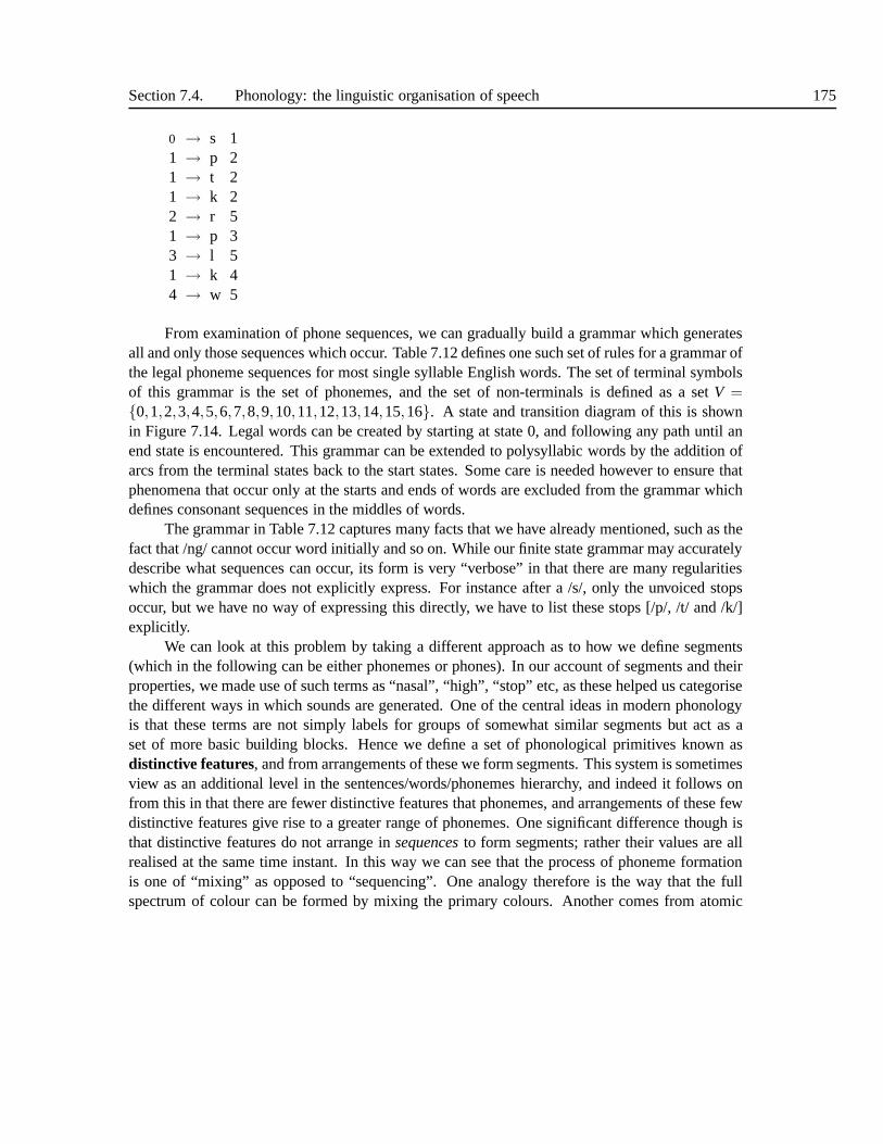
Section 7.4. Phonology: the linguistic organisation of speech 175
0 → s 11 → p 21 → t 21 → k 22 → r 51 → p 33 → l 51 → k 44 → w 5
From examination of phone sequences, we can gradually builda grammar which generatesall and only those sequences which occur. Table 7.12 defines one such set of rules for a grammar ofthe legal phoneme sequences for most single syllable English words. The set of terminal symbolsof this grammar is the set of phonemes, and the set of non-terminals is defined as a setV =0,1,2,3,4,5,6,7,8,9,10,11,12,13,14,15,16. A state and transition diagram of this is shownin Figure 7.14. Legal words can be created by starting at state 0, and following any path until anend state is encountered. This grammar can be extended to polysyllabic words by the addition ofarcs from the terminal states back to the start states. Some care is needed however to ensure thatphenomena that occur only at the starts and ends of words are excluded from the grammar whichdefines consonant sequences in the middles of words.
The grammar in Table 7.12 captures many facts that we have already mentioned, such as thefact that /ng/ cannot occur word initially and so on. While our finite state grammar may accuratelydescribe what sequences can occur, its form is very “verbose” in that there are many regularitieswhich the grammar does not explicitly express. For instanceafter a /s/, only the unvoiced stopsoccur, but we have no way of expressing this directly, we haveto list these stops [/p/, /t/ and /k/]explicitly.
We can look at this problem by taking a different approach as to how we define segments(which in the following can be either phonemes or phones). Inour account of segments and theirproperties, we made use of such terms as “nasal”, “high”, “stop” etc, as these helped us categorisethe different ways in which sounds are generated. One of the central ideas in modern phonologyis that these terms are not simply labels for groups of somewhat similar segments but act as aset of more basic building blocks. Hence we define a set of phonological primitives known asdistinctive features, and from arrangements of these we form segments. This system is sometimesview as an additional level in the sentences/words/phonemes hierarchy, and indeed it follows onfrom this in that there are fewer distinctive features that phonemes, and arrangements of these fewdistinctive features give rise to a greater range of phonemes. One significant difference though isthat distinctive features do not arrange insequencesto form segments; rather their values are allrealised at the same time instant. In this way we can see that the process of phoneme formationis one of “mixing” as opposed to “sequencing”. One analogy therefore is the way that the fullspectrum of colour can be formed by mixing the primary colours. Another comes from atomic
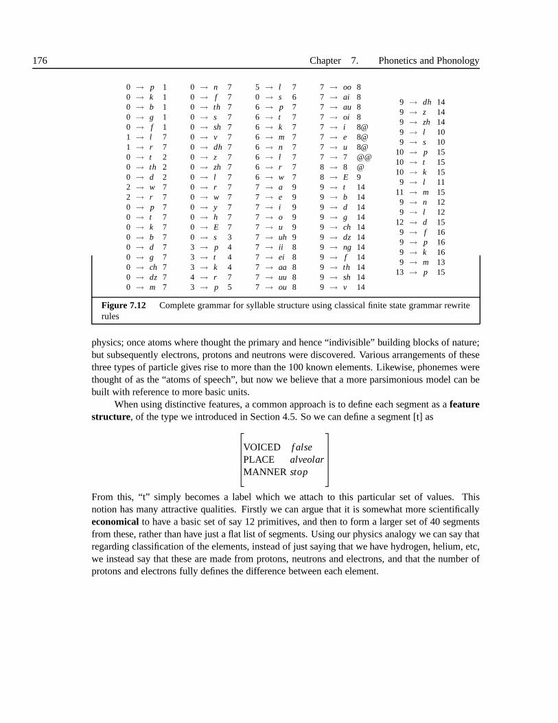
176 Chapter 7. Phonetics and Phonology
0 → p 10 → k 10 → b 10 → g 10 → f 11 → l 71 → r 70 → t 20 → th 20 → d 22 → w 72 → r 70 → p 70 → t 70 → k 70 → b 70 → d 70 → g 70 → ch 70 → dz 70 → m 7
0 → n 70 → f 70 → th 70 → s 70 → sh 70 → v 70 → dh 70 → z 70 → zh 70 → l 70 → r 70 → w 70 → y 70 → h 70 → E 70 → s 33 → p 43 → t 43 → k 44 → r 73 → p 5
5 → l 70 → s 66 → p 76 → t 76 → k 76 → m 76 → n 76 → l 76 → r 76 → w 77 → a 97 → e 97 → i 97 → o 97 → u 97 → uh 97 → ii 87 → ei 87 → aa 87 → uu 87 → ou 8
7 → oo 87 → ai 87 → au 87 → oi 87 → i 8@7 → e 8@7 → u 8@7 → 7 @@8 → 8 @8 → E 99 → t 149 → b 149 → d 149 → g 149 → ch 149 → dz 149 → ng 149 → f 149 → th 149 → sh 149 → v 14
9 → dh 149 → z 149 → zh 149 → l 109 → s 10
10 → p 1510 → t 1510 → k 159 → l 11
11 → m 159 → n 129 → l 12
12 → d 159 → f 169 → p 169 → k 169 → m 13
13 → p 15
Figure 7.12 Complete grammar for syllable structure using classical finite state grammar rewriterules
physics; once atoms where thought the primary and hence “indivisible” building blocks of nature;but subsequently electrons, protons and neutrons were discovered. Various arrangements of thesethree types of particle gives rise to more than the 100 known elements. Likewise, phonemes werethought of as the “atoms of speech”, but now we believe that a more parsimonious model can bebuilt with reference to more basic units.
When using distinctive features, a common approach is to define each segment as afeaturestructure, of the type we introduced in Section 4.5. So we can define a segment [t] as
VOICED f alsePLACE alveolarMANNER stop
From this, “t” simply becomes a label which we attach to this particular set of values. Thisnotion has many attractive qualities. Firstly we can argue that it is somewhat more scientificallyeconomicalto have a basic set of say 12 primitives, and then to form a larger set of 40 segmentsfrom these, rather than have just a flat list of segments. Using our physics analogy we can say thatregarding classification of the elements, instead of just saying that we have hydrogen, helium, etc,we instead say that these are made from protons, neutrons andelectrons, and that the number ofprotons and electrons fully defines the difference between each element.

Section 7.4. Phonology: the linguistic organisation of speech 177
0 →
VOICED f alseMANNER f ricativePLACE alveolar
1
1 →
VOICED f alseMANNER stop
2
1 →
VOICED f alseMANNER stopPLACE labial
3
2 7→
MANNER liquidPLACE alveolar
7
3 →
MANNER liquidPLACE lateral
7
0 →
VOICED f alseMANNER f ricativePLACE alveolar
4
4 →
MANNER stopVOICED f alse
7
4 →[
OUTPUT nasal
]
7
4 →[
MANNER liquid
]
7
4 →
MANNER glidePLACE labial
7
0 →
MANNER stopPLACE non−alveolar
5
0 →
MANNER f ricativeVOICED f alsePLACE labio−dental
5
5 →[
MANNER liquid
]
7
0 →
MANNER stopPLACE alveolar
6
0 →
MANNER f ricativeVOICED f alsePLACE dental
6
6 →
MANNER glidePLACE labial
7
6 →
MANNER liquidPLACE alveolar
7
0 →
TYPE consonantOUTPUT oral
7
0 →
TYPE consonantOUTPUT nasalMANNER non−velar
7
7 →
TYPE vowelLENGTH long
8
7 →
TYPE vowelLENGTH shortHEIGHT midFRONT mid
8
7 →
TYPE vowelLENGTH short
9
Figure 7.13 Partial grammar for syllable structure using feature structures and finite state grammarrewrite rules.
Using this formalism the generalisation that we can have /s/followed by /p/ /t/ /k/ but not /b//d/ /g/ can be written:
1→
VOICED f alseMANNER stop
2
the idea being thatregardless of any other feature valuesif a segment has features which matchthis definition then it is allowed by the rule. Hence this rulegenerates all unvoiced stops in thisposition. This single rule replaces three rules in the symbol grammar. Even more powerfully wecan state:

178 Chapter 7. Phonetics and Phonology
0
1
p
k
b
g
f
2t
th
d
7
k
b
d
g
ch
dz
m
n
f
th
s
sh
v
dh
z
zh
lrwyhE
p
t
3
s
6
s
l
r
w
r
9
a
e
i
o
uuh
8
ii
ei
aa
uu
ou
oo
ai
au
oi
i@
e@
u@
@@
@
4p
tk
5p
p
t
k
m
nlr
w
r
l
14
t
b
d
g
ch
dz
ng
f
th
sh
v
dh
zzh
10
l
s
11
l
12
n
l
16
f
p
k
13m
E
15
p
t
k
md
p
Figure 7.14 Diagram of finite state machine for the phonotactics of single syllable words.

Section 7.4. Phonology: the linguistic organisation of speech 179
0
1s
4s
5
non-alveolar-stopf
6alveolar-stopth
7
non-ng-consE
2unvoiced-stop
3p
unvoiced-stopnasalliquid
wliquidwr
9
short-vowel
8long-vowel
schwa
rl
14non-h-cons
11l
12
nl
16
fpk
13m
E
15
m
d
p
10
unvoiced-stop
Figure 7.15 Diagram of phonotactics using features rather than atomic phoneme symbols.
0 →
TYPE consonantMANNER non−nasal
7
0 →
TYPE consonantMANNER nasalPLACE non−velar
7
which states that a syllable may start with any consonant except /ng/, using two rules, rather thanthe 14 in the symbol grammar. In this way, we can build a finite state grammar based on featuredefinitions and in so doing arrive at a much more succinct set of rules. Table 7.13 defines a set ofrules which use feature structures rather than symbols as the terminals. A finite-state automata ofthis grammar is shown in Figure 7.15. While the rules may takea little skill to read and interpret,it should be clear that far fewer rules are needed than before. It is important to note the differencebetween the formal devices we use and the sequences they define: the use of features does notitself gives us a grammar which more accurately describes which phoneme sequences occur andwhich do not. Different types of rules, feature systems and operators do allow us to express somethings more succinctly than others, and it can be argued thata system that allows us to succinctlygenerate correct sequences with a small number of rules are morenatural.
The grammar defined in Table 7.13 is not without its problems and we shall now turn tothese. Firstly, one sequence which this grammar does not generate is /s f V/ where V is a vowel.This sequence is found in only a very few words, such asSPHEREandSPHINX. Therefore it seemsthat we have to add a rule to account for these few words. Furthermore, this rule would be theonly one to have two fricatives in the same consonant cluster. Another, somewhat more contrivedexample isVROOM, which while being an onomatopoeic word, is listed in most dictionaries asbeing a valid word of English. Again this requires its own rule, which would be the only rulewhich uses a voiced fricative in a consonant cluster. A further sequence this grammar does notallow is /y/ in a pre-vowel position, as inMULE /m y uw l/. The existing grammar is composed of

180 Chapter 7. Phonetics and Phonology
three distinct parts; a set of initial consonant sequences (all the sequences leading from state 0 tostate 7), a set of vowels (states 7 to 9) and a set of final consonant sequences (states 9 to 16). In thegrammar, each is fairly independent, so that any initial consonant sequence can be attached to anyvowel. The inclusion of /y/ in the initial consonant sequence part would destroy this simplicitybecause /y/ can only be followed by a /uw/ vowel thereby ending the separation. This phenomenais even stranger in that it accounts for one of the main accentdifferences between American andBritish English, namely that in American, the standard pronunciation ofDUKE is /d uw k/, whereasin British English it is /d y uw k/. This generalisation covers all words with this pattern (with thepossible exception ofNEWS in which many Americans say the /y/). Hence there is some importantgeneralisation going on here.
We will return to thorny problems such as these in the discussion, but the real point is thatwithin a rule and feature system, there will always be a trade-off between accounting for all thefacts, and doing so in a neat and succinct way.
7.4.2 Word formation
One of the central topics in phonology is the study of what is called word formation or lexicalphonology. Simply put, this concerns the processes by which individual morphemes combineinto whole words. To demonstrate some aspects of word formation, let us look at what the case ofplural formation in English. In spelling, the “regular” plural in English is the characters, so thatthe plural ofDOG andCAT is represented asdogs andcats. In speech however, the phonemicform differs for these words, and so we get /d ao g z/ and /k ae t s/; that is, in one case the phoneme/z/ forms the plural, while in the other it is the phoneme /s/.What explains why one form is chosenrather than another? If we look at /d ao g z/ and /k ae t s/ we see that the last phoneme before theplural suffix is voiced in one case and unvoiced in the other; this in fact turns out to be the basisof the distinction, and we see that all words which end in an unvoiced consonant take a /s/ plural,while those that end with a voiced consonant take a /z/ plural.
As before, we could express this in purely phonemic terms as:
g + PLURAL → g + zb + PLURAL → b + zv + PLURAL → v + zk + PLURAL → k + zt + PLURAL → t + zf + PLURAL → f + s
...
and so on. But as with the case of the phonotactic grammar, this entails a large number of ruleswhich are somehow missing the generalisation that this is simply a matter of voicing. If we usedistinctive features, we can succinctly write the rule as:

Section 7.4. Phonology: the linguistic organisation of speech 181
[
VOICING true
]
+ PLURAL →[
VOICING true
]
z[
VOICING f alse
]
+ PLURAL →[
VOICING f alse
]
s
In fact, we can do better than this, by making use of some further devices common in phonologicaltheory. One is the principle ofmarkednesswhich is a linguistic term for the concept ofdefault.The idea is that given a binary or other distinction, one formof behaviour is normal, unremark-able and thereforeunmarked, whereas the other form is noticeable, stands out and is thereforemarked. In our example, we could say that the unmarked plural morpheme is simple /s/, but somespecial behaviour is invoked if this is added to a word that ends in a voiced consonant. Hence wewould not need a rule for joining /s/ to many words; this wouldbe the default rule that happenswhen any morphemes are joined (i.e. no changes occur). Hencewe only need a rule for voicedcases, which would be:
[
VOICING true
]
+ s →[
VOICING true
]
z
We might well ask why it should be that /s/ is chosen as the default rather than /z/ (note that weshouldn’t be misguided by the spelling convention here) andthis is in fact a prime concern indeveloping phonological theories, namely that we choose “natural” rules rather than simply onesthat describe the date.
At this stage it is worth examining why we have chosen to describe the plural formationeffect as a phonological one rather than a phonetic one. Wouldn’t it be possible to simply saythat this is a matter of allophonic variation or coarticulation? While the rule is clearly based onarticulatory principles, it is included as part of the phonological because it is seen as a rule ofEnglishrather than a general process of speech. It is quite possibleto overrule this effect and say/d ao g s/ and /k ae t z/. More importantly however, we see that there are many non-plural Englishwords that end in /s/ which don’t undergo this rule, for example BASIS, /b ey s ax s/ andSENSE,/s eh n s/. It no more difficult or natural to sayPENSas /p eh n z/ thanPENCEas /p eh n s/. Thisdemonstrates that this plural formation rule is one of grammar and phonological organisation andnot some speech encoding effect.
English is rich with such word formation rules. For example,one common process, knownaspalatalisation, describes the process whereby consonants move from their original place ofarticulation to a palatal place of articulation, usually resulting in a [sh] phoneme. So if we takeexamples such as:

182 Chapter 7. Phonetics and Phonology
PRESS PRESSURE
CREATE CREATION
DIVIDE DIVISION
we see that in the process of formingPRESSUREfrom PRESSthe /s/ has palatalised to a /sh/,and this process has happened withCREATE andDIVIDE also. We can still observe the historicaleffects in the way the words are spelled; inpressure andcreation the original consonant ispreserved (even though the pronunciation has changed) whereas indivision the spelling haschanged to reflect the sound more accurately (but not completely accurately). Another commonprocess is that of vowel tensing in derived forms that we see in words such as:
DIVINE DIVINITY
PROFANE PROFANITY
SERENE SERENITY
Phonological rules can extend beyond purely phonemic distinctions; stress shift (explained fullybelow) also happens in pairs such as:
PHOTOGRAPH PHOTOGRAPHY
TELESCOPE TELESCOPIC
ANGEL ANGELIC
In studying word formation in this way, it becomes nearly inevitably to adopt a paradigmwhere we have a basic representation of a word or morpheme, which when combined with otherwords or morphemes interacts in some way, and then produces afinal version. So for example, wehave two wordsCAT, /k aa t/ andDOG, /d ao g/ and a plural morpheme +S/s/. We combineCAT and +S to form CATS/k ae t s/ and this is simple enough. In the case ofDOGS however, thepronunciation is /d ao g z/, and we observe that the /s/ has “changed” into a /z/. In this paradigm,we start with adeeprepresentation, and by rules, convert this into asurfacerepresentation. Some-times the difference between the two is relatively simple, as in the plural example, but in othersit is more complicated. If we consider the wordSIGN, we see that it has derived formsSIGNAL,SIGNIFY and so on. What is noteworthy here is that these derived formscontain a /g/ whereas theroot form does not. Rather than saying a /g/ is inserted, it has been argued rather that the deepform of SIGN is really /s ay g n/ (or even /s ih g n/) and that by process of rule, this is convertedto surface form /s ay n/. Thus the rules can operate even when there is no word formation perse. Such solutions have always attracted controversy in phonology. Firstly, it can be argued thatthe statement of such rules is heavily influenced by the orthography, and as often the exact natureof orthography derives from some whim of a printer, it is a poor basis on which to form rules.Secondly, once such processes are allowed there seems no limit to what devices can be employed.
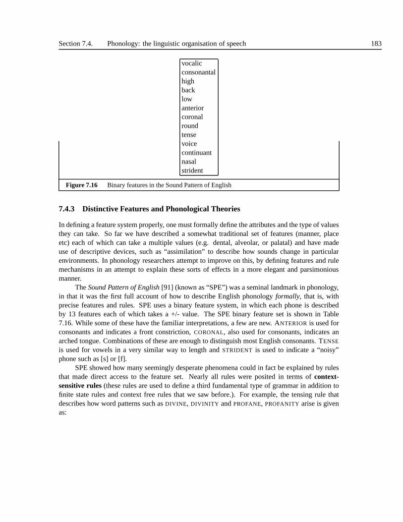
Section 7.4. Phonology: the linguistic organisation of speech 183
vocalicconsonantalhighbacklowanteriorcoronalroundtensevoicecontinuantnasalstrident
Figure 7.16 Binary features in the Sound Pattern of English
7.4.3 Distinctive Features and Phonological Theories
In defining a feature system properly, one must formally define the attributes and the type of valuesthey can take. So far we have described a somewhat traditional set of features (manner, placeetc) each of which can take a multiple values (e.g. dental, alveolar, or palatal) and have madeuse of descriptive devices, such as “assimilation” to describe how sounds change in particularenvironments. In phonology researchers attempt to improveon this, by defining features and rulemechanisms in an attempt to explain these sorts of effects ina more elegant and parsimoniousmanner.
TheSound Pattern of English[91] (known as “SPE”) was a seminal landmark in phonology,in that it was the first full account of how to describe Englishphonologyformally, that is, withprecise features and rules. SPE uses a binary feature system, in which each phone is describedby 13 features each of which takes a +/- value. The SPE binary feature set is shown in Table7.16. While some of these have the familiar interpretations, a few are new. ANTERIOR is used forconsonants and indicates a front constriction,CORONAL, also used for consonants, indicates anarched tongue. Combinations of these are enough to distinguish most English consonants. TENSE
is used for vowels in a very similar way to length andSTRIDENT is used to indicate a “noisy”phone such as [s] or [f].
SPE showed how many seemingly desperate phenomena could in fact be explained by rulesthat made direct access to the feature set. Nearly all rules were posited in terms ofcontext-sensitive rules(these rules are used to define a third fundamental type of grammar in addition tofinite state rules and context free rules that we saw before.). For example, the tensing rule thatdescribes how word patterns such asDIVINE , DIVINITY andPROFANE, PROFANITY arise is givenas:

184 Chapter 7. Phonetics and Phonology
V → [−tense] / CVCV
meaning that the vowelV in question, becomes lax (the opposite of tense) when it occurs beforeaCVCV sequence (such as the /n ih t iy/ ofPROFANITY). Even for different feature sets, modelsand theories, rules of this type are very common. It is worth noting however that the use ofcontext-sensitive rules here is merely a notational convenience; most phonological rules do notuse recursion, and so the above can readily be implemented with finite state rules, if required forpractical purposes.
Despite its success in many regards, several problems immediately appeared with SPE. Oneof the main problems is that if there are 13 binary features, this should give rise to 213 = 8192possible phones. Not only is this considerably greater thanmost phonologists would agree exist,it is clear that many combinations (e.g.[+tense, +anterior, +high]) simply don’t correspond toany known or even theoretically possible phone. For this andmany other reasons, a huge flurryof activity started with the aim of defining more succinct andmore “natural” systems of features,and accompanying rules.
In the 1970s, two theories broke from the mold of SPE by proposing that sound patternscould better be understood if more elaborate rule and representation mechanisms were used.Au-tosegmental phonology[180] uses two (or more)tiers, in which we have a phoneme tier (roughlysimilar to SPE) and a tonal tier. The idea is that rules can be written to operate on just one tier orthe other, which is much simpler that would be the case if the phonemes and tones had to be repre-sented on a single tier. The other theory is that ofMetrical Phonology [284] which was designedto explain phonological phenomena of stress and intonation(described below). Together, thesetheories and some that follower were often callednon-linear phonology (this is a different useof the term “non-linear” to that in mathematics), because their representations were not sequencesof segments as in traditional phonetics, phonology and SPE.Since then a bewildering variety ofother theories and models have been produced. Among these areNatural Phonology [137] whichargued against the sometimes very abstract positions takenin theories such as SPE (for instancethe example we gave where the underlying representation ofSIGN would require a [g] segment).
Despite the large number of different theories, some trendshave stood out in how phonologyhas developed. One strand of work has attempted to move away from the context-sensitive ruleformalisms described above. Mainly this follows a general move in this direction in other fields oflinguistics such as syntax, and is motivated by a desire to avoid the complications of determiningwhat these rules really stand for cognitively. For instance, it is often difficult to believe that aspeaker or hearer has to apply a whole sequence of rules in just the right order to generate thesurface form of a word. Instead, a series of constraints are proposed, from which new words canbe formed. Theories of this school includeDependency Phonology[145], [144], andGovern-ment Phonology[248]. Many theories use feature systems more elaborate than those expressiblenaturally in feature structures. The idea here being that features form hierarchies, and in doing so,we can use these hierarchies to naturally limit the number offeature combinations and rules, thus
Section 7.4. Phonology: the linguistic organisation of speech 185
avoiding the “segment explosion” problem of SPE. The theories ofArticulatory Phonology [70]andFeature Geometry[100], [306], [386] are based on this idea.
In addition to the issues discussed in this chapter, it should be understood that the field ofphonology tackles many issues which aren’t directly relevant to speech synthesis needs, such assay finding the set of language universals.Optimality Theory is one such model which hasgained particular attention in recent years [362]. In addition to this, the emphasis on phonol-ogy even within directly relevant topics is often somewhat different from what we require froman engineering perspective. In particular the old issue of “economy” comes up again and again,with phonologists striving for every more natural and economical representations, without usuallymuch interest in assessing the processing requirements incurred. The general trends in phonol-ogy are clear though; a move away from finite state, linear models towards more complex featureorganisations, a move from ordered context-sensitive rules to systems which use constraints anddependencies, and a move from procedural systems to declarative systems. Somewhat ironically,while most phonologists trace their work back to SPE, the “formal” side of this approach haslargely been forgotten, and few works in phonology since have anywhere near the level of ex-plicitness and comprehensiveness of that work. A notable exception comes from the work ofComputational Phonology[43].
7.4.4 Syllables
One of the most important aspects of phonology concerns the structural representation of soundpatterns above the phoneme. We have already seen that morpheme boundaries are significant (e.g.in the difference between the realisation ofPENSandPENCE) as are word boundaries. In additionto these, we find it is very useful to make use of a third unit, thesyllable as this also helps explainmany of the effects and patterns in speech.
As we have already seen, the syllable provides a solid basis for defining the phonotacticgrammars of what constitutes a legal word. If we define a grammar for a syllable, it is an easymatter to define a grammar for any words by simply including more syllables and any possiblyspecial sequences for word beginnings and ends. That said, it is interesting to ask real evidencedo we have for syllables as real entities. We seem to instinctively know that SET, FROM andBATH have one syllable; thatTABLE, WATER andMACHINE have two, andOPERATE, COMPUTER
andORGANISE have three. These judgments seem intuitive and are not dependent on any expertknowledge. Secondly, if we consider singing we see that in normal singing each note is sung withone syllable. If this principle is broken the singing can sound awkward if syllables are inappropri-ately squeezed in or elongated over several notes. Thirdly,syllables seem to act as the basic unitof many aspects of prosody. Syllables carry stress such thatin THE PROJECTthe first syllable ofPROJECTis stressed, but inPROJECT THAT LIGHTthe second gets the stress. There are no otherpossibilities - it is not possible to stress the /p r/ and not the vowel, or any other individual phone.
So what exactly is a syllable? We will take the view that the syllable is aunit of organisation.As such, all words are composed of a whole number of syllables, and all syllables are composed

186 Chapter 7. Phonetics and Phonology
of a whole number of phonemes. For an initial working definition, we will state that a syllableis avowel surrounded by consonants. This definition seems to fits the facts fairly well - in allthe above cases the numbers of vowels and numbers of syllables were the same, and again fromsinging we can see that the vowel seems to be the “centre” of the note. There is one commonlyraised exception to this, namely the existence of so calledsyllabic consonants. Some phoneticiansgive two syllable words such asBOTTLE andBUTTON the transcriptions /b aa t l/ and /b ah t n/, inwhich the second syllable is comprised only of /l/ and /n/ sounds. Conventions differ as whether toallow this, or use the alternative, which gives these words the transcriptions /b aa t ax l/ and /b aht ax n/. There is probably no real way to decide from a phoneticpoint of view, but practical TTSexperience has shown no deficiencies in using /ax/ and as thismakes the definition of the syllablesimpler, we shall use that and not use syllabic consonants.
So, taking the vowel as the centre of the syllable, all we haveto do is decide which conso-nants belong to which syllables. In words such asHOTEL, we can safely say that the /h/ belongsto the first syllable and the /l/ to the last, but what about the/t/? There are a number of positionsto take on this. One position is the so-calledmaximal onset principle where consonants thatpotentially could be in the onset or coda of a syllable are taken as being in the onset. Using thesymbol /./ to denote a syllable boundary,HOTEL is then represented as /h ow . t eh l/.
This will provide a satisfactory account for many words, andit can be argued that this hassome cognitive reality because, again from singing, we find that consonants tend to follow thispattern. There are a number of problems however. Firstly, innon-word-initial syllables whichhave /s t r/ and other such sequences,INSTRUCT, /ih n s t r ah k t/ it can be argued that the /s/attaches to the first syllable and not the second. Secondly, consider such words as BOOKEND, /buh k eh n d/ - here it definitely seems that the /k/ attaches to the first syllable - in fact a syllablefinal /k/ and an syllable initial one sound quite different and so /b uh k . eh n d/ sounds differentfrom /b uh . k eh n d/. There is an obvious reason to this, namelythat BOOKEND is a wordformed by compoundingBOOK and END, and it seems that the word/morpheme boundary hasbeen preserved as a syllable boundary.
One of the main reasons we are interested in syllables is thatpattern of syllables withina word, and the pattern of phonemes within a syllable helps determine much of the phonemicvariation due to allophones and coarticulation. Hence it isoften useful to assign a basic constituentstructure to describe the structure of phonemes internal toa syllable. We will explain one way ofdoing this, in which four basic constituents are used, called theonset, rhyme, nucleusandcoda.The syllable structure for the single syllable wordSTRENGTH in these terms is:
Onset
s t r
Rhyme
Nucleus
eh
Coda
ng th
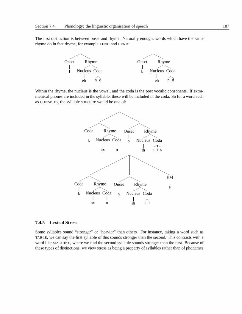
Section 7.4. Phonology: the linguistic organisation of speech 187
The first distinction is between onset and rhyme. Naturally enough, words which have the samerhyme do in fact rhyme, for exampleLEND andBEND:
Onset
l
Rhyme
Nucleus
eh
Coda
n d
Onset
b
Rhyme
Nucleus
eh
Coda
n d
Within the rhyme, the nucleus is the vowel, and the coda is thepost vocalic consonants. If extra-metrical phones are included in the syllable, these will be included in the coda. So for a word suchasCONSISTS, the syllable structure would be one of:
Coda
k
Rhyme
Nucleus
ax
Coda
n
Onset
s
Rhyme
Nucleus
ih
Coda
s t s
Coda
k
Rhyme
Nucleus
ax
Coda
n
Onset
s
Rhyme
Nucleus
ih
Coda
s t
EM
s
7.4.5 Lexical Stress
Some syllables sound “stronger” or “heavier” than others. For instance, taking a word such asTABLE, we can say the first syllable of this sounds stronger than thesecond. This contrasts with aword like MACHINE, where we find the second syllable sounds stronger than the first. Because ofthese types of distinctions, we view stress as being a property of syllables rather than of phonemes

188 Chapter 7. Phonetics and Phonology
or words, and hence we always talk about the stress of a syllable, rather than the stress of a wordor phoneme.
It is important to note that the term stress is used in a numberof different ways in the linguis-tics literature. The most fundamental distinction is between lexical stressandsentential stress.Lexical stress is a core property of a word, and as such doesn’t change. In our previous exam-ple, TABLE is stressed on the first syllable whileMACHINE is stressed on the second; and theseare properties of the words themselves. Sentential stress on the other hand describes the effectwhereby one syllable in the sentence receives more stress than the others; and this is normally dueto some pragmatic or communication reason, and is not a fundamental property of the word itself(e.g. I SAID I WANTED THAT ONE. We shall ignore this second type of stress for now as this isdealt with in detail in Chapter 8.
As usual, there are many different theories and models of lexical stress. Here we will adopta relatively simple model which describes the stress patterns without necessarily tackling the issueof how these patterns arise in the first place. In this model, each multi-syllable word has exactlyoneprimary stressed syllable. Using the IPA symbolhto indicate primary stress, we can writeTABLE and MACHINE as /’t ey b . ax l/ and /m ax .’sh iy n/. It is also common practicetouse numbers to indicate stress, so that we have /t ey 1 b . ax l/ and /m ax . sh iy 1 n/, whereagain by convention, the number immediately follows the vowel. We can indicate stress in longerwords such asINFORMATION in the same way as /ih n . f ax . m ey1 . sh ax n/. What of theother syllables? It appears that the first syllable ofINFORMATION is stronger than the second andfourth, but less strong than the third, so we call thissecondary stress. Some linguists go furtherand have tertiary stress and so on, but primary and secondarystress patterns are usually taken assufficient. Secondary stress is denoted by the IPA symboli, or alternatively by a 2 following thevowel.
We can identify a third category calledreduced. This is mainly used to indicate the stresslevel of syllables containing the schwa vowel. Reduced vowels occur in at least three subtlydifferent cases. First, some words naturally, or always, have a schwa in a certain position, forexample in the first syllable ofMACHINE / m ax sh iy n/. But consider the second syllable ofINFORMATION. We have given this a schwa in our annotation and most speakers would agree withthis pronunciation. Now consider the wordINFORM, /ih n f ao r m/, here the second syllable isa normal full vowel. We can say thatINFORMATION is created fromINFORM by the applicationof morphological rules, and in the process, the second syllable has beenreducedfrom a full vowelto a schwa. A third form of reduction occurs in function words, when for instance a word suchasFROM, / f r ah m/ is produced as /f r ax m/ in many instances. Finally, when people speakquickly, they often under-articulate vowels, which leads to a loss of distinction in their identityleaving them sounding like a schwa. This effect is also termed reduction. The number 0 is used torepresent a reduced vowel, so the full transcription forINFORMATION is /ih2 f ax0 r m ey2 sh ax0n/
In English, stress is a fundamental part of the pronunciation of a word, and as such weak-ens our the notion we have been adopting until now that a word’s pronunciation can be repre-

Section 7.4. Phonology: the linguistic organisation of speech 189
sented only by its phonemes. There are main related noun/verb pairs in English which are dis-tinguished by stress, such that we haveRECORD NOUN, / r eh1 k ax0 r d/ contrasting withRECORD VERB, / r ax0 k ao1 r d/ ; and likewisePROJECTNOUN /p r aa 1 j eh2 k t/ contrast-ing with PROJECTVERB, / p r ax0 j eh1 k t/. That said, there are very few genuine minimalpairs in English. Some have gone to considerable lengths to argue that stress can in fact be derivedfrom just the phonemes (this is advocated in SPE). Valiant though these attempts are, there aresimply too many words with unpredictable stress patterns for us to be able to derived stress fromphonemes for all words.
Stress can be graphically represented in the sort of tree used to describe syllable constituentstructure. In our previous example the nodes at the syllablelevel were unlabelled; we can nowshow the same tree but with stress labels at the nodes:
2
Rhyme
Nucleus
ih
Coda
n
0
Onset
f
Rhyme
Nucleus
ax
Coda
r
1
Onset
m
Rhyme
Nucleus
ey
0
Onset
sh
Rhyme
Nucleus
ax
Coda
n
An alternative to the use of absolute levels of stress such asprimary and secondary, is thetheory ofmetrical stress [284], [286] in which stress is purely relative. In this, a binary tree isused to represent each word, and within this, each syllable is defined as eitherstrong or weak. SoINFORMATION would be defined as:
W
S
in
W
for
S
S
ma
W
tion
The strongest syllable is the one which only hasSnodes above it; everything else is defined relativeto this.
If lexical stress is a relative phenomenon, what of single syllable words? As there are noother syllables to contrast with, the stress status of such words is technically undefinable. However,
190 Chapter 7. Phonetics and Phonology
by convention, most of these words are given a primary stressor strong stress in their syllable. Theexception is content words, which are given a primary stressif in their full form (/f r ah m/) or nostress in their reduced form (/f r ax m/).
In order for us to perceive stress differences, stress patterns must of course manifest them-selves in the acoustic signal. How is this achieved? Firstly, taking a contrast between “normal”syllables and their stressed version, we can say that in the case of stress, the syllable is spokenwith greater articulation effort, that is, the articulators are more likely to move to their canonicalpositions, and in so doing, produce a syllable with many of the idealised sounds which we wouldexpect from our discussion of articulatory phonetics. As a by product of this, we can see the thatthe syllable seems more “distinct” in the spectrogram; the formants of the vowel are clearly ob-servable, and it is often easier to ascertain the identity ofthe vowel from the formants of stressedsyllables than for unstressed ones. Likewise with the consonants, stops often have more distinctclosure and burst patterns in stressed syllables and so on. Following from the great articulationeffort, stressed syllables are general longer in time than normal versions. The source acts differ-ently in stressed syllables also. The voice quality is likely to be more clearly periodic (not creakyor breathy). Also, the pitch of the syllable is likely to be higher in a stressed syllables than in thesyllables immediately surrounding it. This effect is difficult to determine in isolation however, asthe intonational patterns of the utterance interact strongly here (described in more detail in Section9.1.
By contrast, in reduced syllables, the opposite effects seem to occur. The articulation effortis diminished to the extent that any distinctiveness in the vowel quality is absent - all vowels areeither /ax/ or /ih/. Consonants in reduced syllables tend tobe less clear. The duration of reducedsyllables can be very short indeed, even to the extent of being non-detectable in faster or morecasual speech. Finally, it is unlikely that the pitch in an unstressed syllable with be higher thanits surrounding syllables (note however, that the presenceof a reduced syllable does not cause adecrease in pitch).
7.5 DISCUSSION
The study of phonetics has a long and rich history [97]. Just as the world’s most famous detec-tive is the fictional Sherlock Holmes, so indeed is the world’s most famous phonetician. Today theHenry Higgins of Pygmalion and My Fair Lady would probably appall any self-respecting linguistor phonetician with his dogmatic and prescriptive view of how English should be spoken. Nev-ertheless, Higgins probably does share some genuine features in common with the early Britishschool of phonetics.
The study of modern phonology is widely regarded to have started with the “Prague School”of linguists, of which the main figures were Nikolay Trubetzkoy and Roman Jakobson. Theyestablished the principle of the formal (or scientific) study of phonology and the notion of thephoneme. Most importantly, they showed the semiotic basis of phonological contrast with the

Section 7.5. Discussion 191
idea being that the linguistic use of sounds could only be studied as within a system and not inindividual, purely phonetically terms. Jakobson collaborated with two other notable figures inspeech and linguistics, Morris Halle and Gunnar Fant to produce a coherent system of distinctivefeatures. As already mentioned, theSound Patter of Englishwas a seminal work, both in its scopeand its affect in proposing formal methods for phonologicalwork.
7.5.1 Further reading
The most popular work in introductory phonetics is undoubtedly Peter Ladefoged’s classicacourse in phonetics[271], and is highly recommended. Another excellent book, which extendsthe subject and gives more detail on acoustic issues is Clarkand Yallop [97]. A more advancedand comprehensive book is Laver’sPrinciples of Phonetics[275].
There are many excellent introductory text books on phonology including Giegerich [174],Katamba [245], Lass [274] and Anderson [17]. Clark and Yallop [97] is again particularly recom-mended as it gives a thorough introduction to phonology, does so with reference and comparisonto phonetics, and discusses the issues involved from the type of traditional scientific perspectivefamiliar to most engineers and scientists. Unfortunately,nearly all these works are quite introduc-tory and few venture beyond SPE type phonology. While there are plenty of books and articleswhich cover more recent work, they typically focus on one particular theory or model, making ithard to perform the type of comparison that would be necessary for us to adopt any one of thesefor speech technology purposes. Books and articles on the various schools of phonology are listedabove.
7.5.2 Summary
Phonetics
• Speech sounds can be described with reference to either their articulatory or acoustic fea-tures.
• Vowel sounds are described with the primary dimensions of high/low and front/back, andsecondary dimensions of rounding and length.
• Consonants are described in terms of voicing, manner and place of articulation. The mainvalues manner can take are stop, fricative, nasal, affricate and approximant.
• Computer analysis can be used to study the acoustic patternsin speech. The primary repre-sentation is that of the spectrogram.
• The resonances of the vocal tract are called formants, and these are thought to be the primarymeans by which listeners differentiate between different vowel sounds.
Communication with speech
• A phoneme is a linguistic unit of speech defined on the semiotic principle of contrast.

192 Chapter 7. Phonetics and Phonology
• We communicate via speech by using the speech apparatus to encode words as strings ofphonemes, which are then fed through the speech production apparatus.
• In traditional phonetics, phones are seen as concrete objective units, while phonemes arecontrastive linguistic units. Phonemes are realised as phones and if a phoneme has morethan one phone the set of phones are called allophones.
• Even for a single allophone, there is a large amount of variability. This is mostly a conse-quence of coarticulation effects from the continuous movement of the articulators.
• In the modern view, there are no objective phones; these are just descriptively useful pointsin a continuous space.
• There are no boundaries or markers in continuous speech; it is not possible to bottom updetermine the phoneme or phone boundaries in speech.
• We can described the linguistic content of speech using sequences of phonemes or phones;this is known as transcription. Transcription is inherently difficult because we are enforcinga discritisation of a continuous encoding.
Phonology
• Phonology is the study of the linguistic use of speech
• A phonotactic grammar describes which sequences of phonemes are legal for a language
• Lexical phonology describes how words are formed from constituent morphemes
• Phonemes and phones can be described with distinctive features. More compact and “nat-ural” rules can be created by making use of distinctive features rather that phonemes orphones.
• The syllable is a useful organisational unit which sits between the words and phonemes.All words have an integer number one of syllables, each of which has an integer number ofphonemes.
• Lexical stress is manifested at the syllable level. Exactlyone syllable in a word is desig-nated as the primary stressed syllable, all other syllableshave either secondary stress or arereduced.
8 PRONUNCIATION
We now turn to the problem of how to convert the discrete, linguistic, word based representationgenerated by the text analysis system into into a continuousacoustic waveform. One of the pri-mary difficulties in this task stems from the fact that the tworepresentations are so different innature. The linguistic description is discrete, the same for each speaker for a given accent, com-pact and minimal. By contrast, the acoustic waveform is continuous, is massively redundant, andvaries considerably even between utterances with the same pronunciation from the same speaker.To help with the complexity of this transformation, we breakthe problem down into a number ofcomponents. The first of these components,pronunciation, is the subject of this chapter. Whilespecifics vary, this can be thought of as a system which takes the word-based linguistic represen-tation and generates a phonemic or phonetic description of what is to be spoken by the subsequentwaveform synthesis component. In generating this representation, we make use of alexicon tofind the pronunciation of words we know and can store, and agrapheme-to-phoneme(G2Palgo-rithm to guess the pronunciation of words we don’t know or can’t store. After doing this we mayfind that simply concatenating the pronunciations for the words in the lexicon may not be enough;words interact in a number of ways and so a certain amount ofpost-lexical processingis required.Finally, there is considerable choice in terms of how exactly we should specify the pronunciationsfor words, and hence rigorously defining a pronunciation representation is in itself a key topic.
8.1 PRONUNCIATION REPRESENTATIONS
In this section we shall define just what exactly the pronunciation component should do, what itsinput should be and what its output should be.
8.1.1 Why bother?
First of all, we should ask ourselves - why bother at all with apronunciation component? Whynot just synthesise directly from the words? To answer this,consider an approach where we don’thave any pronunciation component per se, but attempt synthesis directly from the words. In doingso, let us imagine a concatenative synthesiser in which we have a database of recorded samples for
193

194 Chapter 8. Pronunciation
each word. If we take even a modest size vocabulary, we might have more than 50,000 words, andso this would require 50,000 basic types in our synthesiser.It is not possible for the most part tosuccessfully join words directly; the nature of continuousspeech means that the effect of one wordinfluences its neighbours and this must be dealt with in some way. There are two possible solutionsto this; either we could adopt an “isolated word” style of synthesiser, where we record each wordin isolation and then join the words with a short pause, or we could record one example of eachword in the context of each other word. The first approach is taken by many simple concatenatedprompt systems, and while quite reliable, will never perform well in terms of naturalness. Theproblem with the second approach is that for our vocabulary of 50,000, recording each word inthe left and right context of each other word would mean 50,0003 = 1.25× 10¹⁴ types in all.Recording this number of words from a single speaker is clearly impossible, but even if some wayof reducing this was found, it is clear that the number of required recordings could still be vast.Even if we avoid a concatenative type of approach, we would still have to build a model for everyword in the database, and this would still be an enormous undertaking.
This is clearly a problem ofdata sparsityin that we can’t collect or design models for sucha large number of types. When we consider that the required vocabulary for a real system mayin fact be even larger, and that unknown words will have to be handled somehow, we see that inreality the situation may be even worse.
8.1.2 Phonemic and phonetic input
Now consider an approach where we transform each word into its phonemes and use those as theinput to the synthesiser. In doing so, we have drastically reduced the number of base types from50,000 words to the 40 or so phonemes. We still have to deal with continuous speech influence,but if we assume that the scope of this is limited to the immediately neighbouring phonemes, thenwe will need a left and right context for each type, and this will give us a total of 403 = 64,000types which is clearly more manageable. The total number is however still quite large, so it isnatural to ask if we can reduce this further. The source of thelarge number is of course havingto take the left and right context into account, rather than the number of phonemes themselves.Hence it is reasonable to ask whether we can transform the phonemic representation further into aspace which has a further reduction in the number of base types.
We can do this by attempting to predict the effect of the context of a phoneme’s neighbours.As we saw in Chapter 7, the traditional model of phonetics states that phonemes are be realisedas phones and that in general this realisation process is controlled by context. For example, an /l/has two allophones, described asclear anddark , where the clear phone is found at the start of asyllable and the dark one at the end; a /t/ is aspirated at the start of a word, but unaspirated whenfollowing an /s/ in a consonant cluster. So if we could apply this process to every phoneme, wecould generate a sequence of phones for the input, and in doing so free the base types from manyof the effects of context. With a phoneme representation, wemight have a type /s-t-r/, representinga /t/ in the context of being after an /s/ and before an /r/. With a phonetic representation we replace
Section 8.1. Pronunciation representations 195
this with just [t] (the IPA symbol for an unaspirated [t]), using [th] for cases where aspiratingexists. Context will still play a part, because coarticulation (as opposed to allophonic variation)still operates, but the degree of contextual effect will be lessened. As many phonemes have morethan one allophone, the number of base types may well increase (to say 60), but because we cando without a left and right context for each, then the overallnumber will be considerably lower.
8.1.3 Difficulties in deriving phonetic input
There is however a drawback with this approach. The problem with phone representations wasdiscussed previously in Section 7.3.2 where we stated that although phone descriptions could bevery useful in certain circumstances, they should be treated with caution as they are a discreterepresentation enforced on a continuous space; and as such only crudely reflect the actual pro-cesses going on. To give an example, let us consider again an example of place of articulationassimilation that occurs with words such as
TEN+ BOYS→ t e n + b o i z→ t e m b o i z
where the alveolar place of articulation of the /n/ of the first word assimilates to the bilabial placeof articulation of the /b/ of the second word (bilabial). There is no doubt that that somethingis going on here; the [n] certainly seems somewhat differentfrom a “normal” [n], and this canbe verified from both acoustic and articulatory measurements. This is not the issue; rather, it iswhether the [n] hasturned intoan [m]. Such a statement says that there are only two choices;an[n] or an [m] and in certain situations the [n] keeps its identity and in others it changes. Considerthe situation of sayingTEN BOYS with a pause between the two words; it should be clear thatthe [n] sounds like a “normal” [n] and that if we said the (madeup word)TEM (/t e m/) asTEM
BOYS with a short pause, we can tell the difference between the two. Now if we say a sequenceof utterancesTEN BOYS starting with a long pause and gradually shortening it, until there is nopause, we see that there is agradual shift in the nature of the /n/, until, when we talk quickly, itseems impossible to make the distinction betweenTEN andTEM. This shows that assimilation iscertainly taking place, but that it is not the case that an underlying [n] is at one point realised bythe phone [n] but at a certain points suddenly becomes a different phone [m]. The process is acontinuous one of change, and it is quite inappropriate to model it as a discretely. We see exactlythe same effects with /r/ colouring, nasalisations and reduction.
In a way, we are forcing a discrete level of representation onto a range of effects that havea substantial continuous component; and this is damaging inall sorts of ways. As an example,consider again the phenomena of reduction; whereby we haveAND represented underlyingly as [an d], but where this undergoes reduction, resulting in a range of possible phonetic forms including[a n], [n d], [n], [n] and so on. It may be clear that some level of reduction has occurred, but atwhat stage do we delete the [d]? Where do we draw the boundary between a full [a] and it beingreduced to a schwa? Studies of hand human labelling have shown that even trained phoneticians

196 Chapter 8. Pronunciation
often give different labels to the same utterance, and much of this disagreement stems from wherethe draw the boundaries as to whether something is reduced ordeleted.
8.1.4 A Structured approach to pronunciation
In essence, our situation is this. If we stick with high-level representations such as words, we canhave a high degree of confidence about the accuracy of these, but the number of base types is fartoo large. As we generate representations nearer the signal, we see that the number of base typesreduces considerably, but at a cost, in that we are more likely to create a representation that isinaccurate in some way. There is no single solution to this problem: the answer lies in picking apoint where the compromise between number of types and accuracy of representation best suits aparticular system’s needs.
Perhaps unsurprisingly, the consensus as to where this point should be has shifted over theyears. When more traditional systems were developed, memory was very tight and hence the num-ber of base types had to be kept low regardless of any errors. In more recent years technologicaldevelopments have eased the pressure on memory making more abstract representations possible.Given this, there is more choice over where exactly the idealrepresentation should lie. In fact,as we shall see in Chapter 16, the most successful systems adopt a quite phonemic representationand avoid any rewriting to a phonetic space if at all possible. Because of this, the pronunciationcomponent in modern systems is in fact much simpler than was perhaps the case in older systems,and quite often the input to the synthesiser is simply canonical forms themselves, direct from thelexicon.
Hence the solution we advocate for a state of the art unit selection synthesiser can be de-scribed as astructured phonemic representation, where we use the phonemic information moreor less as it is specified in the lexicon, but do so in such a way that the synthesiser also has directaccess to the context, syllable structure and stress information that governs the allophonic andcoarticulation processes. In doing so we are relying on the subsequent synthesis component tomodel the allophonic and coarticulation effectsimplicitly. This can be achieved very effectivelyby representing pronunciation as a phonological tree of thetype introduced in Sections. 7.4.4 and7.4.5, as this allows us to describe the phonemes, syllablesand stress information in a single rep-resentation. In such a scheme, the wordsSTRENGTH, TOP, LAST andHAND would for examplebe represented as follows:
Onset
s t r
Rhyme
Nucleus
eh
Coda
ng th
Onset
h
Rhyme
Nucleus
a
Coda
n d

Section 8.1. Pronunciation representations 197
Onset
t
Rhyme
Nucleus
aw
Coda
p
Onset
l
Rhyme
Nucleus
a
Coda
s t
From these trees, we can access the information we require; the phonemic context can beread directly by accessing a phoneme’s neighbours; the syllable structure is presented as a tree,and from this we can distinguish between /s t/ in a syllable onset in STRENGTH, and offset inLAST.
8.1.5 Abstract phonological representations
We have just seen that despite potential issues with data sparsity, in general, higher level phonemicrepresentations are preferred over lower level phonetic ones. In pursuing this approach however,we should ask ourselves whether the phonemic representations we have been using are in factoptimal; might there not be an even more abstract, and less linear representation that would helpthe dimensionality problem? Progress in modern phonology has in fact moved away from usinglinear sequences of phonemes or phoneme like units as the “deep” or canonical representation;freed from the constraint that representations must be linear, the more structured “non-linear”representations reviewed in Section 7.4.3 could be considered instead.
Ogden et al [334] discusses just this issue and point outs that the problem with specifyingphonemic style representations is that this concentrates overly on the paradigmatic dimension; thephonemic system is based on what contrasts occur at a particular point, and the issue of whatphonemes follow what other phonemes is left to a different, phonotactic part of the phonology. Infact, we see that it is indeed possible to construct representations in which both the normal notionof phonemic contrast, and a mechanism for governing legal sequences are handled in a unifiedway. While phonemic representations are less susceptible to borderline decisions than phoneticrepresentations, they are not entirely free of problems.
At present, we know of no unit selection techniques which make use of such abstract phono-logical representations, but this possibility is sure to beexplored eventually. While there is everychance the field will indeed move in this direction, because of the lack of practical proof we willcontinue with phonemic representations for the remainder of the book. We should point out thatphonemic representations do have one significant advantageover virtually any other type of pho-netic or phonological representation in that they are generally easy for people to work with. Overlyphonetic representations can be difficult in that it takes time and effort to fill in the phonetic detail;overly abstract representations require a significant knowledge and understanding of the partic-ular theory which underlies them. With a little training, most people get the hang of phonemictranscription and are able to read and generate transcriptions. This is important for text-to-speech

198 Chapter 8. Pronunciation
because at some stage, someone must of course actually enterall the lexicon entries by hand. Indoing so, we wish to have a system which is both quick (there might be hundreds of thousandsof entries) and accurate, and the phonemic system seems to fulfill these criteria reasonably well.That said, we should make the point that it is perfectly possible toenter the pronunciation for aword in the lexicon in terms of phonemes, and then by ruleconvertthis to either a deeper or moresuperficial representation.
Finally, using a linear phonemic representation has the benefit that it makes automatic databaselabelling considerably easier. In Chapter 17 we shall consider the issue of labelling a speechdatabase with phoneme units, both by hand and by computer. Aswe shall see, it is easier to per-form this labelling if we assume a linear pronunciation model, as this works well with automatictechniques such as hidden Markov models.
8.2 FORMULATING A PHONOLOGICAL REPRESENTATION SYSTEM
Having in principle chosen a system which uses phonemes and syllable structure, we now turn tothe issue of how to actually define this for a given speaker, accent or language. It is essential thatthis is done with care; if we decide say to use a single phoneme/ch/ instead if /t/+/sh/, we have toconsistently use this, such that we representCHURCH as /ch u r ch/ and not /t sh u r ch/ or /ch u r tsh/ and so on.
The following sections explain how a phonological system isdeveloped. The first thing thatwe must decide is which accent we are dealing with from the language in question. In general itis not possible to define a phoneme inventory which can cover multiple accents, so whatever willwe develop will be particular to that accent. One solution isto this is to use the actual speaker theTTS system will be based on, and from analysis of his or her phonemic contrasts ensure that thecorrect pronunciation system is found. This solution can require too much effort, so more generalaccents often have to be defined. In this chapter, we will conduct an exercise on developinga representation for just two accents of English, namely General American and British Englishreceived pronunciation (RP). The principles involved however are the same for most other accentsand languages.
It does seem somewhat wasteful that separate pronunciationsystems and therefore lexiconsare required for British English and American English; while differences of course exist, pronun-ciations in the two accents aren’tcompletelydifferent. Fitt [161], [162], [163] proposed a solutionto this where a more abstract pronunciation drawn from a large set of phonemes was used as abase lexicon. From this, filters could be used to generate accents for any accent of English.
8.2.1 Simple consonants and vowels
Here we will adopt the standard approach of using the principles ofminimal pairs andphoneticsimilarity to develop a phoneme inventory (see Section 7.3.2). This is not an exact procedure and

Section 8.2. Formulating a phonological representation system 199
it is possible to come up with two equally valid phoneme inventories for a given accent. Thereis therefore some discretion in determining a phoneme inventory; the key point is not to find“absolute truth” of what constitutes the set of sound contrasts; but rather to define an inventorythat suits our purposes, and thenstandardiseon this; so that exactly the same conventions are usedin all parts of the system. Experience has shown that “drift”in phoneme conventions, whereby saywe transcribeBOTTLE as /b aa t el/ in one place and as /b aa t ax l/ in another can have adisastrouseffect as the data, rules, synthesiser and lexicon can become misaligned. The crucial point is tochose a standard as best we can and stick to just that standardeverywhere in the system.
Recall that the principle of minimal pairs states that it is not the similarity or dissimilarity oftwo sounds per se which is the issue, but rather whether they distinguish two separate words. Byusing this test, it is straightforward to determine a set of contrasts in a particular position. So if wetake the form [X i p], we can find a set of contrasts as follows:
p PIP m MIP l LIP
t TIP n NIP r RIP
k KIP s SIP w WHIP
b BIP sh SHIP y YIP
d DIP z ZIP h HIP
The /X i p/ pattern doesn’t give the full list of possible contrast because not every possible legalphoneme sequence actually ends up as a real existent word. But if we take some further patterns,we can elicit further contrasts:
X /X eh t/ X /X ih n/ X /X ay n/p PET sh SHIN v VINE
b BET f FIN dh THINE
d DEBT th THIN f FINE
g GET s SIN s SIGN
m MET sh SHINE
n NET
When we consider one particular pattern, the analysis seemsclear: PET and BET are differentwords, so /p/ and /b/ must be different phonemes. It is reasonable to ask though, how we knowthat the sound at the start ofPET is the same sound as at the start of sayPIT? There is no knowndeterministic or objective way to prove that this is the case, all we can do is rely on judgment andstate that in terms ofarticulation, the two sounds are both produced with the lips, are unvoicedare stops and so on, and that if we examine themacousticallywe see they are similar. But theyare rarely so similar to be taken as identical; their articulation and acoustic patterns are affectedby the following vowel and this does have some effect. To a certain extent, there is a leap of faithrequired to say thatPET andPIT start with the same phoneme. This problem is even more acutewhen we consider sound contrasts in different positions:

200 Chapter 8. Pronunciation
p RIP m RIM n RAN
t WRIT n RING m RAM
b RIB f RIFF n RANG
d RID s REECE b BRIT
g RIG d WRITHE t STRING
So while we have no problem is saying that the last sounds inRIP, WRITE andRIB are differentphonemes, it is a harder matter to say that the last sound ofRIP should be the same phoneme asthe first of PIT. We can again only appeal to some notion of acoustic and articulatory similar-ity. We should bear in mind though that we are attempting a compromise between an accuraterepresentation and a minimal one, and that different possibilities can be tried and tested.
If we consider the wordsSPAN, STAN andSCAN, we see that we have a three way contrast,in which the second sound differs in terms of place of articulation. There is however no voicingcontrast possible at these points, so there are only three possible phonemes, unlike in word initialposition where we have three place of articulation contrasts in addition to a voicing contrast, givingus six phonemes in all. The question then is, shouldSPAN be transcribed as /s p ae n/ or /s b ae n/?The phonetic evidence tends to favour /p/, but this is not conclusive, and will vary from speakerto speaker and accent to accent. Clearly though there is a systematic effect going on. There isprobably no objective answer to this, so we obey the normal convention (which may have beeninfluenced by the spelling) and represent these words with the unvoiced phonemes /p/, /t/ and /k/.
A similar minimal pair test can be used for vowels, in which pairs (or n-tuples) of words canbe compared and phoneme identities determined. In the following:
iy HEAT uw HOOT
ih HIT ah HUT
eh HET ae HAT
ao HAUGHT aa HOT
we can clearly identify a number of distinct vowel phonemes.
8.2.2 Difficult consonants
Now we turn to some more problematic cases. In English, the consonants /dh/, /zh/, /ng/ and /h/are a little more difficult to deal with. There are clearly exactly four unvoiced fricatives; /th/, /f/,/s/ and /sh/ in English and of these, /f/ and /s/ have the voiced equivalents /v/ and /z/, and these areunproblematic. The voiced equivalent of /th/ is /dh/ and while /th/ is a common enough phoneme,/dh/ only occurs in very particular patterns. For a start, the number of minimal pairs that occurbetween /dh/ and /th/ are few; real examples includeTEETH NOUN, / t iy th/ andTEETH VERB, /tiy dh/, while most are “near” minimal pairs such asBATH /b ae th/ andBATHE / b ey dh/ wherethe quality of the vowel differs. Even if we except /dh/ as a phoneme on this basis, it occurs instrange lexicon patterns. In an analysis of one dictionary,it occurred in only about 100 words outof a total of 25,000. But if we taketokencount into consideration, we find in fact that it is one ofthe most common phonemes of all; in that it occurs in some of the most common function words

Section 8.2. Formulating a phonological representation system 201
such asTHE, THEIR, THEM, THEN, THERE, THESE, THEY andTHIS. When we take the remainderof the words in which /dh/ is found we see that it is found in many “old” or traditional soundingEnglish words such asFATHOM, HEATHEN, HITHER, LATHE, LITHE, LOATHE, NETHER, SCATHE,SCYTHE, SEETHE, SHEATHE and TETHER. In fact, it only occurs in a relatively few “normal”English words such asMOTHER, LEATHER and HEATHER. Clearly /dh/ is a phoneme, and forpurposes of defining our phoneme inventory, it gets a place along with the other fricatives. Thereare consequences that arise from its use though, in that because of the dominance of its used infunction words, it is difficult to obtain “typical” characteristics of the phoneme (say in terms of itsaverage duration) that are not swamped by the fact that it is used as a function word (which areoften very short, regardless of what phonemes make them up).
Now consider /zh/, the voiced equivalent of /sh/. This occurs in words such asBEIGE /b eyzh/. Again, while there are few direct minimal pairs, some exist (BEIGE vs BAIT or BANE) andso we classify /zh/ as a phoneme. Problems again arise from patterns of use. It has been argued(e.g. [97]) that /zh/ is a relative newcomer to the English language as in the past, words such asTREASURE and MEASURE were pronounced /t r eh z y uh r/ and /m e z y uh r/ and that it isrelatively recently that these have been spoken as/ t r eh zh er/ and /m eh zh er/. /zh/ presents thesame problems that arose with /dh/, but in this case they are even more difficult because of the veryfew words naturally occurring with /zh/. These problems with /zh/ and /dh/ can lead to problemsin database collection and analysis (see Section 14.1).
The sounds [ng] and [h] are noteworthy because they are severely restricted as to the posi-tions they can occur in. Primarily, /h/ can not occur at the end of a syllable or a word, and /ng/can not occur at the beginning of a syllable or word. There arefurther issues with /ng/ in that asit only occurs in a post-vocalic position, it suffers from the loss of contrast that affects all nasalsin this position. So while it is clear thatSIN, / s ih n/,SIM, /s ih m/ andSING, /s ih ng/ all end indifferent sounds, it is less clear what the correct representation for words likeTHINK should be.In words such as this the last stop is in a velar position, and the nasal takes on a velar quality also(this is similar to theTEN BOYS effect we discussed earlier). The issue is then whether we shoulduse a velar nasal /ng/ or a dental nasal /n/; there is no contrast possible in this position and so it isa question of convention which we should pick. As with other such issues, the main goal is to aimfor consistency; if /ng/ is used here then it should be used inall other post-vocalic pre-velar stoppositions.
8.2.3 Diphthongs and affricates
So far we have concentrated on the paradigmatic dimension, by contrasting (say)HAT, HEAT andHOT and showing that in a frame of /h X t/ we can distinguish a number of phonemes. We were ableto do this because a word such asHOT, clearly divides into three segments. We assign provisionalphonemic status to each, swap in other sounds and thereby determine the system of phonemiccontrasts. In many words however, it is not so easy to segmentthe word into distinct parts, andin such words we face a question of not only what the contrastsare, but how many positions are

202 Chapter 8. Pronunciation
there to have contrasts within.In words such asCHAT, the sound before the vowel can be represented as either a combina-
tion of /t/ and /sh/ or as a distinct single phoneme /ch/. A similar case arises with words such asJUICE which can be represented as a combination of /d/ and /zh/ or asa distinct single phoneme/dz/. The argument for using two phonemes stems from the principal of keeping the numbers ofphonemes as low as possible; the argument for a single phoneme arises from the idea that theseact as a single coherent unit and are more than the sum of the two parts. There is no real way tosettle this argument, so we will somewhat arbitrarily decide to use single phonemes /ch/ and /dz/.
A similar situation arises with the diphthong vowels in words such asBOY, TOE, TIE andBAY . In each of these, the vowel does not hold a single steady state position, either acousticallyor in terms of articulation. Rather, sayTIE has an /ae/ sound followed by an /iy/ sound. We facethe same situation that we did with affricates in that we could use a more minimal paradigmaticrepresentation by saying two phonemes exist here, or inventnew single phonemes to reflect thefact that these sounds seem to act as single coherent units. Again, there is no real objective wayto decide, so we will follow our previous example and use a single symbol for each. One benefitfrom this is that, as well shall see below, this allows us to state a rule that every syllable is formedwith exactly one vowel.
8.2.4 Approximant-vowel combinations
The approximants /r/, /w/, /j/ and /l/ in many ways operate like normal consonants, so that wehave contrasts in words such asROT, WATT, YACHT andLOT. Of these /l/ is probably the moststraightforward and the main point to note is that the acoustic patterns of dark /l/ in words such asPULL, andSMALL is very different from that with clear /l/, such asLOOK andLAMP. This does notpose much of a problem phonemically, but is an important different to bear in mind when tryingto decide whether two /l/ units will join well together.
The glides /w/ and /y/ are interesting in the ways they interact with vowels. Firstly, there isconsiderable phonetic similarity between /w/ and /u/ and /y/ and /i/, and in many phonetic analyses,words such asSHOW are transcribed as /sh o w/. If we follow our diphthong principle above, werule out these cases and transcribe this as /sh ow/. The process of /w/ or /y/ following a vowel issometimes called anoff-glide. As mentioned in Section 7.4.1, one of the difficulties in determininga phonotactic grammar for English is that /y/ often acts as what we can call anon-glide. So inBritish English, speakers sayTUNE as /t y uw n/ andDUKE as /d y uw k/. There is evidence thatthe /y/ should be attached to the vowel however, just like a diphthong, to give /t yuw n/ and /d yuwk/. Further evidence for this comes from other English accents; in the US, most speakers say /t uwn/ for TUNE and /d uw k/ forDUKE. The effect is systematic, and would seem easier to explain ifonly one factor (the realisation of a phoneme /yuu/) was changing between accents. Despite thisargument, it is most common to regardVIEW as being composed of three segments, and we shalladopt this convention and say it is represented as /v y uw/.
Finally, we consider /r/. This is perhaps the strangest and most interesting sound in human

Section 8.2. Formulating a phonological representation system 203
speech. Setting aside the phonemic question, consider for amoment how this differs phoneticallyacross languages. In English, an alveolar approximant /r/ ([G] in IPA) is most common and it isquite common for this to have a retroflex (curling of the tongue) quality as well. In contemporaryScottish English, a tapped alveolar (D) is quite common, and is separate again from the “classical”Scottish trill [r] (now usually only seen on stage or in film).In French and many accents of Germana uvular [J] sound is the norm, with other accents of German having a morealveolar quality. InSpanish, words such asPERROare formed with a trilled [r], and this forms a minimal pair with thetapped [D] of words such asPERO. It seems incredible given all this variety, that somehow all thesesounds are grouped together across languages and represented in writing as anr. Do they evenhave anything in common? While we will not go into cross language issues here, it is worth notingthat words are quite commonly shared across languages, for example the wordsEMAIL , APRIL andMETRE. In the case ofMETRE, we see that it contains anr in all languages and is pronounced in awide variety of ways. If we study the acoustics however, we see that these different “types” of /r/do share somewhat more in common in that they have characteristic energy bands at certain partsof the spectrum.
When we consider the phonemics of /r/, we find that it has an interesting effect. First wedistinguish betweenrhotic accents which have /r/ in post-vocalic position (in English, these areScottish, Irish, General American) andnon-rhotic accents which have no realised /r/ (most Eng-land English, Australian and some New York accents). For example, in Irish English, there is no“long a” sound [aa], which is found in RPBATH /b aa th/; this word is pronounced /b a th/. How-ever, in words which have an /a/ and a /r/ following it, the /a gets lengthened, andphoneticallywe have something like [h aa r d]. Being a phonetic realisation effect, this doesn’t concern usunduly, but it does show how significant (and unexpected to the unwary) the presence of an /r/ canbe. More significant are the non-rhotic accents. In these, itis not the case that the /r/ is simplynot present; rather (historically or by having some deep presence) it has the affect of altering thequality of the vowels before it. So in a word likeHER, which might be represented as /h uh r/ ina rhotic accent, we do not get /h uh/ but rather /h @@/ which hasan extended vowel. It is almostas if the /r/ has turned into a /@/ and is still present. Because of this, we are faced with a choicebetween transcribing non-rhoticFIRE as /f ai @/ or invent a new symbol /ai@/ which would beregarded as a triphthong.
8.2.5 Defining the full inventory
From the above we should have sufficient knowledge to construct a phoneme inventory for anyaccent or language we are interested in. In practice we find that we don’t always have to designa phoneme inventory from scratch; for many languages or accents the existence of a significantcomputer speech research community means that phoneme inventories already exist. As thesecommunities often develop and distribute resources using these phoneme inventories, it can behighly beneficial to adopt one of these rather that start fromscratch. In the past, databases ofspeech which contained hand labelled phone or phoneme transcriptions were highly valued, but

204 Chapter 8. Pronunciation
as phonetic/phonemic transcription can now be done automatically, today by far the most usefulresource is in fact a comprehensive lexicon. As the development of a large (> 100,000 word)lexicon can take years of work, any existing resources greatly help. Lexicons are in general tiedto a specific accent of the language, and as such come with a phoneme inventory pre-defined.
So in many cases a phoneme inventory may exist for the accent we are interested in. By andlarge, most phoneme inventories developed for computational work roughly follow the guidelinesjust described. As just pointed out, there are however several ways to resolve some of the issues,and so it is worth examining any predefined phoneme inventories in light of the above discussionto assess suitability. Most predefined phoneme inventorieshave not been developed with TTS inmind, rather they were developed for purposes of speech recognition or are just “general” phonemeinventories developed for a variety of uses. Experience hasshown that minor modifications inpredefined phoneme inventories can sometimes be beneficial for TTS purposes. The most commonproblem is that sometimes the phoneme inventory has some “phonetic” features (such as markersfor aspirated or unaspirated, or a different label for the stop closure than the stop release), but thesecan normally be removed with some automatic processing.
Table 8.1 gives a definition of a complete phoneme inventory based on a modification ofthe TIMIT phoneme inventory. This was originally designed for use with the acoustic-phoneticdatabase of the same name and now one of the most well known phoneme inventories for GeneralAmerican [173]. Most of the modifications we have made have been to eliminate some of thepurely phonetic distinctions in the original TIMIT inventory1. The main peculiarity of the TIMITinventory relates to the fact that sequences of schwa followed by /r/ are represented by a singlephoneme /axr/, and the vowel in words such asBIRD is treated similarly and represented as /b erd/. All other combinations of vowel and /r/ are treated as twoseparate phonemes. Table 8.2 givesa phoneme inventory for the British English RP accent, basedon the University of Edinburgh’sMRPA (machine readable phonetic alphabet) system [276]. The consonant system is more orless the same; this is what we would expect from the facts of English accent variation. Thevowel system is different, and in particular the treatment of “r” is different because RP is a non-rhotic accent. The pseudo-diphthong vowels /i@/, /u@/ and /e@/ are used in cases where there
1 For the record, the differences between this and the standard phone inventory are:
1. The /axr/ unstressed schwa+/r/ phoneme has been replacedby /er/. /er/ and the old /axr/ are now distinguishedby stress alone
2. the close phones bcl, tcl etc have been removed
3. the nasal tap /nx/ has been merged with the /n/ nasal
4. /hv/ has been merged with /hh/
5. the glottal stop phone /q/ has been removed
6. the syllabic consonants /en/, /em/, /eng/ and /el/ have been replaced by /ax/ + consonant sequences, e.g. /en/→/ax n/
7. /ix/ has been replaced by either /ax/ or /ih/, /ux/ by /uw/ and /ax-h/ by /ax/
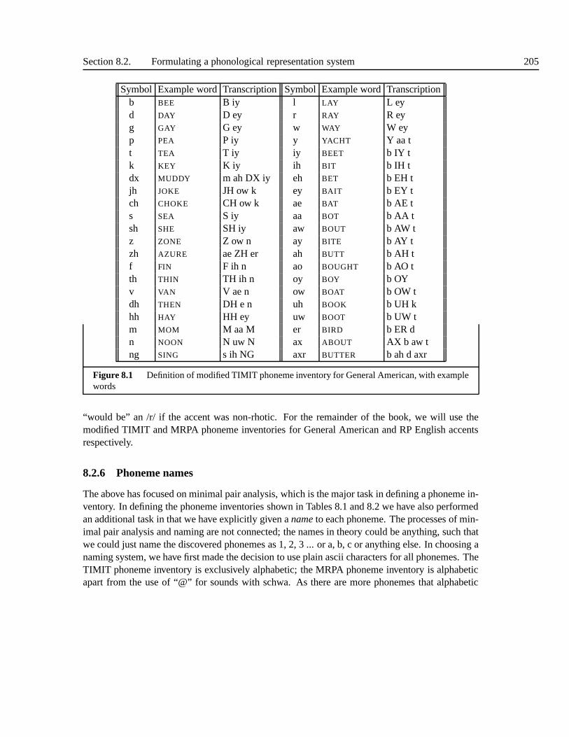
Section 8.2. Formulating a phonological representation system 205
Symbol Example wordTranscription Symbol Example wordTranscriptionb BEE B iy l LAY L eyd DAY D ey r RAY R eyg GAY G ey w WAY W eyp PEA P iy y YACHT Y aa tt TEA T iy iy BEET b IY tk KEY K iy ih BIT b IH tdx MUDDY m ah DX iy eh BET b EH tjh JOKE JH ow k ey BAIT b EY tch CHOKE CH ow k ae BAT b AE ts SEA S iy aa BOT b AA tsh SHE SH iy aw BOUT b AW tz ZONE Z ow n ay BITE b AY tzh AZURE ae ZH er ah BUTT b AH tf FIN F ih n ao BOUGHT b AO tth THIN TH ih n oy BOY b OYv VAN V ae n ow BOAT b OW tdh THEN DH e n uh BOOK b UH khh HAY HH ey uw BOOT b UW tm MOM M aa M er BIRD b ER dn NOON N uw N ax ABOUT AX b aw tng SING s ih NG axr BUTTER b ah d axr
Figure 8.1 Definition of modified TIMIT phoneme inventory for General American, with examplewords
“would be” an /r/ if the accent was non-rhotic. For the remainder of the book, we will use themodified TIMIT and MRPA phoneme inventories for General American and RP English accentsrespectively.
8.2.6 Phoneme names
The above has focused on minimal pair analysis, which is the major task in defining a phoneme in-ventory. In defining the phoneme inventories shown in Tables8.1 and 8.2 we have also performedan additional task in that we have explicitly given anameto each phoneme. The processes of min-imal pair analysis and naming are not connected; the names intheory could be anything, such thatwe could just name the discovered phonemes as 1, 2, 3 ... or a, b, c or anything else. In choosing anaming system, we have first made the decision to use plain ascii characters for all phonemes. TheTIMIT phoneme inventory is exclusively alphabetic; the MRPA phoneme inventory is alphabeticapart from the use of “@” for sounds with schwa. As there are more phonemes that alphabetic

206 Chapter 8. Pronunciation
Symbol Word initial exampleWord final example Symbol Word initial exampleWord final examplep PIP RIP j YIP -t TIP WRIT ii HEAT PEEL
k KIP KICK ih HIT PILL
b BIP RIB ei HATE PATE
d DIP RID e HET PET
g GAP RIG aa HEART PART
ch CHIP RICH a HAT PAT
dz GYP RIDGE uu HOOT POOT
m MIP RIM u FULL PUT
n NIP RUN ou MOAT BOAT
ng * RING uh HUT PUTT
f FOP RIFF oo HAUGHT CAUGHT
th THOUGHT KITH o HOT POT
s SIP REECE ai HEIGHT BITE
sh SHIP WISH au LOUT BOUT
v VOTE SIV oi NOISE BOIL
dh THOUGH WRITHE i@ HEAR PIER
z ZIP FIZZ e@ HAIR PEAR
zh VISION u@ SURE PURE
h HIP - @@ HER PURR
l LIP PULL @ CHINA ABOUT
r RIP CAR w WIP -
Figure 8.2 Definition of British English MRPA phoneme inventory, with example words
characters, we use two and sometimes three characters for a single phoneme. Often this is whenwe have a sound with two phonetic components such as /ch/ or /oy/, but this is also used for simplephonemes such as /th/ and /sh/.
In naming these phoneme inventories we have also not worriedwhether the “same” phonemein one accent has the same name in another accent. As we have noneed to mix phonemic tran-scriptions across accents in normal synthesis, this is unproblematic (see however Section 17).Strictly speaking, the principles of phonemic analysis imply that this is a meaningless comparisonanyway: phonemes only have status as units of contrast for a single accent, and so it is of no con-sequence whether we use the same symbol for the vowel inBUY in British or American English.In practice, it is clear from the TIMIT and MRPA definitions that the vowel sets are different butthe consonant sets are nearly identical (this of course partly reflects the fact that vowel contrastsare the main source of phonemic differences between accentsin English). We have also avoidedthe possibility of naming the phonemes after one of their allophones in the IPA alphabet. This isbecause it is generally easier to use a separate and self contained symbol set for phonemes and not

Section 8.2. Formulating a phonological representation system 207
use IPA symbols as this can lead to confusions about the phoneme/phone divide.In both the TIMIT and MRPA phoneme inventories, we have only used lower case letters. To
some extent this is a purely aesthetic issue as we wish to avoid upper case (which has a somewhat“aggressive” quality) and mixed case (which can look ugly).There is an additional benefit in thatupper case equivalents of the symbols can be used in cases where some emphasis is required, suchas stress or other highlighting. In the above, we have chosenthough to give simple mnemonicnames to each phoneme, so that the first phoneme ofTIP is named “t”, the first ofSHIP is named“sh” and so on. Mnemonic names are usually helpful as we oftenhave to enter words in the lexiconourselves or perform transcriptions, and this is easier if we can easily recall the symbols to use.These names can sometimes trip us up, especially with vowels, so a little care should be taken.
8.2.7 Syllabic issues
We have shown previously that in addition to simple or “linear” phonemic context, a major factorin determining the realisation of phonemes is their place inthe syllabic structure. Phonemes atthe starts of syllables or words can be realised differentlyfrom ones at the ends; the position ofa phoneme in a consonant cluster is important, and stress effects, which are expressed at sylla-ble level, also have an important bearing on phonetic realisation. We therefore have to give thewaveform generation component access to this syllabic information.
If we actually know where the syllable boundaries lie withina word, it is a simply matterto assign the type of tree structures described in Section 7.4.4. Quite simply, the vowel servesas the nucleus, the consonants after the nucleus up until theend of the syllable are assigned tothe coda, and the consonants between the vowel and the syllable start are assigned to the onset.In this way, the syllable structure is found deterministically from the syllable boundaries andphonemes. As we saw in Section 7.4.4, syllable boundaries can in the most part be determinedby using the maximal onset principle. In the few cases where this is not so (recall ourBOOKEND
example) the boundary needs to be marked explicitly. As system designers we therefore facesome choices. On the one hand, we can choose to explicitly mark every syllable boundary in thelexicon. This is costly however; many existing lexicons do not have syllable boundaries markedand the additional effort in marking these may be prohibitive. Alternatively we could determinethe syllable boundaries automatically by application of the syllable onset rule. In doing so wewill of course get the syllable boundaries wrong for the difficult cases just mentioned. A thirdpossibility is a compromise between the two, where the difficult transcribed are marked by hand,and where the rest are transcribed by algorithm.
For languages such as English, three levels of stress are necessary. While some phonologicalsystems use more (e.g. SPE), our experience has shown that, at the lexical level at least, three isclearly sufficient. Following from a convention adopted forTIMIT, we use1 for primary stressedsyllables,2 for secondary stressed syllables and0 for reduced syllables. The stress numbers areplaced adjacent and after the vowel, so, for example, the entry for INFORMATION would be /ih2 n. f ax0 . m ey1 . sh ax0 n/.

208 Chapter 8. Pronunciation
All syllables receive a stress mark, and hence most vowels will be marked 2. All wordsexcept function words must have a single primary stressed vowel. All normal schwa vowels (/ax/)receive a 0. There are a number of possibilities regarding whether to transcribe normal vowelswith a 0 or a 2. One option is to regard 0 and 2 as weak and strong versions of one another,such that any vowel could receive either 0 or 2. Another option is to regard 0 as being only forschwa vowels; this means that in effect every other vowel is a2 regardless. This last option hasthe benefit of simplicity, but some feel that this disregardsphonetic facts. In traditional phonetics,the last vowel ofHAPPY is quite often transcribed as /ih 0/ or /iy 0/. In addition, many think that itis most appropriate to transcribe the last vowel ofHABIT as /ih 0 / giving /h ae1 b ih0 t/. Here weagain face the issue of phonological organisation versus phonetic explicitness. Either option canbe taken, but it is worth noting that direct experience showed that it was possible to take the 0 forschwa option everywhere, and label all other vowels as 2. This would then given /h a1 p iy2/ and/h a b ax0 t/.
Finally, we come to the issue of phonotactics. This is an important part of defining a phonol-ogy; there is little point in spending time defining a phonemeinventory which define the paradig-matic relations if we then ignore the phonotactics which define the syntagmatic relations. Defininga phonotactic grammar is necessary for a number of practicalreasons. Firstly, we need to definewhat we think the synthesiser should be able to say in terms ofphoneme sequences. Even if wecreate a very simple grammar, that states for instance that /ng/ can’t occur at the start of a word,we can find any case where this is passed to the synthesiser by mistake and take corrective action.Secondly, we need to keep a check of the entries in the lexicon; as these entries are made by handthere is a chance that errors will be made. Hand in hand with the phonotactic grammar comes a setof conventions that we must establish regarding how words should be transcribed. Finally, havingan explicit phonotactic grammar helps in database collection as we can easily tell how complete aparticular database is with regard to phonemic sequence coverage.
8.3 THE LEXICON
In our introduction to the nature of language, we explained that one of its fundamental properties isthat there is an arbitrary relation between the meaning and form of a word. A word’s pronunciationcannot be inferred from its meaning, nor vice versa. Obviously for a language to work, thesearbitrary relations need to be somehow stored, and the device used to do this is call alexicon.We can talk about aspeaker’s lexicon, meaning the lexicon that a particular individual uses tostore his or her words; we can also talk about thelanguage lexiconwhich is a store of all themeaning/form pairs (words) in that language (a traditionaldictionary is this type of lexicon). Forlanguage engineering purposes however, we talk about thecomputer lexicon, which is a physicalcomputer data object containing known descriptions of words.
In machine understanding and generation systems, or any systems which deal with seman-tics and meaning, the lexicon is a vital component in a systemas it is here that the connection
Section 8.3. The Lexicon 209
between meaning and spoken or written form is stored. In speech synthesis and recognition taskshowever, the meaning element is largely ignored, so in principle the lexicon is not strictly speakinga necessarycomponent. However, lexicons are in fact widely used in synthesis and recognitionto store the correspondences between the two main forms of the word; that is the spelling andpronunciation of a word. As such these are calledorthography-pronunciation lexicons.
8.3.1 Lexicon and Rules
While the relation between the meaning and form of all languages is completely arbitrary, ingeneral the relation between the two main forms, i.e. the spoken and written form, is not. The twomain forms do not have an equal status; speech is the primary form of the language and writing isa secondary, invented form designed to record the spoken form. The degree to which these formsare related is dependent on many factors, and it is clear thatin some languages the written formclosely follows the spoken form (e.g Spanish), in others therelationship is discernible but complex(e.g. English and French) while in others it is nearly as arbitrary as the meaning/form relationship(e.g. Chinese). Hence for native words in some languages it is possible to infer one form from theother, and this mapping can be performed by agrapheme-to-phonemealgorithm. We will leavea discussion of these until Section 8.4, but for now let us assume that we can build such a systemthat always generates a pronunciation form from an orthographic form, even if the accuracy ofdoing this can be quite low for some languages. Due to this lowaccuracy of these rules for somelanguages we have to store the correspondences in a lexicon.It is important to realised that evenfor the more direct languages, the widespread use of Englishloan-words, technical words andacronyms means that at least some use of a lexicon is required.
Most text-to-speech systems use a combination of a lexicon and rules to perform pronun-ciation. The justification for this two pronged strategy haschanged somewhat over the years.In traditional systems, the explanation usually went something like this: “grapheme-to-phonemerules are used as the main pronunciation mechanisms, but in addition we use anexceptions dic-tionary which deals with cases which don’t follow the normal patterns of the language”. Thusit was rules which were primary, and the lexicon was used for cases where the rules failed. Thereasons for the primacy of the rule system were that, firstly,this was still in the days when using“knowledge” was a respectable way of building all types of speech, language and AI systems, andso using rules was a natural way that anyone would approach this problem. Secondly, memoryspace was limited, such that storing tens of thousands of words was prohibitive. Note that usingrules to save memory typical incurs a processing cost, but atthe time speed was not generally seenas a critical issue (ie, it was simply impossible to have enough memory to store the words, but itwas possible to use slow rules, even if it resulted in a non-real time system). Finally, it takes timeto develop a quality lexicon, and in the past there simply weren’t the resources and experience tohave built a comprehensive lexicon. More common today is thejustification “We use a lexicon tostore pronunciations, and resort to rules for missing entries in the lexicon.” Hence the situation isreversed; the lexicon is seen as primary and the rules are there as backup when the lexicon fails.
210 Chapter 8. Pronunciation
The reader should be aware that there is still a lingering hangover in the literature from theearlier period regarding the rules vs lexicon issue. Rules are often inherently favoured over thelexicon and one often comes across statements stating that there is not enough memory to storeall the words in a language. Such reasoning is rarely solid, as no decision can be taken about thisuntil the actual size of the lexicon and the processing cost of the rules are quantified. For smallerfootprints systems (say< 10 megabytes), lexicon size will definitely be an issue, but for largersystems the size of the unit selection database will far out weigh the size of the lexicon. One alsofinds that alongside this we also see justifications that rules are a more sophisticated approach andthat simply storing words in the lexicon is a dumb brute forceapproach. As we shall see below,this is a false argument; rules and lexicons are simply different techniques which trade-off memoryand processing cost; both have their place and one is not a priori better, more sophisticated or evenmore accurate than the other. One occasionally encounters the opposite view, in which lexiconsare seen as the only true way to handle pronunciation, and hence the use of very large lexicons isadvocated. This can be dangerous too; while most people are aware that rules often make mistakesthere is sometimes a failure to realise that significant errors can exist within the lexicon also; toooften this possibility is ignored and the lexicon is taken asthe absolute truth.
Most accounts of the lexicon and rule setup in a TTS system would give a reader the ideathat these were two completely separate mechanisms, which just happen to have been brought tobear on the same problem. In fact, the distinction between lexicon and rule approaches is not asclear cut as it seems, and in moderns TTS systems, it is best tothink of what we normally thinkof as “lexicons” and “rules” as being at certain points on a scale. From the outside, the distinctionseems clear; a lexicon is a declarative data structure (e.g.a list) which contains entries, a rule setis a series of processes which examine the grapheme sequenceand generate a phoneme sequence.The distinction is however not always clear cut. Most rule systems (see below) use a contextwindow on the orthography to help disambiguate which phoneme should be generated. If we takea word such asIRAQ for instance, it is quite possible that no other words with anything like thisgrapheme pattern will be found; so if the rules correctly predict this word, can we not say that therules have learned the pronunciation for this and only this word, and that the rules have in factimplicitly stored the pronunciation?
In machine learning, this phenomenon is calledmemorising the data: this is often consid-ered harmful if the system learns exactly those examples it was given but not any generalities; ifthis is the case we say that the model hasover fitted the data. For a trainable model with enoughparameters, it is entirely possible that it will end up memorising all the training data rather thanlearn the generalisations behind it. This is normally seen as an undesirable property in a rule sys-tem, but in our case, it can be argued that this is not strictlyso. In most machine learning problems,thepopulationof data is effectively infinite, and the training data is a small sampleof the popula-tion. As the sample is not identical to the population care must be taken not to learn it too exactly,otherwise the trained algorithm will not perform well when presented with different samples fromthe population. As we shall see below, learning grapheme-to-phoneme rules is somewhat differ-ent, in that the population (all existent words) is large butfinite, and there is a good chance of
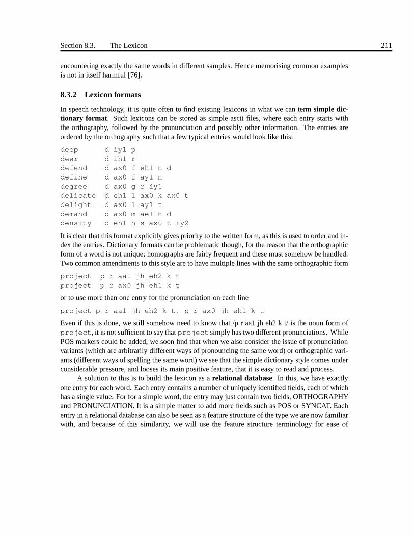
Section 8.3. The Lexicon 211
encountering exactly the same words in different samples. Hence memorising common examplesis not in itself harmful [76].
8.3.2 Lexicon formats
In speech technology, it is quite often to find existing lexicons in what we can termsimple dic-tionary format . Such lexicons can be stored as simple ascii files, where eachentry starts withthe orthography, followed by the pronunciation and possibly other information. The entries areordered by the orthography such that a few typical entries would look like this:
deep d iy1 pdeer d ih1 rdefend d ax0 f eh1 n ddefine d ax0 f ay1 ndegree d ax0 g r iy1delicate d eh1 l ax0 k ax0 tdelight d ax0 l ay1 tdemand d ax0 m ae1 n ddensity d eh1 n s ax0 t iy2
It is clear that this format explicitly gives priority to thewritten form, as this is used to order and in-dex the entries. Dictionary formats can be problematic though, for the reason that the orthographicform of a word is not unique; homographs are fairly frequent and these must somehow be handled.Two common amendments to this style are to have multiple lines with the same orthographic form
project p r aa1 jh eh2 k tproject p r ax0 jh eh1 k t
or to use more than one entry for the pronunciation on each line
project p r aa1 jh eh2 k t, p r ax0 jh eh1 k t
Even if this is done, we still somehow need to know that /p r aa1jh eh2 k t/ is the noun form ofproject, it is not sufficient to say thatproject simply has two different pronunciations. WhilePOS markers could be added, we soon find that when we also consider the issue of pronunciationvariants (which are arbitrarily different ways of pronouncing the same word) or orthographic vari-ants (different ways of spelling the same word) we see that the simple dictionary style comes underconsiderable pressure, and looses its main positive feature, that it is easy to read and process.
A solution to this is to build the lexicon as arelational database. In this, we have exactlyone entry for each word. Each entry contains a number of uniquely identified fields, each of whichhas a single value. For for a simple word, the entry may just contain two fields, ORTHOGRAPHYand PRONUNCIATION. It is a simple matter to add more fields such as POS or SYNCAT. Eachentry in a relational database can also be seen as a feature structure of the type we are now familiarwith, and because of this similarity, we will use the featurestructure terminology for ease of
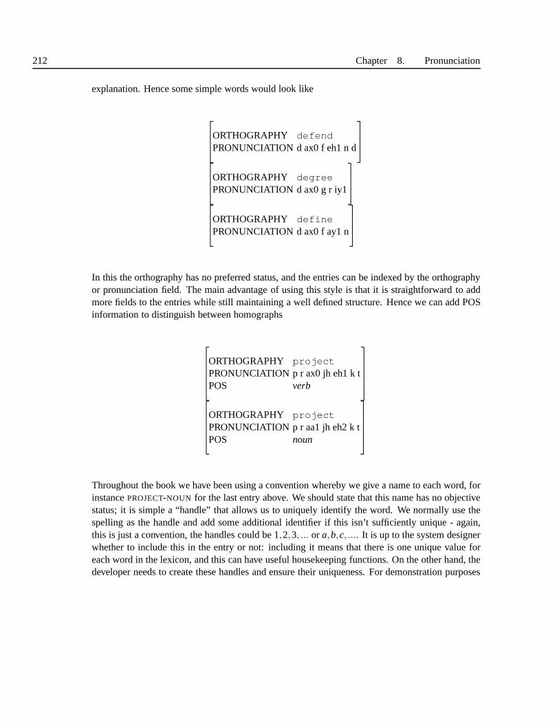
212 Chapter 8. Pronunciation
explanation. Hence some simple words would look like
ORTHOGRAPHY defendPRONUNCIATION d ax0 f eh1 n d
ORTHOGRAPHY degreePRONUNCIATION d ax0 g r iy1
ORTHOGRAPHY definePRONUNCIATION d ax0 f ay1 n
In this the orthography has no preferred status, and the entries can be indexed by the orthographyor pronunciation field. The main advantage of using this style is that it is straightforward to addmore fields to the entries while still maintaining a well defined structure. Hence we can add POSinformation to distinguish between homographs
ORTHOGRAPHY projectPRONUNCIATION p r ax0 jh eh1 k tPOS verb
ORTHOGRAPHY projectPRONUNCIATION p r aa1 jh eh2 k tPOS noun
Throughout the book we have been using a convention whereby we give a name to each word, forinstancePROJECT-NOUN for the last entry above. We should state that this name has noobjectivestatus; it is simple a “handle” that allows us to uniquely identify the word. We normally use thespelling as the handle and add some additional identifier if this isn’t sufficiently unique - again,this is just a convention, the handles could be 1,2,3, ... or a,b,c, .... It is up to the system designerwhether to include this in the entry or not: including it means that there is one unique value foreach word in the lexicon, and this can have useful housekeeping functions. On the other hand, thedeveloper needs to create these handles and ensure their uniqueness. For demonstration purposes

Section 8.3. The Lexicon 213
we will include them in the following examples, and so the above would look like
NAME PROJECT-VERB
ORTHOGRAPHY projectPRONUNCIATION p r ax0 jh eh1 k tPOS verb
NAME PROJECT-NOUN
ORTHOGRAPHY projectPRONUNCIATION p r aa1 jh eh2 k tPOS noun
NAME DEFEND
ORTHOGRAPHY defendPRONUNCIATION d ax0 f eh1 n dPOS verb
It is often useful to make use of lists as values as we want to describe the full range of possibilitieswithout necessarily ascribing any causes to them. For example, many noun/verb pairs don’t differin orthography or pronunciation, and so for our purposes we treat these as a single word (seeSection 4.2). We still wish to record the fact that the word can have several parts of speech; thismay for instance be used by the POS tagger
NAME WALK
ORTHOGRAPHY walkPRONUNCIATION w ao1 kPOS verb,noun
Orthographic and pronunciation variants can be handled this way also:
NAME EITHER
ORTHOGRAPHY eitherPRONUNCIATION iy1 dh er0, ay1 dh er0
NAME COLOUR
ORTHOGRAPHY colour, colorPRONUNCIATION k ah1 l axr

214 Chapter 8. Pronunciation
8.3.3 The offline lexicon
Now let us consider the issue ofcertaintyor knowledgewith regard to pronunciation. To help inthis, let us make a distinction between two types of lexicon.The first is thesystem lexicon: thisis the database of word pronunciations actually used by the system at run time. The other is theoffline lexicon; this is a database of everything we know about the words in our language: it is thesum of our recorded knowledge. The offline lexicon has all sorts of uses; we use it to label speechdatabases, to train the POS tagger, for help with text analysis and so on. The system lexicon iscreated from the offline lexicon, and there are a range of choices about what entries and fields toinclude. We should stress that regardless of the needs and requirements of the system lexicon, it ishighly beneficial to have as large and comprehensive an offline lexicon as possible.
When we consider the offline lexicon, it is not the case that a given word is strictly “in” or“not in” the lexicon. For instance, we may have entries that are incomplete, in that we know thevalues for some fields but not others. Most likely there will be missing words also, that is wordsthat we know of but which we haven’t entered. Not every value in every field will be correct;errors may occur or there may be entries which we are not entirely certain of. More formally, wecan evaluate our off-line lexicon in terms ofcoverage, completeness, andquality :
Coverage This is a measure of how many words in the language are in the lexicon. For everyword in the language, we can assign it to one of three categories:
known Words which are present in the lexiconmissing Words which exist, are known to the developers, but which areare not present in
the lexicon.unknown Words which exist, are not known to the developers and are notin the lexicon.
CompletenessEvery lexicon entry has a number of fields, but some of these may be unfilled.
Quality A measure of how correct the values in an entry are.
What is perhaps less clear is that these measures can be traded off against one another. Recallthat we said (Section 4.2) that for our purposes the derived forms of a word are also consideredwords in their own right, soWALK , WALKING and WALKED are all distinct words. It is quitecommon for dictionary writers to only define the main, base form, so that if we come across anexisting lexicon it is quite likely that we would findWALK but notWALKING or WALKED . We caneasily create the empty entries forWALKED andWALKING , and in this way we have improved ourcoverage, but have left these entries incomplete as we have only specified the orthography, not thepronunciation. To complete these entries, we can use rules to add the pronunciations, for exampleby simply concatenating /ih0 ng/ to the end of the stem to create WALKING . In doing so, we don’thowever know if the rule generated the correct form; so at this stage, the quality of the new entryis unknown. Finally by performing a manual check, we can tellif the rule has operated correctly.
In this example we have seen how our knowledge of missing words (that is words known tous, but not in the lexicon) can be used to improve coverage. Wehave also seen that we can use rulesto improve the completeness of the lexicon, but in doing so wedon’t necessarily know if the rule

Section 8.3. The Lexicon 215
has generated the correct answer. This is one example of the way the rules and lexicon can interact.We can generalise this approach to providing more extensivecoverage and completeness. Withregard to the unknown versus missing distinction, with a well developed lexicon the most likelymissing entries are of the type just mentioned, that is absent derived forms of known words: we canimprove our coverage of missing words by the process just outlined. By contrast we can be surethat the number of unknown words is vast; this will include a huge number of technical or medicalterms and of course many names. For unknown words, the task isreally to find these words fromsources outside our personal knowledge. One way of doing this is to conduct a search for uniquewords in any text corpus, or any collection of text material (e.g. the internet). Given such a list,we have effectively improved our coverage but done so in sucha way that the completeness for allthese new entries is limited to an orthographic definition. We can improve completeness as before,but this time we have to generate the base form of the pronunciation as well as any derived forms.We can find the base form by a grapheme-to-phoneme algorithm,and use the morphological rulesto find the derived forms, and in that way general a complete lexicon. Our only issue now iswith quality; as we have used a grapheme-to-phoneme algorithm there is a good chance that manyentries will be completely wrong. All the automatically generated entries can be labelled as such,so that we know not to have the same degree of confidence in these as the other hand checkedentries. In due course all these can of course be checked and edited so as improve the certaintyand quality of the lexicon.
These processes show the value of the off-line lexicon; it isin effect the full depository ofour knowledge about words in the language. Creating this is highly beneficial in that gives us afull database of words from which to generate the system lexicon, to train or develop a grapheme-to-phoneme algorithm, and for other uses mentioned above.
8.3.4 The system lexicon
If we generate the offline lexicon by the above process we willhave a lexicon that is very large,but will have a considerable number of entries whose qualityis unknown. In traditional TTS, thenormal approach was to only have entries which were carefully checked in the lexicon, with theidea that the rules would be used for all other cases. However, it should now be clear that whetherwe use the rules at run-time to handle words not in the lexicon, or use the rules offline to expandthe lexicon will not have any effect on the overall quality: all we are doing is changing the placewhere the rules are used.
Given this large offline lexicon, we see then that the real debate about rules vs lexicons isnot one of quality, but rather one of balance between run-time and off-line resources. If we takethe case where we include the entire off-line lexicon in the system lexicon, we will have a systemwhich uses a considerable amount of memory, but where the processing speed is minimal (simplythe small amount of time taken to look up a word). If on the other hand we create a systemlexicon that is only a small subset of the offline lexicon, this will result in a smaller footprint,but as the pronunciation of absent words will have to generate at run-time, the processing costs

216 Chapter 8. Pronunciation
could be considerable. One very useful technique for lexicon reduction is to take a set of rules,run them over all the words in the database and record which entries agree with the pronunciationsgenerated by the rules. If we then delete all these entries, we have saved considerable space butwill generate exactly the same quality output. In fact this technique is just the opposite of whatwe did before where we used the rules to create pronunciations for incomplete entries. There weused the rules to create the largest possible lexicon, whilenow we have used the rules to create thesmallest possible lexicon. In both cases the quality of the output is the same.
In fact, there are a number of possibilities beyond this. Considering the last point again,what we did was to use the rules to reduce the size of the lexicon, in effect the rules summarisethe redundancy in the lexicon. This technique can be thoughtof as lossless compression; thisis, the output isexactlythe same as when the full lexicon is used, its just that the generalities ofthe lexicon have been exactly captured in a set of rules. If wedesire a smaller system still, wecan opt forlossy compressionwhere the output is not the same as before and can be expected tocontain some errors. After we delete the entries which the rules correctly predict, we further deletesome less frequently occurring entries, resulting in a smaller system, but one in which a few morewords will be wrong. We can tune this exactly to our space requirements right down to the pointwhere we have no run-time lexicon at all and simply rely on therules every time. We can move inthe other direction too; if we have some additional memory and we find that the “decompressiontime” needed to use the rules is too slow, from a lossless compression system we can add in somecorrectly predicted common words back into the lexicon. This will have the effect of increasingmemory but speeding the system up.
8.3.5 Lexicon quality
As the lexicon is the repository of all knowledge regarding the orthography and pronunciation ofwords, it is vital that the quality of the entries that it contains is as high as possible. All too oftenthis issue is overlooked, and unfortunately many lexicons that are used today have significantnumbers of errors. It should be obvious enough that if the pronunciation of a word is enteredincorrectly in the lexicon, when the TTS system comes to say that word it will sound wrong.Often listeners are completely thrown by this; they don’t perceive that the correct word has beenspoken wrongly, rather they suffer a complete loss of comprehension. Other consequences arisefrom errors in the lexicon; if this is used to label the speechdatabase, we might find a case wherean instance of an /uh/ vowel is wrongly labelled as /uw/. Whenthis unit is used in synthesis tosaw a word such as /b uh k/ the result will be /b uw k/; again throwing the listener. This is evenmore serious than the first case because this will affect words other than the one where the mistakeoccurs. Personal experience has shown, that after the recording of a high quality speech database,the quality of the lexicon is the single biggest factor in determining overall TTS quality.
A certain amount of skill is required to add entries by hand; the primary requirements are thatone should have a familiarity with the pronunciation schemebeing used and a knowledge of theaccent in question. In many cases the person adding or checking entries has the same accent as the
Section 8.3. The Lexicon 217
lexicon itself, but this isn’t always the case, and so particular care needs to be taken when addingentries of a different accent; it is all too easy to mistakenly think we know how someone else saysa word. That said, it is certainly not the case that one needs to be an expert phonetician; personalexperience has shown that most developers can perform this task if given adequate training.
Many errors result from a small number of basic causes. A primary source of error is thatpeople make the pronunciation too close to the orthography.Inexperienced developers could forinstance add /e/ phonemes at the ends of words where the orthography has ane, such that wewould get /h ey t e/ instead of /h ey t/ forHATE. Other simple errors include using /j/ for /jh/, using/c/ for /k/ and so on. One simple trick is to find an existing checked word that we know rhymeswith the word we are about to enter; so that when enteringHATE we look upLATE and simplychange the first phoneme. This is particularly useful when working with an accent one isn’t sureof. Another is to use an existing version of a synthesiser to playback the word synthesised with thenew transcription; this technique very quickly exposes errors such as adding an /e/ to the ends ofwords. Finally, we can build an automatic pronunciation verification system, that simply checkswhether the pronunciations for a entry is legal within the phoneme inventory, stress system andphonotactic grammar definitions.
Those more experienced in phonetics often make the oppositemistake of creating lexiconentries that are too close to the phonetics. Here we see caseswhere many multiple variants areadded because of a slight perceived difference or possibility of difference in a pronunciation. Forthe wordMODERATE we might get /m o1 d ax0 r ax0 t/, /m o1 d r ax0 t/, /m o1 d eh0 r ax0 t/and soon all being added because of perceived differences. In general, the tendency to “split hairs” andadd many pronunciation variants for each word should be avoided. Even if two speakers do seemhave have a difference in how they pronounce a word, it shouldbe remembered that the phonemicrepresentation is only approximate in any case, and can not be expected to cover all differences.Using too many variants can be harmful as it leads to a fragmentation of the data, and makes itdifficult to learn and generalise.
8.3.6 Determining the pronunciation of unknown words
Even with experienced lexicon developers, severe difficulties can arise because of unknown words.Recall that these are legitimate words which exist in the language but which the developer isnot personally familiar with. To see the extent of this problem, take any large (i.e. unabridged)dictionary, open it at random and have a look - it usually doesn’t take long to find unfamiliarwords. The profusion of words unknown to us is quite considerable as we see the dictionary isfull of medical, chemical and nautical terms, old words thathave fallen out of usage, and so on. Ifwe then add to these the issue of names we see that the problemsmount up. For many unknownwords, even though the word’s meaning and form is unfamiliarto us, the patterns of letters seemsfamiliar, and because of this we have a reasonable chance of guessing the correct pronunciation.Many are in groups of words that may be personally unfamiliarto the developer, but which arecommon enough for other people. Sailing terms are a good example of this, where for example,

218 Chapter 8. Pronunciation
most people can correctly read aloudbobstay, cringles andjibe even they don’t knowwhat these words mean. Other terms are ore difficult however,such that most struggle with howto read aloudfo’c’sle boatswain andgunwale if they are not familiar with the terms.For such groups of words, the only answer is to consult a knowledgeable source; either a book onsailing or a sailor in person.
In considering this issue, we come across an interesting philosophical issue regarding thepronunciation of words. Quite simply, how do weknowwhat the correct pronunciation foranyword is? Saying that word pronunciations are properly defined in traditional dictionaries avoids thepoint; this would imply that words not in a dictionary have nostandard pronunciation, and missesthe fact that dictionary writers try and listen to real speakers to elicit the actual pronunciation [484].The best we can do is say that the “correct” pronunciation fora word is X because that is whatthe population of speakers believe. For most common words, this is unproblematic; and everyoneof a particular accent will say the wordsWALK , DOG and HOUSE the same way. Problems doarise though because people do not in fact always pronounce words the same way, even within asingle accent. The issue is whether we can establish a correct pronunciation, relegating the othersto some “incorrect” status, or whether we have to accept multiple correct forms. Establishing theboundaries here is difficult, it seems equally absurd to insist on a “gold standard” of a single correctpronunciation, or an “anything goes” policy where all pronunciations are equally legitimate. Thereis a personal element in this as well; it doesn’t bother me whether someone saysCONTROVERSY
as /k o1 n t r ax0 v er2 s iy/ or /k ax0 n t r o1 v ax0 s iy2/, but somehow when someone says /nuw1 k uw2 l ax0 r/ forNUCLEAR this just seems wrong. To take another example, it is now quitecommon to hear American English speakers to pronounce the “silent” /l/ in words like CALM andSALMON - while this may seem clearly “wrong”, how can it be if millions of people now followthis habit?
Difficulties most arise with regard to rare names. In most European countries, the nativepronunciation of names is well established, and even if a name is borrowed from one language tomake a new name in another language, we can often find the correct pronunciation in the originallanguage. The situation in the United States is significantly different, in that the sheer diversityof names outweighs any other country. In the US, we see firstlythat many names have movedconsiderably from their original pronunciation, but secondly many names are genuinely made upor so altered from the original that they effectively becamenew names2. This situation createsmany cases where there is only a handful of families with a particular name, making it difficult forthe lexicon developer to find the pronunciation. Even more problematic is that we find cases wherea handful of families share the orthography for their name but have different pronunciations. It isoften unknown even if these names share a common origin. How then do we determine the correct
2 Note that there is a consistent myth in that peoples; names were changed by officials during transit through the EllisIsland immigration service. What evidence we have suggeststhat this is not in fact the major source of new names,as some degree of consistency had to be kept between embarkation in the origin country and immigration procedure.Many minor changes in spelling and so on certainly happened,but it was not the case that immigration officials simplyinvented new names because they thought the real name was tooawkward to handle.
Section 8.4. Grapheme-to-Phoneme Conversion 219
pronunciation for such a name? As Spiegel [409] says:
Complicating the issue is that everyone is a pronunciation expert for their own name,and (only slightly less so) for the people they know. Sometimes people are unawareof other (valid) pronunciations for their names, even when the pronunciation is morecommon.
Hence even if we decide that the correct pronunciation forsmith is /s m ih1 th/ we will stillfind enough people who complain that the system got it wrong because their name is pronounced/s m ay1 th/. There is no objective real solution to this problem as this is one of system usage anduser requirements. The real point is that developers who deploy TTS systems should be aware thatthe may not be any objective truth as to whether a system is saying a name correctly or not.
8.4 GRAPHEME-TO-PHONEME CONVERSION
A grapheme-to-phoneme(G2P) algorithm generates a phonemic transcription of a word givenits spelling. Thus it generates a sequence of phonemes from asequence of characters3.
8.4.1 Rule based techniques
Grapheme-to-phoneme conversion by rule is perhaps the classic application of traditional knowl-edge based rules in TTS. Indeed, in the past it was thought that this was how humans performedthe task; when presented with an unknown word they would apply a set of rules to find the pro-nunciation. The most common approach is to process the character sequence left-to-right, and foreach character apply one or more rules in order to generate a phoneme. It should be clear thatthese rules can’t operate in isolation, otherwise at character would always result in a /t/ phoneme.Rather the character context of the character is used and in this was we can generate /th/ whentis followed byh.
Most approaches use context sensitive rewrite rules of the type introduced in Section 5.2.4.Recall that these are of the form
A→ B/d/C
which reads as “A is converted (rewrites to) d when preceded by B and followed by C”. In any welldeveloped system, multiple rules will match a given context, and so a means of choosing amongstrules is required. A common technique for this is toorder the rules and apply each in turn, so that
3 In this book, the use of the termgrapheme-to-phonemeconversion relates specifically to algorithms which performjust this task; elsewhere this term is sometimes used for theprocess which uses algorithms and the lexicon, and indeedsometimes used for the entire process of text analysis. The term letter-to-sound rules is also encountered, but thisis increasingly misleading as most modern techniques don’tused rules in the traditional way. A final complicationregarding the terminology of this field is that strictly speaking a grapheme is a minimal unit of spelling rather than asingle character, so inthat theth is described as a single grapheme. As our input is always a sequence of characters,we are really performing character-to-phoneme conversion.

220 Chapter 8. Pronunciation
the first matching rule is the one chosen. As this is a purely hand written technique the developerhas to order these rules him or herself. A common technique isto order the rules with the mostspecific first. Rule systems of this kind include [8], [307], [155], [226], [136].
These systems can often produce quite reasonable results for highly regular systems witha shallow orthography (e.g. Spanish). The results are generally very poor though for languageslike English and French, which has increasingly led to the adoption of data driven and statisticaltechniques [300].
8.4.2 Grapheme to phoneme alignment
All the data driven techniques described below use algorithms to learn the mapping between char-acters and phonemes. They use an existing lexicon as training data, and often words in this areheld out as test data and so these data driven techniques are only usable in cases where there acomprehensive lexicon is available. In general words do nothave a one-to-one correspondencebetween characters and phonemes: sometimes two or more characters produce a single phoneme(e.g.gh→ /f/ in rough) and sometimes they don’t produce a phoneme at all (e.g. thee in hate→ /h ey t/). A pre-requisite for training then is toalign the characters with the phonemes for eachentry in the lexicon.
Most techniques for performing this are based on adynamic time warping, (DTW ) tech-nique [343]. This works by assigning a cost to every phoneme that can align with a grapheme.“Good” correspondences are given low costs while “bad” correspondences are given high costs.The DTW technique is a dynamic program algorithm which effectively searches all possible align-ments and picks the one which has the lowest total cost. This is a significantly easier task thaneither writing the rules by hand or aligning every word in thelexicon by hand. For example, thecharacters maps to the phoneme /s/ with a low cost, but maps to /n/ with a much high cost. Inmany cases there is an obvious phoneme which maps from the character, but in other cases, e.g.h this is used to represent many different phonemes (/sh/, /th/, /dh/ etc) in writing and so has anumber of low costs.
A probabilistic version of this was used by Jelinek [239], who used the hidden Markovmodel Baum-Welch training technique (described in Section15.1.8 to learn the probability that acharacter would generate a phoneme. This was extended by Taylor [433] who showed that it waspossible to do this from aflat start meaning that no initial seeding is necessary. In general, thealignment method is independent of the actual algorithm used, so that any alignment techniquecan be used with any of the algorithms described below.
8.4.3 Neural networks
The first data driven G2P algorithm was the NetTalk algorithmdeveloped by Sejnowski and Rosen-berg [397], [396], [377]. This work became genuinely famous, not for its raw performance or usein practical text-to-speech, but because it was one of the first real demonstrations of a neural net-

Section 8.4. Grapheme-to-Phoneme Conversion 221
work in operation. A popular demonstration of the system speaking the pronunciations it hadlearned added to the fame of the system as it showed how the system performed better with eachtraining iteration. NETtalk uses a feed-forward network consisting of an input layer, a hiddenlayer and an output layer. The input considers a character ata time, and uses a context window ofthree characters before and three after. This results in a total of 7 groups of units in the input layerof the neural network. Each group has a series of nodes which can be used in a binary codingfashion to represent each character (For example, if we have5 nodes, thena would be 00001,bwould be 00001,c would be 00001, andz would be 11010. A single group of units is used in theoutput and a single phoneme is therefore generated.
A number of further studies have also used neural networks for G2P [191],[240] but thistechnique’s importance is mostly due to it being an powerfuldemonstration in the early days ofmachine learning.
8.4.4 Pronunciation by analogy
Pronunciation by analogy is a popular data driven technique first introduced by DedinaandNusbaum [127] and popularised by Damper and colleagues [422],[122],[123], [300], [27]. Itsmotivation comes from studies of human reading and draws from studies by Glushko [175] andKay and Marcel [247]. The basic idea is that given an unknown word, a human considers knownwords which are orthographically similar, and adapts a pronunciation of the nearest word to usefor the unknown word. For example, if we are confronted with anew wordzate, we considerthat while we don’t know the pronunciation of this, we do knowof many similar wordsdate,late, mate, all of which have the same ending pronunciation. In addition, we also know thatmost words that start withz generate a /z/ phoneme, and so we apply both these analogies anddecide thatzate should be pronounced /z ey t/. Marchand and Damper [300] givea review ofthis technique and describe it as belonging to the family of machine learning techniques known asmemory based learning[119].
The algorithm works by comparing the characters in the inputword with each entry in thelexicon. For each matching substring, a lattice is built with the input characters and the out-put phonemes (which are found by the alignment process). Thelattice comprises a path of thecharacters< c1, ...,cN > and a set of arcs which span character sequences in the path. Each arcrepresents one match between a sequence of characters and a sequence of output phonemes. Hencein through we would have an arc fromc0 (a dummy start character) toc2, showing the matchbetween the letterst h and the phoneme /th/. In addition a frequency count is kept ofhow manytimes this match is found in the lexicon. This lattice then represents a summary of all the matchesin the lexicon for this word. Finally, a decision function isused to find the single best sequence ofphonemes.
The decision function can take a number of forms, and finding better methods of designingthis function is the main goal of research in pronunciation by analogy. Marchand and Damper[300] give a review of some techniques. The original approach is to find the shortest paths through

222 Chapter 8. Pronunciation
the lattice, meaning choosing the matches which have the longest individual spans. If more thanone shortest path is found, then the one with the highest frequency count is used. Other approachesinclude calculating the product of arc frequencies, the standard deviation of the path structure, thefrequency of thesamepronunciation, the number of different pronunciations generated, and theminimum of arc frequencies.
8.4.5 Other data driven techniques
A number of other data driven techniques have also been used to G2P conversion. Pagel et al[343] introduced the use of decision trees for this purpose,a choice which has been adopted asa standard technique by many researchers [249], [198]. The decision tree works in the obviousway, by considering each character in turn, asking questions based on the context of the characterand then outputing a single phoneme. This can be seen as a way of automatically training thecontext-sensitive rules described above.
Other data driven techniques include support vector machines [114], [111], [18], transfor-mation based learning [67], [519] and latent semantic analysis [38]. Boula de Mareuil et al [62]describe a formal evaluation of grapheme-to-phoneme algorithms and explains the complexitiesinvolved in ensuring that accurate and meaningful comparisons can be performed.
8.4.6 Statistical Techniques
The statistical approach has been somewhat of a latecomer tographeme-to-phoneme conversion,perhaps because of the success of other data driven techniques such as pronunciation by analogyor the impression that context-sensitive rewrite rules areadequate so long as they can be automat-ically trained, e.g. by a decision tree. In recent years however a number of approaches have beendeveloped which give a properly statistical approach.
As mentioned previously, Jelinek [239] proposed a system toalign graphemes and phonemesusing the Baum-Welch algorithm original developed for speech recognition. His intention was toexpand the lexicon to include unknown words that would then be used in a speech recogniser.His use of the statistical approach was limited only to the alignment step however, the actualgrapheme-to-phoneme conversion was performed by other techniques. Taylor [433] took this workto its logical conclusion by using HMMs to perform the whole task. In this approach, states repre-sent the phonemes, each of which has a discrete output probability distribution over the characterswhich form the observations. The system therefore mimics a “writing” process where the under-lying form (phonemes) generates the surface representation (characters). G2P is then the oppositeprocess of recovering the phonemes from the characters. If performed with a standard HMM, theresults are quite poor but with various refinements the technique can be made to perform as well asany other. These include using context in the models, using an n-gram over the phoneme sequenceand by performing pre-processing steps to make the alignment task easier. The main advantageof this technique is that no explicit alignment is required;the system implicitly generates a “soft”

Section 8.5. Further Issues 223
alignment during training. The use of the n-gram phoneme constraint also means that even if theanswer is wrong, the generated phoneme sequence should be a likely one, and not simply a randomsequence that is un pronounceable.
A more common approach is to use technique proposed by Galescu and Allen where a searchis performed using a joint n-gram model over both the grapheme and phoneme sequences [44],[172], [223], [86]. Typically, the alignment is performed in the normal way. This training datathen gives a collection of short sequences of phonemes and graphemes which are aligned. Forexample, the wordPHONEMEgives ph, f , o, ow , n, n , e, iy , m e, m . Once theentire training lexicon has been converted to this format ann-gram is calculated over all sequences.At run time, a simple search gives the most likely sequence given the characters. The techniqueis completely general and allows for a variety of refinementsin terms of n-gram smoothing andestimation techniques. It avoids the pre-processing stepsof the HMM technique described abovebut does does however require a separate alignment step.
8.5 FURTHER ISSUES
8.5.1 Morphology
It is common in linguistics to say that words are not atomic entities with regard to syntax orsemantics but rather are composed ofmorphemes. If we consider the wordsBIG, BIGGER andBIGGEST we see there is a clear connection between the three words. The issue that concerns usis whether we should consider all of these as separate words,and store them in the lexicon, or juststore the root formBIG and then use rules to derive the other forms.
There is no right or wrong answer to this; the fundamental issue of one of size vs speed. Ifwe have plenty of storage space and require quick processing, it is better to store all words. Ifstorage space is limited it may be better to store only the root and generate other examples nothe fly. In modern TTS systems, the first approach is generallytaken as memory is cheap, andeven for large lexicons, the size of these is swamped by the size of the unit selection database. Itis traditional to defined two types of morphology;inflectional, where (in English) we typicallyadd well defined suffixes to words to make other words in the same class (as above). This is incontrast toderivational where we make new words that often have different parts of speech ordifferent meanings, such that we formCREATION from CREATE. While in general it is possibleto store all common derived and inflected forms of words, the set of possible words is very largeindeed; for example we can attach the suffix -ESQUE to virtually and noun or proper noun (e.g.TAYLORESQUE).
We can deal with this in a number of ways, but the most common approach is to store allroots and common inflections and derivations in the lexicon.When other inflections or derivationsare encountered, these are treated as unknown words and passed to the grapheme-to-phonemeconvertor. This then can attempt a basicmorphological decompositionwhich attempts to find

224 Chapter 8. Pronunciation
known morphemes within the word. Either this succeeds for all parts of the word, in which casethe pronunciation can be formulated by using these parts, oronly some of the morphemes areidentified, in which case a mixture of a lookup table for the known morphemes and a grapheme-to-phoneme conversion for the unknown morphemes can be used. The difference may be slightfor English, but this approach is certainly more attractivefor languages with rich morphology suchas German [370], [460], [483].
8.5.2 Language origin and names
A further clue to how to pronounce a word is given by the originof the word. While we know thatlate is pronounced /l ey t/, and that the finale is not pronounced; we also know thatlatte ispronounced /l ah t ey/ with a pronounced finale. The reason is of course thatLATTE is an Italianword and so receives an “Italian” pronunciation. We should note however that the word isnotpronounced the way an Italian person would say it, but ratheran English pronunciation using anapproximation of the Italian phoneme sequence. Quite how “natively” words such as this shouldbe spoken is by and large a cultural issue, many native English speakers pronounce the final /t/in RESTAURANT many do not. Given, there have been approaches which have used analysis ofcharacter sequences to find the language of origin, typically using n-grams trained on separatelexicons from each language [94], [289].
A final point concerns the types of words that are most likely to be used by grapheme-to-phoneme algorithms. The approach taken by most machine learning research is to arbitrarilydivide the lexicon into training and test data, for example by assigning every tenth word to the testset. When using G2P algorithms for lexicon compression purposes this is a reasonable thing to do,but when using the G2P algorithm for rare words that are unknown to the system, this becomesless valid. In a system with a large, well developed lexicon,the words most likely to be processedby a G2P convertor are vary rare, new formations (e.g.email) loan words or proper names. Thechances are that G2P algorithms will fare worse on these thannormal words, so care should betaken in assuming results taken from a normal word test set apply to the words we are likely tofind in real usage. Taking this into account, a better approach would be to design or train G2Psystems on just those words which we are most likely to see. For instance Spiegel [409] describesa system which uses an extensive set of rules to model proper names. The system includes allthe types of names found in the United States and is designed primarily for directory enquiry andother telephony applications.
8.5.3 Post-lexical processing
Some systems use the output from the lexical lookup process and/or grapheme-to-phoneme con-version directly as the input to the synthesizer. In some systems however, an additional step oftenknown aspost-lexical processingis performed which modifies the output in some way. Themost significant factor in determining how much post lexicalprocessing is the specific form of

Section 8.6. Summary 225
the input to the synthesizer. This was discussed in Section 8.1.3, where we saw that we couldchoose high level phonemic representation or a low level detailed phonetic representation. A lowlevel representation will require significant processing,for example to turn an /n/ into an /m/ ina labial context, but as many modern systems use high level representations often no post-lexicalprocessing of this type is required.
Some processes operate at a purely phonological level, and so regardless of the type of inputto the synthesizer, some processing may still be required. English doesn’t really have any cleardemonstrations of this, but when we consider French we see that the process ofliaison must bemodelled. In general, the wordLES is pronounced /l ey/, but when followed by a word starting ina vowel, it is pronounced /l ey z/ as inLES AMIS→ /l ey z a m iy z/.
8.6 SUMMARY
Basis for pronunciation
• Using a phonemic or phonetic representation helps reduce the size of the specification forthe synthesizer.
• A choice has to be made between a high level abstract representation or low level detailedrepresentation
• In general, modern systems use high level representations.
Pronunciation systems
• Phoneme inventories can be designed using the principles ofphonetic similarity and minimalpairs.
• There is no single correct phoneme system for a language but if care is taken an adequatesystem is normally not too hard to define.
• In many cases, suitable phoneme sets already exist, especially for well studied accents andlanguages
Lexicons and rules
• Pronunciations can be generated by lexicon look up or by algorithm. These two techniquesshould be viewed as points on a scale.
• lexical lookup is fast by expensive in memory
• using rules is expensive in processor time but cheap in memory
Grapheme-to-phoneme conversion
• Grapheme-to-phoneme conversion is the process of guessinga word’s pronunciation fromits spelling.

226 Chapter 8. Pronunciation
• Traditional systems used context-sensitive rules. These are generally inaccurate for lan-guages like English, but can still produce good results for languages with more regularspelling.
• Many data driven techniques exist, including neural networks, pronunciation by analogy anddecision trees.
• Some statistical techniques have recently been proposed.

9 SYNTHESIS OF PROSODY
This chapter is concerned with the issue of synthesising acoustic representations of prosody. Theinput to the algorithms described here varies but in generaltakes the form of the phrasing, stress,prominence and discourse patterns which we introduced in Chapter 6. Hence the complete processof synthesis of prosody can be seen as one where we first extract a prosodic form representationfrom the text, described in Chapter 6, and then synthesize anacoustic representation of this form,described here.
The majority of this chapter focuses on the synthesis ofintonation. The main acousticrepresentation of intonation is fundamental frequency (F0), such that intonation is often defined asthe manipulation of F0 for communicative or linguistic purposes. As we shall see, techniques forsynthesizing F0 contours are inherently linked to the modelof intonation used, and so the wholetopic of intonation, including theories, models and F0 synthesis is dealt with here. In addition, wecover the topic of predicting intonation form from text, which was deferred from Chapter 6 as wefirst require an understanding of intonational phenomena theories and models before explainingthis.
Timing is considered the second important acoustic representation of prosody. Timing isused to indicate stress (phones are longer than normal), phrasing (phones get noticeably longerimmediately prior to a phrase break) and rhythm.
9.1 INTONATION OVERVIEW
As a working definition, we will takeintonation synthesisto be the generation of an F0 con-tour from higher level linguistic information. Intonationis probably the most important aspect ofprosody (the others being phrasing and prominence) in that it has a richer degree of expression. Aswe explained in Chapter 6, the primary semantic content of prosody is in affective representationssuch as emotion and attitude, and intonation is the primary way in which this is communicated. Asentence can be made to sound believing or incredulous simply by changing the intonation. Into-nation is also used augmentatively in that many prominencesare indicated with changes in localF0. Phrasing is also often indicated by a lowering of F0 at phrase ends and a subsequent raising
227

228 Chapter 9. Synthesis of Prosody
of F0 at phrase beginnings. Finally even if intonation is notused for any affective or augmentativepurpose, all utterances have characteristic intonation patterns which must be modelled correctly ifthe speech is to sound natural.
9.1.1 F0 and pitch
In this book we have used the terms F0 (fundamental frequency) and pitch interchangeably, asthere are few cases where the difference matters. Strictly speaking, pitch is what is perceived,such that some errors or non-linearities of perception may lead this to be slightly different tofundamental frequency. Fundamental frequency is a little harder to define; in a true periodicsignal this is simply defined as the reciprocal of the period,but as speech is never purely periodicthis definition itself does not suffice. An alternative definition is that it is the input or driving,frequency of the vocal folds.
In prosody, F0 is seen as the direct expression of intonation; and often intonation is definedas the linguistic use of F0. The relationship between the twois a little more subtle than this thoughas it is clear that listeners do not perceive the F0 contour directly, but rather a processed version ofthis. The exact mechanism is not known, but it is as if the listener interpolates the contour throughthe unvoiced regions so as to produce a continuous, unbrokencontour.
9.1.2 Intonational form
There is probably no area of linguistics were there is less agreement than when it comes to thenature of intonational form. In the following sections we will cover many of the well knownmodels and theories, and it will be clear that there is enormous variation in how researchers havechosen to represent intonation. Disagreements occur in allother areas of linguistics; it is justthe degree to which the theories differ in intonation that isso noticeable. For instance, when weconsider the theories of verbal phonology described in Section 7.4, we do in fact find that there arequite a number of approaches to the problem, but all researchers at least agree that thereis such athing as phonology.
We can give an overview of the situation as follows. The function of intonation is to expressemotion and attitude, to augment the verbal component by firstly emphasising or marking words,and secondly by giving phrases and utterances characteristic patterns which show their structureand type. Although rarely expressed as such, this much is uncontentious1 At the other end ofthe scale, it is widely accepted that F0 is the main acoustic manifestation of intonation. Thedisagreement stems around how any intermediate intonational form should be represented. Insome early studies, researchers did actually try to map directly from intonational semantics toacoustics [107], [287], but these studies were criticised by many, summarised clearly by Ladd[269]. Basically, in measuring say the F0 of anger, we must ofcourse do this with reference
1 Any disagreement would be based around the notion of whetherthere was a pure linguistic intonational core, and aseparate para-linguistic or extra-linguistic component.

Section 9.1. Intonation Overview 229
to particular speakers and if we did this, the difference in basic physiological behaviour betweenspeakers might well swamp any subtleties in the effects of anger itself. Put more plainly, regardlessof how high or low a speakers voice, a woman, child or man plainly exhibits clear regularities inhow these effects are expressed, and we are missing something if we state that the mean value ofanger is say 150Hz. This leads us to the conclusion that theremust be some sort ofintonationalform that speakers of a language/accent share, and which is readily identifiable to those speakers.This is obviously somewhat similar to the idea of the form of words and phonemes in verballanguage, and often just this parallel is drawn such that we are trying to find the intonationalequivalents of notions such as word, phoneme, phone and allophone.
The basic problem is that while nearly everyone agrees that some representation of prosodicform must exist, we have no equivalent test to the minimal pair test for phonemes. Recall fromSection 7.3.2, that this said that if two sounds could be found that distinguished two words, thenwe could call these phonemes. If however we had two sounds which clearly sounded different (saydark and light [l] in English), but which did not distinguishwords, then these were not phonemesbut allophones. Crucially, this test lies on the extremely convenient ability of listeners to tellwhether two words are the same or not - this can be done withouteven knowing what the wordsmean. In intonation, and other aspects of prosody, we simplydo not have such a test, and the“semantic space” while perhaps simpler overall, doesn’t arrange itself into nice discrete categoriesthe way the words in a lexicon do.
We should realise from the start however that not every modelwas designed with the samegoals in mind; for instance, theBritish school (explained in Section 9.3.1) evolved from oldstyle prescriptive linguistics, and even quite recent publications were concerned with the teachingof “correct” intonation patterns to non-native learners ofEnglish. The aims ofautosegmental-metrical (AM) (Section 9.3.3) school were to provide a theory of intonation that worked crosslinguistically such that phenomena from African and Asiantone languages, pitch accent lan-guagessuch as Swedish, andintonation languagessuch as English could all be described with aunified model. An aim of theFujisaki model (Section 9.3.5) was to create a model that followedknown biological production mechanisms, whereas the aim oftheTilt model (Section 9.3.6) wasto create a model solely for engineering purposes.
The models differ significantly in what they take as the primary form of intonation. In theAM model this is quite abstract while in the Tilt model this isquite literal or “acoustic”. Thesedifferences in primary form should not be taken to mean that the proponents of these models donot believe that there should be more abstract or more concrete representations, just that the “best”representation happens to lie where they describe it. In themany synthesis schemes based on theAM model there are other, more phonetic or acoustic levels, and in the Tilt model there is alwaysthe intention that it should serve as the phonetic description of some more abstract higher levelrepresentation.

230 Chapter 9. Synthesis of Prosody
9.1.3 Models of F0 contours
Imagine that we have an adequate representation of intonational form and that we have extractedsuch a representation from the input text. How then should wego about generating an F0 contour?We have seen a consistent pattern throughout the book where mappings between one domainand another are performed by means of either explicit rule, or, in more recent systems, machinelearning algorithms such as decision trees or neural networks. The general formulation of this isas a mapping between a set of features and a label:
X( f1, f2, ... fN)→ Li
This approach worked for semiotic classification homographdisambiguation, POS taggingphrase break prediction, prominence prediction and many other problems described in Chapters 4and 5. It would therefore seem reasonable to try such an approach for intonation synthesis. Strictlyspeaking, the algorithms used in text analysis are calledclassifiers; as they attempt to classify anentity using features which descrive it. This is a labellingprocess of assigning one label from a pre-defined set to the entity. In F0 and timing (discussed below) the problem is similar but now we haveto assign a continuous value to our entity, and techniques which perform this are calledregressionalgorithms. In many cases the same algorithms can be use for both; for example decision trees arereally classifiers but can be adapted to become regression algorithms by replacing the labels at thenodes with distributions. Neural networks are really regression algorithms but can be converted toclassifiers by interpreting each output node as representing a binary part of a label.
In practice standard regression algorithms are difficult touse directly for F0 prediction, be-cause of a serious mismatch in the nature of the input and output representations. In general theinput representation is a representation of intonational form as just discusses (for example, pitchaccent types and positions) whereas the output is a continuous list of real valued numbers. Inparticular, the feature combination needs to generate not one, but a sequence of F0 values, whichis further complicated because the number of values in this sequence can vary from case to case:
X( f1, f2, ... fN)→ F01,F02, ...F0M,
Furthermore, when we come to performing a bottom up analysis, where we wish to describethe continuous contour with a discrete set of linguistic units, we find the mapping even morecomplicated. Because of these problems, it is nearly universal to use some sort ofacoustic modelwhich acts as an interim representation between the abstract intonational form and the F0 contour.This model has a fixed number of parameters per unit, and so we can use one of the standardmapping algorithms (such as CART) to generate these parameters from the intonational form:
X( f1, f2, ... fN)→ P1,P2, ...PL,
As a second step we can use the specialised model to generate the F0 values themselves:
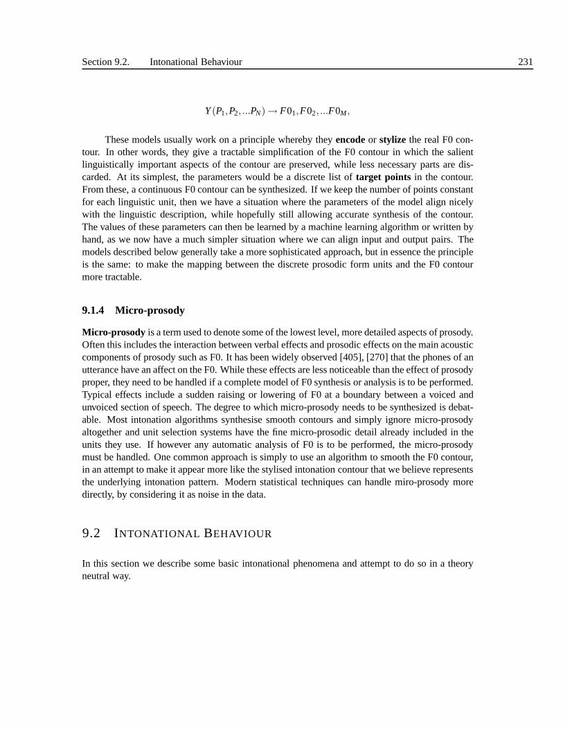
Section 9.2. Intonational Behaviour 231
Y(P1,P2, ...PN)→ F01,F02, ...F0M,
These models usually work on a principle whereby theyencodeor stylize the real F0 con-tour. In other words, they give a tractable simplification ofthe F0 contour in which the salientlinguistically important aspects of the contour are preserved, while less necessary parts are dis-carded. At its simplest, the parameters would be a discrete list of target points in the contour.From these, a continuous F0 contour can be synthesized. If wekeep the number of points constantfor each linguistic unit, then we have a situation where the parameters of the model align nicelywith the linguistic description, while hopefully still allowing accurate synthesis of the contour.The values of these parameters can then be learned by a machine learning algorithm or written byhand, as we now have a much simpler situation where we can align input and output pairs. Themodels described below generally take a more sophisticatedapproach, but in essence the principleis the same: to make the mapping between the discrete prosodic form units and the F0 contourmore tractable.
9.1.4 Micro-prosody
Micro-prosody is a term used to denote some of the lowest level, more detailed aspects of prosody.Often this includes the interaction between verbal effectsand prosodic effects on the main acousticcomponents of prosody such as F0. It has been widely observed[405], [270] that the phones of anutterance have an affect on the F0. While these effects are less noticeable than the effect of prosodyproper, they need to be handled if a complete model of F0 synthesis or analysis is to be performed.Typical effects include a sudden raising or lowering of F0 ata boundary between a voiced andunvoiced section of speech. The degree to which micro-prosody needs to be synthesized is debat-able. Most intonation algorithms synthesise smooth contours and simply ignore micro-prosodyaltogether and unit selection systems have the fine micro-prosodic detail already included in theunits they use. If however any automatic analysis of F0 is to be performed, the micro-prosodymust be handled. One common approach is simply to use an algorithm to smooth the F0 contour,in an attempt to make it appear more like the stylised intonation contour that we believe representsthe underlying intonation pattern. Modern statistical techniques can handle miro-prosody moredirectly, by considering it as noise in the data.
9.2 INTONATIONAL BEHAVIOUR
In this section we describe some basic intonational phenomena and attempt to do so in a theoryneutral way.
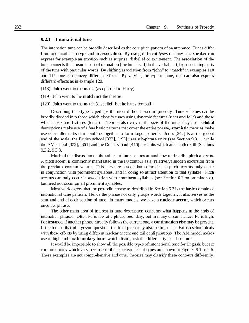
232 Chapter 9. Synthesis of Prosody
9.2.1 Intonational tune
The intonation tune can be broadly described as the core pitch pattern of an utterance. Tunes differfrom one another intype and inassociation. By using differenttypesof tunes, the speaker canexpress for example an emotion such as surprise, disbelief or excitement. Theassociationof thetune connects the prosodic part of intonation (the tune itself) to the verbal part, by associating partsof the tune with particular words. By shifting association from “john” to “match” in examples 118and 119, one can convey different effects. By varying the type of tune, one can also expressdifferent effects as in example 120.
(118) John went to the match (as opposed to Harry)
(119) John went to thematch not the theatre
(120) John went to the match (disbelief: but he hates football !
Describing tune type is perhaps the most difficult issue in prosody. Tune schemes can bebroadly divided into those which classify tunes using dynamic features (rises and falls) and thosewhich use static features (tones). Theories also vary in thesize of the units they use.Globaldescriptions make use of a few basic patterns that cover the entire phrase,atomistic theories makeuse of smaller units that combine together to form larger patterns. Jones [242] is at the globalend of the scale, the British school [333], [193] uses sub-phrase units (see Section 9.3.1 , whilethe AM school [352], [351] and the Dutch school [446] use units which are smaller still (Sections9.3.2, 9.3.3.
Much of the discussion on the subject of tune centres around how to describepitch accents.A pitch accent is commonly manifested in the F0 contour as a (relatively) sudden excursion fromthe previous contour values. This is where association comes in, as pitch accents only occurin conjunction with prominent syllables, and in doing so attract attention to that syllable. Pitchaccents can only occur in association with prominent syllables (see Section 6.3 on prominence),but need not occur on all prominent syllables.
Most work agrees that the prosodic phrase as described in Section 6.2 is the basic domain ofintonational tune patterns. Hence the phrase not only groups words together, it also serves as thestart and end of each section of tune. In many models, we have anuclear accent, which occursonce per phrase.
The other main area of interest in tune description concernswhat happens at the ends ofintonation phrases. Often F0 is low at a phrase boundary, butin many circumstances F0 is high.For instance, if another phrase directly follows the current one, acontinuation risemay be present.If the tune is that of a yes/no question, the final pitch may also be high. The British school dealswith these effects by using different nuclear accent and tail configurations. The AM model makesuse of high and lowboundary toneswhich distinguish the different types of contour.
It would be impossible to show all the possible types of intonational tune for English, but sixcommon tunes which vary because of their nuclear accent types are shown in Figures 9.1 to 9.6.These examples are not comprehensive and other theories mayclassify these contours differently.

Section 9.2. Intonational Behaviour 233
Fo
time
anna came with manny
*
Figure 9.1 Typical Fall Accent. “Anna came with Manny.” The nuclear fall is on the stressedsyllable of “manny” denoted by an* . The fall is a commonly found intonation accent and is oftenused in neutral declarative situations.
Fo
time
anna came with manny
*
Figure 9.2 High Fall, “Anna came with Manny !”. This shape corresponds to a British “highfall”, +raised or pitch level 4. In this particular utterance there is still a single intonation phrase,and the word “anna” also has an accent, but this accent is pre-nuclear. Some may argue that thereis no phonological distinction between fall and high fall, and that the high fall is really just an extraprominent fall.
The examples merely demonstrate some of the intonational effects that can be produced.
9.2.2 Downdrift
It has been observed by many researchers that there is often agradualdowndrift in the value ofF0 across a phrase [446], [447], [351], [107], [285], [167].How downdrift (often referred to asdeclination) is dealt with by different theories varies widely. Ladd [267] gives a review of someof the different theories.
Many treat downdrift as an automatic physiological effect arising from changes in sub-glottalpressure during the course of an utterance [287], [107]. This account gives the speaker littleconscious control over declination. The approach of the Dutch School [446], has been to use three

234 Chapter 9. Synthesis of Prosody
Fo
time
it was amazing
*
Figure 9.3 Rise fall accent, “It was Amazing !”. Spoken with a sense of wonderment, this accentis similar to a fall, but with a much larger preceding rise. The peak value of the F0 contour is alsolater than with a simple fall accent.
Fo
time
*
with annamanny comedid
Figure 9.4 Fall rise accent, “Did Manny come with Anna ?” A peak in the F0 contour occurs inthe stressed syllable of “manny” (* ). After coming down from the peak, the contour rises slowly andfinishes with a sharp rise at the end of the phrase. This type ofaccent is often used for simple yes/noquestions.
parallel declination lines, which refer to a baseline, a mid-line and a line corresponding to the topof the speaker’s normal range. The contour must follow one ofthese lines or be rising or fallingbetween them. Fujisaki’s model is more flexible in that the rate of declination and initial startingvalue can be varied, but the overall effect is still automatic [167]. Liberman and Pierrehumbert[285] show that the final F0 value for utterances is invariantunder a wide range of utterancelengths and pitch ranges which is inconsistent with the viewthat declination slope is constant.They propose an exponential decay downdrift effect, with the additional feature offinal loweringat the end of the phrase. Figure 9.7 shows three different views of declination.
A major claim of Pierrehumbert’s thesis [351] was that more than one factor was responsiblefor the downdrift of F0 contours. As with many other theories, she proposed that the phonetic dec-lination effect exists, but also argued that the major contribution to the downdrift of utterances wasdownstepwhich was a phonological effect and therefore controllableby the speaker. Figure 9.8

Section 9.2. Intonational Behaviour 235
Fo
time
did come with anna
*manny
Figure 9.5 Low Rise, “Did Manny come with Anna ?!”. This accent shape mayat first glance looksimilar to the fall-rise, but differs in that the stressed syllable (* ) of the word which carries the nuclearaccent is not a peak but a valley. Thus the F0 contour rises from the nuclear accent. Quite often thisaccent is preceded by a falling F0. This accent can be used to convey incredulity or disbelief.
Fo
time
did come with annamanny
*
Figure 9.6 High Rise, “Did Manny come with Anna ?”. Here the accent fallson the first syllableof Anna. There is no valley as with the low rise, and the F0 on the nuclear syllable is much higher.High rise accents are often used for yes/no questions where the speaker is looking for confirmation ina statement, as in “ok?” or “ right?”. It is similar in many ways to the low rise, with the F0 contourrising from the nuclear accent, the main difference being that the nuclear accent occurs considerablyhigher in the speaker’s pitch range, and is often not preceded by a falling section of contour.
shows a downstepping and non-downstepping version of the same sentence. These two sentencesare not only different in F0 shape, they also have subtly different meanings. (The first sounds moreexcited, the second sounds more relaxed and confident.)
9.2.3 Pitch Range
In music, if a sequence of notes is repeated an octave higher than the original, the tune remainsthe same, even though the frequency values of the notes are different with respect to the original.Rather it is the constancy of thepatternthat gives the perceptions of the tunes being the same.

236 Chapter 9. Synthesis of Prosody
00.5
1.0
1.5
(a)
(b)
(c)
Fo
Fo
Fo
Figure 9.7 The Dutch model, figure(a), has three declination lines, which refer to a baseline, amid-line and a line corresponding to the top of the speaker’snormal range. The contour must followone of these lines or be rising or falling between them. Pierrehumbert’s system (figure (b)) scalesthe pitch range 0.0 to 1.0 for normal speech but allows higherlevels. The contour is not required tofollow any of these declination lines - they are merely the “graph paper” on which the F0 contouris produced. Note how the lines converge with respect to time. The Fujisaki model (figure (c)) onlyspecifies a baseline, which decays exponentially.
The same effect is observable in intonation: by increasing the overall pitch of an utterancewhile keeping the basic tune pattern constant, the perceived tune remains the same. The relation-ship between intonational tunes in different pitch ranges is not as simple as the musical equivalent.It has been shown that the increase or decrease in pitch rangeneed not be constant throughout thephrase, as utterances always tend towards a fairly constantfinal F0 value.
Pitch range varies for a number of reasons. In single isolated utterances it can be used forincreasing the overall emphasis of the utterance. When one “raises one’s voice” in anger one isusing an increased pitch range. Pitch range factors also have a role to play in longer utterances. If
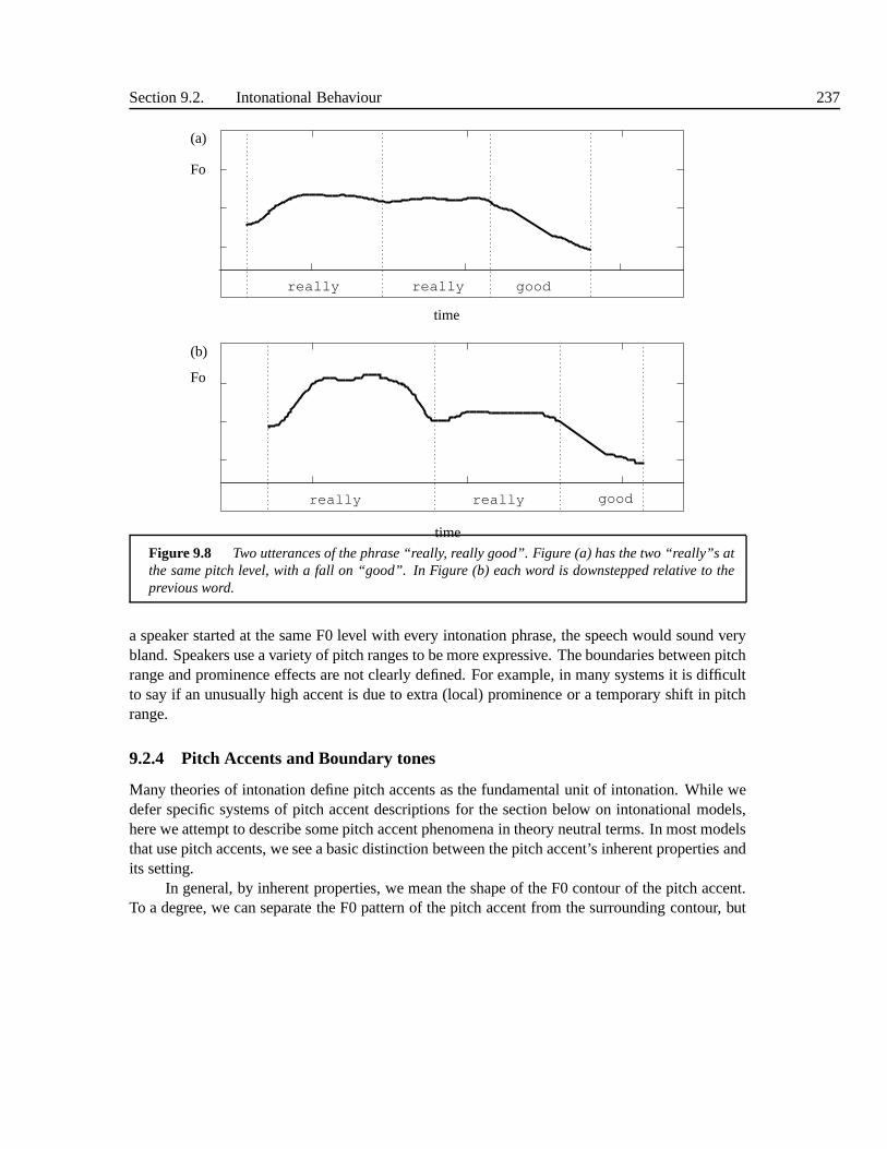
Section 9.2. Intonational Behaviour 237
really really good
Fo
Fo
(a)
(b)
really really good
time
time
Figure 9.8 Two utterances of the phrase “really, really good”. Figure (a) has the two “really”s atthe same pitch level, with a fall on “good”. In Figure (b) eachword is downstepped relative to theprevious word.
a speaker started at the same F0 level with every intonation phrase, the speech would sound verybland. Speakers use a variety of pitch ranges to be more expressive. The boundaries between pitchrange and prominence effects are not clearly defined. For example, in many systems it is difficultto say if an unusually high accent is due to extra (local) prominence or a temporary shift in pitchrange.
9.2.4 Pitch Accents and Boundary tones
Many theories of intonation define pitch accents as the fundamental unit of intonation. While wedefer specific systems of pitch accent descriptions for the section below on intonational models,here we attempt to describe some pitch accent phenomena in theory neutral terms. In most modelsthat use pitch accents, we see a basic distinction between the pitch accent’s inherent properties andits setting.
In general, by inherent properties, we mean the shape of the F0 contour of the pitch accent.To a degree, we can separate the F0 pattern of the pitch accentfrom the surrounding contour, but

238 Chapter 9. Synthesis of Prosody
this is only for convenience, in reality the pitch accents rarely have distinct beginnings and ends.The most common type of pitch accent takes the form of a peak inthe F0 contour. The
actual shape of this map be a rise followed by a fall, or a rise followed by a relatively level sectionand then a fall. The degree of the excursion is important, andgenerally speaking the higher theexcursion the more prominent the pitch accent will sound. There are many other types of pitchaccent also. One common type is the simple fall, where the contour is level, falls over a shortregion and then continues at a reasonably level rate. Another important type is the low pitchaccent, or rising pitch accent. The local shape of this is a little harder to define, but basically thistype of accent is marked by a negative excursion in the F0 contour. This can take the shape of afall followed by a rise, or just a specific low point in the contour. This is often associated withquestion intonation, or cases where the speaker is doubtingthe listener and so on. Beyond these,theories differ as the range of additional types. The important point about pitch accent shape isthat too often these are thought of as simple peaks in the contour; falls and low pitch accents arejust as important.
The pitch accent’s setting in the overall contour is also vital. This is governed by two factors;its height, meaning how high or low it occurs in the speaker’s range and its alignment with thephonetic content. In terms of height, we find a few characteristic patterns. In general, pitchaccents height decreases as a function of time throughout the utterance, as we just mentioned onthe section about downdrift. We also find that as with the sizeof the excursion, the accent heightis correlated with the degree of prominence (in fact in many models, accent height and excursionsize are governed by the same parameters).
The issue of alignment is more subtle. While intonation doeshas a form of its own, itsinteraction with the verbal phonetic content of the utterance is important to how it is produced andperceived. We have already seen that association is a key link between the prosodic and verbalcomponent as it determines which syllable or which word is accented. In addition to this, theprecise position of the accent in time with respect to the accented syllable is very important. Somemodels [260], [259], [258], talk ofearly accents andlate accents, and some argue that exactlythe same intrinsic pitch accent shape can give rise to quite different overall perceptions if only thealignment differs. Quite detailed studies of alignment have been conducted [465], [266] and [132],and found that this is a complex issue, and it is not even clearjust what should be aligned withwhat. Some suggest that the start of the vowel in the accentedsyllable should act as one anchorpoint, with the peak or mid point of the pitch accent acting asthe other. Many other alignmentmodels are however possible and in general the interactionsbetween the intonation and phoneticsare quite complicated.
The other major intonational effect is the behaviour at phrase boundaries. The F0 at thesepoints can be systematically raised or lowered for specific effect. The termboundary tone isoften used as the equivalent intonation unit to pitch accent. Strictly speaking, this term is onlyapplicable to AM models, but it has gained wide enough usage that we use it here to describegeneral behaviour at boundaries regardless of whether the particular model uses tones or not.

Section 9.3. Intonation Theories and Models 239
9.3 INTONATION THEORIES ANDMODELS
9.3.1 Traditional models and the British school
The British School of intonation includes contributions made as far back as Palmer [344]. Othermajor contributions in this school have come from O’Connor and Arnold [333], Crystal [117], andHalliday [193]. All these variants on Palmer’s original theme use dynamic features such asriseandfall to describe intonation.
In the account given by Crystal, the most important part of the contour is the nucleus whichis the only mandatory part of an intonation phrase. The nuclear accent can take one of severalconfigurations, e.g. fall, fall-rise, low rise. Other partsof the contour are termed thetail (T) whichfollows the nucleus, thehead(H) which starts at the first accented syllable of the intonation phraseand continues to the nucleus, and thepre-head(P) which precedes the head. The intonation phrasehas a grammar of (P) (H) N (T), where the brackets denote optional elements.
The relationship between the form and acoustics of this school is the most loosely definedof all the models described here; this is hardly surprising however as none of the originators ofthis system had the technology to analyse F0 contours in detail. The description of form is relatedto actual contour shapes that are found, but the descriptions should not be interpreted too literally.Both “fall” and “rise-fall” accents have rises followed by falls, the difference being that the risein the fall accent is much smaller and earlier in the syllablethan the rise in the rise-fall accent.Halliday describes his tones using rise and fall terminology, but does away with the standardnaming system preferring simply to name his tones 1, 2, 3, 4 & 5.
Some more formal descriptions have been proposed for use with the British School phonol-ogy. In particular, two models which have been designed for speech synthesis purposes are thoseof Isard and Pearson [231] who use Crystal’s phonology and Vonwiller et al [479], who use Hall-iday’s. Both these synthesis models use the full range of theBritish school tune descriptions andIsard and Pearsons’s scheme is capable of variations in prominence and pitch range.
9.3.2 The Dutch school
The Dutch School [446], [447] is based on the principle ofstylization of F0 contours. Stylizationin the Dutch system involves taking a F0 contour and attempting to fit a series of straight linesas closely as possible to the original contour. This stage isuseful as it reduces the amount ofdata needed for further analysis: a small number of straightlines are easier to deal with than acontinually varying F0 contour. From these stylizations, aseries of basic patterns can be found -this process is calledstandardization.
The version of the theory presented in t’Hart and Cohen [446]describes contours in termsof three declination lines - high, middle and low. Pitch accents are realised by rising and fallingbetween these declination lines. An example of a stylized and standardized contour is shown inFigure 9.9 (from Willems [494]).

240 Chapter 9. Synthesis of Prosody
0.0 0.3 0.6 0.9 1.2 1.5
100
200
300
500
50
and the weather turned out fine
Fo (Hz)
time (seconds)
Figure 9.9 Example of a standardized contour in the Dutch system. The dotted lines denote thethree declination lines and the thicker solid line shows thepath of the F0 contour. The first excursionto the top declination line is a head accent (British school). The second accent which rises to the topline and then falls to the baseline is a fall accent. The rise at the end is a continuation rise.
Because of the stylization process, the continuously varying nature of the F0 contour iseliminated, and because of the standardization process, the contour description is further reducedinto a small number of units (rises, falls etc). The idea of F0stylisation has proved popular withmany models and techniques outside the Dutch school [481], [121].
9.3.3 Autosegmental-Metrical and ToBI models
Ladd terms this group theautosegmental-metrical (AM) model of intonation. Its origins arein Liberman’s [284] and Bruce’s [286] work, but its first fullexposition was in Pierrehumbert’sseminal thesis [351]. From that basic model, a number of alternatives and amendments have beenproposed, but the basics remained unchanged. Most significantly, the intonation part of theToBIscheme comes directly from Pierrehumbert’s work in this school. Before these early publications,it was rare to associate the word “phonology” with prosody, but these early works promoted theidea that intonation and prosody could be described and modelled with much the same technicalapparatus as normal phonology. Hence this school is often referred to asintonational phonology[266], [269].
The AM model describes intonation as a series of high and low tones. By using a system ofdiacritics which distinguish tones located on accented syllables from those occurring at boundariesand between accents, Pierrehumbert argued that intonationcould be described by patterns of twobasic tones, which she calledH (high) andL (low). Pitch accents can be represented as either asingle or double tone. Every pitch accent has astarred tone (* ) which signals that it is that tonewhich is directly associated with the accented syllable. The possible pitch accents areH*, L*, H*+ L, H + L*, L + H* andL* + H . At phrase boundaries,boundary tonescan be found, which

Section 9.3. Intonation Theories and Models 241
are marked with a (% ). Phrase tonesare used to show path of the contour from the last (nuclear)accent to the phrase boundary, marked with a (-).
Unlike the British school analysis, there is no strict division of the contour into regionssuch as head and nucleus. Both nuclear and pre-nuclear accents can be any one of the six typesdescribed above. The nucleus accent is distinguished because the phrase and boundary tones thatfollow it allow a much larger inventory of intonational effects.
Each tone forms a target from which F0 contours can be realised by using interpolationrules. As with many other theories, the AM model retains the idea of a declination baseline,but says that the downdrift commonly observed in F0 contoursis mainly due to the phonologicaleffect ofdownstepwhich again is controllable by the speaker. In her original work, Pierrehum-bert proposed that the downstep effect is triggered by the speaker’s use of a sequence ofH L Htones, using evidence from African tone languages as justification (see Figure 9.8 for examples ofdownstepping and non-downstepping contours).
The history of the AM model is particularly interesting in that it has a dual character of beingintended as a “pure” linguistic theory in the MIT, Chomsky/Halle phonology tradition, and as aworking model for the Bell Labs TTS system. It is important torealise that from a theoreticallinguistic point of view, the model as just described is not intended to be a “complete” model ofintonation as used in human communication. Rather, the AM school divides the general intonationsystem into a part which is properly linguistic, a part whichis para-linguistic and a part that isextra-linguistic. The distinction is seen as important within this school as the properly linguisticpart, i.e. that described above, is the main area of interestas it forms part of the general grammar ofa speaker’s language faculty. For a complete description however, we require the para-linguisticeffects too, which include for instance the degree of prominence of a pitch accent, and extra-linguistic effects such as global F0 settings. For our purposes, the distinctions between thesesubsystems are less important, but it is important to realise that the system ofH* + L accents andso on is only a partial representation of an utterance’s intonation.
9.3.4 The INTSINT Model
The INTSINT model of Hirst et al [212], [213], [211], was developed in an attempt to providea comprehensive and multi-lingual transcription system for intonation. The model can be seenas “theory-neutral” in that it was designed to transcribe the intonation of utterances as a way ofannotating databases and thereby providing the raw data upon which intonational theories could bedeveloped. Hirst has described the development of INTSINT as an attempt to design an equivalentof IPA for intonation. As stated in Section 6.10, there is no such thing as completely theory neutralmodel as all models make some assumptions. Nevertheless, INTSINT certainly fulfills its maingoals of allowing a phonetic transcription of an utterance to be made without necessarily decidingwhich theory or model of intonation will be subsequently used.
INTSINT describes an utterance’s intonation by a sequence of labels each of which repre-sents a target point. These target points are defined either by reference to the speaker’s pitch range,

242 Chapter 9. Synthesis of Prosody
in which case they are marked Top (T), Mid (M) or Bottom (B), orby reference to the previous tar-get point, in which case they are marked Higher (H), Same (S) or Lower (L). In addition, accentscan be marked as Upstepped (S) or Downstepped (D).
Hirst [212] describes this system in detail and shows how it can be applied to all the majorlanguages. Several algorithms have also been developed forextracting the labels automaticallyfrom the acoustics and for synthesizing F0 contours from thelabels2. Applications of this modelto synthesis include Veronis et al [475].
9.3.5 The Fujisaki model and Superimpositional Models
Fujisaki’s intonation model [166] takes a quite different approach to the models previously dis-cussed in that it aims for an accurate description of the F0 contour which simulates the humanproduction mechanism. Fujisaki’s model was developed fromthe filter method first proposed byOhman [335].
In the model, intonation is composed of two types of components, thephraseand theaccent.The input to the model is in the form of impulses, used to produce phrase shapes, and step functionswhich produce accent shapes.
This mechanism consists of two second order critically damped FIR filters (these are intro-duced fully in Section 10.4). One filter is used for the phrasecomponent, the other for the accentcomponent. The F0 contour can be represented by equations 9.1, 9.2 and 9.3.
lnF0(t) = lnFmin+I
∑i=1
Api Gpi (t−T0i)+J
∑j=1
Aaj (Gaj (t−T1j )−Gaj (t−T2j )) (9.1)
where
Gpi (t) =
α2
i te−αit for t ≥ 0
0 for t < 0(9.2)
and
Gaj (t) =
min[1− (1+ β jt)e−β j t ,θ] for t ≥ 00 for t < 0
(9.3)
2 In addition to being an expert on multi-lingual intonation,Hirst is also know for being able to do a particularly finerendition of “Don’t Cry For Me Argentina”.
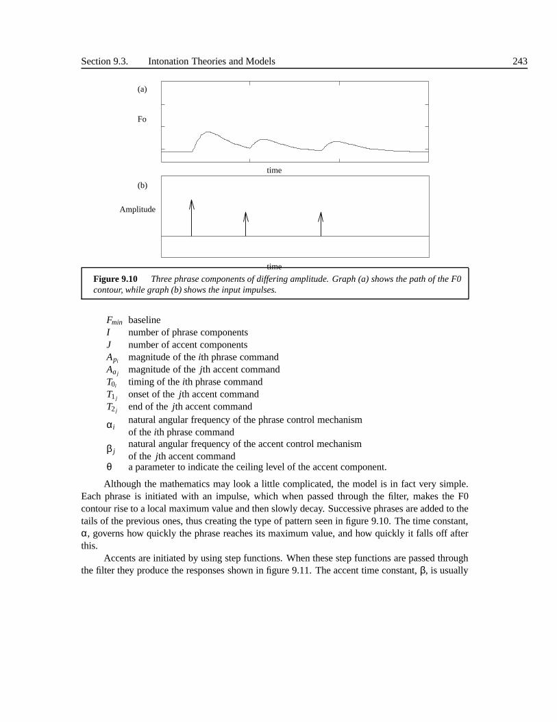
Section 9.3. Intonation Theories and Models 243
time
time
Fo
Amplitude
(b)
(a)
Figure 9.10 Three phrase components of differing amplitude. Graph (a) shows the path of the F0contour, while graph (b) shows the input impulses.
Fmin baselineI number of phrase componentsJ number of accent componentsApi magnitude of theith phrase commandAaj magnitude of thejth accent commandT0i timing of theith phrase commandT1j onset of thejth accent commandT2j end of thejth accent command
αinatural angular frequency of the phrase control mechanismof the ith phrase command
β jnatural angular frequency of the accent control mechanismof the jth accent command
θ a parameter to indicate the ceiling level of the accent component.
Although the mathematics may look a little complicated, themodel is in fact very simple.Each phrase is initiated with an impulse, which when passed through the filter, makes the F0contour rise to a local maximum value and then slowly decay. Successive phrases are added to thetails of the previous ones, thus creating the type of patternseen in figure 9.10. The time constant,α, governs how quickly the phrase reaches its maximum value, and how quickly it falls off afterthis.
Accents are initiated by using step functions. When these step functions are passed throughthe filter they produce the responses shown in figure 9.11. Theaccent time constant,β, is usually
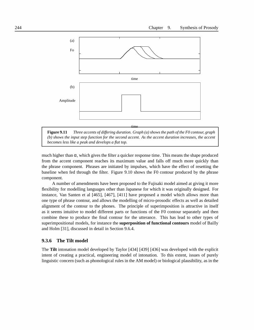
244 Chapter 9. Synthesis of Prosody
time
Fo
time
Amplitude
(b)
(a)
Figure 9.11 Three accents of differing duration. Graph (a) shows the path of the F0 contour, graph(b) shows the input step function for the second accent. As the accent duration increases, the accentbecomes less like a peak and develops a flat top.
much higher thanα, which gives the filter a quicker response time. This means the shape producedfrom the accent component reaches its maximum value and falls off much more quickly thanthe phrase component. Phrases are initiated by impulses, which have the effect of resetting thebaseline when fed through the filter. Figure 9.10 shows the F0contour produced by the phrasecomponent.
A number of amendments have been proposed to the Fujisaki model aimed at giving it moreflexibility for modelling languages other than Japanese forwhich it was originally designed. Forinstance, Van Santen et al [465], [467], [411] have proposeda model which allows more thanone type of phrase contour, and allows the modelling of micro-prosodic effects as well as detailedalignment of the contour to the phones. The principle of superimposition is attractive in itselfas it seems intuitive to model different parts or functions of the F0 contour separately and thencombine these to produce the final contour for the utterance.This has lead to other types ofsuperimpositional models, for instance thesuperposition of functional contoursmodel of Baillyand Holm [31], discussed in detail in Section 9.6.4.
9.3.6 The Tilt model
TheTilt intonation model developed by Taylor [434] [439] [436] was developed with the explicitintent of creating a practical, engineering model of intonation. To this extent, issues of purelylinguistic concern (such as phonological rules in the AM model) or biological plausibility, as in the
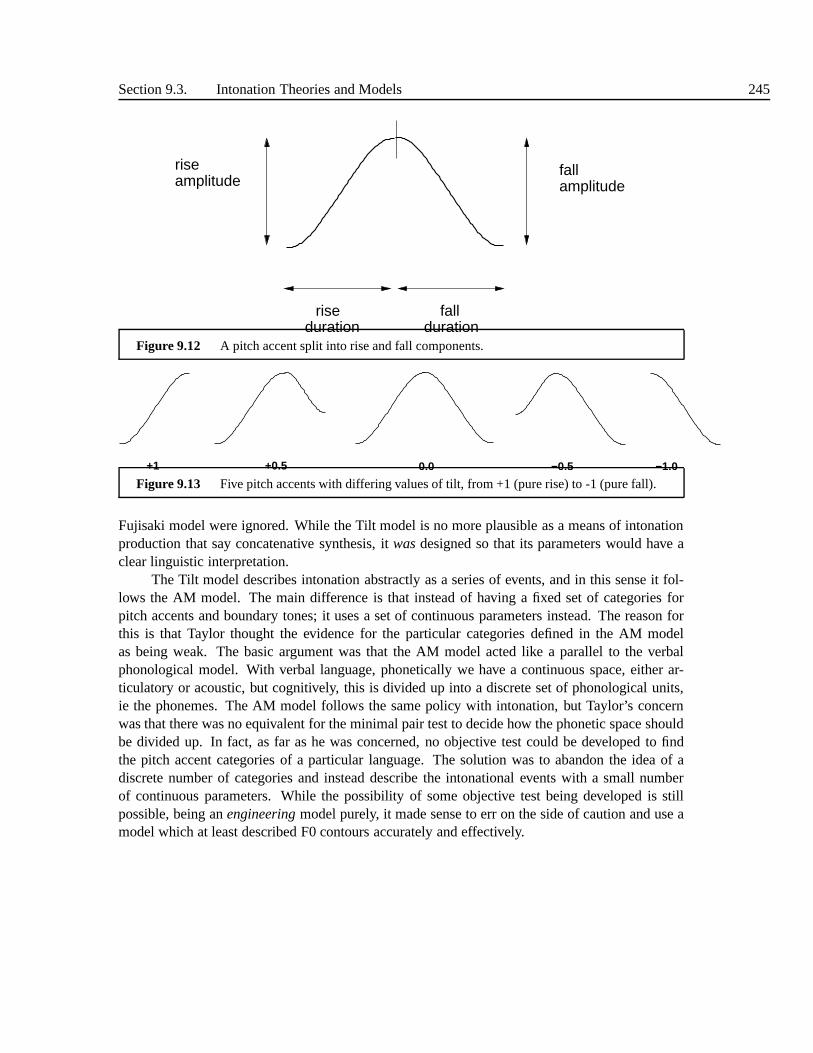
Section 9.3. Intonation Theories and Models 245
riseamplitude amplitude
fall
riseduration
fallduration
Figure 9.12 A pitch accent split into rise and fall components.
+1 +0.5 0.0 −0.5 −1.0
Figure 9.13 Five pitch accents with differing values of tilt, from +1 (pure rise) to -1 (pure fall).
Fujisaki model were ignored. While the Tilt model is no more plausible as a means of intonationproduction that say concatenative synthesis, itwasdesigned so that its parameters would have aclear linguistic interpretation.
The Tilt model describes intonation abstractly as a series of events, and in this sense it fol-lows the AM model. The main difference is that instead of having a fixed set of categories forpitch accents and boundary tones; it uses a set of continuousparameters instead. The reason forthis is that Taylor thought the evidence for the particular categories defined in the AM modelas being weak. The basic argument was that the AM model acted like a parallel to the verbalphonological model. With verbal language, phonetically wehave a continuous space, either ar-ticulatory or acoustic, but cognitively, this is divided upinto a discrete set of phonological units,ie the phonemes. The AM model follows the same policy with intonation, but Taylor’s concernwas that there was no equivalent for the minimal pair test to decide how the phonetic space shouldbe divided up. In fact, as far as he was concerned, no objective test could be developed to findthe pitch accent categories of a particular language. The solution was to abandon the idea of adiscrete number of categories and instead describe the intonational events with a small numberof continuous parameters. While the possibility of some objective test being developed is stillpossible, being anengineeringmodel purely, it made sense to err on the side of caution and use amodel which at least described F0 contours accurately and effectively.

246 Chapter 9. Synthesis of Prosody
In the Tilt model, there are two types of eventaccentandboundary (these are effectively thesame as the pitch accents and boundary tones in the AM model).Each event comprises two parts,a rise and afall , as shown in Figure 9.12. Between events straight lines called connectionsareused. All variation in accent and boundary shape is governedby firstly changing the relative sizesof the rise and fall components, and secondly by how the eventaligns with the verbal component(basically, whether it is higher or lower in the pitch range,or occurs earlier or later with respectto the accented syllable). This then gives a total of six parameters, 4 describing the shape ofthe event and 2 describing how it aligns. This basic model (called the rise/fall/connection model[439]) models contours accurately but is not particularly amenable to linguistic interpretation. TheTilt model itself is a transformation of the 4 parameters foreach event (rise and fall amplitude, andrise and fall duration) into the 3 Tilt parameters. Amplitude and duration are given by
Amplitude= A = |Arise|+ |Af all |Duration= D = |Drise|+ |D f all |
The Tilt parameter itself is used to define the general shape of the event, independent of its am-plitude, duration or alignment. To find the value of Tilt, we first calculate an interim value,Tiltamplitude, found by taking the ratio of the differences of the rise and fall amplitudes divide bythe sum of the rise and fall amplitudes:
tiltamp=|Arise|− |Af all ||Arise|+ |Af all |
and likewise for duration
tiltdur =|Drise|− |D f all ||Drise|+ |D f all |
these two quantities are highly correlated, which allows usto combine them into the single finalTilt parameter:
tilt =tiltamp+ tiltdur
2Figure 9.13 shows a number of event shapes for different values of the Tilt parameter.
9.3.7 Comparison
Many other models have been proposed in addition to the above, but the models described areperhaps the most popular and at least cover the range of models available. An entire book couldbe devoted to discussing the philosophical, historical, theoretical and practical issues surroundingwhy one model has the features it does and why it may or may not be better than another model.For now, however we will simply describe some of the differences in the model to help betterunderstand why these differences occur.

Section 9.3. Intonation Theories and Models 247
Purpose
Not all models were designed for the same purposes. The AM models are usually not described asmodels at all, but as theories as to how intonation actually works in human communication. Issuessuch as cross-language studies and links with other components of human grammar and so on areparticularly important in this group. The Fujisaki model isoften said to be biologically justifiable,meaning that it mimics the actual articulation of the human production mechanisms. The Tiltmodel is only described in practical terms, as a tool to get the job done and has no claims to modelany aspect (cognitive or biological) of human behaviour. These different approaches are of coursequite common in all areas of language study; what is of note isthat intonation seems to be oneof the few areas where engineering and scientific approachesstill have enough commonality toconstitute a single field.
Phonological vs Phonetic vs Acoustic
The AM model is phonological, the INTSINT model phonetic andthe Fujisaki and Tilt modelsacoustic. While these differences are obviously important, one should be wary as to placing toomuch significance on these as being statements about what themodel developers think is the“real” nature of intonation. For example, Hirst proposed INTSINT as an intonational equivalentto IPA that would allow researchers to label what intonationinformation a contour containedindependent of linguistic theory, in just the same way that aphonetician might make detailedtranscriptions of verbal phenomena. Once done, a phonological theory can be built using thesetranscriptions as data, and so it is not correct to say that Hirst thinks intonation is “phonetic” incharacter. Likewise, in the AM model, there is the assumption that production includes phoneticand acoustic components, and in acoustic models the assumption again is that there are higherlevel more abstract representations. In fact, there is nothing to stop creating a single formulationwhere the AM model would serve as the phonological representation, the INTSINT model as aphonetic representation and the Tilt model as the acoustic representation.
Tones vs Shapes
There is a basic distinction in most models as to whether intonation is an inherently tone or pitch-level based system (as in AM models), or whether it is based onpitch shapes or pitch dynamics(as in the Dutch model, Fujisaki model or Tilt). In theoretical linguistics this debate is seen asparticularly important as researchers are attempting to find the “true nature” of intonation, with“conclusive” evidence occasionally being produced for oneview over the other. The issue is hardto resolve, and it may be case where intonation is actually a mixture of both.
Superimpositional vs Linear
Some models have a superimpositional nature (Dutch, Fujisaki) where pitch accents are seen asbeing relatively short term which “riding” on top of a phrases which are seen as being relativelylong. By contrast, in linear models (AM/Tilt) contours are composed of linear sequences of in-

248 Chapter 9. Synthesis of Prosody
tonational units. Often a grammar is used which states whichunits can follow each other, but solong as the sequence lies within the grammar, any unit can follow any other.
Being brief, the main reason for supporting the superimpositional model is that F0 contoursdo seem to exhibit patterns of global behaviour, where phrases define particular F0 patterns. Themain reason for supporting linear models comes from speech production concerns. Here, we seethat if we support a superimpositional model then the speaker has topre-plan the utterance someway ahead of time. This doesn’t seem to correspond to known facts in speech production, wherewe know for example that a speaker can change the course of theF0 contour at any time.
Finally we should note that some papers have shown how labelsin one model can be trans-lated to labels in another [436], [374].
9.4 INTONATION SYNTHESIS WITH AM MODELS
We now turn our attention to this issue of intonation synthesis itself. In Chapter 6 we described avariety of techniques for generating the prosodic form representations of phrasing and prominencefrom text. We only made passing reference to the issue of generating intonational form from textas this really required a thorough discussion on the issue ofintonational form first. With this jobnow done, we can describe techniques for both generating intonational form descriptions from textand for generating F0 controls from intonational form.
While it is possible to build synthesis algorithms with any of the models outlined in Section9.3.3, we will focus our attention on the most popular techniques, which divide into those basedon AM models (described here) and those based on acoustic models (described next).
9.4.1 Prediction of AM labels from text
We approach the task of predicting intonation from text in much the same way as we predictedphrasing and prominence from text. With the AM model, our jobis to assign an intonational labelto each syllable, and no matter what algorithm is used, this is formulated as a mapping from aset of features describing the syllable and its context to a label. A typical approach of this typeis given by Lee [280] who trained a decision tree to generate ToBI labels using linguistic featuressuch as position in phrase, part of speech tags and syntacticinformation. In general though, anyof the standard text prediction machine learning techniques introduced in Chapter 5 can be usedon this task, and the approach is by and large the same as for prominence prediction and phrasingprediction. Many other approaches for the prediction of AM and other intonation representationsfrom text have been proposed, including HMMs [325], decision trees/CART [513], [378] and rules[462], [365].

Section 9.4. Intonation Synthesis with AM models 249
9.4.2 Deterministic synthesis methods
Given a representation of intonational form predicted fromtext, we next attempt to synthesizean F0 contour from this. In this section we will examine two rule based deterministic proposalsfor doing this, the first developed for use the with original Pierrehumbert model and the second,developed more specifically for use with ToBI.
Anderson, Pierrehumbert and Liberman [16] proposed a synthesis scheme (hereafter calledAPL) which generated an F0 contour from an arbitrary AM tone description. Recall that a featureof the AM model is that it is linear in the sense that there is noglobal pattern to intonation,each intonational unit in the sequence operates largely independently. This is reflected in thesynthesis algorithm where an acoustic model made of target points is used. In the algorithm, eachintonational event generates a set of target points which define the basic shape of the event. Pitchrange in the model is expressed by two lines, thereference linewhich expresses the default or “atrest” value of F0, and thebaselinewhich is the minimum F0 value, and the value that F0 falls toat the end of a phrase which is terminated by anL- L% boundary tone. Declination as a globaltrend is absent from the model; rather, downdrift is synthesized by a trend where each successivepitch accent is in general placed lower in the pitch range. Between pitch accents, phrase accentsand boundary tones, linear interpolation is used to “fill in”the F0 values. An important nuancein the algorithm is its treatment of phrase final behaviour. Following extensive studies reported inprevious work [285], Anderson et al added a component to the algorithm which dropped the F0contour to the baseline after the nuclear accent, regardless of whether the model itself would havepredicted such a value. This greatly increases the naturalness of the contours produced as theyhave a proper impression of finality compared to other synthesis algorithms they investigated.
A more recent algorithm designed to work with the ToBI schemewas proposed by Jilka,Mohler and Dogil [241]. This in many ways extends the original work by Anderson et al as it toosynthesises the ToBI events as isolated units, places them in context in the utterance, and then usesinterpolation to cover the regions between. The algorithm improves on the original work in that itpays particular attention to where target points should be placed with respect to their syllables, andfor instance models in some detail the fact that accents thatoccur early in phrases are often laterwith respect to their syllable position than accents which occur later in phrases (its as if the phraseboundaries are repelling the accents in both directions). In this algorithm, a topline and baselineare used as the reference points. When downstepping occurs,it triggers a lowering in the topline,and this is the general mechanism by which downdrift occurs.Example rules for the position ofthe target points are given below:

250 Chapter 9. Synthesis of Prosody
Intonational eventcontext resultant time positionH* First syllable in phrase 85%
Last syllable in phrase 25%One syllable phrase 50%All other cases 60%
L* First syllable in phrase 85%Last syllable in phrase 25%One syllable phrase 50%All other cases 60%
L+H* (H part) First syllable in phrase 90%Last syllable in phrase 25%One syllable phrase 70%All other cases 750%
L+H* (L part) Normal case 0.2s beforeH*If voiceless region 0.2s beforeH* (reference point)90 %of voiced region to left of reference
9.4.3 Data Driven synthesis methods
Black and Hunt [51] described a data-driven technique for synthesising F0 contours from ToBIlabels. In fact, their work can be seen as a data-driven version of the APL algorithm, in which thetarget points are learned from the data rather than specifiedby hand. The approach was based onlearning the mapping between ToBI labels, which had been marked on a database by hand, and F0contours extracted automatically. The APL model defines target points at very specific locations,but these are difficult to determine bottom-up so the Black and Hunt approach instead uses threetarget points for each ToBI label. These are place the beginning, middle and end of the syllableassociated with the label. This gives us a representation where the input is a ToBI label and a setof features describing the linguistic context of the label,and the output is three target points. Inthis form, the mapping is now amenable for use by a standard machine learning algorithm.
Black and Hunt in fact used a linear regression technique, with features such as lexical stress,numbers of syllables between the current syllable and the end of the phrase, identity of the previouslabels and so on. Once learned, the system is capable of generating a basic set of target points forany input, which we then interpolated and smoothed to produce the final F0 contour. Other datadriven techniques such as CART have proven suitable for synthesizing from AM representations[292], [340].
9.4.4 Analysis with Autosegmental models
The biggest difficulty with the AM models is the difficulty in labelling corpora. Several studieshave been conducted in labelling with ToBI with the general conclusion that while labellers canoften identify which syllables bear pitch accents, they arevery poor at agreeing on which particular

Section 9.5. Intonation Synthesis with Deterministic Acoustic Models 251
accent is correct. As we explained in Section 6.10, the inter-labeller agreement with models suchas ToBI is worryingly low, and in many practical database labelling projects many of the pitchaccent distinctions have been dropped [488], [487].
Two major problems stem from this. Firstly, any database which has been labelled with ToBIwill have a significant amount of noise associated with the pitch accent label classes. Secondly,for any large scale machine learning or data driven approach, we need a considerable amount oflabelled data to the extent that it is impractical to label data by hand. As we shall see in Chapters15 and 16, virtually all other aspects of a modern data drivenTTS system’s data are labelledautomatically, and so it is a significant drawback if the intonation component can not be labelledautomatically as well. Because however the level of human labeller agreement is so low, it is veryhard to train a system successfully on these labels; we can hardly expect an automatic algorithmto perform better than a human at such a task.
One solution that is increasingly adopted is to forgo the distinction between label typesaltogether, see for instance [488]. While the break index and boundary tone components are oftenkept, only a single type of pitch accent is used; in effect thelabellers are marking whether a wordis intonationally prominent or not. However, it should be clear that such an approach effectivelyreduces ToBI to a data driven system of the type described below.
9.5 INTONATION SYNTHESIS WITH DETERMINISTIC ACOUSTICMOD-ELS
Here we describe how to synthesise F0 contours using the Fujisaki and Tilt models and as wewill see, the approach is similar in both cases. Synthesis from the Fujisaki or Tilt parameters isof course given by the models themselves, and so presents no problems. For TTS purposes then,the issue is to generate the Fujisaki or Tilt parameters fromthe text. Two basic approaches can betaken in this regard; either we try and generate the parameters directly from the text, or we takea two stage approach where we first generate an abstract, discrete prosodic form representationfrom the text, and then proceed to generate the model parameters from these.
9.5.1 Synthesis with superimpositional models
The Fujisaki model is most commonly used with Japanese, but has been used or adapted to manyother languages. In Japanese, we find that the range of pitch accent phenomena is narrower thanin languages such as English, which means that the model’s single type of accent is particularlysuited. In addition, the nature of intonation in Japanese means that accents are marked in thelexicon, which greatly simplifies the problem of prominenceprediction. Hence a simple approachto this, which uses accent information from the lexicon alone, is often sufficient. A commonapproach therefore is to determine phrase breaks and prominent syllables from the text, and thenphrase by phrase and syllable by syllable generate the inputcommand parameters for the Fujisaki

252 Chapter 9. Synthesis of Prosody
model using one of the standard machine learning techniques.Hirose et al [206], [205] describes such an approach for Japanese. In doing so, he makes use
of the basic lexicon tone distinctions in Japanese to given where accents occur, thus simplifyingthe prominence and accent prediction process considerably. To generate the accent commands, heuses parts of speech, syllable structure, relative positions of these, numbers of proceeding phrasesand punctuation. Syntactic units are also optionally used.A number of neural network algorithmsare used, including recurrent networks. In addition, multiple regression analysis in a vein similarto the ToBI Black and Hunt [51] technique was investigated, in most cases the results were verysimilar regardless of which algorithm is used (this of course follows the pattern for other prosodyprediction problems).
One significant advantage that Hirose makes note of is that even when the prediction algo-rithm generates incorrect parameters for the Fujisaki model, the result is still a “natural” contourbecause the model itself is tightly constrained. In other words, the contour produced issomecon-tour, just not the right one. By comparison, when predictionis poor with target models, the resultmay be a contour that bears no similarity to the type that a human could produce.
9.5.2 Synthesis with the Tilt model
Dusterhoff et al [146] described a three stage technique forsynthesising intonation with the Tiltmodel. First, they predict where accents are placed; this iseffectively a prominence predictionalgorithm of the type described in Section 6.8. Next, for each accent, the three intrinsic and 2extrinsic Tilt parameters are generated. This is done with adecision tree, using features such assyllable position in phrase, length of phrase and so on. Finally, the Tilt model itself generatesthe F0 contour. In general though there are many similarities between synthesis with Tilt and theFujisaki model, so a technique which works with one can probably be adapted to the other.
9.5.3 Analysis with Fujisaki and Tilt models
An advantage that the Tilt model has over many others is that automatic analysis is significantlyeasier using this model. Taylor [436] describes a complete technique for first finding pitch accentsand boundary tones and then determining the Tilt parametersfrom the local F0 contour in thesurrounding region. Many algorithms have also been developed for automatically finding theFujisaki model parameters from data [165], [71], [314], [7], [379].
9.6 DATA DRIVEN INTONATION MODELS
A common criticism of the Fujisaki model [285], [436] is thatthere are many contours whichthe model can not generate. These include gradual low risingcontours which occur when a lowaccent occurs early in a phrase, and the effect of phrase finallowering where the contour falls pastthe normal baseline to a final baseline in declarative utterances. Suggestions that fix the problems

Section 9.6. Data Driven Intonation Models 253
have been made, for instance by including phrase-final negative phrase commands and so on, butsuch suggestions detract from the elegance of the original model. The Tilt model can be criticisedasovergenerating in that there are contours it can generate which are never observed. When weconsider simpler stylisation models we see that these models often massively over generate.
To solve these problems, we can of course refine the models, but this can result in endless“tinkering” in which the models loose their originally elegance and simplicity. The basic problemis that when we design a model, we wish it to be elegant and easyto interpret, but we alwaysrun the risk that some intonational phenomena that we haven’t taken into account may appear andbe outside the model’s capabilities. We then face the choiceof adding to the model, which oftenappears as a “hack” or designing a completely new model.
We can however consider a quite a different approach where wecompletely abandon the ideaof creating an explicit model, but instead infer the model from data. Bailly [29] has consideredthis issue and asked whether explicit intonation models arerequired at all; perhaps we shouldconcentrate on databases and labelling, and leave the specifics of the model to be determined bymodern machine learning techniques. As we shall see in Chapter 13, it is convenient to describesynthesis techniques in terms of three generations, where the first generation used explicit handwritten rules, the second generation uses basic and quite constrained data driven approaches, anda third generation which used general data driven and statistical approaches. The same pattern canbe seen in intonation synthesis, where for example the APL algorithm is first generation and theBlack and Hunt decision tree ToBI algorithm is second generation. The techniques described herecan be considered third generation as they match closely theapproaches used in the HMM andunit selection synthesis techniques described in Chapters15 and 16.
In the following sections, we give an overview of the techniques used, but as many of thesefollow the synthesis techniques described in Chapters 15 and 16, we wait until then to give a fullyformal account.
9.6.1 Unit selection style approaches
The unit selection synthesis technique described in Chapter 16 uses an entirely data driven ap-proach, whereby recorded speech waveforms are cut up, rearranged and concatenated to say newsentences. Given the success of this approach in normal synthesis, a number of researchers haveapplied these algorithms to F0 synthesis [296], [310], [311].
F0 contours extracted from real utterances are by their verynature perfect. The basic ideatherefore is to collect a database of naturally occurring F0contours, and use these at synthesistime for new utterances. It is extremely unlikely that one ofthe complete contours in the databasewill be exactly what we want; for this to be the case we would have have to have exactly the sametext for the synthesis and database utterance. At a smaller scale, say at the phrase, word or syllablelevel, it is however possible to find exact or close matches and so the database processed to createa set ofF0 units. Each unit has a set of features describing it, and at run time, these features arecompared with features generated by the prosodic prediction. Sometimes exact matches are found,

254 Chapter 9. Synthesis of Prosody
but often only close matches are found in which case a distance, called thetarget costis calculatedfrom the desired features to the ones for each unit in the database. The lower the distance, thecloser a unit is to the desired features. Obviously we wish toavoid large discontinuities in F0values when we move from one unit to the next, and so a second distance, called thejoin costis used to give a measure of how similar two units are at their edges. For F0 contours, a simplemetric such as absolute F0 difference is often sufficient.
The idea then is to find the best sequence of F0 units for our desired features, and this iscalculated by summing the target and join costs for a complete sequence of units. Formally, this isgiven by:
C(U,S) =T
∑t=1
T(ut ,st)+T−1
∑t=1
J(ut ,ut+1) (9.4)
whereU is a sequence of units from the database,S is the sequence of desired features,ut is oneunit, st is one set of desired features andT(.) andJ(.) are the target and join costs respectively. Asearch is then conducted to find the single sequence of unitsU which minimises this cost:
U = argminu
T
∑t=1
T(ut ,st)+T−1
∑t=1
J(ut ,ut+1)
(9.5)
The advantage of this approached is that we areguaranteedto synthesise a natural contour,the only question is whether it will be the “correct” naturalcontour for the linguistic context. Thisapproach is appealing in that is simple and should work for all languages and genres. Furthermore,as database sizes grow, the quality of this technique will continually improve as we will becomemore and more likely to find good matches in the database.
9.6.2 Dynamic System Models
The main drawback of the above unit selection approach is that the algorithm suffers from a “hitor miss” problem with respect to finding matches in the database. In other words, we have a fixednumber of units, and it is sometimes a matter of luck whether we find a good match or not. Whilethe technique can produce excellent F0 contours, occasionally no good matches are found and theresults can be poor. Unit selection approaches can be seen asones where certain F0 contours arememorised by the system. We can contrast this with statistical approaches, where the aim is tolearn the general nature of all F0 contours, by learning model parameters (not memorising) froma limited amount of training data. The advantage is that the technique is more robust when weneed to synthesize contours we have not previously come across. The downside is of course thatin building our model we have made some assumptions, and so the reproduction of F0 contoursmay not be as accurate for cases that we have in fact seen.
Ross and Ostendorf developed a model based on thedynamic system model, a model wellknown in control engineering (also know as aKalman filter ). This model is described by astateequation and anobservation equation, given respectively as follows:
Section 9.6. Data Driven Intonation Models 255
xk+1 = Fjxk +u j +wk (9.6)
F0k = H jxk +b j +vk (9.7)
The idea here is that the state equation describes a trajectory through time. The above is a firstorder IIR filter of the type we will describe in Section 10.4, for now all we need know is that byappropriate setting of the parametersFj , u j andwk, we can generate a wide variety of trajectoryshapes. By inferring these parameters from data, we can train this equation to generate contours.The termu j can be seen as an input, and can be thought of as the equivalentof the phrase or accentcommand in the Fujisaki model.wk is a term for modelling noise, and is what gives the model itsstatistical nature; for now we can think of this as an error term in the model, which allows us torobustly and statistically learn the other parameters.
Rather than use this equation as is, we also use the observation equation which performs amapping from each point in the state trajectory to an actual F0 value, again with trainable param-eters determining the exact nature of this mapping. While weshould be somewhat cautious aboutgiving explicit interpretations to statistical models, wecan think of the overall process as follows.The state equation generates a “true” intonation contour that properly expressed the actual lin-guistic manifestation of the prosodic form. These trajectories are smooth, clean and simple. Weknow however that real F0 values, as measured by pitch detection algorithms (see Section 12.7)are noisy, in that the contours are rarely smooth or predictable at the lowest level. The observationequation models this part of the system. If we used the outputof the state equation to model F0values directly, our problem would be significantly harder as we would then have to model everyperturbation in the contour, and would miss the general and underlying trends in the contour.
During synthesis, the model is “driven” by means of the inputparametersu j andb j and alsooptionally by varyingFj andH j . This can be done in a number of ways, but Ross and Osterndorfuse simple equations which link the usual linguistic features (position within the phrase, stressvalue of the syllable etc) to change the values of the parameters every syllable. During synthesis,the noise terms are ignored. Training the model is somewhat complicated, but in essence weattempt to generate F0 contours on a training corpus and adjust the parameters until the best matchbetween is found between the F0 contours produced by the model and the natural ones. Thisapproach is very similar to the expectation maximisation (EM) technique used to train hiddenMarkov models. This is explained in full in Section 15.1.8.
9.6.3 Hidden Markov models
The dynamical system model is a natural choice for statistical generation of F0 contours as it iswell suited to the job of generating continuous trajectories. If it has any weakness we can point tothe fact that the state trajectories are limited to being those of a first order filter, the noise termshave to be Gaussian and the training process can be quite intricate. An alternative is to use hidden

256 Chapter 9. Synthesis of Prosody
Markov models (HMMs) as these are in general easier to train and allow more complexity withregard to noise/covariance terms.
HMMs are however similar to dynamic system models in certainways in that they havea hidden state space, within which the model dynamics operate, and a projection from this toan observation space. We have used HMMs before for various tasks including part-of-speechtagging and phrase-break prediction. In those cases, the output distributions were discrete andgave the probability of seeing (say) a word given a POS tag. Itis also possible to have HMMswith continuous output distributions which give the probability of seeing a continuous value givena state. This sort of HMM can therefore be used for F0 generation. In the dynamic system model,the hidden state space is a continuous trajectory, and this seems very natural for F0 contours.HMMs by contrast have a discrete state space, and when we movefrom one state to another duringgeneration, the observation probabilities suddenly change. In this mode an HMM will generateextremely unnatural contours where we have a series of constant F0 values, a jump to a differentseries of constant F0 values and so on. No real F0 contours have behaviour anything like this. Ifwe however adopt the formulation of Tokuda et all [453], we can generate from the HMM stateswhile also taking into account the learned dynamics of F0 behaviour. Inanoglu [230] describes asystem where F0 for various emotions can be accurately generated by HMMs (diagrams of thisare shown in Figures 15.14 and 15.15). This method of HMM synthesis is the subject of Chapter15 and so we leave further explanation of HMM F0 synthesis until then. We finish however withthe observation that by using this formulation, extremely natural F0 contours can successfully begenerated with HMMs.
9.6.4 Functional models
Given the considerable difficulties in constructing a modelof prosodic form, never mind anydifficulties in using such a model, we can ask whether an explicit model of prosodic form isreally necessary. While experience has shown thatsomenotion of prosodic form is necessary(see Section 9.1.2), it may not in fact be necessary to model this explicitly; rather we can learn amodel of prosodic form and keep it as a hidden part of a more general model [501], [502]. Thesuperposition of functional contours (SFC) [216], [321], [217], [31] is a model in which themapping from the meaning and linguistic structure to F0 is attempted in a unified fashion. TheSFC model is based on the idea that there are a number of identifiable prosodicfunctions3 andthat each has a characteristic prosodic pattern. As the scope of each function is variable, and as wecan have several independent functions operating on a particular part of the utterance (for instancesyntax and emotion), then we need to combine these effects together to form a single prosodicpattern.
In the SFC model, the syllable is used as the unit of prosodic control and each is describedby three F0 values and a duration value representing the prosodic lengthening to be applied. Each
3 Here the word “function” means “purpose” and is a combination of affective and augmentative prosody.

Section 9.7. Timing 257
prosodic function is assigned a generator, whose purposes is to generate the prosodic output for theparticular sequence of syllables given when that prosodic function is active. A training databasetherefore comprises a set of utterances, each marked with the multiple prosodic functions and the4-parameter descriptions for each syllable. Each generator is then trained by an iterative procedurewhich learns globally what prosodic patterns each generator should produce. In the original paperBailly and Holm used neural networks as the generators, but in principle, any trainable modelcan be used for this, including the dynamic system models andHMMs described above. Theadvantage of this approach is that realistic and natural prosody can be generated without the needfor determining which syllables receive pitch accents and what type they should be. All this ismodelled and optimised implicitly in the model.
9.7 TIMING
Many aspects of intonation, prominence and phrasing are manifested in differences in thetimingof speech. It is therefore the task of the timing module in a TTS system to assign a temporalstructure to the utterance. The first question then to ask is how exactly should we specify thesetiming values? Most commonly this is formulated in terms of unit durations, although othermodels assign timing values to significant points in the utterance [35]. The question then is, whattype of units should we assign these durations to? It is well known from experimental phoneticsthat the temporal properties of speech are complex. If one talks more quickly, it is not the case thatevery part of the utterance contracts by a constant factor. Emphasis generally lengthens sectionsof speech, but in very particular ways. At a micro-level, we know that the articulators all havespecific dynamic properties and when a phone is spoken at a faster rate, some articulators mayundershoot their target more than others.
A completely comprehensive approach to timing would therefore attempt to model all thesefactors, but in general it is very hard to determine any reliable anchor points at a level lower thanthe phone. In practical TTS, the complex sub-phone timing patterns are often ignored as firstlyit is difficult to predict the interactions and secondly it issubsequently difficult to know what todo with the sub-phone information once obtained. In practice then the most common approachesare to predict syllable durations or phone durations. Syllables are attractive as they seem to bethe natural units of prosody; we have seen elsewhere that they are the units of prominence andtherefore pitch accent placement. In addition, we usually think of the syllable as being the naturalunit of rhythm. Phones are attractive as they are the smallest units we can predict and thereforeallow the most detail in prediction.
9.7.1 Formulation of the timing problem
Unlike intonation, timing synthesis can timing synthesis can in fact be formulated as a regressionalgorithm directly as our goal is to predict a single continuous value from a set of features. Re-

258 Chapter 9. Synthesis of Prosody
gardless of whether we are predicting a phone duration or syllable duration, the problem can beformulated as a mapping from a set of features to a single value, expressed in seconds:
X( f1, f2, ... fN)→ di
Apart from the fact that we are predicting a continuous valueinstead of a class label, thisformulation is the same as we have been using throughout the book for other classification prob-lems and so it is natural to apply these approaches directly to the duration problem. In addition tothese, a number of specialised approaches have also been developed for use with this problem.
9.7.2 The nature of timing
The most common view of timing is that it is governed by both phonetics and prosody. Regardlessof other factors, the fundamentals of articulatory speech production give a basic temporal pattern tospeech. The articulation required to produce some vowels, such as /ii/ mean that they are inherentlylonger than others such as /o/. In addition to these, largely“automatic” aspects of timing, we alsohave phonetic timing factors that are part of the allophonicsystem of the language. The classicexample in English is with words such asMELT andMELD where we see that the vowel inMELD
is considerably longer than inMELT. This is a consistent phenomenon (BENT vs BEND, TIGHT vsTIDE), but isnot a physiological phenomenon alone; it is quite possible to speak these word pairswith equal durations, and some accents of English, most noticeably Scottish do in fact do this. Ingeneral however, it seems that the identity and interactions of phones has a strong bearing on theduration of each.
In addition to this we have prosodic factors. It is well observed that the durations at theends of phrases are longer than elsewhere. The extent of thisphrase final lengthening is notcompletely understood, but roughy speaking we expect the last syllable in a phrase to be longerthan otherwise, and that the amount of lengthening in each phone increases towards the end of thatsyllable. It is important to realise that more than timing isaffected by the presence of a phraseend; voice quality changes here too and the in general the speech is spoken with considerably lessvocal effort.
The other main prosodic factor affecting timing is prominence, with prominent syllables be-ing considerably longer than non-prominent ones. Althoughnot a proper prosodic factor, lexicalstress behaves in the same way so that lexically stressed syllables are longer than unstressed syl-lables. It is hard to determine whether intonation has much of an effect on duration as all pitchaccents lie on prominent syllables and so it is difficult to separate the effects of each. One ob-served phenomenon occurs when a complex intonation form is used with a very short, say singlesyllable, utterance. If we say the nameSUE? with a doubting intonation pattern which has a lowaccent followed by a rise, we find that the length of the word seems to stretch to accommodate thecomplex pitch pattern.

Section 9.7. Timing 259
9.7.3 Klatt rules
One of the most widely set of deterministic rules was developed by Dennis Klatt [253], [10].Although designed for use with the MITalk formant synthesiser, these rules can be used with anysynthesis technique.
In this, the basic properties of each type of phone are given by two values, aminimumduration M and aninherent duration . The inherent duration is a sort of average, but is bestthought of as the duration of the phone spoken in a neutral canonical context. The final is thengiven by
Duration= [(inherent duration−minimum duration)×A]+minimum duration (9.8)
The termA is calculated by the successive application of a set of rules, where each firing rulemultiplesA by a factor. The factors are calculated as follows:
clause-final lengtheningIf a segment is the vowel or in the coda of a clause-final syllable, thenA = 1.4A.
non-phrase-final shortening If a segment is not in a phrase final syllableA = 0.6A. If the seg-ment is a phrase-final postvocalic liquid or nasalA = 1.4A.
non-word-final shortening If a segment is not in a word final syllableA = 0.85A.
Poly-syllabic shortening If a vowels is in polysyllabic words,A = 0.80A.
Non-initial-consonant shortening If a consonants is in non-word-initial position,A = 0.85A.
Unstressed shorteningUnstressed segments are half again more compressible; so that minimumduration = minimum duration/2. If the segment is unstressedor reduced, setA as follows:
• vowel in word medial syllable:A = 0.5A• other vowels:A = 0.7A• prevocalic liquid or glide:A = 0.1A• all others:A = 0.7A
Prominence if the segment is in a prominent syllable,A = 1.4A.
Post vocalic context of vowelsA vowel is modified by the consonant that follows it in the fol-lowing ways:
• no following consonants, word final:A = 1.2A• before a voiced fricative:A = 1.6A• before a voiced plosive:A = 1.2A• before a nasal:A = 0.85A• before a voiceless plosive:A = 0.7A• before all others voiced fricative:A = A
These effects are less in non-phrase final positions, in which case setA = 0.7+(0.3A)

260 Chapter 9. Synthesis of Prosody
Shortening in clusters • vowel followed by a vowel:A = 1.2A
• vowel preceded by a vowel:A = 0.7A
• consonant surrounded by consonants:A = 0.5A
• consonant followed by a consonant:A = 0.7A
• consonant preceded by a consonant:A = 0.7A
In addition, Klatt also states that pauses should be 200ms long, and that non-reduced vowelspreceded by voiceless plosives should be lengthened by 25ms.
9.7.4 Sums of products model
Van Santen [411], [464] proposed thesums-of-products modelwhich can be seen as a semi-trainable generalisation of the Klatt model described above. Van Santen makes a few key obser-vations regarding the nature of duration prediction. Firstly he notes that many possible featurecombinations will never be observed in the training data (this of course is the same sparse dataproblem we have come across before). Crucially however, he notes that duration modelling canbe seen as a well behaved regression modelling problem, in which certain properties of the prob-lem allow us to make assumptions that can help ease data sparsity. Specifically, he states that toa large degree the factors influencing duration aremonotonic (or “directionally invariant” in histerms). In practice this means, while we know that emphasis and phrasing both affect the lengthof a phone, and that while strictly speaking we can not consider these features as being indepen-dent, their general influence on the duration is well behaved, such that emphasis always lengthensa phone as does phrasing; it is not the case that the effects ofthese features ever reverses. Thismeans that it is possible to build a model where the interactions of these features do not have to becomprehensive.
In general, models of this type will not work because they don’t model interactions be-tween the features. In van Santen’s approach however, the process of building the model is touse knowledge to design the features. Hence the features actually used in the model will oftenbe transformations of the ones generally available in the utterance structure. This process of handdesign helps produce features which can operate more independently than the original features.The parameters can be set in a number of ways; how this is done is independent of the model itself.A sampling approach is one possibility.
9.7.5 The Campbell model
Campbell [83] proposed a model that uses the syllable as the fundamental unit of duration. In thisa syllable duration is predicted from a set of linguistic features after which the individual phonedurations within the syllable are then calculated. This approach has the attraction in that it is moremodular, where we have one component modelling the prosodicpart of the duration and anothermodelling the phonetic part.

Section 9.8. Discussion 261
The prosodic part of the Campbell model uses a neural networkto calculate a syllable du-ration. This is an attractive approach as the neural network, unlike the Klatt or sums-of-productsmodel, can model the interactions between features. A somewhat awkward aspect of the modelhowever is the fact that the syllable duration itself is of course heavily influenced by its phoneticcontent. If left as is, the phonetic variance in model duration may swamp the prosodic variancethat the neural network is attempting to predict. To allow for this, Campbell also includes somephonetic features in the model. Campbell maps from syllableto phone durations using a modelbased on hiselasticity hypothesiswhich states that each phone in a syllable expands or contractsaccording to a constant factor, normalised by the variance of the phone class. This operates asfollows. A “mean” syllable is created containing the correct phones with their mean durations.This duration is then compared to the predicted duration, and the phones are either expanded orcontracted until the two durations match. This expansion/contraction is performed with a constantvariance, meaning that if the vowel is expanded by 1.5 standard deviations of its variance, theconstant before it will be expanded by 1.5 standard deviations of its variance.
The problem of the absolute syllable duration can be easily solved by having the neuralnetwork predict this z-score instead of an absolute duration, an approach followed by [456]. Thisthen frees the neural network from phonetic factors completely and allows it to use only prosodicfeatures as input.
In general this model is quite effective as it solves the feature explosion problem by positinga modular approach. One significant weakness however is thatthe elasticity hypothesis is demon-strably false. If it was true then we would expect the z-scores for all the phones in a syllable to bethe same, but this is hardly ever the case; depending on context, position and other features the z-scores for phones across a syllable vary widely. This is a problem with only the second componentin the model and a more sophisticated model of syllable/phone duration interaction could solvethis. In fact, there is no reason why a second neural network could not be used for this problem.
9.7.6 Other regression techniques
As we might expect by this stage in the book, most of the usual classification/regression algo-rithms have been applied to the duration prediction problem. These include decision trees [372],,neural networks for phone prediction [109], [157], geneticalgorithms [319] and Bayesian beliefnetworks [182]. Comparative studies of decision trees and neural networks found little differencein accuracy between either approach, [473], [187], [72].
9.8 DISCUSSION
In this chapter, we have considered techniques for synthesizing the acoustics of prosody. Anydiscussion on this topic will draw more or less the same conclusions as given in the discussion inChapter 6, where we explained that there was an enormous range of models, theories and explana-

262 Chapter 9. Synthesis of Prosody
tions for prosodic phenomena. The consequence of this is that developing engineering solutionsto practical prosodic problems was considerably more difficult than with the verbal componentof language. Hence the problem is complicated because thereis no commonly agreed way ofrepresenting the linguistic form of the phenomena we are attempting to synthesize.
While many of the AM models and deterministic acoustic models provide useful and ad-equate representations for intonation, the trend is clearly towards the data driven techniques de-scribed in Section 9.6. These have several advantages; besides bypassing the thorny theoreticalissues regarding the “true nature” of intonation, they havethe ability to automatically analysedatabases, and in doing are also inherently robust against any noise that can occur in the data,whether it be from errors in finding F0 values or from other sources.
The purpose of all the prosody algorithms described in this chapter is to provide part of thespecification which will act as input to the synthesizer proper. In the past, the provision of F0and timing information was uncontested as a vital part of thesynthesis specification and mostof today’s systems still use them. As we shall see in Chapters15 and 16, however, some thirdgeneration systems do not require any acoustic prosody specification at all, making used of higherlevel prosodic representations instead. Rather than use F0directly, stress, phrasing, and discourseinformation are used. While such an approach completely bypasses all the problems described inthis chapter, it does have the consequence of increasing thedimensionality of the feature spaceused in unit selection or HMM synthesis. It is therefore a practical question of tradeoff whethersuch an approach is better than the traditional approach.
Most work on the acoustics of prosody has focused on the modelling of F0 and timing. Thishas mainly been because these are the parts of prosody which are most readily identifiable andseparable from the influence of verbal factors. In addition,these are the aspects of speech whichsignal processing algorithms find easiest to modify. It is quite clear however that prosodic factorshave a strong influence on a range of other acoustic aspects ofthe signal. For instance at the endsof phrases the vocal effort is considerably reduced, and theoverall voice quality is quite differentthan elsewhere. To date, only a few studies have considered these effects [424], [417], [183]. Ifthe prosodic influence on voice quality is not modelled within a TTS system the naturalness withdefinitely suffer, but it is unclear whether these affects should be modelled explicitly, or implicitlywithin a unit selection or HMM synthesizer.
9.8.1 Further Reading
Articles on all the models and techniques described here arereadily available, but there are fewwhich consider all models together and offer comparisons. The best account of the AM modelis given by Ladd [269]. Ladd not only describes the model and its development, but also servesas a solid introduction to the whole field of intonational phonology and the practical phoneticsassociated with it. Accounts of the INTSINT model are given in Hirst [212], the Tilt model inTaylor [436], the Fujisaki model in Fujisaki [166], the SFC model in Bailly and Holm [31], theDutch model in [447], the British school in O’Connor and Arnold [333].

Section 9.8. Discussion 263
9.8.2 Summary
Prosodic form and acoustics
• The history of intonation research is full of attempts at finding a system of prosodic formwhich could act as the equivalent of phonemes in the verbal component of language
• No consensus has been reached on this issue, which has lead tothe large number of quitedifferent models that have been developed.
• F0/pitch and timing are the two main acoustic representations of prosody, but this is largelybecause these are quite easy to identify and measure, other aspects of the signal, most notablyvoice quality are heavily influenced also.
Intonation models
• The British school describes intonation contours as comprising a pre-head, head, nucleusand tail, and each has an inventory of shapes.
• The AM school (which includes ToBI) describes intonation interms of abstract High andLow tones. Diacritics (*, %, -) are used to specify which tones align with syllables andboundaries. The tones can be combined in various ways to forman inventory of pitch accents(e.g. H* +L).
• The INTSINT model provides a way of labelling intonation across theories and languages,and provides a way of labelling data for further analysis in much the same was as the IPA isused in phonetics.
• The Fujisaki model describes intonation as a sequence of commands with continuous param-eters which when fed into the appropriate filters generates an F0 contour. The model has anaccent component and phrase component which are superimposed to give the final contour
• The Tilt model describes intonation with a sequence of events, each of which is describedby a set of continuous parameters.
• Many more intonation models exist, some of which are modifications of the above.
Intonation Synthesis
• The acoustic models, such as Tilt and Fujisaki, have synthesis algorithms “built-in” andhence synthesis is fairly trivial with these.
• The phonological models usually have independently developed synthesis algorithms
• In recent years, the notion of explicit models has been challenged by a number of data-driventechniques which learn intonation effects from data.
• Some models, such as SFC, do away even with notions of explicit prosodic form and learnthe all the processes and representations of intonation from data.

264 Chapter 9. Synthesis of Prosody
Timing
• The purpose of a timing algorithm is to assign a time, usuallyin the form of a duration toeach linguistic unit.
• Nearly all algorithms take the form of a regression algorithm, where a number of linguisticfeatures are used as input to a algorithm which outputs a time.

10 SIGNALS AND FILTERS
This chapter introduces the fundamentals of the field ofsignal processing, which studies howsignals can be synthesised, analysed and modified. Here, andfor the remainder of the book, weuse the term signal in a more specific sense that before, wherewe take it to mean awaveformthat represents a pattern of variation against time. This material describes signals in general, butserves as a precursor to the following chapters which describe the nature of speech signals andhow they can be generated, manipulated and modified. This chapter uses the framework ofDigitalSignal Processing, a widely adopted set of techniques used by engineers to analyse many types ofsignals.
10.1 ANALOGUE SIGNALS
A signal is a pattern of variation thats encodes information. Signals which encode the variationof information over time can be represented by atime waveform, which is often just called awaveform. Figure 10.1 shows an example speech waveform. The horizontal axis represents timeand the vertical axis represents amplitude, hence the figureshows how the amplitude of the signalvaries with time. The amplitude in a speech signal can represent different physical quantities: forexample, the variation in air pressure in front of the mouth,the displacement of the diaphragmof a microphone used to record the speech or the voltage in thewire used to transmit the speech.Because the signal is a continuous function of amplitude over time, it is called ananalogue signal.By convention, analogue signals are represented as a continuous functionx over timet. This is, ifwe give a value for time, the functionx(t) will give us the amplitude at that point.
Signals can be classified asperiodic, that is signals which repeat themselves over time, or
-20000
-15000
-10000
-5000
0
5000
10000
15000
20000
0 0.02 0.04 0.06 0.08 0.1 0.12 0.14 0.16 0.18 0.2
amplitude
time
Figure 10.1 An example speech wave of /... ii th .../
265

266 Chapter 10. Signals and Filters
-1
-0.8
-0.6
-0.4
-0.2
0
0.2
0.4
0.6
0.8
1
0 2 4 6 8 10 12 14 16
ampl
itude
time
(a) The sine wave
-1
-0.8
-0.6
-0.4
-0.2
0
0.2
0.4
0.6
0.8
1
0 2 4 6 8 10 12 14 16
ampl
itude
time
(b) The cosine wave
Figure 10.2 Sine and cosine waves
aperiodic, that is signals which do not. Strictly speaking, no speech sound is ever exactly periodicbecause there is always some variation over time. Such signals are termedquasi-periodic. InFigure 10.1 it should be clear that the vowel sound is quasi-periodic, whereas the fricative isaperiodic. In the subsequent sections we will build a framework for describing signals, by firstconsidering periodic signals and then moving on to considering any general signal.
10.1.1 Simple periodic signals: sinusoids
The sinusoid signal forms the basis of many aspects of signal processing.A sinusoid can berepresented by eithersine function or acosinefunction
x(t) = sin(t)
x′(t) = cos(t)
It may not be immediately clear why the sine and cosine function, which we probably first en-countered in trigonometry, have anything to do with waveforms or speech. In fact it turns outthat the sinusoid function has important interpretations beyond trigonometry and is found in manyplaces in the physical world where oscillation and periodicity are involved. For example, both themovement of a simple pendulum and a bouncing spring are described by sinusoid functions.
Plots of these functions against time are shown in Figure 10.2, and from these it should beclear that both are periodic, that is that they exactly repeat over time. Theperiod T is the lengthof time between any two equivalent points on successive repetitions. In the simple sinusoid, theperiod isT = 2π; that is, for any give point, the signal has the same value 2π seconds later.
From Figure 10.2 we see that the sine and cosine function haveidentical shape, and differonly in their alignment. That is, if we shifted the cosine wave π/2 to the right, it would exactlymatch the sine wave:
sin(t) = cos(t + π/2)

Section 10.1. Analogue signals 267
-1
-0.8
-0.6
-0.4
-0.2
0
0.2
0.4
0.6
0.8
1
0 50 100 150 200 250 300
ampl
itude
time
(a) The cosine function with phase shifts−1,−2,−3,−4
-1.5
-1
-0.5
0
0.5
1
1.5
0 0.05 0.1 0.15 0.2
ampl
itude
time
(b) The cosine function with frequency 100Hz
Figure 10.3
The extra term in the cosine function is called thephase shift, denotedφ, and can be used tomove sinusoids earlier and later in time. Whenφ = π/2 the cosine exactly aligns with the sine,but different values will produce different alignments, asshown in figure 10.3a. It should be clear,that because the signal has period 2π, φ need only have values in the range 0 to 2π to account forall possible phase shifts. Because a sine can be representedby a cosine with an appropriate phaseshift and vice versa, we can use either sines or cosines exclusively. By convention, cosines aregenerally used, giving the general formula:
x(t) = cos(t + φ)
We definefrequency, F, as the number of times the signal repeats in unit time, and this is clearlythe reciprocal of the period:
F =1T
(10.1)
The frequency is measured in cycles per second,Hertz, and so the frequency of our sinusoidis 1/2π Hz. A sinusoid of a different frequency can be generated by multiplying the variabletinside the sine function. For a frequency of 1Hz, we multiplyt by 2π, and so for any frequencyFexpressed in Hz, we multiplyt by 2πF. Figure 10.3b shows a sinusoid.with frequency 100Hz.
x(t) = cos(2πFt + φ)
To save us writing 2π everywhere, a quantity calledangular frequency is normally used, whichis denoted byω and has unitsradians per second:
ω = 2πF =2πT
(10.2)
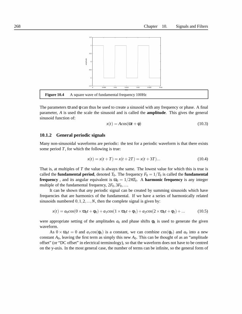
268 Chapter 10. Signals and Filters
-1.5
-1
-0.5
0
0.5
1
1.5
0 0.005 0.01 0.015 0.02 0.025 0.03am
plitu
de
time
Figure 10.4 A square wave of fundamental frequency 100Hz
The parametersω andφ can thus be used to create a sinusoid with any frequency or phase. A finalparameter,A is used the scale the sinusoid and is called theamplitude. This gives the generalsinusoid function of:
x(t) = Acos(ωt + φ) (10.3)
10.1.2 General periodic signals
Many non-sinusoidal waveforms are periodic: the test for a periodic waveform is that there existssome periodT, for which the following is true:
x(t) = x(t +T) = x(t +2T) = x(t +3T)... (10.4)
That is, at multiples ofT the value is always the same. The lowest value for which this is true iscalled thefundamental period, denotedT0. The frequencyF0 = 1/T0 is called thefundamentalfrequency , and its angular equivalent isω0 = 1/2πT0. A harmonic frequency is any integermultiple of the fundamental frequency, 2F0,3F0, ....
It can be shown thatany periodic signal can be created by summing sinusoids which havefrequencies that are harmonics of the fundamental. If we have a series of harmonically relatedsinusoids numbered 0,1,2, ...,N, then the complete signal is given by:
x(t) = a0cos(0×ω0t + φ0)+a1cos(1×ω0t + φ1)+a2cos(2×ω0t + φ2)+ ... (10.5)
were appropriate setting of the amplitudesak and phase shiftsφk is used to generate the givenwaveform.
As 0×ω0t = 0 anda1cos(φ0) is a constant, we can combinecos(φ0) and a0 into a newconstantA0, leaving the first term as simply this newA0. This can be thought of as an “amplitudeoffset” (or “DC offset” in electrical terminology), so thatthe waveform does not have to be centredon the y-axis. In the most general case, the number of terms can be infinite, so the general form of

Section 10.1. Analogue signals 269
-1.5
-1
-0.5
0
0.5
1
1.5
0 0.005 0.01 0.015 0.02 0.025 0.03
ampl
itude
time
(a) superimposed sine waves of the first and thirdharmonics
-1.5
-1
-0.5
0
0.5
1
1.5
0 0.005 0.01 0.015 0.02 0.025 0.03
ampl
itude
time
(b) superimposed sine waves of the first to seventhharmonics
-1.5
-1
-0.5
0
0.5
1
1.5
0 0.005 0.01 0.015 0.02 0.025 0.03
ampl
itude
time
(c) synthesised wave of the first and third harmon-ics
-1.5
-1
-0.5
0
0.5
1
1.5
0 0.005 0.01 0.015 0.02 0.025 0.03
ampl
itude
time
(d) synthesised waves of the harmonics 1 to 7
-1.5
-1
-0.5
0
0.5
1
1.5
0 0.005 0.01 0.015 0.02 0.025 0.03
ampl
itude
time
(e) synthesised waveform of harmonics 1 to 29
Figure 10.5 Fourier synthesis of a square wave for different numbers of harmonics

270 Chapter 10. Signals and Filters
equation 10.5 is:
x(t) = A0 +∞
∑k=1
akcos(kω0t + φk) (10.6)
Equation 10.6 is a specific form of theFourier series, one the most important concepts in signalprocessing. The process as just described is known asFourier synthesis, that is the process ofsynthesising signals by using appropriate values and applying the Fourier series. It should be notedthat while the sinusoids must have frequencies that are harmonically related, the amplitudes andphases of each sinusoid can take on any value. In other words,the form of the generated waveformis determined solely by the amplitudes and phases.
To demonstrate some of the properties of Fourier synthesis consider the task of synthesisinga square wave, as shown in Figure 10.4, and defined by:
x(t) =
1 for 0≤ t ≤ 12T0
−1 for 12T0≤ t ≤ T0
(10.7)
This signal can be generated by adding only the odd harmonicsof the fundamental, using the samephase for every harmonic, and choosing appropriate amplitudes:
ak =
4/kπ k = 1,3,5, ...0 k = 0,2,4,6, ...
(10.8)
Figure 10.5 shows the process of creating a square waveform by adding more and more harmonicsto the fundamental sinusoid.
We have only been able to generate the square waveform because we knew the appropriatevalues forak andφk for every harmonic. The converse problem, of finding unknownak andφk
for a known waveform functionx(t) is termedFourier analysis and will be described in section10.1.4.
10.1.3 Sinusoids as complex exponentials
While the general form of the sinusoid,x(t) = Acos(ω0t + φ) faithfully represents a sinusoid, itturns out that for types of operations we consider below, a different form of the sinusoid, knownas thecomplex exponentialgreatly simplifies the mathematics and calculations. The basis of thisrepresentation isEuler’s formula which states:
ejθ = cosθ+ jsinθ (10.9)
whereθ is any number andj =√−1. Theinverse Euler formulas are:
cosθ =ejθ +e− jθ
2(10.10)
sinθ =ejθ−e− jθ
2 j(10.11)
Section 10.1. Analogue signals 271
From here on, we will make frequent use ofcomplex numbers, which comprise of a realpartx, and an imaginary partjy, where j =
√−1, such thatz= x+ jy.
If we add an amplitude and setθ = ωt + φ, we get;
Aejω+φ = Acos(ωt + φ)+ jAsin(ωt + φ) (10.12)
where A, ω and φ are all real and have the same meanings as before. At first glance, thisseems insane - why on earth should we replace our previous, easily interpretable representationof a sinusoid, A cos(ωt + φ), with a different equation, that includes an extra, imaginary term,jAsin(ωt +φ), and then rewrite it as an exponential? The reason is purely that it makes manipula-tion much easier. As a demonstration, consider the following, which allows us to represent phasedifferently:
x(t) = Aejωt+φ = Aejφejωt (10.13)
ejφ is a constant, not dependent ont, and we can combine this with the amplitudeA to form a newconstant,X, giving:
x(t) = Xejωt = Aejωt+φ = Aejωtejφ (10.14)
Here, the new quantityX, is acomplexamplitude and describes both the original amplitude and thephase. The purely sinusoid part,ejωt is now free of phase information. This is highly significant,because it turns out that in general, we want to describe, modify and calculate amplitude and phasetogether. (From here on, amplitude terms in complex exponential expressions will generally becomplex - if the pure amplitude is required, it will be denoted |A|.)
While the complex exponential form has an imaginary part.jsin(ωt) to the waveform, inphysical systems such as speech, this does not exist and the signal is fully described by the realpart. When requiring a physical interpretation, we simply ignore the imaginary part ofejωt .
Using the complex exponential form, we can write a more general form of the Fourier syn-thesis equation:
x(t) =∞
∑−∞
akejkω0t (10.15)
whereak is a complex amplitude representing the amplitude and phaseof thekth harmonic:
ak = Akejφk (10.16)
Equation 10.15 is the general form of Fourier synthesis which sums harmonics from−∞ to +∞.It can be shown that for all real valued signals (that is ones like speech with no imaginary part),the complex amplitudes areconjugate symmetricsuch thata−k = ak. In this case, the negative

272 Chapter 10. Signals and Filters
harmonics don’t add any new information and the signal can befaithfully constructed by summingfrom 0 to∞:
x(t) =∞
∑0
akekω0t (10.17)
In fact, the summation from−∞ to +∞ keeps the mathematics easier, so we often use the completeform.
10.1.4 Fourier Analysis
What if we know the equation for the periodic signalx(t) and wish to find the complex amplitudesak for each harmonic? TheFourier analysis equation gives this:
ak = 1/T0
Z T0
0x(t)e− jkω0tdt (10.18)
It should be clear, that integrating a sinusoid over a singleperiod will give 0 for all sinusoids1
Z T0
0sin(ω0t)dt = 0
This holds for any harmonic also - while we have more positiveand negative areas, as we have anequal number of them then the sum will always be zero. In exponential form, we can thereforestate:
Z T0
0ekω0tdt = 0
Now consider the calculation of theinner product of two harmonically related sinusoids, whereone is the complex conjugate of the other
Z T0
0ejkω0te− jl ω0tdt
this can be written:Z T0
0eω0(k−l)tdt
Whenk 6= l , this quantityk− l is an other integer, which will represent one of the harmonics. Butwe know from equation 10.1.4 that this will always evaluate to 0. However, whenk = l , thenk− l = 0 so the integral is
Z T0
0ejω00tdt =
Z T0
01dt = T0
1 This can be seen by using the interpretation that integration over an interval is finding the area between the curveand the x-axis. From the sine wave in Figure 10.2 we see the area between 0 andπ will cancel out the area betweenπand 2π.

Section 10.1. Analogue signals 273
-1.5
-1
-0.5
0
0.5
1
1.5
0 0.005 0.01 0.015 0.02
ampl
itude
time
(a) The square wave and sine waves of the firstharmonic
-1.5
-1
-0.5
0
0.5
1
1.5
0 0.005 0.01 0.015 0.02
ampl
itude
time
(b) multiplication of square wave and sine wave ofthe first harmonic
-1.5
-1
-0.5
0
0.5
1
1.5
0 0.005 0.01 0.015 0.02
ampl
itude
time
(c) The square wave and sine wave of the secondharmonic
-1.5
-1
-0.5
0
0.5
1
1.5
0 0.005 0.01 0.015 0.02
ampl
itude
time
(d) multiplication of square wave and sine wave ofthe second harmonic
-1.5
-1
-0.5
0
0.5
1
1.5
0 0.005 0.01 0.015 0.02
ampl
itude
time
(e) The square wave and sine wave of the thirdharmonic
-1.5
-1
-0.5
0
0.5
1
1.5
0 0.005 0.01 0.015 0.02
ampl
itude
time
(f) multiplication of square wave and sine wave ofthe third harmonic
Figure 10.6 Fourier synthesis of a square wave for different numbers of harmonics. We can seethat the curve in figure d has symmetry about the x-axis and so there is an equal amount of area aboveand below the x-axis. The total area is therefore 0, hence thecontribution of the second harmonic to asquare wave is 0. Figures b and f have more area beneath the x-axis than above, hence the total areawill sum to a non-zero value.
274 Chapter 10. Signals and Filters
Using these results, we can state theorthogonality property of sinusoids:
Z T0
0ejkω0te− jl ω0tdt =
0 if k 6= lT0 if k = l
(10.19)
Imagine we have a signalx(t) = ejl ω0t of known fundamental period but unknown harmonic (thatis, we knowω0 but notl ). We can calculate the inner product of this signal with eachharmonick=1,2,3... of the fundamental. All the answers will be zero except the one for when the harmonicsare the same (k = l ). As a general periodic signal is just the sum of a set of harmonics, we canuse this method to find the value of every harmonic in a signal.Mathematically, we show this bystarting with the Fourier series:
x(t) =∞
∑−∞
akejkω0t
If we multiply both sides by the complex conjugate exponential and integrate over periodT0 weget:
Z T0
0x(t)e− jl ω0tdt =
Z T0
0
( ∞
∑−∞
akejkω0t
)
e− jl ω0tdt
=∞
∑−∞
ak
(Z T0
0ejkω0te− jl ω0tdt
)
=∞
∑−∞
ak
(Z T0
0e− j(k−l)ω0tdt
)
= al T0 (10.20)
and if we replacel with k we get the Fourier analysis definition.Fourier analysis can easily be demonstrated graphically. Figure 10.6 shows the multiplica-
tion of a square wave with sinusoids of different harmonics.It can be seen from the graphs that thefirst and third harmonics have a non-zero area, and so their Fourier coefficient will be non-zero.The multiplication of the square wave and second harmonic produces a curve which is symmetri-cal about the x-axis and so the area beneath the x-axis will exactly match the area above, resultingin a total area of 0.
One interesting point about the Fourier synthesis and analysis equations is that while theyhave a similar form, one is a sum while the other is an integral. This is solely because periodicsignals are composed of a integer number (possibly infinite)of discrete harmonics, necessarilyenforcing a discrete frequency description. The waveform however, is a continuous function. Aswe shall see, there are several variations on these equations in which frequency can be continuousor time discrete.
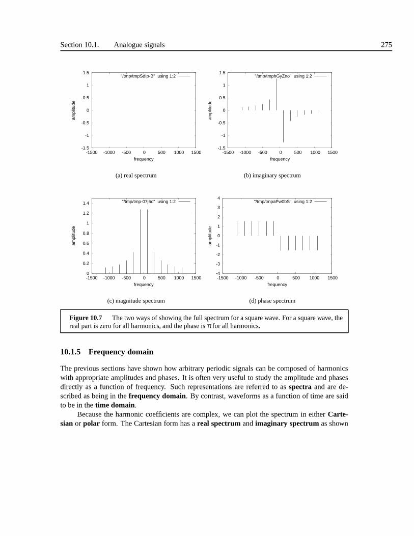
Section 10.1. Analogue signals 275
-1.5
-1
-0.5
0
0.5
1
1.5
-1500 -1000 -500 0 500 1000 1500
ampl
itude
frequency
"/tmp/tmpSdIp-B" using 1:2
(a) real spectrum
-1.5
-1
-0.5
0
0.5
1
1.5
-1500 -1000 -500 0 500 1000 1500
ampl
itude
frequency
"/tmp/tmphGyZno" using 1:2
(b) imaginary spectrum
0
0.2
0.4
0.6
0.8
1
1.2
1.4
-1500 -1000 -500 0 500 1000 1500
ampl
itude
frequency
"/tmp/tmp-07j6o" using 1:2
(c) magnitude spectrum
-4
-3
-2
-1
0
1
2
3
4
-1500 -1000 -500 0 500 1000 1500
ampl
itude
frequency
"/tmp/tmpaPw0bS" using 1:2
(d) phase spectrum
Figure 10.7 The two ways of showing the full spectrum for a square wave. For a square wave, thereal part is zero for all harmonics, and the phase isπ for all harmonics.
10.1.5 Frequency domain
The previous sections have shown how arbitrary periodic signals can be composed of harmonicswith appropriate amplitudes and phases. It is often very useful to study the amplitude and phasesdirectly as a function of frequency. Such representations are referred to asspectra and are de-scribed as being in thefrequency domain. By contrast, waveforms as a function of time are saidto be in thetime domain.
Because the harmonic coefficients are complex, we can plot the spectrum in eitherCarte-sian or polar form. The Cartesian form has areal spectrum andimaginary spectrum as shown

276 Chapter 10. Signals and Filters
-1.5
-1
-0.5
0
0.5
1
1.5
-1500 -1000 -500 0 500 1000 1500
ampl
itude
frequency
"/tmp/tmphBTt1l" using 1:2
(a) real spectrum
-1.5
-1
-0.5
0
0.5
1
1.5
-1500 -1000 -500 0 500 1000 1500
ampl
itude
frequency
"/tmp/tmpDlzYtT" using 1:2
(b) imaginary spectrum
0
0.2
0.4
0.6
0.8
1
1.2
1.4
-1500 -1000 -500 0 500 1000 1500
ampl
itude
frequency
"/tmp/tmpY-nEpG" using 1:2
(c) magnitude spectrum
-4
-3
-2
-1
0
1
2
3
4
-1500 -1000 -500 0 500 1000 1500
ampl
itude
frequency
"/tmp/tmpi4kvjA" using 1:2
(d) phase spectrum
Figure 10.8 Spectra for square wave with delay. The real and imaginary spectra are clearly differ-ent from figure 10.7. The magnitude spectrum is the same, and the phase spectrum is the same apartfrom the additional shift.
in Figures 10.7a and 10.7b . Alternatively, we can plot the coefficients in polar form with amag-nitude spectrum andphase spectrum, as shown in Figures 10.7c and 10.7d. For the Cartesianinterpretation, we see that the all the real parts are 0, and only the imaginary spectrum has values.This is equivalent to saying that no cosine functions were used, only sines: this can be seen inFigure 10.5. This can also be seen from the phase spectrum, were all the phases have a value ofπ/2, again showing that only sine waves are used.
Now consider the square wave that is identical to the one we have been analysing, exceptthat it is shifted 1/4 period to the left. If we subject this to Fourier analysis, we get the spectra
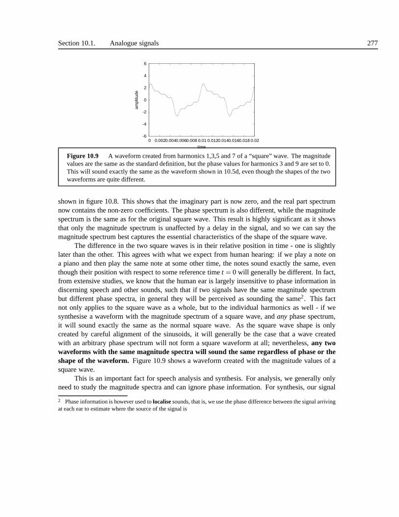
Section 10.1. Analogue signals 277
-6
-4
-2
0
2
4
6
0 0.002 0.004 0.006 0.008 0.01 0.012 0.014 0.016 0.018 0.02am
plitu
de
time
Figure 10.9 A waveform created from harmonics 1,3,5 and 7 of a “square” wave. The magnitudevalues are the same as the standard definition, but the phase values for harmonics 3 and 9 are set to 0.This will sound exactly the same as the waveform shown in 10.5d, even though the shapes of the twowaveforms are quite different.
shown in figure 10.8. This shows that the imaginary part is nowzero, and the real part spectrumnow contains the non-zero coefficients. The phase spectrum is also different, while the magnitudespectrum is the same as for the original square wave. This result is highly significant as it showsthat only the magnitude spectrum is unaffected by a delay in the signal, and so we can say themagnitude spectrum best captures the essential characteristics of the shape of the square wave.
The difference in the two square waves is in their relative position in time - one is slightlylater than the other. This agrees with what we expect from human hearing: if we play a note ona piano and then play the same note at some other time, the notes sound exactly the same, eventhough their position with respect to some reference timet = 0 will generally be different. In fact,from extensive studies, we know that the human ear is largelyinsensitive to phase information indiscerning speech and other sounds, such that if two signalshave the same magnitude spectrumbut different phase spectra, in general they will be perceived as sounding the same2. This factnot only applies to the square wave as a whole, but to the individual harmonics as well - if wesynthesise a waveform with the magnitude spectrum of a square wave, andany phase spectrum,it will sound exactly the same as the normal square wave. As the square wave shape is onlycreated by careful alignment of the sinusoids, it will generally be the case that a wave createdwith an arbitrary phase spectrum will not form a square waveform at all; nevertheless,any twowaveforms with the same magnitude spectra will sound the same regardless of phase or theshape of the waveform.Figure 10.9 shows a waveform created with the magnitude values of asquare wave.
This is an important fact for speech analysis and synthesis.For analysis, we generally onlyneed to study the magnitude spectra and can ignore phase information. For synthesis, our signal
2 Phase information is however used tolocalisesounds, that is, we use the phase difference between the signal arrivingat each ear to estimate where the source of the signal is

278 Chapter 10. Signals and Filters
generator need only get the magnitude information correct,the phase is much less important.We will now discuss thefrequency rangeover which the spectrum is defined. First note that
when considering frequency plots of continuous signals, itis important to realise that the upperlimit in the graph is arbitrarily chosen - in fact all continuous signals have frequency values to∞. Just because humans can only hear frequencies up to say 20,000Hz doesn’t mean to say theystop being physically present above this level. Secondly note that the spectra for the square wavein Figures 10.7 and 10.8 are plotted with negative as well as positive values for frequency. Ourinitial definition of frequency stated that it was the inverse of the period, and since we can’t havea negative period, why negative frequency? The use of negative frequency comes from the factthat a true continuous signal, is defined in time from−∞ to ∞. As we shall see later, time andfrequency share a duality, with neither being more “real” than the other. As time extends from−∞to ∞, so does frequency.
If we take the cosine sinusoid definition and write it in termsof complex exponentials usingthe inverse Euler equation 10.11,
x(t) = cos(ωt) =ejωt +e− jωt
2
x′(t) = sin(ωt) =
ejωt +e− jωt
2 j
we see that this signal actually hastwo frequencies, a positiveω and a negativeω. This is a generalproperty of allreal signals: they will have conjugate symmetry aroundω = 0, i.e. the vertical axisin the spectrum. Conjugate symmetry is a complex property, in which the real part of the spectrumis reflected in the vertical axis, and the imaginary part is reflected in the vertical axis and again inthe horizontal axis. This is clearly seen in Figures 10.7 and10.8.
Signals which are not purely real, such asejωt itself, only have one frequency value. Becauseof this, it can be argued that complex exponentials really are a simpler form that the sine or cosineform.
10.1.6 The Fourier transform
In general, we need to analyse non-periodic signals as well as periodic ones. Fourier synthesisand analysis can not deal with non-periodic signals, but a closely related operation, theFourierTransform is designed to do just this. By definition, the Fourier transform is:
X( jω) =
Z ∞
−∞x(t)e− jωdt (10.21)
Its similarity to Fourier analysis (Equation 10.18) shouldbe clear:
ak = 1/T0
Z T0
0x(t)e− jkω0tdt

Section 10.1. Analogue signals 279
-1.5
-1
-0.5
0
0.5
1
1.5
-0.03 -0.02 -0.01 0 0.01 0.02 0.03
ampl
itude
time
(a)
-0.6
-0.4
-0.2
0
0.2
0.4
0.6
0.8
1
1.2
1.4
-1500 -1000 -500 0 500 1000 1500
ampl
itude
frequency
"/tmp/tmp_V_JV0" using 1:2
(b)
-1.5
-1
-0.5
0
0.5
1
1.5
-0.03 -0.02 -0.01 0 0.01 0.02 0.03
ampl
itude
time
(c)
-0.2
0
0.2
0.4
0.6
0.8
1
-1500 -1000 -500 0 500 1000 1500
ampl
itude
frequency
"/tmp/tmped7xML" using 1:2
(d)
-1.5
-1
-0.5
0
0.5
1
1.5
-0.03 -0.02 -0.01 0 0.01 0.02 0.03
ampl
itude
time
(e)
-0.2
-0.1
0
0.1
0.2
0.3
0.4
0.5
-1500 -1000 -500 0 500 1000 1500
ampl
itude
frequency
"/tmp/tmpvld6dE" using 1:2
(f)
Figure 10.10 Real spectra for a signal of constant shape but decreasing period. As the perioddecreases, the harmonics get closer, but the envelope of thespectrum stays the same. In the limit,period→ ∞, the harmonics will be infinitely close and the spectrum willbe be a continuous functionof frequency.

280 Chapter 10. Signals and Filters
The differences are that firstly we are now computing an integral from−∞ to ∞ rather than overa single period: as our signal now may not have a period we can not of course integrate over it.Secondly, the result is acontinuousfunction over frequency, not simply the complex amplitudesfor a set of discrete harmonics. For non-periodic signals wehave to abandon the idea of harmonics:the magnitude and phase are instead expressed as a continuous function of frequency.
The Fourier transform can be explained as follows. Imagine we have arectangular pulsewaveformx(t), which has values for a finite durationT, defined as follows:
x(t) =
1 for −1/2T ≤ t ≤ 12T
−1 otherwise
This is equivalent to just a single period of a square wave, centred att = 0 with values−1 every-where else. This is clearly not periodic. But imagine we artificially make a periodic version byreplicating its shape as shown in Figure 10.10a. This gives us our familiar square wave and byFourier analysis we get the spectrum, the real part of which is shown in Figure 10.10b. Now imag-ine we perform the same trick, but move the repetitions further apart - in effect we are increasingthe period of our waveform (Figure 10.10c). After performing Fourier analysis, we get the realspectrum shown in Figure 10.10d. It should be immediately apparent that the overall shape (theenvelope) is the same, but that the harmonics are now much closer together, as we would expectof a waveform of longer period. If we extend the period further still (Figure 10.10e), we get thereal spectrum shown in Figure 10.10f and here the harmonics are closer still. AsT0→ ∞, the“harmonics” in the spectrum become infinitely dense, resulting in a continuous function.
Let us now calculate the continuous spectrum of the rectangular pulse directly. From itsdefinition, the Fourier transform of the waveform is:
X( jω) =
Z T/2
−T/2e− jωtdt
=e− jωT/2
− jω− −ejωT/2
− jω
We can use the inverse Euler formula to simplify this as:
X( jω) =sin(ωT/2)
ω/2(10.22)
Any function of the formsin(x)/x is known as asinc function. The real spectrum of this isshown in Figure 10.10b, and we can see that this has the exact shape suggested by the envelopeof the harmonics in Figure 10.10. Figures 10.10c and 10.10d show the waveform and Fouriertransform for a pulse of shorter duration. The Fourier transform is now more “spread-out”, andthis demonstrates an important of the Fourier transform known as thescaling property.
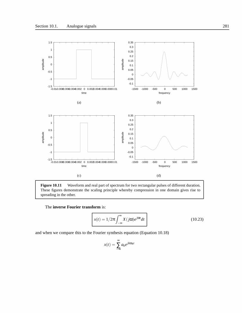
Section 10.1. Analogue signals 281
-1.5
-1
-0.5
0
0.5
1
1.5
-0.01-0.008-0.006-0.004-0.002 0 0.002 0.004 0.006 0.008 0.01
ampl
itude
time
(a)
-0.1
-0.05
0
0.05
0.1
0.15
0.2
0.25
0.3
0.35
-1500 -1000 -500 0 500 1000 1500
ampl
itude
frequency
(b)
-1.5
-1
-0.5
0
0.5
1
1.5
-0.01-0.008-0.006-0.004-0.002 0 0.002 0.004 0.006 0.008 0.01
ampl
itude
time
(c)
-0.1
-0.05
0
0.05
0.1
0.15
0.2
0.25
0.3
0.35
-1500 -1000 -500 0 500 1000 1500
ampl
itude
frequency
(d)
Figure 10.11 Waveform and real part of spectrum for two rectangular pulses of different duration.These figures demonstrate the scaling principle whereby compression in one domain gives rise tospreading in the other.
The inverse Fourier transform is:
x(t) = 1/2πZ ∞
−∞X( jω)ejωtdt (10.23)
and when we compare this to the Fourier synthesis equation (Equation 10.18)
x(t) =∞
∑−∞
akejkω0t

282 Chapter 10. Signals and Filters
-1.5
-1
-0.5
0
0.5
1
1.5
-2000 -1500 -1000 -500 0 500 1000 1500 2000
ampl
itude
frequency
-0.15
-0.1
-0.05
0
0.05
0.1
0.15
0.2
0.25
0.3
0.35
-0.08 -0.06 -0.04 -0.02 0 0.02 0.04 0.06 0.08
ampl
itude
time
Figure 10.12 Figure a) is the real part of a spectrum, and figure b) is its inverse Fourier transform.Along with Figure 10.11, these figures demonstrate the duality principle.
we can see that the discrete frequency representation of a fundamental frequency multiplied by aharmonic index has now been replaced with a continuous frequency variableω.
Let us now use the inverse Fourier transform to find the waveform for a defined spectrum.Consider a spectrum which is 1 within a certain frequency region and -1 elsewhere:
X( jω) =
1 for −ωb≤ t ≤ ωb
−1 otherwise(10.24)
The inverse Fourier transform of this is:
x(t) = 1/2πZ ωb
−ωb
ejωtdt
=12π
e− jωbt
− j2πt− −e− jωbt
− j2πt
=sin(ωbt)
πt(10.25)
This is shown in figure 10.12. When we compare equation 10.25 to equation 10.22 and figure10.11 to figure 10.12 we see that the Fourier transform of a rectangular pulse is a sinc spectrum,and the inverse Fourier transform of a rectangular spectrumis a sinc waveform. This demonstratesanother special property of the Fourier transform known as theduality principle . These and othergeneral properties of the Fourier transform are discussed further in section 10.3.

Section 10.2. Digital signals 283
10.2 DIGITAL SIGNALS
We now turn our attention todigital signals. All the signals we have discussed up until now areanalogue signalsin which the amplitude and time dimensions are represented by real numbers.By contrast, Digital signals are represented by a sequence of integers. In the “real-world”, mostsignals are analogue, including speech signals, where the amplitude is a measure of sound pressurelevel or some other physical quantity. Digital signals are mostly found in computers.
10.2.1 Digital waveforms
A digital signal is represented by a sequence of evenly spaced points, the value at each point beingthe amplitude, represented by an integer. This integer amplitude value can be interpreted as thedigital manifestation of sound pressure level, or voltage or some other such analogue quantity.Formally, a digital sequence is represented as follows:
x[n] = ...,x−2,x−1,x0,x1,x2, ... (10.26)
For digital sequences, it is usual to usen and writex[n], to distinguish from continuous timet in analogue signals. Each point in the sequence is called asample, and the distance between onesample and the next is called thesample period, Ts. Thesample rateor sample frequencyis givenby Fs = 1/Ts. The sample rate limits the frequencies which the digital signal can describe. Thehighest frequency that a digital signal can contain is called theNyquist frequency and is exactlyhalf the sample rate.
The choice of sample rate is a compromise between wanting to have the highest possiblequality (high sample rate) and the lowest storage or transmission cost (low sample rate). Practicaldata from human perception studies shows that the limit of human hearing is about 20,000Hz andthis figure would lead us to use sampling rates of>40,000 Hz. Indeed, compact discs and digitalaudio tapes have sampling rates of 44,100Hz and 48,000Hz respectively. However, it can be shownthat for speech signals, very little useful speech energy isfound in the higher frequencies, and sosample rates of 16,000Hz are often used and found to be perfectly adequate for accurate represen-tation of speech signals. Where space is tight, lower sampling rates are used, most commonly inthe telephone which has a standardised sample rate of 8000Hz. While speech at this sample rateis normally quite intelligible, it is clear that it sounds much poorer than when higher sample ratesare used.
The bit range describes thedynamic range of a digital signal, and is given by the rangeof the integer used to store a sample. Widely used values are 16 bits, which gives an absolutedynamic range of 216, meaning the amplitude of the sample can range from -32,768 to 32,767.Dynamic range is normally expressed in the logarithmic decibel scale. In digital signals, we takethe reference as 1 and therefore the dynamic range of a 16 bit signal is:
10log(216)≈ 96dB (10.27)

284 Chapter 10. Signals and Filters
To save on space and transmission bandwidth, telephones andother systems frequently use 8bits (48db) and 12 bits (72db). At 8 bits, speech quality is noticeably worse than at 16 bits. 12 bitsis a reasonable compromise, but if space is not an issue (and with most types of speech synthesisit is not), 16 bits is normally used.
10.2.2 Digital representations
We use somewhat different notation when dealing with digital signals. First, an integern is usedinstead oft for the time axis, wheren is related tot by the sample period:
n = tTs (10.28)
From this, we can relate the continuous signalx(t) and digital signalx[n] by x[n] = x(n/Ts). Weuse square brackets “[ ]” rather than parentheses (round brackets) “( )” when describing digitalfunctions. Strictly speaking, a signalx[n] is in then-domain but we shall informally refer to it asbeing in the time domain.
Secondly, it is common to usenormalised frequency, rather than natural frequency. From10.28 we see that the relationship between frequency, angular frequency and normalise angularfrequency is
ω =ωTs
=2πFTs
(10.29)
Using n and normalised angular frequencyω makes calculations easy as the equations arethe same regardless of sample rate. To convert to real frequency, the normalised frequency issimply multiplied by the sample rate. In general, we use the same terms for amplitude and phasefor both analogue and digital signals.
10.2.3 The discrete-time Fourier transform
For a continuous signal, we can move from the time domain to the frequency domain via theFourier transform, but as we are now dealing with digital signals, this formula cannot be used di-rectly. We will now derive an equivalent transform for digital signals. Starting with the previouslydefined Fourier transform (Equation 10.21)
X( jω) =
Z ∞
−∞x(t)e− jωtdt
we can use this on a digital sequence with the relationx[n] = x(n/Ts). The Fourier transformis calculated as a integral over a range, which can be interpreted as finding the area under thecurve over this range. The numerical method of the Riemann sum says that we can approximate acontinuous area function by adding up the areas of separate rectangles. The area of each rectangleis the value of the function at that point multiplied by the width of the rectangle. In our case,

Section 10.2. Digital signals 285
the width of the rectangle is the sample periodTs. This gives a numerical version of the Fouriertransform:
X( jω) =∞
∑−∞
(x(nTs)e− jωt)Ts
Ts is independent of the integral, we move it outside, and usex[n] in place ofx(nTs) giving:
X( jω) = Ts
∞
∑−∞
x[n]e− jωnTs
We can get rid of theTs by making use of normalised frequency,ω = ω/Ts. The result is thediscrete-time Fourier transform or DTFT :
X(ejω) =∞
∑−∞
x[n]e− jωn (10.30)
It should be clear that the DTFT is a transform in which time isdiscrete but frequency is contin-uous. As we shall see in later sections, the DTFT is a very important transform in its own rightbut for computational purposes, it has two drawbacks. Firstly, the infinite sum is impractical, andsecondly we wish to obtain a representation for frequency that is useful computationally, and sucha representation must be discrete.
10.2.4 The discrete Fourier transform
For the first problem, we choose a sufficiently large intervalL such that the samples outside 0<n < L are zero. For the second problem, we will use a similar operation to time domain samplingand “sample” the spectrum at discrete intervals. Just asn = t.Ts, we define the spacing betweeneach discrete frequency asFs/N = 1/(NTs) whereN is the total number of frequency values wewant. Each angular frequency therefore lies at
ωk =2πNTs
giving the transform:
X(ejωk) =L
∑n=0
x[n]e− jωkn
If we setL = N (discussed below), and use the above definition ofωk, we can write 10.2.4 in amore compact usable form:
X[k] =N−1
∑n=0
x[n]e− j 2πN kn (10.31)

286 Chapter 10. Signals and Filters
which gives us the standard definition of theDiscrete Fourier Transform or DFT.The interpretation is the same as for the Fourier transform defined in section 10.1.6; For
each required frequency value, we multiply the signal by a complex exponential waveform ofthat frequency, and sum the result over the time period. The result is a complex number whichdescribes the magnitude and phase at that frequency. The process is repeated until the magnitudeand phase is found for every frequency.
The DFT states that the length of the analysed waveform and the number of resultant fre-quency values are given byN. This makes intuitive sense: if we only analyse a few samples, wecan only expect a somewhat crude version of the spectrum; by analysing more samples, we havemore information “to go on” and can fill in more detail in the spectrum: that is, the points in thespectrum (ωk) get closer and closer. AsN→ ∞, we analyse all the waveform values, and the dis-tance between the frequency points in the spectrum→ 0. This is exactly the case that the DTFTdescribes.
Both the DTFT and DFT have inverse transforms:
x[n] =12π
Z π
−πX(ejω).ejωndω (10.32)
x[n] =1N
N−1
∑n=0
x[n]ej 2πN kn (10.33)
In practice an algorithm called theFast Fourier Transform or FFT is commonly used tocalculate the DFT. This is not anothertypeof transform, merely a fast way of calculating a DFT:the result for the FFT is exactly the same as for the DFT. The FFT only works for values ofNwhich are powers of 2, hence it is common to findN set to 256, 512. If a DFT of a differentN isrequired, a time signal of the next highest power of 2 is chosen, and the extra values are set to 0.So for example, if we have a signal of length 300, we setN = 512, “pad” the extra 212 values with0, and the calculate a 512 point FFT. The use of the FFT is pervasive in practice, and one oftenhears references to “the FFT of the signal” etc. We repeat, interms of the outcome, the FFT andDFT are exactly the same and hence taking “the FFT of the signal” is no different from “takingthe DFT”. An overview of the FFT can be found in Oppenheim and Schafer [342].
10.2.5 The z-Transform
We now introduce another important transform, thez-transform 3. The z-transform is perhaps themost useful of all transforms in practical digital signal processing. It is defined as:
X(z) =∞
∑n=−∞
x[n]z−n (10.34)
3 what? you can’t be serious -anothertransform!

Section 10.2. Digital signals 287
This should look familiar - if we usez= ejω, we get:
X(ejω) =∞
∑−∞
x[n]e− jωn
which is the discrete-time Fourier transform, Equation 10.30. Just like the DTFT, the z-transformis a transform which operates on adigital signal but which produces acontinuousfunction.
An important property of the z-transform is its affect on a delay. If we define a signal
y[n] = x[n−nd]
that is, a delayed version ofx[n]. By use of a dummy variablem = n− nd, we can find its z-transform as follows
Y(z) =∞
∑n=−∞
y[n]z−n
=∞
∑n=−∞
x[n−nd]z−n
=∞
∑m=−∞
x[m]znd−m
=∞
∑m=−∞
x[m]z−mznd
The summation inm is just the z-transform ofx defined inm rather, thann and so we can write:
Y(z) = X(z)znd (10.35)
Hence delaying a signal bynd multiplies its z-transform byznd . This important property of thez-transform and is discussed further in section 10.3.5.
Why use yet another transform? The reason is that by settingz to ejω we greatly simplifythe DTFT, and this simplification allows us to perform sophisticated operations in analysis andsynthesis with relatively simple mathematical operations. The key to the ease of use of the z-transform, is that equation 10.34, can be re-written as:
X(z) =∞
∑n=−∞
x[n](z−1)n (10.36)
That is, the transform can be written as apolynomialin z−1, so that the techniques of polynomialsolving can be brought to bear.
A final transform, theLaplace Transform, is frequently used in continuous time signalprocessing, and is the continuous time version of the z-transform. The z-transform and the Laplacetransform can be thought of as generalisations of the DTFT and Fourier transform respectively.The Laplace transform is not required in this book, as all oursignal processing is performed ondigital signals. We mention it here for completeness only.

288 Chapter 10. Signals and Filters
10.2.6 The frequency domain for digital signals
For continuous signals, we showed that the frequency domainextends to from−∞ to ∞ . However,for digital signals, we stated that a frequency of half the sampling rate, the Nyquist frequency, wasthe highest possible frequency that could be represented bya digital signal. What then is the rangeof the frequency domain? As for continuous signals the rangeextends from−∞ to ∞, but nonewinformation is found outside the Nyquist range. Rather, thespectrum repeats itself at multiplesof the Nyquist frequency. In other words, the spectrum of a digital signal isperiodic. It is forthis reason that the spectrum of digital signals, calculated from the DTFT is described asX(ejωt),rather thatX( jω) as is the normal for the Fourier transform. The “period” of the spectrum istwice the Nyquist frequency, as the spectrum is defined from−FN to +FN. In terms of normalisedfrequency, the frequency range is just−π to +π and so the “period” is 2π.
Just as with real continuous signals, real digital signals exhibit conjugate symmetry in thefrequency domain. Hence in a 512 point DFT the first 256 valueswill be conjugate symmetricwith the second 256. For this reason only half a digital spectrum is normally plotted, and this willhave half the number of values used to calculated the DFT.
10.3 PROPERTIES OFTRANSFORMS
At first sight the number of transforms can seem unnecessarily large. (recall that each has aninverse transform also.) Why do we need so many? The differences are simply attributable to uswanting to use both continuous and discrete representations for time and frequency, and to makeanalysis easier (in the case of the z-transform and Laplace transform). The differences betweenthem can be clearly shown in the following table:
Discrete Time Continuous timeDiscrete Frequency Discrete Fourier Transform (DFT) Fourier analysis, periodic waveformContinuous Frequency Discrete Fourier Transform (DTFT)Fourier TransformContinuous variable z-transform Laplace Transform
We now describe various general properties of the transforms we have introduced. Fordemonstration purposes, we will describe these using the Fourier transform, but in general thefollowing hold for all our transforms.
10.3.1 Linearity
All the transforms arelinear. If we have an inputx(t) = αs1(t)+βs2(t), thenX( jω) = αX1( jω)+βX2( jω). The proof of this for the Fourier transform is:

Section 10.3. Properties of Transforms 289
X( jω) =Z ∞
−∞(αx1(t)+ βx2(t))e
− jωt
= αZ ∞
−∞x1(t)e
− jωt + βZ ∞
−∞x2(t)e
− jωt
= αX1( jω)+ βX2( jω) (10.37)
10.3.2 Time and Frequency Duality
The Fourier transform and inverse Fourier transform have very similar forms. If we have a functiong(.) and define a signal asg(t) then its Fourier transform will beG( jω) = F g(t) (here we usethe notationF to denote the operation of the Fourier Transform). If we define the spectrum interms of our function asg(ω) and take the inverse Fourier transform, we getG(t) = 2πF g(ω).It should be clear that the form is the same apart from the 2π term, which is required because ofour use of angular frequency.
g(t)F−→ G(w) (10.38)
g(ω)I F←−− G(t) (10.39)
Figure 10.12 demonstrates this property.
10.3.3 Scaling
We have already described the Fourier transform of a pulse ofdifferent durations in section 10.1.6.The shorter duration pulse has a spectrum that is more spreadout, and the longer duration pulsehas a more contracted spectrum. This is known as thescaling property, which states that:com-pressing a signal will stretch its Fourier transform and vice versa. This can be formally statedas:
x(at)F−→ 1|a|X( j(w/a)) (10.40)
10.3.4 Impulse Properties
From the scaling property, we know that as the duration of thepulse approaches zero, the spectrumspreads out more and more. In the limit, we reach theunit impulse, which has zero width. Thisis a particularly important signal. For digital signals, this is simply defined as a signal,δ[n], whichhas a value 1 at time 0 and a value 0 elsewhere. For continuous-time signals, the definition is alittle trickier, but is described as a signal which has values of zero everywhere apart at time 0 (i.e.zero width), and at that time it is described by an integral which defines itsarea(not height) as 1:
δ(t) = 0 for t 6= 0 (10.41)Z ∞
−∞δ(t)dt = 1 (10.42)

290 Chapter 10. Signals and Filters
As expected from the scaling property, the Fourier transform of an impulse is a function thatis “infinitely stretched”, that is, the Fourier Transform is1 at all frequencies. Using the dualityprinciple, a signalx(t) = 1 for all t will have a Fourier transform ofδ(ω), that is, an impulse attime ω = 0. This is to be expected - a constant signal (a d.c. signal in electrical terms) has novariation and hence no information at frequencies other than 0.
δ(t)F−→ 1 (10.43)
1F−→ δ(ω) (10.44)
10.3.5 Time delay
A signalx(t) that is delayed by timetd is expressed asx(t− td). If we denote the Fourier transformof x(t) asX( jω) and the Fourier transform ofx(t − td) asXd( jω), we see that from the Fouriertransform definition thatXd( jω) is:
Xd( jω) =
Z ∞
−∞x(t− td)e
− jωtdt (10.45)
To simplify the integration, we use a dummy variablev and make the substitutionv = t− td:
Xd( jω) =Z ∞
−∞x(v)e− jω(v+td)dv
= e− jωtdZ ∞
−∞x(v)e− jωvdv
Xd( jω) = e− jωtdX( jω)
So delaying a signal bytd seconds is equivalent to multiplying its Fourier transformby e− jωtd . Ifwe apply this to a unit impulse,x(t− td) = δ(t− td), we get:
Xd( jω) =
Z ∞
−∞δ(t− td)e
− jωtdt
= e− jωtdZ ∞
−∞δ(v)e− jωvdv
and from the impulse property, we know the Fourier transformof of δ(t) is 1, leaving:
Xd( jω) = e− jωtd (10.46)
At first sight, this may seem strange as the Fourier Transformfor a shifted impulse seems verydifferent for a normal impulse which simply had a Fourier Transform of 1. Recall however, thatthe magnitude ofe− jωtd , will be 1, and so the magnitude spectrum will be the same as the deltafunction. The phase ofe− jωtd is simply a linear function oftd - this is as we should expect, thelonger the delaytd the more the phase spectrum will be shifted. It should be noted that the aboveresult is the Fourier transform result of the z-transform delay derived in equation 10.35.

Section 10.3. Properties of Transforms 291
10.3.6 Frequency shift
From the duality principle, it then follows that if we have a signal x(t) = ejω0t (i.e. a sinusoid),the Fourier transform will be 2πδ(ω−ω0), that is a single impulse at the frequencyω0. This isentirely to be expected - the frequency domain impulse can beinterpreted as a harmonic and isconsistent with the Fourier analysis result.
More generally, if we multiply a signal bye jω0t we cause afrequency shift of ω0 in theFourier transform:
x(t)ejω0t ← X( j(ω−ω0)) (10.47)
Shift in the frequency domain corresponds tomodulation in the time domain.
10.3.7 Convolution
Convolution is defined as the overlap between two functions when one is passed over the other,and is given by:
f (t) = g(t)⊗h(t) =
Z
h(τ)g(t− τ)dτ (10.48)
If we take the Fourier transform of this, we get:
F( jω) = FZ ∞
τ=−∞h(τ)g(t− τ)dτ
=Z ∞
t=−∞
(Z ∞
τ=−∞h(τ)g(t− τ)
)
e− jωtdt
=
Z ∞
τ=−∞h(τ)dτ
Z ∞
t=−∞g(t− τ)e− jωtdt (10.49)
from the time-delay property (equation 10.3.5) we know that:Z ∞
τ=−∞g(t− τ)e− jωt = e− jωτG( jω)
and substituting this into 10.49 gives
F( jω) =Z ∞
τ=−∞h(τ)e− jωτG( jω)
TheR
h(τ)e− jωτ term is simply the Fourier transform ofh(t) defined in terms ofτ rather thant, sowe can state:
F(ω) = G(ω)H(ω) (10.50)
Hence,convolution in the time domain corresponds to multiplication in the frequency do-main. It can also be proved that multiplication in the time domaincorresponds to convolution inthe frequency domain.

292 Chapter 10. Signals and Filters
10.3.8 Analytical and Numerical Analysis
The main practical difference between the transforms is whether an analytical or numerical methodis used in the calculation. For transforms and inverse transforms that contain integrals, it should beclear that we must be able to find the analytical form of integral. This can be a blessing in that wecan use analytical techniques to find and succinctly describe the transforms of some signals, butthis can also be a difficulty, because first we have to be able torepresent the signal as an analyticfunction, and second we have to be able to find its integral. When dealing with arbitrary signals,say from a recording, it is nearly certain that we will not know the form of the signal, and so anumerical method must be used.
10.3.9 Stochastic Signals
All the transforms we have examined either integrate or sum over an infinite sequence. This willonly give a meaningful result if the sum of the signal over that range is finite; and it can easilybe shown that this is the case for all periodic and many non-periodic signals. There are howeversignals for which this is not so, and in such cases we say that the Fourier (or other transform) doesnot exist for these signals. One important class of such signals arestochastic signals, which aresignals generated by some random process. The “noisy” signals (for example found in fricatives)that we have been mentioning up until now are such signals.
In trying to characterise these signals we face two problems. Firstly, we cannot exactlydescribe them in the time domain as the very nature of the random process means that there is nostrict pattern in the samples. Secondly, as the transforms we have introduced can not be calculated,we can not express these signals directly in the frequency domain either. We get round these issuesby focusing onaverageswithin the signal, and specifically we use a measure of theself similarityof a signal called itsautocorrelation function. For a signalx[n], this is defined as
R( j) =∞
∑n=−∞
x[n]x[n− j] (10.51)
which is the expected value of the product of a stochastic signal with a time shifted version ofitself. This functiondoeshave a Fourier transform, and this gives thepower spectral densityofthe signal.
10.4 DIGITAL FILTERS
A filter is a mathematically definedsystemfor modifying signals. In signal processing filters areput to many uses; as their name might suggest they can “filter out” some unwanted portion of asignal. In speech synthesis, we are interested in them mainly because of the acoustic theory ofspeech production, (section 11.1), which states that speech production is a process by which a

Section 10.4. Digital Filters 293
glottal sourceis modified by a vocal tractfilter. This section explains the fundamentals of filtersand gives insight into how they can be used as a basis for modelling the vocal tract.Digital filtersare of course filters which operate on digital signals. Here,we describe a specific but powerfulkind of filter, called thelinear time invariant (LTI ) filter.
Using the notationx[n] 7→ y[n] to describe the operation of the filter (“7→” is read “maps to”),we state the time invariance property as:
x[n−n0] 7→ y[n−n0] for any n0 (10.52)
which states that the system behaviour is not dependent on time. A linear systemhas the propertyof scaling, such that ifx[n] 7→ y[n] then
αx[n] 7→ αy[n]
andsuperposition, such that ifx1[n] 7→ y1[n] andx2[n] 7→ y2[n] then:
x[n] = x1[n]+x2[n] 7→ y[n] = y1[n]+y2[n]
These combine to form thelinearity principle:
x[n] = αx1[n]+ βx2[n] 7→ y[n] = αy1[n]+ βy2[n] (10.53)
The linearity property combines with the principle of Fourier synthesis - as the filter linearlycombines the components in a waveform, we can construct and analyse a filter for componentsseparately and not have to worry about their interactions.
10.4.1 Difference Equations
Digital LTI Filters are often described in terms of their time domaindifference equation, whichrelates input samples to output samples. Thefinite impulse responseor FIR filter has the differ-ence equation:
y[n] =M
∑k=0
bkx[n−k] (10.54)
The infinite impulse responseor IIR filter has the difference equation:
y[n] =M
∑k=0
bkx[n−k]+N
∑l=1
al y[n− l ] (10.55)
As well as operating on the input, the IIR filter operates on previous values of the output and forthis reason these filters are sometimes referred to asfeedbacksystems orrecursive filters. The
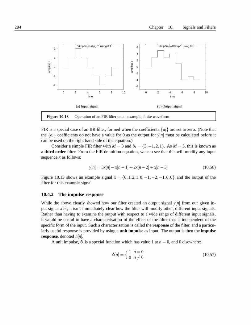
294 Chapter 10. Signals and Filters
-2
-1
0
1
2
0 2 4 6 8 10
ampl
itude
time
"/tmp/tmpos4p_z" using 0:1
(a) Input signal
-6
-4
-2
0
2
4
6
0 2 4 6 8 10
ampl
itude
time
"/tmp/tmpwO0Pqx" using 0:1
(b) Output signal
Figure 10.13 Operation of an FIR filter on an example, finite waveform
FIR is a special case of an IIR filter, formed when the coefficientsal are set to zero. (Note thattheal coefficients do not have a value for 0 as the output fory[n] must be calculated before itcan be used on the right hand side of the equation.)
Consider a simple FIR filter withM = 3 andbk = 3,−1,2,1. As M = 3, this is known asa third order filter. From the FIR definition equation, we can see that this will modify any inputsequencex as follows:
y[n] = 3x[n]−x[n−1]+2x[n−2]+x[n−3] (10.56)
Figure 10.13 shows an example signalx = 0,1,2,1,0,−1,−2,−1,0,0 and the output of thefilter for this example signal
10.4.2 The impulse response
While the above clearly showed how our filter created an output signaly[n] from our given in-put signalx[n], it isn’t immediately clear how the filter will modify other,different input signals.Rather than having to examine the output with respect to a wide range of different input signals,it would be useful to have a characterisation of the effect ofthe filter that is independent of thespecific form of the input. Such a characterisation is calledtheresponseof the filter, and a particu-larly useful response is provided by using aunit impulse as input. The output is then theimpulseresponse, denotedh[n].
A unit impulse,δ, is a special function which has value 1 atn = 0, and 0 elsewhere:
δ[n] = 1 n = 0
0 n 6= 0(10.57)

Section 10.4. Digital Filters 295
-6
-4
-2
0
2
4
6
0 2 4 6 8 10
ampl
itude
time
"/tmp/tmpszD3oV" using 0:1
(a) FIR filter
0
0.5
1
1.5
2
0 5 10 15 20 25 30
ampl
itude
time
"/tmp/tmpHwWEdb" using 0:1
(b) IIR filter
Figure 10.14 Example impulse responses for FIR and IIR filters. Note whilethe number of coef-ficients in the IIR filter is actually less than for the FIR filter, the response will continue indefinitely(only values up to 30 samples are shown)
The output of the example FIR filter for an impulse is given in figure 10.14a, which shows thatthe impulse response is simply the coefficients in the filter.Because of this, the duration of theimpulse will always be the order of the filter. As the order is finite, the impulse response is finitewhich gives rise to the name of the filter.
Consider now an example first order IIR filter, witha1 = −0.8, andb[0] = 1. Its differenceequation is therefore:
y[n] = x[n]−0.8y[n−1] (10.58)
If we give this filter the unit impulse as an input, then we can calculate the output for anynafter 0. The output is shown in Figure 10.14b. First of all we observe that the output is not ofa fixed duration: in fact it is infinite as the name of the filter implies. Secondly we observe thatthe response takes the form of a decaying exponential. The rate of decay is governed by the filtercoefficient,a1. (Note that ifa1 > 1 the output will grow exponentially: this is general undesirableand such filters are calledunstable.)
Consider the impulse response of the second order IIR filtera1 = −1.8,a2 = 1, shown infigure 10.15a. Just as in the first order case, this filter has aninfinite response, but this time takesthe form of a sinusoid. This shows the power of the IIR filter - with only a few terms it canproduce a quite complicated response. The filtera1 = −1.78,a2 = 0.9, has its impulse responseshown in Figure 10.15b. We can see that it is a decaying sinusoid; we have in effect combined thecharacteristics of examples 10.14b and 10.15a. The key point to note is that in all cases, the inputis the same, ie a unit impulse. The characteristics of the output are governed solely by the filter -after all the input has no periodicity or decay factor built in. If we choose a slightly different set

296 Chapter 10. Signals and Filters
-6
-4
-2
0
2
4
6
0 10 20 30 40 50 60 70 80 90 100
ampl
itude
time
-4
-3
-2
-1
0
1
2
3
4
0 10 20 30 40 50 60 70 80 90 100
ampl
itude
time
Figure 10.15 Impulse response for 2 IIR filters, showing a sinusoid and damped sinusoid response.
of coefficients, we can create an output with a different period and decay factor.Different filters can produce a wide range of impulse responses; the decaying sinusoid pat-
terns here only come from a specific type of second order IIR filter. In general though, the moreterms in the filter, the more complicated the impulse response will be. The impulse response isimportant for a number of reasons. Firstly, it provides us with a simple way of examining thecharacteristics of the filter. Because the input only lasts for a single sample, the output is not “clut-tered” with the further interference from subsequent inputsamples. Impressionistically, excitingthe filter with an impulse response can be thought of as “giving the filter a nudge and seeing whathappens”. Secondly, and more importantly, we can use the principle of linearity andtime invari-anceto describe the responses of more general signals by using the impulse response, explainednext.
10.4.3 Filter convolution sum
The response for a non-unit impulse is simply the unit impulse response scaled. So using thelinearity principle, we can state that:
3δ[n] 7→ 3h[n]
As the unit impulse is simply a single sample, a full input sequencex[n], can be characterised by asequence of scaled unit impulses:
x[n] = ∑w[k]δ[n−k]
What are the values ofw? As the delta function will set everything outsiden−k to 0, it should beclear thatw[n] = x[n] for a givenn.Therefore, we can state:
x[n] =K
∑k=0
x[k]δ[n−k] (10.59)
Section 10.4. Digital Filters 297
This may seem a rather trivial result, but it shows that a signal can be fully described by a set ofappropriately scaled impulse responses. The time invariance property of LTI systems tells us thata shifted input will give a shifted response. For the impulsefunction, the following is thereforetrue:
δ[n] 7→ h[n]δ[n−1] 7→ h[n−1]δ[n−2] 7→ h[n−2]δ[n−k] 7→ h[n−k] for any integerk
The linear property states thatαδ[n] 7→ αh[n] for anyα and so the following is also true:
x[0]δ[n] 7→ x[0]h[n]x[1]δ[n−1] 7→ x[1]h[n−1]x[2]δ[n−2] 7→ x[2]h[n−2]x[k]δ[n−k] 7→ x[k]h[n−k] for any integerk
We can use these two properties on equation 10.59 to find the output of the filter
∑k
x[k]δ[n−k] 7→∑k
x[k]h[n−k]
which gives us:
y[n] = ∑k
x[k]h[n−k] (10.60)
which is known as theconvolution sum. It shows that we can calculate the output for a filter forany input, provided we know the impulse responseh[n].
10.4.4 Filter transfer function
We will now examine the frequency domain description orfrequency responseof the LTI filterby means of the z-transform. The IIR difference equation (10.55), expanded to a few terms, is:
y[n] = b0x[n]+b1x[n−1]+ ...+bMx[n−M]+a1y[n−1]+ ...+aNy[n−N]
By using the notationZ . to denote the z-transform, we can take the z-transform of both sides asfollows:
Y(z) = Z b0x[n]+b1x[n−1]+ ...+bMx[n−M]+a1y[n−1]+ ...+aNy[n−N]
The coefficients are not affected by the z-transform, so using the linearity of the z-transform, thissimplifies to:
Y(z)= b0Z x[n]+b1Z x[n−1]+ ...+bn−MZ x[n−M]+a1Z y[n−1]+ ...+aNZ y[n−N]

298 Chapter 10. Signals and Filters
The z-transform time delay property (equations 10.35 and 10.46) states thatZ x[n−k]= X(z)z−k
and so our equation becomes:
Y(z) = b0X(z)+b1X(z)z−1 + ...+bn−MX(z)zM +a1Y(z)z−1 + ...+aNY(z)zN
If we group theY(z) terms on one side, and factor the commonY[z] andX[z], we get
Y(z) =b0 +b1z−1+ ...+bMzM
1−a1z−1− ...−aNzN X(z)
The term is known as thetransfer function of the filter
H(z) =Y(z)X(z)
=b0 +b1z−1 + ...+bMzM
1−a1z−1− ...−aNzN (10.61)
=
M∑
k=0bk
1−L∑
l=1al
(10.62)
and fully defines the characteristics of the filter in the z-domain. From this, the frequency domaincharacteristics of the filter can easily be found (explainedbelow).
10.4.5 The transfer function and the impulse response
We have previously shown that the impulse response, which completely characterises the filter,allows us to calculate the time domain output for any input bymeans of the convolution sum:
y[n] =∞
∑k=−∞
h[k]x[n−k] (10.63)
Section 10.3 showed how to derive the Fourier transform for aconvolution and we can apply thisto a digital signal by using the z-transform in the same way.
Y(z) = Z ∞
∑k=−∞
h[k]x[n−k]
=∞
∑k=−∞
h[k]∞
∑n=−∞
x[n−k]z−n
=∞
∑k=−∞
h[k]z−kX(z) (10.64)
The∑h[k]z−k term is simply the z-transform ofh[n] defined in terms ofk rather thann, so 10.64simplifies to
Y(z) = H(z)X(z) (10.65)

Section 10.5. Digital filter analysis and design 299
which is the same result as equation 10.62. This shows thatthe transfer function H(z) is thez-transform of the impulse responseh[n]. This gives us the following two important properties:
1. a LTI filter is completely characterised by its impulse response,h[n] in the time domain.The z-transform of the impulse response is the transfer function, H(z), which completelycharacterises the filter in the z-domain.
2. The transfer function is a ratio of two polynomials, with the same coefficients as used in thedifference equation.
10.5 DIGITAL FILTER ANALYSIS AND DESIGN
Section 10.4 fully described the relationship between the time domain difference equations andthe z-domain transfer function of a LTI filter. For first orderfilters, the coefficients are directlyinterpretable, for example as the rate of decay in an exponential. For higher order filters thisbecomes more difficult, and while the coefficientsal andbk fully describe the filter, they aresomewhat hard to interpret (for example, it was not obvious how the coefficients produced thewaveforms in Figure 10.15). We can however usepolynomial analysisto produce a more easilyinterpretable form of the transfer function.
10.5.1 Polynomial analysis: poles and zeros
Consider a simple quadratic equation defined in terms of a real variablex:
f (x) = 2x2−6x+1
This equation can befactorised into
f (x) = G(x−q1)(x−q2)
and then theroots q1,q2 of the quadratic can be found by settingf (x) to 0 and solving forx (inthis case the roots arex = 0.38 andx = 2.62). G is thegain, which simply scales the function.
We can plot the polynomial as shown in Figure 10.16a. The roots of this expression (thepoints at whichf (x) = 0) are marked on the graph. Although the roots only mark two points, theydo in fact describe the general curve. Figure 10.16b shows the effect of varying the gain - thecurve can become steeper or shallower, or even inverted if the gain is set to a negative number, butin all cases the general shape of the curve is the same. Because settingx to one of the roots resultsin f (x) = 0, we call these rootszeros. Now consider the same polynomial used as a denominatorexpression, where by convention we keep the gain as a numerator term:
f (x) =1
2x2−6x+1=
G′
(x− p1)(x− p2)

300 Chapter 10. Signals and Filters
-5
0
5
10
15
20
-2 -1 0 1 2 3 4 5
ampl
itude
time
(a) plot of 2x2−6x+1
-20
-15
-10
-5
0
5
10
15
20
-2 -1 0 1 2 3 4 5
ampl
itude
time
(b) plot of g× (2x2−6x+ 1) for different valuesof g
Figure 10.16 Plot of polynomial. The points where the curve intersects the x-axis are called “zeros”
-2
-1
0
1
2
3
4
5
-2 -1 0 1 2 3 4 5
ampl
itude
time
(a) plot of 1/(2x2−6x+1)
-2
-1
0
1
2
3
4
5
-2 -1 0 1 2 3 4 5
ampl
itude
time
(b) plot of |1/(2x2−6x+1)|
Figure 10.17 Plot of function with a polynomial as the denominator. The points where the function→ ∞ are called “poles”.
The plot of this is shown in Figure 10.17a. The shape of this curve is very different, but is againcompletely characterised by the roots plus a gain factor. This time values at the roots cause thefunction to “blow up”,x→ p1, f (x)→±∞. Such roots are calledpolesas they create a “pole-like”effect in the absolute (magnitude) version of the function,shown in 10.17b.
We will now show how polynomial analysis can be applied to thetransfer function. Apolynomial defined in terms the complex variablez takes on just the same form as when defined

Section 10.5. Digital filter analysis and design 301
-1.5-1-0.5 0 0.5 1 1.5imaginary
-1.5-1
-0.5 0
0.5 1
1.5real
0 2 4 6 8
10 12 14
|H(z)|
(a) z-domain, filter A
-1.5-1-0.5 0 0.5 1 1.5imaginary
-1.5-1
-0.5 0
0.5 1
1.5real
0 2 4 6 8
10 12 14
|H(z)|
(b) z-domain, filter B
-1
-0.5
0
0.5
1
-1 -0.5 0 0.5 1
imagin
ary
real
"/tmp/tmpdfuJQM" using 1:2"/tmp/tmpDsB2Ku" using 1:2
(c) pole-zero plot, filter A
-1
-0.5
0
0.5
1
-1 -0.5 0 0.5 1
imagin
ary
real
"/tmp/tmpdLQl-H" using 1:2"/tmp/tmpxcpciY" using 1:2
(d) pole zero plot, filter B
Figure 10.18 z-domain and pole-zero plots for two filters, A and B.
in terms ofx. Thez form is actually less misleading, because in general the roots will be complex(e.g. f (z) = z2 +z−0.5 has roots 0.5+0.5 j and 0.5−0.5 j.). The transfer function is defined interms of negative powers ofz - we can convert a normal polynomial to one in negative powersbymultiplying byz−N. So a 2nd order polynomial is:
H(z) =1
z2−a1z−a2=
z−2
1−a1z−1−a2z−2 = Gz−2
(1− p1z−1)(1− p2z−1)
Figure 10.18a shows a 3-dimensional plot of the above transfer function witha1 = 1.0,a2 =−0.5. The numerator has two roots atz= 0, which form zeros. The roots of the denominator are

302 Chapter 10. Signals and Filters
complex (0.5+0.5 j and 0.5−0.5 j) and it can be seen that the poles do not now lie on the x-axis(which would only happen if they were completely real).
As the poles and zeros completely characterise the filter (apart from the gain), we can dis-pense with the need to draw 3-dimensional graphs and simply plot where the poles and zeros lieon the z-plane. This is shown in Figure 10.18c. Figures 10.18b and 10.18d show the 3-d plot andpole-zero plot for a different 2nd order filter.
This analysis can be extended to any digital LTI filter. As thegeneral form transfer function,H(z) is defined as the ratio of two polynomials
H(z) =b0 +b1z−1 + ...+bMz−M
1−a1z−1− ...−aNz−N
this can always be expressed in terms of its factors:
H(z) = g(1−q1z−1)(1−q2z−1)...(1−qMz−1)
(1− p1z−1)(1− p2z−1)...(1− pNz−1)
from which pole-zero analysis can be performed. Furthermore, a factored filter can be split intosmaller filters:
H(z) = g1−q1z−1
1− p1z−1︸ ︷︷ ︸
.1−q2z−1
1− p2z−1︸ ︷︷ ︸
...1−qMz−1
1− pMz−1︸ ︷︷ ︸
= H1(z)H2(z)...HN(z) (10.66)
which is often a useful step when constructing or analysing complicated filter.
10.5.2 Frequency Interpretation of z-domain transfer function
Recall that we showed the relationship between the z-transform
X(z) =∞
∑n=−∞
x[n]z−n
and the discrete-time Fourier transform by settingz= ejω:
X(ejω) =∞
∑−∞
x[n]e− jωn
Given any z-domain expression, we can generate the equivalent frequency domain expression bysimply replacingz with ejω. In section 10.2.6, we explained that the spectrumX(ejω) of a digitalsignal is periodic with period 2π for normalised frequency. This can be thought of as a functionwhich sweeps out a circle of radius 1 in the z-domain. The frequency domain is in effect theparticular ‘slice” on the z-domain that this circle describes.
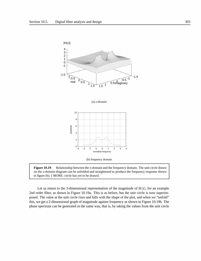
Section 10.5. Digital filter analysis and design 303
-1.5-1-0.5 0 0.5 1 1.5imaginary
-1.5-1
-0.5 0
0.5 1
1.5real
-1 0 1 2 3 4
|H(z)|
(a) z-domain
0
2
4
6
8
10
-4 -3 -2 -1 0 1 2 3 4
ampl
itude
normalise frequency
(b) frequency domain
Figure 10.19 Relationship between the z-domain and the frequency domain. The unit circle drawnon the z-domain diagram can be unfolded and straightened to produce the frequency response shownin figure (b). [ MORE: circle has yet to be drawn]
Let us return to the 3-dimensional representation of the magnitude ofH(z), for an example2nd order filter, as shown in Figure 10.19a. This is as before,but the unit circle is now superim-posed. The value at the unit circle rises and falls with the shape of the plot, and when we “unfold”this, we get a 2-dimensional graph of magnitude against frequency as shown in Figure 10.19b. Thephase spectrum can be generated in the same way, that is, by taking the values from the unit circle

304 Chapter 10. Signals and Filters
from the z-domain phase function. As previously mentioned,we can dispense with 3-d graphsbecause the pole-zero diagram fully characterises the transfer function. The frequency domaincan easily be obtained from the z-domain by use of the poles and zeros.
10.5.3 Filter characteristics
We will now use the above results on pole zero analysis and frequency domain interpretation toexamine the properties of first order and second order filters, and show how these can be extendedto the general case of all digital LTI filters.
Consider again a first order IIR filter:
h[n] = b0x[n]−a1y[n−1]
H(z) =b1
1−a1z−1
H(ejω) =b1
1−a1e− jω
Figure 10.20, shows the time domain, z-domain pole zero plotand frequency domain magnitudespectrum for this filter withb0 = 1 anda1 varying over 0.8,0.7,0.6,0.4. Figure 10.20d shows a3-d z-domain magnitude plot for a single value,a1 = 0.7.
It is clear that the value of the coefficienta1 completely describes the shape of the threefunctions. For a single term polynomial, the root of 1−a1z−1 is simplya1. As the filter coefficientis real, so will the root, and hence the pole will always line on the real axis in the pole-zero plot.
This type of filter is commonly called aresonator because it accurately models the typesof resonances commonly found in nature. The peak in the the frequency response is known asa resonancebecause signals at or near that frequency will be amplified bythe filter. For ourpurposes, it provides a good model of a single vocal tractformant . Resonances are normallydescribed by three properties:amplitude - the height of the peak,frequency - where the peak liesin the spectrum, andbandwidth - a measure of the width or sharpness of the peak.
The radius of the pole,r controls both theamplitude and thebandwidth of the resonance.As the value ofa1 decreases, its pole moves towards along the real axis towards the origin, andhence the frequency response has a lower amplitude atω = 0. From the difference equations, weknow that a first order IIR filter witha1 < 1 is simply a decaying exponential. Small values ofa1
correspond to slow decay and narrow bandwidth, large values(still < 1) a steeper decay and widerbandwidth. This is exactly what we would expect from the Fourier transform scaling property
The standard measure of bandwidth is the3db down point which is the width of the reso-nance at 1/
√2 down from the peak. For larger values ofr = |a1|, two useful approximations of
the bandwidth (in normalised frequency) are:
B ≈ −2ln(r)
B ≈ 2(1−r)√r
0.5 < r < 1.0 (10.67)
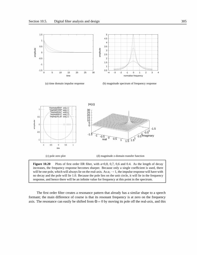
Section 10.5. Digital filter analysis and design 305
-1.5
-1
-0.5
0
0.5
1
1.5
0 5 10 15 20 25 30
ampl
itude
time
(a) time domain impulse response
0.5
1
1.5
2
2.5
3
3.5
4
4.5
5
-4 -3 -2 -1 0 1 2 3 4
ampl
itude
normalise frequency
(b) magnitude spectrum of frequency response
-1
-0.5
0
0.5
1
-1 -0.5 0 0.5 1
am
plitu
de
time
"/tmp/tmpkwRBSH" using 1:2"/tmp/tmpECGNt0" using 1:2"/tmp/tmpfrEsNU" using 1:2"/tmp/tmp90NYI2" using 1:2"/tmp/tmpLR2LJB" using 1:2
(c) pole zero plot
-1.5-1
-0.5 0
0.5 1
1.5
imaginary-1.5 -1 -0.5 0 0.5 1 1.5real
0 5
10 15 20 25 30
|H(z)|
(d) magnitude z-domain transfer function
Figure 10.20 Plots of first order IIR filter, with a=0,8, 0,7, 0,6 and 0.4. Asthe length of decayincreases, the frequency response becomes sharper. Because only a single coefficient is used, therewill be one pole, which will always lie on the real-axis. Asa1→ 1, the impulse response will have withno decay and the pole will lie 1.0. Because the pole lies on theunit circle, it will lie in the frequencyresponse, and hence there will be an infinite value for frequency at this point in the spectrum.
The first order filter creates a resonance pattern that already has a similar shape to a speechformant; the main difference of course is that its resonant frequency is at zero on the frequencyaxis. The resonance can easily be shifted fromω = 0 by moving its pole off the real-axis, and this
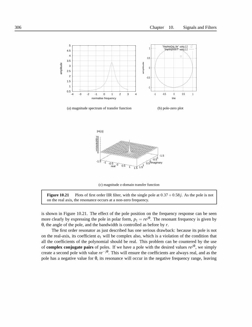
306 Chapter 10. Signals and Filters
0.5
1
1.5
2
2.5
3
3.5
4
4.5
5
-4 -3 -2 -1 0 1 2 3 4
ampl
itude
normalise frequency
(a) magnitude spectrum of transfer function
-1
-0.5
0
0.5
1
-1 -0.5 0 0.5 1
am
plitu
de
time
"/tmp/tmpQog_8w" using 1:2"/tmp/tmp0vdv7f" using 1:2
(b) pole-zero plot
-1.5-1
-0.5 0
0.5 1
1.5
imaginary-1.5 -1 -0.5 0 0.5 1 1.5real
0 10 20 30 40 50 60 70
|H(z)|
(c) magnitude z-domain transfer function
Figure 10.21 Plots of first order IIR filter, with the single pole at 0.37+0.58j. As the pole is noton the real axis, the resonance occurs at a non-zero frequency.
is shown in Figure 10.21. The effect of the pole position on the frequency response can be seenmore clearly by expressing the pole in polar form,p1 = re jθ. The resonant frequency is given byθ, the angle of the pole, and the bandwidth is controlled as before byr.
The first order resonator as just described has one serious drawback: because its pole is noton the real-axis, its coefficienta1 will be complex also, which is a violation of the condition thatall the coefficients of the polynomial should be real. This problem can be countered by the useof complex conjugate pairsof poles. If we have a pole with the desired valuesre jθ, we simplycreate a second pole with valuere− jθ. This will ensure the coefficients are always real, and as thepole has a negative value forθ, its resonance will occur in the negative frequency range, leaving

Section 10.5. Digital filter analysis and design 307
0
1
2
3
4
5
6
7
-4 -3 -2 -1 0 1 2 3 4
ampl
itude
normalise frequency
(a) pole-zero plot
-1
-0.5
0
0.5
1
-1 -0.5 0 0.5 1
am
plitu
de
time
"/tmp/tmpV_ny2Q" using 1:2"/tmp/tmpYSkHQr" using 1:2
"/tmp/tmpmWEdeH" using 1:2"/tmp/tmp5L1og7" using 1:2"/tmp/tmpwCVli3" using 1:2
(b) frequency response
Figure 10.22 Plots of second order IIR filter for a series of poles. All havethe same angle, butdiffer in distance from the unit circle. The poles in the pole-zero diagram are conjugate symmetric,meaning they are symmetric in the real-axis. Because of thisthe frequency response will have peaksat the same positive and negative values
a single pole in the positive range. If we have two poles, we naturally now have a second orderfilter:
h[n] = b0x[n]−a1y[n−1]−a2y[n−2]
H(z) =b1
1−a1z−1−a2z−2
H(z) =1
(1− p1z1)(1− p2z1)
H(ejω) =b1
1−a1e− jω−a2e−2 jω
The full frequency response can be seen more clearly by expressing the poles in polar form:
p1 = re jθ
p2 = p∗1 = re− jθ

308 Chapter 10. Signals and Filters
Using this we can write the transfer function and frequency response as:
H(z) =1
(1− re jθz−1)(1− re− jθz−1)
=1
1−2rcos(θ)z−1 + r2z−2
H(ejω) =1
1−2rcos(θ)e− jω + r2e− j2w
The following table gives four sets of example poles and coefficients for this filter, and the pole-zero plot and frequency responses for these are shown in Figure 10.22.
r θ p1 p2 a1 a2
0.9 1.0 0.48 + 0.75j 0.48 - 0.75j 0.97 -0.810.8 1.0 0.43 + 0.67j 0.43 - 0.67j 0.86 -0.640.7 1.0 0.38 + 0.59j 0.38 - 0.59j 0.75 -0.480.6 1.0 0.32 + 0.51j 0.32 - 0.51j 0.65 -0.36
From the table and the pole-zero plot, the complex conjugateproperty of the poles can clearlybe seen. This property gives rise to the symmetry in the frequency domain about the y-axis. Itshould also be clear that the relationship between the polesand coefficients is less obvious. Theseexample responses were defined by keeping the angleθ constant, while varying the distance of thepole from the origin,r. It can be seen that asr approaches 1, and the position of the pole nears theunit circle, the frequency response becomes sharper. Exactly the same effect was observed withthe first order filter. Moving the poles off the real-axis has the effect of moving the peaks awayfrom the origin in the frequency response. For larger valuesof r (> 0.5) the resonant frequencyis approximated byθ, as for the first order complex pole. For smaller values, the approximationbreaks down because theskirts of each pole (that is, the rol-off area on either side of the actualresonance) interact and cause a shifting of frequency.
Figure 10.23 and the table below show the effect of keepingr constant while varying theangleθ. As we might expect, the peaks now all have similar shape, buttheir location in thefrequency response is different.
r θ p1 p2 a1 a2
0.8 0.75 0.58+0.54j 0.58-0.54j 1.17, -0.640.8 1.0 0.43+0.67j 0.43-0.67j 0.86 -0.640.8 1.25 0.25+0.76j 0.25-0.76j 0.50 -0.640.8 1.5 0.056+0.78j 0.05-0.78j 0.11 -0.64

Section 10.5. Digital filter analysis and design 309
-1
-0.5
0
0.5
1
-1 -0.5 0 0.5 1
am
plitu
de
time
"/tmp/tmpK2req4" using 1:2"/tmp/tmp33KyD9" using 1:2"/tmp/tmpohsE85" using 1:2"/tmp/tmpeS7T51" using 1:2
"/tmp/tmpE1flb-" using 1:2
(a) pole-zero plot
0
0.5
1
1.5
2
2.5
3
3.5
4
4.5
-4 -3 -2 -1 0 1 2 3 4
am
plitu
de
normalise frequency
(b) frequency response
Figure 10.23 Plots of second order IIR filter for a series of poles with the same radius but differentangles. While position of the peaks varies with the angle of the poles. The bandwidth of the peaks isconstant, but the amplitudes differ because as the poles near the frequency axis their skirts affect eachother, giving each peak a lift.
0
1
2
3
4
5
6
7
-4 -3 -2 -1 0 1 2 3 4
ampl
itude
normalise frequency
(a) pole-zero plot
0
2
4
6
8
10
12
-4 -3 -2 -1 0 1 2 3 4
ampl
itude
normalise frequency
(b) frequency response
Figure 10.24 Plots of second order IIR filter with poles and zeros for different pole positions.Figure (a) has a zero on the unit circle on the real axis. Figure (b) has a zero on the unit circle at theimaginary axis.
In general it is the poles which define the most important characteristics of a resonator,namely resonance amplitude, frequency and bandwidth. Zeros do have a role to play and can beused to achieve other effects in the spectrum. Figure 10.24 shows the affect of using a termb1 = 1,

310 Chapter 10. Signals and Filters
which will place a zero at the origin, andb1 = −1 which will place a zero at the ends limit of thespectrum. Extra zeros can be used to generate notches oranti-resonancesin the spectrum.
We know that the vocal tract has multiple formants. Rather than developing more and morecomplicated models to relate formant parameters to transfer functions directly, we can insteadmake use of the factorisation of the polynomial to simplify the problem. Recall from equation10.66 that any transfer function polynomial can be broken down into its factors. We can thereforebuild a transfer function of any order by combining simple first and second order filters:
H(z) = H1.H2...HN (10.68)
This greatly simplifies the construction of a complicated filter as we can make simple resonatorsin isolation using pole-zero analysis to set their parameters, and afterwards combine them bymultiplication. It should be noted that poles which are close together will interact, and hencethe final resonances of a system can not always be predicted from the constituent resonators.Nevertheless, this provides a powerful model for building an arbitrarily complicated filter.
10.5.4 Putting it all together
We will now demonstrate some of the practical properties of the LTI filter. the previous sectionshowed how we could build a model of a single formant. We will now extend this to generatea simple three formant model of a vowel. In discussing digital filters, we have mostly used nor-malised angular frequencyω. Recall that normal frequency (expressed in Hertz) can be convertedto normalised angular frequency by multiplication by 2π/Fs, whereFs is the sampling rate. Thisgives the following formulas for estimating the pole radiusand angle for a single formant of peakfrequencyf and bandwidthB.
θ =2πFFs
(10.69)
r = e−2πB/Fs (10.70)
We know from acoustic phonetics that typical formant valuesfor an /ih/ vowel are 300Hz, 2200Hz,and 3000Hz. Formant bandwidths are harder to measure accurately, but less us assume a valueof 250Hz for all three formants. Assuming a sampling frequency of Fs = 16000Hz, the followingtable shows how to calculate the poles from the formant frequencies and bandwidths.
Formant Frequency (Hz)Bandwidth (Hz) r θ (normalised angular frequency) poleF1 300 250 0.95 0.12 0.963 + 0.116jF2 2200 250 0.95 0.86 0.619 + 0.719jF3 3000 250 0.95 1.17 0.370 + 0.874j

Section 10.5. Digital filter analysis and design 311
0
20
40
60
80
100
120
0 1000 2000 3000 4000 5000 6000 7000
ampl
itude
frequency (Hz)
(a) frequency response
-1
-0.5
0
0.5
1
-1 -0.5 0 0.5 1
imagin
ary
real
"/tmp/tmpKzOhgH" using 1:2"/tmp/tmp8uLEzm" using 1:2
(b) pole-zero plot
Figure 10.25 Three formant, 6 pole model of /ih/ vowel
We construct a second order IIR filter for each formant,Fn:
Hn(z) =1
(1− pnz−1)(1− p∗nz−1)
wherepn is the pole andp∗n is complex conjugate of the pole for the formantn. We create thecomplete transfer functionH/ih/ for the /ih/ vowel by simply multiplying each formant’s transferfunction:
H/ih/(z) = H1(z)H3(z)H3(z)
=1
(1− p1z−1)(1− p∗1z−1)(1− p2z−1)(1− p∗2z−1)(1− p3z−1)(1− p∗3z−1)
Figure 10.25 shows the pole-zero plot and frequency response of the transfer function. From theplot, we can see that the formant frequencies do indeed appear at the approximately the desiredlocations.
By definition, H gives the transfer function and frequency response for a unit impulse. Inreality of course, the vocal tract input for vowels is the quasi-periodic glottal waveform. Fordemonstration purposes, we will examine the effect of the /ih/ filter on a square wave, which wewill use as a (very) approximate glottal source. We can generate the output waveformsy[n] byusing the difference equation, and find the frequency response of this vowel fromH(ejω). Theinput and output in the time domain and frequency domain are shown in figure 10.26. If thetransfer function does indeed accurately describe the frequency behaviour of the filter, we shouldexpect the spectra ofy[n], calculated by DFT to matchH(ejω)X(ejω). We can see from figure10.26 that indeed it does.

312 Chapter 10. Signals and Filters
-1.5
-1
-0.5
0
0.5
1
1.5
0 0.005 0.01 0.015 0.02 0.025 0.03 0.035 0.04 0.045 0.05
ampl
itude
time
(a) input square wave
-1.5
-1
-0.5
0
0.5
1
1.5
0 0.005 0.01 0.015 0.02 0.025 0.03 0.035 0.04 0.045 0.05
ampl
itude
time
(b) output
-4
-3
-2
-1
0
1
2
3
4
5
0 1000 2000 3000 4000 5000 6000 7000 8000
log
mag
nitu
de
frequency (Hz)
(c) frequency responseH(ejω) for the filter
-1
0
1
2
3
4
5
6
0 1000 2000 3000 4000 5000 6000 7000 8000
log
mag
nitu
de
frequency (Hz)
(d) spectrumX(ejω) of input
-2
-1
0
1
2
3
4
5
6
0 1000 2000 3000 4000 5000 6000 7000 8000
log
mag
nitu
de
frequency (Hz)
(e) DFT of output
Figure 10.26 Operation of simulated /ih/ vowel filter on square wave. Figure (b) shows the timedomain output for the square wave input (a). While the shape of the output is different, it has exactlythe same period as the input. Figure (d) is the magnitude spectrum of the square wave. Figure (e) isthe magnitude spectrum of the output, calculated by DFT. Theharmonics are at the same intervals asthe input spectrum, but each has had its amplitude changed. Figure (e) demonstrates that the effect ofthe filter is to multiply the input spectrum by the frequency response, Figure (c).

Section 10.6. Summary 313
Filtering a periodic signal demonstrates an important point of all LTI filters. While they am-plify and change the phase of components of an input signal, they do not change the fundamentalperiod of the signal itself. In figure 10.26, it is clear that the output waveform has the same periodas the input, and the harmonics have the same spacing in the input and output. Again, this clearlymodels speech behaviour - if we generate a voiced sound with our glottis, we can move our mouthinto a number of configurations, each of which will produce a different sound, but in all cases thefundamental frequency of the sound is unchanged.
10.6 SUMMARY
Periodic signals
• A complex exponential,ejωt describes a sinusoidal waveform
• A harmonic is any integer multiple of the fundamental frequency of a periodic waveform.
• Any periodic waveform can be made from a sum of suitably scaled and phase shifted sinu-soids. This is the Fourier series.
• Fourier analysis can be used to find the amplitudes and phasesof the component harmonicsin a periodic waveform.
Frequency domain
• A representation in the frequency domain is called a spectrum
• Spectra are complex, and are usually represented by the magnitude spectrum and phasespectrum.
• The ear is relatively insensitive to phase, and so the magnitude spectrum is normally suffi-cient to characterise the frequency domain representationof a signal.
• For all real signals, the spectrum is conjugate symmetric.
Digital signals
• A digital signal can be obtained from a continuous signal by sampling at even intervals,given by the sampling period.
• The sampling rate is the reciprocal of the sampling period.
• A digital signal has an upper bound on the frequencies it can represent. This is called theNyquist frequency and is exactly half the sample rate.
• Use of normalised frequency,ω = ω/Fs, avoids having to keep track of the sampling rate indigital signal processing expressions.
• Spectra obtained from digital signals are periodic, with normalised period 2π.

314 Chapter 10. Signals and Filters
Transforms
• The Fourier transform converts a continuous waveform into acontinuous spectrum:
X( jω) =Z ∞
−∞x(t)e− jωdt
• The discrete-time Fourier transform converts a digital waveform into a continuous spectrum:
X(ejω) =∞
∑−∞
x[n]e− jωn
• The discrete Fourier transform converts a digital waveforminto a discrete spectrum:
X[k] =N−1
∑n=0
x[n]e− j 2πN kn
• The z-transform converts a digital waveform into a continuous z-domain representation:
X(z) =∞
∑n=−∞
x[n]z−n
• All transforms have the properties of linearity, scaling, time delay, frequency shift and con-volution.
Digital filters
• Digital, time-invariant linear filters operate on an input signal x[n] and produce an outputsignaly[n].
• A filter is fully defined by two sets of real coefficientsal andbk.• The operation of the filter in the time domain is given by the difference equation.
y[n] =M
∑k=0
bkx[n−k]+N
∑l=1
al y[n− l ] (10.71)
• The time domain characteristics of a filter are fully captured by the responseh[n] to a unitimpulseδ[n].
• The operation of the filter in the z-domain is given by the transfer function.
H(z) =b0 +b1z−1 + ...+bMz−M
1−a1z−1− ...−aNz−N
• The transfer functionH(z) is the z-transform of the impulse responseh[n].

Section 10.6. Summary 315
• The frequency response of the filter is given by settingz= ejω which gives:
H(e− jω) =b0 +b1e− jω + ...+bMe− jMω
1−a1e− jω− ...−aNe− jNω
• The z-domain transfer function can be factored into two polynomials, the roots of which arecalled poles and zeros
H(z) = g(1−q1z−1)(1−q2z−1)...(1−qMz−1)
(1− p1z−1)(1− p2z−1)...(1− pNz−1)
• Poles have an easy to understand interpretation, and in manycases, formant frequency andbandwidth can be directly related to pole values. By suitable choice of pole, a frequencyresponse with appropriate resonances can usually be constructed.
• Complicated filters can by created by combining simpler filters.
• Filters change the amplitude and phase of the components in the input. They do not changethe fundamental period or fundamental frequency.

11ACOUSTIC MODELS OFSPEECH PRODUCTION
The speech production process was qualitatively describedin Chapter 7. There we showed thatspeech is produced by a source, such as the glottis, which is subsequently modified by the vocaltract acting as a filter. In this chapter, we turn our attention to developing a more formal quantita-tive model of speech production, using the techniques of signals and filters described in Chapter10.
11.1 ACOUSTICTHEORY OFSPEECHPRODUCTION
Such models often come under the heading of theAcoustic Theory of Speech Production, whichrefers both to the general field of research in mathematical speech production models, and to thebook of that title by Fant [158]. While considerable previous work in this field had been done priorto its publication, this book was the first to bring together various strands of work and describethe whole process in a unified manner. Furthermore, Fant backed his study up with extensiveempirical studies with x-rays and mechanical models to testand verify the speech productionmodels being proposed. Since then, many refinements have been made to the model, as researchershave investigated trying to improve the accuracy and practicalities of these models. Here we focusthe single most widely accepted model, but conclude the chapter with a discussion on variationson this.
As with any modelling process, we have to reach a compromise between a model whichaccurately describes the phenomena in question, and one which is simple, effective and suitedto practical needs. If we tried to capture every aspect of thevocal organs directly, we wouldhave to account for every muscle movement, articulator shape and tissue absorption characteristicdirectly, and then determine how each of these affected how speech production. This would be ahuge undertaking, and even if an accurate description of allthese factors could be determined, theresult may be too complicated for useful analysis. We therefore have to make quite a number ofsimplifying assumptions in order to obtain a usable model.
316

Section 11.1. Acoustic Theory of Speech Production 317
nasal cavity
oral cavity
tonguepharynx
glottis
larynx
vocal folds
hard palatesoft palate
lips
nostril
alveolar ridge
teeth
velum
uvula
(a) mid-sagittal drawing of vocal organs (b) Model of vocal organs with dis-crete components identified
Figure 11.1 Diagram and model of vocal organs.
11.1.1 Components in the model
Our first task is to build a model where the complex vocal apparatus is broken down into a smallnumber of independent components. One way of doing this is shown in Figure 11.1b, wherewe have modelled the lungs, glottis, pharynx cavity, mouth cavity, nasal cavity, nostrils and lipsas a set of discrete, connected systems. If we make the assumption that the entire system islinear (in the sense described in Section 10.4) we can then produce a model for each componentseparately, and determine the behaviour of the overall system from the appropriate combination ofthe components. While of course the shape of the vocal tract will be continuously varying in timewhen speaking, if we choose a sufficiently short time frame, we can consider the operation of thecomponents to be constant over that short period time. This,coupled with the linear assumptionthen allows us to use the theory of linear time invariant (LTI) filters (Section 10.4) throughout.Hence we describe the pharynx cavity, mouth cavity and lip radiation as LTI filters, and so thespeech production process can be stated as the operation of aseries of z-domain transfer functionson the input.
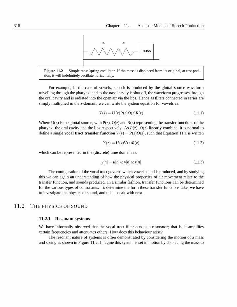
318 Chapter 11. Acoustic Models of Speech Production
mass
Figure 11.2 Simple mass/spring oscillator. If the mass is displaced from its original, at rest posi-tion, it will indefinitely oscillate horizontally.
For example, in the case of vowels, speech is produced by the glottal source waveformtravelling through the pharynx, and as the nasal cavity is shut off, the waveform progresses throughthe oral cavity and is radiated into the open air via the lips.Hence as filters connected in series aresimply multiplied in the z-domain, we can write the system equation for vowels as:
Y(z) = U(z)P(z)O(z)R(z) (11.1)
Where U(z) is the glottal source, with P(z), O(z) and R(z) representing the transfer functions of thepharynx, the oral cavity and the lips respectively. AsP(z), O(z) linearly combine, it is normal todefine a singlevocal tract transfer function V(z) = P(z)O(z), such that Equation 11.1 is written
Y(z) = U(z)V(z)R(z) (11.2)
which can be represented in the (discrete) time domain as:
y[n] = u[n]⊗v[n]⊗ r[n] (11.3)
The configuration of the vocal tract governs which vowel sound is produced, and by studyingthis we can again an understanding of how the physical properties of air movement relate to thetransfer function, and sounds produced. In a similar fashion, transfer functions can be determinedfor the various types of consonants. To determine the form these transfer functions take, we haveto investigate the physics of sound, and this is dealt with next.
11.2 THE PHYSICS OF SOUND
11.2.1 Resonant systems
We have informally observed that the vocal tract filter acts as a resonator; that is, it amplifiescertain frequencies and attenuates others. How does this behaviour arise?
The resonant nature of systems is often demonstrated by considering the motion of a massand spring as shown in Figure 11.2. Imagine this system is setin motion by displacing the mass to

Section 11.2. The physics of sound 319
spring
damper
mass
Figure 11.3 Mass/spring/damped system. The mass and spring combine as before to create oscil-lation, but the damper continually dissipates energy when the system is in motion, and will eventuallycause the system to stop.
the right and then letting go. The extended spring will try toreturn to its original position and indoing so will set the mass in motion. Initially, the speed of movement will be slow as the inertiaof the mass must be overcome. As the spring reaches its original position, it will no longer exertany force, but as the mass is now moving, it will continue to move and pass the original position,moving to the left. As it does so, the spring will again be displaced from its original position, andthe more this is done, the stronger the force will become, until eventually the mass stops and thespring pulls the mass towards the at rest position again. From Newton’s laws we also know thatthe system will continue moving until acted upon by an external force.
The frequency at which the system oscillates is determined by the inertia of the mass andthecomplianceof the spring;
resonant frequency=12π
√
km
Hence a heavier mass will mean a slower oscillation and a stiffer spring will mean a quickeroscillation. The important point is that the system has a single resonant frequency determined bythe physical properties of the mass and spring.
The above equates to a source filter system where a single impulse has been given to the sys-tem; we saw in Chapter 10 that the impulse response from a system is a good way to characterisethe system itself independent of the input. Now let us consider the case where a periodicforcingfunction is exerted on the mass, shown in Figure 11.3. Assuming the force is of sufficient strength,the mass will move with the periodicity of the driving (source) force. Again, this is what we wouldexpect from Chapter 10, where we showed that the source and not the filter largely determines theoutput frequency of a system. Imagine now that we send sources of different frequencies into thesystem. We will find that at frequencies near to the resonant frequency the size of the oscillationswill increase. In fact, at the resonant frequency itself, the oscillations will get larger and larger,and if no other factors are involve, will eventually become so large as to break the system1 Hence
1 This is what happens when things “shake themselves apart”, most famously the Tacoma Narrows bridge.

320 Chapter 11. Acoustic Models of Speech Production
damper
mass
spring
forcing function
Figure 11.4 Mass/spring/damped system driven by an external force. Here a periodic force isapplied, and this will determine the frequency at which the system oscillates. As the driving frequencynears the natural resonant frequency (determined by the mass and spring) the size of the oscillationswill increase.
a mass-spring system with a driving force acts as a linear filter fed with a source.The above is of course somewhat idealised because we know that in general systems don’t
shake themselves apart, and in the unforced case, when a massand spring are set in motion,eventually the motion will stop. This is due to the third property known asresistance. In themechanical world, resistance is opposition to velocity, and is often described as adamping effecton the system. Normally resistance is caused byfriction in which the energy in the movementis converted into heat. As in general the heat cannot be converted back into motion energy, theeffect of friction is to causeenergy lossin the system, which will eventually bring the system toa halt. One of the important features of resistance is that usually its effect on the frequency ofthe resonance is negligible; that is, while the amount of resistance will determine how quickly theoscillations die out, it does not affect the frequency at which those oscillations occur. This is animportant point for our model, as it often allows us to study the frequencies of resonances withoutneeding to consider the damping effects.
All these affects were shown in our examination of linear filters in Chapter 10. For exam-ple, Figure 10.15a shows the displacement of the mass against time for the undamped case, whileFigure 10.15b shows the same system with damping. Figures 10.22 and 10.23 show the separa-tion of frequency and damping effects on a pole-zero plot. There, the angle of the pole or zerodetermined the frequency, whereas the radius of the pole determined the damping, with poles onthe unit circle meaning that the damping was zero. In terms ofa frequency response, the dampingmanifests itself as amplitude and bandwidth of the resonantpeak, with high amplitude and narrowbandwidth arising from cases of low damping.
The three factors of inertia (mass), resistance and capacitance (the reciprocal of spring com-pliance) are collectively known asimpedanceas intuitively, the system “impedes” the motion inthe system.

Section 11.2. The physics of sound 321
fixedend
Figure 11.5 If the held end of the rope is given a jerk, this creates an impulse, which will travelalong the rope towards the wall.
11.2.2 Travelling waves
The behaviour of the vocal tract is in many ways similar to thebehaviour of the mass/spring/dampedsystem just described. The input, “forcing function” is theglottal source, which is used to drive thesystem (the vocal tract) whose physical properties determine resonant characteristics, which thenmodify the input signal so as to amplify some frequencies andattenuate others. One crucial differ-ence however, is that the mass/spring/damped system is whatis known as alumped parametersystem in that it comprises easily identifiable, discrete components such as the mass and spring.By contrast, the vocal tract is adistributed system, in which the properties of inertia, capacitanceand resistance are evenly distributed throughout the system. We can formulate the properties ofa distributed system by modelling it as a large number of small connected discrete systems; thatis. Using calculus, we can determine the behaviour of a distributed system by considering thebehaviour of the system as the size of the elements tends to zero. This steps involved in this arefully described in Rabiner and Schafer [368]; for our purposes though, we will simply take theresults of this analysis and apply it to the problem of the sound propagation in the vocal tract.
Before considering this directly, we will appeal again to anequivalent physical system, asthis will let us examine an aspect of resonant behaviour thatis central to our study, namely thatof travelling waves. Consider first the easy to visualise example of waves travelling in a rope,in which one end is in a person’s hand and the other is tied to a wall. This is shown in Figures11.5 and 11.6. If the person introduces some energy in the rope by giving the rope a jerk (i.e. animpulse), a wave will form at that end and travel down the rope. When the wave reaches the tiedend at the wall, it will be reflected, and will travel backwards towards the person. When it reachesthe held end, the wave will be reflected back again towards thewall and so on, until all the energyhas eventually been lost from the system.
The person can create a forcing function (i.e. source) inputto the system by moving theirhand in a repetitive fashion. In doing so, a series of pulses will form and travel forwards downthe rope towards the wall, and these pulses will create atravelling wave, the frequency of whichis dictated by the hand movement. When this forwards travelling wave is reflected, a backwardstravelling wave will be created. The forward wave and backward wave will interfere - if the twohave a peak at a given point, a large peak will occur, and if onehas a negative peak while theother has a positive peak then these will cancel out leaving the rope at that point in its neutral

322 Chapter 11. Acoustic Models of Speech Production
Figure 11.6 The impulse in the rope travels towards the wall, where is is reflected out of phasewith the original pulse. The reflected pulse travels backwards along the rope.
position. In general, the observed shape of the rope will notform a simple pattern. However atsome frequencies, the reflected wave will exactly reinforcethe forward wave, and the rope willsettle down into a fixed pattern. In such cases, the wave does not look like it is travelling at all,so this is termed astanding wave. The term is a little misleading because it might be taken tomean that there is no motion - this is not the case. It merely appears that the waves are not moving.Standing waves are only created at certain frequencies. At these frequencies, the wave is amplified,that is the overall displacement in the rope at a peak is greater than the input. Thus the rope acts asa resonator, amplifying certain frequencies and attenuating others. The frequencies at which theresonances occur are governed by the length of the rope and the speed of wave travel.
The above demonstrates some of the fundamental properties of travelling waves. First, notethat some of the behaviour is determined by the motion of the hand, while some is determined by
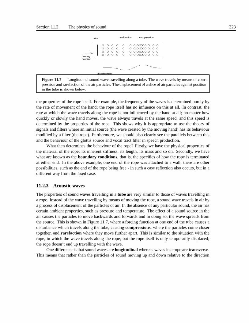
Section 11.2. The physics of sound 323
displacement
rarefraction compression
forcingfunction
tube
Figure 11.7 Longitudinal sound wave travelling along a tube. The wave travels by means of com-pression and rarefaction of the air particles. The displacement of a slice of air particles against positionin the tube is shown below.
the properties of the rope itself. For example, the frequency of the waves is determined purely bythe rate of movement of the hand; the rope itself has no influence on this at all. In contrast, therate at which the wave travels along the rope is not influencedby the hand at all; no matter howquickly or slowly the hand moves, the wave always travels at the same speed, and this speed isdetermined by the properties of the rope. This shows why it isappropriate to use the theory ofsignals and filters where an initial source (the wave createdby the moving hand) has its behaviourmodified by a filter (the rope). Furthermore, we should also clearly see the parallels between thisand the behaviour of the glottis source and vocal tract filterin speech production.
What then determines the behaviour of the rope? Firstly, we have the physical properties ofthe material of the rope; its inherent stiffness, its length, its mass and so on. Secondly, we havewhat are known as theboundary conditions, that is, the specifics of how the rope is terminatedat either end. In the above example, one end of the rope was attached to a wall; there are otherpossibilities, such as the end of the rope being free - in sucha case reflection also occurs, but in adifferent way from the fixed case.
11.2.3 Acoustic waves
The properties of sound waves travelling in atube are very similar to those of waves travelling ina rope. Instead of the wave travelling by means of moving the rope, a sound wave travels in air bya process of displacement of the particles of air. In the absence of any particular sound, the air hascertain ambient properties, such as pressure and temperature. The effect of a sound source in theair causes the particles to move backwards and forwards and in doing so, the wave spreads fromthe source. This is shown in Figure 11.7, where a forcing function at one end of the tube causes adisturbance which travels along the tube, causingcompressions, where the particles come closertogether, andrarefaction where they move further apart. This is similar to the situation with therope, in which the wave travels along the rope, but the rope itself is only temporarily displaced;the rope doesn’t end up travelling with the wave.
One difference is that sound waves arelongitudinal whereas waves in a rope aretransverse.This means that rather than the particles of sound moving up and down relative to the direction

324 Chapter 11. Acoustic Models of Speech Production
of wave motion, they move backwards and forwards along the axis of wave motion. Despite thissignificant physical difference, the behaviour can be modelled in exactly the same way. As withthe rope, the specifics of how the wave travels in the air are determined by the physical propertiesof the air, and in the case of standing waves by the boundary conditions. The physics of generalsound wave propagation are complicated and form an extensive area of study. For our purposeshowever, we only need consider one specific type of sound propagation, that of sound propagationin a tube. Furthermore, we can assume that the tube has constant cross sectional area along itslength, as this can generalise to cases where the tube variesin area.
An important property of the air is itsspeed of sound, denoted byc. For a given pressure andtemperature, this is constant, and while this can be calculated from more fundamental properties,it is easily measured empirically. A typical value is that a sound wave travels 340 metres in onesecond at room temperature and pressure. By speed of sound wemean the distance travelledby one part of the wave in unit time. Note the similarity with the rope; as the speed of soundpropagation is constant, it doesn’t matter what the source does, all waves travel at exactly thesame speed.
In sound propagation in general, the signal or wave is manifested asparticle velocity. Thisis the pattern of movement of air particles which makes up thesound wave. In tubes however,the mathematics is considerably simplified if we use a related quantityvolume velocity, which isjust the particle velocity multiplied by the area. As the area of the tube is constant, this doesn’tcomplicate our analysis. The air in the tube has an impedanceZ, and the effect of this is to“impede” the volume velocity. This brings us topressure, which can be thought of as the workrequired to move the air particles through a particular impedance. The fundamental equationlinking the three is:
P = ZU (11.4)
Hence for a constant pressure a high impedance will mean a reduced particle velocity, or con-versely to maintain a constant particle velocity, more pressure will be needed if the impedanceincreases. This can easily be visualised; imagine pushing something in a pipe; if the pipe is un-constricted (nothing “impeding”, low impedance) a small amount of pressure (effort) will movesomething down the tube. If the tube is blocked, considerably more effort will be required to movethe object.
Acoustic impedance is formulated in a similar fashion to themechanical impedance de-scribed in Section 11.2.1. First we haveacoustic inductance, meaning that when a sound wavepasses through the air, the inertia in the air impedes any acceleration of the air particles. Next wehave a property calledacoustic capacitance, which is equivalent to the effect of the spring in themechanical system. This arises because th air is compressible, and the capacitance is a measure ofhow strongly the air resists this compression. Unlike inertia, this is a property which reacts to dis-placement, that is, distance moved, rather than acceleration. Finally we haveacoustic resistance,which dampens the system and is responsible for energy loss.

Section 11.2. The physics of sound 325
u+
u−
Figure 11.8 A uniform tube with forwards travelling wave,u+, and backwards travelling waveu−.
In our uniform tube, the impedance is distributed evenly along the entire length of the tuberather than existing at a single point, as in a single mass or spring. Hence, the length of the tube isan important factor and the distributed nature means that determining the resonant characteristicsis somewhat more complicated. As length is a factor a standard measure of impedance in suchsystems is call thecharacteristic impedancewhich is the impedance that would occur if the tubewas infinitely long. This is termedZ0 and is given
Z0 = ρc (11.5)
whereρ is the density of the air. In air, the inductance is given by density divided by areaρ/Aand capacitance is given byA/ρc2. For now, we shall assume that the resistance is air is in factzero. We do this firstly because it helps simplify the derivation of the full model, but in fact thisis further justified because the friction due to the air itself is relatively minor, and in reality otherresistive factors (such as the contact with the tube walls) provide a greater (and more complicated)contribution to the overall energy loss. Tubes which have a zero resistance component are termedlossless tubesfor obvious reasons.
11.2.4 Acoustic reflection
Consider again the properties of properties of waves travelling in a rope. There we saw that at thetermination of the rope, the travelling wave was reflected, and the reflected backwards travellingwave interfered with the forward wave to determine the behaviour of the complete system. Trav-elling sound waves move along the tube in a similar way. Depending on the boundary conditionsat the end of the tube, some portion of the acoustic wave is reflected back, and this interferes withthe wave travelling forwards. At specific frequencies, governed by the length of the tube and thespeed of sound, the backwards and forwards waves will reinforce each other and cause resonances.
In such a system, the volume velocity at a given point and timecan be expressed as:
u(x, t) = u+(t−x)−u−(t +x) (11.6)
whereu+(t) is the forward travelling wave, andu−(t) is the backwards travelling wave. This isshown in Figure 11.8. The minus sign between the terms indicates that the two waves can cancel

326 Chapter 11. Acoustic Models of Speech Production
lungs
lipsglottis
Figure 11.9 Vocal tract model composed of sequence of joined uniform tubes.
each other out; when the forward wave meets an equal size volume velocity of the backward wave,the overall effect is to have no motion.
Equation 11.5 allows us to state an expression for pressure in terms of the forward andbackward volume velocities at a point in space and time in a similar way
p(x, t) =ρcA
(
u+(t−x)+u−(t +x))
(11.7)
Hereρc/A is the characteristic impedanceZ0 of the tube. Note that in this case, the terms areadditive; an increase in pressure from the forward wave meeting an increase in pressure from thebackward wave results in an even higher combined total pressure. If the area of the tube remainsconstant, the wave simply propagates through the tube. If however the area changes, then theimpedance changes, and this causes reflection. The reflections set up standing waves and thesecause resonances. In this way, the impedance patterns of thetube govern the resonant propertiesof the model2
11.3 VOWEL TUBE MODEL
In vowel production, the glottal source creates a wave whichpasses through the pharyngeal cavity,then the oral cavity and finally radiates through the lips. The nasal cavity is blocked off, and sothe pharyngeal cavity and mouth can be combined and modelledas a single tube. This tube variesin cross sectional area along its length, and it is the ability of a speaker to vary the configurationof this tube that gives rise to the different vowel sounds. Modelling a continuously varying tube iscomplicated, but we can approximate this by considering a series of short uniform tubes connectedin series, shown in Figure 11.9. If the number of tubes is sufficiently large, a continuous tube canbe modelled with arbitrary accuracy using this method (we return to the issue of just how manytubes are needed in Section 11.3.6).
Recall that we described the overall process of vowel production as one where a signal fromthe glottisu[n] travels through and is modified by the vocal tract and lips to produce the speechwaveformy[n]. In the z-domain, this is represented by Equation 11.2:
Y(z) = U(z)V(z)R(z)
2 Note that the above expressions can be derived from a first principles solution of the wave equations and the proper-ties of air. This is beyond the scope of our study, but severalgood accounts are available [368] [364].

Section 11.3. Vowel Tube Model 327
whereU(z) is the z-transform of the glottal source,V(z) is the vocal tract filter andR(z) is theradiation effect from the lips. Initially, we wish to findV(z) as the is the part of the expressionthat characterises the phonetic nature of the sound. FromV(z) we can find the spectral envelope,formants and other linguistically useful information. To findV(z), we study the evolution of thevolume velocity signal from the glottis to the lips. We will denote the volume velocity at the lipsUL(z), and to avoid confusion, with denote the volume velocity glottal source asUG(z) rather thansimply asU(z). Hence our expression is
UL(z) = V(z)UG(z) (11.8)
After this, we can determine the final speech signalY(z) by applying the radiation characteristicR(z) to UL(z). Rather than attempt to findV(z) from the tube properties directly, we will use thetube model to findUL(z) in terms ofUG(z), and divide these to findV(z).
11.3.1 Discrete time and distance
In practice we wish to use our analysis on digital signals, soour first task is to convert the expres-sions for volume velocity and pressure in a tube into a digital form, so that we can perform theanalysis independent of sampling rate.
Recall from Section 10.2.1 that we can convert timet to a discrete representation time vari-ablen by
n = tFs
whereFs is the sampling rate. As is standard in discrete signal processing, we will use normalisedfrequency (F) and normalised angular frequency (ω), which are calculated from frequency (F)and angular frequency (ω) by
F =ω2π
=FFs
In addition, it is convenient to normalise our measure of distance from the start of the tube,x, withrespect to the sampling frequency. It also helps simplify the analysis if we normalise this withrespect to the speed of sound. As with time and frequency normalisation, this allows us to derivegeneral expressions for the system independent of the sampling frequency used and the speed ofsound in the medium. Hence normalised distanced is given by
d =xFs
c(11.9)
Using this result we can state the volume velocity and pressure functions, given in Equations11.6, 11.7 and 11.9, in discrete normalised time and distance as
u[d,n] = u+[n−d]−u−[n+d] (11.10a)
p[d,n] =ρcA
[
u+[n−d]−u−[n+d]]
(11.10b)
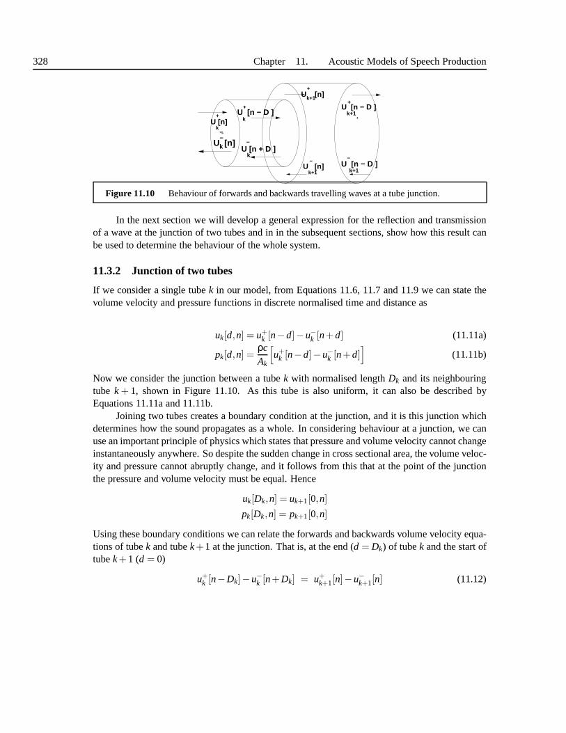
328 Chapter 11. Acoustic Models of Speech Production
U [n − D ]k
+
k
−
U [n]−
U [n]k
+
U [n]k+1
−
U [n − D ]k+1
+
U [n − D ]k+1
−
U [n]k+1
+
−
+
k
−U [n + D ]
Figure 11.10 Behaviour of forwards and backwards travelling waves at a tube junction.
In the next section we will develop a general expression for the reflection and transmissionof a wave at the junction of two tubes and in in the subsequent sections, show how this result canbe used to determine the behaviour of the whole system.
11.3.2 Junction of two tubes
If we consider a single tubek in our model, from Equations 11.6, 11.7 and 11.9 we can state thevolume velocity and pressure functions in discrete normalised time and distance as
uk[d,n] = u+k [n−d]−u−k [n+d] (11.11a)
pk[d,n] =ρcAk
[
u+k [n−d]−u−k [n+d]
]
(11.11b)
Now we consider the junction between a tubek with normalised lengthDk and its neighbouringtube k + 1, shown in Figure 11.10. As this tube is also uniform, it can also be described byEquations 11.11a and 11.11b.
Joining two tubes creates a boundary condition at the junction, and it is this junction whichdetermines how the sound propagates as a whole. In considering behaviour at a junction, we canuse an important principle of physics which states that pressure and volume velocity cannot changeinstantaneously anywhere. So despite the sudden change in cross sectional area, the volume veloc-ity and pressure cannot abruptly change, and it follows fromthis that at the point of the junctionthe pressure and volume velocity must be equal. Hence
uk[Dk,n] = uk+1[0,n]
pk[Dk,n] = pk+1[0,n]
Using these boundary conditions we can relate the forwards and backwards volume velocity equa-tions of tubek and tubek+1 at the junction. That is, at the end (d = Dk) of tubek and the start oftubek+1 (d = 0)
u+k [n−Dk]−u−k [n+Dk] = u+
k+1[n]−u−k+1[n] (11.12)

Section 11.3. Vowel Tube Model 329
U [n]
U [n]
U [n − D ]
AA
transmissioncoefficient
reflectioncoefficient
k
+
+
k+1
−
k+1
k k+1
Figure 11.11 Tube junction showing how wave u+ is made from reflection of U-in tube k+1, andtransmission of u+ from tube k
and likewise with the pressure:
ρcAk
[u+
k [n−Dk]+u−k [n+Dk]]=
ρcAk+1
[u+
k+1[n]+u−k+1[n]]
(11.13a)
1Ak
[u+
k [n−Dk]+u−k [n+Dk]]=
1Ak+1
[u+
k+1[n]+u−k+1[n]]
(11.13b)
we can substitute these equations into one another and eliminate one of the volume velocity terms.For example, from Equation 11.12 we know thatu−k [n+ Dk] = u+
k+1[n]− u−k+1[n] + u+k [n−Dk],
which we can substitute into Equation 11.13b to give an expression foru+k+1[n]
u+k+1[n] =
[ 2Ak+1
Ak +Ak+1
]
u+k [n−Dk]+
[Ak+1−Ak
Ak +Ak+1
]
u−k+1[n] (11.14)
This equation is interesting in that it shows the make up of the forward travelling wave in tubek+1. As we would expect, this is partly made up of the forward travelling wave from tubek andpartly from some of the backward travelling wave being reflected at the junction. The coefficientof u+
k in Equation 11.14 is the amount ofu+k that istransmitted into the next tube,k+ 1, and is
termed thetransmission coefficient. The coefficient ofu−k+1 is the amount ofu−k+1 that isreflectedback into tubek+ 1 at the junction and is termed thereflection coefficient. As they are simplyrelated, only one is needed to describe the junction and by convention reflection coefficients areused. The reflection coefficient is often denotedrk (meaning the reflection between tubesk andk+1) and from 11.14 is given by:
rk =Ak+1−Ak
Ak +Ak+1(11.15)
Of particular importance is that fact that the boundary condition is completely described by thereflection coefficient, and this is only governed by the areasof the tubes; the speed of sound and

330 Chapter 11. Acoustic Models of Speech Production
density terms have been eliminated. We shall see that reflection coefficients are a simple and usefulway to define the characteristics between two tubes and we will henceforth use them instead oftube areas. Using reflection coefficients, we can find expressions that relate the forward wave orthe backward in one tube with the forward and negative waves in the other tube:
u+k [n−Dk] =
11+ rk
u+k+1[n]+
rk
1+ rku−k+1[n] (11.16a)
u−k [n+Dk] =−rk
1+ rku+
k+1[n]+1
1+ rku−k+1[n] (11.16b)
11.3.3 Special cases of junction
The above result can be used to help set boundary conditions for the tube at the lips and the glottis.To see this, let us consider three special cases resulting from changing areas in the tubes.
Firstly, if two connected tubes have the same cross sectional area we see from 11.15 thatthe reflection coefficient is 0 and the transmission coefficient is 1. That is, there is no reflectionand all the wave is transmitted past the boundary. This is entirely what we would expect fromour uniform tube model. Next, let us consider the situation where the tube is completely closed atone end. A closed termination can be modelled by having the second tube have an infinitely smallarea (that is, the size of the junction between the tubes disappears to nothing and hence createsa solid wall). The effect of this can be found from Equation 11.15. As the area of the secondtube,Ak+1→ 0, the reflection coefficientrk→−1. Now consider a completely open tube. Thiscan again be modelled with the tube junction model, but this time the area of the second tube isinfinitely big. Hence, from Equation 11.15, asAk+1→ ∞ the reflection coefficientrk→ 1. Henceboth a closed termination and a open termination completelyreflect the wave.
There is a crucial difference between the two situations however and this can be seen fromthe sign of the reflection coefficient. In the closed termination case, the tube ends in a solid walland the reflection coefficient is -1. From Equation 11.16b we can see that in such a case thevolume velocity will be 0. If we find the equivalent pressure expressions for Equation 11.16b, wesee that the pressure terms add, and hence the pressure at this point is(ρc)/A1. Intuitively, we canexplain this as follows. The solid wall prevents any particle movement and so the volume velocityat this point must be 0. The pressure however is at its maximum, as the wall stopping the motionis in effect an infinite impedance, meaning no matter how muchpressure is applied, no movementwill occur. In the open end situation, when the reflection coefficient is 1, we see from Equation11.16b that the volume velocity is at a maximum and now the pressure is 0. Intuitively, this canbe explained by the fact that now the impedance is 0, and henceno pressure is needed to move theair particles. Hence the pressurep(L, t) is 0, and the volume velocity is at its maximum.

Section 11.3. Vowel Tube Model 331
lips
lungs
r rG 1
glottis
tube 1 tube 2
rL
reflection coefficients
open air
Figure 11.12 Two tube model with terminations at the glottis and lips. This system has threereflection coefficients. In the middle we haver1 the only “real” reflection coefficient, whose valueis given by the area Equation 11.15. The lips and glottis reflection coefficients are artificial valuesdesigned to ensure there are some losses from the system. Note that there is no backwards waveentering at the lips, and no forwards wave (save the source) entering at the glottis.
11.3.4 Two tube vocal tract model
Here we will consider a model in which we have two connected tubes of different cross sectionalareas. In this formulation, the tubes have areasA1 andA2, and normalised lengthsD1 andD2,such thatD1 + D2 = D, the total normalised length of the vocal tract. Using the results fromSection 11.3.3, we represent the behaviour at the boundary by the reflection coefficientr1. Thelips and glottis are modelled by two special tubes which havereflection coefficientsrL and rG
respectively. We can set these so as to produce different effects - one configuration is to havethe glottis completely closed and the lips completely open;another is to have values for eachcoefficient being slightly less than this value so that some losses occur and so that some soundpropagates from the lips. These lip and glottis tubes are special because we add an extra conditionsuch that any tube entering these tubes is never reflected back again. Examining a two tube modelin depth gives us a feel for how this system operates as a whole; following this section we willconsider the behaviour of a single tube, the behaviour when we consider losses, and a final modelwhere we have an arbitrary number of tubes.
Our goal is to find the z-domain transfer function of the system, and we will find this bydividing the z-domain expressions for output at the lips by the input at the glottis. The best wayto proceed is to define the volume velocity at the lips, use this to find the volume velocity at thejunction between the two proper tubes, and use this to find thevolume velocity at the glottis. Todo this we use Equations 11.16b and 11.16b which relate the volume velocity in one tube to the

332 Chapter 11. Acoustic Models of Speech Production
volume velocity in the next. As our end point is a z-domain expression, we will make repeated useof the z-transforms of equations 11.16b which are
U+k (z) =
zDk
(1+ rk)U+
k+1(z)−rkzDk
(1+ rk)U−k+1(z) (11.17a)
U−k (z) =−rkz−Dk
(1+ rk)U+
k+1(z)+z−Dk
(1+ rk)U−k+1(z) (11.17b)
We start by definingUL(z) as the output at the lips. We now feed this into Equations 11.17band 11.17b and use the fact that there is no backwards wave (U−L = 0) to set the volume velocitiesat junctionk = 2 as:
U+2 (z) =
zD2
1+ rLUL(z) (11.18a)
U−2 (z) =−rLz−D2
1+ rLUL(z) (11.18b)
By feeding these values into Equation 11.17b again, we can calculate the volume velocitiesU+1
andU−1 at the junctionk = 1.
U+1 (z) =
zD1
1+ r1.U2(z)−
r1zD1
1+ r1U2(z)
=zD1.zD2
(1+ r1)(1+ rL)UL(z)+
r1rLzD1z−D2
(1+ r1)(1+ rL)UL(z)
U−1 (z) =−r1z−D1
1+ r1.U2(z)+
z−D1
1+ r1U2(z)
=r1z−D1.zD2
(1+ r1)(1+ rL)UL(z)−
z−D1z−D2
(1+ r1)(1+ rL)UL(z)
We have now reached the glottis, modelled by a special tube oflength 0 and reflection coefficientrG. We take the length of this tube to be 0, and asz0 = 1 then
Ug(z) = =1
1+ rGU+
1 (z)− rG
1+ rGU−1 (z)
To findU+G we simply repeat the above procedure again. Note that we don’t need to knowU−G as
we are assuming this gets fully absorbed into the lungs.
U+G (z) =
zD1zD2 + r1rLzD1z−D2 + r1rGz−D1zD2 + rLrGz−D1z−D2
(1+ rG)(1+ r1)(1+ rL)UL(z)

Section 11.3. Vowel Tube Model 333
r = 1L
completereflection
completereflection
Gr = −1
glottis lips
open air
Figure 11.13 Uniform tube model of vocal tract where the glottis end is closed and the lips endopen
By rearranging to getUL/UG and by dividing top and bottom byzD1zD2 we get the standard formof the transfer function as a rational function inz−1:
V(z) =UL
UG=
(1+ rG)(1+ r1)(1+ rL)z−(D1+D2)
1+ r1rLz−2D2 + r1rGz−2D1 + rLrGz−2(D1+D2)
The terms containingr in the numerator sum to form the gain,G. The normalised tube lengthsD1andD2 must sum to the overall lengthD1+D2= D, which gives
V(z) =UL
UG=
Gz−D
1+ r1rLz−2(D−D1) + r1rGz−2D1 + rLrGz−2D(11.19)
Note that the lengths of the tubesD1,D2 must be integers; this is a constraint imposed by thediscrete modelling of the vocal tract. The discrete modelling also dictates the number of poles: fora higher sampling rate requires more poles and hence the granularity of the tube lengths increases.
11.3.5 Single tube model
A special case of the two tube model is the single tube or uniform tube model where the crosssectional area is constant along the entire length of the tube. This is a reasonable approximation ofthe vocal tract when producing the schwa vowel. IfA1 = A2, then the refection coefficientr1 = 0and hence Equation 11.19 simplifies to
V(z) =Gz−D
1+ rLrGz−2D(11.20)
Recall thatD is the length of the vocal tract in units of the normalised distance that we usedto simplify the equation for discrete time analysis. By use of Equation 11.9, we can determine a

334 Chapter 11. Acoustic Models of Speech Production
value for D from empirically measured values. For instance,if we set the length of the vocal tractas 0.17m (the average for a male), the speed of sound in air as 340ms-1, and choosing a samplingrate of 10000Hz, Equation 11.9 gives the value ofD as 5. Hence the transfer function becomes
V(z) =Gz−5
1+ rLrGz−10 (11.21)
that is, an IIR filter with 5 zeros and 10 poles. It can be shown that a polynomial 1+ rLrGz−10 canbe factorised to a set of 10 complex roots, such that in polar terms the radius of each root isrLrG,and the angle is given by
θn =π(2n−1)
10(11.22)
The numerator of the transfer function tells us that the output is delayed by a factor whichis a function of the length of the tube. All these zeros lie at 0, and can be ignored for purposesof determining the frequency response of the transfer function. The poles are evenly spaced onthe unit circle at intervals ofπ/5. The first is atπ/10 = 0.314, which when converted to a realfrequency value with Equation 10.29, gives 500Hz. Subsequent resonances occur every 1000Hzafter that, i.e. 1500Hz, 2500Hz and so on.
Recall that the losses in the system come from the wave exiting the vocal tract at the glottisand lips, and the degree to which this is done is controlled bythe special reflection coefficientsrL
and rG. Let us first note, that since these are multiplied, it doesn’t affect the model as to wherethe losses actually occur, and in fact in some formulations the losses are taken to occur only at theglottis or only at the lips. Secondly, recall from Section 11.3.3, that the special case of completeclosure at the glottis would produce a reflection coefficientof 1, and the special condition ofcomplete openness at the lips would produce a reflection coefficient of -1. This is a situationwhere there are no losses at all in the system (unrealistic ofcourse, for the simple fact that nosound would escape and hence a listener would never hear the speech.) For these special cases theproduct isrLrG is 1, which means that the denominator term is
V(z) =Gz−5
1−z−10
It can be shown that when this is factorised, all the poles arespaced as before, but lie on the unitcircle. This is of course exactly what we would expect from a lossless case.
We can find the frequency response of the vocal tract by setting z = ejω. For the speciallossless case then,
V(ejω) =2ej5ω
1+ej10ω

Section 11.3. Vowel Tube Model 335
0 500 1000 1500 2000 2500 3000 3500 4000 4500 50000
2
4
6
8
10
12
14
16
18
20
Figure 11.14 Magnitude spectrum for uniform tube, showing that the resonances are sharp spikes(because there is no damping) and that the resonances lie at even intervals along the spectrum.
Making use of the inverse Euler expression, Equation 10.11 can also be written as:
V(ejω) =1
cos(5ω)(11.23)
This frequency response is shown in Figure 11.14, and it can be seen that the formants are verysharp (no damping) and lie at evenly spaced intervals, as predicted by the transfer function.
11.3.6 Multi-tube vocal tract model
We will now develop a general expression for the transfer function of a tube model for vowels, inwhich we have an arbitrary number of tubes connected together.
We saw in Section 11.3.5 that the order of the final transfer function is determined by thenormalised length of the tubeD. This is turn is a function of sampling rate and vocal tract lengthand so longer vocal tracts or higher sampling rates will require higher order filters. Staying withthe case of a 0.17m vocal tract with 340ms-1 speed of sound and10000Hz sample rate, we findwe need a 10th order transfer function as shown in the cases ofthe uniform and two tube models.The difference in the transfer function for these two modelsis simply in the inclusion of the extranon-zero coefficients in the denominator. Extending this principle, we find that the most powerfultransfer function is one with a non-zero coefficient for every term inz−1. Such a transfer functioncan be created by a model with exactly 10 equal length tubes, each of which has lengthDN = 1/2.Importantly, for the given sample rate, no extra accuracy isachieved by increasing the number oftubes beyond this value.

336 Chapter 11. Acoustic Models of Speech Production
The principle behind finding the N tube transfer function is the same as for the two tubemodel - start at the lips and apply Equations 11.18a and 11.18b for each tube in turn. This is tediousto perform in the manner used for the two tube system, but we can use matrix multiplication tospeed up the process.
Equations 11.17b and 11.17b can be expressed in matrix form as:
Uk = QkUk+1
where
Uk =
[
U+k (z)
U−k (z)
]
and becauseD = 1/2, then
Qk =
[z1/2
1+rk
−rkz1/2
1+rk−rkz−1/2
1+rk
z−1/2
1+rk
]
We can use the special reflection coefficients at the lips and glottis to model the terminating bound-ary conditions as before. In the matrix formulation, this gives
UN+1 =
[
UL(z)0
]
=
[
10
]
UL(z) (11.24)
for the lips and
UG =[ 1
1+ rG
1rG
1+ rG
]
U1(z) (11.25)
for the glottis. We can use these boundary conditions to formulate an expression for the transferfunction for an arbitrary number of tubes
1V(z)
=UG
UL=[ 1
1+ rG
1rG
1+ rG
] N
∏k=1
Qk
[
10
]
which can be solved by iteratively calculating the terms. The result of this will always take theform:
V(z) =1+ r0
2
z−N/2N∏
k=1(1+ rk)
1−a1z−1−a2z−2...−aNz−N (11.26)
which as we saw before, is simply a delay in the numerator, followed by an all-pole expression inthe denominator. This is an important result, because it shows that a vocal tract without internallosses can be accurately modelled by an all-pole filter.3
3 Rabiner and Schafer [368] show that the above can be calculated more easily, and without direct matrix multiplicationif we assume that the glottal impedance is infinite.

Section 11.3. Vowel Tube Model 337
It is possible to simplify the calculation by making the further assumption that glottis is acompletely closed end, with infinite impedance and reflection coefficient 1. If we take
AN(z) =N
∑k=1
akz−k
it is possible to show that in the case thatrg = r0 = 1 that the following equation holds
AN(z) = AN−1(z)+ rkz−kDk−1(z
−1) (11.27)
That is, the Nth order polynomial inz−1 can be determined from the N-1 order polynomial inz−1,zand the reflection coefficientrk. If we therefore start atN = 0 and setA0(z) = 1 we can calculatethe value forA1, and then iteratively for allA(z) up toN. This is considerably quicker than carryingout the matrix multiplications explicitly. The real value in this however, will be shown in Chapter12, when we consider the relationship between the all-pole tube model and the technique of linearprediction.
11.3.7 The all pole resonator model
This general result is important as it shows that for any number of tubes, the result is alwaysan all-pole filter. From Section 10.5.1, we know that this canbe factorised into an expressioncontaining individual poles, and these can often be interpreted directly as formant resonances.Here we see we have come full circle; in Section 10.5.3 we showed that a second order IIR filtercould faithfully model the shape of a single formant, in Section 10.5.4 we showed that several ofthese could be cascaded to model a number of formants. In thischapter, we saw in Section 11.2.1that a physical mass/spring/damped system can be modelled by the same Equations, and that asingle mass, spring and damper create a resonance pattern ofexactly the same type as a secondorder IIR formant model. In the preceding section, we have just shown that a connected tubemodel has an all-pole transfer function, with the number of poles equalling the number of tubes.From this result, it is clear that an all-pole tube model can faithfully create any formant patternif the parameters to the tubes (i.e. the cross sectional areas) are set correctly. Furthermore, thetransfer function for the tube model can be factorised so as to find the poles, and possibly identifyindividual formants.
An important point to realise is that the formant patterns that arise from this all-pole modelare a function of the whole model; while the transfer function can be factorised, it isnot appro-priate to ascribe individual poles or formants to individual tubes in the model. The situation ismore complex than this, and the formant patterns are createdfrom the properties of all the tubesoperating together.

338 Chapter 11. Acoustic Models of Speech Production
openphase
returnphase
closedphase
Figure 11.15 Plot of idealised glottal source, as volume velocity over time. The graph shows theopen phase, where air is flowing through the glottis, the short return phase, where the vocal folds aresnapping shut, and the closed phase, where the glottis is shut, and the volume velocity is zero. Thestart of the closed phase is the instant of glottal closure.
11.4 SOURCE AND RADIATION MODELS
11.4.1 Radiation
So far, we have developed a transfer functionV(z) which is defined as the ratio of the volumevelocity of the lips over the volume velocity at the glottis.In practice however, when we mea-sure sound, we normally in fact measure pressure signals, asthis is what most microphones aredesigned to respond to. Most microphones exist in thefar-field , that is at some distance fromthe lips, and hence the signal is influenced by aradiation impedance from the lips. This can bemodelled by another transfer function,R(z), which, from Equation 11.4 is defined as
R(z) =P(z)
UL(z)(11.28)
Modelling radiation accurately soon becomes very complicated, so for our purposes, we usea very simple model that has been shown to do a reasonable job at approximating the radiation.This takes the form of a function which differentiates the signal, and this can be modelled by aFIR filter with a single zero:
R(z) = 1−αz−1 (11.29)
whereα is a value less than but quite near to 1 (e.g. 0.97). This creates a high frequency boost ofabout 6dB per octave.
11.4.2 Glottal source
We qualitatively described in Section 7.1.2 the process of how the glottis produces sound. Invoiced speech, the vocal folds undergo a cycle of movement which gives rise to a periodic source
Section 11.4. Source and radiation models 339
sound. At the start of this cycle the vocal folds are closed. Pressure is exerted from the lungs whichcauses a build up in pressure beneath the folds until eventually the pressure forces open the folds.When the folds open, air moves through them and as it does do, the pressure beneath the foldsreduces. Eventually the pressure is low enough so that the tension closes the vocal folds, afterwhich the cycle repeats. The rate at which this cycle occurs determines the fundamental frequencyof the source, and ranges from about 80Hz to 250Hz for a typical male, and 120Hz to 400Hz fora typical female or child. A plot of volume velocity against time for the glottal source is shown inFigure 11.15. Here we see the three main parts of the cycle: the open-phasewhere the glottis isopening due to the pressure from the lungs, thereturn phase where the glottis is closing due tothe vocal tract tension, and theclosed phase.
Modelling the glottis is a tricky problem in that building a simple model seems relativelyeasy, but developing a highly accurate model that mimics glottal behaviour in all circumstances isextremely difficult and has not in any way been solved. We willreturn to the difficulties in accurateglottal modelling in Section 13.3.5, but for now we will demonstrate a simple model which at leastgives us a flavour of how this works.
An extensive study into glottal modelling is given in Flanagan [164], which describes variousmass/spring/damped systems. These models can be somewhat difficult to model in discrete timesystems, so instead we adopt models which simply generate a time domain function which has theproperties described above. One such model [376] [368] is given by:
u[n] =
12
(1−cos(πn
N1
)0≤ n≤ N1
cos(π(n−N1)2N2
)N1≤ n≤ N2
0 otherwise
(11.30)
whereN1 marks the end of the open phase andN2 marks the end of the return phase/start of theclosed phase. Another quite widely used model is the Lijencrants-Fant model [159] (sometimesknown as the LF model). This describes the glottal waveform derivative and is given by
u[n] =
0 0≤ n < To
E0eα(n−T0)sin[Ωo(n−T0)] T0≤ n < Te
−E1[eβ(n−Te)−eβ(Tc−Te)] Te≤ n < Tc
(11.31)
whereT0 is the instant of glottal opening,Te is the position of the negative minimum,Tc is theinstant of glottal closure,α, β andΩ control the shape of the function, andE0 andE1 determinethe relative heights of the positive and negative part of thecurve. The LF function and its integral,which is the normal glottal flow function, is shown in figure 11.16. Quatieri [364] gives a thirdmodel, in whichg(n) is created by two time reversed exponentially decaying sequences:
u[n] = (β−nu[−n])∗ (β−nu[−n]) (11.32)
which have the nice property of having a simple z-transform

340 Chapter 11. Acoustic Models of Speech Production
0 50 100 150 200 250 300−15000
−10000
−5000
0
5000
Figure 11.16 Plot Lijencrants-Fant model for glottal flow and derivativeglottal flow for a singleperiod.
U(z) =1
(1−βz)2 (11.33)
The most important control element in the glottal source is of course the rate at which thecycles occur. In Equation 11.30, this is determined by the positions ofN1 andN2; in Equation11.32 byT0, Te andT0; and in Equation 11.31 this is determined by the impulse function u[n].In the last case, the glottal volume velocity function can bethought of as a low pass filtering ofan impulse stream. From these expressions and empirical measurements, it is known that this lowpass filter creates a roll off of about -12dB per octave. It is this, combined with the radiation effect,that gives all speech spectra their characteristic spectral slope.
While Equation 11.32 gives a reasonable approximation of the glottal volume velocity signal,it does not model the secondary effects of jitter, shimmer and ripple as mentioned in Section 17.More realism can be added to the glottal signal by the addition of zeros into the transfer function,giving the expression:
U(z) =
M∏
k=1(1−ukz−1)
(1−βz)2 (11.34)
We have definedU(z) as a volume velocity signal, mainly for purposes of developing thevocal tract transfer function. While in reality, the radiation R(z) occurs after the operation ofV(z),we aren’t restricted to this interpretation mathematically. As we shall see, it is often useful tocombineU(z) and R(z) into a single expression. The effect of this is to have a system wherethe radiation characteristic is applied to the glottal flow waveform before it enters the vocal tract.
Section 11.5. Model refinements 341
This is equivalent to measuring the pressure waveform at theglottis, and if we adopt the radiationcharacteristic of Equation 11.29, the effect of this is to differentiate the glottal flow waveform. Wecall this signal theglottal flow derivative, denoted ˙s[n] andS(z) and and this is shown along withthe normal glottal flow in Figure 11.16.
The interesting feature of the glottal flow derivative is that it shows that the primary formof excitation into the vocal tract is a large negative impulse. This is useful in that the output ofthe vocal tract immediately after this should approximate well to the true impulse response of thesystem.
11.5 MODEL REFINEMENTS
11.5.1 Modelling the nasal Cavity
When the velum is lowered during the production of nasals andnasalised vowels, sound entersvia the velar gap, propagates through the nasal cavity and radiates through the nose. Hence for amore complete model, we have to add a component for the nasal cavity. This in itself is relativelystraightforward to model; for a start, it is a static articulator, so doesn’t have anywhere near thecomplexity of shapes that occur in the oral cavity. By much the same techniques we employedabove, we can construct an all-pole transfer function for the nasal cavity.
The complication arises because of the behaviour of the oralcavity. For the case of vowels,the sound wave moved from the glottis through the oral cavityand radiated from the lips. Inthe case of nasalised vowels, the sound propagates from the glottis and through the pharynx asbefore, but at the velum some sound enters the nasal cavity while the remainder propagates throughthe mouth. The sound entering through the velum is filtered bythe nasal cavity and radiatesthrough the nose. The sound continuing through the oral cavity radiates through the lips in themanner described above. One complication to this is that thesome sound in the oral cavity isreflected backwards and will enter the velar gap, and likewise some sound in the nasal cavity willbe reflected backwards and will enter the oral cavity. If we however ignore this interaction fornow, the system for nasalised vowels can be modelled as shownin Figure 11.17 with a simplesplitting operation at the velum. Because we now have two filters operating in parallel, it is notpossible to derive a single transfer function for the whole system. Rather we construct a transferfunction for the oral cavity, a different one for the nasal cavity and then simply add the outputs ofboth to find the final signal.
The case of nasal consonants is more complicated. As with nasalised vowels, the sound wavestarts at the glottis moves through the pharynx and partly through the mouth. Some sound nowtravels through the velum, nasal cavity and radiates through the nose. The remainder continuestravelling through the oral cavity, but instead of being radiated at the lips, now meets a closure atthe lips. Hence a full reflection occurs, and so the sound travels backwards through the mouth, andsome continues down towards the glottis and some enters the nasal cavity and radiates from the

342 Chapter 11. Acoustic Models of Speech Production
P(z) M(z) R(Z)U(z) U(z)LL
(a) vowel and approximant
P(z) M(z)U(z) U(z)LL
N(z) R (Z)N
R (Z)
(b) nasalised vowel
P(z) M(z)U(z)
N(z) R (Z)N
U (z)L
(c) nasal)
U (z)LM (z)V (z)B
noisesourceU (z)
R (z)L
(d) unvoiced obstruent
U (z)LM (z)V (z)B
R (z)Lsource
glottal
G
noisesource
U (z) W U (z)
(e) voiced obstruent
Figure 11.17 LTI filter models for different types of sound production.

Section 11.5. Model refinements 343
nose. In addition to this, there are of course the forwards and backwards reflections being causedall the time by the changing cross sectional areas of the noseand mouth. An equivalent way oflooking at this is that the pharynx, nasal cavity and nose operate for nasals in the same the wayas the pharynx, oral cavity and lips operate for vowels. In addition, there is now aside resonatorof the front of the mouth. In phonetic terms the effect of thisoral side cavity is very important;as the nasal cavity is static, it is in fact the ability of the tongue to create different oral side cavityconfigurations which is responsible for the nasal sounds /m/, /n/ and /ng/ all sounding different.
Acoustically, the effect of the side branch is to “trap” someof the sound, and this createsanti-resonances. These can be modelled by the inclusion of zeros in the transfer function. As withthe case of nasalised vowels, the parallel nature of the system means we can’t use a single transferfunction; rather we have a system with an all-pole transfer function for the pharynx and back ofthe mouth, a splitting operation, an all-pole function for the nose and a pole and zero function forthe oral cavity.
11.5.2 Source positions in the oral cavity
Many consonant sounds, such as fricatives and stops have a sound source located in the oral cavity.This is created by the tongue nearing another surface (the roof of the mouth, the teeth etc) so asto cause a tight constriction. In the case of unvoiced obstruents, the glottis is open, and air flowsthrough it until it reaches the constriction, at which pointturbulence occurs. For voiced obstruents,the glottis behaves as with vowels, but again this air flow is made turbulent by the constriction. Thedifference in placement of the constriction is what gives rise to the difference between the variousfricative and stop sounds of the same voiced. Hence /s/ has analveolar construction whereas /sh/has a palatal constriction. It is important to realise however that the constrictions themselves donot generate different sounding sources; it is the fact thatthe constrictions configure the vocaltract into different shaped cavities through which the source resonates that is responsible for theeventual difference in the sounds.
The effect of a sound source in the middle of the vocal tract isto split the source such thatsome sound travels backwards towards the glottis while the remainder travels forwards towards thelips. The vocal tract is thus effectively split into a backward and forward cavity. The forward cavityacts a tube resonator, similar to the case of vowels but with fewer poles as the cavity is considerablyshorter. The backwards cavity also acts as a further resonator. The backwards travelling sourcewill be reflected by the changes in cross sectional area in theback cavity and at the glottis, creatinga forward travelling wave which will pass through the constriction. Hence the back cavity has animportant role in the determination of the eventual sound. This back cavity acts as a side resonator,just as with the oral cavity in the case of nasals. The effect is to trap sound and create anti-resonances. Hence the back cavity should be modelled with zeros as well as poles in its transferfunction.

344 Chapter 11. Acoustic Models of Speech Production
11.5.3 Models with Vocal Tract Losses
The tube model described in Section 11.3 is termed “lossless” because no energy losses occurduring the propagation of sound through the tube itself. Anyenergy losses which do occur happenthrough the lips and glottis, where the signal travels outwards but is not reflected back. Severalstudies have been made into modelling the losses which of course do occur in the tubes themselves.In terms of the discussion given in Section 11.2.3, this means that the impedance now is justcomposed of an inductive and capacitance component, but also has a resistive component.
Rabiner and Schafer [368] give an extensive review of this issue and summarise that thereare three main ways in which losses can occur. First, the passage of the wave will cause the wallsof the vocal tract (e.g. the cheeks) to vibrate. This can be modelled by refinements to the transferfunction. The effect is to raise the formant centre frequencies slightly, dampen the formants andespecially the lower formants; we should expect this as it the mass of the vocal tract walls willprevent motion at the higher frequencies. The effects of friction and thermal conduction can alsobe modelled by adding resistive terms to the transfer function. The overall effect of these is theopposite of above; the formant centre frequencies are somewhat lowered, and the effects of thisare more pronounced at higher frequencies.
Apart from the overall contribution to damping, these effects tend to cancel each other out,and so the overall contribution of these resistive terms is quite small. As the degree of loss fromthe lips and glottis is considerably higher, these loss terms are often ignored altogether as they addconsiderable complication to the model with little gain in modelling accuracy. It should be notedthat it is the particular form of the IIR expression that we derived that gives rise to a lossless tube;other IIR filter expressions can easily model losses.
11.5.4 Source and radiation effects
Our model of the glottis and lips was extremely simple in thatwe used special reflection coeffi-cientsrG andrL to generate reflections and losses (for values other that|1|). As we might expect,in reality the situation is much more complicated. Firstly,there is no such thing as an “idealsource” where we can simply add volume velocity into a systemwithout any further effect. Thesource in fact is always to a greater or lesser degree coupledto the rest of the system, and has tobe modelled if more accuracy is desired. In general this is modelled by having a real impedanceconnecting the source to the rest of the system. Again, assuming that sound can just propagatefrom the lips and “disappear” with no further effect is quitesimplistic. A more accurate model canbe created by modelling the radiation as a complex impedanceconnected as part of the system.
In this chapter we have concentrated on sound propagation through a tube, and saw that eventhis, the simplest of all acoustic systems can be quite complicated. Another entire branch of thefield of acoustics is devoted to sound propagation through three dimensional spaces, and this canbe drawn on to produce a better model of radiation through thelips. As with the other refinementsmentioned in this section, modelling both the source and liplosses with more realistic expressions

Section 11.6. Discussion 345
does increase the accuracy of the overall model, but does so at considerable modelling expense.
11.6 DISCUSSION
In developing our model, we have attempted to balance the needs of realism with tractability. Theall-pole vocal tract model that described in Section 11.3 will now be adopted for the remainder ofthe book as the model best suited to our purposes. In subsequent chapters, we shall in fact see thatthis model has some important properties that make its use particularly attractive.
One of the key jobs in making assumptions in a model is to recognise that such assumptionshave indeed been made. So long as this is done, and these assumptions are borne in mind, weshould not run into too many problems when we rely on the modelto deliver faithful analyses.With this in mind, we will now note the main assumptions we have made and discuss any potentialproblems that might arise because of these. The following list is in approximate increasing orderof severity.
Linear filter Throughout we have assumed that the system operates as a timeinvariant linear(LTI) filter of the type described in Chapter 10. While it is well known that there are manynon-linear processes present in vocal tract sound propagation, in general the linear modelprovides a very good approximation to these.
Time invariance During normal speech, the vocal tract is constantly moving,so long as the rateof change is very slow compared to the sampling rate, it is quite adequate to model thesystem as a sequence of piecewise stationary configurations. In Chapter12, we will discussfurther the issue of quantising the time dimension so as to produce stationary “snapshots” ofspeech, but for now let us say that a good approximation to a continuously varying tract is togenerate a new stationary vocal tract configuration about every 10ms.
Straight tube One of the first assumptions we made was that we could model thevocal tract by astraight tube or sequence of straight tubes. The vocal tractis of course curved; very roughly itstarts as a vertical tube at the glottis, takes a 90 degree turn at the top of the pharynx and thencontinues horizontally through the mouth. In fact it is one of the main principles of acousticmodelling that so long as any bend is not too severe, there is little difference between thepropagation in straight or curved tubes. This can be seen clearly in music, where a moderntrumpet is actually a quite long (10m) tube which has been wrapped many times to makeits playing and carrying more convenient. The bends in the trumpet have little effect on theoverall sound.
Discrete tube modelThe number of tubes determines the granularity at which we model the real,continuously varying tube. As we saw in Section 11.3.6, the number of tubes is determinedby the sampling rate, and so long as we have the correct numberof tubes for the samplingrate being used, there will be no loss of accuracy. A rule of thumb is that we use one tube forevery 1kHz sampling rate, so that 10KHZ requires 10 tubes andso on. For a true continuous

346 Chapter 11. Acoustic Models of Speech Production
signal (equivalent to an infinite sampling rate) we see that we require an infinite number ofzero length tubes, ie a continuous tube. For all practical purposes, the discrete nature of thetube has no effect on accuracy.
All pole modelling Only vowel and approximant sounds can be modelled with complete accuracyby all-pole transfer functions. We will see in Chapter 12 that the decision on whether toinclude zeros in the model really depends on the applicationto which the model is put,and mainly concerns tradeoffs between accuracy and computational tractability. Zeros intransfer functions can in many cases be modelled by the addition of extra poles. The polescan provide a basic model of anti-resonances, but can not model zero effects exactly. Theuse of poles to model zeros is often justified because the ear is most sensitive to the peakregions in the spectrum (naturally modelled by poles) and less sensitive to the anti-resonanceregions. Hence using just poles can often generate the required spectral envelope. Oneproblem however is that as poles are used for purposes other than their natural one (to modelresonances) they become harder to interpret physically, and have knock on effects in saydetermining the number of tubes required, as explained above.
Lossless tubeThe real losses in the vocal tract are slight, but as the difference between a polebeing on the unit circle (no loss whatsoever) and slightly within the circle (say at a radiusof 0.95) is quite noticeable, then any loss factors will affect the overall system. That said,so long as any ignored losses in the vocal tract are compensated for by increased loss at thelips and glottis, the effect should not be too great. If only the lips and glottis are used forcontrolling losses, the effect is that a single damping factor is applied to all the formants, andhence it is not possible to generate formants with independent bandwidths.
Radiation characteristics The use of a reflection coefficient to model the radiation fromthe lipsis really quite crude. In reality, radiation is very complicated and effected by the exact shapeof the lips and head. In our simple example we effectively modelled the region outsidethe lips as an additional tube - for the complete reflection case this is an infinitely widetube, that is, the vocal tract opens into a wall that extends infinitely far in all directions.For the cases of less that total reflection, an additional tube of finite area was used. As areal head is actually concave with respect to the direction of radiation, rather than convexin the additional tube case, we see that this in fact is a very crude model. Rabiner andSchafer, and Flanagan develop more sophisticated expressions for lip radiation [368] [164].An important radiation effect that we have not touched upon is that the radiation determinesthe directional characteristics of the sound propagation.One commonly observed effect isthat high frequencies are more narrowly directed, so that ifa speaker is facing away from thelistener, the high frequencies are not heard - the speech sounds “muffled”.
Source filter separation This is one area where our model starts to break down significantly.Firstly we saw that modelling the glottis as a completely isolated source is quite unrealistic.In addition however, there are many physiological effects that make a complete source/filterseparation unrealistic. For example, it is clear that when speaking with a high fundamental

Section 11.6. Discussion 347
frequency, the entire set of muscles in the throat and mouth are much tenser than in lowpitched speech.
Glottal source Our model of the source itself is perhaps the crudest and least accurate part ofour model. We know for example that the shape of the volume velocity waveform changeswith frequency - it is not the case that a fixed low pass filter will do. The model describedabove also says nothing aboutvocal effort. It is clear that shouting is not just the sameas speaking with a louder source input - the entire characteristic of the glottal source haschanged. Furthermore, the dynamics of glottal signals are very complicated. In particular,when real glottal signals are studied in the regions where voicing starts and stops, we seemany irregular pitch periods, isolated periods of very short duration, and glottal signals thatseem very noisy. The glottal model described in Section 11.4models none of these affects. Asignificant amount of research has been conducted into building more sophisticated models,and progress has been made. However, many of these more sophisticated models are difficultto implement and control and hence the simple model explained above is often used. Weshall return to this issue in Section 13.3.5, where we shall see that difficulties in modellingsource characteristics well are in fact the most difficult problem in speech synthesis, to theextent that they have been one of the main driving factors in determining the path of speechsynthesis in recent years.
11.6.1 Further reading
Many books deal extensively with modelling the vocal tract acoustically, including Flanagan [164],Rabiner and Schafer [368] and of course Frant [158].
11.6.2 Summary
Model of the Vocal Organs
• The vocal apparatus can be modelled as a set of discrete, interconnected components.
• Each component functions as either a source component, which generates a basic sound, ora filter component, which modifies this sound.
• The filter components are joined in various configurations (Figure 11.17) to form tubes.
• For vowels, nasals and approximant, the source component isthe glottis. The glottis islocated at the end of the vocal tract tube.
• Radiation occurs at the lips and nose, and this can also be modelled by a filter.
• The filter components are the pharynx, oral cavity and nasal cavity.
• All of the above are modelled as lossless tubes.
• All of the above act as linear time invariant filters.
• Each component tube can be modelled, without loss of accuracy, as a series of connectedshorter uniform tubes. The number of uniform tubes requiredis a function of the required

348 Chapter 11. Acoustic Models of Speech Production
length of the main tube and the sampling rate.
Lossless tube models
• The sound wave generated by the source travels along the tubeand in so doing is modified.
• The tubes are assumed lossless, hence all the impedance terms are reactive, meaning thatthey only alter the frequency characteristics of the travelling wave, but do not cause energylosses.
• The main source of this is reflection, which occurs when the tube changes in cross sectionalarea.
• A tube which has a closed termination and a tube which has a completely open terminationcause complete reflection. At a closed termination, the pressure is at a maximum and thevolume velocity is zero; at an open termination the pressureis zero and the volume velocityis at a maximum.
• At other changes in area, some part of the sound is transmitted and some is reflected back-wards.
• The backwards waves interfere with the forwards waves, so that they reinforce at certainfrequencies. This causes resonances and hence creates formants.
• While each tube in itself is lossless, losses occur in the system because some sound escapesfrom the lips and glottis.
Transfer function
• By iterative application of the equations relating volume velocity in one tube to volumevelocity in the next, we can determine a transfer function for the whole tube.
• It is shown (Equation 11.26) that all such models produce a transfer function containing onlypoles (i.e. a polynomial expression inz−1 in the denominator).
• We know, from Section 10.5.4, that such transfer functions naturally produce resonancepatterns and hence formants.
• The polynomial expression can be factorised to find the individual poles.
• The values of the coefficients in the denominator polynomialare determined by the set ofreflection coefficients in the tube. There is no simple relationship between the reflectioncoefficients and the poles, but they can be calculated if needbe.
• The bandwidths of the resonances are determined by the losses in the system, and as theseonly occur at the lips and glottis (or even just the lips or just the glottis), there is only one ortwo parameters in the system controlling all of these.
• Modelling nasals and obstruents is more complicated because of the inclusion of side branchesin the model. These “trap” the sound, and are best modelled with filters which also containzeros.

Section 11.6. Discussion 349
• As nasals and obstruents involved parallel expressions, they can not be expressed as a singletransfer function.

12ANALYSIS OF SPEECHSIGNALS
In this chapter we turn to the topic ofspeech analysis, which tackles the problem of deriving rep-resentations from recordings of real speech signals. This book is of course concerned with speechsynthesis- and at first sight it may seem that the techniques for generating speech “bottom-up” asdescribed in Chapters 10 and 11 may be sufficient for our purpose. As we shall see however, manytechniques in speech synthesis actually rely on an analysisphase which captures key propertiesof real speech and then uses these to generate new speech signals. In addition, the various tech-niques here enable useful characterisation of real speech phenomena for purposes of visualisationor statistical analysis. Speech analysis then is the process of converting a speech signal to an alter-native representation that in some way better represents the information which we are interestedin. We need to perform analysis because waveforms do not usually directly gives us the type ofinformation we are interested in.
Nearly all speech analysis is concerned with a three key problems. First, we wish to removethe influence of phase; second, we wish to perform source/filter separation, so that we can studythe spectral envelope of sounds independent of the source that they are spoken with. Finally weoften wish to transform these spectral envelopes and sourcesignals into other representations, thatare coded more efficiently, have certain robustness properties, or which more clearly show thelinguistic information we require.
All speech signals in the real world are continuous signals which describe the pattern of airpressure variation over time. These signals can be recordedwith a variety of analogue means,but for computer analysis, we require our signals to bedigitised such that the continuous signalis converted to a discrete signal. For our needs, we need not go into the details of analoguesound capture and recording as it is most likely that any reader will either come across signalsthat are already digitised, or that they will be able to “record” any acoustic signal directly into adigitised form by using a standard computer sound card, without the need for any interim analoguerecording step1.
1 Many standard books explain the analogue to digital conversion process, for instance see Rabiner and Schafer [368].
350

Section 12.1. Short term speech analysis 351
12.1 SHORT TERM SPEECH ANALYSIS
A common starting point in speech analysis is to find the magnitude spectrum from a speech signal.We want this to be in a discrete form that is easy to calculate and store store in a computer, so weuse the discrete Fourier transform (DFT) as our principle algorithm. In practice the fast Fouriertransform (FFT) implementation is nearly always used due toits speed (see Section 10.2.4).
12.1.1 Windowing
When we speak, the glottis and vocal tract are constantly changing. This is problematic for most ofthe techniques we introduced in Chapter 10 as these were designed to work on stationary signals.We can get around this problem by assuming that the speech signal is in fact stationary if consid-ered over a sufficiently short period of time. Therefore we model a complete speech waveform asa series of short termframes of speech, each of which we consider as a stationary time-invariantsystem.
A frame of speechx[n] is obtained from the full waveforms[n] by multiplication by awindoww[n] in the time domain:
x[n] = w[n]s[n] (12.1)
Three common windows are therectangular window, hanning window andhamming window:
rectangular w[n] =
1 0≤ n≤ L−1
0 otherwise(12.2)
hanning w[n] =
0.5−0.5cos(2πnL ) 0≤ n≤ L−1
0 otherwise(12.3)
hamming w[n] =
0.54−0.46cos(2πnL ) 0≤ n≤ L−1
0 otherwise(12.4)
Figure 12.1 shows a sinusoid after windowing by the three windows just described. The rectangu-lar window abruptly cuts off the signal at the window edges, while the hanning tapers the signal sothat the discontinuities are absent. The hamming window is just a raised version of the hanning,and so has a similar shape accept for a slight discontinuity at the window edge.
While an essential part of speech analysis, the windowing process unfortunately introducessome unwanted effects in the frequency domain. These are easily demonstrated by calculating theDFT of the sinusoid. The “true” frequency domain representation for this, calculated in continuoustime with a Fourier transform, is a single delta peak at the frequency of the sinusoid. Figures 12.2show the DFT and log DFT for the three window types. The DFT of the rectangular window

352 Chapter 12. Analysis of Speech Signals
-1
-0.5
0
0.5
1
0 100 200 300 400 500
amplitud
e
samples
(a) Rectangular window
-1
-0.8
-0.6
-0.4
-0.2
0
0.2
0.4
0.6
0.8
1
0 100 200 300 400 500
amplitud
e
samples
(b) Hanning window
-1
-0.8
-0.6
-0.4
-0.2
0
0.2
0.4
0.6
0.8
1
0 100 200 300 400 500
amplitud
e
samples
(c) Hamming window
Figure 12.1 Effect of windowing in the time domain
shows a spike at the sinusoid frequency, but also shows prominent energy on either side. Thiseffect is much reduced in the hanning window. In the log version of this, it is clear there thereis a widermain lobe than in the rectangular case - this is the key feature as it means that moreenergy is allowed to pass through at this point in comparisonwith the neighbouring frequencies.The hamming window is very similar to the hanning, but has theadditional advantage that the sidelobes immediately neighbouring the main lobe are more suppressed. Figure 12.3 shows the effectof the windowing operation on a square wave signal and shows that the harmonics are preservedfar more clearly in the case where the Hamming window is used.
12.1.2 Short term spectral representations
Using windowing followed by a DFT, we can generateshort term spectra from speech wave-forms. The DFT spectrum is complex and and can be representedby its real and imaginary partsor its magnitude and phase parts. As explained in section 10.1.5 the ear is not sensitive to phaseinformation in speech, and so the magnitude spectrum is the most suitable frequency domain rep-resentation. The ear interprets sound amplitude in an approximately logarithmic fashion - so adoubling in sound only produces an additive increase in perceived loudness. Because of this, it isusual to represent amplitude logarithmically, most commonly on the decibel scale. By convention,we normally look at thelog power spectrum, that is the log of the square of the magnitude spec-trum. These operations produce a representation of the spectrum which attempts to match humanperception: because phase is not perceived, we use the powerspectrum, and because our responseto signal level is logarithmic we use the log power spectrum.

Section 12.1. Short term speech analysis 353
0
20
40
60
80
100
120
140
0 500 1000 1500 2000 2500 3000 3500 4000
log m
agnit
ude
frequency (Hz)
(a) Rectangular window
-300
-250
-200
-150
-100
-50
0
50
0 500 1000 1500 2000 2500 3000 3500 4000
log m
agnit
ude
frequency (Hz)
(b) Rectangular window
0
10
20
30
40
50
60
70
0 500 1000 1500 2000 2500 3000 3500 4000
log m
agnit
ude
frequency (Hz)
(c) Hanning window
-300
-250
-200
-150
-100
-50
0
50
0 500 1000 1500 2000 2500 3000 3500 4000log
mag
nitud
efrequency (Hz)
(d) Hanning window
0
10
20
30
40
50
60
70
0 500 1000 1500 2000 2500 3000 3500 4000
log m
agnit
ude
frequency (Hz)
(e) Hamming window
-300
-250
-200
-150
-100
-50
0
50
0 500 1000 1500 2000 2500 3000 3500 4000
log m
agnit
ude
frequency (Hz)
(f) Hamming window
Figure 12.2 Effect of windowing in the frequency domain, with magnitudespectra on the left handside and log magnitude spectra on the right hand side.
Figures 12.4 and 12.5 show some typical power spectra for voiced and unvoiced speech.For the voiced sounds, we can clearly see the harmonics as theseries of spikes. They are evenlyspaced, and the fundamental frequency of the the source, theglottis, can be estimated by takingthe reciprocal of the distance between the harmonics. In addition, the formants can clearly beseen as the more general peaks in the spectrum. The general shape of the spectrum ignoring theharmonics is often referred to as theenvelope.

354 Chapter 12. Analysis of Speech Signals
0
20
40
60
80
100
120
140
160
0 1000 2000 3000 4000 5000 6000 7000 8000
log m
agnit
ude
frequency (Hz)
(a) Magnitude spectrum Hamming window
-3
-2
-1
0
1
2
3
4
5
6
0 1000 2000 3000 4000 5000 6000 7000 8000
log m
agnit
ude
frequency (Hz)
(b) Log magnitude spectrum Hamming window
0
50
100
150
200
250
300
350
0 1000 2000 3000 4000 5000 6000 7000 8000
log m
agnit
ude
frequency (Hz)
(c) Magnitude spectrum Rectangular window
-3
-2
-1
0
1
2
3
4
5
6
0 1000 2000 3000 4000 5000 6000 7000 8000
log m
agnit
ude
frequency (Hz)
(d) Log magnitude spectrum Rectangular window
Figure 12.3 Comparison of rectangular and hamming window on a square wave of fundamentalfrequency 400Hz and DFT length 512. Both spectra show significant deviation from the ideal of asingle spike for each harmonic, but it is clear that the general pattern is that of a square wave, ie onlyodd harmonics which are exponentially decaying. More distortion occurs for the weaker harmonicsas their own energy is swamped by the side lobes of the other harmonics. This effect is much worsefor the rectangular window case for which the higher harmonics are barely discernible.
12.1.3 Frame lengths and shifts
While the spectra of the hamming and hanning windowed sinusoid give a truer frequency repre-sentation than the rectangular window, the spike has a noticeable width, and is not the ideal deltafunction that the continuous Fourier transform predicts. The width of the spike is an inverse func-tion of window length - as the window lengthens the spike becomes narrower, as demonstrated inFigure 12.6. This of course is predicted by the scaling property (see Section 10.3.3). While longerwindows give produce a more accurate spectrum, the amount ofspeech required to generate a (say)2096 length window is such that the frame-based stationary assumption will have been violated,as the vocal tract shape and glottal period may have changed substantially within this time.
Hence we encounter the problem referred to as thetime-frequency trade-off in speech. Thespeech spectrum is constantly varying as we move from sayingone sound to another. In fact it is arare case when two consecutive frames of speech share exactly the same frequency characteristics.From the definition of the DFT we know that to achieve a high frequency resolution we need a
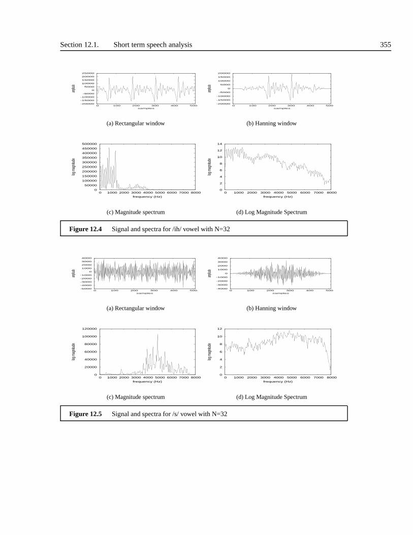
Section 12.1. Short term speech analysis 355
-20000
-15000
-10000
-5000
0
5000
10000
15000
20000
25000
0 100 200 300 400 500
amplitud
e
samples
(a) Rectangular window
-20000
-15000
-10000
-5000
0
5000
10000
15000
20000
0 100 200 300 400 500
amplitud
e
samples
(b) Hanning window
0
50000
100000
150000
200000
250000
300000
350000
400000
450000
500000
0 1000 2000 3000 4000 5000 6000 7000 8000
log m
agnit
ude
frequency (Hz)
(c) Magnitude spectrum
0
2
4
6
8
10
12
14
0 1000 2000 3000 4000 5000 6000 7000 8000
log m
agnit
ude
frequency (Hz)
(d) Log Magnitude Spectrum
Figure 12.4 Signal and spectra for /ih/ vowel with N=32
-5000
-4000
-3000
-2000
-1000
0
1000
2000
3000
4000
0 100 200 300 400 500
amplitud
e
samples
(a) Rectangular window
-4000
-3000
-2000
-1000
0
1000
2000
3000
4000
0 100 200 300 400 500
amplitud
e
samples
(b) Hanning window
0
20000
40000
60000
80000
100000
120000
0 1000 2000 3000 4000 5000 6000 7000 8000
log m
agnit
ude
frequency (Hz)
(c) Magnitude spectrum
0
2
4
6
8
10
12
0 1000 2000 3000 4000 5000 6000 7000 8000
log m
agnit
ude
frequency (Hz)
(d) Log Magnitude Spectrum
Figure 12.5 Signal and spectra for /s/ vowel with N=32
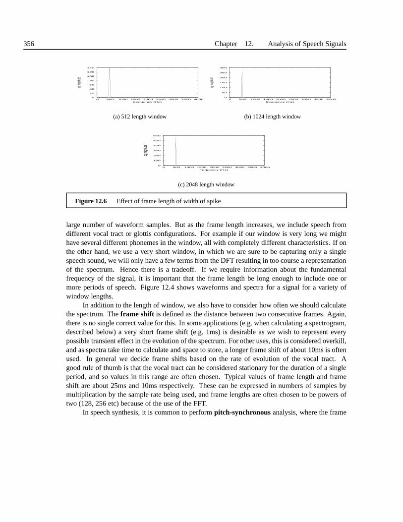
356 Chapter 12. Analysis of Speech Signals
0
20
40
60
80
100
120
140
0 500 1000 1500 2000 2500 3000 3500 4000
log mag
nitude
frequency (Hz)
(a) 512 length window
0
50
100
150
200
250
300
0 500 1000 1500 2000 2500 3000 3500 4000
log mag
nitude
frequency (Hz)
(b) 1024 length window
0
100
200
300
400
500
600
0 500 1000 1500 2000 2500 3000 3500 4000
log mag
nitude
frequency (Hz)
(c) 2048 length window
Figure 12.6 Effect of frame length of width of spike
large number of waveform samples. But as the frame length increases, we include speech fromdifferent vocal tract or glottis configurations. For example if our window is very long we mighthave several different phonemes in the window, all with completely different characteristics. If onthe other hand, we use a very short window, in which we are sureto be capturing only a singlespeech sound, we will only have a few terms from the DFT resulting in too course a representationof the spectrum. Hence there is a tradeoff. If we require information about the fundamentalfrequency of the signal, it is important that the frame length be long enough to include one ormore periods of speech. Figure 12.4 shows waveforms and spectra for a signal for a variety ofwindow lengths.
In addition to the length of window, we also have to consider how often we should calculatethe spectrum. Theframe shift is defined as the distance between two consecutive frames. Again,there is no single correct value for this. In some applications (e.g. when calculating a spectrogram,described below) a very short frame shift (e.g. 1ms) is desirable as we wish to represent everypossible transient effect in the evolution of the spectrum.For other uses, this is considered overkill,and as spectra take time to calculate and space to store, a longer frame shift of about 10ms is oftenused. In general we decide frame shifts based on the rate of evolution of the vocal tract. Agood rule of thumb is that the vocal tract can be considered stationary for the duration of a singleperiod, and so values in this range are often chosen. Typicalvalues of frame length and frameshift are about 25ms and 10ms respectively. These can be expressed in numbers of samples bymultiplication by the sample rate being used, and frame lengths are often chosen to be powers oftwo (128, 256 etc) because of the use of the FFT.
In speech synthesis, it is common to performpitch-synchronousanalysis, where the frame

Section 12.1. Short term speech analysis 357
-20000
-15000
-10000
-5000
0
5000
10000
15000
0 100 200 300 400 500
amplitud
e
samples
(a) 64 sample frame
3
4
5
6
7
8
9
10
11
0 1000 2000 3000 4000 5000 6000 7000 8000
log m
agnit
ude
frequency (Hz)
(b) log magnitude spectrum of 32 sample frame
-20000
-15000
-10000
-5000
0
5000
10000
15000
20000
0 100 200 300 400 500
amplitud
e
samples
(c) 128 sample frame
-2
0
2
4
6
8
10
12
14
0 1000 2000 3000 4000 5000 6000 7000 8000log
mag
nitud
efrequency (Hz)
(d) Log Magnitude Spectrum
-20000
-15000
-10000
-5000
0
5000
10000
15000
20000
25000
0 100 200 300 400 500
amplitud
e
samples
(e) 256 sample frame
0
2
4
6
8
10
12
14
0 1000 2000 3000 4000 5000 6000 7000 8000
log m
agnit
ude
frequency (Hz)
(f) Log Magnitude Spectrum
-20000
-15000
-10000
-5000
0
5000
10000
15000
20000
25000
0 100 200 300 400 500
amplitud
e
samples
(g) 512 sample frame
0
2
4
6
8
10
12
14
0 1000 2000 3000 4000 5000 6000 7000 8000
log m
agnit
ude
frequency (Hz)
(h) Log Magnitude Spectrum
-20000
-15000
-10000
-5000
0
5000
10000
15000
20000
25000
0 100 200 300 400 500
amplitud
e
samples
(i) 1024 sample frame
0
2
4
6
8
10
12
14
0 1000 2000 3000 4000 5000 6000 7000 8000
log m
agnit
ude
frequency (Hz)
(j) Log Magnitude Spectrum
Figure 12.7 Signal and spectra for a vowel with different window lengths. For the shorter frames,only a course spectrum can be discerned. The harmonics are clearest for 512 length case; above thisthe fundamental frequency changes across the window mean that there is no single harmonic spacing.
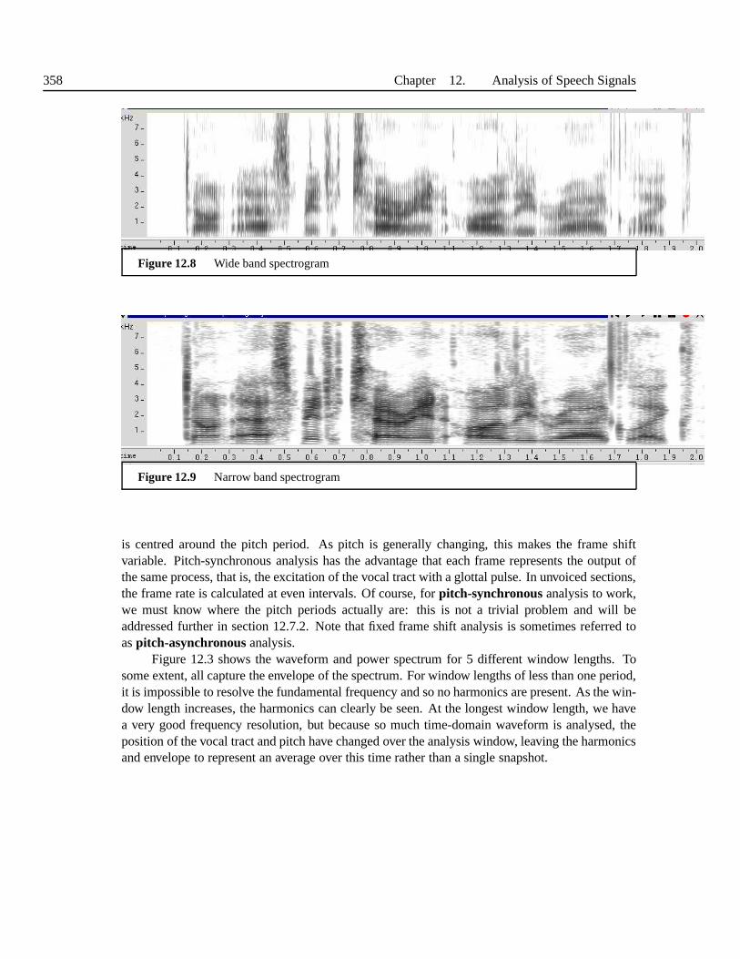
358 Chapter 12. Analysis of Speech Signals
Figure 12.8 Wide band spectrogram
Figure 12.9 Narrow band spectrogram
is centred around the pitch period. As pitch is generally changing, this makes the frame shiftvariable. Pitch-synchronous analysis has the advantage that each frame represents the output ofthe same process, that is, the excitation of the vocal tract with a glottal pulse. In unvoiced sections,the frame rate is calculated at even intervals. Of course, for pitch-synchronousanalysis to work,we must know where the pitch periods actually are: this is nota trivial problem and will beaddressed further in section 12.7.2. Note that fixed frame shift analysis is sometimes referred toaspitch-asynchronousanalysis.
Figure 12.3 shows the waveform and power spectrum for 5 different window lengths. Tosome extent, all capture the envelope of the spectrum. For window lengths of less than one period,it is impossible to resolve the fundamental frequency and sono harmonics are present. As the win-dow length increases, the harmonics can clearly be seen. At the longest window length, we havea very good frequency resolution, but because so much time-domain waveform is analysed, theposition of the vocal tract and pitch have changed over the analysis window, leaving the harmonicsand envelope to represent an average over this time rather than a single snapshot.
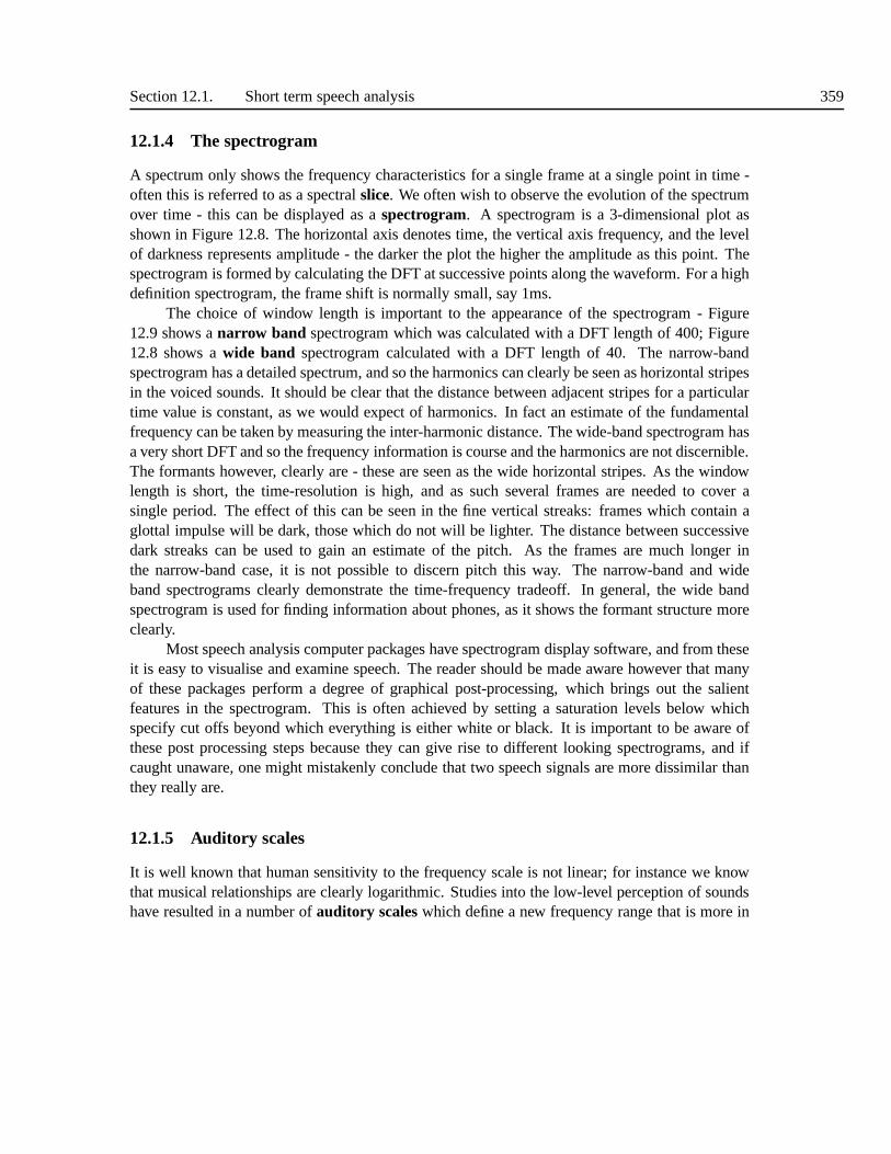
Section 12.1. Short term speech analysis 359
12.1.4 The spectrogram
A spectrum only shows the frequency characteristics for a single frame at a single point in time -often this is referred to as a spectralslice. We often wish to observe the evolution of the spectrumover time - this can be displayed as aspectrogram. A spectrogram is a 3-dimensional plot asshown in Figure 12.8. The horizontal axis denotes time, the vertical axis frequency, and the levelof darkness represents amplitude - the darker the plot the higher the amplitude as this point. Thespectrogram is formed by calculating the DFT at successive points along the waveform. For a highdefinition spectrogram, the frame shift is normally small, say 1ms.
The choice of window length is important to the appearance ofthe spectrogram - Figure12.9 shows anarrow band spectrogram which was calculated with a DFT length of 400; Figure12.8 shows awide band spectrogram calculated with a DFT length of 40. The narrow-bandspectrogram has a detailed spectrum, and so the harmonics can clearly be seen as horizontal stripesin the voiced sounds. It should be clear that the distance between adjacent stripes for a particulartime value is constant, as we would expect of harmonics. In fact an estimate of the fundamentalfrequency can be taken by measuring the inter-harmonic distance. The wide-band spectrogram hasa very short DFT and so the frequency information is course and the harmonics are not discernible.The formants however, clearly are - these are seen as the widehorizontal stripes. As the windowlength is short, the time-resolution is high, and as such several frames are needed to cover asingle period. The effect of this can be seen in the fine vertical streaks: frames which contain aglottal impulse will be dark, those which do not will be lighter. The distance between successivedark streaks can be used to gain an estimate of the pitch. As the frames are much longer inthe narrow-band case, it is not possible to discern pitch this way. The narrow-band and wideband spectrograms clearly demonstrate the time-frequencytradeoff. In general, the wide bandspectrogram is used for finding information about phones, asit shows the formant structure moreclearly.
Most speech analysis computer packages have spectrogram display software, and from theseit is easy to visualise and examine speech. The reader shouldbe made aware however that manyof these packages perform a degree of graphical post-processing, which brings out the salientfeatures in the spectrogram. This is often achieved by setting a saturation levels below whichspecify cut offs beyond which everything is either white or black. It is important to be aware ofthese post processing steps because they can give rise to different looking spectrograms, and ifcaught unaware, one might mistakenly conclude that two speech signals are more dissimilar thanthey really are.
12.1.5 Auditory scales
It is well known that human sensitivity to the frequency scale is not linear; for instance we knowthat musical relationships are clearly logarithmic. Studies into the low-level perception of soundshave resulted in a number ofauditory scaleswhich define a new frequency range that is more in
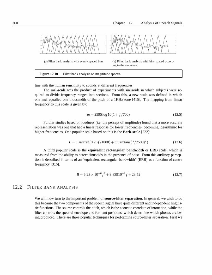
360 Chapter 12. Analysis of Speech Signals
0 50 100 150 200 250 300−12
−10
−8
−6
−4
−2
0
2
(a) Filter bank analysis with evenly spaced bins
0 50 100 150 200 250 300−12
−10
−8
−6
−4
−2
0
2
(b) Filter bank analysis with bins spaced accord-ing to the mel-scale
Figure 12.10 Filter bank analysis on magnitude spectra
line with the human sensitivity to sounds at different frequencies.The mel-scalewas the product of experiments with sinusoids in which subjects were re-
quired to divide frequency ranges into sections. From this,a new scale was defined in whichonemel equalled one thousandth of the pitch of a 1KHz tone [415]. Themapping from linearfrequency to this scale is given by:
m= 2595log10(1+ f/700) (12.5)
Further studies based on loudness (i.e. the percept of amplitude) found that a more accuraterepresentation was one that had a linear response for lower frequencies, becoming logarithmic forhigher frequencies. One popular scale based on this is theBark-scale [522]:
B = 13arctan(0.76f/1000)+3.5arctan(( f/7500)2) (12.6)
A third popular scale is theequivalent rectangular bandwidth or ERB scale, which ismeasured from the ability to detect sinusoids in the presence of noise. From this auditory percep-tion is described in terms of an ”equivalent rectangular bandwidth” (ERB) as a function of centrefrequency [316].
B = 6.23×10⁻⁶ f 2 +9.33910−2 f +28.52 (12.7)
12.2 FILTER BANK ANALYSIS
We will now turn to the important problem ofsource-filter separation. In general, we wish to dothis because the two components of the speech signal have quite different and independent linguis-tic functions. The source controls the pitch, which is the acoustic correlate of intonation, while thefilter controls the spectral envelope and formant positions, which determine which phones are be-ing produced. There are three popular techniques for performing source-filter separation. First we

Section 12.3. The Cepstrum 361
will examinefilter bank analysis in this section, before turning tocepstral analysisand linearprediction in the next sections.
If we visually examine a short length DFT such as that in Figure 12.4, or in fact any spec-trogram, we can see the general shape of the spectral envelope. That is, if we “squint” and ignorethe harmonics, in many cases the shape of spectral envelope is discernible independent of the par-ticular positions of the harmonics. When doing this we are effectively averaging out the influenceof individual harmonics and creating a blurring effect and this is the principle behind filter bankanalysis.
Filter bank analysis is performed by first creating a series of bins each centred on a particularfrequency. Time domain filter-bank analysis can be performed by creating aband passfilter(either FIR or IIR) which allows frequencies at or near the bin frequency to pass, but attenuatesall other frequencies to zero. After the filtering, the amount of energy is calculated and assignedto that bin. Once this has been done for every bin, we have a representation of how energy variesaccording to frequency. The effect of the filtering operation is to blur the effect of individualharmonics, such that the final representation is largely that of the vocal tract and not the source.Alternatively, we can perform filter bank analysis on spectra. Here, we take a magnitude spectraand multiply it by a windowing function centred on a bin frequency. This has the effect of settingall energy outside the window to zero, while allowing us to measure the energy inside the window.This is show in Figure 12.10a. Often the bins are not spaced atequal frequencies, but definedlogarithmically or according to one of the frequency scalesof Section 12.1.5. This is shown inFigure 12.10b.
Filter bank analysis is a simple and robust technique for finding the spectral envelope, butit is only a partial solution to source filter separation. First, the amount of “blurring” requiredto eliminate the harmonics may be too severe and may eliminate some of the detail we require;alternatively, and especially with high pitched speech, wecan find that peaks in the envelope fallbetween two harmonics and therefore are ignored. Secondly,filter bank analysis only gives usthe spectral envelope derived from the vocal tract transferfunction; it does not give us the source.For many applications (e.g. ASR) this is not a problem, but inTTS we generally require bothcomponents of the signal, and so other techniques are normally used.
12.3 THE CEPSTRUM
12.3.1 Cepstrum definition
The cepstrum is (most commonly) defined as theinverse DFT of the log magnitude of the DFTof a signal:
c[n] = F −1 log| F x[n] |
(12.8)

362 Chapter 12. Analysis of Speech Signals
0
20
40
60
80
100
120
0 1000 2000 3000 4000 5000 6000 7000 8000
ampli
tude
normalise frequency
(a) Magnitude spectrum and envelope
0
2
4
6
8
10
12
14
0 1000 2000 3000 4000 5000 6000 7000 8000
ampli
tude
normalise frequency
(b) log Magnitude spectrum and envelope
-300
-200
-100
0
100
200
300
400
500
600
700
0 50 100 150 200 250
ampli
tude
samples
(c) Cepstrum
Figure 12.11 Steps involved in calculating the cepstrum. For demonstration purposes, an estimateof the spectral envelope has been overlaid on the two DFT spectra. The “periodicity” of the harmonicsin the log spectrum can clearly be seen. this gives rise to thespike at point 120 in the cepstrum. Thelow values (<30) in the cepstrum describe the envelope. It should be clearthat these low values areseparated from the spike - because of this it is a simple task to separate the source and filter.
whereF is the DFT andF −1 is the inverse DFT. For a windowed frame of speechy[n] thecepstrum is therefore
c[n] =N−1
∑n=0
log( ∣∣∣
N−1
∑n=0
x[n]e− j 2πN kn∣∣∣
)
ej 2πN kn (12.9)
Figure 12.11 shows the process of calculating the DFT, log, and inverse DFT on a single frame ofspeech. We will now look at how this operation performs source/filter separation.
12.3.2 Treating the magnitude spectrum as a signal
Consider the magnitude spectrum of a periodic signal, such as that shown in Figure 12.11. As wehave proved and seen in practice, this spectrum will containharmonics at evenly spaced intervals.Because of the windowing effects, these harmonics will not be delta function spikes, but will besomewhat more “rounded”. For most signals, the amplitude ofthe harmonics tails off quite quickly

Section 12.3. The Cepstrum 363
as frequency increases. We can reduce this effect by compressing the spectrum with respect toamplitude; this can easily be achieved by calculating the log spectrum. It should be clear in themany examples of log spectra in this chapter that the relative amplitudes of the harmonics aremuch closer in the log spectra than the absolute spectra. Figure 12.5b shows this effect.
Now, forget for a moment what the log spectrum actually represents, and consider it awave-form instead. In we were told Figure 12.11b was a waveform, we would informally describe thisas some sort of quasi-periodic signal (after it, it has a repeating pattern of harmonics), with a timeevolving “amplitude effect” which makes some “periods” higher than others. It is clear that therate at which the “periods” change is much greater than the evolution of the “amplitude effect”.If we wished to separate these, we would naturally turn to ourstandard tool for analysing thefrequency content of waveforms, namely the Fourier transform. If we calculate the DFT of our“waveform” we get a new representation, which we will designate thecepstrum. This is shown inFigure 12.11c. As we would expect, the periodicity of the “waveform” is shown by a large spikeat about position 120. Because we haven’t performed any windowing operations which causeblurring, we would expect this to be close to a delta function.
Again, as we would expect, because the “periods” were not sinusoidal, this has harmonicsat multiples of the main spike. The “amplitude effect” will be present in the cepstrum also, but asthis is varying much more slowly than the “periods”, it will be in the lower range of the cepstrum.As the “amplitude effect” is the spectral envelope and the spikes represent the harmonics (ie thepitch), we see that these operations have produced a representation of the original signal in whichthe two components lie at different positions. A simple filter can now separate them.
12.3.3 Cepstral analysis as deconvolution
Recall from Section 11.1 that Equation 11.2 described the speech production process as
y[n] = u[n]⊗v[n]⊗ r[n]
where whereu[n] is the glottal or other source,v[n] is the vocal tract filter andr[n] is the radiation.In the time domain, these expressions are convolved and so are not easily separable. If we don’tknow the form of the vocal tract filter, we can’t perform any explicit inverse filtering operation toseparate these components.
We can however perform separation as follows. Let us subsumethe radiation filterr[n] intov[n] to give a single filterv′[n]. We can then write the time domain expression of Equation 11.2 as
y[n] = u[n]⊗v′[n] (12.10)
Taking the Fourier transform of Equation 12.10 gives
Y(ejω) = U(ejω)V ′(ejω)

364 Chapter 12. Analysis of Speech Signals
-6
-4
-2
0
2
4
6
8
0 1000 2000 3000 4000 5000 6000 7000 8000lo
g m
agni
tude
frequency (Hz)
Figure 12.12 Series of spectra calculated from cepstra. The 512 point cepstrum has all its valuesafter a cut off pointK set to 0 and then a 512 point DFT is applied to generate a spectrum. Thefigure shows this spectrum for 4 values ofK, 10, 20, 30, 50. (In the figure each has been graphicallyseparated for clarity, withK = 10 as the bottom spectrum andK = 50 as the top. In reality all lie in thesame amplitude range.) As the number of coefficients increases, so does the level of spectral detail,until effects of harmonics start appearing. The choice of optimal cut-off point depends on whetherspectral precision or elimination of harmonics is the top priority.
If we now take the log of the magnitude of this we get
log(|Y(ejω)|) = log(|U(ejω|)V ′(|ejω)|)= log(|U(ejω)|)+ log(|V ′(ejω)|)
in which the source spectrum and filter spectrum are now just added together. We can now returnto the time domain by taking an inverse DFT, giving us
c[n] = cu[n]+cv[n] (12.11)
that is, a time domain representation created by addition ofsource and filter. Unlike Equation12.10, the source and filter are now added and not convoluted in the time domain.
12.3.4 Cepstral analysis discussion
If we take the DFT of a signal and then take the inverse DFT of that, we of course get back towhere we started. The cepstrum calculation differs in two important respects. First we are onlyusing the magnitude of the spectrum - in effect we are throwing away the phase information. Theinverse DFT of a magnitude spectrum is already very different from the inverse DFT of a normal(complex) spectrum. The log operation scales the harmonicswhich emphasises the “periodicity”of the harmonics. It also ensures that the cepstrum is the sumof the source and filter componentsand not their convolution.
The cepstrum is useful as it splits the signal into an envelope, given by the first few coeffi-cients, and a source, given by the spike. Subsequent analysis usually throws away one of these
Section 12.4. Linear prediction analysis 365
parts: if we are interested in the vocal tract we use only the low coefficients, if we are interested inthe pitch and behaviour of the glottis we study the peak. We can demonstrate this by calculating aspectrum in which the spike is eliminated - this is done by simply setting a cut off pointK abovewhich all the cepstral coefficients are set to zero. From this, we can create a log magnitude spec-trum by applying a DFT on the modified cepstrum. Figure 12.12 shows this for 4 different valuesof K. The figure shows that a reasonably accurate spectral envelope can be generated from about30 coefficients, but the number chosen really depends on the degree of precision required in thespectrum.
For many cases where the spectral envelope is required, it isadvantageous to keep the lowpart of the cepstrum as it is, and not convert it back to a frequency domain spectrum. The lowcepstral coefficients form a very compact representation ofthe envelope, and have the highly de-sirable statistical modelling property of being independent so that only their means and variances,and not their covariances, need be stored to provide an accurate statistical distribution. It is for thisreason that cepstral are the feature representation of choice in most speech recognition systems.Despite this, cepstra are quite difficult to visually interpret, so we often find that while systems usecepstra internally, we still use spectra when we wish to visually inspect a signal. The higher partof the cepstrum contains the pitch information, and is oftenused as the basis for pitch detectionalgorithms, explained in section 12.7.1
12.4 LINEAR PREDICTION ANALYSIS
Linear Prediction (LP) is another technique for source filter separation, in which we use thetechniques of LTI filters to perform an explicit separation of source and filter. In LP we adopt asimple system for speech production, where we have an input sourcex[n], which passed through alinear time invariant filterh[n], to give the output speech signaly[n]. In the time domain this is:
y[n] = x[n]⊗h[n] (12.12)
The convolution makes it difficult to separate the source andfilter in the time domain, but this iseasily achieved if we transform our system to the z-domain
H(z) =X(z)Y(z)
(12.13)
In Section 12.12, we showed that the lossless tube model was areasonable approximation for thevocal tract during the production of a vowel. If we assume fornow thatH(z) can therefore berepresented by an all-pole filter, we can write
Y(z) = X(z)H(z) (12.14)
=1
1−P∑
k=1akz−k
.X(z) (12.15)

366 Chapter 12. Analysis of Speech Signals
whereak are the filter coefficients. By taking the inverse z-transform2 we see that in the timedomain this becomes:
y[n] =P
∑k=1
aky[n−k]+x[n] (12.16)
The importance of this equation is that it states that the value of the signaly at timen can bedetermined by a linear function of the previous values ofy, apart from the addition of the currentvalue of the inputx[n]. Because of this, the technique is known aslinear prediction . In essence,this states that an output signal is closely approximated bya linear sum of the previous samples:
y[n] =P
∑k=1
aky[n−k] (12.17)
and this is identical to the difference Equation 12.16 except for the input term. In linear pred-ication, the inputx[n] is usually referred to as theerror , and is often writtene[n] to show this.This may seem a little harsh, but the concept comes from the fact thaty[n] is the actual signal and
˜y[n] is its approximation by the model, the only difference beingthe contribution fromx[n]. Asthis accounts for the difference between the predicted and actual signal it is called the error. Wenow turn to the issue of how to automatically find the predictor coefficients ofH(z) for a frame ofspeech.
12.4.1 Finding the coefficients: the covariance method
The goal of linear prediction is to find the set of coefficientsakwhich generate the smallest errore[n], over the course of the frame of speech. We will now examine two closely related techniquesfor finding theak coefficients based on error minimisation. We can sate equation 12.16 in terms ofthe error for a single sample:
e[n] = y[n]−P
∑k=1
aky[n−k] (12.18)
2
We can most easily prove this in reverse; if
y[n] =P
∑k=1
aky[n−k]+x[n]
then taking the z-transform of both sides results in
Y(z) =n=∞
∑n=−∞
( P
∑k=1
aky[n−k])
z−n +E(z)
=P
∑k=1
ak
( n=∞
∑n=−∞
y[n−k]z−n)
+E(z)
Using the dummy substitutionm= n−k gives
=P
∑k=1
ak
( m=∞
∑m=−∞
y[m]z−mz−k)
+E(z)
=P
∑k=1
akY(z)z−k +E(z)
rearranging theY(z) terms gives the all-pole transfer func-tion of Equation 12.15.

Section 12.4. Linear prediction analysis 367
We wish to find the valuesak which minimise the squared error, summed over the frame ofspeech. UsingE to denote the sum squared error we can state:
E =N−1
∑n=0
e2[n]
=N−1
∑n=0
(
y[n]−P
∑k=1
aky[n−k]
)2
We can find the minimum ofE by differentiating with respect toeachcoefficientak, and settingto zero:
δEδa j
= 0 =N−1
∑n=0
(
2(
y[n]−P
∑k=1
aky[n−k])
y[n− j]
)
for j = 1,2,3...P
= −2N−1
∑n=0
y[n]y[n− j]+2N−1
∑n=0
P
∑k=1
aky[n−k]y[n− j]
which gives
N−1
∑n=0
y[n− j]y[n] =P
∑k=1
ak
N−1
∑n=0
y[n− j]y[n−k] for j = 1,2,3...P (12.19)
If we defineφ(k, j) as
φ( j,k) =N−1
∑n=0
y[n− j]y[n−k] (12.20)
Equations 12.19 can be written more succinctly as:
φ( j,0) =P
∑k=1
φ( j,k)ak (12.21)
the full form of which is
φ(1,0) = a1φ(1,1)+a2φ(1,2)+ ...+aPφ(1,P)φ(2,0) = a1φ(2,1)+a2φ(2,2)+ ...+aPφ(2,P)φ(3,0) = a1φ(3,1)+a2φ(3,2)+ ...+aPφ(3,P)
...φ(P,0) = a1φ(P,1)+a2φ(P,2)+ ...+aPφ(P,P)
We can easily calculate all the quantitiesφ(1,0),φ(2,0), and so it should be clear that this is a setof P equations withP unknown terms, namely theak coefficients. This can be written in matrixform as

368 Chapter 12. Analysis of Speech Signals
φ(1,0)φ(2,0)φ(3,0)
...φ(P,0)
=
a1
a2
a3...
aP
φ(1,1) φ(1,2) · · · φ(1,P)φ(2,1) φ(2,2) · · · φ(2,P)φ(3,1) φ(3,2) · · · φ(3,P)
...φ(P,1) φ(P,2) · · · φ(P,P)
(12.22)
and expressed asφa = ψ
We can find the value ofa (that is, the coefficientsak) by solving this equation. This can bedone simply, by solving fora1 in terms of the other coefficients and substituting again, but this isextremely inefficient. Because the square matrixφ is symmetric a much faster technique knownasCholskey decompositioncan be used [302] [295].
This method is called thecovariance method(for somewhat obscure reasons). It works bycalculating theerror in the region of samples fromn = 0 ton = N−1, but in fact usessamplesinhe regionn =−P to n = N−1 to do so. This is because the method requires a full calculation ofthe error at timen = 0, and to do so, it must use some previous samples to do so. The calculationover many frames can be found by either simply using the main signal itself, and moving thestart positionn to the designated frame start each time; or by creating a separate windowed frameof speech, of lengthN + P samples, and performing the calculation startingP samples into theframe. The choice is mainly determined by implementation issues (e.g. a system may have alreadyperformed the windowing operation before we start). No special windowing functions are requiredwith this method: either we can perform the calculations directly on the main waveform, or arectangular window can be used if windowing must be performed.
12.4.2 Autocorrelation Method
A slightly different method know as theautocorrelation method can also be used, and as thishas many practical advantages over the covariance method, it is often the method most used inpractice.
Recall from Section 10.3.9 that the autocorrelation function of a signal is defined as:
R[n] =∞
∑m=−∞
y[m]y[n−m] (12.23)
This is similar in form to Equation 12.20, and if we can calculate the autocorrelation, we canmake use of important properties of this signal. To do so, in effect we have to calculate thesquared error from−∞ to ∞. This differs from the covariance method, where we just consider thespeech samples from a specific range. To perform the calculation from−∞ to ∞, we window thewaveform using a hanning, hamming or other window, which hasthe effect of setting all valuesoutside the range 0<= n < N to 0.

Section 12.4. Linear prediction analysis 369
While we are calculating the error from−∞ to ∞, this will always be 0 before the windowedarea, as all the samples are 0 and hence multiplying them by the filter coefficients will just produce0. This will also be the case significantly after the window. Importantly however, forP samplesafter the window, the error will not be 0 as it will still be influenced by the last few samples at theend of the region. Hence the calculation of the error from−∞ to ∞ can be rewritten as
φ( j,k) =∞
∑−∞
y[n− j]y[n−k]
=N−1+P
∑n=0
y[n− j]y[n−k]
which can be rewritten as
φ( j,k) =N−1−( j−k)
∑n=0
y[n]y[n+ j−k] (12.24)
As this is a function of one independent variablej−k, rather than the two of 12.24, we can rewriteit as
φ( j,k) =N−1−k
∑n=0
y[n]y[n+k] (12.25)
As the limits of this expression equate to−∞ to ∞, this is the same as the autocorrelation function12.23, and we can write:
R( j−k) = φ( j,k)
Now we can rewrite the matrix form of 12.21 in terms of the autocorrelation function:
φ( j,0) =P
∑k=1
φ( j,k)ak (12.26)
R( j) =P
∑k=1
R( j−k)ak (12.27)
This significance of all of this is that the autocorrelation function (of any signal) is even, that isR( j−k) = R( j +k) = R(| j−k|), and this means that when we now write the matrix in Equation12.22 in terms ofR:
R(1)R(2)R(3)
...R(P)
=
a1
a2
a3...
aP
R(0) R(1) R(2) · · · R(P−1)R(1) R(0) R(1) · · · R(P−2)R(2) R(1) R(0) · · · R(P−3)
...R(P−1) R(P−2) R(P−3) · · · R(0)
(12.28)
370 Chapter 12. Analysis of Speech Signals
Unlike the square matrix in Equation 12.22, this matrix is symmetric and all the elements in itsdiagonals are symmetric. This is known as aToeplitz matrix, and because of the properties justmentioned, it is significantly easier to invert.
12.4.3 Levinson Durbin Recursion
The matrix given in Equation 12.24 can of course be solved by any matrix inversion technique.Such techniques can be slow however (usually of the order ofp3 wherep is the dimensionality ofthe matrix) and hence faster techniques have been developedto find the values ofak from theautocorrelation functionsR(k). In particular, it can be shown that theLevinson-Durbin recursiontechnique can solve Equation 12.28 inp2 time. For our purposes, analysis speed is really not anissue, and so we will forgo a detailed discussion of this and other related techniques. However,a brief overview of the technique is interesting in that it sheds light on the relationship betweenlinear prediction and the all-pole tube model discussed in Chapter 11.
The Levinson-Durbin recursion operates by considering a set of initialisation conditions,and using these to find the coefficients of a first order polynomial (that is, just a single term inz−1.) which minimise the mean squared error. From this we find thecoefficients of a second orderpolynomial, third order and so on, using the previous polynomial and minimisation of the error,until we have reached a polynomial of the required filter order P.
The algorithm initialises by setting the error and predictor coefficients of a (contrived) 0order polynomial as:
a00 = 0
E0 = R(0)
Next we define a weighting factor for theith model as:
ki =
R(i)−i−1∑j=1
ai− jj R(i− j)
Ei−1
using this, we find the predictor coefficients for theith model:
aii = ki (12.29)
aij = ai−1
j −kiai−1i− j 1≤ j ≤ i−1 (12.30)
and from this, we can update the minimum mean squared prediction error for this step as:
Ei = (1−k2i )E
i−1
These steps are repeated untili = p where we have a polynomial and hence set of predictor coef-ficients of the required order. We have just seen how the minimisation of error over a window canbe used to estimate the linear prediction coefficients. As these are in fact the filter coefficients thatdefine the transfer function of the vocal tract, we can use these in a number of ways to generateother useful representations.
Section 12.5. Spectral envelope and vocal tract representations 371
12.5 SPECTRAL ENVELOPE AND VOCAL TRACT REPRESENTATIONS
The preceding sections showed the basic techniques of source filter separation using first cepstralthen linear prediction analysis. We now turn to the issue of using these techniques to generate avariety of representations, each of which by some means describes the spectral envelope of thespeech.
12.5.1 Linear prediction spectra
The main motivation in LP analysis is that it provides an automatic and explicit means for sepa-rating the source and filter components in speech. Recall thebasic equation (11.2) of the vocaltract,
Y(z) = U(z)V(z)R(z)
HereY(z) is the speech,U(z) is the source,V(z) is the vocal tract andR(z) is the radiation.Ideally, the transfer functionH(z) found by linear prediction analysis would beV(z), the vocaltract transfer function. In the course of doing this, we could then findU(z) andR(z). In reality,in generalH(z) is a close approximation toV(z) but is not exactly the same. The main reason forthis is that LP minimisation criterion means that the algorithm attempts to find the lowest error forthewholesystem, not just the vocal tract component. In fact,H(z) is properly expressed as
H(z) = G(z)V(z)R(z)
for voiced speech, whereG(z) represents the glottal transfer function, and
H(z) = V(z)R(z)
for unvoiced speech. The distinction between the linear prediction coefficient representingH(z)instead ofV(z) has most significance for source modelling, and so we will delay a full discussionof this until Section 12.6. For most purposes, the fact that theseH(z) models more than justthe vocal tract isn’t a big problem, the upshot is that some additional poles are included in thetransfer function, but the effect of these can oftne be ignored, and a good estimate of the vocaltract envelope can be found by convertingH(z) directly to the frequency domain. If a purerestimate ofV(z) is required, one of the techniques described in Section 12.6can be used instead.
The transfer functionH(z) that we have been estimating can be converted to the frequencydomain by simply settingz= ejωt (see Section 10.5.2) to giveH(ejωt). Doing this gives us thespectral envelope of the linear prediction filter, which apart from the extra poles, we can interpretas the vocal tract spectral envelope. A plot of this LP envelope overlayed on the DFT is shownin Figure 12.13a. It is quite clear that the LP spectrum is indeed a good estimate of the spectralenvelope.
Figures 12.14 show spectral envelopes for a range of sounds.Here we can see a much noted“weakness” of LP envelope estimation; which is that the spectrum can appear very “peaky”. This

372 Chapter 12. Analysis of Speech Signals
0 1000 2000 3000 4000 5000 6000 7000 8000−4
−3
−2
−1
0
1
2
3
4
5
(a) Linear prediction spectrum superimposed onDFT
0 1000 2000 3000 4000 5000 6000 7000 8000−4
−2
0
2
4
6
8
10
12
Frequency
Am
plitu
de
(b) Linear prediction spectra for analysis of order 4,6,8,10,12,14,16and 18. In reality the plots lie on top of one another, but eachhasbeen vertically separated for purposes of clarity. The bottom plot isfrom LP analysis of order 4, the top plot order 18.
Figure 12.13 Examples of linear prediction spectra

Section 12.5. Spectral envelope and vocal tract representations 373
arises because in many speech sounds, particularly vowels,the poles lie close to, but not on theunit circle. At such locations, even a very small differencein their distance from the unit circle canresult in a much sharper formant peaks. For example, for a sampling rate of 10000Hz, a pole withradius 0.96 will produce a formant bandwidth of 130Hz, whilea pole of 0.98 produces a formantof bandwidth 65Hz, and so any slight error in determining theradius of the pole can produce aspectrum with exaggerated formants. This problem does not occur with pole frequencies, and sothe LP envelope can normally be relied upon to find the positions of resonances quite accurately.
Recall that in Chapter 11 we showed the number of tubes required is directly related to thesampling rate, length of tube and speed of sound (see Section11.3.5) . For a speed of sound of340ms−1 and vocal tract length of 17cm, we showed that 10 tube sections were required for asampling rate of 10000Hz. Assuming these values for the speed of sound and vocal tract length,we see that we require one tube section per 1000Hz sampling rate. As each tube section gives riseto one pole, we conclude thatV(z) should be a 10th order all-pole filter for a 10000Hz samplingrate, 16th order filter for a 16000Hz sampling rate and so on. The source (G(z)) and radiation(R(z)) filters are considerably simpler, and can be adequately modelled by 4 to 6 additional polesfor both. It is highly advantageous to keep the number of poles even, and so an overall value of14 poles or 16 poles is normally adopted for a 10000Hz sample rate, and 20 or 22 poles for a16000Hz sample rate.
Figure 12.13b shows the spectra predicted from linear prediction filters for a range of orders.It is quite clear that as the order increases, so does the detail in the spectrum. It is interesting tocompare this to Figure 12.12 which shows the same investigation but with cepstra. It is clear thatthe cepstral spectra are much more heavily influenced by the harmonics as the order of analysisincreases.
12.5.2 Transfer function poles
As with any filter, we can find the poles by finding the roots of the transfer function polynomial.
12.5.3 Reflection coefficients
Consider again the all-pole transfer function we have been using all along
V(z) =G
A(z)
whereA(z) is
A(z) = 1−P
∑k=1
akz−k (12.31)
Recall that the key equation in the Levinson-Durbin recursion is the step that relates a predictorcoefficienta j to the quantityk and the previous predictor coefficienta j−1 given in Equation 12.30.

374 Chapter 12. Analysis of Speech Signals
0 1000 2000 3000 4000 5000 6000 7000 8000−3
−2
−1
0
1
2
3
4
5
Frequency
Am
plitu
de
(a) /ow/
0 1000 2000 3000 4000 5000 6000 7000 8000−0.8
−0.6
−0.4
−0.2
0
0.2
0.4
0.6
0.8
1
Frequency
Am
plitu
de
(b) /s/
0 1000 2000 3000 4000 5000 6000 7000 8000−3
−2
−1
0
1
2
3
4
5
Frequency
Am
plitu
de
(c) /eh/
0 1000 2000 3000 4000 5000 6000 7000 8000−3
−2
−1
0
1
2
3
4
Frequency
Am
plitu
de
(d) /iy/
0 1000 2000 3000 4000 5000 6000 7000 8000−2
−1
0
1
2
3
4
5
Frequency
Am
plitu
de
(e) /ae/
0 1000 2000 3000 4000 5000 6000 7000 8000−3
−2
−1
0
1
2
3
4
5
Frequency
Am
plitu
de
(f) /ae/
Figure 12.14 Examples of spectra calculated from LP coefficients for a range of different sounds.Note how all the spectra are absent from any harmonic influence, and that all seem to describe thespectral envelope of the speech. Note the characteristic formant patterns and roll-off for all vowels,and compare this with the spectra for /s/. The same vowel is present in both examples (e) and (f). Notethat while the formant positions occur in the same positionsin both, the amplitudes and bandwidthsare quite different, especially in the fourth formant, which is barely noticeable in example (e).

Section 12.5. Spectral envelope and vocal tract representations 375
aii = ai−1
j −k2ai−1i− j (12.32)
Let us now examine what happens when we substitute Equation 12.31 into equation 12.32.For demonstration we shall choose the case for a third order filter, in which case we have threeexpressions:
a33 = k3
a32 = a2
2−k3a21
a31 = a2
1−k3a22
The expansion ofA3(z) is
A3(z) = 1−a31z−1−a3
2z−2−a33z−3 (12.33)
and if we substitute equations for 12.31 into this we get
A3(z) = 1− [a21−k3a2
2]z−1− [a2
2−k3a21]z−2−k3z−3
= 1−a21z−1−a2
2z−2 +k3a22z−1 +k3a2
1z−2−k3z−3
The first terms, 1−a21z−1−a2
2z−2, are of course just the expansion of the second order filterA2(z)
A3(z) = A2(z)−k3[a22z−1 +a2
1z−2 +z−3] (12.34)
The other terms are similar to the polynomial expansion, except that the coefficients are in thereverse order to normal. If we multiply each term byz3 we can express these terms as a polynomialin z rather thanz−1 which gives:
A3(z) = A2(z)−k3z−3[a22z2 +a2
1z+1]
A3(z) = A2(z)−k3z−3A2(z−1) (12.35)
In a similar fashion, the above relation can shown for any order of filter.The significance of all this can be seen if we compare Equation12.35 with Equation 11.27.
Recall that Equation 11.27 was used to find the transfer function for the tube model from thereflection coefficients, in the special case where losses only occurred at the lips. The equations arein fact identical if we setrk =−ki. This means that as a by product of Levinson-Durbin recursion,we can in fact easily determine the reflection coefficients which would give rise to the tube modelhaving the same transfer function to that of the LP model. This is a particularly nice result; notonly have we shown that the tube model is all-pole and that theLP model is all pole; we havenow in fact shown that the two models are in fact equivalent and hence we can find the variousparameters of the tube directly from LP analysis.
Reflection coefficients are a popular choice of LP representation because they are easilyfound, they are robust to quantisation error and can in fact be used directly without having to
376 Chapter 12. Analysis of Speech Signals
be converted into predictor coefficients (see Rabiner and Schafer [368] for how this is done).Furthermore, and perhaps most significantly for our purposes, they have a physical interpretation,which means that they are amenable to interpolation. For example, if we had two different vocaltract configurations and wished to generate a set of vocal tract configurations between these, wecould do by interpolating the reflection coefficients, in theknowledge that by doing so we arecreating a set of reasonable vocal tract shapes. This process could not be done with the predictorcoefficients themselves, as this would very likely lead to unnatural or unstable filters.
12.5.4 Log area ratios
Recall from our tube model, that the reflection coefficients were originally defined in terms ofthe ratio of the areas between two adjacent tubes. Equation 11.15 stated that the amount of theforward travelling wave that was reflected back into the tubewas given as:
rk =Ak+1−AkAk+1 +Ak
Rearranging this gives:Ak
Ak+1=
1− rk
1+ rk(12.36)
Hence it is possible to find the ratio of two adjoining tubes from the reflection coefficients. It isnot however possible to find the absolute values of the areas of the tubes (this is independent, justas the gain is independent of the filter coefficients). A common way of representing 12.36 is interms oflog area ratios, which are defined as:
gk = ln( Ak
Ak+1
)
=(1− rk
1+ rk
)
(12.37)
log area ratios come in useful in a variety of ways, for example as a means of smoothing acrossjoins in a manner that reflects physical reality.
12.5.5 Line spectrum frequencies
Recall from the tube model of Section 11.3 that losses in the model are only caused by wavepropagation from the ends of the tube; no losses occur withinthe tube itself. Recall also fromsection 11.5.3 that the resistance factors which cause the losses have virtually no effect on thelocation of the resonant peaks. In using the Levinson-Durbin solution to the LP equations, wehave simplified the loss situation further by assuming that losses only occur from one end of thetube.Line spectrum frequencies (LSFs)are found from an adaption of the tube model where weeliminate the losses from the glottis. This can be thought ofas a process of creating a perfectlylossless tube and calculating its transfer function. Because the resistive factors have a minor impactof the locations of the formants in the frequency domain, this modelling assumption helps us findgood estimates for the formant positions.

Section 12.5. Spectral envelope and vocal tract representations 377
0 50 100 150 200 2500
1000
2000
3000
4000
5000
6000
7000
8000
Figure 12.15 An example speech wave of /... ii th .../
If the tube is completely lossless, all the poles will lie on the unit circle, the formants will notbe damped and hence have infinite amplitude. The spectrum of this will therefore be extremely“spiky” and it is this property that gives rise to the name, inthat the spectrum appears as a patternof lines rather than a smooth function.
We start the LSF analysis by constructing two new transfer functions for the lossless tube.We do this by adding a new additional tube at the glottis, which reflects the backwards travellingwave (whose escape would otherwise cause the loss) into the tube again. As explained in Section11.3.3 , this can be achieved by either having a completely closed or completely open termination.In the closed case, the impedance is infinite, which can be modelled by a reflection coefficientvalue 1, by contrast the open case can be modelled by a coefficient value -1.
Recall that we showed in section 12.5.3 that the operation ofthe Levinson-Durbin calculationwas in fact equivalent to the determination of the transfer function for the tube model from itsreflection coefficients. In both cases, we made use of an expression where we can formulate a newtransfer function of orderP+1, from an existing transfer function of orderP and a new reflectioncoefficientrp+1:
Ap+1(z) = Ap(z)+ rp+1zP+1A(z−1)
We can therefore use this to construct the transfer functionfor the LSF problem, where we wish tosimulate a completely lossless system by addition of one extra tube and reflection coefficient. We

378 Chapter 12. Analysis of Speech Signals
do this for both the open and closed case, which gives us two new transfer functions, by conventioncalledP(z) andQ(z):
P(z) = Ap(z)−zP+1A(z−1) (12.38)
Q(z) = Ap(z)+zP+1A(z−1) (12.39)
As with any polynomial, these can be factorised to find the roots, but when we do so in thiscase, we find that because the system is lossless then all the roots lie on the unit circle. If wesolve forP(z) andQ(z) we find that the roots are interleaved on the unit circle. In essence, theLSF representation converts the linear prediction parameters from a set ofP/2 pairs of complexconjugate poles which contain frequency and bandwidth information, into a set ofP/2 pairs of fre-quencies, one of which represents the closed termination and the other the open termination. Notethat while the LSF tube is lossless, the loss information in the original LP model is still present.In the process of generatingA(z) back fromP(z) andQ(z), the extra±1 reflection coefficient isremoved and hence the loss and the bandwidths can be fully recovered.
The LSF representation is attractive for our purposes because it is in the frequency domainand hence amenable to many types of analysis. This is true of the original linear prediction polesas well of course, we can convert these to a set of frequenciesby taking their angle from the pole-zero plot. The LSFs have shown to be superior however in that they can be robustly estimatedand interpolated, whereas the original pole frequencies can be quite sensitive to noise and quan-tisation. A final property of the LSFs is that when two occur close together, the overall value ofthe transfer functionH(z) = 1/a(z) is high. This implies that the original poles responsible forthese frequencies form a formant, and are not simply poles “making up the shape” of the spectralenvelope.
12.5.6 Linear prediction cepstrum
The cepstral representation has benefits beside its implicit separation of the source and filter. Oneoften cited property is that the components of a cepstral vector are to a large extent uncorrelated,which means that accurate statistical models of such vectors can be built using only means andvariances and so covariance terms are not needed (see Section 15.1.3). Because of this and otherproperties, it is often desirable to transform the LP coefficients into cepstral coefficients. Assumingthat we wish to generate a cepstrum of the same order as the LP filter, this can be performed bythe following recursion:
ck =
ln(G) k = 0
ak + 1k
k−1∑
i=1iciak−1 1 < k≤ p
(12.40)
Section 12.5. Spectral envelope and vocal tract representations 379
12.5.7 Mel-scaled cepstrum
A very popular representation in speech recognition is themel-frequency cepstral coefficientorMFCC . This is one of the few popular represenations that does not use linear prediction. Thisis formed by first performing a DFT on a frame of speech, then performing a filter bank analysis(see Section 12.2) in which the frequency bin locations are defined to lie on the mel-scale. Thisis set up to give say 20-30 coefficients. These are then transformed to the cepstral domain by thediscrete cosine transform(we use this rather than the DFT as we only require the real part to becalculated):
ci =
√
2N
N
∑j=1
mj cos
(πiN
( j−0.5)
)
(12.41)
It is common to ignore the higher cepstral coefficients, and often in ASR only the bottom 12MFCCs are used. This representation is very popular in ASR asit firstly has the basic desirableproperties that the coefficients are largely independent, allowing probability densities to be mod-elled with diagonal covariance matrices (see Section 15.1.3). Secondly, the mel-scaling has beenshown to offer better discrimination between phones, whichis an obvious help in recognition.
12.5.8 Perceptual linear prediction
It is possible to perform a similar operation with LP coefficients. In the normal calculation ofthese, spectral representations aren’t used and so scalingthe frequency domain (as in the caseof mel-scaled cepstrum) isn’t possible. Recall however that in the autocorrelation technique ofLP, that we used the set of autocorrelation functions to find the predictor coefficients. In Section10.3.9 we showed that the power spectrum is in fact the Fourier transform of the autocorrelationfunction, and hence the autocorrelation function can be found from the inverse transform of thepower spectrum.
So instead of calculating the autocorrelation function in the time domain, we can calculateit by first finding the DFT of a frame, squaring it, and then performing an inverse DFT. In thisoperation it is possible to scale the spectrum as described above. The final LP coefficients willtherefore be scaled with respect to the Mel or Bark scale, such that more poles are used for lowerfrequencies than higher ones.
12.5.9 Formant tracking
The above representations are all what can be termed as “bottom-up” representations in that theyare all found from the original speech frame by means of a mathematical function or process. Wecan also consider other representations where we move away from these techniques and movetowards representations which we believe more accurately represent the properties of the signalthat are most perceptually important. In Chapter 7, we showed that formants are considered one of

380 Chapter 12. Analysis of Speech Signals
Figure 12.16 Example spectrogram with formants superimposed, as calculated by a formant track-ing algorithm.
the most important representations in traditional phonetics, but in addition they are used in formantsynthesis, explained later in Section 13.2, and they have also been used as cost functions in unitselection, as explained in Section 16.
In traditional algorithms, which operated by a mixture of signal processing and rules, a threestage approach is generally followed. First the speech is pre-processed, for example to downsam-ple the speech to the frequency range where the formants occur; second candidate formants arefound, and finally a heuristic step is applied. that determines the formants from the most likelycandidates. As we have just seen, in many cases the poles which result from LP analysis can beconsidered to give rise to formants, and so it is natural thatmany formant tracking algorithms useLP poles as their initial candidates. An alternative is to find peaks in either the DFT or LP spec-trum and assign these as candidates. Yet another technique is that ofmultiple centroid analysis,based on the properties which define the overall shape of the spectrum [116]. Often the algorithmsfix the number of formants to be found (usually three), and thepost processing stage uses dynamictime warping to find the best formant paths (formant tracks) across the course of the utterance.
More recently, statistical processing has been brought to bear on this problem. In essence,formant tracking is no different from any statistical problem in which we have evidence extractedfrom features, and constraints determined from a knowledgeof the problem. Given such an ap-proach, it is possible to put this in statistical terms in which the candidates form a likelihood,and the known dynamics of the formants (e.g. their number andhow much they can move fromframe to frame) can form a prior. With this, a Viterbi search can be performed which finds themost likely formants for a sentence in a single step. Algorithms of this kind make use of HiddenMarkov Models [4], nonlinear prediction algorithms [129],and graphical models [297]. Thesestatistical algorithms are significantly more accurate androbust than their heuristic counterparts.
In the early days of speech research, formants held the centre stage asthe representationfor speech. Today however, it is extremely rare to find formants used in speech recognition,synthesis or other systems. This is partly because robust formant trackers have always provedhard to develop, and so researchers moved towards cepstra and LP representations that could berobustly found from speech, even if their form didn’t explicitly show the type of information that

Section 12.6. Source representations 381
was thought most important. Furthermore, formants are really only a powerful representation forvowel sounds; they are not particularly good discriminators of most consonants. Hence even ifa perfect formant tracker was available, other types of representations would be needed for someconsonant sounds.
12.6 SOURCE REPRESENTATIONS
We now turn to the topic of finding and analysing the source signal from the speech waveform. Ofcourse linear prediction attempts to do just this, but just as the LP transfer function doesn’t alwaysequate to the vocal tract transfer function, neither doesx[n] equate to the source signal. This isbasically because in LP analysisH(z) over-extends itself due to the minimisation criteria, and sosubsumes some of the characteristics of the true glottal source. With a little effort however, wecan in fact extract a good representation of the source by a number of techniques which we willnow examine. As with all our other modelling problems, we have a range of trade-offs betweenmodelling complexity and ease of use, and we will examine a few of these now.
12.6.1 Residual signals
In the LP formulation of Equation 12.16
y[n] =P
∑k=1
aky[n−k]+x[n]
we termedx[n] the error signal, because it is the difference between the predicted and actualsignal. Hence for a single frame of speech, if we perform LP analysis and note the values ofx[n]we will have a complete error signal for that frame. Alternatively, we can find this by a process ofinverse filtering. From simple rearrangement of Equation 12.16, we can express x[n] as follows:
x[n] = y[n]−P
∑k=1
aky[n−k]
=P
∑k=0
aky[n−k] where a0 = 1
Here we have expressedx[n] purely in terms of the coefficientsak and the current and previousvalues ofy[n]: if we compare this to equation 10.54, we see that this is justa standard FIR filter.Hence if we have the speech signal and the coefficients for a single frame, we can findx[n] by astandard FIR filter operation. Apart from a gain normalisation, this will be identical to the errorsignalx[n]. The inverse filtering technique is useful because often we are required to find the errorsignal after the LP analysis has been performed, or for cases(explained below) where we wish to

382 Chapter 12. Analysis of Speech Signals
find the residual for a different interval than that used for analysis. If the residual signal is then fedthrough the normal LP (IIR) filter, the original speech is reconstructed. This process is shown inFigure 12.17.
If we apply the inverse filtering technique to each frame in the entire speech waveform, wecreate a sequence of residual signals, one for each frame. A single residual waveform for thewhole utterance can be made from these residual frames; but as the details of this are somewhatsubtle, a description of this is left until section 12.6.5.
How do we now find the glottal source signal from the residualx[n]? Recall that in thez-domain, the main filter expression is
Y(z) = U(z)V(z)R(z)
whereY(z) is the speech output,U(z) is the source,V(Z) is the vocal tract andR(z) the radiation.Recall from section 11.4, that we can model this source in twomain ways. Firstly, we can modelit explicitly as a time domain function, which has a number ofparameters determining the lengthof the opening phase, the length of the closed phase and so on.The Lijencrants-Fant (LF) [159]model of this is shown in Figure 11.16. Alternatively, we canmodel it as a sequence of impulseswhich are passed through a glottal filterG(z). From experimentation and explicit modelling, weknow that this glottal filter will contain poles and zeros, but will be of considerably lower orderthan the vocal tract filter. Here we will examine the filter model, as a proper understanding of thishelps in the determination of the equivalent parameters forthe time domain model. UsingI(z) torepresent the impulse sequence, we can therefore expressU(z) as:
U(z) = G(Z)I(z) (12.42)
U(z) =
M∏
k=0bG
k z−k
1−N∏l=1
aGl z−l
I(z) (12.43)
wherebGk andaG
l represent the coefficients of the glottal filterG(z). Recall from section 11.4that the radiation can be approximated as a differentiator,which can be expressed as a single zeroFIR filter. Because the filter coefficients of theG(z)V(z)R(z) will combine, the result will be thatthe numerator will have the zeros of the glottal source and radiation, while on the denominator,the poles of the glottal filter will combine with the poles of the vocal tract. The problem is thatthe result of LP analysis will give us a single expressionH(z) for the glottal and vocal tract poles,without being able to show which poles belong to which filter.Furthermore, the fact that we areattempting to model a system with poles and zeros with an all-pole analysis further complicatesthe matter. To perform more explicit source/filter separation, we need to find a way of cancellingthe effect of the zeros and separating the poles into their component filters.

Section 12.6. Source representations 383
0 50 100 150 200 250 300 350 400−0.04
−0.02
0
0.02
0.04
0.06
(a) One windowed frame of voiced speech
0 50 100 150 200 250 300 350 400−0.01
−0.005
0
0.005
0.01
(b) The residual for the frame of speech, calculated with an inverse filterof the predictor coefficients. Note that the error is highesta) at the start ofthe frame, where there are no proper previous values on whichto base thepredication, and b) at the instant of glottal closure. The prediction error ishighest at this point because it is here that the glottal derivative flow is atits highest.
0 50 100 150 200 250 300 350 400−0.04
−0.02
0
0.02
0.04
0.06
(c) Reconstructed waveform, created by passed the residualthrough filter.This is virtually identical to the original speech
Figure 12.17 Comparison of residual with original and reconstructed waveforms.
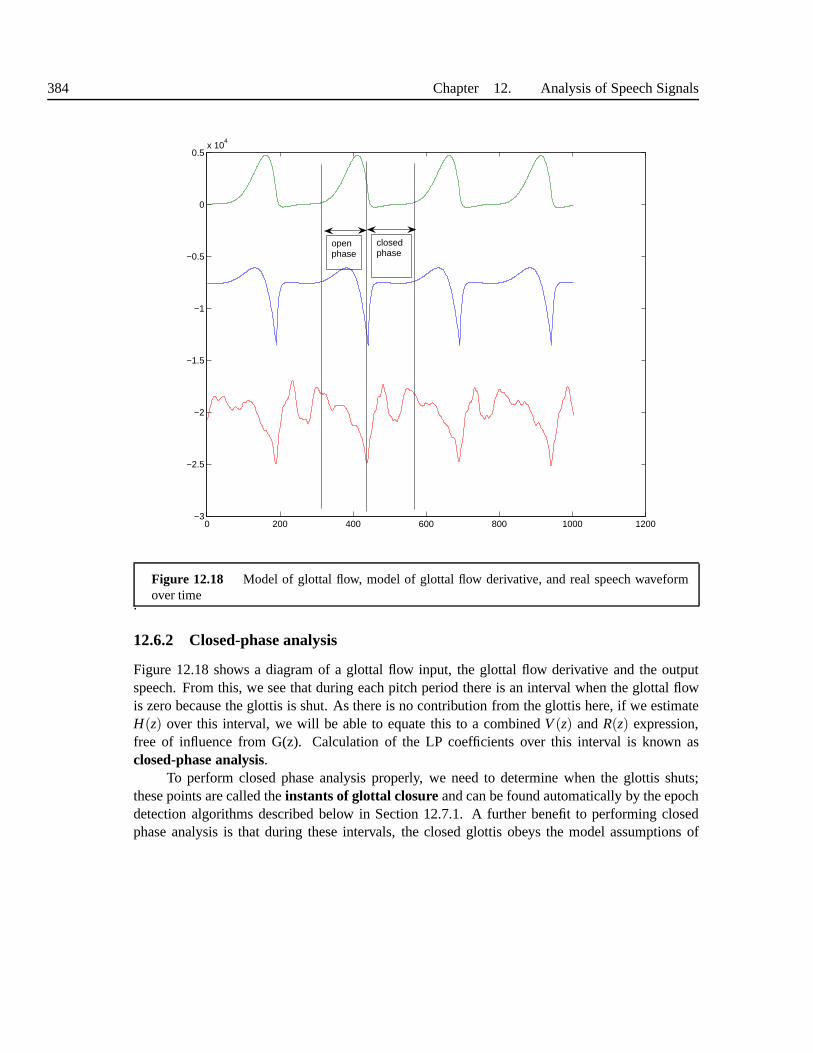
384 Chapter 12. Analysis of Speech Signals
0 200 400 600 800 1000 1200−3
−2.5
−2
−1.5
−1
−0.5
0
0.5x 10
4
openphase
closedphase
Figure 12.18 Model of glottal flow, model of glottal flow derivative, and real speech waveformover time
.
12.6.2 Closed-phase analysis
Figure 12.18 shows a diagram of a glottal flow input, the glottal flow derivative and the outputspeech. From this, we see that during each pitch period thereis an interval when the glottal flowis zero because the glottis is shut. As there is no contribution from the glottis here, if we estimateH(z) over this interval, we will be able to equate this to a combined V(z) andR(z) expression,free of influence from G(z). Calculation of the LP coefficients over this interval is known asclosed-phase analysis.
To perform closed phase analysis properly, we need to determine when the glottis shuts;these points are called theinstants of glottal closureand can be found automatically by the epochdetection algorithms described below in Section 12.7.1. A further benefit to performing closedphase analysis is that during these intervals, the closed glottis obeys the model assumptions of
Section 12.6. Source representations 385
being completely reflective and having an infinite impedance; by contrast, during the open phasethere are losses at the glottis, but worse there will definitely be interaction with the sub-glottalsystem (that is, the assumption made in section 11.3.3 wherewe assume that no signal is reflectedback from the lungs will not hold).
So given that G(z) has negligible effect during the closed phase, all we need now do is removethe effect ofR(z) to findV(z). From experimentation and knowledge of radiation properties, wecan approximateR(z) as a differentiator of the signal. This can be modelled by a first order FIRfilter of the form:
y[n] = x[n]−αx[n−1]
Hence the effect of this can be removed by multiplying the signal with the inverse equivalent ofthis, which is an IIR filter, acting as an integrator:
x[n] = y[n]+ αx[n−1]
For reasons of stability, it is best to haveα slightly less than the “true” integrating/differentiatingvalue of 1; values in the range 0.95 to 0.99 are often used. This process is known aspre-emphasis.
Now we have a reasonably accurate expression for the vocal tract transfer function, we caninverse filter the speech to find the glottal flow signal. The trick here is to inverse filter the signalover awholepitch period (or longer) rather than just the interval over which the LP coefficientswere calculated. By doing this, we inverse filter over the region where the glottis is open, and fromthis we can find the form of the input, glottal signal. This process is shown in Figure 12.19, alongwith the shapes of the glottal flow and glottal flow derivativefrom the Lijencrants-Fant model.The figure clearly shows that the glottal flow derivative is highly similar to the residual signal,especially with regard to the large negative spike at the instant of glottal closure. The figure alsoshows that the assumptions made about the impulse excitation in the basic LP model are also quitejustified; the excitation in the closed phase comes from the large negative going spike in the glottalderivative signal can be approximated by an impulse quite easily.
In many cases, especially in female or other high pitched speech, the length of the closedphase can be very small, perhaps only 20 or 30 samples. In the autocorrelation method, the initialsamples of the residual are dominated by the errors caused bycalculating the residual from thezero signal before the window. The high (and erratic) error in the residual can be seen in the firstfew samples of the residual in Figure 12.17b. For short analysis windows this can lead to a residualdominated by these terms, and for this reason, covariance analysis is most commonly adopted forclosed phase analysis.
It should be noted that in many real-life cases, the pre-emphasis term is not applied, andhence the calculated residual is in fact a representation ofthe glottal flow derivative. This is thecase for most speech synthesis purposes, and henceforth we will assume that all residuals arecalculated in this way, unless otherwise stated.

386 Chapter 12. Analysis of Speech Signals
0 200 400 600 800 1000 1200−3.5
−3
−2.5
−2
−1.5
−1
−0.5
0
0.5x 10
4
Figure 12.19 From top to bottom, model of glottal flow, model of glottal flowderivative, realspeech waveform and real residual
.
12.6.3 Open-phase analysis
It is not always possible or desirable to used closed-phase analysis. Sometimes other constraintsin an application mean a fixed frame spacing is required, and sometimes it is simply not possibleto find the instant of glottal closure with any degree of accuracy. What then happens if the LPanalysis is performed over an arbitrary section of speech? The main upshot of this is that the LPanalysis will attempt to model the effect of the zeros in the glottal transfer function, and in doingso include the effect of the zeros in its poles.
From the basic Maclaurin expansion of
∞
∑n=0
xn = 1+x+x2+x3 + .... =1
1−x
Section 12.6. Source representations 387
we can show that∞
∑n=0
bnz−1 =z
z−b=
11−bz1
inverting this, we get:1
∞∑
n=0bnz−1
= 1−bz1
which shows that a single zero can be exactly modelled by an infinite number of poles. It can beshown that so long as the number of poles≫ than the number of zeros, a reasonable approximationof the effect of zeros can in fact be modelled by the poles. In doing do however, we are in effectmodelling these zeros withall the poles in the transfer function, and so the poles will all be atslightly different locations than in the case of closed-phase analysis. Luckily, this doesn’t seemto have too great an influence on the frequency response of theLP transfer function, but it doeshave a knock on effect when the LP filter is used to find the residual. As we have modelled theglottal zeros with poles, the residual now does not closely resemble the glottal derivative, rather itis significantly “noisier”, and “spikier”. This means, thatfirst, the spectrum of the residual will beflat, and that secondly the main excitation will be in the formof isolated impulses rather than theshape of the glottal derivative function of closed phase analysis. This can be seen by comparingthe open phase residual of Figure 12.17 with the closed-phase residual of 12.19. In general, fixedframe LP analysis is the norm, and so the open phase residual signals such as that shown in Figure12.17 are most commonly observed. Note that this ability to model zeros with poles also allowsus to provide a means to represent vocal tract transfer functions for nasals and obstruents withall-pole functions. While the accuracy of these all-pole expressions is not as high as for vowels,the convenience in being able to use a single method and expression for all speech sounds usuallyoutweighs any issues arising from the inability to model vocal tract zeros properly.
It is worth making a final point about residuals when they are used as sources. Recall fromthe original LP equation that as well as the residual being the outcome when the speech is inversefiltered, it is also simply the error in the LP analysis. Henceif a residual is used to excite the filterfrom which it came, the result should be a perfect reconstruction of the original signal. As we shallsee in Section 14, there are many implementation issues to dowith frame edges and so on, but itis worth noting that no matter how crude any of the assumptions we have made with regard to LPanalysis in general, a powerful feature of the model is that the speech can be exactly reconstructedif excited with the correct input.
12.6.4 Impulse/noise models
Linear prediction was in fact primarily developed for use inspeech coding applications. As wehave just seen, performing LP analysis allows us to deconvolve the signal into a source and filter,which can then be used to reconstruct the original signal. Simply separating the source and filter

388 Chapter 12. Analysis of Speech Signals
doesn’t actually save any space, the trick comes in replacing the residual by a much simpler (andmore economical) source signal.
In what we shall henceforth callclassical linear prediction the source is modelled by twosystems; one for voiced sounds and one for obstruent sounds.In Figure 12.19, we saw that the in-tegrated residual signal was a reasonably close approximation to the glottal flow derivative signal.The primary feature in such a signal is the negative spike caused by the glottal closure. As this isreasonably close to an impulse, the classical LP model simply uses a single impulse as the excita-tion for voiced sounds. To do this properly, one impulse is generated for every pitch period, and soin analysis, an estimation of the pitch period has to be foundand stored/transmitted. All obstruentsounds have a frication source, generated by white noise in our model from section 11.5.2. In theclassical LP system, all we need store/transmit is the fact that we have an obstruent sound, uponwhich a noise source is used during reconstruction. For voiced obstruents, both the impulse andnoise source are used.
The impulse/noise model provides a very efficient means of encoding the residual, but doesso at some cost, the effects of which can clearly be heard in the reconstructed signal as a buzz ormetallic sound. Apart from the space saving, having an impulse excited system has the additionalbenefit in that we are free to generate the impulses when we like; in other words, we are notlimited to generating the impulses at the same spacing as in the analysis. This provides a meansof changing the pitch of a signal and in fact forms the basis ofthe synthesis technique describedin Section 13.3.
12.6.5 Parameterisation of glottal flow signal
Performing the above analysis allows us to find a reasonable estimate of the glottal flow or glottalflow derivative. In fact, we can go one stage further and parameterise this by further analysis. Onetechnique described by Quatieri [364] involves fitting the Lijencrants-Fant model to the residual bymeans of least squares minimisation. In philosophy, this isof course similar to linear predictionanalysis itself, where we attempt to find the set of predictorcoefficients which give the lowesterror. In practice, the LF model is non-linear and so the LP technique is not available to us.Instead, numerical techniques such as the Gauss-Newton method are used to iterate to a set ofoptimum model parameters. Dutoit [148] describes a different technique where the glottal sourceparameters are actually found at the same time as the predictor coefficients.
While we can find the optimal parameters for any given frame for a model such as LF, wenever actually achieve a perfect fit. In fact, we can determine a sample by sample differencebetween the model and the residual. This of course, is another “residual” or “error” signal, whichnow represents the modelling error after the LP model and theLF model have been taken intoaccount. One interesting study by Plumpe et al [356] describes how this signal is in fact highlyindividual to speakers and can be used as the basis of speakerrecognition or verification.

Section 12.7. Pitch and epoch detection 389
12.7 PITCH AND EPOCH DETECTION
12.7.1 Pitch detection
The process of finding the fundamental frequency (F0) or pitch from a signal is known aspitchdetectionor pitch tracking . Recall from Chapter 7 that fundamental frequency is definedas thefrequency at which the glottis vibrates during voiced speech, whereas pitch is the perceived rateof periodicity in the speech signal by the listener. In general, we ignore this distinction, mainlybecause in most cases any difference between these two values is less than the known accuracy ofany detection algorithm. One point that is important thoughis that F0 tracks are in fact used formany quite different purposes. In some of the signal processing operations described below, anaccurate frame by frame value is required; however in intonational analysis, we are usually onlyinterested in the general shape of the track, and so small perturbations are often smoothed for suchneeds.
As with formant tracking, traditionalpitch detection algorithms PDAsoften have threestages; a pre-processing stage, where for instance the speech is downsampled or low-pass filtered,a bottom up candidate finding step, and a decision making stepwhereby the best candidates arepicked.
A wide variety of techniques have been proposed for pitch tracking, including:
• Using the cepstrum. As cepstral analysis generates a representation where the pitch infor-mation appears as a spike, it is possible to find this spike anddetermine the pitch from that.
• Autocorrelation function. In the time domain, successive pitch periods are usually similar toone another. As the autocorrelation functions measure how similar a signal is to itself whenshifted, it will have a high value when a a pitch period is mostclosely overlapped with itsneighbour. We can hence find the period by finding these pointswhere the autocorrelationfunction is at a maximum. In a similar fashion, the normalised cross correlation function canbe used.
• Frequency domain. As the harmonics in the DFT are spaced at multiples of the period,these can be used to find the period. One strength in this technique is that there are multipleharmonics and hence more than one measurement can be made. A drawback is that they canoften be hard to measure accurately, especially at higher frequencies.
• Residual analysis. As the residual is mostly free from vocaltract influence, it represents thesource, and from this the period can be seen. In practice thistechnique is rarely used as theartefacts in LP analysis often make the determination of theperiod quite difficult.
The classic work on pitch detection is that of Hess [202] who gives a thorough overviewof all the PDA techniques just mentioned. With PDAs, the basic techniques only go so far andan important component of the algorithm is the use of many heuristic or empirically determinedfactors. Bagshaw [28] conducted an objective test on 6 popular techniques and claims that the timedomain super resolution pitch determination algorithm [309] is the best. Other well known pitch-
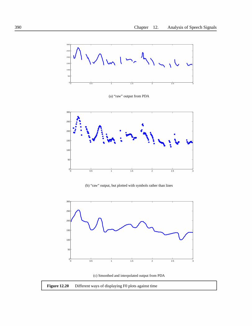
390 Chapter 12. Analysis of Speech Signals
0 0.5 1 1.5 2 2.5 30
50
100
150
200
250
300
(a) “raw” output from PDA
0 0.5 1 1.5 2 2.5 30
50
100
150
200
250
300
(b) “raw” output, but plotted with symbols rather than lines
0 0.5 1 1.5 2 2.5 30
50
100
150
200
250
300
(c) Smoothed and interpolated output from PDA
Figure 12.20 Different ways of displaying F0 plots against time
Section 12.7. Pitch and epoch detection 391
trackers include Talkin’s getf0 and RAPT algorithms [431] (these were not included in Bagshaw’stest, but are generally acknowledged to be very accurate). As with formant tracking, traditionalPDAs suffer somewhat from their heuristic rather than probabilistic formulation. Recently, moreinterest in probabilistic techniques has arisen [141], andfor instance Li et al [283] cite accuracyresults for a probabilistic technique which is significantly more accurate than getf0.
12.7.2 Epoch detection: finding the instant of glottal closure
We have just seen that closed phase linear prediction requires that we analyse each pitch periodseparately. This type of speech analysis is calledpitch synchronous analysisand can only beperformed if we are in fact able to find and isolate individualperiods of speech. We do this bymeans of anpitch marking orepoch detectionalgorithm (EDA).
The idea behind an EDA is to locate a single instant in each pitch period that serves as an“anchor” for further analysis. These positions are often known aspitch marks, pitch epochsorsimply epochs. In general, they can refer to any reference point, but are often described in termsof salient positions on the glottal flow signal, such as the peak of the flow for each pitch period.For many types of analysis (such as TD-PSOLA described in Section 14.2) it doesn’t really matterwhere the anchor point is chosen, so long as it is consistent from period to period. Often a time-domain reference point such as the peak of the highest excursion in each period is used, or thetrough of the lowest excursion. That said, many analysis techniques focus on one particular pointknown as theinstant of glottal closure (IGC). This is manifested as a large negative going spike inthe glottal flow derivative, as shown in Figure 12.21. If we view this as the input to the vocal tract(which we do be including the radiation term), we see that it closely resembles a large negativeimpulse. Such an impulse excites the filter in such a way that we can examine the filter propertieswithout interference from the ongoing effects of the glottis. As we saw above, this is the basis onwhich close-phase LP analysis is performed.
Locating the instant of glottal closure and epoch detectionin general is widely acknowledgedas a thorny problem. In the past, most pitch synchronous applications could use a rough estimateof the ICG, as the technique was not particularly sensitive to determining these instants exactly.Indeed, the closed phase LP technique described above does not need a particularly accurate esti-mate - the window used by the technique does not have to start exactly at the ICG. With the morewidespread adoption of pitch synchronous speech synthesistechniques (described in Chapter 14)it becomes more important to locate the exact ICG, or some other anchor point, more exactly.Dutoit [148] gives a review of some of the difficulties involved, and describes a process commonin the early 1990s whereby researchers would actually mark epochs by hand. This was seen asbeing an acceptable burden when speech databases were smalland when the only alternative wasto use other much poorer sounding synthesis techniques. Dutoit describes some of the difficultiesinvolved in this, most specifically the fact that because of various phase effects, it is not alwaysthe largest negative peak in the waveform which correspondsto the IGC. Furthermore, it is knownthat phase distortion can make time domain marking of waveforms virtually impossible for either

392 Chapter 12. Analysis of Speech Signals
0 2000 4000 6000 8000 10000 12000 140000.2
0.4
0.6
0.8
1
1.2
1.4
1.6
1.8
2
2.2
Figure 12.21 Comparison of (from top to bottom) waveform, laryngograph signal, integrated resid-ual and residual.
machine or human.These difficulties led many to a radical alternative, which was to measure the glottal be-
haviour by means other than from the speech waveform. A common techniques was to use adevice known as anelectroglottograph or a laryngograph. This consists of two metal discswhich are placed on each side of the protruding part of the larynx (the “adam’s apple”). A veryhigh frequency alternating current is passed through the system, such that the current passes fromone disc, through the larynx, to the other disc, and from thisthe electrical impedance and flow ofcurrent across the larynx can be measured. If the glottis is open, the impedance is high and thecurrent is low; if the glottis is shut the impedance is low andthe current is high. Laryngograph sig-nals (known as Lx signals) do not however generate the glottal flow signal itself as the relationshipbetween the electrical impedance and flow is not simply related. The Lx signal is however quitesimple, and from it, it is usually possible to find the instants when the glottis shuts (the IGC) andopens. Figures 12.21 and 12.22 show a speech waveform, an Lx signal and a LP derived estimateof the glottal flow derivative. The Lx signal clearly shows each pitch period, and is particularlyclear at showing exactly when the transition between voicedand unvoiced sounds occurs, whichis one of the most difficult areas to perform accurate epoch detection. Epoch detection by meansof Lx signals has been quite widely used in TTS in the last 15 years, but it is rare to find explicitmention of this. Acero [3] does however provide a good account of the process of Lx use for TTS.
There are two main problems with Lx use. Firstly, the technique doesn’t work well for some

Section 12.7. Pitch and epoch detection 393
6000 6200 6400 6600 6800 70000.2
0.4
0.6
0.8
1
1.2
1.4
1.6
1.8
2
2.2
instant of glottal closure
instant ofglottal opening
Figure 12.22 Fine grained comparison of (from top to bottom) waveform, laryngograph signal,integrated residual and residual. The vertical lines show the instants of glottal closure and glottalopening. Here we can see that while the general periodicity of the form of the LX and residual glottalflow are similar, the functions are not simply related in shape. Note that when the glottis is open, theLX signal is at a minimum because the current flow is at a minimum. The integrated residual signal(c) approximates the glottal volume velocity. Ideally the closed phase in this signal should be flatter,but the many modelling errors combine to give this part of thewaveform a gradual upward slope. Asmall sharpening in the gradient of this can be seen at the instant of glottal opening.
speakers due to physiological reasons. Secondly, it is simply awkward to have to record all thespeech data with both a microphone and the Lx device. It is notparticularly comfortable (althoughit is completely safe) and some speakers, particularly highly paid voice talents, are not happy withits use. Thankfully, a number of fully automatic techniquesnow do exist that can extract theIGCs from the speech waveform directly. Many of these work onthe residual, and it is knownthat the negative pulse of the residual can give quite an accurate estimation of the IGC if care istaken with the analysis and the signal does not suffer from phase distortion. Recently several othertechniques have been developed for automatic extraction from speech. Brookes [68] describes atechnique which uses the glottal energy flow, and claims thatthis is significantly more accuratethan residual analysis. Vedhius describes a general technique that uses dynamic programmingto constrain the epoch search, and shows that this techniquecan be extended to other points ofinterest besides the IGC [469].
394 Chapter 12. Analysis of Speech Signals
12.8 DISCUSSION
For those approaching these topics for the first time, some ofthe formulations, reasoning andsheer number of representations can make the speech analysis subject seem quite daunting. It isin fact virtually impossible to learn this subject purely from the mathematics: speech analysis is apractical subject and requires practical study, and by far the best means to study this is by interac-tively playing with real speech signals. Luckily a number ofpackages exist which allow intimateexamination of speech signals. Using these, it is possible to examine magnitude spectra, linearprediction envelopes, spectrograms of different types andso on. In fact, a good understanding ofthe speech representations described here can be gained from interactive study alone without anyunderstanding of the equations involved (although this of course is not recommended).
Speech analysis is a broad topic and is used in many applications. Historically, most of thetechniques described here were first developed for use in speech coding, where the aim is to trans-mit a signal down a wire as efficiently as possible. With any general type of data, there is oftenconsiderable redundancy, and by studying the patterns in which the data naturally occurs we canstudy this redundancy and eliminate it. These general techniques only go so far, and it soon be-came apparent that special purpose coders designed specifically for speech signals could be muchmore efficient, delivering more than a factor of 10 compression rate. In fact, linear predictionwas developed for just this purpose. Linear predictive coding (LPC) as it is known, separates thesource and filter for each frame, but only sends the filter coefficients, normally encoded as reflec-tion coefficients or line spectral frequencies. The residual is not transmitted, rather an estimate ofthe pitch is sent for voiced signals, and a flag stating whether the source is noisy (ie is an obstruentsound). When the speech is to be reconstructed, the pitch information is used to generate an im-pulse sequence for voiced signals, and white noise is added if the noise flag it set. The quality ofLPC speech is considerably worse than the original, but it has proved a popular choice, especiallyfor situations with user acceptance and requirements for very low transmission rates (usually mili-tary). More recently, LPC coders with more sophisticated residual reconstruction techniques havebeen used in normal commercial applications.
Automatic speech recognition systems use speech analysis as their first stage. All ASRsystems are essentially pattern recognisers, and so work well with when presented with inputfeatures with certain properties. These include that the representation should be compact, so thatthe number of parameters to be learned is low; and this sharesobvious common ground with thespeech coding applications just mentioned. A good example is that many ASR systems use multi-variate Gaussians to model phone distributions (see Chapter 15). For a vector with 10 components,doing so fully requires a set of 10 means and a set of 10 by 10 (100) covariances. If however thecomponents are statistically independent of each other, wecan ignore most of the covariance termsand model the distribution with 10 means and just 10 variances. In addition, it is desirable thatthe representations should be invariant for a single class;for this reason, recognition is neverperformed on the waveform itself, as the phase aspect makes signals with the same envelope look

Section 12.8. Discussion 395
quite different.Currently, mel-scale cepstral coefficients, and perceptual linear prediction coefficients trans-
formed into cepstral coefficients, are popular choices for the above reasons. Specifically they arechosen because they are robust to noise, can be modelled withdiagonal covariance, and with theaid of the perceptual scaling are more discriminative than would otherwise be. From a speechsynthesis point of view, these points are worth making, not because the same requirements existfor synthesis, but rather to make the reader aware that the reason MFCCs and PLPs are so oftenused in ASR systems is for the above reasons, and not because they are intrinsically better in anygeneral purpose sort of way. This also helps explain why there are so many speech representationsin the first place; each has strengths in certain areas, and will be used as the application demands.In fact, as we shall see in Chapter 16, the application requirements which make, say, MFCCs sosuitable for speech recognition are almost entirely absentfor our purposes. We shall leave a dis-cussion as to what representations really are suited for speech synthesis purposes until Chapter16.
12.8.1 Further reading
There are several good books on speech analysis, most of which adopt an application neutralattitude. The classic work is Rabiner and Schafer [368] and while written several decades ago,this book remains an excellent reference for all the fundamentals of speech analysis. It assumesthe reader is familiar with basic signal processing, and so can be a little difficult for those withno prior experience. Given an understanding of the topics covered in Chapter 10 of this book, thereader should have little difficulty. An excellent more recent book is Quatieri [364]. The subjectmatter doesn’t differ much from that of Rabiner and Schafer,but the book covers many of thetechniques developed since. Other good references includeFurui [168], Huang et al [224], Kleijnand Paliwal [256], Deller and Proakis [128] and Gold and Morgan [176].
12.8.2 Summary
• Speech analysis is in general concerned with three main problems:
1. eliminate phase; the magnitude DFT does this2. separate source and filter; this can be done with cepstral analysis or linear prediction3. transform the representation into a space which has more desirable properties; log mag-
nitude spectra follow the ear’s dynamic range; mel-scaled cepstra scales according tothe frequency sensitivity to the ear. Log area ratios are amenable to simple interpolationand line spectral frequencies show the formant patterns robustly.
• The continuously varying signal is divided by a process called windowing into a sequenceof stationary smaller signals called frames.
• Windowing affects the signal and so a perfect representation of the original waveform is notpossible.

396 Chapter 12. Analysis of Speech Signals
• The most common spectral representation is achieved by applying a discrete Fourier trans-form (DFT) to the frame of speech.
• Successive application of DFTs can be used to generate a spectrogram.
• The cepstrum is the inverse Fourier transform of the log magnitude spectrum. It separatesvariation in frequency across the range and so implicitly separates source and filter compo-nents in the spectrum.
• Linear prediction performs source/filter separation by assuming an IIR system represents thefilter. This allows the filter coefficients to be found by a process of minimising the errorpredicted from the IIR filter.
• The linear prediction equations can be solved by the autocorrelation or covariance methods.Each involves solving the equations by means of efficient matrix inversion.
• The direct linear prediction, IIR, coefficients are inherently unrobust with regard to quanti-sation and interpolation. A set of derived representations, including reflection coefficients,log area ratios and line spectral frequencies avoid these problems.
• The source signal, called the residual, can be found by inverse filtering the speech signalwith the linear prediction coefficients.
• With appropriate care during analysis and filtering, this commonalities between this residualand the glottal flow derivative signal can be shown.
13SYNTHESISTECHNIQUES BASED ONVOCAL TRACT MODELS
In this chapter we introduce the three main synthesis techniques which dominated the field up untilthe late 1980s, collectively known asfirst generation techniques. While these techniques are usedless today, it is still useful to explore them, as apart from simple historical interest, they give us anunderstanding of why today’s systems are configured the way they are. As an example, we need toknow why today’s dominant technique of unit selection is used rather than the more basic approachwhich would be to generate speech waveforms “from scratch”.Furthermore, modern techniqueshave only been made possible by vast increases in processingpower and memory, so in fact forapplications which require small footprints and low processing cost, the techniques explained hereremain quite competitive.
13.1 SYNTHESIS SPECIFICATION: THE INPUT TO THE SYNTHESISER
First generation techniques usually require a quite detailed, low-level description of what is tobe spoken. For purposes of explanation, we will take this to be a phonetic representation for theverbal component, along with a time for each phone, and an F0 contour for the whole sentence.The phones will have been generated by a combination of lexical lookup, LTS rules and post-lexical processing (see Chapter 8), while the timing and F0 contour will have been generated bya classical prosody algorithm of the type described in Chapter 9. It is often convenient to placethis information in a new structure called asynthesis specification. Hence the specification is theinput to the synthesiser and the waveform is the output.
Initially, we will assume a simple model where the specification is a listSSS===<<< sss1,,,sss2,,, .........,,,sssN >>>,in which each itemsssj contains the phoneme identity, a duration, and one or more F0values. Recallfrom Chapter 9, that the F0 contour is necessarily dependenton the timing information, as the F0generator must produce an F0 contour that matches the lengthof the utterance. One option is tospecify the F0 contour on a frame by frame basis, so that if we had say a 50ms duration phonemeand a 10ms frame shift, we would have 5 F0 values in the specification. A 70ms duration phonemewould have 7 frames and so on:
397

398 Chapter 13. Synthesis Techniques Based on Vocal Tract Models
[F0 ] = < 121,123,127,128,126> (5 frame example)[F0 ] = < 121,123,127,128,126,121,118> (7 frame example)
and so a example of a complete specification item would look like
sssj =
PHONEME /ah/DURATION 70F0 < 125,123,119,117,115,115,114>
Having different numbers of F0 values per item can be unwieldy, so sometimes the F0 contour issampled at the mid point of the unit or other key positions to give a simpler specification:
sj =
PHONEME /ah/DURATION 50F0 START 121F0 MID 123F0 END 127
Once the specification has been created, the synthesis process itself can begin.
13.2 FORMANT SYNTHESIS
Formant synthesiswas the first genuine synthesis technique to be developed andwas the domi-nant technique until the early 1980s. Formant synthesis is often calledsynthesis-by-rule; a terminvented to make clear at the time that this was synthesis “from scratch” (at the time the term“synthesis” was more commonly used for the process of reconstructing a waveform that had beenparameterised for speech coding purposes). As we shall see,most formant synthesis techniquesdo in fact use rules of the traditional form, but data driven techniques have also been used.
Formant synthesis adopts amodular, model-based, acoustic-phoneticapproach to the syn-thesis problem. The formant synthesiser makes use of the acoustic tube model, but does so in aparticular way so that the control elements of the tube are easily related to acoustic-phonetic prop-erties than can easily be observed. A typical basic layout ofa formant synthesiser in shown inFigure 13.1. Here we see that the sound is generated from a source, which is periodic for voicedsounds and white noise for obstruent sounds. This basic source signal is then fed into the vocaltract model. In virtually all formant synthesisers, the oral and nasal cavities are modelled sep-arately as parallel systems. Hence the signal passes into the component which models the oralcavity, but can also pass into the component for modelling the nasal cavity if required for a nasalor nasalised sound. Finally, the outputs from these components are combined and passed through

Section 13.2. Formant Synthesis 399
source
nasalcavity
pharyngeal/oral cavity
radiation
speechpressurewaveform
volumevelocity
source lip/nosevolumevelocity
Figure 13.1 Block diagram of basic formant synthesiser
a radiation component, which simulates the load and propagation characteristics of the lips andnose.
The first point of note regarding the formant synthesiser is that it is not an accurate modelof the vocal tract. Even taking into account the crude assumptions regarding all-pole modelling,losses and so on, the formant synthesiser structure differssignificantly in that it allows separateand independent control of each formant. In the vocal tract model developed in Chapter 11, theformants emerged as a result of the whole, concatenated-tube model; it was not possible to pointto just one section of tube and say that that section was responsible for the behaviour of a partic-ular formant. Hence the formant synthesiser is based on alumped parameter model of speechgeneration, rather than thedistributed model developed in Chapter 11. The reason for modellingthe formants as individual components is that this allows the system designer to gain direct controlof the formants and the reason for wishing to do this is that atthe time when formant synthesiserswere developed, it was much easier to read real formant values from spectrograms than to deter-mine real vocal tract configurations. Even today, with MRI and EMA, the logistics of acquiringformant values are considerably simpler than those of determining vocal tract shapes. Hence con-structing a synthesis paradigm based on formant control is one of pragmatics (being able to controlwhat we can observe) and modularity (where each component can be separately controlled).
That said formant synthesis does share much in common with the all-pole vocal tract model.As with the tube model, the formant synthesiser is modular with respect to the source and vocaltract filter. The oral cavity component is formed from the connection of between 3 and 6 individualformant resonators in series, as predicted by the vocal tract model, and each formant resonator isa second order filter of the type discussed in Section 10.5.3.
13.2.1 Sound sources
The source for vowels and voiced consonants can be generatedeither as an explicit time domainperiodic function, of the type described in Section 11.4.2,or by an impulse sequence that is fedinto a glottal LTI filter. For obstruent sounds a random noisegenerator is used. Sounds such as

400 Chapter 13. Synthesis Techniques Based on Vocal Tract Models
voiced fricatives use both sources. If we adopt the impulse/filter approach, we see that in factthese sources are equivalent to those of classical impulse/noise linear prediction model (Section12.6.4). One difference between the impulse/glottal filtersource and linear prediction models isthat in the impulse/glottal filter model the voiced source isformed by a series of impulses whichpass through a simple filter to generate a periodic source signal. In classical linear prediction onthe other hand, the source is the impulses themselves and anymodification performed on these iscombined in with the filter use to model the vocal tract.
13.2.2 Synthesising a single formant
Recall from Section 10.5.3 that a formant can created by a second order IIR filter whose transferfunction is:
H(z) =1
1−a1z−1−a2z−2
This can be factorised as
H(z) =1
(1− p1z−1)(1− p2z−1)
To generate filter coefficientsa1 anda2 with real values, the poles have to form a complex conju-gate pair. Recall that a second order expression like this generates a spectrum with two formants,but as only one of these lies in the positive frequency range,the above expression does in fact gen-erate a single usable formant with the full range of amplitude, bandwidth and frequency position.
The poles can be represented in polar form. As they form a complex conjugate pair, theyhave the same magnituder and anglesθ and−θ:
H(z) =1
(1− re jθz−1)(1− re− jθz−1)(13.1)
As explained previously, poles can be visualised on a pole-zero plot, such as that shown in Figure10.22. The magnitude of the pole determines the bandwidth and amplitude of the resonance; forlow values ofr, the formant will be very flat, asr increases the formant will become sharp, untila pole with a value of 1 will have an infinite amplitude (which should not occur in practice).The angleθ determines the normalised angular frequency position of the pole and is expressedin radians; it can be converted to a frequency in Hertz by multiplication by 2πFs whereFs is thesampling frequency. If we multiply Equation 13.1 out again,we can write the transfer function interms of the radius and angle of the poles:
H(z) =1
1− r(ejθ +e− jθ)+ r2z−2
and from Euler’s formula (Equation 10.9) we can see that the complex terms cancel out to give avalue for the first coefficient expressed in cosine terms.
H(z) =1
1−2rcos(θ)+ r2z−2

Section 13.2. Formant Synthesis 401
input output
F1 F2 F3 F4
(a) Cascade or serial configuration
F2
F3
F4
F1
input+
output
A1
A2
A3
A4
(b) Parallel configuration
Figure 13.2 Different formant configurations.
While we can generate a formant of any desired frequency directly by appropriate use ofθ, con-trolling the bandwidth directly is a little more difficult. The position of the formant will change theshape of the spectrum somewhat and so a precise relationshipfor all cases is not possible. Notealso, that when two poles (from two separate second order filters) are close together, they have theeffect of combining into a single resonant peak and this again makes bandwidth calculation some-what difficult. However, it can be shown that a reasonable approximation linking the normalisedbandwidth of a formant to the radius of the pole is
B =−2ln(r)
Using this, we can the write the transfer function in terms ofthe normalised frequencyF andnormalised bandwidthB of the formant:
H(z) =1
1−2e−2Bcos(2πF)z−1 +e−2Bz−2
As before, values for the normalised frequencyF and bandwidthB can be determined from thefrequencyF and bandwidthB by dividing byFs, the sampling rate. Figures 10.23 and 10.24 showthe spectrum for a single formant with different values for frequency and bandwidth.
13.2.3 Resonators in series and parallel
A transfer function that creates multiple formants can be formed by simply multiplying severalsecond order filters together. Hence the transfer function for the vocal tract is given as:

402 Chapter 13. Synthesis Techniques Based on Vocal Tract Models
H(z) = H1(z)H2(z)H3(z)H4(z) (13.2)
=1
1−2e−B1cos(2πF1)z−1 +e−2B1z−2︸ ︷︷ ︸
H1
...1
1−2e−B4cos(2πF4)z−1 +e−2B4z−2︸ ︷︷ ︸
H4
(13.3)
whereF1 is the frequency of the first formant,B1 is the bandwidth of the first formant and so on.The terms in the denominator are multiplied out to give the standard all-pole filter transfer function
H(z) =1
1−a1z−1−a2z−2− ...−a8z−8 (13.4)
and time domain difference equation
y[n] = x[n]+a1y[n−1]+a2y[n−2]+ ...+a8y[n−8] (13.5)
These equations show the main advantage of the formant technique, namely that for a given setof formant values, we can easily create a single transfer function and difference equation for thewhole oral tract. In a similar fashion, a nasal system can be created, which likewise links thevalues of the nasal formant to a transfer function and difference equation.
This formulation is known as aserial or cascadeformant synthesiser and was the first typeto be developed. Note that the relative amplitudes of the formants are determined as part of thiscalculation and are not set explicitly. This works because each formant sits on the skirt of theothers, and this naturally generates formants of the correct amplitude. Hence the generated spec-trum from such a formulation will always seem “natural” in terms of its shape. Counter to theseadvantages is the problem that the interactions of the formants when cascaded can sometimes havesome unwanted effects. In particular, when two formants areclose, the resultant values as mea-sured from the spectrum can often differ from the input formant parameters and hence a lack ofcontrol appears.
An alternative formulation is theparallel formant synthesiser, in which each formant is mod-elled in isolation, and during speech generation, the source signal is fed through each separately.After this, the signals from all the formants are combined. The advantage is that the frequencyof each formant can be more accurately specified, the disadvantage is that now the amplitudes ofeach must be carefully controlled; they do not appear on their own unlike in the cascading method.In addition, there is no neat single transfer function or difference equation for the parallel case,rather each formant has its own transfer function

Section 13.2. Formant Synthesis 403
H1(z) =1
1−a11z−1−a12z−2 (13.6)
H2(z) =1
1−a21z−1−a22z−2 (13.7)
... (13.8)
and difference equation
y1[n] = x[n]+a11y1[n−1]+a12y1[n−2] (13.9)
y2[n] = x[n]+a21y2[n−1]+a22y2[n−2] (13.10)... (13.11)
which are added in the time domain to give the final signal
y[n] = y1[n]+y2[n]... (13.12)
The two configurations are shown in Figure 13.2. Note that theparallel configuration has anamplitude (gain) control for each formant.
13.2.4 Synthesising consonants
The source characteristics of consonants differ dependingon the class of sound being produced.All unvoiced sounds use only the noise source; nasals and approximants use only the periodicsource while voiced obstruents (i.e. voice fricatives, affricates and stops) use both sources. Ap-proximants are generated in much the same way as vowels. Someconsonants (such as [h]) can besynthesised in the same way as vowels; that is by sending a sound source through the oral cavityresonators. Most other consonants are however more complicated than /h/ because their source isnot at one end of the vocal tract.
Recall from Section 11.5 and Figure 11.17 that we used a number of different tube configu-rations for each consonant type. The same approach is used informant synthesis. In the case ofnasals, the nasal cavity acts as a resonator and the nose is the only place where sound escapes. Theoral cavity does however still have an effect - even with the velum lowered sound from the glottisstill passes into the oral cavity, but now is reflected at the lips rather than escaping. The oral cavitystill operates as a resonator and some of the glottal source wave that it modifies enters the nasalcavity through the lowered velum. The oral cavity thereforehas a significant effect on the soundof the nasal and this explains why we can have different sounding nasals even though the nasalcavity itself only has a single, unmoving shape.

404 Chapter 13. Synthesis Techniques Based on Vocal Tract Models
In real speech obstruents have their frication source generated at a place of constriction andnot by the glottis. Normally this place of constriction is caused by the tongue nearing the roofof the mouth. In these cases, some of the sound created at the place of constriction travels backtowards the glottis, is reflected there and travels forwards, through the constriction and towardsthe lips. Hence the vocal tract is effectively split into a separate front and rear cavity which haveseparate resonant properties.
While details differ from system to system, in formant synthesis these more complex vocalorgan configurations can be modelled by the use of parallel resonators. In the case of nasals, oneset of resonators can be used to model the nasal cavity while another models the oral cavity. Theoutputs of these are then simply added to generate the output. While this obviously differs fromthe real vocal tract (where the output of the oral cavity is further modified by the nasal cavity),with appropriate choices of parameters, a convincing effect can be achieved. Fricative soundsare generated in a similar fashion, with one combination of resonators being used for the forwardcavity and another for the back cavity. Again this is simplerthat the real vocal tract, but this canbe overcome with appropriate choice of parameters.
Further refinement can be achieved by the use of zeros. These can be used to create anti-resonances, corresponding to a notch in the frequency response. Here the format synthesis modelagain deviates from the all-pole tube model, but recall thatwe only adopted the all-pole modelto make the derivation of the tube model easier. While the all-pole model has been shown to beperfectly adequate for vowel sounds, the quality of nasal and fricative sounds can be improved bythe use of some additional zeros. In particular, it has be shown [254] that the use of a single zeroanti-resonator in series with a the normal resonators can produce realistic nasal sounds.
13.2.5 Complete synthesiser
TheKlatt synthesiser [254] [10] is one of the most sophisticated formant synthesisers developed.It combines all the components just described, and includesboth a parallel and cascade resonatorsystem. A diagram of this system is shown in Figure 13.3. Recall that from the tube model, wedetermined that see we require about 1 formant per 1000Hz. The Klatt synthesiser was set up towork at 10KHz and 6 main formants are used. It is worth noting that most literature on formantsynthesis uses a sampling rate of 8KHz or 10KHz; not because of any principled quality reasonbut mostly because space, speed and output requirements at the time prevented higher samplingrates being used. If a higher sampling rate is required, thisnumber can easily be extended. Thatsaid, it has been shown that by only the first three formants are used by listeners to discriminatesounds, and so the higher formants are there simply to add naturalness to the speech.
When generating speech, in principle all the parameters (that is, the formant values, band-width, voicing, F0 etc) could be changed on a sample by samplebasis. In principle however, aslower rate of parameter update, such as every 5ms, is used.

Section 13.2. Formant Synthesis 405
Firstdiff
Firstdiff
+output
A2
A3
A4
RNPAN
A1
A5
A6
AB
R5
R6
R4
R3
R2
R1
R5
R4
R3
R2
R1
RNZ
RNP
RGZ
RGS
AV
AVS
RGPGEN
IMPULSE
GENNOISE
LPF
AH
AF+
+
+
Figure 13.3 Complete Klatt synthesiser. The boxes R1, R2 etc correspondto resonators generatingformants. The A boxes control amplitudes at those points. The diagram shows both the serial andparallel configurations of the formants.

406 Chapter 13. Synthesis Techniques Based on Vocal Tract Models
vowel2 vowel3vowel1
(a) Schematic target and transition formant posi-tions for three vowels
vowel1 vowel2 vowel3
(b) As before, but here vowel 2 is so short that thesteady state target positions are not reached.
Figure 13.4 Formant patterns for different speech rates.
13.2.6 The phonetic input to the synthesiser
The formant synthesis technique just described is of courseonly half the problem; in additionto generating waveforms from formant parameters, we have tobe able to generate formant pa-rameters from the discrete pronunciation representationsof the type represented by the synthesisspecification. It is useful therefore to split the overall process into separateparameter-to-speech(i.e. the formant synthesiser just described) andspecification-to-parametercomponents.
Before going into this, we should ask - how good does the speech sound if we give the for-mant synthesiser “perfect” input? The specification-to-parameter component may produce errorsand if we are interested in assessing the quality of the formant synthesis itself, it may be difficultto do this from the specification directly. Instead we can usethe technique ofcopy synthesis,where we forget about automatic text-to-speech conversion, and instead artificially generate thebest possible parameters for the synthesiser. This test is in fact one of the corner stones of speechsynthesis research; it allows us to work on one part of the system in a modular fashion, but moreimportantly it acts as a proof of concept as to the synthesiser’s eventual suitability for inclusionin the full TTS system. The key point is that if the synthesis sounds bad with the best possibleinput, then it will only sound worse when potentially error-full input is given instead. In effectcopy synthesis sets the upper limit on expected quality fromany system.
A particularly interesting event in speech synthesis history occurred in 1972 when JohnHolmes demonstrated just such a parameter-to-speech copy synthesis experiment with his then

Section 13.2. Formant Synthesis 407
Figure 13.5 Example spectrogram with formant values marked
state of the art parallel formant synthesiser [218]. Holmesdemonstrated quite convincingly thatmost people found it impossible to tell the difference between an original recording of his voicesaying a particular sentence, and a copy synthesis version of the same sentence. Holmes’ demon-stration was met with considerable excitement and optimism. It had been assumed by many thatthe synthesiser itself would be too crude to faithfully mimic human speech, but this was shownnot to be the case by Holmes1
Given hindsight and an improved understanding of the issuesinvolved, we should per-haps be less surprised that copy formant synthesis performsso well. From our exposition ofthe source/filter model we see that while the way in which the synthesiser is controlled is verydifferent to human articulation, it is in essence a reasonable analogue. Also, from linear predic-tion resynthesis, we know that an all-pole filter excited by the correct residual signal can generatea perceptually perfect reconstruction of the original speech. The effect of Holmes’ and similardemonstrations was to convince people that the parameter-to-speech part of the problem was ineffect solved; attention should focus on the specification-to-parameter part of the problem. In factmany believed that this would be a significantly easier problem than the parameter to speech one,and hence some thought the whole synthesis problem was closeto being solved.
As we shall see, this optimism was misplaced, but to help showthis, we will return to
1 Admittedly, in this experiment, the sample rate was 10KHz and the audio quality of the original sentence wasn’tperfect (which would help cover up some slight differences). Furthermore, it appears that Holmes spent an enormousamount of time carefully adjusting the parameters; it wasn’t just the case that he measured a few values from a spectro-gram and the results sounded fine. These issues aside, the demonstration was still impressive.

408 Chapter 13. Synthesis Techniques Based on Vocal Tract Models
the issue of how to generate parameters from pronunciation,in the knowledge that if we canmanage to do this well, the resultant speech should sound very good. For many sounds, it isfairly straightforward to determine suitable parameters.If we look at the spectrogram in Figure13.5, we can readily identify the formant frequencies for the marked vowels. A serial synthesiserdetermines the amplitude values by itself, in the parallel case these can be found by simple ruleslinking the amplitude to the bandwidth and formant position. Non-vowel sounds are somewhatmore difficult in that the parameters are not as easily measurable.
In adopting such an approach, we have to take allophones intoaccount; while each phonemay have typical formant values, a single phoneme with two ormore allophones will obviouslyrequire a separate set of parameters for each. Hence the provision of an adequate phoneme toallophone component is an essential step of such an approach. In most systems, an allophonesequence is generated from the phoneme sequence by context sensitive rules of the type describedin Section 8.1.2. For each allophones it is often possible byexperimentation to determine suitableparameter values. This however only gets us part of the way. In Section 7.3.4, we explainedthat it is not the case that each phoneme has a single unique articulatory or acoustic pattern;the phenomena of coarticulation, where the movement of the articulators between the requiredposition for one phone and the next, ensures that a huge variety of acoustic patterns are observedfor each phoneme.
One technique, originally developed by Holmes, Mattingly and Shearme [219] is to definea target that represents the steady state portion of each phone. Depending on the duration of thephone, this will be longer or shorter. Between the steady state portion of one phone and the next,a transition region occurs, where the parameter values are interpolatedbetween the steady stateof the first phone and the second. The rate of change of the transition is constant, and hence fordifferent durations of the same phone sequence the transition portion will look the same whilethe steady state portion will change. An enhancement to the model allows for the possibility thatthe speech is spoken so quickly that the steady state portionis never reached; in such cases theparametersundershoot the target and continue on and try and reach the target valuesfor the nextphoneme. By this means, an attempt is made to mimic the more casual speaking style of fastspeech. This process is shown in Figure 13.4.
13.2.7 Formant synthesis quality
The general assessment of formant synthesis is that it is intelligible, often “clean” sounding, butfar from natural. It looking for reasons for this, we can say firstly that the source model is justtoo simplistic; we shall however leave discussion of this until Section 13.3.5 as problems with thishave much in common with the linear prediction technique explained next. Secondly, the targetand transition model is also too simplistic, and misses manyof the subtleties really involved inthe dynamics of speech. While the shapes of the formant trajectories are measured from a spec-trogram, the underlying process is one of motor control and muscle movement of the articulators.While each articulator may move in a fairly simple fashion, when they are combined the overall
Section 13.3. Classical Linear Prediction Synthesis 409
system is highly complex. Furthermore, this complexity is simply that of the vocal tract; as thisacts as a recursive filter, the effect on the passage of the source waveform is even more com-plicated. Finally, the assumptions made about the nature ofthe vocal tract model do have someeffect, and even though each of these assumptions is valid onits own, the lack of precision addsup and affects the overall model. Significantly, while it canbe shown that most of the bad effectscaused by these assumptions can be by-passed, but this can only be done by manipulating theparameter values away from their “natural” interpretation. In other words, while by appropriatemanipulation the formant synthesiser can produce very natural speech, this is at a cost of havingto use the parameters in strange ways that don’t relate to their observable and easy to understandinterpretations. As this is the main motivation for using formant synthesis, we see there is a realconflict in having a model which has easy control and one whichproduces high quality speech.
That said, the main criticism of formant synthesis is that itdoesn’t soundnatural. It canin fact produce quiteintelligible speech, and is still competitive in that regard with some of thebest of today’s systems. The reason for this goes back to our initial discussion on the nature ofcommunication in Chapter 2. There we showed that a primary factor in successful communi-cation was that of contrast between symbols (phonemes in ourcase). Hence the success of themessage communicating aspect of speech (i.e. the intelligibility) can be achieved so long as thesignal identifies the units in a contrasting fashion such that they can successfully be decoded. Inthe target-transition model, the targets are of course based on typical or canonical values of theformants for each phoneme; and as such should be clear and distinct from one another. The factthat the transitions between them don’t accurately follow natural patterns only slightly detractsfrom the ability to decode the signal. In fact, it could be argued that good formant synthesis couldproducemoreintelligible speech than slurred natural speech as the targets are harder to identify inthe later.
Given that one of the main problems lies with generating natural dynamic trajectories of theformants, we now turn to a series of techniques designed to dojust that by means of determiningthese dynamics from natural speech.
13.3 CLASSICAL L INEAR PREDICTION SYNTHESIS
One of the main difficulties in building a more sophisticatedtarget-transition model is that it is notalways straightforward to find the formant values directly from speech. While formant values canoften be determined by visually scanning a spectrogram, this can be time consuming and prone tohuman error. Use of an automatic formant tracker can bypass these practical difficulties, but in theyears when formant synthesis was at its height accurate formant trackers had yet to be developed.In addition, both visual and automatic techniques suffer from the problem that in some cases theformants simply aren’t easily discernible. The vocal tracttransfer function at that point is not ina position where it generates clear resonant peaks; rather the poles are well within the unit circleand hence the spectral envelope is not particularly “peaky”. Hence while formants may be the

410 Chapter 13. Synthesis Techniques Based on Vocal Tract Models
primary means of distinguishing between different certainphonemes, their values are not alwaysclear foreveryframe of speech, and so having formants as the primary means of control can leadto difficulties. Finally, even if we could find the formant values, it is certainly not the case thattheir dynamics conform to simple target/transition models; in reality the movements are complexand hard to predict by a simple formula.
An alternative to using formants as the primary means of control is to use the parameters ofthe vocal tract transfer function directly. The key here is that if we assume the all-pole tube model,wecan in fact determine these parameters automatically by means of linear prediction, performedby the covariance or autocorrelation technique described in Chapter 12. In the following sectionwe will explain in detail the commonality between linear prediction and formant synthesis, wherethe two techniques diverge, and how linear prediction can beused to generate speech.
13.3.1 Comparison with formant synthesis
With the series formant synthesiser, we saw that the transfer function for a single formant withspecified frequency and bandwidth could be created by a second order filter:
Hn(z) =1
1−2e−2Bcos(2πF)z−1 +e−2Bz−2
and that a single transfer function for the whole oral cavitycould then be made by cascadingseveral of these second order filters together:
H(z) = H1(z)H2(z)H3(z)H4(z) (13.13)
=1
1−2e−B1cos(2πF1)z−1 +e−2B1z−2︸ ︷︷ ︸
H1
...1
1−2e−B4cos(2πF4)z−1 +e−2B4z−2︸ ︷︷ ︸
H4
(13.14)
which when multiplied out can be expressed in terms of a polynomial of filter coefficientsA =a1,a2, ...,aP:
H(z) =1
1−a1z−1−a2z−2− ...−apz−p (13.15)
For an inputX(z) and outputX(Z), we write
Y(z) =X(z)
1−a1z−1−a2z−2− ...−apz−p (13.16)
and the inverse z-transform of this gives the time domain difference equation;
Section 13.3. Classical Linear Prediction Synthesis 411
y[n] = x[n]+a1y[n−1]+a2y[n−2]...+apy[n− p] (13.17)
=P
∑k=1
aky[n−k]+x[n] (13.18)
Recall that Equation 13.18 is exactly the same as the linear prediction Equation 12.16, whereA= a1,a2, ...,aP are the predictor coefficients andx[n] is the “error” signale[n]. This shows thatthe result of linear prediction gives us the same type of transfer function as the serial formantsynthesiser, and hence LP can produce exactly the same rangeof frequency responses as theserial formant synthesiser. The significance is of course that we can derive the linear predictioncoefficients automatically from speech and don’t have to make manual or perform potentiallyerrorful automatic formant analysis. This is not however a solution to the formant estimationproblem itself; reversing the set of Equations 13.14 to 13.18 is not trivial, meaning that while wecan accurately estimate the all-pole transfer function forarbitrary speech, we can’t necessarilydecompose this into individual formants.
Beyond this the similarities between the formant synthesiser and LP model start to diverge.Firstly, with the LP model, we use a single all-pole transferfunction for all sounds. In the formantmodel, there are separate transfer functions in the formantsynthesiser for the oral and nasal cavity.In addition a further separate resonator is used in formant synthesis to create a voiced sourcesignal from the impulse train; in the LP model the filter that does this is included in the all-polefilter. Hence the formant synthesiser is fundamentally moremodular in that it separates thesecomponents. This lack of modularity in the LP model adds to the difficulty in providing physicalinterpretations to the coefficients.
13.3.2 Impulse/noise source model
One of the commonalities with the formant model is that LP synthesis maintains a source/filterseparation. This means that for a sequence of frames, we can resynthesise this with a differentfundamental frequency to that of the original. The benefit isthat for a given transition effect thatwe wish to synthesise, we need only analyse one example of this; we can create the full range offundamental frequency effects by the separate control of the source.
In performing LP analysis, we are trying to find the set of predictor coefficients which min-imisee[n] over the analysis period. It can be shown that in doing so, we are in fact attempting tofind the set of predictor coefficients which give rise to the error signal with the flatest spectrum.This is why the glottal filter is subsumed within the LP all-pole filter; if it wasn’t the spectrumof the error signal wouldn’t be flat. From this we conclude that the proper form of the source forthe LP filter then is also a signal with a flat spectrum. For period sounds this can be provided bya sequence of impulses, for obstruent sounds this is provided by a noise source. When creatingthe source then, we first pick the type of source that is appropriate to the phoneme class of the

412 Chapter 13. Synthesis Techniques Based on Vocal Tract Models
phones
diphones sil−h
sil h
h−e
e
e−l
l
l−ou
ou sil
ou−sil
Figure 13.6 Phones and Diphones
coefficients: impulse train for voiced speech, noise sourcefor obstruents, and both for voiced ob-struents. Then for voiced sounds, we generate an impulse train with period given by the F0 valuesgiven in the specification.
It is worth noting that this is the same as the source generation method used in formantsynthesis. The main difference is that there, the impulse sequence was fed into a special glottalfilter in an attempt to produce a realistic glottal volume velocity signal, whereas in the LP synthesisthe impulse train is passed directly into the filter. The reason for this difference has been explainedbefore, namely that LP analysis generates the coefficients for a filter that model both the glottaland vocal tract characteristics. The fact that we use an impulse/noise model is why we call thisclassical linear prediction synthesis; this distinguishes it from the other source techniques thatuse linear prediction which we will described in Chapter 14.
13.3.3 Linear prediction diphone concatenative synthesis
By using LP analysis over a number of frames, we can exactly capture the vocal tract dynamics ofthose frames. We therefore solve the transition modelling problem implicitly: as we can measurethe dynamics directly, we simply do so for all the types of transitions we are interested in and storethe results. By then synthesising from these patterns, we can exactly recreate the original speechdynamics that we analysed. Independently, we generate a source signal using the noise source forobstruent sounds and the impulse source for voiced sounds. We control the fundamental frequencyof the source by controlling the rate of impulses, which allows us to generate speech with a rangeof fundamental frequencies for a single set of stored frames.
This use of the LP model leads us to the technique calledconcatenative synthesis. Here,no explicit vocal tract modelling is performed; rather an exhaustive set ofunits is acquired andsynthesis is performed byconcatenatingthese units in appropriate order. The targets and transi-tions are stored within the units, and so long as suitable units and good original speech are used, itshould be possible to generate realistic parameter patterns via the concatenation technique.
One of the most the most popular choices of unit is that of thediphone. A diphone is definedas a unit which starts in middle of one phone and extends to themiddle of the next phone. Thejustification for using diphones follows directly from the target-transition model where we have astable “target” region (the phone middle) which then has a transition period to the middle of the

Section 13.3. Classical Linear Prediction Synthesis 413
next phone. Because the diphones start and stop in these middle, stable, target regions, they shouldhave similar vocal tract shapes at these points and therefore join together well. By comparison,concatenating units at phone boundaries is much less likelyto be successful as this is where thevariance in vocal tract shapes is greatest.
A diphone synthesiser requires a different type of synthesis specification from the phonecentred one used previously. For a phoneme string of lengthN, a diphone specification of phonepairs of lengthN−1 is required. Each item in the specification is comprised of two statesknownhere ashalf-phones2, namedSTATE 1 andSTATE 2. Each of these half-phones has its own dura-tion. We can define the start and end points of the diphones in anumber of ways, but the simplestis to place them in the half way between the start and end of each phone. A number of options areavailable for the F0 component as before, but one neat way is to have a single F0 value for eachhalf-phone, measured from the middle of that half phone. This is shown graphically in Figure13.6. A single item in a diphone specification would then for example look like:
st =
STATE 1
PHONE nF0 121DURATION 50
STATE 2
PHONEE tF0 123DURATION 70
For convenience, we often denote a single diphone by both itshalf-phones joined by a hy-phen. Hence the phone string /h eh l ow/ gives the diphone sequence /h-eh eh-l l-ow/ or /h-eh/,/eh-l/, /l-ow/.
A key task is to carefully determine the full set of possible diphones. This is dealt with infull in Section 14.1, but for now, it suffices to say that we should find a database where there is ahigh degree of consistency, to ensure good continuity and joins, and where there is a broad rangeof phonetic contexts to ensure that all diphone combinations can be found. While it is possible touse existing databases, it is more common to specifically design and record a speech database thatmeets these particular requirements.
Once the diphone tokens have been identified in the speech database we can extract theLP parameters. This is normally done with fixed frame analysis. First we window the sectionof speech into a number of frames, with say a fixed frame shift of 10ms and a window length of25ms. The coefficients can be stored as is, or converted to oneof the alternative LP representations.
2 The terminology regarding unit names is unfortunately complicated by historical naming quirks. We’ll go into thismore thoroughly in section 16

414 Chapter 13. Synthesis Techniques Based on Vocal Tract Models
When storing the units in the database, it is important that the durations and F0 values of the twohalf phones are recorded as these are needed in the prosodic modification process.
13.3.4 Complete synthesiser
From the diphone specification, we find the matching units in our database, and concatenate theminto a unit sequence. From this we extract the sequence of LP parameters for each unit andconcatenate them into a single sequence of parameters. In doing this we should have created a se-quence of frames with appropriate targets and transitions for the phone sequence we are attemptingto synthesise. Next we need to ensure that the speech we generate has the correct duration and F0as given in the specification. From now on, it is easiest to think of the task in terms of half-phones,and so for each half-phone in the specification, we have a specified duration and specified F0.These can be compared with the database durations and F0 values of each half phone in our unitsequence, and from this we can determine the amount of prosodic modification to be performedfor each half-phone.
The unit durations can be made to match the specification durations in a number of ways.Firstly, we can simply stretch and compress the frame rate. Imagine we have a unit which isoriginally 120ms long. This will comprise 12 frames at 10ms intervals. Imagine now the targetduration tells us to create a unit 90ms long. This can be created by change the synthesis framerate to 7.5ms, in which case the 12 frames will have a durationof 12× 7.5ms= 90ms. If alonger duration is required the synthesis frame rate can be lengthened. An alternative is to shortenthe unit by keeping the frame rate the same but by leaving out every 4th frame - this will resultin 9 frames of 10ms = 90ms. To lengthen the unit, appropriate frames can be duplicated. Theleaving out/duplication strategy is cruder than the compression/stretching strategy, but so long asthe change is not too large (say within a factor of 2) it works surprisingly well. By using one ofthese duration techniques we can generate a single sequenceof LP frames for the entire utterance.
Given the durations, we can calculate the source signal for the utterance. We use an impulsesource for sonorant phones, a noise source for unvoiced consonants, and a combined impulse andnoise source for voiced obstruents. The source characteristics are switched at phone boundaries.For voiced sounds, the impulse sequence is created by placing impulses at a separation distancedetermined by 1/F0 at that point. Finally we feed the source signal into the filter coefficients togenerate the final speech waveform for the sentence.
There are a number of minor modifications we can make to this basic model. Firstly, it ispossible to lessen the switching character of the sound source at phone boundaries by appropriateuse of amplitude control on the noise and impulse source. This is motivated from measurementsof glottal activity which show that it may take a frame or two for the glottis to change modes. Atboundaries between frames, we will encounter the situationthat at one point we are having oursynthetic speech signals[n] being generated by the coefficients of framej, but as we reach the endof the frame we will have to start using the coefficients of thenext framej +1. During this cross-over, at a pointK less than the filter orderP, we will be using the low valued coefficients (< K) of
Section 13.3. Classical Linear Prediction Synthesis 415
frame j +1 and the high valued coefficients (> K) of the previous frame,j. This can occasionallylead to unwanted artefacts and so it is often sensible to perform some sort of filter interpolationat this point. The simplest way is simply to smooth and interpolate the filter coefficients at theP samples around the frame boundary. Alternatively, one can adopt a technique of constant in-terpolation where in effecteverysample has its own unique set of coefficients interpolated fromthe two nearest frames. This equates to a constantly moving vocal tract rather than the piecewisestationary model assumed by normal frame based analysis. While interpolation can be performedon the other representations as before, experimentation has shown that often the linear predictioncoefficients are sufficiently similar from one frame to the next to allow direct interpolation on thecoefficients themselves.
13.3.5 Problems with the source
Despite its ability to faithfully mimic the target and transition patterns of natural speech, standardLP synthesis has a significant unnatural quality to it, oftenimpressionisticly described as “buzzy”or “metallic” sounding. Recall that while we measured the vocal tract model parameters directlyfrom real speech, we still used an explicit impulse/noise model for the source. As we will now see,it is this, and specifically the interaction of this with the filter, which creates the unnaturalness.
We can demonstrate that this is so with objective and subjective evidence. Recall fromSection 12.6.1 that we can synthesis a signaly′[n] that is exactly the same as the original speechsignaly[n] that we analysed provided we excite the LP filter with the residual. If we look at a realresidual signal such as that shown in Figure 12.17 we can clearly see a major spike for each pitchperiod. This is what we are modelling with our single impulse. We can however see that there aremany other smaller spikes and patterns in the residual, and as these are being completely ignoredin the impulse/noise model, we can see that we are considerably over simplifying the source.
Subjectively, we can analyse the source of the unnatural “buzzy” sound by again performinga copy synthesis experiment. This time we take a complete, natural sentence (no diphones or otherunits), and synthesise it under different conditions. The first is to use the standard LP resynthesismodel whereby the analyse the sentence into frames and resynthesise with a noise source andsequence of impulses which match the original pitch. The resultant speech sounds reasonablygood, but clearly different (degraded) from the original, especially if we do this with good audioconditions and a high sampling rate (the good audio conditions allow us to hear more detail inthe signal, and from this we can therefore detect errors moreeasily). If we now change the pitchbut keep everything else the same (by changing the impulse sequence), we find that the speechbecomes noticeably more buzzy. Thirdly, we can keep the original frames and pitch patterns, butchange the durations by one of the two techniques described above. This sounds reasonably good,and for small duration modifications the speech does not sound noticeable worse than condition 1.Finally, we resynthesise, not using the impulse/noise source, but by the actual residual error signal(details described below). That is, during analysis we record the error at every sample, and make acomplete residual waveform. When the speech is resynthesised using this as a source, the speech
416 Chapter 13. Synthesis Techniques Based on Vocal Tract Models
sounds perfect and is in fact completely indistinguishablefrom the original. From this, we cansafely conclude that the buzzy nature of the speech is indeedcaused by use of an overly simplisticsound source.
13.4 ARTICULATORY SYNTHESIS
Perhaps the most obvious way to synthesise speech is to try a direct simulation of human speechproduction. This approach is calledarticulatory synthesis and is actually the oldest in the sensethat the famous talking machine of von Kempelen can be seen asan articulatory synthesizer [478].This machine was mechanical device with tubes, bellows and pipes which with a little trainingcould be used to produce recognisable speech The machine was“played” in much the same waythat one plays a musical instrument. The device is of course mimicking the vocal tract usingsources and filters, it is just that this time the physical nature of these is acoustic. While it mayseem amazing that a device developed as long ago as this can produced half reasonable speech,we should now realise that a major reason for this is that the “specification-to-parameter” part ofthis device is controlled by a human in real time, and this adds many advantages to the system inthat the human can use mechanisms such as feedback to controlthe playback and hence mimicthe natural speech production process. In modern times, articulatory synthesis is tackled froma different perspective as it is obviously incomplete and impractical to have someone “play” thesynthesizer in this way.
Many modern articulatory synthesisers are extensions of the acoustic tube models describedin Chapter 11 [164], [382], [11], [288]. As we saw there, a complex tube shape can be approx-imated by a number of smaller uniform tubes, and as we know thesound propagation propertiesof such systems, we can use these to build a more complex general model. Hence the differencebetween articulatory synthesis and our other techniques isthat with formant synthesis we are im-plicitly using the tube model, but in fact using the resultant behaviour of the tube model as ourparameter space rather than the tubes themselves. With linear prediction synthesis, we are usingone form of the tube model (i.e. the all-pole model), but acquiring the tube parameters from dataand not attempting to build a model of how the tubes themselves behave. The attractive part ofarticulatory synthesis is that as the tubes themselves are the controls, this is a much easier andmore natural way to generate speech; small, “natural” movements in tubes can give rise to thecomplex patterns of speech, thus bypassing the problems of modelling complex formant trajecto-ries explicitly. Often articulatory synthesis models havean interim stage, where the motion of thetubes is controlled by some simple process (such as mechanical damping, or filtering) intended tomodel the fact that the articulators move with a certain inherent speed. Thismotor control spaceis then used as the parameters for the specification to parameter component.
The two difficulties in articulatory synthesis are firstly, deciding how to generate the controlparameters from the specification, and secondly finding the right balance between a highly accu-rate model that closely follows human physiology and a more pragmatic model than is easy to

Section 13.4. Articulatory synthesis 417
design and control. The first problem is similar to that of formant synthesis. There however, inmany cases (but not all) it is straightforward to find the formant values from real speech; we simplyrecord the speech, calculate the spectrogram and determinethe formant values. The problem isconsiderably more difficult with articulatory synthesis inthat finding what the correct articulatoryparameters can not be found from recordings, rather we must resort to more intrusive measuressuch as x-ray photography, MRI or EMA imaging (explained in Section 7.1.7). Not only is thissort of data inherently more difficult to collect, many of these techniques are relatively recent de-velopments, meaning that during the early days of articulatory synthesis acquiring this data wasparticularly difficult.
The second problem concerns just how accurate our model of articulation should be. Aswe saw in our discussion on tube models, there is always a balance between the desire to mimicthe phenomenon accurately and with being able to do so with a simple and tractable model. Theearliest models, were more or less those described in Chapter 11, but since then a wide numberof improvements have been made many along the lines described in Section 11.5. These haveincluded modelling vocal tract losses, source-filter interaction, radiation from the lips, and ofcourse improved glottal source characteristics REFS. In addition many of these have attempted tobe models of both the vocal tract itself and the controls within it, such that many have models formuscle movement and motor control.
Both these problems present considerable difficulty, such that the best articulatory synthesisis quite poor compared to the best synthesis from other techniques (however, some good copy syn-thesis has been demonstrated). Because of this, articulatory synthesis has largely been abandonedas a technique for generating high quality speech for engineering purposes. However, while thisapproach may not provide a good engineering solution for text-to-speech, it still arouses inter-est in a number of related disciplines. Firstly, there is considerable interest in the scientific fieldof speech production. Many have argued that because the articulatory domain is the natural andtrue domain for speech production, that it does in fact help explain the systematic organisation ofhigher level aspects of speech. For instance thearticulatory phonology of Browman and Gold-stein [69] is based on the idea ofarticulatory gestures as the phonological primitives rather thanthe segment based features described in Section 7.4.3. Boersma [60] is also notable for developinga theory of phonology coupled with a articulatory synthesiser. A second, related, field of interestis what we can termarticulatory physiology where the goal is to create fully accurate models ofarticulator movement. The emphasis here is somewhat different in that we are attempting to modelspecific articulators or effects precisely, rather than build a complete (but necessarily approximate)model, or to link this with linguistic/phonetic model [490], [468]. Finally, articulatory synthesis isimplicitly connected to the field ofaudio-visual synthesisor talking head synthesis, where theidea is to build a completevisualanimated model of the head while talking. Talking heads can bebuilt in a number of ways, from systems which attempt a bottomup reconstruction of the head bymodelling the articulators directly, to more data-driven approaches which take photos or videos ofreal heads and then use morphing techniques to create animation [32], [304], [188].
418 Chapter 13. Synthesis Techniques Based on Vocal Tract Models
13.5 DISCUSSION
In order to gain a better understanding of contemporary techniques, it is important to understandthe strengths and weakness, and ultimate shortcomings of three techniques described here. In ourexploration, we have seen a number of factors that enable us to draw up a “wish-list” for a perfectsynthesiser:
Modularity It is advantageous to have a modular system, so that we can control componentsseparately. All three techniques provide a source/filter modularity, with the formant andarticulatory techniques scoring better in this regard in that the glottal waveform itself is fullyseparable. The formant and articulatory synthesisers havefurther modularity, in that theyallow separate control of the oral and nasal cavities. Beyond this, the formant synthesiserallows individual control of each formant, giving a final level of modularity which greatlyoutweighs the other techniques.
Ease of data acquisitionWhether the system is “rule-driven” or “data-driven”,somedata has tobe acquired, even if this is just to help the rule-writer determine appropriate values for therules. Here linear prediction clearly wins, because its parameters can easily be determinedfrom any real speech waveform. When formant synthesisers were mainly being developed,no fully reliable formant trackers existed, so the formant values had to be determined eithermanually or semi-manually. While better formant trackers now exist, many other parametersrequired in formant synthesis (e.g. zero locations or bandwidth values) are still somewhatdifficult to determine. Articulatory synthesis is particularly interesting in that in the past itwas next to impossible to acquire data. Now, various techniques such as EMA and MRIhave made this much easier, and so it should be possible to collect much bigger databasesfor this purpose. The inability to collect accurate articulatory data is certainly one of themain reasons why articulatory synthesis never really took off.
Effectiveness of modelAll three techniques are based on related but different models of speech,but some are more inherently “natural”, meaning that the waythe parameters change overtime can be specified by simpler means.
It should be clear from our exposition that each technique has inherent tradeoffs with respectto the above wish list. For example, we make many assumptionsin order to use the losslessall-pole linear prediction model for all speech sounds. In doing so, we achieve a model whoseparameters we can measure easily and automatically, but findthat these are difficult to interpretin a useful sense. While the general nature of the model is justified, the assumptions we make toachieve automatic analysis mean that we can’t modify, manipulate and control the parameters inas direct a way as we can with formant synthesis. Following onfrom this, it is difficult to producea simple and elegant phonetics-to-parameter model, as it isdifficult to interpret these parametersin higher level phonetic terms.
On the other hand, with formant synthesis, we can in some sense relate the parameters to thephonetics in that we know for instance that the typical formant values for an /iy/ vowel are 300Hz,

Section 13.5. Discussion 419
2200Hz and 3000Hz. But because we can’t find the required parameters easily for some arbitrarysection of speech, we have to resort to a top-down fully specified model for transitions, whichwhen compared to real transitions is often found severely lacking. Because parameter collectionis so hard, it is difficult to come up with more accurate phonetics-to-parameter models as thedevelopment and test cycle is slow and inaccurate.
Moving on from these issues, we see problems that are common to all techniques. Firstly,there is the issue of source quality. In effect, all use the same or similar sources. While theseperform theirbasic job of generating a glottal waveform signal of specified F0 quite well, theyfall far short of producing a genuinely natural sounding one. In fact, our understanding of sourcecharacteristics now is such that we know that this part of thespeech apparatus is highly individual,and something that gives individual speakers their identity. Having a single, “mean” model for allspeakers is very crude. Furthermore, the shape of the signalchanges with frequency, with vocaleffort and with other speaking factors. We know that the source and filter aren’t in fact completelydecoupled, and this has an impact. Finally, the source has its own version of coarticulation, so thatthe source characteristics can become very complex over a phone boundary, especially when thevoicing is switched on and off. More sophisticated source models of the type described in Section11.4 improve matters somewhat, but even these are not close to accurately generating the complexsource patterns observed in real speech.
A second issue is that as we demand ever greater fidelity in theoutput speech, the variousassumptions we have made in our models start having a more noticeable negative effect. Wehave already shown this for the source modelling, but these are present too in the various filtermodel variants. In Section 11.6 we listed several assumptions in the source/tube model such asassumptions made with losses, simple radiation characteristics, linearity of the filters and so on.As we wish to create ever higher quality speech, each of thesestarts to have an effect.
The final further issue concerns the specification-to-parameters problem. In going fromformant synthesis to LP synthesis the key move was to abandonan explicit specification-to-parameters model of vocal tract configurations and instead measure the required parameters fromdata. From this we can use a look-up table at synthesis time which simply lists the parametersfor each unit (typically a diphone). The cost in doing so is firstly to loose explicit control of thephenomenon, and secondly of course to incur significant extra storage. If we now however look athow closely the LP parameters for one diphone follow parameters for lots of examples of that samediphone in many different real situations, we see that in fact even this purely data driven approachis severely lacking, and in many cases the set of parameters for our diphone bear only match onespecific linguistic context and can be quote different from that diphone in other linguistic contexts.
We have presented LP synthesis from one particular viewpoint; specifically one where weshow the similarity between this and formant and articulatory synthesis. It is quite common tosee another type of explanation of the same system. This alternative explanation is based on theprinciple that in general we wish to record speech and play itback untouched; in doing so wehave of course exactly recreated the original signal and hence the quality is perfect. The problemis of course that we can’t collect an example of everything wewish to say; in fact we can only
420 Chapter 13. Synthesis Techniques Based on Vocal Tract Models
collect a tiny fraction. This leads us to the idea that we should perform synthesis from natural data,which has had the minimum, “non-intrusive” modification required to make it obey the synthesisspecification.
These two final points are in fact the essence of the modern synthesis problem as currentlydefined. Firstly, we wish to create speech with a set of parameters which can faithfully gener-ate the patterns of as wide a range of naturally occurring speech sounds as possible. Secondly,and because we may not be able to collect everything we wish, we will then modify those gen-erate parameters to deliver speech which matches the specification. These two problems, naturalparameter generation, and speech modification, are the subject of the next chapters.
13.5.1 Further reading
Klatt’s 1987 article,Review of Text-to-Speech Conversion for English[255] is an excellent sourcefor further reading on first generation systems. Klatt documents the history of the entire TTS field,and then explains the (then) state of the art systems in detail. While his account is heavily biasedtowards formant synthesis, rather than LP or articulatory synthesis, it none the less remains a verysolid account of technology before and at the time.
In the article Klatt gives a very thorough and fascinating account of text-to-speech from theearly days until the mid 1980s, and as such documents the development of the first generationtechniques explained in this chapter. Klatt starts his discussion with an examination of what wemight now term “pre-first generation” systems which were notintended to be used in text-to-speech, but rather as basic demonstrations that machines could generate speech. The first widelyrecognised modern speech synthesiser is thevodor developed at the AT&T telephone company byDudley [143]. This was in many ways an electronic counterpart to von Kempelen’s talking ma-chine in that the vodor was “played” by human operators, who with a little practice could generatesomewhat intelligible speech. The next notable system was the “pattern playback” developed atHaskins labs in the US [106] This devices worked by reading parameters from a roll of paper thatwas fed into the machine. The marks on the roll could be measured from spectrograms or paintedon by hand.
The development of the source filter model and the general acoustic theory of speech produc-tion by Fant and others (see Chapter 11 was a key breakthroughstep and allows the developmentof the type of formant synthesisers described here. The Parametric Artificial Talker (PAT) de-veloped by Walter Lawrence and colleagues (including PeterLadefoged) at Edinburgh University[278] worked in a similar fashion to the Haskins system except that the roll of paper now specifiedformant values. Fant developed the OVE I and OVE II synthesissystems which were fully elec-tronic, and their modular structure allowed phoneticians to apply the knowledge they had acquiredof speech directly to the synthesis problem. Further development in formant synthesis progressedby the exploration of enhancements such as parallel formants, nasal branches, anti-formants andso on. Two of the leading figures in this stage were Denis Klatt[252], [254] and John Holmes[219], [218].

Section 13.5. Discussion 421
The development of linear prediction synthesis was really aby-product of research intospeech compression or coding. Linear prediction is of course the basis of linear predictive coding(LPC) which was developed in the late 1960s and early 1970s [233], [20] [301] [294]. The com-pression was achieved by source/filter separation in which the LP coefficients were transmittedbut the source was replaced by just a pitch value. One of the most famous developments in speechtechnology was the Texas Instruments Speak’n Spell toy [486] which used LP coding to compressa considerable number of words, with the aim of speaking thatword and getting a child to spell iton a keyboard so as to learn how to spell3. One of the first complete synthesisers to use LP wasdeveloped at Bell Labs, [339] [338] and this started a line ofunbroken TTS development for manyyears.
13.5.2 Summary
There are three main techniques which make use of the classical acoustic theory of speech pro-duction model:
Formant synthesis
• Formant synthesis works by using individually controllable formant filters which can be setto produce accurate estimations of the vocal tract transferfunction
• An impulse train is used to generate voiced sounds and a noisesource obstruent sounds.These are then passed through the filters to produce speech.
• The parameters of the formant synthesiser are determined bya set of rules which examinethe phone characteristics and phone context.
• In general formant synthesis produces intelligible but notnatural sounding speech.
• It can be shown very natural speech can be generated so long asthe parameters are set veryaccurately. Unfortunately it is extremely hard to do this automatically.
• The inherent difficulty and complexity in designing formantrules by hand has led to thistechnique largely being abandoned for engineering purposes.
Classical Linear Prediction
• This adopts the all-pole vocal tract model, and uses an impulse and noise source model.
• In terms of production, it is very similar to formant synthesis with regard to the source andvowels. It differs in that all sounds are generated by an all-pole filter, whereas parallel filtersare common in formant synthesis.
• Its main strength is that the vocal tract parameters can be determined automatically fromspeech.
3 As a child I tried this, and while I marvelled at the technology then, and so so even more today, it had no noticeableeffect on my awful spelling.

422 Chapter 13. Synthesis Techniques Based on Vocal Tract Models
Articulatory synthesis
• These models generate speech by direct modelling of human articulator behaviour
• As such they are the most “natural” way of generating speech,and in principle speech gener-ation in this way should involve control of a simply parameter space with only a few degreesof freedom.
• In practice, acquiring data to determining rules and modelsis very difficult
• Mimicking the human system closely can be very complex and computational intractable.
• Because of these difficulties, there is little engineering work in articulatory synthesis, but itis central in the other areas of speech production, articulator physiology and audio-visual ortalking head synthesis.
14SYNTHESIS BYCONCATENATION ANDSIGNAL PROCESSINGMODIFICATION
We saw in Chapter 13 that while vocal tract methods can often generate intelligible speech, theyseem fundamentally limited in terms of generating natural sounding speech. We saw that in thecase of formant synthesis, the main limitation is not so muchin generating the speech from theparametric representation, but rather in generating theseparameters from the input specificationwhich was created by the text analysis process. The mapping between the specification and theparameters is highly complex, and seems beyond what we can express in explicit human derivedrules, no matter how “expert” the rule designer. We face the same problems with articulatorysynthesis and in addition have to deal with the fact that acquiring data is fundamentally difficultand that improving naturalness often necessitates a considerable increase in complexity in thesynthesiser.
A partial solution to the complexities of specifiction to parameter mapping is found in clas-sical linear prediction technique where we bypassed the issue of generating of the vocal tract pa-rameters explicitly and instead measured these from data. The source parameters however, werestill specified by an explicit model, and this was identified as the main source of the unnaturalness.
In this chapter we introduce a set of techniques that attemptto get around these limitations.In a way, these can be viewed as extensions of the classical LPtechnique in that they use a data-driven approach: the increase in quality however largely arises from the abandonment of the oversimplistic impulse/noise source model. These techniques are often collectively calledsecondgeneration synthesis systems, in contrast to thefirst generation systems of Chapter 13. Whiledetails vary we can characterise second generation systemsas ones where we directly use datato determine the parameters of the verbal component as with classical linear prediction. Thedifference is that the source waveform is now also generatedin a data driven fashion. Theinputto the source however is still controlled by an explicit model. So for instance we might have aexplicit F0 generation model of the type described in Section 9.5 which generates an F0 valueevery 10ms. The second generation technique then realises these values in the synthesized speechby a data driven technique, rather than the impulse/noise model (Section13.3.2).
The differences in the second generation techniques mainlyarise from how explicitly theyuse a parametrisation of the signal. While all use a data driven approach, some use an explicit
423

424 Chapter 14. Synthesis by Concatenation and Signal Processing Modification
speech model (for example using linear prediction coefficients to model the vocal tract) whileothers perform little or no modelling at all, and just use “raw” waveforms as the data.
As we saw in Chapter 9, the acoustic manifestation of prosodyis complex and affects manyparts of the speech signal. In second generation synthesis,this is greatly simplified and generallyjust reduces to modelling pitch and timing. This in many waysis a matter of expediency; whilepitch and timing are clearly heavily influenced by the prosodic form of an utterance, they alsohappen to be the two aspects of the signal that are the most easy to modify. Other aspects such asvoice quality (say breathiness at the end of a sentence) can’t easily be accommodated within thisframework and therefore are usually ignored.
The standard setup in a second generation system is to have a specification composed ofa sequence of items where each contains a phone description,an F0 value and a duration forthat phone. The phone description is matched to the data, andvarious techniques are used tomodify the pitch and duration of this. In general, the verbalor phonetic component of secondgeneration systems is quite trivial. Typically, just one recorded speech unit is available for eachunique phonetic specification, and to generate the synthesis waveform we simply find these unitsin a database and concatenate them. Modifying the pitch and timing without introducing anyunwanted side effects can however by quite tricky, and it is for this reason that the majority ofinterest in second generation systems lies with the development of these techniques. The followingsections therefore mostly concentrate on the signal processing techniques used to change the pitchand timing of concatenated waveforms.
14.1 SPEECH UNITS IN SECOND GENERATION SYSTEMS
Historically, we can view second generation systems as the further development of classical lin-ear prediction concatenative synthesis, where the goal of the new systems was to eliminate theproblems caused by assuming the over simplistic impulse/noise source model. A subtly differentperspective can be formed by considering that in first generation systems (developed in the 1970sand early 1980s) the hard reality of memory limitations meant that alternatives to explicit sourcemodels were impossible; in fact storing the LP parameters themselves was often prohibitive. Bythe time second generation systems were mature, memory was cheaper such that it was possible tostore significant numbers of whole waveforms recorded at higher sampling rates (often 16KHz).The quality of unanalysed speech that is simply played back is of course perfect, and this leadsto a different view on the nature of second generation systems: rather than seeing them as a wayof acquiring model parameters directly from data, alternatively we can see them as a techniquewhere we record good quality natural speech and use recombination techniques to generate phoneand word sequences that weren’t originally in the data. The only problem is that while we canacquire enough real data to cover the range of phonetic effects, we can’t do this and also coverall the prosodic effects. Hence we use signal processing to help us with this last stage. Giventhat the quality of the basic recombined speech can be very high, the goal of the signal processing

Section 14.1. Speech units in second generation systems 425
algorithms can then be stated as one where we want to achieve the required prosody but do so in away that leaves all the other aspects of the signal as they were. From this perspective, we see whyclassical linear prediction synthesis can sound so poor, asin this technique we are performing thequite brutal modification of replacing the natural source with a simple impulse.
14.1.1 Creating a diphone inventory
The most common type of unit is second generation systems is the diphone, so a key task is tocarefully determine the full set of possible diphones. Our investigation into phonotactics (Section7.4.1) showed that phonemes occurred in characteristics sequences, so at the beginning of a wordwe may find /s t r/ but not /s b r/. We can use such a phonotactic grammar to help us determine thefull set of diphones; if a pair of phonemes in sequence is impossible according to the grammar wewill not include it in our legal diphone set. It is worth noting that while phoneme sequences withinwords can be quite constrained, because we need to consider sequences across word boundariesalso, the number of possibilities is quite large. In fact compared to the theoretical maximum (ie allpossible pairs), there are only a few which are not legal. These all arise from constraints on whatphones can occur word finally so because /h/, /w/ and /y/ don’toccur word finally, /y-l/, /w-t/ and/h-ng/ are all out.
The full list of diphone types is called thediphone inventory, and once determined, we needto find units of such diphones in real speech. As we are only extracting one unit for each diphonetype, we need to make sure this is in fact a good example for ourpurposes. We can state threecriteria for this.
1. We need to extract diphones that will join together well. At any join, we have a left diphoneand a right diphone which share a phoneme. For each phoneme wewill have about 40 leftdiphones and 40 right diphones, and the aim is to extract units of these 80 diphones such thatthe last frame of all the left diphones is similar acoustically to the first frame of all the rightdiphones.
2. We wish for the diphones to be typical of their type - as we only have one unit of each, itmakes sense to avoid outliers.
3. As we will have to change the duration and pitch of this unit, it makes sense to pick unitswhich are least likely to incur distortion when these changes are made. As the distortionincurred is proportional to the amount of change, it makes sense again to pick units withaverage pitch and duration values, as this minimises the average amount of change. Onesubtlety to this is that it is easier to make a long unit shorter than make a short unit longer;this is because short units often lack the clearly define target regions of the longer unitsand if these are lengthened the result can sound unnatural. If on the other hand a long unitis shortened, some perception of “over articulation” may occur, but the result is generallyacceptable.

426 Chapter 14. Synthesis by Concatenation and Signal Processing Modification
14.1.2 Obtaining diphones from speech
A number of techniques have been proposed for acquiring the diphone units based on these threecriteria. Firstly we can simply search for them in any corpusof speech from a single speaker.This can have the advantage that we need not necessarily collect new data for out synthesiser, butit can be difficult to find units which meet the criteria. An alternative is to carefully design andrecord a corpus of isolated words in which one or perhaps two diphones are embedded in eachword. The advantage here is that firstly we can control the phonetic context of the diphone so thatlonger range allophonic and coarticulation effects are absent. For example, if we wish to obtain atypical diphone /t-ae/, it is probably best not to record this in the context of a following /n/ phone,as in the word /t ae n/. The /n/ will colour the /ae/ vowel, and this will sound unnatural when the/t-ae/ diphone is used in non-nasal contexts. Secondly, thespeaking and recording conditions canbe carefully controlled and it is generally easier to elicita diphone with the necessary prosodiccharacteristics in such circumstances. One approach alongthese lines is to search a lexicon andfrom this define a word list which covers all required diphones. A variation on this is to speciallydesign a set of invented words (callednonsense wordsor logotomes) which exactly match thecriteria we require. In doing so, we can create a template (e.g. /ax X Y t ax/) for a diphone suchthat the context is nearly always the same for every unit, forexample/ax r uh t ax//ax l uh t ax//ax p uh t ax//ax b uh t ax/One last major difficulty is that while our phonotactic grammar may give us all the possiblephoneme pairs which exist in a language, in reality a significant minority may never occur inany known word. In English this is particularly problematicwith the /zh/ phoneme as is nearlyalways followed by /er/ (e.g.MEASURE). For cases like this, imaginative use of phoneme pairsacross word boundaries or the creation of nonsense words will be required.
Experience has shown that with a suitably recorded and analysed diphone set, it is usuallypossible to concatenate the diphones without any interpolation or smoothing at the concatenationpoint. This is to be expected if the steady-state/transition model is correct (see Section 13.2.6). Aswe shall see in Chapter 16 however, this assumption is reallyonly possible because the diphoneshave been well articulated, come from neutral contexts and have been recorded well. It is not safeto assume that other units can always be successfully concatenated in phone middles.
Once we have a sequence of diphone units which match the phonetic part of the specification,we need to modify the pitch and timing of each to match the prosodic part of the specification.The rest of the chapter focuses on techniques for performingthis task.

Section 14.2. Pitch synchronous overlap and add (PSOLA) 427
14.2 PITCH SYNCHRONOUS OVERLAP AND ADD(PSOLA)
Perhaps the mostly widely used second generation signal processing techniques are the familycalledpitch synchronous overlap and add, (shortened toPSOLA and pronounced /p ax s owl ax/). These techniques are used to modify the pitch and timing of speech but do so withoutperforming any explicit source/filter separation. The basis of all the PSOLA techniques is toisolate individual pitch periods in the original speech, perform modification, and then resynthesiseto create the final waveform.
14.2.1 Time domain PSOLA
Time domain pitch synchronous overlap and addor TD-PSOLA is widely regarded as themost popular PSOLA technique and indeed may well be the most popular algorithm overall forpitch and timing adjustment [194], [322], [474].
The technique works pitch-synchronously, which means thatthere is one analysis framesper pitch period. A pre-requisite for this is that we need to be able to identify the epochs in thespeech signal, and with PSOLA it is vital that this is done with very high accuracy. To performthis step, an algorithm of the the type discussed in Section 12.7 is used. The epoch positions areoften taken to be at the instant of glottal closure for each period (Sections 12.6.2, 12.7.2) but solong as the epoch lies in the same relative position for everyframe PSOLA should work well.The signal is then separated into frames with a hanning window which extends one pitch periodbefore and one pitch period after the epoch, as shown in Figure 14.1. These windowed frames canthen be recombined by placing their centres back on the original epoch positions, and adding theoverlapping regions (hence the name, overlap and add). Whenthis is done, the result is a speechwaveform perceptually indistinguishable from the original. The waveform is notexactlythe same,as the sinusoid multiplication carried out during analysisis not exactly reversed during synthesis,but the overlap add procedure comes close enough that the difference is not noticeable.
Time-scale modification is achieved by elimination or duplication of frames, shown in Figure14.2. For a given set of frames, if we duplicate one of these frames and insert it again into thesequence and then perform overlap and add, we will create a speech waveform that is nearlyidentical to the original except that it is one frame longer.In general, listeners can’t detect thatthis operation has been performed and the desired effect of alonger stretch of natural speech ispercieved. Importantly, the listeners can’t detect that inthe new signal two consecutive framesare identical, rather than slowing evolving which is what wesee in real speech. By eliminating aframe we can achieve the converse effect, and again, listeners normally do not detect that a frameis missing. A rule of thumb is often quoted that these processes can be used to lengthen or shortena section of speech by a factor of about 2 without any or much noticeable degradation. In reality,it is fairer to say that the more modification one performs themore likely it is that the listener willnotice.
Pitch-scale modification is performed by recombining the frames on epochs which are set at

428 Chapter 14. Synthesis by Concatenation and Signal Processing Modification
different distances apart from the analysis epochs, shown in Figure 14.3. All other things beingequal, if we take for example a section of speech with an average pitch of 100Hz, the epochs willlie 10ms apart. From these epochs we perform the analysis andseparate the speech into the pitchsynchronous frames. We can now create a new set of epochs which are closer together, say 9msapart. If we now recombine the frames by the overlap add method, we find that we have createda signal which now has a pitch of 1.0/0.009 = 111Hz. Conversely, if we create a synthetic set ofepochs which are further apart, and overlap and add the frames on those, we find that we generatea synthetic waveform of lower pitch. This lowering process partly explains why we need frameswhich are twice the local pitch period; this is to ensure thatup to a factor of 0.5, when we movethe frames apart we always have some speech to add at the frameedges. Just as with timingmodification in general listeners can not detect any unnaturalness in slight modifications.
14.2.2 Epoch manipulation
One of the key steps in both TD-PSOLA and FD-PSOLA is proper manipulation of the epochs.First, an epoch detector of the type described in Section 12.7.2 is used to find the instants of glottalclosure. This results in theanalysis epoch sequenceTa =< ta
1, ta2, ..., ta
M >. From this, the localpitch period at any epoch can be found. A simple means of determining this is just to measure thedistance between the previous and next epochs and divide by two:
pam =
tam+1− ta
m−1
2(14.1)
Alternatively, more sophisticated means such as taking a running average of the epoch distancescan be employed. Given the sequence of epochs and local pitchperiods, we can extract a sequenceof analysis frames by successively windowing the original signal with a hanning window:
xam[n] = wm[n]x[n] (14.2)
the limits ofn in the above are proportional to twice the local analysis pitch period.Next, a set of synthesis epochsTs =< ts
1, ts2, ..., t
sM > is created from the F0 and timing values
given in the specification. If a synthetic F0 contour has already been created, the synthesis epochscan simply be calculated from this by placingts
0 at 0, reading the first frequency value, taking thereciprocal of this to find the first pitch period, advancing this distance and settingts
1 at this position.The F0 at this point is then found, the reciprocal taken to findthe next pitch period and so on.
A mapping functionM[i] is then created. The job of the mapping function is to specifywhich analysis frames should be used with which synthesis epoch. We should note at this stagethat the duration and pitch modifications interact. Figure 14.4 demonstrates this. Taking the caseof duration modification first, we see in the example that we have 5 frames of 100HZ speechspanning 40ms, we can produce a segment with the same pitch (100Hz) but with a new duration.We do this by creating a sequence of synthesis epochs that have the required pitch but span thenew duration. If we wish to increase the duration we add more epochs, if we wish to decrease
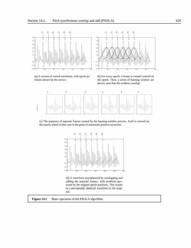
Section 14.2. Pitch synchronous overlap and add (PSOLA) 429
0 200 400 600 800 1000 1200−0.03
−0.02
−0.01
0
0.01
0.02
0.03
0.04
0.05
0.06
54 6321
(a) A section of voiced waveform, with epoch po-sitions shown by the arrows.
0 200 400 600 800 1000 1200−0.03
−0.02
−0.01
0
0.01
0.02
0.03
0.04
0.05
0.06
54 6321
(b) For every epoch, a frame is created centred onthe epoch. Here, a series of hanning window areshown; note that the windows overlap
123456
1 2 3 4 5 6
0 50 100 150 200 250 300−0.03
−0.02
−0.01
0
0.01
0.02
0.03
0.04
0.05
0 50 100 150 200 250 300−0.03
−0.02
−0.01
0
0.01
0.02
0.03
0.04
0.05
0 50 100 150 200 250 300−0.03
−0.02
−0.01
0
0.01
0.02
0.03
0.04
0.05
0.06
0 50 100 150 200 250 300−0.03
−0.02
−0.01
0
0.01
0.02
0.03
0.04
0.05
0.06
0 50 100 150 200 250 300−0.03
−0.02
−0.01
0
0.01
0.02
0.03
0.04
0.05
0 50 100 150 200 250 300−0.03
−0.02
−0.01
0
0.01
0.02
0.03
0.04
0.05
(c) The sequence of separate frames created by the hanning window process. Each is centred onthe epoch, which in this case is the point of maximum positiveexcursion.
0 200 400 600 800 1000 1200−0.03
−0.02
−0.01
0
0.01
0.02
0.03
0.04
0.05
0.06
54 6321
(d) A waveform resynthesised by overlapping andadding the separate frames, with positions gov-erned by the original epoch positions. This resultsin a perceptually identical waveform to the origi-nal.
Figure 14.1 Basic operation of the PSOLA algorithm.
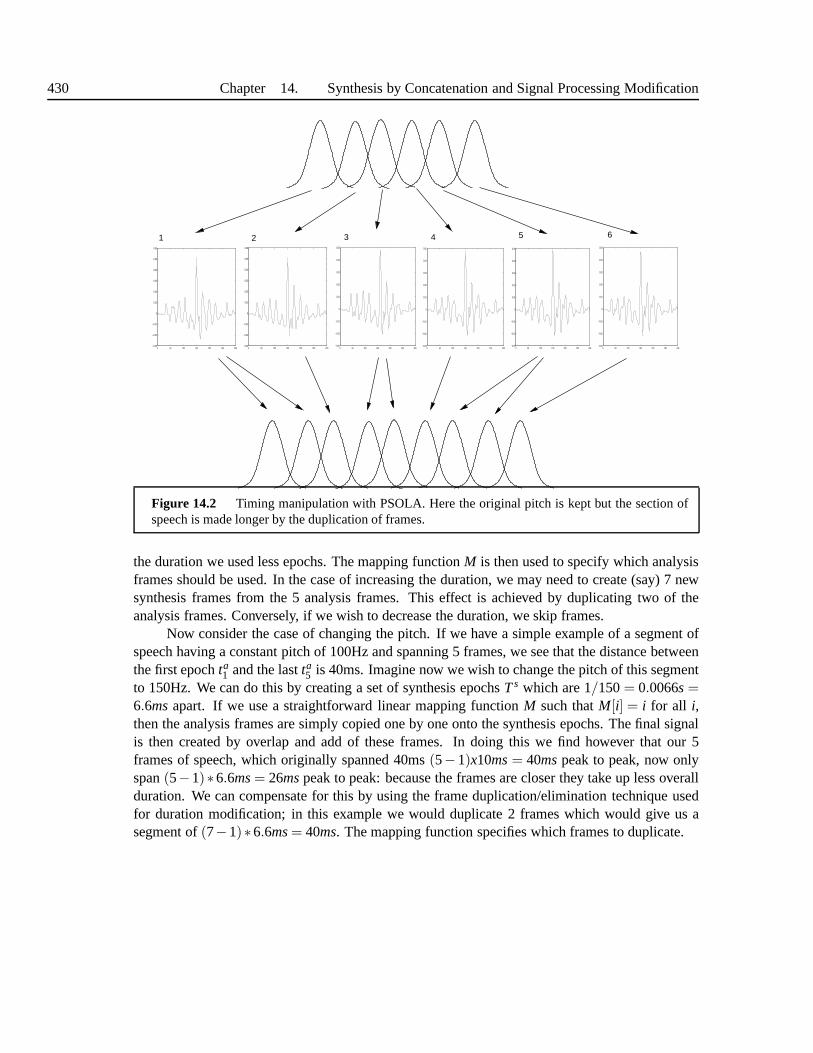
430 Chapter 14. Synthesis by Concatenation and Signal Processing Modification
654321
0 50 100 150 200 250 300−0.03
−0.02
−0.01
0
0.01
0.02
0.03
0.04
0.05
0 50 100 150 200 250 300−0.03
−0.02
−0.01
0
0.01
0.02
0.03
0.04
0.05
0 50 100 150 200 250 300−0.03
−0.02
−0.01
0
0.01
0.02
0.03
0.04
0.05
0.06
0 50 100 150 200 250 300−0.03
−0.02
−0.01
0
0.01
0.02
0.03
0.04
0.05
0.06
0 50 100 150 200 250 300−0.03
−0.02
−0.01
0
0.01
0.02
0.03
0.04
0.05
0 50 100 150 200 250 300−0.03
−0.02
−0.01
0
0.01
0.02
0.03
0.04
0.05
Figure 14.2 Timing manipulation with PSOLA. Here the original pitch is kept but the section ofspeech is made longer by the duplication of frames.
the duration we used less epochs. The mapping functionM is then used to specify which analysisframes should be used. In the case of increasing the duration, we may need to create (say) 7 newsynthesis frames from the 5 analysis frames. This effect is achieved by duplicating two of theanalysis frames. Conversely, if we wish to decrease the duration, we skip frames.
Now consider the case of changing the pitch. If we have a simple example of a segment ofspeech having a constant pitch of 100Hz and spanning 5 frames, we see that the distance betweenthe first epochta
1 and the lastta5 is 40ms. Imagine now we wish to change the pitch of this segment
to 150Hz. We can do this by creating a set of synthesis epochsTs which are 1/150= 0.0066s=6.6msapart. If we use a straightforward linear mapping functionM such thatM[i] = i for all i,then the analysis frames are simply copied one by one onto thesynthesis epochs. The final signalis then created by overlap and add of these frames. In doing this we find however that our 5frames of speech, which originally spanned 40ms(5−1)x10ms= 40mspeak to peak, now onlyspan(5−1)∗6.6ms= 26mspeak to peak: because the frames are closer they take up less overallduration. We can compensate for this by using the frame duplication/elimination technique usedfor duration modification; in this example we would duplicate 2 frames which would give us asegment of(7−1)∗6.6ms= 40ms. The mapping function specifies which frames to duplicate.

Section 14.2. Pitch synchronous overlap and add (PSOLA) 431
654321
0 50 100 150 200 250 300−0.03
−0.02
−0.01
0
0.01
0.02
0.03
0.04
0.05
0 50 100 150 200 250 300−0.03
−0.02
−0.01
0
0.01
0.02
0.03
0.04
0.05
0 50 100 150 200 250 300−0.03
−0.02
−0.01
0
0.01
0.02
0.03
0.04
0.05
0.06
0 50 100 150 200 250 300−0.03
−0.02
−0.01
0
0.01
0.02
0.03
0.04
0.05
0.06
0 50 100 150 200 250 300−0.03
−0.02
−0.01
0
0.01
0.02
0.03
0.04
0.05
0 50 100 150 200 250 300−0.03
−0.02
−0.01
0
0.01
0.02
0.03
0.04
0.05
Figure 14.3 Pitch manipulation with PSOLA. A new set of synthesis epochsare created which arespaced further apart than the analysis set. When the frames are overlapped and added, the new pitchis now lower due to the wider frame spacing.
Hence duration modification can be performed without reference to pitch values, but pitchmodification will necessarily change duration as a by product of moving the frames closer orfurther apart. In practice, both modifications are done at once, by a segment by segment calculationof the mapping function. This ensures that each segment has the required pitch and duration asspecified by the TTP component. A number of options are available for the form of the mappingfunction. The simplest is to have a simple linear function, whereby if we wish to create 15 framesfrom 10, we duplicate every second frame. Likewise if we wishto create 5 from 10, we eliminateevery second frame. More sophisticated functions are also possible, where for instance frames areduplicated and eliminated in the middles of phones in an attempt to preserve transition dynamicsand have maleable steady state portions as with formant synthesis.
14.2.3 How does PSOLA work?
We can now ask ourselves, how does TD-PSOLA work? Or in other words, after all we have saidabout explicit source/filter separation how is it that we have been able to change the characteristics
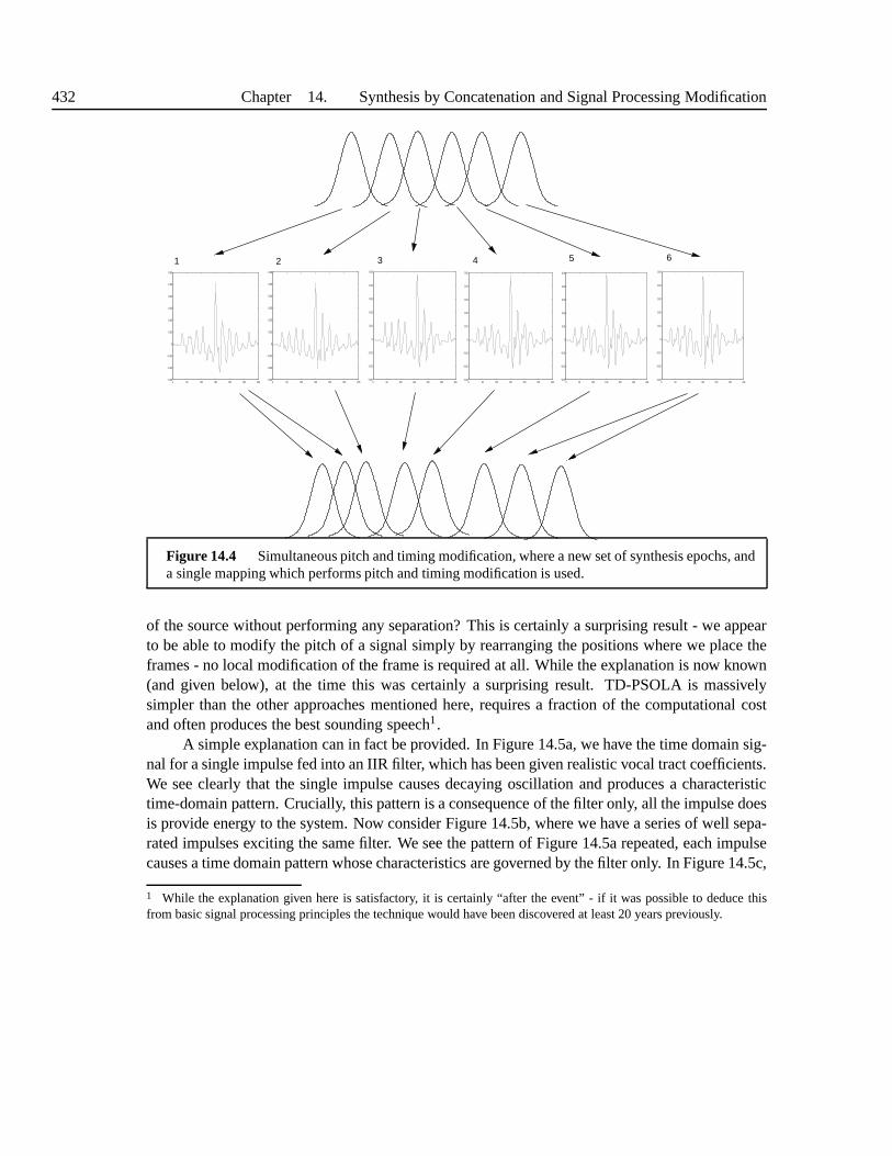
432 Chapter 14. Synthesis by Concatenation and Signal Processing Modification
654321
0 50 100 150 200 250 300−0.03
−0.02
−0.01
0
0.01
0.02
0.03
0.04
0.05
0 50 100 150 200 250 300−0.03
−0.02
−0.01
0
0.01
0.02
0.03
0.04
0.05
0 50 100 150 200 250 300−0.03
−0.02
−0.01
0
0.01
0.02
0.03
0.04
0.05
0.06
0 50 100 150 200 250 300−0.03
−0.02
−0.01
0
0.01
0.02
0.03
0.04
0.05
0.06
0 50 100 150 200 250 300−0.03
−0.02
−0.01
0
0.01
0.02
0.03
0.04
0.05
0 50 100 150 200 250 300−0.03
−0.02
−0.01
0
0.01
0.02
0.03
0.04
0.05
Figure 14.4 Simultaneous pitch and timing modification, where a new set of synthesis epochs, anda single mapping which performs pitch and timing modification is used.
of the source without performing any separation? This is certainly a surprising result - we appearto be able to modify the pitch of a signal simply by rearranging the positions where we place theframes - no local modification of the frame is required at all.While the explanation is now known(and given below), at the time this was certainly a surprising result. TD-PSOLA is massivelysimpler than the other approaches mentioned here, requiresa fraction of the computational costand often produces the best sounding speech1.
A simple explanation can in fact be provided. In Figure 14.5a, we have the time domain sig-nal for a single impulse fed into an IIR filter, which has been given realistic vocal tract coefficients.We see clearly that the single impulse causes decaying oscillation and produces a characteristictime-domain pattern. Crucially, this pattern is a consequence of the filter only, all the impulse doesis provide energy to the system. Now consider Figure 14.5b, where we have a series of well sepa-rated impulses exciting the same filter. We see the pattern ofFigure 14.5a repeated, each impulsecauses a time domain pattern whose characteristics are governed by the filter only. In Figure 14.5c,
1 While the explanation given here is satisfactory, it is certainly “after the event” - if it was possible to deduce thisfrom basic signal processing principles the technique would have been discovered at least 20 years previously.
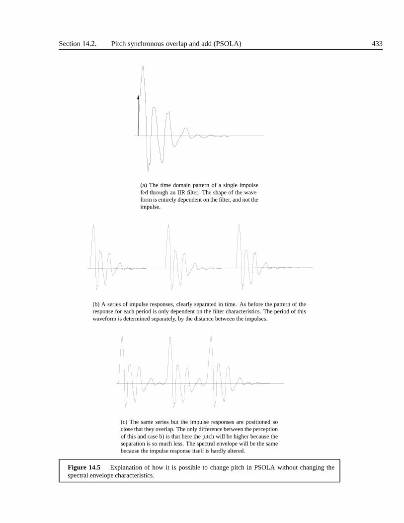
Section 14.2. Pitch synchronous overlap and add (PSOLA) 433
(a) The time domain pattern of a single impulsefed through an IIR filter. The shape of the wave-form is entirely dependent on the filter, and not theimpulse.
(b) A series of impulse responses, clearly separated in time. As before the pattern of theresponse for each period is only dependent on the filter characteristics. The period of thiswaveform is determined separately, by the distance betweenthe impulses.
(c) The same series but the impulse responses are positionedsoclose that they overlap. The only difference between the perceptionof this and case b) is that here the pitch will be higher because theseparation is so much less. The spectral envelope will be thesamebecause the impulse response itself is hardly altered.
Figure 14.5 Explanation of how it is possible to change pitch in PSOLA without changing thespectral envelope characteristics.
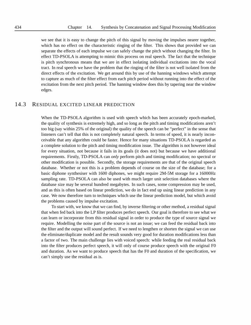
434 Chapter 14. Synthesis by Concatenation and Signal Processing Modification
we see that it is easy to change the pitch of this signal by moving the impulses nearer together,which has no effect on the characteristic ringing of the filter. This shows that provided we canseparate the effects of each impulse we can safely change thepitch without changing the filter. Ineffect TD-PSOLA is attempting to mimic this process on real speech. The fact that the techniqueis pitch synchronous means that we are in effect isolating individual excitations into the vocaltract. In real speech we have the problem that the ringing of the filter is not well isolated from thedirect effects of the excitation. We get around this by use ofthe hanning windows which attemptto capture as much of the filter effect from each pitch period without running into the effect of theexcitation from the next pitch period. The hanning window does this by tapering near the windowedges.
14.3 RESIDUAL EXCITED LINEAR PREDICTION
When the TD-PSOLA algorithm is used with speech which has been accurately epoch-marked,the quality of synthesis is extremely high, and so long as thepitch and timing modifications aren’ttoo big (say within 25% of the original) the quality of the speech can be “perfect” in the sense thatlisteners can’t tell that this is not completely natural speech. In terms of speed, it is nearly incon-ceivable that any algorithm could be faster. Hence for many situations TD-PSOLA is regarded asa complete solution to the pitch and timing modification issue. The algorithm is not however idealfor every situation, not because it fails in its goals (it does not) but because we have additionalrequirements. Firstly, TD-PSOLA canonly perform pitch and timing modification; no spectral orother modification is possible. Secondly, the storage requirements are that of the original speechdatabase. Whether or not this is a problem depends of course on the size of the database; for abasic diphone synthesiser with 1600 diphones, we might require 2M-5M storage for a 16000Hzsampling rate. TD-PSOLA can also be used with much larger unit selection databases where thedatabase size may be several hundred megabytes. In such cases, some compression may be used,and as this is often based on linear prediction, we do in fact end up using linear prediction in anycase. We now therefore turn to techniques which use the linear prediction model, but which avoidthe problems caused by impulse excitation.
To start with, we know that we can find, by inverse filtering or other method, a residual signalthat when fed back into the LP filter produces perfect speech.Our goal is therefore to see what wecan learn or incorporate from this residual signal in order to produce the type of source signal werequire. Modelling the noise part of the source is not an issue; we can feed the residual back intothe filter and the output will sound perfect. If we need to lengthen or shorten the signal we can usethe eliminate/duplicate model and the result sounds very good for duration modifications less thana factor of two. The main challenge lies with voiced speech: while feeding the real residual backinto the filter produces perfect speech, it will only of course produce speech with the original F0and duration. As we want to produce speech that has the F0 and duration of the specification, wecan’t simply use the residual as is.
Section 14.3. Residual excited linear prediction 435
14.3.1 Residual manipulation
Hunt [228] proposed a technique for modifying the original residual so as to produce a syntheticresidual of desired F0 and duration. The key to this technique is to find and isolate each pitchperiod in the residual. Once this is done, a special asymmetric window function is applied to eachpitch period which isolates it from the rest of the residual and we can therefore use the elimina-tion/duplication technique to change the timing. The F0 canbe increased by moving the pitchperiods closer together, and decreased by moving the pitch periods further apart. This rearrange-ment of the pitch periods is analogous to creating an impulsetrain from scratch; there we createda high F0 with impulses which were close together and a low F0 with impulses further apart. Withthe Hunt technique we are performing a similar operation, but adjusting the spacing of the primaryimpulse plus secondary impulses. Once the synthetic residual has been created, it is fed into theLP filter in exactly the same way as the impulse/noise residual.
The resultant speech is much more natural than speech generated with the impulse/noisemodel. If the pitch and duration are not modified at all the speech sounds indistinguishable fromthe original; and if slight (less than 25%) pitch and duration modifications are made hardly anydegradation can be heard. The main downside is that the storage requirements are significantlyhigher as now the residual waveform for each frame must be stored as well as the coefficients. Inaddition, pitch synchronous analysis must be performed which is prone to error if not not doneproperly.
14.3.2 Linear Prediction PSOLA
The above technique bears some similarities to the TD-PSOLAtechnique in that it uses a pitch-synchronous analysis to isolate individual pitch periods,after which modification and resynthesisis performed. In fact in a technique calledlinear prediction pitch synchronous overlap andadd or LP-PSOLA, we can use the PSOLA more or less directly on the residual rather than thewaveform. As above, epoch detection is used to find the epochs. The residual is then separated intoa number of symmetrical frames centred on the epoch. Pitch modification is performed by movingthe residual frames closer or further away, and duration modification is performed by duplicationor elimination of frames, in just the same way as in TD-PSOLA.The only difference is that theseoperations are performed on the residual which is then fed into the LP filter to produce speech.This technique differs only from the Hunt technique in the shape of the frames. Both techniquesuses window functions with their highest point at the epoch;in Hunt’s technique the windows areasymmetrical with the idea that they are capturing a single impulse, in LP-PSOLA the windowsare symmetrical. In listening tests, the two techniques produced virtually identical quality speech.
A number of other refinements on residual excited LP have beenproposed. Hirai et al [203]proposed a technique fairly similar to Hunt’s which performs a particular type of manipulationon the residual before using it to excite the filter, and a number of studies have attempted to findan LP analysis technique which gives a parameterised sourcerather than simply a residual [336]

436 Chapter 14. Synthesis by Concatenation and Signal Processing Modification
[337], [135] [476].There is no convincing evidence that these techniques produce better quality modifications
than TD-PSOLA, but they do have the advantages in that they offer a unifed framework forpitch/timing modification and compression. A typical system might be able to efficiently encodethe LP paramaters as reflection coefficients or line spectralfrequencies. In classicial linear predic-tion the main compression gain comes from being able to encode the source signal as a single F0value which is then used to generate an impulse sequence at synthesis time. In a residual excitedmodel we cannot use this approach as we have to store the complete residual. It is however knownthat the dynamic range of this is less than for real speech, and so this can savings can be made thisway.
In addition to these advantages we also have the possibilityto modify the spectral character-istics of the units. One use of this would be to ensure that thespectral transitions at diphone joinsare completely smooth. While careful design and extractionof the units from the database shouldhelp ensure smooth joins, they can’t always be guarenteed, and so some spectral manipulation canbe useful.
14.4 SINUSOIDAL MODELS
Recall in our introduction to signal processing, we saw thatwe could use the Fourier series togenerate any periodic signal from a sum of sinusoids (Section 10.1.2).
x(t) =L
∑l=1
Alcos(ω0l + φl ) (14.3)
The family of techniques known assinusoidal modelsuse this as their basic building block andperforms speech modification by finding the sinusoidal components for a waveform and perform-ing modification by altering the parameters of the above equation, namely the amplitudes, phasesand frequencies. It has some advantages over models such as TD-PSOLA in is that it allowsadjustments in the frequency domain. While frequency domain adjustments are possible in thelinear prediction techniques, the sinusoidal techniques facilitate this with far fewer assumptionsabout the nature of the signal and in particular don’t assumea source and all-pole filter model.
14.4.1 Pure sinusoidal models
In principle we could perform Fourier analysis to find the model parameters, but for reasons ex-plained below, it is in fact advantageous to follow a different procedure that is geared towards oursynthesis goals. For purposes of modifying pitch, it is useful to perform the analysis in a pitchsynchronous manner and in fact one of the main advantages of sinusoidal modelling is that theaccuracy of this does not have to be as high as that for PSOLA [420], [293], [520].

Section 14.4. Sinusoidal models 437
Figure 14.6 Original waveform (solid line) and reconstructed synthetic waveform (dashed line) ofa short section of speech. (From Kain [244].)
For a frame of speech, basic sinusoidal analysis can be foundin a means similar to linearprediction (Section 12.4), where we use the model to create an artificial signal ˆs(n):
s(n) =L
∑l=1
Alcos(ω0l + φl))2
We then attempt to find the set of values forAl , ω0 andφl
and choose then best artificial signal as the one that has the lowest error between it and theoriginal s(n). So in the expression
E = ∑n
w(n)2(s(n)− s(n))2 (14.4)
= ∑n
w(n)2(s(n)−L
∑l=1
Alcos(ω0l + φl))2 (14.5)
we find the signal ˆs(n) that minimisesE. Unlike the case with LPC, there is no direct solutionto this. Rather, we determine the model parameters by a complex linear regression [421], [364].The reason why we use Equation 14.5 rather than Fourier analysis is that Equation 14.5 uses awindow function which concentrates the modelling accuracyin the centre of the window. Thishas advantageous effects when the synthesis step is performed. Secondly, this analysis can be

438 Chapter 14. Synthesis by Concatenation and Signal Processing Modification
performed on relatively short frames of speech, rather thanthe fixed frame lengths required instandard Fourier analysis.
Given the parameters of the model, we can reconstruct a time domain waveform for eachframe by use of the synthesis Equation 14.3. Figure 14.6 shows a real and resynthesised frameof speech. An entire waveform can be resynthesised by overlapping and adding the frames justas with the PSOLA method (in fact the use of overlap add techniques was first developed forconjunction with sinusoidal models).
Modification is performed by separating the harmonics from the spectral envelope, but thisis achieved in a way that doesn’t perform explicit source/filter separation as with LP analysis.The spectral envelope can be found by a number of numerical techniques. For example, Kain[244] transforms the spectra into a power spectrum and then uses an inverse Fourier transform tofind the time domain autocorrelation function. LP analysis is performed on this to give an all-pole representation of the spectral envelope. This has a number of advantages over standard LPanalysis in that the power spectrum can be weighted so as to emphasise the perceptually importantparts of the spectrum. Other techniques use peak picking in the spectrum to determine the spectralenvelope. Once the envelope has been found, the harmonics can be moved in the frequency domainand new amplitudes found from the envelope. From this, the standard synthesis algorithm can beused to generate waveforms.
14.4.2 Harmonic/Noise Models
The technique just described works very well for perfectly periodic signals, but performance candegrade because the signal is rarely perfectly periodic. This is particularly true for signals whichhave a high sampling rate, where the inherent roll-off characteristics of the voiced source mean thatvery little periodic source information is found at high frequencies. To see this, consider Figure14.7 which shows a magnitude spectrum of a vowel from a signalsampled at 16000Hz. While thelower frequencies clearly exhibit the “spikes” that we associate with the harmonics of a periodicsignal, at higher frequencies we see that this pattern breaks down, and the signal is significantlynoisier. The non-periodic part of the signal arises from many sources, including breath passingthrough the glottis and turbulence in the vocal tract. It should be realised that normal voicedspeech is in fact significantly noisier than we often assume.We can see this by comparing stablesung notes to speech; in the signing case the noise is often greatly reduced. In fact a well knownexercise in classical singing is to sing a note at full volumein front of a candle flame. The idea isto sing without causing the candle to flicker, which it will doif there is any breath in the singing.The fact that this is incredibly hard to do demonstrates thatthere is nearly always a small butsignificant amount of breath in normal speech (and in rock singing, which is one reason why thissounds different to classical singing).
This observation has lead to a number of models which includea stochastic component inaddition to the harmonic one, giving:

Section 14.4. Sinusoidal models 439
0 50 100 150 200 250 300−12
−10
−8
−6
−4
−2
0
2
Harmonic
Noisy
Figure 14.7 Log magnitude DFT at 16000Hz sample rate. We can see that the lower part of thespectrum is more regular and clearly exhibits the spikes spaced at even intervals that we expect fromperiodic sounds. At higher frequencies the spectrum is considerably less regular as the roll-off fromthe voice source takes effect and other sound sources such asbreath appear.
s(t) = s(t)p + s(t)r (14.6)
=L
∑l=1
Al cos(ω0l + φl )+s(t)r (14.7)
where the noise components(t)r is assumed to be Gaussian noise. A number of techniques basedon this principle have been proposed, include themulti-band excitation (MBE) model [185],[281] and a parallel hybrid approach [2]. The same idea has been applied to LP residuals in anattempt to separate the periodic and noise components of thesource [485], [118], [461].
We will now explore theHarmonic/Noise model (HNM) of Stylianou [421] in detail, asthis model was developed specifically for TTS. As the name suggests the model is composedof a harmonic component (as above) and a noise component. This noise component is moresophisticated that some models in that it explicitly modelsthe fact that noise in real speech canhave very specific temporal patterns. In stops for example, the noise component is rapidly evolvingover time, such that a model which enforces uniformity across the frame will lack important detail.The noise part is therefor given by
sr(t) = e(t)[h(t,τ)⊗b(t)] (14.8)

440 Chapter 14. Synthesis by Concatenation and Signal Processing Modification
whereb(t) is white Gaussian noise,h(t,τ) is a spectral filter applied to the noise, ande(t) is afunction applied to give the filtered noise the correct temporal pattern.
The first analysis stages in HNM concern classifying the frames into voiced and unvoicedportions, which then dictate the parameters of the harmonicand noise component and the relativestrengths of the contribution of each component to the frame. First we estimate pitch and with thisperform a basic pitch synchronous analysis. This does not have to be performed with the aim offinding the instant of glottal closure, rather a simple location of pitch periods is sufficient. Nexta harmonic model, using a fundamental frequencyω0 estimated from the pitch tracking, is fittedto each frame, and from this the error between the speech generated with the model and the realwaveform is found. Highly harmonic frames will have a low error, noisy frames will have a higherror. For frames which we believe are voiced, we then determine the highest harmonic frequency,that is, the boundary between the low frequency harmonic part and the higher frequency noisypart. We carry this out by moving through the frequency rangeand continually testing how well asynthetic waveform generated from the best matching model parameters fits the real waveform.
Once this cutoff has been found, we proceed to find a more accurate estimation of the pitchusing only the lower part of the signal. This is now possible as we are not attempting to pitch tracknoise. The amplitudes and phases are now found from Equation14.5 as before, by minimisingthe error between the real and synthetic waveforms. This search can be performed in a numberof ways; Stylianou presents a fast technique for minimisingEquation 14.5 directly [420]. Thenoise component essentially has two parts;h(t) which describes the impulse response of the noise(which describes the spectrum of the noise envelope when transformed to the Frequency domain),ande(t) which describes the sub-frame time evolution of the noise. For each frame,h(t) is found ina manner similar to linear prediction ande(t) is estimated indirectly by calculating several valuesof h(t) at shifted positions within the frame.
A final step is required to ensure that phase mismatches don’toccur between frames. As thepitch synchronous analysis was performed without reference to the instant of glottal closure theydo not necessarily align. A time domain technique is now usedto adjust the relative positions ofthe waveforms within the frames to ensure that they all align.
At synthesis time, a set of synthesis epochs is generated anda mapping function from theanalysis epochs is calculated in exactly the same was as for PSOLA. Timing modification is per-formed by this mapping function in the same was as for PSOLA. For pitch modification, we haveto adjust the harmonics of the frames, this is done by resampling the spectrum of the frame andapplying these values to each sinusoidal component. The noise component is created by passingthe Gaussian noiseb(t) through the filterh(t). This is performed several times per frame to ensurethat the temporal characteristics are successfully generated. For voiced frames, the noise is highpass filter at the cut-off point of the harmonic component; inthis way, no low frequency noiseis generated. The noise is then modulated in the time domain to ensure it is synchronised withthe harmonic component. This stage is essential to ensure that the perception is of a single soundrather that two separate unrelated sounds. Finally, synthesis is performed by overlap and add, aswith PSOLA.

Section 14.5. MBROLA 441
14.5 MBROLA
The only real drawback of TD-PSOLA in terms of quality is thatit is very sensitive to errors inepoch placements. In fact, it is safe to say that if the epochsare not marked with extremely highaccuracy, then the speech quality from TD-PSOLA systems cansound very poor. The effect ofinaccurate epochs is to make the synthetic speech soundhoarseas if the speaker is straining theirvoice, or has an infection or some other ailment. This is not surprising as it is known that the effecthoarseness in natural speech arises because of irregular periodicity in the source.
Dutoit [148] investigates the issue of epoch accuracy and concludes that the problem iscomplicated, partly due to a lack of formal definition as to where exactly the epoch should lie(the instant of glottal closure is only one possibility). Since then, more accurate epoch detectionalgorithms have been developed (see Section 12.7.2) but there are cases (for example with poorerquality recordings) where perfect automatic epoch detection may not be possible.
The MBROLA technique was developed partly as a solution to this problem. It uses a syn-thesis technique similar to the Harmonic/Noise model, but uses an additional step to help dealwith the problems associated with epochs. The MBROLA methodoperates pitch-synchronouslyas before, but unlike TD-PSOLA the exact position of the epoch in the frame need not be consis-tent from frame to frame. Hence a more course-grained epoch detection suffices. During analysis,the frames are found as before, but during resynthesis, the phases are adjusted so that every framein the database has matching phase. This step, which is easy to perform with a sinusoidal model,effectively adjusts all the epochs so as to lie in the same relative positions within the frames. Minorepoch errors are hence eliminated. Another way of looking atthis is view the analysis algorithm asanalysing the speech and resynthesising it at a constant pitch for the whole database. TD-PSOLAcan then be performed with complete accuracy.
14.6 SYNTHESIS FROMCEPSTRALCOEFFICIENTS
We now turn to techniques used to synthesize speech from cepstral representations and in particu-lar the mel-frequency cepstral coefficients (MFCCs) commonly used in ASR systems. Synthesisfrom these is not actually a common second generation technique, but it is timely to introduce thistechnique here as it is effectively performing the same job as pure second generation techniques.In Chapter 15 we will give a full justification for wanting to synthesise from MFCCs, but the mainreason is that they are a representation that is highly amenable to robust statistical analysis becausethe coefficients are statistically independent of one another.
Figure 14.8a shows the operations involved in creating the normal, complex cepstrum. Mostof these operations are invertible, though the fact that we use the magnitude spectrum only anddiscard the phase means that information has been lost at this stage. Figure 14.8b shows the stepsinvolved in MFCC analysis and we see that the situation is somewhat more complicated. First,

442 Chapter 14. Synthesis by Concatenation and Signal Processing Modification
DFT mag log IDFTspeech coefficients
(a) Steps involved in standard cepstral analysis
DFT mag mel−scalefilterbank
log DCTemphasispre−
speech lifteringcoefficients
(b) Steps involved in MFCC-style cepstral analysis
Figure 14.8 Steps in cepstral analysis
it is common to perform pre-emphasis so as to remove the inherent tilt in the spectrum. Nextwe perform the filter bank operation that smoothes the spectrum and performs the mel-scaling.Finally after the cepstrum has been created, we perform a “liftering” operation where we discardthe higher cepstral coefficients, to leave typically only 12. The liftering operation and the filterbank operation are not invertible because information is lost at these points.
A number of techniques have been developed which attempt to reverse these operations andgenerate speech [229], [261], [419], [85]. Here we follow one such technique described by Milnerand Shao [313]; described in the following steps:
1. Remove the pre-emphasis and the influence that the mel-scaling operation has on spectraltilt. This can be performed by creating cepstral vectors foreach process, and then simplysubtracting these from the MFCC vector.
2. Perform an inverse liftering operation by padding the mel-scale cepstrum with zeros. Thisthen gives us a vector of the correct size.
3. Perform an inverse cosine transform, which gives us a mel-scaled spectrum. This differsfrom the analysis mel-scale cepstrum because of the liftering, but in fact the differencesin the envelopes of the original and reconstructed spectra have been shown to be minor,particularly with respect to the important formant locations.
4. Partially reverse the filter bank operation. This is not trivial and it is impossible to recovereven an approximation of the original spectrum as we threw away all the information aboutthe harmonics in the original filter bank operation. Instead, we attempt to find the spectralenvelope, and do this by a process of “up-sampling” the filterbank to a very detailed spec-trum, and then sampling this at the required intervals, so asto give a spectrum with 128points.
5. From the magnitude spectrum, we calculate the power spectrum, and from this calculate aset of autocorrelation coefficients by performing an inverse DFT.
6. Calculate the LP coefficients from the autocorrelation coefficients by solving Equation 12.27.

Section 14.7. Concatenation Issues 443
0 100 200 300 400 500 600 700−0.03
−0.02
−0.01
0
0.01
0.02
0.03
0.04
0.05
0 100 200 300 400 500 600 700−0.03
−0.02
−0.01
0
0.01
0.02
0.03
0.04
0.05
Figure 14.9 Phase problems can be caused by inconsistencies in epoch locations across join bound-aries.
7. Choose a value for F0, use this to generate an impulse trainwhich then excites the LPcoefficients. Use a noise source for unvoiced components.
This technique successfully reverses the MFCC coding operation. The main weakness isthat because we threw away the harmonic information in the filter bank step, we have to resort to aclassical LP style technique of using an impulse to drive theLP filter. A number of improvementshave been made to this, with the motivation of generating a more natural source, while still keepinga model systems where the parameters are largely statistically independent. For example in thetechnique of Yoshimura et al [510] a number of excitation parameters are used that allow mixingof noise and impulse, and allow a degree of aperiodicity in the positions of the impulses.
14.7 CONCATENATION ISSUES
Having described a number of techniques for prosodic modifcation, we turn to the final issuein second generation synthesis, that of how to successfullyjoin sections of waveform, such thatthe joins can not be heard so that the final speech sounds smooth continuous and not obviouslyconcatenated.
When discussing concatenation, it is useful to make a distinction betweenmicro-concatenationandmacro-concatenation. Micro-concatenation concerns the low level issues of joining signals.For example, if we join two voiced waveforms such that there is a large jump between samplesat the boundary, this may result in a “click” being heard. This is because the effect of the jumpis the same as a high frequency impulse, and even though such an effect may only last for oneor two samples, it is easily noticed by the lister. Macro-concatenation is concerned with higherlevel, longer range effects, such as ensuring that the general pattern of spectral evolution across ajoin is natural. In this section we concentrate on the issuesof micro-concatenation, as the issue of

444 Chapter 14. Synthesis by Concatenation and Signal Processing Modification
macro-concatenation is discussed extensively in Section 16.5.1.In general, the goal in concatenating speech is to do so such that the listener can not hear
the join at all. The problem of clicks, caused by discontinuities in waveforms, can nearly alwaysbe solved by tapering the frames to be overlapped at their edges so that the samples near the endof the frame (and hence the join) are zero or close to zero. We can see that this works fromPSOLA, where we sucessfully “join” frames of speech all the time in the overlaop add operation.Furthermore, the timing modification part of PSOLA, which eliminates or duplicates frames isproof that frames not originally contiguous can be successfully joined. This principle can beextended to cases where the frames to be joined are from different diphones; by simply overlappingand adding at diphone edges, successful micro-concatenation can be achieved.
One significant problem in many types of synthesis is that there may bephase mismatchesbetween units. An example of this is shown in Figure 14.9 where we have a situation where bothunits have accurate epochs, resulting in “correct” pitch synchronous analysis, but where the pointof reference for the epochs is different for each unit. When concatenated, this will result in asingle irregular period at the join, which is usually detectable. Many proposals have been made asto how to fix this problem [149]. Obviously, we can try and ensure consistent epoch detection inthe first place. While good epoch detectors are now more common, this was not always possiblein the past. Other solutions include a cross-correlation technique where the frames at the joins areshifted over one another until their cross-correlation is at a minimum [420]. Techniques such asMBROLA were in fact developed to handle such problems; recall that the solution there was toeffectively resynthesis the whole database at a fixed pitch to ensure phase consistency. Bellegardahas proposed a technique similar to latent semantic analysis, where the DFT decomposition of thesignal is avoided altogether, and joins are judged according to a measure of their distance in atransformed space [39].
A further issue in micro-concatenation concernswherein the unit we should make the join.So far, in describing our example of diphone synthesis, we have talked about placing the diphoneboundary in the “middle” of the phone, without defining exactly what we mean by this. Optionsinclude taking the temporal middle (i.e. the half way point through the phone), but we can alsoopt for a strategy that selects the acoustically most stableregion, as this is after all our motivationfor using diphones in the first place. The best place to join units may of course depend on theparticular units themselves and the technique ofoptimal coupling was developed to find a uniqueboundary location for every pair of diphones to be joined [445], [105]. In this, the diphones arestored as complete phone pairs, extending from the start of the first phone to the end of the second.When two phones are to be joined, the two halves of each diphone are “slid over” each otherframe by frame, and the distance between an acoustic representation (e.g. cepstra) of the phonesis measured for that alignment. The idea is to match the general trajectories of the phones and notjust the values at the concatenation point. The alignment with the lowest distance is chosen andthe diphones are cut and then joined at these points.
While in second generation synthesis signal processing in mainly used to modify pitch andtiming, it can also be used in concatenation. If we are using atechnique which gives us some

Section 14.8. Discussion 445
sort of spectral representation, such as residual excited LP or sinusoidal modelling, then we cansmooth or interpolate the spectral parameters at the join. This is only possible in models with aspectral representation, and is one of the reasons why residual excited LP and sinusoidal modelsare chosen over PSOLA.
14.8 DISCUSSION
Second generation techniques are characterised by a hybridapproach of using data to determinethe behaviour of the verbal or phonetic part of synthesis, and an explicit model plus signal pro-cessing to generate the correct prosody.
It should be clear that apart from the cepstral technique, there is a considerable degree ofsimilarity between the main signal processing techniques described here. All operate pitch syn-chronously and all avoid an explicit model of the source. It is in their detail that where we can seedifferences. For example, the PSOLA technique clearly avoids a modelling approach altogether,and only assumes that the signal is composed of pitch periods. The sinusoidal models also makeassumptions, but they are little more than general ones which are true of all periodic or quasi-periodic signals. While the linear prediction techniques make the strongest assumptions, manyof the negative consequences of these are lessened by the useof whole natural residuals. Whileall the techniques are pitch-synchronous, again we see subtle differences where the PSOLA tech-niques in particular are very sensitive to epoch location errors, while the sinusoidal and MBROLAtechniques are more robust to these because they can controlthe phase details during synthesis.In general, the synthesis quality of all these techniques isvery similar, such that the choice of onetechnique over another is usually governed by other factors, such as speed vs size tradeoffs andother practical factors.
14.8.1 Further Reading
A number of books cover the area of speech modification quite thoroughly. Kleijn and Paliwal[256] gives a good introduction to many aspects of speech analysis, coding, modification and syn-thesis. Dutoit [148] stands out as being one of the few books to tackle the signal processing issuefrom a TTS only perspective, describing all the algorithms mentioned here in considerable detail.Many more general purpose books exist which cover a number oftopics in analysis, synthesis,coding and modifcation including Quatieri [364], Rabiner and Schaffer [367] and Huang et al[224].
14.8.2 Summary
• Second generation synthesis systems are characterised by using a data driven approach togenerating the verbal content of the signal.

446 Chapter 14. Synthesis by Concatenation and Signal Processing Modification
• This takes the form of a set of units where we have one unit for each unique type. Diphonesare the most popular type of unit.
• The synthesis specification, generated by the TTP system is in the form of a list of items,each with a verbal specification, one or more pitch values anda duration.
• The prosodic content is generated by explicit algorithms, and signal processing techniquesare used to modify the pitch and timing of the diphones to match that of the specification.
• A number of techniques have been developed to modify the pitch and timing. These include:
– PSOLA which operates in the time domain. It separates the originalspeech into framespitch-synchronously and performs modification by overlapping and adding these framesonto a new set of epochs, created to match the synthesis specification.
– Residual excited linear predictionperforms LP analysis, but uses the whole residualin resynthesis rather than an impulse. The residual is modified in a manner very similarto that of PSOLA.
– Sinusoidal modelsuse a harmonic model and decompose each frame into a set ofharmonics of an estimated fundamental frequency. The modelparameters are the am-plitudes and phases of the harmonics. With these, the value of the fundamental can bechanged while keeping the same basic spectral envelope.
– Harmonic Noise modelsare similar to sinusoidal models, except that they have anadditional noise component which allows accurate modelling of noisy high frequencyportions of voiced speech and all parts of unvoiced speech.
– MBROLA is a PSOLA like technique which uses sinusoidal modelling todecomposeeach frame and from this resynthesise the database at a constant pitch and phase, thusalleviating many problems in inaccurate epoch detection.
– MFCC synthesisis a technique which attempts to synthesise from a representation thatwe use because of its statistical modelling properties. A completely accurate synthesisfrom this is not possible, but it is possible to perform fairly accurate vocal tract filterreconstruction. Basic techniques use an impulse/noise excitation method, while moreadvanced techniques attempt a complex parameterisation ofthe source.
• The quality of these techniques is considerably higher thanclassical, impulse excited linearprediction
• All these have roughly similar quality, meaning that the choice of which technique to use ismostly made on other criteria, such as speed and storage.

15HIDDEN MARKOVMODEL SYNTHESIS
We saw in Chapter 13 that despite the approximations in all the vocal tract models concerned, thelimiting factor in generating high quality speech is not so much in converting the parameters intospeech, but in knowing which parameters to use for a given synthesis specification. Determiningthese by hand written rules can produce fairly intelligiblespeech, but the inherent complexitiesof speech seem to place an upper limit on the quality that can be achieved in this way. Thevarious second generation synthesis techniques explainedin Chapter 14 solve the problem bysimply measuring the values from real speech waveforms. While this is successful to a certainextent, it is not a perfect solution. As we will see in Chapter16, we can never collect enoughdata to cover all the effects we wish to synthesize, and oftenthe coverage we have in the databaseis very uneven. Furthermore, the concatenative approach always limits us to recreating what wehave recorded; in a sense all we are doing is reordering the original data.
An alternative is to use statistical, machine learning techniques to infer the specification-to-parameter mapping from data. While this and the concatenative approach can both be described asdata-driven, in the concatenative approach we are effectivelymemorisingthe data, whereas in thestatistical approach we are attempting tolearn the general properties of the data. Two advantagesthat arise from statistical models are that firstly we require orders of magnitude less memory tostore the parameters of the model than memorise the data, andsecondly that we can modify themodel in various ways, for example to convert the original voice into a different voice.
While many possible approaches to statistical synthesis are possible, most work has focusedon usinghidden Markov models (HMMs). This along with the unit selection techniques of thenext chapter are termedthird generation techniques. This chapter gives a full introduction tothese and explains how they can be used in synthesis. In addition we also show how these canbe used to automatically label speech databases, which findsuse in many areas of speech tech-nology, including unit selection synthesis. Finally, we introduce some other statistical synthesistechniques.
447

448 Chapter 15. Hidden Markov Model Synthesis
prob
abili
ty
observation
1 standard deviation
mean
Figure 15.1 The Gaussian function.
15.1 THE HMM FORMALISM
HMMs themselves are quite general models and although originally developed for speech recog-nition [36] have been used for many tasks in speech and language technology, and are now in factone of the fundamental techniques in biology (to such an extent that their use there now completelydwarfs speech technology applications). General introductions to HMMs can be found in [243],[224]; but here we focus only on the type of HMMs most relevantto modern speech recognitionand synthesis. In doing so, we closely follow the HTK speech recognition toolkit of Young et al[511]. This is the most widely used HMM system in research labs today, and also forms the basisof one of the most successful ASR engines of the past few years[192], [171], [170], [407]. Anintroduction/refresher course in probability can be foundin Appendix A.
15.1.1 Observation probabilities
The input to an ASR system is a sequence of frames of speech, known asobservationsand denotedas
O =< o1,o2, ...oT >
The frames are processed so as to removed phase and source information. The most com-mon representation is based on mel-scale cepstral coefficients (MFCCs), introduced in Section12.5.7. Hence each observationo j is a vector of continuous values. For each phone we build aprobabilistic model which tells us the probability of observing a particular acoustic input.
So far in the book, all the probabilities we have considered have been ofdiscreteevents, forexample, the probability that we will observe a wordwi in a particular context. In all the caseswe have so far considered, this effectively means keeping a unique record of each event (e.g. theprobability of observing wordwi in the context of wordw j ); no “general” properties of the process
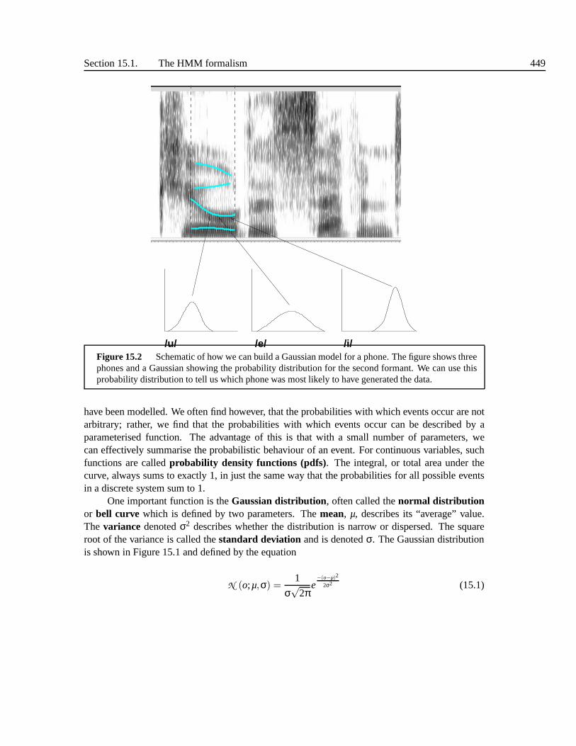
Section 15.1. The HMM formalism 449
/u/ /e/ /i/Figure 15.2 Schematic of how we can build a Gaussian model for a phone. Thefigure shows threephones and a Gaussian showing the probability distributionfor the second formant. We can use thisprobability distribution to tell us which phone was most likely to have generated the data.
have been modelled. We often find however, that the probabilities with which events occur are notarbitrary; rather, we find that the probabilities with whichevents occur can be described by aparameterised function. The advantage of this is that with asmall number of parameters, wecan effectively summarise the probabilistic behaviour of an event. For continuous variables, suchfunctions are calledprobability density functions (pdfs). The integral, or total area under thecurve, always sums to exactly 1, in just the same way that the probabilities for all possible eventsin a discrete system sum to 1.
One important function is theGaussian distribution, often called thenormal distributionor bell curve which is defined by two parameters. Themean, µ, describes its “average” value.The variance denotedσ2 describes whether the distribution is narrow or dispersed.The squareroot of the variance is called thestandard deviation and is denotedσ. The Gaussian distributionis shown in Figure 15.1 and defined by the equation
N (o;µ,σ) =1
σ√
2πe−(o−µ)2
2σ2 (15.1)

450 Chapter 15. Hidden Markov Model Synthesis
Figure 15.3 Mixtures of Gaussians. This shows how three weighted Gaussians, each with its ownmean and variance, can be “mixed” (added) to form a non-Gaussian distribution. Note that the totalprobability, given by the area under the curve must equal 1 and so the mixture weights are set to ensurethis.
The Gaussian has many interesting mathematical propertiesand because of these and thefact that a large range of natural phenomena seem to belong tothis distribution (e.g. the range ofpeoples’ heights in a population), it is often seen as the most “natural” or elementary probabilitydistribution.
When dealing with vector data, as in our case where the observations are acoustic frames,we need to use amultivariate Gaussian. This is the natural extension of the univariate one,but it is important to note that while we have one mean value for each component in the vector,we have acovariance matrix, Σ, not a variance vector. This is because we wish to model notonly the variance of each component, but thecovariance between each component. The pdf of anN-dimensional Gaussian is given by:
N (o;µ,Σ) =1
√
(2π)N|Σ|e−
12(o−µ)′Σ−1(o−µ) (15.2)
whereN is the dimensionality,µ is the vector of means andΣ is the covariance matrix.With this, we can therefore build a system in which we have a model for every phone,
each described by its own multivariate Gaussian. For an unknown utterance, if we know the phoneboundaries, we can therefore test each phone model in turn and find which model gives the highestprobability to the observed frames of speech, and from this find the sequence of phones that aremost likely to have given rise to the observations in the utterance in question. A diagram of this isshown in Figure 15.2.
We can improve on the accuracy of these models in a number of ways. First, we note that thetrue density of a phone model is in fact rarely Gaussian. Rather than use other types of distribution,we adopt a general solution whereby we use amixture of Gaussians, shown in Figure 15.3 andgiven by
b(ot) =M
∑m=1
cmN (ot ;µm,Σm) (15.3)
In this, we haveM Gaussians, each with a mean vectorµm and covariance matrixΣm. The pa-rameterscm are known as themixture weights and are used to determine the relative importanceof each Gaussian. As with any pdf, the area under the curve should sum to 1. We can draw a
Section 15.1. The HMM formalism 451
comparison between mixtures of Gaussians here and the Fourier series of Section 10.1.2. Here wecan model a pdf of arbitrary complexity by summing weighted Gaussians, there we could build aperiodic signal of arbitrary complexity by summing weighted sinusoids.
15.1.2 Delta coefficients
A second common addition to the observation function arisesfrom our knowledge that the frameswithin a phone are not static, rather they evolve as a function of time. For this reason it is standardto include extra coefficients in the observations that not only describe the data itself, but alsothe rate of change of the coefficients, and the rate of change of the rate of change. These extracoefficients are termed thevelocity or delta coefficients, and theacceleration or delta deltacoefficients respectively. As we shall see in Section 15.2, not only do these encode this rate ofchange information, but they also in quite powerful way makeup for some of the weakness in themodelling power of the HMMs.
A simple rate of change calculation is given by
dt =ct+1−ct−1
2
wheredt is the delta coefficient andct is the original cepstral coefficient. Such calculations canhowever be quite unstable as a little noise in either of the coefficients can give rise to a largevariation indt . A more robust solution then is to calculate the rate of change over several frames.One way of doing this is with:
dt =
L∑
l=1l(ct+ l −ct−l)
2L∑
l=1l2
(15.4)
WhereL can be thought of as the length of window over which the rate ofchange calculation isperformed. This can also be written as
dt =L
∑l=−L
wl (ct+l ) (15.5)
where the weightsw can be calculated from Equation 15.4.
15.1.3 Acoustic representations and covariance
A final point regarding the probabilistic modelling of observations concerns issues with the co-variance matrix. If we use say 13 acoustic coefficients (often a standard number made from 12cepstral coefficients and one energy coefficient), and then use delta and acceleration coefficients,we have a total of 39 coefficients in each observation frame and so the mean vector has 39 values.

452 Chapter 15. Hidden Markov Model Synthesis
b b b1 2 3
1 2 3
a a a2 23 3a01 41
a a a311 22 3Figure 15.4 Schematic of HMM with three states. Each with a separate Gaussian, denotedb1, b2
andb3. The transition probabilities are given byai j wherei is the start state andj is the destinationstate. Ifi = j then this is the self-transition probability, that is, the probability that we will stay in thesame state. The transition probabilities exiting a state always sums to 1.
The covariance matrix however has 392 = 1521 values. It is often difficult to find enough data toaccurately determine each of these values, and so a common solution is to ignore the covariancebetween coefficients, and simply model the variance of each coefficient alone. This is termed us-ing adiagonal covariance, as only the diagonal values in the covariance matrix are calculated; the

Section 15.1. The HMM formalism 453
other values are set to zero. In general, using such a covariance matrix is not advised as the cor-relations (covariances) between coefficients often contain useful information. However, if we canshow that the coefficients in the data vary more or less independently of one another, no modellingpower is lost in this assumption.
It is partly for this reason that we find mel-frequency cepstral coefficients (MFCCs) areused as the representation of choice in many ASR systems (in addition, they are deemed to havegood discrimination properties and are somewhat insensitive to differences between speakers).It is important to note however HMMs themselves are neutral to the type of observation used,and in principle we could use any of the signal processing derived representations of Chapter 12.Another way of producing data with independent coefficientsis to perform a projection of theoriginal data into a new space. Principle component analysis (PCA) does this, as do a number ofmore sophisticated techniques. These not only ensure that the coefficients in the new space areindependent, they can also be used to reduced the dimensionality of the data being modelled.
15.1.4 States and transitions
As we noted above, the pattern of frames within a phone is not static. In addition to modellingthe rate of change, it is also normal to split each phone modelinto a number ofstates, each ofwhich represents a different part of the phone. In principleany number of states is allowable, butit is quite common to use three, which can informally be thought of as modelling the beginning,middle and end of each phone. We usetransition probabilities which give us the probability ofmoving from one state to the next (this “moving” process is most easily visualised if we think ofthe models as the generators of the acoustic data). In general, we can move from any state to anyother state, and so for a model withP states, the transition probabilities can be stored in aP×Pmatrix. This matrix stores a set of set of discrete probabilities ai j which give the probability ofmoving from statei to statej.
One common HMM topology is to use three states, each its own observation probability.Each state has is linked to the next state and back to itself again. This last transition is knownas theself transition probability and is basically the probability that we will generate the nextobservation from the state we are already in. A phone’s statetransition probabilities govern thedurational characteristics of the phone; if the self transition probabilities are high, it is more likelythat more observations will be generated by that phone whichmeans the overall phone length willbe longer. Such a model is shown in Figure 15.4
15.1.5 Recognising with HMMs
Each HMM state has a probability density function and so for any single observationot we canfind the state whose pdf gives the highest probability for this. Note that because of the wayHMM recognisers are configured, we don’t in fact have an explicit function that gives us the mostprobable model given the data. Rather, we have a set of modelseach of which has a pdf. Hence

454 Chapter 15. Hidden Markov Model Synthesis
1
2
3
N
2 31 T
stat
es
time slots
Figure 15.5 Schematic of how we can build a Gaussian model for a phone. Thefigure shows threephones and a Gaussian showing the probability distributionfor the second formant. We can use thisprobability distribution to tell us which phone was most likely to have generated the data.
the way recognition works is that we assume that one of the models generatedthe data that weare observing1, and that the recognition job is to find which model. It does this by calculatingthe probability that each model generated the observation,and picks the one with the highestprobability as being correct. This is why HMMs are calledgenerative models.
If we only had one observation, it would be easy to find the state which gives the highestprobability. Instead of course we have a sequence of observations, which we assume has beengenerated by moving through a sequence of states. In principle any oneof the possible statesequences could have generated these observations; its just that some are more likely than others.Because of this, we can not deterministically find the state sequence from the observations, andthis is why we say these arehiddenMarkov models.
For a state sequenceQ, we can find the total probability that this sequence generated theobservations by calculating the probabilities of the observations and transitions of that sequence,
1 Of course it didn’t really, the speaker generated the data, but the idea is that if we pretend that a speaker has an HMMgenerator inside his/her head and it is this process we are trying to model.

Section 15.1. The HMM formalism 455
so for a sequence that moves through states 1, 2 and 3, for example we would have:
P(O,Q|M) = a12b1(o1)a23b2(o2)a34b3(o3)
In general then, for a sequence of statesQ =< q1,q2, ..,qt >, the probability for that sequence isgiven by
P(O,Q|M) = aq(0)q(1)
T
∏t=1
bq(t)(ot)aq(t)q(t+1) (15.6)
whereq(0) is a special entry state andq(T +1) is a special exit state.By definition, all probabilities are< 1 and so it should be clear that the final calculated values
in Equation 15.6 may be very small, even for the single highest probability case. Because of this,it is common to uselog probabilities, in which case Equation 15.6 becomes:
log(P(O,Q|M)) = aq(0)q(1) +T
∑t=1
bq(t)(ot)+aq(t)q(t+1) (15.7)
To uses these equations for recognition, we need to connect state sequences with what wewish to eventually find, that is, word sequences. We do this byusing the lexicon, so that if theword HELLO has a lexicon pronunciation /h eh l ou/, then a model for the whole word is createdby simply concatenating the individual HMMs for the phones /h/ /eh/ /l/ and /ou/. As the phonemodel is made of states, a sequence of concatenated phone models simply generates a new wordmodel with more states: there is no qualitative difference between the two. We can then also joinwords by concatenation; the result of this is a sentence model, which again is simply made from asequence of states. Hence the Markov properties of the states and the language model (explainedbelow) provide a nice way of moving from states to sentences.Given the input observation sequenceO=< o1,o2, ...oT > and a word sequenceW =< w1,w2, ...WN >,we can use Equation 15.7 to find the probability that this wordsequence generated those obser-vations. The goal of the recogniser is to examine all possible word sequences and find the oneWwhich has the highest probability according to our model:
W = argmaxw
P(W|O)
HMMs are generators, configured so that we have a model for each linguistic unit which generatessequences of frames. Hence the HMM for a single wordwi, which has been concatenated fromsingle phone models, is of the form
P(O|wi)
So the HMM itself gives us the probability of observing a sequence of frames given the word, andnot the probability we require which is that of observing theword given the frames. We convertone to the other using Bayes rule (SectionA.2.8) so that:
456 Chapter 15. Hidden Markov Model Synthesis
P(wi|O) =P(wi)P(O|wi)
P(O)
and if we consider this for the entire sentence, we have
P(W|O) =P(W)P(O|W)
P(O)(15.8)
P(W) is called theprior and represents the probability that this particular sequence of wordsoccurs independently of the data (after all, some words are simply more common than others).P(O|W) is called thelikelihood and is the probability given by our HMMs.P(O) is theevidenceand is the probability that this sequence of frames will be observed independent of everything else.As this is fixed for each utterance we are recognising, it is common to ignore this term.
Our recognition algorithm then becomes
W = argmaxw
P(W)P(O|W)
15.1.6 Language models
In Equation 15.8 the termP(W), gives us the prior probability that the sequence of wordsW =<w1,w2, ...,wN > will occur. Unlike the case of acoustic observations, we know of no naturaldistribution that models this. Partly this is due to the factthat the number of possible sentences (ieunique combinations of words) is extremely large. We therefore model sentence probabilities bya counting technique as follows.
The probability of a sentenceW =< w1,w2,w3, ...wM > is given by
P(W) = P(w1,w2,w3, ...wM)
The chain rule in probability (Section A.2.10) can be used tobreak this into a number of terms:
P(w1,w2,w3, ...wM) = P(w1)P(w2|w1)P(w3|w1,w2)...P(wM |w1, ...,wM−1) (15.9)
=M
∏i=1
P(wi|w1, ...,wi−1) (15.10)
The estimation of this becomes tractable if we shorten the number of words such that we approxi-mate the termP(wi|w1, ...,wi−1) as
P(wi|w1, ...,wi−1)≈ P(wi|wi−n+1, ...,wi−1) (15.11)
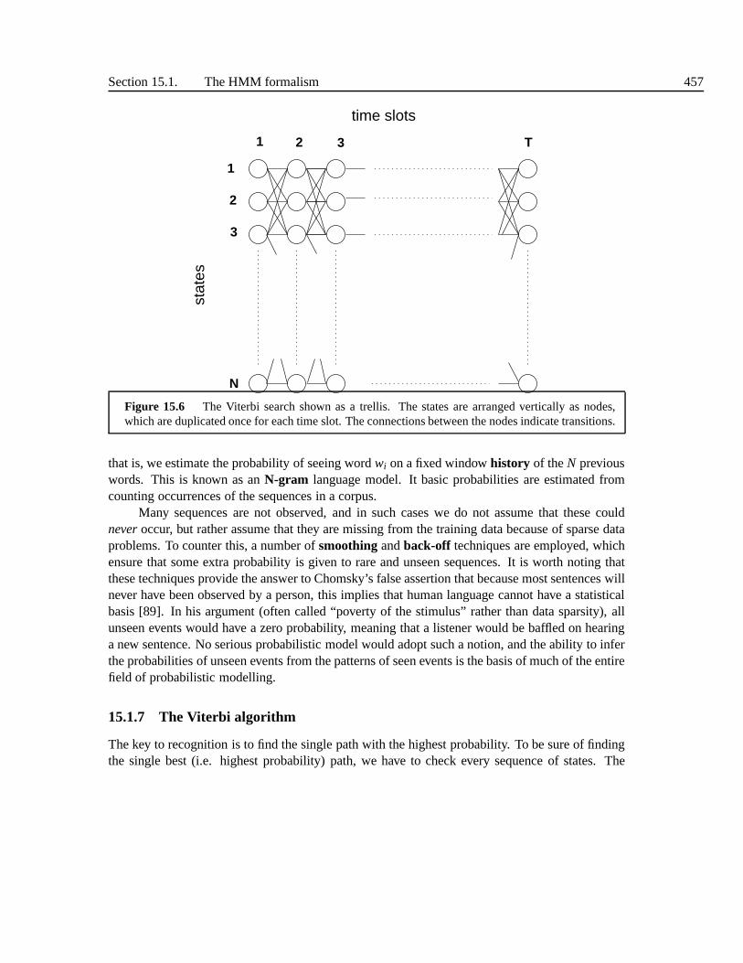
Section 15.1. The HMM formalism 457
1
2
3
N
2 31 T
stat
es
time slots
Figure 15.6 The Viterbi search shown as a trellis. The states are arranged vertically as nodes,which are duplicated once for each time slot. The connections between the nodes indicate transitions.
that is, we estimate the probability of seeing wordwi on a fixed windowhistory of theN previouswords. This is known as anN-gram language model. It basic probabilities are estimated fromcounting occurrences of the sequences in a corpus.
Many sequences are not observed, and in such cases we do not assume that these couldneveroccur, but rather assume that they are missing from the training data because of sparse dataproblems. To counter this, a number ofsmoothingandback-off techniques are employed, whichensure that some extra probability is given to rare and unseen sequences. It is worth noting thatthese techniques provide the answer to Chomsky’s false assertion that because most sentences willnever have been observed by a person, this implies that humanlanguage cannot have a statisticalbasis [89]. In his argument (often called “poverty of the stimulus” rather than data sparsity), allunseen events would have a zero probability, meaning that a listener would be baffled on hearinga new sentence. No serious probabilistic model would adopt such a notion, and the ability to inferthe probabilities of unseen events from the patterns of seenevents is the basis of much of the entirefield of probabilistic modelling.
15.1.7 The Viterbi algorithm
The key to recognition is to find the single path with the highest probability. To be sure of findingthe single best (i.e. highest probability) path, we have to check every sequence of states. The

458 Chapter 15. Hidden Markov Model Synthesis
number of possible sequences is very large indeed, in fact far too large to every calculate no matterhow much computer power we have available. Instead we make use of the principle of dynamicprogramming and use theViterbi algorithm which allows us to find the best path in linear time[477].
The search can be visualised as anN by T size trellis , whereN is the number of statesandT is the number of observations. The trellis is composed ofT time slots, shown arrangedhorizontally in Figure 15.5. In each time slot, we have a set of N nodes, one for each state, andbetween a time slott and the nextt +1 set of transitions exist. For simplicity we will assumed thatthe trellis is fully connected, that is all nodes in time slott are connected to all nodes in time slott +1. The search is performed by “moving” through the trellis, calculating probabilities as we go.
Consider the probabilities associated with a single nodeuk at time slott +1, and the nodes inthe previous time slott, shown in Figure 15.7. For a given nodeui at time slott, the log probabilityof movingfrom ui to uk is simply:
log probability= aik +bi(ot) (15.12)
that is, the log observation probability of the nodeui generating observationot plus the log transi-tion probability between the two nodesui anduk. If we accumulate these probabilities as we movefurther forward in the lattice, thetotal probability is given by
total log probabilityt+1 = aik +bi(ot)+ total probabilityt (15.13)
For a given nodeuk in time slott + 1, we can find the total probability for all the nodes inthe preceding time slot. Given those probabilities, we can find the single highest and rememberthe node in time slott which gave us this probability. This is the crucial step, because it turns outthat for our nodeuk, the identity of the nodeux in the preceding time slot with the highesttotalprobability is all we need to keep track off. This is because if we subsequently find out that ournodeuk is in fact in the highest probability sequence, then is is guaranteed thatux in the precedingtime slot will also be in the highest probability sequence.
The complete search is performed as follows. Starting at time slot 1, we initialise a set ofδfunctions for every node to be 0.
δi(1) = 0 i ≤ j ≤ N (15.14)
We then move to time slot 2 and iterate through each node in turn. For one of these nodes,uk, weiterate through all the nodes in time slot 1, and for each nodecalculate the total probability usingEquation 15.13. We then find the node in time slot 1 which givesthe highest total probability, andrecord its identity inuk. We also store the total probability associated with that node:
δk(2) = maxi
δi(1)+ai j +bi(o1) (15.15)
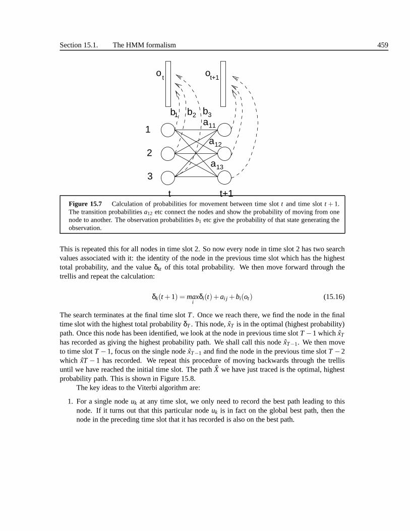
Section 15.1. The HMM formalism 459
a12
a
a
11
13
t+1t
3
2
1
ot t+1o
b b b1 2 3
Figure 15.7 Calculation of probabilities for movement between time slot t and time slott + 1.The transition probabilitiesa12 etc connect the nodes and show the probability of moving fromonenode to another. The observation probabilitiesb1 etc give the probability of that state generating theobservation.
This is repeated this for all nodes in time slot 2. So now everynode in time slot 2 has two searchvalues associated with it: the identity of the node in the previous time slot which has the highesttotal probability, and the valueδkt of this total probability. We then move forward through thetrellis and repeat the calculation:
δk(t +1) = maxi
δi(t)+ai j +bi(ot) (15.16)
The search terminates at the final time slotT. Once we reach there, we find the node in the finaltime slot with the highest total probabilityδT . This node, ˆxT is in the optimal (highest probability)path. Once this node has been identified, we look at the node inprevious time slotT−1 which xT
has recorded as giving the highest probability path. We shall call this node ˆxT−1. We then moveto time slotT−1, focus on the single node ˆxT−1 and find the node in the previous time slotT−2which xT−1 has recorded. We repeat this procedure of moving backwardsthrough the trellisuntil we have reached the initial time slot. The pathX we have just traced is the optimal, highestprobability path. This is shown in Figure 15.8.
The key ideas to the Viterbi algorithm are:
1. For a single nodeuk at any time slot, we only need to record the best path leading to thisnode. If it turns out that this particular nodeuk is in fact on the global best path, then thenode in the preceding time slot that it has recorded is also onthe best path.
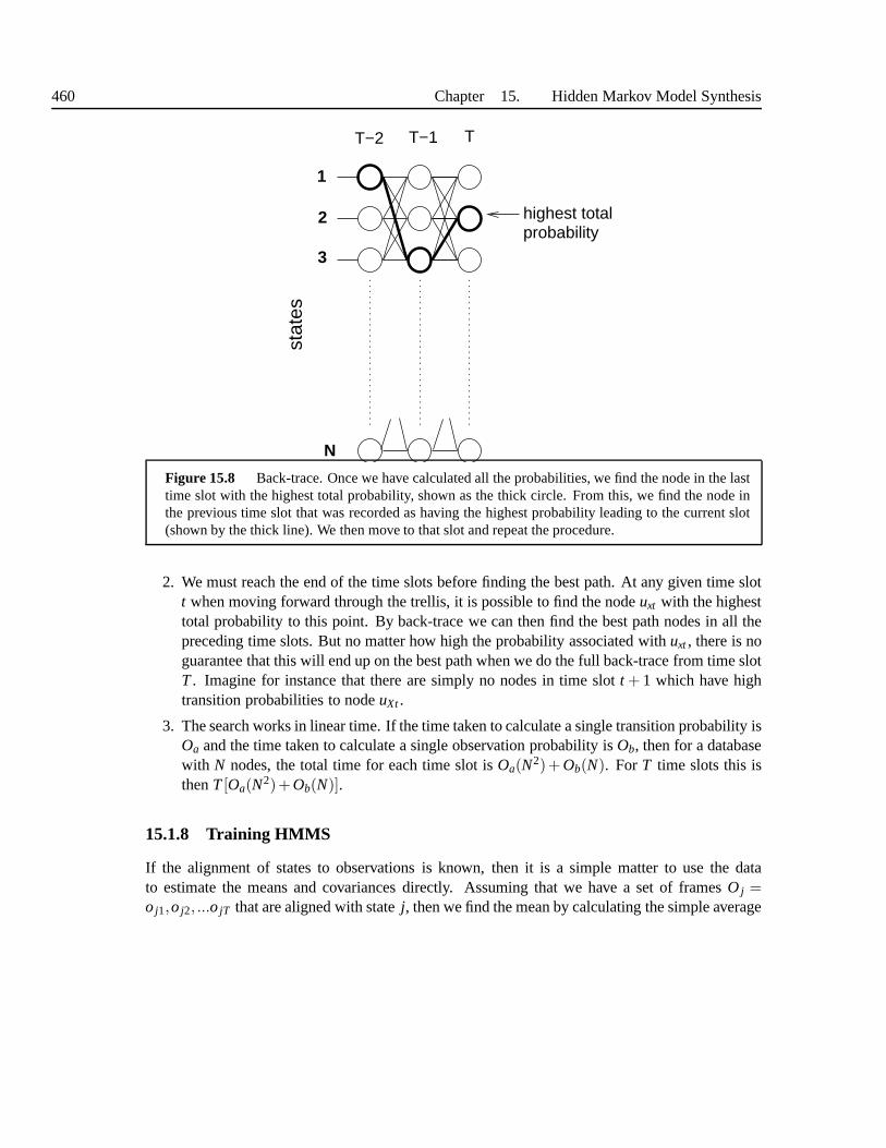
460 Chapter 15. Hidden Markov Model Synthesis
stat
es
TT−1T−2
1
2
3
N
highest totalprobability
Figure 15.8 Back-trace. Once we have calculated all the probabilities,we find the node in the lasttime slot with the highest total probability, shown as the thick circle. From this, we find the node inthe previous time slot that was recorded as having the highest probability leading to the current slot(shown by the thick line). We then move to that slot and repeatthe procedure.
2. We must reach the end of the time slots before finding the best path. At any given time slott when moving forward through the trellis, it is possible to find the nodeuxt with the highesttotal probability to this point. By back-trace we can then find the best path nodes in all thepreceding time slots. But no matter how high the probabilityassociated withuxt, there is noguarantee that this will end up on the best path when we do the full back-trace from time slotT. Imagine for instance that there are simply no nodes in time slot t + 1 which have hightransition probabilities to nodeuXt.
3. The search works in linear time. If the time taken to calculate a single transition probability isOa and the time taken to calculate a single observation probability is Ob, then for a databasewith N nodes, the total time for each time slot isOa(N2)+ Ob(N). For T time slots this isthenT[Oa(N2)+Ob(N)].
15.1.8 Training HMMS
If the alignment of states to observations is known, then it is a simple matter to use the datato estimate the means and covariances directly. Assuming that we have a set of framesO j =o j1,o j2, ...o jT that are aligned with statej, then we find the mean by calculating the simple average

Section 15.1. The HMM formalism 461
µj =1Tj
Tj
∑t=1
o jt (15.17)
and calculate the covariance by
Σ j =1Tj
Tj
∑t=1
(o jt −µj)(o jt −µj)′ (15.18)
So long as we have sufficient examples for each state, this provides a robust way to estimate themeans and covariances. The transition probabilities can becalculated by a simply counting thenumber of times for a statei we move to statej and dividing this by the total number of times weexit statej.
In general however, this state to observation alignment information is not given to us, and sowe can’t use Equations 15.17 and 15.18 on their own. The most common situation in training is tohave a list of the correct words for the sentencew1,w2, ...wM , and the observations,o1,o2, ...,oT
but no information saying which word should be aligned with which observation. In the past (saypre 1990), it was common for researchers to used hand labelled databases where labellers wouldmark the word and phone boundaries by listening and examining spectrograms. Given these, theonly unknowns were the state boundaries with each phone. This hand labelling is a laboriousprocess, but thankfully it turns out that using hand labelled word or phone boundaries in fact is notnecessary, as we instead we can use the HMMs themselves to give the state sequence.
We do this iteratively, so that if we have a set of modelsM1 we can use these, and run therecogniser inforced alignment mode, where instead of “recognising” the words in the utterance,we instead only give it the correct words in the correct sequence to choose from. The recognitionwill obviously be correct, but as the Viterbi algorithm produces the state alignment as a by-product,we now have a state-observation alignment sequence. This can then be used to train a new setof modelsM2 and this process can be repeated until the final set of models is obtained. Thistechnique, calledViterbi training is a very quick and simple way of of training HMMs
Viterbi training does however have a serious drawback in that it enforces hard decisionsduring training. If for instance our alignment picks the completely wrong boundaries, it will thentrain on these, and may pick those same boundaries next time;in effect the iteration gets in a rutfrom which it is hard to recover.
An alternative is to use theBaum-Welchalgorithm2. Instead of using a single state sequenceas in the Viterbi case, the Baum-Welch algorithm considers all possible alignments of states andobservations, not simply the best one as in the case with the Viterbi algorithm. In these align-ments, each state will be aligned with each observation, butin doing this we also make use ofthe probability that that state generated the observation.In other words, instead of assigning eachobservation vector to a specific state as in the above approximation, each observation is assigned
2 The following explanation is taken from the HTK book [511].

462 Chapter 15. Hidden Markov Model Synthesis
to every state in proportion to the probability of that stategenerating the observation. Thus, ifL j(t) denotes the probability of being in statej at timet then the Equations 15.17 and 15.18 canbe modified to give the following weighted averages:
µj =
T∑
t=1L j(t)ot
T∑
t=1L j(t)
(15.19)
and
Σ j =
T∑
t=1L j(t)(ot −µj)(ot −µj)
′
T∑
t=1L j(t)
(15.20)
where the summations in the denominators are included to give the required normalisation.Equations 15.19 and 15.20 are the Baum-Welch re-estimationformulae for the means and co-
variances of a HMM. A similar but slightly more complex formula can be derived for the transitionprobabilities. Of course, to apply equations 15.19 and 15.20, the probability of state occupationL j(t) must be calculated. This is done efficiently using theforward-backward algorithm. Let theforward probability α j(t) for some modelM with N states be defined as
α j(t) = P(o1, . . . ,ot ,x(t) = j|M).
That is,α j(t) is the joint probability of observing the firstt speech vectors and being in statej attime t. This forward probability can be efficiently calculated by the following recursion
α j(t) =
[N−1
∑i=2
αi(t−1)ai j
]
b j(ot).
This recursion depends on the fact that the probability of being in state j at time t and seeingobservationot can be deduced by summing the forward probabilities for all possible predecessorstatesi weighted by the transition probabilityai j . The slightly odd limits are caused by the factthat states 1 andN are non-emitting. The initial conditions for the above recursion are
α1(1) = 1
α j(1) = a1 jb j(o1)
for 1 < j < N and the final condition is given by
αN(T) =N−1
∑i=2
αi(T)aiN .
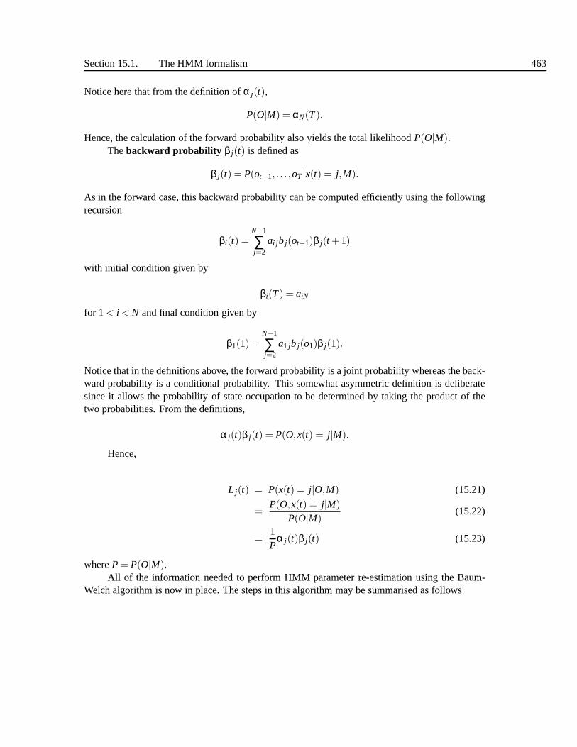
Section 15.1. The HMM formalism 463
Notice here that from the definition ofα j(t),
P(O|M) = αN(T).
Hence, the calculation of the forward probability also yields the total likelihoodP(O|M).Thebackward probability β j(t) is defined as
β j(t) = P(ot+1, . . . ,oT |x(t) = j,M).
As in the forward case, this backward probability can be computed efficiently using the followingrecursion
βi(t) =N−1
∑j=2
ai j b j(ot+1)β j(t +1)
with initial condition given by
βi(T) = aiN
for 1 < i < N and final condition given by
β1(1) =N−1
∑j=2
a1 jb j(o1)β j(1).
Notice that in the definitions above, the forward probability is a joint probability whereas the back-ward probability is a conditional probability. This somewhat asymmetric definition is deliberatesince it allows the probability of state occupation to be determined by taking the product of thetwo probabilities. From the definitions,
α j(t)β j(t) = P(O,x(t) = j|M).
Hence,
L j(t) = P(x(t) = j|O,M) (15.21)
=P(O,x(t) = j|M)
P(O|M)(15.22)
=1P
α j(t)β j(t) (15.23)
whereP = P(O|M).All of the information needed to perform HMM parameter re-estimation using the Baum-
Welch algorithm is now in place. The steps in this algorithm may be summarised as follows
464 Chapter 15. Hidden Markov Model Synthesis
1. For every parameter vector/matrix requiring re-estimation, allocate storage for the numeratorand denominator summations of the form illustrated by equations 15.19 and 15.20. Thesestorage locations are referred to as accumulators.
2. Calculate the forward and backward probabilities for allstatesj and timest.
3. For each statej and timet, use the probabilityL j(t) and the current observation vectorot toupdate the accumulators for that state.
4. Use the final accumulator values to calculate new parameter values.
5. If the value ofP = P(O|M) for this iteration is not higher than the value at the previousiteration then stop, otherwise repeat the above steps usingthe new re-estimated parametervalues.
All of the above assumes that the parameters for a HMM are re-estimated from a singleobservation sequence, that is a single example of the spokenword. In practice, many examplesare needed to get good parameter estimates. However, the useof multiple observation sequencesadds no additional complexity to the algorithm. Steps 2 and 3above are simply repeated for eachdistinct training sequence.
15.1.9 Context-sensitive modelling
As we saw in Section 7.3.2, the acoustic realisation of a phoneme is heavily dependent on thephonemes that surround it. We can make use of this in speech recognition by using separate modelsfor separate phonetic contexts. So instead of having say a single [p] model for all situations, wehave a large number of specialised [p] models, each of which more precisely describes that phonein those contexts. This reduces the level of confusability in the recogniser and thereby increasesrecognition accuracy. The most common way to so this is to useso calledtriphone models, whichare not models made of three phones, but single phone models in the context or the preceding andfollowing phone. Hence for a phoneme set ofN phones, there will be just less thanN3 triphones(some combinations never occur).
Unfortunately, we rarely have enough data to have a sufficient number of examples of everytriphone; either we have insufficient examples to train a model (low occupancy), or no examplesat all (zero occupancy). The solution to this is tocluster the data; in effect we borrow parametersfrom well trained models for use in the ones that suffer from data sparsity. There are a number ofways we could do this for the case of models with low occupancy, in that we can just find examplesin acoustic space which are close to the known examples. The situation is more difficult for thosewith zero occupancy, as we don’t have any acoustic examples at all.
We solve this by making use of some of the common properties ofphones, and the mostcommon way of doing this is to use the phones’distinctive features(see Section 7.4.3). In doingso, we are for instance positing that phones which share the same place of articulation may havemore similar acoustic realisations than ones which don’t. The most common way of performingthis feature based clustering is to use adecision tree: the clever thing about this is that while we

Section 15.1. The HMM formalism 465
xxx
xxx
x x
x
xx
x xx
xxx
xx
xx
x
xx
x
x
x
x x
x xx
x
x
x
xx
x
xx
x
x
xx
Figure 15.9 Schematic of 2 coefficients of the cepstrum for all the contexts of a single phone. Theellipse indicates a line 2 standard deviations from the mean.
xxx
xxx
x x
x
xx
x xx
xxx
xx
xx
x
xx
x
x
x
x x
x xx
x
x
x
xx
x
xx
x
x
xx
xxx
xxx
x x
x
xx
x xx
xxx
xx
xx
x
xx
x
x
x
x x
x xx
x
x
x
xx
x
xx
x
x
xx
xxx
xxx
x x
x
xx
x xx
xxx
xx
xx
x
xx
x
x
x
x x
x xx
x
x
x
xx
x
xx
x
x
xx
yes
nono
no yes
yes
1. is the next phone a fricative? 2. is the next phone voiceed? 3. is the next phone a nasal?
Figure 15.10 The effect of asking three different questions on the data. Each question is asked, thedata is partitioned according to the answer, and the variance calculated for each new cluster. Here wesee that question 1 gives a reasonable separation of the date, question 2 does not, meaning that thisquestion is irrelevant, while question 3 gives the best separation.
xxx
xxx
x x
x
xx
x xx
xxx
xx
xx
x
xx
x
x
x
x x
x xx
x
x
x
xx
x
xx
x
x
xx
xxx
xxx
x x
x
xx
x xx
xxx
xx
xx
x
xx
x
x
x
x x
x xx
x
x
x
xx
x
xx
x
x
xx
Figure 15.11 After choosing question 3 as the best split, the process continues and the set ofquestions is asked again on each cluster, resulting in 2 further splits. In all cases the variance (denotedby the width of the ellipse) is decreasing.

466 Chapter 15. Hidden Markov Model Synthesis
yesyesnonono
yes no
660
1000 is the next phone a nasal?
is the prev phone a voiced? is the next phone a stop?
prev phone stop?
prev phone vowel?
340
125
64
47
30 17
yes
yes
yes
yes
no
no
no
no
LEAF LEAF
next phone voiced?
NEXT:NASALPREV:VOICEDPREV:STOPNEXT:VOICEDPREV:VOWEL
Figure 15.12 An example of part of a trained decision tree. The questions are asked at each node,after which the tree splits. The number indicate the number of data points at each node. The doublecircles indicate leaf nodes, where the splitting processesstops. For clarity, only part of the tree isshown. The feature structure which describes one leaf is shown.
use the features tosuggestcommonality between triphones, we use the actual data to determinehow close any particular feature combination actually is. In other words, the features serve asconstraints or structure on the clustering, but don’t determine what should be clustered with what.
The decision tree operates in a top down manner. It operates on binary features, so as apreprocessing step we convert the original features into binary ones (so for instance the featureCONSONANT TYPE which can take valuesstop, fricative etc gets converted into a new set offeatures which encode the same information but in a binary valued system: often this is done bysimply using simple question features, such as “is this a stop?”, “is this a fricative?”). Initially,all the data points for the state of one phone are grouped together in a single cluster. This clusteris characterised by a measure ofimpurity ; choices of which include variance, log likelihood orentropy. The process of growing a tree is as follows:
1. Create an initial cluster containing all the data points
2. For each feature:

Section 15.1. The HMM formalism 467
(a) form two new clusters based on the value of the feature(b) measure the combined variance of the two new clusters:
3. find the feature which gives the biggest reduction in variance
4. delete this feature from the list of features to be examined.
5. form two new clusters based on this feature.
6. repeat steps 1 to 4 on each new cluster until the stopping criteria have been met.
Stopping criteria usually involve specifying a minimum decrease in impurity, and that clus-ters should have a minimum occupancy (say 10 data points). The process of examining and split-ting clusters is shown in Figures 15.9, 15.10, and 15.11. A trained decision tree is shown in Figure15.12.
An important point about the decision tree grown in this way is that it provides a cluster forevery feature combination, not just those encountered in the training data. So see this, considerthe tree in Figure 15.12. One branch of this has the feature set
NEXT:NASAL yesPREV:VOICED yesPREV:STOP noNEXT:VOICED noPREV:VOWEL no
(15.24)
Which will contain all the training examples matching this feature combination. This is onlya subset of the features we use: the stopping criteria mean that while further feature differencesmay occur after this point, the differences are deemed slight or the model occupancy so low as toprevent further splitting. If we now have a model with features
NEXT:NASAL yesPREV:VOICED yesPREV:STOP noNEXT:VOICED noPREV:VOWEL noPREV:ALEVOLAR yesNEXT:DENTAL noNEXT:VELAR no
which is unobserved in the data, we see that the feature combination of 15.24 is a subset of this,which means that we will use those parameters for this model.While there is no path whichexactly matches this, we find the sub set of features which do (and this is always unique) and thisgives us the cluster we require.
468 Chapter 15. Hidden Markov Model Synthesis
As well shall see in Sections 15.2.4 and 16.4.1, decision tree clustering is a key component ofa number of synthesis systems. In these, the decision is not seen so much as a clustering algorithm,but rather as a mapping or function from the discrete featurespace to the acoustic space. Asthis is fully defined for every possible feature combination, it provides a general mechanism forgenerating acoustic representations from linguistic ones.
15.1.10 Are HMMs a good model of speech?
It is often asked whether HMMs are in fact a good model of speech [317], [63], [102]. This isnot so straightforward to answer. On the surface, the answeris “no” as we can identify manyways in which HMM behaviour differs from that of real speech,and we shall list some of thesedifferences below. However, in their defence, it is important to realise that many of the additionsto the canonical HMM alleviate these weaknesses, and so one must be careful to define exactlywhat sort of HMM is being discussed. Criticisms include:
1. Independence of observations. This is probably the most cited weaknesses of HMMs. Whilean observations depends on its state, and the state depends on the previous states, one obser-vation is not statistically dependent on the previous one. To see effect of this, consider theprobability of a sequence of observations at a single value.If we have a density with a meanof 0.5, we would then find that a sequence of observations of 0.3, 0.3, 0.3, 0.3... would havea certain probability, and as the Gaussian is symmetrical, this would be the same probabilityas a sequence of 0.7, 0.7, 0.7, 0.7.... But as the observations are independent of one another,this would have the same probability as a sequence which “oscillates” such as 0.3, 0.7, 0.3,0.7... Such a pattern would be extremely unlikely in real speech, a fact not reflected in themodel.
2. Discrete states. This problem arises because while real speech evolves more or less smoothly,the HMM switches characteristics suddenly when moving fromone state to the next. Boththis and the independent observation problems are largely solved by the use of dynamicfeatures. When these are included, then we can distinguish between the stable and oscillatingsequences. In fact as we shall see in Section 15.2, very natural trajectories can be generatedby an HMM which uses dynamic features.
3. Linearity of the model. HMMs enforce a strictly linear model of speech, whereby a sentenceis composed of a list of words, which are composed of a list of phones, a list of statesand finally a list of frames. While there is little problem with describing an utterance as alist of words, or as a list of frames, we know that the strict linear model of phones withinwords and worse, states within phones, differs from the morecomplex interactions in realspeech production (see Section 7.3.5). There we showed thatit was wrong to think we couldidentify phones or phonemes in a waveform, rather we should think of speech production asa process where phonemes are input and speech is output and wecan only approximatelyidentify where the output of a phone lies in the waveform. When we consider the alignmentof states and frames in HMMs we see that we have in fact insisted that every frame belongs

Section 15.2. Synthesis from hidden Markov models 469
to exactly one state and one phone, which is a gross simplification of the speech productionprocess.
4. Generative nature. HMMs are generative models, meaning that they declaratively describethe phones, but are not a recognition algorithm in their own right. Furthermore, the max-imum likelihood training normally used has been questionedas to why we want to have asystem which maximises the likelihood of the data rather than have a system which max-imises recognition performance.
While many of these points are valid, there are often solutions which help alleviate anyproblems. As just explained, the use of dynamic features helps greatly with the problems of ob-servation independence and discrete states. As we shall seethe linearity issue is potentially moreof a problem in speech synthesis. Models such as neural networks which perform classificationdirectly have been proposed [375] and have produced reasonable results. More recently, discrimi-native training has become the norm in ASR [495], [360] whereHMMs as described are used, butwhere their parameters are trained to maximise discrimination, not data likelihood.
An alternative argument about HMMs is simply that they have consistently been shown tooutperform other techniques. The HMM recognition systems of today are very different fromthe systems of the early 1990s and so it is important to also realise that HMMs are more of aframework in which a number of ideas can be tried, rather thanjust a single, unified approach.
15.2 SYNTHESIS FROM HIDDENMARKOV MODELS
While HMMs are nearly always described in terms of their use in recognition, there is noth-ing about the models themselves which performs recognition; this is only achieved by using themodels in conjunction with a search algorithm such as Viterbi. The models themselves are justdeclarative representations of the acoustics of a phone andas such, should be just as amenable foruse in speech synthesis as recognition.
If we were to use HMMs for synthesis, we know that the specification gives us the requiredphone sequence and possibly a duration for each phone. The phone sequence tells us which modelsto use in which order, but not which states to use, or which observations to generate from the stateGaussians. If we have a duration in the specification, this tells us how many observations that weshould generate from this model, but again not which states to generate from. The question thenis, if we want to use the models for synthesis how do we actually go about this?
A possible approach is just to randomly sample from each HMM.So starting in the first stateof the first phone, we simply use a random number generator to generate a value which we usewith the state’s Gaussian to generate an observation. We generate another random number and usethis to decide which state we will use next. This process is repeated until we have generated theentire utterance. This approach is valid in a statistical sense in that over a sufficiently large numberof syntheses, the utterances generated will have the same statistical properties as the models. (That

470 Chapter 15. Hidden Markov Model Synthesis
is, if we were to retrain on the generated data, we should end up with very similar models). Thisapproach does not however produce natural speech; the main reason being that such an approachcauses the spectra changes rapidly and randomly from one frame to the next. Real speech incontrast evolves with some level of continuity.
A second approach is to use a maximum likelihood solution, inwhich instead of randomlysampling from the model in accordance with its mean and variance, we just generate the mostlikely sequence of observations from the sequence of models. (Unlike the first approach, retrainingon this data will not give us the same models as the values for all states will be exactly the same andhence all the variances will be zero). It should be obvious that in all cases each state will generateits mean observation. This avoids the problem of the previous approach in which the observationswere “jumping around” from one frame to the next, but now has the problem that the spectraclearly “jumps” at each state boundary. Furthermore the spectra are the same during each state,meaning that, in one dimension, the generated speech is a flatline followed by a discontinuity,followed by a different flat line. This again does not look or sound like natural speech. In effectwe are ignoring all variance information - if we retrained onspeech generated by this model wewould always see the same observation for each state and hence would calculate the same meanbut calculate a zero variance in all cases.
15.2.1 Finding the most likely observations given the statesequence
The approach just described can be stated as one which generates the most likely observationsfrom the models in the normal sense. The problem with this is that the states always generatetheir mean values, which results in jumps at state boundaries. A solution to this problem waspresented in a series of articles by Tokuda and colleagues [453], [452], [454] which showed howto generate a maximum likelihood solution that took the natural dynamics of speech into account.The key point in this technique is to use the delta and acceleration coefficients as constraints onwhat observations can be generated.
Here we show the original system by Tokuda et al [453], which uses delta coefficients as theconstraint. It is simple to extend this to cases which use acceleration and higher order constraintsalso. As before we represent the observations as
O =< o1,o2, ...oT >
but we split each observation into its constituent parts of coefficients and delta coefficients:
ot = ct ,∆ct
All we require for actual synthesis are the coefficientsC =< c1,c2, ...cT >, so the problem isto generate the highest probability sequence of these thatalso obeys the constraints of the deltacoefficients∆C =< ∆c1,∆c2, ...∆cT >. As we have to find both the observations and the statesequence, we can’t use the Viterbi algorithm as above but rather use an algorithm specific to this

Section 15.2. Synthesis from hidden Markov models 471
problem. First, we assume that we have a state sequenceQ. This probability of observing asequence of acoustic vectors is therefore equal to
P(O|q,λ) = bq1(o1)bq2o2, ...bqT (oT) (15.25)
Recall that the observation probability for a single N-dimensional Gaussian is given by
N (o;µ,Σ) =1
√
(2π)N|Σ|e−
12(o−µ)′Σ−1(o−µ) (15.26)
The observation probability of a statej, which includes the coefficients and delta coefficients isgiven by
b j(ot) = N (ct ;µj ,Σ j).N (∆ct ;∆µj ,∆Σ j). (15.27)
It is easier to work with log probabilities. Equation 15.25 becomes
logP(O|q,λ) = bq1(o1)+bq2o2 + ...+bqT (oT) (15.28)
If we substitute Equation 15.26 into 15.27, we get the following expressed in log probabilities:
b j(ot) =−1/2[
2Nlog2π+ |Σ|+(c−µ)′Σ−1(c−µ)+ |∆Σ|+(∆c−∆µ)′∆Σ−1(∆c−∆µ)]
If we then put this into Equation 15.28, we can find generate anexpression that gives us the logprobability for the state sequence. As everything is in the log domain, all these terms add giving:
logP(O|q,λ) =−1/2[
(ccc−µµµ)′ΣΣΣ−1(ccc−µµµ)+ (∆∆∆ccc−∆∆∆µµµ)′∆∆∆ΣΣΣ−1(∆∆∆ccc−∆∆∆µµµ)+K]
where
ccc = [c1,c2, ...,cT ]
∆∆∆ccc = [∆c1,∆c2, ...,∆cT ]
µµµ= [µ1,µ2, ...,µT ]
∆∆∆µµµ= [∆µ1,∆µ2, ...,∆µT ]
ΣΣΣ =
Σ1 0 . . . . . . 00 Σ2 0 · · · 0...
......
0 . . . . . . . . . . ΣT
∆∆∆ΣΣΣ =
∆|Σ1 0 . . . . . . 00 ∆Σ2 0 · · · 0...
.. ....
0 . . . . . . . . . . . ∆ΣT

472 Chapter 15. Hidden Markov Model Synthesis
K = 2TNlog2π+ ∑Tt=1 |Σ|+ ∑T
t=1 |∆Σ|Note that now we have vectors such asccc which represent the entire sequence of coefficients forthe sentence. We now introduce Equation 15.5 into our derivation. Recall, this is how we calculatethe delta coefficients from the normal coefficients, and by replacing the∆c terms with weightedversions ofc we now have our maximum likelihood expression expressed purely in terms of thenormal coefficientsc:
−1/2[
(ccc−µµµ)′ΣΣΣ−1(ccc−µµµ)+ (WWWccc−∆∆∆µµµ)′∆∆∆ΣΣΣ−1(WWWccc−∆∆∆µµµ)+K]
(15.29)
HereWWW is a matrix which expresses the weights of Equation 15.5. This is given by
www =
w(0)I · · · w(L)I 0... w(0)I
.. .
w(L)I. . . w(L)I
. . . .. ....
0 w(0)I · · · w(0)I
(15.30)
To maximise Equation 15.29, we differentiate with respect to c which gives
ΣΣΣ−1+WWW′′′∆∆∆ΣΣΣ−1WWWccc = ΣΣΣ−1µµµ+WWW′′′∆∆∆ΣΣΣ−1∆∆∆µµµ (15.31)
which can be solved to findccc by any matrix solution technique.
15.2.2 Finding the most likely observations and state sequence
This gives us the most likely observation sequence for a given state sequence. The state sequenceis partly determined by the synthesis specification in that we know the words and phones, but notthe state sequence within each phone. Ideally, we would search every possible state sequence tofind the observation sequence that maximiseccc in Equation 15.31, but this is too expensive, firstlybecause the number of possible state sequences is very largeand secondly because the solution ofEquation 15.31 for each possible state sequence is expensive.
Rather than solve Equation 15.31 every time we wish to consider a new state sequence,Tokuda et al developed a technique which allows the calculation of P(O|Q′,λ) for a new statesequenceQ′, onceP(O|Q,λ) for a state sequenceQ has been calculated. The only remainingproblem then is how to search the space of possible state sequences effectively. There is no idealsolution to this as finding the optimal sequence requires searching all the possibilities. Further-more, because of the nature of the optimisation, we can not use the Viterbi algorithm as in recog-nition mode. Rather we use a greedy algorithm approach wherewe choose the best states locallyand then calculate the global probability from this.
This result shows us how to generate from HMMs while also obeying the dynamic con-straints of the delta coefficients. In further papers, Tokuda, colleagues and others have extended
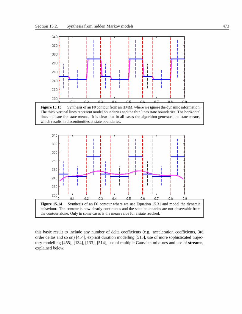
Section 15.2. Synthesis from hidden Markov models 473
Figure 15.13 Synthesis of an F0 contour from an HMM, where we ignore the dynamic information.The thick vertical lines represent model boundaries and thethin lines state boundaries. The horizontallines indicate the state means. It is clear that in all cases the algorithm generates the state means,which results in discontinuities at state boundaries.
Figure 15.14 Synthesis of an F0 contour where we use Equation 15.31 and model the dynamicbehaviour. The contour is now clearly continuous and the state boundaries are not observable fromthe contour alone. Only in some cases is the mean value for a state reached.
this basic result to include any number of delta coefficients(e.g. acceleration coefficients, 3rdorder deltas and so on) [454], explicit duration modelling [515], use of more sophisticated trajec-tory modelling [455], [134], [133], [514], use of multiple Gaussian mixtures and use ofstreams,explained below.
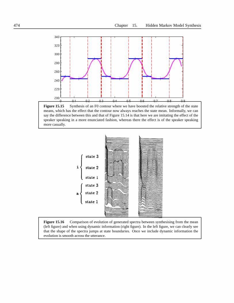
474 Chapter 15. Hidden Markov Model Synthesis
Figure 15.15 Synthesis of an F0 contour where we have boosted the relativestrength of the statemeans, which has the effect that the contour now always reaches the state mean. Informally, we cansay the difference between this and that of Figure 15.14 is that here we are imitating the effect of thespeaker speaking in a more enunciated fashion, whereas there the effect is of the speaker speakingmore casually.
Figure 15.16 Comparison of evolution of generated spectra between synthesising from the mean(left figure) and when using dynamic information (right figure). In the left figure, we can clearly seethat the shape of the spectra jumps at state boundaries. Oncewe include dynamic information theevolution is smooth across the utterance.

Section 15.2. Synthesis from hidden Markov models 475
Figure 15.17 Effect of using more mixtures in synthesis. It is clear that as we use more mixtureswe can more accurately account for spectral detail.
15.2.3 Acoustic representations
While it is true to say that an HMM itself is neutral to the purpose to which it is put (synthesisrecognition or other), it is also true to say that the manner in which it is normally configured inASR systems is specific to the recognition task. For instance, we might use 12 MFCC coefficientswith energy and their delta and acceleration as these are known to be good features for phonediscrimination. We do not however include any F0, other source information or prosody. In facteven the transition probabilities, which in a sense model duration and can be seen as the one aspectof prosody that is present in an ASR HMM, are often ignored in modern ASR systems are theyare not thought to include much information that discriminates phones.
For synthesis therefore, we are required to make some modifications to ASR-style HMMsto ensure good quality speech. MFCCs on their own are not sufficient to generate speech, as weneed (as a minimum) to include F0 information as well. Given avector of MFCCs and an F0value, a number of techniques, detailed in Section 14.6 can be used to generate the waveform.While we can include an F0 value directly in the observation vectorot but it is more common tomake use of an additional aspect of the HMM formalism known asstreams. Each stream has amixture of Gaussians observation pdfs as before. The addition is that we can now have a numberof these observation pdfs, and this is particularly useful when we want to generate observations

476 Chapter 15. Hidden Markov Model Synthesis
that are different in nature, as in our case of MFCCs and F0 values. A generalisation of the outputprobability specification of Equation 15.3 using streams is:
b j(ot) =S
∏s=1
[M
∑m=1
c jmsN (ot ;µjms,Σ jms)
]γs
The streams are considered statistically independent and their relative importance are scaled withthe factorsγ1,γ2, .... Note that these weights are set by the system builder and nottrained automat-ically.
In Figures 15.13 to 15.17 we show some of the synthesis properties of HMMs. The basicoperation of the algorithm is most easily seen with a single dimensional observation, and in Figures15.13, 15.14, 15.15 we show an example of this where we have used an HMM to synthesize anF0 contour. One noted weakness of the HMM approach is that often the observations generatedare over-smoothed; informally we can view this as a result ofthe HMMs being “overly cautious”when generating. The effect of this is shown in Figure 15.14.A principled solution to this hasbeen proposed by Toda and Tokuda [451], but it is possible to alleviate this effect by simplyboosting the relative importance of the mean over the dynamics; this is shown in Figure 15.15. InFigures 15.16 and 15.17 we show synthesis for a multi-dimensional representation of an evolvingspectrum, which again shows the different between simply synthesising from the state mean andsynthesising when including the state dynamics.
15.2.4 Context sensitive synthesis models
We use context sensitive models in ASR as they have lower variance than the general phonemodels. In synthesis, we use context sensitive models for a similar reason, so that a model in aparticular context generates observations appropriate tothat context only. In synthesis however,we are interested in a broader range of factors, as we have to generate the prosodic variation aswell as simply the verbal, phonetic variation.
Because of this, it is common to use a much broader notion of “context”. In essence wedecide what linguistic features we think are required for synthesis and build a separate model forevery possible combination. The issue of features in synthesis is discussed fully in Section 16.2,for here we can just assume that in addition to phonetic context, we also want to include featuressuch as phrasing, stress and intonation.
The context-sensitive models are built in exactly the same way as described in Section 15.1.9,and the resultant decision tree provides a unique mapping from every possible feature combinationto HMM model parameters. One significant point of note is thatin synthesis the extra prosodicfeatures mean that number of possible unique feature combinations can be many orders of magni-tude larger than in ASR. Given that we may be training on less data than in ASR, we see that thesparse data problems can be considerably worse. We will return to this issue in Section 16.4.

Section 15.2. Synthesis from hidden Markov models 477
15.2.5 Duration modelling
In a standard HMM, transition probabilities determine the durational characteristics of the model.If we take a standard topology where a state can loop back to itself (with say probability 0.8) ormove to the next state (with probability 0.2), we see that thedistribution of state occupancy has anexponential form, where it is most common to generate a single observation, with the next mostcommon being 2 observations, then 3 and so on. In reality, we know that this does not follow thepattern of observed phone durations which are much more accurately modelled by a Gaussian, ora skewed Gaussian-like distribution which has low probability for both very short and very longsequences, and higher probability for sequences at or near the mean.
This disparity has been known for some time, and several attempts were made in ASR tocorrect this, the most notable proposal being thehidden semi-Markov model (HSMM) [282]. Inthis model, the transition probabilities are replaced by anexplicit Gaussian duration model. It isnow known that this increase in durational accuracy does notin fact improve speech recognitionto any significant degree, most probably because duration itself is not a significant factor in dis-crimination. In synthesis, however, modelling the duration accurately is known to be importantand for this reason there has been renewed interest in hiddensemi-Markov models [504], [514].
15.2.6 HMM synthesis systems
We now describe some complete HMM synthesis systems. In the HMM system described by Zenand Tokuda [514] 5 streams are used, one for the MFCCs, one each for log F0, delta log F0, deltadelta log, F0 and voicing information. As separate streams are used, these parts of the modelscan in fact be treated separately, to the extent that the decision tree clustering can use differentclusters for each stream. So while the states of one set of models may be clustered togetherfor modelling MFCCs, a completely different set of states would be clustered for F0. Durationswithin phones are modelled by hidden semi-Markov models, and a global variance technique[451] is used to compensate for the over smoothing effect that HMM synthesis can create. TheSTRAIGHT technique [189] is used for signal analysis and synthesis (see Section 14.6).
Acero [4] describes an technique which uses HMMs as described above but with formants asthe acoustic observations. This is particularly interesting in that this can be seen as a direct attemptto fix the problems of traditional formant synthesisers. Formants are indeed a good spectral repre-sentation for HMMs as we can assume, like MFCCs, that each formant is statistically independentof the others. Acero notes that HMMs do in fact generate the sort of formant trajectories oftenobserved in natural data. In particular, he notes that when amodel is only used to generate a fewframes of speech, its generated observations rarely reach their mean value but when the modelis used to generate longer sequences, the mean values are in fact reached. This concurs with theexplanation of coarticulation and targets given in Section7.3.4, but significantly, because the ratesof change of the individual formants can change independently in the HMM, the over-simplistictransition and target model of rule base formant synthesis (see Section 13.2.6 and Figure 13.4) is

478 Chapter 15. Hidden Markov Model Synthesis
avoided. In addition to simply replacing MFCCs with formants, Acero investigates the issue ofthe unnatural source excitation associated with formant synthesis [3].
Taylor [438] has performed some preliminary work on HMM topologies other than the threestate left-to-right models used above. He shows that a standard unit selection system of the typedescribed in Chapter 16 can in fact by modelled by a more general HMM which has many hundredsof states for each model. He shows that one can reduce the number of states by an arbitrary amountallowing one to scale the size of a synthesis system in a principled manner.
15.3 LABELLING DATABASES WITH HMM S
In all types of data driven synthesis, we not only require data, but require this data to belabelledin some way. As a minimum, this normally means we require the words and phones, but anyfeature that we require for model building or unit selectionmust be provided by some means. Inthis section, we concentrate on one such way of carrying out this labelling, based on the HMMprinciples introduced above.
The use of automatic labelling algorithms is normally justified in terms of saving time [384],[5], [279]. In the past, we had small databases which could belabelled by hand, but as thedatabases we use today are larger, and because sometimes we wish to label the database veryquickly, we require an automatic system. This argument basically says that automatic labelling istherefore a matter ofconvenience; if we had an infinite supply of hand labellers we wouldn’t havea problem. A second justification is that automatic systems can out perform human labellers interms of accuracy and consistency, and so convenience aloneis not the only justification; automaticsystems are in factbetter: in our experience this certainly appears to be true.
15.3.1 Determining the word sequence
On its own the issue of the identifying the word sequence< w1,w2, ...,wM > for an utterance is avery difficult problem as it in fact amounts to the speech recognition problem itself. Because of thisit is nearly universally accepted that the word sequence is given in some form, and that the labellingproblem then reduces to finding the word boundaries, the phones and the phone boundaries. Thewords can be provided in a number of ways. One way is to write ascript which the speaker readsaloud; from this it is possible to find the words. This is not always a perfect solution as speakermay deviate from the script. This can be dealt with either by carefully monitoring the speaker andmaking them repeat any sentences which deviate, or by using some sort of verification process tocheck that the words in the utterance correspond with those being used as the input to the labeller[15]. A further problem is that the script will be in the form of text, not words, and so someprocessing is required to determine the words themselves.
Instead of, or in addition to, this technique it is possible to use a human labeller to listento the speech. This labeller would either correct the words when the speaker deviates from the

Section 15.3. Labelling databases with HMMs 479
script, or else if a script is not available, simply record what words were spoken. While thisuse of a human labeller means of course that the technique is not fully automatic, this labellingcan be done quickly and accurately compared to determining the phone sequence or either of theboundary type locations.
15.3.2 Determining the phone sequence
Given the word sequence, our next job is to determine the phone sequence. In considering this,we should recall the discussions of Sections 7.3.2, 7.3.6 and 8.1.3. There we stated that there wasconsiderable choice in how we mapped from the words to a soundrepresentation, with the mainissue being whether to choose a representation that is closeto the lexicon (e.g. phonemes) or onethat is closer to the signal (e.g. phones with allophonic variation marked).
By far the main consideration in determining the phone sequence is that this shouldmatchthesort of sequences produced by the TTP. In both HMM and unit selection synthesis, we are going tomatch the sequences in the specification with the sequences in the database labels, and obviouslyany disparity in labelling procedures or representations will lead to fewer correct matches. Oneway of doing this is to use the TTP for both processes: while weof course always use the TTPfor synthesis, we can in fact also generate the phone string using this using the script as input.While the automatic nature of the TTP may cause errors, the fact that that two representations areconsistent will ensure accurate matching. Sometimes we cannot determine the single best phonesequence for an utterance. Most often this occurs when we have a pronunciation variant such asEITHER, which can be pronounced as /iy dh er/ or /ay dh er/. We can not tell which version is usedform the text, so both are passed into the labelling algorithm.
Another important consideration is that if we are going to use an HMM based labeller, then itmakes sense to use a sound representation system which is amenable to HMM labelling. In generalthis means adopting a system which represents speech soundsas a linear list, and unfortunatelyprecludes some of the more sophisticated non-linear phonologies described in Section 7.4.3.
One approach best avoided (but unfortunately very common) is to base the phone sequenceon labels created by an “expert” labeller. Often this entails an “expert” looking at a portion ofthe data, deciding the phones and their boundaries, and thenusing this to train, test or guide thedesign or the automatic labeller. This runs the risk of firstly being disconnected with the outputthat the TTP system will produce at run time, and secondly being based on what is probably highlyerrorful labels from the human “expert” labeller.
15.3.3 Determining the phone boundaries
Given the word and phone sequence we can construct an HMM model network can to recognisejust those words. “Recognition” is obviously performed with perfect accuracy, but in doing therecognition search we also determine the most likely state sequence, and this gives us the phoneand word boundaries. Often this operation is calledforced alignment.

480 Chapter 15. Hidden Markov Model Synthesis
A number of studies have investigated using a state of the artgeneral purpose speaker in-dependent speech recogniser to perform the alignment. Thisworks to a certain extent, but mostof these studies have shown that the labelling accuracy is not high enough with frequent errorsoccurring [499], [279], [399], [384], [518]. This then is not a complete solution, and so has leadto a number of alternatives. Some systems use HMMs as a first pass and then perform some finetuning others use HMMs but not in the configuration of a general purpose speech recogniser andfinally some systems take a non-HMM approach.
A number of studies have investigated the two pass approach which uses a general purposerecogniser followed by a fine tuning second stage. Studies advocating this approach include [262],[263], [399], [482], [279], [390], [357],[357], [348]. Kominek et al refine the ASR output witha dynamic time warping (DTW) technique3. The DTW approach works by using an existingsynthesiser to synthesise a new sentence which contains thesame words as the sentence to belabelled. We therefore have two sentences with the same words (and hopefully phones) and weuse the boundaries of the synthesized sentence (which we know because we have generated it)to determine the boundaries of the sentence to be labelled. This is achieved by using the DTWalgorithm to find the alignment which gives the lowest distance between the two sentences. Fromthis, we can determine the best phone and word boundaries of the sentence being labelled. Sethyand Narayanan [399] and Wang et al [482] use a technique wherean HMM alignment is then finetuned with a Gaussian mixture model and Lee and Kim [279] propose a technique which uses aneural network to refine the model boundaries. Sandri and Zovato describe techniques for refiningvery specific problems which occur at pause boundaries and insections of speech with low energy[390]. Adell and Bonefonte perform perhaps the most exhaustive study and compare HMMs,neural networks, dynamic time warping, Gaussian mixture models, decision trees and show thatthe neural network and decision tree approaches are the best. We should also note that a number oftechniques have been proposed which use some of these techniques without the HMM step [357],[357], [348].
A different approach is to reason that it is not the HMM formulation itself which is the sourceof labelling inaccuracies, but rather the particular way that it has been configured in a general pur-pose recogniser. Recall, that while algorithmically a recogniser operates in a maximum likelihoodsense, in fact the choice of its acoustic representations, model topologies, context modelling andso on has been chosen using experiments that measure recognition performance, which in effectmeans that such systems are designed for word discrimination. Perhaps most importantly, the sys-tems have been trained on a large number of speakers as they are built in order to recognise anyspeaker. Hence we should maybe not be surprised that generalpurpose recognisers do not performwell at the labelling task when they have in fact been designed for quite different purposes.
This realisation has led to the study of alternative HMM configurations built specificallyfor the purpose of alignment. Matousek et al [235] report a number of experiments using the
3 See Jurafsky and Matrin [243] for an explanation of the DTW algorithm, its history and its relation to the Viterbialgorithm.

Section 15.3. Labelling databases with HMMs 481
HTK toolkit to label the data, where a small amount of hand labelled data is used to provide initialmodels which are then re-trained on the full corpus. In Clarket al [99], [366], the system is trainedonly on the synthesis data, using a flat start approach. In recognition mode these systems are thenrun on the same data as used in training. In normal recognition tasks this is of course anathema,the training data should never be used for testing, but here of course the problem is quite differentin that we are building a separate aligner for each speaker and so the generalisation problem doesnot arise. Because we are training and aligning on the same data, we do not encounter sparse dataproblems, the data to be aligned appears in exactly the same proportion as the data we use fortraining.
Multiple pronunciations, caused by pronunciation variants, can easily be dealt with in anHMM framework, no matter whether a specially trained aligner or general purpose recogniser isused. When a multiple pronunciation occurs, the recognition network simply splits, and allowstwo separate state paths from the start of the word to the end.During alignment, the decoder willpick the path with the highest probability, and this can be taken to be the correct pronunciation.
15.3.4 Measuring the quality of the alignments
It is common when building any labelling system to evaluate its quality by comparing its perfor-mance against that of a human labeller. In fact this type of evaluation is so common and acceptedas to not normally warrant comment (nearly all the techniques cited in the previous section wereevaluated this way). As we shall see in Section 17, this type of evaluation is inherently flawed, asit assumes that in some way the human labeller is inherently better than the automatic algorithm.This is now known to not be the case, and in fact humans in nearly all cases make frequent la-belling mistakes. More importantly, their labelling is subject to somewhat arbitrary decisions inclose cases which can produce a high level of inconsistency in the labels. Comparing an automaticsystem to a human one is therefore often best avoided.
Apart from the issue of the errors that human labellers make,comparing the quality of thelabelling in this way ignores the fact that this is simply an interim stage in the synthesis process.Automatic algorithms often have a consistency which means that even if “errors” occur, theyoften cancel out at synthesis time. To take a simple example,if every single phone boundary wasmarked one frame too late, this would clearly look wrong, butwould probably have little effect onthe quality of the synthesis. Matousek et al [235] points this out and shows that even their poorestsystem can produce good quality synthesis because of this “consistency of errors”. So the onlyreal evaluation of labelling quality is in final synthesis quality.
It is genuinely difficult to reconcile the various opinions and results on this issue, and settlethe issue of whether HMMs alone are of sufficiently high quality to be used in labelling. Somepoints we can make though:
1. Human labelling should be avoided if possible.2. State of the art speech recognition systems do not performlabelling adequately.3. A HMM systems set up and trained specifically for the purpose perform the task well

482 Chapter 15. Hidden Markov Model Synthesis
4. A level of find adjustment can be performed by a number of machine learning algorithms.
5. The quality of labelling should be measured in terms of thefinal synthesis, not by comparisonwith human labels.
15.4 OTHER DATA DRIVEN SYNTHESIS TECHNIQUES
While the HMM techniques described in this chapter are the leading technique, a number of otherdata driven techniques have been developed. All in a sense share the same basic philosophy; thatit is inherently desirable to use a model to generate speech as this enables compact representa-tions and manipulation of the model parameters, and all are attempts at solving the problems ofspecifying the model parameters by hand.
Hogberg [215] uses a decision tree technique to generate formant patterns. This in a senseshows the general power of the decision tree technique; justas with the context-sensitive cluster-ing described in Section 15.1.9, Hogberg uses the decision tree to create a mapping between thediscrete linguistic space and the the space of formant values, and in doing so uses the decision treeto alleviate sparse data problems. Mori et al [320] also attempt to learn formant synthesiser rulesfrom data, and so so by building a number of modules using an auto-regressive procedure, whichis similar to the linear prediction analysis of Section 12.4.
15.5 DISCUSSION
HMM synthesis is an effective solution to the problem of how to map from the specification to theparameters. While most approaches aim to generate cepstralparameters, some generate formantsand in this sense the HMM approach can be seen as a direct replacement for the provision of theserules by hand as described in Chapter 13. Issues still remainregarding the naturalness parameter-to-speech part of HMM synthesis, but as confidence gains in the ability to solve the specification-to-parameter part, new techniques will be developed to solve these naturalness problems.
15.5.1 Further Reading
General introductions to HMMs can be found in [243], [224]. The original papers on HMMsinclude Baum et al [36], Viterbi [477], Baker [33], Jelink etal [237]. These are mentioned forpurposes of general interest; the ASR systems of today are quite different and apart from the basicprinciple, not too much of that early work has survived in today’s systems. The best practical guideto modern HMM systems is Cambridge University’s HTK system [511]. This is a general purposepractical toolkit that allows quick and easy building of elementary ASR systems, and serves asthe basis for state-of-the-art systems for the research community. The HTK book is an excellentintroduction to the theory and practice of HMM recognition.
Section 15.5. Discussion 483
HMM synthesis started with the now classic paper by Tokuda etal [453] which explained thebasic principles of generating observations which obey thedynamic constraints. Papers explainingthe basic principle include [452], [454] [305]. From this, agradual set of improvements havebeen proposed, resulting in today’s high quality synthesissystems. Enhancements include: morepowerful observation modelling [509] duration modelling in HMMs [504], [515] trended HMMs[134], [133], trajectory HMMs [515], HMM studies on emotionand voice transformation [232],[429], [404], [505].
15.5.2 Summary
HMM synthesis
• A trained HMM systems describes a model of speech and so can beuse to generate speech.
• A number of representations can be used as observations; a common set up is to use MFCCs,and F0 and their delta values, and perhaps additional information about the source.
• The most obvious way to do this is via a maximum likelihood approach, but this will simplygenerate the state mean vectors if used normally.
• Instead we use an approach which generates the maximum likelihood sequence of vectorswhich also obey the state dynamics, as determined by the delta and acceleration coefficients,determined during training.
• A feature system is defined and a separate model is trained foreach unique feature combi-nation.
• Decision tree clustering is used to merge parameters for lowand zero occupancy states.
• A number of refinements to the basic HMM technique have been proposed, including morerealistic duration modelling and accounting for global variance.
• Advantages of HMM synthesis:
– HMM synthesis provides a means to automatically train the specification-to-parametermodule, thus bypassing the problems associated with hand-written rules.
– The trained models can produce high quality synthesis, and have the advantages ofbeing compact, and amenable to modification for voice transformation and other pur-poses.
• Disadvantages of HMM synthesis:
– The speech has to be generated by a parametric model, so no matter how naturally themodels generate parameters, the final quality is very much dependent on the parameter-to-speech technique used.
– Even with the dynamic constraints, the models generate somewhat “safe” observationsand fail to generate some of the more interesting and delicate phenomena in speech.
HMMs for labelling databases

484 Chapter 15. Hidden Markov Model Synthesis
• As the state to frame alignment is a by-product of recognition with HMMs, they can be usedto label and segment a speech database.
• This is done by running a recognition system in forced alignment mode, where the correctword sequence is given to the recogniser before hand.
• Studies have shown that general purpose speaker independent HMM recognisers do not pro-duce alignments of acceptable quality.
• One approach therefore is to do a first pass with a speech recogniser and then adjust theboundaries with a fine tuning technique.
• An alternative approach is to train an HMM system solely on the synthesis data, ensuringconsistency.
• It is inadvisable to measure the accuracy of an alignment system by comparing it to hand-labelled data, as the quality of hand-labelled data is usually worse than the best automaticsystems.

16UNIT SELECTIONSYNTHESIS
We now turn tounit selection synthesiswhich is the dominant synthesis technique in text-to-speech today. Unit selection is the natural extension of second generation concatenative systems,and deals with the issues of how to manage large numbers of units, how to extend prosody beyondjust F0 and timing control, and how to alleviate the distortions caused by signal processing.
16.1 FROM CONCATENATIVE SYNTHESIS TOUNIT SELECTION
The main progression from first to second generation systemswas a move away from fully explicitsynthesis models. Of the first generation techniques, classical linear prediction synthesis differsfrom formant synthesis in the way that it uses data, rather than rules, to specify vocal tract be-haviour. Both first generation techniques however still used explicit source models. The improvedquality of second generation techniques stems largely fromabandoning explicit source models aswell, regardless of whether TD-PSOLA (no model), RELP (use of real residuals) or sinusoidalmodels (no strict source/filter model) is employed. The direction of progress is therefore clear; amovement away from explicit, hand written rules, towards implicit, data driven techniques.
By the early 1990s, a typical second generation system was a concatenative diphone systemin which the pitch and timing of the original waveforms were modified by a signal processingtechnique to match the pitch and timing of the specification.In these second generation systems,the assumption is that the specification from the TTP system comprises a list of items as before,where each item is specified with phonetic/phonemic identity information, a pitch and timingvalue. As such, these systems assume that:
1. Within one type of diphone, all variation is accountable by pitch and timing differences
2. The signal processing algorithms are capable of performing all necessary pitch and timingmodifications without incurring any unnaturalness.
In turns out that these assumptions are overly strong, and are limiting factors on the quality ofthe synthesis. While work still continues on developing signal processing algorithms, even analgorithm which changed the pitch and timing perfectly would still not address the problems thatarise from assumption 1. The problem here is that it is simplynot true that all the variation within
485

486 Chapter 16. Unit Selection Synthesis
a diphone is accountable by pitch and timing differences. Asan example, we can see that lowpitch can occur in an unaccented function word, in an accented syllable with a “low” intonationaccent and in the last syllable in a sentence, and in all threecases the actual F0 values may be thesame. However, all three sound quite different; the function word may have low energy and inexactarticulation; the low accented syllable may have a high energy and more careful articulation, andthe phrase final syllable may have prominent voice quality effects such as creak and breathinessas low energy from the lungs can create a significantly different source signal.
This overly simplistic second generation model was mainly adopted for pragmatic, engineer-ing reasons. Firstly, making this three way distinction is fairly clean, as we can readily identifyand measure the behaviour of each part. Secondly, pitch and timing are simply easier to modifywith signal processing than other factors. Finally, from a higher level sense, it is a reasonableapproximation to say that phones come from the verbal component and pitch and timing from theprosodic component of language. In other words, there are a mixture of linguistic and physiologi-cal reasons for concentrating on these two factors, which were further promoted as these were theonly things we could modify in any event.
16.1.1 Extending concatenative synthesis
The observations about weakness with second generation synthesis lead to the development of arange of techniques known collectively as unit selection. These use a richer variety of speech,with the aim of capturing more natural variation and relyingless on signal processing. The idea isthat for each basic linguistic type we have a number ofunits, which vary in terms of prosody andother characteristics. During synthesis, an algorithmselectsone unit from the possible choices, inan attempt to find the best overall sequence of units which matches the specification.
We can identify a progression from the second generation techniques to full blown unitselection. With the realisation that having exactly one example (ie one unit) of each diphone waslimiting the quality of the synthesis, the natural course ofaction was to store more than one unit.Again, the natural way to do extend this is consider featuresbeyond pitch and timing (e.g. stressor phrasing) and to have one unit for each of the extra features. So for example, for each diphone,we could have a stressed and unstressed version and a phrase-final and non-phrase final version.So instead of the type of specification used for second generation systems

Section 16.1. From Concatenative Synthesis to Unit Selection 487
st =
STATE 1
PHONEME nF0 121DURATION 50
STATE 2
PHONEME tF0 123DURATION 70
(16.1)
we include additional linguistic features relating to stress, phrasing and so on
st =
STATE 1
PHONEME nF0 121DURATION 50STRESS truePHARSE FINAL f alse
STATE 2
PHONEME tF0 123DURATION 70STRESS truePHARSE FINAL f alse
One way of realising this is as a direct extension of the original diphone principle. Instead ofrecording and analysing one version of each diphone, we now record and analyse one version foreach combination of specified features. In principle, we cankeep on expanding this methodology,so that if we wish to have phrase initial, medial and final units of each diphone, or a unit for everytype or variation of pitch accent, we simply design and record the data we require.
As we use more features, we see that in practical terms the approach becomes increasinglydifficult. This is because we now have to collect significantly more data and do so in just such away as to collect exactly one of each feature value. Speakerscannot of course not utter specificdiphones in isolation, and so must do so in carrier words or phrases. This has the consequence thatthe speaker is uttering speech in the carrier phrases that isnot part of the required list of effects.If we adhere strictly to this paradigm, we should throw this extra speech away, but this seemswasteful. The unit selection approach offers a solution to both these problems, which enables us

488 Chapter 16. Unit Selection Synthesis
to use the carrier speech, and also lessen the problems arising from designing and recording adatabase that creates a unit for every feature value.
In unit selection, the idea is that we obtain a database and perform the analysis such thatpotentially the entire database can be used as units in synthesis. Systems vary to the degree inwhich the content of database is designed. In some systems, an approach similar to that just out-lined above is taken, in which the words, phrases or sentences to be spoken are carefully designedso as to illicit a specific range of required feature values. Any extra speech is also added to thedatabase as a beneficial side effect. At the other extreme, wecan take any database (designed ornot), analyse it and take the all the units we find within this as our final unit database. The differ-ence is really one of degree as in both cases we will end up withan arbitrary number of each of thefeatures we want; and depending on how rich the feature set weuse, we may end up with manycases of missing units, that is, feature combinations whichwe may require at synthesis time butfor which there are no examples in the database. This means weneed some technique for choosingamongst units which match the specification, and of dealing with cases where an exact match offeatures is not possible.
A further issue concerns how we concatenate units in unit selection. Recall that in secondgeneration synthesis the diphones were specifically designed to join together well, in that theywere all taken from relatively neutral phonetic contexts such that when the two diphones werejoined, the left side of the first diphone could be relied uponto join well with the right side of thesecond diphone. The whole point of extending the range of units on offer is to increase variability,but this has the side effect of increasing the variability atthe unit edges. This results in a situationwhere we can not rely on the units always joining well and so steps must to be taken to ensure thatonly unit combinations which will result in good joins are used.
Unit selection is made possible by the provision of a significantly larger database than withsecond generation techniques, and in fact it is clearly pointless having a sophisticated selectionsystem if the choice of units is very limited. With a large database we often find that long con-tiguous sections of speech are chosen, and this is one of the main factors responsible for the veryhigh quality of the best utterances. Often in unit selection, no signal processing modification isperformed, and we refer to this approach aspure unit selection. In fact, an alternative view ofunit selection is that it is aresequencing algorithm[84], which simply cuts up speech and rear-ranges it. Thinking of unit selection this way can be helpfulit leads us to theprinciple of leastmodification. This states that the naturalness of the original database is of course perfect, and thatany modification we perform, whether cutting, joining or using signal processing runs the risk ofmaking the original data sound worse. Hence our aim our aim should be to meet the specificationby rearranging the original data in as few ways as possible soas to try and preserve the “perfect”quality of the original.

Section 16.1. From Concatenative Synthesis to Unit Selection 489
16.1.2 The Hunt and Black Algorithm
A number of proposals were put forth in answer to these problems of managing larger databasesof units, enabling selection within a class of units, copingwith missing units and ensuring goodjoins [387], [327], [503], [234]. However, in 1996 Andrew Hunt and Alan Black [227] proposeda general solution to the problem which was the culmination of many years of unit selection workat ATR labs. In this (now classic) paper, Hunt and Black put forward both a general frameworkfor unit selection and specific algorithms for calculating the various components required by theframework1.
For easy comparison with second generation techniques, we will assume that we also usediphones in unit selection, but as we will see in Section 16.2.1 a wide variety of other types arepossible. As before, the specification is a list of diphone itemsS=< s1,s2, ...,sT >, each describedby a feature structure. The database is a set of diphone units, U = u1,u2, ...,UM, each of whichis also described by a feature structure. Thefeature systemis the set of features and values usedto describe both the specification and the units, and this is chosen by the system builder to satisfya number of requirements. The purpose of the unit selection algorithm is to find the best sequenceof unitsU from the databaseU that satisfies the specificationS.
In the Hunt and Black framework, unit selection is defined as asearchthrough every possiblesequence of units to find the best possible sequence of units.There are several options as to howwe define “best”, but in the original Hunt and Black formulation this is defined as the lowestcost,as calculated from two local components. First we have thetarget costT(ut ,st) which calculatesa cost ordistancebetween the specificationst and a unit in the data baseui . This cost is calculatedfrom specified values in feature structure of each. Second, we have thejoin cost, J(ut ,ut+1) whichis a measure of how well two units join (low values mean good joins). This is calculated for a pairof units in the database, again from specified values in the units’ feature structures. The totalcombined cost for a sentence is given by
C(U,S) =T
∑t=1
T(ut ,st)+T−1
∑t=1
J(ut ,ut+1) (16.2)
and the goal of the search is to find the single sequence of unitsU which minimises this cost:
U = argminu
T
∑t=1
T(ut ,st)+T−1
∑t=1
J(ut ,ut+1)
(16.3)
Section 16.6 will explain how to perform this search, but fornow we will simply note that theabove search can be performed by a Viterbi-style search (introduced in Section 15.1.7).
1 As such there are really a number of related ideas in this work, and we need to be careful in distinguishing these asit is more the general framework proposed by Hunt and Black which has become standard, rather than the specific wayin which the system was configured. In our explanation then, we will propose a somewhat more general approach thanthat put forth in the original paper, but in spirit this approach is a direct descendant.

490 Chapter 16. Unit Selection Synthesis
PHONEME nF0DURATION 50
121
PHONEMEF0DURATION
12370
t
PHONEME nF0DURATION 50
121STATE 1
STATE 2
PHONEME nF0DURATION 50
121
PHONEMEF0DURATION
12370
t
PHONEME nF0DURATION 50
121STATE 1
STATE 2
join
targetcost
units
costt t+1 t+2t−1
specification
st+1
s t
Figure 16.1 Diagram of Hunt and Black algorithm, showing one particularsequence of units andhow the target cost measures a distance between a unit and thespecification, and how the join costmeasures a distance between the two adjacent units.
The power of the Hunt and Black formulation as given in Equation 16.2 is that it is a fullygeneral technique for unit selection. We can generalise theidea of target and join costs in termsof target and joinfunctions which don’t necessarily have to calculate a cost. The targetfunctionis so called because it gives a measure of well a unit in the database matches the “target” givenby the specification. The join function again can accommodate a wide variety of formulations allof which can encompass the notion of how well two units join. Finally, the formulation of thealgorithm as a search through the whole space of units allowsus to ensure that the algorithm hasfound the optimal set of units for the definitions of target and join functions that we have given.
Of course, the very general nature of this algorithm means that there is enormous scope inhow we specify the details. In the next sections, we will explore the issues of what features to use,how to formulate the target function, the join function, theissue of the choice of base type andfinally search issues.
16.2 FEATURES
16.2.1 Base Types
The first “feature” we will examine is thebase type, that is type of units we will use in thesynthesiser. The base type chosen in second generation systems was often the diphone, as theseoften produced good joins. In unit selection, the increasedvariability in the units means that wecan’t always rely on diphones joining well, and so the reasons for using diphones are somewhatlessened. Indeed, from a survey of the literature, we see that almost every possible kind of base

Section 16.2. Features 491
type has been used. In the following list we describe each type by its most common name2, citesome systems which use this base type, and give some indication of the number of each type,where we assume we haveN unique phones andM unique syllables in our pronunciation system.
frames Individual frames of speech, which can be combined in any order [204].
states Parts of phones, often determined by the alignment of HMM states [140], [138].
half-phones These are units which are “half” the size of a phone. As such, they are either unitswhich extend from the phone boundary to a mid-point (which can be defined in a number ofways), or are units which extend from this mid-point to the end of the phone. There are 2Ndifferent half-phone types [315].
diphones These units extend from the mid-point of one-phone to the mid-point of the next phone.There are just less thanN2 diphones, as not all combinations occur in practice (e.g. /h-ng/)[108], [273], [383], [99].
phones Phones or phonemes as normally defined. There areN of these [227], [54] [388]
demi-syllables The syllable equivalent of half-phones, that is units whicheither extend from asyllable boundary to the mid point of a syllable (the middle of the vowel) or extend from thismid-point to the end of the syllable. There are 2M demi-syllables [349].
di-syllables Units which extend from the middle of one syllable to the middle of the next. ThereareM2 di-syllables.[86], [277]
syllables Syllables as normally defined [236] [388] [512]
words Words as normally defined [480], [416], [359].
phrases Phrases as normally defined [139].
The reason why a developer chooses one base type over anotherare varied, and is oftensimply down to personal preference. Many systems use the “family” of units which have joins inthe middle of phones (half phones, diphones, demi-syllables) as these are thought to produce betterjoins. Sometimes the phonology of the language is the main consideration; European languagesare often consider phoneme based, and therefore phones, diphones and half-phones are normalchoices. Chinese by contrast is often considered syllable based, and many systems in that languageuse the syllable or variant as their main unit [190], [500], [93].
In addition tohomogeneoussystems which use a single type of unit, we haveheterogeneoussystems which use a mixture of two or more types of unit. One reason for using different types ofunits is when we have a primary unit of one type, which requires some units of another type forjoining purposes; a good example of this is the phrase splicing system of Donovan [139] whichconcatenates whole canned phrases with smaller units for names. The termnon-uniform unitsynthesiswas popular in the early development of unit selection as it was seen that the explicituse of long sequences of contiguous speech was the key to improving naturalness [503]. Forthe remainder of this chapter, we shall use continue to diphones for explanatory reasons, but it
2 One unfortunate aspect of base types is that there is no consistent naming scheme for types, and therefore the namesof the base types are somewhat haphazard.

492 Chapter 16. Unit Selection Synthesis
should be noted that in general the unit selection frameworkworks for all base types. We consideragain the issue of base type in Section 16.6.1 on search, and show in fact that so long as certainconditions are met, the choice of base type does not have as big an impact on quality as otherfactors in the setup of the system.
16.2.2 Linguistic and Acoustic features
Both the target and join functions operate on a feature structure of the units and specification andconveniently we can use the feature structure formalism forboth. The Hunt and Black frameworkdoesn’t limit the type or nature of the features or their values in any way, so in principle we areable to use any features we want.
Each unit has a waveform representation, i.e. the waveform found from the recordings of thespeaker. This in a senseis the fundamental representation of the unit. In addition we can have oneor more linguistic representations, and systems differ in how these representations are created. Onecommon technique is to use ascript which the speaker reads during the recording session. Thisscript may be raw text, annotated text, or text in a form that is close to the underlying words (i.e. allambiguity has been removed or marked). The script can then serve as a fundamental representationfrom which other features can be derived. Another possibility is to usehand labelling where ahuman labeller listens or views the recordings and makes annotations, for example to show wherephrase boundaries occur.
We can view both the waveform and text representations asoriginal features and from thesewe can now generate a number ofderived features. From the waveform, we can derive any of theacoustic representations introduced in Chapter12 by usingsignal processing algorithms. From thetext we can use automatic processes to generate other linguistic representations, but significantly,we can just treat this text as input to the TTS system and use the TTP system to generate allthe linguistic representations normally used in live synthesis. This has the advantage that thefeature structures of the units will have the same type of information as the feature structures ofthe specification, which will obviously help us in assessingtheir similarity.
Unlike the units, the specification items have no acoustic representation (after it is this weare trying to generate) and so are impoverished with respectto the units in this regard. So inchoosing features for the join function, we to some extent have an easier problem in that we havetwo entities of the same type with equal access to the same information. In the case of the targetfunction, we have one unit with both linguistic and acousticfeatures (the unit) and one with onlylinguistic features (the target).
All specification items and units then have atarget feature structure that is used in thetarget function. In addition, units have ajoin feature structure , or more precisely, aleft joinfeature structure and aright join feature structure , one for each side of the unit. These featurestructures can be completely separate, but it is common for features to be shared (e.g. F0 is oftenused in both the target and join feature structure). As with all the feature structures we consider,each is an instance drawn from a defined feature system, comprising defined features and their

Section 16.2. Features 493
values which can be categorical, binary, discrete or continuous. In the following, we use the termfeature combination to refer to a unique set of values for a feature structure. If any of the featurestake a continuous value there will be an infinite number of feature combinations, but for simplicityand without loss of generality we shall assume that all features in fact take discrete values, meaningthat there is a finite set of feature combinations within boththe target and join feature systems.
16.2.3 Choice of features
In choosing our features, we are free to use any features thatcan be obtained from the utterancestructure. Of course, the whole point of building the utterance structure has been to provide thefeatures for use at this point, so it is putting the cart before the horse to suggest that we are fortunatethat we can pick any features we have previously derived. Rather, we should think of the processas one of deciding what features we really want in unit selection, finding what features we canderive from the text input, and then formulating the rest of the system so as to provide these. It isimportant to stress that the rest of the system really does serve to provide features for this stage;all too often the process of TTS design is seen as one where thefeatures are somehow set in stone(this is particularly common in systems which just provide pitch and timing as features), or onewhere the features are first produced and just fed into the unit selection with little thought as towhat is really required. In using features from the utterance we have a choice as to whether wesimply use the values as they are or perform further processing.
As we will see in Section 16.3 each feature has a distance function associated with it and ifthe features are used directly, these distance functions can become quite complicated. Hence it issometimes appropriate to perform further processing on thefeatures to convert them into a formthat simplifies the distance function. As a simple example, let us assume that we want to measureF0 differences logarithmically; to do this we can either usethe absolute F0 value and perform thelog conversion in the function, or convert the F0 value to logform and store this in the specificationand units, so that the distance function can be a simply difference. Often this pre-processing offeatures is beneficial as this can be performed offline and saves computation effort in the distancefunction calculations at run time.
In general, we should see that in terms of the target function, the richer the features we use,the more exact we can be in our requirements. So in a simple system we may just have a feature forstress, whereas in a more detailed system we would have features for stress, intonation, phrasing,emotion, speaking style and so on. It should be clear howeverthat we have a fundamental tradeoffbetween precision and data sparsity. If we only have a small number of features we will quiteoften get exactly the feature combination we want, whereas with a large, detailed feature systemwe will rarely get exact matches. The number and type of features doesn’t affect the unit selectionalgorithm itself, but we should note that for detailed feature combinations the target function hasto be “cleverer”, in that as it will rarely find an exact match it will have to find close matches. Thisis not a simple process as we will see in Section 16.3. Target function complexities aside, there isstill considerable scope and discretion in what features wecan and should use, and we will now

494 Chapter 16. Unit Selection Synthesis
investigate this issue.
16.2.4 Types of features
One of the fundamental problems in unit selection is that thespecification items lack the acousticdescription(s) that would make matching them with units a fairly easy process. We can approachthis problem in two ways. Firstly, we can just ignore the factthat the units have acoustic featuresand just match on the linguistic features alone. Alternatively, we can try and perform apartialsynthesis, where we attempt to generate some or all of the acoustic features and then match thesewith the acoustic features derived by signal processing from the waveforms.
To demonstrate the issue of choice of feature system, let us consider how to represent in-tonation in the specification. In second generation systemsand in some unit selection systems,this is represented solely by the F0 contour (sampled in someappropriate way). But as we sawin Sections 9.4, 9.5, when F0 contours are generated, they are generated from other features thathave been previously calculated. As we cannot actually generate new information, the F0 contouris clearly just a transformation of the information contained in the original features into a differentform. Hence there is noa priori reason why we can’t just use the features we use to calculate theF0 contour directly and forgo any actual F0 calculation.
How then should we choose one approach over the other? This comes down to a tradeoffbetweendimensionality reduction andaccuracy. If we consider the possible input features toan F0 generation algorithm, we might have stress, accentuation, phrasing, and phonetic identity.These multiple input features give rise to a F0 value, and in doing this we can see the value ofcalculating the F0 value as it very succinctly captures and effectively summarises the values of theother features. As we explained above, having a large numberof features incurs a considerablecost in the complexity of the design of the target function and so, on its own this dimensionalityreduction is highly desirable. However, there are potential drawbacks to representing the prosodythis way. Firstly, any algorithm attempting this transformation process is bound to make errors, andso the generated F0 will be a less accurate representation than the original features. Because of thiswe have therefore to weigh up the benefits of dimensionality reduction against the disadvantagesof inaccurate generation. This really is an empirical matter and is dependent on the particularF0 algorithms used. Two further points influence our decision in our choice of features. If wegenerate an F0 contour from the higher level features and then use that alone, we are in fact statingthat theonly influence of these features is on the F0 contour. This is a verystrong claim and aswe explained in Chapter 9 the traditional view of prosody as only being expressed in pitch, timingand phrasing is too restricted. These high level features are also likely to influence voice qualityand spectral effects and if these are left out of the set of specification features then their influencecan not be used in the synthesiser. This can lead to a situation where the high level features areincluded in addition to the F0 contour. This adds even more complexity to the target functiondesign as any statistically formulated target function hasto consider the statistical dependenciesbetween the features. Finally, it can be argued that as features such as F0 are real valued, there

Section 16.3. The Independent Feature Target Function Formulation 495
is a natural distance metric between the specification and units and this simplifies the design ofthe target function. To a certain extent, this is true, but when we consider the complexities of theperceptual comparison of F0 values (whereby for instance listeners are much more sensitive topeak and timing F0 differences than F0 differences in unstressed syllables) we see that this mayonly provide partial help.
When we consider the issue of describing units with featureswe see that to some extent thereverse problem is apparent. With units we have the waveformand so of course measure low-levelfeatures such as F0 and timing very accurately. It is obtaining high-level features which is harder.To see this consider the issue of finding values for stress. This can be done either by examiningthe acoustics and determining stress on that basis, or by using the stress values of the unit’s wordfrom the lexicon, or a combination or both. Regardless, there is still some significant chance thatan error will be made.
The choice of features is therefore dependent on many factors and we cannot a priori saythat one approach is better than the others. However we should note that that there has been acontinual move in TTS from exact specification of low level features towards using higher levelfeatures, see for example [65], [436], [92],[448], [103]. Given this, an approach where we usehigh level features and leave the influence that they have on the speech up to a trainable targetfunction seems to be more in keeping with the principles of modern systems.
16.3 THE INDEPENDENT FEATURE TARGET FUNCTION FORMULA-TION
16.3.1 The purpose of the target function
We will now turn to the issue of how to design a target function. The job of the target function is toassess the suitability of a unit, and this can be formulated as a function which when given a specifi-cation item and unit returns adistanceor cost. While there are other possible formulations, whichfor instance simply rank the candidates (no “spacing” between each candidate is given) or wherewe have a generative probabilistic model where we calculatethe probability that specificationst
generates unitui , we will limit ourselves here to the distance formulation. In the most generalsense this function will return a ranked list of all the unitsin the database, each with a score, costor distance. In practice though, we usually eliminate from consideration any unit which does notmatch the base type of the specification. In other words, if our specification is a /n-iy/ unit, weonly consider units in database which have this base type. Weterm the set of all units which matchthe base type as thefull set of candidates. The size of this set varies considerable, with sometimesonly one or two units for rare cases (e.g. /zh-uw/) to large numbers (in the thousands or tens ofthousands) for common units such as /s-ax/ or /ax-ng/); an average number however might be 500.As the total number of candidates can be quite large, sometimes only a subset of this full set isused in the search, in which case we call this the set ofsearch candidates.

496 Chapter 16. Unit Selection Synthesis
When examining the full set of candidates, if we are lucky we may find units that are exactmatches to the specification, and these will therefore have atarget cost of zero. Usually thoughwe find insufficient units with exact matches or no units with exact matches. As we increase thenumber of features we wish to consider, low and zero match situations become the norm, so thatoften we never have exactly the units we want. In such cases wehave to consider non-matchingunits, and this is where the target cost really does its work.We might ask ourselves how units withdifferent feature combinations from the specification willsound: surely as they have differentfeatures the listener will hear this and decide that the speech simply sounds wrong? It turns outthat the situation is not as bleak as just portrayed for two reasons. Firstly the acoustic space whichunits from a particular feature structure lie often overlaps with the acoustic space from other units.This means that although two units may have different feature combinations they do in fact havethe same acoustic representation. This many-to-one mapping is of course what makes speechrecognition difficult; it is well known that acoustic spacesassociated with one phone overlap withthose of other phones, and this extends to different featuredefinitions within phones as well. Thisleads us to one aspect of the target cost definition, namely that it should be a measure ofhowsimilar two units sound. If two units sound the same to a listener, then it is safe to use one inplace of the other. Significantly, in such cases the listenerwill not realise a unit with the “wrong”feature combination is being used. A very good demonstration of the use of ambiguity is given inAylett [25] who uses a normal unit selection database to synthesise a type of speech which wascompletely absent from the training data.
Often however, we will have neither exact feature matches, nor units which have differentfeatures but the same acoustics. We therefore have to use units which definitely do sound differentfrom the specification. This leads us to the second aspect of target cost, which is a measure ofhow muchdisruption is caused when one feature combination is used instead of another. In thesecases, we are not trying to “bluff” the listener that what they are hearing is true to the specification,but rather to choose a unit that is different but “acceptable”. This is a subtle notion and somewhatdifficult to define, but to see this consider our initial decision to restrict ourselves to just using thematching base types. If we wished to synthesize /n-iy/ and used a unit /m-aa/ the results would bequite disastrous and the feeling of disruption - that the speech simply sounds wrong - is very strong.Hence matching the phonemes is clearly very important. After this, simple experimentation showsthat features such as stress and phrasing and certain context features are also important to match.After this, we then find that often finding a unit with exactly the right context isn’t so important, asis the case for instance in finding a unit that has slightly lower or higher F0 than we ideally require.In a sense, this idea of minimal disruption is what inspires the design of second generation diphonedatabases. There we have to use one unit for all circumstances. While we know it is impossible topick a unit which will cover all eventualities, we instead pick one that is safe, and that causes leastdisruption when used in the “wrong” context.
We can combine the principles of ambiguity and disruption minimisation into a single gen-eral principle ofperceptual substitutability, where the idea is to define a target cost which whencomparing specification and unit gives a measure of how well one feature combination substitutes
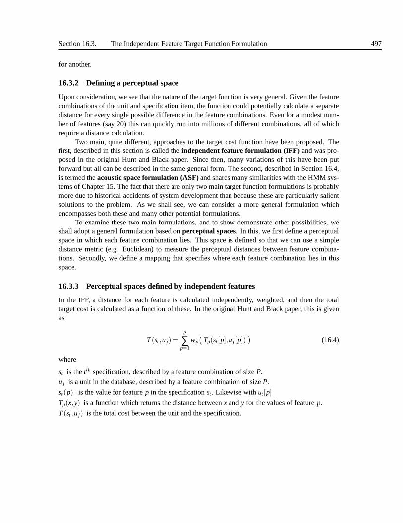
Section 16.3. The Independent Feature Target Function Formulation 497
for another.
16.3.2 Defining a perceptual space
Upon consideration, we see that the nature of the target function is very general. Given the featurecombinations of the unit and specification item, the function could potentially calculate a separatedistance for every single possible difference in the feature combinations. Even for a modest num-ber of features (say 20) this can quickly run into millions ofdifferent combinations, all of whichrequire a distance calculation.
Two main, quite different, approaches to the target cost function have been proposed. Thefirst, described in this section is called theindependent feature formulation (IFF) and was pro-posed in the original Hunt and Black paper. Since then, many variations of this have been putforward but all can be described in the same general form. Thesecond, described in Section 16.4,is termed theacoustic space formulation (ASF)and shares many similarities with the HMM sys-tems of Chapter 15. The fact that there are only two main target function formulations is probablymore due to historical accidents of system development thanbecause these are particularly salientsolutions to the problem. As we shall see, we can consider a more general formulation whichencompasses both these and many other potential formulations.
To examine these two main formulations, and to show demonstrate other possibilities, weshall adopt a general formulation based onperceptual spaces. In this, we first define a perceptualspace in which each feature combination lies. This space is defined so that we can use a simpledistance metric (e.g. Euclidean) to measure the perceptualdistances between feature combina-tions. Secondly, we define a mapping that specifies where eachfeature combination lies in thisspace.
16.3.3 Perceptual spaces defined by independent features
In the IFF, a distance for each feature is calculated independently, weighted, and then the totaltarget cost is calculated as a function of these. In the original Hunt and Black paper, this is givenas
T(st ,u j) =P
∑p=1
wp(
Tp(st [p],u j [p]))
(16.4)
where
st is thetth specification, described by a feature combination of sizeP.
u j is a unit in the database, described by a feature combinationof sizeP.
st(p) is the value for featurep in the specificationst . Likewise withut [p]
Tp(x,y) is a function which returns the distance betweenx andy for the values of featurep.
T(st ,u j) is the total cost between the unit and the specification.
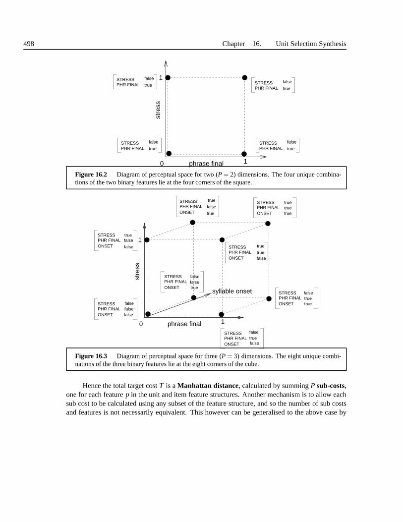
498 Chapter 16. Unit Selection Synthesis
STRESSPHR FINAL
false
true
STRESSPHR FINAL
false
true STRESSPHR FINAL
false
true
STRESSPHR FINAL
false
true
stre
ssphrase final
1
10
Figure 16.2 Diagram of perceptual space for two (P = 2) dimensions. The four unique combina-tions of the two binary features lie at the four corners of thesquare.
stre
ss
phrase final
1
10
syllable onset
STRESSPHR FINALONSET
STRESSPHR FINALONSET
STRESSPHR FINALONSET
STRESSPHR FINALONSET
STRESSPHR FINALONSET
STRESSPHR FINALONSET
STRESSPHR FINALONSET
STRESSPHR FINALONSET
false
false
true true
true
false
true
falsefalsefalse
falsetrue
falsefalse
false
true
truetrue
truefalse
truetrue
falsetrue
Figure 16.3 Diagram of perceptual space for three (P = 3) dimensions. The eight unique combi-nations of the three binary features lie at the eight cornersof the cube.
Hence the total target costT is aManhattan distance, calculated by summingP sub-costs,one for each featurep in the unit and item feature structures. Another mechanism is to allow eachsub cost to be calculated using any subset of the feature structure, and so the number of sub costsand features is not necessarily equivalent. This however can be generalised to the above case by

Section 16.3. The Independent Feature Target Function Formulation 499
pre-processing the features.An alternative formulation is to use theEuclidean distance[450].
T(st ,u j) =
√√√√
P
∑p=1
wp(
Tp(st [p],u j [p]))2
(16.5)
The sub-costs define separate distance functions for each ofthe features. For the categorical fea-tures, this may simply be a binary decision saying whether they match or not. For the continuousfeatures such as F0, this may be some standard difference such as absolute or log distance. Somefeature differences are seen as more important than others:this is reflected in the choice of valuesfor the weightswp for each feature distance.
We can visualise this using our perceptual space formulation as follows. If we take a simplefeature system where every feature is binary valued, we see that the IFF defines a perceptual spaceof dimensionalityP, where each axis represents exactly one feature. The features themselves maponto the corners of a P-dimensional hypercube in this space.This is shown in Figure 16.2 forP = 2 and Figure 16.3 forP = 3. In these Figures, we can clearly see that the more two featurecombinations differ the greater the distance between them.Continuous features have a single axistoo, and the metric chosen to measure their difference is used to scale the axis (so if the metric islinear, then the axis just represents the feature values in their original form). For N-ary categoricalvariables, we can use a single axis if the differences between the values can be ordered. Otherwise,we simply encode the category values into a number of binary features (so that a category with 8values would have 3 binary features), and use an axis for eachone as before.
The relative contribution of each feature is given by the setof weightswp. These have theeffect of scaling the feature axes in the perceptual space, shown in Figure 16.4. The differencebetween the Manhattan distance (Equation 16.4) and the Euclidean distance (16.5) is that in theManhattan case the distance is composed of distances that run parallel to each of the axes. In theEuclidean case, the shortest line is drawn between the two points and the length of this gives thedistance.
The IFF solves the problem of the complexity of the target function by its assumption offeature independence. If we take an example feature set of 20binary variables, we see that inthe IFF, this requires setting 20 weights, whereas in a fullygeneral system this would require220 > 1,000,000 separate weights.
16.3.4 Setting the target weights using acoustic distances
A number of ways have been proposed for setting the weights automatically. As the Hunt andBlack algorithm is not probabilistic, we can not directly use the most standard probabilistic trainingtechnique of maximum likelihood. We can however investigate similar types of techniques whichtry and set the parameters so as to generate data that is closest to a set of training data.
A maximum likelihood approach would be to find the set of weights W = w1,w2, ...wp

500 Chapter 16. Unit Selection Synthesis
STRESSPHR FINAL
false
true
STRESSPHR FINAL
truetrue
stre
ss
phrase final
1
10
STRESSPHR FINAL
truefalse
STRESSPHR FINAL
falsefalse
2.1
Figure 16.4 The effect of the weights is toscalethe axes; in this case the weight for stress is setat 1.0 and phrasing at 2.1. The effect of this is to make differences in phrasing give rise to biggerdifferences in distance that for stress.
STRESSPHR FINAL
false
true
STRESSPHR FINAL
truetrue
stre
ss
phrase final
1
10
STRESSPHR FINAL
truefalse
STRESSPHR FINAL
falsefalse
2.1
2.1
1.0
(a) Illustration of the Manhattan distance formulationbetween two feature combinations. The distance iscalculated separately for each feature and the totalsadded, coming in this case to 2.1 + 1.0 = 3.1
STRESSPHR FINAL
false
true
STRESSPHR FINAL
truetrue
stre
ss
phrase final
1
10
STRESSPHR FINAL
truefalse
STRESSPHR FINAL
falsefalse
2.1
1.76
(b) Illustration of the Euclidean distance formulationbetween the same two features. In this case, the short-est line between the two points is found and its dis-tance measure. In this case, the distance is(2.1)2 +1.02 = 1.76
that generates utterances which are closest to the trainingdata. To do this we require a distancemetric that measures the distance between a synthesised utterance and the natural utterance. As weshall see in Section 16.7.2, defining such a distance is a difficult problem as it is in effect the sameproblem as defining the target function itself; a good distance would be one where utteranceswhich are perceptually similar would receive a low score. For the time being however, let usassume that we do in fact have a distance functionD that can tell us how similar two utterancesare. A further complication arises because the unit selection system isn’t a generative model inthe normal probabilistic sense. Rather it is a hybrid model that uses a function to select units(which is not problematic) but then just concatenates the actual units from the database, ratherthan generating the units from a parameterised model. This part is problematic for a maximumlikelihood type of approach. The problem arises because if we try and synthesise an utterancein the database, the unit selection system should find those actual units in the utterance and use

Section 16.3. The Independent Feature Target Function Formulation 501
those. Exact matches for the whole specification will be found and all the target and join costswill be zero. The result is that the synthesized sentence in every case is identical to the databasesentence3.
The solution to this then is to use aheld out test set, where we leave out say 10% of thetraining data, and train on the remainder. When we now attempt to synthesize the test set, theseutterances aren’t of course present in the unit database andso meaningful synthesis is performed.
The Hunt and Black paper proposes this technique and uses a linear regression method toset the weights. In one experiment they use a separate set of weights for each base type. Foreach unit in the held out test set, they find theN closest units in the training data using a distancemetricD, which in their case is just the Euclidean distance between the cepstra of the original andsynthesized utterance. These are taken to be the units whichwe wish the target function to find forus. A linear regression algorithm is then used to train a function that predicts the distances fromthe sub-costs. The weightsW of this linear regression are then taken to be the sub-cost weightsthemselves. In principle any function learning technique could be used in this manner, the ideais to design a function that predicts the distances from the sub-costs and then use this to directlyor indirectly set the weights. Other approaches include theuse of neural networks [131], geneticalgorithms [9] and discriminative techniques [385].
Perceptual approaches
The weakness of the left-out data approach is that we are heavily reliant on a distance functionwhich we know only partially corresponds to human perception. A number of approaches havetherefore taken been designed to create target functions that more directly mimic human percep-tion. One way of improving the distance metric is to use an acoustic representations based onmodels of human perception; for example Tsuzaki [457] uses an auditory modelling approach.But as we shall see in Section 16.7.2, even a distance function that perfectly models human au-ditory perception is only part of the story; the categoricalboundaries in perception between onediscrete feature value and another mean that no such measureon its own can sufficiently mimichuman perception in the broader sense.
A more “global” perceptual technique is that to use real human judgments of similaritiesbetween units to assist in the design of the target function.The most comprehensive approach tothis was proposed by Lee [292] who has listenersrank sentences and then trains a model to predictthe rankings. The parameters of this model are then taken as the weights. Although the actualtraining technique is different (thedownhill simplex method as opposed to linear regression), theframework of this is somewhat similar to the original Hunt and Black technique. The differencenow is that the system is trained to predict real human perception, not a distance based on acoustic
3 In fact, synthesising the training data is a very useful diagnostic tool in unit selection. In all cases, if we synthesizeasentence in the training data, the speech synthesised should be exactly that that was recorded. If the unit selection picksdifferent units then this is often indicative that something has gone wrong. A common cause for this is that the TTSsystem has produced different pronunciations, or that the prosody generated is very different from the natural prosody.

502 Chapter 16. Unit Selection Synthesis
measurements. Another approach is that advocated by Wouters and Macon [497] who playedlisteners sets of pairs of words with one phoneme different and ask them to rank the differences.In principle this technique could be extended to any difference in values for a feature, and theresulting data would be a truly accurate reflection of human judgment of sound substitutability.Toda et al [449] use a technique which uses subjective evaluations of individual sub-costs to trainthe weights.
The only drawback with perceptual techniques is that they can be timely to implement, ashuman subjects are involved in the training process. It can be argued however that the weights inthe IFF are in fact largely independent of the particular database being used; so once the weightsare found they can be used again, or as time goes on more and more experiments can be performedwhich will add to the total quantity of data available for training.
Tuning by hand
A final approach to “training” the weights is to not attempt any automatic training at all but tosimply set the weights “by hand” [65], [108], [99]. Typically a system designer listens to somesynthesis output and using a mixture of previous knowledge and results from this listening, setseach weight individually. Such an approach is of course anathema to all that we believe in themodern world of machine learning, statistics and science, and it can be claimed that this is aretrograde step back to the setting of rules by hand in formant synthesis.
We can however justify this approach to some extent. Firstlythere is significant evidence thatthis produces the best results (and of course the real reasonwhy we believe in statistical rather thanknowledge based approaches is actually because they give better results). It should also be stressedthat in a typical system there may only be 10 or 20 weights, andthis is a manageable amount fora person. By comparison with setting rules by hand in formantsynthesis, all we are doing here isbiasing a data driven system in a particular direction, and the setting of a few parameters is a longway from settingeveryparameter by hand.
A final point is that nearly all machine learning approaches adopt anequal error rate ap-proach to learning, in which one classification error is as bad as another. In real life of course,we know this to be false (consider the relative importance ofrecognising the word “not” in thesentence “I am definitely not guilty”), but this simplification is adopted in many machine learningtasks with the idea that biases reflecting different degreesof error can be set independently. Theadvantage of setting the weights by hand is that by using global judgments about how good thespeech sounds, we are implicitly defining which features aremost important to get right. As wesaw in Section 16.3.1, we can rank the importance of featuresindependent of any acoustic dis-tances. This is probably most evident in word identity; no matter what effects the other featureshave, any feature which causes a mis-recognition of a word islikely to be regarded as particularlyimportant to get right. When humans tune a system “by-hand” they are implicitly making judg-ments of this type and incorporating them into the weights, and it is possible that it is this that isresponsible for the high quality of systems which set the weights by hand.

Section 16.3. The Independent Feature Target Function Formulation 503
16.3.5 Limitations of the independent feature formulation
The main design feature of the IFF is that it assumes the features operate independently. Thisensures that the number of parameters (weights) to be determined is very low, and hence easyto learn from data or set by hand. The formulation doesn’t in general suffer from sparse dataproblems, as there are nearly always enough examples of eachfeature present in the data.
The assumption that features operate independently is however very strong, and it is notdifficult to find instances where this falls apart. The starkest demonstration of this is that twodifferent feature combinations will always have a non-zerodistance: this clearly contradicts whatwe know from above, namely that ambiguity is rife in speech and that there are frequent cases ofdifferent feature combinations mapping to the same acoustics (and hence same sound). So long asa weight is not zero (which would imply that that feature is irrelevant in every single case) the IFFensures that we can not make use of the power of ambiguity.
To show a real example of this, imagine our simple two featuresystem as shown in Figure16.2. From this, we see that the feature combinations:
STRESS f alsePHRASING true
and
STRESS truePHRASING f alse
and
STRESS f alsePHRASING f alse
and
STRESS truePHRASING true
give the largest distance (regardless of whether Manhattanor Euclidean distances are used).In fact, it is well known that stressed and phrase final versions of a phone are longer than
the unstressed and non-phrase final versions. Imagine for sake of demonstration that both thesefeatures double the length of the phone, then we would expectthe following duration values foreach feature combination:
STRESS f alsePHRASING f alse
= D
STRESS truePHRASING f alse
= 2D

504 Chapter 16. Unit Selection Synthesis
STRESS f alsePHRASING true
= 2D
STRESS truePHRASING true
= 4D
This clearly shows that
STRESS f alsePHRASING true
and
STRESS truePHRASING f alse
both have the same duration value, which means that one is well suited to be used in place of theother. But as we just saw the IFF gives the largest distance tothese, and furthermore, gives thesamedistance to two feature combinations which are entirely unsuitable.
These problems arise from the very severe constraints the IFF puts on the nature of features,by insisting that all feature combinations with the same value for one feature lie on a single line.It fails to take into account any interaction between features, and therefore is unable to make useof ambiguity and other complex aspects of the feature to acoustic mapping.
16.4 THE ACOUSTICSPACE TARGET FUNCTION FORMULATION
Theacoustic space formulation (ASF)is a quite different way of defining the target function, sodifferent in fact that often it is regarded as a completely different way of performing unit selection.This approach attempts a different solution to the problem of the specification items lacking anacoustic description. The formulation uses apartial-synthesis function to synthesize an acousticrepresentation from the linguistic features. Once this acoustic representation is obtained, a searchis used to find units which are acoustically similar to it. In general, the partial-synthesis functiondo not go “all the way” and generate an actual waveform; this would amount to a solution ofthe synthesis problem itself. Rather, an approximate representation is found, and synthesis isperformed by using real units that that are close to this.
We can also describe the ASF using the idea of perceptual spaces. The key idea of the ASFis that an existing, predefined, acoustic space is taken to bethe perceptual space. Thus, ratherthan define an abstract perceptual space, we use one that we can measure directly from speechdata. Often the cepstral space is used, but in principle any space derivable from the waveform ispossible. In the acoustic space, the distance between points is Euclidean, so that the only issue ishow to place feature combinations within this space. In the case of feature combinations for which

Section 16.4. The Acoustic Space Target Function Formulation 505
we have plenty of units, we can define adistribution for this feature combination which we findfrom the units. This can be done in a number of ways, but an obvious way to do this is to use theobservations to build an hidden Markov model (HMM). The simplest HMM would have one state,whose observations would be modelled with a single multivariate Gaussian [54]. The means andvariances of this Gaussian can be calculated directly from the units in the usual way (i.e. Equation15.17, 15.18). As the speech representing the feature combination will have dynamic properties, itis also natural to consider using more than one state in the HMM; common choices are to use threestates as is standard in ASR [140], [138]. If a diphone base-type is used, we should also considerusing one state for each half of the unit. From these parameters, we can easily measure the targetcost by measuring the distances, in acoustic space, betweenthe model and any unit. The onlyremaining problem now is how to calculate the distance if oneor both of the feature combinationsis unobserved.
16.4.1 Decision tree clustering
The key part of the ASF is the design of a partial-synthesis function that can take any featurecombination and map it onto the chosen acoustic space. The most common way of doing this is touse the decision tree method, in more or less the same way it isused in HMM (see Section 15.1.9).As context accounts for a significant level of variance within a phone model, using separate phonemodels for each possible context greatly reduces the overall variance of the models. The problemfaced however is that while many of the required models have few or no observations in thetraining data, their parameters still have to be estimated.The similarity with our problem can nowbe seen: if we describe HMM context in terms of features, we see that the problem in ASR is onewhere a set of model parameters are required for each unique feature combination, many of whichhave not been included in the training data, whereas in unit selection the problem is we requirea distance between each unique feature combination, again many of which have not been seen inany training data. In the ASF of unit selection, the decisiontree is trained in just the same wayas with HMMs, the only difference being that “prosodic” features such as stress, phrasing and soon are included. While the method just described is now more or less standard, it is important tonote that the decision tree method itself is based on thecontext oriented clustering technique,developed for speech synthesis by Nakajima and colleagues [327], [326]. This was later extendedand incorporated into the ASR-style decision tree method byDonovan and Woodland [140]. Othersystems of this type include [54], [115], [355], [220], [197], [381].
The usefulness of the tree is that it provides natural metrics of similarity betweenall featurecombinations, not just those observed. The clever bit is that the tree will always lead us to acluster even for feature combinations completely missing from the data. As with observed featurecombinations, we can just measure the distance between the means of these to give us the valuefor our target function.
The main benefit of the ASF is that it does not assume that the features operate independently.This therefore avoids two of the weakness of the IFF. Firstlywe can define complex feature depen-

506 Chapter 16. Unit Selection Synthesis
STRESSPHR FINAL
falsefalse
STRESSPHR FINAL
false
true
STRESSPHR FINAL
truefalse
1c
STRESSPHR FINAL true
true
c2
Figure 16.5 Diagram of 4 feature combinations lying in acoustic space, where only 2 dimensions ofthe high dimensional acoustic space are shown for clarity. Note that unlike Figure 16.4, the positions ofthe feature combinations are not determined by the feature values but rather by the acoustic definitionsof each feature combination. Hence, these can lie at any arbitrary point in the space. In this case, wesee that two feature combinations with quite different values lie close to each other, a situation whichwould not be possible in the IFF. The dotted ellipses indicate the variances of the feature combinations,which are used in some algorithms to measure distances.
dencies. Secondly, we can use ambiguity in speech to our advantage; it is the acoustic similarityof two different feature structures which allows us to buildcomposite models in the first place. Ifwe compare Figure 16.7 to Figure 16.4 we see that now the positions of the feature combinationsare not defined by the values of the features, but rather by theacoustic space and the feature toacoustic mapping. In Figure 16.7 we see that the two feature combinations which have no featurevalues in agreement but which nonetheless sound very similar are now in fact close to each otherin the perceptual space.
We have some degree of choice as to how we actually use the decision tree to form thetarget function. Firstly, we could just accept the units in the chosen cluster as candidates andleave the process at that. An addition to this is to score eachunit in terms of its distance fromthe cluster mean [54], in an attempt to somehow reward typical units within the cluster. If thecluster size is small however, these approaches may lead to only a small number of units beingused as candidates. Alternatives include going back up the tree and accepting leaves which are

Section 16.4. The Acoustic Space Target Function Formulation 507
1c
u u u
u u
u
uu
u
u u
u
u u
u u
u
uu
uu
u
u
u
u
uu
u
uu
uu
X
Figure 16.6 Diagram of 4 feature combinations lying in acoustic space, where only 2 dimensions ofthe high dimensional acoustic space are shown for clarity. Note that unlike Figure 16.4, the positions ofthe feature combinations are not determined by the feature values but rather by the acoustic definitionsof each feature combination. Hence, these can lie at any arbitrary point in the space. In this case, wesee that two feature combinations with quite different values lie close to each other, a situation whichwould not be possible in the IFF. The dotted ellipses indicate the variances of the feature combinations,which are used in some algorithms to measure distances.
neighbours to the current one. Again, these can be given someextra cost to show that they arefurther away from the specification than the original cluster. Finally, is its possible to expand anycluster without reference to the tree. To do this, we decide how many candidates we require andthen simply find the nearestN units to the mean of the cluster. This can be done with or withoutusing the variances of the cluster.
16.4.2 General partial-synthesis functions
There are two main weaknesses to the decision tree technique. Firstly the assumption that anacoustic space such as the cepstral space is a good approximation of the true perceptual space isa very strong claim; we examine the full extent of this problem in Section 16.7.2. The secondweakness is a consequence of using decision trees and is not aweakness of the ASF itself. Thebasic problem is that the decision tree divides the observations into fixed clusters by only takinginto account the particular feature combinations which areobserved: no thought is given to thegeneral shape of the space or the properties of the missing feature combinations. The decision tree

508 Chapter 16. Unit Selection Synthesis
1c
u
u
u
u
u
uu
u
uu
X
u
u
u
u
uu
u
u
uu
u
u
u
u
u
u
u
u
u
u
u
u
u
(a) Decision tree behaviour of ASF for unobservedfeature combinations. In this figure, we have afeature combination whose true position is givenby the point X. In the decision tree formulation,we find the cluster which has the most feature val-ues which match the unobserved feature combi-nation. Once found, we use this cluster “as is” (ineffect we set a pointer from the unobserved featurecombination to the chosen cluster). All the unitsin this cluster are used, even though some are aconsiderable distance from the true value and arefurther away than units in other clusters.
1c
u
u
u
u
u
uu
u
uu
u
u
u
u
u
u
u
u
u
u u
u
u
uu
u
u
u
u
uu
uXX
(b) General projection function behaviour of ASFfor unobserved feature combinations. In this case,we use a general function to generate a valueXwhich is an estimate of where the unobservedfeature combination should lie in acoustic space.Given this, we then find the closestN units, whichare shown in bold inside the ellipse. This tech-nique has the advantage in that it finds the unitswhich are closest to the predicted value, and notsimply a whole cluster for a different feature com-bination.
Figure 16.7 .
effectively assigns each missing feature combination to anobserved cluster; in computer terms wecan think of this as being a “pointer” from the missing feature combination to an observed one.With this however it is possible to find a better set of units for the unobserved feature combinationby building a new cluster that doesn’t necessarily correspond to any existing one. This is shownschematically in Figure 16.7a.
An alternative to the decision tree approach is to train a function that estimates an acousticpoint directly for a given feature combination. The difference between this and the decision treeapproach is that while the decision tree function gives an acoustic point for every feature combi-nation, all the feature combinations which share the feature values in a branch of a tree are giventhesamepoint. In the general approach, all feature combinations can in principle generate uniquepoints in acoustic space, and so there is no assumption of equivalence. Given this generated point,it is possible to find the closest N points to this and therefore form a new cluster. This is shownschematically in Figure 16.7b. One solution to this is to usea neural network to learn this function[437]. It can be argued that despite some often noted disadvantages to these algorithms, neural
Section 16.5. Join functions 509
networks are quite suited to this task as they can easily accommodate binary input and generatecontinuous vector output. The strength of the neural network is that it can learn the idiosyncrasiesof certain feature combinations while generalising over others. The use of a neural network isonly one possible solution to this; in principle any function learning algorithm could be used forthis task. While this helps solve the problem of the fixed clusters, it is still however reliant on theassumption that the acoustic space is a good approximation to the true perceptual space.
16.5 JOIN FUNCTIONS
16.5.1 Basic issues in joining units
The purpose of the join function is to tell us how well two units will join together when concate-nated. In most approaches this function returns a cost, suchthat we usually talk aboutjoin costs.Other formulations are however possible, including thejoin classifier, which returns true or false,and thejoin probability , which returns the probability that two units will be found in sequence.
Before considering the details of this, it is worth making some basic observations aboutconcatenation in general. We discussed the issue of micro-concatenation in Section 14.7, whichexplained various simple techniques for joining waveformswithout clicks and so on. We alsouse these techniques in unit selection, but now because the variance at unit edges is considerablygreater, we can’t use the concatenation method of second generation systems which solved thisproblem by only using very neutral, stable units. Instead the because units have considerablevariability, we now also have to consider the issue ofmarco-concatenation, often simply calledthe join problem.
Knowing whether two units will join together well is a complex matter. It is frequently thecase however that we do in fact find a “perfect” join (that is one that is completely inaudible). Westress this as it is often surprising to a newcomer to TTS thatsuch manipulations can be performedso successfully. Of course, many times when we join arbitrary sections of speech the results arebad; the point is that there are a considerable number of cases where speech from completelydifference sentences and contexts can be joined with no audible join whatsoever. We stronglysuggest that anyone involved in unit selection should spendsome time just playing around withjoining waveforms in this way. Furthermore, when we examinesome objective representationsof the speech, such as the spectrogram, we canvisually clearly observe the join, but not audibly.We mention these facts to show that in many cases considerable separation and recombination ofspeech can be achieved with no noticeable effects; and this is of course a fortunate outcome forour general concatenation framework.
The join feature issue is considerably more straightforward than with target features. Firstly,we have access to both linguistic features and the true acoustic features; secondly as all units havehad their features measured and derived in the same way, we don’t have to worry about issues ofcomparing generated acoustic values with ones determined by signal processing. In addition to

510 Chapter 16. Unit Selection Synthesis
Broad phonetic class Percentage of joins detectedLiquid 54.7Glide 54.7glottal fricative 54.3nasal 47.4unvoiced weak fricative 35.3voiced weak fricative 23.3unvoiced strong fricative 22.2voiced strong fricative 13.6
Figure 16.8 How detectability of joins varies with phonetic class. FromSyrdal [428].
these “theoretical” advantages, experience has shown thatjoining units can be easier in practice:in the best systems often there are virtually no bad joins.
The basic principle of the join cost is to use the features from the two units to decide whetherthe join will be good or not. While this forms the basis of mostcalculations, it is common toemploy an additional “trick” whereby we use a separate routeand always assign a zero join costto any two units which were neighbouring in the original data. As these two units were “joined”originally, we know that they form a perfect join and receivea cost of 0, regardless of what thefeatures or join cost proper tells us. This is a powerful addition, and it biases the search to choosesequences of units that were originally concatenated. Thuswhile nearly all the joins we considerin the search are chosen by the join cost proper, when we consider the joins of the units which areactually chosen, we find many have be calculated by this othermethod.
In the following sections we describe techniques for deciding how well two units join, andlimit ourselves to doing this solely on the properties of theunits. In addition to this, we can alsouse the techniques mentioned in Section 14.7 where we explored further techniques for smoothingand interpolation of the units on either side of the join.
16.5.2 Phone class join costs
A significant factor is the type of phone that is being joined.In the formulations which joinin the middle of phone (e.g. diphone, half-phone) we are always joining units which share thesame phone across the boundary (e.g. we join a /s-iy/ to a /iy-n/). The identity of this phone has asignificant impact on the quality of the join as it appears that some phones are more sensitive andothers more robust to being chopped and recombined.
Syrdal and colleagues have conducted extensive formal studies of these effects [426], [428]and showed that there is a basic hierarchy of phone classes, ranked by how often listeners candetect a join. The results of this are shown in Table 16.8 and show that, regardless of the actualunits involved some phone types simply join better than others. Informally, we can think of thisas a type of “prior” on the join cost, which is used to bias the search to pick joins which fall in

Section 16.5. Join functions 511
Euclidean Absolute MahalanobisMFCC 0.6 0.64 0.66MFCC +∆ 0.55 0.55 0.50LSF 0.63 0.64 0.64LSF +∆ 0.63 0.64 0.58Formant 0.59 0.58 0.55Formant +∆ 0.46 0.46 0.62
Figure 16.9 Correlation of perceptual ratings of “goodness” of join with various acoustic measuresand distance functions for a single vowel /ey/. From Vepa et al [472].
the low detection classes (i.e. fricatives). Thisphone class join costshould play an importantpart in any well designed join cost function; such an approach is taken by Bulyko and Ostendorf[74] who use a phone class cost (termedsplicing cost in their paper) in addition to other costsmeasured between actual units.
16.5.3 Acoustic distance join costs
It is clear that the acoustic differences between the units being joined have a significantimpact on how successful the join will be, and this observation is the basis of theacoustic distancejoin cost. Perhaps the simplest way of implementing this is to comparethe last frame in the leftdiphone with the first frame in the right diphone. For instance in Hunt and Black [227], twocepstral vectors are compared.
This on its own is known to produce a number of bad joins, whichhas prompted an areaof research in which researchers have examined various acoustic measures and distance metrics.Several studies investigated these with the aim of seeing which agreed best with human perception.In doing so, two main approaches were used. In Klabbers and Veldhuis [250], [251], and Syrdal[426] [428] the perceptual studies focused on asking listeners whether they could detect a join. Asecond approach, used in Wouters and Macon, and Vepa et al [472] [470] [471] asked listeners torate the quality of the join on a scale. A typical set of results for this second approach is given inTable 16.9.
Among the acoustic representations investigated were:
1. Cepstral coefficients (Section 12.3) [496]
2. LP Cepstral coefficients (12.5.6) [496]
3. Mel-scaled cepstral coefficients (MFCCs) (Section 12.5.7) [251], [472]
4. Line spectral frequencies (Section 12.5.5) [496], [472]
5. Perceptual linear prediction (Section 12.5.8)
6. Formants and formant like measures [472]
7. Linear prediction log area ratios (Section 12.5.4) [496]

512 Chapter 16. Unit Selection Synthesis
Among the metrics used to calculate the distances include:
1. Manhattan distance
D =N
∑i=1
abs(xi −yi)
2. Euclidean distance
D =
√N
∑i=1
(xi −yi)2
3. Mahalanobis distance. The Euclidean distance treats allcomponents of the vector equally,whereas the Mahalanobis distance computes a distance whichscales each component by theinverse of its variance. It can be thought of as a measure which normalises the space beforecomputing the distance.
D =
√N
∑i=1
(xi −yi
σi
)2
4. Kullback Leibler style distances. The Kullback Leibler divergence is a measure of “dis-tance” between two probability distributions. From this, we can derive an expression whichcalculates the distance between two spectral vectors [251], [472]:
D =N
∑i=1
xi−yi)logxi
yi
16.5.4 Combining categorical and and acoustic join costs
The above studies shed interesting light on the relationship between acoustic measures and theirperception, but they also show that there seems to be an upperlimit as to how far this approachcan go. From Table 16.9, we see that thebestcorrelation between an acoustic cost and perceptualjudgment is only 0.66, which is far from the type of correlation that we would be happy to accept asa scientific rule. Given the number of studies and that nearlyall the well known acoustic measures(MFCCs, LSFs, formants etc) and all the distance metrics (Euclidean, Mahalanobis, Kullback-Leibler) have been studied, we can be fairly sure that this area has been thoroughly investigatedand that combination of features and distance metric is likely to significantly improve on the resultsin Table 16.9.
While it is possible that the distance metrics are at fault, amore likely explanation is that theacoustic features alone don’t contain the information required. If we think about joins as a purelylow level phenomenon, this may be surprising, but in fact by only concentrating on acoustics wemay be enforcing low costs on units which are quite differentfrom a purely linguistic perspec-tive. Recall from Section 7.3.2 that often the acoustic differences between linguistic categories areslight, but as the listener always perceives these categorically, a slight difference across a category
Section 16.5. Join functions 513
boundary may cause a big difference in perception. Hence small acoustic differences within cat-egories may be fine, small acoustic differences across categories may not. The obvious thing todo is to therefore include categorical/linguistic information in the join cost. By doing this, we aresaying that units which share the same stress value, or the same general phonetic context are likelyto produce good joins. Some systems have based their join costs entirely on linguistic features[65], [14], [441], [442], and often the quality of the joins in these systems are as good as thosethat use purely acoustic measures. A more common approach isto use a mixture of acoustic andcategorical features in the join cost [74], [108], [210], [427]. As far as we are aware, only oneserious study by [427] has looked at join functions which usecategorical features and this foundthat the use these features in addition to acoustic featuresmade significant improvements.
One possible reason for this is that acoustic distances are limited in that they usually onlyconsider frames near the join, whereas we know that context effects can be felt over a distance oftwo or three phones. As the categorical features often operate at the phone level or above, theycompensate for the short term nature of the acoustic features. As Coorman et al [108] state, it iswell known that vowels followed by an [r] are heavily influenced by the [r] and this fact alone isuseful in designing the join cost (where we could for instance have a sub-cost which states thatunits to be joined should either both have an [r] context or both not have an [r] context). Syrdal[427] investigates the listener responses of a mixed system.
16.5.5 Probabilistic and sequence join costs
Another way of improving on the basic acoustic distance joincost is theprobabilistic sequencejoin function , which takes more frames into account than just those near the join. Vepa and King[470] used a Kalman filter to model the dynamics of frame evolution, and then converted this intoa cost, measured in terms of how far potential joins deviatedfrom this model. A full probabilisticformulation, which avoids the idea of cost altogether was developed by Taylor [438].
The Taylor technique uses a model which estimates the probability of finding a sequenceof frames, with the idea that if we find a high probability frame sequence across a join, thisindicates a natural sequences of frames which in turn implies a natural join. The model uses ann-gram approach of the type used for HMM language models (seeSection 15.1.6). N-grams workon discrete entities, and so frames have to quantised as a pre-processing step. This is done viaa codebook of the type used in discrete probability HMMs [511], [367], which uses a bottomup clustering to quantise the data, followed by a mapping, which assigns any frame a numbercorresponding to its nearest cluster. Given this, we can calculate the probabilityP(O) of observinga sequence of frames:
P(O) = P(o1,o2,o3, ...oM)
The idea is to measure the probability of this for the sequence of frames across every pair ofcandidate units across a join, and use the result as a measureof join quality in the search.P(O) istoo difficult to estimate in full, so we make the n-gram assumption and estimate this on a shorter

514 Chapter 16. Unit Selection Synthesis
sequence of frames (say 2 before and 2 after the join). The powerful thing about this approach isthat the model can be trained on all the data in the speech database, and not just examples near unitboundaries. This often results in many millions or tens of millions of training examples, whichmeans that robust estimates ofP(O) can be obtained.
The general probabilistic sequence join function approachhas a number of advantages.Firstly, it gets around a core weakness of the acoustic distance technique. There, frames whichare identical have a zero cost, and this in general is the onlyway in which a zero join cost can beachieved. But in real speech, we see that this is hardly ever observed: the speech signal is changingfrom frame to frame. The key point is that in natural speech, while the signal evolves from frameto frame, all these frames “join” perfectly: in other words,if we separated these frames and re-combined them, the joins would be perfect. But in none of these cases would the acoustic distancebetween the frames be zero. Thus we have an enormous number ofcases where the perceptual costis clearly zero but the acoustic cost as measured by acousticdistances is not zero. This is shownup in the trick whereby we set the join cost of units which wereoriginally side by side to be zero(Section 16.5.1). While this is a very useful addition to theoverall system, it shows the inherentweakness of an acoustic distance join cost, as naturally neighbouring units rarely get a zero costas calculated by that method. Secondly, we know that dynamicinformation is often importantin speech. While we can use dynamic features in an acoustic distance join cost, the probabilisticsequence join function models this more directly. Finally,the probabilistic sequence join functiongives us a probability rather than a cost. Vepa and King [470]convert this back into a cost and usein the standard way, but Taylor [438] shows this can be kept asa probability, which is one way offormulating a unit selection system based on probabilitiesrather than costs.
Bellegarda [39] describes a join cost algorithm which uses sequences of frames, but in a quitedifferent way. Bellegarda’s approach defines a function foreach type of join, which in a diphonesystem would be one for each phoneme. This technique is particularly interesting in that it workson waveforms, and not any derived acoustic representation.This is so that the technique can solvenot only the macro-concatenation problems normally associated with join costs, but also micro-concatenation problems such as phase mismatches. The algorithm works by forming a matrix foreach type of join where the rows represent the frames and the columns the instances of units. Thismatrix captures all the acoustic information relevant to that type of join. Because the data is storedas raw waveforms direct comparison is inadvisable (for all the usual reasons) and so a real valuedtransform is performed by means of asingular value decomposition (SVD).The join cost is thenmeasured using the cosine of the angle between two vectors inthe matrix. The reason for using anSVD is that it transforms the waveforms into representations where the most salient parts are mostprominent, but does so in a way that does not throw away phase information as would be the casewith any measure based on Fourier analysis. Bellegarda reports that this technique significantlyoutperforms standard acoustic measures such as MFCCs in listening experiments.

Section 16.5. Join functions 515
perc
eptu
al d
ista
nce
objective distance
(a) The normal formulationwhere the relationship betweenobjective distance and perceptualdistance is linear.
perc
eptu
al d
ista
nce
objective distance
floorvalue
ceilingvalue
(b) The use of floor and ceilingvalues, which say that beyond athreshold all distances are percep-tually equivalent. Between thesevalues the relationship is linear.
perc
eptu
al d
ista
nce
objective distance
badjoinsjoins
good
(c) The situation where the linerregion is negligibly small, mean-ing that the join cost function ef-fectively becomes a join classifierwhere every join is either “good”or “bad”.
16.5.6 Join classifiers
Another angle on the problem of why acoustic measures and perception correlate so badly isto consider whether the notion of a joincost is really the correct formulation in the first place.Coorman et al [108] show that using costs directly often contradicts basic properties of humanperception. They argue that it is good policy to ignore any objective cost differences below acertain value as humans will not perceive such small differences. Additionally, they argue thatabove a certain value, the costs are so high as to make any distinction between one high cost andanother meaningless: once the join sounds “terrible” thereis no point in making the distinctionbetween this and an even worse pair of units whose join is “truly appalling” etc. We can termthese thresholds thefloor value and theceiling value; their affect on the cost function can be seenin Figure 16.5.6 and this formulation can apply to both target and join costs. For the case of joincosts this shows that there are basically three regions; thefirst where all units join perfectly, themiddle where units join well to a greater or lesser degree, and the third region where all units joinbadly.
A more extreme view is to consider the middle region very small, such that we take the viewthat units either join together well (we can’t hear the join)or they don’t (we can hear the join).Then, the join cost becomes a function which returns a binaryvalue. Another way of stating thisis that the join function is not returning a cost at all, but isin fact aclassifierwhich simply returnstrue of two units will join and false if they don’t. To our knowledge Pantazis et al [345] is the onlypublished study that has examined this approach in detail. In that study, they asked listeners to tellif they could hear a join or not, and use this to build a classifier which made a decision based onacoustic features. In their study, they used a harmonic model as the acoustic representation (see

516 Chapter 16. Unit Selection Synthesis
Section 14.4.2), and Fishers linear discriminant as the classifier [160],[45], but in essence, anyfeatures or classifier would be amenable to this approach.
As with all the studies which directly use perceptual evidence, the amount of data availablefor training is often very limited due to the high cost of collection. It is possible however toconsider classifiers which do not rely on making human judgments. Thissequence join classifierhas a similar philosophy to the probabilistic sequence joinfunction. We use the fact that ourentire speech corpus is composed of large amounts of naturally occurring perfect “joins”, as everysingle example of two frames found side by side is an example of such. Therefore we have threesituations;
1. Two frames which occurred naturally and therefore form a good join.
2. Two frames which did not occur naturally but form a good join
3. Two frames which did not occur naturally but form a bad join
The goal of this approach is to use the data of case 1 (which we have plenty of) to build a classifierthat separates cases 2 and 3. In naturally occurring speech,we have of course only data of type 1,but there are in fact machine learning techniques which are trainable on only positive data, or largeamounts of positive data and a small amount of negative data,which can be obtained as before[298]. To our knowledge this approach has not been tried, butshould be worthy of investigationas the very large amount of training data should allow for a robust classifier to be built.
16.6 SEARCH
Recall that in the Hunt and Black algorithm (Equations 16.2 and 16.3) the total cost of one se-quence of units from the databaseU =< u1,u2, ...,uT > with the specificationS=< s1,s2, ...,sT >is given by
C(U ,S) =T
∑t=1
T(ut ,st)+T
∑t=2
J(ut ,ut−1) (16.6)
This calculates the cost for just one possible sequence of units. Our goal is of course to find thesingle sequence of units in the database which gives the lowest cost:
U = argminT
∑t=1
T(ut ,st)+T
∑t=2
J(ut ,ut−1) (16.7)
and the issue of unit selection search concerns how to find this one best sequence of units from allthe possible sequences.
To give some idea of the scale of this, consider a typical casewhere we have say 20 wordsin the input sentence which gives rise to 100 diphone items inthe specification. If we have 100units for each diphone, this means that there are 100100 = 10200 unique possible sequences of

Section 16.6. Search 517
t−a
t−a
t−a a−n
a−n
a−n
Figure 16.10 Diphone search, where every unit which has edge matches are linked in the network.
diphones. If we calculated Equation 16.2 for every sequencethis would still take an astonishinglength of time regardless of computer speed4. Luckily, we can employ the well knowndynamicprogramming algorithm, a speciality of which isViterbi algorithm described in Section 15.1.5This algorithm operates inN2T time, whereN is the number of units, andT is the length of thespecification sequence. This algorithm takes linear time inT, which is obviously an improvementon the exponentialNT time of the exhaustive search.
As described in Section 15.1.5 the Viterbi algorithm seeks the highest probability paththrough an HMM network. The only real difference between that and unit selection search isthat here we are trying to find thelowestcost path. This is in fact a trivial difference, and so theViterbi algorithm as previously described can be used directly to find the lowest cost sequence ofunits in unit selection.
16.6.1 Base Types and Search
On the surface, it seems that the issue of what base type we should pick for our system (e.g.phones, diphones, half-phones etc) is a fundamental designchoice. Here we will show that in fact,so long as certain conditions are met, the choice of base typedoes not greatly affect the quality ofthe final speech, but is really an issue of size and speed in thesearch.
Consider again the case of a diphone unit selection system. In a well designed system witha good database, we should have at least one example of nearlyevery diphone. However, even inthe best systems it is sometimes the case that we have missingdiphones in our unit database, andwe need to be able to synthesize these at run time. A potentialsolution is to use the same approachto missing data that we used in the target function formulation. Recall there that the problem wasthat while we had plenty of examples of units for the requiredbase type, we did not have all ofthe possible feature combinations within this. As this problem seems similar, one solution wouldtherefore be to use decision trees; adopting this for missing base types would mean for instancethat if we were missing the diphone /t-i/ we would simply use the units from a similar diphone,
4 For example if we could perform 10000 calculations per second, it would still take about a billion times the knownlength of the universe to calculate all the costs. (This assumes that the universe is 16 billion years old. For thosecreationist readers, the number is even larger!)
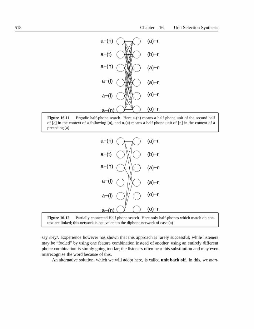
518 Chapter 16. Unit Selection Synthesis
a−(n)
a−(t)
a−(l)
a−(n)
(a)−n
(a)−n
(a)−n
(b)−n
(o)−n
(o)−n
a−(l)
a−(n)Figure 16.11 Ergodic half-phone search. Here a-(n) means a half phone unit of the second halfof [a] in the context of a following [n], and n-(a) means a halfphone unit of [n] in the context of apreceding [a].
a−(n)
a−(t)
a−(l)
a−(n)
(a)−n
(a)−n
(a)−n
(b)−n
(o)−n
(o)−n
a−(l)
a−(n)Figure 16.12 Partially connected Half phone search. Here only half-phones which match on con-text are linked; this network is equivalent to the diphone network of case (a)
say /t-iy/. Experience however has shown that this approachis rarely successful; while listenersmay be “fooled” by using one feature combination instead of another, using an entirely differentphone combination is simply going too far; the listeners often hear this substitution and may evenmisrecognise the word because of this.
An alternative solution, which we will adopt here, is calledunit back off . In this, weman-

Section 16.6. Search 519
ufacturenew units from pieces of existing units. Thus instead of using a /t-iy/ unit instead of a/t-ih/ unit, we instead use only the first part of /t-iy/, and join this to the second half of a /d-ih/ unitto create the required /t-ih/ diphone. There is no standard way of doing this, but as the number ofmissing diphones is often small, it is not too difficult to specify how to build the missing diphonesby hand. As in the example just given, we can use criteria suchas place of articulation to guideus, and so advocate using a /d/ instead of a /t/.
In effect, for our missing diphones, we are using a half-phone solution. We maintain phoneidentity, but use diphones where we have them and half phoneselsewhere. Now consider a half-phone system in which we can assume that there are no missing half-phones (which is a fairlysafe assumption as we only have 2N base types for half phones but just less thanN2 base typesfor phones, where N is the number of phonemes). In the construction of the diphone lattice, it isstandard to allow only diphone units whose base type matchesthe specification. In other words,in the lattice all edges match in phone identity to be considered, so for instance if we have a set of/t-ih/ candidates in slott, we will only consider diphones starting with /ih/ in slott + 1. In a halfphone lattice, we have more flexibility, in that while it makes sense that the phone middle of eachhalf phone must match across the boundary, we can in principle join any half-phone at the otheredge. This is shown in Figure 16.11. This would be the most general formulation, but if we adoptthis we see that the number of possible joins to be calculatedat each time slot is now very high.
If we haveN phonemes in our system, we will have 2N half phone base types, andN2
diphones. Assuming we have on average 500 units for each diphone base type, we would have onaverage 250N units for each half phone base type. Thus if we consider every unit which matchesthe specification, we now have 250N units at each time slot in the search for half-phones, comparedwith 500 for diphones, so ifN = 40 this means we have, 10000 units, ie 20 times more units at eachslot. Given that the join function is calculated over every combination of units at a join, this meansthat instead of 5002 = 250,000 join costs to calculate we now have(250N)2 = 100,000,000 joins,400 times more. These calculations are of course for the samesized database, which means thatjust by changing the base type, we now have to compute 400 times more join costs.
To speed up the search when dealing with half-phones, it is possible to restrict the type ofunits for which we calculate the join cost. The simplest way to do this is to restrict the numbers ofjoins in base types with plenty of units, so as only to consider joining units which have a matchingcontext at their edge. So for example, if we have a /-i/ half phone unit that is followed by a /t/ in theoriginal data, we only consider joining this to /t-/ units which are proceed by an /i/ in the originaldata. We do this for all base types which have more than a threshold N number of units. For thisbelow this, we consider more and possible all possible joins. This is shown in Figure 16.12.
We should now see that in effect, the diphone formulation with the half-phone back-off, andthe half-phone formulation with restricted join possibilities are in fact identical in terms of whatspeech is passed to the search. This equivalence between base types, back-off strategies and searchtopologies can be shown for all base types which share the same type of join (e.g. this is true forall those that allow joins in phone middles). This thereforeshows that the choice of base typereally isn’t as fundamental as it seems; the choices of whichfeatures to use and how to formulate

520 Chapter 16. Unit Selection Synthesis
the target and join functions are much more significant in determining final quality.Using non-uniform units complicates the search somewhat asnow we don’t have a lattice
of time slots where each time slot aligns one-to-one with thespecification. We can however stillperform a fully optimal search. First we define a “grammar” which specifies which units canfollow which others (this grammar is no different from the rules which state which diphones orhalf-phones can be joined). Next we expand each large unit into a number of nodes, equivalent tothe smallest base type in the system. This then gives a lattice with time slots and nodes as before,which can be searched in the same manner as above. This further demonstrates that the impactof unit choice is neutralised by the search; the resulting lattice is in many ways identical to oneconstructed for a uniform unit system built around the smallest base type. In effect, all the non-uniform system is doing is restricting the possible joins from all those that agree a basic phonematch to ones specified by the particular choice of non-uniform units.
16.6.2 Pruning
While the Viterbi search is clearly vastly superior to any exhaustive search, in its pure form it isoften still too slow for many practical applications. To speed up the search, we can use one ormore methods ofpruning , all of which reduce the number of unit sequences under consideration.Pruning is a bit of an art: in the full Viterbi search we areguaranteedto find the lowest costsequence of units, and if we eliminate any of the possibly sequences from consideration, we runthe risk of eliminating the best path. With a little skill, knowledge and judgment, it is often possibleto configure a search which considers far fewer sequences, but still has the correct sequence withinit. Alternatively, it is often the case that while the singlebest path may not be found, a path witha very close score to that is found instead. It is not always a disaster if the best path is missed,this very much depends on whether or not there are plenty of paths close to the score of the best.This in turn mostly depends on whether there are plenty of units which are close matches to thespecification; if not, we may only have a few close matching units and bad results will ensue ifthese are not considered in the search. It should be stressedhowever, that there is no silver bulletto pruning; if we remove any unit sequences from consideration there is always a risk that the bestunit sequence will not be found, and in cases with rare base types and feature combinations, theconsequences of this can be severe.
In considering issues of speed, recall that the Viterbi search operates by considering allpossible joins at each time slot. If we assume that there are the same number of units,N on theright and left side of a join this gives usN2 join function calculations. We will useOJ to denotethe time taken for one join function, and so the total time forone set of join function isOJ(N2).Each time slot requires a target function calculation for each unit, and if we useOT to denote thetime for a single target function calculation, the total time per time slot isOT(N). So immediately,we see that the number of join calculations isN larger than the number of target calculations. Forlarger values ofN, the target calculation will only have a significant impact on time if OT ≫OJ.
Section 16.6. Search 521
16.6.3 Pre-selection
The first pruning technique we will consider is that ofpre-selection, where we aim to reduceN,that is the number of candidates being considered during thesearch. In general, the target functionwill return a score or cost for all the units of the base type, and so create a ranked list. It is easythen to place a cut off at either the number of units passed to the search or the absolute score. It isnormally seen as better practice to define the cutoff in termsof numbers of units, as this ensuresan evenness in the search, and also incidentally allows us toensure thatN really is the same forevery time slot, thus allowing us to accurately predict the time taken in the search. This methodstill requires a time ofOT(N) for each time slot, which may or may not be acceptable. If not,thena two-pass strategy can be adopted (see below). To give an example, assume for simplicity thatO = OT = O j , and thatNT is the total number of units available, and that this equals 500. We seethat full search will takeO(NT) + O(N2
T) = 500.O+ 250,000.O = 250,500.O (which of coursedemonstrates quite clearly that the join cost calculation dominates in the full search). Let us nowdefineNC as the number of the chosen sub set of units to be passed, and set this to be 50. We stillhave to calculate all the target costs (NT), but after doing so only pass the best 50 into the search.This means that we now have a time ofO(NT)+ O(N2
C) = 500.O+ 502.O = 3000.O. And herewe see that while the join function time still dominates, it does not do so to the degree of the fullsearch. If we setNC lower still, say 10, we see that now the search takes 500.O+100.O = 600.Owhere finally the target function time dominates. This of course is under the assumption that thetimes for each join and target functions are equivalent; this is seldom true in practice, but it is hardto make generalisations about which takes more time as this is very system specific.
16.6.4 Beam Pruning
In cases whereOT ≫ OJ, the above technique does not help us much as this always requires afull set of target costs to be calculated. An alternative is to perform a different type of searchingknown asbeam pruning, which dynamically prunes the candidates during search.
In beam pruning we move from time slot to time slot as before, but instead of enumeratingthe full set of paths, we only enumerate theNb best paths. At a given time slot, after we havecalculated the join costs, for each node we have the best pathup to that point and the total scoreof the best path that leads to that point. Now we sort these by total score, and discard all but thetop Nb paths. We then move to the next time slot by calculating all the join costs between theseNb nodes and the full set ofN nodes in the next slot. This process is repeated until the search iscomplete. Beam pruning reduces the number of target cost calculations fromTN to TNb and thenumber of join cost calculations fromTN2 to TN.Nb.
16.6.5 Multi-pass search
The risk of employing the pre-selection technique is that wereduce the number of candidatesbeing considered in the search without taking the join function into account; the operation only

522 Chapter 16. Unit Selection Synthesis
considers target functions. Thus while the reduced list of candidates may have eliminated thosecandidate with the highest target costs, the ones left may end up having the worst join costs.A more sophisticated version of this is to employ amulti-pass searchwhere first we do a searchusing all the candidates but using approximate and quick calculations of both costs. We then selectthe candidates from the best paths and pass this onto a searchwhich uses the more sophisticated(and slower) cost calculations. We are not even limited to doing two passes, in principle we canperform as many as we need with each being more detailed than the ones before.
16.7 DISCUSSION
At time of writing, unit selection is judged the highest quality synthesis technique. Theintelligi-bility of unit selection compares well with other techniques, and is sometimes better, sometimesworse. Thenaturalnessof unit selection is generally consideredmuchbetter and is why the tech-nique wins overall. Unit selection is not perfect however and a frequent criticism is that the qualitycan be inconsistent. This is to a degree inherent in the technique: occasionally completely unmod-ified originally contiguous sections of speech are generated which of course will have the qualityof pure recorded waveforms. On the other hand sometimes there simply aren’t any units whichare good matches to the specification or which join well. It isclear that synthesis of in these caseswill sound worse compared to the stretches of contiguous speech.
It is vital to note that the quality of the final speech in unit selection is heavily dependent onthe quality of the database used; much more so than with othertechniques. This makes assess-ments of individual algorithms quite difficult unless they are using the same data. The point hereis that it is very difficult to conclude that say linguistic join costs are really better than acousticjoin costs just because a system which uses the former soundsbetter than one that uses the latter.Only when such systems are trained and tested on the same datacan such conclusions be drawn.This is not to say however, that using a good quality databaseis “cheating”; in fact it can be arguedthat obtaining a high quality, large, speech database is thesingle most vital factor in making a unitselection system sound good.
That the size of the database is a critical factor in determining overall quality shouldn’t betoo surprising: we know success largely rests on how many close or exact matches we find intarget costs, and so the more data we have the more likely we are to find such matches. That said,it is difficult to come up with hard and fast rules about how much data we need. While bigger isgenerally better,coverage, which is a measure of how diverse the units are in terms of their featurecombinations is a vital issue also. For instance, should we design the database so as to have a “flat”coverage where we have at least one example of every feature combination, or should we designit to have a “natural” coverage where the feature combinations are distributed according to howoften we will require them? These and other database issues will be dealt with in more detail inChapter 17.
It is useful to look at the trade off between the relative contributions of the data and unit

Section 16.7. Discussion 523
selection algorithms another way. We can imagine that for any given specification, there is asingle best set of units in the data. That is, if we had all the time in the world5 and could listento all the possibilities, we would always find one sequence ofunits that sounded the best. Thedesign of the unit selection algorithm then is concerned with finding this sequence automatically.The design of the database on the other hand is a question of ensuring that there is at least onegood sequence of units for every specification. It is very hard to prove this in a formal manner,but informally it appears to be the case that with a state-of-the-art system, most errors, or poorsounding sequences of units, arise from algorithm rather than data problems. That is, if the searchproduces a bad sequence of units, it is often possible to find other units that do in fact sound good.This is actually quite encouraging, as it is logistically easier to work on algorithmic rather thandatabase improvements.
Whether unit selection remains the dominant technique is hard to say. While the systemscontinually improve, and at a rapid rate, it is also worth noting that there are some fundamentallimits. Most importantly, while we recognise that the size of the database is a crucial factor increating high quality speech, there is a limit to how much onecan record from a single speaker.Often it is simply not practical to record for weeks on end, and therefore improvement in qualityby database improvement alone is inherently limited.
16.7.1 Unit selection and signal processing
Once we have found the units by our search, the actual synthesis process is often trivial. Inpure unit selection, we have stored our units as waveforms, and so a simple overlap and addtechnique at the waveform boundaries is sufficient. If we have stored the units in a more parametricrepresentation (e.g. LP coefficients and residuals), thesecan be synthesized in the same way aswith second generation diphone synthesis. Some systems perform spectral smoothing betweenunits, but again this can be performed with the same techniques as with second generation systems.
Some systems have a somewhat hybrid nature in that they perform unit selection as above,but in addition perform prosodic modification by signal processing. In cases where for instancethe specification requires a unit with a particular F0 value and the database has no unit of thisvalue, it is possible to use signal processing to adjust the unit to the required value. If the degreeof modification is too high, poor quality will result, and in particular if the modified speech ispresent in the same utterance as unmodified speech then a listener may be able to sense the shift inquality. If the degree of modification is slight however, it is possible to use signal processing withno adverse affect. A further possibility is to anticipate signal processing in the search. We do thisby giving lower priority (ie. weights) to the features we know we can compensate for with signalprocessing.

524 Chapter 16. Unit Selection Synthesis
stressed
unstressed
a
b
d
c
Figure 16.13 The effect of category boundaries on perception. The acoustic distance between unitsa andb and betweenc andd is relatively high, and that of unitsb andc is relatively low. Howeverbecause unitsb andc belong to different linguistic categories they will be perceived to have the largestperceptual distance.
16.7.2 Features, costs and perception
Here we make some observations about the nature of features and how they are employed in boththe target and join functions. Firstly, it is important to note that the term “perceptual” is often usedin a very general manner, which can lead to confusion over what we are actually talking about.The main point is to not confuse any idea ofauditory perception withlinguistic perception. It iswell known that the ear cleverly processes the signals it receives and has a non-linear responseover the spectrum. While this can, and perhaps should be modelled, it is important to note thatthis will only go so far, as “on top” of this sits an independent linguistic perceptual space whichbehaves in a quite different manner.
To see this, consider the fact that within a base type there are many feature combinations,and while there is anacousticcontinuum within the base type, as one moves from one point toanother, there may be sudden changes in the values of the categorical features. To take an exampleconsider Figure 16.13 where we consider the stress feature.If we have a feature system whereunits are either stressed or unstressed, then while the acoustic values that determine stress may becontinuous, listeners will judge any given unit as being stressed or unstressed. Even if the acousticdifference between two units is small, if one is judged stressed and the other unstressed, then abad join may ensue if these are concatenated as the listener perceives a mismatch in the identity ofthe feature combination being used.
Another angle on the problem of why acoustic measures and perception correlate so badly isthat the cost function as normally portrayed contradicts basic properties of human perception. As
5 or many billions of times this to be frank.

Section 16.7. Discussion 525
we saw in section 16.5.6, it is good policy to ignore any objective cost differences below a certainvalue as humans will not perceive such small differences. Additionally, above a certain value, thecosts are so high as to make any distinction between one high cost and another meaningless.
16.7.3 Example unit selection systems
Here we review a few well known unit selection systems to givea feeling of how they use thevarious components described in this chapter to effect fullsynthesis.
The ATR family and CHATR Advanced Telecommunications Research (ATR) labs in Kyotohas played a particularly central role in the development ofunit selection. It was there that Yoshi-nori Sagisaka proposed the idea of unit selection [387] and then demonstrated the significant in-crease in naturalness that could be brought about by using larger units in synthesis [503]. A secondmajor development was the proposal by Naoto Iwahashi et al [234] to use a dynamic programmingframework for unit selection. From 1993, Alan Black and PaulTaylor developed the CHATR sys-tem [56], which served as a general purpose synthesis systemand development platform, whichwas to form the backbone of much ATR synthesis research. In 1996, Andrew Hunt and Alan Black[227] published the unit selection framework used in this chapter, incorporating this into CHATRand giving demonstrations in both English and Japanese. Partly because of the formulation itselfand partly because CHATR could speak English, this work gathered considerable attention; thiswas the first time after all that anyone had succeeded in building a complete unit selection sys-tem in English. Additionally, the system did not use signal processing for prosody modificationand thus can lay claim to being the first “pure” unit selectionsystem6. The CHATR implementa-tion was not without faults, and was seen as notoriously inconsistent, but the quality of the bestspeech it generated was so good as make people believe that a significant quality improvementover second generation systems was possible.
Partly because of its institutional nature, where visitingresearchers would come for a fewmonths to a few years and then leave to another organisation,ATR spawned a whole “family tree”of synthesis systems, including the Festival work at Edinburgh university [49] and the AT&T NextGen system [42], [104], which in turn spawned many other commercial systems. In fact, it isprobably true to say that the only major unit selection systems that are not in some way associatedwith ATR are those of Laureate and Donovan (see below).
Laureate The Laureate system, developed by Andrew Breen and colleagues at BT labs in Eng-land, was developed independently and simultaneously withthe original ATR systems, but was
6 In fact, I remember quite clearly listening to an early demo of the unit selection from CHATR (I had left ATR at thisstage). It sounded very impressive and natural, and I remember saying to Alan Black, “Well I admit this sounds good,but you haven’t used any signal processing yet, and when you do it will degrade the speech quality significantly.” Alanthen told me he had no intention of using any signal processing, which was a shocking idea to me. Of course from myown statement it is clear that not doing this was the obvious thing to do as the side effects of the signal processing werethe main source of the unnaturalness.

526 Chapter 16. Unit Selection Synthesis
only published for the first time in 1998 [65]. This has some similarity with the ATR systems, inthat it uses costs similar to the target and join cost, and also uses a dynamic programming search tofind the best sequence of units. Laureate has many other interesting features though; for example itnearly exclusively used categorical features for its target and join costs. Laureate also used signalprocessing in much the same way as second generation systems.
AT&T NextGen The NextGen system developed by AT&T labs directly used components fromCHATR, and so is included in the ATR family [42], [104]. The AT&T group however made sig-nificant improvements in all aspects of the system, for example in issues of search [291] and theperceptual design of the cost functions [426],[428]. The most significant impact of NextGen how-ever, is that it can lay claim to being the first unit selectionsystem that actuallyworked. WhileCHATR and other systems often produce good speech, there were many bad examples, and tosome extent the “jury was still out” regarding whether unit selection could be made sufficientlyreliable to be used as a replacement to second generation systems. To me, one of the most signifi-cant moments in speech synthesis was at the Jenolan Caves Speech Synthesis Workshop in 1998.There the theme of the workshop was evaluation, and the idea was that everyone would bring theirsystems and test them on the same sentences and listening conditions. In listening to the varioussystems, it soon became clear that the AT&T system was a clearwinner and had a naturalness thatwas significantly better than any other system. This to me wasthe crossing of the Rubicon, afterthis it became virtually impossible to argue that second generation systems were superior to unitselection systems.
Cambridge University and IBM The HMM system developed by Rob Donovan initially atCambridge University [140], and then at IBM, is notable as one of the systems independent fromthe ATR family. It was based on Cambridge University’s HTK ASR system, and used decisiontrees to segment and cluster state sized units [138], [150],[196]. Particularly interesting recentdevelopments have concerned expressiveness and emotion intext-to-speech [151] [195].
RealSpeak The RealSpeak system [108] was another significant landmarkin that it was thefirst commercial unit selection system to be deployed. RealSpeak achieved yet further heightsin terms of naturalness, and was showed that unit selection could be deployed in real time com-mercial systems, proof that practical constraints such as database size and search speed could besolved. Because of commercial acquisitions, today’s (2006) RealSpeak has brought together ideasfrom many other systems, including the SpeechWorks system (itself a successor of the NextGensystem), the Nuance system (a successor of Laureate) and rVoice, described below.
rVoice rVoice was the TTS system developed by Rhetorical Systems, aspin-out from EdinburghUniversity’s Centre for Speech Technology Research. rVoice was the leading system in termsof naturalness in the period 2001-2004. Noteworthy aspectsof rVoice include it being the firstsystem to offer custom voices, meaning that Rhetorical could add any voice into the system andconsistently produce high quality results. The rVoice unitselection system was developed byMatthew Aylett, Justin Fackrell, Peter Rutten, David Talkin and Paul Taylor.
Section 16.7. Discussion 527
16.7.4 Further Reading
Despite being the dominant technique, there are few good review articles on unit selection. Thebest sources of information are to read the papers associated with the above mentioned systems.
16.7.5 Summary
Unit selection framework
• Unit selection synthesis operates by selecting units from alarge speech database accordingto how well they match a specification and how well they join together.• The specification and the units are completely described by afeature structure, which can be
any mixture of linguistic and acoustic features.• Two functions, normally defined as costs are used. The targetfunction/cost gives a measure
of similarity between specification and unit, and the join function/cost gives a measure ofhow well two units join.• A Viterbi style search is performed to find the sequence of units with the lowest total cost.
Target functions
• The independent feature formulation (IFF) calculates a weighted sum of sub-costs, whereeach sub-costs concentrates on one or more features.• The acoustic space formulation (ASF) which uses the acoustic distance between feature com-
binations to determine distance. A function is used to project from a feature combination to apoint in acoustic space, and this function is normal trainedfrom example data. A number oftechniques can be employed to estimate this point in acoustic space for feature combinationsunobserved during training.• Both these formulations have weaknesses, and it is an unsolved problem how to calculate
and train target functions.
Join functions
• The join function tells us how well two units will join.• Quite often units join perfectly, with no audible join whatsoever.• Some types of phones class (e.g. fricatives) are easier to join than others (e.g. vowels) and a
good join function should account for this.• An acoustic join cost which measures the acoustic distance across a join gives a reasonably
indication of how well two units will join.• A linguistic join cost can be defined which looks at the differences between categorical/linguistic
features across a join. Acoustic and linguistic join costs cab be combined in a number ofways.• An alternative view is to see join functions as classifiers which give us a binary decision as
to whether two units will join well.

528 Chapter 16. Unit Selection Synthesis
• An further view is to define the join function as something which gives us a probability ofseeing the frames across a join, with the idea that high probability sequences will soundgood, and low probability ones will sound bad.
Features and costs
• The issue of which features to use in both the target and join cost is a complicated issue.Factors include:
• High-level, linguistic features are often easy to determine, but lack natural distances and canlead to an explosion in feature combinations.
• Low-level, acoustic features are usually easy to determinefor units, but very hard to deter-mine for the specification.
• Measuring costs in acoustic space often does not agree with perception as a small acousticdistance which crosses an important linguistic boundary may result in a large perceptualdistance
17 FURTHER ISSUES
This chapter contains a number of final topics which have beenleft until last because they spanmany of the topics raised in the previous chapters.
17.1 DATABASES
Data-driven techniques have come to dominate nearly every aspect of text-to-speech in recentyears. In addition to the algorithms themselves, the overall performance of a system is increasinglydominated by the quality of the databases that are used for training. In this section, we thereforeexamine the issues in database design, collection, labelling and use.
All algorithms are to some extent data-driven; even hand written rules use some “data”;either explicitly or in a mental representation where the developer can imagine examples and howthey should be dealt with. The difference between hand written rules and data driven techniqueslies not in whether one uses data or not, but how the data is used. Most data-driven techniqueshave an automatic training algorithm such that they can be trained on the data without the need forhuman intervention.
17.1.1 Unit Selection Databases
Unit selection is arguably the most data-driven techniquesas little or no processing is performedon the data, rather it is simply analysed, cut up and recombined in different sequences. As withother database techniques, the issue of coverage is vital, but in addition we have further issuesconcerning the actual recordings.
There is no firm agreement on how big a unit selection system needs to be, but it is clear thatall other things being equal, the larger the better. As far aswe know, no formal studies have beenperformed assessing the effect of database size on final unitselection speech quality. Informally,it seems that about 1 hour of speech is the minimum and many systems make use of 5 hours ormore. Below 1 hour, data sparsity issues start to dominate, and as little can be done about datasparsity in the unit selection framework, the problems can be quite serious.
In general, unit selection databases are acquired by havinga single speaker read a specially
529

530 Chapter 17. Further Issues
preparedscript. A number of approaches advocate that the script should be carefully designedin order to have the most efficient coverage of phonetic contexts. Others advocate that the scriptshould rather be normal text materials (for example from a news service website) as these are morerepresentative of the language as a whole. Hybrid approaches are also possible where a specialset ofcore sentences is designed, which are supplemented with more natural materials from othersources. If the TTS system is to be used for a particular application, it makes sense that the non-core materials should come from that application. So for instance in a weather reading application,the script might contain a core section to cover all phoneticeffects and then a series of weatherreports to ensure that common phrases such asEARLY MORNING MIST or HIGHS MID-60S orRAIN OVER SCOTLAND occur.
In terms of the actual recording, we face two main issues; thechoice of speaker and therecording conditions. Speaker choice is perhaps one of the most vital areas, and all commercialTTS operations spend considerable time choosing a “good” speaker. The speaker must be ableto read the script accurately, without straining his or her voice, and keep their voice at a regularstyle throughout. In addition, it makes sense to pick a speaker who has a “good” voice. This isof course a very subjective matter, but there should be no doubt that some people have voices thatlisteners greatly prefer over others, otherwise radio announcers, hosts, DJs and readers of talkingbooks would not be specifically chosen. No objective means ofselecting a good speaker is as yetknown, but a good idea is to play recordings of potential speakers to a target listening group andask them which they prefer. As a good unit selection system will sound very similar to the speakerit is based on, selecting a speaker that a group of listeners like is a good step towards having thefinal system sound good.
As far as recording conditions are concerned, it is highly desirable that these be as highquality as possible as background noise, reverberations and other effects will all be heard in thesynthesized speech. In addition, it is essential to ensure that a consistency in recordings is main-tained. The speaker should speak in the same tone of voice throughout, with a constant distancekept between the microphone. That said, it is important not to put too much pressure on thespeaker to speak one way or another; the best results are obtained when the speaker is relaxed andspeaking in their natural voice.
17.1.2 Text materials
It is not always necessary to use data that has actually been spoken in TTS; for many of the textmodules text data alone will suffice. This is highly beneficial as it is much quicker and cheaper tocollect text data than speech data. Many public text corporaare available, but today by far the bestsource of text material is on the internet. Many billions of words of data exist there, and so longas copyright restrictions are adhered to, this can provide aplentiful supply of high quality data.
Section 17.1. Databases 531
17.1.3 Prosody databases
Great care must be taken when recording prosodic databases as the recording conditions can in-fluence the speaker to the extent that the prosody is unrepresentative of real speech. In particularit is inadvisable to instruct the speaker to speak differenttypes of pitch accent and so on as thiswill inevitably lead to artificial exaguration of the intonation. It can even be argued that prosodyrecorded in a studio will nearly always be artificial as the speaker is not engaged in a normaldiscourse [81].
17.1.4 Labelling
Regardless of whether the data is to be used for homograph disambiguation, F0 synthesis, unitselection or any other purpose, the data nearly always has tobe labelled. The labels differ fromcomponent to component but often they are intended to represent the truth or gold standard interms of the linguistic content of the data, and this can be used in training and testing the modules.The main issues in labelling concern:
1. What sort of linguistic description is needed?
2. What is the inventory of labels that we should select from?
3. How is the labelling to be performed?
The type of linguistic description is closely bound to the purpose of the component it isbeing used for. As an example, for a homograph disambiguation module we would first list allthe homographs we know (e.g.BASS-FISH, BASS-MUSIC), identify all the tokens belonging toeach group e.g.bass, and then label each token we find of this type in a corpus as being eitherBASS-FISH or BASS-MUSIC. As the nature of the problem is clearly expressed in the identity ofthe token, we can even search for cases ofbass in raw text data and so specifically collect enoughexamples for this particular case.
This may all seem rather obvious but it should be noted that this approach differs from moretraditional approaches where databases were labelled withgeneral linguistic labels (e.g. POStags), and used for a variety of purposes besides training TTS components. By labelling just thetype of information required by contrast, the database is more relevant to purpose to which it isput.
In many cases the labelling is quite easy to perform. In the above example of homographs,the relevant tokens are easy to identify, and the disambiguation easy to make. However, this isnot always the case. If we consider intonation labelling, described in Section 6.10.1 and Section9.3, we see that the process is much more difficult. First, there is no commonly agreed theory ofintonation and hence there is no commonly agreed set of labels. The choice of which intonationmodel to use is of course based on which model is used in the intonation component, but as thismay be decided on the availability of data, the two issues areintimately connected. As reportedin Section 6.10.1 , intonation labelling is one of the most difficult tasks, with labeller agreement

532 Chapter 17. Further Issues
figures being as low as 70%. If a database is labelled in this way, we face the issue of having ahigh degree of noise in the labels, which will hamper training and testing.
17.1.5 What exactly is hand labelling?
An issue that is seldom addressed on the issue of labelling isthat of just what a labeller is doingwhen he or she hand labels some data. One sees the terms “hand labelling” and “expert labeller”quite frequently in this context, but what do these mean?
Here we take the position that there are really two types of labelling; intuitive andanalytical.Intuitive labelling is where the human labeller makes a judgment using their own language ability,but without using any explicit reasoning based on this. The homograph example above is a goodcase of this. If we present the sentencehe plays bass guitar to someone and ask themwhich wordbass corresponds to, they will quickly and certainly say that it is BASS-MUSIC. Noknowledge of linguistics or any of the issues involved is required to make this judgment. Nowconsider a case where someone is asked which ToBI pitch accent is used on a word in a spokensentence. It is impossible to perform this task without specialist training; even most experiencedlinguists or speech engineers would have trouble with this unless they had direct experience inToBI labelling itself.
Our position is that intuitive labelling is nearly always useful and reliable, whereas analyti-cal labelling is usually neither. With intuitive labelling, we are in effect using a person’s in built,natural linguistic ability to make a judgment. As most people are perfect speakers of their lan-guage, tapping into this knowledge gives access to a very powerful knowledge source. The tasksin TTS that come under this sort of labelling include homographs, sentence boundaries, semioticclassification and verbalisation.
Analytic labelling normally relies on the labeller applying a set of procedures or labellingrules to the data. Consider a case where a labeller is asked todecide whether a prosodic phrasebreak should occur between two words in a spoken sentence. Todo this, the labeller must first beinstructed as to what a prosodic phrase break is. Next they need to have an explanation of howto find one, and this may consist of clues such as “listen for lengthening at the ends of words”,“examine pauses and see if these constitute phrase breaks” and so on. In many cases the labellerwill apply these rules easily, but in a significant number of cases the labeller will be in doubt,and maybe further rules need be applied. It is here where the problem lies. From considerableexperience in labelling databases of all kinds and with all types of labels it is clear that there are alarge number of problematic cases where the “correct” labelis not immediately obvious. This canoften lead to labellers making spot judgments, and this can often lead to considerable inconsistencyin labelling, both between labellers and between differentsessions of the same labeller.
One of the main sources of difficulty in labelling is that the labelling model which providesthe labels to be chosen is in some sense lacking. As we saw in Section 9.3, there is an enormousrange of intonation models and theories, and while we reserve judgment on which one is betterthan another, it is clear that they can’tall be right. A more accurate statement is that they all have
Section 17.1. Databases 533
good aspects but none are complete or an accurate model of thereality of intonation. Hence inevery labelling situation, in many cases the labeller is trying to force a square peg in a round hole,and difficulties will always ensue.
The problem results in very poor labelling agreement. As previously stated, “good” agree-ment in intonation labelling is considered to be 70% [406], which not only shows how poor theagreement is but also how low the expectations in the community that this can be considered good.Furthermore, experience has shown that the more complicated or difficult the labelling system is,the longer this takes to perform, and the result may not only be an inaccurately labelled databasebut one that was time consuming and expensive to collect. This situation strongly contrasts withintuitive labelling where labellers usually make quick, effortless judgments with a high degree ofaccuracy.
17.1.6 Automatic labelling
We believe there are two possible answers to these problems in analytical labelling. The reasonintuitive labelling works so well is that we are tapping a fantastic source of linguistic knowledge;namely the labeller’s own language faculty. With analytical labelling however, while some intu-itive aspects may be present, we are really asking the labeller to follow a set of rules. Labellingschemes can be improved to some extent by specifying more andmore detailed rules; but thishas the effect of making the the labelling scheme more complicated. If however, the answer toimproved labelling is to specify more rules, why use humans at all? Instead why not use some-thing that excels at following rules, namely a computer? Using a computer for analytical labellingcertainly has difficulties, but a major advantage is that consistency is guaranteed. Many processeswhich make of the resulting labels would rather have a consistent set of labels with some inaccura-cies than a set of labels with an unknown degree of consistency. In addition, automatic analysis isof course much quicker and when training on multiple databases from many speakers, this speedincrease becomes invaluable. The pros and cons of automaticlabelling differ from problem toproblem, and there may still be cases where analytic hand labelling is better, but in our experi-ence computer labelling is generally to be preferred. We should note however that this statementonly applies to analytical labelling; the ability of humansto perform intuitive labelling still greatlyout-performs automatic techniques.
17.1.7 Avoiding explicit labels
A second solution to the problem of inadequate human labelling is to ask whether we need thelabels at all. Older systems used a large number of modules, each of which had specific linguisticinputs and outputs. More modern systems are in general more integrated, such that HMM and unitselection systems often subsume tasks such as phonetic assimilation, F0 generation and timinggeneration which existed in previous systems. This is not tosay that these modern systems haveno concept of (say) phonetic assimilation, but rather theseprocesses are carried outimplicitly in

534 Chapter 17. Further Issues
the system, and so no explicit rules of the type /n/→ /m/ in the context of a labial are needed. Instatistical terminology, we say that these processes are hidden, and that the levels of representationin which these inputs and outputs occur are hidden variables. Hence a good system can learn theseimplicitly and there is no need for explicit representationand hence no need for explicit labels intraining. Such an approach is taken, for example, in the SFC system of Bailly and Holm [31],where the F0 is generated directly from functional input (e.g. syntax and semantics), bypassingthe need for intonation labels for pitch accents. Some concept of pitch accent is still present in themodel, but this is implicit and does not need labelled training data.
In conclusion, labelling should be performed in line with a module’s requirements. Intuitivelabelling is a useful and accurate method of labelling training data for modules. Analytical la-belling is often best performed by computer, and in many cases can be avoided altogether by theuse of hidden variables in a module. Analytical labelling byexpert human labellers is best avoidedif at all possible.
17.2 EVALUATION
Throughout the book, we have made statements to the effect that statistical text analysis outper-forms rule methods, or that unit selection is more natural than formant synthesis. But how do weknow this? In one way or another, we haveevaluatedour systems and come to these conclusions.How we go about this is the topic of this section.
There is no single answer to the question of how or what to evaluate. Much synthesis re-search has proceeded without any formal evaluation at all; the researchers simply examined orlistened to the output of a system and made an on the spot judgment. Beyond this, a number ofvery specific tests have been proposed, and these are still employed by many in the field. The re-sult is that testing in TTS is not a simple or widely agreed on area. Throughout the book, we haveadopted an engineering mentality to all issues; and we will continue to do so in this section. Aswell as keeping a certain homogeneity, the field of engineering is very rich in the area of testing inthat real systems have to undergo rigourous testing before they are deployed. It therefore followsthat when interested in testing TTS systems designed for practical purposes, we can follow thetesting and evaluation procedures used in mainstream engineering.
The first question to ask is not what testing we should perform, but rather to specify a set ofuser requirementsthat we expect or hope our system will meet. These will often be specific to anapplication, so in a telephony system that reads addresses,we might state that the system shouldbe at least as good as a human in reading addresses. If the address reading application is simply toconfirm a user’s address we might be happy with significantly lower performance: so long as thesystem reads an address that sounds something like the user’s address this may suffice. A screenreader for the blind would be expected to read a very wide range of information accurately, and itis quite likely in such a situation that the user would preferthe content to be read very accuratelybut with an unnatural voice, than vice vera. Hence a good engineer will always state the user

Section 17.2. Evaluation 535
requirements first.Once the user requirements have been stated, we can then moveon to the issue of how to
test whether a system meets these. Such tests are calledsystem testsas they test the overallperformance of the system. For the above examples, a test might include measuring how manyaddresses drawn from a random sample are understandable by alistener. Often the results ofthese can be surprisingly low, so another key part of a test would be to get a human to read thesame addresses. We may then find that the human struggles also, and the comparison betweenhuman and machine may give a much better indication of the usefulness of a TTS system in anapplication.
Testing the system as a whole may not always be the best approach; TTS developers may beworking on a specific component and may want to know how well itis performing and whether itis performing better than a previous version. This sort of testing is calledunit testing as it testsa particular “unit” or component in the system. Sometimes system testing is calledblack boxtesting because the evaluation progresses without any knowledge of how the system operates, andby contrast unit testing is sometimes calledglass boxtesting as we are “seeing inside” the system(“box”) when doing the tests.
17.2.1 System Testing: Intelligibility and Naturalness
It is widely agreed that the two main goals of a TTS system are to sound intelligible and natu-ral. This much is agreed, but defining exactly what we mean by intelligible and natural can besomewhat trickier.
Considering the issue of intelligibility first, we have to define again what exactly our goalsare. For example, in many cases we may find that so long as the message isunderstoodit maynot be necessary for the listener to recognise every single word. It is often the case in normalconversation that we get the “gist” of a message and miss someparts, and this may be accept-able. In such casescomprehension testscan be used. Often comprehension is judged by askinglisteners to answer questions on speech they have just heard[425]. Other approaches attempt todetermine the comprehension in some other way, e.g. Swift etal REF describe a technique whereeye movement response times are measured.
17.2.2 Word recognition tests
A quite different approach focuses onword recognition and tests of this type are perhaps themost common sort of intelligibility test. Here listeners are played words either in isolation or insentences and asked which word(s) they have heard. One groupof tests plays listeners similarwords and asks them to make distinctions. The most commonly used test is perhaps themodifiedrhyme test (MRT) [221]. In this test, listeners are played a set of 50 groups 6 words each. Thewords in each group are similar and differ in only one consonant and the users are asked to recordwhich word they have heard on a multiple choice sheet. A typical set of words might beBAD BACK

536 Chapter 17. Further Issues
BAN BASS BAT BATH. A number of tests have been developed for testing word intelligibilityat the sentence level. TheHarvard sentences[341] contain sentences such asTHESE DAYS A
CHICKEN LEG IS A RARE DISH, and have been designed to provide a test which follows the naturaldistributions of phonemes in English. Care must be taken with sentence design in these tests aslisteners can quite often guess what word is coming next, which turns the test from a recognitionone to a verification one. To counter this,semantically unpredictable sentencesare often usedwhere the words in the syntax obey the “rules” of normal syntax, but where the sentences don’tmake any particular sense [181], [358], [414]. While some syntactic predictability is thereforepresent, it is very difficult to guess correctly the word following the current one. Examples ofthese include theHaskins sentences, such asTHE WRONG SHOT LED THE FARM[353].
It is arguable whether such tests have much value as real system tests as the types of wordsor sentences being used have little validity in terms of a real world application. The tests arecertainly useful for diagnostic purposes and hence should really be considered as unit tests fortesting for instance a measure of raw consonant ability in a system. For real applications their useis not recommended as the tests are not good samples of the type of material that a system mightactually be used for: highly confusable words only rarely occur in contexts where they might beconfused, and in general normal sentences are highly semantically predictable. Despite this, theuse of the MRT and semantically unpredictable sentences is unfortunately quite commonplace insystem evaluations. To see why these tests are inappropriate, consider a hypothetical situationwhere a developer might build a system that couldonly read confusable isolated content wordswell; this system could not synthesize sentences or function words. Such a system might scorevery well on the MRT, but would clearly be useless as a real TTSsystem.
17.2.3 Naturalness tests
Most approaches to measuring naturalness adopt an assessment technique where listeners areplayed some speech and simply asked to rate what they hear. Often this is in the form of ameanopinion score, where listeners indicate their assessments on a scale of 1 to 5 where 1 is bad, and5 is excellent. These tests are fairly simple to perform and give a reasonably accurate picture ofa system’s performance. The main difficulty lies in how to interpret the results; specifically indetermining what the listeners are actually assessing. In principle, we would like the listeners tostate hownatural the system sounds, but it seems that in general listeners areactually recordinghow much theylike the system. This can be seen in tests where real speech is included along withsynthetic speech [308]. Often the likability and naturalness of a system are highly correlated, butproblems can occur when we consider that different scores are achieved when real speech is beingused in the test. If naturalness were being assessed all realspeech would receive a perfect 5 rating;but this is not the case: “pleasant” sounding voices outscore unpleasant or jarring voices.
A further problem can occur in that it is sometimes difficult to compare tests carried out atdifferent times and different conditions and just because asystem scores 3.5 in one test does notnecessarily mean it is better than another system that scored 3.2 in a different test. MOS tests are

Section 17.2. Evaluation 537
probably best seen as ranking tests, where if say five systemsare compared in a single test wecan rank them with confidence, but should be wary of comparingtheir absolute scores with othertests. Some include some natural speech in MOS tests, as thisshould always achieve a score of 5and hence “anchor” the scale. A common technique that bypasses the problem of absolute qualityjudgments is to performcomparison tests. This is often done when a developer wishes to assesthe quality contribution from a new component or technique.The same sentence is played throughthe old and new synthesiser and a listener is asked which is preferred (without of course knowingwhich system is which) [463].
17.2.4 Test data
It is vital that thetest setused in testing is not used in training. If this is done, any automaticalgorithm will overfit the data meaning that it will show very good performance on this data,butas it has not generalised, will show poor performance elsewhere. In addition, strictly speaking adeveloper should not evenlook at the test data, as this may bias any design decisions. A com-monly adopted solution is to have adevelopment test setwhich is used many times during thedevelopment of an algorithm, and anevaluation test setwhich is saved and left unexamined, tobe used as a one-off test at the end of a development period. Ideally the size of the test sets shouldbe set on the basis of statistical significance such that results on one test set will be very close toresults on another.
17.2.5 Unit or Component testing
This type of testing is used by TTS developers to help them improve specific aspects or com-ponents of the system they are working on [517]. Each system will of course have its own setof components and hence we can’t provide a single exhaustivetesting framework which will en-compass all systems. We can however identify several important areas in which testing can takeplace.
When considering designing a test for a component, the two most important questions are:is the output discrete or continuous, and is there a single correct answer. The easiest componentsto assess are those with discrete outputs in which there is a single correct answer. Such compo-nents are usually classifiers and include homograph disambiguation, semiotic classification, POStagging and LTS rules. The methodology for assessing these is to design a test set in which thecorrect answers have been marked by hand. The components aregiven the text of the test sen-tences as input and their output is compared to the truth of the hand marked versions. From this apercentage accuracy can be computed.
The situation is more difficult in cases where there is more than one correct answer. Thisarises in verbalisation, where for example there are many possible ways of converting3:15 intowords, for exampleTHREE FIFTEENor A QUARTER PAST THREE. One way of handling this is tomark all the possible outputs for a test sentence. This can prove impractical, so an alternative is to
538 Chapter 17. Further Issues
assess the output “live” by a developer or test subject and see if the output is acceptable.The problem is even more complicated when the output is continuous, as is the case in
F0 synthesis algorithms and when assessing the speech synthesis modules themselves. For F0synthesis, an equivalent of the above tests is often used, where a set of real speech recordingsis used for the test corpus. The F0 contours of these, measured by a pitch detection algorithm,are compared to the F0 contours produced by the system. Popular metrics include the Euclideandistance and correlation measures [98]. The problem here isthat the Euclidean distance betweentwo contours only vaguely correlates with human perception. For instance, slight differences inalignment may result in quite different perceptions in the listener, whereas large differences in F0values between pitch accents may be irrelevant [269]. Further difficulties arise because nearly allsynthesis components have more than one valid answer. As with verbalisation, one solution is tohave multiple versions of the correct answer, but again too many sentences may be required tomake this a comprehensive solution.
It is when assessing speech itself that we are presented withthe most difficult problems. Thisis not only continuous and has many correct answers, but worse than F0 comparison, there isn’teven a simple distance metric (such as the Euclidean distance) which can help in such cases. Someattempts at objective testing have been tried; for instanceby measuring the distances between cep-stra of the synthetic and reference sentences, but this again suffers from the problem that such acomparison only crudely compares with human perception. When assessing speech output listen-ing tests are nearly always required. Even this can be problematic, as it is very hard to get normallisteners (i.e. not linguists or speech engineers) to listen to just one aspect of the output. Alvarezand Huckvale [12] conducted an extensive study of several systems along several dimensions (e.g.listening effort, word distinguishability) and found a broad correlation, indicating that some ideaof overall quality was always present.
One solution to assessing components separately was made byBunnel et al [75] who de-veloped a technique of transplanting prosody from one utterance to another, and by comparingscores on all possible combinations could determine individual contributions to overall qualityseparately. Hirai et al [204] describes a technique where listening tests are performed on fully au-tomatic and hand corrected versions of sentences which helps to show which errors listeners judgemost harshly.. Sonntag and Portele [408] describe a technique where sentences are delexicalisedmeaning that the listener could only listen to the prosody. Anumber of techniques where thenused to elicit and compare judgments from listeners.
One final point to consider when looking at unit testing is thedanger of local optimisation.This can occur when the individual components each give a good score, but when combined donot work together effectively, resulting in a poor overall performance. Wherever possible, unittests should be compared to system tests to ensure than an increase in score in a unit test does infact lead to an overall improvement in the system as a whole.

Section 17.3. Audiovisual Speech Synthesis 539
17.2.6 Competitive evaluations
The speech recognition research community has long adopteda policy of competitive evalua-tion where a number of different research groups run their systems on the same test data andreport results. In this way, performance differences between systems can easily been seen, and thecompetitive nature of the evaluation program has been credited with driving forward progress.
At time of writing, the Blizzard Challenge [50], [40], [48] is becoming a recognised standardin TTS testing. Blizzard involves testing a number of TTS systems on the same materials and atthe same time. This ensures the testing conditions are as even as possible. While this developmentis new, if it can match the success of evaluation competitions in other areas of speech and languageprocessing it should have enormous positive benefits on the rate of progress in TTS.
17.3 AUDIOVISUAL SPEECHSYNTHESIS
In many real world situations, we communicate face-to-face. While speech, encoding language,seemsto be the medium by which communication is primarily performed, face to face situationsprovide a considerable amount of what is frequently callednon-verbal communication and itis clear that people put significant value on this. In principle, everything in business could beconducted over the telephone, but in fact busy people will travel considerable distances just toengage in face to face communication.
It is natural then that many have considered the issue of how to automatically generate facialand other non-verbal aspects of communication, so that in addition to the synthetic speech, a morecomprehensive communication process can be created. The field of audiovisual synthesis, alsoknown astalking heads is concerned with the artificial generation of natural looking faces bymeans of computer graphics which speak in a realistic fashion. As such, the problem involvescreating realistic looking faces, animating them in realistic ways, and thensynchronizingtheirmovement and behaviour with a speech signal, to generate theillusion that the face is doing theactual talking.
Developments in this field have mirrored those in speech synthesis to a considerable degreeand Bailly et al [30] give a review of the developments in thisfield1 Many early systems comprisedmeshmodels in which the face and the vocal organs are described asa series of polygons whosevertices are repositioned to create movement. In essence articulation is performed by moving thepoints in the 3D mesh, and subsequently a face can be drawn by filling in the polygons in the meshand by other basic graphical techniques such as smoothing. The models can be rotated and viewedfrom any angle and give a recognisable, but somewhat artificial looking talking head [346], [347],[101], [41].
These models offer a basic set of movements which far exceedswhat a real face can achieve,and so a research goal has to find the natural patterns of movements which constitute an effective
1 This section draws heavily on Bailly and Holms’ paper.

540 Chapter 17. Further Issues
set of control parameters. A basic problem concernswherein the overall process should the controlbe manifested. While we may be able to build a realistic lip model that exhibits the correct degreesof freedom for the lips, the lips themselves are the outputs of other more fundamental controls suchas speaking, smiling and other actions governed by other facial movements. An attractive solutionthen is to use more fundamental controls based on articulatory degrees of freedom
An alternative approach is to create models which mimic the actual biomechanical propertiesof the face, than simple rely of deformations of the grid [154], [354], [492], [493], [491]. Thisis the parallel approach to articulatory synthesis described in Section 13.4, and the pros and consare just the same. While this in a sense is the “proper” and ultimate solution, the enormouscomplexities of the muscle movements involved makes this a complex process. Furthermore, aswith articulatory synthesis, there is no single solution asto how complex each muscle modelshould be; approaches range from simple models to close mimics. At present the computationalrequirements and complexity of this approach rule it out forengineering purposes. It continues tobe an interesting field for scientific purposes though, as is articulatory synthesis itself.
These approaches are attractive from a modelling point of view, and offer a powerful meansof controlling all the movements of the face. On their own though, they don’t generate highlynatural faces; it is clear that a computer image is being viewed. Unlike speech however, highlyartificial, stylized faces are in many applications completely acceptable; for example in cartoonsor other types of animation. The annoyance factor which nearly everyone feels when listeningto highly unnatural speech is absent when viewing highly artificial faces. In many applicationshowever, more realistic face generation is required. To achieve this with the above techniques,we can use a process oftexture mapping. Here we first obtain a 3D image of a real face (fromphotographs at various angles), and identify a series of points on this which correspond to thepoints on the mesh. The image can then be warped using the movements of the mesh [371].
Again following parallels in speech synthesis2 a number of data driven techniques have alsobeen developed. For example, TheVideo Rewrite approach [66] collects a series of video imagesof a real face talking. The face is then divided up into sections and a unit selection style approachof picking units and concatenating them together is used. A number of techniques specific tographics are use to cope with artefacts arising from the concatenation. A second approach is touse statistical analysis to find the principle components offacial movement resulting in aeignefacemodel (cf. Section 17.4.2 on eigenvoices). Once identified the eigenfaces can be linearly combinedto generate a full scale of facial patterns.
17.3.1 Speech Control
Turning to the issue of making the face talk, we see that any idea of co-production of the speechsignal and facial images is discarded, and instead the speech signal is taken as primary and used todrive the control of the face.Visemesare the minimal set of distinct facial movements related to
2 Note, we are not making any claim that TTS wasfirst in any of these developments.

Section 17.4. Synthesis of Emotional and Expressive Speech 541
speech. In general there are less of these than for phonemes,as dimensions of distinctive featuresfor speech which are not visible can be ignored. The most important of these is voicing, so that/b/ and /p/ are represented by a single viseme, as are /k/ and /g/. The distinctiveness of facialmovements related to speech is what makes lip reading possible, and although the confusability isinherently higher than for speech, the basic redundancy in language normally makes lip readingpossible by skilled practitioners. Generally the synchronization between speech and facial move-ments is performed at the phone level, where each phone and its duration is given as input to theprocess controlling the facial movements. Greater precision in synchronization (e.g. with stopconsonants) would potentially be possible if sub-phone units were used.
Just as with speech however, we do not have a discrete model where one viseme has onefacial shape which is held constant until the next viseme. Rather the face is in constant and smoothmotion. Furthermore, content plays an important part, justas with speech. One approach toproduction realistic facial articulation is Cohen and Massaro’sco-production model [101] whichuses targets and interpolation techniques. A different approach is to collect a much larger set ofunits in context and use patterns in the data to model the context effects.
17.4 SYNTHESIS OFEMOTIONAL AND EXPRESSIVESPEECH
Until recently, most synthetic speech was delivered in whatcan be described as a neutral style,somewhat akin to the tone of voice that a television newsreader would use. Recently though therehas been considerable interest in going beyond this and building systems capable of generatingemotional or expressive speech. The interest in this is partly due to a realisation that synthesissystems need to generate a wider range of affects to become fully usable in certain applications.In addition, there is a general feeling that many of the problems of neutral speech synthesis whilenot quite solved, are in the “end game”, and so researchers, as beings who like a challenge, aremoving on to some of these more advanced topics.
17.4.1 Describing Emotion
The scientific study of emotion can be seen as starting with Darwin [124] who postulated thathuman emotions were innate, biological mechanisms which had existed before the developmentof language. A key study was that performed by Ekman [152] whoconducted experiments acrosscultures and showed that there is a considerable universality in human emotion. Ekman used whatare now called thebig six emotional categories ofdisgust, anger, fear, joy, sadness, andsur-prise in his experiments and these have been widely adopted as a popular taxonomy of emotions.Quite how emotions should be described though is a difficult topic; while we can all describe themeanings given by terms such as “hesitancy”, “aggression”,“humiliation” and so on, it is quite adifferent matter to come up with a solid scientific model of the full range of emotions. Practicalresearch has to proceed on some basis however, and the most common approaches are to adopt

542 Chapter 17. Further Issues
the six emotions described above or a subset of these, usually happiness, anger and sadness. Analternative is to use the system developed by Schlosberg [393] who described emotion with thethree continuous variables ofactivation, evaluation andpower. The debate about defining a fun-damental taxonomy of emotions will not be settled any time soon. Good reviews from a speechperspective of the full range of theories of emotion and their interaction with language is given inCowie et al [113] and Tatham and Morton [432].
17.4.2 Synthesizing emotion with prosody control
The techniques for synthesizing emotion have followed closely the general developments in speechsynthesis algorithms. “First generation” techniques include the work by Murray [324] and Cahn[79], [80] who used formant synthesisers, and as such we ableto vary every parameter of the syn-thesizer as desired. The experimental paradigm used in these systems was to synthesize multipleversions of the same sentence each with a different emotion,and then perform a listening testwhere a subject has to make a forced choice as to which emotionhe or she is listening to. Theresults of these systems are quite good, with most emotions being recognised with a fair degree ofaccuracy. One of the problems with this approach though is that formant synthesis lends itself tobeing able to generate quite distinct linguistic effects, but in doing so can create speech where the“distance” between two categories is artificially large. Inother words, as with other aspects of for-mant synthesis, intelligibility (that is distinctivenessof emotions) is achieved only at the expenseof naturalness.
A large number of “second generation” techniques have been developed [73], [521]. Theapproach here is data driven in nature, where typically a database containing labelled emotionalspeech is analysed to determine the characteristics of eachemotion. Often these are taken tobe the traditional prosodic dimensions of F0 and timing. Once these patterns are known, normalspeech can be converted into the emotional speech by using one of the signal processing techniquesdescribed in Chapter 14 to change the F0 and timing. In forcedtests of the type described above,these systems perform quite well, but again naturalness suffers to some extent because only the F0and timing is being changed; other important factors such asvoice quality are often ignored.
As techniques become in general more data driven, the issue of how to collect emotionaldata comes to the fore. There are basically two approaches. One can either collect natural, per-haps spontaneous speech from a conversation and then label each sentence as to its emotionalcontent. This produces the most natural data, but has the difficulty that the speech then has to belabelled, difficulties which should not be lightly dismissed as we saw in Section 17.1.4. Databasescollected in this way are described by Campbell [81] and Douglas-Cowie et al [112]. An alterna-tive strategy is to have actors produce sentences intentionally spoken with particular emotions. Asthe type of emotion is an “input” to this process then no labelling is required. This approach has adifferent problem in that the resultant speech may not be particularly natural; an actor’s version ofa particular emotion may be too “hammed up”.
Section 17.4. Synthesis of Emotional and Expressive Speech 543
17.4.3 Synthesizing emotion with voice transformation
A further approach, which may perhaps still be called secondgeneration is to use more generalsignal processing techniques that change other aspects of the signal. The principle is still thesame; a general speech database is used to build a neutral sounding synthesizer, which can thenbe adapted to sound as if speaking with a particular emotion.One way of achieving this is toborrow from the field ofvoice transformation. The goal here is to take speech from one speakerand transform it so that it sounds like another. The words areunchanged but every other part ofthe signal can be adapted to sound like the new, target, speaker. It is beyond our scope to givean account of this interesting field, the main point is that some of the techniques developed forconverting speech from one speaker to another can also be used to convert from oneemotiontoanother [222], [246], [430], [458], [459], [120].
17.4.4 Unit selection and HMM techniques
There is nothing to stop the techniques just described beingused for unit selection synthesis [47].The problem is not that the techniques would not create speech that reflects the desired emotion,but rather that the whole approach of using signal processing to modify the signal may lead todegradation which would lower the overall quality of the unit selection speech. The “pure” unitselection technique would of course be to record all the normal material but a number of times,once for each emotion. This is however nearly universally acknowledged to be impractical asevery additional emotion will mean that several hours of extra speech will have to be recorded. Anumber of alternative solutions have therefore been put forth. Van Santen et al [466] describe ahybrid scheme in which a general unit selection database is mixed with units recorded with specificemotion states. Aylett [25] describes a system where a normal unit selection system (i.e. usinga normal database without signal processing) is used to synthesize particularly emphatic speech.The result is quite convincing and works on the principle that in the natural distribution of unitswill be ones thatwhen combinedcan produce effects quite different to the original speech.Inprinciple this technique could be extended to other emotions.
HMM synthesis arguably provides the best technique for synthesizing emotional speech[458], [222], [230]. This requires far less data than unit selection so in principle can be usedin a situation where representative data from each requiredemotion is collected and used for sys-tem training. Beyond this however, HMMs have a number of other advantages, primarily arisingfrom the ability of the model parameters to be modified. This implies that a small amount of targetdata can be used to globally modify a normal HMM synthesizer to convey the emotion of the targetdata. Furthermore, spectral and temporal parameters can bemodified as well as the F0. Finally,HMM themselves may offer a solution to the emotion taxonomy problem. Shichiri et al [404] de-scribe a system whereby they use a principle component technique to determining theeigenvoicesof a set of trained models. These effectively describe the main dimensions of variation within avoice. Once found, their values can be altered and a number ofdifferent voices or emotions can

544 Chapter 17. Further Issues
be created. This is a purely data driven technique. The result is quite curious and the variationssoundalmostlike variations attributable to recognised emotions like happiness and sadness.
We are only in the very early stages of research into emotion in speech in general and speechsynthesis in particular. As such much current interest involves database collection and analysis[22], [34], [81], [82], [112], [130] and ways to describe andcontrol emotion [150]. The studyof emotion and expression in speech synthesis will certainly grow into a rich and exciting majortopic of research.
17.5 SUMMARY
Databases
• Most modern synthesis techniques require a database.
• The quality of a unit selection databases is a critical factor in overall performance, withspecial attention being required for choice of speaker and recording conditions.
• There are two types of human labelling, intuitive and analytical
• Intuitive labelling can be performed by non-specialists and draws on the labellers own lan-guage faculty. It is generall very useful and accurate
• Analytical labeller also known as expert labelling is performed by a labeller following rulesand using a linguistic theory. In general it is error prone and best avoided.
• Analytical labelling can usually be performed better by a computer or can be avoided alto-gether by use of hidden variables.
Evaluation
• A good testing regime is one where user requirements are specified ahead of time and testsare subsequently designed to see if the system meets these requirements.
• Intelligibility testing is often performed with the modified rhyme test or semantically unpre-dictable sentences. While these give a measure of word recognition, care should be takenwhen using results from these tests to indicate performancein applications.
• naturalness is normally measured by mean opinion scores (MOS).
• Testing of individual components in TTS is often difficult due to there being continuous out-puts, differences between objective measures and perception and components having morethan one correct answer.
Audio-visual synthesis
• This can be performed in a number of ways ranging from explicit models which afford alarge degree of control to data driven techniques which use video clips as basic units.

Section 17.5. Summary 545
Emotion
• There is no widely agreed set of emotions but common categories include the six emotions ofdisgust, anger, fear, joy, sadness, surprise, or the three continuous dimensions of activation,evaluation and power.
• “first generation” synthesis systems have specific rules foreach emotion type
• “second generation” techniques transplant prosody patterns of particular emotions onto neu-tral speech
• voice conversion techniques can be used to transform speechfrom one emotion to another.
• HMM synthesis offers a powerful way to learn and manipulate emotion.
18 CONCLUSION
We finish with some general thoughts about the field of speech technology and linguistics and adiscussion of future directions.
18.1 SPEECHTECHNOLOGY AND L INGUISTICS
A new comer to TTS might expect that the relationship betweenspeech technology and linguisticswould parallel that between more traditional types of engineering and physics. For example, inmechanical engineering, machines and engines are built based on the principles of dynamics,forces, energy and so on developed in classical physics. It should be clear to a reader with moreexperience in speech technology that this state of affairs does not hold between the engineeringissues that we address in this book and the theoretical field of linguistics. How has this state ofaffairs come about and what is or what should be the relationship between the two fields?
It is widely acknowledged that researchers in the fields of speech technology and linguisticsdo not in general work together. This topic is often raised atconferences and is the subject ofmany a discussion panel or special session. Arguments are put forward for the lack of unity, allpolitely agree that we can learn more from each other, and then both communities go away anddo their own thing just as before, such that the gap is even wider by the time the next conferencecomes around.
The first stated reason for this gap is the “aeroplanes don’t flap their wings” argument. Theimplication of this statement is that even if we had a complete knowledge of how human languageworked, it may not help us greatly as we are trying to develop these processes in machines, whichhave a fundamentally different architecture. This argument certainly has some validity, but it doesnot explain the rift, as we can point to many cases where some knowledge of human languagehas proved useful and where we can identify other areas wherea break though in fundamentalknowledge would help greatly. A second stated reason is that“our goals are different”, and thisagain is partly true. A quick glance at a linguistics journalwill show many papers on studylanguages other than the main European and Asian languages.Furthermore, we find that someareas of linguistic study (e.g. syntax) receive an enormousamount of attention, while others,
546

Section 18.1. Speech Technology and Linguistics 547
such as prosodic phrasing, are rarely studied at all. This focus on particular areas is not of courseunique to our fields, there are many areas of physics which arekeenly investigated but whichhave no immediate engineering purpose. A final reason which is often given is that there is a“cultural divide”. This certainly exists; I am saddened by the fact that most linguists have little orno understanding of how an HMM speech recognition system works, and that most engineers cannot read spectrograms or perform simple phonetic transcriptions. While it is unrealistic to expectpeople in one field to understand the advanced concepts in another, the fact that many coursesregularly teach phonetics and HMMs to students shows that the concepts can not be too difficultto grasp.
These reasons are certainly valid, but in my opinion, but don’t give the full picture. Consid-ering the issue of differences in culture, it is important torealise that this was not always the case.In the 1970s, most speech technology groups were a mixture ofpeople from linguistics, electricalengineering, artificial intelligence and so on. The gap in culture started to develop then and hasbeen spreading ever since. The reason is quite clear, namelybecause the theories and models thatthe linguists proposed proved not to work robustly enough for speech technology purposes. Agrowing frustration was felt by the engineers who graduallybecame tired of implementing yet an-other linguistic theory only to find that this did not work in areal system. This state of affairs wasstated by Fred Jelinek who famously said that “whenever I firea linguist our system performanceimproves”. [238]. The question though iswhy did the knowledge of linguists prove so useless(and indeed damaging as it diverted resources from other approaches)?
Linguistics itself is not a homogeneous field and there are many different schools and pointsof view. For discussion purposes, we can divide the field verycrudely into a number of camps.The most famous camp of all is the Chomskian camp, started of course by Noam Chomsky andwhich advocates a very particular approach. Here data is notused in any explicit sense, quantitiveexperiments are not performed and where little credence is put on explicit formal description ofthe theories advocated1. While Chomskian linguistics was dominant from the 1960s onwards,it is now somewhat isolated as a field, and rarely adopted as a model of language outside theimmediate Chomskian camp. We can identify another area of linguistics, which we shall callexperimental linguistics, which really should be the “physics of language” that would serve asthe scientific bedrock of speech engineering. By experimental linguistics we include the fields ofexperimental phonetics, psycholinguistics, and many other areas of discourse and dialogue study.Here traditional scientific methods of experimentation arerigorously used and so this field can notbe dismissed in the way the Chomskian field can. While accepting that to a certain extent the focusof this field is often on different issues, we do though find that many studies are conducted in justthe areas that would be on benefit in speech synthesis. So why then are these studies ignored?
In my opinion, the answer lies in thecurse of dimensionality introduced in Section 5.2.1.
1 Note that in his early work (pre-1970s) Chomsky put considerable emphasis on formally describing his theories,for example SPE [91] is full of explicit rules and formula. From this point on however, the formal side more or lessdisappeared and recent work is not described in terms familiar to those from a traditional scientific background.
548 Chapter 18. Conclusion
To show this, let us consider just one example, of a topic in experimental linguistics which couldbe of benefit in TTS. In Section 9.2.4 we introduced the issue of pitch accentalignment whichconcerned how the peak in a pitch accent should align with thephones. There have been numerousstudies on this topic. To take one example, Ladd [21] conducted an experiment into the alignmentof pitch accents in Northern and Southern varieties of German. Several hypotheses were of in-terest in the experiment, but the main goal of this and related work is to come up with a generalmodel, or set of rules, which describe how this alignment works. The work can’t be faulted inits experimental design, procedures and methodology and the results show consistent patterns inhow speakers align designated points in the F0 contour to thephones; in conducting this and otherstudies Ladd and colleagues have advanced our understanding of pitch alignment enormously. Sowhy then do such studies not form the basis of pitch alignmentalgorithms in TTS? What then isthe problem in applying this knowledge?
The problem lies in thegeneralisation or scalability of the results. While the results areprobably quite valid for the conditions in which they were measured, we simply can’t extrapolatethese results to other situations. For example, the phonetic contexts in which the accents appearedwere all of a particular type: what then do we do if we (as will definitely be the case in TTS) wantto synthesize a pitch accent for a different segmental context? The study concerns two varietiesof German, but what about the others? What about differencesin speaking rates? What happenswhen the accented syllables are at different positions in the words or phrases or sentences? Whatabout different languages and do differences occur in conversational, informal or disfluent speech?As we can see, the number of unknowns is vast, and while the studies carried out in this area sufficeto shed light on those areas; this amounts to only a tiny fraction in the types of situations that canoccur. Worse still, as we explained in Section 5.2.1, it is generally not the case that features operateindependently; so if we for instance adopted a tactic which is common in experimental linguisticswhere we hold all variables (features) constant and then change just one, we might think that bydoing this for every feature we could build a complete model.But this would rarely suffice; thefeatures interact and hence studying the effect of each feature separately will not lead to completeknowledge of the problem. These of course are exactly the same problems which occur in machinelearning; rarely do simple rules or simple classifiers (likenaive Bayes) work very well for exactlythis problem of feature interaction. Successful machine learning techniques then are those whichacknowledge problems of data sparsity, the interaction of features and the curse of dimensionality.While no silver bullet yet exists in machine learning, at least the problem is clearly identified andhandled with the more sophisticated learning algorithms.
In my view then this is the main reason why linguistic knowledge of the traditional kinddoes not andwill not be applicable in speech technology. I do not have an answer tothis problem,but would at least argue that an acknowledgment of this fundamental difficulty of generalisationand scalability as being the source of the problem. I certainly think that the field of experimentallinguistcs could benefit from engaging with the knowledge acquired in machine learning. Specificmachine learning techniques do not have to be adopted, but the procedures and understanding usedfor dealing with complex, messy and sparse data would surelyhelp build more scalable models of

Section 18.2. Future Directions 549
human language.I will finish though by saying that a solid knowledge of the basics of linguistics has been
invaluable to me in my own TTS research, and that in my view, a solid knowledge of acousticphonetics is one of the key skills required to build a good unit selection system. I would thereforestill recommend that anyone wishing to work in TTS should obtain a basic understanding of keyareas in linguistics.
18.2 FUTURE DIRECTIONS
In the words of Sam Goldwyn “Never make predictions, especially about the future” [489]. Ingeneral when we look back on predictions of the future made inthe past, the comparisons betweenour life now and the prediction are laughable. So considering the futility of making predictions itwould be easily forgivable if I were to forgo this section, but perhaps mainly to give future readersjust such a laugh, I will now state how I see the future of text-to-speech evolving.
Text analysis A sensible starting point for any prediction would be to extrapolate current trends.To this extent, it is reasonable to assume that TTS will become entirely data driven. I thinkit is incontestable that the front end, or text processing component will become entirelystatistical. In recent years the advances in statistical NLP have been enormous, fueled by theuse of search engines and the need to translate documents. I think many of these techniquesare directly applicable to TTS and will be adopted.
Integrated systems I think that systems will in general become more integrated,to the extent thatthere may only be a single integrated text analysis component, and a single integrated speechsynthesis component. It is of course possible that a single system could do both, but from myperspective I can’t see how this could be done. This will havethe greatest consequence onthe field of prosody. I don’t think that the traditional approach to prosody in TTS, where F0contours and timings are generated by algorithm, has much future. This is because prosodyaffects so much more in the signal, and for truly realistic prosody to be generated all aspectsof voice quality need to be modelled. As this is so intertwined with the phonetic aspectsof synthesis it makes sense to generate the phonetics, voicequality and prosody parts ofsynthesis in an integrated fashion. This to some extent has already happened in many unitselection and HMM systems. If explicit F0 modelling is stillused, it will be by statisticalalgorithms such as Dynamic System models and HMMs; deterministic models such as Tiltand Fujisaki will be used less.
Synthesis algorithms A harder prediction concerns speech synthesis algorithms.A few yearsago, unit selection seemed the dominant technique, but recently HMM synthesis has caughtup, and depending on how one evaluates the systems, HMM synthesis may even have theedge at present. The main thing holding HMM synthesis back isthe signal processing al-gorithms that are required to generate the speech from coefficient representations still have

550 Chapter 18. Conclusion
buzziness and other artefacts. Signal processing in TTS is now receiving much attentionafter having been somewhat neglected at the height of unit selection. If these problems canbe overcome, I believe that HMM or other statistical synthesis techniques will become dom-inant, as they allow so much more control over the synthesis than the inherently hit and missnature of unit selection.
Quality improvements In terms of overall quality and performance, I think that theproblems oftext analysis can be fully solved with today’s technology; all that is needed are good qualitydatabases and a concerted drive to increase performance. I also believe that the best synthesissystems are close to being fully acceptable for certain styles of speaking, in particular theneutral styles required for news reading. In more limited domains, e.g. weather reports,systems are on the brink of passing Turing tests to the extentthat listeners can’t tell (or moresignificantly don’t care) that they are listening to a TTS system. The overall problem is farfrom solved however; the amount of data to train a unit selection system is unattractive forquickly adding a new voice, and the range of speech styles that can be elicited is limited.
Concept-to-speechIn Section 3.4.2 we briefly mentionedconcept-to-speechsystems which aresystems which can directly take a structured linguistic input, bypassing all problems of textanalysis. Concept-to-speech systems have to a large extentfailed to take off, and it is notentirely clear why this should be given the potential advantages. One reason may be that thesophistication of dialogue systems and other systems whichuse language generation is notyet at a level which could for instance make good use of discourse prosody. An alternativeexplanation is that while text may be inherently ambiguous it is at least familiar and can evenbe described as a “standard”, resulting in it still being an attractive interface to a system. Soregarding the future, the question isn’t so much whether concept-to-speech systems will playa prominent role in future speech synthesis systems, but rather why they haven’t already doneso.
Relationship with linguistics Going back to the issue of the interaction between the fields ofspeech technology and linguistics, we find many who believe that speech technology prob-lems will only be solve by using the results of basic researchin linguistics. It should be nosurprise to the reader by now that I completely disagree withsuch an idea. To put my viewclearly the field of linguistics, as currently practiced, will neverproduce any research thatwill facilitate a major leap forward in speech technology. This is for the reasons explainedabove, that much of linguistics is not experimental and so has no real evidence to back up itsclaims, and that part of linguistics which is experimental operates in a paradigm that makesit results inherently difficult to scale because of the fundamental problems of the curse ofdimensionality.
In fact, my prediction is that just the opposite will occur, and the field of linguisticswill sooner or later cease to exist in its current form, and that the rigourous experimen-tal, data-driven, formal, mathematical and statistical techniques developed in speech andlanguage technology will be adopted and start to provide theanswers to many of the long

Section 18.2. Future Directions 551
running problems in linguistics. This is already happeningto some extent, in that researchusing probability is making inroads into mainstream linguistics (see [59] for instance). Theprogress though is slow, and one gets the feeling that the researchers using probability in lin-guistics do so somewhat apologetically. Hopefully this transition period will not be too long,and that the techniques used in speech technology will quickly find their way into main-stream linguistics. If this does in fact happen, the benefitswould be enormous for all, as,for the first time, those in speech technology could start to use linguistic knowledge directly.Furthermore, the use of these techniques in linguistics should solve many of the problems inthat field and lead to more accurate and rich knowledge of how human language works.
Applications The most difficult prediction concerns a topic which hasn’t be mentioned much inthe book, namely applications for TTS. After nearly 40 yearsof TTS research and systembuilding, it is fair to say that no “killer ap” for TTS has yet emerged. This is fundamental toall aspects of research as it is ultimately the commercial use of TTS that funds and maintainsinterest in the field. In the late 1990s many thought that telephony dialogue systems werethe killer ap for speech technology, and many companies achieved considerable success inthis area. At time of writing though, the market for this has been flat for several years, andshows no sign of improvement. I am doubtful that dialogue systems will be a killer for TTSor other speech technologies.
The use of the web will gradually replace nearly all automated telephony services and thetypes of systems currently being used will be discontinued.If given a choice, people simplydo not want to converse with computers. The main problem withdialogue systems as theycurrently stand is that they do not perform any realunderstanding. Hence the dialogues haveto be heavily constrained and managed or else low performance will result. What wouldmake dialogue systems genuinely popular would be where people could spontaneously andnaturally speak and beunderstood, in much the same way as they would talk to a real person.This of course requires speech understanding technology which is many years away (perhapsdecades). TTS is simply a component in dialogue systems, butits adoption is inherently tiedup in the success of the overall systems
I have no real insight or ideas as to where the killer ap for TTSlies, or even if there isone. This should not be interpreted as overly negative however, the history of technology isfull of sudden shifts and of technologies suddenly being found useful in areas their inventorscould never have imagined. Another perspective can be foundif we look at the use ofspeech, and not just speech synthesis, in technology. Here we see that the use of pre-recordedmessages is widespread, from car navigation systems to computer games. If we in the speechsynthesis community can make TTS as good quality and as easy to use as recorded spokenmessages, then the technology will surely be adopted due to its increased flexibility. AsMoore [318] points out, one of the key problems is that all speech technology today isthat each component performs its function in a processing “vacuum”, and that the model ofcommunication described in Chapter 2 is ignored. Successful interaction by natural language

552 Chapter 18. Conclusion
can only occur when the components are sensitive to their role in the communication process.
18.3 CONCLUSION
This then concludesText-to-Speech Synthesis. Despite the continual exhortations to adhere toengineering principles through the book, I will finish by saying that building TTS systems shouldalways be regarded as a fun activity. In academic life, I haveseen that virtually everyone regardstheir own field as more important or more interesting than anyother. I will make no such claimsabout TTS, but I will claim that there is something about making computers talk that is simplyfunand that in this it may have an edge over some other activities. After doing this for 18 years I stillfind it a great moment when a new system speaks for the first timeand I never fail to laugh at thesometimes absurd output of even the best systems. The demonstrations of speech synthesis I giveat conferences nearly always attract a smile and often laughter, both with me and at me. I wouldencourage any reader who has not yet built a system to have a go, as doing so sheds immediatelight on many ideas of how language and human communication works. And in doing so a newconvert might just agree that doing research and building systems in TTS is just about one of themost enjoyable things you can do with your working time.

A PROBABILITY
This appendix1 gives a brief guidel to the probability theory needed at various stages in the book.The following is too brief to be intended as first exposure to probability, but rather is here to actas a reference. Good introductory books on probability include Bishop [45], [46] and Duda, Hartand Stork [142].
A.1 DISCRETEPROBABILITIES
Discrete events are the simplest to interpret. For example,what is the probability of:
• it raining tomorrow?• a6 being thrown on a die?
Probability can be thought of as the chance of a particular event occurring. We limit the range ofour probability measure to lie in the range 0 to 1, where
• Lower numbers indicate that the event islesslikely to occur, 0 indicates it willneveroccur.• Higher numbers indicate that the event ismorelikely to occur, 1 indicates that the event will
definitelyoccur.
We like to think that we have a good grasp of both estimating and using probability. For simplecases “will it rain tomorrow?” we can do reasonably well. However as situations get more compli-cated things are not always so clear. The aim of probability theory is to give us a mathematicallysound way of inferring information using probabilities.
A.1.1 Discrete Random Variables
Let some event have haveM possible outcomes. We are interested in theprobability of each ofthese out comes occurring. Let the set of possible outcomes be
X = v1,v2, . . . ,vM1 Nearly all this appendix is taken from the lecture notes of Mark Gales given for the MPhil in Computer Speech, Textand Internet Technology at the University of Cambridge.
553
554 Appendix A. Probability
The probability of a particular event occurring is
pi = P(x = vi)
wherex is a discreterandom variable. For a single die there are 6 possible events (M = 6)
X = 1,2,3,4,5,6
For a fair die (for example)
p1 =16, p2 =
16
and so on.
A.1.2 Probability Mass Function
It is more convenient to express the set of probabilities:
p1, p2, . . . , pM
as aprobability mass function (PMF), P(x). Attributes of a probability mass function (PMF):
P(x)≥ 0; ∑x∈X
P(x) = 1
In words:
1. The first constraint means that probabilities must alwaysbe positive (what would a negativeprobability mean?).
2. The second constraint states that one of the set of possible must occur.
From these constraints it is simple to obtain
0≤ P(x)≤ 1
A.1.3 Expected Values
There are usefulstatistics that may be obtained from PMFs. Theexpected values(think of it asan average) is often extracted
E x= ∑x∈X
xP(x) =M
∑i=1
vi pi
This is also known as themean:
µ= E x= ∑x∈X
xP(x)

Section A.2. Pairs of discrete random variables 555
The mean value from a single roll of a die is
µ= 116
+216
+316
+416
+516
+616
= 3.5
The expected values over functions and linear combinationsof the random variable are
E f (x) = ∑x∈X
f (x)P(x), E α1 f1(x)+ α2 f2(x)= E α1 f1(x)+E α2 f2(x)
A.1.4 Moments of a PMF
Thenth moment of a PMF is defined as
E xn= ∑x∈X
xnP(x)
The second moment and thevariance are often used. The variance is defined as
Varx = σ2 = E(x−µ)2= E
x2− (E x)2
i.e. it is simply the difference between the second moment and the first moment squared. Anattribute of the variance is
σ2≥ 0
Again taking the example of the die, the second moment is
E
x2= 1216
+2216
+3216
+4216
+5216
+6216
= 15.1667
Therefore the variance is
σ2 = 15.1667−3.5×3.5 = 2.9167
A.2 PAIRS OF DISCRETE RANDOM VARIABLES
For many problems there are situations involving more than asingle random variable. Considerthe case of 2 discrete random variables,x andy. Herey may take any of the values of the setY .Now instead of having PMFs of a single variable, thejoint PMF , P(x,y) is required. This may beviewed as the probability ofx taking a particular valuesand ytaking a particular value. This jointPMF must satisfy
P(x,y) ≥ 0, ∑x∈X
∑y∈Y
P(x,y) = 1
Take a simple example of the weather - whether it rains or not on 2 particular days. Letx be therandom variable associated with it raining on day 1,y on day 2. The joint PMF may be describedby the table

556 Appendix A. Probability
P(x,y) rain sunrain 0.4 0.2sun 0.3 0.1total 1.0
A.2.1 Marginal Distributions
Given the joint distribution it is possible to obtain the probability of a single event. From the jointPMFmarginal distributions can be obtained as
Px(x) = ∑y∈Y
P(x,y), Py(y) = ∑x∈X
P(x,y)
For ease of notationPx(x) is written asP(x) where the context makes it clear. Take the rain andsun example
P(x,y) rain sunrain 0.4 0.2 0.6sun 0.3 0.1 0.4total 0.7 0.3 1.0
Hence
P(x = rain) = 0.6
P(x = sun) = 0.4
and similarly for the marginal distribution fory.
A.2.2 Independence
An important concept in probability isindependence. Two variables are statistically independentif
P(x,y) = P(x)P(y)
This is very important since it is only necessary to know the individual PMFs to obtain the jointPMF. Take the “sun and rain” example. Is whether it rains or noon the second day independent ofthe first day. Take the example of raining on both days and assume independence
P(x = rain,y = rain) = P(x = rain)P(y = rain)
= 0.6×0.7 = 0.42
6= 0.4
So from the joint PMF the two random variables arenot independent of one another.

Section A.2. Pairs of discrete random variables 557
A.2.3 Expected Values
The expected values of two variables is also of interest.
E f (x,y) = ∑x∈X
∑y∈Y
f (x,y)P(x,y)
This follows directly from the single variable case.
A.2.4 Moments of a joint distribution
Using vector notation where
x =
[xy
]
The first moment is defined as
µµµ= E x=
[E xE y
]
= ∑x∈X Y
xP(x)
A.2.5 Higher-Order Moments and covariance
In the same fashion as single variable distributions, higher-order moments can be considerd. Theone of most interest is the second-order moment
E
xx′
= ∑x∈X Y
P(x)xx′
This can be used to find thecovariance matrix as
ΣΣΣ = E(x−µµµ)(x−µµµ)′
=
[E(x−µx)
2E (x−µx)(y−µy)
E (x−µx)(y−µy) E(y−µy)
2
]
The covariance matrix may also be expressed as
ΣΣΣ = E
xx′−µµµµµµ′
Covariance matrices arealwayssymmetric.
558 Appendix A. Probability
A.2.6 Correlation
For two random variablesx andy the covariance matrix may be written as
ΣΣΣ =
[σxx σxy
σxy σyy
]
=
[σ2
x σxy
σxy σ2y
]
where
σxy = E (x−µx)(y−µy)
andσ2x = σxx. The correlation coefficient,ρ, is defined as
ρ =σxy
σxσy
This takes the values
−1≤ ρ≤ 1
In general whenρ = 0 the two random variables are said to beuncorrelated. Note that indepen-dent random variables are always uncorrelated (you should be able to simply show this).
A.2.7 Conditional Probability
The probability of an event occurringgiven that some event has already happened is called theconditional probability .
P(y|x) =P(x,y)P(x)
This is simple to illustrate with an example. From the “sun and rain” example: “What is theprobability that it will rain on the second daygiven it rained on the first day?” From the aboveequation and using the joint and marginal distributions
P(y = rain|x = rain) =P(x = rain,y = rain)
P(x = rain)
=0.40.6
= 0.6667
It is worth noting that when thex andy are independent
P(y|x) =P(x,y)P(x)
= P(y)

Section A.2. Pairs of discrete random variables 559
1 2 3 4 5 60
0.02
0.04
0.06
0.08
0.1
0.12
0.14
0.16
0.18
(a) Single Die
1 2 3 4 5 6 7 8 9 10 11 120
0.02
0.04
0.06
0.08
0.1
0.12
0.14
0.16
0.18
(b) Sum of 2 Dice
A.2.8 Bayes’ Rule
One important rule that will be used often in the course isBayes’ Rule. This is a very useful wayof manipulating probabilities.
P(x|y) =P(x,y)P(y)
=P(y|x)P(x)
P(y)
=P(y|x)P(x)
∑x∈X P(x,y)
=P(y|x)P(x)
∑x∈X P(y|x)P(x)
The conditional probabilityP(x|y) can be expressed in terms of
• P(y|x) the conditional probability ofy givenx• P(x) the probability ofx
A.2.9 Sum of Random Variables
What happens if two random variables are added together?
• Mean: the mean of the sum of 2 RVs is
E x+y= E x+E y= µx +µy

560 Appendix A. Probability
• Variance: The variance of the sum of 2 independent RVs is
E(x+y−µx−µy)
2 = E(x−µx)
2+E(y−µy)
2+2E (x−µx)(y−µy)= σ2
x + σ2y
A.2.10 The chain rule
The chain rule computes joint probabilities from conditional probabilities :
P(x,y,z) = P(x|y,z)P(y|z)P(z)
To see why this holds, consider the what happens when we expand out the conditional probabilitieswith their definitions from Bayes rule:
P(x,y,z) =P(x,y,z)P(y,z)
P(y,z)P(z)
P(z)
Each of the terms numerator cancels the previous terms denominator, leaving us with a simpleexpression that P(X, Y, Z) equals itself.
A.2.11 Entropy
It would be useful to have a measure of how “random” a distribution is. Entropy,H, is defined as
H = −∑x∈X
P(x) log2(P(x))
= E
log2
(1
P(x)
)
• log2() is log base 2, not base 10 or natural log.
• By definition 0log2(0) = 0.
For discrete distributions the entropy is usually measuredin bits. One bit corresponds to theuncertainty that can be resolved with a simple yes/no answer. For any set ofM possible symbols
• the PMF which has themaximum entropy is the uniform distribution
P(x) =1M
• the PMF which has theminimum entropy is the distribution where only a single probabilityis non zero (and so must be one).

Section A.3. Continuous Random Variables 561
4 4.5 5 5.5 6 6.5 7 7.5 80
0.2
0.4
0.6
value
Height
(c) “True” distribution
4 4.5 5 5.5 6 6.5 7 7.5 80
0.5
1
1.5
2
2.5
3
3.5
4x 10
4
Height
Numb
er of
Peo
ple
(d) Raw counts
4 4.5 5 5.5 6 6.5 7 7.5 80
0.005
0.01
0.015
0.02
0.025
0.03
0.035
0.04
Height
Value
of P
MF
(Pro
babil
ity)
(e) Probabiliy mass function
A.3 CONTINUOUS RANDOM VARIABLES
Not everything in life is discrete. Many examples occur, forexample
• the correlation between height and weight?• precisely when the last student arrives at a lecture• speech recognition...
Continuous random variables are not as easy to interpret as discrete random variables. We usu-ally convert them into discrete random variables, for example we quote our height to the nearestcentimetre, or inch.
A.3.1 Continuous Random Variables
As continuous random variables are being considered, the probability of aparticular event oc-curring is infintely small. Hence the probability of an eventoccurring within a particular rangeof values is considred. Rather than having a PMF aprobability density function (PDF), p(x) is
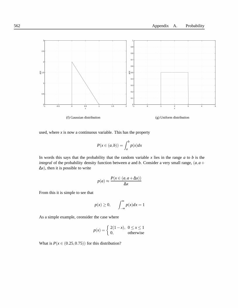
562 Appendix A. Probability
−1 −0.5 0 0.5 1 1.5 20
0.5
1
1.5
2
2.5
3
x
p(x)
(f) Gaussian distribution
−1 0 1 2 3 4 50
0.1
0.2
0.3
0.4
0.5
0.6
0.7
0.8
0.9
1
x
p(x)
(g) Uniform distribution
used, wherex is now a continuous variable. This has the property
P(x∈ (a,b)) =Z b
ap(x)dx
In words this says that the probability that the random variable x lies in the rangea to b is theintegral of the probability density function betweena andb. Consider a very small range,(a,a+∆x), then it is possible to write
p(a) ≈ P(x∈ (a,a+ ∆x))∆x
From this it is simple to see that
p(x) ≥ 0,Z ∞
−∞p(x)dx= 1
As a simple example, ceonsider the case where
p(x) =
2(1−x), 0≤ x≤ 10, otherwise
What isP(x∈ (0.25,0.75)) for this distribution?
Section A.3. Continuous Random Variables 563
A.3.2 Expected Values
In a similar fashion to the discrete case the expected valuesof continuous random variables can beobtained
E f (x) =Z ∞
−∞f (x)p(x)dx
This naturally leads to the moments of continuous variables. For example the mean,µ, is definedas
µ= E x =Z ∞
−∞xp(x)dx
For the simple example overleaf
µ=
Z ∞
−∞xp(x)dx=
Z 1
0x(2(1−x))dx=
13
Similarly the higher order moments and variance may be calculated (any doubts work this out).The same rules apply for continuous variables as discrete variables for linear combinations.
A.3.3 Gaussian Distribution
The most commonly used distribution (for reasons explainedlater) is theGaussian(or Normal)distribution. This has the form
p(x) =1√
2πσ2exp
(
−(x−µ)2
2σ2
)
Looking at the first few moments of a Gaussian distribution
E x0= E 1 = 1, E x1= µ, E x2= σ2 +µ2
A.3.4 Uniform Distribution
Another distribution is theuniform distribution . This is defined as
p(x) =
1b−a, a≤ x≤ b0, otherwise
Again it is simple to compute the moments of the uniform distribution. For the example above
E x =Z ∞
−∞xp(x)dx=
Z 3
1
12
xdx= (9−1)/4 = 2

564 Appendix A. Probability
−3 −2 −1 0 1 2 3 4 50
0.05
0.1
0.15
0.2
0.25
0.3
0.35
0.4
x
p(x)
(h) Gaussian Distribution
−3 −2 −1 0 1 2 3 4 50
0.1
0.2
0.3
0.4
0.5
0.6
0.7
0.8
0.9
1
x
F(x
)
(i) Gaussian CDF
A.3.5 Cumulative Density Functions
In addition to PDFs we sometimes use cumulative density functions (CDFs). These are defined as
F(a) = P(x≤ a) =
Z a
−∞p(x)dx
But from earlier
p(a) ≈ P(x∈ (a,a+ ∆x))∆x
=F(a+ ∆x)−F(a)
∆x
So in the limit∆x→ 0
p(a) =dF(x)
dx
∣∣∣∣a
In words the value of the PDF at pointa is the gradient of the CDF ata. The above figure showsthe Gaussian and associated CDF.
A.4 PAIRS OF CONTINUOUS RANDOM VARIABLES
All the aspects of discrete distributions have continuous equivalents.
• Marginal distributions : By analogy
px(x) =Z ∞
−∞p(x,y)dy

Section A.4. Pairs of Continuous Random Variables 565
−1.5 −1 −0.5 0 0.5 1 1.5−1.5
−1
−0.5
0
0.5
1
1.5
• Conditional probability :
p(y|x) =p(x,y)p(x)
=p(x,y)
R ∞−∞ p(x,y)dy
• Independence: For two random variables to be independent of one another
p(x,y) = p(x)p(y)
The same definition for correlation coefficient is used. It isinteresting to look at uncorrelated vsindependent data.
A.4.1 Independence vs Uncorrelated
Consider data generated by the following functionx =
[r cos(θ)r sin(θ)
]
θ is uniformly distributed in the range(0,2π) andr is Gaussian distributed,µ = 1.0 andσ = 0.1.From this data:
ΣΣΣ =
[0.50 0.000.00 0.50
]
The data is uncorrelated -Is it Independent?

566 Appendix A. Probability
A.4.2 Sum of Two Random Variables
In some situations (consider adding some noise to a clean speech signal) the distribution of thesum of two independent random variables,x andy, is required Let
z= x+y
pz(z) is required given thatpy(y) andpx(x) are known (in the same fashion as PMFs the subscriptson the PDFs have been added to make the distribution clear). From previous results it is easy toobtain
• the mean (even ifx andy are not independent)
• the variance
The expression for the complete PDF ofz is required. This may be obtained byconvolving thetwo distributions
pz(z) = px(x)⊗ py(y) =
Z ∞
−∞px(x)py(z−x)dx
A.4.3 Entropy
For discrete RVs entropy was used as a measure of how “random”a distribution is. For continuousRVs entropy,H, is defined as
H = −Z ∞
−∞p(x) log(p(x))dx
= E
log
(1
p(x)
)
Note:
1. log() is the natural log, not base 10, or base 2.
2. By definition 0log(0) = 0.
Entropy of continuous random variables is measured in nats (compare to bits for the discretedistributions). It is worth noting that of all the continuous distributions having meanµand varianceσ2 the distribution with the greatest entropy is the Gaussian distribution. (Try and compute theentropy of a Gaussian distribution).
A.4.4 Kullback-Leibler Distance
It will be useful to measure how “close” two distributions are. One measure if the Kullback-Leiblerdistance (or relative entropy). This is defined as
DKL(p(x),q(x)) =
Z ∞
−∞q(x) log
(q(x)p(x)
)
dx

Section A.4. Pairs of Continuous Random Variables 567
This has the attribute that
DKL(p(x),q(x)) ≥ 0
and
DKL(p(x),q(x)) = 0
if, and only if, p(x) = q(x). Note that Kullback-Liebler distance is not necessarily symmetric, nornecessarily satisfy the triangular inequality (will be discussed later in the course).

B PHONE DEFINITIONS
Symbol Example wordTranscription Symbol Example wordTranscriptionb BEE B iy l LAY L eyd DAY D ey r RAY R eyg GAY G ey w WAY W eyp PEA P iy y YACHT Y aa tt TEA T iy iy BEET b IY tk KEY K iy ih BIT b IH tdx MUDDY m ah DX iy eh BET b EH tjh JOKE JH ow k ey BAIT b EY tch CHOKE CH ow k ae BAT b AE ts SEA S iy aa BOT b AA tsh SHE SH iy aw BOUT b AW tz ZONE Z ow n ay BITE b AY tzh AZURE ae ZH er ah BUTT b AH tf FIN F ih n ao BOUGHT b AO tth THIN TH ih n oy BOY b OYv VAN V ae n ow BOAT b OW tdh THEN DH e n uh BOOK b UH khh HAY HH ey uw BOOT b UW tm MOM M aa M er BIRD b ER dn NOON N uw N ax ABOUT AX b aw tng SING s ih NG axr BUTTER b ah d axr
Figure B.1 Definition of modified TIMIT phoneme inventory for General American, with examplewords
568

569
Symbol Word initial exampleWord final example Symbol Word initial exampleWord final examplep PIP RIP j YIP -t TIP WRIT ii HEAT PEEL
k KIP KICK ih HIT PILL
b BIP RIB ei HATE PATE
d DIP RID e HET PET
g GAP RIG aa HEART PART
ch CHIP RICH a HAT PAT
dz GYP RIDGE uu HOOT POOT
m MIP RIM u FULL PUT
n NIP RUN ou MOAT BOAT
ng * RING uh HUT PUTT
f FOP RIFF oo HAUGHT CAUGHT
th THOUGHT KITH o HOT POT
s SIP REECE ai HEIGHT BITE
sh SHIP WISH au LOUT BOUT
v VOTE SIV oi NOISE BOIL
dh THOUGH WRITHE i@ HEAR PIER
z ZIP FIZZ e@ HAIR PEAR
zh VISION u@ SURE PURE
h HIP - @@ HER PURR
l LIP PULL @ CHINA ABOUT
r RIP CAR w WIP -
Figure B.2 Definition of British English MRPA phoneme inventory, with example words
æ V* ••<••T•'• u•5•o• • =••••Œ•a•
œ••ø•e•
y•i •
Figure B.3 IPA Vowel chart. The position of each vowel indicates the position of the tongue used toproduce that vowel. Front vowels are to the left, back vowelsto the right. Where a unrounded/roundedpair occurs, the unrounded version is on the left.
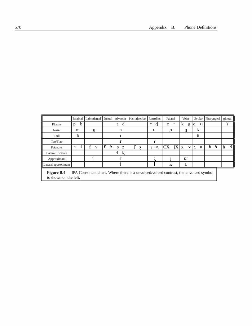
570 Appendix B. Phone Definitions
Bilabial Labiodental Dental Alveolar Post-alveolarRetroflex Palatal Velar Uvular Pharyngeal glottal
Plosive p b t d P c , k g q bNasal m 4 n 9 7 8 :Trill B r R
Tap/Flap D FFricative C f v S s z M ` L _ CX jX X [ K # h $
Lateral fricative / 1Approximant Y G H j 6
Lateral approximant l 0 \ L
Figure B.4 IPA Consonant chart. Where there is a unvoiced/voiced contrast, the unvoiced symbolis shown on the left.

Bibliography
[1] A BNEY, S. Chunks and dependencies: Bringing processing evidenceto bear on syntax.In Computational Linguistics and the Foundations of Linguistic Theory, J. Cole, G. Green,and J. Morgan, Eds. CSLI, 1995, pp. 145–164.
[2] A BRANTES, A. J., MARQUES, J. S.,AND TRANCOSO, I. M. Hybrid sinusoidal modelingof speech without voicing decision. InProceedings of Eurospeech 1991(1991).
[3] ACERO, A. Source filter models for time-scale pitch-scale modification of speech. InProceedings of the International Conference on Speech and Language Processing 1998(1998).
[4] ACERO, A. Formant analysis and synthesis using hidden markov models. In Proceedingsof Eurospeech 1999(1999).
[5] A DELL, J., AND BONAFONTE, A. Toward phone segmentation for concatenative speechsynthesis. InProceedings of the 5th ISCA Speech Synthesis Workshop(2004).
[6] A DRIEN, K. Andean Worlds: Indigenous History, Culture and Consciousness. Universityof New Mexico Press, 2001.
[7] AGUERO, P., WIMMER , K., AND BONAFONTE, A. Joint extraction and prediction ofFujisaki’s intonation model parameters.Proceedings of International Conference on SpokenLanguage Processing(2004).
[8] A INSWORTH, W. A system for converting english text into speech.IEEE Transactions onaudio and electroacoustics 21(1973).
[9] A LIAS, F., AND LLORA, X. Evolutionary weight tuning based on diphone pairs for unitselection speech synthesis. InProceedings of Eurospeech 2003(2003).
[10] ALLEN , J., HUNNICUT, S., AND KLATT, D. From Text to Speech: the MITalk System.Cambridge University Press, 1987.
[11] ALLWOOD, J. On the analysis of communicative action.Gothenburg Papers in TheoreticalLinguistics 38(1978).
[12] ALVVAREZ , Y. V., AND HUCKVALE , M. The reliability of the itu-t p.85 standard for theevaluation of text-to-speech systems. InProceedings of the International Conference onSpeech and Language Processing 2002(2002).
571
572 Appendix B. Phone Definitions
[13] ALWAN , A., NARAYANAN , S., AND HAKER, K. Towards articulatory-acoustic modelsfor liquid consonants based on MRI and EPG data. part II: The rhotics. Journal of theAcoustical Society of America 101, 2 (1997), 1078–1089.
[14] AMD M TATHAM , E. L. Word and syllable concatenation in text-to-speech synthesis. InProceedings of the European Conference on Speech 1999(1999).
[15] AMDAL , I., AND SVENDSEN, T. Unit selection synthesis database development usingutterance verification. InProceedings of Eurospeech 2005(2005).
[16] ANDERSON, M. D., PIERREHUMBERT, J. B.,AND L IBERMAN , M. Y. Synthesis by ruleof English intonation patterns. InProceedings of the International Conference on AcousticsSpeech and Signal Processing 1984(1984).
[17] ANDERSON, S. R.Phonology in the Twentieth Century. University of Chicago Press, 1985.
[18] ASANO, H., NAKAJIMA , H., MIZUNO, H., AND OKU , M. Long Vowel Detection forLetter-to-sound Conversion for Japanese Sourced Words Transliterated into the Alphabet.In Proceedings of Interspeech 2004(2004).
[19] ASCHER, M., AND ASCHER, R. Code of the Quipu: A Study in Media, Mathematics, andCulture. University of Michigan Press, 1980.
[20] ATAL , B. S.,AND HANAUER, L. Speech analysis and synthesis by linear prediction of thespeech wave.Journal of the Acoustical Society of America 50(1971), 637–655.
[21] ATTERER, M., AND LADD , D. R. On the phonetics and phonology of ”segmental anchor-ing” of f0: Evidence from german.Journal of Phonetics 32(2004), 177–197.
[22] AUBERGE, V., AUDIBERT, N., AND RILLIARD , A. Why and how to control the authenticemotional speech corpora. InProceedings of Eurospeech 2003(2003).
[23] AYLETT, M. P. The dissociation of deaccenting, givenness and syntactic role in sponta-neous speech. InProceedings of the XIVth International Congress of Phonetic Science1999(1999), pp. 1753–1756.
[24] AYLETT, M. P. Stochastic suprasegmentals: Relationships betweenredundancy, prosodicstructure and care of articulation in spontaneous speech. In Proceedings of the InternationalConference on Speech and Language Processing 2000(2000).
[25] AYLETT, M. P. Synthesising hyperarticulation in unit selection TTS. In Proceedings ofEurospeech 2005(2005).
[26] BACHENKO, J., AND FITZPATRICK, E. A computational grammar of discourse-neutralprosodic phrasing in English.Computational Linguistics 16, 3 (1990), 155–170.
[27] BAGSHAW, P. Phonemic transcription by analogy in text-to-speech synthesis: Novel wordpronunciation and lexicon compression.Computer Speech & Language 12, 2 (1998), 119–142.
[28] BAGSHAW, P. C., HILLER , S. M., AND JACK , M. A. Enhanced pitch tracking and theprocessing of F0 contours for computer aided intonation teaching. InProceedings of Eu-rospeech 1993(1993), pp. 1003–1006.
573
[29] BAILLY , G. No future for comprehensive models of intonation?Computing prosody:Computational models for processing spontaneous speech, Y. Sagisaka, N. Campbell, andN. Higuchi, Editors. Springer Verlag(1997), 157–164.
[30] BAILLY , G., BERAR, M., ELISEI, F., AND ODISIO, M. Audiovisual speech synthesis.International Journal of Speech Technology 6(2003), 331–346.
[31] BAILLY , G., AND HOLM , B. SFC: A trainable prosodic model.Speech Communication46, 3-4 (2005), 348–364.
[32] BAILLY , G., AND TRAN, A. Compost: A rule compiler for speech synthesis. InProceed-ings of Eurospeech 1989(1989), pp. 136–139.
[33] BAKER, J. K. The DRAGON system–an overview.IEEE Transactions on Acoustics,Speech, and Signal Processing 23(1)(1975), 24–29.
[34] BANZINER, T., MOREL, M., AND SCHERER, K. Is there an emotion signature in into-national patterns? and can it be used in synthesis? InProceedings of Eurospeech 2003(2003).
[35] BARBOSA, P., AND BAILLY , G. Characterization of rhythmic patterns for text-to-speechsynthesis.Speech Communication 15, 1 (1994), 127–137.
[36] BAUM , L. E., PETERIE, T., SOULED, G., AND WEISS, N. A maximization techniqueoccurring in the statistical analysis of probabilistic functions of Markov chain.The Annalsof Mathematical Statistics 41, 1 (1970), 249–336.
[37] BELL, P., BURROWS, T., AND TAYLOR , P. Adaptation of prosodic phrasing models. InProceedings of Speech Prosody 2006(2006).
[38] BELLEGARDA, J. Unsupervised, language-independent grapheme-to-phoneme conver-sion by latent analogy. Acoustics, Speech, and Signal Processing, 2003. Proceed-ings.(ICASSP’03). 2003 IEEE International Conference on 1(2003).
[39] BELLEGARDA, J. R. A novel discontinuity metrica for unit selection text-to-speech syn-thesis. In5th ISCA Workshop on Speech Synthesis(2004).
[40] BENNETT, C. L. Large scale evaluation of corpus-based synthesizers: Results and lessonsfrom the blizzard challenge 2005. InProceedings of the Interspeech 2006(2005).
[41] BESKOW, J. Rule-based visual speech synthesis. InProceedings of Eurospeech 1995(1995).
[42] BEUTNAGEL, M., CONKIE, A., AND SYRDAL , A. Diphone synthesis using unit selection.In Proceedings of the Third ISCA Workshop on Speech Synthesis(1998).
[43] BIRD, S. Computational Phonology: A Constraint-Based Approach. Studies in NaturalLanguage Processing. Cambridge University Press, 1995.
[44] BISANI , M., AND NEY, H. Investigations on joint-multigram models for grapheme-to-phoneme conversion.Proc. Int. Conf. on Spoken Language Processing 1(2002), 105–108.
[45] BISHOP, C. M. Neural Networks for Pattern Recognition. Oxford University Press, 1995.[46] BISHOP, C. M. Pattern Recognition and Machine Learning. Springer, 2006.

574 Appendix B. Phone Definitions
[47] BLACK , A. Unit selection and emotional speech. InProceedings of Eurospeech 2003(2003).
[48] BLACK , A., AND BENNETT, C. L. Blizzard challange 2006. InProceedings of the Inter-speech 2006(2006).
[49] BLACK , A., AND TAYLOR , P. Automatically clustering similar units for unit selection inspeech synthesis. InProceedings of Eurospeech 1997(1997), vol. 2, pp. 601–604.
[50] BLACK , A., AND TOKUDA , K. Blizzard challange 2006: Evaluating corpus-based speechsynthesis on common datasets. InProceedings of the Interspeech 2005(2005).
[51] BLACK , A. W., AND HUNT, A. J. Generation F0 contours from ToBI labels using linearregression. InComputer Speech and Language(1996).
[52] BLACK , A. W., AND LENZO, K. A. Limited domain synthesis. InProceedings of theInternational Conference on Speech and Language Processing 2000(2000).
[53] BLACK , A. W., AND TAYLOR , P. CHATR: A generic speech synthesis system. InCOLING1994(1994), pp. 983–986.
[54] BLACK , A. W., AND TAYLOR , P. Assigning phrase braks from part-to-speech sequences.In Proceedings of Eurospeech 1997(1997).
[55] BLACK , A. W., TAYLOR , P., AND CALEY, R. The Festival Speech Synthesis System.Manual and source code avaliable at http://www.cstr.ed.ac.uk/projects/festival.html, 1996-2006.
[56] BLACK , A. W., AND TAYLOR , P. A. A framework for generating prosody from high levellinguistics descriptions. InSpring meeting, Acoustical society of Japan(1994).
[57] BLOOMFIELD, L. Language. New York: Henry Holt, 1933.[58] BLUMSTEIN, S.,AND CUTLER, A. Speech perception: Phonetic aspects. InInternational
Encyclopedia of Language, W. J. Frawley, Ed., vol. 4. Oxford University Press, 2003.[59] BOD, R., HAY, J., AND JANNEDY, S. Probabilistic Linguistics. MIT Press, Cambridge,
M.A., 1999.[60] BOERSMA, P. Functional Phonology Formalizing the interactions between articulatory
and perceptual drives. PhD thesis, University of Amsterdam, 1998.[61] BOSWELL, J. The Life of Samuel Johnson. Everyman’s Library, 1791.[62] BOULA DE MAREUIL , P., YVON, F., DALESSANDRO, C., AUBERGE, V., BAGEIN, M.,
BAILLY , G., BECHET, F., FOUKIA , S., GOLDMAN , J., KELLER, E., ET AL. Evaluationof grapheme-to-phoneme conversion for text-to-speech synthesis in French.Proceedings ofFirst International Conference on Language Resources & Evaluation (1998), 641–645.
[63] BOULARD, H., HERMANSKY, H., AND MORGAN, N. Towards increasing speech recog-nition error rates.Speech Communication 18(1996), 205–255.
[64] BOYER, C. B. History of Mathematics. Princeton University Press, 1985.[65] BREEN, A. P., AND JACKSON, P. A phonologically motivated method of selecting non-
uniform units. InInternational Conference on Speech and Language Processing (1998).
575
[66] BREGLER, C., COVELL, M., AND SLANEY, M. Video rewrite: Visual speech synthesisfrom video. InProceedings of Eurospeech 1997(1997).
[67] BRILL , E. Transformation-based error-driven learning and natural language processing: Acase study in part of speech tagging.Computational Linguistics(1995).
[68] BROOKES, D. M., AND LOKE, H. P. Modelling energy flow in the vocal tract with ap-plications to glottal closure and opening detection. InProceedings of the InternationalConference on Acoustics Speech and Signal Processing, 1999(1999).
[69] BROWMAN, C. P.,AND GOLDSTEIN, L. Towards an articulatory phonology.PhonologyYearbook 3(1986), 219–252.
[70] BROWMAN, C. P.,AND GOLDSTEIN, L. Articulatory phonology: an overview.Phonetica49 (1992), 155–180.
[71] BU, S., YAMAMOTO, M., AND ITAHASHI, S. An Automatic Extraction Method ofF0 Generation Model Parameters.IEICE Transactions on Information and Systems 89, 1(2006), 305.
[72] BUHMANN , J., VEREECKEN, H., FACKRELL, J., MARTENS, J. P.,AND COILE, B. V.Data driven intonation modelling of 6 languages. InProceedings of the International Con-ference on Spoken Language Processing 2000(2000).
[73] BULT, M., BUSSO, C., TILDIM , S., KAZEMZADEH , A., LEE, C. M., LEE, S., AND
NARAYANAN , S. Investigating the role of phoneme-level modifications in emotional speechresynthesis. InProceedings of the International Conference on Speech and Language Pro-cessing 2002(2002).
[74] BULYKO , I., AND OSTENDORF, M. Unit selection for speech synthesis using splicing costswith weighted finite state transders. InProceedings of Eurospeech 2001(2001).
[75] BUNNELL, H. T., HOSKINS, S. R.,AND YARRINGTON, D. Prosodic vs segmental con-tributions to naturalness in a diphone synthesizer. InProceedings of the International Con-ference on Speech and Language Processing 1998(1998).
[76] BUSSER, B., DAELEMANS, W., AND VAN DEN BOSCH, A. Machine learning of wordpronunciation: the case against abstraction. InProceedings Eurospeech 1999(1999).
[77] BUSSER, B., DAELEMANS, W., AND VAN DEN BOSCH, A. Predicting phrase breaks withmemory-based learning. In4th ISCA Tutorial and Research Workshop on Speech Synthesis(2001).
[78] C J FILLMORE, P KAY, P.,AND O’CONNOR, C. Regularity and idiomaticity in grammat-ical constructions: The case of let alone.Language 64(1988), 501–538.
[79] CAHN , J. The generation of affect in synthesized speech.Journal of the American VoiceI/O Society 8(1990), 1–19.
[80] CAHN , J. A computational memory and processing model for prosody. In InternationalConference on Speech and Language Processing(1998).

576 Appendix B. Phone Definitions
[81] CAMPBELL, N. Towards synthesizing expressive speech; designing andcollecting expres-sive speech data. InProceedings of Eurospeech 2003(2003).
[82] CAMPBELL, N. Conventional speech synthesis and the need for some laughter. IEEETransactions on Audio, Speech and Language Processing 14, 4 (2006).
[83] CAMPBELL, W. N. Syllable-based segmental duration. InIn Talking Machines: Theories,Models and Designs, C. B. G Bailly and T. R. Sawallis, Eds. Elsevier Science Publishers,Amsterdam, 1992, pp. 211–224.
[84] CAMPBELL, W. N. A high-definition speech. re-sequencing system.Proceedings of thethird ASA/ASJ Joint Meeting(1996), 373–376.
[85] CHASAN, D. Speech reconstruction from mel frequency cepstral coefficients and pitch. InProceedings of the International Conference on Acoustics Speech and Signal Processing2000(2000).
[86] CHEN, S. F. Conditional and joint models for grapheme-to-phoneme conversion. InPro-ceedings of Eurospeech 2003(2003).
[87] CHEN, W., LIN , F., AND ZHANG, J. L. B. Training prosodic phrasing rules for chineseTTS systems. InProceedings of Eurospeech 2001(2001).
[88] CHOMSKY, N. Syntactic Structures. Mouton, The Hague, 1957.[89] CHOMSKY, N. Aspects of the Theory of Syntax. MIT University Press, 1965.[90] CHOMSKY, N. Knowledge of Language: Its Nature, Origin and Use. Praeger, 1986.[91] CHOMSKY, N., AND HALLE , M. The Sound Pattern of English. Harper and Row, 1968.[92] CHU, M., PENG, H., YANG, H. Y., AND CHANG, E. Selecting non-uniform units from a
very large corpus for concatenative speech synthesizer. InProceedings of the InternationalConference on Acoustics Speech and Signal Processing 2001(2001).
[93] CHU, M., PENG, H., ZHAO, Y., NIU , Z., AND CHAN , E. Microsoft mulan - a bilingualTTS system. InProceedings of the International Conference on Acoustics Speech andSignal Processing 2003(2003).
[94] CHURCH, K. W., AND GALE, W. A. A comparison of the enhanced good-turing anddeleted estimation methods for estimating probabilities of english bigrams. ComputerSpeech and Language 5(1991), 19–54.
[95] CLARK , H. H. Using language. Cambridge University Press, 1996.[96] CLARK , H. H., AND CLARK , E. V. Psychology and language: An introduction to psy-
cholinguistics. Harcourt Brace Jovanovich, 1977.[97] CLARK , J., AND YALLOP, C. An Introduction to Phonetics and Phonology. Basil Black-
well, 1990.[98] CLARK , R., AND DUSTERHOFF, K. Objective methods for evaluating synthetic intonation.
In Proceedings of Eurospeech 1999(1999).[99] CLARK , R. A. J., RICHMOND, K., AND K ING, S. Festival 2 - build your own general pur-
pose unit selection speech synthesiser. In5th ISCA Workshop on Speech Synthesis(2004).

577
[100] CLEMENTS, G. N. The geometry of phonological features.Phonology Yearbook 2(1985),225–252.
[101] COHEN, M. M., AND MASSARO, D. W. Modeling coarticulation in synthetic visualspeech. InModels and Techniques in Computer Animation(1993), pp. 141–155.
[102] COLE, R. Roadmaps, journeys and destinations: Speculations on the future of speechtechnology research. InProceedings of Eurospeech 2003(2003).
[103] COLOTTE, V., AND BEAUFORT, R. Linguistic features weighting for a text-to-speechsystem without prosody model. InProceedings of Eurospeech 2005(2005).
[104] CONKIE, A. A robust unit selection system for speech synthesis. In137th meeting of theAcoustical Society of America(1999).
[105] CONKIE, A. D., AND ISARD, S. Optimal coupling of diphones. InProceedings of Eu-rospeech 1995(1995).
[106] COOPER, F. S., LIBERMAN , A. M., AND BORST, J. M. The interconversion of audibleand visible patterns as a basis for research in the perception of speech.Proceedings of theNational Academy of Science 37(5)(1951), 318–325.
[107] COOPER, W. E.,AND SORENSEN, J. M. Fundamental Frequency in Sentence Production.Springer-Verlag, 1981.
[108] COORMAN, G., FACKRELL, J., RUTTEN, P.,AND COILE, B. V. Segment selection in theLH realspeak laboratory TTS system. InProceedings of the International Conference onSpoken Language Processing 2000(2000).
[109] CORDOBA, R., VALLEJO, J. A., MONTERO, J. M., GUTIERREZ-ARRIOLA, J., LOPEZ,M. A., AND PARDO, J. M. Automatic modeling of duration in a Spanish text-to-speechsystem using neural networks. InProceedings of Eurospeech 1999(1999).
[110] CORNELIUS, R. Theoretical approaches to emotion. InICSA Workshop on Speech andEmotion(2000).
[111] CORTES, C., AND VAPNIK , V. Support-vector networks.Machine Learning 20, 3 (1995),273–297.
[112] COWIE, R., DEVILLERS, L., MARTIN , J.-C., COWIE, R., SAVVIDOU , S., ABRILIAN ,S., AND COX, C. Multimodal databases of everyday emotion: Facing up to complexity. InProceedings of Eurospeech, Interspeech 2005(2005).
[113] COWIE, R., DOUGLAS-COWIE, E., TSAPATSOULIS, N., VOTSIS, G., KOLLIAS, S., FEL-LENZ, W., AND TAYLOR , J. Emotion recognition in human-computer interaction.IEEESignal Processing Magazine(2001).
[114] CRISTIANINI , N., AND SHAWE-TAYLOR , J. Nello Cristianini and John Shawe-Taylor. AnIntroduction to Support Vector Machines and other kernel-based learning methods. Cam-bridge Universtity Press, 2000.

578 Appendix B. Phone Definitions
[115] CRONK, A., AND MACON, M. Optimized stopping criteria for tree-based unit selectionin concatenative synthesis. InProceedings of the International Conference on Speech andLanguage Processing 1998(1998).
[116] CROWE, A., AND JACK , M. A. A globally optimising format tracker using generalisedcentroids.Electronic Letters 23(1987), 1019–1020.
[117] CRYSTAL, D. Prosodic Systems and Intonation in English. Cambridge Studies in Linguis-tics. Cambridge Universtity Press, 1969.
[118] D’ A LESSANDRO, C., AND MERTENS, P. Automatic pitch contour stylization using amodel of tonal perception. InComputer Speech and Language(1995).
[119] DAELEMANS, W., VAN DEN BOSCH, A., AND ZAVREL, J. Forgetting Exceptions isHarmful in Language Learning.Machine Learning 34, 1 (1999), 11–41.
[120] D’A LESSANDRO, C., AND DOVAL , B. Voice quality modification for emotional speechsynthesis. InProceedings of Eurospeech 2003(2003).
[121] D’A LESSANDRO, C., AND MERTENS, P. Automatic pitch contour stylization using amodel of tonal perception.Computer Speech & Language 9, 3 (1995), 257–288.
[122] DAMPER, R., AND EASTMOND, J. Pronunciation by analogy: Impact of implementationalchoices on performance.Language and Speech 40, 1 (1997), 1–23.
[123] DAMPER, R., MARCHAND, Y., ADAMSON, M., AND GUSTAFSON, K. Evaluating thepronunciation component of text-to-speech systems for English: A performance compari-son of different approaches.Computer Speech and Language 13, 2 (1999), 155–176.
[124] DARWIN , C. The Expression of the Emotions in Man and Animals. John Murray, 1872.
[125] DAVID D. LEWIS, W. A. G. A sequential algorithm for training text classifiers. In 17thACM International Conference on Research and Development in Information Retrieval(1994).
[126] DAVITZ , J. Auditory correlates of vocal expression of emotional feeling. In The Commu-nication of Emotional Meaning. Mcgraw Hill, 1964.
[127] DEDINA, M., AND NUSBAUM, H. Pronounce: a program for pronunciation by analogy.Computer speech & language(Print) 5, 1 (1991), 55–64.
[128] DELLER, J. R.,AND PROAKIS, J. Discrete-Time Processing of Speech Signals. John Wileyand Sons, 2000.
[129] DENG, L., BAZZI , I., AND ACERO, A. Tracking vocal track resonances using an analyticalnonlinear predictor and a target guided temporal constraint. In Proceedings of Eurospeech2003(2003).
[130] DEVILLERS, L., AND VASILESCU, I. Prosodic cues for emotion characterization in real-life spoken dialogs. InProceedings of Eurospeech 2003(2003).
[131] DIAZ , F. C., ALBA , J. L., AND BANGA , E. R. A neural network approach for the designof the target cost function in unit-selection speech synthesis. InProceedings of Eurospeech2005(2005).

579
[132] DILLEY, L., LADD , D., AND SCHEPMAN, A. Alignment of L and H in bitonal pitchaccents: Testing two hypotheses.Journal of Phonetics 33, 1 (2005), 115–119.
[133] DINES, J., AND SRIDHARAN , S. Trainable speech with trended hidden markov models.In Proceedings of the International Conference on Acoustics Speech and Signal Processing2001(2001).
[134] DINES, J., SRIDHARAN , S.,AND MOODY, M. Application of the trended hidden Markovmodel to speech synthesis. InProceedings of Eurospeech 2001(2001).
[135] DING, W., AND CAMPBELL, N. Optimising unit selection with voice sourse and formantsin the Chatr speech synthesis system. InProceedings of Eurospeech 1997(1997).
[136] DIVAY , M., AND V ITALE , A. J. A computational grammar of discourse-neutral prosodicphrasing in English.Computational Linguistics 23, 4 (1997), 495–523.
[137] DONEGAN, P. J., AND STAMPE, D. The study of natural phonology. InCurrent Ap-proaches to Phonological Theory, D. Dinnsen, Ed. Indiana University Press, 1979, pp. 126–173.
[138] DONOVAN, R. E.,AND EIDE, E. The IBM trainable speech synthesis system. InProceed-ings of the International Conference on Speech and LanguageProcessing 1998(1998).
[139] DONOVAN, R. E., FRANZ, M., SORENSEN, J. S.,AND ROUKOS, S. Phrase splicing andvariable substitution using the IBM trainable speeech synthesis system. InProceedings ofProceedings of the International Conference on Acoustics Speech and Signal Processing1999(1999), pp. 373–376.
[140] DONOVAN, R. E.,AND WOODLAND, P. C. Automatic speech synthesiser parameter esti-mation using HMMS. InProceedings of the International Conference on Acoustics Speechand Signal Processing 1995(1995).
[141] DROPPO, J.,AND ACERO, A. Maximum a posteriori pitch tracking. InProceedings of theIEEE International Conference on Acoustics, Speech, and Signal Processing 1998(1998).
[142] DUDA , R. O., HART, P. E.,AND STORK, D. G. Pattern Classification. John Wiley andSons, 2000.
[143] DUDLEY, H. Remaking speech.Journal of the Acoustical Society of America 11(1939),169–177.
[144] DURAND, J. Dependency and Non-Linear Phonology. Croom Helm, 1986.
[145] DURAND, J., AND ANDERSON, J. Explorations in Dependancy Phonology. Foris, 1987.
[146] DUSTERHOFF, K., AND BLACK , A. Generating f0 contours for speech synthesis using thetilt intonation theory. InProceedings of Eurospeech 1997(1997).
[147] DUSTERHOFF, K. E., BLACK , A. W., AND TAYLOR , P. Using decision trees within thetilt intonation model to predict F0 contours. InProceedings of Eurospeech 1999(1999).
[148] DUTOIT, T. An Introduction to Text to Speech Synthesis. Kluwer Academic Publishers,1997.

580 Appendix B. Phone Definitions
[149] DUTOIT, T., AND LEICH, H. Text-to-speech synthesis based on an MBE re-synthesis ofthe segments database.Speech Communication 13(1993), 435–440.
[150] EIDE, E., AARON, A., BAKIS, R., COHEN, P., DONOVAN, R., MATHES, W. H. T.,PICHENY, M., POLKOSKY, M., SMITH , M., AND V ISWANATHAN , M. Recent improve-ments to the IBM trainable speech synthesis system. InProceedings of the InternationalConference on Acoustics Speech and Signal Processing 2003(2003).
[151] EIDE, E., AARON, A., BAKIS, R., HAMZA , W., AND PICHENY, M. J. A corpus-basedapproach to AHEM expressive speech synthesis. InProceedings of the 5th ISCA Workshopon Speech Synthesis(2005).
[152] EKMAN , P. Universals and cultural differences in facial expressions of emotion. InNe-braska Symposium on Motivation(1972), University of Nebraska Press.
[153] EKMAN , P. Basic Emotions The Handbook of Cognition and Emotion. John Wiley Ltd,1999.
[154] EKMAN , P., AND FRIESEN, W. V. Unmasking the Face. Consulting Pscyhologists Press,1975.
[155] ELOVITZ , H. S., JOHNSON, R., MCHUGH, A., AND SHORE, J. Letter-to-sound rules forautomatic translation of English text to phonetics.IEEE Transactions acoustics speech andsignal processing 24(1976), 446–459.
[156] F GROSJEAN, L. G., AND LANE, H. The patterns of silence: Performance structures insentence production.Cognitive Psychology 11(1979), 58–81.
[157] FACKRELL, J. W. A., VEREECKEN, H., MARTENS, J. P.,AND COILE, B. V. Multilingualprosody modelling using cascades of regression trees and neural networks. InProceedingsof Eurospeech 1999(1999).
[158] FANT, G. Acoustic Theory of Speech Production. Mouton, 1960.
[159] FANT, G. Glottal flow: models and interaction.Journal of Phonetics 14(1986), 393–399.
[160] FISHER, R. A. the use of multiple measures in taxonomic problems.Annals of Eugenics 7(1936), 179–188.
[161] FITT, S., AND ISARD, S. The generation of regional pronunciations of english for speechsynthesis. InProceedings Eurospeech 1997(1997).
[162] FITT, S., AND ISARD, S. Representing the environments for phonological processes in anaccent-independent lexicon for synthesis of english. InProceedings of the InternationalConference on Speech and Language Processings 1998(1998).
[163] FITT, S., AND ISARD, S. The treatment of vowels preceding ’r’ in a keyword lexicon ofenglish. InProceedings ICPhS 99(1999).
[164] FLANAGAN , J. L. Speech analysis, synthesis and perception. Springer-Verlag, 1972.
[165] FUJISAKI, H., AND HIROSE, K. Analysis of voice fundamental frequency contours fordeclarative sentences of Japanese.Journal of the Acoustical Society of Japan 5, 4 (1984),233–241.

581
[166] FUJISAKI, H., AND KAWAI , H. Modeling the dynamic characteristics of voice fundamentalfrequency with applications to analysis and synthesis of intonation. InWorking Group onIntonation, 13th International Congress of Linguists(1982).
[167] FUJISAKI, H., AND KAWAI , H. Realization of linguistic information in the voice fun-damental frquency contour of the spoken Japanese. InProceeding of the InternationalConference on Acoustics Speech and Signal Processing 1988(1988).
[168] FURUI, S. Digital Speech Processing, Synthesis and Reccognition. Marcel Dekker, 2001.
[169] GALE, W. A., CHURCH, K. W., AND YAROWSKY, D. Using bilingual materials to de-velop word sense disambiguation methods. InInternational Conference on Theoretical andMethodological Issues in Machine Translation(1992), pp. 101–112.
[170] GALES, M. J. F., JIA , B., LIU , X., SIM , K. C., WOODLAND, P. C.,AND YU, K. De-velopment of the CU-HTK 2004 Mandarin conversational telephone speech transcriptionsystem. InProceedings of the International Conference on Acoustics Speech and SignalProcessing 2005(2005).
[171] GALES, M. J. F., KIM , D. Y., WOODLAND, P. C., CHAN , H. Y., MRVA , D., SINHA ,R., AND TRANTER, S. E. Progress in the CU-HTK Broadcast News transcription system.IEEE Transactions Audio, Speech and Language Processing(2006).
[172] GALESCU, L., AND ALLEN , J. Name Pronunciation with a Joint N-Gram Model for Bi-directional Grapheme-to-Phoneme Conversion.Proc. ICSLP(2002), 109–112.
[173] GAROFOLO, J. S., LAMEL , L. F., FISHER, W. M., FISCUS, J. G.,PIKEETT, D. S.,AND
DAHLGREN, N. L. The DARPA-TIMIT acoustic-phonetic continuous speech corpus. Tech.rep., US Department of Commerce, Gaithersburg, MD [CD-ROM], 1990.
[174] GIEGERICH, H. J.English phonology: An introduction. Cambridge University Press, 1992.
[175] GLUSHKO, R. The organization and activation of orthographic knowledge in reading aloud.Journal of Experimental Psychology: Human Perception and Performance 5, 4 (1979),674–691.
[176] GOLD, B., AND MORGAN, N. Speech and Audio Signal Processing: Processing andPerception of Speech and Music. John Wiley and Sons, 1999.
[177] GOLDBERG, A. Constructions: A Construction Grammar Approach to Argument Structure.University of Chicago Press, 1995.
[178] GOLDFARB, C. F. The SGML Handbook. Oxford, Clarendon Press, 1990.
[179] GOLDSMITH, J. An overview of autosegmental phonology.Linguistic Analysis(1976),23–68.
[180] GOLDSMITH, J. Autosegmental and Metrical Phonology. Blackwell, 1990.
[181] GOLDSTEIN, M. Classification of methods used for the assessment of text-to-speech sys-tems according to the demands placed on the listener.Speech Communication 16(1995),225–244.

582 Appendix B. Phone Definitions
[182] GOUBANOVA , O., AND K ING, S. Predicting consonant duration with Bayesian beliefnetworks. InProceedings of the Interspeech 2005(2005).
[183] GRANSTROM, B. The use of speech synthesis in exploring different speaking styles.SpeechCommunication 11, 4-5 (1992), 347–355.
[184] GRICE, H. P. Logic and conversation. InSyntax and Semantics: Speech Acts, P. Cole andJ. Morgan, Eds., vol. 3. Academic Press, 1975.
[185] GRIFFIN, D., AND L IM , J. Multiband excitation vocoder. InIEEE Transactions on Acous-tics, Speech and Signal Processing(1988), vol. 36.
[186] GROSJEAN, F.,AND GEE, J. P. Prosodic structure and spoken word recognition.Cognition,156 (1987).
[187] GROVER, C., FACKRELL, J., VEREECKEN, H., MARTENS, J., AND VAN COILE, B.Designing Prosodic Databases for Automatic Modelling in 6 Languages. InProceedingsICSLP 1998(1998).
[188] GUSTAFSON, J., LINDBERG, N., AND LUNDEBERG, M. The August spoken dialoguesystem. InProceedings of Eurospeech 1999(1999).
[189] H KAWAHARA , I. M.-K., AND DE CHEVEIGNE, A. Restructuring speech representationsusing a pitch-adaptive time-frequency smoothing and an instantaneous-frequency-based F0extraction: Possible role of a repetitive structure in sounds. Speech Communication 27(1999), 187–207.
[190] H M MENG, C. K. K., K C SIU , T. Y. F., AND CHING, P. C. Cu vocal: Corpus-basedsyllable concatenation for chinese speech synthesis across domains and dialects. InPro-ceedings of the International Conference on Speech and Language Processing 2002(2002).
[191] HAIN , H.-U. A Hybrid approach for grapheme-to-phoneme conversion based on a com-bination of partial string matching and a neural network.Proceedings of the InternationalConference on Speech and Language Processing(2000).
[192] HAIN , T., WOODLAND, P. C., EVERMANN , G., GALES, M. J. F., LIU , X., MOORE,G. L., POVEY, D., AND WANG, L. Automatic transcription of conversational telephonespeech - development of the CU-HTK 2002 system.IEEE Transactions Audio, Speech andLanguage Processing(2005).
[193] HALLIDAY , M. A. Intonation and Grammar in British English. Mouton, 1967.
[194] HAMON , C., MOULINES, E., AND CHARPENTIER, F. A diphone synthesis system basedon time-domain modifications of speech”. InProceedings of the International Conferenceon Acoustics Speech and Signal Processing 1989(1989).
[195] HAMZA , W., BAKIS, R., EIDE, E. M., PICHENY, M. A., AND PITRELLI , J. F. The IBMexpressive speech synthesis system. InProceedings of the International Conference onSpoken Language Processing 2004(2004).

583
[196] HAMZA , W., BAKIS, R., SHUANG, Z. W., AND ZEN, H. On building a concatenativespeech synthesis system from the blizzard challenge speechdatabases. InProceedings ofthe Interspeech 2005(2005).
[197] HAMZA , W., RASHWAN, M., AND AFIFY, M. A quantitative method for modelling contextin concatenative synthesis using large speech database. InProceedings of the InternationalConference on Acoustics Speech and Signal Processing 2001(2001).
[198] HAN , K., AND CHEN, G. Letter-To-Sound for Small-footprint Multilingual TTSEngine.In Proceedings of Interspeech 2004(2004).
[199] HARRIS, R. Signs of Writing. Routledge, 1996.
[200] HENRICHSEN, P. J. Transformation-based learning of Danish stress assignment. In”Pro-ceedings of Eurospeech 2001(2001).
[201] HERTZ, S. R. Papers in Laboratory Phonology I: Between the Grammar and the Physicsof Speech. Cambridge University Press, 1990.
[202] HESS, W. Pitch Determination of Speech Signals. Springer-Verlag, 1983.
[203] HIRAI , T., TENPAKU, A., AND SHIKANO , K. Manipulating speech pitch periods accord-ing to optimal insertion/deletion position in residual signal for intonation control in speechsynthesis. InProceedings of the International Conference on Speech and Language Pro-cessing 2000(2000).
[204] HIRAI , T., AND TENPAKU, S. Using 5 ms segments in concatenative speech synthesis. In5th ISCA Workshop on Speech Synthesis(2005).
[205] HIROSE, K., ETO, M., AND M INEMATSU, N. Improved corpus-based synthesis of funda-mental frequency contours using generation process model.In Proceedings of the Interna-tional Conference on Acoustics Speech and Signal Processing 2002(2002).
[206] HIROSE, K., ETO, M., M INEMATSU, N., AND SAKURAI , A. Corpus-based synthesis offundamental frequency contours based on a generation process model. InProceedings ofEurospeech 2001(2001).
[207] HIRSCHBERG, J. Pitch accent in context: Predicting intonational prominence from text.Artificial Intelligence 63(1993), 305–340.
[208] HIRSCHBERG, J. Communication and prosody: functional aspects of prosody. SpeechCommunication 36(2002), 31–43.
[209] HIRSCHBERG, J., AND RAMBOW, O. Learning prosodic features using a tree representa-tion. In Proceedings of Eurospeech 2001(2001).
[210] HIRSCHFELD, D. Comparing static and dynamic features for segmental cost function cal-culation in concatenative speech synthesis. InProceedings of the International Conferenceon Spoken Language Processing 2000(2000).
[211] HIRST, D. Automatic analysis of prosody for multilingual speech corpora. Improvementsin Speech Synthesis. Chichester, UK: Wiley(2001).
584 Appendix B. Phone Definitions
[212] HIRST, D., AND DI CRISTO, A. Intonation Systems: a survey of twenty languages. Cam-bridge University Press, 1998.
[213] HIRST, D., DI CRISTO, A., AND ESPESSER, R. Levels of representation and levels ofanalysis for the description of intonation systems.Prosody: Theory and Experiment, Dor-drecht: Kluwer Academic Publishers(2000).
[214] HOCKETT, C. F. The origin of speech.Scientific American 203(1960), 88–96.
[215] HOGBERG, J. Data driven formant synthesis. InProceedings of Eurospeech 1997(1997).
[216] HOLM , B., AND BAILLY , G. Generating prosody by superposing multi-parametric over-lapping contours.Proceedings of the International Conference on Speech and LanguageProcessing(2000), 203–206.
[217] HOLM , B., AND BAILLY , G. Learning the hidden structure of intonation: Implementingvarious functions of prosody.Speech Prosody(2002), 399–402.
[218] HOLMES, J. N. The influence of the glottal waveform on the naturalness of speech froma parallel formant synthesizer.IEEE Transactions on Audio Electroacoustics 21(1980),298–305.
[219] HOLMES, J. N., MATTINGLY, I. G., AND SHEARME, J. N. Speech synthesis by rule.Language and Speech 7(1964), 127–143.
[220] HON, H., ACERO, A., HUANG, X., L IU , J., AND PLUMPE, M. Automatic generation ofsynthesis units for trainable text-to-speech systems. InProceedings of the IEEE Interna-tional Conference on Acoustics, Speech, and Signal Processing 1998(1998).
[221] HOUSE, A., WILLIAMS , C., HECKER, M., AND KRYTER, K. Articulation-Testing Meth-ods: Consonantal Differentiation with a Closed-Response Set.The Journal of the AcousticalSociety of America 37(1965), 158.
[222] HSIA, C.-C., WE, C. H., AND L IU , T.-H. Duration embedded bi-hmm for expressivevoice conversion. InProceedings of Interspeech 2005(2005).
[223] HUANG, J., ABREGO, G., AND OLORENSHAW, L. System and method for performing agrapheme-to-phoneme conversion. InProceedings Interspeech 2006(2006).
[224] HUANG, X., ACERO, A., AND HON, H.-W. Spoken Language Processing: A Guide toTheory, Algorithm and System Development. Prentice Hall, 2001.
[225] HUCKVALE , M. Speech synthesis, speech simulation and speech science. In Proceedings ofthe International Conference on Speech and Language Processing 2002(2002), pp. 1261–1264.
[226] HUNNICUT, S. Phonological rules for a text-to-speech system.Americal Journal of Com-putational Linguistics 57(1976), 1–72.
[227] HUNT, A. J., AND BLACK , A. W. Unit selection in a concatenative speech synthesissystem using a large speech database. InProceedings of the International Conference onSpeech and Language Processing 1996(1996), pp. 373–376.
585
[228] HUNT, M., ZWIERYNSKI, D., AND CARR, R. Issues in high quality lpc analysis andsynthesis. InProceedings of Eurospeech 1989(1989), pp. 348–351.
[229] IMAI , S. Cepstral analysis synthesis on the mel frequency scale,. In Proceedings of theInternational Conference on Acoustics Speech and Signal Processing 1983(1983), pp. 93–96.
[230] INANOGLU, Z., AND CANEEL, R. Emotive alert: HMM-based emotion detection in voice-mail messages.Proceedings of the 10th international conference on Intelligent user inter-faces(2005), 251–253.
[231] ISARD, S. D., AND PEARSON, M. A repertoire of British English contours for speechsynthesis. InProceedings of the 7th FASE Symposium, Speech 1988(1988).
[232] ISOGAI, J., YAMAGISHI , J., AND KOBAYASHI , T. Model adaptation and adaptive train-ingusing ESAT algorithm for HMM-based speech synthesis. In”Proceedings of Eu-rospeech 2005(2005).
[233] ITAKURA , F., AND SAITO , S. Analysis synthesis telephony based on the maximum likelihood method. InReports of the 6th International Conference on Acoustics(1968).
[234] IWAHASHI , N., KAIKI , N., AND SAGISAKA , Y. Speech segment selection for concatena-tive synthesis based on spectral distortion minimization.Transactions of Institute of Elec-tronics, Information and Communication Engineers E76A(1993), 1942–1948.
[235] J MATOUSEK, D. T., AND PSUTKA, J. Automatic segmentation for Czech concatenativespeech synthesis using statistical approach with boundary-specific correction. In”Proceed-ings of Eurospeech 2003(2003).
[236] J MATOUSEK, Z. H., AND TIHELKA , D. Hybrid syllable/triphone speech synthesis. In”Proceedings of Eurospeech 2005(2005).
[237] JELINEK , F. Continuous speech recognition by statistical methods.Proceedings of theIEEE 64(1976), 532–556.
[238] JELINEK , F. Talk. In Workshop on Evaluation of NLP Systems, Wayne, Pennsylvania(1988).
[239] JELINEK , F. Statistical Methods for Speech Recognition. MIT press, 1998.
[240] JENSEN, K. J., AND RIIS, S. Self-organizing letter code-book for text-to-phonemeneuralnetwork model. Proceedings of the International Conference on Speech and LanguageProcessing(2000).
[241] JILKA , M., MOHLER, G., AND DOGIL, G. Rules for the generation of ToBI-based ameri-can english intonation. InSpeech Communication(1999).
[242] JONES, D. An Outline of English Phonetics, 8 ed. Cambridge: Heffer & Sons, 1957.
[243] JURAFSKY, D., AND MARTIN , J. H. Speech and Language Processing: An Introduc-tion to Natural Language Processing, Computational Linguistics, and Speech Recognition.Prentice-Hall, 2000.
586 Appendix B. Phone Definitions
[244] KAIN , A., AND MACON, M. Design and evaluation of a voice conversion algorithm basedon spectral envelope mapping and residual prediction. InProceedings of the InternationalConference on Acoustics Speech and Signal Processing 2001(2001).
[245] KATAMBA , F. An Introduction to Phonology. Longman, 1989.
[246] KAWANAMI , H., IWAMI , Y., TODA, T., SARUWATARAI , H., AND SHIKANO , K. Gmmbase voice conversion applied to emotional speech synthesis. InProceedings of Eurospeech2003(2003).
[247] KAY, J., AND MARCEL, A. One process, not two, in reading aloud: Lexical analogies dothe work of non-lexical rules.Quarterly Journal of Experimental Psychology 33a(1981),397–413.
[248] KAYE, J., LOWENSTAMM, J.,AND VERGNAUD, J. R. The internal structure of phonolog-ical elements: A theory of charm and government.Phonology Yearbook 2(1985), 305–328.
[249] KIENAPPEL, A. K., AND KNESER, R. Designing very compact decision trees forgrapheme-to-phoneme transcription. InProceeding of Eurospeech 2001(2001).
[250] KLABBERS, E., AND VELDHUIS, R. On the reduction of concatenation artefacts in di-phone synthesis. InProceedings if the International Conference on Speech and LanguageProcessing 1998(1998).
[251] KLABBERS, E., AND VELDHUIS, R. Reducing audible spectral discontinuities.IEEETransactions on Speech and Audio Processing 9(1)(2001), 39–51.
[252] KLATT, D. H. Acoustic theory of terminal analog speech synthesis.In Proceedings of theInternational Conference on Acoustics Speech and Signal Processing 1972(1972), vol. 1,pp. 131–135.
[253] KLATT, D. H. Interaction between two factors that influence vowel duration. JournalAcoustical Society of America 5(1973), 1102–1104.
[254] KLATT, D. H. Software for a cascade/parallel formant synthesizer. Journal of the Acousti-cal Society of America 67(1980), 971–995.
[255] KLATT, D. H. Review of text-to-speech conversion for english.Journal of the AcousticalSociety of America 82, 3 (1987), 0–0.
[256] KLEIJN, W. B., AND PALIWAL , K. K. Speech Coding and Synthesis. Elsevier, 1995.
[257] KOEHN, P., ABNEY, S., HIRSCHBERG, J., AND COLLINS, M. Improving intonationalphrasing with syntactic information. InProceedings of the International Conference onAcoustics Speech and Signal Processing 2000(2000).
[258] KOHLER, K. J. A model of German intonation. InStudies in German Intonation, K. J.Kohler, Ed. Universitat Kiel, 1991.
[259] KOHLER, K. J. The perception of accents: Peak height versus peak position. In Studies inGerman Intonation, K. J. Kohler, Ed. Universitat Kiel, 1991, pp. 72–96.

587
[260] KOHLER, K. J. Terminal intonation patterns in single-accent utterances of German: Pho-netics, phonology and semantics. InStudies in German Intonation, K. J. Kohler, Ed. Uni-versitat Kiel, 1991, pp. 53–71.
[261] KOISHIDA, K., TOKUDA , K., AND IMAI , S. Celp coding on mel cepstral analysis. InProceedings of the International Conference on Acoustics Speech and Signal Processing1995(1995).
[262] KOMINEK , J., BENNETT, C., AND BLACK , A. M. Evaluating and correcting phonemesegmentation for unit selection synthesis. InProceedings of Eurospeech 2003(2003).
[263] KOMINEK , J.,AND BLACK , A. W. A family-of-models approach to HMM-based segmen-tation for unit selection speech synthesis. InProceedings of the International Conferenceon Spoken Language Processing 2004(2004).
[264] KRISHNA, N. S., TALUKDAR , P. P., BALI , K., AND RAMAKRISHNAM , A. G. Durationmodeling for Hindi text-to speech synthesis system. InProceedings of the InternationalConference on Speech and Language Processing 2004(2004).
[265] KUBRICK, S. 2001: A Space Oddessy, 1968.
[266] LADD , D., MENNEN, I., AND SCHEPMAN, A. Phonological conditioning of peak align-ment in rising pitch accents in Dutch.The Journal of the Acoustical Society of America 107(2000), 2685.
[267] LADD , D. R. Declination reset and the hierarchical organizationof utterances.Journal ofthe Acoustical Society of America 84, 2 (1988), 530–544.
[268] LADD , D. R. Compound prosodic domains.Edinburgh University Linguistics DepartmentOcassional Paper(1992).
[269] LADD , D. R. Intonational Phonology. Cambridge Studies in Linguistics. Cambridge Uni-versity Press, 1996.
[270] LADD , D. R., AND SILVERMAN , K. E. A. Vowel intrinsic pitch in connected speech.Phonetica 41(1984), 31–40.
[271] LADEFOGED, P. A Course in Phonetics. Thompson, 2003.
[272] LADEFOGED, P.An introduction to phonetic fieldwork and instrumental techniques. Black-well Publishing, 2003.
[273] LAMBERT, T., AND BREEN, A. A database design for a TTS synthesis system usinglexical diphones. InProceedings of the International Conference on Speech and LaguageProcessing 2004(2004).
[274] LASS, R. An introduction to basic concepts. Cambridge University Press, 1984.
[275] LAVER, J. Principles of Phonetics. Cambridge University Press, 1995.
[276] LAVER, J., ALEXANDER, M., BENNET, C., COHEN, I., DAVIES, D., AND DALBY, J.Speech segmentation criteria for the ATR/CSTR database. Tech. rep., Centre for SpeechTechnology Research, University of Edinburgh, 1988.
588 Appendix B. Phone Definitions
[277] LAW, K. M., AND LEE, T. Using cross-syllable units for cantonese speech synthesis. InProceedings of the International Conference on Spoken Language Processing 2000(2000).
[278] LAWRENCE, W. The synthesis of speech from signals which have a low information rate.In Communication Theory, W. Jackson, Ed. Butterworth & Co., Ltd, 1953, pp. 460–469.
[279] LEE, K.-S., AND K IM , J. S. Context-adaptive phone boundary refining for a tts database.In Proceedings of the International Conference on Acoustics Speech and Signal Processing2003(2003).
[280] LEE, Y. J., LEE, S., KIM , J. J.,AND KO, H. J. A computational algorithm for F0 con-tour generation in korean developed with prosodically labeled databases using K-ToBI sys-tem. InProceedings of the International Conference on Spoken language Processing 1998(1998).
[281] LEICH, H., DEKETELAERE, S., DBMAN , I., DOTHEY, M., AND WERY. A new quanti-zation technique for LSP parameters and its application to low bit rate multi-band excitedvocoders. InEUSIPCO(1992).
[282] LEVINSON, S. Continuously variable duration hidden Markov models for automatic speechrecognition.Computer Speech and Language 1(1986), 29–45.
[283] LI , X., MALKIN , J., AND BILMES, J. A graphical model approach to pitch tracking. InProceedings of the International Conference on Spoken Language Processing 2004(2004).
[284] LIBERMAN , M. The Intonational System of English. PhD thesis, MIT, 1975. Published byIndiana University Linguistics Club.
[285] LIBERMAN , M., AND PIERREHUMBERT, J. Intonational invariance under changes in pitchrange and length. InLanguage Sound Structure, M. Aronoff and R. T. Oehrle, Eds. MITPress, 1984, pp. 157–233.
[286] LIBERMAN , M. Y., AND PRINCE, A. On stress and linguistic rhythm.Linguistic Inquiry8 (1977), 249–336.
[287] LIEBERMAN, P. Intonation, Perception and Language. M.I.T. Press, 1967.
[288] LILJENCRANTS, J. Reflection-type line analog synthesis. PhD thesis, Royal Institution ofTechnology, Stockholm, 1985.
[289] LLITJOS, A., AND BLACK , A. Knowledge of Language Origin Improves PronunciationAccuracy of Proper Names.Proceedings of Eurospeech 2001(2001).
[290] LYONS, J. Introduction to Theoretical Linguistics. Cambridge University Press, 1968.
[291] M BEUTNAGEL, M. M., AND RILEY, M. Rapid unit selection from a large speech corpusfor concatenative speech synthesis. InProceedings of Eurospeech 1999(1999).
[292] M LEE, D. P. L.,AND OLIVE , J. P. A text-to-speech platform for variable length optimalunit searching using perceptual cost functions. InProceedings of the Fourth ISCA Workshopon Speech Synthesis(2001).
[293] MACON, M. W. Speech synthesis based on sinusoidal modeling. PhD thesis, Georgia Tech,1996.

589
[294] MAKHOUL , J. Spectral analysis of speech by linear prediction.IEEE Transactions onAudio and Electroacoustics 3(1973), 140–148.
[295] MAKHOUL , J. Linear prediction: A tutorial review.Proceedings of the IEEE 63, 4 (1975),561–580.
[296] MALFRERE, F., DUTOIT, T., AND MERTENS, P. Automatic prosody generation usingsuprasegmental unit selection. Inpresented on International Conference on Speech andLanguage Processing, but the name is ”Fully Automatic Prosody Generator For Text-to-Speech”(1998).
[297] MALKIN , J., LI , X., AND BILMES, J. A graphical model for formant tracking. InPro-ceedings of the IEEE International Conference on Acoustics, Speech, and Signal Processing2005(2005).
[298] MANEVITZ , L. M., AND YOUSEF, M. One-class SVMs for document classification.Jour-nal of Machine Learning Research 2(2001), 139–154.
[299] MANNING , C. D., AND SCHUTZE, H. Foundations of Statistical Natural Language Pro-cessing. MIT Press, Cambridge, M.A., 1999.
[300] MARCHAND, Y., AND DAMPER, R. A multistrategy approach to improving pronunciationby analogy.Computational Linguistics 26, 2 (2000), 195–219.
[301] MARKEL, J. D. The SIFT algorithm for fundamental frequency estimation. IEEE Trans-actions on Audio and Electroacoustics 20(1972), 367–377.
[302] MARKEL, J. D.,AND GRAY, A. H. Linear Prediction of Speech. Springer-Verlag, 1976.
[303] MARSI, E., BUSSER, B., DAELEMANS, W., HOSTE, V., REYNAERT, M., AND BOSCH,A. V. D. Combining information sources for memory-based pitch accent placement. InProceedings of the International Conference on Speech and Language Processing 2002(2002).
[304] MASSARO, D. W. Categorical perception: Important phenomena or lasting myth. InProceedings of the International Conference on Speech and Language Processing 1998(1998), pp. 2275–2278.
[305] MASUKO, T., TOKUDA , K., KOBAYASHI , T., AND IMAI , S. Speech synthesis usingHMMs with dynamic features. InProceedings of the International Conference on AcousticsSpeech and Signal Processing 1996(1996).
[306] MCCARTHY, J. Feature geometry and dependency: a review.Phonetica 43(1988), 84–108.
[307] MCILROY, D. M. Synthetic english speech by rule. Tech. rep., Bell System TechnicalJournal, 1973.
[308] MCINNES, F. R.,ATTWATER, D. J., EDGINGTON, M. D., SCHMIDT, M. S., AND JACK ,M. A. User attitudes to concatenated natural speech and text-to-speech synthesis in anautomated information service. InProceedings of Eurospeech 1999(1999).
[309] MEDAN, Y., YAIR , E., AND CHAZAN , D. Super resolution pitch determination of speechsignals.Proceedings of the IEEE Transactions in Signal Processing 39 (1991), 40–48.

590 Appendix B. Phone Definitions
[310] MERON, J. Prosodic unit selection using an imitation speech database. InProceedingsFourth ISCA ITRW on Speech Synthesis(2001).
[311] MERON, J. Applying fallback to prosodic unit selection from a small imitation database.In Proceedings of the International Conference on Speech and Language Processing 2002(2002).
[312] MICHAELIS, L. A., AND LAMBRECHT, K. Toward a construction-based model of lan-guage function: The case of nominal extraposition.Language 72(1996).
[313] MILNER, R. Bigraphs as a model for mobile interaction. InProceedings of the InternationalConference on Graph Transformation 2002(2002).
[314] MIXDORFF, H. A novel approach to the fully automatic extraction of Fujisakimodel pa-rameters. Innternational Conference on Acoustics, Speech, and Signal Processing, 2000(2000).
[315] MOHLER, G., AND CONKIE, A. Parametric modeling of intonation using vector quan-tization. In Proceedings of the third ESCA/IEEE workshop on speech synthesis (1998),p. 311=314.
[316] MOORE, B. C. J.,AND GLASBERG, B. R. Suggested formulae for calculating auditory-filter bandwidths and excitation patterns.Journal of the Acoustical Society of America 74(1983), 750–753.
[317] MOORE, R. K. Twenty things we still don’t know about speech. InProceedings of Eu-rospeech 1999(1995).
[318] MOORE, R. K. Research challenges in the automation of spoken language interaction. InISCA Tutorial and Research Workshop on Applied Spoken Language Interaction in Dis-tributed Environments(2005).
[319] MORAIS, E., AND V IOLARO, F. Exploratory analysis of linguistic data based on geneticalgorithm for robust modeling of the segmental duration of speech. InProceedings of theInterspeech 2005(2005).
[320] MORI, H., OHTSUKA, T., AND KASUYA , H. A data-driven approach to source-formanttype text-to-speech system. InProceedings of the International Conference on Speech andLanguage Processing 2000(2000).
[321] MORLEC, Y., BAILLY , G., AND AUBERGE, V. Generating prosodic attitudes in French:data, model and evaluation.Speech Communication 33, 4 (2001), 357–371.
[322] MOULINES, E., AND VERHELST, W. Time-domain and frequency-domain techniques forprosodic modification of speech. InSpeech Coding and Synthesis, W. B. Kleijn and K. K.Paliwal, Eds. Elsevier Science B.V., Netherland, 1995, pp.519–555.
[323] MULLER, A. F., AND HOFFMANN, R. Accent label prediction by time delay neural net-works using gating clusters. InProceedings of Eurospeech 2001(2001).

591
[324] MURRAY, I. R., AND ARNOTT, J. L. Toward the simulation of emotion in synthetic speech:A review of the literature on human vocal emotion.Journal of the Acoustical Society ofAmerica 93, 2 (1993), 1097–1108.
[325] NAGANO, T., SHINSUKE, M., AND NISHIMURA , M. A Stochastic Approach to Phonemeand Accent Estimation. InProceedings of Interspeech 2005(2005).
[326] NAKAJIMA , S. English speech synthesis based on multi-layered context oriented clustering.In Proceedings of the third European conference on speech Communication and technology,Eurospeech 1993(1993).
[327] NAKAJIMA , S.,AND HAMADA , H. Automatic generation of synthesis units based on con-text oriented clustering. InProceedings of International Conference on Acoustics Speechand Signal Processing 1988(1988).
[328] NAKATANI , C. H. The Computational Processing of Intonational Prominence:A Func-tional Prosody Respective. PhD thesis, Harvard University, 1997.
[329] NAKATANI , C. H. Prominence variation beyond given/new. InProceedings of Eurospeech1997(1997).
[330] NAKATANI , C. H. Coupling dialogue and prosody computation in spoken dialogue genera-tion. In Proceedings of the International Conference on Spoken Language Processing 2000(2000).
[331] NARAYANAN , S., ALWAN , A., AND HAKER, K. An articulatory study of fricative conso-nants using mri.Journal of the Acoustical Society of America 98, 3 (1995), 1325–1347.
[332] NARAYANAN , S., ALWAN , A., AND HAKER, K. Towards articulatory-acoustic modelsfor liquid consonants based on MRI and EPG data. part I: The laterals. Journal of theAcoustical Society of America 101, 2 (1997), 1064–1077.
[333] O’CONNOR, J. D., AND ARNOLD, G. F. Intonation of Colloquial English. Longman,1973.
[334] OGDEN, R., HAWKINS, S., HOUSE, J., HUCKVALE , M., LOCAL, J., CARTER, P.,DANKOVICOVA , J., AND HEID, S. Prosynth: An integrated prosodic approach to device-independent, natural-sounding speech synthesis.Computer Speech and Language 14(2000), 177–210.
[335] OHMAN , S. Word and sentence intonation: A quantitative model.STL-QPSR 2-3(1967).
[336] OHTSUKA, T., AND KASUYA , H. An improved speech analysis-synthesis algorithm basedon the autoregressive with exogenous input speech production model. InProceedings of theInternational Conference on Speech and Language Processing 2000(2000).
[337] OHTSUKA, T., AND KASUYA , H. Aperiodicity control in ARX-based speech analysis-synthesis method. InProceedings of Eurospeech 2001(2001).
[338] OLIVE , J. P. Rule synthesis of speech from diadic units. InProceedings of the InternationalConference on Acoustics Speech and Signal Processing 1977(1977).

592 Appendix B. Phone Definitions
[339] OLIVE , J. P.,AND SPICKENAGLE, N. Speech resynthesis from phoneme-related parame-ters.Journal of the Acoustical Society of America 59(1976), 993–996.
[340] OLIVER , D., AND CLARK , R. Modelling Pitch Accent Types for Polish Speech Synthesis.In Proceedings of Interspeech 2005(1995).
[341] ON SUBJECTIVE MEASUREMENTS, I. S. Ieee recommended practices for speech qualitymeasurements.IEEE Transactions on Audio and Electroacoustics 17(1969), 227–246.
[342] OPPENHEIM, A. L., AND SCHAFER, R. W. Digital Signal Processing. Prentice Hall,1975.
[343] PAGEL, V., LENZO, K., AND BLACK , A. Letter to Sound Rules for Accented LexiconCompression. InProceedings ICSLP 1998(1998).
[344] PALMER , H. English Intonation with Systemaic Exercises. Cambridge Universtity Press,1922.
[345] PANTAZIS, Y., STYLIANOU , Y., AND KLABBERS, E. Discontinuity detection in concate-nated speech synthesis based on nonlinear speech analysis.In Proceedings of Eurospeech,Interspeech 2005(2005).
[346] PARKE, F. I. Computer generated animation of faces. InACM national conference(1972).
[347] PARKE, F. I. A parametrized model for facial animations.IEEE transactions on ComputerGraphics and Animations 2, 9 (1982), 61–70.
[348] PAULO , S.,AND OLIVEIRA , L. C. Dtw-based phonetic alignment using multiple acousticfeatures. InProceedings of Eurospeech 2003(2003).
[349] PEARSON, S., KIBRE, N., AND NIEDZIELSKI , N. A synthesis method based on concate-nation of demisyllables and a residual excited vocal tract model. In Proceedings of theInternational Conference on Speech and Language Processing 1998(1998).
[350] PEIRCE, C. S. The Essential Peirce, Selected Philosophical Writings, vol. 2. IndianaUniversity Press, 1998.
[351] PIERREHUMBERT, J. B. The Phonology and Phonetics of English Intonation. PhD thesis,MIT, 1980. Published by Indiana University Linguistics Club.
[352] PIKE, K. L. The Intonation of American English. University of Michigan, 1945.
[353] PISONI, D., AND HUNNICUTT, S. Perceptual evaluation of mitalk: The mit unrestrictedtext-to-speech system. InProceedings of the International Conference on Acoustics Speechand Signal Processing 1980(1980).
[354] PLATT, S. M., AND BADLER, N. I. Animating facial expression.Computer Graphics 15,3 (2001), 245–252.
[355] PLUMPE, M., AND MEREDITH, S. Which is more important in a concatenative speechsynthesis system - pitch duration of spectral discontinuity. In Third ESCA/IEEE Workshopon Speech Synthesis(1998).

593
[356] PLUMPE, M. D., QUATIERI , T. F., AND REYNOLDS, D. A. Modeling of the glottal flowderivative waveform with application to speaker identification. Proceedings of the IEEETransactions on speech and audio processing 1, 5 (1999), 569–586.
[357] POLLET, V., AND COORMAN, G. Statistical corpus-based speech segmentation. InPro-ceedings of the Interspeech 2004(2004).
[358] POLS, L. Voice quality of synthetic speech: Representation and evaluation. InProceedingsof the International Conference on Speech and Language Processings 1994(1994).
[359] PORTELE, T., STOBER, K. H., MEYER, H., AND HESS, W. Generation of multiple syn-thesis inventories by a bootstrapping procedure. InProceedings of the International Con-ference on Speech and Language Processing 1996(1996).
[360] POVEY, D., AND WOODLAND, P. Minimum phone error and I-smoothing for improveddiscriminative training. Inproceedings of the International Conference on Acoustics Speechand Signal Processing 2002(Orlando, FL, May 2002).
[361] POWER, R. J. D. The organisation of purposeful dialogues.Linguistics 17(1979), 107–152.
[362] PRINCE, A., AND SMOLENSKY, P. Optimality Theory: Constraint Interaction in Genera-tive Grammar. Blackwell, 2004.
[363] QANG, M. Q., AND HIRSCHBERG, J. Automatic classification of intonational phraseboundaries.Computer Speech and Language 6(1992), 175–196.
[364] QUATIERI , T. F. Speech signal processing. Prentice Hall, 2002.
[365] QUENE, H. The derivation of prosody for text-to-speech from prosodic sentence structure.Computer Speech & Language 6, 1 (1992), 77–98.
[366] R A CLARK , K. R., AND K ING, S. Multisyn voices from ARCTIC data for the blizzardchallenge. InProceedings of the Interspeech 2005(2005).
[367] RABINER, L., AND JUANG, B.-H. Fundamentals of Speech Recognition. Prentice Hall,1993.
[368] RABINER, L. R., AND SCHAFER, R. W. Digital processing of Speech signals. PrenticeHall, 1978.
[369] READ, I., AND COX, S. Stochastic and syntactic techniques for predicting phrase breaks.In Proceedings of Eurospeech 2005(2005).
[370] REICHEL, U. Improving Data Driven Part-of-Speech Tagging by Morphologic KnowledgeInduction. Proc. Advances in Speech Technology AST(2005).
[371] REVERET, L., BAILLY , G., AND BADIN , P. Mother: A new generation of talking headsproviding flexible articulatory control for video-realistic speech animation. InProceedingsof the International Conference on Speech and Language Processing 2000(2000).
[372] RILEY, M. Tree-based modelling of segmental duration. InIn Talking Machines: Theories,Models and Designs, C. B. G Bailly and T. R. Sawallis, Eds. Elsevier Science Publishers,1992, pp. 265–273.

594 Appendix B. Phone Definitions
[373] RIVEST, R. L. Learning decision lists.Machine Learning 2(1987), 229–246.
[374] ROACH, P. Conversion between prosodic transcription systems:”Standard British” andToBI. Speech Communication 15, 1-2 (1994), 91–99.
[375] ROBINSON, T., AND FALLSIDE, F. A recurrent error propagation network speech recogni-tion system.Computer Speech and Language 5, 3 (1991).
[376] ROSENBERG, A. E. Effect of glottal pulse shape on the quality of naturalvowels.Journalof the Acoustical Society of America 49(1970), 583–590.
[377] ROSENBERG, C., AND SEJNOWSKI, T. NETtalk: A parallel network that learns to readaloud. EE & CS Technical Report no JHU-EECS-86/01. Johns Hopkins University, Balti-more, MD(1986).
[378] ROSS, K., AND OSTENDORF, M. Prediction of abstract prosodic labels for speech synthe-sis. InComputer Speech and Language(1996).
[379] ROSSI, P., PALMIERI , F., AND CUTUGNO, F. A method for automatic extraction ofFujisaki-model parameters.Proceedings of Speech Prosody 2002, Aix-en-Provence(2002),615–618.
[380] ROUCO, AND RECASENS, D. Reliability of EMA data acquired simultaneously with EPG”.In Proceedings of the ACCOR Workshop on Articulatory Databases (1995).
[381] ROUIBIA , S.,AND ROSEC, O. Unit selection for speech synthesis based on a new acoustictarget cost. InProceedings of the Interspeech 2005(2005).
[382] RUBIN , P., BAER, T., AND MERMELSTEIN, P. An articulatory synthesizer for perceptualresearch.Journal of the Acoustical Society of America 70(1981), 32–328.
[383] RUTTEN, P., AYLETT, M., FACKRELL, J., AND TAYLOR , P. A Statistically MotivatedDatabase Pruning Technique For Unit Selection Synthesis. In Proceedings of the ICSLP(2002), pp. 125–128.
[384] S COX, R. B., AND JACKSON, P. Techniques for accurate automatic annotation of speechwaveforms. InProceedings of the International Conference on Speech and Language Pro-cessing 1998(1998).
[385] S S PARK , C. K. K., AND K IM , N. S. Discriminative weight training for unit-selectionbased speech synthesis. InProceedings of Eurospeech 2003(2003).
[386] SAGEY, E. The representation of features and relations in non-linearphonology. PhDthesis, MIT, 1986.
[387] SAGISAKA , Y. Speech synthesis by rule using an optimal selection of non-uniformsynthesisunits. In Proceedings of the International Conference on Acoustics Speech and SignalProcessing 1988(1988).
[388] SAITO , T., HASHIMOTO, Y., AND SAKAMOTO , M. High-quality speech synthesis us-ing context-dependent syllabic units. InProceedings of the International Conference onAcoustics Speech and Signal Processing 1996(1996).

595
[389] SAN-SEGUNDO, R., MONTERO, J. M., CORDOBA, R., AND GUTIERREZ-ARRIOLA, J.Stress assignment in Spanish proper names. InProceedings of the International Conferenceon Speech and Language Processing 2000(2000).
[390] SANDRI , S., AND ZOVATO, E. Two features to check phonetic transcriptions in text tospeech systems. InProceedings of Eurospeech 2001(2001).
[391] SAUSSURE, D. F. Cours de linguistique generale. InCours de linguistique generale,C. Bally and A. Sechehaye, Eds. Kluwer Academic Publishers,1916.
[392] SAUSSURE, D. F. Saussure’s Second Course of Lectures on General Linguistics (1908-09).Elsevier, 1997.
[393] SCHLOSBERG, H. Three demensions of emotion.Psychological Review 61(2)(1954),81–88.
[394] SCWEITZER, A. Speech parameter generation algorithm considering global variance forHMM-based speech synthesis. InProceedings of Eurospeech, Interspeech 2005(2005).
[395] SEARLE, J. R.Speech Acts. Cambridge University Press, 1969.
[396] SEJNOWSKI, T., AND ROSENBERG, C. Parallel networks that learn to pronounce Englishtext. Complex Systems 1, 1 (1987), 145–168.
[397] SEJNOWSKI, T., AND ROSENBERG, C. NETtalk: a parallel network that learns to readaloud. MIT Press Cambridge, MA, USA, 1988.
[398] SELKIRK , E. O. Phonology and Syntax. MIT Press, 1984.
[399] SETHY, A., AND NARAYANAN , S. Refined speech segmentation for concatenative speechsynthesis. InProceedings of the International Conference on Speech and Language Pro-cessing 2002(2002).
[400] SHANNON, C. E. A mathematical model of communication. Tech. rep., Bell SystemTechnical Journal, 1948.
[401] SHANNON, C. E.,AND WEAVER, W. A Mathematical Model of Communication. Univer-sity of Illinois Press, Urbana, Illinois, 1949.
[402] SHENG, Z., JIANHUA , T., AND L IANHONG, C. Prosodic phrasing with inductive learning.In Proceedings of the International Conference on Spoken Language Processing, Inter-speech 2002(2002).
[403] SHI , Q., AND FISCHER, V. A comparison of statistical methods and features for thepre-diction of prosodic structures. InProceedings of the International Conference on Speechand Language Processing 2004(2004).
[404] SHICHIRI , K., SAWABE, A., YOSHIMURA, T., TOKUDA , K., MASUKO, T., KOBAYASHI ,T., AND K ITAMURA , T. Eigenvoices for HMM-based speech synthesis. InProceedings ofthe 8th International Conference on Spoken Language Processing (2002).
[405] SILVERMAN , K. The Sructure and Processing of Fundamental Frequency Contours. PhDthesis, University of Cambridge, 1987.

596 Appendix B. Phone Definitions
[406] SILVERMAN , K., BECKMAN , M., PIERREHUMBERT, J., OSTENDORF, M., WIGHTMAN ,C., PRICE, P., AND HIRSCHBERG, J. ToBI: A standard scheme for labelling prosody.In Proceedings of the International Conference on Speech and Language Processing 1992(1992).
[407] SINHA , R., GALES, M. J. F., KIM , D. Y., LIU , X., SIM , K. C., AND WOODLAND,P. C. The CU-HTK Mandarin Broadcast News transcription system. InProceedings of theInternational Conference on Acoustics Speech and Signal Processing 2006(2006).
[408] SONNTAG, G. P.,AND PORTELE, T. Comparative evaluation of synthetic prosody for thepurr method. InProceedings of the International Conference on Speech and LanguageProcessing 1998(1998).
[409] SPIEGEL, M. F. Proper name pronunciations for speech technology applications. InPro-ceedings of 2002 IEEE Workshop on Speech Synthesis(2002).
[410] SPROAT, R. English noun-phrase accent prediction for text-to-speech. InComputer Speechand Language(1994).
[411] SPROAT, R. Multilingual Text-to-speech Synthesis: The Bell Labs Approach. Kluwer Aca-demic Publishers, 1997.
[412] SPROAT, R. Corpus-based methods and hand-built methods. InProceedings of the Inter-national Conference on Spoken Language Processing 2000(2000).
[413] SPROAT, R. Pmtools: A pronunciation modeling toolkit. InProceedings of the Fourth ISCATutorial and Research Workshop on Speech Synthesis(2001).
[414] STEVENS, C., LEES, N., AND VONWILLER, J. Experimental tools to evaluate intelli-gibility of text-to-speech (tts) synthesis: Effects of voice gender and signal quality. InProceedings of Eurospeech 2003(2003).
[415] STEVENS, S., VOLKMAN , J., AND NEWMAN , E. A scale for the measurement of thepsychological magnitude of pitch.Journal of the Acoustical Society of America 8(1937),185–190.
[416] STOBER, K., PORTELE, T., WAGNER, P., AND HESS, W. Synthesis by word concatena-tion. In Proceedings of Eurospeech 1999(1999).
[417] STRIK , H., AND BOVES, L. On the relation between voice source parameters and prosodicfeatures in connected speech.Speech Communication 11, 2 (1992), 167–174.
[418] STROM, V. From text to prosody without tobi. InProceedings of the International Confer-ence on Speech and Language Processing 2002(2002).
[419] STYLIANOU , Y. Concatenative speech synthesis using a harmonic plus noise model. InProceedings of the third ESCA Speech Synthesis Workshop(1998).
[420] STYLIANOU , Y., AND SYRDAL , A. K. Perceptual and objective detection of discontinu-ities in concatenative speech synthesis. InProceedings of the International Conference onAcoustics Speech and Signal Processing 2001(2001).
597
[421] STYLIANOU , Y., AND SYRDAL , A. K. Perceptual and objective detection of discontinu-ities in concatenative speech synthesis. InInternational Conference on Acoustics Speechand Signal Processing(2001).
[422] SULLIVAN , K., AND DAMPER, R. Novel-word pronunciation: a cross-language study.Speech Communication 13, 3-4 (1993), 441–452.
[423] SUN, X., AND APPLEBAUM, T. H. Intonational phrase break prediction using decisiontree and n-grammodel. InProceedings of Eurospeech 2001(2001).
[424] SWERTS, M., AND VELDHUIS, R. The effect of speech melody on voice quality.SpeechCommunication 33, 4 (2001), 297–303.
[425] SYDESERFF, H. A., CALEY, R. J., ISARD, S. D., JACK , M. A., MONAGHAN, A. I. C.,AND VERHOEVEN, J. Evaluation of speech synthesis techniques in a comprehension task.Speech Communication 11(1992).
[426] SYRDAL , A. K. Prosodic effects on listener detection of vowel concatenation. InProceed-ing of Eurospeech 2001(2001).
[427] SYRDAL , A. K., AND CONKIE, A. D. Data-driven perceptually based join costs. InInternational Conference on Spoken Language Processing 2004 (2004).
[428] SYRDAL , A. K., AND CONKIE, A. D. Perceptually-based data-driven join costs: Compar-ing join types. InProceedings of Eurospeech, Interspeech 2005(2005).
[429] TACHIBANA, M., YAMAGISHI, J., MASUKO, T., AND KOBAYASHI, T. Speechsynthesis with various emotional expressions and speakingstyles by style interpolation andmorphing. IEICE Transactions on Information and Systems 2005 E88-D11(2004), 2484–2491.
[430] TAKAHASHI , T., TAKESHI, NISHI, M., BANNO, H., IRINO, T., AND KAWAHARA , H.Voice and emotional expression transformation based on statistics of vowel parameters inan emotional speech database. InProceedings of Interspeech 2005(2005).
[431] TALKIN , D. A robust algorithm for pitch tracking RAPT. InSpeech Coding and Synthesis,W. B. Kleijn and K. K. Paliwal, Eds. Elsevier, 1995, pp. 495–518.
[432] TATHAM , M., AND MORTON, K. Expression in Speech: Analysis and Synthesis. OxfordUniversity Press, 2004.
[433] TAYLOR , P. Hidden Markov Models for Grapheme to Phoneme Conversion. In Proceedingsof Interspeech 2005(2005).
[434] TAYLOR , P. A. A Phonetic Model of English Intonation. PhD thesis, University of Edin-burgh, 1992. Published by Indiana University Linguistics Club.
[435] TAYLOR , P. A. The rise/fall/connection model of intonation.Speech Communication 15(1995), 169–186.
[436] TAYLOR , P. A. Analysis and synthesis of intonation using the tilt model. Journal of theAcoustical Society of America 107, 4 (2000), 1697–1714.
598 Appendix B. Phone Definitions
[437] TAYLOR , P. A. The target cost formulation in unit selection speech synthesis. InPro-ceedings of the International Conference on Speech and Language Processing, Interspeech2006(2006).
[438] TAYLOR , P. A. Unifying unit selection and hidden Markov model speech synthesis. InPro-ceedings of the International Conference on Speech and Language Processing, Interspeech2006(2006).
[439] TAYLOR , P. A.,AND BLACK , A. W. Synthesizing conversational intonation from a linguis-tically rich input. InProceedings of the Second ESCA/IEEE Workshop on Speech Synthesis(1994), pp. 175–178.
[440] TAYLOR , P. A.,AND BLACK , A. W. Speech synthesis by phonological structure matching.In Proceedings of Eurospeech 1999(1999), pp. 623–626.
[441] TAYLOR , P. A., BLACK , A. W., AND CALEY, R. J. Hetrogeneous relation graphs as amechanism for representing linguistic information.Speech Communication special issueon anotation(2000).
[442] TAYLOR , P. A., BLACK , A. W., AND CALEY, R. J. Hetrogeneous relation graphs as amechanism for representing linguistic information.Speech Communication special issueon anotation(2000).
[443] TAYLOR , P. A., KING, S., ISARD, S. D., AND WRIGHT, H. Intonation and dialoguecontext as constraints for speech recognition.Language and Speech 41, 3-4 (1998), 491–512.
[444] TAYLOR , P. A., KING, S., ISARD, S. D., WRIGHT, H., AND KOWTKO, J. Using into-nation to constrain language models in speech recognition.In Proceedings of Eurospeech1997(1997).
[445] TAYLOR , P. A., NAIRN , I. A., SUTHERLAND, A. M., AND JACK , M. A. A real timespeech synthesis system. InProceedings of Eurospeech 1991(1991).
[446] T’H ART, J., AND COHEN, A. Intonation by rule: a perceptual quest.Journal of Phonetics1 (1973), 309–327.
[447] T’H ART, J., AND COLLIER, R. Integrating different levels of intonation analysis.Journalof Phonetics 3(1975), 235–255.
[448] TIHELKA , D. Symbolic prosody driven unit selection for highly natural synthetic speech.In Proceedings of Eurospeech, Interspeech 2005(2005).
[449] TODA, T., KAWAI , H., AND TSUZAKI , M. Optimazing sub-cost functions for segmentselection based on perceptual evaluations in concatenative speech synthesis. InProceedingsof the International Conference on Acoustics Speech and Signal Processing 2004(2004).
[450] TODA, T., KAWAI , H., TSUZAKI , M., AND SHIKANO , K. Segment selection consideringlocal degradation of naturalness in concatenative speech synthesis. InProceedings of theInternational Conference on Acoustics Speech and Signal Processing 2003(2003).

599
[451] TODA, T., AND TOKUDA , K. Speech parameter generation algorithm considering globalvariance for HMM-based speech synthesis. InProceedings of Eurospeech, Interspeech2005(2005).
[452] TOKUDA , K., KOBAYASHI , T., AND IMAI , S. Speech parameter generation from HMM us-ing dynamic features. InProceedings of the International Conference on Acoustics Speechand Signal Processing 1995(1995).
[453] TOKUDA , K., MASUKO, T., AND YAMADA , T. An algorithm for speech parameter genera-tion from continuous mixture HMMs with dynamic features. InProceedings of Eurospeech1995(1995).
[454] TOKUDA , K., YOSHIMURA, T., MASUKO, T., KOBAYASHI , T., AND K ITAMURA , T.Speech parameter generation algorithms for HMM-based speech synthesis. InProceedingsInternational Conference on Acoustics Speech and Signal Processing 2000(2000).
[455] TOKUDA , K., ZEN, H., AND K ITAMURA , T. Trajectory modeling based on HMMs withthe explicit relationship between static and dynamic features. InProceedings of Eurospeech2003(2003).
[456] TOUREMIRE, D. S. Automatic transcription of intonation using an identified prosodic al-phabet. InProceedings of the International Conference on Speech and Language Process-ing 1998(1998).
[457] TSUZAKI , M. Feature extraction by auditory modeling for unit selection in concatenativespeech synthesis. InProceedings of Eurospeech 2001(2001).
[458] TSZUKI, R., ZEN, H., TOKUDA , K., K ITAMURA , T., BULUT, M., AND NARAYANAN , S.Constructing emotional speech synthesizers with limited speech database. InProceedingsof the Interspeech 2004(2004).
[459] TURK, O., SCHRODER, M., BOZKURT, B., AND ARSLAN, L. Voice quality interploationfor emotional speech synthesis. InProceedings of Interspeech 2005(2005).
[460] UEBLER, U. Grapheme-to-phoneme conversion using pseudo-morphological units. InProceedings of Interspeech 2002(2002).
[461] V DARSINOS, D. G., AND KOKKINAKIS , G. A method for fully automatic analysis andmodelling of voice source characteristics. InProceedings of Eurospeech 1995(1995).
[462] VAN DEEMTER, K. Towards a blackboard model of accenting.Computer Speech andLanguage 12, 3 (1998).
[463] VAN HERWIJNEN, O., AND TERKEN, J. Evaluation of pros-3 for the assignment ofprosodic structure, compared to assignment by human experts. In Proceedings of Eu-rospeech 2001(2001).
[464] VAN SANTEN, J. Assignment of segmental duration in text-to-speech synthesis.ComputerSpeech and Language 8(1994), 95–128.
[465] VAN SANTEN, J. Quantitative Modeling of Pitch Accent Alignment.International Confer-ence on Speech Prosody. Aix-en-Provence, France(2002), 107–112.

600 Appendix B. Phone Definitions
[466] VAN SANTEN, J., BLACK , L., COHEN, G., KAIN , A., KLABBERS, E., MISHRA, T.,DE V ILLIERS, J., AND NIU , X. Applications and computer generated expressive speechfor communication disorders. InProceedings of Eurospeech 2003(2003).
[467] VAN SANTEN, J., KAIN , A., KLABBERS, E., AND M ISHRA, T. Synthesis of Prosodyusing Multi-level Unit Sequences.Speech Communication 46(2005), 365–375.
[468] VATIKIOTIS -BATESON, E., AND YEHIA , H. Unified physiological model of audible-visible speech production. InProceedings of Eurospeech 1997(1997).
[469] VELDHUIS, R. Consistent pitch marking. InProceedings of the International Conferenceon Speech and Language Processing 2000(2000).
[470] VEPA, J., AND K ING, S. Kalman-filter based join cost for unit-selection speechsynthesis.In Proceedings of Eurospeech 2003(2003).
[471] VEPA, J.,AND K ING, S. Subjective evaluation of join cost functions used in unit selectionspeech synthesis. InProceedings of the International Conference on Speech and LanguageProcessing 2004(2004).
[472] VEPA, J., KING, S., AND TAYLOR , P. Objective distance measures for spectral disconti-nuities in concatenative speech synthesis. InProceedings of the International Conferenceon Speech and Language Processing 2002(2002).
[473] VEREECKEN, H., MARTENS, J., GROVER, C., FACKRELL, J., AND VAN COILE, B.Automatic prosodic labeling of 6 languages. InProceedings ICSLP 1998(1998), pp. 1399–1402.
[474] VERHELST, W., COMPERNOLLE, D. V., AND WAMBACQ , P. A unified view on syn-chronized overlap-add methods for prosodic modification ofspeech. InProceedings of theInternational Conference on Spoken Language Processing 2000 (2000), vol. 2, pp. 63–66.
[475] VERONIS, J., DI CRISTO, P., COURTOIS, F., AND CHAUMETTE, C. A stochastic modelof intonation for text-to-speech synthesis.Speech Communication 26, 4 (1998), 233–244.
[476] VINCENT, D., ROSEC, O.,AND CHONAVEL, T. Estimation of LF glottal source parametersbased on an ARX model. InProceedings of Eurospeech, Interspeech 2005(2005), pp. 333–336.
[477] VITERBI, A. J. Error bounds for convolutional codes and an asymptotically optimumdecoding algorithm.IEEE Transactions on Information Theory 13, 2 (1967), 260–269.
[478] VON KEMPELEN, W. Mechanismus der menschlichen Sprache nebst Beschreibung einersprechenden Maschine and Le Mchanisme de la parole, suivi dela description d’une ma-chine parlante. Vienna: J.V. Degen, 1791.
[479] VONWILLER, J. P., KING, R. W., STEVENS, K., AND LATIMER , C. R. Comprehensionof prosody in synthesized speech. InProceedings of the Third International AustralianConference in Speech Science and Technology(1990).
601
[480] VOSNIDIS, C., AND DIGALAKIS , V. Use of clustering information for coarticulation com-pensation in speech synthesis by word concatenation. InProceedings of Eurospeech 2001(2001).
[481] WANG, D., AND NARAYANAN , S. Piecewise linear stylization of pitch via wavelet analy-sis. Proceedings of Interspeech 2005(2005).
[482] WANG, L., ZHAO, Y., CHU, M., ZHOU, J., AND CAO, Z. Refining segmental boundariesfor tts database using fine contextual-dependent boundary models. InProceedings of theInternational Conference on Acoustics Speech and Signal Processing 2004(2004).
[483] WEBSTER, G. Improving Letter-to-Pronunciation Accuracy with AutomaticMorphologically-Based Stress Prediction. InProceedings of Interspeech 2004(2004).
[484] WELLS, J. C.Longman Pronunciation Dictionary. Pearson Education Limited, 2000.
[485] WER, B. R., LEROUX, A., DELBROUCK, H. P., AND LECLERCS, J. A new paramet-ric speech analysis and synthesis technique in the frequency domain. InProceedings ofEurospeech 1995(1995).
[486] WIGGINS, R. An integrated circuit for speech synthesis.Proceedings of the InternationalConference on Acoustics Speech and Signal Processing 1980(1980), 398–401.
[487] WIGHTMAN , C. ToBI or not ToBI.Speech Prosody(2002), 25–29.
[488] WIGHTMAN , C. W., AND ROSE, R. C. Evaluation of an efficient prosody labeling systemfor spontaneous speech utterances.Proceedings. IEEE Automatic Speech Recognition andUnderstanding Workshop 1(1999), 333–336.
[489] WIKIPEDIA . Main page — wikipedia, the free encyclopedia, 2007. [Online; accessed30-January-2007].
[490] WILHELMS-TRICARICO, R. Physiological modeling of speech production: Methods formodeling soft-tissue articulators.Journal of the Acoustical Society of America 97(5)(1995),3085–3098.
[491] WILHELMS-TRICARICO, R. A biomechanical and physiologically-based vocal tractmodeland its control.Journal of Phonetics 24(1996), 23–28.
[492] WILHELMS-TRICARICO, R., AND PERKELL, J. S. Biomechanical and physiologicallybased speech modeling. InProceedings of the Second ESCA/IEEE Workshop on SpeechSynthesis(1994), pp. 17–20.
[493] WILHELMS-TRICARICO, R., AND PERKELL, J. S. Towards a physiological model ofspeech production. InProceedings of the XIVth International Congress of Phonetic Science1999(1999), pp. 1753–1756.
[494] WILLEMS, N. J. A model of standard English intonation patterns.IPO Annual ProgressReport(1983).
[495] WOODLAND, P. C.,AND POVEY, D. Large scale discriminative training of hidden Markovmodels for speech recognition.Computer Speech and Language 16(2002), 25–47.
602 Appendix B. Phone Definitions
[496] WOUTERS, J.,AND MACON, M. W. A perceptual evaluation of distance measures for con-catenative speech. InProceedings of the International Conference on Speech and LanguageProcessing 1998(1998).
[497] WOUTERS, J., AND MACON, M. W. Unit fusion for concatenative speech synthesis. InProceedings of the International Conference on Spoken Language Processing 2000(2000).
[498] WRENCH, A. A. An investigation of sagittal velar movement and its correlation withlip, tongue and jaw movement. InProceedings of the International Congress of PhoneticSciences(1999), pp. 435–438.
[499] WU, Y., KAWAI , H., NI , J., AND WANG, R.-H. Minimum segmentation error baseddiscriminative training for speech synthesis application. In Proceedings of the InternationalConference on Acoustics Speech and Signal Processing 2004(2004).
[500] XU, J., CHOY, T., DONG, M., GUAN , C., AND L I , H. On unit analysis for cantonesecorpus-based TTS. InProceedings of Eurospeech 2003(2003).
[501] XU, Y. Speech melody as articulatory implemented communicative functions. SpeechCommunication 46(2005), 220–251.
[502] XU, Y. Speech prosody as articulated communicative functions. In Proceedings of SpeechProsody 2006(2006).
[503] Y SAGISAKA , N KAIKI , N. I., AND M IMURA , K. ATR – ν-TALK speech synthesis sys-tem. InProceedings of the International Conference on Speech and Language Processing1992(1992), vol. 1, pp. 483–486.
[504] YAMAGISHI , J., MASUKO, T., AND KOBAYASHI , T. MLLR adaptation for hidden semi-Markov model based speech synthesis. InProceedings of the 8th International Conferenceon Spoken Language Processing(2004).
[505] YAMAGISHI , J., ONISHI, K., MASUKO, T., AND KOBAYASHI , T. Modeling of vari-ous speaking styles and emotions for hmm-based speech synthesis. InProceedings of Eu-rospeech 2003(2003).
[506] YAROWSKY, D. Homograph disambiguation in speech synthesis. InSecond ESCA/IEEEWorkshop on Speech Synthesis(1994).
[507] YAROWSKY, D. Homograph disambiguation in text-to-speech synthesis. In ComputerSpeech and Language(1996).
[508] YOON, K. A prosodic phasing model for a korean text-to-speech synthesis system. InProceedings of the International Conference on Speech and Language Processing 2004(2004).
[509] YOSHIMURA, T., TOKUDA , K., MASUKO, T., KOBAYASHI , T., AND K ITAMURA , T.Simultaneous modelling of spectrum, pitch and duration in hmm-based speech synthesis.In Proceedings of Eurospeech 1999(1999).

603
[510] YOSHIMURA, T., TOKUDA , K., MASUKO, T., KOBAYASHI , T., AND K ITAMURA , T.Mixed excitation for HMM-based speech synthesis. InProceedings of European Confer-ence on Speech Communication and Technology 2001(2001), vol. 3, pp. 2259–2262.
[511] YOUNG, S. J., EVERMANN , G., KERSHAW, D., MOORE, G., ODELL, J., OLLASON, D.,POVEY, A., CALCHEV, V., AND WOODLAND, P. The HTK book, 1995-2006.
[512] YU, Z.-L., WANG, K.-Z., ZU, Y.-Q., YUE, D.-J., AND CHEN, G.-L. Data pruningapproach to unit selection for inventory generation of concatenative embeddable chinese ttssystems. InProceedings of the Interspeech 2004(2004).
[513] YUAN , J., BRENIER, J., AND JURAFSKY, D. Pitch Accent Prediction: Effects of Genreand Speaker.Proceedings of Interspeech(2005).
[514] ZEN, H., AND TODA, T. An overview of Nitech HMM-based speech synthesis systemforblizzard challenge 2005. InProceedings of the Interspeech 2005(2005).
[515] ZEN, H., TOKUDA , K., MASUKO, T., KOBAYASHI , T., AND K ITAMURA , T. Hidden semi-markov model based speech synthesis. InProceedings of the 8th International Conferenceon Spoken Language Processing, Interspeech 2004(2004).
[516] ZERVAS, P., MARAGOUDAKIS, M., FAKOTAKIS , N., AND KOKKINAKIS , G. Bayesianinduction of intonational phrase breaks. InProceedings of Eurospeech 2003(2003).
[517] ZHANG, J., DONG, S.,AND YU, G. Total quality evaluation of speech synthesis systems.In International Conference on Speech and Language Processing (1998).
[518] ZHAO, Y., WANG, L., CHU, M., SOONG, F. K., AND CAO, Z. Refining phoneme seg-mentations using speaker-adaptive contex dependent boundary models. InProceedings ofthe Interspeech 2005(2005).
[519] ZHENG, M., SHI , Q., ZHANG, W., AND CAI , L. Grapheme-to-Phoneme ConversionBased on a Fast TBL Algorithm in Mandarin TTS Systems.LECTURE NOTES IN COM-PUTER SCIENCE 3614(2005), 600.
[520] ZOLFAGHARI, P., NAKATANI , T., AND IRINO, T. Glottal closure instant synchronoussinusoidal model for high quality speech analysis/synthesis. In Proceedings of Eurospeech2003(2003).
[521] ZOVATO, E., SANDRI , S., QUAZZA , S., AND BADINO , L. Prosodic analysis of a multi-style corpus in the perspective of emotional speech synthesis. In Proceedings of the Inter-speech 2004(2004).
[522] ZWICKER, E., AND FASTL, H. Psychoacoustics, Facts and Models. Springer Verlag, 1990.
Copyright © 2022 FDOKUMEN