HANDBOOK

And

PROCEEDINGS

Of the

TENNESSEE JUNIOR

ACADEMY OF SCIENCE

2012

Sponsored by the

Tennessee Academy of Science

Edited and Prepared by Jack Rhoton, Director Tennessee Junior Academy of Science

P.O. Box 70301 East Tennessee State University

Johnson City, TN 37614 RhotonJ@etsu.edu

ii

TENNESSEE JUNIOR ACADEMY

OF SCIENCE

ANNUAL MEETING

Belmont University

Nashville, Tennessee

Friday, April 20, 2012

Sponsored by the

TENNESSEE ACADEMYOF SCIENCE

iii

TABLE OF CONTENTS

Page

TENNESSEE ACADEMY OF SCIENCE (TAS) OFFICERS ...................................................... 1

TENNESSEE JUNIOR ACADEMY OF SCIENCE COMMITTEES ........................................... 1

INSTRUCTIONS FOR PARTICIPATION IN TJAS ……………………………………………2

TJAS SCIENCE CALENDAR FOR 2012 (Tentative) ...................................................................... 4

RESEARCH GRANTS FOR SCIENCE PROJECTS BY HIGH SCHOOL STUDENTS ............ 4

TJAS SPRING MEETING – 2012 ................................................................................................. 5

TJAS REGULATIONS .................................................................................................................. 5

WHAT YOU CAN DO NOW ........................................................................................................ 6

PURPOSE OF THE ACADEMIES OF SCIENCE ........................................................................ 6

DIRECTORS OF THE TENNESSEE JUNIOR ACADEMY OF SCIENCE 1942-2012 ............. 7

TENNESSEE JUNIOR ACADEMY OF SCIENCE ANNUAL MEETING ................................. 8

PAPERS PRESENTED AT ANNUAL MEETING ....................................................................... 9

STUDENTS WHO SUBMITTED PAPERS ................................................................................ 12

PAPERS OF EXCELLENCE ....................................................................................................... 14

ABSTRACTS ............................................................................................................................ 143

1

TENNESSEE ACADEMY OF SCIENCE OFFICERS: 2012

William H. Andrews……………………………………………………….…..…….. … President

Oak Ridge National Laboratory, Oak Ridge

Mandy Carter-Lowe………………………………………………….…….…… ...President-Elect

Columbia State Community College, Columbia

Jeffrey O. Boles……………………………………………………….....Immediate Past President

Tennessee Technological University, Cookeville

Teresa Fulcher…………………………………………………….……….………. …….Secretary

Pellissippi State Technical Community College, Knoxville

C. Steven Murphree……………………………………………….…….………….…….Treasurer

Belmont University, Nashville

Stephen J. Stedman……………………………….Editor, Tennessee Academy of Science Journal

Tennessee Technological University, Cookeville

TENNESSEE JUNIOR ACADEMY OF SCIENCE

Sponsored by the

TENNESSEE ACADEMY OF SCIENCE

Jack Rhoton…………………………….…..Director Tennessee Junior Academy of Science

East Tennessee State University, Johnson City

READING COMMITTEE 2011-2012

Jack Rhoton…………………………………………………East Tennessee State University

Gary Henson……..………………………………………….East Tennessee State University

Timothy McDowell…………………………………………East Tennessee State University

Chi-Che Tai…………………………………………………East Tennessee State University

JUDGES

M. Gore Ervin……………………………………………Middle Tennessee State University

Elbert Myles………………………………………………..…….Tennessee State University

Preston J. MacDougall…………………………………...Middle Tennessee State University

Ningfeng Zhao………………………………………………East Tennessee State University

LOCAL ARRANGEMENTS

C. Steven Murphree...…………………………………………………….Belmont University

2

INSTRUCTIONS FOR PARTICIPATION IN THE TENNESSEE JUNIOR ACADEMY OF SCIENCE

Purpose. The Tennessee Junior Academy of Science (TJAS) is designed to further the cause of

science education in Tennessee high schools by providing an annual program of scientific

atmosphere and stimulation for capable students. It is comparable to scientific meetings of adult

scientists. The Junior Academy supplements other efforts in the encouragement of able students

of science by providing one venue of stimulation and expression

Rewards and Prizes. The student’s primary rewards are the honor of being selected to appear

on the program, experience in presenting his/her paper, opportunity to discuss this work with

other students of similar interests, membership in the Tennessee Junior Academy of Science, and

publication of his/her paper in the Handbook and Proceedings of the Tennessee Junior Academy

of Science. However, the top two student writers will receive $500 each from the Tennessee

Academy of Science, and other top writers will receive $200 for each paper published in the

Handbook. In addition, the TAS will award $500 to each of the top two writers to participate in

the Annual Meeting of the American Junior Academy of Science (AJAS). The AJAS meeting is

held in a different city each year. All students who present papers to the TJAS are encouraged to

enter their papers in other competitive programs, such as the Westinghouse Science Talent

Search and the International Science and Engineering Fair. Students are also encouraged to

solicit scholarships from individuals, companies, or institutions.

Preparation of the Report. The report should be an accurate presentation of a science or

mathematics project completed by the student. It should be comprehensive, yet avoid excessive

verbosity. Maximum length should be 1500 words. The report and the project it describes must

be original with the student, not just a review of another article. It should be obvious that the

experimentation and/or observations have been scientifically made. The paper should reflect

credit on the writer and the school represented.

Visual aids such as slides, mock-ups, and charts may be used in presentation of the report.

PLEASE NOTE THE FOLLOWING: ILLUSTRATIONS WITHIN THE REPORT

MUST BE RESTRICTED TO TABLES AND/OR SIMPLE LINE DRAWINGS. These

must be done in BLACK ON 8 ½ X 11 WHITE PAPER. COLORED FIGURES CANNOT

BE PRINTED IN THE HANDBOOK. Total width of the illustration itself cannot be more

than 7”. Illustrations submitted with the paper MUST be originals, NOT COPIES, and

MUST be BLACK AND WHITE.

The report must be DOUBLE-SPACED on 8 ½” by 11” paper. Give careful attention to

spelling and grammar. IT IS VERY IMPORTANT that YOU prepare a COVER SHEET for

the report, giving ALL the required information as specified, INCLUDING YOUR HOME

TELEPHONE NUMBER AND E-MAIL ADDRESS. IF YOUR PAPER SHOULD BE

SELECTED FOR PUBLICATION, IT MAY BE NECESSARY FOR OUR EDITORS TO

CONTACT YOU. FAILURE TO PROVIDE CONTACT INFORMATION COULD PREVENT

YOUR PAPER FROM BEING PUBLISHED. The cover sheet included with this material may

be duplicated as needed. Prepare an abstract to accompany your paper (not more than 100

3

words). NO PAPER WILL BE CONSIDERED UNLESS IT IS ACCOMPANIED BY AN

ABSTRACT.

Scientific or Technical Report Writing. A very important phase of the research of a scientist is

the effective reporting of the research project attempted and completed. The technical report is

different from other kinds of informative writing in that it has a single, predetermined purpose:

to investigate an assigned subject for particular reasons. Technical reporting is done in the

passive voice. Use of personal pronouns should be avoided except in rare instances. The telling

portion of the research job is often underrated. Thus, communication is a very necessary part of

research work. Any breakdown in communication means that the report has failed. The

following functional analysis of the parts of the report is suggested to aid in organizing and

presenting the results of scientific and experimental efforts.

I. Introduction

A. Purpose of the investigation (why the work was done)

B. How the problem expands/clarifies knowledge in the general field

C. Review of related literature

II. Experimental procedure (how the work was done)

A. Brief discussion of experimental apparatus involved

B. Description of the procedure used in making the pertinent observations and

obtaining data

III. Data (what the results were)

A. Presentation of specific numerical data in tabulated or graphic form

B. Observations made and recorded

C. Any and all pertinent observations made that bear on the answer to the

problem being investigated

IV. Conclusions (final contributions to knowledge)

A. General contributions the investigations have made to the answer to the

problem

B. Further investigation suggested or indicated by the work

V. References –should be the WORKS CITED ONLY (the literature sources

that are ACTUALLY CITED in the paper)

A. Items arranged alphabetically by author’s surname

1. Author (surname, with initials only)

2. Date, in parentheses

3. Title, capitalize first work only

4. Source: (periodical) (NO ABBREIVATIONS)

(book) city, state of publication, publisher.

Each item in the Works Cited MUST ALSO BE CITED WITHIN THE TEXT of the student

paper, using the parenthetical format of the APA Style Manual. Plagiarism is a serious offense,

and is not limited to direct quotations. Any word, thought, statement, or instruction written by

4

another author and used in the student paper must be appropriately cited in the student paper

presented to the Junior Academy.

Submission of the Report. Each report must bear an OFFICIAL COVER SHEET, which may

be obtained in advance from:

Director of the Tennessee Junior Academy of Science

Dr. Jack Rhoton

East Tennessee State University

Box 70301

Johnson City, TN 37614

E-mail: Rhotonj@etsu.edu

The ORIGINAL COPY of the report should arrive on or before March 1, 2013. The parts of

each report should be stapled or clipped, not bound. Heavy covers increase the cost of postage.

The student should keep a copy of the report; the original cannot be returned. (We MUST have

the ORIGINAL of all papers –and illustrations- for publication.)

Selection of the Report. Each report submitted must be endorsed by a local science or

mathematics teacher. The teacher should approve the report as the first member of a selection

committee. IT SHOULD BE APPROVED ONLY IF IT IS OF HIGH QUALITY AND

REPRESENTS THE STUDENT’S OWN WORK IN RESEARCH AND PREPARATION. The

science or math faculty submitting two or more papers in a given category will be asked to serve

as judges for those papers and rate them in the order of 1, 2, 3, 4, etc., according to merit before

submission to the Tennessee Junior Academy of Science for final judging. The report will then

be read by a committee of two or more additional scientists in the field appropriate to the report.

Reports will be selected on the basis of research design (30 points), creative ability (20 points),

analysis of results (20 points), grammar and spelling (20 points), and general interest (10 points).

TENNESSEE JUNIOR ACADEMY OF SCIENCE CALENDAR FOR 2013

March 1 Final Date for Receiving Reports

March 20 Completion of Report Evaluation

March 30 Mailing of Invitations

April 19 Annual Meeting – Nashville

RESEARCH GRANTS FOR SCIENCE PROJECTS BY HIGH SCHOOL STUDENTS

The Tennessee Academy of Science has available a limited number of small research grants

($100-$300 per student) to assist high school students involved in developing scientific projects

for the TJAS program. These grants are intended to be need-based. That is, we want to support

good proposals from motivated students of adequate ability, where lack of some outside financial

support might result in a poor project or possibly no project at all. These grants should not be

regarded as competitive merit awards for outstanding proposals or outstanding students, and

5

should not be given to students whose families, or whose project mentors, can readily provide

the resources needed. For instance, a project being conducted under the mentorship of a

university professor would not, in general, be a good choice for a TAS grant, no matter how able

the student and how good the proposed project. It is intended that the TAS research grants

program create opportunities for adequately motivated students with access to limited resources

to conduct significant, competitive projects. The Tennessee Academy of Science will depend on

the sponsoring science or math teachers to provide input into the decision-making process as it

concerns the need of applying students and worthiness of their proposed projects.

The application form for the TAS research grant included in these materials may be duplicated as

needed. Please note the deadline for receiving grant applications is NOVEMBER 15, 2012.

However, the earlier grant applications are received, the sooner grant application funds can be

distributed. If you desire further information concerning the TAS research grants program,

please write to Dr. Jack Rhoton, Division of Science Education, Box 70684, East Tennessee

State University, Johnson City, TN 37614 or E-mail: Rhotonj@ETSU.edu.

TENNESEE JUNIOR ACADEMY OF SCIENCE SPRING MEETING – 2013

The Sixty-Fourth Annual Meeting of the Tennessee

Junior Academy of Science will be held in

Nashville, on Friday, April 19, 2013

All Tennessee high schools are invited to participate in the TJAS program leading up to the

spring meeting. The program provides state-wide and national recognition for high school

students’ investigative or research-type science projects

TENNESSEE JUNIOR ACADEMY OF SCIENCE REGULATIONS

The following regulations have been developed to govern the Tennessee Junior Academy

meeting by the Standing Committee on Junior Academies of the Academy Conference. Papers

must be of a research problem type, with evidence of creative thought. Papers presented should

be suitable for publication (typewritten, double-spaced, one side of paper only, name and address

on each sheet) and between 1000 and 1500 words in length. Oral presentation will be limited to

10 minutes. Projectors and other audiovisual equipment will be available. Questions on paper

presentation will be limited to 3 minutes. All papers should be postmarked NO LATER THAN

MARCH 1, 2013, and sent to Dr. Jack Rhoton, PO Box 70684, East Tennessee State University,

Johnson City, TN 37614. Certificates will be presented to all participants. Sponsoring schools

or clubs should have insurance coverage to protect school participants. The Tennessee Junior

Academy of Science can assume no responsibility in this matter.

6

WHAT YOU CAN DO NOW

If there is no science club at your high school, why not start one? A science club will provide

many opportunities to work on problems that will be fun and relaxing. The ready, mutual

exchange of ideas can provide a challenging experience in proposing, designing, and completing

research into the unknown. Begin now to work on a scientific project to present at the next

annual meeting of your local, state, and national Junior Science Clubs. For further information

on the Junior Academy program, contact:

Tennessee Junior Academy of Science

Dr. Jack Rhoton, Director

PO Box 70301

East Tennessee State University

Johnson City, TN 37614

Phone: 423-439-7589

E-mail: Rhotonj@etsu.edu

Fax: 423-439-7530

PURPOSE OF THE ACADEMIES OF SCIENCE

The purpose of the various state and municipal Junior Academies is to promote science as a

career at the secondary school level. The basic working unit is the science club or area in each

school where the extracurricular science projects and activities are supervised by science

teachers/sponsors. The American Junior Academy serves a state or city organization much the

same as do the professional societies, and it functions in a similar manner; e.g., holding annual

meetings for presenting research papers. The parent sponsor of a Junior Academy of Science is

the State Academy of Science. The primary activity of the American Junior Academy of Science

is the Annual Meeting held with the Annual Meeting of the American Association for the

Advancement of Science and the Association of Academies of Science. Top young scientists in

each state or city academy are encouraged to present papers and exchange research ideas at the

national level. Tours and social hours are also arranged.

7

DIRECTORS OF THE TENNESSEE JUNIOR ACADEMY OF SCIENCE

1942-2013

The Tennessee Academy of Science has been the sponsor of the Tennessee Junior Academy of

Science since its initial organizational meeting on the Vanderbilt University campus in 1942.

The Directors of the Junior Academy of Science since 1942 are as follows:

Dr. Frances Bottom – 1942-1955…………………………............. George Peabody College

Nashville

Dr. Woodrow Wyatt – 1955-1958……………………………...The University of Tennessee

Knoxville

Dr. Myron S. McCay – 1958-1963……………………………..The University of Tennessee

Knoxville

Dr. Robert Wilson – 1963-1965………………………………..The University of Tennessee

Chattanooga

Dr. John H. Bailey – 1965-1976…………………………….East Tennessee State University

Johnson City

Dr. William N. Pafford – 1976-1992………………………..East Tennessee State University

Johnson City

Dr. Jack Rhoton – 1992-present………………………….….East Tennessee State University

Johnson City

8

TENNESSEE JUNIOR ACADEMY OF SCIENCE Sponsored by the

TENNESSEE ACADEMY OF SCIENCE

Annual Meeting

Belmont University

Nashville, Tennessee

Friday, April 20, 2012

PROGRAM

9:00 –9:30 a.m. Registration

9:30 – 9:40 a.m. Welcome

9:40 –11:30 a.m. Paper Presentations

11:35 a.m. Special Presentations

12:00 –1:00 p.m. Lunch

1:30 –4:00 p.m. Paper Presentations

4:00 p.m. Adjournment

9

TENNESSEE JUNIOR ACADEMY OF SCIENCE

Papers to be Presented at Annual Meeting Title of Paper, Student’s Name, School, City

CLIMATE EFFECTS ON JUVENILE AND ADULT SALAMANDER Zoology

POPULATION DENSITIES: A FOUR-YEAR STUDY

Nathaniel Wade Hubbs

Camden Central High School, Camden

VARIATION OF MAGNETIC FIELD STRENGTH WITH TEMPERATURE Physics

Ashley Corson

Greenbrier High School, Greenbrier

EFFECTS OF LIGHT POLLUTION ON NOCTURNAL ANIMAL ACTIVITY Physics

Maximilian Carter & Jonathan Davies

School for Science and Math at Vanderbilt, Nashville

THE EFFECTS OF CIRCUMFERENCE ON A PARACHUTE’S Physics

VELOCITY Cathleen Humm & Sarah Link

Pope John Paul II High School, Hendersonville

REACTION DRIVEN MIXING: A SECOND YEAR STUDY-REACTION Chemistry

KINETICS

Gavin Brent Nixon

Greenbrier High School, Greenbrier

THE EFFECTS OF PLASMA GASIFICATION ON DIFFERENT Chemistry

WASTE FOR THE PRODUCTION AND ANALYSIS OF ITS PRODUCTS Gavin Dorrity

Northwest High School, Clarksville

THE EFFECTIVENESS OF VARIOUS METHODS OF PURIFICATION Chemistry

OF WATER

Robert Sellmer

Northwest High School, Clarksville

THE DESIGN AND FABRICATION OF A CAPACITANCE- Electrical Engineering

BASED SENSOR CIRCUIT

Zach Anderson, Braxton Brakefield, Melissa Guo & Sam Klockenkemper

School for Science and Math at Vanderbilt, Nashville

DISCOVERING ASTEROIDS Astronomy

Olufunke Tina Anjonrin-Ohu

Sullivan South High School, Kingsport

10

THE EFFECTS OF METRO WATER BIO-SOLIDS ON SOIL Environmental Science

QUALITY AND PRODUCTIVITY OF BUCKWHEAT Jenny Zheng, Rachel Waters, Zoe Turner-Yovanovitch

School for Science and Math at Vanderbilt, Nashville

AN INVESTIGATIONAL ANALYSIS ON THE GROWING TRENDS Botany

Of Opuntia humifusa

Jarrod Shores

Siegel High School, Murfreesboro

SOIL COMPOSITION OF A TYPICAL CEDAR GLADE HABITAT Soil Science

IN MIDDLE TENNESSEE

Joseph Kennedy, Lauren Pearson & Amanda Sudberry

Siegel High School, Murfreesboro

ECOLOGICAL REQUIREMENTS FOR Corbicula fluminea Zoology

POPULATIONS Grant Currin

Cleveland High School, Cleveland

THE EFFECTS OF REDBREAST SUNFISH POPULATION ON THE Zoology

POPULATIONS OF THE NATIVE Lepomis FISHES IN SOUTH MOUSE

CREEK, CLEVELAND, TENNESSEE Justin Jones

Cleveland High School, Cleveland

THE DEVELOPMENT OF AN ELECTROOSMOSIS-BASED Physics

ATTOSYRINGE Abhi Goyal, Aditya Gudibanda & Will Cox

School for Science and Math at Vanderbilt, Nashville

RUBEN’S TUBE: DETERMINING THE EFFECT OF FREQUENCY Physics

ON WAVELENGTH

Simran Mahtani

Pope John Paul II High School, Hendersonville

THE REGULATION OF THE Egr1 PROMOTER BY c-MYC, A Molecular Biology

STUDY ENCOMPASSING 1200 BASE PAIRS

Scherly Gomez, Busra Gungor & Ranine Haidous

School for Science and Math at Vanderbilt, Nashville

THE RELATIONSHIP BETWEEN INITIAL INHIBITION ZONE Biology

SIZE OF UNKNOWN BACTERIA AND ITS EFFECTIVENESS IN

OUTCOMPETING Serratia marcescens

Rachel M. Hinlo

Pope John Paul II High School, Hendersonville

11

THE EFFECT OF GLYPHOSATE ON Vanessa cardui Environmental Science

Kishan Bant

Hillwood Comprehensive High School, Nashville

DECEMBER, 2011 PATHOGEN SURVEY OF THREE Environmental Science

MURFREESBORO TENNESSEE AREA STREAMS Maggie Denton

Siegel High School, Murfreesboro

PLANT AND MICROBIOLOGICAL CRUST COMPOSITION IN A Botany

CEDAR GLADE COMMUNITY

Victoria Cooley, Joseph Flaherty & Samuel Stockard

Siegel High School, Murfreesboro

THE EFFECT OF POROSITY UPON THE STRENGTH OF A Physics

POLYMER SCAFFOLD

Emily Peel

Pope John Paul II High School, Hendersonville

12

Students Who Submitted Papers to the Tennessee Junior Academy of Science

Allen, Christian; Northwest High School, Clarksville

Anderson, Zach; School for Math and Science at Vanderbilt, Nashville

Anjonrin-Ohu, Olufunke Tina; Sullivan South High School, Kingsport

Bant, Kishan; Hillwood Comprehensive High School, Nashville

Barlow, Cortnee; Northwest High School, Clarksville

Biemesderfer, John T; Northwest High School, Clarksville

Brakefield, Braxton; School for Science and Math at Vanderbilt

Burroughs, Jennifer; Northwest High School, Clarksville

Buskirk, Alexandria; Northwest High School, Clarksville

Cahoon, Joe; Siegel High School, Murfreesboro

Cardwell, McKinzi; Northwest High School, Clarksville

Carter, Maximilian; School for Science and Math at Vanderbilt, Nashville

Chance, Caitlin; Northwest High School, Clarksville

Cleek, Hailey; Pope John Paul II High School, Hendersonville

Clifford, Zachary; Northwest High School, Clarksville

Cook, Taylor; Northwest High School, Clarksville

Cooley, Victoria; Siegel High School, Murfreesboro

Corson, Ashley; Greenbrier High School, Greenbrier

Cox, William; School for Science and Math at Vanderbilt, Nashville

Crabtree, Erica; Northwest High School, Clarksville

Currin, Grant; Cleveland High School, Cleveland

Davies, Jonathan; School for Science and Math at Vanderbilt

Denton, Maddie; Siegel High School, Murfreesboro

Diaz, Adam; Northwest High School, Clarksville

Dorrity, Gavin; Northwest High School, Clarksville

Dorsey, Hailey; Northwest High School, Clarksville

Dorthalina, Christian; Northwest High School, Clarksville

Endsley, Megan; Northwest High School, Clarksville

Evans, Arthur; Northwest High School, Clarksville

Fitzke, Kayla; Northwest High School, Clarksville

Flaherty, Joseph; Siegel High School, Murfreesboro

Fleming, Mary Catherine; Pope John Paul II, Hendersonville

Goforth, Tara; Cleveland High School, Cleveland

Gomez, Scherly; School for Science and Math at Vanderbilt, Nashville

Gottschalk, Tayler; Northwest High School, Clarksville

Goyal, Abhi; School for Science and Math at Vanderbilt, Nashville

Gudibanda, Aditya; School for Science and Math at Vanderbilt, Nashville

Gungor, Busra; School for Science and Math at Vanderbilt, Nashville

Gunn, Morgan; Northwest High School, Clarksville

Guo, Melissa; School for Science and Math at Vanderbilt, Nashville

Haidous, Ranine; School for Science and Math at Vanderbilt, Nashville

Harrell, Kelsey; Pope John Paul II, Hendersonville

Heard, Michelle; Northwest High School, Clarksville

Hedge, Sam; Camden Central High School, Camden

Hinlo, Rachel M.; Pope John Paul II High School, Hendersonville

Horton, Laura; Northwest High School, Clarksville

Hubbs, Nathaniel Wade; Camden Central High School, Camden

13

Humm, Cathleen; Pope John Paul II High School, Hendersonville

Jones, Justin; Cleveland High School, Cleveland

Kennedy, Joseph; Siegel High School, Murfreesboro

Kindle, Brittany; Northwest High School, Clarksville

Klockenkemper, Sam; School for Science and Math at Vanderbilt, Nashville

Lavelle, Ian; Northwest High School, Clarksville

Link, Sarah; Pope John Paul II High School, Hendersonville

Mahtami, Simran; Pope John Paul II High School, Hendersonville

Manning, Ann; School for Science and Math at Vanderbilt, Nashville

Morgan, Cody; Northwest High School. Clarksville

Munjal, Havisha; School for Science and Math at Vanderbilt, Nashville

Nielsen, Niels; Northwest High School, Clarksville

Nixon, Gavin B.; Greenbrier High School, Greenbrier

Orozco, Dirk K.; Siegel High School, Murfreesboro

Patel, Meera; School for Science and Math at Vanderbilt, Nashville

Pearson, Lauren; Siegel High School, Murfreesboro

Peel, Emily; Pope John Paul II High School, Hendersonville

Pigott, Zachary; Northwest High School, Clarksville

Price, Dylan; Northwest High School, Clarksville

Reagan, David; Siegel High School, Murfreesboro

Reed, Minka; School for Science and Math at Vanderbilt, Nashville

Reed, Sasha; School for Science and Math at Vanderbilt, Nashville

Robinson, Coty W.; Northwest High School, Clarksville

Rose, Kimberly; Northwest High School, Clarksville

Schmittou, Hunter; Northwest High School, Clarksville

Scott, Deidre; Northwest High School, Clarksville

Sellmer, Robert; Northwest High School; Clarksville

Seloff, Jacob; School for Science and Math at Vanderbilt, Nashville

Shores, Jarrod; Siegel High School, Murfreesboro

Slight, Andrew; Northwest High School, Clarksville

Smith, Anastasia; Northwest High School, Clarksville

Stasiorowski, Rosana; Northwest High School, Clarksville

Stevens, Tonya; Northwest High School, Clarksville

Stockard, Samuel; Siegel High School, Murfreesboro

Sudberry, Amanda; Siegel High School, Murfreesboro

Sudheendra, Nainika; Siegel High School, Murfreesboro

Sulkowski, John T.; Siegel High School, Murfreesboro

Tippy, Justin; Northwest High School, Clarksville

Waters, Rachel; School for Science and Math at Vanderbilt, Nashville

Weather, Lytavia; Northwest High School, Clarksville

White, Michaela; Northwest High School, Clarksville

Wilson, Martavia; Northwest High School, Clarksville

Wright, Hailey; Northwest High School, Clarksville

Turner-Yovanovitch, Zoe; School for Science and Math for Vanderbilt, Nashville

Zheng, Jenny; School for Science and Math at Vanderbilt, Nashville

14

Ruben’s Tube: Determining the Effect of Frequency on Wavelength

Simran Mahtani

Pope John Paul II High School, Hendersonville

Abstract

Sound waves are very frequent in everyday life, though they are never seen. They create

standing waves, which is when one sound wave collides with another sound wave moving in

the opposite direction, thus creating a wave that looks like it is not moving. The standing

waves then generate sounds. With the help of the Ruben’s Tube, the standing sound waves

were represented physically by fire. The tube was first tested to determine the accuracy of the

representation, and then it was used to measure different wavelengths. First, calculations were

made to predict the wavelengths of predetermined frequencies. These calculations were then

compared to the wavelengths generated by the Ruben’s Tube and the accuracy was calculated.

By confirming the accuracy of the Ruben’s Tube, it was determined that higher frequencies

produce sound waves with shorter wavelengths

Introduction

Sound waves are longitudinal, sine waves that can travel through any medium other

than a vacuum (“The Nature of Sound,” n.d.). In woodwind and brass instruments, organs, and

our vocal tracts, standing sound waves are created, which can only occur in an enclosed wave

medium, such as a tube closed on one side. The standing waves then create the sounds we hear

(“Standing Sound Waves,” 1999). A standing wave occurs when the sound wave is reflected

off one end of the enclosed space and superimposes with the forward moving sound wave,

thus creating a wave that appears to be stationary or “standing,” rather than representing the

fact that it is two opposite travelling waves (Taylor, 1953; Nave, n.d.).

Sound waves are also pressure waves, as can be proven by watching the membrane of a

speaker move outwards (Budak, 2009). This occurs when there is a higher pressure. Since

15

sound waves move in a longitudinal motion, represented by sine waves, they compress and

decompress at certain points. The areas in which they are compressed have higher pressures,

and thus create a node, or a maximum or minimum height on the wave. The areas in which

they are decompressed have lower pressures and create an anti-node, the points on the wave

that do not move at all, or on a sine graph, the points where the function crosses the x-axis

(“Standing Wave Formation,” n.d.).

The first visual representation of a standing wave was by August Kundt, who created

the Kundt tube, consisting of fine powder in a tube. At resonance, the settled dust represented

the standing waves through the visible nodes and antinodes. August Kundt was the mentor of

Heinrich Leopold Rubens, who is believed to have gotten his inspiration from Kundt’s work.

Ruben teamed up with Otto Krigar-Menzel, and they created the Ruben’s tube, which

represents the standing waves by fire (Gee, 2011).

This experiment will be measuring the wavelength for different frequencies using a

Ruben’s tube. Wavelength and frequency are inversely proportional, as shown by this

equation: ƒ=v/λ

where ƒ is frequency, v is velocity, or speed of sound, and λ is wavelength (Budak,

2009). Since the sound waves will be travelling through propane rather than air, the velocity

has to be the speed of sound in propane, not air. The value for the velocity of sound in gases

can be calculated by: v=(K/ρ)1/2

where K is the bulk modulus of the gas, and ρ is the density of the gas (“The Nature of

Sound,” n.d.). The bulk modulus is a substance’s resistance to uniform compression. It is the

ratio of the change in pressure to the fractional volume compression (Nave, n.d.). K can be

calculated by the equation: K=γ • p

16

where γ is the specific heat ratio of the gas, which for propane is 1.127, and p is the

pressure of the gas (“The Engineering Toolbox,” n.d.). Using the ideal gas law to solve for p:

pV=nRT

p=nRT/V

and using

ρ=nM/V

these equations can be substituted into the original equation for the speed of sound in

gas: v=(K/ρ)1/2

v=(γ • p/ρ)1/2

v=(γ•R•T/M)1/2

v=(γ•k•T/M)1/2

where γ is the specific heat ratio of propane, k is Boltzmann’s constant,

1.38 x 10-23 J/K, T is the absolute temperature measured in Kelvin, and M is the molecular

mass (“The Nature of Sound,” n.d.) The velocity is found to be 235 m/s.

In this experiment, different frequencies will be tested to determine their affect on the

wavelength. The predicted wavelengths will be measured by inserting the velocity found (235

m/s) into the original equation (ƒ=v/λ). The hypothesis is that as the frequency gets higher, the

wavelengths will shorten. There will therefore be more nodes and antinodes for higher

frequencies than for lower frequencies.

Materials and Methods

Materials:

17

Materials that were needed for this experiment were a propane gas tank, a 6-foot, 2’’

diameter metal pipe, a drill, a gas line, an end cap, metal fitting, a rubber glove, a 2’x4’ piece

of wood, four 2”x4”x1’ long slabs of wood, and speakers. General equipment that was used

includes a LabQuest, a lighter, and a meter stick.

Methods:

To construct the Rubens tube 6 inches were measured and marked from each end of the

tube and a straight line was drawn between the marks. Holes were then drilled into the tube

along the line, each 1-inch apart. To make the stands, the 2’x4’ wood was cut diagonally, and

then a 2’’ hole was cut 5-inches from the top of both the halves. The wooden slabs were used

as bases and were attached to the bottom of each half to add stability. Each end of the Rubens

tube was then put into the holes of the stands. To connect the gas tank to the Rubens tube, the

gas line was connected to both the gas tank as well as the metal fitting, which was then

threaded into the end cap. The end cap was then cemented to one end of the Ruben’s tube and

the rubber glove was stretched over the other end to serve the purpose of a rubber membrane

to reflect the sound waves. The speaker was then connected to the frequency generator on the

LabQuest and set to full volume. The gas was turned on and was allowed to spread through the

tube for 20 seconds. Then the lighter was used to light the flames directly above each hole.

Multiple frequencies were sent through the speakers to see which ones gave the best

representation of sound waves. It was decided to use frequencies of 300 Hz, 400 Hz, 500 Hz,

600 Hz, and 700 Hz. The calculations for the predicted wavelength for each frequency were

made using λ=(v/f)x2. When each frequency was being played, the meter stick was used to

measure the distance from one node to the next node, which is half a wavelength. This

18

measurement was doubled and compared to the predicted value using percent error analysis.

Each frequency was tested three different times and the results averaged.

Data Analysis

The purpose of the experiment was to determine the effect of frequency on wavelength.

In order to measure the wavelengths, the waves were physically represented by fire through a

Ruben’s Tube. The values for three different trials were averaged for each wavelength. The

predicted value were then compared to the experimental values and the accuracy of the tube

was found using error analysis, thus enabling the proof of the hypothesis that higher

frequencies yield smaller wavelengths.

Testing the Ruben’s Tube and seeing the range of frequencies that could be seen the

clearest determined the chosen frequencies. Once the experimental average was found, a

percent error analysis was conducted. Seeing as the experimental value was in some cases

larger than the expected value, a negative percent is expected. The percent error for all of the

wavelengths apart from 600 Hz stayed between -5% and 5% (refer to Table 1). The higher

percent error for 600 Hz can be attributed to the fact that it was the least defined curve;

therefore, the chance for human error was much greater in measuring wavelength. Other

reasons for the margin of error could be air, such as from the air conditioning, blowing the

flames. Due to the visible affect on the flames, the AC was covered up before the experiment

was continued.

Figure 1 shows the sine graph that was generated using Geometer’s Sketch Pad to

represent the sound wave overlaid onto a photo taken during the experiment. This wave

represents 500 Hz. The low percent error affirms that the Ruben’s Tube gives an accurate

19

presentation of sound waves, thus allowing the values obtained to be used in proving the

hypothesis correct.

Figure 1:

500 Hz sound wave generated by Ruben’s Tube overlaid by 500 Hz sine graph

TABLE 1

Wavelengths yielded for chosen frequencies and percent error analysis

WAVELENGTH

FREQUENCY TRIAL

1

TRIAL

2

TRIAL

3

AVERAGE EXPECTED

VALUE

(λ=(v/f)x2)

% ERROR

((avg.-

expected/

expected)x

100)

300 Hz 78 cm 83 cm 79 cm 80 cm 78 cm -2.5%

400 Hz 54 cm 63 cm 55 cm 57.33 cm 59 cm 2.83%

500 Hz 51 cm 49 cm 47 cm 49 cm 47 cm -4.26%

600 Hz 28 cm 45 cm 36 cm 36.33 cm 39 cm 6.85%

700 Hz 30 cm 37 cm 39 cm 35.33 cm 34 cm -3.91%

Conclusion

If a scenario is created where two opposite moving sound waves collide, a

standing wave is formed (Taylor, 1953; Nave, n.d.). Standing waves create the sounds we hear

though they cannot be seen by the naked eye (“Standing Sound Waves,” 1999). With the

Ruben’s tube, the pressure created by standing waves can be manipulated so that the standing

wave is visible through fire. The sound waves create areas of high and low pressure within the

20

tube, releasing either a high or a low amount of gas through the holes. Higher pressures create

the high points on the wave, the nodes, and the lower pressures create the low points on the

wave, or anti node (“Standing Wave Formation,” n.d.). The Ruben’s Tube was used to test the

idea that higher frequencies create shorter wavelengths.

The study of the nature of sound has been going on since Newton first calculated the

speed of sound in air. It continued when Laplace and Poisson began to discover the

significance of thermodynamics in sound (Yazaki, 2008). Though plenty of research has been

done on sound, the first time it was represented in a way visible to the naked eye was when

Kundt created the Kundt tube. His apprentice, Heinrich Leopold Ruben then took it to the next

level and found how to Ruben then took it to the next level and found how to represent waves

in flame, making it easier to make measurements (Gee, 2011).

By doing a percent error analysis on the waves measured from the Ruben’s tube, it was

found that the tube does indeed give an accurate representation of the sound waves. By both

the visual representation and the calculations made, it was found that sound waves do have

shorter wavelengths with higher frequencies. This finding may not be revolutionary, but it will

add to the history of research on sound waves.

Works Cited

Budak, S. (2009, May). In A research about the effect of sound waves on standing waves by

using Ruben’s Tube. Retrieved Aug. 22, 2011, from

http://eprints.tedankara.k12.tr/41/1/2009%2DSelene%20Budak.pdf

Daw, H. A. (1986, Nov 17). A two-dimensional flame table. American Journal of Physics.

55(8), 733-737. Retrieved Aug 27, 2011, from Vanderbilt Library

Flame Tube (Ruben's Tube). (ND). Retrieved Aug. 27, 2011, from

http://www.physics.isu.edu/physdemos/waves/flamtube.htm

21

Gee, K. (2011, Aug 21). Proceedings of Meetings on Acoustics. Acoustical Society of

America.

8 Retrieved Aug 28, 2011, from Vanderbilt Library

Nave, R. (ND). In Standing Waves. Retrieved Aug. 27, 2011, from http://hyperphysics.phy-

astr.gsu.edu/hbase/waves/standw.html

PROJECT-Ruben's tube. (2007). Retrieved Aug. 27, 2011

Sound Flames: The Rubens Tube. (2009, Feb. 5). Retrieved Apr. 28, 2011, from

http://www.vuw.ac.nz/scps-

demos/demos/light_and_waves/soundflames/sound_flames_Discussion.htm

Spagna, Jr., G. F. (1982, Aug 18). Rubens flame tube demonstration: a closer look at the

flames.

American Journal of Physics. 51(9), 848-850. Retrieved Aug 27, 2011, from Vanderbilt

Library

Standing Sound Waves. (1999, Oct. 11). Retrieved Aug. 27, 2011, from

http://hep.physics.indiana.edu/~rickv/Standing_Sound_Waves.html

Standing Wave Formation. (ND). Retrieved Aug. 27, 2011, from

http://www.physicsclassroom.com/mmedia/waves/swf.cfm

Taylor, G. ( Jun 9). An Experimental Study of Standing Waves. Proceedings of the Royal

Society of London. 218(1132), 44-59. Retrieved Aug 15, 2011, from Jstor

The Nature of Sound. (ND). Retrieved Aug. 26, 2011, from http://physics.info/sound/

The Rubens' Tube: Soundwaves in Fire! (2008, Oct. 19). Retrieved Aug. 27, 2011, from

http://www.instructables.com/id/The-Rubens--Tube%3a-Soundwaves-in-

Fire!/?ALLSTEPS

Villanueva, J. C. (2009, Jul. 24 ). In Wavelength and Frequency. Retrieved Aug. 25, 2011,

from

http://www.universetoday.com/35769/wavelength-and-frequency/

Yazaki, T. (2007, Nov 8). Measurements of Sound Propagation in Narrow Tubes. Royal

Society

Publishing. 463(2087), 2855-2862. Retrieved Aug 17, 2011, from Jstor

Acknowledgements

22

This project was conducted under the supervision of both, Jennifer Dye, Chair of Pope

John Paul II Science Department, and Luke Diamond, Associate Dean at Pope John Paul II.

The tube for this project was donated by Taylor Elkins.

Climate Effects on Juvenile and Adult Salamander Population Densities: A

Four Year Study

Nathaniel Wade Hubbs Camden Central High School, Camden

Abstract

For four years, trends between adult and juvenile salamander densities and climate data

were evaluated. Artificial cover boards were used for salamander monitoring. Captured

salamanders (59 Spotted Dusky and 90 Mississippi Slimy) were identified to species,

measured, and released. Temperature and precipitation data were collected from a weather

station near the study area. Adult and juvenile densities were the highest (2.20 and 2.25

salamanders/square meter, respectfully) during the study period when the mean fall

temperature was below average and the total fall precipitation was above average (2009).

Adult and juvenile densities were the lowest (0.55 and 0.60) during the warmest and driest

study period (2010). Strong inverse correlations with temperature were shown between the

juvenile slimy salamander density (-0.91) and the adult slimy salamander density (-0.84). The

adult and juvenile spotted dusky densities showed strong positive correlations with

precipitation (0.97 and 0.81, respectfully). Based on these findings, the adult and juvenile

spotted salamander densities increased with rainfall while the adult and juvenile slimy

salamander densities decreased with increasing temperatures.

23

Introduction

Scientists have estimated that one-third of the 5,743 known amphibian species are

endangered or threatened with extinction (Wake 2009). Worldwide declines have been

reported for approximately 43% of the amphibian species (Pounds, et al. 2005). Since

amphibians are considered the indicator species of overall environmental health, these reports

of population declines have resulted in much public concern.

Tennessee has 77 amphibians thus making it the third most diverse state following

North Carolina with 90 amphibians and Virginia with 78 (TWRA 2009). Tennessee has 22

species of frogs and 58 species of salamanders (Niemiller and Reynolds 2011). Six of the

frogs and 24 of the salamanders are currently listed as Species of Greatest Conservation Need

(GCN) in the State's Wildlife Action Plan.

In order to understand the cause for amphibian declines, more field research over

longer periods is needed. Scientists should focus on salamander populations that are doing

well, and not just those that are declining or threatened. Scientists may be able to interpret

what is happening in declining populations by understanding what makes other populations or

species more stable (Science Daily 2010).

The reasons for amphibian declines are thought to be due to factors such as global

climate change, disease, invasive animal species, habitat loss, pollution, and xenobiotices

(Niemiller and Reynolds 2011). Human activities have resulted in large increases in the

concentration of carbon dioxide, methane, nitrous oxide and other heat-trapping gases in the

Earth's atmosphere during the past century. These gases, known as the greenhouse gases, are

coming from emissions from cars, power plants, and other human activities. Over the last

century, the average global temperature rose by more than 0.74 degrees Celsius and rose by as

24

much as 3 degrees Celsius in some regions. Scientists have projected that if the increase in

man-made greenhouse gas emissions continues, temperatures will rise by as much as three

degrees Celsius by the end of the century (Pew Center on Global Climate Change).

There is growing evidence that accelerated climate change has already affected fish and

wildlife populations and their habitats. The Intergovernmental Panel on Climate Change

(IPCC) Fourth Assessment Report estimates that 20 to 30 percent of the world’s plant and

animal species are likely to be at an increasing high risk of extinction as global mean

temperatures exceed a warming of 1.5 to 2.5 degrees Celsius above preindustrial levels. Since

amphibians are so reliant on moisture, any rapid change in seasonal precipitation could have a

severe impact on amphibian populations (Niemiller and Reynolds 2011). Climate change will

likely result in abrupt ecosystem changes and increased species extinctions (U. S. Fish &

Wildlife Service Website).

Experimental Procedure

The purpose of this study was to investigate trends between terrestrial salamander

densities and climate data. For four years, Mississippi Slimy and Spotted Dusky salamanders

were monitored using artificial cover boards. Precipitation and temperature data were collected

from a weather station located within five miles of the study area. Monthly counts were used

to calculate the terrestrial salamander density.

Terrestrial salamanders were chosen as the target species for this study because they

are known to be good indicators of forest health (Droege and Welsh 2001). In 2008, twenty

survey stations were established along two transects. Two twenty-station transects were added

in August 2009. The stations, placed 20-meters apart, consisted of 1-m by 0.25-m cover boards

25

along a 200-meter transect. Each station was marked with numbered blue flagging for easy

identification during field monitoring. Peterson's Field Guide for Reptiles and Amphibians

(third edition, 1998) was used for salamander identification. The observations were performed

by a crew of two people. The cover boards were checked by lifting the board, scanning, and

securing all salamanders. Once the salamanders were captured, they were placed in a

moistened 3.78-l plastic bag to prevent desiccation. The salamanders were counted, measured

(snout to vent length, mm), and identified to species. Salamanders were released by carefully

placing them back under the cover boards. At each station, one crewmember took

measurements while the other crewmember recorded data. Data recorded included date, time,

outside temperature, field observations, number, length (mm), and species of salamanders

observed at each station. During this study, bimonthly (2009, 2010, 2011) and monthly (2008)

counts were conducted during the fall season (September through November).

Data were analyzed after the four-year monitoring period. The monthly salamander

density was calculated by dividing the total number of salamanders observed by the total cover

board area. Precipitation and temperature data for the area were collected from a nearby

weather station. Historical climate data was also downloaded from the National Climatic Data

Center’s website. Microsoft Excel's Data Analysis Tools were used to calculate correlation

coefficients and perform regression analyses.

Terrestrial salamanders were chosen as the target species for this study because they

are known to be good indicators of forest health (Droege and Welsh 2001). The two species

chosen for this study were the Mississippi Slimy Salamander (Plethodon mississippi) and the

Spotted Dusky Salamander (Desmognathus conanti).

26

The Mississippi Slimy Salamanders are large lungless salamanders measuring 120-190

mm in total length (TL). They are dark bluish gray to black with yellow, brassy, or white

flecks or spots. As the salamanders age, the spots migrate to the sides of the body. Hatchlings

are 18-30 mm (TL) and are uniformly gray to black. These salamanders are found in the

western third of Tennessee, generally west of the north-flowing Tennessee River. The

Mississippi Slimy Salamanders habitat is mesic, deciduous forests generally below 1,500 m.

They can be found on the forest floor under rocks, logs, and other cover. They are most active

on the surface during summer and can be found on the forest floor at night during favorable

weather. During cold periods and drought, the salamanders retreat underground. Their diet

includes a variety of small invertebrates. When the salamanders are threatened or handled,

they produce copious secretions. Their predators include several species of snakes, other

salamanders, birds, and mammals. For Tennessee, there is little documentation about the

breeding activities of the Slimy Salamanders. Courtship usually occurs from the spring

through early autumn. Mississippi Slimy Salamanders have been reported to reach 11 years of

age (Niemiller and Reynolds 2011).

The Spotted Dusky Salamanders are medium-sized measuring 60-130 mm (TL). The

head is flat and broad with large protruding eyes. These salamanders have a well-defined light

line that extends on each side of the head, from the eye to the angle of the jaw. They are light

brown to gray to even black. Spotted Dusky Salamanders range from the Gulf Coast, north

into Georgia and northern Alabama, central and western Tennessee, and western Kentucky.

Spotted Dusky Salamanders are found in many habitats within forested areas, including

springs, seeps, and in and along medium sized streams. They are seldom found more than a

few meters away from water except during rainy weather at night. The Spotted Dusky

27

Salamanders are usually found within the same small section of stream for their entire lives.

Breeding occurs in spring and autumn. These salamanders are secure across their range, but

many populations are being affected by urbanization and stream degradation (Niemiller and

Reynolds 2011).

Data

Table 1 summarizes the data collected during the four-year study.

Table 1: Salamander Count and Density Data for Four-Year Study

Sampling

Period

No. of Slimy

Salamanders

Captured

No. of

Spotted

Salamanders

Captured

Total

Square

Area of

Cover

Boards

(m2)

Slimy

Mississippi

Salamanders

per m2

Spotted

Dusky per

m2

9/2008 3 0 5 0.60 0.00

10/2008 8 1 5 1.60 0.20

11/2008 3 0 5 0.60 0.00

2008 Total: 14 1 2.80 0.20

9/2009 9 1 5 1.80 0.20

10/2009 18 9 20 0.90 0.45

11/2009 18 4 20 0.90 0.20

2009 Total: 45 14 3.60 0.85

9/2010 6 1 20 0.30 0.05

10/2010 4 2 20 0.20 0.10

11/2010 8 2 20 0.40 0.10

2010 Total: 18 5 0.90 0.25

9/2011 6 12 20 0.30 0.60

10/2011 2 13 20 0.10 0.65

11/2011 5 14 20 0.25 0.70

2011 Total: 13 39 0.65 1.95

Total: 90 59 7.95 3.25

In order to identify trends, the total juvenile and adult salamander densities and the

climate data were graphed. The climate data (temperature and precipitation) were downloaded

28

from a remote automated weather station located within five miles of the study area (National

Interagency Fire Center’s Weather Station, “Camden Tower ID MCMDT1”). In addition,

historical climate data for the region was downloaded from the National Climate Data Center.

The climate data and the total juvenile and adult salamander densities for the four-year study

period are shown in Figure 1 and the historical climate data for the region are shown in

Figures 2 and 3.

29

Figure 1: Climate Data and Adult and Juvenile Salamander Density

Figure 2: Fall Temperature for Jackson, TN 1948-2011 (Sept-Nov)

30

Figure 3: Average Fall Precipitation for Jackson, TN 1948-2011 (Sept-Nov)

The adult and juvenile densities were the highest (2.20 and 2.25 salamanders/square

meter) when the mean fall temperature was below average and the total fall precipitation was

above average (2009). From 2009 to 2010, there was a 73.3% decrease in total juvenile density

and a 75% decrease in total adult density. The decrease in densities may be due to the warmer

and drier climate experienced during 2010. The mean fall temperature during 2010 was 0.40

degrees Celsius higher than the average fall temperature for the region (16.1 ⁰C) and the fall

precipitation was 147.84 mm below average. From 2010 to 2011, there was a 71.8% increase

in adult salamander density but only an 8.3% increase in juvenile density. The small change in

juvenile density may be due to the warmer temperatures experienced during 2010. Regression

analyses were performed between the climate data and the juvenile and adult salamander

densities. The correlation coefficients are shown in Table 2.

31

Table 2: Correlation Coefficients/Adult and Juvenile Salamander Densities and

Climate

Juvenile

Density

Adult Density Precipitation Mean

Temperature (⁰C)

Juvenile

Density

1

Adult Density 0.48 1

Precipitation -0.03 0.86 1

Mean

Temperature

(⁰C)

-0.91 -0.42 -0.005 1

Notes: (1) Density Units: Salamanders per square meter (2) Temperature and

precipitation data were collected at an automated weather station and downloaded

from the National Climatic Data Center. The station is maintained by the National

Interagency Fire Center (CO-OP ID: 401352) and is located within five miles of the

study area.

Strong correlations were shown for the adult salamander density and precipitation (0.86)

and for the juvenile salamander density and temperature (-0.91). There was a very weak

correlation between juvenile density and precipitation (-0.03) and a fair correlation between

adult density and temperature (-0.42). Based on these correlations, it appears that the juvenile

salamander populations are more affected by temperature while the adult populations are more

sensitive to periods during low rainfall. Linear regressions were calculated for the parameters

that showed a strong correlation (juvenile densities and temperature; adult densities and

precipitation). These analyses are shown in Figures 4 and 5.

32

Figure 4: Regression Analysis - Juvenile Salamander Density and Temperature

33

Figure 5: Regression Analysis - Adult Salamander Density and Precipitation

Since a strong correlation exists, these equations could be used to predict future adult

and juvenile salamander densities. The salamander densities for the species observed are

shown in Figure 6.

34

Figure 6: Salamander Densities for Species Observed

Slimy salamanders were observed more often than the spotted dusky salamanders in

three of the four study periods (2008 through 2010). In order to determine the effects of

climate on the densities, correlation coefficients were calculated. The results are shown in

Table 3.

35

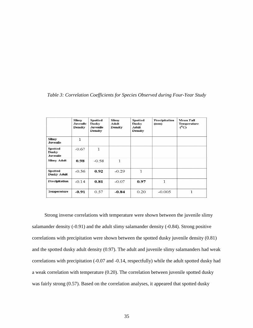
Table 3: Correlation Coefficients for Species Observed during Four-Year Study

Strong inverse correlations with temperature were shown between the juvenile slimy

salamander density (-0.91) and the adult slimy salamander density (-0.84). Strong positive

correlations with precipitation were shown between the spotted dusky juvenile density (0.81)

and the spotted dusky adult density (0.97). The adult and juvenile slimy salamanders had weak

correlations with precipitation (-0.07 and -0.14, respectfully) while the adult spotted dusky had

a weak correlation with temperature (0.20). The correlation between juvenile spotted dusky

was fairly strong (0.57). Based on the correlation analyses, it appeared that spotted dusky

36

salamander densities were affected more by precipitation while slimy salamanders were more

sensitive to temperatures. The high correlation coefficient between the spotted dusky densities

and precipitation would be expected since these salamanders are rarely found more than a few

meters away from water (Niemiller and Reynolds 2011).

Conclusions

The monthly salamander observations and data analysis resulted in the following conclusions

and recommendations:

1. Adult and juvenile densities were the highest (2.20 and 2.25 salamanders/square meter)

during the study period when the mean fall temperature was below average and the total fall

precipitation was above average (2009).

2. Adult and juvenile densities were the lowest (0.55 and 0.60) during the warmest and driest

study period (2010).

3. Strong correlations with temperature were shown with the total juvenile density (-0.91), the

juvenile slimy salamander density (-0.91), and the adult slimy salamander density (-0.84).

4. Strong correlations with precipitation were shown with the total adult density (0.86), the

spotted dusky juvenile density (0.81), and the spotted dusky adult density (0.97).

5. Based on the correlation analyses, it appeared that spotted dusky salamander densities were

affected more by precipitation while slimy salamanders were more sensitive to temperatures.

6. Slimy salamanders were observed more often than the spotted dusky salamanders in three of

the four study periods (2008 through 2010).

37

7. From 2009 to 2010, there was a 73.3% decrease in total juvenile density and a 75% decrease

in total adult density. The decrease in densities may be due to the warmer and drier climate

experienced during 2010.

8. From 2010 to 2011, there was a 71.8% increase in adult salamander density but only an

8.3% increase in juvenile density. The small change in juvenile density may be due to the

warmer temperatures experienced during 2010.

9. During field observations, it was noted that salamanders were more prevalent in soils with

higher moisture content.

10. A longer study period and more transects would provide more data for interpretation, thus

yielding more definitive results.

Works Cited

Conant, Roger and Joseph T. Collins. Peterson's Field Guide, Reptiles and Amphibians,

Eastern/Central North America. Third ed. Boston: Houghton Mifflin, 1998.

Droege, S. and H. H. Welsh. "A Case for Using Plethodontid Salamanders for Monitoring

Biodiversity and Ecosystem Integrity of North American Forests." Conservation

Biology. 15:558-569. 2001.

Lannoo, M. (editor). 2005. Amphibian Declines, The Conservation Status of United States’

Species. University of California Press, Berkeley and Los Angeles, CA.

Niemiller, Matthew L. and Reynolds, R. Graham. The Amphibians of Tennessee. Knoxville:

The University of Tennessee Press, 2011.

Pew Center. Climate Change 101. January 2009. <www.pewclimate,org>.

Pounds, A., A.C.O.Q. Carnaval, and S. Corn. 2005. Climate Change, Biodiversity Loss, and

Amphibian Declines. Pages 19-20 in Amphibian Conservation Action Plan,

Proceedings: IUCN/SSC, Amphibian Conservation Summit 2005.

Tennessee Wildlife Resources Agency. 2009. Climate Change and Potential Impacts to

Wildlife in Tennessee. Nashville: TWRA.

38

University of Maryland. Young salamanders' movement over land helps stabilize populations.

Science Daily 27 April 2010. 09 November 2010 <http://www.sciencedaily.com­

/releases/2010/03/100330142433.htm>.

United States Department of Agriculture, Natural Resource Conservation Service. “Acreage

and Proportionate Extent of Soils in Benton County, Tennessee”. August 2006. 16

December 2008. http://soildatamart.nrcs.usda.gov/ReportViewer.aspx?File.

U.S. Fish & Wildlife Service. Climate change is real. 2 Dec 2010. 09 November 2010.

http://www.fws.gov/home/climatechange/climate101.html.

Wake, David. 2009. Dramatic declines in neotropical salamander populations are an important

part of the global amphibian crisis. PNAS 106.9: 3231-3236.

The Regulation of the Egr1 Promoter by c-Myc, A Study Encompassing

1200 Base Pairs

Scherly Gomez, Busra Gungor & Ranine Haidous School for Science and Math at Vanderbilt, Nashville

Abstract

The overexpression of the proto-oncogene c-Myc causes hyperproliferation and also

induces apoptosis, as part of a fail-safe mechanism, through the tumor suppressor p53.

Subsequently, c-Myc induces p53-independent apoptosis through Egr1. To understand this

non-canonical pathway, the study served to pinpoint the binding and activating sites of c-Myc

on the Egr1 promoter. Transfection of mutated plasmids into Rat1a cells was performed

followed by a luciferase assay. A binding site may exist within -1227 to -1028 of the Egr1

promoter due to decreased transcriptional activity compared to the full-length promoter.

Understanding the repertoire of c-Myc’s functions is critical in stopping cancerous cells.

Introduction

Cancer is mainly caused by the activation of proto-oncogenes and inactivation of

tumor-suppressor genes. A regulator gene that codes for a transcription factor, c-Myc (cellular

myelocytomatosis) is an essential proto-oncogene in the human genome. It controls cell

39

growth and plays a role in activating or repressing target genes. However, overexpression of c-

Myc can lead to deregulated cell cycle progression, hyperproliferation, and tumorigenesis.

A paradox in cancer biology has revealed that oncogenes can be advantageous to cells

by enhancing cell cycle progression, yet they can also put cancerous cells at risk for cell

suicide. This is a natural fail-safe mechanism that has evolved to stop cancerous cells; thus,

when oncogenes are overexpressed, the cell dies instead of growing in an uncontrolled

manner. Apoptosis, or programmed cell death, is induced by c-Myc through either p53-

dependent or p53-independent pathways. The prevalent pathway for c-Myc to induce apoptosis

is with the tumor suppressor ARF (Alternative Reading Frame protein) (Figure 1a). MDM2

functions to inactivate p53 through nuclear export or ubiquitination to target p53 for

degradation. By inhibiting MDM2, ARF reduces the interaction of MDM2 with p53. As a

result, p53 activity is increased, inducing apoptosis (Qi et al, 2004).

a)

b)

Figure 1 c-Myc induced pathways to apoptosis

a) Canonical p53-dependent c-Myc induced pathway to apoptosis b) Noncanonical p53-

independent c-Myc mediated pathway to apoptosis

Apoptosis

c-MYC

ARF MDM2 p53

cMYC

ARF

Egr1 ARF

c-MYC

Apoptosis

40

Cells without p53 have been found to follow a non-canonical pathway to apoptosis

through which ARF binds to c-Myc, then subsequently binds to the Egr1 (Early Growth

Response) promoter, leading to apoptosis (Figure 1b) (Boone et al, 2011). In-depth research

has been recently conducted by a study involving the noncanonical p53-independent c-Myc

mediated pathway to apoptosis as well as c-Myc binding sites (Boone et al, 2011). It was

shown that c-Myc directly binds to the Egr1 promoter. However, the exact location of the

interaction was unresolved as was whether or not this binding site resulted in the activation of

the Egr1 promoter.

According to the assay in Boone et al 2011, this study predicted that c-Myc would bind

approximately at the deletion site -904 to -1319. Deletions throughout the Egr1 promoter were

created and then the activation of these mutants by c-Myc was directly tested in order to

examine the regulation of Egr1. Therefore, the research further provides additional

information on the fail-safe mechanism found in cells to eliminate those with overexpressed c-

Myc.

Methods

Primer Design and Mutagenesis PCR

To examine the behavior of c-Myc, primers of approximately 20 base pairs were

designed to produce six deletions in the region -2621 to -1010 of the Egr1 promoter

(QuikChange II XL Site-Directed Mutagenesis Kit, Stratagene). The parental Egr1 plasmid

was provided (Boone et al 2011). Deletions of approximately 200 base pairs, as shown in

Figure 2, were made based on the finding that large deletions could be made using the kit

(BioTechniques, 2000). Mutagenesis PCR was then used to amplify the mutated DNA. The

Luciferase Δ -2603: -2404

41

thermocycler conditions were the following: 1 cycle at 95°C (2 minutes), 18 cycles with 95°C

(1 minute), 60°C (1 minute), and 68°C (2 minutes), and 1 cycle at 68°C (7 minutes).

Dpn I Digestion and Transformation

Dpn I digestion was performed to remove any methylated parental unmutated plasmids of

DNA. The mutated DNA was then transformed into XL10-Gold ultracompetent cells

(Stratagene).

Mini-prep, Gel Electrophoresis, and Maxi-prep

To purify the DNA from the resulting bacterial colonies, a mini-prep was performed

(Qiagen). A BglII digestion was used to slice out the Egr1 promoter from the plasmid. A gel

electrophoresis was used to confirm that deletions were present in the plasmids. Accordingly,

bands in the gel were approximately 200 base pairs shorter than the original plasmid. All

deletions were confirmed by sequencing, and then Maxi-preps were conducted on positive

clones in order to acquire larger amounts of pure DNA. (EndoFree Plasmid Purification,

Qiagen).

42

Transfection and Luciferase Assay

Rat1a cells have previously shown the largest activation of the Egr1 promoter by c-Myc

(Boone et al 2011). Rat1a cells with exogenous c-Myc and Rat1a cells with vector (control)

were transfected with the mutated or parental unmutated DNA plasmids along with SV40-

Renilla Luciferase using the transfection reagent Lipofectamine 2000 (Invitrogen). The Egr1-

Luciferase constructs were used to visualize c-Myc activation of the Egr1 promoter. SV40-

Renilla Luciferase is not regulated by c-Myc; therefore, it functioned as an internal control in

the cells. The cells were transfected in a 6-well plate and harvested after 48 hours. Luciferase

assays were conducted according to manufacturer instructions to observe c-Myc transcriptional

activity in the cells (Dual-Luciferase Reporter Assay System, Promega). The readings of

luminescence from the luminometer were used to calculate transcriptional activity.

Results

Of the six deletions that were originally proposed on the Egr1 promoter, three were

successful according to the gel electrophoresis: -1765 to -1565, -1509 to -1308, and -1227 to -

1028 (Figure 2). Then luciferase essays were performed on the three successful deletions.

The intended results were to find that the transcriptional activity of the luciferase

promoter in the Rat1a cells depicted by the deletion construct is significantly different from

that of the Egr1 wild-type, demonstrating the decrease in c-Myc activity. Consequently, it was

expected that if a true c-Myc binding and activating site were found, the level of luciferase

activity from the deletion construct in the cells expressing exogenous c-Myc (“Myc” Figure

3a) would be similar to the level of luciferase activity from the deletion construct in the

endogenous c-Myc only cells (“Vector” Figure 3a). One of the deletion constructs, -1227 to -

43

1228, fit these conditions. The full length Egr1 construct (Egr1 Luc 2.8) was activated 1.6 fold

more in cells with overexpressed c-Myc (Figure 3b), as it was in Boone et al 2011, thus

confirming the assay was working properly. The Δ -1765 to -1565 was more active

irrespective of the amount of c-Myc in the cells (Figure 3a), but was induced by c-Myc by 1.7

fold (Figure 3b). The expression values from the Egr1-luciferase deletion constructs -1765 to

-1565 and -1509 to -1308 were significantly different (p<0.05) from cells expressing only

endogenous c-Myc as well as the Egr1 wild-type (Figure 3a). The transcriptional activity of

Egr1-luciferase in Rat1a cells with exogenous c-Myc was not significantly different (p>0.05)

from the control Rat1a vector cells with endogenous c-Myc in Δ-1227 to -1028 (Figure 3a).

The transcriptional activity of exogenous c-Myc was calculated relative to the endogenous to

normalize the data and ensure that the results depicted strictly c-Myc activity rather than other

tumor suppressors (Figure 3b). The activity of the deletion construct -1227 to -1028 is

confirmed in Figure 3b to be similar to vector (p>0.05) but significantly different to the full

length Egr1 construct (p<0.05). The deletion sites -1509 to -1308 and -1765 to -1565 are both

not significantly different to Egr1 in Figure 3b in contrast with being significantly different to

it in Figure 3a, thus indicating that the fluctuation in transcriptional activity in these two

deletion sites was not strictly due to c-Myc.

44

a.

45

Discussion/Conclusion

The results of this study support the non-canonical mechanism of p53-independent c-

Myc induced pathway to apoptosis. The hypothesis that c-Myc binds and activates within the -

1227 to -1028 region on the Egr1 promoter was confirmed since the construct with this region

deleted is significantly different from the full length Egr1 promoter, but is activated to similar

levels in the cells irrespective of the levels of c-Myc. The luciferase assays were able to show

that a decrease in c-Myc activity different from that of the original Egr1 promoter could have

been due to the removal of a potential c-Myc binding and activating site. When the

transcriptional activity in the Rat1a cells with exogenous c-Myc is significantly different to the

* Significantly Different (p<0.05)

◊ Not Significantly Different (p>0.05)

Figure 3 Transcriptional activity in Rat1a cells

a)Overall c-Myc Transcriptional activity b) c-Myc transcriptional activity (relative to vector)

b. *Significantly Different (p<0.05)

◊ Not Significantly Different (p>0.05)

46

cells with only endogenous c-Myc, it suggests that the region of the Egr1 promoter under c-

Myc control is still present. However, if the transcriptional activity in the Rat1a cells is not

significantly different to the endogenous c-Myc expression, it means that the initial cause in

the increase in activity has been removed. The region -1227 to -1028 falls in-between the site -

904 to -1319, which was a potential binding site found by Boone et al 2011. The expression

levels of the deletion construct -1765 to -1565 was significantly different to both Egr1 and its

vector, suggesting that an Egr1 suppressor binds in that region; thus, removing this region

increases the level of transcriptional activity on the promoter .

Although the unique c-Myc induced pathway is unsettled, figuring out the binding and

activating sites has the potential to prevent the spread of cancer in cells. While biotechnology

companies are developing cancer drugs targeting c-Myc, these drugs are attempting to block

all c-Myc function in the cells. This, however, would also block the advantageous functions of

c-Myc within a cell, such as regulation of cell growth and cell cycle progression. Therefore, a

better understanding of the c-Myc induced pathway as well as pinpointing the exact location at

which c-Myc binds and activates the promoter would ultimately allow scientists to create

enhanced drugs to block c-Myc functions in only cancerous cells. As a result, further research

is essential to preventing cancer with the most effective drugs possible.

Works Cited

Boone, D. N., Y. Qi, Z. Li & S. R. Hann. (2010). Egr1 mediates p53-independent c-myc-

induced apoptosis via a noncanonical arf-dependent transcriptional mechanism. PNAS,

108(2), 632-637. Retrieved from http://www.pnas.org/content/108/2/632.full.pdf

47

L. Gardner, L. Lee, and C. Dang (2002). The c-Myc Oncogenic Transcription Factor. The

Encyclopedia of Cancer, Second Edition. Retrieved from http://www.myc-cancer-

gene.org/documents/MycReview.pdf

Makarova O, Kamberov E, Margolis B (2000). Generation of deletion and point mutations

with one primer in a single cloning step. BioTechniques, 29:970-972. Retrieved from

http://www.ncbi.nlm.nih.gov/pubmed/11084856

Qi, Y., M. A. Gregory, Z. Li, J. P. Brousal, K. West & S. R. Hann (2004). p19ARF directly

and differentially controls the functions of c-Myc independently of p53. Nature, 431, 712-

717. Retrieved from http://www.ncbi.nlm.nih.gov/pubmed/15361884

Discovering Asteroids

Olufunke Tina Anjonrin-Ohu

Sullivan South High School, Kingsport

Abstract

Nine images were taken along the ecliptic on the evening of December 7, 2011 with the

intent of searching for asteroids. After calibrating and analyzing the data, twenty-nine moving

objects were detected. Seven objects were discarded due to problems with the data. Twenty-

two of the moving objects were approved of being asteroids based on the Point Spread

function. PSF of an optical system is the light distribution that results from a single point

source in object space. All of the asteroids were previously known.

48

Introduction

Recent discoveries in the astronomical field are constant reminders that the earth as a

whole is vulnerable to interplanetary impacts. There are craters on the earth (and on the moon)

which show a long history of large objects hitting the planet. On a daily basis, the earth is

bombarded with tons of interplanetary material of which the majority disintegrates before

reaching the earth’s surface (Yeomans, 2012). If an object has enough mass and speed to

successfully make it through the earth’s atmosphere, the results of the impact can be extremely

destructive (Brian,2012). Evidence suggests an asteroid caused the extinction of dinosaurs.

An asteroid impact could begin a number of chain reactions that could lead to the annihilation

of mankind.

Asteroids have modified the earth’s biosphere in the past (Yeomans, 2012). They vary in

composition most of them are made of stone, but some contain metals and other materials.

Asteroids can contain metals like gold, silver, platinum, nickel, and iron. (Dyck, 2006). There

is the potential in the future to harvest asteroids as a resource, since they offer a source of an

extraordinarily rich supply of minerals which can be exploited for them years to come

(Yeomans, 2012).

Experimental Procedure

Data for this project was acquired using the 0.9-meter telescope of the Southeastern

Association for Research in Astronomy (SARA). This telescope is located at the National

Observatory (NOAO)at Kitt Peak, Arizona. East Tennessee State University(ETSU), along with nine

other colleges and universities are members of SARA.The 0.9-meter telescope is equipped with a four-

49

port instrument selector which allows use of several instruments during a given night of observation

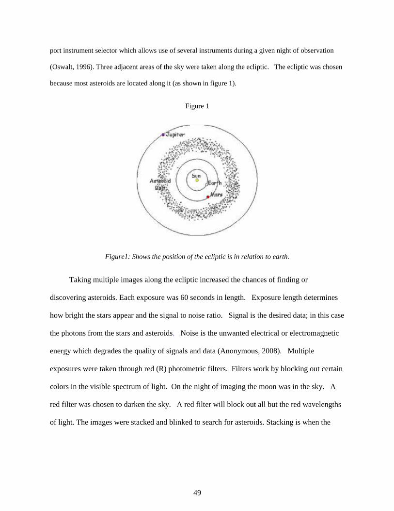
(Oswalt, 1996). Three adjacent areas of the sky were taken along the ecliptic. The ecliptic was chosen

because most asteroids are located along it (as shown in figure 1).

Figure 1

Figure1: Shows the position of the ecliptic is in relation to earth.

Taking multiple images along the ecliptic increased the chances of finding or

discovering asteroids. Each exposure was 60 seconds in length. Exposure length determines

how bright the stars appear and the signal to noise ratio. Signal is the desired data; in this case

the photons from the stars and asteroids. Noise is the unwanted electrical or electromagnetic

energy which degrades the quality of signals and data (Anonymous, 2008). Multiple

exposures were taken through red (R) photometric filters. Filters work by blocking out certain

colors in the visible spectrum of light. On the night of imaging the moon was in the sky. A

red filter was chosen to darken the sky. A red filter will block out all but the red wavelengths

of light. The images were stacked and blinked to search for asteroids. Stacking is when the

50

images are laid on top of one another. Blinking is when the images are shown in rapid

sequence.

Images of the same section of the sky were taken at different times and stacked, so that

the stars would remain unaffected but the asteroids would have changed its location in the

amount of time between images. Using Astrometrica and MaximDL, astronomical software

used to process CCD images, the images were then blinked. This made the motion of any

asteroids apparent

Data

After the data was received from Kitt Peak it was calibrated. Some of the miscellaneous

effects caused by the camera includes hot and cold pixels, dirt, and dust inside the telescope.

The majority of these effects were eliminated before the data was analyzed through a process

called calibration. The telescope was pointed at a blank surface to show vignetting and dust in

the telescope these images are called Flats. Cold pixels are less sensitive than the surrounding

pixels or have no sensitivity (Mackenty, 2011). On the images cold pixels appear to be a

black box with sharp ninety degree angles. SARA then took images, called Darks, with the

cover over the front of the telescope so that the hot pixels would appear. Hot pixels are pixels

with excessive charge compared to the surrounding pixels (Mackenty, 2011). On the images

hot pixels appear to be white squares, which can be mistaken for a star.

A few of the darks had a row of what appeared to be cold pixels also known as a dead

column. An image with zero exposure length, called bias, with the shutter closed to show

where the electrical noise in the camera and telescope electronics. The flat images, dark

images, and bias images were averaged separately making a master flat, a master dark, and a

51

master bias using the program MaximDL.MaximDL subtracted the master dark, master flat,

and the master bias, from the images ridding them of problems the telescope might have

caused.

Figure 2

52

Figure2.Shows the dead column (towards the lower right of the screen) in the calibrated image.

Three adjacent images were taken at three separate times. The images were centered at

:(04:20:45.9’ +21:50:42.3’), (04:30:50.2 +21:52:17.3),and (04:40:57.1 +21:52:17.3),

respectively going from east toward west. The images were taken at 14:17, 22:01, 47:43 in

universal times. These coordinates were chosen because they were at the opposition point this

is the point in space opposite the sun. At this location in its orbit asteroids would be brightest

and have the greatest speed as seen from the earth. As shown in figure 3 the asteroid, at its

opposition point, is opposite the sun in relation to the earth.

53

Figure3

Figure 3.The position of 8430 Florey, a found asteroid, is shown from a different view on the

night of imaging.

After reviewing all the data it was apparent that A3 had the brightest asteroids.

Astrometrica, software used for the data reduction of CCD images, was used to detect the

moving objects on the images. For the results to be more accurate the coordinates (longitude

and latitude) of SARA were inputted and nine reference stars were found by Astrometrica.

Twenty-nine moving objects were detected, five of which were discarded because of their

close proximity to the edge of the image. Another two moving objects were discarded because

they were hot pixels that were not taken out during calibration. Hot pixels were found by the

data given by the point spread function. Astrometrica identified the other twenty-two moving

objects as asteroids and gave their names along with their expected path.

54

Table 1

Name of Asteroids Right Ascension Declination

8430 FLOREY 04 39 28.94 +21 59 35.6

308872 2006 SB42 04 40 01.39 +22 09 0.8

131705 2001 YE11 04 41 25.27 +22 09 09.2

(94493) 2001 UB42 04 41 25.27 +22 03 08.6

(245149) 2004 RZ331 04 40 74.14 +21 52 45.7

(177939) 2005UV137 04 39 49.23 +22 07 16.3

2005 RZ331 04 40 33.98 +21 50 24.8

(312543)2009 FP5 04 40 07.24 +21 52 56.1

2006 VD66 04 40 26.40 +22 04 24.3

308872 2006 SB42 04 40 07.24 +22 10 27.7

94493 2001 UB 04 40 40.84 +22 08 18.9

2011 WE78 04 40 11.44 +22 14 11.7

(177939) 2005 UV137 04 40 35.96 +22 14 11.7

134577 1999 SY2Y 04 39 39.02 +22 03 06.4

(63884) 2001 SF1 04 40 47.08 +22 01 17.6

308874 2006 SM61 04 40 25.31 +21 58 29.0

2011 WW96 04 39 49.41 +21 58 08.2

63884 2001 SF1 04 40 42.14 +21 57 29.6

2006 UE173 04 40 51.36 +22 05 22.6

2011 YE11 04 40 51.36 +21.55 34.5

2002 TD 145 04 40 22.09 +21 53 39.5

The brightest asteroid detected was 8430 Florey discovered on December 25, 1997by Frank B.

55

Zoltowski at Woomera in South Australila. More information about 8430 Florey is shown in

Table1.

Table 1: Gives information about the actual path of the asteroid,

Conclusions

Numerous asteroids were easily detected using Astrometica and MaximDL. No

previously undiscovered asteroids were found in this section of sky. A longer exposure would

have detected the fainter objects. Imaging the sky during the dark of the moon would also

help detect more asteroids. A different filter might then be chosen.

Future Direction

Research could be done to discover fainter asteroids by having a longer exposure

length, and having a darker night. A variation on this project could be undertaken by taking

images of the same section of the sky, allowing time for the asteroid to move, in different

56

colored filters.When the images were stacked the asteroid would appear a different color for

each image took and in a different position.

Thank You

I would like to thank Dr. Bloomer, and Mr. Rutherford for helping me obtain the

images for my project as well as explaining and teaching me how to analyze them. I would

also like to thank TJAS for accepting my paper.

Works Cited

Anonymous.(2008) “What is noise?”http://whatis. techtarget.

com/definition/0,,sid9_gci212667,00. html Tech Target ©2008.

Anonymous.(2007)

“View”http://www.telescopes.com/telescopes/howdifferentfilterscanbetteryourviewarti

cle. cfmHayneedle. Inc ©2007-2012

Brian, M. (1998)“What if an asteroid hit the earth?”http://science. howstuffworks.

com/nature/natural-disasters/asteroid-hits-earth. htmHowstuffworks. Inc ©

Cullen, S.(2011) “Discover an asteroid!”.Astronomy.pages 62-63

Dyck, R. (2001) “Asteroid mining”http://chapters.marssociety. org/winnipeg/asteroid.

htmlCyberTeams.Inc ©

Mackenty, J.(2012) “Hot and cold pixels”http://www. stsci. edu/institute/org/do/director

Februrary 24 2011AcademicPublisher.

Moore, K.(2012) “What is point-spread function?”http://www.radiantzemax.com/kb-

en/KnowledgebaseArticle50255.aspx McGraw Hill ©

Oswalt, T. (1996) “Back to the future: the Southeastern Association for Research in

Astronomy (SARA) observatory at Kitt Peak and the future of small telescopes at

national sites”http://www. noao. edu/aura/stma/abs/toswalt. html

Talcott, R.(2012) “Spot a near-earth asteroid”. Astronomy.pages 48-49

Yeomans, D.(1995) “Why study asteroids?”http://carlkop. home. xs4all. nl/comastr. html ©

copyright

57

The Effect of Porosity upon the Strength of a Polymer Scaffold

Emily Peel

Pope John Paul II High School, Hendersonville

Abstract

Current surgical techniques regarding reconstruction of fractured bones have risk of a

variety of complications such as extended recovery time or rejection of the donor bone. New

technology has introduced the idea of an implantable scaffold, which allows the regrowth of

the patient’s own bone; however, many variables must be considered to create the essential

environment for bone regeneration. To test the effect of a scaffold’s porosity upon the strength

of the scaffold itself, a three point bending test was constructed. The data resulting from the

experiment did not produce any definitive results that were conclusive with literary sources;

unlike these sources, the data indicated no correlation between scaffold strength and porosity.

Nevertheless, the experiment introduced a better understanding of the regeneration of bone and

the future of surgical reconstruction.

Introduction

As the number of American soldiers returning from war with bone related injuries

increases, the need for improvements in the technology of reconstruction surgeries increases as

well. According to recent studies, one in six surgeries fail to rebuild one’s jawbone by using

that person’s hip bone (Kaufman, n.d). Conventional surgeries include autografting, in which

the biomaterial needed is taken from the patient’s body, and allografting, in which a donor

provides the biomaterial needed. However complications arise from these two methods.

Autografting is generally more expensive and carries an increased risk of blood loss and

infection, as well as an increased recovery time; accordingly, allografting complications

58

include a rejection of the donor’s biomaterial as well as a lack of compatible donors. Man-

made materials are yet other substitutes, but are subject to stress and fracture, causing the need

for more surgical procedures to replace the old material (Krotec, 2000). Therefore, scientists

have developed biodegradable scaffolds, a type of matrix that simulates the environment

conducive to cell growth as a potential solution to the complications.

The key to conducting compatible scaffolds lies within the knowledge of how bones

themselves grow. Bone is composed of three elements: bone matrix, bone cells, bone marrow

as well as each element’s blood supply network. The matrix acts as the support structure,

providing strength for the bone and a supply of minerals. The bone cells are the maintenance

facilitators of the matrix, while the marrow and vasculature allow for communication between

the bones and the rest of the body as well as provide stem cells for osteogenesis, the

production of new bone growth (Hing, 2004 and Krotec, 2000). Through the use of peptides,

specifically growth factors, new tissue is formed. These growth factors may act upon certain

osteoblasts, which are local bone forming cells, to instigate growth; accordingly, the growth

factors may induce osteogenesis through cell differentiation and migration as well (Hing,

2004). For bone to grow and repair itself, osteoblasts must be present, as they are the

producers of this growth; however, the environment must also be suitable for osteoblasts,

which require the availability of nutrients as well as oxygen. This criterion is available if an

internal vascular network is present, which subsequently allows the cell differentiation that

leads to the formation of an osteoblast. The first step in the reparation of a fractured bone is a

blood clot that subsequently starves the blood supply from the mature bone cells nearest the

fracture, osteocytes, resulting in their death and signaling a demand for the bone repair. White

blood cells, macrophages, and fiber producing cells, known as fibroblasts, then enter the

59

fracture site and clean out the damaged area. Growth factors send signals to obtain stem cells

from the bone marrow that differentiate into osteoprogenitor cells. If these cells are in contact

with the blood supply, they differentiate into osteoblasts, cells that ultimately form the new

bone. The formation of a new blood supply, angiogenesis, occurs, and as the fracture becomes

stable, osteoclasts break down the existing bone tissue to allow the osteoblasts to lay the

foundation of the new bone (Hing, 2004 and Krotec, 2000). In figure one, an osteoclast

(green) is shown destroying bone while osteoblasts (star shaped figures) are shown rebuilding

new bone in the process of bone resorption (Osterwalder, Britannica Image Quest 9/26/11).

Figure two depicts the process of rebuilding new bone, while also indicating the necessity of

angiogenesis as shown by the presence of the blood vessel (www.bonefractures.org 9/26/11).

60

Figure 1

Figure 2

The goal of an effective bone graft is to not only provide a framework for regrowth of

the fractured bone, but to create a connection between the graft and the existing bone, fully

incorporating the graft and the newly formed bone into the body (Hing, 2004). A major

component of cell regrowth within the scaffold depends on the compatibility of the material of

the scaffold itself. In a study designed for the use of scaffolds to help repair a patient’s spine,

the researchers used porous hydroxyapatite and β-tricalcium phosphate to stabilize and fuse

dorsal and lumbar spinal injuries. Out of the thirty patients tested within the study, graft

incorporation and fusion was successful in all thirty patients, using the bone-graft substitute.

61

This indicates the usefulness of porous hydroxyapatite and β-tricalcium phosphate as

compatible scaffolding materials (Laurencin, 2009).

In addition to the material of the scaffold itself, an important step in the regrowth of

bone is the ability for the scaffold to attract cell attachment and induce cell differentiation. The

surface morphology and roughness, as well as the wettability and porosity of the implants are

important factors in producing the integration of the bone into the scaffold (Harris et al, 2007).

Accordingly, researchers have discovered that the expansion of bone into the scaffold

increases with increasing macroporosity, that is, a scaffold with pores greater than 50 μm in

diameter. This finding is believed to be the result of increased permeability, which allows the

cells ease of access in not only infiltrating the scaffold, but also connecting to each other

within the matrix (Hing, 2004). Because individualized and custom made scaffolds provide

better surgical results, including reduced recovery time and easier integration of the scaffold,

researchers are continually investigating new techniques for creating scaffolds. Rapid

manufacturing techniques sequentially build scaffolds by layering the materials. A recent study

used selective laser sintering by clustering the mass of materials used to build the scaffold

using heat supplied by the laser. This study indicates that a rougher surface for the scaffold

provides a better environment for bone integration, which was achieved by the experiment;

accordingly, the wettability, which is an indicator of the surface chemistry of the porosity, is a

key component for inducing osteoblasts to attach and differentiate upon the scaffold (Harris et

al, 2007).

While the components of the scaffold itself are essential to bone integration, scientists

have studied the inducement of growth signals to promote cell growth, a successful endeavor

regarding the engineering of new tissue (Mooney, 2002). Other studies involving the

62

differentiation of osteoblasts upon a titanium surface suggest that the protein α2 β1 is essential

to this process, implying that proteins also play a role in the integration of bones into a

scaffold (Schwartz, 2008). Unlike the previous studies in which cells were attracted to a

scaffold, scientists have also investigated the use of implanting osteoblasts within collagen

microcarrier beads, creating a spherical environment in which the cells can proliferate

(Frondoza, 2003). The use of collagen replicates the conditions found within the extra-cellular

matrix of the cell, which is composed of organic collagen fibers (Hing, 2004). Because of the

various elements involved in creating a suitable scaffold, researchers are continually

discovering new methods useful for replicating the environment of bone regrowth.

Because porosity affects the ability of cell growth within a scaffold, and scaffolds must

withstand a certain amount of stress inflicted upon the structure during bone regrowth, the

purpose of this experiment was to determine the affects of porosity upon the strength of the

scaffold. The independent variable to be tested was porosity, while the dependent variable was

the strength of the scaffold. The hypothesis was that if the porosity of the scaffold decreases,

then the strength of the scaffold will increase.

Materials and Methods

Materials:

The materials needed to construct the polymer scaffold were the following: cardboard,

box cutter, hot glue and glue gun, aluminum foil, ruler, stir stick, plastic bins, scales, mortar

and pestle, coffee filter paper, plastic cups, a ten pound bag of MAPEI Powder Polymer-

Modified Mortar, water, and NaCl. Tables, sand, a plastic pint cup, force plate, lab quest and a

five gallon plastic bucket were needed to test the strength of the scaffold.

63

Method:

A four centimeter by four centimeter by twenty centimeter mold, in the shape of a

rectangular prism, was first constructed out of cardboard and hot glue. One four centimeter by

twenty centimeter side was left out, so as to provide an opening for the polymer to be poured

into the mold. The interior of the mold was then covered by a single sheet of aluminum foil so as to

protect the cardboard and to prevent leaks. The polymer scaffold was constructed using a ten

pound bag of MAPEI Powder Polymer-Modified Mortar, water, and NaCl. A single scaffold

was first constructed with twenty percent porosity as a test trial. 192 grams of the polymer and

48 grams of NaCl were each weighed separately in coffee filter paper. 74 milliliters of water

was measured in a graduated cylinder. The polymer was added to a plastic cup, as well as the

NaCl. The water was added last. The mixture was stirred for five minutes and was allowed to

sit for the next ten minutes. The mixture was then poured into the cardboard mold and stirred

for two minutes. The mold was left to harden overnight. After the mold hardened, the next day

the mold was submersed in a plastic bin of water to allow the NaCl to leach out. After a few

days, the mold was taken out of the water and allowed to dry overnight.

To determine the strength of the scaffold, the polymer scaffold was placed between two

tables of equal height for a three point bending test. The mass of the five gallon bucket was

measured. Five centimeters of the scaffold on each side were resting on the table. The handle

of the five gallon plastic bucket was placed in the middle of the scaffold, as determined by a

ruler. Sand was then poured into the plastic bucket by using a plastic cup, measuring one pint,

until the scaffold snapped in half. Afterwards, the bucket and sand was massed.

The porosity of the scaffold was varied, ranging from ten percent to forty percent. The

percentages were calculated by varying the amount of NaCl added. The total amount of NaCl

64

and polymer never differed, an amount of 240 grams. The porosity was then calculated by

adding the percentage of NaCl that was equated to the percentage of porosity. For example,

twenty percent of 240 grams equals 48 grams, the amount of NaCl added to the rest of the

polymer mass to make a scaffold of twenty percent porosity. Figure 3 displays the mixtures

used for each porosity. The porosities of the scaffolds were tested using the three point

bending test, and the bending test was repeated three times for each porosity percentage.

Figure 3: Mixtures used for different Porosities

Porosity

(%)

Water

(mL)

Polymer

(g) NaCl (g)

10 94 216 24

20 74 192 48

30 45 168 72

40 35 144 96

Each trial was then plotted on a graph of force versus porosity to determine a pattern.

Data Analysis

The purpose of the experiment was to observe the effects of porosity upon the strength

of a polymer scaffold. Twelve scaffolds were made. These scaffolds were composed of four

different types of porosities, and each porosity was tested three times by means of a three point

bending test. The results are shown below.

Figure 4: Trial 1 Results Figure 5: Trial 2 Results

Trial 1 Porosity

Force

(N)

10% 54

20% 132

30% 114

40% 111

Trial 2 Porosity

Force

(N)

10% 235

20% 146

30% 218

40% 194

65

Figure 6: Graph of Force vs. Porosity Results

As the data shows, there is no particular general trend based upon the relationship

between porosity and force. Figure 6 shows Trial 1 to have a positive slope for its line of best

fit, while Trial 2 has a negative slope for its line of best fit. The positive slope indicates that

strength increases as porosity increases whereas the negative slope indicates that strength

decreases as porosity decreases. However, if the ten percent porosity of the first trial and the

0

50

100

150

200

250

0 10 20 30 40 50

Fo

rce

(N

)

Porosity (%)

Force vs. Porosity

Trial 1

Trial 2

Linear (Trial 1)

Linear (Trial 2)

66

twenty percent porosity of the second trial were eliminated, the data would indicate a negative

correlation in relationship between force and porosity, thereby proving the hypothesis.

Nevertheless, these two data points exist, skewing the significance of the data. The two trials

also show a difference of about seventy Newton’s of force, indicating a discrepancy in the

strength of the two sets of scaffolds. As the two sets of scaffolds did not differ in how they

were made, this deviation points to an unforeseen variable that

may have been affecting the data results. Figure 7 shows the

standard deviation for the different porosities calculated by the

following equation:

Figure 7: Standard Deviation for Porosities

As figure 7 shows, the only acceptable standard deviation value was for the twenty

percent porosity. The extremely large standard deviation values for the rest of the porosities

indicate the lack of validity for the data

Conclusion

To determine the effect of porosity on the strength of a polymer scaffold, a three point

bending test was conducted upon a twenty centimeter scaffold. According to the data, the

Porosities Deviation

10% 90.5

20% 7

30% 52

40% 41.5

67

hypothesis that strength of the scaffold decreases with increasing porosity was disproven, as

the data indicated there was little correlation between the independent and dependent variable.

However, studies conducted have proven the relationship between bone mass density

and the increased risk of hip fractures in women. One particular study stated that the increased

hip fractures did not vary significantly for factors including weight or age, only for the bone

density of the subject (Himes and Huang, 1997). Accordingly, a study done on a large sample

size of Norwegian women stated that weight loss after the age of 25, as well as the amount of

years since menopause, causes low bone mass density. The bone mass density of these women

created an increase risk for hip fractures, indicating a weakness of the bone strength (Skag et

al., 2000). Because porosity necessarily means a lack of bone, and therefore its mass, over a

certain area, these studies prove the hypothesis correct and indicate mistakes or inaccuracies in

the data collection.

After recording the dissimilar trials, a bathroom scale was used to determine the

integrity of the force plate, and the plate was found to have been erratic, despite repeated

attempts to calibrate it. Nevertheless, the strength of the scaffolds still did not produce

consistent data with the porosities. On further examination, the scaffolds composed of forty

percent of salt did not appear as porous as the twenty percent scaffolds. Consequently, this

error was caused because of the lack of consistency in the time allowed for the salt to leach out

of every scaffold. This discrepancy indicates the erratic data, as the scaffolds did not have their

recorded porosities.

Through the use of implantable scaffolds, reductions in complications resulting from

allografting or autografting may be reduced, due to the fact that the patient’s own bone is

subsequently regrown around the surgical implant. While implantable scaffolds are slowly

68

becoming more common in surgical procedures, they may not necessarily become a staple of

surgery due to the upcoming research regarding the use of the platelet derived growth factor.

The company BioMimetic Therapeutics has created an Augment Injectable Bone Graft in

which the scaffold, composed of the platelet derived growth factor, is injected through a

syringe onto the surgical site. The growth factor, through pre-clinical studies has drastically

improved the rate and quality of healing in fractures of diabetic rats (BioMimetic

Therapeudics, n.d). Through the use of these new technologies and the utilization of new

techniques, the surgical complications and extended recovery time may be brought to a new

minimum as the science of new bone growth becomes fully realized.

Works Cited

Biomimetic Therapeudics. (n.d.). Retrieved from http://biomimetics.com/overview.htm

A denatured collagen microfiber scaffold seeded with human fibroblasts and keratinocytes for skin

grafting. (2011, July). Biomaterials.

Improving scaffold fabrication by a design based rapid prototyping technique. (2011, April 15).

Advanced Manufacturing Technology. Retrieved from http://go.galegroup.com/ps/

i.do?&id=GALE%7CA257129373&v=2.1&u=tel_k_pjphs&it=r&p=GPS&sw=w

Kaufman, R. (n.d.). The Research of Regrowth. The American Legion, 12,14.

Krotec, M. (2000). An Education Outreach Manual in Tissue Engineering (R. Rubin, Ed.).

Laurencin, C. T. (2009). Bone Graft Substitute Materials. Retrieved from Medscape Reference

database.

Lerner, L., & Lerner, B. W. (2008). Stem Cells. In The Gale Encyclopedia of Science (4th ed.).

Retrieved from Gale Database.

Painless bone substitute could offer new era for surgeons . (2003, May 15). Sandia National

69

Laboraties. Retrieved from http://www.sandia.gov/news-center/news-releases/2003/other/

bone.html

Soft matrix supports osteogenic differentiation of human dental follicle cells. (2008, July 8).

Biochemical and Biophysical Research Communications. Abstract retrieved from http:/

dx.doi.org/10.1016/j.bbrc.2011.06.031

Eben Alsberg; Kenneth W. Anderson; Amru Albeiruti; Jon A. Rowley; David J. Mooney.

(Sep.

17, 2002).Proceedings of the National Academy of Sciences of the United States of

America, Vol. 99, No. 19 ,pp. 12025-12030.Engineering Growing Tissues. National

Academy of Sciences

R. Olivares-Navarrete; P. Raz; G. Zhao; J. Chen; M. Wieland; D. L. Cochran; R. A. Chaudhri;

A. Ornoy; B. D. Boyan; Z. Schwartz. (Oct. 14, 2008). Proceedings of the National

Academy of Sciences of the United States of America, Vol. 105, No. 41 pp. 15767-

15772.Integrin α2β1 Plays a Critical Role in Osteoblast Response to Micron-Scale

Surface

Structure and Surface Energy of Titanium Substrates.

National Academy of Sciences

Michael Overstreet; Afshin Sohrabi; Anna Polotsky; David S. Hungerford; Carmelita G.

Frondoza. (May - Jun., 2003). Collagen Microcarrier Spinner Culture Promotes

Osteoblast. In Vitro Cellular & Developmental Biology. Animal, Vol. 39, No. 5/6 pp.

228-234. Proliferation and Synthesis of Matrix Proteins. Society for In Vitro Biology

L. Hao; M. M. Savalani; Y. Zhang; K. E. Tanner; R. J. Heath; R. A. Harris. (Aug. 8, 2007).

Characterization of Selective Laser-Sintered Hydroxyapatite-Based Biocomposite

Structures for Bone Replacement. Proceedings: Mathematical, Physical and

Engineering

70

Sciences, Vol. 463, No. 2084 pp. 1857-1869. The Royal Society

Y. Liu; J. P. Li; E. B. Hunziker; K. de Groot. (Jan. 15, 2006). Incorporation of Growth Factors

into Medical Devices via Biomimetic Coatings. Philosophical Transactions:

Mathematical, Physical and Engineering Sciences, Vol. 364, No. 1838, Engineered

Foams and Porous Materials pp. 233-248. The Royal Society

Karin A. Hing. Bone Repair in the Twenty-First Century: Biology, Chemistry or

Engineering?. (Dec. 15, 2004). Philosophical Transactions: Mathematical, Physical

and

Engineering Sciences, Vol. 362, No. 1825, Triennial Issue: Chemistry and Life Science

pp. 2821-2850. The Royal Society

Robert F. (Sep. 1, 2000). Service Tissue Engineers Build New Bone.

Science, New Series, Vol. 289, No. 5484 pp. 1498-1500. American Association for the

Advancement of Science

Zhiping Huang and John H. Himes. (Mar., 1997). Bone Mass and Subsequent Risk of Hip

Fracture. Epidemiology , Vol. 8, No. 2 pp. 192-195. Lippincott Williams & Wilkins

Line M. Omland, Grethe S. Tell, Snorre Øfjord and Arne Skag. (Mar., 2000). Risk Factors for

Low Bone Mineral Density among a Large Group of Norwegian Women with Fractures.

European Journal of Epidemiology , Vol. 16, No. 3 pp. 223-229. Springer

Pierce, Rod. (18 May 2011). "About Math is Fun". Math Is Fun. Retrieved 9 Jan 2012 from

http://www.mathsisfun.com/aboutmathsisfun.html

Acknowledgements

71

I would like to thank Mrs. Dye for her help in getting my project started as well as her

direction in problem solving for my experiment. I also want to thank my family for their

support in all of my stressful endeavors

The Design and Fabrication of a Capacitance-Based Sensor Circuit

Zach Anderson, Braxton Brakefield, Melissa Guo & Sam Klockenkemper School for Science and Math at Vanderbilt, Nashville

Abstract

Testing for biological viruses can be costly and requires sophisticated equipment. A

cheaper, more portable way to test for viruses using a printed circuit board (PCB) was designed

based on a former research project. It was hypothesized that if a sufficient amount of antigen

was bonded to the antibody on the PCB, the change could be detected. When sodium chloride

72

and glucose were dispensed on the capacitor changes in voltage ranged from 1 mV to 14 mV,

depending on the tested material. This proves the circuit is capable of detecting small changes

in material composition.

Introduction

In 2005, a group of scientists developed a silicon microchip used for virus detection

(Balasubramanian 2005). In this conception, an antibody is bound to the sensing capacitor, and

then a solution possibly containing an antigen is washed over both the sense and control

capacitor. If there is antigen in the solution, it will bind to the antibody on the sense capacitor

and the biological volume will increase the capacitance of that capacitor. The outputs of both

capacitors are connected to a comparator, which compares the two signals and outputs one signal

depending on which input is higher. This design was made on an integrated circuit (IC);

however, the IC design was discovered to be impractical because the surface area that blood had

to be deposited on was a 300 micron by 300 micron square, far too small for efficient deposition.

This size limitation caused a problem with both coating the sensing capacitor with antibody and

delivering the antigen to the sensing and dummy capacitors. An additional challenge that exists

when working with liquids at a volume this small is overcoming surface tension and evaporation

(Hisatake, Tanaka Aizawa, 1993). To surmount this problem, a printed circuit board (PCB) was

created to scale up the technology. This PCB offers a viable alternative because it enlarges the

circuit while preserving the functionality of the technology. It not only allows the coating of the

sensing capacitor with antibodies and the delivery of the antigen, but also eliminates the need to

manipulate small volumes of liquid. This printed circuit board is based on the change in stored

charge. The change occurs when a material, in this case blood with an antigen or a solution-

73

containing antigen, is placed on the pad capacitors (Figure 1).

Methods

3.1. Circuit Diagram. The design that was used to create the printed circuit board was derived

from the design based on the integrated circuit previously created by Balasubramanian et al

(Balasubramanian, 2005). The main features of the design are a sense and a dummy capacitor

(Figure 1), the outputs of which were connected directly to an oscilloscope to measure the

difference in the output voltage. Next the circuit diagram was integrated with the pin connections

to functionalize the circuit (Figure 1). This was instrumental in transferring the design from

theory into a digital design. The design also included a 555 timer, an inverter, and a series of

switches to alternate the capacitors between two states: charging and reading. In the charging

state, the switches from high voltage (Vcc) to the capacitors (as indicated by B12, B13, D6 and

D12 in Figure 2) are closed and the switches from the capacitors to the oscilloscope (S5 and S13

in Figure 2) are open. This allows the capacitor to charge up to its full capacitance. In the reading

state, the switches from (Vcc) to the capacitors (B12, B13, D6 and D12 in Figure 2) are open,

and the switches from the capacitors to the oscilloscope are closed. This allows the capacitors

to discharge while showing the two voltages. The voltages can then be measured and the

difference between them calculated. The switches changed state based on the high and low

output voltages, oscillating from the clock.

74

3.2. Printed Circuit Board. After the circuit was finalized on paper, the schematic was then

made on a computer circuit design program, FreePCB (2007). FreePCB allows circuit

components to be routed in a virtual setting in the program and then add wiring to connect the

pins as needed. The file contains all the information necessary for a company, in this case

Advanced Circuits, to manufacture the board to the design, including drilling holes for the pins

of parts, adding integrated wiring to connect the pins, and spaced components correctly. The

first rendition of the design required three separate power sources to run, and an oscilloscope to

visualize the outputs. The second version of the circuit could run off of a 9-volt battery, but still

required an oscilloscope; it also incorporated switches to isolate the capacitors so that the entire

chip would not need to be powered off and then back on when applying aqueous solutions.

Maintaining power to the chip while solutions were applied was advantageous because the

voltages from the three power sources had to stay constant during a test.

Figure 1: This is the schematic of the circuit with the connections labeled (B,D, and S are switches)

75

3.3. Soldering. After the final design was finished on FreePCB, it was sent to Advanced Circuits

to be fabricated. A timer (LM555), an IC hex inverter (SN74HC04N), three IC quad bilateral

switches (296-2039-5-ND), and an IC differential comparator (296-9579-5-ND) were purchased

from Digi-Key (Thief River Falls, MN). Resistors (150.1kΩ, 14.7kΩ, and 14.7kΩ) and

capacitors (.01μF, .33μF, .47μF, 1μF, and 47F) were purchased from RadioShack (Nashville,

TN) and configured to control the frequency of the timer so that the circuit would oscillate

between charging and reading states at 1 Hz. The optimized PCB (version 2) contained rocker

switches (GH7115), obtained from Digi-Key, to change the configuration of the resistors and

capacitors with the timer to allow for flexibility in oscillation speeds (1 Hz and 60 Hz). Once

the PCB and its parts arrived, the parts were soldered onto the board.

3.4. Testing. The finished PCB was then tested preliminarily with direct touch and Styrofoam.

After the functionality of the PCB had been confirmed, the board was experimentally tested

with variable amounts of sodium chloride and glucose placed directly on the sense capacitor.

These two materials were used because of the large difference in their dielectric values, 6.1

and 1.5-2.2 respectively according the Dielectric Constants Chart and the Dielectric Constants

of Common Materials. The change in capacitance due to the sodium chloride and glucose was

measured and recorded using an oscilloscope.

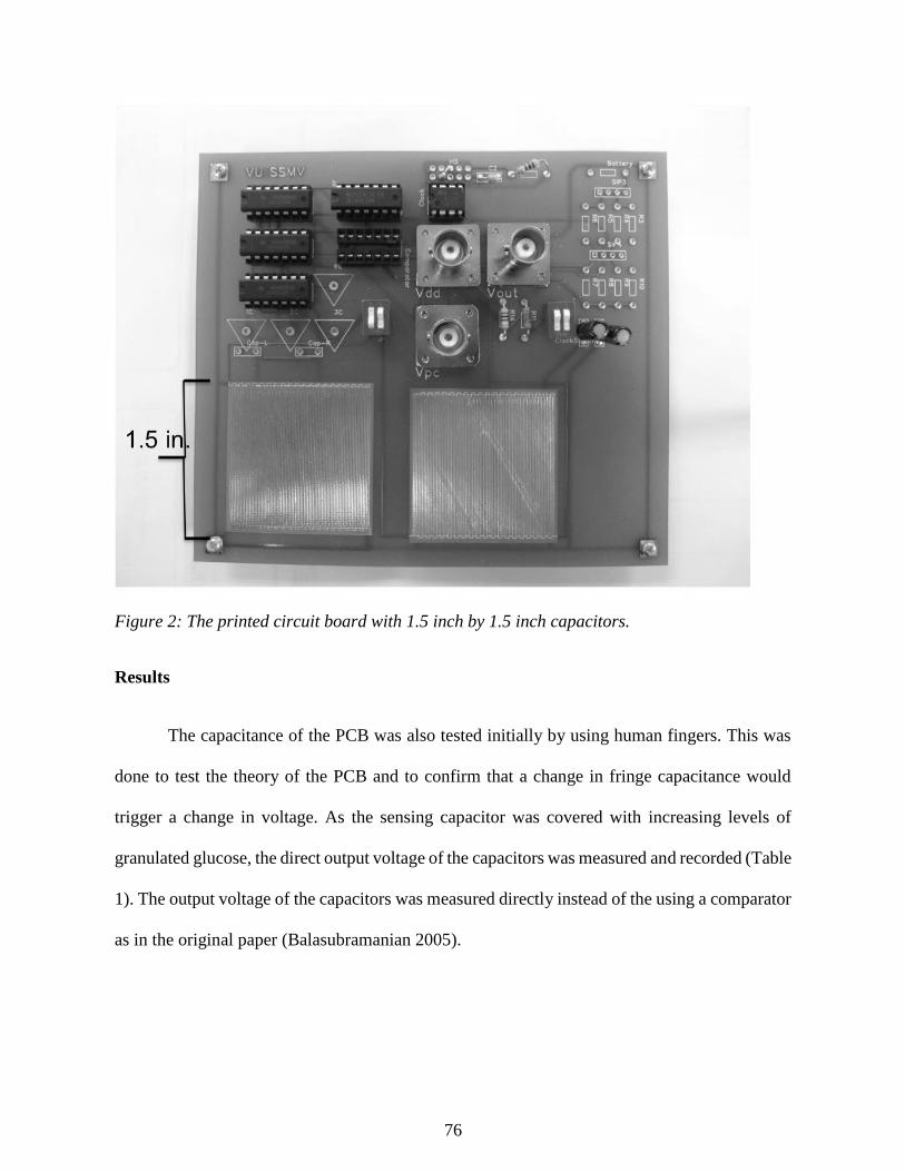
76

Figure 2: The printed circuit board with 1.5 inch by 1.5 inch capacitors.

Results

The capacitance of the PCB was also tested initially by using human fingers. This was

done to test the theory of the PCB and to confirm that a change in fringe capacitance would

trigger a change in voltage. As the sensing capacitor was covered with increasing levels of

granulated glucose, the direct output voltage of the capacitors was measured and recorded (Table

1). The output voltage of the capacitors was measured directly instead of the using a comparator

as in the original paper (Balasubramanian 2005).

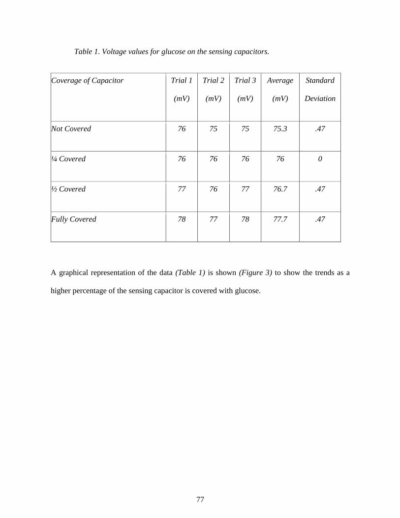
77

Table 1. Voltage values for glucose on the sensing capacitors.

Coverage of Capacitor Trial 1

(mV)

Trial 2

(mV)

Trial 3

(mV)

Average

(mV)

Standard

Deviation

Not Covered 76 75 75 75.3 .47

¼ Covered 76 76 76 76 0

½ Covered 77 76 77 76.7 .47

Fully Covered 78 77 78 77.7 .47

A graphical representation of the data (Table 1) is shown (Figure 3) to show the trends as a

higher percentage of the sensing capacitor is covered with glucose.

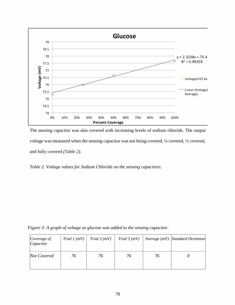
78

The sensing capacitor was also covered with increasing levels of sodium chloride. The output

voltage was measured when the sensing capacitor was not being covered, ¼ covered, ½ covered,

and fully covered (Table 2).

Table 2. Voltage values for Sodium Chloride on the sensing capacitors.

Coverage of

Capacitor

Trial 1 (mV) Trial 2 (mV) Trial 3 (mV) Average (mV) Standard Deviation

Not Covered 76 76 76 76 0

Figure 3: A graph of voltage as glucose was added to the sensing capacitor.

79

¼ Covered 79 79 79 79 0

½ Covered 82 83 82 82.3 .58

Fully Covered 90 88 87 88.3 1.58

A visual representation of the data for sodium chloride (Figure 4) shows the trends as a higher

percentage of the sensing capacitor is covered with sodium chloride.

Conclusions

As the results show, there is a positive correlation between the dielectric constant of a

Figure 4: A graph of voltage as sodium chloride was added to the sensing capacitor.

80

material and its output voltage on the PCB. As more material was measured, the capacitance

increased in a linear relationship for both glucose and sodium chloride. Sodium chloride had a

R2 value of .97 and glucose a R2 value of .99 on the linear regression applied to the average of

the output voltage as can be seen on the graphs. Over the course of the three trials, the PCB

consistently measured a larger difference in voltage as material was added to the capacitor. The

output voltages of the capacitors differ greatly between the two substances tested. When glucose

was added the voltages varied by 2.4 mV, whereas when sodium chloride was added the voltage

varied by 11 mV.

This PCB is capable of detecting a change in capacitance as seen when sodium chloride,

glucose, and human fingers were tested. With this design, the PCB could detect anything

yielding a significant capacitance change. Essentially, a sensor has been made that detects two

things: the first is when materials of different dielectric values are placed on the sensor, and the

second is when different amounts of the same substance are placed on the sensor. Because the

size of the capacitors has an inverse relationship with its sensitivity, a way to improve the PCB

would be to decrease the size of these capacitors, thus increasing the sensitivity. Making the

metal plates in the capacitors closer together rather than decreasing the actual dimensions of the

capacitor would do this. By enhancing the sensitivity of the capacitors, smaller changes in

capacitance can be detected which allows smaller volumes to be tested if the yielded capacitance

change is measurable. Also, installing a battery pack onto the chip would contribute to the goal

of having a cheap and portable virus chip, thus eliminating the need for plug-in power sources.

This could potentially lead the way for a portable and battery-powered device. Adding some

form of output onto the board, such as an LED or speaker, would allow the board to be read

without an oscilloscope such that a significant change in voltage would invoke a light or sound

81

indicator for presence of a material. Future plans include testing the PCB using a virus and

antibody. The use of an applied PCB would not only decrease the costs and resources required,

but also provide a cheaper, more portable approach to virus detection. This is the goal of using

the PCB that was created because it would provide a needed service at a reasonable cost. This

PCB could be used for other applications as well. It is very versatile and can be used for things

such as a touch sensor or adapted for other medical purposes.

Works Cited

Balasubramanian, A., Bhuva, B., Mernaugh, R., Haselton, F. R. (2009). Si-Based Sensor for

Virus Detection. IEEE SENSORS JOURNAL, 5(3), 340-344. http://ieeexplore.

ieee.org/stamp/stamp.jsp?arnumber=01430684

Hisatake, K., Tanaka, S., Aizawa, Y. (1993). Evaporation rate of water in a vessel. Journal of

Applied Physics, 73(11), 7395-7401. doi: 10.1063/1.354031

FreePCB web page, http://www.freepcb.com/, accessed on March 2, 2011

Dielectric Constants of Common Materials (n.d., p. 20,43) Retrieved from http://www.rafoeg

.de/20,Dokumentenarchiv/20,Daten/dielectric chart.pdf

Dielectric Constants Chart, (2011) Retrieved from

http://www.asiinstr.com/technical/Dielectric% 20Constants.htm.

Ilic, B., Yang, Y., Craighead, H. G. (2004). Virus detection using nanoelectromechanical

devices. American Institute of Physics, 2604.

Leonardi, G. P., Leib, H., Birkhead, G. S., Smith, C., Costello, P., Conron, W. (1994).

Comparison of rapid detection methods for influenze a virus and their value in health-

care management of institutionalized geriatric patients. Journal of Clinical

Microbiology, 32(1), 70-74. Retrieved from http://jcm.asm.org.

82

Reaction Driven Mixing: A Second Year Study-Reaction Kinetics

Gavin B. Nixon

Greenbrier High School, Greenbrier

Abstract

As a second-year study, this research sought to accomplish many goals that its predecessor

did not. Through the construction of a more advanced apparatus, designed to measure volume,

pH, and temperature simultaneously, these goals were achieved more accurately and effectively

than that previously reported (1). A major factor that could not be accounted for earlier was that

of pH change throughout the course of the research. By mounting electronic pH meters

permanently within a calibrated cylinder, this was accomplished, and the introduction of time-

lapse photography made for a more accurate tracking of the process. This research also sought

to prove that the reaction-driven mixing process is not a simple diffusion process. The varying

of concentrations of the reactants to determine the dependency of concentration and

consequently, density on reaction rate was also examined and is presented here.

Introduction

Reaction-driven mixing is the process by which substances at different densities that are

capable of reacting with one another will mix during the reaction without mechanical agitation.

Prior research in this area appears to be limited and very elusive, and a mathematical model for

the process was only recently reported (2). To date, only a few different reactants have been

83

demonstrated to undergo spontaneous mixing at the interface between them if not previously

mixed (3). Difficulty has resided in the creation of an apparatus capable of observing the

process.

Through this research, density gradients were utilized in order to carefully layer the

reactants to allow the reaction to proceed. A density gradient is a variation in density between

two liquids that would ordinarily be miscible. This process is often encountered both

intentionally and unintentionally throughout the chemical manufacturing industry and is evident

in such common circumstances as atmospheric separation of high and low pressure areas (8).

Convection often drives mixing in unexpected ways between fluids. In fact, this could

play a previously unrecognized role in geochemical processes (3, 4). Convection certainly

causes mixing. However, when that action is performed mechanically, the reaction accelerates.

In the beginning research on the subject, scientists layered a hydrochloric acid solution

containing phenolphthalein indicator (low density) on top of a sodium hydroxide solution (high

density) in a special cell designed to prevent any mechanical agitation. Convection instability

occurred when these two reacted to form water (5, 6).

HCl + NaOH → NaCl + H2O

This instability could also occur when rivers or streams flow into lakes where

neutralization occurs (8).

The previous research was done in our laboratory in order to develop an effective method

for the process of observing reaction-driven mixing and determine the relationship between the

rate of mixing and the density difference of the reactants (1). The mathematical relationship (Db

– Dt) = kR was derived to relate the density difference and rate of mixing. The reaction-driven

84

mixing process was shown to be a very long process that could probably not be effective for

industrial processes.

This second-year study was done in order to achieve several different goals:

1. The construction of a new apparatus that contains a reaction cell which will have a

uniform volume.

2. The continuous monitoring of pH and temperature changes using four pH electrodes

and a thermistor-based temperature probe.

3. The continuous monitoring of the progress of the reaction using time-lapse

photography.

4. To prove that the process is not a diffusion.

5. To vary the concentrations of the reactants to determine the dependency of reaction

rate on concentration.

6. To determine the density as a factor in reaction rate.

7. To develop an equation for the rate of reaction.

8. To describe the reaction that the indicator undergoes during the process.

Methods and Materials

The density of each solution that was used was determined prior to experimentation, and

following the method that was used in the original research, two solutions (acid and base) were

carefully layered upon one another depending wholly on density difference. Because reaction-

driven mixing is a very tedious process, a way of layering the two substances with very limited

interruption was developed. The original research used two separatory funnels to accomplish

85

this feat as air could be easily removed from the apparatus without disturbance of the two

materials. This second-year study followed suit with some significant changes. Because the

volume was difficult to measure due to the varying widths of the separatory funnels, an apparatus

was built utilizing a 120 mL syringe to accurately measure volume changes (Figure I)

Figure I – Apparatus for Reaction-Driven Mixing

pH1

pH2

pH4

pH3

Acid Solution

Base Solution

Separatory

Funnel

Solution

Interface

86

This way, an exact measurement of the changes that occurred at the interface could be

seen and easily recorded. However, this apparatus served more than just giving a precise

measurement of volume. To measure the temperature at the interface, a temperature probe was

used to detect any variation throughout the process. Electronic pH meters were also used to

record pH changes on both sides of the interface as well as the interface itself. In order to record

these many data points for a significant time and to make sure no fluctuations were occurring

during the mixing process, a time-lapse camera was used. This camera would take a photograph

every 30 minutes to give an accurate representation of the process.

Results and Discussion

The density of each reactant in g.cm-3 was measured and is presented in increasing order in Table

1.

Table 1

0.01M HCl 0.9719

0.1M HCl 0.9792

0.01 M NaOH 0.9839

0.01 M HC2H3O2 0.9848

0.1 M NH3 0.9865

1.0 M HC2H3O2 0.9906

1.0 M NH3 0.9910

0.1 M HC2H3O2 0.9958

1.0 M HCl 1.00061

0.1 M NaOH 1.0018

87

0.01 M NH3 1.0041

1.0 M NaOH 1.0448

The pairs selected for experimentation (Table 2) were as follows due to density difference (ease

of layering) and very fast reaction time under ordinary mixing conditions.

Table 2 Experimental Runs

1.0 M NaOH/0.01 M HCl Density Difference = 0.0729 g.cm-3

1.0 M NaOH/0.10 M HC2H3O2 Density Difference = 0.0490 g.cm-3

1.0 M NaOH/1.0 M HCl Density Difference = 0.0442 g.cm-3

1.0 M NaOH/0.10 M HCl Density Difference = 0.0656 g.cm-3

Since the NaOH solutions always had a higher density that the acid solutions, the acid

solutions with pre-added phenolphthalein indicator solution was put into the apparatus first and

allowed to stand for a few minutes to stabilize. The NaOH solution was added from a separatory

funnel to the reaction cylinder very slowly by opening the stopcock and pinch clamp. The NaOH

layer formed beneath the acid solution with a thin pink line at the interface. This line shows the

space in which reaction was taking place, and which gradually increased in size as the reaction

proceeded.

HIn (colorless) → H+ + In- (pink) Indicator Reaction

88

In – phenolphthalein indicator

Although there were four pH meters in place during the reactions, only one was

significant. The top and bottom meters generally showed low pH (acid solution) at the top and

high pH (base solution) at the bottom. These meters only changed near the end of the reactions

as the reaction interface reached those positions.

Table 3 shows the results of reacting 1.0 M NaOH with 0.01 M HCl. Because they did not

change during the course of the experiment, the pH results from meters 1, 2, and 4 are not

included. Also, note that the temperature remained the same. This was likely due to the small

temperature changes that occurred were less than 0.1 oC and therefore not measureable.

Table 3

Reaction of 1.0 M NaOH with 0.01 M HCl

Time (min) pH 3 Temperature (oC) Indicator Band Width (cm3)

0 3.12 21.7 3.5

30 2.09 21.6 7.0

60 2.00 21.6 8.0

90 2.01 21.6 8.5

120 2.15 21.6 11.0

150 3.02 21.6 17.5

180 6.38 21.6 20.0

210 9.10 21.6 21.5

89

240 10.45 21.6 25.0

Figure 2 shows the change in pH over time for the reaction given in Table 3. The chart shows

the sharp inflection typical of strong acid/strong base reactions. Figure 3 shows the change in

band width for the same reaction. The linear trend line has been added to smooth the data.

pH

Reaction Time (min)

Figure 2pH Changes During the Reaction of 1.0 M NaOH

and 0.01 M HCl

y = 0.0903x + 2.7222R² = 0.9605

Ban

d W

idth

(cm

3)

Reaction Time (Min)

Figure 3Band Width Change During the Reaction of 1.0

M NaOH and 0.01 M HCl

90

Where the equation for the trend line is

Band width = 0.0868t + 3.0 (t = time in minutes)

The other experiments performed in the series followed similar trends.

The reaction as measured by pH meter 1 was complete at 190 min (1.14x104s) which

represented a band width change of 16.5 cm3. Calculating rate as band width change per second,

Rate = ∆b/∆t

Where b = band width and t = time.

For the above reaction the rate would be 1.45x10-3 cm3.s-1.

Conclusions

A number of research projects done in past years have demonstrated density gradients can

be established which remain unmixed for long periods of time (a week or longer). These

gradients in fact were used in ultracentrifugation to separate cellular components (8). Thus

diffusion, although it can be significant at low density differences, appears to have very little

effect at the concentrations and density differences used in this research.

Since the concentrations of reactants continuously change from bottom to top in the reaction

mixture as the reaction progresses, using the standard rate calculation of

Rate = -∆[H+]/∆t

changes to the equation

Rate = ∆b/∆t.

where the change in band-width volume is substituted for the change in reactant concentration.

91

The apparatus designed and used for this research proved effective for demonstrating reaction-

driven mixing as a real phenomenon.

Future Direction

This research could be extended to a wide variety of different reactants with an even

greater range of densities in order to get a better idea of how some reactions may have an

increased rate due to nothing more than chemical makeup or how important concentration is to

the reaction-driven mixing process. Possible introduction of a catalyst for reactions other than

neutralization (neutralization is a very rapid reaction under most circumstances) may have an

important effect on overall rate of mixing to the point at which this process could be used

industrially.

Acknowledgements

Mr. Ronnie Nixon’s support and encouragement throughout this research was greatly

appreciated as his experience within the laboratory is of great worth.

Works Cited

1. Proceedings of the Tennessee Junior Academy of Science, 2011. “Reaction-Driven Mixing

during Acid-Base Neutralization, Nixon, G.B.

2. http://pubs.acs.org/cen/news/88/i06/8806notw5.html; Reaction-Driven Mixing; Mitch

Jacoby

3. http://onlinelibrary.wiley.com/doi/10.1002/ame.201001854/abstract; Reaction-Driven

92

Mixing and Dispersion; Grybowski Barfosk A.

4. http://pre.aps.org/abstract/PRE/v77/il/e015304; Pattern formation driven by an acid-base

neutralization reaction

5. http://www.hindawi.com/journals/apc/2009/350424/; Spatial Heterogeneity and Imperfect

Mixing in Chemical Reactions: Visualization of Density-driven Pattern Formation;

Sabrina G. Sobel

6. http://www.mycalculations.com/chem/jmm/chem04.html; Liquid-Phase Diffusion

Coefficients

7. http://library.wur.nl/WebQuery/wda/lang/1957399; Reaction and Seperation

Opportunities

with Microfluidic Devices; R. C. Kolfschoten

8. http://www.math.ube.calmwieloge/PREPRINT/PaperInstab.pdf; A Novel law inertial

sheer

flow instability triggered by a chemical reaction

9. Research Communications in Chemical Pathology and Pharmacology. “Effects of

Progesterone, Β-Estradiol, and Testosterone on the Uptake and Metabolism of

Norepinephrine, Dopamine, and Serotonin by Rat Brain Synaptosomes” Nixon,

R.L,

Janowsky, D.S., and J.M.Davis, 7(1), January, 1974.

93

The Relationship Between Initial Inhibition Zone Size of Unknown Bacteria

and Its Effectiveness in Outcompeting Serratia marcescens

Rachel M. Hinlo

Pope John Paul II High School, Hendersonville

Abstract

Antibiotic resistance is an ever evolving problem that is plaguing today’s world. In an

effort to discover new antibiotics and new sources of antibiotics, a series of microbial

competitions were conducted of unknown bacteria extracted from soil against Serratia

marcescens to see if the initial inhibition zone size of the unknown bacteria in culture with

other soil bacteria would affect how well it out competed Serratia marcescens when it was

placed in competition with it. The results concluded that not only should the initial inhibition

zone size be taken into account, but also the kind of bacteria selected to compete with the

unknown bacteria.

Introduction

94

In 1929, Alexander Fleming began the “antibiotic era” when he discovered penicillin.

He observed a Penicillium mold inhibited the bacterium Staphylococcus aureus, an example of

microbial competition. Fleming named the chemical that Penicillium produced penicillin, and

continued studies to prove that penicillin was not toxic to human and animal tissues and killed

many common pathogenic bacteria (Burkholder, 1959). However, Fleming’s research was

discontinued until 1938 when Florey and Florey were able to derive a stable form of penicillin

in order for it to be used by the masses (Morris, 1945) (Jacobs, 1985).

When used correctly, antibiotics stop bacterial infections and illnesses. They work by

killing the bacteria causing the infection or illness or they stop reproduction, letting the

immune system kill the rest of the bacteria (Levison, 2003). This is done by inhibiting specific

enzymes in bacteria to stop production of cell walls, for example, which is how penicillin stops

bacterial infections and illnesses (Campbell & Reece, 2008). Antibiotics should be taken as

indicated by the pharmacist’s instructions to ensure all the bacteria are effectively killed. If

treatment is stopped early, it can lead to bacterial resistance to the antibiotic. Also, bacterial

resistance can also occur if antibiotics are taken for non-bacterial infections, such as for colds.

Not only will the antibiotics not work in curing a viral illness (Steckelberg, 2009), but misuse

of antibiotics can lead to antibiotic resistance by bacteria present in the body (Mayoclinic,

2010). Antiobiotic resistant bacteria pose a threat to future generations because these antibiotic

resistant bacteria will continue to evolve to become more resistant as time goes on (Morell,

2997). Without antibiotics that have the ability to effectively kill the designated bacteria,

illnesses, infections, and diseases will go untreated. The World Health Organization, also

known as the WHO, detected at least 440,000 cases of multidrug resistant tuberculosis. The

95

malaria parasite, Plasmodium, is also acquiring increased resistance to antibiotics (Grogan,

2011).

Bacteria become antibiotic resistant because they have the ability to adapt by acquiring

DNA from their environment through their cell walls, a process called transformation (Umelo-

Njaka, 2005). Through transformation, bacteria change in genotype and phenotype, accounting

for their resistance to antibiotics

(Campbell & Reece, 2008). Bacteria

usually obtain the DNA from the

external environment due to the death

and lysis of other bacteria, caused by

antibiotics. Two other ways bacteria can

obtain DNA is through conjugation and

transduction. In conjugation, two

bacteria come in direct contact with

each other and exchange a DNA molecule that is small and double stranded, called plasmid.

Transduction occurs when bacteriophages exchange DNA between two closely related bacteria

(Todar, 2008).

Antibiotics are produced through microbial competition. In microbial competition,

microbes use chemicals they produce in order to compete with other microbes (Burkepile,

2006). This competition occurs because microbial strains fight each other for limited nutrients

in an environment (Hansen & Hubbel, 1980). The survivor outlasts the other bacteria because

it excretes chemicals that are toxic and inhibitory to its competitors (Fredrickson &

Todar, 2008

96

Stephanopoulos, 1981). These chemicals are called antibiotics (Burkholder, 1959). In an

experiment to demonstrate how microbes produce these chemicals, microbe-laden carrion, or

rotting fish, was put into a crab trap, and clean carrion was put into another crab trap. The crab

traps were checked to see how many crabs were captured. In the end, the crab trap with the

clean carrion attracted the most crabs because the microbes in the other carrion excreted

chemicals that were toxic and drove the crabs away because they affected the attractiveness of

the carrion. The chemicals were produced by bacteria in order to kill off other bacteria in

competition for the source of food, the carrion (Burkepile, 2006).

As antibiotic resistance has grown more and more common, measures to discover and

create new antibiotics have been taken. Only about 9,000 species of bacteria have been

discovered, which pales in comparison to the predicted 107 to 109 species that dwell on Earth

(Curtis, Sloan, & Scannell, 2002). In addition to discovering new bacteria, scientists at the

University of Minnesota and University of Michigan realized that if they could get the

enzymes in bacteria to produce new molecules, they would be able to make new antibiotics.

This discovery is particularly useful when dealing with macrolides, which are typically

antibiotics. Macrolides are constructed in a large ring structure where the molecules function

in an assembly line, triggered by the enzyme. By manipulating this enzyme, the macrolide can

change shape, resulting in a change in antibiotic formation. In short, researchers can

manipulate an old drug in order to create a new, updated version of it (University of

Minnesota, 2006).

In another experiment, Rhodococcus bacteria were recognized to have hidden

properties that could make new antibiotics because they have many genes that contribute to the

97

production of antibiotic chemicals. However, some genes only expressed these antibiotic

producing qualities under adverse conditions. Temperature and nutrient supply were tested to

see if those conditions would affect the genes, but they had little effect. Rhodococcus was then

pitted against Streptomyces, the best studied of antibiotics, and Rhodococcus inhibited

Streptomyces. The antibiotic derived from this competition was dubbed rhodostreptomycin. To

test its effectiveness, rhodostreptomycin was pitted against other bacteria, and it inhibited a

vast majority of the bacteria (Robinson, 2008).

Based on microbial competition and the production of antibiotics, if a bacterium

collected from the soil has a large zone of inhibition, then it will more readily compete and

defeat Serratia marcescens, a red pigmented bacteria that was discovered by Bartholomew

Bizio in 1819 (Acar, 1986), with the antibiotic it produces. Furthermore, if there are a small

number of Serratia marcescens colonies after the bacterium has been placed in competition

with Serratia marcescens, then it will act as a more effective antibiotic.

Materials and Method

Nine petri dishes, nutrient broth, nutrient agar, one sample of Serratia marcescens on

nutrient agar, ten clear culturing vials, two 400 mL Erlenmeyer flasks, a coffee filter, water, a

funnel, a sample of soil, twenty inoculating loops, ten disposable pipets, a ruler, bleach, a

98

500mL beaker, a colorimeter, five cuvettes, four mini centrifuge tubes, and a LabQuest were

obtained to perform this experiment.

Before anything was done with the bacteria, the petri dishes and culturing vials were

prepared by adding nutrient agar or nutrient broth to them. The nutrient agar was heated up

and then poured onto the petri dishes. The nutrient broth was poured into the culturing vials.

The experiment was begun by adding water to the soil sample collected and then

straining the solution through a coffee filter into an Erlenmeyer flask so most of the dirt is

separated from the solution and only the bacteria filled water is left. Five petri dishes were

filled with 0.1 mL of the solution each using a disposable pipet, and then they were put into

the incubator set at 25°C and allowed to grow for 24-36 hours. When they were removed from

the incubator, any colonies that had any zones of inhibition were marked with a permanent

marker on the petri dish and the zones of inhibition were measured. Only the bacteria colonies

that were small and still had a zone of inhibition were marked because those were the purest

bacteria. The bacteria with the zones of inhibition were then picked up individually with

inoculating loops and transferred into separate culturing vials by swirling the loops in the

nutrient broth. The culturing vials were put into the incubator set at 25°C, and the bacteria

were allowed to grow for 24-36 hours. After the bacteria were allowed to grow, the vials were

removed from the incubator and put into the refrigerator for storage. The loops and the petri

dishes were disposed of by putting them in bleach diluted with water and then throwing them

away.

The tube of Serratia marcescens was cultured in nutrient broth. The vial was put into the

incubator set at 28°C for 24-36 hours so the bacteria could grow.

99

About the same concentrations of each bacterium were necessary for the experiment, so

to check concentrations of the bacteria, a colorimeter was used to check light absorbency. To

calibrate the colorimeter, a cuvette was filled with nutrient broth and then placed into the

colorimeter. The colorimeter was calibrated to the blue wavelength, or 470 mm, after being

hooked up to a LabQuest. Each bacteria, including Serratia marcescens was put into a cuvette

using a disposable pipet and then placed into the colorimeter and the reading was taken. The

bacteria were diluted in 10% increments (9 mL of nutrient broth to 1 mL of bacteria) and

readings were taken and the bacteria were diluted until they were the same concentration.

To simulate microbial competition, the unknown bacteria and the Serratia marcescens

were put onto the same nutrient agar covered petri dish to see which one could outcompete the

other. To do this, the four bacteria samples that had the highest zones of inhibition were used

(samples 3, 4, 5, and 6). Four mini centrifuge tubes were obtained and labeled 3, 4, 5, and 6 for

the corresponding unknown bacteria. 0.5 milliliters of Serratia marcescens and 0.5 milliliters

of unknown bacteria three were put into the mini centrifuge tube labeled “3”. This step was

repeated for each tube. The tubes were then inverted so the bacteria could mix and a

micropipette was used to put 100 microliters of the bacteria mix onto a plate labeled with the

corresponding number. The bacteria mix was then spread across the plate using an inoculating

loop. These two steps were done for each bacteria mix.

The petri dishes were put into the incubator set at 28°C for 24-36 hours. After that time

had elapsed, they were removed and the number of Serratia marcescens colonies was counted.

Data

100

Zone of

Inhibition

(cm)

Bacteria 3 .17

Bacteria 4 .25

Bacteria 5 .15

Bacteria 6 .16

Analysis

Number of

Serratia

marcescens

colonies

Bacteria 3 99

Bacteria 4 71

Bacteria 5 77

Bacteria 6 167

0

20

40

60

80

100

120

140

160

180

0 0.05 0.1 0.15 0.2 0.25 0.3

Zone of Inhibition vs. Number of Serratia marcescens Colonies

(0.15,77

)

(0.16, 167)

(0.17, 99)

(.25, 71)

Zone of Inhibition (cm)

Num

ber

of

Ser

rati

a m

arc

esce

ns

colo

nie

s

Table 1: Inhibition zone sizes of

bacteria 3-6

Table 2: Number of Serratia

marcescens colonies after competition

with bacteria 3-6

101

When compared to the number of Serratia marcescens colonies present in bacteria three,

five, and six, which had zones of inhibition of .17 cm, .15 cm, and .16 cm respectively,

bacteria four with its zone of inhibition of .25 cm and Serratia marcescens colony count at 71,

the lowest of all four bacteria samples, confirmed my hypothesis of bacteria that had the

highest zone of inhibition would more readily inhibit Serratia marcescens due to its

production of antibiotic chemicals. Bacteria three, five, and six had nearly the same zones of

inhibition (.17 cm, .15 cm, and .16 cm respectively); however, the colony counts for each one

were skewed. Bacteria three had 99 Serratia marcescens colonies, bacteria 5 had 77 Serratia

marcescens colonies, and bacteria 6 had 167 Serratia marcescens colonies. Using my original

hypothesis, my prediction for colony count from most colonies to least was bacteria five,

bacteria six, and then bacteria three. This discrepancy could be due to the fact that because all

three bacteria’s inhibition zone size were within .01 cm of each other, the antibiotics produced

by each could have had different effects on the inhibition of Serratia marcescens. What my

data shows is that inhibition zone size is not the only factor that should be taken into account

when determining effectiveness against Serratia marcescens. For example, bacteria six could

have been effective in outcompeting the bacteria that it was grown in culture with the bacteria

from the soil sample, but it was not very effective in outcompeting Serratia marcescens due to

its colony count being at 167 when compared to bacteria five which had a smaller inhibition

size at 0.15 centimeters, but only had 77 Serratia marcescens colonies that remained on the

plate.

102

Conclusion

In this experiment, it was found that although inhibition size is important in determining

how effective the unknown bacteria would be at inhibiting Serratia marcescens, the type of

bacteria that is being put into competition with Serratia marcescens must also be taken into

consideration because different types of bacteria with different inhibition zone sizes could

more effectively out compete Serratia marcescens. To have more comprehensive data, the

antibiotic derived from the Serratia marcescens and unknown bacteria competition could be

put into competition with other types of bacteria to see how effectively the antibiotic inhibits

different bacteria, modeled after an experiment where Rhodococcus was put into competition

against Streptomyces and then the antibiotic was pitted against other bacteria (Robinson,

2008). These antibiotics were formed through transformation which is a process where

bacteria obtain DNA from dead bacteria, causing the bacteria to undergo a change in DNA.

This change in DNA can result in antibiotic being excreted, like in the experiment performed.

The reason bacteria have the ability to evolve so quickly is because they have a circular strand

of DNA, known as a plasmid, which is located in the cytoplasm since bacteria do not have

nuclei. In certain environments, genes in the plasmid can activate to respond to the

environment and competition, sometimes resulting in the production of an antibiotic if the

bacterium has the ability to produce an antibiotic (Campbell & Reece, 2008).

Another way to further the data collection would be to pit the unknown bacteria against

bacteria that cause illnesses, such as Streptomyces instead of Serratia marcescens because it is

a bacterium commonly found in the soil and in water; however it does not cause many

pathogenic illnesses (Michigan State Univeristy, 1999). By putting the unknown bacteria into

competition with different types of known bacteria, the effectiveness of the unknown bacteria

103

against the known bacteria can be found and the antibiotics produced can be geared towards a

certain type of bacteria causing illness. These further experiments will help to discover more

antibiotics in order to delay antibiotic resistance while a solution to eliminating antibiotic

resistance can be found.

Works Cited

Acar, Jacques. (1986). Serratia marcescens infections. Chicago, IL: The university of Chicago

press.

Burkepile, D.E., Parker, J.D., Woodson, C.B., Mills, H.J., & Kubanek, J. (2006). Chemically

medicated competition between microbes and animals: microbes as consumers in food

webs. Ecology, 87(11)

Burkholder, P.R. (1959). Antibiotics. Science, 129(3361), 1457-1465.

Campbell & Reece, (2008). Biology. (8 ed., p. 156, 306, 397). San Francisco, CA: Pearson

Education, Inc.

Curtis TP, Sloan WT, Scannell JW (2002). "Estimating prokaryotic diversity and its limits".

Proceedings of the National Academy of Sciences of the United States of America 99 (16):

10494–9.

Fredrickson, A.G. & Stephanopoulos, G. (1981). Microbial competition. Science, 213(4511),

972-979. Retrieved from: http://www.jstor.org/stable/1687040

Grogan, K. (2011, April 08). Spread of antibiotic resistance creating a crisis- WHO.

Pharmatimes, http://www.pharmatimes.com/article/11-04-

104

08/Spread_of_antibiotic_resistance_creating_a_crisis_-_WHO.aspx.

Dr. Hani (2010). History of Antibiotics. Retrieved from Experiment Resources:

http://www.experiment-resources.com/history-of-antibiotics.html

Hansen, S. & Hubbel, S. (1980). Single-nutrient microbial competition: qualitative agreement

between experimental and theoretically forecast outcomes. Science, 207(4438), 1491-

1493. Retrieved from: http://www.sciencemag.org/content/207/4438/1491.short

Jacobs, Francine. Breakthrough: The True Story of Penicillin. New York: Dodd, Mead &

Company, 1985.

Levison, M.E. (2003). Antibiotics. (2003). The merck manual of medical information.

Whitehouse Station, New Jersey: Merck Research Laboratories.

McKillip, J.L. & Drake, M. (1999). Isolating “unknown” bacteria in the introductory

microbiology laboratory: a new selective medium for gram positives. The American

Biology Tearcher, 61(8), 610-611

Michigan University. "Serratia Marcescens." 4-H Children's Garden Home. Michigan State

University, 1999. Web. 11 Dec. 2011.

<http://4hgarden.msu.edu/kidstour/zoo/microbes/serratia.html>.

Morell, Virginia. “Antibiotic Resistance: Road of No Return.” Science 278 (October 24,

1997):

575-576

105

Robinson, D. (2008, March 5). Fighting bacteria produce new antibiotic. Retrieved from

http://www.in-pharmatechnologist.com/Materials-Formulation/Fighting-bacteria-

produce-new-antibiotic

Steckelberg, James. “Bacterial infection vs. viral infection: What’s the difference? –

MayoClinic.com” Mayo Clinic. N.p., 14 Oct. 2009. Web. 28 Aug. 2011.

<http://www.mayoclinc.com/health/infectious-disease/AN00652>.

Todar, K. (2008). Bacterial resistance to antibiotics. Retrieved from

http://textbookofbacteriology.net/resantimicrobial_3.html.

University of Minnesota (2006, September 18). New Way To Make Antibiotics: Discovery

Will

Help In Fight Against ‘Superbugs’. ScienceDaily.

“Science Diction: The Origin of ‘Antibioic’: NPR.” NPR : National Public Radio : News &

Analysis, World, US, Music & Arts : NPR. N.p., n.d. Web. 28 Aug. 2011.

<http://www.npr.org/2011/02/11/133686020/Science-Diction-The-Origin-Of-

Antibiotic>.

Acknowledgements

I would like to thank Mrs. Jennifer Dye and her continued support of this project, Dr.

Mary Farone who brought clarity to the subject of extracting bacteria from soil samples, the

Pope John Paul II High School science department for funding this project, and my parents

who have privileged me with the opportunity to

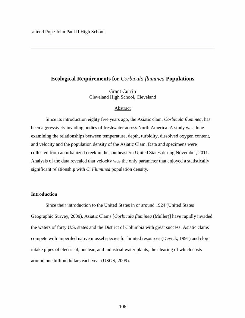
106

attend Pope John Paul II High School.

Ecological Requirements for Corbicula fluminea Populations

Grant Currin

Cleveland High School, Cleveland

Abstract

Since its introduction eighty five years ago, the Asiatic clam, Corbicula fluminea, has

been aggressively invading bodies of freshwater across North America. A study was done

examining the relationships between temperature, depth, turbidity, dissolved oxygen content,

and velocity and the population density of the Asiatic Clam. Data and specimens were

collected from an urbanized creek in the southeastern United States during November, 2011.

Analysis of the data revealed that velocity was the only parameter that enjoyed a statistically

significant relationship with C. Fluminea population density.

Introduction

Since their introduction to the United States in or around 1924 (United States

Geographic Survey, 2009), Asiatic Clams [Corbicula fluminea (Müller)] have rapidly invaded

the waters of forty U.S. states and the District of Columbia with great success. Asiatic clams

compete with imperiled native mussel species for limited resources (Devick, 1991) and clog

intake pipes of electrical, nuclear, and industrial water plants, the clearing of which costs

around one billion dollars each year (USGS, 2009).

107

A major factor contributing to the stunning success of Asiatic clams in North America

is their high level of tolerance for a host of environmental variables, including salinity (King et

al., 1986), substrate composition, pH (Devick, 1991), and water hardness (Belanger et al.,

1985). While a fair number of studies concerning the environmental requirements of Asiatic

clams have been conducted in laboratory settings, few have examined Asiatic clam

populations in relation to habitat and water quality in the field. (Foster et al., 2010)

Much of what is known about the ecological requirements of Asiatic clams based on

observational study comes from a single paper funded by the National Museum of Natural

Science in Madrid, Spain and written by R. Araujo, D. Moreno and M. A. Ramos. Published in

1993, their research, which examined the entire genus Corbicula, indicated that these bivalves

were able to thrive in waters with temperatures ranging from 9.2ºC to 27ºC, pH values of 5.9

to 8.2, and dissolved oxygen contents from 7.8 to 12.4 ppm. Corbicula were sampled a depth

of up to 8 cm, meaning that some of the organisms spent some amount of time out of the

water. A higher population density was observed at a depth of 6 meters and in substrates of

gravel and sand than was observed in shallower sand and mud.

The advancement of knowledge concerning the Asiatic clam, and particularly its

weaknesses, is paramount in the control of this highly invasive mussel (Wittmann, 2008). The

objective of this study is to gather information concerning factors that limit population

densities of Asiatic clams. Habitat and water quality parameters tested for include turbidity,

depth, dissolved oxygen, temperature, and velocity.

Experimental Procedure

108

All organisms and samples were taken in November, 2011. In total, eleven sites were

surveyed. Sampling began in South Mouse Creek approximately fifty meters upstream from

the intersection of Raider Drive in Cleveland, Tennessee. Mouse Creek has a watershed

drainage area of 39.4 miles2 and is a part of the Southern Limestone/Dolomite Valleys and

Low Rolling Hills subdivisions of the Ridge and Valley Ecoregion. Mouse Creek is listed by

the Tennessee Department of Environment and Conservation on the 303d list as impaired due

to sediment (United States Environmental Protection Agency, 2011). Each subsequent site was

located approximately ten meters upstream from the previous site. To be considered suitable

for use as a sample site, at least ½ m2 of the stream bed was required to a) lie at a depth of less

than fifty centimeters, b) have a grade less than 35%, and c) be composed of fine gravel or

very fine gravel, 2-8 mm in diameter.

The sampling and collecting technique was consistently conducted by a 2-man team at

each site. After a sample site was established and named, #1-11, a 2-liter container was filled

mid-channel above the sample site and immediately measured for dissolved oxygen content, in

miligrams per liter, using a Pasco Dissolved Oxygen Sensor and Pasco Spark Learning System

data logger. Meanwhile, a turbidity tube (transparency tube) was filled and used to measure

turbidity, which was recorded in milimeters.

A weighted PVC pipe square with internal dimensions of 25cm X 25cm was placed at

the center of the sample site. The top three centimeters of sediment from the area within the

square was transferred to a bucket, which was immediately taken to shore. The contents of the

bucket were examined by one team member for C. fluninea, which said team member

removed. Specimens were identfied using information from the United States Geographical

Survey (Foster, 2011). The sediment was then examined by the other team member to ensure

109

accuracy. After the organisms were counted and recorded, they were released well downstream

of the sample site. The ¼ m2 population size results were extrapolated to number per m2, the

standard unit for mussel studies (Hubbs, 2011).

Depth, temperature, and velocity were measured using a PASPORT Flow

Rate/Temperature Sensor, which was connected to the aforementioned data logger.

Temperature and velocity were conveyed on the digital display of the data logger while depth

was measured using the centimeter labels on the side of the pole.

The results from two of the eleven sample site were deemed invalid after closer

examination of each of the sites. Site 2, the shallowest site, was found to lie above the water

line after only 4 days’ drought, and upon further examination, the sediment at site ten was

found to be well outside the acceptable 2-8mm range.

Data

The full results of the study have been compiled on Table 1. The relationships between

C. fluminea/m2 and temperature (r2=0.023, P>.1), turbidity (r2=-0.032, P>.1), dissolved oxygen

(r2=0.274, P>.1), and depth (r2=0.048, P>.1) are displayed in Figure 1, Figure 2, Figure 3, and

Figure 4, respectively. Each of these relationships was found to be insignificant.

There was a highly significant relationship between population densities of C. fluminea

and the velocity of the surrounding water (r2=0.895, p<.01). This relationship is displayed in

Figure 5. Population densities of C. fluminea were found to be extremely high (up to 272

organisms/m2) in quickly-moving runs and extremely low in deep, slow-moving pools (in one

such pool, only a single specimen was found in the .25m2 sample area).

110

Conclusions

As was expected, this study revealed no relationship of significance between the

population density of C. fluminea and depth. It has already been well established that C.

fluminea can tolerate depths far in excess of the deepest point in Mouse Creek.

Turbidity also was found to have a statistically insignificant relationship with

population density of C. fluminea (r2=-0.032, p>.1). This relationship should be studied in

greater detail in bodies of water that have greater diversities of turbidity than Mouse Creek,

where the range was 6 NMU.

While also insignificant (r2=0.274, p>.1), the correlation between dissolved oxygen and

the population density of C. fluminea was slightly higher than that of C. fluminea and the

majority of the other variables measured. As was the case with turbidity, the limitations of

Mouse Creek, a highly channelized urban stream with few riffles, prevented a comprehensive

examination of this relationship.

The correlation between temperature and the population density of C. fluminea was

also insignificant (r2=0.023, p>.1). Previous studies have demonstrated that C. fluminea are

capable of tolerating temperatures greatly outside the range of 14.3-15.1ºC, so this comes as

no surprise.

There was a highly significant relationship between population densities of C. fluminea

and the velocity of the surrounding water (r2=0.895, p<.01). Population densities of C.

fluminea were found to be extremely high (up to 272 organisms/m2) in quickly-moving runs

and extremely low in deep, slow-moving pools (in one such pool, only a single specimen was

found in the .25m2 sample area). This is consistent with the findings of Lauritsen and Mozley.

111

Causes for this strong relationship may have to do with food and waste, as was

suggested by Mr. Don Hubbs of the Tennessee Wildlife Resources Agency; C. fluminea in

areas with strong currents have access to more food than do those in pools with lesser

currents. Additionally, the waste of C. fluminea in stronger currents is rapidly washed away

while that of C. fluminea experiencing slower currents is removed less rapidly.

These conclusions are not meant to imply that C. fluminea are tolerant to any depth,

temperature, turbidity level, or dissolved oxygen content, but rather that, within, the confines

of a small stream in southeast Tennessee, the significant factor limiting the population size of

C. fluminea is velocity. While this data may be limited to a single stream in a relatively small

geographic area, it will certainly help to present a clearer picture of the ecological

requirements of C. fluminea and can assist policy makers and wildlife managers in the

informed, responsible control of this highly-invasive species.

Acknowledgements

I extend thanks to Javier Francisco and Justin Jones for help in collecting samples and

specimens. I’d also like to thank Mr. Tyler F. Baker, Ms. Mary Allen, Dr. Milton Riley, Dr.

James Drake, Mr. Jim Herrig, Mrs. Jeannie Cuervo, and the Aquatic Biology class at

Cleveland High School for their expertise, suggestions, and data. Lastly, this project would not

have been possible without the generous assistance of Mr. Don Hubbs of the TWRA.

Works Cited

AAraujo, R., Moreno, D., & Ramos, M. A. (1993). The Asiatic clam Corbicula fluminea (Müller,

1774) (Bivalvia: Corbiculidae) in Europe. American Malacological Bulletin, 10(1), 39-

49.

Retrieved from

112

http://digital.csic.es/bitstream/10261/32551/1/Amer%20Malac%20Bull.pdf

BBelanger, S.E., J.L. Farris, D.S. Cherry, and J. Cairns, Jr. (1985). Sediment preference of the

freshwater Asiatic clam, Corbicula fluminea. The Nautilus 99(2- 3):66-73.

DDevick, W. S. (1991). Patterns of introductions of aquatic organisms to Hawaiian freshwater

habitats. Pages 189-213 in New Directions in Research, Management and

Conservation of Hawaiian Freshwater Stream Ecosystem. Proceedings Freshwater

Stream Biology and Fisheries Management Symposium. Department of Land and

Natural

Resources, Division of Aquatic Resources, Honolulu, HI.

Foster, A. M., Fuller, P., Benson, A., Constant, S., & Raikow, D. (2011, September 14).

Corbicula Fluminea. USGS Nonindigenous Aquatic Species Database. Retrieved

November 28, 2011, from http://nas.er.usgs.gov/queries/factsheet.aspx?speciesID=92

Hubbs, Don Tennessee Wildlife Resources Agency biologist, (personal communication, 28

October, 2011)

King, C.A., C.J. Langdon, and C.L. Counts, III. (1986). Spawning and early development of

Corbicula fluminea (Bivalvia: Corbicularidae) in laboratory culture. American

Malacological Bulletin 4(1):81-88.

Lauritsen, D. D., Mozley, S. C. (1989). Nutrient extretion by the Asiatic clam Corbicula

fluminea. Proceedings of the North American Benthological Society. 8(2):134-139.

United States Environmental Protection Agency (1 December 2011). Tennessee Impaired

Waters. United States EPA. Retrieved from

http://iaspub.epa.gov/tmdl_waters10/attains_impaired_waters.control?p_state=TN

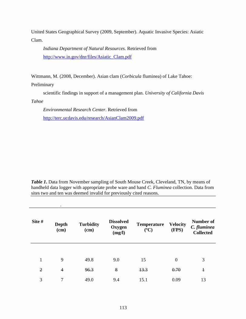
113

United States Geographical Survey (2009, September). Aquatic Invasive Species: Asiatic

Clam.

Indiana Department of Natural Resources. Retrieved from

http://www.in.gov/dnr/files/Asiatic_Clam.pdf

Wittmann, M. (2008, December). Asian clam (Corbicula fluminea) of Lake Tahoe:

Preliminary

scientific findings in support of a management plan. University of California Davis

Tahoe

Environmental Research Center. Retrieved from

http://terc.ucdavis.edu/research/AsianClam2009.pdf

Table 1. Data from November sampling of South Mouse Creek, Cleveland, TN, by means of

handheld data logger with appropriate probe ware and hand C. Fluminea collection. Data from

sites two and ten was deemed invalid for previously cited reasons.

.

1 9 49.8 9.0 15 0 3

2 4 96.3 8 13.3 0.70 1

3 7 49.0 9.4 15.1 0.09 13

Site # Depth

(cm)

Turbidity

(cm)

Dissolved

Oxygen

(mg/l)

Temperature

(ºC)

Velocity

(FPS)

Number of

C. fluminea

Collected

114

4 11 37.0 8.8 14.5 0.0 1

5 32 45.0 9.5 14.8 0.12 6

6 25 45.0 7.8 14.8 0.0 8

7 14 47.5 8.6 14.4 0.0 3

8 15 47.0 9.7 14.7 0.40 27

9 17 45.0 8.7 14.7 0.24 11

10 16 50.0 8.7 14.7 0.46 9

11 22 40.0 8.1 14.3 0.34 17

Figure 1. Relationship between temperature and C. fluminea population density, data

collected November 2011 at South Mouse Creek, Cleveland, TN.

13.8

14

14.2

14.4

14.6

14.8

15

15.2

0

50

100

150

200

250

300

350

400

450

500

1 3 4 5 6 7 8 9 11

Co

rbic

ula

Flu

min

ea/S

qu

are

Met

er

Data Points by Site

A Comparison of the Relationship between Temperature and Corbicula fluminea Population Density

Corbicula/m2

Temperature (ºC)

115

Figure 2. Relationship between turbidity and C. fluminea population density, data collected

November 2011 at South Mouse Creek, Cleveland, TN.

Figure 3. Relationship between dissolved oxygen content and C. Fluminea population density,

data collected November 2011 at South Mouse Creek, Cleveland, TN.

0

10

20

30

40

50

60

050

100150200250300350400450500

1 3 4 5 6 7 8 9 11Co

rbic

ula

Flu

min

ea/S

qu

are

Met

er

Data Points by Site

A Comparison of the Relationship between Turbidity and Corbicula fluminea Population Density

C. fluminea/Square Meter

Turbidity (mm)

0

2

4

6

8

10

12

0

50

100

150

200

250

300

350

400

450

500

1 3 4 5 6 7 8 9 11

Co

rbic

ula

Flu

min

ea/S

qu

are

Met

er

Data Points by Site

A Comparison of the Relationship between Dissolved Oxygen Content and Corbicula flumineaPopulation Density

Corbicula fluminea/square meter

Dissolved oxygen(mg/l)

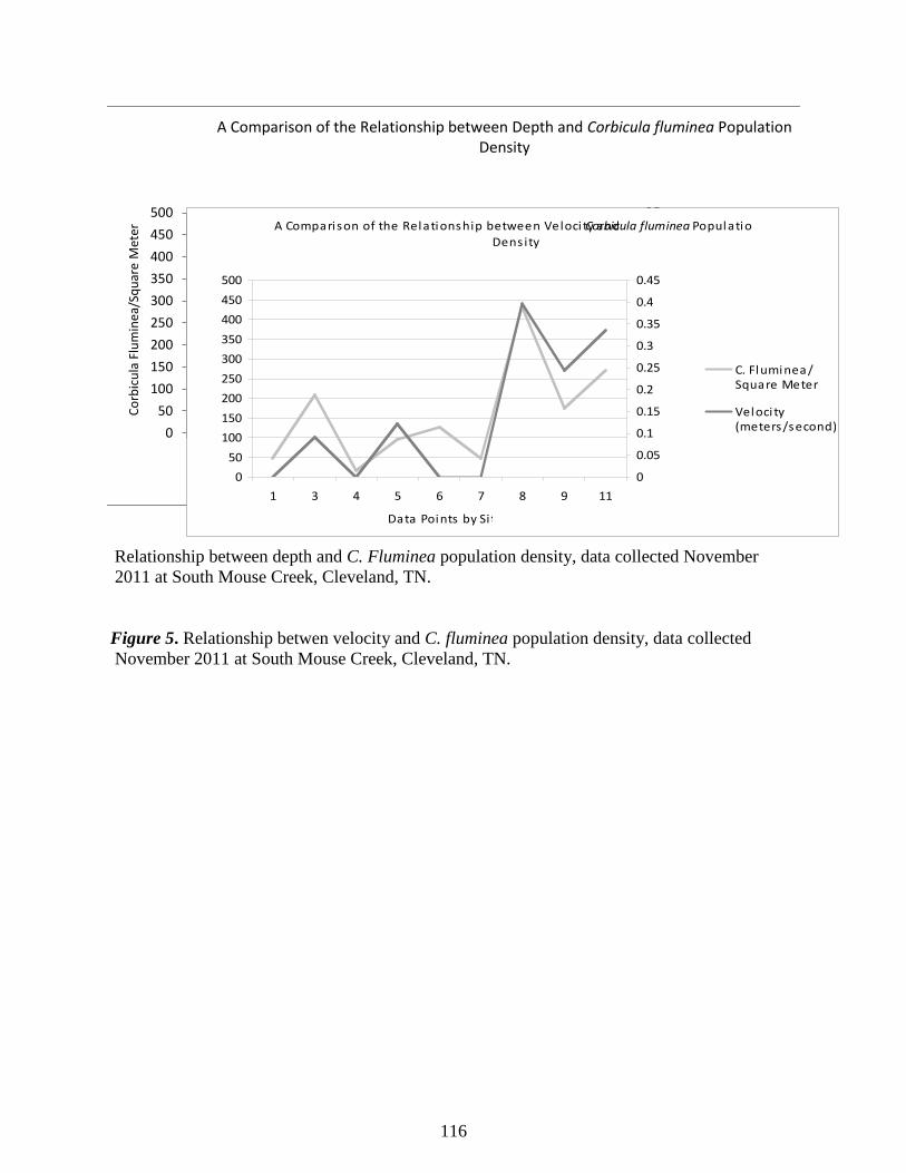
116

Relationship between depth and C. Fluminea population density, data collected November

2011 at South Mouse Creek, Cleveland, TN.

Figure 5. Relationship betwen velocity and C. fluminea population density, data collected

November 2011 at South Mouse Creek, Cleveland, TN.

0

5

10

15

20

25

30

35

0

50

100

150

200

250

300

350

400

450

500

1 3 4 5 6 7 8 9 11

Co

rbic

ula

Flu

min

ea/S

qu

are

Met

er

Data Points by Site

A Comparison of the Relationship between Depth and Corbicula fluminea Population Density

corbicula/m2

Depth (cm)

A Comparison of the Relationship between Veloci ty and Corbicula fluminea Population

Dens ity

0

50

100

150

200

250

300

350

400

450

500

1 3 4 5 6 7 8 9 11

Data Points by Si te

C. F

lum

inea

/Squ

are

Met

er

0

0.05

0.1

0.15

0.2

0.25

0.3

0.35

0.4

0.45

C. Fluminea /Square Meter

Veloci ty(meters/second)

117

December, 2011 Pathogen Survey of Three Murfreesboro Tennessee Area

Streams

Maggie Denton

Siegel High School, Murfreesboro

Abstract

In December, 2011, three Murfreesboro streams were sampled for the pathogen,

Escherichia coli (E. coli). Pathogens are bacteria and other organisms known to cause illness

in humans. Streams and sampling locations were selected from area waters previously found

to be violating E. coli criteria by the Tennessee Department of Environment and Conservation

(TDEC). Streams chosen for sampling were Town Creek (one station), Sinking Creek (two

stations) and Lytle Creek (two stations). Previous TDEC sampling stations were selected for

this study.

Following development of a study plan, samples were collected on December 7, 8, 12,

13, and 14, and transported to the Murfreesboro Water Treatment Plant for analysis. Sample

collection and handling followed protocols established by TDEC. The geometric mean of each

location was calculated and results from three stations (Lytle Creek at Hwy 70, Lytle Creek at

Old Fort, and Sinking Creek at Memorial Blvd) failed to meet the water quality standard for E.

coli, which is 126 colony forming units (cfu) as a geometric mean of five samples collected

within a 30 day period. Additionally, concentrations at the two Lytle Creek stations on

December 7 and 8 exceeded the single sample maximum concentration criterion for a park

(487 cfu). The results from this study will be provided to the Murfreesboro Storm Water

Department and TDEC with the hope that data can be used in future assessment efforts.

Introduction

118

Everyone has a right to clean water in Tennessee, according to the Tennessee Water

Quality Control Act. For this reason, waters are held in public trust and the Department of

Environment and Conservation has been established to plan for the uses of these waters and to

protect them for future generations. Water quality monitoring and assessment are integral

parts of this process.

There are seven designated uses for waters in Tennessee: domestic water supply, fish

and aquatic life protection, irrigation, recreation, industrial water supply, navigation, livestock

and wildlife watering (TDEC, 2007). Water quality criteria are established for each use

(TDEC, 2007). One of the criteria established for the protection of recreation is for

Escherichia coli, commonly called E. coli.

Section 305(b) of the Federal Water Pollution Control Act, commonly called The

Clean Water Act, requires a reporting of the water quality in Tennessee (TDEC, 2010).

Additionally, Section 303(d) of the act establishes that each state should maintain a listing of

the streams known to be polluted. These resources were used to identify the streams impaired

by E. coli in the Murfreesboro area.

In order to fulfill its statutory mission, TDEC maintains a network of statewide

monitoring stations. Chemical, physical, biological, and bacteriological data are then

compared to water quality criteria. Streams where criteria are violated are considered to be

polluted, or not meeting their designated uses (TDEC, 2010).

Once streams are identified as impacted by pollutants, they become priorities for

restoration. By statute, streams on the 303(d) List must have a specialized study called a Total

Maximum Daily Loading (TMDL). The TMDL identifies the sources of a pollutant and

119

proposes a control strategy. A TMDL for E. coli was completed for the Stones River

watershed in 2006 (TDEC, 2006).

Control strategies depend on the nature of the sources. In the case of pathogens,

sources can vary depending on land uses. In an urban area such as Murfreesboro, pathogen

sources can include leaking sewage collection systems plus runoff that may include pet and

wildlife wastes.

Authority to deal with local water quality issues related to runoff can be delegated from

the state to a local storm water management program. Murfreesboro has such a program, part

of the Water and Sewer Department. The program has an important role educating the public

regarding how pollutants in runoff can be controlled (City of Murfreesboro, 2012).

One example related to pathogens involves pet wastes along the Murfreesboro

greenway, which follows the lower portions of Town and Lytle creeks. Because wastes from

pets can be a source of pathogens, signs along the greenway encourage owners to pick up after

their pets. Plastic bags are provided to assist in this process.

In partial fulfillment of the requirements of a senior level AP Biology course at Siegel

High School, the author researched local water quality issues related to pathogens in area

streams, developed a study plan, approached the Murfreesboro Storm Water Department for

assistance, collected samples, analyzed data, and developed conclusions.

Materials, Methods, and Procedures

Before any water sampling could be done, research regarding the condition of area

streams was needed. Using the 2010 303(d) List, a detailed compilation of the impaired

120

waters in Tennessee, three pathogen impaired local streams were identified for further study:

Lytle Creek, Town Creek, and Sinking Creek. Historical TDEC sampling locations on these

streams were determined using the GIS-based mapping system on the department’s website.

The following stations were selected for this project: Town Creek at Cannonsburgh,

Lytle Creek at U.S. Hwy 70, Lytle Creek at Old Fort, Sinking Creek at Memorial Blvd, and

Sinking Creek at Thompson Lane. These stations are illustrated in Figure 1 and Figure 2.

All sample collections followed the policies established by TDEC in the 2011 Quality

Systems Standard Operating Procedure for Chemical and Bacteriological Sampling of Surface

Water (TDEC, 2011). Protocol C of this document contains detailed instructions for testing

streams for pathogens, such as E. coli, the focus of the study. These standardized procedures

ensure that data quality objectives are met.

According to the procedures, the following equipment and materials were needed:

25 Sodium Thiosulfate (Na2S2O3) Preserved Bottles *

(sodium thiosulfate is used to remove any chlorine present in the water)

Powder Free Latex Gloves*

Sample Labels*

Zip-type Plastic Bags*

Wading Boots**

Watch (cell phone)

Thermometer for Air Temperature (Cell Phone)

121

Project Sampling Locations

Figure 1

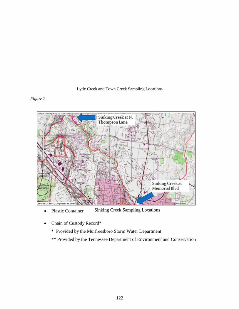
122

Sinking Creek Sampling Locations

Lytle Creek and Town Creek Sampling Locations

Figure 2

Plastic Container

Chain of Custody Record*

* Provided by the Murfreesboro Storm Water Department

** Provided by the Tennessee Department of Environment and Conservation

123

Upon arrival to the first test site, wading boots and latex gloves were donned. In

accordance with Protocol C, the tester waded out to the middle of the stream and removed the

top of the preserved sample bottle. The sample was collected upstream from the tester and the

water was allowed to clear in order to avoid sample contamination from debris possibly

disturbed by the movements of the sampler.

The sample bottle was placed it into the water at a 45 degree angle to avoid displacing

the Na2S2O3. An inch of air space was left in the bottle to allow the preservative to be mixed

with the water. To facilitate this mixing, the tester shook the bottle immediately following

collection.

Next, the collector measured the air temperature and determined the military time. A

sample label was filled out with this information- along with the station location, the station ID

number, the date, indication of the presence of the preservative Na2S2O3, and an indication of

the pathogen being analyzed (in this case, E. coli) - and placed on the sample bottle. Then the

bottle was placed in a zip type bag inside the plastic container.

The collector repeated the testing procedures at the next four sampling locations.

When finished, the plastic container held five zip type bags, each containing a sample bottle

and label. Finally, all samples were transported to the Murfreesboro Water Treatment Plant

for analysis. The chain of custody record, a form used to ensure the integrity of the samples,

was received and signed each day by Alison McGee.

Results

124

Figure 3

Samples were analyzed with the Colilert system. Figure 3 compares the geometric

means calculated at each station with the water quality criterion for E. coli (126 cfu per 100

ml). Table 1 shows a summary of the data collected.

Table 1. E. coli Concentrations in Studied Streams

0

50

100

150

200

250

300

350

Town Creek atCannonsburgh

Lytle Creek at Hwy70

Lytle Creek at OldFort

Sinking Creek atMemorial Blvd.

Sinking Creek atThompson Ln.

Geometric Mean of Assessed Streams

E. coli geo mean criterion: 126 cfu

Failed to meet water quality standards Met water quality standards

125

Table 1. E. coli Concentrations in Studied Streams (continued)

Sample Site Date Collected E. coli Level

Geometric Mean

TOWN000.1RU

Town Creek @

Cannonsburgh

12/7/11

82

92.3

12/8/11 60

12/12/11

104

12/13/11

104

12/14/11 126

LYTLE001.3RU

Lytle Creek @ Hwy

70

12/7/11 974

200.4

12/8/11 576

12/12/11

150

12/13/11 62

12/14/11 62

LYTLE000.6RU

Lytle Creek @ Old

Fort

12/7/11 1366

308.1

12/8/11

690

12/12/11 220

12/13/11

62

12/14/11 216

126

* Geometric Mean= ((X1)(X2)(X3)(X4)(X5))1/5

X= Individual Value

Conclusions

According to the TDEC, about 42 percent of the assessed streams in Tennessee are

impaired to some extent (TDEC, 2010). The pathogen E. coli is noted as a pollutant in 24

percent of them. Several Rutherford County streams are identified as impaired by pathogens,

including the streams selected for this study (TDEC, 2010).

Sample Site Date Collected E. coli Level

Geometric

Mean

SINK1003.8RU

Sinking Creek @

Memorial Blvd.

12/7/11 336

135.0

12/8/11 124

12/12/11 104

12/13/11 82

12/14/11 126

SINK1000.2RU

Sinking Creek @

Thompson Lane

12/7/11

346

96.3

12/8/11

104

12/12/11

62

12/13/11

62

12/14/11 60

127

The results of this experiment showed that 60 percent of the five assessed streams did

not meet water quality standards in December, 2011. Stations where elevated levels were

documented were Lytle Creek at U.S. Hwy 70, Lytle Creek at Old Fort, and Sinking Creek at

Memorial Boulevard. In addition, samples from two Lytle Creek stations exceeded the single

sample maximum concentration for a park. (One of the stations was in Cannonsburgh and the

other was in Old Fort Park.)

Water quality standards violations at two Lytle Creek stations and one Sinking Creek

station confirmed the previous assessments of impairment by TDEC. Stations at Town Creek

and Sinking Creek at Thompson Lane met criteria for support of the recreation use and may

suggest improved conditions. However, it may simply indicate that pathogen sources near

these sites are more associated with low rather than high flows. More data will be necessary

to confirm water quality improvements.

It is hoped that the data generated by this study can be used by TDEC and the

Murfreesboro Storm water program in their ongoing efforts to improve the quality of

Rutherford County streams.

Works Cited

Denton, G.M., M.H. Graf, D.H. Arnwine, L.K. Cartwright. 2010. 305(b) Report

The Status of Water Quality in Tennessee. Tennessee Department of Environment and

Conservation, Division of Water Pollution Control. Nashville, TN. 104 Pages.

http://www.tn.gov/environment/wpc/publications/pdf/2010_305b.pdf.

City of Murfreesboro. 2012. Murfreesboro Storm water Department Website, Robert Haley,

Director. http://www.murfreesborotn.gov/default.aspx?ekmenu=42&id=3774

Tennessee Department of Environment and Conservation. 2011. Year 2010 303(d) List.

Tennessee Department of Environment and Conservation, Division of Water

128

Pollution Control. Nashville, TN. Page 32.

http://www.tn.gov/environment/wpc/publications/pdf/2010proposed_final_303dlist.pdf

.

_____. 2011. Quality Systems Standard Operating Procedure for Chemical and

Bacteriological Sampling of Surface Water. Tennessee Department of Environment

and

Conservation, Division of Water Pollution Control. Nashville, TN. Pages 58-64.

http://www.tn.gov/environment/wpc/publications/pdf/ChemSOP03QUAP.pdf.

_____. 2007. General Water Quality Criteria. Tennessee Department of Environment and

Conservation, Division of Water Pollution Control. Nashville, TN. 35 Pages.

http://tn.gov/sos/rules/1200/1200-04/1200-04-03.pdf.

_____. 2007. Use Classifications for Surface Waters. Tennessee Department of Environment

and Conservation, Division of Water Pollution Control. Nashville, TN. 34 Pages.

http://tn.gov/sos/rules/1200/1200-04/1200-04-04.pdf.

_____. 2006. Total Maximum Daily Load for E. coli in the Stones River Watershed,

Tennessee. Department of Environment and Conservation, Division of Water

Pollution Control. Nashville, TN. 35 Pages, plus appendices.

http://www.tn.gov/environment/wpc/tmdl/approvedtmdl/StonesEcoli.pdf

Tennessee’s Online Water Quality Assessment. 2012. Tennessee Department of Environment

and Conservation, Division of Water Pollution Control. Nashville, TN.

http://tnmap.tn.gov/wpc/default.aspx?resetSession=true.

Acknowledgements

The author gratefully acknowledges the advice and assistance of the following people:

Robert Haley, Murfreesboro Storm Water Department Director, for sponsoring the

analysis of the samples and providing some of the materials needed.

Staff at the Murfreesboro Water Treatment Plant, Randy Blurton, Lab Manager.

Special thanks to Alison McGee who provided direct assistance and a smile throughout

this project. Kim Burritt graciously analyzed all of the samples.

129

The Tennessee Department of Environment and Conservation’s Division of Water

Pollution Control staff: Jimmy Smith, Joey Holland, and Greg Denton.

Kelsea Stephens, Shannon Allen, Marcia Denton, Hannah McDonald, Madeline

d’Oliveira, and Hayden Bilyeu for accompanying the author to sampling locations.

The Francescon family for allowing the author to access Sinking Creek from their

property.

130

The Development of an Electroosmosis-Based Attosyringe

Abhi Goyal, Aditya Guidibanda & Will Cox School for Science and Math at Vanderbilt, Nashville

Abstract

As research in the fields of microbiology and genetics advances, many investigators find

the need to pipette sub-picoliter volumes of liquid. To this date, no efficient mechanism has

been developed to solve this problem. We have developed an electrophoretic picosyringe,

which creates an electrochemical gradient between an organic solvent and the pipetted liquid.

Using a one-way ANOVA coupled with a Tukey-Kramer T-Test, we have determined that

62V and a 3 minute run time yields the maximum deposition efficiency. Here we present the

results of our testing and creation of an electrophoretically driven picosyringe.

Introduction

Frequently in the fields of microbiology and microuidics, researchers find the need to

pipette restrictive amounts of liquid from one area to another. Administering fluids to a small

target area requires precise, sub-nL volumes of liquid. A specific case of this challenge is

transmitting a volume of biological liquid to an integrated circuit surface (100 nm x 100 nm)

that is designed for detecting viruses (Balasubramanian, 2005). Before the creation of

nanopipettes, other, less efficient pipettes were developed to pipette small volumes of liquid.

These pipettes, known as Rainin pipettes (Prager, 1965), are capable of handling liquids down

to about 100 nL, but researchers handling extremely small environments, such as a cell,

require the command of liquids down to several pL. Other pipettes were developed to very

effectively dispense solutions down to several pL (Prager, 1965); these utilize both bulk-

131

pressure driven flow and iontophoresis. The former process involves applying a burst of

positive pressure to drive liquid through a tube onto a small surface, and the latter involves

using electrophoresis to drive a drug across a barrier into a fluid stream. However, since these

methods could not pick up solutions, these could not be used as pipettes.

132

Current nanopipettes, initially developed in 1965 by Prager, et al., could dispense

liquid approximately 1 nL in volume but were very difficult to calibrate, and thus were

inaccurate (Prager, 1965). More recently, pipettes

have been developed by Byun et al. that

implement electroosmosis, the motion of liquid

induced by an applied voltage. The existence of a

chemical equilibrium between a static surface and

an electrolyte solution results in the formation of

a fixed electric charge, forming a layer of ions

near the surface called the electric double layer

(EDL) (Grahame, 1941). When an electric field is

applied to the fluid, Coulomb force induces the

net charge of the EDL to move in accordance

with electrostatic interactions, and the liquid is

carried along with it.

EO-driven pipettes maintain several

advantages, including low stable flow rates,

convenience in adjustments, and no motile parts.

The major disadvantage to primitive EO-driven

pipettes is the inability to control direction of

current. In 2007, to overcome the problem of

calibration and inability to control direction

of current, Byun et al. developed an electroosmosis-based nanopipette containing a

Figure 7 -Diagram of Nanopipette (Byun, 2007)

133

polyacrylamide grounding interface (PGI). The nanopipette consisted of a high voltage (HV)

reservoir and a grounding (GND) reservoir both filled with 50mM sodium tetraborate solution.

The HV reservoir was connected to a microfluidic pump, which was connected to the

polyacrylamide grounding interface and the pipette tip (utilizing a T-shaped tube), which then

ended at the GND reservoir. The entire pipette was connected using tygon tubing, glass

capillary tubing, and silicone adhesive. The PGI enabled ion flow, but not liquid flow, through

itself. This allowed for the creation of the EDL between the HV and GND reservoirs, but

forced the liquid through the pipette tip rather than into the GND reservoir. A diagram of this

apparatus is shown in Figure 1 to the right. Figure 1a is the entire schematic of the

nanopipette, and Figure 1b is a schematic of the PGI. There were several drawbacks to this

EO-based pipette. In order to surmount the resistance within the nanopipette and enhance

liquid flow, a 5 kV source was required. The work presented here builds on this, elucidating

potential drawbacks and offering an alternative to this specific EO-based design. In order to

make a system more economically practical and user-friendly, an electrochemical picosyringe

was utilized. Our design was adapted from a previously built picosyringe (Laforge, 2007).

Methods

First, a PGI (Figure 1b) was created with 2.5% T (%T stands for the total weight

concentration acrylamide and bis in the solution) and 12% C (%C represents bis concentration

relative to acrylamide). These concentrations are similar to those used by the designers of the

electrophoretic nanopipette (Byun, 2007). A tygon T-tube was created with the polyacrylamide

grounding interface on one end and the capillary tube on the other. All the materials were

caulked together, and colored liquid was injected into the device using a syringe. Next, the

positive electrode was inserted into the pre-filled tube containing the liquid to be dispensed,

134

and the negative electrode was placed into the buffer solution. The schematic of the

picosyringe is shown in Figure 2.

The PGI and the capillary were immersed into the beaker containing buffer solution,

and the experiment ran for 5 minutes at various voltages.

Figure 3 shows the length of the void that is introduced after deposition. This void is

the amount of volume in the tygon tubing that becomes empty of fluid after deposition has

occurred. The volume of this void is therefore directly equal to the deposited volume and is

approximated as a cylinder. Figure 3 shows the diagram of the void volume.

Figure 8 - Schematic of the Electrochemical Picosyringe

135

The volume V of the void is given by

𝑉 = 𝜋𝑟2𝑙

where r is the radius of the base of the void and l is the length of the void.

After the creation of the picosyringe, the data were input into the JMP software. A one-

way ANOVA (analysis of variance) test and a Tukey-Kramer T-test (Figure 4) were

conducted. The test statistic of the Tukey-Kramer test, qs, is given by

𝑞𝑠 =𝜇𝑎 − 𝜇𝑏

𝑠

√𝑛

where µa and µb represent the means of population a and b respectively, s is the sample

standard deviation, and n is the sample size.

Figure 9 - Diagram depicting the introduction of the void

136

Using Excel, a graph comparing average void volume with time (Figure 5) was created

for each of the voltages that we tested. Linear regressions and correlation coefficients were

calculated for each voltage, and these data were inserted into Figure 5.

Results

Figure 4 shows the statistical relationship between the average void volume and

voltages over time. The different symbols represent the different times over which we iterated

the test. The one-way ANOVA tests for differences among our six independent means

(voltages) to test for which voltages are significantly different from each other. The test

performed afterwards was the Tukey-Kramer t-test, which restricts the ANOVA to pairwise

comparisons (see Equation (2)) which generated the circles seen in Figure 4. The circles above

the dividing line (30V, 60V, and 90V) represent voltages that are statistically significant to

each other, while the circles below the dividing line (10V and 120V) represent voltages that

are not statistically significant to the others. The data show that the distribution of void volume

with respect to voltage is parabolic, with a maximum of 62V.

137

Figure 4- One way ANOVA with Tukey-Kramer t-test

Figure 5 shows average void volume in pL for each of the five different voltages over our

three iterations. Each data set has a very high correlation for a linear trend line, implying a

directly proportional relationship for each of the voltages between time and void volume

Figure 11- Average void Volume vs. Time

Figure 10- One-way ANOVA with Tukey-Kramer t-test

138

Discussion

Figure 4 shows that although there was a high level of similarity between 30V, 60V,

and 90V, the mean voltage was 62V and the mean time was 3 minutes. This means that

running one's power source at 62V will yield the most efficient rate of dispension of water

over time and will economize the power use of the device.

Figure 5 shows average void volume in pL for each of the different voltages over the

three iterations. Each data set has a very high correlation for a linear trend line, implying a

directly proportional relationship for each of the voltages between time and void volume.

Using the quadratic relationship between voltage and void volume shown in Figure 4, as well

as the linear relationship between time and void volume generated in Figure 5, an artificial-

intelligence based device can deposit sub-nanoliter volumes of liquid with high precision.

Doctors wishing to deposit very accurate volumes of a drug solution to a patient need only

utilize the extremely precise relationships between voltage, time, and void volume in order to

achieve desired deposition of drug solution.

139

Conclusion

The volume of the vacuum of air that results from liquid dispension indicates that there

was an injection of liquid into the beaker solution. There were statistical significances between

the voltages, with 62V being the mean. In addition, there was a positive direct correlation

between time and void volume. Therefore, the volume pipetted is a multivariable function of

voltage and time. For future direction, it is intended to employ this device for microbiological

applications, for example to inject precise volumes of liquids into individual living cells. For

example, the injection of fluorescent dye into breast cancer cells can lead to enhanced cancer

visualization. It is also intended to attempt to deposit small volumes of liquid outside of the

water for use in a virus detection chip or other microfluidic devices in order to realize the

immense range of applications this device could have.

Works Cited

Balasubramanian, Anupama, et al. "Si-Based Sensor for Virus Detection." IEEE SENSORS

5.3

(2005): 5. Print.

Byun, Chang Kyu, et al. "Electroosmosis-Based Nanopipettor." Analytical Chemistry 79.10

(2007): 3862-66. Print.

Grahame, David C. "The Electrical Double Layer and the Theory of Electrocapillarity.".

Chemical Reviews 1941. 441-501. Vol. 41. Print.

Laforge, et. al., "Electrochemical attosyringe." PNAS. 104.29 (2007): 11895 - 11900. Print.

140

Prager, Denis J., Robert L. Bowman, and Gerald G. Vurek. "Constant Volume, Self-Filling

Nanoliter Pipette: Construction and Calibration. “Science 147.3658 (1965): 606-08.

Print.

The Effects of Plasma Gasification on Different Waste for the Production

and Analysis of Its Products

141

Gavin Dorrity

Northwest High School, Clarksville

Abstract

With an ever increasing population, the amount of garbage produced is potentially

endless. As we search for new methods of waste disposal there are not many obvious solutions

and the most used method today is to bury it in a landfill. Plasma gasification may be the

solution that can clean up our planet. The primary elements of waste can be broken down by

gasification in order to yield a flammable mixture of gas that can be further refined into liquid

fuels with the inorganic substances remaining as slag. This experiment was to demonstrate that

principle and using waste types as a variable, analyze the products of said types to identify an

ideal type for the gasification process. Unfortunately, those results were not reached due to a

failure to produce sufficient plasma for the gasification process. Failure aside, there are many

facets to this experiment that could lead to a successful experimental future.

Introduction

There is an endless amount of waste being produced around the world. In fact,

according to the Environmental Protection Agency, the United States alone produces over 220

million tons of waste each year (EPA, n.d.). There is a limited amount of space available for

landfills, especially in urban areas; not to mention that non-biodegradable materials and toxic

wastes remain in the ground to pollute the land and the water table. If these wastes could be

removed then it would be very beneficial to the environment. Recycling is already an

important step in the right direction. However, recycling consumes energy and the by-products

of producing the energy to run the recycling plant is the same as it would be for any other

factory. Now there might be a solution to these problems, and that is plasma gasification.

Plasma gasification is a technique that uses a high temperature electric arc that creates plasma

142

in a chamber that contains an inert atmosphere or sometimes regular air or even water (Young,

2008). Waste is placed within the chamber inside the plasma which can reach temperatures

between 10,000 to upwards of 30,000 degrees Fahrenheit, which is hotter than the surface of

the sun. This high temperature vaporizes all the substances and breaks apart the molecules into

their primary elements. Organic materials are mainly carbon, oxygen, and hydrogen, which are

funneled out of the chamber and naturally form a mixture of carbon monoxide and hydrogen

gases, known as syngas, which is combustible, similar to natural gas (Van Rossum, 2008).

This gas is filtered of trace amounts of contaminating elements and sent to a generator to be

burned and generate power that is enough to power the whole plasma process with excess. The

inorganic materials become a slag that collects at the bottom to form a glass-like substance that

resembles obsidian. This slag can then be sent for processing into concrete or pavers. The

garbage is reduced in volume by a significant amount. Overall this is an energy producing

process. The Department of Renewable Energy Sources along with the College of Technology

and Engineering calculated that “from one kilogram of 20% moisture wood it is possible to

obtain 4.6-4.8 MJ of electricity (net of electricity input) and 9.1-9.3 MJ of thermal energy

when using wood with average elemental composition and with a LHV energy content of 13.9

MJ, when using a combined Brayton and Steam cycle generating plant. Experimental data

from an air plasma gasification plant using alternating current (AC) plasma torches was

integrated with a thermodynamic model showing that the chemical energy in the produced

syngas was 13.8-14.3 MJ kg.sup.-1 with a power input of 2.2-3.3 MJ kg.sup.-1.” (Panwar,

2012). Plasma gasification clearly offers an advantage over other waste processing techniques

in many ways. This process differs from combustion, because there are technically no flames

involved, and therefore it is not the same as incineration. According to Canada’s Alter NRG

143

Corp “not only can plasma gasification produce 50% more energy than incineration, but the

syngas and other products can be refined into hydrocarbon fuels such as methanol, artificial

natural gas or diesel”(Canada, 2010). There are of course certain problems that are sorted out

during the process, such as the buildup of contaminating toxic elements that need to be filtered

or just physically separated before the by-products can be processed. On the other side, most

elements that would normally be toxic, such as heavy metals, are locked inside the stable

vitrified matrix of the slag (Fatta, 2005). Despite all the benefits of this process, there are

currently no running plasma gasification plants in the United States; although some plants

being constructed estimate that they could process up to 3000 tons of waste per day (Carlson,

2009). There are however some plants set up in Japan, Canada and several other first world

countries in the world. This project will not only demonstrate the principles of plasma

gasification, but will be designed to analyze the output of the system from different wastes in

order to find the ideal input materials. This project will also vary from the standard method of

using an inert atmosphere and will instead be using water with the garbage mixed up as slurry.

The benefit of this is that it will be out of an atmosphere altogether, it is more practical then

adding an inert gas, the products will be more hydrogen and oxygen, and it is possible that the

slag will not have an opportunity to crystalize, leaving it in a more manageable state for

filtration and processing. There is an argument that the plasma gasification process is too

difficult to maintain and has too many problems with toxic by-products to pursue it for waste

processing. Therefore, the objective is to examine the effects of plasma gasification on

different wastes for processing and analysis.

Methods and Materials

144

The construction of the gasification apparatus was the primary hurtle of the

experimentation process. The reactor chamber itself was put together out of a stainless steel

bucket that is approximately 1.75 gallons in volume and is suitable for high pressure if

necessary. A pressure gauge and thermometer were mounted on the lid and sealed air tight. A

gas outlet was also attached to the lid so that any gas being produced could be sent through a

gas hose and bubbled through water so it could be allowed to fill a 1 liter container so a

measurement of the gas production could be achieved. The next step was to cut a hole in the

container and attach a viewing window made of furnace glass, normally used for viewing

inside a combustion chamber. For power, a wire was fed underwater and attached to a

construction of three tungsten electrodes, one of which was grounded, the other two are

electric arc acceptors. The electrodes should not be allowed to touch on another so that there is

a small gap to permit an arc. The correct distance is variable due to the power supply and

materials used. The power supply was a combination of two transformers which were attached

to a switch and then to a wiring terminal which were attached to the plug. The plug was then

plugged into a power meter that is used for appliances to measure amperage, voltage, and

wattage. When everything is attached correctly the switch may be turned and the arc will

result. Safety gear was worn at all times, which included goggles, gloves, and a lab coat.

Distilled water should be used for testing to avoid contaminants from tap water. The chamber

is then filled with the water and results were observed. Due to the predicted lack of

conductivity provided by the distilled water, electrically conductive activated carbon was

added in powder form to the water in the reactor. An Arduino microcontroller was set up and

programmed with several types of gas sensors such as hydrogen, carbon monoxide, carbon

dioxide, methane, alcohol, and ozone, with the object of measuring a variety of gas

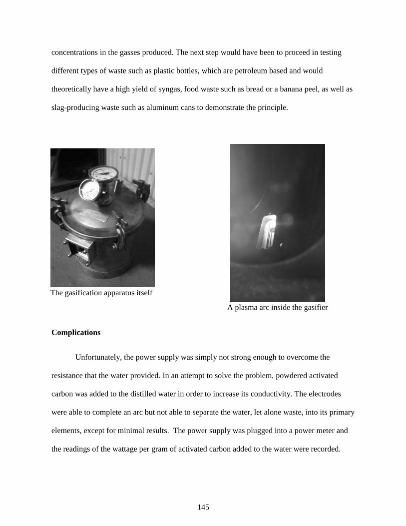
145

concentrations in the gasses produced. The next step would have been to proceed in testing

different types of waste such as plastic bottles, which are petroleum based and would

theoretically have a high yield of syngas, food waste such as bread or a banana peel, as well as

slag-producing waste such as aluminum cans to demonstrate the principle.

Complications

Unfortunately, the power supply was simply not strong enough to overcome the

resistance that the water provided. In an attempt to solve the problem, powdered activated

carbon was added to the distilled water in order to increase its conductivity. The electrodes

were able to complete an arc but not able to separate the water, let alone waste, into its primary

elements, except for minimal results. The power supply was plugged into a power meter and

the readings of the wattage per gram of activated carbon added to the water were recorded.

A plasma arc inside the gasifier

The gasification apparatus itself

146

Results

Conclusion

Unfortunately, my experiment is inconclusive for what I originally planned on

measuring. There was not enough production from the reactor to even give me a measurable

amount of syngas. However, with the miniscule amount of gas that was produced I was able to

light it on fire and demonstrate that it was most likely a combustible mixture of hydrogen and

oxygen. Although not relevant to the designed experiment, there was however a trend in the

wattage measured with each addition of activated carbon. The voltage remained nearly the

same with each addition of carbon, while the amperage decreased, resulting in an overall

0

50

100

150

200

250

0 1.7 3.1 6.6 10.5 16.6 22.4 30.5

Watts per Grams of Carbon

Watts

147

decrease in wattage consumption. The addition of the carbon in the first place was what started

the arc, which was otherwise unachievable with only distilled water. This is comprehensible,

because the easier it is for the electricity to flow, the less power is consumed.

Future Research

If this project were to be repeated there would be a better chance for successful results

based on these failures. The water would be replaced with an inert atmosphere, such as helium

or argon, to decrease resistance and hopefully the majority of the experiment could be carried

out as a result. A stronger power supply may also be acquired to take the experiment further.

Materials that are traditionally toxic when burned, such as Styrofoam, may additionally be

processed in order to show that those harmful molecules can also be broken into simpler form

and then combusted themselves. If nothing else, the experiment will be repeated in order to

understand these failures.

Acknowledgements

For this experiment I would like to thank my chemistry teacher, Mrs. Constance

Brown, for helping me participate in TJAS. I would like to thank the Tennessee Junior

Academy of Science for providing me with the funding that allowed me to construct this

experiment. Most importantly I would like to thank my brother, Calin Dorrity, without whom I

could not have even completed what I did on this experiment.

Works Cited

Bratsev, A. N., Kuznetsov, V. A., Popov, V. E., Rutberg, P. G., Shtengel', S. V., &

Ufimtsev, A. A. (2011); On efficiency of plasma gasification of wood residues.

Biomass and Bioenergy, 35(1), 495+. Retrieved from

148

http://go.galegroup.com/ps/i.do?&id=GALE%7CA245749578&v=2.1&u=tel_s_tsla

&it=r&p=AONE&sw=w.

Canada : (2010); Alter NRG corp. announces advancement and site license for proposed

commercial scale energy from waste facility. TendersInfo News. Retrieved from

http://go.galegroup.com/ps/i.do?id=GALE%7CA237617362&v=2.1&u=tel_s_tsla&i

t=r&p=GPS&sw=w.

Carlson, C.; (2009). Out of gas; Waste Age, 40(2). Retrieved from

http://go.galegroup.com/ps/i.do?id=GALE%7CA193799389&v=2.1&u=tel_s_tsla&i

t=r&p=GPS&sw=w.

EPA. (n.d.); Municipal Solid Waste | Wastes | US EPA.(2010) US Environmental

Protection Agency. Retrieved from http://www.epa.gov/osw/nonhaz/municipal/.

Fatta, D., Haralambous, K., Loizidou, M., Malamis, S., Moustakas, K. (2005);

Demonstration plasma gasification/vitrification system for effective hazardous waste

treatment. Journal of Hazardous Materials, 123(1-3), 120t. Retrieved from

http://go.galegroup.com/ps/i.do?&id=GALE%7CA195719499&v=2.1&u=tel_s_tsla

&it=r&p=GPS&sw=w.

Panwar, N. L., Kothari, R, Tyagi V.V.; (2012). Thermo chemical conversion of

Van Rossum, G.; (2008); Production of syngas via catalytic gasification of dry biomass;.

Industrial bio processing. Retrieved from

http://go.galegroup.com/ps/i.do?&id=GALE%7CA183317793&v=2.1&u=tel_s_tsla

&it=r&p=GPS&sw=w.

biomass- Eco friendly energy routes. Renewable and Sustainable Energy Reviews

Retrieved from

http://www.sciencedirect.com/science/article/pii/S1364032112000251.

149

Sigo, S. (2006). Florida county approves bonds for plasma arc gasification plant; The

Bond Buyer, 358(32519), 4; Retrieved from

http://go.galegroup.com/ps/i.do?&id=GALE%7CA155487504&v=2.1&u=tel_s_tsla

&it=r&p=GPS&sw=w.

Young, G. C.; (2008); From waste solids to fuel: a look at the economics of a plasma arc

gasification technology to produce energy and liquid fuels from a municipal solid

waste facility suggests a potential for wide-scale energy savings; Pollution

Engineering, 40(2), 45+; Retrieved from

http://go.galegroup.com/ps/i.do?&id=GALE%7CA193833846&v=2.1&u=tel_s_tsla

&it=r&p=GPS&sw=w.

150

Abstracts of Papers

Presented at the Annual Meeting

Belmont University

Nashville, Tennessee

April 20, 2012

The Effect of Glyphosate on Vanessa cardui

Kishan Bant

Hillwood Comprehensive High School, Nashville

Abstract

Herbicides and pesticides are forms of chemicals used to destroy pests and herbs. The

effect of herbicides and pesticides on non-target species is fatal. The following research and

experiment simulates the effect of herbicides, such as glyphosate, on the non-target species, such

as Painted Lady Butterflies, scientifically known as Vanessa cardui. During our experiment, my

partner and I utilized a common herbicide known as Roundup to determine the effect of its active

ingredient, glyphosate, on the sixty Vanessa cardui purchased from California Biological Supply

Co. The Vanessa cardui documented from larvae to maturity during the research. It was found

that the active ingredient, glyphosate, had a heavy impact on the Painted Ladies. The glyphosate

decreased physical activity dramatically. Many of the Vanessa cardui died before chrysalises and

maturity. Additionally, a large amount of the Vanessa cardui never made it out the larvae stage.

Out of the sixty larvae experimented upon, only nine survived. The Vanessa cardui that survived

at the end displayed defects and abnormalities. The matured and surviving butterflies were kept

until death. The experiment conducted reveals the effects of chemical such as pesticides and

herbicides on a small scale.

151

Effects of Light Pollution on Nocturnal Animal Activity

Maximilian Carter & Jonathan Davies School for Science and Math at Vanderbilt, Nashville

Abstract

Light pollution is unwanted artificial illumination. This study tested the effects of light

pollution on nocturnal activity at two locations, one with high light pollution levels (HLP) and

one with low (LLP). Shuboni and Yan [1] proved artificial light altered circadian rhythms in

mice; based on this, it was hypothesized that light pollution would deter nocturnal animal

activity. Animal activity was measured using insect traps, sound recorders, infra-red cameras,

and track and scat identification. Statistically significant differences were found in comparing

illuminance, insects, and tracks. Nocturnal activity was higher in LLP, suggesting light pollution

curtails nocturnal activity, supporting the hypothesis.

Plant and Microbiological Crust Composition in a Cedar Glade Community

Victoria Cooley, Joseph Flaherty & Samuel Stockard

Siegel High School, Murfreesboro

Abstract

Microbiotic crusts are highly specialized communities of cyanobacteria, mosses, and

lichens that are most commonly found in semiarid to arid environments. By conducting

biological surveys of plant communities in the cedar glades of Middle Tennessee, the

microbiotic crusts, plant, and soil ratios are examined in evaluating glade structure and

potential correlations with disturbance. In order to assess the microbial crust and plant

community of the glade, random sites were selected in an open glade area and evaluated for

biotic ground cover. Four foot by four foot plots were examined using a measuring square to

assess the biotic life for each random site. Results showed the total biotic cover accounted for

152

approximately twenty eight percent of the ground cover with a majority of the biotic ground

cover composed of various plant species. Plant growth was positively correlated with

microbial crust cover suggesting microbial crusts play a vital role in plants ability to inhabit

the open glade area.

Variation of Magnetic Field Strength with Temperature

Ashley Corson

Greenbrier High School, Greenbrier

Abstract

Magnetic field strength has been shown to correlate to temperature particularly by the

work of Pierre Curie. In the research presented here, the magnetic field strength was accurately

measured by a Vernier Magnetic Field Probe positioned at a selected distance from the tested

magnets, and the temperature was continuously monitored with a remote-sensing thermometer.

The average temperature change during this work was from 85°C to 165°C which caused a drop

in magnetic field strength from 225 to 160 teslas. This result follows the previously held

knowledge that magnets lose their strength when heated.

The Effects of Circumference on a Parachute’s Velocity

Cathleen Humm & Sarah Link

Pope John Paul II High School, Hendersonville

Abstract

Although parachutes may seem to be simple inventions made for the purpose of sport or

delivery, they are excellent items to be used to test the laws of physics when it comes to their

circumference in reference to the rate at which they reach terminal velocity. The circumference

of a parachute does, in fact, change the rate at which an object being carried by a parachute

reaches terminal velocity. Seeing this relationship, it can be said that the greater the

circumference of a parachute is, the quicker it will reach a terminal velocity. Testing a series of

parachutes with increasing diameters, and calculating the elapsed time for each trial measure

this. From this method, the results show that the parachute with a diameter of 5 cm fell with an

153

average velocity of 2.7 m/s, and the parachute with a diameter of 25cm fell at an average

velocity of 0.73 rn/s. This shows that the parachutes circumference directly affects the rate at

which an object falls, thus proving that there is a relationship between the circumference of a

parachute and the rate at which an object reaches terminal velocity.

The Effects of Redbreast Sunfish Population on the Populations of the Native

Lepomis Fishes in South Mouse Creek, Cleveland, Tennessee

Justin Jones Cleveland High School, Cleveland

Abstract

Redbreast sunfish, Lepomis auritus, are not native to South Mouse Creek. A study was

done examining the populations of redbreast sunfish and other native Lepomis fishes. Four other

Lepomis species were collected: green sunfish (Lepomis cyanellus), bluegill (Lepomis

macrochirusy, longear sunfish (Lepomis megalotis), and redear sunfish (Lepomis microlophus).

It was found that redbreast sunfish population had negative affects on these fishes. Previous

studies suggest that this occurs because of similarities among these fishes and competition

between these fishes. Although, the redbreast sunfish population was found to have a negative

impact, the percentage of the Lepomis population comprised of the redbreast sunfish fluctuated.

Soil Composition of a Typical Cedar Glade Habitat in Middle Tennessee

Joseph Kennedy, Lauren Pearson & Amanda Sudberry Siegel High School, Murfreesboro

Abstract

Cedar glades are rare ecosystems located in the southeastern United States. The

shallow soil in conjunction with exposed limestone bedrock has shaped these ecosystems and

led their species'. to adapt to the unique living environment. The plants in the cedar glades

have adapted to live in the shallow, rocky, and dry areas with low nutrient levels. The

objective ofthis study was to compare the soil nutrients between the inner and outer zones of

two glades at Flat Rock Cedar Glades and Barrens of Middle Tennessee. Soil depth,

154

phosphorous, nitrogen, and potassium levels were measured for comparison between glades

and zones within glades (inner and outer). The results ofthe soil tests showed consistently low

levels of phosphorous and nitrogen for the inner zone of both glades. The outer zones also had

consistently low nitrogen levels, but potassium and phosphorus levels were higher than those

of the inner zones. These results supported our hypothesis that shallow soil would have lower

nutrient levels than the surrounding forested areas.

The Effectiveness of Various Methods of Purification of Water

Robert Sellmer

Northwest High School, Clarksville

Abstract

Water is something that everyone must concern themselves with. Being that this water

must be clean, there are various methods that come in handy when trying to purify water of

contaminants that are not biological. These include distillation, carbon filtration, and the use

of purification tablets. During the experiment, these methods were carried out on four

different samples of water. By using a TDS meter before and after these were done, the effect

of each method on the purity of the water samples could be analyzed. The purpose of the

experiment was to figure out which method is the most effective when removing the

impurities from a range of water samples. The data showed that distillation was the most

effective method, followed by the purification tablets, and then carbon filtration. These

results were not obscene due to the effectiveness of the methods correlating in the same order

as the cost of the methods.

An Investigational Analysis on the Growing Trends of Opuntia humifusa

Jarrod Shores Siegel High School, Murfreesboro

Abstract

In this study, the growing trends of the Opuntia humifusa in a cedar glade

environment were analyzed. Since the cedar glades provide for little plant life, it was

155

expected that the 0. humifusa would be especially prominent in the cedar glade

environment since cacti tend to thrive in areas that are marginally hospitable for plant life.

After locating various 0. humifusa populations in the glade area, data was collected in three

specific categories- soil depth, soil texture, and canopy cover. These factors were

considered important for determining growing trends in this particular species. Soil

samples were taken at each cacti population found in the glade area. In addition, canopy

cover was measured in percent by using a densitometer for each location. The results

indicated that although soil depth was found to greatly differ between each sample site,

while canopy cover was very consistently high at every sample site. Finally, soil texture

tests proved to be vital in determining a relative consistency between the five sample sites.

The data indicates that canopy cover may be an important factor in determining where 0.

humifusa can grow in a cedar glade area while soil depth is insignificant.

The Effects of Metro Water Bio-solids on Soil Quality and Productivity of

Buckwheat

Jenny Zheng, Rachel Waters, Zoe Turner-Yovanovitch School for Science and Math at Vanderbilt, Nashville

Abstract

Although organic fertilizers are made using "green" techniques, it's uncertain how

fertilizers affect the environment surrounding an area. The effects of organic fertilizers, both

man-made and natural, on buckwheat and soil chemistry were studied. After preliminary

testing, buckwheat was planted on a 20x20m plot, half of which previously grazed by

chickens, and randomly fertilized by pelletized bio-solids. After maturation, random plots

were harvested and soil collected. Analysis shows that the previous chicken inhabited plots

yield more crops and have significant increase in plant height, seed count, and nitrate levels.

The bio-solids did not have any significant effects on the growth.