Fisheries Research 63 (2003) 303–313

Temporal variation in the virgin biomass of the edible jellyfish,Catostylus mosaicus(Scyphozoa, Rhizostomeae)

Kylie A. Pitt a,∗, Michael J. Kingsforda,ba School of Biological Sciences, A08 The University of Sydney, Sydney, NSW 2006, Australia

b School of Marine Biology and Aquaculture, James Cook University, Townsville 4811, Australia

Received 22 March 2002; received in revised form 17 February 2003; accepted 7 March 2003

Abstract

Temporal variation in the virgin biomass and abundance of a single stock of the edible jellyfish,Catostylus mosaicus(Scyphozoa, Rhizostomeae) was estimated at Lake Illawarra, a coastal lagoon in New South Wales, Australia. Density andbiomass were estimated three times within 3 weeks during three survey periods: April 1997, October 1997 and May 1998.Density and biomass were estimated for two size classes: all medusae easily counted from a moving boat (i.e. medusae≥50 mm bell diameter (BD)) and those considered to be vulnerable to the fishery (≥200 mm BD). Densities of medusae≥50 mm BD varied greatly between survey periods and between days within survey periods. Densities of medusae≥200 mmBD were similar between survey periods but varied within survey periods. The virgin biomass of medusae≥50 mm BD rangedbetween 1831 t during April 1997 and 18,526 t during May 1998. The biomass of medusae that was vulnerable to the fisheryvaried between 207 t in May 1998 and 2865 t in April 1997.© 2003 Elsevier Science B.V. All rights reserved.

Keywords:Virgin biomass; Temporal variation; Jellyfish; Scyphozoa;Catostylus mosaicus

1. Introduction

Jellyfish have been harvested in Asia for over 1000years (Omori and Nakano, 2001). Since the 1970s,however, development of large-scale commercialfisheries has seen the annual harvest increase almostexponentially and catches now regularly exceeded500,000 mt per year (FAO, 2000). Although tradi-tionally confined to Asia, fisheries for jellyfish nowoccur in the USA, UK, Namibia and Australia (FAO,2000).

∗ Corresponding author. Present address: School of Environmen-tal and Applied Sciences, Griffith University, PMB 50 GCMC, Qld9726, Australia. Tel.:+61-75-552-8324; fax:+61-75-552-8067.E-mail address:k.pitt@griffith.edu.au (K.A. Pitt).

The population dynamics of jellyfish are very dif-ferent from those of most commercially harvestedspecies. They have a complex life history that incor-porates sexual and asexual stages (e.g.Uchida, 1926;Calder, 1973; Pitt, 2000), grow extremely rapidly(mm per day;Kikinger, 1992; Kingsford et al., 2000)and the life span of the medusae is generally short,ranging from months to 1–2 years (Arai, 1997). Con-sequently, the abundance and biomass of a stock ofmedusae can fluctuate several orders of magnitudeover short (weeks–months) and long (years) timescales (Garcia, 1990; Pitt and Kingsford, 2000). Suchtemporal variability must be considered when design-ing biomass surveys for fisheries for jellyfish.

In Australia the rhizostome jellyfishCatostylus mo-saicusis harvested. This large (up to 350 mm diameter)

0165-7836/03/$ – see front matter © 2003 Elsevier Science B.V. All rights reserved.doi:10.1016/S0165-7836(03)00079-1

304 K.A. Pitt, M.J. Kingsford / Fisheries Research 63 (2003) 303–313

medusa occurs commonly along the east and northcoasts of Australia (Kramp, 1965) and forms denseaggregations in surface waters of bays and estuaries.A developmental jellyfish fishery was initiated in theestuaries and coastal lagoons of the northern half ofthe state of New South Wales (Fig. 1) in 1995 and wasexpanded to include the waters along the entire state in1997. Due to the lack of knowledge about the biomassof medusae in NSW waters, a conservative total al-lowable catch (TAC) was set at 1500 mt for the first 2years of the fishery. Fishers could only use hand netsto harvest medusae since this method enabled themto selectively target large individuals and minimisedby catch of small medusae. No size limit was set forthe fishery but large medusae produce a more valu-able product (R. Naidoo, Centre for Food Technology,Department of Primary Industries, Queensland, pers.comm.) and, therefore, are more likely to be targetedby fishers.

The major objective of our study was to developmethods for quantifying temporal variation in the vir-gin biomass of a single stock ofC. mosaicus. Restric-tion of the fishery to the northern part of the stateprovided an opportunity to make an empirical esti-mate of the temporal variability in the virgin biomassof a stock ofC. mosaicusin the southern part of thestate. Crucial to this study was the knowledge that theunit stock appears to consist of populations that oc-cur within individual bays or coastal lagoons (Pitt andKingsford, 2000).

2. Materials and methods

The study was conducted in Lake Illawarra, a shal-low (<4 m) coastal lagoon approximately 80 km southof Sydney, Australia (Fig. 1). Lake Illawarra is typicalof coastal lagoons along the NSW coast where jelly-fish are harvested. The lagoon is connected to the seaby a shallow channel that opens and closes intermit-tently. The lagoon was open to the sea for most of thestudy but closed in May 1998.

The biomass of medusae in Lake Illawarra was as-sessed on three occasions (periods): April 1997, Oc-tober 1997 and May 1998. Although the fishery insouthern NSW officially commenced during Novem-ber 1997 (Anon., 1997), no medusae were harvestedin the lake during the 1997/1998 season and this en-

abled the pre-harvest biomass to be estimated a thirdtime (May 1998). During each period, the size dis-tribution and size weight relationship were estimatedand abundances were counted three times within 3weeks. Abundance was estimated three times to inves-tigate short-term, temporal variation in abundances.During April 1997, the depth distribution of medusaewas also estimated. Although there is no limit on thesize of medusae harvested by fishers, medusae lessthan 200 mm bell diameter (BD) produce a productthat has a low commercial value and, therefore, it isnot economically viable to harvest small medusae (R.Naidoo, Centre for Food Technology, Department ofPrimary Industries, Queensland, pers. comm.). Dataon large medusae (i.e.≥200 mm BD) were presentedseparately, therefore, to provide an indication of theabundance and biomass of medusae that could havebeen vulnerable to the fishery at the time sampled.

2.1. Estimates of abundance/density

The abundance of medusae was estimated using vi-sual counts. Numbers of jellyfish were counted fromthe bow of a boat along transects 500 m long, 3 m wideand 1 m deep. Only medusae approximately≥50 mmBD were counted since smaller medusae are translu-cent and can be difficult to see and count accurately.Width of transects was measured using a 3 m pole thatwas positioned across the bow of the boat. Due to theangle with which the observer viewed the end of thepole, it is possible there was some error in estimatingthe area swept. However, given that the pole was posi-tioned only approximately 40 cm above the water andthe observer viewed the pole from above, it is consid-ered that this error was minimal. The length of tran-sects was measured by maintaining the boat at a con-stant speed of 10 km h−1 for 3 min. Existing informa-tion on the distribution of medusae in Lake Illawarra(unpublished data) indicated that there were some-times great differences in the distribution of medusaebetween the northern and southern ends of the lake.A proportional stratified sampling design was used toestimate abundance, therefore, as stratification can in-crease the precision of the estimates (Cochran, 1977).The survey area was defined as those parts of thelake >1 m deep. Although some medusae may occurin water shallower than 1 m, most areas outside the1 m contour area were too shallow to be accessed by

K.A. Pitt, M.J. Kingsford / Fisheries Research 63 (2003) 303–313 305

Fig. 1. Lake Illawarra. Hatching indicates survey area (1 m depth contour). Areas outside the survey area were too shallow to survey. (- - -)Division between northern and southern strata.

306 K.A. Pitt, M.J. Kingsford / Fisheries Research 63 (2003) 303–313

a boat and could not be surveyed. The survey areawas divided into two strata (north and south) that hadequal areas of 13.4 km2 (Fig. 1) and 30 transects wererun haphazardly in each. The area surveyed by tran-sects accounted for approximately 0.34% of the totalsurvey area. Care was taken to ensure that transectswere spread across a wide area of each stratum to en-sure that samples were representative. On 13/5/1998and 27/5/1998 great concentrations of medusae wereobserved on some transects and this made it diffi-cult to count them accurately. When such aggrega-tions were encountered, the width of the transectswas reduced from 3 to 1.5 m. Due to variation inthe area of transects, counts were converted to densi-ties m−2 transect−1.

Differences in the mean density of medusae amongperiods and among days within periods were testedusing two-way, nested ANOVAs. Separate testswere conducted for medusae≥50 mm BD and those≥200 mm BD. To reduce the risk of type I error, thedata set was divided into two and densities from 30replicate transects were used to test for differences inthe mean densities of the two size classes of medusae.The assumption of homogeneity of variances wasassessed prior to analyses using Cochran’s test. Vari-ances for both analyses were heteroscedastic andcould not be stabilised by transformation. However,the analyses were still done because the samplingdesign was balanced and contained a large number ofreplicates and in such circumstances, heteroscedastic-ity is unlikely to greatly increase the probability ofmaking a type I error (Underwood, 1997). The rela-tive contribution of each factor to the total variationwas estimated using variance components.

2.2. Size distributions

The size structure of the population was determinedby measuring the maximum BD of medusae, while onsnorkel. The BD was measured to the nearest 10 mmusing a ruler and all measurements were made whilethe bell was expanded to its maximum size prior tocontraction. Measurements were made while swim-ming in a straight line to ensure that individuals werenot measured repeatedly. Usually the size distributionwas measured by two people to minimise any effectof bias between observers. During each period, a min-imum of 100 medusae was measured at 8–12 sites

within the lake to ensure representative coverage of allareas. A total of 1796 medusae was measured in April1997, 940 in October 1997 and 1502 in May 1998.

2.3. Depth distribution

During April 1997 visibility in the lake was goodand it was possible to see the bottom of the lakefrom the surface. This enabled the depth distributionof medusae to be estimated. Most of the medusae thatwere measured to determine the size distribution werecategorised according to whether they occurred aboveor below 1 m depth (n = 1594). One metre depth wasestimated by the divers positioning themselves verti-cally in the water column and determining whetherthe jellyfish occurred above or below a known pointon the diver’s body that corresponded to 1 m depth.The depth distribution of medusae was estimated atdifferent sites at different times over a period of 3days. Poor visibility during October 1997 and May1998 prevented the depth distribution of medusae frombeing examined further and so the depth distributionrecorded during April 1997 was assumed to representthe depth distribution during the other periods.

2.4. Size/weight relationships

The relationship between size and weight ofmedusae was measured during each period (April1997, n = 65; October 1997,n = 70; May 1998,n = 84). A minimum of two medusae from each sizeclass present was weighed. Weight was measured us-ing a hand-held spring balance and size was recordedas the maximum BD of the upturned medusa, out ofthe water. Although the BD of medusae was measuredout of the water, the size weight measurements werecommensurate with the estimates of the size distribu-tion of the population made in the water since thereis no difference in the size of medusae measured inor out of the water (KP, unpublished data). Variationin the size/weight relationship among surveys wastested using analysis of covariance (ANCOVA). Dueto variation in sample sizes, data were randomly elim-inated from the October 1997 and May 1998 samplesuntil an equal sample size of 65 was achieved forall three samples. Data were linearised using a logetransformation and the assumption of homogeneity ofslopes was tested prior to performing ANCOVA.

K.A. Pitt, M.J. Kingsford / Fisheries Research 63 (2003) 303–313 307

2.5. Calculations of total biomass and 95%confidence intervals

Estimates of the biomass on each transect werecalculated based on measurements of abundance,size frequency distributions, size weight relationshipsand depth distribution of medusae. For each period,the mean weight (w) of medusae≥50 mm BD and≥200 mm BD was calculated according to the fol-lowing:

w =N∑

i=1

piwi (1)

wherewi is the mean weight (kg) of medusae in eachsize class andpi the proportion of medusae in eachsize class.

The density (number m−2) of medusae on each tran-sect (dj) was calculated by:

dj = nj

Aj

(2)

wherenj is the number of medusae on each transect,Aj the transect length× width.

The biomass in each stratum (s) was estimated as

Bs = wiγiAs

(1

Ns

) N∑j=1

djs (3)

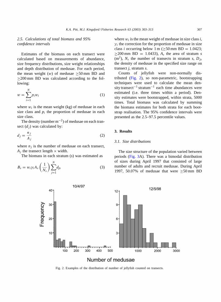
Fig. 2. Examples of the distribution of number of jellyfish counted on transects.

wherewi is the mean weight of medusae in size classi,γi the correction for the proportion of medusae in sizeclassi occurring below 1 m (≥50 mm BD= 1.0423;≥200 mm BD = 1.0433), As the area of stratums(m2), Ns the number of transects in stratums, Djs

the density of medusae in the specified size range ontransectj, stratums.

Counts of jellyfish were non-normally dis-tributed (Fig. 2), so non-parametric, bootstrappingtechniques were used to calculate the mean den-sity transect−1 stratum−1 each time abundances wereestimated (i.e. three times within a period). Den-sity estimates were bootstrapped, within strata, 5000times. Total biomass was calculated by summingthe biomass estimates for both strata for each boot-strap realisation. The 95% confidence intervals werepresented as the 2.5–97.5 percentile values.

3. Results

3.1. Size distributions

The size structure of the population varied betweenperiods (Fig. 3A). There was a bimodal distributionof sizes during April 1997 that consisted of largenumber of adults and recruit medusae. During April1997, 50.07% of medusae that were≥50 mm BD

308 K.A. Pitt, M.J. Kingsford / Fisheries Research 63 (2003) 303–313

Fig. 3. (A) Size frequency distributions, (B) size weight relationships, (C) mean density (±1S.E.) and (D) total biomass (±95% CI) forsurveys conducted during April 1997, October 1997 and May 1998. (�) Medusae≥50 mm BD, ( ) medusae≥200 mm BD.

K.A. Pitt, M.J. Kingsford / Fisheries Research 63 (2003) 303–313 309

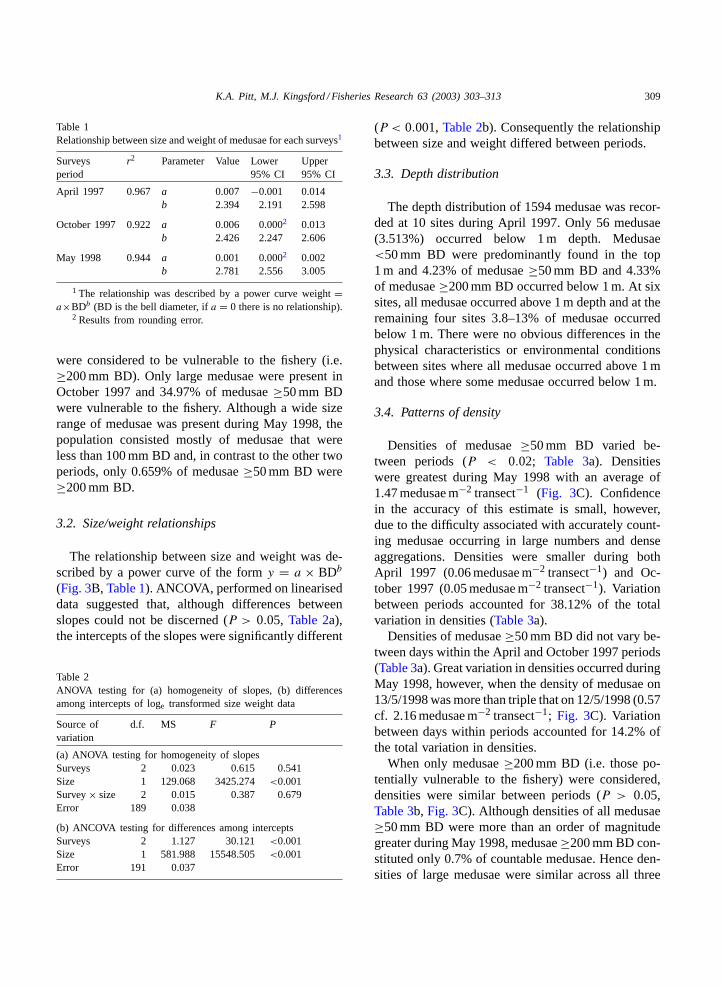
Table 1Relationship between size and weight of medusae for each surveys1

Surveysperiod

r2 Parameter Value Lower95% CI

Upper95% CI

April 1997 0.967 a 0.007 −0.001 0.014b 2.394 2.191 2.598

October 1997 0.922 a 0.006 0.0002 0.013b 2.426 2.247 2.606

May 1998 0.944 a 0.001 0.0002 0.002b 2.781 2.556 3.005

1 The relationship was described by a power curve weight=a×BDb (BD is the bell diameter, ifa = 0 there is no relationship).

2 Results from rounding error.

were considered to be vulnerable to the fishery (i.e.≥200 mm BD). Only large medusae were present inOctober 1997 and 34.97% of medusae≥50 mm BDwere vulnerable to the fishery. Although a wide sizerange of medusae was present during May 1998, thepopulation consisted mostly of medusae that wereless than 100 mm BD and, in contrast to the other twoperiods, only 0.659% of medusae≥50 mm BD were≥200 mm BD.

3.2. Size/weight relationships

The relationship between size and weight was de-scribed by a power curve of the formy = a × BDb

(Fig. 3B, Table 1). ANCOVA, performed on lineariseddata suggested that, although differences betweenslopes could not be discerned (P > 0.05, Table 2a),the intercepts of the slopes were significantly different

Table 2ANOVA testing for (a) homogeneity of slopes, (b) differencesamong intercepts of loge transformed size weight data

Source ofvariation

d.f. MS F P

(a) ANOVA testing for homogeneity of slopesSurveys 2 0.023 0.615 0.541Size 1 129.068 3425.274 <0.001Survey× size 2 0.015 0.387 0.679Error 189 0.038

(b) ANCOVA testing for differences among interceptsSurveys 2 1.127 30.121 <0.001Size 1 581.988 15548.505 <0.001Error 191 0.037

(P < 0.001,Table 2b). Consequently the relationshipbetween size and weight differed between periods.

3.3. Depth distribution

The depth distribution of 1594 medusae was recor-ded at 10 sites during April 1997. Only 56 medusae(3.513%) occurred below 1 m depth. Medusae<50 mm BD were predominantly found in the top1 m and 4.23% of medusae≥50 mm BD and 4.33%of medusae≥200 mm BD occurred below 1 m. At sixsites, all medusae occurred above 1 m depth and at theremaining four sites 3.8–13% of medusae occurredbelow 1 m. There were no obvious differences in thephysical characteristics or environmental conditionsbetween sites where all medusae occurred above 1 mand those where some medusae occurred below 1 m.

3.4. Patterns of density

Densities of medusae≥50 mm BD varied be-tween periods (P < 0.02; Table 3a). Densitieswere greatest during May 1998 with an average of1.47 medusae m−2 transect−1 (Fig. 3C). Confidencein the accuracy of this estimate is small, however,due to the difficulty associated with accurately count-ing medusae occurring in large numbers and denseaggregations. Densities were smaller during bothApril 1997 (0.06 medusae m−2 transect−1) and Oc-tober 1997 (0.05 medusae m−2 transect−1). Variationbetween periods accounted for 38.12% of the totalvariation in densities (Table 3a).

Densities of medusae≥50 mm BD did not vary be-tween days within the April and October 1997 periods(Table 3a). Great variation in densities occurred duringMay 1998, however, when the density of medusae on13/5/1998 was more than triple that on 12/5/1998 (0.57cf. 2.16 medusae m−2 transect−1; Fig. 3C). Variationbetween days within periods accounted for 14.2% ofthe total variation in densities.

When only medusae≥200 mm BD (i.e. those po-tentially vulnerable to the fishery) were considered,densities were similar between periods (P > 0.05,Table 3b, Fig. 3C). Although densities of all medusae≥50 mm BD were more than an order of magnitudegreater during May 1998, medusae≥200 mm BD con-stituted only 0.7% of countable medusae. Hence den-sities of large medusae were similar across all three

310 K.A. Pitt, M.J. Kingsford / Fisheries Research 63 (2003) 303–313

Table 3ANOVA testing for temporal differences in the mean density of (a) medusae≥50 mm BD and (b) medusae≥200 mm BD

Source of variation d.f. MS F P Denom. MS Variance components Total variation (%)

(a) Medusae≥50 mm BD; Cochran’sC = 0.6135 (P < 0.01)a

Period 2 59.87 9.01 0.0156 Day (period) 0.59 38.31Day (period) 6 6.65 9.06 <0.0001 Error 0.22 14.29Error 261 0.73 0.73 47.40

(b) Medusae≥200 mm BD; Cochran’sC = 0.4608 (P < 0.01)b

Period 2 0.0086 4.48 0.0645 Day (period) 7.44× 10−5 1.45Day (period) 6 0.0019 4.02 0.0007 Error 4.67× 10−5 0.91Error 261 0.0005 5.0× 10−3 97.64

a Student Newman Keuls (SNK) tests—Period: April 1997= October 1997< May 1998 (S.E. = 0.22718, d.f . = 6); Day (period)—April 1997: Day 1= Day 2= Day 3; October 1997: Day 1= Day 2= Day 3; May 1998: Day 1< Day 2, Day 1< Day 3, Day 2> Day 3.

b SNK tests for Day (period)—April 1997: Day 1< Day 2 = Day 3; October 1997: Day 1= Day 2 = Day 3; May 1998: Day 1=Day 2= Day 3.

periods. There was no variation in densities betweendays within the October 1997 and May 1998 peri-ods, however, during the April 1997 period, densitieson the first day sampled were smaller than those esti-mated on the second and third day (0.0166 cf. 0.0392and 0.0331 m−2 transect−1, respectively).

3.5. Estimates of the biomass of C. mosaicus in LakeIllawarra

Trends in biomass were similar to those observedfor density (Fig. 3D), however, as larger medusae wereheavier than smaller ones they contributed proportion-ately more in terms of biomass than they did in density.For example, during April and October 1997, medusae≥200 mm BD contributed approximately 50% of thetotal density of medusae, however, they made up morethan 67% of the total biomass. The total biomass ofmedusae≥50 mm BD was similar during April andOctober 1997 and ranged between 1831 and 4618 t(Fig. 3D). The enormous abundance of medusae ob-served during May 1998, however, lead to an esti-mated biomass that ranged from 4875 to 18,527 t. Thebiomass of medusae that were vulnerable to the fish-ery (i.e.≥200 mm BD), however, varied between 207and 2866 t across all three periods (Fig. 3D).

4. Discussion

Our study contrasts with most studies that estimatethe biomass of a stock in that multiple estimates of

biomass were obtained at short (days–weeks) and long(months) intervals in a cost-effective way. Few stud-ies that estimate biomass consider different scales oftemporal variability. This is often due to the expenseand the size of the areas that have to be surveyed. Yet,understanding the temporal scales over which biomasscan vary is vital for effective management of fisheries.Such measures can be obtained only using a hierar-chical sampling design. We have demonstrated thatvariation over short periods of time is important whensurveying jellyfish and our measures of temporal vari-ability in the virgin biomass of a stock of jellyfishprovide vital base-line information against which theeffects of future harvesting could be compared.

4.1. Strengths of the approach

The major strengths of the method we used to esti-mate the biomass of medusae were that it was inexpen-sive, rapid and could be undertaken by just two people.Jellyfish are a relatively low value product comparedto other species, such as prawns, that are also targetedby fishers. If the costs associated with managing theresource are imposed on the fishers then expensivesurveys are likely to render the fishery economicallynon-viable. Hence it is important that costs of surveysare minimised. The surveys we conducted requiredcosts associated with travel to and from Lake Illawarra,use of a small boat and wages for two people.

The second major benefit of our survey is that a sin-gle location could be surveyed in 1 day. Given that theunit stock forC. mosaicusis a population within an

K.A. Pitt, M.J. Kingsford / Fisheries Research 63 (2003) 303–313 311

individual bay or estuary (Pitt and Kingsford, 2000),several stocks could be surveyed repeatedly over ashort period. Since abundances and biomass can fluc-tuate greatly over short periods, multiple surveys maybe required during the harvesting season. The surveytechnique we have proposed would enable multiplesurveys to be undertaken relatively inexpensively.

4.2. Sources of uncertainty

There are several possible sources of uncertaintythat may have contributed to variation in estimatesof biomass. Sources of uncertainty relate to errorsassociated with estimating abundances, the size dis-tribution of the population, the relationship betweensize and weight of medusae, the depth distributionof medusae and possible migration into or out of thelake. The number of medusae measured to describethe size distribution of the population was very large(≥940 individuals per period) and medusae were mea-sured at multiple sites in the lake. Also, two peoplemeasured sizes during each survey, which would haveminimised any effect of observer bias. Hence we con-sider our estimates of the size distribution to have ac-curately represented the population. Similarly, therewas a very good relationship between size and weightof medusae with 92–97% of the variation in weightbeing explained by size (Fig. 3A). Migration was alsoconsidered to be unlikely to influence the biomass ofthe population since Lake Illawarra has only a nar-row, shallow opening to the ocean and movement ofmedusae into and out of the lake is considered min-imal. During May 1998 the entrance of the lake hadclosed completely and the population was retainedwithin the lake.

The depth distribution, although only estimated dur-ing the April 1997 period, indicated that medusae usu-ally occur in the top 1 m of the water column. It waspossible to estimate the depth distribution of medusaeonly when visibility in the lake was good and moremedusae may have occurred deeper during October1997 and May 1998 when the visibility was poor. Re-cently, however, it has been determined thatC. mo-saicuscontains zooxanthellae in its tissues (KP & MK,unpublished data). Although the degree of nutritionprovided to the medusae by the zooxanthellae is un-certain, we would consider that to maximise the ex-posure of their zooxanthellae to sunlight, under turbid

conditions medusae would be more likely to occur inthe surface waters. Further investigation of the depthdistribution of medusae and how it varies under differ-ent conditions is required and could be obtained usinga towed camera or depth-stratified trawls.

The major source of error associated with estimatesof biomass came from estimates of the abundanceof medusae. There are great difficulties in estimatingabundances of pelagic organisms that form dense ag-gregations (Wiebe, 1972; Omori and Hamner, 1982).Suggestions postulated to increase the precision ofsamples are to sample a large volume of water (Omoriand Hamner, 1982) or, for sampling with planktonnets, to increases the distance towed (Wiebe, 1972).In the current study it was important that counts becompleted within 1 day. The number of replicates was,therefore, largely dictated by the time taken to sample(approximately 6 h). This still resulted in a relativelylarge proportion of the possible sampling area beingsampled (0.34%). The length of the transects was op-timised to maximise precision while ensuring that thetime taken to run a transect was not so long that theconcentration of the observer was compromised. Al-though the transect length and number was optimal,the patchy distribution of medusae still resulted in es-timates of abundance that had large statistical error.

During April 1997 and May 1998 large discrepan-cies in estimates of abundance and biomass occurredbetween consecutive days. Indeed, in May 1998 theabundance and biomass of the population were esti-mated to have more than tripled between the first andsecond days sampled. Surprisingly, estimates of abun-dance and biomass made 2 weeks apart were moresimilar than those made on consecutive days, sug-gesting that abundances of medusae may have beengreatly under-estimated on the first day surveyed. Theconcentrations of medusae observed during May 1998were the greatest ever encountered in 12 years of sam-pling jellyfish in New South Wales (KP and MK, pers.obs.). Although vast aggregations of jellyfish were en-countered on the first day of the May 1998 period,during the second and third day jellyfish appeared tobe more concentrated within aggregations resulting insubstantially larger counts. Such concentrations pos-sibly also existed on the first day but, by chance, werenot sampled. This seems unlikely, however, given thelarge number of replicate transects used and the factthat such concentrations were not observed despite

312 K.A. Pitt, M.J. Kingsford / Fisheries Research 63 (2003) 303–313

spending approximately 10 h on the water. Anotherreason for the discrepancy between the counts may bethat more medusae were dispersed deeper during thefirst day.

4.3. Recommendations for estimating biomass ofjellyfish

Great variation in the abundance of medusaeover short (within weeks) periods of time suggeststhat multiple counts of medusae need to be madesince sampling on only one occasion may under-, orover-estimate abundance. Counts should be made onlyin calm conditions since turbulence at the water’s sur-face may influence the depth distribution of medusae.The aggregated distribution commonly observed forscyphozoans makes it difficult to obtain precise es-timates of abundance. Sampling methods, therefore,need to be optimised so that precision is maximised.A large proportion of the sampling area should besampled, however, it is important that counts becompleted within a single day, since movement ofmedusae may confound estimates made over multipledays. Consequently, the proportion sampled shouldbe the maximum proportion that can be sampled in 1day. The tendency for medusae to sometimes occur inlarge numbers and extreme concentrations may makeaccurate estimates of abundance difficult to achieve.During such times it may be preferable to count onlylarge medusae or to count medusae on a logarithmicscale. A combination of units could also be used. Forexample, large medusae could be counted as integersand small medusae could be counted on a logarithmicscale (Kingsford, 1998).

Existing knowledge of patterns of distribution andabundance of medusae should be considered whenplanning surveys. For example, in more open estuariesand embayments,C. mosaicusoccurs in greater abun-dances in the inner estuary at sites close to the mouthsof rivers (Pitt and Kingsford, 2000). The precision ofestimates of abundance in such locations may be max-imised if an optimal stratified sampling approach isadopted. Estuaries may be divided into strata accord-ing to distance from a river, or distance into the es-tuary, and the number of samples per strata would beallocated based on estimates of variance.

More accurate estimates of abundance may beobtained using towed nets or by videoing transects.

Towed nets are probably unsuitable for very shallowestuaries and are destructive. Video transects could bea useful alternative to visual counts when concentra-tions of medusae are large. The number of medusaealong a transect could be counted from a video and thespeed at which the video was played could be slowedto enable medusae to be counted accurately whendense concentrations of medusae were encountered.A disadvantage of this method is that it increasesthe cost of infrastructure needed and also requires agreater amount of time to analyse the video.

5. Conclusion

Due to the difficulties associated with accuratelyestimating abundances of medusae, there is a degree ofuncertainty associated with estimates of their biomass.Repeating counts of medusae multiple times over shortperiods, however, provides useful information aboutthe precision of the estimates of biomass and the smallcost of conducting surveys enables this to be done.The low cost and rapid nature of the survey methodwe have used provides a useful tool for estimatingbiomass of a relatively low-value but rapidly growingfishery.

Acknowledgements

We would like to thank N. Williams and R. Forrestfor assisting with fieldwork and M. Anderson and J.Scandol for statistical advice. Comments made by twoanonymous reviews greatly improved the manuscript.This study was funded by Environment Australia.

References

Anon., 1997. Jellyfish Fishery Management Plan 1997–2001 forthe JellyfishCatostylus mosaicusin New South Wales Oceanand Estuarine Waters. New South Wales Fisheries ManagementPublication Number 2.

Arai, M.N., 1997. A Functional Biology of Scyphozoa. Chapman& Hall, London.

Calder, D.R., 1973. Laboratory observations on the life history ofRhopilema verrilli (Scyphozoa: Rhizostomeae). Mar. Biol. 21,109–114.

Cochran, W.G., 1977. Sampling Techniques, 3rd ed. Wiley, NewYork.

K.A. Pitt, M.J. Kingsford / Fisheries Research 63 (2003) 303–313 313

FAO, 2000. FAO Yearbook. Fishery Statistics, vol. 90/1. CaptureProduction 2000.

Garcia, J.R., 1990. Population dynamics and production ofPhyllorhiza punctata(Cnidaria: Scyphozoa) in Laguna Joyuda,Puerto Rico. Mar. Ecol. Prog. Ser. 64, 243–251.

Kikinger, R., 1992.Cotylorhiza tuberculata(Cnidaria: Scypho-zoa)—life history of a stationary population. Mar. Ecol. 13 (4),333–362.

Kingsford, M.J., 1998. Analytical aspects of sampling design.In: Kingsford, M.J., Battershill, C.N. (Eds.), StudyingTemperate Marine Environments, Canterbury University Press,Christchurch, pp. 49–83.

Kingsford, M.J., Pitt, K.A., Gillanders, B.M., 2000. Managementof jellyfish fisheries, with special reference to the orderRhizostomeae. Oceanogr. Mar. Biol. Ann. Rev. 38, 85–156.

Kramp, P.L., 1965. Some medusae (mainly scyphomedusae) fromAustralian coastal waters. Trans. Roy. Soc. S. Aust. 89, 257–278.

Omori, M., Hamner, W.M., 1982. Patchy distribution ofzooplankton: behaviour, population assessment and samplingproblems. Mar. Biol. 72, 193–200.

Omori, M., Nakano, E., 2001. Jellyfish fisheries in Southeast Asia.Hydrobiologia 451, 19–26.

Pitt, K.A., 2000. Life history and settlement preferencesof the edible jellyfish Catostylus mosaicus(Scyphozoa:Rhizostomeae). Mar. Biol. 136, 269–279.

Pitt, K.A., Kingsford, M.J., 2000. Geographic separation of stocksof the edible jellyfish,Catostylus mosaicus(Rhizostomeae) inNew South Wales, Australia. Mar. Ecol. Prog. Ser. 196, 143–155.

Uchida, T., 1926. The anatomy and development of a rhizostomemedusaMastigias papuaL. Agasiz, with observations on thephylogeny of rhizostomae. J. Faculty Sci. Imperial Univ. Tokyo(Section 4, Zoology) 1, 45–95.

Underwood, A.J., 1997. Experiments in Ecology: Their LogicalDesign and Interpretation Using Analysis of Variance.Cambridge University Press, Cambridge, UK.

Wiebe, P.H., 1972. A field investigation of the relationship betweenlength of tow, size of net and sampling error. Journal du ConsielConseil International Pour L’exploration de la Mer. 34 (2),268–275.