Technical-economic Analysis of Fast Chargers for Plug-in ...

June 2010Kjell Sand, ELKRAFT

Master of Science in Energy and EnvironmentSubmission date:Supervisor:

Norwegian University of Science and TechnologyDepartment of Electric Power Engineering

Technical-economic Analysis of FastChargers for Plug-in Electric Vehicles inDistribution Networks

Nina Wahl Gunderson

Problem DescriptionLyse is the regional utility company in Rogaland, Norway. They have built three filling stations forbio gas and are planning to combine filling stations with fast charging stations for electric vehicles.The location of the first combined filling and fast charging station is Luravika in Sandnes. Theinstallation starts in autumn 2010. The main load at the filling station is a compressor rated120kW. The load is connected to the 400V low voltage grid.

Task:

1. Give an overview of fast charging technologies and their characteristics based on literaturestudies2. Establish load flow models suited for the given case representing Lyse s supply area3. Evaluate possible consequences for the grid from the case studies using technical-economicanalysis based on appropriate analysis criteria4. Evaluate the fulfilment of the Norwegian power quality code

Assignment given: 22. January 2010Supervisor: Kjell Sand, ELKRAFT

Preface I would like to thank Lyse Neo AS and Audun Aspelund for giving me the opportunity to work on a current problem. It has been very inspiring to know that my analyses will be useful and put to life. Audun was very helpful and enthusiastic about my work during my visit at Lyse in February. I would also like to thank the Hana family for a nice stay during my few days in Sandnes and Stavanger.

I wish thanks to my supervisor Kjell Sand and Sintef Energy AS. They have provided me with a large office and all tools needed to do the necessary analysis. Kjell has long experience on network planning and quality of supply which has come in handy. He has given me good ad-vice on the overall structure and goals of my project. I thank Sintef Energy for giving me great opportunities and hiring me as an Energy Trainee. Starting in August, I will spend the next two years in three different companies. First stop is Sintef Energy in Trondheim, then Lyse in Stavanger and Statnett in Oslo as the final stay.

I would also like to thank all those who have answered all my detailed questions, especially Reidar Ognedal in Powel AS.

Trondheim, June 2010

Nina Wahl Gunderson

1

Contents 1 Summary ............................................................................................................................. 4

2 List of Acronyms .................................................................................................................. 5

3 Introduction ........................................................................................................................ 6

4 Literature............................................................................................................................. 9

4.1 Plug-in Electric Vehicle Technology ............................................................................. 9

4.1.1 Battery Electric Vehicle (BEV) ............................................................................... 9

4.1.2 Plug-in Hybrid Electric Vehicle (PHEV) ................................................................. 9

4.2 Battery Technologies ................................................................................................. 11

4.2.1 Lead-acid (Pb-acid) ............................................................................................. 11

4.2.2 Nickel-Cadmium (NiCd) ...................................................................................... 11

4.2.3 Nickel-Metal-Hydride (NiMH) ............................................................................ 11

4.2.4 Lithium-ion (Li-ion) ............................................................................................. 11

4.2.5 Sodium-Nickel-Chloride (Zebra) ......................................................................... 12

4.2.6 Life Cycle Assessment ......................................................................................... 12

4.3 Charging Technologies ............................................................................................... 13

4.3.1 Charging Times ................................................................................................... 16

5 Methodology ..................................................................................................................... 18

5.1 Economic Principals ................................................................................................... 18

5.1.1 Capitalised Value ................................................................................................ 18

5.1.2 Annuity ............................................................................................................... 18

5.1.3 Present Value ..................................................................................................... 19

5.2 Network Planning ...................................................................................................... 19

5.3 Utilisation Time .......................................................................................................... 20

5.4 Cost of Losses ............................................................................................................ 21

5.4.1 Cable Costs ......................................................................................................... 22

5.4.2 Transformer Cost ................................................................................................ 22

5.5 Quality of Supply........................................................................................................ 23

5.6 Harmonic Voltage ...................................................................................................... 25

6 Approach ........................................................................................................................... 26

6.1 Load Description ........................................................................................................ 26

6.2 Tools ........................................................................................................................... 28

2

6.2.1 Powel Netbas ...................................................................................................... 28

6.2.2 Dynko .................................................................................................................. 28

6.2.3 GeoNIS ................................................................................................................ 28

6.3 Load Data ................................................................................................................... 29

6.3.1 Water Pumps at Luravika ................................................................................... 29

6.3.2 Compressor for Gas Filling Station ..................................................................... 29

6.3.3 EV Charging Station ............................................................................................ 29

6.4 Assumptions .............................................................................................................. 30

7 Results ............................................................................................................................... 31

7.1 Optimal Dimensioning ............................................................................................... 31

7.1.1 Optimal Cross Section ........................................................................................ 31

7.1.2 Optimal Transformer Rating .............................................................................. 34

7.2 Load Cases ................................................................................................................. 35

7.3 Load Flow Analysis ..................................................................................................... 36

7.3.1 Solutions Using the Existing Distribution Substation ......................................... 37

7.3.2 Solutions Including a New Distribution Substation ............................................ 47

7.3.3 Other Charging Alternatives ............................................................................... 52

7.3.4 High Voltage Distribution Grid ........................................................................... 52

7.3.5 Utilisation Time of Losses ................................................................................... 52


7.4.1 Supply Voltage Variations .................................................................................. 53

7.4.2 Rapid Voltage Changes ....................................................................................... 53

7.4.3 Harmonic Voltage ............................................................................................... 54

7.4.4 Summary ............................................................................................................ 54

8 Discussion .......................................................................................................................... 55

8.1 Optimal Cable Cross Section ...................................................................................... 55

8.2 Optimal Transformer Power Rating........................................................................... 55


9 Conclusions ....................................................................................................................... 59

10 Further Work ................................................................................................................. 60

11 References ..................................................................................................................... 61

12 Appendices .................................................................................................................... 62

3

12.1 Cost Data for Components ........................................................................................ 62

12.2 Cost of Losses ............................................................................................................ 63

12.3 Consumer Price Index ................................................................................................ 64

12.4 Technical Data of Components .................................................................................. 65

12.5 Harmonic Voltages..................................................................................................... 66

12.6 Output File from Dynko ............................................................................................. 67

4

1 Summary This project focuses on finding the optimal grid connection of fast charging stations for elec-tric vehicles. The project was carried out in cooperation with Lyse, which is the regional util-ity company in Rogaland, Norway. Lyse is developing combined filling stations for gas vehi-cles and fast chargers for electric vehicles. The first combined station will be built close to an existing petrol station in Luravika, Sandnes. There is space for four fast chargers at the site. The distance to the closest distribution substation is 200m along the road. There are both a gas pipe and a 22kV cable close to the site. The area is in an urban environment and the dis-tribution grid consists of underground cables and pipes.

Different load cases were studied using Powel Netbas for load flow simulations and a simula-tion tool called Dynko for economic analysis. Each load case included a certain power rating on the EV charging station. To achieve short charging times, the power rating should be high. Power ratings spanning from 125kW to 500kW were analysed for the charging station. Two solutions for grid connection were evaluated. One involved using the existing distribution substation. The other involved installing a new substation close to the new load. The optimal dimensioning of cables and transformers were analysed. The quality of supply and fulfilment of the Norwegian PQ code were evaluated.

The economic results showed that it is optimal to use the existing distribution substation as long as the total maximum load at the combined filling and charging station is less than 263kVA. For larger loads, a new substation should be built close to the new load. Replacing the transformer in the existing substation is not an optimal solution for any of the load cases. The cables should be chosen so that the loading is close to 30%. The average optimal transformer loading was around 75%, but the results had a large variance.

The quality of supply was investigated for the worst case scenario. All values concerning voltage variations and harmonics were well within the limits of the Norwegian PQ code. The loading of the high voltage distribution grid was considered acceptable. No adjustments are needed in the 22kV grid.

5

2 List of Acronyms BEV – Battery Electric Vehicle capex – Capital cost CENS – Cost of Energy Not Supplied DOD – Depth of Discharge ENS – Energy Not Supplied EV – Electric Vehicle EVSE – Electric Vehicle Supply Equipment GIS – Geographical Information System HEV – Hybrid Electric Vehicle ICE – Internal Combustion Engine LCA – Life Cycle Assessment NIS – Network Information System opex – Operating cost PHEV – Plug-in Hybrid Electric Vehicle PQ code – Power Quality code SLI – Start, Lightning, Ignition SOC – State Of Charge

6

3 Introduction The first electric vehicles were built the 1830s. In the early 20th century, commercial electric automobiles were commonplace and had the majority of the car market. Several countries were lacking natural resources of fossil fuel, which lead to development of electric transport. Electric rail transport was developed and first used in coal mines and trams. In the 1920s, gasoline became cheaper and more available. The engine starter was invented and the tech-nology of the combustion engine was improved. Since then, the internal combustion engine (ICE) has totally dominated the car market. Electric vehicles have been used for specialist roles such as forklift trucks, golf carts and airport ground service equipment [7].

Since the 1990s, the electric car has regained popularity. Currently, all major automobile manufacturers are either producing or developing electric vehicles (EV) or plug-in hybrid electric vehicles (PHEV). Start-up car companies that develop and commercialise plug-in ve-hicles are increasing in numbers and size [4].

Currently, there are many factors driving commercial production of plug-in vehicles for the highway. National and international agreements aim to reduce emission of green house gas-ses and other pollutants. Vehicle tail-pipe emissions are a major source of pollutants, and there is great potential to cut emissions in the sector. There is a growing public awareness of climate changes which promotes clean products. Fuel prices are rising and we acknowledge that there is limited supply of petroleum. The battery technology is driven by demand for laptops computers and mobile phones. The battery electric vehicle (BEV) marketplace bene-fits from this development [3].

EVs have many advantages to the ICE vehicle. There are no local emissions and little noise. The energy efficiency is higher, even if the electricity is made from fossil fuels [3]. Electricity may be produced from a variety of energy sources including both fossil fuel and renewables. This makes electric transport less dependent on oil prices than ICE vehicles. The Norwegian electricity mix consists of mostly hydro power, which makes EVs in Norway low carbon emit-ters. Biofuel is another net CO2 neutral technology, which may play an important role to re-duce green house gas emissions in the transport sector [3].

The energy efficiency in ICE vehicles is still improving. This development is expected to flat-ten out [3]. At the same time, the number of cars on the road is increasing. The total emis-sion from road transport is increasing. EU has set a goal to reduce emissions from new cars to 120 g CO2/km by 2012 and 95 g CO2/km by 2020. To reduce emissions from road trans-port, zero emission vehicles have to gain a substantial market share [3].

In Norway, there are many incentives promoting EVs. They have no taxes or annual fees. Toll roads, ferries and parking are fee, and you can drive in the bus lane. Currently, there are about 2850 EVs in Norway, which is about 1‰ of the road vehicles [14]. The amount of EVs and PHEVs is expected to be 5% by 2020 [8].

7

The Norwegian report Klimakur 2020 suggests measures to reach the climate goals set by the parliament [8]. The annual emission from the Norwegian road sector is 17 million tons CO2, and this number is expected to increase to 21 million tons in a business as usual sce-nario. The report concludes that the emissions from the transport sector can be reduced by 3-4.5 million tons CO2-equivalents. The price is less than 1500 NOK/ton CO2 for most of the means evaluated.

The main means to reduce emissions in the transport sector introduced in Klimakur 2020 is a large introduction of biofuel. Other means are to improve the existing ICE technology, invest more in public transport and introduce economic incentives to promote research and envi-ronmentally friendly transport. There is a great uncertainty as to which technology that will break through, and the report does not favour any technology over the others.

The ICE technology has been developed for more than 100 years. Conventional vehicles per-form very well: they are comfortable and roomy, have a long range, you can tank anywhere and the speed and performance are high. The vehicles are mass produced, and the price is low. The customers have high expectations to vehicles. To get mass appeal for EVs, they have to reach the performance of ICE vehicles.

The key customer concern regarding EVs is the limited range and the fear of being stranded, called range anxiety. This leads to a demand for fast charging. A study from Japan illustrates the concept [1]. The driving pattern for EV delivery trucks in Tokyo was studied before and after installation of fast chargers at various locations in the city. Before the installation, the state of charge at the end of the day was 50-80%, and average mileage was 203 km/month. After the installation, the state of charge was 15-45% and average mileage was more than seven times higher. When fast chargers are available, the fear of being stranded disappears. This raises the acceptance of EVs as an adequate alternative to an ICE vehicle.

This report will look into an actual problem given by Lyse Neo AS which is a part of the Lyse Corporation, the regional utility company in Rogaland, Norway. Lyse delivers electricity, gas, district heating, broadband and security systems. The gas system contains of both natural gas and biogas. Lyse is building filling stations for gas vehicles. So far they have three stations in operation, and they are planning to build in total 10-15 stations over the next few years. Fast chargers for electric vehicles will be installed at the same locations. This will be a part of their profile for more environmentally friendly road transport. Starting autumn 2010, a com-bined gas filling station and fast charging station for electric vehicles will be built in Luravika in Sandnes close to Stavanger. At the gas filling station, the dominating load is a compressor of 120 kW.

This project aims to answer the following:

1. Give an overview of fast charging technologies and their characteristics based on lit-erature studies

2. Establish load flow models suited for the given case representing Lyse’s supply area

8

3. Evaluate possible consequences for the grid from the case studies using technical-economic analyses based on appropriate analysis criteria

4. Evaluate the fulfilment of the Norwegian power quality code

The project focuses on finding the minimum cost grid connection for the new load that is within the restrictions. The different solutions for grid connection will be ranked according to cost and the relative cost difference between the solutions will be evaluated. One goal is to develop general dimensioning guidelines based on loading of components at maximum load. The total cost calculated for each solution is not accurate. In this analysis, only the dif-ference in cost between the solutions is of interest. Cost elements like Cost of Energy Not Supplied (CENS) and operating costs (opex) are not included.

The first section contains the literature study which gives an overview of technologies re-lated to plug-in vehicles. The second section contains theory which is needed for the analy-sis. The main part contains the results from the analyses. There are results from theoretical calculations, technical-economic analyses and power quality analysis. The last section con-tains discussion, conclusion and further work.

9

4 Literature This chapter is intended to give an introduction to electric vehicles and charging technolo-gies. Extensive literature studies vehicle technology, batteries and charging technologies are not a part of this project. The literature section contains an overview of technologies on plug-in vehicles, batteries and charging.

4.1 Plug-in Electric Vehicle Technology This section is a summary of a Canadian report on guidelines for EV infrastructure in British Colombia [4]. The section describes the basic technology of Battery Electric Vehicles (BEV) and Plug-in Hybrid Electric Vehicles (PHEV). Electric vehicles are common for applications like golf carts, forklifts and airport ground support. The project focuses on vehicles registered for public roads. Plug-in electric vehicles span from low speed city vehicles and bicycles to high-way speed vehicles and buses.

4.1.1 Battery Electric Vehicle (BEV) BEVs use on-board battery energy storage as its only power for propulsion. Energy is sup-plied by connecting the battery charger to the grid. Most BEVs have regenerative braking that recaptures energy to the battery during breaking and down-hill driving. The charger works as a rectifier to deliver DC power to the battery.

The basic technology of the vehicle is displayed below. The battery is the only energy source and has to have large energy and power abilities to meet the demands of the vehicle.

Figure 1: Battery Electric Vehicle Configuration [4]

4.1.2 Plug-in Hybrid Electric Vehicle (PHEV) PHEVs are powered by both an internal combustion engine (ICE) and an electric motor. There are two energy sources on-board the vehicle: a battery and a liquid or gas fuel like petrol, diesel, ethanol, hydrogen or biogas. There are two main technology designs for hybr-id electric propulsion: series and parallel hybrids.

10

Figure 2: Parallel Plug-in Hybrid Electric Vehicle Configuration [4]

The figure above displays the design of a parallel plug-in hybrid. The shaft is propelled by both the ICE and the electric motor. The two energy sources are coupled mechanically through a differential gear. Energy is recaptured through regenerative breaking. This tech-nology is the most common hybrid design at the present.

Figure 3: Series Plug-in Hybrid Electric Vehicle Configuration [4]

The figure above displays the design of a series hybrid. This configuration is also called a range-extended electric vehicle. The ICE runs as a generator and delivers energy to the bat-tery through the power electronics to extend the range of the vehicle. The ICE may run at its best set-point to reach higher efficiency. The electric drive system propels the vehicle. The electric motor provides high efficiency and torque over a wide speed range. The motor may be coupled directly to the shaft without a gear box. The electric motor works as a generator during regenerative breaking. This design is already used in ships and locomotives. The de-

11

sign gives a much higher efficiency than the parallel design. The battery pack needs to be larger and provide more power than for a parallel hybrid.

4.2 Battery Technologies This section is a summary of a Belgian study that performed a life cycle assessment on bat-teries used in vehicles [15]. The technology of batteries is advancing. Highway electric vehi-cles require batteries that contain a large amount of energy and can provide high power for acceleration. The weight and volume should to be low. This section gives an overview of the different technologies. The table below gives a summary of the properties of the different battery technologies.

Table 1: Specific Energy and Power of Battery Technologies [15] Pb-acid NiCd NiMH Li-ion Zebra

Specific En-ergy (Wh/kg)

30-35 50-60 60-70 60-150 125

Specific Power (W/kg)

80-300 200-500 200-1500 80-2000 150

4.2.1 Lead-acid (Pb-acid) Lead acid is the oldest technology on the market. It dominates the market of start, light igni-tion (SLI) batteries and is also used in fork lifts, golf carts, small EVs and other industrial ap-plications. The cost is low, and so is the specific energy which is about 30Wh/kg. Lead is toxic, and the batteries may explode during overcharging. Hydrogen gas is emitted during charging and ventilation is required when the battery is charged indoors.

4.2.2 Nickel-Cadmium (NiCd) The specific energy is higher than for lead acid, around 50Wh/kg and the specific power is good. The cost is quite high, but the battery is still widely used in EVs today. NiCd batteries suffer from memory effect. The batteries gradually lose their maximum energy capacity if they are repeatedly recharged after being only partially discharged. Cadmium is a toxic heavy metal, and needs to be handled carefully during recycling.

4.2.3 Nickel-Metal-Hydride (NiMH) This battery has many similarities to the NiCd battery, but the performance is better. The battery has high specific power and is well suited for hybrid electric vehicles. The battery is used in many EVs and PHEVs. However, the battery is affected by high self-discharge when not in use.

4.2.4 Lithium-ion (Li-ion) Lithium-ion batteries are of many considered to be the next generation in EV battery tech-nology. The specific energy and power are very high. It has no memory effect and little self-discharge. The resources of material in the battery are generally considered abundant and non-hazardous. Damage can be made to the battery if it experiences deep discharge, and

12

the battery has poor working life time. Li-ion batteries are widely used in electronics like computers and mobile phones. The current challenge is scaling up the size of the batteries while lowering the cost.

4.2.5 Sodium-Nickel-Chloride (Zebra) The Zebra battery uses a molten electrode and requires a high temperature around 300°C. The specific energy is high. The battery is placed in an insulated container, and the battery needs energy supply during standstill to for heating.

4.2.6 Life Cycle Assessment Life Cycle Assessment (LCA) is a cradle-to-grave analysis of products or services to determine their environmental impact. Raw materials production, manufacture, distribution, use, dis-posal and transportation are taken into account. The environmental stressors from each process are identified. Each stressor contributes to one or more impact categories such as global warming or human toxicity. The assessment gives an overview of how the different stages of the product’s life contributes to the different impact categories. The product may be given a total score that indicates the total environmental impact of the product. The score makes it possible to compare the environmental impact of similar products or services. Assessment tools and commercial databases are used to carry out the analysis. There are ISO standards that give requirements and guidelines for the assessment.

Figure 4: Environmental Impact of Batteries [15]

A Belgian assessment on battery technologies for EVs and HEVs was carried out [15]. The functional unit was a 60 km one-charge range. The European electricity mix was used and

13

the recycling rate was set to 95%. Each battery technology was given eco-indicator points using Eco-indicator 99. The results are displayed in Figure 4.

It appears that the energy losses in the battery and losses due to the weight of the battery have a significant environmental impact. This impact depends strongly on the electricity mix. If the electricity mix contains more renewable energy than the European mix, the environ-mental impact will be significantly lower. The Norwegian electricity mix contains mostly hy-dro power. The environmental impact of vehicle use in Norway will be lower than the results displayed here. The results show that lithium-ion and sodium-nickel chloride batteries have lower environmental impact than the other three batteries assessed.

4.3 Charging Technologies Charging technologies for electric vehicles are described in Society of Automotive Engineers (SAE) Surface Vehicle Recommended Practice J1772 [12]. The EV charging technologies are divided into three groups: Level 1, Level 2 and Level 3 charging. Level 1 charging is described in the figure below. The battery and charger is located on-board the vehicle. The conversion from AC to DC occurs in the charger. Power and information are delivered through the inlet, which is coupled to the off-board connector. The EV Supply Equipment (EVSE) is located off-board the vehicle and consists of all devices between the power grid and the connector.

Figure 5: Level 1 Charging Diagram [4]

Level 1 charging uses a single phase 120V standard US socket-outlet (NEMA 5-15R/20R). The maximum rated current at the output is 15-20A, and the power is limited to about 1.4kW [4]. In Norway, the common low voltage output is 230V or 400V. Level 1 charging will therefore not be considered in this project.

14

Level 2 charging uses 240V single phase and requires dedicated supply equipment which is hard wired to the electric utility. The charger is on-board the vehicle. A charging diagram for level 2 is displayed in Figure 6. The SAE standard J1772 describes a charge coupler for elec-tric vehicles [12]. The coupler allows currents up to 80A. However, current levels that high are not common and a more typical rating would be 16 or 32A. This provides 3.6kW or 7.6kW [4]. The vehicle is charged faster with level 2 charging than with level 1 charging. Most EV producers recommend level 2 charging as the primary charging method for EVs.


Figure 7: AC level 2 System Configuration [12]

15

A common coupler for level 1 and level 2 charging is described in the SAE standard. The sys-tem configuration is displayed in Figure 7. The connector has five pins. The functions of the connectors are listed below.

1. AC Power (L1) – Power for AC Level 1 and 2 2. AC Power (L2, N) – Power for AC Level 1 and 2 3. Ground – Connect EVSE equipment grounding conductor to EV/PHEV chassis ground

during charging. This pole is the first to make contact and the last to break contact. 4. Control pilot – Primary control conductor 5. Proximity Detection – Allows vehicle to detect presence of charger connector

The control pilot performs five functions. For further details, see SAE J1772 [12].

1. Verification of vehicle connection. The pilot indicates that the vehicle is properly connected by sensing the resistance R3.

2. EVSE is ready to supply energy. The square wave oscillator in the control electronics of the EVSE is turned on to indicate that the EVSE is ready to supply energy.

3. EV is ready du accept energy. When the square wave is sensed, S2 is turned on to in-dicate that the vehicle is ready to accept energy.

4. Determination of indoor ventilation. Some batteries emit hazardous gasses during charging, and ventilation is needed if the charger is placed indoors. A specified dc voltage level on the control pilot indicates that ventilation is needed.

5. EVSE current capacity. The duty cycle of the square wave indicates the current capac-ity of the EVSE.

6. Verification of equipment grounding continuity. The ground connection is used as a return path for the control pilot current to insure a safe connection between the EV chassis ground and the EVSE equipment ground.

The proximity detection detects the presence of a connector. This is to prevent inadvertent disconnection or driving during charging. It may be coupled to the drive interlock in the vehi-cle. The proximity detection may also be used to reduce electrical arcing during disconnect. The switch S3 is mechanically linked to the connector latch release actuator. When the con-nector is decoupled, S3 opens and the charge control provides a controlled shutoff of charge power prior to disconnection.

16

Figure 8: SAE J1772 EV Charge Coupler [5]

Level 3 charging is also called fast charging. A recharge of 50% takes 10 to 15 minutes, and the charger is intended to perform similar to a petrol service station. The vehicle’s on-board battery management system controls the off-board charger to deliver DC power directly to the battery. The configuration is displayed in the figure below.


The charger is supplied with 3-phase 230VAC to 600VAC. A standard coupler is not devel-oped yet. Even so, charging stations are available on the market. AeroVironment™ EV Solu-tions provide EV Fast-Fuel Charging Stations. They provide charging stations rated from 30 to 250kW. The configuration displayed in the figure above is used.

4.3.1 Charging Times The charging time spans from many hours to a few minutes. This is caused by a large span in battery sizes and charging power. Plug-in hybrid vehicles normally have small batteries be-cause the vehicles are powered by several fuel sources. Battery electric vehicles of the same size have much larger batteries because they are the only power source in the vehicle. The

17

charging time also depends on the state of charge. Driving habits, hilliness of the terrain and weight of the vehicle and load affect the rate of depletion and the range of the vehicle.

Table 2: Minimum Charging Times 0-100% State of Charge [4]

Vehicle Type

Usable Battery

Capacity (kWh)

Level 2 10A cir-

cuit (hrs)

Level 2 16A cir-

cuit (hrs)

Level 2 32A cir-

cuit (hrs)

Level 3 (min)

Level 3 (min)

Level 3 (min)

Level 3 (min)

2kW 3.5kW 7.5kW 30kW 60kW 125kW 250kW

PHEV-10 4 2 1.1 0.5 8 4 1.9 1.0

PHEV-20 8 4 2.3 1.1 16 8 3.8 1.9

PHEV-40 16 8 4.6 2.1 32 16 7.7 3.8

City EV 20 10 5.7 2.7 40 20 9.6 4.8

BEV (mid-size) 35 17.5 10.0 4.7 70 35 16.8 8.4

BEV (large) 50 25 14.3 6.7 100 50 24.0 12.0

Hybrid Bus 40 20 11.4 5.3 80 40 19.2 9.6

The table above displays approximate charging times for different battery sizes. The battery pack is assumed to be fully depleted when the charging starts. Charging times for level 3 charging are longer than what the table suggests. Most batteries are not capable of receiving full power during the entire charging cycle. The charging power needs to be gradually in-creased at the beginning and decreased at the end of the charging cycle. The charging pat-tern is controlled by electronics in the vehicle so that the battery is not harmed during charg-ing. Charging times will be different for every battery type and every car manufacturer.

18

5 Methodology The elements described in this section are needed in the further calculations and analyses. The economic principals are basis for calculating the cost of losses. The section on network planning describes the overall method which is used when planning reinforcements or ex-tensions in distribution networks. This is the basis for some of the analysis in this project. The cost functions which are used in further analysis are described. Some phenomena in-cluded in the Norwegian Power Quality (PQ) code are defined. Three of the phenomena are evaluated for specific load cases in the results section. One of the phenomena evaluated is harmonic voltage. The last part of this chapter includes the basis for calculating the har-monic voltage.

5.1 Economic Principals The following principals are used in calculating the capitalised costs in Table 40 and Table 41. In network planning, investment costs occur at the beginning of the year, and running costs and payments occur at the end of the year. Power grid components normally have a long lifetime. The period of analysis should be long, in the range 15 to 30 years. Economic lifetime of a component is the expected time that the component will be useful.

5.1.1 Capitalised Value The capitalised value represents today’s value of a stream of fixed costs over a specified pe-riod of time in the future.

Figure 10: Capitalised Value [13]

(1)

Where

CV – Capitalised value a – Annual investment N – Period of analysis R – Rate of interest (%p.a.) λR,N – Capitalisation factor

5.1.2 Annuity The annuity is a stream of fixed costs over a specified period of time that represents an in-vestment made today. It can be considered as the opposite of the capitalised value.

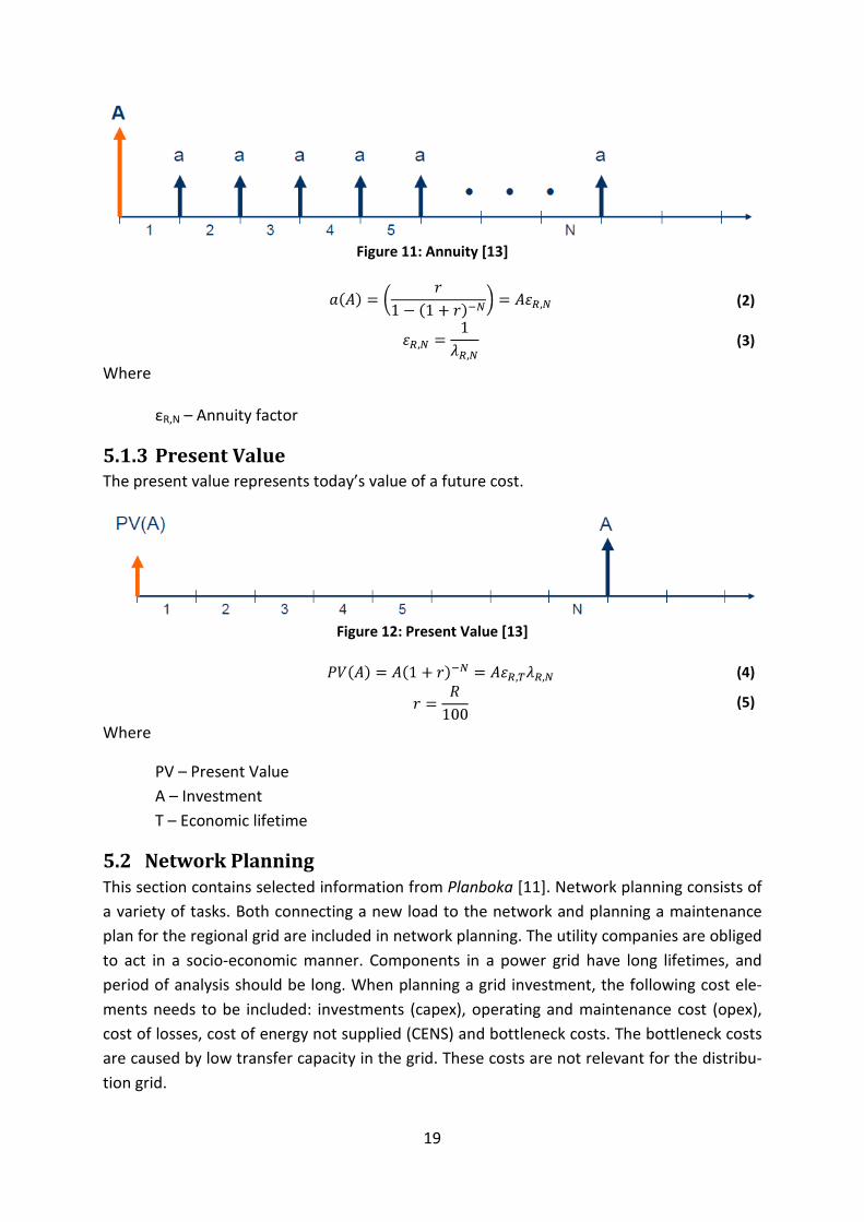
19

Figure 11: Annuity [13]

(2)

(3)

Where

εR,N – Annuity factor

5.1.3 Present Value The present value represents today’s value of a future cost.

Figure 12: Present Value [13]

(4)

(5)

Where

PV – Present Value A – Investment T – Economic lifetime

5.2 Network Planning This section contains selected information from Planboka [11]. Network planning consists of a variety of tasks. Both connecting a new load to the network and planning a maintenance plan for the regional grid are included in network planning. The utility companies are obliged to act in a socio-economic manner. Components in a power grid have long lifetimes, and period of analysis should be long. When planning a grid investment, the following cost ele-ments needs to be included: investments (capex), operating and maintenance cost (opex), cost of losses, cost of energy not supplied (CENS) and bottleneck costs. The bottleneck costs are caused by low transfer capacity in the grid. These costs are not relevant for the distribu-tion grid.

20

The calculation interest represents the cost of tying up capital and taking risk. The risk con-tains uncertainty concerning interest level, advance in prices, exchange and tax regulations. The calculation interest is set to 4.5% by the Norwegian Department of Energy, NVE. This interest does not include inflation.

The goal when planning an extension of the power grid is to minimise the expected socio-economic costs. In the distribution grid, a simplified analysis is used. The grid consists mostly of radials going from the distribution transformer to the end-user. CENS and opex can be neglected. The goal of the analysis is to minimise the investment cost and the capitalised cost of losses. The planning process can be split into four phases:

• Phase 1: Establishing data o The customer’s needs o Electric grid data: Load flow of high voltage grid and electric data for compo-

nents and low voltage grid o Data on existing loads in the network and new loads o Restrictions on electric quantities, quality of supply and environmental con-

cerns

• Phase 2: Technical solutions o Evaluate different points of connection and dimensioning of components o Perform load flow simulations and evaluate restrictions

• Phase 3: Selecting the optimal solution o Calculate investment costs and capitalised cost of losses o Select the cheapest solution that meets the restrictions

• Phase 4: Control of cost absorption o Evaluate if the project is profitable o If not: charge the costumer for the connection

5.3 Utilisation Time The utilisation time describes use pattern of the load. It is defined by the formula below.

(6)

Where

Tu – Utilization time W – Energy consumption for the period (kWh) Pmax – Maximum power during the period (kW)

The annual duration curve in Figure 13 illustrates the concept. The curve represents the load for a year sorted from largest to smallest. The area PmaxTu equals the time integral of the curve. Tu gives an indication for the variations in the load over a year.

21

Figure 13: Annual Duration Curve [11]

The utilisation time of losses is defined in the same way as for the load.

(7)

Where

TΔP – Utilisation time of losses ΔW – Energy losses ΔP – Power losses

5.4 Cost of Losses The cost of losses is an important factor when planning a power network. The energy losses are about 8% of the annual energy production and the power losses can be up to 15% of the power production. The cost of losses has to be included in the socio-economic analysis.

The specific cost of losses is given:

(8)

Where

kΔP – Cost of losses (NOK/year) kp – Power cost (NOK/kW) ΔPmax – Maximum power losses (kW) kw – Average energy cost (NOK/kWh)

22

Tl – Utilisation time of losses (h/year) Kpekv – Equivalent cost of losses (NOK/kW,year)

The power cost kp is given in Table 39. Capitalised costs of losses are given in Table 40 and Table 41. A simplified, radial network is used to calculate the constants. There are different columns for different loading conditions. When analysing, the constants for the highest volt-age level included in the analysis is to be used.

5.4.1 Cable Costs The cable cost consists of two elements: investment and cost of losses. The investment costs are proportional to the length of the cable:

(9) The cost of losses:

(10)

(11)

Where

KI – Total cost of investment (NOK) KL – Cost per length (NOK/m). Data is given in Table 36. L – Length (m) k0 – Cross section independent cost (NOK/m) kcs – Cross section dependent cost (NOK/m,mm2) A – Cross section (mm2) ΔP – Power losses (kW) I – Current (A) R – Resistance (Ω) P – Power of the load (kW) U2 – Voltage at the load (V) cosφ – Power factor of the load r – Resistance per length (Ω/m). Data is given in Table 43. KΔP – Cost of losses (NOK) Kpekv – Capitalised cost of losses (NOK/kW). Data is given in Table 40.

5.4.2 Transformer Cost The cost of a transformer consists of three elements: investment, copper losses and no-load losses. The copper losses are caused by the resistance in the windings of the transformer. These losses increase in pace with the loading of the transformer. The no-load losses are due to magnetising of the iron core. They are independent of the loading, and dominate when the loading is low.

23

(12)

(13)

ΔP – Copper losses (kW) Pk – Losses at rated power (kW). Data is given in Table 44. S – Load at transformer (kVA) Sn – Transformer rating (kVA) K – Total cost of transformer (NOK) Kpekv – Capitalised cost of losses (NOK/kW). Data is given in Table 40. KTekv – Capitalised cost of no-load losses (NOK/kW). Data is given in Table 41. P0 – No-load losses (kW). Data is given in Table 44. I – Investment (NOK). Data is given in Table 38.

5.5 Quality of Supply The Norwegian utility companies have to fulfil the regulations European Standard EN50160 and the Norwegian PQ code given in Forskrift om Leveringskvalitet [2], [9]. The standards define the properties of the voltage at the point of delivery. The two regulations include the same phenomena, but the Norwegian PQ code is stricter than EN50160 on several of the phenomena included. The phenomena that are evaluated in this report are described in Ta-ble 3.

24

Table 3: Some Phenomena Included in the Norwegian PQ Code [2], [9]

Phenomenon Definition Require-

ments Supply

voltage variations

Increase or decrease of voltage. Un±10%

Rapid voltage changes

A single rapid variation of the r.m.s. value of a voltage between two consecutive levels which are sustained for definite but unspecified du-rations

ΔUstat>3%: <24/day

ΔUmax>5%: <24/day

Flicker

Impression of unsteadiness of visual sensation induced by a light stimu-lus whose luminance or spectral distribution fluctuates with time. Flicker severity: Intensity of flicker annoyance defined by the UIE-IEC flicker measurement method and evaluated by the following quantities: Short term severity (Pst): measured over a period of ten minutes. Long term severity (Plt): calculated from a sequence of 12 Pst-values over a two hour interval, according to the following expression:

Pst≤1.2 95% of the time

Plt ≤1.0 100% of the time Measured

for one week

Supply voltage

unbalance

Condition in a poly-phase system in which the r.m.s. values of the line-to-line voltages (fundamental component), or the phase angles be-tween consecutive line voltages, are not all equal. The degree of ine-quality is calculated from the relation U-/U+, where U- and U+ are the negative and positive sequence voltage components.

U-/U+<2%

Harmonic voltage

Sinusoidal voltage with a frequency equal to an integer multiple of the fundamental frequency of the supply voltage. Harmonic voltages can be evaluated individually by their relative amplitude (Uh) which is the har-monic voltage related to the fundamental voltage U1, where h is the order of the harmonics or globally, for example by the total harmonic distortion factor THD, calculated using the following expression:

THD≤8% measured

with 10 min-utes average. Table of in-dividual val-ues is in Ta-

ble 46.

Inter-harmonic voltage

Sinusoidal voltage with a frequency not equal to an integer multiple of the fundamental

No specific require-ments

Voltage dip A temporary reduction of the voltage at a point in the electrical supply system between 90% and 1% of the reference voltage, with duration from 10ms to 60s.

Dips caused by load: <24/day

Other causes: no

require-ments.

25

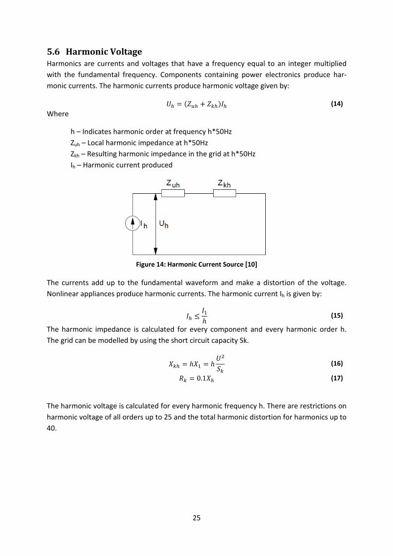
5.6 Harmonic Voltage Harmonics are currents and voltages that have a frequency equal to an integer multiplied with the fundamental frequency. Components containing power electronics produce har-monic currents. The harmonic currents produce harmonic voltage given by:

(14) Where

h – Indicates harmonic order at frequency h*50Hz Zuh – Local harmonic impedance at h*50Hz Zkh – Resulting harmonic impedance in the grid at h*50Hz Ih – Harmonic current produced

Figure 14: Harmonic Current Source [10]

The currents add up to the fundamental waveform and make a distortion of the voltage. Nonlinear appliances produce harmonic currents. The harmonic current Ih is given by:

(15)

The harmonic impedance is calculated for every component and every harmonic order h. The grid can be modelled by using the short circuit capacity Sk.

(16)

(17)

The harmonic voltage is calculated for every harmonic frequency h. There are restrictions on harmonic voltage of all orders up to 25 and the total harmonic distortion for harmonics up to 40.

26

6 Approach This section covers phase 1 of the network planning method. A detailed description of the new load is given. The computer tools and network data which will be used are described. Load data and assumptions used in the analysis are given.

6.1 Load Description The preferred charging method for EVs is level 2 charging at home or at work, while fast charging is a range extending measure for EV owners on long drives. The charging time needs to be low as low as 5-10 minutes for the EV to gain popularity [3]. Fast charging should be similar to filling a tank of petrol. Therefore, high power level 3 chargers rated 60kW or 125kW will be evaluated. At 125kW, the charging time for a mid-size BEV is minimum 17 minutes for a full charge. More charging times are displayed in Table 2.

A filling station for gas and fast chargers for electric vehicles (EVs) will be installed close to an existing petrol station at Luravika in Sandnes, Norway. A map of the area is displayed in Fig-ure 15. The closest distribution substation is marked N0520. It contains a transformer rated 630kVA and a pump station that pumps surface water into the sewer. Technical specifica-tions for the pump station are given at page 29. The local distribution grid consists of under-ground electric cables and gas pipes. The low voltage arrangement is a 400V TN-C network.

The main load at the gas filling station is a compressor from the Argentinean producer Gali-leo. The EV charging station is delivered by the Californian manufacturer of fast charging solutions AeroVironment Inc. Technical specifications for both components are given at page 29. The location of the compressor and the EV charging station are marked in the map.

This project aims to find the optimal grid connection for the load. Several solutions will be evaluated. One alternative is to connect the load to the existing substation. The connection will be made with PEX isolated 4x240mm2 Al 400V cables. One or more cables will be in-stalled for each of the two loads and connected directly to the substation. A trench will be dug along the existing 22kV-cable for the new low voltage cables. The cable lengths are 290m for the compressor and 200m for the EV chargers. The trench needs to cross the road. Underneath the road, there is a pipe with available space that can be used for drawing the cables. At the moment, the substation is only serving one load. The load is connected di-rectly to the transformer. To serve more loads, a low voltage installation has to be made at the substation to connect the new cables.

Another solution is to build a new substation close to the new load. It can be connected to the existing high voltage cable which is marked in the map. The new substation will be in-stalled close to the EV charging station by the green X in the map. A cable for the compres-sor station needs to be installed. The cable length is 90m. Technical specifications for the transformers used in the analysis are given in Table 45.

27

Figure 15: Map of Luravika. Red line: 22kV Cables. Yellow line: Gas Pipes. Blue X: Compressor.

Green X: EV Charging Station.

28

6.2 Tools Load flow simulations and economic calculations were carried out in this project. The com-puter tools that were used are described in this section.

6.2.1 Powel Netbas Netbas is a network information system developed for distribution and transmission of elec-tric energy. It is developed by the Norwegian company Powel. The system is suited for utility management and includes tools for planning, design, operations and maintenance of the network. The grid is represented in a graphical user interface that is easy to use. All the components in the grid are included containing position, technical specifications and con-nectivity. The system can be integrated with other systems which gives numerous opportu-nities to the utility companies.

In this project, Netbas was used for load flow. Lyse provided a mesh file that contains the 22kV distribution grid close to Lure transformer station in Sandnes. Detailed information about the low voltage grid was not included in the file. The network was modified to include the new load and different technical solutions were implemented. Load flow analyses were performed to get outputs like power losses, voltages, currents and more. Detailed simula-tions were made to simulate a whole year.

6.2.2 Dynko Dynko is a program that was first developed in 1972 by EFI, which is called SINTEF today. The version used in the project was last modified in 1988. It is a cost minimising program for electric distribution grids. The program has a text based user interface. It is used when de-veloping a new grid or when strengthening an existing grid. The program compares different technical solutions economically considering investments, cost of losses and energy not sup-plied over the period of analysis. The maximum period of analysis is 25 years. The cost of losses is calculated from peak power losses and kpekv, which is given in Table 39. To include the no-load losses of the transformers, the capitalised value is calculated and added to the investment. The cost of no-load losses KTekv is given in Table 41. Cost elements can be en-tered with one decimal. Losses are entered in kW. The losses are given without decimals. This leads to inaccurate results. To give more accurate results, all data on costs and losses were scaled up by a factor of 10. Still the losses are given with only two or three valid digits.

The total cost during the period of analysis is calculated for each solution. The results are represented by ranking the solutions and giving each a score. The solution ranked 1 is the least costly solution. This is given score 100. The other solutions get a score greater than 100, which represent the total cost of the solution relative to the cost of the cheapest solu-tion. An example of an output file is displayed from page 67.

6.2.3 GeoNIS GeoNIS is a Geographical Network Information System. The system contains all of Lyse’s in-frastructure networks represented the same map. The networks included are electricity,

29

telecommunication, street lights, gas and district heating. Information about all components is included, from the delivery point and up to 300kV. The placement of all components is available. Detailed information about the low voltage grid is represented in this system. The system is coupled to the customer database. Information about annual consumption and peak power is available for the loads. The background map is very detailed and contains all street addresses.

GeoNIS was used for planning the location of the installation, placement of cables and the cable lengths. Distances may be measured in the map. The system also contained useful in-formation about the grid components and loads.

6.3 Load Data The load data for the pump station, the compressor and the EV charging station was ob-tained. The data for the pump station was given by Odd Woster in IVAR. The data for the compressor was given by Audun Aspelund on behalf of Galileo S.A., Argentina. The informa-tion about the EV charging station was given by vice president Kirsten Helsel of AeroViron-ment Inc., California.

6.3.1 Water Pumps at Luravika There are four pumps for surface water. The load is at maximum during wet seasons. At maximum load, three pumps run continuously. Otherwise there are 6-7 starts per hour.

Power rating: 132 kW Voltage rating: 400 V Rated current: 260 A. Measured value: 238 A cosφ: 0.82 Start-up cosφ: 0.41 Start-up current: 1952 A at locked rotor. Start-up type: direct start.

6.3.2 Compressor for Gas Filling Station The expected daily load pattern is 20 start-ups per day; 3 per hour in hour 9 and 17, other-wise one per hour from 7 to 23. Each start lasts 15 minutes.

Type: Galileo Microbox Power rating: 120 kW Voltage rating: 400 V cosφ: 0.91

6.3.3 EV Charging Station The daily load pattern is expected to be equal to the pattern for the compressor.

Type: AeroVironment™ EV Solutions DC charger Output power rating: 30 / 60 / 125 / 250 kW

30

Input voltage: 400 V three phase at 50 Hz Output voltage: 50-600 V DC Output current: 50-550 A DC cosφ: 0.95 Efficiency: >90%

6.4 Assumptions The restrictions are the same as was used a previous report on dimensioning of low voltage grids [5].

Period of analysis: 25 years Economic lifetime components: 30 years Calculation interest: 4.5% Voltage level: 400V/22kV Maximum allowed voltage drop in low voltage parts: 8% Maximum allowed load at transformers: 130% Load increase in period of analysis: 0% Advance in prices in period of analysis: 0% Energy not supplied: 0 kWh/year

31

7 Results This chapter contains three sections. The first is a general dimensioning guide of cable cross sections and transformer power ratings. The second section contains network planning phases 2 and 3, which are described in the methodology chapter. Numerous technical solu-tions for connecting the load are analysed including two different points of connection. The dimensions of cables and transformers are investigated and load flow analyses are carried out. The costs of investments and losses are evaluated and the cheapest solution which meets the restrictions is chosen for each load case. The last section of this chapter looks at the fulfilment of the Norwegian PQ code.

7.1 Optimal Dimensioning This section gives a general dimensioning guide for cable cross section and transformer power rating. It may be used when connecting new load to the network. The graphs are based on the formulas given in the section 5.4. The costs included are investments and capi-talised cost of losses. Cost of Energy Not Supplied (CENS) and operating costs (opex) are not included.

7.1.1 Optimal Cross Section By using the formulas (9), (10) and (11), graphs that show the cost of different cross sections for one load was made. Graphs are shown for 250kW and 500kW in Figure 16 and Figure 17. Table values for material costs and cost of losses are used, given in sections 12.1 and 12.2. The utilisation time of losses used in the tables is 2400h/year.

The largest available cross section for low voltage cables is 240mm2. The cross sections used for low voltage in this project are different number of 240mm2 cables in parallel. The optimal cross section is independent of the length of the cable. From Figure 16 one can see that the cost of 3, 4 or 5 cables in parallel is about the same for a 250kW load. The optimal cross sec-tion is 4x240mm2. The graph is steep on the left side of the minimum, and quite even on the right side of the minimum. It is more expensive to make an underinvestment than to make an overinvestment. The cost increases little as the cross section increases by one step. The losses and heat generation decrease as the cross section goes up. High temperature causes damage to the isolation of cables and shortens the lifetime. By choosing a larger cross sec-tion than the optimal choice, the cable does not need to be changed if the load increases. In general, a larger cross section gives a more robust alternative.

32

Figure 16: Cost of Cross Sections for 250kW Load

The graph in Figure 17 shows similar results for a 500kW load. The cost is about the same for 6, 7, 8 and 9 cables in parallel. The optimal cross section for 500kW load is 7x240mm2. The cost increases little if the cable is upgraded to 8x240mm2.

Figure 17: Cost of Cross Sections for 500kW Load

The optimal cross section is represented differently in Figure 18 and Figure 19. The graphs are based on formulas (9), (10) and (11). From Figure 18, one can see that the optimal cross section for a 250kW load is 4x240mm2. The optimal cross section for a 125kW load is

0

200

400

600

800

1000

1200

1400

1600

1 2 3 4 5 6 7 8

Cost

(NO

K/m

)

Cross section dx240mm2

Cost for 250kW load

0

500

1000

1500

2000

2500

2 3 4 5 6 7 8 9 10 11 12 13

Cost

(NO

K/m

)

Cross section dx240mm2

Cost for 500kW load

33

2x240mm2. From Figure 19 one can see that the optimal cross section for 500kW is 7x240mm2. As the load increases, the cost varies little for a variety of cross sections. 6, 7 or 8 cables in parallel are almost equal in cost for a 470kW load.

Figure 18: Cable Cost

Figure 19: Cable Cost

50 100 150 200 250 300 3500

200

400

600

800

1000

1200

1400

1600

1800Optimal cross section

Power (kW)

Cos

t (kr

/m)

1x2402x2403x2404x2405x240

350 400 450 500 5501000

1100

1200

1300

1400

1500

1600

1700

1800

1900

2000

Optimal cross section

Power (kW)

Cos

t (kr

/m)

5x2506x2407x2408x240

34

7.1.2 Optimal Transformer Rating The graphs below are based on formulas (12) and (13). The data used for the graphs are given in the appendices. The graphs show the total cost of a transformer for different loads. By studying the graphs, the optimal transformer for different loads can be decided. The re-sults are given in the Table 4.

Figure 20: Transformer Cost

Figure 21: Transformer Cost

250 300 350 400 450 500 550 600 650 7001.5

2

2.5

3

3.5

4

4.5

5x 105

Optimal transformer

Power (kVA)

Cos

t (kr

)

315kVA500kVA630kVA800kVA

700 750 800 850 900 950 1000 1050 1100 1150 12003

3.5

4

4.5

5

5.5

6x 105

Optimal transformer

Power (kVA)

Cos

t (kr

)

800kVA1000kVA1200kVA1600kVA

35

Table 4: Optimal Transformer Load

Transformer Rating (kVA) Optimal Load (kVA)

315 <320

500 320-570

800 570-970

1250 970-1170

1600 >1170

The transformers rated 630kVA and 1000kVA are not included in the table. The reason for this is visible in the graphs. The pink line in Figure 21 displays the costs for the 1000kVA transformer. This line is never the bottom line. The 1000kVA transformer is not an optimal investment for any load. The same phenomenon occurs for the 630kVA transformer in Fig-ure 20. The cost of the 630kVA transformer is marked with the orange line. The line is never at the bottom, so it is never an optimal investment.

The cost of the different transformer is quite equal at many loads. When a new transformer is installed, one should consider increase of load in the future. By choosing a transformer with a higher power rating, the load may increase more before the transformer needs to be replaced.

7.2 Load Cases At Luravika, there is space for maximum four charging outlets for EVs. They will be located at the green X in Figure 15. The compressor for gas filling will be located at the blue X. Three different load scenarios for the EV station will be evaluated. The three scenarios involve dif-ferent power ratings of the EV charger. The compressor for the gas filling station will be equal in all scenarios. Different grid connections will be evaluated for each load scenario. There are several ways to connect the load to the grid. One way is to connect the cables to the nearest distribution substation, which is marked N0520 in Figure 15. The cables for the compressor and the charging station will be placed in the same trench. Another solution is to build a new substation close to the EV charging station. There is a 22kV cable close to the site, as with a red line in the map. The new substation will serve both the compressor and the charging station.

Three load scenarios are investigated. Scenario 1 has a charging station rated 125kW. The load may be distributed on one outlet rated 125kW or two outlets rated 60kW each. The last alternative produce a total maximum load of 120kW, but the difference is considered so small that the alternatives are investigated as one scenario.

Scenario 2 has an EV charging station rated 250kW. The charging station can consist of four outlets rated 60kW or two outlets rated 125kW. Scenario 3 has an EV charging station rated 500kW. The load consists of four 125kW outlets.

Five load cases are studied. In case 1, 2 and 3 the maximum load occurs at the same time on all delivery points. Case 1 uses load scenario 1, case 2 uses scenario 2 and case 3 uses sce-

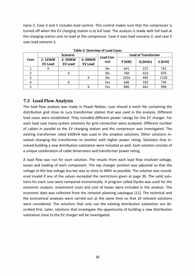
36

nario 3. Case 4 and 5 includes load control. This control makes sure that the compressor is turned off when the EV charging station is at full load. The analysis is made with full load at the charging station and no load at the compressor. Case 4 uses load scenario 2, and case 5 uses load scenario 3.

Table 5: Overview of Load Cases

Case Scenario

Load Con-trol

Load at Transformer 1: 125kW EV Load

2: 250kW EV Load

3: 500kW EV Load

P (kW) Q (kVAr) S (kVA)

1 X No 641 372 741 2 X No 766 413 870 3 X No 1016 495 1130 4 X Yes 646 359 739 5 X Yes 896 441 999

7.3 Load Flow Analysis The load flow analysis was made in Powel Netbas. Lyse shared a mesh file containing the distribution grid close to Lura transformer station that was used in the analysis. Different load cases were established. They included different power ratings for the EV charger. For each load case many system solutions for grid connection were analysed. Different number of cables in parallel to the EV charging station and the compressor was investigated. The existing transformer rated 630kVA was used in the simplest solutions. Other solutions in-volved changing the transformer to another with higher power rating. Solutions that in-volved building a new distribution substation were included as well. Each solution consists of a unique combination of cable dimensions and transformer power rating.

A load flow was run for each solution. The results from each load flow involved voltage, losses and loading of each component. The tap changer position was adjusted so that the voltage at the low voltage bus bar was as close to 400V as possible. The solution was consid-ered invalid if any of the values exceeded the restrictions given at page 30. The valid solu-tions for each case were compared economically. A program called Dynko was used for the economic analysis. Investment costs and cost of losses were included in the analysis. The economic data was collected from the network planning catalogue [11]. The technical and the economical analyses were carried out at the same time so that all relevant solutions were considered. The solutions that only use the existing distribution substation are de-scribed first. Later, solutions that investigate the opportunity of building a new distribution substation close to the EV charger will be investigated.

37

7.3.1 Solutions Using the Existing Distribution Substation The solutions that are considered in this section all make use of the existing substation, which is marked N0520 in Figure 15. The electric configuration is displayed in the figure be-low.

Figure 22: Electric Configuration

The cables for the compressor and the charging station will be placed in the same trench. The solutions contain different number of cables in parallel for the EV charging station and the compressor. Some solutions include the existing transformer rated 630kVA. In other so-lutions, the transformer is replaced by another with higher power rating. The water pump is the existing load at the transformer. It is connected directly to the low voltage side of the transformer. This load will be equal in all load scenarios.

The costs considered in the analysis are:

• 290m trench and cables for the compressor

• 200m cables for the EV charging station

• No-load losses for the transformer during the period of analysis

• Possible investment in new transformer

Prices are adjusted to 2010 price level using the consumer price index given in Table 42.

38

7.3.1.1 Load Case 1 This case contains the smallest EV charger that is considered in the analysis. The EV charger is rated 125kW. The maximum load on the transformer is 741kVA. The technical solutions that were considered are given in the table below.

Table 6: Load Flow Results for Case 1

Solution

Trans-former Rating (kVA)

EV Cables Compres-sor Cables

Trans-former

Loading (%)

EV Cable Loading (%)

Compres-sor Cable

Loading (%)

Losses (kW)

1 630 1 2 124 52 26 14.04

2 630 2 2 124 26 26 12.52

3 630 3 2 124 17 26 12.04

4 630 2 1 124 26 53 14.81

5 630 2 3 124 26 17 11.79

6 800 2 2 96 25 26 10.55

7 1000 2 2 77 25 26 9.44

8 1250 2 2 61 25 26 7.82

Load flow analyses were carried out using Netbas. The results are displayed in the table above. The losses are the sum of losses in the transformer and the cables for the EV charger and the compressor. Several elements should draw the reader’s attention. The loading of the transformer and the voltage is only dependent on the rating of the transformer. The number of cables for the loads does not matter. The loading of the cables is only dependent on the number of cables in parallel, not the transformer rating. Another element that should be noticed is the loading at the 630kVA transformer. The loading is 124%, which is close to the limit of 130%. This overloading might lead to overheating.

Economic analyses were carried out using Dynko. The program presents the results by rank-ing the solutions. The solution ranked as number 1 is the least costly solution, and is consid-ered to be the economically optimal one. Each solution is given a score that represents the costs. The cost of each solution is compared to the cost of the optimal solution. The best solution gets score 100, and the other solutions get a score which is greater than 100.

The results from Dynko for case 1 are given in the in Figure 7. The economic analysis was only performed on a selection of the technical solutions. The least costly alternative is solu-tion 2, which includes keeping the existing transformer and installing two cables in parallel to the EV charging station and the compressor. The second best alternative includes three cables in parallel to the EV chargers and two to the compressor. This gives a more robust solution at 1.9% higher costs.

39

Table 7: Economic Results for Case 1

Solution Transformer Rating (kVA)

EV Cables Compressor

Cables Ranking Score

1 630 1 2 3 102.7

2 630 2 2 1 100.0

3 630 3 2 2 101.9

4 630 2 1 5 104.5

5 630 2 3 4 102.9

6 800 2 2 8 120.9

7 1000 2 2 7 117.6

8 1250 2 2 6 117.0

The optimal transformer rating is investigated in the table below. The existing transformer can still be used, which is the cheapest solution. If the transformer is to be replaced, a 1250kVA or a 1000kVA transformer is preferred. They are loaded 61% and 77% at maximum load. This will cost about 17% more over the period of analysis. The optimal transformer rating is displayed graphically in Figure 21. According to the graph, the optimal choice is an 800kVA transformer. The results from the two calculations are not consistent.

Table 8: Results on Transformers for Case 1

Transformer Rating (kVA)

Loading (%) Score

630 124 100.0

800 96 120.9

1000 77 117.6

1250 61 117.0

Table 9 shows the solutions for the number of cables in parallel for the EV charger. The opti-mal number is two. The cables are loaded 26% at maximum load. Upgrading to a more ro-bust solution with three cables in parallel will cost 2.8% more. The optimal cross section is displayed in Figure 18. The graphs give the same results as the simulation: 2x240mm2 is the optimal cross section.

Table 9: Results on EV Cables for Case 1

EV Cables Loading (%) Score

1 52 102.7

2 26 100.0

3 17 101.9

40

Table 10: Results on Compressor Cables for Case 1

Compressor Cables

Loading (%) Score

1 53 104.5

2 26 100.0

3 17 102.9

Table 10 shows the economic results for the number of cables in parallel to the compressor. The optimal number is two. The load at the compressor and the EV charging station are al-most equal in this load case. The cable lengths are a little different. The optimal cross section is only dependent on the load, not the length of the cable. This results in an equal optimal cross section for the compressor and the EV charger in this load case. The loading at the op-timal cross section is 26%, which is consistent with the results for the EV charging station and with the graph in Figure 18. In further analysis, the compressor will always be connected with two cables in parallel.

7.3.1.2 Load Case 2 This load case consists of is load scenario 2 with maximum load at all delivery points. The load at the transformer is 870kVA. The EV charging station is rated 250kW. Many different solutions were analysed. The results were used to draw general conclusions on the dimen-sioning of cables and transformers. The conclusions were useful when investigating the other load cases to limit the number of solutions. The results from the load flow analysis are displayed in the table below. Only a selection of the solutions is displayed here.


Solution


EV Cables Trans-former

Loading (%)

EV cable Loading

Voltage Drop (%)

Voltage (V) Losses (kW)

1 630 1 148 108 6.29 394.7 27.06

2 630 3 147 36 2.86 394.9 18.28

3 630 5 146 21 2.20 394.9 16.67

4 800 3 114 34 1.39 400.7 15.39

5 1000 2 91 52 1.56 400.8 15.81

6 1000 3 91 34 1.38 400.8 13.83

7 1000 4 91 26 1.54 400.8 12.85

8 1250 2 72 52 2.10 401.1 13.31

9 1250 3 72 34 1.29 401.1 11.33

10 1250 4 72 26 0.89 401.1 10.39

11 1250 5 72 20 0.65 401.1 9.83

12 1600 3 56 34 1.23 402.3 11.06

13 1600 4 56 26 0.59 402.3 10.08

41

Several elements in the results are of interest. The existing transformer rated 630kVA is overloaded by more than 30%. A new transformer has to be installed. The solutions that involve the existing transformer will not be considered in the further analysis. The first solu-tion includes only one cable for the EV charging station. The cable is overloaded by 8%. All solutions including one cable for the EV charging station are invalid and are not considered in the further analysis. Another important element is the voltage drop. The voltage drop is the difference between the system voltage and the voltage at the delivery point of the EV charging station. The largest voltage drop in Table 11 is 6.29%, which is lower than the limit of 8%. All other solutions have a smaller voltage drop and are well within the limits.


Solution Transformer Rating

(kVA) EV Cables Ranking Score

4 800 3 10 106.2

5 1000 2 9 106.1

6 1000 3 4 102.6

7 1000 4 5 102.7

8 1250 2 6 103.5

9 1250 3 1 100.0

10 1250 4 2 100.1

11 1250 5 3 101.1

12 1600 3 8 104.0

13 1600 4 7 103.8

Only the valid solutions were analysed economically. The results are displayed in the table above. The least costly solution is number 9, which includes a transformer rated 1250kVA and three cables in parallel for the EV charging station. The second best solution is number 10, which includes the 1250kVA transformer and four cables in parallel for the EV charger. This solution costs 0.1% more, so the two solutions can be considered economically equal. Summaries of the results are given in the following tables.



Loading (%) Score

800 114 106.2

1000 91 102.6

1250 72 100.0

1600 56 104.0

The table above shows the results for the different transformer ratings. The optimal solution includes a 1250kVA transformer, which is loaded 72% at maximum load. The second best solution is a 1000kVA transformer, which will cost 2.6% more over the period of analysis.

42

According to the graph in Figure 21, the optimal transformer is an 800kVA transformer. The results from the two calculations are not consistent.

The table below displays the score for different number of EV cables. Three cables in parallel is the cheapest solution, followed closely by four cables. The other solutions are more ex-pensive. Both cables are loaded around 30% at maximum load. The graph in Figure 18 shows that the optimal cross section for 250kW load is 4x240mm2, while the simulation shows 3x240mm2. The difference in cost between 3 and 4 cables in parallel is small in both the simulation results and the graph.



2 52 103.5

3 34 100.0

4 26 100.1

5 20 101.1

7.3.1.3 Load Case 3 This case has the highest load which is investigated in this analysis. The EV charging station is rated 500kW. The load at the transformer is 1130kVA at maximum load. The results from the load flow analysis are given in the table below. Only a selection of the analysis performed is given here.



EV Cables Transformer Loading (%)

Cable Loading (%)

Losses (kW)

1 800 7 149 30 24.37

2 1000 2 121 107 40.05

3 1000 6 119 35 22.81

4 1000 7 119 30 21.66

5 1000 8 119 26 20.80

6 1250 5 94 41 19.75

7 1250 6 94 34 18.18

8 1250 7 94 30 17.03

9 1250 8 94 26 16.25

10 1250 9 94 23 15.59

11 1600 6 73 34 17.44

12 1600 7 73 29 16.36

13 1600 8 73 26 15.50

By looking at the load flow results it should be noticed that solution 1 and 2 are invalid. Solu-tion 1 exceeds the limit for transformer loading, and solution 2 exceeds the limit for cable

43

loading. The other solutions show that the loading at the transformer and the cables are independent.


Solution Transformer

Rating (%) EV Cables Ranking Score

3 1000 6 11 109.3

4 1000 7 9 108.8

5 1000 8 10 108.8

6 1250 5 8 102.8

7 1250 6 3 100.8

8 1250 7 1 100.0

9 1250 8 2 100.6

10 1250 9 4 101.3

11 1600 6 7 102.7

12 1600 7 5 102.4

13 1600 8 6 102.5

The table above shows the results from Dynko for the technically valid solutions for case 3. The best solution is number 8, which includes the 1250kVA transformer and 7 cables in par-allel for the EV charger. Solution 7 and 9 cost 0.6 and 0.8% more and can be considered equal to solution 7.

Table 17: Results on Transformer for Case 3


Loading (%) Score

1000 119 108.8

1250 94 100.0

1600 73 102.4

The table above shows the economic results for the transformers on case 3. The least costly solution includes the 1250kVA transformer, which is loaded 94%. The 1600kVA transformer is loaded 73% and the cost over the period of analysis is 2.4% higher that the 1250kVA trans-former. The 1000kVA transformer is loaded 119% and the cost is 8.8% higher. The optimal transformer for 1130kVA load in Figure 21 is rated 1250kVA.

Table 18 compares the different cable alternatives for the EV charger. The least costly alter-native is 7 cables in parallel. This cable is loaded 30%. The solutions that include 6 or 8 cables are almost equal in costs. These cables are loaded 34 or 26%. It seems that the optimal load-ing of cables is in the span 25-35%. The optimal cross section for a 500kW load is displayed in Figure 19. The results are consistent with the Dynko simulation.

44



5 41 102.8

6 34 100.8

7 30 100.0

8 26 100.6

9 23 101.3

7.3.1.4 Load Case 4 This case includes load control. The control limits the maximum load. The compressor will not start if the EV charging station is at maximum load. The maximum load at the trans-former in this load case is 739kVA. The charging station is expected to be little in use for the first 10 years after installation. The load control will most likely not bother the users of nei-ther the gas filling station nor the EV charger. Case 4 is load scenario 2 with load control. The EV charger is rated 250kW.




EV Cable Load-ing (%)

Losses (kW)

1 630 3 124 34 12.75

2 630 4 123 26 11.78

3 630 5 123 21 11.21

4 800 4 96 25 9.83

5 1000 4 77 25 8.73

6 1250 4 61 25 7.13

7 1600 4 47 25 7.01

The table above shows the results from the load flow analysis on case 4. When load control is introduced, the existing transformer rated 630kVA does not need replacement. The trans-former is loaded 123%, which is close to the overloading limit at 130%.




1 630 3 2 100.5

2 630 4 1 100.0

3 630 5 3 101.8

4 800 4 6 126.0

5 1000 4 4 122.5

6 1250 4 5 123.2

7 1600 4 7 130.7

45

The economic results in Table 20 show that the optimal solution is to keep the existing trans-former and install 4 cables in parallel to the EV charger. The second best solution includes 3 cables in parallel. The difference in cost between the two is small, only 0.5%. If the trans-former is to be upgraded, the cost increases by almost 22.5%.



Loading (%) Score

630 123 100.0

800 96 126.0

1000 77 122.5

1250 61 123.2

1600 47 130.7

The table above shows a summary of the technical and economical results for different transformer ratings on case 4. It is technically possible to keep the existing transformer rated 630kVA. This solution has a significant lower cost than the other alternatives and is pre-ferred. Out of the other solutions, the least costly one is the transformer rated 1000kVA. It is loaded 77% at maximum load. In the graphical representation in Figure 21, the optimal transformer at 740kVA load is rated 800kVA.



3 34 100.5

4 26 100.0

5 21 101.8

The table above displays the alternatives for the number of cables in parallel to the EV charger. The least costly solution is four cables in parallel closely followed by three cables. Four cables in parallel are more robust than three cables and is the preferred solution. The cables are loaded 26%.

7.3.1.5 Load Case 5 This load case uses load scenario 3 with load control. The EV charging is rated 500kW. The maximum load at the transformer is 999kVA. The table below shows the results from the load flow analysis. The weakest solution includes an 800kVA transformer. This solution ex-ceeds the limit of 130% overload and is invalid.

46




EV Cable Load-ing (%)

Losses (kW)

1 800 7 131 29 18.81

2 1000 7 105 29 16.74

3 1250 6 83 34 14.43

4 1250 7 83 29 13.34

5 1250 8 83 26 12.48

6 1600 7 64 29 12.83




2 1000 7 5 105.5

3 1250 6 3 100.6

4 1250 7 1 100.0

5 1250 8 2 100.4

6 1600 7 4 103.0

The table above displays the results from the economic analysis of the valid solutions. The optimal solution includes a 1250kVA transformer and 7 cables in parallel for the EV charging station. The solutions that include the same transformer and 6 or 8 cables in parallel are al-most equal in cost. The existing transformer has to be replaced. All the solutions that are considered are quite equal considering the costs.



Loading (%) Score

1000 105 105.5

1250 83 100.0

1600 64 103.0

The table above displays the different transformer alternatives for case 5. The preferred so-lution is a 1250kVA transformer, which is loaded 83%. A 1600kVA transformer will only cost 3% more over the period of analysis. This is a more robust alternative. The optimal loading of the transformer is 94% in this load case. The simulation results fit well with the graph in Fig-ure 21. According to the graph, the optimal transformer for 1000kVA load is rated 1250kVA.

Table 26 shows the different cable alternatives for case 5. The preferred alternative is 7 cab-les in parallel. 6 or 8 cables give almost the same cost, 0.4 and 0.6% more. The preferred alternative is loaded 29%.

47



6 34 100.6

7 29 100.0

8 26 100.4

7.3.1.6 Summary Load case 1 to 5 is analysed both technically and economically in the previous sections. The economic analysis includes both investment costs and cost of losses over the period of analysis of 25 years. The connection between the loading of the components and the total cost in the period of analysis is investigated. The optimal number of 240mm2 Al cables in parallel for the EV charger and the compressor was analysed. By comparing Table 9, Table 10, Table 14, Table 18, Table 22 and Table 26 it is evident that the optimal cable loading is in the range 26-34%. The solution where the cable loading is closest to 30% is the optimal solu-tion. The results from the Dynko analysis are consistent with the theoretical optimal cross section displayed in Figure 18 and Figure 19.

The optimal transformer rating was investigated. The results for case 1 and 4 are given in Table 8 and Table 13. In these two cases it is technically possible to keep the existing trans-former rated 630kVA. The investment costs of a new transformer are avoided, and this is the economically optimal solution. The results from case 2, 3 and 5 are displayed in Table 13, Table 17 and Table 25. The loading at the optimal transformer varies from 72% to 94%. In all the three cases, the cost of the second best transformer is less than 3% higher than the op-timal solution. These solutions can be considered close to equal to the optimal solutions. The transformer loading at these six solutions varies from 64% to 94%, and the average is 79.5%.

In load case 3 and 5, the results of the analysis fits well with the graph displayed in Figure 21. In load case 1, 2 and 4, the results from the two analyses are not consistent. It seems as the analysis and the graph give the same results for the largest loads. The results from Dynko seem to favour the 1250kVA transformer, while the graphical representation favours the 800kVA transformer.

7.3.2 Solutions Including a New Distribution Substation The option to build a new distribution substation close to the EV chargers was analysed. For each case, the best solution from the previous analysis was compared to different solutions that involved a new substation.

The new distribution substation will be installed close to the green X in Figure 15. The EV station and the compressor will be located at the same places as earlier. The substation will be connected to the existing 22kV cable, which is marked with a red line at the map. The substation is detached and air isolated. The trench from substation N0520 is then unneces-sary. A 90m trench from the new substation to the compressor will be needed. The existing

48

transformer in substation N0520 will stay unchanged. It’s only load will be the water pumps, just as it is today. The new electric configuration is displayed in the figure below.

Figure 23: Electric configuration including a new distribution substation

The costs considered in solutions using the new substation are:

• Investment of new transformer. Given in Table 38.

• Investment and installation of the distribution substation. Given in Table 37.

• Connecting the new transformer to the existing 22kV cable. Costs NOK 35000.

• 90m trench and cables for the compressor. Given in Table 36.

Prices are adjusted to 2010 price level using the consumer price index given in Table 42.

49

7.3.2.1 Load Case 1 This load case uses load scenario 1, which includes a 125kW EV charger. The load at a trans-former that only serves the EV charger and the compressor will be 263kVA.


Solution New Sub-station?

Trans-former

Rating (%) EV Cables

Comp-ressor Ca-

bles

Trans-former

Loading (%)

Comp-ressor Ca-

ble Loading (%)

Losses (kW)

1 No 630 2x200m 2x290m 124 26 12.52

2 Yes 315 - 2x90m 86 25 7.66

3 Yes 500 - 2x90m 54 25 6.79

4 Yes 630 - 2x90m 43 25 6.67






1 No 630 2x200m 2x290m 1 100.0

2 Yes 315 - 2x90m 2 101.3

3 Yes 500 - 2x90m 3 104.6

4 Yes 630 - 2x90m 4 108.9

The optimal solution is to keep the existing transformer in the existing substation. The in-vestment costs for this solution are low because no new transformer has to be purchased. However, the losses are almost double compared to the solutions that involve a new substa-tion. The solution that includes a new 315kVA transformer costs only 1.3% more over the period of analysis of 25 years. Considering the large reduction in losses, this solution should be considered when building the charging station.

7.3.2.2 Load Case 2 This load case includes load scenario 2. At maximum load, a transformer serving the EV chargers and the compressor will be loaded with 395kVA.




EV Cables Comp-

ressor Ca-bles

Trans-former

Loading (%)

Compres-sor Cable

Loading (%)

Losses (kW)

1 No 1250 3x200m 2x290m 72 26 11.33

2 Yes 500 - 2x90m 81 25 8.23

3 Yes 630 - 2x90m 64 25 7.91

4 Yes 800 - 2x90m 50 25 7.48

50


Solution New Substa-

tion? Transformer Rating (kVA)



1 No 1250 3x200m 2x290m 4 131.3

2 Yes 500 - 2x90m 1 100.0

3 Yes 630 - 2x90m 2 103.0

4 Yes 800 - 2x90m 3 105.9

The optimal solution is to build a new substation close to the EV charging station. The solu-tion that includes using the existing substation with a new transformer costs 31.3% more over the period of analysis. The new transformer should be rated 500kVA. The results from Dynko fit well with the graph in Figure 20.

7.3.2.3 Load Case 3 This load case uses load scenario 3, which gives it the largest load. The maximum load at a transformer serving only the EV charging station and the compressor is 658kVA.





Cables Transformer Loading (%)

Losses (kW)

1 No 1250 7x200 2x290m 94 17.03

2 Yes 630 - 2x90m 108 11.94

3 Yes 800 - 2x90m 84 10.40

4 Yes 1000 - 2x90m 67 9.60

5 Yes 1250 - 2x90m 54 8.59

The optimal solution is to build a new substation with a transformer rated 1000kVA. The solution that includes an 800kVA transformer costs about the same. In the graphical repre-sentation in Figure 20, the optimal transformer is rated 800kVA. If the existing substation is used, the costs over the period of analysis increase by 33%.






1 No 1250 7x200 2x290m 5 133.0

2 Yes 630 - 2x90m 4 103.2

3 Yes 800 - 2x90m 2 101.2

4 Yes 1000 - 2x90m 1 100.0

5 Yes 1250 - 2x90m 3 101.8

51

7.3.2.4 Load Case 4 This load case is scenario 2 with load control. The control makes sure that the compressor is turned off when the EV charger is at full load. The load flow is made with the EV charger at full load and the compressor at no load. The load at the transformer at the new substation is 263kVA.

Table 33: Results for Case 4




Loading (%) Losses (kW) Ranking Score

1 No 630 4x200m 123 11.78 3 108.1

2 Yes 315 - 86 7.02 1 100.0

3 Yes 500 - 53 6.20 2 105.4

In the previous analysis, the optimal solution for case 4 was to keep the existing transformer rated 630kVA. From the table above one can see that the costs are lower if a new substation is built close to the EV charging station. If the existing transformer is used, the costs increase by 8.1%. The losses are almost double if the existing substation is used compared to the op-timal solution. The optimal transformer is rated 315kVA. This corresponds to the optimal transformer in Figure 20.

7.3.2.5 Load Case 5 The load in this case is scenario 3 with load control. The load flow is run with full load at the EV charging station and no load at the compressor. The loading at the new transformer is 526kVA. Table 34 displays the results. In the pervious section, the optimal solution included a 1250kVA transformer and 7 cables for the EV charger. In this analysis, the optimal solution is to build a new substation with a transformer rated 500kVA. Several solutions are almost equal in costs. The results correspond to the graphical representation in Figure 20. The graph shows that the cost of transformers rated 500, 630 and 800kVA cost about the same at this load. The solution that involves using the existing substation has a 46.2% higher cost than the optimal solution.

Table 34: Results for Case 5




Loading (%) Losses (kW) Ranking Score

1 No 1250 7x200m 83 13.34 5 146.2

2 Yes 500 - 108 9.67 1 100.0

3 Yes 630 - 86 9.12 2 101.6

4 Yes 800 - 67 8.13 3 101.9

5 Yes 1000 - 54 7.63 4 101.9

52

7.3.2.6 Summary The five load cases were investigated in this section. In four of the cases, the optimal solu-tion involved installing a new substation close to the EV charging station. Compared to the results from the previous section, the losses were reduced by up to 50%. Solutions that in-volve lower losses are more energy efficient and can be considered the more environmen-tally friendly alternative.

The optimal loading of the transformer is close to the results from the previous section. The average loading of the transformer for the solutions that have a score lower than 103 at case 2, 3, 4 and 5 is 76%. The transformer loading of these solutions spreads from 54% to 108%. It seems that the transformer rating has little influence on the total costs over the period of analysis. The results from Dynko fit well with the graphical representation of transformer costs in Figure 20.

7.3.3 Other Charging Alternatives EV chargers with lower power ratings will be evaluated. Level 2 chargers using singe phase 230V can be used. The power rating is less than 10kW. Small DC chargers with power rating around 30kW are also evaluated. There are many manufacturers that deliver chargers in this power range. The charging time will be significantly longer. The best location of public slow chargers is probably not at a petrol station, but rather shopping centres or other places where people are occupied while the vehicle charges.

The load case will be similar to case 1, with a smaller EV charger. The optimal solution in case 1 is to use the existing substation with the transformer rated 630kVA. When connecting an even smaller EV charging station, a new substation does not need to be built. The number of cables in parallel for the EV charging station should be chosen so that the maximum loading is around 30%.

7.3.4 High Voltage Distribution Grid The 22kV cable going to Lura transformer station was investigated in load case 3. This load case has the largest load that was analysed in this project. Load flow analysis was made to look at the 22kV cable connection to Lura transformer station. At maximum load the cable is loaded 37% and carries 136A. The losses are 9.28kW, which is 0.18% of the power. Through-out the year, the losses are 21.658MWh, which is 0.094% of the energy consumed. The load-ing of the cable is acceptable. It is not necessary to do improvements in the high voltage dis-tribution grid when connecting the new load.

7.3.5 Utilisation Time of Losses The utilisation time of losses is set to 2400h/year in the Dynko analysis, which is the stan-dard value used in Table 39. The utilisation time of losses was investigated for the optimal solution of case 1 and case 3 using Powel Netbas. The same load variation was used for the compressor and the EV charging station. The load was constant over the year and did not vary according to temperature. The daily load pattern is given in the table below.

53

Table 35: Daily Load Pattern for Charging Station and Compressor, Percentage of Maximum Load

Hour Week-

day Week-

end Hour

Week-day

Week-end

1 0 25 13 25 50 2 0 25 14 25 50 3 0 0 15 25 50 4 0 0 16 25 50 5 0 0 17 100 25 6 0 0 18 25 25 7 0 0 19 25 25 8 25 0 20 25 25 9 100 0 21 25 25

10 25 25 22 25 25 11 25 25 23 25 25 12 25 25 24 0 25

For case 1, the utilisation time of load was 3966h/year, and the utilisation time of losses was 2438h/year. The value is close to the value used in the analysis, and no adjustments need to be made.

For case 3, the utilisation time of load was 3105h/year, and the utilisation time of losses was 3996h/year. The utilisation time is expected to be higher for the load than for the losses. The high value may be caused by the low loading of the transformer, which is 67% at maximum load. The no-load losses are dominating during low load conditions. The utilisation time of the no-load losses is close to 8760h/year. The daily load pattern which is used in the analysis is based on an expected use pattern, and the information is not certain. Considering the un-certainty, the standard utilisation time of losses is used in the analysis.

7.4 Quality of Supply The power quality was investigated for the optimal solution of case 1 and case 3. Case 1 is the only load case where the optimal solution includes the existing substation and a long cable for the load. Case 3 has the largest load, and the load is connected close to the trans-former. Three phenomena were investigated: supply voltage variations, rapid voltage changes and harmonic voltage. The phenomena are described in Table 3.

7.4.1 Supply Voltage Variations For case 1, the voltage is 397.5V when the load is at maximum and 415.1V when there is no load. Both voltages have less than 10% deviation from the system voltage, which is 400V. For case 3, the maximum voltage is 409.5V and the minimum voltage is 404.5%. Both voltages are within the limits of ±10% of the system voltage. Neither of the cases exceeds the limits of supply voltage variations.

7.4.2 Rapid Voltage Changes This phenomenon consists of rapid variations of the r.m.s. value of the voltage. Variations larger than 3% of the system voltage can not occur more often than 24 times a day. In the

54

system analysed here, a rapid voltage change can be caused by a rapid load increase or de-crease of the EV charging station. The voltage at the low voltage side of the transformer was investigated for different loads. The largest voltage change occurs when there is maximum load at all delivery points, and the EV charging station is turned off suddenly. For case 1, this change is 0.6%. For case 3, the change is 1.0%. The limits are not exceeded in any of the load cases.

7.4.3 Harmonic Voltage No detailed information about the harmonic currents from the EV chargers was obtained. Approximation of the harmonic voltage was made through calculations. The equations are given in formulas (14) to (17). The worst case was considered to calculate the maximum harmonic voltage. It was assumed that the EV charger is a 6-pulse rectifier without filtering.

For case 1, the minimum short circuit capacity at the connection point of the EV charging station is 5.255MVA. The 5th and 7th harmonic voltage was calculated, which are the domi-nating harmonics from a 6-pulse rectifier. The current was calculated from formula (15). This gives the largest possible current. The first harmonic current is 97A in each cable. As there are two cables, the total fundamental current is 194A. Using formula (14), the harmonic voltage is calculated to 5.908V for both the 5th and the 7th harmonic. This is 1.48% of the system voltage. The limits given in Table 46 are 6% for the 5th harmonic and 5% for the 7th harmonic. The voltages are well within the limits.

For case 3, the minimum short circuit capacity is 11.006MVA at the connection point of the EV chargers. The fundamental current drawn by the chargers is 749A. The harmonic voltages for the 5th and the 7th harmonic are both 2.78% of the system voltage. The restrictions are fulfilled.

7.4.4 Summary Three phenomena were investigated for load case 1 and 3. These two cases are expected to have the worst quality of supply out of the five load cases. The worst cases were considered. All values were within the regulations.

55

8 Discussion The discussion addresses the three main topics of the analysis: optimal dimensioning of ca-bles and transformers and fulfilment of Norwegian PQ regulations.

8.1 Optimal Cable Cross Section In all load cases that were analysed, the optimal cable loading was in the range 26-34% at maximum load. The solution that includes cable loading closest to 30% is the optimal alter-native. The results from the simulations fit well with the graphs in Figure 16 through Figure 19. The cost of upgrading the cross section is small in cases where the load is large. A larger cross section leads to lower current and lower losses. The temperature in the cables is re-duced, which reduces the wear and tear of the isolation. A reduction of losses lowers the energy production, which gives less use of resources and minimises the environmental ef-fects. A larger cross section is also favourable in cases where the load is expected to increase in the future.

The loading of the cable does only depend on the number of cables in parallel. The voltage and rating of the transformer have no impact in the analysis made in this project. The reason for this is that the voltage is very stiff at the point of connection.

The cable loading of the 22kV cable going to Lura transformer station is 37% at the heaviest load case. This is acceptable, and no adjustments need to be made on the high voltage dis-tribution grid.

8.2 Optimal Transformer Power Rating The loading on the transformer depends only on the load and of the rating of the trans-former. The voltage variations for the different cable alternatives are too small to make an impact.

The first analysis does not consider the option to build a new distribution substation close to the load. The existing transformer fulfils the restrictions for the two cases with smallest power ratings. The overloading of the transformer is close to the limit of 30% and the losses are high. Still, it is economically optimal to keep the existing transformer. To install a larger transformer will increase the costs by around 20%.

In the other three load cases, the loading of the existing transformer exceeds the limit of overloading. The transformer is replaced by another with higher power rating. The loading at the optimal transformer varies from 72% to 94%. The difference in cost between the optimal and the second best transformer is low, less than 3% in all cases. When all solutions with a score lower or equal to 103 are included, the loading spans from 64% to 114%.

In the cost minimising program Dynko, there is a certain inaccuracy in the input data. In-vestments are entered in kNOK with one decimal while losses are entered in kW without decimals. To increase the accuracy, the input data was scaled up by a factor of 10. Still the losses are given with only two or three valid digits. This can be the source of the large variety

56

in transformer loading of the optimal solutions. The variety of investment costs and losses are small for the different solutions. The inaccuracy in the program is possibly a reason for the variety in the results concerning the optimal transformer loading. Another limitation of the program is the period of analysis, which is set to maximum 25 years. The period of analy-sis used when making the general dimensioning graphs was 30 years.

The second analysis looked at the opportunity to build a new distribution substation close to the load. The optimal solution of the previous analysis was compared with different solu-tions for the new substation. This reduces the losses significantly. Especially for the large loads, a reduction of the losses improves the economy. Out of the five load cases that were analysed, only one case had an optimal solution that included using the existing substation. This case had the smallest load. Even for this case, the cost of installing a new substation was only 1.3% more expensive than to use the existing substation. Even if this solution costs a little bit more, it is the preferred solution. A new substation results in shorter cables and lower losses. The reduction in losses increases the efficiency and can be considered both a more robust alterative and better for the environment.

For the second smallest load case, the optimal solution is to build a new substation. The ex-isting transformer does not exceed the loading limits, and may still be used. Even so, it is economically preferable to build a new substation. The investments are higher, but the losses are reduced significantly. For the last three load cases, it is preferable to build a new substation. The results from the analysis on transformer size fit well with the graph in Figure 20.

The size of a new distribution substation might be critical. There is limited space at the site. Dimensions of substations were not obtained in this project. Before choosing the solution for connection, the size and placement of a substation and the EV charging stations needs to be considered.

If the existing substation is used, a 290m long trench has to be dug to install the load. If the load is large, a new transformer with a higher power rating has to be purchased. When a new substation is built, the long trench is avoided. A new transformer has to be purchased, but it will be smaller and less costly than if a new transformer is installed in the existing sub-station. The investment costs might be larger when a new substation is built. However, the losses are much smaller. The reduced cost in losses compensate for the investment in the larger load cases.

57

Figure 24: Variation in Optimal Transformer Loading

The scatter above describes the connection between the transformer loading and the eco-nomic score of the corresponding solution. The data included are from all load cases where a new transformer is installed. The loading of the optimal transformer spreads from 67 to 108%. The optimal transformer at different loads was also investigated in Figure 20 and Fig-ure 21. The results from the analysis and the graphs correspond for loads less than 600kVA and larger than 900kVA. For loads between 600 and 900kVA, the results from Dynko suggest a larger transformer than the results displayed in the graphs. One difference between the two methods is the period of analysis. Dynko allows maximum 25 years in the period of analysis, while the graphs are based on capitalised values that use 30 years as the period of analysis.

8.3 Quality of Supply An EV charging station is a large, nonlinear load. This might cause problems with the quality of supply. If the charger is suddenly turned on or off, it can cause rapid voltage variations. The nonlinear load can lead to harmonics in the network.

Three phenomena on quality of supply were investigated: supply voltage variations, rapid voltage variations and voltage harmonics. The two load cases that were expected to have the worst quality of supply were analysed. The voltage variations were investigated through load flow analysis. All values were within the limits given by the regulations. No detailed data was available for the EV charger, so the analysis was made with simple calculations. Simplifi-cations were made so that the maximum harmonics were calculated. Still, the values were well within the limits of the regulations. The real harmonics are expected to be lower than what was calculated in this report.

40

50

60

70

80

90

100

110

120

130

99 100 101 102 103 104 105 106 107 108 109 110

Tran

sfor

mer

Loa

ding

(%)

Score

58

The energy not supplied has not been investigated in this project. The network in the area around Luravika is mostly cables in the ground. These are well protected from elements like wind, birds and lightning. The energy not supplied is expected to be low.

59

9 Conclusions A combined station for gas filling and vehicle charging will be built at Luravika in Sandnes. Two main solutions for grid connection were considered. The new load may be connected to the closest distribution substation or a new substation can be built close to the load. If the new load is less than 263kVA, the cheapest solution is to use to existing substation with the transformer rated 630kVA. Up to 290m long underground cables need to be installed. The losses are high and the installation is expensive. For larger loads, the cheapest alternative is to build a new distribution substation close to the new load. The long underground cables are avoided, and the losses are significantly lower.

When choosing cable cross section, investment and cost of losses need to be considered. The optimal choice is a cable which is loaded 30% at maximum load. The graphs in Figure 18 and Figure 19 may be used for dimensioning. The cost of overinvesting in cables is low. By choosing a larger cross section, the losses are reduced and the system gets more robust.

When deciding which transformer to install, investment and cost of copper losses and no-load losses need to be considered. Table 4 may be used for dimensioning. The table is based on the graphs in Figure 20 and Figure 21, and suggests transformer sizes for different loads. The results from the analysis correspond to the table when the load is smaller than 600kVA or larger than 900kVA. For loads in between 600 and 900kVA, the economic analysis sug-gests a larger transformer than what is suggested in the table. The results from the detailed analysis give a large variety in optimal transformer loading. The average maximum loading of the optimal transformer alternative is in the range 75% to 80%.

The quality of supply was investigated. The phenomena supply voltage variations, rapid volt-age variations and voltage harmonics were analysed. No values were close to the limits given in the Norwegian PQ code [9]. The high voltage distribution grid close to the new load was investigated. The 22kV cable connecting the substation to Lura transformer station is loaded 37% at maximum load. This value is acceptable, and no improvements need to be made.

60

10 Further Work The charging station in Luravika will be built in the autumn 2010. This report contains the necessary results to make decisions on technical solutions and dimensioning of the grid con-nection. This report does also suggest general guidelines for dimensioning of components when connecting new load. The dimensioning guide can be improved and expanded.

More detailed information on load characteristics should be obtained. The information is useful for further analysis on power quality issues. An EV charger is a large nonlinear load which emits current harmonics to the grid. This can disturb neighbour loads. Power quality is of particular interest if the load is installed in weak grids i.e. in rural areas. Benefits from in-telligent load control and means to improve the reliability of supply should also be consid-ered.

The previous analysis did not produce accurate cost estimates. Reliability of supply, CENS and maintenance costs were not included. The daily load pattern used in the analysis was not accurate. A more detailed pattern can be obtained by using data from other gas filling stations and EV chargers already installed in a similar environment. The data may be used for calculating utilisation time of load and losses. This information gives more accurate cost cal-culations.

61

11 References [1] Anegawa, T. Desirable Characteristics of Public Quick Charger. Tokyo Electric Power

Company. Tokyo, 2009. [2] CENELEC. European Standard EN-50160. IEC. Brussels, 2009. [3] Econ Pöyry. Lavutslippskjøretøy i Norge mot 2020. Statens forurensningstilsyn. Oslo,

2008. [4] Electric Transportation Engineering Corporation. Electric Vehicle Charging Infrastruc-

ture Deployment Guidelines British Colombia. British Colombia Hydro and Power Au-thority. Vancouver, 2009.

[5] Electric Vehicle Authority. evauthority.com [6] EFI, Fordelingsnettkomiteen. Teknisk-økonomisk utforming av luftnett for lavspen-

ning. Norges energiverkforbund. Oslo, 1986. [7] Kirsch, David. The Electric Car and the Burden of History: Studies in Automotive Sys-

tems Rivalry in America, 1890-1996. University of California. Los Angeles, 1997. [8] Klima- og forurensningsdirektoratet. Klimakur 2020: Tiltak og virkemidler for å nå

norske klimamål mot 2020. Miljøverndepartementet. Oslo, 2010. [9] Norges vassdrags- og energidirektorat. Forskrift om leveringskvalitet i kraftsystemet.

Olje- og energidepartementet. Oslo, 2004. [10] Sand, Kjell. Overharmoniske i kraftnett. NTNU. Trondheim, 2009. [11] SINTEF Energi AS. Planleggingsbok for kraftnett. Energi Norge. Trondheim, 2007. [12] Society of Automotive Engineers International. SAE J1772: Surface Vehicle Recom-

mended Practice. Pittsburg, 2010. [13] Solvang, Eivind. Economic Principles. NTNU. Trondheim, 2008. [14] Statistisk sentralbyrå. www.ssb.no [15] Van den Bossche P, Vergels F, Van Mierlo J, Matheys J, Van Autenboer W. Assessment

of the Sustainability of Battery Technologies through the SUBAT Project. Brussels, 2005.

http://evauthority.com/

http://www.ssb.no/

62

12 Appendices

12.1 Cost Data for Components Table 36: Cost for 1kV Earth Cable 4 Conductors without Screen per km [10]

Table 37: Cost of Building Distribution Substations, Exclusive Transformer [10]

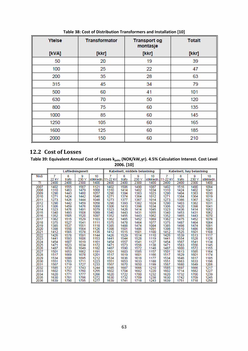
63

Table 38: Cost of Distribution Transformers and Installation [10]

12.2 Cost of Losses Table 39: Equivalent Annual Cost of Losses kpekv (NOK/kW,yr). 4.5% Calculation Interest. Cost Level

2006. [10]

64

Table 40: Capitalised Equivalent Cost of Losses Kpekv (NOK/kW). Period of Analysis 30 Years. 4.5% Calculation Interest. Cost Level 2006. [10]

Table 41: Capitalised Equivalent Cost of No-load Losses KTekv (NOK/kW). Period of Analysis 30 Years. 4.5% Calculation Interest. Cost Level 2006. [10]

12.3 Consumer Price Index Table 42: Norwegian Consumer Price Index, 1998=100 [14]

Jan. Feb. March Apr. May June July Aug. Sept. Oct. Nov. Dec. Average

2010 127.1 128.7 129.3 129.6

2009 124.0 125.0 125.1 125.4 125.7 126.4 125.7 125.4 126.4 126.2 126.6 126.9 125.7

2008 121.3 121.9 122.0 121.9 122.0 122.2 123.0 123.1 124.9 125.4 124.7 124.4 123.1

2007 117.0 117.5 118.2 118.2 118.3 118.2 117.9 117.8 118.6 118.9 120.8 121.8 118.6

2006 115.6 116.6 116.9 117.9 117.9 117.7 117.4 117.3 119.0 119.1 119.0 118.5 117.7

2005 113.6 113.7 114.2 114.8 115.2 115.3 114.9 115.1 116.0 116.0 116.0 115.9 115.1

2004 112.4 112.6 113.1 113.3 113.4 113.4 113.3 113.0 113.7 114.0 114.0 113.8 113.3

2003 114.5 114.6 113.8 112.9 112.3 112.0 111.6 111.9 112.5 112.4 112.6 112.6 112.8

2002 109.0 109.3 109.7 109.7 110.0 110.1 109.9 109.6 110.2 110.6 111.0 111.9 110.1

2001 107.6 108.4 108.6 109.1 109.6 109.7 108.2 108.1 108.7 108.6 108.7 108.9 108.7

2000 104.1 104.6 104.7 105.1 105.1 105.7 105.4 105.3 106.2 106.3 106.8 106.7 105.5

65

12.4 Technical Data of Components Table 43: PEX Isolated 1kV Earth Cable 4 Conductors without Screen. [10]

Table 44: Distribution Transformers [10]

The values given in the table are related to the components in the figure below.

Figure 25: Electric Equivalent Circuit of Transformer [10]

In the figure above, the resistance RT represents the resistance of the windings, while XT represents the leakage inductance. Xm represents the magnetising inductance. The value is large and can be neglected. The resulting impedance is then:

(18)

66

The impedances are often given in per unit. The reference impedance Zn is given from the rated values of the transformer, and used to calculate the per unit values short circuit im-pedance ek and its resistive part er and reactive part ex. The copper losses in the transformer are given by Pk.

(19)

(20)

(21)

(22)

(23)

(24)

Table 45: Transformers Used in Analysis Power Rating

(kVA) er ex

Tap Change Position

Winding Type No-load Losses

(kW)

315 1.03 4.606 ±2x2.5% Dyn11 0.530

500 0.84 3.583 ±2x2.5% Dyn11 0.790

630 0.92 5.301 ±2x3.67% Dyn5 0.846

800 0.84 4.310 ±2x2.5% Dyn5 1.019

1000 0.86 5.685 ±2x2.5% Dyn11 1.036

1250 0.69 4.871 ±2x2.5% Dyn5 1.382

1600 0.78 5.330 ±2x2.5% Dyn11 1.609

12.5 Harmonic Voltages Table 46: Limits for Harmonic Voltages Given in the Norwegian PQ Code [9]

67

12.6 Output File from Dynko

***************************************************** ***************************************************** Program : D Y N K O EFI : 1991-02-15 Versjon nr. : 6 Manual : EFI-TR NR. 3531 Program ansvarlig : K.SAND ***************************************************** DATAFIL : lura500.dat BEGRENSNINGER : MAX. ANTALL SYSTEML\SNINGER : 25 MAX. ANTALL DELUTBYGGINGER : 25 MAX. ANTALL ]R I ANALYSEPERIODEN : 25 MAX. ANTALL ]R MED GITTE DRIFTSKOSTNADER : 25 MAX. ANTALL PROGNOSEVARIANTER (EKSKL.0%) : 2 MAX. ANTALL KALKYLRENTEVARIANTER : 3 1 *** LURAVIKA 500kW elbillast 1. KONTROLLDATA. 1.1 BESKRIVELSE AV DELUTBYGGINGER OG UTBYGGINGSALTERNATIV DELUTBYGGINGER: NR. TEKST TYPE KOSTNAD \KONOM. L]NE- AMORT. LEVETID RENTE TID (KKR.) (]R) (%) (]R) 1 ,1000kVA trafo 1 2212.4 30 10.0 15 2 ,1250kVA trafo 1 2632.4 30 10.0 15 3 ,1600kVA trafo 1 2985.3 30 10.0 15 4 ,5x240 kabel elbil 1 1130.0 30 10.0 15 5 ,6x240 kabel elbil 1 1356.0 30 10.0 15 6 ,7x240 kabel elbil 1 1582.0 30 10.0 15 7 ,8x240 kabel elbil 1 1808.0 30 10.0 15 8 ,9x240 kabel elbil 1 2034.0 30 10.0 15 UTBYGGINGSALTERNATIV UTSTR. I TID NR. DELUTBYGGINGSKODE FRA TIL 1 2 3 4 5 6 7 8 2010 2040 1 X X 2010 2040 2 X X 2010 2040 3 X X 2010 2040 4 X X 2010 2040 5 X X 2010 2040 6 X X

68

2010 2040 7 X X 2010 2040 8 X X 2010 2040 9 X X 2010 2040 10 X X 2010 2040 11 X X 1 1.2 OVERGANGSKOSTNADSMATRISE. OVERGANGSKOSTNADER I KKR. REF. T=0. KOSTNADSELEMENTER AV TYPE 2 ER IKKE INKLUDERT. OVERG. TIL ALT.*** FRA ALT. * * 0 1 2 3 4 5 6 7 8 9 10 11 XXXX 3568 3794 4020 3988 4214 4440 4666 3762 4341 4567 4793 XXXX XXXX XXXX XXXX XXXX XXXX XXXX XXXX XXXX XXXX XXXX 1 1.3 EKVIVALENTE \K. LEVETIDER REF. T=0 BEREGNINGEN ER HER FORETATT VED KALKULASJONSRENTENIV] 4.50 % . KOSTNADSELEMENTER AV TYPE 2 ER IKKE INKLUDERT. OVERG. TIL ALT.*** FRA ALT. * * 0 1 2 3 4 5 6 7 8 9 10 11 XXXX 30 30 30 30 30 30 30 30 30 30 30 XXXX XXXX XXXX XXXX XXXX XXXX XXXX XXXX XXXX XXXX XXXX 1 1.4 LEVETIDSDIAGRAM. ]RLIGE MAKSIMALTAP I KW. 1.4.1 AVVIK FRA OPPR. PROGNOSE: .00 % ]RLIGE MAKSIMALTAP I KW. ]R 2010 2011 2012 2013 2014 2015 2016 2017 2018 2019 2020 2021 2022 2023 2024 2025 2026 2027 2028 2029 2030 2031 2032 2033 2034 ALT.NR.

69

1 228 228 228 228 228 228 228 228 228 228 228 228 228 228 228 228 228 228 228 228 228 228 228 228 22 2 217 217 217 217 217 217 217 217 217 217 217 217 217 217 217 217 217 217 217 217 217 217 217 217 21 3 208 208 208 208 208 208 208 208 208 208 208 208 208 208 208 208 208 208 208 208 208 208 208 208 20 4 182 182 182 182 182 182 182 182 182 182 182 182 182 182 182 182 182 182 182 182 182 182 182 182 18 5 170 170 170 170 170 170 170 170 170 170 170 170 170 170 170 170 170 170 170 170 170 170 170 170 17 6 163 163 163 163 163 163 163 163 163 163 163 163 163 163 163 163 163 163 163 163 163 163 163 163 16 7 156 156 156 156 156 156 156 156 156 156 156 156 156 156 156 156 156 156 156 156 156 156 156 156 15 8 198 198 198 198 198 198 198 198 198 198 198 198 198 198 198 198 198 198 198 198 198 198 198 198 19 9 174 174 174 174 174 174 174 174 174 174 174 174 174 174 174 174 174 174 174 174 174 174 174 174 17 10 164 164 164 164 164 164 164 164 164 164 164 164 164 164 164 164 164 164 164 164 164 164 164 164 16 11 155 155 155 155 155 155 155 155 155 155 155 155 155 155 155 155 155 155 155 155 155 155 155 155 15 ]RLIG IKKE LEVERT ENERGI I MWH. ]R 2010 2011 2012 2013 2014 2015 2016 2017 2018 2019 2020 2021 2022 2023 2024 2025 2026 2027 2028 2029 2030 2031 2032 2033 2034 ALT.NR. 1 2 3 4 5 6 7 8 9 10 11 1.5 UTGANGSPUNKT FOR BEREGNING AV TAP(SKOSTNADER). TAP VED DE GITTE STADIER. (OPPR. PROGN.): ]RLIGE MAKSIMALTAP I KW. TAP VED DE GITTE STADIER. (OPPR. PROGN.): ]RLIGE MAKSIMALTAP I KW. STADIUM: 2010 2020 ALT. NR. 1 228 228 2 217 217 3 208 208 4 182 182 5 170 170 6 163 163 7 156 156 8 198 198

70

9 174 174 10 164 164 11 155 155 ]RLIG IKKE LEVERT ENERGI . (OPPR. PROGN.): GITT I MWH. STADIUM: 2010 2020 ALT. NR. 1 0 0 2 0 0 3 0 0 4 0 0 5 0 0 6 0 0 7 0 0 8 0 0 9 0 0 10 0 0 11 0 0 TABELL 1.6 / 1.7 SPESIFIKKE TAPS OG AVBRUDDSKOSTNADER ]R TAPSKOST. AVBRUDDSKOST (KR/KW) (KR/KWH) 2010 1384 0 2011 1386 0 2012 1403 0 2013 1420 0 2014 1436 0 2015 1453 0 2016 1465 0 2017 1475 0 2018 1487 0 2019 1498 0 2020 1510 0 2021 1525 0 2022 1539 0 2023 1554 0 2024 1567 0 2025 1583 0 2026 1600 0 2027 1613 0 2028 1629 0 2029 1646 0 2030 1663 0 2031 1680 0 2032 1697 0 2033 1714 0 2034 1732 0 1 2. RESULTATUTSKRIFT.

71

BEREGNING NR.: 1 *** LURAVIKA 500kW elbillast FORUTSETNINGER. KALKULASJONSRENTE : 4.50 % PRISSTIGN. FASTE KOSTN. : .00 % PRISSTIGN. DRIFTSKOSTN. : .00 % ANALYSEPERIODE : 25 ]R AVVIK FRA OPPR. PROGNOSE : .00 % STARTALTERNATIV : 0 OPTIMAL UTBYGGINGSPLAN NR. ]RSTALL 10 11 12 13 14 15 16 17 18 19 20 21 22 23 24 25 26 27 28 29 30 31 32 33 34 1 5 5 5 5 5 5 5 5 5 5 5 5 5 5 5 5 5 5 5 5 5 5 5 5 5 2 6 6 6 6 6 6 6 6 6 6 6 6 6 6 6 6 6 6 6 6 6 6 6 6 6 3 4 4 4 4 4 4 4 4 4 4 4 4 4 4 4 4 4 4 4 4 4 4 4 4 4 4 7 7 7 7 7 7 7 7 7 7 7 7 7 7 7 7 7 7 7 7 7 7 7 7 7 5 10 10 10 10 10 10 10 10 10 10 10 10 10 10 10 10 10 10 10 10 10 10 10 10 10 6 11 11 11 11 11 11 11 11 11 11 11 11 11 11 11 11 11 11 11 11 11 11 11 11 11 7 9 9 9 9 9 9 9 9 9 9 9 9 9 9 9 9 9 9 9 9 9 9 9 9 9 8 8 8 8 8 8 8 8 8 8 8 8 8 8 8 8 8 8 8 8 8 8 8 8 8 8 9 2 2 2 2 2 2 2 2 2 2 2 2 2 2 2 2 2 2 2 2 2 2 2 2 2 10 3 3 3 3 3 3 3 3 3 3 3 3 3 3 3 3 3 3 3 3 3 3 3 3 3 11 1 1 1 1 1 1 1 1 1 1 1 1 1 1 1 1 1 1 1 1 1 1 1 1 1 \KONOMISK OPPSUMMERING (NB. KUN DEN ANDEL AV KOSTNADENE SOM P]L\PER INNENFOR ANALYSEPERIODEN INNG]R I KOSTNADSTALLENE) NR. INVESTERINGS- TAPS- AVBRUDDS- TOTALT ANNUITET RELATIV KOSTNADER KOSTNADER KOSTNADER VURDERING (KKR) (KKR) (KKR) (KKR) (KKR/]R) (%) 1 3836.5 3817.0 .0 7653.5 516.1 100.0 2 4042.2 3659.8 .0 7702.0 519.4 100.6 3 3630.7 4086.4 .0 7717.2 520.4 100.8 4 4247.9 3502.7 .0 7750.6 522.7 101.3 5 4157.7 3682.3 .0 7840.0 528.7 102.4 6 4363.5 3480.2 .0 7843.7 529.0 102.5 7 3952.0 3906.8 .0 7858.8 530.0 102.7 8 3425.0 4445.7 .0 7870.7 530.8 102.8 9 3454.1 4872.3 .0 8326.4 561.5 108.8 10 3659.9 4670.2 .0 8330.1 561.8 108.8 11 3248.4 5119.3 .0 8367.7 564.3 109.3 KONKLUSJON. F\LGENDE UTBYGGINGSPROGRAM GIR MINST SUM DISKONTERTE KOSTNADER I ANALYSEPERIODEN: ]RSTALL UTBYGGING INVEST.(KKR)

72

2010 - 1. ,1250kVA trafo 2632.4 - 2. ,7x240 kabel elbil 1582.0

Technical-economic Analysis of Fast Chargers for Plug-in ...

Documents

Transcript of Technical-economic Analysis of Fast Chargers for Plug-in ...