Technical Development for S-CO2 Advanced Energy ...
241
Project No. 11-3039 Technical Development for S-CO2 Advanced Energy Conversion Reactor Concepts Dr. Mark Anderson University of Wisconsin - Madison In collaboration with: Texas A&M University Brian Robinson, Federal POC Jim Sienicki, Technical POC Nuclear Energy University Programs U.S. Department of Energy
-
Upload
khangminh22 -
Category
Documents
-
view
3 -
download
0
Transcript of Technical Development for S-CO2 Advanced Energy ...

Project No. 11-3039
Technical Development for S-CO2 Advanced Energy Conversion
Reactor ConceptsDr. Mark Anderson
University of Wisconsin - Madison
In collaboration with:Texas A&M University
Brian Robinson, Federal POC Jim Sienicki, Technical POC
Nuclear Energy University Programs
U.S. Department of Energy

Project Number: NU-11-WI-UWM-0303-03 (Project 11-3039)Project Title: Technical Development for S-CO2 Advanced Energy Conversion Report: 2014 Annual Report (Final Report)2014 Final Report Due: November 10, 2014
Milestone Status:
M1: ActivityNU-11-WI-UWM_-0303-031: Monthly Spend Plan - Completed 11/10/14
M1NU-11-WI-UWM_-0303-032: FY2013 Go/No-Go Review - (Project 11-3039) Technical Development for S-CO2 Advanced Energy Conversion - Completed 9/30/2013
M1NU-11-WI-UWM_-0303-033: Final Report - (Project 11-3039) Technical Development for S-CO2 Advanced Energy Conversion - Completed 11/10/2014
M3NU-11-WI-UWM_-0303-034: Design and construction of HEX - Completed 6/30/2012
M3NU-11-WI-UWM_-0303-035: Calibration of HEX facility - Completed 7/31/2013
M3NU-11-WI-UWM_-0303-036: Design and construction of seal testing facility -Completed 10/20/2013
M3NU-11-WI-UWM_-0303-037: Obtain test data for S-Co2 through orifice -Completed 10/20/2013
M3NU-11-WI-UWM_-0303-038: Implement coupled algorithm into open foam -Completed 10/20/2014
Student Information:
Matt Wolf - Received Master’s degree in Nuclear Engineering from UW- June 2014 Jacob Mahaffey - Continuing on to PhD-UWJohn Dyreby - Received PhD in Mechanical Engineering UW- Sept 2014 Haomin (Kirk) Yuan - Continuing on to PhD- UW Sandeep Pidaparti - Continuing on to PhD- Georgia Tech
Abstract
This report is divided into four parts. First part of the report describes the methods used to
measure and model the flow of supercritical carbon dioxide (S-CO2) through annuli and straight-
through labyrinth seals. The effects of shaft eccentricity in small diameter annuli were observed
for length-to-hydraulic diameter (L/D) ratios of 6, 12, 143, and 235. Flow rates through tooth-
cavity labyrinth seals were measured for inlet pressures of 7.7, 10, and 11 MPa with
corresponding inlet densities of 325, 475, and 630 kg/m3. Various leakage models were
compared to this result to describe their applicability in supercritical carbon dioxide
applications. Flow rate measurements were made varying tooth number for labyrinth seals of
same total length. Flow rate measurements were also made for a stepped labyrinth seal similar
to shaft seal found in Sandia National Laboratories research facility.
The effect of eccentricity on flow through small diameter annuli was found to be minimal for
the lengths typically found in labyrinth type shaft seals. There is an expected flow increase
when moving a shaft from a concentric position to an eccentric position which is driven by a
change in the fluid friction. This flow increase was found to be small for short annular orifices.
An observed increase in flow rate of 3% was observed for short length annular orifices and was
increased to 8.5% when the orifice length was increased beyond a distance equal to the
developing entrance length and frictional effects were manifested.
Flow rate measurements for a straight through labyrinth seal with three teeth were made at
inlet pressures of 7.7, 10, and 11 MPa with corresponding inlet densities of 325, 475, and 630
kg/m3. Various labyrinth seal leakage models were applied to the data calculated to compare
applicability. Applying the Homogeneous Equilibrium Model (HEM) with an experimentally
determined discharge coefficient to predict the mass flow rate gave results with less than 5%

error for the higher pressure cases of 10 and 11 MPa and less that 14% error for the lower
pressure case of 7.7 MPa. The HEM model works well when the inlet condition chokes prior to
entering the two phase region and begins to deviate when two-phase effects become more
prevalent. Other models were unable to predict property changes along with poor response to
changes in geometry due to their lack of complexity. A Stepped labyrinth seal was designed to
mimic the geometry used in the supercritical flow research loop at Sandia National Laboratories.
This provided a more complex geometry to further test the capabilities of the facility and
validate models. The results showed that the data could be used to scale to larger diameters
and apply to more practical geometries. Three-tooth and four-tooth cases were tested an inlet
pressure of 10 MPa with a corresponding inlet density of 325 kg/m3. It was found that
increasing the tooth number decreased the flow by 5% from the three-tooth case to the four-
tooth case.
Second part of the report describes the computational study performed to understand the
leakage through the labyrinth seals using Open source CFD package OpenFOAM. Fluid Property
Interpolation Tables (FIT) program was implemented in OpenFOAM to accurately model the
properties of CO2 required to solve the governing equations. To predict the flow behavior in the
two phase dome Homogeneous Equilibrium Model (HEM) is assumed to be valid. Experimental
results for plain orifice (L/D ~ 5) were used to show the capabilities of the FIT model
implemented in OpenFOAM. Error analysis indicated that OpenFOAM is capable of predicting
experimental data within ±10% error with the majority of data close to ±5% error. Following the
validation of computational model, effects of geometrical parameters and operating conditions
are isolated from each other and a parametric study was performed in two parts to understand
their effects on leakage flow.

Results of the geometrical parametric study indicated that the carryover coefficient of a seal is
independent of pressure drop across the seal and is only a function of geometry. A model for
carryover was developed as a function of c/s (clearance to pitch ratio) and wcavity/c (cavity width
to clearance). It has been identified that the major non-dimensional parameter influencing the
discharge through an annular orifice is wtooth/c (tooth width to clearance) and a model for Cd
(discharge coefficient) can be developed based on the results. Flow through labyrinth seals can
be considered as a series of annular orifices and cavities. Using this analogy, leakage rate can be
modeled as a function of the discharge coefficient under each tooth and the carryover
coefficient, which accounts for the turbulent dissipation of kinetic energy in a cavity. The
discharge coefficient of first tooth in a labyrinth seal is similar to that of an annular orifice,
whereas, the discharge coefficient of the rest of the tooth was found to be a function of the Cd
of the previous tooth and the carryover coefficient. To understand the effects of operating
conditions, a 1-D isentropic choking model is developed for annular orifices resulting in upper
and lower limit curves on a T-s diagram which show the choking phenomenon of flow through a
seal. This model was applied to simulations performed on both annular orifices and labyrinth
seals. It has been observed that the theory is in general valid for any labyrinth seal, but the
upper and lower limit curves on T-s diagram depend on number of constrictions. As the number
of constrictions increase these two curves move further away from the critical point.
Third part of the report provides the details of the constructed heat exchanger test facility and
presents the experimental results obtained to investigate the effects of buoyancy on heat
transfer characteristics of Supercritical carbon dioxide in heating mode. Turbulent flows with
Reynolds numbers up to 60,000, at operating pressures of 7.5, 8.1, and 10.2 MPa were tested in
a round tube. Local heat transfer coefficients were obtained from measured wall temperatures
over a large set of experimental parameters that varied inlet temperature from 20o C to 55o C,
mass flux from 150 to 350 kg/m2s, and a maximum heat flux of 65 KW/m2. Horizontal, upward
and downward flows were tested to investigate the unusual heat-transfer characteristics to the
effect of buoyancy and flow acceleration caused by large variation in density. In the case of
upward flow, severe localized deterioration in heat transfer was observed due to reduction in
the turbulent shear stress and is characterized by sharp increase in wall temperature. In the case
of downward flow, turbulent shear stress is enhanced by buoyancy forces leading to an
enhancement in heat transfer. In the case of horizontal flow, flow stratification occurred leading
to a circumferential variation in wall temperature. Thermocouples mounted 180o apart on the
tube revealed that the wall temperatures on the top side are significantly higher than the
bottom side of the tube. Buoyancy factor calculations for all the test cases indicated that
buoyancy effects cannot be ignored even for horizontal flows at Reynolds number as high as
20,000. Experimentally determined Nusselt numbers are compared to existing correlations
available in literature. Existing correlations predicted the experimental data within ±30% with
maximum deviation around the pseudo-critical point.
Final part of this report presents the simplified analysis performed to investigate the possibility
of using wet cooling tower option to reject heat from the supercritical carbon dioxide Brayton
cycle power convertor for AFR-100 and ABR-1000 plants. A code was developed to estimate the
tower dimensions, power and water consumption, and to perform economic analysis. The code
developed was verified by comparing the calculations to a vendor quote. The effect of ambient
air and water conditions on the sizing and construction of the cooling tower as well as the cooler
is studied. Finally, a cost-based optimization technique is used to estimate the optimum water
conditions which will improve the plant economics. A comparison of different cooling options
for the S-CO2 cycle indicated that the wet cooling tower option is a much more feasible and
economical option compared to dry air cooling or direct wet cooling options.

Table of Contents
Abstract.....................................................................................................................................................2
List of Figures......................................................................................................................................... 12
List of Tables.......................................................................................................................................... 19
Introduction........................................................................................................................................... 20
1 Background....................................................................................................................................22
1.1 Supercritical Working Fluids................................................................................................22
1.1.1 The S-CO2 Brayton Cycle Turbomachinery.................................................................24
1.2 Previous Work.......................................................................................................................27
1.2.1 Annular Seals............................................................................................................... 27
1.2.2 Eccentric Flow Increase.............................................................................................. 28
1.2.3 Eccentric Entrance Length ......................................................................................... 30
1.2.4 Leakage Models .......................................................................................................... 31
1.2.5 Measured Seal Leakage ............................................................................................. 41
2 Data Collection............................................................................................................................. 43
2.1 Test Facility .......................................................................................................................... 43
2.1.1 Test Section....................................................................................................................50

2.1.2 Seal Geometries 52
2.2 Test Conditions .................................................................................................................... 57
2.3 Data Collection......................................................................................................................58
2.3.1 Assembly Procedure/Eccentricity Measurement...................................................... 58
2.3.2 Data Collection Procedure.......................................................................................... 61
3 Computational model.................................................................................................................. 62
3.1 Governing Equations........................................................................................................... 63
4 Experimental Results ................................................................................................................... 72
4.1 Shaft Eccentricity ................................................................................................................ 72
4.1 Straight through Labyrinth Seals......................................................................................... 76
4.1.1 Property Variation and HEM Model ......................................................................... 76
4.1.2 Tooth Number Optimization.......................................................................................79
4.1.3 Leakage Models .......................................................................................................... 82
4.2 Stepped Labyrinth Seal ....................................................................................................... 85
4.3 Empirical Discharge Coefficient .......................................................................................... 92
5 Numerical Results ........................................................................................................................ 94
5.1 Validation of computational model 97

5.1.1 Effect of radius of curvature 101
5.2 Effect of geometrical parameters.....................................................................................102
5.2.1 Effect of Radial clearance...........................................................................................102
5.2.2 Effect of Tooth width................................................................................................. 104
5.2.3 Effect of tooth height................................................................................................. 107
5.2.4 Effect of Shaft Diameter.............................................................................................108
5.2.5 Correlation for Carry over coefficient...................................................................... 109
5.2.6 Effect of radial clearance...........................................................................................110
5.2.7 Effect of Tooth Height................................................................................................ 111
5.2.8 Effect of cavity width ................................................................................................ 113
5.2.9 Effect of Shaft Rotation on annular orifices and labyrinth seals........................... 116
5.3 Effect of Operating Conditions......................................................................................... 122
5.3.1 Results for Annular orifice........................................................................................ 130
5.3.2 Results for Labyrinth Seal.......................................................................................... 138
6 Heat transfer characteristics of supercritical CO2.................................................................... 146
6.1 Experimental facility overview...........................................................................................146
6.2 Validation of the test facility 149

6.3 Experimental and data analysis procedure 150
6.3.1 Uncertainty analysis...................................................................................................151
6.4 Results and Discussion ....................................................................................................... 152
6.4.1 Effect of operating pressure.....................................................................................152
6.4.2 Effect of flow configuration......................................................................................153
6.4.3 Effect of inlet temperature....................................................................................... 156
6.4.4 Effect of heat flux....................................................................................................... 159
6.4.5 Buoyancy criteria ...................................................................................................... 160
6.4.6 Evaluation of existing correlations........................................................................... 167
7 Wet Cooling tower option for S-CO2 Cycle...............................................................................169
7.1 Introduction to cooling towers......................................................................................... 169
7.1.1 Classification of cooling towers................................................................................169
7.1.2 Components of a cooling tower................................................................................172
7.2 Cooling tower theory......................................................................................................... 174
7.3 Design procedure.............................................................................................................. 180
7.3.1 Estimation of optimum mw/ma.................................................................................181
7.3.2 Merkel number 182
7.3.3 Estimation of floor area 183
7.3.4 Estimation of fill height............................................................................................. 187
7.3.5 Water consumption rate........................................................................................... 189
7.3.6 Power requirements..................................................................................................190
7.3.7 Estimation of cooling tower cost..............................................................................191
7.3.8 Factors affecting cooling tower size ....................................................................... 192
7.4 Design Calculations...........................................................................................................193
7.4.1 Verification of the code............................................................................................ 194
7.4.2 Effect of ambient air conditions................................................................................196
7.4.3 Control of water conditions......................................................................................198
7.4.4 Effect of design water conditions............................................................................ 201
7.5 Cost based optimization .................................................................................................. 209
Conclusion.................................................................................................................................................1
References............................................................................................................................................... 9
Appendix A............................................................................................................................................. 15
8 Uncertainty Analysis.....................................................................................................................15
8.1 Pressure Transducers 15

8.2 Temperature 16
8.3 Mass Flow Rate and Density.............................................................................................. 17
8.4 Discharge Coefficient Uncertainty......................................................................................18
8.5 Uncertainty Summary.......................................................................................................... 19
APPENDIX B............................................................................................................................................ 20
APPENDIX C............................................................................................................................................ 21
APPENDIX D............................................................................................................................................ 22

List of Figures
Figure 1. Sandia National Laboratory engineering diagram of labyrinth seal (A). The seal is made of brass and has four teeth that approach the steps on the rotating shaft. The compressor wheel (B) shows the four steps on the shaft.
Figure 2. Calculated windage loss for the S-CO2 SNL turbo-alternator-compressor as a function of rotor cavity pressure [2].
Figure 3. Conventional pocket damper seal [10].
Figure 4. Piercy's result for increase in volumetric flow rate due to eccentricity in narrow fully- developed annular flow. The dashed line shows effects in the laminar region and the solid line shows effects in the turbulent region.
Figure 5. Detail of SNL main compressor, labyrinth seals, ball bearings, and location of other major components [14].
Figure 6. Sandia National Laboratory engineering diagram of labyrinth seal (A). The seal is made of brass and has four teeth that approach the steps on the rotating shaft. The compressor wheel (B) shows the four steps on the shaft [14].
Figure 7. Measured (brown) and predicted (red) leakage flow rate through the SNL four tooth stepped labyrinth seal [14].
Figure 8. Conceptual layout of the UW-Madison test facility.
Figure 9. Single Stage HydroPac compressor used in UW-Madison facility.
Figure 10. Heated and insulated buffer tank used to reduce pressure fluctuations from compressor shifting.
Figure 11. Precooler heat exchanger utilizing chilled water.
Figure 12. Preheater consisting of three heated and insulated pipes in parallel controlled via PID in Labview.
Figure 13. Conditions for various locations on the loop (Figure 8), shown on a temperature- specific entropy diagram during typical experiment conditions.
Figure 14. Cross Section of pressure vessel showing a) seal location/configuration, b) collet subassembly, c) shaft, d) seal, e) spacer drill bushing, f) test section flange [15].
Figure 15. Cross Section of test section flange showing seal configuration [15].

Figure 16. Seals and cavities used in the straight-through labyrinth tests, do=9.525 mm, di, seal=3.175 mm, di, cavity=4.763 mm and length = 1.27 mm.
Figure 17. 3-D model of seal curvature taken with Zygo NewViewTM white light interferometer.
Figure 18. Stepped labyrinth design showing pertinent dimensions.
Figure 19. Stepped labyrinth seal.
Figure 20. Shaft used to activate all four teeth within the stepped labyrinth design.
Figure 21. Shafts used in stepped labyrinth geometry, a) 4 land shaft b) 3 land shaft.
Figure 22. Temperature-specific entropy plot for CO2 with the test section inlet conditions shown for inlet pressures of 7.7 MPa (green), 10 MPa (blue), and 11 MPa (red) at corresponding inlet densities of 325, 475, and 630 kg/m3 in three-tooth labyrinth seal tests.
Figure 23. Assembly procedure of shaft-seal sub-assembly [15].
Figure 24. Result of image processing code used to measure eccentricity at shaft-seal interface.
Figure 25. Measured mass flow rate of CO2 through three tooth labyrinth seal as a function of pressure ratio for an upstream stagnation pressure of 10 MPa and an upstream stagnation density of 475 kg/m3.
Figure 26. OpenFOAM syntax for differential equations, picture taken from [36]
Figure 27. Density ratios for two phase CO2 and water
Figure 28. Specific heat ratios for two phase CO2 and water
Figure 29. Duct flow approximation flow area determination. Dividing lines show division where radial clearance was taken, a) concentric case b) eccentric case.
Figure 30. Duct flow approximation results for DH=0.1956 mm.
Figure 31. Experimental mass flow rate for annuli of varying L/Dh with a DH=0.195 mm and inlet conditions of Pin = 10 MPa and pin=325 kg/m3.
Figure 32. Temperature-specific entropy diagram for 3 tooth straight through labyrinth showing inlet conditions (filled markers) and outlet conditions (hollow markers).
Figure 33. Discharge coefficient results for three-tooth straight through labyrinth seal at varying inlet conditions.
Figure 34. Measured flow rate for three-tooth straight through labyrinth for inlet conditions P=10 MPa and p=325 kg/m3. The blue line shows calculated flow rate using isentropic HEM

model and the red line shows the calculated flow rate applying a constant discharge coefficient to the isentropic HEM model.
Figure 35. Variation in tooth number for the same total length. One Tooth a: short length, depicts maximum flow rate. One Tooth b: Tooth occupies entire length and depicts the flow rate approached as tooth number is further increased [20].
Figure 36. Variation in tooth number for the same total length. Variation in pressure ratio shows an optimal tooth number of three [20].
Figure 37. Measured flow rate for variation in tooth number for the same total length compared to calculated flow rate using Open Foam simulation [7]. Minimum leakage is found at a tooth number of three. Inlet Pressure is 10 MPa with corresponding inlet density of 325 kg/m3.
Figure 38. Comparison of measured flow rate to CFD calculated flow rate for varying tooth number with same total length.
Figure 39. Measure flow rates through straight through 3-tooth labyrinth seal for inlet pressure of 10 MPa and inlet density of 325 kg/m3 compared to various labyrinth seal leakage models.
Figure 40. Incompressible and ideal gas condition check for Martin and Egli model over prediction. Inlet pressure of 6.8 MPa with corresponding inlet temperature of 200oC.
Figure 41. Measure flow rates through straight through 3-tooth labyrinth seal for inlet pressure of 11 MPa and inlet density of 630 kg/m3 compared to various labyrinth seal leakage models.
Figure 42. Four-tooth stepped labyrinth geometry for inlet pressure of 10 MPa and inlet density of 640 kg/m3. Compared to calculated SNL leakage flow rate which is within 20% of measured flow rate.
Figure 43. Area normalized mass flow rate comparison of four-tooth stepped labyrinth seal to SNL leakage calculation for inlet conditions of 10 MPa and 640 kg/m3
Figure 44. Area normalized leakage for four-tooth stepped labyrinth seal compared to calculated flow rate from SNL compressor facility.
Figure 45. Three-tooth and four-tooth stepped labyrinth seal flow rate measurement for inlet pressure of 10 MPa and inlet density of 640 kg/m3.
Figure 46. Mass flow rate experimental measurements and calculations for three and four tooth stepped labyrinth seal including the SNL Martin leakage equation and the HEM model with constant discharge coefficient.
Figure 47. Experimentally determined discharge coefficient for three and four tooth stepped labyrinth seal at an inlet condition of 10 MPa with corresponding inlet density of 640 kg/m3.
Figure 48. A sample computational mesh used for simulations

Figure 49.
Figure 50.
Figure 51.
Figure 52.
Figure 53.
Figure 54.
Figure 55.
Figure 56.
Figure 57.
Figure 58.
Figure 59.
Figure 60.
Figure 61.
Figure 62.
Figure 63.
Figure 64.
Figure 65.
Figure 66.
Figure 67.
Figure 68.
Figure 69.
Figure 70.
Figure 71.
Variation of leakage rate prediction with number of nodes
Variation of discharge coefficient with number of nodes
Leakage rate for inlet condition of 9 MPa, 372 kg/m3 (case 1 in Table D.3)
Leakage rate for inlet condition of 9 MPa, 498 kg/m3 (case 2 in Table D.3)
Leakage rate for inlet condition of 10 MPa, 372 kg/m3 (case 3 in Table D.3)
Leakage rate for inlet condition of 10 MPa, 498 kg/m3 (case 4 in Table D.3)
Leakage rate for inlet condition of 11 MPa, 372 kg/m3 (case 5 in Table D.3)
Error analysis for plain orifice data
Effect of radius of curvature on leakage rate
Variation of leakage rate with Radial clearance
Variation of discharge coefficient with radial clearance
Variation of leakage rate with tooth width
Variation of Cd with tooth width
Cd of annular orifices having same w/c
Variation of leakage rate with tooth height
Variation of Cd with tooth height
Variation of Cd with shaft diameter
Measurement of divergence angle in the cavity
Effect of clearance on y
Effect of tooth/cavity height on y
Effect of cavity height on leakage rate
Effect of cavity width on leakage rate
Variation of y with cavity width
Figure 72. Velocity profile at the entrance of each tooth

Figure 73. Influence of shaft rotation on Cd of annular orifices
Figure 74. Variation of y with shaft speed
Figure 75. Variation of the Cd with shaft speed for labyrinth seals
Figure 76. Pressure variation along centerline in the radial clearance region
Figure 77. Temperature variation along centerline in the radial clearance region
Figure 78. Leakage rate prediction using 1-D isentropic model for case 2 in Appendix C
Figure 79. Inlet conditions used for testing 1-D isentropic model
Figure 80. Isentropic flow behavior for Sin=-1.0 KJ/kg-K
Figure 81. Isentropic flow behavior for Sin=-1.338 KJ/kg-K
Figure 82. Isentropic flow behavior for Sin=-1.5 KJ/kg-K
Figure 83. Downstream velocity and local sound speed of an annular orifice as a function of outlet pressure
Figure 84. Choking theory for isentropic flow
Figure 85. Leakage rate for inlet condition of 9 MPa and 372 kg/m3
Figure 86. Leakage rate for inlet condition of 9 MPa and 498 kg/m3
Figure 87. Cd for cases 4 and 5 in Table D.1 of Appendix D
Figure 88. Leakage rate for inlet condition of 10 MPa and 372 Kg/m3
Figure 89. Leakage rate for inlet condition of 10 MPa and 498 Kg/m3
Figure 90. Cd for case 3 in Table D.1 and case 2 in Appendix B
Figure 91. Leakage rate for inlet condition of 11 MPa and 372 Kg/m3
Figure 92. Leakage rate for inlet condition of 11 MPa and 498 Kg/m3
Figure 93. Cd for cases 1 and 2 in Table D.1 of Appendix D
Figure 94. Cd for case 6 in Table D.1 of Appendix D
Figure 95. Choking point calculations for annular orifice (Flow curve)
Figure 96. Leakage rate for inlet condition of 9 MPa and 372 Kg/m3
Figure 97. Leakage rate for inlet condition of 9 MPa and 498 Kg/m3
Figure 98. Leakage rate for inlet condition of 9 MPa and 630 Kg/m3
Figure 99. Cd for an inlet pressure of 9 MPa (cases 3, 4 and 5 in Table D.1)
Figure 100. Leakage rate for inlet condition of 10 MPa and 372 Kg/m3
Figure 101. Leakage rate for inlet condition of 10 MPa and 498 Kg/m3
Figure 102. Cd for an inlet pressure of 10 MPa
Figure 103. Cd for an inlet pressure of 11 MPa
Figure 104. Cd for an inlet pressure of 7.7 MPa
Figure 105. Choking point calculations for labyrinth seal (Flow curve)
Figure 106. Downstream velocity of labyrinth seal and local sound speed as a function of outlet pressure
Figure 107. Schematic of the experimental facility and the test section
Figure 108. Wall temperature and Nusselt Number for water validation test
Figure 109. Effect of operating pressure on heat transfer for downward flow, G - 195 kg/m2s, Q"PS - 13.5 kW/m2
Figure 110. Effect of flow configuration on heat transfer for p - 8.1 MPa, G - 195 kg/m2s, Q"PS - 24 kW/m2, Tin - 46°C
Figure 111. Effect of inlet temperature on the wall temperatures for p - 7.5 MPa, G - 320 kg/m2s, Q"PS -24 kW/m2
Figure 112. Effect of heat flux on downward flow heat transfer for p - 7.5 MPa, G- 195 kg/m2s
Figure 113. Normalized Nusselt number versus Jackson's buoyancy parameter, Bu
Figure 114. Normalized Nusselt number versus Jackson's buoyancy parameter, Boj
Figure 115. Calculated Nusselt number using Mokry et al. correlation
Figure 116. Calculated Nusselt number for downward flow
Figure 117. Proposed schematic of the cooler and induced draft cooling tower
Figure 118. Concept of different fill types

Figure 119. Control volume of counterflow fill configuration
Figure 120. Air side control volume
Figure 121. Counterflow cooling diagram
Figure 122. Delta cooling towers Inc. one cell plan [80]
Figure 123. Effect of heat load
Figure 124. Effect of range
Figure 125. Effect of approach
Figure 126. Effect of wet-bulb temperature
Figure 127. Variation of requirements for AFR-100 at optimum mw/ma conditions
Figure 128. Effect of mw/ma on the power consumption and make-up water requirements
Figure 129. Effect of water conditions on the cooler variables
Figure 130. Effect of water conditions on the tower floor area in Idaho Falls
Figure 131. Effect of water conditions on the fill height in Idaho Falls
Figure 132. Effect of water conditions on the total power consumption in Idaho Falls
Figure 133. Effect of water conditions on the cooling tower cost in Idaho Falls
Figure 134. Effect of water conditions on the cooler cost
Figure 135. Effect of water conditions on plant capital cost in Idaho Falls
Figure 136. Effect of water conditions on plant capital cost for all three locations

List of Tables
Table I. Experimental flow increase due to eccentricity for DH=0.195 mm and inlet conditions of Pin =10 MPa and pin= 325 kg/m3
Table II. Empirical discharge coefficient results
Table III. Choking and saturation pressures for various operating conditions
Table IV. Reference cooler design conditions for AFR-100 and ABR-1000 plants
Table V. Tower Merkel number calculation example
Table VI. Manufacturer data for different cell types
Table VII. Comparison of calculations to the manufacturer quotation
Table VIII. Monthly design ambient air conditions
Table IX. Cost-based optimization results for AFR-100 and ABR-1000 plants
Table X. Comparison of different cooling options for ABR-1000
Table XI. Pressure transducer uncertainty and configuration summary.
Table XII. Temperature uncertainty and configuration summary.
Table XIII. Mass flow and density uncertainties and configuration summary.
Table XIV. Summary of key parameter uncertainties.

Introduction
The widespread use and success of the Rankine cycle has, until recently reduced interest in
developing alternative methods of power conversion. There is now increased research into
alternatives to the steam Rankine cycle because of the higher thermal efficiencies that are
possible at the high temperatures associated with next generation nuclear power and
concentrating solar power. One potential alternative power cycle which takes advantage of
these higher temperatures to achieve greater efficiency is the supercritical carbon dioxide
Brayton cycle. As a result, the development of a fundamental understanding of the behavior of
S-CO2 as a working fluid in these cycles has become an important area of research for the turbo
machinery community [1-4].
The operating conditions associated with the S-CO2 Brayton cycle provide both potential
advantages and interesting engineering concerns. The wide variation in properties across the S-
CO2 system demands a thorough understanding of the working fluid and its behavior under a
variety of conditions. This need is compounded by the relatively small turbo machinery
dimensions that are possible in the S-CO2 Brayton cycle. Windage losses caused by the high
density S-CO2 can have a large effect, reducing efficiencies due to the high speed of the turbine
[5, 6].
Several aspects of the S-CO2 Brayton Cycle still require significant research and development,
and this work addresses few of these areas. The behavior of S-CO2 as it flows through
restrictions such as valves, turbo machinery seals, and pipe ruptures is not well understood, but
the development of models describing these phenomena is integral to the practical
implementation of the S-CO2 Brayton Cycle. For example, approximations for flow rates and
pressure drops associated with annular orifices and labyrinth seals are necessary in computer

models used for predicting the performance of the power cycle. Models, such as Computational
Fluid Dynamics (CFD), that are validated by this data can then be used to model more complex
geometries [7].
The most relevant and basic flow situation related to this problem is flow through circular and
annular orifices [8]. Therefore, flow through an annular space must be understood in order to
model and optimize more complex seals such as labyrinth seals. When the annular geometry is
understood the more complex labyrinth geometry can be observed and then optimized. The
first objective of this study is to collect and use experimental data to model and optimize simple,
small diameter shaft seals to aid in the practical design and use within S-CO2 environments. The
second objective is to develop computational model to understand the flow behavior through
seals in more detail. Open source CFD package OpenFOAM is used for this task. The effect of
geometrical parameters and operating conditions are isolated and studied individually.
Another biggest challenge in development of the cycle is that the detailed heat transfer
mechanisms are still not completely understood. Due to drastic variation in thermophysical
properties, heat transfer to supercritical fluids is quite different compared to ideal fluids.
Qualitative explanation of different heat transfer mechanisms to supercritical fluids is provided
by Licht et al. [62]. In a pipe flow, both axial and radial variation in density results in strong
buoyancy effects deteriorating or enhancing the heat transfer depending on flow configuration
and operating conditions [43-62]. Hence, the third objective of this work is to investigate such
buoyancy effects on heat transfer to supercritical fluids (CO2 in this case) and identify the
conditions under which buoyancy effects are significant.
Rejecting the heat from power generation plants is also a big issue. There are numerous ways to
achieve this task. One of the traditional options is to circulate cooling water from a nearby water

sources like river, lake, pond etc. which acts as an ultimate heat sink. The use of this direct wet
cooling option is severely restricted due to the new environmental policies and scarcity of water
resources in some locations. Alternatively, the dry air cooling option can be used with air as
ultimate heat sink. However, recent calculations [67] suggested that the use of dry air cooling
option would increase the cost of electricity by 40% compared to the direct wet cooling option.
Hence, dry air cooling would be an expensive option for the AFR-100 or ABR-1000. The final task
of the current work is to analyze the possibility of using the evaporative cooling tower option to
reject the heat from these proposed power plants.
1 Background
1.1 Supercritical Working Fluids
A supercritical fluid is a substance whose temperature and pressure lie above the critical point.
The critical point is found at the top of the vapor dome on the boundary of the two-phase
region. This point is defined mathematically as the condition when the first and second
derivatives of pressure with respect to volume at constant temperature are zero [9]. Within the
supercritical region there is no distinct separation between the liquid and gas phases. This
causes unusual behavior especially near the critical point where physical properties such as
density and specific heat vary greatly.
The advantages of these property changes as applied to power cycles have been investigated for
quite some time. Using supercritical fluid in power cycles allows for greatly increased power
output and compression efficiency. This can be done by operating the compressor portion of
the power cycle near the critical region where the density varies greatly with temperature.
There is a considerable amount of work necessary to compress a low density fluid and this
reduces the turbine output. By operating near the critical point and making use of the high

density of the fluid within the compressor the backwork ratio can be lowered, increasing
efficiency. This effect can be seen in the Rankine cycle where compression takes place in the
liquid region where the density is higher and shaft work can be reduced. Operating in this
region invites some disadvantages; to achieve this liquid state the cycle must include
evaporation and condensation stages. This complicates the cycle by requiring more equipment
to facilitate the phase change. Also more complexity is introduced to problems that arise from
cavitations within the system which can damage materials and reduce efficiency.
Several power cycles that operate within the supercritical region have been heavily researched.
The front-runner working fluids are supercritical water (SCW), supercritical helium, and
supercritical carbon dioxide (S-CO2). Each poses different engineering advantages and
challenges in terms of materials and operating conditions.
SCW is operated in a Rankine cycle where the high pressure side operates above the critical
point. This allows the phase transition on the high pressure side to be avoided which eliminates
many complications. This has a large effect on the total efficiency of the cycle which improves
from 33% to 44% in a nuclear power cycle [4]. This is achieved by operating the turbine at a
pressure of 25 MPa and a temperature of 500oC.
Supercritical helium is operated in a Brayton Cycle and can achieve a much higher thermal
efficiency of 51% [5]. This may seem like a considerable improvement but to achieve this the
helium cycle needs to achieve temperature between 800 and 900oC. With current materials
technology these temperatures are hard to handle. This makes the helium cycle a technology
that requires more research and development.

S-CO2 can be used as a working fluid in a Brayton cycle entirely above the critical point. This
allows for the negative effects associated with fluid phase changes within the cycle to be
avoided. The critical pressure is much lower than that of water which allows for a wider range
of inlet pressures. Typical conditions for moderate heat sources (400o-650oC) include
compressor inlet pressure of 7.5 MPa and outlet pressure of 22 MPa for power levels below 50
MWe. Wright compares the S-CO2 cycle to other advanced power cycles and find's it has a
competitive 44-46% thermal efficiency for an inlet temperature of 550oC and reduces capital
costs by approximately 23% [6]. If inlet temperature is pushed to 700oC efficiencies can
approach 50%.
1.1.1 The S-CO2 Brayton Cycle Turbomachinery
To obtain these high thermal efficiencies with the S-CO2 Brayton cycle it is important to have
properly designed turbomachinery. The main goal of this investigation is to examine the
problem of leakage through the shaft seals used within the cycle both experimentally and
computationally. With a moving shaft it is not possible to have a hermetic seal across a large
pressure gradient, meaning there will be leakage from the high pressure compressor region into
the low pressure generator cavity. This causes frictional windage losses within the generator
cavity that reduce the efficiency of the system.
The frictional losses from this leakage into the generator cavity are highly related to the density
in the cavity. One way to reduce the flow into the generator cavity is to separate the
compressor region by including a series of expansions and contractions called a labyrinth seal.
As the labyrinth seal does not provide a perfect seal there is some leakage that is expected. If
this leakage is not addressed the pressure within the generator cavity will increase to match the
pressure in the compressor region. On method of eliminating this pressure from the generator
cavity is to incorporate a secondary system to draw out the residual working fluid from the
generator cavity. This may be done by placing pumps within the system to remove the excess S-
CO2 from the generator cavity. This introduces losses due to the work required to operate the
pumps. With this method in mind it is of interest to minimize leakage through the optimization
of shaft seals.
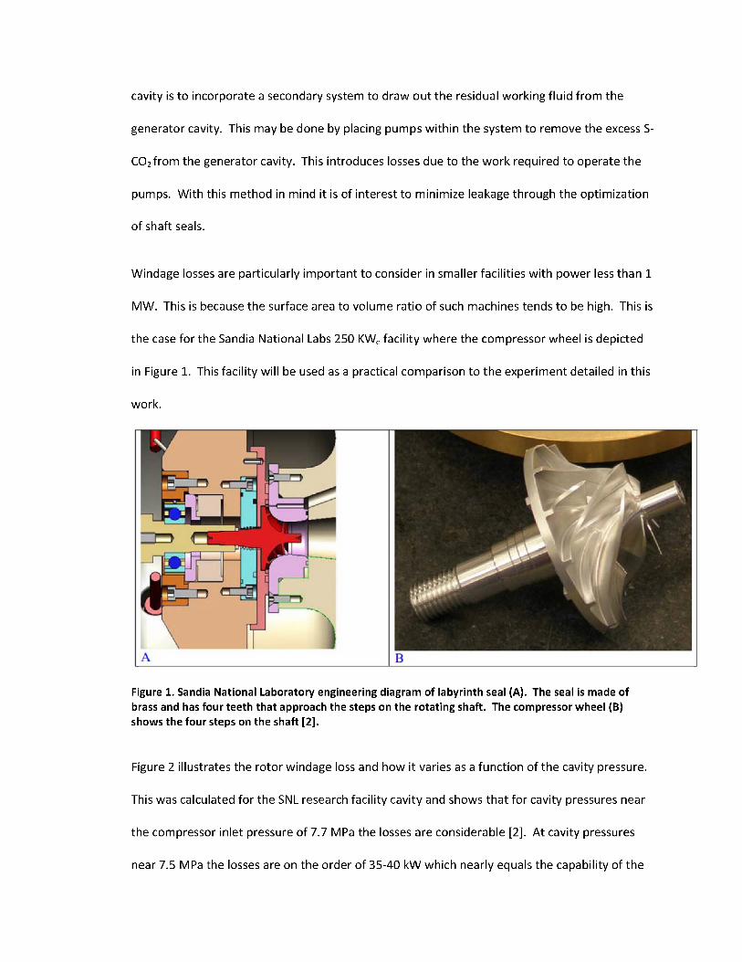
Windage losses are particularly important to consider in smaller facilities with power less than 1
MW. This is because the surface area to volume ratio of such machines tends to be high. This is
the case for the Sandia National Labs 250 KWe facility where the compressor wheel is depicted
in Figure 1. This facility will be used as a practical comparison to the experiment detailed in this
work.
Figure 1. Sandia National Laboratory engineering diagram of labyrinth seal (A). The seal is made of brass and has four teeth that approach the steps on the rotating shaft. The compressor wheel (B) shows the four steps on the shaft [2].
Figure 2 illustrates the rotor windage loss and how it varies as a function of the cavity pressure.
This was calculated for the SNL research facility cavity and shows that for cavity pressures near
the compressor inlet pressure of 7.7 MPa the losses are considerable [2]. At cavity pressures
near 7.5 MPa the losses are on the order of 35-40 kW which nearly equals the capability of the

motor control system and the pumping power for the compressor used. This led design to
operate the cavity at pressures of 1.78 MPa to reduce the losses due to cavity pressure to 4% of
the generated power down from 35%. The optimization of shaft seals limits the amount of
power needed to operate pumps which are used to achieve these low cavity pressures. The
investigation into this problem shown here depicts the need for the optimization of shaft seals
to limit the leakage into the cavity. Fortunately it is expected that the fractional pumping power
for large commercial systems is much smaller than for the SNL proof-of-principle test loop. This
is largely because more conventional sealing technologies can be used. Another reason is that
in a larger system the generated power will grow as the radius squared, while the leakage flow
rate grows proportional to the radius, thus it will be much easier to keep the fractional windage
losses low in larger systems.
Windage Rotor Loss as a function of Cavity Pressure
§, 20
loCL
~
Nee
1
ir Criti
1 i
cal Priassure\
Gr Ne<ar Cavity Design Pressuire
Q 100 200 300 400 500 600 700 800 900 1000
Pressure (psia)Figure 2. Calculated windage loss for the S-CO2 SNL turbo-alternator-compressor as a function of rotor cavity pressure [2].

1.2 Previous Work1.2.1 Annular Seals
The high demands of the power industry have caused turbomachinery to be designed with
higher efficiency and higher shaft speeds in mind. This results in a need to reach optimal
balance between a turbomachine's leakage characteristics and its rotordynamic performance,
while dealing with ever-tightening clearances. Research on one particular component used in
such machines, the annular shaft seal, has been instrumental in achieving the operating speeds
and efficiency levels that are necessary to attain today. Annular shaft seals limit fluid flow across
regions of unequal pressure. These seals have desirable leakage prevention performance and
are designed with a non-contacting nature. This non-contacting design allows rotor speeds to
be increased significantly. One of the simplest designs that employ these characteristics is the
annular labyrinth seal. Labyrinth seals are made up of a series of contractions and expansions
referred to as teeth and cavities. The ratio of the radial clearance to the shaft diameter is
usually on the order of 1:100. The annular constrictions formed by the teeth cause the working
fluid to throttle and then expand repeatedly, reducing the total pressure of the fluid from one
cavity to the next and limiting the overall axial leakage rate. The labyrinth seal is one of the
simplest and widest used shaft seals but it suffers from some undesirable rotordynamic effects
related to instability. Also labyrinth seals offer only limited damping of shaft vibrations. To
account for this more complex seal designs have been created and one of these designs is the
pocket damper seal.
The pocket damper seal is made up of teeth dividing the seal into active and inactive cavities.
The cavities are then partitioned into pockets at points along the circumference of the seal; this
can be seen in Figure 3. What this does is resist the flows ability to move in the radial direction
and increases the shaft stability provided by the seal [10].

Seal Blade
Inactive Cavity
Journal
Active Cavity
Partition Wall Exit Blade Notch
Figure 3. Conventional pocket damper seal [10].
Before more complex seals like the pocket damper seal can be examined the simpler examples
like the straight-through labyrinth geometry must be investigated. Modeling the flow through
these simpler seals allows validation of models which can then be applied to more complex
geometries. Labyrinth seals are an easily fabricated and adjustable design which allows for a
large number of parameters to be tested. By looking at different geometrical parameters, such
as cavity depth and tooth width in labyrinth seals, the design of more complex geometries can
be performed more efficiently. The investigation of labyrinth seals is in itself valuable as they
provide a cheap and effective seal. Labyrinth seals may also be combined with other designs in
more complex geometries. All these factors point to a need for research into the flow of S-CO2
through labyrinth seals
1.2.2 Eccentric Flow Increase
In assembling a labyrinth seal the shaft position within the seal has a large effect on the
geometry of the flow. The concern for this work, with respect to eccentricity, is knowing the
assembled eccentricity and understanding what effect that has had on the measured flow rate.
Two factors that contribute to this are described here to better understand the effect of
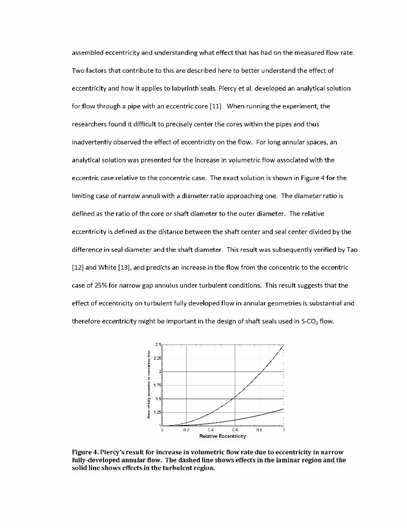
eccentricity and how it applies to labyrinth seals. Piercy et al. developed an analytical solution
for flow through a pipe with an eccentric core [11]. When running the experiment, the
researchers found it difficult to precisely center the cores within the pipes and thus
inadvertently observed the effect of eccentricity on the flow. For long annular spaces, an
analytical solution was presented for the increase in volumetric flow associated with the
eccentric case relative to the concentric case. The exact solution is shown in Figure 4 for the
limiting case of narrow annuli with a diameter ratio approaching one. The diameter ratio is
defined as the ratio of the core or shaft diameter to the outer diameter. The relative
eccentricity is defined as the distance between the shaft center and seal center divided by the
difference in seal diameter and the shaft diameter. This result was subsequently verified by Tao
[12] and White [13], and predicts an increase in the flow from the concentric to the eccentric
case of 25% for narrow gap annulus under turbulent conditions. This result suggests that the
effect of eccentricity on turbulent fully developed flow in annular geometries is substantial and
therefore eccentricity might be important in the design of shaft seals used in S-CO2 flow.
2.5
2.25
2
1.75
1.5
1.25
10 0.2 0.4 0.6 0.8 1
Relative Eccentricity
Figure 4. Piercy's result for increase in volumetric flow rate due to eccentricity in narrow fully-developed annular flow. The dashed line shows effects in the laminar region and the solid line shows effects in the turbulent region.

1.2.3 Eccentric Entrance Length
The increase in flow due to eccentricity is a frictional effect. The entrance length where flow has
yet to fully develop has a relatively high effect because of this. This effect is compounded by the
particularly short lengths expected in seal design. Jonsson's study [14] of the eccentric effect in
turbulent conditions noted a large change in the entrance length from concentric to the
eccentric case. He describes the entrance length at the location where flow reaches within 2%
of the fully developed pressure drop. This length was measured with circumferential pressure
taps installed along the length of the test section. At four lengths along the annulus six pressure
taps were spaced evenly around the circumference of the test sections outer wall. The
experimental measurements show that under some conditions, the eccentric entrance length is
triple that of the concentric entrance length. This increase in entrance length is caused by the
additional length required to transport fluid from the narrow part to the wider part of the
annulus. These results are further compounded by the fact that these data show that the effect
from eccentricity increases as the diameter ratio approaches one [15]. The results indicate
there is a distance past the concentric entrance length where the eccentric case is still
experiencing the increased friction associated with the entrance region. The increase in the
developing distance and associated increase in the shear stress then tends to offset to some
extent the decrease in the friction factor associated with the eccentric geometry. For very long
annular gaps (i.e., ones with lengths that are much longer than the eccentric entrance length)
the increase in flow due to eccentricity will reach a maximum value. However, for relatively
short annular gaps (i.e., ones with lengths that are comparable to the eccentric entry length) the
increase in flow will be less significant.

1.2.4 Leakage Models
Straight Through Labyrinth Seals
A considerable amount of work has been done to model leakage flow in labyrinth seals. In this
study several models which are used within the industry shall be compared to the experimental
data gathered. These models assume incompressible ideal gas behavior but will be observed to
evaluate their performance with S-CO2. The conditions seen in the operation of an S-CO2
Brayton cycle are far from ideal or incompressible, but these models are designed for labyrinth
seal leakage and if they perform well can provide a simple method for predicting leakage when
given only the minimum amount information about the seal and the conditions it is under.
Vennard and Street [16] carried out an energy balance on a one dimensional flow element to
obtain the Euler equation shown in Equation (1). Applying isentropic assumptions and
integrating yields the velocity expression in Equation (2). Where the subscript i denotes the ith
cavity and y denotes the ratio of specific heat values.
dP-----\-u-du + g ■ dz = 0 (1)P
uj -u*av rPi dP Pj y
2 _ Jpi+1 p ~ Pi r-1
y-il_ (Pj+i\ y
V Pi(2)
r y-ilPi_ 2 • Y
1
3) +
Pi 7-1 V Pi )Ui = (3)

r 2 y-ljPf A, 2- y2 (pi+iV (Pi+l\ V
Vr • R- Tt 7-1 V pi ) V pi )(4)
For seal constrictions it is assumed that the upstream condition is a stagnation condition. This
means the flow velocity in the cavity upstream of the constriction can be neglected relative to
the velocity of the flow through the constriction. After rearranging and again applying isentropic
assumptions the St. Venant leakage equation is shown in Equation (4). This equation was first
used by Schultz [17] for the calculation of leakage through pocket damper seals. It is an iterative
method which calculates the pressure drop at each cavity.
Martin presented the first leakage equation specifically intended for labyrinth seals. His formula,
which assumes incompressible ideal gas behavior, is shown in Equation (5). Martin's Equation is
derived based on an approach of determining the number of teeth, n, required to achieve a
given pressure drop, then relating that number to the work done in dropping the pressure. The
work done is then related to the flow-rate through the kinetic energy of the fluid.
m = (5)
Egli [18] used Martin's Equation as a starting point and suggested the use of a flow correction
factor and a kinetic energy carry-over coefficient, which he determined empirically.
empirical m = pii (6)
Egli' s flow coefficient is not based on the clearance area of the seal or the area at the vena
contracta, but the area of the jet of fluid at some point after it passes through the constriction.

The use of the jet area comes from the assumption that at some point along the jet, shortly
after the constriction, the pressure in the jet is equal to the cavity pressure in the downstream
cavity (the cavity being entered). The need for a kinetic energy carry-over coefficient is evident
from Egli's description of the flow through the constrictions of a labyrinth seal: "as the steam
flows through the labyrinth, a pressure drop occurs across each throttling. After each throttling,
a small part of the kinetic energy of the steam jet will be reconverted into pressure energy, a
second part will be destroyed and transferred into heat, and the remaining kinetic energy will
enter the following throttling." The carry-over coefficient therefore represents the portion of
kinetic energy carried over from one cavity to the next. Egli reasons that since the jet emerging
from the constriction increases with increasing axial distance, the percentage of kinetic energy
carried over from one throttling to the next must decrease with increasing spacing between the
blades or with decreasing clearance. Using Egli's method, the flow through a labyrinth seal can
be shown to follow the proportionality of Equation (7) and this proportionality can be
approximated to nas.
m K
(7)
Another modification on Egli's equation is the Hodkinson's equation [19] which is shown in
Equation (8). Where Egli used an empirical coefficient to account for kinetic energy carry-over,
Hodkinson developed a semi-empirical expression for this coefficient based on an assumption
regarding the gas jet's geometry. His assumption pertained to the shape of the fluid jet as it
expands after the constriction. A conical expansion at a small angle from the tip of the
upstream tooth moves through with a small portion entering the next cavity undisturbed.

Hodkinson makes note that Egli does not take into consideration the higher velocity through
the final constriction and then derives a carry-over factor based on a linear increase in the
pressure drop with each constriction. He incorporates his idea of a conically shaped stream and
does not take into account vena contracta effects. For the conical angle he uses a stream angle
with a tangent of 0.02 which best described his data.
m( = #A • P-Hodkinson_____ ln
V^T'"(tT)
(8)
.Hodkinson
(9)
The carry over coefficient defined in Equation (9) cannot increase indefinitely. There is a
numerical limit which Hodkinson defines since if clearances continue to increase, the fluid will
blow straight through and the seal will act like one with a single constriction. At very large
pressure drops, Hodkinson notes that the carry-over coefficient becomes unnecessary since at
the acoustic velocity the seal leakage is more or less determined by the clearance of the final
tooth. At pressures further from the critical ratio or with a liquid in place of a gas, the carry-over
effects become significant.
Developing his own carry-over coefficient Vermes [20] modified Martin's leakage equation. This
equation is developed based on boundary layer theory and is shown in Equation (10).

(10)m( = Vermes
..Vermes 1
(1-«i)(11)
8.52«t = h — tj
Ci+ 7.23
(12)
Neumann [Childs 21] developed the empirical leakage expression of Equation (13) which
contains a semi-empirical leakage flow coefficient^. The coefficient accounts for the further
contraction of flow after it has passed through the plane of the physical constriction.
= Cf,i • Neumannn2 _ n2 rt rt + l
fi • T(13)
nCfli ~ n + 2 - 5 • pi + 2- (14)
y-i-1 (15)

..NeumannPi
nn
M• ((1- aj)) + at
(16)
at = 1 -(1 + 16.6- |
(17)
Zimmerman and Wolf [22] treated the problem of straight through labyrinth seals by applying a
method which treated the initial constriction differently. As the carry-over coefficient is not
present in the first constriction it is more effective at reducing the flow than at least some of the
downstream constrictions. They state that this holds true even though the "effectiveness" of
each constriction increases as the flow moves downstream. This method applies the St. Venant
equation to the first constriction and then applies Martin's equation with a carry-over
coefficient to the remainder of the seal, Equation (18).
r 2 y-ilPi'At 2- y2 (Pi+1Y (Pi+A y
Vr- R- Tt 7-1 V Pi ) y Pi )for i = 1 (18)
m( = ftHodkinson A 'PinVftf
1 (PoutY V pin )
n-lnpin
for i > 1
Scharrer [23] developed a two control volume model in which he used the non-constant kinetic
energy carry-over coefficient developed by Vermes. He then applied this to Neumann's
equation and is shown in Equation (19).
(19)mt = Cf,i • ^Vermes
M
n2 _ n2 rt rt + l
fi • T
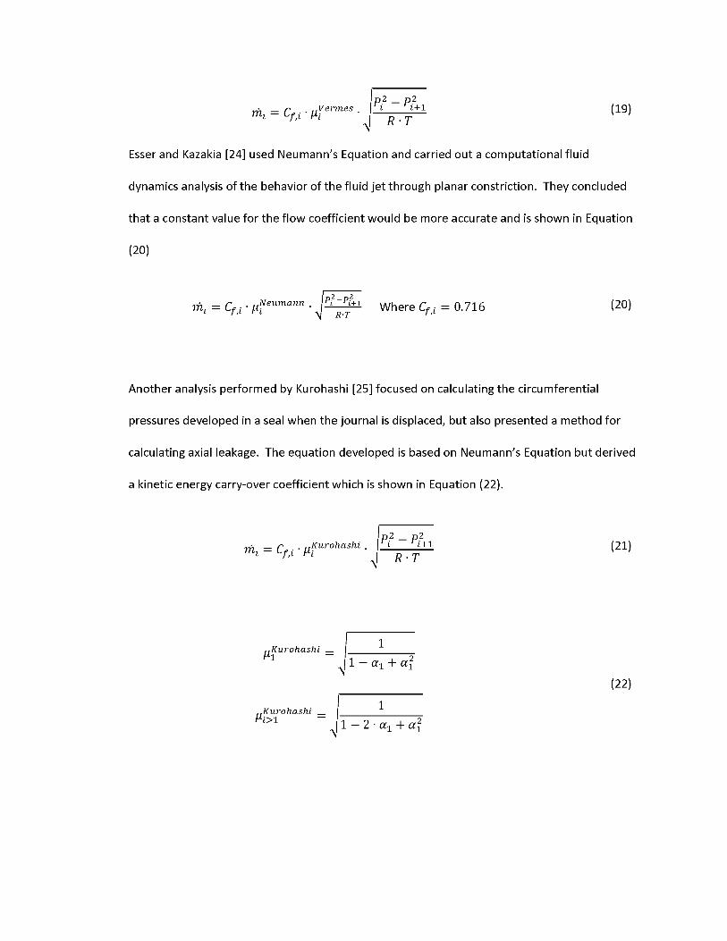
Esser and Kazakia [24] used Neumann's Equation and carried out a computational fluid
dynamics analysis of the behavior of the fluid jet through planar constriction. They concluded
that a constant value for the flow coefficient would be more accurate and is shown in Equation
(20)
= Cf,i .Neumann Pj-Pl+i R-T
Where Cf,t = 0.716 (20)
Another analysis performed by Kurohashi [25] focused on calculating the circumferential
pressures developed in a seal when the journal is displaced, but also presented a method for
calculating axial leakage. The equation developed is based on Neumann's Equation but derived
a kinetic energy carry-over coefficient which is shown in Equation (22).
_ r ..Kurohashi— L/,t Min2 p2rt rt + l
R - T(21)
..KurohashiMl1
1M
— a1 + a^
KurohashiMt>l
M1-2- a1 + a(
(22)
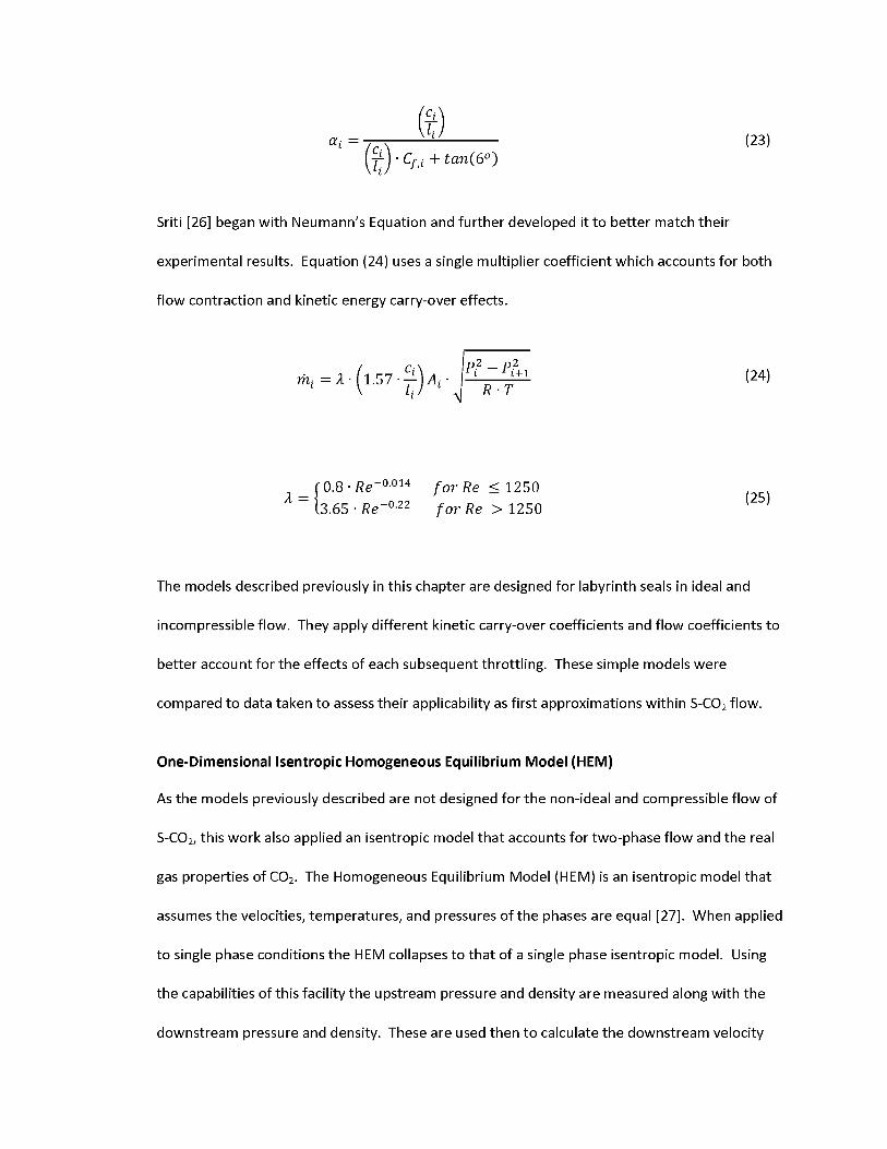
(23)«i =(7J-) - fa + tan{60)
Sriti [26] began with Neumann's Equation and further developed it to better match their
experimental results. Equation (24) uses a single multiplier coefficient which accounts for both
flow contraction and kinetic energy carry-over effects.
The models described previously in this chapter are designed for labyrinth seals in ideal and
incompressible flow. They apply different kinetic carry-over coefficients and flow coefficients to
better account for the effects of each subsequent throttling. These simple models were
compared to data taken to assess their applicability as first approximations within S-CO2 flow.
One-Dimensional Isentropic Homogeneous Equilibrium Model (HEM)
As the models previously described are not designed for the non-ideal and compressible flow of
S-CO2, this work also applied an isentropic model that accounts for two-phase flow and the real
gas properties of CO2. The Homogeneous Equilibrium Model (HEM) is an isentropic model that
assumes the velocities, temperatures, and pressures of the phases are equal [27]. When applied
to single phase conditions the HEM collapses to that of a single phase isentropic model. Using
the capabilities of this facility the upstream pressure and density are measured along with the
(24)
0.8 -Re"°.°14 for Re < 1250 3.65 - Re~°.22 for Re >1250
(25)
downstream pressure and density. These are used then to calculate the downstream velocity
using the energy balance in Equation (26). This is then used with the annular area to define the
mass flow rate in Equation (27).
foin (26)
LHEM Pout - V-OUt - Aannular (27)
To apply this to two-phase flow the fluid is treated as a single phase fluid with mixture
properties [28]. These mixture properties are here defined as average properties based on mass
averages defined in Equation (28) and Equation (29). Where x is the quality and the g and f
subscripts denote gas and fluid properties respectively.
1Pmix = x | 1_x (28)
Pg Pf
fornix ^ fog C1 ^0 - fof (29)
Due to the assumptions made by the HEM the flow predicted by this model will always be the
maximum possible flow through an annular geometry. This means that the calculation will
always over predict the measured flow rate for a given geometry and condition. To account for
this an empirically determined discharge coefficient may be defined as shown in Equation (30).
Q =^measured.
™-HEM(30)

Leakage Model Summary
A number of leakage models have been described here which can be applied to the flow of S-
CO2 through labyrinth seal geometries. One dimensional models designed for labyrinth seal flow
that assume ideal and incompressible flow, were chosen to validate their depiction of the
geometrical complexity in labyrinth seals. The isentropic HEM was also described as it allows for
the characterization of the real gas properties that are present in S-CO2.
The ideal and incompressible models gain value from their description of the geometry in
labyrinth seals. By accounting for carry-over effects, with the inclusion of a carry-over
coefficient and/or flow coefficient, they better account for changes in tooth number, cavity
depth, and cavity width, etc. Several models allow for the pressure drop to be calculated quickly
across the entire seal in one step, where others allow for the pressure drop through each
constriction to be calculated. Although these models offer geometrical complexity they do not
account for the real gas properties of S-CO2 or the two phase conditions experienced in the S-
CO2 Brayton cycle. Care must be used when applying these models near the critical point and
two-phase dome.
The HEM accounts for these real gas properties and uses mixture properties to better capture
two-phase effects. This allows the model to better predict when the flow will choke and what
the critical mass flow rate is. The HEM does not however account for changes in geometry as it
is solely based on the annular flow area at the entrance of the seal. Changes in tooth number,
tooth dimensions, or cavity dimensions cannot be captured by the model. This means that an
empirically determined discharge coefficient which can be used to account for the models over
prediction of the flow needs to be measured for each change in geometry. The HEM is then
best applied when experimental data is available for the geometry of interest.
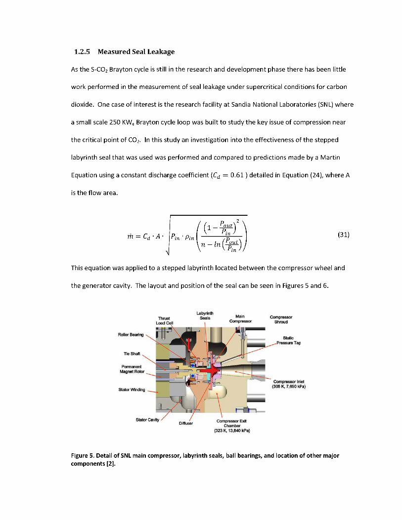
As the S-CO2 Brayton cycle is still in the research and development phase there has been little
work performed in the measurement of seal leakage under supercritical conditions for carbon
dioxide. One case of interest is the research facility at Sandia National Laboratories (SNL) where
a small scale 250 KWe Brayton cycle loop was built to study the key issue of compression near
the critical point of CO2. In this study an investigation into the effectiveness of the stepped
labyrinth seal that was used was performed and compared to predictions made by a Martin
Equation using a constant discharge coefficient (Cd = 0.61) detailed in Equation (24), where A
is the flow area.
1.2.5 Measured Seal Leakage
m = Cd - A- Pin • Pin (31)
This equation was applied to a stepped labyrinth located between the compressor wheel and
the generator cavity. The layout and position of the seal can be seen in Figures 5 and 6.
Load Cell
LabyrinthMain CompressorSee#Thrust
Compressor Shroud
Roller BeanngStatic
Tie Shaft
PermanentMagnet Rotor
Compressor Inlet(305 K. 7.690 kPa
Stator Winding
Stator Cavity Compressor ExitDiffuser Chamber323 K. 13.840 kPa)
Figure 5. Detail of SNL main compressor, labyrinth seals, ball bearings, and location of other major components [2].
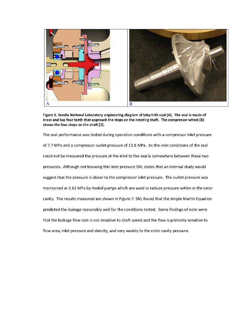
Figure 6. Sandia National Laboratory engineering diagram of labyrinth seal (A). The seal is made of brass and has four teeth that approach the steps on the rotating shaft. The compressor wheel (B) shows the four steps on the shaft [2].
The seal performance was tested during operation conditions with a compressor inlet pressure
of 7.7 MPa and a compressor outlet pressure of 13.8 MPa. As the inlet conditions of the seal
could not be measured the pressure at the inlet to the seal is somewhere between these two
pressures. Although not knowing this inlet pressure SNL states that an internal study would
suggest that the pressure is closer to the compressor inlet pressure. The outlet pressure was
maintained at 3.62 MPa by Haskel pumps which are used to reduce pressure within in the rotor
cavity. The results measured are shown in Figure 7. SNL found that the simple Martin Equation
predicted the leakage reasonably well for the conditions tested. Some findings of note were
that the leakage flow rate is not sensitive to shaft speed and the flow is primarily sensitive to
flow area, inlet pressure and density, and very weakly to the rotor cavity pressure.

13700 13800 13900 14000 14100 14200 14300 14400
Time(s)
Figure 7. Measured (brown) and predicted (red) leakage flow rate through the SNL four tooth stepped labyrinth seal [2].
2 Data Collection
2.1 Test Facility
The UW-Madison Seal Test Facility is logically depicted in Figure 8. It was used to measure flow
rate in seal geometries under S-CO2 conditions. The facility allows for a wide variety of
geometries and inlet conditions to be achieved. All plots and calculations were performed with
Engineering Equation Solver (EES) [29].
To energize the system a single-stage, linear actuated compressor manufactured by HydroPac
(Model No.: C02.4-40-2050LX/SSCO2) is used [30]. The HydroPac compressor has a maximum
discharge pressure of 16.55 MPa (2400 psia) and a minimum suction pressure of 1.38 MPa (200
psia), which allows the facility to achieve a range of orifice inlet pressures that are both above

and below the critical pressure. A photograph of the HydroPac compressor is shown in Figure 9.
The compressor has gas cylinders on either side of the oil cylinder so as to allow for compression
on each stroke.
CWVWVBuffer Tank
Test SectionHf ItC •Buffer Tank
rrecooler
Mass flow rate &Bode Hr i i • . M r,compmui
Stepper Motor
Stepper Motor
Test Section
SupplyReservoir Tank ram
Figure 8. Conceptual layout of the UW-Madison test facility.
The facility is comprised of a test section loop and a bypass loop. Control of the bypass loop is
achieved by the adjustment of two valves located, this regulates the flow of fluid through this
section and forces more fluid to pass through the test section.
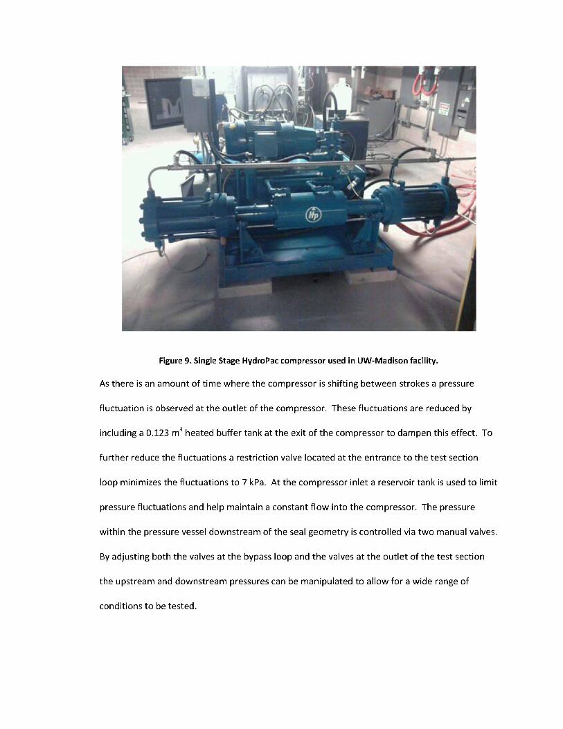
Figure 9. Single Stage HydroPac compressor used in UW-Madison facility.
As there is an amount of time where the compressor is shifting between strokes a pressure
fluctuation is observed at the outlet of the compressor. These fluctuations are reduced by
including a 0.123 m3 heated buffer tank at the exit of the compressor to dampen this effect. To
further reduce the fluctuations a restriction valve located at the entrance to the test section
loop minimizes the fluctuations to 7 kPa. At the compressor inlet a reservoir tank is used to limit
pressure fluctuations and help maintain a constant flow into the compressor. The pressure
within the pressure vessel downstream of the seal geometry is controlled via two manual valves.
By adjusting both the valves at the bypass loop and the valves at the outlet of the test section
the upstream and downstream pressures can be manipulated to allow for a wide range of
conditions to be tested.

The buffer tank requires heating in order to maintain a discharge pressure above the critical
pressure. The buffer tank is wrapped with four HTS Amptek Duo-Tape® heater tapes [31], each
capable of providing 1.25 kW. The temperature of the tank is controlled using these heaters
with a Proportional Integral Derivative (PID) controller implemented in Labview™. Feedback for
the PID controller is provided by three thermocouples welded to the surface of the buffer tank.
During normal operation, the fluid in the buffer tank is maintained at a temperature that is
between 70°C and 100°C in order to reduce the mass of CO2 required in the system to reach
high pressures (7.7 MPa-16.55MPa) in the supercritical region. The buffer tank is shown here
insulated in Figure 10.
Figure 10. Heated and insulated buffer tank used to reduce pressure fluctuations from compressor shifting.As the temperature of the fluid is greatly increased due to the buffer tank heaters a precooler is
required to reduce the temperature of the fluid prior to entering the test section. The precooler
is a shell and tube heat exchanger with the CO2 passing through a helically wound pipe inside of
a canister through which water flows. The device is controlled by varying the amount of chilled
water that flows through the precooler can, this is done with a ball valve located at the water
inlet. The precooler heat exchanger is shown in Figure .
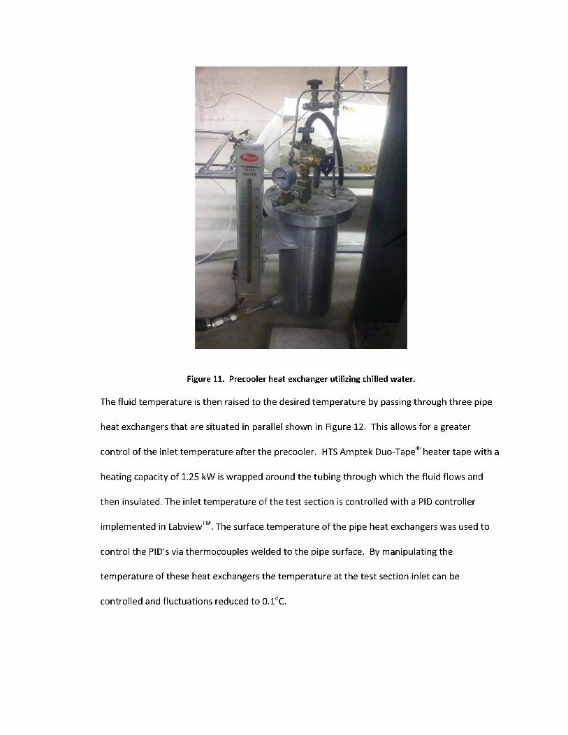
Figure 11. Precooler heat exchanger utilizing chilled water.
The fluid temperature is then raised to the desired temperature by passing through three pipe
heat exchangers that are situated in parallel shown in Figure 12. This allows for a greater
control of the inlet temperature after the precooler. HTS Amptek Duo-Tape® heater tape with a
heating capacity of 1.25 kW is wrapped around the tubing through which the fluid flows and
then insulated. The inlet temperature of the test section is controlled with a PID controller
implemented in Labview™. The surface temperature of the pipe heat exchangers was used to
control the PID's via thermocouples welded to the pipe surface. By manipulating the
temperature of these heat exchangers the temperature at the test section inlet can be
controlled and fluctuations reduced to 0.1oC.
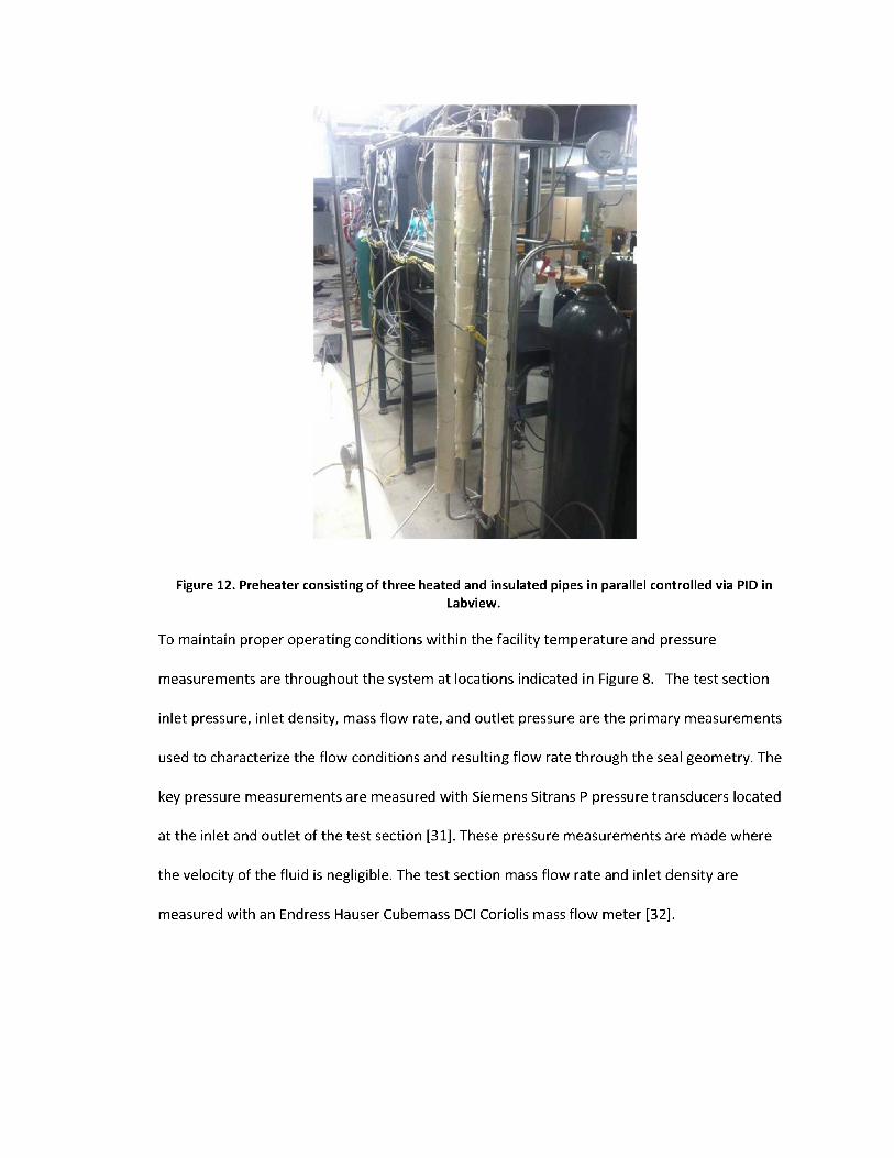
Figure 12. Preheater consisting of three heated and insulated pipes in parallel controlled via PID inLabview.
To maintain proper operating conditions within the facility temperature and pressure
measurements are throughout the system at locations indicated in Figure 8. The test section
inlet pressure, inlet density, mass flow rate, and outlet pressure are the primary measurements
used to characterize the flow conditions and resulting flow rate through the seal geometry. The
key pressure measurements are measured with Siemens Sitrans P pressure transducers located
at the inlet and outlet of the test section [31]. These pressure measurements are made where
the velocity of the fluid is negligible. The test section mass flow rate and inlet density are
measured with an Endress Hauser Cubemass DCI Coriolis mass flow meter [32].
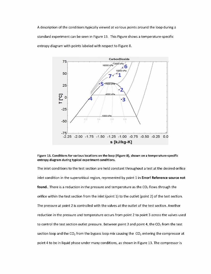
A description of the conditions typically viewed at various points around the loop during a
standard experiment can be seen in Figure 13. This Figure shows a temperature-specific
entropy diagram with points labeled with respect to Figure 8.
CarbonDioxide
-751------------------------------------------------------------------------ -------------------------------------------------------------------------------------------------- ------------------------ ---------------------<
-2.25 -2.00 -1.75 -1.50 -1.25 -1.00 -0.75 -0.50 -0.25 0.0s [kJ/kg-K]
Figure 13. Conditions for various locations on the loop (Figure 8), shown on a temperature-specific entropy diagram during typical experiment conditions.
The inlet conditions to the test section are held constant throughout a test at the desired orifice
inlet condition in the supercritical region, represented by point 1 in Error! Reference source not
found.. There is a reduction in the pressure and temperature as the CO2 flows through the
orifice within the test section from the inlet (point 1) to the outlet (point 2) of the test section.
The pressure at point 2 is controlled with the valves at the outlet of the test section. Another
reduction in the pressure and temperature occurs from point 2 to point 3 across the valves used
to control the test section outlet pressure. Between point 3 and point 4, the CO2 from the test
section loop and the CO2 from the bypass loop mix causing the CO2 entering the compressor at
point 4 to be in liquid phase under many conditions, as shown in Figure 13. The compressor is

designed to take in single-phase (either liquid or gas) or two-phase CO2. From point 4 to point 5,
the CO2 is compressed and mixed with high temperature CO2 from the buffer tank (point 6),
which results in an increase in both the pressure and temperature of the CO2. The pressure and
temperature of the CO2 is reduced as it passes through the restriction valve at the entrance to
the test section loop, and the temperature is further reduced in the precooler, resulting in point
7 shown in Figure 13. Finally, the temperature is increased to the desired test section inlet
temperature (point 1) in the preheater.
2.1.1 Test Section
The test section can be seen in Figure 14, which shows the inlet at the top and dual outlet ports
from the side. The pressure vessel allows for stagnation conditions to occur immediately
following the orifice and the upper flange (Figure 15) is where the orifice is secured. Press fit
drill bushings are used to provide the correct outer diameter for the orifices and the clamp
shown in Figure 14 holds the seals in place. This method allows for variation in seal geometry by
changing the length and diameters of the bushings and allows for the stacking of seals. The
collet holder sub-assembly (Figure 14b) is used to hold the shaft in place. A BK Precision Collet™
(Model N.:NBC8-3.5AA) is used to hold the miniature shaft sizes. The collet holder sub assembly
is attached to the test section allowing the shaft to be placed through the fixed orifice as shown
in Figure 14.
This design allows for a wide range of geometries to be tested. The length of seals and cavities
may be varied along with the diameter of the shaft. This ability can be seen in Figure 15. Figure
15 shows a cross section of the test section flange with a configuration of seals stacked within in
the flow channel.

d
Inlet
Inlet
Outletr Outlet
Figure 14. Cross Section of pressure vessel showing a) seal location/configuration, b) collet sub-assembly, c) shaft, d) seal, e) spacer drill bushing, f) test section flange.

Figure 15. Cross Section of test section flange showing seal configuration.
2.1.2 Seal Geometries
Three types of geometries were tested for this study. Annular geometries were tested to
observe the effect of shaft eccentricity and to determine discharge coefficients for a single
annular constriction. Straight-tooth labyrinth seals were tested to observe the effects of inlet
conditions and tooth number. A stepped-tooth labyrinth seal was also designed to observe
more practical geometries and compare test results to the data found with the SNL research
facility.
To construct different geometries orifices with different inner diameters were stacked onto
each other. These orifices as shown in Figure 16 were machined to tight tolerances to provide
an accurate description for modeling purposes. For the annular geometries the seals were had
inner diameters of 3.175 mm and lengths of 1.272, 2.341, 27.890, and 45.825 mm. The
diameter was measured optically using a microscope with 0.9 micron uncertainty.

Figure 16. Seals and cavities used in the straight-through labyrinth tests, do=9.525 mm, d^ seai=3.175 mm, d,, cavity=4.763 mm and length = 1.27 mm.
To determine the inlet and outlet curvatures of the seals and cavities a Zygo NewView™ white
light interferometric microscope [34]. Figure 17 shows the results of examining a single seal
using the Zygo interferometer. The results clearly indicate that all seals and cavities had a very
sharp inlet and exit curvature. This test was repeated after measurements were made with the
seals and there was no change seen.
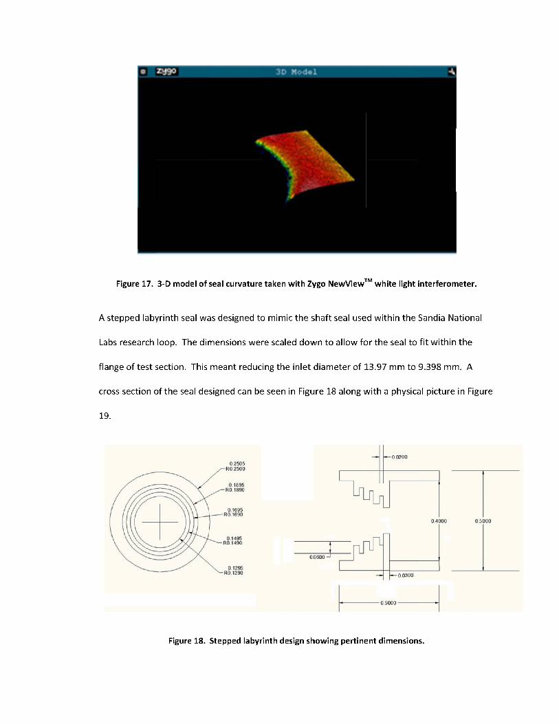
Figure 17. 3-D model of seal curvature taken with Zygo NewView™ white light interferometer.
A stepped labyrinth seal was designed to mimic the shaft seal used within the Sandia National
Labs research loop. The dimensions were scaled down to allow for the seal to fit within the
flange of test section. This meant reducing the inlet diameter of 13.97 mm to 9.398 mm. A
cross section of the seal designed can be seen in Figure 18 along with a physical picture in Figure
19.
02505R02500
0 1895 R0 1890
0 1695 R0 1690
0 1495 R0 1490
0 1295 R0 1290
— 0 0200
i Cfl
00000 -1
— 0 0300
0 5000
0 5000
Figure 18. Stepped labyrinth design showing pertinent dimensions.
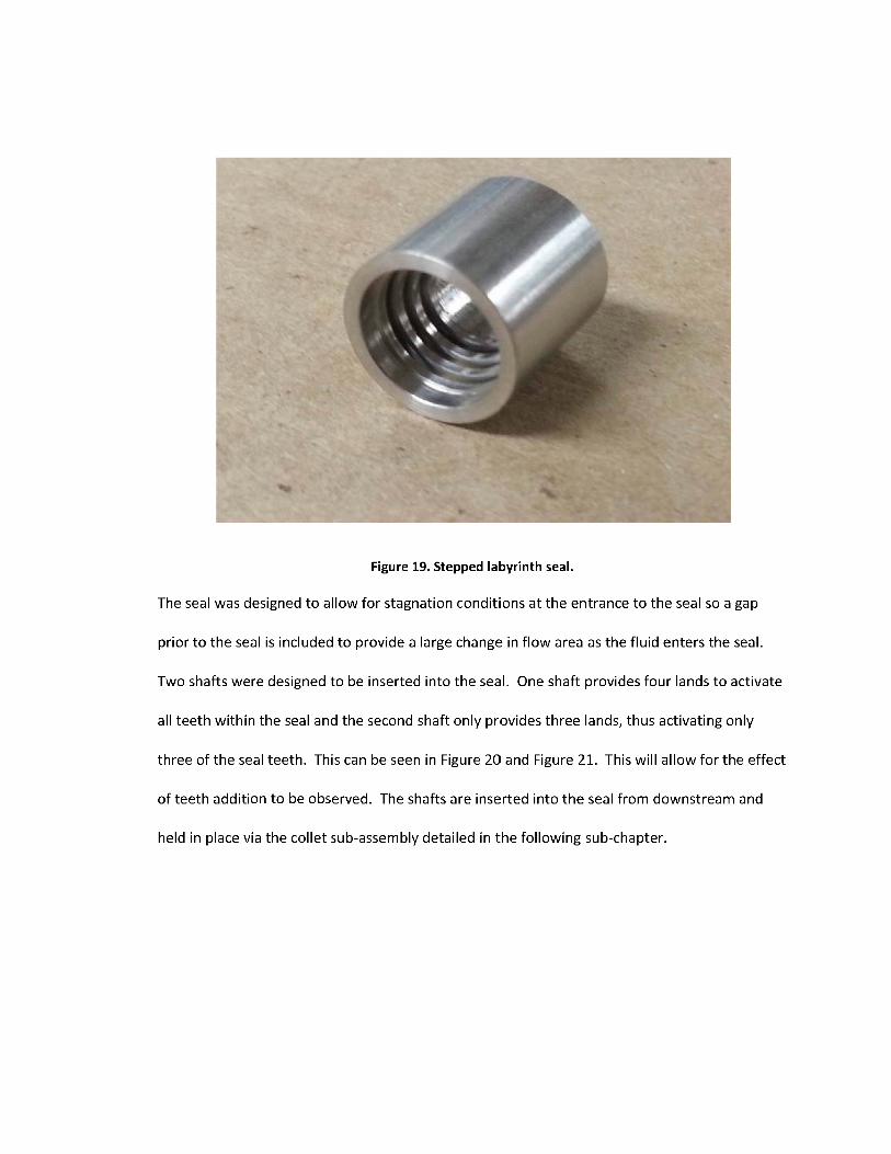
Figure 19. Stepped labyrinth seal.
The seal was designed to allow for stagnation conditions at the entrance to the seal so a gap
prior to the seal is included to provide a large change in flow area as the fluid enters the seal.
Two shafts were designed to be inserted into the seal. One shaft provides four lands to activate
all teeth within the seal and the second shaft only provides three lands, thus activating only
three of the seal teeth. This can be seen in Figure 20 and Figure 21. This will allow for the effect
of teeth addition to be observed. The shafts are inserted into the seal from downstream and
held in place via the collet sub-assembly detailed in the following sub-chapter.

RO 1875
0 05050 0500
^.0 05050 0500
0 1880
f 1 !■■■’:RO 1675
0 3350 0 :v5u0 2550 0 2950
ii \ -VAORO 1475
01280RO 1275
0 10050 1000
Figure 20. Shaft used to activate all four teeth within the stepped labyrinth design.
Figure 21. Shafts used in stepped labyrinth geometry, a) 4-land shaft b) 3-land shaft.

2.2 Test Conditions
The objective of this study is to observe the flow of S-CO2 through various shaft seal geometries
over a wide range of conditions. Even though the S-CO2 Brayton cycle operates well above the
two phase region it is of use to study flow through seal geometries and what effect transitioning
to two phase exit conditions has on the leakage. For the examination of the shaft eccentricity
effect the inlet condition was kept at 10 MPa and 325 kg/m3. This allowed a better control over
conditions at the inlet and exit and it avoided the two phase region but allowed observations to
be made of the eccentric effect in the supercritical region. Figure 22 shows the range of inlet
conditions performed for the three-tooth labyrinth seal to demonstrate the effects of property
variation.
CarbonDioxide125
18 MPa10012 MPa
10 MPa.
75
7.7 MPa
50
0.4 0.8
0.6c. 0.:
-2000 -1750 -1500 -1250 -1000Specifice Entropy [J/kg-K]
Figure 22. Temperature-specific entropy plot for CO2 with the test section inlet conditions shown for inlet pressures of 7.7 MPa (green), 10 MPa (blue), and 11 MPa (red) at corresponding inlet densities of 325, 475, and 630 kg/m3 in three-tooth labyrinth seal tests.

2.3 Data Collection
2.3.1 Assembly Procedure/Eccentricity Measurement
The eccentricity of the assembled test section comprised of the components shown in Figure 23
was measured using optical methods and assembled as follows. The seal to be tested was
clamped into the test section flange and a plug gauge of the same diameter was used to align
the collet holder sub-assembly onto the flange. The plug gauge was then removed and the shaft
was installed through the full length of seal. This was considered to be the minimum
eccentricity assembly as it was as close to concentric as possible. In order to obtain the
maximum eccentricity assembly, the previous process was repeated but after the shaft was
installed the collet holder sub assembly was loosened and the shaft moved until it touched the
side of the seal.
Seals (stackabledrill bushings)
Seal Clamp
Collet holder sub-assembly
Figure 23. Assembly procedure of shaft-seal sub-assembly.

The eccentricity of these assembled cases is measured using a long focal length microscope and
camera. The test section is mounted horizontally onto an optics table in front of a high
magnification, long focal length lens attached to a Nikon D7000 digital camera that allows for
images of the assembled shaft seal interface to be taken. Since the shaft and seal faces are not
aligned, an image cannot be taken with both the seal face and the shaft face in focus
simultaneously. To address this, two images were taken. The first image had the seal edge in
focus and the second had the shaft face in focus. Both images were taken using back lighting to
provide distinct edges for each object. These two images are then processed using a script in
MATLAB™ r2012b [34]. This processing determines the outlines of the two shapes (the shaft
and seal), overlays them, and measures the distances from their respective centers. This
distance is then taken to be the eccentricity of the test.
The image processing converts the measurements to a binary image. The binary images are
then processed using the standard MATLAB™ function regionprops() which locates contiguous
objects within the image and applies an equivalent diameter to the area. This equivalent
diameter is defined as the diameter of a circle having the same area as the region. This method
was used with all images and was tested by repeatedly taking images of a known diameter shaft
and comparing the value calculated from the image with the value measured using a
micrometer. These values were consistently within 1% of each other. An example of the
resulting image can be seen in Figure 24 which shows final images for both the concentric case
and the eccentric case for one of the tests.
The combined uncertainty in the measurement of the eccentricity throughout the assembly
procedure is approximately 5%. This uncertainty stems from two major contributions: the
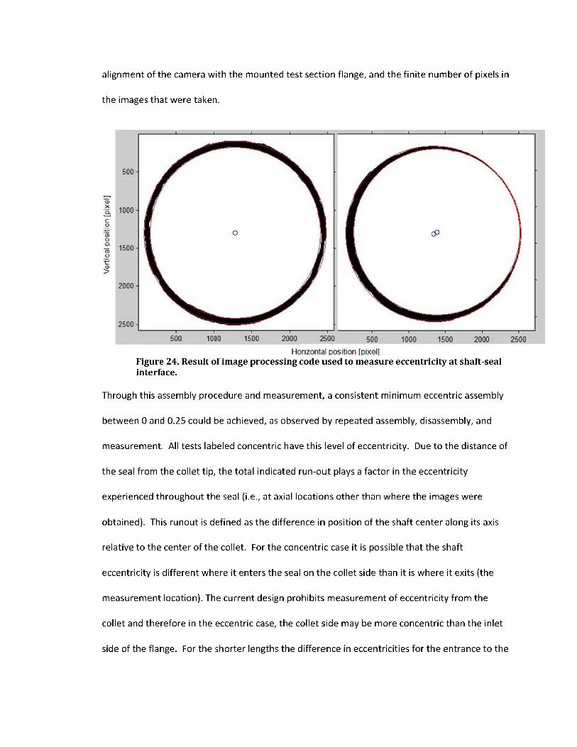
alignment of the camera with the mounted test section flange, and the finite number of pixels in
the images that were taken.
1000 -
1500-
2000-
2500-
Horizontal position [pixel]Figure 24. Result of image processing code used to measure eccentricity at shaft-seal interface.
Through this assembly procedure and measurement, a consistent minimum eccentric assembly
between 0 and 0.25 could be achieved, as observed by repeated assembly, disassembly, and
measurement. All tests labeled concentric have this level of eccentricity. Due to the distance of
the seal from the collet tip, the total indicated run-out plays a factor in the eccentricity
experienced throughout the seal (i.e., at axial locations other than where the images were
obtained). This runout is defined as the difference in position of the shaft center along its axis
relative to the center of the collet. For the concentric case it is possible that the shaft
eccentricity is different where it enters the seal on the collet side than it is where it exits (the
measurement location). The current design prohibits measurement of eccentricity from the
collet and therefore in the eccentric case, the collet side may be more concentric than the inlet
side of the flange. For the shorter lengths the difference in eccentricities for the entrance to the
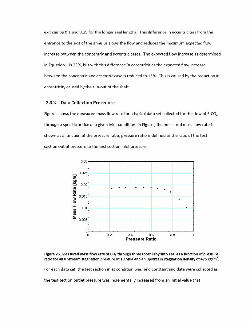
exit can be 0.1 and 0.25 for the longer seal lengths. This difference in eccentricities from the
entrance to the exit of the annulus slows the flow and reduces the maximum expected flow
increase between the concentric and eccentric cases. The expected flow increase as determined
in Equation 1 is 25%, but with this difference in eccentricities the expected flow increase
between the concentric and eccentric case is reduced to 15%. This is caused by the reduction in
eccentricity caused by the run-out of the shaft.
2.3.2 Data Collection Procedure
Figure shows the measured mass flow rate for a typical data set collected for the flow of S-CO2
through a specific orifice at a given inlet condition. In Figure , the measured mass flow rate is
shown as a function of the pressure ratio; pressure ratio is defined as the ratio of the test
section outlet pressure to the test section inlet pressure.
0.03
0.025
0.02
0.015
0.005
00 0.2 0.4 0.6 0.8 1
PressureRatio
Figure 25. Measured mass flow rate of CO2 through three tooth labyrinth seal as a function of pressure ratio for an upstream stagnation pressure of 10 MPa and an upstream stagnation density of 475 kg/m3.
For each data set, the test section inlet condition was held constant and data were collected as
the test section outlet pressure was incrementally increased from an initial value that

corresponded to a pressure ratio of approximately 0.3. At each outlet pressure, the experiment
was allowed to reach steady state and data were collected for 30 seconds. Steady state was
defined as a period of 60 seconds during which the downstream pressure fluctuated by no more
than 20.7 kPa (3 psi) and the upstream temperature, based on the thermocouple immersed in
the fluid at the test section inlet, fluctuated by no more than 0.1°C. In Figure , each data point
represents the average measured mass flow rate for data collected over the 30 seconds at a rate
of 1000 Hz while the experiment was at steady state.
3 Computational model
The computational model was developed in the open source software OpenFOAM 2.1.1.
OpenFOAM is a C++ based CFD (Computational Fluid Dynamics) toolbox for development of
customized numerical solvers based upon the applications of users. The applications developed
in OpenFOAM fall under two categories: solvers, that are designed to solve a specific problem in
continuum mechanics; and utilities, that are designed to perform tasks that involve data
manipulation. The OpenFOAM distribution contains numerical solvers and utilities covering a
wide range of applications, details of these can found in chapter 3 of OpenFOAM user manual
[36] under standard solvers and standard utilities section.
One of the solvers of interest for this study is rhoSimplecFoam [36] which is a steady-state
SIMPLEC based solver designed for laminar and turbulent RANS (Reynolds averaged Navier-
Stokes) flows of compressible fluids. This solver solves a set of modified continuity, momentum,
and energy equations programmed in C++ and necessary to represent a scenario in hand. The
closure to these equations is provided by modeling properties of the fluid being simulated. One
of the distinguished features of OpenFOAM is its syntax for tensor operations and partial

differential equations that closely resemble the equations being solved. Equation (32) is
represented by the code shown in Figure 26.
V.cpU- V.nVU= -Vp (32)
solve(
fvm::ddt(rho,0)+ fvm::div(phi,U)- fvm::laplacian(mu,U)- fvc::grad(p)
>;
Figure 26. OpenFOAM syntax for differential equations, picture taken from [36]
A new solver termed as hrhoSimplecFoam has been developed in OpenFOAM which solves the
same set of partial differential equations as rhoSimplecFoam but provides closure to the
governing equations by using the user defined CO2 properties instead of standard
thermodynamic models used by the original solver.
This chapter provides an in-depth explanation of the solver hRhoSimplecFoam. First, the
theoretical governing equations being solved by the application will be discussed. Next, details
will be provided about the user defined CO2 properties modeled into the application, wherein
the problem setup is explained as well. Finally, a table is generated showing the seal geometries
and the operating conditions used in this study (Appendix B, C, D).
3.1 Governing Equations
The Navier-Stokes (NS) equations are the basic governing equations for a viscous, heat
conducting fluid flow problem and consist of equations for the conservation of mass and
momentum. The momentum equation is a vector equation obtained by applying Newton's laws
of motion to a fluid element. It is supplemented by the mass conservation equation, also called
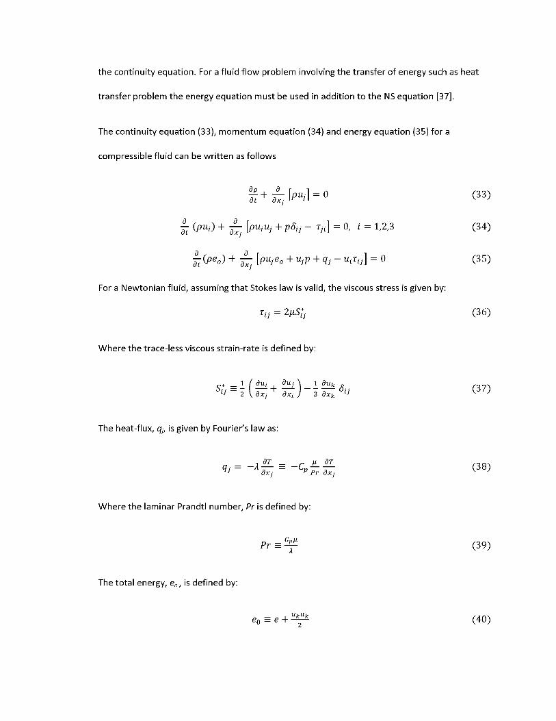
the continuity equation. For a fluid flow problem involving the transfer of energy such as heat
transfer problem the energy equation must be used in addition to the NS equation [37].
The continuity equation (33), momentum equation (34) and energy equation (35) for a
compressible fluid can be written as follows
£+4Kl = » <33)
(pUi^ + [puiuj +pSiJ ~ TJi\ = 0, i = 1,2,3 ( 3 4)
[puj-e0 +Ujp + qj -uiTij] = 0 ( 3 5)
For a Newtonian fluid, assuming that Stokes law is valid, the viscous stress is given by:
Tu = 2^5*. (3 6)
Where the trace-less viscous strain-rate is defined by:
* _ if duj , duj\ 1 duk ?9 2 \ dxj dxi j 3 dxk 9
The heat-flux, q, is given by Fourier's law as:
— _i _£L _ _r ^ dTdxj P Pr dxj
Where the laminar Prandtl number, Pr is defined by:
The total energy, eo , is defined by:
eQ_e + Ukuk
(3 7)
(3 8)
(39)
(40)2

Since, flow through seals is highly turbulent, turbulence modeling is important to capture the
real scenario. There are numerous ways to model turbulence in a flow ranging from a simple
linear eddy viscosity model to large eddy simulation (LES) and direct numerical simulation (DNS).
In this study, two equation turbulence models which are one of the most common types of
turbulence models are used. By definition, two equation models include two extra transport
equations to represent the turbulent properties of the flow. Most often one of the transported
variables is the turbulent kinetic energy, K. The second transport variable varies depending on
what type of two-equation model is being used. Common choices are the turbulent dissipation,
£, or the specific dissipation, u [37].
The equation for the ensemble averaged velocity is shown in equation 41.
ui = ui+u'^ (4 1)
The over-bar implies that the velocity is averaged, while the prime, ', implies the fluctuating
component to the velocity. This same format is used for various other properties. A new set of
equations can be developed for turbulent flows by modifying equations (33) through (35). The
conservation of mass equation (33) remains the same for turbulent flow as well, while the
momentum equation becomes:
dp ^ d
dxi dxj+ £“/ _ 1 g dui
dxj dxi 3 dxjt (42)
These equations are known as the Reynolds averaged Navier-Stokes equations (RANS).
The basis for all two equation models is the Boussinesq eddy viscosity assumption, which
postulates that the Reynolds stress tensor, r,y, is proportional to the mean strain rate tensor, 5,y,
as shown in equation (43).

(43)
Where, ^t is a scalar property called the eddy viscosity which is normally computed from the two
transport variables. The same equation can be written more explicitly as:
The drawback of two equation models is the Boussinesq assumption which is a significant
simplification. There might be some complex flows, like flows that are strongly accelerated,
strongly rotating flows where Boussinesq assumption is simply not valid. Throughout this study,
the standard ks turbulence model with enhanced wall treatment was chosen. Transport
equations for standard k-epsilon model can be derived as [40],
5>>+^0>fc«<) = 4 + + + + ^ (45)
i o*)+£ <p=“">=4[("+9i!]+£f(Pt+c=-p»>-£iF+x« (46)
The turbulent viscosity is modeled as,
pC^k2to= — (47)
Production of k can be written as
(48)
Pk =vts2 (49)
Where S is the modulus of the mean rate-of-strain tensor, defined as:
S — ^ZSijSij (5 0)

The model constants used for these equations are,
Cl£ = 1.44, C2£ = 1.92, C3£ = -0.33, = 0.09, ak = 1.0, a£ = 1.3
For turbulent flows, the velocity distribution near the wall can be divided into three distinct
regions: the laminar sub layer, buffer region, and log-law region. Due to the no-slip condition at
the wall, turbulent flows are greatly affected by the presence of the laminar sub layer. To
accurately capture the aspects of this laminar sub-layer an enhanced wall treatment provided by
OpenFOAM is used. More details of the near wall treatment can be found in the OpenFOAM
user guide [36]. The non-dimensional parameter y+ needs to be employed for use of the wall
treatment. The parameter is defined as:
y+=^ ( 5 1)VW
Where y is the distance from the wall, and vwis kinematic viscosity at the wall. The friction
velocity, u is defined by:
It has been suggested by many CFD experts in the past that value of y+ should be less than 5 in
order to use the enhanced wall function. Using a certain y+ the distance of first node from the
wall can be estimated approximately and a mesh can be generated accordingly.
All the governing equations derived earlier are in general valid for any Newtonian fluid. To
provide closure for a particular fluid, an equation of state (EOS) to model properties of the fluid
(5 2)
has to be specified. Most commercial packages like FLUENT provides a direct link to the National
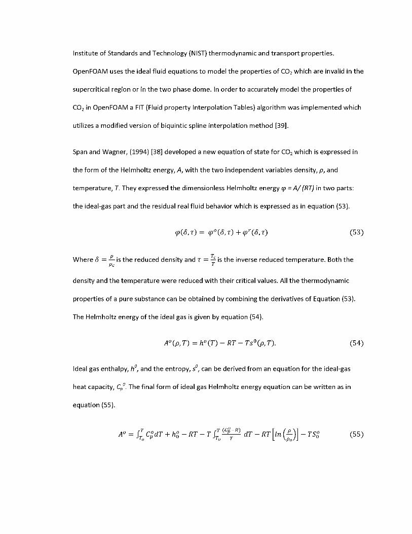
Institute of Standards and Technology (NIST) thermodynamic and transport properties.
OpenFOAM uses the ideal fluid equations to model the properties of CO2 which are invalid in the
supercritical region or in the two phase dome. In order to accurately model the properties of
CO2 in OpenFOAM a FIT (Fluid property Interpolation Tables) algorithm was implemented which
utilizes a modified version of biquintic spline interpolation method [39].
Span and Wagner, (1994) [38] developed a new equation of state for CO2 which is expressed in
the form of the Helmholtz energy, A, with the two independent variables density, p, and
temperature, T. They expressed the dimensionless Helmholtz energy y = A/(RT) in two parts:
the ideal-gas part and the residual real fluid behavior which is expressed as in equation (53).
<p{S,T)= (p°(S,T) + q)r(S,T) ( 5 3)
Where S = — is the reduced density and t = — is the inverse reduced temperature. Both thePc T
density and the temperature were reduced with their critical values. All the thermodynamic
properties of a pure substance can be obtained by combining the derivatives of Equation (53).
The Helmholtz energy of the ideal gas is given by equation (54).
A0(p,T) =h0(T)-RT-Ts0(p,T) . (5 4)
Ideal gas enthalpy, h0, and the entropy, s0, can be derived from an equation for the ideal-gas
heat capacity, Cp0. The final form of ideal gas Helmholtz energy equation can be written as in
equation (55).
A0 = CgdT + h%-RT-T f dT - RT [in -TS$ (5 5)

Where, subscript indicates the properties at reference state. The final equation for ideal gas part
is,
q)°(S, t) = ln(S) + a° +a.2t + ln(r) + a? ln[l — exp(—Td°)]
(5 6)
(5 7)
Since, there is no theoretical approach to accurately model the residual part of the Helmholtz
energy which is valid in the whole fluid region of a pure substance Span and Wagner modeled
the residual part in an empirical way by optimizing its functional form and fitting its coefficients
to a large database of experimental results. The actual empirical form of the residual part is
quite complicated and the bank of terms which were used in the optimization of the final EOS
contained a total of 860 terms. More details about the coefficients in equation (57) and the
residual part can be found in [38].
From the Helmholtz energy other properties can be calculated based on following
thermodynamic relationships in reduced form
7^=1+ « (5 8)
S-^T= T((P? + tf)-Cp° ~<Pr (5 9)
^ = T(<pT0 + O 'c o
^=-T2(<pr0r + <r) (61)
R7, =1 + + 0 + 8(ps (62)
Cp(5.r) _ _2| ^ | (1+5V5-5t^5t)R Wrr ' VrrJ ' i+2SVrs+S^Vrss /o
>
Where, W - , S55 - .*-[£],. <P„ - [£], . W, -

FIT libraries are based on a piecewise biquintic interpolation of Helmholtz free energy.
From Helmholtz free energy and all its derivatives as described in equations (58 through 63), all
the other thermodynamic properties are calculated. If the Helmholtz free energy and its
derivatives are known at the control points then the interpolated surface can be written as,
Mp.T) = ll0l5j=0aijpiTj ( 6 4)
This representation will result in 36 unknown coefficients and these coefficients can be
calculated from a set of equations obtained at the control points. The transport properties like
k, a, p etc. are interpolated independently. The results of the FIT algorithm for CO2 were
compared to REFPROP (Software for fluid properties developed by NIST) and agreed well with a
typical error on the order of ~0.01%.
To solve the mass, momentum, and energy equations, the pressure based solver was
used along with the SIMPLEC (Semi-Implicit Method for Pressure Linked Equations Corrected)
algorithm for pressure-velocity coupling. A second order Gauss upwind scheme was used to
solve the governing equations for the simulations performed on annular orifices and labyrinth
seals. For simulations performed on plain orifices a first/second order accurate Gauss van leer
scheme was used for better accuracy. More details about these schemes can be found out in a
CFD book or the OpenFOAM user guide [36]. The boundary conditions selected for this study
were a constant pressure at the inlet and outlet of the seal. A constant enthalpy/temperature
boundary condition is used at the inlet.
When the flow expands into the saturation dome, the properties of CO2 depend on
quality and both the phases will be out of equilibrium to some extent traveling at different
velocities with different temperatures. In this case the problem becomes complicated and in

order to capture the two phase flow field accurately, a separate set of equations have to be
developed for both the phases taking into account the properties of each phase. However, for
this thesis these complications are eliminated by assuming that there is no slip between phases
and that both the phases are in thermal equilibrium. These are the basic assumptions of the
"Homogeneous equilibrium model" explained in literature review section. Based on previous
work using steam, authors in the past reported that they obtained good results using HEM
except for very low quality steam. So, then the question is: "How valid is the HEM for CO2?"
To answer this question, let us look at Figures (27 and 28). The density ratio of liquid to
gas is much smaller for CO2 compared to that of water in the pressure range of interest. This
would imply that slip between liquid and gas is much smaller for CO2 and relative velocity
between phases is not as important as that of water. Hence, it is reasonable to assume that both
the phases are travelling at same velocities.
200 180 160 140 12060100
a80 60 40 20
01 2 3 4 5 6 7
P [MPa]
X Water
\
CO2
X
\x
• • . •—•—.__•----•---.__(—1- .
Figure 27. Density ratios for two phase CO2 and water

2.1
1.95
1.8
1.65
bfi&■
1.5u 1.35
CL,O 1.2
1.05
0.9
0.75
0.6
—WaterCO2
" •..^
.. .
*---- -
■ .
4 5P[MPa]
3 6 7
Figure 28. Specific heat ratios for two phase CO2 and water
Similarly, the ratio of the gas specific heat to the liquid specific heat for CO2 is comparable to
that of water. These two plots indicate that if the HEM works reasonably well for water, it
should work much better for CO2. This is in fact true and will be shown in chapter 5 where some
numerical results are compared to the experimental data for plain orifices.
4 Experimental Results
4.1 Shaft Eccentricity
To qualitatively understand the behavior of the entrance length effect and to provide a basic
physical model the annular geometry was approximated using two simple duct flow models.
The concentric case was modeled using a single rectangular duct with height that is equal to the
concentric radial clearance of the tested annular geometry. The eccentric case was modeled by
separating the flow area into two regions, one narrow and the other wide, as illustrated in
Figure 29. The wide region has a height that provides the same hydraulic diameter of the upper
180o segment centered at the maximum clearance point shown in Figure 29b. The narrow
region has a height that provides the same hydraulic diameter of the lower 180o segment in
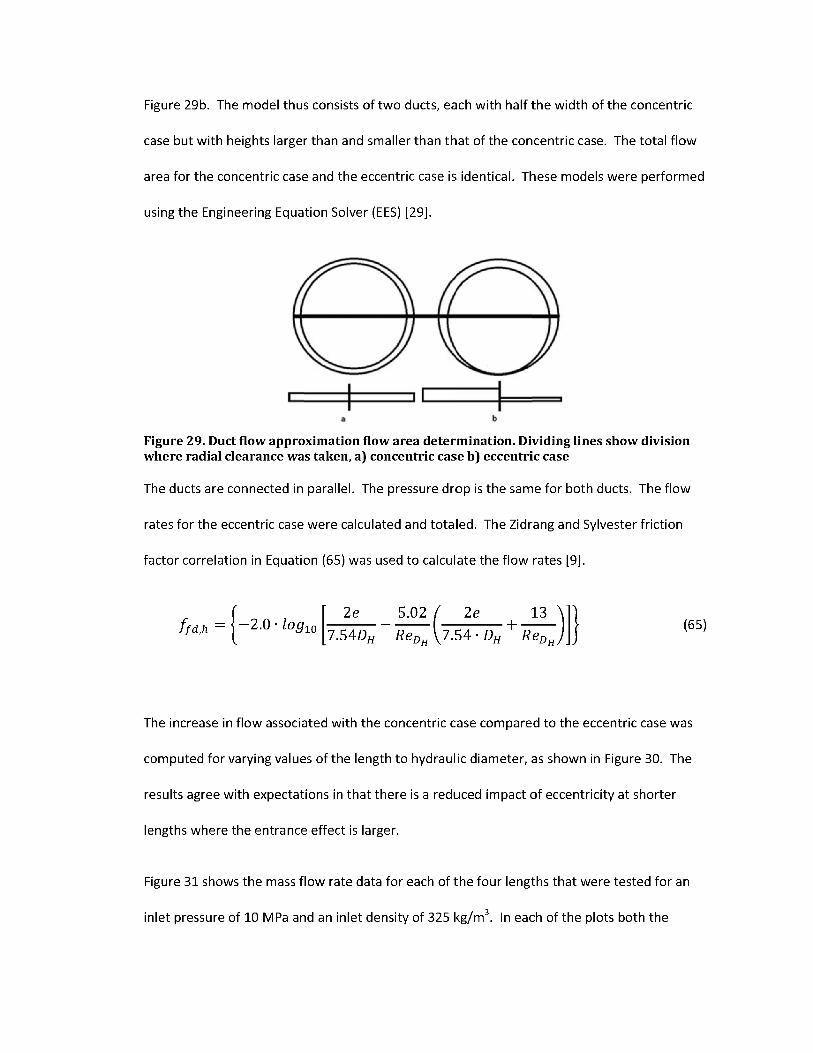
Figure 29b. The model thus consists of two ducts, each with half the width of the concentric
case but with heights larger than and smaller than that of the concentric case. The total flow
area for the concentric case and the eccentric case is identical. These models were performed
using the Engineering Equation Solver (EES) [29].
Figure 29. Duct flow approximation flow area determination. Dividing lines show division where radial clearance was taken, a) concentric case b) eccentric case
The ducts are connected in parallel. The pressure drop is the same for both ducts. The flow
rates for the eccentric case were calculated and totaled. The Zidrang and Sylvester friction
factor correlation in Equation (65) was used to calculate the flow rates [9].
2e 5.02 / 2e 13 V
7.SADH ReDH\7.SA-DH RsDh)(65)
The increase in flow associated with the concentric case compared to the eccentric case was
computed for varying values of the length to hydraulic diameter, as shown in Figure 30. The
results agree with expectations in that there is a reduced impact of eccentricity at shorter
lengths where the entrance effect is larger.
Figure 31 shows the mass flow rate data for each of the four lengths that were tested for an
inlet pressure of 10 MPa and an inlet density of 325 kg/m3. In each of the plots both the

concentric and eccentric mass flow rates are shown. Table I shows the average percent increase
over the pressure ratios measured between the concentric and eccentric case observed for each
length. The measurements show a small increase in flow between the eccentric and concentric
case for the short length annular orifice. As the length of the orifice is increased past the
experimentally determined turbulent fully developed length, described by Jonsson [13] as being
approximately 120 hydraulic diameters, a greater effect of 5% increase is seen between the two
cases. For the longest case that was tested, the eccentric case is observed to have an 8.5%
higher flow than the concentric case.
1.1
1.09
1.08
1.07
1.06
1.05
1.04
1.03
1.02
1.01
0.1 1 10 100 270Length/Hydraulic Diameter [-]
Figure 30. Duct flow approximation results for Dh=0.1956 mm.

004
0 035.
0 03
0 025
UD„=11
10S 0 02
0015
• Eccentric• Concentric
004
|o 00310 K3 oU.W» 0 02s
0015
UDh=23
■ .• • • • ■ . •. 1 V.,
*
•
.
ccentric
Concentric1
03 04 0.5 0.6 0.7 08 0.9Pressure Ratio
004
0035
F5 0 03
1 0 025q:J 002ILS 0015<o£
001
0 005
LT)h=146
Eccentric
Concentric
.......• . .
*’ .. ;
*
004
0035
F9 0 03fJ5 0 025
O 0 02u.
04 05 06 07 08 09Pressure Ratio
UDh=235
• Eccentric
• Concentric
atat
0.5 06 07 08 0.9Pressure Ratio
0015
0.01
03 0.5 06 0.7 08Pressure Ratio [-]
Figure 31. Experimental mass flow rate for annuli of varying L/Dh with a Dh=0.195 mm and inlet conditions of Pin = 10 MPa and pin=325 kg/m3.
These data show that for SCO2 at short lengths, where the entrance effect is significant, the
increase in flow due to eccentricity may not be significant. The maximum expected fully
developed increase in flow from eccentricity in the turbulent region as predicted by Piercy's
model is 25%, this expected value was reduced to 15% due to the effective eccentricity present
in the assembly of the test section. As the increase at the longest length tested (235 L/DH) was
8.5%, this shows that fully developed flow was achieved within the annulus and that there is a
clear dependence on length for the increase in flow due to eccentricity. As the lengths used in
shaft seal design are much shorter than fully developed lengths a minimal effect from
eccentricity may be seen. This has the result of possibly reducing the capital cost from the
tolerance on eccentricity in the design of shaft seals for use with S-CO2.

L/D„ Eccentric Flow Increase [%] Re [*]
6 3 370,000
12 3 360,000
143 5 240,000
235 8.5 211,0000
Table I. Experimental flow increase due to eccentricity for DH=0.195 mm and inlet conditions of Pin =10 MPa and pto= 325 kg/m3
4.1 Straight through Labyrinth Seals
4.1.1 Property Variation and HEM Model
Flow in a straight-through labyrinth geometry was measured at varying inlet conditions. These
conditions mimic the wide range of possible conditions within the S-CO2 Brayton cycle along
with spanning the sharp property changes that occur near the critical point. The temperature-
entropy diagram in Figure 32 shows the inlet conditions (solid markers) along with each outlet
condition (hollow markers), assuming isentropic expansion, that comprise a data set. Data was
taken for inlet pressures of 7.7, 10, and 11 MPa at corresponding inlet densities of 325, 475, and
630 kg/m3 for a three-tooth labyrinth seal.
The objective of these tests is to attempt to characterize the leakage for a seal given an inlet
pressure, outlet pressure, and inlet density. This was done by observing the predictions made
by the HEM model using an annular area. The results are shown in Figure 33. The discharge
coefficient can be used as a description of how well the HEM model predicts the form of the
measured flow rate. If the HEM predicts the choking point at the given condition the discharge
coefficient will remain constant at all pressure ratios. This result is not predicted but would
allow an empirically determined constant discharge coefficient to be applied to an HEM model
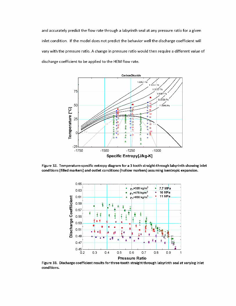
and accurately predict the flow rate through a labyrinth seal at any pressure ratio for a given
inlet condition. If the model does not predict the behavior well the discharge coefficient will
vary with the pressure ratio. A change in pressure ratio would then require a different value of
discharge coefficient to be applied to the HEM flow rate.
CarbonDioxide
1.80E7 Pa1.50E7 Pa
1.20E7 Pa75
1.00E7 Pa
9.00E6 Pa
50 7.70E6 Pa
250.4 □ 0.8
0.2
-25-1750 -1500 -1250 -1000
Specific Entropy[J/kg-K]
Figure 32. Temperature-specific entropy diagram for a 3 tooth straight-through labyrinth showing inlet conditions (filled markers) and outlet conditions (hollow markers) assuming isentropic expansion.
0.65
0.63
£ 0.61Q>
0.59
0.57OO 0.55Q>
0.53reo 0.51 inQ 0.49
0.47
0.450.2 0.3 0.4 0.5 0.6 0.7 0.8 0.9 1
Pressure RatioFigure 33. Discharge coefficient results for three-tooth straight through labyrinth seal at varying inlet conditions.
l• po=325 kg/m3 • 7.7 MP
m3 • 10 MP3 11 MP
a■ po=475 kg a
aP
I 1-‘V \ f
1 n • I Ai ■ iis-
1•
' 1s l I h
' i
. si
■ ■
* ?■ 1
v _
i 1
S If
l 3,i• Hrj
; -n-‘■i! e s
i * 1 *iL
I j..JJ-T ■if
"i '

For the inlet pressures of 10 and 11 MPa the discharge coefficient in Figure 33 can be seen to
only vary slightly with a change in pressure ratio. This means that the model accurately predicts
the choking point for those conditions. This is because for these two conditions the flow chokes
before entering the two phase region. As can be seen from Figure 33, the 7.7 MPa case varies
considerably more than the higher pressure cases. This is because the model chokes before the
measured flow rate and causes the discharge coefficient to increase until the measured flow
rate chokes. If the model choked after the measured flow rate the inverse of this would be true
and the discharge coefficient would decrease until the measured flow rate choked.
The reason this difference is more prevalent in the 7.7 MPa case is that it chokes well into the
two-phase region as can be seen in Figure 34. This is shown at the pressure ratio where the
mass flow rate ceases to increase with a decrease in pressure ratio. This occurs because the
fluid has reached the sound speed and changes in pressure drop cease to affect the flow rate
through the seal. The number of assumptions that the HEM model makes begins to become
apparent as two-phase conditions become more dominant. This could be remedied by
employing a more sophisticated model that makes fewer assumptions about the flow within the
seal.
The value of the experimentally determined discharge coefficient can be seen in Figure 34.
Averaging the discharge coefficients and applying it to the HEM model with a value of 0.51
results in a prediction of the measured flow rate for the 10 and 11 MPa cases with less than 5%
error. For the 7.7 MPa case, which is less well predicted by the HEM, applying the same
constant discharge coefficient of 0.51 predictions are made with less than 13% error. This
allows for the leakage of a seal to be easily calculated using a simple model based on inlet
conditions and a predetermined discharge coefficient.
0.04
0.035
vT0.03
fl)0.025(U
O'0.02
LL
W 0.015 re §
0.01
0.0050.3 0.4 0.5 0.6 0.7 0.8 0.9 1
PressureRatioFigure 34. Measured flow rate for three-tooth straight through labyrinth for inlet conditions P=10 MPa and p=325 kg/m3. The blue line shows calculated flow rate using isentropic HEM model and the red line shows the calculated flow rate applying a constant discharge coefficient to the isentropic HEM model.
4.1.2 Tooth Number Optimization
In many shaft seal engineering designs there is a limited amount of space available to include a
shaft seal. This means that a seal needs to be optimized for a given total length to provide the
least leakage. Yuan [20] performed a Computational Fluid Dynamics (CFD) investigation of the
mass flow rate through a labyrinth seal increasing the number of teeth for the same total length.
What is expected is that as the number of constrictions increases the decreasing distance
between constrictions eliminates the benefit of the expansion into the cavity. There is less
kinetic energy transferred to pressure and heat energy in the expansion and more
communicated to the downstream cavity. This reduces the effectiveness of the seal. As the
distance between constrictions decreases the flow eventually mimics that of a long annular
\\
1 5— —$—
--- HEMConst. Cd HEM Experiment
■ l . I . 1 .• "
orifice. This prediction can be seen in Figures 35 and 36.

0.034</>
0.032
0.03
0.028
§ 0.026
0.024</>(0
EE
0.022
0.02
0.018
0.016
One toioth a■
One t ooth b
23Tooth Number
4 5 6
Figure 35. Variation in tooth number for the same total length. One Tooth a: short length, depicts maximum flow rate. One Tooth b: Tooth occupies entire length and depicts the flow rate approached as tooth number is further increased [7].
0.034 0.032 0.03
0.028 0.026
°.°24 0.022 0.02
| 0.018 0.016 0.014 0.012
0.01 0.008 0.006
0.4 0.5 0.6 0.7 0.8 0.9 1
PR
A■
One tooth a One tooth b Two teeth— Three teeth Four teeth Five teeth
A■
Figure 36. Variation in tooth number for the same total length. Variation in pressure ratio shows anoptimal tooth number of three [7].

To examine this, measurements were made for straight-through labyrinth seals with tooth
numbers of 2, 3, and 5. A cavity diameter of 4.783 mm and seal diameter of 3.175 mm were
used with lengths of 1.782 mm to achieve a total length of 11.43 mm, with a shaft diameter of
3.000 mm. An inlet condition of 10 MPa and 325 kg/m3 was used to provide a single phase test
condition that was easily controlled. The measured flow rates are shown in Figure 37 and
clearly show the expected result. Figure 38 shows that there is a clear optimization given a
limited space to design a straight-through labyrinth seal and the model accurately predicts this.
The increase in tooth number past this optimal reduces the effectiveness of the seal by reducing
the amount of kinetic energy dispersed during the expansion into the cavity.
0.035
0.03vT
0.025
0)0.02
O'
O 0.015LI-
0.01roS
0.005
00.2 0.4 0.6 0.8 1
Pressure RatioFigure 37. Measured flow rate for variation in tooth number for the same total length compared to calculated flow rate using Open Foam simulation [7]. Minimum leakage is found at a tooth number of three. Inlet Pressure is 10 MPa with corresponding inlet density of 325 kg/m3.
CFD-2 Tooth • 5 ToothCFD-5 Tooth 3 Tooth
-
i 6h-
1 *?
i Q
,
LL1 o1 oth ■ 2 Tooth ■
- ■ ■; • • •
■ ■ D E"0--- -C
-
►>► -
■
■ ^ :■
▼ ;
'
■
- , . , , - . . . . , . "
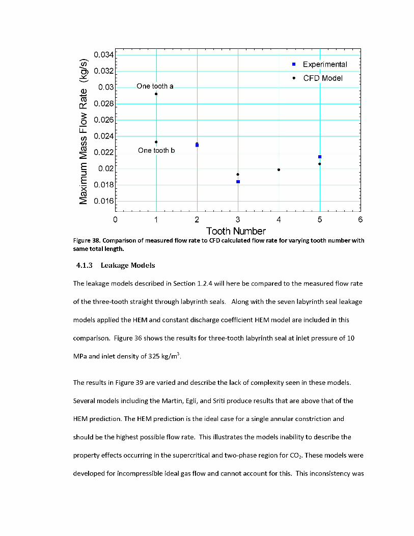
■ Experimental0.032
• CFD ModelOne tooth a0.03
0.028
0.026
0.024
One tooth b0.022
0.02
0.018
0.016
2 3 4 5 6Tooth Number
Figure 38. Comparison of measured flow rate to CFD calculated flow rate for varying tooth number with same total length.
4.1.3 Leakage Models
The leakage models described in Section 1.2.4 will here be compared to the measured flow rate
of the three-tooth straight through labyrinth seals. Along with the seven labyrinth seal leakage
models applied the HEM and constant discharge coefficient HEM model are included in this
comparison. Figure 36 shows the results for three-tooth labyrinth seal at inlet pressure of 10
MPa and inlet density of 325 kg/m3.
The results in Figure 39 are varied and describe the lack of complexity seen in these models.
Several models including the Martin, Egli, and Sriti produce results that are above that of the
HEM prediction. The HEM prediction is the ideal case for a single annular constriction and
should be the highest possible flow rate. This illustrates the models inability to describe the
property effects occurring in the supercritical and two-phase region for CO2. These models were
developed for incompressible ideal gas flow and cannot account for this. This inconsistency was

investigated by exploring the result for steam properties at a low pressure and high temperature
where the state is considered ideal and incompressible.
SritiEsser
HEM
HEM Cd
Martin
Egli
KurohashiNeumannVermes
• Experimental
0.06
0.04
§ 0.02
0.3 0.4 0.5 0.6Pressure Ratio
0.7 0.8
Figure 39. Measure flow rates through straight through 3-tooth labyrinth seal for inlet pressure of 10 MPa and inlet density of 325 kg/m3 compared to various labyrinth seal leakage models.
This can be seen in Figure 40 where the mass flow rate for the Egli, Martin, and isentropic single
phase model are shown for a steam inlet pressure of 6.83 MPa and corresponding inlet
temperature of 200oC. This shows that the real gas properties of S-CO2 are causing the
unrealistic prediction of the Egli and Martin Equations in Figure 39. Figure 41 shows the results
for the inlet condition of 11 MPa and 630 kg/m3 for the same three-tooth labyrinth seal
geometry. The results are similar to the 10 MPa case with several models greatly under
predicting the flow and some vastly over predicting it. As with the 10 MPa case the HEM model,
with an experimentally determined discharge coefficient, is the most accurate and determines
both the maximum flow rate and the pressure ratio at which the flow chokes. The assumptions
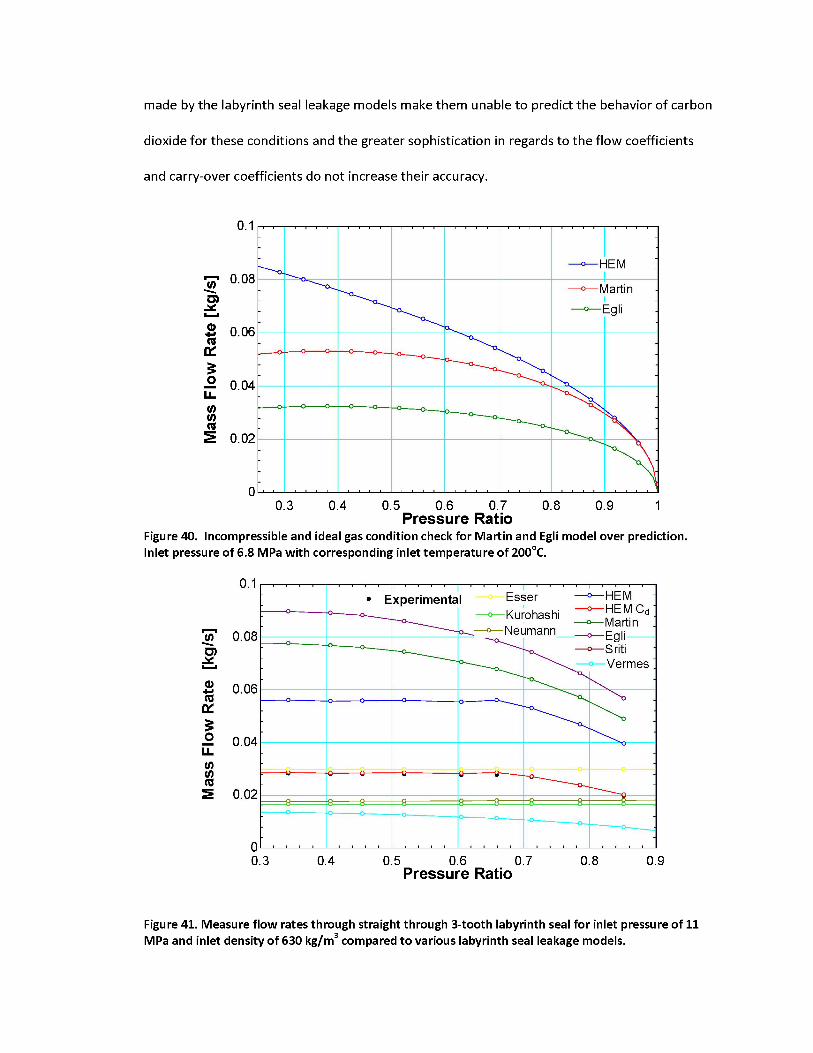
made by the labyrinth seal leakage models make them unable to predict the behavior of carbon
dioxide for these conditions and the greater sophistication in regards to the flow coefficients
and carry-over coefficients do not increase their accuracy.
0.1
0.08
0.06reO'£
0.04LL</>Wre
0.02
00.3 0.4 0.5 0.6 0.7 0.8 0.9 1
Pressure RatioFigure 40. Incompressible and ideal gas condition check for Martin and Egli model over prediction. Inlet pressure of 6.8 MPa with corresponding inlet temperature of 200oC.
HEM
Martin
Egli
0.1HEM HEM Cd MartinEgli------SritiVermes
EsserKurohashiNeumann
Experimental
0.08
0.06
0.04
0.02
0.3 0.4 0.5 0.6 0.7 0.8 0.9Pressure Ratio
Figure 41. Measure flow rates through straight through 3-tooth labyrinth seal for inlet pressure of 11 MPa and inlet density of 630 kg/m3 compared to various labyrinth seal leakage models.

The one-dimensional, ideal, incompressible models described here were unable to accurately
predict the measured flow rate for the three tooth labyrinth seal at the different conditions
tested. These models were tested despite their applicability to the non-ideal and compressible
conditions of the S-CO2 as they provide a simple one step calculation based only upon the inlet
pressure, inlet density, outlet pressure, and flow geometry of the seal. This means that a simple
model might be applied quickly and with minimal information. They apply different carry-over
and flow coefficients based on the seal geometry to approximate the fluid dynamics within the
seal. These added complexities did little to improve the accuracy of the predicted flow rate.
This shows a necessity to model the correct fluid properties in the CO2. The HEM model
achieves this and with a constant empirical discharge coefficient it provided the best results
which were within 5% of the measured flow rate for both conditions.
4.2 Stepped Labyrinth Seal
Flow rate measurements were made for a stepped labyrinth seal with three and four teeth at
inlet pressure of 10 MPa and inlet density of 640 kg/m3. This was done to test the seal
geometry being used in practical research facilities for the S-CO2 Brayton cycle. Results for the
four-tooth case can be seen in Figure 42. The inlet conditions were chosen based upon the test
conditions seen for the SNL seal [2].
The geometry tested has 15% the flow area of the SNL geometry and does not immediately
reflect agreement. Looking at the mass flow rate normalized to the area shows better
agreement. Figure 43 shows the mass flow rate normalized with the annular flow area. The
values differ by 25% but one of the main points made in the SNL report is that the inlet
condition to the seal was not known. This means that the inlet pressure could be anywhere
between the compressor inlet pressure of 7.7 MPa and the compressor outlet pressure of 13.83
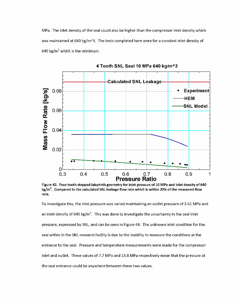
MPa. The inlet density of the seal could also be higher than the compressor inlet density which
was maintained at 640 kg/mA3. The tests completed here were for a constant inlet density of
640 kg/m3 which is the minimum.
4 Tooth SNL Seal 10 MPa 640 kg/mA3
0.08o>
0)0.06
CC
£0.04
-ed SNL Li
-
■^a kag e
• Ex perimentEML Model
- -------HE-------SN
- -
II U.UH-CO(/>ro
S 0.02
n
--
- • e • • • • • ••-
0.3 0.4 0.5 0.6 0.7 0.8 0.9 1Pressure Ratio
Figure 42. Four-tooth stepped labyrinth geometry for inlet pressure of 10 MPa and inlet density of 640 kg/m3. Compared to the calculated SNL leakage flow rate which is within 20% of the measured flow rate.
To investigate this, the inlet pressure was varied maintaining an outlet pressure of 3.61 MPa and
an inlet density of 640 kg/m3. This was done to investigate the uncertainty in the seal inlet
pressure, expressed by SNL, and can be seen in Figure 44. The unknown inlet condition for the
seal within in the SNL research facility is due to the inability to measure the conditions at the
entrance to the seal. Pressure and temperature measurements were made for the compressor
inlet and outlet. These values of 7.7 MPa and 13.8 MPa respectively mean that the pressure at
the seal entrance could be anywhere between these two values.

4 Tooth SNL Seal 10 MPa 640 kg/mA325000
EiV)O)
20000ro0)
<15000
LL Q)COcc£ 10000o
LL</>V)
50000.3 0.4 0.5 0.6 0.7 0.8 0.9 1
Pressure RatioFigure 43. Area normalized mass flow rate comparison of four-tooth stepped labyrinth seal to SNL leakage calculation for inlet condition of 10 MPa and 640 kg/m3.
The flow rate shown in Figure 44 is normalized to the flow area of the two different seals. The
seal tested at UW-Madison required a smaller outer diameter to be placed within the test
section flange. The inlet pressure was varied between the SNL reported compressor inlet and
outlet pressures maintaining an inlet density of 640 kg/m3. This was done to see at what
pressure the flow seen in the SNL research facility is approached. Here it can be seen that the
flow rate approaches the leakage seen in the SNL geometry at an inlet pressure of 12.5 MPa and
would suggest that the difference in the measured flow rates is due to the difference in inlet
conditions seen at the seal. Whether this difference is only in the pressure or the density or a
combination of both is unknown but most likely due to both.
An internal study performed at SNL reported that the inlet condition experienced at the seal
■'.
-
-.
-------SNL Model.
• Experiment
• • • • e• •
•
-
■
, , , ,
•
,
• •••
,
-
entrance is most likely closer to the compressor inlet pressure of 7.7 MPa due to the pump out
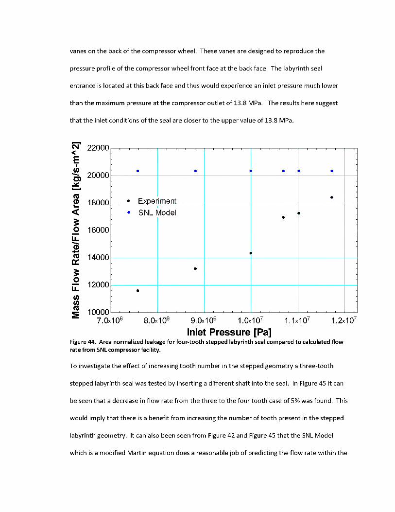
vanes on the back of the compressor wheel. These vanes are designed to reproduce the
pressure profile of the compressor wheel front face at the back face. The labyrinth seal
entrance is located at this back face and thus would experience an inlet pressure much lower
than the maximum pressure at the compressor outlet of 13.8 MPa. The results here suggest
that the inlet conditions of the seal are closer to the upper value of 13.8 MPa.
22000
Ei</)
20000£
$ 18000<£
16000LLa>re 14000
£j2 12000
(/></>
100007.0x106 8.0x10⁶ 9.0x10⁶ 1.0x10⁷ 1.1x10⁷ 1.2x10⁷
Inlet Pressure [Pa]Figure 44. Area normalized leakage for four-tooth stepped labyrinth seal compared to calculated flow rate from SNL compressor facility.
To investigate the effect of increasing tooth number in the stepped geometry a three-tooth
stepped labyrinth seal was tested by inserting a different shaft into the seal. In Figure 45 it can
be seen that a decrease in flow rate from the three to the four tooth case of 5% was found. This
would imply that there is a benefit from increasing the number of tooth present in the stepped
labyrinth geometry. It can also been seen from Figure 42 and Figure 45 that the SNL Model
• • • 1 • • •■
Exper iment•
-
SNL Model • •■
-
<-
-
•
■
- •■
which is a modified Martin equation does a reasonable job of predicting the flow rate within the

stepped labyrinth geometry. It gives an approximate flow rate within 30%, which agrees with
the results found in the SNL investigation. As with the three-tooth straight-through geometry
though, the model does not have sufficient ability to capture the geometry and property effects
that are present.
0.04
</>0.03
0)+->ro
CC0.02
oLL</>in
0.01
00.3 0.4 0.5 0.6 0.7 0.8 0.9 1
Pressure RatioFigure 45. Three-tooth and four-tooth stepped labyrinth seal flow rate measurement for inlet pressure of 10 MPa and inlet density of 640 kg/m3.
The Martin equation may be appropriate for a first step approximation to understand the scale
at which a labyrinth seal may leak within a system. Figure 46 shows that it may also be used to
predict the change in leakage due to increasing the number of teeth in the stepped labyrinth
seal tested. A better approximation may be possible by using an effective flow area for higher
pressure ratios. The HEM using an empirical constant discharge coefficient is shown in blue on
Figure 46. The HEM with constant discharge coefficient predicts the form of the mass flow rate
• Three tooth ■ Four Tooth
HEMSNL Model
well giving a good estimation of the choking point along with the critical flow rate. This can be

seen in Figure 47 which shows the discharge coefficients for the three and four tooth stepped
labyrinth geometries. This is for the inlet condition of 10 MPa with corresponding inlet density
of 640 kg/m3. The difference in discharge coefficient is due to the change in leakage from
increasing the tooth number which the HEM model cannot predict.
0.012
0.01wo>
0.008CD+■><00£
0.006o
LL0.004
0.002
00.3 0.4 0.5 0.6 0.7 0.8 0.9 1
PressureRatioFigure 46. Mass flow rate experimental measurements and calculations for three and four tooth stepped labyrinth seal including the SNL Martin leakage equation and the HEM model with constant discharge coefficient.
The stepped labyrinth seal geometry tested here was tested to investigate the more complex
geometries seen in practical research facilities such as the facility at Sandia National Labs. The
geometry within this test facility was mimicked with a smaller flow area and was tested at
conditions seen in the SNL facility. The results show that this facility can be used to replicate
conditions seen in practical loops and that these smaller geometries can be scaled to larger
geometries. The Martin leakage equation used by SNL was compared to the HEM model using a
• Three tooth ■ Four Tooth —SNL Model-3 Tooth —SNL Model-4 Tooth —HEM Const. Cd
constant empirical discharge coefficient. The Martin equation although it is designed for ideal
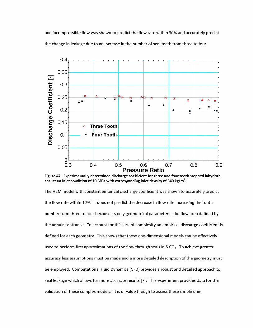
and incompressible flow was shown to predict the flow rate within 30% and accurately predict
the change in leakage due to an increase in the number of seal teeth from three to four.
0.4
0.35
^ 0.30)
0.25a>
0.20)g> 0.15ro
Q0.05
00.3 0.4 0.5 0.6 0.7 0.8 0.9
Pressure RatioFigure 47. Experimentally determined discharge coefficient for three and four tooth stepped labyrinth seal at an inlet condition of 10 MPa with corresponding inlet density of 640 kg/m3.
The HEM model with constant empirical discharge coefficient was shown to accurately predict
the flow rate within 10%. It does not predict the decrease in flow rate increasing the tooth
number from three to four because its only geometrical parameter is the flow area defined by
the annular entrance. To account for this lack of complexity an empirical discharge coefficient is
defined for each geometry. This shows that these one-dimensional models can be effectively
used to perform first approximations of the flow through seals in S-CO2. To achieve greater
accuracy less assumptions must be made and a more detailed description of the geometry must
be employed. Computational Fluid Dynamics (CFD) provides a robust and detailed approach to
seal leakage which allows for more accurate results [7]. This experiment provides data for the
■ a a A n a * a
: . • *■' •: •e; •
5 A
T
A S s ;
•: !•:
TFhree Tooth
validation of these complex models. It is of value though to assess these simple one

dimensional models as they require very little information and are quickly calculated. Thus
giving a useful first approximation and in the case of the HEM model a description of the critical
flow rate and choking point.
4.3 Empirical Discharge Coefficient
The isentropic HEM has been applied to the data collected here for straight-through and
stepped labyrinth seal. It provides a model that accounts for the real gas properties of CO2 and
uses mixture properties to model two-phase effects. The HEM assumes that the velocities,
temperatures, and pressures between the phases are equal and when calculated for a single
phase condition collapses to a one-dimensional isentropic model. These assumptions cause the
model to always over predict the measured flow rate. To account for this an empirical discharge
coefficient is applied to the model which then provides an accurate description of the leakage
through a seal.
The results for the empirical discharge coefficient for the geometries tested are listed in Table II.
The labyrinth seal results show that for the high inlet pressures of 10 and 11 MPa a constant
discharge coefficient was found with an error of less than 4%. For the lower pressure tests of
7.7 MPa, it is necessary to define a range of pressure ratios with different constant discharge
coefficients to maintain an error of 5%. This occurs because the higher pressure cases choke
prior to or early in the two-phase region and the HEM correctly predicts the critical pressure
ratio and critical mass flow rate. The lower pressure case chokes well into the two-phase region
where the difference in properties between the phases is much greater. The HEM mixture
properties do not accurately accommodate this and the accuracy of the model deteriorates.
The model predicts a different choking point than is found in the measured data and this is
reflected by a non-constant behavior in the discharge coefficient. To provide a more accurate

description of the flow rate a different discharge coefficient can be applied to two different
ranges of pressure ratios. These regions are defined by the choking point predicted by the HEM.
As the model chokes prior to the data, at pressure ratios higher than the model calculated
critical pressure ratio the discharge coefficient is the same as predicted for the higher inlet
pressure cases. Below this pressure ratio the discharge coefficient begins to deviate and a
different average discharge coefficient is applied.
GeometryTotal
Length[mm]
Inlet Pressure [MPa]
Pressure Ratio [-]
Discharge Coefficient [-]
Error[%]
Straight-ThroughOne-Tooth 1.27 10,11 0-0.93 0.79 2.1
Three-Tooth 3.81 7.7 0-0.7 0.56 5.2Three-Tooth 3.81 7.7 0.7-0.93 0.51 2
Three-Tooth 3.81 10,11 0-0.93 0.51 2
Two-Tooth 11.43 10 0-0.93 0.7 3Three-Tooth 11.43 10 0-0.93 0.55 3.8Five-Tooth 11.43 10 0-0.93 0.6 8.5
SteppedThree-Tooth 10.67 10 0-0.93 0.25 2.3Four-Tooth 10.67 10 0-0.93 0.22 8.1
Table II. Empirical discharge coefficient results.
As the flow geometry becomes more complex the ability of the HEM to predict the choking
point of measured flow also deteriorates. This can be seen in the increased error found for the
more complex geometries of the five-tooth straight-through labyrinth seal and the four-tooth
stepped labyrinth seal. As the length of the seal increases and the tooth number increases the
amount of friction within the seal increases. This effect causes the flow to choke at a lower
pressure ratio which the HEM cannot predict.
The HEM with an empirical discharge coefficient gives a prediction for all measured flow rates
within 15%. This error is reduced to less than 10% for all labyrinth seals with three or less teeth
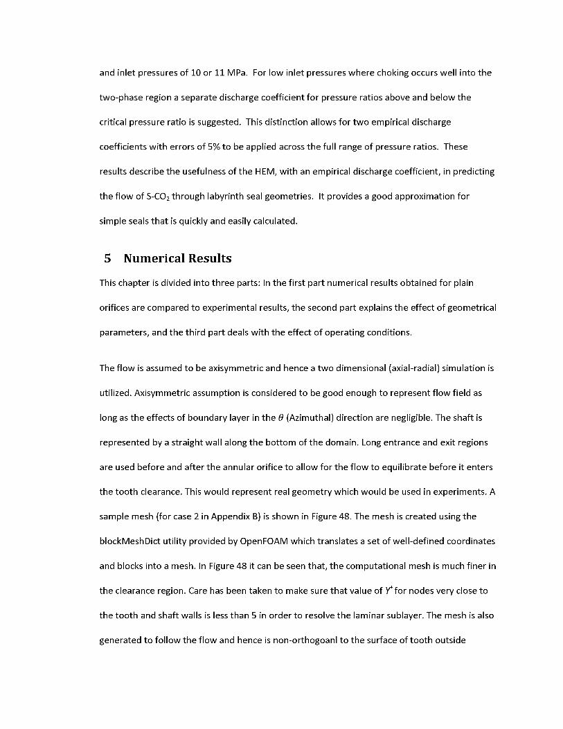
and inlet pressures of 10 or 11 MPa. For low inlet pressures where choking occurs well into the
two-phase region a separate discharge coefficient for pressure ratios above and below the
critical pressure ratio is suggested. This distinction allows for two empirical discharge
coefficients with errors of 5% to be applied across the full range of pressure ratios. These
results describe the usefulness of the HEM, with an empirical discharge coefficient, in predicting
the flow of S-CO2 through labyrinth seal geometries. It provides a good approximation for
simple seals that is quickly and easily calculated.
5 Numerical Results
This chapter is divided into three parts: In the first part numerical results obtained for plain
orifices are compared to experimental results, the second part explains the effect of geometrical
parameters, and the third part deals with the effect of operating conditions.
The flow is assumed to be axisymmetric and hence a two dimensional (axial-radial) simulation is
utilized. Axisymmetric assumption is considered to be good enough to represent flow field as
long as the effects of boundary layer in the d (Azimuthal) direction are negligible. The shaft is
represented by a straight wall along the bottom of the domain. Long entrance and exit regions
are used before and after the annular orifice to allow for the flow to equilibrate before it enters
the tooth clearance. This would represent real geometry which would be used in experiments. A
sample mesh (for case 2 in Appendix B) is shown in Figure 48. The mesh is created using the
blockMeshDict utility provided by OpenFOAM which translates a set of well-defined coordinates
and blocks into a mesh. In Figure 48 it can be seen that, the computational mesh is much finer in
the clearance region. Care has been taken to make sure that value of Y for nodes very close to
the tooth and shaft walls is less than 5 in order to resolve the laminar sublayer. The mesh is also
generated to follow the flow and hence is non-orthogoanl to the surface of tooth outside

clearance region. Error due to this non-orthogoanlity is minimized by performing non-
orthogonal corrections after every iteration. Before validating the computational model, it was
necessary to perform a grid independence study to make sure that results obtained from the
computational studies are independent of mesh. Since, OpenFOAM doesn't have the capabilities
to refine the mesh based on the gradient in variables, the mesh was subjected to various levels
of manual refinement.
Figure 48. A sample computational mesh used for simulations
Results of the grid independence studies are presented in Figures (49 and 50). The leakage rate
prediction error between the mesh with 20000 nodes and the orthogonal mesh with 50000
nodes was about 3 % for higher pressure ratios and less than 0.6 % for lower pressure ratios.
This error at higher pressure ratios might slightly effect the prediction of Cd as shown in Figure
49. The error between the mesh with 30000 nodes and that of orthogonal mesh is about 1 % for
higher pressure ratios and less than 0.3 % for lower pressure ratios. Hence, the mesh with 30000
nodes is employed for computational studies on the annular orifice.
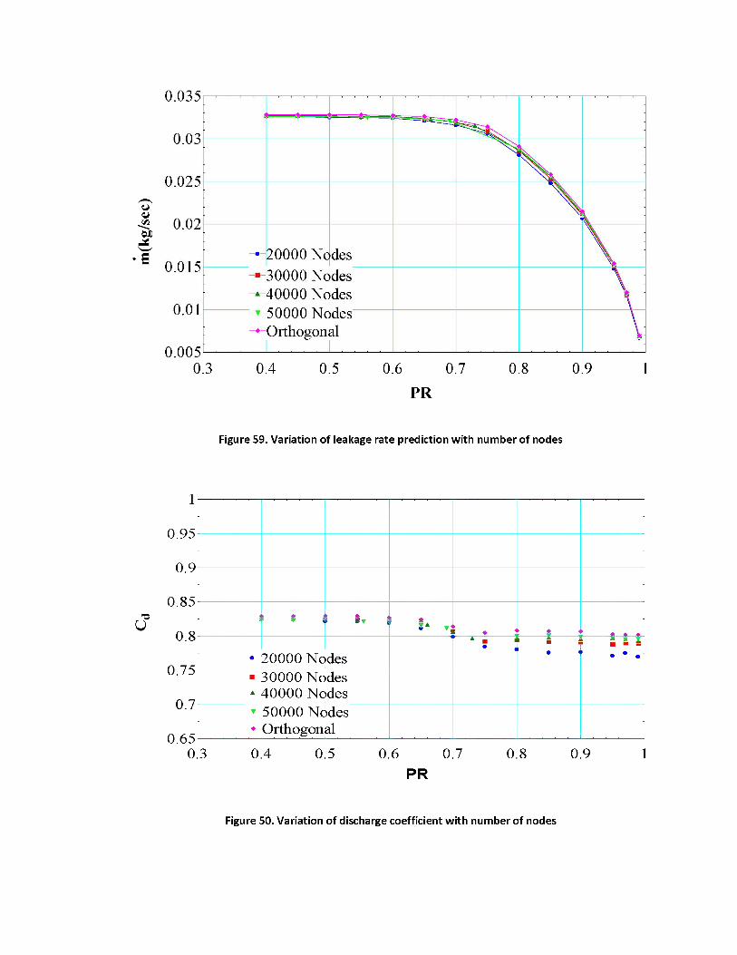
Cd
m(k
g/se
c)
0.035
0.03
0.025
0.02
20000 Nodes 30000 Nodes 40000 Nodes 50000 Nodes Orthogonal
0.015
0.01
0.0050.3 0.4 0.5 0.6 0.7 0.8 0.9 1
PR
Figure 59. Variation of leakage rate prediction with number of nodes
1
0.95
0.9
0.85
0.8
0.75
0.7
0.650.3 0.4 0.5 0.6 0.7 0.8 0.9 1
PR
$ ►♦1) *
-A i ♦ : : t :• ozoooo<N des
* m ■ <•
|||• • .
■▲
30000 No 40000 Nc50000 No Orthogon
desdes
▼♦
desal
Figure 50. Variation of discharge coefficient with number of nodes

Experimental data is used to show the capabilities of model developed in OpenFOAM. The data
used is that of a plain orifice having an inner diameter of 1.006 mm and a length of 5 mm
resulting in L/D~5. The radius of curvature of the inlet edge has been carefully measured and it
has been found that the edge can be considered as a sharp edge. Hence, a sharp edge has been
used for these computational studies. However, it is very important to measure the radius of
curvature accurately as it has a significant effect on the leakage rate as shown later in this
section. Simulations are performed for this particular orifice for different operating conditions
(Table D.3) and leakage rate results are presented in Figures 51 through 55.
0.04
0.035
0.03
~ 0.025
0.02*
•H 0.015
0.01
0.005
00.2 0.3 0.4 0.5 0.6 0.7 0.8 0.9 1
PR
5.1 Validation of computational model
lsv... .......
*..
3 N9 MPa, 3 72 Kg/m \\mExperimt
HIV1rntal
Figure 51. Leakage rate for inlet condition of 9 MPa, 372 Kg/m3 (case 1 in Table D.3)

m(K
g/se
c)
m(K
g/se
c)
0.04
0.035
0.03
0.025
0.02
0.015
0.01
0.005
■-----------■---------- ■----------- —------------------■---- _
▲---------A--------- —A------------ A— ------- A----------A-♦-----------♦- ---------♦----------- ----------------- —
X\ \
\\9 is4Pa, 498
mOpenFO
mExperim
|a
\AM
ental
0[ 0.2 0.3 0.4 0.5 0.6
PR0.7 0.8 0.9 1
Figure 52. Leakage rate for inlet condition of 9 MPa, 498 Kg/m3 (case 2 in Table D.3)
0.04
0.035
0.03
0.025
0.02
0.015
0.01
0.005
00.2 0.3 0.4 0.5 0.6 0.7 0.8 0.9 1
PR
-------A^A zx x --------T *------------i
Os 1
10 M4Pa, 372
mOpenFO AM
mExperimental
> :
Figure 53. Leakage rate for inlet condition of 10 MPa, 372 Kg/m3 (case 3 in Table D.3)

0.04
0.035
0.03
^ 0.025
0.026£
0.015
0.01
0.005
00.2 0.3 0.4 0.5 0.6 0.7 0.8 0.9 1
PR
------■--------■------------- --------■---- 1--
1xX\
IPa, 498
mOpenFO
mExperim
\\10 M
♦Kg/m3 X
A
AM
sntal
Figure 54. Leakage rate for inlet condition of 10 MPa, 498 Kg/m3(case 4 in Table D.3)
0.2 0.3 0.4 0.5 0.6PR
0.7 0.8 0.9 1
Figure 55. Leakage rate for inlet condition of 11 MPa, 372 Kg/m3 (case 5 in Table D.3)

It can be qualitatively concluded from these Figures that OpenFOAM, is in general, capable of
predicting the experimental data for all operating conditions. For each operating condition, the
PR's at which experimental data is available doesn't match with that of computational data and
hence, in order to facilitate a comparison, a 6th order polynomial curve is fit to the experimental
data and the leakage is calculated for the needed PR's. An error analysis is performed to
compare the numerical simulation data with that of the experimental data and the results are
plotted in Figure 56 for all operating conditions. It can be concluded from the error analysis that
the majority of the simulation data for higher PR and low leakage rate are within ± 10 % of
experimental values and for low PR and high leakage rate all data points are within ±10 % of
experimental values with majority of the data close to a 5 % error. This slight error could be due
to the fact that there are adverse property changes as S-CO2 flows through an orifice and a
refined mesh based on gradients in properties is needed to capture the flow field more
accurately. Implementing an adaptive mesh refinement algorithm in OpenFOAM to refine the
mesh automatically based on gradients in properties will minimize the error further and is to
future work.
0.045
0.04
U 0.035CD
0.03&
0.025i
0.015
0.01
0.005
00 0.005 0.01 0.015 0.02 0.025 0.03 0.035 0.04 0.045
mOpenFOAM(Kg/sec)
0 % err
± 5 % e1 1 A 0/
or
rror
x C1JLU1
/m3
g/m3
/m3
g/m3
g/m3
9 MPa, 372 Kg
, 372 K
498 Kg
, 498 K
, 372 K—
10 MPa
9 MPa,
10 MPa
11 MPa
Figure 56. Error analysis for plain orifice data
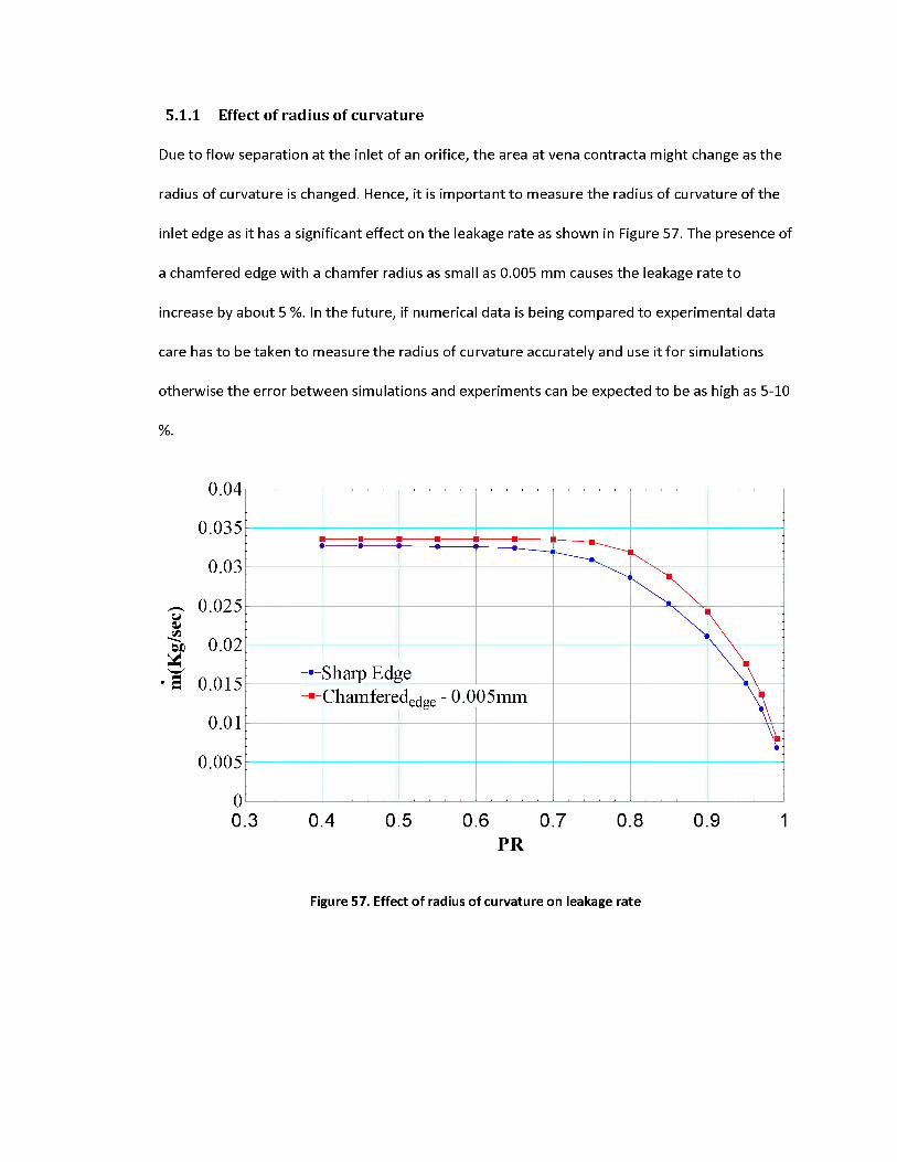
5.1.1 Effect of radius of curvature
Due to flow separation at the inlet of an orifice, the area at vena contracta might change as the
radius of curvature is changed. Hence, it is important to measure the radius of curvature of the
inlet edge as it has a significant effect on the leakage rate as shown in Figure 57. The presence of
a chamfered edge with a chamfer radius as small as 0.005 mm causes the leakage rate to
increase by about 5 %. In the future, if numerical data is being compared to experimental data
care has to be taken to measure the radius of curvature accurately and use it for simulations
otherwise the error between simulations and experiments can be expected to be as high as 5-10
%.
0.04
0.035
0.03
0.025uQJ0.02
*•s' 0.015
0.01
0.005
00.3 0.4 0.5 0.6 0.7 0.8 0.9 1
PR
-_^, x
Sharp Edg Chamfere
e
Vi4
\ ■XX
dedge - °.°05mm 1■
Figure 57. Effect of radius of curvature on leakage rate

There are various geometrical parameters which affects the leakage rate through orifices. Some
of the important parameters which will be analyzed in this section are the effects of radial
clearance, tooth width, tooth depth, inlet radius of curvature, shaft diameter.
5.2.1 Effect of Radial clearance
The first parameter that is of interest when designing seals for turbo-machines is the radial
clearance. Simulations were performed for four different radial clearances (cases 1-4 in
Appendix B) with the rest of the geometrical parameters held constant for all four cases. The
leakage rate is calculated by integrating the mass flow at each node of the inlet and scaling the
2-D axisymmetric mass flow rate to a 3-D model. Then the discharge coefficient is predicted by
calculating the ratio of this scaled mass flow rate with respect to the 1-D isentropic mass flow
rate. Figures (58 and 59) present the results of the leakage rates and discharge coefficients
respectively for all four cases.
5.2 Effect of geometrical parameters
0.06
0.05
0.04
0.03
0.02-•-RC - 0.06mm
■ RC - 0.09mm RC - 0.12mm
-♦-RC - 0.15mm
0.01
0.3 0.4 0.5 0.6 0.7 0.8 0.9PR
Figure 58. Variation of Leakage rate with Radial clearance

The leakage rate increases with an increase in radial clearance, which is a fairly obvious result as
an increase in clearance area allows more fluid to be forced underneath the tooth. It should be
noted that the inlet operating condition for all these simulations is fixed at a pressure of 10
MPa, and a density of 498 kg/m3. Although the leakage rate increases by a magnitude of
approximately 3 times between the clearances of 0.06 mm and 0.15 mm, it is interesting to note
that the discharge coefficient for all the four cases doesn't vary by much.
1
0.95
0.9
0.85 U
0.8
0.75
0.7
0.650.3 0.4 0.5 0.6 0.7 0.8 0.9 1
PR
Figure 59. Variation of discharge coefficient with radial clearance
This result implies that the 1-D isentropic model is able to predict the leakage rate for all radial
clearances equally well. One more interesting thing to note is how the Cd remains constant for
higher PR's, increases over a certain range of PR and stays constant below the choked PR. The
reason for this increase in Cd over a range of PR is due to the fact that the 1-D isentropic model
and real flow choke at different PR's. In reality, the mass flow rate continues to increase even
after the 1-D isentropic model chokes and hence, the Cd increases till the real flow chokes and
iff!
RC - 0.06mm
! •:
* * 111■ ■ ■ ■ ■* • • • •
■ RC - 0.09RC - 0.12 RC - 0.15
mm
mm
stays constant after that.
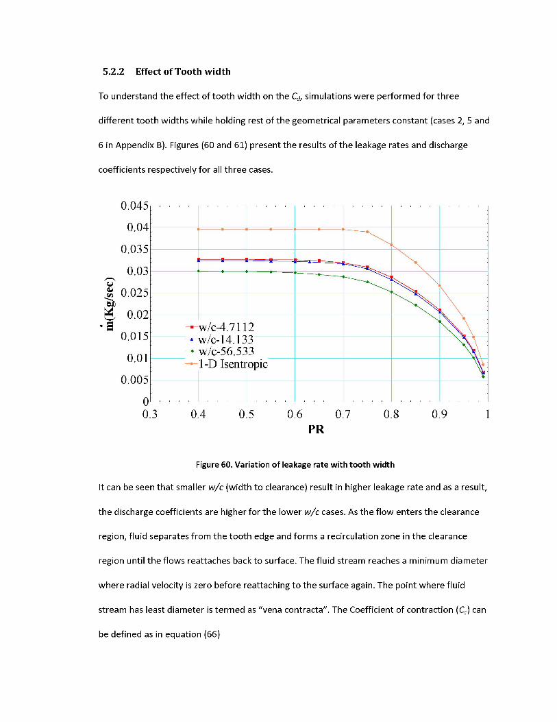
5.2.2 Effect of Tooth width
To understand the effect of tooth width on the Cd, simulations were performed for three
different tooth widths while holding rest of the geometrical parameters constant (cases 2, 5 and
6 in Appendix B). Figures (60 and 61) present the results of the leakage rates and discharge
coefficients respectively for all three cases.
0.045
0.04
0.035
0.03
0.025
0.02w/c-4.7112 w/c-14.133 w/c-56.533 1-D Isentropic
0.015
0.01
0.005
0.3 0.4 0.5 0.6 0.7 0.8 0.9 1PR
Figure 60. Variation of leakage rate with tooth width
It can be seen that smaller w/c (width to clearance) result in higher leakage rate and as a result,
the discharge coefficients are higher for the lower w/c cases. As the flow enters the clearance
region, fluid separates from the tooth edge and forms a recirculation zone in the clearance
region until the flows reattaches back to surface. The fluid stream reaches a minimum diameter
where radial velocity is zero before reattaching to the surface again. The point where fluid
stream has least diameter is termed as "vena contracta". The Coefficient of contraction (Cc) can
be defined as in equation (66)

Area at vena contractaQ =
Area at vena contracta
Area of orifice(66)
The typical value of Cc is 0.64 for a sharp orifice. The smaller the value of Cc, the more effective
the vena contracta is. After the flow reattaches to the surface the pressure drop in the orifice
can be treated equivalent to a flow through pipe. In the case of laminar pipe flow for a given
pressure drop the flow rate gets smaller as the length of the pipe increases, as shown in
equation (67). This can be extended to complicated turbulent flow and said that the leakage rate
is inversely proportional to the tooth width.
nD4AP
128,ul(67)
As presented in Figure 61, Cd doesn't change much for lower w/c cases. If the fluid reattaches to
the surface of tooth very close to the downstream edge, the effect of tooth width might not be
very significant, as observed for lower w/c cases. As w/c increases the effect of tooth width
becomes more and more significant. In fact, while understanding the effect of radial clearance,
w/c for the least clearance (0.06mm) case is about 7.06 whereas for the maximum radial
clearance (0.15mm) case it is about 2.82 which is the reason why the discharge coefficients
didn't vary much even though the leakage rates increased by 3 times between minimum and
maximum clearance cases. It has been shown by many authors [18] in the past that the major
non-dimensional parameter influencing the discharge coefficient is w/c.
In order to reassert the theory that w/c is the only geometrical parameter that significantly
affects the discharge coefficient of an annular orifice, two simulations were performed with
different widths and clearances but having the same w/c (cases 2 and 7 in Appendix B). Figure
62 indicates that the discharge coefficient of both the cases show nearly the same functional
relationship with PR thus verifying that w/c is the correct non-dimensional geometrical

parameter that influences the discharge coefficient of an annular orifice. It might also be
worthwhile to affirm the theory at higher w/c of 56.533 or above, which is left to be part of
future work.
1
0.95
0.9
0.85 U
0.8
0.75
0.7
0.650.3 0.4 0.5 0.6 0.7 0.8 0.9 1
■ w/c-4.7112w/c-14.133w/c-56.533
; A ■
" '■ ■ "* A A
4
* • .
PR
Figure 61. Variation of Cd with tooth width
1
0.95
0.9
0.85
0.8
0.75c - 0.06mm, w - 0.424mm c - 0.09mm, w - 0.2827—0.7
0.650.3 0.4 0.5 0.6 0.7 0.8 0.9 1
PR
Figure 62. Cd of annular orifices having same w/c
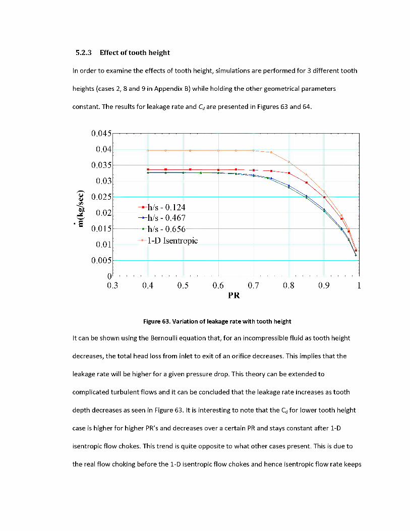
5.2.3 Effect of tooth height
In order to examine the effects of tooth height, simulations are performed for 3 different tooth
heights (cases 2, 8 and 9 in Appendix B) while holding the other geometrical parameters
constant. The results for leakage rate and Cd are presented in Figures 63 and 64.
0.045
0.04
0.035
0.03
IT 0.025t/20.02'w'
’S 0.015
0.01
0.005
00.3 0.4 0.5 0.6 0.7 0.8 0.9 1
PR
Figure 63. Variation of leakage rate with tooth height
It can be shown using the Bernoulli equation that, for an incompressible fluid as tooth height
decreases, the total head loss from inlet to exit of an orifice decreases. This implies that the
leakage rate will be higher for a given pressure drop. This theory can be extended to
complicated turbulent flows and it can be concluded that the leakage rate increases as tooth
depth decreases as seen in Figure 63. It is interesting to note that the Cd for lower tooth height
case is higher for higher PR's and decreases over a certain PR and stays constant after 1-D
isentropic flow chokes. This trend is quite opposite to what other cases present. This is due to
■ \ •* "\x\
—h/s - 0.12' h/s - 0.46' h/s - 0.65(1-D Isentr
t XX* 1
\x)opic
the real flow choking before the 1-D isentropic flow chokes and hence isentropic flow rate keeps

increasing even after the real flow chokes. The physical reason behind why the real flow chokes
before the isentropic flow is unknown at this point and requires more detailed study. As tooth
height increases, discharge coefficient is nearly independent of tooth height and can be
assumed that it has no effect on Cd. It has to be noted that the aspect ratio of cavities of most
real world labyrinth seals is over 0.5 and rarely exceeds 1.5.
1
0.95
0.9
0.85 U
0.8
0.75
0.7
0.650.3 0.4 0.5 0.6 0.7 0.8 0.9 1
PR
Figure 64. Variation of Cd with tooth height
5.2.4 Effect of Shaft Diameter
It can be observed from Figure 65 that the Cd of annular orifice doesn't change with shaft
diameter, even after increasing the shaft diameter to 3 times the initial value (Cases 2 and 10 in
Appendix B). Hence, it can be concluded that shaft diameter does not influence the value of Cd
and a model which is developed for a particular shaft diameter can be applied to any shaft
■■ ■ ■.
4 * i
h/s - 0 12zl♦A ♦
▲ A A* ♦ ♦
* h/s - 0.46'h/s - 0.65(
76
diameter.

1
0.95
0.9
0.85U
0.8
0.75
0.7
0.650.3 0.4 0.5 0.6 0.7 0.8 0.9 1
PR
Figure 65. Variation of Cd with shaft diameter
5.2.5 Correlation for Carry over coefficient
As described by Hodkinson [18], leakage rate through a labyrinth seal can be estimated as,
m= aymideal (68)
Where mideal is the 1-D isentropic flow rate for labyrinth seals, y is the carry over coefficient of
the cavity, a is the flow coefficient similar to discharge coefficient. Following the definition
presented by Hodkinson, y is calculated as a function of the divergence angle, fi, measured from
the streamline separating the fluid recirculating in the seal cavity and that passing under the
tooth. The carry over coefficient can be calculated based on following relationships provided by
Hodkinson.
D- 3mm D - 9mm
Y 2 1i-x
(69)

(70)
The divergence angle, , is the angle made between the line connecting the lip of the upstream
tooth to the point of impingement of the jet onto the downstream tooth and a line parallel to
the rotor surface. Radial velocity data is collected along the downstream tooth surface and the
point where radial velocity is zero is taken as the point of impingement of the jet, as shown in
Figure 66. The cavity geometrical parameters are varied (single parameter is varied at a time)
and model for carry over coefficient is developed to include the geometrical effects.
Figure 66. Measurement of divergence angle in the cavity
5.2.6 Effect of radial clearance
Hodkinson [35] used, the clearance to pitch ratio (c/s) as the only non-dimensional parameter to
develop an empirical correlation for y based on geometry. Four cases are simulated for fixed
pitch but with varying clearance (cases 1-4 in Appendix C). The carry over coefficient for each of
these cases is calculated and the results are presented in Figure 67. It is very important to note
that y is not a function of PR and stays constant for a fixed clearance to pitch ratio. A higher
value of c/s results in higher carry over coefficient as, for a given jet divergence, more fluid flows
under the tooth when the clearance is higher. However, increasing the clearance by a factor of

2.5 increases the carry over coefficient by only 2%. Based on these results, the carry over
coefficient can be written as shown in equation (71).
7 = 0.3948 0 + 1.001 (71)
1.045
1.04
1.035
1.03
1.025
1.02
1.015
1.01
1.005
10.3 0.4 0.5 0.6 0.7 0.8 0.9 1
PR
Figure 67: Effect of clearance on y
5.2.7 Effect of Tooth Height
Changing the tooth height to pitch ratio (h/s) changes the aspect ratio and could possibly have
some effect on recirculation in the cavity. To verify if changing the aspect ratio of the cavity
affects the carry over coefficient or not, three simulations were performed by varying the cavity
depth while leaving other geometrical parameters constant (cases 9, 10 and 11 in Appendix C). It
can be seen from Figure 68 that the carry over coefficient is independent of h/s. Therefore, the
conclusions from these simulations is that tooth height or cavity height has no effect on the
kinetic energy carry over coefficient, which is one of the basic assumptions made by Hodkinson
c/s = 0 .03546 •-c/s = 0 0 5319 c/'s = 0.070 92 c/s _ 0.08865
kk------ ▲------ [---------A--------- a ------ ▲------ k--------- A--------- k------ A------ k------ A
[18].
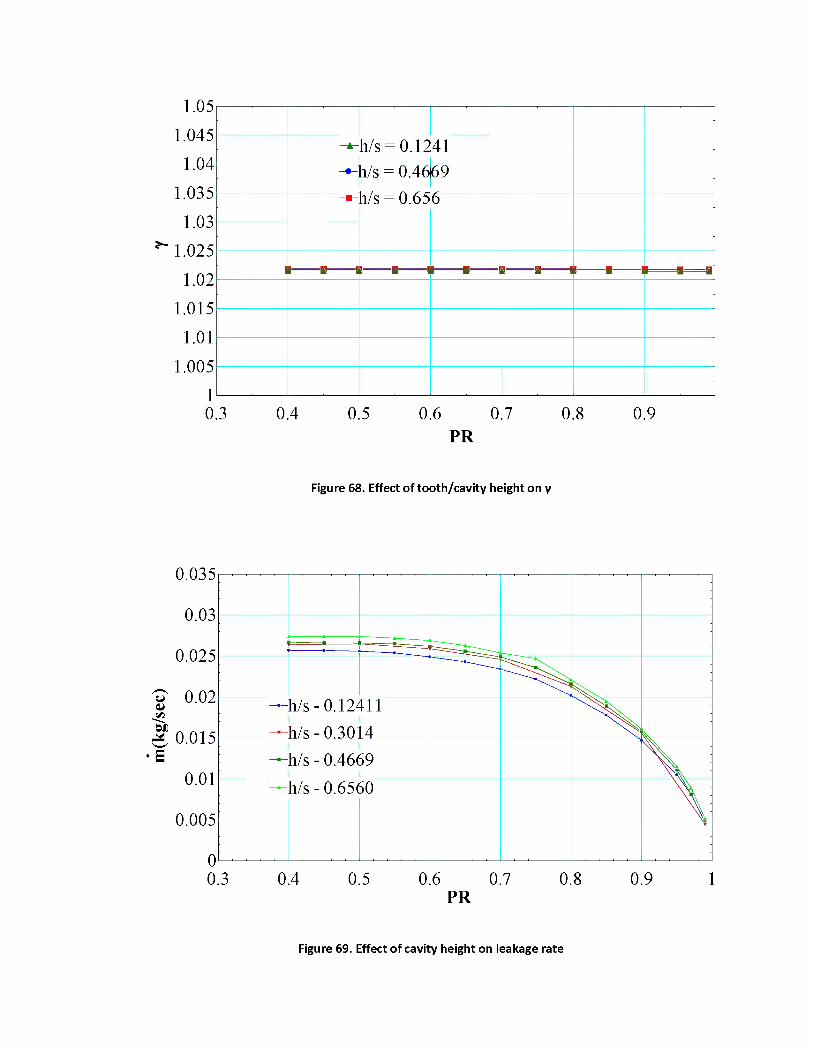
m(k
g/se
c)
y
1.05
1.045
1.04
1.035
1.03
1.025
1.02
1.015
1.01
1.005
10.3 0.4 0.5 0.6 0.7 0.8 0.9
PR
A h/s = 0.1241h/s = 0.46
h/s = 0.65
69
6
Figure 68. Effect of tooth/cavity height on y
0.035
0.03
0.025
0.02
0.015
0.01
0.005
00.3 0.4 0.5 0.6 0.7 0.8 0.9 1
PR
i
".......
h/s - 0.12411h/s - 0 3014
h/s - 0.4669 Xh/s - 0.65( 0
\
Figure 69. Effect of cavity height on leakage rate
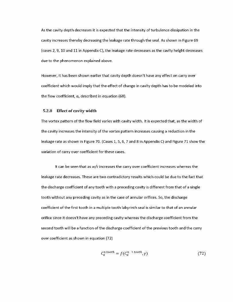
As the cavity depth decreases it is expected that the intensity of turbulence dissipation in the
cavity increases thereby decreasing the leakage rate through the seal. As shown in Figure 69
(cases 2, 9, 10 and 11 in Appendix C), the leakage rate decreases as the cavity height decreases
due to the phenomenon explained above.
However, it has been shown earlier that cavity depth doesn't have any effect on carry over
coefficient which would imply that the effect of change in cavity depth has to be modeled into
the flow coefficient, a, described in equation (68).
5.2.8 Effect of cavity width
The vortex pattern of the flow field varies with cavity width. It is expected that, as the width of
the cavity increases the intensity of the vortex pattern increases causing a reduction in the
leakage rate as shown in Figure 70. (Cases 1, 5, 6, 7 and 8 in Appendix C) and Figure 71 show the
variation of carry over coefficient for these cases.
It can be seen that as w/c increases the carry over coefficient increases whereas the
leakage rate decreases. These are two contradictory results which could be due to the fact that
the discharge coefficient of any tooth with a preceding cavity is different from that of a single
tooth without any preceding cavity as in the case of annular orifices. So, the discharge
coefficient of the first tooth in a multiple tooth labyrinth seal is similar to that of an annular
orifice since it doesn't have any preceding cavity whereas the discharge coefficient from the
second tooth will be a function of the discharge coefficient of the previous tooth and the carry
over coefficient as shown in equation (72)
tooth =f(Cn~l toothy (72)
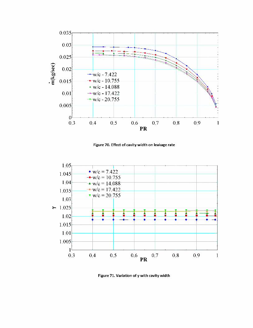
y m
(kg/
sec)
0.035
0.03
0.025
0.02
0.015
0.01
0.005
_ *
--- 1—------ J— t------ :
w/c - 7.42 w/c - 10.7 w/c - 14.0 w/c - 17.4 w/c - 20.7
2558822 V55
V"\0L0.3 0.4 0.5 0.6 0.7
PR0.8 0.9 1
Figure 70. Effect of cavity width on leakage rate
1.05
1.045
1.04
1.035
1.03
1.025
1.02
1.015
1.01
1.005
•.
w/c = 7.4: w/c = 10.' w/c = 14. w/c = 17.' w/c = 20.'
22755088422755
;-----z----- ; :-----%----- : i-----------f-----%-----x----- ; ;-----Z----- —z—z-----A----- -----A----- -----A-----A-----A----- -----A--- A
1 0.3 0.4 0.5 0.6 0.7 0.8 0.9
PR1
Figure 71. Variation of y with cavity width

This can be proved by analyzing the velocity profiles at the entrance of each tooth in a three
teeth labyrinth seal (Case 1 in Appendix C). Figure 72 indicates that the velocity profile at the
entrance of each tooth is different. It is interesting to note that velocities at the entrance of last
tooth are much higher than that of previous teeth which is due to the pressure drop being
largest for the last tooth which will be shown later.
0.00157
0.00156
0.00155
0.00154
& 0.00153
0.00152
0.00151
0.0015
0.001490 10 20 30 40 50 60 70 80 90 100
U(m/sec)
Figure 72. Velocity profile at the entrance of each tooth
Taking into account the effect of cavity width, equation (71) is modified and model for y
is developed with c/s, w/c as the non-dimensional parameters.
---------- -
"-•Xjj. \1II }
First toothSecond toothThird tooth /
f
/j
y = 0.91559 + |0.395745 + 0.113839 Q (73)
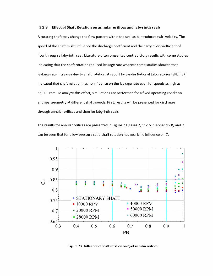
5.2.9 Effect of Shaft Rotation on annular orifices and labyrinth seals
A rotating shaft may change the flow pattern within the seal as it introduces swirl velocity. The
speed of the shaft might influence the discharge coefficient and the carry over coefficient of
flow through a labyrinth seal. Literature often presented contradictory results with some studies
indicating that the shaft rotation reduced leakage rate whereas some studies showed that
leakage rate increases due to shaft rotation. A report by Sandia National Laboratories (SNL) [34]
indicated that shaft rotation has no influence on the leakage rate even for speeds as high as
65,000 rpm. To analyze this effect, simulations are performed for a fixed operating condition
and seal geometry at different shaft speeds. First, results will be presented for discharge
through annular orifices and then for labyrinth seals.
The results for annular orifices are presented in Figure 73 (cases 2, 11-16 in Appendix B) and it
can be seen that for a low pressure ratio shaft rotation has nearly no influence on Cd.
1
0.95
0.9
0.85 U
0.8
0.75
0.7
0.650.3 0.4 0.5 0.6 0.7 0.8 0.9 1
PR
♦
X
♦ x_____T T X
$1 ! t Z4 1
5 ► X ◄
1►
X> ■ ►
• STATIONvfARY SHAFT
9 : 5
■
A
10000 RP20000 RP28000 RP
. . .
MM z
40000 RP50000 RP60000 RP
MM
H
....
M. . . .
♦ M
Figure 73. Influence of shaft rotation on Cd of annular orifices
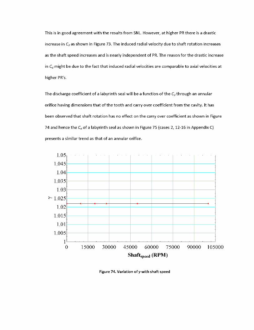
This is in good agreement with the results from SNL. However, at higher PR there is a drastic
increase in Cd as shown in Figure 73. The induced radial velocity due to shaft rotation increases
as the shaft speed increases and is nearly independent of PR. The reason for the drastic increase
in Cd might be due to the fact that induced radial velocities are comparable to axial velocities at
higher PR's.
The discharge coefficient of a labyrinth seal will be a function of the Cd through an annular
orifice having dimensions that of the tooth and carry over coefficient from the cavity. It has
been observed that shaft rotation has no effect on the carry over coefficient as shown in Figure
74 and hence the Cd of a labyrinth seal as shown in Figure 75 (cases 2, 12-16 in Appendix C)
presents a similar trend as that of an annular orifice.
1.05
1.045
1.04
1.035
1.03
1.025
1.02
1.015
1.01
1.005
10 15000 30000 45000 60000 75000 90000 105000
Shaftspeed (RPM)
Figure 74. Variation of y with shaft speed

0.85
0.8
0.75
0.7U
0.65
0.6
0.55
0.50.3 0.4 0.5 0.6 0.7 0.8 0.9 1
PR
Figure 75. Variation of the Cd with shaft speed for labyrinth seals
This would imply that it is sufficient to model the influence of shaft rotation into Cd of an annular
orifice. However, at these high shaft speeds, the influence of boundary layer in the d direction
might be significant and it is good practice to validate some of these results against a 3-D model
or experimental data for an annular orifice, which is left as a part of future work.
To predict leakage through labyrinth seal, each tooth can be treated individually and leakage
rate equation for each tooth can be written as,
^ Cd\ntoothYmisentropic C74)
Where Cd of the first tooth is same as that of an annular orifice and Cd from the second tooth
depends on the Cd of previous tooth and y of the cavity. For first constriction y is equal to 1. A
correlation for y is developed earlier in this section. In future, it is proposed to develop a
• STATION
10000 RP20000 RP
z
JARY SHAFT1
28000 RPM X■
A
,
MM
♦X
50000 RP100000 R
MPM
X '
1►a. S ■•
i 8• 1
X♦
• 1 ♦: ;
: ♦ 'z- i
♦♦ ▼X 1 A■ ■ ■•
correlation for the discharge coefficient which can be applied to each tooth as in equation (74).
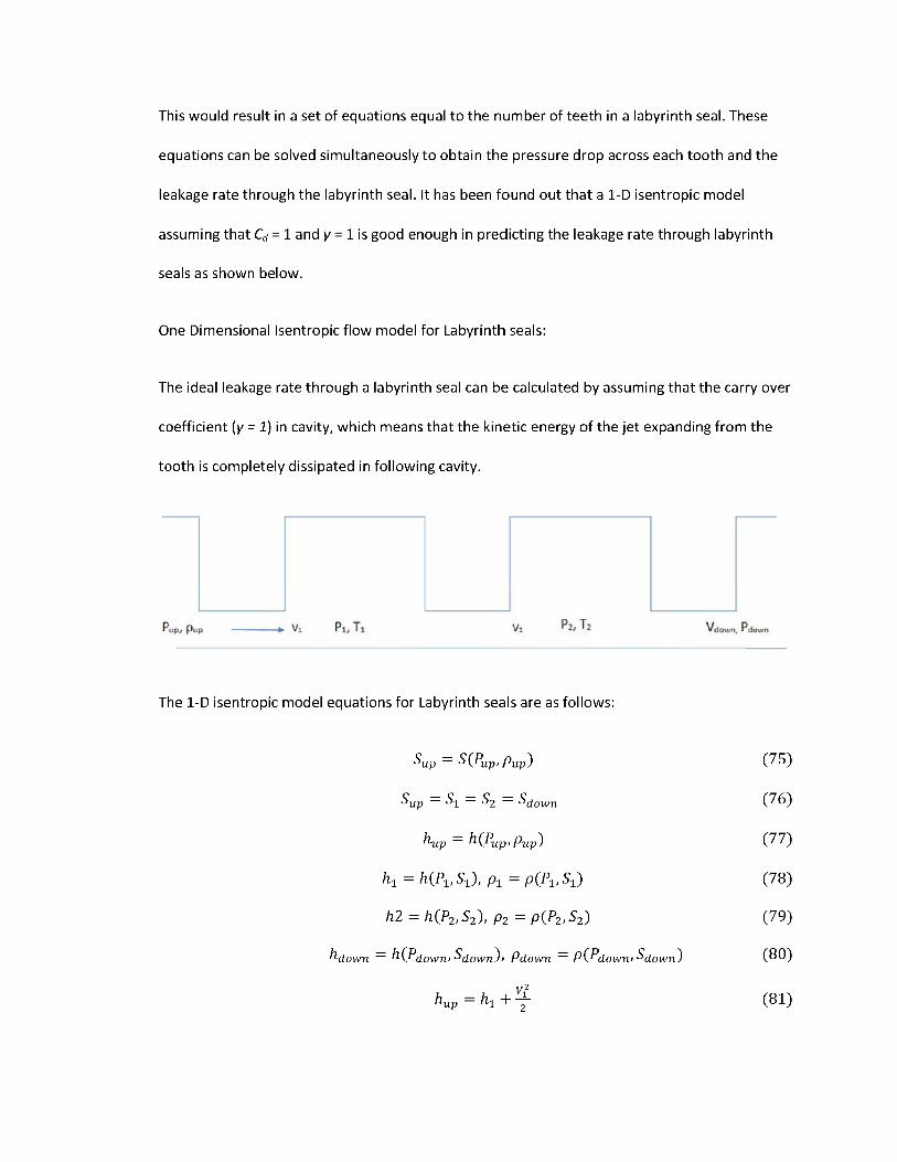
This would result in a set of equations equal to the number of teeth in a labyrinth seal. These
equations can be solved simultaneously to obtain the pressure drop across each tooth and the
leakage rate through the labyrinth seal. It has been found out that a 1-D isentropic model
assuming that Cd = 1 and y = 1 is good enough in predicting the leakage rate through labyrinth
seals as shown below.
One Dimensional Isentropic flow model for Labyrinth seals:
The ideal leakage rate through a labyrinth seal can be calculated by assuming that the carry over
coefficient (y = 1) in cavity, which means that the kinetic energy of the jet expanding from the
tooth is completely dissipated in following cavity.
The 1-D isentropic model equations for Labyrinth seals are as follows:
$up S(Pu-p, Pup) (75)
Q —C —C — C°up 1 2 down (76)
h-up h(Pup,pUp) (77)
h1 = h(P1,S1), pt =p(P1,51) (78)
h.2 = h{P2,S2), P2 =P(P2>$2) (79)
h-down down>Sdown)> Pdown P^Pdowrn^down) (80)
h —h + —‘‘■up 1 2 (81)

(82)
h2 = hdown + V-4f* (83)
^ideal Pl^clearance^l P2^clearance^2 Pdown^clearance^down (84)
The Above set of equations are modeled in EES and solved simultaneously to obtain 1-D
isentropic leakage rate for labyrinth seals without carry over. Although, the equations presented
here are for three teeth cases, these equations can be extended to a labyrinth seal with any
number of teeth. The behavior of this model is quite similar to that of an annular orifice model.
The isentropic leakage rate increases until the choking PR and then starts decreasing. Again,
these calculations are run through min/max function in EES and the modified leakage rate will
be used for multiple teeth cases as well. The model assumes temperature and pressure to be
constant across the cavity in the radial clearance region. The question now is: "How valid is this
assumption?"
To answer this question, temperature and pressure in the radial clearance region are plotted for
one of the cases (Case 1 in Appendix C). From Figure 76 it can be observed that for a pressure
drop as high as 6 MPa, pressure remains fairly constant throughout the cavity. It can also be
seen from Figure 77 that temperature also follows the same trend. It is also interesting to note
that majority of the pressure and temperature drop occurs across the last tooth. This would
imply that leakage rate through labyrinth seal is dictated by the Cd of last tooth.
The 1-D isentropic model for labyrinth seal, described above is applied to case 2 in Appendix C.
From Figure 78, it can be seen that a simple 1-D isentropic model for labyrinth seals assuming
the Cd and the y are equal to 1, works reasonably well in predicting leakage through multiple
constrictions. The drawback of this 1-D isentropic model is that it doesn't take into
hi = h2+^-
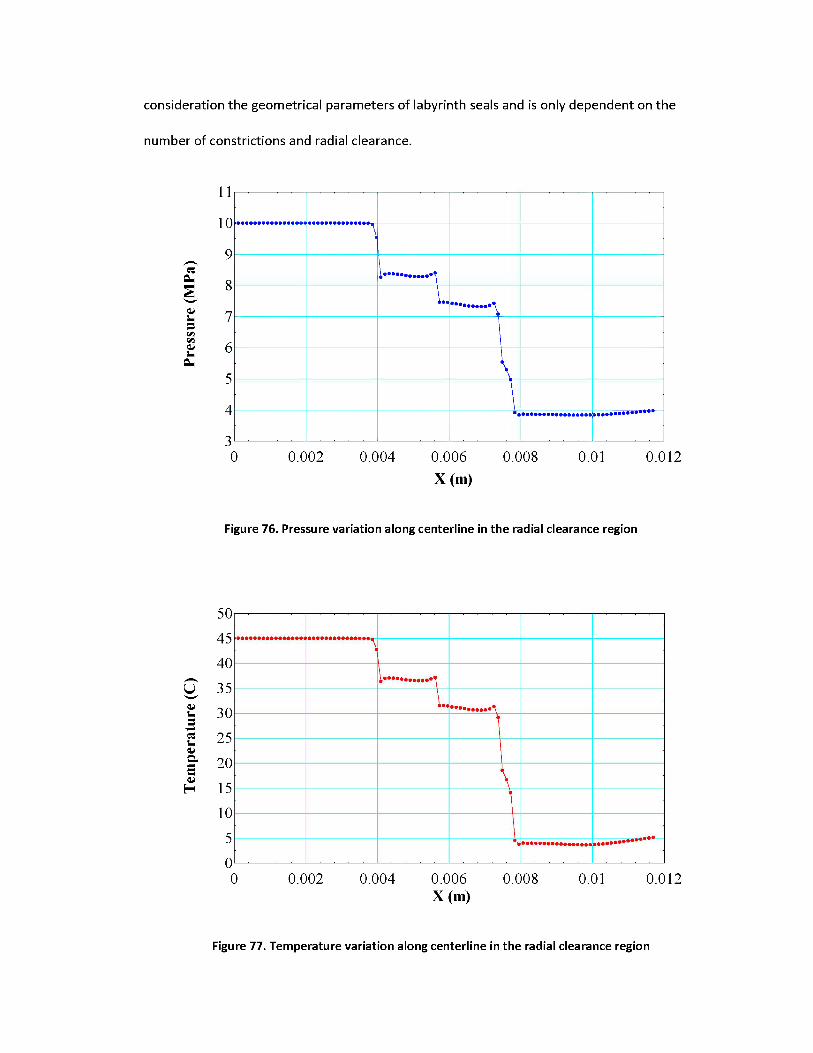
Tem
pera
ture
(C)
Pres
sure
(MPa
)
consideration the geometrical parameters of labyrinth seals and is only dependent on the
number of constrictions and radial clearance.
11
10
9
8
7
6
5
4
30 0.002 0.004 0.006 0.008 0.01 0.012
X(m)
"\
L-\
1
\Figure 76. Pressure variation along centerline in the radial clearance region
50 45 40 35 30 25 20 15 10
5 00 0.002 0.004 0.006 0.008 0.01 0.012
X(m)
Figure 77. Temperature variation along centerline in the radial clearance region

0.035
0.03
0.025
0.02*
■H 0.015
0.01
0.005
0 0.3
------- ■----- ------ ■____------- •------- •____ J
^1
mOpenFOA
1-D IsentrM
opic mode\
' ~u~ :l X
0.4 0.5 0.6 0.7PR
0.8 0.9
Figure 78. Leakage rate prediction using 1-D isentropic model for case 2 in Appendix C
1
5.3 Effect of Operating Conditions
The previous section explained the effects of geometrical parameters while holding the inlet
operating condition constant at 10 MPa, 498 kg/m3. In this section we will look at the effect of
operating conditions without changing geometry. First, the effect of operating conditions on an
annular orifice will be studied and then the theory will be extended to labyrinth seals. Before
even performing simulations, a simple 1-D isentropic model for annular orifices is used to
understand the effects of operating conditions.
According to the 1-D isentropic flow model for annular orifices,
^ Pdown *^down *Aclearance (85)
^'down \2(.^up h-down) (86)
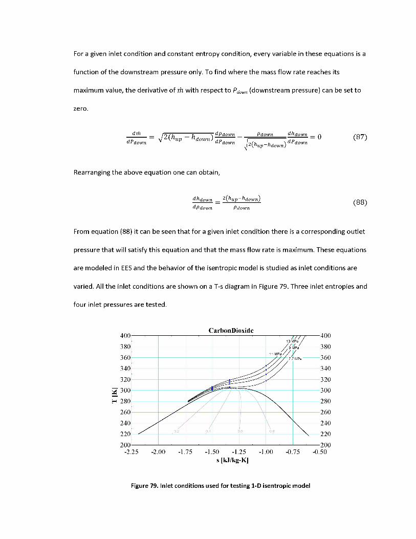
For a given inlet condition and constant entropy condition, every variable in these equations is a
function of the downstream pressure only. To find where the mass flow rate reaches its
maximum value, the derivative of m with respect to Pdown (downstream pressure) can be set to
zero.
dmdP down
V2 (huv-hdown)do1
_____ Pdown_____ dh^own
Jl(hup-haown) dPd0Wn(87)
Rearranging the above equation one can obtain,
dhgown _ 2(hup hdown) (88)d-Pdown Pdown
From equation (88) it can be seen that for a given inlet condition there is a corresponding outlet
pressure that will satisfy this equation and that the mass flow rate is maximum. These equations
are modeled in EES and the behavior of the isentropic model is studied as inlet conditions are
varied. All the inlet conditions are shown on a T-s diagram in Figure 79. Three inlet entropies and
four inlet pressures are tested.
CarbonDioxide400 400380 380360 360340 340320 320
g 300 280
300280
260 260240 240220 220
200-2.25
200-0.50-2.00 -1.75 -1.50 -1.25 -1.00 -0.75
s[kJ/kg-K]
Figure 79. Inlet conditions used for testing 1-D isentropic model
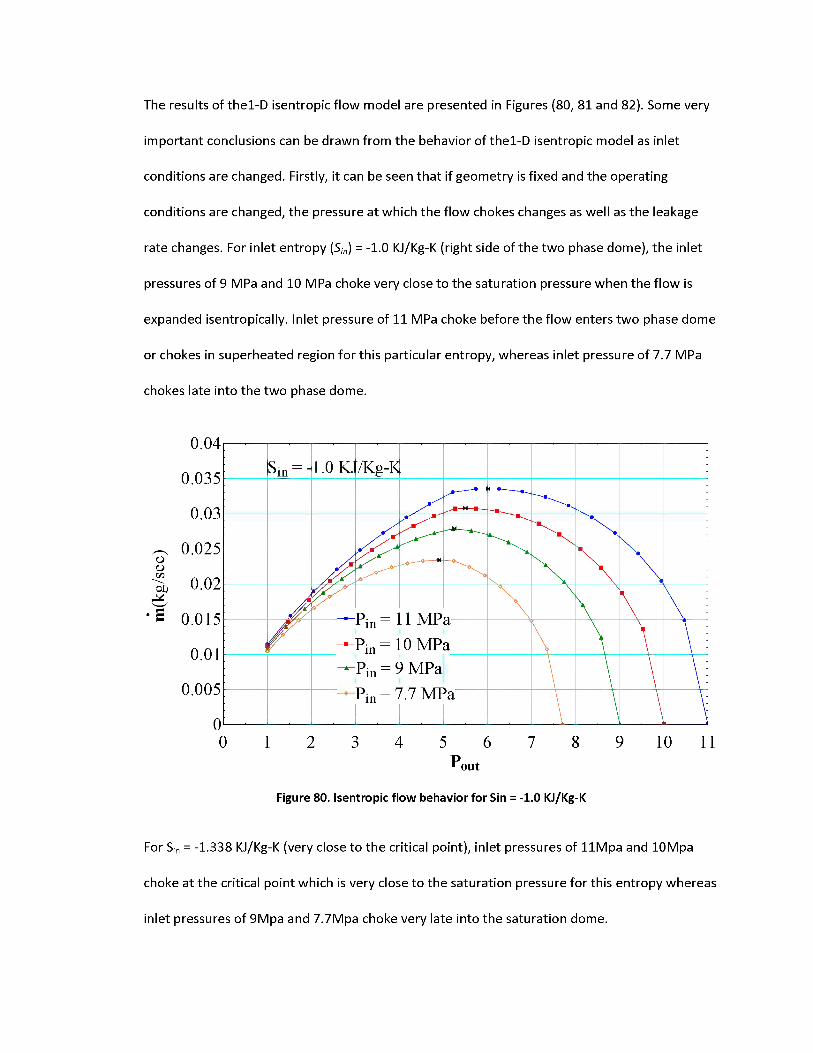
The results of the1-D isentropic flow model are presented in Figures (80, 81 and 82). Some very
important conclusions can be drawn from the behavior of the1-D isentropic model as inlet
conditions are changed. Firstly, it can be seen that if geometry is fixed and the operating
conditions are changed, the pressure at which the flow chokes changes as well as the leakage
rate changes. For inlet entropy (Sn) = -1.0 KJ/Kg-K (right side of the two phase dome), the inlet
pressures of 9 MPa and 10 MPa choke very close to the saturation pressure when the flow is
expanded isentropically. Inlet pressure of 11 MPa choke before the flow enters two phase dome
or chokes in superheated region for this particular entropy, whereas inlet pressure of 7.7 MPa
chokes late into the two phase dome.
o<L>05
15b
0.04
0.035
0.03
0.025
0.02
0.015
0.01
0.005
0
Sin = - 1.0 KJr/Kg-K—•-*<-•—
X • xiX^—♦—W-x_ x\
\\ \
4 Pin = Pin =
U MP10 MP
\ \X\ X \
/ aa \ \ \
Pin = 9 MPa \ \Pin = /.7 MPa \ \
2 4 7 9 10 11P,out
Figure 80. Isentropic flow behavior for Sin = -1.0 KJ/Kg-K
3 6 85
For Sin = -1.338 KJ/Kg-K (very close to the critical point), inlet pressures of 11Mpa and 10Mpa
choke at the critical point which is very close to the saturation pressure for this entropy whereas
inlet pressures of 9Mpa and 7.7Mpa choke very late into the saturation dome.
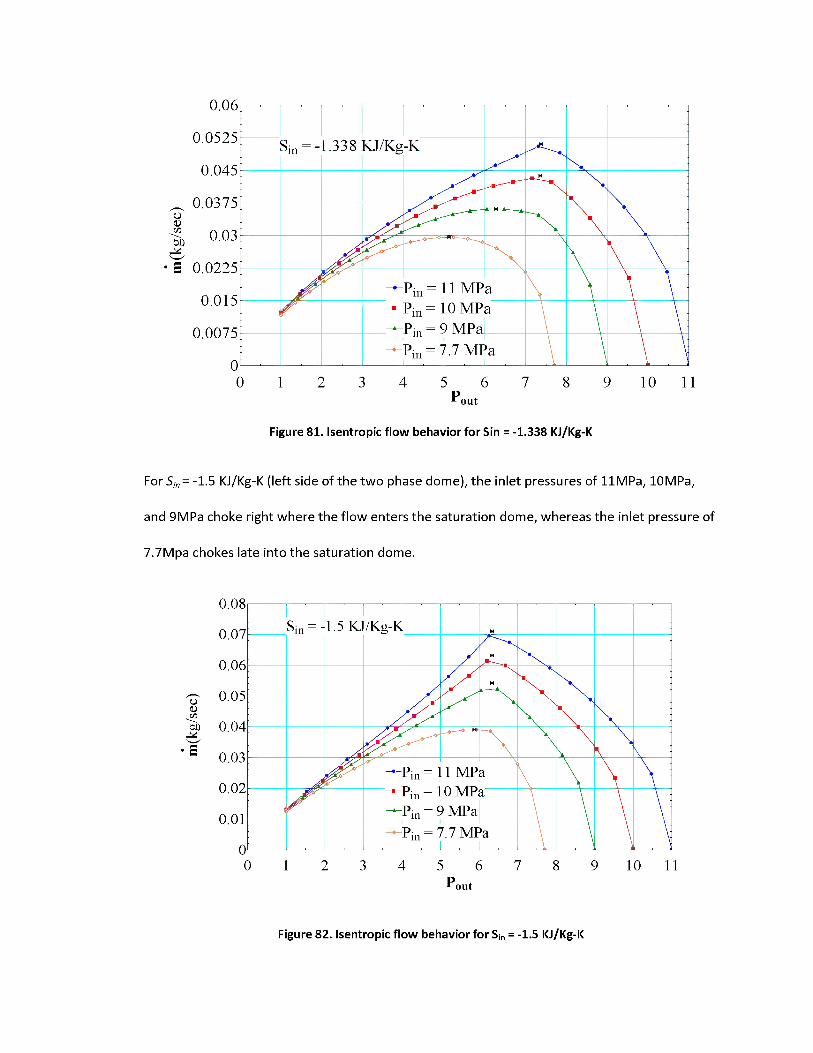
m(k
g/se
c)
For S,-,
0.06
0.0525
0.045
0.0375
0.03
0.0225
0.015
0.0075
00123456789 10 11
Pout
Figure 81. Isentropic flow behavior for Sin = -1.338 KJ/Kg-K
-1.5 KJ/Kg-K (left side of the two phase dome), the inlet pressures of 11MPa, 10MPa,
and 9MPa choke right where the flow enters the saturation dome, whereas the inlet pressure of
7.7Mpa chokes late into the saturation dome.
Sm = - 1.338 KJ/Kg-Kex
X
/■.■ X X
■ \XX X
\\\
M
X\
X\ \ \
AN V \ xe
x Pin = 11 MPa \ \ \—Pin = 10 MPa \ \ \ \
P;„ = 9 MPa \ \ \ \—Pin = 7.7 MPa. . . \ \ \ \
o(D
•¥
0.08
0.07
0.06
0.05
0.04
0.03
0.02
0.01
0
1Sin = - 1.5 KJr/Kg-K
/ X
X /■ / sx.X-X
x. XX\
X,\ \
\\ \
X, \
\
X Pin = 1 MPa \ \■ \
; iPin = 10 MPa Pin = 9 MPa V \ \
—Pin = 7.7 MPai i \ \ \
56Pout
10 112 3 4 7 8 9
Figure 82. Isentropic flow behavior for Sin = -1.5 KJ/Kg-K

Table III is generated to show the choking and saturation pressures for different inlet pressures
and entropy conditions. From this analysis, we can ask ourselves a very valid question: "What is
determining the choking point for each operating condition?" The isentropic flow theory
explained in the next few pages of this report gives an idea about the choking behavior as
operating conditions are varied.
Table III Choking and saturation pressures for various operating conditions
[KJ/Kg-K] Pin[MPa] Pchoking[MPa] Psaturation[MPa]
-1.0 11 6.011 5.243
-1.0 10 5.494 5.243
-1.0 9 5.243 5.243
-1.0 7.7 4.892 5.243
-1.5 11 6.338 6.338
-1.5 10 6.338 6.338
-1.5 9 6.338 6.338
-1.5 7.7 5.887 6.338
-1.338 11 7.376 ~ critical pressure
-1.338 10 7.362 ~ critical pressure
-1.338 9 6.271 ~ critical pressure

-1.338 7.7 5.121 ~ critical pressure
From first law of Thermodynamics for a quasi-static process,
dh = SQ + v dP (89)
According to Clausius equality, for a reversible process
yields----- > SQ T ds (90)
Hence,
dh = T ds + vdP (91)
For an isentropic flow,ds = 0 implies
pdh= dP (92)
Equation (92) can be applied to downstream condition as,
_ dh-down Pdown
uPdown
dPdown __ ^2
dp down (93)
Equation (93) can be rearranged as,
dh-down _ 2(hMp hdown)
d-Pdown Pdown(94)
_ dhaownPdown
aPdown 2(jhip ^down) ^ 2down (95)
From equations (93 and 95), the true definition of the choking point is
V} =c1v down v (96)
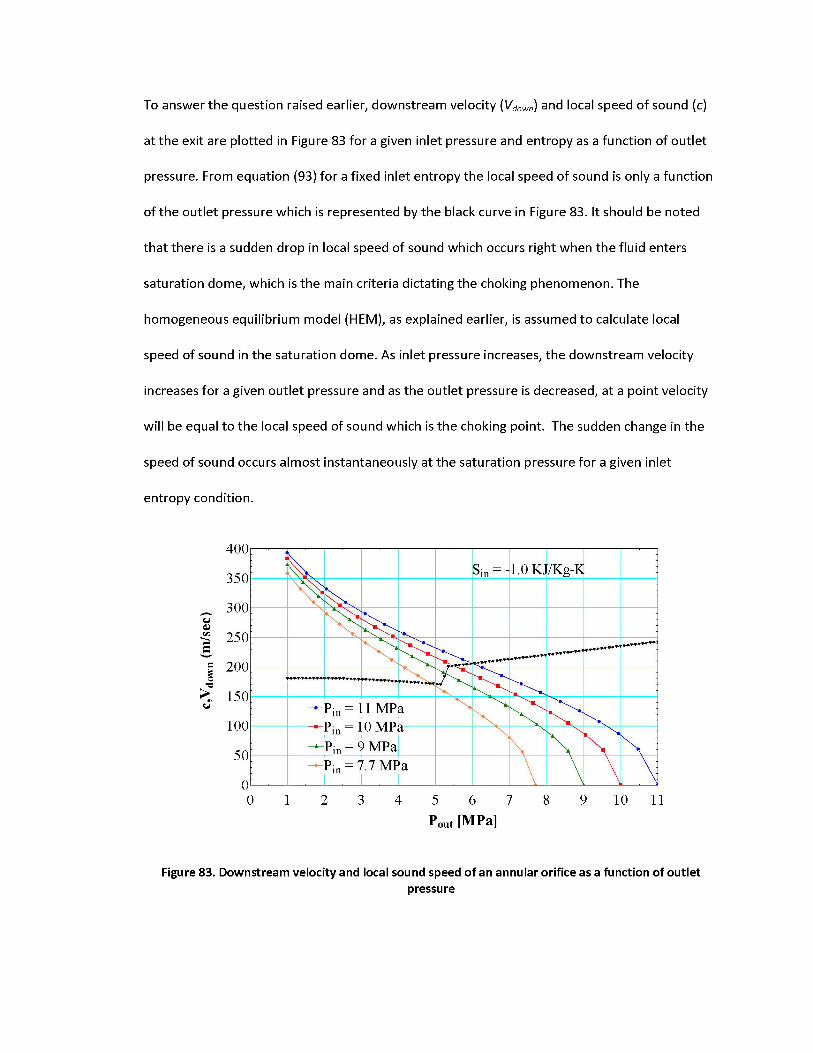
To answer the question raised earlier, downstream velocity (Vdown) and local speed of sound (c)
at the exit are plotted in Figure 83 for a given inlet pressure and entropy as a function of outlet
pressure. From equation (93) for a fixed inlet entropy the local speed of sound is only a function
of the outlet pressure which is represented by the black curve in Figure 83. It should be noted
that there is a sudden drop in local speed of sound which occurs right when the fluid enters
saturation dome, which is the main criteria dictating the choking phenomenon. The
homogeneous equilibrium model (HEM), as explained earlier, is assumed to calculate local
speed of sound in the saturation dome. As inlet pressure increases, the downstream velocity
increases for a given outlet pressure and as the outlet pressure is decreased, at a point velocity
will be equal to the local speed of sound which is the choking point. The sudden change in the
speed of sound occurs almost instantaneously at the saturation pressure for a given inlet
entropy condition.
4 5 6 7Pout [MPa]
10 112 3 8 9
Figure 83. Downstream velocity and local sound speed of an annular orifice as a function of outletpressure

From a general observation of Figure 83 it can be said that for a given inlet entropy condition,
there exists a range of inlet pressures for which the downstream velocity intersect the sound
speed curve very close to the saturation pressure. Following the above theory, inlet entropy is
varied from —0.75 KJ to —1.75 KJ with an increment of —0.05 KJ and the upper andKg-K Kg-K Kg-K
lower limit of inlet pressure for which the flow chokes at the saturation point is calculated for
each Sn. The results of the above calculations are presented in Figure 84 and the following
conclusions are made:
a) If the inlet condition is bounded by the two curves, the flow chokes very close to the
saturation point/ when flow enters the saturation dome.
b) If the inlet condition is above both the curves, the flow chokes before it enters the
saturation dome.
c) If the inlet condition is below both the curves, the flow chokes late into the
saturation dome.
CarbonDioxide400380360340
Upper limit Lower limit
320300280260240
0.2 0.4 0.6
220200
-2.25 -2.00 -1.75 -1.50 -1.25 -1.00 -0.75 -0.50s[kJ/kg-K]
Figure 84. Choking theory for isentropic flow.
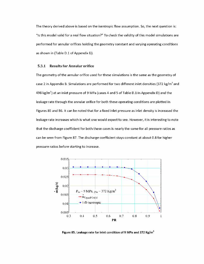
The theory derived above is based on the isentropic flow assumption. So, the next question is:
"Is this model valid for a real flow situation?" To check the validity of this model simulations are
performed for annular orifices holding the geometry constant and varying operating conditions
as shown in (Table D.1 of Appendix D).
5.3.1 Results for Annular orifice
The geometry of the annular orifice used for these simulations is the same as the geometry of
case 2 in Appendix B. Simulations are performed for two different inlet densities (372 kg/m3 and
498 kg/m3) at an inlet pressure of 9 MPa (cases 4 and 5 of Table D.1 in Appendix D) and the
leakage rate through the annular orifice for both these operating conditions are plotted in
Figures 85 and 86. It can be noted that for a fixed inlet pressure as inlet density is increased the
leakage rate increases which is what one would expect to see. However, it is interesting to note
that the discharge coefficient for both these cases is nearly the same for all pressure ratios as
can be seen from Figure 87. The discharge coefficient stays constant at about 0.8 for higher
pressure ratios before starting to increase.
0.035
0.03
0.025
0.02
Pin = 9 MPa, pin = 372 Kg/m'
mOpenFOAM
■ 1-D isentropic
0.015
0.01
0.0050.3 0.4 0.5 0.6 0.7 0.8 0.9
PR
Figure 85. Leakage rate for inlet condition of 9 MPa and 372 Kg/m3

0.035
0.03
0.025
0.02• S
0.015Pin = 9 MPa, pln = 498 Kg/m"
mOpenFOAM
1 -D isentropic0.01
0.0050.3 0.4 0.5 0.6 0.7 0.8 0.9
PR
Figure 86. Leakage rate for inlet condition of 9 MPa and 498 Kg/m3
1
0.95
0.9
0.85
0.8
0.75
0.7
0.650.3 0.4 0.5 0.6 0.7 0.8 0.9 1
PR
Figure 87. Cd for cases 4 and 5 in Table D.1 of Appendix D
Next, the inlet density is fixed as (372 kg/m3 and 498 kg/m3), the inlet pressure is increased to 10
MPa (case 3 in Table D.1 of Appendix D and case 2 in Appendix B) and the leakage rate through
the annular orifice for both these operating conditions is plotted in Figures (88 and 89). Again,
the leakage rate is higher for higher density case and the discharge coefficient is the same for
both these cases as shown in Figure 90.

0.045
0.04
0.035
0.03
0.025
■¥ 0.02
0.015
0.01
0.0050.3 0.4 0.5 0.6 0.7 0.8 0.9 1
PR
-----------------
*----....•. X\
\Pin = 10 MPa,
mOpenFOA
1-D isentr
Pin “ 372 Kg/m3 N\N■
M
opic\\
x-
Figure 88. Leakage rate for inlet condition of 10 MPa and 372 Kg/m3
0.045r
0.04
0.035
^ 0.03'm>
0.025• S
0.02
0.015
0.01
0.005[0.3
z//
I
X\ ,
Pin = 10 MPa,
mOpenFOA
1-D isentr
Pin - 498 Kg/m3 \\M
opic
0.4 0.5 0.6 0.7PR
0.8 0.9 1
Figure 89. Leakage rate for inlet condition of 10 MPa and 498 Kg/m3
It can be noted from a comparison of the discharge coefficient plots (Figures 87 and 90) that as
pressure increases, the increase in Cd from higher PR to lower PR decreases. In other words, as
the pressure increases, the discharge coefficient tends to stay constant over the whole range of

PR. In order to see if this is really true, the inlet pressure was increased to 11 MPa and
simulations (Cases 1 and 2 in Table D.1 of Appendix D) are performed for two inlet densities
(372 kg/m3 and 498 Kg/m3) and the results for leakage rate are presented in Figures (91 and 92).
The discharge coefficient for these two cases is plotted in Figure 93.
1
0.95
0.9
0.85
^ 0.8
0.75
0.7
0.650.3 0.4 0.5 0.6 0.7 0.8 0.9 1
PR
Figure 90. Cd for case 3 in Table D.1 and case 2 in Appendix B
It is interesting to note that discharge coefficient stays nearly constant at 0.8 for both these
cases which would mean that choking pressure ratio predicted by the simulations and isentropic
model are nearly the same.
One case very close to the critical pressure is simulated (case 6 in Table D.1). It can be seen from
the Cd plot, shown in Figure 94 that spread in the Cd is much higher for this case compared to
the high pressure cases (9, 10 or 11Mpa). Inlet conditions which are near the critical point are
particularly hard to simulate because they are very close to the saturation dome and tend to
deviate from the homogeneous equilibrium model as soon as they enter the saturation dome.
-------- A 10Mpa,372kg/m3
■ 10Mpa,498kg/m3
* 1 4 _______ ___ s___i ' ■ ■
As the discharge coefficient is only a function of the inlet pressure for inlet densities tested, it
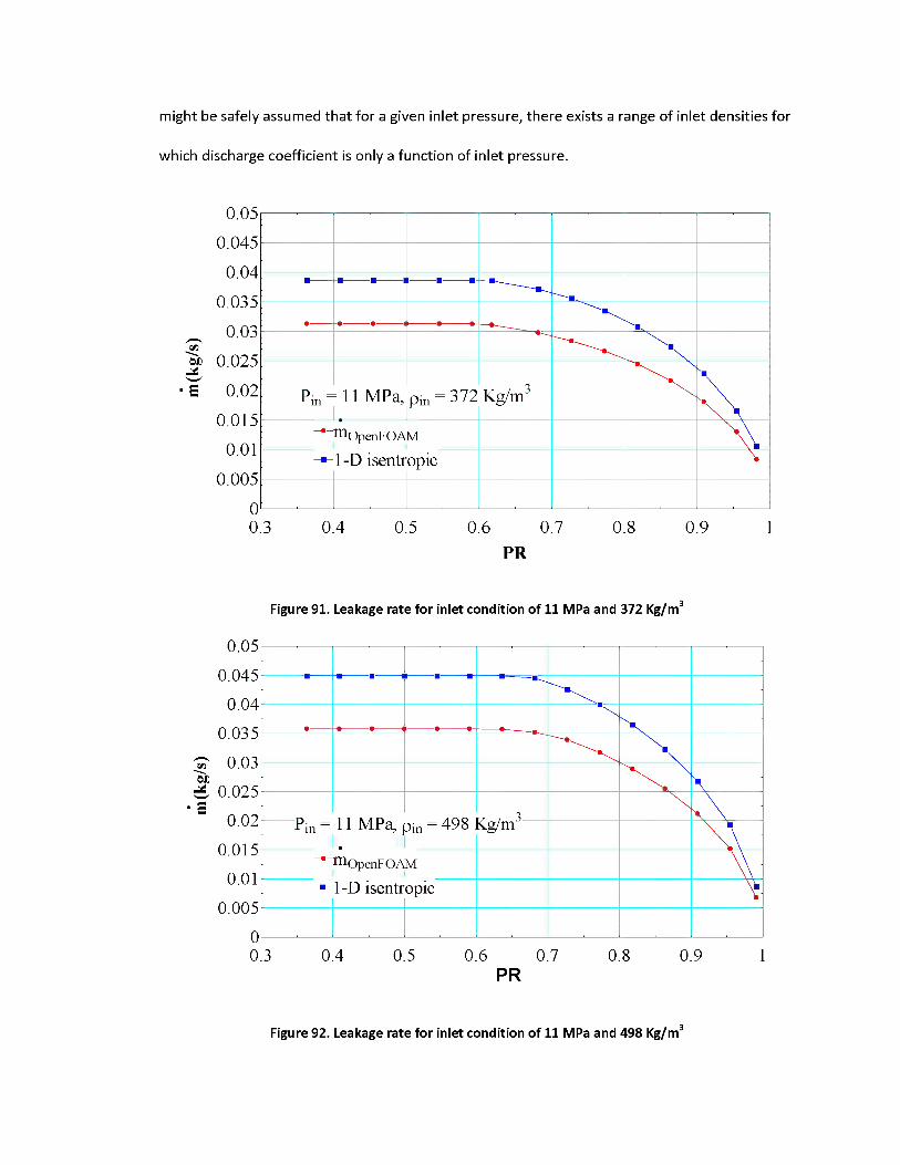
(s/Sjj)u
i |!i
-,S'll,u
might be safely assumed that for a given inlet pressure, there exists a range of inlet densities for
which discharge coefficient is only a function of inlet pressure.
0.05
0.045
0.04
0.035
0.03
0.025
0.02
0.015
0.01
0.005
00.3 0.4 0.5 0.6 0.7 0.8 0.9 1
PR
^ ' ‘ ■
3Xx ■
\Pin - 11 MPa, pin = 372 Kg/m3 XX\
mOpenFOA
1-D isentrM
opic X
Figure 91. Leakage rate for inlet condition of 11 MPa and 372 Kg/m3
0.05
0.045 0.04
0.035
0.03 0.025
0.02
0.015 0.01
0.005 00.3 0.4 0.5 0.6 0.7 0.8 0.9 1
PR
Xx
-^ri / /
x\
11 MPa,
mOpenFOA
Pin - 498
M
3\X
Pin - Kg/m
Xx■ 1-D isentropic Ye
Figure 92. Leakage rate for inlet condition of 11 MPa and 498 Kg/m3

1
■au
0.95
0.9
0.85
0.8
0.75
0.7
0.65L 0.3
11Mpa,37
11Mpa,49
3
! ■
2kg/m
)8kg/m3
■ ▲ ▲ A . k A A* A
■ ■ 6 i ± * ■ 8 ■
0.4 0.5 0.6 0.7PR
0.8 0.9
Figure 93. Cd for cases 1 and 2 in Table D.1 of Appendix D
■3
u
1
0.95
0.9
0.85
0.8
0.75
0.7
0.65L 0.3
▼ ▼ ▼ T ▼▼
▼▼
1 P Q\ o FT t > U>
T Y
▼
0.4 0.5 0.6 0.7 0.8PR
0.9
1
1
Figure 94. Cd for case 6 in Table D.1 of Appendix D
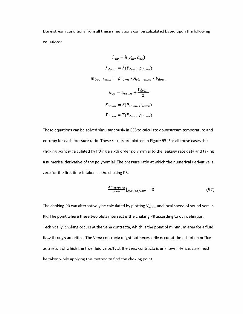
Downstream conditions from all these simulations can be calculated based upon the following
equations:
own
These equations can be solved simultaneously in EES to calculate downstream temperature and
entropy for each pressure ratio. These results are plotted in Figure 95. For all these cases the
choking point is calculated by fitting a sixth order polynomial to the leakage rate data and taking
a numerical derivative of the polynomial. The pressure ratio at which the numerical derivative is
zero for the first time is taken as the choking PR.
The choking PR can alternatively be calculated by plotting Vdown, and local speed of sound versus
PR. The point where these two plots intersect is the choking PR according to our definition.
Technically, choking occurs at the vena contracta, which is the point of minimum area for a fluid
flow through an orifice. The Vena contracta might not necessarily occur at the exit of an orifice
as a result of which the true fluid velocity at the vena contracta is unknown. Hence, care must
dw-curvefitdPR
(97)
be taken while applying this method to find the choking point.
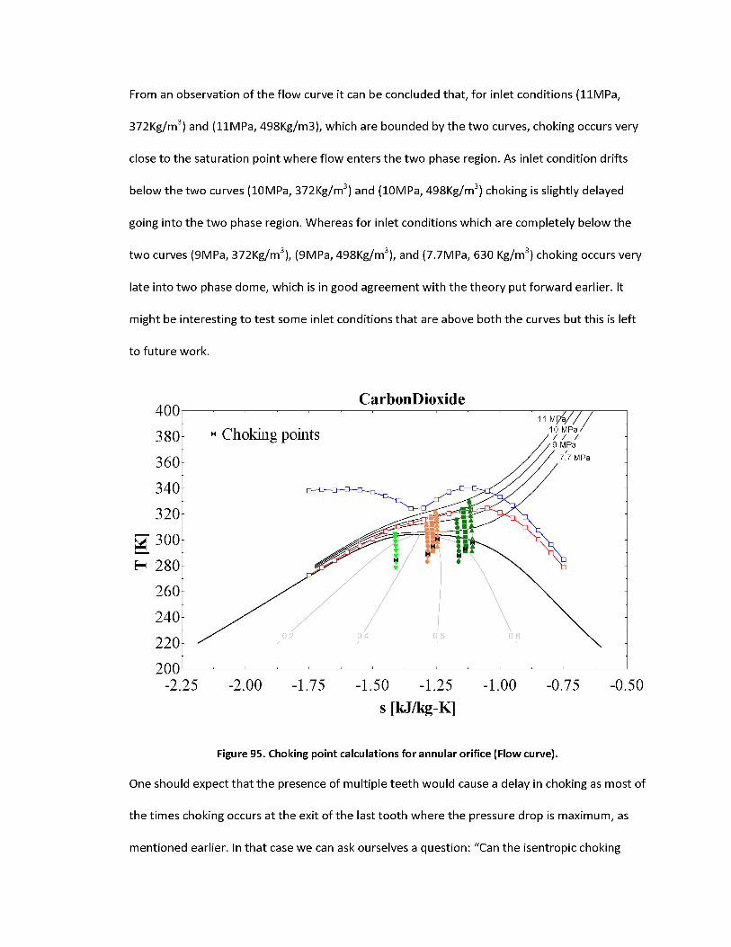
From an observation of the flow curve it can be concluded that, for inlet conditions (11MPa,
372Kg/m3) and (11MPa, 498Kg/m3), which are bounded by the two curves, choking occurs very
close to the saturation point where flow enters the two phase region. As inlet condition drifts
below the two curves (10MPa, 372Kg/m3) and (10MPa, 498Kg/m3) choking is slightly delayed
going into the two phase region. Whereas for inlet conditions which are completely below the
two curves (9MPa, 372Kg/m3), (9MPa, 498Kg/m3), and (7.7MPa, 630 Kg/m3) choking occurs very
late into two phase dome, which is in good agreement with the theory put forward earlier. It
might be interesting to test some inlet conditions that are above both the curves but this is left
to future work.
CarbonDioxide400
Choking points3809 MPa
/ 77 MPa360
340
320
300
260
2400.2 0.4 0.6 0.8
200-2.25 -2.00 -1.75 -1.50 -1.25 -1.00 -0.75 -0.50
s[kJ/kg-K]
Figure 95. Choking point calculations for annular orifice (Flow curve).
One should expect that the presence of multiple teeth would cause a delay in choking as most of
the times choking occurs at the exit of the last tooth where the pressure drop is maximum, as
mentioned earlier. In that case we can ask ourselves a question: "Can the isentropic choking

theory which worked well for annular orifices, be applied to labyrinth seals?" To answer this
question the geometry is held constant, which is the same as case 2 in Appendix C, and the inlet
operating conditions are varied. The inlet conditions simulated are the same as those used for
annular orifices so that a direct comparison can be made (cases 1-6 in Table D.2 of Appendix D,
case 2 in Appendix C).
5.3.2 Results for Labyrinth Seal
Three inlet densities (372, 498 and 630 Kg/m3) are simulated for an inlet pressure of 9 MPa
(cases 3-5 in Table D.2 of Appendix D) and leakage rate results for these three cases are
presented in Figures (96, 97 and 98).
0.045
0.04 0.035
0.03 0.025
Ml
0.02• s
0.015 0.01
0.005 00.3 0.4 0.5 0.6 0.7 0.8 0.9 1
PR
Figure 96. Leakage rate for inlet condition of 9 MPa and 372 Kg/m3
The discharge coefficient for all three cases is plotted in Figure 99. It is interesting to note that
the Cd for these inlet densities is nearly the same for all pressure ratios as observed in the case
of annular orifices. However, the Cd which is 0.8 for higher PR's in the case of an annular orifice
is now 0.6 for three teeth labyrinth seals indicating that the leakage rate has been reduced due
\\■——
9 M[Pa, 372 K g/m3 ■. \.g/m\\
1-D isentropic \\
to the presence of multiple constrictions.
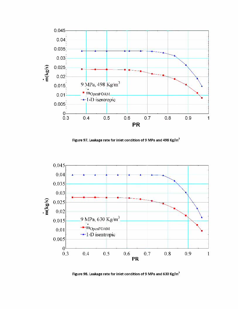
m(k
g/s)
m
(kg/
s)
0.045
0.04
0.035
0.03
0.025
0.02
0.015
0.01
0.005
00.3 0.4 0.5 0.6 0.7 0.8 0.9 1
PR
9 MPa, 498 Kg/m3
mOpenFOAM_____
-*-1-D isentropic
Figure 97. Leakage rate for inlet condition of 9 MPa and 498 Kg/m3
0.045
0.04
0.035
0.03
0.025
0.02
0.015
0.01
0.005
00.3 0.4 0.5 0.6 0.7 0.8 0.9 1
PR
\-- \■——■__ _
9 IMPa, 630 Kg/m3"x
\Xx■ mOpenFOAM
N-\
— 1-D isentropic
Figure 98. Leakage rate for inlet condition of 9 MPa and 630 Kg/m3

0.8
U
0.75
0.7
0.65
0.6
0.55
0.5
0.45
0.40.3 0.4 0.5 0.6 0.7 0.8 0.9 1
PR
▼ ▼ ▼ 1 1 m a I ■
■ ■s
—■—_
9 Mpa, 372 kg/m3 9 Mpa, 498 kg/m3 9 Mpa, 630 kg/m3
Figure 99. Cdfor an inlet pressure of 9 MPa (cases 3, 4 and 5 in Table D.1)
To see if this is true for other pressures as well, the pressure was increased to 10 MPa and two
inlet densities (372 Kg/m3 and 498 Kg/m3) are simulated (case 2 in Table D.1 and case 2 in
Appendix C). Results for the leakage rates are self-explanatory and are presented in Figures 100
and 101. The Cd for both these cases, plotted in Figure 102, collapse on to each other just like in
the case of annular orifices reassuring our claim that, there exists a range of inlet densities for
which Cd is only a function of inlet pressure.
One simulation was performed for an inlet pressure of 11MPa and density of 498 Kg/m3 (case1
in Table D.1 of Appendix D) to check if Cd stays constant over the whole range of PR's like in the
case of an annular orifice. The Cd for this case is presented in Figure 102 and it can be seen that
the Cd is not constant but is tending towards becoming constant. Further increase in pressure
should result in a constant Cd over the whole range of PR.

m(k
g/s)
m
(kg/
s)0.045
0.04
0.035
0.03
0.025
0.02
0.015
0.01
0.005
: ■------ ■------ 1 -------■-------
3
-------l \ ;
\10 MPa, 3/2 Kg/m X
mOpenFOAM \1-D isentronic
0[ 0.3 0.4 0.5 0.6 0.7
PR0.8 0.9
Figure 100. Leakage rate for inlet condition of 10 MPa and 372 Kg/m3
1
0.045
0.04
0.035
0.03
0.025
0.02
0.015
0.01
0.005
00.3 0.4 0.5 0.6 0.7 0.8 0.9 1
PR
x------ ■____ \\■------ 1 \
3 i\\
10 MPa, 498 Kg/m■
mOpenFOAM
1-D isentronic
\■
Figure 101. Leakage rate for inlet condition of 10 MPa and 498 Kg/m3

0.8
U
0.75
0.7
0.65
0.6
0.55
0.5
0.45
0.40.3 0.4 0.5 0.6 0.7 0.8 0.9 1
PR
9 9
▲ ■
' i 9 I
10 MPa, 372 Kg/m3
10 MPa, 498 Kg/m
Figure 102. Cd for an inlet pressure of 10 MPa.
0.8
0.75
0.7
0.65
U 0.6
0.55
0.5
0.45
0.40.3 0.4 0.5 0.6 0.7 0.8 0.9 1
PR
■ ■ ■ ■ ■ ■ B ■ ■ ■ ■■ '
11 MPa, 498 Kg/r■ n3
Figure 103. Cd for an inlet pressure of 11 MPa
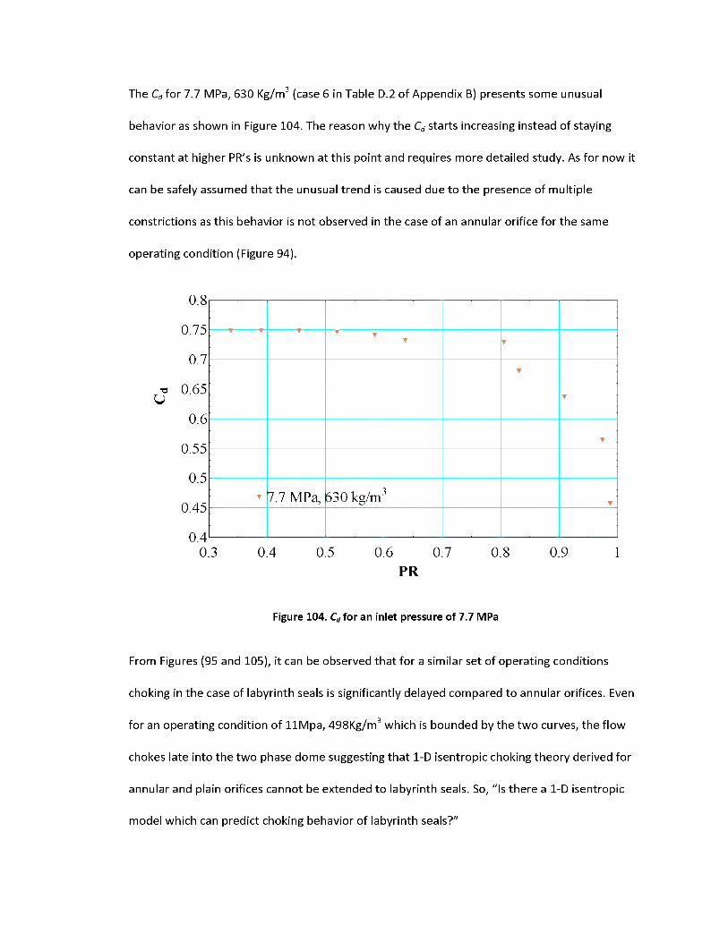
The Cd for 7.7 MPa, 630 Kg/m3 (case 6 in Table D.2 of Appendix B) presents some unusual
behavior as shown in Figure 104. The reason why the Cd starts increasing instead of staying
constant at higher PR's is unknown at this point and requires more detailed study. As for now it
can be safely assumed that the unusual trend is caused due to the presence of multiple
constrictions as this behavior is not observed in the case of an annular orifice for the same
operating condition (Figure 94).
0.8
0.75
0.7
0.65U
0.6
0.55
0.5
0.45
0.40.3 0.4 0.5 0.6 0.7 0.8 0.9 1
PR
Figure 104. Cd for an inlet pressure of 7.7 MPa
From Figures (95 and 105), it can be observed that for a similar set of operating conditions
choking in the case of labyrinth seals is significantly delayed compared to annular orifices. Even
for an operating condition of 11Mpa, 498Kg/m3 which is bounded by the two curves, the flow
chokes late into the two phase dome suggesting that 1-D isentropic choking theory derived for
annular and plain orifices cannot be extended to labyrinth seals. So, "Is there a 1-D isentropic
T ▼ ▼ ▼
▼
▼
▼
▼ 7.7 MPa, 630 kg/m" ▼
model which can predict choking behavior of labyrinth seals?"
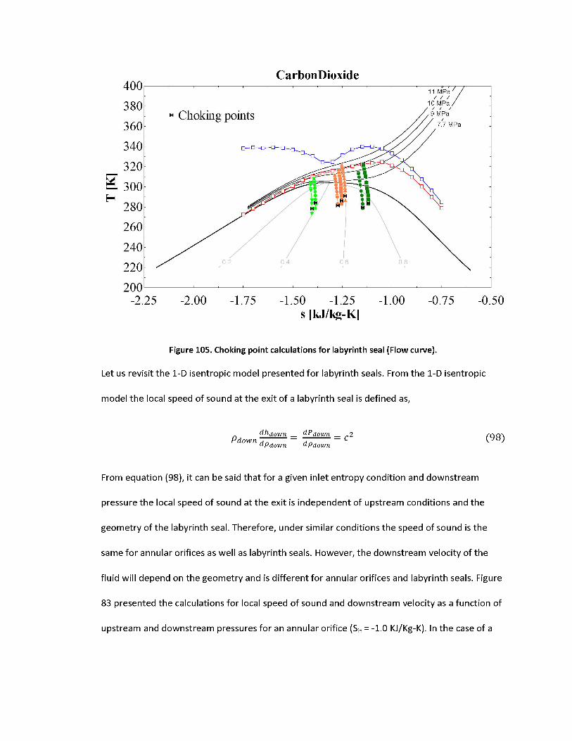
CarbonDioxide400
11 MPa / / /
10 MPa380Choking points 9 MPa
360 7.7 MPa
340
320
300
280
260
2400.2 0.4 0.6 0.8
220
200-2.25 -2.00 -1.75 -1.50 -1.25 -1.00 -0.75 -0.50
s [kJ/kg-K]
Figure 105. Choking point calculations for labyrinth seal (Flow curve).
Let us revisit the 1-D isentropic model presented for labyrinth seals. From the 1-D isentropic
model the local speed of sound at the exit of a labyrinth seal is defined as,
From equation (98), it can be said that for a given inlet entropy condition and downstream
pressure the local speed of sound at the exit is independent of upstream conditions and the
geometry of the labyrinth seal. Therefore, under similar conditions the speed of sound is the
same for annular orifices as well as labyrinth seals. However, the downstream velocity of the
fluid will depend on the geometry and is different for annular orifices and labyrinth seals. Figure
83 presented the calculations for local speed of sound and downstream velocity as a function of
upstream and downstream pressures for an annular orifice (Sin = -1.0 KJ/Kg-K). In the case of a

labyrinth seal, equations (75 - 84) are used to calculate the downstream velocity and the results
are presented in Figure 106 for Sin = -1.0 KJ/Kg-K.
450
400
350
300
250
200>
150
100
50
0
kPin = Pin =Pm = Pm = Pm =
11 MPa12 MPa13 MPa14 MPa15 MPa
% in = -1.0 KJ/Kgy-K"
O ?K
XBL,5
X \
0 1 2 3 4 5 6 7 8 9 10 11 12 13 14Pout [MPa]
Figure 106. Downstream velocity of labyrinth seal and local sound speed as a function of outletpressure
Figures 83 and 106 indicate that for an inlet pressure of 11MPa, the 1-D isentropic model for
labyrinth seals chokes in the saturation dome and the 1-D isentropic model for an annular orifice
chokes above the saturation dome. Therefore, the curves developed using 1-D isentropic
choking model for annular orifices cannot be extended to labyrinth seals. However, from a
general observation of Figure 106 it can be said that there exists a range of inlet pressures for
which the downstream velocity curve intersects the sound speed curve very close to the
saturation pressure. Following this theory, the inlet entropy can be varied and the upper and
lower limit of the inlet pressure for which the flow chokes at saturation point can be calculated
for each inlet entropy. This would result in two different sets of curves but the conclusions made
for annular orifices are still valid in the case of labyrinth seals.

6 Heat transfer characteristics of supercritical CO2
This chapter describes the third task of this report, which is to investigate the heat transfer
characteristics of S-CO2. The first section of this chapter provides the details of the experimental
facility constructed to achieve this task. This is followed by the validation results of the facility
using distilled water. Finally, the experimental results will be presented to investigate the effects
on buoyancy on heat transfer characteristics of supercritical carbon dioxide.
6.1 Experimental facility overview
The schematic of the experimental facility and test section is shown in Figure 107. The loop
consists of a liquid CO2 cylinder, high pressure liquid chromatography (HPLC) pump, circulation
pump, Coriolis flow meter, high pressure CO2 preheater, test section, high-pressure CO2 cooler,
DC power supply, buffer tank, and data acquisition system.
Pre heater Coriollis Flow meter
GearPumpDAQ System
WaterChillerpower supply
Test section
Figure 107. Schematic of the experimental facility and the test section

System operating pressure is monitored and controlled by a Scientific Systems, Inc. SFC-24,
positive displacement, constant pressure HPLC pump (S10SNXP1). It is capable of pressurizing
the system to 69 MPa (~10,000) psi, with an accuracy of ±2% of full scale. A buffer tank of
volume ~0.5 m3 is used to increase the system volume and minimize the pressure fluctuations in
the loop due to the temperature fluctuations from the chiller.
The circulation pump is a Micropump (GLH25) magnetically driven gear pump. It is capable of
handling flow rates between 0.6-7.0 GPM, a differential pressure of 0.86 MPa (~125 psi), and a
maximum operating pressure of 10.35 MPa (~1500 psi). This pump is coupled to Baldor variable
frequency drive and this in conjunction with a throttling valve is used to precisely control the
mass flow rate in the loop.
A Micro Motion Coriolis flow meter (F025P) and transmitter are used to measure the mass flow
rate in the system. The flow meter is capable of measuring flow rates up to 0.27 kg/sec with an
accuracy of ±0.1% full scale. Measurements from the flow meter serve as a feedback control for
the variable frequency drive.
Temperatures in the loop excluding the test section are controlled using a high-pressure CO2
preheater and cooler. In the preheater, CO2 splits into two tubes that run next to a 5.5 kW
cartridge heater. This preheater is used to raise the temperature of CO2 to the desired test
section inlet temperature. Upon exiting the test section, the CO2 enters into a high pressure
cooler where excess heat is removed facilitating the pump to move liquid-like CO2. The cooler is
a concentric tube-in-tube heat exchanger where the chilled water and CO2 run through the
outside and inside tubes respectively. Chilled water is provided using Advantage Engineering
(M1-1.5A) water chiller with a maximum cooling capacity of 1.5 refrigeration tons. Inlet and
outlet temperatures to the test section are measured by Omega 3 wire platinum RTDs having
maximum uncertainty of ±0.3 C. These RTDs are calibrated against boiling water and an ice bath
to quantify the systematic error. The pressure is monitored by Omega gauge pressure
transducers (PX309) within a manufacturer specified accuracy of ±0.25% of full scale accuracy.
Several K-type thermocouples are used in the loop to monitor the amount of energy that was
being put in or removed from the flow by each component.
The test section is a stainless steel 316 circular pipe with 12.7 mm OD, 10.9 mm ID, and is 1 m
long. Constant heat flux boundary condition is provided to the test section using a Magna-Power
electronics TSD10-500/480 DC power supply. The heat flux to the test section is varied by
adjusting the voltage between copper clamped terminals at the ends. The accuracy of voltage
control is ±0.01% of full scale and current control is ±0.04% of full scale. The test section is
electrically and thermally insulated from the rest of the loop by using Swagelok dielectric fittings
at each end of the test section.
Outer wall temperatures of the test section are measured using 20 E type stick on
thermocouples. Out of these 20 thermocouples, 10 thermocouples are mounted on the top side
and 10 on the bottom side at axial locations which are 75 mm apart from each other. The first
thermocouple is mounted 300 mm from the inlet side to allow for the flow to be
hydrodynamically fully developed. It should be noted that the perspective of top and bottom
side is with respect to horizontal orientation of the test section. These E-type thermocouples
have a manufacturer specified uncertainty of ±1.0 C or 0.4% of the measurement, whichever is
greater. Drift in wall thermocouples reading is minimized by performing specific in-situ
calibration under no heat flux conditions.
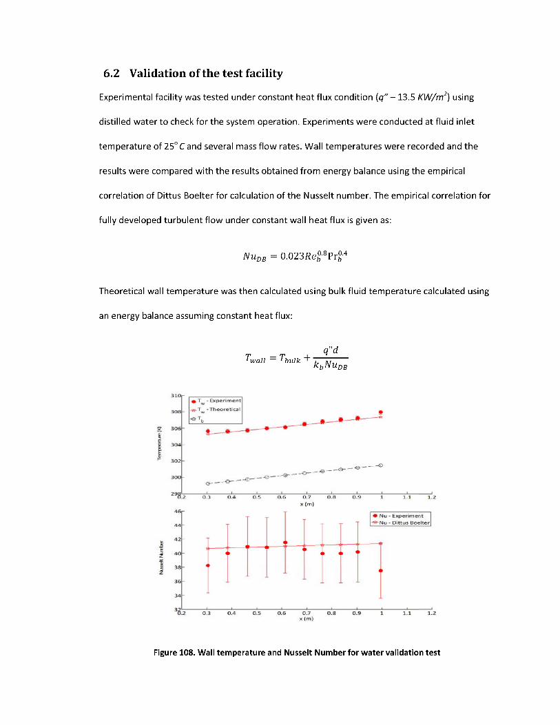
6.2 Validation of the test facility
Experimental facility was tested under constant heat flux condition (q" - 13.5 KW/m2) using
distilled water to check for the system operation. Experiments were conducted at fluid inlet
temperature of 25o C and several mass flow rates. Wall temperatures were recorded and the
results were compared with the results obtained from energy balance using the empirical
correlation of Dittus Boelter for calculation of the Nusselt number. The empirical correlation for
fully developed turbulent flow under constant wall heat flux is given as:
Nudb = 0.023fte£'8Pr£'4
Theoretical wall temperature was then calculated using bulk fluid temperature calculated using
an energy balance assuming constant heat flux:
Figure 108. Wall temperature and Nusselt Number for water validation test
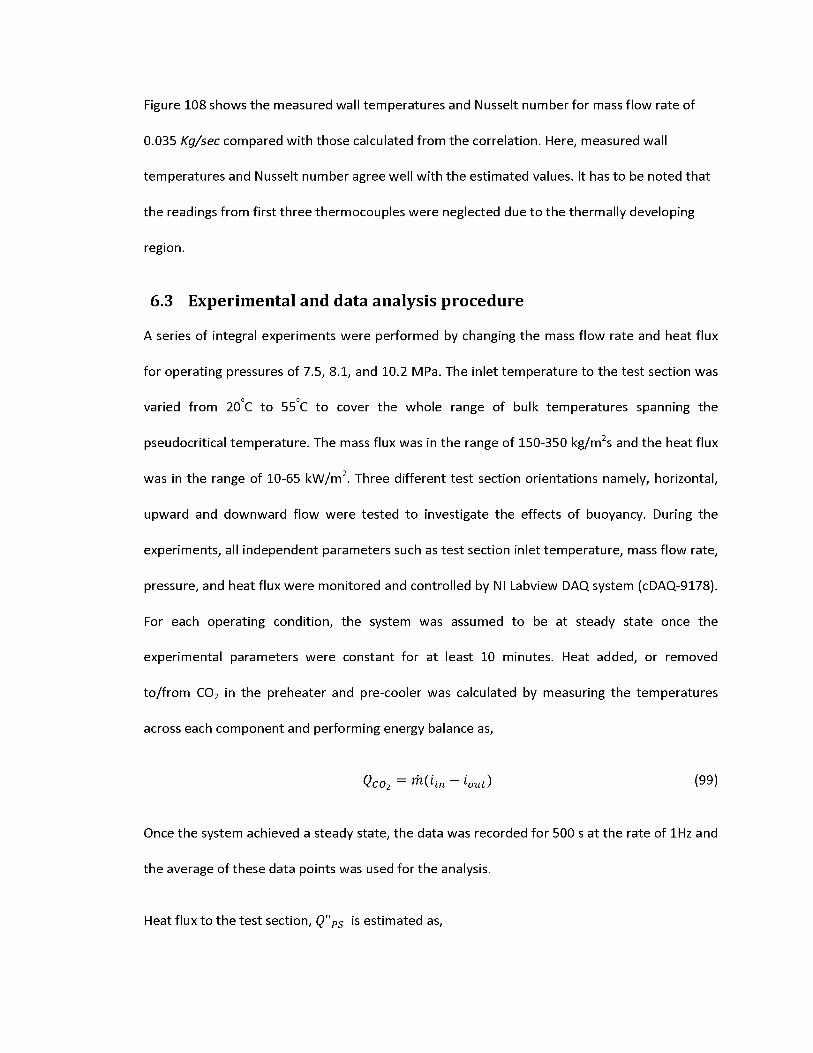
Figure 108 shows the measured wall temperatures and Nusselt number for mass flow rate of
0.035 Kg/sec compared with those calculated from the correlation. Here, measured wall
temperatures and Nusselt number agree well with the estimated values. It has to be noted that
the readings from first three thermocouples were neglected due to the thermally developing
region.
6.3 Experimental and data analysis procedure
A series of integral experiments were performed by changing the mass flow rate and heat flux
for operating pressures of 7.5, 8.1, and 10.2 MPa. The inlet temperature to the test section was
varied from 20°C to 55°C to cover the whole range of bulk temperatures spanning the
pseudocritical temperature. The mass flux was in the range of 150-350 kg/m2s and the heat flux
was in the range of 10-65 kW/m2. Three different test section orientations namely, horizontal,
upward and downward flow were tested to investigate the effects of buoyancy. During the
experiments, all independent parameters such as test section inlet temperature, mass flow rate,
pressure, and heat flux were monitored and controlled by NI Labview DAQ system (cDAQ-9178).
For each operating condition, the system was assumed to be at steady state once the
experimental parameters were constant for at least 10 minutes. Heat added, or removed
to/from CO2 in the preheater and pre-cooler was calculated by measuring the temperatures
across each component and performing energy balance as,
Qc02 rildin i-out) (99)
Once the system achieved a steady state, the data was recorded for 500 s at the rate of 1Hz and
the average of these data points was used for the analysis.
Heat flux to the test section, Q"PS is estimated as,

(100)Q PS —VPSIPS
nDL
Outer wall temperatures are measured and inner wall temperatures are estimated by using a
simple one-dimensional, steady-state conduction equation,
T ■ = T + ■1 wi 1u/n 14kss (¥) -(it)
Q {Dout\ (£out\2kss v 2 / \ D[n )
(101)
Where q is the volumetric heat rate (W/m3) expressed as,
• _ VPSIPS
^ [^2out-Dfn)L\ (102)
Using the assumption of constant heat flux, the bulk fluid temperature at the locations of the
thermocouples was obtained by performing an energy balance on a differential control volume,
and using the following equations [41],
TM=Tb+^nDX
The local heat transfer coefficient was then defined by,
h= fQps 'A(Twi Tfo)
Finally, the experimental local Nusselt number was determined as,
NubhD
kb
(103)
(104)
(105)
6.3.1 Uncertainty analysis
Using the method proposed by Kline and McClintock [42], the uncertainty in the measurement
of the heat transfer coefficient can be expressed as follows,
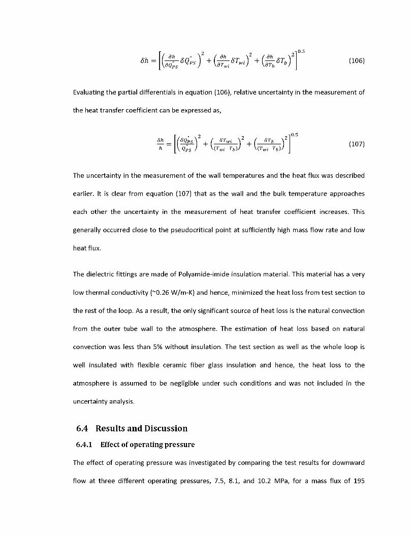
(106)
Evaluating the partial differentials in equation (106), relative uncertainty in the measurement of
the heat transfer coefficient can be expressed as,
The uncertainty in the measurement of the wall temperatures and the heat flux was described
earlier. It is clear from equation (107) that as the wall and the bulk temperature approaches
generally occurred close to the pseudocritical point at sufficiently high mass flow rate and low
heat flux.
The dielectric fittings are made of Polyamide-imide insulation material. This material has a very
low thermal conductivity (~0.26 W/m-K) and hence, minimized the heat loss from test section to
the rest of the loop. As a result, the only significant source of heat loss is the natural convection
from the outer tube wall to the atmosphere. The estimation of heat loss based on natural
convection was less than 5% without insulation. The test section as well as the whole loop is
well insulated with flexible ceramic fiber glass insulation and hence, the heat loss to the
atmosphere is assumed to be negligible under such conditions and was not included in the
uncertainty analysis.
6.4 Results and Discussion6.4.1 Effect of operating pressure
The effect of operating pressure was investigated by comparing the test results for downward
(107)
each other the uncertainty in the measurement of heat transfer coefficient increases. This
flow at three different operating pressures, 7.5, 8.1, and 10.2 MPa, for a mass flux of 195
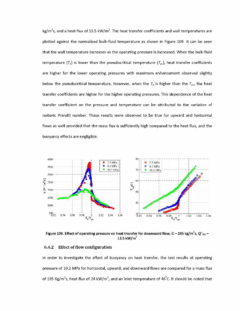
kg/m2s, and a heat flux of 13.5 kW/m2. The heat transfer coefficients and wall temperatures are
plotted against the normalized bulk-fluid temperature as shown in Figure 109. It can be seen
that the wall temperature increases as the operating pressure is increased. When the bulk-fluid
temperature (Tb) is lower than the pseudocritical temperature (Tpc), heat transfer coefficients
are higher for the lower operating pressures with maximum enhancement observed slightly
below the pseudocritical temperature. However, when the Tb is higher than the Tpc, the heat
transfer coefficients are higher for the higher operating pressures. This dependence of the heat
transfer coefficient on the pressure and temperature can be attributed to the variation of
isobaric Prandtl number. These results were observed to be true for upward and horizontal
flows as well provided that the mass flux is sufficiently high compared to the heat flux, and the
buoyancy effects are negligible.
Tb/Tp Tb/T
Figure 109. Effect of operating pressure on heat transfer for downward flow, G - 195 kg/m2s, Q"PS -13.5 kW/m2
6.4.2 Effect of flow configuration
In order to investigate the effect of buoyancy on heat transfer, the test results at operating
pressure of 10.2 MPa for horizontal, upward, and downward flows are compared for a mass flux
of 195 Kg/m2s, heat flux of 24 kW/m2, and an inlet temperature of 46 C. It should be noted that

this inlet temperature is close to the pseudocritical temperature for 10.2 MPa. Figure 110 shows
the variation of heat transfer coefficient and wall temperature along the length of the tube.
In the case of horizontal flow, it has been observed that the wall temperatures on the top side
are significantly higher than the wall temperatures on the bottom side indicating that there is a
circumferential variation in the wall temperature. This was particularly true when Tb < Tpc < Tw.
Under these conditions, the density of CO2 near the wall is significantly lower than the density of
CO2 in the bulk of the flow and hence, the buoyancy effects become prominent. This density
gradient causes the low density CO2 to rise from the bottom side of the tube thereby, enhancing
the heat transfer on the bottom side whereas the top side is covered by a blanket of CO2 having
low thermal conductivity deteriorating the heat transfer on the top side. This phenomenon has
been experimentally observed in previous horizontal flow studies on supercritical water [43-45]
and supercritical CO2 [46]. The circumferential variation in wall temperature was observed to be
more pronounced at low mass flux and high heat flux.
3000120
2500110
2000100
1500
1000 80
500 70
0.2 0.4 0.6 0.8 1.2 0.4 0.6 0.8 1.2
■ Horizontal flow - top ► Horizontal flow - bottom • Upward flow ^ Downward flow
■ Horizontal flow - top ► Horizontal flow - bottom • Upward flow ^ Downward flow
x(m) x(m)
Figure 110. Effect of flow configuration on heat transfer for p - 8.1 MPa, G - 195 kg/m2s, Q"PS -24kW/m2, Tin - 46°C
In the case of upward flow, localized peaks in the wall temperature were observed as can be
seen from the wall temperature profile of upward flow in Figure 110. This severe localized
deterioration was observed initially by Shitsman [47], Ackerman [48], and was originally
believed to be similar to the film boiling phenomenon at subcritical pressures. However,
experiments [49], [50] showed occurrence of localized peaks even when the wall temperature
was well below the pseudocritical temperature. These conditions should result in a liquid like
blanket in the near wall-region and hence, does not support the theory of film boiling.
These localized peaks often referred to as "buoyancy peaks" occur as a result of modification of
turbulent shear stress by the buoyancy forces acting on the flow [51]. It is believed that, as the
fluid is heated along the tube, the density difference between the near wall region and the bulk
flow increases as a result of which the boundary layer experiences a buoyancy force due to its
reduced density. In case of upward flow, this buoyancy force opposes the wall shear stress
reducing the turbulence production. As the boundary layer grows, for a particular boundary
layer thickness, there might occur a situation where the wall shear stress is balanced by the
buoyancy force and at this point the bulk flow is de-coupled from the wall causing the wall
temperature to spike. As the buoyancy force increases further, a region of negative shear stress
develops resulting in formation of an "M-shaped" velocity profile restoring turbulence
production and hence, the wall temperature decreases after the spike.
Experimental evidence of the "M-shaped" velocity profile was provided [52-55] using pitot tubes
and micro thermocouples. Bourke and Pulling [53], showed formation of "M-shaped" profile
after the spike in wall temperature, whereas Kurganov et al. [55] found that the "M-shaped"
profile occurred at the spike in wall temperature.
In the case of downward flow, the buoyancy force acts in the direction of wall shear stress
increasing the turbulence production and thereby, enhancing the heat transfer compared to the
values where buoyancy is absent. As can be seen from Figure 110, wall temperatures for the
downward flow don't exhibit any localized peaks and are significantly lower than that of the
upward flow.
6.4.3 Effect of inlet temperature
It is expected that the effect of buoyancy on heat transfer is influenced by the inlet temperature
due to variation in both radial and axial properties. In order to investigate this effect, wall
temperatures are recorded for different inlet temperatures at operating pressure of 7.5 MPa,
mass flux of 320 kg/m2s, and heat flux of 24 kW/m2 are compared. These plots are shown in
Figure 111 for horizontal, upward, and downward flows.
In the case of horizontal flow, for inlet temperature below the pseudocritical temperature (for
instance, Tin=20 C), it has been observed that the wall temperatures on the top side are
significantly higher than the wall temperatures on bottom side as discussed in the previous
section. However, when the inlet temperature was raised above the pseudocritical temperature
(for instance, T,n=36.5 C), the difference between the top and bottom surface temperatures
reduced as can be seen from Figure 111. This is because as the Tb moves away from the Tpc, the
CO2 bulk density nearly approaches the value of density at the wall and the buoyancy effects are
minimized [45]. It is expected that with further increase in the inlet temperature, the
temperature difference between top and bottom sides will nearly be zero. However, due to
limitations of the current test facility, this phenomenon could not be tested but was
experimentally proven for supercritical water by Bazargan et al. [45].

Horizontal flow - top75
70
65
60
55
50
45
35
30„20 25 30 35 40 45
Tb(C)50 55 60
Horizontal flow - bottom75
70
65
60
55
50
45
40
35
30 L 20
f \ i-B-Tin=20o C
-e-Tin=26o C
-6-Tm=29.5o C
Tin=31.25o C
-+■ Tin=32.5o C
-V-Tin=36.5o C
/40f
*
25 30 35 40 45Tb(C)
50 55 60
Upward flow Downward flow75
70
65
60
45
40
35
3020 25 30 35 40 45
Tb(C)50 60
75
70
65
60
50
45
40
3020 25 30 35 40 45 50 55
Tb(C)60
Figure 111. Effect of inlet temperature on the wall temperatures for p - 7.5 MPa, G - 320 kg/m2s, Q"PS-24 kW/m2
It is also interesting to note that as the inlet temperature is changed, severe discontinuity in the
wall temperature was observed. This effect was more pronounced on the top side than on the
bottom side. It is believed that this could be due to the effect of thermal entry length which is
not well defined in the case of supercritical fluids. For constant property fluids, thermal entry
length is defined as the tube length required to achieve constant radial temperature
distribution. From this perspective, the thermal entry length in the case of supercritical fluids
can be very long or in some cases impossible to achieve due to continuous radial and axial
variation in thermophysical properties along the tube length [56]. The effect of thermal
entrance length was less pronounced as the bulk temperature moves away from the
pseudocritical temperature due to less variation in properties.
In the case of upward flow, sharp localized peaks are observed for inlet temperature below the
pseudocritical temperature as discussed earlier. However, when the inlet temperature was
raised above the pseudocritical temperature (for instance, T,„=32.5 C), there was no evidence of
localized peaks. In this case, the density of bulk CO2 is nearly the same as density of CO2 in the
near wall region. As a result of this, the boundary layer doesn't experience significant opposing
buoyancy force and hence, the turbulence production is not affected irrespective of flow
direction. In fact, the wall temperatures for both upward and downward flows were observed to
be similar as can be seen from Figure 111. It can also be seen that the location of localized peaks
can be readily changed by varying the fluid inlet temperature. For instance, spike in wall
temperature for inlet temperature of 20 C occurred at the location of second thermocouple
whereas for inlet temperature of 26°C it occurred at the location of first thermocouple. Hence,
as the inlet temperature increases, the localized peaks in wall temperature appear to move
towards the inlet of the tube. This can again be attributed to the thermal entrance length effects
[57], [58] and was observed to be true for all the test cases.
It is also interesting to note the steep increase in wall temperature in the case of downward
flow for inlet temperatures close to the pseudocritical temperature. This was also observed on
the bottom side of the tube in the case of horizontal flow under similar conditions. This could be
due to a phenomenon which is similar to film boiling at subcritical pressures and is often
referred to as "pseudo-film" boiling phenomenon in literature [48].

6.4.4 Effect of heat flux
In order to investigate the effect of heat flux and pseudo-film boiling phenomenon further, tests
were conducted for downward flow at operating pressure of 7.5 MPa, mass flux of 195 Kg/m2s
for varying heat fluxes. The results are presented in Figure 112 in the form of the wall
temperatures and heat transfer coefficients versus the bulk temperatures for different heat
fluxes.
For low heat flux cases (Q"PS - 13.5, and 24 kW/m2), the energy input to the test section was not
sufficient to span the pseudocritical region. As a result, inlet temperature was changed to span
the pseudocritical region and hence, it was initially believed that the sharp increase in wall
temperature was due to the thermal entrance length effects. However, for high flux cases (Q"PS
- 50, and 62.5 kW/m2), the energy input to the test section is high enough to span the
pseudocritical region and the sharp increase in wall temperature was still observed as can be
seen from Figure 112.
4500
4000
3500
| 3000
2500U£ 2000
1500H1000
5000.96 0.98
Jtil
Q”- 13.5 KW/m2 Q”- 24.0 KW/m2 Q”- 50.0 KW/m2 Q”- 62.5 KW/m2
#• 9 e1 1.02 1.04 1.06 1.08
Normalized Temperature, Tb/Tpc [-]1.1
200
180
160
140
120
100
80
60
40
2020 30 40 50
Tb(C)60 70 80
Figure 112. Effect of heat flux on downward flow heat transfer for p - 7.5 MPa, G- 195 kg/m2s

This indicates that the phenomenon is due to pseudo-film boiling and not due to the thermal
entrance length or buoyancy effects. It should also be noted that the heat transfer
enhancement reduces with increase in heat flux. As the heat flux increases, the region of the
maximum specific heat moves away from the boundary layer and hence, it is easier to overcome
the region of highest specific heat. In other words, the area integrated values of specific heat
decrease near the pseudocritical region causing a reduction in enhancement.
6.4.5 Buoyancy criteria
As seen in previous sections, the heat transfer to supercritical CO2 is quite different than that of
heat transfer to constant property fluids. One of the reasons for this unusual heat transfer can
be associated with the effect of buoyancy due to large variations in axial and radial density
profiles. Hence, it is important to identify the conditions for which the effects of buoyancy are
significant and also differentiate these effects from other unusual heat transfer phenomenon.
The effects of buoyancy can be effectively quantified based on Grashof number which
represents the ratio of buoyancy forces to viscous forces and is defined as,
Gr = gP(Tw-T„)D3 (108)
Buoyancy parameters based on the variants of Grashof number are suggested in literature both
for horizontal and vertical flows. In order to investigate the influence of buoyancy,
experimentally determined Nusselt numbers are normalized with respect to Jackson's
correlation [59] and compared with the existing buoyancy criteria. Jackson's correlation as
shown in equation (109) is proven to best capture the heat transfer to S-CO2 under forced
convection conditions in the absence of buoyancy effects or any sort of deterioration.
Nujackson = 0.0183Re°'82Pr°'5 (^)°'3 (109)

Where the subscript n is proposed as,
n = 0.4, for Tb < Tw< TPc and 1.2TpC < Tb < Tw
n = 0.4 + 0.2^-l), for Tb < Tw< TpC
n = 0.4 + 0.2 Q^-ljM-S^-lH for TpC < Tb < 1.2Tpc
Jackson [58] suggested a buoyancy parameter, Bu, for vertical flows which was derived from
boundary layer theory taking into account the property variations:
Bu — CBBobFVP1FVP3FVP 4 (110)
Corresponding terms in equation (110) are defined as,
Bob GrbRe2.625pr0.4
FVpi —
FvP3
Pvpa —Pb~Pav
Pb~Pw
It was suggested that for CB value of 4600, the flow can be assumed to be in forced convection
regime if the parameter suggested in equation (110) is less than 0.04. This criterion was
investigated for our upward and downward flow data. The results are presented in Figure 113,
where the normalized Nusselt numbers obtained from the experiments were plotted against the
Jackson's non-dimensional buoyancy parameter, Bu. The red (circle), blue (square), and green
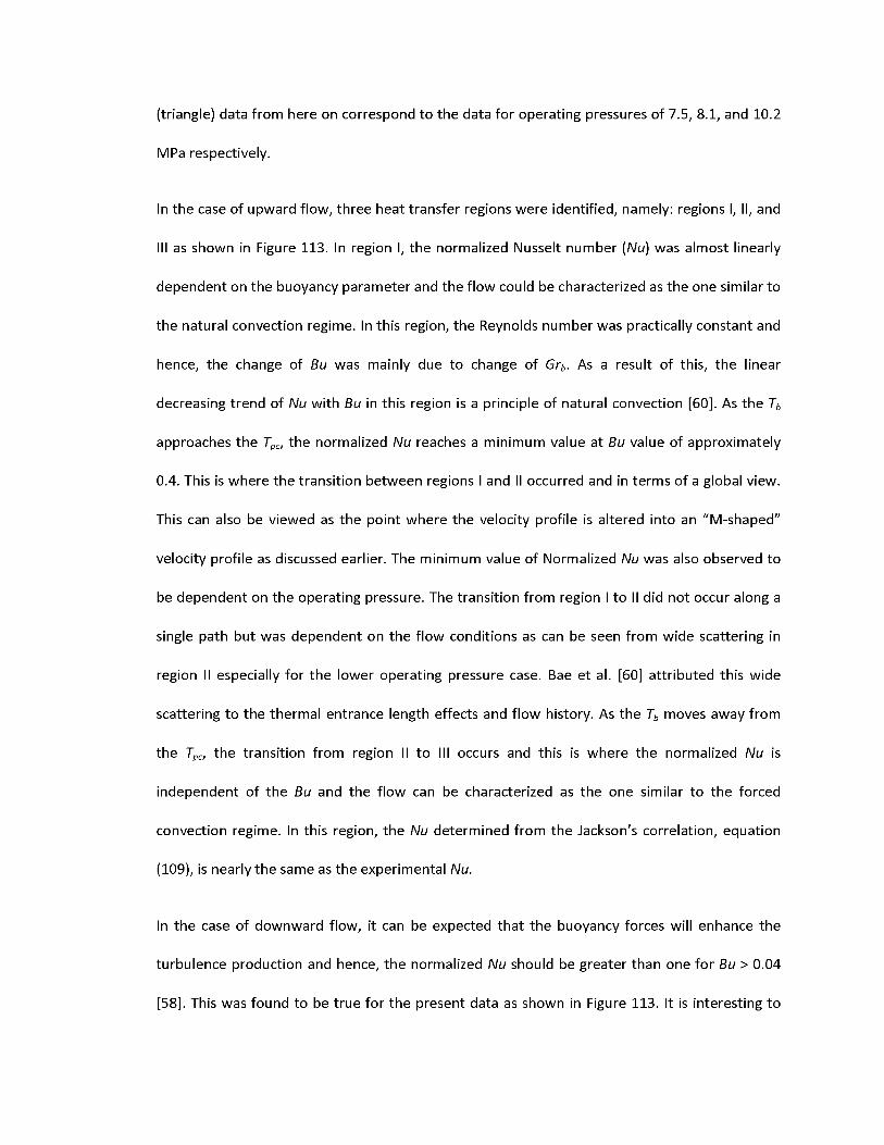
(triangle) data from here on correspond to the data for operating pressures of 7.5, 8.1, and 10.2
MPa respectively.
In the case of upward flow, three heat transfer regions were identified, namely: regions I, II, and
III as shown in Figure 113. In region I, the normalized Nusselt number (Nu) was almost linearly
dependent on the buoyancy parameter and the flow could be characterized as the one similar to
the natural convection regime. In this region, the Reynolds number was practically constant and
hence, the change of Bu was mainly due to change of Grb. As a result of this, the linear
decreasing trend of Nu with Bu in this region is a principle of natural convection [60]. As the Tb
approaches the Tpc, the normalized Nu reaches a minimum value at Bu value of approximately
0.4. This is where the transition between regions I and II occurred and in terms of a global view.
This can also be viewed as the point where the velocity profile is altered into an "M-shaped"
velocity profile as discussed earlier. The minimum value of Normalized Nu was also observed to
be dependent on the operating pressure. The transition from region I to II did not occur along a
single path but was dependent on the flow conditions as can be seen from wide scattering in
region II especially for the lower operating pressure case. Bae et al. [60] attributed this wide
scattering to the thermal entrance length effects and flow history. As the Tb moves away from
the Tpc, the transition from region II to III occurs and this is where the normalized Nu is
independent of the Bu and the flow can be characterized as the one similar to the forced
convection regime. In this region, the Nu determined from the Jackson's correlation, equation
(109), is nearly the same as the experimental Nu.
In the case of downward flow, it can be expected that the buoyancy forces will enhance the
turbulence production and hence, the normalized Nu should be greater than one for Bu > 0.04
[58]. This was found to be true for the present data as shown in Figure 113. It is interesting to

note the region I for downward flow, where deterioration was observed, contrary to the
generally understood belief that deterioration does not occur in a downward flow. Most of the
data in this region is the data having Tb close to the Tpc and operating pressure of 7.5 MPa.
1.61.41.2
1
0.8
°.6
0.4
0.210 10 10 10
Bu
BuFigure 113. Normalized Nusselt number versus Jackson's buoyancy parameter, Bu

Hence, this data can be classified as the deterioration data for downward flow due to the
pseudo-film boiling phenomenon as discussed earlier. This deterioration was not observed for
higher operating pressures as can be seen from gradual increase in wall temperature around the
pseudocritical region in Figure 109. Hence, excluding region I, it can be safely assumed that the
Normalized Nu monotonically increases with Bu.
Recently a global parameter based on Froude number (Fr) was developed by Seo et al. [61] to
study the influence of buoyancy.
It was suggested by Licht et al. [62] that for inverse Froude number < 0.1, the buoyancy effects
buoyancy just like the Jackson's criterion for vertical flows.
For horizontal flows, Jackson [46] proposed a criterion to neglect the buoyancy effects and is in
the form of,
This criterion was tested by plotting the normalized Nu versus the Boj for both the top and
bottom sides of the test section as shown in Figure 114. For the top side, two regions of heat
transfer were identified, namely: regions I and II. In region I, the flow is dominated by natural
convection and the change of Reynolds number was found to be relatively small compared to
the change in Grb and normalized Nu was found to almost linearly increase with decrease in the
(111)
are negligible. This criterion was verified using the current data for upward and downward
flows. It has been found out that the criterion can satisfactorily predict the influence of
(112)
Boj on a log-log plot.

Horizontal flow - Top side1.61.41.2
1ac
kson 0.8
S's
0.6
&Zs<: 0.4
0.2
J.
100 101 10 10
Bo,
10 10 10
S's
3s 0.7-
0.410 10 10 10 10 105 106
Boj
Figure 114. Normalized Nusselt number versus Jackson's buoyancy parameter, Boj
Transition from region I to II occurred at a Boj value of approximately 100. In region II, the Tb is
greater than the Tpc and the effects of buoyancy are minimized resulting in forced convection
heat transfer. The normalized Nu in this region is independent of the Bo values and the Nu
values predicted by the Jackson's correlation are nearly the same as the experimental values.
For the bottom side, no clear trend in normalized Nu was observed with respect to the Boj.
However, as the Boj is approaching 10, the normalized Nu values are approaching towards one
as suggested by Jackson [46]. Similar to the downward flow, a region of deteriorated heat
transfer was observed for the bottom side. This region, marked as region I, consists of data close
to the pseudocritical region for operating pressure of 7.5 MPa. This can again be attributed to
pseudo-film boiling phenomenon.
Petukhov et al. [63] studied horizontal flows and derived a threshold value of Grashof number,
Grth, above which the buoyancy effect can be neglected. Grth is defined as,
0 -7C-----0.5Grth = 3e — 5 Reb75Pr 1 + 2.4 Rebs Pr3 -1 (113)
Where,
pP _Tw — Tb \kb)
They also defined a Grashof number based on heat flux as,
Grq = 'Mjf- (114)
Where,
~o 1 /Pb~Pw\
Pfllm 'Tw-Tb'
Petukhov et al. [63] stated that the flow is completely dominated by forced convection for Grq <
Grth. When this criterion was applied to the present data, no clear trend in the data was
observed for either top or bottom sides. Although the criterion was not violated, Grq was found
to be greater than Grth for all the data points indicating that the buoyancy cannot be neglected

for any of the flow conditions. Hence, this criterion can be considered as a stringent test for
predicting the influence of buoyancy.
6.4.6 Evaluation of existing correlations
In this section, widely accepted correlations for supercritical fluids in literature will be evaluated.
Mokry et al. [64] proposed a correlation (equation (115)) for supercritical water using data
obtained in a vertical bare tube for upward flow at the Institute for Physics and Power
engineering (Russia).
____ 0 684 / n \ 0.564NuMokry = 0.0061Re£-904Prb' (&-) (115)
Pw
Although this correlation was developed with supercritical water, it performs equally well for
supercritical carbon dioxide as can be seen in Figure 115.
Horizontal Flow - Top side500
+30%400
300
200 -30%
100
200Nu Calculated
250 350
500 r
400
300
200sz
100
Upward Flow
50 100 150 200 250 300Nu Calculated
350
Figure 115. Calculated Nusselt number using Mokry et al. correlation
The correlation was able to capture over 95% of the data within ±30% accuracy for both upward
flow and the top side of horizontal flow. Extremely good agreement was observed at lower
Nusselt numbers, or the region of deteriorated heat transfer. Slightly higher standard deviation

was observed at higher Nusselt numbers where the data is dominated by forced convection. The
standard deviation was much higher when the same correlation was used to predict the Nusselt
numbers for downward flow and the bottom side of horizontal flows.
Swenson et al. [65] suggested a correlation (equation (116)) for upward flow of supercritical
water. This correlation is based on the wall properties and was reported that the correlation
performs equally good for supercritical CO2 as well. No evaluation of this correlation was
reported for downward flows. As can be seen in Figure 115, the Swenson et al. correlation was
able to capture over 90% data of the within ±30% accuracy.
Nuswenson = 0.0459Re™23Prw' (^) (116)Pb
Swenson correlation800
700
600
= 500
400
_-30%300
200
100
200 300 400Nu Calculated
500 600
Bishop correlation
Figure 116. Calculated Nusselt number for downward flow
Bishop et al. [66] suggested a correlation (equation (117)) based on bulk properties for upward
flow of supercritical water. It was reported that the correlation could be used for supercritical
CO2 as well [60]. As can be seen in Figure 116, this correlation was able to capture over 95% of
the data within ±30% accuracy.
____ 0 66 /n \ 0.43 / /n\\
Nubishop = 0.0069Re™Prb' (^) [l + 2.4(^)J (117)
It should be noted that the Swenson et al. correlation which is based on the wall properties over
predicted majority of downward flow data, whereas, the bishop et al. correlation which is based
on the bulk properties performed much better than the Swenson et al. correlation.
7 Wet Cooling tower option for S-CO2 Cycle
This chapter describes the final task of this report, which is to investigate the use of indirect wet
cooling tower option for an S-CO2 cycle. To perform this task a code was developed in
Engineering Equation Solver (EES) to estimate the tower dimensions, power and water
consumption, and to perform economic analysis. The first two sections of this chapter will
provide brief introduction to cooling towers and cooling tower theory. Third section will explain
the details of the code developed at Argonne National Laboratory (ANL) and finally results of the
investigation will be discussed.
7.1 Introduction to cooling towers7.1.1 Classification of cooling towers
Cooling towers can be classified into different categories as follows [67]:
Based on heat transfer mode
a) Dry towers in which the working fluid, in this case S-CO2, flows through finned coiled
sections and the air is blown over the coils. Hence, the working fluid is cooled totally by
the sensible heat transfer as there is no direct contact between air and the working
fluid. In such towers, the theoretically possible lowest temperature that can be achieved
is equal to the dry bulb temperature of ambient air.

b) Wet cooling towers or simply evaporative cooling towers operate on the principle of
evaporation. Heat from the working fluid is rejected to the circulating water in the
cooler and ultimately heat from the water is rejected to atmosphere through a wet
cooling tower. In a wet cooling tower, theoretically, the water can be cooled down to
the wet bulb temperature of ambient air.
c) Fluid coolers are hybrid towers in which the working fluid is passed through a tube
bundle, upon which water is sprayed and a fan-induced draft applied. The resulting heat
transfer performance is closer to that of a wet cooling tower.
Based on the air circulation
a) Natural draft towers are the large hyperbolic towers in which the air flow is produced by
the density differential between the heated air in the tower and the relatively cool
ambient air outside the tower. These towers have a very high capital costs due to their
large size and operate efficiently only in the regions of high relative humidity.
b) Mechanical draft towers use either single or multiple fans to provide required
volumetric flow rate of air through the tower. These towers are in general smaller than
the natural draft towers and the presence of fans provide a means of better regulating
air flow to compensate for changing atmospheric and load conditions. These towers can
be sub-categorized as forced draft and induced draft towers. Forced draft towers have
the fan located in the ambient air stream entering the tower and are characterized by
high air entrance velocities and low exit velocities. Due to low air exit velocities, these
towers are more susceptible to recirculation, thereby, altering the entering air stream
conditions. Induced draft towers have the fan located in the exit air stream and are
characterized by low air entrance velocities and high exit velocities.
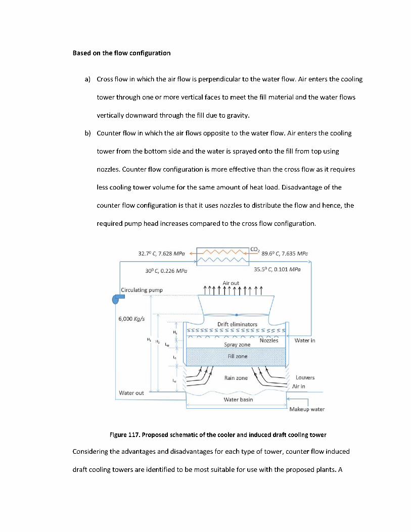
Based on the flow configuration
a) Cross flow in which the air flow is perpendicular to the water flow. Air enters the cooling
tower through one or more vertical faces to meet the fill material and the water flows
vertically downward through the fill due to gravity.
b) Counter flow in which the air flows opposite to the water flow. Air enters the cooling
tower from the bottom side and the water is sprayed onto the fill from top using
nozzles. Counter flow configuration is more effective than the cross flow as it requires
less cooling tower volume for the same amount of heat load. Disadvantage of the
counter flow configuration is that it uses nozzles to distribute the flow and hence, the
required pump head increases compared to the cross flow configuration.
Drift eliminators
Spray zone
Fill zone
Rain zone
Water basin
32.7° C, 7.628 MPa - 89.6° C, 7.635 MPa
35.5° C, 0.101 MPa30° C, 0.226 MPa
Air outtmttttttftCirculating pump
6,000 Kg/s
Nozzles Water in
LouversAir in
Water out
Makeup water
Figure 117. Proposed schematic of the cooler and induced draft cooling tower
Considering the advantages and disadvantages for each type of tower, counter flow induced
draft cooling towers are identified to be most suitable for use with the proposed plants. A

simple schematic of the cooler and selected cooling tower is shown in Figure 117. Also shown in
the Figure are the key components of a cooling tower which include fill material, water-basin,
drift eliminators, louvers, nozzles, fans, and circulating pump.
7.1.2 Components of a cooling tower
A brief explanation of the key components of a cooling tower is provided below.
Fill material is the key component of a cooling tower and is an area of active research for cooling
tower manufacturers. The purpose of the fill material is to enhance the heat transfer by
increasing the area and time of contact between water and air. A proper design of the fill
material can reduce the required fill volume significantly. Two common types of fills are
identified in literature [69]:
1) Splash fill - Water splashes over successive layers of horizontal or inclined splash bars,
continuously breaking the water into small droplets, while also wetting the fill surface as
shown in Figure 118. Most commonly used materials for splash bars are wood and
plastic. Plastic splash fills are known to promote better heat transfer than wood splash
fills.
2) Film fill - Is the most commonly used fill type nowadays because of its ability to expose
greater water surface within a given packed volume. Water flows in the form of a thin
film over vertically oriented sheets of corrugated pattern fill as shown in Figure 118.
With the use of film fill same amount of cooling can be achieved within a smaller
volume compared to the splash fill. Plastic is the most common material used for film
type fills.

Splash type fill Film type fill
Figure 118. Concept of different fill types
Cold-water basin is located at or near the bottom of the cooling tower, and it is used to collect
the cooled water that flows through the fill. The capacity of cold water basin should be large
enough to provide the required water flow. This is also the point of water exchange between
the cooling tower and external water bodies like pond, river etc.
Drift eliminators capture the water droplets entrapped in the air stream by providing a tortuous
path for the air out. These water droplets should not be confused with the evaporated water
and would be lost to the atmosphere if not captured, thereby, increasing the makeup water
requirements. Promoting better design of drift eliminators will limit the drift losses to 0.2 - 0.5%
of the total water flow.
Louvers are used to equalize the air flow in the tower and retain the water within the cooling
tower. Louvers are commonly used for cross-flow towers and many counter flow tower designs
do not require louvers.

Nozzles are used to distribute or spray water onto the fill. It is important to ensure that the
water distribution is uniform at the top of fill to achieve proper wetting of the entire fill surface.
Fans can be of either axial or centrifugal type. Axial fans are generally used in induced draft
towers and centrifugal fans are more common in forced draft towers. These fans should be
equipped with either adjustable pitch blades or variable frequency drives so that the air flow can
be varied due to the change in load and atmospheric conditions.
Circulating pump is used to transport the water between the cooling tower and the cooler. The
water is pumped from the cold-water basin through to the cooler, where it is used as cooling
medium. The hot water then returns back to the nozzle distribution system for evaporative
cooling in the cooling tower. Hence, the pump should be able to overcome the pressure losses
in the cooler, piping, and the tower.
7.2 Cooling tower theory
Heat and mass transfer in the cooling tower occurs in three zones namely; spray zone, fill zone,
and the rain zone as shown in Figure 117. More than 90% of the heat transfer occurs in the fill
zone and it has been reported [70] that the error in prediction of tower volume due to exclusion
of spray and rain zones is about 6.5%. When the spray and rain zones are included in the model
the error was reduced to 2.65% compared to the full scale 3-D modeling of the tower. Hence,
the spray and rain zones are not explicitly modeled in the current study. The governing
equations in the fill zone of a counterflow cooling tower are derived by making certain
simplifying assumptions. Water droplets are assumed to be surrounded by a thin film of
saturated air at water temperature. Heat and mass transfer between this thin layer and the
surrounding air occur due to temperature and humidity ratio difference respectively. Figure
119shows a control volume in the fill of a counterflow cooling tower.
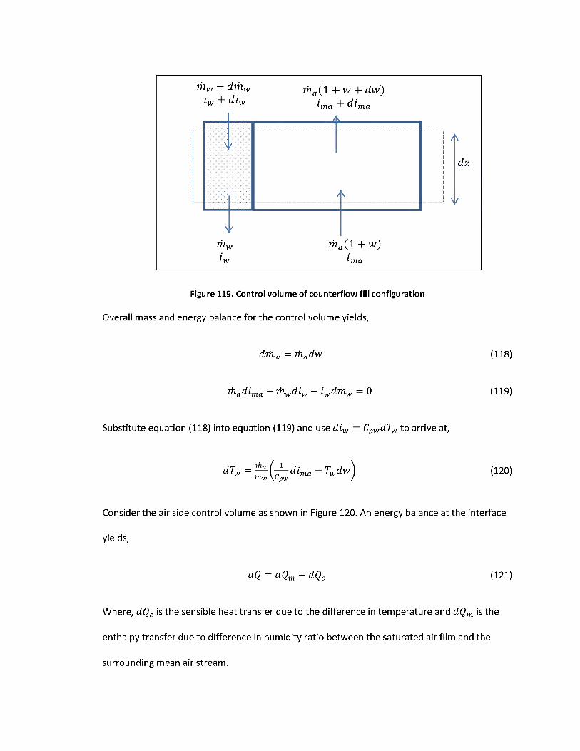
mw + dmw i-w + diw
V:
iv
ma(1 + w + dw) i-ma +dima
______ A_________
ma(1 + w)
Figure 119. Control volume of counterflow fill configuration
Overall mass and energy balance for the control volume yields,
dmw = madw (118)
madima ~mwdiw -iwdmw = 0 (119)
Substitute equation (118) into equation (119) and use diw = CvwdTw to arrive at,
dTw=^(-^dima-Twdww Lpw (120)
Consider the air side control volume as shown in Figure 120. An energy balance at the interface
yields,
dQ — dQm + dQc (121)
Where, dQc is the sensible heat transfer due to the difference in temperature and dQm is the
enthalpy transfer due to difference in humidity ratio between the saturated air film and the
surrounding mean air stream.
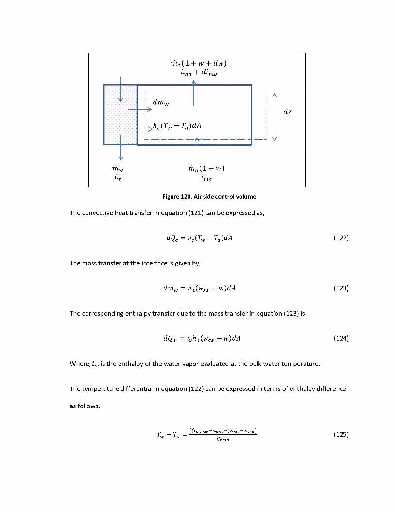
ma(1 + w + dw) i-ma + dima
V. dmwN
A
.............................
hc(Tw — Ta)a
mw ma(1 + w)iw i-ma
A
V
dz
Figure 120. Air side control volume
The convective heat transfer in equation (121) can be expressed as,
dQc = hc(Tw — Ta)dA (122)
The mass transfer at the interface is given by,
dmw = hd(wsw —w)dA (123)
The corresponding enthalpy transfer due to the mass transfer in equation (123) is
dQm w^dA (124)
Where,iv, is the enthalpy of the water vapor evaluated at the bulk water temperature.
The temperature differential in equation (122) can be expressed in terms of enthalpy difference
as follows,
T =1 a(fomasw i-ma) (wsw w) iy) (125)
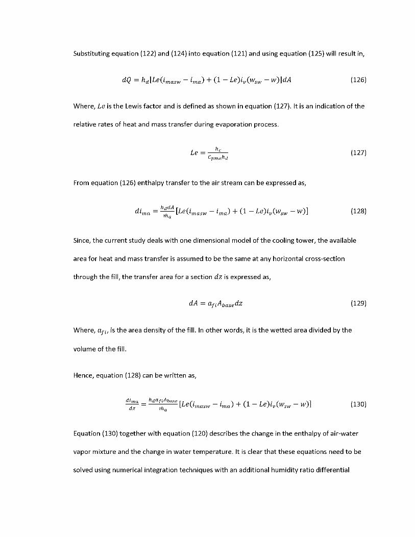
Substituting equation (122) and (124) into equation (121) and using equation (125) will result in
dQ hd.\L&(.im.asw i"ma) ^ C1 w)]dA (126)
Where, Le is the Lewis factor and is defined as shown in equation (127). It is an indication of the
relative rates of heat and mass transfer during evaporation process.
Le = —Cpmahd
(127)
From equation (126) enthalpy transfer to the air stream can be expressed as,
dima = [Le(imasw -ima) + (1 -Le)iv(wsw -w)] (128)ma
Since, the current study deals with one dimensional model of the cooling tower, the available
area for heat and mass transfer is assumed to be the same at any horizontal cross-section
through the fill, the transfer area for a section dz is expressed as,
dA afiAbasedz (129)
Where, , is the area density of the fill. In other words, it is the wetted area divided by the
volume of the fill.
Hence, equation (128) can be written as,
= hda^ase [Le(imasw -ima) + (1 -Le)iv(wsw -w)] (130)
Equation (130) together with equation (120) describes the change in the enthalpy of air-water
vapor mixture and the change in water temperature. It is clear that these equations need to be
solved using numerical integration techniques with an additional humidity ratio differential
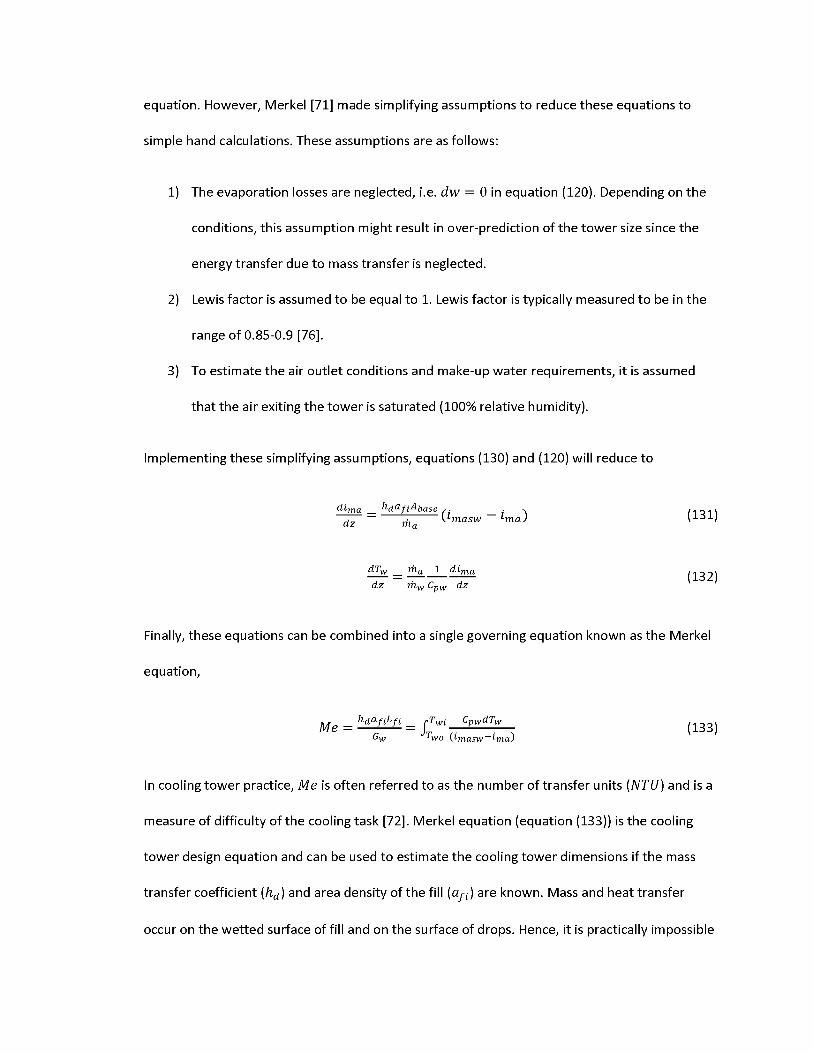
equation. However, Merkel [71] made simplifying assumptions to reduce these equations to
simple hand calculations. These assumptions are as follows:
1) The evaporation losses are neglected, i.e. dw = 0 in equation (120). Depending on the
conditions, this assumption might result in over-prediction of the tower size since the
energy transfer due to mass transfer is neglected.
2) Lewis factor is assumed to be equal to 1. Lewis factor is typically measured to be in the
range of 0.85-0.9 [76].
3) To estimate the air outlet conditions and make-up water requirements, it is assumed
that the air exiting the tower is saturated (100% relative humidity).
Implementing these simplifying assumptions, equations (130) and (120) will reduce to
dima _ hdafiAbase (131)dz ~ m \Lmasw hna) (131)
dTw _ ma 1 dima (132)dz mw Cpw dz
Finally, these equations can be combined into a single governing equation known as the Merkel
equation,
_ hdafiLfi _ jl'wi CpwdTw (133Gw T'wo dmctsw — imcL)
In cooling tower practice, Me is often referred to as the number of transfer units (NTU) and is a
measure of difficulty of the cooling task [72]. Merkel equation (equation (133)) is the cooling
tower design equation and can be used to estimate the cooling tower dimensions if the mass
transfer coefficient (hd) and area density of the fill (o^) are known. Mass and heat transfer
occur on the wetted surface of fill and on the surface of drops. Hence, it is practically impossible

to measure hd and individually. Fortunately, these two exist as a product in equation (133)
and individual values are not needed for design calculations. Fill and cooling tower vendors
don't release the values of hda^t. However, empirical correlations are available in literature
which can used to estimate fill dimensions.
Cooling process in the fill can be represented on an enthalpy-temperature diagram as shown in
Figure 121. As the water is cooled flowing downwards, the saturated air film enthalpy follows
the saturation curve AB. The air operating line is represented by CD. The linear nature of air
operating line is due to the fact that the solution of equation (132) is linear. The slope of the air
operating line equals the liquid to gas ratio,mw/ma. BC represents the initial enthalpy driving
force and the projected length of CD on to the temperature axis represents the range of the
cooling tower.
Range = Twi -Two (134)
The cooling tower approach is the difference between the cold water temperature leaving the
tower and the ambient air wet bulb temperature. From economic standpoint, a cooling tower
should be designed such a way that the approach is greater than 50For 2.20C. For fixed water
conditions, the water operating curve will always be AB, whereas, the air operating line can be
adjusted by changing mw/ma or the ambient wet bulb temperature. An increase in the
ambient wet bulb temperature shifts the air operating line upward and to the right to establish
equilibrium conditions. It can also be seen from Figure 121 that as the mw/ma increases the
potential enthalpy difference within the tower decreases and for mw/ma > 2.5, energy transfer
can occur from air to water in part of the tower. This undesirable situation should be avoided,
but sometimes is necessary when the wet bulb temperature of the ambient air is extremely low

like in the winter months. Typically, mechanical draft counter flow cooling towers are designed
for mw/ma ranging from 0.5 to 1.75 [73].
500—•—Water operating line
-■-m* / ma = 0.5
-4-m* / ma = 1.5
-x-m* / ma = 2.5
-*-m* / ma = 3.0
400
300
200
100
27 30 33 36 39 42 45 48 51 54 57 60 63
Figure 121. Counterflow cooling diagram
7.3 Design procedure
In this study, the cooling tower design analysis was carried out for an S-CO2 cycle developed for
the AFR-100 and ABR-1000 reactor applications. The reactor power of the AFR-100 is 250 MWth,
for net cycle efficiency of 42.27% results in 104.8 MWe. The reactor power of the ABR-1000 is
1000 MWth and for net cycle efficiency of 40.26% results in 400.3 MWe. Reference cooler design
water conditions for both these power plants are tabulated in Table IV and these conditions are
selected for the base case cooling tower design. The effect of changing the water conditions on
cooling tower and cooler size design will be presented later.

Table IV. Reference cooler design conditions for AFR-100 and ABR-1000 plants
Cooler conditions
7.3.1 Estimation of optimum mw/ma
For a given set of cooling tower design conditions an optimum value of mw/ma exists. This
optimum mw/ma will result in minimum construction and operating costs. As a rule of thumb
[74], to find the optimum mw/ma, air outlet temperature is taken as the average of hot and
Power plant AFR-100 ABR-1000
Reactor power (MWth) 250 1000
Electrical output (MWe) 104.8 400.3
CO2 inlet temperature (0C) 89.6 87.3
CO2 outlet temperature (0C) 32.8 32.7
CO2 pressure drop (MPa) 0.007 0.009
Cycle efficiency (%) 42.27 40.26
Water inlet temperature (0C) 30 30
Water outlet temperature (0C) 35.5 36.8
Water flow rate (kg/s) 6,000 20,000
Water pressure drop (MPa) 0.125 0.104
Cooler thermal load (MW) 137.2 569.2
cold water temperature entering and exiting the tower.

Twi+Two2
(135)T =1 ao
It has been reported [74] that the approximated air outlet temperature is very close to the
actual optimal design temperature. For a given water flow rate, air flow rate can be estimated
within ±10% of the actual optimum design flow rate. Once the optimum air outlet conditions are
known, mw/ma can be calculated according to,
™w _ i-map-i-mai (136)™-a Cpw(Twi — Two')
7.3.2 Merkel number
The tower Merkel number, Me, from equation (133) can be solved numerically using the
Chebyshev four point numerical integration method [73] as follows:
Me or NTU = Cpw rTwiTwo
dTw(j-masw — i-ma)
Cpw(Twi Two)4 XAti At2 Atg Ai4) (137)
where,
Ah Value Of i-masw hna at ^wo "t"
Ai2 = value of imaSw ~hna at Two + 0.4Range
A^3 value of i-masw ima at ^wo "t" 0.6^UU^e
Aj4 = value of imaSw — ima at Two + 0.9Range
Table V presents an example of calculation of the Merkel number for AFR-100. Calculations are
performed in engineering equation solver (EES) [75]. Plotting several values of Me as a function
of mw/ma produces the tower demand curves. The tower characteristic curve is then found for
design mw/ma by field testing under variable flow and atmospheric conditions.

Table V. Tower Merkel number calculation example
Water side Air sideEnthalpydifference
DescriptionT
(°C) ^rnasw (J/kg) Description ima (J/kg)1/(J-masw i-ma)
T‘wo+ 0.1 Range 32.5 56647.8
^mai
+ 0.1 f—Range \maJ
45571.70.0903e-3
T‘wo+OARange 35 63342.6
imai(mw\+ 0.4 ( ) Range\maJ
51214.70.0825e-3
T1wo+ 0.6 Range 36.67 68259.1
imai
+ 0.6 f—Range \maJ
54976.70.0753e-3
T‘wo+ 0.9 Range 39.17 76401.3
imai
+ 0.9 f—Range \maJ
60619.7 0.0634e-3
^1/(^rnasw hna) 0.3114e-3
Merkel number (Me) = 11/(imasw -ima) * Range * Cpw/4 1.1677
7.3.3 Estimation of floor area
Instead of using a single large cooling cell it is common to use a certain number of small cells to
provide better temperature control as well as reduce the total power consumption. Table VI
shows the different cell types used by a manufacturer [79]. These cells are classified based on
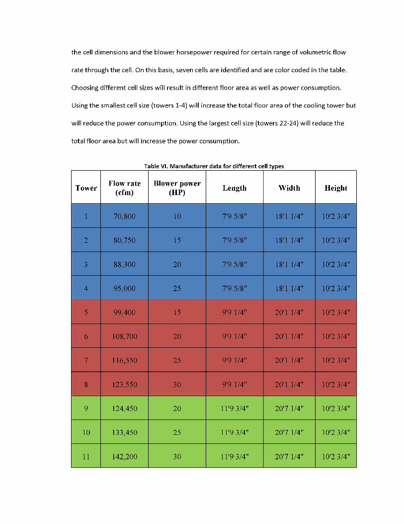
the cell dimensions and the blower horsepower required for certain range of volumetric flow
rate through the cell. On this basis, seven cells are identified and are color coded in the table.
Choosing different cell sizes will result in different floor area as well as power consumption.
Using the smallest cell size (towers 1-4) will increase the total floor area of the cooling tower but
will reduce the power consumption. Using the largest cell size (towers 22-24) will reduce the
total floor area but will increase the power consumption.
Table VI. Manufacturer data for different cell types
Tower Flow rate (cfm)
Blower power(HP) Length Width Height
1 70,800 10 7'9 5/8" 18'1 1/4" 10'2 3/4"
2 80,750 15 7'9 5/8" 18'1 1/4" 10'2 3/4"
3 88,300 20 7'9 5/8" 18'1 1/4" 10'2 3/4"
4 95,000 25 7'9 5/8" 18'1 1/4" 10'2 3/4"
5 99,400 15 9'9 1/4" 20'1 1/4" 10'2 3/4"
6 108,700 20 9'9 1/4" 20'1 1/4" 10'2 3/4"
7 116,550 25 9'9 1/4" 20'1 1/4" 10'2 3/4"
8 123,550 30 9'9 1/4" 20'1 1/4" 10'2 3/4"
9 124,450 20 11'9 3/4" 20'7 1/4" 10'2 3/4"
10 133,450 25 11'9 3/4" 20'7 1/4" 10'2 3/4"
11 142,200 30 11'9 3/4" 20'7 1/4" 10'2 3/4"

12 143,800 30 11'9 3/4" 20'7 1/4" 11'6"
13 157,550 40 11'9 3/4" 20'7 1/4" 11'6"
14 166,050 30 11'9 3/4" 22'1 1/4" 13'3 5/8"
15 181,800 40 11'9 3/4" 22'1 1/4" 13'3 5/8"
16 195,000 50 11'9 3/4" 22'1 1/4" 13'3 5/8"
17 193,800 40 11'9 3/4" 22'1 1/4" 15'11 5/8"
18 207,800 50 11'9 3/4" 22'1 1/4" 15'11 5/8"
19 220,150 60 11'9 3/4" 22'1 1/4" 15'11 5/8"
20 221,550 50 11'9 3/4" 22'1 1/4" 18'7 5/8"
21 235,000 60 11'9 3/4" 22'1 1/4" 18'7 5/8"
22 255,400 50 13'11 7/8" 24'1 1/4" 18'7 5/8"
23 270,700 60 13'11 7/8" 24'1 1/4" 18'7 5/8"
24 290,050 75 13'11 7/8" 24'1 1/4" 18'7 5/8"
Several years ago a quotation was obtained from Delta cooling towers Inc. for one similar (but
lower power) design condition and the cell used by the company has dimensions very close to
that of the cell used for towers 1-4 in Table VI. Hence, cell #1 is chosen for this particular study.
Later in this report it is concluded that using the smallest cell size is more economical to the
plant and this justifies the use of cell #1. Two extreme options are possible for a selected cell
type:

1) Lowest power consumption - In this option, lowest possible air flow rate per cell is
selected from the table. For cell #1 this value is 70,800 cfm. This will reduce the power
consumption per cell but will increase the total number of cells required to achieve the
desired performance. Overall, this option will result in least power consumption and
largest cooling tower size. Number of required cells is estimated as,
Number of cells = Qao70800
(138)
2) Lowest footprint - In this option, highest possible air flow rate per cell is selected. For
cell #1 this value is 95,000 cfm. This will increase the blower power consumption per cell
but will decrease the total number of cells. This option will result in highest power
consumption and smallest tower footprint/cost. Number of required cells is calculated
as,
Number ofcells =95000
(139)
Total volumetric flow rate of air required for all the cells is calculated from the known air mass
flow rate in section 7.3.1 as,
Qao = ^ [cfm] (140)Pao
Once the number of required cells is calculated for each option, the required floor area is
calculated as,
Afioor = Number of cells * Aceii (141)
Where, Acett is the area of one cell and is equal to 7'9 5/8" X 18'1 1/4" for cell #1. Figure 122
shows the one cell plan of Delta cooling towers Inc. [80].

Figure 122. Delta cooling towers Inc. one cell plan [80]
It should be noted that the outlet air density is used to estimate the required volumetric flow
rate of air in equation (140) because the fan is located at the exit for an Induced draft cooling
tower. If these calculations are being performed for a forced draft cooling tower, inlet air
density has to be used and this will change the required floor area and number of cells
accordingly.
7.3.4 Estimation of fill height
As explained in the introduction section, there are different types of fills and use of better fill
design will reduce the size of fill significantly. Empirical correlations for different fill types are
available in literature and can be used to estimate the size of cooling fill. Kloppers et al [76]
performed experiments to investigate different types of fill and proposed correlations to predict
NTU for splash, trickle (film fill with round channels), and film type (with rectangular channels)
fills.
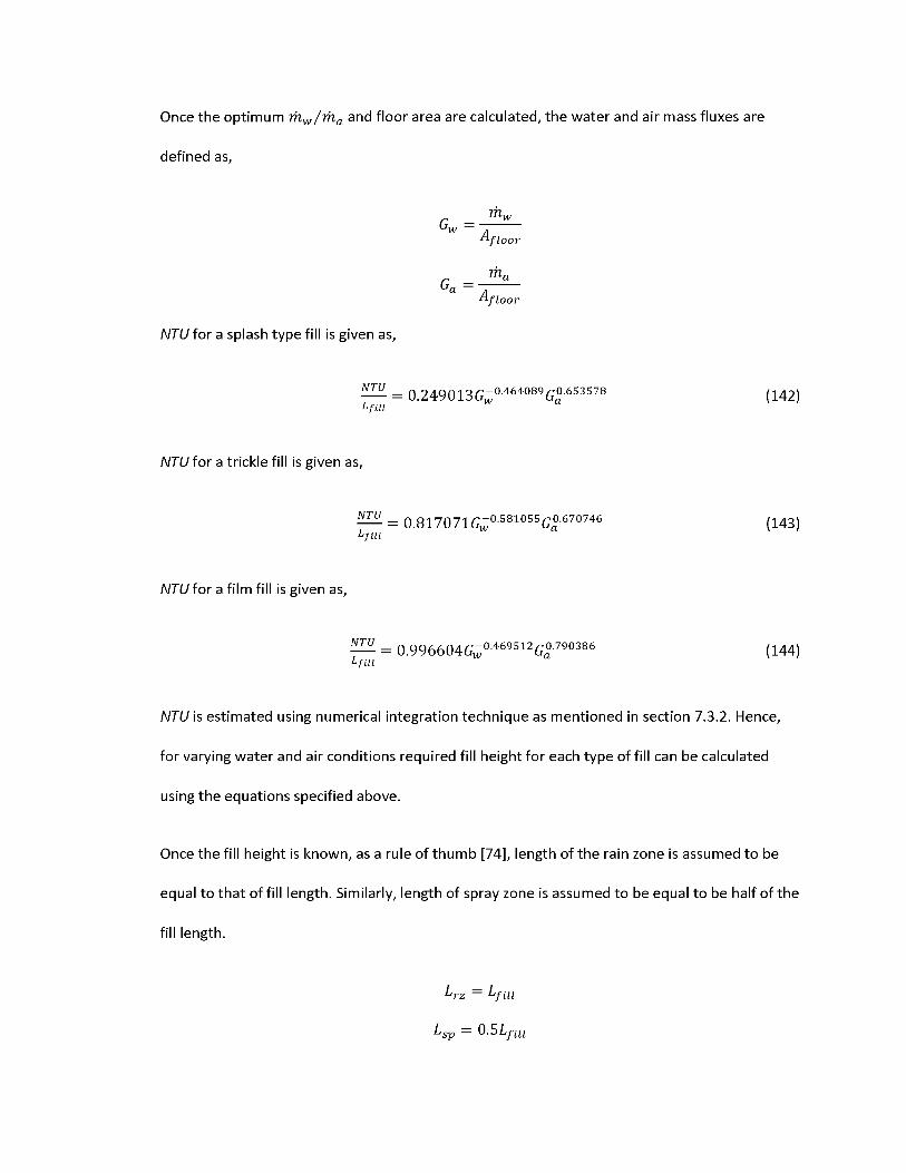
Once the optimum mw/ma and floor area are calculated, the water and air mass fluxes are
defined as,
NTU for a splash type fill is given as,
Afloor
Afloor
— = 0.249013G-°.464O8X°.653578Lfill
(142)
NTU for a trickle fill is given as,
— = 0.817071 G^°.581055 G°.670746Lfill
(143)
NTU for a film fill is given as,
— = 0.996604G-°.469512Ga°.790386 (144)Lfill
NTU is estimated using numerical integration technique as mentioned in section 7.3.2. Hence,
for varying water and air conditions required fill height for each type of fill can be calculated
using the equations specified above.
Once the fill height is known, as a rule of thumb [74], length of the rain zone is assumed to be
equal to that of fill length. Similarly, length of spray zone is assumed to be equal to be half of the
Lrz Lfui
Lsp 0-5Lfni
fill length.

7.3.5 Water consumption rate
There are three major water losses in a wet cooling tower:
1) Evaporation Losses - As the water is cooled in the cooling tower, portion of water gets
evaporated into the air stream. The difference between amount of water vapor in the
entering and exiting air streams will provide the quantity of water evaporated.
E = ma(w0-wi) (145)
2) Blow-down Losses - As the water evaporates, solids and chemical matter concentrate in
the cooling water. If this is ignored, it will result in severe corrosion and chemical build
up affecting the performance of tower in long run. Hence, some amount of circulating
water needs to be replaced by fresh water to avoid solids/chemical build up. The
amount of water which needs to be replaced can be estimated as,
B = E
COC-1(146)
Where, COC is known as cycles of concentration and is defined as,
COC = Concentration of solids in the cooling tower water
Concentration of solids in the cooling tower makeup water(147)
Cycles of concentration is typically limited from 3-7. Value of 3 is used in this report for an upper
estimate of blow-down losses.
3) Drift Losses - As the air flows in the cooling tower, some of the water droplets get
carried away by the air stream. With the use of drift eliminators, these losses can be
minimized to within 0.2-0.5% of the total water flow rate.
W = 0.005mw (148)

Total water consumption rate is estimated as the sum of evaporation, blow-down, and drift
losses.
7.3.6 Power requirements
Power required to operate the cooling tower comprises of two parts - water pump power and
the air blower power. The power required to operate the pump is estimated as,
_ mwHpgpump ~ „
'Ipump(149)
Where, Hp is the net required pump head and is equal to the sum of required head in the
cooling tower and the cooler.
Hp Hcoonngtower + Hcooier
The net cooling tower head is equal to the head required to raise the water from the water
basin to the nozzle sprays,
Hcoolingtower Lsp rz 2-5-^/tii
An additional head of 10ft is added to the cooling tower head to compensate for the
assumptions made and to better match the vendor quotations.
The net cooler head is the head required to overcome the water side pressure drop across the
cooler, expressed in the units of height of water column.
Hcooler ^-^cooier[m]
Efficiency of the pump is assumed to be 90%.
Blower power for the lowest footprint option is calculated as,

Pbiower = 10[HP] * Number of cells (151)
Blower power for the lowest power consumption option is calculated as,
Pbiower = 25[HP] * Number of cells (152)
7.3.7 Estimation of cooling tower cost
Delta cooling towers Inc. quoted $448,439 for 12 cells. Hence, the price of each cell is calculated
to be $37,370. Total cost of the cooling tower is then estimated as,
Towercost = Cost per cell * Number of cells (153)
Alternatively, Zanker et al [74] proposed an empirical correlation in 1967 for the estimation of
cooling tower construction cost:
P1967_ Qload^P-]
C*A + 39.2R-586 (154)
Where, R and A are range and approach in Fahrenheit respectively. C in equation (154) is
defined as,
C = 279[1+0.0335 (85 — WBT)1-143] (155)
Where, WBT is the design wet bulb temperature in Fahrenheit. It should be noted that the
above correlation was proposed in 1967 when the material and fabrication costs were different
compared to the present day. Due to inflation rate, $1 in 1967 has the same buying power as
$7.08 in 2014 [77]. These statistics are based on change in average consumer price index from
1967 to 2014. Hence, the value estimated from equation (154) is multiplied by a factor of 7.08
to estimate the cost of tower in 2014.

C0Stt0wer — 7.08 * $1967 (156)
7.3.8 Factors affecting cooling tower size
There are several factors which affect the design of a cooling tower. Some of the important
variables are mentioned below:
1) Heat load is dependent on the cycle conditions and for steady state design calculations
it is assumed to be constant (137.2 MW for AFR-100, and 569.2 MW for ABR-1000). In
general, if other variables are held constant, heat load is directly proportional to the
mass flow rate of water according to the heat balance equation,
Qload ^w^pwiTw Twi) (157)
Hence, the tower volume increases linearly with the heat load as shown in Figure 123.
2) Range - If other variables (i.e., heat load, approach, and wet bulb temperature) are held
constant, tower volume varies inversely with the range as shown in Figure 124. This is
primarily due to two reasons. First, increasing the range at a constant heat load requires
the water flow rate to be lowered. Second, increasing the range will increase the
enthalpy difference between the entering hot water temperature and the entering wet
bulb temperature of air.
3) Approach - Tower volume varies inversely with the approach, provided that other
variables are held constant. A longer approach requires smaller tower as shown in
Figure 125. It can be seen that the tower volume starts to increase asymptotically for
approach lower than 2.20C. For this reason, it is not economical to design cooling towers
for any approach values of less than 50F or 2.20C.

4) Wet bulb temperature - Tower size varies inversely with wet bulb temperature as
shown in Figure 126. In a hypothetical situation, for fixed heat load, approach, and
range, reducing the design wet bulb temperature will increase the size of the tower. This
is due to the fact that the ability of air to absorb moisture reduces with temperature.
40 60 80 100 120 140 160 180
Qload [MW]
Figure 123. Effect of heat loadRange [0C]
Figure 124. Effect of range
8 10 12 14 16
\\
x\x
V
012345678
Approach [oC]Figure 125. Effect of approach
10 15 20 25
WBT [oC]Figure 126. Effect of wet-bulb temperature
7.4 Design Calculations
Equations described in section 7.3 are modeled in EES [75] to perform design calculations. The
10000
8000
6000
4000
2000
5
code is verified by comparing the calculations to the vendor quotation. Later in this section,
effect of air ambient conditions and water conditions on the cooling tower and cooler design
will be described. The original idea was to develop the cooling tower code in FORTRAN and
integrate it with ANL Plant Dynamics Code to perform the calculations. However, cooling tower
calculations require psychrometric properties which are not readily available in FORTRAN. Due

to the limited time this project, EES was used instead to perform the calculations since the
psychrometric properties are readily available. The current code developed in EES will be
modified into FORTRAN in the near future.
7.4.1 Verification of the code
The code is verified by comparing the estimated power requirements, tower dimensions, and
tower cost to the quotation obtained from Delta cooling towers, Inc. for the conditions specified
in their quotation. These calculations are presented in Table. VII.
It should be noted that the quotation obtained from Delta cooler towers Inc. is for the lowest
footprint option and the values are close to the code predictions. The required blower and
pumping power are slightly underestimated by the code. The manufacturer used a 30HP fan per
cell whereas the code uses 25HP fan per cell, which explains why the code underestimates the
required blower power. To compensate for the underestimation of pumping power, an
additional 10ft of head is added (to the values in Table. VII) to the total pump head as
mentioned in section 7.3.6. Required number of cells and the floor area matches extremely
close to the vendor quotation indicating that the assumption made regarding the optimum
mw/ma is valid. The table also compares the different fill types described in section 7.3.4. As
can be seen from the table, the fill height and hence, the pumping power are much smaller for
the film fill type compared to splash or trickle type fills. Moreover, predictions using the film
type fill are closer to the manufacturer specifications. Therefore, film type fill is used for all the
calculations from here on. The table also compares the lowest power consumption and lowest
footprint options. For the described conditions, the required number of cells, floor area, and
tower cost for lowest horse power option are about 33% more than the lowest footprint option
whereas, the power consumption is about 40% less compared to the lowest footprint option.

Hence, it is important to understand which option is economical for the plant. This is explained
in more detail in the plant optimization section. Cost estimation using Zanker et al correlation
mentioned in the section 7.3.7 is closer to the lowest footprint option. It should be noted that
the correlation doesn't differentiate between the two options as it is only a function of heat
load, approach, and range which are same for both the options. Hence, for accurate cost
estimate the cost per cell method is used throughout this report.
Table VII. Comparison of calculations to the manufacturer quotation
Variable DeltaCalculated
(Lowest footprint)
Calculated
(Lowest Power)
Number of cells 84 83 111
Water flow rate [kg/s] 4,900 4,900 4,900
Tin [0C] 35.78 35.78 35.78
Tout [0C] 28.88 28.88 28.88
Twbt [0C] 25.55 25.55 25.55
Splash Trickle Film Film
Pblower [MW] 1.88 1.545 1.545 1.545 0.8295
Ppump [MW] 0.182 0.7415 0.2634 0.1588 0.1712
Lfill [m] ~ 1.3 5.553 1.973 1.167 1.282
Afloor [m ] 1147 1088 1088 1088 1459

Cost [$]*106 3.139 3.1017 4.148
Cost[$]*106 - Zanker et al 2.8977 2.8977
7.4.2 Effect of ambient air conditions
Since ambient air conditions (wet and dry bulb temperature) depend on the location and time of
the year, design calculations are performed for three possible locations of the power plant to
investigate the effect of air conditions.
1) Chicago, IL
2) Las Vegas, NV
3) Idaho Falls, ID
For all the calculations presented in this section and next section, water conditions are held
constant at the reference conditions described in Table IV.
At these three locations, monthly design temperature data is extracted from the ASHRAE
climatic design conditions online software (http://ashrae-meteo.info/) and is presented in
Table. VIII. The ambient conditions for each location do not exceed the values in the table for
more than 5% of the time each month. Calculations are performed for all the months to identify
the maximum requirements for the whole year at each location.
Monthly variation of the requirements at each of these locations for optimum design condition
(mw/ma) are shown in Figure 126 for an AFR-100 power plant. It can be seen that the required
tower volume, total power consumption, and make-up water requirements are highest for the
month of July at all the locations.

Table VIII. Monthly design ambient air conditions
Chicago
Data Jan Feb Mar Apr May June July Aug Sep Oct Nov Dec
WBT (0C) 4 5.33 11.72 15.66 20.11 22.77 24.88 24.11 21.61 16.94 12.83 6.66
DBT (0C) 5.44 7.55 15.44 20.72 24.33 28.16 30.16 28.33 25.66 20.61 15.05 8.33
Las Vegas
Data Jan Feb Mar Apr May June July Aug Sep Oct Nov Dec
WBT(0C)
11.94 13.16 14.66 16.33 19.83 22.5 23.88 23.5 22.38 17.94 14.66 11.33
DBT(0C)
16.66 21.83 27.44 31.72 37.83 39.5 39.27 37.16 32.16 30.83 22.11 16.94
Idaho Falls
Data Jan Feb Mar Apr May June July Aug Sep Oct Nov Dec
WBT (0C) 3.88 6.66 8.88 11.88 15.27 17.83 20.22 19.11 17.16 12.33 8.94 4.88
DBT (0C) 6.11 10.77 16.11 23.83 26.27 29.38 30.27 30.16 26.44 22.5 12.66 7.55
Comparing these plots to the wet bulb temperature data in Table. VIII, it can be concluded that
the requirements are higher for higher wet bulb temperatures. The main purpose of this study is
to identify the maximum requirements and hence, from here on, calculations presented will be

for the month of July. It is also interesting to note that the total required volume and power
consumption are smaller in Las Vegas compared to Chicago for the month of July. The weather
in Las Vegas is extremely hot and dry resulting in a lower wet bulb temperature than Chicago in
the summer. This means that the cooling tower in Las Vegas consume more water but less
power as can be seen in Figure 127.
2.6
2.5•—Chicago
Las Vegas Idaho Falls
2.4
2.3
2.2
2.1
1.9
1.8
1.7
1.6Jan Feb Mar Apr May Jun Jul Aug Sep Oct Nov Dec
J2o>*
Q-
Oto£
•E
200
190
180
170
160
150
140
130
120
. 1 . 1 . 1 .
ChicagoLas Vegas
s/I
xl\/ \
—Z !\\ \yz / V" z xl
r
Jan Feb Mar Apr May Jun Jul Aug Sep Oct Nov Dec
1000
—•—Chicago -■-Las Vegas
Idaho Falls
900
800
700
600
500
400
300Jan Feb Mar Apr May Jun Jul Aug Sep Oct Nov Dec
‘—Chicago0.95-■-Las Vegas —a—Idaho Falls
0.9
0.85
0.8
0.75
0.7Jan Feb Mar Apr May Jun Jul Aug Sep Oct Nov Dec
Figure 127. Variation of requirements for AFR-100 at optimum mw/ma conditions
7.4.3 Control of water conditions
It is extremely important to maintain the water temperature and flow rate at design conditions
in order to achieve the desired cycle efficiency. Once the tower dimensions are fixed, in absence
of any sort of temperature control, the water temperature can change drastically due to
changes in ambient air conditions on daily as well as monthly basis, thereby, severely affecting
the efficiency of the cycle. This section provides an example of how to control the water
conditions. These calculations are performed for Chicago but similar curves can be generated for
other locations as well. The curves shown in Figure 128 are generated using the Merkel
equation. The right hand side of the equation (133) is only a function of water and air
conditions. Therefore, a series of NTU curves can be generated for changing ambient conditions.
These curves are known as "tower demand curves" in cooling tower theory. However, the left
hand side of the equation (133) is always the same independent of air conditions and can be
seen as the linear curve on the log-log NTU plot shown in Figure 128. This curve is also known as
the "tower characteristic curve" and is a function of fill type used. Film type fill is used in this
case to generate the tower characteristic curve. Typically, the cooling tower manufacturers
provide the tower characteristic curve during the purchase. However, the characteristic curve
can also be generated during field testing of the cooling tower under varying air and water
conditions.
The point where the tower characteristic curve intersects the tower demand curve will provide
the required mw/ma for that particular ambient air condition. Then the mw/ma value needs to
be adjusted to achieve constant water temperature. Makeup water requirements also change
with the air conditions. Once the required mw/ma is obtained, the makeup water plot in Figure
128 can be used to estimate the amount of water to be added to maintain a constant water flow
rate. As mentioned earlier, the wet bulb temperature exceeds the design value only for 5% of
the time in month of July. This corresponds to less than 36 hours for the whole year. Excluding
these 36 hours, the value of mw/ma will always be higher than the designed value and this will
increase the required mw/ma and reduce the make-up water consumption rate.
Value of mw/ma in a cooling tower can be adjusted by adopting two methods: adjusting the
water flow rate or air flow rate per cooling cell.

1) Adjusting water flow rate - Temperature control is achieved by switching on/off the
water flow to one or multiple cells as the air conditions change. The water flow rate per
changes while air flow rate per cell is maintained constant, thereby, adjusting mw/ma.
2) Adjusting air flow rate - In this technique variable frequency drives (VFDs) are used to
adjust the fan speed and hence, air velocity through one or multiple cells to account for
changing ambient conditions. The water flow rate is maintained constant and air flow
rate per cooling cell changes, thereby, adjusting mw/ma.
0.1
mw / ma
6
*52O)*
Q.3&roE
•E
200
190
180
170
160
150
140
130
120
110
100
—•—Approach - 260 C
—■—Approach - 24.50 C
— Approach - 18.20 C
—M—Approach - 14.30 C
—V—Approach - 9.80 C
—S—Approach - 7.20 C
—♦—Approach - 5.10 C
irJrJr'*
3
mw / ma
2 4 5 6
Figure 128. Effect of mw/ma on the power consumption and make-up water requirements
Each technique has its advantages and disadvantages. Adjusting water flow rate will eliminate
need of variable frequency drives (VFDs), however, accurate control of water temperature is
difficult to achieve. Adjusting air flow rate will provide almost accurate temperature control but
will increase the operation cost of the tower.
7.4.4 Effect of design water conditions
The calculations performed in the previous sections were for a constant design water
temperature and flow rate as shown in Table IV. However, for a fixed heat load, infinite
combinations of water temperature and mass flow rate are possible. Changing the water
temperature and flow rate will affect both the cooling tower as well as the cooler design. This
section describes the effect of water conditions on both the cooler as well as cooling tower
variables. Plant Dynamics Code (PDC) developed at ANL [67] is used for the cooler calculations.
Due to corrosion issues, range of the tower should not exceed 220C [80] and this limits the
lowest possible water flow rate to 1,500kg/s for an AFR-100 plant and 6,200kg/s for an ABR-
1000 plant.
The minimum water temperature that can be achieved is limited to 22.50C in Idaho Falls. This
limitation is due to the restriction that the approach of the cooling tower has to be greater than
2.20C as explained in section 7.3.7. Effect of series of water flow rates and water temperatures
on cooler design is presented in Figure 129.
The water inlet and outlet temperatures to the cooler are related according to equation (157).
Hence, for all the water flow rates slope of the equation is always close to 1. However, the
intercept of the equation is inversely proportional to the water flow rate. Hence, as the water
flow rate increases the intercept decrease asymptotically. This can be seen in Figure 129, for the
same water inlet temperature, the difference in water outlet temperatures become smaller as

the water flow rate increases. This is also reflected in the required cooler length and minimum
approach plots.
54 —•—1500 Kg/s -■-2050 Kg/s — 2800 Kg/s
3600 Kg/s 4400 Kg/s
51
48
42
39
36
30
2720 22 24 26 28 30 32 34
Twl [0C]
£
•—1500 Kg/s ■—2050 Kg/s
2800 Kg/s 3600 Kg/s 4400 Kg/s 5200 Kg/s 6000 Kg/s 7200 Kg/s
Twi [0C]
■•—1500 Kg/s •■-2050 Kg/s
2800 Kg/s 3600 Kg/s 4400 Kg/s 5200 Kg/s 6000 Kg/s 7200 Kg/s
Tw [0C] Twl [0C]
Figure 129. Effect of water conditions on the cooler variables
Approach of the cooler, which is defined as the minimum difference in temperature of cold and
hot streams increases as the water temperature decrease or the water flow rate increase. For
this reason, a longer cooler is needed if the flow rate is decreased or the water temperature is
increased. It should be noted that the required cooler length starts to increase asymptotically as
the water inlet temperature get close to the CO2 outlet temperature in the cooler. Similar
behavior can be observed for the water pressure drop as it is proportional to the cooler length
and water flow rate. Changing the water flow rate and temperature will also affect the size of
cooling tower, power consumption as well as the cost. Figure 130 presents how the required
floor area changes with the water conditions for both the lowest power consumption and
lowest footprint options.

2750
2500
2250
2000
1750
£ 1500
1250
** 1000
750
500
25020
-1500 Kg/s 2050 Kg/s: 2800 Kg/s 3600 Kg/s 4400 Kg/s '
-*-5200 Kg/s 6000 Kg/s
:: " ?
28
> [0C]
22 24 26 30 32 34
T
Lowest power consumption option
2750
2500
2250
2000
^ 1750
“ 1500
1250
1000
750
500
25020 22 24 26 28 30 32 34
Two [0C]
—•—1500 Kg/s -■-2050 Kg/s —*-2800 Kg/s
3600 Kg/s —▼—4400 Kg/s —*—5200 Kg/s -♦-6000 Kg/s
7200 Kg/s
Lowest footprint option
Figure 130. Effect of water conditions on the tower floor area in Idaho Falls
All these calculations are performed for constant air conditions (month of July) in Idaho Falls.
For constant air and water temperature the optimum mw/ma is always the same irrespective
of the water flow rate. Hence, as the water flow rate decreases the required volumetric flow
rate of air decreases leading to a total reduction of floor area as can be seen in Figure 130 for
both the options. Obviously, the required floor area increases as the cold water temperature
approaches the wet bulb temperature as is evident from these plots. It is also worthwhile to
note again that the required floor area for lowest power consumption option is significantly

higher than lowest footprint option for all the water conditions. Figure 130 presents the fill
height calculations for both the options. As can be seen, the required fill height increases with
decrease in water outlet temperature. This is exactly opposite to the effect of water
temperature on the cooler length. This is expected because an increase of approach in the
cooler leads to decrease in the approach of the cooling tower and vice versa. However, the
effect of water flow rate on the fill height is similar to what has been observed in the case of the
cooler and is due to the fact that overall driving enthalpy decreases with decrease in flow rate.
Just like the required floor area, the required fill height is higher for the lowest power
consumption option than the lowest footprint option.
The effect of water conditions on the total power consumption to operate the cooling tower
and the cooler is presented in Figure 132. For both the options, it is clearly evident that there is
an optimum water temperature for each flow rate that results in least power consumption. This
is expected because a decrease of pumping head in the cooler will lead an increase of pumping
head in the cooling tower as explained earlier. Also, the total power consumption decreases
with water flow rate due to lower blower power consumption. It should be noted that the total
power consumption for the lowest power consumption option is significantly lower than the
lowest footprint option for all the water conditions.
Although the results presented here are for Idaho Falls, similar conclusions can be drawn about
other locations as well. The only change would be the optimum water temperature at each flow
rate. In general, it has been observed that as the design wet bulb temperature of the ambient
air increases the optimum water temperature move slightly towards hotter conditions (see
Table IX in the next section for details). The effect of water conditions on cooling tower cost is

presented in Figure 133 for both the options. And the trend is similar to the required floor area
as the floor area dictates the total number of cells and in turn, the total cost of the tower.
2.4
2.2
2
1.8
1.6
1.4
1.2
1
0.8
0.620
—•—1500 Kg/s -■-2050 Kg/s
2800 Kg/s 3600 Kg/s 4400 Kg/s 5200 Kg/s
-♦-6000 Kg/s 7200 Kg/s
22 24 26 28 30 32
Two [0C]34
Lowest power consumption option
2.4
2.2
—•—1500 Kg/s -■-2050 Kg/s —A—2800 Kg/s —M-3600 Kg/s
4400 Kg/s -*-5200 Kg/s
6000 Kg/s —*—7200 Kg/s
1.8
1.6
= 1.4J
1.2
0.8
0.620 22 24 26 28 30 32 34
Lowest footprint option
Figure 131. Effect of water conditions on the fill height in Idaho Falls
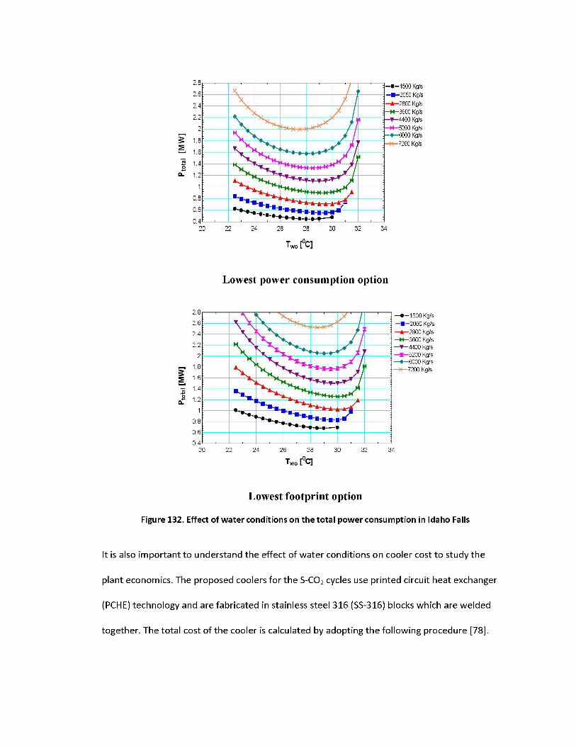
2.8
2.6
2.4
2.2
1.8
1.6
1.4
Q- 1.2
0.8
0.6
0.422 24 26 28 30 32 34
Lowest power consumption option
2.8 -•-1500 Kg/s -■-2050 Kg/s
2800 Kg/s 3600 Kg/s 4400 Kg/s 5200 Kg/s 6000 Kg/s 7200 Kg/s
2.6
2.4
2.2
1.8
1.6
1.4
1.2
0.8
0.6
0.422 24 26 28
Two [0C]30 32 34
Lowest footprint option
Figure 132. Effect of water conditions on the total power consumption in Idaho Falls
It is also important to understand the effect of water conditions on cooler cost to study the
plant economics. The proposed coolers for the S-CO2 cycles use printed circuit heat exchanger
(PCHE) technology and are fabricated in stainless steel 316 (SS-316) blocks which are welded
together. The total cost of the cooler is calculated by adopting the following procedure [78].

1) The volume of each PCHE block is calculated from the Plant Dynamics Code and the total
material required to fabricate the block is calculated as,
Massbiock = Volumebiock * 55316 density @ 20o C
2) The cost of SS316 material as per the current market is 8.48 $/kg and the total material
cost of one PCHE block is calculated.
3) The fabrication cost to chemical etch the channels and perform diffusion bonding is
estimated to be $48,480 per block.
4) The total cost of each block is estimated by adding up the material cost and the
fabrication cost of each block and the total cost of the cooler is calculated as,
Costcooier = Costbiock * Number of blocks
5) Number of PCHE blocks is assumed to be fixed at the reference design conditions at 72
for AFR-100 and 288 for ABR-1000 plants.
: 106
20 22 24 26
Two I
28 30 32 34
Lowest power consumption option

c106
sa>1
V)OO
22 24 28 30 32
wo [0C]
—•-1500 Kg/s -■-2050 Kg/s
2800 Kg/s 3600 Kg/s 4400 Kg/s 5200 Kg/s 6000 Kg/s 7200 Kg/s
34
Lowest footprint option
Figure 133. Effect of water conditions on the cooling tower cost in Idaho Falls
Figure 134 shows how the cooler cost changes with the water conditions for an AFR-100 plant
and these results don't depend on the location as the ambient air conditions have no influence
on the cooler design. It is obvious that the cost of the cooler has a similar trend to the cooler
length as it is the only variable changing during the calculations from the PDC.
5o
toOO
x 106 9
8.5
8
7.5
7
6.5
6
5.5
5
4.5
-•—1500 Kg/s -■-2050 Kg/s
2800 Kg/s 3600 Kg/s 4400 Kg/s 5200 Kg/s 6000 Kg/s 7200 Kg/s
420 22 24 26 28 30 32
r034
Two [0C]
Figure 134. Effect of water conditions on the cooler cost
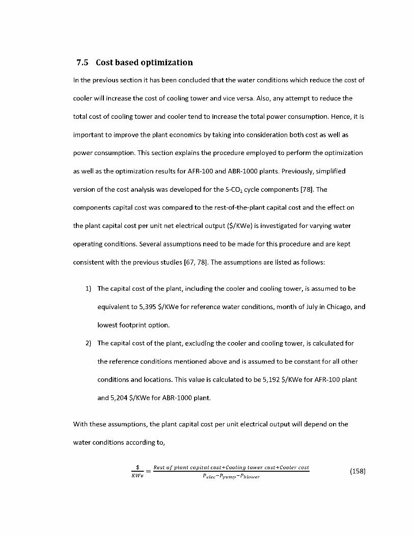
7.5 Cost based optimization
In the previous section it has been concluded that the water conditions which reduce the cost of
cooler will increase the cost of cooling tower and vice versa. Also, any attempt to reduce the
total cost of cooling tower and cooler tend to increase the total power consumption. Hence, it is
important to improve the plant economics by taking into consideration both cost as well as
power consumption. This section explains the procedure employed to perform the optimization
as well as the optimization results for AFR-100 and ABR-1000 plants. Previously, simplified
version of the cost analysis was developed for the S-CO2 cycle components [78]. The
components capital cost was compared to the rest-of-the-plant capital cost and the effect on
the plant capital cost per unit net electrical output ($/KWe) is investigated for varying water
operating conditions. Several assumptions need to be made for this procedure and are kept
consistent with the previous studies [67, 78]. The assumptions are listed as follows:
1) The capital cost of the plant, including the cooler and cooling tower, is assumed to be
equivalent to 5,395 $/KWe for reference water conditions, month of July in Chicago, and
lowest footprint option.
2) The capital cost of the plant, excluding the cooler and cooling tower, is calculated for
the reference conditions mentioned above and is assumed to be constant for all other
conditions and locations. This value is calculated to be 5,192 $/KWe for AFR-100 plant
and 5,204 $/KWe for ABR-1000 plant.
With these assumptions, the plant capital cost per unit electrical output will depend on the
water conditions according to,
$ _ Rest of plant capital cost+Cooling tower cost+Cooler cost . .KWe Pelec Ppump Pblower
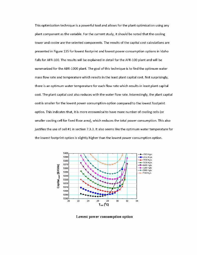
This optimization technique is a powerful tool and allows for the plant optimization using any
plant component as the variable. For the current study, it should be noted that the cooling
tower and cooler are the selected components. The results of the capital cost calculations are
presented in Figure 135 for lowest footprint and lowest power consumption options in Idaho
Falls for AFR-100. The results will be explained in detail for the AFR-100 plant and will be
summarized for the ABR-1000 plant. The goal of this technique is to find the optimum water
mass flow rate and temperature which results in the least plant capital cost. Not surprisingly,
there is an optimum water temperature for each flow rate which results in least plant capital
cost. The plant capital cost also reduces with the water flow rate. Interestingly, the plant capital
cost is smaller for the lowest power consumption option compared to the lowest footprint
option. This indicates that, it is more economical to have more number of cooling cells (or
smaller cooling cell for fixed floor area), which reduces the total power consumption. This also
justifies the use of cell #1 in section 7.3.3. It also seems like the optimum water temperature for
the lowest footprint option is slightly higher than the lowest power consumption option.
*3»
to
ro°5.roU
20 22 24 26 28 30 32
Two [0C]
—•—1500 Kg/s -■-2050 Kg/s
2800 Kg/s 3600 Kg/s 4400 Kg/s 5200 Kg/s 6000 Kg/s 7200 Kg/s
34
Lowest power consumption option
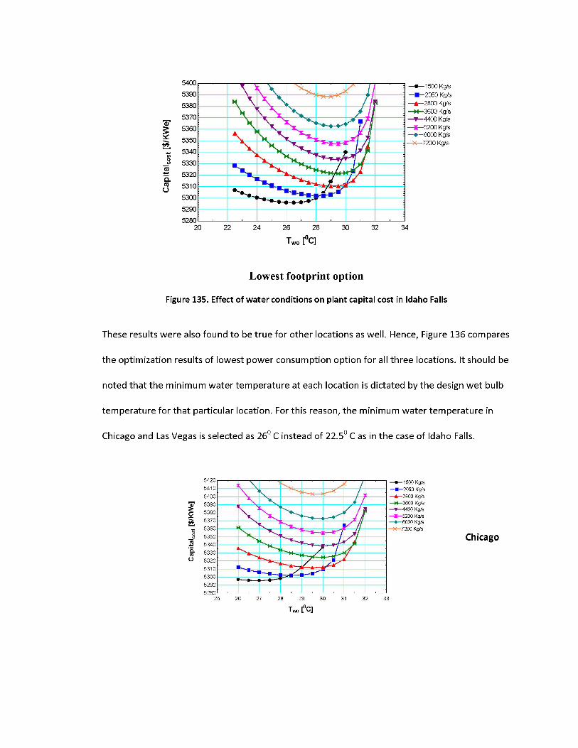
woro°Q.roo
20 22 24 26 28 30 32
Two [0C]
—•—1500 Kg/s -■-2050 Kg/s
2800 Kg/s 3600 Kg/s
—V—4400 Kg/s 5200 Kg/s 6000 Kg/s
—X—7200 Kg/s
34
Lowest footprint option
Figure 135. Effect of water conditions on plant capital cost in Idaho Falls
These results were also found to be true for other locations as well. Hence, Figure 136 compares
the optimization results of lowest power consumption option for all three locations. It should be
noted that the minimum water temperature at each location is dictated by the design wet bulb
temperature for that particular location. For this reason, the minimum water temperature in
Chicago and Las Vegas is selected as 260 C instead of 22.50 C as in the case of Idaho Falls.
5420
5410
5400
5390
5380
5370
5360
5350
5340
5330
5320
5310
5300
5290
5280
—•—1500 Kg/s -■-2050 Kg/s
2800 Kg/s 3600 Kg/s 4400 Kg/s 5200 Kg/s 6000 Kg/s 7200 Kg/s
26 27 28 29
Two [0C]30 31 32 33
Chicago
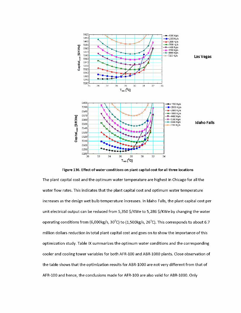
£
Two [0C]
Las Vegas
5400 —•—1500 Kg/s -■-2050 Kg/s —A—2800 Kg/s —M—3600 Kg/s
4400 Kg/s 5200 Kg/s 6000 Kg/s 7200 Kg/s
539053805370536053505340533053205310530052905280
20 22 24 26 28
Two [0C]30 32 34
Idaho Falls
Figure 136. Effect of water conditions on plant capital cost for all three locations
The plant capital cost and the optimum water temperature are highest in Chicago for all the
water flow rates. This indicates that the plant capital cost and optimum water temperature
increases as the design wet bulb temperature increases. In Idaho Falls, the plant capital cost per
unit electrical output can be reduced from 5,350 $/KWe to 5,286 $/KWe by changing the water
operating conditions from (6,000kg/s, 300C) to (1,500kg/s, 260C). This corresponds to about 6.7
million dollars reduction in total plant capital cost and goes on to show the importance of this
optimization study. Table IX summarizes the optimum water conditions and the corresponding
cooler and cooling tower variables for both AFR-100 and ABR-1000 plants. Close observation of
the table shows that the optimization results for ABR-1000 are not very different from that of
AFR-100 and hence, the conclusions made for AFR-100 are also valid for ABR-1000. Only

difference being that the power consumption, water consumption rate, and heat rejection cost
(cooling tower + cooler costs) are scaled according to the heat load, which is higher for ABR-
1000.
Table IX. Cost-based optimization results for AFR-100 and ABR-1000 plants
AFR-100 ABR-1000
Location Chicago LasVegas
IdahoFalls
Chicago LasVegas
IdahoFalls
Number of cells 53 52 46 227 223 196
Water flow rate [kg/s] 1,500 1,500 1,500 6,200 6,200 6,200
Tin [0C] 48.86 48.36 47.86 48.44 47.94 47.44
Tout [0C] 27 26.5 26 26.5 26 25.5
Design WBT [0C] 24.88 23.88 20.22 24.88 23.88 20.22
Afloor [m ] 685.1 675.7 596.5 2,971 2,925 2,566
Lfill [m] 2.219 2.056 1.61 2.46 2.231 1.676
Blower power [MW] 0.3984 0.3841 0.3391 1.688 1.663 1.459
Pump power [MW] 0.1757 0.1655 0.1446 0.7642 0.7132 0.6097
Peak water consumption [kg/s]
126.1 144.1 130 524.1 602.3 540.8
Cooler PCHE volume [m3] 34.78 31.86 29.55 131.3 121.5 113.6
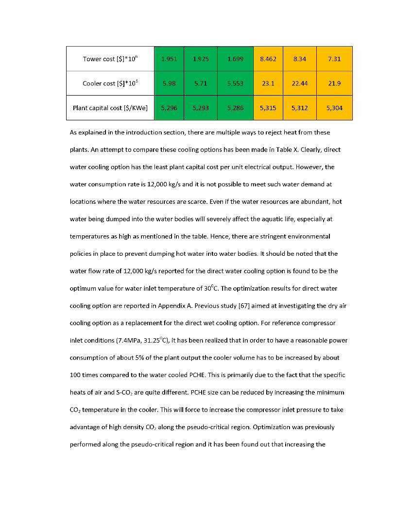
Tower cost [$]*106 1.951 1.925 1.699 8.462 8.34 7.31
Cooler cost [$]*106 5.98 5.71 5.553 23.1 22.44 21.9
Plant capital cost [$/KWe] 5,296 5,293 5,286 5,315 5,312 5,304
As explained in the introduction section, there are multiple ways to reject heat from these
plants. An attempt to compare these cooling options has been made in Table X. Clearly, direct
water cooling option has the least plant capital cost per unit electrical output. However, the
water consumption rate is 12,000 kg/s and it is not possible to meet such water demand at
locations where the water resources are scarce. Even if the water resources are abundant, hot
water being dumped into the water bodies will severely affect the aquatic life, especially at
temperatures as high as mentioned in the table. Hence, there are stringent environmental
policies in place to prevent dumping hot water into water bodies. It should be noted that the
water flow rate of 12,000 kg/s reported for the direct water cooling option is found to be the
optimum value for water inlet temperature of 300C. The optimization results for direct water
cooling option are reported in Appendix A. Previous study [67] aimed at investigating the dry air
cooling option as a replacement for the direct wet cooling option. For reference compressor
inlet conditions (7.4MPa, 31.250C), it has been realized that in order to have a reasonable power
consumption of about 5% of the plant output the cooler volume has to be increased by about
100 times compared to the water cooled PCHE. This is primarily due to the fact that the specific
heats of air and S-CO2 are quite different. PCHE size can be reduced by increasing the minimum
CO2 temperature in the cooler. This will force to increase the compressor inlet pressure to take
advantage of high density CO2 along the pseudo-critical region. Optimization was previously
performed along the pseudo-critical region and it has been found out that increasing the
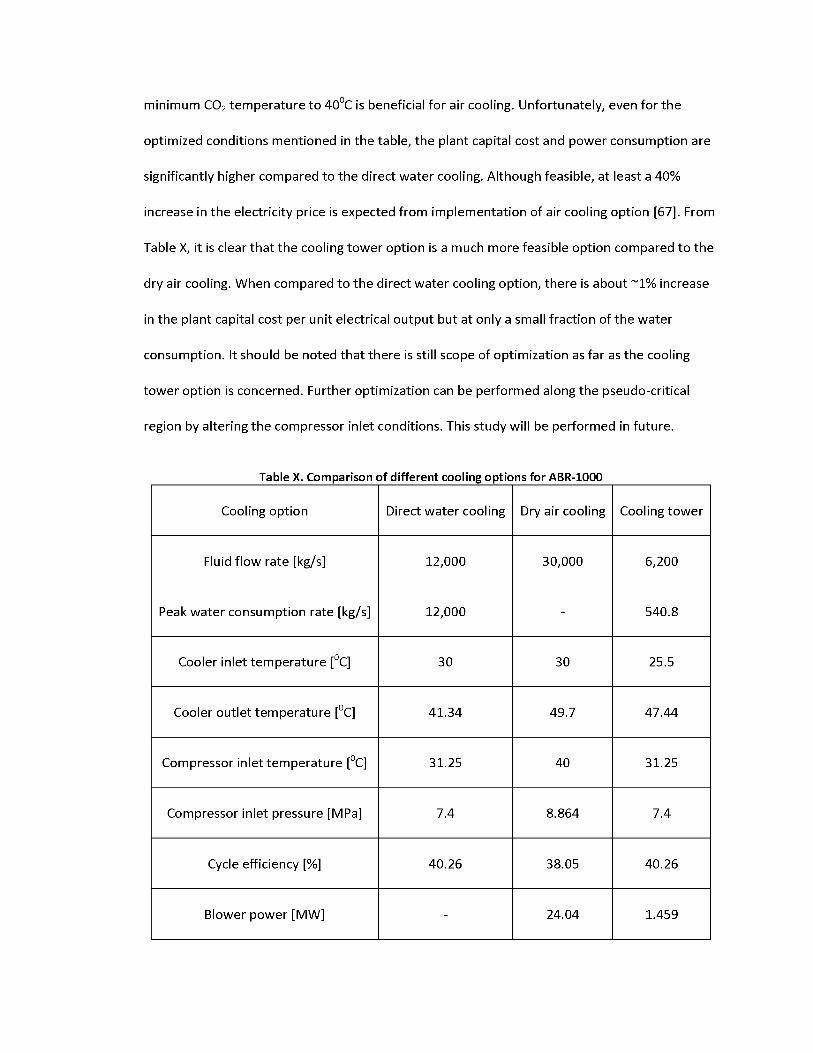
minimum CO2 temperature to 400C is beneficial for air cooling. Unfortunately, even for the
optimized conditions mentioned in the table, the plant capital cost and power consumption are
significantly higher compared to the direct water cooling. Although feasible, at least a 40%
increase in the electricity price is expected from implementation of air cooling option [67]. From
Table X, it is clear that the cooling tower option is a much more feasible option compared to the
dry air cooling. When compared to the direct water cooling option, there is about ~1% increase
in the plant capital cost per unit electrical output but at only a small fraction of the water
consumption. It should be noted that there is still scope of optimization as far as the cooling
tower option is concerned. Further optimization can be performed along the pseudo-critical
region by altering the compressor inlet conditions. This study will be performed in future.
Table X. Comparison of different cooling options for ABR-1000
Cooling option Direct water cooling Dry air cooling Cooling tower
Fluid flow rate [kg/s] 12,000 30,000 6,200
Peak water consumption rate [kg/s] 12,000 - 540.8
Cooler inlet temperature [0C] 30 30 25.5
Cooler outlet temperature [0C] 41.34 49.7 47.44
Compressor inlet temperature [0C] 31.25 40 31.25
Compressor inlet pressure [MPa] 7.4 8.864 7.4
Cycle efficiency [%] 40.26 38.05 40.26
Blower power [MW] - 24.04 1.459

Pump power [MW] 0.7843 - 0.6097
Cooler PCHE volume [m3] 126.7 3290.4 113.6
Heat rejection cost [$]*106 22.7 603.4 29.21
Plant capital cost [$/KWe] 5,271 7,670 5,304

Conclusion
With the growing energy concern in the world it is important for the research into alternative means of
power processing to be continued. As a result of relatively high efficiencies and low capital costs, the S-
CO2 Brayton Cycle is a promising technology for power production. To do this, research must be
performed to better understand S-CO2 as a working fluid within advanced turbomachinery designs. The
objective of this work was to focus on different challenging aspects of the cycle and to gain working
experience with supercritical fluids.
The first task was to experimentally measure leakage through annular and labyrinth seal geometries to
evaluate one-dimensional models and provide data for the optimization of seal design within S-CO2 flow
conditions.
The effect of eccentricity on flow through small diameter annuli was found to be minimal for the lengths
typically found in labyrinth type shaft seals. The variation in fluid friction between eccentric and
concentric shaft placements is the driving parameter behind the increase in flow due to shaft
eccentricity and at the short lengths typical of shaft seals this is not seen. An increase in flow rate of 3%
was observed for short length annular orifices. This effect was increased to 8.5% when the orifice length
was increased passed the developing entrance length and frictional effects became dominant.
Flow rate measurements for a straight through labyrinth seal with three teeth were made at inlet
pressure of 7.7, 10, and 11 MPa at inlet densities of 325, 475, and 630 kg/m3. Various labyrinth seal
leakage models were applied to the data calculated to compare applicability. Among the one
dimensional models that assume ideal and incompressible flow the equation described by Esser and
Kazakia performed the best. Their equation is a modification of the Neumann equation applying a
1
constant flow coefficient and performs within 30% for all the conditions tested. The flow coefficient
used in this formula was experimentally determined from a geometry that was most similar to the
geometry tested here. This similarity in the geometry used to determine the flow coefficient allowed
the Esser and Kazakia equation to outperform the other models based on Neumann's equation which
predicted the flow within 40%.
Empirical discharge coefficients were defined for all geometries tested to be applied to the
Homogeneous Equilibrium Model (HEM). With an experimentally determined discharge coefficient the
HEM predicted the mass flow rate with less than 5% error for the higher pressure cases of 10 and 11
MPa and less than 14% error for the lower pressure case of 7.7 MPa. The HEM works well when the
inlet condition chokes prior to entering the two phase region and begins to deviate when two-phase
effects become more prevalent. In the low inlet pressure case of 7.7 MPa where this was prevalent two
discharge coefficients were defined for two pressure ratio ranges. Using these values within their
respective ranges allowed the predicted mass flow rate to remain within 10%.
A Stepped labyrinth seal was designed to mimic the geometry used within the research loop at Sandia
National Laboratories. This provided a more complex geometry to further test the capabilities of the
facility and validate models. Three-tooth and four-tooth cases were tested at an inlet pressure of 10
MPa with a corresponding inlet density of 325 kg/m3. It was found that increasing the tooth number
decreased the flow by 5% from the three-tooth case to the four-tooth case. Inlet pressure was varied
for a constant inlet density of 640 kg/m3 and outlet pressure of 3.62 MPa to determine a probable inlet
pressure seen for the SNL leakage results. The results predicted a seal inlet pressure closer to the
compressor outlet pressure of 13.8 MPa. The results showed that the data could be used to scale to
larger diameters and apply to more practical geometries. This is an important result as it shows that
operating conditions can be duplicated in a controlled environment to better understand the conditions
2

experienced by seals and orifices within the more complex facilities. The data and models described
here are useful for creating and validating models that will be used in next generation plant dynamics
code. This data can be used as a starting point for the validation of models for more complex
geometries such as pocket damper seals and dry liftoff seals.
The second task was to develop a computational model and to understand the flow behavior of S-CO2
through labyrinth seals. An Open source CDF software OpenFOAM was used to perform a series of
simulations for S-CO2 flows through annular orifices, labyrinth seals and some plain orifices. To
accurately model the properties of S-CO2, a FIT (Fluid Interpolation Tables) algorithm was implemented
in OpenFOAM which is based on biquintic spline interpolation resulting in an error of about ~0.01%. To
solve the Navier-Stokes equations in the saturation dome, HEM is assumed to be valid. A parametric
study was performed which was divided into two parts:
The first part explained about the effect of geometrical parameters on leakage rate through seals while
holding operating condition constant. (Appendix B and C)
Conclusions that can be drawn from study of geometrical parameters are as follows:
1) Wtooth/c (Tooth width to clearance ratio) is the only major geometrical parameter influencing
discharge coefficient of an annular orifice.
2) There exists a certain range of Wtooth/c for which Cd is independent of Wtooth/c.
3) Except for very low h/s (tooth height to pitch ratio) tooth depth has no significant effect on Cd.
4) The carry over coefficient, y as defined by Hodkinson is independent of pressure ratio and stays
constant for a fixed geometry of a seal.
5) The major geometrical parameters influencing y is c/s (clearance to pitch ratio) and to some
extent Wcavity/c (Cavity width to clearance ratio).
3

6) Based on the results from numerical simulations a model for y has been developed. This model
is developed for constant tooth width and needs modification in the future to include effect of
tooth width.
7)
8)
9)
y = 0.91559 + [0.395745 + 0.113839 (WcaJtty)] Q
Shaft rotation has no effect on Cd of an annular orifice at lower PR's but has a significant effect
for a smaller pressure drop and needs further validation to develop a model for the same.
Shaft rotation has no influence on the carry over coefficient.
To predict leakage through a labyrinth seal, each constriction can be treated individually and
leakage rate equation for each constriction can be written as,
^ Cd\ntoothYmisentropic
Where the Cd of the first tooth is same as that of an annular orifice and Cd for the following
tooth depends on the Cd of previous tooth and y of the cavity. For first constriction y is equal to
1.
10) A simple 1-D isentropic model for labyrinth seals assuming Cd and y equal to 1, works
reasonably well in predicting leakage through multiple constrictions.
The second part explained about the effect of operating conditions on the leakage rate and choking
through a seal while holding the geometry constant.
Conclusions that can be drawn from study of operating conditions are as follows:
1) Changing the inlet operating condition changes leakage through seals significantly depending on
inlet density and pressure.
2) A 1-D isentropic choking theory has been put forward which predicts that there exist a range of
inlet pressures for which the flow chokes at the saturation point for a given inlet entropy
4

condition. Based on this theory, two curves are presented for an annular orifice. These two
curves control choking based on inlet operating condition as follows:
a. If the inlet condition is bounded by the two curves, the flow chokes very close to the
saturation point when the flow enters the saturation dome.
b. If the inlet condition is below both the curves, flow chokes late into the saturation
dome.
c. If the inlet condition is above both the curves, the flow chokes before it enters the two
phase dome.
3) The 1-D isentropic choking theory developed is applied to simulations performed on annular
orifices for a range of operating conditions (Table D.1) and it has been observed that the theory
works reasonably well for all the cases.
4) From simulations performed on annular orifices and labyrinth seals (Table D.1 and D.2) it has
been shown that, for a given inlet pressure there exist a range of inlet densities for which the
discharge coefficient is independent of density and is only a function of inlet pressure.
5) At high enough inlet pressures where properties are not sensitive to temperature changes, S-
CO2 behaves more like an incompressible fluid and the discharge coefficient stays constant over
the whole range of PR's. This inlet pressure increases as the number of constriction in a
labyrinth seal increases.
6) It has been concluded that the 1-D isentropic choking model is in general valid for any labyrinth
seal geometry but the upper and lower pressure limit curves depend on the number of
constrictions present in the labyrinth seal. As number of constrictions increases these two
curves move farther away from the critical point.
5

The third task of this project was to investigate the effects of buoyancy on heat transfer to supercritical
CO2. This task was achieved by performing systematic experiments for horizontal, upward, and
downward flows under similar conditions. When the bulk temperature is less than and the wall
temperature is greater than the pseudocritical temperature, significant influence of buoyancy was
observed for all three flow orientations. Enhancement and deterioration in the heat transfer was
observed on the bottom and top sides respectively for horizontal flow leading to a circumferential
variation in wall temperature. Turbulent shear stress was modified by buoyancy forces for both
downward and upward flows. For upward flow, the buoyancy forces act to reduce the turbulent shear
stress resulting in localized spikes in wall temperature. For downward flow, buoyancy forces act to
enhance the turbulent shear stress enhancing the heat transfer compared to cases with no influence of
buoyancy. The effect of buoyancy was observed to be most severe near the pseudocritical region and
pressures closer to the critical pressure. When both the bulk and wall temperatures are above the
pseudocritical temperature, the effect of buoyancy was greatly minimized due to presence of more gas
like CO2 in both the bulk and near wall regions. The only mode of heat transfer deterioration for
downward flow was observed to be due to the pseudo-film boiling phenomenon. Buoyancy parameters
suggested in literature were investigated by normalizing the experimental Nusselt numbers with that of
a forced convection correlation suggested by Jackson and Hall. For vertical flows, the buoyancy criteria
suggested by Jackson (Bu), and Seo et al. (1/Fr) were able to correctly predict the influence of buoyancy
on heat transfer. For horizontal flows, the buoyancy criterion suggested by Jackson (Bo) performed
satisfactorily. Existing correlations proposed for supercritical water were evaluated for supercritical CO2.
The correlation suggested by Mokry et al. performed well for upward flow whereas the correlations
suggested by Swenson et al., bishop et al. performed well for downward flow.
The final task of this project was to investigate the possibility of using wet cooling tower option for S-CO2
cycle as opposed to direct water cooling or dry air cooling. Two plants namely AFR-100 and ABR-1000
6

were selected as a part of investigation. A thorough literature survey was performed to explore different
types of cooling towers and their advantages and disadvantages were analyzed in detail. Finally, a
counter flow induced draft tower was chosen for investigation as it is believed to be most suitable for
the current application.
Counter flow cooling tower can be modeled using one dimensional heat and mass transfer equations.
However, nonlinear governing equations in the original form require simultaneous solutions of water
temperature, air humidity ratio and air enthalpy to obtain detailed temperature profile of water inside
the tower. Since, the purpose of this study is just to look at the design aspects of the cooling tower and
not to predict the detailed temperature distributions, certain reasonable assumptions were made to
simplify the governing equations and a code was developed which can predict the size of the tower,
water consumption as well as the power consumption rate. Two extreme options namely lowest power
consumption and lowest footprint were identified. As the names suggest, lowest power consumption
option will result in the largest plant footprint and least power consumption. And, lowest footprint
option will result in the smallest footprint and highest power consumption.
The results from the code were verified by comparing them to a vendor quotation for lowest footprint
option. After verification, the effect of ambient air conditions on the cooling tower variables was
investigated for fixed water conditions. Since, the ambient air conditions depend on the geographical
locations as well as the time of the year, three possible plant sites namely Chicago, IL, Las Vegas, NV,
and Idaho Falls, ID were selected. The design ambient conditions at each of these locations were
extracted from the ASHRAE climatic design software for all the months in a year. It has been realized
that the size of the tower, power consumption as well as the water consumption rate are maximum for
the highest wet bulb temperature. Hence, the cooling tower was designed for the month of July at all
the locations.
7

An example was demonstrated to provide an insight about the accurate control of the water conditions
to account for the changing ambient air conditions. Next, effect of water conditions on the cooler and
cooling tower variables was investigated for fixed ambient air conditions. It has been realized that the
water conditions have opposite effect on the cooling tower and cooler. For example, decreasing the
water temperature lead to a decrease in the size as well as the cost of the cooler but an increase in the
cooling tower size and cost. Similar effect was observed as far as the water flow rate is concerned. Also,
total power consumption was found to be minimum for particular optimum water conditions. Hence, a
cost-based optimization procedure was employed to determine the optimum water conditions at all
three locations which would result in least plant capital cost per unit electrical output. For optimized
conditions, direct wet cooling, cooling tower, and dry air cooling options for ABR-1000 were compared
and it can safely be concluded that the wet cooling tower option is a much more feasible and
economical option than the dry air cooling option. Moreover, replacing the direct water cooling option
with the cooling tower option would increase the plant capital cost per unit electrical output by only
~1% and consumes only a fraction of water. Hence, at locations where the water resources are scarce
and/or stringent environmental policies are in place, cooling tower option is a better option than the
direct water cooling option. Further optimization can be possibly performed by modifying the
compressor inlet conditions and this will be undertaken as a part of the future work.
8

References
[1] "A Technology Roadmap for Generation IV Nuclear Energy Systems," U.S. DOE Nuclear Energy Research Advisory Committee and the Generation IV International Forum2002.
[2] T. Conboy, S. Wright, J. Pasch, D. Fleming, G. Rochau, and R. Fuller, "Performance Characteristics of an Operating Supercritical CO2 Brayton Cycle," Journal of Engineering for Gas Turbines and Power, vol. 134, 2012.
[3] V. Dostal, P. Hejzlar, and M. J. Driscoll, "High-Performance Supercritical Carbon Dioxide Cycle for Next-Generation Nuclear Reactors," Nuclear Technology, vol. 154, pp. 265-282, 2006.
[4] R. J. Allam, M. R. Palmer, G. W. Brown Jr., J. Fetvedt, D. Freed, H. Nomoto, et al., "High Efficiency and Low Cost Electricity Generation from Fossil Fuels while Eliminating Atmospheric Emissions, Including Carbon Dioxide," Energy Procedia, vol. 37, pp. 1135-1149, 2012.
[5] T. Held, M. Persichilli, A. Kacludis, and E. Zdankiewicz, "Supercritical CO2 Power Cycle Developments and Commercialization: Why SCO2 Can Displace Steam," presented at the Power-Gen India and Central Asia, New Delhi, India, 2012.
[6] V. Dostal, P. Hejzlar, and M. J. Driscoll, "The Supercritical Carbon Dioxide Power Cycle: Comparison to Other Advanced Power Cycles," Nuclear Technology, vol. 154, pp. 283-301, 2006.
[7] Yuan, H. "Simulations of Supercritical Fluids Flow through Complex Geometries," University of Wisconsin-Madison, 2014.
[8] J. P. Edlebeck, “Measurements and Modeling of the Flow of Supercritical Carbon Dioxide,” University of Wisconsin-Madison, 2013.
[9] S. Klein and G. Nellis, Thermodynamics. New York, NY: Cambridge University Press, 2012.
[10] N.A.V. Piercy, M.S. Hooper, H.F. Winny. “Viscous Flow through Pipes with Cores,” London Journal. of Science, vol. 15-99, pp. 647-676, 1933.
[11] Tao, L.N., and Donovan, W.F., 1955, “Through-Flow in Concentric and Eccentric Annuli of Fine Clearance With and Without Relative Motion of the Boundaries”, Transactions of the ASME, Vol. 77, pp. 1291-1299.
[12] White, F.M., 2006, Fluid Mechanics. McGraw-Hill.
9

[13] V.K. Jonsson, E.M. Sparrow. “Experiments on turbulent-flow phenomena in eccentric annular ducts,” Journal of Fluid Mech. vol. 25, part 1, pp.64-86, 1966.
[14] K. Velusamy, V. K. Garg. “Entrance flow in eccentric annular ducts,” J. Num. Meth. in Fluids, vol. 19(6), pp. 493-512,1994.
[15] Vennard, J. K. and Street, R. L., 1982, Elementary Fluid Mechanics, John Wiley & Sons, New York
[16] Shultz, R. R., 1996, “Analytical and Experimental Investigation of a Labyrinth Seal Test Rig and Damper Seals for Turbomachinery,” M.S. thesis, Mechanical Engineering Department, Texas A&M University, College Station, TX
[17] Egli, A., 1935, “The Leakage of Steam through Labyrinth Seals,” Transactions of the ASME, 57, pp. 115-122
[18] Hodkinson, B., 1939, “Estimation of the Leakage through a Labyrinth Gland,” Proceedings of the Institution of Mechanical Engineers 141, pp. 283-288
[19] Vermes, G., 1961 (April), “A Fluid Mechanics Approach to the Labyrinth Seal Leakage Problem,” ASME Transactions - Journal of Engineering for Power, 83(2), pp. 161-169
[20] Childs, D. W. and Hale, K., 1994, “A Test Apparatus and Facility to Identify theRotordynamic Coefficients of High-Speed Hydrostatic Bearings,” ASME Journal of Tribology, 116, pp. 337-344
[22] Scharrer, J., 1988, “Theory Versus Experiment for the Rotordynamic Coefficient of Labyrinth Gas Seals: Part I - A Two Control Volume Model," Journal of Vibration, Acoustics, Stress and Reliability in Design, 110, pp. 270-280
[23] Esser, D. and Kazakia, J. Y., 1995, “Air Flow in Cavities of Labyrinth Seals,” International Journal of Engineering Science, 33 (15), pp. 2309-2326 [24]
[24] Kurohashi, M., Inoue, Y., Abe, T., and Fujikawa, T., 1980, “Spring and Damping Coefficients of the Labyrinth Seals,” Vibrations in Rotating Machinery, pp. 215-
[25] Sriti, M, Agouzoul, M., Ouazar, D., and Micheau, P., 1997 (May), “Simulation Numerique D’Ecoulement Compressible dans les Joints Labyrinthe,” Journal De Physique, III, 7 (5), pp. 1025-1037
[26] M. L. Corradini. (1997). Fundamentals of Multiphase Flow.
[27] G. B. Wallis, One-dimensional Two-phase Flow: McGraw-Hill, Inc., 1969.
[28] S. A. Klein, "Engineering Equation Solver," ed. Madison, WI: F-Chart Software, 2013.
10

[29] "Instruction Manual-Hydro-Pac LX Compressor," ed. Fairview, PA: Hydro-Pac, Incorporated, 2010.
[30] Duo-Tape Heavy Insulated Tape. Available: http://www.heatingtapes.com/Duo_All.pdf
[31] "SITRANS P, Series DIII Transmitter," 4 ed: Siemens Energy and Automation, 2004.
[32] "Cubemass DCI-Coriolis mass flow measuring system," ed. Reinach, Switzerland: Endress+Hauser, 2010.
[33] "NewView 7300 Specifications," ed. Middlefield, CT: Zygo Corporation, 2013.
[34] Steven A. Wright, et al., 2010. "Operation and Analysis of a Supercritical Carbon Dioxide Brayton Cycle", Albuquerque, New Mexico: Sandia National Laboratories
[35] Benvenuti, E., Ruggeri, G. & Tomasini, E., 1981. "Analytical and experimental development of labyrinth seals for process centrifugal compressors. ASME, Volume 32, pp. 21-35.
[36] OpenFOAM, 2012. "User Guide 2.1.1". [Online]Available at: http://www.openfoam.org/docs/user/userch1.php
[37] CFD, [Online]Available at http://www.cfd-online.com/Wiki/Two equation turbulence models
[38] Span, R. & Wagner, W., 1996. "A New Equation of State for Carbon Dioxide Covering the Fluid Region from the Triple-Point Tempearture to 1100 K at Pressures up to 800 MPa". American Institute of Physics and American Chemical Soceity, 25(6), pp. 1509-1596.
[39] Dyreby, J., Northland Numerics. [Online]Available at: http://www.northlandnumerics.com/
[40] Wilcox, D., 1993. "Turbulence Modeling for CFD". DCW Industries, Inc.
[41] Incropera, F.P., A.S. Lavine, and D.P. DeWitt, Fundamentals of heat and mass transfer. 2011: John Wiley & Sons.
[42] Kline, S.J. and F. McClintock, Describing uncertainties in single-sample experiments. Mechanical engineering, 1953. 75(1): pp. 3-8.
[43] Belyakov, I., Krasyakova, L. Y., Zhukovskii, A. V., and Fefelova, N. D., Heat-transfer in vertical risers and horizontal tubes at supercritical pressure. Thermal Engineering, 1972. 18(11): pp. 55-59.
11
[44] Yamagata, K., Nishikawa, K., Hasegawa, A., Fujii, T., Yoshida, S., Forced convective heat transfer to supercritical water flowing in tubes. International Journal of Heat and Mass Transfer, 1972. 15(12): pp. 2575-2593.
[45] Bazargan, M., D. Fraser, and V. Chatoorgan, Effect of buoyancy on heat transfer in supercritical water flow in a horizontal round tube. Journal of heat transfer, 2005. 127(8): pp. 897-902.
[46] Adebiyi, G. and W. Hall, Experimental investigation of heat transfer to supercritical pressure carbon dioxide in a horizontal pipe. International Journal of Heat and Mass Transfer, 1976. 19(7): pp. 715-720.
[47] Shitsman, M., Impairment of the heat transmission at supercritical pressures(Heat transfer process examined during forced motion of water at supercritical pressures). High temperature, 1963. 1: pp. 237-244.
[48] Ackerman, J., Pseudoboiling heat transfer to supercritical pressure water in smooth and ribbed tubes. Journal of Heat transfer, 1970. 92(3): pp. 490-497.
[49] Vikhrev, Y.V., Y.D. Barulin, and A. Kon’Kov, A study of heat transfer in vertical tubes at supercritical pressures. Thermal Engineering, 1967. 14(9): pp. 116-119.
[50] Alferov, N.S., Balunov, B.F., Rybin, R.A., Features of heat transfer due to combined free and forced convection with turbulent flow. Heat Transfer-Soviet Research, 1973.5(4): pp. 57-59.
[51] Jackson, J. and W. Hall, Influences of buoyancy on heat transfer to fluids flowing in vertical tubes under turbulent conditions. Turbulent forced convection in channels and bundles, 1979. 2: pp. 613-640.
[52] Wood, R.D. and J. Smith, Heat transfer in the critical region—temperature and velocity profiles in turbulent flow. AIChE Journal, 1964. 10(2): pp. 180-186.
[53] Bourke, P. and D. Pulling, An Experimental Explanation of Deterioration in Heat Transfer to Supercritical Carbon Dioxide. 1971: Atomic Energy Research Establishment.
[54] Miropol'skiy, Z. and V. Baigulov. Investigation in heat transfer, velocity and temperature profiles with carbon dioxide flow in a tube over the nearly critical region of parameters. in Proceedings of the Fifth International Heat Transfer Conference. 1974.
[55] Kurganov, V., V. Ankudinov, and A. Kaptilnyi, Experimental study of velocity and temperature fields in an ascending flow of carbon dioxide at supercritical pressure in a heated vertical pipe. High Temperature, 1986. 24(6): pp. 811-818.
12
[56] Hall, W., J. Jackson, and A. Watson. Paper 3: A Review of Forced Convection Heat Transfer to Fluids at Supercritical Pressures. in Proceedings of the Institution of Mechanical Engineers, Conference Proceedings. 1967. SAGE Publications.
[57] Shiralkar, B. and P. Griffith, The effect of swirl, inlet conditions, flow direction, and tube diameter on the heat transfer to fluids at supercritical pressure. Journal of heat transfer, 1970. 92(3): pp. 465-471.
[58] Jackson, J., Fluid flow and convective heat transfer to fluids at supercritical pressure. Nuclear Engineering and Design, 2013. 264: pp. 24-40.
[59] Jackson, J. and W. Hall, Forced convection heat transfer to fluids at supercritical pressure. Turbulent forced convection in channels and bundles, 1979. 2: pp. 563611.
[60] Bae, Y.Y., Mixed convection heat transfer to carbon dioxide flowing upward and downward in a vertical tube and an annular channel. Nuclear Engineering and Design, 2011. 241(8): pp. 3164-3177.
[61] Seo, K.W., Kim, M.H., Anderson, M.H., Corradini, M.L., Heat transfer in a supercritical fluid: classification of heat transfer regimes. Nuclear technology, 2006. 154(3): pp. 335-349.
[62] Licht, J., M. Anderson, and M. Corradini, Heat transfer to water at supercritical pressures in a circular and square annular flow geometry. International Journal of Heat and Fluid Flow, 2008. 29(1): pp. 156-166.
[63] Petukhov, B.S., Polyakof, A.F., Kuleshov, V.A., Sheckter, Y.L., Turbulent flow and heat transfer in horizontal tubes with substantial influence of thermo-gravitational forces. in Proc. of Fifth Int. Heat Transfer Conference. 1974.
[64] Mokry, S., Pioro, I., Farah, A., King, K., Gupta, S., Peiman, W., Kirillov, P., Development of supercritical water heat-transfer correlation for vertical bare tubes. Nuclear Engineering and Design, 2011. 241(4): pp. 1126-1136.
[65] Swenson, H., J. Carver, and C.d. Kakarala, Heat transfer to supercritical water in smooth-bore tubes. Journal of Heat Transfer, 1965. 87(4): pp. 477-483.
[66] Bishop, A., R. Sandberg, and L. Tong, Forced-convection heat transfer to water at near-critical temperatures and supercritical pressures. 1964, Westinghouse Electric Corp., Pittsburgh, Pa. Atomic Power Div.
[67] Moisseytsev, A., & Sienicki, J. J. (2013). Investigation of a Dry Air Cooling Option for an S-CO2 cycle.
[68] John, H. C. (2009). Cooling Tower Fundamentals . Kansas: SPX Cooling Technologies, Inc.
13

[69] SPX Technologies,. Retrieved from spxcooling.com/pdf/CTII-2
[70] Qureshi, A. B., & Zubair, M. S. (2006). A complete model of wet cooling towers with fouling in fills. Applied Thermal Engineering , 1982-1989.
[71] Merkel, F. (1925). Verdunstungskuhlung VDI Forschungsarbeiten., (p. 275). Berlin.
[72] Braun, J., Klein, S., & Mitchell, J. (1989). Effectiveness models for cooling towers and cooling coils. ASHRAE Transactions, 164-174.
[73] ASHRAE. (1996). ASHRAE Handbook - HVAC Systems and Equipment. American Society of Heating, Refrigerating, and Air-Conditioning Engineers Inc.
[74] Leeper, S. A. (1981 ). "WET COOLING TOWERS: 'RULE-OF-THUMB' DESIGN AND S IMULATION" . Idaho National Engineering Labratory: U.S. Department of Energy.
[75] Klein, S. A. Engineering Equation Solver . F- Chart Software.
[76] Kloppers, J., & Kroger, D. (2005). Refinement of the Transfer Characteristic Correlation of Wet-Cooling Tower Fills. Heat Transfer Engineering, 35-41.
[77] DollarTimes. Retrieved fromhttp://www.dollartimes.com/calculators/inflation.htm
[78] Moisseytsev, A. and Sienicki, J. J., "Cost-Based Optimization of Supercritical Carbon Dioxide Cycle Equipment," Transactions of the American Nuclear Society, Americal Nuclear Society 2011 Winter Meeting, Washington, DC, October 30-November 3, 2011
[79] Lilly, D. E. (1998). Analysis and Performance of Gas-Electric Hybrid Chiller Systems. Atlanta: Georgia Institute of Technology.
[80] Delta Cooling Towers, TM Series Cooling Tower - Installation, Operation and Maintainance Manual.
14
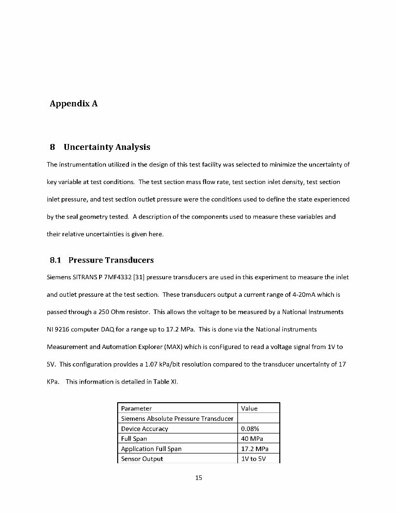
Appendix A
8 Uncertainty Analysis
The instrumentation utilized in the design of this test facility was selected to minimize the uncertainty of
key variable at test conditions. The test section mass flow rate, test section inlet density, test section
inlet pressure, and test section outlet pressure were the conditions used to define the state experienced
by the seal geometry tested. A description of the components used to measure these variables and
their relative uncertainties is given here.
8.1 Pressure Transducers
Siemens SITRANS P 7MF4332 [31] pressure transducers are used in this experiment to measure the inlet
and outlet pressure at the test section. These transducers output a current range of 4-20mA which is
passed through a 250 Ohm resistor. This allows the voltage to be measured by a National Instruments
NI 9216 computer DAQ for a range up to 17.2 MPa. This is done via the National instruments
Measurement and Automation Explorer (MAX) which is conFigured to read a voltage signal from 1V to
5V. This configuration provides a 1.07 kPa/bit resolution compared to the transducer uncertainty of 17
KPa. This information is detailed in Table XI.
Parameter ValueSiemens Absolute Pressure TransducerDevice Accuracy 0.08%Full Span 40 MPaApplication Full Span 17.2 MPaSensor Output 1V to 5V
15

NI 9215 DAQ CardBits 16Range -10V to 10V
NI MAXFull Span 17.2 MPaLimits 1V to 5V
SummaryTransducer Uncertainty 17 kPaBit Change 305 |V/bitDAQ Card Limitation 1.07 kPa/bit
Table XI. Pressure transducer uncertainty and configuration summary.
As can be seen from Table XI the NI card used provides ample resolution for the instrumentation
uncertainty from the Siemens pressure transducers. The pressure transducers were calibrated using a
dead weight oil tester. This allowed for a known pressure to be applied to the pressure transducer to
calibrate the 1V to 5V output signal measured using MAX. The pressure was varied from 0.41 MPa to
12.4 MPa and a line was fit using EES. The calibration equation is shown in Equation (159). This
equation is then used to calculate the actual pressure from the pressure measured by the transducer.
PActual - 1.20931 + 1.00003 • PMeasured (159)
8.2 Temperature
Thermocouples are used to monitor and record the temperature throughout the facility. Type E
thermocouples are used throughout the facility as they offer high resolution and work well at
temperature below 0oC. The pertinent information regarding the thermocouples is listed in Table XI
which describes the expected error. Type K thermocouples are also described in Table XII as they are
used to control the temperature of the heaters used in the system to control the inlet condition.
16
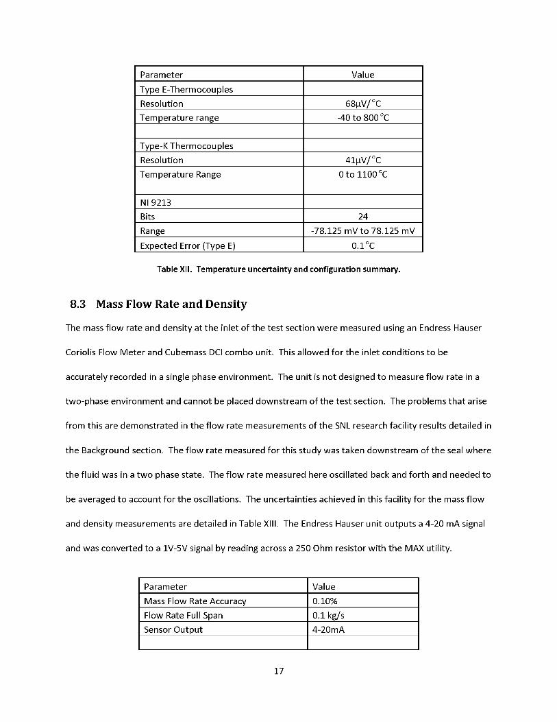
Parameter ValueType E-ThermocouplesResolution 68|V/oCTemperature range -40 to 800 oC
Type-K ThermocouplesResolution 41|V/ oCTemperature Range 0 to 1100 oC
NI9213Bits 24Range -78.125 mV to 78.125 mVExpected Error (Type E) 0.1 oC
Table XII. Temperature uncertainty and configuration summary.
8.3 Mass Flow Rate and Density
The mass flow rate and density at the inlet of the test section were measured using an Endress Hauser
Coriolis Flow Meter and Cubemass DCI combo unit. This allowed for the inlet conditions to be
accurately recorded in a single phase environment. The unit is not designed to measure flow rate in a
two-phase environment and cannot be placed downstream of the test section. The problems that arise
from this are demonstrated in the flow rate measurements of the SNL research facility results detailed in
the Background section. The flow rate measured for this study was taken downstream of the seal where
the fluid was in a two phase state. The flow rate measured here oscillated back and forth and needed to
be averaged to account for the oscillations. The uncertainties achieved in this facility for the mass flow
and density measurements are detailed in Table XIII. The Endress Hauser unit outputs a 4-20 mA signal
and was converted to a 1V-5V signal by reading across a 250 Ohm resistor with the MAX utility.
Parameter ValueMass Flow Rate Accuracy 0.10%Flow Rate Full Span 0.1 kg/sSensor Output 4-20mA
17

NI 9215 DAQBits 16Bit Change 305pV/bit
Mass Flow Rate Uncertainty 1.0E-4 kg/sFlow Rate Quantization 0.0075 kg/s/mADAQ Card Limitation 2.2E-06 kg/s
Density Uncertainty 1.0 kg/ m3
Density Quantization 200 kg/ m3/VDAQ Card Limitation 0.061 kg/m3/bit
Table XIII. Mass flow and density uncertainties and configuration summary.
8.4 Discharge Coefficient Uncertainty
An important result from this work is the empirical discharge coefficients calculated for used with the
HEM. The method for calculating the uncertainty for the discharge coefficient shall be described here.
The discharge coefficient is defined as the ratio of the measure mass flow rate to the calculated mass
flow as shown in Equation (30) repeated here.
n mmeasuredLd — :
mHEM
Performing propagation of uncertainty on Equation (160) yields Equation (161).
(160)
°cd =M
2 . ( 1 V^™-measured ____ J
— • \2 ^measured \\-VT7 / ~"lhem l • 2 1
HEM' V ™-hem /
The uncertainty in the measured mass flow rate, Equation (162), is a combination of the instrument
uncertainty and the uncertainty due to variations in the pressure ratio.
(161)
a™-measured instrument2 + aPR2 (162)
The instrument uncertainties involved here are calculated from the steady state data measurements.
The equation used to calculate the HEM mass flow rate is shown in Equation (163).
18

^HEM Aannular Pin • (163)
Where Aannuiar is the measured annular flow area, pin is the measured inlet density, and v is the
calculated fluid velocity through the orifice. The combination of the uncertainties is shown in Equation
(164).
annular^ " (Pin " ^0^ ^^Pin^^Aannuiar " v')^ ^^v^^Aannuiar " Pin(164)
The value in Equation (164) is the value reported for all discharge coefficient plots with respect to
pressure ratio. The uncertainty of the empirical discharge coefficients determined are found when the
result of Equation (164) is then combined with the uncertainty in averaging the discharge coefficients
across a range of pressure ratios. This is shown in Equation (165).
^CaJotal ^^Ca,Average (165)
The dominant uncertainty in this analysis is the standard deviation of the average discharge coefficient.
This uncertainty cannot be reduced and is a result of the models ability to predict the measured flow
rate.
8.5 Uncertainty Summary
Care was taken to accurately measure the inlet and outlet conditions experienced by the seal geometry
tested. This allows for models to be accurately evaluated using the data acquired. The uncertainties
with respect to the key variable are summarized in Table XIV.
Measurement Instrument Range UncertaintyInlet Pressure Siemens Sitrans P 0-17.2 MPa 17 kPaOutlet Pressure Siemens Sitrans P 0-17.2 MPa 17 kPaInlet Density Endress Hauser Cubemass DCI 0-1000 kg/ m3 1.0 kg/ m3
Mass Flow Rate Endress Hauser Coriolis Flow 0-0.1 kg/ m3 1E-04 kg/s
Table XIV. Summary of key variable uncertainties.
19
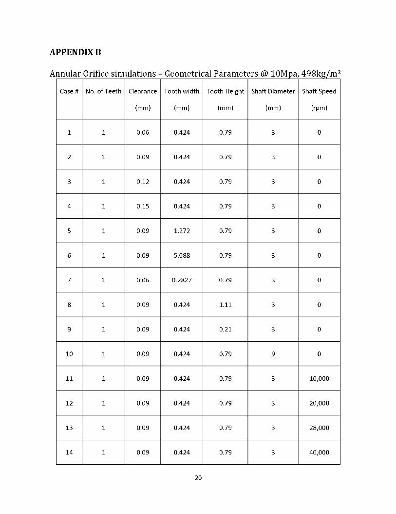
APPENDIX B
Annular Orifice simulations - Geometrical Parameters @ 10Mpa, 498kg/m3
Case # No. of Teeth Clearance Tooth width Tooth Height Shaft Diameter Shaft Speed
(mm) (mm) (mm) (mm) (rpm)
1 1 0.06 0.424 0.79 3 0
2 1 0.09 0.424 0.79 3 0
3 1 0.12 0.424 0.79 3 0
4 1 0.15 0.424 0.79 3 0
5 1 0.09 1.272 0.79 3 0
6 1 0.09 5.088 0.79 3 0
7 1 0.06 0.2827 0.79 3 0
8 1 0.09 0.424 1.11 3 0
9 1 0.09 0.424 0.21 3 0
10 1 0.09 0.424 0.79 9 0
11 1 0.09 0.424 0.79 3 10,000
12 1 0.09 0.424 0.79 3 20,000
13 1 0.09 0.424 0.79 3 28,000
14 1 0.09 0.424 0.79 3 40,000
20
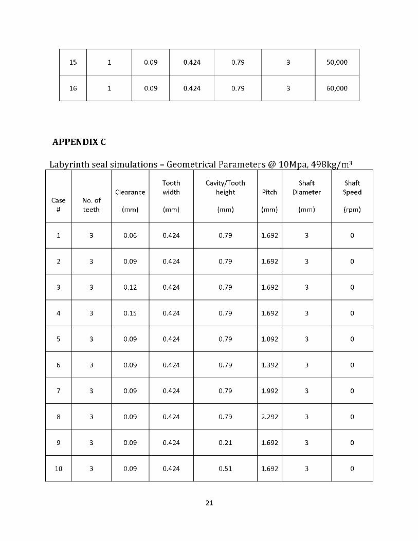
15 1 0.09 0.424 0.79 3 50,000
16 1 0.09 0.424 0.79 3 60,000
APPENDIX C
Labyrinth seal simulations - Geometrical Parameters @ 10Mpa, 498kg/m3
Case#
No. ofteeth
Clearance
(mm)
Toothwidth
(mm)
Cavity/Toothheight
(mm)
Pitch
(mm)
ShaftDiameter
(mm)
ShaftSpeed
(rpm)
1 3 0.06 0.424 0.79 1.692 3 0
2 3 0.09 0.424 0.79 1.692 3 0
3 3 0.12 0.424 0.79 1.692 3 0
4 3 0.15 0.424 0.79 1.692 3 0
5 3 0.09 0.424 0.79 1.092 3 0
6 3 0.09 0.424 0.79 1.392 3 0
7 3 0.09 0.424 0.79 1.992 3 0
8 3 0.09 0.424 0.79 2.292 3 0
9 3 0.09 0.424 0.21 1.692 3 0
10 3 0.09 0.424 0.51 1.692 3 0
21
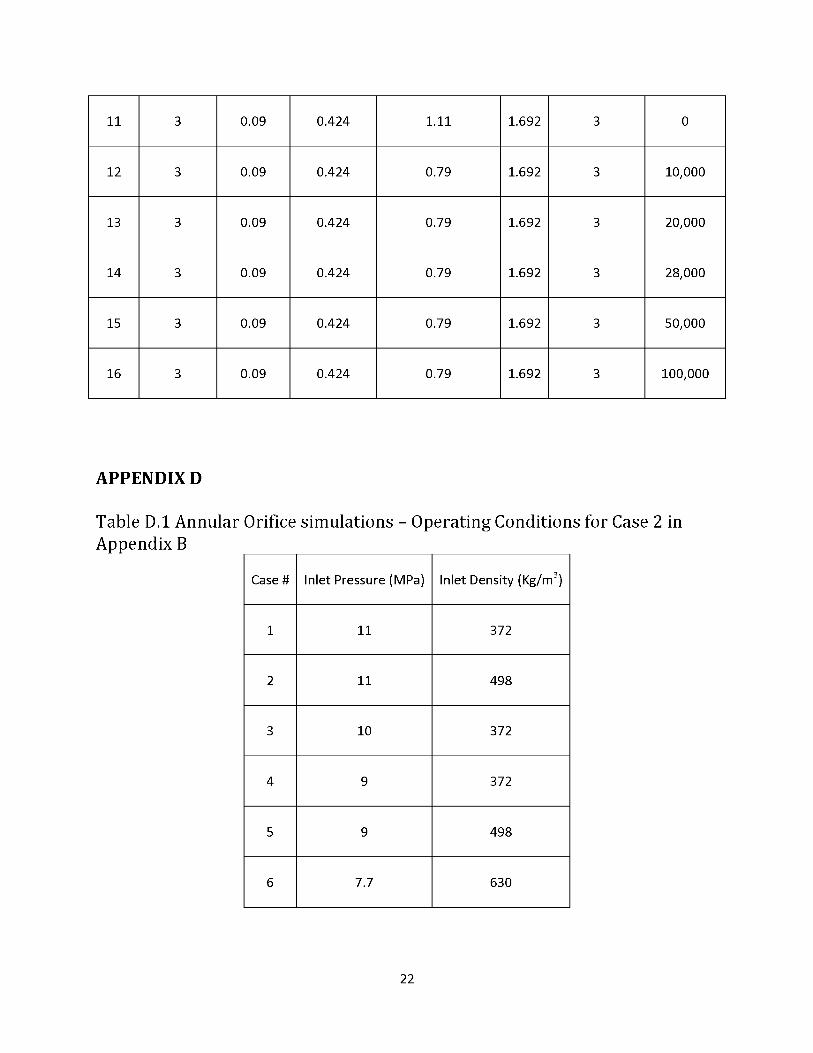
11 3 0.09 0.424 1.11 1.692 3 0
12 3 0.09 0.424 0.79 1.692 3 10,000
13 3 0.09 0.424 0.79 1.692 3 20,000
14 3 0.09 0.424 0.79 1.692 3 28,000
15 3 0.09 0.424 0.79 1.692 3 50,000
16 3 0.09 0.424 0.79 1.692 3 100,000
APPENDIX D
Table D.1 Annular Orifice simulations - Operating Conditions for Case 2 in Appendix B _____________________ _______________
Case # Inlet Pressure (MPa) Inlet Density (Kg/m3)
1 11 372
2 11 498
3 10 372
4 9 372
5 9 498
6 7.7 630
22
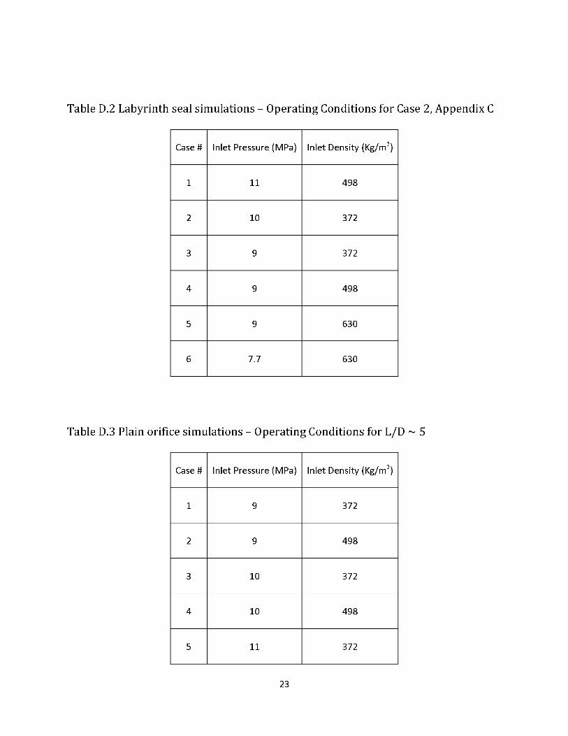
Table D.2 Labyrinth seal simulations - Operating Conditions for Case 2, Appendix C
Case # Inlet Pressure (MPa) Inlet Density (Kg/m3)
1 11 498
2 10 372
3 9 372
4 9 498
5 9 630
6 7.7 630
Table D.3 Plain orifice simulations - Operating Conditions for L/D ~ 5
Case # Inlet Pressure (MPa) Inlet Density (Kg/m3)
1 9 372
2 9 498
3 10 372
4 10 498
5 11 372
23

24