TB2J: a python package for computing magnetic interaction parameters

Xu Hea,b,c,∗, Nicole Helbigc, Matthieu J. Verstraeteb,c, Eric Bousqueta

aPhysique Theorique des Materiaux, Q-MAT, CESAM, Universite de Liege, B-4000 Sart-Tilman, BelgiumbCatalan Institute of Nanoscience and Nanotechnology (ICN2), CSIC, BIST, Campus UAB, Bellaterra, Barcelona, 08193, Spain

cNanomat, Q-Mat, CESAM, and European Theoretical Spectroscopy Facility, Universite de Liege, B-4000 Liege, Belgium

Abstract

We present TB2J, a Python package for the automatic computation of magnetic interactions, including exchange andDzyaloshinskii-Moriya, between atoms of magnetic crystals from the results of density functional calculations. Theprogram is based on the Green’s function method with the local rigid spin rotation treated as a perturbation. As input,the package uses the output of either Wannier90, which is interfaced with many density functional theory packages,or of codes based on localised orbitals. A minimal user input is needed, which allows for easy integration into high-throughput workflows.

1. Introduction

First-principles simulations of magnetic materialshave attracted strong interest in the last decade dueto an increase in precision provided by density func-tional theory (DFT) codes for strongly correlated mag-netic atoms and also because of the developments inspintronics applications [1, 2, 3, 4, 5, 6]. Understand-ing the complex microscopic origin of the magnetic in-teractions often requires a reduction of the full many-body electronic interactions to effective Hamiltonians,the two most important ones being the Heisenberg andthe Hubbard Hamiltonians [7]. The parameters of theseHamiltonians are fit to DFT data to give access to aneasier understanding of the magnetic interactions andto allow for simulations of larger systems and/or withdynamics. Novel sensing, storing and computing tech-nologies have been proposed using spin waves [8] andskyrmions [9, 10]. Theoretical models have consis-tently opened new vistas and explained experimentalfindings in complex new chemistries, geometries, andheterostructures. Reliable ab initio calculations of theeffective Hamiltonian parameters is crucial for predic-tive and quantitative simulations. Fitting these param-eters is, however, often very cumbersome and necessi-tates a case-by-case construction [11].

For the Heisenberg Hamiltonian, one of the mostcommon fitting procedures is through total energy cal-

∗Corresponding authorEmail address: mailhexu@gmail.com (Xu He)

culations or energy mapping analysis [11]. This ap-proach necessitates the calculation of the total energiesof different magnetic configurations. The parameters ofthe Heisenberg Hamiltonian are then fit to these ener-gies under the supposition that the change in energy isonly related to the magnetic interactions. This requiresto have at least as many calculated magnetic configura-tions as the number of parameters of the Hamiltonian(though more magnetic configurations are usually nec-essary to converge the fit), which often requires the useof large supercells. This simple method gives good re-sults in some cases but the Heisenberg model itself canbreak down if the chosen magnetic configurations devi-ate too much from the ground-state one. This can hap-pen, e.g., if a magnetic phase, often the ferromagnetic(FM) one, closes the band gap of an insulating antifer-romagnetic (AFM) ground-state. Also, the method be-comes unsuitable if the supercell needed to probe all ofthe pertinent magnetic configurations is too large to behandled by DFT. For example, if certain configurationsshow a delocalized picture for the electrons they mustbe excluded from the fit, which typically leads to an in-crease in the size of the supercell needed to provide asufficiently large number of configurations.

Another method to determine the parameters is theGeneralized Bloch Theorem (GBT) [12, 13] whichadapts the boundary conditions on the spin orientationto account for a spin spiral. From the change in totalenergy one can extract the magnetic interaction parame-ters. As yet another alternative, Density Functional Per-turbation Theory (DFPT) has been extended to magnetic

Preprint submitted to Elsevier September 8, 2020

field perturbations by Savrasov [14] and yields the sus-ceptibility and the magnetic exchange as a sub-product.This perturbation has been implemented in abinit [15]and quantum Espresso [16], and has also been com-bined with atomic displacements within non-collinearformalisms [17]. For several magnetic ions in the unitcell, a local perturbation DFPT scheme is presented inRef. [18].

A different procedure, which avoids the problems ofthe total energy mapping, employs Green’s functions bytaking the local spin rotation as a perturbation, as pro-posed in the seminal work of Liechtenstein, Katsnel-son, Antropov and Gubanov (LKAG) [19]. The Green’sfunction method allows to determine the Heisenbergmagnetic interaction parameters from the ground-statesolution of the system, regardless of whether it is FMor AFM. This method also allows access to a band-by-band decomposition of the different magnetic in-teractions, and it is easier to automatize than the to-tal energy mapping [20]. The method was also ex-tended to correlated systems in Refs. [21, 22]. Bytaking into account relativistic effects (spin-orbit cou-pling), the Dzyaloshinskii-Moriya interaction (DMI)[23, 24, 25, 26] and the magnetic anisotropy can becalculated as well [21, 22]. The method has been ex-tended to orbital-spin and orbital-orbital magnetic in-teractions [27, 28]. Higher order terms in the Hamil-tonian, like the four-spin interaction or the biquadraticterm, were also calculated through this method [29, 30].The LKAG method of computing magnetic interactionshas been initially implemented with the Korringa-Kohn-Rostoker Greens function (KKR-Green) [31, 32] andtight-binding linear muffin-tin methods [33], and hasproven to be quite efficient. Its extension to other basissets popular for DFT calculations will strongly broadenits usage.

Constructing the Green’s function has proven to becumbersome for non-localized basis sets (e.g. planewaves), but this difficulty is greatly reduced by the useof Wannier functions (WF) as done by Kokorin et al.in [34]. The WFs can be constructed from first prin-ciples with the widely used open source code Wan-nier90 [35, 36]. Wannier90 has been interfaced with alarge number of DFT codes, including Abinit [37, 38],Quantum Espresso [39], Siesta [40], VASP [41, 42],Wien2K [43], Fleur [44], Octopus [45, 46], OpenMX[47], GPAW [48], ELK [49], and many others. Sev-eral codes, including exchange.x [34], nojij [50], and Jx[51], exist which calculate magnetic exchange param-eters from Wannier functions or linear combination ofatomic orbitals (LCAO) DFT results. However, to thebest of our knowledge, DMI and anisotropic exchange

from non-relativistic effects have not been integratedyet.

Here, we present a Python package, TB2J, that al-lows for automatic and systematic calculations of theparameters of a Heisenberg Hamiltonian through theKorotin approach [34]. The script can compute theisotropic exchanges, the anisotropic exchanges, and theDMI from the output of the Wannier90 code or from aLCAO Hamiltonian (Siesta and OpenMX through theSISL package [52], and GPAW) following the schemeproposed in Refs. [19, 24, 30]. TB2J is designed withthe goal to minimize the number of inputs and actionsfrom the user. In most cases, only the paths of the Wan-nier or DFT related files and the species of magneticatoms are mandatory. Several types of output files aregenerated which can then be used in spin dynamics andMonte Carlo codes. TB2J’s API is implemented in anabstract manner that eases interfacing with new tight-binding-like Hamiltonians or spin dynamics simulation.

We first present the general methods used in TB2Jand then describe how these methods are implemented.Next, we exemplify the usage of TB2J by applying it to,BCC Fe, HCP Co bulk, SrMnO3, BiFeO3, and La2CuO4crystals. In the end we discuss the advantages and limi-tations of this method.

Throughout this paper, vectors are denoted with the~notation while matrices are represented with bold char-acters.

2. Formalism and algorithms

The main idea of the method is to perturb a localizedspin, in both the Heisenberg spin model and the DFTelectronic model. For the latter, the rigid spin-rotationperturbation is done within the single-particle Green’sfunction method. The Heisenberg parameters are thenmapped to the electron expressions [19]. We will con-sider the quantization axis along z in the following.

2.1. Heisenberg model

The Heisenberg Hamiltonian contains four differentparts and reads as

E =−∑i

Ki(~Si ·~ei)2

−∑i, j

[Jiso

i j~Si ·~S j

+~SiJanii j~S j

+~Di j ·(~Si×~S j

)], (1)

2

Convention Ji j

− 12 ∑

i jJi j~Si ·~S j 2Ji j

− ∑<i j>

Ji j~Si ·~S j 2Ji j

12 ∑

i jJi j~Si ·~S j −2Ji j

∑<i j>

Ji j~Si ·~S j −2Ji j

∑i j

Ji j~Si ·~S j −Ji j

Table 1: The conversion of Ji j to other conventions, where J is theexchange parameter in that convention. The notation < i j > means apair of i j without counting it twice. The DMI parameters ~D can beconverted in the same way.

where the first term represents the single-ion anisotropy(SIA), the second is the isotropic exchange, and thethird term is the symmetric anisotropic exchange, whereJani is a 3× 3 symmetric tensor. The final term is theDMI, which is antisymmetric. Importantly, the SIA isnot accessible from Wannier90 as it requires separatelythe spin-orbit coupling part of the Hamiltonian [53].However, it is readily accessible from constrained DFTcalculations [54]. We note that there are several con-ventions for the Heisenberg Hamiltonian, here we take acommonly used one in atomic spin dynamics: we use aminus sign in the exchange terms, i.e. positive exchangeJ values favor ferromagnetic alignment. Every pair i jis taken into account twice, Ji j and J ji are both in theHamiltonian. The spin vectors ~Si are normalized to 1,so that the parameters are in units of energy. The othercommonly used conventions differ in a prefactor 1/2 ora summation over different i j pairs only. The conver-sion factors to other conventions are given in Table 1.For other conventions in which the spins are not nor-malized, the parameters need to be divided by |Si|

∣∣S j∣∣

in addition.From the total energy due to the spin interactions, Eq.

(1), we obtain the following variation with respect to the~Si and ~S j

δEi j =−2Jisoi j δ~Si ·δ~S j

−2δ~SiJanii j δ~S j

−2~Di j · (δ~Si×δ~S j)

(2)

2.2. Tight-binding Hamiltonian and Green’s function

We start from a generalized tight-binding Hamilto-nian. The localized basis functions are denoted asψimσ (~r) with i, m, and σ being the site, orbital, and spin

indices, respectively. Due to translation symmetry, thetight-binding Hamiltonian, H, and the overlap, S, matri-ces can be parameterized as

Him jm′σσ ′(~R) = 〈ψimσ (~r)|H |ψ jm′σ ′(~r+~R)〉 ,(3)

Sim jm′σσ ′(~R) = 〈ψimσ (~r)| |ψ jm′σ ′(~r+~R)〉 , (4)

where~r is the position inside the unit cell, ~R is the lat-tice vector, and H denotes the total Hamiltonian. Theoverlap matrix S reduces to the identity matrix whenthe basis functions are orthonormal. TB2J can use bothnon-orthogonal LCAO basis sets and orthogonal Wan-nier basis sets. Below we discuss only the results foran orthogonal basis set. The non-orthogonal basis setis discussed in Ref. [50], where it is shown that the ex-pressions for the exchange parameters are the same asfor an orthogonal basis.

In the following, we drop all orbital and spin indicesfor simplicity, Hence Hi j is a sub-matrix of H contain-ing all the spin and orbital components for atoms i andj. We note that in DFT it is possible to do non-collinearcalculations with or without SOC (the exchange correla-tion potential can induce a non-collinear ground state).If one were to perform a calculation with SOC and thespin constrained to one direction, it would be catego-rized as collinear. In the collinear case, H is diagonal inthe spin subspace.

The Green’s function in reciprocal space is defined as

G(~k,ε) =(

εS(~k)−H(~k))−1

, (5)

where H(~k) = ∑~R H(~R)ei~k·~R, and S(~k) = ∑~R S(~R)ei~k·~R.The Green’s function in real space is obtained using thefollowing expression

G(~R,ε) =∫

BZG(~k,ε)e−i~k·~R d~k. (6)

In the following, we drop the ~R in the atom pair la-beled by i, j,~R, e.g. Gi j means Gi j(~R), and G ji meansG ji(−~R). From Eq. (7) all equations are given in realspace.

For each atom i, the intra-atomic component of H isdefined as Pi = Hii(~R = 0) and is of size 2Norb×2Norb.Each Pi,mm′ is a 2× 2 matrix in spin, which can be de-composed into its scalar and vector parts

Pimm′ = p0imm′ I+~pimm′ ·~σ , (7)

= p0imm′ I+ pimm′~eimm′ ·~σ ,

where ~pimm′ is the vector part of P, (upper case P de-notes matrices in spin and orbitals, lower case p is used

3

for matrices in orbitals only) which has the x, y, and zcomponents px

imm′ , pyimm′ , pz

imm′ . ~eimm′ is the unit orien-tation vector of ~pimm′ , and ~σ = (σx,σz,σz) are the threePauli matrices. In condensed form, the spin and orbitalmatrix for site i is now Pi = p0

i I+~pi ·~σ . We can decom-pose the Green’s function for each inter-site orbital pairGim, jm′ in the same way

Gim, jm′ = G0im, jm′I+ ~Gim, jm′ ·~σ , (8)

where G0im, jm′ and ~Gim, jm′ form the G0

i j and ~Gi j matrices,respectively.

2.3. Magnetic force theoremAccording to the force theorem the total energy vari-

ation due to a small perturbation from the ground statecoincides with the change of the single-particle energiesat fixed ground-state potential

δE =∫ EF

−∞

εδn(ε) dε =−∫ EF

−∞

δN(ε) dε (9)

where n(ε) = − 1π

ImTr(G(ε)) is the density of statesand N(ε) = − 1

πImTr(ε−H) is the integrated density

of states. The traces are taken over orbitals only, notspin. Thus, the first order variation of N due to δH canbe written as δN(ε) = 1

πImTr(δHG); the second order

variation is δ 2N(ε) = 1π

ImTr(δHGδHG).Now we use the spin rotation as a perturbation. For

the rotation of the spin at site i, the change in the energyup to the second order reads as

δE1spini =− 1

π

∫ EF

−∞

ImTr(δHiG+δHiGδHiG) dε.

(10)Similarly, for the rotation of the spins at sites i and j,the change in energy is given by

δE2spini j =− 1

π

∫ EF

−∞

ImTr [δHiG+δHiGδHiG

+δH jG+δH jGδH jG+2δHiGδH jG ] dε.

(11)

The energy variation due to the two-spin interaction isthen

δEi j =δE2spini j −δE1spin

i −δE1spinj =

− 2π

∫ EF

−∞

ImTr(δHiGδH jG) dε.(12)

The change of H due to the rotation of spin is ~δφ ×~pwith the rotation axis along ~δφ and the angle

∣∣∣ ~δφ

∣∣∣.

By putting this into Eqn. 12, we get

δEi j =−2[A00i j − ∑

u=x,y,zAuv

i j ]δ~ei ·δ~e j

−2 ∑u,v∈x,y,z

δeui [A

uvi j +Avu

i j ]δevj

−2~di j · (δ~ei×δ~e j)

(13)

in which the 4×4 matrix Ai j is defined as

Auvi j =−

1π

∫ EF

−∞

Tr{

pzi G

ui jp

zjG

vji

}dε, (14)

where u,v ∈ {0,x,y,z}, and the component of ~di j, dui j =

Re(A0ui j −Au0

i j ). Comparing Eq. (13) to Eq. (2), we canfind that the values of the isotropic exchange Jiso , theanisotropic exchange Jani, and the DMI ~D can be ex-pressed as

Jisoi j = Im(A00

i j −Axxi j −Ayy

i j −Azzi j), (15)

Jani,uvi j = Im(Auv

i j +Avui j ), (16)

Dui j = Re(A0u

i j −Au0i j ), (17)

which is the same with Ref. [30].If spin-orbit coupling (SOC) is neglected, A0u

i j = Au0i j ,

i.e. the DMI term is zero and both p and G only havecomponents along the spin quantization axis, say thez direction. Then, the x and y components of ~p and~G vanish. Thus, ~pi = (0,0,pz

i ), Gx = Gy = 0, G0 =12 (G

↑+G↓), Gz = 12 (G

↑−G↓). The isotropic exchangeparameter then reduces to

Jisoi j = Im(A00

i j −Azzi j). (18)

Defining ∆i = p↑i −p↓i = 2|~pi|= 2pzi we obtain from Eq.

(18) the LKAG [19] expression for isotropic exchange

Jisoi j =− 1

4π

∫ EF

−∞

ImTr{

∆iG↑i j∆ jG↓ji}

dε. (19)

2.4. xyz average strategyWe note that when all spins are oriented along one

direction (e.g. z), the components with u = z or v = z inthe J tensor are non-zero if the variation with respect tothe rotation is only kept to first order. The xz, yz, zx, zy,and zz components of the anisotropic exchange, and theDz in the DMI cannot be obtained from a single calcula-tion with magnetization along the z direction. It shouldbe noted that this does not affect the properties too muchif the system stays close to the reference spin state, asthese terms are small and higher order in the spin ro-tation angles. For example, in a AFM with small spin

4

canting system, the parameters obtained from the AFMreference state can be used directly to get the cantingangles. To determine the missing parameters, we ro-tate the whole system and lattice, (equivalently one canrotate the quantization axis) from z to the x and y direc-tions and apply the back-rotation to the DMI vectors. Aweighted average over all three directions is taken: theinaccessible components are given a weight of 0 and therest have the same weight. This small trick allows notonly to obtain the full set of Jani ~D vector components, but also to reduce the numerical noise. The DMI isusually much smaller than the isotropic exchange, suchthat its calculation is more numerically delicate. This is-sue arises in particular when Wannier functions are usedwhose symmetry is not guaranteed, and where the dis-entanglement procedure can introduce numerical errors.

A direct approach to calculate the Dz term is pro-posed in Ref. [25], taking the spin-rotation perturbationto higher order. This is not implemented in TB2J, andwould also be more sensitive to numerical noise.

2.5. Higher order termsIt has been shown by several authors that the pa-

rameters from the Green’s function method cannot bemapped exactly onto a bilinear J tensor [29, 55, 30]and higher order terms need to be considered, which in-clude multi-spin interactions and the higher-order two-spin terms. In the simplest case, following Ref. [30], theHamiltonian can be written in a biquadratic form as

HQ =−∑i, j

J′i j~Si~S j−∑

i, jBi j

(~Si~S j

)2, (20)

where J′i j and Bi j are determined by the A matrices as

J′i j = A00i j −3Azz

i j , (21)Bi j = Azz

i j . (22)

When~Si and ~S j are close to their reference values, wehave

Ji j = − d2HQ

d~Sid~S j= J′i j +2Bi j~Si~S j (23)

' J′i j +2Bi j~Srefi~Sref

j = J′i j +2Bi j = A00i j −Azz

i j ,

which is equivalent to the Ji j expression with only bi-linear terms considered, and it shows that the effectivebilinear J term depends on the orientation of Si and S j.This method was proposed in order to improve the de-scription of the system when the deviation from the ref-erence state is large [30]. From our limited experience,however, the parameters produced by Eqs. (21) and (22)are not always physical and their fit is more complex.

3. Implementation

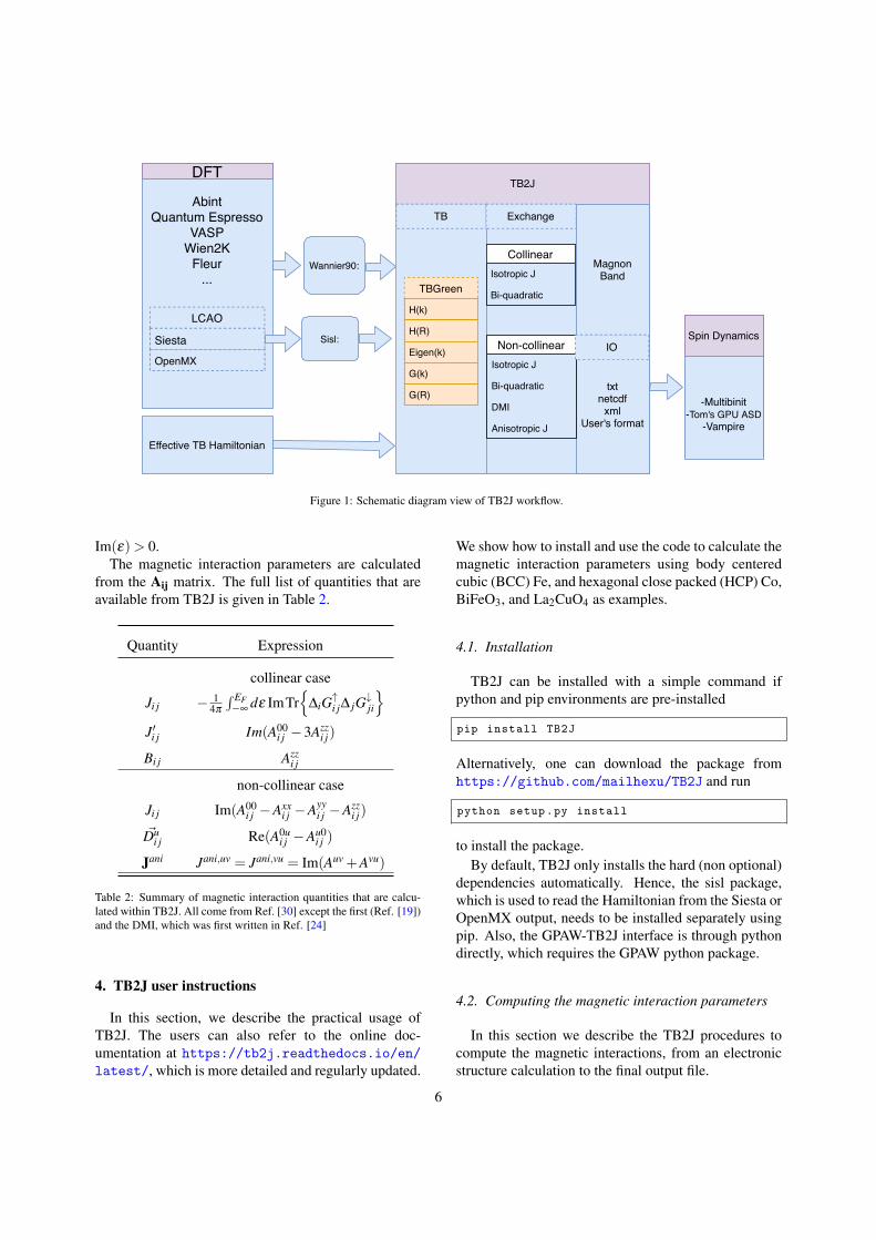
The TB2J package is implemented with three mainmodules, the tight-binding (TB) module, the exchangemodule, and the output module (see Fig. 1 for aschematic view). The TB module provides the inter-face with external DFT and Wannier function codes andcalculates the Green’s function. The exchange moduleuses the Green’s function to calculate the magnetic in-teraction parameters. The output module writes theseparameters to output files and provides a python APIfrom which the magnon band structure can be calcu-lated.

The TB module defines the classes of the TB modeland the Green’s function. The internal TB module canread the Wannier90 output data files to build the Hamil-tonian. The WF’s are assigned to the nearest atom withthe crystal periodicity taken into account. A warning isissued if a WF is far away from any atom. The code uti-lizes the “duck type” feature: a class can be pluggedin if the specific required methods are defined. Themethods include the calculation of H(~k) and the eigen-values and eigenvectors. Hence, external libraries canbe wrapped easily. An interface to the sisl library [52]has been implemented, which includes the tight-bindingmodel from Siesta and OpenMX. We also wrap directlythe python based DFT code GPAW in LCAO mode in-stead of reading the Hamiltonian from the output files.

Starting from the eigenvalues and eigenvectors, theGreen’s functions can be calculated without invert-ing the εS(~k) − H(~k) matrix for every ε . Instead,the Green’s functions are calculated with G(~k,ε) =

Ψ(~k)[εI−Diag(E(~k))

]−1Ψ(~k)†, where E(~k) and Ψ(~k)

are the eigenvalues and the eigenvector matrices, re-spectively. The real-space Green’s function can then becalculated by Fourier transforming G(k).

Once the Green’s functions are calculated, the ex-change module calculates the magnetic interaction pa-rameters using Eqs. (15)-(17). The Hamiltonian andthe Green’s functions are first decomposed into their{0,x,y,z} components. Then, the elements of the 4×4matrix, Tr

{piGu

i jp jGvji

}for each ε are calculated and

later integrated to obtain the Ai j matrix.A contour integration method is used for the

∫ EF dε

integration. The range of the integration is (Emin,EF),where Emin is either below the lowest band energy orchosen such that the orbitals below Emin have only negli-gible interaction with those near EF . By default, a semi-circle path is used, which is centered at (Emin +EF)/2on the real axis and has a radius of (EF −Emin)/2, go-ing through the upper half of the complex plane with

5

Wannier90:

Sisl:

DFT

AbintQuantum Espresso

VASPWien2K

Fleur...

TB2J

TBGreen

H(k)

H(R)

Eigen(k)

G(k)

G(R)

TB Exchange

MagnonBand

txtnetcdf

xmlUser's format

LCAO

SiestaOpenMX

Effective TB Hamiltonian

Spin Dynamics

-Multibinit-Tom's GPU ASD

-Vampire

CollinearIsotropic J

Bi-quadratic

Non-collinearIsotropic J

Bi-quadratic

DMI

Anisotropic J

IO

Figure 1: Schematic diagram view of TB2J workflow.

Im(ε)> 0.The magnetic interaction parameters are calculated

from the Aij matrix. The full list of quantities that areavailable from TB2J is given in Table 2.

Quantity Expression

collinear case

Ji j − 14π

∫ EF−∞

dε ImTr{

∆iG↑i j∆ jG

↓ji

}J′i j Im(A00

i j −3Azzi j)

Bi j Azzi j

non-collinear case

Ji j Im(A00i j −Axx

i j −Ayyi j −Azz

i j)

~Dui j Re(A0u

i j −Au0i j )

Jani Jani,uv = Jani,vu = Im(Auv +Avu)

Table 2: Summary of magnetic interaction quantities that are calcu-lated within TB2J. All come from Ref. [30] except the first (Ref. [19])and the DMI, which was first written in Ref. [24]

4. TB2J user instructions

In this section, we describe the practical usage ofTB2J. The users can also refer to the online doc-umentation at https://tb2j.readthedocs.io/en/latest/, which is more detailed and regularly updated.

We show how to install and use the code to calculate themagnetic interaction parameters using body centeredcubic (BCC) Fe, and hexagonal close packed (HCP) Co,BiFeO3, and La2CuO4 as examples.

4.1. Installation

TB2J can be installed with a simple command ifpython and pip environments are pre-installed

pip install TB2J

Alternatively, one can download the package fromhttps://github.com/mailhexu/TB2J and run

python setup.py install

to install the package.By default, TB2J only installs the hard (non optional)

dependencies automatically. Hence, the sisl package,which is used to read the Hamiltonian from the Siesta orOpenMX output, needs to be installed separately usingpip. Also, the GPAW-TB2J interface is through pythondirectly, which requires the GPAW python package.

4.2. Computing the magnetic interaction parameters

In this section we describe the TB2J procedures tocompute the magnetic interactions, from an electronicstructure calculation to the final output file.

6

4.2.1. Preparation of electronic structure and tight-binding Hamiltonian

To obtain the magnetic interaction parameters, thefirst step is to do a converged DFT calculation of amagnetic crystal, at the collinear or non-collinear level.Preferably, this calculation treats the magnetic groundstate of the system, however, the magnetic interactionparameters can also be calculated for a different refer-ence state. It should be noted that the spin quantizationaxis is presumed to be along the z axis throughout TB2J.

The next step is to construct the tight-binding Hamil-tonian. For DFT codes using non-local basis sets, likeplane waves, the WFs can be constructed for any codewhich has an interface with Wannier90. All the spin-polarized orbitals of all atoms contributing to the mag-netic interaction should be carefully selected to computeaccurately the magnetic interactions interaction parame-ters. For example, in the case of a transition metal oxidethe d orbitals of the transition metal cation should be in-cluded, but also the oxygen 2p orbitals that are involvedin the superexchange or DMI mechanism through hy-bridization with d orbitals. This forms the minimal basisof orbitals to be included in the construction of the WFsbut other orbitals might be important as well. The num-ber of orbitals to be included is system dependent andshould be checked by the user (convergence of the cal-culated magnetic interactions with respect to the num-ber of Wannier orbitals). For example, in the case ofSrMnO3 the Mn-3d, O-2p orbitals are necessary. Theoptions to build the Wannier functions should be en-abled in the DFT codes. For example, in Abinit, the“prtwant 2” and “w90iniprj 2” options (ABINIT ver-sion 9.x) are needed for the calculation of maximallylocalized Wannier functions (MLWFs). The input filefor Wannier90 also needs to be present in the executiondirectory. THe quality of the Wannier function Hamil-tonian is need to be checked. The magnetic interactionparameters are often meV or µeV, which requires thenoise in the Hamiltonian to be lower.

The rigid spin rotation on one site is performed byrotating all the spins of the WFs associated to a givenatom, which requires the WFs to be centered on an atomor at least very close to it. TB2J uses the Wannier cen-ters to decide which atom each WF “belongs” to. Asa result, using the MLWFs [56] might not always bethe best choice. Projected WFs or selectively localizedWFs [57], which add a constraint on the Wannier cen-ters, can be used instead. The Wannier centers for oneatom might be located closer to a periodic copy of thatatom than the original atom. To solve this problem,TB2J shifts the Wannier centers by using the transna-

tional symmetry and modifies the Hamiltonian accord-ingly. The WF Hamiltonian and the center positionsneed to be output by Wannier90 using the “write hr”and the “write xyz” input flags.

For DFT codes based on LCAO basis sets, suchas Siesta, the Hamiltonian is already localized andneeds no further transformation. For calculatingthe parameters of the Heisenberg Hamiltonian onlythe localized DFT Hamiltonian and the overlap ma-trix need to be saved. For example, one can usethe options “CDF.Save=True”, “SaveHS=True”, and“Write.DMHS.Netcdf=True” in Siesta (version 4.x) toenable the saving of these matrices.

4.2.2. Running TB2JTB2J has two Python executables: wann2J.py and

siesta2J.py, for calculating J from Wannier90 andSiesta output, respectively. A similar script namedopenmx2J.py is in the TB2J OpenMX package. Thesescripts are designed to have a minimal user input whereonly the paths to the files containing the electron Hamil-tonian information and defining the magnetic atomspecies need to be provided.

With Wannier90. The executable script wann2J.py canbe used with the Wannier90 output files. For a non-collinear calculation, the spin up and spin down channelWannier functions need to be present. In addition, thefollowing parameters need to be specified:

• Whether the calculation is collinear or non-collinear, given by the –spinor option. TB2J as-sumes a collinear calculation by default, and theusage of –spinor specify that the calculation isnon-collinear, where the Hamiltonian is in a spinorform.

• the prefix to the paths of up and down Wan-nier functions, (–prefix up abinito w90 up –prefix down abinito w90 down, for non-collinearcalculations, and –prefix spinor for non-collinearcalculations). The filename of the Hamiltonian isthe prefix plus “ hr.dat”.

• The posfile specifies the name of a file contain-ing the atomic structure and cell parameters. ASEfile formats are also readable (the full list of whichcan be found on https://wiki.fysik.dtu.dk/

ase/ase/io/io.html). It should be noted thatsome ASE formats cannot be used, e.g. xyz, be-cause they do not contain the cell parameters whichare required by TB2J. We also recommend usingformats with the cell matrix rather than only the

7

(a,b,c,α,β ,γ), which will cause trouble if thereare anisotropic or DMI terms as they are not rota-tionally invariant.

• The Fermi energy in units of eV.

• The type of magnetic elements (symbol from theperiodic table).

Here is an example for calculating the Js in the non-collinear case:

wann2J.py --posfile abinit.in --efermi

5.8 --elements Fe --prefix_up

abinito_w90_up --prefix_down

abinito_w90_down

In the case of a non-collinear, the WF Hamiltonian is ina single file and we need to specify the calculation type:

wann2J.py --posfile abinit.in --efermi

5.8 --elements Fe --prefix_spinor

abinito_w90 --spinor

With Siesta. Only a minimal set of parameters isneeded for Siesta: the filename of the input for theSiesta calculation. The other information needed, in-cluding whether the calculation has SOC enabled andthe Fermi energy, are found in the Siesta results:

siesta2J.py --element Fe --input -fname=’

siesta.fdf ’

With OpenMX. The interface to OpenMX is distributedas a plugin to TB2J called TB2J OpenMX under theGPL license, which need to be installed separately, be-cause code from OpenMX which is under the GPL li-cense is used in the parser of OpenMX files.

pip install TB2J_OpenMX

In the DFT calculation, the ”HS.fileout on” optionsshould be enabled, so that the Hamiltonian and the over-lap matrices are written to a ”.scfout“ file. The neces-sary input are the path of the calculation, the prefix ofthe OpenMX files, and the magnetic elements:

openmx2J.py --path ./ --prefix openmx --

elements Fe

General options. There are several tunable parameters,which the user usually does not need to specify. Amongthem, there are:

• nz: The number of steps in the path of the contourintegration.

• emin, emax: the integration lower and upperbounds, relative to the Fermi energy. The valueof emin is automatically determined if not given,emax should be about 0 for metallic systems,whereas it lies in the band gap for insulating sys-tems.

• rcut: the cutoff or max distance between spin pairs.

The full list of options can be accessed using “–help”.As discussed in the previous section, the z compo-

nent of the DMI, and the xz, yz, zx, zy, zz componentsof the anisotropic exchanges are non-physical, and anxyz average is needed to get the full set of magneticinteraction parameters. In this case, scripts to rotatethe structure and merge the results are provided, theyare named TB2J rotate.py and TB2J merge.py. TheTB2J rotate.py reads the structure file and generatesthree files containing the z → x, z → y and the non-rotated structures. The output files are named atoms x,atoms y, atoms z. A large number of output file formatsis supported thanks to the ASE library [58] and the for-mat of the output structure files is provided using the“–format” parameter. An example for using the rotatefile is:

TB2J_rotate.py BiFeO3.cif --format cif

The user has to perform DFT single point energy cal-culations for these three structures in different directo-ries, keeping the spins along the z direction, and runTB2J on each of them. After producing the TB2J re-sults for the three rotated structures, we can merge theDMI results with the following command by providingthe paths to the TB2J results of the three cases, e.g.:

TB2J_merge.py BiFeO3_x BiFeO3_y BiFeO3_z

--type structure

A new TB2J results directory is then made which con-tains the merged final results.

4.2.3. Output filesIn the following we describe the output files which

TB2J produces. By running wann2J.py or siesta2J.py, adirectory with the name TB2J results will be generated,which contains the following output files:

• exchange.out: A human readable output file, whichsummarizes the results.

• Multibinit: A directory containing output whichcan be read directly by the Multibinit code [38].

8

==========================================================================================

Information:

Exchange parameters generated by TB2J 0.2.8.

==========================================================================================

Cell (Angstrom):

0.030 3.950 3.950

3.950 0.030 3.950

3.950 3.950 0.030

==========================================================================================

Atoms:

(Note: charge and magmoms only count the wannier functions .)

Atom_number x y z w_charge M(x) M(y) M(z)

Bi1 0.2413 0.2413 0.2413 2.1878 -0.0010 -0.0005 -0.0045

Bi2 4.2060 4.2060 4.2060 2.1878 0.0005 0.0010 0.0045

Fe1 2.0165 2.0165 2.0165 6.1722 -0.0027 -0.0021 4.1151

Fe2 5.9812 5.9812 5.9812 6.1722 0.0021 0.0027 -4.1151

O1 5.5238 2.1558 3.9388 4.8807 -0.0005 0.0011 -0.0568

O2 6.0903 5.5389 3.9539 4.8807 -0.0011 0.0005 0.0568

O3 3.9388 5.5238 2.1558 4.8806 -0.0016 -0.0027 -0.0559

O4 3.9539 6.0903 5.5389 4.8806 0.0001 -0.0031 0.0562

O5 2.1558 3.9388 5.5238 4.8806 0.0031 -0.0001 -0.0562

O6 5.5389 3.9539 6.0903 4.8806 0.0027 0.0016 0.0559

Total 46.0038 0.0015 -0.0015 -0.0000

==========================================================================================

Exchange:

i j R J_iso(meV) vector distance(A)

----------------------------------------------------------------------------------------

Fe2 Fe1 ( 0, 1, 1) -26.7976 ( 3.934, 0.015 , 0.015) 3.934

J_iso: -26.7976

[Experimental !] Jprime: -34.444, B: -3.810

[Experimental !] DMI: ( 0.1590 -0.0996 0.0358)

[Experimental !] J_ani:

[[ -0.026 0.002 -0.01 ]

[ 0.002 -0.027 -0.05 ]

[-0.01 -0.05 -7.62 ]]

Listing 1: An example of the output sections for BiFeO3 with SOC enabled, calculated with spin along the z axis.

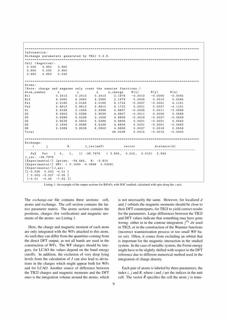
The exchange.out file contains three sections: cell,atoms and exchange. The cell section contains the lat-tice parameter matrix. The atoms section contains thepositions, charges (for verification) and magnetic mo-ments of the atoms: see Listing 1.

Here, the charge and magnetic moment of each atomare only integrated with the WFs attached to this atom.As such they can differ from the quantities coming fromthe direct DFT output, as not all bands are used in theconstruction of WFs. The WF charges should be inte-gers, for LCAO the values depend on the band energycutoffs. In addition, the exclusion of very deep lyinglevels from the calculation of J can also lead to devia-tions in the charges which might appear both for WFsand for LCAO. Another source of difference betweenthe TB2J charges and magnetic moments and the DFTones is the integration volume around the atoms, which

is not necessarily the same. However, for localized dand f orbitals the magnetic moments should be close totheir DFT counterparts, for TB2J to yield correct resultsfor the parameters. Large differences between the TB2Jand DFT values indicate that something may have gonewrong: either in in the contour integration

∫ EF dε usedin TB2J, or in the construction of the Wannier functions(incorrect wannierization process or too small WF ba-sis set). Often, it comes from excluding an orbital thatis important for the magnetic interaction in the studiedsystem. In the case of metallic system, the Fermi energymight have to be slightly shifted with respect to the DFTreference due to different numerical method used in theintegration of charge density.

Each pair of atoms is labeled by three parameters, theindex i, j and R, where i and j are the indices in the unitcell. The vector ~R specifies the cell the atom j is trans-

9

lated to, i.e. the reduced positions of the two atoms are~ri and ~r j + ~R, respectively. By default, the interactionis calculated within a supercell corresponding to the k-mesh. For example, with a 7×7×7 k-mesh, all i j pairswill be produced for the spin labeled i in the center cellof a 7× 7× 7 supercell. With the “rcut” flag, only theparameters for i j pairs within a distance of rcut are cal-culated. The exchange parameters are reported as fol-lows: magnetic atom i connected with magnetic atom j,R is the lattice vector between the unit cells containingi and j, the value of J for this pair of magnetic atoms inmeV, the vector connecting them, and the distance be-tween the pair of atoms. If SOC is enabled, the DMIand anisotropic Jani parameters are given in addition.The DMI vectors ~D and the anisotropic Jani are printedas vectors and matrices, respectively.

Apart from the main exchange.out file, TB2J deliv-ers several other outputs, which provide the input forspin dynamics (SD) and Monte Carlo (MC) simula-tions. TB2J is interfaced with several SD and MCcodes. It has native support to the Multibinit code de-livered as part of the Abinit code since version 9.0 [38].The TB2J results/Multibinit directory contains the tem-plates of input files for this code. One can usually runspin-dynamics with slight or no modification of thesefiles. “Experimental” inputs are also generated for Vam-pire [59] and Thomas Ostler’s GPU-ASD code [60].The Output module of TB2J provides a versatile API,described in the online documentation (see Discussionsection), which makes it easy to generate data for anyother code.

4.2.4. Magnon band structureOnce the J have been obtained in real space from

TB2J, the magnon dispersion curves Emagnon(~q) can beobtained from the Fourier transform of J to the~q space:

J(~q) = ∑~R

J(~R)ei~q·~R, (24)

In the simple FM case this reduces to diagonalizing4M (J(0)− J(~q)), where M is the one site magnetic mo-ment. The magnon band structure for more complicatedmagnetic configurations is more complex. Also, multi-ple types of magnetic sites cannot be treated at the mo-ment. Both features will be added in a future version ofTB2J.

With TB2J, the magnon band structure is obtained us-ing the following command:

TB2J_magnon --qpath GNPGHP --show

where the qpath option specifies the q-point path. If itis not specified, an automatically generate qpoint-pathwill be used from the information of the lattice struc-ture by using ASE[58]. The details of the q-point pathcan be found on https://wiki.fysik.dtu.dk/ase/ase/dft/kpoints.html.

A file, named “exchange magnon.pdf”, containingthe magnon band structure will be generated. The low-est energy eigenvector of J(~q) is printed, from which,together with the ~q vector, one determines the ground-state spin configuration.

4.3. Examples

In order to demonstrate the usage of TB2J, we usefive different examples, body centered cubic (BCC) Fe,hexagonal closed packed (HCP) Co, SrMnO3, BiFeO3,and La2CuO4. The BCC Fe and HCP Co systems areamong the most studied magnetic materials and are usedas standard benchmarks. The other three materials werechosen to represent a wide range of properties: SrMnO3as a prototype structure for superexchange, BiFeO3 asa multiferroic material [61], and La2CuO4 as a layeredperovskite with a canted spin structure.

4.3.1. BCC FeAs a first benchmark, we calculate the magnetic inter-

action parameters for the probably most studied mag-netic structure, BCC Fe. The isotropic exchange iscalculated with TB2J-Siesta and compared with resultsfrom the TB-LMTO method in Ref. [62], and KKRmethod in Refs. [60] and [30]. We do not show TB2J-Wannier90 results because the localization procedurecreates Wannier functions centered on bonds instead ofatoms. Then, the mapping to a Heisenberg model is notwell defined and the resulting exchange parameters areunphysical.

The DFT calculations were performed with the Siestacode [40] Max-1.0.13 version, with a double-zeta-polarized numerical atomic orbital basis set. TheGGA-PBE [63] functional and the norm-conservingpseudopotentials from the pseudo-dojo [64] “standard”dataset in the psml [65] format were used. A 9× 9× 9k-point grid was used to sample the Brillouin zone.

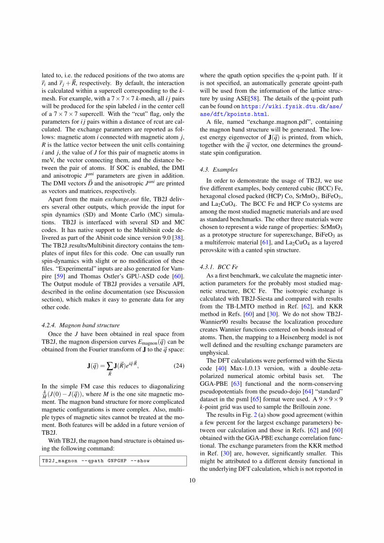
The results in Fig. 2 (a) show good agreement (withina few percent for the largest exchange parameters) be-tween our calculation and those in Refs. [62] and [60]obtained with the GGA-PBE exchange correlation func-tional. The exchange parameters from the KKR methodin Ref. [30] are, however, significantly smaller. Thismight be attributed to a different density functional inthe underlying DFT calculation, which is not reported in

10

0

5

10

15

20

J (m

eV)

(a) TB2J-SiestaTB-LMTOKKR1KKR2

0.5 1.0 1.5 2.0 2.5 3.0rij/a

20

0

20

40

60

J (m

eV)

(b) J ′ TB2J-SiestaB: TB2J-SiestaJ ′: KKR2B: KKR2

Figure 2: Exchange parameters for BCC Fe. (a) J from TB2J-Siesta,TB-LMTO (Ref. [62]), and KKR (KKR1: Ref. [60], and KKR2: Ref.[30]). (b) The bilinear (J′) and biquadratic (B) exchange of BCC Feusing TB2J-Siesta, and KKR-Green method (Ref. [30]). ri j is thedistance between the Fe atom pairs, and a is the cubic cell parameter.

Ref. [30]. The decomposition of the exchange into bi-linear and biquadratic terms is also calculated, see Fig. 2(b), and compared with the KKR method from Ref. [30].The J′ and B from our calculation follow the same trendbut are again larger than those in Ref. [30].

Fig. 3 shows an example of the magnon band struc-ture of BCC Fe. As we can see, the ground state corre-sponds to a q = Γ eigenvector, which identifies a ferro-magnetic structure. The energy minimum and the cor-responding eigenvector are also printed to the standardoutput:

The energy minimum is at:

q = [0. 0. 0.]

The ground state eigenvector is:

Fe1: [1.0 0.0 0.0]

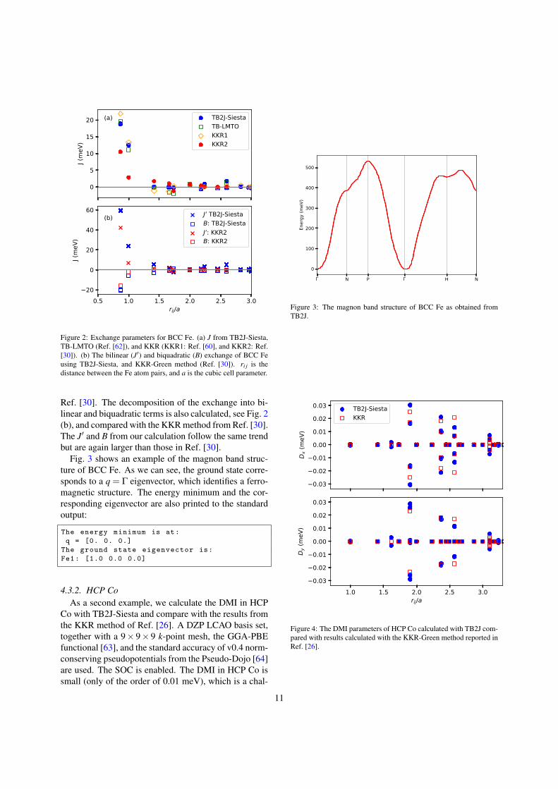
4.3.2. HCP CoAs a second example, we calculate the DMI in HCP

Co with TB2J-Siesta and compare with the results fromthe KKR method of Ref. [26]. A DZP LCAO basis set,together with a 9× 9× 9 k-point mesh, the GGA-PBEfunctional [63], and the standard accuracy of v0.4 norm-conserving pseudopotentials from the Pseudo-Dojo [64]are used. The SOC is enabled. The DMI in HCP Co issmall (only of the order of 0.01 meV), which is a chal-

N P H N

0

100

200

300

400

500

Ener

gy (m

eV)

Figure 3: The magnon band structure of BCC Fe as obtained fromTB2J.

0.03

0.02

0.01

0.00

0.01

0.02

0.03

Dx (

meV

)

TB2J-SiestaKKR

1.0 1.5 2.0 2.5 3.0rij/a

0.03

0.02

0.01

0.00

0.01

0.02

0.03

Dy (

meV

)

Figure 4: The DMI parameters of HCP Co calculated with TB2J com-pared with results calculated with the KKR-Green method reported inRef. [26].

11

|S| 1NN 2NN 3NN

TB2J-W90-Abinit 2.81 -8.16 -0.36 -0.02TB2J-Siesta 2.85 -7.70 -0.02 0.11

TE [70] -6.98 -0.36 -0.01

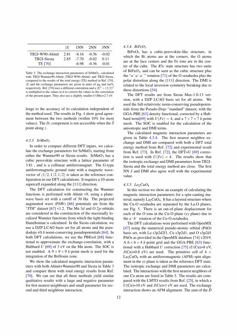
Table 3: The exchange interaction parameters of SrMnO3, calculatedwith TB2J-Wannier90-Abinit (TB2J-W90-Abinit) and TB2J-Siesta,compared to the results of the total energy (TE) method in Ref. [70].|S| and the exchange parameters are given in units of µB and meV,respectively. Ref. [70] uses a different convention and a |S|2 = (3/2)2

is multiplied to the values in it to convert the values to the conventionof the present paper. They also use a slightly smaller U(Mn)=2.7 eV.

lenge to the accuracy of its calculation independent ofthe method used. The results in Fig. 4 show good agree-ment between the two methods (within 10% for mostvalues). The Dz component is not accessible when the ~Spoint along z.

4.3.3. SrMnO3

In order to compare different DFT inputs, we calcu-late the exchange parameters for SrMnO3 starting fromeither the Wannier90 or Siesta results. SrMnO3 has acubic perovskite structure with a lattice parameter of3.81 , and is a collinear antiferromagnet. The G-typeantiferromagnetic ground state with a magnetic wave-vector of (1/2,1/2,1/2) is taken as the reference con-figuration in our DFT calculations. It requires a 10-atomsupercell expanded along the [111] direction.

The DFT calculation for constructing the Wannierfunctions is performed with Abinit v9, using a plane-wave basis set with a cutoff of 30 Ha. The projectedaugmented wave (PAW) [66] potentials are from the“JTH” dataset [67] v1.2. The Mn 3d and O 2p orbitalsare considered in the construction of the maximally lo-calized Wannier functions from which the tight-bindingHamiltonian is calculated. In the Siesta calculation, weuse a DZP LCAO basis set for all atoms and the pseu-dodojo v0.4 norm-conserving pseudopotentials [64]. Inboth DFT calculations, we use the PBEsol [68] func-tional to approximate the exchange-correlation, with aHubbard U [69] of 3 eV on the Mn atom. The SOC isnot enabled. A 9× 9× 9 k-point mesh is used for theintegration of the Brillouin zone.

We show the calculated magnetic interaction param-eters with both Abinit+Wannier90 and Siesta in Table 3and compare them with total energy results from Ref.[70]. We can see that all three methods yield similarqualitative results with a large and negative parameterfor first nearest neighbours and small parameter for sec-ond and third neighbour interaction.

4.3.4. BiFeO3

BiFeO3 has a cubic-perovskite-like structure, inwhich the Bi atoms are at the corners, the O atomsare at the face centers and the Fe ions are in the cen-ter of the cube. The R3c state structure has two unitsof BiFeO3, and can be seen as the cubic structure plusthe “a−a−a−” rotation [71] of the O octahedra plus thepolar distortion along the [111] direction. The DMI isrelated to the local inversion symmetry breaking due tothese distortions [54].

The DFT results are from Siesta Max-1.0-13 ver-sion, with a DZP LCAO basis set for all atoms. Weused the full-relativistic norm-conserving pseudopoten-tials from the Pseudo-Dojo ”standard” dataset, with theGGA-PBE [63] density functional, corrected by a Hub-bard term[69] with U(Fe) = 4, and a 7× 7× 7 k-pointmesh. The SOC is enabled for the calculation of theanisotropic and DMI terms.

The calculated magnetic interaction parameters aregiven in Table 4.3.4. The first nearest neighbor ex-change and DMI are compared with both a DFT totalenergy method from Ref. [72] and experimental resultfrom Ref. [73]. In Ref. [72], the DFT+U [69] correc-tion is used with U(Fe) = 4. The results show thatthe isotropic exchange and DMI parameters from TB2J-Siesta and the total energy method are close. The firstNN J and DMI also agree well with the experimentalvalue.

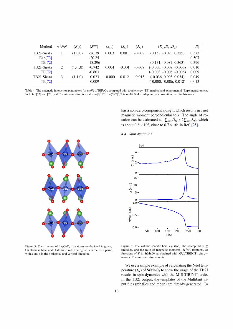
4.3.5. La2CuO4

In this section we show an example of calculating themagnetic interaction parameters for a spin-canting ma-terial, namely La2CuO4. It has a layered structure wherethe Cu-O octahedra are separated by the La-O planes,see Fig. 5. There is an out-of-plane displacement foreach of the O ions in the Cu-O plane (xy plane) due tothe a−b− rotation of the Cu-O octahedra.

The DFT calculations were performed with OpenMX[47] using the numerical pseudo-atomic orbital (PAO)basis set, with La s3p2d2f1, Cu s3p2d1, and O s3p2d1PAOs as provided in the OpenMX database [74] v2019.A 6× 6× 4 k-point grid and the GGA-PBE [63] func-tional with a Hubbard U correction [75] (U(Cu)=8 eV,J(Cu)=0.8 eV) are used. The primitive cell of 4 ×La2CuO4 with an antiferromagnetic (AFM) spin align-ment in the xy plane is taken as the reference DFT state.The isotropic exchange and DMI parameters are calcu-lated. The interactions with the first nearest neighbors ofone Cu atom are listed in Table 5. The results are com-pared with the LMTO results from Ref. [25], in which aU(Cu)=10 eV and J(Cu)=1 eV are used. The exchangeinteraction shows an AFM alignment. The sum of the ~D

12

Method nthNN (Ri j) (Jiso) (Jxy) (Jyz) (Jxz) (Dx,Dy,Dz) |D|TB2J-Siesta 1 (1,0,0) -26.79 0.003 0.001 -0.008 (0.158, -0.093, 0.325) 0.373

Exp[73] -20.25 0.507TE[72] -18.296 (0.131, -0.087, 0.363) 0.396

TB2J-Siesta 2 (1,-1,0) -0.742 0.004 -0.001 -0.008 (-0.003, -0.009, -0.003) 0.010TE[72] -0.603 (-0.003, -0.006, -0.006) 0.009

TB2J-Siesta 3 (1,1,0) -0.023 -0.000 0.012 -0.013 (-0.036, 0.003, 0.034) 0.049TE[72] -0.009 (-0.000, -0.006,-0.012) 0.013

Table 4: The magnetic interaction parameters (in meV) of BiFeO3 compared with total energy (TE) method and experimental (Exp) measurement.In Refs. [72] and [73], a different convention is used, a −|S|2/2 =−(5/2)2/2 is multiplied to adapt to the convention used in this work.

Figure 5: The structure of La2CuO4. La atoms are depicted in green,Cu atoms in blue, and O atoms in red. The figure is in the x− z planewith x and z in the horizontal and vertical direction.

has a non-zero component along x, which results in a netmagnetic moment perpendicular to x. The angle of ro-tation can be estimated as |∑ j,i~Di j|/|2∑ j,i Ji j|, whichis about 0.8×103, close to 0.7×103 in Ref. [25].

4.4. Spin dynamics

T (K)0

2

4

C v (a

.u.)

1e4

T (K)0

5

10

15

(a.u

.)

50 100 150 200 250 300T (K)

0.0

0.5

1.0

M/M

s (a.

u.)

Figure 6: The volume specific heat, CV (top), the susceptibility, χ

(middle), and the ratio of magnetic moments, M/MS (bottom), asfunctions of T in SrMnO3 as obtained with MULTIBINIT spin dy-namics. The units are atomic units.

We use a simple example of calculating the Neel tem-perature (TN) of SrMnO3 to show the usage of the TB2Jresults in spin dynamics with the MULTIBINIT code.In the TB2J output, the templates of the Multibnit in-put files (mb.files and mb.in) are already generated. To

13

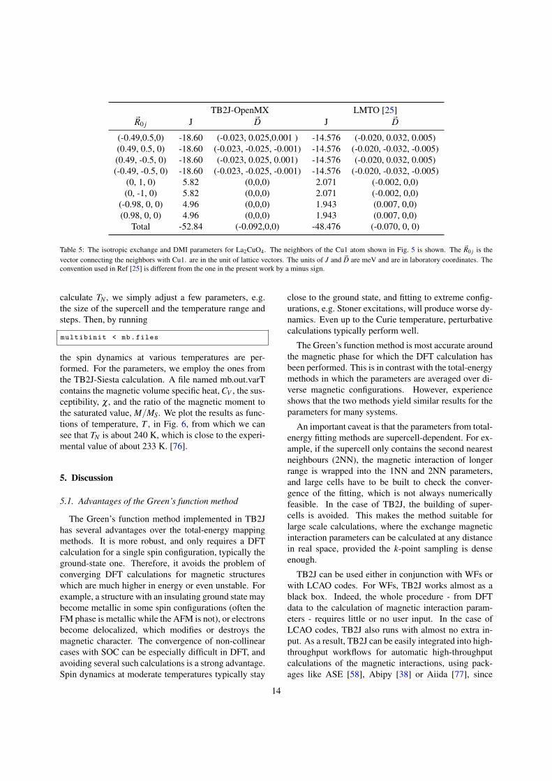
TB2J-OpenMX LMTO [25]~R0 j J ~D J ~D

(-0.49,0.5,0) -18.60 (-0.023, 0.025,0.001 ) -14.576 (-0.020, 0.032, 0.005)(0.49, 0.5, 0) -18.60 (-0.023, -0.025, -0.001) -14.576 (-0.020, -0.032, -0.005)(0.49, -0.5, 0) -18.60 (-0.023, 0.025, 0.001) -14.576 (-0.020, 0.032, 0.005)(-0.49, -0.5, 0) -18.60 (-0.023, -0.025, -0.001) -14.576 (-0.020, -0.032, -0.005)

(0, 1, 0) 5.82 (0,0,0) 2.071 (-0.002, 0,0)(0, -1, 0) 5.82 (0,0,0) 2.071 (-0.002, 0,0)

(-0.98, 0, 0) 4.96 (0,0,0) 1.943 (0.007, 0,0)(0.98, 0, 0) 4.96 (0,0,0) 1.943 (0.007, 0,0)

Total -52.84 (-0.092,0,0) -48.476 (-0.070, 0, 0)

Table 5: The isotropic exchange and DMI parameters for La2CuO4. The neighbors of the Cu1 atom shown in Fig. 5 is shown. The ~R0 j is thevector connecting the neighbors with Cu1. are in the unit of lattice vectors. The units of J and ~D are meV and are in laboratory coordinates. Theconvention used in Ref [25] is different from the one in the present work by a minus sign.

calculate TN , we simply adjust a few parameters, e.g.the size of the supercell and the temperature range andsteps. Then, by running

multibinit < mb.files

the spin dynamics at various temperatures are per-formed. For the parameters, we employ the ones fromthe TB2J-Siesta calculation. A file named mb.out.varTcontains the magnetic volume specific heat, CV , the sus-ceptibility, χ , and the ratio of the magnetic moment tothe saturated value, M/MS. We plot the results as func-tions of temperature, T , in Fig. 6, from which we cansee that TN is about 240 K, which is close to the experi-mental value of about 233 K. [76].

5. Discussion

5.1. Advantages of the Green’s function method

The Green’s function method implemented in TB2Jhas several advantages over the total-energy mappingmethods. It is more robust, and only requires a DFTcalculation for a single spin configuration, typically theground-state one. Therefore, it avoids the problem ofconverging DFT calculations for magnetic structureswhich are much higher in energy or even unstable. Forexample, a structure with an insulating ground state maybecome metallic in some spin configurations (often theFM phase is metallic while the AFM is not), or electronsbecome delocalized, which modifies or destroys themagnetic character. The convergence of non-collinearcases with SOC can be especially difficult in DFT, andavoiding several such calculations is a strong advantage.Spin dynamics at moderate temperatures typically stay

close to the ground state, and fitting to extreme config-urations, e.g. Stoner excitations, will produce worse dy-namics. Even up to the Curie temperature, perturbativecalculations typically perform well.

The Green’s function method is most accurate aroundthe magnetic phase for which the DFT calculation hasbeen performed. This is in contrast with the total-energymethods in which the parameters are averaged over di-verse magnetic configurations. However, experienceshows that the two methods yield similar results for theparameters for many systems.

An important caveat is that the parameters from total-energy fitting methods are supercell-dependent. For ex-ample, if the supercell only contains the second nearestneighbours (2NN), the magnetic interaction of longerrange is wrapped into the 1NN and 2NN parameters,and large cells have to be built to check the conver-gence of the fitting, which is not always numericallyfeasible. In the case of TB2J, the building of super-cells is avoided. This makes the method suitable forlarge scale calculations, where the exchange magneticinteraction parameters can be calculated at any distancein real space, provided the k-point sampling is denseenough.

TB2J can be used either in conjunction with WFs orwith LCAO codes. For WFs, TB2J works almost as ablack box. Indeed, the whole procedure - from DFTdata to the calculation of magnetic interaction param-eters - requires little or no user input. In the case ofLCAO codes, TB2J also runs with almost no extra in-put. As a result, TB2J can be easily integrated into high-throughput workflows for automatic high-throughputcalculations of the magnetic interactions, using pack-ages like ASE [58], Abipy [38] or Aiida [77], since

14

TB2J can work as a python library.The construction of MLWFs was a sophisticated task

in the past, since input parameters would vary for eachstructure and had to be tuned by hand. However, the sit-uation has been largely changed thanks to the recent de-velopment of several methods, in particular the selectedcolumns of density matrix (SCDM) algorithms [78, 79].With these advances, fully automated building of WFshas been demonstrated [80].

The output of TB2J is directly usable by spin simula-tion codes. Therefore, the full procedure from the DFTexchange calculation to the spin system simulation canbe easily automated.

5.2. LimitationsIn the limit where the method implemented in TB2J

applies (rigid spin rotation approximation, magneticmoments localized on the atoms, etc.) and that the limi-tations of the DFT for magnetic systems (selection of acorrect enough exchange-correlation functional, choiceof the values of DFT+U parameters, etc [81, 82, 83]) thecalculation of the DMI and anisotropic exchange param-eters through the Wannier basis set might still be prob-lematic. The user should always verify that the elec-tronic band structure obtained with the Wannier func-tions is in good agreement with the DFT one (choice ofgood disentanglement energy window, choice of projec-tors, etc). However, even if that is the case, the Wannier-ization process itself can introduce noise of the order ofmagnitude of a few µeV. For small quantities, like theDMI or anisotropic exchanges, which are of the samesize as the noise, the parameters cannot be determinedwith sufficient resolution. The problem occurs, in par-ticular, when strong disentanglement of bands is neces-sary, i.e. when no gap is present between selected bands.It can be reduced in cases where the bands of interest arenot entangled too much with higher unoccupied bandsby including more unoccupied bands in the Wanneriza-tion process. Therefore, a validation of the quality ofWannier function Hamiltonian should be performed tomake sure that the calculation is meaningful, by com-paring the band structures from DFT and from Wannierfunction based Hamiltonian. We have tested using thesymmetry-adapted Wannier functions [84] which, how-ever, does not fully solve the problem. It appears thatthe calculation of very small parameters using Wannierfunctions poses a challenge which hopefully future de-velopments in the Wannierization methods can addressby reducing the noise introduced in the disentanglementprocedure.

At last, the Heisenberg model might not be valid forall circumstances, for instance, when spins are itinerant

or when the non-bilinear magnetic interactions are non-negligible. The rotation of the spins is described in abasis set, either Wannier functions, or numerical atomicorbitals. In some cases, especially when the spins arenot localized at or close to the centers of the basis func-tions, the result can be basis set dependent.

5.3. Code availability

The code is freely available under the BSD 2clause license and can be found at https://github.com/mailhexu/TB2J/. Documentation is provided athttps://tb2j.readthedocs.io/en/latest/. Theinterface to OpenMX is in a separate package,TB2J OpenMX (https://github.com/mailhexu/TB2J-OpenMX), under the GPLv3 license, which useTB2J as a library. Contribution to the code is wel-come. In particular, we are happy to integrate interfacesto additional codes, be it on the input side (other first-principles or tight-binding codes), or the output side(e.g. outputs to atomic spin simulation packages).

6. Conclusions and perspectives

In this paper we present the TB2J python packagewhich calculates the magnetic interaction parametersfrom Wannier and LCAO Hamiltonians, using a Green’sfunction method. The isotropic and anisotropic ex-change, and the DMI can be systematically calculatedby TB2J. The code can use results from a large numberof first-principles DFT codes, either through the Wan-nier90 interface (for plane wave codes but also other ba-sis sets) or directly from LCAO codes (SIESTA, GPAW,and OPENMX). TB2J requires a minimal number of in-put parameters, such that it can be easily integrated inhigh-throughput workflows. One of the most appeal-ing features of TB2J is the requirement of only one unitcell DFT calculation (or eventually 3 for numerical av-eraging of x, y, z spin orientations) to evaluate the mag-netic interactions at any distance between the magneticatoms. We hope this development will simplify the lifeof future users, in their calculations of the magnetic in-teractions from first-principles ingredients, and enablelarger scale and more accurate micromagnetics calcula-tions, exploring novel physical phenomena.

Future versions will include a wider range of inter-faces with DFT and ASD codes, as well as expandedfeature sets, including single ion anisotropy, magnonband structures for more complex systems. A promis-ing avenue is the calculation of higher order parame-ters (3 spin, 4 spin), which has been explored only verysparsely in the literature (e.g. Refs. [85, 86, 87, 88]).

15

Acknowledgements

The authors thank Yajun Zhang, Alireza Sasani, JorgePilo Gonzlez, and Zachary Romestan for the testing ofthe code, Thomas Ostler, Bertrand Dupe and PhivosMavropoulos for explanations about the limits and in-tricacies of fitting the Heisenberg model.

This work has been funded by the Commu-naute Francaise de Belgique (ARC AIMED G.A.15/19-09).XH thanks the support by the EU H2020-NMBP-TO-IND-2018 project ”INTERSECT” (GrantNo. 814487). EB thanks the FRS-FNRS for sup-port, as does MJV for an “out” sabbatical grant toICN2 Barcelona in 2018-2019. The authors acknowl-edge the CECI supercomputer facilities funded by theF.R.S-FNRS (Grant No. 2.5020.1) and the Tier-1 super-computer of the Federation Wallonie-Bruxelles fundedby the Walloon Region (Grant No. 1117545). Com-puting time was also provided by PRACE-3IP DECIgrants 2DSpin and Pylight on Beskow (G.A. 653838 ofH2020).

References

[1] Hirohata, A. et al., Journal of Magnetism and Magnetic Materi-als 509 (2020) 166711.

[2] Baltz, V. et al., Rev. Mod. Phys. 90 (2018) 015005.[3] Bhatti, S. et al., Materials Today 20 (2017) 530 .[4] Joshi, V. K., Engineering Science and Technology, an Interna-

tional Journal 19 (2016) 1503 .[5] Lu, J. W., Chen, E., Kabir, M., Stan, M. R., and Wolf, S. A.,

International Materials Reviews 61 (2016) 456.[6] Zutic, I., Fabian, J., and Das Sarma, S., Rev. Mod. Phys. 76

(2004) 323.[7] Fazekas, P., Lecture notes on electron correlation and mag-

netism, Series in modern condensed matter physics 5, WorldScientific, 1999.

[8] Chumak, A. V., Vasyuchka, V. I., Serga, A. A., and Hillebrands,B., Nat. Phys. 11 (2015) 453.

[9] Kiselev, N. S., Bogdanov, A. N., Schfer, R., and Rßler, U. K.,Journal of Physics D: Applied Physics 44 (2011) 392001.

[10] Fert, A., Cros, V., and Sampaio, J., Nat. Nanotechnol. 8 (2013)152.

[11] Xiang, H., Lee, C., Koo, H.-J., Gong, X., and Whangbo, M.-H.,Dalton Trans. 42 (2013) 823.

[12] Herring, C., Magnetism: a treatise on modern theory and mate-rials. 4. Exchange interactions among itinerant electrons, Aca-demic Press, 1966.

[13] Sandratskii, L. M., physica status solidi (b) 136 (1986) 167.[14] Savrasov, S. Y., Phys. Rev. Lett. 81 (1998) 2570.[15] Romero, A. H. et al., The Journal of Chemical Physics 152

(2020) 124102.[16] Cao, K., Lambert, H., Radaelli, P. G., and Giustino, F., Phys.

Rev. B 97 (2018) 024420.[17] Ricci, F., Prokhorenko, S., Torrent, M., Verstraete, M. J., and

Bousquet, E., Phys. Rev. B 99 (2019) 184404.[18] Phillips, J. J. and Peralta, J. E., The Journal of Chemical Physics

138 (2013) 174115.

[19] Liechtenstein, A. I., Katsnelson, M., Antropov, V., andGubanov, V., Journal of Magnetism and Magnetic Materials67 (1987) 65.

[20] Steenbock, T. and Herrmann, C., Journal of ComputationalChemistry 39 (2018) 81.

[21] Katsnelson, M. I. and Lichtenstein, A. I., Phys. Rev. B 61 (2000)8906.

[22] Katsnelson, M. I., Kvashnin, Y. O., Mazurenko, V. V., and Licht-enstein, A. I., Phys. Rev. B 82 (2010) 100403.

[23] Solovyev, I., Hamada, N., and Terakura, K., Phys. Rev. Lett. 76(1996) 4825.

[24] Antropov, V., Katsnelson, M., and Liechtenstein, A., Physica B:Condensed Matter 237 (1997) 336.

[25] Mazurenko, V. V. and Anisimov, V. I., Phys. Rev. B 71 (2005)184434.

[26] Mankovsky, S. and Ebert, H., Phys. Rev. B 96 (2017) 104416.[27] Secchi, A., Lichtenstein, A. I., and Katsnelson, M. I., Annals of

Physics 360 (2015) 61.[28] Secchi, A., Lichtenstein, A. I., and Katsnelson, M. I., Journal of

Magnetism and Magnetic Materials 400 (2016) 112.[29] Lounis, S. and Dederichs, P. H., Phys. Rev. B 82 (2010) 180404.[30] Szilva, A. et al., Phys. Rev. Lett. 111 (2013) 127204.[31] Yavorsky, B. Y. and Mertig, I., Phys. Rev. B 74 (2006) 174402.[32] Ebert, H. and Mankovsky, S., Phys. Rev. B 79 (2009) 045209.[33] Andersen, O. K. and Jepsen, O., Phys. Rev. Lett. 53 (1984)

2571.[34] Korotin, D. M., Mazurenko, V. V., Anisimov, V. I., and Streltsov,

S. V., Phys. Rev. B 91 (2015) 224405.[35] Mostofi, A. A. et al., Comput. Phys. Commun. 178 (2008) 685 .[36] Pizzi, G. et al., Journal of Physics: Condensed Matter 32 (2020)

165902.[37] Gonze, X. et al., Comput. Phys. Commun. 180 (2009) 2582

, 40 YEARS OF CPC: A celebratory issue focused on qualitysoftware for high performance, grid and novel computing archi-tectures.

[38] Gonze, X. et al., Comput. Phys. Commun. 248 (2020) 107042.[39] Giannozzi, P. et al., Journal of Physics: Condensed Matter 29

(2017) 465901.[40] Soler, J. M. et al., Journal of Physics: Condensed Matter 14

(2002) 2745.[41] Kresse, G. and Furthmuller, J., Phys. Rev. B 54 (1996) 11169.[42] Kresse, G. and Joubert, D., Phys. Rev. B 59 (1999) 1758.[43] Blaha, P., Schwarz, K., Madsen, G. K., Kvasnicka, D., and

Luitz, J., An augmented plane wave+ local orbitals programfor calculating crystal properties (2001).

[44] Blugel, S. and Bihlmayer, G., Forschungszentrum Julich GmbH(2006) 85.

[45] Andrade, X. et al., Physical Chemistry Chemical Physics 17(2015) 31371.

[46] Tancogne-Dejean, N. et al., The Journal of Chemical Physics152 (2020) 124119.

[47] Ozaki, T. and Kino, H., Physical Review B 72 (2005) 045121.[48] Enkovaara, J. et al., Journal of physics: Condensed matter 22

(2010) 253202.[49] The Elk Code, http://elk.sourceforge.net/.[50] Oroszlany, L., Ferrer, J., Deak, A., Udvardi, L., and Szunyogh,

L., Phys. Rev. B 99 (2019) 224412.[51] Yoon, H., Kim, T. J., Sim, J.-H., and Han, M. J., Comput. Phys.

Commun. 247 (2020) 106927.[52] Papior, N. R., B., J. L., Frederiksen, T., and Wuhl, S. S., zeroth-

i/sisl: v0.9.8, 2020.[53] Solovyev, I., Dederichs, P., and Mertig, I., Physical Review B

52 (1995) 13419.[54] Weingart, C., Spaldin, N., and Bousquet, E., Phys. Rev. B 86

(2012) 094413.

16

[55] Udvardi, L., Szunyogh, L., Palotas, K., and Weinberger, P.,Phys. Rev. B 68 (2003) 104436.

[56] Marzari, N. and Vanderbilt, D., Phys. Rev. B 56 (1997) 12847.[57] Wang, R., Lazar, E. A., Park, H., Millis, A. J., and Marianetti,

C. A., Phys. Rev. B 90 (2014) 165125.[58] Larsen, A. H. et al., Journal of Physics: Condensed Matter 29

(2017) 273002.[59] Evans, R. F. et al., Journal of Physics: Condensed Matter 26

(2014) 103202.[60] Di Gennaro, M., Miranda, A. L., Ostler, T. A., Romero, A. H.,

and Verstraete, M. J., Phys. Rev. B 97 (2018) 214417.[61] Catalan, G. and Scott, J. F., Adv. Matter. 21 (2009) 2463.[62] Pajda, M., Kudrnovsky, J., Turek, I., Drchal, V., and Bruno, P.,

Phys. Rev. B 64 (2001) 174402.[63] Perdew, J. P., Burke, K., and Ernzerhof, M., Phys. Rev. Lett. 77

(1996) 3865.[64] Van Setten, M. et al., Comput. Phys. Commun. 226 (2018) 39.[65] Garcıa, A., Verstraete, M. J., Pouillon, Y., and Junquera, J.,

Comput. Phys. Commun. 227 (2018) 51.[66] Torrent, M., Jollet, F., Bottin, F., Zrah, G., and Gonze, X., Com-

putational Materials Science 42 (2008) 337 .[67] Jollet, F., Torrent, M., and Holzwarth, N., Comput. Phys. Com-

mun. 185 (2014) 1246 .[68] Perdew, J. P. et al., Phys. Rev. Lett. 100 (2008) 136406.[69] Anisimov, V. I., Zaanen, J., and Andersen, O. K., Phys. Rev. B

44 (1991) 943.[70] Lee, J. H. and Rabe, K. M., Phys. Rev. B 84 (2011) 104440.[71] Glazer, A., Acta Crystallographica Section B: Structural Crys-

tallography and Crystal Chemistry 28 (1972) 3384.[72] Xu, C., Xu, B., Dupe, B., and Bellaiche, L., Phys. Rev. B 99

(2019) 104420.[73] Matsuda, M. et al., Phys. Rev. Lett. 109 (2012) 067205.[74] Ozaki, T. and Kino, H., Phys. Rev. B 69 (2004) 195113.[75] Liechtenstein, A., Anisimov, V., and Zaanen, J., Phys. Rev. B

52 (1995) R5467.[76] Chmaissem, O. et al., Phys. Rev. B 64 (2001) 134412.[77] Pizzi, G., Cepellotti, A., Sabatini, R., Marzari, N., and Kozinsky,

B., Computational Materials Science 111 (2016) 218.[78] Damle, A., Lin, L., and Ying, L., Journal of chemical theory

and computation 11 (2015) 1463.[79] Damle, A. and Lin, L., Multiscale Modeling & Simulation 16

(2018) 1392.[80] Vitale, V. et al., npj Computational Materials 6 (2020) 1.[81] Varignon, J., Bibes, M., and Zunger, A., Nature Commun. 10

(2019) 1658.[82] Himmetoglu, B., Floris, A., de Gironcoli, S., and Cococcioni,

M., International Journal of Quantum Chemistry 114 (2014) 14.[83] Bousquet, E. and Spaldin, N., Phys. Rev. B 82 (2010) 220402.[84] Sakuma, R., Phys. Rev. B 87 (2013) 235109.[85] Fedorova, N. S., Ederer, C., Spaldin, N. A., and Scaramucci, A.,

Phys. Rev. B 91 (2015) 165122.[86] Ostler, T. A., Barton, C., Thomson, T., and Hrkac, G., Phys.

Rev. B 95 (2017) 064415.[87] Mankovsky, S., Polesya, S., and Ebert, H., Phys. Rev. B 101

(2020) 174401.[88] Hoffmann, M. and Blugel, S., Phys. Rev. B 101 (2020) 024418.

17