Task Scheduling Based on Degenerated Monte Carlo Estimate in Mobile Cloud

International Journal of Grid and Distributed Computing

Vol.7, No.1 (2014), pp.179-196

http://dx.doi.org/10.14257/ijgdc.2014.7.1.16

ISSN: 2005-4262 IJGDC

Copyright ⓒ 2014 SERSC

Task Scheduling Based on Degenerated Monte Carlo Estimate in

Mobile Cloud

Cai Zhiming1,2 and Chen Chongcheng1*

1Key Lab of Spatial Data Mining & Information Sharing of Ministry of Education,

Fuzhou University, Fuzhou, 350002, China

2School of Information Science and Engineering, Fujian University of Technology,

Fuzhou, 350108, China

[email protected], [email protected]

Abstract

Mobile cloud computing, which comes up in recent years, is a new computing paradigm. It

enables people to access remote clouds by mobile device, even to build mobile micro-

cloud(MuCloud) with mobile device to provide lightweight service. Despite extensive studies

of task scheduling in wired cloud, effective scheduling in mobile cloud still remains

challenges:1) Unreliable wireless connection and dynamic join and quit of MuCloud often

result in decreased reliability of scheduling; 2) As the process capacities of wired clouds and

MuClouds vary greatly, it is hard to achieve load balancing; 3) During moving, tasks, such as

traffic navigation, may be scheduled consecutively by mobile users as space-time changes.

Such application scenarios often incur makespan accumulation which impairs user

experience, even causes system crash. Our work aims at such problems. We firstly illustrate

the reason for selection of makespan and load balancing as two key performance indicators

for task scheduling in the proposed architecture of mobile cloud which integrates MuClouds.

Then after introduction to Monte Carlo method, degenerated Monte Carlo estimate is defined

and a scheduling algorithm based on degenerated Monte Carlo estimate (DMCE) is

presented. With extensive simulation experiments, the two above-mentioned indicators of task

scheduling using different algorithms including DMCE, Max-Min, Min-Min and IGA are

compared and evaluated. Accumulative effect and relative load are introduced to measure

scheduling performance. The experimental results show that: 1)Compared with other

algorithms, DMCE achieves smallest makespan on average when scheduled respectively; 2)

DMCE has least accumulative effect when task sets scheduled consecutively, which makes

makespan of a task set hardly relevant to the order of scheduling; 3)Among these algorithms,

DMCE outperforms others in keeping relative load balancing by assigning tasks to clouds in

proportion to each cloud’s process capacity.

Keywords: Task Scheduling, Degenerated Monte Carlo Estimate, Mobile Cloud, Makespan,

Relative Load Balancing

1. Introduction

In mobile cloud, as computing and storage services are delivered by clouds, user

terminals are freed. With mobile devices, mobile users can access and schedule the

resources or services in remote clouds via wireless networks, which we call mobile

*Corresponding author. Email: [email protected]

mailto:[email protected]

mailto:[email protected]


Vol.7, No.1 (2014)

180 Copyright ⓒ 2014 SERSC

cloud task scheduling. Considering the inherent deficiencies of mobile devices, such as

resource scarceness and finite energy, researches of mobile cloud task scheduling pay more

attention to energy efficiency[1]. Liu et al., [2]introduce a concept of Universal Mobile

Service Cell which mobile agent is used to shield the unequivalence between mobile devices

and the clouds, and adopt genetic algorithm to schedule the services of clouds. Fekete et al.,

[3] present a computation offloading model for mobile phone and a measurement

infrastructure which is used to analyze the energy consumption of smartphones. Zhang et al.,

[4] investigate the scheduling policy for collaborative execution between mobile device and

cloud. They use LARAC algorithm to obtain the objective for minimizing the energy

consumed by mobile device. Various cloud-assisted mobile service platforms have been

proposed for remote task scheduling, for instance, Cloudlet [5], SIFT [6], MoCAsH [7]. What

they have in common is offloading computing or storage from mobile device to remote cloud

to improve service performance. Along with the development of technology, many occasions,

such as train, airport and car, provide the convenience for charging. Meanwhile, battery’s

capacity is enhanced these years and mobile user also can use backup battery when hungry

for energy. Therefore, reducing energy consumption becomes less urgent. With the

improvement of the performance of mobile devices, and the enhancement of bandwidth in

wireless communication, the difference of task scheduling between mobile cloud and wired

cloud decreases. However, the inherent characteristics of mobile communication still exist,

such as blind area of wireless coverage, available bandwidth competition by multiple users,

low connectivity when roaming as signal strength being time-varying, etc. Such

characteristics often incur unreliability. Obviously, finishing tasks as quickly as possible will

improve user experience. We also prove in Section 2 that decreasing the execution time of

tasks is a feasible way to lower the probability of failure of scheduling. For mobile users, they

pursue minimum makespan of tasks. From the clouds’ perspective, they seek load balancing

and maximum utilization. Therefore, task scheduling is a multi-objective optimization

problem.

As traditional heuristics [8], such as Max-Min, Min-Min, usually cater to tackle single-

objective scheduling, they obtain sub-optimal scheduling. Thus, optimization algorithms are

applied to task scheduling. Omara et al., [9] develop a genetic algorithm with some heuristic

principles added to improve the performance. Liu et al., [10] improve particle swarm

optimization algorithm with dynamic multi-group collaboration and reverse flight of mutation

particles. To some extent, the former helps to achieve faster convergence speed and the latter

helps to avoid local optimum. Nayak et al., [11] propose a genetic based bacteria foraging

algorithm which aims to overcome premature convergence and to conduct fine-tuning in the

search space. For general genetic algorithm, the amount of tasks and resource IDs are viewed

as chromosomes length and genes respectively, which leads to slow convergence when task

number is great. Hence the authors in [12] modify coding method of chromosomes and apply

two fitness functions to minimize the total execution time and to achieve load balancing.

More than one fitness function can be allocated to optimization algorithms which make them

applicable for solution of multi-objective problems. However, a multi-objective optimization

increases computational complexities and often tends to get stuck on local optima or meet

premature.

Some other literatures [13-15] employ probabilistic methods to tackle task scheduling as

task execution time usually deviates from what is predicted. SHEFT[13] assumes the

expected value and variance of stochastic processing time obeying exponential distribution or

normal distribution and statistical profiling is used to determine such distribution. In order to

minimize the mean response time and total makespan of the tasks, DTMC[14] uses discrete

time Markov chain to model the task scheduling process. It obtains connection probabilities


Vol.7, No.1 (2014)

Copyright ⓒ 2014 SERSC 181

between user and resource by nonlinear programming and achieves the minimum mean

response time consequently. MCS[15] consists of two phases: producing and selecting. In the

former phase, a number of samples are conducted from the input space which consisting of

random task execution time predictions. Then a specific scheduling algorithm (it could be

any) is employed to produce schedules. In the latter phase, a certain number of samples are

taken again to evaluate the generated schedules and output the schedule with the minimum

average makespan. The common of these probabilistic methods is that task execution times

are assumed to follow a specific distribution, which enhances computational complexity.

From all aforementioned literatures, we also find that they care more about single task

set’s scheduling. Little attention is paid to consecutive schedulings. In fact, after consecutive

schedulings, the complete time of tasks may accumulate. From discussion above, naturally,

minimizing the complete time of tasks submitted by mobile users and achieving load

balancing among clouds become our major objectives for mobile cloud task scheduling. We

introduce degenerated Monte Carlo estimate for the first time and propose a scheduling

algorithm based on degenerated Monte Carlo estimate, which shows good performance to

obtain our objectives.

The rest of the paper is organized as follows: Section 2 presents a mobile cloud

architecture and fundamentals of scheduling. In Section 3, after illustration of some

theoretical basis, our algorithm is advanced. A series of simulation evaluations are

demonstrated in Section 4. And Section 5 concludes the whole paper.

2. Architecture of Mobile Cloud and Scheduling Description

2.1. Architecture of Mobile Cloud

The advised architecture for mobile cloud is shown in Figure 1. It is composed of

cloud side and mobile user side. On mobile user side, mobile devices are classified into

thin clients and fat clients. The thin ones only provide interfaces to access cloud. While

the fat ones can even be used as mobile micro cloud (shorted as MuCloud) for service

deployment or resource renting while roaming among wireless networks. On the cloud

side, it is a federal cloud system which consists of many wired clouds and MuClouds.

They are organized by peer to peer (P2P) topology at overlay network layer.

P2P

P2P

PDA

3G/Wimax/4G Cell

Federation Cloud

P2P

Cloud A

MD

Cloud B

hand offHPC

vm

vm

vm

MuCloud

vmvm

vm

MDHPC

Internet

Cloud

User

Figure 1. Architecture of Mobile Cloud


Vol.7, No.1 (2014)


2.2. Estimate of Time of Complete

For task scheduling, tasks can be divided into dependent tasks and independent tasks.

The former can be decomposed into independent ones[16]. This paper only considers

independent task scheduling. We denote },...,,{ 21 mJJJJ as the task set submitted by

mobile user, and },...,,{ 21 nCCCC as the candidate clouds for processing tasks. The

scheduling schemas can also be classified into two. One is resource scheduling,

including computing and storage. Another is service scheduling, such as Web Services.

For the former, the amount of computation of each task and the process capacity of each

cloud are generally assumed known. For the latter, we assume that the cloud which

providing service has the knowledge of complete time for the service. For example, it

can be obtained by building a historic table and using statistical profiling[17]. So, we

can get the estimated time of complete of every task assigned to every cloud, denoted as

ijTOC ， mi 1 , nj 1 .

In mobile cloud, reliability of wireless connection has great impact on success rate

during scheduling. Since outage probability of wired network is much smaller than

wireless network’s, we only consider the latter. Our tolerance mechanism for outage is

rescheduling, namely if one task is interrupted, it will be scheduled one time again. In

cellular mobile communication systems, SIR (signal-to-interference rate) obeys

lognormal distribution[18], and the outage probability can be expressed as

][)( 00 SIRSIRPSIRP rdisc

dxxSIR

SIR

SIR

SIR

0

0 2

2

2

)(exp

2

1

(1)

where SIR , SIR are the mean and standard deviation of SIR, 0

SIR is the threshold of

wireless link.

When MuCloud is scheduled, TOC should be rectified to be )1( discij PTOC . So, we

have

MuCloudPTOC

cloudfixedTOCt

discij

ij

ij )1( (2)

where mi 1 , nj 1 .

2.3. Relationship of TOC and Reliability of Task Scheduling

We use the success rate of task scheduling to describe reliability of task scheduling.

As shown in Figure 2, in the period of k

bb0 , there are two kinds of statuses for network

connection: Good status( iG , ki 1 ) and Bad status( iB , ki 1 ), which emerge

alternately.

1G 1B 2G 2B iG iB. . . . . . kG kB1g

1b 2g2b ig

ib1ib0b kbkg

L L

Figure 2. Statuses of Network


Vol.7, No.1 (2014)


The durations of iG and iB are 1 ii bg and ii gb respectively. Let L denote

the TOC of a task. If kiGL i 1 , the scheduling will succeed. Otherwise, the

scheduling will fail. Suppose the start point of task scheduling, S , distributed in k

bb0

uniformly, we have the following theorem.

Theorem 1 In unreliable connection conditions, for a given sequence of statuses

kk BGBGBGBG ...332211 , the probability of success of task scheduling, sP decreases with

the increase of the execution time of the task, L .

Proof The probability of success of task scheduling in iG is denoted as iGP . We have

three situations:

Case 1: L is small and LGi , ki 1

Since S located in k

bb0 uniformly, the probability of success of task scheduling can

be given by

k

i

Gs iPP

1

1

ii

k

i

gSbP

1

1

k

k

i i bbLG 01/

k

k

i i bbkLG 01/

(3)

Obviously, 1sP decreases with the increase of L .

Case 2: L is greater and LGi , },...,2,1{ ki

For LGi , 0iGP . Thus

1

1

2 s

k

i

Gs PPPi

(4)

Case 3: L is very large and LGi , ki 1

We easily get

2

1

3 0 s

k

i

Gs PPPi

(5)

In above description, 1sP , 2sP and 3sP are the values of sP in different situations.

Therefore, we can conclude that sP decreases with the increase of L . Instead, L can be

reduced to improve sP . For task set J , whose tasks are assigned to different clouds, we

define makespan of J as the duration from the start to the end of all tasks finished.

Then we have the lemma below.

Lemma 1 The probability of success of a task set scheduling decreases with the

increase of its makespan.


Vol.7, No.1 (2014)


From Lemma 1, we can conclude that, to improve reliability of task scheduling, makespan

must be minimized. In the following we use modified Monte Carlo method to achieve

optimized makespan.

3. Degenerated Monte Carlo Estimate-based Task Scheduling

3.1. Monte Carlo Method

Monte Carlo method is also referred to as stochastic simulation. Its basic idea is to

create a probabilistic model, whose parameter is equal to the solution of the problem,

and then solves the approximation solution by sampling estimate[19]. It has been

widely used in many domains, such as simple length, area estimation, reliability

evaluation[19] and so on. In this paper, we consider interval sampling estimate. As

shown in Figure 3(a), there is an interval vu xx in line segment

ba xx . Carry out sampling

according to uniform distribution in ba xx . We specify an event A for sampling point

falling in the range of vu xx . Repeat sampling for a large number of times, n . Then

count the number of occurrences, An , corresponding to event A . We define Monte

Carlo estimator of probability of event A as

n

nP A

A ˆ (6)

. . . . . .

ux vxax bx

. . . . . .

... ...1mt

. . . . . .

11t 21t 12t 22t 2mt ... mnt

(a)Interval uniform sampling

(b)Distribution of TOC

Figure 3. Monte Carlo Sampling

Theorem 2 When n , AP̂ is an unbiased and consistent estimator for

abuv LL / , namely

abuv

A LLn

n/ (7)

where uvL ,abL is the length of interval

vu xx andba xx respectively.


Vol.7, No.1 (2014)


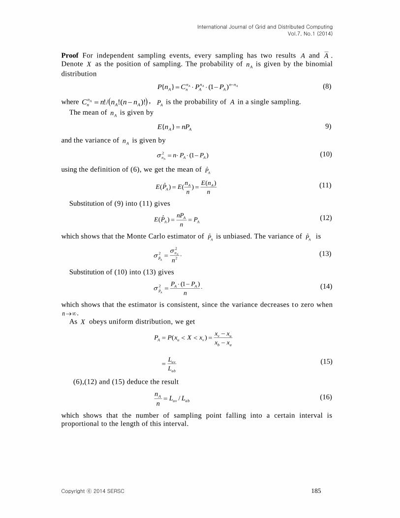
Proof For independent sampling events, every sampling has two results A and A .

Denote X as the position of sampling. The probability of An is given by the binomial

distribution

AAA nn

A

n

A

n

nA PPCnP

)1(}{ (8)

where )!(!/! AA

n

n nnnnC A ，AP is the probability of A in a single sampling.

The mean of An is given by

AA nPnE }{ 9)

and the variance of An is given by

)1(2

AAn PPnA

(10)

using the definition of (6), we get the mean of AP̂

n

nE

n

nEPE AA

A

)()()ˆ( (11)

Substitution of (9) into (11) gives

A

AA P

n

nPPE )ˆ( (12)

which shows that the Monte Carlo estimator of AP̂ is unbiased. The variance of

AP̂ is

2

2

2ˆ

nA

A

n

P

(13)

Substitution of (10) into (13) gives

n

PP AA

PA

)1(2ˆ (14)

which shows that the estimator is consistent, since the variance decreases to zero when

n .

As X obeys uniform distribution, we get

ab

uvvuA

xx

xxxXxPP

)(

ab

uv

L

L (15)

(6),(12) and (15) deduce the result

abuv

A LLn

n/ (16)

which shows that the number of sampling point falling into a certain interval is

proportional to the length of this interval.


Vol.7, No.1 (2014)


Definition 1 Let n , the accuracy of estimator AP̂ decreases and we only get

approximation of (7), that is Aabuv

A PLLn

n / . We define it as degenerated Monte

Carlo estimate(DMCE).

3.2. DMCE-based Task Scheduling Algorithm

For a given task set J , the TOC can be calculated as above. Suppose the TOC matrix

to be as follow.

mnmm

n

n

ttt

tt

ttt

T

...

............

......

...

21

221

11211

(17)

where ijt ( mi 1 , nj 1 ) is the estimated time to complete task i by cloud j .

During scheduling, every task can only be assigned to one cloud. The core of the

algorithm is trying to delete the biggest or bigger element in T with degenerated Monte

Carlo estimate at every iteration. The iterative computation process is implemented

through the following steps:

Step1: Initialize array }1{ minhH i , which used to judge if a task is assigned

to only one cloud. Task assignment matrix }1,10{ njmiaA ij , and if task i

is assigned to cloud j , 1ija . Elements in T are picked out column by column and

loaded into vector List , ],...,,...,,,,...,,[ 2221212111 mnmm tttttttList . Generate interval

series ],...,,...,,,,...,,[ 2221212111 mnmm IIIIIIII whose lengths in terms of the values in

List , as shown in Figure 3(b). }1,10{ njmisS ij , where ijs is used to record

the number of sampling points falling into ijI . sC is sampling coefficient, which

determines the degenerated degree of Monte Carlo estimate.

Step2: Sample I in accordance with uniform distribution. Sampling times is

determined by

m

i is hC1

. Count ijs of every interval in I .

Step3: Search interval xyI , where )},...,2,1{},,...,2,1{max( njmiss ijxy

1xhIf , then

1 xx hh

delete xys and delete xyI of I , and produce I .

1xhelseif , then

1xya ，delete xys , xyI ,, and produce I .

endif

Step4: If }11{ mihi , go to Step5. Otherwise, II , go to Step2.


Vol.7, No.1 (2014)


Step5: Assign tasks according to assignment matrix A

},...,2,1{ mieachfor

},...,2,1{ njeachfor

1ijaIf , then

assign task i to cloud j

endif

endfor

endfor

4. Simulation Experiment and Performance Evaluation

CloudSim[20] is a toolkit for modeling and simulation of cloud computing

environments. Clouds can be simulated by the Datacenter entity. Researchers and

developers can extend DatacenterBroker entity for evaluating their scheduling strategies

as this entity provides the ability of binding tasks to cloud resource. So we use

CloudSim to evaluate the performance of DMCE. Though MCS[15] also uses the

concept of Monte Carlo method for task scheduling, unfortunately, its scheduling

performance relies heavily on the specific scheduling approach in producing phase,

which make it infeasible for comparison. In this paper, we make comparisons with

classical algorithm Max-Min, Min-Min and improved genetic algorithm IGA[12].

4.1. Experiment Configurations

Experiment circumstance is composed of mobile devices, wired clouds and MuClouds.

For simplicity, we ignore data transfer time during scheduling and assume the outage

probabilities of MuClouds to be a fixed value of 5%. The configurations are listed at

Table 1.

Randomly generate clouds C1, C2, ..., C8, including two MuClouds C3 and C7. The

numbers of virtual machines in every cloud are set randomly too. These configurations

keep unchanged after generation. Nevertheless, the amount of computation of each task

in every mobile user’s task set ( }100,...,2,1{ iJJ i) is generated following standard

uniform distribution on the close interval [10,20] during all tests. ijTOC is calculated by

)/( jiij VmNumVmMIPSJTOC , where VmMIPS is the process capacity of one virtual

machine and jVmNum is the number of virtual machines belonging to cloud j . For

MuCloud, ijTOC is rectified with equation (2). Experimental evaluations below mainly

cover makespan and relative load.


Vol.7, No.1 (2014)


Table 1. Experiment Configurations

Items Configurations

Total number of clouds, including 25% of MuClouds. 8

Number of virtual machines for one wired cloud 50-100

Number of virtual machines for one MuCloud 2-4

Process capacity of one virtual machine

(MIPS, million instructions per second) 1

Number of tasks of a mobile user 100

Amount of computation of each task

(MI, million instructions) 10-20

sC 0.0019

Number of mobile users, or Number of task sets

(every user owns a task set) 20

4.2. Makespan and Accumulative Effect

Case 1: Task sets are scheduled individually. Tasks of a task set J are assigned to

different clouds. For each cloud, let jTTOC ( 81 j ) denote the total time of complete of

all tasks belonging to J . According to previous definition, the makespan of J is

}81max{ jTTOCmakespan j. Figure 4 (a) is the snapshots of TTOC of every cloud for 20

task sets, showing that DMCE has minimum makespan on average, followed by IGA, while

Max-Min and Min-Min’s are very large.

Case 2: Task sets are scheduled consecutively. Figure 4 (b) and (c) show the accumulative

TTOCs of Max-Min and Min-Min are much greater than IGA and DMCE. Moreover,

compared with IGA, the accumulation of DMCE is flatter and smaller. Let k

jAccuTTOC

( 81 j , 201 k ) represent the accumulation of TTOC at cloud j after k times of

consecutive schedulings. Then the makespan of the task set scheduled at k th time can

be calculated by

}81max{ jAccuTTOCMakespan k

jk- }81min{ 1 jAccuTTOCk

j (18)

As the number of tasks of a task set is fixed as 100 and the amount of computation of each

task is drawn randomly from standard uniform distribution on the interval [10, 20], the

makespan of each task set will be equal on average. However, as shown in Figure 4 (d),

makespan changes with scheduling order and the later task set is scheduled, the bigger it’s

makespan becomes. We call it accumulative effect. The phenomenon is resulted from the

accumulative TTOC which derives from the unequal process capacities of different clouds.

As the accumulative TTOC of DMCE nearly keeps balance for all clouds, DMCE has least

accumulative effect of makespan which make the makespan of task set is hardly relevant to

the order of scheduling. Such feature is significant. When the same task set is scheduled at

different time, its makespan will nearly keep unchanged. Nevertheless, for Min-Min, Max-

Min and IGA, the task sets scheduled in front and those of scheduled later have different

scheduling performance.


Vol.7, No.1 (2014)


0

20

40

60

C1 C2 C3 C4 C5 C6 C7 C8

0

200

400

600

C1 C2 C3 C4 C5 C6 C7 C8

TT

OC

(se

con

d)

Cloud

Cloud

Acc

um

ula

tio

n o

f

TT

OC

(se

con

d)

(b)Accumulative TTOC of every cloud after 10 consecutive schedulings

Acc

um

ula

tio

n o

f

TT

OC

(se

con

d)

C1 C2 C3 C4 C5 C6 C7 C8Cloud

(c)Accumulative TTOC of every cloud after 20 consecutive schedulings

Task set No.

Mak

esp

an (

seco

nd

)

(d)Makespan of every task set which scheduled continuously

0

500

1000

1500

(a)Snapshots of TTOC of every cloud for every scheduling

1 2 3 4 5 6 7 8 9 10 11 12 13 14 15 16 17 18 19 200

200

400

600

800

Min-Min

Max-Min

IGA

DMCE

Figure 4. Accumulative Effect of TTOC and Makespan

4.3. Relative Load

Figure 5(a) depicts that the number of tasks assigned (NTA) to each cloud by Max-

Min and Min-Min is nearly identical when each task set is scheduled respectively. Even

scheduled consecutively, Max-Min and Min-Min still tend to keep NTA balance for

each cloud. In contrast, DMCE and IGA tend to distribute tasks to cloud according to

cloud’s process capacity, which make accumulative NTA fluctuate, as shown in Figure

5(b)(c)(d). Moreover, from Figure 5(d), we observe that after consecutive schedulings,

the accumulative NTAs of wired clouds C1,C2,C4,C5,C6 and C8 are nearly equal for

DMCE, while differ greatly for IGA.


Vol.7, No.1 (2014)


Cloud

Nu

mber

of

task

s as

sig

ned

(NT

A)

(a)Snapshots of NTA of every cloud for every scheduling

C1 C2 C3 C4 C5 C6 C7 C8A

ccu

mula

tion o

f N

TA

C1 C2 C3 C5 C6 C7 C8C4

(b)Accumulative NTA of every cloud after one schedulingCloud

C1 C2 C3 C4 C5 C6 C7 C8

(c)Accumulative NTA of every cloud after 10 consecutive schedulingsCloud

C1 C2 C3 C5 C6 C7 C8C4

(d)Accumulative NTA of every cloud after 20 consecutive schedulingsCloud

Acc

um

ula

tio

n o

f N

TA

Acc

um

ula

tion

of

NT

A

100

200

300

400

0

0

50

100

150

200

0

10

20

0

10

20

30DMCE

Min-Min

Max-Min

IGA

Figure 5. Snapshots of NTA and its Accumulation after Consecutive Schedulings

Since different clouds have different process capacities, equal task assignment

inevitably leads to TOC accumulating sharply at clouds which have lower process

capacity and, consequently, makes makespan of task set extended. Hence, it is

unreasonable to measure load balancing with NTA. So we introduce the concept of

relative load. Let iMI denote the computation of i th task of task set J , jMIPS be the

process capacity of cloud j . In theory, clouds should share the tasks of J in proportion

to their process capacities. That is, the computation undertaken by cloud j is

100

1

8

1)/(

i ik kjj MIMIPSMIPSL . Assuming the total computation of tasks, which

app:ds:inevitably


Vol.7, No.1 (2014)


belong to J and are assigned to j , is jCMI . Relative load of cloud j is defined as

jjr LCMIL / . There are three situations for rL : 10 rL , 1rL and 1rL , which are

called under load, full load and over load, respectively. The ideal situation of a cloud is

to work at full load. And if all clouds are at full load, we call it relative load balancing.

We calculate the average of relative load(ARL) of 20 consecutive schedulings for each

cloud, as shown in Figure 6. From this figure, C3 and C7 are overloaded heavily for

Max-Min and Min-Min. But for IGA and DMCE, the relative load is better balanced.

DMCE nearly keeps each cloud full loaded as the ARL is close to 1. Compared with

DMCE, IGA is obviously over loaded at C3 and C7. From Figure 4(d) and Figure 6, it is

easy to think of using the standard deviation of ARL, denoted as ARLV , to indicate load

balancing. These two figures show that small ARLV tends to obtain load balancing and to

decrease accumulative effect. From preceding discussion, we can conclude that in order

to achieve relative load balancing, the NTA should be adjusted dynamically. It is just

because the better dynamic adjustment capability of DMCE, which make it achieve

better relative load balancing.

IGA Max-Min Min-Min DMCE-3

1

5

10

15C1 C2 C3 C4 C5 C6 C7 C8

Algorithm

Avera

ge o

f re

lati

ve l

oad

(AR

L)

(VARL=1.0715) (VARL=4.0468) (VARL=4.5485) (VARL=0.2900)

Figure 6. Average of Relative Load after 20 Consecutive Schedulings

4.4. Degenerated Degree

In DMCE, the only parameter which needs to be determined is sC . We define

degenerated degree dD as sd CD /1 . Through a lot of experiments, we find that too large

of dD will lead to equal assignment of tasks, while too small of dD may cause some

super clouds to be overburdened ,nevertheless some weak clouds to be under-loaded.

Therefore, determining dD becomes an important job. From the analyses above, for

ARLV , the smaller the better. So we seek sC subjected to ARLV , where is a

threshold. Let’s denote total number of clouds as CNum, number of tasks of a mobile

user as TaskNum . In the procedure of DMCE, interval series I is divided into

CNumTaskNum intervals. The value of sC determines the sampling number in I .

Thus, experiments are conducted to investigate the relationship of TaskNum, CNum

and sC . Given TaskNum and CNum , adjust sC to satisfy 35.0ARLV and get

Table 2. And in Figure 7, we lay out all the snapshots of ARL after 20 consecutive

schedulings in different conditions listed in Table 2. Note that in Figure 7 each ARLV is

the result of a group of given TaskNum , CNum , and specific sC which satisfy

35.0ARLV .


Vol.7, No.1 (2014)


Table 2. The Searched Result of Cs in Different Conditions

Test No. TaskNum Cnum Cs

1 100 8 0.0019

2 200 8 0.00093

3 400 8 0.00046

4 800 8 0.00023

5 1600 8 0.000115

6 100 2 0.0075

7 100 4 0.0037

8 100 8 0.0019

9 100 16 0.00093

10 100 32 0.00046

0

0.5

1

1.5

0

0.5

1

1.5

0

0.5

1

1.5

0

0.5

1

1.5

2

0

0.5

1

1.5

2

0

0.5

1

1.5

0

0.5

1

1.5

0

0.5

1

1.5

0

0.5

1

1.5

0

0.5

1

1.5

2

cloudsAve

rage

of r

elat

ive

load

cloudsAve

rage

of r

elat

ive

load

cloudsAve

rage

of r

elat

ive

load

cloudsAve

rage

of r

elat

ive

load

cloudsAve

rage

of r

elat

ive

load

clouds

Ave

rage

of r

elat

ive

load

cloudsAve

rage

of r

elat

ive

load

cloudsAve

rage

of r

elat

ive

load

cloudsAve

rage

of r

elat

ive

load

cloudsAve

rage

of r

elat

ive

load

(a)TaskNum=100, CNum=8,Cs=0.0019

(b)TaskNum=200, CNum=8,Cs=0.00093

(c)TaskNum=400, CNum=8,Cs=0.00046

(d)TaskNum=800, CNum=8,Cs=0.00023

(e)TaskNum=1600, CNum=8,Cs=0.000115

(f)TaskNum=100, CNum=2,Cs=0.0075

(g)TaskNum=100, CNum=4,Cs=0.0037

(h)TaskNum=100, CNum=8,Cs=0.0019

(i)TaskNum=100, CNum=16,Cs=0.00093

(j)TaskNum=100, CNum=32,Cs=0.00046

VARL=0.1639

VARL=0.2900

VARL=0.2683

VARL=0.2649

VARL=0.2907

VARL=0.0816

VARL=0.0962

VARL=0.2900

VARL=0.2646

VARL=0.3064

Figure 7. Snapshots of ARL after 20 Consecutive Schedulings in Different Conditions


Vol.7, No.1 (2014)


From Table 2, we discovery that the product of TaskNum, CNum and sC in every

condition is close to each other. Let sCCNumTaskNumM . As shown in Figure 8,

M fluctuates around 1.5. Then we get CNumTaskNumCs /5.1 or

5.1/CNumTaskNumDd approximately. To verify the applicability of the result,

we arbitrarily give TaskNum and CNum and calculate sC correspondingly. For

example, given TaskNum=470, CNum =13, as shown in Figure 9, the calculated result

of sC (equal to 0.0002455) still maintains small accumulative effect and keeps better

load balancing compared with other algorithms. Extensive experiments have been

conducted, including reconfiguring or regulating the parameters in Table 1, and the

experimental results also direct that degenerated degree can be resolved by

deterministic computation, namely, by the equation presented here.

11.11.21.31.41.51.61.71.81.9

2

1 2 3 4 5 6 7 8 9 10Test times

Val

ue o

f M

Figure 8. Value of M of Tests

1 2 3 4 5 6 7 8 9 10 11 12 13 14 15 16 17 18 19 200

1000

2000

3000

4000

-5

1

10

20

30

(a)Accumulative effect of Makespan

Mak

esp

an

(seco

nd)

AlgorithmIGA Max-Min Min-Min DMCE

Av

era

ge o

f re

lati

ve l

oad

(AR

L)

Task set No.

(b)ARL of different algorithms

Min-Min

Max-Min

IGA

DMCE

Figure 9. Accumulative Effect and ARL after 20 Consecutive Scheduling (TaskNum=470,CNum=13,Cs=0.0002455)


Vol.7, No.1 (2014)


5. Conclusions and Future Works

Lowest makespan and load balancing are pursued by mobile users and cloud service

providers respectively. For the former, lowering tasks’ makespan helps to enhance mobile

user’s experience and resist the affect of uncertain outage of network link in mobile

cloud. For the latter, load balancing helps to improve utility of cloud and fairness for

service providers. We introduce degenerated Monte Carlo estimate and formulate our

scheduling strategy, DMCE. Comparisons with Max-Min, Min-Min and IGA show that

our strategy is applicable for large scale task scheduling in mobile cloud as it not only

has little accumulative effect and low makespan, but also keeps relative load balancing.

For future works, since mobile users’ requirements may be various, we want to improve

our strategy to meet much more requirements, such as service price, credit and so on.

Furthermore, as dependent tasks scheduling has received lots of attention, our interest is

stimulated to improve our algorithm for dependent tasks scheduling too.

Acknowledgments

This work is supported by National Science & Technology Support Program of China

(Grant No. 2013BAH28F00), Science and Technology Plan Project of Fujian,

China(2010I0008, 2010HZ0004-1), Cooperation Project of European Framework Program

Seven (FP7-2009-People-IRSES, No.247608) and High-level Expert Recruitment Program

of Fujian, China(Grant No.033091) and Major Scientific and Technological Projects of

Fujian, China(Grant No. 2013HZ0001-4).

References

[1] X. Ma, Y. Cui and S. Ivan, “Energy Efficiency on Location Based Applications in Mobile Cloud Computing:

A Survey”, Procedia Computer Science, vol. 10, (2012), pp. 577-584.

[2] Q. F. Liu, J. Xie and J. H. Hu, “An Optimized Solution for Mobile Environment Using Mobile Cloud

Computing”, Proceedings of 5th International Conference on Wireless Communications, Networking and

Mobile Computing, Beijing, China, (2009) September 24-26.

[3] K. Fekete, K. Csorba, B. Forstner, F. Marcell and T. Vajk, “Energy-efficient computation offloading model

for mobile phone environment”, Proceedings of IEEE 1st International Conference on Cloud Networking,

Paris, France, (2012) November 28-30.

[4] W. W. Zhang, Y. G. Wen and D. O. Wu, “Energy-efficient scheduling policy for collaborative execution in

mobile cloud computing”, Proceedings of the 32nd IEEE International Conference on Computer

Communications, Turin, Italy, (2013) April 14-19.

[5] M. Satyanarayanan, P. Bahl, R. Caceres and N. Davies, “The case for vm-based cloudlets in mobile

computing”, IEEE Pervasive Computing, vol. 8, no. 4, (2009), pp. 14-23.

[6] Z. Ye, X. Chen and Z. Li, “Video based mobile location search with large set of SIFT points in cloud”,

Proceedings of the 2010 ACM multimedia workshop on Mobile cloud media computing, Firenze, Italy,

(2010) October 29.

[7] D. B. Hoang and L. F. Chen, “Mobile Cloud for Assistive Healthcare (MoCAsH)”, Proceedings of 2010

IEEE Asia-Pacific Services Computing Conference, Hangzhou, China, (2010) December 6-10.

[8] T. D. Braun, H. J. Siegel and N. Beck, “A Comparison of Eleven Static Heuristics for Mapping a Class of

Independent Tasks onto Heterogeneous Distributed Computing Systems”, Journal of Parallel and Distributed

Computing, vol. 61, no. 6, (2001), pp. 810-837.

[9] F. A. Omara and M. M. Arafa, “Genetic algorithms for task scheduling problem”, Journal of Parallel and

Distributed Computing, vol. 70, no. 1, (2010), pp. 13-22.

[10] W. J. Liu, M. H. Zhang and W. Y. Guo, “Cloud Computing Resource Schedule Strategy Based on MPSO

Algorithm”, Computer Engineering, vol. 37, no. 11, (2011), pp. 43-44, 48.

[11] S. K. Nayak, P. S. Kumari and S. P. Panigrahi, “A novel algorithm for dynamic task scheduling”, Future

Generation Computer Systems, vol. 28, no. 5, (2012), pp. 709-717.

[12] Y. Liu, Z. W. Zhao, X. L. Li, L. R. Kong, S. H. Yu and Y. F. Yu, “Resource Scheduling Strategy Based

Optimized Generic Algorithm in Cloud Computing Environment”, Journal of Beijing Normal

University(Natural Science), vol. 48, no. 4, (2012), pp. 378-384.


Vol.7, No.1 (2014)


[13] X. Y. Tang, K. L. Li, G. P. Liao and K. Fang, “A stochastic scheduling algorithm for precedence constrained

tasks on Grid”, Future Generation Computer Systems, vol. 27, no. 8, (2011), pp. 1083-1091.

[14] E. M. Reza and M. Ali, “A probabilistic task scheduling method for grid environments”, Future Generation

Computer Systems, vol. 28, no. 3, (2012), pp. 513-524.

[15] W. Zheng and R. Sakellariou, “Stochastic DAG scheduling using a Monte Carlo approach”, Journal of

Parallel and Distributed Computing, vol. 73, no. 12, (2013), pp. 1673-1689.

[16] H. J. Ju and L. J. Du, “Research on related tasks scheduling in mobile grid”, Computer Engineering&Science,

vol. 35, no. 6, (2013), pp. 57-64.

[17] S. Mark and S. Thomas, “A new average case analysis for completion time scheduling”, Journal of the ACM,

vol. 53, no. 1, (2006), pp. 121-146.

[18] P. Cardieri and T. S. Rappaport, “Statistical analysis of co-channel interference in wireless communications

systems”, Wireless Communications and Mobile Computing, vol. 1, no. 1, (2001), pp. 111-121.

[19] X. L. Zhi and X. D. Lu, “Using Monte Carlo Simulation to Evaluate the Reliability of Web Services System”,

ACTA ELECTRONIC SINICA, vol. 30, no. 12A, (2002), pp. 2172-2176.

[20] R. N. Calheiros, R. Ranjan, A. Beloglazov, C. A. F. D. Rose and R. Buyya, “CloudSim: a toolkit for

modeling and simulation of cloud computing environments and evaluation of resource provisioning

algorithms”, Software: Practice and Experience. vol. 41, no. 1, (2010), pp. 23-50.

Authors

Cai Zhiming was born in 1977. He received the Master degree in

Communication and Information System from Fuzhou University in

2004. Now he is a Ph.D. candidate of Fuzhou University and associate

professor of Fujian University of Technology. His research interest is

mobile cloud service and distributed computing.

Chen Chongcheng got his PhD degree in Cartography & GIS from

The institute of Geography & Resource, Chinese Academy of Science,

China in 2000. He has more than 15 years of experience of research and

education in field of geoinformatics and applications. He is a full-time

professor at Fuzhou University.His research interests include spatial data

mining & geographical knowledge grid/cloud, spatial decision system,

and geo-visualization & virtual geographical environment. He has

coauthored more than 150 referred conferences and journal papers. He is

currently leading his research group to develop an applicable

geographical knowledge grid/cloud platform – GeoKSGrid.He is

organizing an International Knowledge Cloud Consortium (IKCC) with

the mission of leading Medusa Knowledge Cloud design and

development, an innovative initiative for developing intelligent and

advanced cloud applications.


Vol.7, No.1 (2014)


Task Scheduling Based on Degenerated Monte Carlo Estimate in Mobile Cloud

Documents

Transcript of Task Scheduling Based on Degenerated Monte Carlo Estimate in Mobile Cloud