
Task Force Retail Trade Quality - CIRCABC - European Union
159
Task Force Retail Trade Quality Final Report (Version 1.1) NOVEMBER 2010
-
Upload
khangminh22 -
Category
Documents
-
view
0 -
download
0
Transcript of Task Force Retail Trade Quality - CIRCABC - European Union

Task Force Retail Trade Quality
Final Report
(Version 1.1)
NOVEMBER 2010

Task Force Retail Trade Quality – Final Report
II
Executive Summary
The monthly retail trade turnover (volume/value) index and its deviated growth rates are
believed to belong to the European and Euroarea's most important short-term business
indicators. It is the first available official indicator for consumer behaviour. In recent years
there have been complaints from our main users regarding the quality of this specific index.
The first estimate was mainly considered as being too unstable and the index prone to rather
high revisions.
The following report of the “Task Force Retail Trade Quality” deals with several aspects to
increase the quality of the monthly retail trade turnover index. The quality aspects covered in
particular are accuracy1 and relevance2:
Analyses (see Book I) made by the task force members showing that the main reason for early
revisions was a result of raw data on unit level either being missing or not having arrived in
time. Thus the accuracy, especially for the first results, should be improved by introducing
new, sophisticated methods for compensating missing information. This approach suggests
compensating on the unit level by always using the individual best method for each separate
unit for which data is missing (Book II).
Another big issue is the relevance of the index. Calculating the monthly retail trade index is
more than just adding up results collected by a certain number of retailers and setting them in
relation to previous collections. To have a useful and meaningful index, it is necessary to
respect the relationship of the units with each other as well as the development of the retailers'
structures (dealing adequately with the problem of “non-comparable changes”). In Book III a
chain linking based model taking into account only certain economic developments of an
enlarged scope of units of the basic or sample population is proposed. This proposal of
combining, displaying only certain, for the purpose of short-term business analysis, relevant
economic developments of significant units; slightly divergent coverage including a broader
interpretation of retail trade and; a chain linking approach helping to minimise the influence
of non-comparable changes is supposed to deliver more stable (= better accuracy) and more
relevant results. However the broader interpretation of retail trade necessary to increase the
relevance and the stability of the indicator it is not fully compliant with the actual STS-
regulation.
1 the degree of closeness of estimates to the true values. 2 the degree to which statistical outputs meet current and potential user needs.

Preface
III
Another aspect having significant influence on the accuracy, especially on the later revisions,
is working day and seasonal adjustment (Book IV): Different methods have different pros and
cons regarding quality and the susceptibility to revisions. However, here we are normally
faced with a trade-off between these two aspects. In addition to this, working day and
seasonal adjustment also affect the relevance: using improper specifications could heavily
distort results and make them tell different stories. Certain specific developments in retail
trade such as the change of shop opening hours and consequent changes in shopping habits
made working day adjustment in this domain rather difficult. As the task force was not
composed of experts in seasonal and working day adjustment, this document is limited to
giving an overview and summary of the most relevant documents and guidelines.

Task Force Retail Trade Quality – Final Report
IV
Contents
EXECUTIVE SUMMARY INTRODUCTION MEMBERS OF THE TASK FORCE
BOOK I INVESTIGATING AND EXPLAINING SINGLE UNUSUAL HIGH REVISIONS IN RETAIL TRADE TURNOVER INDICES
SUMMARY INTRODUCTION
1 NOMENCLATURE OF REVISIONS 2 REASONS FOR SINGLE UNUSUAL HIGH REVISIONS
3 SYNOPSIS OF SINGLE UNUSUAL HIGH REVISIONS AND MEASURES TO REDUCE REVISIONS
BOOK II COMPENSATING NON-RESPONSE IN RETAIL TRADE TURNOVER INDICES
SUMMARY
1 INTRODUCTION
2 REDUCING NON-RESPONSE IN SHORT-TERM STATISTICS - EXCURSUS
3 ASPECTS RELATED TO COMPENSATING NON-RESPONSE IN SHORT-TERM STATISTICS
4 A CONCEPTUAL FRAMEWORK FOR ESTIMATING IN THE PRESENCE OF NON-RESPONSE
5 COMPENSATING NON-RESPONSE IN PRACTICE 6 FUTURE WORK
7 CONCLUSIONS
ANNEX 1 METHODS USED FOR IMPUTING IN SHORT- TERM STATISTICS
ANNEX 2 REFERENCES

Preface
V
BOOK III CALCULATION OF THE RETAIL TRADE TURNOVER INDICES
SUMMARY AND CONCLUSIONS
1 INTRODUCTION 2 GENERAL DEFINITIONS AND EXPLANATIONS 3 COMPENSATION METHODS AND INDEX TYPES
4 CLASSIFICATION PROBLEMS AND PROBLEMS OF DEFINING TURNOVER
5 DETECTION OF CHANGES 6 PRACTICAL PROBLEMS 7 CONCLUSIONS
BOOK IV MOVING TRADING-DAY EFFECTS WITH X-12-ARIMA AND TRAMO-SEATS
INTRODUCTION
SUMMARY
1 MODELLING TRADING-DAY EFFECTS
2 MOVING TRADING-DAY EFFECTS WITH X-12-ARIMA AND TRAMO-SEATS
3 BIBLIOGRAPHY
BOOK V SEASONAL ADJUSTMENT OF THE RETAIL TRADE TURNOVER INDICES
GLOSSARY

Task Force Retail Trade Quality – Final Report
VI
Introduction
The task force on retail trade quality was set up by the Short-Term Statistics Working Group
in December 2008 to investigate the revisions and volatility of the retail trade
turnover/volume indices concerning our users. Its mandate refers to the request of the
Economic and Financial Committee Status Report 2008 asking Eurostat to convene a task
force with Member States to analyse the causes and seek solutions for the rather high
revisions in the index of retail trade turnover.
Within a virtual (e-mail) kick-off meeting during February 2009 the task force members
agreed on a general work programme (see below) for the task force. A first meeting of the
task force was held in April 2009; The conclusions of this first meeting, the documents
prepared and research undertaken in the meantime, backboned by the task force's work
programme formed the agenda of a second meeting that took place in November 2009.
The task force's work programme covered four main topics:
1. The problem quantifying;
2. Estimation techniques;
3. Data processing and index calculation; and
4. Working day/seasonal adjustment.
These main topics led to the reports forming the “Books” I to V below in this document. All
“books” have more or less the same structure and give at their beginning a short introduction
into the topic and summary of the discussion and results.
The first steps of the first main topic – the problem quantifying – were done long before the
actual task force started to work: in a theoretical self assessment the NSIs judged the main
reasons for the questionable quality, some of which were more or less based on assumptions.
The main reason stated was the insufficient quantity and quality of available raw data, but
several other reasons were also mentioned. This discussion was supported by a short revision
analysis using the information and data from old Eurostat news releases. It was generally
agreed that different kinds of revisions within the results (noise and single high peaks, as well
as revisions at different moments) might have different reasons. That is why a brought
approach of investigation and examination of all processes was seen as necessary. This was
reflected by the following main topics. In addition to this, the NSIs' members of the task force

Preface
VII
investigated more closely the problems in retail trade. They have the unadjusted data and the
micro data available and could evaluate best the problems and their reasons. This step was
necessary to assure that no problematic area was forgotten and not treated and areas that
seemed to be less problematic were not overweighed. The focus of these investigations was
especially on revisions that could not be seen as “normal” noise. The results of these
investigations can be found in “Book I – Investigating and explaining single unusual high
revisions”.
As missing raw data was seen to be one of the main problems – for noise and for high
revisions in single periods – the task of estimating this missing data got extra weight. A
document describing best practices for estimating non-available data can be found at “Book
II – Compensating non-response in short term statistics” part of this report.
Another problematic issue identified – for revisions, but much more for the volatility of the
index –is non-comparable changes. The question of their treatment is rather long ranged and
influences the whole procedure of index calculation. That is why this problem was discussed
in this broad context in “Book III – Index calculation” with a special focus on methods
producing a trustworthy, and, for our clients, useful index.
In particular, Books II (“Compensating non-response in short term statistics”), III (“Index
calculation”) and IV (“Moving Trading-Day Effects with X-12-Arima and Tramo-Seats”)
are documents that could be used as “stand-alone” documents and might be – at least
partially – of interest for domains other than retail-trade as well.
The problem area of working-day/seasonal adjustment was seen as on the one hand being
important for the problem of reducing revisions; on the other hand the task force was
somehow tied to the general recommendations3 already existing for working-day and
seasonal adjustment. This is why this problem area was limited to the special needs of the
retail trade indices and discussed with the experts responsible in charge of these adjustments
methods. The results of this discussion are part of this task force's final report.
During the task force's lifetime several different documents related to the topics mentioned
above have been written and discussed. Some of them are early stages of bits of this final
report. Others are intermediate input used for the task forces' discussions and only the results
are reflected by this report. Regardless which kind of document or presentation it is;all of
3 especially the ESS Guidelines on Seasonal Adjustment

Task Force Retail Trade Quality – Final Report
VIII
them, together with the meetings' agenda and minutes, can be found for documentation in the
Circa-STS-interest-group in the folder “task forces – task force retail trade quality 2009”.

Preface
IX
Members of the Task Force
APOSTOL, Liliana (Eurostat);
ATTAL -TOUBERT, Ketty (Institut National de la Statistique et des Études Économiques, FR);
BERZINA , Dzintra (Centrālā statistikas pārvalde, LV);
de BONDT, Hugo (Centraal Bureau voor de Statistiek, NL);
BREUNING SLUTH , Lasse (Danmarks Statistik, DK);
DIEDEN , Heinz Christian (European Central Bank, ECB);
FINLAY , Alan (Príomh-Oifig Staidrimh/ Central Statistics Office, IE);
FOLEY , Patrick (Príomh-Oifig Staidrimh/ Central Statistics Office, IE);
GIANNOPLIDIS , Anastassios (Eurostat);
JACKETT , Kate (Organisation for Economic Co-operation and Development, OECD);
KAUMANNS , Sven C. (Eurostat);
KHÉLIF , Johara (Institut National de la Statistique et des Études Économiques, FR);
KÜHL ANDERSEN, Søren (Danmarks Statistik, DK);
McLAREN, Craig (Office for National Statistics, UK);
NAGY , Julianna (Központi Statisztikai Hivatal, HU);
NERLEWSKA , Marta (Główny Urząd Statystyczny, PL);
NEWSON, Brian (Eurostat);
ROßMANN , Peter (Statistisches Bundesamt, DE);
VINGREN , Frida (Statistiska centralbyrån, SE);
VIRTANEN , Ulla (Tilastokeskus/ Statistikcentralen, FI);
WEIN , Elmar (Statistisches Bundesamt, DE);
WESTER. Daniel (Statistiska centralbyrån, SE).


Book I Investigating and explaining single
unusual high revisions in retail trade turnover indices1
1 Compiled by Heinz Dieden; ECB Reference: S/EAE/GES/2009/DARWIN

Task Force Retail Trade Quality – Final Report
Book I-2
Summary As a contribution to the Eurostat Task Force on Retail Trade Data Quality, this paper
summarises the information on reasons for single, unusually high revisions in retail trade
statistics. The information was provided by Task Force members from national statistical
institutes (NSIs) of Denmark, Germany, Ireland, France, the Netherlands, Hungary, Poland,
Finland, Sweden and the United Kingdom.
To help both producers and users of official statistics to better understand the revisions
process, it is considered helpful to have a framework for classifying revisions to their causes.
This paper applies the nomenclature for classifying reasons for revisions to short term
statistics as developed by the joint OECD/Eurostat Task Force on Revisions Analysis.2
In summary, there are a number of statistical events which are identified by all or almost all
NSIs as a source for unusual and high revisions, e.g. the incorporation of late data, the
correction of errors in data as well as sudden changes in enterprise structure and changes to
methods. Furthermore, the working-day and seasonal adjustment process is a widely
mentioned source of high revisions. Exceptional events such as the introduction of new
classifications are typically considered as a source of unusual revisions as well.
Measures to overcome or, at least, to reduce the impact of statistical events to retail trade
statistics currently differ across NSIs partly because they depend on the methodological as
well as organisational setting of the data collection and computation. However it seems there
is scope for exchange of best practices in defining effective statistical routines. Moreover, an
adequate IT environment has been identified as a prerequisite for robust, reliable and efficient
production and error control systems where information about the magnitude and impact of
revisions can be easily extracted and assessed. Proper adjustment procedures (e.g. good
calendar day adjustment), improved procedures for imputed data (e.g. for the production of
flash estimates) as well as methodological improvements (e.g. annual chain linking, outlier
treatment) are proposed ways towards the reduction in revisions and ensuring high quality
estimates. Finally, the high expertise of staff is considered as an indispensable asset
throughout the production chain of retail trade statistics.
2 See outcome of the joint OECD/Eurostat Task Force on Revisions Analysis; at the OECD website at: http://www.oecd.org/document/37/0,3343,en_2649_34257_40014309_1_1_1_1,00.html

Investigating and explaining single unusual high revisions
Book I-3
Contents
SUMMARY ............................................................................................................................................ 2
INTRODUCTION ................................................................................................................................. 4
1 NOMENCLATURE OF REVISIONS ............................................................................. 6
2 REASONS FOR SINGLE UNUSUAL HIGH REVISIONS ........................................... 7
2.1 DENMARK ............................................................................................................................. 8 2.2 GERMANY ............................................................................................................................. 9 2.3 IRELAND ............................................................................................................................. 11 2.4 FRANCE............................................................................................................................... 12 2.5 THE NETHERLANDS............................................................................................................ 13 2.6 POLAND .............................................................................................................................. 14 2.7 FINLAND ............................................................................................................................. 15 2.8 SWEDEN.............................................................................................................................. 16 2.9 UK ...................................................................................................................................... 17
3 SYNOPSIS OF SINGLE UNUSUAL HIGH REVISIONS AND MEASURES TO REDUCE REVISIONS ...................................................................... 19

Task Force Retail Trade Quality – Final Report
Book I-4
Introduction As a rule, most economic statistics are revised after the initial release and revisions are
necessary in order to improve the accuracy and level of detail of economic statistics3.
Revisions are, in general, the result of new information becoming available. Another source
for revisions is the introduction of conceptual changes, in order to cope with a changing
environment or improvements (e.g. enhanced source statistics, the change in classifications,
and the availability of better deflators for some product groups). As many infra-annual
statistics are adjusted for seasonal and working day variations, changes in the concomitant
adjustment factors can also cause revisions. Finally, revisions can result from the correction
of errors in source data or in computations. Generally, these reasons apply to both primary
statistics (e.g. collected directly from a reporting entity) as well as to derived statistics
(compiled using primary statistics, e.g. national accounts). An additional dimension of
revisions exists when different geographical or institutional layers contribute to the
production of aggregate statistics, e.g. country results are used to compile euro area
aggregates.
It should be borne in mind that low revisions are not necessarily proof of accurate
measurement. Statistical offices may not, for example, recompile long back series after
methodological revisions, because of resource constraints. Of course, the resulting relatively
small average revisions for such series do not signal best practice. The same applies if
statistics are revised less because the first estimate becomes available much later or because
late information is simply not incorporated at any point in time. As many infra-annual
statistics are adjusted for seasonal and working day variations, changes in the concomitant
adjustment factors can also cause revisions. New or revised raw data may introduce re-
estimations of seasonal and calendar effects typically resulting in revisions of the seasonally
and working day adjusted series in several periods. Nevertheless, it is clear that information
about revisions can help analysts and forecasters in interpreting new releases.
Timeliness is another key element of data quality and indicates the delay between the end of
the reference period and the availability of these data to users. Users like the ECB had
3 Initial estimates are typically based on incomplete source information and can only be made at a rather aggregate level.

Investigating and explaining single unusual high revisions
Book I-5
expressed timeliness requirements for economic statistics4; timeliness requirements are also
reflected in the list of Principal European Economic Indicators (PEEIs).5 Regarding the last
decade, the European Statistical System (ESS) has made significant progress in the timeliness
of several economic statistics for the euro area as a whole. For example, first estimates of
GDP became available with a delay of around 70 days in 2000, whereas the flash GDP
estimate is now published after around 45 days. Similar improvements were achieved for euro
area retail trade turnover, which is now available after around 35 days, whereas timeliness
was at around 67 days during 2000.
Typically, these two key elements of economic statistics, reliability and timeliness, are often
considered under the headline “trade-off”, indicating that improvements in one aspect are paid
for with deteriorations in the other aspect.6 From a user’s point of view, a right balance
between these two elements is required, for example the very timely availability of reliable
results for total aggregates with more detailed results becoming available somewhat later.
Such approaches to compile “flash” estimates for total aggregates have been developed and
successfully implemented by the ESS for a number of economic indicators such as HICP,
GDP and retail trade turnover. Regarding retail trade statistics, users and producers of
(monthly) retail trade turnover data observe a still relatively large amount of revisions,
somehow limiting the reliability of the data.
As a contribution to the final output of the Task Force on Retail Trade Data Quality, this
paper summarises the information on reasons for single, unusually high revisions in retail
trade statistics. The information was provided by members of the Task Force from national
4 For example, the ECB published its requirements for general economic statistics in a report entitled “Review of the requirements in the field of general economic statistics”, December 2004, available via: http://www.ecb.europa.eu/pub/pdf/other/reviewrequirementsgeneconomstat200412en.pdf 5 The PEEIs are a reference dataset for European short-term economic indicators for users at the European level (e.g. European Commission services and the ECB), at a national level and for the public at large. The Economic and Financial Committee (EFC) prepares annual Status Reports on Information Requirements in EMU; the 2008 Status Report is available at: http://www.cmfb.org/pdf/EFC%20Opinion%20EU%20statistcs%20Spring%202008.pdf 6 Numerous papers on timeliness, proposals to improve it as well as on revisions are available. A comprehensive and systematic list of papers for short-term economic statistics is e.g. available from the OECD Timeliness Framework at: http://www.oecd.org/document/40/0,2340,en_2649_34257_30460520_1_1_1_1,00.html. For euro area aggregates as well as for selected national data, the ECB’s Occasional Paper “Analysis of revisions to General Economic Statistics” from October 2007 by M. Branchi, H. C. Dieden et al. (available via: http://www.ecb.europa.eu/pub/pdf/scpops/ecbocp74.pdf) provides a range of revision indicators applied to key economic indicators. Specific GDP related indicators are described in “Joint ECB’s DG-S/Eurostat Task Force on quality in quarterly national accounts – Final Report”, http://www.cmfb.org/pdf/CMFB%2004-06-A.7.1%20FinalCMFBreport%20TF%20QNA.pdf

Task Force Retail Trade Quality – Final Report
Book I-6
statistical institutes from Denmark, Germany, Ireland, France, Latvia, the Netherlands,
Hungary, Poland, Finland, Sweden and the United Kingdom.
1 Nomenclature of revisions 7
To help both producers and users of official statistics to better understand the revisions
process, it is considered helpful to have a framework for classifying revisions by their causes.
Producers of short term statistics want to know why revisions have occurred in the past, in
part to explain them to users, but also so that they can better understand causes of greatest
significance. Most users also want to know why revisions have occurred, for example to allow
them to anticipate the extent to which similar revisions might occur in future. For this
purpose, at the very least, it is helpful to distinguish between revisions which occur as a
‘regular’ part of the compilation cycle, and those which might be best considered as ‘one-off’.
This viewpoint can be called the “origin-view”, highlighting that the origin of revisions is the
main focus.
Another important viewpoint can be the “impact-view”, focussing on what revisions are
visible to the users. Here, (at least) three different aspects can be distinguished: (i) “noise”,
i.e. all values of a series change in a (small) but erratic way, (ii) “shift” i.e. the entire series or
a large part of it moves in one direction and (iii) “single peaks”, i.e. one or a few single values
of the series change rather radically. Many more different ways for classifying revisions to
short term statistics have been proposed8; the example shown below of nomenclature for
classifying reasons for revisions to short term statistics has been developed by the joint
OECD/Eurostat Task Force on Revisions Analysis.
1. Routine revisions
1.1 Data revisions
1.1.1 Incorporation of ‘late’ data (e.g. from increased response rates to surveys)
1.1.2 Replacement by data of judgment or of values derived largely by statistical techniques
7 This chapter makes use of the outcome of the joint OECD/Eurostat Task Force on Revisions Analysis; in particular the chapter on “Comprehensive Framework of Reasons for Revisions and their Timing”, available from the OECD website at: http://www.oecd.org/document/37/0,3343,en_2649_34257_40014309_1_1_1_1,00.html 8 See Annex 1 of the chapter on “Comprehensive Framework of Reasons for Revisions and their Timing”, it includes classifications from the OECD, the IMF, Statistics Canada, ISTAT, the ONS and the ECB; paper is available from the OECD website at: http://www.oecd.org/document/37/0,3343,en_2649_34257_40014309_1_1_1_1,00.html

Investigating and explaining single unusual high revisions
Book I-7
1.1.3 Incorporation of data more closely related to the concept being measured (e.g. alignment
with estimates based on annual structural surveys)
1.1.4 Correction of data/compilation errors
1.2 Time series adjustment revisions
1.2.1 From concurrent adjustment
1.2.2 From reassessment of adjustment
1.2.3 From changes to the time series model
2. Exceptional revisions
2.1 Changes in concepts, definitions, and classifications.
2.1.1 Changes in classifications
2.1.2 Rebasing
2.1.3 Re-referencing
2.1.4 Other changes in concepts, definitions, and classifications
2.2 Methodological improvements
2.2.1 Improvements to estimation methods
2.2.2 Revisions arising from changes in surveys
2.2.3 Introduction of new data sources
2.2.4 Other methodological improvements
2 Reasons for single unusual high revisions
Single, unusual high revisions are rare but eye-catching. The common explanation for
revisions to early estimates – i.e. more raw data – is not apposite in the case of these
revisions. That suggests that other (rare) aspects have a very visible impact.
The sections below summarise the feedback from TF Members on the identification of and
the reasons for such single unusual high revisions in retail trade statistics.9 If available,
information on how such revisions could be avoided in the future has been added. The reasons
that lead to high revisions might be rather different. That is why the following chapters reflect
9 The majority of Task Force members considers changes in statistical classifications and rebasing of time series as a single unusual high revision. However, the introduction of a new classification (such as the change from NACE Rev. 1.1 to NACE Rev 2) or the change to 2005 as the new base year for retail trade statistics are considered by one Task Force delegation as the production of new series, which are often not comparable to the old series. As such changes in nomenclature will most likely change the structure of the population and thus the weights, they cannot be considered as a revision in the strict sense.

Task Force Retail Trade Quality – Final Report
Book I-8
the identification of revisions by country and list briefly the reasons for them. A synoptic
overview and a grouping of the reasons are included in Chapter 4.
2.1 Denmark On a regular basis, between the compilation of estimates at t+30 and the estimates at t+53
routine revisions occur due to more raw data. Such revisions in raw data equally lead to
revisions in working day and seasonally adjusted data. Overall, these revisions are small.
Occasionally, these differences are larger; for example, in February 2006, they amounted to
around 2 ½ percentage points. Further investigations point to erroneous data for January 2006.
Such error detection is only successful if enough documentation and information is readily
available.
The corrections of errors in raw data, in computations or during the grossing up process are
mentioned as sources of unusual high revisions. An example highlights the reason for such an
error: turnover data for pharmacies was wrongly registered as including VAT, whereas the
underlying data excluded VAT. The underestimation influenced aggregates and the error was
only identified a couple of months later (by coincidence).
Problem solving: introduction of an automatic “Error detection process”, which identifies
for each individual respondent deviations for the current reporting month from the previous
month(s)/previous year month above/below a certain threshold. Furthermore, the monthly
growth of each individual respondent is compared with the monthly growth of the industry the
respondent belongs to. Observations above/below the threshold trigger individual follow-up.
DK is confident that because of the way its retail trade index is computed and monitored,
future revisions can be minimised. The new turnover is calculated by linking the new growth
rate to the total turnover calculated last month. The advantage of this way of calculation is
that the level of the turnover calculated from the sample does not influence the calculated
turnover – only the growth rate does. However, a disadvantage of this method is that if one
month contains an error which is not detected immediately, it will cause a wrong growth rate,
and this will affect the index in the future months. Correcting such an error will affect all
months since the error occurred.

Investigating and explaining single unusual high revisions
Book I-9
2.2 Germany Retail trade statistics in DE are compiled in a decentralised manner, i.e. statistical offices of
the German Länder collect the data and Destatis computes national results. High workload
due to savings in budgets and a rather old fashioned IT-system characterise the production
environment.
Besides unusual high revisions, German monthly statistics on retail trade are more affected by
ongoing revisions due to non-response on the one hand and a less powerful estimation method
on the other. As a consequence, Destatis developed a new estimation methodology which may
reduce the revisions considerably as proved by extensive internal analysis. Regardless of
present problems, it is expected that the new methodology will be implemented by the end of
2009.
Routine revisions may also happen when models of seasonal and calendar adjustment need to
be adapted. This development took place two years ago after the elimination of the official
summer and winter sales.
DE mentions several sources of unusual high revisions
o Reintegration of one German Land (early 2006): main sources for revisions were
the integration of an additional sample of new enterprises and missing methods for
linking indices. This can be considered as a single, historical event which will not take
place in the future again.
o Dynamic enterprise developments like the actual acquisition of discounters or a
purchase of services such as package holidays by discounters. Experienced staff
reports that the dynamics of the business has increased during the recent years.
o Structural changes of the sub sample due to changing NACE codes of the
dynamic enterprises in combination with an inappropriate processing.
The main reason for not being able to avoid revisions is due to the current IT-system (e.g. no
information on the weighted fraction of an enterprise’s turnover and on the effects caused by
changing NACE codes of enterprises); furthermore, no macro editing techniques, that could
document structural changes in the numerous national time series, are available.
Another reason lies in the set-up of retail trade statistics as it is based on a sub sample of the
structural business statistics (SBS) on retail trade. The completion of an annual SBS leads to
an update of the sub sample. From this point of view revisions are inevitable and justified

Task Force Retail Trade Quality – Final Report
Book I-10
because they are caused by actual structural changes. A lot of changed NACE codes are often
detected during the data editing of the structural survey when enterprises report the turnover
related to purchased groups of goods. As there were no regulations for this processing
available the changes were performed in an inappropriate manner. Finally, no manual was
available that treats extraordinary developments of enterprises.
Problem solving:
The development of a fit-for-purpose IT-system is considered a key element, but will not
materialise until at least 2013. The design of the new IT-system shall allow the treatment of
important enterprises (flagged “TOP-Enterprises”) so that the statisticians can monitor their
data more carefully than others. DE expects these new indicators to be integrated in the IT-
system in early 2010.
DE started with the development of a macro editing method in 2008 and hopes to use this
approach for the production process in the course of 2009, allowing for the detection of
structural changes. DE considers the macro editing method to be a very relevant tool.
By mid-2009, DE will introduce an annual updating of the sample based on annually
updated information of the universe. As a result, 1/3 of the enterprises will be replaced by
new ones between 2009 and 2011. After that period around 17% of the old enterprises will be
replaced annually. A part of the new enterprises will also represent newly founded enterprises
which often initiate trends and will be checked intensively – especially as regards their NACE
codes. The integration of the new enterprises in the STS will be performed two years
backward e.g. for the first time in 2010 but from 2009 on. In spite of the planned linking of
the indices a structural break between 2008 and 2009 is expected. Revisions due to structural
breaks especially on lower levels of the NACE will annually occur in the future. The new
processing will reduce structural changes caused by changing NACE codes that could be
observed during the last two years. Based on the available experience a permanent higher
portion of estimates due to the annual integration of new enterprises will occur. This may
cause new revisions. Due to missing available data it cannot be estimated at the moment how
far the positive and negative effects will compensate.
A manual for the treatment of extraordinary developments of enterprises was approved
in 2007; it describes firstly the priorities among the statistical results and secondly, the
possibilities to integrate extraordinary developments in the data. DE observed a higher
sensibility as regards the handling of unusual developments since then.

Investigating and explaining single unusual high revisions
Book I-11
2.3 Ireland Retail trade statistics in Ireland are compiled from turnover data supplied from approximately
1,500 retail enterprises. The turnover indices are calculated based on turnover data reported
on a standardised 4-4-5 reporting period.10 The “usual” revisions in the unadjusted series are
typically caused by revised/corrected micro data as well as by additional micro data. The
amount of revisions is larger for data released at t+30, whereas at t+45 most of the data are
incorporated and subsequent revisions tend to be small. Data arriving after the finalisation of
the monthly results at t+75 are not processed any more.
IE mentions several sources of unusual high revisions
o New base year (every five years); the corresponding weights are compiled from the
Annual Services Inquiry and these updated weights lead to revisions. In 2009, the
number of revisions is further increased by the fact that the retail sales classification
moved from NACE Rev. 1.1 to NACE Rev. 2.
o During February 2008 the release of an error was discovered in the deflators used to
convert the unadjusted value figures into unadjusted volume figures. The deflators
were corrected and the unadjusted volume figures were corrected from January 2000
to February 2008. An explanatory note was included in the release.
o Seasonal adjustment is applied using the X-12 RegARIMA modelling and all time series are
seasonally adjusted on an individual basis. The seasonal adjustment model takes into account;
level shifts, temporary changes, outliers, moving holidays and the phase shift effect
(associated with the 4-4-5 standard reporting period). Seasonal factors are calculated
concurrently and therefore updated each month.
Problem solving:
IE informs users with an explanatory note on (extra-ordinary large) error corrections.
10 In order to overcome the fact that months differ in length i.e. the number of days in each month, “standardised months” in which the number of days in every month is equalised, are used. To fit this within a calendar year a 4-4-5 pattern is used i.e. the first two months of every quarter comprises of 4 weeks while the third month has 5 weeks. The 4-4-5 pattern adds up to a 364 day year and consequently requires a re-calibration every 5th or 6th year (depending on when leap years fall) to account for the missing week. Here the exact 52 week year is replaced by an exact 53 week year. This additional week is added to February, replacing the 4-4-5 pattern with a 4-5-5 pattern for the 1st quarter of the re-calibrated year.

Task Force Retail Trade Quality – Final Report
Book I-12
2.4 France Retail trade statistics in France are compiled at t+30 (flash estimate) using econometric
models with data from the Banque de France’s retail trade survey, INSEE’s fuel consumer
price index and a set of indicators used to build the household’s consumption in National
Accounts. A second set of results is compiled at t+60, using survey results on VAT
declarations (administrative data). Larger revisions are identified after the release of the
results at t+60, hence pointing to quality problems in the flash estimate.
FR decomposes the revisions at t+60 and mentions several sources of unusual high revisions
o Seasonal adjustment: the results for the flash estimate are directly adjusted, whereas
the results at t+60 are indirectly adjusted; this change in the seasonal adjustment
method might cause larger revisions.
o Quality of the flash estimate: the forecasting errors in the flash estimate seem to be
the largest source of revisions. A review of the methodology of the Flash index is
underway.
o Methodological changes: since 2006, FR uses only comparable samples for t and t-
12; previously, non-comparable samples were used as enterprise demography
information was included.
o Once a year, late replies are included in the retail trade results.
o Judgement of experts on problematic series can alter the original data.
Such an experience happened with the turnover index of large and predominantly-
food stores in volume in february 2009. The evolution of the index (G47-FOOD)
between January and February 2009 was published as following (raw data) :
o T+30: -6.9%
o T+60: -6.9%
o T+90: -10.4%
o T+120: -10.4%
o T+150: -6.9%
o T+180: -6.9%
The T+30 estimate, calculated with an econometric method was a quite normal
evolution, the T+60 release contained non-respondant and no problem was
detected, but the T+90 and T+120 releases were a sharp decline. The phenomenon
was interpreted only at the T+150 release. The sharp decline was due to the end of

Investigating and explaining single unusual high revisions
Book I-13
the “ refunds” system and came from the fact that this system had suddenly
become illegal. Thus the refunds payments from the agrofood industry to the
stores stopped suddenly and this caused the sharp decline of the turnover in value.
In the national accounts, these refunds payments were considered as commercial
services from the stores to the food industries. As these payments disappeared,
their price suddenly became 0 and the service itself (volume) remained unchanged.
In order to remain in line with the national accounts, it was decided to compensate
the drop of the value by an equal drop of the deflator and to correct the index in
volume. More detail can be obtained in French on the INSEE website :
http://www.insee.fr/fr/indicateurs/ind94/20090806/supplement_cadetpar.pdf
o Changes in classifications (NACE Rev 1.1 to NACE Rev 2) and rebasing.
Problem solving:
FR performs a comprehensive revision analysis by decomposing revisions and identifying
sources of revisions due to changes in raw data and to seasonal adjustment (direct adjustment
of the flash and indirect adjustment of the later results as well as due to residual seasonality).
Furthermore, a review of the methodology of the flash estimate is underway with the aim to
make use of the flash estimation method developed by the European Statistical System (ESS).
INSEE also has introduced a Statistical Quality Report on seasonally adjusted series, mainly
testing the quality of the models and the presence of residual seasonality and trading-day
effects.
2.5 The Netherlands The Dutch STS retail statistics are compiled using a sample of approximately 9,000 enterprise
units. Unusually large revisions have been observed on high aggregate levels and lower
levels.
NL mentions several sources of unusual high revisions
o Outdated enterprise information: for example, franchising stores often change from
one enterprise/formula to the other but these changes are processed by the business
frame with a delay of about 8 months. End-2006/start-2007 unprecedented changes in
franchising happened due to a ‘supermarket price war’ and the under-coverage of the
frame was noticed with a delay which has led to a large revision.

Task Force Retail Trade Quality – Final Report
Book I-14
o Reporting period different from one month: A predetermined set of enterprises
reports turnover on a four-weekly basis, which is transformed in a monthly turnover
by estimating the missing part. When new turnover information of the following
period arrives, monthly turnover is re-estimated and this can lead to significant
differences because of lack of seasonal adjustment.
o IT system errors: A programming error in the outlier filter structurally
underestimated the monthly and annual growth rates. The resulting bias increased
every month. The reason for the underestimation was found in the imputation process.
The programming error has been corrected.
o Methodological weaknesses: Most notably, the grossing-up procedure does not
follow the sample design correctly. Sometimes the bias resulting from the
methodology makes an ad hoc correction of the results necessary.
o Enterprises with exceptional seasonal patterns are not always imputed correctly
when missing data had to be estimated, for example sellers of school books.
o Errors in the sample: Wholesalers in the sample are not always detected in time.
Wholesalers can have a large influence on retail figures.
Problem solving:
NL investigates the possibility to use VAT-data from the Tax Administration for turnover.
Such a change can make some of the above mentioned reasons for high revisions obsolete.
Correction of the IT-system: the correction of errors in the IT-system has stabilised the
results.
2.6 Poland o PL mentions several sources of unusual high revisions
o Change in classifications: from NACE Rev1 to NACE Rev2.
o Change of base year: from 2000=100 to 2005=100.
o Differences between provisional and final data. The preliminary indices of retail
trade turnover are disseminated within 30 days after the end of reporting month and
include estimates for enterprises with 9 or less employees; such estimates are not
always correct.

Investigating and explaining single unusual high revisions
Book I-15
o Adjustment process: Update of seasonal adjustment parameters at the beginning of
the year.
o Enterprise developments: Reclassifications of, in particular, larger enterprises due to
changes of main economic activity can lead to significant revisions. The impact is
either with retail trade groups or classes without impacting the total, or, if new
enterprises come into scope and some disappear, the total retail trade might also be
affected. The base and sample frame is updated monthly (>9 employees) or annually
(9 or less employees).
o Incorrect figures in reports from enterprises with high weights in retail trade, for
example due to errors in value (value in PLN instead of in thousand PLN).
Problem solving:
PL applies a control system to check incoming information; atypical indices or values are
clarified with the reporting unit and, if necessary, corrections are made prior to the data being
entered into the compilation system.
2.7 Finland FI makes use of two main data sources for compiling the STS turnover index in retail trade:
VAT-data from the Tax Administration’s payment control data, which is very comprehensive
as it includes all enterprises that are liable to pay taxes and data directly collected. Here,
approximately the 300 largest enterprises are included in the inquiry of which almost 250
provide information early enough for the flash estimate (t+27); these enterprises make up
approximately 50% of the total turnover for retail trade.
FI mentions several sources of unusual high revisions
o New data: the main cause for revisions between the first estimates and the later
releases is the data source. When VAT-data becomes available the total sum of
turnover included in the index calculations almost doubles. The VAT-data updates and
accumulates 5 times after the first delivery. Therefore indices may revise up to 6
months after the first publication.
o Imputation errors: teething problems with the new system, errors due to differences
in the calendar (e.g. Easter in different months),
o Economic crisis: the change in business cycle has influenced the bigger enterprises
earlier than the rest of the population; as the early estimates are solely based on the

Task Force Retail Trade Quality – Final Report
Book I-16
results from an inquiry among larger retailers, the early estimates from end-2008
onwards were revised more than usual after the data from the smaller retailers (VAT-
data) were incorporated.
o Compilation process: different procedures and actions on manual editing step in
various releases (e.g. at t+27, t+45) have led to revisions. For instance, different
enterprises have been selected to outlier treatment concerning the same month’s index
compilation.
o Adjustment process: differences in the calendar can lead to revisions as no trading
day adjustment procedure is in place
o Enterprise developments: Reclassifications of enterprises due to the change of main
economic activity, mergers or split-offs of enterprises.
Problem solving:
FI introduced a new compilation system (May 2008), mainly to better regulate the
production process, improving the quality of indices and to speed up the compilation. In
further steps, the coherence of the different estimates and imputation techniques will be
improved. The new system offers mainly information about the magnitude of revisions rather
than the sources.
FI considers a properly functioning trading day correction for imputation as a tool to
further reduce the amount of revisions.
2.8 Sweden SE mentions several sources of unusual high revisions
o New data: more source data and new data from VAT-sources
o Imputation errors: wrong data from, in particular, larger enterprises
o Compilation process: errors in manual editing at micro level e.g. the outlier treatment
in which deviant data items are marked manually to have smaller weight in the
compilation.
o Enterprise developments: Reclassifications of enterprises due to the change of main
economic activity, mergers or split-offs of enterprises.

Investigating and explaining single unusual high revisions
Book I-17
o Change of base year. With every change of the fixed base year, large revisions occur.
Since 2009, SE retail trade statistics has a chain index which do not cause the same
problem.
o Adjustment process: Differences in the calendar can cause poor imputation because
trading day correction is not in use. Poor working day adjustment can cause
revisions in the seasonally adjusted data. SE calculates working-day adjusted data
based on results from large enterprises (NACE 5211 and 5225) and uses regression
models for smaller enterprises. Often when the results for period T is estimated the
seasonally adjusted index change for period T-1. In some cases this changes are rather
big even if nothing has changed in the original data.
Problem solving:
For the production of early estimates of retail trade turnover, SE makes use of an estimator to
compensate for the low response rate in the early estimates. This has helped to decrease
revisions significantly.
SE replaced the constant price base index with a chain index; this avoids revisions with every
change of the base year.
2.9 UK The UK mentions several reasons for revisions; which can cause both typical and unusually
high revisions depending on the magnitude of the impact;
o New data: new source data replace imputed values
o Imputation errors: wrong data from, in particular, larger enterprises can cause
revisions, particularly when imputations are replaced with real data.
o Enterprise developments: Reclassifications of enterprises due to the change of main
economic activity, mergers or split-offs of enterprises. The update of the business
register takes place later than the actual change in the frame.
o Adjustment process: revisions due to changes in non-adjusted data, update of
seasonal adjustment parameters.
o Methodological changes: use of annual chain-linking rather than fixed based
methods, use of more appropriate price indices in the calculation of the volume

Task Force Retail Trade Quality – Final Report
Book I-18
estimates, changing the level of seasonal adjustment to include a greater level of
detail.
Problem solving:
UK has implemented a detailed revision policy for retail trade statistics, including a
comprehensive communication package with each release (revision analysis of all the main
indicators included in the press release with further details, such as spreadsheet information,
available form the ONS website). The current revision policy for UK Retail Sales estimates is
that data revisions for the non-adjusted estimates are taken on each month, and the seasonally
adjusted data is revised along the length of the series.

Investigating and explaining single unusual high revisions
Book I-19
3 Synopsis of single unusual high revisions and mea sures to reduce
revisions
From the available information, NSIs associate reasons for unusual high revisions with almost
every category of revisions included in the framework of revisions. The following table
summarises in a synoptic way the various reasons of unusual high revisions by applying the
nomenclature for revisions as developed by the joint OECD/Eurostat Task Force on Revisions
(see Chapter 2 above). Information from NSIs on measures on how to reduce such revisions is
added in the last column of the table.
In summary, there are a number of statistical events which are identified by all, or almost all,
NSIs as a source for unusual and high revisions, e.g. the incorporation of late data and the
correction of errors in data as well as sudden changes in enterprise structure and changes to
methods. Furthermore, the adjustment process (working-day, seasonal adjustment) is a widely
mentioned source of high revisions. Exceptional events such as the introduction of new
classifications are typically considered as a source of unusual revisions as well.
Measures to overcome or, at least, to reduce the impact of statistical events to retail trade
statistics currently differ across NSIs, partly because they depend on the methodological as
well as organisational setting of the data collection and computation. However, it seems there
is scope for exchange of best practices in defining effective statistical routines. Moreover, an
adequate IT environment has been identified as a prerequisite for robust, reliable and efficient
production and error control systems where information about the magnitude and impact of
revisions can be easily extracted and assessed. Proper adjustment procedures (e.g. good
calendar day adjustment), improved procedures for imputed data (e.g. for the production of
flash estimates) as well as methodological improvements (e.g. annual chain linking, outlier
treatment) are proposed ways towards the reduction in revisions and ensuring high quality
estimates. Finally, the high expertise of staff is considered as an indispensable asset
throughout the production chain of retail trade statistics.

Task Force Retail Trade Quality – Final Report
Book I-20
Table 1 Unusual high revisions in retail trade and measures to reduce revisions Relevance
(countries) Measures to reduce revisions
Routine revisions Data revisions - Incorporation of ‘late’ data All
- Sufficient IT system - Control System - Estimator for missing data - Revision policy
- Replacement of imputed data DK, FR, NL, FI, SE, UK
- Proper treatment of exceptional seasonal patterns - Revision policy
- Incorporation of data more closely related to the concept being measured
DE, UK
- Regular update of the sample
- Correction of data/compilation errors All
- Automatic error detection process with individual follow-up - Review of aggregation/calculation procedure
Time series adjustment revisions - Concurrent adjustment DK, IE, NL, FI,
FR, SE, UK - Improve calendar adjustment - Introduce trading day correction
- Reassessment of adjustment DK, IE, PL, FI, FR, SE, UK
- Revision policy
- Changes to time series model DK, DE, PL, FI, FR, SE, UK
Exceptional revisions Changes in concepts, definitions, and classifications. - Changes in classifications
DE, IE, NL, PL, FI, FR, UK
- adequate IT-based tools and procedures
- Rebasing IE, SE, FR, UK - Change to annual chain linking - Re-referencing DE, FR, UK - Other FR
FI
- Avoid non-comparable changes in samples - Change in business cycle/economic crisis in end-2008
Methodological improvements - Estimation methods
NL, FR, FI, UK
- Good grossing-up procedure - Good outlier treatment - Improve flash estimation - Annual chain linking
- Changes in surveys - New data sources NL - Use of VAT-data - Other DE, FR, NL
- Macro-editing method - Manual for treatment of extraordinary developments - Correction of errors in samples - Statistical Quality Report

Book II Compensating non-response in retail
trade turnover indices1
1 Compiled by Ulla Virtanen and Elmar Wein

Task Force Retail Trade Quality – Final Report
Book II-2
Summary European short term statistics in retail trade disseminates first results already 30 days after the
reporting month. Due to a non-ignorable non-response in nearly all European countries, the
first estimates are revised. As a consequence, Eurostat founded the task force “Retail Trade
Quality” of statisticians responsible for short term statistics in retail trade with the aim to
collect suitable methods that will help European countries to reduce current revisions. The
task force worked out a contribution that covers the most important aspects as regards the
development and use of an estimation system for compensating non-response.
Given the acknowledged demand for data, the development of an estimation system should
start with an analysis of the present non-response to clarify the influence, amount,
distribution, and patterns of non-response. In addition, the existing data should be analysed to
find out how actual developments, the size of an enterprise, trends, calendar effects, regional
aspects, and the economic branch influence reports on turnover development. Patterns among
existing data can be observed by graphical methods as well as statistics. Detailed information
can be found in Chapter 2 on page 9f.
On the basis of the analysis, a decision should be made whether non-response should be
compensated by imputation, weighting, forecasting, or by a combination of different
approaches. An imputation approach may consist of one method or an automated
determination of the best imputation method for an enterprise among current available
imputation methods (inventory on page 18f.). Methods that take into account current
information may lead to better imputations if they can be used for non-respondents. After
imputing detected patterns on historical estimation, errors may be used for a post-adjustment
of imputed values (page 24f.). An empirical assessment of a modified or new estimation
system represents the end of the development (page 24f.). It requires an adequate length of
time series and could consist of comparing a present estimation system with a new one or
showing the impact of an estimation system on totals. The assessment can be based on
different benchmarks such as (absolute) mean / median estimation errors and frequencies of
used estimation methods.
A weighting approach (page 26f.) may be a superior method for compensating non-response
of small enterprises whose turnover often does not possess patterns caused by calendar and
seasonal effects nor relations to similar enterprises. Opposed to imputation it offers better
opportunities to take calendar and seasonal aspects into account. Another suitable approach in

Compensating non-response in short-term statistics
Book II-3
this context may be the use of forecasting methods, e.g. Winters-Method or forecasting
functions of seasonal adjustment software, e.g. X-12-ARIMA (page 27f.). A short summary
of the advantages and disadvantages of the different approaches will be given on page 27f.).
The development of an estimation system should take into account practical aspects from the
beginning on. This includes for example, the number of available historical data, the
availability of current data, the functionalities of present IT-systems, the level of expertise of
the users, and the demand on documentation (see page 28f. for further aspects). Special
estimation problems occur in practice for new enterprises with no historical data that often
refuse to participate in surveys.
The current practices of selected European countries (page 31f.) show that nearly all of them
use one of the three estimation approaches mentioned above. Opposed to that, one country
combines imputation with weighting. A comparison of the national practices reveals that
current information is in many countries obtained from surveys among the most important
enterprises nationally. If non-response occurs in these cases it is compensated by imputation
methods. The great majority of the selected countries use one method, a couple of countries
use an approach by an automated determination of the best method and two other countries
use different sources for estimation given that defined prerequisites are fulfilled. Opposed to
this unique situation the approaches used for compensating non-response for smaller
enterprises vary from imputing over-weighting to forecasting.
Chapter 7 (page 41f.) contains the main conclusions of this document. They cover the need
for estimating and favour a mixed approach of an estimation system consisting of an imputing
module for the most important enterprises which deliver current information and national
specific approach for estimating the non-response of smaller enterprises.
This document was written by Ulla Virtanen (Statistics Finland) and Elmar Wein (Destatis
Germany).
Representatives of the statistical offices from Denmark, France, Hungary, Ireland, Poland, the
Netherlands, Sweden, and the United Kingdom contributed to this document. The authors
thank them for their contributions.

Task Force Retail Trade Quality – Final Report
Book II-4

Compensating non-response in short-term statistics
Book II-5
Contents
SUMMARY ............................................................................................................................................ 2
1 INTRODUCTION .............................................................................................................. 6
1.1 BACKGROUND ...................................................................................................................... 6 1.2 CONTENTS OF THIS CONTRIBUTION...................................................................................... 7
2 REDUCING NON-RESPONSE IN SHORT-TERM STATISTICS - EXCURSUS........................................................................................................................ 8
3 ASPECTS RELATED TO COMPENSATING NON-RESPONSE IN SHORT-TERM STATISTICS ..................................................................................... 9
3.1 THE NATURE OF NON-RESPONSE IN SHORT-TERM STATISTICS............................................. 9 3.2 FACTORS THAT AFFECT THE MONTHLY TURNOVER............................................................ 13
4 A CONCEPTUAL FRAMEWORK FOR ESTIMATING IN THE PRESENCE OF NON-RESPONSE................................................................................ 16
4.1 COMPENSATING NON-RESPONSE BY IMPUTING.................................................................. 18 4.1.1 OBJECTIVES TO BE ACHIEVED BY IMPUTING...................................................................... 18 4.1.2 METHODS USED FOR IMPUTING.......................................................................................... 19 4.1.3 AUTOMATIC CHOICE OF THE BEST IMPUTATION METHOD.................................................. 23 4.1.4 POST-TREATMENT OF IMPUTED VALUES............................................................................. 24 4.1.5 THE EMPIRICAL EVALUATION OF IMPUTATION METHODS.................................................. 24 4.2 COMPENSATING NON-RESPONSE BY WEIGHTING................................................................ 26 4.3 COMPENSATING NON-RESPONSE BY FORECASTING............................................................ 27 4.4 ASSESSMENT OF THE DIFFERENT APPROACHES - SUMMARY .............................................. 27
5 COMPENSATING NON-RESPONSE IN PRACTICE................................................ 28
5.1 PRACTICAL ASPECTS ON DEVELOPMENT AND USE OF ESTIMATION SYSTEMS.................... 28 5.1.1 DEVELOPING ESTIMATION SYSTEMS.................................................................................. 28 5.1.2 PERFORMING ESTIMATIONS................................................................................................ 29 5.1.3 INTERNAL DOCUMENTATION OF ESTIMATIONS.................................................................. 30 5.1.4 EXTERNAL DOCUMENTATION OF ESTIMATIONS................................................................. 30 5.2 COMPENSATING NON-RESPONSE IN SELECTED EUROPEAN COUNTRIES............................. 31 5.2.1 IMPUTATION APPROACH..................................................................................................... 31 5.2.2 FORECASTING APPROACH................................................................................................... 35 5.2.3 COMBINED APPROACHES.................................................................................................... 36
6 FUTURE WORK .............................................................................................................. 39
7 CONCLUSIONS............................................................................................................... 41
ANNEX 1 METHODS USED FOR IMPUTING IN SHORT TERM STATISTICS .................................................................................................................... 44
ANNEX 2 REFERENCES.................................................................................................................. 57

Task Force Retail Trade Quality – Final Report
Book II-6
1 Introduction
1.1 Background The European regulation of short term statistics imposes high demands on the timeliness of
statistics in retail trade because first results have to be disseminated only 30 days after a
month under observation. As a consequence there is only a limited period for enterprises to
report monthly data on turnover and persons employed.
In general, retailers / tax accountants transmit the data to the statistical offices when they fill
out the forms of the tax authorities. During the last years, more and more small enterprises
were permitted to report only at the end of a quarter or after 6 months. So, a growing share of
smaller enterprises does not meet the deadlines and thus the respective statistics suffer from
unit non-response.
The impact of non-response varies between statistical offices depending on applied sampling
methods, size of the samples, use of register data and inevitably on the share of non-
responding units. At the time of the first release, the unweighted non-response rate ranges
from 5 to 46 percent (DE, FI, FR, HU, NL and SE).
The analysis below shows the amount of imputed turnover related to the reported one for
results at t+45 in the German Länder of retail trade in 2006:
Table 2
LandMean
A 23,1 21,7 22,7 18,8 17,0 18,7 22,1 20,8 20,0 18,9 20,9 19,8 20,4B 14,1 21,3 14,0 12,1 13,9 30,6 18,0 13,5 12,8 19,3 21,5 15,1 17,2C 27,8 14,4 11,0 23,1 21,9 19,5 22,6 22,9 21,0 18,3 23,9 28,1 21,2D 19,8 12,8 13,5 13,9 12,7 20,5 9,6 12,0 8,2 13,8 13,4 9,1 13,3E 25,2 18,8 22,1 21,8 27,2 30,2 16,2 19,7 14,2 15,6 15,4 16,0 20,2F 21,9 19,1 17,8 18,6 19,2 20,1 21,6 14,4 19,5 14,0 19,0 23,6 19,1G 24,7 24,8 19,4 24,7 23,5 18,3 28,8 24,9 20,9 21,1 24,3 26,9 23,5H 11,1 8,4 8,2 6,5 10,7 8,8 6,2 5,6 5,8 6,0 13,5 5,6 8,0I 21,7 16,3 16,0 15,2 16,8 16,2 12,6 14,9 14,7 13,1 17,6 16,3 16,0J 32,0 26,1 19,4 32,8 26,6 16,6 25,5 24,4 18,8 14,9 16,3 28,1 23,5K 31,6 19,5 19,1 29,7 25,5 29,1 16,5 20,2 16,3 19,1 18,9 15,6 21,8L 28,0 22,3 25,1 22,0 22,6 22,2 20,2 19,0 18,9 19,6 30,3 19,0 22,4M 21,2 16,1 17,8 18,6 15,4 16,4 13,2 17,4 13,0 14,6 18,2 13,5 16,3N 25,7 19,5 16,1 18,9 17,1 17,6 22,0 15,2 15,0 16,2 18,9 14,6 18,1O 30,6 24,4 16,9 18,7 19,0 18,3 22,7 17,7 16,0 22,3 20,7 15,6 20,2P 28,8 19,3 17,8 20,9 22,7 17,4 21,4 18,1 13,9 13,2 18,2 20,8 19,4
Q 13,8 11,7 6,5 11,7 7,9 5,3 9,3 8,0 4,0 6,6 6,6 10,2 8,5Total 22,8 17,5 17,1 18,3 19,9 20,5 16,8 16,7 14,9 14,7 18,3 17,2 17,9
Minimum (Länder) 11,1 8,4 8,2 6,5 7,9 8,8 6,2 5,6 4,0 6,0 13,4 5,6 8,0Maximum (Länder) 32,0 26,1 25,1 32,8 27,2 30,6 28,8 24,9 21,0 22,3 30,3 28,1 23,5Median (Länder) 25,0 19,4 17,8 18,9 19,1 18,5 20,8 17,9 15,5 15,9 18,9 16,2 19,8
12Reporting month
01 02 03 04 05 06 07 08 09 10 11
0 10 20 30

Compensating non-response in short-term statistics
Book II-7
The row “Total” shows that German results in retail trade at t+45 are affected by imputations
on an average of nearly 18% in 2006. This amount of non-response did not change in 2007
and 2008. Some Länder of Germany obtain higher response rates than others which can be
explained by the size of the enterprises and the treatment of the respondents. Due to the tough
timeliness of first results the proportion of imputed turnover increases to 35% on average in
2009. This non-response is caused by 30% of the enterprises.
The practice shows that first results of the member states are revised from time to time. As a
consequence the aim of this contribution is to document estimation methods that may help to
reduce the revisions mentioned above. The term “compensation” represents a wide approach
because the countries participating in the task force Retail Trade Quality use imputation
methods as well as weighting and forecasting approaches.
1.2 Contents of this contribution The dissemination of reliable results for European short term statistics requires a high rate of
responding enterprises. As a consequence, Chapter 2 describes all possible activities that
ensure a high response rate.
As European short term statistics in retail trade induce high demands on the timeliness, non-
response cannot be avoided and has to be compensated. The consideration starts – as it should
also be done when developing an estimation system - with a useful analysis for obtaining
information on patterns of non-response and available data. At the end of Chapter 3 factors
that may influence turnover developments will be explained. They are relevant for the
development of new estimation methods and also useful for the assessment of existing ones.
Chapter 4 represents the focal point of this document because it describes a conceptual
framework for developing an estimation system. Estimation methods, an automated choice of
an imputation method, a post-treatment of imputed values, and the assessment of estimations
represent the basic elements of this framework. It is completed by an inventory of imputation
methods in annex 1.
Opposed to Chapter 4, Chapter 5 describes practical aspects e.g. prerequisites for realising an
estimation system and estimating in some critical situations. The chapter terminates with an
overview of existing estimation methods in selected European countries. The variety of the
practice, that also represents combinations of different estimation approaches, should also
inspire the development of new estimation systems. It documents very well how several
statistical offices try to take advantage of their individual basic conditions.

Task Force Retail Trade Quality – Final Report
Book II-8
Although the conceptual framework described in Chapter 4 may help to reduce revisions,
parts of it could be improved. As a consequence, Chapter 6 contains proposals for a future
work.
The contribution ends with conclusions of optimal practices and final remarks on
compensating non-response in Chapter 7.
European short-term statistics in retail trade deliver information on turnover and employees.
As the turnover is of greater public interest, the following considerations treat only
estimations for missing turnover values. The limitation on turnover does not mean that the
following considerations cannot be used for employees as well. Analysis of Destatis,
Germany (Kless/Wein 2009) shows that this may be an appropriate procedure because of the
lower volatility of German short term statistics on employees.
2 Reducing non-response in short-term statistics - Excursus Accurate short-term statistics in retail trade require the collection of current information on
turnover development. Some member states of the EU rated the timeliness pressures and
respondent’s burden caused by concise deadlines so highly, that they decided to publish flash
estimates of turnover development on the basis of preliminary data of the most important
national retailers or auxiliary information.
In the case of short-term statistics with tight deadlines, the challenge is to keep the response
rate as high as it is possible on limited resources. A high response rate depends on the ability
of enterprises to report turnover just in time and the data collection instruments offered by the
national statistical institutes.
Instruments that supports a rapid transmission of the enterprises’ data are ...
o Automated systems for data collection and transmission
Enterprises establish one time relations between their reporting systems and the data to
be transferred to the statistical institutes and electronic connections for the data
transmission. The established relations and connections are used for the monthly
reporting as it will be supported by the eSTATISTIK.core-system.2
o Internet questionnaires
The benefit of this data collection instrument is the rapid transmission of the data via
2 An English description of eSTATISTIK.core is provided by Michael Schäfer: “eSTATISTIK.core: Collecting Raw Data from ERP Systems”, www.unece.org/stats/documents/ece/ces/ge.44/2006/wp.2.e.pdf, Bonn 2007

Compensating non-response in short-term statistics
Book II-9
secured internet connections. The benefit for the statistical institutes is that no data
capture is necessary.
o Telephone and fax service
These data collection instruments support a rapid data transmission, but they require a
data capture.
Other aspects that may assist in a successful data collection are:
1. Carefully planned and tested questionnaire with detailed instructions.
2. Putting emphasis on most influential non-respondents, especially when making
personal contacts.
3. Creating personal contacts to respondents which enable motivating.
4. Allowing reports of proper estimated figures if final ones are not timely enough.
The possible activities mentioned above clearly show that they require the willingness of the
enterprises to cooperate with the statistical institutes. On the other hand, some enterprises
need a little bit more time, e.g. one day for the reporting. As a consequence, it may be a good
practice to find out the relevant persons that are in charge of the reports and coach them by
specialised employees of the national statistical institutes. As this proposal is costly in terms
of labour, a priority setting based on an internal list with the most important enterprises may
solve this problem.
Some countries such as Denmark, Germany, and Hungary use fines as final persuasion. The
results vary from useful to even harmful. Experience derived from German statistics in
wholesale trade indicates that forcing enterprises to report in time by higher administrative
fines may lead to bad estimations instead of accurate reports.
3 Aspects related to compensating non-response in s hort-term statistics
3.1 The nature of non-response in short-term statis tics Non-response occurs for a number of reasons: a respondent could not be reached or is unable
or unwilling to provide the information in time. The possibilities of the national statistical
institutes for reducing non-response (mentioned in Chapter 2) clearly show that maintaining a
high response rate may reach some limitations under tight basic conditions. This leads to the
conclusion that non-response, at least at some level, is unavoidable. The amount of non-

Task Force Retail Trade Quality – Final Report
Book II-10
response varies from survey to survey depending on data collection matters such as the
amount of follow-up, respondent’s willingness to co-operate and many other factors.
Missing values do not only mean less efficient estimates, but may also lead to bias because
respondents often systematically differ from the respondents in a stratum. Usually the precise
reason for non-response is not known, thus the elimination of the bias is difficult. In fact
taking no action on non-response makes the assumption that there is no non-response bias
with the respect to missing information.
The development of an estimation method should start by evaluating the type and amount of
non-response as well as the source of data. The source can affect the nature of non-response
and chances of getting additional information. Examining the non-response is also important
when considering the type of estimation system. This ensures that the most appropriate
auxiliary information is chosen and leads to choosing the most suitable methods.
Evaluating the non-response in repeated business surveys is favourable compared to many
other types of surveys because of information obtainable from previous surveys or from
administrative sources. In addition, a strong correlation usually exists between current and
historical data. Comparing the characteristics of non-respondents and respondents is a good
starting point in choosing the appropriate compensation method for non-response. By
evaluating the type of non-response, the most effective auxiliary information to assist the
estimation can be chosen.
Besides the general considerations mentioned above, an important aspect is to discover
patterns among the data for months/quarters and NACE positions over several years. The
following diagram illustrates the share of non-response in German retail and wholesale trade
statistics in 2007:

Compensating non-response in short-term statistics
Book II-11
Figure 1
Non response in German retail trade statistics in 2006 and 2007
0
5
10
15
20
25
1 2 3 4 5 6 7 8 9 10 11 12
Month
Por
tion
of n
on r
espo
nse
[per
cent
of
turn
over
]
Retail Trade 2006
Retail Trade 2007
The graph shows that there is in general a higher portion of non-response in January (month
1). Imputation methods that are based on the turnover of the previous month would cause
bigger revisions for this month. Comparing the months September until and including
December, the bars indicate an increase of the non-response. This may be a problem as
regards measuring the important turnover development in retail trade in November and
December. Opposed to that, there are no clear patterns for the summer season.
After clarifying the basics of non-response, analysis should go more into detail to detect
patterns that would help to develop imputation methods. As an example, the German monthly
wholesale trade statistics of March 2007 is being evaluated. The statistics below shows the
distribution of enterprises with missing turnover reports:
Table 3 Number of imputations
1 2 3 4 5 6 8 9 10 11 13 14 18 25
Enterprises 1,550 334 178 68 56 4 1 7 1 5 2 57 1 4
This illustrates that for over 2,000 of approximately 11,000 enterprises, at least one turnover
report is missing. An internal statistics on revisions of the monthly retail trade statistics
indicates a similar development in this sector.

Task Force Retail Trade Quality – Final Report
Book II-12
The following diagram illustrates the drop in missing turnover reports in past reporting
months in the German wholesale trade that is similar to the non-response in German retail
trade:
Figure 2
The diagram shows that the missing reports can be disregarded 6 months after the current
processing month. On the other hand, it also illustrates that for some enterprises' turnover
must be imputed for a number of months in succession. When imputation methods are based
on imputed previous month’s information, this can particularly limit their effectiveness
(accumulating effects) for these enterprises. It is therefore important for the imputation that a
specific, especially suitable imputation method for the current reporting month is chosen for
each enterprise in order to limit subsequent errors in ensuing imputations.
The number of imputations reduces significantly two months after the reporting month. This
development offers the opportunity to use this new information for adjusting still available
imputations.
After the occurrence of non-response, the statistical properties of missing turnover values will
be discussed by the respective imputations. Using the following diagram, we see that in the
German wholesale trade the median of the imputed turnover is less than the median of
turnover reports. This fact indicates that smaller enterprises generally tend to cause non-
response. The consequence for compensating missing turnover values is that missing values

Compensating non-response in short-term statistics
Book II-13
may not be completely at random but may be influenced by the sizes of the respective
enterprises.
Figure 3
If there are clear references that smaller enterprises cause the non-response it shall be
analysed how their turnover development differs from the one of bigger enterprises.
Differences would complicate the use of nearest neighbour imputation methods.
As mentioned in the introduction, enterprises cause non-response by transmitting their data
too late. As a consequence, the non-response is unit non-response which means the turnover is
missing as well as the persons employed. This fact offers the opportunity to compensate
missing values either by re-weighting enterprises that reported just in time or with imputing
both variables.
3.2 Factors that affect the monthly turnover An analysis of available data should follow the analysis of the non-response. The analysis of
existing time series provides first insights in patterns among existing data:

Task Force Retail Trade Quality – Final Report
Book II-14
Figure 4
Nominal turnover development in the retail trade (NACE 52 ) from 1999 until and including 09/2008 (nominal measure d figures, 2003 = 100)
80
85
90
95
100
105
110
115
120
125
130
1999 2000 2001 2002 2003 2004 2005 2006 2007 2008
Years
Mea
sure
d fig
ures
Nominalmeasuredfigures
Moving average12-month basis
The graph of German retail trade shows clearly seasonal patterns as well as a business cycle.
As a consequence, estimation methods should take advantage of them.
Deeper analysis of patterns among existing data can be done by using the autocorrelation
function. It reveals dependencies between a turnover of a month and preceding months if the
time series is shifted by k months (=lag k). The following graph shows autocorrelations
among turnover data of the German retail trade:
Figure 5
-0,2
-0,1
0
0,1
0,2
0,3
0,4
0,5
0 1 2 3 4 5 6 7 8 9 10 11 12
lag
The illustration shows a clear autocorrelation between the actual month and the month one
year ago where the influence of all months between is not eliminated. In addition to this, it is
worth noticing that there is also a non-ignorable relation between the actual month and the

Compensating non-response in short-term statistics
Book II-15
previous one. So, a consequence for imputing may be a method that is based on the respective
month of the previous year as well as the previous month.
After completing the analysis of existing data it becomes clear that methods for estimating
turnover should bear in mind the following aspects:
1. Short-term economic trends and current developments
They positively or negatively influence the turnover levels over a medium or longer
period and are influenced by national and increasingly by international developments.
The short-term economic trend can differ in individual economic sectors.
German analysis in the context of developing new imputation methods for short term
statistics (see Sascha Kless, Elmar Wein, 2009) reveals that an adequate use of current
information may lead to a better compensation of non-response.
2. Influence of traded goods
This fundamentally influences the level of turnover, e.g. car dealers have different
turnover than ice cream parlours. The influence of the goods traded in on the turnover
of an enterprise is significantly influenced by the product line. The influence of traded
goods can be taken into account by the enterprises’ specific NACE-positions.
3. Enterprise developments
This factor takes into consideration both the pressure of competition in a sector, i.e.
the behaviour of other enterprises on the market, and the policies of an observed
enterprise and is measured indirectly via the turnover achieved. In addition to the
traded goods, the services offered by an enterprise also play a role (factor 2). The
enterprise development in addition to the above-cited influences, leads to fluctuating
turnover.
Another enterprise’s specific development is the turnover’s dependency on the
turnover of the previous month. It can be observed on the basis of available data from
the past.
4. Calendar and seasonal influences
The influencing factors are developments for periods of less than a year. In the retail
trade typical factors are the Easter and Christmas business and in the accommodation
industry, for example, the holidays. These events cause seasonal patterns in turnover
developments, which can be used for compensating non-response. German analysis
shows that these effects can be better observed for larger enterprises than for smaller

Task Force Retail Trade Quality – Final Report
Book II-16
ones.
The calendar influence, for example the number of days open for business, is set down
by the existing calendar in the observation period of a statistics. Analysis performed
by Destatis, Germany reveals that significant calendar effects can only be measured
for the turnover of large enterprises.
5. Regional influence
Especially in regions with a lower mean income, the turnover in the retail trade may
be lower than in regions with higher mean incomes. On the other hand, regions with a
high tourism industry may possess a turnover development that is different from
regions without such an industry.
6. Random developments
The monthly turnover is to a certain degree at random. Randomness is caused by new
clients or extraordinary orders / purchases.
On principle, we can assume that the factors 1-5 can be well observed as a rule. Factor 2, in
contrast, is entirely unknown for enterprises without any information. In contrast, factor 6 is
generally unknown and therefore not predictable.
Imputation methods shall take into account the aspects mentioned above. They can be
classified for enterprises with a …
o seasonal turnover development,
o turnover development influenced by the preceding month and
o turnover development at random.
4 A conceptual framework for estimating in the pres ence of non-response Estimation in the presence of non-response is a collective term for the methods used to
produce statistics when the survey is affected by non-response (Särndal and Lundström,
2005). In this case the data doesn’t include values for all the sampled units. There are two
types of approaches for compensating non-response: imputation and weighting. Imputation is
a procedure whereby missing values on one or more variables are ‘filled in’ with substitutes
(Särndal and Lundström, 2005). Weighting on the other hand uses only the responding units
to produce the estimates. Values of sampling weights are then increased to add up to the
population total.

Compensating non-response in short-term statistics
Book II-17
The term full imputation is used if all the missing values are imputed, whether they are
missing by unit or by item non-response. This results in completed data set. If adjusting for
non-response relies completely on weighting, then full weighting approach is being used. The
two methods can also be combined. This widely employed method uses imputation for the
item non-response and weighting for the unit non-response.
Besides the general distinction mentioned above the compensation of non-response for short
term statistics can be structured as shown by the following illustration:
Figure 6
First the illustration shows that non-response may be affected by different aspects e.g. the
NACE position and traded goods, calendar and season effects, and enterprises’ specific
developments. There are different approaches for compensating non-response: imputing,
weighting, and forecasting. Each of them may be performed alone or they may be combined.
Forecasting and weighting are simplified because they do not belong to the focal point of this

Task Force Retail Trade Quality – Final Report
Book II-18
document. Decisive parameters of the imputation process are the use of one method versus an
automatic choice of an adequate method.
Analysis performed by the German Federal Statistical Office indicates that a post-treatment
could potentially improve the quality of the imputed values if most of the methods are used
that are documented in the annex.
The following chapters will treat these different aspects. The considerations will be
supplemented by methods used for assessing imputation methods.
4.1 Compensating non-response by imputing Deleting units that are not fully observed, using only the remaining units is a popular, easy to
implement approach. Unfortunately this can possibly lead to severe bias. Ideally imputation is
not just filling missing information, but good imputation attempts to limit the bias caused by
non-response. Values can also be imputed for the whole population, not only for the sample.
This procedure is called mass imputation.
When an imputation approach is used, care must be taken not to impute the dead or out-of-
scope units. Over imputation occurs if these units are assigned imputed values different from
zero. In this case the unit’s value is really not missing. This is especially important when
using administrative sources without direct contact to enterprise.
Imputations can be formed in a variety of ways. Most of the methods assume that the data are
originated from a multivariate normal distribution. This assumption becomes invalid as soon
as there is a concentration of enterprises, which is often the case in business surveys.
4.1.1 Objectives to be achieved by imputing
Besides the overall objective to minimise the revisions of short term statistics there are three
additional aims that ideally should be fulfilled:
o As a statistical variable is defined by its distribution imputations shall neither distort
its location nor its variance. This demand is of greater importance if micro data of
short-term statistics are also disseminated because external analysts may perform
analysis of the variance.
o The imputation procedure should lead to imputed values that are plausible. In
particular, they should be acceptable values on editing procedure’s criteria. Specific
aspects of short term statistics are that imputed values should be consistent with

Compensating non-response in short-term statistics
Book II-19
seasonal patterns of an enterprise / NACE-Position as well as representing to an extent
the trend of the respective NACE-Position.
o If imputing is used for compensating unit non-response, it shall not distort the
covariance between variables that are disseminated together e.g. turnover and persons
employed for European short term statistics.
4.1.2 Methods used for imputing
Available imputation methods are documented and categorized in annex 1 (page 44f.). They
can be classified in several ways. One of the classifications divides methods into the three
general categories: “deterministic imputation methods”, “stochastic imputation methods”, and
“expert based methods”.
1) Deterministic imputation methods, which would lead to same values if repeated, include:
o historical imputation
o single donor nearest-neighbour imputation
o regression imputation
o ratio imputation
o mean imputation and
o logical imputation.
These methods can be further divided into methods that rely exclusively on data available for
the non-respondent and other auxiliary data (logical and historical) and those that make use of
the observed data for other responding units. Values from responding units can be used
directly or by means of models (ratio and regression).
Nearly all imputation methods mentioned above assume that missing values are at random -
that means that the turnover development of non-respondents does not significantly differ
from the one of the respondents.
The historical imputation method can be useful in repeated economic surveys if the
turnover development of a respondent exhibits periodical patterns. In short-term statistics the
use of the historical value of one season ago is recommended. It is often the value of the
previous year (see annex 1, method M45, page 51). With u as turnover and t as period (e.g.
month) the turnover of an actual month can be imputed by:

Task Force Retail Trade Quality – Final Report
Book II-20
Equation 1
12ˆ
−= tt uU
If there are no patterns recognisable or if the current turnover depends on the turnover of the previous period the use of the latest existing value, say the month or quarter, may be an appropriate method (annex 1, method M90, page 56):
Equation 2
1ˆ
−= tt uU
The methods described in the precedent parts are mentioned because of the two fundamental
types of historical imputation methods. In general historical methods are most effective when
the relationships between occasions are stronger than the relationship between units. Both
methods may lead to biased imputed values if they are not corrected for moving holidays like
Easter.
A German analysis of imputation methods shows that modifications of historical methods
would yield better imputed values. One variant of the method 1 adjusts previous values by a
trend component (annex 1, method M40, page 50):
Equation 3
12112212312
123ˆ−
−−−−−−
−−− ⋅++
++= tttt
tttt u
uuu
uuuU
Another variant (annex 1, method M30, page 49) leads to improvements if it is ensured that information of the reporting month can be used for adapting a historical value:
Equation 4
12,,ˆ
−⋅= tiNACE
tti uVU , NACE ∈i with
Equation 5
iNACEi
ti
iNACEi
tiNACE
t
hfu
hfuV
′∈′
−′
′∈′
′
⋅
⋅=
∑
∑
12,
, whereby
estimated be toenterprise ... i (month) period ... t
month t reporting in theover with turnenterprise ... i ′ ifactor ion extrapolat s'enterprisean ... fih
Calendar effects significantly affect the turnover of large enterprises (see Kless/Wein, 2009).
Method M25 in annex 1 on page 48 considers this aspect via a simple component:
Equation 6
( ) 12,12112212312
123 1ˆ−−
−−−−−−
−−− ⋅⋅∆+⋅++
++= tkttttt
tttt utk
uuu
uuuU

Compensating non-response in short-term statistics
Book II-21
with 55 ≤∆≤− k (calendar difference) and 1,00 ≤≤ kt (influence of a day open for business
on the turnover of an enterprise in available reports).
Single donor nearest-neighbour imputation methods use an existing value of a similar
respondent. Similar respondents are often determined on the basis of categorical data. The
difficulty of short-term statistics in retail trade is to define a nearest-neighbour enterprise on
the basis of the turnover – a variable with a high degree of volatility and enterprises’ specific
patterns. Method M10 (annex 1, page 45) uses the current turnover development of a similar
enterprise for adapting the historical value of a non-respondent. The similarity of the turnover
development is measured by the correlation between historical turnover of a donor and a
respondent:
Equation 7
1212112212312
123 25,075,0ˆ−
−−−−−−−
−−− ⋅
⋅+
++++⋅= tcorr
t
corrt
ttt
tttt u
u
u
uuu
uuuU
An advantage of the method is the use of plausible values and thus don’t need intensive
control. The reverse of this fact is that the range of all true values is limited by the distribution
of the reported ones.
Regression imputation methods make use of auxiliary variables and can be an excellent
imputation method for business surveys (Kovar 1995) if actual qualitative auxiliary variables
are available. The use of the methods has to be controlled when new business cycle
developments occur which cannot be used for configuring the underlying models set in the
past. This is one reason why national statistical institutes often use single donor nearest-
neighbour imputation methods.
Ratio imputation methods assume a constant relation between a non-respondent and a
second respondent / collection of respondents. As previously mentioned, the volatility of the
non-respondent’s turnover development may complicate the computation of reliable ratios.
From that point of view this method may be more useful for aggregates.
Mean imputation however is in general used as the last resort and demands a good choice of
imputation classes to perform satisfyingly. It may be an appropriate method if the values of
non-respondents neither show patterns nor similarities to other enterprises in short-term
statistics. Means may be constructed as average of the last available data of a non-respondent
(annex 1, M70, page 54). A precondition for this processing is that there are no outliers

Task Force Retail Trade Quality – Final Report
Book II-22
observable. If this is true, the use of trimmed means is recommended. If the turnover is very
volatile the median may produce more reliable imputed values:
Equation 8
titi UU ,,
~ˆ = , 12- t..., 1,-t =t
If there are no values from new enterprises available imputing with the median or perhaps the
mean from the respondents of the same stratum/publication cell (depending on the
concentration of the enterprises) may be an appropriate method. This is especially the case if
reweighting can not be used for compensating this unit non-response. A repetitive use of this
method leads to an underestimation of the variance. A simple solution for this problem is
documented in Chapter 5.1 on page 28.
The logical imputation method is often performed as a part of the editing process. The
appliance of this method in short-term statistics seems to be limited because the method needs
an explicit combination of information that yields only one imputed value for a non-
respondent, e.g. if information a is given and information b then only value c is permissible.
2) Stochastic imputation methods, that means repeated imputations usually produce different
values, include:
hot deck, where missing values are replaced by random with values of similar responding
units
o nearest neighbour imputation where a random selection is made from several “closest”
nearest neighbours
o regression with random residuals
o multiple imputation and
Stochastic methods have been introduced in an attempt to preserve the distribution and
variability of the data set and many are variations of deterministic methods. Most of the cited
methods above are variants of the deterministic methods with random components. Opposed
to that, the multiple imputation produces m (e.g. m=3) datasets with m different imputed
values, analyses the completed datasets, and combine the results in one final dataset.
3) Special imputation based on expert opinion is often needed for the most influential non-
responding units.
According to an investigation of the EUREDIT project most statistical offices use imputation
methods based on either hot-deck or deterministic versions of nearest neighbour approach.

Compensating non-response in short-term statistics
Book II-23
These methods can be used easily in the case of discrete survey variables. As already
mentioned, it is hard to determine a nearest neighbour for imputing turnover – a continuous
variable with a high volatility. As a consequence, a standard practice of business surveys is to
use methods based on historical values of the non-responding unit. An advantage of this
processing is that imputing considers the specific turnover development of a non-responding
unit. Additional project findings were that only in a few cases were model-based methods
used in time series data. Stochastic imputation methods are rarely used in business surveys.
One reason may be the need for developing a proper, robust model that does not lead to
suspect imputations.
4.1.3 Automatic choice of the best imputation metho d
The previous chapter reveals that the imputation methods possess advantages as well as
disadvantages and their use often depends on several prerequisites. As a consequence, the use
of one method for all non-respondents of a survey can only be considered as a compromise.
Given this background, an automatic determination of the best imputation method for a non-
respondent may be one permissible solution for this problem.
An automatic choice of the best imputation method consists of the following steps:
(a) Perform test imputations for different imputation methods on the basis of historical
data.
(b) Compare for each method the imputed values with existing historical ones.
(c) Determine the best method by the use of a decision criterion.
Point (a) is a necessary pre-condition as well as one disadvantage of this procedure because
the historical data may not reflect new, current developments of an industry as well as of a
non-respondent.
After performing the test imputations the determination of the best method (step b) consists of
comparing the imputed values with available historical data. The results of the comparisons
are then used as decision criterion for the choice. A suitable decision criterion for a period t
and a method m may be the estimation error tme , expressed as absolute difference between the
imputed and existing value:
Equation 9
tttm uue −= ˆ, .

Task Force Retail Trade Quality – Final Report
Book II-24
A variant of the estimation error may be the squared estimation error. This decision criterion
punishes more extreme deviations.
As the decision on the best method should be based on more than one month, the monthly
absolute estimation errors should be weighted by the monthly turnover and divided by the
sum of the monthly turnovers. This produces the weighted mean estimation error in percent
for an imputation method, which is comparable so that it can be used for comparisons:
Equation 10
∑
∑
=
=⋅−
=k
tt
t
k
ttt
m
u
uuue
1
1
ˆ
.
4.1.4 Post-treatment of imputed values
One idea of a post-treatment of imputed values is to discover systematic patterns among the
estimation errors, e.g. under- or overestimation, which can be used for improving an imputed
value. The idea can be adopted with a simple mechanism, which computes the estimation
errors and combines them to the mean or median. This statistic is then used for adjusting an
imputed value. The procedure should be restricted to the absolute mean estimation error that
is smaller than 0.5 times the mean imputed values. If this condition is fulfilled it can be
assumed that the most suitable imputation method was found.
A second mechanism is to count the under and over estimations. If one type of estimation
error significantly dominates, then the average of this error should be computed and used for
adjustment. This variant should be limited in the same way as the previous alternative.
4.1.5 The empirical evaluation of imputation method s
The assessment is the last step of developing or advancing imputation methods. It can be done
by logical considerations or by an empirical evaluation. Empirical evaluations may start with
a comparison between new methods on one hand and no imputation on the other if this
situation is an option. If imputation has to be done, old (and new) methods have to be
compared against real data. The consequence of this consideration is that the respondents
chosen for the evaluation possess the same turnover development as non-respondents. A
second important aspect of an empirical evaluation is the choice of the time span. It should
possess typical turnover developments and an adequate length so that the power of the tested
imputation methods could be clearly observed. Imputation can be performed for all existing

Compensating non-response in short-term statistics
Book II-25
values, or an alternative is to randomly create non-response from returned values and test
imputation methods on these.
The progress achieved by new imputation methods can be measured by the absolute weighted
mean estimation error in percent (formula 9 divided by the turnover). This statistic should be
supplemented by the weighted mean estimation error to see how estimation errors
compensate. The evaluation should be made for deep NACE positions because of the low
number of cases and possibly bad compensation. Both statistics should be computed for the
individual months of a time span to see how the methods react on moving holidays, booms,
and downturns. To provide information for a final decision both statistics should be
aggregated as done in formula 10.
The next table shows empirical deviations from existing values of 6 imputation methods from
annex 1 to be used for estimations in wholesale trade statistics and the present imputation
method:
Table 4
Weighted mean absolute deviations in percent
Method09.06 10.06 11.06 12.06 01.07 02.07 03.07 Mean Median
M10 11 11 11 13 17 15 15 13.4 13.3M20 12 16 16 30 21 17 21 18.9 16.5M40 12 13 16 18 17 15 12 14.7 15.0M25 10 8 11 14 14 16 14 12.6 13.9M30 13 15 15 22 22 21 16 17.8 16.4M70 17 17 19 34 35 26 25 24.7 24.8
Total 13 14 15 23 22 19 17 17.5 17.3
Present estimation method20 20 21 24 23 22 19 21.4 21.0
Improvement -34 -33 -30 -4 0 -16 -8 18 17
Reporting months Method
If more than one method will be used, the evaluation shall be expanded on the use of the
individual methods. Relevant aspects in this context are the contribution of a method to the
estimates and the attributes of the non-respondents corresponding to a particular imputation
method:
Contribution of an imputation method to the estimates measured by the portion of imputed
turnover.

Task Force Retail Trade Quality – Final Report
Book II-26
Table 5 Conditional turnover in percent of the total estimated turnover
Method09.06 10.06 11.06 12.06 01.07 02.07 03.07 Mean value Median
M10 21 24 21 20 23 25 27 23 23M20 12 10 10 13 15 15 12 12 12M40 6 7 3 4 6 7 9 6 6M25 13 14 19 17 18 15 16 16 16M30 19 17 17 18 14 18 20 17 18M70 31 28 30 28 23 20 16 25 28
Total 100 100 100 100 100 100 100 17 17
Reporting months
It is a good practice to supplement this analysis by the frequencies of the individual
imputation methods.
The next table shows that some imputation methods are only used for smaller enterprises:
Table 6
Mean values of the estimated extrapolated turnoverMethod
09.06 10.06 11.06 12.06 01.07 02.07 03.07 Mean value MedianM10 6 452 400 7 265 920 6 889 975 6 359 340 6 140 876 6 131 265 7 328 325 6 652 586 6 452 400M20 8 446 205 7 049 324 7 521 952 9 061 923 9 465 038 8 989 296 7 502 673 8 290 916 8 446 205M40 8 840 757 10 652 758 5 911 657 6 376 032 8 270 393 8 988 320 11 392 451 8 633 196 8 840 757M25 10 740 827 11 460 457 13 293 102 11 754 864 11 085 715 8 909 723 10 365 588 11 087 182 11 085 715M30 8 048 363 7 355 979 7 683 196 8 075 369 5 790 723 6 017 278 7 082 157 7 150 438 7 355 979M70 5 393 046 5 178 980 5 551 254 5 118 568 4 624 477 4 226 151 3 926 165 4 859 806 5 118 568MonthsMean values 7 986 933 8 160 570 7 808 523 7 791 016 7 562 870 7 210 339 7 932 893 7 779 021 7 883 271Medians 8 247 284 7 310 950 7 205 963 7 225 701 7 205 635 7 520 494 7 415 499 7 720 677 7 901 092
Months Method
4.2 Compensating non-response by weighting The means of imputing are limited when there is no adequate and current information for a
non-respondent available. This development happens especially for new enterprises. Another
critical situation for imputing takes place when a turnover series does not possess patterns -
neither for a non-respondent alone nor for a non-respondent in relation to respondents. The
use of a weighting approach may be a superior method especially for these situations.
When a weighting approach is used, sampling weights are adjusted to compensate the non-
response. The weights can be calculated in different ways. A simple approach is a reweighting
where the weights of the respondents from a stratum obtain the weights from the non-
respondents of the same stratum. This procedure assumes that there are enough respondents
available who are representative for the non-respondents.
Advanced methods include a regression approach, post-stratification, and a calibration
approach. The basic principle is to compute the non-response factors by using the inverse of

Compensating non-response in short-term statistics
Book II-27
response probabilities. However, response probabilities are unknown and must be estimated,
as opposed to inclusion probabilities, which are known. The key to successful weighting for
non-response lies in the use of powerful auxiliary information. This will reduce both the non-
response bias and its variance. Recent trend in weighting methods has been to use auxiliary
information not only to reduce the bias caused by non-response but also the variance of the
estimator.
If the amount of non-response is not negligible and systematic non-response patterns exist
both events can lead to serious biases in estimates. Also the size of the non-responding units
plays a critical role in the measurement of unit non-response in short-term statistics. Therefore
weighted response rates should be used whenever possible.
According to Särndal (2005), imputation may be preferable to weighting when population is
highly skewed as in many business surveys or large influential non-responding units are
present.
4.3 Compensating non-response by forecasting The term “forecasting” means that a method extracts patterns from an existing series, e.g. a
trend, seasonal, and irregular component and uses them for estimating. Estimates can be
improved by current auxiliary information such as the calendar, tax information, and/or a
survey of the biggest enterprises.
It is a common requirement of all methods that they are more suitable for predicting
aggregates than volatile monthly turnover of enterprises. Advanced methods such as
regARIMA-Models require in addition longer time series of at least 5 years. The quality of
their estimates also depends on the quality of auxiliary information.
4.4 Assessment of the different approaches - Summar y All approaches for compensating non-response have advantages as well as disadvantages. In
the case of repeated business surveys, the most notable arguments for and against are:
Imputation
+ Data can be cumulated at unit level and the quarterly/annual estimates are easy to produce.
If this is required, for instance, for the use of National accounts, then imputation is
preferable.
+ A complete data set is produced which makes the production of the estimates of different
domains as well as the data analysis operationally easier.

Task Force Retail Trade Quality – Final Report
Book II-28
- An inappropriate imputing may distort the variance of the statistical results.
- If non-response is high, the procedure can be costly and causes long process duration,
especially in the case of an expert-based imputation for large units.
- The development and realisation of an imputation system may be more complex than for a
weighting adjustment.
Weighting
+ In the case of variables with a high volatility, weighting takes a better use of current
trends and thus may lead to more reliable estimates.
+ A weighting approach does not underestimate the true variance.
+ Weighting should be easier to implement.
- This approach requires that the weight adjustment classes exist and can be determined.
This can take much time and effort. In some cases it may be difficult or almost impossible
to find a good set of weights.
- Longitudinal cumulation and analysis can only be done at some aggregate level because
of missing data. The missing data complicates analysis of micro data.
Forecasting
+ Advanced standard methods are available.
- Some standard methods, e.g. Holt-Winter-Method, perform forecasts exclusively on the
basis of historical series.
- Common standard methods need relatively long series for valid estimations.
- The reliability of the estimations depends on the quality of auxiliary information if it is
used for the estimation.
- Due to the volatility of the turnover standard, methods are only useful for aggregates.
5 Compensating non-response in practice 5.1 Practical aspects on development and use of est imation systems 5.1.1 Developing estimation systems
A certain amount of non-response is inevitable when efforts to prevent it are limited.
Especially if the non-response rate has been able to be kept at a low level, simple methods
may lead to good results.

Compensating non-response in short-term statistics
Book II-29
The development of a system used for compensating non-response should take into
consideration the following informational, methodological, and organisational preconditions:
o The number of available data in the past per enterprise determines the methods to be
employed. In general more powerful methods need longer time series to observe
patterns that can be used for estimations.
o Another prerequisite is the availability of current data – either obtained by a survey or
taken from administrative sources. In general the sample sizes of surveys are small to
restrict the enterprises’ burdens. As a consequence, the basis of available current data
on deeper NACE positions is so small that they have to be combined in many cases to
obtain reliable information for estimating.
o The functionalities of existing IT-systems determine the implementation of estimation
methods. Statisticians use in many cases database systems for producing statistics.
Older systems especially do not possess interfaces for integrating additional statistical
methods on one hand, and offer only a limited number of own methods on the other.
o The tough demands regarding the timeliness of the short term statistics require highly
automated systems.
o One significant disadvantage of highly automated IT-systems is that they cannot be
easily modified. So, if a decision for modernizing was made, it should be ensured that
the best available methods and algorithms should be implemented.
o The level of expertise of those using the methods should also be considered and the
amount of training possibly required.
A chosen approach should be carefully developed and tested. Regardless of which method is
chosen, a good policy is to review and regularly upgrade the used methods.
5.1.2 Performing estimations
In practice, especially new, enterprises refuse to report for the first months when they became
part of a sample. In that case the prerequisites for imputing are very difficult because there is
only information on the NACE digit, the annual turnover and persons employed of the
respective enterprises in the enterprise register available. National tax authorities are in many
cases another source used for imputing. Unfortunately the use of this information may be
critical because it refers to previous periods. In addition to this, seasonal patterns of the

Task Force Retail Trade Quality – Final Report
Book II-30
respective enterprises are in many cases completely unknown if data from national tax
authorities are missing.
One solution for imputing under these basic conditions may be the use of the (adapted)
information from the enterprise business register. It could be adapted by seasonal patterns
derived from the enterprises of the same NACE branch to which a new enterprise belongs.
This proposal assumes a certain reliability of the information used for imputing.
If the information of the enterprise register seems to be implausible, imputing by the mean /
median of the turnover computed on the basis of the available current information may be an
alternative. The choice between the median and the mean should be made whether the new
information belongs to the smaller or bigger ones. As the repeated imputing of the mean /
median distorts the variance the imputations should be modified by a random component that
takes into account the variance. An advantage of this processing is the plausible base used for
imputing.
5.1.3 Internal documentation of estimations
In particular, the tough demands on the timeliness of short-term statistics promote the
realisation of highly automated IT-systems – preferably as “one button solutions”. This fact
may promote an extensive use of imputing. Opposed to that simulation, studies on the basis of
German wholesale trade survey data show very clearly that the most used methods need
current data of respondents. As a consequence, it is recommended to monitor the amount of
imputed values.
5.1.4 External documentation of estimations
Experience of German short-term statistics in retail trade shows that national users demand
information on historical revisions so that they can judge actual results. In this context further
questions are often asked regarding the estimation system – especially when actual results do
not meet the expectation of national experts. Given this background, it is strictly
recommended to publish information on the estimation system – summaries for non-
experienced users and detailed versions for the experts, e.g. available methodological
concepts.

Compensating non-response in short-term statistics
Book II-31
5.2 Compensating non-response in selected European countries All estimation approaches are used in national statistical institutes taking part in the task force
Retail Trade Quality. The applied methods vary from another although some similarities can
be found.
5.2.1 Imputation approach
The current imputation system in retail trade statistics of Finland was first introduced in the
other services domain in the year 2004. Five different methods are used that rely solely on
adjusted historical values of units concerned. In detail, these are the methods M40 (annex 1,
p. 50f.), M45 (annex 1, page 51f.), M70 (annex 1, page 54f.), M80 (annex 1, page 55f.), and
M90 (annex 1, page 56f.). Non-response is only partially treated by imputing because a
certain degree of reliability against the historical data is required for each imputation. Expert
based imputation is used for the largest non-responding units when the automatically imputed
values need to be altered.
The imputation method is chosen automatically for each non-responding unit using data of the
last six months. The method, which produces the smallest maximum prediction error, is
considered the best. Whether imputed value is admitted, is determined by maximum
proportional forecast error of the chosen model. If it is less than 20%, then imputed value is
included into calculations. If it is greater than 20%, but less than 50%, then the imputed value
can be accepted in the manual editing step. Due to the strict criteria, the proportion of units
for which a value is imputed is rather low.
The most significant imputations are checked manually and the statistician is also able to edit
the values. During the manual editing, information about the impact of the imputations on an
aggregate level is available. This includes number of imputed units, combined growth rate of
imputed units and the impact of the imputations on growth rate on each aggregate. If the
imputations seem to fail all the imputed values, they can be excluded from calculations for
this once.
The information obtainable from the compilation system on the performance of imputations is
on aggregate level. For the other services, there is information for an almost 2.5 years period
(10/2005 – 2/2008). In this time span, imputations improved the growth rate estimate for 89
percent of the monthly estimates. The performance is measured by how much the growth rate
is revised compared to not using imputations. The revision is calculated between the initial
estimates and the later ones, which also utilise the most recent VAT data i.e. complete data.

Task Force Retail Trade Quality – Final Report
Book II-32
The average impact on the growth rates was 0.8 percentage points. Only about every tenth
missing unit was imputed.
Information on imputations for retail trade has been available since the beginning of 2009. In
this rather short time period, the imputations have improved the accuracy of the preliminary
results:
Although the imputation system has reduced revisions, it is hoped that it will be more
efficient. Some easily implementable changes of the system are to be made in the near future.
Most likely a regression-based method will be added which will take into account the
influence of the companies outside the survey.
The statistical offices of Germany currently use the method M40 (annex 1, page 50f.) for
imputing in retail statistics. All units that did not report in time were imputed to produce first
results. The method has caused some big revisions in the past. As a consequence, seven
different imputation methods (M10, M20, M 25, M30, M40, M60, M70, and M90, annex 1,
page 45f.) were developed and tested for improving the estimations. The methods are based
on historical data of the non-responding unit adjusted by seasonally adjusted historical data or
current nearest neighbour data. The imputation process consists of determining the best
method by test imputations over 5 months and the absolute mean estimation error as decision
criterion. The end of the process is an adjustment of the imputed value by the observed mean
estimation error only if the estimation is smaller than the half of an imputed value.
The following results were obtained comparing to the present estimation system:
Month 1 2 3 4 5 6
Annual change of sales with imputation (t + 28 days) 2,5 -5,7 -1,0 -0,1 -4,3 -0,2Annual change of sales without imputations (t + 28 days) 2,7 -5,5 -1,3 0,4 -4,0 0,4Definite annual change of sales (t +75 days) 1,4 -6,2-0,3 -1,9 -4,8 -1,2Revision with imputation -1,0 -0,5 0,7 -1,8 -0,5 -1,0Revision without imputation -1,3 -0,6 1,0 -2,3 -0,8 -1,6
Retail trade turnover, impact of imputations 1-6/2009
Table 7

Compensating non-response in short-term statistics
Book II-33
Table 8
Present imputation method New imputation approach Imputation error [%] Mean Median Mean Median
Original 5.7 5.9 0.1 -0.1
Absolute 18.7 18.1 12.4 11.2
The table shows that the absolute mean imputation error could be reduced from more than
18% to 12%. The mean original imputation error of the new imputation approach is
negligible. This result may be at random and similar results cannot be expected to be achieved
for economic branches on deeper NACE digits.
The new approach will be realised in steps starting from October 2009. The methods M40 and
M70 and the new procedure will be available in March 2010. The methods will be used first
for wholesale trade from that month on to see how the new approach will work in practice. If
it will yield better estimations, the approach will be introduced in German retail trade
statistics some months later. The methods M30 and M90 will be realised in the course of
2010.
The retail trade statistics of Hungary employs two ways of imputing depending whether
historical data is available or not. Historical values such as data of the previous month are
adjusted according to growth rates for the reporting month and month of the previous year of
responding units (Variant of M60, annex 1, page 52f.). If the data of the previous month is not
available, the data for non-respondents are imputed by the average of the units belonging to
the same activity class and type of retail trade shops. These averages are calculated separately
for full scope part and representative sampling by activity of retail trade shops. The
calculation of averages only takes account of the data of shops having retail sales. Data of
closed retail shops are excluded. If an enterprise had never sent data, missing values can be
imputed by using administrative (VAT) data of the previous month.
Rather than grossing up to a register/population, Ireland adopts a matched sample approach
to measure changes in retail trade, therefore the effectiveness of imputation is limited.
However, in some cells certain enterprises cannot be ignored since their exclusion will have a
significant impact on the reported results. Generally these are the very large retailers who
dominate a particular sector, or in non-specialised stores they may be large retailers whose
growth patterns are atypical of that sector. The method used is an extension of a nearest
neighbour and last observation carried forward. All imputations are performed manually in an
ad-hoc manner. The annual changes in the turnover figures for the missing enterprises are

Task Force Retail Trade Quality – Final Report
Book II-34
reviewed for the previous 12 months, with most weight being given to the most recent returns.
An imputation for the annual change is made by the statistician based on the returns for the
previous 12 months. This imputation is then benchmarked against the return of similar
enterprises within the cell. Imputation is usually due to late returns, so the impact of
imputation only affects early estimates.
The retail trade statistics of the Netherlands use mainly historical data to impute. That means
the turnover in t-1, is used for imputations adjusted by the average turnover development in
the stratum (variant of M60, annex 1, page 52f.). The condition to use this method is the
presence of one surveyed turnover to a maximum of 6 months in the past.
If historical data is not available, adjusted VAT-turnover in period t-x is used instead. This
turnover is then multiplied by the surveyed stratum-turnover divided by VAT stratum-
turnover for all companies which are both present in the sample and VAT-registry.
When this is not possible, the value is calculated as the sum of all turnover in the stratum in
period t divided by the number of respondents in the stratum in period t. Inactive and outlier
units are omitted from the imputation procedure.
In the United Kingdom non-responders are imputed using ratio imputation wherever there is
a value for the business available from the previous period (either a response or a previous
imputation). The method works by multiplying the previous value by an imputation link. The
link is based on two growth factors: 1) the average growth in the stratum between the
previous period and the current period, and 2) the average growth in the stratum between the
same two months a year ago. In both cases the average growths are trimmed, where the 10%
largest and 10% smallest growths in each stratum are not included when calculating the
average (unless there are less than eleven growths in the stratum, in which case there is no
trimming). The imputation link is then calculated as the weighted average of the two growths,
with a weight of 80% on the previous period growth and 20% on the growth from a year ago.
These weights are fixed across the survey.
For non-responders without a previous value, imputation uses the business register value. The
average ratio between the returned and register value for respondents in the stratum is
multiplied by the register value for the non-respondent. As above, the average ratio is
trimmed as long as there are eleven or more respondents in the stratum.

Compensating non-response in short-term statistics
Book II-35
5.2.2 Forecasting approach
At t+30 Retail trade statistics of France are the result of aggregating indices (food retail trade,
non-food retail trade except fuel, fuel retail trade) obtained using an econometrical method
(two-stage autoregressive models) on variables coming from different sources:
o The Bank of France’s surveys giving the volume turnover of certain products and
certain sorts of retail trade;
o INSEE’s fuel consumer price index;
o A set of indicators used to build the household’s consumption in National Accounts
(consumption of pharmaceutical products, hardware, and medical products...).
For several years now, INSEE has been leading a turnover survey among big alimentary
shops (supermarkets, hypermarkets). Investigations are currently being led in order to
improve the t+30 day’s index using this survey.
The t+60 day’s indices are implemented using administrative data (French firms VAT
declarations). Missing values are imputed by the average of the twelve values (real or
imputed) of the preceeding year for the unit and a seasonal coefficient computed at the NACE
5-digits level. This automatic imputation can be modified by an expert using external
information.
Retail trade statistics of Poland is compiled basing on monthly report concerning economic
activity of enterprises employing 10 and more persons and quarterly survey (monthly data,
collected with quarterly periodicity) on turnover of trade enterprises employing less than 10
persons. Thus at t+30 turnover for small trade enterprises is not available, this data is
estimated with help of Winters method. For estimation of “late data” is adopted linear,
multiplicative Winters model with constant trend and seasons = month. The estimation for
population of small trade enterprises is compiled for 3 months.
Imputation for non-respondents, which employ 10 and more persons, is conducted based on
some expert’s methods – deductive imputation, model based imputation etc.
If data from the previous months is available, i.e. the unit has submitted at least one
questionnaire within the year, data is imputed based on previous value taking into account
specifics of particular months. In situations when economic units disappear from the scope of
the survey (reclassifications out of the trade sector, finishing of activity, inactive units…)
there is no data imputation for these entities even if the changes happen during the observed
year. Data for these units is being carried over only in the accumulated database. If data from

Task Force Retail Trade Quality – Final Report
Book II-36
the previous months is not available, values for non-respondents are calculated based on re-
weighting. Re-weighting is also used to compensate non-response among small enterprises.
5.2.3 Combined approaches
Retail trade statistics of Denmark is compiled on the basis of current data from the biggest
national retailers that are adjusted by regression models with VAT-turnover as regressor. As
the current information from the biggest retail enterprises plays an important role, expert-
based imputation is carried out for these companies on an ad-hoc basis. Data from the
previous month and for the same two months the previous year were used (possibly taking
into account the entire movement of the industry) to estimate a growth rate, leading to an
estimated turnover of the actual month.
After completing the current information, a regression-based weighting is performed with
VAT turnover as regression variable. The correlation between retail trade turnover (RT) and
VAT turnover is known to be strong in Denmark. This correlation is exploited assuming that
the relationship between the RT totals in the sample and the RT totals in the complete
population (which are tried to estimate) are similar to the same relationship in VAT turnover
(where the total of the population is known because this is register data). The regression line
for each stratum is estimated (the strata are defined by our 6-digit national industry codes (an
extension of NACE rev.2) each with four strata defined by size (of turnover)).
During the data collection process non-responded enterprises are divided in following groups
in Latvia :

Compensating non-response in short-term statistics
Book II-37
Table 9 Groups of
non-respondents
Reason for non-response Categories of non-response
1 The enterprise has no turnover, was not active in the survey period, but there is other information confirming that enterprise is active. Trading is stopped for the short period, for example, repair of the premises of the shops.
Non-responding units which belong to the target population
2 The enterprise has stopped its activity; even if it is not reported to the state authority yet.
Units not belonging to the target population
3 It is not possible to contact the enterprise, but information from the administrative sources (the number of employees, income) is available that shows that it is active.
Non-responding units which belong to the target population
4 The enterprise is active, but it refuses to provide information.
Non-responding units which belong to the target population
5 The enterprise is active but it has changed its activity out of retail trade (out of scope).
Non-responding units not belonging to the target population
The data collection team adds codes for all non-respondent enterprises before the estimations
start. These codes allow for treating enterprises differently according the reason of non-
response.
During the non-response treatment process, units not belonging to the target population are
assumed as respondents with no turnover, because they represent the total over-coverage in
the frame.
In the other case, the two standard methods for compensating non-response (non-responding
units which belong to the target population) are applied - imputation and re-weighting:
o For the largest enterprises, expert-based imputation technique is applied in the
exhaustive enumeration part of the survey. These enterprises are always included in
the survey without sample. The historical data of the previous month are adjusted
according to average month/month growth rate of the responded enterprises in the
same NACE class. If the historical data is not available, the VAT data from previous
month is adjusted.

Task Force Retail Trade Quality – Final Report
Book II-38
o Re-weighting is used for unit non-response adjustment in the sampling part of survey.
Strata are assumed as response homogeneity groups in the sampling part of survey –
unit non-response is corrected in each stratum independently.
The frame population for the Retail Trade survey in Sweden is first divided into strata based
on economic activity, so called activity strata. Each activity strata is then divided into six size
strata, based on annual turnover. A simple random sample is drawn in each stratum.
A combined ratio estimator is used to estimate total turnover in each domain of study (activity
strata). The auxiliary information used is annual turnover and the information is collected
from the Value Added Tax (VAT) - register (on the enterprise level). The information on
annual turnover refers to the most recent 12-month period available and the model groups are
the earlier mentioned activity strata. The main objectives of using the combined ratio
estimator are to improve the quality in terms of standard errors and to reduce bias caused by
non-response.
Large enterprises (the completely enumerated) are excluded from the combined ratio
estimator due to their large impact on the estimates. Total turnover from large enterprises is
“estimated” by a Horvitz-Thompson estimator. Full response is expected among large
enterprises and each of the non-responding large enterprises is individually imputed based on
expert opinion. There are usually 20-30 enterprises each month that are imputed. The
information used to impute large enterprises is VAT-data, returned questionnaires from an
earlier period etc. Reweighing compensates for non-response among the smaller sample
surveyed enterprises.
Statistics Sweden has been publishing timely preliminary estimates for the retail trade from
January 2003. From start, the revisions indicated that the preliminary estimates were
systematically under-estimated in comparison with the definitive estimates. Statistics Sweden
found that the share of over-coverage units in the response set used for the preliminary
estimates was larger compared to the share in the response set used for the definitive
estimates. The reason for this, according to a study, is that over-coverage units often respond
in time for the production of the preliminary estimates. In addition, a large number of over-
coverage units are identified when a new sample is introduced once a year (and those units are
classified as over-coverage until the next sample occasion).
In the Retail Trade survey, over-coverage units are treated as responding units with the value
zero. An unreasonably large share of over-coverage units in the response set in combination

Compensating non-response in short-term statistics
Book II-39
with reweighting for non-response leads to under-estimation. An adjustment is now made in
the estimation phase when producing the preliminary estimates. The objective of the
adjustment is to have the same share of over-coverage units in the response set used for
producing the preliminary estimates as in the response set used for the definitive estimates.
6 Future work Although the described approach takes into account a lot of different factors that influence the
turnover of an enterprise, the following considerations should stimulate its advancement. The
sequence of the following considerations takes into account the necessity of a proposal as well
as the assumed potential of the possible improvement.
Advancing the imputation methods
Easter is a movable feast and can fall into different months in consecutive years. These
occasions considerably influence the estimations made by all methods in annex 1. Only
method M25 takes into account calendar effects but in a simple way. It should be investigated
whether some methods could be improved by adjusting with calendar / seasonal factors
obtained from X-12-ARIMA. Methods that are based on the turnover of the respective month
from the last year should be preferable candidates for this proposal because these types of
methods strictly refer to seasonal effects that determine the turnover development.
All imputation methods are designed for compensating non-response at micro level. The
analysis of the results obtained by imputing at micro level for smaller enterprises of German
domestic trade revealed that imputation methods that did not take into account calendar or
seasonal effects performed very well. This result is a little bit suspicious because it indicates
that the turnover of small enterprises is not even influenced by Easter or Christmas. As a
consequence, this result should be verified by analysing the aggregate of small enterprises’
turnover. If this analysis led to different results, imputing at macro level in the case of smaller
enterprises would lead to a better compensation of non-response.
Adjusting the imputation for the latest month
The approach proposes the adjustment of an imputation by the mean / median of the observed
estimation errors in the past. Opposed to this, the Holt-Winters-Methods e.g. and other
methods adapt an estimated value by weighted estimation errors observed in previous periods
whereas weights in the past are smaller than actual ones.

Task Force Retail Trade Quality – Final Report
Book II-40
In practice it may happen that the turnover of a non-responding enterprise may be influenced
by macro-economic developments in different ways that means for imputations that the
estimation error in the case of a recession may differ significantly from the one in the case of
an upswing. As a consequence, the imputation of the latest month should be adjusted by the
category of estimation errors that fits to the current macro-economic development.
Extending the automated choice of an imputation method
The proposed automated choice of an imputation method assumes that the selected method is
superior to a second or third one. This assumption is only justified if the difference of the
imputation error between the first and the second/different is statistically significant. This
assumption must not be true for every enterprise that needs imputation because the
(estimation of the) turnover is very volatile so that the choice may be at random. As a
consequence, the significance of the imputation errors of the first two / three imputation
methods should be checked if they do not differ a lot or if the estimation errors are not
statistically significant. If no method can be determined on the basis of an optimal criterion,
an automated choice should also take into account the reliability of a method expressed by the
standard deviation of its estimation errors. This second criterion may hinder inconsistent
estimations.
Automated determination of permissible imputation methods for a NACE group
The proposed approach for compensating non-response automatically selects the most
suitable imputation method from a fixed set of imputation methods. For some NACE groups
the permissible set of imputation methods may be only a subset of the methods documented in
annex 1 and this work has to be done by statisticians. Determining a set of permissible
imputation methods should be automated by an algorithm because this step would be of great
relief for statisticians.
Adjusting imputations in the case of significant unusual macro-economic events
With the exception of the methods M10 and M30, all other methods documented in annex 1
are based on historical data. Unusual events such as a financial crisis lead to big revisions. It
should be investigated whether they can be reduced using the following idea: A selected
imputation method is tested by similar responding enterprises for the latest month. If these
test imputations led to revisions that are significantly different from the estimation errors of
the non-responding enterprise the estimated turnover would be adjusted using the information
derived from the revisions observed by similar responding units for the latest month.

Compensating non-response in short-term statistics
Book II-41
7 Conclusions When evaluating the different approaches for compensating non-response, none of them can
be found superior because of specific national basic conditions. Comparing the present
approaches of selected European countries the following conclusions can be drawn:
1. Reliable and up-to-date statistics in retail trade require current information. Due
to the tough demands as regards the timeliness of retail trade statistics the
practice of selected European countries shows that only the most important
enterprises may deliver actual information on turnover development just in time.
Justification:
o Practice of Statistics Denmark, Finland, and Poland with national surveys
among the most important or bigger enterprises.
o Growing non-response rates caused by smaller enterprises in Germany and
procedure of e.g. German tax authorities to set smaller enterprises free from
monthly tax declarations.
2. If non-response occurs among the most influential responding units, imputation
is an appropriate approach for its compensation.
Justification:
o Analysis for retail trade carried out by Destatis Germany: Significant patterns
of turnover development observed for bigger enterprises facilitate imputing.
o Expert based processing in Denmark and Finland.
3. If there are different patterns observed among the turnover development of retail
enterprises an adequate (automatic) determination of the most suitable
imputation method may lead to a better compensation.
Justification:
o Approach of Statistics Finland and similar approach with significant
improvements compared to the current approach with one method of Destatis
Germany.
o The EUREDIT project studied the effectiveness of several imputation
strategies on real statistical data, including several time series data. The project
result was that no general advice could be given on which imputation method

Task Force Retail Trade Quality – Final Report
Book II-42
would stand up to every condition in practice. The very simple “Last Value
Carried Forward” (LVCF) techniques generally outperformed those methods
that relied on cross-sectional data. All the model-based methods require a
substantial amount of human intervention and expert knowledge to succeed.
LVCF-type methods are very easy to implement and work quite well when
only small clusters of missing values occur. Therefore switching to more
complex methods should lead to considerable improvements in the results in
order for the change to be beneficial.
4. The analysis of one European country indicates that the inclusion of adequate
information derived from historical estimation errors in the estimation process
may improve estimated values. These first results should be verified by other
countries.
Justification:
o Analysis for retail trade carried out by Destatis Germany.
o Estimation error used by Statistics Poland (Winters-Method).
5. The turnover developments of smaller retail enterprises differ in many cases
from the ones of the bigger enterprises and often do not possess patterns that
provide good prerequisites for imputing.
Justification:
Analysis of Destatis Germany: Missing values of a non-ignorable portion of smaller
enterprises were imputed by the mean / median derived from the last 5 months in spite
of obvious seasonal patterns in German retail trade.
6. Specific practices of some European countries indicate that weighting may be an
appropriate approach for compensating non-response of smaller enterprises. Due
to different national basic conditions, the current approaches represent national
specific solutions that cannot be generalised.
Justification:
o Approaches and small revisions in retail statistics of Denmark.
High-performance estimation approaches are national specific solutions and
inevitably system-based. That means they are not based on one idea or

Compensating non-response in short-term statistics
Book II-43
technique, but adapt the best features of many ideas and techniques. An
estimation system has to be tailored according to a given demand for data and
metadata by external and internal users on one hand versus occurring non-
response plus the limits set by national specific basic conditions such as
available auxiliary data, IT- and human capacities, and the level of expertise of
those using the methods on the other.

Task Force Retail Trade Quality – Final Report
Book II-44
Annex 1 Methods used for imputing in short term sta tistics
Content
M10 Same month of the previous year adapted by a trend component + current seasonal development from correlative information 45
M20
Same month of the previous year adapted by a trend component + seasonal development from the previous year of the enterprise 47
M25
Same month of the previous year adapted by a trend component of the enterprise + calendar-adjusted same month of the previous year 48
M30 Updating the previous year’s turnover with current turnover trend 49
M40 Same month of the previous year adjusted by the trend of the enterprise 50
M45 Same month of the previous year 51
M60 Previous month + historical information one year ago 52
M65 Previous month updated by actual and seasonal information 53
M70 Median/mean from the available reports of the previous months 54
M80 Geometric mean of monthly changes 55
M90 Previous Month 56

Compensating non-response in short-term statistics
Book II-45
Abbreviation M10 Designation Same month of the previous year adapted by a trend component + current
seasonal development from correlative information Brief description
Turnover of the same month of the previous year is updated with a trend component from the previous months and three months of the previous year as well as with the current turnover trend of a correlative enterprise.
Categories Imputation method: Historical imputation
Actual information of reporting month: Nearest neighbour method
Trend component: yes
Seasonal pattern required: Necessary
Considering calendar effects:-
Considering economic branch: possible, e.g. NACE
Considering regional aspect: possible
Formula
1212112212312
123 25,075,0ˆ−
−−−−−−−
−−− ⋅
⋅+
++++
⋅= tcorrt
corrt
ttt
tttt u
u
u
uuu
uuuU
1,2,3j )0,( )0,( 1212 ∈∀=> −−−−−− jtjtjtjt uuoruuwith
If ),,(),,( 1112112111211212 −−−−−−−−− −< ttttttt uuustddevuuumedianu or
),,(),,( 1112112111211212 −−−−−−−−− +> ttttttt uuustddevuuumedianu
then
111211212 25,05,025,0 −−−−− ⋅+⋅+⋅= tttsmoothedt uuuU
Prerequisites for use
012 ≠−tu
Availability of data from 24 preceding months. The method is suitable for enterprises with a turnover having a regular
pattern compared to the previous year. Correlation between the turnover of the past 12 and 13-24 months of a
suitable enterprise from the same stratum / publication cell > 0.6, i.e. recurring seasonal movements.
Procedure Check whether enough donors are available in a stratum / publication cell. If not, combine similar strata / publication cells.
Compute correlations for turnover/full-/part-time employees for all preceding months between the enterprise that needs an estimate and possible donor enterprises.
Determine the enterprise (nearest neighbour) with the biggest correlation coefficient.
Outlier trend/seasonal components are recognized and corrected using the following check: If trend > 4 then trend = 4
Round the result. ID 10, if smoothed: 11, if smoothed and trend-limited: 12, if trend-limited: 13

Task Force Retail Trade Quality – Final Report
Book II-46
Effectiveness The trend component may be biased if an enterprise does not respond for the months that forego the reporting month.
The method leads to over- and underestimations in the case of varying business days. These are desired when preparing the short-term economic statistics in the domestic trade and the hotel and restaurant industry since they offset one another in most cases.
Imputation of recurring seasonal movements in the retail trade can lead to distortions if the Easter business moves between March/April in 2 years.
Status The method has been tested by Destatis Germany for wholesale trade.

Compensating non-response in short-term statistics
Book II-47
Abbreviation M20 Designation Same month of the previous year adapted by a trend component + seasonal
development from the previous year of the enterprise Brief description
Turnover of the same month of the previous year is updated with a trend component from the previous months and three months of the previous year as well as with the seasonal component of the relevant enterprise. The method is suitable for enterprises with a turnover having a regular pattern compared to the previous year.
Categories Imputation method: Historical imputation
Actual information of reporting month: -
Trend component: Yes
Seasonal pattern required: Necessary
Considering calendar effects:-
Considering economic branch: possible, e.g. NACE
Considering regional aspect: possible
Formula 12
12112212312
123 ˆˆ−
−−−−−−−
−−− ⋅+++
+++= ttttt
stttt u
uuuu
uuuuU
with
1112
112121ˆ−
−−
−−− ⋅
−+= tt
tts u
u
uuU and
1,2,3j )0,( )0,( 1212 ∈∀=> −−−−−− jtjtjtjt uuoruu
If ),,(),,( 1112112111211212 −−−−−−−−− −< ttttttt uuustddevuuumedianu or
),,(),,( 1112112111211212 −−−−−−−−− +> ttttttt uuustddevuuumedianu
then
111211212 25,05,025,0 −−−−− ⋅+⋅+⋅= tttsmoothedt uuuU
Prerequisites for use
00 112 ≠∧≠ −− tt uu
Availability of data from 24 preceding months. Procedure Outlier trend/seasonal components are recognised and corrected using
the following check: If trend > 4 then trend = 4 Round the result.
ID 20, if smoothed: 21; if smoothed and trend-limited: 22; if trend-limited: 23 Effectiveness The trend component may be biased if an enterprise does not respond
for the months that forego the reporting month. The method leads to over- and underestimations in the case of varying
business days. Imputation of recurring seasonal movements in the retail trade can lead
to distortions if the Easter business moves between March/April in 2 years.
Status The method has been tested by Destatis Germany for domestic trade.
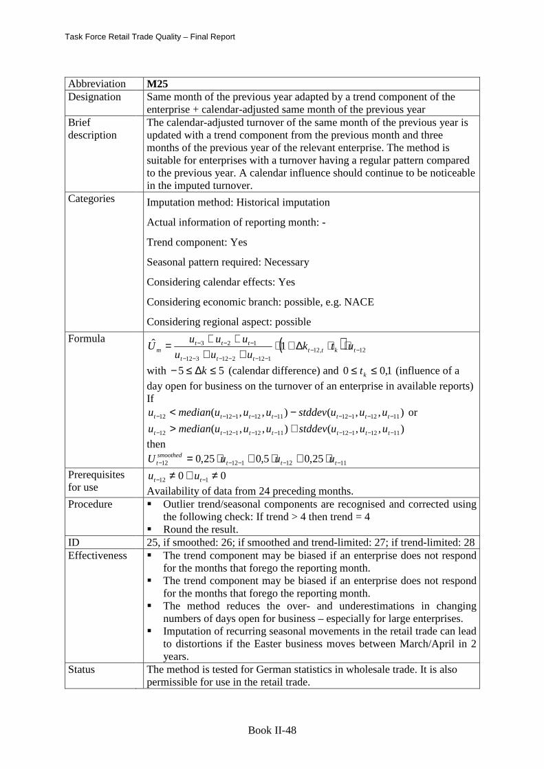
Task Force Retail Trade Quality – Final Report
Book II-48
Abbreviation M25 Designation Same month of the previous year adapted by a trend component of the
enterprise + calendar-adjusted same month of the previous year Brief description
The calendar-adjusted turnover of the same month of the previous year is updated with a trend component from the previous month and three months of the previous year of the relevant enterprise. The method is suitable for enterprises with a turnover having a regular pattern compared to the previous year. A calendar influence should continue to be noticeable in the imputed turnover.
Categories Imputation method: Historical imputation
Actual information of reporting month: -
Trend component: Yes
Seasonal pattern required: Necessary
Considering calendar effects: Yes
Considering economic branch: possible, e.g. NACE
Considering regional aspect: possible
Formula ( ) 12,12112212312
123 1ˆ−−
−−−−−−
−−− ⋅⋅∆+⋅++
++= tkttttt
tttm utk
uuu
uuuU
with 55 ≤∆≤− k (calendar difference) and 1,00 ≤≤ kt (influence of a
day open for business on the turnover of an enterprise in available reports) If
),,(),,( 1112112111211212 −−−−−−−−− −< ttttttt uuustddevuuumedianu or
),,(),,( 1112112111211212 −−−−−−−−− +> ttttttt uuustddevuuumedianu
then
111211212 25,05,025,0 −−−−− ⋅+⋅+⋅= tttsmoothedt uuuU
Prerequisites for use
00 112 ≠∧≠ −− tt uu
Availability of data from 24 preceding months. Procedure Outlier trend/seasonal components are recognised and corrected using
the following check: If trend > 4 then trend = 4 Round the result.
ID 25, if smoothed: 26; if smoothed and trend-limited: 27; if trend-limited: 28 Effectiveness The trend component may be biased if an enterprise does not respond
for the months that forego the reporting month. The trend component may be biased if an enterprise does not respond
for the months that forego the reporting month. The method reduces the over- and underestimations in changing
numbers of days open for business – especially for large enterprises. Imputation of recurring seasonal movements in the retail trade can lead
to distortions if the Easter business moves between March/April in 2 years.
Status The method is tested for German statistics in wholesale trade. It is also permissible for use in the retail trade.

Compensating non-response in short-term statistics
Book II-49
Abbreviation M30 Designation Updating the previous year’s turnover with current turnover trend Brief description
The previous year’s turnover of the enterprise to be imputed is updated with the turnover trend of enterprises with reports from the same stratum / publication cell. The turnover trend is defined as the quotient from current and previous yearly turnover.
Categories Imputation method: Historical imputation
Actual information of reporting month: Units of the same stratum / publication cell
Trend component: Indirect, by use of turnover development of responding units
Seasonal pattern required: Necessary
Considering calendar effects:-
Considering economic branch: possible, e.g. NACE
Considering regional aspect: possible
Formula 12,,
ˆ−⋅= ti
NACEtti uVU , Position-NACE ∈i
with
iNACEi
ti
iNACEi
tiNACE
t
hfu
hfuV
′∈′
−′
′∈′
′
⋅
⋅=∑
∑
12,
,
whereby
estimated be toenterprise ... i (month) period ... t
mmonth reporting in theover with turnenterprise ... i ′ ifactor ion extrapolat s'enterprisean ... fih
Procedure Round the result. Prerequisites for use
012, ≠−tiu
Number of the respondents of a stratum / publication cell > number of enterprises to be imputed in the same stratum / publication cell
0>NACEtV
ID 30 Effectiveness The method leads to very good results if several prerequisites are
fulfilled (see below). The general development/trend is better met, outlier deviations
avoided. The imputation is better the higher the turnover percentage of the reporting enterprise is in the total turnover of a stratum / publication cell and the greater the turnover trends of the individual enterprises correlate with the development of the respective stratum / publication cell. Poor imputation results could occur if the number of reporting enterprises of a stratum / publication cell is very low or if the turnover percentage of the reporters is very low and the turnover percentage of the enterprise to be imputed is very high.
Status The method has been tested by Destatis Germany for domestic trade.

Task Force Retail Trade Quality – Final Report
Book II-50
Abbreviation M40 Designation Same month of the previous year adjusted by the trend of the enterprise Brief description
Turnover of the same month of the previous year is updated with a trend component from the previous months and three months of the previous year of the relevant enterprise. The method is suitable for enterprises with a turnover having a regular pattern compared to the previous year.
Categories Imputation method: Historical imputation
Actual information of reporting month: -
Trend component: Yes
Seasonal pattern required: Necessary
Considering calendar effects:-
Considering economic branch: possible, e.g. NACE
Considering regional aspect: possible
Formula
12112212312
123ˆ−
−−−−−−
−−− ⋅++
++= tttt
tttt u
uuu
uuuU
If ),,(),,( 1112112111211212 −−−−−−−−− −< ttttttt uuustddevuuumedianu or
),,(),,( 1112112111211212 −−−−−−−−− +> ttttttt uuustddevuuumedianu
then
111211212 25,05,025,0 −−−−− ⋅+⋅+⋅= tttsmoothedt uuuU
Prerequisites for use
00 112 ≠∧≠ −− tt uu
Availability of data from 24 preceding months. Procedure Outlier trend/seasonal components are recognized and corrected using
the following PL check: If trend > 4 then trend = 4 Round the result.
ID 40, if smoothed: 41; if smoothed and trend-limited: 42; if trend-limited: 43 Effectiveness
The trend component may be biased if an enterprise does not respond for the months that forego the reporting month.
The method leads to over- and underestimations in the case of varying business days.
Imputation of recurring seasonal movements in the retail trade can lead to distortions if the Easter business moves between March/April in 2 years.
Status The method is used in the sectors of retail trade and wholesale trade of German short term statistics.

Compensating non-response in short-term statistics
Book II-51
Abbreviation M45 Designation Same month of the previous year Brief description
Turnover of the same month of the previous year. The method is suitable for enterprises with a turnover having a regular pattern compared to the previous year.
Categories Imputation method: Historical imputation
Actual information of reporting month: -
Trend component: -
Seasonal pattern required: Necessary
Considering calendar effects: -
Considering economic branch: possible, e.g. NACE
Considering regional aspect: possible
Formula
12ˆ
−= tt uU
Prerequisites for use
012 ≠−tu
Availability of data from 12 preceding months. Procedure Round the result. ID 45 Effectiveness
The method may lead to over- and underestimations in the case of varying business days. It does not take into account the historical trend development of an enterprise.
Imputation of recurring seasonal movements in the retail trade can lead to distortions if the Easter business moves between March/April in 2 years.
Status The method is used by Statistics Finland.

Task Force Retail Trade Quality – Final Report
Book II-52
Abbreviation M60 Designation Previous month + historical information one year ago Brief description
Imputation with the previous month The method uses partial autocorrelations between the turnover of a month and of the previous month as well as the corresponding months of the previous year. It is suitable for enterprises that impute the turnover in the current month with the data from the previous month.
Categories Imputation method: Historical imputation
Actual information of reporting month: -
Trend component: -
Seasonal pattern required: partly
Considering calendar effects:-
Considering economic branch: possible, e.g. NACE
Considering regional aspect: possible
Formula 1ˆˆ
−⋅= tst uuU with
−+=−−
−−−
112
112121ˆt
tts u
uuU
and general limitation of the seasonal component:
4ˆ0,25 ≤≤ sU
Prerequisites for use
00 1121 ≠∧≠ −−− mm uu
Availability of data from 14 preceding months. Procedure If coefficient of variation >= 0.6:
−⋅+
−⋅+
−⋅+=−
−−
−
−−
−
−−
12
1211
13
1312
14
1413 25,05,025,01ˆ t
tt
t
tt
t
tts u
uu
u
uu
u
uuUwith
ID If previous month: 60; if smoothed: 61 Effectiveness
The method leads to improvements compared with the previous imputation method. The effectiveness of the method is greatly
improved by averaging the ‘seasonal component’ su for variation
coefficients of >= 0.6. Delayed reactions for current enterprise developments are possible if
no reports, but also only imputations are available for an enterprise in the previous months.
Status The method has been tested by Destatis Germany for retail trade. A variant of the method is used in retail trade statistics of Hungary and the Netherlands: The value of the previous month is adapted by the change rate for the reporting month and month of the previous year of responding units from the same activity class and type of retail trade shops.

Compensating non-response in short-term statistics
Book II-53
Abbreviation M65 Designation Previous month updated by actual and seasonal information Brief description
Imputation with the previous month The method updates the turnover of a previous period by the average growth in the stratum between the previous period and the current period the average growth in the stratum between the same two months a year ago. In both cases the average growths are trimmed, where the 10% largest and 10% smallest growths in each stratum are not included when calculating the average (unless there are less than eleven growths in the stratum, in which case there is no trimming). The imputation link is then calculated as the weighted average of the two growths, with a weight of 80% on the previous period growth and 20% on the growth from a year ago. These weights are fixed across the survey.
Categories Imputation method: Combination of historical imputation and actual information
Actual information of reporting month: partly
Trend component: -
Seasonal pattern required: partly
Considering calendar effects: -
Considering economic branch: possible, e.g. NACE
Considering regional aspect: possible
Formula 1ˆˆ
−⋅= tst uuU with
( )( )trimstt
trimstts gcgcU ,1,,112,12 1ˆ
−−−− ⋅−+⋅=
with
∑∈ −−
−−−−−−
−⋅=
Ss st
stst
s
trimstt u
uu
ng
,112
,112,12,112,12
1, ∑
∈ −
−−
−⋅=
Ss st
stst
s
trimstt u
uu
ng
,1
,1,,1,
1, and
10 << c Prerequisites for use
01 ≠−mu
Availability of data from 13 preceding months. Procedure Compute the growths of all enterprises that belong to the same stratum as a
non-respondent. If there are more then eleven respondents in a stratum do not include the 10%
largest and 10% smallest growths when calculating the average growth rate. ID 65 Effectiveness
The method takes into account actual developments as well as seasonal patterns.
Status The method is used by the Office for National Statistics of the United Kingdom in retail trade.

Task Force Retail Trade Quality – Final Report
Book II-54
Abbreviation M70 Designation Median/mean from the available reports of the previous months Brief description
Imputation using the median of turnover from one or more previous months. The method is suitable for enterprises with a turnover having no regular pattern compared to the previous year but instead to the previous month.
Categories Imputation method: Historical imputation
Actual information of reporting month: -
Trend component: partly
Seasonal pattern required: partly
Considering calendar effects: -
Considering economic branch: possible, e.g. NACE
Considering regional aspect: possible
Formula titi UU ,,
~ˆ = , 12- t..., 1,-t =t
with estimated be toenterprise ... i
(month) period ... t Prerequisites for use
At least 1 previous month’s report must be available.
Procedure The median is used when the coefficient of variation >= 0.6 or number of available months < 3 The mean is used when the coefficient of variation < 0.6 and number of months > 3
Round the result. ID 70; if the mean is used: 71 Effectiveness
Analysis of Destatis Germany reveals that this method can be regarded as a compromise for enterprises whose turnover development does not show usable patterns.
Delayed reactions to current enterprise developments are possible. Status The method is used by Statistics Finland.

Compensating non-response in short-term statistics
Book II-55
Abbreviation M80 Designation Geometric mean of monthly changes Brief description
Imputation using the previous month.
Categories Imputation method: Historical imputation
Actual information of reporting month: -
Trend component: partly
Seasonal pattern required: -
Considering calendar effects: -
Considering economic branch: possible, e.g. NACE
Considering regional aspect: possible
Formula
3
2
2
11ˆ
−
−
−
−−=
t
t
t
ttt u
u
u
uuu
with estimated be to turnover ... u
(month) period ... t Prerequisites for use
3 previous months must be available.
Procedure Round the result. ID 80 Effectiveness
The method is suitable for enterprises with a turnover having no regular pattern compared to the previous year but instead to the previous month.
Delayed reactions to current enterprise developments are possible.
Status The method is used by Statistics Finland.

Task Force Retail Trade Quality – Final Report
Book II-56
Abbreviation M90 Designation Previous month Brief description
Estimating turnover with data of the previous month The method assumes partial autocorrelations between the turnover of an actual and preceding month.
Categories Imputation method: Historical imputation Actual information of reporting month: - Trend component: partly Seasonal pattern required: - Considering calendar effects: - Considering economic branch: possible, NACE Considering regional aspect: possible
Formula 1
ˆ−= tt uU
Prerequisites for use
Availability of data from five preceding months
Procedure If ( ) ( )u
tttttu
tttt uuu 1,...,51,...,511,...,51,...,5~~
−−−−−−−−− −<<+ σσ
then
321 2,03,05,0ˆ −−− ⋅+⋅+⋅= tttt uuuU
Round the result. ID 90; if smoothed: 91 Effectiveness
The method does not consider seasonal and calendar aspects. Delayed reactions on actual developments are possible.
Status The method is used by Statistics Finland.

Compensating non-response in short-term statistics
Book II-57
Annex 2 References Data editing and imputation Carl-Erik Särndal, Sixten Lundström: “Estimation in surveys with non-response”, Cornwall
2005
Diane K Willimack, Elizabeth Nichols and Seymour Sudman: “Understanding Unit and Item Non-response in Business Surveys” in Groves et al. (eds.) Survey Non-response, New York: Wiley 2002
Donald B. Rubin: “Multiple Imputation for Non-response in Surveys”, New York: Wiley, 1987
Eurostat: “Recommended Practices for Editing and Imputation in Cross-Sectional Business Surveys”, http://edimbus.istat.it/dokeos/document/document.php?openDir=%2FRPM_EDIMBUS
John Kovar and Patricia J. Whitridge: “Imputation of Business Survey Data.” in Business Survey Methods, New York: Wiley, 1995
John Charlton (eds): “Towards Effective Statistical Editing and Imputation Strategies - Findings of the Euredit project”, 2003 www.cs.york.ac.uk/euredit/
Sascha Kless, Elmar Wein: “Reducing the need for revisions in German retail trade statistics by means of improved estimations”, report of Destatis, Wiesbaden 2009
Statistical Offices of the Federal Government and the Länder: Concept for data editing, internal document, Wiesbaden 2005
UNECE: “Statistical Data Editing”, Volume 1, 1994 www.unece.org/stats/publications/editing/SDE1.htm
Data collection Michael Schäfer: “eSTATISTIK.core: Collecting Raw Data from ERP Systems”,
www.unece.org/stats/documents/ece/ces/ge.44/2006/wp.2.e.pdf, Bonn 2007
Data quality guidelines Eurostat: “Verhaltenskodex Europäische Statistiken”,
http://epp.eurostat.ec.europa.eu/pls/portal/docs/PAGE/PGP_DS_QUALITY/TAB47141301/VERSIONE_TEDESCO_WEB.PDF
Statistics Canada: “Statistics Canada Quality Guidelines”, Fourth edition, 2003 www.statcan.gc.ca/pub/12-539-x/12-539-x2003001-eng.pdf
Statistical Offices of the Federal Government and the German Länder: Quality standards of the German official statistics, Document on the website of the Federal Statistical Office, Wiesbaden 2003
Statistical legal acts European Community: Council Regulation (EC) No 1165/98 of 19 May 1998 concerning
short-term statistics, Official Journal EC No L 162 p. 1, amended by Annex III No 78 of Regulation (EC) No 1882/2003 of the European Parliament and of the Council of 29 September 2003 (Official Journal EU No L 284 p. 1), amended by Regulation (EC) No

Task Force Retail Trade Quality – Final Report
Book II-58
1158/2005 of the European Parliament and the Council of 6 July 2005 (Official Journal EU No L 191 p. 1), amended by Article 2 of Commission Regulation (EC) No 1503/2006 of 28 September 2006 (Official Journal EU No L 281 p. 15), amended by Article 12 of Regulation (EC) No 1893/2006 of the European Parliament and the Council of 20. December 2006 (Official Journal EU No L 393 p. 1).
Statistical methods Joachim Hartung: “Statistics” (only in German), 14th edition, Munich 2005
NIST/SEMATECH: “e-Handbook of Statistical Methods”, 2008
Time Series Analysis Douglas C. Montgomery; Cheryl L. Jennings; Murat Kulahci: “Time series analysis”,
Hoboken 2008
Klaus Neusser: “Time series analysis in business sciences” (only in German), Wiesbaden 2006
U.S. Census Bureau: „X-12-ARIMA Reference Manual Version 0.3“, 2007
Weighting M.A. Hidiroglu, C. Särndal and D.A. Binder: “Weighting and estimation in business
surveys.“ in Business Survey Methods, New York: Wiley, 1995
Lenka Mach: “Imputation vs. Reweighting for Total Nonresponse in a Business Survey” Proceedings of SSC Annual Meeting, 1995 www.ssc.ca/survey/documents/SSC1995_L_Mach.pdf

Book III Calculation of the retail trade turnover
indices1
1 Compiled by Sven Kaumanns

Task Force Retail Trade Quality – Final Report
Book III-2
Summary and Conclusions In 2008, the Economic and Financial Committee (EFC) of the European Union asked Eurostat
to increase the quality and reliability of the monthly retail trade turnover/volume statistics.
Supported by this mandate the Short-term Statistics Working Party in December 2008 set up a
Task Force to investigate the reasons for revisions and volatility of the retail trade
turnover/volume indices and to develop and suggest proposals for solutions.
The members of the task force agreed that it is insufficient to look at the revisions or volatility
as isolated problems. They have to be seen in the general context of the monthly retail trade
turnover and volume statistics' quality. This means not only to stop revisions or to “iron" the
development to make the results seem to be more reliable. This document follows this broader
approach by offering a complete and integrated description how an index should be compiled
and what should be covered by such an index of monthly retail trade turnover/volume2.
This report is on the one hand part of the Task Forces Report to the Working Party and on the
other a complete guideline to be used by the statisticians in the National Statistical Institutes
for developing the national indices as well as for compiling them in their normal, periodical
work routine.
Calculating the monthly retail trade volume/value index is more than just adding up results
collected by a certain number of retailers and set them in relation to previous collections. To
archive a useful and meaningful index it is absolutely necessary to respect the relation of the
units among each other as well as the development of the retailers' structures. In some few
cases, special treatments seem to be necessary to ensure that the development of the retailers'
structures and their relations do not influence the monthly indices. A detailed description of
these cases, their potential impact and the development expected is given in section 2.
This document is not able to give very detailed work instructions. The problem here is the
different production processes in general among all Member States and, the availability of
information among the Member States and even within a Member State from case to case.
What this document is able to do is to introduce calculation methods that enable the indices'
producers to compensate for undesirable developments if sufficient information is available.
Different methods suitable for different situations are discussed (Chapter 3) and set out in
relation to the definition of the indicator (Chapter 4). A set of tools detecting the mentioned
2 Other documents of this Task Force cover questions of seasonal adjustment and estimation of data being not available.

Index Calculation
Book III-3
objectionable influences is discussed in Chapter 5 and additional practical problems described
in Chapter 6.
Consequently this document does not offer a full service automatic solution. It describes the
problems, it clearly specifies the results that should be achieved and offers the producers of
monthly retail trade volume/value indices in the different Member States a toolbox of
methods and options to be adopted according to their special production methods, situations
and requirements.

Task Force Retail Trade Quality – Final Report
Book III-4

Index Calculation
Book III-5
Content
SUMMARY AND CONCLUSIONS.................................................................................................... 2
1 INTRODUCTION.............................................................................................................. 6
2 GENERAL DEFINITIONS AND EXPLANATIONS............... ...................................... 6
2.1 INTRODUCTION..................................................................................................................... 6 2.2 DEFINITION OF “CHANGES" .................................................................................................. 7 2.3 DEFINITION OF INDICATORS................................................................................................. 9 2.4 DIFFERENT KINDS OF CHANGES.......................................................................................... 10
3 COMPENSATION METHODS AND INDEX TYPES ................................................ 23
3.1 GENERAL REMARKS............................................................................................................ 23 3.2 DIRECT APPROACHES.......................................................................................................... 24 3.2.1 INTRODUCTION DIRECT CALCULATIONS............................................................................. 24 3.2.2 BACKWARD ORIENTED (ORIENTED ALWAYS TO BASE PERIOD).......................................... 24 3.2.3 FORWARD ORIENTED (ORIENTED ALWAYS TO CURRENT PERIOD)...................................... 25 3.2.4 REPORTING PERIOD ORIENTED (ORIENTED TO RESPECTIVE REPORTING PERIOD)............... 25 3.2.5 CONCLUSIONS DIRECT CALCULATIONS.............................................................................. 26 3.3 INDIRECT APPROACHES......................................................................................................26 3.3.1 INTRODUCTION................................................................................................................... 26 3.3.2 CHAIN-LINKING TO THE PREVIOUS MONTH........................................................................ 27 3.3.3 CHAIN-LINKING TO THE PREVIOUS YEAR'S AVERAGE......................................................... 27 3.4 CONCLUSIONS..................................................................................................................... 28
4 CLASSIFICATION PROBLEMS AND PROBLEMS OF DEFINING TURNOVER ................................................................................................ 29
5 DETECTION OF CHANGES......................................................................................... 33
5.1 INTRODUCTION................................................................................................................... 33 5.2 PLAUSIBILITY CHECKS........................................................................................................ 34 5.3 INDICATOR SERIES.............................................................................................................. 35 5.4 DETECTION QUESTION........................................................................................................ 35 5.5 THIRD PARTY INFORMATION .............................................................................................. 36 5.6 CONCLUSION ...................................................................................................................... 36
6 PRACTICAL PROBLEMS............................................................................................. 37
6.1 INTRODUCTION................................................................................................................... 37 6.2 INCOMPLETE INFORMATION............................................................................................... 38 6.3 LEVEL OF PRESENTATION................................................................................................... 39 6.4 “EXTRAORDINARY" TURNOVER......................................................................................... 41 6.5 RETROSPECTIVE “RE-"INCLUSION OF NON-COMPARABLE-CHANGES AND BENCHMARKING ................................................................................................................ 42
7 CONCLUSIONS............................................................................................................... 43

Task Force Retail Trade Quality – Final Report
Book III-6
1 Introduction When looking at the existing documents related to the monthly retail trade turnover and
volume indices they do offer on the one hand a lot of freedom and room for interpretation –
on the other hand this leads to uncertainties, different and un-harmonised treatments and in
the end to often volatile results, and results with different content and thus only limited
comparability.
In general, the monthly retail trade turnover and volume indices use combined data of the
micro level – data from single reporting units, mainly enterprises – to describe the
development on the macro level, the level of the retail sector in total or its sub-sectors.
In contrast to the structural business-statistics the task of short-term statistics is not to describe
the level of turnover/volume but their development. That is why the users' focus is usually
more on the growth rates rather than the index numbers. Because of their economic relevance,
the even more unstable month-on-month growth rates, describing the rather short term
development, are often of more interest than the much more stable month-on-previous-year's-
month growth rates are. Thus the main attention should be turned in quality improvement of
these quite unstable month-on-month growth rates.
It is important for compilation of such developments to have comparable periods. How to
achieve such comparability is one of the main problems of short-term statistics and one main
issue of this text.
2 General definitions and explanations 2.1 Introduction The sections in this chapter (2 General definitions and explanations) define on a general basis
how the indices should be composed and look like. These descriptions are based on the
assumption that all relevant information about the basic population, its units and their
development are available. Different effects of developments are described, discussed how
they should influence the indicators, and how – if necessary – compensations should be made.
While knowing well that what is described here is based on highly theoretical assumptions, it
is necessary for decisions about the actual production processes and of course benchmarking
the actual production process.

Index Calculation
Book III-7
2.2 Definition of “changes" Economic units define, based on numerous criteria such as their legal form or their performed
main economic activity, the population used for short-term statistics. However these units
develop by-and-by. The result is that no population – neither the basic population nor a
sample – consists of exactly the same units, and the same composition of units in different
periods. In general this development is not only unproblematic but necessary for short-term
statistics. Otherwise – if no development at all would happen – each period and each result for
each period would be equal. It is a part of this development that short-term statistics wants to
explain.
As mentioned, there are developments within each unit and in the composition of all units. All
these developments are changes. Generally speaking changes are – and in this sense they are
understood in this document – any differences between two states within the micro data by
variation of time.
These changes within the micro data could have, depending on their type and the production
and compensation methods used, an impact on indices produced as result. Depending on
whether these changes within the micro data should impact the results or not changes can be
classified into three different types:
1. changes, that should be shown by the results (short-term development),
2. non-comparable changes, and
3. comparable ones (having no impact on the results).
The first type, the changes that should be shown, represents the normal case of economic
development that should be explained by short-term statistics: An existing unit varies its
turnover by selling more or less without changing its relations to other units. As a matter of
course these changes have - and they should have - an impact on results of short-term
Figure 7 Different kinds of changes
Changes without impact on results
Changes with wanted impact on results
Changes with unwanted impact on results
Development that should be measured.
Non-comparable changes
Comparable changes

Task Force Retail Trade Quality – Final Report
Book III-8
statistics. In sum they represent the variation in quantity and value of goods supplied by the
retail-trade sector.
Figure 8 Changes at micro level
Non-comparable and comparable changes always go along with a modification of the
relations of one unit to others, or the way a unit organises its business thus with a structural
change. A non-comparable change is a change in the structure of the basic or sample
population that has an unwanted impact on the STS-results3. Hence these non-comparable
changes are parts of all changes happening on the micro level. The changes in structure of the
population consist of different changes – such as main activity, size, relations to other units
(…), of the population's single entities. Often changes happening at the same time are linked
to each other and should not be treated separately. If some linked changes countervail their
effects, they have to be seen as only one comparable one. These changes compensate and
thus do not significantly influence statistical results on the macro level (see Example 1),
others influence statistical results to a negligible degree and some of them are so aggravating
that they distort actual statistics.
Example 1 Combination of changes leading to a comparable change
A totally new retailer is entering a market. This new retailer creates turnover by selling goods to customers. Abstracting from possible one-time effects resulting from commercial campaigns when opening, this does not create new turnover. Turnover is just “shifted" from the existing retailers to the new ones as people do not buy more but at different places. This creates the following changes (in brackets the evaluation of the change if treated separately):
3 In contrast a comparable change is a change without impact on the STS-results.
Change
?
Micro level (e.g. enterprise)
Macro level (e.g. sector)
time

Index Calculation
Book III-9
o “new shop" with “new turnover" (non-comparable change) o declining turnover in “established shops" (normally wanted change) In sum these changes lead to comparable changes. They do not affect the result in total as they X out each other. Under normal conditions the declining turnover in “established shops" could be seen as expression of normal economic development and thus is a “wanted change". However here it has to be seen in relation with the opening of a new shop and thus has a component relating to other units making it to a non-comparable change.
2.3 Definition of indicators What is problematic in this context, is defining which changes have unwanted impacts on the
results and thus are non-comparable changes. To do this it is essential to agree on the exact
use of the indices.
The European monthly turnover index of retail trade is included by the European Commission
as one of the most important key short-term business indicators for Europe and the euro area
(PEEI ) and it is covered by the European short-term statistics regulation and related
documents. Following the European legislation, the national indices measure the development
of the turnover of enterprises having their main economic activity within the relevant retail
trade activities. Turnover is defined by annex I of the Commission Regulation (EC) No
1503/2006 as “the totals invoiced by the observation unit during the reference period. This
corresponds to market sales of goods or services supplied to third parties. Turnover also
includes all other charges (transport, packaging, etc.) passed onto the customer, even if these
charges are listed separately in the invoice. (…)" In the same paragraph the regulation names
as purpose of this variable: “It is the objective of the turnover index to show the development
of the market for goods and services." Article 1 of the short-term statistics regulation just
states that all short-term statistics variables are necessary within the framework of short-term
Community statistics on business cycles as variables for the analysis of the short-term
evolution of supply and demand, production factors and prices.
This shows a certain ambiguity within the European regulations. On one hand, the base
regulation reflects the development of the summed up turnover of enterprises having their
main economic activity within one sector defined by NACE. On the other hand, the definition
regulation refers to the market developments of certain goods. This ambiguity is a result of
the two different perceptions of the retail trade indices – the technical statisticians' perception
of what seems to be fairly easy to measure (development of the turnover of enterprises having
their main economic activity within retail trade) and the analytical perception of the users of

Task Force Retail Trade Quality – Final Report
Book III-10
what makes sense to picture, is meaningful to interpret and necessary for fulfilling their
analytical tasks (development of the market).
The balancing act continues in the production and use of the indices. Even though nothing is
clearly said about the exact content or use of this indicator – or to be more precise these
indicators (value and volume) – the main intended purpose of the monthly turnover index of
retail trade is to have an indicator of developments in final consumption: National
accountants, central banks and other financial institutions (as the main users of short-term
statistics) and many other economists use it for this purpose. Other users might be interested
in other aspects but it is absolutely necessary for producing consistent and meaningful retail
trade indices to decide on one to make all methodological decisions comprehensible and the
behaviour of the index explicable. This is the prerequisite for a methodological sound and
useful index. As our main users request an indicator of developments in final consumption,
the retail trade indices should as best as possible follow the volume and value of goods
flowing through retail trade into final consumption. This idea has to be the determining factor
whether in general a change will be seen as non-comparable or not within this.
Together with the legal requirements resulting out of Council Regulation (EC) No 1165/98 of
19 May 1998 concerning short-term statistics as amended from time to time and relating legal
documents, this would mean to only cover turnover resulting out of retail trade activities by
units classified due to their main economic activity within the retail trade sector (see Figure
9).
Figure 9 Covered turnover
2.4 Different kinds of changes Before the decision can made on how to treat which change, a thorough analysis and
collection is necessary to enquire which changes could happen.
retail trade sector other sectors and import
final consumption intermediate input and other whereabouts
covered not covered not covered

Index Calculation
Book III-11
A A
X
The examination within this section is based on the basic population to show full coherency.
Further problems and limitations described later on might appear depending on the production
system and data source (random sample, administrative data etc.) used.
To comprehend the influence of non-comparable changes on statistical results and to facilitate
their detection it is important to know which types of changes could appear, how they interact
and probably cancel out. That is why a lot of different kinds of changes have to be described
and analysed deeply.
Overview: Case Item Page CASE 1 NEW UNIT 12 CASE 2 EXISTING UNIT DISSOLVES 12 CASE 3 INACTIVE UNIT BECOMES ACTIVE AGAIN 13 CASE 4 ACTIVE UNIT BECOMES INACTIVE 13 CASE 5 AN EXISTING UNIT OPENS A NEW SHOP 13 CASE 6 AN EXISTING UNIT CLOSES AN EXISTING SHOP 14 CASE 7 AN EXISTING UNIT IS RECLASSIFIED INTO THE RETAIL TRADE MAKET 14 CASE 8 AN EXISTING UNIT IS RECLASSIFIED OUT OF THE RETAIL TRADE MAKET 14 CASE 9 SPIN-OUT (SPLIT-OFF) 15 CASE 10 SPLIT-UP 18 CASE 11 TAKE OVER 18 CASE 12 FUSION-TO-NEW-FOUNDATION 20 CASE 13 TAKE-OVER BY SPIN-OUT 20 CASE 14 PSEUDO SPIN-OUT 23 MORE THAN ONE CHANGE WITHIN ON PERIOD (MONTH) 23
To illustrate the particular changes the following symbols shown beside are used.
Active unit retail trade sector
Inactive unit sector irrelevant
no unit

Task Force Retail Trade Quality – Final Report
Book III-12
X A
B B
X A
A X
Case 1 New Unit
In this case a new unit is entering the retail trade market. Following
the definitions this would be a structural change and thus should not
be shown by the retail trade indices as defined above. However this
appearance of the new unit (“A") cannot be seen as isolated. On the level of the retail trade
market, the appearance of a new found unit is often only a redistribution of the existing cake.
The volume does normally not increase just because of the appearance of a new unit (see
Example 1 on page 8 as well). Thus this case has to be split in two sub-cases that interact:
o the appearance of the new unit (as illustrated above), and
o the development of the existing units already active on this market.
Here we have two contrary effects: Unit “A" is creating new turnover
while the other units in sum (here illustrated as unit “B") are losing
part of their market share to unit “A". Together these effects lead to a
comparable change.
By implication, not taking the new turnover of unit “A" into account
would create a non-comparable change as the development of the other units (“B") contains at
least as part, a compensation for the change unleashed by the appearance of the new unit
(“A").
The appearance of units is via the market shares linked to the turnovers generated by other
units. Thus there are no special treatments necessary as long as the new unit is implemented
immediately when entering the market. If this is not the case the total turnover for the sector
will be underestimated.
Case 2 Existing unit dissolves
An existing unit dissolves and is leaving the market. This case is the
opposite of Case 1. Following the strict definitions this would be a
non-comparable change as well as it is effects the structure of a unit.

Index Calculation
Book III-13
A A
B B
A X
A A
A A
However as before this cannot be seen as isolated. The turnover the unit would have made in
the following period in case it would not have dissolved is compensated by the turnover other
units make. Thus the complete context would:
o a reduction of turnover for unit “A" until zero, and
o a hypothetical increase of the other units' turnovers.
Here again we see two contrary effects: The turnover of unit “A" is
disappearing totally while additional turnover is created by the
remaining other units in sum (here illustrated as unit “B") They take
over the hypothetical market share of unit “A". Together these effects
lead to a comparable change.
The dissolving of units is via the market shares linked to the turnovers generated by other
units. Thus there are no special treatments necessary.
Case 3 Inactive unit becomes active again
This case is pretty much the same as Case 1. A unit, that was inactive
before, is (re-)entering the retail trade market. It is not important
whether the unit was in the retail trade sector before getting inactive
or not. The effects are the same as described above for Case 1. Thus this case should be
treated as a “new" unit entering retail trade (Case 1).
Case 4 Active unit becomes inactive
A unit that was active in the retail trade market is becoming inactive.
The unit still exists but does no business any more. The turnover of
this unit is zero. The effects are the same as for units leaving the
market, thus this case should be treated as a unit leaving the market (Case 2).
Case 5 An existing unit opens a new shop
A unit active in the retail trade sector opens a new shop. In total (for
the whole sector) no new turnover is expected. As in Case 1 the
additional turnover of unit A are for account of the other units (and

Task Force Retail Trade Quality – Final Report
Book III-14
A A
A A
A A
A A
unit a itself) of the retail trade sector. No special correction is necessary.
Case 6 An existing unit closes an existing shop
A unit active in the retail trade sector closes an existing shop. In total
(for the whole sector) no new turnover is expected. Like in Case 1 the
additional turnover of unit A are for account of the other units (and
unit a itself) of the retail trade sector. No special correction is necessary.
Case 7 An existing unit is reclassified into the retail trade maket
Here two different scenarios are thinkable: A unit could either have
changed its activities radically (performed something different before
and now became a retailer [Case 7A]), or it was a gradual process
(the unit performed retail trade since several periods and now reached the critical mass to be
reclassified[Case 7B]).
Case 7A is comparable to a situation of a new unit (Case 1). It was not active on the retail
trade market before and it is now. Thus there is “new" retail trade turnover made by Unit “A"
and this additional turnover is compensated by the turnover of all other retailers on the same
market.
In Case 7B is problematic. No, or only very few, “new" retail trade
turnover is generated; nevertheless all of the retail trade turnover
was not in the retail trade sector but will be allocated newly to the
retail trade sector. The complete retail trade turnover was (partly) “compensated" by not
being made by units in the retail trade sector before. Thus this case would lead to an unwanted
increase of turnover within the retail trade sector.
For Case 7A no special treatment is necessary. This case should be treated as a “new" unit
entering retail trade (Case 1). Case 7B is problematic. Here corrections are necessary.
Case 8 An existing unit is reclassified out of the retail trade maket
Again two different scenarios are thinkable: A unit could either have
changed its activities radically (performed retail trade before and now
changed to something different [Case 8A]) or it was a gradual process
(the unit performed retail trade and other activities since several periods and now reached the
critical mass to be reclassified [Case 8A]).

Index Calculation
Book III-15
A A
A A A2
Case 8A is comparable to a situation of a new unit (Case 2). It was active on the retail trade
market before and it is not any longer. Thus the turnover not made any longer by Unit “A" is
compensated through the market.
Case 8B is problematic. The amount of retail trade turnover made
by unit “A" does not change much – however the total turnover is
now classified outside of the retail trade sector. As the retail trade
turnover remains on the market, no compensation through turnover variations of the units
remaining within the retail trade sector happens.
For Case 8A no special treatment is necessary. This case should be treated as a dissolving unit
(Case 2). Case 8B is problematic. Here corrections are necessary that require rather detailed
information.
Case 9 Spin-Out (Split-Off)
During a spin-out, a part of an existing unit splits-off by taking assets,
property, technology, etc. from the parent unit. In the basic case the
parent unit was and remains in the retail trade sector and the split-off
“new" unit is classified here as well (Case 9A). This case could lead
to different situations: The unit “A" could generate turnover with the “new" unit “A2" and
vice versa or not. Thus four different situations could occur:
o Case 9A1: Unit “A" and “A2" do not trade with each other, o Case 9A2: Unit “A" creates turnover by trading with unit “A2", o Case 9A3: Unit “A2" creates turnover by trading with unit A, o Case 9A4: Unit “A" and unit “A2" create turnover by trading each with the other
unit.
Not measuring the split-off new child would lead to a decrease of total retail trade sector's
turnover. In the Case 9a1 no additional further correction is necessary as it can be assumed
that the turnover of the both units is equal to the turnover of the old parent unit.
As a speciality of the retail trade indices no further corrections for additional amounts of
turnover are necessary in the cases of A2, A3 and A4 as normally no retail trade turnover can
be created between units.4
4 No retail trade turnover can result out of transactions between units. However if not retail trade but total turnover is monitored correction becomes necessary. That is why in the following the compensation of turnover is mentioned knowing that it is impossible to create retail trade turnover out of transactions between units.

Task Force Retail Trade Quality – Final Report
Book III-16
A A A2
A A A2
A A A2
A quite common case is that the parent unit was and remains in the
retail trade sector but the new unit is not to be classified in retail
trade. Case 9B describes this situation with a unit A in the retail trade
sector splitting-off some mainly non-retail trade activities in a new
unit. Here it is of interest for the further treatment whether the split-off activities had external
market relations and created turnover with retail trade activities.5 Before being split-off (Case
9B1) or not (Case 9B2). If not, this case (Case 9B2) can be split in two different sub-cases
depending on whether unit “A" is creating turnover by trading with “A2" (Case 9B2a) or not
(Case 9B2b). If not (Case 9B2b), no additional corrections are necessary. If yes (Case 9B2a),
a correction for “A'"s turnover with unit “A2" might have to be done to avoid an
overestimation of the turnover development. However this case seems to be rather unlikely.
If unit “A 2 " takes over some of unit “A"'s former market relations (Case 9B1) compensation
in the turnover development of unit “A" is necessary. As before, this case can be split in cases
were unit “A" creates turnover with unit A2 (Case 9B1a) or not (Case 9B1b). If yes (Case
9B1a), an additional correction for A's turnover with unit A2 might have to be done to avoid
an overestimation of the turnover development. However this case seems to be rather
unlikely. If not (Case 9B1b), no additional corrections are necessary.
The following cases (Case 9C and Case 9D) should be very uncommon but nevertheless
could happen:
Due to a spin-out, the parent unit, which was classified in the retail
trade sector, has to be reclassified out of it but the child remains
within (Case 9C). Here it seems to be pretty clear that the child-unit
A2 takes over (some) of A's market activities. Moreover, A2's
turnover compensation for A's remaining turnover– if A2 creates new turnover with A for this
new turnover – corrections could be necessary.
Another case (Case 9D) is that the parent unit was classified in retail
trade but is not any more. For retail trade statistics this situation is
comparable to a normal reclassification out of the retail trade sector
as described in Case 7.
5 It is assumed that only retail trade turnover is covered by the retail trade indices (see 2.3 Definition of indicators). If this is not the case the statement is valued for total turnover.

Index Calculation
Book III-17
A A A2
A A A2
A A A2
In all cases described above the parent unit was classified within the retail trade sector. In the
following cases described, the parent unit was classified as not within
retail trade.
The most likely case is Case 9E with a unit “A" splitting off its retail
trade activities in a separate unit (“A2"). This case is basically
comparable to normal reclassification of an existing unit into the
retail trade sector (Case 7). As mentioned already (Case 7B), compensation might be
necessary if the unit “A" has performed retail activities before and now carried (some of)
them over to “A2". If “A 2" performs turnover out of business activities with A an additional
compensation is required (as described in case e.g. for Case 9A3).
This case (Case 9F) is less likely. A unit “A" splits of some of its
previous activities and afterwards has to be classified into the retail
trade sector. The split of part remains outside. In general this case is –
as the one before – basically comparable to normal reclassification of
an existing unit in to the retail trade sector (Case 7). As mentioned
already there (Case 7B) compensation might be necessary if the unit “A" has performed retail
activities before and now carried (some of) them into the retail trade sector. If “A" performs
turnover out of business activities with “A2" an additional compensation is required (as
described in case e.g. for Case 9A2).
This case (Case 9G) seems to be rather improbable. A unit “A" splits
off some of its previous activities and afterwards both parts have to
be classified as within the retail trade sector. However it is not
impossible. It has to be, depending on the situation, seen either (Case
9Gopt1) as a reclassification into the retail trade sector and splitting
off (Case 7 and Case 9A) or as (Case 9Gopt2) a splitting off and two reclassifications into the
retail trade sector (Case 9A and Case 7 twice). Depending on which case is appropriate, the
corrections as described above (Case 7 and Case 9A) are required.
Spin-Outs (Split-Offs) could be rather complex and impact the results of STS in different
ways. For good compensation very detailed knowledge of the situation and very thorough
analysis is required in each single case. The correction itself could be rather complex as well.

Task Force Retail Trade Quality – Final Report
Book III-18
A A B
A B C
Case 10 Split-up
While after spin-off the former parent unit remains existing, in a
split-up two or more new units consisting of the redistributed parent's
assets (…) appear. This situation could either be seen (a) as one unit
leaving the market and two (or more) entering or as a situation (b)
comparable to a spin-out with the parent unit becoming one of the new units. This second
option (b) has the advantage that it gives the possibility to compensate for new turnover
between the Units B and C, which is not possible when treating them as entirely new units.
When following this axiom (Split-up is just a special case of a spin-out) all sub-forms
regarding the in- or exclusion in the retail trade sector described there apply to this case as
well. Split-ups should be treated as special cases of spin-outs.
Case 11 Take over
During a takeover, an existing unit incorporates another existing one.
It is more or less the opposite of a spin-out and thus all different
varieties of spin-outs reflect in exactly the same different varieties of
takeovers.
In the basic case, the unit taking over (A) was and remains in the retail trade sector and the
unit taken over (B) was classified here as well (Case 11A). This case could lead to different
situations: The unit A could have generated turnover with the unit B before taking it over and
vice versa or not. Thus four different situations could occur:
o Case 11A1: Unit A and B did not trade with each other before the takeover, o Case 11A2: Unit A created turnover by trading with unit B before the takeover, o Case 11A3: Unit B created turnover by trading with unit A before the takeover, o Case 11A4: Unit A and unit B created turnover by trading each with the other unit
before the takeover.
Not respecting both the unit taking over and the one taken over would lead to an
unsubstantiated increase of total retail trade sector's turnover. In the Case 11A1 no additional
further correction is necessary as it can be assumed that the turnover of both the units is equal
to the turnover of the old parent unit. For the Cases Case 11A2, Case 11A3 and Case 11A4
corrections for the dropping out amounts of turnover could be necessary (see Footnote 4 on
page 15).

Index Calculation
Book III-19
A A B
A A B
A A B
A A B
A quite common case is that the unit taking over was and remains in
the retail trade sector, but the unit taken over was not classified
within retail trade. Case 11B describes this situation with a unit A in
the retail trade sector taking over a unit some non-retail trade
activities in a new unit. Here it is obvious that B had external market relations but
questionable if it had activities within the retail trade sector5) (Case 11B1) or not (Case 11B2).
If the unit B had no activities within the retail trade sector it has to be distinguished whether
the unit A created turnover by trading with unit B (Case 11B2a) or not (Case 11B2b). If no,
no further corrections are necessary. If unit B (Case 11B1) was active in the retail trade sector
(turnover was out of scope) correction for this becomes necessary. In case of not monitoring
retail trade turnover but total turnover (see Footnote 4 on page 15) it has to be distinguished
whether unit B created turnover by trading with unit A or not (Case 11B1a and b). If yes
(Case 11B1a) a corresponding correction has to be done.
This case (Case 11C) describes the situation of a retail trade unit B
taken over by a non-retail unit A. As A remains outside the retail
trade sector this case can be treated as a normal reclassification of B
(see Case 8 on page 14).
The next case (Case 11D) is at first view more complex. The unit B
classified within the retail trade sector is taken over by a unit A
classified outside retail trade. After taking over B, A had to be
reclassified into retail trade. But infact this case is quite comparable
to the one mentioned above under Case 11B. For the statistical results
it is irrelevant which of the units (A or B) “survives" as successor of both. I.e. all statements
made for Case 11B and its sub-cases apply to this one as well.
This rather unlikely case (Case 11E) with unit A and B classified
within the retail trade sector and the successor (in this case unit A)
after the take over outside of retail trade can be seen in two different
ways: Either a reclassification out of the retail trade sector followed
by a takeover (Case 11Eopt1) or as a takeover within the retail trade
sector followed by a reclassification of the remaining unit (Case 11Eopt2). Depending on the
situation the adjusters as described in Case 11A and Case 8, or Case 8 (twice) are required.
For the information site the treatment described as Case 11E1 might have some practical
advantages.

Task Force Retail Trade Quality – Final Report
Book III-20
A A B
A A B
A A B B
A C B
Another rather unlikely case is described here (Case 11F). A unit A
classified outside of retail trade takes over another unit (B) that is
classified outside of retail trade as well. After the takeover the unit A
has to be reclassified into the retail trade sector. As before, this case
could either be seen as two reclassifications into the retail trade sector
followed by a takeover (Case 11Fopt1), or as a takeover followed by a reclassification (Case
11Fopt1).
In the case described here (Case 11G) a unit A, classified within retail
trade, takes over a unit B that is classified outside of retail trade.
After the takeover unit A is classified out of retail trade. This case
can be treated as a normal reclassification of unit A out of retail trade
as described in Case 8 above. If A keeps on creating turnover out of
retail trade (as described in Case 8A) and B was client of A this has to be kept in mind for the
necessary compensation.
On the first view takeovers look rather simple. However, depending on the concrete form they
could have a significant impact on the results of STS in different ways. For good
compensation very detailed knowledge of the situation and very thorough analysis is required
in each single case to select the right methods to compensate unwanted effects.
Case 12 Fusion-to-new-foundation
During a fusion-to-new-foundation two (or) more existing units join
together and form – in contrast to a takeover – a new unit. For short-
term statistics results there should be no difference in impact between
a fusion-to-new-foundation and a takeover. Thus all explanations
made there (Case 11) are valid for a fusion-to-new-foundation as
well.
Case 13 Takeover by Spin-Out
A takeover by spin-out is the combination of a split-off (Case 9) with
the part being split-off taken over (Case 11) by another unit. It is not
necessary that the units have business relations after the split-
off/takeover-process; but they could.

Index Calculation
Book III-21
A A B B
A A B B
A A B B
A A B B
Here again the method of compensation very strongly depends on the specific situation. If all
units have been and remain within the retail trade sector (Case 13A), in general no special
treatment is necessary. An exception would be new turnover made by the split-off part with
its former parent.
In Case 13B the unit A splits off some activities taken over by a unit
outside the retail trade sector. In its treatment this case is in general
identical to Case 9B and its sub-cases.
In this case (Case 13C) a unit B, classified within the retail trade
sector) takes over some retail trade activities of unit A. Afterwards
unit A has to be reclassified out of retail trade. Here two different
corrections might be necessary: Fist of all for the turnover leaving the
sector by reclassifying unit A. If the split-off and taken-over part had
turnover out of business with unit B before taken over correction for this is necessary as well.
Case 13C describes a situation with a unit A, classified within retail
trade, and takes over a split-off part of a unit B classified outside of
retail trade. Unit A remains in retail trade. Here a compensation
becomes necessary, as long as the taken-over part leads to an increase
in A's turnover.
This situation (Case 13D) is one of the most complex ones. Unit A,
classified within retail trade, is transferring retail trade activities to
Unit B, classified not within retail trade. After the transfer A and B
have to be reclassified. This situation could, depending on details,
lead to a need for various corrections:
o A is leaving retail trade. If it is taking retail trade turnover6 out of the retail trade
sector this has to be compensated.
o B is entering the retail trade sector. If it brings turnover into the retail trade sector
compensation for this additional turnover becomes necessary.
o If the split-off and taken-over part created turnover with B before or A after its
transfer, corrections for these turnovers might be necessary to ensure that the turnover
6 In case that not retail trade but total turnover is measured: always.

Task Force Retail Trade Quality – Final Report
Book III-22
A A B B
A A B B
A A B B
A A B B
development of the retail trade sector is described correctly in sense of the these
indices.
This Case 13E is comparable with a classification out of the retail
trade sector as described in Case 8. Here a reclassification of B
becomes necessary because of additional activities it gets from unit
A. However for calculation of the comparable reference month it is
important to keep this split-off part in mind.
The next case (Case 13F) is somehow comparable. Here unit A splits-
off some retail trade activities and has to be reclassified. The unit
taking over theses parts was and stays outside of retail trade. Again
this can be seen as a reclassification out of the retail trade sector. For
calculating the compensation, again both parts – A and the split-of
part – should be taken into account.
The following two cases (Case 13G and H) are the opposites of Case
13E and F: The not within retail trade classified unit A splits of some
parts taken over by B – classified as well outside of retail trade – and
either unit A (Case 13G) or unit B (Case 13H) have to be reclassified
into retail trade as a result of this transaction. This reclassification of
unit A or B can be seen as a normal reclassification into the retail
trade sector as described in Case 7A and B. For calculating the
comparable period the split-off and taken-over parts have to be
respected.

Index Calculation
Book III-23
A A B B
A A B B
A A B B
For information:
The two situations shown on the left-hand side cannot only be a result
of a split-off and takeover. Here at least one additional change or
development took place. (see: More than one change within on
period)
Case 14 Pseudo Spin-Out
“Pseudo" spin-outs are located somewhere in the middle between
“normal" spin-outs (Case 9), and takeovers by split-offs (Case 13).
Here activities, assets, property, technology, etc of unit A is split-off
and does not form a new unit but is taken over by an already existing
but inactive unit B. For the retail trade indices the impact of this and
the necessary compensations should be exactly like the ones in cases of “normal" spin-outs
(Case 9).
Case 15 More than one change within on period (month)
In some cases a unit might be affected by more than one change during one month. In this
case all of the different changes have to be taken into account to decide if so, and if yes, how
corrective actions are required.
3 Compensation methods and index types 3.1 General remarks The chapter above described the different kinds of changes that could happen and how they
should be reflected within monthly retail trade turnover and volume indices. This knowledge
how certain changes should impact the indices and growth rates is necessary prerequisite.
Sufficient conditions for reliable growth rates and consistent indices are strong, solid and
comprehensible methods adjusting the data to ensure comparability between the periods to be
compared. Here different options are cogitable. In general, they can be distinguished into

Task Force Retail Trade Quality – Final Report
Book III-24
st st
st st
st st
Results in all Periods
Results for period t t+1 t+2
Structure used for the reporting period (st+x) Structure used for the base period (st)
direct and indirect methods, whether the focus should be more on the index or on a (month-
on-month or month-on-previous-year's-month) growth rate, and whether the base, the current
period or a mixture of both should be adjusted to be comparable. In the following, some
methods will be introduced, discussed and compared:
3.2 Direct approaches
3.2.1 Introduction direct calculations
The normal way of calculating an index is to divide the reporting period's value by the
reference (base) period's value (and to multiply the result with 100). This approach is very
basic and does not take into account that the structure of the retail trade sector might have
changed in the meanwhile. As the base period is normally not a real monitored period but an
artificial average of the base year's periods it is possible that for certain units changes already
happened within the periods used for calculating this artificial base period.
To adjust for the influences caused by changes as described in Chapter 2.4 it is necessary to
modify the results for the base and/or the reporting period in such a way that they reflect
results that would arrive in case of equal structures in both periods. Depending on which
structure is used as reference, it is possible to calculate a kind of Laspeyres-Index – using the
structure of the reference period (3.2.2) – or a kind of Paasche-Index – using the structure of
the units in the reporting period (3.2.3 and 3.2.4). In some cases it could be even necessary to
do a kind of mixture; e.g. in cases where due to a lack of information it is only possible to
adjust the base- or the actual period.
To illustrate the methods described below the following symbol shows the
.
3.2.2 Backward oriented (oriented always to base pe riod)
Using this method would mean that all
periods are modified in such a way, that
all units have the same structure they
had in the reference (base) period. The
advantage of this method is that all periods are comparable among each other. However
this approach might be problematic: The longer the distance in time between reference
period and the current period gets the more modifications in the current periods become

Index Calculation
Book III-25
st+1 st+1
st+1 st+1
st+2 st+2
st+2 st+2
st+2 st+2
st st
Result in base period
Results in period t+1
Results in period t+2
Results for period t t+1 t+2
st st
st+1 st+1
st st
st+1 st+1
st+2 st+2
st st
Result in base period
Results in period t+1
Results in period t+2
Results for period t t+1 t+2
necessary. The question might be if it is feasible to track and perform all these
modifications.
3.2.3 Forward oriented (oriented always to current period)
This method always modifies all
previous periods (back to the reference
period) to make them comparable to the
current one. On the one hand this might
increase the acceptance of this method
as always the “newest" information is
used. On the other hand, all previous
periods always have to be recalculated.
The complexity of this method is much higher than for the one above, while perpetuating
the same problem: The longer the difference in time between the reference period and the
current period, the more modifications in all periods become necessary.
A second problem of this approach is that every period of the artificial base period
(average base year) has to be recalculated. This is linked to some difficulties. A third
problem is that with each new period the results for the previous ones have to be
recalculated using the new structure. This is a potential risk for permanent revisions.
3.2.4 Reporting period oriented (oriented to respec tive reporting period)
This method combines the need not to
change the previous periods – except
the reference period – and the forward
orientation. For each reporting period
the structure of the reference period is
modified in a way that makes it
comparable to the particular reporting
period. That means for each reporting
period a private, fitting reference is created. This leads to a set of different reference
periods with different structures. However, the main problems remain:
o For each new period a new structure has to be adopted by the artificial base
period and

Task Force Retail Trade Quality – Final Report
Book III-26
o the longer the distance between reporting and reference period gets, the harder
the modification to ensure the absence of differences gets.
3.2.5 Conclusions direct calculations
As seen, there are two main problems when calculating an index directly:
1. possible non-comparable changes within the periods used to calculate the “artificial"
base period, and
2. the time span between the reference and the reporting period,
The first problem is especially annoying when it is either necessary to always manipulate this
artificial period or if other periods have to be transferred to the structure of this period and
units are affected which couldn't be represented clearly in the artificial base period change
again. The second problem is the time span between the reference and the reporting period.
This leads to an accumulation of all the non-comparable changes between the reference (base)
period and the reporting period. The longer the time span gets, the more corrections have to
be made and the more complex and confusing the calculation gets. However, if it is possible
to cope with these problems, there is no reason not to use a direct approach for calculating an
index.
The growth rates for the month-on-month and month-on-precious-year's-month developments
are calculated for the methods described above by normal division of the index for the
reporting month and the previous or previous year's month. This makes this approach a direct
approach for calculating indices and an indirect one for calculating the growth rates.
3.3 Indirect approaches
3.3.1 Introduction
If it does not seem to be comfortable to live with the disadvantages described above, a method
has to be found that reduces the time span between the reference and the reporting period and
leaves the artificial base period unchanged. This could be achieved by distinguishing between
the base and the reference period.
The indirectness of these approaches refers to the index figures: They are calculated indirectly
by multiplying existing index figures with certain growth rates. Conversely this means that
certain growth rates have to be calculated directly. Knowing that the users' main focus of the
monthly retail trade statistics are more the month-on-month growth rates than the index
figures these approaches could offer some additional advantages. However special attention

Index Calculation
Book III-27
base year
Ø prev. year
Jan.
Feb.
…
Ø prev. year
Ø prev. year
Ø prev. year
Ø prev. year
base year
- -
- -
- -
- -
should not only be turned on easy ways for making periods comparable, but also on a
consistency between the published index figures, the month-on-month, month-on-previous-
years'-month growth rates and to some extend the average annual and quarterly growth rates.
3.3.2 Chain-linking to the previous month
This is the easiest chain-linking approach. Every month the growth rate to
the previous month is calculated by using either the structure of the new
month, the structure of the previous month or a mixture of both for both
months. Here it is even possible to vary this method form period to period.
Because each month is referred to its directly preceding month, it is –
compared to other methods – quite easy to adopted changes and makes both
periods comparable. As a result each period has – except the first and the
most recent one – both an upward and downward comparable value, i.e. each
period exists in a version for comparison with the previous one and a version
as basis for the following.
The index value is calculated by using the existing previous index value and multiplying it
with the growth rate calculated as described above: 1
1−
− ⋅=t
ttt Value
ValueIndexIndex .
The connection to the base period is not direct, but made by linking the preceding period to its
predecessor and so forth.
This very easy approach is quite flexible to react to non-comparable changes. Due to the short
time distances between the two neighbouring months, the modification of either the previous
or the actual period to make it comparable is fairly simple. No changes have to be kept and
observed in the following or previous periods. The month-on-previous-month growth rates –
the product most in focus – are calculated directly and not affected by revisions in other
periods except the directly affected ones. However, a revision of a month-on-previous-month
growth rate always leads to a revision of the index values in all
following periods (level-shift).
3.3.3 Chain-linking to the previous year's average
Another classical chain-linking approach is to refer the reporting
period always to the average of the previous year. This previous

Task Force Retail Trade Quality – Final Report
Book III-28
year is referred to the actual base year. This makes this way of index production to a kind of
two-step-approach:
In a first step, the relation between the previous year and the base year has to be calculated.
This is done by one of the methods described above in Chapter 3.2. The challenge here is to
make the two periods – the base year and the average of the previous year – comparable. As
both are artificial values and the time span between these two periods could be rather long,
quite a lot of changes might have to be incorporated.
In a second step, the actual reporting period is set in relation to the average of the previous
year. This relation has to be multiplied with the result calculated in the first step to receive the
index figure. In general, all methods described above under 3.2 are possible to calculate this
step. For practical reasons, this approach is definitely linked to a Laspeyres-Index using an
average structure of the previous year for all periods of the following year. It is not necessary
that the value for the average of the previous year is identical to the one used in step one. All
problems described above for the direct calculation of an index are valid here as well.
However, the time span between the reporting period and the referring period is a maximum
twelve months. Nevertheless, all changes have to be tracked. Another problem when using
this approach might be that the average of the previous year which is already necessary to
calculate the January figure is not yet available so early.
3.4 Conclusions There is no “silver bullet" for calculating an index. The classical direct approach is the easiest
way, generally understandable and simple to communicate. However this straightforward
approach has significant weaknesses when trying to compensate for changes. Here chain
linking solutions are a good alternative to the direct calculation of an index. However,
depending on how the chain-linking in detail is performed, other problems might arise. When
deciding for one or the other way it has to be assured that an effective correction for non-
comparable changes is possible. How this is done is up to the NSI's preference.
Method Evaluation 1 Index types and compensation for compensating non-comparable changes
A method All non-comparable changes can be compensated effectively. They do not lead to a distortion of the index. A non-comparable change only requires modifications in the basic data of two months at maximum. Non-comparable changes that occurred in previous months have not to be taken into account. In case of revisions of the gross data for one month, the (unadjusted) month-on-previous-month growth rate of two months changes at

Index Calculation
Book III-29
maximum.
B method All non-comparable changes can be compensated effectively. They do not lead to a distortion of the index. A non-comparable change might require modifications in the basic data of more than two months. Non-comparable changes that occurred in previous months have to be taken into account. A failsafe mechanism guarantees that the modifications required are undertaken properly for all months. In case of revisions of the gross data for one month, the (unadjusted) month-on-previous-month growth rate of two months changes at maximum.
C method Non-comparable changes cannot be compensated on a structured basis. Revisions of the gross data for one month could have impacts on more than two month-on-previous-month growth rates.
4 Classification problems and problems of defining turnover As already stated in Chapter 2.3, the key purpose of the retail turnover/volume indices is to
estimate the development of private consumption. Figure 9 already explained that some
private consumption is not supplied by enterprises classified within the retail trade sector. It is
even questionable if some activities that are commonly considered by ordinary people to be
retail trade activities really are retail trade. Some activities are normally counted for the
manufacturing sector, even if they also could be classified as retail operations (such as
activities of bakeries or pastry shops). If, however, only a slight transformation takes place,
which is no real change, the activity is classified as trade.
Example 2 Bakery
Bread is sold to customers in general though different trade channels. One is the typical retail trade: A supermarket buys the bread from a bread factory and sells it to final consumers. A second one is a bakery distributing their own products through their own bread shops directly to the final consumers. This is very common in most European regions. In a strict view, this second distribution channel is not retail trade, but manufacturing: The producer does not buy things to sell them but sells its own products. A third way that became rather popular during the recent years is that back shops are just “crisping–up" pre-processed bread. If they do not belong to the unit manufacturing these semi-prepared breads they are counted as retail trade.
It is not even necessary that a manufacturer runs its own shops for selling typical retail trade
items to the final customers. Quite often they use shops run by trade agents. These trade
agents sell in the name of and/or for the account of the manufacturer or other large scale
supplier and are paid on a commission basis. The different ways manufacturers or other large

Task Force Retail Trade Quality – Final Report
Book III-30
scale suppliers could use trade agents to sell their products are described below by using the
example of filling stations (Example 3a – 3c):
Example 3a Filling station as commercial agent
A petrol station7 as a commercial agent is selling petrol in the name and for the account of a large scale supplier (often one of the well-known mineral oil companies) as third party to a customer. The petrol station has not the duty to deliver the fuel to the customer; it is just acting as agent bringing the mineral oil company and the customer together and providing some services for the mineral oil company (such as organising the forecourt, staffing and doing the encashment). In this case the turnover – the price of the fuel – has to be counted for the mineral oil company (and is just an item in transit through the petrol station). On the other hand, the petrol station is compensated by the mineral oil company for providing the agency service. The fee the petrol station gets from the mineral oil company has to be counted as turnover for the petrol station – however it is very questionable whether the service offered by the filling station is retail trade.
Example 3b Filling station as general agent
The petrol station is selling petrol in its own name but for the account of a large scale supplier to a customer. In this case the petrol station has the duty to deliver the fuel to customer – it is acting in its own name – the full price paid by the customer has to be counted as turnover for the filling station. However the money is transferred directly to the mineral oil company and the petrol station is paid by the mineral oil company for offering the service. This fee the petrol station gets from the mineral oil company is turnover for the petrol station as well – not from retail trade but for the service offered to the mineral oil company.
Example 3c Filling station as false agent
The petrol station is selling the fuel for its own account but in the name of a third party (mineral oil company). In this case the mineral oil company debits the provision and provokes the supply. However, the petrol station does not forward the money directly to the mineral oil company, but receives it for its own account. The filling station transfers just a fixed amount that is independent (higher or lower) from the amount it received from its customer.
If the filling station is paid by the mineral oil company for offering the service, this fee it receives is turnover for the petrol station. However as the petrol station is not just collecting the money for the mineral oil company and forwarding it directly, the amount that the filling station receives could be different form what the mineral oil company gets from the filling station. So it is not implicitly necessary that the filling station receives a fee from the mineral oil company for offering the service. The filling station could finance itself by transferring less than it gets from its customers.
These examples make it apparent that with given money the client has to spend for a given
quantity of goods (here litres of fuel) the different business models lead to different types and
amounts of turnover in the relevant units. The following table gives an overview:
7 to make it easier to read the examples were written without the normally obligatory "unit running the…".

Index Calculation
Book III-31
Table 10 Turnover in relation to business model (Example filling station) Case (classification of petrol station)
Unit Kind of turnover Amount
petrol station
retail-trade turnover quantity x price of the fuel (transaction with customer)
principal: own account and name
mineral oil comp.
wholesale-trade/production turnover
quantity x price of the fuel (transaction with petrol station)
petrol station
turnover from other services fee (service for mineral oil comp.)
commercial agent: in the name and for account of 3rd party
mineral oil comp.
retail-trade turnover quantity x price of the fuel (transaction with customer)
petrol station
retail-trade turnover quantity * price of the fuel (transaction with customer)
petrol station
turnover from other services fee (service for mineral oil comp.)
general commission agent: own name but for account of 3rd party
mineral oil comp.
wholesale-trade/production turnover (only for tax reason)
quantity x price of the fuel (fictitious transaction with petrol station)
petrol station
retail-trade turnover (only for tax reason)
quantity x price of the fuel (fictitious transaction with customer)
petrol station
turnover from other services fee (service for mineral oil comp.)]
mineral oil comp.
retail-trade turnover (not relevant for tax) or
quantity x price of the fuel (transaction with customer)
false agent: for own account but in the name of 3rd party8
mineral oil comp.
wholesale-trade/production turnover (only for tax reason)
quantity x price of the fuel (fictitious transaction with petrol station)
The “trade agents problem " does not only occur in the sector of retail trade with automotive
fuel where it is very visible in some Member States. Due to various retail trade concepts
(franchising, shop-in-shop etc.) other sectors are affected as well. These concepts are not
standardised, but are often very unique and differ not only between Member States but among
the economic units involved as well. Some big department stores or supermarket chains for
example hire shelf or even plain floor space to large scale suppliers or producers and get paid
for all additional services (such as commercials, encashment etc.) they do for them. So it is on
the one hand often not very clear for whom the turnover in relation to the customer has to be
counted for. On the other hand, “retail trade units" might have turnover resulting out of many
other activities then retail trade (renting, other services, commissions etc.).
The problems described above provoke several questions: Should this turnover resulting from
non-retail trade activities such as rents or commissions be included? The regulation is rather
8 This compendium abstracts from the case of an illegal false agent acting in the name of a 3rd party without its knowledge/permission.

Task Force Retail Trade Quality – Final Report
Book III-32
undetermined: If it is resulting from the particular unit's typical activities - yes; if it comes
from “non-typical" activities - no. This is often a rather unclear matter of interpretation. In the
end, this decision might even have an impact on the classification of a unit. What about
turnover resulting from sales to consumers not being retail trade (e.g. from direct marketing)
or retail trade turnovers made by units not classified within retail trade?
For the purpose of monitoring the development of private consumption, it does not make
much sense to treat the customer expenditures differently regarding who they buy a product
from. In a very worst case, this could even lead to frequent non-comparable changes as all
distribution channels are in competition. In addition to this, they do not only influence the
development of the indices but have as well an enormous impact on the weights used to
aggregate among countries (and probably in some countries to aggregate among different
sectors).
To give a complete as possible picture of the private consumption, it is desirable:
(a) to abstract from all other kinds of turnover and
(b) to incorporate all sales of typical consumer goods.
This result could be achieved differently:
One solution would be to collect the value of all goods sold in all shops (regardless of
their ownership and the economic classification of their owner) as turnover for this
sector. This would exclude income from commissions, rents and other service fees,
but include the turnover of shops not owned by units classified in retail trade (such as
some factory outlets, COCOs etc.) and the value of goods sold in the name/for account
of a third party.
A second option leading to the same result would be only collecting the retail trade
turnover made by shops owned by units classified within retail trade, and in addition
to this collecting the value of typical retail trade goods sold by the manufacturers or
other large scale suppliers directly (through own factory outlets, COCOs etc.) or
through trade agents to the consumers.
Both methods described have pros and cons. The first concept would be close to a shop
concept. This would be very much in line with the other STS indicators, especially in
industry, where a kind of “factory-concept" (local activity unit) is used. However, it could be
questionable to define the total value of goods sold through these shops as their own turnover.

Index Calculation
Book III-33
When using administrative data it might even be problematic to collect turnover following
this definition. This problem does not exist in the second option. Here, only turnover that was
made in the unit's own name and on its own account would be collected. Units having only
commission or other service income would be reclassified out of retail trade as trade agents or
into other service sectors which is in line with the regulation. Here it would be problematic to
collect the sales of units not classified within the retail trade sector. The creation of “pseudo-
units" could be necessary: splitting off the sales to consumers from the other businesses of
these units and bundling them in a separate unit.
Method Evaluation 2 Gross data9
A method10 With the gross data collected the whole value of (almost) all goods sold to private consumers is covered. Additional income such as commissions, rents or service fees are excluded.
B(A*) method11 The gross data contain the retail trade turnover of units having their main economic activity within retail trade. Additional income such as commissions, rents or service fees are excluded.
C method The gross data collected are a mish-mash of different incomes of units running mainly retail trade shops.
5 Detection of changes 5.1 Introduction It is not only necessary to know what might happen, how to calculate and how to react when
it happens – it is important as well to recognise that it happened. This is one of the crucial
problems of the non-comparable changes. Some of the non-comparable changes might be
spotted when checking the incoming information or when the results calculated look strange.
These methods might be good to find a few of them, but not the majority. What is needed is a
systematic approach for detecting non-comparable changes. This detection should be ex-ante,
i.e. before the final first results are calculated and published. Very different ways could be
used to detect non-comparable changes. These ways might vary depending on the data source.
9 The suggested content and classification of the collected gross data might be not identical with the definitions and classifications used by the national tax administrations for their variables and purposes. The definitions and methods described here are optimised for the production of a meaningful short-term business indicator showing the development of retail trade as a useful proxy for the development in final consumption. In how far data produced by the national tax administrations can be used as input for the production of the retail trade indices has to be explored in theoretical and empirical ways to describe the differences in what is measured and to show how much these biases between the needed information and the tax data influence the results. 10 Method A is currently not in line with the STS-regulation. It is considered as being rather complex in terms of data availability. Nevertheless this method represents best the data expectancy of our main clients. 11 Method B is fully in line with the STS-regulation and should be considered as an "A" method in terms of compliance issues. However the results created by this method do not meet our client's expectations best.

Task Force Retail Trade Quality – Final Report
Book III-34
5.2 Plausibility checks Various plausibility checks are of high importance. In general, these checks for non-
comparable changes are the same ones already in use for outlier detection. They compare the
data to be evaluated with existing reference data and taking into account an enterprise’s (if
micro level) or sector's (if macro level) specific volatility.
This reference could either be another period of the same series or the same period's data from
a series that is supposed to have a parallel or at least comparable development. In spite of this
higher effort, a portion of uncertainty - expressed by confidence intervals for permissible
turnover development - remains due to the volatility of the variable turnover so that only
influential non-comparable changes can be detected by this method.
This is the most problematic issue of these checks: They only show if e.g. a non-comparable
change leads to an unexpected – i.e. higher than a defined threshold – development of the
time series. If the kind of non-comparable change or its impact on the time series does not
lead to an unexpected development it is not indicated by these plausibility checks.
Checks can be performed on a micro (unit)-level and on an aggregated (macro) level. Both
methods have pros and cons:
The check at micro level could be performed immediately when the data comes in
already before any further calculations are necessary. It will potentially detect more
problematic cases such as checks at macro level without knowing if – even if a non-
comparable change or an error occurred – they have a significant impact on the results
at macro level. As already shown in Example 1 and in several “cases" in section 2.4, a
lot of “potential" non-comparable changes at the micro-level do not necessarily lead to
non-comparable changes at the macro level (α-error).
For the checks at macro level, the results have to be calculated first. If all
developments are below a defined threshold, no further checks are performed at all.
However this might require the results to be recalculated several times if checks are
performed at macro level. Results have to be calculated first and in case of any
noticeable problems, checks at micro level (“drill-down-approach”) and a new
calculation of the results have to follow. In general, the risk of not finding a non-
comparable change is higher (β-error) is higher than when using checks at micro level.
From a quality point of view, checks at micro level have some advantages in comparison to
checks at macro level. Much more information is gained during the checking procedures, but

Index Calculation
Book III-35
this information has to be processed which can require quite a lot of resources. If an error or
non-comparable-change is detected, it often can be corrected immediately or at least before
the calculation of the final results. This is an advantage compared to the checks at macro level
where problems are detected at the end of the production process and time consuming new
calculations might become necessary. This might be problematic in case of short deadlines
like in short-term-statistics.
5.3 Indicator series Short-term statistics in retail trade deliver information on turnover and employees for
numerous time series. Opposed to the variable turnover, the variable employee is in general
less volatile and thus a good indicator for non-comparable changes caused by changed NACE
codes and units leaving or entering a survey. This opens another, indirect approach of
detecting non-comparable changes: Some non-comparable changes can be detected by
comparing the employees of the current month with the ones of the same month from the
previous year and by comparing data of the actual and last month in the case of ignorable
seasonal effects, i.e. that the employment series is used to detect the non-comparable changes
and the information gained about the existence of the non-comparable change is then used to
do the necessary adjustments of the turnover series. Again, this approach could be used on a
micro or on a macro level with the same pros and cons as mentioned above.
5.4 Detection question For survey data a type of “detection question" within the survey, in addition to the plausibility
checks performed, might anyhow be the best solution. For example, the German statistical
office uses this method and includes a question in their forms asking about the opening and
closing down of shops. A question like this could be a first step in detecting non-comparable
changes. It provides a hint and offers the statistical office the chance to enquire and get more
information in the particular cases. However asking for data on the opening and closing down
of shops might be insufficient for recognising the relevant non-comparable changes. In fact, it
is questionable if an opening or closing down of a shop is a non-comparable change at all.
More relevant are – as already described before – the relationships of the units among each
other. i.e. that questions have to be developed and asked covering this subject. These
questions could be either open questions asking the unit in general if a specific change
happened or closed questions giving certain alternatives. Using closed questions has the
advantage that it is often easier to answer for the unit and easier to process for the statistical

Task Force Retail Trade Quality – Final Report
Book III-36
office. The disadvantage is that they are normally limited in possibilities to answer and the
risk to not catch relevant information is high. They should always be complemented by open
questions or a “remark-field".
The approach with detection questions only works if the units cooperate. When using
administrative data, this might be unrealisable as no direct contact to the units exists.
5.5 Third party information When using administrative data, there is only a small chance to get supplemental information
in time. Normally it is not even possible to get information directly from the affected units
when spotting a suspect development within the plausible checking process. For some units
some information might be available though the press – presumably for larger, more
important ones. This information could be used as a supplement but it should not be the only
basis for the “non-comparable change detection".
Registration courts/offices could be a source of information as well, but these sources are
rather limited. They offer information on the development of the legal structure and some
address information. Depending on national legislation, even this information is only
provided on request and not automatically, thus these sources could be a first hint, but are not
sufficient for a comprehensive detection and clarification.
Business registers might be another source. However, often the data in the business registers
is outdated. That makes it useless for a statistic with a very high periodicity that often has
much newer information (and which is sometimes even used to update the registers).
5.6 Conclusion The best results are achieved by using more than one of the detection-methods described
above. It is much more efficient to use a combination of several methods. Different
combinations are compiled below:
Method Evaluation 3 Detection of changes A[+] method contains the use of:
o plausibility checks [and indicator series] at micro and macro level
o meaningful detection questions, o enquiry calls in case of uncertainties and requests for
information from additional units if necessary, o (and supplementary third party information)

Index Calculation
Book III-37
B[+] method contains the use of: o plausibility checks [and indicator series] at macro level only, o plausibility checks on micro level only if indicated by results
of the checks on macro level o meaningful detection questions, o enquiry calls in case of uncertainties and requests for
information from additional units if necessary, o (and supplementary third party information)
C method contains the use of : o plausibility checks at micro or macro level, o enquiry calls in case of uncertainties, o (and supplementary third party information)
This compilation shows that, especially when using administrative data, it is almost
impossible to have effective detection methods. Even requests in cases of uncertainties are
often impossible in this case.
6 Practical problems 6.1 Introduction The previous parts of this document described the theoretical way of how to compile a retail
trade turnover/volume index that best fulfils the requirement of estimating consumer
expenditures. It has explained what non-comparable changes are (2.2), which kind of non-
comparable changes exist and how they would impact the retail trade indices in general (2.4),
how calculation methods can be used to compensate them (3), and how they can be detected
(5). With this set of tools it would be possible to calculate meaningful indices and
successfully eliminate non-comparable changes if all information required is available: and
this might be the crux. This first part of the document emanated from the rather theoretical
situation that all necessary information is available and it is just a question of detection and
calculating or compelling the data in the right way to get a meaningful index. These are
certainly essential criteria, but unfortunately, the situation is not guaranteed that all
information required will be available.
Changes on the micro level could lead to rather complex situations. The two main problems
are the need for very detailed information and probably quite complicated methods that might
be necessary for compensation. The treatment of changes on the micro-level is very much
linked to the information available and the way the macro-level is calculated. For some, at
first impression, very obvious non-comparable changes (e.g. Case 1), no corrections are
necessary to achieve meaningful results on the macro level. However, this is only true if data
for all relevant units is used directly to calculate the indicators. When using sample surveys or

Task Force Retail Trade Quality – Final Report
Book III-38
other sources that do not offer data for all units involved and that, for example, require a
grossing up, the situation is different. Here, the internal balancing of the sector might not be
reflected in the results of the macro level.
For some kind of changes (e.g. Case 10 or Case 11) very detailed information about the
structure and the relation to other units is needed to make sound compensations. This very
detailed information is often not available. On top of this, the calculation of the
compensations could quite quickly become rather complex. Following the definitions
suggested in Chapter 4 (page 29) could make some of the problems described here obsolete.
6.2 Incomplete information
Often not all the required information is available. The main problems are that changes not
only have to be recognised, but done so early enough, evaluated correctly and sufficient
information for potential counteractive measures be available.
The problem with incomplete information can be split into different parts:
o Information required to recognise the change,
o information required to evaluate the change,
o and information required for potential counteractive measures.
For the first and partly for the second bullet point, suggestions can be found in Chapter 5
where favourable solutions are described. Often problematic is the third bullet point, where
depending on the legal situation, timeliness restrictions and on how a survey is designed, it
could be impossible to gather additional information that would be necessary to decide on
how counteractive measures should look like and even to do these modifications. Here
different options exist:
o The results can be compiled including the change (and the change can be
compensated later when the required information becomes available),
o intuitive correction methods could be applied on a case to case basis, or
o systematic correction methods could be used that need no additional information.

Index Calculation
Book III-39
The first approach, probably including an explanation, is the most honest one. Knowing and
showing that there is something that should be, but is not yet compensated for. However, it
might create huge problems in the downstream processing. Seasonal adjustment procedures
for example work best on series with clear seasonal pattern and without outliers and
unexpected movements. In addition to this, results with such movements might be quite
difficult to communicate.
The second approach could overcome these problems in the downstream processing and
produce more reliable looking results. Depending on how much additional information is
necessary and available, this might be the best of the three alternatives.
The third approach replaces often only one problem by another. Example 1 on page 8 gives an
example of a “systematic correction method" and its possible influence. Here often one wrong
story is only replaced by another one which is different but not truer. In the end, this approach
could create the same problems as the first one. If using such a systematic correction method
it is very important to investigate carefully and to be aware of the impact this approach has.
6.3 Level of presentation Until now only the non-comparability of changes for the results on the level of retail trade in
total have been discussed. However, changes on the micro level could have different impacts
on different levels of presentation. Sometimes changes at micro level have no impact on the
level of retail trade in total but might led to incomparabilities on the level of specific retail
trade classes: e.g. if a retailer changes from selling fuel to selling tobacco, this might have no
impact on the results of the retail sector in total, but of course could lead to non-comparable
situations on the level of retail trade with fuels and retail trade with tobacco.
Following the STS Regulation, the results have to be transmitted not only for “total retail
trade" – Division 47, but also broken down into several different fragmentations12.
All problems caused by non-comparable changes as described above for the level of retail
trade in total, could be repeated on the lower aggregated levels when looked at in detail.
In theory, situations could occur that only lead to non-comparable changes on one or some of
these levels without having any impact on the others and/or on higher aggregates. This has to
be respected when trying to compensate.
12 classes (47.11; 47.19 and 47.91), sums of separate classes (sum of 47.73, 47.74 and 47.75; sum of 47.51, 47.71 and 47.72; sum of 47.43, 47.52, 47.54, 47.59 and 47.63; sum of 47.41, 47.42, 47.53, 47.61, 47.62, 47.64, 47.65,

Task Force Retail Trade Quality – Final Report
Book III-40
As the priority attention is on the main aggregate – total retail trade – it is essential to have
this aggregate free of distortions caused by non-comparable changes. This could be done
differently through either by direct or indirect approaches.
Using direct approaches means that at each level of presentation an adjustment for the
distortions caused by non-comparable changes is made. This could be only at the top level,
but could also be at the top and some selected lower aggregated levels. The advantage of this
approach is that it reaches the highest quality of correction on every single level. Quite often
the corrections made are linked to assumptions and/or estimates and based on incomplete
information. The less corrections necessary to be done, the better the result for the individual
level.
For higher aggregates – including the top aggregate retail trade in total – naturally many
effects have been already cancelled out as they refer to changes between different fragments
of the retail trade sector. Regarding these changes, no corrections are necessary for the results
on these highly aggregated levels – contrast of cause corrections become necessary for the
different fragments of the retail trade affected by these developments. The major disadvantage
of this approach is its very high complexity: For each level of presentation for which
corrections are foreseen, separate treatments for the same unit become necessary. This is
almost unfeasible.
A solution could be to have a kind of mixed approach: Corrections are made if necessary for
the units in the lowest relevant level of presentation and all other units, included in any level
of presentation, affected by these corrections. This corrected data is used for calculation of all
relevant aggregates.
An important benefit of the direct or the mixed approach is that corrections could be made
only on the levels that are in focus and not necessarily on all subordinated fragments.
However, if corrected results for all subordinated fragments are available, an indirect
approach could safe work.
An indirect approach works by simply aggregating all relevant subordinated fragments, which
must have already been corrected for distortions caused by non-comparable changes. This
approach might reach a high comparability between the subordinated fragments and the
higher aggregates. It is problematic that the smaller the fragments get, the more non-
47.76, 47.77 and 47.78), single groups (47.2; 47.3), sums of group(s) and class(es) (sum of 47.11 and 47.2; sum of 47.19, 47.4, 47.5, 47.6, 47.7, 47.8 and 47.9) and in other combinations (47 without 47.3).

Index Calculation
Book III-41
comparable changes could be expected – and this effect might not even be linear, so lots of
corrections might become necessary. For the higher aggregates, this approach would lead to a
loss in quality. The relevant information for compensating these non-comparable changes on
the low levels will often not be available. Thus estimations and assumptions have to be made
and they will affect, due to the aggregation, the higher aggregates; whereas when using a
direct approach, often no non-comparable change would exist and so no correction would be
necessary. Thus the risk of using an indirect approach is the aggregation of unnecessary
estimation-errors.
A good start in the correction for the effects of non-comparable changes is certainly using a
direct approach for the top aggregate (total retail trade) and some other high level aggregates,
which are of special interest.
6.4 “Extraordinary" turnover The idea behind the concept of “extraordinary" turnover is that sometimes some shops have
income resulting out of special, one-time sales' deals– e.g. a bakery13 sells as special offers,
for one month only, packaged holiday tours14, or a grocery store sells, as a one-time offer,
discounted laptop-computers.
At first it is relevant to explore whether the additional income really is turnover. Normally,
turnover results out of the “ordinary" business of the unit. This question could already be the
first hurdle: Is the selling of computers or of packaged holiday tours for a bakery or a grocery
store really ordinary business activity for this kind of store? In example of packaged holiday
tours the answer is quite easy: usually no. In Chapter 4, starting on page 29, the question
about the definition of turnover in general was already discussed and recommendations given.
Only slightly more problematic is the second case described above (grocery store selling
laptop-computers). It is certainly not the ordinary business activity of such a shop to sell home
electronics. Otherwise it is not uncommon any more for specialised shops to sell retail trade
goods that are not normally expected to be within their assortment of goods. Meanwhile, from
the sectoral perspective, this kind of income loses its extraordinary character – it is made by
selling retail trade goods, thus should be turnover within the focus. From the perspective of
total retail trade, such cases do not require special treatments as non-comparable changes.
13 As long as the bakery is classified as retail trader. See remarks in Example 2 on page 29. 14 Packaged holiday tours might not even be retail trade and thus it is questionable if they are turnover at all as they do not result out of the ordinary activity. Normally they are "only" brokered between the client and the tour operator by the shop (on behalf and in the name of).

Task Force Retail Trade Quality – Final Report
Book III-42
When looking at the different divisions below, this decision might be different - but which
options do exist? Not taking this “extraordinary" turnover into account might lead to “more"
correct results on the level of the lower aggregate to which the specific shop is considered to
belong to. However, for the level of total retail trade and the aggregate to which the turnover
with these specific “extraordinary" items would normally be added to, this turnover would be
missing and thus the development would be underestimated. Consumers buy the laptop-
computer only once – either in the grocery store or in the electronics retailer.
These special, one-time sales' deals might lead to an unexpected development of the turnover
on unit of observation level and could have an influence on the results presented on the sector
level. In the case of a significant impact of this extraordinary turnover, it should be detected
by the methods described in 5.2. A special treatment seems to be – at least in cases where
“extraordinary" turnover could be seen as turnover made by selling retail trade goods –
unnecessary.
6.5 Retrospective “re-"inclusion of non-comparable- changes and benchmarking
Often the question arises if it is necessary and/or useful to “re-include" the compensated
effects of non-comparable changes after a certain time. The idea behind this concept is have
smooth, unbiased results in the short-term at the current edge of the time series, and in the
long term, a better comparability with the development of the structural business statistics'
(SBS) results. The moment for an inclusion is dependent on the decision of whether a non-
comparable change shall influence the annual or semi-annual change rate.
On the first view this looks quite intelligent and seems to offer a Swiss Army knife solution.
In particular, the German Bundesbank and German national account favour such a solution.
However this proceeding does not only offer advantages: an index created in this way would
have values with different meanings depending on the time. Historical values would represent
something else than the current ones. Other big disadvantages would be the creation of new
revisions, an additional effort caused by the retrospective inclusion and the risks regarded to
the re-inclusion of the previously corrected effects.
If a constant velocity for STS and other statistics is necessary, a much easier and much less
fault-prone way would be to benchmark the STS series by using this source. However,
besides the creation of revisions, benchmarking would artificially force the STS development
to follow another putatively more correct development and might make the results appear to
be more coherent. However, it totally camouflages that short-term statistics and SBS show,

Index Calculation
Book III-43
and they have to show different developments by purpose. It would just be a cosmetic change,
making it harder to understand the development of the indicators produced.
7 Conclusions The different business models used, their development over time, and the changing relations
between the various stakeholders involved in retail trade – or supply of goods to the
consumers by using other channels – could influence the retail trade volume/value indices in
many different ways. As described above, not all these influences should be reflected in the
retail trade indices. In addition to this, due to insufficient availability of information, these
influences are often only reflected in an incomplete way; e.g. when using sample survey as
source and only the development of one of the units involved in a change of relations is
included. This could lead to unwanted misrepresentation of the development of retail trade
and consumer behaviour and misinterpretation of the data by our clients. On top of this, later
corrections of these misrepresentations could lead to considerable revisions.
However statistics are not powerless. Several different tools for detecting potential non-
comparable changes have been introduced in Chapter 5 and different ways of methods to
calculate stable and meaningful indices and at the same time compensating for these
unwanted influences have been described in Chapter 3.
The passport to both identification and sensible compensation of non-comparable
developments is information. Only with as complete as possible knowledge of the
developments happening, can a sufficient estimation be possible whether the developments
lead to a situation making it necessary to undertake corrective interventions or not. Often the
influence on the indicator on aggregated level might be so small that a corrective intervention
could not be justified. On the other hand, if it would be justified, sufficient information is
necessary to undertake reasonable corrections. As the available information varies among the
countries and might even vary from case to case within a country, no Swiss Army Knife
solution can be offered.
Besides, the problem of insufficient information compensating for non-comparable changes
can be rather labour intensive. Staff with good knowledge of the situation in the relevant
business is necessary and might be constrained by these problems for some time every
reporting period.

Task Force Retail Trade Quality – Final Report
Book III-44
Thus specific, simple workarounds might be necessary. Here it is essential to be aware that
these workarounds do not produce new, unwanted non-comparable change problems or just
replace one problem by another.

Book IV
Moving Trading-Day Effects with X-12-Arima and Tramo-Seats1
1 written by Ketty Attal-Toubert, Dominique Ladiray, Marco Marini

Task Force Retail Trade Quality – Final Report
Book IV - 2
Introduction The retail trade sector experienced major changes in recent years. Some years ago most
Member States had a rather rigid (often legally imposed) regime of opening hours. In the
extreme case, shops only opened on weekdays during the daytime (sometimes with lunch
break) and on Saturday mornings. It was fairly normal that the shops had common opening
hours. This system had as an effect a fairly stable working day pattern.
In recent years, a movement towards greater flexibility of opening hours took place and with
this greater flexibility people changed their “shopping-habits". While in some Member States
a few years ago shops closed at noon on Saturdays and did not open on Sundays; these days
may now have become the most important shopping days of all. Another liberalisation took
place on weekdays. While in the past shops had to close in the evening, they are now often
allowed to stay open until late at night or even around the clock. That does not necessarily
mean that they do it and it is not sure if these extra shopping opportunities lead to more
consumption. The result is a rather unclear situation with different opening hours that might
change depending on the season, market situation, etc., which might be different from shop to
shop and might affect different kind of shops differently.
Another influence is internet trade which is effectively open 24/7. The internet order is
usually processed immediately by the IT-System.
All these changes lead to an unstable working day pattern of the unadjusted turnover series.
These processes took place at different periods in time in the different Member States. Some
made them already several years ago and have had to cope with this flexible working day
pattern since then; whilst others are just inside or have just left the transition periods and are
faced with this problem now. These countries might have quite different working day patterns
within a relatively short period.
One might consider dealing with such changing working day patterns by restricting the length
of the time series to which the model is fitted. However, this approach does not necessarily
produce reliable results. The main reason is that the working day and seasonal adjustments are
rather complex subjects relying on – in the ideal case – long time series with a stable working
day and seasonal pattern. At least some years of stable time series seem to be necessary. In
their paper for a seminar in the ECB, Antonio Matas Mir and Vitaliana Rondonotti concluded
that analysts should use great caution when studying monthly developments from seasonally
adjusted data derived from short time series. In fact, the seasonal adjustment of short time

Moving Trading-Day Effects with X-12-Arima and Tramo-Seats
Book IV - 3
series has been the subject of numerous studies, which have led to similar conclusions, i.e.
that one has to be cautious when estimating and interpreting seasonally adjusted data from
short time series.
The standard method of working day adjustment proposed to the Member States (and
performed by the Eurostat STS-unit if necessary) is a regression method with ARIMA
structure for residuals, which produces fixed working-day coefficients. This method is
incorporated in the standard packages X-12 ARIMA and Tramo Seats. One can almost use up
as many regressors as wished (for each day of the week, for leap year effects, Easter effect
and for certain other special effects).
The use of the models with fixed working-day effects becomes more and more problematic,
the more the situation on the same weekdays changes over time. The construction of proper
working-day regressors when dealing with changing working-day patterns (the working-day
pattern may be different from shop to shop, depending on the season, market situation etc) is a
crucial problem that cannot be ignored. However, taking less “historical" data into account is
not a very satisfactory solution.
Models allowing time-varying working-day coefficients have been the subject of more recent
researches. However, such an approach seems to be quite complex and currently it is not
implemented in the standard seasonal adjustment programmes.
Analysing the time-varying approach in estimating the regression coefficients, the Task Force
on Seasonal Adjustment of National Accounts concluded the following:
“Whilst modelling calendar adjustments according to time-varying coefficients is an attractive
and statistically founded option to improve the estimation of calendar components of certain
series, notably trading days, implementation aspects, the availability of short time series and
the complexity of the estimation process in a production environment strongly limit its
practical application". For a monthly series of retail trade, the effect is certainly much greater
than for quarterly national accounts.
The following document was written by Ketty Attal-Toubert2, Dominique Ladiray3 and
Marco Marini4.
2 INSEE, Short-Term Statistics Department, Paris, France.: [email protected]. 3 INSEE, Short-Term Statistics Department, Paris, France, [email protected]. 4 ISTAT, Methods Development in Quarterly National Accounts, Rome, Italy, [email protected].

Task Force Retail Trade Quality – Final Report
Book IV - 4

Moving Trading-Day Effects with X-12-Arima and Tramo-Seats
Book IV - 5
Contents
INTRODUCTION........................................................................................................................................ 2 SUMMARY ................................................................................................................................................ 6
1 MODELLING TRADING-DAY EFFECTS .................................................................... 7
1.1 THE BASIC MODEL WITH FIXED COEFFICIENTS..................................................................... 7 1.2 STOCHASTIC MODELS FOR TIME-VARYING TRADING-DAY COEFFICIENTS............................ 8
2 MOVING TRADING-DAY EFFECTS WITH X-12-ARIMA AND TRAMO-SEATS ............................................................................................................... 12
2.1 THE X-12-ARIMA “CHANGE OF REGIME” SPECIFICATION.................................................. 12 2.2 THE SLIDING-SPANS SPECIFICATION.................................................................................. 14 2.3 USING ROLLING WINDOWS TO ESTIMATE MOVING TRADING-DAY EFFECTS...................... 15 2.3.1 THE PRINCIPLE.................................................................................................................... 15 2.3.2 AN EXAMPLE: THE FINISH RETAIL TRADE INDEX ............................................................... 15
3 BIBLIOGRAPHY ............................................................................................................. 17

Task Force Retail Trade Quality – Final Report
Book IV - 6
Summary A large part of economic indicators related to production, imports-exports, inventories and
sales are affected by trading-day or calendar variations. Trading-day effects reflect variations
in monthly time series due to the changing composition of months with respect to the
numbers of times each day of the week occurs in the month. These variations are systematic
and can strongly influence the short-term variations of the series and the month-to-month
comparisons.
A trading-day regression model with Arima errors, derived from the simple model proposed
by Young (1965), is currently used by X-12-Arima version 0.3 and Tramo-Seats. This model
assumes that the trading-day coefficients are constant over time. As long as the relative
weight of daily activities is fixed on the span of the series, this deterministic model gives
reasonable estimates. However, this is not always a realistic assumption. In the European
Union, Member states legislations used to prohibit the opening of retail trade stores on
Sunday. This situation, as well as consumers’ shopping patterns, has changed substantially in
recent years. Seasonal adjustment practitioners sometimes deal with this issue by restricting
the length of the series to which the trading-day model is fit. However, this can provide only a
crude approximation to trading-day effects that vary through time.
Stochastic models for time-varying trading-day coefficients have been proposed in the
literature and some of them are already implemented in seasonal adjustment procedures like
STAMP, BAYSEA, DECOMP and Reg-Component.
In this short paper we explore a very simple strategy to mimic time-varying coefficient
models in X-12-Arima and Tramo-Seats. It is important to note that Demetra+ already
implements this strategy and that the next version of Tramo-Seats should incorporate a time-
varying coefficient trading-day model.
INSEE's STS department worked in collaboration with ISTAT on the problem of time varying
working day impacts and how it is possible to cope with it in X-12-Arima and Tramo-Seats.

Moving Trading-Day Effects with X-12-Arima and Tramo-Seats
Book IV - 7
1 Modelling Trading-Day Effects
1.1 The basic model with fixed coefficients It will be assumed below, following the notation of Findley et al. (1998), that the j th day of the
week has an effect jα where, for example, j=1 refers to Monday, j=2 refers to Tuesday, etc.,
and j=7 refers to Sunday. Each jα represents for example the average sales for one day j. If
jtD represents the number of days j in the month t, the length of the month will be
∑=
=7
1jjtt DN and the cumulative effect for that month, the total sales of the month, will be:
∑=
7
1jjtj Dα . We also have ∑
=
=7
17
1
jjαα the mean daily effect, the average sales for one day.
Since by design we have ( )∑=
=−7
1
0j
j αα , we may write:
( ) ( )( )∑∑∑===
−−+=−+=6
17
7
1
7
1 jtjtjt
jjtjt
jjtj DDNDND ααααααα (1)
Thus, the cumulative monthly effect is decomposed into an effect directly linked to the length
of the month and a net effect for each day of the week.
Note that the sum ( )∑=
−7
1jjtj Dαα involves only the days of the week occurring five times in a
month; every month contains four complete weeks, for which by definition the effect linked to
the days is cancelled out, plus 0, 1, 2 or 3 days which contribute to the trading-day effect for
the month.
Equation (1) must be adjusted to remove possible seasonality and trend.
• Potentially, part tNα of the equation contains such components because the months vary in length and because, as we have seen, variable tN is periodic (period of 400 years).
These effects can be summarized by the quantity *tNα where *
tN represents the average,
over 400 years, of the length of the month t. In other words, *tN is equal to 30 or 31 if the
month in question is not the month of February, and is equal to 28.25 otherwise. Thus, we have: )( **
tttt NNNN −+= ααα , an equation whose second part is zero except for the month of February.
• The second part of the equation includes jtD , the number of times that day j is present in
month t. These variables are periodic (period of 33600 months or 400 years) with equal means for a given month. In the second part of the equation, the difference tjt DD 7− is

Task Force Retail Trade Quality – Final Report
Book IV - 8
used, and since these variables show the same behaviour, the difference involves no seasonality and no trend.
The procedure used to adjust equation (1) for these effects depends on the decomposition
model used.
For an additive model, *tNα must be subtracted logically from equation (1). We thus have:
tj
tjtjttt eDDNNI +−+−= ∑=
6
17
*0 )()(ˆ ββ
where αβ =0 and ααβ −= jj for 61 ≤≤ j This model is implemented in X-12-ARIMA
using the Regression specification, and in Tramo-Seats using the TD=7 parameter. Other
specification of the model, week-day regressor and no leap year regressor, are available in
both softwares.
1.2 Stochastic models for time-varying trading-day coefficients We find in the literature several proposals of models with time-varying coefficients for
trading-day effects. Monsell (1983) used random walk models for the coefficients. Dagum,
Quenneville and Sutradhar (1992) and Dagum and Quenneville (1993) considered a more
general formulation, including seasonal, trend and irregular components in the model along
with time-varying trading-day effects. Bell (2004) introduced the RegComponent model, a
regression model whose errors follow an ARIMA component time series model. This class of
models is quite general and can be used to allow for stochastic time-varying regression
coefficients. This model encompasses the structural time series model of Harvey (1989),
which is the basic formulation of the software STAMP. As we will use STAMP as a
“benchmark”, we present in this section an extension of a well-known structural time series
model to include time-varying calendar (not only trading-day) effects.
A structural time series model is based on the principle that a time series consists of
interpretable unobserved components such as trend, seasonal, cycle and irregular (Harvey,
1989). One particular useful model for seasonal adjustment is the Basic Structural Model
(BSM). Let ty be a (monthly) time series. The BSM is given by
, 1, , ,t t t ty t nµ γ ε= + + = K (1) where tµ is the trend, tγ is the seasonality and tε is the irregular component. Such
components are unobserved and modelled by stochastic processes.
The trend component tµ is usually specified as

Moving Trading-Day Effects with X-12-Arima and Tramo-Seats
Book IV - 9
),0( ,
),0( ,2
1
21
ζ
η
σζζνν
σηηνµµ
NID
NID
tttt
ttttt
≈+=
≈++=
+
+ (2)
with ),0(1 κµ N≈ and ),0(1 κν N≈ where κ is large (Koopman et al., 1998). The initial
conditions for 1µ and 1η indicate that no information is available. Model (2) is called a local
linear trend. The term tν is the slope of the trend: when 2 0ζσ = , 1t tν ν ν+ = = and (2) becomes a
local trend model. When also 2 0ησ = , then the trend is linear deterministic and (2) reduces to a
deterministic linear trend model.
The seasonal component tγ can be specified in various ways. The trigonometric seasonal
model (Koopman et al., 1998, and Koopman and Franses, 2001) is given by
6
,1
t j tj
γ γ=
=∑ (3)
where
, 1 , ,* * *, 1 , ,
cos sin,
sin cosj t j j j t j t
j t j j j t j t
γ λ λ γ ωγ λ λ γ ω
+
+
= + −
(4)
with frequencies / 6j jλ π= , for 1, ,6j = K . The disturbances are mutually uncorrelated and
normally distributed with mean zero and variance matrix
2
,* 2,
0
0j t j
j t j
var ω
ω
ω σω σ
=
.
The terms associated with different frequencies have different variances. Each initial seasonal
value ,1jγ and *,1jγ , for 1, ,6j = K is initialized with a diffuse prior, that is ),0(1, κγ Nj ≈ and
),0(*1, κγ Nj ≈ . The trigonometric seasonal model (3) has the property to evolve very
smoothly over time. Finally, the irregular term tε follows a normal random variable with
mean zero and variance 2εσ .
The BSM can be written in state space form, which is particularly useful for estimating time-
varying models. The following state space representation is chosen (adopted by the SsfPack
package):
ntPaN
GGHG
GHHH
G
Hu
Z
T
c
d
NIDuuy
tttt
ttttt
tt
tt
t
tt
t
tt
ttttttt
t
,,1 ),,(
,
,,,
),0( ,
1
''
''
1
K=≈
=Ω
=
=Φ
=
Ω≈+Φ+=
+
α
εδ
αδα
(5)

Task Force Retail Trade Quality – Final Report
Book IV - 10
The ( 1m× ) vector tα is the state of the system, containing unobserved stochastic processes
and fixed effects. The ( 1N × ) vector ty contains the observations at time t of the observed
variables. The matrix tΦ , of dimension(( )m N m+ × ), defines the state and measurement
equations. The deterministic matrices tT , tZ , tH and tG are referred to as system matrices.
In our case the state vector tα is defined as
( )* *1, 1, 5, 5, 6,t t t t t t t tα µ υ γ γ γ γ γ ′= L
and has dimension (13 1× )5, while the observational vector ty is one-dimensional.
The vector tδ is null, while Φ is defined as
[ ]
1 1
1 1
5 5
5 5
1 1 0 0 0 0 0 0 0
0 0 cos sin 0 0 0 0 0
0 0 sin cos 0 0 0 0 0
0
0 0 0 0 0 0 cos sin 0
0 0 0 0 0 0 sin cos 0
0 0 0 0 0 0 0 0 1
1 0 1 0 1 0 1 0 1 0 1 0 1
T
Z
T
Z
λ λλ λ
λ λλ λ
Φ =
− =
− −
=
L
L
L
L L
L
L
L
The matrix Ω is diagonal with elements ( )2 2 2 2 2 2 2
1 1 5 5 6η ζ ω ω ω ω ωσ σ σ σ σ σ σK . (6)
Note that the time index has been dropped by the notation of Φ and Ω . The initial state
vector is assumed to follow a diffuse distribution, that is
),0( 131 IN κα ≈
with κ arbitrarily large.
The classical BSM can be extended to include time-varying calendar effects. Model (1) is
modified as follows:
, 1, , ,t t t t t ty x t nβ µ γ ε′= + + + = K (7)
where tx is the ( 1k × ) vector of regressors with calendar effects at time t and tβ is the ( 1k × )
vector containing the corresponding time-varying coefficients. We assume that these follow
independent random walk models:
5 The seasonal coefficient
*
6 ,tγ is excluded from the state because
6λ π= and
6sin 0λ = .

Moving Trading-Day Effects with X-12-Arima and Tramo-Seats
Book IV - 11
, 1 , , , 1, , , 1, , .i t i t i t i k t nβ β ξ+ = + = =K K (8)
The ,i tξ ’s are mutually independent normally distributed processes with variance 2iξσ . When
2, 1 ,0,i i t i t iξσ β β β+= = = : a coefficient is thus fixed when the corresponding innovation variance is
zero. The hypothesis of a random walk is particularly appealing for capturing possible time
variation in calendar effects: in fact, it avoids too much erratic variation around the average
level, instead allowing the coefficients to change more smoothly over long periods of time
without being tied to fixed means (Bell and Martin, 2004).
The state space representation of the BSM needs to be changed to introduce the regression
effects tx . The state vector is augmented at the top with the calendar effects:
( )*1, 1, 6, .t t t t t t txα µ υ γ γ γ ′= K
With T and Z defined as above, the new matrix tΦ becomes
8 0
0t
t
I
T
x Z
Φ = ′
which is a time-varying matrix, for the presence of tx in the measurement equation. Time-
varying regression coefficients are introduced in the state space model by defining the
diagonal matrix Ω as
( )1 2 3
2 2 2 2 2 2 2 2 2 2 21 1 5 5 6kx x x x η ζ ω ω ω ω ωσ σ σ σ σ σ σ σ σ σ σK K (9)
i.e. by augmenting the matrix tΦ with the variances of each calendar effect.
The BSM augmented with time-varying calendar effects tx can be estimated by maximum
likelihood through the software STAMP or the Ox package SsfPack, which is a collection of
routines for implementing, fitting and analysing models in state space forms (Koopman et al.,
1998).

Task Force Retail Trade Quality – Final Report
Book IV - 12
For people using the SAS system, PROC UCM gives a clone of STAMP using the following
basic code:
PROC UCM DATA=MySASfile; ID MyDateVariable INTERVAL=12; MODEL MyVariable; IRREGULAR; LEVEL; SLOPE; SEASON LENGTH=12 TYPE=TRIG; ESTIMATE OUTEST=Stamp_Est; FORECAST OUTFOR=Stamp_Comp; RANDOMREG MyTDRegressors; RUN;
2 Moving Trading-Day effects with X-12-Arima and Tram o-Seats
X-12-Arima provides the user with 2 ways to check for moving trading day effects: the
change of regime specification and the sliding-span specification. We use the idea behind
sliding-spans to derive a “Rolling window technique” to estimate moving trading day effects.
2.1 The X-12-Arima “change of regime” specification 6 Change-of-regime regression variables can be specified for seasonal (seasonal), trigonometric
seasonal (sincos), trading day (td, tdnolpyear, or tdstock), leap year (lpyear), length-of-month
(lom),and length-of-quarter (loq) regression variables. Two types of change-of-regime
regressors are available: full and partial.
As the following table shows, change of regime regressors are specified by appending the
change date, surrounded by one or two slashes, to the name of a regression variable in the
variables argument of the regression spec. The date specified for the change of regime divides
the series being modelled into two spans, an early span containing the data for times prior to
the change date and a late span containing the data from on and after this date. Partial change
of regime variables are restricted to one of these two spans, being zero in the complementary
span. The full change of regime variables estimate both the basic regression of interest and the
partial change of regime regression for the early span.
6 Extracted from the X-12-ARIMA Reference Manual, Version 0.3

Moving Trading-Day Effects with X-12-Arima and Tramo-Seats
Book IV - 13
For example, the full change of regime specification variables = (td/1990.jan/) is equivalent to
the specification variables = (td td/1990.jan//). It causes the program to output the coefficients
estimated for td and for td/1990.jan// along with trading day factors for their combined
effects.
Table: Change of Regime Regressor Types and Syntax Type Syntax Example Full change of regime regressor reg/date/ td/1990.jan/ Partial change of regime regressor, zero before change date reg//date/ td//1990.jan/ Partial change of regime regressor, zero on and after change date
reg/date// td/1990.jan//
The coefficients resulting from use of a full change of regime regression have convenient
interpretations: Let the basic regressors be denoted by jtX , and let 0t be the change point.
Then the partial change of regime regressors for the early regime are
≥<
=0
0
for 0
for
tt
ttXX jtE
jt
And those for the late regime can be calculated as Ejtit
Ljt XXX −= . For the data transformed
as indicated in the transform spec, the effect estimated by the full change of regime regression
has the form
∑∑∑∑ ++=+j
Ejtjj
j
Ljtj
j
Ejtj
jjtj XbaXaXbXa )(
From the right-hand-side formula, we observe that the coefficients ja of the basic regressors
jtX can be interpreted as the coefficients of the late-span regressors LjtX , and the coefficients
jb of the EjtX can be interpreted as measuring the change in the coefficients of the late-span
regressors required to obtain coefficients for the early-span effects. Therefore, statistically
significant jb indicate the nature of the change of regime.
A usual output of this change of regime is shown hereafter. This example shows a clear
change in the trading-day pattern: Sunday had no significant effect before 1990 and a clear
negative effect on the series after 1990.

Task Force Retail Trade Quality – Final Report
Book IV - 14
2.2 The Sliding-Spans specification 7 Optional spec providing sliding spans stability analysis. These compare different features of
seasonal adjustment output from overlapping subspans of the time series data. The user can
specify options to control the starting date for sliding spans comparisons (start), the length of
the sliding spans (length), the threshold values determining sliding spans statistics (cutsf,
cuttd, cutchng), how the values of the regARIMA model parameter estimates will be obtained
during the sliding spans seasonal adjustment runs (fixmdl), and whether regARIMA
automatic outlier identification is performed (outlier).
7 Extracted from the X-12-ARIMA Reference Manual, Version 0.3

Moving Trading-Day Effects with X-12-Arima and Tramo-Seats
Book IV - 15
2.3 Using Rolling Windows to estimate moving tradin g-day effects
2.3.1 The principle
The basic idea, which is very simple, is a direct extension of the “sliding span” specification.
It can therefore easily be done with both Tramo-seats or X-12-Arima. In fact, this strategy has
already been implemented in Demetra+.
Let us suppose for example a monthly time series with N observations.
• The estimation is first done on the complete time series. That gives you the Arima model of the series, the outliers and the estimation of the fixed trading day effect;
• You now do the estimation on the first n observations, using or not the same Arima model and the previously detected outliers;
• You add the next observation to your span (observation n+1), remove the first one and estimate the trading-day effect on this new series of n observations, using or not the same Arima model and the previously detected outliers;
• You do it again and again and get at the end N-12n+1 estimations of the trading day coefficients.
Of course, you can use your own trading-day regressors, taking into account for example your
national calendar.
2.3.2 An example: The Finish retail trade index
In order to have enough observations to perform a relevant analysis, the data were extracted
from the OECD Main Economic Indicators database and covers the period from January 1969
to February 2010.
• We use the total retail trade index, in volume and not seasonally adjusted. • We use the default calendar and 7 regressors (the 6 contrasts and the Leap Year
regressor). • We use X12 and a 12-year running window. • We also estimate a time-varying TD effect using PROC UCM, the “SAS
implementation” of STAMP. The following graph illustrates the results on the evolutions of the Wednesday and Friday effects.
• The horizontal black line is the fixed effect; the dotted black lines are the confidence limits;
• The green line shows the moving effect estimated with PROC UCM; • The red line is the “rolling window” effect. The blue line is the smoothed “rolling
window” effect. The smoothing was done using the loess smoother; A red circle indicates that the coefficient was statistically significant.

Task Force Retail Trade Quality – Final Report
Book IV - 16
This graph can easily be commented: • The “rolling window” effect shows a clear increase of the Friday coefficient. This
moving effect is coherent with the effect obtained using the STAMP-like stochastic model. A rupture can be noted roughly in 1997.
• As shown by the confidence limits, the rolling window effect for Friday is statistically different from the fixed effect and the hypothesis of a moving effect is therefore accepted.
• On the opposite, the Wednesday coefficient appears to be stable across time. • The “rolling window” effect is anyway quite erratic and requires some smoothing.
This can be done as here using a specific smoother or by increasing the number of points to skip in the rolling window process (here we add one point each time).
FRIDAY
-0.1
0.0
0.1
0.2
0.3
0.4
0.5
0.6
0.7
0.8
0.9
1.0
1.1
1.2
1.3
1.4
1.5
1.6
1.7
1.8
1.9
date
JAN80 JAN82 JAN84 JAN86 JAN88 JAN90 JAN92 JAN94 JAN96 JAN98 JAN00 JAN02 JAN04 JAN06 JAN08 JAN10 JAN12
Friday (FINLAND)
WEDNESDAY
-0.5
-0.4
-0.3
-0.2
-0.1
0.0
0.1
0.2
0.3
0.4
date
JAN80 JAN82 JAN84 JAN86 JAN88 JAN90 JAN92 JAN94 JAN96 JAN98 JAN00 JAN02 JAN04 JAN06 JAN08 JAN10 JAN12
Wednesday (FINLAND)

Moving Trading-Day Effects with X-12-Arima and Tramo-Seats
Book IV - 17
3 Bibliography [1] Bell, W. R. (1984), Seasonal Decomposition of Deterministic Effects, Research Report,
Statistical Research Division, U.S. Bureau of the Census, Washington D.C., RR84/01. [2] Bell, W. R. (1995), Correction to ‘Seasonal Decomposition of Deterministic Effects’ (n°
RR84/01), Research Report, Statistical Research Division, U.S. Bureau of the Census, Washington D.C., RR95/01.
[3] Bell, William R. (2004), “On RegComponent Time Series Models and Their Applications,” in State Space and Unobserved Component Models: Theory and Applications, eds. Andrew C. Harvey, Siem Jan Koopman, and Neil Shephard, Cambridge, UK: Cambridge University Press
[4] Bell, W. R., Hillmer, S. C. (1983), Modeling Time series with Calendar Variation, Journal of the American Statistical Association, 383, 78, 526-534.
[5] Bell, W. R., Hillmer, S. C. (1984), Issues Involved with the Seasonal Adjustment of Economic Time Series, Journal of Business and Economic Statistics, 4, 2, 291-320.
[6] Bell, W. R., Martin, D. E. K. (2004), Modeling Time-Varying Trading-Day Effects in Monthly Time Series, ASA Proceedings of the Joint Statistical Meetings.
[7] Dagum, E. B., Quenneville, B. (1988), Deterministic and stochastic models for the estimation of trading-day variations, Working Paper, Time Series Research and Analysis Division, Statistics Canada, Ottawa, 88-003E.
[8] Dagum, E. B., Quenneville, B. (1993), Dynamic linear models for time series components, Journal of Econometrics, 1-2, 55, 333-351.
[9] Dagum, E. B., Quenneville, B., Sutradhar, B. (1992), Trading-day variations multiple regression model with random parameters, International Statistical Review, 1, 60, 57-73.
[10] Findley, David. F., Monsell, Brian C., Bell, William R., Otto, Mark C., and Chen, Bor-Chung, (1998), “New Capabilities and Methods of the X-12-ARIMA Seasonal Adjustment Program (with discussion),” Journal of Business and Economic Statistics, 16, 127-177.
[11] Monsell, B. C. (1983), “Using the Kalman Smoother to Adjust for Moving Trading Day,” Research Report 83/04, Statistical Research Division, U.S. Census Bureau.
[12] Quenneville, B., Cholette, P., Morry, M. (1999), Should Stores Be Open on Sunday? The Impact of Sunday Opening on the Retail Trade Sector in New Brunswick, Journal of Official Statistics, 3, 15, 449-463.
[13] U.S. Census Bureau (2006), X-12-ARIMA Reference Manual, Version 0.3 (Beta), Time Series Staff, Statistical Research Division, Washington, DC
[14] Young, A. H. (1965), Estimating trading-day variations in monthly economic series, Technical Paper, U.S. Department of Commerce, U.S. Bureau of the Census, Washington D.C.


Book V
Seasonal adjustment of the retail trade turnover indices
Summary The monthly retail trade turnover index is one of Europe's most important short-term
economic indicators (PEEI). A similar index is not only published for Europe and/or the Euro
Area, but also by most of the Member States for their countries. The main attention is on the
working day and seasonally adjusted form of this volume index. It forms the basis for many
economic decisions and is an important input for several economical models. In the area of
working day and seasonal adjustment the task force on retail trade quality covered two
different aspects. One is the treatment of time series with an evolving working day pattern, the
other is the influence of the adjustment processes on the time series stability. For this topic
this Task Force is not the expert board to deal with these questions as a general issue. What
we could accomplish is presenting the relevant recommendations given in the ESS guidelines
for seasonal adjustment.

Task Force Retail Trade Quality – Final Report
Book V - 2
Impact of seasonal adjustment on the time series st ability Seasonal adjustment has a significant effect on revisions. This is explicitly visible for the later
revisions after t+60 (60 days after the first publication)1. The seasonally adjusted figures'
average revisions for the vast majority of the Member States after this period (t+60) are
significantly higher than they are for the (only) working day adjusted data. New and revised
raw data are mainly incorporated during the first periods after the initial publications.
Afterwards the underling series gets more and more stable2 and the occurring revisions are
mainly generated by seasonal adjustment3. The fact, that the picture looks different for the
early revisions is not, that the impact of seasonal adjustment is smaller during this period but
the revisions resulting out of new data are much stronger her. This shows that seasonal
adjustment is one important factor for all revisions and the determining one for revisions in
the later stage – abstracting from rare occasions as recalculations due to changes of the base
year, the weighting system, or the classification.
The method how the seasonal adjustment actually is performed has a huge impact when and
in which scale revisions occur:
When using a current adjustment all parameters are estimated in advance with the existing
time series and used for future periods, and the historical data is re-adjusted by using the
newly estimated parameters. This method is rather revision resistant until the next re-
estimation of the models and parameters. In between only changes in the underlining series
are transferred one by one to the related period (month) in the seasonally adjusted series.
Revisions caused by the seasonal adjustment process are concentrated in selected periods. The
main disadvantage is that a current adjustment does not taking into account all and new
available information for the determination of the model and the factors and thus could lead to
less precise results. This might lead to a higher volatility of the series.
In opposite to this a totally concurrent approach is rather prone to revisions. Using this
approach means to re-estimate and re-identify the model, filters, outliers, regression
parameters and the respective parameters and factors every time new or revised data becomes
available. This approach leads to the most precise results as all information is used for the
adjustment process. On the other hand due to this process new data for a new period or
revised data for only one or some periods could lead to revisions in several others. Especially
1 details in STS WG December 07-2008 2 Abstracting from revisions due to changes of classification, base year or weighting system.

Seasonal adjustment in the retail trade turnover indices
Book V - 3
changes in the model or the in- or exclusion of outliers or regressors might create visible
revisions.
An approach trying to use the advantages of both, the current and the concurrent adjustment is
the partial concurrent approach: Model, filters, outliers and calendar regressors are kept
constant (i.e. they are re-identified e.g. once a year) and the respective parameters and factors
are re-estimated every time new or revised data becomes available. This leads to more stable
results and respects all available information. However using a partial concurrent approach
still leaves the seasonally adjusted series vulnerable to revisions by new or revised data in all
periods: Factors are re-estimated with every new or revised data and this could have impact
on all periods of the time series – not only the one for which new data is available.
Another alternative is the controlled current adjustment. That means to forecast seasonal
and calendar factors derived from a current adjustment to seasonally adjust the new or revised
raw data but check the performance of this method against the results of a partial concurrent
approach, which is preferred if a perceptible difference exists. A full review of all seasonal
adjustment parameters should be undertaken – as in the concurrent approach - at least once a
year and whenever significant revisions occur (e.g. annual benchmark). This means that each
series needs to be seasonally adjusted twice. Thus this approach is only practicable for a
limited number of important series.
A detailed comparison of the different approaches and suggestions which to use when can be
found in the ESS guidelines on seasonal adjustment4. In general the guidelines tend to suggest
using a partial concurrent approach. When past data are revised for less than two years and/or
new observations are available, partial concurrent adjustment is preferred to take into account
the new information and to minimise the size of revisions due to the seasonal adjustment
process. However, if the seasonal component is stable enough, controlled current adjustment
could be considered to minimise the frequency of revisions. In this case, a full review of all
seasonal adjustment parameters should be undertaken at least once a year.
Following the ESS guidelines we have to live with a certain amount of revisions – either
monthly (partial concurrent approach) or at certain few times (controlled current adjustment).
It is impossible to determine a clearly preferable approach. Which method to use is mainly
determined by the individual situation of each single series.
3 That includes cases where changes in certain periods lead indirectly to revions in others (e.g. caused by re-estimation of model or factors). 4 http://epp.eurostat.ec.europa.eu/cache/ITY_OFFPUB/KS-RA-09-006/EN/KS-RA-09-006-EN.PDF

Task Force Retail Trade Quality – Final Report
Book V - 4

Glossary - 1
Glossary

Task Force Retail Trade Quality – Final Report
Glossary - 2
In the following glossary, terms are defined and explained that were of relevance for the work
of the task force on retail trade quality. This glossary is not intended to be a common, stand-
alone glossary having an overall entitlement for all statistical domains. It was designed as a
tool supporting the work of the task force, should help in the understanding of the documents
presented above, and could be a guide in cases where the reader is in doubt of the meaning of
a specific term. If available and meaningful, the definitions included are adopted from, or
based on existing statistical, legal and/or economics sources.
Commercial agent Unit acting in the name and for account of a third party.
Commission Commissions include all income in respect of all services supplied to third parties.
This includes commissions for the sale and/or purchase of goods on behalf of a third
party. 1
False agent Unit acting for own account but in the name of a third party.
For/on account of a third party The payment is not recorded for the account of the party providing a service at the
customer's side, delivering a good or/and collecting the payment but for a third party's
(normally the principal's) account.
Forecasting Forecasting is a special form of imputation using mainly information of the series
history – sometimes complemented by actual auxiliary information – to predict the
next series' value.
Grossing-up factor -> Raising factor
1 see Council Directive (ECC) No 86/635 of 8 December 1986

Glossary
Glossary - 3
General commission agent Unit acting in its own name but for account of third party
Imputation Imputation is a method of compensation for non-complete datasets. The missing
value(s) of an item are imputed by substitution with estimated data on a micro level.
After imputation all items of a dataset carry valid values for all variables.
In the name of a third party -> on behalf of a third party
(Trade) Margin On goods level “a trade margin is the difference between the actual or imputed price
realised on a good purchased for resale and the price that would have to be paid by
the distributor to replace the good at the time it is sold or otherwise disposed of"
(SNA 1993).
Conveying this to enterprise level and practical STS environments the (trade) margin
represents total turnover less purchase cost of goods sold.
Non-comparable change (NCC) A non-comparable change is a structural change or change in relation to other units of
an observation unit happening in the basic population having unwanted impacts on the
presentation of the parameter's development on the level of the unit of presentation.
Observation unit -> Unit of observation
On behalf of a third party The party responsible for fulfilling the delivery commitment (normally the principal)
in case the party providing a service at the customer's side or delivering a good is
doing this not on its own responsibility.
Principal Owner of a good, or person that is obliged to provide a service.

Task Force Retail Trade Quality – Final Report
Glossary - 4
Raising factor “The coefficients of a linear function of the values of the sample units used to estimate
population, stratum, or higher stage unit totals are called raising, multiplying,
weighting or inflation factors of the corresponding sample units."2
Sampling weights -> Raising factor
Third party -> for account of a third party
-> in the name of a third party
-> on behalf of a third party
Turnover The concept of turnover is defined by article 28 of the 4th Council Directive of 25 July
1978 based on Article 54 (3) (g) of the Treaty on the annual accounts of certain types
of companies (78/660/EEC): “The net turnover shall comprise the amounts derived
from the sale of products and the provision of services falling within the company's
ordinary activities, after deduction of sales rebates and of value added tax and other
taxes directly linked to the turnover." The definitions used in the European STS
regulations follow this specification and define turnover as: “…the totals invoiced by
the observation unit during the reference period, and this corresponds to market sales
of goods or services supplied to third parties. (…)
Turnover excludes VAT and other similar deductible taxes directly linked to turnover
as well as all duties and taxes on the goods or services invoiced by the unit.
Reduction in prices, rebates and discounts as well as the value of returned packing
must be deducted. Price reductions, rebates and bonuses conceded later to clients, for
example at the end of the year, are not taken into account. "3
Note: SBS definition of turnover excludes VAT but includes other taxes on products, in
line with valuations used in ESA 1979.
2 OECD Glossary of Statistical Terms (A Dictionary of Statistical Terms, 5th edition, prepared for the International Statistical Institute by F.H.C. Marriott. Published for the International Statistical Institute by Longman Scientific and Technical.)

Glossary
Glossary - 5
Unit of observation The units of observation are the units of the basic population for which the
development of the given parameter value(s) are surveyed (e.g. an enterprise).
Unit of presentation The unit of presentation is the unit for which the results of the surveyed units of
observation parameter value developments are calculated and presented (e.g. a sector).
3 Commission Regulation (EC) No 1503/2006 of 28 September 2006