NASA Contractor Report 195472

/

Task 7_ADPAC User's Manual

E.J. Hall, D.A. Topp, and R.A. Delaney

Allison Engine Company

Indianapolis, Indiana

April 1996

Prepared forLewis Research Center

Under Contract NAS3-25270

National Aeronautics and

Space Administration

https://ntrs.nasa.gov/search.jsp?R=19960017943 2020-06-16T05:03:18+00:00Z

Contents

SUMMARY 1

INTRODUCTION 3

2.1 Mulliph,-Block Soluliol, l)olnain (loncel)ts ................... 3

2.2 Multiple Blade Row Solution (_on('el)lS ..................... -1

2.3 ]';ndwal] Tl'Oallll(qll SoIulion ('on('el)IS ..................... 12

2.1 2-I)/:3-1) ,_oIulion Zoolnillg; (!ollc(,i)ls ...................... l I

2.5 Mulligrid ('onverg(mce Acceleration ('OllC(?i)ls ................. 14

2.6 (;(meral ,_O[llti()ll Pro('P(tlll'( _ _e(lll(HlCe ...................... [[J

2.7 (!onsoli(lale(l S0rial/Parallel ('o(le (lapal)ility ................. 19

2._ l)arallelizalion Slralegy . ............................ 20

ADt{t('07: 3-D EULER/NAVIER-STOKES FLOW SOLVER OPERAT-

ING INSTRUCTIONS 21

3.1 h,troduction to AI)I)A('(]7 ........................... 21

:3.2 (;(,noral Informalion (lon('erning lh(,()l)eralion oflhe.4DP.t('07 ('ode . . 21

3.3 (!onfiguring AI)t).,t('O7 Maximum Array I)imensions ............. 22

:3.1 :l/)/).,l('0)('Oml)ilation Using Ilak(fih ..................... 27

3.5 AI)t)A('07 Int)u|/Oull)ul Files ......................... 33

3.6 .lDP:t('OTSlan(lar(l lnl)U! File l)es('rit)lioll .................. 35

3.7 :11)1:.1('(17 Bcmt,larv l)ata Fil(, Descril)tion .................. 62

BCINT1 Non-('onliguous Mesh lnlerl)olalion Boundary (!on(tilion .... 71

BCINTM Mulliple Blo('k Non-(:onliguous Xlesh Interl)olalion Boundary

( !on(lilion ................................. 7s

BCPRM Multiple Block Relatively Rotating Mesh l_<>undarv (:ondition ,_-1

BCPRR llelatively Rolating Mesh Boundary ('olMition .......... S9

BDATIN Exlorlml File Read Boundary (!ondilion .............. 91

BDATOU Exlernal File V_;rile Boundary (:on(lilion ............. 97

ENDATA 13oun(larv File Terminalor . .................... 100

ENDTTA En(Iwall Trealmenl Time-Average Boundary Con(lition ..... 102

EXT2DG 2-I) (;elleric Exil How Boundary (:ondilion ........... 105

EXITG (;elwri(' Exi! How Boundary (londilion ............... 10s

EXT2DP 2-I) Palched Turbomachhwry Exil Boundary Condilion ..... Ill

EXITP Pat('h0(I Turbomachinery Exil Boundary ('ondition ......... 11.1

EXT2DT 2-I)Turl)omachinerv Exil l{oundary (:on(liliolJ .......... 117

EXITN Vnslea(ly Nol>Retlecting Boundary (!ondilion ........... 121

EXITT Turbomachinery Fxit Boundary (:ondilion ............. 123

3.83.9:3.103.113.123.133.143.153.163.17

EXITX Steady Non-Reflecting Boundary (_ondition ............. 127

FIXED Direct Data Imposition Boundary (londition ............ 130

FRE2D 2-D Far-Field Boundary Condition .................. 13:3

FREE Far-Field Boundary Condition ..................... 136

INLETA Angled Inflow Boundary (_ondition ................. 139

INL2DG 2-l) Generic Inflow Boundary Condition .............. 142

INLETG Generic Inflow Boundary Condition ................ 145

INLETR Radial Flow Tnrl)oma('hinerv Inflow Boundary ('on(lilion .... 14,_

INL2DT 2-D Turbomachinery Inflow Boundary (Iondition ......... 152

INLETN Unsteady Non-Reflecting Inflow Boundary ('ondition ....... 155

INLETT Turi)olnachinery Inflow Boundary ('ondilion ............ 157

INLETX Steady Non-Reflecting Inflow Bou ndarv (londition ........ 161

KIL2D 2-D Solution Kill Boundary Condition ................ 165

KILL Solution Kill Boundary Conditioll .................... 16_

LAMSS Porous Surface Injection Boundary ('ondilion ........... 171

MBCAVG Mulliple Block Circnmferential Average(Mixing Plane) Bound-

a,rv ('ondition ............................... 17-1

PATCH (Ionliguous Mesh Block Direct Patching Boundary Condition . . 17_

PINT Non-contiguous Mesh Block Interpolated Patching Boundary Condilion 1,_l

SS2DIN 2-D Inviscid Solid Surface Boundary Condition .......... lS-1

SS2DVI 2-D Viscous Solid Surface Boundary (londition ........... l_(i

SSIN Inviscid Solid Surface Boundary (_ondition ............... 190

SSVI Viscous Solid Surface Boundary Condition ............... 192

SYSTEM System Routine Calling Specification ............... 195

TRAF TRAF21)/TtlAF3D Nonaligned Wake Boundary (_ondilion ..... 19,_

Mesh File Descrip!ion .............................. 201

Body Force File Description ........................... 205

Standard Output File Description ....................... 207

Plot File 1)escriplion ............................... 207

Restart File Description ............................. 209

Convergence File Description .......................... 212

hnage File Description .............................. 213

Rnlming ADPAC07 With 2-Equation Turbulence Mo<tel ........... 21.1

2-Equation Turl)nlence Model Solution Sequence ............... 214

Troubleshooting an ADPA('07 Failure ..................... 215

RUNNING ADPA('07 IN PARALLEL

4.1

4.2

4.3

4.4

221

Parallel Solution Sequence ............................ 221

S'IXPA ('( Block Subdivision) Program ..................... 223

4.2.1 SL\'PA(' Input .............................. 223

4.2.2 cas(nam_.,ixpac File Contents ..................... 221

4.2.3 Restart Files in SIXPA(' ........................ 226

4.2.4 SIXPACOutput ............................. 226

4.2.5 Running SIXPA(' ............................ 227

BA ('PA (' . .................................... 227

4.3.1 BA ('PA C Input .............................. 227

4.:3.2 BA('PA('Output .............................. 22_

Parallel .4 Dt_t ('07 Block/Processor Assignmeut ............... 22_

:1I:1KE,4 D(;RID PROGRAM DESCRIPTION 231

5.1 (lontiguring :ilAKEADC;R1D Maxinmtu Arrav l)itnet_siou+,-+ .......... 231

5.2 ('oml)ilin,_ lh(_ AI:t/x'E,4DC;R[D l)rograt, .................... 232

5.3 Running tit(, M:tI(E:ID(;RID Program ..................... 232

5.4 Sample Session 1Tsitlg the .II+4Ix'I:':tD(;RII) 1)to,ram ............. 233

6 :tDI).,t('07 INTERACTIVE GRAPHICS DISPLAY 237

6.1 .";oiling u 1) lit(' I)ro_ratl+ ............................. 237

(J.'2 (;ral)hics Win(low ()p(¢atiol_ .......................... 23.0)

6.3 A(;TPI.T-I,('I+ Program l)(,s('ril)tiolt ...................... 23.9

7 :l DISI ('07 TOOL PROGRAMS DESCRIPTION 243

T.1 +II)t)I:'RI: Tool t)rogra|n I)es('ril)tion ...................... 243

7.2 +tD,+','T:tTTool l)rogram l)(,s('ril)tiolt ...................... 244

7.3 :I ():I 2+I XI To()l l)rogratn l)escription ...................... 211

7..1 IL,II-('III,'IXDI:'R Tool t:'rograms 1)es('ril)'tion .................. 2-1.1

'7.5 I)L()T:ID Tool Progratns I)(+scril)tion ...................... 2.15

7.(S l+LOTB('Tool 1)rograttls Dost.ril)tiott ...................... 24S

Bibliograp hy 251

A .I D/_I ( '07 DISTRIBUTION AND DEMONSTRATION INSTRUCTIONS 253

.\.l h_l ro(luclioJt .................................... 253

:\.2 t_xlt'a('titlg th(, Sour('(' I,'il(,s ........................... 253

A.3 ('oml)i[ing Ill(, Sour('e ('o(1_ . .......................... 25-1

:\.1 RunlLitt_Z tit(, l)istril)tttion l)em(mstl'ation Tosl (+as('s ............. 257)

+.,

Ill

List of Figures

2.1 A Df{4(Y)7 2-D single block mesh structure illuslralion ............ 5

2.2 ADI{4('07 2-I) two block mesh structure illuslration ............. 6

2.:3 ADt_4('07 2-D mullil)le block mesh structure illustration .......... 7

2.4 (?Oul)led O-H grid systmn for a turbine vane cascade ............. s

2.5 (:ontl)utalional domain conmmnication schenle for l lll'l)ille vane O-It grid

system ....................................... 9

2.6 Multil)le Blade Row Numerical Solulion Schemes ............... 10

2.7 Endwall treatment numerical boundary conditions .............. 1:3

2.S 2-D axisymmetric flow representalion of a turl)omachinery I)la(le row . . . . 15

2.9 Multigrid mesh coarsening strategy and mesh index relation ......... 17

3.8

3.9

3.10

3.11

3.12

3.1 ADPA('07 Body-Centered Mesh Turbulence Model Nomenclature Summary 40

3.2 ADPA('07 input keyword multigrid cycle and lime-marching iteration man-

agement flowchart ................................. 52

3.3 2-D mesh block phantom cell representatiol| .................. 63

3.4 ADPA('07 3-D boundary condition specification ............... t'i,l

3.5 Effect of ordering in application of boundary condilions tor lhe _tDP_1 ('07 code 65

3.6 A DPA('07 I)oundary data tile st)ecification formal ............... 67

3.7 Boundary condition BCPRM provides an alternate method of patching rela-

tively rotating blocks in a time-dependent cah'ulation ............. _7

ADPA(Y)7 INLETR boundary speciticalion flow ang]e reference ...... 151

ADPA('07 INLETT boundary sl)ecificatioll flow angle reference ...... 160

ADPA('07 rotational speed orientation illustration .............. lSs

:IDPA(Y)7 mesh coordinate reference descril)tion ............... 202

ADt{4('07 left-handed coordinate system description ............. 203

4.1 ('areful blo('k division can t)reserve levels ot' multigrid ............. 225

6.1 ADPA('07 interactive gral)hics dist)lay network configuration Ol)tions .... 23_

6.2 ADPA ('07 interactive graphics dist)la,v mouse conlrol ............. 2.10

7.1 Al)l)mximate wall clock run linles for various P.,t 7(HFINI)ER lesl case con-

figurations ..................................... 246

A.I NASA 1.15 pressure ratio fan test case ..................... 257

A.2 ,4 DPA C07 ('onvergence History for NASA 1.15 Pressure l{atio Fan Tes! ('ase :2.5s

i V

List of Tables

3, [ I)escril)t ion of input/out put files and U NIX-based tilena nle_ for ,l I)P+t ('07 Euler/Navier-

Slokes solver . .................................. 31

7.1 /)LOl'H('comnland file names and t>oundarv condition categories ..... 219

NOTATION

A lisl of lhe symbols used lhroughoul this document and their definitions is provided below

fOl' COllVelliell ('e.

Roman Symbols

¢1.

('f

('1)

('p

(

i

Jk

k

l

p.

[.

Fy

tl'_,r I

d" ..

el..

A+

speed of sound

• skin friction coefficient

• gas specific heal at consta.nt l)ressure

• ?,as sl)ecili<" heat at constant volume

1oral internal energy

first grid index of mmwrical solution

second grid index o[" numerical solution

thh'd grid index of numerical solution or thermal conductiviLv

lurl>ulent kinelic energy

Van Driest daml>ing function

rotational speed (revohltions per second) or time step lew, l

])l'eSSll I'e

radius or radial <'<)ordinate

lillle

• velocil.v in the (!artesian coordinate system x <lire<'lion

• velocity in the (!arlesian coordinate svslem v direction

• velocity in lhe (larlesian coordinate system z direction

• velocily in lh.e cylindrical eoordinale syslenl radia] (lireclion

• velocity in the cylindrical coordinate system circumferential direction

.. relative velocity in the circumferential <lirection (= co- rw,)

(+artesian coordinate system coordinate

('artesialt coordinate system <'oor<linate

(+artesian coordinale system coordilmte

.. t ilrl)ulellCe model ('OllSl, atll

.tl)l'.-t('07... Advanced 1)ucle<l Propfatl ),.tmlysis ('ode Version 07

ADPERF... ADPA(_ post processing program for propellers

AD,5'PIN... ADPAC post l)rocessing l)rogranl

APPL... NASA Application Portable Parallel Library

AS('II... American Standard Code for Information Interchange

( ' F L . . . ('ourant-Freidrichs-Lewy number (-Xt /-Xl,,,,_..st,,bl_ )

D... diameter

F... i coordinate direction flux vector

FAST... NASA Flow Analysis Software Toolkit

(;... j coordinate direction flux vector

(;RID(;EN... Multiple block general purpose mesh generation system

GROOI']'... Treatment groove mesh generation programH... h coordinate direction flux vector

Ht_,t_l... total enthall)y

J... advance ratio (J = U/nD)

JERR)'('... TRAF2I) Airtoil (!asca<le C-Mesll (;eneralion Program

h'... cylindrical coordinate system source vector

L... reference length.11... Mach numt)er

MAKEAD(iRID... ADPAC multiple-block mesh assembly program

MI:LA('... NASA-Lewis ('olnpressor Mesh ('eneration Program

N ... Number of blades

Q ... vector of conserved variables

P... turbulence kinetic energy t)ro(luction term

IL4T('HFINDER... Multiple block mesh boundary data file construction routine

PLOT3D... NASA graphics flow visulaization l)rogram

Pr... gas Prandtl Number

R... gas constant or residual or maximum radius

"P_... lurbulenl Reynolds nulnt)er

R(... Reynolds Number

S... surface area normal vector

SDBLIB... Scientific DataBase Library (binary file I/O routines)

T... Teml)eratnre

TRAF2D... TRAF2D Navier-Stokes analysis code

TRAF3D... TRAF3D Navier-Stokes analysis code

TOM('... TRAF2D Airfoil Cascade (l-Mesh Generation Program

U... Freestream velocity (units of length/time)F... volume

Greek Symbols

.. specific hea! ratio

_X .. calculation increment

(.. turbulence dissil)ation t)arameter

X'- .. gradieni vector operator

_,, .. vorticily

p .. density

p .. coefficient of viscosity

r .. ficli_ous time or shear stress

IIi,j... fluid stress tensor

vi

Subscripts

[]t... in[el value[]2... exil value[ ],,,,. •.. pertaining to the axial (x) cylindrical coordinate

[ ]_.,,,. ...... coarso mesh value

[]_ff_cliv .... of[oct iv(, valuo

[]f,, ..... fill(' mesh value

[ ].f,.: ,.,t,. ......... fr('('sl ream valuo

[ ],.i.a .... grid poinl index of variablo

[]1 ..... ;,,,,.... laminar flow value

[ ],,,It.,'... lllaXillll[lll V_I[llP

[ ],,i, .... minilnunl valu(,

[] ...... .,,.,,It... near wall vahle

[] ......... *i........ i ..... ,I ... non-dimonsional value

[ ],.... p('rtaillillg to l lw radial (r) cylindrical coordinate

[ ],',f,.. ro[ol'('ll('(' value

[ ].st,d,I .... va]ll(' implied i)y liJloal" slabilily

lit-., turbul(,nt flow value

[ ]t:,t,I.-. tola] (slagnalioll) value

[ ],,,./,,d,,¢... turbul(mt tlow value

[] ..... *t... wflue a! Ill(, wall

[].,.... perlaimng 1o lbe .r (:al-lesiall coordinate

[ ],_... pertaining Io lhe !1 ('arlosian coordinalo

[]=... perlaining 1o lhe = (:arlosian coordinale

[ ]0--- pertaining to the ('ircumferenlial (O) cylindrical coordinate

Superscripts

[l+I]"[]"[].[].[].[].

.. Turbulent velocity profile coordinate.. hllernlodiate value

.. Time sle 1) indox

• (no overs('ore) nondimensional variable

• Dimensional varial)lo

• T inw-averaged variable

• l)('nsity-weighted time-averaged variable

• Vector variable

[]... Tensor variable

vii

VIII

Chapter 1

SUMMARY

The overall objective of this siudv was to develop a 3-I) numerical analysis for COml)t'essor

(a:.,lll,g lreallnont flowfields, and to 1)et'form a series of detailed numerical predictions Io

assess the e|l'e('li'cetmss of various endwall lreatlnel|ts tot enhancit,g lhe efficiency and stall

margin of modern high speed fan rotors. Particular attention ,,',,as given to examining the

effectiveness of emlwal] lreailnent:-; to counter the utldesiral)le effects of inflow distortion.

T[Io IIIOliValiOll I),_']ti,ltl this sludy was the relalive lack c,f physical underslat,ding of lhe

mechanics associal od wilh t he ell'oct s of endwall ! foal merit s and I he availability of (let ailed

COlllpllla| ional ttui<t dynamics (('FI)) co<les which llligh| b(' ill ilized lo gain a belier lllld01'-

sla,,ding of lhese [lows. The <'urren! version of the colnpuler codes resulting from lhis :..;ludv

are referred 1o as .tDt_4('07 (Advanced I)ucled Propfan Analysis ('o<les-Versio,_ 7). This

reporl is intended Io serve as a <'ompuler program user's manual for the :t DP.t('07 code de-

wqoped under Tasks VI and VII of NASA ('ol|lracl NAS3-25270. The A DI_4('07 progran,

is based on a flexible mulliple-block grid discretization schenle l>ermil|ing coupled 2-I)/3-I)

mesh block solul ions wil h application lo a wido varielv of g,pomelries. Aerodynamic cal<'ula-

lions are based on a four-stage ]{Ul,Re-l(ulla linm-marching [inile volume sohlliol| lechnique

wilh added numerical (lissipalion. Sleady tlov, prediclions are acceleraled by a mulligrid

procedure. The consolidaled code g:enerated during this sludy is capable ofexeculing in

el! her a serial or parallel co,npuling mode from a single source code.

Chapter 2

INTRODUCTION

This document contains the ('onlputer Prograln User's Manual for the consolidated A D-

t).1('07 (Advanced 1)ucled lh'opfan Analysis (!odes - Version 7) Euler/Navier-S/okes anal-

ysis developed by the Allison Engine ('ompany under Tasks VI and VII o1" NASA ('on-

tract N AS3-25270. The objective of the development of the ADPA('series of codes was

)o develo I) a three-dimensional lime-marching Euler/Navier-Slokes anal'csis for aerodv-

namic/heal 1i'a.lt,':,fi'ranalysis of modern lurl)omachinery flow contiguralions. The analysis is

('al)able of predic)ing both sleady stale and time-dependenl flowfields using COUl)led 2-D/3-

D solulion zooming; concepls (described in delail in Seclion 2.:I). The consolidaled co(le

was developed to l>e cal)able of either serial execution or parallel execulion on massively

parallel or worksta)ion clus)er compu)ing l)latfornls from a single source. The serial/l>avallel

executioll cal)al)ilily is delernthled at conH)ilation. T]lroughou! 1he res( ofl]Jis do('unlen!.

the aerodylmlnic analysis is referred to as ADPA('07 to signify lhat il is versioll 7 of file

,| DPA (' series of codes.

A theoretical developmenl of the ADtM('07 program is outlined in the Final Ret)orl for

Task VII of NASA ('ontract NAS3-25270 [21]. Addiliona[ information is preselfled in the

Final Repor)s for Tasks V [4] and VIII [3] of NASA ('ontract NAS3-25270. In brief. !he

program utilizes a [inile-volume. time-marching numerical procedure in conjunction wilh a

ttexible, couph,d 2-I)/3-I) multiple grid block geometric represenlalion to portal! delailed

aerodynamic simulations al)out coml)lex configuralions. The analysis has been tested and

resuIls verified for I)oth lurbolnachinery and non-lurl)omachinery t)ased al)pli<:a|ions. The

ability 1o accurately predict the aerodynamics due to the inleractions between adja.cen(

conl[)Oltenls of [noderl|, high-sl)eed lurbomachinerv was of particular illleres! during 'this

program, and (herefore. emphasis is given to these types of calculations tl)roughou! l})e

)'emainder of this docunten't. I1 should be eml)hasized a.l 1his poinl lha( allhough lhe

ADPA('07 prograln was developed 1o analyze the sleady and uns'teady aerod.vnamics of

high-l)ypass ducted fans employing mull iple l)lade rows, the code l)ossesses inany f(,alllr(,s

which mako it l)raclica] )o compule a number of other COml)licaled flow conliguralions as

well.

2.1 Multiple-Block Solution Domain Concepts

In or(le, r (o apl)re('iale an<l ulilize the fealures of lhe +l I)I'A ('07 s<>lul ion system. I he ('oncel)(

of a n)))ltiple-block grid system mus) be fully understood. I( is exl>ecled (ha( lhe rea(h,r

:)

,1 Multipl_ Blade Row Solution ('onc_pts

possesses at least some understanding of the concepts of computational fluid dynamics

(CFD), so the use of a numerical grid to discretize a flow domain should not be foreign.

Many CFI) analyses rely on a single structured ordering of grid points upon which the

numerical solution is perlbrmed. MultiI)le-block grid systems are differen! only in that

several structured grid systenls are used in harnlonv to generale lhe numerical solution.

This concept is illustrated graphically in two dimensions for lhe flow through a nozzle in

Figures 2.1-2.3.

The grid system in Figure 2.1 employs a single slructured ordering, resulting in a sin-

gle computational space to contend with. The mesh systeln in Figure 2.2 is comprised of

two. separate structured grid blocks, and consequently, tile numerical solution consisls of

two unique computational domains. In theory, the nozzle ttowpat h could be subdivided into

any numl)er of domains employing structured grid blocks resulting in an identical number of

computational domains to contend with, as shown in tile 20 block decomposition illust rated

in Figure 2.3. The complicating factor in this domain decomposition approach is lha! the

numerical solution must provide a means for the isolaled COml)utational domains to com-

municate will, each other in order to satisfy the conservation laws governing the desire(I

aerodynamic solution. Hence, as tile number of sub(lomaius used to complete the aerodv-

uamic solulion grows larger, the uunlber of tilter-domain COmlnunication paths increases in a

corresponding manner. (It should be noted thai this domain decomposition/communication

overhead relationshi I) is also a key concep! in l)arallel processing for large scale computa-

tions, and thus, the ADPA('07 code possesses a natural domain decoinposition division tot

parallel processing afforded by the multiple-block grid data structure.)

For the silnple nozzle case illustrated in Figure 2.1 it would seem thai there is no real

advantage in using a multil)le-block grid, and this is t)robably true. For more complicate(I

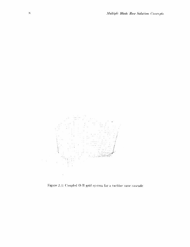
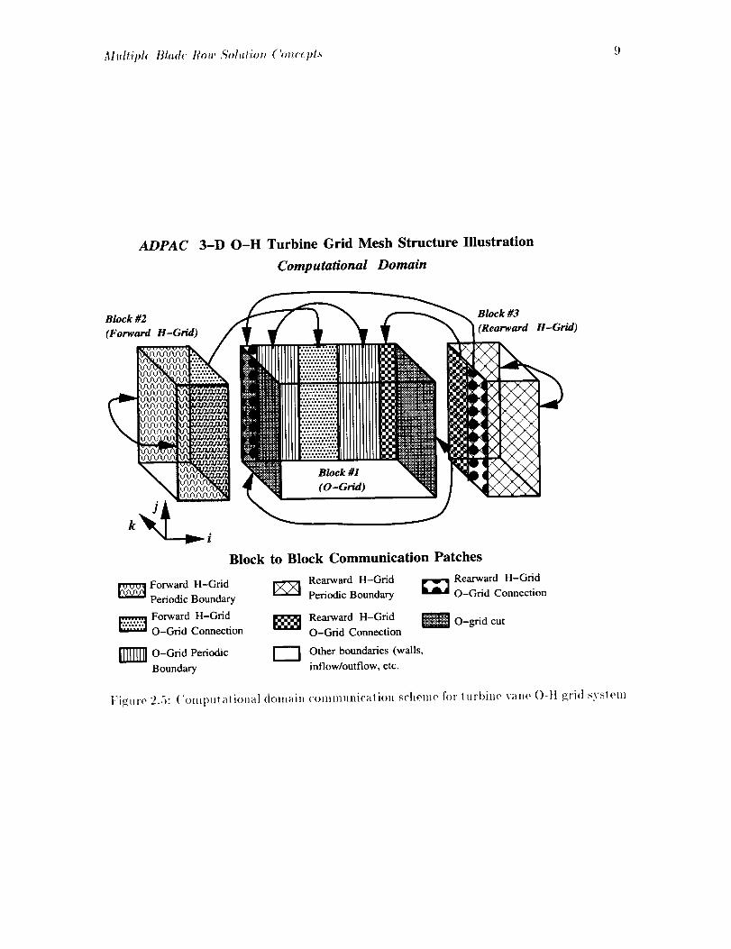
geometries, such as the turbine vane coupled O-It grid systeln shown in Figure 2.4 and the

corresponding COlnl)ntational domain communication scheme shown in Figure 2.5. it may

not be possible to generate a single structured grid to encompass the domain of interes!

without sacrificing grid quality, and therefore, a multiple-block grid system has significant

a,d van t ages.

The ADPA('07 code utilizes the multil)le-block grid concepl to Ill(' full exten| by per-

milling an arl)itrary numt)er of structured grid blocks with use," specifiable comlnunicalion

paths 1)etween blocks. The inter-block communication l)aths are implelnented as a series

of boundary condilions on each block which, in some cases, communicate flow infi)rma-

tion from one block to another. The advantages of the multiple-block solnlion concept are

exploited throughout the remainder of this doculnent as a means of treating complicated

geometries, multiple blade row turl)onlachines of varying blade number, endwall lrealmenls.

and to exploit computational enhan('emenls such as multigrid.

2.2 Multiple Blade Row Solution Concepts

Armed with an understanding of the multiple-I)lock mesh solution concept discussed in the

l)revious sect.ion, il is now possible to describe how this numerical solution technique cal, be

applied to pre(tic! complicated flows. Specifically. this section dea.ls with the predicliou of

flows through rotating machinery with multil)le I)lade rows. ][istorically. the 1)rediction of

t.hree-dimensional flows through mull istage turl)omachinery has been based on one of three

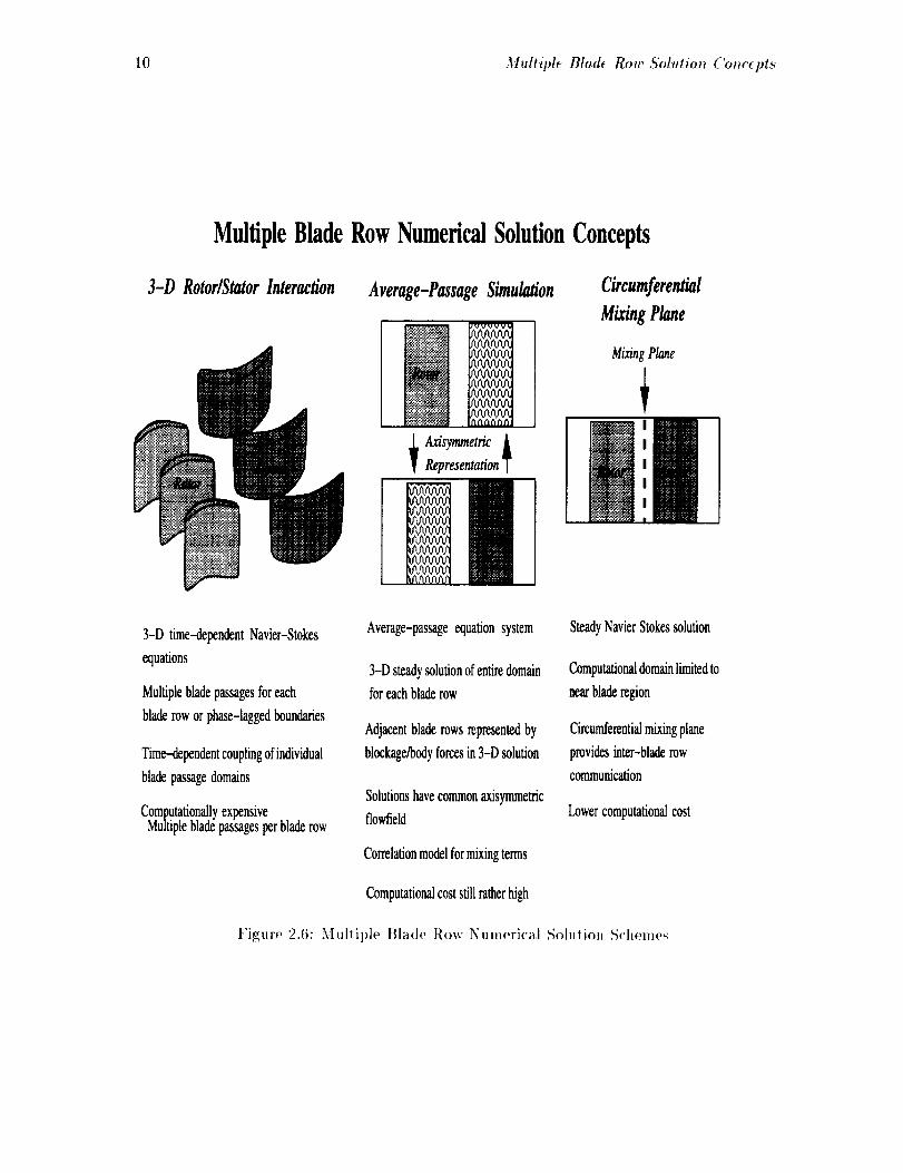
solution schenms. These schemes are t)riefly illustraled and described in Figure 2.6.

Mulliplt Bladt Row ,S'olulio_ ('ot_ccpts 5

ADPAC 2-D Nozzle Single Block Mesh Structure Illustration

Physical Domain

Computational Domain

l:'i_ure 2.1: A DPA ('07 2-D single block mesh struclure illuslration

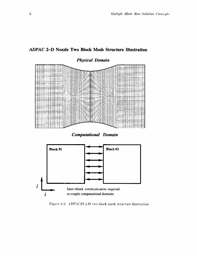
6 Multipl_ Blade Row ,5'olutioT_ ('o_wept._

ADPAC 2-D Nozzle Two Block Mesh Structure Illustration

Physical Domain

Computational Domain

Block #I

v

i

Block #2

Inter-block communication required

to couple computational domains

Figure 2.2:.4DPA('07 2-D two block mesh structure illustration

-llultipl_ Blade Row ,_'ol'.tim_ ('mwcpt._ 7

ADPAC 2-D Nozzle Multiple Block Mesh Structure Illustration

Physical Domain

Computational Domain

Inter-block communication required

to couple computational domains

Figure 2.3: A DPA ('07 2-1) ntult, il)le block mosh struclur¢, illust ralion

Multiple Blade Row 5'olutio_ ('oucept._

i:

j=

J

1

Figure 2.-1: (!ouple<l O-It grid system for a turbine vane cascade

Multipl( Blad_ Bow 5'olutio_ ( mwept. _ 9

ADPAC 3-D O-H Turbine Grid Mesh Structure Illustration

Computational Domain

Block #2

(Forward H-Grid)

v v

Block #1

(O-Grid)

_ (RBlock#3

earward H-Grid)

Block to Block Communication Patches

[_ Forward H-GridPeriodic Boundary

_ Forward H-GridO-Grid Connection

[]']T_ O-Grid Periodic

Boundary

Rearward H-Grid Rearward H-Grid

Periodic Boundary _ O-Grid Connection

_ l_e_a_dH-Grid _! O-_dcu_O-Grid Connection

F--'] Other boundaries (walls,

inflow/outflow, etc.

l:ig_lre 2..5: ('ol_q)_llaliof_al domain comm_znicatior_ scheme for l_zrbi_w vano O-tl grid sb's_etH

10 Multiple Blade Row ,5'ohttio_, ('o_e_'pts

MultipleBladeRowNumericalSolutionConcepts

3-D Rotor/StatorInteraction Average-Passage Simulation

I,J,I,PlSIJU

nftflftfl_

[Iflilll/IftJ

I/fl/lfi/l_

Nfttlftf/NJ

ftl'l/bq/l_

f/l'l/lfi/ll_

flf//I,q//fU

fO'l./I,q/U'U

nf/flllflI/J

n [i fill ii[ll

_ AxisymmetricARepresentation-

Circumferential

MixingPlane

MixingPlane

m'llI

I

I

II

3-D time-dependentNavier-Stokes

equations

Multiplebladepassagesforeach

bladeroworphase-laggedboundaries

Time-dependentcouplingofindividual

bladepassagedomains

ComputationallyexpensiveMultiplebladepassagesperbladerow

Average-passageequationsystem

3-D steadysolutionofentiredomain

for eachbladerow

Adjacentbladerows representedby

blockage/bodyforcesin3-D solution

Solutionshavecommonaxisymmetric

flowfield

Correlationmodelformixingterms

SteadyNavierStokessolution

Computationaldomainlimitedto

nearbladeregion

Circumferentialmixingplane

providesinter-bladerow

communication

Lowercomputationalcost

Computationalcoststillratherhigh

Figure 2.6: ._lullil)le f_lad(, Row Numerical Solulion S('h(mles

.llultipl( Blad( How S'olution (Tmc_pls 11

The first scheme involves predicting tile time-resolved unsteady aerodynanfics resulling

from the interactions occurriu?_; between relatively rotaling bla<le rows. Examples of this

type of calculation are ?_;iven by Rao and Delaney [7]. ,Jorgense, and ('hima [s], and Rai [12].

This approach re<luires either lhe simulation of multiple bla<le passages per t>lade row, or

the incorporatiol_ of a phase-lagged boundary con<li_io, to accoun_ for tile <lifforollces in

spatial perio<licity for blade rows with dissimilar blade counls. ('alculatio,s of lifts tyl>e are

typically <'ompulaliona[ly expensive, and are presenlly impraclical for machines wilh morethan 2-3 blade rows.

The second solution technique is based on the average-passage e<luatio, syslem devel-

oiled by A<lamczvk /9]. In this apl_roa<'h, separate 3-D soluli<m <lomai,s at'<, define<t for

each t>lade row which en¢'Oml>asses Ill(' overall domain for lhe enlire tux'l>omachille. The

it,dividual solution domains are specifi<' lo a parti<'ular blade row. allhough all I>lade row

domains share a comnloll axisymmetric flow. In lhe solulio, for 1he flow lhrough a spe-

cific l>lade passage, a<ljacenl blade rows are represente<l by lheir lime and space-avera?_;ed

blocka_e, l)o<lv for<,'<', a,d etiergy sour<'<, <'ontrib,ti<ms lo the overall flow. A c<>rrelatioti

model is used t<> represetg the lime and space-avera_;e<l tlow [luclualions rel>resenlin _ the

intera<'lions t>elweeu blade rows. The advantage of lhe average-passage approach is lha!

the lemporally aim spalially averaged e(luations system reduce the solulion io a steady flow

et,vironmenl, and. wilhin lhe a<'curacv of the correlation model, the soluliotl is represe,-

tative of the avera_;e aerodyt_at,ic condition experienced l_y a giv+, blade row under the

influence of all other bla<le rows in the machine. The disadvantage of lhe avera?ge-passage

approach is lhal the sohllion complexily and cosl ?_;row rapidly as the ,umber of blade rows

increases, and the accuracy of the correlalion model is as yel unverified.

The lhird approach for lhe prediction of flow lhrough multistage t tH'l>ol,achinerv is

based on the mixing l>[aue cotwept. A mixing plane is an arbitrarily imposed boundary

inserte<l belween a<ljacel_t blade rows across which the flow is "'mixed out" circumferen-

l ially. This <'ircumferenlial mixing al>proximales the l ime-average<l condilion al the mixing

piano and allows the aero<lvnamic solution for each bla<le passage to be performed in a

sleadv flow environmelll. The mixing plane <'oncel)l was applied lo realislic lul'bofan en-

?_;iue configuratio,s t>v I)awes [10]. Flow varial>les o, either side of the mixing plane are

circumferenlially averaged and passed io the neighl>oriug bla<le row as a means of smearing

ou! the circumferenlial nonuniformities resulting from dissimilar bla<le counts. The mixing

plane concept is a llluch 111or0 cost-effeclive approach computalionally because tile flow is

stea<ly, and lhe i,dividua] blade passage domains are limited Co a ,ear-blade region. Un-

fortunately, the accuracy of this approach is clearly <lueslionable under some circumstances

be<'ause of the lflacement of 1he mixing plane and the loss of spatial information resultin_

front t he circumferential averaging operator.

The A I)])A ('07 program possesses features which permil mull iple I)]ade row solulions us-

iH_ eilher the lime-del_e,den! inleraction approach or the mixing l>]ane <'<)ncep_, <lescribe<t

alcove. :\vera?_;o-passage siululalions for realislic turbofan engine configurations were re-

porled under Task IX,' of lifts <'ontract. and further details on this approach can I>e found in

t{efereu<'e [11]. A I)t"A('07 ]>redictions ulilizin_ the time-accurate rotor/stator inleraction

lechni(l,e requires lhal a sM[icie_l number of blade passages be represelJ_ed in each row

such lha_ the circumferenlia] distance represented in each blade row is <'onslanl. This limils

lhe blade cou,ts _vhich ca, be eff_<q, ively simulated thr<)u_h lids technique. For example,

['or the simple siu?_;le-sla_e calculation sug?_;esle<l in Figure 2.6. if tile rotor has 36 blades an<l

the stalor has ,IS blades, a lime depen<lenl solution xvouhl require, as a minimum. 3 rolor

blade passages an<] -I stalor blade t>assa_es to accom,_o<la_e _he ('ommot_ cir(',n_Fere,tial

12 Multipl_: Blod_ Row Solution Concepts

pitch requirement. If tile rotor has 35 blades, and the stator has 47 blades, however, then

I)oth blade rows would require that. ever), blade passage be modeled as no simpler reduc-

tion in blade count is possible. This restriction will appear quite often, as turbomachinery

designers often do not like to design neighboring blade rows with blade counts which have a

common integer factor. Ultimately, this type of problem will require the incorporation of a.

phase-lagged boundary condition which would permit time-dependenl interaction solutions

for neighboring blades using only one blade passage per blade row.

If, instead, a mixing plane type of calculation is (lesired. lhen lhe multiple block scheme

may again be invoked by utilizing a single blade passage per blade row, where each grid

block has a colnmon mating surface with a neighboring blade row. The on]v special re-

quirement here is that boundary condition routines be available to adequately perform the

circumferential averaging between blade rows and supply the block-to-block communication

of this information in the multiple-block mesh solution algorithm. Section 3.7 describes the

techniques for applying this type of boundary condition.

2.3 Endwall Treatment Solution Concepts

In this section, numerical techniques used to l)redict turl)omachinery flowfields with en(lwall

treatments are descrit)ed. The general approach is to exploit the multil)le block mesh cat)a-

bilities of the A DPA ('07 flow solver to couple eudwall treatment and blade passage flowfields.

Separate comt)utational domains (mesh blocks) may be utilized for t)oth the blade l)assage

and at least one (or more) endwal] treatment passages (grooves. slots, recessed vanes, etc.).

Three sl)ecialized boundary conditions were developed to couple the indel)edent flow do-

mains. These boundary conditions result fi'om various degrees of modeling assuml)tions

used to simplify the blade passage/treatnlent passage aerodynamic interaction. Each of the

three boundary conditions and the assumptions inheren! to each al)proach are described in

detail below.

For the prediction of coml)ressor endwall treatment flows, separate numerical mesh sys-

tems are utilized for both the compressor airfoil blade l)assages and the endwal] treatment

passages. The three different boundary condition procedures available to couple the end-

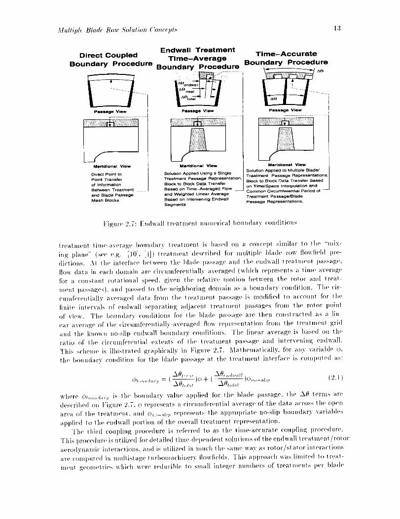
wall treatment/blade passage fiowfiehls are illustrated graphically in Figure 2.7. The first

technique, referred to as the direct-coupled apl)roach, is utilized for those cases where there

is a direct correspondence between mesh t)oints in the I t'eatment meshes and the blade

passage meshes at the endwall interface. This construction t)ermits a direct, point to l)oint

transfer of information fi'om one mesh block to another. This approach is limited to geome-

tries for which contiguous mesh systems can be generated, which, in general, is limited to

circumferential groove casing treatments.

The second al)t)roach, referred to as the endwall treatment time-average apt)roach,

is applie(I to endwall treatments which are non-axisymmetric in nature. This type of

treatment iucludes discrete axial or l)lade angle slots, recessed vane sets, and circumfer-

ential grooves. The 1)rimary objective of this al)proach was to develop a numerical cou-

I)ling scheme for discrete treatments which would represent the time-averaged influence

of the treatment l)assage/1)lade i)assage aerodynamic interaction. This approach is re-

stricted to stead), state flows due to the time-averaged assumption inherent in the pro-

cedure, but siml)lifies the analysis in that only a single blade passage and a single dis-

crete endwall treatlnent passage requires modeling in the overall solution. The endwall

M_tltiph Bla& Row Eohttion ('oT_cepts 13

Direct Coupled

Boundary Procedure

Passage View i

Meridlonal View

Direct Point to

Point Transfer

of Information

Between Treatment

and Blade Passage

Mesh Blocks

Endwall Treatment

Time-Average

Boundary Procedure

...............

/

Passage View

Merldionel View

Solution Applied Using a Single

Treatment Passage Representation.

Block to Block Data Transfer

Based on Time-Averaged Flew --

and Weighted Linear Average

Based on Intervening Endwall

Segments

Time-Accurate

Boundary Procedure

Passage View

r .........................................................

Meridional View

Solution Applied to Multiple Blade/

Treatment Passage Representations.

Block to Block Data Transfer Based

on Time/Space interpolation end

Common Circumferential Period of ---

Treatment Passage/Blade

Passage Representations.

t.'iguro 2.7: l']n<lwa[l treatment nulnerical I)oulMary conditions

treatment lime-average boundary treatment is based on a concept similar to the "'mi×-

ing plane" (see e.g. [10], [-1]) treatment described for multiple bla<le row flowfield pre-

dictions. At the interface between the blade passage and the en<lwall treatment t>assag.;e,

flow data in each domain are circumfereldially averaged (which represents a lime aw, rage

for a COllSlalll rotational speed, given the relative ]notion t)elween the rotor and treat-

n/ont passages), and passed 1o the neighboring domain as a 1)oundarv condition. The ('ir-

cumferent.ially averaged data from the trea|ment passage is nlodified to account for the

finite intervals of endwall separating adjacent treatment passages from the rolor point

of view. The boundary conditions for the blade passage are then constructed a.s a lin-

ear average of the circulnferentially-averagod flow i'el)resentatio]l from the treatmenl grid

and the known no-slip endwall boundary conditions. The linear average is based on the

ratio of the circumferelltial extents of the treatment passage and intervening endwall.

This scheme is illustrated graphically in Figure 2.7. MatlleInatica.lly, for any variable O,

the boundary condition for the blade passage at the t.reatnlenl interface is compul.ed an:

AOt,.,,,t AE,, t,,,,ll

O!,,,,,,,+,,,,j = (_)o + ( A0t_,t,,l )0 ....... li_, (2.1)

where Of,o,,,t,,,.v in the boundary value applied for the blade passage, the X0 tel'IllS are

(lencribed on Figure 2.7. O rel)resents a circunlferential average of the data across the open

area of the treatment, and O,,,-._h], ]'epresents tile a l)prol)riate no-slip boundary variables

applied to the endwall portion of the overall treatment representation.

The third coupling procedure is referred to as the time-accurate coup[ing procedure.

This pro('edtlre is utilized for detailed t itne-(lel)endettt solutions of the endwall treatlnent/rotor

aerodvnamic interactions, and in utilized in much the same way as rotor/slalor inte]'actiollS

are conlpul,pd in multistage turl)omachinery flowfields. This approach was limiled to ireal-

menl geometries which were reducil>h, to small integer numhers of tl'eatmenls t)er blade

14 Multigrid Conv_ rg_ nce Acceleration Uo_cept_

passage. Tills was clone in order to minimize tile circumferential extent of tile rotor or

treatment passages which must be modeled in order to employ a spatially periodic relation-

ship for the overall blade passage/treatment representation.

2.4 2-D/3-D Solution Zooming Concepts

A fourth unique feature of the ADPAC07 solution system involves the concel)! of COul)lin?;

two-dimensional and three-dimensiollal solution domains to ol)tain representative simula-

tions of realistic high bypass duct ed fan engine concepts. A coml)licating factor in the

analysis of flows through turbofan engine systems results fl'om the interactions t)etween

adjacent blade rows. and, in the case of a ducted fan, the effects of downstream blade rows

on the aerodynamics of the upstream fan rotor. Historically. in tile design of lnultistage

turbomachinery, an axisymmetric representation of the flow through a given blade row has

been used to effectively reduce the complexity of the overall prol)lems to a manageal)le level.

Similarly, an efficient approach to the numerical simulation of downstream blade rows could

naturally utilize an axisymmetric representation of the effects of these rows through a lwo-

dimensional grid system, with I)lade blockage, I)ody force, au(l energy terms representing

the a xisymnletric average(I aerodynamic influence imparted t)y the embed(le(I blade row.

This concept is illustrated graphically in Figure 2._ for a ret)resentative turbine stag(,.

A numerical sohltiofl of the flow through tile fan rotor is complicated bv the presence of

the core stator, I)ypass stator, and bypass splitter. It is undesirable to restrict tile solution

(lomain to the fan rotor alone as this al)proach neglects the l)otential interactions between

the fan rotor and the downstream geolnetry. The ADPA('07 program permits COUl)led

solutions of 3-D and 2-D mesh blocks with embedded blade row blockage, bod.v force,

and energy terms as a means of efficiently treating these more complicated configurations.

Blade force terms may l)e determilmd fl'om a separate 3-D solution, or may t)e directly

specified based on siml)ler design system analyses. Neighboring 2-I) and 3-D mesh blocks

are numerically coupled through a circumferential averaging procedure which attempts to

globally satisfy the conservation of mass, nlon|eltlunl and energy across the solution domain

interface. The "'dimensional zooming" capability permitte(I t)y the 2-D/3-D mesh coupling

scheme is considered a vital asset for the a ccurat(, prediction of the flow through inodern

high-speed turl)ofal_ engine systems.

2.5 Multigrid Convergence Acceleration Concepts

For completeness, a brief section is included here to discuss t [,e multigrid convergence accel-

eration solution technique incorporated into tile A DPA('07 code. Multigrid (please do no!

confuse this with a multiple-block grid!) is a numerical solution technique which attempts

to accelerate the convergence of an iterative process (such as a steady flow prediction using

a time-marching scheme) by computing corrections lo the solution on coarser meshes and

propagating these changes to the fine mesh through interpolation. This operation may be

recursively applied to several coarsenings of the original mesh to effectively enhance the

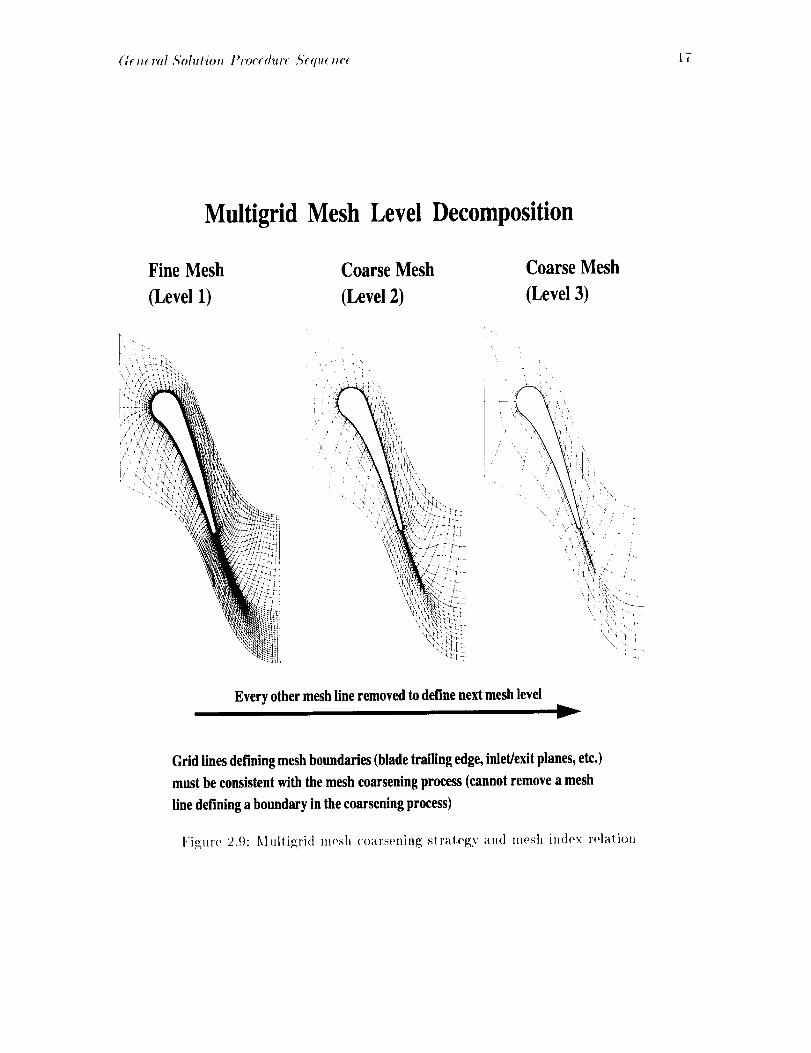
overall convergence. (!oarse meshes are derived from the preceding finer mesh bv eliminat-

ing every other mesh line in each coordinate direction as shown in l:igure 2.9. As a result.

the number of multigrid levels (coarse mesh divisions) is controlled by the mesh size, and, in

Alultigrid ('ol_,ergcl_c_ Arc_leratiol_ ('ol_'_pt._ 15

2-D AxisymmetricBladeRowRepresentation

3-D Geometry 2-D AxisymmetricRepresentation

3-D Computational

Domain

2-D AxisymmetricRepresentation

ofStatorBladeRow- Includesthe

EffectsofBlockage,BodyForcesand

EnergySources

Figure 2.,_: 2-1) axisymmetric flow rel)resenlation of a turl)on_achinery I)la¢l(, row

16 Gen e ral Solu t io_ Procedu'rv Seque rice

the case of tile ADPA('07 code, by the mesh indices of tile boundary patches used to define

tile boundary conditions on a given mesh block (see Figure 2.9). These restrictions suggest

that mesh blocks should be constructed such that the internal boundaries and overall size

coincide with numbers which are compatible with the multigrid solution procedure (i.e., the

mesh size should be 1 greater than any numl)er which can be divided bv 2 several times

and remain whole numbers: e.g. 9, 17, 33, 65 etc.) Further details on the application of the

_t Dt_4('07 multigrid scheme are given in Section 3.6 and in Reference [d].

A second multigrid concept which should be discussed is the so-called "'full" multigrid

starlup i)rocedure. The "ffull" multigrid method is used to sla.rt up a soluliot, by initialing

the calculation on a coarse lnesh, l)erfornfing several time-marching iterations on tha! mesh

(which, by the way could be multigrid iterations it" successively coarser meshes are available).

and then interpolating the solution at that point to the next finer mesh, and repeating

the entire process until the finest mesh level is reached. The intent here is to generale

a reasonably approximate solution on the coarser meshes before undergoing the expense

of the fine mesh multigrid cycles using a "'grid sequencing" leclmique. Again. the "'full'"

multigrid technique only applies to starting up a solution, and therefore, it is not normally

advisable to utilize this scheme when the solution is restarted from a previous solution as the

information provided by the restart data will likely, be lost in the coarse mesh initialization.

2.6 General Solution Procedure Sequence

The ADPA('07 code is distributed as a COml)ressed tar file which must lye processed before

the code ma,v be utilized. The instructions in Appendix A describe how to obtain the

distributiol_ file, and extract the necessary data to run the code. This ol)eration is typically

required only once when the initial distribution is received. Once the source files have been

extracted, the sequence of tasks listed I)elow are typical of the events required to perform

a successful analysis using the ADPA('07 code.

Step 1.) Define the problem:

This step normally involves selecting the geometry and flow conditions, anti defining

which specific results are desired fi'om the analysis.The definition of the t)roblem lnusl

involve sl)ecifying whether steady state or time-det)endent data are re(luired, whether an

invisci<l calculation is sufficient, or whether a viscous flow solution is required, and some

idea of the relative merits of solution accuracy versus solution cost (CPU time) ltlust [)e('onsidered.

Step 2.) Define the geometry and flow domain:

Typically', geolnetric features such as airfoils, ducts, and flowl)ath endwalls are required

to geolnetrically define a given l)roblem. The solution domain may lye chosen to include

the external flow. internal engine passage flows, and/or leakage flows, The flow domain is

normally defined large enough such that the region of interest is fat" enough away from tit<,

external boundaries of the l)roblem to ensure lhat the solution is not unduly influenced by

the external l)Oulldary conditions.

Step 3.) Define a block structure:

Once the geometry and solution (lon,ain has been numerically defined, the iml)lemen-

ration of lhe solution mesh structure must be considered. This process begins with a

(;e l_,eral A'ohltiol_ Procedure A'equc_we 17

Multigrid Mesh Level Decomposition

Fine Mesh

(Level 1)

Coarse Mesh

(Level 2)

Coarse Mesh

(Level 3)

1

I

Every other mesh line removed to define next mesh level

V

Grid lines defining mesh boundaries (blade trailing edge, inlet/exit planes, etc.)

must be consistent with the mesh coarsening process (cannot remove a mesh

line defining a boundary in the coarsening process)

Figure 2.9: .klultigrid mesh coarsening siralegy and mosh illdex relalion

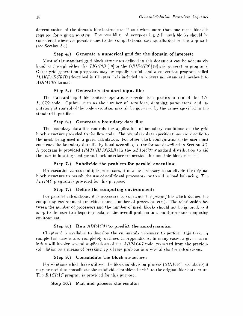
18 Ge1,eral Eolution Procedur_ ,%quenc_

determination of the domain block structure, if and when more than one mesh block is

required for a given solution. Tile possibility of incorporating 2-D mesh blocks should t)e

considered whenever possible due to the computational savings afforded by this al)proach

(see Section 2.3).

Step 4.) Generate a numerical grid for the domain of interest:

Most of the standard grid block structures defined in this doculnent calf be adequately

ha,ndled through either the TIGG3D [lS] or lhe GRIDGEN [19] grid generation programs.

Other grid generation progralns may be equally useful, and a conversion program called

MAKEADGRID (described in (!hal)ter 7)is include(l to converl non-slan<tard meshes into

A DPA ('07 format.

Step 5.) Generate a standard input file:

The standard inl)Ul file controls oI)eralions specific to a particular run of the AD-

15t('07 code. ()l)tions such a,s tile number of iterations, damping parameters, aim in-

put/outpu! control of the code execution may all be governed by the values specified in the

st,alldar<l input tile.

Step 6.) Generate a boundary data file:

The boundary data file controls the application of boundary condilions on the grid

block structure provided to the flow code. The boundary data specifications are specific to

the mesh being used in a given calculation. For other block configurations, the user must

construct life boundary data file by hand according to the forlnat described in Section 3.7.

A program is provided (P,,tTCtlFINDER)in the ADPA('07 standard distribution to aid

tile user in locating contiguous |)lock interface connections for multiple block meshes.

Step 7.) Subdivide the problem for parallel execution:

For execution across multiple processors, it, lnay t>e necessary to subdivide the original

block structure to permit the use of a<lditional processors, or to aid in load balancing. The

£'IXPA(' program is provided for this purpose.

Step 7.) Define the computing environment:

For parallel calculations, il is necessary to construct the pr</'&ffile which <lefines l]le

computing environment (machine name, number of processes, elc.). The relationship be-

tween the number of processors and the number of mesh blocks should not be ignored, as il

is up to the user to adequately balance the overall problem in a multiprocessor computingenvironment.

Step 8.) Run ADPA('07 to predict the aerodynamics:

('hapter 3 is available to describe the commands necessary to perform this task. A

saml)le test case is also completely outlined in Appendix A. In many cases, a given calcu-

lation will involve several apl)lications of the ADPA('07 co<le, restarted from the previous

calculation as a nleans of breaking up a large problem into several shorler calculations.

Step 9.) Consolidate the block structure:

For solutions which have utilized the block subdivision process (5'IXI-'A(', see above) it

may be useful to consolidate the subdivided problem back into the original block structure.

The B+I('PA(' program is provided for this purI>ose.

Step 10.) Plot and process the results:

G< r_eral ,_'ohttio_ Pr<,c: dur( .<i:qu_.l_ce' 19

All interactive post processing program called AD,S'PINis t)rovi<led to handle tasks such

as mass-averaging tlow variables to simt)lit_" tile interpretation of the computed l"osulls (see

(lhapter .1). Output data is also provide¢l for widely available plotting progralnS such a.s

m, o7': I) [l.q and

A condensed (lescril)tion of the commands involved in the slel>s described al)ove begin-

nine; wilh extracting lit(' source co(le frolll tit(' (lislril)ulion. compiling the codes, selling u t)

a case, and running a ('as(,. is given ill lhe A1)l)en(lix. Sei)arale sections are 1)rovi(le(l in the

('hal)ters which follow lo (les<'ril)e in (letail the basis and Ol)eralioll of lhe codes used in t he

slel)s above.

I1 is worthwhil(' menlioning that lh(, <tevelol)nlent and at)l)licalion of lhe ('()(los (lescribed

ill this manual were t>(,rl'orme<l on Unix-based COml)uters. All files are stored ill machine-

indellen(lent formal. Small files utilize slan(lard A%(!II f()rmat, while larger files, which

t)ell0fil frOlll settle type of binary slorage forlnat, are l>ase(1 on lhe Scienlific l)alatlase Li-

Ilrarv ( SI)BI_IB ) formal [13]. The SI)B IAB formal ulilizes machine-del)endenl inl)ul/oull>ut

roulinos which permit machine independence of tllel>inarv data file. The,ql)BLltl roulines

were (10velol)e(l a! the NASA Lewis Ilesearch (lenter.

Most of the plolling and gral)hical ]>ostI)rocessing of tile solutions was performed on

graphics workslations. Tile I)LOT.']I)[14]. and f:.t,_'T [16] graphics s(>flware t)acka_;es de-

velot)e<l al NASA Ames R(,sear<'h (lenter were exlensively used for Ibis purpose, and <lala

files for these plotting l)ackapges are ?_;chert.let1 autonlatically. These dala files at'(' writl('n in

what is known as PLO'F3D mullil)le-grid formal. (See .I DPA('07 File l)escril)lion. Seclion

:1.5).

2.7 Consolidated Serial/Parallel Code Capability

One of the practical <titficulties of performing CFI) analyses is finding suffi('ien! COml)uta-

tional resources lo allow for a(le(luate mo(leling of ('onq)lex geolnelries. Oftentimes, work-

stalions are nol lar_;e enough, alld supercomt)uters have eilher long queues, high costs, or

bolh. ('learly, a means of circmnvent ing lhese difficulties withoul giving ut> the flexibilily of

tile ('FI) code or the COml)lexily of th(' model would l)e welcome. One l)ossibilily is to wrile

a code which could run in parallel across a nulllber of processors, with each one having only

a piece of lhe [)roblem. Then. a numt>er of lesser machines could I)e harnesse(t together to

make a virl ual sul)('rconll)uler.

The mosl likely can(li(lat('s lot" crealing such a machine are the workstalions which

are fully loade(l (luring the (lay. l>u! sit idle at nighl. Tremendous l)ower could I)e ma(le

availal)le at no exlra cost. There are also massively parallel coml)utel's availal)le on 1he

markel designed sl)ecitically f<)r such applications. These machines are aiming al order of

ma_;nitude iml)rovenlenls over presen! Slq)ercoml)ulers.

The t)rotllent, of course, lies in lit(, software. 1)arallelization is today al)oul a.s i)ainful as

vectorization was a (leca<le aN(). There is no slan(lar(I t>arall('l syntax, ait(I no conil)iler exists

which <'all aulontali('ally and elf'eclively parallelize a code. It is difficult lo wrile a parallel

co<le whi<'h is ])latform independent. What makes things worse is thal there is no clear

lea<ler in lh(, parallel COml)U_('r industry, as there has I)een in tile sut>ercomlluter in(luslry.

The ot)je('live I)('hind the <l('velol)nlenl of the ('onsoli<lated .l I)1".t( '07 co(h' (l(,scril)ed in

this manual was to create a l)lall'ornL in(lel)en(lent l)arallel <'o(h'. The inl(,nl was Io design a

l)arallel code which looks and feels like a traditional code, cal)al)le of running on nelworks of

20 (/eT_eral ,qolutio'l_ Procedure ,%qucnee

workstations, on massively parallel COml)uters, or on tile traditional supercomputer. User

effort was to be minimized by creating simple procedures to migrate a serial problem into

the parallel environment and back again.

2.8 Parallelization Strategy

The ADPA('07 code has some innate advantages for 1)arallelization: il is an exl)lMt, multi-

block solver with a very flexible implementation of the boundary con<litions. This presents

two viable options for parallelizalion: i)arallelize lhe internal solver (the "'fine-grained'"

approach), or parallelize only the boundary conditions (the "'coarse-graine(l'" apl)roach).

The fine-grained al)l)roach has the advantage thai block size is 11o1lira!led by processor size.

This is the apl)roach frequently taken when writing code lot massively parallel computers.

which are typically made 111) of many small processors. The coarse-grained approach is

favored when writing code for clusters of workstations, or other machines with a few large

processors. The dilemma is that a parallel ADPA('07 needs to run well on I)oth kinds ofmachines.

The fine grained al)proach is est)ecially enticing for explicit solvers. Exl)licit codes have

proven to be the easiesl 1o parallelize because there is little data dependency between points.

For a single block explicit solver, flue-grained l)arallelization is the clear choice, l|owever,

with a multiblock solver, the boundary conditions musl ])e parallelized in addition to the

interior point solver, and that can add a lot of programming eflbrt. The coarse-grained

approach is admittedly easier for multi-block solvers, but what if 1he blocks are too big for

the processors? The simplest answer is to require the user to block o111 111('l)robtem so lhal

it fits on the chosen machine. This satisfies the l>rogrammer, but the user is faced wilh a

tedious chore. If the user decides 1o run on a different machine, then the job may have to

be redone. The pain saved by the wogrammer is passed directly to the user.

A comt_romise posilion was reached for parallel A DPA('07 code. The coarse-graine<t

approach is used, t>ut supplemental tools are provide<l l<) automatically generate new grid

blocks and boundary conditions for a user-specified topography. In this way. the parallel

portions of the code are isolated to a, few routines within ADPA('07. and the user is not

undnly burdened with architecture considerations. Details of running A DPA('O7in parallel

are given in a later chapter.

Chapter 3

ADPAC07 : 3-D

EULER/NAVIER-STOKESFLOW SOLVER OPERATING

INSTRUCTIONS

3.1 Introduction to ADPAC07

This chal)ler conlains lhe operaling instruclions fox" the ADPA('071inm-dependonl nlulli-

pie grid block 3-D Euler/Navier-Stokes aero(lynanfic analysis. These instructions inch,de

some general information (overing executing the code, defining array limits. ('Oml)iling lhe

(low solver, S('llillg 11I) inl)ul files, running lhe code, and examining oult)lll (lala. The

,,tDl{t('OTflow solver source programs are written in FORTRAN 77, and have been used

successfully on ('ray VNI('()S and IBM \;M/(:MS lnainfranw conll)uter svslenls as well as

IBM AIX OperatiIig System and Silicon Grat)hics workstations using a [;NIX operaling

syslelll.

3.2 General Information Concerning the Operation of the

ADPA C07 Code

A l)l)roximate COml)ulalional storage and ('PU requirenlenls for tile ,,1DPA('07 code Call t)e

conservalivelv estimaled from lhe h)llowing fornlulas:

('I)U se(" _-l.(}xl0-_(# grid t)oints)(# ileralions)

,_lenlory MW _ 6.0xl(}-s(# grid poinls)=real numl)er sloragelocations

These formulas are valid for a ('ray-(:90 COlnl)uler operating under lhe VNI(I()S environ-

men! and Ill(, cf77 compiler, version 6.0A.5. The limes rel)orted are for a single processor

oMv. and are nol indicalive of any para.llelizalion availabh, lhrough Ill(, (!ray autolaskilJg

or microlasking facililies. The formulas are based on lhe standard, exl)licit solution a lgo-

rilhnl using file alg(,I))'ai(' tu)'l)ule)we mode[. Irse of lhe iml)licil flow solver or higher oMer

lurbulen('e model could effeclivelv increase I)olh numbers bv a lacier of 1.4 or more. l;s(, of

t)arallel processing ('all subslanlially reduce )hese eslimales on a 1)er ('I)U basis. \Vilhoul

mulligri(l, sleadv inviscid ttow calculaliol)s normally require apl)roximalely 2000 ileraliol)s

21

22 CoT_figurin9 A D PA ('07 Maximum A tray Dimension,s

to reduce the maxinmnl residual by three or<lers of magnitude (10:5) which is normally all

acceptable level of convergence for most calculations. Viscous flow calculations generally

require 3000 or more iterations to converge. When multigrid is used. the number of itera-

lions required to obtain a converged solution is often one third to one fourth the number

of iterations re(luired for a non-multigrid cMculation. (lonvergence for a viscous flow case

is generally less well behaved than a corresponding inviscid flow calculation, and in many

cases, it is not possible to reduce the maximum resi(lual by three orders of magnitude due

to oscillations resulting fi'om vortex shedding, shear layers, e!c. A determination of conver-

gence fox" a viscous flow case mus! often be base<l on observing 111o mass flow rate, pressure

ratio, or other global 1)arameter. and terminating the calculation when these varia|)les 11o

longer change. The numl)er of iterations required for an unsteady flow calculation is highly

case-del)endent, and may be based on mesh spacing, overall lime-period, complexity of theflow, etc.

The A DPA ('07 program produces out l)ut files suitable for plotting using the PLOTdD[14].

,S7:RF [15], al|d FAST [16] graphics software packages developed at the NASA Ames Re-

search (:enter. PLOFdD formal data files are written for both absolute and relative fows

(see (!hapter 2 for a description of the PLOTdD tbrmat). The user may also elect to have

additional PLOT,']D absohlte flow data files output at constant iteration intervals during

the course of tile solution. These files may be used as inslanlaneous flow "snapshots" of an

unsteady flow prediction.

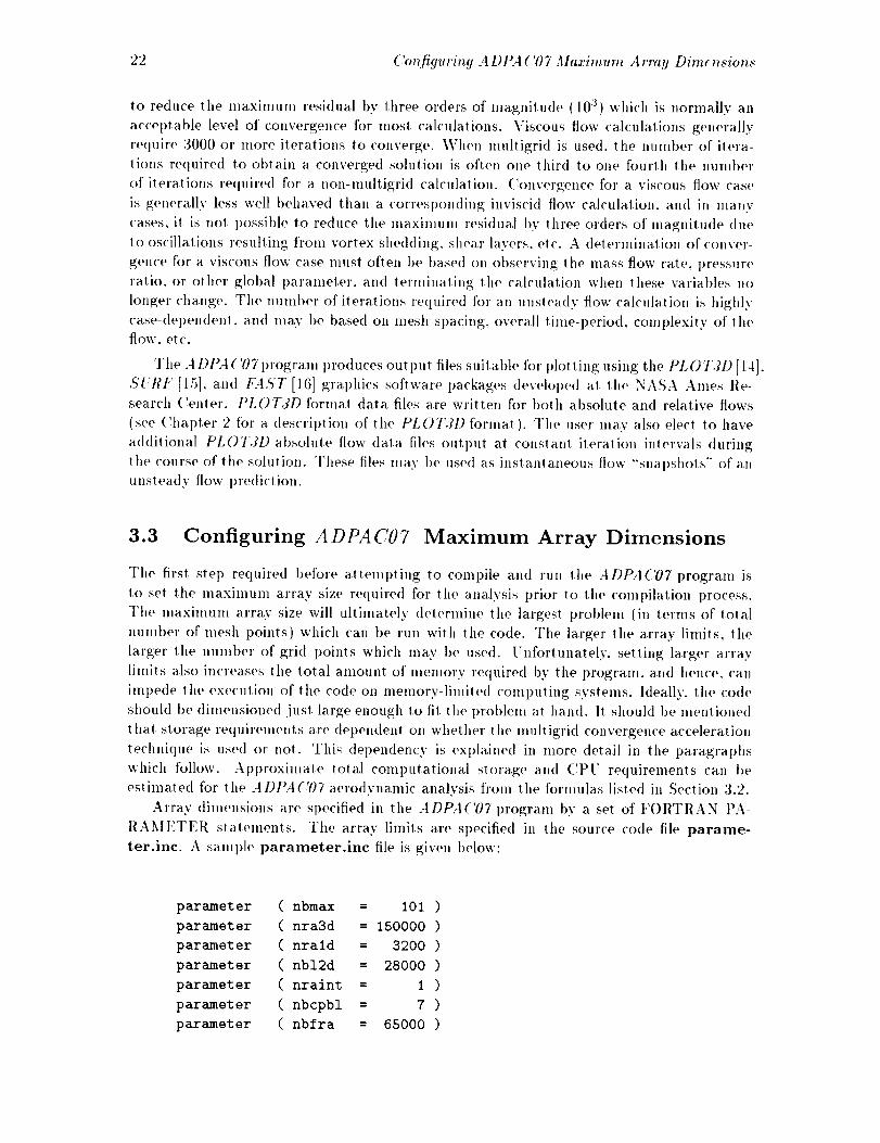
3.3 Configuring ADPAC07 Maximum Array Dimensions

The first, step required before attempting to compile and run the ADPA('07 program is

to set the maximunl a.rrav size required for the analysis prior to the compilation process.

The maximunl array size will ultimately determine the largest l)rol)lem (in terms of total

number of mesh points) which can be run with the code. The larger the array limits, the

larger the number of grid points which may be used. Unfortunately, setting larger array

limits also increases the total amount of meInory required bv the program, and hence, can

impede the execution of the code on menmry-limited computing systems. Ideally. the code

should be dimensioned just large enough to fit the problem at hand. It should be mentioned

t hat storage requirements are dependent on whether the nmltigrid convergence acceleration

technique is used or not. This del)endency is explained in more detail in the paragrat)hs

which follow. Approximate total computational storage and CPU requirements can be

estimated fox' the ADPA('07 aerodynamic analysis from tile formulas listed in Section 3.2.

Array dimensions are specified in the ADPA('07 1)rogram by a set of FORTRAN PA-

RAMI_;TER statenmnts. The array limits are specified in the source code file parame-

ter.inc. A samph, parameter.ine file is given below:

parameter ( nbmax = I01 )

parameter ( nra3d = 150000 )

parameter ( nrald = 3200 )

parameter ( nbl2d = 28000 )

parameter ( nraint = I )

parameter ( nbcpbl = 7 )

parameter ( nbfra = 65000 )

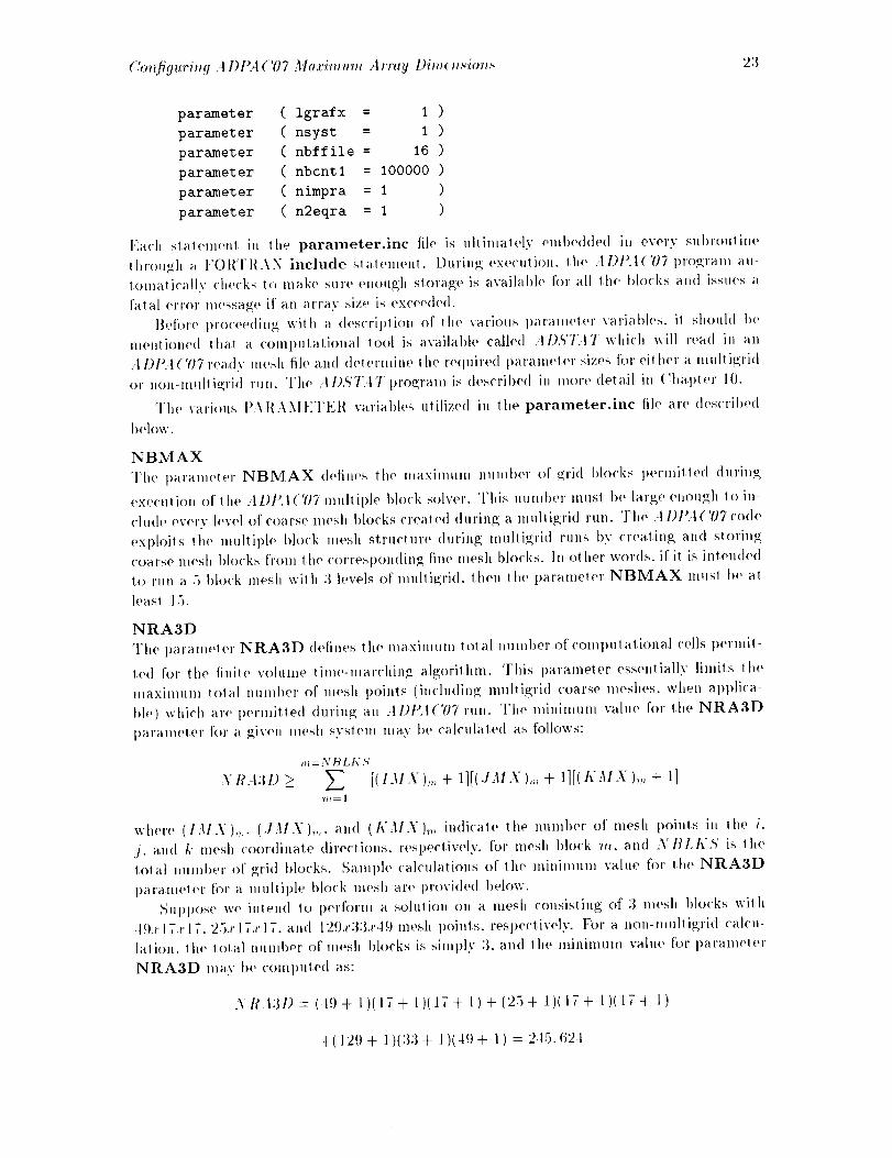
( 'm(fig,lri_g A DPA (7)7 Maximum A rray Di_ n._ion._ 23

parameter ( Igrafx = i )

parameter ( nsyst = i )

parameter ( nbffile = 16 )

parameter ( nbcntl = I00000 )

parameter ( nimpra = I )

parameter ( n2eqra = 1 )

Each slalem(,nl in l],e parameter.inc file ix ullimalely (,ml)e(hle(1 il) every subroutilw

lhrou_h a F()I(TI(AN include s1_dem(,nt. During ex(,('ulioH, the ADI_A(7)7 I)ro_ram _u-

tomatically ('he('ks to make sl_re eno_tgb storage ix available for all the blocks at_d isslle,_ a

thlal error message if an array size is exceede([.

t{ef'ore I)ro('eedin_ with a ([es('rit)lio|_ of the various parameter variables, ii should be

mentio|w(l thud a ('onq)utatiotlal tool is available called A/)S'T.tT which will read ill an

.t DI'.I ('07 re;l(lv mesh file and determine 1he re(luffed p',u'am(qer sizes for either a mulli_ri<l

or non-mull i_ri(t run. The .4 D,";TA 7' [)re,ram is descril)e(1 ill more detail in (!hal)t er 10.

The vari(ms i):\t{AMI_TFEt( varial)l(,s utilized in the parameter.inc file are described

below.

NBMAX

The parameter NBMAX (letines the maximum number of _;rid t)lo('ks l)ermilled (turin,_

ex(,('_lt}on of the A DPA (7)7 mu]t iple block solv(,r. This lmmber must b(' large (mo,lgh _o in-

ch,le every l('vel of coarse mesh blocks create(t (luring a mult i_;rid run. The A I)PA('07 code

exploits lhe multiple block mesh structure during multigrid runs by creating and sloring

coarse mesh 1)lo('ks from the correspon(lin_ fine mesh blocks. In ot her words, if it is intended

io run a 5 block mesh vilh 3 levels of mullig;ri(I, then the parameter NBMAX musl t)e a_

least 15.

NRA3D

The 1)arameler NRA3D defitws the maximum total number of computational ('ells permit-

led for the finite '¢oh|lne time-mar('hin_ a l_orilhm. This parameter essentially limit_ the

maximum tolal number of mesh points (includi|lg; multi,_rid coarse meshes, when al)t)lica-

I)]e) whi('h are permitle(I (luring all ADtbI(7)7 run. The ntinimum value tot Ill(" NRA3D

paralmqer t'ora given mesh system may be ('alculaled as follows:

,,=NBLK5

> + + + ]]

where (IJIA),,. (.IMX),,. and (A'MX),. indicate the number of mesh points itt lit(, i.

j, and L' mesh ('oor(linale directions, respectively, h)r mesh block m, attd N tiLL,'; is the

1oral number o['?4ri(t blocks. Saml)h'calculations oflhe mitfimum va[uc for the NRA3D

l)arameter for a multil)le t)k)('k mesh are l)rovide(I l)elov;.

SUpl)ose we intend 1o perform a solution on a mesh consisting of 3 lllesh blocks wilh

-19.r I Lr 17.25.r 17x 17. a_(1 129.r33,r.19 mesh ])oinls. res/)e('tively. For a not_-muhigrid cah'u-

lation, the _otal number of mesh blocks is simply 3. and lhe minimum value for 1)arametcr

NRA3D may be compltted as:

>,/L-I;ID=(49+I)(17+I)(17+ 1)+(25+1)(17+ 1)(17+ 1)

+(129+ 1)(33+ 1)(49+ 1)= 2.15.621

24 Configuriu9 A DPA C07 Maximum Array Dime nsion._

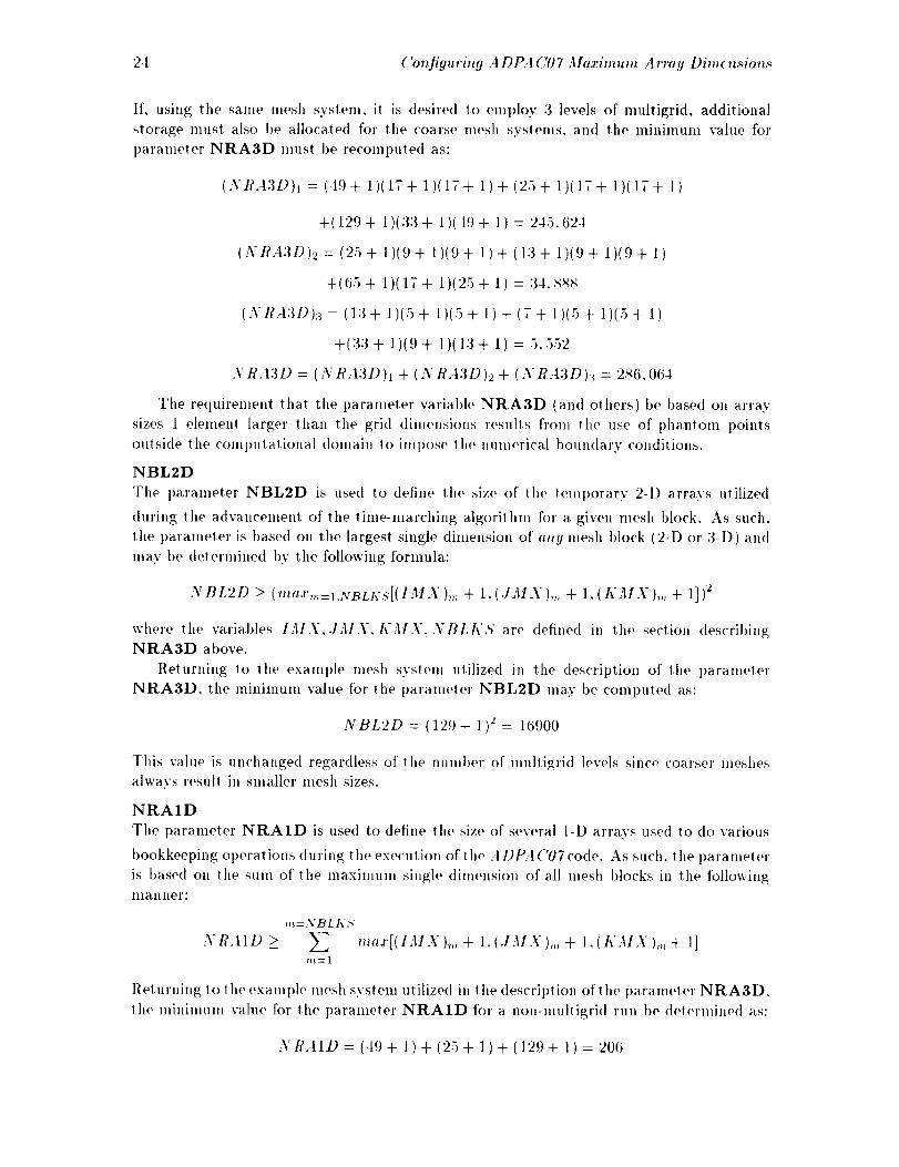
If, using tile same mesh system, it is desired to employ 3 levels of multigrid, additional

storage must also be allocate([ for the coarse mesh systems, and the minimum value for

parameter NRA3D must be recomputed as:

NRA3Dh = (49+ 1)(17+ 1)(17+ 1)+ (25+ 1)(17+ 1)(1_- + 1)

+(129 + 1)(33 + 1)(49

(NRA3D)2=(25+ l)(9+ l)(9+

+(65+1)(17+ 1)(25

(NRA3D)3= (13+1)(5+ 1)(5+1

+ 1) = 245.62-1

1)+ (13+ 1)(9+ 1)(9+ t)

+ 1) = 34,sSs

)+(7+ 1)(5+ 1)(5+ 1)

+(33+ 1)(9+ 1)(13+1)=5.552

X RA3D = ( N R A3D )_ + ( N RA3D )2 + ( X R:I3D):3 = 2,_6,064

The reqmrement that the l)arameter variable NRA3D (and others) be base<l on array

sizes 1 elemen! larger lhan the grid dilnensions results from the use of 1)hanlom points

oulsi<le the comt>utalional domain to impose the numerical boun<lary conditions.

NBL2D

The l)arameter NBL2D is used to define the size of the temporary 2-D arrays utilized

during the advancement of the time-marching algorithnl for a given mesh block. As such,

the parameter is based on the largest single dimension of <my mesh block (2-D or 3-D) and

may be determined by the following formula:

N BL2D >_ (tt_(tJ'm=I.NBLIi'/[( IMX ),_ + 1. (.]MX),,_ + 1. (A'MX),,_ + 1] )2

where the variables IMX, JMX. KMX. NBLK,S' are defined in the section descrit)ingNRA3D above.

Returning 1o the example mesh system utilized in the description of the parameter

NRA3D, the minimum value for the parameter NBL2D may be computed as:

NBL2D = (129+ 1) 2 = 16900

This value is un<'hange(l regardless of the numl)er of multigrid levels since coarser meshes

always result in smaller mesh sizes.

NRAID

The parameter NRA1D is used to define the size of several I-D arrays used to (lo various

t>ookkeeping operations (luring the execution of the A DPA ('07 code. As such, the l)arameter

is based on the sum of the lnaximuln single dimension of all mesh blocks in the following

lllanlter:

NRA1D >_ _ ma.r[(IMX),, + 1.(.IMA),,, + I.(hMX),,, + 1]m=l

Returning lo lhe example mesh system utilize<l in the descril)tion of lhe parameter NRA3D.

the minimum value for the parameter NRA1D for a non-multigrid run be determined as:

NRA1D=(49+ l)+(25+ 1)+(129+1)=206

Configuring A Dt{4 ('07 3la.ri_m_ A tray Dim¢ n._ion_ "25

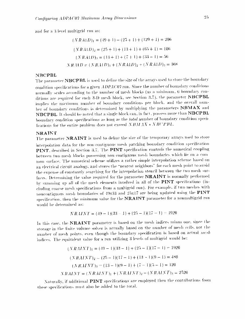
and tbr a 3 level multigrid run as:

(NHAID)I = (-19+ 1)+(:25+ 1)+(129+ 1) = 206

(NR:IlD)2 = (_5 + 1) + (13 + 1) + (65 + 1) = 106

(XRAID):_=(13+ 1)+(7+ 1)+(33+ 1)=56

X H:III) = (NBAID)_ + (N RAID)2 + (X RAID):_ = 36_

NBCPBL

The paratnel(,r NBCPBL is used lo define the size oft ire arrays used lo st ore the boundary

co],li! ion spe('ilications for a given A 1)1_4 ('07 run. Sittce the nu mbev of boundar,v ('ondi! ions

normally scales a<'('ordin_ to the number of mesh blocks (as a minimum, 6 boun(larv con-

ditions are required for each 3-D mesh block, so(, Section 3.7). the paranwtev NBCPBL

implies lhe maximum numt)ev of l>oundary condilions per block, and 1he overall m]tn-

I)er of I>oundarv conditions is (letevmined by mu/(iplyin_ _he 1)aramelers NBMAX and

NBCPBL. I1 should I)e noted lhal a single block can, in fa<'t, possess more than NBCPBL

l)oundavv co]Mitten sl>ecilications as Ion_ as the total number of boundary condition sl)eci-

fi('ations for the entire problem (lees no1 exceed X IIMAX , NH('I'ttL.

NRAINT

The parameter NRAINT is use</ to define the size of the tempol'ary a H'ays used to st<)re

interpolation (lala lot the n<)n-contigu(>us lnesh patchin_ t)oun(larv con(Ill ion Sl)ecilicalion

PINT, descril)e(l in Section 3.7. The PINT specification controls the numerical c<>ul)lin_

between 1we mesh t)locks possessing non-contiguous mesh l)oun(laries which lie on a con,-

men surfa<'e. The numerical s<'heme utilizes a rather siml)le inlerl>olati(>n scheme I)ased on

an eleclri('M <Tircuil analogy, and slows tit(' "'nearesl neighbors" for each mesh poinl l<)avoid

the expense of ('oxtslantly searchinp_; for tit(' inlerl)olation slenci] l)etween tit(, two mesh sm'-

fa<'es. ])eterminin_ the value re<lldre<l for the parameter NRAINT is n<)rtna]ly performed

by summing; up all o[" tit(, mesh elentents involve<l in all of the PINT sl)ecificalions (in-

chldin_ coarse mesh specifications fi'om a mulligrid run). For example, if lwo lneshes wilh

non('ontiKttous mesh boun(lavies of 4.qx33 and 25x17 are I)ein_ updated ttsin_; the PINT

sl)e('iIication, then the minimum value for lhe NRAINT parameler for a nomnultip_.;rid run

would be determined as:

NRAIXT= (,19- 1)(33- 1)+(25- 1)(17- 1)= 1920

In this case, tit(' NRAINT parameter is base<l on tit(, mesh indices minus one. since lhe

sl<>va_;e in t l,e finite volume solver is actually base<[ on the number of mesit c(//._, not lhe

number of mesh l)oints, even though the l>oun<lary sl>ecilicati<)n is t)ase(I on a('lual m<s.h

il,(li('es. The e<luivalen! value for a run ulilizinp_; 3 levels of mullip_;ri(l would I)e:

(NIL4INY')1 = (-l.()- 1)(33-1)+(25- 1)(17- 1)= 1!)20

(NRAI+YT)2= (25- i)(17- !)+(13- 1)(9- l)=+lS0

(NR.-tlN7_):+ = (13 - 1)(9 - 1) + (7 - 1)(5 - 1) = 120

NI_:IINT = (X R.I/NT)t + (,\/_'A/XT)2 + (XtLiI-VF):_ = 2520

Nalurally, if ad(titional PINT spe<'ifications are en/ploye(I t hen tit(, ('onl ril)utions from

these spe('ifi<'ati<)tls mttst also I)e added to the total.

26 Configuring A D PA C07 Maximum A rray Dime nsion._

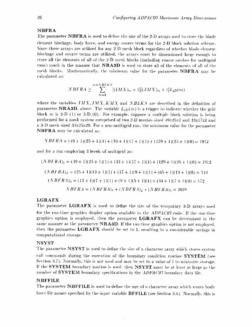
NBFRA

The parameter NBFRA is used to define the size of the 2-D arrays used to store the blade

element blockage, body force, and energy source terms for the 2-D block solution sclmme.

Since these arrays are utilized for an)' 2-D mesh ])lock regardless of whether ])lade element

blockage and source lerms are utilized, the arrays must be dimensioned large enough to

store all the elements of all of the 2-D mesh blocks (including coarse meshes for muir]grid

runs) much in the maimer that NRA3D is used to store all of the elemenls of al] of the

mesh ]>locks. Mathemalically, the minimum vahw for tile ])arameter NBFRA lrlay becalculated as:

N BFRA >

7_=NBLK,',"

[(IMX),. + I][(.IMX)., + 1]L2D(,,,)

where the variables IMX, JMX, KMX and NBLKS are descril)ed in the definition of

paranmter NRA3D, above. The variable L2D(m) is a trigger to indicate whelher the grid

block 7_ is 2-D (1) or 3-D (0). For' example, suppose a multil)le block solulion is being

performed for a mesh system comprised of two 2-D meshes sized 49x25xl and 33x17xl and

a 3-I) mesh sized 33x25x29. For" a non-mull]grid run, the minimum value for lhe paranmter

NBFRA may be cah'ulated as:

NBFRA = (-19+ 1)(25+1)(1)+(33+ 1)(1T+1)(1)+(129+ 1)(25+ 1)(0)= 1912

and for a run employing 3 levels of lnultigrid as:

(NBFRA)I = (49+ 1)(25+ 1)(1)+(33+ 1)(17+ 1)(1)+(129+ 1)(25+1)(0)= 1912

(NBFRA)2 =(25+ 1)(13+ 1)(1)+(17+1)(9+ 1)(1)+(65+ 1)(13+ 1)(0)=544

(NBFRA):_ = (13 + 1)(7 + 1)(l) + (9 + 1)(5 + 1)(l) + (33 + 1)(7 + 1)(0) = 172

NBFRA = (NBFRA)_ + (NBFRA)2 + (NBFRA):3 = 262_

LGRAFX

The parameter LGRAFX is used to define the size of the teml)orary 3-D arrays used

for the run-time gral)hics (lisl)lay ol)tion available in the ADPA('07 code. If the run-lime

graphics ol)tion is employed, then the i)arameter LGRAFX can be determined in the

same manner as the parameter NRA3D. If tire run-time graphics option is not eml)loyed,

then the parameter LGRAFX should be set to 1, resulting in a considerable savings in

COml)Ut ational storage.

NSYST

The parameter NSYST is used to define the size of a character array which stores system

('all commands during the execution of the boundary condition routine SYSTEM (see

Section 3.7). Normally, this is not used and may be set to a value of 1 to minimize storage.

If the SYSTEM boun(lary routine is used, then NSYST must be a! least as large as the

number of SYSTEM boundary specitications in the ADPA('07 boundary data file.

NBFFILE

The parameter NBFFILE is used to define the size of a character array which stores body

force file names specified by the int)ut variable BFFILE (see Section 3.(i). Normally, lhis is

A DP+I('07 ('ompilatiol_ Usi_g Makefil¢ 27

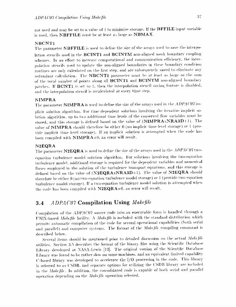
no! used and may l>e set 1o a value of 1 to minimize storage. If tit(' BFFILE inpul variabh,

is used, then NBFFILE lnusl ])eal h'asl as large as NBMAX.

NBCNT1

The paranleler NBFFILE is used 1o define file size of Ill(' arrays use<l to save the inferp<)-

lalion stencils used in the BCINT1 and BCINTM non-aligned mesh boundary coupling

sclmmes. In an effort to increase computational and communication ef[iciency, ill(, inler-

polation slencils use(I to update lhe non-aligned boundaries in lhese boundary condilion

routines are only calculaled on lhe tits! step. and are subsequenlly saved to eliminale any

reduudant calculalion. The NBCNT1 paranleler must ])e al leasl as large as the sum

of the total number of points along all BCINT1 and BCINTM non-aligned boundary

palches. If BCNT1 is sel to 1, then lhe interl)olalion slenc]l saving; feature is disabled,

and Ill(' hllerpolalion slencil is recalculated at every lime step.

NIMPRA

The parameler NIMPRA is used to define the size of tile arrays llsed in *lie :t DI>.I ( '1)7 im-

plici! solution alg;orilhm, l:or tilne-del>endent solutions involving Ill(, iteraliw, implicit so-

fulton algori_tlm. Ul) to two a<l<litionaf lime levers of the conserved flow variables must be

stored, and this storage is deline<l based on the value of (NIMPRAxNRAaD+I). The

value of NIMPRA should lherefore />e eilher 0 (no implicit lime level storage) or [ (pro-

vide implici! time level slorage). If an iml)licit solution is atteml)ted when Ill(, <'ode has

been corot>ileal wilh NIMPRA=0, all error will result.

N2EQRA

The parameter N2EQRA is used to define tile size of the arrays used in tile ADI>,t('O7 !wo-

eq,latioll t111"btJlellce model soil, riot1 algol"Jlh111. For soJt2!iOllS hlvoJvhlg !be l,W()-ec, lllalJoll

turl)ulen<'e model, additional storage is required for the dependent variables and nmnerical

tluxes employed i1_ the solulion of the turbulence lransporl equalions, and !his storage is

defined based on lhe value of(N2GQRAxNRA3D+[). The value of N2EQRA sl,ould

I herefore })eeit her 0 (no lwo-e<lualion turl)ulence model storag;e) or 1 (l)rovide (we-equation

lurbulence model storage). If a two-equalion turbulence model solution is atlelnl)led when

the co<te ]las been compiled with N2EQRA=0. at) error will result.

3.4 ADPAC07 Compilation Using Makcfilc

(!Oml>ilation of the ADI>:I('07 source code into an executable form is handled through a

UNIX-t>ased Mrd,'cfil< facility. A M<lg'clile is included with the standard dislribution which

permils automatic COlnpilation of the code for several operational capabilities (both serial

and ilarallel) att<t colnpuler svstelns. The fo1"ltlal of the Makcfih compiling command is

(tescril)ed below.

Several items shoul(l be menlioned prior to (telailed discussion on lhe aclual .llal,'clil¢

u!ilities. Section 3.5 des('ribes lit(, format of the binary files using lit(, Scienlific l)alal)as(,

l:il>ral'v develol>ed at NASA-Lewis [13]. The original version of lhe Scienlific 1)atabase

Library was found 1o be rather slow on some machines, and an e(luivaIenl [imile(l cal)abi[i!y

('-based library was develope<l 1o accelerate lhe I/0 processing in 111(' code. This library

is referre(I 1o as (:SI)B, and separate options for utilizinp.; tit(, (:SI)B library are included

in Ill(, Ma_'clih. In ad(lition, lhe consolidated code is cal>able of I)olh serial an(I t)arallel

ol)eration <lel)en<ling on lhe Mtlkcfil( operation selected.

28 ADPA('07 (bmpilation Using Mak_fil_

Ill the directory containing the FORTRAN source of the ADPA('07 code. comi)ilation

is t)erfonned by executing the command:

make option

Tile make command is standard on UNIX systems and automatically interrogates the

file Mal,'cfilt for instructions on how Io 1)erforln the compilation. The option argument may

be any of the variables listed below:

Standard UNIX (Silicon Graphics) .llat:_ Options

(No argument) This is tile standard UNIX systeIn compilation for the

serial version of the A DPA('07 code. All non-standard programnfing

constructs are avoided (such as graphics, or lnulti-processor features).

This option will deliver a working executal)le on most UNIX systems

which supl)orl standard namillg conventions (f77 as the slandard corn-

prier, etc.). The compilation includes basic compiler optimizalion (f77

-O). Tile executable nanle is adpac.

<.sdb This is the same a.s liuk above, except thai the fa.sler (:-based scientific

database library is linked instea(t of the slanda.rd scientific dalal)ase

library. Prior to performing this comt)ilation, the apl)ropriate ma/:t

cotlllllal/d nltlst t)e issued in the CSDB directory to asselnble the ('SI)B

library for tile local machine. The executable name is adpae.

pfa This option is used on Silicon Grat)hics computers sut)l)orting the

Power FORTRAN compiler option. Power FOI/TRAN is a Silicon

Graphics pro(luct which does automalic multiprocessor compilation

and is therefore not related to the ADPA('07 message-passing paral-

lelizalion strategy. The pfa compiled (:()de is therefore still ol)erale(t

as a serial code. although it may execuie on Inultiple processors for

Silicon Gral)hics workstalions. The nulnl)er of t)rocessors use(t is sel

by the NUM_THREADS environment variable. The compilation ill-

eludes basic compiler optimization (f77 4)). The executable name is

adpae_pfa.

csdb_pJ}l This option is the same as pfa above, excei)t that the faster ('-based

scientific database lil)rary is linked instead of tile standard scientific

database library. Prior to performing this compilation, tile a.ppropri-

ate ma/¢e command must be issued ill the CSDB directory to a.ssemble

the CSDB library for the local machine. Tile executable name is ad-

pac_pfa.

graphics This option compiles ADPA('07 with the necessary routines needed to

permit interactive gral)hics bet.weell network connected Silicon Graph-

ics workstations. This option will only work when COml)iling on a. Sili-

con Graphics workstation with IRIX operating system 4.0.1 or al)ove.

The full Silicon Graphics shared graphics libraries and X-windows sys-

tem gral)hics lit)raries must be installed on tile compiling workstation

in order for this option to work. This feature is not recommended as

it generally decreases performance and other visualization techniques

are likely to produce more desirable results. The executable name is

adpac_graphics.

A DPA('07 Compilatio_ Using Mak_fih 29

c._db_graph its

db2"

c._db_db:r

db.c_ graph ic._

paroll< I

paralleLcsdb

pa rtllh l_db.r

This option is lhe same as graphics above, excepl thal lhe fasler (!-

based scientific dalabase library is linked instead of the standard sci-

entific database library. Prior to performing this COml)ilalion, lhe ap-

propriale ma/,'¢ command musl I)o issued in the (!._I)B directory to

assemble the CSDB library for the local machine. The execulat)le

name is adpae_graphics.

This option is used for generaling an executable versio)) of l lye serial

code which is compatil>le with the standard UNIX db.r-I)ase<l debug-

ging facility'. This should work on any slandard I, NIX machine which

suppr)rls db.r {Not(,: tl)e code will run much more slowly wl)e)) com-

piled in lhis fashion.) This option is used inainlv for code (tevelol>ment

or debugging. The execulable name is adpae_dbx.

This option is used for generating all executable version of the serial

code which is compalible with lhe standard UNIX db,r-based debug_ging

facilily using; lhe ('SI)B library. This should work on any slandard

UNIX machi[_e which supporls db.r(Note: the code will rut) much more

slowly when compiled in this fashion.) This oplion is used mainly for

code dewqoptnent or debugging. The executable name is adpac_dbx.

This ()plion is used for generatinpg an execulable version of the se-

rial code with run-time graphics enabled which is COml)alil>le wilh the

standard UNIX db.r-based debugging facilil.v using the ('SI)B library.

This should work on any standard UNIX machilm which supl)orls db.r

(Note: the code will run much more slowly when compiled in lhis fash-

ion.) This option is used mainly for code developmenl or debugging.

The exe<'utable ltame is adpac_dbx_graphics.

This is the slandard UNIX svslem compilalion for the parallel version

of the ADtYt('07 code. The standard APPL message passing library

is incorl)oraled, and therefore creation of this executal>le re<luires ilia(a ma/<< has been issued in the APPL directory on the current machine.

Tl,e p<lrall_l code may only be execule<l using the APPL comfmh rune-

lion with a <'orrest)onding APPL procd<ffile. Prior 1o performing; this

compilation, tile appropriate ma/,:e command lllllSl be issued in lho

APPL direclory to asseml>le the APPL library for the local machine.

The executable name is adpacp.

This is the same as paralhl above, excelH thal the faster ('-based

scientific database library is linked instead of l he standard scientifi<"

database library. Prior to performing this compilation, t he apl>ropriate

ma#_ COlnmand must I>e issue<l in the ('SI)B and APPI_ <lirectories to

assemble tlle ('SI)B and APPL lil>raries for the local nlachine. The

execulable name is adpacp.

Tl)is is the same as porall_l above, excepl thai specilic compil(,r oi)! ions

have been enabled to utilize the UNIX dbx del)ugging facilily, l)rior

to performing this compilation, the al)l)rot)riate real,'< command must

b<' issued it) l])e SDBLIB and APPL directories 1<) assemble the SI)B

and A|)t>I: libraries for the local machine. This should work <)n any

slan<tar<t UNIX machine which SUl)t>orls db,r (Nole: (h(' <'ode wi[[ run

much more slowly when compiled in (his fashion.) This option is used

30 A DPA 4.'1)7 Compilation U._in9 31akefil_

paralld_csdb_dbx

mainly for code development or debugging. The executable name is

adpacp.

This is tile same as parall(l_csdb_dbx above, except that the faster

C-I)ased scientific database library is linked instead of tile standard

scientific database lil)rary. Prior to performing this compilation, theapprol)riate mak_ command must be issued in the CSDB anti APPL

directories to assemble tile (".SDB and APPL libraries for the local

machine. This should work on any standard [:NIX machine which

supports dbx(Note: the code will run n|uch more slowly when compiled

in this fashion.) This option is used mainly tot code development or

debugging. The execu!able name is adpaep_dbx.

ptlrall_l_prm This is the standard UNIX systeln compilation for the paratM ver-

sion of the ADPA('07 code using the PVM message passing library.

The standard APPL message passing library is incorporated as a sub-

laver between the native PVM calls and the ADI).4('07 programnfing

message-passing calls, and therefore creation of this execul able requires

that a make has been issued in the APPI, directory on the currenl

ma.chil_e. The parallel code may only be executed using the APPL

compul_ function with a. correspon(ling APPL plvcdeJ" tile. Prior to

performing this compilation, the al)prot)ria.te mat'_ ('olnnland musl be

issued in the APPL directory to assemble the API)L lil)rarv for the

locM machine. The executable name is adpacp_pvm.

Silicon Graphics Power Challenge Makt Options

pow(r_challeng( This option is utilized when compiling the standard serial code on

a. Silicon Graphics R8000 (Power ('hallenge @) computer. For besl

performance, several machine specific optimizations are enabled. The

executable name is adpac_power_challenge.

Cray (UNICOS) 3htk¢ Options

tray This option is utilized when compiling the standaM code on a (!ray

computer (implies a serial code). For best periormance, the aggressive

optimization oI)tion of the Cray compiler has been invoked (cf77 -Zv

-Wf"-o aggress"). The executable name is adpac_cray.

croy_dbx This option is used for generating an executable version of the code

which is compatible with the Cray cdbx debugging facility. (Note:

the code will run much more slowly when compiled in this fashion.)

This option is used mainly for code developmenl or debugging. The

executable name is adpac_cray_dbx.

nCUBE2 Vertex Operating System Makt Options

i_cub¢ This is the standard n(_UBE 2 system compilation tor the parallelversion of the ADPA('07 code. The nCUBE version of the APPL

message passing library is incorporated, and therefore creation of this

executable requires that a make has been issued in lhe APPL direclory

on the current machine. The parallel code may only be execute(l using

the APPL compute function with a corresponding APPL procd(f tile.

A DPA (7)7 ('ompilation l'si_q Makefilc 31

_wu&_c._'db

n,'ub(_db,r

ncubc_csdb_db.r

ucubc _c.'_db_noOd

(l i3"

aia'_,".,,db

aia'_dbx

o i.r_c._db_dba"

Prior 1o perforlnillg this con@lalion, the apl)ropriale ma/<_ command

,,,,,st be issued in the APPL directory to assemble the APPL library

for the local machine. The executable name isadpacp_ncube.

Tiffs option is idenlical to ncub< above, except tha! lhe faster ('-based

scienlific database library is linked instead of lhe slan(lard scienlific

dalat)ase library. Prior to performing I his compilation, lhe apt)ropriale

reed'( command must 1)e issued in lhe ('SI)B and A1)PI_ direclories 1o

assemble lhe ('SI)B and .\Plq, libraries for lhe local machine. The

executable name is adpacp_neube.

This oplion is used when compiling; lhe parallel code for lhe n('ITI_IE

parallel computer using the \:ERTEX operating system and the n( 'UBI']

db.r <lelmgging facililv. ( Not(,: lhe code will rllll lllllch ll|Ol'e slowly when

corot)ileal ill this fashion.) This option is used mainly tor code dewq-

opmenl or debugging. The oxeculable name is adpaep_neube_dbx.

This oplion is lhe same as u¢.ub(_db.r abow,, excepl thal lhe fasler ('-

based s<'ienlifi<" database library is used illslead of 111e slandard scien-

lific (lalat)ase lil)rarv. (Not(,: lhe code will run much more slowly when

('omf)ile(1 ill this fashion. ) The (,xe('ut able name is adpacp_ncube_dbx.

This Ol)lion is used when ('oml)iling; Ill(, t)aralM code for lhe n('Utlt'_

I)arallel COlnl)uler usinp_; 1he VI':I{TEX operaling; svslelll and 1he faster

('-based scientific database lil)rarv instead of Ill(' slandard scientific

database library. This option also eliminates all 2-D subroutines Io

minimize the size of 1be execulal)le, which is useful for slrictly 3-1)

l)rol)lems on multil)rocessing COml)ulers wilh limited memory per pro-

cessor. Prior to performing this compilation, tile a t)propriate ma,{',"

command musl 1)e issued ill ill(' ('SI)B and API>L direclories 1o as-

semble lhe (:SI)B and AI'PL libraries for lhe local machine. The

exe('ulable name is adpaep_ncube_no2d.

IBM RS-6000 AIX 3hd,'_ Options

This option is used when comt)iling the slandard serial code on an

IBM RS-6000 workslalion runnittg the AIX operating system. The

executable name is adpac_aix.

This oplion is idenlical 1o ai.r above, excepl thai lhe faster (:-l)ase(I

scienlific database library is linke(t instead of the standard scientitic

dalabase library. Prior 1o performing this compilation, lhe approt)ri-

ale ma,{'_ conlnlalld lnusl |)e issued in the ('SDB directory to assemble

lhe ('S1)Blibrary h)r the local machine. Theexeculable name isad-

pac_aix.

This option is used for generaling an executable version of lhe code

which is COml)atible with lhe IBM AIX db.r (lel)ugging facilily. (Nole:

the co(le will run lnllch lnore slowly when ('Oral)ileal ill this fashion.)

This el)lion is used mainly for code (tevelol)menl or debugging. The

executable name is adpac_aix_dbx.

This option is identical to aix_(lbx al)ove, except that the fasler ('-based

scienlific database library is linked inslead of lhe slandard scientific

32 A DtL4('07 Compilation l:si_,g 3lak¢fil_

aix_pamlh I

aix_parallt Lc._db

a ix_pa ralld_dbx

database library. Prior to perfornfing this con_pilation, the apl)ropriate

ma_'e command must be issued in the ('SDB directory to assemble

the CSDB library for the local machine. (Note: the code will run

lnuch more slowly when compiled in this fashion.) This option is used

mainly for code develol>menl or debugging. The executable name is

adpac_aix_dbx.

This is the standard IBM RS-6000 AIX UNIX system COlnl)ilation

for the parallel version of the ADPA('07 code. The slandard APPL

message passing library is incorl)orated, and therefore creation of this

executable requires thai a mak( has been issued in the APPL direclorv

on lhe current machine. The parallel co<h' may only be executed using

the APPL compute function with a correspondillg AI'PL procd_ffile.

Prior to perforlning this compilation, the a pt)rot)riale mak( command

must be issued in the APPL (lireclory to asseml)le the APPL library

for the local machine. The executat)le name is adpacp_aix.

This option is identical to aix_t)arallel above, excel)l that llw fasler

el-based scientific database lil)rary is linked instead of the slandar(t

scientific database lil)rary. Prior to performing this compilation, the

apt)ropriate make command must be issue(t in the ('SDB directory

to assemble the CSDB library for the local machine. The executal)le

name is adpacp_aix.

This option is used for generating an executable parallel version of

the code which is compatible with the IBM AIX db_' det)ugging facil-

ity. (Note: the code will run much more slowly when compiled ill this

fashion.) This option is used mainly for ('ode develol)menl or (lebug-

ging. The executat)le name is adpacp_aix_dbx.

NASA-Lewis Research Center Specific .llake Options

l(/C(

lace _c._db

#ath_r

l_athcr_csdb

This ot)tion is used when COml)iling the standard parallel code for the

NASA-Lewis LACE workstation cluster computing envirollment. The

executable name is adpacp_lace.

This option is identical to lace above, except that the faster ('-base<t

scientific database library is linked instead of the standard scientific

database library. Prior to l)erforming this compilation, the appropri-

ate mak, command must be issued in the ('SDB directory to assemble

the (:SDB library for the local machine. The executable naule is ad-

pacp_lace.

This option is used when compiling the standard parallel code for

the NASA-Lewis SP2 (leather) workstatioll cluster computing envi-

ronment. The executable nanle is adpacp_leather.

This option is identical to leather above, except that the faster (M)ased

scientific database library is linked instead of the slan(lard scientific

database library. Prior to performing lhis comt)ilation, the appropri-

ate make command must be issued in the CSDB directory to assemble

lhe CSI)B library for the local machine. The executable name is ad-

pacp_leather.

A Dt54 ('07 1,pul/Oulpul Fih._ 33

Source Directory Maintainance Ma_'e Options

h<Ip This ot)tion lisls and describes all available mal_:cfih options. No exe-cula])le is creale([.

<'/<,, This option cleans up lhe source direclory by removing all obje<'t files.

No oxeculab/e is ('realed.

r_al_'l<ol_ This oplion really cleans up the source directory I)v removing all object

and library files. Noexeculal)le is crealed.

o,_sourc'< This option collcalellales all the ..tDI>A(W7 source tiles illlo a sitlg;h,

source tile name adpac..on<._o,,v.t.J_ This single S()lll'('(, ('7tll lholl l)e

compiled by haltd on lhose machines for whi<'h atJ al)propriale ,_ct,_'<

ot)tion is no! available. I1 is Ul) to the user 1o link ill lhe necessary

library files ((:SI)B, API)L. elc) for creation of an exe('ulab[e. No

execulable is <'reared.

:\I the cOnll)lel loll of the comt)ila! ion process on any s\'sleln, an executable version of ! he

code is written in the source direclorv (see Appendix A for an apl)lit'alion of!he COml)ilalion

and execulion processes for a sample lesl case).

3.5 ADPAC07 Input/Output Files

IJl this seclion. !be various i_lpul/<)utpu! dala files relaled to a calculation) usiJ_g Ibe A I)-

t"A('07 l)rogranl are descril)ed. In order to understand lhe file naminv; ('onvenlion. Ill('

<'on<'('pt of a case name ttltlSl _il's! be detailed. All files used in an ADt>A('07 cal('ula!ion

are named a('('or(lin R 1o a slandard naming conve||tion of lhe form:

('(I._( .{ .l:t( Ilsioll

wher'e case is a unique, user-specifiable !tame i<tentifying the geometry or flow con<lilion

being; invesligated, and <.r& ,._io_z is a name describing; lhe lype of file. The <'a._e name musl

be specified in the slandar<l inpul file describe<l below. A list and descril>tion of each of the

files used or generated by ADPA('07 is g;iven in Table 3.1.

The standard inl>ut, standard oulpu!, boundary data, and convergence history files are

slored in AS(!II ['orma!. All o|her files utilize the Scientific l)alaBase Library (SDBLIB) [13]

formal. The mesh file and I'>LOI_3D plot output files are compatible with tile I+L07"3I)

multiple grid. binary definition (see Sections 3.s an(t 3.11 for a description and ('o<lil_g

examples of Ill(, SI)BI, IB binary formal). Files dealing with lhe parallel execution of the

A I)I>A ( '1)7 <'ode are <lescril)e<l in (!hap!or -1.

The st+ttl(lard input and standard outl)l|l files are dire('le(I at l'ttlllillle Ilsitlg; the slandar(1

('NIX l"e(lire('lion sylllaX as:

adpac < case.input > case.output

If a reslar! run is desired, lhe user musi move lhe most ('urr(,lll ¢)Ull)Ul resla|'! tile from

('(I._(. l'es ( il 1'1 ,lleW

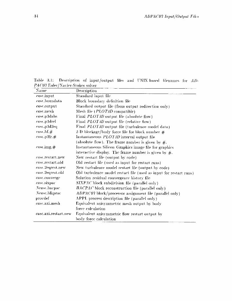
34 ADPA C07 Input�Output Files

Table 3.1: Description of input/outl)Ul files and UNIX-based tilenames for AI)-

PA ('07 Euler/Navier-Stokes solver

Name Description

casc.input

(.as(.boundata

case.output

COS;( .lllesh

cese.l)3(tabs

cose.p3drel

ra._(.p3d2eq

ca._. bf. #

ras_.p3fr.#

ca._.ilng.#

('as(.rest art.llew

cas_.restarl .old

cas(.2eqrest.new

cas(.2eqrest.old

('(Is(. COil verge

('a._( .sixpac

N('asr.bacpac

Ncas_.blkproc

procdef

case.axi,mesh

cas(.axi.rest art .new

Standard input file

Block t)oundary definition file

Standard output file (fl'Onl outpu! redirection only)

Mesh file ( PL 0 T3D COnlpatible)

Filial PLOT3D outpul file (absolule flow)

Final PL 0 I"31) out pul file ( relative flow)

Final PLOT3D outpul tile (turbulence model data)

2-D I)lockage/I)ody force file for t)lock number #

Instantaneous I)L 0 T3D interval outpul file

(absolute flow). Tlle frame nllnd)er is given by #.

Instantaneous Silicon Graphics image file for gral)hics

interactive disl)lay. The franle lmmber is given by #.

New restart file (outl)ut by code)

Old restart file (used as illput for restart runs)

New turbulellce model restart file (output by code)

Ohl lurt)ulence model restart file (used as inpul for restart runs)

Solution residual convergence history file

SIXPA (' block su bdivision file (parallel only )

BA ('t_4 (' block reconstruction file (parallel only )

A DPA ('07 block/processor assignlnent file ( parallel only)

APPL process description file (parallel only)

EquivMen! axisymmetric nlesh OUtl)Ul by bodyforce calculation

Equivalent axisynnnetric flow restart output by

body force calculation

.,t DPA ('07 ,S'tamhtrd Input File Dc'scription 35

to the defaull input l'eslarl file name

<'a.+<.rest at) .old

each lime Ill(, co<le is resiarte<l. A more deiaile<l description of Ill(, llSO and torulat of ihe

A l)I>,.t ('07 files is l)resen! e<l in Ill<" see( i<m s whi<'h follow.

3.6 ADPAC07 Standard Input File Description

The slau(lar(I .4Ill>A('07 inl)ul file <.ast.input contains lhe user-specifiable paranwlers

which control the basic <)t)eralion of the code during exe('utioll. These l)aranleiers lend

lo be less <'as(, <lependelll (as opl)<)se<l Io lhe 1)oun(lary daia file which i_ enlirely case <le-

t>ell(leI:). I)urin_ co<le exe<'lllioH, lhe input file is rea<t one lilw at a time as a chara('ler

slrill_, and ea<'h St l'iug is parsed se<lueniiall,v io determine tile spe<'i|ic program aclion in

each ('as(,. The slandard iul)ui file ulilizes a kevwor(t input foi'nlal, su('h lhal allY line which

does nol c(>nlain a l'e('ogliizat)h' keywor<l is lreated as a ('Omlueni line. Therefore. the user

may place aiU uunll)er of <'omlneuts ill lhe file (so lonp4 as llle line does lie! conlain a key-

wor(I inl)Ul sil'ing in lhe forui des<'ril)e(l below), and <'ode execution is unaliel'e<l. ('OmlllelllS

may also be placed ariel' 1fie val'ial)]e assigned to lhe keyword as loll_; as tllere are one or

more blanks set)aratin?-; lhe kevword value fi'om the ('Ollllnenl Sll'ing. All ilq>Ul file lines

are e<'hoed !o the slan(lard outt)lil, and file ])rogralll response 1o each line is lisled when a

sl>e<'ific at!ion is taken,

All kewvol'd input lines are _iven ili tile following forliial:

KEYWORD = Value Comment String

where I'(EYWO[{I) is one of lhe re<'ognize(] keywords <lescril)e<t I)elow. a lid Vahle is lhe

sl)e('ifi(' value 1o l)e assigned to lhal varialile. The Jill)ill line lllllSl COlilain llie equals sign

(=) with Olle or ]llore blanks Oil both sides in order 1,O be recoguized. Tile Comment

String iiiusl l)e separated I>y oiie or niore t)lank sl)aces frolil lhe Vahle. Therefore, lhe lines

DIAM = I0.000

DIAM =

DIAM = I0.000 This is the diameter.

i0.000

are valid keywor<I int)ul lilies assip_;ning the value 10.0 lo lhe variable associated with the

keyword I)IAXI. ('onversely. lhe lilies

DIAM= I0.000

DIAM =i0.000

DIAM=IO.O00

are no! recognizal>le kevwor(l llll)Ul lilies (in sl)ile of lhe l)resence of lhe kevwor<t DIAM),

1)e('ause of lhe lack of prol)er placenient of tile blanks about the equals (--) sigu. The

l)llrlios( , for lhis restri('lion is to l)erniil keyword varial)les in conilllenl lines, and to hel l)

ilsei's to gelierate readal>le inl)ul files. All keyword vahies are either real llllllll)ers (which,

ill lllally cases, are ('Oilverte([ i,o integers ill the code) or chal'acler strings.

A sample :1DI>A ('07 sialltlard hi l)Ul file containiug a llUliit)('r of lyl)ica] use kevwor(ls is

lisied l>el<)w:

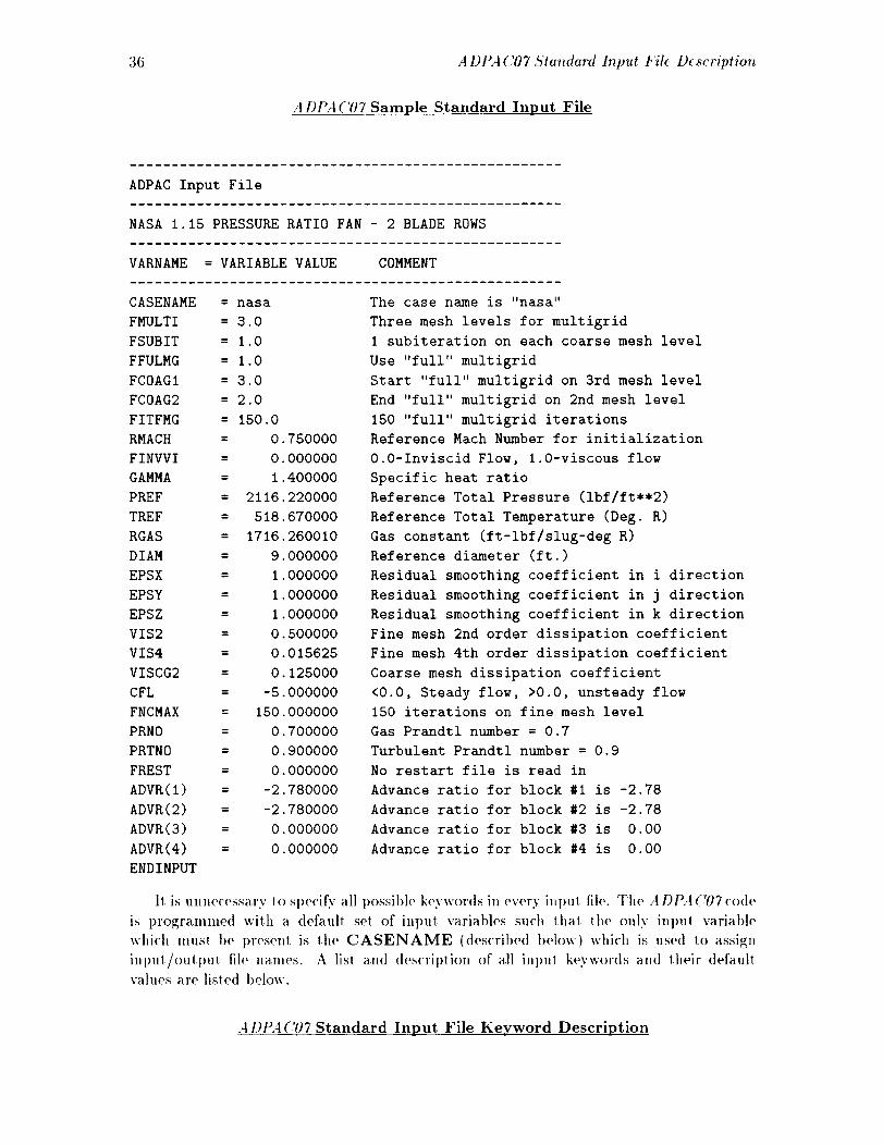
36 ADPAC07 Sta_Mard Input Fil_ Description

A DPAC07 Sample Standard Input File

CASENAME = nasa

FMULTI = 3.0

FSUBIT = 1.0

FFULMG = 1.0

FCOAGI = 3.0

FCOAG2 = 2.0

FITFMG = 150.0

RMACH = 0.750000

FINVVI = 0.000000

GAMMA = 1.400000

PREF = 2116.220000

TREF = 518.670000

RGAS = 1716.260010

DIAM = 9.000000

EPSX = 1.000000

EPSY = 1.000000

EPSZ = 1.000000

VIS2 = 0.500000

VIS4 = 0.015625

VISCG2 = 0.125000

CFL = -5.000000

FNCMAX = 150.000000

PRNO = 0.700000

PRTNO = 0.900000

FREST = 0.000000

ADVR(1) = -2.780000

ADVR(2) = -2.780000

ADVR(3) = 0.000000

ADVR(4) = 0.000000

ENDINPUT

The case narae is "nasa"

Three mesh levels for multigrid

i subiteration on each coarse mesh level

Use "full" multigrid

Start "full" multigrid on 3rd mesh level

End "full" multigrid on 2nd mesh level

150 "full" multigrid iterations

Reference Mach Nutaber for initialization

O.O-Inviscid Flow, 1.0-viscous flow

Specific heat ratio

Reference Total Pressure (ibf/ft**2)

Reference Total Temperature (Deg. R)

Gas constant (ft-lbf/slug-deg R)

Reference diameter (ft.)

Residual smoothing coefficient in i direction

Residual smoothing coefficient in j direction

Residual smoothing coefficient in k direction

Fine mesh 2nd order dissipation coefficient

Fine mesh 4th order dissipation coefficient

Coarse mesh dissipation coefficient

<0.0, Steady flow, >0.0, unsteady flow

150 iterations on fine mesh level

Gas Prandtl number = 0.7

Turbulent Prandtl number = 0.9

No restart file is read in

Advance ratio for block #I is -2.78

Advance ratio for block #2 is -2.78

Advance ratio for block #3 is 0.00

Advance ratio for block #4 is 0.00

It is unnecessary 1o specify all 1)ossib]e keywords in every inl)Ul file. Tile A DPA('07 code

is pl'ogrammed with a default, set of input variables such that the only input variable

which must 1)e present is the CASENAME (described below) which is used to assign

ilq)Ul/oulput file UallleS. A list and description of all inl)ut keywords and their default

values are listed below.

A DI_4 ('07 Standard Input File Keyword Description

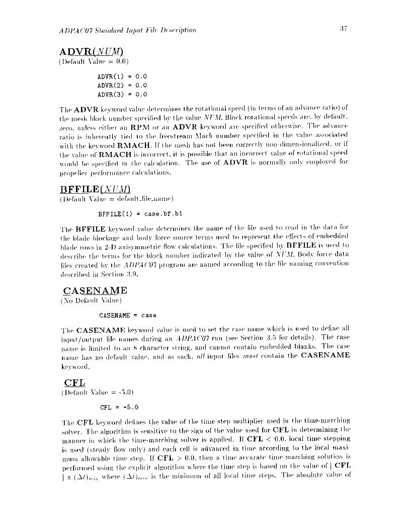
A DI_4('07 ,S'tandaed h_put Fib D_s_'ription 37

ADVR(NUM)(Default Vahle = 0.0)

ADVR(1) = 0.0

ADVR(2) = 0.0

ADVR(3) = 0,0

The ADVR keywoM vahle detenllitles the rotational speed (ill terms of all advance ca/M} of

the mesh l)lock llunlber st)ociNe(I by tile vahie NUM. Block rolalioual speeds are. bv default.

zero. [iMe._s either a, RPM or an ADVR keyword are specifi(,d otherwise. The a dvali('e

ratio in iuherently lied lo the freesiream Math lmnlt)er specified in the value associaled

with lhe kevwoM RMACH. It' lhe mesh has not beeu corre('t]v nou-(linleilsioualized, or if

the vahle o[" RMACH in illcorrect, i! is possible tha! an incorre('l vahle of rol arterial speed

woul(l be sl)ecifi(,(I in lit(' ealc(llation. The use of ADVR is iioriilallv only einl)loyed for

l)r(:)lieller l)erforlllallce ('ai('ulaliOll,_.

BFFILE(NU3I){])eial_Jl V_l,ie = defanll_fih,_n;lme)

BFFILE(1) = case.bf.bl

The BFFILE kovwoM vahi(, (lelernihles tile name of lhe file used lo tea(1 in the data for

the blade t)lo('ka_e ali([ I)ody force SOlll'Ce tel'illS used 1o l'el)resenl the effects of enihe(l(ie(I

blade rows ill 2-1) axisynllnelrie flow calculations. The file specified I)v BFFILE in use(I to

des<'ril)e lhe terins for the hlo<'k llUllllier indicate(t t>y tile vahle of NI:.II. Body force (lata

files created I)v the .t D15t(!07 ])rogranl are llanie(l a('cordhlg 1o tile file llanlillg ('OllVellliOll

des('ribe(I ill Sect ioll 3.9.

CASENAME(No l)efaull Vahle)

CASENAME = case

The CASENAME keyword vahle is used to set: the case nalne which in used to define all

inl)ul/oulput file nantes dul'hlg an ADf_4(Y/7 run (see Section 3.5 for (Ietails). The case

liallle in liiniled to all g C]lal'acler slrillg, and CallllOl ('onlain enll)edded I)lanks. The case

naiue has no defaull vahle, and as such, all inliut files mu,_t contain lhe CASENAME

keywoM.

CFL(I)ef'aull Value = -5.0)

CFL = -5.0

The CFL keywor(t (le|ines the value of lhe tiuie step niuliip|ier used in the tinie-niarching

solver. The alg;orii hin is sensilive to life sign of tile vahie used for CFL in delerlnining the

lllallner hi which the thlle-lllal'e[lillg solver is aI)t)lied. If CFL < 0.0. local time sl;epl)ing

is used (steady flow only)and each cell is advanced in thne according; to the local niaxi-

11111111allowable tillle step. If CFL > 0.0, l[leli a t illle-a('('llrale thlle-lnarchillg soluliOll is

t)erfornie(l uSill_ the exlilicit alg;orithui where lhe tinle sle l) is 1)ase(l Oil tile vahle of i CFL

I x (Al),,_;, where (Al),,,, is tile lllininiunl of all local linie slel)s. The al)sohlle vahie of

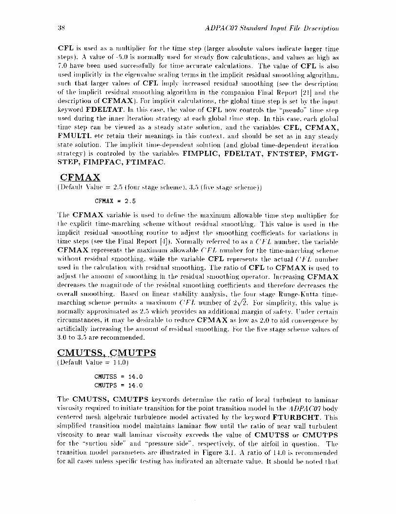
3_ ADPA ('07 Standard Input File De.scription

CFL is used a.s a multiplier for the time step (larger absolute values indicate larger time

steps). A value of-5.0 is nornlally used for steady flow calculations, and values as high as

7.0 have been used successfully for time-accurate calculations. Tile value of CFL is also

used implicitly in tile eigenvalue scaling terms ill the implicit residual smoolhing algorithm.

such that larger values of CFL imply increased residual smoolhing (see tho description

of tile implicit residual smoothing algorithm in the companion Final Report [21] and the

description of CFMAX). For implicit calculations, the global time step is set t)5' the input

keyword FDELTAT. In this case, the va.lue of CFL now controls the "pseudo" time step

used during tlle inner iteration strateg.v a.t each global time step. In this case. each global

time step can be viewed as a steady state solution, and the variables CFL, CFMAX,

FMULTI, et.c retain their meanings in this context, and shouhl be set a.s in any sleadv

state solution. The implicit time-dependen! solution (and global time-dependent iteration

strategy) is controled I)y tile variables FIMPLIC, FDELTAT, FNTSTEP, FMGT-

STEP, FIMPFAC, FTIMFAC.

CFMAX

(Default Value = 2.5 (four stage schenm). 3.5 (five stage scheme))

CFMAX = 2.5

The CFMAX variable is used to define the maxinmm allowable lime step multiplier for

the explicit, tinm-nlarching schelne without residual smoothing. This value is used in the

implicil residual smoothing routine to adjust tile smoothing coefficients for variations in

time steps (see the Final Report [4]). Normally referred to as a ('FL number, the variable

CFMAX represents the maximum allowable ('FL number for the time-marching scheme

without residual smoothing, while the variable CFL represents the actual ('I_'L number

used ill the calculation with residual smoothing. Tile ratio of CFL to CFMAX is used to

adjust the amount of smoothing in the residual smoolhing operator. Increasing CFMAX

decreases the magnitude of the residual smoothing coefficients and lherefore decreases tile

overall smoothing. Based on linear stability analysis, the four stage Runge-Kutta time-

marching scheme permits a lnaxinmm ('FL number of 2v/2. For simplicity, this value is

normally approximated as 2.5 which provides an additional margin of safety. Under cerla.in

circumstances, it may be desirable to reduce CFMAX as low as 2.0 to aid convergence by

artificially increasing the amount of residual smoothing. For the five stage scheme values of3.0 to 3.5 are recommended.

CMUTSS, CMUTPS(Default Value = 14.0)

CMUTSS = 14.0

CMUTPS = 14.0

The CMUTSS, CMUTPS keywords determine the ratio of local lurbulenl to laminar

viscosity required to initiate transition for the point transition model in the A DPA ('07 body

centere(I mesh alget)raic turbulence model activated by tile keyword FTURBCHT. This

simplified transition model maintains laminar flow until the ratio of near wall turbulent

viscosity to near wall laminar viscosity exceeds the value of CMUTSS or CMUTPS

for the "suction si(le'" and "'pressure side", rest)ectively, of the airfoil in question. The

transition model paramelers are illustrated in Figure 3.1. A ratio of 14.0 is recommen(led

for all cases unless specific testing has indicate(t an alternate value. It should be noted tha!

A DPA ('/)7 Standard lnp_d File Descriplio_ 39

lhese variables will have no effect when FINVVI=0.0 (invisci<t flow), or when F2EQ= 1.0

(two-equalion turbulence model enabled) or when FTURBCHT=0.0 (transit ion nlo<lel

n<>1 activated ).

DIAM

(I)efauh Value = 1.(})

DIAM = 1.0

The DIAM keyword is used as a <[imensionalizing length scale for the mesh system for a

given case. The A l)l_A('OYcode assumes lhat the mesh has been generaled itl a ,J<)l,di-

mensional fashion, and musl be dimensionalize<l before exec,ttion. The value of the DIAM

variable is used to convert the supl)osed nondimensional mesh c<)ordinates into a (limen-

sional lenglh scale wit It units of feet. In other words, if the mesh has been generated using

a length scale of inches, then the value of DIAM should I>e _.1 or 0.0S3333in order 1<>

<'onverl lhe mesh units t<> units of Feel. If the mesh unils are ah'ea<ly in feet. lhen the

vahle of DIAM shouhl l>e siml)ly 1.0. Many mesh generation syslems for turt)omachinery

geometries non<limensionalize the mesh by a reference diameter determined from the 1ur-

homachinery ?geomelry such thai the maximuln value of any radial coordinate in the mesh

is 0.5. In this <'as(,. the value of DIAM should t>e the diameter (>f the turbolna<'hine in fee!

used to nondimel,sionalize the mesh. Proper specification of the DIAM value is crilical

to achieve lhe correcl flow t{eynohls number and rotational speed for rotatitlg geometries.

Many problems can be traced io improper specification of the DIAM value and lhe user

should take care to understand the use of this kevword. Whet, in doubt, the user shouhl re-

member the siml>le rule lhat the actual mesh milts, when nmltiplied by the value of DIAM

should result in t>hysica[ lenglhs expressed in feet.

ENDINPUT

ENDINPUT

Whet, the AI)P.I('07 program encounlers lhe keyword ENDINPUT. the l>arser which

searches ea('h line for a vali(I input keywor<l string is terminated, an(l no ad(lilional input file

lines are parse<l for input kevword vahtes. Any lines followin_ the ENDINPUT slatemel,!

are ignore<l, except when the graphics display system is in effect across a network, in which

case lhe statemenls following the ENDINPUT statement musl contain two blank lines

aim the Internet network address of the destination display device (see Chapter 9 for a

description of lhe Interactive (;rat>hics Displa5 _ option).

EPSTOT(l)efaull Value = O.l)

EPSTI]T = O. 1

The EPSTOT keyword delermines the value of lhe smoothing coefficient employed in tit(.

post multigrid smoothing algorithm described by the trigger FTOTSM. This coetti<'ien! is

only used when FTOTSM = 1.0. The value of the coeificient may be any positive mJml)er.

but for most circumstances, a value between 0.0 aim 0.25 is suggested (larger values iml)l.v

more stnoothi_g). This option is normally employed for enhance<l code stability during the

mulligri(t sohgion process.

EPSX, EPSY, EPSZ(l)efaldt \'aim, = 1.0)

40 ADPA C'07 A'ta_do, rd h_put Fil_' DeseriptioT_

Body-Centered Mesh Block

Turbulence Model Nomenclature

XTRANSS

CMUTSS sets transition

when x<XTRANSS

Transition forced at XTRANSS

on suction surface

Suction Side

Pressure Side

CMUTPS sets transition

when x<XTRANPS

XTRANPS

Transition forced at XTRANPS

on pressure surface

fj

0.0 Axial Chord 1.0

• . ! ,

i direction

Figure 3.1:ADPA('07 Bo<ty-(lentered Mesh Turbulence Model Nomenclature Sununary

A DPA ('07 Standard Input File D_scription 41

EPSX = 1.0

EPSY = 1.0

EPSZ = 1.0

Tiw EPSX, EPSY, EPSZ keywor<ls set tlle value of tile implicil residual ,_moolidng

coeflicie,t multipliers in the i. j, and k cooMinato directions, respectively. The values

of EPSX, EPSY, and EPSZ are used as siml)le mullipliers for _he residual smoolhi,g

coefficie.ts <'alc,lated by lhe eigenvalue s<'alin_; residual smoolhin_ scheme <lescribed ill ! he

Final Report [-1]. 1[" EPSX, EPSY or EPSZ = 0.0. lhen no smoothing is applied for Ill(,

give, coordinate direction. The user should be ;_ware lhal the kevwoM variable FRESID

controls the global al)pli('alio, of residual smoolhing in the solulioll a l_orilhm, and in lhe

case where FRESID=0,0 (residual smoothing disabled), the EPSX, EPSY, EPSZ have

no impact o, lhe solution. The <lefaull value for ill(, coeflicienl mullipliers is 1.0. Any value

lar_er lhan 1.0 simply implies oxcess smoolhing all(l lnav I)e useful for c_ses wilh poor

<'o,vergen<'e or un<h,siral)le me.sh quMily. Ifa ':aJ,e larger than :].0 is required to stabilize a

solution, this ge,erally indi<'ales some sort of problem in ill(, calculation (sucil as poor mesh

asl)ecl ralio, bad I)ou,(larv sl)ecifi('ation, el('.), or mighl suggesl lhal FRESID has I)eell

set Io 0.0. Values less lhan 1.0 will likely cause code instM)ilities for values of CFL greater

thal_ 2.0. O<'<'asio,ally for cylin(lri('a] ('oordinate syslem solulions involving , ceulerline (>r

sling with very small radii, lhe value of EPSX, EPSY, EPSZ which ('orresl)olM,_ _o lhe

"radial" <lirectio, musl l>e reduced to 0.25-0.5 l(> mainlain slal)ilily.

F2EQ(I)efaull Value -- 0.0)

F2EQ = 0.0

The F2EQ keywor<t assigns a lrigger which deterlnines the aclivalion of Ill(, Iwo-e(lualion

(k_)lurl)ulen('e mo<M. This lurbu]ence model ('a, provide Sul)erior pre(liclion <)1'lm'bu]enl

flows with separation, t>ul al a sul)slantially larger COml)ulationaI cosI. The lw(>-equalion

model utilizes a d<Iilional sl)eciticalion of dala al ini]ow boundaries (see e.g. INLETT,

INLETG to t)rescribe the "'freeslrealn'" turbulen('e level, a,ll(] Ill(, lurl>ulenl vi,,cositv is

Ul)dated through the solutio, of two a(ldilional lranst)ort equations and a "'t)oinlwise'" eddy

vis('osily evalualion (for additional details, see tile Final Report [21]). The lwo-equation

model ix not enabled when F2EQ=0, and i._ enab]ed when F2EQ=I.0.

FBCONF([)e['all]l \:a,hle---- 99999.0)

FBCONF = 99999.0

The FBCONF keyword assigns a lrigger which delormines Ill(, ileralion number al which

lhe boun<larv ('o.(lilions are frozen. This trigger wax added for those cases where ('OliVer-

gence is al)l)arenlly hindered by "'noise" fi'om tile boundary con(Ill ions. ('aution llll, lSl be

exer<'ised when _tsing the FBCONF variable due to tile fact that the A DPA C07 code cotll(l

ultimately (liverlze wheH all of the bomMary conditions are frozen. This option is norlnally

only use<l for del)uggiug l)urt)oses.

FBCWARN(l)(,l'_/_lt Val,e = 1.0)

42 A DPAC07 Standard Input Fi& Description

FBCWARN = 1.0

Tile FBCWARN keyword assigns a trigger which controls tile error checking for outer

block boundary conditions normally performed by the ADPA('07 code prior to execution.

Following initialization, ADPAC07 normally processes each mesh block and checks to see

if the user has adequately specified boundary conditions over the six outer surfaces of each

mesh bh)ck. If any 1)ortion of an outer bouudary does not have some type of boundary con-

ditions speciiied, an error lnessage is normally issued and the code will ternfinate l)rocessing.

Under some conditions, the user may have intentionally neglected to specify a boundary

condition on an outer mesh block surface, and it is therefore convenient to eliminale this

error processing. The FBCWARN trigger controls the actuation of this error handling

facility. When FBCWARN= 1.0, the error handling is enabled. When FBCWARN=0.0,

the error handling is (lisabled.

FCARB(NUM){Default Values = 0.0)

FCARB(1) = 1.0

FCARB(2) = 0.0

FCARB(3) = 0.0

FCAKB(4) = 0.0

FCARB(5) = 0.0

The keyword FCARB(NUM) sets a block specific trigger for the mesh block numl)er

specified bv NI;.ll which determines, on a block t)y block basis, whether tile (lartesian

(FCARB(NUM) = 1.0) or the cylindrical (FCARB(NUM) = 0.0) sohltion algorithnl is

employed by that block. The ADPA('07 code pernfits nfixed cylindrical and (!artesian so-

lution blocks in a single calculation. While the variable FCART may l)e used to set the

glol)al value of mesh blocks for either cylindrical or Cartesian solution s)atus, the variable

FCARB(NUM) may be utilized to set specific blocks one way or the other. It mus)l)e

noted that the variable FCARB(NUM) will always override the sta)us implied by FCART.

A1 l)resent, the only boundary condition which l)ermits interblock communication between

mixed cylindrical and Cartesian blocks is BCPRR (see See(ion 3.7).

FCART

(Default Value = 0.0)

FCART = 0.0

Tile FCART keyword assigns a trigger which conlrols the cylindri(:al/Cartesial_ coordinate

system solution scheme ill tile the ADPAC07 code. If FCART = 0.0, then all blocks

(except those specifically altered by the FCARB inpul va.riable) are treated as cylindrical

coordinate systeln blocks. If FCART = 1.0, then all blocks (except those specifically

altered by the FCARB input variable) are treated as (lar(esian coordinate system blocks.

FCOAG1

(I)efault Value = 1.0)

FCOAGI = 1.0

A I)tL4('07 Standord Input Fih Description 13

The FCOAG1 keyword specities the initial, or coarsest coarse mesh level upon which the

"full" multigrid calculation is initially applied (for additional details, see the descrit)tion of

FFULMG). When multiple coarse mesh levels are available for processing, it is occasionally

useful lo specify the initial coarse mesh level in the "'full'" mulligrid se,luence it, order to

avoid wasled conll)utalions Oll lower lllesh levels. Typically, FCOAG1 is set 1o FMULTI

(slarl "full'" mulligrid on coarsesl mesh level). In some cases (when FMULTI is larger lhan

;3.(}) il may be advisable to se! FCOAG1 to 3.0. and avoid athlilional l)rocessing on coarser

meshe_ dul'in_ lhe "'full'" mull i_rid slarlu l) process. A flowcharl of lit(, ,i DI:I('07 iteration

and multigrid control Mgori!hm is given in Figure :{.2. An example is given in the descriplion

of FCOAG2.

FCOAG2(Default Value = 2.0)

FCOAG2 = 2.0

The FCOAG2 kevword specilies the final, or tines1 coarse mesh level upon which tit(, "'full'"

mulligri(l calculation is applied (for a(l(lilional (lelails. see the description of FFULMG).

Vl:hen mullit)le coarse mesh level_ are available for t)rocessing, il is occasionally useful Io

sl)ecify lhe [trial coarse mesh level in the "'full'" mull igrid sequence in order io examine lhe

flowiield wilhoul aclually l)erf()rming any calculalions on the fine mesh. For examl)le. 1he

combinalion

FMULTI = 3.0

FCOAGI = 3.0

FCOAG2 = 3.0

FNCMAX = i0.0

FITFMG = iO0.O

wouhl direcl a "full'" mulligrid starlu 1) of 100 iterations on mesh level 3, and since FCOAG2=3.0,

tit(' "full" mulligrid sequence is on(led at lifts mesh level. The solution is then inlerpolaled

to the fine mesh. and then 10 [it,(' mesh ilerations using ;3 levels of mulligri(I would be per-

formed. Typically. FCOAG1 is sel Io 2.0. which in(licales lhal lit(, "'full" multigrid _tarlul)

procedure utilizes all mesh levels front FCOAG1 to 2 1)efore starling any processing on the

fine mesh. A flowchart of'lhe ADI_4('07 iteration and mulligrid conlrol algorithm is given

in Figure 3.2.

FCOCOM(I)efaull Value = 0.0)

FCOCOM = 0.0

The FCOCOM keywor(l assigns a trigger which (lelermines the method by which ('ell face

areas and cell volumes are delermine(l for lhe coarse mesh levels of a multigrid solulion.

When FCOCOM=0.0. coarse mesh ceil face areas and cell volumes are determined in

exaclly the same manner as lhe fine mesh (using the s mesh l)oinls defining 1he vertices of the

cell anti ('ompllting a sevi(,s of cell face diagonal ('ross produ('Is for lhe areas, and computing

a cell ('enler art(1 acldilional (Iol l)ro(lucts for lhe cell volume). When FCOCOM= 1.0, the

coarse mesh c('ll face areas and cell volumes are contt)ule(l 1)v sulnnlinp_£ |he cell face areas

and cell volumes of the enclosed fin(' mesh ceils relative to each coarse mesh ('ell. The

44 ADPA C07 Standard I i_put File Description

procedure defined by FCOCOM=I.0 is believed to be a more consistent representation of

the coarse to fine mesh injection/interpolation process, but experience has not shown ally

greal difference using either method.

FCONVRG(Default Value = - 100.0)

FCONVRG = -7.0

Tile FCONVRG keyword specifies the log 10 root-mean-s(luare resi<lual level at which

the solution is deemed converged. The solution convergence is monitored and when the log

l0 root-mean-square residual level is less than FCONVRG, the time-marching process is

terntinated and the solution is OUtl)ut. In general, the solution should not be considere(l

converged unless the log l0 root-mean-square residual is less lhan -6.0. The authors do not

recomlnend the use of this varial)le for exl)licil tilne-det)endent calcula!ions. The FCON-

VRG varial)le is useful for terminating the inner iteralions of an implicit time-del)en(tentsolution.

FDEBUG (NUM)(I)efault Vahms = 0.0)

FDEBUG(1) = 0.0

FDEBUG(2) = 0.0

FDEBUG(3) = 3.0

FDEBUG(4) = 0.0

FDEBUG(5) = 0.0

The keyword FDEBUG(T)PE) defines a block numl)er for the debug output lype specified

by TI'PE which determines, on a type by tyl)e basis, whether debug outt)u! from the

ADPAC07 run is printed to the stan(tard output. When enabled, this variable will generate

an extreme amount of output and should therefore be used only in a controled debugging

environment. The value of the variable FI)EBUG(TYPE) determines for which blocks

the particular type of output is enabled. The following del)ug output tyt)es are currently

supported:

FI)EBUG( 1 ) Prinl the input (Cartesian) mesh l)oints

FDEBUG( 2 ) Print t he (converted) cylindrical mesh points

FDEBUG(3) Print the cell face areas

FDEBUG(4) Print the ('ell volulnes

FDEBUG(5) Print the cell flow data

FI)EBU(;(6) Print the cell tilne steps

FDEBUG(7) Print the cell convective fluxes

FDEBUG(8) Prin the cell <lissipative fluxes

FDEBUG(9) Print the cell diffusive fluxes

A DPA ('07 Sta_dard Input Fih D(._cription 45

I:I)Et_UG(10) Print lhe cell implicit residual smoothing data

F D E LTAT

(l)efaul! Value = 0.0)

FDELTAT = 1.0e-7

The FDELTAT keyword assigJls lhe value for the physical lime i.crem(,nl (i, seconds)

used (luring a t ime-(lel)ell(letl( soluliotl (either explicit or implicit). For e×l)licil sollltio.s.

il is up l o (he user )o ensur(, lhal the value of FDELTAT (loe,_ nol viola(e lhe slat)lilly

chara('lerislics of the exl)licil flow solver. For implicil solu(iol,s, lifts value should refte('l

a reasoHal)le .uml)(,r ()f global lime steps over lhe course of the unslea(ly aero(lyttamic

phe_lom('E_a <)f ili)<'res('.

FDESIGN

(l)('f_lull \'ah.' = 0.0)

FDESIGN = 0.0

Th(' FDESIGN kevwor(I assigx,s a trigger which delermines direclly whelher to use lho

body for('e ([esign ,_vslel|l cal('ula)ion I)rocedure developed under Ta,_k 1_ of NASA ('on(rat(

NAS3-25950. Wh('H e.al)le(l, lifts el)lie, (li('lales that a solu(ion I)e i)erforlned ou a 2-I)

axi,'_vmmelric _ri(t represenlalive of a lhroughflow calculation for a furl)oma('hill(,ry |lov-

1)alh. The solulion requires th(' ihl)U! of a t)ody force file (see (he (lescril)liou of BFFILE)

which sl)ecifies lhe 1)lade blockage (a description of the contents of a I)odv force tile is givell

ill Seclio, 3.9). The 2-I) grid must I)e conslructed such lhal it ret)r(,senls the 2-1) hub 1o

tip mean flow stream surface, hi other words, if the mean flow i.volv(,,_ swirl, thet_ the grid

is wa,rl)e(l i. the circumferential direction to in(licate the degree of swirl rel)reseHl('([ l)v tim

mean sl]'eam surface. The A I)I_A('07 flow solver then ilera(ively u])(|ales lhe body forc(,_

in(ernal Io lhe ('ode uu(i] lhe l)redicte(l mean Sl,l'ea,n} surface matches lhe IHeal[ ,_Ireall| Silt-

face defined l)v lhe mesh. Thi,_ lea,lure wa,,_ develol)ed [br use i. a desig.-like envirollmenl

wh('reill gross flow l)roperl ie,_ such as (urning may l)e k.own, l)ul ,_l)e('ifi(' airfoil shapes may

llol I)e kl|o',vn.

FFAST

(l)ef_._ Value = 0.0)

FFAST = 0.0

:Fit(' FFAST kevword assigtls a trigger which incorporales some simplification,_ of (he AD-

PA('07 mul(igrid algorithm which reduces the (TU time l>er mul(igri<l cycle. The ('PU

._avillgs afforded w]|ell this el)lion is enal)led (FFAST=I.0)is es)imaled to be about 20(_.

U.f<>r(unalely. )he A I)I',I('07 algorithm is less slable usiug the l)r(>cedures enabled by

FFAST= 1.0 a_<t in general, this el>lion is no1 recommended.

FFILT

(I)efaul_ Value = 1.0)

FFILT : l.O

46 A DPAC07,6'tandard Input I;'i# De._eription

TtLe FFILT keyword assigns a trigger which determines directly whether the added dissipa-

tion routines are called during tile time-marching process. If FFILT ---- 0.0, then no added

dissipation is calculated. I! is also possible to turn off tlle added dissipation by setting the

values of VIS2 an<t VIS4 to 0.0; however, the use of FFILT avoids the calculation of the

dissipation terms entirely. It is unlikely that any value other lhan 1.0 is required except for

code debugging purposes.

FFULMG(Default Value = 0.0)

FFULMG = 0.0

The FFULMG keyword assigns a trigger which determines whether the "full'" multigrid

solution procedure is applied or whether the standard lnultigrid procedure is used. The use

of "'full" multigrid is advisable (t)U| l|Ot required) when a new calculation is l)eing started

as a means of rapidly generaling a better initial guess for the final flowfiehl. If the solution

is being restarted from a previous calculation (FREST=I.0). it is usually advisable to se!

FFULMG to 0.0 to avoid destroying the initial data read from the restarl file (a warning

message is issued when this combinat ion is specified ). A flowchart of the A DPA ('07 iteration

and multigrid control algorithm is given in Figure 3.2.

FGRAFINT(Default Value = 1.0)

FGRAFINT = 1.0

The FGRAFINT keyword (letermines the uumt)er of iterations t)etween flowfield display

updates for the A DPA('07 real time gral)hics display systeul. This option is only valid

when FGRAFIX = 1.0, and is sul)ject t<) a number of other restrictions tor the graphics

display system (see the description of input keywords FGRAFIX and FIMGSAV. and the

description of the graphics display system, ChaI)ter 9). The default value for FGRAFINT

is 1.0, which indicates that the graphics display will be updated every iteralion. This can

cause excessive computational and network overhead, and the user should be aware of the

potential problems when using the grat)hics display features. The use of the graphical

display features of the A DI_4('07 code are not generally recommended.

FGRAFIX(Default Value = 0.0)

FGRAFIX = 0.0

The FGRAFIX keyword sets a trigger which controls the generation of the real time

interactive graphics display in the ADPA('07 program. A value of FGRAFIX = 1.0

indicates that the interactive gral)hics display facility is desired, while FGRAFIX = 0.0

turns this option off. When functional, the graphics screen is updaled with the latest

available flow dala every FGRAFINT iterations. Graphics images can be automatically

captured on sl)ecific comi)uter hardware every FIMGSAV iterations as a means of creating

fiowfield animations (see Graphics Display. Chapter 9). In order for the grai)hics display to

work, the code IllllSt be compile(I with either the 9rttphic._ or pfagraphics Makefile opt toll (see

Seclion 3.4 for a description of the Makefile and the A DI{4('07 code COml)ilation t)rocess).

There are also specific machine requirements for this option to work as well (see the section

A I)I_4 ('07 5;tandard h_put Fil_ Descriptio_ 47

on Gral)hics Display, Chapter 9). I"11(' generation of interactive, real time graphics images

increases the overall computational cost., and can cause network overloading in some cases

due to lhe lransmission of _;raphics information. The use of the graphical display features

of the A DPA (Y)7 code are not generally recommended.

FIMGINT(l)efaull Value = 99999.0)

FIMGINT = 99999.0

The FIMGINT kevword determines the number of it eralions belween flowfiehl graphics

display image ('apt urillg available on Silicon (;ral)hics computers for the A 1)1_1('07 real l inle

_raphics display svslem. This option is only valid when FGRAFIX = 1.0, and FIMGSAV

: 1.0, and is subject to a nulnber of other restrictions for the _raplfics display system (see

lhe des('ril)lioll of in l)Ul kevwords FGRAFIX and FGRAFINT, and lhe des('ril)tion of

the graphics display svslem. ('hal)ter 9). The defaull value for FIMGINT is 99999.0.

which indicates l[|al a s('reell image will l)e save(1 every 99999 ileralions. This large value

was chosen to prohibi! acci(lental image ca l)turing, which can quickly fill u 1) a lary4e alllOll[ll

of disk slorag_e. The gral)hi('s dist)lay system can cause excessive coral)U! at ional and net work

overhead, at,d the user shoul(l be aware of the l)otential prol)lems when using this fealure

of the A DI'A ('07 ('o(le. The use of lhe gral)hi('al display teal ures of lhe ,,t I)t:4 ('07 co(le at'('

no! generally re('omme,l(le(l.

FIMGSAVE(I)efaul! Value = 0.0)

FIMGSAV = 0.0

The FIMGSAV keyword sets a I rigger which controls the Silicon Graphics COlnl)uter screen

image capturing facility of !he real time interactive gral)hics display in tile ADPA('07 t)ro-

gram. A value ofFIMGSAV = 1.0indicales that lhe graphics image cat)luring facility is

desired, while FIMGSAV = 0.0 lurns this option off. When the interactive graphics display

el)lion has been enabled (see delails for input keywor(ls FGRAFIX, FGRAFINT) the

graphics screen is up(laled wilh the lalest available flow data every FGRAFINT ileration.

When the image ca t)turing facility is enabled, these graphics images can be automatically

cal)lured on specific computer hardware every FIMGINT iterations as a means of ('real-

ing flowfiehl animations (see Grat)hics Display, ('hapter .0).ln order for lhe graphics disl)lay

in,age capturing faciliiy 1o work, the code must ])e coral)tied with eilher lhe graphic.,,, or

pfagr'al;hic.,_ Make[ih' option (see Section 3.-1 for a description of tile Makefile and the A I)-

PA('07 code ('olnpilatioil process). There are also si)ecific machine requirements fi)r lhis

opli<m I<) work as well (see ill(' sectkm on (;ral)hics Display. ('hal)ler 9). The general!on

of inlera<'live, real time gral)hics images increases lhe overall computational cosl, and can

cause rwtwork overloading ill some cases due 1o lhe tra llsmissioll of p_;rat>hics informal!on.

The cal)lurin_; el many screen images will also require a large amount of file slorage sl)ace

(see Section 3.') !'era descril>tiotl of the image capluring file naming convenlion). The use

of lhe gral)hical display features of the A Dt>A('07 code are not generally recommended.

FIMPFAC

(Default Value = 2.0)

FIMPFAC = 2.0

48 ADPA(;'07 Standard Input File Description

The FIMPFAC keyword is a simple trigger which determines the degree of time-accuracy

employed ill the implicit solution algorithm enabled by the keyword FIMPLIC. There are

four options available for this keyword. Values of" 1.0 and 2.0 utilize the "fully" implicit

strategy described in [21] and are first and second order accurate ill time, respectively.

Values of-1.0 and -2.0 utilize a "'lagged" "fifllC' implicit strategy (thought to improve

stability) and are first and second order accurate in lime. respectively.

FIMPLIC(Default Value = 0.0)

FIMPLIC = 0.0

The FIMPLIC keyword is a simple trigger to determine whether the iterative implicit

solution mode is enabled (enabled when FIMPLIC= 1.0). Tile implicit algorithm is used

only for time dependent flow calculations, and requires that the additional input flow

variables FDELTAT. and FNTSTEP be specified. The ADPA('07 code must also be

compiled with array parameter FIMPRA set to 1 to properly allocate array storage in

the co(le. When enabled, the implicit algorithnl performs a global time marching loop

strategy whereby each interation of tile global loop involves an iterative solution of a pseudo

steady state problem using the standard explicit time-marchillg strategy. The features of

this inner iteration problem is still governe<l by input variables such as CFL, CFMAX,

FMULTI, FNCMAX. etc. The global time increment for the outer loop is set by the

value of FDELTAT. The implici! algorittm) occasionally exhibits unstable behavior and

the solution shouht initially be closely monitored. The user should fully understand the

im[)lications and use of the implicit algoritlun before atteml)ting to utilize this option. A

theoretical description of the procedure is given in Reference [21].

FINVVI(Default Value = 0.0)

FINVVI = 0.0

The FINVVI keyword is a siml)le trigger to determine whether the solution mode is for

inviscid flow (FINVVI = 0.0) or for viscous flow (FINVVI = 1.0). This trigger con-

trols whether the viscous stress flux contributions are calculated during the time-marching

process. This does not affect tile application of boundary conditions, as this is completely

controled by the specifications ill the boundary data file (see Section 3.7). As such, it is pos-

sible to run viscous boundary conditions in an inviscid flow solution, and inviscid I)oundarv

conditions ill a viscous flow solution.

FITCHK(Default Value = 100.0)

FITCHK = I00.0

The FITCHK keyword controls the nunlber of iterations between job checkl)ointing in

tile ADPAC07 wogram. .lob checkpointing refers to the l)rocess of periodically saving

tile fiowfield information to minimize the loss of data ill the event that the job does not

terminale normally. As a safety feature, the ADPA('07 l)rogI'am writes out an updated

restarl file every FITCHK ilerations in case the job slops ])efore the final restarl file

out[)ut procedures are('omp]eted. It is not necessary to wrileoul inlermediate restar! files,

A Dt>A('07 ,S'ta.dard Input Fil( D_._criptiolt -19

but this is considered a good precaution against unexpecled problems such as compuler

failures, or syslem administration quotas. A mood interval for checkpoinling is 100 iterations

(FITCHK = 100.0). The intermediale restart files, as well as lhe tinal restart tile. are all

writlen to the same file name, and therefore previous (:heckl)oinls cannot be retrieved when

t he file is <)verwrillen (see Section 3.5 for restar! file naming conventions). Job checkpointing

only applies to the ilerative cycles involving the fine mesh, and does not apply 1o lhe coarse

mesh ileralions calculaled during a "'full" multigrid starlup (see FFULMG ).

FITFMG

(l)efaull Value = 100.0)

FITFMG = I00.0

The FITFMG kevword dictates the llumber of iterations t<) be performed on each of

lhe coarse mesh levels during; a "'full'" multigri<l startut> sequence (see the des('ril)lion of

FFULMG). Tyl)i<'ally. the startup sequeuce is used o)dy _o generate a reas<mabh, initial

guess for lhe line mesh, so Ill(' value of FITFMG is kel)! relalively low (_ 100). The

fil_.'_i<m of tb+' keyword FITFMG is ill_stra_e<l grapbi<'ally b_ Fi_Zm'e 3.2.

FMASSAVG(Default \:alue = 3.0)

FNASSAVG = 3.0

The FMASSAVG keywor<l <lescribes a lrigger whi<'h deterniines tile type ofniass averaging

use<l in tile A DPA('07 co<le for various boundary condil, ions. hi t)articular, the MBCAVG

boundary condition which imposes a circumferential mixing plane for siml)Iified representa-

lion of multislage lurl)omachinery blade row flows is the most COllllllOllly afl'e('ted routine.

A value of FMASSAVG = 0.0 implies lhal all algebraic average is to I)e used in the av-

(,raging operalor in lhe ADl)A('OTcode. A value ofFMASSAVG = 1.0 implies thai an

area average is 1o I)e used in lhe averaging ol)eralor in tile Al)t>A('OTcode. A value of

FMASSAVG = 2.0 ilnplies lhal a mass-weighted average is io be use<l in the averaging

operator in Ill(, .tl)I-'+1('07 code. \:alues of 2.0 and 3.0 are recommended, as the algebrai("

average introduces a fair amount of error.

FMGTSTEP

(Defa,lt Vabw = 0.0)

FMGTSTEP = iO0.O

The FMGTSTEP kevword assigns Ill(, numt)er of global time steps to l>e evalualed on

('oarse mesh levels for lhe iml)licil flow solver when the "full'" multigrid option FFULMG

is enal>led. In lhe processing of large lime-dependent calculations using tile iml)lici! [low

solver, it has been found useful to eml)loy the "'full'" multigrid tyl)e of star!u t) 1)rocedure

for the l ime-dependenl runs as well as lhe steady stale analyses. This t)asically initializes

Ill(' mull it)le lime levels dala arrays such that when the lille mesh solution is a('livaled, ill(,

(lala itt the previous time level arrays are initialized wil h something olher than lit(, current

sohgion, and a hol)efully better al)l>roxilnation of l,he time-derivatives can l)e performed.

FMGTSTEP sels the number of implicit lime steps i)erfl)rme<l on tile coarse meshes during

the "'full'" nmlligri(l starlup. This keyword will only be a('live when FIMPLIC=I.0. an(l

50 ADPA C07 Standard Input File D_scriptio1_

FFULMG= 1.0. For a more detailed description of tlle "full" multigrid startup procedure,

see the descriptions of FFULMG, FCOAG1, FCOAG2, and Section 2.5.

FMULTI

(Default Value = 1.0)

FMULTI = 1.0

The FMULTI kevword assigns the number of multigrid levels to be used during the cal-

culation (fora description of the mulligrid a lgorilhm, see Reference [4]). The code will

analyze the dimensions of the fine mesh to delermilm whether it can be properly subdi-

vided according to lhe number of nmlligrid levels requested. If FMULTI _< t.0, lhen lhe

number of" Inulligrid levels is set to 1, and the calculation is performed on the finest mesh

only without mulligl'id acceleration. For' unsteady flows using the explicit linm-marching

strategy, the current lnultigrid scheme is riot valid, and FMULTI shouhl be set to 1.0. For

tinm-dpendent flows based on the implicit time-marching strategy (FIMPLIC=I.0). the

multigrid algorithm may be enabled as with ally steady slate solution. A flowcharl ot" the

ADPA('07 iteration and mulligrid control algorilhm is given in Figure :].2.

FNCMAX

(Default Value = I00.0)

FNCMAX = i00.0

The FNCMAX keyword controls the total numl)er of iterations for a non-multigrid cal-

culation (FMULTI < 1.0), or the number of global iterations on the finest mesh for a

multigrid ca lculalion (FMULTI > 1.0). The total number of iterations performed on

all meshes for a multigrid run is controled by a combination of FNCMAX, FMULTI,

FCOAG1, FCOAG2, FFULMG, FITFMG, and FSUBIT. For example, the values

FNCMAX = 200.0

FMULTI = 1.0

FITFMG = 0.0

FFULMG = 0.0

FSUBIT = 0.0

wouht t)rescribe 200 iterations of a. lron-multigrid run (only the fine mesh is used). Theva111QS

FNCMAX = 200.0

FMULTI = 3.0

FITFMG = 0.0

FFULMG = 0.0

FSUBIT = 1.0

would prescribe 200 multigrid iterations using 3 mesh levels (but still only 200 global iter-

ations, where each iteration involves a single subiteration on each of 3 mesh levels). And

finally, the va.lues

A DPA('07 .qtandard Input Fil_ D<scription 51

FNCMAX = 200.0

FMULTI = 3.0

FITFMG = 50.0

FFULMG = 1.0

FSUBIT = 1.0

FCOAGI = 3

FCOAG2 = 2

would prescribe ;.41[i.it ial pass of 50 iterations on the third mesh level, followed by 50 multi-

,grid iteralions on lhe second mesh level, and finally 200 g3ol)al muhigri(l iterations o. lhe

finest mesh level. See lh(' (tes<'viplio.s of the variables FNCMAX. FMULTI. FCOAG1.

FCOAG2. FFULMG. FITFMG, att<l FSUBIT [or f`urthor details..\ flowchart o[lhe

,t I)P.I('07 iteration and ntultig;rid conlrol algorithm is given in Figure 3.2.

FNTSTEP(I)ef`aul! Value = 0.0)

FNTSTEP = lO0.O

The FNTSTEP keywor(1 assigns the, number of global time slel)s to be evaluale(l on

the tinest mesh during alt iml)li('it time-dependent solution. FNTSTEP essel:iallv s('l_

lhe ltumi)ev <ff global lime steps por[orme<l (while FNCMAX sets the number o[ inner

ileralions for each _loi)al time .step). The total physical time of" the tilne-d(,l>endent implicit

solulion is lheref"ore FNTSTEP muhiplied I)y FDELTAT. This variable is only active

when FIMPLIC= 1.0.

FRDMUL

(l)e[ault Value = 0.0)

FRDMUL = 0.0

The FRDMUL keyword determines wllether boundary condition data for the coarse mesh

levels o[ a multigri<l i'lllt al'e generated f`rom the fine mesh l)oun<lary conditions Sl)ecilie(I

in ti_e AI)I_A('07 I)ouu(larv data file (FRDMUL = 0.0). o1" whether the coarse mesh

I)out,lary specifications are actually read in from tit(' boundary data file (FRDMUL =

1.0). hi most ('ases, FRDMUL should I)e set to 0.0. and the l>rogram will <tetevmino

1he equivalent coarse mesh boundary conditions fi'om the fine mesh specifications. For the

purposes of code <[ebu_gi,g, or to permit multigri([ <'aicuiation on a mesh which <foes no!

possess l)er[ect "multigri(l'" boundary segments (a I>ou.dary condition for the fine mesh does

not I)e_in or end al a mesh index which is compatible with the multigri(l se(luence), it is

pos.ql)h, l<) "fool'" lhe I)ro_ram into running; multi_rid 1)v artiticially sl>ecifyin_; an e(luivalent

coarse mesh t>oun<lar.v co.(litton.

FRESID(I)e[ault Value -- 1.0)

FRESID = 1.0

The FRESID keyword assi_us a trigger v:hich de_ermines directly whether _he impli<'it

residual st.o<)thin_ vouti.es are ('alh,<l (luring the time-marchin_ l)rocess. If` FRESID =

0.0. the. no vosi(lua] sm<)othiu_; is applied. It is also l)ossil)le to turu off" _he residual

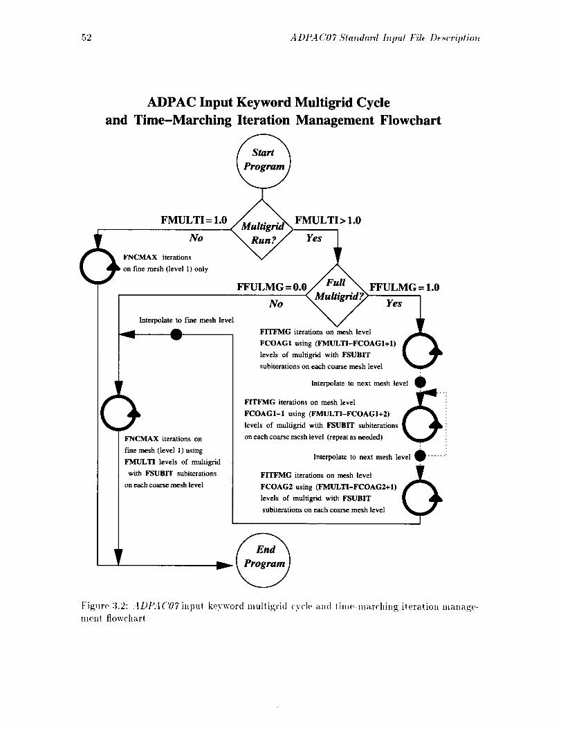
52 A DPA (i'07 A't_mdard Input File Descriptio_l

ADPAC Input Keyword Multigrid Cycle

and Time-Marching Iteration Management Flowchart

__ FNCMAX iteration NO

on fine mesh (level 1) only

FMULTI = 1.0 FMULTI > 1.0

_u,._ =oo/d :::___,,,, ..,FFU,._No \-----°--7 Yes

Interpolate to fine mesh level _/

AW

)FNCMAX iterations on

f'me mesh (level 1) using

FMULTI levels of multigrid

with FSUBIT subiterations

on each coarse mesh level

= 1.0

FITFMG iterations on mesh level

FCOAG1 using (FMULTI-FCOAGI+I)

levels of multigrid with FSUBIT

subiterations on each coarse mesh level

Interpolate to next mesh level O

FITFMG iterations on mesh level

FCOAGI-1 using (FMULTI-FCOAGI+2)

levels of multigrid with FSUBIT subiterations

on each coarse mesh level (repeat as neexi_)

Interpolate to next mesh level O

FITFMG iterations on mesh level

FCOAG2 using (FMULTI-FCOAG2+I)

levels of mulfigrid with FSUBIT

subiterations on each coarse mesh level

Figure 3.2:ADf_A('07 i.l)Ut keyword multigrid cycle and (ime-lnar('lfing ileratiou manage-meld flowchart

A DI A E 0 / ,Sla.dard Inpul f'il_ l)_._('ripl/oo 53

smoolhiup_; by setlinp_; tit(, values of EPSX, EPSY. and EPSZ to 0.0: however, the use

of FRESID avoids the calculation of the smoolhe([ residuals entirely. It is unlikely tilat

any value other lhan 1.0 ix required except for code (tebuggin_; purposes, or for calc,laii(>ns

involvi._; CFL_< 2.0.

FREST(l)efa,lt Val.e = 0.0)

FREST = 0.0

The FREST kevword assigns a tri_;ger which conlrols lhe restart characteristics of tit(,

.iD1>.4('07 code. If FREST = 0.0. then no restart file ix ,sed, aJ_(I the flow variables

are initialized a('cordin_ to tile s<'helne (tescril)ed under the inl)ut keyword RMACH. If

FREST = 1.0. then tit(, co(le attempts to ol)en a restart file (ca._(.r<._larl,old) described

by tit(, file naming convention (see Section 3.5), and the flow variables are initialized hv tit(,

val,es _;iven in lit(, restart file. Restarting a calc,lation fl'om a t)revious calculation is often

,seful for I)reakiJl_ ,i ) large cah',lalio,s into smaller comp,tationa] pieces, and may also

provide faster convergence for cases which involve luther cha,p,;es to a t)revious cah',lation.

A I hir<l option is provided (FREST = - 1.0 ) which allows the A DIL4 ( '07 to reslart fronl

a coarser mesh solution t'esla.l't file. For very large meshes which permit multi_ri(l, it may be

desirable to initiate the solutio, using lesser ('Olll[)lltet's I)y run,ing on a coarsened mesh level

gem'rale(l indel>en(lenlly from the line mesh sol,lion (,sing Ibe ('OAI{,VF,V program). I:or

examl)le, if a solutiolt is ultimately desired on a 257x257x257 mesh, this obviously we.hi

re<l,ire a fair amount of computer resources io COml)Iele. l)urin_; the solution iniliation

phase, it mi_;ht t)(, desirat)Ie to start the solution on a coarsened version of the final fine

mesh (129x129x129) using a smalh, r conll)uter (a workstation for examt>le). This can I>e

accomplished tltrough the following procedure. First, create a coarse mesll equivalent of the

<lesi)'ed fine mesh solutiolt (the ('O,ttL<,'I'LV program was develol)ed for this l),rl)ose). ('reate

a solutioll for 1he coarsened mesh ,si,g A DfLt('07 using whatever COlnt)uter is available.

Next, using the restart fife from t he coarsened mesh solution. "'restart" t he line mesh sol.t ion

usilt_; FREST = -1.0. Tit(, coarsened mesh must represent an exact coarsened mesh from

the ,ltimate fire, mesh (every ot her mesh lit)(, removed) for this procedure to work t)rol)erly.

It should be mentioned that restart files generate<] by the implicit time-dependent so-

ltttiotl strate_;y will contain additional time level data cotttl)ared to a steady state restart

file. Ii is t)ossible to restart a time-dependent implicit sohltion from an explicit steady

state restart file and vice versa, at tit(, expense of some loss of information. For long t ime-

<lel)e,<le,l solutions i,voh'i,g m_dtil)le restarts, the proper restart files ,_+.,'l be utilized to

[>rol)erly predict the time-<ll)en<lent flow I)ehavior.

FSAVE

(Defa,lt Val.e = 1.0)

FSAVE = 1.0

The FSAVE kevwor<l assig,s a trigger which controls the restart file O,tl)ut chara('teris-

tics <)f the ADP.t('07 code. If FSAVE = 0.0. then ,o restart file is written at the end

of an AI)ILI('07 run. If FSAVE = 1.0. the, the co<h, attel, pts t() open a restart file

( ca._<, r<.start.,_ ,.) describe<l by t he file [ialliing conve,tion (see Sect ion 3.5). and t he th)w

variables are wriltell to the restart file for f, tltre l>rocessi,_. ]lestartittg a calc,lali<>z_ f'ronl

54 ADPA C07 Standard Input Fib Description

a previous calculation is often useful for breaking up large calculations into smaller con>

putational pieces, and may also provide faster convergence for cases which involve minor

changes to a previous calculation. Tile recommended procedure is to alwoy._ write a restart

file.

FSOLVE( Default Value = 1.0)

FSOLVE = 1.0

Tile FSOLVE keyword assigns a trigger which determines which type of tinm-marching

strategy is employed on both fine and coarse meshes. For FSOLVE = 0.0. the stan-

dard 4-stage Runge Kutta tinie-marching scheme is used with a single added dissipatiou

evaluation, and implicit residual smoothing at alternating stages. _br FSOLVE = 1.0, a

modified 4-stage Runge Kutta time-marching scheme is used with two evaluations of the

added dissipation, and implicit residual smoothing a,t every stage. For FSOLVE = 2.0,

a 5-stage Runge Kutta time-marching scheme is used with three weighted added dissipa-

tion evaluations, and implicit, residual smoothing at every stage. FSOLVE = 1.0 is the

recommended value, although the other schemes may provide improved convergence at, a

somewhat different colnputational cost, per iteration.

FSUBIT

(Default Value =- 1.0)

FSUBIT = 1.0

The FSUBIT kevword deternfines the number of subiterations performed on coarse meshes

during the coarse mesh portion of the multigrid cycle. As such, this variable is aclually onlv

used when FMULTI > 1.0. Additional subiterations on coarse meshes during the multigrid

cycle can often improve convergence, at the ex])ense of some additional computational work.

The numt)er of subiterations specified by FSUBIT is applied at each coarse mesh level

during the multigrid calculations process. A value of 1.0, 2.0. or 3.0 is typically best. A

complete description of the multigrid calculation process is given in the Final Report [-1]. A

flowchart of the A DP,4 ('07 iteration and multigrid control algorithm is given in Figure 3.2.

FTIMEI(Default Value = 1.0)

FTIMEI = 1.0

The FTIMEI keyword assigns a trigger which determines the number of ilera,tions between

tilne step evaluations. For best results, this shouhl be 1.0, which implies that tim time step

is re-evaluated at every iteration. However, this value can be increased (< 10) to reduce

(!PU time by reevaluating the time step every FTIMEI iteralions instead (at the possible

exl)ense of irregular convergence).

FTIMERM

(Default Va,lue = 0.0)

FTIMERM = 0.0

A Dt_4('07 £'lmMard h_pul File Descriptio_ 55

The FTIMERM keyword is utilized io conlrol (IPU quota during a run of ILL(, A1)-

PAt!07 code. The effecl of lhis variable is dif[erenl during execution on a (!ray ('OlUl)uter

and a UNIX workstalion. On Ill(, ('ray, for jobs running under the Nelwork Queuing Sys-

tem (NQS). any nonzero value for FTIMERM direcls lhe code 1o delermine how much

CPU lime remains alh)cated it) the cllrrenl job during each lime-marching; ileralion, and

the ADPA('07 code estimates how much of thai (!p[7 lime is required to normally shut

down the Clll'l'elll job. If the lime remaining to lhe job allocation is indicaled by TI:IIE.

and if the time required lo shuldown is Sill;T, then lhe code will evaluaie ill(, expression

7' 1 :_I E - 5 ti l' 7' + 1"7' I 11 E R :_I

where each lerm is ill (,pIT seconds. If Ibis expression is less than 0.(). lhen 1lie code ,,',:ill

hall lhe lime marching t)rocess and al l('tlll)t 1,O S]llll (I(}WI| SO lift" various OIII[)FI1 tiles can

be wrillen prior to lernFillatioll by NQS ([llo 1o ('1>[_ quola. Nolo thal if FTIMERM is a

negalive number, ihen ihe code vcill shut down "'early" in case addiiiona] programs mus! ruu

Ult(ler a given NQS l'Fln. ()h a UNIX works|alien, NQS is USFtallv not available, and ill this

case, the code keeps track of accumulated ('PU tithe attd iernliuales normal job processing

wh('n the a('('(mlulate(I ('P(_ time t,xcee(ls the vahu' of FTIMERM. If FTIbIERM=(].O,

then no action is taken ull([er any ('ircumslan('es.

FTIMFAC

(I)efaull Value = 1.0)

FTIMFAC = i.O

The FTIMFAC kevword is a coefficient multiplier which (lelermilws the limiting lime

slep for lhe implicil iteralion stralegy eual)led I)y life keyword FIMPLIC. Under mosl

circumstances, Ill(, l)seudo lime slop (as opposed 1o Ill(, ph.q._icallime slep) employed by

the implicil inner iteralion slralegy requires st)me [imiling to t)reveut inslal)ililies in lift,

global tinte nlar('hing t)ro('ess. The value of FTIMFAC is a "'saDly ['actor" of sorts I)V

simply fimiliug the value of lhe l)sue(to lime step. Larger values of FIMPFAC imply

more limitiug, and hence improved stal)ilily (lheorelically). Under no circumslances shouhl

FTIMFAC over I)e less than 1.0. Values of [)etween 1.0 and 10.0 are recommended. :\Rain,

this value on[y has meaning when FIMPLIC = 1..0.

FTOTSM

(/)efaul_ \%lue = 0.0)

FTOTSM = 0.0

The FTOTSM kevword is used io trigger lhe l)osi mulligrid smoothing algorithnl. In

lhis scheme, lhe residual corrections from lhe multigl'id t)rocess are coml)ined with the line

mesh residuals and are smoolhed globally using a simp[e ('onstanl ('oet_icient version of lhe

implicil residual smoolhiug algorilhm. The smoolhing coefficienl is determined bv the value

of the input keyword variable EPSTOT. The scheme is disabled when FTOTSM has a

value of 0.0. and is employed when FTOTSM has a value of 1.0. This scheme has been

found Io aid stal)ility, but can a('lually hinder convergence iu some cases.

FTURBB

(l)efaull Value = 10.0)

56 A DPA C07 Sta_dard Input Fil( D(._eriptio_

FTURBB = i0.0

The FTURBB keyword assigns a trigger which determines the number of iterations before

the turbulence model is activated. Fox' laminar flow, set FTURBB to a very large number

(FTURBB > FNCMAX + (FMULTI-1) * FITFMG) * FFULMG) so tile turbulence

model is never called. For turbulent flow, the value should be large enough (e.g., _> 10) to

ensure that the solution has developed adequately enough to permit stable implemenlation

of the turbulence model (i.e., the flowfiehl should at least exhibit the gross characleristics

(correct flow direction, some boundary laver develol)ment ) of the expected final flow befi)re

the turt)ulence model is activated).

FTURBCHT(NUM)(Default Values = 0.0)

FTURBCHT(1) = 1.0

FTURBCHT(2) = 0.0

FTURBCHT(3) = 0.0

FTURBCHT(4) = 0.0

FTURBCHT(5) = 0.0

The keyword FTURBCHT(N/_M) sets a block specific (rigger for the mesh block number

specified by the value NUM to enable the body-centered mesh turl>ulence model described

in Figure 3.1. If FTURBCHT(NUI D is set to 0.0, the standard turbulence model is used

for the block specified by NI_M. If FTURBCHT(NUM) is set to 1.0, then the special

transition and body centered turbulence model is used for the block specified by NUM. The

body-centered turbulence model locates the airfoil Leading and trailing edges, and utilizes

axial chord notation in conjunction with the input variables XTRANSS, XTRANPS

and CMUTSS, CMUTPS to determine the natural transition point on the airfoil. This

turl)ulence model was developed during an analysis of surface heat transfer(where transition

plays a critical role) on a turbine vane cascade using a ((type mesh. The use of this model

is recommended whenever the mesh topology is compatible with the scheme illustrated in

Figure 3.1. Note tha! the "pressure" and "'suction" surfaces defined in Figure 3.1 actually

refer to geometric orientation rather than aerodynamic function.

I! should be noted that these variables will have no effect when FINVVI=0.0 (inviscid

flow ), or when F2EQ= 1.0 (two-equation turbulence model enabled) or when FTURBCHT=0.0

(transition model not activaled).

FTURBF(Default Value = 99999.0)

FTURBF = 99999.0

The FTURBF keyword assigns a (.rigger which determines the iteration number at which

the turbulence model is frozen. This trigger was added for those cases where convergence is

apparently hindered by "noise" from the turbulence model. (laution nmst be exercised when

using the FTURBF variable due to the fact that the A DPA ('07 restart file does not contain

any turl)ulent viscosity data. If the ADPA('07 code is restarte([ from a turbulent flow

solution when the value of FTURBF is less than the current iteration level, no turbulent

quantities wi]] be generated and (he flow will exhibit laminar flow characteristics. In general,

it is safes( lo make this a very large number to avoid probhqns.

A DIZ4 ('07 .q'ta,dard l,put File Des.r'ription 57

FTURBI(1)efaull Value = 1.0)

FTURBI = 0.0

The FTURBI keyword assigns a trigger which deterniines the mnnt>er ofiteralions between

turbulence model evalualions. For best resulls, this should be 1.0. which implies that

the lurbulence paramelers are reevahtaled at every ileralion. Ilowever, this value can

be increased (< 10) to reduce (!PU time by reevaluating the turbulence <luanlities every

FTURBI iterations inslea<l (al the possible expense of irregular conver_;ence).

FUNINT(l)efaul_ Vahle = 99999.0)

FUNINT = 99999.0

The FUNINT kevwor<l is used 1<) delermilw lhe mllnber of iteralions belween instanta-

ne<)us 1>L0731) al)solule tlow file OUlltUl. For a liine-depen(h'llt <'alculalion, il is ofteH

desirable Io l)rint oul (lala at several intervals (luring the course of lhe solution lo examine

lhe l ime-(lepen<lenl hal ure of the flow. The ,4 I)PA ('07 l)r<)gram l)rovi(les a me<'halfiSm by

which a I>LOT3I)f()vmal tlow ill(' can be printed a! a fixed ileration interwl (lhe inlerval

<hqined 1)y lhe value of FUNINT) as a means of extracling lime-deI>enden! <tala <luriHg a

cah'ulalion. For slea(l.v ttow cal('ulalions, it is normally desirable lo sol FUNINT Ioa very

large mind)el', and simply use the final outpul PLOT3D formal files if nee(led. For unslea<ly

flow cal<'ulatiolls, _he value of FUNINT can be highly case <h,pemlenl, and some nunwri<'al

experimentation may I)e required lo prevenl excessive OUtl>Ul, oi' a deficiency in dala. The

file uaming ('<invention for lhe Ullsleady OUll)Ul tiles is given in Section 3.5. ])roper se]eclion

<>["FDELTAT and FUNINT resulling in PL()T:_D oult>ul tiles at specific intervals of lime

will likely pvoduc(' 111(' m<)sl useful results.

FUPWIND(I)ef, ult \'ahw = 0.0)

FUPWlND = 0.0

Tit(' FUPWIND keywor<l is a siml>le trigger to activate the upwind <tifferencing scheme

(on=l.0. off=0.0) available for the 2-D mesh blo<'k soh'er in the ADPA('07 code. The

ui)win<t diff'eren<'illg scheme is a firs! order scheme available for experimentatioll only. and

is not _ recommen<led solu!ion technique for actual flow calculations at this point.

FVTSFAC(I)efaull Value = 2.5)

FVTSFAC = 2.5

The FVTSFAC kevwor(l (lelermilws the value of the viscous time ste t) evaluation fac-

tor used lo stabi[ize the lime-marching solulion for viscous flows. This factor is used to

magnify the importance of the diffusion-relale<l conlril)utions to the time step evaluatiol_

(lar'oger values suggest larger reslrictions due to diffusion related parameters). This factor is

parlicularly useful for meshes with rapid changes in grid spacing, aim lhe defaull vahm of

2.5 was l)rescrit)e(I somewhat arl)itvarily following numerit'al experimentation. II is unlikely

lhal thi._ value nee(Is mo<lificalion for n,osl cases.

58 A DPAC07 Standard Input File Description

FWALLF( Default Value = 1.0)

FWALLF = 1.0

Tile FWALLF keyword is used to trigger the use of wall functions in tile A DPA ('07 turbu-

lence model. Wall functions are normally desirable for meshes which are not highly clustered

near solid surfaces. The ADPAC07 code can determiue when the wall function model is

necessary and will automatically disable the wall function model (even if FWALLF is en-

abled) in favor of the standard turbulence model wall treatment for meshes with acceptable

near wall spacing (roughly 0.0001 limes airfoil chord for turbonlachillery applications). The

wall function model is not recommended for applications inw)lving signiticant heal lra,nsfer

or massive flow separation at this point.

GAMMA(Default Value = 1.4)

GAMMA = 1.4

The GAMMA keyword sets the value for the gas specific heat ratio. For most cases

involving air at moderate pressures and temperatures, a value of 1.4 is adequate. For cases

involving colnl)ustion t>roducts, this value may be <tuite different, and should be considere<t

appropriately. Extreme care must be taken when post-processing a calculation which is

based on a va,hm of GAMMA other than 1.4 as many post processors use an assumed

value of the specific heat ratio equal to 1.4 (PLOT3D is a common example). It shouht

be mentioned that the present version of tile code does not permit user specification of the

fuid viscosity, as the formula for air is hardwired into the code.

P3DPRT

(Default Value = 1.0)

P3DPRT = 1.0

The P3DPRT keyword assigns a trigger which determines whether PLOT3D forxnat output

files are written at, the end of a calculation. A value of P3DPRT = 1.0 indicates thal the

output files should be written. Conversely, a value of P3DPRT = 0.0 indicates that the

PLOT3D format output files should not be written. The PLOT3D output files (see Section

3.5 for file naming conveut, ions for output files) are useful for graphically examining the

predicted flow quantities using widely available t)lotting software such as PLOT3D. FAST,

SURF, etc. Occasionally, however, due to disk space limita,tions or simply to speed up

execution, it lnav I>e desirable t,o eliminate lhis outpul feature, and theretore P3DPRT

can be used t,o control this output.

PREF( Default Value = 2116.22)

PREF = 2116.22

The PREF keyword sets the dimensional value (ill pounds h)rce l>er square foot) of tile

reference total pressure used to nondimensionalize the flowfield. For viscous flows, this value

must be accurately specified in order to l)rot)erly set the nondimensional flow viscosity, (and

.4 DPA (7)7 ,_'tal_dard h_pu/ Fil: D:._:'ription 59

hence, tile Revnol¢ls number), l_br inviscid flow predictions, this value has 11o real signifi-

cance because of lhe similarity of invisci¢l ttows with Mach mlml)er. Ii ix very iml)ortan!

to ('hoose an average representalive va.lue for this variable, such l[la.l the nondinmnsional

tot.al pressure al any point ill the flow is near a value of 1.0. An exlended discussion on lhe

reason for lifts choi<'e is giwm in lho description of RMACH. In general. PREF ix sol to

tit(, freestream or inlet flow average total pressure.

PRNO(Default Value = 0.7)

PRN0 = 0.7

The PRNO kevword assigns the value of the gas Prandtl number. For air (and many other

gases) at moderale pressures a._d temperatures, a. value of 0.7 in appropriale.

PRTNO(l)efaul_ Value = 0.9)

PRTN0 = 0.9

The PRTNO keyword assigns 111(, value of the gas lurl)ulenl Prand|l number. The lur-

bulence model i1_ A Dt>.4(Y)7 determines lb(' turbulent thermal col_(luctivity via a lur})u]ent

t)ran([ll numl)er and the cal('ulaled turl)ulenl viscosity (see the Final Report [.1]). The

recommeIided value is (1.9.

RGAS(I)efaul! \'alue = 1716.20)

RGAS = 1716.26

The RGAS keyword sels the dimensional value (in fool-pounds for('e per slug-degree Rank-

ine) of the gas ('ollst.al||.. The <lefault value is for a.tmOslJheric air a_ slandard pressure and

leml)eralure. This value is used in ('OlLjun('lion with GAMMA in determining lhe gas

st)ecific heals al consl.anl t)ressure and ('ot,slanl volume.

RMACH(l)efaull Value = 0.5)

RMACH = 0.5

The RMACH kevword value is intended to sel an inilial or reference flow Ma('h number.

This value in use([ 1)rin,arily to se! 111o inilial freeslream flow variables (densily. t)ressure,

lell,l)eralure alld axial velocity) for a given ('alculalion based Oll a fixed .\lath nunlt)er.

The freeslream values are used to initialize lhe ttowtiehl prior lo '{.he execution of the tin,e-

mar('hing soh'er in the al)sen('e of a restart file. It should t)e mentioned thai lhe inilial

(lala x'a.lues are assigned based on the assumption lhal the nondimensional freeslream lola[

pressure and fetal temt)erature are 1.0 where the nondimensional values are referenced to

the (limensio_ml values determined bv the PREF and TREF input variables. This implies

thal it is advisable 1o set u[) al] inpl,! varJab]es (i_1 particular PREF atl(I TREF), and

boundary <]ala lot PEXIT (described it, Se('lion 3.7 on l)oundary data file spe('iti('alions)

su('h that the imposed inlet att<t exit flow boulldary conditiolls are COml)atil)le with tim

60 A DPAC07 Standard Input Fil_ Description

initial conditions derived from RMACH, based on the assumed global nondimensional total

pressure a ud temperature. For example, suppose that the desired solution for an internal

stage compressor rotor has an inlet total pressure of 24 psia, and all exit static pressure

of 23.5 psia. For compressor designers, these numbers might commonly be referenced to

standard atmospheric pressure (14.7 psia), resulting in nondimensional upstream total and

exit static pressures of 1.6326 and 1.59_6. respectively. If RMACH is set to 0.5. and the

reference pressure is 14.7 psia, then the interior mesh points will be initiated with a static

pressure value of 0._4302. It is unlikely that a slable solution will result when the exit

static pressure is 1.5986, and the interior static pressure is 0.S4302 (reversed flow at the

exit boundary will result ). A better approach is to specify 24 psia as the reference pressure.

such that the nondimensional inlet total and exit static pressures are 1.0, and 0.97917. and

tlre initial nondimensional static pressure at the interior cells is 0.s4302. With these values.

it is much more likely that a stable solution will result. In addition, the value of RMACH is

used in conjunction with the value of advance ratio specified by the keyword ADVR, when

the rotational speed is defined in this manner. In this case. tire value of RMACH must be

the fi'eestream Mach number associated with the advance ratio specified by ADVR or an

incorrect rotational speed will be calculated. A common error when using the RMACH

input variable is to assume that the specification of the reference Mach number will sel the

flow for the case of interest. This is not lrue, as tire boundary <'ondilion specifications will

ultimately determine lhe flow con<titions for any case.

RPM(NUM)(I)efault Value = 0.0)

RPM(1) : 0.0

RPM(2) = 0.0

RPM(3) = 0.0

RPM(4) = 0.0

RPM(5) = 0.0

The RPM keyword value <letermines the rota_tional sl)eed (in revolutions per minute) of

the mesh block nulnl)er slrecified by tire value NUM. The value of RPM is. by nature, a

(timensional value. Block rotational speeds are, by default, zero, unless either an RPM or an

ADVR kevword are specified otherwise. The user shouhl be aware that if the mesh has not

been correctly non-dimensionalized, i! is then possible that an incorrect value of rotational

speed would be used in the calculation (see the description of the keyword DIAM). Tire

user should also be aware that this value is sign specific, and many computational problems

traced to geometries which were rotating the wrong way. The trroper orientation for the

RPM specification is illustrated in Figure 3.10.

TREF

(I)efault Vahle = 51s.67)

TREF = 518.67

The TREF keyword sets tire dimensional value (in degrees Rankine) of the reference total

temperature used to nondimensionalize the flowfield. For viscous flows, this value must be

accurately specified in order to properly set the nondimensional flow viscosity. (and hence.

the Reynolds nu tuber). This value is also important for the specification of wall temtrerature

used in the viscous wall boundary condition SSVI, SS2DVI (see the description of the

A Dt_,t ('07 Standard Input File De.,,cription 61

boundary data file, Se('tion 3.7). For inviscid flow prediclions, thi._ value has no real sigllili-

canoe because of Ill(' similarity of inviscid tlow,s with Math number. It is very important to

choose an average representative value for this variable, such that the nondimensional tolal

lelllperalllre at ally point in the ttow is near a vahle of 1.0. All extended discussion on Ill(,

reason for this choice is given in the description of RMACH. In general, TREF is set to

Ill(, freestrealll or illlel [low average |<)la] l ellll)eralure.

VIS2(l)efaull Value = 1/2)

VIS2 = 0.5

The VIS2 keyword defines the value of lhe second order added dissipaliou term used ill

the fine mesh time-marching solver (see Ill(' Final Reporl [t]). This value is a simple

mullil)lier of the second or(ler (lissil)atiou |el'lll. and ]leuce, larger values imply more ad(led

dissipalion. Second order (lissii)aliml is used mainly tocontrol the soluliolk in the vicinity

of [low discontinuilies such as shock waves, but can aim() 1)e iml)ortant in any higih gradienl

re_ion. The recommended value is 0.5. but values from ().() (no second order dissit)alion)

to 2.0 may t)e necessary. :\nv value larger than 2.0 is of questionable u.se, as Ill(, addetl

dissil)aliou will likely dominate Ill(' solutioll.

VIS4(l)el'aul! Value = l/(i.l)

VIS4 = 0.015625

The VIS4 keywor(l (letines the value of tile fourth order added (lissil)ation term used in

the til,e mesh lime-marching solver (sot, lhe t:inal l(el)ort [4]). This value is a simple

tuullil)li+,r of the fourth order (lissil)alioll lerln, and hence, larger values imply more added

(lissil)ation. t"ourt h or(ter dissipation is used mainly lo l)rovide a t)ackground (lissil)alion to

control the o<hl/eveu point de('oupling asso¢'ia_ed with centered differencing s('hemes. The

re('omluel,(led value is 0.015625 (1/(i:l), l)ulvalues from 0.0 (no fourth or(ter <lissil>atio_l) t(>

().()(i25 (1/16) may t)e necessary. Any value larger than ().()(i25 is of questionable use, as the

a(hle(1 dissil)ation will likely dominate the solution.

VISCG2

Format:( Default Value = 1/,_)

VISCG2 = 0.125

The VISCG2 keywor(l controls the value ()[' the second order added dissipation ('oefIicienl

for ('o}ll'.'-;e llleS]l Sill)iterations during llle lnultigrid time-marching solution process. (loarse

mesh sul)iterations utilize a simpler dissipation scheme than the lille mesh time-marching

scheme, and thereI'ore, a (tifferenl damping ('onstallt is required. Larger values iml)l,v in-

creased a(hle<l <li,ssipation. The recommended value is VISCG2 = 0.125. although values

from 0.0 (no dissipation) 1¢) 1.0 are possible. Values larger than 1.0 are not recommended

as l he solutioll would lhezl likely I)e dominated I)v Ill(, dissil)alion.

XTRANSS, XTRANPS(Default Value = 0.0)

62 ADPA('07 Boundary Data File Description

XTRANSS = 0.0

XTRANPS = 0.0

The XTRANSS, XTRANPS keywords determine the percentage of axial chord at which

transition is forced to occur for the point transition model in the A DPA('07 body centered

mesh turbulence model activated by the keyword FTURBCHT. This simplified transition

model maintains laminar flow until the percentage of axial chord indicated by XTRANSS,

XTRANPS is exceeded a! which point complete transition is forced. Separate variables are

provided for the "suction side" and "pressure side", respectively, of the airfoil in question.

The transition model parameters are illustrated in Figure 3.1. Fully turbulent (nontran-

silional) flows should set XTRANSS, XTRANPS to 0.0 (transition occurs at leading

edge). Other values must lye determined on a case t) 5' case basis.

It should lye noted that these variables will have no effect when FINVVI=0.0 (inviscid

tlow ), or when F2EQ= 1.0 ( two-equation turbulence model enabled) or when FTURBCHT=0.0

(transition model not ac!ivated).

ZETARAT(Default Value = 0.6)

ZETARhT = 0.6

The keyword ZETARAT controls a paralne!er used in the eigenvalue s('aling ol)el'ator in

the residual smoothing algorithm (see the Final Rel)ort [4]). The vahm of ZETARAT

rel)resents the exponent the ratio of two coordinate eigenvahms and therefore large values

of ZETARAT (_> 0.6) imply increased bias for meshes with large differences in coordinale

spacing while small values of ZETARAT ( _< 0.5) ilnply decreased bias for meshes with large

differences in coordinate spacing. Normally, values between 0.5 and 0.6 are recommended.

3.7 ADPAC07 Boundary Data File Description

The A DPAC07 boundary data file contains the user-sl)ecifiable paranmters which control

the application of boundary, conditions on the multiple-block mesh during a !into-marching

solution. These t)oundary sI)ecifications determine the localion of solid walls, inl)ut/outt)ul

flow regions, and I)lock-to-block communication paths. Prior to a detailed discussion of the

actual I)oundary condition specifications, several boundary condit, ion apl)lication concepts

should be explained. It is iml)ortant to understand how boundary conditions are applied ill

the A DPA('07 finite volume solution scheme. Finite volume solution algorithms typically

employ the concept of a phantonl cell to impose I)oundary condilions on the external faces

of a mesh I)lock. This concel)! is illusll'ated graphically for a 2-D mesh rel)resentation in

Figure 3.3.

A phantom cell is a fictitious neighl)oring cell which is utilized in the application of

boundary conditions on the outer boundaries of a mesh block. Since flow variables cannot

be directly specified at a mesh surface in a fnite volume solution (the flow variables are

calculated and stored a! cell centers, where the corners of a cell are described by the

surroun(ling lnesh points), the boundary data specified in the phantom (:ell are ul, ilized

to control the flux con(litton at the cell faces of the outer boundary of the mesh t)lock.

and, in turn, satisfy a t)arlicular I)oundary condition. All ADPA('07 boundary condition

sl)ecifications t)rovide data values for phantom cells to iml)lement a particular malhenlatical

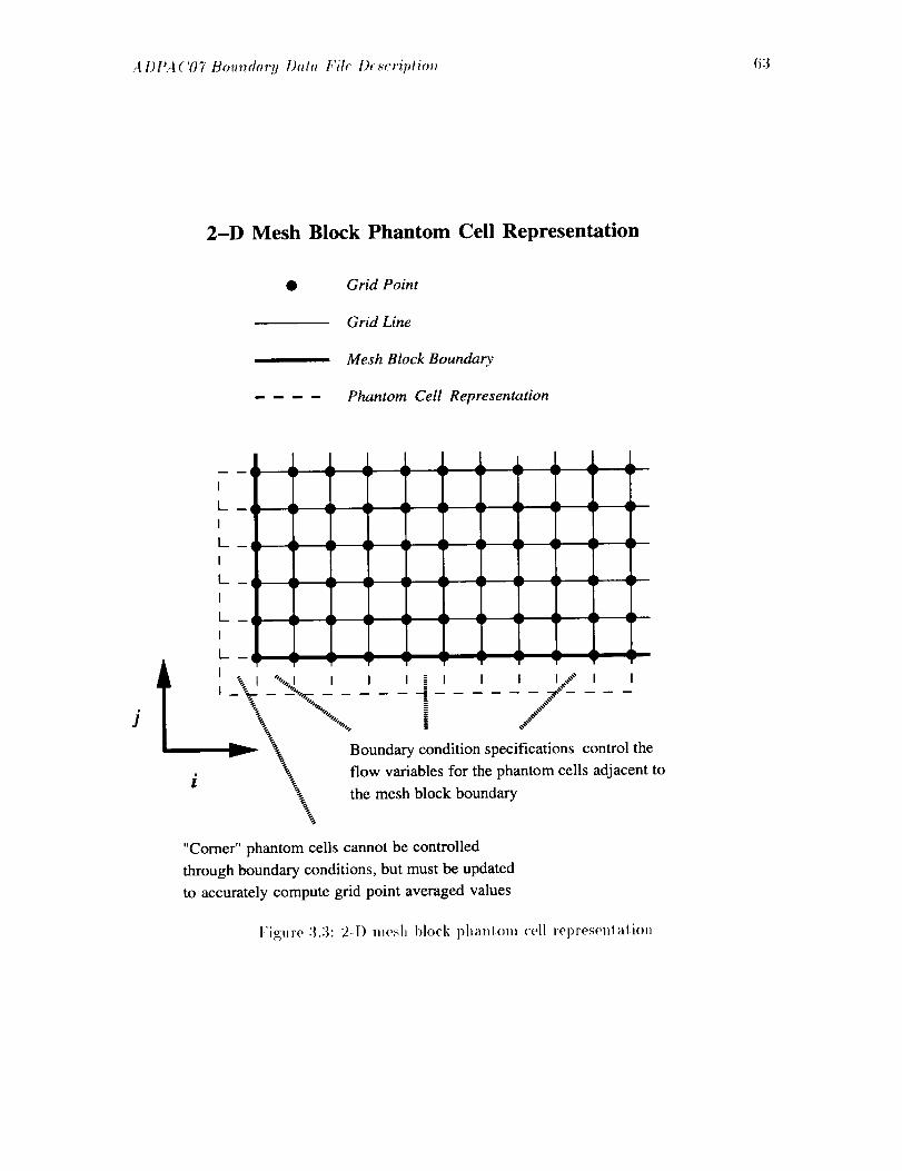
A DPA('07 Boun<lar_l Dat. File D<scriptio'l_ 63

2-D Mesh Block Phantom Cell Representation

Grid Point

Grid Line

Mesh Block Boundary

Phantom Cell Representation

• •v

I

L _ _: _:I

L_ ,, _: ::

I

L _ _,: _:

I

I

LI -- • •

lw •r •u _F

i ,_l ' %..I I I i -= I I I I_,,," i I

-_-_'.._ - - -4 - - - J- - -% _-, _,,,,,

\ Boundary condition specifications control the

\ flow variables for the phantom cells adjacent to

i _ the mesh block boundary

"Comer" phantom cells cannot be controlled

through boundary conditions, but must be updated

to accurately compute grid point averaged values

Figure 3.3: 2-I) mesh block phantom cell rel)resenlalioh

64 .4 DPA (i'07 Botmdary Dato Fil_ De,scriptio_

ADPAC 3-D Boundary Condition Specification

All block boundary conditions are specified as a grid-defined

"patch" on an i=constant, j=constant, or k=constant mesh face

Boundary condition "patch"

on a j=constant face

I

Boundary condition "patch"

on an i=constant face

Boundary condition "patch"

on a k=constant face

k

Patches may be internal to the mesh as well

Figure 3.-1:ADPA('07 3-I) boundary condition specifica,tion

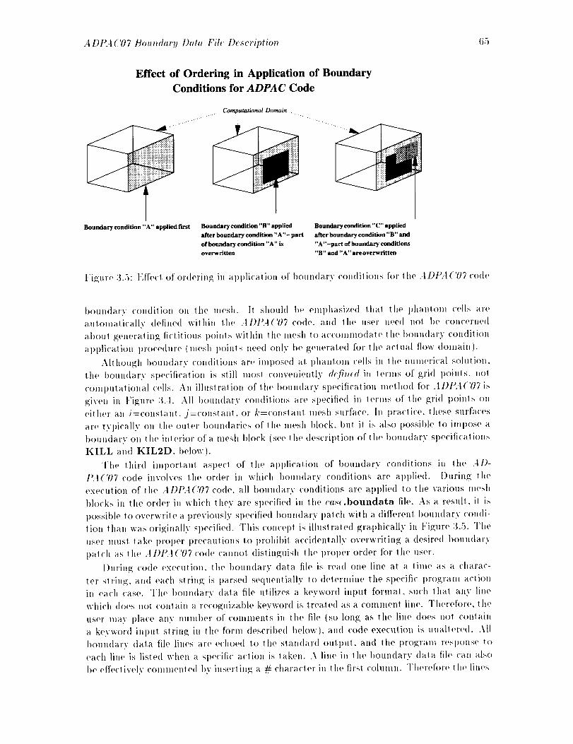
A DPA ('07 Botlndary Data File Description 65

Effect of Ordering in Application of Boundary

Conditions for ADPAC Code

Boundary condition "A" applied first Boundary condition "B" applied

after boundary condition "A"- part

of boundary condition "A" is

overwritten

Boundary condition "C" applied

after boundary condition"B" and

"A"-part of boundary conditions

"B" and "A" are overwritten

l:igure 3.5: t';ffect of ordering in a l)l)licalion of boundary con(litions for the ..tDt_l('07 code

boundary condition on the mesh. It should be eml)hasized )hal the phantom ('ells are

automalically delined within tile A1)PA('07 code. arm !he user need not be COl)('er)le(l

abou| generaling fictitious points within lhe mesh to accommodate the boundary condition

al)plication procedure (mesh poinls need only be generale<t for 1he actual flow domain).

Although boundary conditions are imposed a! phantom ('ells in lhe numerical solution.the boundary specification is still most conveniently de;fi_ed it) terms of gri<l l)oinls, no!

<'Oml)utaiional cells. An illustralion of the boundary specificatk)n metho<l for .tDP+I('07 is

given in Fi_;ure 3.t. All boun<larv conditions are specified in terms of the _ri<l poinls on

either an i=constant, j=c<mstant, or ],.:constant mesh surface, in pra<'lice, lhese surfaces

are typically on the outer boundaries of lhe mesh block, but it is also possible 1o impose a

t)oun<lary on the interior of a mesh block (see the <tescription of the boundary sl)e('ificalions

KILL and KIL2D, below).

The third imporlant asl)ec! of the a l)t)lication of boundary condilions in the All-

PAl'07 code involves the order in which 1)oundary condilions are applied. During the

execution of tit(' A DPA('07 co(h', all bout)(tary conditions are apl)lie(t to the various mesh

blocks in the order in which they are specified in '(he cas¢.boundata file. As a result, il is

possible to overwrite a previously specified boundary l)alch with a different boundary condi-

lion than was originally specified. This <'on('el)t is illuslrated grat)hically in t,'igure 3.5. The

user musl lake l>rol)er l)recautions to l>rohibil accidentally overwriting a desired l)oundary

l)atch as the .I I)I>A ('07 code cannot dislin_;uish llw proI)er order for lhe user.

During <'o(le execution, the I)oundary data file is rea(I one line at a time as a charac-

ter string, and each siring is t)arsed se<luentially to <lelermine the sl>ecifi(" l)rogram aclion

in each <'ase. The boundary (tara ill(, utilizes a keyword inpu! formal, such that any line

which does not conlain a recognizable keyword is treate(1 as a comment line. Therefore, the

user mav place any number of comments it) the file (so long as the line does not contain

a keyword inl)ut string in the form des(tilled below), and code execuIion is unallered. All

boundary <lata file lines are echoed to the start(lard output, and the program resl)onse t<>

ea<'h line is listed when a sl)e<'ifi(" action is lake)). A line in lhe boundary (lala file cat, also

I)e efl'ectivel.v ('ommenled I)v inserling a # character in the firsl column. Therefore the lines

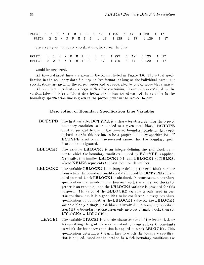
66 A DPAC07 Boundary Data File De._cription

PATCH 1 I K K P M I J I 17 1 129 1 17 1 129 1 17

PATCH 2 2 K K P M I J 1 17 1 129 1 17 I 129 1 17

are acceptable boundary specifications; however, the lines

#PATCH 1 1 K K P M I J 1 17 1 129 I 17 i 129 1 17

#PATCH 2 2 K K P M I J I 17 i 129 I 17 i 129 1 17

would be neglecled.

All keyword input lines are given ill the format listed in Figure 3.6. Tile actual sl)eci-

fication in the boundary data file may 1)e fi'ee format, as long as the individual parameter

specifications are given in the correct order and are separated by one or more blank spaces.

All boundary specificatiol_s begin with a line containing 19 variables as outlined by the

vertical labels in Figure 3.6. A description of the funclion of each of lhe variables in _he

boundary specification line is given in the proper or<ter in the seclion below:

Description of Boundary Specification Line Variables

BCTYPE

LBLOCK1

LBLOCK2

LFACE1

The first variable, BCTYPE, is a character string (lefining the tyl)e of

boundary condition to be applied to a given mesh block. BCTYPE

musl correspond to one of the reserved boundary condition keywords

defined later in this section to be a proper boundary sl)ecification. If

BCTYPE is not one of the reserved names, then the boundary speci-

fication line is ignored.

The variable LBLOCK1 is an integer defining the grid block uum-

bet to which the I)oundary condition implied by BCTYPE is applied.

Naturally, this implies LBLOCK1 21, and LBLOCK1 _< NBLKS,

where NBLKS represents the last, mesh block number.

The variable LBLOCK2 is an integer defining the grid blo('k number

fi'om which the boundary condition data implied by BCTYPE and at)-

plied to mesh block LBLOCK1 is obtained. In some cases, a, boundary

specification may involve more than one block (patching two blocks to-

gether is an example), and the LBLOCK2 variable is provided for this

purpose. The value of the LBLOCK2 variable is onh" used in cer-

tain routines, but it is a good idea to be consistent in every I)oundary

specification by dul)licating the LBLOCK1 value tbr the LBLOCK2

variable if only a single mesh block is involved in a boundary sl)ecifica-

tion (If the boundary sl)ecification only involves a single block, then set

LBLOCK2 = LBLOCK1).

The variable LFACE1 is a single character (one of the letters 1..l, or

K) specifying the grid plane (i=constaul, j=constant, or /,:=constant)

to which the boundary condition is applied in block LBLOCK1. This

sl)ecification determines the grid face to which the boundary specifica-

tion is applied, based on the method bv which boundary conditions aro

.4 DPA ('07 hlom_dar9 Data Fi# De.¢criptiol, 67

CASE.BOUNDATA FILE

Thisfile containscase-specificboundarydata information.All boundary

conditionapplicationsare representedby 1 ormore lines in thisfile.

A sample line is given in the highlightedregionbelow:

This is the keDvo_

_.,scribing the ty_ of I

bounda"/condition _o ]

beappfied t

This is the mesh block [

numberto which __ [_e boundarydata I

is apglied

This is the mesh block

number from which_7

boundarydata

isdi_'Ived

]'his indicates the

gridsurface (ij,k)

dataisappliedinbkx:k [

i

t

LBLOCKI

This indicates the ]I

grid surfacefi,j,k) Ifromwhich_

dataisdmv_ inblock

LBL(X'K2

B

CT

Y

P

E

LLLLLLLLLLMMNNMMNNBBFFDDSS1211112222

LLAAI I PPLLLLLLLLLLOOCCRREEI IIIII II II

C C E E 12 C C MMMMMMMMMM

KK12 12 12121212

12

[I I[ I

ThisthdicaL_thedirection

(+=P,-=M)alongtheLFACEI

coordinatewhichtravelstowards

theinterioroftheflow(awayfrom

thebo_dthgsurf_c)in mesh

blockIYlLOCKI

Thisindicatesttz di_-_on

(+=P.-=M) alongtheLFACE2

coordinatewhich_vcls towards

_c hiterior of the flow(awayfrom

tlteboundingsurface)inmesh

blockLBLOCK2

Throearctrigg_resvctwed

for slr-.ciduse in sotac

boondarycondidons(usually

the valuelJ,ofI(, whichindicates

the corre_cc oftlz eonrthmcs

inmesh block LBLOCK2 with the

tcraaz_ing(non LFACEI)coordinates

in mesh blockLBLOCKI

These are the bcgimng

andending radices for

the correspondingconrdiunte

directions in block

LBLOCKI from which

boundary da_ is applied

T'lzse arc the begimng

and e_thng indices for

the rematm'ngcoordinate

" directions in block

[,BLOCKIto which

boundary data is apptJed

This is the thdex in the

LDIR2 direclion for

boundary data inblock

LBLOCK2

Thisisthcindex inthe

LDIRIdirectionfor

boondarydatainblock

LBLOCKI

l,'igure 3.6:AI)t_A('07 boundary data file sl)ecifica,l, ion format

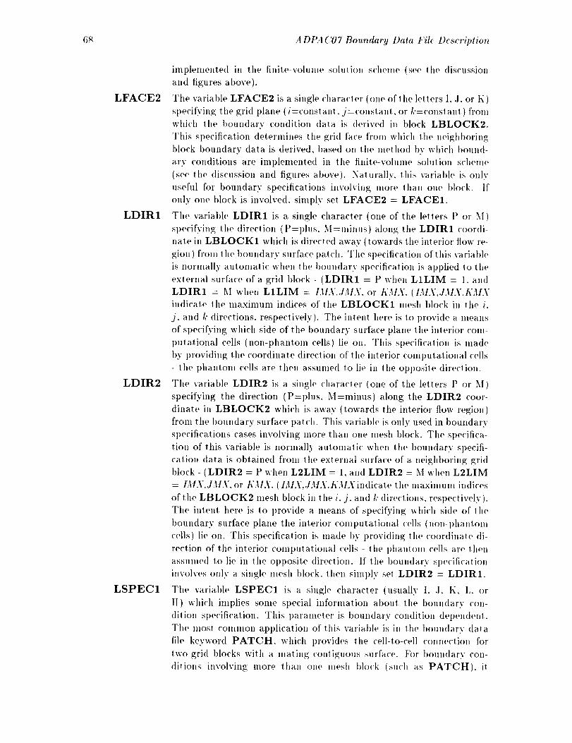
6g ADPA('07 Boundary Data Fi& Description

LFACE2

LDIR1

LDIR2

LSPEC1

implen,ente<l in tile finite-volume solution scheme (see the discussion

and figures above).

The variable LFACE2 is a single character (one of the letters I, 3, or K)

specifying the grid plane (/=constant. j=constant, or/,'=constan! ) fronl

which the boundary condition (tata is derived in block LBLOCK2.

This specification deternfines the grid face fi'om which the neighboring

block boundary data is derived, based on the method by which bound-

ar.v conditions are implemented in tile finite-volume solution scheme

(see the discussion and figures at)eve). Nalurally. this variable is only

useful for boundary specifications involving more than one block. If

only one block is involved, simply set LFACE2 = LFACE1.

The variable LDIR1 is a single character (one of the letlers t ) or M)

specifying the direction (P=plus, M=minus) along the LDIR1 coordi-

nate in LBLOCK1 which is dii'ected away (towards the interior flow re-

gion) fI'om the boundary surface patch. The specification of this variat)le

is normally automatic when the boundar.v specification is applied Io the

external surface of a. grid block - (LDIR1 = P when L1LIM = 1. and

LDIR1 = M when L1LIM = IMX.,IMX. or h'MX. (1MX,.IMX.KMXindicate the maxilnum indices of lhe LBLOCK1 mesh block in lhe i,

j. and /,' directions, resl)ectively). The intent here is to provide a means

of sl)ecifying which side of the boundary surface plane the inlerior con>

putational cells (non-phantom cells) lie on. This specitication is made

by providing the coordinate direction of the interior computational cells

- the phantont cells are then assumed to lie ill the opposite direclion.

The variable LDIR2 is a single characler (one of the letters P or M)

specifying the direction (P=plus, M=minus) along the LDIR2 coor-

dinate in LBLOCK2 which is away (towards the interior flow region)

from the boundary surface patch. Tiffs variat)le is only used in boundary

specifications cases involving more than one mesh block. The specifica-

tion of this variable is normally automatic when the boundary st)ecifi-

cation data is obtained from lhe external surface of a neighboring grid

block- (LDIR2 = P when L2LIM = 1, and LDIR2 = M when L2LIM

= IMX,JMX, or KMX. (IMX.dMX.h'MXindicate the maximum indices

of the LBLOCK2 Inesh block in the i, j, and/< directions, respectively).

The intent here is to provide a means of specifying which side of the

boundary surface plane the interior computational cells (non-phanton,

cells) lie on. This specification is made by providing the coordinate di-

rection of the interior computational cells - the phantom cells are lhen

assumed to lie in the opposite direction. If the boundary specification

involves only a single lnesh block, then simply sel LDIR2 = LDIR1.

The variable LSPEC1 is a single character (usually 1..I, K, L, or

H) which implies some special informatioll about the boundary con-

dition specification. This parameter is boundary condition dependent.

The most common apl)lication of this variable is in the boundary data

file keyword PATCH, which provides the cell-to-cell connection for

lwo grid blocks with a lnating contiguous surface. For boundary con-

ditions involving more thall o11(, nlesh 1)lock (such as PATCH). il

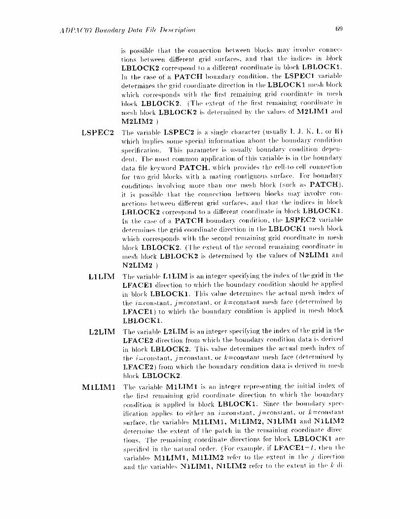
A DPA ('07 Boundaw Data File Descriptio,_ 69

LSPEC2

LILIM

L2LIM

MILIM1

is possible that the connection between blocks nlay involve connec-

tions between different grid surfaces, and that the indices in block

LBLOCK2 correspond to a different coordinate in block LBLOCK1.

In lhe case of a PATCH boundary condition, the LSPEC1 variable

delermines the grid coordixlate direction in the LBLOCK1 mesh block

which corresponds with the firsl remaining grid coordinat(' in mesh

block LBLOCK2. (The exlenl of Ill(' firsl remaining coordinate ill

mesh 1)lock LBLOCK2 is (lelermined by the vahles of M2LIM1 and

M2LIM2 )

The variable LSPEC2 is a single characte2" (usually I..I, K. L, or 1[)

which inlplies some special information al>ou! 112(' I)oundary condilion

spe<'ificalion. This i)al'anieter is usually boundary ('on(lilioll (lel)en-

dent. The lllOSl COlllll2<)I2 application of this variable is in the l)oundary

data file keywor<t PATCH. which provides the ('ell-t(>-cell ('olHleclion

for two grid blocks with a nlatinp,; ('ontiguous surface, t:or l)oun(lar.v

conditions involving more lhan one nlesh block (such as PATCH),

il is 1)ossil)le thal lhe connection t)eiween I)lo('ks nlav involve con-

neclions between diff(,rent grid surfaces, and lhat the in(lices in I)lock

LBLOCK2 correspond lo a (litferent ('oordinate in block LBLOCK1.

hi the ('as(' of a PATCH boun(lary condition, the LSPEC2 variable

(let ermines the grid coor(linate direclion in the LBLOCK1 nlesh block

which corresponds with the second remaining grid coor(linale in mesh

block LBLOCK2. (The extel2| o]' |lie second renlailiing coordinale in

nlesh block LBLOCK2 is delermined by tile values of N2LIM1 and

N2LIM2 )

The variable L1LIM is all inleger specifying lhe index of the grid in the

LFACE1 direction to whMl lhe boundary condition should be apl)lied

in block LBLOCK1. This value determines the aclual m(,sh index of

tile i=conslant, j=coliSlal21, or k=conslant mesh far(' (determined bv

LFACE1) to which lhe boundary condition is applied in mesh block

LBLOCK1.

The variable L2LIM is an integer specifying the in(lex of lhe _;rid in 112e

LFACE2 direction fronl which the boundary condition dala is derive(I

in block LBLOCK2. This value determines tile actual nlesh index of

the /=constant. j=constant, or /:--constalg mesh face (determined bv

LFACE2) fi'om which 112(' boundary condition dala is derive(I il2 mesh

block LBLOCK2.

The variable M1LIM1 is an integer rot)resenting the initial index of

the first remaining grid coordinale direction to whicll Ill(' boundary

('ondilion is apl)lie(I in block LBLOCK1. Since the boun(lary spec-

ificalion al)l)lies lo eilher an i=conslanl, j=constant, or L'=constanl

surface, tile variables MILIM1, M1LIM2, NILIM1 and N1LIM2

(telernfine the extent of 112o i)atch in tile remaining coor(tinale (lirec-

titres. The remaining coordinate directions for block LBLOCK1 are

specitied in 112(' natural order. (For example, if LFACEI=I. lh(,n 112o

va2"iables M1LIM1, M1LIM2 refer Io the extenl ill lh(' .] direclion

and Ill(' variat)les NILIM1, N1LIM2 refer to the exlenl in the 1,"(It-

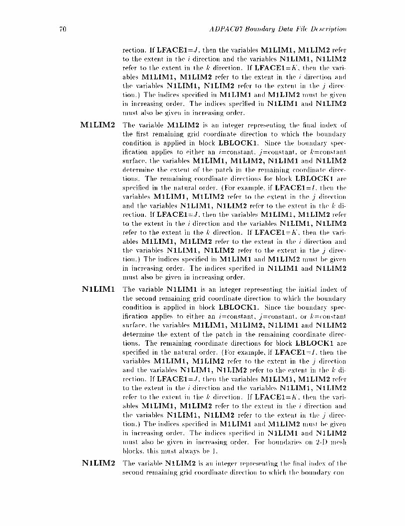
70 ADPAC07 Bouudarg Data File DescriptioT,

MILIM2

N1LIM1

N1LIM2

rection. If LFACEI=J. then tile variat)les M1LIM1, M1LIM2 refer

to the extent ill the i direction and the variables NILIMI_ NILIM2refer to the extent in the k direction. If LFACEI=A'. then tile vari-

ables M1LIM1, M1LIM2 refer to the extent in the i direction and

the variables NILIM1, NILIM2 refer to the extent in the j dire(':

tion.) The indices specified in MILIM1 and MILIM2 mus! be given

in increasing order. The indices specified in NILIM1 and N1LIM2

must also be given in increasing order.

The variable MILIM2 is an inleger representing the final index of

the first remaining grid coordinate direction to which the boun(larv

condition is applied in block LBLOCK1. Since the boundary st)ec-

ification al)plies to either an i=constan_, j=constant, or k=conslant

surface, the variables MILIM1, MILIM2, NILIM1 and NILIM2

determine tile extent of lhe patch in tile remaining coordinate direc-

tions. The remaining coordinate directions for block LBLOCK1 are

specified in the natural order. (For examt)le, if LFACEI=I. then ilL(,

variables MILIM1, MILIM2 refer to tlLe extent in the j direction

and the variables N1LIM1, N1LIM2 refer to the exlent in the k di-

rection. If LFACEI=J. then the variables MILIM1, MILIM2 refer

to the extent ill the i direction and the variables N1LIM1, NILIM2

refer to the extent in the k <lirection. If LFACEI=K. then the vari-

ables M1LIM1, M1LIM2 refer to the extent in the i direction and

the variables N1LIM1, NILIM2 refer to the extent in tile j <lirec-

tion.) The indices specified in MILIM1 and MILIM2 must be given

in increasing order. The indices specified in NILIM1 and N1LIM2

must also be given in increasing order.

The variable NILIM1 is an integer representing the initial index of

the second remaining grid coordinate direction to which the boulL(tary

condition is applied in block LBLOCK1. Since the boundary sl)ec-

ification applies to either an /=constant, j=constanl, or k=(-onstanl

surface, the variables MILIM1, MILIM2, NILIM1 and N1LIM2

deternfine tile extent of the patch in tile remaining coordinate direc-

tions. The remailfing coordinate direclions for block LBLOCK1 are

specified in the natural order. (For example, if LFACEI=I. then the

variables MILIM1, M1LIM2 refer to the extent in the j direction

and the variables N1LIM1, N1LIM2 refer to the extent in the k di-

rection. If LFACEI=.I. then the variables MILIM1, MILIM2 refer

to the exten! in the i direction and the variables NILIM1, N1LIM2refer to the extent in the k direction. If LFACEI=ff. th('n the vari-

ables MILIM1, M1LIM2 refer to the extent in the i direction and

the varial)les N1LIM1, NILIM2 refer to the exten! in ILL(,j direc-

tion.) The indices specified in M1LIM1 and MILIM2 must I)e given

in increasing order. TILe indices Sl)eCilie(l in NILIM1 and NILIM2

lUUSI also be given in increasing order, l%r I)oun(laries on 2-I) mesh

blocks, this mus! always be I.

The variable N1LIM2 is an integer rel)resenling the final index of 1he

second remaining grid coordinate direction to which the boundary con-

A DPA(Y)7 Boundary Data Fil< D_.+criptio_ 71

M2LIM1

M2LIM2

N2LIM1

dillon is applied in block LBLOCK1. Silwe the boundary specificalion

applies to either an/=constant, j=constant, or/,'=constanI surface, tile

variables M1LIM1, M1LIM2, NILIM1 and N1LIM2 determine

the extent of the patch in the remaining coordinale directions. The

remaining coordinate directions for' block LBLOCK1 are specified in

the natural order. (For example, if LFACEI=I. lhen the variables

M1LIM1, M1LIM2 refer Io the extent in the j direclion and Ill(,

variablos NILIM1, NILIM2 refer lo the extenl i,, (he t' direction.

If LFACEI=J, then the variables M1LIM1, MILIM2 refer to (he

extent ill lho i direction and lhe variables N1LIM1, NILIM2 refer

to the extent in tile k direction. If LFACEI=/(. lhen the variables

MILIM1, M1LIM2 refer lo the extenl in the i (lireclion and 1he

variables NILIM1, NILIM2 refer to (he exlen( in 111(' j direclion.)

The indices specified in M1LIM1 and MILIM2 must 1)e given in ill-

creasing order. The indices specified in NILIM1 and NILIM2 musl

also I>e given in increasing order. I%r l)oundaries on 2-1) mesh blo<'ks.

this must always be 2.

The varial)le M2LIM1 is an integer representing the initial index of the

grid <'oor<lizm.te direc( i<m i_) block LBLOCK2 corresl)on(ling _(>the fi)'sl

remaining coordinale in block LBLOCK1. For boundary condilions

involving more than one mesh block, i( is possible that )he connection

between blocks may involve connec(ions l>(,lween (lifferen( grid surfaces.

and )hal the i)1<]i<'es in bh)ck LBLOCK2 correspond ).o a differen! cool

dinale in block LBLOCK1. The variables MELIM1, M2LIM2 con-

tr<>] t))e i11dico,_ il1 _})e LSPECI directiol_ il) block LBLOCK2 which

corresl)ond 1o the indices deterlnined by MILIM1, MILIM2 in 1)lock

LBLOCKI. The user should hole thal i( is possible for M2LIM1

> M2LIM2 and N2LIM1 > N2LIM2 bul it is not l)ossil)le for

MILIM1 > MILIM2 and NILIM1 > NILIM2. If only a single

mesh block is i]rvolved in (Ire boundary sl>eciIicalion, set M2LIM1 =

MILIM1.

The variable M2LIM2 is an integer representing the final index of the

grid coordinale dir(,clion in block LBLOCK2 corresl>onding to the first

r'emaining coordinate in block LBLOCK1. For boundary conditions

h+volving more than one itLeSll 1)lock. it: is possible that the connection

belween blocks may involve connections between differen( grid surfaces.

and that t he indices irl block LBLOCK2 correspond )o a different coor-

dinate in block LBLOCK1. The variables M2LIM1, M2LIM2 con-

trol the indices in )he LSPEC1 direction in block LBLOCK2 which

correspond )o the indices determined bv MILIM1, MILIM2 in t)lock

LBLOCK1. The user should nolo that it is possible for M2LIM1

> M2LIM2 and N2LIM1 > N2LIM2 bu! i( is not l)ossible for

MILIM1 > M1LI/_I2 a t)d NILIM1 > NILIM2. If ot_ly a si)_gle

mesh block is involved in the boundary specification, set M2LIM2 =

M1LIM2.

The variable N2LIM1 is an inleger rel)resenting the initial index of

)he grid coordinate direction in block LBLOCK2 corresl)onding [o

72 A DPA ('07 Boundary Data File' De._eriptimt

tile second remaining coordinate ill block LBLOCK1. For bound-

ary conditions involving more than one mesh block, it is possible tha!

the connection between blocks may involve connections between dif-

ferent grid surfaces, and that the indices in block LBLOCK2 corre-

spond to a different coordinate in block LBLOCK1. The variables

N2LIM1, N2LIM2 control the indices in the LSPEC2 direclion

in block LBLOCK2 which corresl)ond to the indices determined t)v

N1LIM1, NILIM2 in block LBLOCK1. The user shouhl note that

it is possible for M2LIM1 > M2LIM2 and N2LIM1 > N2LIM2 bul

it is not possible for M1LIM1 > MILIM2 and NILIM1 > NILIM2.

If only a single mesh block is invoh, ed in the bonndary sl)ecification, sol

N2LIM1 = NILIM1. For t)oundary data on 2-1) mesh blocks, this

must always be 1.

N2LIM2 The variable N2LIM2 is an integer representing the final index of

the grid coordinate direction in block LBLOCK2 corresponding to

the second remaining coordinate in block LBLOCK1. For bound-

ary conditions involving lnore than one mesh block, i! is l)ossible lhal

the connection between blocks may involve connections between dif-

ferent grid surfaces, and that the indices in block LBLOCK2 corre-

Sl)ond to a differen! coordinate in block LBLOCK1. The variables

N2LIM1, N2LIM2 control the indices in the LSPEC2 direction

in block LBLOCK2 which correspond to the indices determined by

N1LIM1, N1LIM2 in block LBLOCK1. The user should hole thai

it is possible for M2LIM1 > M2LIM2 and N2LIM1 > N2LIM2 but

it is not possible for M1LIM1 > M1LIM2 and NILIM1 > NILIM2.

If only a single mesh block is involved in the boundary specificalion, sol

N2LIM2 = N1LIM2. For 1)oundary data on 2-1) mesh t)locks, 1his

musl always be 2.

Some boundary condition specificalions require additional data beyon(I thal incorpo-

rated in !he boundary specification line. In these cases, described in detail for the sl)ecific

boundary types laler in this Section. the additional data is included immedialely after the

boundary specification line.

A sample A DPA ('07 boundary dala file conlailfing several keywords ix lisled below.

Sample A DPA ('07 Boundary Data File

BLOCKDATA FOLLOWS : LABELS

B L L L L L L L L L L M M N N M M N N C

C B B F F D D S S 1 2 1 i I i 2 2 2 2 0

T L L A A I I P P L L L L L L L L L L M

Y 0 0 C C R R E E I I I I I I I I I I M

P C C E E I 2 C C M M M M M M M M M M E

E K K 1 2 1 2 1 2 1 2 1 2 1 2 N

1 2 T

#

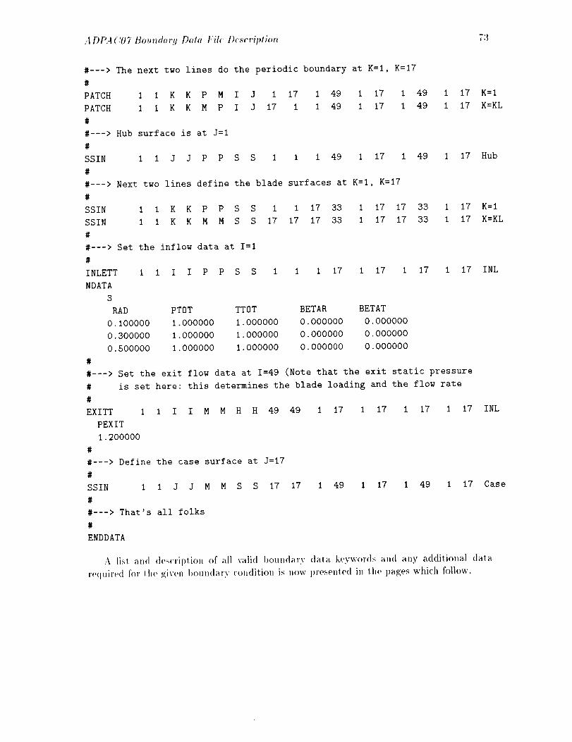
ADPA('07 Boundor!l Data Fil_ D_._criptior_ 7:]

#---> The next two lines do the periodic boundary at K=I, K=17

#

PATCH 1 1 K K P M I J i 17 i 49 1 17 i 49

PATCH I 1 K K M P I J 17 1 1 49 1 17 1 49

#

#---> Hub surface is at J=l

#

SSIN I I J J P P S S 1 1 1 49 1 17 1 49

#

#---> Next two lines define the blade surfaces at K=I, K=17

#

SSIN 1 I K K P P S S 1 1 17 33 1 17 17 38

SSIN 1 I K K M M S S 17 17 17 33 1 17 17 33

#

#---> Set the inflow data at I=1

#

INLETT i i I I P P S S 1 i 1 17 1 17 1 17

NDATA

3

RAD PTOT TTOT BETAR BETAT

0.I00000 1.000000 1.000000 0.000000 0.000000

0.300000 1.000000 1.000000 0.000000 0.000000

0.500000 1.000000 1.000000 0.000000 0.000000

#

#---> Set the exit flow data at I=49 (Note that the exit static pressure

# is set here: this determines the blade loading and the flow rate

#

EXITT i 1 I I M M H H 49 49

PEXIT

1.200000

#

#---> Define the case surface at J=17

#

SSIN 1 1 J J M M S S 17 17

#

#---> That's all folks

#

ENDDATA

i 17 K=I

I 17 K=KL

I 17 Hub

1 17 K=I

1 17 K=KL

i 17 INL

I 17 I 17 1 17 1 17 INL

I 49 1 17 1 49 i 17 Case

.:\ lisl and doscril)lion of all valid boundary data k¢,ywords and any additional data

re(luirt_(l for lh(, g4iv('n I)oun(lary condition is now ])rese]lto(I in the pages which follow.

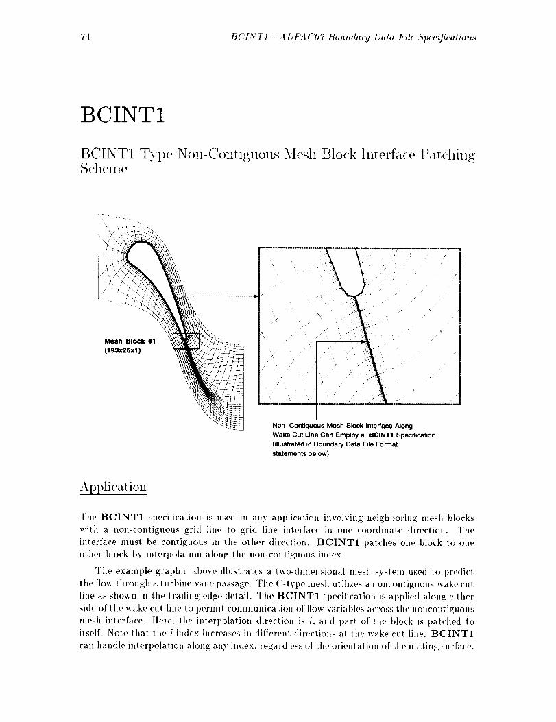
74 BCIN T1 - ,4 D PA ('07 Boundary Data Fil_ ,S'pec'ification._

BCINT1

BCINT1 Type Non-C, ontiguous _Iesh Block Interface Pat('hingS(helne

Mesh Block #1

( 193x25x I )

i!

i;

i

Non-Contiguous Mesh Block Interface Along

Wake Cut Line Can Employ a BCINT1 Specification

(illustrated in Boundary Data File Format

statements below)

Application

The BCINT1 specification is used in any application involving neighboring mesh blocks

with a non-contiguous gri(t line to grid line interface in one coordinate direction. The

interface must be contiguous in the other direction. BCINT1 patches one block to one

other block by interpolation along the non-contiguous index.

The example graphic above illustrates a two-dimensional mesh system used to l)redict

the flow through a turbine vane passage. The C-tyl)e mesh utilizes a noncontiguous wake ('ut

line as shown in the trailing edge detail. The BCINT1 specification is al)plied along either

side of the wake cut line to permit communication of flow variables across the noncontiguous

mesh interface. Here, the interpolation direction is i, and part of the block is t)atched to

itself. Note that the i index increases ill different directiolls a,! the wake ('ul line. BCINT1

can halMle interpolation along any index, regardless of the orient at ion of the mating surfa('e.

,4 DIL4 ('07 Boundary Data Fil< ,qp<c(fic'a.tio_._ - B('INT1 75

Boundary Data File Format

The boundary data ill(, sl)ecificalions for Ill(, mesh inlerface indicated in lhe illuslralive

graphic ]'or 1he BCINT1 boundary condilion are given below:

BCINTI I i J J P P L L i

IDIRNTI IDIRNT2

I I

ISHFTDR DSHIFT

2 0.0

BCINT1 1 1 J J P P L L 1

IDIRNT1 IDIRNT2

I I

ISHFTDR DSHIFT

2 0.0

1 1 33 1 2 193 177 1 2

1 177 193 1 2 33 1 1 2

Nole lhal a complete BCINT1 specification p_;enerallv requires lwo BCINT1 slalemenl

lines in lhe boundary dala file. In lhe example above, lhe firsl specilicalioll provi<h's the

in! ert>lock communi<'al ion for one side of tide ('-grid wake <'ul, while lhe second sl>ecilical ion

provides lhe communication for lhe other si<le of lhe (!-_;ri<l wake <'ul. I1 is a common error

Io un(lersl)ecify a BCINT1 boundary 1)y only providing a single line per inlerfa('e.

Des<'rii)tion

The BCINT1 I)oun<lary statemenl l)rovi(tes a means for block lo I)lock communicatiol_

for <'ases involving neighl)oring mesh I)oun<laries which share a common surface, but are

non-conliguous in one y_;rid index. BCINT1 can t)(, at)l)lie<l lo eilher slalionary or rolalin_

block interfaces, t>ul the resulls are t>hysically correcl only if both I>locks are r<>lalin_ at

lhe same speed. (The BCPRR specification should be use<l for cases with relalively ro-

l.a_in_ blocks.) A l)rOl>er BCINT1 boundary is sl>ecifie<l much like a PATCH I)oun(lars".

The LFACE1 and LFACE2 determine which faces are mated logelher. BCINT1 also

re(luires the specificatioll of additional information. The secon(I line in a BCINTM sl)eci-

ti('alion is a ('ommenl line. normally lal)eling lhe variables INTDIR1 and INTDIR2. The

third line defines tide varial)les INTDIR1 and INTDIR2 as either 1..1, or Ix', depending

on the <lireclion of interl)olatioll for the receiving; and sen<ling 1)locks, respectively. One

mesh restriction 1o hole is that BCINTM allows only one inlerpolation direction for each

side of lhe interface. The fourth line is a commenl line normally lal)eling the varial)les

ISHFTDR and DSHIFT. The fifth line defines the values for the variables ISHFTDR

and DSHIFT. These variabh,s provide a mechanism for shifting the I)oundarv in one of

the three <'oor(tinate directions (.r.y. z for (!artesian flows, or .r, r,O for cylindrical flows).

The value of ISHFTDR i(lelllifies the varial)le to I)e shifted (l-x, 2-y, 3-z for (!arlesian

and (l-.r. 2-r. 3-0 for cvlindri('al) and the value of DSHIFT is the increment t)y which tide

._<,dinfl I)oun(lary is shifte<l (normalized iDl the same 1harmer as tide mesh coordinates) 1o

male i<) lhe receiving I)oundary. BCINTM expects lhal lhe lwo sides o[' the iuterfa<'e lie

<m a common t)hysical surface, l)u| liD(' grid itself nDav not have l)olh si(les of the interfa('e

in the same l)hysica] location. The lll<)sl COIIIIIIOII llse for |his feature is a nonconliguous [)e-

riodic I)oun(lary for a single passage turt)oma<'hinery I)lade row sohnion. The ISHFTDR

76 BCINT1 - A DPAC07 Boundary Data File Sp_cification._

and DSHIFT variables age provided to allow the user to teml)orarily shift the l)hysical

location of the "sending" blocks to the "receiving" blocks physical location. For the case

of a noncontiguous periodic boundary in a 2-D turbine cascade, for example, ISHFTDR

would be 2 (shift in the y direction) and the amount of the shift, defined by DSHIFT would

be the circumferential spacing of the blade rows in mesh units. The blocks are assumed

to be contiguous in the remaining index. The M2LIM or N2LIM varial)les are specified

much as they would be for a PATCH specificalion. The excel)tion is that the number of

1)oints spanned by the limils in lhe direction of intert)olalion need not be equal.

The search routine which determines the interpolation stencil assumes that the maling

grid lines are piecewise linear apl)roximalions to the same curve ill the interpolation direc-

lion. A global search is performed for the proper mating cell of lhe first index. The closest

<'ell 1o the point of interest is taken as the mating cell. A localized search is performe<l for

the mating cells of the remaining points, The local search starts at the mating cell of the

I)rece<ling point and searches along the mating boundary until the mating cell containing

the new point is found. In the event that the matillg <'ell is not found before the upl)er

limit is reached in the mating block, the search continues fl'om the lower limit in lhe tnatilkg

t)lock. This implies two things: the physical domain of the inleri)olation mus! be the same

in lhe two blocks, and the domail, is assumed to t>e periodic if the search routine goes past

an endpoint.

Rest ri<'tiolls/Lilnitations

The BCINT1 boundary specification is restricted to mesh interfaces which lie on a common

surface(no significant overlap).

Generally, endpoints of the interpolated region in the two blocks should be coincident.

There is at least one exception to this rule based on the above description of the search

routine. In the case of concentric O-grids. the endpoints of the two blocks may be nlisa.ligned

as shown in the figure below. The interpolation routine will find the apI>ropriate stencil for

each point because the grids are periodic.

The A DPA (!07 COARSEN prograin cannot properly handle subdivision of mesh hound-

aries involving a BCINT1 or BCINTM specification.

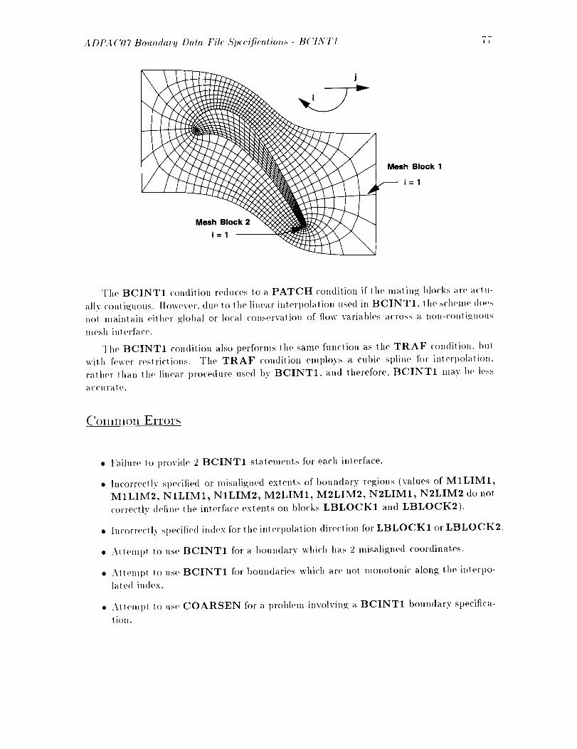
A DPA ('07 Boundary Data Fil( ,qp_ciJicatiot_.q - B('INT1 77

J

Mes.h Block 2

i=1

Mesh Block 1

i=1

Who BCINT1 c(mditiou reduces to a PATCH condition if tilt, maling; blot'ks are aclu-

ally ('ou(i_uous. ttowever, due (o tile linear in(erpola!ion used in BCINT1. _he st'henw does

not mainlain eilher global or local COllServation of flow variables across a non-conti_uous

mesh inlerface.

The BCINT1 rtmdition also perform._ the same function as the TRAF ('ondiliou. l)ul

wilh fewer restrirtious. The TRAF ron(lition employs a cubic spliue for interl)olatit)u.

rather (hau)he linear procedure used I)y BCINT1. and therefore. BCINT1 may be less

a('('lll'al o.

CollllllOll E 1TO1',¢-;

• Failure to provide 2 BCINT1 stalements for each iulerface.

• Incorrectly specified or misalipoled exleuts of boundary regions (values of MILIM1,

MILIM2, NILIM1, NILIM2, M2LIM1, M2LIM2, N2LIM1, N2LIM2 do not

correc(ly deiilw the interface extents ou blocks LBLOCK1 and LBLOCK2).

• Incorrectly specified index for (he interpolalion direclion for LBLOCK1 or LBLOCK2.

• Atteml)( to use BCINT1 for a bouudary which has 2 misaligned coordinates.

• Attempt lo use BCINTI for bouiMaries which are t)o( monotonic along the iuterpo-

lated index.

• All(,ml)t to u,_(' COARSEN for a problem involving a BCINT1 boundary sl)ecifica-

lion.

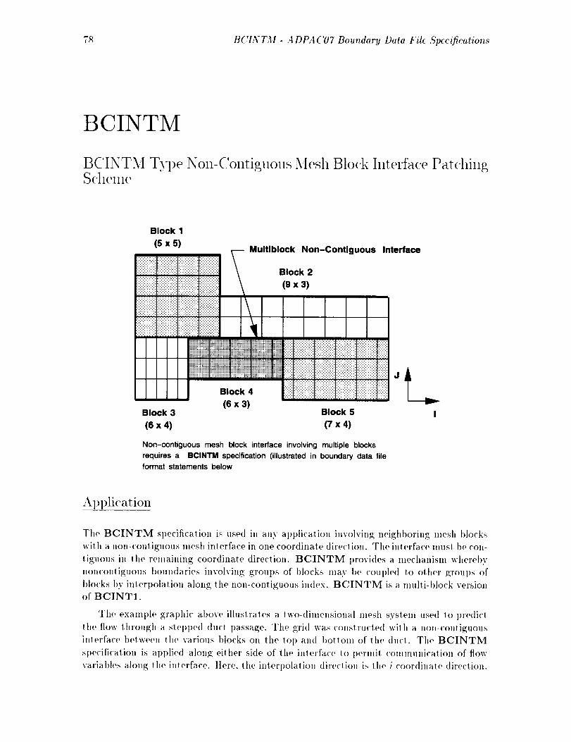
7_ BCINTM - ,4DPA C07 Boundary Data Fih Epecifications

BCINTM

BC'INTXl Type Non-Contiguous 5lesh Block Interface PatchingSchelne

Block 1

(s x s)

ii!i!i}i!i!iii!._i!iiiii!ili!i'!'il}iiiiiiiiii:!iiiiiiiiiiii:

iiiiiiiiiiiliiiiiiiiil iii':iIiiiiiiiiiiiiii;iiiii::i:::::iiiiV::iii:::!::!i!::[!i!::!::!::!::!i!:i!i!iii!i!i!i!iiiiiii!iiiiiiiiiiiiiiiiiiiiiiiiiiiii!i!i!iii!i!i'.'.'.'.'.'.'...',',',','.'...'.'.'.'.'.'.T.'.'.'.'.'.'.'

iiiililililiiiijiiiililiiiiiiiijiiiiiiiiiii:ii_iii!:!:!:!:!:?.:.:.:.:.:.:.'.'r .:.:.;.:.;.:.','.1.;.:.:.:.:.;1:.:.;.:.:.:.:.' ,

::::::::::::::::::::::::::::::::::::::::::::::::::::::::::::::

Multiblock Non-Contiguous Interface

Block 2(9x 3)

iii_ii_i_i_i_i_]_iiii_iiiiiiii_iiiiiiiiiiii_iiE_|:!ii:i_i:i:i:i:i:i:i:i_i:i:i:_:}:_:!:_!:!:!:!:!:!:!:iIi:i:i:i:i:i:i:i_i:_:_:|ili::i::[:iiiii::i::i::!ililii::i!i::iiiii::i]::i::i::iiiiiiiii]::i::i:.i::i::i::iii::l::iiiil

Block 4 ::_:::::::":::':':::':::::::+:::::::":::i:i:i:i:!::::::::::::::::::::i:ii:i:i:i:i:i:i:ii:i:i:}:}:i:!::!:i:

(6 x 3)Block 3 Block 5

(6 x 4) (7 x 4)

Non-contiguous mesh block interface involving multiple blocks

requires a BClNTM specification (illustrated in boundary data fileformat statements below

A1)l)lication

The BCINTM specification is used in any al)plication involving neighboring mesh blocks

will, a non-contiguous mesh interface in one coordinate direction. The interface mus! I)e con-

tiguous in the remaining coordinate direction. BCINTM provides a mechanism whereby

noncontiguous boundaries involving groups of blocks may I)e COul)led to other grout)s of

blocks bv illterpolalion along the non-contiguous index. BCINTM is a multi-block version

of BCINT1.

The example graphic above illustrates a two-dimensional mesh syslem used to l)redicl

the flow through a slel)t)ed dtl('t passage. The grid was ('onstrucled wit h a non-contiguous

inlerface between the various blocks on the to I) and l)ottoln of l he duct. The BCINTM

sl)e('iti('atiolJ is applied along either side of lhe interface to permit communicalion of flow

variables along the interface. I[ere. the inlert)olation direction is the i coordinale direclion.

.4 DPA ('07 Bo.ndary Data Fih ,qp(c_fication._ - BCL,YTM 79

B(mndarv Data File Format

The boundary data file specifications for the mesh interface indicated ill Ill(' illustrative

graphic for the BCINTM boundary condition are given below:

BCINTM i 3 J J P M I K I 4 I 5 I i I 5 I I

INTDIRI INTDIK2 - DIRECTION OF INTERPOLATION

I I

ISHFTDR DSHIFT

2 0.0

NBLINT2 - NUMBER OF LBLOCK2 BLOCKS

3

NBLDAT LFACE2 LDIR2 L2LIM M2LIMI M2LIM2 N2LIMI N2LIM2

3 J M 4 1 6 1 1

4 J M 3 1 6 I 1

5 J M 4 1 7 1 1

NBLINTI - NUMBER OF LBLOCKI BLOCKS

2

LBLKIRR LFACEI LDIRI LILIM MILIMI MILIM2 NILIMI NILIM2

1 J P 1 1 5 1 1

2 J P 1 1 9 1 1

BCINTM 3 I J J M P I K 4 1 1 5 I i I S i I

INTDIRI INTDIR2 - DIRECTION OF INTERPOLATION

I I

ISHFTDR DSHIFT

2 0.0

NBLINT2 - NUMBER OF LBLOCK2 BLOCKS

2

NBLDAT LFACE2 LDIR2 L2LIM M2LIMI M2LIM2 N2LIMI N2LIM2

1 J P 1 1 5 1 1

2 J P 1 1 9 1 1

NBLINT1 - NUMBER OF LBLOCKI BLOCKS

3

LBLKIRR LFACEI LDIRI LILIM MILIMI MILIM2 NILIMI NILIM2

3 J M 4 I 6 I I

4 J M 3 1 6 1 1

5 J M 4 l 7 I 1

Note lhal a ('omplete BCINTM sl)ecificalion generally requires lwo BCINTM slate-

merit lines in the 1)oundary data file. In the examt)le above, the firsl specification l)rovid('s

the inlerl)lo('k communicaliol_ for the upper blocks along lhe interface, while lhe second

st)e('ili('alion 1)rovi(les lhe ('ommunicaliol_ for lhe lower blocks al(mg th(' inlerface. I! is a

('ommon error to un(lersl)ecif.v a BCINTM boundary by onh, providing a singl(, line per

interface.

Des('riI)tioll

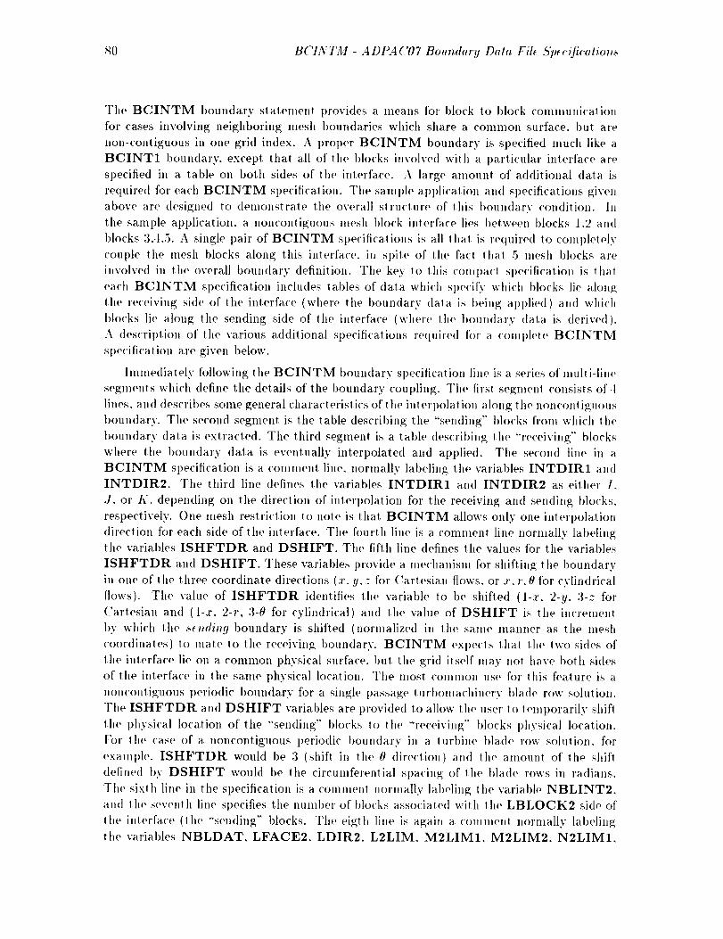
80 BCINTM- A DPAC07 Boundary Data Fil_: S)_¢cification._

The BCINTM boundary statement t)rovides a means tor block to block comnlunicaliol,

for cases involving neighboring mesh boundaries which share a common surface, but are

non-coutiguous in one grid index. A proper BCINTM boundary is specified much like a

BCINT1 boundary, except that all of the blocks involved wilh a l)articular interface are

specified in a table on both sides of the interface. A large amoun! of additiolJal data is

require(l for each BCINTM specification. The sample application aud sl)ecificatioJ,s gix'ell

above are desiglle(t to demonstrate the overall structure of this t)oul,(tary conditioll, hi

the sample application, a noncouliguous mesh block illterface lies between blocks 1.2 a_(l

I)locks 3.4.5. A single pair of BCINTM st)e('ifications is all thal is re(luire(I to coult)lelely

couple the mesh blocks along this iHterface, ill spite of the fac! tha! 5 mesh blocks are

involved in the overall boundary definitiou. The key to this compacl Sl)(,cificalioil is lha_

each BCINTM specification includes tal)les of data which specif)" which blocks lie alollg

the receiviug side of the interface (where the boundary (lala is t)eiug applied) all(I which

blocks lie a lonp_; the sending side of _he interface (where lhe t)ou1_dary (lata is derived).

A descriptioll of the various additional specifi('ations required for a complete BCINTM

Sl)ecificatioll are given below.

hnnlediately following the BCINTM boundary specilicatioH line is a series of multi-lilm

segments which define the details of the boundary coupling. The fit's! segmenl collsists of .1

lines, and descril)es some general characteristics of the interpolatioH along the non('oHtiguoIJs

boundary. The second segment is the tal)le describing the "seu(ling" blocks from which lhe

boundary data is extracted. The third segment is a table (lescrit)illg the "'receiviHg'" blocks

where the boundary data is eventually interpolated and applied. The second line in a

BCINTM specification is a comlnent lille, normally tal)elillg the variables INTDIR1 and

INTDIR2. The third line defines the variables INTDIR1 a ll(I INTDIR2 as either I.

J. or K. depeuding on the directioll of interpolatiol_ for the receiving an(I seudiug [)locks.

respectively. One mesh restriction to note is that BCINTM allows only one inlerl)olation

direclion for each side of the interface. The fourth line is a comlneut line l_ormally labeling

the variables ISHFTDR and DSHIFT. The fifth line defines the values for the variat)les

ISHFTDR and DSHIFT. These variat)les provide a mechaHism for shifti_g the 1)ouudary

in one of _he three coordinate directious (x, y. z for (_artesia_, flows, or x. r. 0 for cylindrical

flows). The vahle of ISHFTDR identifies the variable to be shifted (l-x, 2-y. 3-z for

(_artesian and (l-x. 2-r, 3-0 for cylindrical) and the value of DSHIFT is the in('remenl

by which the ._nding boundary is shifted (normalized in the same manner as the mesh

coordinates) to mate to the receiving boundary. BCINTM expects thai the two sides of

the interface lie on a common physical surface, but the grid itself may _ot have both si(les

of the interface in the same physical location. The most common use for this feature is a

noucontiguous l)eriodic boundary for a siugle passage _url)omachiuery 1)lade row solution.

The ISHFTDR a_(l DSHIFT variables are 1)rovided to allow lhe user to leml)orarily shift

the 1)hysi('al location of the "'seudiug" blocks to the "receiving" blocks physical locatiot_.

[br the case of a noncontiguous periodic boundary in a turbine blade row solution, for

example. ISHFTDR would 1)e 3 (shift in _he 0 directio_) at_(t the amount of the shift

(tefi_e(l I)y DSHIFT would I)e the circumferential spacing of the blade rows i_ radia_s.

The sixth line hi the specificatio_ is a co_umenl normally ]al)eli_p_; the variable NBLINT2.

and the seventh line specifies the uuml)er of blocks associate(I with the LBLOCK2 side of

the interface (the "'sending" blocks. The eigth line is agait_ a ('emmet: _lormally labeling

the varial)les NBLDAT. LFACE2. LDIR2. L2LIM. M2LIM1, M2LIM2. N2LIM1.

A DPA ('07 Boundary Daln Fih ,_'p:r'ificolions - B('INTM Sl

and N2LIM2. The next NBLINT2 lines define 1.11otable containing l.he limits, dire(lions

and faces for each of lhe LBLOCK2 blocks. For each block in this tabh,. LFACE2 detines

the coordinate face upon which the inlerface lies 1, J, or K), and LDIR2 deIines the

direction (P for plus. or M for minus) along the LFACE2 coordinale which Iravels away

fi'om lhe bounding surface (see Section :1.7 tbr more details). L2LIM defines lhe value

of lhe LFACE2 ('oor(li_ato upon which the surface is located, and M2LIM1. M2LIM2.

and N2LIM1, and N2LIM2 (leIine tiw extenl of liw remaining coordinales for each of

the NBLINT2 bh)cks in !hell" "natural" order (again see Seelion 3.7 for more details).

Following lit(' lal>le for the LBLOCK2 side of the interface, lh('ve is a commment line

normally labeling lhe variable NBLINT1. followed I>v a line spe<'if_:ing the number o[" I>locks

on lhe LBLOCK1 side oflhe interface. Nexl a COlnmenl line labeling lhe varial)les L1LIM,

MILIM1. MILIM2. NILIM1. and NILIM2 is pgiven. Finally. a table ('onsisting of

NBLINT1 lines defining the LBLOCK1 side ("receiving" blocks) informalion similar 1o

lhe LBLOCK2 ("sen(line;" blocks) table is specified.

BCINTM ('reales a sin_;le inlerl)olation stencil fi'om all of _he blo<'ks in the LBLOCK2

tal)h'. This slencil must I)e monotonic in the INTDIR2 direclion. Thus. lhe blocks in lhe

LBLOCK2 musl be specified in the order they occur l)hysically, and lhe limils musl be

specified so thai they form a continous line. The block mlml)ers and extents i(lenlilied in

the first line of the BCINTM sl)e('ifica_(ion shouhl match the tits! emry in each of the

respective LBLOCK tables.

.ks wit h BCINT1. lit(' search routine which (lelermines lhe inlerpolalion sl('n('il assumes

'(hal lhe mating _ri(t lines are l)iecewise linear approximations Io lhe same curve in lhe

interpolation <lirection. A global search is l)erh)rmed for the l)rot>er matitJ_ cell of the tirsl

index. The ('losest cell to the point of interest is taken a,s the mating cell. A localized

search is performe<l [br the mating ('ells of the remaining points. The local search slarts al

[he maling cell oflhe l)recedillg t>oin! and searches along the matinp4 t>oull<lary unlil lhe

mating cell containing !he new poin! ix found. In lhe evelll thal the maling cell is not found

I)efore !he ul>per limi! is reache<l in lhe mating 1)lo('k, !he search continues from !he h)wer

limi! in the matinN block. This implies tw<> things: the physical domain of the inlerl)olation

must be lhe same in the two blocks, and the domain ix assumed to l>e perle(lie if'_he search

routine goes pax| an en(ll)oint.

Restrictions/Limitations

The BCINTM l>oun(larv specification is rextricte<t to mesh interfaces which lie on a com-

mon xurfa('e (no significan! overlap). Generally. endpoints of the interpolated region in 'the

two bh)cks should I)e ('oincidenl. As wilh BCINT1. there is at least one exception to this

rule baxe([ <>n the above <h'scril)tion of the search routine. In the ('axe of concentric O-grids,

the e,dl)Oints of the !we 1)k)cks may be misaligned (see the BCINT1 description for (le-

tails). The in! erl)olat ion routine will tind! he approl)riate st encil for each point because !he

gri<ls are perle(lie.

The .4 DP.t ('07 COARSEN program cannot properly handle subdivision of mesh I>oun(t-

aries involving a BCINT1 or BCINTM Sl)ecification. A kvpical fan re,or was analyzed

using lhe BCINTM boun<lary ('o_(lilion al _he interface l)etween the lip clearance gri(t and

lhe neighboring ()-lyl)e grid. The tigure I)elow shows l he non-conliguous inlerface I)elween

_2 BCLVTM- A DPAC07 Boundary Data Fil_ ,S)_¢e_ficatio1,s

the two grid blocks, and the corresponding predicted static pressure contours. The solulion' lwas run in parallel on an n( (BE 2 comt)uter.

BCINTM Boundary Condition Results

No_-ContJguous Boundary in Tip Clmrlmce Region

Mesh

StsHc ISrossurl

Tile BCINTM condition reduces to a PATCH condition if lhe mating blocks are

actually contiguous. However. due 1o the linear interpolation used in BCINTM, the

scheme does not maintain either global or local conservation of flow variables across a

non-contiguous mesh interface.

The BCINTM condition is the only non-contiguous patching routine for multiple

blocks. The BCINTM condition will run in either serial or parallel ADPA('07 cah'u-lations.

CollllllOll Errors

• Failure to provide 2 BCINTM statements for each interface.

• Incorrectly specified or misaligned extents of boundary regions (values of M1LIM1,

MILIM2, NILIM1, NILIM2, M2LIM1, M2LIM2, N2LIM1, N2LIM2 do not

correctly define the interface extents on blocks LBLOCK1 and LBLOCK2).

• Incorrectly specified index for the interpolation direction for LBLOCK1 or LBLOCK2.

• Attempt to use BCINTM for a boundary which has 2 misaligned coordinates.

• Attempt to use BCINTM for boundaries which are not monotonic along the illter-

polaled index.

.4 DPA ('07 Boundary Data Fil( S'pce(fieation._ - B(TNI_AI _:_

• Incorrect ordering of the LBLOCK2 table of data.

• At teml)t to use BCINTM tb," interfaces with multiple interl)olation directions on the

same side of tile inlerface.

• A1 lemI)t to use BCINTM for iKllerfac('s with multiple LFACE or LDIR requirement s

in the LBLOCK1 table of (lala.

• .\llemt)l to use COARSEN for a l)rol)lem involvin_ a BCINTM I)oulldary st)(wifi-

('atioH.

84 BCPRM- Botmdory Data Fil¢ ,S'peeifl'eatiol_._

BCPRM

Boundary Condition Procedure tbr Patched Belativelv Rotating).Iesh Blocks with Multil)le S1)e(,ifications

Mesh Block #2

(81x6x7)

•i_ _ Mesh Block #5

(81 x6x7)

Mesh Block #4

_ (81x6x7)tl

, _ Mesh Block #3(81 x6xT)\

Relatively Notating Mesh Block Interface Between

Grids in Adjacent Blade Rows Can Employ a BCPRM Specification

(illustrated in Boundary Data File Formatstatements below)

Mesh Block #1

(81x6x7)

Application

The BCPRM specificatioll is used in al)plication involving_; lmighborillg relatively rotating

mesh I)locks, such as in rotor/slator interaction problems.

Boundary Data File Forlnat"

The boundary data file specifications for the mesh interface indicated in the illustrative

graphic for the BCPRM boundary condition and a simple outline of the mesh tolmgraphy

are given below. Note that blocks 1 and 2 require multiple BCPRM entries in lhe data

tables due to the location of the O-grid cut line. The topogral)hy below depicts a multiple

passage 3-D O-grid system ['or a turbine stage.

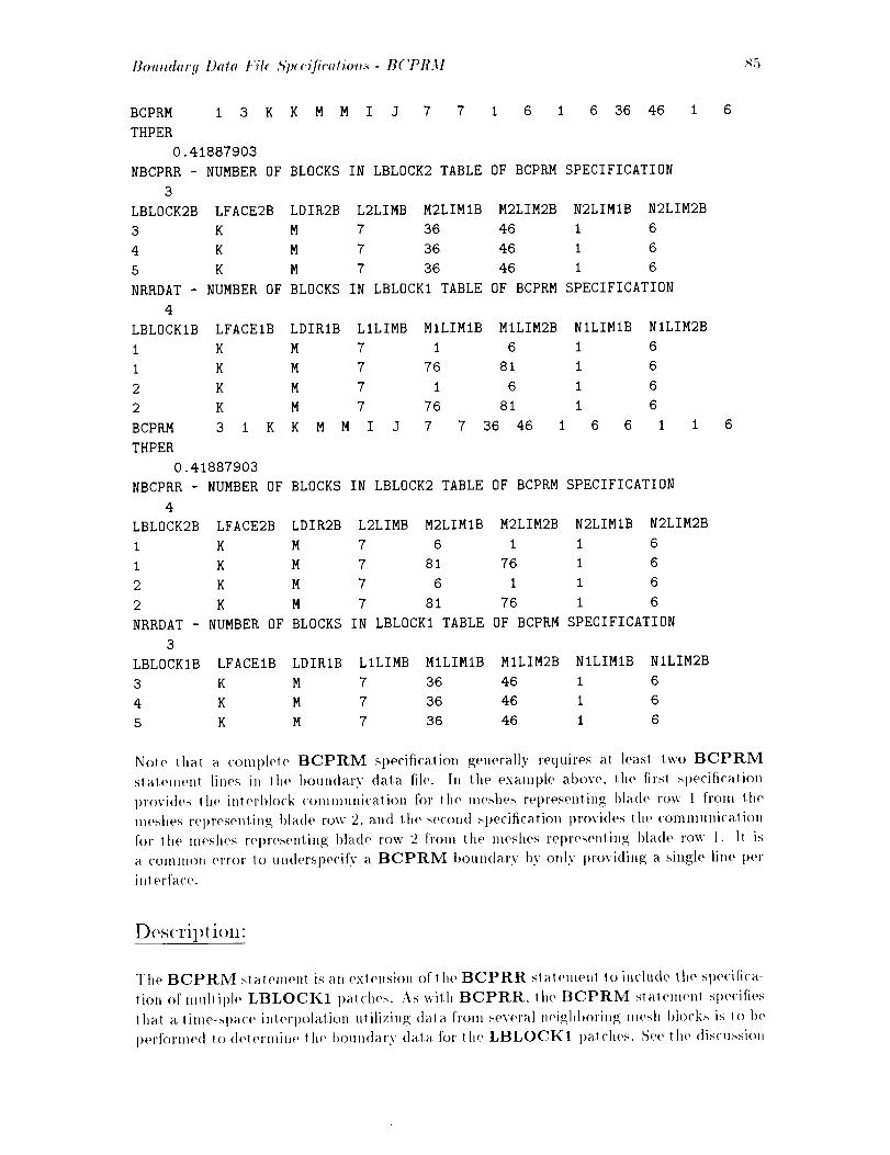
Boundary Data Fil_ ,S)_<clTiration._"- B('PRM S5

BCPRM 1 3 K

THPER

0.41887903

NBCPRR - NUMBER OF

K M M I J 7 7 1 6 1 6 36 46 I 6

BLOCKS IN LBLOCK2 TABLE OF BCPRM SPECIFICATION

3

LBLOCK2B LFACE2B LDIR2B L2LIMB M2LIMIB M2LIM2B N2LIMIB N2LIM2B

3 K M 7 36 46 1 6

4 K M 7 36 46 1 6

5 K M 7 36 46 I 6

NRRDAT - NUMBER OF BLOCKS IN LBLOCKI TABLE OF BCPRM SPECIFICATION

4

LBLOCKIB LFACEIB LDIRIB LILIMB MILIMIB MILIM2B NILIMIB NILIM2B

1 K M 7 1 6 1 6

1 K M 7 76 81 1 6

2 K M 7 1 6 1 6

2 K M 7 76 81 1 6

BCPRM 3 1 K K M M I J 7 7 36 46 1 6 6 1 I

THPER

0.41887903

NBCPRR - NUMBER OF BLOCKS IN LBLOCK2 TABLE OF BCPRM SPECIFICATION

4

LBLOCK2B LFACE2B LDIR2B L2LIMB M2LIMIB M2LIM2B N2LIMIB N2LIM2B

1 K M 7 6 1 1 6

1 K M 7 81 76 1 6

2 K M 7 6 1 1 6

2 K M 7 81 76 i 6

NRRDAT - NUMBER OF BLOCKS IN LBLOCKI TABLE OF BCPRM SPECIFICATION

3

LBLOCKIB LFACEIB LDIRIB LILIMB MILIMIB MILIM2B NILIMIB NILIM2B

3 K M 7 36 46 1 6

4 K M 7 36 46 1 6

5 K M 7 36 46 1 6

Note that a cotnplete BCPRM specification generally requires at leas! two BCPRM

sta.tenmnt lines in tile boundary data file. Ill the example above, the fil's| Slm('ificalion

provides lhe inlerl)lo<'k communicalion for lhe meshes representing blade row 1 from lhe

meshes represeming bla<le row 2. and tile secon<l specification provides the communi<'ation

for Ill(, ineshes representing I>lade row 2 from tile meshes representing bla<le row l. It is

a common error 1o underspe<'ify a BCPRM boundary by only providing a single line per

int efface.

Des<'ril>tion:

The BCPRM statement is an exlension of the BCPRR slatemenl to include the spe('ifica-

lion o[" [nulliple LBLOCK1 [)alches. :ks wilh BCPRR, lhe BCPRM stalemenl specifies

thai a time-space inlel'polalion utilizing data from several neighboring mesh blocks is to be

performed Io (]elernline the boundary data for tile LBLOCK1 l)al('hes. See lhe discussion

86 BCPRM- Boundary Data Fi& Specifications

of BCPRR for details about specifying the LBLOCK2 table of data, and restrictions

on the use of BCPRM. BCPRM differs from BCPRR only ill the following way: an

additional table of values allows multiple LBLOCK1 patches to be specified. One advan-

tage of BCPRM is clearly visible in the above example: only two boundary specifications

are required to patch the two blade rows together, compared to seven specifications using

BCPRR. Another, less obvious advantage is that BCPRM executes much faster than

BCPRR in a parallel colnputing environment. Ally BCPRM specification can be equally

represented as a series of BCPRR sl)ecifications. The additional table of data associated

wilh tile LBLOCK1 patches in a BCPRM statement is essentially the same as the table

for the LBLOCK2 patches (see the description of BCPRR for additional details. A com-

ment line is followed by a line containing the lmmber of patches in the LBLOCK1 row.

Another comment line is followed by the specification of the limits on each LBLOCK1

1)atch. One restriction on the use of BCPRM is that all of the LBLOCK1 patches must

share a <'olmnon LFACE and LDIR. This requirement can be met by the use of multiple

BCPRM or BCPRR sl)ecifications.

I! should be noted that B('PRM is limited to silnilarlv oriented row 1 blocks. In t)artic-

ular, the face and direction of all blocks ill row 1 are, taken to be the same as those specified

for LBL0(!KI. B(!PRR may be used in cases requiring more generality.

BCPRM has been successfully applied to a compressor stage with H-type grids and to

a turbine stage using O-type grids. The results were verifie(l to be the same as if multiplecalls to BCPRR were used.

The significance of B('PRM is not in new capability, but ill performance. Obviously, the

I)enefits of B(:PRM are extremely problem a,nd machine dependenl, but a small turboshafl

compressor test case (36 })locks,-1 blade rows, 2,000,000 mesh points) serves as an example.

The use of BCPRM instead of BCPRR ill a line grid calculation resulted in a,n estimated

factor of 1.5 improvement in total CPU time on the LACE cluster of workstations (without

the ALLNODE switch). With the ALLNODE swit('h, the improvement was on the order

of 20</:,, which is still significant. The ALLNODE switch is a special hardware device to

enable low latency communications betweell IBM RS6000 workstations in a cluster. This

means that overhead from B(:PRR comnmnications was taking a,t least 1/3 of the total run

time per iteration when the ALLNODE switch was not used. This is t)robably a worsl-case

scenario for BCPRR because of the large number of blocks in each airfoil row, but it is

typical of multistage compressor simulations.

Restrictions/Limitations

The BCPRM t)oundary sl)ecification is restricted to mesh interfaces which lie on a cmmnon

surface (no significant overlap), and have common axial and radial mesh coordinates. The

mesh lnusl salisfv the coor(linate restrictions listed in the table above. The LBLOCK1

table of l)atches must share a common face and direction as note(1 al)ove. The BCPRM

l)ro('edure is only apl)licable to 3-D mesh systems.

Co111111OllErrors

Boundory Data File 5'p(c(fications- BCPRM S7

Time dependent patch condition for multiple relatively rotating blocks

(LBLOCK2 row values are interpolated into phantom cells of LBLOCK1 row)

/,'

BCPRM 1 5 I I M P J K 49 1 1 31 1 31 1 31 1 31

PERIODIC SPACING

1.57079637

NBCPRR - NUMBER OF BLOCKS IN ROW 2 (LBLOCK2 ROW)

9

NRRDAT

5

6

7

8

9

10

11

12

13

- RELATIVELY ROTATING BLOCK NUMBERS

P 1 1 31 1 31

P 1 1 31 1 31

P 1 1 31 1 31

P 1 1 31 1 31

P 1 1 31 1 31

P 1 1 31 1 31

P 1 1 31 1 31

P 1 1 31 1 31

P 1 1 31 1 31

IN ROW 1 (LBLOCK1 ROW)NUMBL1 - NUMBER OF BLOCKS

4

BLOCKS IN LBLOCK1 BLADE ROW

1 49 1 31

2 49 1 31

3 49 1 31

4 49 1 31

block# Ilim mliml mlim2

1 31

1 31

1 31

1 31

j.

f

.f'-...

nliml nlim2 ,_

5LBLOCK1 rows LBLOCK2 row

BCPRM is similar to BCPRR except that multiple Row 1 blocks are specified. This

condition is more efficient than BCPRR in parallel, and reduces the length of the

casename.boundata file. BCPRM requires fewer interprocessor messages than

BCPRR, but total amount of data passed is unchanged. BCPRRM is limited to

patches involving similarly oriented Row 1 blocks.

t.'igure 3.7: Boundary condition B( IPI{ .XI providos an allernale method of t)atching relatively

rotating blocks in a lime-dependent calculation.

8_ BCPRM- Boundary Data f'ih Hpecification._

* Failure to provide 2 BCPRM statements for each interface

• Incorrectly specified o1" misaligned extents of boundary regions {values of M1LIM1,

M1LIM2, N1LIM1, N1LIM2, M2LIM1B, M2LIM2B, N2LIM1B, N2LIM2B

do not, correctly define the interface extents on blocks LBLOCK1 and LBLOCK2B)

• Attelnpl to use BCPRM on a 2-D mesh ])lock.

• Alteml)l to use BCPRM at an interface between lwo ('arlesian solution lneshes.

• Meshes do nol satisfy coordinate restrictions listed above.

• Meshes have dissimilar axial and radial coordinates al the interface.

• Neighboring blade row 1 segments not listed in increasing theta coordinate.

* Application of BCPRM to mesh interfaces which do not share a common surface, or

which have excess overlap.

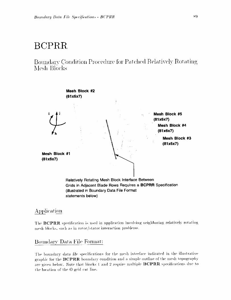
Bolmdary Dota Fih £'pec(ficatio_._- BCPRR _.)

BCPRR

Boun(larv Condition Pro(edure for Patched IRelativelv 1Rotatingl_lesh Blocks

Mesh Block #2

(81 x6x7)

1

Mesh Block #1

(81 x6x7)

\

Relatively Rotating Mesh Block Interface Between

Grids in Adjacent Blade Rows Requires a BCPRR Specification

(illustrated in Boundary Data File Format

statements below)

Mesh Block #5

(81x6x7)

Mesh Block #4

(81 x6x7)

Mesh Block #3

(81x6x7)

Application

The BCPRR spe('ificalio,i is used in application involving neighboring relatively rolating

m(,sh blocks, sudl as in rolor/slator interaction problems.

Boundary Data File Format:

The boundary data file specifications for the mesh interface indicaled in lhe illustralive

graphic for the BCPRR boun<larv condilion and a simple oulline of lhe mesh topogral>hy

are given below. Nole lhal I)locks 1 and 2 require multiple BCPRR spe('ili<'alions due Io

lhe localion of lhe O-grid cul line.

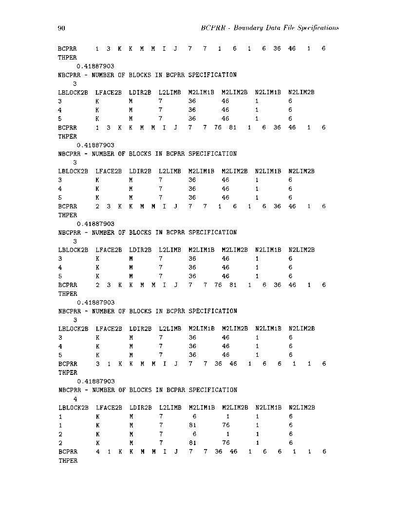
90 BCPRR - Boundary Dtda File Specification_

3

4

5

BCPRR

THPER

BCPRR I 3 K K M M I J 7 7 i 6 I 6 36 46 I 6

THPER

0.41887903

NBCPRR - NUMBER OF BLOCKS IN BCPRR SPECIFICATION

3

LBLOCK2B LFACE2B LDIR2B L2LIMB M2LIMIB M2LIM2B N2LIMIB N2LIM2B

K M 7 36 46 1 6

K M 7 36 46 1 6

K M 7 36 46 1 6

I 3 K K M M I J 7 7 76 81 1 6 36 46 1 6

3

4

5

BCPRR

THPER

0.41887903

NBCPRR - NUMBER OF BLOCKS IN BCPRR SPECIFICATION

3

LBLOCK2B LFACE2B LDIR2B L2LIMB M2LIMIB M2LIM2B N2LIMIB N2LIM2B

3 K M 7 36 46 I 6

4 K M 7 36 46 i 6

5 K M 7 36 46 i 6

BCPRR 2 3 K K M M I J 7 7 1 6 1 6 36 46 1 6

THPER

0.41887903

NBCPRR - NUMBER OF BLOCKS IN BCPRR SPECIFICATION

3

LBLOCK2B LFACE2B LDIR2B L2LIMB M2LIMIB M2LIM2B N2LIMIB N2LIM2B

K M 7 36 46 i 6

K M 7 36 46 I 6

K M 7 36 46 i 6

2 3 K K M M I J 7 7 76 81 I 6 36 46 i 6

3

4

5

BCPRR

THPER

0.41887903

NBCPRR - NUMBER OF BLOCKS IN BCPRR SPECIFICATION

3

LBLOCK2B LFACE2B LDIR2B L2LIMB M2LIMIB M2LIM2B N2LIMIB N2LIM2B

K M 7 36 46 I 6

K M 7 36 46 1 6

K M 7 36 46 1 6

3 1 K K M M I J 7 7 36 46 1 6 6 1 1 6

1 K M 7 6 1 1 6

1 K M 7 81 76 1 6

2 K M 7 6 1 1 6

2 K M 7 81 76 1 6

BCPRR 4 1 K K M M I J 7 7 36 46 1 6 6 1

THPER

1 6

0.41887903

NBCPRR - NUMBER OF BLOCKS IN BCPRR SPECIFICATION

4

LBLOCK2B LFACE2B LDIR2B L2LIMB M2LIMIB M2LIM2B N2LIMIB N2LIM2B

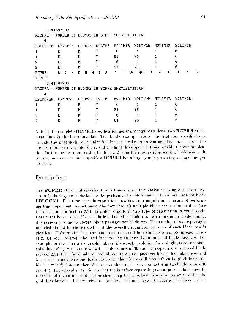
Boundary Data Fil_ £j_:c_ficalion.+- B(!PRR 91

0.41887903

NBCPRR - NUMBER OF BLOCKS IN BCPRR SPECIFICATION

4

LBLOCK2B LFACE2B LDIR2B L2LIMB M2LIMIB

1 K M 7 6

1 K M 7 81

2 K M 7 6

2 K M 7 81

BCPRR 5 I K K M M I J 7 7

THPER

0.41887903

M2LIM2B N2LIMIB N2LIM2B

I I 6

76 1 6

i I 6

76 1 6

36 46 I 6 6 i i

NBCPRR - NUMBER OF BLOCKS IN BCPRR SPECIFICATION

4

LBLOCK2B LFACE2B LDIR2B L2LIMB M2LIMIB M2LIM2B N2LIMIB N2LIM2B

1 K M 7 6 i I 6

1 K M 7 81 76 1 6

2 K M 7 6 1 1 6

2 K M 7 81 76 1 6

Nole lhal a COlnplete BCPRR sl)e<'ificalion generally requires a l least lwo BCPRR slale-

menl lines in Ill(, t>oulMarv (tala file. h, the example at>ore, the first four sl)e('ificaliotls

l)rovi(le the inierl)lo('k <'OlnmUlfi('alion for lhe meshes tel)resenting blade row 1 from the

meshes represelding blade row 2, and the tinal three sl>ecificalions provide lhe co]|lnlunica-

lion for the meshes representing; blade row 2 from the meshes represent ing blade row I. It

iS a C()ll|lllOll el'forlt) undersl)ecify a BCPRR boundary bv only providing; a single line per

interface.

Des<.ril)tion"

The BCPRR statement sl)e('ities that a time-space inlerpolation utilizing data from sev-

eral neighboring mesh blocks is to I)e i)erlbrmed to delermine lhe boundary data for l)]ock

LBLOCK1. This tinte-sl)ace interpolation provides lhe compulalional means of perform-

ing time-dependent predictions of the flow through mulliph, blade row I urbomachines (see

the discussion in Section 2.2). In order to perform this type of calculation, several condi-

lions IllllSl be satisfied, f'or calculations involving blade rows with dissimilar blade counts,

it is necessary to mo(lel several bla<le passages t>er 1)lade row. The number of blade passages

modeled should be chosen such thai the overall circumferential sl>an of each blade row is

idenlical. This iml>lies that lhe blade counts should l)e reducil)le to siml)le inleger ratios

(1:2.3:4. etc.) to avoid the need for modeling an excessive number of blade passag;es. For

example, in the illustrative graphic above, if we seek a solulion for a single slag(" lurl)oma-

chine invoh'ing two blade rows with bla<le counts of 30 and -15, respe<'lively (reduced blade

ratio of 2:3). then lhe simulation would require 2 bla<te passages for the first blade row and

3 passages from the second blade row, such that lhe overall circumferenlial pitch for eilher

blade row is 2_, (lhe numl)er 1.5 ('hoselt as the la "gest <onlmon factor in the blade counts 30

and 45). The second ['esll'iCliOll is thai lhe inlerface sel)aralhlg lwo adja('enl blade l'OWS |)e

a surface of revohdion, and thai meshes along this interface have common axial and radial

grid distributions. This restriction simplities the time-space interpolation provided by lhe

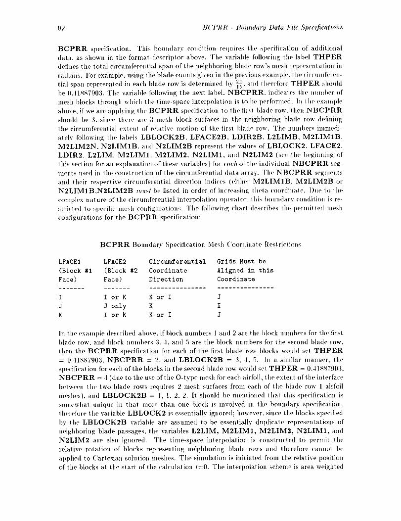
92 BCPRR - Boundary Data Fil_ ,S'p¢cifications

BCPRR specification. This boundary condition requires the specification of additional

data, as shown in the format descriptor above. The variable following the label THPER

defines the total circulnferential span of the neighboring blade row's mesh representation in

radians. For example, using the blade counts given in the previous example, the circumferen-2_, aim therefore THPER shouldtial span represented in each l)lade row is determined by 7g

be 0.41S87903. The variable following the next label. NBCPRR, indicales the number of

mesh blocks through which the tiine-space intert)o]alion is to be l)erfornled. In the exaln])le

above, if we are al)t)lying the BCPRR specification to the firs! bla(le row. then NBCPRR

should be 3, since there are 3 mesh ])lock surfaces in the neighboring blade row detining

the circumferential extent of relative motion of the first blade row. The numbers immedi-

ately following the labels LBLOCK2B. LFACE2B, LDIR2B, L2LIMB, M2LIM1B.

M2LIM2N, N2LIMIB, and N2LIM2B represent the values of LBLOCK2, LFACE2,

LDIR2. L2LIM, M2LIM1, M2LIM2, N2LIM1, and N2LIM2 (see lhe 1)eginning of

this section for an explanation of these variables) for each of the individual NBCPRR seg-

ments used in the construction of the circumferential data array. The NBCPRR segments

and their respective circumferential direction indices (either M2LIMIB. M2LIM2B or

N2LIM1B,N2LIM2B must be listed in order of increasing lhela coordinate. Due to the

comt)lex nature of the circumferential interpolation operator, this boundary condition is re-

stricled to specifi(" mesh configurations. The following char! describes the l)ermitte(I mesh

configurations for the BCPRR specification:

BCPRR Boundary Specification Mesh Coordinate Restrictions

LFACEI LFACE2 Circumferential Grids Must be

(Block #I (Block #2 Coordinate Aligned in this

Face) Face) Direction Coordinate

...............................

I I or K K or I J

J J only K I

K I or K K or I J

In the example described above, if ])lock numbers 1 and 2 are the block numbers for the tirst

blade row, and block nuinbers 3.4, and 5 are the block numbers for the second blade row,

then the BCPRR specification for each of the first blade row ])locks would set THPER

= 0.418_7903, NBCPRR = 2, and LBLOCK2B = 3, 4, 5. In a similar manner, the

specification for each of the blocks in the second blade row would set. THPER = 0.41S_7903,

NBCPRR = 4 (due to the use of the 0-type mesh for each airfoil, the extent of the interface

between the two blade rows requires 2 mesh surfaces froln each of the blade row 1 airfoil

meshes), and LBLOCK2B = 1, 1, 2.2. It should be mentioned that this specification is

somewhat unique in that more than one block is involved in the boundary specification,

therefore the variable LBLOCK2 is essentially ignored; however, since the ])locks specified

by the LBLOCK2B variable are assumed to be essentially duplicate representations of

neighboring blade passages, the variables L2LIM, M2LIM1, M2LIM2, N2LIM1, and

N2LIM2 are also ignored. The time-space interpolation is constructed to permit the

relative rotation of blocks representing neighboring blade rows and therefore cannot be

a.pplie(l to Cartesian solution meshes. The simulation is initiated fl'om the relative position

of the blocks at !he start of the calculation t=0. The interpolation scheme is area weighted

Boundary Data Fil_ £'p<c(fications- B('PRR 93

to maintain a conserval iw, properly across lhe inlerface I)elween the relatively rot ating mesh

blo('ks (see the Final Report ['oz" additional details on lhe implementation of this boundary

proced ul'e).

1Restrictiolts/Limitations

The BCPRR boundary specification is restricted to mesh interfaces which lie on a common

surface (no significanl overlap), and have common axial and radial llleS[i coordinates. The

mesh musl satisfy lho coordinale reslrictions lisled in the table above. The BCPRR

procedure is only apl)licable t() 3-1) mesh systems.

CollllllOll Errors

• Failure to provide 2 BCPRR statements for each inlerface

• lncorreclly spocilied or misaligned extents of boundary regions (values of MILIM1,

MILIM2, N1LIM1, N1LIM2, M2LIM1B, M2LIM2B, N2LIMIB, N2LIM2B

do not correctly define lhe inleri3('e extents on blocks LBLOCK1 and LBLOCK2B)

• Allempt to use BCPRR on a 2-I) mesh block.

• Meshes <1o not satisfy coordinate restrictions listed above.

• Meshes have dissimilar axial and radial coordinates al the interface.

• Noighborillg blado row segments not lisle<l in increasing theta coordinale.

• Al>plicalioll of BCPRR to mesh interfaces which do not share a common surl'avo, or

which hay(, excess overlap.

• BCPRR runs very slowly on multiple processors - use BCPRM instead.

94 BDA TIN - A DPA C07 Bou_dary Data Fil_ ,S'p_cification.s

BDATIN

File tRea(l In Iesh Interface Pat(,hing $chelne

Mesh Block #1

(51x3x51)

--4"--_-;-_;""_/.-_:-._,>_-"-_-:-".-<:__-;"-_.__'_;,_::;-..:

.. S _

Mesh Block #2

(51x3x51)

BDATIN/BDATOU Combination Used

to Provide Disk Read/Write of BoundaryData for Interblock Communication

Between Blocks #1 and #2

AI)plication

The BDATIN specification is used to read in boundary data from an external file. This

file :nay be either 1)e created by a.n external t)rogram, OZ" b v the ADPA('O7 t)Oul_dary

specification BDATOU. The al)plication illus_ra.te(1 ahove indicaies an a.1)I)lica_ion of the

BDATIN/BDATOU combination for a two block nozzle flow case. The BDATIN/BDATOU

combination is applied _o lhe interface between the two mesh blocks and is e(luivalen! to a

PATCH specification, excel)! that the interblock communication is accoml)lishe(l _hrough

disk read/write rather lhan shared memory communication.

Boundary Data File Format

The boundary dala file specificalions for the mesh interface indicaled in the illuslrative

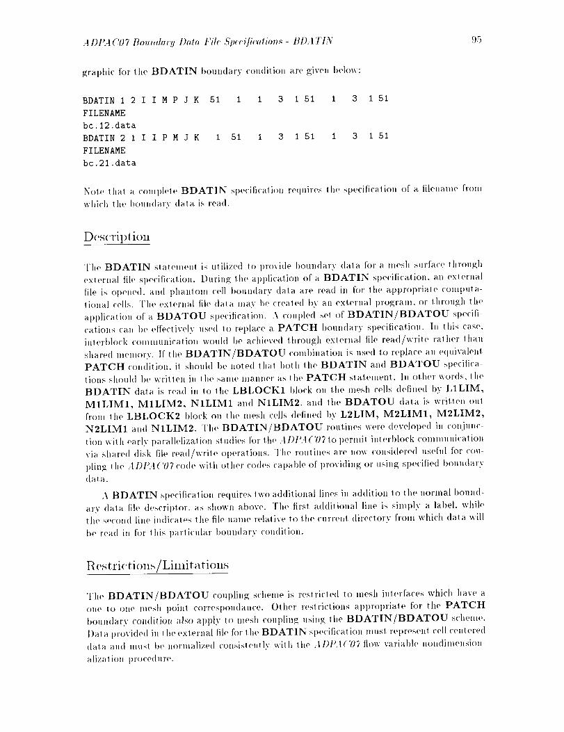
A DPAC07 Bmmdory Dam Fil_ ,Fpceifieation._- BDATIN 95

graphic for the BDATIN boundary condition are given 1>clew:

BDATIN i 2 1 1 M P J K 51 I I 3 I 51 I 3 i 51

FILENAME

be. 12.data

BDATIN 2 i I I P M J K I 51 I 3 I 51 I 3 1 51

FILENAME

bc.21.data

Nolo (hal a con_l)hqe BDATIN specilicalion requires lhe specification of a tilename from

which lhe I)oundary dala is read.

Descril>ti(m

The BDATIN slatemen! ix ulilized 1o provide boun(tarv data for a mesh surface through

exlernal file specification. During lhe application of a BDATIN st>ecification, an exlernaI

file ix opened, and phantom cell boundary dala are read in for the a t>l)rOl>riale computa-

tional cells. The exlernal file dala may be crealed I>v an external program, or _hrough _he

application of a BDATOU sl)ecitication. A coupled set of BDATIN/BDATOU specifi-

cations can be effectively used Io replace a PATCH 1)oundary specilicalion. In this case,

inlerbhwk communication wouhl 1)e achieved thr<)ugh external tile rea<t/wrile ralher than

shared menl<)ry. If [he BDATIN/BDATOU combination ix used to replace an ecluivalenl

PATCH condition, il should be noted (hal I)oth lhe BDATIN and BDATOU specifica-

_iOllS S_l()lll(I 1)(' Wl'iIlell ill lille Sa.lll(, lllalllle[" as (l_le PATCH statemen(. In olher words, (he

BDATIN <la_a is read in 1o lhe LBLOCK1 1)h)ck on the mesh ceils define<t by L1LIM,

MILIM1, M1LIM2, N1LIM1 and NILIM2. and the BDATOU data ix writlen out

fronl the LBLOCK2 block on the mesh ('ells defined t>y L2LIM, M2LIM1, M2LIM2,

N2LIM1 and N1LIM2. The BDATIN/BDATOU routines were developed in conjunc-

tion wi! h early l)aralMizalion sludies for Ill(, A DI>A ('07 to permit interl)lock corn munication

via share(/ disk file read/write operations. The routines are now ('onsi<lere<l useful for <'ou-

piing the :1 l)l'+l('07 co<le with other codes cal)al)le of providing or using specifie<t boundary

clara.

A BDATIN specification requires lwo additional lines in ad<tilion lo lhe normal bound-

arv dala file descril>tor, as shown above. The tirsl a ddilional line is simply a label, while

the second line indicales 1he file name relative 1o the current directory fi'om which dala will

t>e read in for this particular boundary conclilion.

1Restri<'tions/Limitations

The BDATIN/BDATOU coupling scheme ix restricled 1o mesh inlerfaces which have a

one to one mesh poilll corresl)ondance. Other resl.riclions al)l)ropriale for the PATCH

boun(larv con(litioi_ a}so apply to mesh c<)ui)ling using the BDATIN/BDATOU scheme.

l)al a I)rovided in _he exlerna[ file for Ill(, BDATIN sl)ecificat ion musl ret)resenl ('ell ('entered

(lala and musl be normalized consislenlly wilh the ,II)P.t('07 tlow variat)le nondimension-

alizat ion procedure.

96 BDA TIN - A DPA (,'07 Boundary Data Fil_ £'p_eificatioT_._

COllllllOll Errors

Failure to provide file name for BDATIN boundary data file specification.

Incorrectly specified or" misaligned extents of boundary regions (vahms of MILIM1,

MILIM2, NILIM1, N1LIM2, M2LIM1, M2LIM2, N2LIM1, N2LIM2 do not

correctly define tile interface extents on blocks LBLOCK1 and LBLOCK2).

BDATIN/BDATOU coupling scheme desired, bu! only one of the BDATIN/BDATOU

sl)ecificatiolls l)rovided.

BDATIN/BDATOU coupling scheme boundary specification for a periodic bound-

ary is al)plied to a nonperiodic mesh.

BDATIN/BDATOU coupling scheme I)oundary sl)ecification a,pl)lied to a spatially

periodic (!a,rlesian geonletry using the cylindrical coordinate solution schenle or vice

versa (results in incorrect spatial I)eriodicity relationships) The BDATIN/BDATOU

coupling scheme boundary specifications for (iartesian geometries mus! use t he (!arlo-

sia,n solution algorithm in A DPA('07 (see input variable FCART).

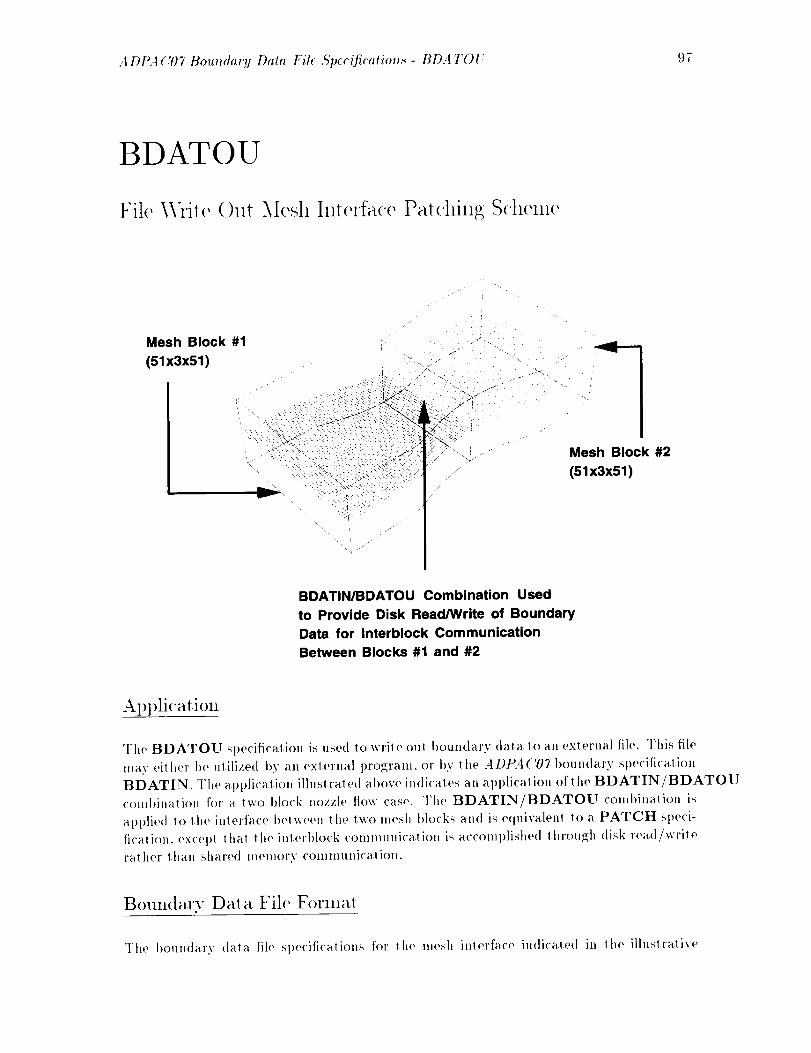
.4 Dl_4 ('07 Boul_¢lary Data File ,S'pcc_fic'¢ltio_,_ - BD.4 TOU 97

BDATOU

File \\rite ()11t lkle,sh Interface Patc]linx Scheme

Mesh Block #1

(51 x3x51 )

Mesh Block #2

(51x3x51)

BDATIN/BDATOU Combination Used

to Provide Disk Read/Write of Boundary

Data for Interblock Communication

Between Blocks #1 and #2

Al)I)lication

The BDATOU specification is used to wrile ()lit I)oundary data to all external file. This file

ma N eilher be utilized b 5" an exterllal program, or by the ADPA('07 boundary specificalioll

BDATIN. The applicalion illus! raied above indicales an applicalion of the BDATIN/BDATOU

coml)ination for a lwo block nozzle flow case. The BDATIN/BDATOU combination is

applied Io lhe interface belween the two mesh blocks and is equivalenl 1o a PATCH speci-

ficalion, excel)l that the interblo<'k conlmunica,tion is acconq)lishe(l through <tisk read/wrile

ralher than shared memory communi<'ation.

Boull(larv Data Fil(' Forniat

The t)oundarv data file sl)ecifi('alions for the mesh inlerface in(licaled in lhe illuslralive

9_ BDA TO U - A DPA C07 Boundary Dattl File ,qpcc_ficatio_t._

graphic fox" the BDATOU boundary condition are given below:

BDATOU I 2 I I M P J K 51 1 1 3 I 51 1 3 I 51

FILENAME

bc. 12. data

BDATOU 2 I I I P M J K 1 51 1 3 i 51 1 3 I 51

FILENAME

bc.21 .data

Note that a complete BDATOU specification requires lhe specificalion of a filename fronl

which the boundary data is read.

Des<'ril) tion

The BDATOU statement is utilized to export boundary data for a mesh surface through ex-

ternal file specification. During the application of a BDATOU sl)ecification, an external file

is opened, and near l)oundary cell-centered data are written in for the apl)ropriale ('Oml)uta-

tional ('ells. The external file data may then be utilized by an external program, or through

the application of a BDATIN specification. A coupled set of BDATIN/BDATOU spec-

ifications can be effectively used t.o replace a. PATCH boundary specification. In this case,

interblock communication would be achieved through external file read/write rather than

shared memory. If the BDATIN/BDATOU combination is used to replace an equivalent

PATCH condition, it shoul<l be noted thal both the BDATIN and BDATOU specifica-

tions should be written in the same maimer as the PATCH statement. In other wor(ls, the

BDATIN data is read in Io the LBLOCK1 block on the mesh cells defined by LILIM,

M1LIM1, M1LIM2, N1LIM1 and N1LIM2, and the BDATOU data is written ou!

1o the LBLOCK2 block on the mesh cells defined by L2LIM, M2LIM1, M2LIM2,

N2LIM1 and NILIM2. The BDATIN/BDATOU routines were developed in conjunc-

tion with early parallelization studies for the ADPA('07 to permit interblock communication

via shared disk file read/write ol)erations. The routines are now ('onsidered useful for cou-

l)ling the A DPA('07 code with ot her codes cat)able of i)roviding or using specified ])<)undarydata.

A BDATOU specification requires two additional lines in addition to the normal bound-

arv data file descriptor, as shown above. The first a(lditional line is simply a label, while

the second line indicates the file name relative to the current director), to which data will

be written out for this particular boundary condition.

R estri<'tiolls/Limitations

The BDATIN/BDATOU COul)ling scheme is restricted lo mesh interfaces which have a

one to one mesh point correspondance. Other restriclions approl)riale for the PATCH

boundary condilion also apply to mesh coupling using the BDATIN/BDATOU scheme.

Data provided in the external file for the BDATOU specification represents near-boun<lary

('ell centered data and is normalized consistently with the ADl<4C07 flow varial)le nondi-

mensionalization procedure.

A DPA ('07 Boundary Data File S'pee_fication._ - BDA TO U 99

CollllllOllErrors

Failur(, to provi(l(, file ham(, for BDATOU boundary (lala file +_t)(wificalioll.

Incorreclly Sl)e('ili('(I or misaligne(l extents of boundary regions (values of MILIM1,

M1LIM2, NILIM1, NILIM2, M2LIM1, M2LIM2, N2LIM1, N2LIM2 do not

corre('lly (lefillo the inlet'fat(' extents on blocks LBLOCK1 all(1 LBLOCK2).

BDATIN/BDATOU co,ll,lin_ scheme desired, but only o1_(, of lh(, BDATIN/BDATOU

sl)ecitical ions l)rovide(I.

BDATIN/BDATOU COul)lillg scho,ne boundary specific_liotl for a perle(tic bound-

ary is al)t)lie(I to a nOnl)eriodic mesh.

BDATIN/BDATOU coupling schetne boutJdary sp('cification applied to a spatially

periodic (lart(,siatl _eolnelry using the ('vlitl(h'ical coordinate ._ohtlion schet,,e or vice

v(,t'_a (t+(,mHl1_ il_ itlcorr(+ct sl)ali_l periodicity t'elatioxl._hil)s) The BDATIN/BDATOU

('ouplill_ s(+h('m(' boundary specifi('aliOllS fl)r (larlesian geometries must use the ('al'te -

_i_lt solution algorithm ill A DI+'A ('07 (see input w_riat)le FCART).

1O0 ENDDA TA - A DPA C07 Boundary Data Fil_ ,S'peeificatio,_._

ENDDATA

Boundary Data File Read Terminator

Apl)lication

Tile ENDDATA statement causes the ADPA('07 boundary data file read utility to dis-

continue reading lines in the boundary data file and proceeds with normal ('ode processing.

Any lines following an ENDDATA statement in a boundary data file are ignored.

Boundary Data File Format

The boundary data file specification for an ENDDATA statement is given below:

ENDDATA

Note that the ENDDATA statement does not require the accompanying vahles of LBLOCK1,

LBLOCK2, LFACE1. et('. as do all other boundary data file keywords.

Description

The ENDDATA statement is utilized to provide a terminator for the boundary data file

read sequence in the ADPA('07 code. ITnder normal ot)erating conditions, the boundary

data file is read in one line at a time and parsed to determine if a boundary data file

keyword is present and uncommented on each line. When the end of the file is reached,

the boundary data file read sequence stops, and normal l)rocessing continues as usual. In

some cases, it may be desirable to lerminale the boundary data file read se(luence before

the end of the file, and the ENDDATA statement is provided for this purpose. Whenever

an ENDDATA statement is reached, the boundary data file read sequence is terminated,

and all remaining lines in the boundary data file are ignored. The ENDDATA keyword is

useful for debugging boundary con(litton prol)lelns, as whole portions of the I)oun(lary (lala

file can be effeclively eliminated by simply precee(ling lhe section with an ENDDATA

statement.

t/estrictiolis/Limitations

The ENDDATA kevword has no restriclions.

A DPAC'07 BouIMaw Data Fih £'p_cificatiol,._- ENDI)A TA

Common Errors

101

• Desired boundary conditions specificalions following all ENDDATA statemenl are

ignored.

• .4 PP.4 ('/)7 complaius because an insufficient number of boundary conditions were pro-

viCh,d for lho external boundaries of each mesh block (exlerna[ boundaries of some

mesh blocks do 1lO1 haw, a boundary condition see inpu! kevword FBCWARN).

102 END T TA - A DPA ('07 Bmmdary Dat. File A'pecifieation.s

ENDTTA

Endwall Treatlnent Time-Average Mesh Block Interface Patch-ing S('helne

Geometry

Casing

Treatment

Fan

Rotor

L_:!::ii:i:::ii:iii!i:i:iii!i!i:i:i:i!i

m m mm

Block #2

(17x17x33)f'-'3

Block #I

(99x33x33) ____

tat'ona'Endwell Regions Between

Discrete Treatments are

Accounted for In END'irA

Single Blade Passage

Representation

m IDiscrete Endwsll Treatment

Repressntetlon (Only One

Treatment Pssssge Required)

ENDTI'A Boundary Specification

Used to Couple Blade Passage

Flowfleld to Discrete Treatment/

Endwall Flow

AI)I)lication

The ENDTTA boundary specification was developed specifically to permit nulnerical pre-

diction of turbomachinery airfoil blade row flows employing endwall treatments such as

slots, grooves, or embedded bladed passages in a time-averaged fashion. The exalnph,

ygra,phic above illustrates a 3-D blocked mesh system for a turbofan engine fan rotor em-

ploying an axial slot casing trea,tmen[. The ENDTTA boundary specification employs a

time-averagillg operator (circumferential aw, rage of flow variables) between a,djacenl rotat-

ing and nonrotating mesh blocks i,o simulate the effects of the blade row/endwall treatment

interaction. As such, it is possible to perform steady state (representative of a time average)

numerical analysis of Iurl)<)machinery blade passages al|(] endwall trealments which have

arl)ilrarv blade passage/treatlnent passage count ralios.

A DPA ('07 Bou,Mary Data File ,qpcc_ficatio_t._ - ENDTTA

B<mndarv Data File Format

103

The boundary data file specifications for the mesh interface indicated in the illustratiw'

graphic for tile ENDTTA boundary con<litiou are given t>elow:

ENDTTA i 2 J J M P L L 49 I 49 81 I 33 I 33 I 17

NTREAT RPMWALL TWALL

113 0.0 0.0

MBCAVG 2 1 J J P M I K 1 49 1 33 1 17 49 81 1 33

NSEGS

I

BLK LFACE2 LDIR2 L2LIM M2LIMI M2LIM2 N2LIMI N2LIM2

1 J M 49 49 81 I 33

Note that a COmlflele ENDTTA specification g4ene]'ally requires a cOnll>aniolL MBCAVG

specificalion to ('onlplete t he blade passage mesh/t ['eat Illellt passage tnesh interface specifi-

cation. Ill theexanll)le above, lhe first specification provides the inlet'block conlmunication

for block I (1 he blade passage mesh) to block 2 (the treatnwn! passage nlesh) which ulti-

lnately ac('ounls for the influellce of the true endwall in tile boundary specification. The

second speci[icatiou (MBCAVG) is applied lo the treatment passage mesh I>oundarv to

si,nulale the time-average (circumferential average)of tile neighl>oring blade passage mesh.

It is a <'ot|lnlon err'or to underspecit_ + an ENDTTA t>oundarv by only providing; a single

lille per interface.

Des<u'il>tion

The ENDTTA boundary statement provides a means for block to block communication for

the prediction of the time-averaged flow for turbonlachinery blade rov,'s employing endwall

treatments such as discrete slots, grooves, or enllw<t<led bladed passages. This bound-

arv condition was <levelol>ed under Task 6 of NASA ('ontract NAS3-25270 and theoretical

details of the pro('edure are provided in the Final t{eport for Task 7 of NASA ('Olllra('t

NAS3-25270 [21]. Tile boundary condition is restricled toj=constant mesh surfaces oM 9

all([ IllUSl possess aligned coordinates ill the/direction, bill have misalignetl mesh points

and extents ill the <'ircumDrential (k) direction. An example of an appropriate application

of tile ENDTTA specification is given in the illustratiw, graphic. Tile ENDTTA bound-

arv specitication is vali<t for 3-1) cylindrical solution mesh blocks only. Tile ENDTTA

specilicalion requires tile sl>ecification of additional data. as sllown in the format descriplor

above. The first additional lille following an ENDTTA sl)ecification is assumed to be a

label for the variables NTREAT, RPMWALL. and TWALL. The next line contains the

values for 1he variables NTREAT, RPMWALL, and TWALL. Tile variabh' NTREAT

represents the total nulnl)er of discrete treatments for tile (,_ti** rotor. The analysis is nor-

really performe<t for a single rotor blade passage and a single treatlnent blade passage, and

the value of NTREAT is used to effectively set the circumferential spacing between dis-

crete treat nlenl passages. Tile next variat)le, RPMWALL, sets the value of the rot atioual

sl)ee<l of tile endwall regions which separate the discrete treatnletlts. Naturally. this also

implies lhe rotational spee<l of the treallllellls thenlselw, s. and lhe value of RDMWALL

ill Ibis conlext nlust be consislent with lhe value of RPM specified in the input tile for the

104 END TTA - A DPA C07 Boundary Data File Specifications

treatment passage mesh block. Tile third variable, TWALL, sets tile tlwrmal boundary

condition for the wall segments separating the discrete treatment passages, and is specified

in the same manner as the TWALL variable described h_r the SSVI (viscous solid wall)

boundary condition.

Restrictiolls/Limitations

The ENDTTA boundary st)ecification is restricted to mesh inlerfaces which lie on a COlll-

mort surface (no significant overlap). The ENDTTA procedure permits only that the k

coordinates between adjacent mesh surfaces are misaligned. The ENDTTA procedure is

only valid if applied to j=constant mesh surfaces. ENDTTA will _*ot run across multiple

processors in a parallel COlnputing environment.

Co111111oi1 Errors

** Failure to provide a coupled pair of ENDTTA and MBCAVG statements for each

interface.

, Failure to properly specify the values for RPM, TWALL and/or NTREAT

• Incorrectly specified or misaligned extents of boundary regions (values of M1LIM1,

M1LIM2, N1LIM1, N1LIM2, M2LIM1, M2LIM2, N2LIM1, N2LIM2 do not

correctly <lefine the interface extents on blocks LBLOCK1 and LBLOCK2).

• Attempt t,o use ENDTTA for an i or k constant boundary.

• Attempt to use ENDTTA for a Cartesian solution mesh.

• Attempt to use ENDTTA for a boundary which has 2 misaligned coordinales.

• Attempt to use ENDTTA with multiple processors.

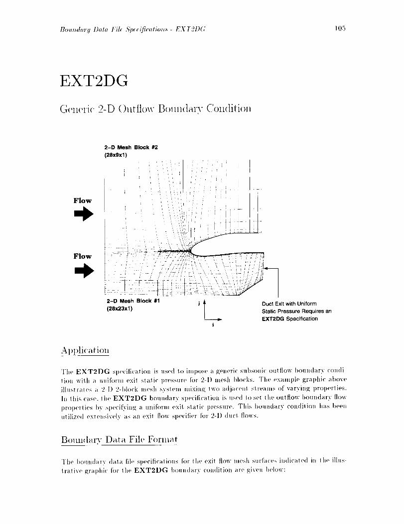
Boundary Data Fih £'p_c(ficatiolt.s- EXT2DG 105

EXT2DG

Generi( 2-D ()lltflow Boun(lar\ (!on(litton

2-D Mesh Block #2

(28x9x1)

Flow

Flow

2-D Mesh Block #I

(28x23x1)

i

Duct Exit with Uniform

Static Pressure Requires an

EXT2DG Specification

Al)plication

The EXT2DG specification is used to iml)ose a generic subsonic oulflow boundary condi-

tion with a unifornl exit static pressure for 2-1) mesh blocks. The example graphic above

illustrales a 2-I) 2-block mesh system mixing Ixvo ad.iacent streams of varying properties.

In this case, the EXT2DG boundary specification is used to sel the outflow boundary tlow

prolmrlies by specifying a uniform exit static pressure. This boundary condition has been

ulilized extensively as an exil flow specifier for 2-I)duc! flows.

Boundary Data File Format

The I)oun(lary data tile specilicalions for lhe exit flow mesh surfaces indicaled in lhe illus-

irative graphic for lhe EXT2DG boundary ('on(litio]_ are given below:

106 EXT2DG - Bou_,dary Data File Specifications

EXT2DG 1

PEXIT

0.625

i I I M M J K 28 28 1 23 1 2 I 23 1 2

o1' the alternate specification:

EXT2DG i 1 I I M

PEXlT EMDOT PRELAX

0.625 11.4 0.i

M J K 28 28 1 23 1 2 1 23 1 2

Note that a complete EXT2DG specification requires two additional lines following lhe

EXT2DG boundary data file specification line. Failure 1o prol)erly specify tile data ill

these additional lines is a ('onmlon EXT2DG specification error.

Descril)tion

The EXT2DG statement st)ecifies that a generic, subsonic, uuiform stalic pressure exit

flow boundary condition is to be applied to the mesh surface specified by LFACE1 on

the 2-D mesh block specified I)y LBLOCK1. Tile EXT2DG boundary condition shouhl

I)e applied for those cases where ally other "specialized" exit. boundary condition (such as

EXT2DT, EXT2DP, etc.) does not apply. Tile EXT2DG t)oundary condition is also

likely to be somewhat more efficient computationally than the other exit boundary condi-

tion procedures, at the expense of some physical simplification. The EXT2DG procedure

utilizes a Riemann invariant formulation to compute exit w, locities based on a specified

constant exit static pressure. Included in the EXT2DG procedure is a special correctioll

scheme which forces the flow to pass out of the flow domain at the 1)oundary. In other words,

if tile computed velocities result in a local inflow at the EXT2DG boundary, no matter

how small the magnitude of the inflow, the velocities are reset to zero at that point. This

1)oundary condition requires the st)ecification of additional data, as shown in the boundary

data format descriptor above. Tlle first additional line following the EXT2DG specifica-

tion is assumed to be a label and may contain ally information; however, for consistency it

is recomnmnded that the lal)el PEXIT be used. 1['lie next line contains the value imposed

for the variables PEXIT which represents the (towustr(,am exil static pressure ratio used

in the EXT2DG characteristic solution sequence. The value of the PEXIT variable is the

desired normalized downstream static pressure computed as:

PEX IT = Pstrltic,d_si,._d

P,._f

where the varial)le P,.¢: is specified by the inl)ut variable PREF. It should be mentioned

that tbr most geometries, tile value of PEXIT, ill combination with any inlet flow boundary

conditions, will normally govern the resulting solution mass flow rate (exceptions to lhis

rule will occur when the inlel mass flow rate boundary condition procedure INLETM is

applied). Vahms of PEXIT <0.0 are not permitted. As the value of PEXIT is reduced,

the flow through the boundary will ultimately choke, and further reductions of PEXIT

will no longer increase lhe mass flow lhrough the boundary. Naturally, poor convergence or

solution divergence can occur if PEXIT is too high or too low when COml)ared to the rest

of the flow domain. In such cases where this occurs, it is recommended t,hal tile solution ])e

BouIMary Delta File ,5'pec(fiealio_._- EXT2DG 107

slarled with more conservalive boundary values, and then restarted using the final boundaryv_/lue,'4.

An allernale specification is provided for the EXT2DG boundary speci[ication as shown

in the sample apl)lication above. In this case, three values are included following the original

boundary Sl_e<'ilication line. The a lternale specilica!ion is provided as a means of achieving

a desired mass flow rate lhrou_h lhe houri<ling surface using lhe EXT2DG al_orilhm.

The <lesired mass flow rale is achieved ileralively bv increlnentall.v a<ljusting the exi! stalic

pressure sl>eciticatioll until the desire<l flov," rate is achieved. Th<'refore. in thi.,, specili<'at ion,

the varial>le PEXIT <tescrit>ed in detail above is the initia] exi! stalic pressure used in llle

iteralive ]+rocess. EMDOT tel>resents the desired mass [low rate throua;h the boundin_

surface in l)<mnds mass, and PRELAX is a relaxation faclor to stabilize lhe ilera|ive

process (values may range from 0.0 1o 1.0, though l>OOr convergence is likely tbr values

larger thar_ 0.1). t:or (!artesian flow calculations a unit depth (1.0 in mesh co<)r<linates) is

assumed for lhe third coor<tinate direction to determine lhe mass flow ,'ale. For cvlimlrical

tic)v,: calculations. _he ¢;eometry is assumed to be axisymmelric and a mul[il>le of 2_ is used

in the mass fl<>w integration (the mass tlov,: is computed as if the full circumference of lhe

axisynlmetric _eometrv were employed). This procedure is ,tot foolproof, and suffers fi'om

the fac! 1hal when a job is restarted, if an updated exi! pressure is no1 inserled in 1he

b<>un<lary <lala file, 1hen the pressure-mass tlow iteralive process will essentially star1 over.

The ,4 I)P.t('07 <'ode will automat ically determine when to eml>loy the iteralive pro<'ess I)v

identifying the additional boundary specification variables.

Restrictions/Limitations

CollllllOll Errors

• t"ailure to specify the additional <lala value PEXIT.

• Iml>rOl)er specification of the allernate (mass flow) ilerative scheme.

,, lledu('tions in the value of PEXIT <lo nol increase the mass flow rate I)ecause of flow

choking.

• Value of PEXIT is too high (flow cannot get slatted).

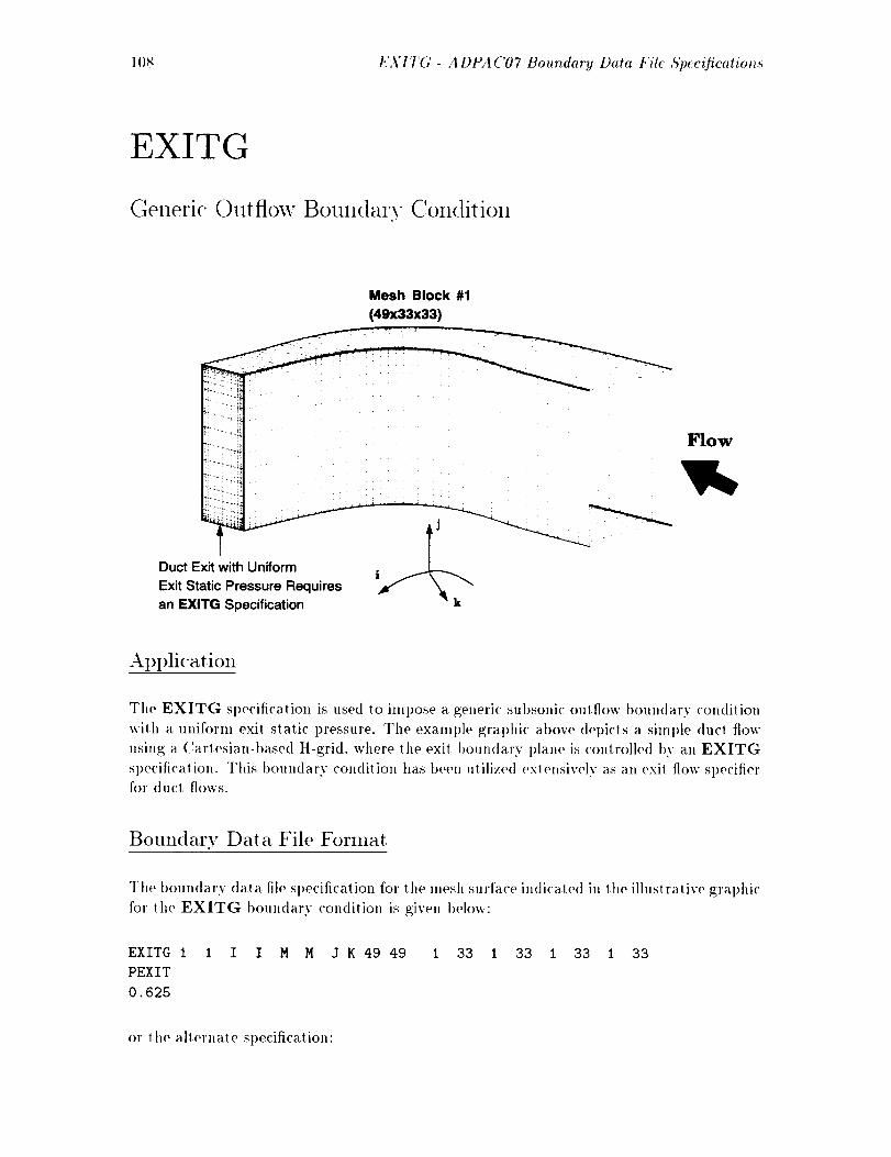
108 EXIT(; - .4 DPA C07 Boundary Data File Specifications

EXI'FG

Generi(' Outflow Boundary Condition

Mesh Block #1

(49x33x33)

ii!iiiii!

i!iiiiiiill

Duct Exit with Uniform

Exit Static Pressure Requires

an EXlTG Specification

l__ow

Application

Tile EXITG specification is used to impose a. generic subsonic outflow boundary condition

with a unifornl exit static pressure. The example graphic above depicts a simple duct flow

using a Cartesian-based H-grid, where the exit boundary plane is controlled by an EXITG

specification. This boundary condition has been utilized exlensivelv a.s an exit flow specifierfor duct flows.

Boundary Data File Format

The boundary data file specificatioll for the mesh surface indicated ill the illustralive graphic

for the EXITG boundary condition is given below:

EXITG I

PEXIT

0.625

I I I M M J K 49 49 I 33 I 33 I 33 i 33

or the a.l_ernate specification:

A DF4 ('07 Bou,dary Data File ,qpr<'iJicatiol_._ - EXIT(; 109

EXITG i 1 1 1 M M

PEXIT EMDOT PRELAX

0.625 40.0 0.001

J K 49 49 1 33 1 33 1 33 1 33

Note that a complete EXITG specification requires two additional lines following the EX-

ITG boundary data file specification fine. Failure to properly specify the data in these

additional lines is a common EXITG specification error.

Description

The EXITG statement spocilies that a generic, subsonic, uniform static pressure exit ttow

boundary condition is to he applied to the mesh surface specified by LFACE1 on the block

sl)ecitied 1)v LBLOCK1. The EXITG I)oundary condition should t)e al>plie(l for those

cases where auv other "'sl)ecialized'" exit I)ountlary condition (such as EXITT, EXITP,

et('.) does not apply. The EXITG t)oml(lary condition is also likely to he st)mewhal more

efficient computationally than the other exit boundary con<lit!oil procedures, at the expense

of some physical simplification. EXITG may I)e used on any mesh face (I, .1, or K constant )

for eit her cylindrical or (lal'tesian-hased solution schemes (see the input varial)le FCART).

The EXITG procedure utilizes a Re!mann invariant ft>rmulalioll It) ('Oml>Ule exit velocities

base<l on a sl)ecified constant exit slat!<" l)ress,re. Inchl<le<l ill the EXITG procedure is

a sl)ecial correction scheme wltich fbrces the flow to pass out of the flow domain at the

boundary. In ot her wor(Is, iflhe COml)ute<l velocities result in a local inflow at the EXITG

1)oun(lary, no matter how small the magnitu(le of Ihe iuflow, lhe velocities are reset to zero

at that point. This t)ountlary condition requires the specification of atl(lilional (lala, as

shown in the Boundary I)ala Format descriptor al)ove. The first a(htitional line follow-

tug the EXITG sl)e<'itication is assumed It) t)e a label anti may contain any information:

however, for consislellcy il is recommended lhat the label PEXIT I)e used. 1'he next line

contains the value iml)osed for the variables PEXIT which rel)resent s the dowttstream exit

static pressure ratio used in the EXITG characteristic solution sequence. The value t)f the

PEXIT variable is the ties!reel normalized downstrealn static pressure COml)ule(I as:

) .I st,th',desu'edPEXIT -

P,.,f

where lhe varial>le l;.:: is sl)ecified I)y the input variat)le PREF. It should be mentioned

lha! for lnost geomelries, the value <)f PEXIT. in conlbinatioll with any inlet flow boundary

conditions, will lmrmall.v govern the resulting solution mass flow rate (exceptions to this

rule will occur when the inle( mass flow rate boundary <'ondition l)rocedure INLETM is

al)plied ). Values of PEXIT <0.0 are no( t)ermilted. As the value of EXITP is reduced.

the flow through the l>outttlary will ultimately choke, and further reductions of EXITP

will no longer increase the nlass flow through the boundary. Naturally. poor convergence or

solution (livergelwe can <)('cur if PEXIT is too high or tot) low when coml>ared to the rest

of the Ilow (lolnain. In su<'h cases where this oc('llrs, it is recommended that the solution t>e

starte<l with more conservative boundary values, an<t then reslarted using the final boundary

V;:I] |les.

:\n alternate sl)e('iticatiou is t)rt)vided for the EXITG l)ountlary specification as shown

in lhe sample al>plicatioll al)ove. In this case, three values art' included following the ori_;inal

1)oundary sl)ecificatio]l line. The allei'llale sl)ecilication is ])rovitled as a means of achieving

110 EXITG- ADI_4C07 Boundary Data File 5)_.cifications

a desired mass flow rate through the bounding surface using the EXITG algorittun. Tile

desired mass flow rate is achieved itera.tively by incrementally adjusting the exi! static

pressure specification until the desired flow rate is achieved. Therefore, in this specification.

tile variable PEXIT described in detail above is the initial exit static pressure used in the

iterative process, EMDOT represents the desired mass flow rate through the bounding

surface in pounds mass, and PRELAX is a relaxation factor to stabilize the iterative

process (values may range fl'om 0.0 to 1.0. though poor convergence is likely for values

larger than 0.1). This t)ro('edure is not foolproof, and suffers from the fact that when a

job is restarted, if an updated exit pressure is not inserted in the boundar.v data file, then

the pressure-mass flow iterative l)rocess will essentially start over. The A DPA ('07 code will

automatically determine when to employ the iterative process by identifying the additional

boundary specification variables.

Restrictions/Limitations

The EXITG boundary specification is not restricted to 3-D mesh surfaces (although for

consistency 2-D mesh surfaces may use the EXT2DG boundary specification).

CollllllOll Errors

• Failure to specif.v the additional data value PEXIT.

• hnproI)er specification of the alternate (mass flow) boundary scheme.

• Reductions in the value of PEXIT do not increase the mass flow rate because of flow

choking.

• Value of PEXIT is too lfigh (flow cannot get started).

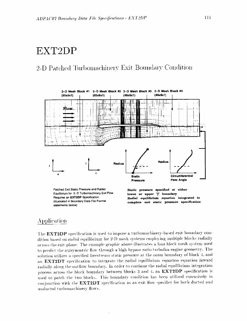
A DR,t('07 Bo_mdary Data Fil_ S)J<c(ficatio_._- EXT21)P 111

EXT2DP

2-D Patched turl)onm(hinery Exit Boun(larv Condition

2-D Mesh Block #1 2-D Mesh Block #2 2-D Mesh Block #3 2-D Mesh Block #4

(65x9xl) (65xgx1) (49xSxl)

T/ 1/_J __ Radius Radius

Static Circumferential

Pressure Flow Angle

Patched Exit Static Pressure and Radial

Equilibrium for 2-D Turbomachinery Exit Flow

Requires an EXT2DP Specification

(illustrated in Boundary Data File Format

statements below)

Static pressure specified at either

lower or upper _j" boundary

Radial equilibrium equation integrated to

complete exit static pressure specification

Ai)pli<'ation

The EXT2DP specification is used to itnl)ose a, lurbolnachinery-based exit, boundary con-

dition based on radial equilibrium ff)r 2-I) mesh svst, ems employilkg multil)le blocks radially

across the exit plal,e. The example graphic above illustrates a four block mesh system used

to 1)redi¢'t t he axisvmml tic tlow through a high bypass ratio lurbofan engine geometry. Tit(,

solution utilizes a specified freestream st.alto pressure at the outer boundary of block 4. and

an EXT2DT specilication to int.ep.;rate the radial equilibriun_ equation eqttation inward

radially Monk lhe om tlow boundary. In order to continue the radial equilibrium integration

process across the block boun<lary between blocks 3 and-1, an EXT2DP specification in

use<l to t>atch the two t)locks. This boulldary <'onditioll has been utilized extensively in

con.iunctioll wilh the EXT2DT specitication as an exit flow specifier for both ducted and

Ul:<lu<'te<l turbonlachinery tlows.

112 EXT2DP - ADPA C07 Boundary Data File S'pt,ciflcations

Boundary Data File Format

The boundary data file specification for the 2-D mesh surface indicated in the illustrative

graphic tbr the EXT2DP boundary condition is given below:

EXT2DP 4 3 I I M M L H 49 49 1 9 1 2 9 9 1 2

Note that the M2LIM1, M2LIM2 variables in the EXT2DP specification define a single

j mesh line in mesh block LBLOCK2. Failure to properly regar<l this requirement is a

common EXT2DP specification error. It shouhl also be mentioned that EXT2DP also

requires proper specification of the LSPEC1 variable for proper execution.

Descriptioll

The EXT2DP keyword specifies that a turbomachinery-based radial equilibrium patched

exit flow boundary condition is to be applied to the mesh surface specified by LFACE1 on

the 2-D block specified by LBLOCK1. The EXT2DP boundary condition was specifically

designed as an exit flow boundary procedure for axial and mixed flow turbomachinery

geonletries employing multiple, stacked 2-D mesh blocks (radially) at an exit boundary

plane. The EXT2DP boundary condition procedure utilizes a combination static pressure

specification and integratioll of the radial equilibrium equation to define the static pressure

field al all points on the boundary surface. The initial static pressure specification used

to initiate the radial equilibriuln integration process is obtained fi'om a neighboring mesh

block. As a result of the complexity of this procedure, several mesh restrictions were

imposed to sinlplify the application of this approach. The primary assumption is that the

integration of the radial equilit)rium equation may be performed along the j coordinate

direction of the mesh. Hence. the j coordinate should be the radial-like direction. A single

specification of static pressure is required at either the maximum or minimum extreme of

the j coordinate of the boundary surface in order to initiate the integration process. The

direction of integration, and location of application of the specified exit static pressure

are determined by the LSPEC1 variable in the calling sequence. If LSPEC1 = L, for

LOW. then PEXIT is applied to the lower (smallest value) of the j index, and the radial

equilibrium equation is integrated outward (increasing j direction). If LSPEC1 = H,

for HIGH. then PEXIT is applied to the upper (largest value) of the j index, and the

radial equilibrium equation is integrated inward (decreasing j direction). The direction of

integration implied by LSPEC1 must be consistent with the location of the neighboring

mesh ])lock (LBLOCK2) from which the initial pressure data is derived. The j coordinate

location from which the pressure is taken in mesh ])lock LBLOCK2 is determined by the

M2LIM1, M2LIM1 variable, and the specification of the LSPEC2 conlrol paranleter.

If the M2LIM1,M2LIM2 combiuation is taken fi'om the higher j index, then LSPEC2

should be H. If the M2LIM1,M2LIM2 confl)iuation is taken from the lower j index, then

LSPEC2 should be L. ITnder most circumstances, the static pressure is taken fi'om either

the uppermost or lowermost j coordinate, in which case LSPEC2 should be either H or

L, respectively. The remaining flow variables on the EXT2DP boundary are updated by

a Re]mann invariant formulation based on the resulting local static pressure field. Included

in the EXT2DP procedure is a special correction scheme which forces the flow to pass out

of the flow dolnain. In other words, if the computed velocities result in a local inflow at the

A DP.4 (7)7 Bou_dary Data File ,S'pecificatio_._ - L\VT2D1 > 113

EXT2DP boun<tary, no matler how small lilt, magnitude of Ill<, inflow, the velocities are

resel Io zero at that t)oinl.

lq estrictions/Linlitations

The EXT2DP boundary condition assumes tha! 1he mesh is oriented in such a fashion Ilia!

the radial coordiliale is defined as r = v@=' + :2. l:or axial flow lurl)omachinery, this implies

)hal the axis of rotalion (or (he cenlerline) coincides wilh (he.r axis. 11 is also required

that (he radial-like direction <)f the mesh l)e defined l)y the j coordinate, and is ther(,for(,

n<)l valid <)n a j =constant mesh plane. This is required in order to l)rol)erly integrate lhe

ra<lial equilibrium equation to complele (lie exil stalic 1)ressure sl)ecificalion. Examl)h's of

)his tyl)e of mesh system can t)e found in the chal)ter defining start<lard configul'alions. The

EXT2DP I)oundarv sl>ecifi<'ation is restricle<l 1o 2-I) mesh surl'a<'es (3-I) mesh sur['aces

should use )he EXITP houn<lary sl)ecitication). By det'ault, il is iml>ortan) (hal this type

of l)oun<lary condilion I>e carefully sl)ecified and the tinal solution car<,ftdlv examined 1o

ensure (hal the desired mesh t)atchinp_, t)e adequately satisfied. 11 is a <'omnlon error l<>

i)alch to the wrong; grid, or (he wrong end of the <'orrec( grid. and mill ol)lain a ('<>nverg;ed

s<)hH ion.

ColillilOll Errors

• Al)t)lication of EXT2DP to a 3-I) mesh svstem.

. l:ailure to t)l'<)t)('rly specify the LSPEC1. LSPEC2 varia,1)les.

) M2LIM1 and M2LIM2 differ.

o Ra(lial-like dire('lion of the mesh is not )he j ('oor(tinale.

o t:idlure 1<) i)rol)erly sl)ecify (he LSPEC1 varial)le on lhe l>oundary (lala file sl>ecifi<'a-

tion line.

,) EXT2DP sI)e<'itication I)alched to lhe wrong grid.

• EXT2DP specilica(ion l)atched to the wrong end of the corl'ec( grid.

• EXT2DP l)<)un(lary condil ion used I)ul no EXT2DT or EXITT t)oundary condition

sl)e('i[ie(1.

• EXT2DP I)oundary condition called before EXT2DT (not required, t)ut could cause

l>rol)lems).

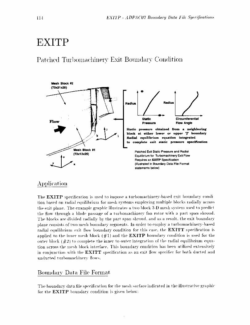
114 EXITP - A DPA C07 Boundary Da t_l Fih 5'peeificatio'n8

EXITP

Patched Turl)omachinery Exit Boundary Condition

Mesh Block #2

(73x21x2s)

Flow

_77L_(2c_) k.1

,__I>.

Static Circumferential

Pressure Flow Angle

Static pressure obtained from a neighboring

block at either lower or upper '_" boundary

Radial equilibrium equation integrated

to complete exit static pressure specification

mD

Patched Exit Static Pressure and Radial

Equilibrium for Turbomachinery Exit Flow

Requires an EXlTP Specification

(illustrated in Boundary Data File Format

statements below)

ApI>lication

The EXITP sl)ecification is used to impose a lurl)oma('hinery-t)ased exit t)oundary condi-

tion based on radial equilibrium for nlesh systelns employing multiple blocks radially across

the exit plane. The example graphic illustrates a two block 3-I) mesh system used to predict

the flow through a blade passage of a turbomachinery fan rotor with a part span shroud.

The blocks are divided radially by the part span shroud, and as a result, the exit boundary

plane consists of two mesh boundary segments. In order to employ a turbomachinery-based

radial equilibl'ium exit flow boundary condition for this case. the EXITT specification is

applied to the imler mesh block (#1) and tile EXITP boundary condition is used for the

Oilier block (#2) to COlnplete the inner to outer integration of the radial equilibrium (,qua-

tion across the mesh I)lock interface. This boundary condition has been utilized extensively

in conjunction with the EXITT sl)ecification as an exit tlow specitier for bolh ducted and

un<tucted tul'l)oma, chinery tlows.

Boundary Data File Format

The boundary data file sl>ecification for tile mesh surface indicated in tile illustrative gI'al)hic

for the EXITP boundary condition is given below:

A DPA ('07 Boundary Data Fil( ,qpee([ie_ttion._ - EXITP 115

EXlTP 2 1 I I M M L H 73 73 1 21 1 25 13 13 1 25

Note thal the M2LIM1, M2LIM2 variables ill the EXITP specification define a single

j mesh line in mesh block LBLOCK2. Failure to l>roperly regard this requirement is a

common EXITP specification error. It should also be mentioned !hal EXITP also requires

proper specification of the LSPEC1 varial)h, for proper execution.

Des<'ril)tioll

The EXITP kovword specifies !ha! a lurboma('hinory-baso<t radial equilibrium pal ched exit

tlow t)oundarv con(lit|oil is to t)(, apl)lied t<)the ]lleS]l surface specified bv LFACE1 on the

1)lock sl)(,('ified by LBLOCK1. The EXITP l)oundary condition was sl)ecifi<'ally designed

as an exit flow I)oul,<lary procedure for axial and mixed flow turbomachinorv g(,ometries

emplo.ving multiple, stacked mesh I>locks (radially) at an exit boundary plane. The EX-

ITP t)oun<larv con(Ill|on proc(`dur(, utilizes a corot)|nation slat|(' pressure specification and

integral|on of 1he radial (`(luilibrium equation 1o define the static pressure fi('l(t at all points

on th(' boundary surface. The initial slalic pr(,ssure specification us(,d to initial(' the radial

equilibrium integration 1)rocess is ol)(ain(`d from a neighboring mesh I)lock. As a resu]! of

the ('omp](`xily of lids ])rote<lure, several mesh restrictions were imposed to simplify Ill(`

application of this a l)proach. The primary assumption is that 111(, integration of the radial

e(luilibrium (`(luation may be performed along the j coordinate (lirection of the mesh. Hence.

the j coordinate should t>e 1he radial-like direction. A single specification of stalic pressure

is required at either !he maximum or minimum extr(une of Ill(' j coo]'dinate of the bound-

ary surfac(' in order to initiate 1110 integration process. The direction of integration, and

location of al)l)licalioll of 111(' s[>(`ciiied ('xit slat|(' pressure are (letormin(`d 1)5"th(` LSPEC1

variable in the calling se(lU(`llce. If LSPEC1 = L, for LOW, then PEXIT is applied to

1he lower (smal]os! wdu(`) of the j in(l(`x, and the radial (`<luilibrium equation is integrated

outward (in('r(`asinp.; j direc! ion ). If LSPEC1 = ][. for HI(;H. then PEXIT is applied t<)

!he Upl)er (larg('sl value) of !he j index, and the radial equilibriunl equation is inlegrat(`d

inward (decreasing j dire('tion). The direclion of integra!ion implied by LSPEC1 must be

('OllSiS!elll wi!h the location of the neighl)oring mesh block (LBLOCK2) from which ill(,

initial pressure data is (t(`rived. The j coordinate location from which the pressure is taken

in mesh block LBLOCK2 is <letormined 1)y the M2LIM1, M2LIM1 varial)le, and the

sl)eciii('a!ion of ! he LSPEC2 control parameter. If !11(` M2LIM1,M2LIM2 coral)|nat ion

is !aken from!he higher j index, then LSPEC2 should I)e H. If the M2LIM1,M2LIM2

('oral)|nation is lak(`n from the lower j index, lh('n LSPEC2 should 1)e L. Un(l('r mos!

circumstances, lhe static pressure is !ak(`n froln either the Ul)t)('rmost or lowermosl j cool

<linat(', in which case LSPEC2 should t)e either H or L, rest)ectively. The rema.ininp4 flow

wlrial)[es on 111e EXITP boundary are updat.ed t)y a Re|mann invariant formulalion t)as(`(I

on the resulting local static pressure field. Included in theEXITP t)roce<lureis a sl>ecial

corre<'tion scheme which forces !he flow t<) pass out of 111o flow domain. In other wor(Is, if

the COml)Ut('d v(`loci!ies result in a local inflow a! the EXITP I)oun<lary, no matter how

small the magnitu<l(` of th(` inflow, the v(`lo<'ities are resel to zero a_ that point.

12estri<'tions/Lilnitations

116 EXITP- ADPAC07 Boundary Data File 5'pecification._

Tile EXITP boundary condition assumes that tile mesh is oriented ill such a fashion tha!

the radial coordinate is defined as 7"= v") 2 + z 2. For axial flow turbolnachinery, this iml)lies

that the axis of rotation (o1" the centerline) coincides with the .r axis. It is also required

lhat tile radial-like direction of the mesh be detined t)y the j coordinate, and is therefore

not valid on a j =constant mesh plane. This is required in order to properly integrate the

radial equilibrium equation to colnl)lete tile exit. static pressure specification. Examples

of this type of lnesh svstem can t)e found in the chapler defining standard cot,tiguralions.

The EXITP boundary specification is restricted to 3-I) mesh surfaces (2-I) mesh surfaces

should use the EXT2DP boundary specificatioll).

Co111111Oll Errors

• Application of EXITP to a 2-1) mesh system.

• Failure to properly sl)ecify the LSPEC2 variable.

• M2LIM1 and M2LIM2 differ.

• Radial-like direction of the mesh is no! tile j coordinate.

• Failure to properly specify the LSPEC1 variable on the boundary data ill(, specifica-

tion line.

A Df_4 ('07 Boundaw Data Fib £'p(e_[ication._ - EXT2DT 117

EXT2DT

2-D Turl)onmchinerv Exit Boundary Condition

2-D Mesh Block #1

(49x17x1)

-1"/:/Static Circumferential

Pressure Flow Angle

;tatic pressure specified at either

lower or upper T boundary

Radial equilibrium equation integrated to

complete exit static pressure specification

ms

Specified Exit Static Pressure and Radial

Equilibrium for 2-D Turbomachinery Exit Flow

Requires an EXT2DT Specification

(illustrated in Boundary Data File Format

statements below)

Ai)I)lication

The EXT2DT specification is used to ilnpose a turbolnachinery-t)ased exit t)oundar.v con-

ditioll based on radial e(luilil)riunl for 2-I) mesh blocks. The example graphic illustrated

abow, depicts an EXT2DT specification for a 2-D (axisymmetric) flow solution fbl'a tur-

bolnachinery blade row. This I)oundar.v condition has been utilized extensively a.s an exit

flow specifier h)l' I)ot h ducted and ullducted 2-1) turbonlachilmry flows.

Bolmdarv Data File Format

The boundary dala file specification for lhe mesh surface indicated in the illustrative gral)hic

for the EXT2DT boundary condilion is given below:

EXT2DT 1

PEXIT

1.10S

I I I M N L L 49 49 1 17 1 2 1 17 1 2

or the alternale Sl)ecilication:

EXT2DT 1 1 I I M M L L 49 49 1 17 l 2 1 17 1 2

118 EX T2D T - A DPA ('07 Boundary Data Fil_ ,S}_(,cification._

PEXIT EMDOT PRELAX

1.105 13.7 0.001

Note that a coml)lete EXT2DT specification requires two addilional lines following the

EXT2DT t)oundary data file specification line. Failure to i)roperly specif,v the data in these

additional lines is a common EXT2DT specification error. It should also be mentioned that

EXT2DT also requires proper specification of the LSPEC1 variable for l)roper execution.

Description

The EXT2DT keyword specifies that a turbonlachilmry-based radial equilibriuln exit flow

boundary condition is to be applied to the mesh surface specified by LFACE1 on the 2-1)

mesh block specified by LBLOCK1. The EXT2DT boundary condition was sl)ecifically

designed as an exit flow boundary procedure for 2-I) axial and mixed flow turbomachinery

geometries. Pure ra(lial flow turbolnachinery exit ttow boun(laries may usually be specifie(t

by the EXT2DG I)oundary condition. Due to the form of tile radial equilibrium equation

utilize(l in the EXT2DG routine, only cylindrical coordinate solution meshes are permitted

to use this routine. The EXT2DT boundary condition procedure utilizes a combinatiol_

static pressure specification and integration of the radial equilibrium equation to define the

static l)ressure field at all points on the 1)oundary surface. As a result of tile complexity of

this procedure, several mesh restrictions were imposed to simplify the application of this

approach. The primary assumption is that the integration of the radial equilibrium equation

may be performed along the j coordinate direction of the mesh. Hence. the j coordinate

should be the radial-like direction. A single specification of static pressure is re<luired at

either the maxinmm or minimum extreme of the j coordinate of the boun(lary surface in

or(let to initiate the integration process. The direction of integration, an(l location of apl)li-

cation of the specilied exit static pressure are determined by the LSPECl variable in the

calling sequence. If LSPEC1 = L, for LOW, then PEXIT is applied to the lower (smallest

value) of the j index, and the radial e<luilibriunl equation is integrated outward (increa, sing

j direction). If LSPEC1 = H, for ttlGIt, then PEXlT is applied to the ut)per (largesl

value) of the j index, a,nd tile radial equilibriuln equation is integrated inwar<l (decreasing

j direction). The remaining flow variables on the EXT2DT boundary are updated by a

Reimann invariant formulation I)a,se(1 on the resulting local static pressure field. Included

in the EXT2DT procedure is a special correction scheme which forces the flow to pass out

of the flow domain. In other words, if the COml)uted velocities resul! in a local inflow al

the EXT2DT boundar,v, no matter how small the magnitude of the inflow, the velocities

are resel to zero a,t that point. This boundary condition requires the specificalion of a,ddi-

tiona,1 (lala, a,s shown in the boundary (tata format <tescriI)tor above. Tile first additional

line following the EXT2DT specification is assume<l to t)e a label an(t may contain any

information: however, for consistency it is recommended that the label PEXIT be used.

The line following the PEXIT label contains the value of specified non(tinmnsional exit

stalic i)ressure use(l to initiate the radial e<luilibrium integration t)rocedure. The value of

tim PEXIT varial)le is computed as follows:

1)_ xit st(_ tic,de sir_ dPEXIT =

F,._ y

The variable t),.,7 is specified bv the input variable PREF. Values of PEXIT <0.0 are

A DP.4 ('07 Bo_u_dar!! Dato Kilt ._'p:c_:ficatiol_._ - E.VT2D T 119

not permitted. Naturally, l>oor conver_en<'e or solution divergence can occur if" tile value of

PEXIT suggests boundary data which are significantly differenl from the remainder of the

flowfield. In such cases where this occurs, it is recommended that the solution be started

with more conservative boundary values, and then restarted using the final b<>un<larv values.

An alternate sl)ecificalion is provide<I for the EXDT2DT boundary specification an

shown in the sample apl)licalion al>ove. In this <'as<,, three values are included following

the original I)oun<larv specification lit,<,. The alternate speciIication is l>rovi<led as a means

of a<'hi(wiz_g a <lesire<l mass llow ,'at<, through the bounding s_rfa('e using the EXT2DT

alp.;<>rilhm. The desired mass flow rate is achieved iteralively bv incrementally a(Ijuslin_

the exil static pressure specification until the desired flow rate is achieved. There[bre. in

lids specification, the varial)le PEXIT described in detail above is the initial exit s_ati<'

pressure used in the ilerative process, EMDOT represents the <lesired mass tlow rate

thro_lgh the bolJndin_ s,rf'ace i, po_,nds mass, and PRELAX is a relaxation factor to

stabilize the iteralive l)rocess (values may range from 0.0 to 1.0. though l)<>or <'onver_ence

is likely for values lar_;er 1has 0.1). F<)r ('aries,an flow calculalions a unit depth (l.0 in

mesh coordinates) is assllill('(l ['of the thh'<l coordinate direction to <telermine the mass tlow

rate. ]:or cv[indrical tlow calculalions, 1he geomelry is assumed to be axisvmmetric and

a [Htlltip]e of 2_" is used in 1he mass flow integration (the mass flow is computed as if the

full circum['erence of the axisymmelric geometry were eml>loyed). This l>rocedure is sol

foolproof, and suffers from the fact 1hat when a job is restarted, if an updale<l exit t>ressure

is not inserted in the boun<larv <la.la file, then the pressure-mass ttow ilerative process will

essentially start over. The .iI)/>A('07co<le will automatically determine when _o emplo.v

the iterative process b_' identig;viltg the additional boundary sl)e<'itication variables.

I/ostri<'tions/Lilnitations

The EXT2DT I)oun<lar.v con<lilies assumes thai the mesh is oriented in such a fashion that

lhe radial coordinate is <let, ned an r = v@ 2 + : 2. For" axial ttow turbomachinery, this implies

thai the axis of rotation (or the centerline) coincides with the.r axis. I1 is also required

1hat lhe ra<lial-like direction of the mesh be defined by the j coordinate, and is therefore

not valid <>n a j =COl,stant mesh plane. This is require<t in or<ter 1.o properly integrate the

ra<tial e<luilil)rium equal,on lo complete the exil slalic pressure specification. Examples of

this type of mesh svslem can be found in the chapter <lefts'rip4 standard configurations. The

EXT2DT I_oundary specification in restricted to 2-1) mesh surfaces (3-D mesh surfaces

should use the EXITT boundary sl)ecificalion).

Collllll()ll Errors

• .\l)plication of EXT2D'I' to a 3-I) mesh system.

• Failure to specit_" the additional data value PEXIT.

• hnproper specificalion of the alternate (mass flow)iteralive scheme.

+ l_adial-like <live<'tiol_ of the mesh is not the j coordit,ate.

120 EXT2DT- ADPAC07 Boundary Data File .5'pceifieation.s

• Cylindrical solution procedure not selected (FCART=I.0)

• Failure to properly specify tile LSPEC1 variable on the boundary data file specifica-tion line.

• Value of PEXIT is too high (flow cannol get st arled).

A DPA ('07 Boumlary Data Fil< ,qp_ciJicatio_s - EXITN 1"21

EXFFN

Non-Refle(ting Outflow Boundary Condition

Mesh Block #1

(49x33x33)

Non-reflecting Duct Exit for

Time-dependent Flow Requires

an EXITN Specification

f_

Flow

AI)plication

Tl,e EXITN specificalion is used to imi>ose a non-reflectin_; outflow boundary condition

for time-del)en<len! flow calculations where Sl)uroius numerical reflections normally imposed

by ol her boundary pro<'e<hu'es ax'e undesirable. The examl>le graphic above depicts a simple

duct flow using a (!arlesian-base<l H-gri<t, where the exit I>oundary plane is controlled t>v

an EXITN specification. This bOUll<tary condilion should be used for time-dependent flow

calculalions only.

BoulMary Data File Forxnat

The I)oumLdarv (lala file sl)ecificalion for the mesh surface indicated in the illuslrative p.;ral)hi<"

['or lhe EXITN I)oun(lary condition is given I)elow:

EXITN 1 1 I I M M J K 49 49 1 33 1 33 1 33 1 33

Des<'ril)ti<)n

122 EXITN- A DPAC07 Bou1_dary Data Fil_ ,S'pecificatio_._

Tile EXITN statelnent specilies that a non-relecting exit flow boundary condition is to be

applied to the mesh surface specified by LFACE1 on tile block specified by LBLOCK1.

The EXITN boundary condition should be used for time-del)endent flow calculations where

Sl)Ul'ious nulnerical reflections which normally occur for other exit boundary conditions (such

as EXITT, EXITP. etc.) are undesirable. EXITN may be used on any mesh face (I. J. or

K constant ) for either cylindrical or (_artesian-based solution schemes (see the input variable

FCART). Tile EXITN procedure utilizes a characterislic-based formulation described il,

the ADPA('07 final report [21].

Restrictions/Lilnitatiolls

The EXITN boundary specification should only be applied for time-dependent flow cal-

culalions. Steady state problems call usually use the EXT2DG. EXITX. or EXITT

boundary specification ).

C o111111OllErrors

• At)plication of EXITN for a steady state sohltion.

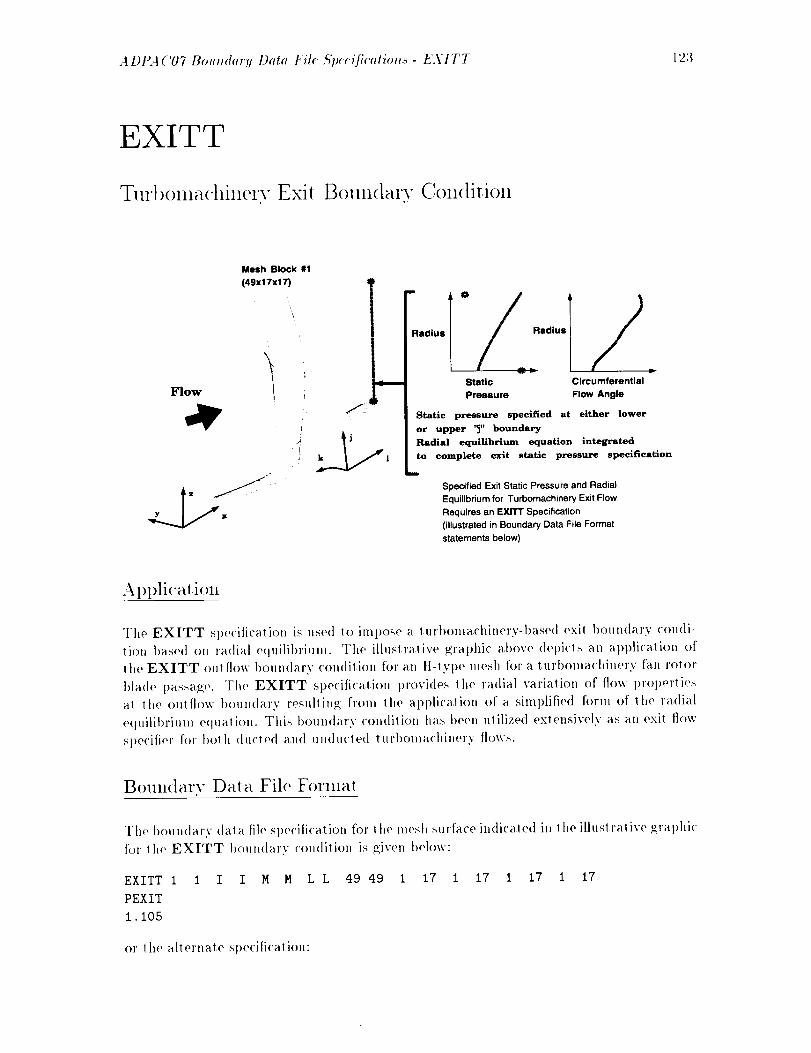
ADPA('07 Botmdar9 Data File .S)_ce_[ieatio,ts- EXITT 123

EX.ITT

Turl onla<'hinerv Exit Boun<larv Condition

Flow

Mesh Block #1

(49x17x17)

J

Ji

Static Circumferential

Pressure Flow Angle

Static pressure specified at either lower

or upper '_" boundary

Radial equilibrium equation integrated

to complete exit static pressure specification

romp

Specified Exit Static Pressure and Radial

Equilibrium for Turbomachinery Exit Flow

Requires an EXlTT Specification

(illustrated in Boundary Data File Format

statements below)

Application

The EXITT sl_e¢'ificalion is used to impose a lurbomachinery-based exil boutl¢lary condi-

lion based on radial equilibriuln. The illustralive graphic above depi<'Is an application of

the EXITT out [low boundary condition for an tt-lype mesh for a turl)olnachinery fan rotor

bla(le passa,oge. The EXITT specification t)rovides the radial variation of flow pl'Ol)erlie,_

at the outtlow boundary resulting from the application of a simplified form of the radial

equilibrium equation. This t>OUl_<lary Col_dition has been utilize<] extensively as an exit flow

sl>eciIier for both du<'led a l_<l unducted turl)omachi,lery flows.

Boun<lary Data File Forlnat

Thel>oundarydatafile specificationforthemeshsurfaceindicatedintheilhlslrativeNraphic

tbrlhe EXITT I)o,lndary<'on<tilion is given below:

EXITT 1 1 I I N M L L 49 49 1 17 1 17 1 17 1 17

PEXIT

I.i05

or the alternate specification:

124 EXIT T- A DPAC07 Boundary Data File 5'pecifications

EXITT I I I I M M L L

PEXIT EMDOT PRELAX

1.105 13.7 0.001

49 49 1 17 1 17 1 17 1 17

Note that a c()ml)lete EXITT specification requires two additional lines following the

EXlTT boundary data file specification line. Failure to l)roperly specify tile data ill these

additional lines is a common EXITT specification error. II should also be mentioned that

EXITT also requires proper sl)ecitication of tile LSPEC1 variable lot proper execution.

Description

The EXITT keyword specifies that a turbomachinery-based radial equilibrium exit. flow

boundary condition is to be applied to the mesh surface specified bv LFACE1 on the block

specified by LBLOCK1. The EXITT boundary condition was sl)ecifically designed as an

exit flow boundary l)rocedure for axial and mixe(I flow lurbonlachinery geomelries (pure

radial flow turl)omachinery exit flow 1)oundaries may t)e usually be specified I)y the EXITG

boundary condition). The EXITT I)oundary condition procedure utilizes a coml)ination

static pressure specification and integration of the radial equilibrium equation to define the

static pressure field at all points on the boundary surface. As a result of the complexity of

this i)roce(lure, several mesh restrictions were imt)osed to simplify the al)l)lication of this

apt)roach. Time primary assulnption is that the integration of the radial equilibrium equation

may t)e t)erformed along the j coordinate direction of the mesh. Hence. the j coordinate

should I)e the radial-like direction. A single sl)ecificatiou of slatic t)ressure is required al

either the maxinmnl or miuimum extreme of time j coordinate of the boundary surface in

order to initiate the integration l)rocess. The direction of integration and location of appli-

cation of the specified exit static pressure are determined by time LSPEC1 variable in the

calling sequence. If LSPEC1 = L, for LOW, then PEXIT is applied to the lower (smallest

value) of the j index, and the radial equilibrium equation is integrated outward (increasing

j direction). If LSPEC1 = H, for HIGH, then PEXIT is apl)lied to the upper (largest

value) of the j index, and the radial equilibriunl equation is integrated inward (decreasing

j direction). The remaining flow variables on the EXITT l)oun(lary are updated by a

Reima lm invariant forlnulation based on the resulting local static pressure field. Included

in the EXITT procedure is a special correction scheme which forces the flow to pass out of

the flow domain. In other words, if tile computed velocities result in a local inltow at the

EXITT boundary, no matter how small the magnitude of tlle inflow, the velocities are reset

to zero at that point. This boundary condition requires the specification of additional data.

as shown in the boundary data format descriptor above. The first addilional line following

the EXITT specification is assumed Io be a label and may contain any information; how-

ever, for consistency it is recommended tha! the label PEXIT be used. The line following

the PEXIT label contains time value of specified non-dimensional exit. static pressure used

to initiate the radial equilibrium integration procedure. The value of the PEXIT va.riat)le

is computed as follows:

t)_ xitst¢_tic.desiredPEXIT =

P,._ :

The variable P,.,] are specilied by the input variable PREF. \:alues of PEXIT <0.0 are

not permitted. Naturally, poor convergence or solution divergence can occur if the vahm of

.4DPA ('07 Boundary Data Fih ,S'p_cification,_ - EXIT T 125

PEXIT suggests boun<lary data which are significalHly <titl'erelH from tile remainder of lhe

ttowfield, h, such cases where this occurs, it is recolnmel,ded that the solution he started

with []_<)]1¢.conservalive l>ollndary values, and then r(`slarted using the final boundary values.

:\n all ernat(` sp(`cificaliol, is provided for the EXITT boundary specification as shown

i,l lh(` sample application al>ove. In this <:as('. lhre(' values are inchld(`d following; the original

l)oun<lary Sl)(`cifi<'alion line. The allernale specificalion is provided as a means of a<'hievilJ¢:

a d(`sir(`<[ ,,lass tlow rate ,hi'ouch th(` houl,<lin_ surface using; the EXITT algorithm. The

<l(`siwd mass flow ral(` is achieved it(`rativ(`ly I)v i,_('r(`m(`nlally a<l.justin_; lh(` exit stalk'

l)r(`ssul'e Sl>(`ci[icali<)ll ul,til th(` <lesiw<l flow ral(` is achieve<l. Therefore. iH this sp(`cification.

th(` variable PEXIT (l(,s('ril)ed in (l(,lail al)ove is lh(` initial (`lit static I)r(`ssur('us(`(l in lh(`

',(`rally(' process. EMDOT ret)res(`nls I h(' <lesir(,<l mass tlow rat(` 1hrough I he houl,liH_

surfa('(` ill I)Oun<ls mass, at,<l PRELAX is a l'e]axatio,, faclor Io stal)ilize lh(` il(,raliv('

l)r<)<'(`ss (values may rang(` fi'om 0.0 t<) 1.0, th<)ugh I)oor co,,v(`rg(,nc(` is lik(`lv for valu(,s

lar_(,r lha,i 0.1). This proc(,<lul'(' is not foolproof, and sufl'(,rs ['roln lh(` facl ,hal wh(,ll a

job is i'(`slart(`<l, if an Ul)daled (`xil I>r(`ssure ix not ins('rled it, th(' l)oundal'v data ti](`, then

the ])r(`ssur(`-mass flow ileral iv(' ])roc(,ss will ess(`miallv sl arl over. The .t I)PA ('07 co<l(, will

aiH(mlali('ally (tet(`rmin(` wh(`ii to (,ml)loy l lw it(`vativ(` process l>v ,(tent'lying the additional

boundary si)(`cifi('alion vadahh's.

R(,stri<'tions/Limitations

The EXITT t>oundarv condiliol, assum(`s thai the mesh is oriented ill such a fashion thai

lhe ra(lial coor(liltal(` ix <t(`fin(`<t am r = V/y 2 + : 2. For axial flow lurbolnachiuery, thi_ iml)li('s

[hal lh(' axis of r(>lati<)n (or [h(` c(`nt(`rlil,e) coincides with lh(` .v axis. It is also r(`quir(`(l

that the radial-like <lir(,<'li¢),l of lh(` m(`sh t)(` (lelill('(I I)v the .j <'oor(lillat(`. and is thel'efore

nol vali<l OIL a j ----constanl mesh l>la,w. This is r(`<luir(`d in order 1o t)rol)('rly illlep.;ral(" th(`

radial (`<luilit)rium ('<lualio,l Io COlnI>l(`t(` l h(` exit slat'(' l)r('SSUl'e st)ecificalioH. Examl)les

o[' lhis tyl)(' of mesh syStelll CAll ])(' ['OUI,(1 ill IIw chapter <l(`fildng; standard COllfi,P_;uraliol,s.

The EXITT 1)O,,ll<lary Sl)(`cifi<'alion is restrict(,<l to 3-l) mesh surfaces (2-I) mesh surfaces

should us(, th(, EXT2DT I)oul,<lary specification).

CollllllOll Errors

* Al>l)licalio,, of EXITT to a 2-1) mesh system.

. t"ailur(' t<) Sl)(`cify the additional (lala ",'ahw PEXIT.

• Illll)rOl)er sl)e<'ilicalion o[" lhe alternale (mass flow)iteralive scheme.

• t{a(tial-lik(` ¢lireclion of the mesh is not lhe j coordinate.

• Mesh <l<)(,s not possess circulnferenlial s vmnletry (axial. radial mesh coor(litmtes vary

in lhe circumf(,rel,tia[ coot<tit,at(` <lirecl loll ).

• t:aihH'(' Io l)rol>erly Sl)(`cify lh(` LSPEC1 variable on lh(` I)oun(lal'v data Ill(' Sl)('('ifica-

t i<m lin('.

126 EXITT - ,4 DPA C07 Bound_ry Data Fib ,S'p(cifi('¢ttio'n._

• Vahw of PEXIT is too high (flow cannot get slarted).

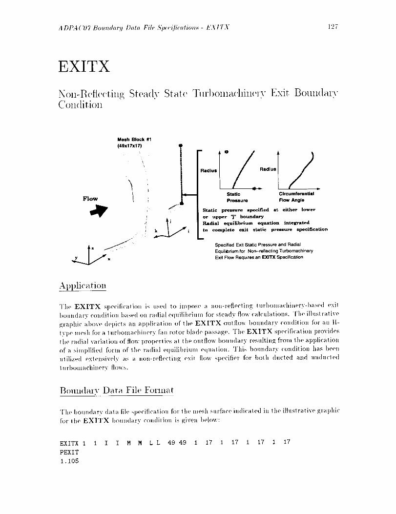
A DPA ('07 Botmdarg D.I. File' £'lU'e(ficatio_._ - EXITX 127

EXITX

Non-Reflecting SteadyCon(lit, ion

State Turl)onm('hinerv Exit Boull(larv

Flow

Mesh Block #1

(49x17x17)

i

Ja

I

m

ladlus Radius

Static Circumferential

Pressure Flow Angle

Static pressure specified at either lower

or upper '_j" boundary

Radial equilibrium equation integrated

to complete exit static pressure specification

mm

Specified Exit Static Pressure and Radial

Equilibrium for Non-reflecting Turbomachinery

Exit Flow Requires an EXlTX Specification

Apl)lication

The EXITX specification is used to iml)ose a liOn-reflecting turl)omachinery-1)ased exit

boundary con(tit ion based on radial equilibrium for steady flow ('alculations. The illustrative

graphic a|)ove depicts an al)l)lication of the EXITX outflow lmun(tary con(lili(m for an ll-

type mesh for a t urbomachinery fan rotor blade passage. The EXlTX specificalion provides

the radial va riation of flow prot)erlies at the outflow boundary resulting fl'om the apl)lication

of a simplified form of the radial e<luilibrium equation. This boundary condition has been

utilized extensively as a non-reflecling exit flow specifier for both ducted and unducled

I urbomachinery flows.

Boundary Data File Format

The I)ou.dary data file spe<'ification for the mesh surfa('e indicated in Ill<, illustrative graphic

for the EXITX I)ou]l<lary condition is given below:

EXITX I

PEXIT

1.105

1 I I M M L L 49 49 1 17 1 17 1 17 1 17

129; EA'ITX- A DPAC07 Boundary Data File S'pecification._

Note that a complete EXITX st)ecification requires two additional lines following the EX-

ITX boundary data file specification line. Failure to properly sI)ecify the data in these

additional lines is a conlmon EXITX specification error. It should also be mentioned that

EXITX also requires proper specification of lhe LSPEC1 variabh, for prol)er execution.

Description

The EXITX keyword specifies that a non-reflecling turbomachil_ery-hased radial equilib-

rium exit ttow boundary condition is to be applied to the mesh surface specified t>y LFACE1

orl the block specified by LBLOCK1. The EXITX boundary condition was sl>ecifically

designed as a non-reflecting exit flow boundary procedure for steady state analysis of ax-

ial and mixed flow turbomachiner.v geometries (pure radial flow lurbomachinerv exi! flow

boundaries may usually t)e specified by the EXITG boun<tary condition). The EXITX

boundary Colldition procedure utilizes a coml)ina.tiol_ static pressure specification and in-

tegration of the radial equilibrium e<luatioll to define the circulnferentially average<l static

pressure field at all points on the boundary surface. The circumferenlially-average<t pres-

sure at the exit boun<lary is forced to match the imposed static pressure. The use of the

circumferential average permits flow properlies 1o vary across the exit plane, while still

maintaining the desired overall flow (additional details for this procedure are given in the

tinal rel)ort [21]. As a result of the colnplexity of this procedure, several mesh restrictions

were imposed to simplify the application of this approa.ch. The primary assumplion is lhat

the integration of the radial equilibrinln equation may be perfl)rme<l along lhe j coordi-

nate direction of the mesh. Hence, the j coordinate should be the radial-like direction.

A single specification of static pressure is required at either the nlaximum or mildmUm

extreme of the j coordinate of the boundary surface in order to irritiale the inlegration

process. The direction of integration and location of application of tire specifie<l exi! static

pressure are delermined I)y the LSPEC1 varial)le in the calling sequence. If LSPEC1 =

L, for LOW, then PEXIT is apl)lied to the lower (smallest value) of the j irr<lex, and the

radial equilibrium equation is integrated oulward (increasing j direction). If LSPEC1 =

tt, for HIGH, then PEXIT is applied to the upper (largest value) of the j index, an<l the

radial equilibrium equatioll is integrated inward (decreasing j <lirection). The remaining

itow variables on the EXITX boundary are updated t)y a Re!mann invariant formulation

based on the resulting local static pressure field. Included in the EXITX procedure is a

special correction scheme which forces the flow to pass ou! of the flow domain. In other

words, if the COlnputed velocities result in a local inflow a! the EXITX I)oundary, no matter

how small the magnitude of the inflow, the veloci!ies are resel to zero at !hal point. This

boundary condition requires the speciiication of additional data, as shown in lhe boundary

data formal descriplor above. The firsl a<tdilional line following lhe EXITX specificaiion

is assumed to be a label and may contain any ilffOrlnation: however, for consistency it is

recommended lha! the lal>el PEXIT t>e nsed. The line following lhe PEXIT label contains

the value of specified non-dimensional exit static pressure used 1o initiate the radial equi-

librium inlegration l>rocedure. The value of the PEXIT variable is cornputed as follows:

Pe a,it.st:_ tic,de sire ,1t>EXIT =

P,,_ :

The variable t),._f are specitied by lhe inpul variable PREF. Values of PEXIT <0.0 are

not pern,itted. Naturally, poor corlvergen<'e or solulion divergence can occur if !he value of

A DPA ('07 Boundary Data f'ih ,qpcc(ficatio,.._ - EXITX 129

PEXIT suggests I)oundary data which are significanlly different fi'oni Ill(, reniainder of theflowiiel(l. II, rases wilei'e lhis occurs, il is reconinlended lhal lhe solution l)e started wilh

more conservative 1)oundary values, and then restarted using the final t>oun(lary values.

t2 ostrictions/Limit ations

The EXITX 1)oltndarv condition assumes that the nlesh is oriented in such a fashion thal

lhe radial ('oor(linale is defined as r = V/)) 2 + z_. l:or axial flow lurl)omachinery, this implies

lhal the axis of roialion (or the centerline) coincides with the a' axis. It is also required

lhal the radial-like (lireclion of the mesh ])e define(l t)y the j coordinate, and is therefore

1101 vali<t eli a j =COllS|alll liiosh plane. This is re(lliire(l in order to prol)erly inlegralo tile

radial equilil)riuni equation 1o conil)lele the exil slalic l)ressul'e sl)ecilicalion. ]']xanit)les of

liiis l yl)e of lilesh svslein Call I)o fOllll(1 in 1]1o (']lal)l('r <telining slan(lar(I con[i_uralions. The

EXITX bOUli(lary sl)ecifi('alion is resl ri<'le(l Io :l-l) niosh slirfac0s. Tile EXITX l)Ollildarv

('on(ill ion is only valid for slea(lv slale flow calcuial ions (a liOli-i'efloc1 ing oxil flow l)oun(lary

('on(lilions is availat>le wilh EXITN).

CollllllOll Errors

t At>l)licalion of EXITX 1o a 2-I) nles]l system.

• Faihlre 1o sI)eci[ _" lhe addilional data value PEXIT.

• Ra<tial-like <tireclion of tile inesti is lie1 the j coor(tinale.

• Mesh does liol possess circtllllferenl, ia] svlliliielry (axial, radial mesh coordinaies vary

in lhe circuniferenlial coordhiale (lireci ion ).

• Faihire 1o t)rolierly sl)e('it )" lho LSPEC1 wirial)le Oll the I)oundary (lala file sl)ecifica-

tion line.

• Value of PEXIT is leo higli (flow callllol get started).

, Applicatioli of EXITX for time-dependeni flow ca lculaiions.

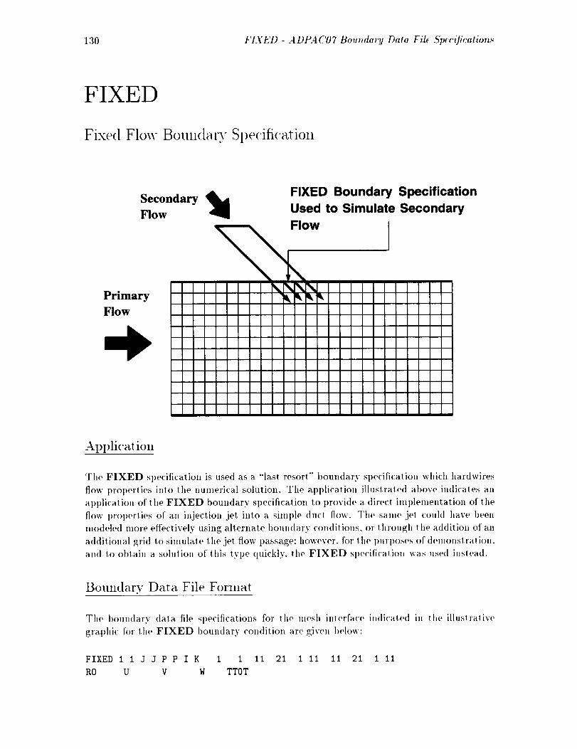
130 FIXED - A DPA C07 Boundary Data File ,S'pecification._

FIXED

Fixed Flow Boundary S1)ecification

SecondaryFlow

PrimaryFlow

FIXED Boundary Specification

Used to Simulate Secondary

Flow I

,rk, i_ ¸,

IIIIIIIII

Application

Tile FIXED specification is used as a "last resort" boundary specification which hardwires

flow properties into the numerical solution. The application illustrated above indicates an

application of the FIXED boundary specification to provide a direct implementation of the

flow properties of an injection jet. into a siml)le duct flow. The same jet could have been

modeled more effectively using alternate boundary conditions, or through the addition of an

additional grid Io simulate the .jet flow passage; however, for the purl)oses of demonstration.

and t.o obtain a. solution of this type quickly, the FIXED specification was used inslead.

Boundary Data File Format

The bouildary data file sl)ecifications for the mesh interface indicated in the illustrative

gral)hic for the FIXED boundary condition are given below:

FIXED 1 1J J P P I K 1 I 11 21 I ii ii 21 I II

RO U V W TTOT

ADPA(7)7 Boundary Data Fil* ,_'pecffication._ - FIXED 131

0.002 100.0 100.0 0.0 600.0

Nolo tha! a conlI)lelo FIXED st)e('ificalion requires the st)ecificalion of additional <lala

beyond the standard boun(larv speciiication line.

Des<'ril>tion

The FIXED slalemenl is uso(l to provi<le a fixe<l specificalion of I)oun<larv flow (lala ill the

al)sence of any olller at)l)rOl)riale I)oun(lary ('on<liiion. This rouline was t)rovi(le(I for thos(,

cases whore other I)oun(lary conditions either cannot I)rovi<le lho boundary specifications

(lesire<l. or il, lhose <'as<,s where a fixed t>oundary sl)ecitication is deemed apl)rOl)riale. In

mosl cases, lhe FIXED spe<'ili<'al ion is un(lesirablo because ill(' boundary con(lilion ilself is

perfectly retlecling, aim will lhereforo inhibil solulion convergence. In a<tdiliou, lhe FIXED

sl)ecili<'atiou does nol l)ormil inleracliou between tile I)oun(larv flow and the inlerior [h)w.

which runs contrary 1<) the normal fluid (lynamics l)ehavior.

A FIXED SlW('ifica_i(m requires two additional liaes iu addi+iorl ¢o the rlor'rnal ho(m<taLv

(lava file <lescril)tOr. as shown above. The firsl achlitiona] hue simply contains lhe labels for

the a.<t<liti<)nal flow variable RO, U, V. W. and TTOT. The next line contains the a<'iual

values for lhe flow variable st)e<'ificalions. The varial)le RO (tefines the ttuid (lensilv in slu_s

l)er cubic fool. The varial)les U. V, and W contain the flui(l velocily componenls in feel

t)er second for the .r, .q, and ,: coordinate (lirections f<)r a (!artesian solution mesh I)lo<'k,

and the .c, r, av_<l 0 <'oordinate <lirections for a cylindrical solution mesh I)lo<'k, resl)e('lively.

Finally, TTOT rel)reselds lhe [tui(l lota] teml)erature in (legrees Rankine for Ill(, boundary

specification, l)urblg the af)pl'watiotl of a FIXED specificatiou, phanlom boundary cell

data are sol a<'('or(ling to the data l)rovi<lod in Ill(, oxlra lines following the bouiMary dala

st)e('ifi<'ation liae as shown above. As a resull, the <ta_a is m)t necessarily al>plie(t at the

boundary, but lhe influence of the <lata is fel! .just outsi(le the I)ouudary. This l)]mnonwnon

is consisleld with the t)ehavior of a finite volume solution algorithm.

R est riot ions/Limit at ions

l)ala l)rovi(le(l ill the FIXED sl)ecilicalion shoul(l tel)resort! t)hanmn! cell centered data

and re,st be dimensionaJized as described above.

CollllllOll Errors

hl<'orre<'tly specitied or misaligned extents of boun<tary regions (va,lues of MILIM1,

MILIM2, N1LIM1, NILIM2, M2LIM1, M2LIM2, N2LIM1, N2LIM2 do not

correctly <h,iino 1he imerface extents on blocks LBLOCK1 and LBLOCK2).

t"ailure 1<) t>rovi(le a<hlili(>nal data for FIXED specitication.

FIXED I)oun(lary Sl)ocificalions for <'ylin(lrical solution mesh blocks mus! I1S(' |he

cylindrical velocity colnponenls.

132 FIXED - A DPA ('07 Boundary Data Fil_ 5'p¢ciJicatioT_s

• FIXED boundary specifications for (!artesian solution mesh blocks mus! use the

(!artesian velocity components.

.4DPA ('07 Bout_dar!l Data Fil_ Spteification.s - FRE2D 133

FRE2D

2-D Far EMd Flow Boundary Condition

Far Field Boundary with Angled

Flow Requires a FRE2D Specification

2-D Mesh Block #2 [ 2-D Mesh Block #4

(12gxlTxl) _ (97x17xl)

' L _

2-D Mesh Block #1 2-D Mesh Block #3

(129x17x1) (97xlTxl)

AI)l)li('ation

The FRE2D specification is used to impose a far field boundary condition with unifornl

far field flow prolwrties. The example graphic above illustrates a four block mesh system

used to t)redict the axisymmelric flow through a high tupass ducted fan. The two outer

blocks (#2 and #4) require a farfield boundary condilion at the outer boundary (j=lT).

The FRE2D boundary specification is used to satisfy the farfield flow requirelnent. This

boundary condition has been utilized extensively for both ducted and unducted 2-D fan

prol)ulsion svst eros.

Boundary Data File Format

T'he boundary dala file specification for the mesh interface indicated in the illustrative

graphic for the FRE2D boundary condition is given below:

FRE2D 2 2 J J M M I K 17

PTOT TTOT EMINF ALPHA

1.0 1.0 0.75 0.0

FRE2D 4 4 J J M M I K 17

PTOT TTOT EMINF ALPHA

1.0 1.0 0.75 0.0

17 I 129 I 2 I 129 1 2 Block 2

17 1 97 1 2 1 97 1 2 Block 4

134 FRE2D - A DPA C07 Boundary Data Fil_ Specifications

Note that a complete FRE2D specification requires two additional lines following the

FRE2D boundary data file specification lille. Failure to l)rol)erly sl)ecify the (tata ill these

additional lines is a ('ommon FRE2D specification error.

Description

The FRE2D statelnenl specifies that an external, free flow boundary condition is to be ap-

plied to the mesh surface specified by LFACE1 on the 2-D block specified by LBLOCK1.

The FRE2D boundary condition is primarily used for external flow problents at a fat' fiehl

boundary to simulate the effects of the atmosphere or other large reservoir with known

properties. The FRE2D procedure utilizes a Reimann invariant formulation to compute

the local flow quantities, and l)erlnits both inflow and outflow through the boun(ling surface

based on the nature of the local flow with respect to the known far fiehl conditions. This

boundary condition requires the specification of additional (tala, as shown in the boundary

data format descriptor al)ove. The first additional line following the FRE2D specifica-

tion is assumed to be a label and may contain any information; however, for consislen('y

i! is recommended that the labels PTOT, TTOT, EMINF, and ALPHA be used. The

next line contains the values imposed for the variables PTOT, TTOT. EMINF. and

ALPHA, which represent the far field nondimensional reservoir total pressure and total

teinl)erature, along with the Mach number and Cartesian angle of attack, respectively, used

in the FRE2D characteristic solution sequence. The value of the PTOT variabh, is the

desired normalized fat' field total pressure computed as:

PTOT = Ptc, t,,l.d:si,._d

Pr_f

and the value of the TTOT variable is tile desired normalized far field total temperature

compute(I as:

_I)o_al.d_ sir_ dTTOT -

The variables P,._/ and T,._j are specified by the input variables PREF and TREF. Values

of PTOT and TTOT <0.0 are not permitted. The variable EMINF represents the far

field Mach number. The far field flow is always assumed to progress along the positive x axis.

and therefore mesh systems should be generated with this in mind. Finally, the variable

ALPHA represents tile farfield Cartesian angle of attack, in degrees, relative to the x axis,

with positive angles resulting in far field velocily components in the z coordinate direction.

For 2-D flows, this must virtually always be zero. The angle of attack velocities are alway._

in the x-z plane and the velocity components in the y coordinate direclion are always zero.

If there is outflow along the FREE boundary, lhen some small y colnl)onent velocities may

occur as a resul! of extrapolation fi'om the near field flow. Naturally. poor convergence or

solution divergence can occur if PTOT, TTOT, EMINF or ALPHA suggest boundary

values which are significantly different front the remainder of the flowfield. In such cases

where this occurs, it is rec<)mmended that the solution 1)e started with more conservative

boundary values, and then restarted using the final boundary values.

Restrictions/Linfitations

A Dl{4 ('07 Boundm'y Data File £'pec({icotion._ - FRE2D 135

Th(' FRE2D boundary specification is not restricted 1o 2-I) mesh surfacos, although for

consistency 3-I) mesh surfaces may use the FREE boundary specification. For 2-I) appli-

cations, lit(' far fiehl [low angle of allat'k must usually be zero.

CollllllOllErrors

• Failur(' to st)('cify the additional data values PTOT. TTOT. EMINF. or ALPHA.

• ALPHA has a nonzero value.

• Failure Io general(' lh(' mesh with +x as th(' primary flow (liroclion.

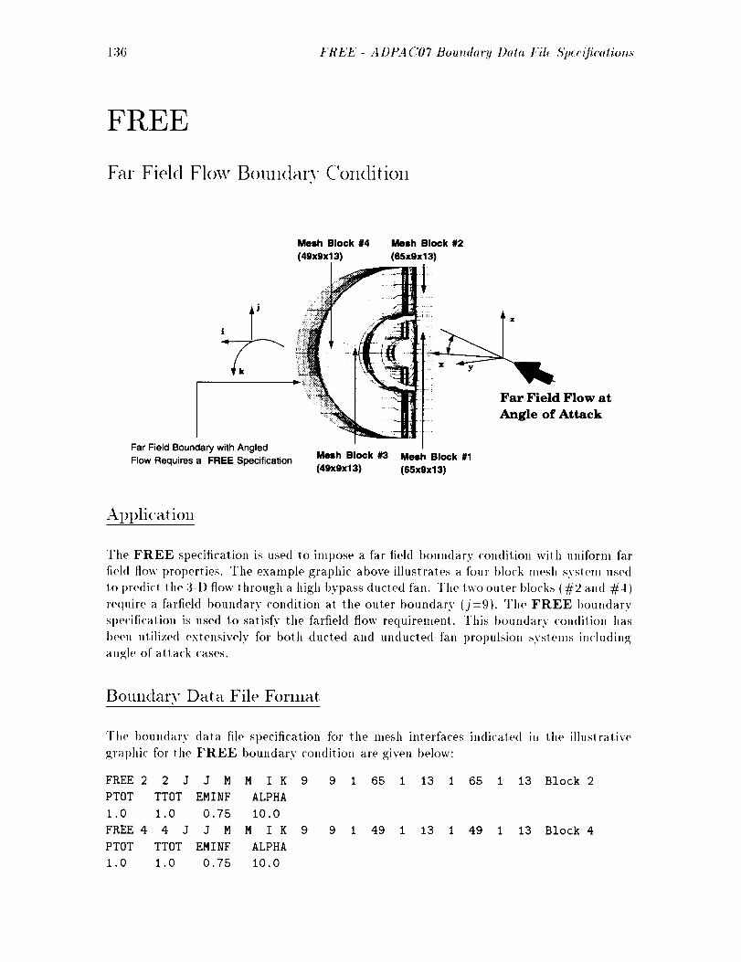
1:36 FREE - A DPA C07 Bou_tdary Data Fil_ 5'pecificatioT_s

FREE

Far Field Flow Boundary Condition

Mesh Block #4 Mesh Block #2

(49xgx13) (65xgx13)

Far Field Boundary with Angled

Flow Requires a FREE Specification

....!!!!! z

Far Field Flow at

Angle of Attack

Mesh Block #3 Mesh Block #1

(49x9x13) (65x9x13)

A1)plication

The FREE specification is used to iInpose a far field boundary condition with uniform far

field flow properties. The example graphic above illustrates a four block mesh syslem used

to predict the 3-D flow through a high t)ypass ducted fan. The two outer blocks (#2 and #4)

require a fa,rfield boundary condition a,t the outer boundary (j=9). The FREE boundary

specification is used to satisfy the farfield flow requirement. This boundary conditioll has

t)een utilized extensively for both ducted and unducted fan propulsion systems including

angle of a/tack cases.

Boundary Data File Format

The boundary data file specification for the mesh interfaces indicated in the illustrative

graphic for the FREE boundary condition are given below:

FREE 2 2 J J M M I K

PTOT TTOT EMINF ALPHA

1.0 1.0 0.75 i0.0

FREE 4 4 J J M M I K

PTOT TTOT EMINF ALPHA

1.0 1.0 0.75 10.0

9 9 1 65 1 13 1 65 1 13 Block 2

9 9 1 49 1 13 1 49 1 13 Block 4

.4DPA ('07 Boundary Dale Fil_ £'pecification._ - FREE 137

Note that a COml)lete FREE specificalion requires two ad(lilional lines following the FREE

boundary data ill(' st)ecificalion line. t:ailure 1o i)rol)erly st)ecify Ill(, data in lh('se additional

lines is a common FREE sl)ecitication error.

D(,scription

The FREE statement specifies that an external, free [h)w t)oun(lary condition is to I)e

al)l)lie(I to the mesh surface sl)e('ified by LFACE1 on th(' I)lock sp('cified t)v LBLOCK1.

Tit(' FREE boundary condition is primarily used for exlernal flow t)rol)lems al a [.a," field

1)oundarv lo silnulate tit(' effects of |he atmosphere or other larrj' ves0rvoir wilh known

1)rol)erties. The FREE procedure utilizes a Reimann invariant formulation to COm l)Ut(' the

local flow (luantiti('s. and l)ernlits t)olh inflow and outtlow through th(' bounding; surface

I)asod on the nature of tit(' local flow with l'esl)ect to the known [.ar fie'l(1 cou([ilions. This

I)oundarv condition requires the specification of additional data, as shown in the 1)oundarv

tiara [.ormat (l(,s('ril)tor al)ov(,. The first additional line following the FREE sl)ecifi('ation

is assumed to t)(, a label and may conlain atly information: however, for consistency it is

l'econlnwnde(l thai the lat)els PTOT, TTOT. EMINF, att(l ALPHA 1)e used. The n(,xl

line contains the values iml)ose(l for the varial)les PTOT, TTOT, EMINF. att(l ALPHA.

which represent lit(, far fiehl nondimetlsional reservoir total pressure and total t('tnl)('rat ure,

alon?; with the Ma('h number and (!artesian angle of attack, respect iv('ly, use(t in the FREE

characleristic solution sequence. The value of lhe PTOT variable is the (lesired normalized

far tield tolal pressure ('ompuled as:

)I tot:d,d: .s_r( d

PTOT -l'. f

at,I the value of the TTOT variat)le is the desire(1 normalize(I ['at' tiel(] lotal ten/l)0rature

computed as:

:l't.t_l,d(_sirc dTTO7' -

7],:f

The varial)les l_.,f att(I Try- f are st)ecifie(] by the inl)ul varial)les PREF and TREF. Values

of PTOT and TTOT <0.0 are nol permitted. The variable EMINF represents lhe

fat" fiehl Mach number. Tit(' far field tlow is ,hvay.'_ assume(t lo progress primarily along

the ])osilive x axis, and therefore mesh systems should I)e generated with this in mind.

Finally. lhe varial)le ALPHA represenls lhe farlield (!arlesian angle of attack, in (le_;rees,

relalive to lhe .r axis. with positive angles resulting in far field velocity components in the

: coordinate direction. The angle ofallack velocities are alway._in the.t-: plane and lhe

velocity ('ompolmnts in the y coordinate direction are elway._ zero. If there is outflow along

lhe FREE boundary, lhen some small y COml)onenl velocities may occur as a result of

exlral)olation from tit(' near field flow. Nalurally, 1)oor convergence or solution (livergenc('

can occur i[" PTOT. TTOT, EMINF or ALPHA suggest I)oundary values which are

signifi('anlly different front the relnainder of the flowfieht. In such cases where this occurs,

it is recommended lhat the solution I)e started with more conservative I)oundarv values,

and then restarted using lhe final 1)oun(lary values.

12('stri('tions/Lilnitations

138 FREE - ADPAC07 Boundary Data File Specifications

Tile FREE boundary specification is not restricted to 3-D mesh surfaces, although 2-D

mesh surfaces may use the FRE2D boundary sl)ecification for consistency. Tile far field

flow angle of attack must be specified relative to the x axis, and produces additional velocity

corot)orients in the z coordinate direclion only. hnposed far-tield velocity coinl)onents in

the y coordinate direction will always t)e zero.

CollllllOll Errors

• Apt)lication of FREE to a t)oundary for which far field y coordinate direclion velocity

conll)onents are required.

• Failure to specify the ad(lilional data values PTOT. TTOT. EMINF. or ALPHA.

• Failure to generate the mesh with +.r as the downstream flow direction.

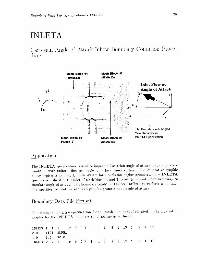
Bo_11_darp Data File ,5'prc_fic'atiot_s- I:YLETA 139

INLETA

Cartesian Angle of Attack Inflow(hll'( _

Boundary Col dition Prate-,

Mesh Block #3

(49xgx13)

Mesh Block #4 Mesh Block #2

(49x9xl 3) (65x9x13)

Mesh Block #1

(65x9x13)

Inlet Flow at

Angle of Attack

z

Inlet Boundary with AngledFlow Requires an

INLETA Specification

Al)plication

The INLETA specification is used to impose a (:arlesia, n angle of attack inflow boundary

condition with uniform flow properties at a local mesh surface. The illuslra, tive graphic

above depi<'ts a four block mesh system for a turbofan engine geometry. The INLETA

specitier is ulilized al lhe inlel of mesh blocks 1 and 2 to set the angled inflow necessary to

simulate angle of a,tlack. This boundary condition has been utilized extensively as an inlet

tlow specifier for inlet, nacelle, and propfan geometries al angle of attack.

Boundary Data File Forlnat

The boundary data file sl)eciticalion for the mesh Imundaries indicated in the illustrative

graphic tbr the INLETA boundary condition are given below:

INLETA 1 1 l I P P J K 1 1 1 9 1 13 1 9 1 13

PTDT TTOT ALPHA

1.0 1.0 20.0

INLETA 2 2 I I P P J K 1 1 1 9 1 13 1 9 1 13

140 INLETA - Boundary Data File ,S'p_cificotions

PTOT TTOT ALPHA

1.0 i .0 20.0

Note that a complete INLETA specification requires two additional lines following tile

INLETA I)oundary data file specification lille. Failure to properly specify tile data ill

these additional lines is a coulmon INLETA specification error.

Description

The INLETA keyword specifies that a uniform prol)erty angle of attack inflow boul,dary

condition is to be applied to tile nlesh surface specified by LFACE1 on the block specified

by LBLOCK1. INLETA is valid for both cylindrical and ('artesian solution meshes (see

the description of the input variable FCART). Tile INLETA procedure utilizes a Reimann

invariant fornlulation to conlpute inflow velocities based on a specitied upstream reservoir

)oral pressure and total tenlperature, and a single Cartesian flow angle as shown in the ilhls-

tralive graphic, above. Included in the INLETA procedure is a special correction schenw

which forces the flow to pass into the flow domaiu. In other words, if the computed velocilies

result in a local outflow at the INLETA boundary, no matter how small the magnitude of

the outflow, the velocities are reset to zero at that point. This boundary condition requires

the specification of additional data, as shown in tile boundary data format descriptor above.

The first a(tditional line following the INLETA specification is assunled to be a label and

may contain any iuformatioll: however, for consistency it is recollmtended that the labels

PTOT, TTOT. and ALPHA be used. The next lille contains (he values iml)osed for

the variables PTOT, TTOT and ALPHA which represent the upstrean_ reservoir total

pressure, total temperature, and Cartesian flow angle, respectively, used in the INLETA

characteristic solulion sequence. The value of tit(, PTOT variable is the desired normalize<t

upstream total pressure computed as:

) •t tot.l.d(s_red

PTOT -P,._y

and the value of the TTOT variable is tire desired normalized Ul)slream to(al temperature

computed as:

_total.de siredTTOT -

T.f

Tile variables P,,¢y and T,._/are specified bv the input variables PREF and TREF. Values

of PTOT and TTOT <0.0 are not pernfitted. The variable ALPHA represents the flow

angle in degrees referenced to the .r axis. For 3-D applications, positive flow angles generate

colnponents of the flow in tire positive z direction, and inle! velocity colnl)ouent ill tile g

direction are set lo zero. For 2-D applications, positive flow angles generate components

of the flow in the positive 9 direction, and inlet velocity conlponent in the z direction

are set to zero. Values of ALPHA must tie between +/- 90 degrees. Naturally, poor

convergence or solution divergence Call occur if PTOT or TTOT suggest boundary values

which are significantly different from tile remainder of the tlowtiehl, or if ALPHA is very

large. In cases where this occurs, it is recomnlended that the solutioll be started with more

conservative I)oundary values, and then restarted using ill(' final boulMary values.

Boutzdary Data File ,5'p(c(fi('atio_,._- L'VLETA 141

12estrictions/Lilnitations

The INLETA boundary specification may l>e applied to either 3-I) o1' 2-D mesh surfaces.

l,'or 2-I) applications, the angle sl)e<'ified by ALPHA is assumed to I)e ill the positive y

('oor<linale. An exampl(' of this type of application is ti)r a planar <'ascade flow where .r is lhe

primary flow direction, and the inflow is a_ an angle of 20 <legrees relaliw _ to the .c axis. thus

result inN in a 9 component ofvelo<'ity (2-I)only). The angle oflhe velocity components

Sl:,ecitie<l bv lhe INLETA procedure musl always be referenced lo lh,_' .r coordinate axis.

anti il is lef! 1o the user lo genoral,_, a mt,sh which is consislenl with lhis f(,allll'('.

CollllllOll Errors

• Apl>lication of INLETA to a 3-I) mesh boundary for which non-zero !] component

velocities are required.

• _\t>plicalion of INLETA to a 2-1) mesh boundary for which llOll-Zel'(i, .7 COllll)OllellI

velocities are required.

• t"ailur<' io specify the addilional dala values PTOT. TTOT. or ALPHA.

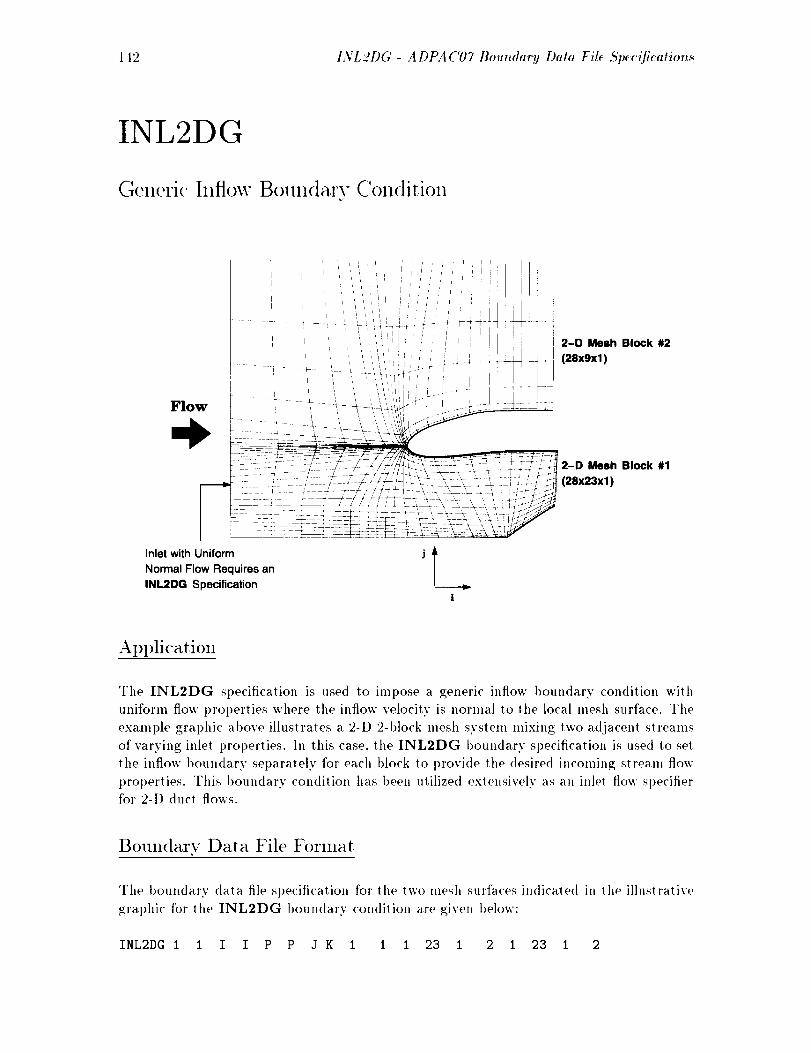
142 I,%LzD6 ADPAC07 Boundary Data Fih Sl)ecification._

INL2DG

Generic Inflow Boundary Condition

Flow

2-D Mesh Block #2

(28x9xl)

2-D Mesh Block #1

(28x23x1)

Inlet with Uniform

Normal Flow Requires an

INI.2DG Specificationi

Al)plication

The INL2DG specification is used to impose a generic inflow boundary condition with

uniform flow prol)erties where tlle inflow velocity is norlnal to the local mesh surface. The

example graphic above illustrates a. 2-D 2-block mesh system lnixing two a.(Ijacellt streams

of varying inlet properties, hi this case, the INL2DG boundary sl)ecification is used io se!

the inflow boundary separately for each })lock to provide the desired incoming stream flow

properties. This boundary condition has been utilized extensively as an inle! ttow sl)ecifier

for 2-I) duct flows.

Boul]darv Data File Format

The I)oundar,v data file specification for the two mesh surfaces indicated in lhe illustrative

graphic for the INL2DG boundary conditiou are given below:

INL2DG 1 1 I I P P J K 1 1 1 23 1 2 1 23 1 2

.4DPA ('07 Boundary Data Fil( ,ffp(c(fication._ - INL2DC 143

PTDT TTDT

I .0 i .0

INL2DG 2 2

PTOT TTOT

1.2 I .8

I I P P J K 1 1 1 9 1 2 1 9 1 2

Nolo 1hal a complete INL2DG specificalion requires two ad(li/io.a] linos followin_ the

INL2DG boundary data file Sl)ecification line. Fail.re 1o properly specify the data in

these a(hlilio.al liues is a common INL2DG Sl)('cificalion error.

Des('rii)tion

Th(, INL2DG slatemen! ,_pe('ities 1ha! a ?_.;eneric. uniform normal inflow i)ouu(lary ('on(li-

lion is 1o I)(* applied 1o the 2-I) m(',_h surface Sl)ecified I)v LFACE1 on the block ,_])(,citi('d

I)v LBLOCK1. Tile INL2DG 1)o.ndary co,(lilio_l should 1)e applied for lhos(' ('ase._ wIl('re

any ot h('r "',_pecialized'" inflow I)oundary condition (s.ch as INL2DT. elc.) does uol apply.

The INL2DG I)o, ndary condition is also likely to I)e somewhal mor(' eflicienl comp.lation-

ally 1hall Ill(' ot her inflow bo.u(larv ('ondilio, procedures, a! th(' ('×l)etls(' of some phy._ical

siml)lifi('a_ion. INL2DG is valid for eiiher cylindrical or (!arlesian-I)ased (,_e(' 1he inpu!

variable FCART) solulions ol_ 2-1) meshes. The INL2DG procedure ulilizes a R(,imann

invarianl formulation _o COml)Ut(' inflow velocitie,_ bas(,d on a specified .l)slream reservoir

tolal l)re,_sur(' and _ota] t(,.ip(vatur('. The velocily componenls al an INL2DG bouiMary

are always ('omt)ule(I to 1)e normal (no transverse velocily components) to the lo('M cell

face a! which 1he procedur(, is al)plied. Incl.ded in _he INL2DG procedur(' is a sl)e('ial

corr(,ctioH scheme which tbr('es lhe flow to pass iuto the flow domain. In other words, if

Ill(' ('Ollll)ulod velocities result ill a local o.tflow al Ill(' INL2DG boun(larv, no mailer how

small the magMtu(le of the outltow, the velocities are resel to zero a! lha! ])oiul. This

boundary ('ondition re(luires Ill(' sl)ecili('aliol_ of additional dala. as shown in lhe bouudary

dala formal (lescriplor above. Th(, firs1 addilional line following lhe INL2DG Sl)eciticalion

is ass.reed to l)e a label au(I may ('onlain all 5" iuformalion: however, for c()nsislen('y i! is

recommended that the labels PTOT and TTOT be used. The nexl line conlains the valu(,s

imposed for the variables PTOT aud TTOT. which represen! the upstream reservoir _otal

pressure and total tempera lure. resl)eclively, used in tile INL2DG characterislic solution

se(lue,,c(,. The value of _he PTOT variabh, is the desired normalized upstream total pres-

Sill'(' ('Olll[)ll(Od _l.S:

]_t,,t_l.d_ sir: :1

PTOT -P,._:

a,(I the value of lh(' TTOT varial)le is the (lesired normalized upstream total lemt)erature

('()111 p UI'O(] aS:

TI'OT =]'l,,t,d.d_ sired

Th(' variables 1_,.:: and T,.,j at(' sl)e('iti('d I)v th(' iupul varial)le._ PREF and TREF. \'alues

of PTOT au(I TTOT <0.0 are 1,oI l)ermitt('(l. Nal.rally. 1)oor convergence or solulion

div('r_4en('(' can oc('ur if PTOT or TTOT suggesl boun(larv val.('s wllich are si_nificaully

144 INL2DG - A DPA C07 Boundary Data File ,S"pecifieatiotts

different fi'om the remainder of the flowfiehl. In such cases where this occurs, it is rec-

ommended that the solution be started with lllore conservative boundary va.lues, and then

restarted using the final boundary vMues.

R estri('tions/Limitatiolls

The INL2DG boundary sl)ecification is not restricted to 2-D mesh surfaces, although for

consistency 3-D mesh surfaces may use the INLETG boundary sl)ecification.

CollllllOI1 Errors

* Application of INL2DG to a boundary for which transverse inflow velocily compo-

nents are required.

• Failure to specify the additional data values PTOT or TTOT.

A !)t_4 ('07 Boundary Data Fil< ,qp_c'_firatiol_._ - 1NLI/TG 1.15

INLETG

Gencli(' Inflow Boundaxv Condition

Mesh Block #1

(49x33x33)

INLETG Specification

Flow

AI)l)lication

The INLETG specification is used to impose a generic inflow boundary condition with

uniform ttow properties where the inflow velocity is normal to the local mesh surface. This

bouttdary condition has t)een utilized extensively as an inle! flow specifier for duc! flows

and turbine blade cooling flow.

Bouxldarv Data File Format

The boundary data file specification for the mesh interface indicated in the illustrative

gra,l)hi<' for the INLETG boundary condition is given below:

INLETG I I I I P P J K

PTOT TTOT AKIN ARIN

1.0 1.0 O.OOi 0.0001

1 1 1 33 1 33 1 33 1 33

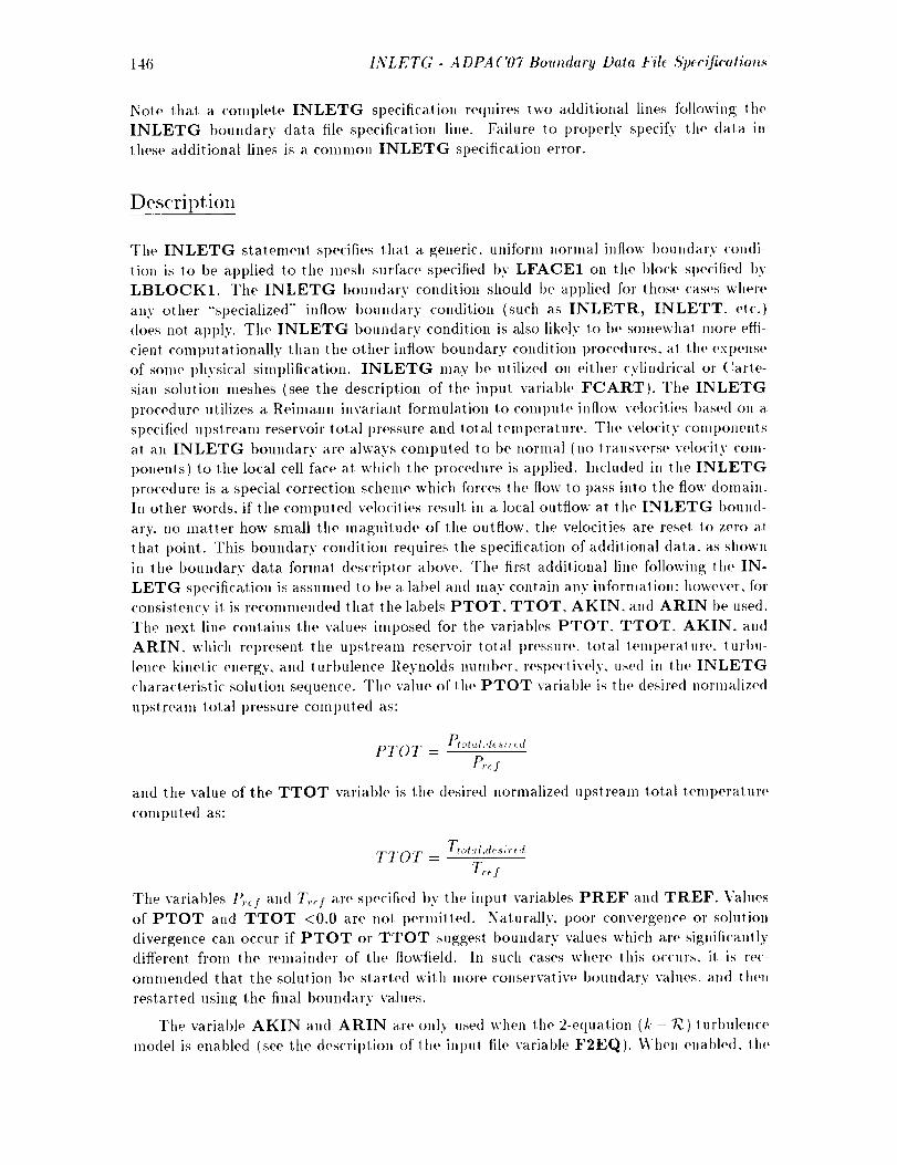
146 INLETG - ADPA (,'07 Boundary Data File Specifications

Nole that a complete INLETG specification requires two additional lines following tile

INLETG boundary data file specification line. Failure to properly sl)ecify the data ill

these additional lines is a colnlnon INLETG specification error.

Description

Tile INLETG statement specifies that a generic, uniform no,'mal inttow 1)oundary condi-

tion is to be al)plied to the mesh surface specified 1)y LFACE1 on tire I)lock spe('itied I)y

LBLOCK1. The INLETG 1)oundary condition should be apt)lied tor those cases where

any other "'sl)ecialized'" inflow boundary condition (such as INLETR, INLETT. etc.)

does not apply. The INLETG boundary condition is also likely to t)e somewhal more effi-

cient computationally than the other inflow boundary condition l)rocedures, al the expense

of some physical siml)lification. INLETG may be utilized on either cylindrical or (larle-

sial, solution meshes (see the description of tile input variable FCART). The INLETG

l)rocedure utilizes a Reimann invariant formulation to compute inflow velocities based on a

sl)ecitied upstream reservoir total l)ressure and lotal teml)erature. The velocity COml)onents

a.l all INLETG boundary are always computed to be normal (no transverse velocity con,-

l)onents) t.o the local cell face at which the procedure is applied. Included in the INLETG

procedure is a special correction scheme which forces the flow to pass into the flow domain.

In other words, if the COlnputed velocilies result in a local outflow at the INLETG 1)ound-

ary, no lnatter how small the magnitude of the outflow, the velocities are reset to zero at

that point. This boundary condition requires the specification of additional data. a.s shown

in the boundary data format descriptor at)eve. The first addilional line following the IN-

LETG st)ecification is assume(I to I)e a label and may contain any information: however, for

consistency il is recommended that the labels PTOT, TTOT, AKIN. and ARIN be used.

The next line contains the values imposed for the variables PTOT. TTOT. AKIN, and

ARIN, which rel)resent the Ul)streanl reservoir total pressure, total lemperalure, turbu-

lence kinetic energy, and turbulence Reynolds numt)er, rest)e('tively, used in ,he INLETG

characteristic solution sequence. The value of the PTOT varial)le is the desired normalize<l

upstream total pressure COml)uted as:

Pt ot,_ l.de sire dPTOT -

P,._:

and tile value of the TTOT varial)le is the desired normalized upstream total teml)erature

colnpute(1 as:

_ tot_,l.desiredTTOT -

The variables P_._f and 7;.¢f are specified by the input variables PREF and TREF. Values

of PTOT and TTOT <0.0 are not perlnitted. Na.lurally, poor convergence or solution

divergence can occur if PTOT or TTOT suggest boundary values which are significantlydifferent from the remainder of the flowfield. Ill such cases where this occurs, it is rec-

ommended that the solution be started with more conservative boundary values, and then

restarted using the final boundary values.

The variable AKIN and ARIN are only used when _he 2-equation (k-_)lurbulence

model is enal)led (see the (tescril)tion of the inl)U! file variable F2EQ). When enabled, the

A DPA('07 Boundary Dale l:i# ,qpcrifieation._- LYLET(; 1,17

variable AKIN rel)resenls the value of the nondimensional freeslream l,ur[)ulonce kinelic

energy defined by L'/l_: where L' is lhe freeslream l url)ulenl kinelic energy and |;.,: is the

reference velocity defined by k/t?,.:jT,.</, llere R,.:f is the gas constant (see [21] for addi-

lional <letails). Tile variable ARIN represe))I the so-called freeslream lurbulem'e Reynolds

numl)er (a_;ain see [2 l]) and is cal<'ula)ed as _/I,.,: L,.::. where L,.:: is lhe reference lenglh

<i<,fi)le<l l)v Ill(' inI)ul variable DIAM.

t] (,stricti<ms/Lilnit atiolls

The INLETG boun(larv speciticalion is no( restricted to 3-I) mesh surfaces (allhough for

('<)nsis)ency 2-D mesh surfaces may use the INL2DG b<>un<lary sl)ecilicalion).

CollllllOll Errors

+ Al)plicatiol_ o[" INLETG (o a b<)undary for which (ransverse inflow velocity comt)o-

nenls are required.

• Failure (o sl)e<'it _" the additional data values PTOT or TTOT.

148 INLETR- ADPAC07 Boundary Data Fih Specificatio_t._

INLETR

1Radial Flow Tml)oma(,hinery Inflow Bo:mdary Condition

FlowAxial Variation of Radial Turbomachinery Inlet _ :.:

Flow Variables Requires an INLETR Specification //! : i: i : _: ,.--: J_'

(illustratedinBoundary Data FileFormat _.i/._ ._ _

II

Axial

Distance ).[<Total Total Axial

Pressure Temperature Flow Angle

Circumferential

Flow Angle

AI)I)lication

The INLETR specification is used to impose an inflow boundary condition with axially

varying flow properties for radial flow turbomachinery. The example graphic above illus-

trates adjacen! passages of a mesh system <lesigned to predict the flow through a radial

diffuser. The inlet boundary is a radial surface of revolution with properties which vary

in the axial direction, and therefore INLETR is used to supply the desired flow char-

acteristics a,t this boundary. INLETR has been successfully used for several radial flow

turbotnachinery geomel ties.

Boundary Data File Format

The boundary data file specification for the mesh surface indicated in the illustrative gral)hic

for the INLETR boundary condition is given below:

INLETR i i I I P P J K I I

NDATA

4

AXIAL PTOT TTOT BETAX BETAT

0.i 0.99 0.99 5.0 -73.3

1 13 1 17 1 13 1 17

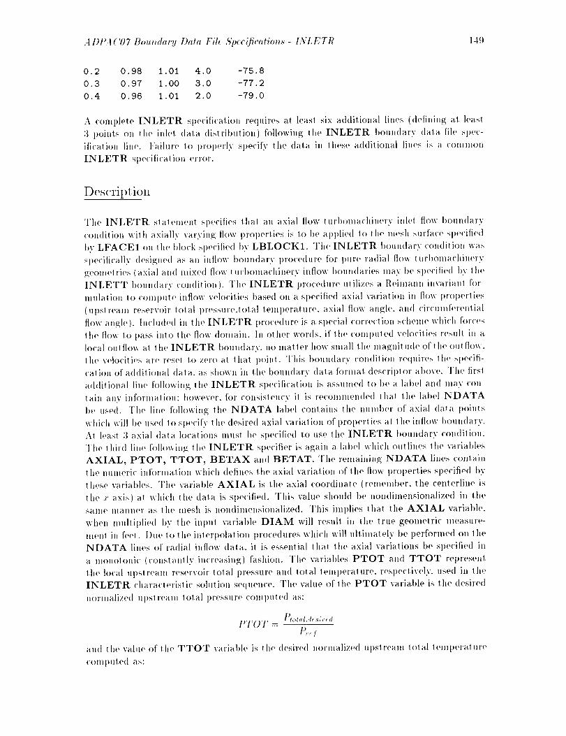
A I)I'+1 ('07 Boundary Data Fih S'pcc(fication._ - INLET1? 149

0.2 0.98 1.01 4.0 -75.8

0.3 0.97 1.00 3.0 -77.2

0.4 0.96 1.01 2.0 -79.0

A conq)lete INLETR specification require,,, at least six additional liaes (deliniug at. least

3 points on (he inlel data <lis(ribution) followin_ the INLETR l)oundarv (lala file sl)ec-

ifi<'aIion lit)('. Failure to l)rol)erly sl)ecify tile data ill these additional lines is a common

INLETR specification error.

Descril)(-ioal

The INLETR stalemem ._pecifies tha) an axial flow I url)oma('hiuery inleI flow l)oundary

con(lilion wilh axially varyiuog flow prol)erlies is (o lie applied (o tile mesh surface sl)e<'ilied

l)v LFACE1 on (he block sI>ecifie<l l>v LBLOCK1. The INLETR boundary coudiIioll wa._

sl)e('ifi<'ally (lesi_ued as an iullow l><>u))<larv procedure for pure radial flow (url)omachinery

geometrie,_ (axial and mixed flow (url)omachiuery inflow l)ouu<laries may lie sl>ecilie<l l)v (he

INLETT boundary condiI ion ). The INLETR procedure utilizes a Reimann invm'iaul for-

mulaiion Io COml)U(e inflow velocities based on a specified axial variation it) flow l)roperlies

(ups(ream reservoir total pressure,total teml>erature, axial flow angle, att<l <'irc'un)feren)ial

flow an e.;le). Inchlded it) (he INLETR I>rocedure is a sl>ecial correction scheme whi('h forces

lit(' flow (o [)ass i)do the flow domain. In olher words, if the <'Oml>uled velo<'ilies result in a

local oul flow a( )he INLETR l>ouudary, no mailer how small the magnitude of Ihe outflow.

the velocilies at'(' resel to zero a(tha) point. Tiffs boundary condiiion requires the sl)e('ifi-

cation of additional data. as shown in the boundary data formal (lescril)lor at>eve. The firs(

a<ldilional line followin?_; lit(' INLETR sl>ecificaliou is assumed lo be a label aud may con-

taill any infornlalion: however, for coasislelwy ii is re<'omnlend('d (hal lhe label NDATA

be used. The liue followiug the NDATA label conlains the mtml)er of axial data l)oiuIs

which will lie used lo specify (he desired axial varial ion of l>rol>erIies aI lhe inflow boundary.

AI leas( 3 axial data locations must l>e specified to use the INLETR boundary conditiou.

The lhird line following the INLETR sl)ecifier is again a label which outlines lit(' variables

AXIAL, PTOT, TTOT, BETAX and BETAT. The remaining NDATA lines contain

tile numeric iuformatiou which defines the axial val'iatiol) of file flow l)rol)erties sl)e<'ified t)v

these variables. The variable AXIAL is the axial coordinate (remember. the centerline is

the ,r axis) a) which the data is specified. This value shoukt tie nondimensionalized in the

same Inanner as lhe mesh is non(limensionalize<l. This iml)lies that (he AXIAL variable,

when multiplied I>v the iul)ul variable DIAM will resull iu lhe true geolnetric measure-

meul ill feel. Due lo lhe ilderl)olation I)rocedures whi<'h will ullimalely be performed on (lie

NDATA lines of radial inflow dala. it is essential [hal the axial variations be sl)ecified in

a mouolonic (conslantlyincreasing) fashion. The variables PTOT and TTOT represent

lhe local upsl ream reservoir lolal pressure and )olal tem])eralure, resl)ectivel.v, used in (he

INLETR ('haraclerislic s<>lu(ion sequence. The value of lhe PTOT variable is the desire<t

normalized ut)sI realll total l)ressure c<)ml)uted as:

)

I'TOT =t%/

and the w_lue of lhe TTOT variable is the desired normalized ut>slream (ol al (emt)eralure

c<)ntl>uled as:

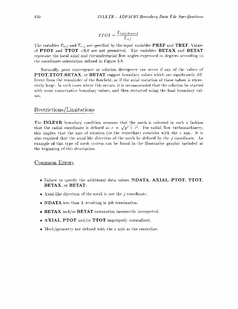
150 INLETR - ADPAC07 Boundarg Data Fil¢ Specification._

_tot:d,desiredTTOT -

T,._ f

The variables P,._f and T,._: are specified by tile input variables PREF and TREF. Valuesof PTOT and TTOT <0.0 are not I)ermitted. The variables BETAX and BETAT

represent the local axial and circumferential flow angles expressed in degrees according to

the coordinate orientation defined in Figure 3.&

Naturally. poor convergence or solution divergence can occur if any of the values of

PTOT.TTOT.BETAX. or BETAT suggest boundary values which are significantly dif-ferent fi'om the remainder of the flowfield, or if the axial variation of these values is exces-

sively large. In such cases where t his occurs, it is recommeuded thai the solution be started

with more conservative boundary values, and then restarted using ll,e final boundary val-

lleS.

12est rictions/Limit ations

The INLETR boulMary condition assumes thai the mesh is oriented in such a fashion

thai the radial coordinate is defined as r = v/g _ + z 2. For radial flow lurbomachinery.

this in, plies that the axis of rotation (or the centerline) coincides wilh the x axis. It is

also required that the axial-like direction of the mesh be defined by the j coordinate. An

example of this type of mesh systeln can be found in the illustrative graphic included at

the beginning of this descriptioi,.

CollllllOll Errors

• Failure to spe<'ify the additional data values NDATA. AXIAL. PTOT, TTOT.BETAX. or BETAT.

• Axial-like direction of the mesh is not the j coordinale.

• NDATA less than 3. resulting in job termina.tion.

• BETAX and/or BETAT orientation incorrectly interpreted.

• AXIAL, PTOT and/or TTOT improperly normalized.

• Mesh/geometry not (lefined with the x axis as the cenlerline.

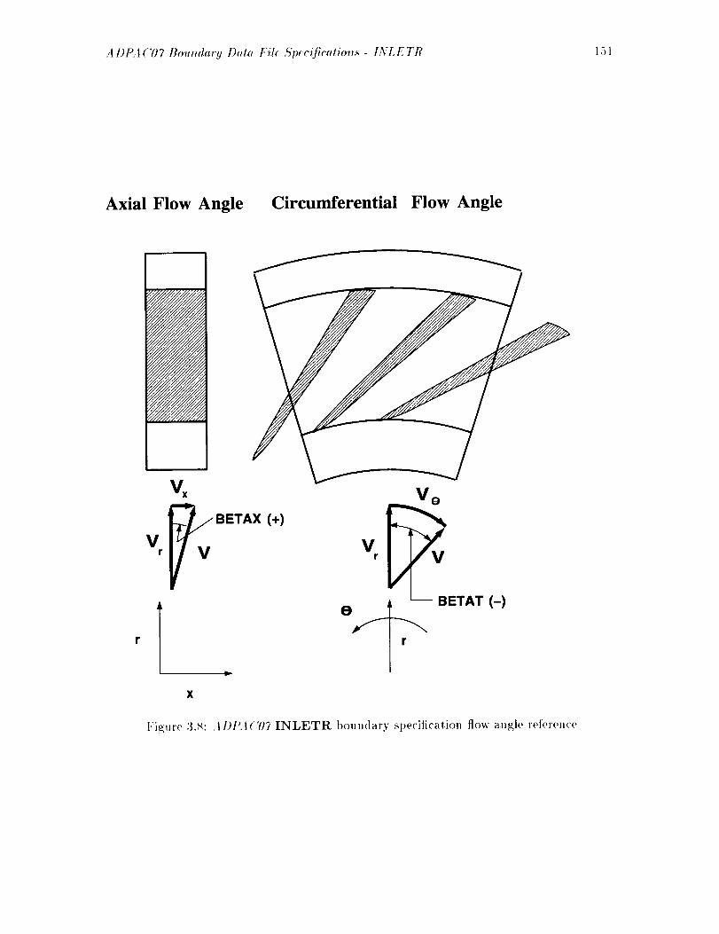
.4I)PA ('07 Boundary Data Fil_ A_ee_fieatio_._ - LYL E TR 151

Axial Flow Angle Circumferential Flow Angle

V _V BETAX (+)

V o

BETAT (-)

r

x

t:igure 3.S: A Did, t('07 INLETR boundary specification flow angle referen('e

152 INL2D T - A DPA C07 Boundar.u Data Filt Specifications

INL2DT

2-D Turbonlachinery Inflow Boundary Condition

Total

Pressure

Radius

Radial

Flow Angle

Total

Temperature

Circumferential

Flow Angle

Radial Variation of Turbomachinery" Inlet

Flow Variables Requires an INL2DT Specification

(illustrated in Boundary Data File Format

statements below)

2-D Mesh Block #1

(49xl 7x 1)

'L L_i x

Application

The INL2DT specification is used t,o impose an inflow boundary condition with radially

varying flow properties for 2-D axisymmetric mesh systems. The example graphic illus-

trated above depicts an EXT2DT specification for a 2-D (axisymmetric) flow solution for

a turbomachitlery blade row. This boundary condition has been utilized extensively as an

inlet flow specifier for 2-D turbomachinery flow passages and solutions for embedded blade

rows with imposed a,xisymmetric body forces.

Boundary Data File Format

The bOulldar.v data file specification for the mesh surface indicated in the illustrative graphic

for the INL2DT boundary conditiotl is given below:

INL2DT I i I I P P J K i

NDATA

7

RAD PTOT TTOT BETAR BETAT

0.20 1.01 0.98 S.0 5.1

1 1 17 1 2 1 17 1 2

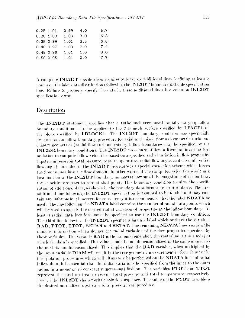
A DPA ('07 Bounda r9 Data File A'pecification._ - INL 2D T 153

25 1

30 1

35 0

40 0

45 0

50 0

01 0.99 4.0 5.7

O0 1.00 3.0 6.3

99 1.01 2.5 6.8

97 1.00 2.0 7.4

96 1.01 1.0 8.0

95 1.01 0.0 7.7

A COmlflete INL2DT sl>e<'ification requires at least six additional lines (definin_z at least 3

points on the inle! data tlistribution) following lhe INL2DT boundary data file specitica!ion

line. Failure to properly specify the data in lhese a ddilional lines is a common INL2DT

speci[ica! io]i error.

Description

The INL2DT statement specifies that a lurbomachinery-t>ased radially varyit]g; inflow

boundary condition is to be applied to the 2-D mesh surface specified by LFACE1 on

lhe t)lock specified by LBLOCK1. The INL2DT boundary condition was specifically

<lesiglw<l as a u in[tow boundary i)ro<'e<lure tor axial and mixed flow axisymn,<,tric lurl)oma-

chhwry geomelries (radial flow lurbomachinery inflow t>oundaries may be spe<'ified t>y the

INL2DR boundary condilion). The INL2DT procedure utilizes a Riemai, H invarianl for-

mulation to COml)ute inflow velocilies based on a specified radial variation ill flow properties

(upstream reservoir total pressure, total temperature, radial flow angle, and circumferential

flow an_;le). Included in the INL2DT procedure is a special correclion scheme which forces

!he flow to pass into the flow domain, hi other words, if the computed veloci!ies result in a

local oul flow at the INL2DT I)oundary. no matter how small the magnitu<le o[the outflow.

the velocities are reset to zero al lhat point. This boundary condition requires the sl>e<'ifi-

cation of additional data, as shown in the I>oundary dala format descril>lor al>ove. The first

a<t<tilional line [ollowing the INL2DT specification is assumed to be a label and may con-

tain any informalion; however, for consistency i! is recommended that the label NDATA |>e

used. The line following the NDATA label contains the number of radial data points which

will t>e used to specify the desired radial variation of properties at the inflow boundary. At

least 3 ra(iial data locations must I)e sl)e('ifie(l i<) use the INL2DT I)oundary condition.

The third line following the INL2DT specifier is again a label which outlines the variables

RAD, PTOT, TTOT, BETAR and BETAT. The remaining NDATA lines contain the

mmmri<" information which defines the ra<lial variation of lhe flow properties sl)ecified by

these varial>les. The varial)le RAD is the radius (rememt)er, the centerline is the .t' axis) a l

whi<'h lhe data is sl>e<'ified. This value shoul<l be nondimensionalized in the same manner as

the mesh is nondimensionalized. This implies that the RAD variable, when multiplied I>v

t lie inpul variable DIAM will result in the true geometric measurement in feet. Due to the

interpola!ion ]>ro<'e<lures which will ultimately l>e t>erformed on the NDATA lines of radia[

inilow data, it is essential that the radial variations I>e specified from the inner to the outer

radius itL a moHotoni<" (constantly increasing) fashion. The variables PTOT and TTOT

rel)resent the local Ul)stream reservoir total pressure and total temperature, respectively.

used in lhe INL2DT characterisli<" solution sequence. The value of lhe PTOT variable is

lhe <lesire<l normalized ul>st ream tot a] pressure <'Oml>uled as:

154 INL2DT- ADPAC07 Boundary Data Fih ,5'peeifieations

PTOT- Ptot,t,a_._i,._tP,.+:

and tile value of tile TTOT variable is the desired normalized upstrealn total tenlperature

computed as:

Ttotal,d: si,,:dTTOT -

7,,:f

The variables t_._f and T,._f are specified by the input variables PREF and TREF. Values

of PTOT and TTOT <0.0 are not permitled. The variat)les BETAR and BETAT

represent the local radial and circumferential flow angles expressed in degrees according to

the coordinate orientation defined in Figure 3.9. Naturally. poor convergence or solution

divergence can occur if any of tile values of PTOT, TTOT, BETAR, or BETAT suggest

boundary values which are significantly different from the remainder of the flowfield, or if"

lhe radial variation of these values is excessively large. In cases where this occurs, il isl'econlniended tha! the solution be starled with more <'onservalive boun(larv values, an(l

then restarted using lhe final I)oundary values.

Restrictions/Limitations

The INL2DT boundary condition assumes that the mesh is oriented in such a fashion

that the radial coordinate is detined as r = v/-92 + z 2. For axial flow tnrbomachinery, lids

inlplies that the axis of rotation (or the centerline) coincides with the :r axis. It is also

required that the radial-like direction of the mesh be defined bv the j coordinate. Examples

of this type of mesh syst.em can be found in the chapter defining standard configurations.

The INL2DT boundary specification is restricted to 2-D mesh surfaces (3-D mesh surfaces

should use the INLETT boundary specification).

ColIllllOll Errors

• Application of INL2DT to a 3-D mesh system.

• Failure to specify the additional data vahms NDATA. PTOT, TTOT. BETAR. orBETAT.

• Radial-like direction of the mesh is not the j coordinate.

• NDATA less than 3, resulling in job termination.

• BETAR and/or BETAT orientation incorrectly interpreted.

• RAD, PTOT and/or TTOT improperly normalized.

• Mesh/geometry not defined with the :r axis as the centerline.

A DPA ('07 Boun&u'y D(lta File ,S'p<c(fications - INLETN 155

INLETN

_Non-lqefle<'ting Unsteady Inflow Boun(larv Con(lition

Mesh Block #1

(49x33x33)

f

J

i_ Time-Dependent Solution-I

for Duct Inlet Requires an--J

INLETN Specification

Flow

A1)plicat ion

The INLETN specification is used Io impose a non-reflecting inflow boundary condition

for time-depenclen! flow ca,lculalions. This I)oundary condition has been utilized for time-

del)en<lenl flows where spurious numerical reltections fron| olher 1)oundary algorithms are

u nde.,dral)le.

B<mn<lary Data File F<)rmat

The boundary data file sl)ecificalion for the mesh interface indicated in lhe i]luslrative

gral)hic tot lhe INLETN boundary ('ondilion is given below:

INLETN I 1 I I P P J K i I I 33 1 33 1 33 i 33

156 I:VL ETN - A DPA (:'07 Boundary Data File ,5)_ccifl'cation,._

Description

The INLETN statement specifies that a generic, non-reflecting inflow boundary condi-

tion is to be applied to tile mesh surface specified |)y LFACE1 on tile block specified by

LBLOCK1. The INLETN boundary condition should only be applied for time-dependent

flow ('alculations where spurious numerical reflections such a.s those normally expected from

other boundary specifications (such a.s INLETR, INLETT. etc.) are ulidesirable. IN-

LETN may be utilized on either cylindrical or (:a.rt.esian solution meshes (see the descril)-

lion of the input variable FCART). Th(, INLETN procedur(, utilizes a characterisli('-l)ased

formulation 1o compute inflow velo('ities l)ased on lo('a] flow conditions only.

Restrictions/Lilnitatiolls

The INLETN boundary Sl)ecification is nol restricted to 3-D mesh surfaces but should only

be applied for time-dependent flow ca.lculalions where a non-retlecting inflow boundary isdesired.

COIIIIlIOll Errors

• Application of INLETN for a steady stale solution.

A DPA ('07 Bmn_dor!j Data File Sp<c_ficrllio,_._ - LYLETT 157

INLETT

Turl)onla('hinerv Inflow Boundary Condition,

Radius

Radius

Radius

P

Total

Pressure

Radial

Flow Angle

/Total

Temperature

Circumferential

Mesh Block #1

(49x17x17)

\

T FI_ow

Flow Angle ,,- . +- f z

/.a ia,venat,ono.:,, omach,nery,°,et IFlow Variables Requires an INLETT Specification

i l

(illustrated in Boundary Data File Format

statements below)

Application

The INLETT specification is used to impose an inflow I)oundary condilion with radially

varying flow properties. The illustrative graphic above depicts an apt>licatioll of the IN-

LETT inflow boundary condit ion for an H-type lnesh for a turbolnachinery fan rotor blade

passage. The INLETT specification provides the radial variation of flow i)roperties at

the inflow l>oun(larv result ing from experimelltal conditions, upstream blade rows, or other

known inlet prol)erty variation. This boundary condition has been utilized extensively as

a]J inlet flow specifier for turbomachinery blade passages an<l annular ducts.

Boull(lal"v Data File Format

The I)oundarv <lata file sl)e<'ification for lhe mesh surface indicaled in the illustrative graphic

['or the INLETT boundary condition is given t)elow:

INLETT I

NDATA

7

1 I I P P J K 1 1 1 17 1 17 1 17 1 17

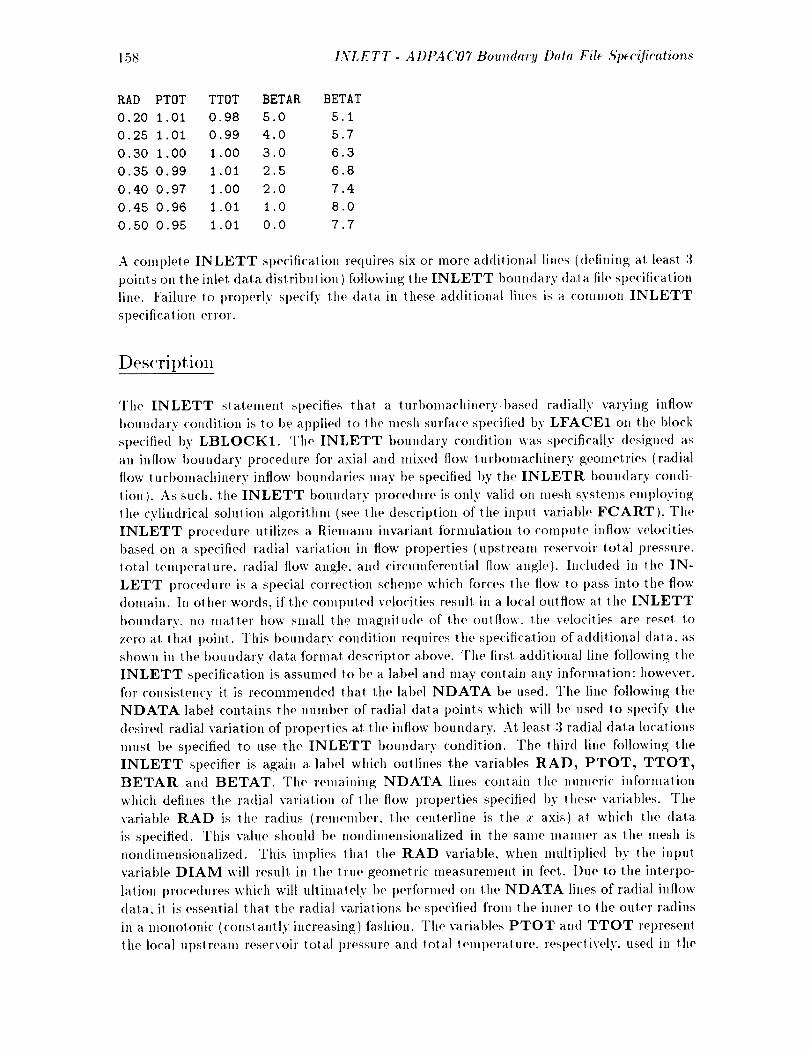
158 INLETT- A DPAC07 Boundary Dttta Filt Specification._

RAD PTOT

0.20 1.01

0.25 1.01

0.30 1.00

0.35 0.99

0.40 0.97

0.45 0.96

0.50 0.95

TTOT

0 98

0 99

1 O0

1 01

1 O0

1 01

1 01

BETAK

50

40

30

25

20

10

O0

BETAT

51

57

63

68

74

80

77

A complete INLETT specification requires six oi" more additional lines (defining at least 3

points ol, tile inlet data distribution) following tile INLETT 1)oun(lary data file specificalion

lille. Failure to 1)roperly specit)' the (lala ill these additional lines is a comlnon INLETT

si)ecificat ion error.

Description

The INLETT statenmnt specifies that a turbonlachinery-I)ased radially varying inflow

boundary condition is to I)e applied to the mesh surface specified by LFACE1 on the block

specified by LBLOCK1. Tile INLETT boundary condition was specifically designed as

an inflow boundary procedure for axial and nlixe(1 flow turbomachinery geometries (radial

flow turbomachinery inflow boundaries may be specified by the INLETR boundary condi-

tion). As such. the INLETT boundary procedure is only valid on mesh systems employing

lhe cylindrical solution algorithm (see the description of the input variable FCART). The

INLETT procedure utilizes a Riemann invariaut formulation 1o comt)ute inflow velocities

based on a specified radial variation in flow properties (upstream reservoir total pressure.

total teml)erature, ra(lia] flow angle, and circumferential flow augle). Included in the IN-

LETT procedure is a special correction scheme which forces the flow to pass into the flow

domain. Ill ot her words, if the computed velocities resul! in a local outflow at the INLETT

1)oundary, no luatter how small the magnitude of the outflow, the velocities are reset to

zero at tha! point. This boundary condition requires tile specification of additional data, as

shown in the boundary (lata format descriptor above. The first additional line following the

INLETT specification is assumed to be a label and may contain any information: however,

for consistency it is recommended that the label NDATA be used. The line following the

NDATA label contains the number of radial data points which will be used to specit)' the

desired radial variation of properties at the inflow boundary. At least 3 radial data locations

must be specified to use the INLETT boundary condition. The third line following the

INLETT sl)ecifier is aga.iv a label which outlines the variables RAD, PTOT, TTOT,

BETAR and BETAT. Tile remaining NDATA lines coutain the numeric infornLation

which defines the radial variation of the flow properties speciiied by these variables. Tile

variable RAD is the radius (remember, the center]the is the x axis) at which the data

is specified. This value shouht be nondimensionalized ill the same manner as the mesh is

nondimeusionalized. This implies that the RAD variable, when multiplied by the input

variable DIAM will result ill the true geometric measnrement in feet. Due to the interpo-

lation procedures which will ultimately be perforlned on the NDATA lines of radial inllow

data, it is essential that tile radial variations be specified from the inner to lhe outer radius

in a monotonic (constautly increasing) fashion. The variables PTOT and TTOT represent

the local ui)stream reservoir total pressure and total teml)erat ure. resl)ectively, used in the

A DPA C07 Boundary Data File ,qp<cifications - I:VLETT 159

INLETT characteristic solution sequence. Tile vahte of the PTOT varial)le is tile desired

nortnalized ILl)St reant total pressure ('Oml)ute(l as:

Pt ot+z l.d_ sir ¢ dPT07' -

I',.<f

and the value of the TTOT variable is lhe desired normalized Ul>streanl lola[ temperalure

conllmled as:

Th,t,d,,t_ si r_ dTTOT -

'T., f

The varial)h's I),.+: and 7;,+] are specified by the inI)Ul varial)les PREF and TREF. Values

of PTOT and TTOT <0.0 are not permitted. The variables BETAR an(I BETAT

rel)t'es(,nl the h)('al ra(lial and circumferential flovc angles expressed in degrees a('cordin_ 1o

the coor(litiale orientation defined in Figure 3.9. Naturally. poor convergence or solution

(tivergetw,+ can oc('uI + if any of the values of PTOT. TTOT, BETAR, or BETAT suggi(,st

boun(lary valtles whMt are significantly different from the remain(h,r of the flowfieht, or if

the radial varialion of these values is excessively larp,;e. Iil cases v,:here lhis <)c('urs, it is

re<'onunetJ(le(l l liar the s<)htlion be started will, more <'ollser','aiive I)<>ltli(lary vahies, and

then restarted using the final l)oundary values.

R('stri<'tions/Limitations

The INLETT t)<)un(lary ('otidilion assunies that the niesh is oriented itl such a fashion that

the radial coor<linate is defined as r = v/y _ + z 2. For axial flow iurt)ontachinery, this inll)lies

that tit(, axis ofrotalion (or the<'enlerline) coincides with tlt('.+' axis. It is also re<luired

that the ra<lial-like direction of the mesh t)e (h, fine(t l>y the j coor<tinaie, i+]xantl)h's of this

ty[)(, ()f mesh sysieni ('all I)(+ foun(I in the chat>tot defining stan(lar(I tii(,sh (+Oli[iguralions.

Tile INLETT l)oundary speci[i('aiion is i'est rioted to 3-I) mesh slirfac(,s ( 7- I) niesh sit rfa('(,s

s]iould its(' the INL2DT t)OUli(lary Sl)('('ilicat ion ).

Coi11111Oll Errors

• Apl)lication of INLETT to a 2-D mesh systenl.

i Faihire i<) specify the addiiional <lata vahtes NDATA, PTOT, TTOT. BETAR. or

B ETAT.

. Radial-like (lire<'liou of the niesh is not the j coordinate.

• NDATA less than 3. resulting in job terniinalioti.

• BETAR an(l/or BETAT orientation incorrectly inleri)rete(I.

• RAD. PTOT an(l/or TTOT iniliroperly nornialized.

• Meshtp_;eonietrv liOi (lefine<l with the .r axis as the cenierline.

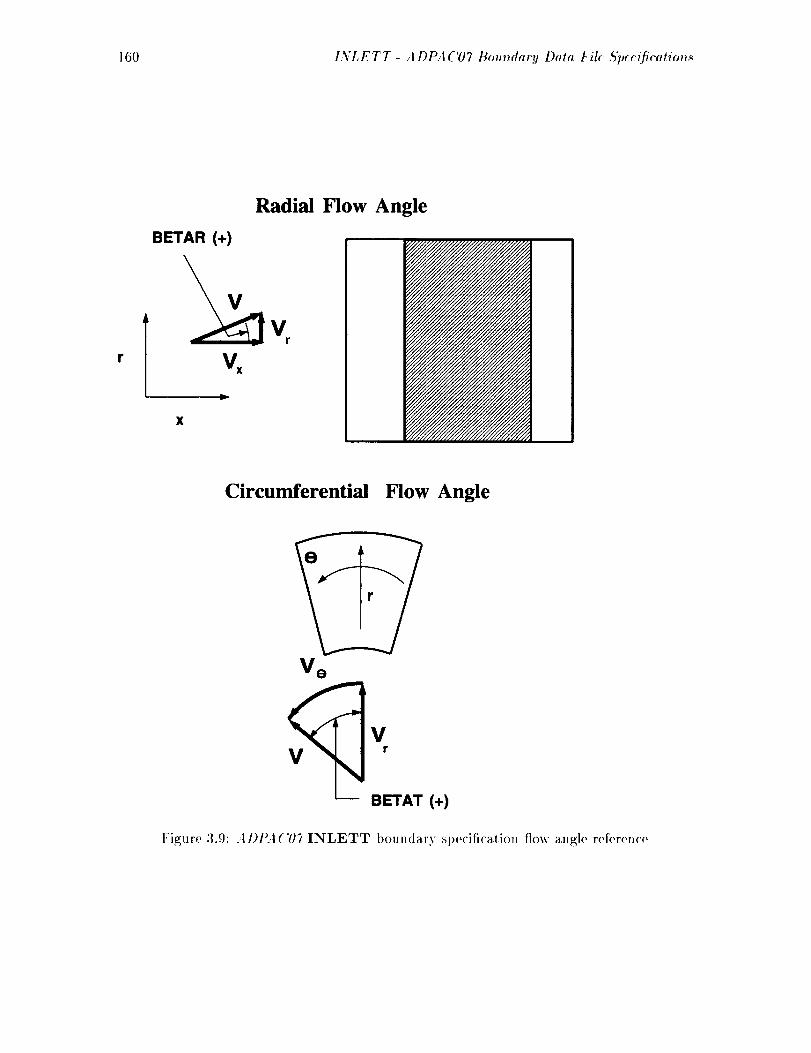
160 INLETT- ADPAC07 Boundary Data Fil_ A'pecifictltion._

Radial Flow Angle

BETAR (+)

r

Circumferential Flow Angle

V o

BETAT (+)

Figure 3.9: A DPA('07 INLETT boundary specification flow angle reference

A Dt_4 ('07 Bouts<lacy Data Fih ,qp(c(fi'catioT_._- INLETX 161

INLETX

.Non-Reflecting Stea<lv State Tlul)onmchincrv Inflow BoundaryCon<lition

Radius

Radius

/Total

Temperature

_ Radius

Total

Pressure

Radial

Flow Angle

?I

Circumferential

Flow Angle

Radial Variation of Turbomachinery Inlet

Flow Variables for Non-reflecting

Boundary Requires an INLETX Specification

Mesh Block #1

(49xlTx17)

\

/

J

<__I>.AI)l)lication

The INLETX specificatioll is used Io impose a non-reflecting lul'l)omachinery inflow bound-

ary ('ondilion with radially varying flow properties. The illustrative graphic above depict s an

al)t>lication of lhe INLETX inflow boundary condition for an H-tyl)e mesh for a turl>oma-

chinerv fan rotor 1)lade passage. The INLETX specification 1)rovides the radial variation

of flow i)roperlies al the inflow boundary resulting from experimental conditions, upstream

t)la<te rows. or other known inlet I)rol)erly variation. This I)oundary condition has been

utilized exlensively as an inlet flow st)ecifier for turl)olna<:hillery blade passages and annular

ducls.

Boundary Data File Forlnat

'The I)<)u (]ary data file Sl>ecitication for the mesh surface indicated in the illustrative graphic

for tit(, INLETX boundary condition is given t>elow:

INLETX I I I I P P J K I I i 17 i 17 I 17 i 17

NDATA

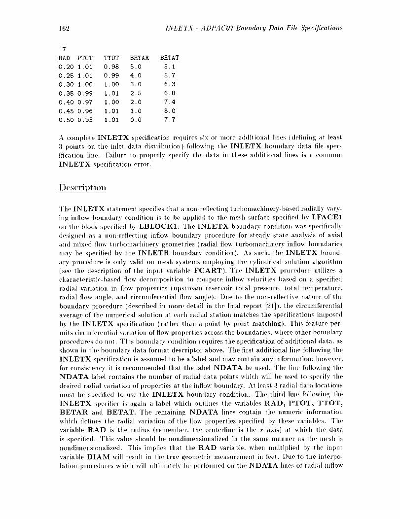
162 LYLETX - ADPA C07 Boundary Data File Specification._

7

RAD PTOT TTOT BETAB. BETAT

0.20 1.01 0.98 5.0 5.1

0.25 1.01 0.99 4.0 5.7

0.30 1.00 1.00 3.0 6.3

0.35 0.99 1.01 2.5 6.8

0.40 0.97 1.00 2.0 7.4

0.45 0.96 1.01 1.0 8.0

0.50 0.95 1.01 0.0 7.7

A comt)lete INLETX sl)ecification requires six or more additional lines (defining al lea sl

3 points oll the inlet data distribution) following the INLETX boundary data file spec-

ification lille. Faihn'e to properly si>ecify the data in these additional lines is a common

INLETX st)ecification error.

Description

The INLETX statemenl specifies that a non-reflecting turbomachinery-I)ased ra(lially vary-

ing inflow boundary condition is to be applie(I to the mesh surface specified I)3' LFACE1

on the block specified by LBLOCK1. The INLETX I)ouudary condition was specifically

designed as a non-reflecting inflow boundary procedure for steady state analysis of axial

and mixed flow turbomachinery geometries (radial flow turbomachillery inflow boundaries

may be specified I)y the INLETR boundary condition). As such, the INLETX bound-

ary t)rocedure is only vali(l on mesh systems employing the cylindrical solution algorithm

(see the description of the input variable FCART). The INLETX procedure utilizes a

characteristic-based flow decoml)osition to compute inflow velocities based on a specified

radial variation in flow 1)rol)erties (tq)stream reservoir lotal l)ressure, total temperature.

radial flow angle, and circumferential flow angle). Due to the non-reflective nature of the

boundary procedure (described in more (tetail in the final report [21]). the circumferential

average of the numerical solution at each l'a(lial stalion matches the sl)ecifications itnl)osed

by the INLETX specification (rather than a point by point matching). This feature per-

nfits circmferential variation of flow prol)erties across the boundaries, where other boundary

procedures do not. This boundary condition requires the sl)ecification of additional data, as

shown in the boundary data format descriptor above. The first additional line following the

INLETX specification is assumed to be a label and may contain any information: however,

for consistency it is recommended that the label NDATA be used. The line following the

NDATA label contains the numt)er of radial data points which will be used to si)ecif.v the

desired radial variation of properties at the inflow t)oundarv. At least 3 ra(lial data locations

must be specified to use the INLETX boundary condition. The third line following the

INLETX specifier is again a label which outlines lhe varial)les RAD, PTOT, TTOT,

BETAR and BETAT. The remaining NDATA lines contain the numeric information

which defines the radial variation of the flow properties st)ecified by these variables. The

variable RAD is the radius (reineml)er, the centerline is the x axis) at which the data

is sl)ecified. This value should be nondimensionalized in tile same lnanner as the mesh is

nondimensionalized. This iml)lies that the RAD variable, when mullit)lied I)v the inl)Ul

variat)]e DIAM will result in lhe true geometri(' measurement in feel. l)ue to the inlerl)o-

lalion l)rocedures which will ultimalelv be 1)erformed on the NDATA lines of radial inflow

A DPA('07 Boundary Data Fi# 5'p<e([ication._- INLETX 163

data, it is essenlial that lhe radial variations be specified from tile inner to the outer radius

in a monolonic (constantly increasing) fashi(.)n. The variables PTOT and TTOT represent

111e local Ul)stream reservoir total pressure an(.l lotal lenlperalure, respeclively, used ill the

INLETX characlerislic solution sequence. Tile value of the PTOT variable is the desired

normalized upstream (olal pressure <'Oml>uled as:

l>t.t,_l.,l_ si,'edPTOT =

I%/

and the value of 1he TTOT variable is [he desired normalize<l Ill)SlFealll 1('/1 al |ellll)el'al ill'e

('OIll [)ll| e(] as:

"l't c,t. l,d_ ,si :., ,/T 1'0 T -

T,._ :

The variables t),,:/ and "/;,_/ are sl)eci[ied by lhe inpul variables PREF and TREF. Values

of PTOT and TTOT <0.0 are no( permitted. The variables BETAR an<l BETAT

rel>resent the local radial and circumferential flow angles exl>ressed ill <le_rees accor<lin_ 1(./

the co<>rdina(e orientation <letined in Figure 3.9. Nalurally. poor convergence or solulion

divergence can occur if ally" of lhe values of PTOT. TTOT. BETAR. or BETAT su,_;gesl

boundary values which are significanlly different from the remainder of the flowlMd, or if

the radial variation oflhese values is excessively large. In such cases, il is reconmlen<led

lhal 111(, solution be slatted with more conservalive boundary vahles, and lhen reslarled

using; (he final boundary values.

Restrictions/Limitations

The INLETX boundary condition assumes lhal the mesh is oriented ill such a fashion that

the ra<lial coor<lina(e is defined as r = W/g ->+ z 2. For axial flow turbomachiner.v, lids imt)lies

thai lhe axis of rotation (or 111(.' <'enterline) coincides with lhe .r axis. I( is also required

lhal Ill<, radial-like direction of tile mesh be defined by the j coor<linate. This implies

(hal INLETX can only lie al)l)lie<l 1<)either constant i or constan( 1,"index mesh surfaces.

INLETX is only vali<I for s)ea<lv sta(e solu(ions (the INLETN boundary procedure is

available for (ime-del)en<tent non-reflecting inflow l>oundaries).

COIIIIIIOll Errors

• Al)l)licalion of INLETX to a (!artesian mesh solution.

• l"ailure 1<) st)ecify )he additional <lata values NDATA, PTOT. TTOT, BETAR, or

BETAT.

• Radial-like direction of (he mesh is no( (he j coordinale.

+ Al)l)licalion of INLETX 1o a conslant j mesh surface.

• NDATA less (hart 3. resultin_ in job (ermil,alion.

• BETAR and/or BETAT oriema(ion incorrec(ly interl)rele<l.

164 INLETX- ADPA('07 Boundary Data Fil( ,S'ptcifications

* RAD, PTOT and/or TTOT improperly normalized.

, Mesh/geometry not defined with the x axis as the centerline.

, Application of INLETX for a time-dependent solution.

A I)PA ('07 Boundar!l Data Fib ,qpc('(fi('alion,_ - KIL2D 165

KIL2D

2-D Solution Kill l_outixle

i ¢ --

2-D Mesh Block #1

(93x51x1)

j_a

Predicted Mach

Number Contours

|

Internal Mesh Obstruction

Requires a KIL2D Specification

Al)pli(ation

The KIL2D keywor<l is a fool to effectively neutralize or "'kill'" the lime-marching solution

over a seglnenl of tim ('onlputaliollal domain for a lwo-dimensional n,esh. The examt>le

graphic above illus! rates a single block 2-D mesh svstem used to predict the tlow lhrough a

converging�diverging nozzle svslem with a square-edged obstruction. Rather than construct

a mulliple block mesh system io treal this case (whereby the ol)slruction is essentially

gridded as block boundaries), the KIL2D specification is used to neulralize the a dvan('hlg

solulion within the ol)struclion, and boundary conditions are applied along the surface of

the obstruclion to predict this ttow.

Boundary Data File Forlnat

The I)oundarv data tih, Sl)ecification for tit(, mesh interface indicated in the illustralive

graphic for lh(, KIL2D boundary condilion is given below:

KIL2D l i I

LSTART LEND

40 60

I M M L L 40 60 21 31 1 2 21 31 1 2

Nol(, that a comph, le KIL2D specificalion re(luires two addilional lines followitlg the

KIL2D boulMary dala tilt' specification line. Failure to p]'olmrly specit_' the dala in lhese

additional lines is a common KIL2D sl)eciticatiol_ error.

166 KIL2D - A DPA (,'07 Boundary Data Fih ,5'p_cification,s

Description

Ill cases where a portion of a 2-D mesh does not represent a valid flow region, the KIL2D

specification can be used, in conjuuction with boundary conditions specified about the

region to be "_killed", to effectively remove a portion of a given mesh block from the com-

putational domain. All example of this technique is illustrated ill tile illustrative graphic

al)ove. Tile figure depicts a single block mesh for the flow through a siml)le nozzle. Suppose

that for whatever reason, the user wished to relnove all inlernal rectangular porlion of lhe

mesh (a.s if there were an obstruction placed in the ttowpath). This could be accomplished

by subdividing tile original mesh into several smaller pieces, and applying tile appropriate

boundary conditions along the outer boundaries of each block. This same configuration

couhl also be modeled using the original mesh t)y invoking the KIL2D specification for the

points inside the obstruction, followed bv an application of the proper boundary specitica-

tions along the obstruction internally on the single-block mesh. This boundary condition

(although really, this is more than a boundary condition) requires tile specification of ad-

ditional data., as shown ill the format descriptor above. The variable following lhe label

LSTART indicates the starting index of the LFACE1 coordinate direction (in the ex-

ample above, this would be the I coordinate direction) for the region to be "killed". The

variable following the label LEND indicates the final index in the LFACE1 coordinate

direction (again, the I coordinate in the example above) for tile region to be "'killed". The

remaining coordinate indices for the region to be "killed" are determined by the variables

MILIM1, M1LIM2 for tile J coordina.le direction and NILIM1, and NILIM2 for the

K coordinate direction. The additional specification of the LSTART, LEND variables

imply that tile variables LILIM, L2LIM are not used ill this sl_ecification. The KIL2D

routine fuctions by constantly resetting tile flow variables inside the region to be killed to

the initial values specified by the RMACH input variable. So, in effecl, the solution is

still being performed ill the region to be killed, but the updated results are constanlly reset

to a uniform flow value. This routine is not without drawbacks. First of all, altl,ough the

mesh points are effectively neutralized by tile KIL2D specification, other routines such as

the residual smoothing algorithm are unaltered, and under cerlain circumstances, this may

cause poor convergence. It. is also possible that divergence may occur within tile "'killed"

cells in spite of tile resetting procedure. Tile best advice is to manipulate block structures

to eliminate the need for the use of the KIL2D routine, but the user should be aware that

under dire circumstances this facility is available. The KILL specification should be given

prior to any other boundary conditions to aw)id "wiping out" previously specified boundary

specifications.

Rest rictions/Lilnit atiolls

Tile KIL2D boundary specification is restricted to 2-D mesh surfaces (3-1) mesh surfaces

should use the KILL boundary specification).

CollllllOll Errors

• A1)plication of KIL2D to a 3-l) mesh system.

A DPA (7)7 Bout_dar!! Data File A'p:eifieatio_,_ - KIL2D 167

• t)OOf ('Ol|Verg('ll('( • due to residual smoothiug across a "killed" regioll (Tile residual

smoolhing opei'alor ca,H be turued off through the RESID iul)Ut variable, although

the time step lllusl ])e rest, ricled (see variable CFL) to maiutain numerical stabilit,y).

• l:ailuro to specify the additiol,al data values LSTART, LEND.

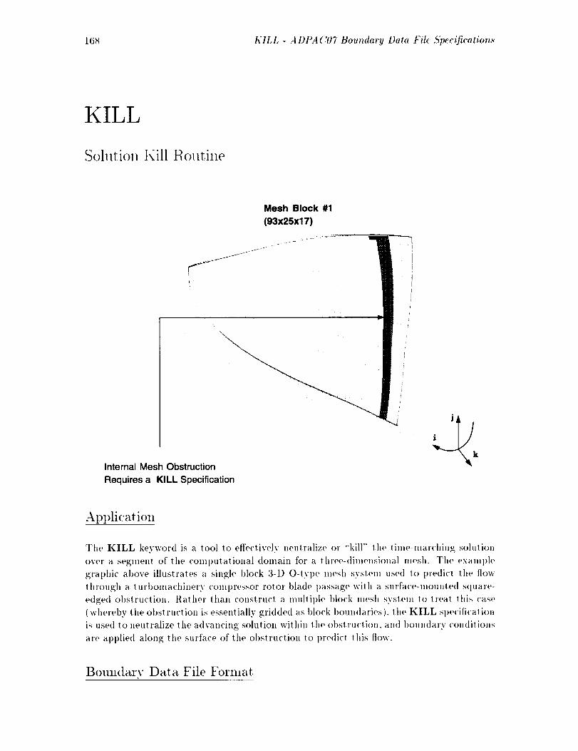
168 KILL - ADPAC07 Boundary Data Fil¢ 5'pecification._

KILL

Solution Kill Routine

Mesh Block #1

(93x25x17)

\

Internal Mesh Obstruction

Requires a KILL Specification

Application

The KILL keyword is a tool to effectively neutralize or "'kill'" the tinle-marching solution

over a segment of the COlnlmtational domain for a three-dinwnsional mesh. The example

gra,t)hic above illustrates a single block 3-D O-type mesh system used to 1)redict the flow

through a turbomachinery COml)ressor rotor blade passage with a surface-mounted square-

edged obstruction. Rather than construct a multiple block mesh system to lrea.l this case

{whereby the obstructioll is essentially gridded as block t)oundaries), the KILL specitication

is used to neutralize the advancing solution within the obstruction, and boundary conditions

are applied along the surface of the obstruction to predic! this flow.

Boundary Data File Format

A Dt{4 (Y)7 Be<radar" 9 Dale File S'pec_ficatiom_ - KILL 169

The boundary data file si>ecificatiot, for the mesh system indicated in the illustrative graphic

for th<, KILL boundary condition is given below:

KILL 1 1 I I

LSTART LEND

49 51

KILL 1 1 I I

LSTART LEND

49 52

P P L L 49 49 1 19 1 5 1 19 1 5

P P L L 49 49 19 21 1 5 19 21 1 5

Note thal a c<)mlilele KILL specilication requires two a<l<li|ional lines tollowing the KILL

I)oundarv data [ile sl)eciticatiolt line. Failure Io l)rol)erly specify the data in tiles<, additional

lines is a COltltl]O[I KILL specification error.

Description

In cases where a portion ofa 3-I) mesh <lees not tel)resent a valid flow re_;ion, lhe KILL sl>ec-

ificalion can be used. in conjunction with boundary conditions sl)ecified abottl the region 1o

be "'killed". to effeclively remove a portion era given mesh block from tile COmlmtational

domain. Au example of lhis technique is illustrale<t in the illustrative graphic el>eve. The

ti_;ure depi<'ls a single mesh block for the flow lhrou_h a high speed rotor passage upon which

surface instrument aliolt is mounted. The blockage associated with the surface insl rutnenta-

ti<m is iucorliorate<l into the solulion throu_;h the applicatiola of lit<' al>propriale boundary

¢'on<lilions <m lhe surface of Ill<, instrumentation, att<l i>v apl)lying tit<' KILL procedure to

ne_ale the tlow variables of lhe <'ells within Ill<' iustrunwnlalion itself. It should be noted

that lids effe<'l could be ac<'oml)lis]wd by sul)<lividing the original mesh into several smaller

pieces, aH<l applying lit(, al)l>ropriate boundary conditions along the outer l>oun<laries of

each l>]ock. This bOltn<lary con<litiou (although really, this is more than a ]>oun<lavy con<li-

lion) requires the spe<'itication of additional data. as shown in ihe formal <lescriptor above.

The variable following the label LSTART indicates the starting index in the LFACE1

coor<linate direction (in the example above, this would be the I coordinate direction) for

the re_iou to be "'killed". The varial>le following the label LEND indicates the final index

in the LFACE1 coordinale <lireclion (again. the I <'oordinale in the example above) for

the i'e_ion to be "killed". The remaining coordinate indices for the region to be "'kille<t'"

are d<,tet'milwd by the variables M1LIM1, M1LIM2 for the J coordinate direction and

N1LIM1, and N1LIM2 for the K coordinate direction. The additional specification of

the LSTART, LEND varial)les imply that the variables L1LIM, L2LIM are not used

in this specificaliot_. The KILL routine fuctions by constantly resetting the flow variables

inside the re_;i<m lo lit, kille<l to the initial values specifie<t l>v tile RMACH input varial)le.

So. ill eft'eel, the solulion is slill I)eing 1)erfornw<l ill the regioll to |)e killed, l>ut tile updaletl

resulls are ('OltStatlllv reset It) a unif<>rnl flow value. This routine is no! without drawbacks.

First of all. although lhe mesh poinls are efl'eclively neutralized by the KILL specification.

o1 her rout ines st+<'h as t he residual stnoot h inp_; al,o.;oril h m are unaltered, and uuder cert.ain

('irt'lllttsla.tt<'os. this ntav callse l)<)or ('otlver_ellce. It is also possible that <tivergen<'e <nay

oc<'ur within the "'kille<l'" cells iu spile of the t'esettin_ procedure. The best a<lvice i_ l<)

manilmlate block st t+tt<'tures lo elilnit+ale lit<' need for Ill<' use oft he KILL r<-,utine, but the

170 KILL - ADPAC07 Boundary Data File ,5'pec(fication._

user should be aware that under dire circumstances this facility is available. The KILL

specification should t)e given prior to any other boundary conditions to avoid "'wiping out"

previously specified boundary specifications.

Rest rictions/Linlitations

The KILL 1)oundary sl)ecification is nol restricled to 3-I) mesh surfaces (although for

consistency, 2-1) lnesh surfaces may use lhe KIL2D l)oun(larv sl)e('ili('ation).

CollllllOll Errors

• Application of KILL to a 2-1) mesh system.

• Poor convergence due to residual smoothing across a "'killed" region (The residual

smoothing operator can 1)e turned off through the RESID int)u! variable, although

the time step lnUS! 1)e restricted (see variable CFL) _o maintain numerical stabilily).

• Failure to st)ecify the additional data values LSTART, LEND.

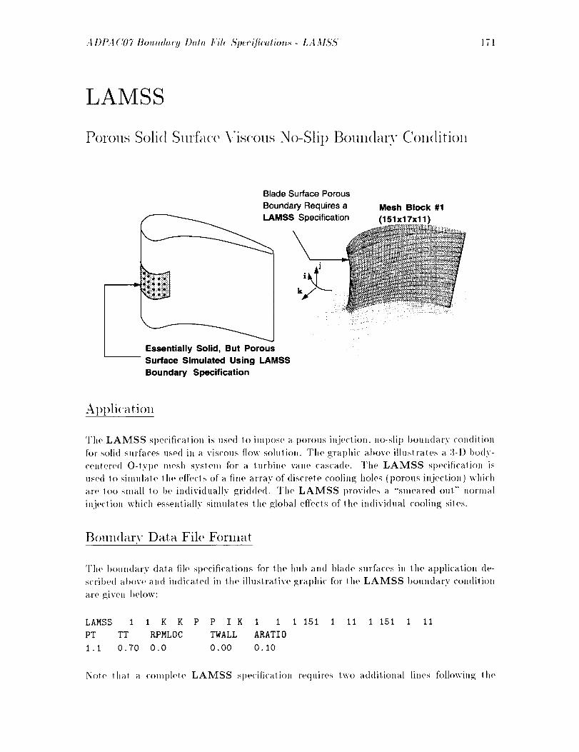
A I)PA ('07 Bo_t,dary Data File A'peeificatiol_._" - LA MSA' 171

LAMSS

Porous Solid Smta<e \'iscous No-Slip Boml(larv Condition

Blade Surface Porous

Boundary Requires a

MSS Specification

Essentially Solid, But Porous

-- Surface Simulated Using LAMSS

Boundary Specification

Mesh Block #1

(151x17x11)

Ai)i)li(ation

The LAMSS specification is used to iml)ose a porous injection, no-slip l)oundary condition

for solid surfaces used ill a viscous flow solution. The graphic above illustrates a 3-1) bo<tv-

centered O-tyi)e mesh system for a turbine vane cascade. The LAMSS st)ecificatiol, is

used to simulate the effects of a fine array of (tiscre_e cooling holes (porous injection) which

are _oo small Io be individually gridded. The LAMSS provides a "'smeared out"' normal

in.iection which essentially simulates the global effects of the individual cooling sites.

BomMarv Data File Fornmt

The l)oundarv data file st)ecifications for the hu|) and 1)lade surfaces in the a.pl)lication <le-

scribed al)ove and indicated in the illustrative graphic for the LAMSS t)oundary con(lilion

are given below:

LAMSS I I K K P P I K I i

PT TT RPMLOC TWALL ARATIO

i.i 0.70 0.0 0.00 0.I0

1 151 1 11 1 151 1 11

Nole thai a COml)lele LAMSS sl)e<'ilicatioll re(luires lwo additional lines following lhe

172 LA MS, q - A DPA C07 Boundary Data Fih Specifications

LAMSS boundary data file specification line. Failure to properly specify tile data in these

additional lines is a common LAMSS specification error.

Description

The LAMSS statement specifies that a solid surface viscous (no-slip) boundary con<ti-

tion is to be applied t.o the mesh surface specified by LFACE1 on the block specified by

LBLOCK1. The LAMSS boundary condition may be applied to either a rotating or non-

rotating surface and may indicate a rotational speed which is different than the rotational

speed of the mesh (RPM) to which the boundary condition is applied (the most common

example of this type of application is a mesh embe<lded in a rotating blade passage with

an endwall which is non-rotating). This houndary condition requires the specification of

additional data, as shown in the houndary data format descriplor above. The first addi-

tional line following the LAMSS specification is assumed to be a label and may contain any

information: however, for consistency it is recommended that the labels PTOT, TTOT,

RPMLOC, TWALL, and ARATIO be used. The next line contains the values imposed

for the variables PTOT, TTOT. RPMLOC, TWALL, and ARATIO. The value of the

PTOT and TTOT variables represent the total pressure and total temperature of the

injected flow. These variables are defined as:

Ptotal

rtotal

(rtot¢,l),,,,__din_nsion_,l- p,.,f

The value of the RPMWALL va.rial)le is the desired solid wall dimensional rotalional

speed in revolutions per minute. This value is sign dependent and follows the orientation

for rotation a.s described in Figure 3.10. The variable TWALL determines which type

of temperature condition is applied to the surface. If TWALL=0.0, an adiabatic wall is

assumed. For TWALL>0.O, a constant temperature surface with a nondimensional wall

temperature of TWALL defined as:

Twcz It( T.,all ),o.-dime nsion,d --

7;._f

is imposed. (Here T,._] is the reference temperature imposed by the input file variable

TREF. A value of TWALL<0.0 is no! perlnitted. Naturally. poor convergence or solution

divergence can occur if RPMWALL or TWALL suggest boundary vahms which are sig-

nificantly different fi'om the remainder of the flowfield. In such cases where this occurs, it

is recommended that the solution be started with lnore conservative boundary values, and

then restarted using the final boundary values. Finally, the value of the variable ARATIO

represents the geometric "porosity" of the surface in the form of the ratio of open (injection)

surface area to total surface area for the boundary segment being defined. In olher words.

if the porous surface has an injection area of .01 square inch per square inch of total surface,

then ARATIO would be 0.01. ARATIO values less lhan zero el" gi'eater than 1.0 are not

permitted.

A 1)1).4 (7)7 Boundary Data Fil_ ,S'p¢cOqeatiol_.¢ - LA MS',_' 173

R estrictions/Linlit aliens

The boundary rolalional speed iml)osed 1)v tile LAMSS boundary condilion can only be

nonzero when using lhe cylindrical coordinale solulion algorilhm in lhe ,tDP.4('07 code.

When using the (:arle.'-;ian coor(linale solulion algorithnl FCART and/or FCARB= 1.0.

I he boundary rotaliollal speed musl be zero ( RPMWALL= 0.0 when FCART or FCARB=

1.0). Refer to the ('hal)ter on input ill(, 1)aratneters for a descril)liotl of TREF. RPM,

FCARB, and FCART. The injeclion process modeled I)y LAMSS is alv,,avs J+,',+mal to

the lo('al surface lOl)Ogral)]ly. At+t)ilrary inj(wlion angle Sl)(,('ili('atioll is not ('urretllly I)OSSi-

bl(_.

COllIIIIOll Errors

• llworrec! sign for valu(, of boundary rotalional sl)eed RPMWALL.

• :\lleml)l 1o ulilize a nonzero l)oun(lary rotational spee(1 wilh lhe ('arlesian ('oor(linat(,

solulion algorithm.

• ARATIO value less than 0.0 or groal(w than 1.0.

• PTOT valu(' significanlly different than freeslream.

• TTOT value significanlly differen! than fi'eestream.

• TWALL valu(' significantly differenl than freestream.

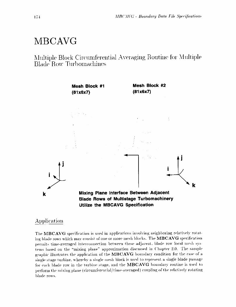
174 MB('A I'G - Bouudary Data Fih ,5'peeifieation._

MBCAVG

5Iultil)le Block Circunfferential Averaging 1Routine for 5Iultil)leBlade Row Turl)oxna(:hines

Mesh Block #1

(81 x6x7)

Mesh Block #2

(81 x6x7)

k Mixing Plane Interface Between Adjacent

Blade Rows of Multistage Turbomachinery

Utilize the MBCAVG Specification

k

Application

Tile MBCAVG specification is used ill applications involving neighboring relatively rolal-

ing blade rows which may consist of one or more mesh blocks. The MBCAVG specification

perlnits time-averaged interconnection between these a djacenl, blade row local mesh sys-

tems based on the "mixing plane" approximation discussed in Chaplet 2.0. The sample

graphic illustra.tes lhe application of the MBCAVG boundar.v condition for tile case of a

single stage turbine, whereby a single mesh block is used to represent a single })lade passage

for each blade row in the turbine slage, and tile MBCAVG boundary routine is used 1o

t)erform the mixing plane (circumferential/linm-aw, raged) coupling of lhe relaliw, ly rotatingblade rows.

Boundar9 Data Fil< 51,_c(fications - MB('A I'G 175

B<mndarv Dat, a File Format:

Tile boundary data file Sl)ecilicalions for tile mesh interfaces indicaled in lhe illustralive

graphic for theMBCAVG boundary('ondilion are given below. Notelhal block 1 re<luires

multiple sl)ecificalions due lo lhe location of the O-grid cul line.

MBCAVG I 2 K K M M I J 7 7 I 6 i 6 36 46 I 6

NSEGS

I

LBLOCK2B LFACE2B LDIR2B L2LIMB M2LIMIB M2LIM2B N2LIMIB N2LIM2B

2 K M 7 36 46 1 6

MBCAVG i 2 K K M M I J 7 7 76 81 1 6 36 46 i 6

NSEGS

I

LBLOCK2B LFACE2B LDIR2B L2LIMB M2LIMIB M2LIM2B N2LIMIB N2LIM2B

2 K M 7 36 46 1 6

MBCAVG 2 I K K M M I J 7 7 36 46 i 6 I 6 I 6

NSEGS

2

LBLOCK2B LFACE2B LDIR2B L2LIMB M2LIMIB M2LIM2B N2LIMIB N2LIM2B

i K M 7 I 6 I 6

i K M 7 76 81 1 6

Not(' lhal a <'Oml>lele MBCAVG specification generally requires a.l leasl lwo MBCAVG

slalelllenl lines in lhe 1)oun(larv data tile for each lnesh interface. In ihe exallll)[e above.

the tirsi two sl)eci[icalions provide the interblock communication for l>lo<'k 1 t'roln I>[oc],: 2.

and the lhird specifi<'ation provi<les the communication for block 2 from blo<'k 1. It is a

common error to underspe<'ify an MBCAVG l)oun<lary by only providing a single line per

interface.

Des<'ril)ti<m:

The MBCAVG specification provides a "'circumferential mixing l>lane'" mesh block COlll-

munication scheme for stea<ly state (lime-averaged) analysis of multiple blade row turboma-

chines. The MBCAVG ot>eralor permits lhe specification of mulliple neighboring blocks

upon which lhe <'ir<'umferelllial averaging is applied to provi<h, boundary data for lhe cur-

rent block of inlerest. This multiph' block averaging scheme perlnits the use of MBCAVG

for I)odv-cenlered mesh svsl.enls (see the illustralive gral>llic al)ove) and also for multiple

blade passage representations of neighborillg blade rows. Due to the conlplex nature of the

cil'cumfi,renlial averaging ol)erator, this boundary condition is restricted to specific mesh

configurations. The following charl descri|)es the permitted mesh configurations for the

MBCAVG speciticat ion:

LFACEI

MBCAVG t;oundaI'y Specification Mesh('<>ordinalelleslrictions

LFACE2 Circumferential Grids Must be

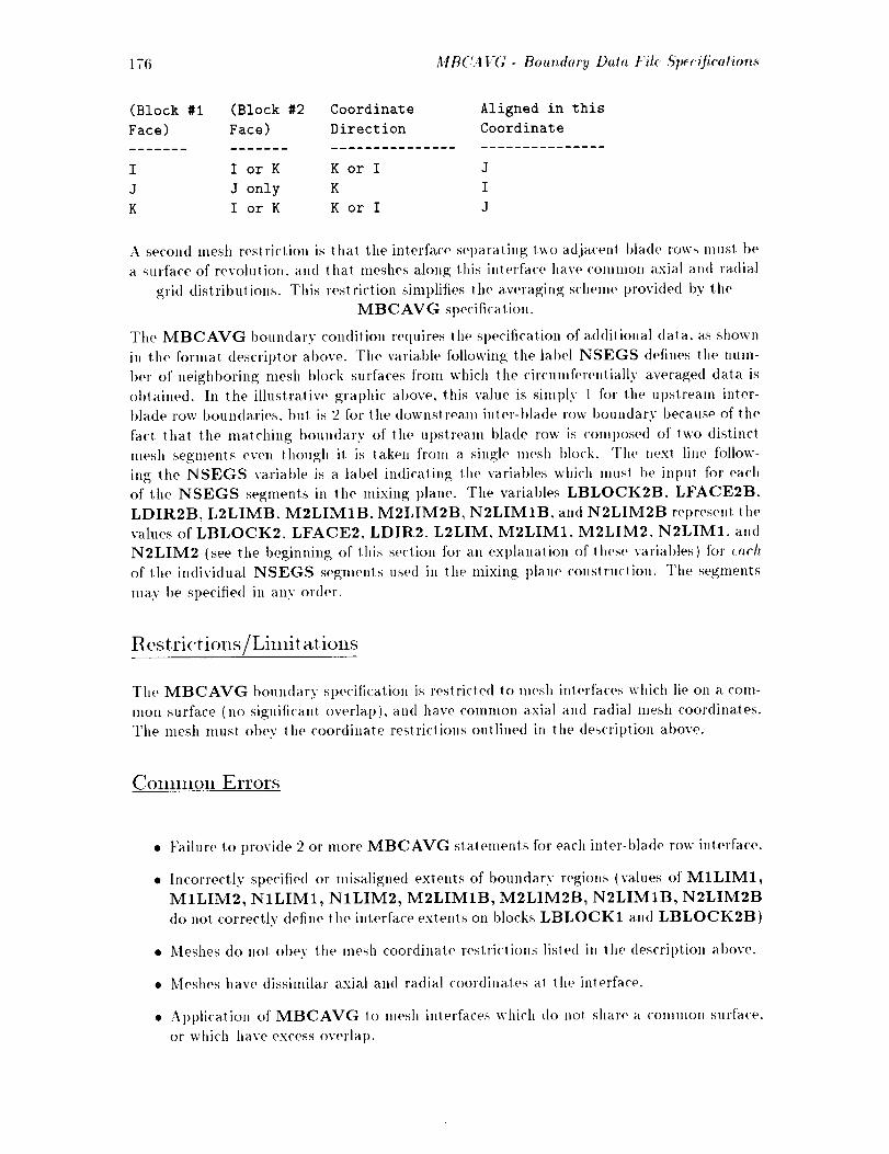
176 MBCA I:G - Boundary D_tt, File Specifications

(Block #i (Block #2 Coordinate Aligned in this

Face) Face) Direction Coordinate

..............................

I I or K K or I J

J J only K I

K I or K K or I J

A second mesh restriction is thai tile inlert'ace separating two adjacenl blade rows must be

a surface of revolution, and that meshes along lifts interface have common axial and radial

grid distributions. This restriction simplifies lhe averaging scheme provided by the

MBCAVG specification.

The MBCAVG boundary condition requires the specification of additional data. as shown

in tile format descriptor above. The variable folk)wing lhe label NSEGS defines the num-

1)er of neighboring mesh block surfaces from which the circumferentially averaged data is

obtained. In the illustrative graphic above, this value is simply 1 for the upstream inter-

blade row boundaries, but is 2 for the downslreanl inter-blade row boundary because of the

fact that the matching boundary <>f the upstream blade row is COml)osed of two distincl

mesh segments even though it is taken fi'om a single mesh }>lock. The nexl line follow-

ing the NSEGS variable is a label indicating the variables which must be input for each

of the NSEGS segments in lhe mixing plane. The variables LBLOCK2B, LFACE2B.

LDIR2B, L2LIMB. M2LIM1B, M2LIM2B, N2LIM1B, an<t N2LIM2B represent the

values of LBLOCN2, LFACE2. LDIR2, L2LIM. M2LIM1. M2LIM2, N2LIM1. and

N2LIM2 (see tile beginniug of this section for an explanation of these variables) for _ach

of the individual NSEGS segments used in the mixing plane conslruction. The segments

may be specified in any order.

Rest ri<'tions/Lindtatiolls

The MBCAVG boundary st>ecilication is reslricted to mesh inlerfaces which lie on a com-

mon surface (no significant overlap), and have common axial and radial mesh coordinates.

The mesh must obey the coordinate reslrictions outline<l in the description above.

CollllnollErrors

Failure to provide 2 or more MBCAVG statements for each inter-blade row interface.

Incorrectly speciIied or misaligned extents of boundary regions (values of MILIM1,

MILIM2, N1LIM1, NILIM2, M2LIM1B, M2LIM2B, N2LIMIB, N2LIM2B

do not correctly define the interface extents on blocks LBLOCK1 and LBLOCK2B)

Meshes do uot obey the mesh coordinate restrictions listed in lhe description above.

Meshes have dissimilar axial and radial coordinates al the interface.

Apl)licalion of MBCAVG lo mesh inlerfaces which do no! sharo a common surface.

or which have excess overlap.

Bottt_dary I)ala Fil: ,S'p(eifieation._ - MB('A I'(; 177

• Application of MBCAVG Io (la,rtesian solutioll mesh systems.

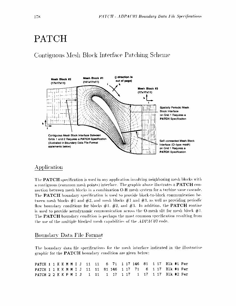
178 PA 7"('H - A DPA C07 Boundary Data Fi& ,S'lu;cification._

PATCH

Contiguous ? Iesh Block Interface Patching Schelne

Mesh Block #2 Mesh Block #1 (j direction isout of page)

(17x17x11) (151x17x11) i k

..........L_;/i,/_;.) " il

hr " / "m_ .

Contiguous Mesh Block Interface Between

Grids 1 and 2 Requires a PATCH Specification

(illustrated in Boundary Data File Format

statements below)

Mesh Block #3

(17x17x11)

,t_.i

Spatially Periodic Mesh

Block Interface

on Grid 1 Requires a

PATCH Specification

Self-connected Mesh Block

Interlace tO-type mesh)

on Grid 1 Requires a

PATCH Specification

ApI)licatioll

Tile PATCH specification is used in any application involving neighboring mesh blocks with

a contiguous (common mesh points) interface. The graphic above ilhlstra.tes a PATCH con-

nection between mesh blocks in a combinatioll O-H mesh system tbr a turbine vane cascade.

The PATCH boutLdary specificalioll is used to provide block-to-block cotnnlunicatiotl be-

tween mesh blocks #1 and #2, and mesh blocks #1 and #3. a.s well as providing periodic

flow boundary conditions for blocks #1, #2, and #3. In addition, the PATCH routine

is used to provide aerodynamic communicatioll across the O-mesh slit for mesh block #1.

The PATCH boundary condition is perhaps the most common specification resulting from

the use of the multiple blocked mesh capat)ilities of lhe .4 DtL4 ('07 code.

Boundary Data File Format

The boundary data file specifications for the mesh interface indicated in the illustrative

graphic for the PATCH I)oundary condition are given below:

PATCH 1 1 K K H H I J 11 11 6 71 1 17 146 81 1

PATCH 1 1 K K H H I J 11 11 81 146 1 17 71 6 1

PATCH 2 2 K K P M I J I Ii 1 17 I 17 1 17 I

17 Blk #1 Per

17 Blk #1 Per

17 Blk #2 Per

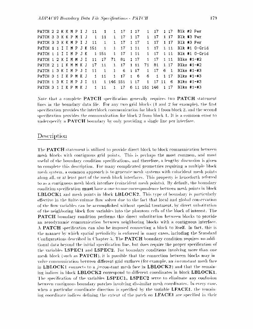
A DPA ('07 Bottndary Data Fil< ,S'p_cJiealions - PA T('H 179

PATCH 2 2 K K M P I J ii I I 17 I 17 1 17 I i7 Blk #2 Per

PATCH 3 3 K K P M I J i 11 I 17 I 17 1 17 1 17 Blk #3 Per

PATCH 3 3 K K M P I J ii I 1 17 I 17 I 17 i 17 Blk #3 Per

PATCH I i I I M P J K 15i I 1 17 I ii I 17 I II Blk #I O-Grid

PATCH I I I I M P J K I 151 1 i7 I ii 1 17 I II Blk #1 O-Grid

PATCH 1 2 K I M M J I II 17 71 81 I 17 1 17 I li Blks #I-#2

PATCH 2 i I K M M K J 17 Ii 1 i7 i ii 71 81 1 17 Blks #I-#2

PATCH i 3 K I M P J I li I 1 6 I 17 I i7 6 i Blks #I-#3

PATCH 3 i I K P M K J I ii 1 17 1 6 6 i 1 17 Blks #i-#3

PATCH I 3 K I M P J I II I 146 151 i 17 1 17 ii 6 Blks #I-#3

PATCH 3 i I K P M K J 1 ii 1 17 6 Ii 151 146 i 17 Blks #I-#3

.Nol0 lha! a complete PATCH specification generally requires 1we PATCH slalement

lines ill lhe bOul_darv data file. For any two grid blocks (1 and 2 for exalnl)le ). lhe firs!

specifical ion provides the inlerl)lock communication for block 1 from block 2. and the second

SlWt'ification l)rovides the communication for block 2 from block 1. I1 is a common error to

underspecify a PATCH l)oulMary bv only provi(lin_ a single line per interface.

Description

The PATCH statement is utilized to provide direct block to block communication between

mesh blocks with contiguous grid points. This is perhaps the rues! common, and most

useful of the l>oundary condition sl)ecifications, and therefore, a lengthy discussion is given

to complete this <tescril)lion. For manv complicaled geometries re<luMng a multiple block

mesh svslem, a common approach is to generale mesh systems with coincident mesh points

along all. or al leas1 l>arl of the mesh block inlerfaces. This t)rol)erty is hen('eforlh referred

t<) as a con1 i_;u<>us mesh block interface (coin<'idenl mesh points). By defaull, the 1)oun<larv

condition sl)ecificalion must have a one to one corresl)ondence between mesh points in I)lock

LBLOCK1 and mesh points in block LBLOCK2. This lyt>e of boundary is l>arlicularly

effective in lhe finile-volume flow solver <lue 1o lhe facl that local and global conservation

of the How variabh, s can I)e accomplished without special treatment, by direct subslilulion

of lhe neighboring block tlow variables into lhe t>hamom <'ells of the block of interest. The

PATCH boundary condition performs lhis direct substitution between blocks to provide

an aerodynamic communication between neighboring blocks with a contiguous interface.

A PATCH specification can also be imposed connecting a block to itself. In fact. this is

the manner by which spatial periodicity is enforced in many cases, including the Standard

('onfigura!ions described in (!hal>tot 5. The PATCH I)oundary condition requires no addi-

l ional (lata I)evond 1he initial sl)ecificalion line. but does require tile l)rol)er st)ecification of

the varial)les LSPEC1 and LSPEC2. For boundary conditions invoh, ing more than one

mesh bh)ck (such as PATCH), it is possible that the connection I)etween blocks may in-

v<)lv(, communication between differenl grid surfaces (for example, an /:constant mesh face

in LBLOCK1 connects to a j=constan! mesh face in LBLOCK2) an(I lhal the remain-

ing indices in t)lock LBLOCK2 correspon<l 1o difl'erent coordinates in block LBLOCK1.

The si)ecilica_ion of tile variables LSPEC1, LSPEC2 serve to eliminate any coufusion

between ('onli_uous boundary l)atches involving dissimilar mesh coor(linales. Ill every case.

when a particular coor<tinale direction is sl)e<'ified 1)v the variable LFACE1, the remain-

ing coordinate indices defining lhe exteul of the l)atch on LFACE1 are st>ecilie(t in their

180 PATCH- A DPAC07 Boundary Data File ,S)_ecification._

"natural" (i. j, k) order. For example, if LFACE1 is a.n/=constant mesh surface, then tile

variables MILIM1, MILIM2 control the indices in the j coordinate direction and the

variables NILIM1, N1LIM2 control the indices in tile k coordinate direction. Similarly,

if LFACE2 is a k=constant mesh surface, then tile variables M2LIM1, M2LIM2 control

the indices in the i coordinate direction and the variables N2LIM1, N2LIM2 conlrol the

indices ill tile j coordinate direction, and so on. Now, in order to relate lhe coordinate

indices in block LBLOCK2 with the indices sl)ecified in bh)ck LBLOCK1. the special

tern> LSPEC1 and LSPEC2 are utilized. The variables LSPEC1 and LSPEC2 should

be defined as either I, J, or K, based on the COlmeclion schelne betweelJ the two blocks.The LSPEC1 variable should define the coordinate direction in blo('k LBLOCK1 which

('orresponds to the first remaining coordinate in block LBLOCK2 (whose range is defined

by M2LIM1, M2LIM2), and the LSPEC2 variable should define the coordinate direc-

tion in block LBLOCK1 which corresponds to the second reInaining coordinate in block

LBLOCK2 (whose range is defined by' N2LIM1, N2LIM2). The PATCH sl)ecification

may also be used for two-diinensional lneshes as long as the third coordinate direclion (k)

limits NILIM1. NILIM2, and N2LIM1, N2LIM2 are "'1"" and "2"', respectively (2-D

patches are specified as if the mesh were actually 2 cells deel) in the/,' direction).

Restrictions/Limitatiolls

The PATCH boundary specification is restricted t.o mesh interfaces which have a one to

one mesh point correspondance. _Ib maintain the conservative property of the governing

equations, the PATCH routine a.ssumes that the mesh points between the 2 blocks of

interest are either contiguous, or share a. spatially periodic relationship, and it is left to the

user to verify that this is so.

COlIIIIIOll Errors

Failure to provide 2 PATCH statements for each interface.

Incorrectly specified or misaligned extents of boundary regions (values of MILIM1,

MILIM2, NILIM1, NILIM2, M2LIM1, M2LIM2, N2LIM1, N2LIM2 do not

correctly define the interface extents Oll blocks LBLOCK1 and LBLOCK2).

Incorrectly specified block coordinate direction relationships (values of LSPEC1,

LSPEC2 do not correctly define the coordinate connection scheine between block

LBLOCK1 and block LBLOCK2).

PATCH boundary specification for a, periodic boundary is applied to a nonperiodic

Inesh.

PATCH boundary specification applied to a spatially periodic Cartesian geometry

using the cylindrical coordinate solution scheme or vice versa (results in incorrect

spatial t)eriodicity relationships) The PATCH boundary specifications for (la.rtesian

geometries must use the (:artesian solution algorithm ill A DPA('O7(see int)u! variable

FCART).

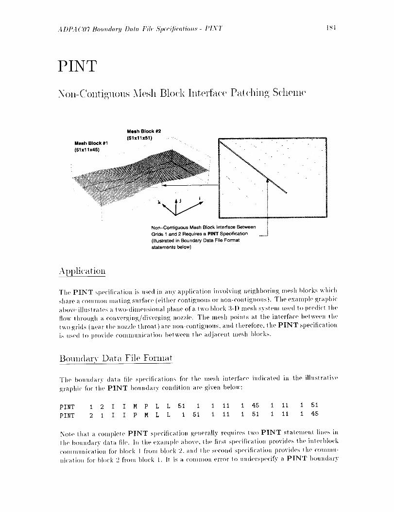
A DPA ('07 BomMary Data Fil( ,S'pec_fication,_ - PIXT I S 1

PINT

Non-Contiguous .Xlesh Block Interfa('e Pat(hing Schelne

Mesh Block #2

(51xllx51) -,--_ ..Mesh Block #1

(51 xl I x45)

Non-Contiguous Mesh Block Interface Between

Grids 1 and 2 Requires a PINT Specification

(illustrated in Boundary Data File Format

statements below)

Apl)lication

The PINT spe('ilication is used in any a l@ication involving neighboring mesh blocks whi<'h

share a common mating surface (either contiguous or llOn-('oltl iguous). The examph' graphic

above illuslralos a, two-dimensional plane of a two block 3-1) mesh svslem used to predicl lhe

tlow lhrough a converging/diverging nozzle. The mesh points at the interface belween the

two grids (near lhe nozzle lhroat ) are non-contiguous, and therefore, the PINT specification

is used Io provide communication between the adjacent lllesh blocks.

Boundary Data File Format

The boundary dala file specifications for the mesh interface indicated in the illustralive

graphic for the PINT boundary condition are given below:

PINT 1 2 I I N P L L S1 1 1 11 1 45 1 11 1 51

PINT 2 1 I I P N L L 1 51 1 11 1 51 1 ll 1 45

Nole lhat a comple!e PINT specification generally re<luires two PINT statement lines in

the boundary data file. In the example above, the firsl speciticalion provides the interl)lock

COmlmlnicalion for blo<'k I from block 2. and |he second speciticalion provides lhe commu-

lfica!i<m for bhwk 2 from block 1. It is a common error lo underspe<'ify a PINT I>oundary

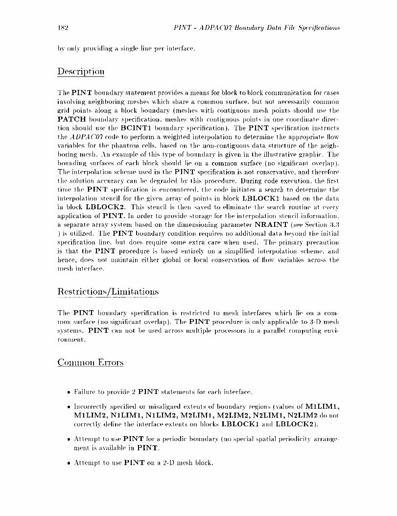
1_2 PINT - A DPA C07 Boundary Data File 5'pccification._

by only providing a single lille per interface.

Description

The PINT boundary statement provides a means for block to block communication for cases

involving neight)oring meshes which share a (Olllnlon surface, but no! necessarilv common

grid points aloug a block boundary (meshes with contiguous mesh points should use the

PATCH boundary st_ecification, meshes with contiguous poinls in one coorclinale direc-

tion should use lhe BCINT1 boundary specification). The PINT specification instructs

the A DPA ('07 code to perforln a weighted interpolation to deternline the al)prol)riate flow

variables for the p]lantonl cells, based on the nOlt-COlltiguous data structure of the neigh-

boring mesh. An example of this type of boundary is given in the illustralive graphic. Tlle

bounding surfaces of each block should lie on a common surface (no significanl overlap).

The interpolatioll scheme used in the PINT specification is not conservative, and therefore

the sohltion accuracy can be degraded t)3' this procedure. During code execution, the til'sl

time the PINT specification is encountered, the code iniliates a search to determine the

interpolation stencil for the given array of points in block LBLOCK1 based on the data

in block LBLOCK2. This stencil is then saved to eliminate the search routine al every

application of PINT. hl order to provide storage for the interpolation stencil information.

a separate array system based on the dilnensioning paranleter NRAINT (see Seclion 3.3

) is ulilized. The PINT boundary conditioll requires no additional data beyond the initial

specification line, but does require some extra care when used. The primary precautioll

is that tile PINT procedure is based entirely on a simplified interpolation scheme, and

hence, does nol lnaintain either global or local conservation of flow variables across thelnesll interface.

R estrictions/Limitations

Tile PINT boundary specification is restricted to mesh interfaces which lie on a com-

mon surface (no significant overlap). Tile PINT procedure is only applicable to 3-D mesh

systems. PINT can not be used across multiple processors in a parallel colnputing envi-

rollnlent.

COIIIlIIOII Errors

Faihlre to provide 2 PINT statelnents for each interface.

Incorrectly specified or lnisaligned extents of boundary regions (values of MILIM1,

MILIM2, NILIM1, NILIM2, M2LIM1, M2LIM2, N2LIM1, N2LIM2 do not

correctly define the interface extents on blocks LBLOCK1 and LBLOCK2).

At, telnpt to use PINT for a periodic boundary (no special spatial periodicity arrange-

ment is available in PINT.

• Attenlpt 1o use PINT on a 2-D mesh block.

:tDPA ('07 BoutMaUt Dat_l Fil: £'p_e_fie_ttio_._ - PLVT lg3

• l:ailure 1o provide enough storage for lhe PINT inlerpolalion stencils via lhe NRAINT

paralllOl, el'.

• Apl_lication of PINT to mesh inlerfaces which do nol share a common surface, or

which have excess overlap.

• Atlempl 1o use PINT across multiple processors in a parallel computing environmenl.

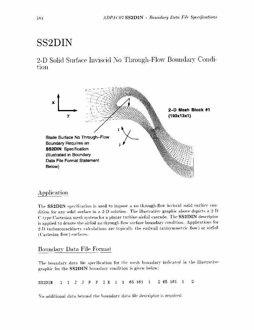
184 A DPA C07 SS2DIN - Boundary Data File ,S'pecification._

SS2DIN

2-D Solid Surface Inviscid No Through-Flow Boundary Condi-tion

I- , 2-D Mesh Block #1

y _-:_ (193x13x1)

Blade Surface No Through-Flow

Boundary Requires anSS2DIN Specification

(Illustrated in BoundaryData File Format Statement

Below)

Application

The SS2DIN sl)ecification is used to intpose a no through-flow inviscid solid surface con-

dition for any solid surface ill a 2-D solution. The illustrative graphic above depicts a 2-D

C-tyl)e Cartesian mesh system for a planar turbine airfoil cascade. The SS2DIN descriptor

is applied to denote the airfoil no through-flow surface boundary condition. A1)plications for

2-D turbmoznachinery calculations are typically the endwall (axisymmetric flow) or airfoil

(Cartesian flow) surfaces.

Bouzldar.v Data File Forznat

The boundary data file specification for tile mesh boundary indica,led in lhe illustrative

graphic for the SS2DIN bOUlMary condition is given below:

SS2DIN 1 1 J J P P I K 1 1 65 161 1 2 65 161 1 2

No additional data t)eyond the boundary data file descriptor is required.

ADPA ('07 Boundary Data Fih ,S'p_c_[ieation._ - S',SgDI,V

Descril)tion

The SS2DIN slatement specifies thai a solid surface inviscid (no ll,rough-ttow) bound-

ary COl,dillon is to be applied Io the mesh surface specified by LFACE1 on the block

specified bv LBLOCK1. The SS2DIN procedure is the 2-1) equivalenl of SSIN. The

SS2DIN I_oundarv cot_dilion may be applied to either t'oialillg or lloll-rotatillg stlrfaces.

The relational speed of lhe I)oundarv is irrelevanl for an inviscid surface ou a l)roperly de-

tiued mesh (el! her lho t)oun(larv rol ales with lhe mesh. or. in lhe case where lhe rot alioual

speeds of lhe mesh aud boundary differ, lhere ix ,to difference in the aplica! ion of a u il,viscid

s,rfa('e boundary coil(litton). SS2DIN may t)e applied for eilher ('vlilldrical or ('arlesiau

soluliou meshes (see the description of the input variable FCART). The SS2DIN algo-

rilhm imposes lie flow uormal 1o the local mesh surface, but perlnits langential veh)citv

components al the boundary. The currenl SS2DIN algorilhnt is based on a loose sl)eci-

tic'alien of the local static pressure ('_ = 0) and is known to introduce some nOul)hysical

loss. llowever, it has been the aul hers experience that lhis formulation provides tile bes!

mix of ac('nra¢'v and reliability for mosl applications. It should I)e noted lhal the SS2DIN

bOUlldarv condition is also very useful as a method of imposiuK a symmetry plane in a solu-

lion forgeometries which possess spatial syntlnetry. Naturally. the mesh lntlst be generated

in a lllallllel' which l'el)l'eSell|,S lhis Sl)alial svlllllle|l'V an well.

R estrictious/LimitatiollS

The SS2DIN boundary sl)ecitication is reslricled to 2-1) mesh surfaces (3-1)mesh surfaces

should use the SSIN boundary specificalion).

Co111111Oll Errors

• Application of SS2DIN to a 3-D mesh svslem.

• Apl)licatiou of SS2DIN as a symmetry plane con(litiolJ for a mesh which does no!

represent a spatially symmetric geometry.

186 5'E2D |'I - .4 DPA ('07 Boundary Data Fil_ £'p¢-eificatio_._"

SS2DVI

2-D Solid Surface Viscous No-Slip Boundary Condition

tx / 2-D Mesh Block #1

/ - (193x33x1)Y

Blade Surface No-Slip

Boundary Requires an

SS2DVI Specification

(Illustrated in Boundary

Data File Format Statement

Below)

J

AI)I)lication

The SS2DVI specification is used to impose a no-slip boundary conditiou fox' any solidsurface used in a 2-D viscous flow solution. Tile example graphic above illuslrales a 2-1)

C-type mesh system used to predict the flow through a planar 2-I) turbine vane cascade.

Applications for 2-D turbmomachinery calculations are typically the endwall surfaces (both

rotating and non-rotating surfaces) for an axisymmetric 2-I) solution or non-rotating solidsurfaces in Cartesian 2-I) solutions.

Boundary Data File Forlnat:

The boundary data file specifications _rthe lnesh interface indicated ill the illustrative

gral)hic _rthe SS2DVIbmmdarycondition are givenbelow:

SS2DVI 1 1 J a P P I K 1 1 65 161 1 2 65 161 1 2

RPMWALL TWALL

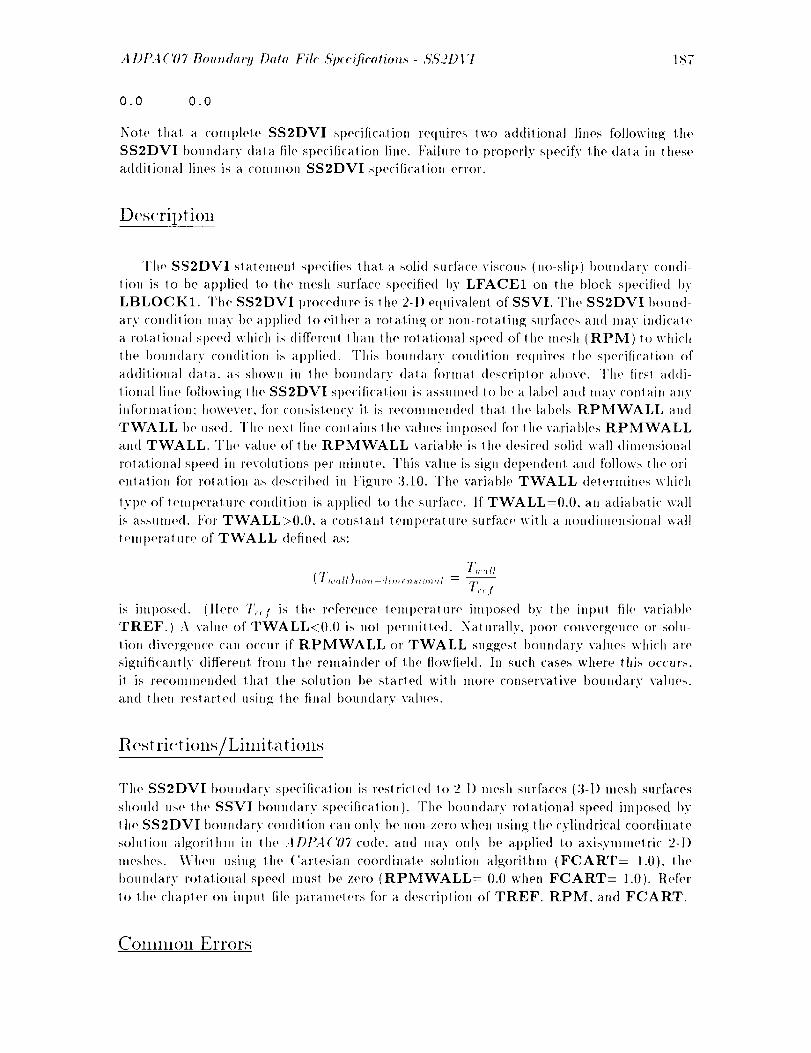
A DPA ('07 Bou_dary Data Fil: A'p(c([ieation._ - A%'2D I "I 187

0.0 0.0

Not(' that a complete SS2DVI specification requires two addilional lines following the

SS2DVI boundary data file specification line. FaihN'eto properly specify tile data in lhese

additional lines is a common SS2DVI sl)ecifi('alion error.

Des('rii)tioll

The SS2DVI statement specifies thal a solid surface viscous (no-slip) boundary condi-

lion is to be applied 1o the mesh surface sl)ecified 1)y LFACE1 on the block specified by

LBLOCK1. The SS2DVI procedure is lhe 2-1) equivalent of SSVI. The SS2DVI bound-

at"5' ('ondiliotl may be applied to either a rotating or non-rotating surfaces and may indicale

a rotational speed which is (lifferent lhan the re! arterial speed of the mesh (RPM) to which

the boundary condilion is applied. This I)oundarv condilion requires lhe st)ecificalion of

additional dala, as shown in the bounldarv data formal descriptor above. The first addi-

tional line following the SS2DVI speciti<'alion is assumed to be a label and may contain any

il_formation: however, for cotJsistency it is recommended that the labels RPMWALL and

TWALL I>e used. The next line contains the values imposed for the variables RPMWALL

and TWALL. The value of the RPMWALL varial>le is the desired solid wall dimetlsiotlal

rotational speed in revolutions l)er ntinttte. This value is sign (lel)etlden! and follows the off-

enlaliot_ for rotatiou as desct'it)ed in Figure 3.10. Tit(' variable TWALL delermines u'hich

type of tentperattlre condition is applied to the surthce. If TWALL=0.0, an adiabatic wall

is assumed. For TWALL>0.0, a conslanl temperature surface wilh a itondimensiona] uall

temperature of TWALL defined as:

T.,,. tt

7; _,f

is imposed. (Here 7',.:: is '(he reference t eml_eralttre imposed by the itq)u! file variable

TREF.) A value of TWALL<0.0 is not perlnitled..Naturally, poor convergence or solu-

lion divergence can occur if RPMWALL or TWALL suggest boundary values uhMt are

significantly different from the remainder of the flowfiehl. In such cases where this occurs.

it is recommended that the solution be started with more conservative boulMary values.

and then restarted using Ill(, final boundary values.

12est ri<'tions/Lilni tat ions

The SS2DVI 1)outMarv sl)ecification is resl rioted to 2-1) mesh surfaces (3-I) mesh surfaces

shot,hi use life SSVI I)oundary sl)e('ificalion ). The I)oundarv rotational speed iml)osed 1)v

the SS2DVI 1)oundary condition can only l)e ilOll-zero whelt using the cylindrical coordinate

sohttiol, algorilhnt in the .IDt)..I('07 code. and may only be applied to axisymmelric 2-I)

meshes. Wh('l, using lhe ('arlesian coordinale solution algorilhm (FCART= 1.0), lhe

botln(larv rotational speed must be zero (RPMWALL= 0.0 when FCART= 1.0). Refer

to lit(' ('hal)ler on inl)u'( file l)arameters for a (lescril)tiotl of TREF. RPM. and FCART.

Co111111Oll Errors

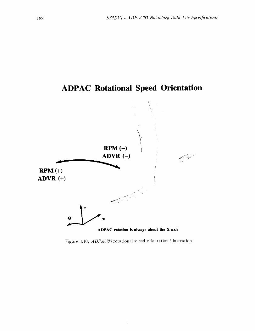
1_8 $5'2D17- A DPA('07 Boundary Data File ,S'p_cification._'

ADPAC Rotational Speed Orientation

RPM (+)

ADVR (+)

RPM (-)

ADVR (-)

\

'i

:!7!

ADPAC rotation is always about the X axis

Figure 3.10:ADPA('07 rotational speed orientalio, illustration

A DPA ('07 Bom_dar!t Data File ,qpec_[ir'alion._ - ,S',_'2D _"I 1_9

• htcorrec) sign for value of boundary ro(ational speed RPMWALL.

• AII('I|I])I lo ulilize a noll-zero boun(larv rolaliona] speed wilh the (!arlesiaH coordinat(,

solu(ion algorithm.

• Applicalion of SS2DVI to a 3-1) mesh system.

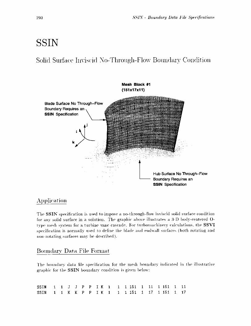
190 5'HIN- Boundary Data Fil( Hpecifications

SSIN

Solid Surface Invis(id No-Through-Flow Boundary Condition

Mesh Block #1

(151x17x11)

Blade Surface No Through-Flow

Boundary Requires an

SSlN Specification

Hub Surface No Through-Flow

Boundary Requires an

SSlN Specification

Apl)lication

The SSIN specification is used to iml)ose a no-through-flow inviscid solid surface condition

for ally solid surface ill a solution. The graphic above illustrates a 3-D t)o<ty-(:entered O-

type mesh syslem for a turbil_e vane cascade. For (url)omachinery calculations, lhe SSVI

specification is normally used to define the blade and endwall surfaces (both rotating and

non-rotating surfaces may be described).

Boundary Data File Forlnat

The boundary data file specification for the mesh boundary indicated in the illuslrative

grat)hic for the SSIN boundary condition is given t)elow:

SSIN I 1 J J P P I K 1 1 1 151 1 11 1 151 1 11

SSIN 1 1 K K P P I K i I I 151 i 17 I 151 i 17

Bou.dary Data File ,qp_¢'(fir'atim_s - ,q'S'IN 191

No addilional data beyond lhe boundary data file descriptor is required.

Des('ription

The SSIN slalemenl specifies lhal a solid surface invis<'id (no lhrough-Itow) bountlarv

c'omlilion is to be applied to the mesh surface specified t)y LFACE1 on the block spe('iIied

I)v LBLOCK1. The SSIN l>oul,<larv conclilion may l>e al)l)lied lo eilher l'olalin_ or non-

rotatillg surfaces. The rotational Sl)ee(l of the boundary is irreleval,t for al, inviscid surface

on a proi)erly defined mesh (eilhev Ill(' boundary rotates with lhe mesh. or. in the ('as(,

where lhe rotational speeds of the mesh and 1)oun<lary differ, there is no <lifferen<'e in the

al)l)licalion of an invis<'id surface l>oundarv ('on<Ill ion). The SSIN a l_orilhm imposes no

[low normal 1o lhe loom mesh surface, bu! I)ermits la,ngenlial velo<'itv ('oml)onenls al the

boundar.v. The currenl SSIN algorithm is based on a loose spe<'ificalion of lhe hwa] slali<'

l)ressu re ( ,.)."'l'"= 0) and is known lo introduce some l,onl)hvsi('al, loss. However. il has been lhe

aulhors experience thai lids fornlulation provides the bes! mix of ac<'uracy and reliabilily

_()1' lllOSl al)l)lications. I1 should l)e holed thal the SSIN I)oun<larv ('on(lilion is also very

useful as a method of imposing a symmelry l>lane in a s()lulioll for geom(,iries which possess

spatial symmetry. Naturally. 1tle mesh must I)e genel'ale(I in a nlal,ner which represei,Is

lids spatial symmetry as well.

12est ri<'tions/Limit at ions

The SSIN boundary specificalion is restricled Io 3-I) mesh surfaces (2-1) mesh surfaces

should use lhe SS2DIN I)oundary sl)eciticalion).

ColillllOll Errors

. Application of SSIN lo a 2-D mesh system.

. At>pli('a'tion of SSIN as a syn,met, ry 1)lane condition for a mesh which does not repre-

sent a spatially symmetric geomelry

192 ,5'SVI - ADPAC07 Boundary Data Fil_ Sp_cification._

SSVI

Solid Surface \:iscous No-Slip Boundary Condition

Mesh Block #1

(151x17x11)

Blade Surface No-Slip

Boundary Requires an

SSVI Specification

Hub Surface No-Slip

Boundary Requires an

SSVI Specification

Application

The SSVI specification is used to iml)ose a no-slip I)oundary condition for solid surfaces

used in a viscous flow solution. The graphic above illustrates a 3-I) 1)ody-centered O-

lyl)e mesh system for a turt)ine vane cascade. For turbolnachinery calculations, the SSVI

st)ecification is normally used to define the blade and endwall surfaces (both rolaling and

non-rotating surfaces may be describe(I).

Boundary Data File Format

Tile boun(lary data file specifications for the hut) al|(t blade surfaces ill the at)plication

descrit)ed above and indicate(l in the illustrative graphic for the SSVI boundary ('ondilion

are given below:

A DPA ('07 BomMary Data File Sp:c(fications - 5',ql 7 193

SSVI 1 1 J

RPMWALL TWALL

0.0 0.0

SSVI 1 1 K

RPMWALL TWALL

0.0 0.0

J P P I K I I 1 151 I Ii 1 151 1 II

K P P I K i i 1 151 I 17 I 151 1 17

Nolo lhal a comph'le SSVI specification requires lwo addilional lines [ollowing Ill<, SSVI

boundary data file spe<'ificatioll line. Failure to 1)roperly specify the data in thes<, additional

lines is a conlnlo, SSVI specificalion error.

Description

The SSVI slalemenl specities lhal a solid surface viscous (no-slip) [)oundarv condi-

lion is to be applied to lit(' mesh surface sl)ecitied I)y LFACE1 on lhe block sl)e('itied t)v

LBLOCK1. The SSVI boundary condilion may be al)l)fied loeilher a rolalinpdor now

rotaling surfa('e a,l(I may indicale a rolalional speed whi(']l is (lifferenl lhan lhe rol alional

speed of lho mesh (RPM) 1o which lhe boun(lary ('on(li!ion is applie(I (lhe mosl common

examl)h' of lifts lyp(' of al)plicalion is a mesh eml)edded in a rolaling blade passage wilh

an endwall which is non-rolaling). This boundary condilio,l requires lhe specilicalion of

addilional dala. as shown in lho 1)()un(lary (lata formal descrit)lor al)ove. The tirsl a(hti-

l ional line following lhe SSVI sl)ecitication is assumed lo be a label and may conlain any

hlformalion: however, for consislency il is re('ontnwnded thai lhe labels RPMWALL and

TWALL be used. The nex! line ('onlains lhe values imposed for lhe variables RPMWALL

and TWALL. The value o[' lhe RPMWALL varial)le is lhe desired solid wall dimel,sional

rolalional sl)eed ill r0volulions per minule. This value is sign del)endenl and follows lhe ori-

entali<m ['or rotation as des('ril)ed in l:igure 3.10. The varial)le TWALL delermines which

type of lelni)eralure condilion is al)l)lied lo the surface. If TWALL=0.0, an adiabali(" wall

is assunled. For TWALL>0.0. a COllStal|! lelnl)erature surface with a non(limensi<)nal wall

l, elllperallll'e <)f TWALL detined as:

"IT,,.,,ll( "ll'w,dl),,e,,,-:li,,,e,,,sio,,_,l --

T,._:

is itnposed. (]|ere T,.:: is the reference temperature imt)osed by lhe inpu! file variable

TREF.) A x'alue of TWALL<0.0 is no! permiited. Naturally. poor convergence or solu-

lion divergence cat, occur if RPMWALL or TWALL suggest boundary values which are

signiticanlly (lifferenI from Ill(' remainder of Ill<, ttowfield. In such cases where this occurs.

il is recomnwnded thai tile solltlioll be slarled wilh more conservative 1)oundary vahles,

and thet_ reslarled using lhe tinal t)oun<tary values.

Restri(-tions/Linfitations

The SSVI boundary specificalion is reslricted Io 3-1) mesh surfaces (2-1) nlesh surfaces

shouhI use Ill<' SS2DVI boundary st)eciticalion). The l)oundarv rolaliona[ sl)eed iml)osed

t)v lhe SSVI I)oundarv condilion can only be notlzel'o when using; Ill(' cvlind,'i('al coordi,lale

194 5',q 17 - A DPA C07 Boundary Data Fil_ ,S'pecifications

solution algorithm ill the ADPAC07 code. When using the (lartesian coordinale solution

a lgorithn_ FCART and/or FCARB= 1.0. the boundary rotational speed musl be zero

(RPMWALL= 0.0 when FCART and/or FCARB= 1.0). Refer to tile Chapter oil input

file parameters for a description of TREF, RPM, FCARB, and FCART.

CollllllOll Errors

• Incorrect sign for value of boundary rotalional speed RPMWALL.

• Attempt 1o utilize a nollzero boundary relational speed with the (:artesian coordinate

solulion algorit bin.

• Apl)lication of SSVI loa 2-I) mesh svslem.

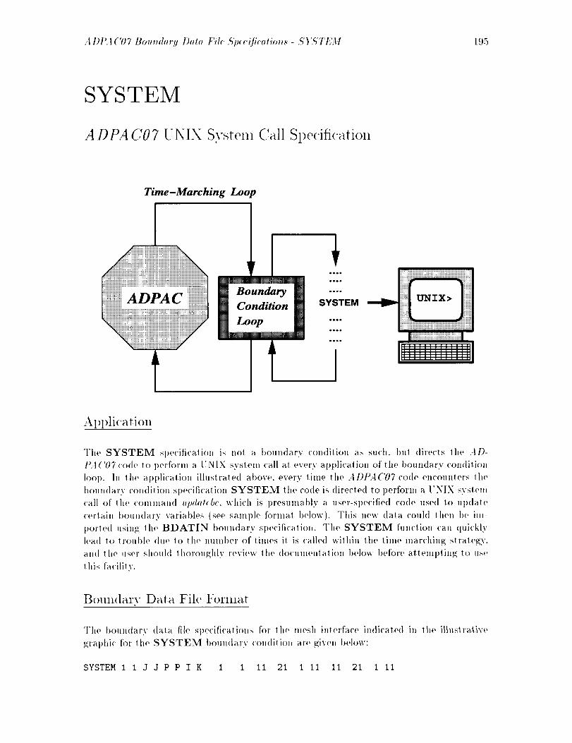
.t DP.4 ('07 Bou't_dat'.q Data File ,ffp_eiJicatiol_ - ,5')',_'TEM 19.5

SYSTEM

ADPA CO7 UNIX Systeln Call Specification

Time-Marching Loop

Boundary

Condition

Loop

oeo.

e*eo

eeee

SYSTEM

eeeo

eooe

ooee

iiiiiiiiiiiiiiiiiiiiiiiiiiiiiiiiiiii!!iiiiiiiiiiiiiiii

_ UNIX> I

AI)l)lication

The SYSTEM Sl)(,cili('ation is no! a boundary condition as such, but directs the AD-

1).4('07 code to perform a ['NIX svstem call a.t every apl)licatioll of the boundary condition

h)op. In lh(, al)l)lication illustrated above, every tim(, the ADPA('07 code encounters the

boun(larv ¢'ondi!ion Sl)Ocification SYSTEM tho code is directed to perform a UNIX svslem

call (>f th(, c<)mman(I _lpdat(bc, which is t)resumably a user-specified code used to update

certain boundary variables (see sample fornlat below). This new data could then be im-

t)ort(,(l using th( _ BDATIN boundary specification. Th(, SYSTEM function can (luickly

h,a.(I 1o lroul)h, (lug' to the number of times it is called within the time-lnarching strategy.

and th(' us(,r should lhoroughly review th(" documentaliozl 1)(,low t)efol'(, attelnl)lillg lo us('

this fa('ilit v.

Boull(larv Data File Format

The boundary (lata ill(, specifications for th0 mesh intorfac0 indica'fed in lho illnslra_i\'_,

_;ral)hic tbz' the SYSTEM I)oundarv condition aro giV('ll t)(qow:

SYSTEM 1 i J J P P I K 1 I II 21 1 ii II 21 I ii

196 S Y,5' TEM - A DPA C07 Boundary Data Fih Sp_cifica tions

INTERVAL

1

COMMAND

/usr/local/bin/updateb¢

Note that a COml)lete SYSTEM specification requires the specification of additional data

beyond tile standard boundary specification lille.

Description

Tile SYSTEM statement is provided to permit the specification of a UNIX system call

from within the AD1)A('07 code. Once the SYSTEM st)ecification is directed into the

ADPA('07 code, at a specified interval of iterations, during every execution of the bound-

arv condition loop, when the SYSTEM specification is encountered, the code executes

the command provided by the SYSTEM specification and pending successful completion,

continues execution. The SYSTEM specification is based on the FORTRAN intrinsic sy._-

tern function which must be available in the compiling system. I! should be noted that

the command dictated l>y the SYSTEM specification could be performed every time the

boundary condition loop is encountered. This suggests that the system call could be made

a minimum of four times for each iteration of the time-lnarching scheme (for the four stage

scheme). This number can grow rapidly if more complicated ileration strategies are used

such as multigrid, subiterations, etc., and the user shouhl be warned ihat such redundant

system calls can wreak havoc on an otherwise friendly solution. A SYSTEM specification.

in conjunction with the BDATIN/BDATOU boundar.v dala specifiers can be effectively

combined to provide a run lime inlerface between the ADPA('OTcode and an external flow

solver.

A SYSTEM specification requires four additional lines in addition to the normal bound-

ary data file descriptor, as shown above. The first additional line simply contains the label

for the iteration interval INTERVAL, tbllowed by the actual value of INTERVAL. The

SYSTEM routine will only be invoked every INTERVAL time-marching iterations. The

next line contains the label for the system call command (COMMAND) variable. The fol-

lowing line contains the actual UNIX comnlan<l to he issued at every SYSTEM encounter

in the boundary condition loop.

Restrictions/Limitations

Data provided in the SYSTEM specificatioll shouhl represen! a valid UNIX system com-

mand. The FORTRAN intrinsic function ._yst_m must 1)e availabh, on the coml)iling system.

The SYSTEM fimct, ion is not available on the ('ray or n('I'BE COml)Utel's.

COIIIIIIOll Errors

• Invalid UNIX system conmland 1)rovided in SYSTEM boundary sl)ecification.

A DPA('07 Bo_mdarg Data Fil_ ,5'pec([icatiol_s - ,S');S'TE-1I 197

• t:ailure lo t)rovid(, i he additional data INTERVAL and COMMAND tor SYSTEM

specification.

• FOllTII:\N intrinsic function system unavailable at compile time.

• User unaware thai SYSTEM action occurs [bur or more limes [)er iteration.

• :\tlempl io use the SYSTEM specificaiion on a ('ray, n('I'BF, or other incompatible

('()111 ]Ill i ('1' SVM ('111.

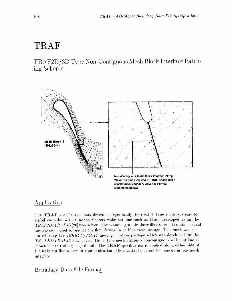
198 TRA F - A DPA C07 Boundary Dat. Fil_ .5'p¢'cificatio_._

TRAF

Tt_AF2D/3D Type Non-Contiguous Mesh Block Interfa('e Patch-ing S(,henle

Mesh Block #1

(I 93x25x1 )

F....................Y-C

Non-Contiguous Mesh Block Interface Along

Wake Cut Line Requires a TRAF Specification

(illustrated in Boundary Data File Format

statements below)

Application

The TRAF specification was developed specifically lo treat C-type mesh systems for

airfoil cascades with a noncontiguous wake cut line such as those developed using the

TRAI"2D/I'RAF3D [20] flow solver. The example graphic above illustrates a two-dimensional

mesh system used to predict the flow through a turbine vane passage. This mesh was gen-

era,ted using the JEI:IRI('/TOM(' mesh generation package which was developed for the

TRAF2D/TftAF3D flow solver. The ('-type mesh utilizes a nonconliguous wake cul line as

shown in lhe trailing edge detail. The TRAF specification is applied along either side of

the wake cut line to permit comlnunicatioll of flow variables across the noncontiguous mesh

interface.

Boundary Data File Format

A DPA (7)7 Bo.ndm'y Data File ,_)uetfieatio_._ - TRA F 199

The boundary data file sl>ecifications for the mesh interface indicate([ in the illuslralivo

_raI>hic for the TRAF boundary condition are giveH below:

TRAF 1 1 J J P P L L 1 1 1 33 1 2 177 193 1 2

TRAF 1 1 J J P P L L 1 1 177 193 1 2 1 33 1 2

.Nole tha! a coml)lete TRAF sl>ecifi('alion _;enerally requires lwo TRAF slalement lines in

lhe t><)un(larv data file. In lhe example above, the tirst sl)ecifi<'atiou l)rovi<tes the iulerl)lo<'k

('omIHuni('alioll for one side of (he ('-_rid wake cut, while lhe second sl)ecificalioH provides

lhe ('Olnmunicalion for the other si<le (>f' the (!-gri<l wake <'ul. I1 is a ('ommoli error to

tHl<lersl)ecify a TRAF l)oulldarv t)5' only ])rovi(lin_ a sin?;le line l>er inlerfa('e.

Des('riI)tion

The TRAF boundary slalemenl l)r<)vi<les a mea_ls for block 1o 1)lock commlllli('alion for

cases inv<)lvill_; Heighborin_ mesh I)oull(laries which share a <'omm(>ll surface, but are _l(m

('onti_uous in erie grid index. The slan(lard example of this tyi)e of mesh is a (!-[yl)e

mesh al)oul an aiv['oil where 1he ]>oin[s alon_ the (l-_;ri(l wake <'ul line are _(>_woHliguons.

This type of lll(,sh system has l)ee]l ulilize<l ex[ensivel.v in the I'IL4I"2I)/TI?.-t]"31) [20]

flow solver syslem, and lhe TRAF boul_dary sl>ecificatioH has been [)r<>vide(I Io l)ermil

A l)l>.l('OTexecution <)n lhese meshes. The implied restrictioll of the TRAF b<>un(larv

sl)e<'iti<'ali<)ll i_ thal lhe mesh is only misaligne<l ill one ('<)or<liuale dire<'lioll, sl>e('ifically lhe

i <'<><)i'(liIlat('. 11 i_ also assumed tha! lhe eudl)oints of lhe TRAF boundary s])e('iticalioll

are collliguous. As such. lhe TRAF boutldarv si)ecificatiol_ is fairly re.slriclive, and should

nol be used as a _(,_eral i)_rt)ose misali?_;_wd mesh rouline. (The BCINT1, BCINTM

and PINT boun<larv Sl)ecifi('atio_s are available for connecling generalized misaligued mesh

t>oul_<tari(',_.) An example of a_ al)pro[)riale al>l)licalion of l he TRAF s])e<'ifi<'alion is given

il_ lhe illu.slralive _ral)hi<'. The TRAF boundary specification is valid for eilher 2-I) or 3-1)

mesh t>locks. For :2-1) mesh I)lo('ks, lhe TRAF sl)ecificalion m,._/be al)l)lied lo a j=<'onslanl

bOUl_<larv. For 3-I) mesh blocks, the TRAF sl)ecifi('aliol_ mu._[ t>e at)l)lie<l to a ],'=('onsla_l

bOUl_<larv. The TRAF bouu<larv condilion requires no additional (lala beyond lhe iHilial

sl>e<'ificalio_ line, t)ul does require some extra care when used. The primary t)re<'auliol_

is lhal lhe TRAF t)roce(hH'e is based et_tirelv on a siml)lilie(I cubic sl)line intert>olali(>_

s<'hetne, at_<l hence, does nol maiHlain eilher global or local conservation of flow variablesacross lhe mesh ilV_erface.

R est l"i<'t ions/Limitations

The TRAF 1)oun(larv sl)e<'ilicatioz_ is restricted 1<>mesh interfaces wtfich lie on a com]zlolz

surface (_o si_;niti('anl overlal)). The TRAF l)r<)cedure I)ermits only tha! lhe i <'oor(li_ales

1)elween a<ljace_t mesh surfaces are misalig_,ed. The TRAF l)rocedure is only valid if lhe

misalig_wd i <'oor(li_ates either i_wrease or decrease in the :_' dire(lion mono_onicall\'. The

endi>oinls of lhe TRAF sl)e<'ifi<'aliol_ surface musl t>e contiguous. The TRAF sl)e<'iiicalio_

may only l)e ai>l)lie(I to j=col_stanl surfaces for 2-I) mesh blocks, a_<I L'=('otlslanl surfa('e.sf<>v3-I) mesh blocks.

200 TRA F - A DPA ('07 Boundary Data File' Spe'cification._

CollllllOll Errors

• Failure to provide 2 TRAF stalements for each interface.

• Incorrectly specified or misaligned extents of boundary regions (values of M1LIM1,

MILIM2, NILIM1, NILIM2, M2LIM1, M2LIM2, N2LIM1, N2LIM2 do no1

correctly define the interface extents on blocks LBLOCK1 and LBLOCK2).

• Attempt to use TRAF for a boundary which has 2 misaligned coordinales.

• A_temt)t to use TRAF for boundaries which are no! monotonic in the x direction.

• Application of TRAF _o mesh in_erfaces which do no1 have contiguous end l)oinls.

• Apl)lication of TRAF to an /=constant or/,'=constanl mesh surface in a 2-I) block.

• Apt)licalion of TRAF 1o at, /=constant or j=constan/ mesh surface il, a 3-I) I)lock.

.4DPA C07 Me._h Fih Descriptiol_ 20 t

3.8 Mesh File Description

The ADI>A('07 ('rise.mesh file is a data file containing tile x,y,z grid coordinales of the

mullil)le mesh blocks which are read in i<) define the l)hysical gri(1 points used in ill(' tinle-

marching solution (see Seclion 3.5 for a <tescrii)tion of the <,as( name and the mesh tile

naming convention). The mesh coordinates are sl)ecifie(l in a (_arlesian fi'ame of reference.

as shown in t:igure 3.11. although the +101).4('07 l)rogranl may ul!imalelv ('<>nverl lhese

coor(linales lo a cylindrical coordinate system during execution, l/egar<lless of whe! her the

user inlends t<) u lilize lhe A 1)PA ('07 code in a (lart('simL or <'ylindri<'M solulion mode. the

mesh tile c<)or(linate,s are ahroy._ defined I)y the ('artesian coordinates .r.y. and z. The

mesh <'o<)r<tinates are stored in what is known as I>LOT?,D multil)le grid formal, and are

forlnatte([ usinp_g 111(, Scientific Database Library (SDBLIB). (The SI)BI:II{ svslem allows

ma<'hine-in(lel)endenl binary file storage.) The cas_.mesh file must be availal)le for ew, rv

A DI)A ('07 run. At the beginning of l)rOgl'am execution, 111(, .;I l)l>.t ('07 l)rogram attem[>l s

to ol)en the mesh file and rea(l in the mesh size to make sure that en<>ugll memory has been

allocated for the given problem. If the mesh file is not found, or if the mesh is too large,

Ill(' al)pr<)l)riale error message is issued, an<l 111e program will ternlinate.

Mesh coordinales are assumed to 1)e nondimensional numbers. The :tl)l>,l('07('<)de

eml)loys a dimensional s<'aling factor (see input file varial)le DIAM) 1o converl the non<li-

mensional mesh coordinales into dimensional coordinates with units of feel. If ll,e mesh

is generaled with units of feet, then the dimensionalizing f'a<'lor in simply 1.0. ])rol)er

no,<limensionalization and specification of the dimensionalizing lacier DIAM is required

in or<let to accurately achieve lhe desire<l flow Reynolds nulnber and relational speed (see

the discussion of inl)ut variable ADVR is Section 3.6). It is also required lhat the ordering

<)f the mesh points form a "left-handed" mesh. This iml)lies that at every l)oinl in the mesh,

tile vectors representing the positive i, j, and 1,"coor<linate directions form a left-handed

coordinate syslem (see t:igure 3.12). Collsi(ler the case of a sheared l[-gri(I <liscretizing a

single blade passage of a compressor (this type of mesh in used extensively in the Slandard

('onIi_,gurations (lescribe(I i, ('hal)ler 5). If we assume thai looking <townslream through

the blade passage is essentially the positive i direction, and that the radial (lirection from

hub to tip is essentially lhe positive j <tirection, a left-handed lnesh would require that the

positive /," direction be froln right t<)left (counterclockwise) in this orientation.

In order to understand lhe PLOT3D multii)le-grid mesh file format, and the utilization

of the ,S'DBLIB routines, a comparison of the FORTRAN coding for each method is given

below for cOral)arisen.

The F()t(Tt(AN coding to tea(1 a PLOT3D unformatted lnultiple-block mesh tile migh!

I)e given as:

PLOT3D Mesh File Format FORTRAN Coding Example

0PEN(UNIT=IGRID,FILE=FNAME,FORM='UNFORMATTED',STATUS='0LD')

READ(IGRID) MG

READ(IGRID) (IL(L), Jt(t), KL(L),L=I,MG)

DO i0 L = i, MG

READ(IGRID) (((X(I,J,K,L),I=I,IL(L)),J=I,JL(L)),K=I,KL(L)),

(((Y(I,J,K,L),I=I,IL(L)),J=I,JL(L)),K=I,KL(L)),

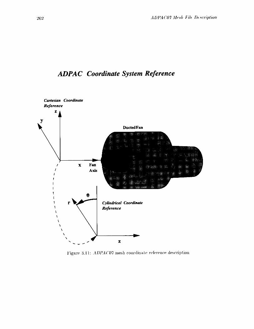
202 .4 DPA C07 Mesh File D_scription

ADPAC Coordinate System Reference

Cartesian Coordinate

Reference

Z

YDuctedFan

/ x Fan

rt/ Axis

0

\\

\

Cylindrical Coordinate

Reference

v

Figure 3.11 : A 1)PA ('07 nlesh coordinate reference des('ript ion

A DI_4('07 M<._h File D_s<'ription 203

ADPAC Left-Handed Coordinate Description

All ADPAC Mesh Blocks Must Be

Based on a Left-Handed Indexing System

Left-Handed Mesh S,

f

f

I"_ f

k

'stem

J

II

I

I

I

f

I

J

J

f t

t I

J

Right-Handed Mesh System

J

k

f

II

I7

ff

fI

f

f •

J

fI

ff

fI

fJ

f

J

f

I

I

f

Figure 3.12: A 1)t_:t ('07 left-handed co<)r<tillal e _v_t em descril)t ion

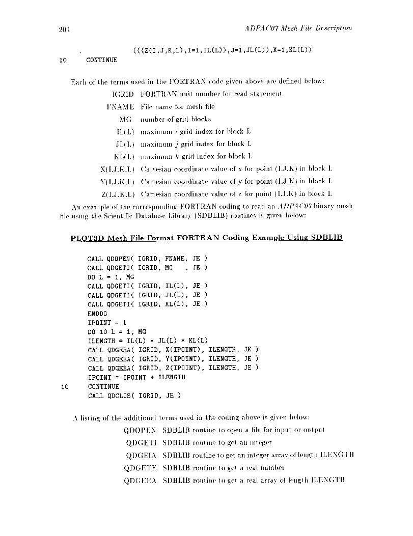
204 A DPA('07 Mesh File Description

l0 CONTINUE

(((Z(I,J,K,L),I=i,IL(L)),J=I,JL(L)),K=I,KL(L))

Each of the terms used ill the FORTRAN code given above are defined t)elow:

FORTRAN unit number for read statemen!

File name for mesh file

uunlber of grid blocks

IGRID

FNAME

M(;

IL(L)

JL(L)

KL(L)

X( I,.I.K,L )

Y ( I,J ,I{,L )

Z(I.,I,K,L)

llla,xinluln

nla,xilnuni

lllaxilllUm

Cartesian

Cartesian

(!artesian

i grid index for block L

j grid index for block L

k grid index for block L

coordinate value of x fox' poinl (I,.1,K) in block L

coordinate value of y for poinl (I.,I,K) in block L

coordinate value of z for poinl (1,J.K) in block L

An example of the corresponding FORTRAN coding to read an A I)PA('071)inary mesh

file using the Scientific Database Library (SI)BLIB) routines is given below:

PLOT3D Mesh File Format FORTRAN Coding Example Using SDBLIB

10

CALL

CALL

DO L

CALL

CALL

QDOPEN( IGRID, FNAME, JE )

QDGETI( IGRID, MG , JE )

= I, MG

QDGETI( IGRID, IL(L), JE )

QDGETI( IGRID, JL(L), JE )

CALL QDGETI( IGRID, KL(L), JE )

ENDDO

IPOINT = 1

DO IO L = i, MG

ILENGTH = In(L) * JL(L) * KL(L)

CALL QDGEEA( IGRID, X(IPOINT), ILENGTH, JE )

CALL QDGEEA( IGRID, Y(IPOINT), ILENGTH, JE )

CALL QDGEEA( IGRID, Z(IPOINT), ILENGTH, JE )

IPOINT = IPOINT + ILENGTH

CONTINUE

CALL QDCLOS( IGRID, JE )

A listing of the additional

QDOPEN

QDGET1

QDGEIA

QDGETE

QDGEEA

terms used in the coding above is given t)elow:

SDBLIB routine to open a file for iul)ul or outpul

SDBLIB routine t,o get a,n inleger

SDBLIB routine 1o get, an iuleger array of length ILEN(;Tlt

SI)BLIB routine to get a real number

SDBLIB routine to get a real array of lenglh ILFNGTll

,4 DPA('07 Body Fore'< File Descriptio_ 205

QI)('LOS

IGRII)

JE

IB

II.t'NGTll

IPOINT

SI)BI, IB routine to close a file

F()I{TI{AN logical unit numt)er for grid input

An error trigger; 0 for no error. ¢ 0 if an error occurs

Integer array containing the IL..IL, and KL g;rid block sizes

Integer length of an array of dala

Integer pointer for block L 1o locate the initial memory lo-

calion for a block of data

The a'.9. z coordinales are read in as a single-dimensioned array in lhe £'l)l]l, lt] for-

real. and lhe _1I)1>=1('07 program inclu<les a conversion rom ine (source tile :'ol_ca._.f) which

converts the single dimension array dale to a lhree-dimensional dala array.

The mesh tile may be utilized direcllv with the PLOI',II) l)rogram when lhe defaull

real number size of the COml)ile<l PLOT:ID code is defined as :12 t>ils (as it is on nlanv

workstations). The corresl)onding PLO Tgl) read comman(l h)r an +l DI>A ('07 mesh file are:

PLOT3D PROMPT> read/mg/bin/x=case.mesh

Obviously, lhe user should sul)stitule his/her own case name in lhe l)LOl'31) inpul line.

Unformalted mesh tiles may be convened 1o A DPA('07 formal using the 3IAhEAI)-

(/RID program described in ('hapter 7. I1 should be emphasize<l the! the t)hantom cells

use<l in lhe alJplication of boundary conditions are aulomalically defined within the AD-

I)A('07 code. and the user need not be c<mcerlwd about generating fictilious points within

the mesh to accommodale the boundary con<litiotl appli<'ation procedure (mesh points need

only be generated for the aciual flow domain).

3.9 Body Force File Description

The .4 DP, t C07 bo(tv force file is a dala file containing the blade blockage, bod.v force, and

energy source terms used in a 2-I) a xiswmnetric representation of an embedded blade row

(see 2-I)/3-I) Solulion (!oncel>ts, Seclion 2.:1). IlMividual body force files contain the cell-

celllere<l bla<le blockage, body forces, and energy source terms for a specific mesh block. As

a result, lhe file naming procedure for lhe body force file is somewhat different than the

mesh. plol an<l reslart files, where a single file contains all the data for a multiple-block

solution (a complele descriplion of the ADPA('07 file naming l)ro<'edure is given ill Seclion

3.5).

The terms in lhe body force file at'(' store<t in binary formal, based on the Scientific

I)atabase Library routines, (The SI)BLIB system permits machine-indet)endellt binary

file storage.) The blockage, body forces, and energy sources are stored as nondimensional

numbers using lhe nondimensionalization strategy described in the Final Report [21].

In order 1o undersland lhe l>o<lv force file fornlal, and lhe ulilizalion of the ,5'DBLItJ

rouliIles, a represelllaliv0 FOllTIIAN co<ling; examl)h' lo read in a body force file is given

t>elow [br comparison.

206 A Dt'AC07 Body Force Fih: D_scription

Body Force File Format FORTRAN Coding Example Using SDBLIB

CALL 0DOPEN( IBODY, FNAME, JE )

CALL QDGETI( IBODY, NG , ILENGTH, JE )

CALL 0DGETI( IBODY, IMX, ILENGTH, JE )

CALL QDGETI( IBODY, JMX, ILENGTH, JE )

CALL 0DGETI( IBODY, KMX, ILENGTH, JE )

ILENGTH = IMX * JMX

CALL 0DGETE( IBODY,

* KMX

DUMMY, JE )

CALL QDGETE( IBODY, DUMMY, JE )

CALL 0DGETE( IBODY, DUMMY, JE )

CALL 0DGETE( IBODY, DUMMY, JE )

CALL QDGEEA( IBODY, BFR (IPOINT(L))

CALL QDGEEA( IBODY, BFRU (IPOINT(L))

CALL QDGEEA( IBODY, BFRV (IPOINT(L))

CALL QDGEEA( IBODY, BFRW (IPOINT(L))

CALL QDGEEA( IBODY, BFRE (IP01NT(L))

CALL QDGEEA( IBODY, BL (IPOINT(L))

CALL 0DGEEA( IBODY, BP (IPOINT(L))

CALL QDCLOS( IBODY, JE )

ILENGTH

ILENGTH

ILENGTH

ILENGTH

ILENGTH

ILENGTH

ILENGTH

JE )

JE )

JE )

3E )

JE )

JE )

JE )

A listing of the FORTRAN

QDOPEN

QDGETI

QI)GETE

QDGEEA

QD(:LOS

IBODY

dE

NG

IMX

JMX

KMX

ILENGTH

IPOINT(L)

BFR

BFRU

BFRV

B F RW

BFRE

variables and their meanings is given below:

SDBLIB routine to open a file for input or outpul

SDBLIB routine Io get an integer

SDBLIB routine 1o get a real number

SI)BLIB routine to gel a real array of length ILEN(;TH

SI)BLIB routine io close a file

FORTRAN logical unit number for body force file input

An error trigger: 0 for no error, # 0 if an error occurs

Number of blocks in body force file (must be 1)

Mesh size+l in the i coordinate direclion

Mesh size+l in the j coordinate direclion

Mesh size+ 1 in the k coordinate direction

Integer length of an array of dala

Integer pointer for block L to locate the inilial memory lo-

cation for a block of data

Body force for density (continuily equation)

Body force for axial momenlum

Body force for radial momentum

Body force for circnmferenlial momenlum

Body force for internal energy

A Df_4 ('07 Output Fil< Dr,_cHpliol_ 207

BL Blockage tern,

BP Pressure correction ternl (currently unused)

The body force dala are read and written as a single-dinwnsioned array in lhe SDBLIB

formal, and lhe A Dt)A('07 program includes a conversion routine (source tilt, co,_vrts.f)

whi<'h converls tilt, one-dimellsional array data 1o lhree dimension array data.

3.10 Standard Output File Description

The .tl)PA ('07 slan<lard oult>ul file cas<.output l)rovides inforlnation regarding the slalus

of a l)arli('ular calculali(m during code exe('lltion. The status information includes slal'! ill),

<'ode resl)onse l<)inpu! files (mesh, reslart, standard input, an([ boundary dala), convergence

hislory, error messages, and Oll|[)llt file generation ([)lol files, reslarl files, l>odv fov<'e files).

The in format ion gjv(,n in ill(' sl andard oHl put file is essentially self explanalory, s<) no ftlrl hey

description is given here..\ sample OUll)Ut file is include(1 ill lhe slandard dislribulion of

the .tDP. I('07 code for Ill(' lest case descril)ed i. Apl)endix A. A<ldilional (lelails may be

found in this Al)l)endix.

3.11 Plot File Description

The ..t I)1).4 ('07 r'a._r.p3dabs and <.asr.p3drel plot tiles <'onlahl predi('ted a l)sohlle and rel-

alive t'ralne of reference flow <lala values, rest)eclively, for each of tile mesh points ill a

mull il)le-I>lo('k mesh ADf>A('07 solulion. The grid-cenlered aerodynamic data is oblained

1)y algel)rai<'ally averaging lhe cell-('enlered <tara generated by Ill(' filfile-volume solver during

the lilne-marching; process. As a result of lhe averaging I)roce<lure. this data can occasion-

ally appear inconsislent al lhe corners of a mesh block, and should lherefore only be used

for gral)hi<'al viewing, and nol for p<)sl processing to <)blain performance (tala, mass tlow

tales, pressure rise. el('. Tl,e flow [)lol dala are specitied in a (:artesian coordinale sys-

tem (velocilies are v.,., vv. c: ) lo I)e <'onsislenl wilh the represenlalion of lhe mesh file (see

Seclion 3.s). The plol files ave wrillen in whal is known as PLOT3D multiple grid binary

formal. The t)1o! data are forma!!ed using lhe Scientific I)alal)ase Library (SDBLIB). (The

SI)BLIB syslem 1)ermils machine-indel)el_denl binary file storage.) The flow data are lisle([

as non(limensional numbers using lhe nondinmnsionalization slrategy described in lhe Final

llel)or! [21].

In order 1o understand the PLOT3D multiple-grid ttow file fornlal, and lhe ulilizalion

of lhe £'1)BI, I1_ roulines, a conlparison of lhe FORTRAN coding for each melhod is given

below ['or comparison.

The e<luivalenl I:ORTI{AN coding for an unformatled PLOT:H) flow file could l>e given

as:

PLOTaD Flow File Format FORTRAN Coding Example

WRITE( ) MG

WRITE( ) (IL(L), JL(L), KL(L),L=I,MG)

DO 20 L = 1, MG

20_ ADPAC07 Plot File De.seription

20

WRITE( ) EM(L), REY(L), ALF(L), TIME(L)

WRITE( ) (((R (I,J,K,L),I=I,IL(L)),J=I,JL(L)),K=I,KL(L)),

(((RU(I,J,K,L),I=I,IL(L)),J=I,JL(L)),K=I,KL(L)),

(((RV(I,J,K,L),I=I,IL(L)),J=I,JL(L)),K=I,KL(L)),

(((RW(I,J,K,L),I=I,IL(L)),J=I,JL(L)),K=I,KL(L)),

(((RE(I,J,K,L),I=I,IL(L)),J=I,JL(L)),K=I,KL(L))

CONTINUE

Each of the terms used ill the FORTRAN code given abow, are defined below:

MG

IL(L)

,1L(L)

1,2L(L)

X(I,.I,K,L)

Y(I,.I,K,I_)

Z( I,.1.K,L )

EM( L )

R EY( L )

ALF(L)

TIME( L )

R ( I..I ,K.L )

RU(I,.I,K,L)

RV(I,.I,K,L)

RW(I,.I,K,L)

R E(I,J.K.L)

number of grid blocks

maximum i grid index for block L

maximum j grid index for block L

maximum /c grid index for block L

Cartesian coordinate value of x tot point (l,J,l{) in block L

Cartesian coordinate value of y for point (I,J.K) in block L

Cartesian coordinate value of z tot poin! (I,.1.K) in block L

PLOT3D Reference Mach number for block L

PLOT3D Reference Reynolds llun|ber for block L

PLOT3D Reference angle for block L

PLOT3D Reference lime for block L

p at, point, (I,J,K) in block L

pu_, a,t poinl (I.J,K) in block L

puy al l)Oinl (I,.1,K)in block L

pu: at point (I,J,K) in block L

p_ at point (I,.I.K)in block L

PLOT3D Flow File Format FORTRAN Coding Example Using SDBLIB

CALL QDOPEN( IFLOW, FNAME, JE )

CALL QDPUTI( IFLOW, MG , JE )

DO L = I, MG

CALL QDPUTI( IFLOW, IL(L), JE )

CALL QDPUTI( IFLOW, JL(L), JE )

CALL QDPUTI( IFLOW, KL(L), JE )

ENDDO

IPOINT = 1

DO 20 L = I, MG

ILENGTH = IL(L) * JL(L) * KL(L)

CALL QDPUTE( IFLOW, EM(L) , JE )

CALL QDPUTE( IFLOW, REY(L) , JE )

CALL QDPUTE( IFLOW, ALF(L) , JE )

A DPA ('¢)7 R_._tart File D_scription 209

2O

CALL QDPUTE( IFLOW, TIME(L), JE )

CALL QDPUEA( IFLOW, R (IP01NT), ILENGTH, JE )

CALL 0DPUEA( IFLOW, RU(IPOINT), ILENGTH, JE )

CALL QDPUEA( IFLOW, RV(IPOINT), ILENGTH, JE )

CALL QDPUEA( IFLOW, RW(IPOINT), ILENGTH, JE )

CALL QDPUEA( IFLOW, RE(IPOINT), ILENGTH, JE )

IPOINT = IPOINT + ILENGTH

C0NTINUE

CALL QDCLOS( IFLOW, JE )

,\ listing of the a<ldilional terms used in tile coding above ix given below:

QI)OI)t';N

QI)I)UTI

QI)I'UTI';

QI)I)UEA

Ql)( 'LOS

IFI:OW

.l E

IB

ILEN(;Ttt

IPOINT

SI)BI,II_ rouline to open a file for inl)Ul or output

SI)I)LIB rouline 1o wrile an integer

SI)BLII) rouline to write a real number

SI)BLIB routine 1o write a real array of [ength II, EN(VI'II

SI)BIAI) rouline Io <'los(, a file

FORTRAN logical uni) number for flow inpu)

:\),error (rigger: 0 for ))o error, # 0 if an error occurs

Inleger array containing the IL. ,Jl,. and KL grid block sizes

Inleger len_lh of an array of (la)a

hgeger l)oinler for block L to locale lhe inilial menlory Io-

ta lion for a block of data

The t)lo( files may t)e u(ilized direclly wilh the PLOF3D program when the <lefaull

real number size of the compiled t'L01'31) code ix defined as 32 I)ils (as i( is Oll many

workslalions). The co)'rest>on<lillg PLOI"3D read commands for an ,,I DI>A ('07 mesh and

flow file are:

PLOT3D PROMPT> read/mg/bin/x=case.mesh/q=case.p3dabs

Obviously. lhe user shoul<t sul)stilute his/her own ease name in the PLOT2D input line.

For sohllions elnl)h)ying the lwo-e(lllal foil k-_ turt>ulence model, an a ddilional PLOT31)-

compalible file is written for plolt[ng (he turbulence parameter data. The c<l.+e.p3d2eq file

is identical in formal to lhal given above excel)! Ilia! the variables RU and RV are replaced

wil]l tit(' l llrt>ulence l)aramelers pk an<[ p_, respectively. The user musl be ('auliolmd Io

avoid usinK this file in conjunclion with PLO'[',3D functions which require sl)ecifica)ion of

all )he velocilv ('Om l)onen(s (pressure and temperature are two examples).

3.12 Restart File Description

The A DI>A('07 )'eslar) file ix a (lala file conlaining the cell-centered ttow varial)les gelleraled

during an A l)l<4('OTsolulion. This ill(' is inlended 1<>permit conlinue(1 exe<'ulion oflhe

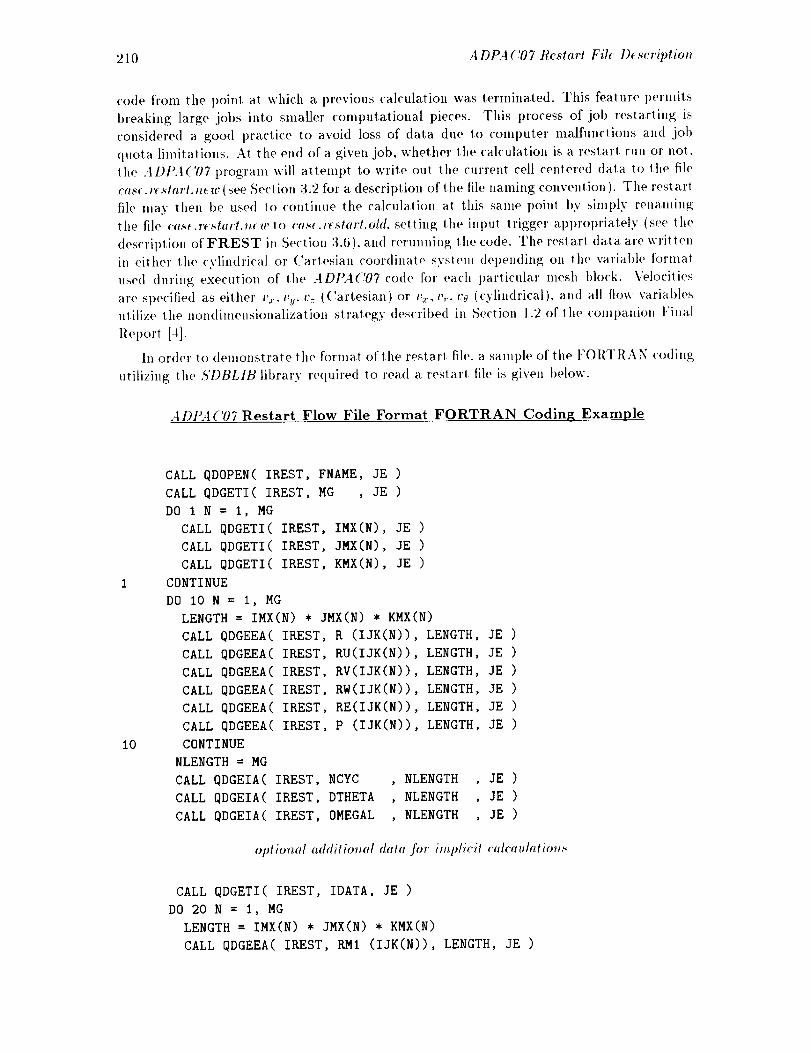
210 ADPAC07 Restart Fih Description

code from the point at which a previous calculation was terminated. This feature permils

I)reaking large jobs into smaller computational pieces. This process of job restarting is

considered a good practice to avoid loss of data due to ('omputer malfunctions and job

quota limitations. AI the end of a given job, whether the calculation is a restarl run or nol.

lhe ADPA('07 I)rogram will attempt to write out the current cell centered data 1o lhe file

ca._(. 1, start, new ( see Secl ion 3.2 for a description of the tile naming convention ). The reslarl

file may then be use<t to continue the calculation at this same point by simply rellalning

the file <'ase.r_slart._rw lo <'as_.restorl.old. setting the input lrigger al)tn'opriately (see lhe

description of FREST in Section 3.6), and rerunning the code. The restaN data are wrilten

in either the cylindrical or Cartesian coordinate svsteln depending on lhe variable fornla!

used during execution of lhe ADPA('07 code for each t)arlicular mesh block. Velocilies

are specified as either _'_.. _'v" _': (Cartesian} or t,.,.. _,_. _'o (cylindrical), and all flow varial)les

utilize the nondimensionalization slralegy described in Section 1.2 of the companion Final

Report [-1].

In order to demonstrate the format of the restarl file, a sample of the FOIITRAN coding

utilizing the ,5'DBLIB library required 1o read a restarl file is given below.

ADtSI('07 Restart Flow File Format FORTRAN Coding Example

10

CALL QDOPEN( IREST, FNAME, JE )

CALL QDGETI( IREST, MG , JE )

D0 I N = I, MG

CALL QDGETI( IREST, IMX(N), JE )

CALL QDGETI( IREST, JMX(N), JE )

CALL QDGETI( IREST, KMX(N), JE )

CONTINUE

D0 i0 N = I, MG

LENGTH = IMX(N) * JMX(N) * KMX(N)

CALL QDGEEA( IREST, R (IJK(N))

CALL QDGEEA(

CALL QDGEEA(

CALL QDGEEA(

CALL QDGEEA(

CALL QDGEEA(

CONTINUE

NLENGTH = MG

CALL QDGEIA(

CALL QDGEIA(

CALL QDGEIA(

IREST, RU(IJK(N))

IREST, RV(IJK(N))

IREST, RW(IJK(N))

IREST, RE(IJK(N))

IREST, P (IJK(N))

LENGTH, JE )

LENGTH, JE )

LENGTH, JE )

LENGTH, JE )

LENGTH, JE )

LENGTH, JE )

IREST, NCYC , NLENGTH , JE )

IREST, DTHETA , NLENGTH , JE )

IREST, OMEGAL , NLENGTH , JE )

optional additional data ]br implicit calcaulation._

CALL QDGETI( IREST, IDATA, JE )

DO 20 N = I, MG

LENGTH = IMX(N) * JMX(N) * KMX(N)

CALL QDGEEA( IREST, RMI (IJK(N)), LENGTH, JE )

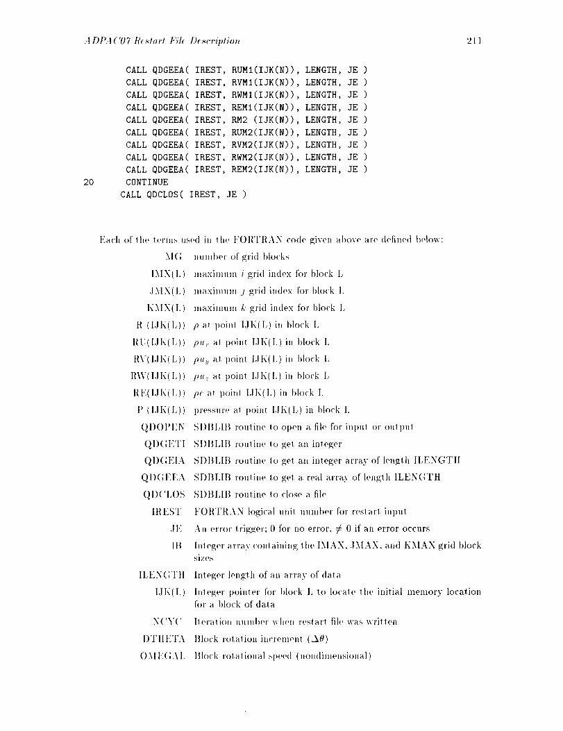
ADPA('07 tlcstart File D¢._cription 211

2O

CALL QDGEEA( IREST

CALL QDGEEA( IREST

CALL QDGEEA( IREST

CALL QDGEEA( IREST

CALL QDGEEA( IREST

CALL QDGEEA( IREST

CALL QDGEEA( IREST

CALL QDGEEA( IREST

CALL ODGEEA( IREST

CONTINUE

RUMI(IJK(N)), LENGTH

RVMI(IJK(N)), LENGTH

RWMI(IJK(N)), LENGTH

REHI(IJK(N)), LENGTH

RM2 (IJK(N)), LENGTH

RUM2(IJK(N)), LENGTH

RVM2(IJK(N)), LENGTH

RWM2(IJK(N)), LENGTH

REM2(IJK(N)), LENGTH

CALL QDCLOS( IREST, JE )

JE )

JE )

JE )

JE )

JE )

JE )

JE )

JE )

JE )

Each of ILL(' term>, used in the FORTRAN code given above are defined below:

XI(;

I.XIX(L)

.JMX(1,)

KMX(L)

R (I.JI<(I_))

RF( l.JK( L ))

RV(HI<(L))

RW(IJI<(1_))

1_l£(l.JI<(1_))

1' (I.JI{(L))

Q l)Ol ) EN

QD(',H'I

QD(;EIA

QI)GEEA

QI)(,I,OS

III I';ST

.l E

IB

ILEN(;TII

I.JI<( I,

N( 'Y(

I)TIlETA

()M E(;A L

number of grid blocks

maximum i gri<t index for block L

maximum j gri<t index for block 1,

maximum L' grM index for block I,

p at point I,JK(L) in block L

pu,. at l>oin(I.JK(L) in block L

pu_: at point I.IK(L)in block L

pu:+ al poin! l.JI£(I,)in I>lock L

p< a( l)oin! I.IK(L) in l)lock I=

pressure a! point I.II{(L) in block L

SI)BLIt) routine to ol)en a ill(, for input or output

SI)BIAB routine to gel an integer

SDBLIB routine to get an integer array of length ILENGTH

SDBLIB routine to get a real array of length ]LENGTH

SI)BI,IB routine 1o close a file

F()I(FIIAN logical unit ]nunber for restart inl)ut

An error (rigger: 0 for no error, ¢ 0 if an error occurs

h)teg<,r array <'onlaining (he IMAX, .JMAX. and KMAX grid )>lock

SiZ("S

Integer length of an array of data

InteKer pointer for block L to loca(e the initial lnemory location

for a. block of dala

I(era, tion numl>er when reslat+t fi]e was written

Block rotation incremenl (.50)

Block ro(ationa] sl>eed (noudimensiol)al)

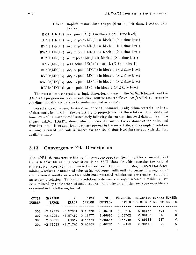
212 ADI_4C07 C'onverge_we File Descriptio_t

IDATA

RMI (I.IK(L))

RUMI(IJK(L))

RVMI(IJK(L))

RWM 1( IlK(L))

REMI(IJK(L))

RM2 (IJI((L))

RUM2(IJK(L))

RVM2( IJ K(L))

RWM2(IJK(L))

REM2(IJK(L))

Implicit restart data trigger (0-no implicit data, l-restart data

follows )

p at point IlK(L) in block L (N-1 time level)

ptt_. at point I.]K(L) in block L (N-1 time level)

pu.,_ at point IlK(L) in block L (N-1 time level)

pu: at point IlK(L) in block L (N-I time level)

p_ at point 1JK(L) in block L (N-1 time level)

p at poinl 1JK(L)in block L (N-2 time level)

p,_. at poin! I.]K(L) in block L (N-2 time level)

pu u at point IlK(L) in block L (N-2 time level)

pu: at point 1JK(L) in block L (N-2 time level)

pC at point IlK(L) in block L (N-2 time level)

The restar! data are read a,s a single-dimensioned array in the SDBLIB format, and the

ADPA('07 program includes a conversion routine (source tile <.o_v,s.f) which converls the

one-dimensional array data to three-dimensional array' data.

For solulion employing tile iterative implicit time-marching a,lgorilhm, several time levels

of data, must be stored in the restart, file to properly restarl the solulion. The additional

lime levels of data are stored immediately following the current time level data and a simple

trigger variable (IDATA. above) which informs tile code of tile existance of the additional

time level data. If no addilional data are present in the reslarl liD, and a,n implicil solution

is being restarted, the code initializes the additional time level data arrays with the best

available values.

3.13 Convergence File Description

The ADPA(!07 convergence history file case.converge (see Section 3.5 for a description of

the ADPA('07 file naming convention)is an ASCII data file which ('ontains the residual

convergence history of the time-marching solution. The residual history is useful for deter-

mining whether the numerical solution has converged sufficiently to l)ermit interrogation of

tile numerical results, or whelher additional restarled calculations are required to obtain

an accurate solution. Typically, a solution is deemed converged when the residuals have

been reduced bv three orders of magnitude or more. The data in lhe ease.converge tile are

organized in the following formal:

CYCLE MAXIMUM RMS MASS

NUMBER ERROR ERROR INFLOW

MASS PRESSURE ADIABATIC NUMBER NUMBER

OUTFLOW RATIO EFFICIENCY SS PTS SEPPTS

301 -2.17895 -5.52081 3.46778 3.46781 1.58615 0.88737 308 0

302 -2.42051 -5.57462 3.46777 3.46656 1.58762 0.89150 315 0

303 -2.65891 -5.64842 3.46774 3.46646 1.58949 0.89685 317 0

304 -2.78033 -5.71740 3.46765 3.46781 1.59123 0.90145 320 0

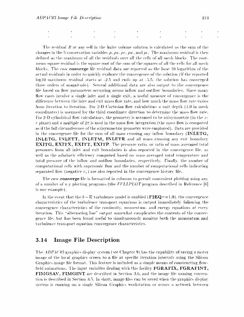
A DPA ('0 7 Imag< File D(._e riptio_ 213

The residual R at any cell in the finile vohmw solution is calculated as lhe sum of the

changes in the 5 conservali<m varial)les p, p,, pc, pu,, and p<. The maximum residual is then

deIined as the maximum of all the residuals over all the cells of all mesh blocks. The reel-

mean S<luare resi<tual is the S<luare roe! of tile sum of the S<luares of all the cells for all mesh

blocks. The <'a._t.converge file residual <lata are reported as lhe ])as<, 10 logarithm of the

actual resi<luals in order t<) quickly evaluate the convergence of the solution (if'the rel)orle<l

1o_;10 maximum residual starts at -2.5 and ends up at-5.5, the sohltion has converged

three orders of magnitude). Several additiol,al data are also OUll)U! to lhe conver_;en('e

file based on flow I)aramelers occurring across inflow and oulflow boun<laries. Sill<'<, nlauv

flow cases involve a six,gle inlet an<l a single exit. a useful measure of convergence is the

difference I)elween 1he inlet and exil mass flow tale, and how much lhe mass flow rate varies

fi'onl iteralion lot<era<ion. For 2-1) (larlesian ttow calculations a unit <leplh (l.0in mesh

COOl'<linales) is assumed for the third coor<linate direclion to (lelermine the mass flow rate.

For 2-I) cvlin<lrical tlow calculations, lhe geometr.v is assumed to I)e axisvmmetric (il, the .r-

r plane) and a multiple of 27r is used in the mass flow integration (the mass ttow is <'Omlmled

as if the full circumference of tile axisvmmetric geomel rv were employed ). [)ala are provided

in tile convergence ill<' for the sum of all mass crossing any inflow boundary (INLETG,

INLETG, INLETT, INLETM, INLETR and all mass crossing any exit bc>undary

EXITG, EXITX, EXlTT, EXITP. The pressure ratio, or ralio of mass-avera.ge<l tolal

pressures from all inM and exit boundaries is also rel)orled ill lhe convergence file. as

well as the adiabatic efficiency computed based on mass-averaged total temperalure and

total pressure of the inflow and outflow boundaries, respeclivelv. Finally. the number of

computational cells with supersonic flow and the number of computational <'ells indicating

separated flow (negative +,:,,)are also reported in the convergence history file.

The cas<.converge file is formatted in columns to permit convenienl plolling using any

of'a number of x-y plotting prod;rams (the FI:LI, I)LOT progranl <lescribed in l{eference [6]

is one examph,).

In the event that the k-'_ turbulence lnodel is enabled (F2EQ== 1.0). the convergence

characteristics of the turl)ulence lransport equations in outt>u! immediately following the

convergence characteristics of tilt, <'ontinuity, molnenlum, and energy e<luations at every

iteration. This "'alternating lille" outl)ut somewhal <'omplicates the conlents of the conver-

gence file. but has been foun<] useful to simultaneously monitor I>oth the momenlum and

turlmlence transport e<lua.tion convergence characleristi<'s.

3.14 Image File Description

The A Dt>A (717 graphi<'s disl)lay svslem (nee ('hapter 9) has the capal>ility of saving a ra.ster

image of lilt' local graphics screen t<) a file al sl)ecific iteration intervals using the Sili<'on

Gral>hics image file format. This feature is inchtded an a simple means of constructing flow-

field ani[naliolts. The in[)l[! variables dealing wit ]1 Ibis facility FGRAFIX, FGRAFINT,

FIMGSAV, FIMGINT aFe (lescril)e<l in Section 3.6, and Ill(, image file naming conven-

lion is descril)e(I in Seclion 3.5. In short, image files can I)e saved when lhe graphics display

svslelll in I'llllllillg Oil a single Silicon Gral)hics workstation or a('ross a network 1)elween

214 Runnin9 A DPA (.'07 2-Equation Turbulence Model

two Silicon Graphics workstations supporting tile IRIX Operating System Version 4.0.1 or

above, and also suplmrting the IRIX set.save command. Image files can be viewed after

they have been saved by issuing the commaud

ipaste ca._e.img. #

Other Silicon Graphics IRIX Operating System-specific COlnmands such as imgri_w, movit

and others ilia)' also be suital)h, tbr viewing image files. Additional intbrmation on the IRIS

image format and the image manipulation commands are availabh' in the Silicon Graphics

system documentation.

3.15 Running ADPACO7With 2-Equation Turbulence Model

3.16 2-Equation Turbulence Model Solution Sequence

Ill order to run A DPA ('07 with the two-equation t'-_v turl)ulence model enabled, the follow-

ing steps must be taken. ]First. the int)ut file trigger F2EQ must t)e enabled ( value= l .0 ).

This activates the additional partial differential equation solution scheme for the t' - _v

lnodel. Note that this coml)letely disables the standard algebraic (Baldwin-Lomax) tur-

bulence model and tlle wall flmction fornmlation. The lack of wall flmctions trot)lies that

the mesh mu,_t be sufficiently refined to adequately resolve the inner (laminar sublayer)

of the turbulent boundary layer flow. There is, at present, no built in mechanism in the

ADPA('07 code to verify that this restriction has been met, and it is therefore up to the

user to 1)erform this check. Ill addition to the modified input file, the t)oundary data file

inust also be modified slightly. The boundary data file modifications apply only to inflow

boundary specitications, specifically the boundary descriptor INLETG. At, present, only

the INLETG specification may be used to properly define an inflow boundary in the k-_v

solution. Since the/+- _ turbulence model is 1)ased on transt>orl equations, it is necessary

to properl,v specify the inflow values of k and _v much in the same malumr that other in-

flow properties (total pressure, etc) must be specified. The inflow values for /,: and _ are

specified on the 2 lines following the INLETG st)ecification as shown in the examl)le below:

INLETG 1 i I I P

PTOT TTOT AKIN ARIN

1.0 1.0 0.0001 0.001

P J K I I i 73 1 2 I 73 i 2

Ilere, the extra variables labele<l as PTOT, TTOT, AKIN, ARIN are tile inlet non-

dimellsional total pressure, total teml)erature, turl)ulent kinetic energ;y (k), and turl)ulent

Reynolds number (g), respectively. Note that AKIN and ARIN are also input as non-

dimensional va,riables using the non-dimensionalization schelne l)reviously described. Typi-

cal values of AKIN and ARIN are 0.0001 and 0.001, respectively. More accurate values for

specific cases where detailed inflow t,urbulell('e characteristics are known ('an ])e (letermined

based on the definitions of/," and _.

The modifications described above are all that is necessary to initiate the 2-equation tur-

bulence model solution sequence. Unfortunately, only a limited alnould of exl)erience with

7)'oubh._hooti.g a_ A DPA ('07 Fnihtr_ 215

this turbulence model is available 1o guide tile user in case a prol)lenl arises. The behavior of

the parlial differential equations can l)e monitored in both the standard output and conver-

gence file ileration hislories of maximum and I{MS residual. Separate convergence history

lines are tabulaled by tile AI)PA('07 code for the k and Pv transporl e<lualions. This data

is prinle<l ilnme<lialely following the conlimfitv, momentum, and energy e<luation resi<lual

information al each iteration. It shouhl be mentioned tim! tile mulligrid solulion slral-

egy employe<l to solve lhe conl.inuily, lnomentum, an<t energy equal ions is nol complelely

enabled for lhe L' - "R. Iransl)orl equalions. This is an area of algorilhmi<'al research and

may be complele<[ in t'ulure releases of the AI)f'A('07 code. The "'full'" multigrid solution

inilializalion sequence is available to rapidly initiale the l,'- 'Pv e<lualion solulion variat>les.

The bes! practice foun<l to date in employing the k -"Pv solution schelne in t<> run lhe

co<le with relatively small values (3.0) of lhe inl)Ul variable CFL and run large numbers

of iterations. Tile full mulligrid starl-up procedure has I>een found Io be somewhal hellfful

(FFULMG= 1.0). The L'- "/'_ solulion scheme <'onverges relalivelv slowly, an<l make take

2-3 time the number of ileralions as the algebraic turbulence mo(h'] Io oomph'rely converge.

In a<hlitiol_, lhe cosl of a given iteration when lhe ],'-'/"v lurl)ulence model in enabled may be

up to-10_/ greater than a corresponding iteration using the algebraic turbulen<'e model. II

shouhl I>e holed thai lhere is no a<lde<l numerical dissipation in Ill<, /,'-_ solulion scheme.

A naturally dissipalive tirsl order upwind differencing is used in Ill(' <liscrelizalion <>f the

<'onveclive fluxes ill Ill<' L'-- _ equations. This implies tha! lhe inl>ul variables VIS2,

VIS4 have no etfec! on lhe two-e<lualion turl)ulence me<tel solution sequence, hnl)li('it

resi<lual smoothing is apl)lie(I 1o the/,'- _ equations, and therefore the varial)les CFMAX,

EPSX, EPSY, EPSZ, FRESID can <trasticallv alter the /+- "P_ convergence behavior.

The /,'- "P_solution scheme ca mlot currently be restarted whi('h is a serious drawt)a<'k for

three-dimensiollal applications which re(luire large an,ount of ('PU lime. Finally. Ul)On

compleli<)n, a PLOT3D-based <lata file representing lhe mesh poinl-avel'aged dala p. pk,

p'P_. an(l t+t,,,._,,,:,,_t is wrillen to the file <'o._mm_.l)3d2eq. This file. in con.junclion with

Ill<' .,IDPA('07 mesh tile (('as_lmme.mesh)may be elnt)loyed to graphically examine tile

l)redicled turl)ulence <:haracleristics of the flowfield.

In Ill+, event that the L'- Pv solution se(luence <liverges, or simply does not converge.

the best known handle to stabilize the solution is controlled by the int)ul varial)le CFL.

Generally, lowering the value of CFL will hel l) stabilize the solulion. Unfort.unately, this

also (lecreases the convergence rate of the solution and increases the overall ('PU time

required for a g;iven run. Limited experience with this model, and interrul)tions in the AD-

PA(Y)7 developlnent s('he(tule prevented a more thorough iml)lemenlation of this promising

model.

3.17 Troubleshooting an ADPAC07 Failure

The ADPA('07 <'ode conlain a large number of error checkillg and handling facilities to

(telermine and l"el)orl 1o tile user when a. problem in the calculal.ion o<'curs. Unfortunalely,

some l)rol)h,ms simply ('a/thor be (telecled an<l it may occur that for a. ])articular case the

solution will diverge (uncolltrolle<t increase in solutioll residual) or simply "'blow Ul)'" as a

resull of nulnerical <lif[i<'ullies or an invali<l numerical ol)eralion (divide by zero for examph,).

These cases are notoriously frustraling for lhe user because the cause is often (li[licull lo

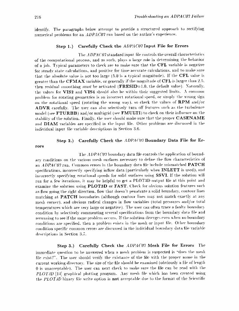
216 Troubleshooting an A DPA C07 Failure

identify. The paragraphs below attenlpt to provide a structured approach to rectifying

numerical problems for all ADPA('07 run based oil the author's experience.

Step 1.) Carefully Check the ADPAC07 Input File for Errors

The A DPA (.'07 standard input file controls the overall characteristics

of the computational process, and a.s such, plays a large role in determining the behavior

of a job. Typical paralneters to check are to make sure that the CFL variable is negative

for steady state calculations, and positive for time-accurate calculations, and to make sure

that the absolute value is not too large (5.0 is a typical magnitude). If the CFL value is

greater than the CFMAX variable, or generally if the magnitude of CFL is larger t.hall 2.5.

then residual smoothing must be activated (FRESID=I.0. the default value). Naturally,

the values for VIS2 and VIS4 should also be within their suggested limits. A common

problem for rotating geometries is an incorrect rotational speed, or simply the wrong sign

on the rotalional speed (rotating the wrong way), so check the values of RPM and/or

ADVR carefully. The user can also selectively turn off features such as the turbulence

model (see FTURBB) and/or multigrid (see FMULTI) to check on their influence on the

stability of the solution. Finally. the user should Inake sure lhat the proper CASENAME

and DIAM variables are specified in the input file. Other ])roblems are discussed in the

individual input file variable descriptions in Section 3.6.

Step 2.) Carefully Check the ADPA('07 Boundary Data File for Er-

rors

The A DPA ('07 boundary data file controls the application of bound-

ary conditions on the various mesh surfaces necessary to define the flow characteristics ofan ADPA('07 run. (:ommon errors in the boundary data file include mismatched PATCH

specifications, incorrectly specif.ving inflow data (particularly when INLETT is used), and

incorrectly specifying rotational speeds for solid surfaces using SSVI. If the solution will

run for a few iterations, it may be helpful to get a PLOT3D output file at this point and

examine the solution using PLOT3D or FAST. Check for obvious solution features such

as flow going the right direction, flow that doesn't penatrate a solid boundary, contour lines

matching at PATCH t)oundaries (although contour lines may not match exactly at any

mesh corner), and obvious radical changes in flow variables (total pressures and/or total

temperatures which are very large or negative). The user can often trace a. faulty boundary

condition by selectively commenting several specifications from the boundary data file and

rerunning to see if the same problem occurs. If the solution diverges even when no boundary

conditions are specified, then a problent exists in the mesh or input file. Other boundary

condition specific common errors are discussed ix, the individual boundary data file, variable

descriptions in Section 3.7.

Step 3.) Carefully Check the ADPA('07 Mesh File for Errors The

immediate question to be answered when a mesh problem is suspected is "'does the mesh

file exist.?". The user shouht verify the existance of the file with the proper naxne ix, lhe

current working directory. The size of the ill(, should be examined (obviously a file of length

0 is unacceptable). The user can next check to make sure the file can be read with the

PLOT3D [14] gral)hical plotting program. Any mesh file which has been created using

the PLOT3D binary tile write option is not acceptable due to the formal of the Scientific

Troubh shooting an A Df_4 ('07 kbilur< 217

Database I,ibrary (although it can be lna(le so by apl)ending 1024 bytes of any data lo lhe

end of lhe mesh file). The :'ILIh'EADGRID program is available to convert unformatled

mesh files to +IDP+I('07 compatil)le mesh files.

Mosl common problems encounlered when lhe .lille. l('07 code does

nol perfornl adequately can l>e traced to poor nlesh quality. All hougll the mesh may be free

t'ronl obvious flaws such as crossed mesh lines and/or zero vohlnles, this does not p_;uarantee

lha! lmmeri('al (lifficullies will be avoided. The mosl common overlooked fealures of mesh

qua lily are !he mesh (,xl)ansion ratio and tilt, mesh shear angle. Mesh <,xpansion ralio

relales 1o the change in physical mesh spacing along a given coordinale direclion from one

l)oinl 1o allolher, t"or slab!lily. !he lnaxinlunl mesh exl)ansioll ralio a! any poinl should

nol exceed 1.3. The .t/)/_A('07 code provides a listing oflnaximuln mesh expansion ralios

for each grid block and issues a warning if lhe mesh expansion ratio exceeds 1.3. The

code ('all lolerale larger ralios ill nlanv cases, t)ul defini!e problems can I)e exl)ec!ed if the

maximunl expansion raliogels larger than 2.0. Mesh shear can also cause l>rot)lems. The

more orlhogonal lhe mesh, the less likely nlesh-induced numerical <ti[[icullies will occur.

:\nolher l)<)lenlial mesh l>roblenl involves mesh <'ells with very small radii (such as aloha a

sting ups! ream of a propeller, el<'.) which may require increasillg the <lianleler of the stine;

to prevenl problelns. Applicatiotl of the lnullip_;rid ileralion stralegy and re<lucine; lhe value

of EPSY in the input file have been found lo be effecliw, relne<lies for such problems.

Step 4.) Check for the Possibility of an Invalid Flow Condition

The author's experience has l)een thai many users feel if a I)roblem

Call be defil,e<l then i( should possess a solution, hi fluid dynanlics lhis is certainly nol

lrue. If a solulion in allenll)le<l for a fan rolor, for examl)le, a! a ])ressure ra!io which in

beyon<l !he stall poinl for that rolor, then no solulion exisls anti lhe co<le will very likely

diverge withoul exl>lanation. In many cases, lhe nulnerical equivalenl of at, invalid flow

condition is 1hal !he solution will either nol converge, or will simply diverge. Anolher

common example is attemt>tin _ to exlract a sleady state solution for a prol)lem whi<'h is

lruly tilne-<lepentlenl. |_hl]ll body flows oflen result in a !.inle-ttependenl s<>lllli<m <tue to

vorlex shedding;, and lhe swa<lv state analysis of this flow will likely never converg;e. This

behavior also occurs frequenlly when a slrong adverse pressure gra<lienl or flow separation is

presen! in lhe solution. Now il is lrue that in some cases, lhe level of convergence may also

be limi!e<] t>y sucll factors an mesh quality, nunlerical accuracy, and/or turbulence model

limit cycles, anti i! is difficul! to <lelermine whelher lhe cause in numerical or physical. This

is unforllmalely a malter of experience and lhe user is elwouragetl 1o question whether their

case call l['uly have a "'steady" solution.

Step 5.) Determine if the Problem is Computer Dependent

The A DFA ('1)7 code was <leveloped and !este<l on UNIX-I)ase<l ol>er-

al ing syslenls using; F()IITIIAN 77 slan(lar(I co<ling lechni<tues. Ill spile of the standardiza-

tion in the computer industry, not all machines l)roduce the same answer for a given problem

due Io cOnll>iler Ol)timizalions and co<h' lmll<lling fealures. Ii has been the author's exl>e-

rience lhaI ('<mlpilers are often a SOlll'Ce of problems, l>arli<'ularly when the code has been

conlpile<l for lhe fil's! lhlle Oil a specific arch!lee1 ure. or when a new release of lhe ol)eraiin_;

system or I,'()RTt{AN compiler has been ins!ailed. Before reporting an unsolval>le prol)lem.

it in a g;oo<l praclice Io coml>letely recompih, the code on a known slable nta<'hilw with a

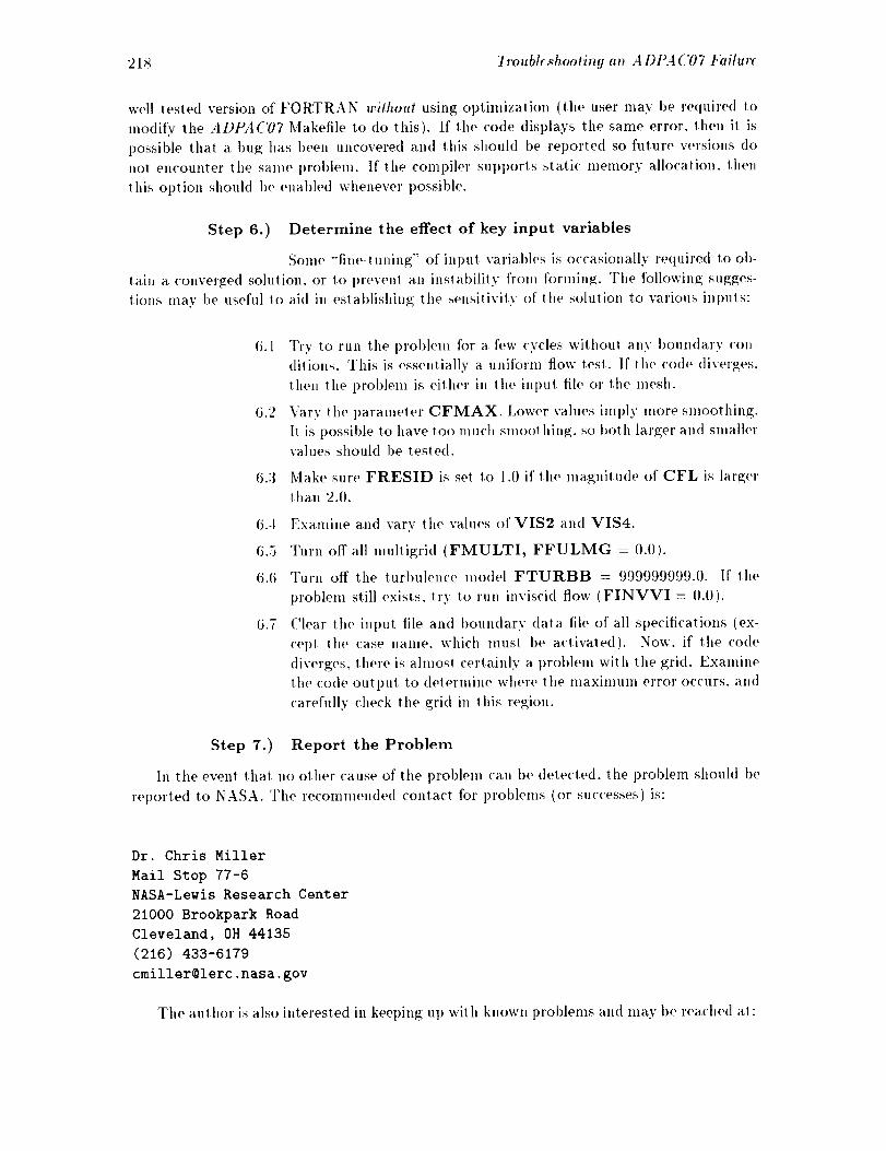
21S Troubleshooting an ADPA ('07 l_hilure

well tested version of FORTRAN without using optimization (tile user may be re(luired to

modify the ADPAC07 Makefile to do this). If the code displays the same error, then it is

possible that a bug has been uncovered and this should be reported so future versions do

not encounter the same l)roblem. If the compiler SUl)ports static memory allocation, then

this option should be enabled whenever possible.

Step 6.) Determine the effect of key input variables

Some "fiue-t u_fing'" of iui)ut varial)les is occasionally re(luired to ob-

tain a converged solution, or to 1)reven! an inslabilily from fornfing. The following sugges-

tions may be useful to aid in establishing the setlsitivity of the solution to various inputs:

6.1 Try to run tile prol)lem fox" a few cycles withou! a,ly boundary coll-

ditions. This is essentially a uniform flow test. If the code diverges,

then the problem is either in the input file or tile mesh.

6.2 Vary the parameter CFMAX. Lower values imply xnore smoothing.

It is possible 1o have leo much smoothing, so I)oth larger and smaller

values should be tested.

(i.3 Make sure FRESID is set to 1.0 it' the magnitude of CFL is larger

than 2.0.

6.4 Examine and vary the values of VIS2 and VIS4.

6.5 Turn off all multigrid (FMULTI, FFULMG = 0.0).

6.6 Turn off the lurbuleuce model FTURBB = 999999999.0. If the

problem still exists, try to run inviscid flow (FINVVI = 0.0).

6.7 Clear the input file and boundary data file of all sl)ecifications (ex-

cept the case name, which must be activated). Now. if the code

diverges, there is almost certainly a problenl with the grid. Examine

the code output to (leterniine where tile maximum error ()(:curs. and

carefully check tile grid in this region.

Step 7.) Report the Problem

Ill the event that no other cause of tile l)roblem can be (letecled. the t)robleln should be

reported to NASA. The reconlmended contact for problems (or successes) is:

Dr. Chris Miller

Mail Stop 77-6

NASA-Lewis Research Center

21000 Brookpark Road

Cleveland, OH 44135

(216) 433-6179

cmiller@lerc.nasa.gov

The author is also interested in keeping ut) with known woblems and may be reached at:

7'to ubh.,,hootit_g an A DPA ('07 F, ihtr¢ 219

Dr. Ed Hall

Speed Code T-14A

Allison Engine Company

Indianapolis, IN 46206-0420

(317) 230-3722

ehall©nas.nasa.gov

ieehl@agt.gmeds.com

220 Trouble_shooting _m ADPA C07 Failur_

Chapter 4

RUNNING

PARALLEL

ADPAC07 IN

4.1 Parallel Solution Sequence

Ill order to run A I)i),4('07 in parallel, ADI)A('07 must be compiled for paralM execution.

The chaplet on code compilalion in 1his User's Manual describes the prol)er comt)ilalion

procedu re.

,4 DPA ('07 is parallelized usin N the Application Portable Parallel Library (AI_PL) mes-

sage passing library, developed a! NASA Lewis. lleh_rence [22] explains how 1o write code

using APPL and how to run codes written with APPL. Whih, APPL runs on many plat-

forms, this manual will deal with only two of them: workstalion clusters and n(!VI]E mas-

sively parallel computers. These two pla,tforms are representative of how A DI)A('07 runs

in parallel. The APPI, document should be consulted for cases not covered in this manual.

Regardless of the l)latform, running A DR4('07 in parallel requires the APt'I, compute

fltnction and a l,v('d_f file. ('odes running under APPI, are no! initiated by typinp; the

executable name. but use the APPL compute function instea,d. The syntax for executing

ADt_4('07 is as follows:

compute < casename.i_pul > output

The compute funclion controls the execution of ADPA('07 Otl the various processors,

taking addil, ional input fi'om the p_v<'d<f file. The proc&f file contains the names of the

executal>le images and the processors that !hey are to I)e loaded on. The compute fuse-

lion establishes con|municalions with each processor specified in lhe procd(ffile, loads the

.tDI)A('07 execulal)le image, and initiates the run on each processor. Also, the compute

function ow, rsees the running processes, monitoring the processors for abnormal termina-

lions. If a COmlntmications error is tral>l)ed, or if a l)rocess has died unexpectedly, tho

compute function shttls down all of lhe remaining processes gracefully. This feattlre is

mosl imporlanl on workslalion cluslers, which have no buill-in mechanism for monitoring

parallel jobs.

The normal A I)IM('07 inpul file is redirecled from standard inpul to the compute

function. The redirecled inpul is available 1o all of lhe processes (allhough :II)I)A('07 cur-

rentlv does all reading from node 0). The ()till)Ill lib' nlay be redirected, or allowed to

221

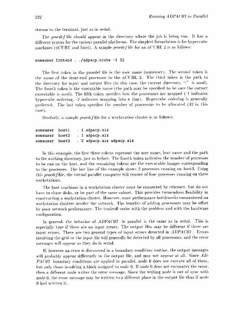
222 Rum_iT_g ADPA ('07 i_ Parallel

stream to tile terminal, just as ill serial.

The proc&f file should appear in tile directory where tile job is being run. It has a

different syntax for tile various parallel platforins. Tile simplest formulation is for hypercube

machines (nCUBE and Intel). A sample proc&J'file for an nCUBE 2 is as follows:

someuser frntend ./adpacp.ncube -i 32

Tile first token ill tile procdef file is tile user name (someuser). Tile second token is

the name of the front-end processor to the nCUBE 2. The third token is the path to

the directory for input and outpu! files (in this case, tile <'urren! directory, ".'" is used).

The fourth token is the executable name (the path may be specified to be sure the correct

executable is used). The fifth token specifies how the processors are mapI>ed (-1 indicates

hyl)ercube ordering. -2 indicates mal)l)ing into a ring). Hyl)ercul)e ordering is generally

l)referred. The lasl token specifies the number of l)rocessors to be allocaled (32 in lhis

case).

Similarly. a sample proc&f file h)r a workstation cluster is as follows:

someuser hostl

someuser hosZ2

someuser host3

1 adpacp.aix

1 adpacp.aix

• 2 adpacp.aix adpacp.aix

Ill this example, the first three tokens represent the user name, hosl name and the palh

to the working directory, just as before. The fourth token indicates the number of processes

to be run on the host, and the remaining tokens are the executable images corresponding

to the processes. The last line of the example shows 2 processes running on host3. Using

lhis procdeffile, the virtual parallel computer will consist of four processes running on three

workstations.

The host machines in a workstation cluster must be connected by ethernet, bul do no!

have to share disks, or be part of the same subnet. This provides tremendous flexibility in

constructing a workstation cluster. However. most performance bottlenecks encountered on

workstatiou clusters involve the network. The benefits of adding processors may be offset

bv poor network performance. The tradeoff varies with the problem and with the hardware

configuration.

In general, the behavior of ADPA('07 in parallel is the same as in serial. This is

especially true if there are no input errors. The output files may be different if' there are

input errors. There are two general types of input errors detected in ADPAC07. Errors

involving the grid or the input file will generally be detected by all processors, and lhe error

messages will appear as they do in serial.

If. however all error is discovered in a boundary condition routine, the output messages

will probably apI)ear differently in tile output file, and may not apl)ear at all. Since AD-

PAC07 boundary conditions are applied in parallel, node 0 does not execute all of them,

but only those involving a block assigned to node 0. If' node 0 does not encounter the error,

then a different node writes the error message. Since tile writing node is out of sync with

node 0, the error message may be written to a different place in the output file than if node

0 had written it.

R._.i.g A DPA ('07 i. Parallel 223

Buffering of OUtl)U( on the various processors (;all also cause a problem. Usually. after

all error message is printed, execution is slopped on all t)rocessors. If execulion is slopped

before (he buffer is flushed, lhen oull>ut ntav be los( from some processors. Tit(, result is

lha( an error message could 1)e caughl in lit(' buffer and never al)l>ear in the OUll)Ul file. If

ADISi('07 terminates for no apl)aren) reason, this may explain the 1)rot>lem. The solulion

is 1o rerun the job wit ho,1 re(lirecling (he OUtl)Ul. If' oult)ul is nol re<lirecle<l, it is normally

no( l)uffere(1, and all of the outpul will al)l)ear.

II is also possible lo gel multiple co])ies of an error message if more lhan one l)ro('e,_sor ell-

counters lhe error. Wherever possil)le. A DP.4 ('07 has heel( co(le<l Io avoi(l lhese problems.

but lhese unforlunale I)ossibililies siill exisl. Therefore. ru.ning AI)I)A('07 inleractivelv

is lhe besl way io track (l()wil int)u( l)roblems.

Aside from (hese ('onsidera! iotls, running +| DPA ('07 in l>arallel is very much like running

ADI>:I('07 iu serial. The ill])llt files are idenli('al, and llle OUl])lll files at'(' very similar. The

lll()Sl ('Ol]llllOll problems in runldu_; ,4 DPA('07 ill i)aralle] are failillg to use lhe compute

fun('! ion. inlt)rol)erly sl)ecifyin_; 1he parallel configuration in lit(, l>ro<'<lef file, aim al leml)t in_

Io rlln a serial e×e('lllal)le in I)arallel.

4.2 SIXPAC (Block Subdivision) Program

,S'IXPA(', whi('h start(Is for Subdivision and Information eXchan_;e for Parallel AI)I'A('

Cal<'ulalions, enables the user 1o redefine the block struclure of an AI)I'A('07 .job. Usi,_;

.%'I.\'I'A('. lar,.9_;(,_rid l)locks ca. I)e subdivided to improve load balance, or to make use of

smaller memory l)rocessors in t)arallel calculalions. ,S'[XP, I(' generales new inl)U(, mesh,

restart, and bounda(a files for lhe subdivided i)robh'm, creating new blocks according lo

user sl)e('ifi('aliolls. The resullin_ files rel)res(m( a l)roblem e(luivalent 1o the orio;inal, l>u(

wilh more. smaller, blocks. Although (he,umber of unique grid points is unchan_e(l, lit('

lolal number of l)oiuts is larger because of duplication al in(erfa('es.

The molivation for ,S'IXt'A(' comes from lhe way ADPA('07 was l)arallelize(l, l_alher

(hau l)arallelize the interior l)oin! solver, :11)I>A('07 was ])aralh,lized through the bouu(tary

con<litions. An in(livi<tual block can't I)e run across multiple processors; each l)rocessor musl

conlain ouly whoh, blocks. This implies (ha) a problem with a single large block couldn't

t>e )',n i. parallel. A'IXP:t(' enables large blocks to I)e recast as groul)S of smaller blocks.

so lha( they can t)e run ill parallel. ,SIXPA(' is no( required to run a problem in l)aralle],

bu( i( siml)lifie,_ the l)rocess of selling up a problem for o[>(imM I>arallel t>erformance.

4.2.1 5;/XI)A(' Input

The inl).( files re(luire(l by .<)'IX/',.[ (' are the ca._(_a,_<.i,p,! file. the <.a._()mm(.m(sh ill(,, lit(,

<.a.+(,,,l(.bo..d, ta file. and )he <',._<_mm(.._izpac file. If a uew res(ar)file is to be create(l.

then a <'<t._(nat,(.r<.<t,rl.ohl file is also re(luire(l. Of (his r;r(>u]), only lhe <'a._:nam(.._ia'lUlr

fih' is <lifferenl front the slan<lard AI)PA('07 inl)Ut.

The <'a.setmm(.._i3'lUtC file contains information which st>celtics how )he blocks are lo t>e

subdivi(le<l. The required information inclu(les the number of ori_;inal blocks, an(t how

each 1)lo<'k is lo I)e sul)(livi(te<l in each indicial <lireclion (i. j. an(t k). In each dire('lion.

)he numl)(,r of sul)(livi<le(I blocks, and l)ossil)ly the lo('alh)ns of tile sul)(livisions, musl I)e

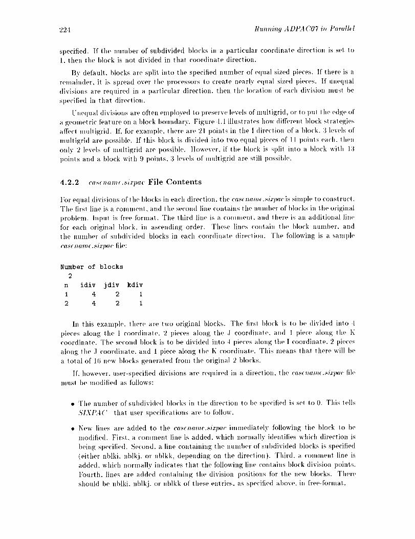
224 Runnin9 A DPA (,'07 i1_ Par, Ill

specified. If the number of subdivided blocks in a particular coordinate direction is se! to

1, then the block is not divided in that coordinate direction.

By default, blocks are split into the specified number of equal sized pieces. If there is a

remainder, it is spread over the processors lo create nearly equal sized pieces. If unequal

divisions are required in a, particular direction, then the location of each division musl be

specified in that direction.

Unequal divisions are often eml>loyed to preserve levels of multigrid, or to l)Ul lhe edge of

a geometric feature on a block boundary. Figure 4.1 illustrates how different block strategies

affect multigrid. If, for examl)le, there are 21 points in the I <lirection of a block, 3 levels of

multigri<l are possible. If this block is divided into two equal pieces of 11 poinls each. then

only 2 levels of mnltigrid are l)ossible. However, if the block is split into a block wilh 13

points and a block with 9 points, 3 levels of lnultigrid are still possible.

4.2.2 ca._mtm_.si.rpac File Contents

For equal divisions of the blocks in each direction, the c,.+_Tmm_ .si_'pa<" is simple to construct.

The firsl line is a comment, and the second line contains the number of blocks in the original

prol)lem. Input is fi'ee forlnat. The third line is a conlnlent, and there is an additional line

for each original block, in ascending order. These lines contain the block number, and

lhe number of subdivided blocks in each coordinate direction. The following is a sample

c,.+_am_, sia'lmC file:

Number of blocks

2

n idiv jdiv kdiv

I 4 2 1

2 4 2 1

I11 this exalnple, there are two original blocks. The first block is to t>e divided into 4

pieces along the I coordinate, 2 pieces along the .l coordinate, and 1 piece along the ]{

coordinate. The second block is to be divided into 4 pieces along the I coordinate, 2 pieces

along the J coordinate, and 1 piece along the K coor<tinate. This means that there will be

a total of 16 new blocks generated fi'om the original 2 blocks.

If. however, user-sl)ecified divisions are reqnired in a direction, the cas_7tam_..+iaTmC file

must be modified as follows:

The number of subdivided blocks in the direclion to be specified is set to 0. This lells

,qIXI_4(' that user specifications are to follow.

New lines are added to the ca.+_am_.ga'l>ac immediately following the block to be

modified. First, a comment line is added, which normally identifies which direction is

being specified. Second. a line containing the number of subdivided })locks is specified

(either nblki, nblkj, or nblkk, depending on the direction). Third, a comment line is

added, which normally indicates that the following line contains block division points.

Fourth, lines are added containing the division t)ositions for the new blocks. There

shouht be nblki, nblkj, or nblkk of these entries, as specitied above, in free-format.

Rum_i_9 A DP.,| ('07 i_ P, ral#l 225

Subdivision of Blocks to Preserve Levels of Multigrid

I 11 -_ _,- I 11

1 11 21

Subdivision into two equal pieces results in blocks with 11 points. Only two

levels of multigrid are possible, even though three levels were possible for

the original block.

1 13-_ _.-1 9

1 13 21

Subdivision into two unequal blocks, one with 13 points and one with 9

points, yields a grid capable of three levels of multigrid, like the original

block.

Figure -I. 1: (!areful hlock division can ])reserve levels of multigrid.

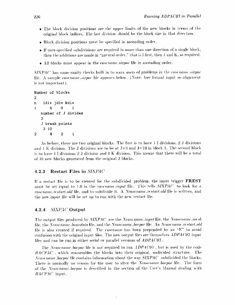
226 Run1,ing A DPA ('07 in Paralld

. The block division positions are the upper limits of the new blocks in terms of the

original block indices. The last division should be the block size ill that direction.

• Block division positions must be specified in ascending order.

• If user-specified subdivisions are required in more than one direction of a single block,

then the additions are made in "'natural order." that is I first, then .] and K. as re<luffed.

• All blocks must appear in the co.,< mtm¢..+ixpac file in a scellding order.

,S'IXPA(' has some sanity checks built in to warn users of l)rol)lems in the <'a._(nttm_.._ixlm<"

file. A sample ca.,<(ttanl(..,_ix])ac file apl)ears below. (Note: free format input so alignment

is not ilnporlanl).

Number of blocks

2

n idly jdiv kdiv

1 4 0 1

number of J divides

2

3 break points

3 I0

2 4 2 1

As before, there are two original blocks. The first is to have 4 I divisions, 2,1 divisions

and l K division. The .1 divisions are to be at .1=3 and .l=10 in block 1. Tile secon(t block

is to have 4 I divisions 2.1 division and 1 K division. This means that there will be a total

of 16 new blocks generated fl'om the original 2 blocks.

4.2.3 Restart Files in 5'LYPAC

If a restart ill(, is to be created for the subdivided problem, the input trigger FREST

must be set equal to 1.0 ill the <'a._emm_t.btput file. This tells ,S'IXPA(' to look for a

ca._nam_.r_tart.ohl file, and to subdivide it. A Nca._nam_.r(._tart.old file is written, and

the new int)ut file will be set up to run with the new restart file.

4.2.4 5'IXt_4(' Output

The out put files prod uced 1)y SIXPA (' are tile .Ycasenam(. input file, t he Ncase _mm(. mesh

file, t he Ncas( name. bmmdata file, and tile Nca._( nam(. bacpae file. An Ncas¢ _am_. r( start.old

file is also created if required. The casename has been l)rel)ended by an "N'" to avoid

confusion with the orip_,;inal input files. The new outl)ut files are themselves ADPA('07 input

files and can be run ill either serial or parallel versions of ADPA('07.

The Nca.+_name.bacpa(" file is llOt required to run ADPA('07. but is used t)y the code

BA('PA(', which reassembles the blocks into their original, undivided structure. The

:\'<'a._ mm_(.bocpoc file contains inforlnation about the way 5'IXI>A (' subdivided l.he blocks.

There is normally no reason for the user to alter the ,'_rca.se_mm_.bacpac file. The form

of the Nc<t.senom<.bacpac is described in the section of the User's Manual dealing wilh

BA('PA (' input.

Running A DPA C07 in Parall_ I 227

4.2.5 Running SIAt_A('

l(unning SIXPA(' is very much like running ADPA('07. Tile command syntax is:

sixpac < ca._mn_(.i_pul > output

Tit(' outp+tt file is sitnilar to an ADI{4('07 outl)ut file, because the routines to rea<t lhe

p_;ri<l, the inl>Ul file an<l tile 1)oundary (tala file are taken directly fi'om AI)I{4('07. One

a(l<lition lo the OUll)Ul lile is a lane of Ill(' new grid blocks and lheir sizes. ,\tier verifying;

lhe new 1)lock slruclure created by ,<YlXI)A( ' . the oull)u! tile can l)e (liscar<le<l.

4.3 BA CPA C

IL|('I>A( '. which stands for Block A<'cumulation and Consoli<lalion Jbr Parallel ADPA(!

Cal<'ulalions, reassembles subdivi(le(t A DPA('07 tiles into t heir original, undivided form.

It is use(l in ('onjuncl:iou with ,SIXtL,I(', a n<t performs essentially the inverse ol)eration of

,S'IXI_A( ' . t>,A('I_,I (' can reconslrucl mesh, t)I,()T3D, or restar! tiles, l)ro(lucing new tiles

whi<'h are e<luivalen! to wha! would have I)een l)roduce<t ha(I the ])rolllem I>een run with the

orip_;inal, un(livi(le(I I)locks. ITs!rig SL\:I_;|(' and BA('t>A( ' , a ]>rolllem can I)e sul)(livide(1

and reconstructed any numl)er of ways 1o !ake advantage of a vailal)le COml)uter resources.

4.3.1 BAC'I_A( 'Input

BA ('PA (' queries tile user for nee<led i,lf<)rma'_ion, and reads from start<lard in l)Ul (normally

the keyboard). The user is firs! llroinllled for the casename. The user then sele("_s which

tiles are 1o I)e reconstructed by enlering al>l)rOl)riate responses t<) questions abou! each file.

l)ue to Ill(' i)olential size of these files, they are not created t).v <tefault.

BA('I>,I( ' expects 1o find a <.a.+(;;,m<.b<+cpo<" file which contains informal!on detailing

how 111(,original l)roblem was sub<livide<l. The ('a.+_;utm(.b<;elmc file is created auloma!ically

t)v ,S'/XI{4 (', and re<luires no motliticaliotls l)v the user. However. if ,S'l,\'t>.t (' was no! used

to create the sul)divi(le<l blocks. !he ilser lllllS/ COllS|I'llC! a ca._e_mm_.b<lcpoc file ill order Io

run IL4 ('f>A ('. A sample ca._e;mm< .bacpa<. file resulting froln tile firsl saml)le ,q/XPA ('input

file given previously at)pears below.

original number of blocks

imax jmax k.max

73 10 9

nblki nblkj nblkk

4 2 1

oldblk newblk global i

73 10 9

nblki nblkj nblkk

4 2 1

oldblk newblk global i

global j global k local im local jm

global j global k local im local jm

local km

local km

In the above (,xaml)le. two blocks are sul)divi(le(I inlo eight new 1)lo('ks each (a '(olal of

16 I)locks). The dimensions of Ill(, original I>locks are 73x10.g). an(l lhere are 1, 2, and 1

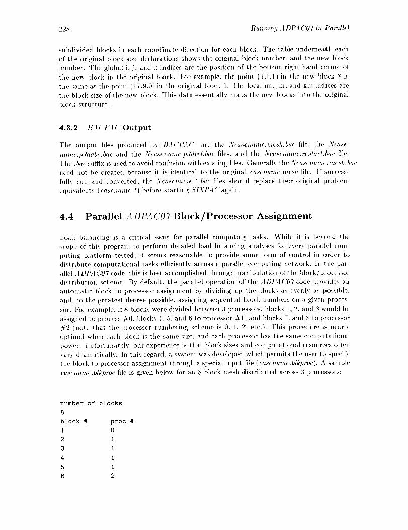
t22,_ Rum, in9 ADP, (07 in Parall_t

sut)divided blocks in each coordinate direction for each block. Tile table underneath each

of the original block size declarations shows the original block number, and the llew block

number. The global i, j, and k indices are the position of tile bottom right hand corner of

lhe new block in the original block. For example, the t)oint (1,1,1) in the new block _ is

the same as the point (17.9,9) in the original block 1. The local ira, jm, and kit, illdices are

the block size of the new block. This data essentially maps the new blocks inlo lhe original

block structure.

4.3.2 BAC't_4('Output

The outl)ut files t)roduced by BA('PA(' are the Ncastnam_.mt._h.bac file. the Ncast-

imm¢.p3dab,_.bac and the Ncast_utm(.p3dr_l.bac files, and the Nca._mme.rt.,dart.b,c fih'.

The. bac suffix is nsed to avoid confusion with existing files. Generally the Nea.,,_'nam_. m_._h.bae

need not be created because it is identical to the original ca._e_ut,nt.me.,J_ file. If success-

fully run and converted, the Nca.,,_n,m_.*.b,e files should replace their original l)roblem

equivalents ( ca._ namr. *) before starting 5;IXPA (' again.

4.4 Parallel ADPAC07 Block/Processor Assignment

I,oad balancing is a crilical issue for parallel computing tasks. While il is beyond lhe

scope of this l)rogranl to t)erform detailed load t)alancing analyses for every l)arallel com-

l)uting platform tested, it seems reasonal)le to provide some form of control in order to

distrit)ute computational tasks efficiently across a parallel computing network, ht the par-

allel A DPAC07 code, this is best acconq)lished through manipulation of lhe I)lock/processor

distribution scheme. By default, the parallel operation of the ADPA('07 code l)rovides all

automatic block to processor assignment by dividing u I) the blocks as evenly as possible,

and. to the greatest degree possible, assigning sequential block numbers Oil a given proces-

sor. For example, if _ blocks were divided between 3 processors, blocks 1, 2. and 3 would be

assigned to process #0, blocks 4, 5, and 6 to t)rocessor #1. and blocks 7. and ,_ to processor

#2 (note that the processor numbering scl,enle is 0. 1, 2. etc.). This t)rocedure is nearly

ol)timal when each block is the same size. and each i)rocessor has the same COml>utational

power, lTnforttmately, our experience is lhat block sizes and computational resources often

vary dramatically. In this regard, a system was developed which permils lhe user t¢) Sl)('ci[ _'

the block to processor assignmenl through a specia.1 input file (ca._:'lmm_.bl_'proc). A sample

c_._mmt.blkproc file is given below for an s block mesh distributed across 3 processors:

number of blocks

8

block # proc #

1 0

2 1

3 1

4 1

5 1

6 2

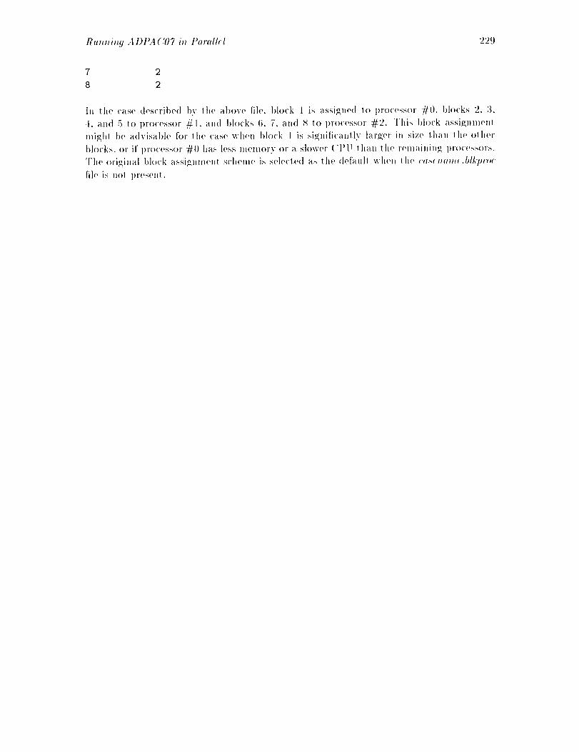
RuT_l_i_g +1DPA ('07 i_ Parollrl 229

7 2

8 2

Ill the case described by lhe above file, I)[ock 1 is assigned 1o processor #0. 1)locks 2. :/,

,I. and 5 to processor #1. and blocks 6, 7, and S to processor #2. This block assi_nmen!

mighJ be advisable for the case when block 1 is significanlly larger in size than lheother

blocks, or if processor #0 has less memory or a slower ('PU lhan lhe remaining processors.

The original block a,s,si_nment scheme is selecled as lhe defaull when lhe <'<l._<_mmr.bl_'luvc

tile is nol presenl.

230 Running A DPA ('07 ilt PaT_tllel

Chapter 5

MAKEADGRID PROGRAM

DESCRIPTION

The staildard (list ril)ul ion for the A DP.| ('07 l)rogram include,_ a l>rogranl called MA K/"A D-

(;RID which aids the user i_h setliH_; Ul) a multiple-block mesh file from isolated unl'orma'_ted

mesh tiles. This program is useful for creatin_ ADt_A('OTcoml>alit)le multil_le-I)lock meshes

from mesh _eneralion programs which do no1 support the use of the Scientilic l)alabase

l:il>rar.v (SI)BI:IB). The MAKF_II)GtHD program is an interactive program which queries

lilt, user f<)r lhe number of blocks to t>e assembled for the final mesh. and lhen re<luests a

tile nmne for each o[" the individual mesh blocks. The user is then reqllested to l,mne the

final Olltl_llt tile ['or tile AI)I>A('07 coml>alible multil>le-t>lock mesh. The individual mesh

blocks are assemt>le<l iu the or<ler in which the mesh file names are sl_e<'ified, so care musl

be taken 1o or<ler lhese names apl>ropriately.

5.1 Configuring MAKEADGRID Maximum Array Dimensions

Maximum array <limellsions in the MA KEADGRID program are set by tile FORTRAN PA-

RA_II';T}';ll s|ale[uonls listed in lhe source file makeadgrid.f include<l wilh lhe standard

<tistrilmliou. The PARAMETEI_ statement and the descriplions of tile various parameler

varial>les appear at the top of the tile as:

C

C

C makeadgrid: This program assembles an ADPAC-compatible mesh file

C

C

C

C

C

C

C

C

from selected other unformatted PLOT3D mesh files

Set parameter size for max grid block to be read in

imax --- > maximum number of grid elements in the i coordinate direction

for any given mesh block

jmax --- > maximum number of grid elements in the j coordinate direction

231

232 _L4KEADGRID Program De._criptioll

C for any given mesh block

C kmax --- > maximum number of grid elements in the k coordinate direction

C for any given mesh block

C nnames - > maximum number of grid blocks for final mesh

C

parameter(imax=251, jmax=82, kmax=53)

parameter(nnames = 100 )

5.2 Compiling the MAKEADGRID Program

The MAKEADGRID program source directory contains a UNIX-based Makefile facilily to

a utonlale conlpilat ion for a number of nlachines. In t he etirectory containing t he FO RTR A N

source of tile MANEAD(;RID code. compilation is t)erfornmd by executing the COlnniall(t:

make optiol_

The make command is standard on [:NIX systems and automatically interrogales lhe file

Mokefih for instructions on how 1o perform the compilation. Tile optio_ argument may be

any of the variables listed below:

No argument- same as link below.

li_,k This is the standard UNIX system compilation. This option will

deliver a working executable on most UNIX systems which support

standard nalning conventions (f77 as the standard compiler, etc.).

The comlfila.tion includes basic compiler optimization (t'77 -O).

tray This option is utilized when con@ling the standard code on a ('ray

conlputer.

aia' This option is used when conlpiling the standard code on an IBM

RS-6000 workstation running the AIX operating system.

5.3 Running the MAKEADGRID Program

Once the code has been compiled, clla.llge directories to the location where the case of

interest, has been stored. The MAKEADGRID progranl requires that each individual mesh

block for the final mesh be stored separately as a. single-grid unformatted PLOT3D file .

The MAKEA DGRID program is invoked by issuing the colnlnand:

path/makeadgrid

where path is the relative or absolute pat.hname of tile directory containing tile MAKEA D-

(;RID execula.ble tile from the current local direclory. For example, if the mesh tile is in

the directory

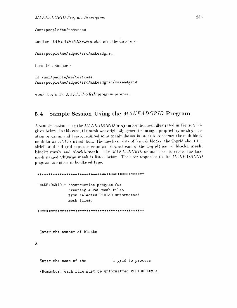
MA KEA D(;Bll) Pr<,gram D<._<'ription 233

/usr/people/me/testcase

and lhe MAKEAD(;I{ID executable is ill tile directory

/usr/people/me/adpac/src/makeadgrid

thell tile commands

cd /usr/people/me/testcase

/usr/people/me/adpac/src/makeadgrid/makeadgrid

would t>e_;in the M+IKI+:+I/)(/RID I>r<)_ram l)ro<'ess.

5.4 Sample Session Using the MAA-EADGRID Program

A sample session using the M.I KE.tD(;I?ID program for lhe mesh illustrated in Fie_;ure 2,1 is

given below. In this ('as(,, lhe mesh was origiually generaled using a l)r<)l)rielary mesh _;euer-

at ion l)rO?_;ram, a u(I hence, required some manipulation in order to conslru<'l the multibl<>ck

mesh for an ADI>.t('07 solulion. The mesh <'onsists of 3 mesh blocks (the O-grid a l)oui the

airfoil, and 2 tf-grid caps upstream and downstream of the O-grid) named bloekl.mesh.

block2.rnesh, aud block3.mesh. The MAKEAD(;IgII)session used _<) create the tinal

mesh named vblvane.mesh is listed below. The user responsos lo lhe M.,II(]:'.tl)(;I?ll)

ln'O_;ram are _iven in bol<lfaced type.

MAKEADGRID - construction program for

creating ADPAC mesh files

from selected PLOT3D unformatted

mesh files.

Enter the number of blocks

3

Enter the name of the I grid to process

(Remember: each file must be unformatted PLOT3D style

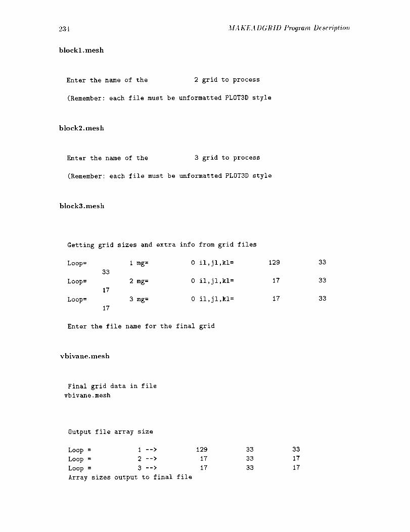
234 MA KEA DGRID Program Desrriptiol_

blockl.mesh

Enter the name of the 2 grid to process

(Remember: each file must be unformatted PLOT3D style

block2.mesh

Enter the name of the 3 grid to process

(Remember: each file must be unformatted PLOT3D style

block3.mesh

Getting grid sizes and extra info from grid files

Loop= I mg= 0 il,jl,kl=

33

Loop= 2 mg= 0 il,jl,kl=

17

Loop= 3 mg= 0 il,jl,kl=

17

Enter the file name for the final grid

129

17

17

33

33

33

vbivane.mesh

Final grid data in file

vbivane.mesh

Output file array size

Loop = 1 --> 129

Loop = 2 --> 17

Loop = 3 --> 17

Array sizes output to final file

33

33

33

33

17

17

JIA KEA DGRID P_'og?'.m D_._c'rip/io_ 235

Reading Grid Data from file

blockl.mesh

il, jl, kl ---> 129

Output grid data to final file

Reading Grid Data from file

block2.mesh

il, jl, kl ---> 17

Output grid data to final file

Reading Grid Data from file

block3.mesh

il, jl, kl ---> 17

Output grid data to final file

PROGRAM COMPLETED NORMALLY

33

33

33

33

17

17

236 MA KEA DGRID Program De._criptio_

Chapter 6

ADPAC07 INTERACTIVE

GRAPHICS DISPLAY

Th(, .l l)ltl ( '07 program i._ e(lUil)l)ed wilh all Ol>iio. whi('h I)('rndts r(,al lira(' inl('ra('tiv('

gral)hi('s display of flow (lal a in I h(' form of('olored ('onlours or v(,h)('ily ve('lors on ge,onl(,l ri(,s

ret)r(,s('nl('(I I)y wiremesh grid surfaces. The inleractive gral)hi('s are based largely on roulill('s

generaled from lhe PLOT31) visualizal ion t)rogram, and many of lhe t'('al ures of lhis oi)1 ion

sho,ld I)(' familiar to anvon(, who has use(I PLOT3D. All inleraclive graphics musl I)(,

dist)lay('d on a Silicon Graphics workstation, IRIX 01)eraling System .1.0.1 or al)ov(,. Th('

_;ral)hics display can t)e Ol)eraled on a single compuling I)latform. or can he (lir(,('l(,d across

a nelwork for specific compul(,r hardware configurations. Thus. il is possihl(, 1o have a

.ioh ru.ni._: remolelv on a ('ray coml)uler, with interactive gral)llics (lisl)layed l<)cally on a

n(,lwork-('onnecled Silicon (;ral)hi('s workstation. When ol)era|in?.; across a nolwork which

involves a noll-Sili('on (;ral)hics ('Oml)uter. the communication program A(;TI_LT-L( 'L musl

1)(, r, nnin_: on ll,(' local disl)lay d(,vi('(' in order to capture the grat)hi('s commands issued

1)v lh(, r(,mol(, ('omt)ul(, serv(,r (details on :t(_TPLT-L('L are given l>elow). A graphic

illustraling lhe 1)ossihl(' graphics disl)lay ol)erating modes is given in Fig, r(' (i. 1. 11should t)(,

menliono(1 lhat lh(' inl(,racliv(, _;ral)hics display was actually deveh)l)ed to aid in d('hu_;ging

tile mullil)le 1)lo('k code. The (tescril)lion of this feature is includ(,d in this mamJal for

COml)l(,teness. t)u| the user should 1)e cautioned due to the immature nalure of this t)ortion

of lh(' code. It is also likely lhal the graphics option may nol 1)orl correctly to future

releases of lho IRIX operating system, and again, the user is cautioned concerning the use

of lifts lea lure.

6.1 Setting up the Program

Th(, firsl step in producing the real time interactive gral)hics dist)lay is to correctly compile

lh(' ('od(' to in('lu(l(' lh(' gral)hics libraries. This is accolnl)lished by utilizing l he al)prol)riale

ot)lion in lhe .IDP.4 ('07 Makofile command (see Section 3.=1). The valid gral)hics options

in('lu(l(' :lral, hic._, pJ'ogmlflHc._, croygraphi('._, aixgraphic'._, and craygraphdbx. These options

in<'orl)orat<, various levels of lh(, in<'lu(l('d graphics libraries for execuli<)n on various ma<'hin(,s

(again. see S(,clion 3.4 for sl)ecifi<" Makefil(' details).

On<'(' lh(, co<le has t)('('n <'orrectlv corot>ileal Io include the grat)hi('s lil)rari(,s, several int)ul

237

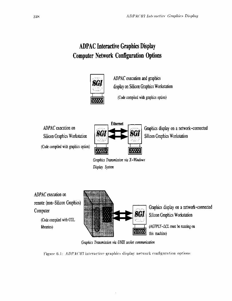
238 A DPA ('07 Inl_roelive Graphic._ Di._'phly

ADPACInteractiveGraphicsDisplay

ComputerNetworkConfigurationOptions

ADPACexecutionandgraphics

displayonSiliconGraphicsWorkstation

(Codecompiledwith graphicsoption)

ADPACexecutionon

SiliconGraphicsWorkstation

(Codecompiledwith graphicsoption)

GraphicsTransmissionvia X-Windows

Display System

Graphicsdisplayon a network-connected

SiliconGraphicsWorkstation

ADPACexecutionon

remote(non-SiliconGraphics)

Computer

(CodecompiledwithCGL

libraries)

Graphicsdisplayon a network-connected

SiliconGraphicsWorkstation

(AGTPLT-LCLmust be runningon

this machine)

Graphics Transmissionvia UNIXsocket communication

Figure 6.1 : A DPA ('07 interactive graphics display network configuration options

A DPA ('07 l_t_r'<tcti_,< Gmphie._ Di._play 239

parameters mus! be correctly initiated to engage tile graphics subroutines during the exe-

culion of tile code. The input keywor(l FGRAFIX musl have a value of 1.0 to initiate any

graphics insl rtt('lions. The keyword FGRAFINT determines the nund>er of lime-marching

iterations between graphics win(low ul)<lates. Tile kevwor(1 FIMGSAV is a lrigger (0.0

off, 1.0 - on) which determines whether periodic image capturing is enable<l, and the

keyword FIMGINT delerndnes the number of tirne-marching iterations between ilnag;e

captures. Additional details concerning these int)ul file kevwords are available in Se<'lion

3.6.

6.2 Graphics Window Operation

Once lhe graphics window has I)een initiated on lit(, local display, att<l lhe initial <lata

has I)een ])lolled. tit(' t)rogram continues an<l tire graphics (lisl)lay data are update(l every

FGRAFINT iterations. This pro<'ess will continue until the program terminates, or until

I]10 II.SOf illl('l'l'll[)|,S the ])i'o('es:-; bv [)l'essirlg lho [("f| [llOllS(' ])ullon ()ll('( _ wilh inl)Ul focus

<lire<'te(1 to tit(' g;ral)hics display will<low. A short lime later, (the delay may I)(, quite lon_;

for a nelwork which is l)ur<lene<l), the graphics display will fi'eeze, att(t tile comt>ulalional

l)ortions of lit(, l)rogram will I)e suspended in order to l)ermi! the user to inleraclively

'(ranslale, rotate, or scale the gral)hics image to their liking. When the disl)lay has I)een

frozen, lhe viewpoint of the display may be altered t>y one of several mouse ('onlrols. The left

mouse t)utlon controls to(alton, the righl mouse button controls translation, an(l lhe mi(hlle

mouse button conlrols scaling (zoom in. zoom oul ). The conlrolling mouse nlovelrlonls are

illustraled in Figure (5.2. The mouse-directe<l viewpoint controls are i(lenti('al Io lhose used

in t>LOT3D [14]. Once lhe viewpoinl has been all(wed, program conlrol is returne(I lo

ADP:I('O7bv hittin_ the ENTER key on the keyl>oard with input focus directed 1o 1he

gral)hics win(low. AI this point, the code will then return to the l)rocess of 1)ert'ormin_;

lime-marching iterations, with periodi<' up<taring of the _;raI>hics screen.

II is also l)ossible for the user to change the l)lolting fun(lion by entering any one of ill('

following characlers with input focus directed lo Ill(, graphics win(low at any lime (luring

th(' l)roc('ss:

Key Result

p Set flow fun('tion to pressure contours

2 Set flow function to velocity vectors

The surfaces plotle(I by the interacl ive graphics disl)lay is current]y hardwired in the code. A

wiremesh representation and lhe ('orresl)onding surface COIIIOllI'S al'(' generaled for tire i=1.

j=l, and /,'=1 mesh surfaces. This restriction could I)e remove(1 in fulure (tevelopmenls.

6.3 AGTPLT-LCL Program Description

The i>rog;ram +t(;TI>LT-L('L is the receiving program for local p.;raphi('s (lisl)lay of an .tD-

I_AC07.iol) rutining on a ('emote. nelwork-('onne('te(l ('Ontl)uting plat forth. The ,_t(;'£I_LT -

L('L l)rogratn is a too(lifted version of the NASA-AMES (levelol)ed t>LOI+3D-L('L program.

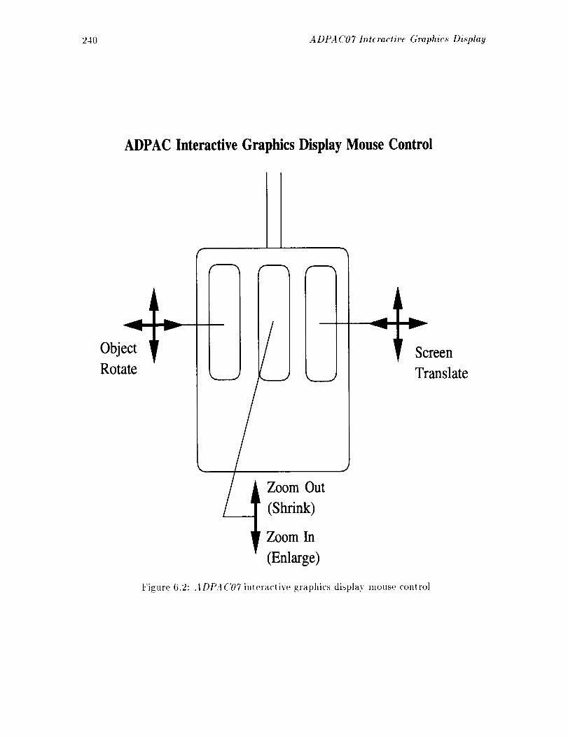
240 A DPA C07 lnt_ ractive Graphic._ Displag

ADPAC Interactive Graphics Display Mouse Control

Object

Rotate

v

///

/

¢,.. m %

/I

(,.m.,

V

Screen

Translate

Zoom Out

(Shrink)

Zoom In

(Enlarge)

Figure 6.2: A DPA('07 interactive graphics display mouse conlrol

A DP:t ('07 h_t: raetiv¢ (;raphic._ Di._play 2-t I

This l)ro_ran_ can only he rul_ Oll a Silicon (;ral)hics Workstatioll running al level 4.0.1

(o1' ahow,) of lhe IRIX operating syslem. ,ks such, compilation of lhe AGTI_L]-L('L pro-

gram has no options, and is performed simt)ly I)v executillg the comma,rid make in the

,t (; TPL 7"- L ('L sou r<'<, dir(wlory. Once illil iated, the A (; I'PL T-L ('L l>rogram waits for an

Ol1| S](]O [)roc,o,'-;H fl'Olll .'t I)P.4 ('07 !o <'ommunicale wilh the local workst alion, and graphi('s

commands received froln the remote joh arC' di._l)layed locally.

An intl)or'lalH consideration in selling up a remole calculation with local g:ral)hics display

usill_ ,I(;7PLT-L('L is the manner in which lho local display is defined ill lhe calculation.

Tho ('(;l, lihraries used io I)ormil the nelwork g:ral)hics inslruclions require all inlern(,l

lwlwo]'k address il, order io l)rot)erly l]'ansmi! the graphics colllmallds to the correcl desti-

nation. This definition sho,ld ho provided in lhe standard inpu! file followi.¢; lhe normal

koyword parameters (seo Seclio_l 3.6 for a saml)lo tik' and kewvovd dt, finiliol,s). A1 lh(, (,t,(I

of tho sla_l(lard inpul k(,vword dala, the user ,_hould ,,_(' a_ ENDINPUT slalolnenl to

lermiual(, the normal input stream. The ENDINPUT slaleme,! sho,ld lll(,n he t'ollow('d

hy two hlal_k lines, and lhen a lille containing lhe destination network a(l<tr(,ss of the lo-

cal Silicon (;ral)hics disl)lay d('vice. Thi_ sl)ecilical ioll will ullimalelv t)(, read hv I he ( '(; L

lihraries in selling uI) the network <'onneclion.

Tho procedure to set u 1) this nolwork-c(mnecled _:ral)hics display option would he to slarl the

joh oll lhe remole machino, and then immedialolv slarl lhe A(;TI'LT-L('L program on the

local di,_l)lay. :ks I(mg as 111(,correct nelwork ad(Iross ha,_ he(,n onlered hi 111('c_/._.input til('.

then lho l'emole l)rOgranl should ho_:in communicaling: wilh lhe :| (; TI'L I'-L('L program,

all(I lho local graphics wi.dow will t)<,gill (lisl)layillg the g;raphics inslruclions ,_t)ecified t)v

lhe retool(, computing i)ro_ranl.

242 .4DPA CO 7 Int¢ raetiv_ Gr_,ph ic.__Di._'play

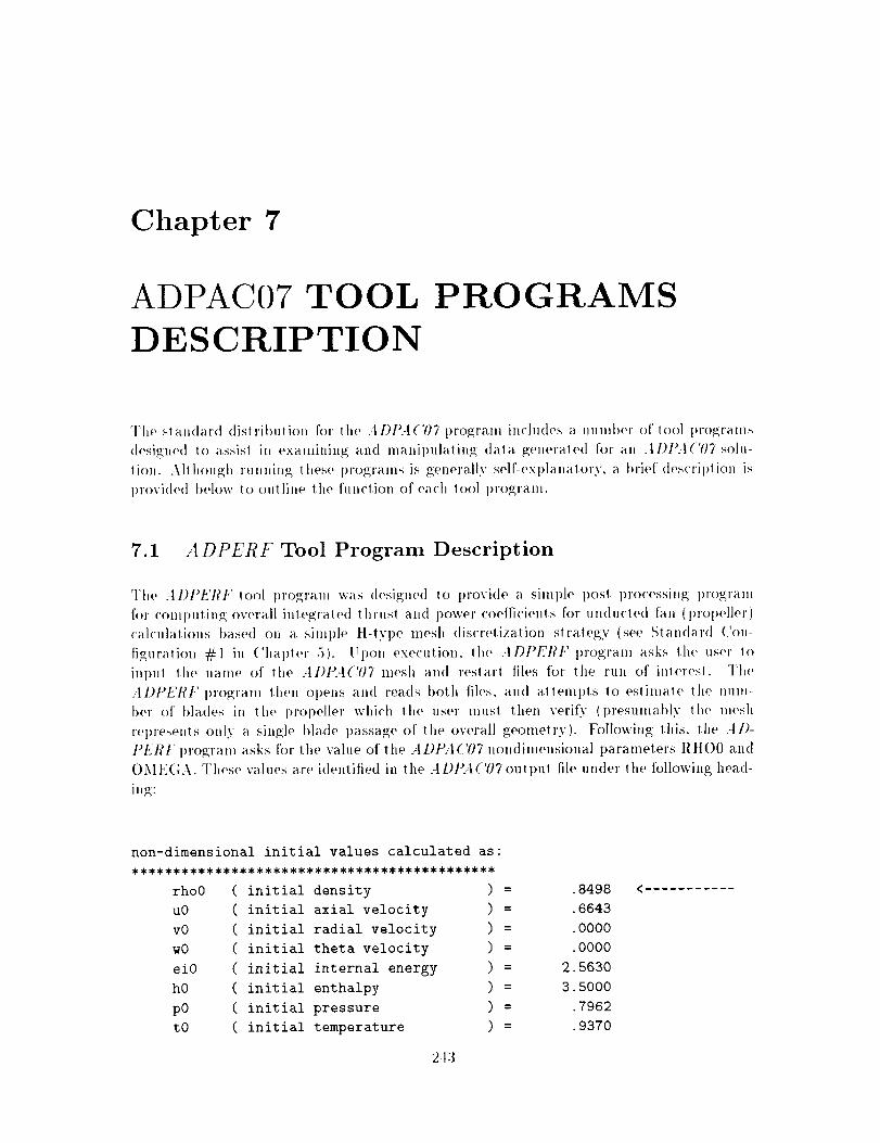
Chapter 7

ADPAC07 TOOL PROGRAMS

DESCRIPTION

The st andard dist ribulion for I he .t Dlbt ('07 progranl includes a munber of tool programs

designed 1o assisl in examining and manipulating dala generaled for an ADI'.t('07 solu-

lion. Allhoug;h running lhese programs is generally self-exl)lanalory, a I)rief <les('ril>lion is

provided below to outline lhe function of each tool program.

7.1 ADPERF Tool Program Description

The AI)PERF fool progranl was designed lo provi<le a simt>le pos! l)ro<'essing program

for COmlmting; overall integrated thrusl and t>ower coefficients for unducted fan (prol>eller)

cah'ulatiotls based on a simple H-tyl)e mesh discretization stralegy (see Stan<lar<l ('on-

tiguralion #l ill ('hapter 5). Ul)ol_ execution, the ADPERF l)rogranl asks lhe user t<)

inI)ul the name of the ADPA('07 mesh and reslart files for the run of inlerest. The

ADI>ERI .' program then opens and reads bolh tiles, and a llenlpts 1o eslimale the num-

ber of blades in the ]>ropeller which the user mus! then verify (presumably the l||esh

represents only a single blade passage of the ow, rall geomelry). Fbllowing this. the AD-

PERI,' program asks for the value of the ADPA('07 nondimensional parameters RtlO0 and

OMEGA. These values are i<lentified in the A DIL4C07 output file under the following head-

ing:

non-dimensional initial values calculated as:

rhoO ( initial density ) =

uO ( initial axial velocity ) =

vO ( initial radial velocity ) =

wO ( initial theta velocity ) =

eiO ( initial internal energy ) =

hO ( initial enthalpy ) =

pO ( initial pressure ) =

tO ( initial temperature ) =

2.13

.8498

6643

0000

0000

2 5630

3 5000

7962

9370

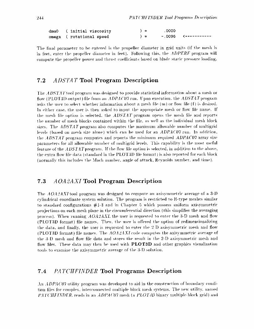
244 PA TCttFINDER Tool Progmm._ D¢scriptio_

dmuO ( initial viscosity

omega ( rotational speed

) = .0000

) = -.0096

Tile final t)arameter to be entered is tile propeller diameter in grid units (if the mesh is

in feel,, enter the propeller diameter in feet). Following this, the ADPERF progranl will

compute lilt, propeller power and thrust coefficients based on blade static pressure loading.

7.2 ADSTAT Tool Program Description

The ADST:t T lool program was designed to provide statistical information about a mesh or

flow (PLOT31) oul pul) file from an A DPA ('07 run. Upon execution, the A D,S'TA T program

asks the user to selec! whether informalion aboul a mesh file (m) or flow file (f) is desired.

In either case, the user is then asked to input the apl)ropriale mesh or flow file name. If

the mesh file option is selected, the AD,S'TAT program opens lhe mesh file and reports

the number of mesh blocks contained within the file, as well as lhe individual mesh block

sizes. The AD.S'TAT program also computes the maximum allowable number of mulligrid

levels (based on mesh size alone) which can be used for an ADPAC07 run. hi addition.

t he ,4 DSTA T 1)rogra,m computes and reports the minimunl required A DPA (:'07 array size

paramelers for all allowable number of mnltigrid levels. This capability is tile most useful

feat ure of t he A DSTA T program. If t he flow file option is selecled, in addi!ion to t he above.

the extra flow tile data (standard in the PLOT3D file formal) is also reported for each block

(normally this includes lhe Ma,ch number, angle of attack, Reynolds number, and lime).

7.3 AOA2AXI Tool Program Description

The AOA2AXI tool wogram was designed to compute an a xisymmelric average of a 3-D

cylindrical coordinate system solution. The prograin is restricted lo H-type meshes similar

to standard configurations #1-3 and in Chal)ter 5 which possess uniform axisymmetric

projections on each mesh plane in the circumferential direction (this simplifies the averaging

process). When running AOA2AXI, the user is requested to enter the 3-D mesh and flt)w

(PLOT3I) formal) file names. Then, the user is offered the ol)tion of redimensionalizing

the data. and finally, the user is requested to enter the 2-D axisynlmetric nlesh and flow

(PLOT3D format) ill(, names. The AOA2AXI code comt)ules the a xisymmetric average of

lhe 3-D mesh and flow file data and stores the resul! in the 2-D axisymmetric mesh and

flow files. These data may then t)e used with PLOT3D and other graphics visualization

tools to examine the a,xis.vmlnetric average of the 3-I) solution.

7.4 PATCHFINDER Tool Programs Description

An A DPAC07 utility program was develol)ed to aid in the construction of boundary condi-

lion files for comt)lex, intercomlected mullil)le block mesh SVStOIIIS. The new utility, nanled

P.4 I'('tfFINDER. reads ill all ADPA('07 mesh (a PLOT3D t)inarv multil)le-block grid) and

PLOT3D 7bol Program._" Dt._criptim_ 215

determines which blocks share matching faces. As the grid is rea<l, the faces are striped off

into a separate array, hldivi<lual points Oll these faces are <'ompared until a "'point'" match is

found. Neig;hboring points are then compared to find a "'cell'" match. This also delermilws

the relative directions of the 1hatching indi<'ies. From this ('ell match, a common face area

is sv(e[)l out and a PATCH l>out,(larv condition st,a,l, elllelll is wrillell llS]llg llle bounding

indicies of the COIIIIIIOII face area.

After all lhe PATCH specilicatiolls have been wrillen, any remaining; surfaces nol ac-

counled for will have a solid surface wall (SSVI) I)oundary condition wrilten oul. This

allows the user I() simply replace a few solid ,,,,'all statements with the l)rol)er inlel and e×it

I)ounclarv condilions and slart running. The IL4T('ttI:INI)I¢I? user inpul tile conl ains ap-

l)roximalely ten variables Io cuslomize a t_4 T('lll:INl)Ell run to each grid all hough many

grids can l>e processed without special input. Since the majority ofl)ouxldarv conditions

prescrit)ed in mosl geometries are block 1)alches and solid walls, running I_t T('III.'INDER

``,.'ill greally simplify lhe generation of a. I)oundary data file.

Several methods were implemented lo accelerate lhe t>A T('HFINDER search and compare

process. Some of these nwtho<ls include using multi-grid and bounding cube limits. If

a mesh is created to be run with Al)l)A('O7using mulli-grid, this can also 1)e used to

accelerate P,t T('It[:INI)EI? since boundary conditions musl l>e consis/enl across multi-grid

levels. Ea('h level of muir i-grid decreases the number of fact, poinl s bv a factor of.l: I herefove.

wilh :_ levels of multi-grid a decrease in run time of roughly sixteen times can l>e e×pected.

The bounding cube lind! melhod creales a limiling cul)e enclosing all the cell cenlers of

a block face. tlefore any indivi<lual face points are checked, the correspoudhig bounding

cubes are checke<t for intersection. If the cubes do not intersect, then no nialchin_ poinls

are possit)le; this greally reduces lhe number o[' individual point searches.

Sew'ral lest cases were rult using t5t T('IIFINDER. These included bolh 2-1) and 3-I) g;eome-

tries with and without mulli-gri<l. Each of these runs was timed loevaluate lheefficiency

of lhe program. The resulting approximate wall clock times are shown in lhe table in Fig-

ure 7.1. All cases were run on the same machine under similar conditions so lhat relalive

comparisons can be made. Most of the lest cases using mulli-grid finished in under two

Illil|ules. One of l lie largest and lnosl complex lesl cases was based on a nlesh wilh over

,IS0,000 poinls and o``'er S00 malching faces. PAT('HF1NDts'R was able 1o correctly idea(it)"

all lhe 1)alches in under 17 minules (on a Silicon Graphics 4D-35 workstatioll) as opposed

to lhe apl)roximalely two days re<luired to correclly specify the PATCH conneclions I)5'

hand. The 151"I('ttH?_:DEIt time was limited in lhis case since the grid conlained only one

level of multi-grid, t;'rom the times re(or<led in the lane. the advantage of using multi-grid

becomes apparent.

7.5 PLOT3D Tool Programs Description

A number of tool programs originally generated for the t>LOTdD program are included with

t he A I)PA ('07 distril)ution I)ecause of their useflllness in manit)ulating ,t DI-'A ('07 mesh

an<t flow (PLOT3D output [brmat ) files. A brief <lesc'ril>tion of lhese codes is given I>e_ow.

I1 should I)e noted that rues! of lhese programs are designed to deal wilh unformatted

files, rather than the ADP, I('07 standard binary format. Fortunately, the PLOI'/H)of

f]IN2U),T 1ool programs <'all be use<l to collvert fronl A1)I{t(7)7 binary to unR)rmatled,

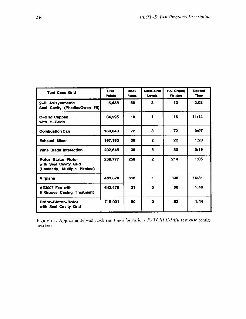
246 PL 0 T3D Tool Progr, m,_ De._cript io7_

Test Case Grid

2-D Axisymmetric

Seal Cavity (Phadke/Owen #5)

O-Grid Cappedwith H-Grids

Combustion Can

Exhaust Mixer

Vane Blade Interaction

Rotor-Stator-Rotor

with Seal Cavity Grid

(Unsteady, Multiple Pitches)

Airplane

AE3007 Fan with

5-Groove Casing Treatment

Rotor-Stator-Rotor

with Seal Cavity Grid

Grid

Points

Block

Faces

Multi-Grid

Levels

5,438 36 3

PATCH(es)

Written

12

Elapsed

Time

0:02

34,595 18 1 16 11:14

160,040 72 3 72 0:07

197,190 36 2 22 1:23

232,645 30 3 30 0:19

214258259,777 2 1:05

483,876 618 1 808 16:31

642,479 21 3 50 1:46

715,001 90 3 62 1:44

Figure 7.1: Approxima, t e wall clock run times for various PA T('HI:'INDI_'tg test case config-

urations.

PLOT3D Tool Progroms D( scriplio, 2-17

and the MAKI'.'AD(;RID program may be used to convert from unformatted format lo

:t DISt ('07 binary.

• CHOPQ ('ut a sul)sel oul of a (31), single grid) I)LOT3I) Q file and write it out as

a new Q file.

• CHOPX ('ul a sul)sel oul of a (31). single grid) PIX)T31) XYZ file and wrile it oul

as a new XYZ lile.

* CHOPXB (!ut a subset out of a (3I), single grid) PIX)T31) XYZ+IBI_ANK file and

write il out as a new XYZ+IBLANK file.

• COMBINEQ (2)ml}ine several (31), single grid) I)I,OT31) Q files inlo a new mullil)]e

g;ri<l Q [ile.

• COMBINEX ('ombine several (31), single grid) PI,()T3I) XYZ files inlo a new mui-

liple grid XYZ file.

• COMBINEXB ('ombine several (3I), single grid) t)I_{)T31) XYZ+IBI.ANi( files into

a new muli iple grid XYZ+II_I_,.\NI( tile.

• IJK (;enerale a (3I), single grid) t)I_OT:31} XYZ file which is simply lhe {'omputational

grid, i.e. (x,y.z)=(i.j,k). Good for looking al flow quanlilies in the eoml)ulational

domain.

• INT3D Interpolate a (3D, single grid) PIA)T3I) Q file fronl one grid onlo anolher.

Old and new XYZ files may have IBLANK. Various options availal}le on whal 1o do

if a new grid l}oin! isn'! found wilhin the old grid. Uses l rilinear inlerl)olalion.

• MIRRORQ Flip a (3I), single grid) PLOTaD Q file al)oul lhe x-. y-. or z-axis.

• MIRRORX l:lit) a (3I). single grid) PLOT3D XYZ file at)oul lhe x-. y-. or z-axis.

• PROPER2D Perform 21) grid line ('tossing check on a (2I), single grid) I)L{)T:II)

XYZ file.

* PROPER3D Perform lelrahe(h'on deeompositioll cell volume cheek on a (3D, single

grid) PI_OT3I) XYZ file.

• PROPER3DN Perform lelrahe{lron decomposition grid crossing cheek on a (3D,

single grid) PLOT3D XYZ file.

• REFINEX (;enerate a new (3D. single grid) PLOT3D XYZ file which is an integer

refinemenl of an existing grid file. Uses paranwlric cubic inlerpolatiou.

• ROTATEX t{olale a (3D. single grid) PLOT3D XYZ file a boul the x-, y-, or z-axis.

• SCALEX Seal(' a (3D. single grid) PLOT3D XYZ file.

• SCALEX Scale a (31), single grid) PLOT3I) XYZ+IBIM.NI,_ file.

* SPLITQ SI)lil a (31)) multiple grid I'LOT3I) Q file inlo set)arale single grid Q files.

(:an skip grids if desired.

24S PLOTBC Tool Program._ De._cription

• SPLITX Split a, (3D) multiple grid PLOT3D XYZ file into separate single grid XYZ

files. Can skip grids if desired.

• SPLITXB Split a (3D) multiple grid PLOT3D XYZ+IBLANK file into separate

single grid XYZ+IBLANK files. Can skip grids if desired.

• TRANSLATEX Translate a (3D. single grid) PLOT3I) XYZ file.

• TRANSLATEXB Translate a, (3D, single grid) PLOT3D XYZ+IBLANK file.

The UNIX mak_ command may be used to compile and link the I)I_OT3D tools as follows:

2xxx/3xxx: make -f Makefile.i2

CRAY 2: make -f Makefile.c2

VAX/VMS: @MAKEFILE.VMS

7.6 PLOTBC Tool Programs Description

In order to facilitate a gral)hical exa.minatioll of an ADPA('07 boundary data file, a utility

program called PLOTB(' was created. The PLOTB(' program reads in a user-specifiable

ADP.4('07 mesh and boundary data file and creates five PLOT3D-compatible command

files. The five command files, in conjunction with the mesh file. l>ern6ts the user to gral)hi-

cally examine (using the PLOT3D wogram) a num|)er of features of the mesh conslruction

and boundary condition specifications. This utility provides a rapid means of assessing the

completeuess of a boundary data file and provides a visual method for determining the

characteristics of an ADPA ('07 computational model.

The PLOTB(' program is invoked by siml)ly running the executable as follows:

plotbc

The at)propriate l)ath to the executable may also have to be specified if the executable file

is no! locally available. The user is !hen prompted for the ADPA('07 ca._( name as tbllows:

Enter ADPAC case name:

After entering the case nanle, the PLOTB(' progranl reads in the ADt{4('07 mesh and

|)Oulldary data files, extracts the boundary conditions at|(1 organizes I]len| into categories.

Each category is then used to construct a PLOT3D command file which allows the user 1o

visualize all boundary conditions in a common category. The resulting PLOT3D conlmand

files and their fimctious are listed in Table 7.6. Each of the ADPA('07 boundary condi-

tions identified by PLOTB('is color-coded such that all the con,mand files can be read

sequentially, thus displaying all the boundaries at once.

Once created, the PLOTBCconlmand files may be used with PLOT3D by reading in the

corresponding mesh file, and then invoking one or nlore of the scripts as shown below:

PLO TB(' 7bol Programs D( scription 249

PL Ol"]D Command Function

File Name

axes.('Olll

inloxt .corn

solid.ct) m

oIll line.conk

l,alch.conl

Grid index orientation

Intlow/out flow boundaries

Solid surfaces

(viscous and inviscid )

(rotating and non-rola!ing;)

Mesh t>lock outline

lnler-I)lo('k PATCH I)oundal'ies

Table 7.1: PLOT'B(' command file names all([ boundary ('ondilioll ('aleg;()ries

UNIX PROMPT> plot3d

Once the t't()l':]l)program is initialized, lhe mesh file should I)e read in using the slan(lar<t

PLO1.]D commands, and lhen lhe <'ommal_d files may I)e invoked I>y a comlnan(l such as:

PLOT3D V3: @outline

The a('lion oflhe<'ommand file is toessenlially define whal is lol)e plolled. The a('lual

[)lolling is not l)erforme<l unlil lhe user enters the t)lol command al lhe PLOI'31) l)rOml)l.

A(hlilional (Imails may t)e found in lhe PLOT3D User's Manual [l-l].

250 PLOTB(' Tool Progr(m_8 D(scriptio_

Bibliography

Ill

[3]

Is]

[_]

7]

[9]

tlall. E..1.. and l)elaney, R. A., "lnvestigalion of Advanced (%unterrolation Blade

(!onfigural ion (!oncepls for [tigh Speed Turbopro 1) Syslems: Task VII - AI)PA(! l:ser'.s

Manual." NASA ('onlract N/\$3-25270, NASA ('ll 195.172, .luly, 1995.

Hall. t"..l., Topp. I). A., Heidegger, N..l.. and I)elaney. R. :\., "'Illw, stigatio,I of

Advanced (!ounlerrotation Blade (lonfiguration (!oncep!s tot tligh Speed Turboprop

Systems: Task VII - Endwal[ TRealmenl Inle! Flow l)islorlion Analysis Final Re-

porl,'" NASA ('onlra¢'t NAS3-25270, NASA (IR-19516,_, July, 1995.

Itall, E. ,I.. Topp, 1). A., lleidegger. N. ,1.. and l)elaney, tl. A.. "qnvestigalion of

Advanced ('ounterrotation Blade (lonfiguration (1oncepts for High Speed Turbol)rop

Svslems: Task VII1 - Cooling Flow/lleat Transfer Analysis, Final Report," NASA

( 'ont tact N AS3-25270, NASA ( 'R- 195359, Seplember, 1994.

ttall. E. J. and I)elaney. R. A., "'Investigation of Advanced (lounterrolation Blade (:on-

[iguralion (loncepls for lligh Speed Turbol>ro p Systems: Task V- Unsleady (!Olllllel'-

re!alien l)ucted l>ropfan Analysis, Final Report ,'" NASA ('1{ IS7126. NASA (lonlra<'t

NAS3-25270, 1992.

Hall. E..I., I)elaney, R. A., and Bettner, J. I,., "Investigation of Advanced ('oun-

terrotation Blade ('onfiguration (_oncepts for [tigh Speed Turboprop Systems: Task

II - Unsteady l)ucted Propfan Analysis, Final Report," NASA (IR 1_7106, NASA

('ontract NAS3-25270, 1991.

tlall, E..1., l)elaney, R. A.. and Betlner, J. L.. "qnvestigalion of Advanced ('ounler-

rotalion Blade (!onfiguration ('oncepts for High Speed Turboprop Syslems: Task II

- lTnsteady 1)ucted Prol)fan Analysis, ('omputer Pr()gram Users Manual," NASA (!R

1,";7105, NASA (:ont rac! NAS3-25270, 1991.

Rao, K. V., and l)etaney. R. A., 1990, "Investigation of Unsleady Flow Through a

Transonic Turbilw Stage: Par1 I- Analysis," AIAA Paper 90-2408.

.Iorgensou. P. ('. E.. and Chima, R. V., "'An Unconditionally Stal)le Runge-I'_utla

Method for Unsteady Flows," AIAA Pal)er 89-0205, 19S9.

Adanlczyk, ,1..l., "'Model Equation for Simulal ing Flows in Ikl ult is! age Tu rl)oma('hill-

cry.'" ASME Paf)er S5-(;T-226, 19S5.

251

252 PLOTBU Tool Program._ D_,_c'riptio_

[lO]

Ill]

[12]

Dawes, W.N., "Multi-Blade Row Navier-Stokes Simulations of Fall Bypass ('onligu-

rations", ASME Paper 91-GT-148, 1991.

('rook, A. J.. and Delaney, R. A., "Investigation of Advanced Counterrotation Blade

('onfiguration (_oncepts for High Speed Turboprop Syst, ems: Task IV - Advanced Fan

Section Analysis, Final Reporl,'" NASA (IR 18712_. NASA (_ontract NAS3-25270,1992.

Rat. M. M., "'Unsteady Three-Dimensional Navier-Stokes Sinlulalions of Turbine

Rotor-Stator Interaction." AIAA Paper s7-205g. 1997.

[13] Whipple. D., "'BI)X-Binary Data Exchange Preliminary Information," NAS:\-LewisResearch Center, IW,9.

[11]

[1.5]

[161

[lr]

[is]

[19]

[2o]

[21]

[22]

Walatka, P. P., and Buning, P. G., "'PLOT3I) User's Manual,." rough draft for NASA

TM, 19SS.

Ptessel, Todd, "SURF User's Guide,," NASA Ames Research ('enter, 19ss.

Walatka, P. P., and Buning, P. G.. "FAST," NASA Ames Research (:enler. 1990.

tlall, E. J.. Delaney, R. A., and Bettner, J. L., "'Invesligation of Advanced (!ounter-

rotation Blade Configuration Concet)ts for High Speed Turboprop Systems: Task I -

Ducted Propfan Analysis." NASA CR 185217, NASA ('onlra('t NAS3-25270, 1990.

(:rook. A. J., and Delaney, R. A., "'Investigation of Advanced (!ounterrotation Blade

Configuration Concepts for High Speed Turboprop Systems: Task Ill - Advanced FanGrid Generation," NASA CR 1_7129, NASA Contract NAS3-2.5270. 1991.

J. Steinbrenner et. al. "Th_ Gridg¢u 3D Multipb Block Grid (;(,¢ratio, ,qyst¢m..'"

Final Report WRD(!-TR-90-3022, 1990

Arnone, A., "'Notes o, th: lr._e of the TRAF ('O&S..'" Departlnent of Energy Engineer-

ing. University of Florence, and Institute for C,omlmtational Mechanics in Propulsion,NASA Lewis Research Center, November, 1992.

Hall, E. J., Topp, D. A., Heidegger, N. J., and Delaney, R. A., "Ixlvestigation of

Advanced Counterrotation Blade Configuration (:oncepts for High Speed Turbol)ro I)

Systenls: Task VII - Unsteady Inlet Distortion Analysis," to be l)ut)lished.

Quealy, A., Cole, (;., and Blech, R., "Portat)le l)rogl'amlnillg on Parallel/Nelwork

(:omputers Using the Al)l)lication Portable Parallel Library (APPL),'" NASA TM-

10623S, July, 1993.

Appendix A

ADPAC07 DISTRIBUTION AND

DEMONSTRATION

INSTRUCTIONS

A.1 Introduction

This apt)endix describes the commands necessary to extract the source ('ode and delno

51es from the A DPA ('07 stan(laM (list rit)ution and run a ('Oml)lele lest case for a ducte<]

fan elnl)loying multiple t>lade rows. The standard A DI>A('07 distribution is a comt)ressed

tar file whi<'h can be deco(le(l into lhe various l)arts 1)v a sequence of commands on any

slan(lard I'NIX system. The sequence listed below is inlende(I to guide lhe user through

the selup from the slan(lard dis!ril)ution Ul) to and including a complete demonslralion of

a calculation fora ducted propfan employing multiple blade rows. The command se(luence

listed below should work oi, mosl svstelns en,l)loying the ['NIX ol)erating svslem. Since

portions of this process are inherently machine-(lel)en(lenl, the exacl commands lisled here

are for a Silicon (;ral)hi('s Workstation running the IRIX Operating System, Revisi<)ll :[,().1.

Alternale commands will be listed when a signiticant machine <lel)endence exists.

A.2 Extracting the Source Files

The .ll)PA(7]7 programs are distributed an a compressed ta'r file named

adlmcO7, tar.Z

This tar file re<tuires roughly 22.0 megabytes of disk space. It shou]<l I)e 1)ossit)le t<) exlract

and run the co([e on any slan(lard UNIX system t¥om this distribution file. The first slep

necessary to exlract the AI)t)A('07 programs is to unCOlnt)ress the tot file with the com-

lllall([:

uncompress adpac07.tar.Z

253

254 ADPAC07 Distribution and D_monstmtion In._truction.s

This operation essentially replaces the compressed file adpacOT.tar.Z with all uncompressed

file adpacO7.tar. The uncompressed tar file requires approxilnately 41.0 megabytes of disk

space.

The next step is to extract the individual files and directories from the .dpacO7.tar file. The

tar command will create a subdirectory named adpac07 in the current directory, so il is up

to the user to move tile adpacO7.tar file to a suitable initial directory before extracting the

embedded subdirectories. Once the tar file is properly placed, the A DPA(Y)7 <listribulion

may be extracted with the command

tar xvof adpacO7.tar

(On some systems tar xvf adpacO7.tar may be sufficient.) Execution of tile UNIX list

cotumand Is -1 will verify that tile adlmc directory has been created. The complete extraction

t)rocess will require about 90.0 Megabytes of disk space (to hold the adpa('O7.tar file and

tile extracted contents).

The unc'ompress and tar steps can be combined ill a single ol)eration Oil lnos| IWIX systelns

by issuing tile command

zeat adpaeO7.tar.Z I tar xvf-

This combined operation conserves overall disk spa('e requirements during the extraction

process.

A.3 Compiling the Source Code

After extracting the source files, the user is naturally interested in compiling tile source files

for execution. A UNIX-compatit)le 3lak_ facility is provided for each of the ADPA 6'07 pro-

grams. Tile Jlak_fil¢ which governs tile coml)ilation process is necessarily machine-del)endenl

and requires that tile user select from one of a number of t)reconfigured syslelllS. The Mak(

commaud is fiflly described in Section 3.4. If no option is specified in the ma/_'f command,

then the standard UNIX compilation is performed.

In order to begin the compilation, it is firsl necessary to enter lhe adpac (tirectory with the

COllllUand:

cd adpac

At this poinl, several files and directories will I)e available. By entering tile UNIX command

Is -1, a listing of the individual directories can be obtained. The output of the ls (:ommand

will look something like:

README demo/ manual/ report/ src/

A Dt_4(Y)7 Di._tribution a,d Demon._tration hr_tructio_r_ 255

A description of each of these listings is given below:

REAI)ME This file is a general descril>lion of the contents of the directory.

dome This <tireclorv contains several geometry and flow input files for generaling

sami)le runs of the A DI>A ('07 co<los.

manual This <tiroclory contains lit(, L,T<Xsource co<te for lids manual. If LaT_X

is installed on your system, il is l)ossible to reproduce this (locumenl (ex-

cluding figures) with tit(, ('olumand latex manual. The result in?_; <levite

in<let>endenl file m<m,al.dvi may lhen l>e couverted to t),.',t,S'cript or l)re-

viewe<l on screen lhrough a number of wi<telv available routines.

rel>orl This (lireclory conlains lhe La77X source code for the final repot1 outlin-

ing the technical <letails of the ADtCt('07 <'o<les. If L<tT_X is installed on

your system, il is possible to reproduce the final tel>or! (excluding figures)

wilh the command latex report. The resulliu_; <levi<'e indel>en<lent file

.[i,alr<port.dvi may then be converle<l to l_o._tS;<'ril+t or l>reviewe(1 on screen

through a number of wi<lelv available routines.

src This direclor.v conlains all lhe FORTRAN source code f<)r the .l l)PA ( '07 pro-

7rams including ,<iET[:I >, RO TGI?ll). MA KLT11)(;IHI). and ,1 (,' TPL T-L( 'L.

II is now possibh, to compile lhe ADPA(7)7 code l>v issuing the <'omntands

ed sre/adpae

make

On a ('ca.,,'. lit<, command make tray is al)l>rot)riale, while on air IBM workslalion make

aix is al)propriate. Other COml>ilation options are availat)le by lyping; real'< h_lp. The

compilation of the executable mo<tule for A DI>A('07 will re<luire roughly 20 megabyles of

disk space.

A.4 Running the Distribution Demonstration Test Cases

Ollce the make facility has properly comt)leted comi>iling the ADPAC07 source code, it is

1)ossil)lo to run tit(, tes! cases t)rovided with the standard distribution. I! is recommended

thal the sample cases be tested to verify l)rol)er comt)ilation and extraction of the AD-

IL4 ('07 <list rit)ul ion.

In or(let to l'llll tile <]elnonsl rat ion cases, il is nocossa,ry lo begin in the demo directory.

Front lhe .:t DPA ('07 source code <lirectory. the <t_mo directory may be enlered l>v issuing

the command

ed ../../demo

Several test cases are l>rovi(led wilh the standard (tislril)ution lo illustrate lhe el)era<ion

of the code for many difl'erenl al)l)licalions. The commands nee<led to run any demo are

similar, s<)<)nlv lit(, case listed under the (life<tory nasa will I>e explaine<l in detail here.

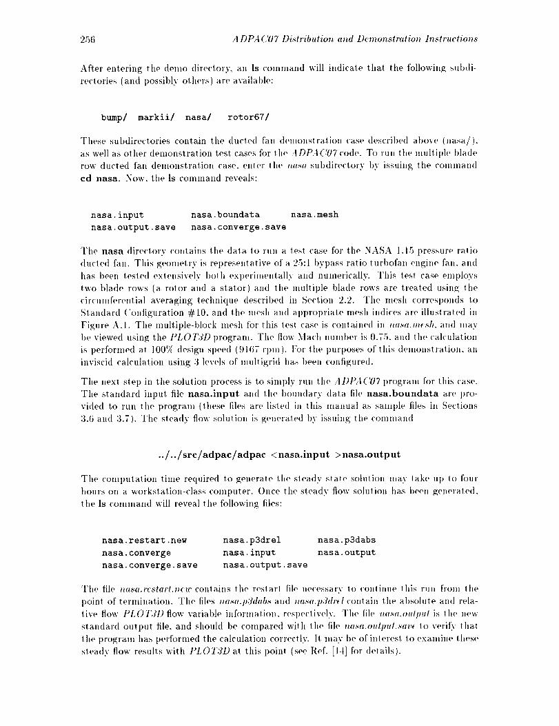
256 ADPAC07 Di._tribution and Demonstratiol, In._truction.s

After entering the demo directory, a.n Is command will indicate thai tile following subdi-

reclories (and possibly others) are available:

bump/ markii/ nasa/ rotor67/

These subdirectories contain the ducted fan demonstration case described above (nasa/).

a.s well a.s other demonstration test cases for the ADP,,t('07 code. To run the multil)le blade

row ducted fan demonstration case. enler tile _utsa sul)directory by issuing the conllnan(I

cd nasa. Now, the Is command reveals:

nasa.input

nasa.output.save

nasa.boundata nasa.mesh

nasa.converge.save

The nasa directory contains the data to run a tesl case for the NASA 1.15 t)ressure ratio

ducled fan. This geometry is ret)resenlative of a 25:1 bypass ratio ttlI'J)ofall engine fan, and

has been tested extensively both experimentally and numerically. This lesl case eml)loys

two blade rows (a rotor and a stator) and lhe multiple blade rows are trealed using the

circumferential averaging technique described in Section 2.2. The mesh corresponds to

Standard ('ontiguration #10, and 111(, mesh and al)prot)riate mesh indices are illustraled in

Figure A.I. The multiple-block mesh for this test case is contained in _ut._a.,t_,_h. and lnav

be viewed using the PLOTYD program. The flow Mach number is 0.75, and the calculation

is t)erformed al 100(7(, design speed (9167 rl)m). For tile l)uri)oses of lhis (lelnonslralion, an

inviscid calculation using 3 levels of multigrid has been contigured.

The next step in the solution process is to siml)ly run tile ADIM('071)rogram for this case.

The standard input file nasa.input and tile boundary data file nasa.boundata are pro-

vided to run the program (these files are listed in this manual as sample files in Seclions

3.6 and 3.7). Tile steady flow solution is generate(l by issuing the COlnmand

../../src/adpae/adpac <nasa.input >nasa.output

The computation time required to generale the steadv slale solution may lake up to four

hours on a workstation-class computer. Once the steady" flow solution has been generaled.

the ls command will reveal the following files:

nasa.restart.new

nasa.converge

nasa.converge.save

nasa.p3drel

nasa.input

nasa.output.save

nasa.p3dabs

nasa.output

The file nasa.re'._tarl.l_w conlains the restart file necessary to continue lhis run fl'om the

poinl of termination. The files _ax,.pYdabs and im._a.p3dt, l conlain the al)solute and rela-

tive flow PLO'I'3D flow variable information, respeclively. The file _m._a.outpul is lhe new

standard output file, and should be compared wilh the file _msa.outpul.sav_ lo verify lhal

the program has performed tile calculation correclly. Ii may be of intel'esl to examine lhese

steady' flow results with PLOTdD a.t this l)Oinl (see Ref. [1-1] for delails).

A DPA ('07 Distrib_ttioJ_ al_d l)emon._tratio_ ll_str_tctiot_s 257

NASA 1.15 Pressure Ratio Fan Test Case Description

Axisymmetric Mesh View

i

Mesh Block Structure

Block #1

(129x17x17)

Block #4

(97x17x17)

i=33

Block #3

(97x17x17)

i=81 i=113 i=17 i=49

Figure A.I: NASA 1.15 pressure l'alio fan tesl case

25_; ADPAC07 Distribution and Demonstration Instructiol,.s

NASA 1.15 Pressure Ratio Fan Test Case

-21

3 t ................ _. - Convergence History .................... ADPAC

D

r,

--'-" -4 i':, ............................................................

4 | ................................:_.;_..........................................

.-.1 -61..........................................................."';, ................

-7i ...............................................................................

-810 100 200 300

Iteration Number

Figure A.2:ADP.4('07 (lonvergence History h)r NASA 1.1.5 Pressure Ratio Fan Test (!ase

A plot of the convergence history for this case is given in Figure A.2. The "'juml)S'" in the

residual history are a resull of the "'full" multigrid startup procedure, and should not be

considered inappropriate.

The standard outt)ul file nasa.output should be compared with the listing provided in

Section 3.10 to make sure l,hal lhe code has l)erforme(t the calculation pr<)l)erly.

I Form ApprovedREPORT DOCUMENTATION PAGE OMB No. 0704-0188

Public reporting burden for this collection of information is estimated to average 1 hour per response, including the time for reviewing instructions, seamhing existing data sources,

gathering and maintaining the data needed, and compiling and reviewing the collection of information. Send comments regarding this burden estimate or any other aspect of this

collection of information, including suggestions for reducing this burden, to Washington Headquarters Services, Directorate for Information Operations and Reports, 1215 Jefferson

Davis Highway, Suite 1204, Arlington, VA 22202-4302, and to the Office of Management and Budget, Paperwork Reduction Project (0704-0188), Washington, DC 20503.

1. AGENCY USE ONLY (Leave blank) 2. REPORT DATE

April 1996

4. TITLE AND SUBTITLE

Task 7--ADPAC User's Manual

6. AUTHOR(S)

E.J. Hail, D.A. Topp, and R.A. Delaney

7. PERFORMING ORGANIZATION NAME(S) AND ADDRESS(ES)

Allison Engine Company

2001 S. Tibbs/P.O. Box 420

Indianapolis, Indiana 46206-0420

9. SPONSORING/MONITORING AGENCY NAME(S) AND ADDRESS(ES)

National Aeronautics and Space Administration

Lewis Research Center

Cleveland, Ohio 44135- 3191

i 3. REPORT TYPE AND DATES COVERED

Final Contractor Report

5. FUNDING NUMBERS

WU-5-03-11

C-NAS3-25270

8. PERFORMING ORGANIZATION

REPORT NUMBER

E-9662

10. SPONSORING/MONITORING

AGENCY REPORT NUMBER

NASA CR-195472

11. SUPPLEMENTARY NOTES

Pr_ectManager, ChristopherJ. Miller, Propulsion Systems Division, NASA Lewis Research Center, organization code

2770,(216) 433-6179.

12a. DISTRIBUTION/AVAILABILITY STATEMENT

Unclassified - Unlimited

Subject Category 61

This publication is available from the NASA Center for Aerospace Information, (301) 621-0390.

12b. DISTRIBUTION CODE

13. ABSTRACT (Maximum 200 words)

The overall objective of this study was to develop a 3-D numerical analysis for compressor casing treatment flowfields.

The current version of the computer code resulting from this study is referred to as ADPAC (Advanced Ducted Propfan

Analysis Codes-Version 7). This report is intended to serve as a computer program user's manual for the ADPAC code

developed under Tasks V! and VII of NASA Contract NAS3-25270. The ADPAC program is based on a flexible multiple-

block grid discretization scheme permitting coupled 2-D/3-D mesh block solutions with application to a wide variety of

geometries. Aerodynamic calculations are based on a four-stage Runge-Kutta time-marching finite volume solution

technique with added numerical dissipation. Steady flow predictions are accelerated by a multigrid procedure. An

iterative implicit algorithm is available for rapid time-dependent flow calculations, and an advanced two equation turbu-

lence model is incorporated to predict complex turbulent flows. The consolidated code generated during this study is

capable of executing in either a serial or parallel computing mode from a single source code. Numerous examples are

given in the form of test cases to demonstrate the utility of this approach for predicting the aerodynamics of modem

turbomachinery configurations.

14. SUBJECT TERMS

Computational fluid dynamics stall

17. SECURITY CLASSIFICATION

OF REPORT

Unclassified

18. SECURITY CLASSIFICATIONOF THIS PAGE

Unclassified

19. SECURITY CLASSIFICATION

OF ABSTRACT

Unclassified

15. NUMBER OF PAGES

262

16. PRICE CODE

AI2

20. LIMITATION OF ABSTRACT

NSN 7540-01-280-5500 Standard Form 298 (Rev. 2-89)

Prescribed by" ANSI Std. Z39-18

298-102

_ _i_ _ _ _

C_ CD _

oz CDo ._LIn

3