SYRCoSE 2019

Editors:

Alexander S. Kamkin, Alexander K. Petrenko, and

Andrey N. Terekhov

Preliminary Proceedings of the 13rd Spring/Summer

Young Researchers’ Colloquium on Software Engineering

Saratov, May 29-31, 2019

2019

Preliminary Proceedings of the 13rd Spring/Summer Young Researchers’

Colloquium on Software Engineering (SYRCoSE 2019), May 29-31, 2019 –

Saratov, Russian Federation.

The issue contains papers accepted for presentation at the 13rd Spring/Summer

Young Researchers’ Colloquium on Software Engineering (SYRCoSE 2019) held in

Saratov, Russian Federation on May 29-31, 2019.

The colloquium’s topics include software development frameworks, programming

languages, software and hardware verification, safety and security, automata and

Petri nets, information search, and others.

The authors of the selected papers will be invited to participate in a special issue of

‘The Proceedings of ISP RAS’ (http://www.ispras.ru/proceedings/), a peer-reviewed

journal included into the list of periodicals recommended for publishing doctoral

research results by the Higher Attestation Commission of the Ministry of Science and

Higher Education of the Russian Federation.

The event is sponsored by Russian Foundation for Basic Research (Project 19-07-20042).

Contents

Foreword ∙∙∙∙∙∙∙∙∙∙∙∙∙∙∙∙∙∙∙∙∙∙∙∙∙∙∙∙∙∙∙∙∙∙∙∙∙∙∙∙∙∙∙∙∙∙∙∙∙∙∙∙∙∙∙∙∙∙∙∙∙∙∙∙∙∙∙∙∙∙∙∙∙∙∙∙∙∙∙∙∙∙∙∙∙∙∙∙∙∙∙∙∙∙∙∙∙∙∙∙∙∙∙∙∙∙∙∙∙∙∙∙∙∙∙∙∙∙∙∙∙∙∙∙∙∙∙∙∙∙∙∙∙∙∙∙∙∙∙∙∙∙∙∙∙∙∙∙∙∙∙∙∙∙5

Committees ∙∙∙∙∙∙∙∙∙∙∙∙∙∙∙∙∙∙∙∙∙∙∙∙∙∙∙∙∙∙∙∙∙∙∙∙∙∙∙∙∙∙∙∙∙∙∙∙∙∙∙∙∙∙∙∙∙∙∙∙∙∙∙∙∙∙∙∙∙∙∙∙∙∙∙∙∙∙∙∙∙∙∙∙∙∙∙∙∙∙∙∙∙∙∙∙∙∙∙∙∙∙∙∙∙∙∙∙∙∙∙∙∙∙∙∙∙∙∙∙∙∙∙∙∙∙∙∙∙∙∙∙∙∙∙∙∙∙∙∙∙∙∙∙∙∙∙∙∙∙6

Tolerant Parsing using Modified LR(1) and LL(1) Algorithms with Embedded "Any" Symbol

A. Goloveshkin∙∙∙∙∙∙∙∙∙∙∙∙∙∙∙∙∙∙∙∙∙∙∙∙∙∙∙∙∙∙∙∙∙∙∙∙∙∙∙∙∙∙∙∙∙∙∙∙∙∙∙∙∙∙∙∙∙∙∙∙∙∙∙∙∙∙∙∙∙∙∙∙∙∙∙∙∙∙∙∙∙∙∙∙∙∙∙∙∙∙∙∙∙∙∙∙∙∙∙∙∙∙∙∙∙∙∙∙∙∙∙∙∙∙∙∙∙∙∙∙∙∙∙∙∙∙∙∙∙∙∙∙∙8

Development of a Software Framework for Real-Time Management of Intelligent Devices

T. Naumović, L. Živojinović, L. Baljak, F. Filipović∙∙∙∙∙∙∙∙∙∙∙∙∙∙∙∙∙∙∙∙∙∙∙∙∙∙∙∙∙∙∙∙∙∙∙∙∙∙∙∙∙∙∙∙∙∙∙∙∙∙∙∙∙∙∙∙∙∙∙∙∙∙∙∙∙∙∙∙∙∙∙∙∙∙20

Graphic DSL for Mobile Development

A. Gudiev, A. Grazhevskaya∙∙∙∙∙∙∙∙∙∙∙∙∙∙∙∙∙∙∙∙∙∙∙∙∙∙∙∙∙∙∙∙∙∙∙∙∙∙∙∙∙∙∙∙∙∙∙∙∙∙∙∙∙∙∙∙∙∙∙∙∙∙∙∙∙∙∙∙∙∙∙∙∙∙∙∙∙∙∙∙∙∙∙∙∙∙∙∙∙∙∙∙∙∙∙∙∙∙∙∙∙∙∙∙∙∙∙∙∙∙∙25

Graphical Modeling of Control Systems Based on Eclipse Technologies

M. Platonova∙∙∙∙∙∙∙∙∙∙∙∙∙∙∙∙∙∙∙∙∙∙∙∙∙∙∙∙∙∙∙∙∙∙∙∙∙∙∙∙∙∙∙∙∙∙∙∙∙∙∙∙∙∙∙∙∙∙∙∙∙∙∙∙∙∙∙∙∙∙∙∙∙∙∙∙∙∙∙∙∙∙∙∙∙∙∙∙∙∙∙∙∙∙∙∙∙∙∙∙∙∙∙∙∙∙∙∙∙∙∙∙∙∙∙∙∙∙∙∙∙∙∙∙∙∙∙∙∙∙∙∙∙∙28

Component-Based Software as a Tool for Developing Complex Distributed Heterogeneous Systems

D. Kulikov, V. Mokhin, S. Zolotov∙∙∙∙∙∙∙∙∙∙∙∙∙∙∙∙∙∙∙∙∙∙∙∙∙∙∙∙∙∙∙∙∙∙∙∙∙∙∙∙∙∙∙∙∙∙∙∙∙∙∙∙∙∙∙∙∙∙∙∙∙∙∙∙∙∙∙∙∙∙∙∙∙∙∙∙∙∙∙∙∙∙∙∙∙∙∙∙∙∙∙∙∙∙∙∙∙∙∙∙32

An Exploration of Approaches to Instruction Pipeline Implementation for Cycle-Accurate Simulators of

"Elbrus" Microprocessors

P. Poroshin, A. Meshkov∙∙∙∙∙∙∙∙∙∙∙∙∙∙∙∙∙∙∙∙∙∙∙∙∙∙∙∙∙∙∙∙∙∙∙∙∙∙∙∙∙∙∙∙∙∙∙∙∙∙∙∙∙∙∙∙∙∙∙∙∙∙∙∙∙∙∙∙∙∙∙∙∙∙∙∙∙∙∙∙∙∙∙∙∙∙∙∙∙∙∙∙∙∙∙∙∙∙∙∙∙∙∙∙∙∙∙∙∙∙∙∙∙∙∙∙36

Approach to Test Program Development for Multilevel Verification

P. Frolov∙∙∙∙∙∙∙∙∙∙∙∙∙∙∙∙∙∙∙∙∙∙∙∙∙∙∙∙∙∙∙∙∙∙∙∙∙∙∙∙∙∙∙∙∙∙∙∙∙∙∙∙∙∙∙∙∙∙∙∙∙∙∙∙∙∙∙∙∙∙∙∙∙∙∙∙∙∙∙∙∙∙∙∙∙∙∙∙∙∙∙∙∙∙∙∙∙∙∙∙∙∙∙∙∙∙∙∙∙∙∙∙∙∙∙∙∙∙∙∙∙∙∙∙∙∙∙∙∙∙∙∙∙∙∙∙∙∙∙∙42

Test Environment for Verification of Multi-Processor Memory Subsystem Unit

D. Lebedev, M. Petrochenkov∙∙∙∙∙∙∙∙∙∙∙∙∙∙∙∙∙∙∙∙∙∙∙∙∙∙∙∙∙∙∙∙∙∙∙∙∙∙∙∙∙∙∙∙∙∙∙∙∙∙∙∙∙∙∙∙∙∙∙∙∙∙∙∙∙∙∙∙∙∙∙∙∙∙∙∙∙∙∙∙∙∙∙∙∙∙∙∙∙∙∙∙∙∙∙∙∙∙∙∙∙∙∙∙∙∙∙∙46

Standalone Verification of IOMMU with Virtualization Supporting

A. Petrykin, I. Stotland, A. Meshkov∙∙∙∙∙∙∙∙∙∙∙∙∙∙∙∙∙∙∙∙∙∙∙∙∙∙∙∙∙∙∙∙∙∙∙∙∙∙∙∙∙∙∙∙∙∙∙∙∙∙∙∙∙∙∙∙∙∙∙∙∙∙∙∙∙∙∙∙∙∙∙∙∙∙∙∙∙∙∙∙∙∙∙∙∙∙∙∙∙∙∙∙∙∙∙∙∙∙51

Digital Modelling of Production Engineering for Metalworking Machine Shops

V. Kotlyarov, A. Maslakov, A. Tolstoles∙∙∙∙∙∙∙∙∙∙∙∙∙∙∙∙∙∙∙∙∙∙∙∙∙∙∙∙∙∙∙∙∙∙∙∙∙∙∙∙∙∙∙∙∙∙∙∙∙∙∙∙∙∙∙∙∙∙∙∙∙∙∙∙∙∙∙∙∙∙∙∙∙∙∙∙∙∙∙∙∙∙∙∙∙∙∙∙∙∙∙∙55

Reputation Systems in E-commerce: Comparative Analysis and Perspectives to Model Uncertainty Inherent

in Them

M. Nosovskiy, K. Degtiarev∙∙∙∙∙∙∙∙∙∙∙∙∙∙∙∙∙∙∙∙∙∙∙∙∙∙∙∙∙∙∙∙∙∙∙∙∙∙∙∙∙∙∙∙∙∙∙∙∙∙∙∙∙∙∙∙∙∙∙∙∙∙∙∙∙∙∙∙∙∙∙∙∙∙∙∙∙∙∙∙∙∙∙∙∙∙∙∙∙∙∙∙∙∙∙∙∙∙∙∙∙∙∙∙∙∙∙∙∙∙∙∙62

The Application of Machine Learning to Improve the Efficiency and Management of Oil Wells

Z. Aung, I. Mikhaylov∙∙∙∙∙∙∙∙∙∙∙∙∙∙∙∙∙∙∙∙∙∙∙∙∙∙∙∙∙∙∙∙∙∙∙∙∙∙∙∙∙∙∙∙∙∙∙∙∙∙∙∙∙∙∙∙∙∙∙∙∙∙∙∙∙∙∙∙∙∙∙∙∙∙∙∙∙∙∙∙∙∙∙∙∙∙∙∙∙∙∙∙∙∙∙∙∙∙∙∙∙∙∙∙∙∙∙∙∙∙∙∙∙∙∙∙∙∙∙∙∙74

Power Dispatcher Support System

D. Nazarkov, A. Prutik∙∙∙∙∙∙∙∙∙∙∙∙∙∙∙∙∙∙∙∙∙∙∙∙∙∙∙∙∙∙∙∙∙∙∙∙∙∙∙∙∙∙∙∙∙∙∙∙∙∙∙∙∙∙∙∙∙∙∙∙∙∙∙∙∙∙∙∙∙∙∙∙∙∙∙∙∙∙∙∙∙∙∙∙∙∙∙∙∙∙∙∙∙∙∙∙∙∙∙∙∙∙∙∙∙∙∙∙∙∙∙∙∙∙∙∙∙∙∙78

Applying High-Level Function Loop Invariants for Machine Code Deductive Verification

P. Putro∙∙∙∙∙∙∙∙∙∙∙∙∙∙∙∙∙∙∙∙∙∙∙∙∙∙∙∙∙∙∙∙∙∙∙∙∙∙∙∙∙∙∙∙∙∙∙∙∙∙∙∙∙∙∙∙∙∙∙∙∙∙∙∙∙∙∙∙∙∙∙∙∙∙∙∙∙∙∙∙∙∙∙∙∙∙∙∙∙∙∙∙∙∙∙∙∙∙∙∙∙∙∙∙∙∙∙∙∙∙∙∙∙∙∙∙∙∙∙∙∙∙∙∙∙∙∙∙∙∙∙∙∙∙∙∙∙∙∙∙∙∙83

Extracting Assertions for Conflicts in HDL Descriptions

A. Kamkin, M. Lebedev, S. Smolov∙∙∙∙∙∙∙∙∙∙∙∙∙∙∙∙∙∙∙∙∙∙∙∙∙∙∙∙∙∙∙∙∙∙∙∙∙∙∙∙∙∙∙∙∙∙∙∙∙∙∙∙∙∙∙∙∙∙∙∙∙∙∙∙∙∙∙∙∙∙∙∙∙∙∙∙∙∙∙∙∙∙∙∙∙∙∙∙∙∙∙∙∙∙∙∙∙∙∙∙90

Towards a Probabilistic Extension to Non-Deterministic Transitions in Model-Based Checking

S. Staroletov∙∙∙∙∙∙∙∙∙∙∙∙∙∙∙∙∙∙∙∙∙∙∙∙∙∙∙∙∙∙∙∙∙∙∙∙∙∙∙∙∙∙∙∙∙∙∙∙∙∙∙∙∙∙∙∙∙∙∙∙∙∙∙∙∙∙∙∙∙∙∙∙∙∙∙∙∙∙∙∙∙∙∙∙∙∙∙∙∙∙∙∙∙∙∙∙∙∙∙∙∙∙∙∙∙∙∙∙∙∙∙∙∙∙∙∙∙∙∙∙∙∙∙∙∙∙∙∙∙∙∙∙∙∙∙94

The Editor for Teaching the Proof of Statements for Sets

V. Rublev, V. Bondarenko∙∙∙∙∙∙∙∙∙∙∙∙∙∙∙∙∙∙∙∙∙∙∙∙∙∙∙∙∙∙∙∙∙∙∙∙∙∙∙∙∙∙∙∙∙∙∙∙∙∙∙∙∙∙∙∙∙∙∙∙∙∙∙∙∙∙∙∙∙∙∙∙∙∙∙∙∙∙∙∙∙∙∙∙∙∙∙∙∙∙∙∙∙∙∙∙∙∙∙∙∙∙∙∙∙∙∙∙∙∙∙∙∙∙99

Local Search Metaheuristics for Solving Capacitated Vehicle Routing Problem: A Comparative Study

E. Beresneva, S. Avdoshin∙∙∙∙∙∙∙∙∙∙∙∙∙∙∙∙∙∙∙∙∙∙∙∙∙∙∙∙∙∙∙∙∙∙∙∙∙∙∙∙∙∙∙∙∙∙∙∙∙∙∙∙∙∙∙∙∙∙∙∙∙∙∙∙∙∙∙∙∙∙∙∙∙∙∙∙∙∙∙∙∙∙∙∙∙∙∙∙∙∙∙∙∙∙∙∙∙∙∙∙∙∙∙∙∙∙∙∙∙∙∙∙109

3

The Generalized Traveling Salesman Problem: Modifications and Ways of Solving

M. Gordenko, S. Avdoshin∙∙∙∙∙∙∙∙∙∙∙∙∙∙∙∙∙∙∙∙∙∙∙∙∙∙∙∙∙∙∙∙∙∙∙∙∙∙∙∙∙∙∙∙∙∙∙∙∙∙∙∙∙∙∙∙∙∙∙∙∙∙∙∙∙∙∙∙∙∙∙∙∙∙∙∙∙∙∙∙∙∙∙∙∙∙∙∙∙∙∙∙∙∙∙∙∙∙∙∙∙∙∙∙∙∙∙∙∙∙∙∙119

Constructive Heuristics for Capacitated Vehicle Routing Problem: A Comparison Study

E. Beresneva, S. Avdoshin∙∙∙∙∙∙∙∙∙∙∙∙∙∙∙∙∙∙∙∙∙∙∙∙∙∙∙∙∙∙∙∙∙∙∙∙∙∙∙∙∙∙∙∙∙∙∙∙∙∙∙∙∙∙∙∙∙∙∙∙∙∙∙∙∙∙∙∙∙∙∙∙∙∙∙∙∙∙∙∙∙∙∙∙∙∙∙∙∙∙∙∙∙∙∙∙∙∙∙∙∙∙∙∙∙∙∙∙∙∙∙∙125

Solving the Generalized Traveling Salesman using Ant Colony Algorithm with Improvement Local Search

Procedures

A. Inkina, M. Gordenko∙∙∙∙∙∙∙∙∙∙∙∙∙∙∙∙∙∙∙∙∙∙∙∙∙∙∙∙∙∙∙∙∙∙∙∙∙∙∙∙∙∙∙∙∙∙∙∙∙∙∙∙∙∙∙∙∙∙∙∙∙∙∙∙∙∙∙∙∙∙∙∙∙∙∙∙∙∙∙∙∙∙∙∙∙∙∙∙∙∙∙∙∙∙∙∙∙∙∙∙∙∙∙∙∙∙∙∙∙∙∙∙∙∙∙∙131

Administration of Virtual Data Processing Center over OpenFlow

V. Solovyev, A. Belousov∙∙∙∙∙∙∙∙∙∙∙∙∙∙∙∙∙∙∙∙∙∙∙∙∙∙∙∙∙∙∙∙∙∙∙∙∙∙∙∙∙∙∙∙∙∙∙∙∙∙∙∙∙∙∙∙∙∙∙∙∙∙∙∙∙∙∙∙∙∙∙∙∙∙∙∙∙∙∙∙∙∙∙∙∙∙∙∙∙∙∙∙∙∙∙∙∙∙∙∙∙∙∙∙∙∙∙∙∙∙∙∙∙∙134

A Survey of Smart Contract Safety and Programming Languages

A. Tyurin, I. Tyulyandin, V. Maltsev, Ia. Kirilenko, D. Berezun∙∙∙∙∙∙∙∙∙∙∙∙∙∙∙∙∙∙∙∙∙∙∙∙∙∙∙∙∙∙∙∙∙∙∙∙∙∙∙∙∙∙∙∙∙∙∙∙∙∙∙∙∙∙140

Ethereum Blockchain Analysis using Node2Vec

A. Salnikov, E. Sivets∙∙∙∙∙∙∙∙∙∙∙∙∙∙∙∙∙∙∙∙∙∙∙∙∙∙∙∙∙∙∙∙∙∙∙∙∙∙∙∙∙∙∙∙∙∙∙∙∙∙∙∙∙∙∙∙∙∙∙∙∙∙∙∙∙∙∙∙∙∙∙∙∙∙∙∙∙∙∙∙∙∙∙∙∙∙∙∙∙∙∙∙∙∙∙∙∙∙∙∙∙∙∙∙∙∙∙∙∙∙∙∙∙∙∙∙∙∙∙∙152

A Tool for Identification of Unusual Wallets on Ethereum Platform

M. Petrov, R. Yavorskiy∙∙∙∙∙∙∙∙∙∙∙∙∙∙∙∙∙∙∙∙∙∙∙∙∙∙∙∙∙∙∙∙∙∙∙∙∙∙∙∙∙∙∙∙∙∙∙∙∙∙∙∙∙∙∙∙∙∙∙∙∙∙∙∙∙∙∙∙∙∙∙∙∙∙∙∙∙∙∙∙∙∙∙∙∙∙∙∙∙∙∙∙∙∙∙∙∙∙∙∙∙∙∙∙∙∙∙∙∙∙∙∙∙∙∙∙158

Vulnerabilities Detection via Static Taint Analysis

N. Shimchik, V. Ignatyev∙∙∙∙∙∙∙∙∙∙∙∙∙∙∙∙∙∙∙∙∙∙∙∙∙∙∙∙∙∙∙∙∙∙∙∙∙∙∙∙∙∙∙∙∙∙∙∙∙∙∙∙∙∙∙∙∙∙∙∙∙∙∙∙∙∙∙∙∙∙∙∙∙∙∙∙∙∙∙∙∙∙∙∙∙∙∙∙∙∙∙∙∙∙∙∙∙∙∙∙∙∙∙∙∙∙∙∙∙∙∙∙∙∙169

C# Parser for Extracting Cryptographic Protocols Structure from Source Code

I. Pisarev, L. Babenko∙∙∙∙∙∙∙∙∙∙∙∙∙∙∙∙∙∙∙∙∙∙∙∙∙∙∙∙∙∙∙∙∙∙∙∙∙∙∙∙∙∙∙∙∙∙∙∙∙∙∙∙∙∙∙∙∙∙∙∙∙∙∙∙∙∙∙∙∙∙∙∙∙∙∙∙∙∙∙∙∙∙∙∙∙∙∙∙∙∙∙∙∙∙∙∙∙∙∙∙∙∙∙∙∙∙∙∙∙∙∙∙∙∙∙∙∙∙177

Fabless-Companies Data Security While using Cloud Services

A. Akhmedzianova, A. Budyakov, S. Svinarev∙∙∙∙∙∙∙∙∙∙∙∙∙∙∙∙∙∙∙∙∙∙∙∙∙∙∙∙∙∙∙∙∙∙∙∙∙∙∙∙∙∙∙∙∙∙∙∙∙∙∙∙∙∙∙∙∙∙∙∙∙∙∙∙∙∙∙∙∙∙∙∙∙∙∙∙∙∙∙∙∙∙183

Artificial Intelligence in Web Attacks Detecting

M. Gromov, S. Prokopenko, N. Shabaldina, A. Sotnikov∙∙∙∙∙∙∙∙∙∙∙∙∙∙∙∙∙∙∙∙∙∙∙∙∙∙∙∙∙∙∙∙∙∙∙∙∙∙∙∙∙∙∙∙∙∙∙∙∙∙∙∙∙∙∙∙∙∙∙∙∙∙∙∙∙186

SQLite RDBMS Extension for Data Indexing using B-tree Modifications

A. Rigin, S. Shershakov∙∙∙∙∙∙∙∙∙∙∙∙∙∙∙∙∙∙∙∙∙∙∙∙∙∙∙∙∙∙∙∙∙∙∙∙∙∙∙∙∙∙∙∙∙∙∙∙∙∙∙∙∙∙∙∙∙∙∙∙∙∙∙∙∙∙∙∙∙∙∙∙∙∙∙∙∙∙∙∙∙∙∙∙∙∙∙∙∙∙∙∙∙∙∙∙∙∙∙∙∙∙∙∙∙∙∙∙∙∙∙∙∙∙∙∙190

Supporting Evolutionary Concepts to Organize Information Search in the Internet

A. Marenkov, S. Kosikov, L. Ismailova∙∙∙∙∙∙∙∙∙∙∙∙∙∙∙∙∙∙∙∙∙∙∙∙∙∙∙∙∙∙∙∙∙∙∙∙∙∙∙∙∙∙∙∙∙∙∙∙∙∙∙∙∙∙∙∙∙∙∙∙∙∙∙∙∙∙∙∙∙∙∙∙∙∙∙∙∙∙∙∙∙∙∙∙∙∙∙∙∙∙∙∙196

Deriving Test Suites with Guaranteed Fault Coverage against Nondeterministic Finite State Machines with

Timed Guards and Timeouts

A. Tvardovskii, N. Yevtushenko∙∙∙∙∙∙∙∙∙∙∙∙∙∙∙∙∙∙∙∙∙∙∙∙∙∙∙∙∙∙∙∙∙∙∙∙∙∙∙∙∙∙∙∙∙∙∙∙∙∙∙∙∙∙∙∙∙∙∙∙∙∙∙∙∙∙∙∙∙∙∙∙∙∙∙∙∙∙∙∙∙∙∙∙∙∙∙∙∙∙∙∙∙∙∙∙∙∙∙∙∙∙∙∙198

Simulating Petri Nets with Inhibitor and Reset Arcs

P. Pertsukhov, A. Mitsyuk∙∙∙∙∙∙∙∙∙∙∙∙∙∙∙∙∙∙∙∙∙∙∙∙∙∙∙∙∙∙∙∙∙∙∙∙∙∙∙∙∙∙∙∙∙∙∙∙∙∙∙∙∙∙∙∙∙∙∙∙∙∙∙∙∙∙∙∙∙∙∙∙∙∙∙∙∙∙∙∙∙∙∙∙∙∙∙∙∙∙∙∙∙∙∙∙∙∙∙∙∙∙∙∙∙∙∙∙∙∙∙∙206

Computing Transition Priorities for Live Petri Nets

K. Serebrennikov∙∙∙∙∙∙∙∙∙∙∙∙∙∙∙∙∙∙∙∙∙∙∙∙∙∙∙∙∙∙∙∙∙∙∙∙∙∙∙∙∙∙∙∙∙∙∙∙∙∙∙∙∙∙∙∙∙∙∙∙∙∙∙∙∙∙∙∙∙∙∙∙∙∙∙∙∙∙∙∙∙∙∙∙∙∙∙∙∙∙∙∙∙∙∙∙∙∙∙∙∙∙∙∙∙∙∙∙∙∙∙∙∙∙∙∙∙∙∙∙∙∙∙∙∙∙212

Method for Building UML Activity Diagrams from Event Logs

N. Zubkova, S. Shershakov∙∙∙∙∙∙∙∙∙∙∙∙∙∙∙∙∙∙∙∙∙∙∙∙∙∙∙∙∙∙∙∙∙∙∙∙∙∙∙∙∙∙∙∙∙∙∙∙∙∙∙∙∙∙∙∙∙∙∙∙∙∙∙∙∙∙∙∙∙∙∙∙∙∙∙∙∙∙∙∙∙∙∙∙∙∙∙∙∙∙∙∙∙∙∙∙∙∙∙∙∙∙∙∙∙∙∙∙∙∙∙217

"Life" in Tensors: Implementing Cellular Automata on Graphics Adapters

N. Shalyapina, M. Gromov∙∙∙∙∙∙∙∙∙∙∙∙∙∙∙∙∙∙∙∙∙∙∙∙∙∙∙∙∙∙∙∙∙∙∙∙∙∙∙∙∙∙∙∙∙∙∙∙∙∙∙∙∙∙∙∙∙∙∙∙∙∙∙∙∙∙∙∙∙∙∙∙∙∙∙∙∙∙∙∙∙∙∙∙∙∙∙∙∙∙∙∙∙∙∙∙∙∙∙∙∙∙∙∙∙∙∙∙∙∙∙223

Modeling of Angular Stabilization System on Processors with Scalable Architecture

D. Melnichuk∙∙∙∙∙∙∙∙∙∙∙∙∙∙∙∙∙∙∙∙∙∙∙∙∙∙∙∙∙∙∙∙∙∙∙∙∙∙∙∙∙∙∙∙∙∙∙∙∙∙∙∙∙∙∙∙∙∙∙∙∙∙∙∙∙∙∙∙∙∙∙∙∙∙∙∙∙∙∙∙∙∙∙∙∙∙∙∙∙∙∙∙∙∙∙∙∙∙∙∙∙∙∙∙∙∙∙∙∙∙∙∙∙∙∙∙∙∙∙∙∙∙∙∙∙∙∙∙∙∙∙∙230

4

Foreword

Dear participants,

It is our pleasure to meet you at the 13rd Spring/Summer Young Researchers’ Colloquium on

Software Engineering (SYRCoSE). This year’s colloquium is hosted by Saratov State University

(SSU), a major higher education and research institution in Russia. The event is organized by

Ivannikov Institute for System Programming of the Russian Academy of Sciences (ISP RAS),

Saint-Petersburg State University (SPbSU), and SSU.

SYRCoSE 2019’s Program Committee (consisting of more than 50 members from more than 25

organizations) has selected 37 papers. Each submitted paper has been reviewed independently by

three referees. The authors and speakers represent well-known universities, research institutes and

companies: Bauman Moscow State Technical University, Demidov Yaroslavl State University,

Fraunhofer FOKUS, Higher School of Economics, INEUM, Institute YurInfor-MSU, ISP RAS,

Kazan Federal University, MCST, Moscow Institute for Physics and Technology, Moscow Power

Engineering Institute, Moscow State University, Peter the Great Saint Petersburg Polytechnic

University, Polzunov Altai State Technical University, Rapid Telecom System Labs, Rostov Law

Institute of the Ministry of Internal Affairs of the Russian Federation, Southern Federal University,

SPbSU, SSU, Tomsk State University, and University of Belgrade (4 countries, 11 cities, and 21

organizations).

We would like to thank all of the participants of SYRCoSE 2019 and their advisors for interesting

papers. We are also very grateful to the PC members and the external referees for their hard work

on reviewing the papers and selecting the program. Our thanks go to the invited speakers, Andrey

Belevantsev (ISP RAS), Jens Gerlach (Fraunhofer FOKUS), and Dmitry Koznov (SPbSU). We

would also like to thank our sponsors: Russian Foundation for Basic Research (Project 19-07-

20042) and Exactpro Systems. Our special thanks go to the local organizers, Dmitry

Andreichenko, Inna Batraeva, Antonina Fedorova, and Alexey Geraskin, for their invaluable help

in organizing the colloquium in Saratov.

Sincerely yours,

Alexander S. Kamkin

Alexander K. Petrenko

Andrey N. Terekhov

May 2019

5

Committees

Program Committee Chairs

Alexander K. Petrenko – Russia Ivannikov Institute for System Programming of RAS

Andrey N. Terekhov – Russia Saint-Petersburg State University

Program Committee

Mikhail B. Abrosimov – Russia Saratov State University

Tiziana Margaria – Ireland Lero – The Irish Software Research Centre

Dmitry K. Andreichenko – Russia Saratov State University

Manuel Mazzara – Russia Innopolis University

Elena Yu. Avdieva – Russia Omsk State Technical University

Alexander S. Mikhaylov – Russia RN-Inform

Sergey M. Avdoshin – Russia Higher School of Economics

Alexey M. Namestnikov – Russia Ulyanovsk State Technical University

Nadezhda F. Bahareva – Russia Povolzhskiy State University of Telecommunications and Informatics

Yaroslav R. Nedumov – Russia Ivannikov Institute for System Programming of RAS

Andrey A. Belevantsev – Russia Ivannikov Institute for System Programming of RAS

Valery A. Nepomniaschy – Russia Ershov Institute of Informatics Systems of SB of RAS

Pavel D. Drobintsev – Russia Saint-Petersburg State Polytechnic University

Mykola S. Nikitchenko – Ukraine Kyiv National Taras Shevchenko University

Liliya Yu. Emaletdinova – Russia Kazan National Research Technical University

Sergey P. Orlov – Russia Samara State Technical University

Victor P. Gergel – Russia Lobachevsky State University of Nizhny Novgorod

Elena A. Pavlova – Russia Microsoft

Susanne Graf – France VERIMAG Laboratory

Ivan I. Piletski – Belorussia Belarusian State University of Informatics and Radioelectronics

Efim M. Grinkrug – Russia Higher School of Economics

Vladimir Yu. Popov – Russia Ural Federal University

Maxim L. Gromov – Russia Tomsk State University

Yury I. Rogozov – Russia Taganrog Institute of Technology, Southern Federal University

Shihong Huang – USA Florida Atlantic University

Rustam A. Sabitov – Russia Kazan National Research Technical University

Iosif L. Itkin – Russia Exactpro Systems

Nikolay V. Shilov – Russia A.P. Ershov Institute of Informatics Systems of RAS

Alexander S. Kamkin – Russia Ivannikov Institute for System Programming of RAS

Alberto Sillitti – Russia Innopolis University

Andrei V. Klimov – Russia Keldysh Institute of Applied Mathematics of RAS

Ruslan L. Smelyansky – Russia Moscow State University

Vsevolod P. Kotlyarov – Russia Saint-Petersburg State Polytechnic University

Valeriy A. Sokolov – Russia Yaroslavl Demidov State University

Alexander N. Kovartsev – Russia Samara State Aerospace University

Petr I. Sosnin – Russia Ulyanovsk State Technical University

Dmitry V. Koznov – Russia Saint-Petersburg State University

Veniamin N. Tarasov – Russia Povolzhskiy State University of Telecommunications and Informatics

Vladimir P. Kozyrev – Russia National Research Nuclear University “MEPhI”

Andrei N. Tiugashev – Russia Samara State Aerospace University

Daniel S. Kurushin – Russia State National Research Polytechnic University of Perm

Sergey M. Ustinov – Russia Saint-Petersburg State Polytechnic University

Peter G. Larsen – Denmark Aarhus University

Vladimir V. Voevodin – Russia Research Computing Center of Moscow State University

Roustam H. Latypov – Russia Kazan Federal University

Dmitry Yu. Volkanov – Russia Moscow State University

Alexander A. Letichevsky – Ukraine Glushkov Institute of Cybernetics, NAS

Mikhail V. Volkov – Russia Ural Federal University

Nataliya I. Limanova – Russia Povolzhskiy State University of Telecommunications and Informatics

Nadezhda G. Yarushkina – Russia Ulyanovsk State Technical University

Alexander V. Lipanov – Ukraine Kharkov National University of Radioelectronics

Rostislav Yavorsky – Russia Higher School of Economics

Irina A. Lomazova – Russia Higher School of Economics

Nina V. Yevtushenko – Russia Ivannikov Institute for System Programming of RAS

Lyudmila N. Lyadova – Russia Higher School of Economics

Vladimir A. Zakharov – Russia Moscow State University

Vladimir A. Makarov – Russia Yaroslav-the-Wise Novgorod State University

Sergey S. Zaydullin – Russia Kazan National Research Technical University

Victor М. Malyshko – Russia Moscow State University

6

Organizing Committee Chairs

Antonina G. Fedorova Saratov State University

Alexander K. Petrenko Ivannikov Institute for System Programming of RAS

Organizing Committee

Dmitry K. Andreichenko Saratov State University

Alexey S. Geraskin Saratov State University

Inna A. Batraeva Saratov State University

Alexander S. Kamkin Ivannikov Institute for System Programming of RAS

Referees

Dmitry Andreichenko Manuel Mazzara

Diego F. Aranha Alexander Mikhaylov

Sergey Avdoshin Alexey Mitsyuk

Andrey Belevantsev Yaroslav Nedumov

Sergey Chernenok Valery Nepomniaschy

Mikhail Chupilko Sergey Orlov

Andrey Gein Alexander Petrenko

Susanne Graf Alexey Promsky

Maxim Gromov Alexander Protsenko

Alexander Kamkin Natalia Shabaldina

Andrei Klimov Nikolay Shilov

Vsevolod Kotlyarov Alberto Sillitti

Alexander Kovartsev Sergey Smolov

Dmitry Koznov Petr Sosnin

Vladimir Kozyrev Dmitry Tanana

Tomas Kulik Andrei Tyugashev

Mikhail Lebedev Mikhail Volkov

Irina Lomazova Nina Yevtushenko

Hugo Daniel Macedo Vladimir Zakharov

Victor Malyshko

7

Tolerant parsing using modified LR(1) and LL(1)algorithms with embedded ”Any” symbol

Alexey GoloveshkinI. I. Vorovich Institute for Mathematics,

Mechanics and Computer ScienceSouthern Federal University

Milchakova str. 8a, 344090, Rostov-on-Don, RussiaEmail: alexeyvale@gmail.com

Abstract—Tolerant parsing is a form of syntax analysis aimedat capturing the structure of certain points of interest presentedin a source code. While these points should be well-described in atolerant grammar of the language, other parts of the program areallowed to be described coarse-grained, thereby parser remainstolerant to the possible variations of the irrelevant area. Islandgrammars are one of the basic tolerant parsing techniques.”Islands” term is used as the relevant code alias, the irrelevantcode is called ”water”. Efforts required to write water rules aresupposed to be as small as possible. Previously, we extendedisland grammars theory and introduced a novel formal conceptof a simplified grammar based on the idea of eliminating waterdescription by replacing it with a special ”Any” symbol. Towork with this concept, a standard LL(1) parsing algorithm wasmodified and LanD parser generator was developed.

In the paper, ”Any”-based modification is described for LR(1)parsing algorithm. In comparison with LL(1) tolerant grammars,LR(1) tolerant grammars are easier to develop and explore dueto solid island rules. Supplementary ”Any” processing techniquesare introduced to make this symbol easier to use while stayingin the boundaries of the given simplified grammar definition.Specific error recovery algorithms are presented both for LLand LR tolerant parsing. They allow one to further minimizethe number and complexity of water rules and make tolerantgrammars extendible. In the experiments section, results of alarge scale LL and LR tolerant parsers testing on the basis of 9open-source project repositories are presented.

Index Terms—tolerant parsing, robust parsing, lightweightparsing, partial parsing, island grammars, simplified grammar,LanD parser generator

I. INTRODUCTION

Tolerant parsing is a syntax analysis technique differingfrom the detailed whole-language (so-called baseline) parsing.The latter is performed by a full-featured compiler of a certainprogramming language to ensure the program satisfies thegrammar and to prepare an internal program representation forsome further steps. Tolerant parsing performs deep structuralanalysis only on certain parts of the program, passing otherparts with minimal effort. It is achieved by generating thecorresponding parser from a tolerant grammar, where theseparts of interest are described in details and some minimaldescription of the irrelevant area is provided. From developer’sperspective, tolerant parsing allows her to focus on the struc-ture of the points valuable in the context of a current task,without worrying about irrelevant code variations. Among

tolerant parsing use cases, the following ones are the mostfrequently mentioned:

• Baseline grammar inaccessibility: Full version of thelanguage grammar can be inaccessible due to proprietaryissues or manual baseline parser writing [1]. Besides,physical accessibility does not assume accessibility interms of grammar comprehension. Baseline grammarusage requires intensive exploration to detect rules de-scribing constructs of interest. Tolerant grammar structureand mapping between its entities and language constructsare transparent to the developer, as she writes it accordingto her own knowledge of the task and the language.

• Language embedding: Some program artifacts assumethe usage of multiple languages in one source file. In thiscase, a parser for the relevant language must be tolerantto all the snippets written in other languages [2].

• Domain-specific idioms: In a certain project, some localdomain-specific patterns can be applied [1], [3]. Theyrepresent a high-level abstraction layer which is notpresented in the language syntax and obviously is out ofscope of the whole-language parser. Nevertheless, tolerantparsers can be strictly focused at these patterns, ignoringthe underlying structure.

According to the island grammars tolerant parsing paradigm[1], [3], parts of the program that are well-described in thegrammar are called islands, others are called water. Detailedgrammar rules describing islands are named patterns, wateris presented with as few liberal productions as possible.However, sometimes it is required to describe some waterparts in a fine-grained island-like style to avoid confusion withproper islands. Water parts mistaken for islands are calledfalse positives, well-structured water productions are calledantipatterns. Island grammar development is always a finiteiterative process consisting of in-the-wild parser testing andsubsequent patterns and antipatterns refinement. Besides, somesituations, when program entity can be treated as an islandand as a water at the same time, are typically solved withgeneralized parsing algorithms [4], [5].

The author of the current paper is interested in tolerantparsing because of the long-term goal to develop a multi-language tool for concern-based markup of software projects.

8

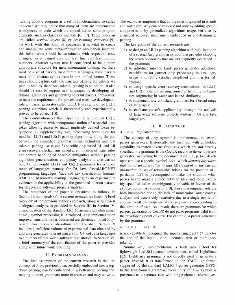
Talking about a program as a set of functionalities, so-calledconcerns, we may notice that many of them are implementedwith pieces of code which are spread across solid programelements, such as classes or methods [6], [7]. These concernsare called vertical layers [8] or crosscutting concerns [9].To work with this kind of concerns, it is vital to createand manipulate some meta-information about their location,this information should be sustainable with respect to codechanges, so it cannot rely on text line and text columnnumbers. Abstract syntax tree is considered to be a moreappropriate structure for meta-information binding, so, theremust be a set of parsers for different languages, these parsersmust build abstract syntax trees in one unified format. Thesetrees should capture only the structure of program entities weplan to bind to, therefore, tolerant parsing is an option. It alsoshould be easy to support new languages by developing ad-ditional grammars and generating tolerant parsers. Previously,to meet the requirements for parsers and trees, we developed atolerant parser generator called LanD. It uses a modified LL(1)parsing algorithm which is theoretically and experimentallyproved to be correct [10].

The contributions of this paper are: 1) a modified LR(1)parsing algorithm with incorporated notion of a special Anytoken allowing parser to match implicitly defined token se-quences; 2) supplementary Any processing techniques formodified LL(1) and LR(1) parsing algorithms, filling the gapbetween the simplified grammar formal definition and realtolerant parsing use cases; 3) specific Any-based LL and LRerror recovery mechanisms aimed at elimination of water rulesand correct handling of possible ambiguities without parsingalgorithm generalization; complexity analysis is also carriedout; 4) lightweight LL(1) and LR(1) grammars for a broadrange of languages, namely, for C#, Java, PascalABC.NETprogramming languages, Yacc and Lex specification formats,XML and Markdown markup languages; 5) an experimentalevidence of the applicability of the generated tolerant parsersfor large-scale software projects analysis.

The remainder of the paper is organized as follows. InSection II, main goals of the current research are listed. A briefoverview of the previous author’s research, along with closestanalogues analysis, is provided in Section III. In Section IV,a modification of the standard LR(1) parsing algorithm aimedat Any symbol processing is introduced, Any implementationimprovements and issues addressed are discussed, novel Any-based error recovery algorithms are described. Section Vincludes a sufficient volume of experimental data obtained byapplying generated tolerant parsers for C# and Java languagesto a number of real-world software repositories. In Section VI,a brief summary of the contribution of the paper is providedalong with future work outlining.

II. PROBLEM STATEMENT

The first assumption of the current research is that theconcept of Any, previously successfully embedded into a top-down parsing, can be embedded in a bottom-up parsing too,making tolerant grammars more expressive and easy-to-write.

The second assumption is that ambiguities originated in islandsand water similarity can be resolved not only by adding specialantipatterns or by generalized algorithms usage, but also bya special recovery mechanism embedded in a deterministicparsing.

The key goals of the current research are:1) to design an LR(1) parsing algorithm with built-in notion

of a special Any grammar symbol that provides skippingthe token sequences that are not explicitly described inthe grammar;

2) to introduce into the LanD parser generator additionalcapabilities for correct Any processing in case Anyusage is not fully satisfies simplified grammar formal-ization;

3) to design specific error recovery mechanisms for LL(1)and LR(1) tolerant parsing, aimed at handling ambigui-ties originating in water and island similarity;

4) to implement tolerant island grammars for a broad rangeof languages;

5) to evaluate parser’s applicability through the analysisof large-scale software projects written in C# and Javalanguages.

III. RELATED WORK

A. ”Any” implementation

The concept of Any symbol is implemented in severalparser generators. Historically, the first tool with embeddedcapability to match tokens from sets which are not directlyspecified in a grammar is the Coco/R recursive-descent parsersgenerator. According to the documentation [11, p. 14], devel-oper can use a special symbol ANY, which denotes any tokenthat is not an alternative to that ANY symbol in the currentproduction. A set of admissible tokens for the position of aparticular ANY is precomputed to make the situation whenparser has to make a choice between ANY and some explic-itly specified token unambiguously solvable in favour of theexplicit option. As shown in [10], these precomputed sets areboth incomplete due to the lack of nonterminal outer contextanalysis and excessively restrictive due to a single restrictionapplied to all the elements of the sequence corresponding tothe iteration of ANY. As a result, there are grammars for whichparsers generated by Coco/R do not parse programs valid fromthe developer’s point of view. For example, a parser generatedby the grammarA = a b c | ANY d.

is not capable to recognize the input string bad$ ($ denotesthe end of the input, ANY denotes zero or more Anytokens).

Similar Any implementation is built into a tool forlightweight LALR(1) parser development, called LightParse[12]. LightParse grammar is not directly used to generate aparser. Instead, it is transformed to the YACC-like formatsupported by the standard LALR(1) parser generator GPPG.In the transformed grammar, every entry of Any symbol ispresented as a separate rule with single-element alternatives,

9

by an alternative for each of the admissible terminal symbols.To ensure these rules are valid in terms of GPPG, LightParseimposes additional restrictions on Any usage. It only deepensdrawbacks inherited from Coco/R.

The most recent Any token implementation is introducedby the author of the current paper for LanD parser generator[10] aimed at LL(1) tolerant parsers generation by islandgrammars. In terms of the island grammars paradigm, Anysymbol allows one not to specify the particular content of thewater area, writing Any instead. Unlike the ANY symbol inCoco/R, our Any corresponds to a sequence of zero or moretokens, not a single token. In its implementation, all the knownshortcomings are eliminated. The decision about the currenttoken’s admissibility at Any position is made dynamically atthe parsing stage and restricts the set of admissible tokensno more than necessary to avoid ambiguities. LanD’s Anyimplementation does not assume the grammar translation tothe form suitable for the standard parsing algorithm. Instead,the standard LL(1) algorithm is modified to integrate thenotion of Any and make it possible to define admissible tokensby the content of a parsing stack.

In the current paper, LanD parser generator is extended withthe capability to generate LR(1) parsers with embedded notionof Any.

B. Formal definition of a simplified grammar

In [10], through the Any token, we formulate a formalconcept of the simplified grammar. We denote by lhs(p)and rhs(p), respectively, the left and the right part of theproduction p. Notation x ∈ rhs(p) for x ∈ N ∪ T meansthat rhs(p) = α1xα2, where α1 ∈ (N ∪ T )∗, α2 ∈ (N ∪ T )∗.SYMBOLS(γ) is used for the set of terminal symbols neededto compose all the ω : γ ∗=⇒ ω, γ ∈ (N ∪ T )∗, ω ∈ T ∗.

Definition 1: Let G = (N,T, P, S) be a context-freegrammar, Any /∈ T . The grammar simplified with respect toG is a grammar Gs = (Ns, Ts, Ps, Ss) defined as follows:

1) Ss = S;2) Ps = p ∈ f(P ) | lhs(p) = Ss ∨ ∃p′ ∈ Ps : lhs(p) ∈

rhs(p′), wheref : P → p = A→ α | A ∈ N,α ∈ (N∪T∪Any)∗is the mapping that satisfies the following criteria:

a) ∃P ′ ⊆ P : P ′ = p ∈ P | f(p) 6= p, P ′ 6= ∅,b) ∀p ∈ P \ P ′, f(p) = p,c) ∀p ∈ P ′, ∃n ∈ N : p is representable

in the form A → α1γ1β1α2γ2β2...αnγnβnand f(p) is representable in the form A →α1Anyβ1α2Anyβ2...αnAnyβn, where ∀i ∈[1..n], αiγiβi ∈ (N ∪ T )∗, and ∀i ∈[1..n], ∀a ∈ FOLLOW(A), SYMBOLS(γi) ∩FIRST(βiαi+1γi+1βi+1...αnγnβna) = ∅;

3) Ns = A ∈ N | ∃p ∈ Ps : lhs(p) = A;4) Ts = a ∈ T | ∃p ∈ Ps : a ∈ rhs(p) ∪ Any.Intuitively, Ps contains productions for the start symbol

of Gs and productions for all the nonterminals which arereachable from the start symbol. The definition of the mapping

f means that some of the strings generated by G containsubstrings which can be replaced with Any, then we obtainstrings generated by Gs. Symbol Any can be written insteadof the parts denoted by γi in production’s right hand side,in case these parts satisfy the criterion 2c of the definition1. Verification of this criterion is possible only when solvinga direct problem: when the grammar Gs is created on thebasis of some available G. In theory, G can correspond to thebaseline language grammar, as well as be a more tolerant ver-sion of the baseline grammar, containing all the anti-patternsdescribed explicitly. In practice, it is usually not available ordoes not exist, so direct problem is rarely considered. Writingan island grammar for a certain programming language isequivalent to solving an inverse problem. Developer writesan initial approximation in the form of a simplified grammarin which Any usage allows one to minimize the efforts todescribe a possible water content. Then she performs aniterative refinement in accordance with parsing results, makingthe grammar more and more corresponding to the languagegenerated by some baseline.

Compliance with the criterion 2c is crucial for correctAny processing. At the same time, it is hard to maintainwhile solving an inverse problem. In this paper, additionalAny processing mechanisms are offered. They allow grammardevelopers to weaken the control over the consistency with theformalization.

C. LL(1) parsing algorithm modification

In Figure 1, modified algorithms from [10] are rewrittenin the form more suitable for further discussion. The deltabetween the standard algorithms and the modified ones ishighlighted with grey. As shown in Figure 1a, when no actioncan be performed with a current token, parser tries to interpretthis token as the beginning of a sequence corresponding toAny. FIRST’ set, a modified version of a standard FIRST,is computed for the parsing stack content to get all the tokensthat are explicitly allowed in the current place. This non-staticapproach is inspired in some sense by full-LL(1) parsing [13,p. 247–251]. Set construction routine is shown in Figure 1c.A modification is needed to handle the consecutive Anyproblem defined in [10], this problem is explained in detail inSection IV-B1 along with a more general solution. M denotes aparsing table, Stack denotes a symbol stack which stores notjust the symbols that are expected to be matched, but nodesof the syntax tree being constructed.

There are grounds for an analogy between the LL(1) parsingmodification given and well-known error recovery algorithms:Any symbol looks similar to the error token denoting placein the grammar where recovered parsing can be resumed,FIRST’ set seems like the set of synchronization tokens.Moreover, speaking in terms of the formal definition, a tolerantparser is built by a simplified grammar Gs, and a program fromL(G) is actually needed to be parsed. In terms of Gs, thisprogram is erroneous. However, here also lies a fundamentaldifference between Any processing and error recovery. Recov-ery is performed for a program which is incorrect regarding to

10

Fig. 1: Modified LL algorithms: (a) LL(1) parsing algorithm, (b) ”Any” processing algorithm, (c) FIRST set construction,(d) Auxiliary algorithms: alternative applying and FIRST set memorization

a baseline grammar G. While success is not guaranteed, themain goal is to resume parsing at any cost, including the loss ofsome significant results of the previous analysis and skippinga significant part of the input stream, possibly containing somepoints of interest. The goal of Any processing is to translatea presumably valid L(G) program into the language L(Gs)by replacing some token sequences with Any. The premisethat the program under consideration is correct with respectto G, in conjunction with the observance of the criterion 2c,makes input tokens skipping totally predictable. One can besure that the parts of the input stream replaced with Anybelongs to the water and can be discarded without loss of theland. Furthermore, predictable and correct replacement withAny is possible for a program that is incorrect with respect toG, in case incorrectnesses are located in water areas.

IV. ALGORITHMS AND MODIFICATIONS

A. LR(1) parsing

Though the modified LL(1) parsing algorithm described inSection III-C is enough to create reliable tolerant parsers,describing a real programming language with LL(1) grammaris a challenge even when this grammar is supposed to be

lightweight and tolerant. Constructs of interest, such as classmembers, usually have a common beginning up to a certainpoint, so they cannot be presented as solid alternatives for asingle nonterminal symbol in LL(1). Instead, we have to writerule sequences in the style of taking the common factor outof the brackets and making a separate rule for a tail:

entity = attribute* keyword* (class_tail | member_tail)member_tail = type name (method_tail | property_tail)method_tail = arguments Any (init? ’;’ | block)

As a result, the grammar structure is not transparent enoughfor a newcomer because the connection between existingisland rules written in such a distributed manner and particularlanguage constructs is non-obvious.

This LL(1) limitation can be overcome through switching toa more complex LR(1) parsing. A modification of the standardLR(1) algorithm is shown in Figure 2a, modified areas arehighlighted with gray. Like in a standard case, two stacks existto keep parser state. SymbolsStack keeps the current viableprefix [14, p. 256]. In fact, similar to LL(1) Stack, in ourimplementation, it keeps not just symbols but nodes for a treeto be build. StatesStack keeps the indices of the statesparser passed through to obtain the current viable prefix. An

11

Fig. 2: Modified LR algorithms: (a) Modified LR(1) parsing algorithm, (b) ”Any” processing algorithm, (c) Shift and reducealgorithms

COMMENT : '//' ~[\n\r]* | '/*' .*? '*/'

STRING : '"' ('\\"'|'\\\\'|.)*? '"'

CHAR : '\'' ('\\\''|'\\\\'|.)*? '\''

MODIFIER : 'transient'|'strictfp'|'native'|'public'|'private'

|'protected'|'static'|'final'|'synchronized'|'abstract'

|'volatile'|'default'

ID : [_$a-zA-Z][_$0-9a-zA-Z]*

CURVE_BRACKETED : %left '' %right ''

ROUND_BRACKETED : %left '(' %right ')'

SQUARE_BRACKETED : %left '[' %right ']'

file_content = entity*

entity = enum | class_interface | method

| field_declaration | water_entity

enum = common_beginning 'enum' name Any block ';'?

class_interface = common_beginning ('class'|'interface')

name Any '' entity* '' ';'?

method = common_beginning type name arguments Any (';' | block)

field_declaration = common_beginning type field (',' field)* ';'

field = name ('['']')* init_value?

water_entity = AnyInclude('@interface', 'import', 'package')

(block | ';')+

common_beginning = (annotation|MODIFIER)*

init_value = '=' init_part+

init_part = Any | type_parameter

name = name_type

type = name_type

name_type_atom = type_parameter? ID type_parameter?

name_type = name_type_atom ((('.'|'::') name_type_atom) | '['']')*

type_parameter = '<' (AnyAvoid(';') | type_parameter)* '>'

arguments = '(' Any ')'

annotation = '@' name arguments?

block = '' Any ''

Fig. 3: Java LR(1) tolerant grammar

element ACTIONS[s, t] of the ACTIONS table keeps theknowledge of what action should be performed by the parserif token t is met while s is the parser’s current state. Thereare two basic types of action in LR algorithm: Shift andReduce, they are shown in Figure 2c. GOTO[s, X] containsthe index of a state to which parser must go from s state afterreducing some part of a viable prefix to X.

The essence of the parsing algorithm modification is similarto LL(1) case: tolerant parser is responsible not only forchecking if the program can be derived from the start symbol,but also for translating it from a baseline language into asimplified one. In case an action for some actual combinationof parser state and input token is undefined, parser tries tointerpret the current token as the beginning of the subsequenceof the program from L(G) that corresponds to Any in thecorresponding program from L(Gs). In case there is an actionavailable for Any, parser calls SkipAny routine (Figure 2b),where firstly all the possible Reduce actions are performedand secondly Any token is shifted. Note that we considerACTIONS table to be cleared from Shift/Reduce conflicts infavour of Shift action. Also there is no additional checkingif Shift action exists, because this existence follows fromthe standard ACTIONS and GOTO construction algorithm.Having moved Any to a viable prefix, parser looks for thefirst token which is explicitly expected in L(Gs) program andthen continues parsing the usual way.

In Figure 3, there is an LR(1) tolerant grammar for Javaprogramming language written in the format supported byLanD parser generator. As it can be seen, island entities,such as enumerables, classes, methods and fields, are clearlypresented as solid rules. In comparison with a baseline Javagrammar, it is significantly shorter: the baseline grammarimplementation for ANTLR parser generator1 consists of 211lines of lexer specification and 615 lines of parser description.

B. ”Any” processing improvements1) Consecutive ”Any” problem: In Figure 1c, FIRST’

algorithm, which is the modified version of the standard

1https://github.com/antlr/grammars-v4/tree/master/java

12

FIRST, is presented. It is intended to solve the problem ofconsecutive Any described in [10]. The problem manifestsitself when two or more Any tokens directly follow each otherat the beginning of the sentence which can be derived from thestack. In this case, the subsequent Any hides some stop tokensfrom the previous one. Consider the following grammar G:

A = (a|b)+ B C; B = d | ; C = (e|f)? c

It can be simplified to the following Gs:

A = Any B C; B = d | ; C = Any c

The string abc$ ∈ L(G) is supposed to be successfullymatched by the parser built for L(Gs), because the followingderivation may be performed:

A⇒ Any BC ⇒ Any C ⇒ Any Any c .

Having met the token a, the tolerant parsing algorithm startsthe first Any processing. If the standard FIRST is used tofind stop tokens, FIRST(Stack) set equals to d, Any,as a result, SkipAny skips all the input and returns an error.Taking into account that Any is allowed to match an emptysequence, FIRST’ modification looks beyond the second Anyand, in general, beyond all the subsequent Any symbols insearching some explicitly specified tokens which may followa sequence corresponding to these Any tokens. Stop token setfound with FIRST’(Stack) equals to d, c, thus thefirst Any captures a and b tokens and stops on c, the secondone matches an empty sequence, and abc$ string is admittedto be correct.

This approach is proved to be enough to build workingparsers for real programming languages, such as C#, Javaor PascalABC.NET. It can also be implemented for LR(1)through ACTION and GOTO static analysis. However, on closerinspection it becomes clear that algorithms modified in thisway work correct only for a subclass of simplified grammars,satisfying an additional constraint:

Definition 2: Let Gs = (Ns, Ts, Ps, Ss) be a grammarsimplified with respect to a context-free grammar G =(N,T, P, S). Enumerate as Any1,Any2, ...Anyn all the Anyentries from the right-hand sides of productions from Ps,which appeared as a result of replacement of the correspond-ing γ1, γ2, ...γn subparts of the right-hand sides of produc-tions from P in compliance with Definition 1. DerivationSs

∗=⇒ αsAnykAny l...Anytbβs, where k, l, ..., t ∈ [1..n],

αs, βs ∈ (Ns ∪ Ts)∗, b ∈ Ts \ Any, is not acceptable inGs if b ∈ SYMBOLS(γkγl...γt).

Informally speaking, the token which is a stop token for thelast Any in a sequence is not allowed to appear in the areacorresponding to one of the preceeding Any, otherwise it willcause premature completion of Any processing. Let G has adifferent structure:

A = (a|b|c|d|e|f)+ B C; B = g | ; C = (h|i)+ a

It can be simplified to

A = Any B C; B = g | ; C = Any a

Herein, both replacements with Any are still satisfy the cri-terion 2c, but the restriction from Definition 2 is not satisfied,as a may follow the second Any, and at the same time it isa valid element of the area corresponding to the first one. Asa result, while parsing abba$, the first Any is matched withan empty token sequence because FIRST’([B, C]) equalsto a, g, the second Any also cannot include a, so, validinput is not accepted.

In practice, the most common case of consecutive Anyappearance does not break the restriction mentioned: in gram-mars we have developed, Any is often used as one of thepossible variants for an element of a list, so, all the Anytokens in the derivation of such a list originate from asingle Any entry in the grammar, therefore, derivation canbe rewritten as Ss

∗=⇒ αsAnykAnyk...Anykbβs, and the

corresponding condition b ∈ SYMBOLS(γk) is false inaccordance with Definition 1. To cover the general case, weintroduce a mechanism for passing an additional information atAny processing stage. Any entry can be supplemented withtwo options: Except and Include. For each of them, alist of literals or token names can be passed as parameters.The concept of AnyExcept initially appeared in LightParseparser generator [15], but there it was intended to compensatethe lack of outer context analysis while constructing the set ofadmissible tokens. Our intention is different: symbols specifiedfor Except option are supposed to compensate the lack ofinformation in consecutive Any problem: they are supposedto be explicitly specified tokens that may follow the areacorresponding to Any in L(G). Include option allows oneto approach this problem from a different angle, specifyingtokens that shouldn’t be interpreted as stop tokens despite theirappearance in FIRST’(Stack). So, for the grammar abovewe can use one of the following simplified analogues:A = AnyExcept(g,h,i) B C; B = g | ; C = Any aA = AnyInclude(a) B C; B = g | ; C = Any a

Having renamed stopTokens sets built in Figure 1b and2b to stopTokensBasic, we transform stop token setconstruction for both LL and LR algorithms tostopTokens := anyExceptSet.Count > 0? anyExceptSet: stopTokensBasic.Except(anyIncludeSet);

where anyExceptSet and anyIncludeSet denote setsof tokens passed as option parameters for Any currentlybeing matched. For error recovery purposes discussed inSection IV-C, Any also supports Avoid option. Its argumentsare tokens the presence of which in the Any-correspondingarea signals about program incorrectness or wrong alternativechoice. To take Avoid into account, while loop conditiontransforms tot ∉ stopTokens and t ∉ anyAvoidSet and t ≠ $.

In case token skipping is interrupted because current tokenequals to one of the Avoid arguments, this token passes toError routine as a second argument.

Unlike in LL(1), there can be a situation in LR(1) whenwe do not know for sure what particular Any entry is being

13

processed at the moment. This information is needed to accessthe corresponding options. To add support of Any options inLR(1), we introduce an additional type of LR(1) conflict calledAny/Any conflict. It is reported when there is a state wheremultiple items have a dot before Any, and is needed to beresolved for successful parser generation.

2) Nesting level checking: While writing a tolerant gram-mar, developer usually has to make an additional effort todetermine what bracketed areas may appear in the particularwater, and if they can influence Any processing. Intuitively,such areas are perceived as a whole, and when Any is writteninstead of some better-grained water description, it may bemissed that bracketed areas exist in that water in a realprogram. These areas may contain something that also appearsright after that Any and therefore should be treated as a stoptoken. For example, being interested in fields of a C# class,we must capture a, b, c and d in the fragmentint a = 0, b = 1;DateTime c = new DateTime(2019, 5, 29),

d = new DateTime(2019, 5, 31);

At the same time, we are not interested in initializers, so, thefirst intention is to describe field declaration with the rulesfields = type name init? (’,’ name init?)* ’;’init = ’=’ Any

Unfortunately, these rules work only for the first declaration.The set ’,’, ’;’ is a stop token set for Any, and in thesecond declaration, comma separates not only fields but alsoarguments bordered with round brackets. Generally speaking,Any does not satisfy the formalization in this case. At thesame time, simplicity is the crucial property of the tolerantgrammar, and the way in which water is described above ismore preferable than the following one:init = ’=’ waters_water = ’[’ (Any | s_water)+ ’]’r_water = ’(’ (Any | r_water)+ ’)’c_water = ’’ (Any | c_water)+ ’’water = (Any | c_water | r_water | s_water)+

To return the first version of init rule to the boundariesof the simplified grammar definition, we add to the parsingalgorithms a capability to take into account nested bracketedstructures. A pair of brackets is described likeROUND_BRACKETED : %left ’(’ %right ’)’

and nesting level is tracked by lexical analyser. If several kindsof pairs are described, it is believed that any pair can be nestedin any pair. When Any is processed, it is allowed to end onlyat the same depth at which it begins. To control this situation,SkipAny methods are modified uniformly both for LL andLR. Firstly, at the beginning of a skip process, an additionalvariable is initialized:depth := Lexer.CurrentDepth();

Secondly, in-loop Lexer.NextToken() call is replacedwith Lexer.NextToken(depth). Passing the initial nest-ing level to a lexer, we force it to read the input stream untilthe depth of the next token equals the depth of the first token in

a (b) b b

Any ( a) b bAny

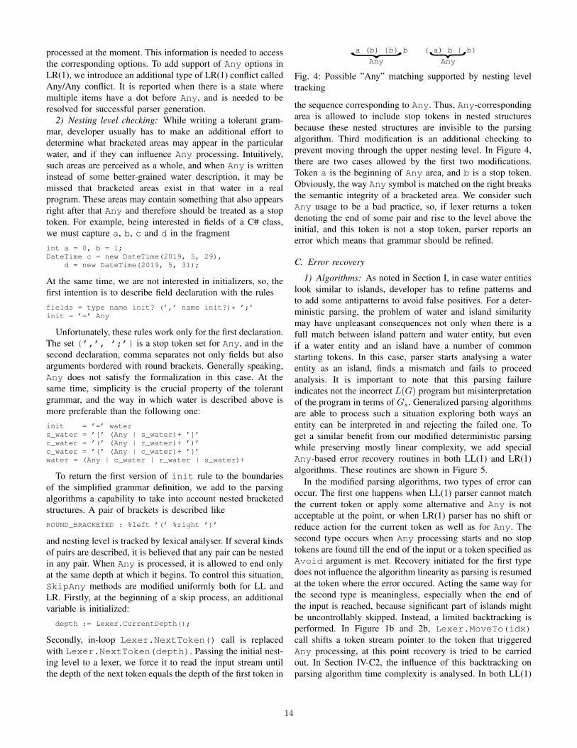
Fig. 4: Possible ”Any” matching supported by nesting leveltracking

the sequence corresponding to Any. Thus, Any-correspondingarea is allowed to include stop tokens in nested structuresbecause these nested structures are invisible to the parsingalgorithm. Third modification is an additional checking toprevent moving through the upper nesting level. In Figure 4,there are two cases allowed by the first two modifications.Token a is the beginning of Any area, and b is a stop token.Obviously, the way Any symbol is matched on the right breaksthe semantic integrity of a bracketed area. We consider suchAny usage to be a bad practice, so, if lexer returns a tokendenoting the end of some pair and rise to the level above theinitial, and this token is not a stop token, parser reports anerror which means that grammar should be refined.

C. Error recovery

1) Algorithms: As noted in Section I, in case water entitieslook similar to islands, developer has to refine patterns andto add some antipatterns to avoid false positives. For a deter-ministic parsing, the problem of water and island similaritymay have unpleasant consequences not only when there is afull match between island pattern and water entity, but evenif a water entity and an island have a number of commonstarting tokens. In this case, parser starts analysing a waterentity as an island, finds a mismatch and fails to proceedanalysis. It is important to note that this parsing failureindicates not the incorrect L(G) program but misinterpretationof the program in terms of Gs. Generalized parsing algorithmsare able to process such a situation exploring both ways anentity can be interpreted in and rejecting the failed one. Toget a similar benefit from our modified deterministic parsingwhile preserving mostly linear complexity, we add specialAny-based error recovery routines in both LL(1) and LR(1)algorithms. These routines are shown in Figure 5.

In the modified parsing algorithms, two types of error canoccur. The first one happens when LL(1) parser cannot matchthe current token or apply some alternative and Any is notacceptable at the point, or when LR(1) parser has no shift orreduce action for the current token as well as for Any. Thesecond type occurs when Any processing starts and no stoptokens are found till the end of the input or a token specified asAvoid argument is met. Recovery initiated for the first typedoes not influence the algorithm linearity as parsing is resumedat the token where the error occured. Acting the same way forthe second type is meaningless, especially when the end ofthe input is reached, because significant part of islands mightbe uncontrollably skipped. Instead, a limited backtracking isperformed. In Figure 1b and 2b, Lexer.MoveTo(idx)call shifts a token stream pointer to the token that triggeredAny processing, at this point recovery is tried to be carriedout. In Section IV-C2, the influence of this backtracking onparsing algorithm time complexity is analysed. In both LL(1)

14

Error(stopTokens):

if (Lexer.CurrentTokenIndex() RecoveredIn) then

return ERROR_TOKEN;

end;

RecoveredIn ∪= Lexer.CurrentTokenIndex() ;

currentNode := Stack.Pop();

do

if (currentNode.Parent ≠ null) then

maxChildIndex :=

currentNode.Parent.Children.Count - 1;

indexOfCurrent :=

currentNode.Parent.Children.IndexOf(currentNode);

for (i from indexOfCurrent + 1 to maxChildIndex) do

Stack.Pop();

end for;

end if;

currentNode := currentNode.Parent;

while(currentNode ≠ null and (

currentNode.Symbol ∉ RecoverySymbols or

Any = GetDerivation(currentNode)[0] or

IsUnsafeAny(stopTokens)

));

if (currentNode ≠ null) then

return SkipAny(false);

else

return ERROR_TOKEN;

end if;

Error(stopTokens):

if (Lexer.CurrentTokenIndex() ∈ RecoveredIn) then

return ERROR_TOKEN;

end;

RecoveredIn ∪= Lexer.CurrentTokenIndex() ;

lastMatched := ;

// possible derivation items

PDI := ;

basePDI := ;

do

if (SymbolsStack.Count > 0) then

lastMatched := SymbolsStack.Pop();

end if;

StatesStack.Pop();

if (StatesStack.Count > 0) then

s := StatesStack.Peek();

basePDI := i = X •Y | i ∈ STATE[s], Y = lastMatched.Symbol,

(PDI = ∨ ∃i' ∈ PDI : i' = X Y•) ;

PDI := basePDI;

do

PDI ∪= i = X •Y | i ∈ STATE[s], ∃i' ∈ PDI : i' = Y •' ;

while (PDI changes);

end if;

while (StatesStack.Count > 0 and (

| basePDI | = | PDI | or

∄i ∈ PDI \ basePDI : i = X •Y, Y ∈ RecoverySymbols or

Any = GetDerivation(lastMatched)[0] or

IsUnsafeAny(stopTokens)

));

if (StatesStack.Count > 0) then

return SkipAny(false);

else

return ERROR_TOKEN;

end if;

(a)

(b)

Fig. 5: ”Any”-based error recovery algorithms: (a) LL(1) algorithm, (b) LR(1) algorithm

and LR(1) error processing algorithms, RecoveredIn setstores all the indices of tokens at which recovery was onceperformed, so, it is guaranteed that from one recovery toanother parsing process moves at least one token forward.

Like in standard recovery algorithms [16, pp. 283–285],a set of nonterminals at which recovery can be performedis defined. These nonterminals are called recovery symbols.Possible recovery symbols can be revealed through the staticgrammar analysis. Given the grammar Gs = (Ns, Ts, Ps, Ss),we formally define the set as follows:

RecoverySymbols = n ∈ Ns | n∗=⇒ Any α∧

@n′ ∈ Ns : (n∗=⇒ n′Any α ∧ n′ ∗=⇒ ε), α ∈ (Ns ∪ Ts)∗.

Recovery symbols are pre-computed at parser constructionstage. Developer can disable recovery at all or specify par-ticular nonterminals from this set which should be used forrecovery, otherwise, all the elements of the set are taken intoconsideration when Error routine is called.

In the context of a deterministic tolerant parsing problem,recovery symbols have specific semantics. They representdecision points at which parser may choose the wrong alter-native, try to match a water entity as an island, and provokean error. Recovery itself means returning to a decision pointthrough the grammar ancestors of the currently unmatchedtoken or unparsed nonterminal and changing the interpretationof the part of the input that is already associated with arecovery symbol’s subtree to water. More precisely, the part of

the input from the first token mistaken for an island part to thefirst token at which the difference between an island patternand an actual water entity manifests itself is supposed to be thebeginning of the sequence corresponding to Any from whichthe water alternative starts. Backtracking to the token a wrongdecision was made at is not needed in this interpretation. Theend of an Any-corresponding sequence is looked for with ausual SkipAny call, then parsing continues in an ordinaryway. In Figure 3, entity is one of the recovery symbols. Itallows the parser to recognize classes, enumerables, methods,and fields as islands, while annotation definitions, constructors,initialization blocks, etc. are skipped as the water, sometimeswith the involvement of recovery mechanisms.

LL(1) error recovery algorithm is presented in Figure 5a.We take advantage of the fact that at any stage of the top-down-parsing a partially built syntax tree is available, andblank nodes for what is expected are on the stack. Knowingthe tree node corresponding to the unparsed symbol, we mayfind a recovery symbol node by moving through its ancestors.The higher we go, the wider area will be reinterpreted.Simultaneously with walking up the syntax tree, right siblingsof the currentNode should be removed from parsing stackas they are unparsed parts of the interpretation being rejected.The appropriate recovery symbol is considered to be foundif it satisfies two additional conditions. Firstly, the wateralternative should not be the alternative in favor of whichthe decision was originally made, otherwise no reinterpreting

15

takes place as error actually occurred in the water. To checkit, GetDerivation is called. It takes the built part ofrecovery symbol’s subtree and returns a leaf sequence whichis a partially revealed part of the L(Gs) program, derived fromthis symbol. This sequence must not start with Any. Secondly,in case error took place at Any skipping, IsUnsafeAnyprevents parsing resumption on Any from the recovery symbolalternative if new skipping will lead to the same erroneoussituation. The decision is made on the basis of old and newstop token sets comparison and Avoid options analysis.

For LR(1) algorithm, recovery is more complex and heuris-tic due to the nature of a bottom-up parsing. Unlike in LLcase, we do not know for sure what are the exact entitiesthat are currently being analysed, so, we try to build a setof possible candidates basing on the information stored onthe stacks. In Figure 5b, there is an LR(1) error recoveryroutine. On each iteration of do-while loop, one of thesymbols already matched is popped along with the state parserwent to after this successful matching, then basePDI set isconstructed. It consists of the current state items having thedot before the last popped symbol. Productions of the itemsadded to this set are possible participants of the erroneousarea derivation. Basing on basePDI, PDI set is constructedin a way that looks like inverted CLOSURE [16, pp. 243–245] algorithm. Additional PDI items capture the higher-levelgrammar entities from which the area that is needed to bereinterpreted may be derived.

Recovery algorithms presented simplify the process ofgrammar extension and reduction. Recovery symbol alter-natives become grammar building blocks: in case we arenot interested in some Java island its alternative can beexcluded from entity rule, then program areas previouslycorresponding to that alternative are recognized as the water,possibly through recovery algorithm application. Inversely, toadd a support for class constructors in the grammar in Figure 3,we have write only one constructor rule and add thissymbol in entry alternatives list, then constructors stop beinginterpreted as the water, because the rule appears allowing toanalyse them from beginning to the end with no error occurred.

2) Complexity analysis: As noted, errors happening onAny processing require limited backtracking. The particularincrease in running time of the algorithm depends on numberand length of backtracked sequences. From the prohibition ofmultiple recovery at the same token, it follows that there canbe only one backtracking to a particular position, so, the worstcase is when the following situation repeats sequentially foreach token except the first one: Any processing starts on thetoken, fails by reaching the end of the input and backtracks tothat token, then recovery starts, the token matches successfullywith the help of the water alternative, and the next tokenbecomes the token under consideration. In this scenario, anumber of times the token is examined equals to its sequentialnumber counting from one. For the ith token, i−1 examinationsare occurred on Any skipping started at previous tokens and atthe current one, and 1 examination is for some final match. Asbacktracking itself consists of a simple index reassignment, it

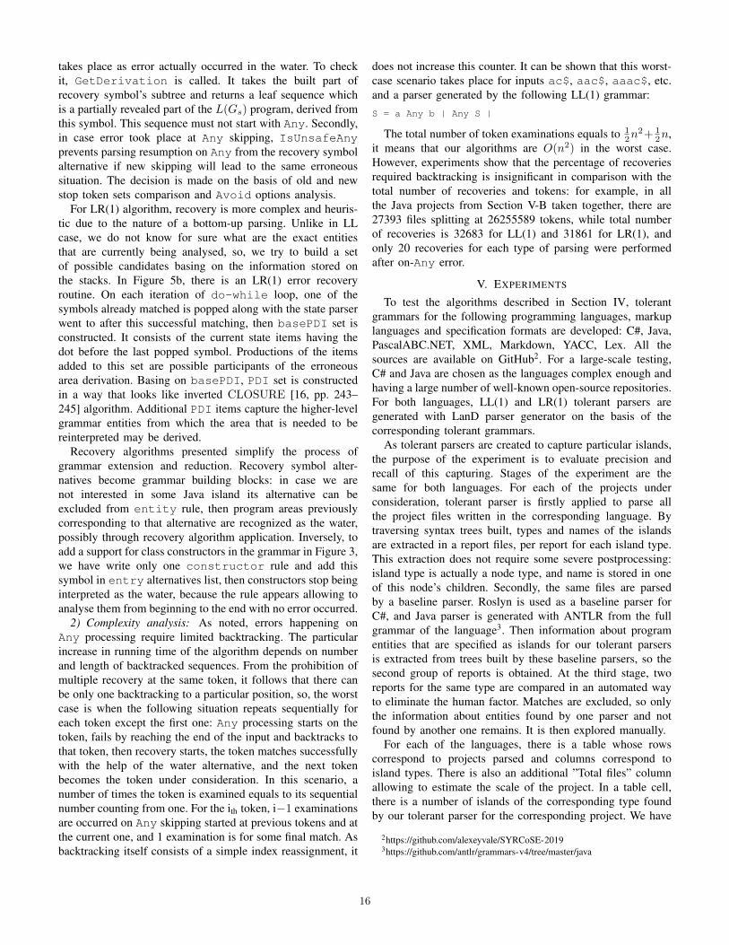
does not increase this counter. It can be shown that this worst-case scenario takes place for inputs ac$, aac$, aaac$, etc.and a parser generated by the following LL(1) grammar:S = a Any b | Any S |

The total number of token examinations equals to 12n

2+ 12n,

it means that our algorithms are O(n2) in the worst case.However, experiments show that the percentage of recoveriesrequired backtracking is insignificant in comparison with thetotal number of recoveries and tokens: for example, in allthe Java projects from Section V-B taken together, there are27393 files splitting at 26255589 tokens, while total numberof recoveries is 32683 for LL(1) and 31861 for LR(1), andonly 20 recoveries for each type of parsing were performedafter on-Any error.

V. EXPERIMENTS

To test the algorithms described in Section IV, tolerantgrammars for the following programming languages, markuplanguages and specification formats are developed: C#, Java,PascalABC.NET, XML, Markdown, YACC, Lex. All thesources are available on GitHub2. For a large-scale testing,C# and Java are chosen as the languages complex enough andhaving a large number of well-known open-source repositories.For both languages, LL(1) and LR(1) tolerant parsers aregenerated with LanD parser generator on the basis of thecorresponding tolerant grammars.

As tolerant parsers are created to capture particular islands,the purpose of the experiment is to evaluate precision andrecall of this capturing. Stages of the experiment are thesame for both languages. For each of the projects underconsideration, tolerant parser is firstly applied to parse allthe project files written in the corresponding language. Bytraversing syntax trees built, types and names of the islandsare extracted in a report files, per report for each island type.This extraction does not require some severe postprocessing:island type is actually a node type, and name is stored in oneof this node’s children. Secondly, the same files are parsedby a baseline parser. Roslyn is used as a baseline parser forC#, and Java parser is generated with ANTLR from the fullgrammar of the language3. Then information about programentities that are specified as islands for our tolerant parsersis extracted from trees built by these baseline parsers, so thesecond group of reports is obtained. At the third stage, tworeports for the same type are compared in an automated wayto eliminate the human factor. Matches are excluded, so onlythe information about entities found by one parser and notfound by another one remains. It is then explored manually.

For each of the languages, there is a table whose rowscorrespond to projects parsed and columns correspond toisland types. There is also an additional ”Total files” columnallowing to estimate the scale of the project. In a table cell,there is a number of islands of the corresponding type foundby our tolerant parser for the corresponding project. We have

2https://github.com/alexeyvale/SYRCoSE-20193https://github.com/antlr/grammars-v4/tree/master/java

16

...

CURVE_BRACKETED : %left '' %right ''

ROUND_BRACKETED : %left '(' %right ')'

SQUARE_BRACKETED : %left ('['|GENERAL_ATTRIBUTE_START) %right ']'

...

namespace = 'namespace' name '' namespace_content ''

entity = enum | class_struct_interface | method

| field_decl | property | water_entity

enum = common 'enum' name Any '' Any '' ';'?

class_struct_interface =

common ('class'|'struct'|'interface') name Any '' entity* '' ';'?

method = common type name arguments Any (init_expression? ';' | block)

field_decl = common type field (',' field)* ';'

field = name ('[' Any ']')? init_value?

property =

common type name (block (init_value ';')? | init_expression ';')

water_entity =

AnyInclude('delegate', 'operator', 'this') (block | ';')+

common = entity_attribute* modifier*

modifier = MODIFIER | 'extern'

init_expression = '=>' Any

init_value = '=' init_part+

init_part = Any | type

arguments = '(' Any ')'

block = '' Any ''

...

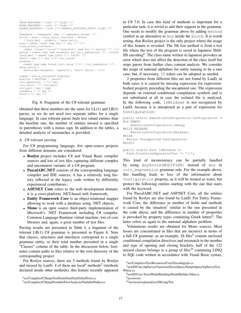
Fig. 6: Fragment of the C# tolerant grammar

obtained that these numbers are the same for LL(1) and LR(1)parser, so we do not need two separate tables for a singlelanguage. In case tolerant parser finds less island entities thanthe baseline one, the number of entities missed is specifiedin parentheses with a minus sign. In addition to the tables, adetailed analysis of mismatches is provided.

A. C# tolerant parsing

For C# programming language, five open-source projectsfrom different domains are considered:• Roslyn project includes C# and Visual Basic compiler

sources and lots of test files capturing different complexand uncommon variants of a C# program;

• PascalABC.NET consists of the corresponding languagecompiler and IDE sources, it has a relatively long his-tory reflected in the legacy code written by differentlyexperienced contributors;

• ASP.NET Core refers to the web development domain:it is a cross-platform .NET-based web framework;

• Entity Framework Core is an object-relational mapperallowing to work with a database using .NET objects;

• Mono is an open source third-party implementation ofMicrosoft’s .NET Framework including C# compiler,Common Language Runtime virtual machine, lots of corelibraries and, again, a great number of test files.

Parsing results are presented in Table I, a fragment of thetolerant LR(1) C# grammar is presented in Figure 6. Notethat classes, structures and interfaces correspond to a singlegrammar entity, so their total number presented in a single”Classes” column of the table. In the discussion below, foot-notes contain paths to files relative to the root directory of thecorresponding project.

For Roslyn sources, there are 5 methods found by Roslynand missed by LanD. 4 of them are local4 methods5 (methodsdeclared inside other methods), this feature recently appeared

4src/Compilers/CSharp/Test/Emit/Emit/EndToEndTests.cs5src/Compilers/CSharp/Portable/FlowAnalysis/NullableWalker.cs

in C# 7.0. In case this kind of methods is important for aparticular task, it is trivial to add their support in the grammar.One needs to modify the grammar above by adding methodsymbol as an alternative to Any inside the block. It is worthnoting, that Roslyn project is the only project where the usageof this feature is revealed. The 5th lost method is from a testfile where the text of the program is saved in Japanese Shift-JIS encoding6. The class name written in Japanese provokes anerror which does not affect the detection of the class itself butstops parser from further class content analysis. We considerthe usage of national alphabets for entity naming to be a rarecase, but, if necessary, ID token can be adopted as needed.

2 properties from different files are not found by LanD, inboth cases it is caused by missing expression for expression-bodied property preceding the uncaptured one. The expressiondepends on external conditional compilation symbols and isnot substituted at all in case the isolated file is analysed.In the following code, IsWindows is not recognized byLanD, because it is interpreted as a part of expression forConfiguration:public static ExecutionConfiguration Configuration =>#if DEBUG

ExecutionConfiguration.Debug;#elif RELEASE

ExecutionConfiguration.Release;#else#error Unsupported Configuration

#endif

public static bool IsWindows =>Path.DirectorySeparatorChar == ’\\’;

This kind of inconsistency can be partially handledby using AnyAvoid(MODIFIER) instead of Any ininit_expression grammar rule. For the example above,this handling leads to loss of the information aboutConfiguration property, as it will be treated as water, butprotect the following entities starting with the one that startswith the keyword.

For PascalABC.NET and ASP.NET Core, all the entitiesfound by Roslyn are also found by LanD. For Entity Frame-work Core, the difference in number of fields and methodsis caused by the situation7 similar to the one presented inthe code above, and the difference in number of propertiesis provoked by property types containing Greek letters8. Thelatter refers us again to the national alphabets problem.

Voluminous results are obtained for Mono sources. Mostlosses are concentrated in files that are incorrect in terms ofa full C# grammar: as an example, 26 files9 contain unclosedconditional compilation directives and mismatch in the numberand type of opening and closing brackets, half of the 122missed classes belongs to a group of files10 containing LINQto SQL code written in accordance with Visual Basic syntax,

6src/Compilers/Test/Resources/Core/Encoding/sjis.cs7test/EFCore.SqlServer.FunctionalTests/Query/SimpleQuerySqlServerTest.

Where.cs8test/EFCore.Tests/ModelBuilding/ModelBuilder.Other.cs9mcs/errors10mcs/tools/sqlmetal/src/DbLinq/Test

17

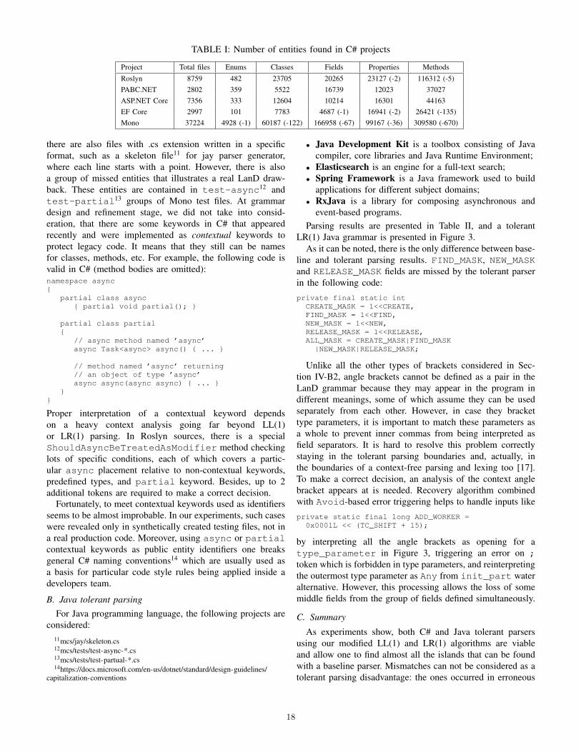
TABLE I: Number of entities found in C# projects

Project Total files Enums Classes Fields Properties Methods

Roslyn 8759 482 23705 20265 23127 (-2) 116312 (-5)PABC.NET 2802 359 5522 16739 12023 37027ASP.NET Core 7356 333 12604 10214 16301 44163EF Core 2997 101 7783 4687 (-1) 16941 (-2) 26421 (-135)Mono 37224 4928 (-1) 60187 (-122) 166958 (-67) 99167 (-36) 309580 (-670)

there are also files with .cs extension written in a specificformat, such as a skeleton file11 for jay parser generator,where each line starts with a point. However, there is alsoa group of missed entities that illustrates a real LanD draw-back. These entities are contained in test-async12 andtest-partial13 groups of Mono test files. At grammardesign and refinement stage, we did not take into consid-eration, that there are some keywords in C# that appearedrecently and were implemented as contextual keywords toprotect legacy code. It means that they still can be namesfor classes, methods, etc. For example, the following code isvalid in C# (method bodies are omitted):namespace async

partial class async partial void partial();

partial class partial

// async method named ’async’async Task<async> async() ...

// method named ’async’ returning// an object of type ’async’async async(async async) ...

Proper interpretation of a contextual keyword dependson a heavy context analysis going far beyond LL(1)or LR(1) parsing. In Roslyn sources, there is a specialShouldAsyncBeTreatedAsModifier method checkinglots of specific conditions, each of which covers a partic-ular async placement relative to non-contextual keywords,predefined types, and partial keyword. Besides, up to 2additional tokens are required to make a correct decision.

Fortunately, to meet contextual keywords used as identifiersseems to be almost improbable. In our experiments, such caseswere revealed only in synthetically created testing files, not ina real production code. Moreover, using async or partialcontextual keywords as public entity identifiers one breaksgeneral C# naming conventions14 which are usually used asa basis for particular code style rules being applied inside adevelopers team.

B. Java tolerant parsingFor Java programming language, the following projects are

considered:11mcs/jay/skeleton.cs12mcs/tests/test-async-*.cs13mcs/tests/test-partual-*.cs14https://docs.microsoft.com/en-us/dotnet/standard/design-guidelines/

capitalization-conventions

• Java Development Kit is a toolbox consisting of Javacompiler, core libraries and Java Runtime Environment;

• Elasticsearch is an engine for a full-text search;• Spring Framework is a Java framework used to build

applications for different subject domains;• RxJava is a library for composing asynchronous and

event-based programs.Parsing results are presented in Table II, and a tolerant

LR(1) Java grammar is presented in Figure 3.As it can be noted, there is the only difference between base-

line and tolerant parsing results. FIND_MASK, NEW_MASKand RELEASE_MASK fields are missed by the tolerant parserin the following code:

private final static intCREATE_MASK = 1<<CREATE,FIND_MASK = 1<<FIND,NEW_MASK = 1<<NEW,RELEASE_MASK = 1<<RELEASE,ALL_MASK = CREATE_MASK|FIND_MASK|NEW_MASK|RELEASE_MASK;

Unlike all the other types of brackets considered in Sec-tion IV-B2, angle brackets cannot be defined as a pair in theLanD grammar because they may appear in the program indifferent meanings, some of which assume they can be usedseparately from each other. However, in case they brackettype parameters, it is important to match these parameters asa whole to prevent inner commas from being interpreted asfield separators. It is hard to resolve this problem correctlystaying in the tolerant parsing boundaries and, actually, inthe boundaries of a context-free parsing and lexing too [17].To make a correct decision, an analysis of the context anglebracket appears at is needed. Recovery algorithm combinedwith Avoid-based error triggering helps to handle inputs like

private static final long ADD_WORKER =0x0001L << (TC_SHIFT + 15);

by interpreting all the angle brackets as opening for atype_parameter in Figure 3, triggering an error on ;token which is forbidden in type parameters, and reinterpretingthe outermost type parameter as Any from init_part wateralternative. However, this processing allows the loss of somemiddle fields from the group of fields defined simultaneously.

C. Summary

As experiments show, both C# and Java tolerant parsersusing our modified LL(1) and LR(1) algorithms are viableand allow one to find almost all the islands that can be foundwith a baseline parser. Mismatches can not be considered as atolerant parsing disadvantage: the ones occurred in erroneous

18

TABLE II: Number of entities found in Java projects

Project Total files Enums Classes Fields Methods

JDK 7704 151 10590 46176 (-3) 88709Elastic 10972 387 14914 36830 94722Spring 7063 100 12060 18402 61515RxJava 1654 36 2728 6258 19931

C# programs are not unexpected since our algorithms aredesigned to work with correct programs, while for the mostpart of the valid programs containing lost islands, possiblegrammar fix can be easily suggested due to grammar simplicityand extensibility. However, there is also a tiny group of validprograms for which it is impossible to catch the missingisland without performing an additional context analysis. Thisproblem is actually not a tolerant parsing problem but acontext-free analysis problem in general.

VI. CONCLUSION

In the present paper, several algorithms and algorithmmodifications aimed at island-grammars-based deterministictolerant parsing are proposed. LR(1) parsing algorithm modifi-cation is performed in accordance with the simplified grammarformal definition previously developed by the author of thepaper. A special Any symbol is integrated into the algorithmto add a capability to match token sequences which are notexplicitly described in the grammar. LR(1) tolerant grammarstend to be shorted and more comprehensible than their LL(1)analogues written for previously modified LL(1) algorithm.Additional restriction defining simplified grammars subclassfor which LL(1) and LR(1) tolerant parsing algorithms arealways able to correctly handle consecutive Any problemis revealed. Any processing mechanisms are introduced toexpand correct consecutive Any processing to entire simplifiedgrammars class. Nested bracketed structures tracking is im-plemented to give the grammar developer a possibility not totake into consideration the content of in-water bracketed areaswhile replacing water description with Any. Error recoveryalgorithms are proposed for LL(1) and LR(1) tolerant parsing.Unlike the standard error recovery, they are designed not toresume parsing for an incorrect program, but to find the areawhich was mistakenly interpreted as an island and reinterpret itas a water. Through the series of experiments with C# and Javaparsers generated by tolerant grammars developed for LanDparser generator, modified LL(1) and LR(1) parsing algorithmsare proved to be able to successfully analyse the source codesof industrial software products.

Though the current tolerant parsing implementation isenough to work on solution of the crosscutting concernsmarkup problem mentioned in Section I, an improvementof parsing results for syntactically incorrect programs maybroaden the markup tool application opportunities. We havean assumption that Any-based recovery responsibility areamay be explicitly specified for a particular grammar, andoutside of this area some other recovery algorithms aimedat parsing resumption for an incorrect program can be used.Thus, our tolerant parsers will be capable to capture constructs

of interest in such a program, like baseline parser successfullydoes in Section V-A, instead of totally failing or interpretingall of these constructs as a single water piece. Besides, asperformance was not the key goal until the present, we weresatisfied with the generally linear dependency between inputlength and running time of the algorithms. However, basingon the knowledge of LanD implementation details, we aresure that performance can be improved (not in terms oftime complexity classes, but in terms of absolute values ofthe algorithm running time). So, algorithms and structuresoptimization is the second possible direction for further workon tolerant parsing.

REFERENCES

[1] L. Moonen, “Generating robust parsers using island grammars,” inProceedings of the Eighth Working Conference on Reverse Engineering(WCRE’01), ser. WCRE ’01. Washington, DC, USA: IEEE ComputerSociety, 2001, pp. 13–22.

[2] A. Afroozeh, J.-C. Bach, M. van den Brand, A. Johnstone, M. Man-ders, P.-E. Moreau, and E. Scott, “Island grammar-based parsing usingGLL and Tom,” in Software Language Engineering: 5th InternationalConference, Revised Selected Papers, K. Czarnecki and G. Hedin, Eds.Berlin, Heidelberg: Springer Berlin Heidelberg, 2013, pp. 224–243.

[3] L. Moonen, “Lightweight impact analysis using island grammars,” inProceedings of the 10th International Workshop on Program Compre-hension (IWPC). IEEE Computer Society, 2002, pp. 219–228.

[4] E. Scott and A. Johnstone, “GLL parsing,” Electron. Notes Theor.Comput. Sci., vol. 253, no. 7, pp. 177–189, Sep. 2010.

[5] M. Tomita, Efficient Parsing for Natural Language: A Fast Algorithm forPractical Systems. Norwell, MA, USA: Kluwer Academic Publishers,1985.

[6] A. Goloveshkin and S. Mikhalkovich, “LanD: instrumental’nyi kom-pleks podderzhki posloinoi razrabotki programm [LanD: a frameworkfor layer-by-layer program development],” in Sovremennye informat-sionnye tekhnologii: tendentsii i perspektivy razvitiya [Proceedings ofthe 25th conference ”Modern information technologies: tendencies andperspectives of evolution”], 2018, pp. 53–56, (in Russian).

[7] A. Goloveshkin, “Searching and analysing crosscutting concerns inmarked up programming language grammar,” University News. North-Caucasian Region. Technical Sciences Series, no. 3, pp. 29–34, Sep.2017.

[8] A. Fuksman, Tekhnologicheskie aspekty sozdaniya programmnykh sys-tem [Technological Aspects of Program Design]. Moscow, Statistika,1979.

[9] J. Conejero, J. Hernandez, E. Jurado, and K. van den Berg, “Cross-cutting, what is and what is not?: A formal definition based on acrosscutting pattern,” Tech. Rep. 5/TR28/07, 2007.

[10] A. Goloveshkin and S. Mikhalkovich, “Tolerant parsing with a specialkind of any symbol: the algorithm and practical application,” Trudy ISPRAN [Proc. ISP RAS], vol. 30, pp. 7–28, 2018.

[11] H. Mossenbock, “The compiler generator Coco/R,” 2014. [Online].Available: http://ssw.jku.at/Coco/Doc/UserManual.pdf

[12] M. Malevannyy, “Legkovesnyi parsing i ego ispolzovanie dlya funktsiisredy razrabotki [lightweight parsing and its application in developmentenvironment],” Informatizatsiya i svyaz [Informatization and communi-cation], vol. 3, pp. 89–94, 2015, (in Russian).

[13] D. Grune and C. J. Jacobs, Parsing Techniques: A Practical Guide (2NdEdition). New York, USA: Springer-Verlag New York, 2008.

[14] A. V. Aho, M. S. Lam, R. Sethi, and J. D. Ullman, Compilers: Principles,Techniques, and Tools (2Nd Edition). Pearson Education, Inc., 2007.

[15] M. Malevannyy and S. Mikhalkovich, “Aspect markup of a source codefor quick navigating a project,” in Proceedings of the 11th Central andEastern European Software Engineering Conference in Russia, ser. CEE-SECR ’15. New York, NY, USA: ACM, 2015, pp. 4:1–4:9.

[16] A. Aho and J. Ullman, “Translations on a context free grammar,”Information and Control, vol. 19, no. 5, pp. 439 – 475, 1971.

[17] E. R. Van Wyk and A. C. Schwerdfeger, “Context-aware scanning forparsing extensible languages,” in Proceedings of the 6th InternationalConference on Generative Programming and Component Engineering,ser. GPCE ’07. New York, NY, USA: ACM, 2007, pp. 63–72.

19

XXX-X-XXXX-XXXX-X/XX/$XX.00 ©20XX IEEE

Development of а software framework for real-time

management of intelligent devices

Tamara Naumović

Faculty of organizational sciences

University of Belgrade

Belgrade, Serbia

tamara@elab.rs

Luka Baljak

Faculty of organizational sciences

University of Belgrade

Belgrade, Serbia

lukabaljak@elab.rs

Lazar Živojinović

Faculty of organizational sciences

University of Belgrade

Belgrade, Serbia lazar@elab.rs

Filip Filipović

Faculty of organizational sciences

University of Belgrade

Belgrade, Serbia filipfilipovic@elab.rs

Abstract—The subject of this paper is development of

software framework for real-time management of intelligent

devices. The framework enables intelligent management of IoT

devices in cyber-physical systems using models based on

recurrence relations and differential equations. The platform

was developed using Python programming language, Django

framework and wide corpus of modules and libraries that

support continuous simulation. The software framework

incorporates application programming interface as well, for

specification of system behaviour, transmission of input

parameters and output results, and sending control actions via

web services to the IoT system.

Keywords—software framework, IoT, continuous simulation,

python

INTRODUCTION

Cyber-physical systems (CPS for short) integrate devices, networks, interfaces, computer systems, and others with physical world. The fact that those elements are heterogeneous, hybrid, distributed and numerous, makes their analysis, design and implementation quite challenging and complex. In addition, CPSs are real time by their nature. Wide corpus of services, applications and interactions within CPS as well as huge growth of Internet of things further fuelled the need to change and improve existing approaches to managing those systems [1][2]. One of the most significant issues is to explore and model properties of CPS' elements, their connections and behaviour [3][4]. CPS immerged from the integration of devices with embedded systems, smart objects, people and physical environment typically connected via communication structure. Thus, it is no surprise that smart environments and systems are among the fields of CPS application.

Smart systems are integral part of CPS. The key technology for developing cyber physical systems is Internet of Things, IoT [5][6][7]. According to [8], cyber-physical systems, Internet of things and big data are related concepts of cooperative solutions, where people, autonomous devices and the environment interact with one another to achieve a certain goal. IoT technologies enable the connection of a large number of users, devices, services and applications to the Internet [9].Management of intelligent devices often needs to be done in real-time. Real-time Control System (RCS) is a reference model of architecture that defines the types of functions needed for intelligent real-time control [10]. RCS provides a comprehensive and basic methodology

for design, engineering, integration and testing of control systems [11].

In RCS systems, the state of many variables changes continuously over time, so the management of these systems can be modelled using differential equations and recurrence relations. Hence, simulation enables investigation of behaviour of such dynamic systems by developing appropriate models and using these models in experiments designed to provide an insight into the future behaviour of the system under specific conditions [12][13][14]. Simulation of CPS is becoming extremely important for both academia and practice as results of simulations have huge potential to be applied in research, business and engineering. [15].

The main idea of the research is to develop a comprehensive platform that would enable modelling and simulation of different smart environments. To achieve this goal, it is vital to define a uniform formal model applicable to any smart environment whose mathematical representation can be mapped to its implementation as one-to-one correspondence. The software framework for real-time management of intelligent devices represents a cyber-physical system incorporating IoT devices as the physical component of the system and software framework accompanied with required network infrastructure as the cyber component. Having available information and input data from intelligent devices in real-time allows the simulation engine, as an integrated part of the solution, to calculate and create a plausible outcome. On the other hand, outcome created as the result of the simulation can be a trigger dispatching control actions towards the IoT system.

The formal model, implementation and example illustrating the applicability of the presented mathematical model will be explained further in the paper.

FORMAL MODEL

A. Continuous system simulation in IoT context

Continuous system simulation refers to experimenting

with models whose states are changing continuously in time

[11]. These types of simulation systems are often described

by differential equitation. Time is independent variable in

most cases. Continuous simulation can be used in different

contexts and covers numerous types of real-world problems

[16]. Considering time as an independent variable, digital

computer has constraints solving differential equations,

20

which is why it was necessary to develop a specific

language to resolve this issue.

Different specialized languages for continuous

simulation were developed, such as: CSMP (Continuous

Simulation Modelling Programme) ESL (European

Simulation Language) ACSL (Advanced Continuous

Simulation Language) CSSL4 (Continuous System

Simulation Language, Simulink, Matlab, Modelica and

others that have been developed to simplify modelling, and

to minimize problems related to programming continuous

systems [16]. However, a majority of simulation tools have

limitations related to low level of flexibility and

adaptability, high costs, platform dependence, maintenance

difficulties, etc. [16]

CSMP/FON platform for continuous system simulation

was developed following these principles [17]:

Minimize required hardware resources and

improve speed of execution

Suitable and easy to use for educational purpose

Simple and rich user interface

Support for scientific research

Saving costs

The CSMP/FON is an open source solution and can be

downloaded from the web site

https://elab.fon.bg.ac.rs/softver/csmp. It has been used for

many years in research and teaching within simulation

related courses at University of Belgrade.

Software framework for real – time management of

intelligent devices and IoT systems in general is a time

dependent system, which requires a tool that can overcome

any time – related performance issues. Ergo, using CSMP

simulation logic in the software development process can be

a way of introducing control mechanism in the system.

B. Formal model of a continuous simulation system

Formal model of a continuous simulation system can be given as a tuple [18]:

M = (U, Y, S, δ, λ, S0) (1)

with the following meanings:

U – set of inputs

Y – set of outputs

S – set of state variables

δ – transfer function: δ: U × S →S

λ – output function: λ: U × S →Y

S0 – set of initial states

Function of a variable φ is a mapping of a non-empty set X, of variables x, signed as domain, in non-empty set Y, of variables y, signed as scope (or codomain, set of function values) [18]:

ϕ: X →Y ,

a function of many variables is presented through mapping:

ϕ: X × X × X ×… × X →Y ,

a block is presented as ordered set of three elements

b = (ϕ, X, Y),

each x ∈ X is input, while y ∈Y is output from the block.

The process of continuous simulation is based on solving

differential equations and recurrence relations [17][18]. CSMP simulation language is a block-oriented language designed for solving systems of differential equations. Each

block is specified by a set of inputs and parameters and a graphic symbol [12]. The graphic display of elements in the general form is presented in Figure 1

Fig1. Graphic display of an element [17]

C. Formal model of a hybrid IoT system for real-time

simulation

The current simulation model describes a system that allows solving differential equation systems in the given time with predefined variables and inputs [17][18]. The software framework for real-time management of intelligent devices requires a broaden model that will be suitable for use in real-time IoT systems [19].

Figure 2 presents the concept of a hybrid IoT system for real-time simulation. This model enables having values measured in the environment in real-time included as variables of the simulation systems. In addition, the model enables managing the IoT system using variables obtained through the simulation.

IoT

Simulation engine

UIoT

UM

YIoT

YM

SIoT SM

Inputs Outputs

Fig2. Hybrid IoT system for real-time simulation

For mathematical modelling of the hybrid IoT system for real-time simulation, the presented formal model needs to be extended with a set of state variables, inputs and outputs from the IoT system:

S = SM ∪SIoT (2)

U = UM ∪UIoT (3)

Y = YM ∪ YIoT (4)

In order to have the set of state variables S in the simulation model, it is necessary to get the values of state variables from the IoT system (SIoT). This is done by developing and providing API of the IoT system. This API needs to implement the following functions:

ρ: SIoT(t) → S(t) (5)

ω: S(t) → SIoT(t) (6)

γ: YIoT(t) → Y(t) (7)

The operation ρ is the operation of reading the values of variables from IoT system. These values then can be used in

21

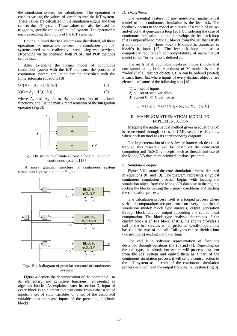
the simulation system for calculations. The operation ω enables writing the values of variables into the IoT system. These values are calculated in the simulation engine and then sent to the IoT system. These values can also be used for triggering specific actions of the IoT system. The operation γ enables reading the outputs of the IoT systems.

Having in mind that IoT systems are distributed, all these operations for interaction between the simulation and IoT systems need to be realized via web, using web services. Depending on the scenario, both PUSH and POP methods can be used.

After extending the formal model of continuous simulation system with the IoT elements, the process of continuous system simulation can be described with the finite automata equations [18]:

S(t) = I × A1 ∙ U(t), S(t) (8)

Y(t) = A2 ∙ U(t), S(t) (9)

where A1 and A2 are matrix representation of algebraic functions, and I is the matrix representation of the integration operator (Fig 3).

IS

A1

A2

U

Y

Fig3. The structure of finite automata for simulation of continuous systems [18]

A more granular structure of continuous system simulation is presented in the Figure 4.

Block b1

φ1(U,S,t)

Block biot

φiot(U,S,t)

Block bn

φn(U,S,t)

S'1

S1

Siot

Sn

S'iot

S'n

Siot, Sn

S1, Sn

S1, Siot

u1 um

u1 um

u1 um

Fig4. Block diagram of granular structure of continuous

systems

Figure 4 depicts the decomposition of the operator A1 to its elementary and primitive functions, represented as algebraic blocks. As explained later in section D, input of every block is an element that can come from either a set of inputs, a set of state variables or a set of the associated variables that represent inputs of the preceding algebraic blocks.

D. Orderliness

The essential feature of any non-trivial mathematical model of the continuous simulation is the feedback. The feedback occurs in the model as a result of a chain of cause-and-effect that generates a loop [20]. Considering the case of continuous simulation the model develops the feedback loop if it is impossible to mark all blocks from the set that satisfy a condition i < j, where block’s bi output is connected to block’s bj input [17]. The feedback loop imposes a compulsory requirement for computability of mathematical model called “orderliness”, defined as:

The set A of all countable algebraic blocks (blocks that correspond to algebraic functions) of M models is called “orderly” if all distinct objects aj ∈ A can be ordered (sorted) in such linear list where inputs of every distinct object aj are elements of some of the following sets [18]:

1) U – set of inputs 2) S – set of state variables 3) Subset Cˈ ⊂ C defined as :

Cˈ = c ∈ C | ∀i < j, ∀ aj = (φi, Xi, Yi,): c ∈ Xi

MAPPING MATHEMATICAL MODEL TO

IMPLEMENTATION

Mapping the mathematical method given in equations 1-9 is represented through series of UML sequence diagrams, where each method has its corresponding diagram.

The implementation of the software framework described through this research will be based on the concurrent computing and NoSQL concepts, such as threads and use of the MongoDB document-oriented database program.

A. Simulation engine

Figure 5 illustrates the core simulation process depicted in equations (8) and (9). The diagram represents a typical continuous simulation process: begins with loading the simulation object from the MongoDB database in the engine, sorting the blocks, setting the primary conditions and starting the calculation process.

The calculation process itself is a looped process where series of computations are performed on every block in the simulation model: block type analysis, output generation through block function, output appending and call for next computation. The block type analysis determines if the current block is an IoT block. If it is, the engine provides a call to the IoT service, which performs specific operations based on the type of the call. Call types can be divided into two groups: a) reading and b) writing.

The call is a software representation of functions described through equations (5), (6) and (7). Depending on the call type, the simulation system will process data sent from the IoT system and embed them as a part of the continuous simulation process, it will send a control action to the IoT system as a result of the continuous simulation process or it will read the output from the IoT system (Fig 6).

22

Fig5. UML sequence diagram of the core simulation process

B. Mapping the values of state variables and output from

the IoT system

The call for executing operation ρ (5) – reading the

values of variables from IoT system, is illustrated in the Figure 5, as a part of the calculation process, where simulation engine should consider IoT values as the part of the calculation.

The control actions, ω (6) – writing the values of variables into IoT system, sent to the IoT system are, also, a type of call. By connecting to the IoT system, the engine can access its API, create a call to the function provided by the user, send data from the simulation engine and thus begin the given process on the IoT platform. Such call is illustrated in the Figure 7.

Fig6. UML sequence diagram of processing calls to IoT system

Fig7. UML sequence diagram of the operation ω – writing the values of variables into IoT system

Through the connection made to IoT system, our engine can retrieve IoT system outputs and display them though the platform interface, which is directly correlated with

23

mathematical operation γ (7) – reading the outputs of the IoT systems (Fig 8.).

Fig8. UML sequence diagram of the operation γ – reading the outputs of the IoT systems

C. Example: Smart watering system simulation

The example of smart watering system simulation is an

illustration of the operation ω (6), where control actions and

variables are being sent to IoT system.

For this example it is necessary to create control actions

that will forward the data collected through the simulation

of the environment and air humidity by the simulation

engine, and signal the beginning of the IoT system actions.

Smart watering system is based on air humidity

predictions, provided as input parameters given by the

simulation engine. If the humidity is under the marginal

value set in the IoT system, the watering process begins.

CONCLUSION

Modelling hybrid IoT system for real-time simulation presents a focal point of this research. Thus, successfully mapping the values of state variables from the IoT system in the implementation process is essential.

The autonomous performance of the simulation program should be implemented using the concepts of concurrent computing – threads:

1) servicing requests for the simulation process control and error reporting,

2) servicing requests for configuration changes, 3) reading data and sending control actions to IoT

system, 4) servicing requests for simulation results, 5) execution of the simulation process

Further research and work should be directed towards execution of the proposed implementation, integration of the platform in the students’ educational process and evaluation and revision of the software performance. Upgrading the existing model with new modules should be considered.

ACKNOWLEDGMENT

Authors would like to thank prof. dr Bozidar Radenkovic, prof. dr Marijana Despotovic – Zrakic, prof. dr Zorica

Bogdanovic, prof. dr Dusan Barac and prof. dr Aleksandra Labus for guidance and mentoring throughout this research and software development.

REFERENCES

[1] E. A. Lee, S. A. Seshia. Introduction to Embedded Systems. A Cyber-Physical Systems Approach, 2017, Second Edition

[2] Y.Z. Lun, A. D'Innocenzo, F. Smarra, I. Malavolta, M. Benedetto, Maria. State of the Art of Cyber-Physical Systems Security: an Automatic Control perspective. Journal of Systems and Software, 2018, vol. 149, pp. 174-216

[3] N. Canadas, J. Machado, F. Soares, C. Barros, L. Varela. Simulation of cyber physical systems behaviour using timed plant models. Mechatronics, 2018, vol. 54, pp.175-185

[4] J. Liu, J. Lin. Design Optimization of WirelessHART Networks in Cyber-Physical Systems. Journal of Systems Architecture, 2019, article in press

[5] K. Carruthers. Internet of Things and Beyond: Cyber-Physical Systems. 2016. Available: https://iot.ieee.org/newsletter/may-2016/internet-of-things-and-beyond-cyber-physical-systems.html

[6] L. Tan, N. Wang. Future Internet: The Internet of Things. In: Proceedings of 3rd International Conference on Advanced Computer Theory and Engineering, 2010, vol. 5, pp. 376- 380.

[7] M. Wu, T. J. Lu, F. Y. Ling, J. Sun, H. Y. Du. Research on the architecture of Internet of Things. In: Proceedings of 3rd International 8 on Advanced Computer Theory and Engineering, 2010, vol.5, pp. 484-487.

[8] S. F.Ochoaa, G. Di Fatta. Cyber-physical systems, internet of things and big data. Future Generation Computer Systems, 2017, vol. 75, pp. 82-84

[9] B. Radenković, M. Despotović-Zrakić, Z. Bogdanović, D. Barać, A. Labus, Ž. Bojović. Internet inteligentnih uređaja. Beograd: Fakultet organizacionih nauka, 2017

[10] Ј. S. Albus. A Reference Model Architecture for Intelligent Systems Design. Springer, 1993. Available: https://web.archive.org/web/20080916153507/http://www.isd.mel.nist.gov/documents/albus/Ref_Model_Arch345.pdf

[11] F. E. Cellier, E. Kofman. Continuous System Simulation. Springer-Verlag, 2006, First Edition.

[12] J. Banks. Handbook of Simulation: Principles, Methodology, Advances, Applications, and Practice. John Wiley & Sons, 1998.

[13] J. S. Keranen , T. D. Raty. Model-based testing of embedded systems in hardware in the loop environment. IET Software, 2012, vol. 6, no. 4, pp. 364-376.

[14] N. L. Celanovic, I. L. Celanovic, Z. R. Ivanovic. Cyber Physical Systems: A New Approach to Power Electronics Simulation, Control and Testing. Advances in Electrical and Computer Engineering, 2012, vol.12, no.1, pp.33-38, 2012

[15] P. Garraghan, D. McKee, X. Ouyang, D. Webster, J. Xu. SEED: A Scalable Approach for Cyber-Physical System Simulation. IEEE Transactions on Services Computing, 2016, vol. 9, no. 2, pp. 199-212.

[16] M. Despotović-Zrakić, D. Barać, Z. Bogdanović, B. Jovanić, B. Radenković. Software Environment for Learning Continuous System Simulation. Acta Polytechnica Hungarica, 2014, vol. 11, no 2, pp. 187-202.

[17] B. Radenković. Program za simulaciju kontinualnih i diskretnih Sistema CSMP/MICRO. Automatika, 1984, vol. 25, pp. 235-238

[18] B. Radenković, M. Stanojević, A. Marković. Chapter 6 Simulacija kontinualnih sistema. Racunarska Simulacija, 2009, IV edition, pp. 89-110.

[19] T.Naumović, B. Radenković, M. Despotović-Zrakić, D. Barać, A.Labus. A framework for real-time management of intelligent devices: an educational perspective. International Conference on New Horizons in Education, 2018, Proceedings Book Volume 1, pp 33-34

[20] A. Ford. Modeling the Environment: An Introduction To System Dynamics Modeling Of Environmental Systems, 2010, Second Edition.

24

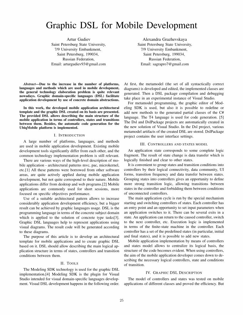
Graphic DSL for Mobile DevelopmentArtur Gudiev

Saint Petersburg State University,7/9 University Embankment,

Saint Petersburg, 199034,Russian Federation,

Email: arturgudiev93@gmail.com

Alexandra GrazhevskayaSaint Petersburg State University,

7/9 University Embankment,Saint Petersburg, 199034,

Russian Federation,Email: sagrapro7@gmail.com

Abstract—Due to the increase in the number of platforms,languages and methods which are used in mobile development,the general technology elaboration problem is quite relevantnowadays. Graphic domain-specific languages (DSL) facilitateapplication development by use of concrete domain abstractions.

In this work, the developed mobile application architecturaltemplate and the graphic DSL created on its basis are presented.The provided DSL allows describing the main structure of themobile application in terms of controllers, states and transitionsbetween them. Besides, the automatic code generation for theUbiqMobile platform is implemented.

I. INTRODUCTION

A large number of platforms, languages, and methodsare used in mobile application development. Existing mobiledevelopment tools significantly differ from each other, and thecommon technology implementation problem is still relevant.

There are various ways of the high-level description of mo-bile application - architectural patterns mvc, pac, microkernel,etc.[1] All these patterns were borrowed from other softwareareas, are quite actively applied during mobile applicationdevelopment, but not quite correspond to their nature. Mobileapplications differ from desktop and web programs.[2] Mobileapplications are commonly used for short sessions, morefocused on specific objectives performance.

Use of a suitable architectural pattern allows to increaseconsiderably application development efficiency, but a biggerresult can be achieved by graphic languages usage. DSL is theprogramming language in terms of the concrete subject domainwhich is applied to the solution of concrete type tasks[3].Graphic DSL languages help to represent applications usingvisual diagrams. The result code will be generated accordingto these diagrams.

The purpose of this article is to develop an architecturaltemplate for mobile applications and to create graphic DSLbased on it. DSL should allow describing the main logical ap-plication structure in terms of states, controllers and transitionconditions between them.

II. TOOLS

The Modeling SDK technology is used for the graphic DSLimplementation.[4] Modeling SDK is the plugin for VisualStudio intended for visual domain-specific languages develop-ment. Visual DSL development happens in the following order.

At first, the metamodel (the set of all syntactically correctdiagrams) is developed and edited, the implemented classes aregenerated. Then a DSL package compilation and debuggingtake place in an experimental instance of Visual Studio.

For metamodel programming, the graphic editor of Mod-eling SDK is used, but also it is possible to redefine oradd new methods to the generated partial classes of the C#language. The T4 language is used for code generation. [5]The Dsl and DslPackage projects are automatically created inthe new solution of Visual Studio. In the Dsl project, variousmetamodel artifacts of the created DSL are stored. DslPackageproject contains the user interface settings.

III. CONTROLLERS AND STATES MODEL

An application state corresponds to some complete logicfragment. The result of state change is data transfer which islogically finished and clear to other states.

It is convenient to group states and transition conditions intocontrollers by their logical connectivity, data community, UIforms, transition frequency and data transfer between states.Grouping states into controllers gives an opportunity to definemore strong transition logic, allowing transitions betweenstates in the controller and forbidding them between conditionsof unconnected controllers.

The main application cycle is run by the special mechanismstarting and switching controllers of states. Each controller hasan entry point and an opportunity to set input parameters whenan application switches to it. There can be several exits in astate. An application can return to the caused controller, switchto the next controller, etc. Execution logic is implementedin terms of the finite-state machine in the controller. Eachcontroller has a set of the predefined states (in particular, initialand final states), and it is possible to add new states.

Mobile application implementation by means of controllersand states model allows to centralize its logical basis, thestructure of the code becomes evident. When using controllers,the aim of the mobile application developer comes down to de-scribing the necessary logical controllers, state and conditionsof transition.

IV. GRAPHIC DSL DESCRIPTION

The model of controllers and states was tested on mobileapplications of different classes and proved the efficiency. But

25

the best results can be achieved, having taken this model as abasis of graphic DSL for mobile applications. (see Fig.1)

Fig. 1: Language implementation in Modelling SDK

Basic elements of the language are controllers and itsstates. States are placed on the controller, can connect amongthemselves and also to ports of the controller for the conditionsdescription of an entrance and an exit from it.

Each state opens in the separate diagram on which con-ditions of an entrance, an exit from a state and its internallogic are described. The logic of states includes a display ofUI forms, processing of their events, services calls, conditionschecking , etc.

There is a display of a UI form for each state in thelanguage. To connect the existing screen form with a statethe ShowForm element is used.

V. CODE GENERATION

The language of T4 templates is used for code generation.The main components of the T4 language are directives,blocks of the text and control units. For a generation of theunchangeable code, text blocks are used, and dynamic partsare implemented by means of control units.

As a result of generation, the controllers’ classes appear.Each controller has several states presented in the transfertype form. Process of work is implemented in terms of thefinite-state machine. On links between states, the template oftransitions are implemented. Controllers can also have ports.Ports are used for transitions between controllers.

The resulting code is applied to UbiqMobile platform.[6]UbiqMobile platform is aimed to cross-platform mobile de-velopment. The main features of the platform are that thebusiness logic of all applications is executed on the server.And mobile devices have only thick clients to represent theresult of application work.

VI. SAMPLES

The purpose of the first sample is to display the trainschedule for the user. The application consists of a singlecontroller and two states. In start state, the user can choosedeparture and destination stations. (see Fig.2) After clickingon the button, the application will switch the current state fromthe first state to the second one. (see Fig.3)

The second sample allows the user to log in and receivethe code which then can be used later. (see Fig. 4) Thereare two controllers in the application: LoginController andMainController. There is also a switching between controllers

implemented by means of ports. In LoginController there isonly one state. At MainController there are two states: a statewith option selection and a state where a user can receive thenecessary code. The UbiqMobile UI forms, corresponding tostates of the application are given below. (see Fig. 5)

Fig. 2: Schedule application scheme

Fig. 3: Schedule application UI form

Fig. 4: Application with authorization scheme

26

Fig. 5: UbiqMobile screens

VII. CONCLUSION

Within this work, the following results were achieved. Thegraphic DSL for mobile application development is imple-mented. The code generation for UbiqMobile platform featureis added. Demonstration samples are represented.

REFERENCES

[1] S. D. Plakalovic D., “Applying mvc and pac patterns in mobile applica-tions.”

[2] H. K.Flora, “An investigation on the characteristics of mobile applica-tions: A survey study.”

[3] D. Koznov. Domain-specific modellingmethodology and tools. [Online]. Available:http://www.math.spbu.ru/ru/mmeh/AspDok/pub/2016/koznov.pdf

[4] Modeling sdk for visual studio - domain-specific languages. [On-line]. Available: https://docs.microsoft.com/ru-ru/visualstudio/modeling/modeling-sdk-for-visual-studio-domain-specific-languages

[5] Code generation and t4 text templates. [Online].Available: https://docs.microsoft.com/ru-ru/visualstudio/modeling/code-generation-and-t4-text-templates?view=vs-2015

[6] A. Terekhov and V. Onosovski. Ubiq mobileplatform for mobile development. [Online]. Available:http://www.math.spbu.ru/user/ant/all articles/076 Terekhov Onos PlatformaUbiq.pdf

27

Graphical modeling of control systemsbased on Eclipse technologies

Mariia PlatonovaDepartment of Software Engineering

St. Petersburg State University28 Universitetsky pr., Saint-Petersburg, 198504, Russian Federation

Email: platonova.maria@outlook.com

Abstract—Only a few years ago Russia took the path ofthe digitalization and this trend is already taking active rootinto various areas of society. Digitalization is closely related tovisualization, that is easily confirmed by the increasing popularityof graphical representation of business processes.

This text describes the work on modeling and subsequentexecution of production processes, such as document circulation,working with CNC machines and analysing production risks, byusing the Eclipse IDE and the BPMN standard.

Index Terms—digitalization, visualization, code generation,business process, document circulation, CNC machine, bpmn,eclipse

I. INTRODUCTION

Information revolutions that took place throughout thewhole history of humanity undoubtedly made considerablechanges in life of society, its culture and lifestyle [1].

For several years Russia has been confidently introducingthe use of digitalization capabilities in many areas of societyand showing great results, which are noticeable on the worldstage [2]. Moreover, it should be noted that such processesinvolve the development of its own processing base, that has tocomply the requirements for quality and reliability of products.In addition these processes in the near future will contributefor Russian companies specializing in software developmentto confidently enter the global market.

The application of digitalization, we think, begins with anintuitive presentation of business processes as they are thebasis of the work of any company [3], and correspondinglyit is necessary to describe them in a convenient form to use.

It is worth considering a graphical representation of the pro-cesses, because the visualization helps to reduce the efforts tounderstand, discuss or modify any necessary information [4].There is an international standard BPMN (Business ProcessModel and Notation) intended for modeling business processes[5]. With the help of it any process can be represented in theform of a diagram, where its elements are any actions of thisprocess. In addition, the generation of an executable program,which is necessary for many processes, becomes much easilywith the use of diagram.

The main goal of this work is to create a tool to visualizeprocesses with the subsequent generation of executable code.Due to the differences of executable programs of variousprocesses, only three types of processes are considering in this

work: document circulation, working with computer numericalcontrol (CNC) machines and analysing production risks.

Similar study of creating a tool to visualize businessprocesses with a code generation feature has already beenconducted at the department of Software Engineering of St.Petersburg State University (department of SE) [6]. This tool isa part of the metaCASE technology based on QReal. However,the use of this practice can be justified only in the case ofcreating not one, but several products at once.

Based on previous experience the use of tools that are notvery common, complex or have many limitations can lead tothe problems with the development and support of the product,moreover, comparing it with analogues can become morecomplex. As IDE Eclipse was chosen, since it is a popular,free, cross-platform system, that is regularly updated, and ithas large developer community, which can make it easier tosolve occurring issues. Moreover, it is important to considerthe differences between open-source licenses, while usingready-made products. For example, General Public License(GPL) involve the free access to source code of the product,that based on any software under this license, so it can causesome problems with commercial use [7]. On the contrary,license Apache 2.0 does not put forward any requirements orother limits for using and distributing [8]. Therefore, in thiswork we decided to use only ready-made product under thislicense.

In conclusion, it is necessary to pay attention to convenienceof use the developed tool. At the department of SE a study ofhuman-computer interaction has been conducted on the baseof visual programming tools [9].

II. GRAPHICS EDITOR

The main task of the graphical editor is to build diagramsusing BPMN notation, another requirements involve the con-siderable expansion of its capabilities.

Full implementation of the editor is by no means easy, andsince there are various options of ready-made solutions, itseemed to us wisely to select the appropriate editor from theexisting versions and remake it according to our demands.Activiti-Designer (Activiti) was chosen from all of consideredoptions as it is popular and evolving application based onEclipse, that has a suitable license [10].

28

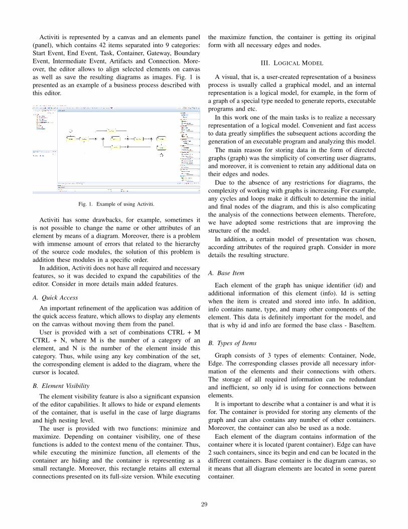
Activiti is represented by a canvas and an elements panel(panel), which contains 42 items separated into 9 categories:Start Event, End Event, Task, Container, Gateway, BoundaryEvent, Intermediate Event, Artifacts and Connection. More-over, the editor allows to align selected elements on canvasas well as save the resulting diagrams as images. Fig. 1 ispresented as an example of a business process described withthis editor.

Fig. 1. Example of using Activiti.

Activiti has some drawbacks, for example, sometimes itis not possible to change the name or other attributes of anelement by means of a diagram. Moreover, there is a problemwith immense amount of errors that related to the hierarchyof the source code modules, the solution of this problem isaddition these modules in a specific order.

In addition, Activiti does not have all required and necessaryfeatures, so it was decided to expand the capabilities of theeditor. Consider in more details main added features.

A. Quick Access

An important refinement of the application was addition ofthe quick access feature, which allows to display any elementson the canvas without moving them from the panel.

User is provided with a set of combinations CTRL + MCTRL + N, where M is the number of a category of anelement, and N is the number of the element inside thiscategory. Thus, while using any key combination of the set,the corresponding element is added to the diagram, where thecursor is located.

B. Element Visibility

The element visibility feature is also a significant expansionof the editor capabilities. It allows to hide or expand elementsof the container, that is useful in the case of large diagramsand high nesting level.

The user is provided with two functions: minimize andmaximize. Depending on container visibility, one of thesefunctions is added to the context menu of the container. Thus,while executing the minimize function, all elements of thecontainer are hiding and the container is representing as asmall rectangle. Moreover, this rectangle retains all externalconnections presented on its full-size version. While executing

the maximize function, the container is getting its originalform with all necessary edges and nodes.

III. LOGICAL MODEL

A visual, that is, a user-created representation of a businessprocess is usually called a graphical model, and an internalrepresentation is a logical model, for example, in the form ofa graph of a special type needed to generate reports, executableprograms and etc.

In this work one of the main tasks is to realize a necessaryrepresentation of a logical model. Convenient and fast accessto data greatly simplifies the subsequent actions according thegeneration of an executable program and analyzing this model.

The main reason for storing data in the form of directedgraphs (graph) was the simplicity of converting user diagrams,and moreover, it is convenient to retain any additional data ontheir edges and nodes.

Due to the absence of any restrictions for diagrams, thecomplexity of working with graphs is increasing. For example,any cycles and loops make it difficult to determine the initialand final nodes of the diagram, and this is also complicatingthe analysis of the connections between elements. Therefore,we have adopted some restrictions that are improving thestructure of the model.

In addition, a certain model of presentation was chosen,according attributes of the required graph. Consider in moredetails the resulting structure.

A. Base Item

Each element of the graph has unique identifier (id) andadditional information of this element (info). Id is settingwhen the item is created and stored into info. In addition,info contains name, type, and many other components of theelement. This data is definitely important for the model, andthat is why id and info are formed the base class - BaseItem.

B. Types of Items

Graph consists of 3 types of elements: Container, Node,Edge. The corresponding classes provide all necessary infor-mation of the elements and their connections with others.The storage of all required information can be redundantand inefficient, so only id is using for connections betweenelements.

It is important to describe what a container is and what it isfor. The container is provided for storing any elements of thegraph and can also contains any number of other containers.Moreover, the container can also be used as a node.

Each element of the diagram contains information of thecontainer where it is located (parent container). Edge can have2 such containers, since its begin and end can be located in thedifferent containers. Base container is the diagram canvas, soit means that all diagram elements are located in some parentcontainer.

29

C. Graph Description

Special classes are responsible for graph representation,such as NodeUtil, EdgeUtil and ContainerUtil. These classesare static, that allows to use the same instance for anyreferences to a class.

Each class is in charge for the current list of relevantelements. Modification of the classes has to be occurred onany diagram changes, for example, when adding, changing ordeleting element.

IV. APPLICATION EXAMPLES

A. Document Circulation

For any companies are important to track its documentsand check their status, that is, during the life cycle of a somedocument, it is necessary to know where and in what conditionit is.

Such process is conveniently presented as a BPMN diagram,for example, Fig. 2. The diagram provides simple to trackthe document and its current status, as its movements occuralong the constructed graph. There is a hierarchy system inmany companies, and with this representation of the documentmovements, it is simple to control that only employees withthe required authority can access to the document.

Fig. 2. Example of BPMN diagram for document circulation.

B. CNC Machines

Recent years many factories have been implementing intotheir working process more and more CNC machines [11],which significantly increase the automation of production andalso the quality of the result.

Full automation of such processes is becoming possible inthe case of using CNC machines along with industrial robots(robot), for example, cylindrical robots, packaging robots andetc. Their main task is transferring the necessary materialsfrom one machine to another.

The question is how to program CNC machines and controlthe robots operations. It is important not only to specify theentire sequence of actions, but also to describe the reaction tothe faulty situations, because robot can strayed or fall down

due to accidental rubbish or uneven surface, which can causethe system malfunctions or the transported cargoes breakages.

Programs for CNC machines, as well as, operations ofrobots can be described as BPMN diagrams, for example,Fig. 3. In this way, it is convenient to set robots failurebranches, that allows to quickly react to any problems andrestore production process.

Fig. 3. Example of BPMN diagram for CNC machines.

C. Production Risks

Analysis of vendors and associated risks are importantfor any companies, since supply disruptions can significantlyaffect the production process, for example, it can cause in-creasing budget or execution time. In addition, vendors forma hierarchical structure, so it is necessary to control the wholesystem, due to the problem can occur on any level of thehierarchy.

One way to describe this structure is using BPMN diagrams.This will allow to implement automatic data analysis and ac-cumulating statistics for each vendor, which will significantlyreduce user actions and the influence of the human factor.

V. CODE GENERATOR

Executable programs of various types of production pro-cesses can significantly differ by its structure and end result.In this regard, code generators are implemented only for theprocesses described in the previous section. Each process isrepresented as a diagram, according to which a logical modelis built with the subsequent generation of the executable code.

The main step, that preceding code generation, is analysis ofthe model. This intermediate step is necessary for identifyingthe start and end nodes, cycles, loops and etc. Data whichobtained at that step is the input for code generator, so it iscertainly useful to be able to visualize them, since variousinaccuracies and errors can be detected that were missedduring the construction of the diagram.

The user is provided with the showModel function, whichexecutes by pressing the Show model button located in themain menu. This function can be applied to any diagram, even

30

if code generation is not possible. Fig. 4 shows an example ofthe diagram and Fig. 5 shows the visualization of its model.

Fig. 4. Example of diagram for model visualization.

Thus, while executing showModel function to a diagram, aparticular window opens where all its elements are displayedin a specific form. Recall that a child node is the destinationof one of its edge and that a container can be used as a node,that is, it can have children and can be a child.

For each container, including the base one, the window dis-plays all the corresponding elements: nodes and their children.Moreover, if the element is a container, then it is marked witha square brackets ([]), and if the element is a Gateway, thenit is marked with a triangular brackets (〈〉). In addition, all itscontainers, that located in the current, will be display singlywith all content. Relations between elements are representedin a certain form: element1 -〉 edge -〉 element2.

Such presentation of a logical model provides easily gen-erating code, as the task is reduced to simple linear graphtraversal with a code generation for each action.

Fig. 5. Example of diagram logical model visualization.

CONCLUSION

In this paper we presented a description of the work oncreation a tool for graphical representation of productionprocesses with the capability of generating an executableprogram. The main part of the work, as the most part of thetext, was focused on the modification of the Activiti graphicaleditor and the creation of a logical model.

REFERENCES

[1] Chusyainov T.M. Informacionnaya revolyuciya i transformaciya zany-atosti. Nauka. Mysl’, 2017.

[2] Chakravorti Bhaskar, Chaturvedi Ravi S. Digital Planet 2017: HowCompetitiveness and Trust in Digital Economies Vary Across the World.Tufts University: The Fletcher School, 2017.

[3] Plotnikov V.A. Cifrovizaciya proizvodstva: teoreticheskaya sushchnost’i perspektivy razvitiya v rossijskoj ehkonomike. Izvestiya UNECON,2018.

[4] Afanas’ev A.A. Tekhnologiya vizualizacii dannyh kak instrument sover-shenstvovaniya processa podderzhki prinyatiya reshenij. Inzhenernyjvestnik Dona, 2014.

[5] Business Process Model And Notation. Object Management Group(OMG), 2011.

[6] QReal:BP. QReal, 2013, url: http://qreal.ru/static.php?link=QRealBP.[7] General Public License. Free Software Foundation, 2007.[8] Apache 2.0. Apache Software Foundation, 2004.[9] Kuzenkova A.S. Avtomatizirovannyj analiz povedeniya pol’zovatelya v

QReal:Robots. 2014.[10] Activiti-Designer. Activiti Team. url: https://github.com/Activiti/Activiti-

Designer.[11] Lovygin A.A., Teverovskij L.V. Osnovy chislovogo programmnogo

upravleniya. Sovremennyj stanok s CHPU i CAD/CAM sistema, 2015.

31

Component-Based Software as a tool for developingcomplex distributed heterogeneous systems

Dmitry KulikovR&D Department

Rapid Telecom System Labs LLC.Nizhny Novgorod, Russia

kulikov@ivc.nnov.ru

Vasilii MokhinR&D Department

Rapid Telecom System Labs LLC.Nizhny Novgorod, Russia

mokhin@ivc.nnov.ru

Sergey ZolotovR&D Department

Rapid Telecom System Labs LLC.Nizhny Novgorod, Russia

sergey@ivc.nnov.ru

I. INTRODUCTION

Robotics is now one of the most sought-after and actualareas of applied sciences. More and more people are interestedin this direction, thanks to which the software of robots doesnot stand still and evolves in huge steps, starting from thefirmware of the device controllers and ending with the mostcomplex software packages designed to solve a wide rangeof tasks. And, as in any software system, there can be manyproblems, for example, problems of architecture, developmentand debugging, etc. In this paper we will consider an exampleof the implementation of the project of automatic controlsystem project with heterogeneous computing nodes the caseof a complex hybrid, distributed computing system created onthe basis of operating system based on the Linux kernel andthe ROS framework [1].

II. OBJECTIVE

The target of the project was to unite all the nodes of thecreated heterogeneous system, in which the computing nodeswere used as part of a personal computer based on IBMPC x86, single-Board computers based on ARM processor(Raspberry PI3) and hardware-software based on the Atmegacontroller(Arduino) into a single computer network capableof receiving information in real time from various sensors,processing it in a given period of time and transmittingcommands to other nodes.

III. CHOOSING A FRAMEWORK

First, it was necessary to choose a framework for heteroge-neous system, because there are quite a large number of themand almost all are suitable for the task. Among all the optionsI chose the most common: ROS, MRDS, URBI, OROCOS,Gazebo, studied them and created a comparative table below,of the 11 most important criteria (see table I):

• open source;• project examples;• documentation;

• the activity of the community;• license;• application architecture;• communication protocol;• kernel;• supported programming languages;• supported OS;• supported devices.

Based on the results of the studies given in the comparativetable it was concluded that ROS is the best choice for thesolution of the problem, because:

• it is open source;• it has complete infrastructure;• implemented a variety of ready-made solutions for a

variety of sensors, controllers, etc;• focused on complex tasks;• it is possible to work in real time;• support for a wide range of Executive computing devices.

IV. THE CONCEPT OF ROS

ROS is a framework for robot developing, provides func-tionality for distributed work and standard operating systemservices such as hardware abstraction, low-level device con-trol, implementation of commonly used functions, commu-nication between processes, and package management [2].ROS based on a graph architecture where data is processedin nodes that can receive and transmit messages to eachother. ROS supports parallel computing, has good integrationwith C++ and Python, can run on single-Board computerssuch as Raspberry Pi, BeagleBone, as well as microcontrollerplatforms running on the ATmega chip (such as Arduino).The concept of ROS :

• node — is a process that performs calculations and isable to communicate with other nodes;

• message — is a type of ROS data by which nodes cancommunicate with each other;

• topic - is the name that is used to identify the content ofthe message;

32

TABLE IROSOBOTS FRAMEWORKS COMPARISON

ROS MRDS URBI OROCOS GAZEBOOpensource + - + + +

Project examples Exists an extensiveand open knowledge

base with ready-madeprojects

Exists many exampleswith MRDS projects

Exists many examplesof working with

URBO

Exists large set ofready-made libraries

Exists many pre-madecomponents

Documentation Well documented Well documented Well documented Well documented Well documentedCommunity Active community Inactive community Inactive community No community Inactive community

License BSD(free for researchand commercial use)

Various(free forresearch)

BSD(Free use, exceptfor the simulator,

which is not in theURBI)

BSD((free forresearch and

commercial use)

GNU General PublicLicense(free for

research)

Architecture Graph architecture Modular architecture Client-Server Not found DistributedProtocol xmlrpc HTTP, DSSP Firmata Not found SDFKernel ReactOS KITL Urbi SDK Not found Not found

Supported languages Python, C++, Lispand experimental

libraries on Java andLua

C#, Visual Basic.NET, JScript and

IronPython

urbiscript Not found C, C++, Java, Tcl andPython

OS Currently, ROS onlyworks on Unix

platforms

Works only onWindows OS

cross-platform Not found Linux, Mac OS X,Solaris and BSD

Supported devices Atmegamicrocontroller, ARMfamily of processors,

etc.

Atmegamicrocontroller, ARMfamily of processors,

etc.

x86, ARM, MIPS,PowerPC, etc.

Not found Atmegamicrocontroller, ARMfamily of processors,

etc.

• master — is a ROS name service that allows nodes todiscover each other, exchange messages, and call thenecessary services;

• rosout — is a live message output;• roscore — Master + Rosout + parameter Server.The main concepts of ROS are nodes, messages, themes,

services. Architecturally, all computing tasks are performed inROS nodes that communicate with each other via messages.These message nodes are published to topics, which divide themessages into groups of interest indeed when a node needs toreceive messages with specific data, that node subscribes toa specific topic. To implement synchronous message passing,which is necessary in certain cases, ROS defines services - amechanism that operates on a question - answer basis.

V. PRACTICAL PART

Thanks to ROS, it was possible to link all the equipmentinto a single computer network with convenient debuggingand rapid prototyping without any problems. Each of themicrocontrollers was a separate node that received data,performed the necessary calculations, made a decisionand could exchange data with other nodes at a specifiedfrequency(see Fig.2.).

To process such a large amount of information for ROS-Master, a separate full-fledged computer(see Fig.1.), whichguaranteed minimal delays in the exchange and processingof information between nodes [3]–[5]. ROS is very welldocumented, has an active community and a lot of ready-madeexamples to work with it, starting from examples of messagetransmission and ending with the basic projects of workingwith 3d SLAM, indeed it was not necessary to spend a huge

Fig. 1. Device layout.

amount of time searching for the necessary information, andif there were any errors during compilation, then in ROScommunity it was possible to find a solution to eliminate thiserror, which contributed to a significant acceleration of thedevelopment process.

VI. SAMPLE CODE FOR ROSAs an example of the implementation of heterogeneous

nodes on the ROS framework, we present several examples ofcode written for different platforms (Arduino and RaspberryPi 3). On Raspberry Pi3 nodes were written on Python, andon Arduino in C++.

A. Example code on Arduino(C++)

Using the rosserial arduino package allows you to useROS in conjunction with the Arduino IDE. rosserial uses a

33

Fig. 2. Device layout with nodes.

data transfer Protocol that works through the Arduino UART(universal asynchronous transceiver). This allows Arduino tobe a full ROS node that can publish and subscribe to ROSmessages, publish TF (spatial) transformations, and receiveROS system time. Linking ROS to Arduino is implementedthrough the use of the Arduino library. To use the rosseriallibraries in your code, first of all, you need to connect them:

# i n c l u d e <r o s . h>

After we should specify the type of message:

# inc lude<s td msgs / I n t 3 2 . h>s td msgs : : I n t 3 2 i msg ;

Tell the master that we are going to be publishing a message oftype std msgs/Int32 on the topic chatter. This lets the mastertell any nodes listening on chatter that we are going to publishdata on that topic:

r o s : : P u b l i s h e r c h a t t e r ( ” c h a t t e r ” , &i msg ) ;

Subscribe to the pwm signal topic with the master. ROS willcall the msgCb() function whenever a new message arrives.

r o s : : S u b s c r i b e r sub ( ” pwm signal ” ,&msgCb ) ;

NodeHandle::subscribe() returns a ros::Subscriber object, thatyou must hold on to until you want to unsubscribe. When theSubscriber object is destructed, it will automatically unsub-scribe from the chatter topic:

nh . s u b s c r i b e ( sub ) ;

NodeHandle::advertise() returns a ros::Publisher object, whichserves two purposes: 1) it contains a publish() method that letsyou publish messages onto the topic it was created with, and 2)when it goes out of scope, it will automatically unadvertised:

nh . a d v e r t i s e ( c h a t t e r ) ;

A ros::Rate object allows you to specify a frequency that youwould like to loop at. It will keep track of how long it has beensince the last call to Rate::sleep(), and sleep for the correctamount of time:

r o s : : Ra te l o o p r a t e ( 1 0 ) ;

Now we actually broadcast the message to anyone who isconnected:

c h a t t e r . p u b l i s h (&i msg ) ;

B. Example code on Raspberry Pi 3(Python)

You need to import rospy if you are writing a ROS Node,this is a pure Python client library for ROS. The rospy clientAPI enables Python programmers to quickly interface withROS Topics, Services, and Parameters. The std msgs.msgimport is so that we can reuse the std msgs/Int32 messagetype (a simple string container) for publishing:

import r o s p yfrom s td msgs . msg import I n t 3 2

After this, you must write a section of code defines thetalker’s interface to the rest of ROS. declares that your nodeis publishing to the chatter topic using the message typeInt32. The queue size argument limits the amount of queuedmessages indeed any subscriber is not receiving them fastenough. Rospy.init node tells rospy the name of your node- as long as raspy does not have this information, it cannotstart communicating with the ROS wizard:

pub = r o s p y . P u b l i s h e r ( ’ c h a t t e r ’ , I n t 3 2 ,q u e u e s i z e =10)r o s p y . i n i t n o d e ( ’ t a l k e r ’ , anonymous=True )

This code declares that your node subscribes to the chattertopic which is of type std msgs.msgs.Int32. When new mes-sages are received, callback is invoked with the message asthe first argument:

r o s p y . i n i t n o d e ( ’ l i s t e n e r ’ , anonymous=True )r o s p y . S u b s c r i b e r ( ’ c h a t t e r , I n t 3 2 , c a l l b a c k )

In this example, the program operation is a call to thepub.publish(condition) that publishes Int32 in our chatter topic.The loop calls rate.sleep(), which sleeps to maintain thedesired rate the loop:

whi le not r o s p y . i s s h u t d o w n ( ) :r o s p y . l o g i n f o ( c o n d i t i o n )pub . p u b l i s h ( c o n d i t i o n )r a t e . s l e e p ( 1 0 )

rospy.loginfo (condition) allows you to:• display messages on the screen• automatically write messages to the host log file• write messages to rosout

With using Rosout it is easier to debug because you can getmessages using rqt console, therefore, we may not to find anduse the console window with the logs of your node [6].Based on the above code examples, it becomes clear thatusing ROS with languages such as C++ and Python is quiteeasy, because after reading the documentation in detail andstudying the ready-made solutions, you can easily make anyof the platforms supported by ROS many nodes that will becombined into a single computer network.

34

VII. CONCLUSION

After analyzing all the currently available frameworks suit-able for creating a distributed heterogeneous real-time networkfocused on complex tasks and supporting work with a widerange of computing devices, I came to the conclusion that ROSis the most suitable for use in solving the task set before me.ROS allows you to develop a flexible heterogeneous structuresuitable for rapid prototyping, modeling and testing of variousvariants of real-time systems, which in turn accelerates theprocess of developing the final device.At this stage, the project is completely ready, the system de-veloped by me has been tested and confirmed its performanceon an unmanned vehicle. The results obtained in the course ofthese studies formed the basis for the creation of an automatedunmanned vehicle, and further refinement and expansion of itsfunctionality will allow to achieve in the future more efficientuse in various vehicles.

REFERENCES

[1] Aaron Martinez, Enrique Fernndez. Learning ROS for Robotics Program-ming. Mumbai: Packt Publishing, 2013. ISBN 978-1-78216-144-8

[2] Jason M. OKane. A Gentle Introduction to ROS. Columbia: University ofSouth Carolina, 2014. ISBN 978-14-92143-23-9

[3] Yukihiro Saito, Futoshi Sato, Takuya Azumi, Shinpei Kato, NobuhikoNishio . ROSCH:Real-Time Scheduling Framework for ROS . 2018 IEEE24th International Conference on Embedded and Real-Time ComputingSystems and Applications (RTCSA), 2018, pp. 52-58.

[4] H. Wei, Z. Huang, Q. Yu, M. Liu, Y. Guan, J. Tan. RGMP-ROS:A real-time ROS architecture of hybrid RTOS and GPOS on multi-core processor. 2014 IEEE International Conference on Robotics andAutomation (ICRA), 2014, pp. 2482-2487.

[5] Y. Saito, T. Azumi, S. Kato, N. Nishio Priority and SynchronizationSupport for ROS. 2016 IEEE 4th International Conference on Cyber-Physical Systems Networks and Applications (CPSNA), 2016, pp. 77-82.

[6] H. Wei, Z. Shao, Z. Huang, R. Chen, Y. Guan, J. Tan, Z. Shao RT-ROS: Areal-time ROS architecture on multi-core processors. Future GenerationComputer Systems, 2016, vol.56, pp. 171-178.

35

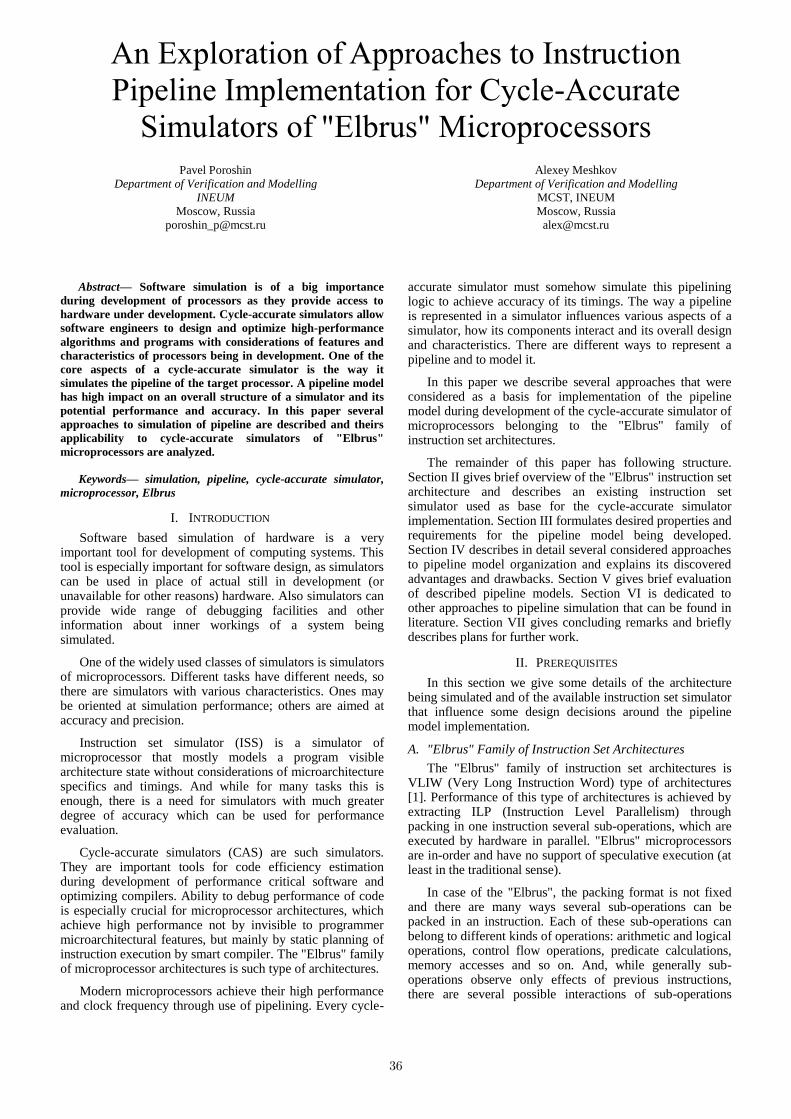
An Exploration of Approaches to Instruction

Pipeline Implementation for Cycle-Accurate

Simulators of "Elbrus" Microprocessors

Pavel Poroshin

Department of Verification and Modelling

INEUM

Moscow, Russia

poroshin_p@mcst.ru

Alexey Meshkov

Department of Verification and Modelling

MCST, INEUM

Moscow, Russia

alex@mcst.ru

Abstract— Software simulation is of a big importance

during development of processors as they provide access to

hardware under development. Cycle-accurate simulators allow

software engineers to design and optimize high-performance

algorithms and programs with considerations of features and

characteristics of processors being in development. One of the

core aspects of a cycle-accurate simulator is the way it

simulates the pipeline of the target processor. A pipeline model

has high impact on an overall structure of a simulator and its

potential performance and accuracy. In this paper several

approaches to simulation of pipeline are described and theirs

applicability to cycle-accurate simulators of "Elbrus"

microprocessors are analyzed.

Keywords— simulation, pipeline, cycle-accurate simulator,

microprocessor, Elbrus

I. INTRODUCTION

Software based simulation of hardware is a very important tool for development of computing systems. This tool is especially important for software design, as simulators can be used in place of actual still in development (or unavailable for other reasons) hardware. Also simulators can provide wide range of debugging facilities and other information about inner workings of a system being simulated.

One of the widely used classes of simulators is simulators of microprocessors. Different tasks have different needs, so there are simulators with various characteristics. Ones may be oriented at simulation performance; others are aimed at accuracy and precision.

Instruction set simulator (ISS) is a simulator of microprocessor that mostly models a program visible architecture state without considerations of microarchitecture specifics and timings. And while for many tasks this is enough, there is a need for simulators with much greater degree of accuracy which can be used for performance evaluation.

Cycle-accurate simulators (CAS) are such simulators. They are important tools for code efficiency estimation during development of performance critical software and optimizing compilers. Ability to debug performance of code is especially crucial for microprocessor architectures, which achieve high performance not by invisible to programmer microarchitectural features, but mainly by static planning of instruction execution by smart compiler. The "Elbrus" family of microprocessor architectures is such type of architectures.

Modern microprocessors achieve their high performance and clock frequency through use of pipelining. Every cycle-

accurate simulator must somehow simulate this pipelining logic to achieve accuracy of its timings. The way a pipeline is represented in a simulator influences various aspects of a simulator, how its components interact and its overall design and characteristics. There are different ways to represent a pipeline and to model it.

In this paper we describe several approaches that were considered as a basis for implementation of the pipeline model during development of the cycle-accurate simulator of microprocessors belonging to the "Elbrus" family of instruction set architectures.

The remainder of this paper has following structure. Section II gives brief overview of the "Elbrus" instruction set architecture and describes an existing instruction set simulator used as base for the cycle-accurate simulator implementation. Section III formulates desired properties and requirements for the pipeline model being developed. Section IV describes in detail several considered approaches to pipeline model organization and explains its discovered advantages and drawbacks. Section V gives brief evaluation of described pipeline models. Section VI is dedicated to other approaches to pipeline simulation that can be found in literature. Section VII gives concluding remarks and briefly describes plans for further work.

II. PREREQUISITES

In this section we give some details of the architecture being simulated and of the available instruction set simulator that influence some design decisions around the pipeline model implementation.

A. "Elbrus" Family of Instruction Set Architectures

The "Elbrus" family of instruction set architectures is VLIW (Very Long Instruction Word) type of architectures [1]. Performance of this type of architectures is achieved by extracting ILP (Instruction Level Parallelism) through packing in one instruction several sub-operations, which are executed by hardware in parallel. "Elbrus" microprocessors are in-order and have no support of speculative execution (at least in the traditional sense).

In case of the "Elbrus", the packing format is not fixed and there are many ways several sub-operations can be packed in an instruction. Each of these sub-operations can belong to different kinds of operations: arithmetic and logical operations, control flow operations, predicate calculations, memory accesses and so on. And, while generally sub-operations observe only effects of previous instructions, there are several possible interactions of sub-operations

36

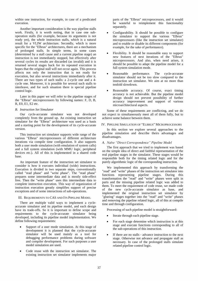
within one instruction, for example, in case of a predicated execution.

Another important consideration is the way pipeline stalls work. Firstly, it is worth noting, that in case one sub-operation stalls (for example, because its arguments is not ready yet), the whole instruction stalls, which is a natural result for a VLIW architecture. Secondly, which is more specific for the "Elbrus" architectures, there are a mechanism of prolonged stalls. In simple terms, in some cases (determined by a stall cause and a current pipeline stage) an instruction is not immediately stopped, but effectively after several cycles its results are discarded (as invalid) and it is returned several stages back for its repeated execution in hopes that the original stall will not occur again. This process affects not only the instruction that is not ready for execution, but also several instructions immediately after it. There are two types of such stalls: a 2-cycle one and a 4-cycle one. Moreover, it is possible for several such stalls to interleave, and for such situation there is special pipeline control logic.

Later in this paper we will refer to the pipeline stages of the "Elbrus" microprocessors by following names: F, D, B, R, E0, E1, E2 etc.

B. Instruction Set Simulator

Our cycle-accurate simulator was not developed completely from the ground up. An existing instruction set simulator for the "Elbrus" architecture was used as a basis and a starting point for the development of its cycle-accurate version.

This instruction set simulator supports wide range of the various "Elbrus" microprocessors of different architecture iterations via compile time configuration. It also supports both a user mode simulation (with emulation of system calls) and a full system simulation (with MMU logic, peripheral devices etc.). All of this is implemented in a shared code base.

An important feature of the instruction set simulator to consider is how it executes individual (wide) instructions. Execution is divided in two separate steps, conventionally called "read phase" and "write phase". The "read phase" prepares some intermediate data and is mostly side-effect free. Then the "write phase" uses this intermediate data to complete instruction execution. This way of organization of instruction execution greatly simplifies support of precise exceptions and of some interactions of sub-operations.

III. REQUIREMENTS TO CAS AND ITS PIPELINE MODEL

There are multiple valid ways to implement a cycle-accurate simulator and its pipeline model, and each design have its trade-offs. So it is important to define scope and requirements to the cycle-accurate simulator being developed, including its pipeline model implementation. We define following requirements:

Support of a user mode simulation. At this stage of development it is planned that the cycle-accurate simulator will be used mainly as a tool for debugging performance problems during software and compiler development. For such purposes a user model simulation are used.

Code reuse with the instruction set simulator. The existing instruction set simulator implements major

parts of the "Elbrus" microprocessors, and it would be wasteful to reimplement this functionality separately.

Configurability. It should be possible to configure the simulator to support the various "Elbrus" microprocessors (like the instruction set simulator) and to enable or disable its different components (for example, for the sake of performance).

Flexibility. It should be reasonable easy to support new features of next iterations of the "Elbrus" microprocessors. And also, when need arises, it should be possible to adapt the pipeline model for a full system simulation mode.

Reasonable performance. The cycle-accurate simulator should not be too slow compared to the instruction set simulator. We aim at no more than tenfold slowdown.

Reasonable accuracy. Of course, exact timing accuracy is not achievable. But the pipeline model design should not prevent possibility of further accuracy improvement and support of various microarchitectural aspects.

Some of these requirements are conflicting, and we do not expect to simultaneously meet all of them fully, but to achieve some balance between them.

IV. PIPELINE SIMULATION OF “ELBRUS” MICROPROCESSORS

In this section we explore several approaches to the pipeline simulation and describe theirs advantages and disadvantages.

A. Naïve “Direct Correspondence” Pipeline Model

The first approach that we tried to implement was based on the simple idea of direct and faithful representation of the real pipeline stages in the simulator. These stages would be responsible both for the timing related logic and for the purely algorithmic logic of the corresponding instruction.

We implemented this approach by transforming the "read" and "write" phases of the instruction set simulator into functions representing pipeline stages. During this transformation the "read" and "write" phases were split in parts and the missing pipeline related logic was added to them. To meet the requirement of code reuse, we made code of the new cycle-accurate simulator as base, and implemented the original instruction set simulator by "glueing" stages together into the "read" and "write" phases and removing the pipeline related logic, all of this at compile time and through configuration.

Processing of such pipeline model is straightforward:

Iterate through each pipeline stage.

For each stage determine which instruction is at this stage and execute functions corresponding to all of the sub-operations of this instruction.

If there are no stalls - advance instruction to the next stage. Otherwise not advance and propagate stall as necessary. In case of the prolonged stalls simulate related pipeline control logic.

37

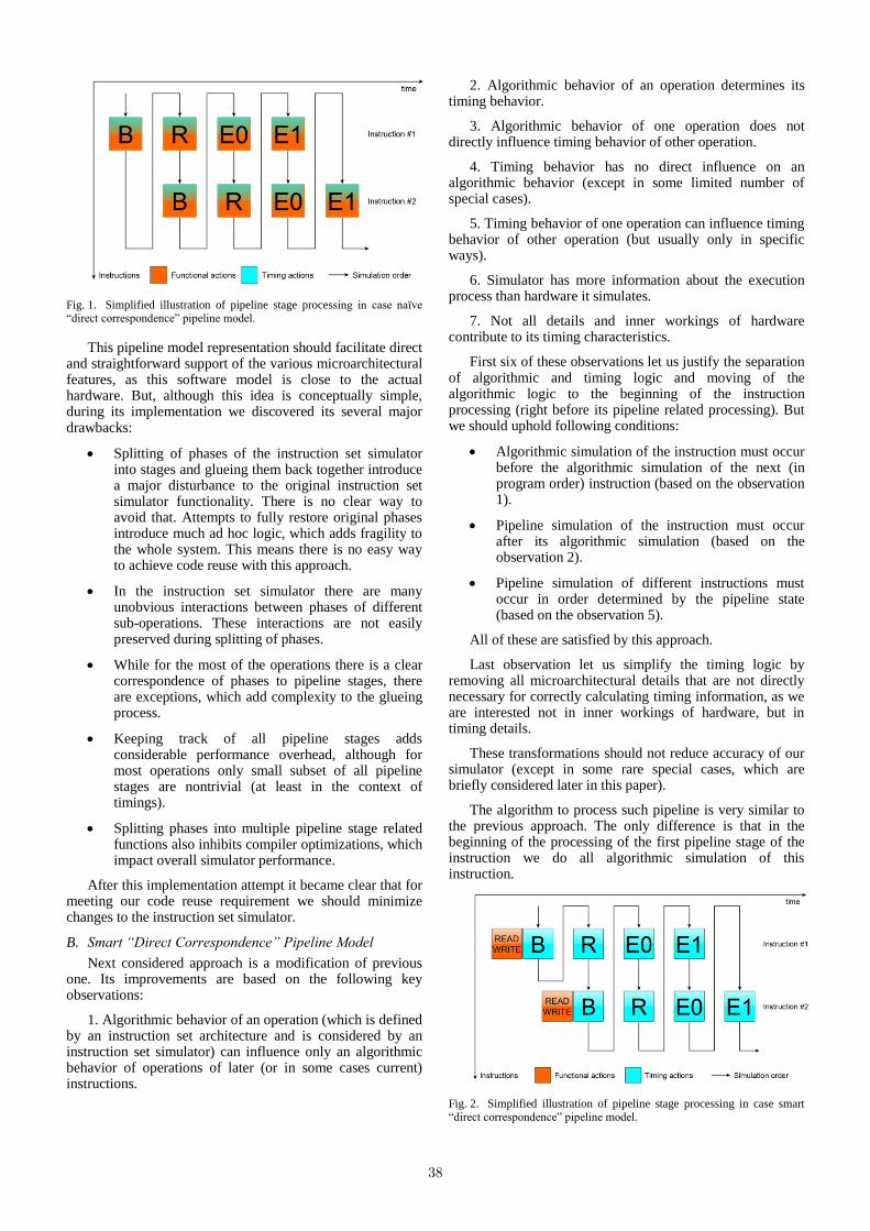
Fig. 1. Simplified illustration of pipeline stage processing in case naïve “direct correspondence” pipeline model.

This pipeline model representation should facilitate direct and straightforward support of the various microarchitectural features, as this software model is close to the actual hardware. But, although this idea is conceptually simple, during its implementation we discovered its several major drawbacks:

Splitting of phases of the instruction set simulator into stages and glueing them back together introduce a major disturbance to the original instruction set simulator functionality. There is no clear way to avoid that. Attempts to fully restore original phases introduce much ad hoc logic, which adds fragility to the whole system. This means there is no easy way to achieve code reuse with this approach.

In the instruction set simulator there are many unobvious interactions between phases of different sub-operations. These interactions are not easily preserved during splitting of phases.

While for the most of the operations there is a clear correspondence of phases to pipeline stages, there are exceptions, which add complexity to the glueing process.

Keeping track of all pipeline stages adds considerable performance overhead, although for most operations only small subset of all pipeline stages are nontrivial (at least in the context of timings).

Splitting phases into multiple pipeline stage related functions also inhibits compiler optimizations, which impact overall simulator performance.

After this implementation attempt it became clear that for meeting our code reuse requirement we should minimize changes to the instruction set simulator.

B. Smart “Direct Correspondence” Pipeline Model

Next considered approach is a modification of previous one. Its improvements are based on the following key observations:

1. Algorithmic behavior of an operation (which is defined by an instruction set architecture and is considered by an instruction set simulator) can influence only an algorithmic behavior of operations of later (or in some cases current) instructions.

2. Algorithmic behavior of an operation determines its timing behavior.

3. Algorithmic behavior of one operation does not directly influence timing behavior of other operation.

4. Timing behavior has no direct influence on an algorithmic behavior (except in some limited number of special cases).

5. Timing behavior of one operation can influence timing behavior of other operation (but usually only in specific ways).

6. Simulator has more information about the execution process than hardware it simulates.

7. Not all details and inner workings of hardware contribute to its timing characteristics.

First six of these observations let us justify the separation of algorithmic and timing logic and moving of the algorithmic logic to the beginning of the instruction processing (right before its pipeline related processing). But we should uphold following conditions:

Algorithmic simulation of the instruction must occur before the algorithmic simulation of the next (in program order) instruction (based on the observation 1).

Pipeline simulation of the instruction must occur after its algorithmic simulation (based on the observation 2).

Pipeline simulation of different instructions must occur in order determined by the pipeline state (based on the observation 5).

All of these are satisfied by this approach.

Last observation let us simplify the timing logic by removing all microarchitectural details that are not directly necessary for correctly calculating timing information, as we are interested not in inner workings of hardware, but in timing details.

These transformations should not reduce accuracy of our simulator (except in some rare special cases, which are briefly considered later in this paper).

The algorithm to process such pipeline is very similar to the previous approach. The only difference is that in the beginning of the processing of the first pipeline stage of the instruction we do all algorithmic simulation of this instruction.

Fig. 2. Simplified illustration of pipeline stage processing in case smart “direct correspondence” pipeline model.

38

This approach let us use functionality of the instruction set simulator (for the algorithmic simulation of instructions) with minimal modifications, which remedy many major drawbacks of the previous approach. But we still have to address the performance concerns, as in this approach the simulator still keeps track of all pipeline stages, even if they are trivial, and the timing logic is still split into multiple independent functions.

C. “Fully Speculative” Pipeline Model

The next approach to the pipeline simulation is based on the assumption of stronger the observation 5:

5*. Timing behavior of operation of one instruction can influence timing behavior only of operations of the same or next instructions.

With this modified observation first five observations can be summarized as follows:

Behavior (algorithmic and timing) of an operation of an instruction cannot depend on the behavior (algorithmic or timing) of operations of next instructions.

This assumption let us simulate all of the instruction's behavior in one go before even considering next instructions. It is just necessary to remember all effects (algorithmic and timing) of the instruction that can influence next instructions. And this is what we do in this approach.

The simulation of pipeline in this approach is as follows:

Simulate algorithmic behavior of the instruction using the instruction set simulator functionality.

"Speculatively" simulate timing behavior of the instruction by processing each of its nontrivial stages one by one from first to last, remembering in the process all information about produced effects and their moments in time for use by next instructions (at the same time using such information from previous instructions).

Move to the next instruction.

Fig. 3. Simplified illustration of pipeline stage processing in case “fully speculative” pipeline model.

Such pipeline organization is expected to be more performant, as it has less overhead related to keeping track of the individual pipeline stages, better processes trivial stages, and in general has more optimization opportunities.

At the same time, with this approach it is necessary to transform the pipeline representation in the new form that supports "speculative" accumulating of effects. This was possible in our case, but may be difficult to achieve in others.

Also, such pipeline model is more complicated and unintuitive. For example, it has no reasonable notion of the current moment in (simulation) time. Time becomes in some sense distributed around the whole pipeline model.

Pipeline is not sole contributor to timing behavior, and it must interact with other components of microprocessor, such as L1 and L2 caches, IB (Instruction Buffer, the component responsible for the fetch of instructions) and others. It may be unfeasible to simulate these components in such "speculative" fashion, and the only reasonable way is the cycle-by-cycle type of simulation. And without a clear "current moment" concept, it is not obvious, when such cycle-by-cycle simulation must occur.

Let's consider L1 cache as a concrete example. Its cycle-by-cycle simulation must occur after all its inputs are available but before its results can influence simulation of the other components (including the pipeline). After careful study of possible interactions of the L1 cache model and the pipeline model we identified that such cycle-by-cycle simulation should occur right after the simulation of the stage R of the instruction. By similar reasoning the cycle-by-cycle simulation of the IB should be placed right after the simulating of the stage F of the instruction. Additional considerations must be made in case of stalls, but overall idea is the same.

Now let's consider interactions between the IB and the L1 cache. In principle, it is possible to the IB request of the future instruction to interfere with the L1 cache state observed by the current instruction. So it is possible to the timing behavior of the future instruction to influence the timing behavior of the current instruction, which is a violation of our earlier assumption. It means that in this approach we cannot accurately simulate some interactions between various microprocessor components.

Another example of violation of our assumption is the complex interactions during the interleaving of prolonged stalls, where stall of the next instruction can influence stall latency of the current instruction.

Overall, while this approach promises performance improvement, it sacrifices accuracy and flexibility and introduces additional complexity.

D. “Hybrid” Pipeline Model

The last approach to the pipeline simulation considered in this paper is a combination of second and third approaches. This pipeline model tries to retain accuracy of the smart "direct correspondence" model and to achieve some of the performance benefits of the "fully speculative" model. It is based on the two additional observations:

8. Pipeline behavior of an instruction interacts with pipeline behaviors of other instructions and other components at specific pipeline stages.

9. There are continuous sequences of stages that executed uninterrupted (without stalls and influence from other instructions and components).

For example, after the stage E2 there is no possibility of any stall and all further timing behavior of the instruction is predetermined. So it is possible to simulate such continuous uninterrupted sequences of stages speculatively in a manner similar to the "fully speculative" approach, but without the risk of decreasing timing accuracy. And after the instruction

39

reached the pipeline stage E3, we can stop keeping track of it, as its timing behavior is completely simulated (partly normally and partly speculatively) at this point. This significantly decreases the pipeline simulation performance overhead and the overhead of dealing with trivial stages.

Processing of such pipeline model is very similar to the smart "direct correspondence" approach:

Iterate through each pipeline stage.

For each stage determine which instruction is at this stage.

If it is a new instruction, then simulate its algorithmic behavior.

If it is the first stage of an uninterrupted sequence, then speculatively simulate all stages of this sequence.

If there are no stalls, then advance the instruction to the next stage. Otherwise not advance and propagate stall as necessary. In case of prolonged stalls simulate related pipeline control logic.

Fig. 4. Simplified illustration of pipeline stage processing in case “hybrid”

pipeline model.

Overall, this approach let us partially get performance gain of the "fully speculative" approach without its major drawbacks of sacrificing accuracy.

Unfortunately, all described approaches (except the naive one) do not cover the special case of the timing behavior influencing the algorithmic behavior. Example of such situation is operations that generate a predicate based on readiness of its arguments. Researching of ways to address this is part of our future work, and we hope it will be possible to implement a solution within the "hybrid" approach.

V. EVALUATION

Although the cycle-accurate simulator is still in development and there is work to be done (for example, memory subsystems are not fully implemented yet and are greatly simplified), it is worth to do some preliminary evaluation of the pipeline model implementations described in this report.

Here we will consider only the "fully speculative" and the "hybrid" models, as the "direct correspondence" models were abandoned much earlier in the development and it is hard to make a fair comparison of them to the other models.

We compare the relative performance and the total number of the simulation cycles that were needed for the test completion. The instruction set simulator is used as a baseline. Individual test cases consist of the executing on the

simulator part of one of the SPEC CPU95 benchmarks. Results presented in Table 1.

At this stage of the development we do not have a reasonable cycle count reference that we can use, because, for example, our simulators do not do proper simulation of various memory accesses. Nevertheless, we hope to get rough estimate of contribution of the more detailed simulation of the pipeline by the “hybrid” model to the total cycle count.

Results show that on average the "hybrid" model is slower than the "fully speculative" model by ~20%. At the same time, average difference in total cycle count is around 0.5% with one significant outlier “146.wave5” with the cycle count difference of 6.1%. We expect that this is because less accurate simulation of the prolonged stalls in the "fully speculative" pipeline model.

It is possible to optimize both models and the performance difference after optimizations can change, but we expect that the "hybrid" model will always be slower. Despite this overall we consider the "hybrid" model as a better approach as it is more fully meets our requirements of accuracy and flexibility, and in a need of performance it should be possible to configure the "hybrid" model accordingly.

TABLE I. PERFORMANCE AND TOTAL CYCLE COUNT RELATIVE TO

INSTRUCTION SET SIMULATOR

Test

"Hybrid" CAS "Fully speculative" CAS

Relative

Performance

Relative

cycle count

Relative

Performance

Relative

cycle count

099.go 0,192 1,747 0,218 1,747

101.tomcatv 0,271 1,415 0,323 1,424

102.swim 0,329 1,983 0,407 1,981

103.su2cor 0,277 1,415 0,322 1,420

110.applu 0,218 1,999 0,266 2,001

124.m88ksim 0,243 1,151 0,299 1,151

126.gcc 0,291 1,376 0,341 1,378

129.compress 0,222 1,522 0,286 1,539

130.li 0,195 2,102 0,224 2,104

132.ijpeg 0,218 1,738 0,261 1,749

134.perl 0,252 1,541 0,301 1,553

141.apsi 0,248 2,364 0,286 2,379

146.wave5 0,328 1,734 0,398 1,840

147.vortex 0,250 1,600 0,308 1,601

VI. RELATED WORK

Cycle-accurate simulation of modern microprocessors is a very active area of research. But only small portion of this research is focused on simulating of general purpose VLIW microprocessors, let alone on the "Elbrus" architecture. And many of the available approaches do not quite translate to the "Elbrus" specifics.

Approaches of simulating a pipeline of VLIW microprocessors, similar to the "direct correspondence" approaches, are described in [2][3][4]. But they do not

40

address the issue of code reuse in the presence of an instruction set simulator.

All of the approaches described in this paper are execution-driven. Trace-driven simulation is one of the alternatives [5][6][7][8][9]. The basic idea of the trace-driven approach is a separation of the whole simulation process in two phases: generation of some data (trace), that represents an execution path, and using that data as an input for a cycle-accurate simulation of some microprocessor aspect. Trace can be generated by real hardware or other simulator (for example, an instruction set simulator). This approach gives benefits, similar to ones we aim to achieve by separation of algorithmic logic and timing logic introduced in our second approach, but makes extremely difficult to account for a possible dependence of an algorithmic behavior on a timing behavior (which we are planning to address in future work in our approach), as these interactions cannot be captured in trace during its generation before cycle-accurate simulation.

The pipeline representation, similar to our "fully speculative" approach, is used in [10]. Authors describe in details various aspects of the pipeline simulation (occupancy of stages, operand dependencies and control flow considerations), but do not discuss limits of this approach and complexities of interaction of such pipeline model with other components of microprocessor.

VII. CONCLUSIONS AND FUTURE WORK

Software based simulation of microprocessors is a very important tool. There are many possible ways to implement such simulators, each of them with its own set of advantages and disadvantages.

In this paper we explored several approaches to the pipeline simulation in the context of the cycle-accurate simulation of the "Elbrus" microprocessors. We made several simple, but general and powerful observations, which were used as the foundation for the design of the various pipeline models and for the analysis of their advantages and drawbacks. We described several of such approaches that were considered and at least partially implemented during development of our cycle-accurate simulator.

The cycle-accurate simulator described in this paper is still in active development. In the future work we are planning to address the issue of dependence of the algorithmic behavior of the instruction on the timing behavior and to explore additional ways to optimize performance of the simulation.

REFERENCES

[1] Ermakov S. G., Kim A. K., Perekatov V. I. Mikroprocessory i vychislitel'nye kompleksy semejstva "Elbrus" [Микропроцессоры и вычислительные комплексы семейства "Эльбрус"], 2012 (in Russian).

[2] Cuppu, Vinodh. "Cycle accurate simulator for TMS320C62x, 8 way VLIW DSP processor." University of Maryland, College Park (1999).

[3] Barbieri I. et al. Flexibility, Speed and Accuracy in VLIW Architectures Simulation and Modeling //Simulation. – Т. 10. – . 11. – С. 12.

[4] Barbieri I., Bariani M., Raggio M. A VLIW architecture simulator innovative approach for HW-SW co-design //2000 IEEE International Conference on Multimedia and Expo. ICME2000. Proceedings. Latest Advances in the Fast Changing World of Multimedia (Cat. No. 00TH8532). – IEEE, 2000. – Т. 3. – С. 1375-1378

[5] Uhlig R. A., Mudge T. N. Trace-driven memory simulation: A survey //ACM Computing Surveys (CSUR). – 1997. – Т. 29. – . 2. – С. 128-170.

[6] Joshua J. Y. et al. The future of simulation: A field of dreams //Computer. – 2006. – Т. 39. – . 11. – С. 22-29.

[7] Agarwal A., Huffman M. Blocking: Exploiting spatial locality for trace compaction. – ACM, 1990. – Т. 18. – . 1. – С. 48-57.

[8] Cho S. et al. TPTS: A novel framework for very fast manycore processor architecture simulation //2008 37th International Conference on Parallel Processing. – IEEE, 2008. – С. 446-453.

[9] Lee H. et al. Two‐phase trace‐driven simulation (TPTS): a fast multicore processor architecture simulation approach //Software: Practice and Experience. – 2010. – Т. 40. – . 3. – С. 239-258.

[10] Böhm I., Franke B., Topham N. Cycle-accurate performance modelling in an ultra-fast just-in-time dynamic binary translation instruction set simulator //2010 International Conference on Embedded Computer Systems: Architectures, Modeling and Simulation. – IEEE, 2010. – С. 1-10.

41

Approach to test program development formultilevel verification

Pavel FrolovJSC MCST, PJSC INEUM

Moscow, RussiaEmail: Pavel.V.Frolov@mcst.ru

Abstract—Development of system-on-chips or network-on-chips requires verification of standalone units (peripherals andcommutators) and a system as a whole. An approach to testdevelopment for verification of programmable standalone unitsis presented. The tests are written in C++ using a specific API toprogram the device-under-test (DUT) and the test environment.The implementation of access to a DUT depends on the testenvironment structure: a standalone device, a device as a partof controllers block or a device as a part of the whole SoC.This approach gives an opportunity to use the same test bothfor standalone and for system-level verification (when the testis compiled as a program for execution on SoC general-purposecore). The implementation of this approach and its application toverification of microprocessors of the Elbrus family are described.

Index Terms—hardware verification, simulation-based verifica-tion, test system, standalone verification, system-level verification

I. INTRODUCTION

Typical test scenarios for programmable standalone units(peripherals and commutators) are based on estimated workpatterns of the designed chip operating. Such test scenariosare an indispensable part of a standalone verification testplan.They also must be included in a device integration testsuite for system-level verification to check considered deviceinteraction with other units.

This paper describes an approach to test development forverification of programmable standalone units which allowsusing the same test both for standalone and system-levelverification. The presented approach also enables tests run indifferent execution environments (via an RTL simulator, anFPGA-based prototype or a manufactured chip).

The rest of paper is organized as follows. Section 2 reviewsthe existing techniques considering the same tests reuse fordifferent execution environments. Section 3 introduces thestructure of the framework for test development, implementingpresented approach. Section 4 describes API provided bythe framework for tests use. Sections 5 and 6 present testtransformation for system-level and standalone verificationrespectively. In Section 7, results are presented and in Section8, possible/planned future work is mentioned.

II. RELATED WORK

The main target of presented approach is to reduce verifi-cation effort through the unit-level test reuse for system-levelsimulation.

Review works on SoC verification suppose high level of theverification components reuse [1] [2], but there is not muchinformation about practical approaches for the test programsreuse. The problem of the stimulus reuse for different execu-tion targets and environments is targeted by The Portable Testand Stimulus Standard (PSS) [3], but this standard providesonly language for a test intent description [4].

Typical approach to unit-level verification is transaction-based verification, implemented, for example, in UVM (Uni-versal Verification Methodoly) standard [5]. Such tests arewritten in SystemVerilog and commonly use constraint-random stimuli generation, implemented via external tools(RTL-simulator, for example). The reuse of such a test forsystem-level verification requires its additional adaptation. Forexample, the work [6] describes an approach which allowsto get a system-level test based on the unit-level one for theseparate IP-block (GPU) of the heterogeneous SoC. A traceof DUT interactions with the testbench is logged during unit-level simulation and then is compiled into assembly, ready forexecution on the CPU at SoC level. The approach copes withregister polling through the test driver library instumentationbut DUT interrupts handling isn’t described.

III. TEST DEVELOPMENT FRAMEWORK

In the presented approach, a test is written in C++, so it canbe translated to different host CPU architectures:

• to PLI-application [7] (PLI is for Program LanguageInterface) interacting with a simulator modeling the RTLdescription of the standalone unit (or the block of con-trollers including this unit);

• for system-level execution on one of the general-purposecores of the verified SoC.

The system-level test runs without an operating system andthis restricts usage of standard C++/C library: no explicit usageof externally linked functions is allowed. Instead, the testdevelopment framework provides a common standard API fordifferent test execution environments. The API is describedin header files as a list of C++ function prototypes. Forevery supported test execution environment the frameworkprovides a corresponding environment library implementingthese functions.

Advantages of C++ as a test implementation languagemainly address system-level test execution. Firstly, C++ allowsto transfer some calculations to the compilation stage via

42

contexpr specifier (since C++11 [8] version of languagestandard). Secondly, C++-templates allow wrap of specificassembly instructions into inline functions to avoid functioncall overhead while preserving test portability. Besides, partsof device drivers or BIOS, commonly written in C, can berelatively simply ported for test use and vice-versa.

IV. ENVIRONMENT LIBRARY API

A typical programmable controller implements three kindsof interaction with a system: it provides access to the internalregisters and memory for configuration (PIO, programmedinput/output), can initiate DMA-transactions (Direct MemoryAccess) to the system memory and send interrupt messages.Thus the environment library API must provide means toperform, control and observe these interactions.

The API contains a description of typical operations:• access to the registers and the internal memory of the

device under test,• system memory handling operations (allocation, pattern

filling, data comparison),• device interrupts handling,• address translation for DMA-transactions programming,• simulated time measuring and timeout setup,• debug test output,• other auxiliary procedures.

V. SYSTEM-LEVEL VERIFICATION

For system-level verification the test program is translatedfor execution on a general-purpose core of the verified SoC aswell as the standard environment library. The framework alsoprovides a bootstrap program for basic system initializationrequired for the test to run. The test and the library arelinked into a single executable image (the system-level test).To run the test the execution environment places this imagein the memory of the SoC (DRAM and/or NVRAM) andtransfers control to the entry point of the environment library,which in turn calls the test function. After the test executionthe environment library handles the exit code and providesdiagnostic information.

The framework allows executing the same unit test withdifferent system settings, providing comprehensive unit inte-gration check. System settings programming is performed bythe bootstrap part of the environment library; their values aredescribed in additional files and are transmitted to the system-level test either via compilation macro definitions or as objectfiles with initialized C-structures during linkage.

Examples of system settings to vary range from separatebits in different control registers of the verified SoC to modeswhich require additional nontrivial setup. For example, DMA-transactions from the tested device can work directly withsystem physical addresses or can be additionally redirectedvia IOMMU (Input/Output Memory Management Unit).

The environment library implements API with functionsexecuted in super-user mode. Read/write access to the deviceregisters is implemented with load/store instructions with spe-cific attributes (memory type specifiers). In microprocessors of

Fig. 1. Typical test algorithm

the Elbrus family registers of external programmable devicesare placed within PCI-address spaces: memory, I/O and PCI-configuration space. The test defines a target device addressin a PCI-configuration space and allocates necessary addressranges in PCI I/O or memory spaces via according APIfunctions.

The environment library provides simple heap managerwithout deallocation implementation. The test program allo-cates data arrays in the heap for use as RAM regions accessedfrom the tested device by DMA-transactions.

Virtual addresses for DMA-transactions are written to thedevice registers and/or to descriptor tables in RAM. In thesimplest case the virtual address is equal to the physical ad-dress: so-called transparent translation, but DMA-transactionsfrom the tested device can be redirected via IOMMU, so theenvironment library provides functions for IOMMU configu-ration and in-test address translation functions. The test usesthat functions for getting virtual addresses from physical ones,which are returned from the heap allocation-function.

The environment library implements functions for the sys-tem interrupt controller configuration and test-defined interrupthandling. The test configures interrupts to be sent by the tested

43

unit and registers callback functions handling those interrupts.During the test execution the environment library catchesinterrupts from the device and calls registered handlers.

Simulated time measuring is implemented via reading ofthe clock-counting register or programming local timer to sendinterrupts in defined time intervals.

The system-level test can be compiled for different exe-cution environments: a functional model, a simulated RTL-description of the tested SoC, an FPGA-based emulator or amanufactured chip. The target execution environment deter-mines the bootstrap procedure and the debug print supportlinked to the test.

The functional model allows fast execution with high ob-servability (instruction execution trace, units programmingtrace), so it is used for the test and the environment librarydebug.

VI. UNIT-LEVEL VERIFICATION

The structure of the unit-level testbench is presented onFig. 2. The testbench consists of the environment library andthe test linked to the testbench as PLI-application, adaptor forthe DUT-system bus interface and, possibly, a specific imitatorof an external device.

The interface of the device-under-test which connects it tothe rest of the SoC requires appropriate adapter for interactionwith the testbench. It provides an interface-specific implemen-tation for DUT registers access operations and redirects DUT-initiated transactions to the environment library.

There are two separate address spaces in the test: ”internal”for direct access from the test and ”external” for DMA-transactions. Memory manager returns to the test pointers with”internal” addresses for memory allocation requests and alllibrary functions for on-core memory processing work with”internal” addresses.

Addresses to be targeted by DMA-transactions are wrappedby translation functions that convert internal pointers to ex-ternal ones and record this translation. DMA-requests aretransferred by the adaptor to the memory manager that checksDMA destination addresses against previously recorded trans-lations. If there is an appropriate record of translation, thememory manager writes data from DMA-transactions or readsit for return to the adaptor. Otherwise an error is detected.

Interrupt messages issued by the device are registered withinthe environment library; when the test calls library functions,pending interrupts are handled and a user-defined callback isexecuted.

Simulated time measuring is implemented by means offunctions DPI-exported from the part of the library writtenin SystemVerilog.

Different devices with one programming interface can betested by the same test program even if they have different businterfaces; different bus interfaces require different adaptorsto be implemented. The tested controller can be connected tothe adaptor not directly, but through the root commutator ofthe block of controllers including the unit in consideration(Figure 3). That variant of the DUT allows verification of

Fig. 2. Unit-level verification testbench. 1 – pending interrupts check. 2 –internal/external address translation.

interaction between system commutator and the tested con-troller (intermediate-level verification). Test scenarios withsimultaneous work of several controllers can be implemented.

Fig. 3. DUT for intermediate-level verification

VII. RESULTS AND USE EXPERIENCE

The described approach to test development has been ap-plied to the verification of peripheral interfaces controllers ofstandalone southbridge ASICs developed in MCST [9], suchas HD Audio, SATA, USB 2.0, PCI and PCI-e bridges, andmultiple low-speed controllers. Now it is used for verificationof embedded IOHubs being developed for a new generation ofthe Elbrus microprocessors. Standalone and embedded south-bridges have different in-house interfaces to transfer packetsbased on PCI Express transaction layer packets [10], thereforedifferent adaptors have been implemented in order to reuse thesame set of tests.

44

MCST designs computing systems based on CPU of Elbrusand SPARC instruction set architectures, thus the environ-ment library for system-level tests is implemented for botharchitectures and for different microprocessor models (startingfrom Elbrus-4C [13] for Elbrus-based microprocessors andR-1000 [14] for SPARC-based ones).

The typical test development and use flow consists of thefollowing subsequent stages:

• system-level build for functional model execution and testlogic debug;

• unit-level build for standalone unit verification;• unit-level build for verification of the unit as a part of the

southbridge;• system-level build for test execution on full system-on-

chip (RTL or FPGA-based prototype [11]).

The system-level environment library supports simultaneousexecution of several tests for different controllers on multi-core systems. Tests are executed on different cores; sharedresources are distributed between tests based on static planning[12].

VIII. FUTURE WORK

The described approach for unit-level verification wasimplemented mainly for southbridge controllers of MCSTprojects. The future work is supposed to embrace adaptationof system-level tests for north-bridge integrated graphics coresto unit-level verification. It requires further development ofinternal system bus interface adapters for different target CPUmodels.

There is also an endeavor to use already developed system-level tests for verification of hardware I/O virtualizationsupport in new microprocessors of Elbrus family. The testprogram is supposed to run as a simple guest OS while the en-vironment library functions are executed in hypervisor mode.Different modes of virtual I/O support are to be implemented:emulation mode and direct device assignment.

REFERENCES

[1] Anil Deshpande. Verification of IP-Core Based SoCs. 9th InternationalSymposium on Quality Electronic Design, 2008, pp.433436. DOI:10.1109/ISQED.2008.4479771

[2] G. Mosensoson. Practical approaches to SoC verification. Proceedingsof DATE User Forum. 2002.

[3] The Portable Test and Stimulus Standard.https://www.accellera.org/downloads/standards/portable-stimulus[Accessed: 11-May-2019].

[4] Bryon Moyer. Portable Stimulus Intent. Accelleras New Stan-dard Goes to Early Adopters. EEJournal, July 31, 2017. Avail-able: https://www.eejournal.com/article/portable-stimulus-intent [Ac-cessed: 11-May-2019].

[5] Standard Universal Verification Methodology.http://accellera.org/downloads/standards/uvm [Accessed: 11-May-2019].

[6] Narendra Kamat. IP Testing for Heterogeneous SOCs. 14th InternationalWorkshop on Microprocessor Test and Verification, 2013, pp. 5861.DOI: 10.1109/MTV.2013.19

[7] IEEE Standard for SystemVerilog. IEEE Std 1800-2009.[8] ISO International Standard ISO/IEC 14882:2011(E) Programming Lan-

guage C++.

[9] A.K. Kim, M.S.Mikhailov, V.M.Feldman. Podsistema vvoda-vyvodadlya sistem na kristalle MCST-4R i Elbrus-S na osnove mikroskhemykontrollera periferiinykh interfeisov. Voprosy radioelektroniki, seriyaEVT, vypusk 3, 2012.

[10] Petrochenkov M. V., Mushtakov R. E., Stotland I. A. Verification of 10Gigabit Ethernet controllers. Trudy ISP RAN/Proc. ISP RAS, vol. 29,issue 4, 2017, pp. 257-268. DOI: 10.15514/ISPRAS-2017-29(4)-17

[11] F. Budylin, I. Polishyk, M. Slesarev, S. Yurlin. The experience ofprototyping MCST CJSC microprocessors. Voprosy radioelektroniki,2012, no. 3.

[12] Frolov P.V. System-level test integration based on static resource allo-cation. Voprosy radioelektroniki, 2018, no. 2, pp. 7680.

[13] ’Centralnyj processor Elbrus-4C’. [Online]. Available:http://www.mcst.ru/elbrus-4c [Accessed: 11-May-2019].

[14] ’Centralnyj processor Elbrus-R1000’. [Online]. Available:http://www.mcst.ru/r1000 [Accessed: 11-May-2019].

45

Test environment for verification of multi-processor

memory subsystem unit

Dmitriy Lebedev

Department of Verification and Modeling

MCST

Moscow, Russia

lebedev_d@mcst.ru

Mikhail Petrochenkov

Department of Verification and Modeling

MCST

Moscow, Russia

petroch_m@mcst.ru

Abstract — Ensuring the correct functioning of the memory

subsystem is one of the cornerstones of modern microprocessor

systems. Functional verification is used for this purpose. In this

paper, we present some approaches for verification of memory

subsystem units of multi-core microprocessors. Some

characteristics of memory subsystems that need to be taken into

account in the process of verification are described. General

scheme of test environment for stand-alone verification of memory

subsystem parts is presented. Classification of checking models

types and their advantages and disadvantages are described. The

approach of construction a standalone verification environment

using Universal Verification Methodology (UVM) is presented in

the paper. Some restrictions that should be taken into account

when verifying memory subsystem unit are listed. Generation

stimulus algorithm stages are presented. Method of using “hints”

from design under verification for elimination of nondeterminism

is used for implementation of checking module. Some other

techniques for checking the correctness of memory subsystem

units, which can be useful at different stages of projects, also

reviewed. An experience of applying the suggested approaches for

verification of Home Memory Unit of microprocessors with Elbrus

architecture is considered. The results and further plan of the test

system enhancement are presented.

Keywords — multicore microprocessors, cache memory,

coherence protocols, test system, model-based verification, stand-

alone verification.

I. INTRODUCTION

With the development of microprocessor technology and growth of the number of computational cores and CPUs in systems processor performance increases rapidly. Unfortunately, the speed of memory access is not growing as fast as the speed of the processor [1]. Thus, one of the biggest bottleneck elements become the memory subsystem. To level the difference in speed, designers of microprocessor systems implement a complex memory subsystem that includes cache hierarchy. State of the art microprocessor systems usually include 3-4 levels of cache memory. This approach is able to reduce the number of accesses to main memory, and, therefore, reduce memory access instructions average execution time.

In the multicore systems if multiple cores are simultaneously allowed to contain copies of a single memory location, the problem of maintaining memory consistency arises. A mechanism must exist to ensure that all copies remain consistent when the contents of that memory location are

modified. Coherence protocols support such mechanism. Usually we have higher-level caches shared between cores and lower-level caches served by a single core. Complex systems that combine several multi-core processors may also have cache memory to speed up other processors' access to their memory.

A large number of processors and processor cores and complexity of system data exchange organization makes coherence protocol very complicated. An implementation of cache coherence protocol is a complex and error-prone task. Errors of this kind are critical and difficult to detect on system-level verification. Thus, a memory subsystem and implementation of coherence protocols in HDL (Hardware Description Languages) models must be thoroughly verified [2].

There are two main methods for verification of memory subsystem: a simulation-based verification and formal verification [3]. Formal verification is used to mathematically prove the correctness of a DUV (Device Under Verification) model with respect to its specification. It is widely known that main advantage of formal methods is their exhaustiveness. Many works are devoted to this method [4-6]. Disadvantages of these methods are complexity of development and high specification requirements. Simulation-based methods are not exhaustive, but they can be applied at earlier stages of development and they are much simpler.

Verification of a memory subsystem, as a part of whole microprocessor, can be provided by means of system verification [7]. However, it is essential to mention that some of the components of a memory subsystem are invisible from the point of view of a testing program and it is hard to recreate necessary conditions for verification with proper quality. To overcome these drawbacks, a stand-alone verification of the memory subsystem is usually used.

There are a number of methods to implement a standalone functional verification of a memory subsystem. One of them is C++TESK Testing ToolKit created in ISP RAS [8]. It is an open-source C++ based toolkit intended for automated functional testing of RTL (HDL) models of digital hardware (in Verilog and VHDL). The tool included a library of C++ classes and macros that define facilities for all parts of a verification environment. Some of disadvantages of this tool are high complexity of the application and needs documentation and checking reference model high accuracy.

46

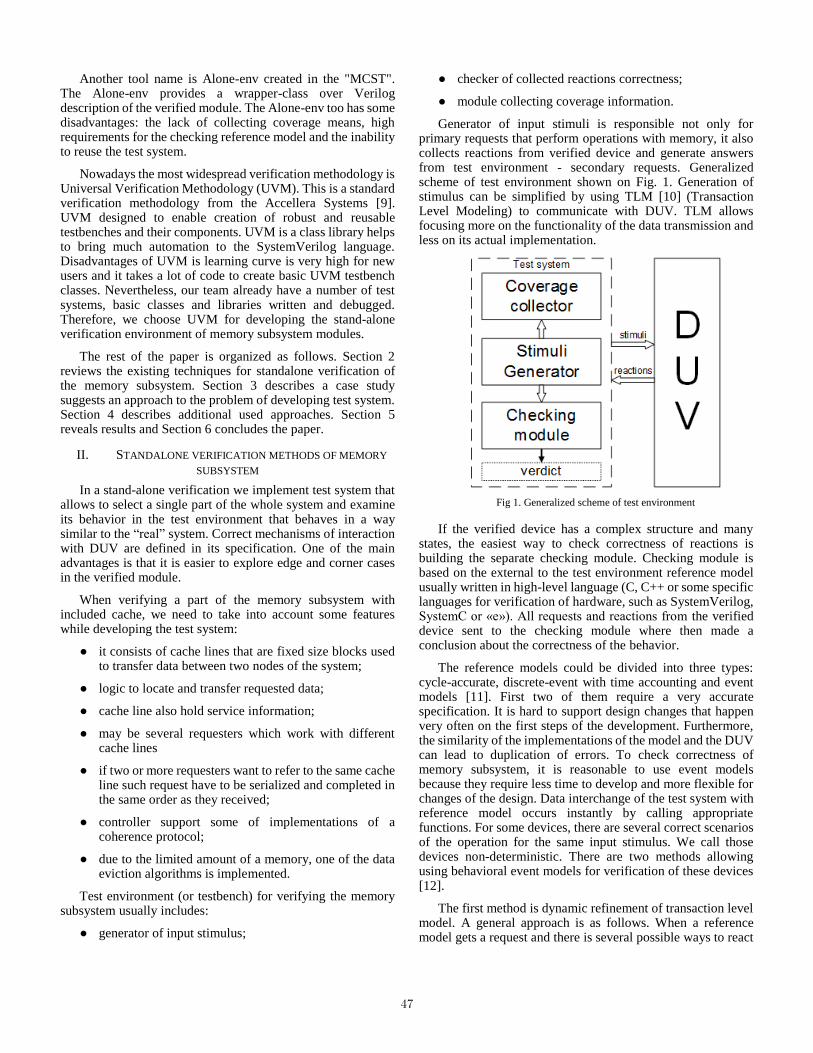
Another tool name is Alone-env created in the "MCST". The Alone-env provides a wrapper-class over Verilog description of the verified module. The Alone-env too has some disadvantages: the lack of collecting coverage means, high requirements for the checking reference model and the inability to reuse the test system.

Nowadays the most widespread verification methodology is Universal Verification Methodology (UVM). This is a standard verification methodology from the Accellera Systems [9]. UVM designed to enable creation of robust and reusable testbenches and their components. UVM is a class library helps to bring much automation to the SystemVerilog language. Disadvantages of UVM is learning curve is very high for new users and it takes a lot of code to create basic UVM testbench classes. Nevertheless, our team already have a number of test systems, basic classes and libraries written and debugged. Therefore, we choose UVM for developing the stand-alone verification environment of memory subsystem modules.

The rest of the paper is organized as follows. Section 2 reviews the existing techniques for standalone verification of the memory subsystem. Section 3 describes a case study suggests an approach to the problem of developing test system. Section 4 describes additional used approaches. Section 5 reveals results and Section 6 concludes the paper.

II. STANDALONE VERIFICATION METHODS OF MEMORY

SUBSYSTEM

In a stand-alone verification we implement test system that allows to select a single part of the whole system and examine its behavior in the test environment that behaves in a way similar to the “real” system. Correct mechanisms of interaction with DUV are defined in its specification. One of the main advantages is that it is easier to explore edge and corner cases in the verified module.

When verifying a part of the memory subsystem with included cache, we need to take into account some features while developing the test system:

it consists of cache lines that are fixed size blocks used to transfer data between two nodes of the system;

logic to locate and transfer requested data;

cache line also hold service information;

may be several requesters which work with different cache lines

if two or more requesters want to refer to the same cache line such request have to be serialized and completed in the same order as they received;

controller support some of implementations of a coherence protocol;

due to the limited amount of a memory, one of the data eviction algorithms is implemented.

Test environment (or testbench) for verifying the memory subsystem usually includes:

generator of input stimulus;

checker of collected reactions correctness;

module collecting coverage information.

Generator of input stimuli is responsible not only for primary requests that perform operations with memory, it also collects reactions from verified device and generate answers from test environment - secondary requests. Generalized scheme of test environment shown on Fig. 1. Generation of stimulus can be simplified by using TLM [10] (Transaction Level Modeling) to communicate with DUV. TLM allows focusing more on the functionality of the data transmission and less on its actual implementation.

Fig 1. Generalized scheme of test environment

If the verified device has a complex structure and many states, the easiest way to check correctness of reactions is building the separate checking module. Checking module is based on the external to the test environment reference model usually written in high-level language (C, C++ or some specific languages for verification of hardware, such as SystemVerilog, SystemC or «e»). All requests and reactions from the verified device sent to the checking module where then made a conclusion about the correctness of the behavior.

The reference models could be divided into three types: cycle-accurate, discrete-event with time accounting and event models [11]. First two of them require a very accurate specification. It is hard to support design changes that happen very often on the first steps of the development. Furthermore, the similarity of the implementations of the model and the DUV can lead to duplication of errors. To check correctness of memory subsystem, it is reasonable to use event models because they require less time to develop and more flexible for changes of the design. Data interchange of the test system with reference model occurs instantly by calling appropriate functions. For some devices, there are several correct scenarios of the operation for the same input stimulus. We call those devices non-deterministic. There are two methods allowing using behavioral event models for verification of these devices [12].

The first method is dynamic refinement of transaction level model. A general approach is as follows. When a reference model gets a request and there is several possible ways to react

47

to the request, the model creates additional instances and executes the requests in each of them. Then the models are waiting for the reactions from the device under verification. The reaction contents service information (such as a response type, a direction of sending, etc) which helps to exclude impossible states. Absence of suitable state for reaction signals about an error. The sign of a successful completion is comparison all the reactions of the DUV and removal of all unnecessary states. The complexity of this approach is that the number of possible states potentially grows exponentially with a number of stimuli. However, this method can be implemented efficiently for memory subsystem units because all requests to a single cache line are serialized and requests to different cache lines are independent.

Second method is identification of a single correct state using hints from the verified device or a "gray box" method. This method replaces usual “black box” method. When we cannot predict the “real” sequence of interactions, we access inner interfaces of the verified device. Information from these interfaces have to be transferred to the test environment and helps to determine a single possible execution scenario and eliminate nondeterminism. This method imposes additional requirements to the device specification, but, as a result, it is quite simple to implement.

Coverage collection module extract information of functional code coverage. This information is used to identify unimplemented test cases and helps to improve stimuli generation by adding new test scenarios.

III. USING GRAY BOX APPROACH FOR VERIFICATION OF

HOME MEMORY UNIT

Home Memory Unit (HMU) is a part of memory subsystem of 16-core “Elbrus” microprocessor responsible for the coherent and non-coherent access to the RAM from different requesters. HMU contains a global directory (MOSI protocol of coherence), which monitors the requests of other processors to its memory and a DMA directory which is a full copy of the DMA caches of all processors (supports the extended coherence protocol MOI). Total volume of the directory in HMU is 2.5 MB, size of entry of a cache line is 80 B, number of banks – 128, bank associativity – 16. Main functions of HMU include:

serialization of all requests to RAM;

reduction of coherence traffic and access time to RAM;

support of interprocessor coherence by sending coherent requests;

collecting short coherent responses and coherent responses with data;

Test system for stand-alone verification of the coherence protocol implementation and other functionality of HMU based on UVM. UVM helps to generate pseudo-random constrained input requests to cover possible states of the verified device.

We have to note some restrictions for generation primary, secondary stimuli and answers. The first of them is limited amount of space in input buffers. Due to process of verification, it is important not to lose some data. When generating random system settings, it is necessary to take into account that the

some setup combinations may be incorrect and lead to errors. There are several types of requesters in the test system. Each of them has special identifier and a set of possible operation codes. The specific implementation of the coherence protocol also imposes restrictions on the used operation codes. Sending an inappropriate operation code may result in undefined results. Address generation is also a non-trivial task. The address have to fit the interleaving conditions. In addition, each requester have to wait for the completion of previous request when working with same cache line.

Stimuli generation is divided into several stages:

1. randomization of device configuration registers. This allows to switch different ways for handling requests and determine request routing;

2. creating list of addresses for current configuration of device with respect to routing setup;

3. choosing random requester and cache line address;

4. checking cache line availability and presence of resources needed for request transfer;

5. choosing random operation code constrained by the current state of cache line;

6. sending primary request, collecting reactions from the device under verification, sending secondary requests;

7. collecting all of necessary reactions and completion of current request;

8. transferring transaction information to checking module;

To simplify handling of requests and reactions we create models of each used cache line. Model of cache line is an object that stores information about primary request, collected reactions, data and some auxiliary functions. For generation of correct requests we created an associative memory storing current states for each cache line. The choice of the next request type is made according to the limitations imposed by the coherence protocol and the current state of the cache line. For example, one of these rules is there cannot be two requesters in a modified (M) state for a single cache line. Another feature, which was necessary to pay attention, is that one address tag corresponds to two-neighbor cache lines information. This mechanism allows increasing the ratio of the directory coverage (the ratio of the cache memory covered by the directory to the cache memory of the directory).

As noted before, there are two ways of building checking module. The choice of “gray box” method is determined by following sources of a nondeterminism inherent to HMU:

HMU contains two input queues of primary requests what means exponential growth of possible device states size (2n+m, where n, m – number of requests inside input queues);

cache eviction algorithm in the global directory.

HMU has two cache memories responsible for different functions of a memory subsystem: the global and DMA directories. The global directory has information only about

48

data belonging to the own processor and used by other processors. Along with that there is no information about presence of this cache line in cache of own processor. Such information located in the L3 cache. DMA writes are also coherent requests. For a fast and correct handling of DMA writes sent by DMA controllers the special DMA cache directory is present inside HMU. This cache directory supports extended coherence protocol MOI with substates. Its main function is processor notification about cache lines captured by DMA controllers and storing their states.

The device under verification connected with other parts of the system by means of network-on-chip and has two input channels for primary requests. All generated primary requests are sent to the DUV and the checking module simultaneously. The checking module (implemented in C++) receives requests and reactions from the verified device by means of DPI (Directed Programming Interface). Using of the DPI is necessary to match the types and classes of the test environment written in SystemVerilog hardware description language with the reference model interface functions. Inside checking module, all requests are received into two queues. Requests to the same cache line can get into the different queues. It is impossible to predict which of these requests will be handled first. Getting a sequence hint from the device under test eliminates the nondeterminism of the current state. Stable and well-described inner interfaces to the point where all request are serialized, made it possible to build simple checking module in the short time. In a similar way, an access to the eviction mechanism interface was obtained. In addition, the checking module and its behavior model may be modified if it will be needed in the future projects. Structure of the test environment with proposed “gray box” method shown in Fig. 2.

Fig 2. Simplified version of the test environment using the “gray box”

method

IV. ADDITIONAL VERIFICATION METHODS

A. Management of transaction flow

To check if the verified device operates correctly, it is necessary to achieve multiple edge and corner cases. This involves filling all input and output primary and secondary requests queues, delaying some necessary types of answers and blocking of transactions from some modules [13]. HMU supports the credit-exchange mechanism, which indicates the devices ability to accept certain type of requests. We added the special configuration module that randomizes time delays of sending requests and credits. Management of delays setup allows to create different test scenarios with overflowing requests and responses buffers. This mechanism helps to detect livelocks and deadlocks. These types of system behavior are hard to implement during system testing.

B. Applying assertions

SystemVerilog Assertions (SVA) is an important subset of SystemVerilog [14]. The assertions are used to specify the behavior of the system. The assertions work as follows: we add some piece of verification code to the test system that monitors a design implementation for compliance with the specifications. In addition, the assertions can be used to flag that input stimuli do not conform to assumed requirements. In the beginning of the project, it may help to find more bugs and locate them faster.

In HMU verification process the assertions are used for checking for uncertain and unconnected states of signals. Usage of coherence protocols in the DUV involves certain restrictions on the stimuli generation and the state of the cache lines for different requesters. Thus, additional function of the assertions, which was used in the test system, is detection of the discrepancy between coherence protocol specification and generated requests types in the certain cache lines states. The disadvantage of this approach is the limitation of the properties of the verified device that can be checked by assertions.

C. On-the-fly ECC errors insertion

ECC bits are stored in a cell that describing the state of the cache line. Special submodules of HMU encode the data written to the RAM and decode data read from RAM. Using ECC bits allows to detect single, double, parity errors and to correct single errors. This mechanism is a potential source of errors in the device. The special module with flexible configuration was developed to insert single and double errors. This module is managed by the test system. Frequency and type of error insertion can be regulated. Detecting and correcting ECC errors additionally loaded computing logic of verified device.

V. RESULTS

The approaches described in this paper were applied for standalone verification of Home Memory Unit of 16-core and 2-core with 6 integrated graphic boosters microprocessors with “Elbrus” architecture.

There are some difference in operating with memory subsystem in the microprocessors. The 16-core microprocessor’s HMU has a global directory and DMA cache, sends coherent requests with accordance to the state in the global directory, and collects short coherent answers and coherent answers with data for write operations. For read

49

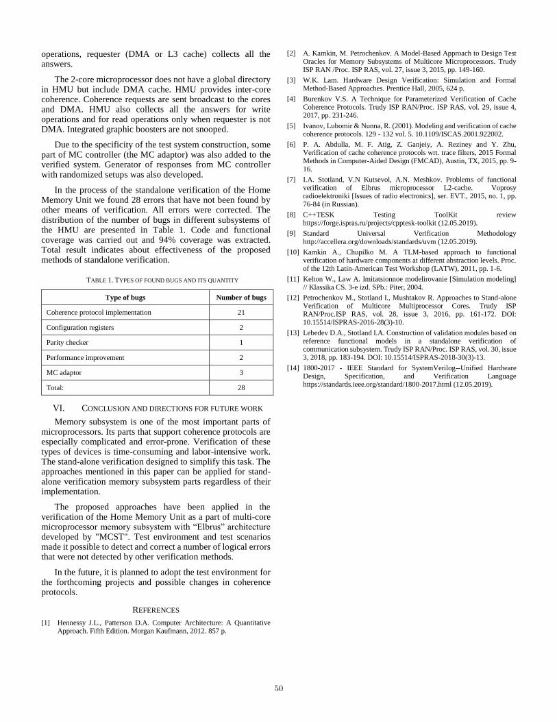
operations, requester (DMA or L3 cache) collects all the answers.

The 2-core microprocessor does not have a global directory in HMU but include DMA cache. HMU provides inter-core coherence. Coherence requests are sent broadcast to the cores and DMA. HMU also collects all the answers for write operations and for read operations only when requester is not DMA. Integrated graphic boosters are not snooped.

Due to the specificity of the test system construction, some part of MC controller (the MC adaptor) was also added to the verified system. Generator of responses from MC controller with randomized setups was also developed.

In the process of the standalone verification of the Home Memory Unit we found 28 errors that have not been found by other means of verification. All errors were corrected. The distribution of the number of bugs in different subsystems of the HMU are presented in Table 1. Code and functional coverage was carried out and 94% coverage was extracted. Total result indicates about effectiveness of the proposed methods of standalone verification.

TABLE 1. TYPES OF FOUND BUGS AND ITS QUANTITY

Type of bugs Number of bugs

Coherence protocol implementation 21

Configuration registers 2

Parity checker 1

Performance improvement 2

MC adaptor 3

Total: 28

VI. CONCLUSION AND DIRECTIONS FOR FUTURE WORK

Memory subsystem is one of the most important parts of microprocessors. Its parts that support coherence protocols are especially complicated and error-prone. Verification of these types of devices is time-consuming and labor-intensive work. The stand-alone verification designed to simplify this task. The approaches mentioned in this paper can be applied for stand-alone verification memory subsystem parts regardless of their implementation.

The proposed approaches have been applied in the verification of the Home Memory Unit as a part of multi-core microprocessor memory subsystem with “Elbrus” architecture developed by "MCST". Test environment and test scenarios made it possible to detect and correct a number of logical errors that were not detected by other verification methods.

In the future, it is planned to adopt the test environment for the forthcoming projects and possible changes in coherence protocols.

REFERENCES

[1] Hennessy J.L., Patterson D.A. Computer Architecture: A Quantitative Approach. Fifth Edition. Morgan Kaufmann, 2012. 857 p.

[2] A. Kamkin, M. Petrochenkov. A Model-Based Approach to Design Test Oracles for Memory Subsystems of Multicore Microprocessors. Trudy ISP RAN /Proc. ISP RAS, vol. 27, issue 3, 2015, pp. 149-160.

[3] W.K. Lam. Hardware Design Verification: Simulation and Formal Method-Based Approaches. Prentice Hall, 2005, 624 p.

[4] Burenkov V.S. A Technique for Parameterized Verification of Cache Coherence Protocols. Trudy ISP RAN/Proc. ISP RAS, vol. 29, issue 4, 2017, pp. 231-246.

[5] Ivanov, Lubomir & Nunna, R. (2001). Modeling and verification of cache coherence protocols. 129 - 132 vol. 5. 10.1109/ISCAS.2001.922002.

[6] P. A. Abdulla, M. F. Atig, Z. Ganjeiy, A. Reziney and Y. Zhu, Verification of cache coherence protocols wrt. trace filters, 2015 Formal Methods in Computer-Aided Design (FMCAD), Austin, TX, 2015, pp. 9-16.

[7] I.A. Stotland, V.N Kutsevol, A.N. Meshkov. Problems of functional verification of Elbrus microprocessor L2-cache. Voprosy radioelektroniki [Issues of radio electronics], ser. EVT., 2015, no. 1, pp. 76-84 (in Russian).

[8] C++TESK Testing ToolKit review https://forge.ispras.ru/projects/cpptesk-toolkit (12.05.2019).

[9] Standard Universal Verification Methodology http://accellera.org/downloads/standards/uvm (12.05.2019).

[10] Kamkin A., Chupilko M. A TLM-based approach to functional verification of hardware components at different abstraction levels. Proc. of the 12th Latin-American Test Workshop (LATW), 2011, pp. 1-6.

[11] Kelton W., Law A. Imitatsionnoe modelirovanie [Simulation modeling] // Klassika CS. 3-e izd. SPb.: Piter, 2004.

[12] Petrochenkov M., Stotland I., Mushtakov R. Approaches to Stand-alone Verification of Multicore Multiprocessor Cores. Trudy ISP RAN/Proc.ISP RAS, vol. 28, issue 3, 2016, pp. 161-172. DOI: 10.15514/ISPRAS-2016-28(3)-10.

[13] Lebedev D.A., Stotland I.A. Construction of validation modules based on reference functional models in a standalone verification of communication subsystem. Trudy ISP RAN/Proc. ISP RAS, vol. 30, issue 3, 2018, pp. 183-194. DOI: 10.15514/ISPRAS-2018-30(3)-13.

[14] 1800-2017 - IEEE Standard for SystemVerilog--Unified Hardware Design, Specification, and Verification Language https://standards.ieee.org/standard/1800-2017.html (12.05.2019).

50

Standalone verification of IOMMU with

virtualization supporting.

Anton Petrykin1, Irina Stotland2, Aleksey Meshkov3

Department of Verification and Modeling

MCST

Moscow, Russia

petrykin_a@mcst.ru1, stotl_i@mcst.ru2, alex@mcst.ru3

Abstract — This article presents an approach to standalone

verification of I/O Memory Management Unit with virtualization

supporting. We presented the base architecture of the test

system. One of the key problems encountered during verification

was the formation of translation table pages. The number of

translation tables depends on the mode of CPU operation. As a

solution of this problem the approach to the dynamic generation

of translation tables is proposed. The problem of validating the

translation of a virtual address into a physical one using two-level

translation tables is solved. The features of the reference model

implementation are considered. Reference model and test system

which have been used for verification of «Elbrus-12c»

microprocessor IOMMU are discribed. The methods of

communication between test system and IOMMU model are

presented. The results of IOMMU verification are considerd.

Keywords — I/O Memory Management Unit, test system,

reference model, «Elbrus – 12C»

I. INTRODUCTION

An I/O Memory Management Unit (IOMMU) is a hardware device that translates virtual address received from the I/O subsystem requests to proper machine physical address. IOMMUs have long been used for prohibiting devices from DMA’ing into the wrong memory and for performance optimization. With the hardware support of operating system virtualization IOMMU is also used for extending the protection and isolation properties of Vms(Virtual Machines) for I/O operations, supporting isolation of interrupts from devices and external interrupt controllers and recording of DMA and interrupt errors to system software that may corrupt memory or impact VMs isolation[1][2]. Therefore, modern IOMMUs are quite complex devices that have many modes of operation and their verification is an important step in the development of the microprocessor system.

In the paper we present a case study for functional verification IOMMU with virtualization supporting of «Elbrus-12C» microporocessor developed by MCST. The paper addresses the problem and methods of standalone verification of IOMMU with virtualization supporting.

The rest of the paper is organized as follows. Section 2 considers the problems arising from the verification of IOMMU. Section 3 suggests an approach to the problem of developing page table lines generator. Section 4 presents a

common approach to the design a test system and describes its components. Section 5 reveals results. And section 6 concludes the paper.

II. IOMMU VERIFICATION CHALLENGES.

For hardware support of operating system virtualization, the translation of a virtual address into a physical one occurs according to a scheme that includes a two-level page structure. At the first level, the virtual guest OS address (GVA) is translated into the physical guest OS address (GPA) using its translation tables. At the second level, the resulting address is translated to the physical address (PA) of the hypervisor using the hypervisor translation tables. Information about the broadcast address for each device is stored in the device table. The table consists of Device Table Entry(DTE) elements. Еach DTE contains information about the Domain ID, host page table root pointer (HPTP) and guest page table root pointer(GPTP). In the IOMMU of Elbrus-12C processor, DID field has an extension and is called EDID. In addition to the domain number, it contains information about whether the device belongs to the guest or the hypervisor.

The pages number of translation tables depends on the mode of device operation and the size of the page themselves. «Elbrus-12C» processors support three page sizes: 4KB, 2MB and 1GB. For guest virtual address translation through 4KB pages, the number of memory hits can reach twenty-five. Each memory hit takes a long time to process. Therefore, as part of IOMMU can be used a lot of different caches[1].

It follows from the above that the main goal of IOMMU verification is to check the correctness of all translation modes and check the following:

Translation on pages with various size.

Error handling.

Caches correctness.

Translations for the greatest possible number of addresses.

Absence of suspensions

Absence of unknown logic value (X-state) on output signals.

51

There are several main problems encountered during the IOMMU verification of Elbrus-12C processors:

The large number of translation tables and different page size.

Large size of the entire address space.

Different virtual addresses can be translated into one physical.

To solve these problems, it was necessary to create the translation page tables. But their formation for the entire address space would require a large amount of computing resources. In paper [3] is presented the approach based on constraint-random generation page table entries (PTEs) which we used for IOMMU verification as a part of northbridge of our previous microprocessor. However the availability of hypervisor and guest translation caches as well as a large number of translation pages required for guest virtual address translation does not allow to use the approach described in [3]. The traditional approach is to generate a static table for a limited set of addresses which is used for verification Translation Lookaside Buffer(TLB) of MMU[4]-[6]. But with using of this approach, it is difficult to verify error handling and virtual address translation over various size pages. Therefore, for functional verification of the IOMMU of«Elbrus-12C» processor, it was decided to develop a dynamic generator of translation table pages, which generates rows of translation tables for any virtual address.

III. GENERATOR OF TRANSLATION TABLE PAGES.

The formation of pages in the generator depends on the translation mode, which is specified directly in the tests and translation request. The algorithm of the generator work could be represented in the form of several consecutive steps:

1) Receiving request for translation;

2) Translation request and mode analysis;

3) DTE formation.

4) Translation pages entry.

Translation modes are divided into single-level or native translations and two-level translations. In turn, native translations can take place in the same domain or split into different domains. Native translations in the same domain doesn’t require DTE. For the rest of translation modes DTE formation is necessary. Since a unique translation identifier in Elbrus-12c processors is an EDID, each DTE element is stored in an associative array indexed by it. The formation of a DTE begins with the selection of a random EDID for a given device, after which the presence of a DTE for a given EDID in the array is checked and if it is missing, the remaining fields are formed.

Translations tables have a 4-level structure and consist of 512 elements. Each line of the table contains information about the access rights to it and whether it is the last in the translation structure. In addition, there is a field named ppn(Physical Page Number), that indicating the line from the next translation level, in case the line is on the last translation level, it contains

the physical address. Hereinafter the pages of hypervisor and guest translations will be called HP(Host Page) and GP(Guest Page), respectively.

For native translation, the address of the first line is formed from the host page table index (hptp) contained in the DTE, and a part of the translated virtual address. Physical page number for each page level is calculated as follows:

ppn(n) = hptp + 512*(5 - n) +VA(n),

where n - host page level, VA(n) – the part of translated

virtual address on level n , hptp - table root pointer.

The full list of pages for native translation is presented in

Table 1.

Page level Addres of page Physical Page Number

HP_L4 hptp, VA(4) hptp + 512 + VA(4)

HP_L3 ppn_L4, VA(3) hptp + 512 * 2 + VA(3)

HP_L2 ppn_L3, VA(2) hptp + 512 * 3 + VA(2)

HP_L1 ppn_L2, VA(1) hptp + 512 * 4 + VA(1)

Table. 1. List of pages for native translation.

When generating rows of a two-level table for guest virtual address translation, the generator first calculates the guest physical address(GPA) for first guest page(GP_L4) according to the formula:

GPA(4) = GPTP + VA(4)

After that, the pages necessary for the translation of this

GPA to HPA are written in the same way as the recording of

the pages of translation VA to PA in the native mode. The list

of pages for that translation may be seen at Table 2.

Page level Addres of page Physical Page Number

HP_L4 hptp, GPA(4) hptp + 512 + GPA(4)

HP_L3 ppn_L4, GPA(3) hptp + 512 * 2 + GPA(3)

HP_L2 ppn_L3, GPA(2) hptp + 512 * 3 + GPA(2)

HP_L1 ppn_L2, GPA(1) hptp + 512 * 4 + GPA(1)

Table. 2. List of pages for guest physical addres translation into host physycal

address.

Then the GP_L4 page itself is written and after that the guest physical address of the next page level(GPA_3) is calculated as the sum of HP_L1 page ppn and part of virtual address:

GPA_3 = ppn + VA(3),

And so on to get the GPA of the original GVA. For the obtained GPA, the pages of the last hypervisor translation are formed, which give the desired HPA. In order to avoid writing identical lines at different translation levels, guest pages addresses and ppns are configured as followed:

addr(x) = ppn, GPA_x(0),

52

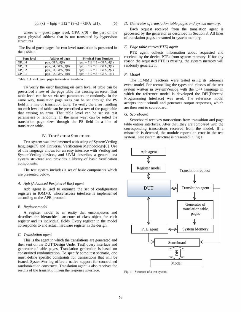
ppn(x) = hptp + 512 * (9-x) + GPA_x(1),

where x – guest page level, GPA_x(0) - the part of the guest physical address that is not translated by hypervisor structures

The list of guest pages for two-level translation is presented in the Table 3.

Page level Addres of page Physical Page Number

GP_L4 ppn, GPA_4(0) hptp + 512 * 5 + GPA_4(1)

GP_L3 ppn_L4, GPA_3(0) hptp + 512 * 6 + GPA_3(1)

GP_L2 ppn_L3, GPA_2(0) hptp + 512 * 7 + GPA_2(2)

GP_L1 ppn_L2, GPA_1(0) hptp + 512 * 8 + GPA_1(1)

Table. 3. List of guest pages in two-level translation.

To verify the error handling on each level of table can be prescribed a row of the page table that causing an error. That table level can be set via test parameters or randomly. In the same way, translation page sizes can be set through the PS field in a line of translation table. To verify the error handling on each level of table can be prescribed a row of the page table that causing an error. That table level can be set via test parameters or randomly. In the same way, can be setted the translation page sizes through the PS field in a line of translation table.

IV. TEST SYSTEM STRUCTURE.

Test system was implemented with using of SystemVerilog langueage[7] and Universal Verification Methodology[8]. Use of this language allows for an easy interface with Verilog and SystemVerilog devices, and UVM describes a general test system structure and provides a library of basic verification components.

The test system includes a set of basic components which are presented below.

A. Apb (Advanced Peripheral Bus) agent

Apb agent is used to entrance the set of configuration registers in IOMMU whose access interface is implemented according to the APB protocol.

B. Register model

A register model is an entity that encompasses and describes the hierarchical structure of class object for each register and its individual fields. Every register in the model corresponds to and actual hardware register in the design.

C. Translation agent

This is the agent in which the translations are generated and then sent on the DUT(Design Under Test) query interface and generator of table pages. Translation generation is based on constrained randomization. To specify some test scenario, one must define specific constraints for transactions that will be issued. SystemVerilog offers a native support for constrained randomization constructs. Translation agent is also receives the results of the translation from the response interface.

D. Generator of translation table pages and system memory.

Each request received from the translation agent is processed by the generator as described in Section 3. All lines of translation pages are stored in system memory.

E. Page table entries(PTE) agent

PTE agent collects information about requested and received by the device PTEs from system memory. If for any reason the requested PTE is missing, the system memory will randomly generate it.

F. Model

The IOMMU reactions were tested using its reference

event model. For reconciling the types and classes of the test

system written in SystemVerilog with the C++ language in

which the reference model is developed the DPI(Directed

Programming Interface) was used. The reference model

accepts input stimuli and generates output responses, which

are then sent to scoreboard.

G. Scoreboard

Scoreboard receives transactions from transaltion and page table entries interfaces. After that, they are compared with the corresponding transactions received from the model. If a mismatch is detected, the module reports an error in the test system. Test system structure is presented in Fig.1.

Fig. 1. Structure of a test system.

Model

DP

I

Scoreboard

System Memory PTE agent

Generator of

translation table

pages

Translation agent

Apb agent

Register model Translation request

DUT

53

V. RESULTS.

The approaches described above were applied to

standalone verification of the IOMMU of Processor «Elbrus –

12C». Due to standalone verification of the device, 58 errors

in the RTL description that have not been found by other

means of verification were found and corrected. Total result

indicates about effectiveness of standalone verification of I/O

memory management unit.

VI. CONCLUSION.

I/O memory management units are among the important

parts of modern microprocessor systems have to be thoroughly

tested. In this article, we presented a method of translation

table pages forming. The main advantages of the described

approach are:

no need to create tables for the entire address space.

the ability to dynamically set the page size.

convenience of exception checking due to dynamic generation of page table row fields.

ease of obtaining maximum coverage, due to the possibility of calls to any address.

The principles described in the paper do not depend

mainly on the IOMMUs implementation and allow their full

standalone verification.

The proposed approaches have been applied in the

verification of IOMMU as a part of microprocessor «Elbrus –

12C», developed by "MCST". The developed test system and

tests made it possible to detect and correct a number of logical

errors that were not detected by other test methods

REFERENCES

[1] Intel Virtualization Technology for Directed I/O Architecture Specification. Intel, 2018.

[2] AMD I/O Virtualization Technology (IOMMU) Specification. AMD, 2016.

[3] Lebedev D.A., Stotland I.A. Construction of validation modules based on reference functional models in a standalone verification of communication subsystem. Trudy ISP RAN/Proc. ISP RAS, vol. 30, issue 3, 2018, pp. 183-194.

[4] Alkassar E., Cohen E., Kovalev M., Paul W.J. (2012) Verification of TLB Virtualization Implemented in C. In: Verified Software: Theories, Tools, Experiments. VSTTE 2012. Lecture Notes in Computer Science, vol 7152, pp 209-224. Springer, Berlin, Heidelberg

[5] Alkassar, E., Cohen, E., Hillebrand, M., Kovalev, M., Paul, W.: Verifying shadow page table algorithms. In: Formal Methods in Computer Aided Design (FMCAD) 2010. pp. 267-270. IEEE, Lugano, Switzerland (2010).

[6] Kamkin A., Kotsynyak A.. (2016) Specification-Based Test Program Generation for MIPS64 Memory Management Units. In: Trudy ISP RAN/Proc, vol. 28(4), 2016. pp. 99-114.

[7] IEEE Standard for SystemVerilog — Unified Hardware Design, Specification, and Verification Language. IEEE Std 1800-2012M. Young, The Technical Writer’s Handbook. Mill Valley, CA: University Science, 1989.

[8] 1800.2-2017 - IEEE Standard for Universal Verification Methodology Language Reference Manual.

54

Digital Modelling of Production Engineering forMetalworking Machine Shops

Vsevolod KotlyarovPeter the Great St.Petersburg Polytechnic University

29 Politekhnicheskaya Str., Saint Petersburg194064, Russian Federation

vpk@spbstu.ru

Alexey MaslakovPeter the Great St.Petersburg Polytechnic University

29 Politekhnicheskaya Str., Saint Petersburg194064, Russian Federationalex.maslakov.ftk@gmail.com

Alexey TolstolesPeter the Great St.Petersburg Polytechnic University

29 Politekhnicheskaya Str., Saint Petersburg194064, Russian Federation

gmlaletol@gmail.com

Abstract—Currently, the engineering industry solves the prob-lem of implementation of efficient production methods for satis-faction of small and diverse orders. The key to the solution is tocreate automated, adaptable small-scale production sites, whichcorresponds to the paradigm of Industry 4.0. The bottleneck ofthe development of small-scale production is the preparation ofits technological processes and their documentation.

The technologist and the workers in the workshop use a setof technological documentation which describes the necessarytechnological equipment (workpieces, machines, cutting tools,mounting fixtures, etc.) and sequences of actions for the manu-facturing of details.

This article presents a modular approach that reduces thelabor costs for the technological preparation of small-scale met-alworking production. Its idea is to formalize the technologicalprocesses, allowing generating them and their documentationfrom pre-prepared parameterized templates stored in the specialdatabase. Any manufactured detail or its part can be representedas the structure of its basic geometric components, such as cylin-ders, cones, parallelepipeds, etc., that require special processingprocedures. For the template of machining operations for eachcomponent, symbolic parameters are fixed, defining the typeand the material of the workpiece used, cutting tool options,machining modes, etc. The template also records restrictions onthe parameters of sequences of operations used, on the usage ofprocessing modes depending on the characteristics of instrument,etc.

The result of formalization is an automatically generatedtechnological route in the form of an MSC diagram encoding it asa sequence of macro-operations for the machinery with symbolicparameters. This symbolic model is adapted to a specific instanceof the detail being manufactured by replacing the symbolicvariables with specific values set by the technologist.

The MSC diagram is supplemented with the results of cal-culating the time and cost of technological routes, which allowsselection of the most efficient one.

The correctness of the technological routes is ensured in theprocess of symbolic verification by checking the permissibleranges of parameters of the MSC diagram, as well as checkingthe correctness of order and compatibility of operations in thesequence.

The results of the whole process obtained from the MSCdiagram are the set of technological documentation of preproduc-tion, which, in particular, includes a set of operating cards, and

the fine-tuned schedule of production after its digital modelingwith the real resources of the workshop taken into account.

According to technologists, by applying the described automa-tion, the time to prepare documentation for details of mediumcomplexity is reduced from several weeks to 1-2 days.

Index Terms—adaptive manufacturing, production engineer-ing, small-scale metalworking manufacturing preparation, au-tomation of the preparation of technological documentation

I. INTRODUCTION

Comprehensive automation of technological processesbased on information technology provides:

• Reduction of the time of pre-production.• Optimization of labor costs and funds for the manufacture

of products.• Operational implementation of changes in the process un-

der the external conditions (replacement of technologicalequipment, material, cutting tools, etc.) with automaticrecalculation of the process characteristics.

Technological preparation of production (TPP) includes thefollowing activities:

• Setting of technological problems.• Selection of the workpiece based on its parameters.• Development of technological processing routes.• Selection of technological equipment.• Formation of technological operations.• Development of a set of technological documentation.

Fields of automation of technological preparation of produc-tion include:

• Development of technological documentation.• Development of control programs.• Development of technological processes.

The tasks of operational planning and automated productionmanagement are carried out by the manufacturing executionsystems (MES) [1]. They occupy an intermediate place inthe hierarchy of enterprise management systems between thelevel of information collection from equipment in workshops

55

done by supervisory control and data acquisition (SCADA)systems [2] and the level of operations over a large amountof administrative, financial and accounting information doneby enterprise resource planning (ERP) [1] systems. The keyprocesses for MES are as follows [3]:

1) Based on the external demand for production (which,in turn, is based on customer orders, sales plans, etc.),as well as previous production programs, taking intoaccount all sorts of nuances and specifics of productionat a particular enterprise, a detailed optimized productionschedule of works and operations for machine tools,equipment, personnel is produced. In addition, automaticgeneration of all the documentation necessary for thework: production programs, outfits, limit maps, tablesand equipment loading diagrams, etc. is also done.

2) In the course of the direct implementation of productionprograms, full dispatching of all operations and theirresults (both positive and negative - rejects, delays, etc.)is carried out.

3) If deviations from the planned programs are identifieddue to the external reasons, or when new demand(orders, etc.) appears, real-time re-planning is performedwith all components corrected accordingly.

It should be noted that there exists an imbalance betweenproduction time and preparation time in single or small-scale productions in case of re-scheduling of the work of aproduction site, because it should be performed for the smallbatch of the details and not for the whole series of them.

Nowadays on the Russian market there are three mostpopular largest solutions, the products of many years of workof three scientific centers for developing systems of this class:PHOBOS system, YSB.Enterprise.Mes system and PolyPlansystem. PHOBOS is traditionally used in large and medium-sized machine-building enterprises. YSB.Enterprise.Mes orig-inated from the woodworking industry and focuses on thesector of medium and small enterprises. The PolyPlan systemhas a smaller set of MES functions, but is positioned asan operational scheduling system for automated and flexiblemanufacturing in engineering [3].

However, with all the attractiveness of such systems, due tothe extensive set of functions provided and deep integrationinto the production processes in the enterprise at all stages,their practical implementation is a whole complex and expen-sive project in itself that not all enterprises, especially small-scale and individual productions, can afford. In addition tothis, in order to work effectively with MES, high qualificationof its operator is required. The automated workplace of thetechnologist given in this article is designed to solve a nar-rower class of problems - to simplify the TPP for small-scalemachine-building production, it does not require interactionswith other systems, and the results in the form of the requiredschedule of work distribution and a set of operating cards canbe obtained in a couple of days of work of a technologist.

Fig. 1. Input detail drawing.

II. FORMALIZATION OF THE TECHNOLOGICAL PROCESS

Let’s look through the features of formalization based on anillustration of a specific example of work with the developedsystem of an automated workplace for a technologist.

The main input information for the technologist is the detaildrawing. It can be done in any graphical design program, forexample, in KOMPAS-3D [4]. The example of the drawingis demonstrated in the Fig. 1

To manufacture a part technologist chooses a workpiecefor it. Several such workpieces may be selected; to determinethe best fitting of them, all calculations of time and cost ofproduction must be made for each selected one and comparedto each other.

The next action of the technologist is the splitting of agiven drawing into a set of sketches of elementary surfaces(ES), the parts of the detail. This step sets the way for themodular approach to the production technology [5]. Each ofthe surfaces is characterized by geometrical parameters and thenumber of stages required to process it. The processing stage isthe smallest atomic operation, for example, turning, drilling ormilling. The parameters of the processing stage are the typesof machines on which it can be performed, the cutting toolsto do so and the selected workpiece in the very beginning.The form for setting information about the processing stagesmanually is shown in the Fig. 2. The description of fields andtables of the form is as follows, from left to right and fromup to down:

• The type of the elementary surface encoded by two digits.• The unique number of the elementary surface used to

distinguish between the surfaces of the same type.• The geometrical parameters of the elementary surface,

here the diameter and length are listed.• The amount of the processing stages to be performed.• The processing stages, divided into the following

columns: the number of the stage, the name of it (here:turning), the codes of the applicable machinery for it, the

56

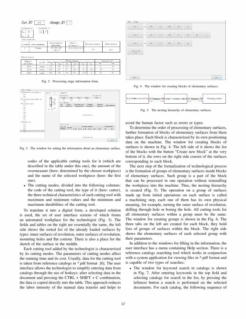
Fig. 2. Processing stage information form.

Fig. 3. The window for setting the information about an elementary surface.

codes of the applicable cutting tools for it (which aredescribed in the table under this one), the amount of theovermeasure (here: determined by the chosen workpiece)and the name of the selected workpiece (here: the firstone).

• The cutting modes, divided into the following columns:the code of the cutting tool, the type of it (here: cutter),the three technical characteristics of each cutting tool withmaximum and minimum values and the minimum andmaximum durabilities of the cutting tool.

To translate it into a digital form, a developed solutionis used, the set of user interface screens of which formsan automated workplace for the technologist (Fig. 3). Thefields and tables on the right are essentially the same, the leftside shows the sorted list of the already loaded surfaces bytypes: inner surfaces of revolution, outer surfaces of revolution,mounting holes and flat contour. There is also a place for thesketch of the surface in the middle.

Each cutting tool added by the technologist is characterizedby its cutting modes. The parameters of cutting modes affectthe running time and its cost. Usually, data for the cutting toolis taken from reference catalogs in *.pdf format [6]. The userinterface allows the technologist to simplify entering data fromcatalogs through the use of hotkeys: after selecting data in thedocument and pressing the CTRL + SHIFT + C combination,the data is copied directly into the table. This approach reducesthe labor intensity of the manual data transfer and helps to

Fig. 4. The window for creating blocks of elementary surfaces.

Fig. 5. The nesting hierarchy of elementary surfaces.

avoid the human factor such as errors or typos.To determine the order of processing of elementary surfaces,

further formation of blocks of elementary surfaces from themtakes place. Each block is characterized by its own positioningdata on the machine. The window for creating blocks ofsurfaces is shown in Fig. 4. The left side of it shows the listof the blocks with the button ”Create new block” at the verybottom of it, the rows on the right side consist of the surfacescorresponding to each block.

The next step of the formalization of technological processis the formation of groups of elementary surfaces inside blocksof elementary surfaces. Such group is a part of the blockthat can be processed in one operation without reinstallingthe workpiece into the machine. Thus, the nesting hierarchyis created (Fig. 5). The operation on a group of surfacesmade up from initial operations on each surface is calleda machining step, each one of them has its own physicalmeaning, for example, turning the outer surface of revolution,drilling through hole or boring the hole. All cutting tools forall elementary surfaces within a group must be the same.The window for creating groups is shown in the Fig. 6. Thethree tabs on the left are created for each block, they holdlists of groups of surfaces within the block. The right sideshows the elementary surfaces of each selected group withtheir parameters.

In addition to the windows for filling in the information, theuser interface has a menu containing Help section. There is areference catalogs searching tool which works in conjunctionwith a system application for viewing files in *.pdf format andis capable of two types of searches:

• The window for keyword search in catalogs is shownin Fig. 7. After entering keywords in the top field andselecting catalogs for search in the list, by pressing theleftmost button a search is performed on the selecteddocuments. For each catalog, the following sequence of

57

Fig. 6. The window for creating groups of elementary surfaces.

Fig. 7. Keywords search user interface.

actions is carried out:1) One page of document is read from disk.2) Search for keywords is performed on this page.3) If at least one of the keywords is detected, the page

is copied into the resulting pdf document.4) If the keywords are not found, proceed to the next

page.As soon as all pages of all catalogs are processed, aresulting document with search results is written to diskand opened in the standard pdf document viewer in thesystem. The right button cancels the search, the bottomone allows technologist to add a catalog to the list.

• Search by image, in contrast to search by keywords,is possible only for catalogs formatted in advance. Itsinterface is shown in Fig. 8. After selecting a pdf catalogfrom the drop-down list, if the necessary markup infor-mation exists for it, images, for example, of surfaces to beprocessed, are shown. By clicking on them a documentcontaining information related only to the selected imagesis formed and, alike to the search by keywords, is opened

Fig. 8. Image search user interface.

Fig. 9. Database fragment.

in a standard pdf documents viewer. The button on theright allows technologist to add a catalog to the list.

The usage of these searching tools, especially in conjunctionwith copying data into tables with hotkeys, achieves a signifi-cant reduction in the complexity of data entry for elementarysurfaces.

A special database based on PostgreSQL database manage-ment system [7] is used to store information entered by thetechnologist in the user interface [8]. The Fig. 9 shows afragment of its tables, where:

• ”public.tb methods” table stores information for calculat-ing the time and cost of processing methods for elemen-tary surfaces.

• ”public.tb app machines” is dedicated to applicable ma-chines for processing methods.

• ”public.tb processing steps” stores the parameters of theprocessing methods;

• ”public.tb app tools” holds information about the appli-cable cutting tools and cutting modes.

• The four lowest tables are used for linkage between othertables.

To formulate the resulting technological route for the pro-cessing of the whole detail technologist must determine all thegroups of elementary surfaces that can be processed together.There can be several routes constructed this way, the choice

58

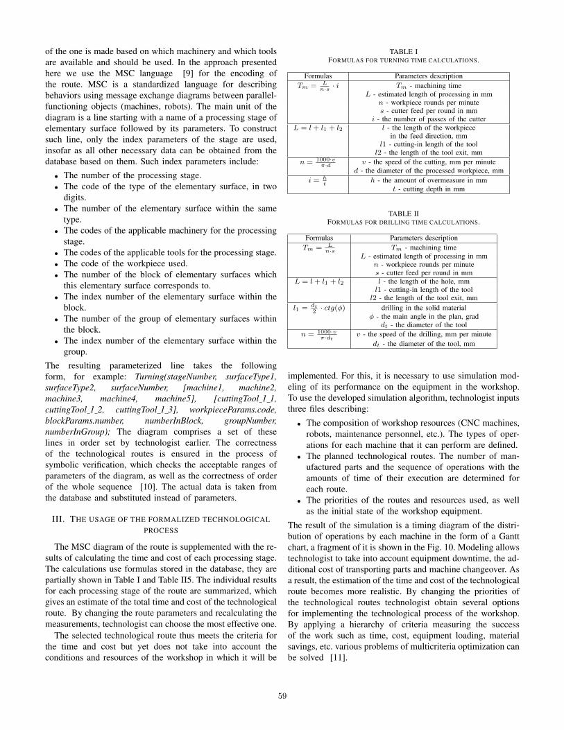
of the one is made based on which machinery and which toolsare available and should be used. In the approach presentedhere we use the MSC language [9] for the encoding ofthe route. MSC is a standardized language for describingbehaviors using message exchange diagrams between parallel-functioning objects (machines, robots). The main unit of thediagram is a line starting with a name of a processing stage ofelementary surface followed by its parameters. To constructsuch line, only the index parameters of the stage are used,insofar as all other necessary data can be obtained from thedatabase based on them. Such index parameters include:

• The number of the processing stage.• The code of the type of the elementary surface, in two

digits.• The number of the elementary surface within the same

type.• The codes of the applicable machinery for the processing

stage.• The codes of the applicable tools for the processing stage.• The code of the workpiece used.• The number of the block of elementary surfaces which

this elementary surface corresponds to.• The index number of the elementary surface within the

block.• The number of the group of elementary surfaces within

the block.• The index number of the elementary surface within the

group.

The resulting parameterized line takes the followingform, for example: Turning(stageNumber, surfaceType1,surfaceType2, surfaceNumber, [machine1, machine2,machine3, machine4, machine5], [cuttingTool 1 1,cuttingTool 1 2, cuttingTool 1 3], workpieceParams.code,blockParams.number, numberInBlock, groupNumber,numberInGroup); The diagram comprises a set of theselines in order set by technologist earlier. The correctnessof the technological routes is ensured in the process ofsymbolic verification, which checks the acceptable ranges ofparameters of the diagram, as well as the correctness of orderof the whole sequence [10]. The actual data is taken fromthe database and substituted instead of parameters.

III. THE USAGE OF THE FORMALIZED TECHNOLOGICALPROCESS

The MSC diagram of the route is supplemented with the re-sults of calculating the time and cost of each processing stage.The calculations use formulas stored in the database, they arepartially shown in Table I and Table II5. The individual resultsfor each processing stage of the route are summarized, whichgives an estimate of the total time and cost of the technologicalroute. By changing the route parameters and recalculating themeasurements, technologist can choose the most effective one.

The selected technological route thus meets the criteria forthe time and cost but yet does not take into account theconditions and resources of the workshop in which it will be

TABLE IFORMULAS FOR TURNING TIME CALCULATIONS.

Formulas Parameters descriptionTm = L

n·s · i Tm - machining timeL - estimated length of processing in mm

n - workpiece rounds per minutes - cutter feed per round in mm

i - the number of passes of the cutterL = l + l1 + l2 l - the length of the workpiece

in the feed direction, mml1 - cutting-in length of the tooll2 - the length of the tool exit, mm

n = 1000·vπ·d v - the speed of the cutting, mm per minute

d - the diameter of the processed workpiece, mmi = h

th - the amount of overmeasure in mm

t - cutting depth in mm

TABLE IIFORMULAS FOR DRILLING TIME CALCULATIONS.

Formulas Parameters descriptionTm = L

n·s Tm - machining timeL - estimated length of processing in mm

n - workpiece rounds per minutes - cutter feed per round in mm

L = l + l1 + l2 l - the length of the hole, mml1 - cutting-in length of the tooll2 - the length of the tool exit, mm

l1 = dt2

· ctg(φ) drilling in the solid materialφ - the main angle in the plan, grad

dt - the diameter of the tooln = 1000·v

π·dtv - the speed of the drilling, mm per minute

dt - the diameter of the tool, mm

implemented. For this, it is necessary to use simulation mod-eling of its performance on the equipment in the workshop.To use the developed simulation algorithm, technologist inputsthree files describing:

• The composition of workshop resources (CNC machines,robots, maintenance personnel, etc.). The types of oper-ations for each machine that it can perform are defined.

• The planned technological routes. The number of man-ufactured parts and the sequence of operations with theamounts of time of their execution are determined foreach route.

• The priorities of the routes and resources used, as wellas the initial state of the workshop equipment.

The result of the simulation is a timing diagram of the distri-bution of operations by each machine in the form of a Ganttchart, a fragment of it is shown in the Fig. 10. Modeling allowstechnologist to take into account equipment downtime, the ad-ditional cost of transporting parts and machine changeover. Asa result, the estimation of the time and cost of the technologicalroute becomes more realistic. By changing the priorities ofthe technological routes technologist obtain several optionsfor implementing the technological process of the workshop.By applying a hierarchy of criteria measuring the successof the work such as time, cost, equipment loading, materialsavings, etc. various problems of multicriteria optimization canbe solved [11].

59

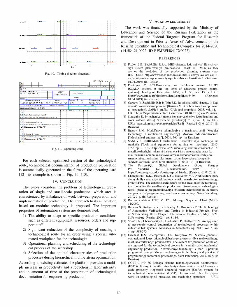
Fig. 10. Timing diagram fragment.

Fig. 11. Operating card.

For each selected optimized version of the technologicalroute, technological documentation of production preparationis automatically generated in the form of the operating card[12], its example is shown in Fig. 11 [13].

IV. CONCLUSION

The paper considers the problem of technological prepa-ration of single and small-scale production, which area ischaracterized by imbalance of work between preparation andimplementation of production. The approach to its automationbased on modular technology is proposed. The importantproperties of automation system are demonstrated:

1) The ability to adapt to specific production conditionssuch as different equipment, resources, orders and sup-port staff.

2) Significant reduction of the complexity of creating atechnological route for an order using a special auto-mated workplace for the technologist

3) Operational planning and scheduling of the technologi-cal process of the workshop.

4) Selection of the optimal characteristics of productionprocesses during hierarchical multi-criteria optimization.

According to existing estimates the platform provides a multi-ple increase in productivity and a reduction in labor intensityand in amount of time of the preparation of technologicaldocumentation for engineering production.

V. ACKNOWLEDGMENTS

The work was financially supported by the Ministry ofEducation and Science of the Russian Federation in theframework of the Federal Targeted Program for Researchand Development in Priority Areas of Advancement of theRussian Scientific and Technological Complex for 2014-2020(14.584.21.0022, ID RFMEFI58417X0022).

REFERENCES

[1] Frolov E.B. Zagidullin R.R-b. MES-sistemy, kak oni est’ ili evolyut-siya sistem planirovaniya proizvodstva (chast’ II) [MES as theyare or the evolution of the production planning systems (partII)]. URL: http://www.fobos-mes.ru/stati/mes-sistemyi-kak-oni-est-ili-evolyutsiya-sistem-planirovaniya-proizvodstva.-chast-ii.html (Retrieved01.04.2019) (in Russian).

[2] Davidyuk Y. SCADA-sistemy na verkhnem urovne ASUTP[SCADA systems at the top level of advanced process controlsystems]. Intelligent Enterprise, 2001, vol. 30, no. 13. - URL:https://www.iemag.ru/platforms/detail.php?ID=16479 (Retrieved01.04.2019) (in Russian).

[3] Garaeva Y. Zagidullin R.R-b. Tsin S.K. Rossiiskie MES-sistemy, ili Kakvernut’ proizvodstvu optimizm [Russian MES or how to return optimismto production]. SAPR i grafika [CAD and graphics], 2005, vol. 11. -URL: https://sapr.ru/article/14614 (Retrieved 01.04.2019) (in Russian).

[4] Statsenko D. Prilozheniya i rabota bez napryazheniya [Applications andwork without stress]. Stremlenie [Tendency], 2017, vol. 1, no. 18. -URL: https://kompas.ru/source/articles/3.pdf (Retrived 01.04.2019) (inRussian).

[5] Bazrov B.M. Modul’naya tekhnologiya v mashinostroenii [Modulartechnology in mechanical engineering], Moscow ”Mashinostroenie”[”Mechanical engineering”], 2001, 366 pp. (in Russian)

[6] SANDVIK COROMANT Instrument i osnastka dlya tocheniya nastankakh [Tools and equipment for turning on machines], 2015,1253 pp. - URL: http://www.lab2u.ru/katalog-sandvik-coromant-2015-metallorezhushchii-tokarnyi-instrument-i-instrumentalnaia-osnastka-dlia-tocheniia-obrabotki-kanavok-otrezki-rezbonarezaniia-reztcy-so-smennymi-rezhushchimi-plastinami-iz-tverdogo-splava-kompanii-sandvik-koromant-lab2u.html (Retrived 01.04.2019) (in Russian).

[7] The PostgreSQL Global Development Group PostgresPro Standard 11.2.1 Documentation, 2019. - URL:https://postgrespro.ru/docs/postgrespro/11/index (Retrived 01.04.2019)

[8] Cherepovskii D.K., Eizenakh D.C., Kotlyarov V.P. Arkhitektura bazydannykh dlya sozdaniya tekhnologicheskikh marshrutov melkoseriinogoproizvodstva [The database architecture for the creation of the technolog-ical routes for the small-scale production], Sovremennye tekhnologii vteorii i praktike programmirovaniya [Modern technologies in the theoryand practice of programming] conference proceedings, Saint-Petersburg,2019, 3 p. (in Russian).

[9] Recommendation ITUT Z. 120. Message Sequence Chart (MSC),11/2000.

[10] Baranov S., Kotlyarov V., Letichevsky A., Drobintsev P. The Technologyof Automation Verification and Testing in Industrial Projects. Proc.of St.Petersburg IEEE Chapter, International Conference, May 18-21,St.Petersburg, Russia, 2005 - pp. 81-86.

[11] Voinov N., Chernorutsky I., Drobintsev P., Kotlyarov V. An approachto net-centric control automation of technological processes withinindustrial IoT systems. Advances in Manufacturing, 2017, vol. 5, no.4, pp. 388-393.

[12] Eizenakh D.S., Cherepovskii D.K., Kotlyarov V.P. Sistema generatsiioperatsionnoi karty tekhnologicheskogo protsessa dlya melkoseriinogomashinostroitel’nogo proizvodstva [The system for generation of the op-erating card for the technological process for a small-scaled mechanicalengineering production], Sovremennye tekhnologii v teorii i praktikeprogrammirovaniya [Modern technologies in the theory and practice ofprogramming] conference proceedings, Saint-Petersburg, 2019, 46 p. (inRussian).

[13] GOST 3.1404-86 Edinaya sistema tekhnologicheskoi dokumentatsii(ESTD). Formy i pravila oformleniya dokumentov na tekhnologich-eskie protsessy i operatsii obrabotki rezaniem [Unified system fortechnological documentation (USTD). Forms and rules for paper-work on technological processes and machining operations]. - URL:

60

http://docs.cntd.ru/document/1200012135 (Retrieved 01.04.2019) (inRussian).

61

Reputation Systems in E-commerce: Comparative Analysis and Perspectives to Model Uncertainty

Inherent in Them

Nosovskiy Mikhail M., Degtiarev Konstantin Y. School of Software Engineering

National Research University Higher School of Economics 3 Kochnovsky Proezd, Moscow, Russia

mmnosovskiy@edu.hse.ru, kdegtiarev@hse.ru

Abstract — E-commerce is a runaway activity growing at an unprecedented rate all over the world and drawing millions of people from different spots on the globe. At the same time, e-commerce affords ground for malicious behavior that becomes a subject of principal concern. One way to minimize this threat is to use reputation systems for trust management across users of the network. Most of existing reputation systems are feedback-based, and they work with feedback expressed in the form of numbers (i.e. from 0 to 5 as per integer scale). In general, notions of trust and reputation exemplify uncertain (imprecise) pieces of information (data) that are typical for the field of e-commerce. We suggest using fuzzy logic approach to take into account the inherent vagueness of user’s feedback expressing the degree of satisfaction after completion of a regular transaction. Brief comparative analysis of well-known reputation systems, such as EigenTrust, HonestPeer, Absolute Trust, PowerTrust and PeerTrust systems is presented. Based on marked out criteria like convergence speed, robustness, the presence of hyperparameters, the most robust and scalable algorithm is chosen on the basis of carried out sets of computer experiments. The example of chosen algorithm’s (PeerTrust) fuzzy version is implemented and analysed.

Keywords — E-commerce, Reputation system, Peer-to-peer computing, Trust management, Uncertainty, Fuzzy logic, Linguistic variable

I. INTRODUCTION

E-commerce is a buying-selling runaway activity, which is widening at an unprecedented rate all over the world and inveigling into fascination of various e-stores people of all ages. Ever-growing number of various websites and apps focusing on e-commerce domain makes it simple and alluring to find and to buy immediately almost anything whatever client’s heart desires [23].

There is no doubt that e-commerce sales opportunities are rapidly progressing day by day. Owing to Internet, many businesses bring their products and services to customers literally in eyewink. The e-commerce share of total retail sales in the United States amounted to 10% in 2018, in expectation of attainment of 12.4% by 2020 with further strengthening its ground [28]. With such perspectives in mind it is easy to realize why e-commerce entrepreneur

position becomes so attractive. With an estimated 95% of purchases that will be made online by 2040 and expected growth of year to year sales standing at the level of 15%, the opportunity to find a niche for selling products online has massive indisputable potential [22]. During the last 5 years the amount of retail sales raised from $1.3 billion to $2.8 billion. The latter is expected to nearly double (up to $4.8 billion) by the end of 2021 [20].

One of the most growing types of e-commerce is online marketplace that can be defined as a website or app that facilitates shopping from many different sources [7]. Among well-known and successful examples of online marketplaces eBay, Amazon, Rakuten (worldwide) and Avito, Ozon (in Russia) can be mentioned. Online marketplace acts as a platform integrating buyers and sellers. Being a peer-to-peer (P2P) network, it allows buyers to purchase any goods or services offered by sellers through this online platform. Usually, peers (people or businesses) communicating through online marketplace remain in the status ‘strangers’ with respect to each other. They don’t have at their disposal reliable information about alter peer, whether it is a buyer or a seller. Therefore, peers must manage the risk associated with transactions on condition that no prior experience and knowledge concerning mutual reputation of sides exists [25]. It becomes possible to address this problem by means of developing a system on top of the network that should help peers to evaluate their past experience with other peers and to manage trust between them as well as reputation of each peer involved. This kind of systems is called reputation systems.

Various implementations of reputation systems exist starting with very simple to more complex ones designed mostly for P2P file-sharing networks [6,10,11,27]. No doubt that such systems have a positive impact on peer’s experience as they help to distinguish trustworthy peers from ill-intentioned and unreliable opponents. For example, in reputation system used by eBay, one of e-commerce leaders, buyers and sellers have a chance to rate each other with numeric scores +1, 0 or -1 after each carried out transaction. The overall reputation of a participant is calculated as a sum of scores earned over the last six months

62

[10]. At that all such systems rest upon notions of trust and reputation. Trust (or, local trust) represents personal experience (attitude) of a user regarding another user, while reputation constitutes an aggregate of these individual trust values on the scale of the whole community. In the long run calculation of local trust and corresponding aggregates underlies implementations of all known reputation systems.

Despite the practical effectiveness of these systems, there is a substantial drawback inherent in them, viz. none of them can handle uncertainty “hidden” in online marketplace’s data. The latter means data that relate to all transactions accomplished on the marketplace along with data collected from users after each transaction and metadata concerned with every user in the marketplace.

The primary concern of the paper is to provide the overview of best known reputation systems and to undertake their general comparative analysis on the basis of several key factors (criteria) – they are speed of convergence, complexity of calculations, use of hyperparameters expressing user’s preferences, robustness and general system’s suitability to handle imprecision and uncertainty of data. In the first place these factors are chosen to convey the requirements of key stakeholders who are owners and developers of a marketplace as well as its users. For the first group of stakeholders general system’s effectiveness becomes important, and it is attributed above all to the efficiency of its functioning, computational resources needed to perform the work and ability for customization. Users are mostly interested in reliability of system’s output and how well it suits each given user. The last factor mentioned above reflects how naturally specific implementation of the system can be extended to handle data uncertainty and imprecision, since the latter being an inherent part of virtually any system reveals itself in different forms. The recognition of such manifestation forms of uncertainty becomes a task of prime importance to represent appropriately (model) its distinctiveness. Consequently, fuzzy logic is getting one of pivotal theories that captures naturally the phenomenon of imprecision and uncertainty [34].

The rest of the paper is organized as follows: in section II notions of trust and reputation, difference between them, are considered. Uncertainty in the marketplace and verbal assessments that are inherent in reputation systems form the contents of section III. Some basic terms and definitions relating to the field of fuzzy sets and logic are covered in section IV. Section V is devoted to the brief comparison of well-known reputation systems (EigenTrust, Absolute Trust, HonestPeer, PowerTrust and PeerTrust) and stressing their key differences as well as intrinsic similarities. Setup of computer-based experimental part of the work (parameters and their values used) constitutes the material of section VI, whereas the results of carried out experiments are discussed in section VII. Thereafter, the transition from crisp to fuzzy PeerTrust algorithm (basic example and analysis of such transition’s outcome) is presented in last but one section VIII. Concluding remarks and observations are drawn in section IX.

II. TRUST AND REPUTATION. WHAT IS THE DIFFERENCE BETWEEN THESE TERMS?

Trust and reputation are the main concepts underlying vast majority of reputation systems. In order to clearly recognize the purpose of reputation systems, we need to define what do trust and reputation in terms of online marketplace stand for. Diverse sources give different definitions of the term ‘trust’. The basic definition presented in Oxford English Dictionary reads as follows: “Trust is a firm belief in the reliability, truth, or ability of someone or something” [29]. However, such definition cannot lay claim to completeness, since notions of trust and reputation as applied to peculiarities of Internet-based activities must be defined in a more context-specific way. Among other things, Alam & Paul define trust as “a belief, the trusting agent has in the trusted agent’s willingness and capability to deliver the services that they are mutually agreed on in a given context and in a given time slot” [1]. In addition, Wang & Vassileva associate term ‘trust’ with “a peer’s belief in another peer’s capabilities, honesty and reliability based on its own direct experiences” [24]. Starting from individual judgments and predictions, Gambetta state that “… trust is a subjective probability that relies on context and reputation, it describes how secure a situation is even though risk is associated with it” [5]. It can be noticed that trust is mainly linked to belief that peers (agents) mentally possess in malicious P2P environment. Thus, trust can be viewed as a soft factor of the system that is difficult to express precisely and in complete form. It is tied to distinction of numerous generally inhomogeneous interactions between peers, organization of the network, in which humans play a pivotal role.

For reputation term situation seems resembling, i.e. there is also no conventional definition that most of sources agree on. According to [24], reputation is defined as “peer’s belief in another peer’s capabilities, honesty and reliability based on recommendations received from other peers”. On the other hand, already cited above Alam & Paul propose to consider reputation as “aggregation of all recommendations provided by the third-party recommendation agents about the quality of the trusted agent” [1]. Abdul-Rahman & Hailes define reputation as “an expectation about an agent's behavior based on information about its past behavior” [2]. Kreps & Wilson link reputation to characteristic or attribute “ascribed to one person by another person (or community)” [3]. A complete (at least, voluminous) overview of definitions relating to trust and reputation can be found in [8]. In the present work we use definitions for terms ‘trust’ and ‘reputation’ from [24] since both definitions agree with basic concepts of reputation system and interaction within P2P community.

Even though trust and reputation are very closely related concepts, and many sources simply use them virtually as synonyms, still there is a major difference to emphasize. While trust is subjective in nature, and it expresses the local attitude of a peer regarding another agent on basis of his/her own past experience, reputation serves as a global and public perception of a given peer in the midst of other peers. With this point in mind, we may list those important (or, core) characteristics of trust and reputation that must be

63

taken into consideration when considering reputation systems – namely, they are: (1) Context awareness (sensitivity) – trust or reputation of a peer is dependent on what the context of communication is. For instance, a peer can be really trustworthy in delivering books, but unreliable in selling electronic accessories, (2) Multi-faceted nature (diversity) – even in the same context, peer can evaluate the quality of communication with another peer on the strength of several aspects. In the case of online marketplaces delivery time, quality and price of goods (services) can be mentioned. While the context-sensitivity of trust underlines the fact that the trust in the same agent may vary with reference to different situations, the multi-faceted nature characteristic stands for manifoldness of trust. It definitely plays a substantive role in deciding whether an agent is trustworthy to interact with or not [24], (3) Dynamism – apparently, levels of both trust and reputation increase or decrease in view of gaining experience (direct interaction). Such changes may alternate in due course depending on arising situation in the system, with a clear-cut declining tendency observed with time [24], (4) Imprecision and uncertainty – it is not very habitual for humans to operate with estimates of trust and reputation in the form of numbers. Without a doubt, it is not difficult to perform relatively simple calculations even in passing, but explanations and interpretations are usually based on verbal forms (words, phrases and short sentences in natural language). The peer can be classified as “very trustworthy”, “not too trustworthy” or in some likewise manner. Thus, we express gradations (imprecise estimates) of the extent, to which the peer is reputed as trustworthy or not. The bounds of gradations (verbal granules) are inexact, but nevertheless linguistic forms are easily perceived and processed by specialists and ordinary people in talks, reasoning and decision-making process. Observing definitions above, we may conclude that trust is a subjective category, and being apparently fuzzy it can be associated with verbal assessment values (granules). The vagueness of the trust is linked outright to uncertainty of reputation as well.

III. UNCERTAINTY IN MARKETPLACE DATA. VERBAL ASSESSMENTS ARE VERY NATURAL IN REPUTATION

SYSTEMS

The paper is focused on reputation systems as applied to e-commerce field (and specifically online marketplaces). Because of that it is essential to consider what kind of data concerning peers and their transactions are available, and what sort of data peer’s feedback about fulfilled transaction contains. In online marketplaces there are two types of peers – they are sellers and buyers; every transaction implies participation of one seller and one buyer. It is important to distinguish these types of ‘players’, because they gain trust and reputation that differ by their gist. In the present work we consider three types of marketplace data: (1) Peer data, i.e. a set of general data pieces that relates to peer itself (personal data, registration date, etc.), (2) Transaction data – general data about transaction held between seller and buyer (delivery time, payment time, total

sum of transaction, date of transaction, etc.), (3) Feedback data refer to data collected from both seller and buyer after completion of each transaction (goods quality, communication quality, shipping service reliability, etc.).

Most of the existing reputation systems work only with peer’s feedback [6,10,11,16,27]. In general, feedback provides some subjective assessment of experience that a peer has with another peer in the course of transaction’s realization. But in certain cases, such experience cannot be thoroughly expressed in terms of integers -1, 0 and +1 as it occurs in eBay system. Why do we think so? Firstly, regarding feedback as a number means neglecting diverse aspects of experience such as those mentioned above. Secondly, and this fact was also underlined earlier, it is more natural for humans to think of evaluating experience in terms of some ordinal scale stretching from “very bad” label to “very good” instead of using “good”, “neutral” or “bad” plain marks as linguistic equivalents of -1, 0 and +1. It should be emphasized that in case of extended scale’ use, its grades may overlap with each other, since each label or grade stands not for a single value, but for a range of values instead. For instance, there is no clear-cut border line between values (labels) “very bad” and “bad”, but almost all people may differentiate these values mentally while talking about them, impacting information chunks to others.

Similar situation comes to pass with reference to transaction data. For example, let us consider delivery time of basic electronic accessories from Moscow to Saint-Petersburg. We know that they are normally delivered within N days. Is it “quickly”, “slowly” or “neither slowly, nor quickly” for a client? Maybe it is a little bit slowly, but not too much? What can be said about N+2, 2N days or even 5N days? At some point it becomes obvious that delivery time can be associated with label “slowly” or even “very slowly”. But what do we mean by that some point? For different people it occurs at different moments, which are not fixed (crisp), and this is when imprecision and uncertainty (fuzziness) of these data reveal themselves.

IV. FUZZY LOGIC THEORY. SOME BASIC TERMS AND DEFINITIONS USED IN THE STUDY

Taking into account uncertainty inherent to notions of trust and marketplace data, we need to consider its formal representation for a possible use in trust management and reputation systems (models). The concept of uncertainty is many-sided and rich; furthermore, uncertainty ‘accompanies’ any interactions of humans with real world [34]. In this connection, reputation systems exemplify active communication of peers based on the exchange of information that is often a matter of human perceptions and interpretations to a various extent. Much depends here on cognition and verbal assessments expressed in the natural language. Such perceived units can be mostly seen as granules with ‘soft’ bounds rather than exact quantities having unified meaning and interpretation by all parties involved into the process. The theory of fuzzy logic (FL) extends the ontology of mathematical research in the context of formation of a composite methodology that leverages quality and quantity [9]. It provides ample means to model

64

the “perceived meaning of words/phrases conveying the expert opinions (estimates) in a graded fashion” [30]. The following is a quick glance at main concepts and definitions concerned with fuzzy logic as used in the present study.

Definition 1. Linguistic variables (LV) – variables whose values are words, phrases or sentences (linguistic terms) expressed in natural or artificial language [26]. In short, we can state that LV constitute a form of information granulation serving as a base for further transition of those granules to computable counterparts [31]. For example, if we consider the case of delivery time from point A to point B, the label (term) “quickly” is one of possible linguistic values assigned to the variable Delivery Time. Its whole term-set can be represented as T(Delivery Time) = “quickly” +

“very quickly” + “slowly” + “more or less quickly” + … , where sign ‘+’ denotes the aggregate of linguistic granules rather than arithmetic sum operation.

Linguistic variable Delivery Time is defined on the universal set U (realistic range of numeric values representing the delivery time in particular situation), i.e. each element stands for the time (minutes, hours, etc.) that can be associated as a result of human’s perception (judgment) with corresponding terms to various degrees. Definition 2. Let U be a set of elements (objects) that are denoted generically as x (U=x); fuzzy set is a set of ordered pairs , where mapping

is a (type-1) membership function of a fuzzy set A. Value is a degree (grade) of membership of x in the set A, and U is a problem’s domain (universal set). Membership function (fuzzy set) represents possibility distribution of x-values over domain U. It can be expressed

as aggregation or union of pairs

, , in continuous and discrete cases, correspondingly. Definition 3. Let A be a fuzzy set on U, then a-cut of A is a crisp (non-fuzzy) set composed of all , whose grades of membership in A are greater or equal to a [26]. Formally, can be expressed as . A fuzzy set A may be decomposed into and restored from a-cut sets

through the resolution identity [12, 13], i.e. , or

, .

An integral part of any formal modeling approach is closely related to the use of functions. Along with pervasive processing of non-vague objects, fuzzy quantities in last three decades became wide-spread in algorithms covering enormous circle of application domains. The need to extend the possibility for functions to operate with arguments having the form of fuzzy sets has led to formulation of extension principle [26,32,33]. As its name speaks for itself, it is directed to spreading nonfuzzy mathematical concepts to fuzzy ones [4]. It is specifically what is required to handle aspects of uncertainty (fuzziness) with reference to existing

reputation systems. Definition 4. Assume is a mapping from universal set U to set V, and A is a fuzzy set defined on U (for the sake of simplicity we may consider finite representation of such set, i.e. ). Relying on the extension principle, the image of A under mapping is obtained as follows:

.

In other words, the image of A under can be deduced from the knowledge of the images . Definition 5. The process of representing initial data (e.g. linguistic values) as membership functions is called fuzzification; most of applications require to perform at final stages the opposite translation from fuzzy functional forms to crisp values – this is achieved through defuzzification procedures [30,32,34,37].

V. BRIEF COMPARISON OF EXISTING REPUTATION SYSTEMS – THEIR DIFFERENCES AND INTRINSIC

SIMILARITIES

The number of publications devoted to trust management and reputation systems is pretty imposing, and it is growing from year to year [10,11,16,17,24,25,27]. In the paper we wittingly touch upon (just brief overview augmented with performance considerations) the most significant systems that proved themselves as effective, robust and applicable to online marketplace reputation management. It is worth mentioning that only those systems that do not use basically fuzzy logic concepts are reviewed in the paper. For instance, systems that utilize fuzzy inference schemes or other fuzzy-logic related notions [9,18,19] constitute an interesting research topic, but on level with other relevant cases it is outside of the scope of the present paper.

Results of the conducted analysis of existing sources provided a basis for selection of those criteria that can be classified as crucial from the viewpoint of systems’ comparison. They can be described concisely as follows: (1) Speed of convergence – iterative algorithms form a core of nearly all reputation systems. Thus, one of important aspects of such algorithms is how fast they converge and produce a result. This feature is covered as a principal one in most of papers related to reputation systems [10,11,25,27], (2) Robustness, i.e. the criterion concerned outright with the main purpose of every reputation system, namely, the prevention of malicious attacks. Therefore, it becomes essential to measure how well a given system is able to hold out against malicious peers’ activities. Such experiments are covered by S.D. Kamvar, M.T. Schlosser, H. Kurdi, N. Chiluka, N. Andrade, Y. Wang, L. Xiong, et al. in [10,11,16,24,25,27]; however, it is important to mention that papers referenced here cover different types of malicious behavior, (3) Hyperparameters – their presence is an important point to consider in the process of system’s deployment, since

Îx U

ÍA U A(x,μ (x))

Aμ : x [0,1]®

Aμ (x)

μ ( )

Îò A

x U

xx

μ ( )

Îå A

x U

xx

( ),μ( )x x μ( ) [0,1]Îx

αA Îx U

αA |μ ( ) α³Ax x

1

α0

α= òA A

ααα=åA A α [0,1]Î

f

1 1 2 2μ ( ) μ ( ) ... μ ( )= + + +A A A n nA x x x x x x( )f A

f

( )1 1 2 2( ) μ ( ) μ ( ) ... μ ( )f f= + + + =A A A n nA x x x x x x

1 1 2 2μ ( ) ( ) μ ( ) ( ) ... μ ( ) ( )f f f= + + +A A A n nx x x x x xf

1 2( ), ( ),..., ( )f f f nx x x

65

they show the extent, to which the system is customizable. But at the same time, factor of their presence is a ‘double-edged sword’, inasmuch as, on the one hand, tuning of hyperparameters may lead to better performance of a specific system. On the other hand, it enhances significantly the complexity of deploying the system, (4) Handling data imprecision and uncertainty. Most of hypothetical or artificial systems do their work in the presence of uncertainty. The latter is often linked to human factor being an integral part of a system in the context of verbally defined and/or interpreted data. The latter are elicited from active discussions with stakeholders and estimations commonly used as inputs in calculations provided for algorithms underlying system’s work specifics. Those pieces of information are often ‘soft’ (imprecise) in their nature, and it opens manifest way for the use of fuzzy logic theory in models of reputation systems. Hence, the comparison of algorithms can be performed in the view of how well system (algorithm) adapts fuzzy logic extension.

A. EigenTrust Algorithm EigenTrust system is originally proposed for a P2P file-sharing network by S.D. Kamvar, M. Schlosser and H. Garcia-Molina in the paper that became one of the most cited papers on reputation systems [10]. EigenTrust calculates a global trust value for each peer based on his/her past behavior by incorporating opinions of all peers in the system [16]. Opinions concerning a particular peer are represented as a local trust value. After each communication peer assesses his/her experience by the value from restricted set comprised by integers -1, 0 or 1. The local trust value is an aggregation of all communication experience assessments. It was shown how to normalize local trust values in a way that leads to elegant probabilistic interpretation similar to the Random Surfer model and efficient algorithm to aggregate these values [10,14]. Pre-trusted peers that can be seen here as a hyperparameter (it must be chosen in advance for the whole system to operate) are used to guarantee convergence and breaking up malicious collectives. What is more, the choice of pre-trusted peers is important, and it can compromise the quality of system to a marked degree [10]. As also shown in [10], for a network with 1,000 peers the algorithm converges after completion of less than 10 iterations. Theoretical base for fast convergence of EigenTrust algorithm is discussed by T.H. Haveliwala and S.D. Kamvar in [21]. Robustness of the system is evaluated under several threat models, and the system shows good overall performance in all cases [10]. For both Individual malicious peers and Malicious collectives threat models, EigenTrust system outperforms non-trust-based systems showing five to eight times better results with fraction of inauthentic downloads (FID) less than 0.2 for every setting. For Malicious collectives with camouflage case (model 3), system shows slightly less impressive results, but still Malicious Spies threat model (fourth model) tends to be the best strategy for malicious peers to attack trust-based network [10].

As already mentioned earlier, EigenTrust system uses aggregated local trust values that must be normalized beforehand to avoid system’s ‘demolition’ due to

assignment of very high and very low local trust values [10]. Normalized local trust value can be calculated as follows:

where is a local trust value. The shown way of normalization isn’t free of drawbacks. For one thing, normalized values don’t draw a distinction between a peer with whom a given peer i did not interact and a peer with respect to whom peer i has had a poor (negative) experience. Secondly, values are relative, and they cannot be interpreted easily in the absolute sense [10]. Thus, an attempt can be made to extend EigenTrust algorithm with fuzzy logic notions to obtain transparent and interpretable modification of the original computational scheme. Particularly, calculation of local trust value may be altered to accumulate different types of marketplace data, but further study that concerns the impact of fuzzification on probabilistic interpretation of EigenTrust algorithm is required.

B. HonestPeer Algorithm HonestPeer as an enhanced version of EigenTrust algorithm is discussed by H. Kurdi [11]. The algorithm endeavors to address one of the major problems with EigenTrust system, viz. pre-trusted peers. HonestPeer minimizes the dependency on that pre-trusted set of peers by choosing one honest peer dynamically for every computation step of global trust value (GTV). This honest peer, i.e. the peer having the highest global trust value, plays a crucial role in further computations of GTV. The speed of HonestPeer’s convergence is almost the same as for EigenTrust algorithm, despite the need to perform additional calculations. Following [11], two benchmarks are considered – they are EigenTrust algorithm and no algorithm. Performance of HonestPeer algorithm is estimated under different experimental settings embracing variable number of users and files as well as number of pre-trusted peers and with the examination of percentage of inauthentic file downloads by good peers and success rate of good peers (success rate of good peers equals the ratio of #valid files received by good peers to #transactions attempted by good peers). HonestPeer algorithm surpasses EigenTrust in effectiveness and capability to ‘help’ good peers to download valid safe files. This fact can be attributed to the ability of HonestPeer to choose honest peers dynamically after each round, while in case of EigenTrust pre-trusted peers are chosen statically irrelative of their performance [11]. Since HonestPeer is basically an enhancement of EigenTrust algorithm, the use of fuzzy logic may be appropriate and explicable as a practical matter to address those forms of uncertainty that are typical for system under consideration.

C. PowerTrust Algorithm The reputation system PowerTrust, which is based on power-law distribution of peer feedbacks discovered after examination of 10,000+ eBay users’ transaction traces, is

ijc

max( ,0) max( ,0)ij ij ijj

c s s= å

ijs

ijc

66

covered by R. Zhou and K. Hwang [15,27]. In PowerTrust system a few power nodes are selected dynamically according to their reputation. These nodes can be dynamically replaced, if they become less active or demonstrate unacceptable behavior. Good reputation of power nodes is accumulated from the operation history of the system – functional modules of PowerTrust system as well as flow scheme that relates to collection of local trust scores and global reputation aggregation are visually demonstrated in [27]. Without going into particulars, it should be mentioned that raw data input for PowerTrust is treated as local trust scores, which are then aggregated to obtain global reputation score of each peer. The Regular Random Walk module supports the initial reputation aggregation, while Look-ahead Random Walk (LRW) module is used to update the reputation score periodically. LRW also works with Distributed Ranking Module to identify power nodes. The system leverages power nodes to update Global Reputation Scores (vector V) [27]. The experimental performance of PowerTrust in terms of reputation convergence overhead to measure aggregation speed, ranking discrepancy to measure the accuracy, and root-mean-square (RMS) aggregation error to quantify system’s robustness to malicious peers shows that PowerTrust algorithm outperforms EigenTrust by more than factor 1.5 in case of convergence speed [27]. Under all settings PowerTrust exhibits its robustness against collusive peer groups of various sizes. In much the same way as for both EigenTrust and HonestPeer, the point of fuzzy logic’s application to PowerTrust algorithm is a local trust value. Several linguistic terms may be defined on [0,1] interval to be used consequently for computation of global reputation. It is of definite interest to research whether the use of fuzzy logic may affect properties of PowerTrust algorithm or not.

D. Absolute Trust Algorithm The algorithm for aggregation of trust among peers in P2P networks (Absolute Trust algorithm) was presented by S.K. Awasthi and Y.N. Singh [17]. Most of reputation systems are built upon scenario when all peers evaluate other peers by way of assigning foregoing local trust values that are a subject for further aggregation aimed at obtaining peers global reputation scores. In general, three different types of evaluation scenarios (one-to-many, i.e. one person is evaluating many persons, many-to-one scheme, under which many persons are evaluating one person, and one-to-one case, which implies that one person is evaluating another person) can be identified. In an effort to strengthen feedback’s reliability in many-to-one evaluation scheme, any evaluation provided must allow for the competence of evaluator (evaluating party in the system) in computations via proportional weight’s factor. Global trust of j-th peer can be used by way of weight in aggregation of local trust scores in calculation of any given i-th peer’s global trust. Thus, a set of peers communicating (providing services) to the i-th peer can be reduced to just one virtual representative. It results in obtaining one-to-one evaluation scheme, and the trust of a set will be dominated by peers having higher global trust [17]. The existence and uniqueness of global trust vector as an

outcome of aggregation approach is proven in [17]. The closed-form peer’s global trust expression lays a basis for direct comparison of global trust values calculated for any two peers in the system (network with N nodes). There is no theoretical explanation of fast algorithm’s convergence, but experiments show that it converges fast (about 7 iterations for 100 peers in the network) [17]. Robustness of Absolute Trust algorithm is evaluated regarding behavior of EigenTrust and PowerTrust systems. Several network configurations are considered in [17] such as the ones under the presence of pure malicious peers, peers with unpredictable behavior as well as malicious collectives (groups of peers whose familiarity positively affects their own reputation values diminishing corresponding values of persons outside such groups). It was shown that for first two configurations the performance of Absolute Trust improves significantly as compared to counterparts (by appr. 2% to 4% of authentic transactions that relate to exchanging files between peers, respectively). As concerns malicious collectives, performances of algorithms are almost identical, with marginal superiority of Absolute Trust over its aforesaid rivals. The local trust metric in this algorithm can be defined in many ways, and it forms prospects to develop a fuzzy local trust metric. It is worth mentioning that aggregation procedure used in the algorithm can be practically retained. The customizable local trust metric allows to use fuzzy logic approach to extend the algorithm in relatively easy and natural way.

E. PeerTrust Algorithm PeerTrust is another example of P2P reputation system designed specifically for e-commerce communities that are characterized by distinctive problems and risks [25]. L. Xiong and L. Liu identify five important factors that relate to evaluation of peer’s trustworthiness as regards supplying other peers with corresponding services. These factors are feedback obtained by a peer, feedback scope (e.g. total number of transactions occurred between peers), credibility of feedback source, transaction context aimed at drawing distinction between extremely crucial and less important or uncritical transactions, and community context to address community-wide characteristics and vulnerabilities. Based on formalization of these parameters, the authors proposed a peer’s j trust value (metric) consisting of two parts [25]. The first one is a weighted multiplicative combination of amount of satisfaction peer obtained after realization of each transaction, adaptive transaction context for i-th transaction of a peer and credibility of the feedback received from peers. Community context factor constituting the second part of ’s expression increases or decreases the impart of the first part to trust value owing to allowance of distinctive community’s features. As it is emphasized in [25], the proposed metric

should be considered as a general form, in which corresponding parts can be ‘tuned’ in terms of parameters and factors used. Every part of the metric can be implemented differently – alternatives of possible credibility measure metrics (trust value/TVM, personalized similarity/PSM) are presented by L. Xiong and L. Liu in

( )T j

( )T j

( )T ×

67

their paper. Speed of convergence and complexity of PeerTrust algorithm appreciably depend on metrics definitions and specific implementation strategies. In general, the performance of system under PSM metric is a bit worse than in case of TVM, but on the other hand, the former provides better results as the number of peers in the network is increasing. System’s robustness is assessed on the grounds of effectiveness against malicious behavior of peers comparing to conventional algorithm, in which the average of the ratings is used to measure the trustworthiness of a peer without taking into account the credibility factor. The trust computation error as a root-mean-square error (RMSE) of the computed trust value of all peers and the actual likelihood of peers performing a satisfactory transaction is computed to evaluate the performance of the algorithm. PeerTrust with PSM metric ensures striking results as calculated RMSE does not exceed the value of 0.05, and transaction success rate attains virtually unity. It must be admitted that PeerTrust system is very flexible over the existing possibility to choose local trust metric. Therefore, it seems that the practical application of fuzzy logic approach to handle naturally nascent uncertainty (vagueness) of certain parameters and characteristics in the algorithm looks justified enough. The system also possesses a great potential to incorporate all types of marketplace data, especially through transaction and community context parts of the general metric that afford means of broad coverage of manifold system’s peculiarities.

VI. EXPERIMENTAL PART – SETUP STAGE

For the experimental part of the study, we implemented a simulator (in Python 3.7), and the section describes the general simulation setup, including the community setting, peer behavior pattern, and trust computation.

We assume that hypothetical (simulated) community consists of N peers, for which two peer types are defined, namely, they are honest and strategic, or malicious, peers [35]. The first one embraces those commitment long-run players focused on cooperation, since the latter maximizes player’s lifetime payoffs, if the player consistently sticks to action in long-range outlook. In contrast, opportunistic player who cheats whenever the occasion is beneficial for him is bound to a strategic type [25]. The percentage of malicious peers in the community we denote by K. It is reasonable that behavior pattern of good peers is to always cooperate and provide honest feedback after each transaction. However, a correct modeling of malicious peers behavior is a bit challenging task that may require certain simplifications. In particular, we may consider that malicious peers always cheat during transactions and give dishonest ratings to other peers, i.e. they rate negatively a peer who cooperates and provides good rating to a peer who cheats. In case of EigenTrust and HonestPeer algorithms there are also pre-trusted peers that play an important role from the standpoint of algorithm’s consistency. Respective PRE_TRUSTED parameter stands for the percentage of pre-trusted peers that relate to good peers only. In general, behavior pattern of peers is a topic on a slippery ground, i.e. it can be placed among those aspects of models of reputation

systems that require close scrutiny. Why? Potentially, the above cited pattern is definitely not unique, so in order to make models viable other feasible options must be addressed hereafter with great care.

We may also assume that community has CAT categories of services that are provided by peers. From amongst these categories each peer is interested only in a specific subset having the cardinality not less than S. Each category is associated with at least P percent of peers in the community. When a peer queries a service of a specific category, only peers associated with this category can respond to such query. At that, two transaction settings are simulated – they are random and trusted. Random (or, simple) setting means that a peer, which responds to the query, is selected randomly (uniform distribution is used) from a set of all peers that can provide queried category of service. In trusted setting the responder is also selected randomly from all peers that can respond to the query, but it is done with respect to their reputation, i.e. a peer with higher reputation has better chances to be chosen. If there are peers with zero reputation, then there is a 10% chance that the responding peer will be chosen uniformly from those peers. It efforts the opportunity for new peers to start building up their reputation.

Binary feedback system is used to evaluate peer after each completed transaction. It means that values 0 and 1 are practised for PeerTrust and Absolute Trust algorithms, -1 and 1 are used in cases of both EigenTrust and HonestPeer approaches. Local trust and reputation computation steps as such depend on the algorithm in use. Some algorithms have their own hyperparameters that must be specified. Default values of parameters are listed in Table I. Simulation session (cycle) consists of SIM_NUM transactions. Global reputation is updated after every UPDATE_NUM transactions. Experimental results are averaged by 5 cycles of simulation. Although we simulate online marketplace community – usually it is big enough, dozens to hundreds of thousands of peers – experiments are performed under the presence of modest number of peers. It may be considered as a perceptible limitation, however, the main aim of simulation is to obtain those prior results that lay down the ground for further analysis of weak/strong points of models considered here in terms of deeper understanding of their potential to incorporate formal representation of uncertainty (imprecision) factors into these models. In real-life environment it seems highly unlikely that the major part of marketplace peers are malicious as it was defined earlier. Therefore, we don’t consider in simulation a malicious peers share exceeding 35%.

VII. EXPERIMENTAL PART – RESULTS AND THEIR COMPARISON

We introduce a metric that shows the effectiveness of the reputation system as a rate of unsuccessful transactions (RUT). The unsuccess of transactions is bound up with the outcome of those transactions, in which responding peer happens to be malicious. It is obvious that the less value of the metric is the better. Besides, for the time being we do not consider PowerTrust algorithm in the empirical study, since it requires more close inspection and implementation cycle.

( )T ×

68

A. Effectiveness against malicious behavior The objective of conducted experiments is to evaluate

the robustness of the reputation systems against peers with malicious behavior. In the first experiment we alter the percentage of malicious peers in hypothetical community from 10% to 35% with other parameters keeping their default values (Table I). As is easy to see in Fig. 1, the rate of unsuccessful transactions grows almost linearly with the increase of values (axis x) for simple setting; trusted settings

TABLE I. PARAMETERS AND THEIR VALUES USED IN EXPERIMENTS

show better results though. EigenTrust, HonestPeer and PeerTrust algorithms show extremely moderate growth of RUT with the increase of malicious peers’ percentage. Absolute Trust algorithm demonstrates quite disappointing results characterized by negligible gain (within appr. 2.1% on average) as compared to simple (random) system’s case.

B. Speed of convergence and scalability In this set of experiments, we take aim at evaluating the

general speed of algorithms convergence and their scalability with regard to the increase of number of peers (Fig. 2). As will readily be observed, algorithms PeerTrust and Absolute Trust generally need not more than 2 iterations to converge, while EigenTrust and HonestPeer need to go through 4+ iterations. More than twofold difference on very

small values practically equalizes rivals under the conditions of experiment. Thus, all algorithms seem to be quite scalable concerning the number of iterations needed to converge, since the latter does not grow substantially with the increase (from 1,000 to 3,500) of number of peers in the community.

Fig. 1. The growth of rate of unsuccessful transactions depending on the increase of malicious peers’ percentage (from 10% to 35%) for different

algorithms We also evaluate how consistent corresponding systems

are against the background of increasing number of peers under “freezing” of other parameters (Fig. 3). It can be seen that situation remains almost indistinguishable be it small or bigger community – the rate of unsuccessful transactions mostly remains unchanged in the context of the same malicious peers percentage.

Fig. 2. The speed of convergence (number of iterations needed) of

algorithms depending on the number of peers (in the range from 1,000 to 3,500)

C. Choice of the “best” (most feasible) system According to the results of experiments summarized

above as well as constraints and assumptions put forward, PeerTrust model appears the most robust and effective

Affiliation with… Parameter Description Default

value

Community setting

N number of peers 1000

K percentage of malicious peers 15

CAT number of categories 10

S minimal number of categories for each peer

3

P minimal percentage of peers associated with each category

5

Simulation setting

SIM_NUM number of queries in a simulation 10000

UPDATE_NUM

number of transactions in reputation update cycle

100

EigenTrust &

HonestPeer PRE_TRUSTED percentage of pre-

trusted peers 5

Absolute Trust

GOOD_W weight of good transactions in local trust

10

BAD_W weight of bad transactions in local trust

1

a

trade-off parameter between speed of convergence and quality

1/3

69

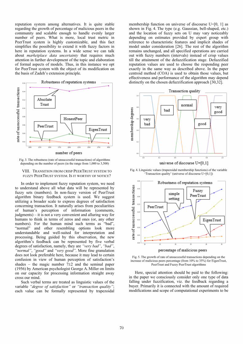
reputation system among alternatives. It is quite stable regarding the growth of percentage of malicious peers in the community and scalable enough to handle evenly larger number of peers. What is more, local trust metric in PeerTrust system is highly customizable, and this fact simplifies the possibility to extend it with fuzzy factors in here in reputation systems. In a wide sense we can talk about marketplace data uncertainty that requires much attention in further development of the topic and elaboration of formal aspects of models. Thus, in this instance we opt for PeerTrust system with the object of its modification on the basis of Zadeh’s extension principle.

Fig. 3. The robustness (rate of unsuccessful transactions) of algorithms depending on the number of peers (in the range from 1,000 to 3,500)

VIII. TRANSITION FROM CRISP PEERTRUST SYSTEM TO FUZZY PEERTRUST SYSTEM. IS IT WORTHY OF NOTICE?

In order to implement fuzzy reputation system, we need to understand above all what data will be represented by fuzzy sets (numbers). In non-fuzzy version of PeerTrust algorithm binary feedback system is used. We suggest utilizing a broader scale to express degrees of satisfaction concerning transaction. It naturally arises from peculiarities of human’s perception of information (comments, judgments) – it is not a very convenient and alluring way for humans to think in terms of zeros and ones (or, any other numbers). For the human mind such terms as “bad”, “normal” and other resembling options look more understandable and well-suited for interpretation and processing. Being guided by this observation, the new algorithm’s feedback can be represented by five verbal degrees of satisfaction, namely, they are “very bad”, “bad”, “normal”, “good” and “very good”. More fine granulation does not look preferable here, because it may lead to certain confusion in view of human perception of satisfaction’s shades – the magic number 7±2 and the seminal paper (1956) by American psychologist George A. Miller on limits on our capacity for processing information straight away cross our mind.

Such verbal terms are treated as linguistic values of the variable “degree of satisfaction” or “transaction quality”; each value can be formally represented by trapezoidal

membership function on universe of discourse U=[0, 1] as shown in Fig. 4. The type (e.g. Gaussian, bell-shaped, etc.) and the location of fuzzy sets on U may vary noticeably depending on estimates provided by expert group with reference to characteristic features and implicit shades of model under consideration [26]. The rest of the algorithm remains unchanged, and all specified operations are carried out with fuzzy numbers (intervals) instead of crisp values till the attainment of the defuzzification stage. Defuzzified reputation values are used to choose the responding peer exactly in the same way as described above. In the paper centroid method (COA) is used to obtain those values, but effectiveness and performance of the algorithm may depend distinctly on the chosen defuzzification approach [30,32].

Fig. 4. Linguistic values (trapezoidal membership functions) of the variable

‘Transaction quality’ (universe of discourse U=[0,1])

Fig. 5. The growth of rate of unsuccessful transactions depending on the

increase of malicious peers percentage (from 10% to 35%) for EigenTrust, PeerTrust and Fuzzy PeerTrust algorithms

Here, special attention should be paid to the following:

in the paper we consciously consider only one type of data falling under fuzzification, viz. the feedback regarding a buyer. Primarily it is connected with the amount of required modifications and scope of computational experiments to be

70

covered by the text of the limited size. But we are aware that other foregoing types must be addressed thoroughly in the course of the ongoing empirical study.

In conditions of maintenance of community and simulation settings (see the details of conducted experiments described above), but under the imprecision (vagueness) taken into account in the feedback system, we compare the experimental components of Fuzzy PeerTrust with original PeerTrust and EigenTrust algorithms.

A. Effectiveness against malicious behavior (fuzzy case) In the first place, we want to evaluate the robustness of

fuzzy modification of PeerTrust system. Experiment settings are retained, the percentage of malicious peers is changing within the range from 10% to 35%. The results as shown in Fig. 5 lead to the conclusion that Fuzzy PeerTrust algorithm is definitely more robust in comparison with Simple system. Under small percentage values (appr. interval [10%,17%]) of malicious peers, the performance’s characteristic of Fuzzy PeerTrust is close enough to original PeerTrust and EigenTrust. However, it demonstrates worse results than crisp algorithms over the whole range of x-axis values concerned.

B. Speed of convergence and scalability Another set of experiments was aimed at estimation of

the speed of convergence of Fuzzy PeerTrust and its scalability in view of the community’s growth. As expected, the speed of convergence remains the same as for original PeerTrust with two iterations on average to converge, and it differs essentially from corresponding characteristic (appr. 4.61 on average) of EigenTrust algorithm (Fig. 6). In terms

Fig. 6. The speed of convergence (number of iterations needed) of

EigenTrust and Fuzzy PeerTrust algorithms depending on the number of peers (in the range from 1,000 to 3,500)

of robustness Fuzzy PeerTrust can also be pronounced scalable, since it does not show significant decrease in quality with the growth of the number of peers in the community (Fig. 7). We observe here smooth fluctuations of RUT at the level of 0.064. It is worth mentioning that all properties of crisp algorithm remain intact in comparison with its fuzzy counterpart.

Computational procedure starts with default trust vector

, where N – the number

of peers in the community, is a default trust value of a peer v, [25]. Reputation of a peer v in the form of fuzzy set (number) is denoted as ;

stands for a feedback of peer v concerning j-th transaction, it is also represented as a fuzzy number; signifies the reduction of a fuzzy argument to crisp value (deffuzzification step). To calculate the product of fuzzy number

and crisp number as well as the sum (1) of thus obtained fuzzy numbers, Zadeh’s extension principle is used [4,36,37]. As a result, steps to be performed (pseudocode) can be expressed as follows:

Repeat

(1)

(2)

Until diff £ e As already mentioned, it is significant to put special emphasis on the choice of defuzzification method to use in (2). It may become a subject of separate research in the future.

Fig. 7. The growth of rate of unsuccessful transactions depending on the

number of peers (in the range from 1,000 to 3,500) for EigenTrust, PeerTrust and Fuzzy PeerTrust algorithms

At the same time, an important point of the algorithm

shown is that certain aforesaid attributes of trust and reputation like context-awareness (sensitivity), decrease (of the level) with time, their multifaceted nature (diversity) are not taken into account. We may regard this version of the algorithm as basic one (or, F-basic if we consider factor of

( )T

T0 0 0 01 2 N

1 1 1, ,..., , ,...,N N N

t t t t æ ö= = ç ÷è ø

0vt

1,Nv =

( )i 1vfuzzy t + ( )( , j)fuzzy S v

( )defuzz !

( )( , j)fuzzy S v I( )i ij kk 1

vt t=å

For 1 to N do v =

( ) ( )i

I( ) ji 1I( )j 1 i

kk 1

( , j)vv v

tfuzzy t fuzzy S v

t+

=

=

= ×åå

( )i 1 iv vt defuzz t+ =

i 1 idiff t t+= -

71

fuzziness in its core); it paves a ‘wide’ way for algorithm’s further revision and improvement.

The results attained enable to speak decidedly about the existing perspectives of fuzzy logic approach’s application in reputation systems (corresponding algorithms). Even despite somewhat higher computational costs compared to original crisp algorithms, greater transparency, better perceptibility by humans and flexibility from a viewpoint of verbal expression and formalization of the scores provide a basis for further studying of the topic. The present paper can be considered as a mere first step in this direction.

IX. CONCLUSION

E-commerce is a fast-growing market that implies continual and utterly active communication between users being ‘strangers’ to each other on numerous occasions. Because of that it is essential to establish reputation systems to better handle available online information with the object to more accurately discern trustworthy and non-trustworthy players in systems creating grounds for peers to be more careful about their reputation. By the far-famed example of eBay reputation system, even relatively simple ones show themselves as very helpful from the viewpoint of malicious behavior’s limitation and trustability increase. Online marketplaces that became immensely popular in the last 10-15 years as sites offering wide enough range of reasonably priced goods from various sources can be also considered as P2P networks. There is a vast range of reputation systems developed for P2P networks (mostly aimed at file-sharing) that can be adapted to e-commerce.

The main problem that is covered in the paper relates to the fact that none of these systems work with uncertainty (blurriness) of marketplace data and vagueness typical for notions of trust and reputation. Uncertainty in different forms of its manifestation is definitely inherent in reputation systems, and some of those forms can be addressed by fuzzy logic. This very inhesion, but not disconfirmed artificial desire, has served as an impellent factor to start this study.

Most likely, it can be argued that it is difficult to identify on the basis of several singled out key criteria unconditional leader among analyzed systems (algorithms EigenTrust, Absolute Trust, HonestPeer, PowerTrust and PeerTrust), since each of them has positive aspects as well as drawbacks. All algorithms, except PowerTrust, were implemented (Python 3.7) under the same conditions discussed in detail in the paper with the purpose of comparing fairly their relative performance. For reasons partially covered in the paper, Absolute Trust and PeerTrust systems were prudently regarded from the standpoint of their robustness and scalability as front-runners, i.e. candidates for fuzzification. Besides undertaking comparative analysis of those five significant and most popular reputation systems, the paper makes a mark for transition from crisp system (by the example of PeerTrust algorithm) to its fuzzy counterpart.

Corresponding fuzzy model (we call it provisionally F-basic algorithm) considers now only one characteristic of trust and reputation, namely, it is transaction quality or degree of peer’s satisfaction. Other important attributes like context-awareness (sensitivity) or decrease of trust’s level with time were not scrutinized yet. Nevertheless, initial

experimental results attained in line with the fact of constant presence and active use of verbal assessments in reputation systems confirm the need to continue research in this field. Verbal forms are both habitual and convenient for human’s perception despite of their intrinsic vagueness. That is why, fuzzy logic approach, to the opinion of authors, has good prospects for use in reputation systems.

At the same time, it should be mentioned that there are immediate tasks related to fuzzy models that require primary attention. The choice of membership functions and their fine tuning (shape and location on the universe of discourse), the switch from the case having dealings with marketplace data vagueness (so-called type-1 fuzzy sets used in the paper) to the case that represents uncertainty (interval type-2 fuzzy sets) and the choice of defuzzification strategy are amongst the most topical ones.

REFERENCES

[1] Alam F., Paul, A., 2016. A Computational Model for Trust and Reputation Relationship in Social Network // Proc. 5th International Conference on Recent Trends in Information Technology, 1-6. [2] Alfarez A.-R., Hailes, S., 2000. Supporting Trust in Virtual Communities // Proc. 33rd Annual Hawaii International Conference on System Sciences, 1-9. [3] Kreps D.M., Wilson, R., 1982. Reputation and Imperfect Information // Journal of Economic Theory, vol. 27, 253-279. [4] de Barros L.C., Bassanezi R.C., Lodwick W.A., 2017. The Extension Principle of Zadeh and Fuzzy Numbers. In: A First Course in Fuzzy Logic, Fuzzy Dynamical Systems, and Biomathematics (Studies in Fuzziness and Soft Computing), vol. 347, Springer, Berlin-Heidelberg [5] Gambetta D., 1980. Can We Trust Trust? Chapter - Trust: Making and Breaking Co-operative Relations, 213–237, Dept. of Sociology, University of Oxford [6] eBay, 2019. web-resource: www.ebay.com (access date 15.03.2019). [7] Forbes.com, 2017. What Are Online Marketplaces and What Is Their Future? web-resource: https://www.forbes.com/sites/richardkestenbaum/2017/04/26/what-are-online-marketplaces-and-what-is-their-future/#704431c13284 (access date 06.02.19). [8] Hussain J.K., Hussain O.K., Chang E., 2007. An Overview of the Interpretations of Trust and Reputation // Proc. IEEE Conference on Emerging Technologies and Factory Automation (EFTA-2007), 826-830. [9] Zhang J., 2009. Trust Management Based on Fuzzy Sets Theory for P2P Networks // Proc. WRI World Congress on Software Engineering, 461-465. [10] Kamvar S., Schlosser M., Garcia-Molina H., 2003. The EigenTrust Algorithm for Reputation Management in P2P Networks // Proc. 12th Int. Conference on World Wide Web, 640-651. [11] Kurdi H., 2015. HonestPeer: An Enhanced EigenTrust Algorithm for Reputation Management in P2P Systems // Journal of King Saud University - Computer and Information Sciences, vol. 27, no. 3, 315-322. [12] Zadeh L.A., 1972. Fuzzy Languages and Their Relation to Human and Machine Intelligence // Proc. Int. Conference on Man and Computer, 130-165. [13] Zadeh L.A., 1971. Similarity Relations and Fuzzy Orderings // Information Sciences, vol. 3, no. 2, 177-200. [14] Page L., Brin S., Motwani R., Winograd T., 1998. The PageRank Citation Ranking: Bringing Order to the Web, Technical Report, Stanford Digital Library Technologies Project. [15] Faloutsos M., Faloutsos P., Faloutsos C., 1999. On Power-Law Relationship of the Internet Technology // Proc. ACM Conference on Applications, Technologies, Architectures, and Protocols for Computer Communication (SIGCOMM-1999), 251-262. [16] Chiluka N., Andrade N., Gkorou D., Pouwelse J., 2012. Personalizing EigenTrust in the Face of Communities and Centrality Attack // Proc. IEEE 26th Int. Conference on Advanced Information Networking and Applications, 503-510. [17] Awasthi S.K., Singh Y.N., 2016. Absolute Trust: Algorithm for Aggregation of Trust in Peer-to-peer Networks, web-resource: http://arxiv.org/abs/1601.01419 (access date 17.03.2019). [18] Rao S., Wang Y., Tao X., 2010. The Comprehensive Trust Model in P2P Based on Improved EigenTrust Algorithm // Proc. Int. Conference on Measuring Technology and Mechatronics Automation, 822-825. [19] Song S., Hwang K., Zhou R., Kwok Y.-K., 2005. Trusted P2P Transactions with

72

Fuzzy Reputation Aggregation // IEEE Internet Computing, vol. 9, no. 6, 24-34. [20] Statista, 2018. Global Retail E-commerce Market Size 2014-2021, web-resource: https://www.statista.com/statistics/379046/worldwide-retail-e-commerce-sales/ (access date 08.02.19). [21] Haveliwala T.H., Kamvar S.D., 2003. The Second Eigenvalue of the Google Matrix, Technical Report, Stanford University. [22] The Next Scoop, 2018. 2019 E-commerce Trends, Statistics and Metrics, web-resource: https://thenextscoop.com/ecommerce-trends-statistics-and-metrics-2019/ (access date 14.02.19). [23] The Next Scoop, 2018. E-Commerce is Growing at an Unprecedented Rate All over the Globe - The Next Scoop, web-resource: https://thenextscoop.com/e-commerce-is-growing-at-an-unprecedented-rate-all-over-the-globe/ (access date 17.02.19). [24] Wang Y., Vassileva J., 2003. Bayesian Network Trust Model in Peer-to-Peer Networks // Int. Workshop on Agents and P2P Computing (Lecture Notes in Computer Science, vol. 2872, 23-34). [25] Xiong L., Liu L., 2004. PeerTrust: Supporting Reputation-Based Trust for Peer-to-Peer Electronic Communities // Proc. IEEE Transactions on Knowledge and Data Engineering, vol. 16, no. 7, 843-857. [26] Zadeh L., 1975. The Concept of a Linguistic Variable and Its Application to Approximate Reasoning – I // Information Sciences, vol. 8, no. 3, 199-249. [27] Zhou R., Hwang K., 2007. PowerTrust: A Robust and Scalable Reputation System for Trusted Peer-to-Peer Computing // Proc. IEEE Transactions on Parallel and Distributed Systems, vol. 18, no. 4, 460-473. [28] Statista, 2018. E-commerce Share of Total Retail Sales in United States from

2013 to 2021, web-resource: https://www.statista.com/statistics/379112/e-commerce-share-of-retail-sales-in-us/ (access date 26.02.19). [29] English Oxford Living Dictionaries, web-resource: https://en.oxforddictionaries.com/ (access date 04.03.19). [30] Semenkovich S., Kolekonova O., Degtiarev K., 2017. A Modified Scrum Story Points Estimation Method Based on Fuzzy Logic Approach // Proc. of the Institute for System Programming, vol. 29, no. 5, 19-38. [31] Zadeh L. A., 1994. Fuzzy Logic, Neural Networks and Soft Computing // Communications of the ACM, vol. 37, no. 3, 77-84. [32] Zimmermann H.-J., 2001. Fuzzy Set Theory – and Its Applications, 4th ed., Springer Science+Business Media, LLC. [33] Zadeh L.A., 1965. Fuzzy Sets // Information and Control, vol. 8, no. 3, 338-353. [34] Çelikyılmaz A., Türkşen I.B., 2009. Modeling Uncertainty with Fuzzy Logic. With Recent Theory and Applications (Studies in Fuzziness and Soft Computing, vol. 240), Springer-Verlag Berlin Heidelberg. [35] Dellarocas C., 2003. The Digitization of Word-of-Mouth: Promise and Challenges of Online Reputation Mechanism // Management Science (Special Issue on E-Business and Management Science), vol. 49, no. 10, 1407-1424. [36] Klir G., Yuan B., 1995. Fuzzy Sets and Fuzzy Logic Theory and Applications, Prentice-Hall/Upper Saddle River. [37] Ross T.J., 2010. Fuzzy Logic with Engineering Applications, 3rd ed., John Wiley & Sons.

73

THE APPLICATION OF MACHINE LEARNING TO IMPROVE THE EFFICIENCY AND MANAGEMENT OF OIL WELLS

Zayar Aung Applies Mathematics and Informatics

National Research University Moscow Power Engineering Institute (MPEI)

Moscow, Russian zayaraung53@gmail.com

Mihailov Ilya Sergeevich Applies Mathematics and Informatics

National Research University Moscow Power Engineering Institute (MPEI)

Moscow, Russian fr82@mail.ru

Abstract: The article deals with the application of the method of

data mining - support vector machine (SVM) to solve the practical problem of evaluating the efficiency of oil wells. This nonlinear meth-od shows better analysis results than the linear regression (LR) meth-od, which is also a machine learning method. The paper presents and analyzes the principles of solving the classification problem using logistic regression methods and support vector machines. The experi-ments calculated and compared the accuracy of these two algorithms under the same conditions.

Key words: machine learning; data mining; support vector ma-chine; oil wells.

I. INTRODUCTION The development of digitalization of the parameters of oil

wells, as sources of values of steam meters for mass production, and methods of data collection in real time, allows to optimize the process of oil production [1]. The use of machine learning for cleaning, integration, data transformation, application devel-opment and optimization of oil well data analysis is a new scien-tific approach to solving the problem of oil well performance analysis. Currently, the parameters of oil wells used in the data analysis algorithm are relatively simple, provided there are no parameters that depend on other groups of parameters, and standard methods for calculating the data evaluation [2-3]. The article proposes a nonlinear algorithm of SVM classification, construction of the structure of the data development system and the model of polyphyletic parameters recognition using SVM through the map of the space of features of high dimension and optimized hyper plane classification to solve the problem of non-linear parameters analysis of oil wells and pattern recognition of parameters values sets of wells, reflecting their current state.

II. POLYPHYLETIC MODEL PARAMETERS OF PATTERN RECOGNITION OF OIL WELLS

In the process of oil production, the monitoring centre col-lects, transmits, analyses and provides real-time data on liquid and gas consumptions of oil well production, production water cut, pressure, temperature, electrical voltage, electric current and load, as well as other primary parameters, which helps the ad-ministrator to understand the operating conditions of the oil well and ensure its operation in the mode of high efficiency and low operating consumption [4-5]. As a rule, these parameters also include peak values of electric current and voltage, pump pres-sure, back pressure, oil pressure and pressure in the annular space of the well. This data is transmitted to the automated con-trol system in real time. After performing a linear approximation and prediction of the data, the decision maker can assess the

state of the well at the moment and predict its behaviour in the future, to take appropriate compensating control actions.

Figure. 1. Model recognition pattern of the state oil wells

Figure 1 shows the recognition process of the current situa-

tion in the oil well.

III. NONLINEAR SVM The kernel method allows solving the problem of nonlinear

classification by means of nonlinear transformation [6]. Provided that the input space is a Euclidean space and the feature space is a Hilbert space, the kernel method means the product of the fea-ture vectors obtained by converting the input data from the input space to the feature space.

Using the method of kernels to explore non-linear data with the aim of obtaining the nonlinear SVM. The whole procedure is a work of the linear SVM method in a multidimensional feature space.

The kernel method is shown in figure 2.

74

Figure. 2. Using the kernel method to solve a nonlinear problem The General idea is to use a nonlinear transformation to change the input space into a feature space that can transform a hyper surface model in the source space into a hyper plane in the feature space. This means that the nonlinear classification prob-lem in the source space it is transformed into a problem that can be solved by a linear SVM in the feature space.

IV. SUPPORT VECTOR MACHINE The General idea of an SVM is to solve the problem of cor-

rectly classifying a set of data and maximizing a geometric field. There can be multiple separating hyper planes, but there is only one separating hyper plane with maximum geometric indenta-tion. A direct explanation for maximizing the geometric field is that the hyper plane with the maximum geometric indentation derived from the classification is equal to classifying the training data by a sufficient certainty factor [7]. It is necessary not only to classify correctly, but also to separate the nearest points with a sufficient coefficient of reliability. This process can provide cer-tain data with a good predictive ability called generalization abil-ity.

When solving a nonlinear problem after converting to multi-dimensional space, it is usually difficult to find a hyper plane that can completely separate the data points, which means that there are some special points. But after removing these special points, most of the points become linearly separable. To solve this problem, we import the sliding variable into the training sample. In a soft-edged situation, the SVM learning task will look like: 𝑚𝑖𝑛!,!,!

!!| 𝑤 |! + 𝐶 𝜀! .!

!!! (1)

s.t. 𝑦! 𝑤𝑥! + 𝑏 ≥ 1 − 𝜀! . (2)

Where C is the penalty parameter. Increasing C also increases the penalty for classification errors. You must adjust the target function to minimize the number of singular points while max-imizing the offset from the hyper plane.

V. LINEAR LOGISTIC REGRESSION ALGORITHM The linear logistic regression algorithm is a classical classifi-

cation method in the study of statistics related to the linear loga-rithmic model [8-9]. This classification model is a conditional probability distribution P (Y / X), which is a judgment model. It can be obtained from the linear regression model hw (x)=

WT

X and the sigmoid curve:

𝑃 𝑌 = 1 𝑋 = !!!!!!"

. (3)

Where X is the input, Y is the output, W is the weighted coef-ficient, and WX is the internal product. The logistic regression distribution function and density function are shown in figure 3.

Figure. 3. Logistic regression distribution function and density function

Logistic regression compares the difference between two

conditional probabilities and classifies the training example x into a larger probabilistic group. For the training set of data you can use maximum likelihood to estimate the parameters of the model to obtain the logistic model. The following assumptions are introduced.

𝑃(𝑌 = 1𝑥) = 𝑓(𝑥),𝑃(𝑌 0 = 𝑥) 1 = 𝑓(𝑥) (4)

Likelihood function

[𝑓 𝑥! ]!![1 − 𝑓 𝑥 ]!!!! .!!!! (5)

Logarithm likelihood function

𝐿 𝑤 = [𝑦! 𝑙𝑜𝑔 𝑓(𝑥!) + (1 − 𝑦!)𝑙𝑜𝑔(1 − 𝑓(𝑥!))]!!!! . (6)

VI. IMPLEMENTATION AND RESULTS OF THE EXPERIMENT The research main goal is to assess the efficiency of oil well

planning. The efficiency of the system is the most important factor in

the quality of the production system. The efficiency of the pro-duction system is the ratio of the useful amount of produced liq-uid to the power consumption per unit of time, which is a signif-icant factor in production. As a result of the experiment, the effi-ciency of the system was chosen as the target factor. It is as-sumed that the value of system efficiency above 45% is positive, less than 45% - negative.

In data mining, parameters such as pump load, temperature, and electrical voltage are suitable for solving the classification problem in the evaluation model. When analyzing the efficiency of the pumping system, the factors that affect it, listed in table 1 and table 2, are considered.

Table 1. Oil well parameters

Parameter Unit Parameter Unit Depth [m] Reactive power [KW] Period of work [/] Oil pressure [MPa] Max load [KN] Max pressure [MPa] Min load [KN] Min pressure [MPa] Production pressure [MPa] Power factor [1] Active power [KW] Voltage [V] Max active power [KW] Current [A]

75

Table 2. Oil well production parameters

Parameter Unit Parameter Unit Liquid Consumption [m3/day] Doppler velocity

(array) [Hz]

Gas Consumption [m3/day] Gas void fraction (array)

[%]

Water cut [%] Sound velocity [m/s] Temperature [ C] Fluid Pressure [MPa]

The primary data was obtained on the Perm region oil fields,

on the oil wells and booster pump stations during the long period of their work.

The first data block, shown in table 1, was relatively easy to acquire, because these parameters are measured directly by the corresponding sensors. Data, shown in table 2, are the measures results of innovative ultrasonic multiphase flowmeter. It was installed on the oil wells and booster pump stations and it con-sists of vertical measuring pipe with two different calibrated crossections, four Doppler sensors, four gas void fraction (GVF) sensors, two sound velocity sensors, the thermometer, the gauge and the calculating unit with multilayer mathematical model. This model sets the line between primary data (Doppler velocity, GVF, sound velocity, temperature, pressure) and calculated data (liquid consumption, gas consumption, and water cut).

Liquid, gas consumption and water cut are the main oil well production efficiency parameters. However, using primary pa-rameters the mixture flow regime can be deremined. There are four main flow regime types: bubble, slug, dispersed annular, dispersed [10]. The flow regime shows the operation oil well stability and it is also must be considered in the efficiency esti-mation.

In order to reduce feature space the Doppler velocity and GVF integral values can be calculated as the arithmetic mean of four corresponding parameters. Parameters are measured in the four points of two different calibrated crossections of the pipe: in the center of the minor crossecton, on the periphery of the minor crossection, in the center of the major crossecton, on the periph-ery of the major crossection.

According to flowmeter mathematical model liquid con-sumption depends on primary data twelve parameter. Neverthe-less, as an example, on the figure 1 it is shown dependence be-tween liquid consumption and integral Doppler velocity.

Figure. 4. Dependence between liquid consumption and integral

Doppler velocity

It follows from the figure 4, that the Doppler velocity in-

creases, the liquid consumption increases. However, liquid con-sumption also correlates from other parameters such as GVF, water cut, temperature, pressure and others. And the main corre-lation between liquid consumption and integral Doppler velocity is blurred by the influence of these parameters.

On the figure 2 it is shown dependence between gas con-sumption and integral gas void fraction.

Figure. 5. Dependence between gas consumption and integral

gas void fraction It follows from the figure 5, that the GVF increases, the gas

consumption increases. However, gas consumption also corre-lates from other parameters such as fluid velocity, water cut, temperature, pressure and others. The main correlation between gas consumption and GVF is also blurred by the influence of these parameters. Moreover, the more is the absolute value of GVF, the more is the gas consumption variation.

Therefore, after analyzing cross correlations in the training set it was determined, that all of the parameters have to be used in the research.

To improve the results of the work performed in accordance with the obtained data, the following actions were performed.

1) With the aim of improving the efficiency of data was col-lected with all possible related information.

2) Data set was pre-processed by smoothing, normalization and noise reduction methods.

3) An evaluation model has been created to solve real prob-lems.

4) Evaluation of the obtained models was performed. 5) Produced an optimal modular scheme. 6) The results are compared with real data and the model is

updated.

VII. CLASSIFICATION RESULTS The experiment was conducted in python on the example of

oil wells data using SVM and LR algorithms [11]. Five years of measuring experience and obtained primary and calculate data where systematized and cleaned. 1980 examples of oil wells and boosting pump stations data were selected as the training set, and the 20 examples - as the test sample. According to experience, the penalty parameter C was set to 0.8, the RBF evaluation func-tion and the standard deviation 0.5 for the SVM model; the pen-alty parameter C=1 for LR. A comparison of projected and actu-al performance is shown in table 3.

76

Real values

Forecast LR

Forecast SVM Real

values Forecast

LR Forecast

SVM

1 0 1 0 11 0 0 1

2 0 0 0 12 0 0 0 3 0 0 0 13 0 0 0

4 0 0 0 14 0 0 0 5 0 0 0 15 0 0 0

6 0 1 1 16 1 1 1

7 1 0 1 17 0 1 0 8 1 1 1 18 0 0 0

9 0 1 1 19 0 0 0 10 1 1 1 20 1 1 1

Using the logistic model, 15 correct classification results were found, which means that the accuracy reaches 75%. Within the framework of the SVM model, 18 correct classifications with an accuracy of 90% were found that satisfy the prediction condi-tions. By using the PCA dimensionality reduction method, data dimension were reduced from 17 to 2.

The result deviation forecast from real values diagram is shown in figure 6.

Figure.6. Results of the SVM and LR experiment

On the figure 6 the deviation between the efficiency real val-ue and LR forecast is shown by triangles and deviation between the efficiency real value and SVM forecast is shown by circles.

In this case current flow regime of oil well production is con-sidered automatically by the combination of primary data lead-ing to lower or higher values of liquid and gas flow rates and to lower or higher efficiency values, without direct classifying oil wells by this parameter. However, it would be very useful to develop such classification for providing forecast of oil well behavior and to prevent emergencies.

In the subject area of oil wells, the distribution of data is complicated by the high dimension of the data space, which can have a great impact on the collection of primary data. In this situation, the possible error collection of one or more types of data, as well as uneven distribution of data. Classical manual analysis, such as the use of charts, linear analysis, or logistic regression, does not achieve high quality classification. In this case, the support vector machine using the kernel method is bet-ter suited for nonlinear complex data processing.

VIII. CONCLUSION The paper presents a theoretical analysis of the support vec-

tor machine and logistic regression. It is shown, that the nonline-ar SVM algorithm works better than the linear LR algorithm in the analysis of the oil well system and forecasting their efficien-cy.

In the future research, based on current survey, it is necessary to develop a method of multiple classification based on the sup-port vector machine, which allows the classification of the origi-nal data set into several classes with the ability to assess the de-gree of proximity to each of these classes.

It is very important for the oil field technological service to determine the multiphase (oil-water-gas) stream flow regime because, for example, even high liquid flow rate in the not corre-sponding regime can lead to feed failure of the pump and to emergency stop of oil well. However, if this situation could be classified at the early stage, it can provide to avoid accident situ-ation and thus to maintain oil well operating efficiency. Literature [1] Bashmakov, A. I., Bashmakov, I. A. Intellectual information technologies. Benefit // –M.: Publishing MGTU im. N.Uh. Bau-man, 2005. [2] Yeon Su Kim. Evaluation of the effectiveness of classifica-tion methods: comparative modeling. Expert systems with appli-cations, 2009, 373 p. [3] Hanuman Thota, Raghava Miriyala, Siva Prasad Akula, K. Mrithyunjaya RAO, Chandra Sekhar Vellanki, et al.. Perfor-mance comparison in classification algorithms using real data sets. Journal of computer science and systems biology, 2009, 02-01. [4] Hung Linh AO, Junsheng Cheng, Yu Yan, Dong Khak Chu-ong. The method of optimization of parameters of support vec-tors is based on the algorithm of optimization of artificial chemi-cal reactions and its application for diagnostics of malfunctions of roller bearings. Journal of vibration and control.2015 (12). [5] Rimjhim Agraval, Thukaram Dhadbanjan. Identification of the fault location in distribution networks using multi-Class sup-port vector machines. International journal of emerging electric power systems.2012 (3). [6] Snehal A. Mulay, P. R. Devale, G. V. Garje. Intrusion detec-tion system using support vector machine and decision tree. In-ternational journal of computer applications.2010 (3). [7] Wang Liejun, Lai Huicheng, Zhang Taiyi. Improved least squares support vector machine algorithm. Journal Of Infor-mation Technologies.2008 (2). [8] R. Cogdill And P. Dardenne. Least squares support vectors for Chemometrics: an introduction to andevaluation. Journal of near infrared spectroscopy.2004 (2). [9] Ke Lin, Anirban Basudhar, Samy Missoum. Parallel con-struction of explicit boundaries using support vector machines. engineering calculation.2013 (1). [10] Brill James P., Mukherjee Hemanta. Multiphase Flow in Wells. // –M.: Publishing Institute of computer research. 2006. 384 p. [11] Ashkan Mousavian, Hojat Ahmadi, Babak, Sakhaei, Reza Labbafi. Support vector machine and K-nearest neighbor for unbalanced fault detection. Journal of quality in the field of maintenance.2014 (1).

77

Power dispatcher support system Dmitri Nazarkov

BMSTU Moscow, Russia

nazarkovdmitriy@mail.ru

Alexey Prutik BMSTU

Moscow, Russia alexeyprutik@gmail.com

Abstract — This paper is devoted to development of power dispatcher support system prototype which main purpose is to notify dispatcher in case of detecting any unplanned deviations from nominal operation mode of power equipment. System uses informational model in CIM XML/RDF format as source of knowledge about nominal operation modes.

Keywords — power dispatcher, telemetry, CIM, XML-RDF, operational information complex, operational information complex new generation, Golang, gRPC, Redis.

I. INTRODUCTION The operational information complex (OIC) is embedded and used in the dispatch centers of the System Operator of Unified power system (Sistemnyj operator Edinoj ehnergeticheskoj sistemy). On its platform implemented a significant count of automated subsystems to solve operational technological tasks. Analysis of the OIC subsystems’ load showed that the complex has reached their limit in terms of increasing amount of processed data. In addition, present OIC architecture does not allow to improve existing technological problems solutions and to introduce new approaches.

Currently, some work as part of the unification of information models in all dispatch centers of the System Operator is carried out to put into operation information models based on IEC 61970, 61968 (Common Informational Model) standards [1]. These standards would be used for calculating power equipment’s established states [2].

In connection with the above, the System Operator is working on the implementation of a new generation operational information complex (OIC NG). Implementation of the OIC NG requires modification of most automated systems that using information from the old OIC. Due to the lack of a ready solution which can replace the old OIC and its associated automated systems is necessary to organize the long-term work on the phased development and implementation of the subsystems of the new generation operational information complex and the adaptation of existing automated systems.

II. POWER DISPATCHER SUPPORT SYSTEM As part of the transition to the OIC NG, a prototype of the power dispatcher support system (DSS) is being developed, which uses common information model of the power system as a source of information necessary for estimating its state, and an Automated Integration Platform (AIP) as the telemetry source. Figure 1 shows the place of the developed support system in the described problem domain.

Fig. 1. The structural scheme of the subject area of the problem

Sensors are installed on the power equipment that send telemetry to the OIC NG’s storage. DSS receives information from the AIP, processes it using algorithms similar to the algorithms implemented in the previous generation OIC, aimed at monitoring a certain equipment parameter (for example, the amperage in an overhead power line). During the telemetry processing DSS is guided by the CIM model of the power system.

III. ORGANIZATION OF STORING AND ACCESS TO COMMON INFORMATIONAL MODEL IN DISPATCHER SUPPORT SYSTEM

System operator unifies information models based on CIM standards. Common Information Model (IEC 61970-301) is a standard in the field of electric power industry, designed to standardize the process of exchanging information about the electric power system between software products [1]. CIM-standard puts one or several objects of its classes in compliance with a real power equipment object [3].

78

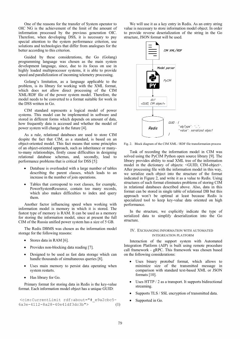
One of the reasons for the transfer of System operator to OIC NG is the achievement of the limit of the amount of information processed by the previous generation OIC. Therefore, when developing DSS, it is necessary to pay special attention to the system performance criterion, use solutions and technologies that differ from analogues for the better according to this criterion.

Guided by these considerations, the Go (Golang) programming language was chosen as the main system development language, since, due to its focus on use in highly loaded multiprocessor systems, it is able to provide speed and parallelization of incoming telemetry processing.

Golang’s limitation, as a language applicable to the problem, is its library for working with the XML format, which does not allow direct processing of the CIM XML/RDF file of the power system model. Therefore, the model needs to be converted to a format suitable for work in the DSS written in Go.

CIM standard represents a logical model of power systems. This model can be implemented in software and stored in different forms which depends on amount of data, how frequently data is accessed and whether the model of power system will change in the future [4].

As a rule, relational databases are used to store CIM despite the fact that CIM, as a standard, is based on an object-oriented model. This fact means that some principles of an object-oriented approach, such as inheritance or many-to-many relationships, firstly cause difficulties in designing relational database schemas, and, secondly, lead to performance problems that is critical for DSS [5]:

• Database is overloaded with a large number of tables describing the parent classes, which leads to an increase in the number of join operations.

• Tables that correspond to root classes, for example, PowerSystemResource, contain too many records, which also makes difficulties to index and query them.

Another factor influencing speed when working with information model is memory in which it is stored. The fastest type of memory is RAM. It can be used as a memory for storing the information model, since at present the full CIM of the Russia unified power system has a size of 5 GB.

The Redis DBMS was chosen as the information model storage for the following reasons:

• Stores data in RAM [6].

• Provides non-blocking data reading [7].

• Designed to be used as fast data storage which can handle thousands of simultaneous queries [8].

• Uses main memory to persist data operating when system restarts.

• Has library for Go.

Primary format for storing data in Redis is the key-value format. Each information model object has a unique GUID:

<cim:CurrentLimit rdf:about="#_e9a2cbc5-6a3e-4112-8a28-40e41df3dc3b"> (1)

We will use it as a key entry in Redis. As an entry string value is necessary to store information model object. In order to provide reverse deserialization of the string in the Go structure, JSON format will be used.

Fig. 2. Block diagram of the CIM XML / RDF file transformation process

Task of recording the information model in CIM was solved using the PyCIM Python open source library [9]. The library provides ability to read XML tree of the information model in the dictionary of objects: <GUID, CIM-object>. After processing file with the information model in this way, we serialize each object into the structure of the format indicated in Figure 2, and write it as a value to Redis. Using structures of such format eliminates problems of storing CIM in relational databases described above. Also, data in this format can be stored in single table of relational DB but this approach won’t be optimal at least because Redis is specialized tool to keep key-value data oriented on high performance.

In the structure, we explicitly indicate the type of serialized data to simplify deserialization into the Go structure.

IV. EXCHANGING INFORMATION WITH AUTOMATED INTEGREATION PLATFORM

Interaction of the support system with Automated Integration Platform (AIP) is built using remote procedure call framework - gRPC. This framework was chosen based on the following considerations:

• Uses binary protobuf format, which allows to minimize size of the transmitted message in comparison with standard text-based XML or JSON formats [10].

• Uses HTTP / 2 as a transport. It supports bidirectional streaming.

• Supports TLS / SSL encryption of transmitted data.

• Supported in Go.

79

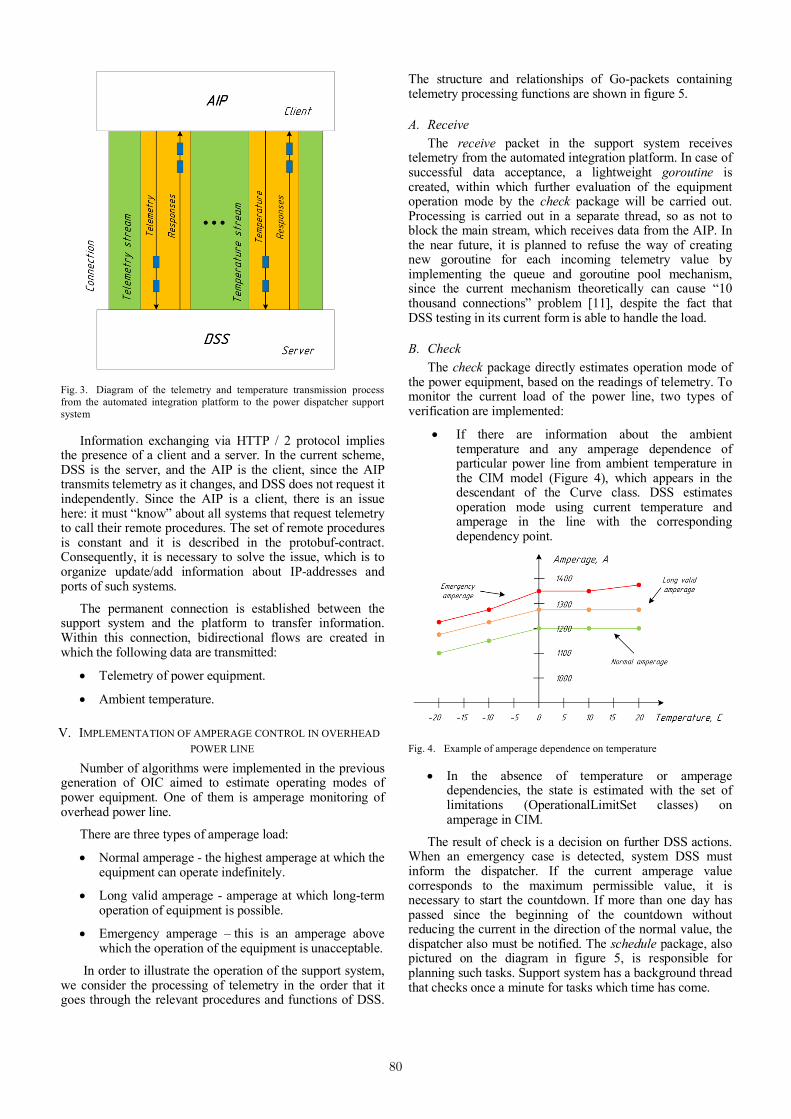
Fig. 3. Diagram of the telemetry and temperature transmission process from the automated integration platform to the power dispatcher support system

Information exchanging via HTTP / 2 protocol implies the presence of a client and a server. In the current scheme, DSS is the server, and the AIP is the client, since the AIP transmits telemetry as it changes, and DSS does not request it independently. Since the AIP is a client, there is an issue here: it must “know” about all systems that request telemetry to call their remote procedures. The set of remote procedures is constant and it is described in the protobuf-contract. Consequently, it is necessary to solve the issue, which is to organize update/add information about IP-addresses and ports of such systems.

The permanent connection is established between the support system and the platform to transfer information. Within this connection, bidirectional flows are created in which the following data are transmitted:

• Telemetry of power equipment.

• Ambient temperature.

V. IMPLEMENTATION OF AMPERAGE CONTROL IN OVERHEAD POWER LINE

Number of algorithms were implemented in the previous generation of OIC aimed to estimate operating modes of power equipment. One of them is amperage monitoring of overhead power line.

There are three types of amperage load:

• Normal amperage - the highest amperage at which the equipment can operate indefinitely.

• Long valid amperage - amperage at which long-term operation of equipment is possible.

• Emergency amperage – this is an amperage above which the operation of the equipment is unacceptable.

In order to illustrate the operation of the support system, we consider the processing of telemetry in the order that it goes through the relevant procedures and functions of DSS.

The structure and relationships of Go-packets containing telemetry processing functions are shown in figure 5.

A. Receive The receive packet in the support system receives

telemetry from the automated integration platform. In case of successful data acceptance, a lightweight goroutine is created, within which further evaluation of the equipment operation mode by the check package will be carried out. Processing is carried out in a separate thread, so as not to block the main stream, which receives data from the AIP. In the near future, it is planned to refuse the way of creating new goroutine for each incoming telemetry value by implementing the queue and goroutine pool mechanism, since the current mechanism theoretically can cause “10 thousand connections” problem [11], despite the fact that DSS testing in its current form is able to handle the load.

B. Check The check package directly estimates operation mode of

the power equipment, based on the readings of telemetry. To monitor the current load of the power line, two types of verification are implemented:

• If there are information about the ambient temperature and any amperage dependence of particular power line from ambient temperature in the CIM model (Figure 4), which appears in the descendant of the Curve class. DSS estimates operation mode using current temperature and amperage in the line with the corresponding dependency point.

Fig. 4. Example of amperage dependence on temperature

• In the absence of temperature or amperage dependencies, the state is estimated with the set of limitations (OperationalLimitSet classes) on amperage in CIM.

The result of check is a decision on further DSS actions. When an emergency case is detected, system DSS must inform the dispatcher. If the current amperage value corresponds to the maximum permissible value, it is necessary to start the countdown. If more than one day has passed since the beginning of the countdown without reducing the current in the direction of the normal value, the dispatcher also must be notified. The schedule package, also pictured on the diagram in figure 5, is responsible for planning such tasks. Support system has a background thread that checks once a minute for tasks which time has come.

80

C. Model Package model is the point of interaction with the CIM of

power system. When handling request from the outside, functions of the package perform a request to Redis, which stores in memory information model. Receiving a CIM object in JSON format, using the developed library, functions convert it into a Go structure and returns it as a result. In order to reduce the number of requests to Redis cache is introduced in the package storing frequently requested model objects.

D. Notify Package notify contains program code intended to

transmit the result of the check to the dispatcher.

Fig. 5. Package structure and connections of the power dispatcher support system

VI. INTEGRATION TESTING OF POWER DISPATCHER SUPPORT SYSTEM

In order to organize DSS testing process following set of tools was developed:

• Test version of Automated Integration Platform. It is a Golang-service with a set of test scenarios. A connection is established between the service and DSS, which allows to call remote DSS procedures for transmitting telemetry and the ambient temperature.

• Test version of power dispatcher’s software. It is also a Golang-service that communicates with DSS via gRPC. Through the connection, the support system transmits the results of telemetry processing. After receiving incoming message from DSS, Golang

service sends it to Centrifugo - a message server [12], which is connected via a websocket to a web page that simulates the dispatcher’s interface.

Fig. 6. Diagram of the test infrastructure of the dispatcher of the power system dispatcher

The DSS testing process is an imitation of the real mode of operation, during which the AIP transmits telemetry and temperature by calling the DSS remote procedures with the appropriate arguments. DSS receives data, processes it and, if necessary, sends a signal to the dispatcher, which is displayed in the interface.

VII. RESULTS Main result of solved task is a prototype of the power

dispatcher support system, designed to integrate into the OIC NG.

At the moment, monitoring of the equipment amperage and voltage at the control points of the power system is implemented in the DSS prototype. In near future, it is planned to implement control over flows and restrictions in sections.

Preparation work to move to OIC NG (DSS prototype is part of it) currently is carried out. It will operate with old generation OIC in parallel when work will be completed. Transition period can last for one year and more. Duration of transition period and its events are determined by System Operator’s clause «About commissioning and decommissioning of information management systems and

81

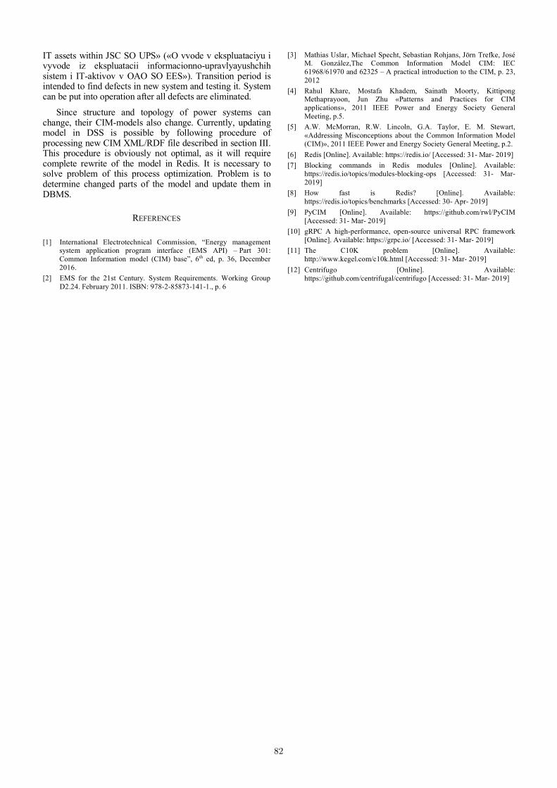
IT assets within JSC SO UPS» («O vvode v ekspluataciyu i vyvode iz ekspluatacii informacionno-upravlyayushchih sistem i IT-aktivov v OAO SO ЕES»). Transition period is intended to find defects in new system and testing it. System can be put into operation after all defects are eliminated.

Since structure and topology of power systems can change, their CIM-models also change. Currently, updating model in DSS is possible by following procedure of processing new CIM XML/RDF file described in section III. This procedure is obviously not optimal, as it will require complete rewrite of the model in Redis. It is necessary to solve problem of this process optimization. Problem is to determine changed parts of the model and update them in DBMS.

REFERENCES

[1] International Electrotechnical Commission, “Energy management system application program interface (EMS API) – Part 301: Common Information model (CIM) base”, 6th ed, p. 36, December 2016.

[2] EMS for the 21st Century. System Requirements. Working Group D2.24. February 2011. ISBN: 978-2-85873-141-1., p. 6

[3] Mathias Uslar, Michael Specht, Sebastian Rohjans, Jörn Trefke, José M. González,The Common Information Model CIM: IEC 61968/61970 and 62325 – A practical introduction to the CIM, p. 23, 2012

[4] Rahul Khare, Mostafa Khadem, Sainath Moorty, Kittipong Methaprayoon, Jun Zhu «Patterns and Practices for CIM applications», 2011 IEEE Power and Energy Society General Meeting, p.5.

[5] A.W. McMorran, R.W. Lincoln, G.A. Taylor, E. M. Stewart, «Addressing Misconceptions about the Common Information Model (CIM)», 2011 IEEE Power and Energy Society General Meeting, p.2.

[6] Redis [Online]. Available: https://redis.io/ [Accessed: 31- Mar- 2019] [7] Blocking commands in Redis modules [Online]. Available:

https://redis.io/topics/modules-blocking-ops [Accessed: 31- Mar- 2019]

[8] How fast is Redis? [Online]. Available: https://redis.io/topics/benchmarks [Accessed: 30- Apr- 2019]

[9] PyCIM [Online]. Available: https://github.com/rwl/PyCIM [Accessed: 31- Mar- 2019]

[10] gRPC A high-performance, open-source universal RPC framework [Online]. Available: https://grpc.io/ [Accessed: 31- Mar- 2019]

[11] The C10K problem [Online]. Available: http://www.kegel.com/c10k.html [Accessed: 31- Mar- 2019]

[12] Centrifugo [Online]. Available: https://github.com/centrifugal/centrifugo [Accessed: 31- Mar- 2019]

82

Applying High-Level Function Loop Invariants forMachine Code Deductive Verification

Pavel PutroSoftware Engineering Department

Ivannikov Institute for System Programming of the RASMoscow, Russia

pavel.putro@ispras.ru

Abstract—The existing tools of deductive verification allowus to successfully prove the correctness of functions written inhigh-level languages such as C or Java. However, this may notbe enough for critical software because even fully verified codecannot guarantee the correct generation of machine code by thecompiler. At the moment, developers of such systems have toaccept the compiler correctness assumption, which, however, isextremely undesirable, but inevitable due to the lack of full-fledged systems of formal verification of machine code. It isalso worth noting that the verification of machine code by aperson directly is an extremely time-consuming task due to thehigh complexity and large amounts of machine code. One ofthe approaches to simplify the verification of machine code isautomatic deductive verification reusing the formal specificationof the high-level language function. The formal specification of thefunction consists of the specification of the pre- and postcondition,as well as loop invariants, which specify conditions that aresatified at each iteration of the loop. When compiling a programinto machine code, pre- and postconditions are preserved, which,however, cannot be said about loop invariants. This fact is oneof the main problems of automatic verification of machine codewith loops. Another important problem is that high-level functionvariables often have projections’ to both registers and memory atthe machine code level, and the verification procedure requiresthat invariants be described for each variable, and therefore themissing invariants must be generated. This paper presents anapproach to solving these problems, based on the analysis ofthe control flow graph, and intelligent search of the locations ofvariables.

Index Terms—deductive verification, formal methods, machinecode

I. INTRODUCTION

In the 1960s Floyd [1] and Hoare [2] put forward theirtheories that the full correctness of the program code can beproved mathematically. The proposed methods are called de-ductive verification, but could not immediately gain popularitydue to the lack of automation, as well as low performanceand the high cost of hardware computing resources. However,in recent decades, these methods are experiencing a rebirthdue to the rapid development of methods for solving theSMT [3] problem, and growing performance of hardwaredevices. Technological leap in this area allowed to verify theapplication and system software by means of personal comput-ers. In this paper, the author adheres to the use of methods ofdeductive verification, because unlike other methods of formalverification, such as for example model checking, deductive

verification allows proving full correctness, but not only theabsence of a certain class of errors.

Increasing the availability of formal verification methodshas led to the fact that now formal verification is becominga standard in the creation of systems designed to work withsafety- and security-critical infrastructure. These systems areverified and tested carefully, but industrial verification toolswork only at source code level when testing can’t guaranteethat are no errors in the program. Here we can notice a securityhole when compilation of the correct code introduces errorsthat can’t be detected by the testing system. Without anywaysfor solving this problem developers have to make ”Theassumption of the correctness of the compiler”. According toa study [4] conducted in 2016, the total number of bugs foundin GCC+LLVM are more than 50000. This is one of the mainreasons why this assumption may not be sufficient for criticalsystems. There are only two ways that can allow developers toabandon this assumption: the first is to create a fully formallyverified compiler, and the second is to formally verify machinecode. There are some tries in recent 15 years that aimedto verify machine code or to create fully formally verifiedcompiler but there is still no generally accepted industrialsolution in machine code verification.

In this paper we consider an approach of deductive veri-fication of machine code obtained by compiling the sourcecode, the correctness of which has been proved by methods ofdeductive verification. The approach proposes to use a numberof techniques designed to reuse the function specification in ahigh-level language to prove the correctness of the compiledmachine code.

The process of deductive verification of machine code hasseveral serious differences from deductive verification of codein high-level languages. The first difference is that in machine-independent high-level programming languages, the set ofbasic operations amounts to several tens, and the size ofinstruction sets of modern processors amounts to hundredsand may even exceed a thousand different instructions. Inaddition, many of these instructions can have side effects,such as setting processor flags or storing the result in apredefined register. This variety of instructions does not allowto effectively generate state-change formulas during parsing ofmachine code and requires a definition of the processor modeland its instruction set. The second difference is that machine

83

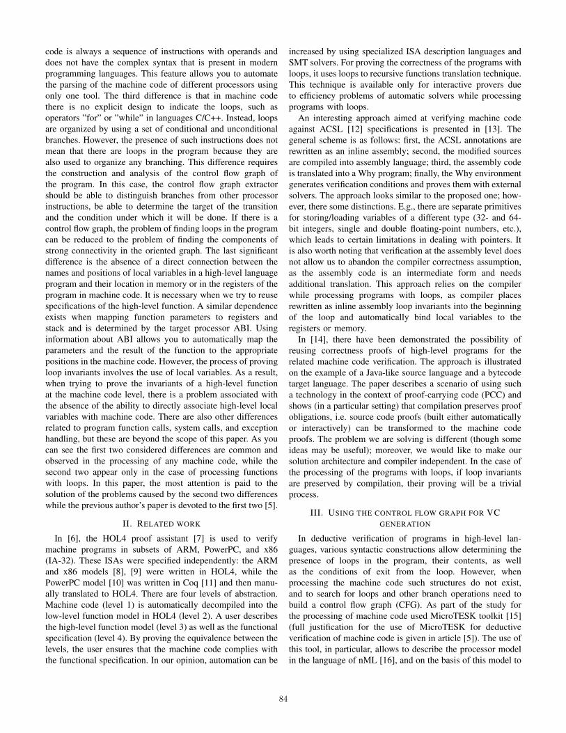
code is always a sequence of instructions with operands anddoes not have the complex syntax that is present in modernprogramming languages. This feature allows you to automatethe parsing of the machine code of different processors usingonly one tool. The third difference is that in machine codethere is no explicit design to indicate the loops, such asoperators ”for” or ”while” in languages C/C++. Instead, loopsare organized by using a set of conditional and unconditionalbranches. However, the presence of such instructions does notmean that there are loops in the program because they arealso used to organize any branching. This difference requiresthe construction and analysis of the control flow graph ofthe program. In this case, the control flow graph extractorshould be able to distinguish branches from other processorinstructions, be able to determine the target of the transitionand the condition under which it will be done. If there is acontrol flow graph, the problem of finding loops in the programcan be reduced to the problem of finding the components ofstrong connectivity in the oriented graph. The last significantdifference is the absence of a direct connection between thenames and positions of local variables in a high-level languageprogram and their location in memory or in the registers of theprogram in machine code. It is necessary when we try to reusespecifications of the high-level function. A similar dependenceexists when mapping function parameters to registers andstack and is determined by the target processor ABI. Usinginformation about ABI allows you to automatically map theparameters and the result of the function to the appropriatepositions in the machine code. However, the process of provingloop invariants involves the use of local variables. As a result,when trying to prove the invariants of a high-level functionat the machine code level, there is a problem associated withthe absence of the ability to directly associate high-level localvariables with machine code. There are also other differencesrelated to program function calls, system calls, and exceptionhandling, but these are beyond the scope of this paper. As youcan see the first two considered differences are common andobserved in the processing of any machine code, while thesecond two appear only in the case of processing functionswith loops. In this paper, the most attention is paid to thesolution of the problems caused by the second two differenceswhile the previous author’s paper is devoted to the first two [5].

II. RELATED WORK

In [6], the HOL4 proof assistant [7] is used to verifymachine programs in subsets of ARM, PowerPC, and x86(IA-32). These ISAs were specified independently: the ARMand x86 models [8], [9] were written in HOL4, while thePowerPC model [10] was written in Coq [11] and then manu-ally translated to HOL4. There are four levels of abstraction.Machine code (level 1) is automatically decompiled into thelow-level function model in HOL4 (level 2). A user describesthe high-level function model (level 3) as well as the functionalspecification (level 4). By proving the equivalence between thelevels, the user ensures that the machine code complies withthe functional specification. In our opinion, automation can be

increased by using specialized ISA description languages andSMT solvers. For proving the correctness of the programs withloops, it uses loops to recursive functions translation technique.This technique is available only for interactive provers dueto efficiency problems of automatic solvers while processingprograms with loops.

An interesting approach aimed at verifying machine codeagainst ACSL [12] specifications is presented in [13]. Thegeneral scheme is as follows: first, the ACSL annotations arerewritten as an inline assembly; second, the modified sourcesare compiled into assembly language; third, the assembly codeis translated into a Why program; finally, the Why environmentgenerates verification conditions and proves them with externalsolvers. The approach looks similar to the proposed one; how-ever, there some distinctions. E.g., there are separate primitivesfor storing/loading variables of a different type (32- and 64-bit integers, single and double floating-point numbers, etc.),which leads to certain limitations in dealing with pointers. Itis also worth noting that verification at the assembly level doesnot allow us to abandon the compiler correctness assumption,as the assembly code is an intermediate form and needsadditional translation. This approach relies on the compilerwhile processing programs with loops, as compiler placesrewritten as inline assembly loop invariants into the beginningof the loop and automatically bind local variables to theregisters or memory.

In [14], there have been demonstrated the possibility ofreusing correctness proofs of high-level programs for therelated machine code verification. The approach is illustratedon the example of a Java-like source language and a bytecodetarget language. The paper describes a scenario of using sucha technology in the context of proof-carrying code (PCC) andshows (in a particular setting) that compilation preserves proofobligations, i.e. source code proofs (built either automaticallyor interactively) can be transformed to the machine codeproofs. The problem we are solving is different (though someideas may be useful); moreover, we would like to make oursolution architecture and compiler independent. In the case ofthe processing of the programs with loops, if loop invariantsare preserved by compilation, their proving will be a trivialprocess.

III. USING THE CONTROL FLOW GRAPH FOR VCGENERATION

In deductive verification of programs in high-level lan-guages, various syntactic constructions allow determining thepresence of loops in the program, their contents, as wellas the conditions of exit from the loop. However, whenprocessing the machine code such structures do not exist,and to search for loops and other branch operations need tobuild a control flow graph (CFG). As part of the study forthe processing of machine code used MicroTESK toolkit [15](full justification for the use of MicroTESK for deductiveverification of machine code is given in article [5]). The use ofthis tool, in particular, allows to describe the processor modelin the language of nML [16], and on the basis of this model to

84

automatically analyze the binary code and build its behaviormodel in the logical language SMT-LIB [17]. In addition, CFGextractor has been added to this tool over the past year.

A. The format of the CFG

MicroTESK toolkit is able to determine whether the in-struction described in nML is a branch instruction, determinethe branch condition and the target address. In addition,MicroTESK has an advanced algorithm for calculating thetarget address of the transition, which allows it to calculateindirect targets, such as in a situation where the target addressis preloaded into the register and the branch is carried outalready on the register. Such capabilities in combination withthe use of nML processor models allow you to automaticallygenerate CFG for any processor modeled using nML. Thegenerated CFG is saved in JSON format [18], and has thefollowing format:

1) All basic blocks are placed in the list with the name”blocks”.

2) Each basic block has an index in the ” blocks” list andhas the following format:

a) The ”range” list that includes the sequence numberof the first and last instruction of the base block inthe context of the entire function being analyzed.Used for extraction of the SMT-LIB representationof the block from the SMT-LIB representation ofmachine code.

b) The ”asm” list that contains instructions of a basicblock in the assembler language of the targetprocessor.

c) The ”vars start” list, which contains the SMT-LIBversions of the main variables of the nML modelof the processor such as registers and memory, butnot temporary and auxiliary variables. Versions arespecified for the entry point of the basic block.

d) The ”vars end” list, contains values similar to thelist of ”vars start”, however, the version specifiedfor the exit point of the basic block.

e) The field ”condition” contains the branch condi-tion. The MicroTESK nML internal representationsyntax is used to write the condition. ”true” forunconditional branches and in the case when thereis no branch in the block.

f) The field ”condition smt” same as ”condition”,however, is recorded using SMT-LIB.

g) The field ”target taken” containing the index ofthe basic block in the ”blocks” list, which will bepassed to the control in the case when ”condition”is met. ”null” for blocks in which is the functionexit point.

h) Optional field ”target ntaken” containing the indexof the basic block in the ”blocks” list, whichwill be passed to the control in the case when”condition” is not met. Defined only for blockswith a conditional branch.

This structure of the graph contains all the necessary in-formation for generating verification conditions. Below is anexample of the extracted CFG for the function of calculatingthe sum of numbers from 0 to N (Table I).

"blocks": ["range": [0, 8],"vars_start": ["MEM!1","XREG!1"],"vars_end": ["MEM!37","XREG!15"],"asm": ["addi sp, sp, -48","sd s0, 40(sp)","addi s0, sp, 48","addi a5, a0, 0","sw a5, -36(s0)","sw zero, -20(s0)","addi a5, zero, 1","sw a5, -24(s0)","jal zero, 0x10"],"condition": "true","target_taken": 1,"range": [16, 20],"vars_start": ["MEM!53","XREG!27"],"vars_end": ["MEM!53","XREG!36"],"asm": ["lw a4, -24(s0)","lw a5, -36(s0)","addiw a4, a4, 0","addiw a5, a5, 0","bge a5, a4, -22"],"condition": "i1 sge i64 a5, a4","condition_smt": "op_20_instruction.operation.action.block_0!1","target_taken": 2,"target_ntaken": 3,"range": [9, 15],"vars_start": ["MEM!37","XREG!15"],"vars_end": ["MEM!53","XREG!27"],"asm": ["lw a4, -20(s0)","lw a5, -24(s0)","addw a5, a4, a5","sw a5, -20(s0)","lw a5, -24(s0)","addiw a5, a5, 1","sw a5, -24(s0)"],"condition": "true","target_taken": 1,"range": [21, 25],"vars_start": ["MEM!53","XREG!36"],"vars_end": ["MEM!53","XREG!45"],"asm": ["lw a5, -20(s0)","addi a0, a5, 0","ld s0, 40(sp)","addi sp, sp, 48","jalr zero, ra, 0"],"condition": "true","target_taken": null]

B. Joining basic blocks for verification conditions generation

The basic blocks themselves are not suitable targets forgenerating verification conditions (VC), as they may notcontain specific targets, but only state change formulas. There

85

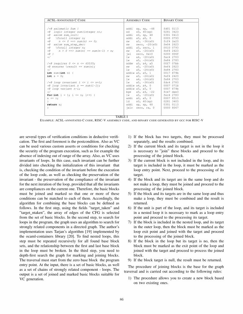
ACSL-ANNOTATED C CODE ASSEMBLY CODE BINARY CODE

/*@ axiomatic Sum

*@ logic integer sum(integer n);

*@ axiom sum_init:

*@ \forall integer n;

*@ n <= 0 ==> sum(n) == 0;

*@ axiom sum_step_dec:

*@ \forall integer n;

*@ n > 0 ==> sum(n) == sum(n-1) + n;

*@

*/

/*@ requires 0 <= n <= 65535;

*@ ensures \result == sum(n);

*/int sum(int n) int s = 0;

/*@ loop invariant l <= i <= n+1;

*@ loop invariant s == sum(i-1);

*@ loop variant n-i;

*/for(int i = 1; i <= n; i++) s += i;return s;

addi sp, sp, -48sd s0, 40(sp)addi s0, sp, 48addi a5, a0, 0sw a5, -36(s0)sw zero, -20(s0)addi a5, zero, 1sw a5, -24(s0)jal zero, 0x10lw a4, -20(s0)lw a5, -24(s0)addw a5, a4, a5sw a5, -20(s0)lw a5, -24(s0)addiw a5, a5, 1sw a5, -24(s0)lw a4, -24(s0)lw a5, -36(s0)addiw a4, a4, 0addiw a5, a5, 0bge a5, a4, -22lw a5, -20(s0)addi a0, a5, 0ld s0, 40(sp)addi sp, sp, 48jalr zero, ra, 0

fd01 01130281 34230301 04130005 0793fcf4 2e23fe04 26230010 0793fef4 24230200 006ffec4 2703fe84 278300f7 07bbfef4 2623fe84 27830017 879bfef4 2423fe84 2703fdc4 27830007 071b0007 879bfce7 dae3fec4 27830007 85130281 34030301 01130000 8067

TABLE IEXAMPLE: ACSL-ANNOTATED C CODE, RISC-V ASSEMBLY CODE, AND BINARY CODE GENERATED BY GCC FOR RISC-V

are several types of verification conditions in deductive verifi-cation. The first and foremost is the postcondition. Also as VCcan be used various custom asserts or conditions for checkingthe security of the program execution, such as for example theabsence of indexing out of range of the array. Also, as VC usesinvariants of loops. In this case, each invariant can be furtherdivided into checking the initialization of this invariant thatis, checking the condition of the invariant before the executionof the loop code, as well as checking the preservation of theinvariant - the preservation of the compliance of the invariantfor the next iteration of the loop, provided that all the invariantsare compliances on the current one. Therefore, the basic blocksmust be joined and marked so that one or more of theseconditions can be matched to each of them. Accordingly, thealgorithm for combining the base blocks can be defined asfollows. In the first step, using the fields ”target taken” and”target ntaken”, the array of edges of the CFG is selectedfrom the set of basic blocks. In the second step, to search forloops in the program, the graph uses an algorithm to search forstrongly related components in a directed graph. The author’simplementation uses Tarjan’s algorithm [19] implemented bythe ocaml-containers library [20]. To find nested loops, thisstep must be repeated recursively for all found base blocksets, and the relationship between the first and last base blockin the loop must be broken. In the third step, you need todepth-first search the graph for marking and joining blocks.The traversal must start from the zero base block the programentry point. At the input, there is a set of basic blocks, as wellas a set of chains of strongly related component - loops. Theoutput is a set of joined and marked basic blocks suitable forVC generation.

1) If the block has two targets, they must be processedseparately, and the results combined.

2) If the current block and its target is not in the loop itis necessary to ”join” these blocks and proceed to theprocessing of the joined block.

3) If the current block is not included in the loop, and itstarget is included in the loop, it must be marked as theloop entry point. Next, proceed to the processing of itstarget.

4) If the block and its target are in the same loop and donot make a loop, they must be joined and proceed to theprocessing of the joined block.

5) If the block and its targets are in the same loop and thusmake a loop, they must be combined and the result isreturned.

6) If the unit is part of the loop, and its target is includedin a nested loop it is necessary to mark as a loop entrypoint and proceed to the processing its target.

7) If the block is included in the nested loop, and its targetin the outer loop, then the block must be marked as theloop exit point and joined with the target and proceedto the processing of the joined block.

8) If the block in the loop but its target is no, then theblock must be marked as the exit point of the loop andjoined with the target and proceed to process the joinedblock.

9) If the block target is null, the result must be returned.

The procedure of joining blocks is the base for the graphtraversal and is carried out according to the following rules:

1) The procedure allows you to create a new block basedon two existing ones.

86

2) Joining is possible if the target (”target taken” or ”tar-get ntaken”) of the first block is the second block. Inall other cases, the result of the join is not determined.

3) The targets of the joined block will be the targets of thesecond block.

4) Condition (”condition smt”) of the joined block will bethe condition of the second block.

5) If the second block is a loop exit point, the initial state”vars start” of the combined block will be the initialstate of the second block, otherwise the initial state ofthe first block.

6) If at least one of the joining blocks is marked as theloop exit point, the joined block must also be markedas the loop exit point.

7) If the second block is marked as the loop entry point,the result should be marked as the loop entry point.

8) If the second block ”closes” the loop, i.e. its target isthe first block, its SMT-LIB representation should bechanged so that all elements of the final state ”vars end”of the second block should get new unique names.Any other conflicts between any variables in SMT-LIBrepresentations of the joining blocks must be resolvedin the same way.

9) SMT-LIB the representation of the joined block must beobtained by concatenating the SMT-LIB representationsof the merged blocks. In this case, if the condition”condition” of the first block is not empty (”true”), itmust be added as SMT-LIB assert to the representationcode of the joined block. Also, if the join follows the”target ntaken” branch, the condition must be inverted.Also, if the blocks do not follow each other in theprogram, the final state of the first block also needs tobe associated with the initial state of the second blockat the level of the SMT-LIB representation.

As a result of following this algorithm, in most cases, youcan create a set of code blocks on which you can directlyprove various verification conditions. The algorithm allowsprocessing machine code with loops, nested loops, sequentialloops, as well as code generated by the presence of the brakeand continue statements in the program, but is not able tocope with tasks when, for example, several entries to oneloop and other non-trivial situations caused by the use oftransition instructions are detected in the control flow graph.However, such situations cause difficulties already at the stageof verification of the source code, and the construction of analgorithm that allows you to automatically deductively verifyany machine code is an unsolvable task.

If we apply the algorithm to the CFG function of the sumof the numbers presented above, we will be able to allocatethree blocks to prove VC. The first block will have index 0,have loop entry status and be used to prove the correctnessof the initialization of the loop invariants. The second blockwill be a join of blocks 1 and 2 and will be used to prove thepreservation of loop invariants. The third block will be a joinof blocks 1 and 3 and will be used to prove the postcondition

provided the invariants are correct.

IV. AUTOMATIC BINDING OF HIGH- AND LOW-LEVELLOCAL VARIABLES

In general, to describe loop invariants, high-level functionsuse local variable names that are not available when workingwith machine code. In general, information about binding localvariables to specific positions on the stack or registers is notavailable. Of course, you can require the user to manuallyprovide this data and even give examples where such require-ments will have a positive impact on system performance.However, in most cases, manual mapping of local variablesto their positions will be a bottleneck in the performanceof the verification system, as well as reduce the degree ofautomation. From the above, we can conclude that the systemshould automatically determine the location of local variables,and the possibility of their manual input should be optional.To determine the positions of local variables, the author hasdeveloped an algorithm for efficient search of positions in theVC generation, which includes the following steps:

1) All potential positions of local variables are calculated.This can be done both by means of machine codeanalysis (similar to those used by modern disassemblersand debuggers) and with the help of an existing logicalmodel of machine code and SMT-solver. The authorproposes to use the second option because it is a moreuniversal approach. In this approach, for each memorywrite instruction it is required to prove by solver thatthere are no positions on the stack that could change asa result of the operation. If solver managed to generatea counterexample, the position found is a potentialposition for the local variable. This algorithm allowsyou to find positions for local variables, but it can bedifficult if there is an array on the stack. In this case, ifsolver fails to determine which position of the array wasrecorded, the result may not be determined and the userwill have to specify the position himself. Similarly, youcan calculate the registers to which the local variablecan be mapped.

2) Each local variable is assigned a potential positions set,which may depend on its size in bytes.

3) For each invariant from the list of invariants for theproof, the ”cost” of proving its correct initializationshould be calculated. Here, the cost is the number ofall possible combinations of potential positions of localvariables involved in the description of this invariant.Here it is necessary to take into account that eachvariable has its own unique memory location, there-fore, combinations of potential positions should consistonly of unique values. It is also worth noting thatthis step should be carried out only when proving theinitialization of the invariants, since the initialization ofthe invariant is proved independently of the other loopinvariants, and the proof of preserving the loop invariantmust be proved given that all other invariants must besatisfied. Thus, when proving the correct initialization of

87

the invariant, it is possible to reduce the number of localvariables necessary for binding, and, as a consequence,the ”cost” of the proof may differ for different invariants.If it is necessary to prove the loop invariant preservationthe cost of all invariants should be considered equal to.

4) For the least cost invariant, it is necessary to try to provecorrectness for each possible combinations of potentialpositions of local variables on which the invariant de-pends. The results (”unsat”/”unknown”/”sat” verdicts)should be saved in a separate list.

5) If there was no one verdict is ”unsat”, it is necessaryto mark the invariant unproven. If at least one verdict”unsat” has been obtained, then the invariant should beconsidered proved and the potential positions of localvariables on which the proved invariant depends shouldbe filtered, leaving only those positions that consistin combinations of potential positions for which theinvariant has been proved (the ”unsat” verdict).

6) Remove the proved invariant from the list of invariantsfor the proof and (if there are still invariants in the list)proceed to step 3.

Using this algorithm, it is possible in some cases to signif-icantly reduce the number of generated targets relative to acomplete search. As an example, let’s take a function with 3different local variables with values s = −1, i = 0, n = 90 atthe loop entry point and three potential positions on the stack:sp−0x10, sp−0x18, sp−0x24, respectively. For simplicity,the size of variables and positions will be considered equal to4 bytes. Initially, the correspondence between the positionsof local variables is not known. Based on these data, wetry to prove the initialization of the following invariants:”0 <= i < 100”, ”s == 2 ∗ i − 1” and ”s < n + i”.According to the algorithm, we calculate the cost of provingthe invariants, which will be equal to 3, 6 and 6, respectively.Next, try to prove the correctness of the first invariant with thecost of 3 and will find two potential positions (sp− 0x18 andsp − 0x24) for the variable i (we will also be able to provethe invariant for variable n). Second, we perform filteringto remove the position of the sp − 0x10 for the variable i.Recalculate the costs of the remaining invariants: the result of4 and 4 (the cause of reducing the cost is reducing the numberof potential positions for the variable i, on which the invariantsdepend). When proving the correctness of the initialization ofthe second invariant, only one set of potential positions for thevariables s and i is sp − 0x10 and sp − 0x18, respectively,will be selected. We filter and proceed to the proof of thelast invariant. It is possible to select only one target for itthe position for n will be selected by the elimination method.We prove the invariant, perform filtering and get the samecorrespondence between variables and their positions on thestack, which was set by the compiler.

V. EVALUATION

At the time of writing, the approach proposed by theauthor was partially implemented in the system of deductiveverification of machine code [5]. Using this approach, the

machine code of the function of the sum of numbers from0 to N (Table I), as well as some other functions with loops,was successfully verified. For each generated VC, a verdictwas obtained confirming its correctness. In addition, the po-sitions of local variables on the function stack were strictlydetermined by the computer during the verification process.More complex testing is planned after the full implementationof the approach.

VI. CONCLUSION

Verification of functions with loops is one of the mainstumbling blocks in the verification of machine code. Variousresearch groups have proposed various solutions that howeverimpose serious limitations, such as the need to use interactiveproof assistants or the introduction of dependency on the targetcompiler. However, due to the high complexity of the machinecode structure, the use of interactive proof assistants cansignificantly slow down the verification process and requirevery experienced staff. Dependency on the target compileralso reduces the universality of the approach and requires itsintegration into the source code compilation process, whichcan cause some difficulties. In contrast to these works, theauthor proposes to use a compiler-independent approach basedon the use of automatic SMT-solvers. To implement theapproach, we propose to use two main algorithms, as well asa tool for CFG extraction. The first algorithm allows the basicblocks of the function CFG to be joined in such a way thatthey become suitable for VC proving. The second algorithmallows restoring the lost links between the local variables ofthe high-level function and their positions in memory or onthe processor registers at the machine code level. Using thisapproach allows in most cases to generate such VC, which willbe sufficient for deductive verification of the machine code ofthe function with loops.

The work is in progress. At the moment, the approachhas been partially implemented in the system of deductiveverification of machine code. Its full implementation andtesting is the nearest direction for further work. Also amongthe possible areas for further research can be identified thestudy of problems arising in the proof of the correctness offunctions containing calls to other functions or system calls.There is a separate issue with the security check of the machinecode execution, i.e. the absence of exceptions at the processorlevel, incorrect memory readings or stack overflows. Alsoof great importance is the study of the applicability of themachine code deductive verification system for solving realindustrial problems.

REFERENCES

[1] R.W. Floyd. Assigning Meanings to Programs. Mathematical Aspects ofComputer Science. Proceedings of Symposia in Applied Mathematics,19, 1967. P. 19-32. DOI: 10.1090/psapm/019/0235771.

[2] C.A.R. Hoare. An Axiomatic Basis for Computer Programming.Communications of the ACM, 12(10), 1969. P. 576-585.DOI: 10.1145/363235.363259.

[3] C Barrett, R Sebastiani, S Seshia, and C Tinelli. Satisfiability ModuloTheories. Handbook of Satisfiability, vol. 185 of Frontiers in ArtificialIntelligence and Applications, (A Biere, M J H Heule, H van Maaren,and T Walsh, eds.), IOS Press, Feb. 2009, pp. 825885.

88

[4] C. Sun, V. Le, Q. Zhang, Z. Su Toward understanding compiler bugs ingcc and llvm. ISSTA 2016, pp. 294-305.

[5] Putro P.A. Combining ACSL Specifications and Machine Code. TrudyISP RAN/Proc. ISP RAS, vol. 30, issue 4, 2018. pp. 95-106. DOI:10.15514/ISPRAS-2018-30(4)-6

[6] M.O. Myreen. Formal Verification of Machine-Code Programs. Ph.D.Thesis. University of Cambridge, 2009. 131 p.

[7] K. Slind, M. Norrish. A Brief Overview of HOL4. Theorem Proving inHigher Order Logics (TPHOLs). Lecture Notes in Computer Science(LNCS), 5170, 2008. P. 28-32. DOI: 10.1007/978-3-540-71067-7 6.

[8] A. Fox. Formal Specification and Verification of ARM6. TheoremProving in Higher Order Logics (TPHOLs). Lecture Notes in ComputerScience (LNCS), 2758, 2003. P. 25-40. DOI: 10.1007/10930755 2.

[9] K. Crary, S. Sarkar. Foundational Certified Code in a MetalogicalFramework. Technical Report CMU-CS-03-108. Carnegie Mellon Uni-versity, 2003. 19 p.

[10] X. Leroy. Formal Certification of a Compiler Back-End or: Program-ming a Compiler with a Proof Assistant. Principles of ProgrammingLanguages (POPL), 2006. P. 42-54, DOI: 10.1145/1111037.1111042.

[11] Y. Bertot. A Short Presentation of Coq. Theorem Proving in HigherOrder Logics (TPHOLs). Lecture Notes in Computer Science, 5170,2008. P. 12-16. DOI: 10.1007/978-3-540-71067-7 3.

[12] P. Baudin, P. Cuoq, J.-C. Filliatre, C. Marche, B. Monate, Y. Moy,V. Prevosto. ACSL: ANSI/ISO C Specification Language. Version 1.13,2018. 114 p.

[13] T.M.T. Nguyen, C. Marche. Hardware-Dependent Proofs of NumericalPrograms. Certified Programs and Proofs (CPP), 2011. Lecture Notesin Computer Science 7086. P. 314-329. DOI: 10.1007/978-3-642-25379-9 23.

[14] G. Barthe, T. Rezk, A. Saabas. Proof Obligations Preserving Compila-tion. Formal Aspects in Security and Trust (FAST), 2005. Lecture Notesin Computer Science 3866. P. 112-126. DOI: 10.1007/11679219 9.

[15] MicroTESK Framework – http://www.microtesk.org[16] M. Freericks. The nML Machine Description Formalism. Technical

Report TR SM-IMP/DIST/08, TU Berlin CS Department, 1993. 47 p.[17] C. Barrett, P. Fontaine, C. Tinelli. The SMT-LIB Standard Version 2.6.

Release 2017-07-18. 104 p.[18] JavaScript Object Notation – https://www.json.org/[19] R. E. Tarjan, Dep-first search and linear graph algorithms SIAM J.

Comput., vol. 1, no. 2, pp. 146-160, June 1972.[20] ocaml-containers library – https://github.com/c-cube/ocaml-containers

89

Extracting Assertions for Conflicts in HDL

Descriptions

Alexander Kamkin1, 2, 3, 4, Mikhail Lebedev1, Sergey Smolov1 1Ivannikov Institute for System Programming of the Russian Academy of Sciences

2Lomonosov Moscow State University 3Moscow Institute for Physics and Technology

4National Research University Higher School of Economics

E-mail: kamkin, lebedev, smolov@ispras.ru

Abstract—Data access conflicts may arise in hardware

designs. We propose a static analysis based approach to data

conflicts extraction from HDL descriptions. Conflicts are

formulated as conditions on variables. Bounded model checking

is used to check whether these conditions are reachable. If true,

counterexamples are generated and then translated to HDL

testbenches. The proposed approach was applied to several open

source HDL benchmarks.

Keywords—hardware design; hardware description language;

functional verification; static analysis; test generation; data access

conflict; guarded action; model checking.

I. INTRODUCTION

Modern hardware designs contain multiple modules and

processes operating on the common set of internal variables.

In this case conflicts, i.e. illegal accesses from different

processes to the same data, may appear. Requirements on how

to operate with modules and avoid conflicts in a

communication protocol can be described both in formal

(machine-readable) and informal (human-readable) ways. In this paper a formal verification based approach to

conflict extraction is proposed. The idea is to analyze an HDL description aimed at finding data access conflicts [1]. Both the conflicts and the target description are then automatically translated into the input format of a model checking tool. The tool generates counterexamples for the feasible conflicts.

II. RELATED WORK

In [1] several categories of data conflicts are described:

read after write (RAW), write after read (WAR) and write

after write (WAW). The HOL verification system [2] was

used to check a RISC processor’s pipeline. The formal

specification of pipeline was implemented manually that is

hard to be done for modern processors because of their

complexity. In [3], a GoldMine methodology is presented for automatic

generation of hardware assertions. The method uses a combination of data mining and static analysis techniques. First, the HDL design is simulated to generate data about the design's dynamic behavior. Then, the generated data are mined for “candidate assertions” that are likely to be invariants. The data mining technique used is a decision-tree-based supervised

learning algorithm. The candidate assertions are then passed through the Cadence Incisive Formal Verifier [4] tool to filter out the spurious candidates. The disadvantages of GoldMine are: 1) usage of commercial tool; 2) invariants’ incompleteness because of random simulation usage at an early stage.

III. ASSERTION EXTRACTION METHOD

We propose a new approach to data access conflicts

extraction in HDL descriptions. Our goal is to detect conflicts

and provide proofs that they may happen. The method is

aimed at conflicts of the following types:

1) read-write (RW): on the same clock tick one process

writes the variable and the other process reads it;

2) write-write (WW): on the same clock tick at least two

processes write the same variable;

3) write-read-write (WRW): we assume that a variable

should be read between two writes;

4) undefined (UNDEF): variable is read before it was

written.

The method consists of the following steps: 1) Control

Flow Graph (CFG) extraction; 2) transformation to Guarded

Actions Decision Diagram (GADD); 3) process invariants and

conflict assertions extraction; 4) invariants and assertions

translation into an input format of a model checking tool; 5)

counterexample generation. All method steps are made

automatically. The CFG representation is built for every

process of the HDL model using an abstract syntax tree

traversal compiler-like approach [5]. From the structural view,

CFG is a directed graph. Nodes of the graph contain HDL

operators; edges of the graph mean control flows. On the left

side of Fig. 1 the fragment of Verilog code is shown; the

related CFG is shown on the right side. Branch operators are

shown as diamond nodes and called as 𝐶𝑖. Basic block

operators are shown as rectangles and called as 𝐵𝑖 . Graph

edges contain the values that the branch conditions should be

equal to for edges to be passed. CFG is supposed to be acyclic:

HDL loops with constant numbers of iteration are unrolled

into sequences of operators.

90

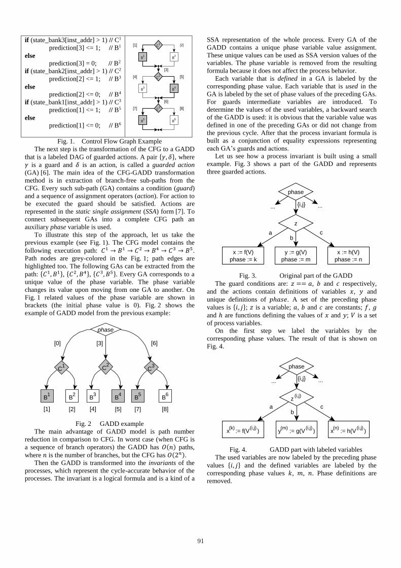
if (state_bank3[inst_addr] > 1) // C1

prediction[3] <= 1; // B1

else prediction[3] = 0; // B2

if (state_bank2[inst_addr] > 1) // C2

prediction[2] <= 1; // B3

else prediction[2] <= 0; // B4

if (state_bank1[inst_addr] > 1) // C3

prediction[1] <= 1; // B5

else prediction[1] <= 0; // B6

Fig. 1. Control Flow Graph Example

The next step is the transformation of the CFG to a GADD

that is a labeled DAG of guarded actions. A pair 𝛾, 𝛿, where

𝛾 is a guard and 𝛿 is an action, is called a guarded action

(GA) [6]. The main idea of the CFG-GADD transformation

method is in extraction of branch-free sub-paths from the

CFG. Every such sub-path (GA) contains a condition (guard)

and a sequence of assignment operators (action). For action to

be executed the guard should be satisfied. Actions are

represented in the static single assignment (SSA) form [7]. To

connect subsequent GAs into a complete CFG path an

auxiliary phase variable is used.

To illustrate this step of the approach, let us take the

previous example (see Fig. 1). The CFG model contains the

following execution path: 𝐶1 → 𝐵1 → 𝐶2 → 𝐵4 → 𝐶3 → 𝐵5.

Path nodes are grey-colored in the Fig. 1; path edges are

highlighted too. The following GAs can be extracted from the

path: 𝐶1, 𝐵1, 𝐶2, 𝐵4, 𝐶3, 𝐵5. Every GA corresponds to a

unique value of the phase variable. The phase variable

changes its value upon moving from one GA to another. On

Fig. 1 related values of the phase variable are shown in

brackets (the initial phase value is 0). Fig. 2 shows the

example of GADD model from the previous example:

Fig. 2 GADD example

The main advantage of GADD model is path number

reduction in comparison to CFG. In worst case (when CFG is

a sequence of branch operators) the GADD has 𝑂(𝑛) paths,

where 𝑛 is the number of branches, but the CFG has 𝑂(2𝑛).

Then the GADD is transformed into the invariants of the

processes, which represent the cycle-accurate behavior of the

processes. The invariant is a logical formula and is a kind of a

SSA representation of the whole process. Every GA of the

GADD contains a unique phase variable value assignment.

These unique values can be used as SSA version values of the

variables. The phase variable is removed from the resulting

formula because it does not affect the process behavior.

Each variable that is defined in a GA is labeled by the

corresponding phase value. Each variable that is used in the

GA is labeled by the set of phase values of the preceding GAs.

For guards intermediate variables are introduced. To

determine the values of the used variables, a backward search

of the GADD is used: it is obvious that the variable value was

defined in one of the preceding GAs or did not change from

the previous cycle. After that the process invariant formula is

built as a conjunction of equality expressions representing

each GA’s guards and actions.

Let us see how a process invariant is built using a small

example. Fig. 3 shows a part of the GADD and represents

three guarded actions.

Fig. 3. Original part of the GADD

The guard conditions are: 𝑧 == 𝑎, 𝑏 and 𝑐 respectively,

and the actions contain definitions of variables 𝑥, 𝑦 and

unique definitions of 𝑝ℎ𝑎𝑠𝑒. A set of the preceding phase

values is 𝑖, 𝑗; 𝑧 is a variable; 𝑎, 𝑏 and 𝑐 are constants; 𝑓, 𝑔

and ℎ are functions defining the values of 𝑥 and 𝑦; 𝑉 is a set

of process variables.

On the first step we label the variables by the

corresponding phase values. The result of that is shown on

Fig. 4.

Fig. 4. GADD part with labeled variables

The used variables are now labeled by the preceding phase

values 𝑖, 𝑗 and the defined variables are labeled by the

corresponding phase values 𝑘, 𝑚, 𝑛. Phase definitions are

removed.

B1

B2

B3

B4

B5

C1

C2

C3

[1] [2]

[3]

[5][4]

[6]

[7]

B6

[8]

phase

C1 C

2C

3

B1

B2

B5

B6

B3

B4

[0] [3] [6]

[1] [2] [7][4] [5] [8]

phase

x := f(V)

phase := k

y := g(V)

phase := m

x := h(V)

phase := n

... ...

z

i,j

ab

c

phase

x(k)

:= f(V (i,j)

) y(m)

:= g(V (i,j)

) x(n)

:= h(V (i,j)

)

... ...

z (i,j)

i,j

ab

c

91

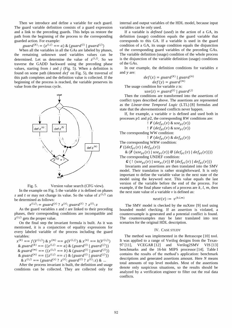
Then we introduce and define a variable for each guard.

The guard variable definition consists of a guard expression

and a link to the preceding guards. This helps us restore the

path from the beginning of the process to the corresponding

guarded action. For example:

𝑔𝑢𝑎𝑟𝑑(𝑘): = (𝑧(𝑖,𝑗) == 𝑎) & (𝑔𝑢𝑎𝑟𝑑(𝑖) | 𝑔𝑢𝑎𝑟𝑑(𝑗)) When all the variables in all the GAs are labeled by phases,

the remaining unknown used variables values can be

determined. Let us determine the value of 𝑧(𝑖,𝑗). So we

traverse the GADD backward using the preceding phase

values, starting from 𝑖 and 𝑗 (Fig. 5). When a definition is

found on some path (denoted 𝑑𝑒𝑓 on Fig. 5), the traversal of

this path completes and the definition value is collected. If the

beginning of the process is reached, the variable preserves its

value from the previous cycle.

Fig. 5. Version value search (CFG view).

In the example on Fig. 5 the variable 𝑧 is defined on phases

𝑠 and 𝑡 or may not change its value. So the value of 𝑧(𝑖,𝑗) can

be determined as follows:

𝑧(𝑖,𝑗): = 𝑔𝑢𝑎𝑟𝑑(𝑠) ? 𝑧(𝑠): 𝑔𝑢𝑎𝑟𝑑(𝑡) ? 𝑧(𝑡): 𝑧 As the guard variables s and t are linked to their preceding

phases, their corresponding conditions are incompatible and

𝑧(𝑖,𝑗) gets the proper value.

On the final step the invariant formula is built. As it was

mentioned, it is a conjunction of equality expressions for

every labeled variable of the process including the guard

variables:

𝑥(𝑘) == 𝑓(𝑉(𝑖,𝑗)) & 𝑦(𝑚) == 𝑔(𝑉(𝑖,𝑗)) & 𝑥(𝑛) == ℎ(𝑉(𝑖,𝑗)) & 𝑔𝑢𝑎𝑟𝑑(𝑘) == ((𝑧(𝑖,𝑗) == 𝑎) & (𝑔𝑢𝑎𝑟𝑑(𝑖) | 𝑔𝑢𝑎𝑟𝑑(𝑗))) & 𝑔𝑢𝑎𝑟𝑑(𝑚) == ((𝑧(𝑖,𝑗) == 𝑏) & (𝑔𝑢𝑎𝑟𝑑(𝑖) | 𝑔𝑢𝑎𝑟𝑑(𝑗))) & 𝑔𝑢𝑎𝑟𝑑(𝑛) == ((𝑧(𝑖,𝑗) == 𝑐) & (𝑔𝑢𝑎𝑟𝑑(𝑖) | 𝑔𝑢𝑎𝑟𝑑(𝑗)))

& 𝑧(𝑖,𝑗) == (𝑔𝑢𝑎𝑟𝑑(𝑠) ? 𝑧(𝑠): 𝑔𝑢𝑎𝑟𝑑(𝑡) ? 𝑧(𝑡): 𝑧) & … After the process invariant is built, the definition and usage

conditions can be collected. They are collected only for

internal and output variables of the HDL model, because input

variables can be only used.

If a variable is defined (used) in the action of a GA, its

definition (usage) condition equals the guard variable that

corresponds to this GA. If a variable is used in the guard

condition of a GA, its usage condition equals the disjunction

of the corresponding guard variables of the preceding GAs.

The variable definition (usage) condition of the whole process

is the disjunction of the variable definition (usage) conditions

of the GAs.

In our example, the definition conditions for variables 𝑥

and 𝑦 are:

𝑑𝑒𝑓(𝑥) = 𝑔𝑢𝑎𝑟𝑑(𝑘) | 𝑔𝑢𝑎𝑟𝑑(𝑛)

𝑑𝑒𝑓(𝑦) = 𝑔𝑢𝑎𝑟𝑑(𝑚)

The usage condition for variable z is:

𝑢𝑠𝑒(𝑧) = 𝑔𝑢𝑎𝑟𝑑(𝑖) | 𝑔𝑢𝑎𝑟𝑑(𝑗) Then the conditions are transformed into the assertions of

conflict types described above. The assertions are represented

as the Linear-time Temporal Logic (LTL) [8] formulas and

state that the abovementioned conflicts never happen.

If, for example, a variable 𝑣 is defined and used both in

processes 𝑝1 and 𝑝2, the corresponding RW conditions are:

! 𝑭 (𝑑𝑒𝑓𝑝1(𝑣) & 𝑢𝑠𝑒𝑝2(𝑣))

! 𝑭 (𝑑𝑒𝑓𝑝2(𝑣) & 𝑢𝑠𝑒𝑝1(𝑣))

The corresponding WW condition:

! 𝑭 (𝑑𝑒𝑓𝑝1(𝑣) & 𝑑𝑒𝑓𝑝2(𝑣))

The corresponding WRW condition:

𝑭 ((𝑑𝑒𝑓𝑝1(𝑣) | 𝑑𝑒𝑓𝑝2(𝑣))

& (𝑭 (𝑢𝑠𝑒𝑝2(𝑣) | 𝑢𝑠𝑒𝑝1(𝑣)) 𝑼 (𝑑𝑒𝑓𝑝1(𝑣) | 𝑑𝑒𝑓𝑝2(𝑣))))

The corresponding UNDEF condition:

𝑮 ( ! (𝑢𝑠𝑒𝑝2(𝑣) | 𝑢𝑠𝑒𝑝1(𝑣)) 𝑼 (𝑑𝑒𝑓𝑝1(𝑣) | 𝑑𝑒𝑓𝑝2(𝑣))) Invariants and assertions are then translated into the SMV

model. Their translation is rather straightforward. It is only important to define the variable value in the next state of the model using the keyword next. This value equals the last version of the variable before the end of the process. For example, if the final phase values of a process are 𝑘, 𝑙, 𝑚, then the next state value of a variable v is defined as:

𝑛𝑒𝑥𝑡(𝑣) ∶= 𝑣(𝑘,𝑙,𝑚)

The SMV model is checked by the nuXmv [9] tool using bounded model checking. If an assertion is violated, a counterexample is generated and a potential conflict is found. The counterexamples may be later translated into test scenarios for the original HDL description.

IV. CASE STUDY

The method was implemented in the Retrascope [10] tool.

It was applied to a range of Verilog designs from the Texas-

97 [11], VCEGAR [12] and Verilog2SMV VIS [13]

benchmarks and the 16-bit MIPS processor [14]. Table I

contains the results of the method’s application: benchmark

descriptions and generated assertions amount. Here N means

total amounts of top level modules. Most of the assertions

denote only suspicious situations, so the results should be

analyzed by a verification engineer to filter out the real data

conflicts.

92

TABLE I. Benchmark descriptions and potential conflicts.

Bench N LOC Assertions

RW WW WRW UNDEF

Texas’97 17/58 69539 408 26 211 211

VCEGAR 20/34 15144 315 25 167 167

Verilog2SMV 12/20 4494 78 0 62 62

mips16 5/12 1007 10 0 9 9

Example of a RW situation, which is not a conflict

(mips16/ID_stage.v):

module ID_stage

…

wire [2:0] ir_dest_with_bubble;

wire [2:0] write_back_dest;

assign ir_dest_with_bubble = ( instruction_decode_en ) ?

ir_dest : 0;

assign write_back_dest = ir_dest_with_bubble;

Signal ir_dest_with_bubble is defined in one process and is

used in the other process at the same time.

Example of a WW situation, which seems to be a real

conflict (Texas97/MPEG/prefixcode.v):

module start_code_prefix(start,done…);

…

reg monitor;

… always @(posedge read_signal) begin

monitor=start;

…

end always if( start==0) begin

…

monitor=0;

end

Variable monitor is defined simultaneously, if read_signal

rises and at the same time start equals 0.

Example of an UNDEF situation, which is also not a

conflict (mips16/ID_stage.v):

module ID_stage

…

reg [15:0] instruction_reg;

…

always @(posedge clk or posedge rst) begin

if (rst) begin

instruction_reg <= 0;

end

else begin

if (instruction_decode_en) begin

instruction_reg <= instruction;

end

end

end

assign ir_op_code = instruction_reg[15:12];

Register instruction_reg is undefined from the start of

simulation until the clk or rst rising edge.

V. CONCLUSION AND FUTURE WORK

In this paper the approach to data access conflicts

extraction from HDL descriptions has been proposed. We

extract assertions from the source code and automatically

translate them into the input format of the model checker. The

tool generates counterexamples that are proofs of conflicts’

reachability. We have implemented the approach in the

Retrascope toolkit and applied it to several open source HDL

benchmarks. One direction for future research is to propagate assertions

from internal variables’ to interface variables. Such assertions can be used to improve protocols of unknown third-party modules or even to reconstruct protocols. Another direction is the generation of checkers, i.e. HDL wrappers for target modules that check their behavior through simulation.

REFERENCES

[1] S. Tahar, R. Kumar. “Formal Verification of Pipeline Conflicts in RISC Processors”, Proceedings of the European Design Automation Conference (EURO-DAC), 1994, pp. 285-289.

[2] M. Gordon, T. Melham. “Introduction to HOL: A Theorem Proving Environment for Higher Order Logic”, Cambridge University Press, 1993, 492 p.

[3] S. Hertz, D. Sheridan, S. Vasudevan, “Mining Hardware Assertions With Guidance From Static Analysis”, IEEE Transactions on Computer-Aided Design of Integrated Circuits and Systems, Vol. 32, No. 6, 2013, pp. 952-965.

[4] Cadence Incisive Formal Verifier. https://community.cadence.com//CSSharedFiles/forums/storage/22/10078/IncisiveFV_ds.pdf

[5] A. V. Aho, R. Sethi, J. D. Ullman, “Compilers: principles, techniques, and tools”, 1986, 796 p.

[6] J. Brandt, M. Gemunde, K. Schneider, S. Shukla, and J.-P. Talpin, “Integrating system descriptions by clocked guarded actions”, Proceedings of Forum on Design Languages (FDL), 2011, pp. 1-8.

[7] R. Cytron, J. Ferrante, B.K. Rosen, M.N. Wegman, F.K. Zadeck, “Efficiently computing static single assignment form and the control dependence graph”, ACM Transactions on Programming Languages and Systems, 1991, pp. 451-490.

[8] A. Pnueli, “The temporal logic of programs”, 18th Annual Symposium on Foundations of Computer Science, 1977, vol. 00, pp. 46-57.

[9] nuXmv model checker. https://nuxmv.fbk.eu

[10] Retrascope toolkit. https://forge.ispras.ru/projects/retrascope

[11] Texas-97 Verification Benchmarks. https://ptolemy.berkeley.edu/projects/embedded/research/vis/texas-97

[12] VCEGAR benchmark collection. https://www.cprover.org/hardware

[13] Verilog2SMV tool. https://es-static.fbk.eu/tools/verilog2smv

[14] Educational 16-bit MIPS Processor. https://opencores.org/projects/mips_16

93

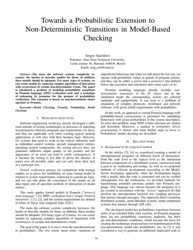
Towards a Probabilistic Extension toNon-Deterministic Transitions in Model-Based

Checking

Sergey StaroletovPolzunov Altai State Technical University,Lenin avenue 46, Barnaul, 656038, Russia

Email: serg soft@mail.ru

Abstract—The more the software systems complexity in-creases, the harder to describe models for them; in addition,these models should be adequate. For many types of systems, wecan create models by replacing complex algorithms of interactionwith occurrences of certain non-deterministic events. The paperis considered a problem of modeling probabilistic transitionsin Promela language (SPIN verification tool) and a techniqueof enhancing its grammar for the purpose of probabilisticverification. The extension is based on non-deterministic choiceoperator in Promela.

Keywords—Model Checking, Promela, Probabilistic ModelChecking

I. RESEARCH OBJECTIVES

Software engineering world has already developed a suffi-cient amount of testing technologies as processes of searchinginconsistencies between programs and requirements for them,and they are applicable well when creating typical desktopapplications or web sites with their business logic. However,for systems that need to work in the critical industries suchas embedded control systems, aircraft management entities,operating system components, the testing process does notguarantee sufficient output quality of the product and theappearance of an error can lead to costly consequences. Itis because the testing is not able to prove the absence oferrors over all possible states and can only show their lackat a particular test.

Formal verification process (in comparison with testing)enables us to prove the infallibility of some formal model inrelation to system requirements, expressed in a predicate logic,and we can talk about the correctness of the model on alldata inputs and all specified methods of interaction of modelentities.

This study applies formal models in Promela (”protocolmeta-language”) for SPIN verification tool (”simple Promelainterpreter”) [1], [2], and the system requirements are definedin terms of linear time temporal logic (LTL).

The more the software systems complexity increases, theharder to describe models for them; in addition, these modelsshould be adequate. For many types of systems, we can createmodels by replacing complex algorithms of interaction withoccurrences of certain non-deterministic events.

The goal of the paper is to move from the non-determinismto probabilities. The two words mean some variations of

unpredicted behaviour, but when we talk about the last one, weoperate with probability values as guards of program actions,and they can be either a priori and a posteriori (pre-definedbefore the execution and calculated after some cases of it).

Promela modeling language already includes non-deterministic transitions in the IF clause, but in thesimulation mode the corresponding actions are selectedrandomly and equiprobably. It can lead to a problem ofsimulation of complex protocols, distributed and networksoftware, with given initial requirements with probabilities.

In this work, an approach to extend Promela language withprobability-based constructions is presented for simulatingbehaviours with given probabilities in the system description.To solve this problem, some SPIN verifier internals are studiedand described. Moreover, a method to probability drivenprogramming is shown, and some further steps to move toProbabilistic model checking are described.

II. RELATED WORK

A. Background of the proposed method

In the articles [3], [4] we considered creating a model ofinteroperational programs on different levels of abstraction:from the code level to the logical level as the interactionbetween components of a distributed system, constructed witha goal to its verification and testing. As well as we proposedmethods of software development (according to the Model-driven developing approach), when the development beginswith a model, then the code is generated and can be verifiedsubsequently. For the verification, we provided methods fortransforming extended automata models into Promela lan-guage. This language was chosen because the programs in itare created in accordance with the ”Actors” approach [5] thatinvolves the interoperation between low coupling processesthat interact through messages. This approach allows modelingdistributed systems, multi-threaded systems, multi-componentsystems that interact through API calls.

The developed model has probabilistic transitions betweenstates of an extended finite state machine. In Promela languagethere are not probabilistic transitions explicitly, but thereare non-deterministic conditions, which became the basis forcreating the technology proposed here for transformation of thenon-deterministic model into probabilistic one. In [3] it wasconsidered a way to generate an additional duplicated code to

94

satisfy a given guard probability in the simulation mode, butit is a very naive approach.

B. Probabilistic model checking

According to [6], the Probabilistic model checking problemis stated as follows:Given a property φ, the Problem consists of checking whethera stochastic system satisfies φ with a probability greater thanor equal to a certain threshold θ.

Herein we consider to LTL properties φ. For an example tounderstand the problem, refer to the Roundabout Maneuver [7]– is a behavior of two aircraft to make Collision Avoidance,and it is a subject to cooperation in air traffic control. Theavoidance of collision is achieved by an agreement on somecommon angular velocity ωxy and common centre cxy aroundwhich both can fly by the circle safely without coming closeto each other not more than Rsafe [7]. There is the followingprecondition to the entry procedure of the Maneuver and thesafe property to verify:

isSafe ::= (x1 − y1)2 + (x2 − y2)2 6 R2safe (1)

where x = (x1, x2) is a first planar position, y = (y1, y2) is asecond planar position.

Model checking approach can be applied to this problem byspecifying an LTL property (for example, in SPIN notation):

[ ] (isSafe == 1) (2)

where ”[]” is the ”Globaly” LTL operator and 1 is an aliasfor true. Statement (2) in natural language means ”during theexecution in all the states of the program model, the rule (1)will be preserved as true”.

When we move to the Probabilistic model checking, wecan specify a PLTL property as

[ ] θ>90% (isSafe == 1) (3)

and here we like to verify that the system satisfies the safeproperty with probability of 90% or higher (that means thesystem will be safe in 90% cases for some reasons when itstart working from an initial state and finish in a final state;or: in 10% cases or less two aircraft can be closer than Rsafe).

C. Probabilistic languages and models to verify

In the work [8] the Probabilistic model checking problemwas faced and an approach was presented to ensure that agiven labeled Markov chain satisfies a given LTL property witha given probability. In [9] the approach is extended to verifythese things effectively using an LTL-BDD representation offormulas.

The authors of the publications [10], [11] state thatMarkovs’ models cannot be useful at the system descriptionlevel since they are not able to describe parallel processes.So, to evaluate aspects such as the probability of systemfailure they construct Discrete Time Markov Chain (DTMC)models from the composition of the Probabilistic Component

Automata (PCA) representations of each component and thenanalyse them in tools such as PRISM [12].

In the work [13] the SMC (Statistical model checking)approach has been introduced, and the tool Uppaal [14] hasbeen extended to check system properties using an extendedautomaton model. The tool offers probabilistic simulation andverification by specifying in the user interface probabilitydistributions that drive the timed behaviors, and the engineoffers computing an estimate of probabilities and comparisonbetween estimated probabilities without actually computingthem.

In the book [16] the author decided to implement classesin Scala language to allow developers to make complexprobabilistic and statistical programs.

In the paper [17] the authors decided to implement fromscratch a language similar to Promela with some probabilisticadditions to satisfy the probabilistic model checking goals.They used SOS-rules in the Plotkin style [15] to describe thelanguage formally. For example, this language offers to writecode with PIF (probability IF clause):

PIF [p1]⇒ P1...[pn]⇒ Pn FIP (4)

That means: probabilities p1..pn lead the code P1..Pn toexecute. In the current paper, we are going to follow thisapproach, but without creating a ”yet another” language anda new tool, because now Promela language and SPIN toolare well-designed and community-approved, and new languagecreation instead of extension of an existing one should be welljustified. Of course, it is possible to declare some inductiverules for a theorem prover for making the evidence of particularproblems like it is done in [18], but extending a modelinglanguage to some conventional structures and rules can involveadditional engineers to the formal proof process of software.

D. How to create non-deterministic transitions in Promela

It is known that the programs in Promela are modeled in theform of instructions in a special language, which at the sametime looks like C and also like functional languages such asErlang (it refers to ”Actors” approach). The language containsconditions in the form

i f: : b o o l e a n e x p r e s s i o n 1 −> a c t i o n s 1: : b o o l e a n e x p r e s s i o n 2 −> a c t i o n s 2

: : b o o l e a n e x p r e s s i o n N −> a c t i o n s Nf i

It is considered that in order to perform a certain action, it isnecessary that the corresponding logical expression was true.However, if multiple logical expressions are true in the sameif construction, it is considered that the next step is one of thenon-deterministic choices of them. Refer to the code snippetin Promela, modeling the Leader Selection algorithm (Dolev,Klawe & Rodeh [19]):

i f /∗ non−d e t e r m i n i s t i c c h o i c e ∗ /: : I n i [ 0 ] == 0 && N >= 1 −> I n i [ 0 ] = I: : I n i [ 1 ] == 0 && N >= 2 −> I n i [ 1 ] = I: : I n i [ 2 ] == 0 && N >= 3 −> I n i [ 2 ] = I

95

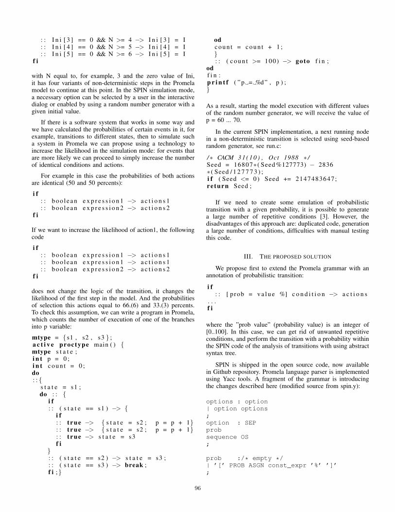
: : I n i [ 3 ] == 0 && N >= 4 −> I n i [ 3 ] = I: : I n i [ 4 ] == 0 && N >= 5 −> I n i [ 4 ] = I: : I n i [ 5 ] == 0 && N >= 6 −> I n i [ 5 ] = I

f i

with N equal to, for example, 3 and the zero value of Ini,it has four variants of non-deterministic steps in the Promelamodel to continue at this point. In the SPIN simulation mode,a necessary option can be selected by a user in the interactivedialog or enabled by using a random number generator with agiven initial value.

If there is a software system that works in some way andwe have calculated the probabilities of certain events in it, forexample, transitions to different states, then to simulate sucha system in Promela we can propose using a technology toincrease the likelihood in the simulation mode: for events thatare more likely we can proceed to simply increase the numberof identical conditions and actions.

For example in this case the probabilities of both actionsare identical (50 and 50 percents):

i f: : b o o l e a n e x p r e s s i o n 1 −> a c t i o n s 1: : b o o l e a n e x p r e s s i o n 2 −> a c t i o n s 2

f i

If we want to increase the likelihood of action1, the followingcode

i f: : b o o l e a n e x p r e s s i o n 1 −> a c t i o n s 1: : b o o l e a n e x p r e s s i o n 1 −> a c t i o n s 1: : b o o l e a n e x p r e s s i o n 2 −> a c t i o n s 2

f i

does not change the logic of the transition, it changes thelikelihood of the first step in the model. And the probabilitiesof selection this actions equal to 66.(6) and 33.(3) percents.To check this assumption, we can write a program in Promela,which counts the number of execution of one of the branchesinto p variable:

mtype = s1 , s2 , s3 ;a c t i v e proctype main ( ) mtype s t a t e ;i n t p = 0 ;i n t c o u n t = 0 ;do: :

s t a t e = s1 ;do : :

i f: : ( s t a t e == s1 ) −>

i f: : t rue −> s t a t e = s2 ; p = p + 1: : t rue −> s t a t e = s2 ; p = p + 1: : t rue −> s t a t e = s3f i

: : ( s t a t e == s2 ) −> s t a t e = s3 ;: : ( s t a t e == s3 ) −> break ;f i ;

odc o u n t = c o u n t + 1 ;: : ( c o u n t >= 100) −> goto f i n ;

odf i n :p r i n t f ( ” p = %d ” , p ) ;

As a result, starting the model execution with different valuesof the random number generator, we will receive the value ofp = 60 ... 70.

In the current SPIN implementation, a next running nodein a non-deterministic transition is selected using seed-basedrandom generator, see run.c:

/∗ CACM 3 1 ( 1 0 ) , Oct 1988 ∗ /Seed = 16807∗ ( Seed %127773) − 2836∗ ( Seed / 1 2 7 7 7 3 ) ;i f ( Seed <= 0) Seed += 2147483647;re turn Seed ;

If we need to create some emulation of probabilistictransition with a given probability, it is possible to generatea large number of repetitive conditions [3]. However, thedisadvantages of this approach are: duplicated code, generationa large number of conditions, difficulties with manual testingthis code.

III. THE PROPOSED SOLUTION

We propose first to extend the Promela grammar with anannotation of probabilistic transition:

i f: : [ p rob = v a l u e %] c o n d i t i o n −> a c t i o n s

. . .f i

where the ”prob value” (probability value) is an integer of[0..100]. In this case, we can get rid of unwanted repetitiveconditions, and perform the transition with a probability withinthe SPIN code of the analysis of transitions with using abstractsyntax tree.

SPIN is shipped in the open source code, now availablein Github repository. Promela language parser is implementedusing Yacc tools. A fragment of the grammar is introducingthe changes described here (modified source from spin.y):

options : option| option options;option : SEPprobsequence OS;

prob :/* empty */| ’[’ PROB ASGN const_expr ’%’ ’]’;

96

where prob – is the new grammar rule for probability transi-tion, SEP is the ”::” terminal, PROB – is the new terminal sym-bol ”prob”, ASGN is the assignment (”=”) and const expr isPromela’s non-terminal (grammar rule) for constant expressionthat is calculated at the parsing time. This grammar extensioncan now allow the previous code snippet as well as usualPromela constructions.

Further, we propose to extend this idea, putting the prob-ability of not only as a constant number but the value ofa variable. In this case, the probability may dynamically berecalculated during program execution on Promela. So, thefollowing Promela grammar addition is presented:

prob :/* empty */| ’[’ PROB ASGN const_expr ’%’ ’]’| ’[’ PROB ASGN expr ’]’;

where expr – is a grammar rule for the Promela expression.

Thus we will be able, for example, simulate and verifyvarious training and recognition algorithms. A new probabilityvalue will be received from a different process, changed incode based on a given probabilistic transition or other differentcases. So, with simple grammar additions and some changingto semantic of SPIN code, we can speak of ”Probability drivenprogramming” in Promela.

To continue this idea, we can propose some ”syntacticsugar” for probabilistic actions with Promela channels. Tosimulate some networking protocols it is required to specifya loss/reliability value for a channel, that means: with agiven probability a channel lose/guarantee some messages andprotocols should correctly handle this. Our new additions forthe channels in the grammar:

one_decl: vis TYPE chan_loss osubt var_list...;chan_loss : /* empty */| ’[’ LOSS ASGN const_expr ’%’ ’]’| ’[’ RELY ASGN const_expr ’%’ ’]’;Special : varref RCV

rargs| varref SND msg_loss

margs;msg_loss : /* empty */| ’[’ LOSS ASGN const_expr ’%’ ’]’| ’[’ RELY ASGN const_expr ’%’ ’]’| ’[’ RELY ASGN expr ’]’| ’[’ LOSS ASGN expr ’]’;

where chan loss is the new grammar rule to define channels,msg loss – is the new rule to annotate the message sendPromela operator (SND terminal); LOSS – is our terminalsymbol ’loss’ (to specify channel loss values after it) andRELY – is our terminal symbol ’rely’ (to specify channelreliability values after it).

So, after the modifications, the extended Promela grammarshould accept the following test code with the new annotations:

mtype = s1 , s2 , s3 ;i n t c o u n t = 0 ;/∗ now d e f i n e a normal chan ∗ /chan a = [ 1 ] of s h o r t ;/∗ now d e f i n e a chan w i t h 30% l o s s v a l u e ∗ /chan [ l o s s = 30%] b = [ 1 ] of s h o r t ;/∗ now d e f i n e a chan w i t h 70% r e l yv a l u e ( or 30% l o s s ) ∗ /chan [ r e l y = 70%] c = [ 1 ] of s h o r t ;

i n t pp = 7 0 ;

a c t i v e proctype main ( ) mtype s t a t e = s1 ;c o u n t = pp − 1 0 ;/∗ send t o a normal chan ∗ /a ! 1/∗ send t o a 30% l o s s chan ∗ /b ! c o u n t ;/∗ send t o a chan w i t h re−d e f i n e d 10%l o s s ∗ /c ! [ l o s s = 10%] 3 ;/∗ send t o a chan w i t h 70% r e l i a b i l i t y ∗ /c ! 2 ;/∗ send t o a chan w i t h re−d e f i n e d 99%r e l i a b i l i t y ∗ /c ! [ r e l y = 99%] 4 ;/∗ send t o a chan w i t h re−d e f i n e d l o s sw i t h c o u n t v a l u e ∗ /b ! [ l o s s = c o u n t ] 1 ;i f

: : t rue −> s t a t e = s2 ;/∗ 10% prob t r a n s i t i o n ∗ /: : [ p rob = 10%] t rue −> s t a t e = s3 ;/∗ dynamic prob t r a n s i t i o n ∗ /: : [ p rob = pp ] t rue −> s t a t e = s3 ;/∗ f o r t h e o t h e r s prob w i l l be ∗ /

c a l c u l a t e d as 100% − a l ls p e c i f i e d p r o b s ∗ /

: : t rue −> s t a t e = s2 ;: : t rue −> s t a t e = s3 ;

f ip r i n t f ( ” s t a t e = %d ” , s t a t e ) ;

IV. STATUS AND PERSPECTIVES OF THE SOLUTION

Currently, we implemented the extension to the grammarwith a goal to extend the semantics and understanding ofthe SPIN internal logic. The advanced program simulation inPromela as well as verification code generation are in progress.Adding probabilities to the transitions and channels with losseswill allow SPIN users to model some complex interactions andprobabilistic algorithms. We are making some additions oninternal nodes (at the parsing time), and some – on dynamicvalues calculation after SPIN processes are scheduled.

With regard to verification, making the addition to Promelawith transitions for a given value of probability should allowus to use probabilities in the system requirements as LTL

97

predicates, after which it would be possible to prove thestatements of the forms ”if the transition probability is given,it satisfied the requirement ...”, ”if a requirement is satisfied,then the probability is ...”; moreover, it is possible to show acounterexample as a sequence of states that can be performedtoo frequently or too infrequently.

Of course, it is easy to implement our approach withprobabilities as given constants in the code - however, muchmore interesting is to represent the implementation of proba-bility values, given by the variables in run time. We wouldlike to experiment with it after doing some programmingstuff with SPIN sources, and we are going to compare theresulting approach with existing probabilistic model checkingapproaches which have been mentioned in the paper.

The advantage of this approach is an attempt to solve prob-lems of Probabilistic model checking by using such existingcommunity-approved verification and simulation instrumentwith relatively little efforts of its improvements; this approachalso allows verification engineers to extend the class of veri-fiable systems with the SPIN verifier.

REFERENCES

[1] Holzmann, Gerard J. ”The model checker SPIN.” IEEE Transactions onsoftware engineering 23.5 (1997): 279-295.

[2] Spin - Formal Verification. http://spinroot.com[3] S. Staroletov. Model of a program as multi-threaded stochastic automaton

and its equivalent transformation to Promela model. Ershov informaticsconference. PSI Series, 8th edition. International workshop on ProgramUnderstanding. Proceedings.At: Novosibirsk, Russia. 2011

[4] S. Staroletov. Model Driven Developing & Model Based Check-ing: Applying Together / Tools & Methods of Program Analy-sis TMPA-2014:Kostroma, 2014. - pp. 215-220. ISBN 975-5-8285-0719-1. Presentation: http://www.slideshare.net/IosifItkin/model-driven-developingmodelbasedchecking

[5] Hewitt, Carl, Peter Bishop, and Richard Steiger. ”Session 8 formalismsfor artificial intelligence a universal modular actor formalism for artifi-cial intelligence.” Advance Papers of the Conference. Vol. 3. StanfordResearch Institute, 1973.

[6] Clarke, Edmund, Alexandre Donz, and Axel Legay. ”On simulation-based probabilistic model checking of mixed-analog circuits.” FormalMethods in System Design 36.2 (2010): 97-113.

[7] Platzer, Andre, ”Differential dynamic logic for hybrid systems”, Journalof Automated Reasoning, vol. 41, no. 2, pp. 143-189, 2008

[8] Courcoubetis, Costas, and Mihalis Yannakakis. ”The complexity ofprobabilistic verification.” Journal of the ACM (JACM) 42.4 (1995): 857-907.

[9] J. Eliosoff. Calculating the probability of an LTL formula over a labeledMarkov chain. McGill University, Montreal, 2003

[10] Rodrigues, Pedro, Emil Lupu, and Jeff Kramer. ”LTSA-PCA: Toolsupport for compositional reliability analysis.” Companion Proceedingsof the 36th International Conference on Software Engineering. ACM,2014.

[11] Lupu, E. C., P. Rodrigues, and Jeff Kramer. ”Compositional reliabilityanalysis for probabilistic component automata.”

[12] M. Kwiatkowska, G. Norman, and D. Parker, ”PRISM 4.0: Verificationof probabilistic real-time systems,” in CAV11, ser. LNCS, G. Gopalakr-ishnan and S. Qadeer, Eds., vol. 6806. Springer, pp. 585591.

[13] Sen, Koushik, Mahesh Viswanathan, and Gul Agha. ”Statistical modelchecking of black-box probabilistic systems.” International Conferenceon Computer Aided Verification. Springer, Berlin, Heidelberg, 2004.

[14] David, Alexandre, et al. ”Uppaal SMC tutorial.” International Journalon Software Tools for Technology Transfer 17.4 (2015): 397-415.

[15] G. D. Plotkin. A structural approach to operational semantics. TechnicalReport DAIMI FN-19, Computer Science Department, Aarhus Univer-sity, 1981.

[16] Pfeffer, Avi. Practical probabilistic programming. Manning PublicationsCo., 2016.

[17] Baier, Christel, Frank Ciesinski, and M. Grosser. ”PROBMELA: a mod-eling language for communicating probabilistic processes.” Proceedings.Second ACM and IEEE International Conference on Formal Methodsand Models for Co-Design, 2004. MEMOCODE’04.. IEEE, 2004.

[18] Shishkin, Evgeniy. ”Construction and formal verification of a fault-tolerant distributed mutual exclusion algorithm.” Proceedings of the 16thACM SIGPLAN International Workshop on Erlang. ACM, 2017.

[19] Dolev, Danny, Maria Klawe, and Michael Rodeh. ”An O (n log n)unidirectional distributed algorithm for extrema finding in a circle.”Journal of Algorithms 3.3 (1982): 245-260.

[20] Hahn, Ernst Moritz, et al. ”PARAM: A model checker for parametricMarkov models.” International Conference on Computer Aided Verifica-tion. Springer, Berlin, Heidelberg, 2010.

98

The editor for teaching the proof of statementsfor sets

Vadim Rublev1 and Vladislav Bondarenko2

1 Department of Theoretical Computer Science, Demidov Yaroslavl State University,Yaroslavl, 150000, Russia,

roublev@mail.ru,ORCID 0000-0002-0252- 9958

2 Department of Theoretical Computer Science, Demidov Yaroslavl State University,Yaroslavl, 150000, Russia,bondarencko40@gmail.com

Abstract. One of the problems of developing a computer system forteaching proof of statements for sets is the development of software thatallows a student to independently conduct step-by-step proving, startingfrom determining initial premise and targeted statement, and which atthe same time controls at each step of proof the correctness of determin-ing the premises of elementary conclusion of step and The correctness ofthe text entered by the conclusion of the step. We called this software theEditor for learning to prove assertions for sets. Namely, the solution ofthe problems of extracting an elementary step of proof, syntactic controlof the input text and logical control of the correctness of the conclusionwere the main ones in the development of the Editor. It is intended todevelop an automated learning system (ALS) "Elements of set theory",the purpose of which will be to teach algebra of sets and the ability tocarry out evidence with the help of the Editor.

Keywords: computer training, proving statements for sets, editor forteaching the proof, step by step proof, control of step correctness

1 Introduction

At present, the problems of teaching the bulk of students in mathematical andcomputer Sciences are associated with underdevelopment of thinking caused bythe low quality of school education. A significant mass of school graduates donot know how to read (understand what they read), do not know how to reason,because they were not taught enough. These problems can be solved only byindividual training, but this approach requires a huge additional time from theteacher, exceeding several times the hours allocated by the curriculum. There-fore, it suggests a solution in the development of computer automated learningsystems (ALS), with which you can not only control the knowledge, but to con-duct training. Basically, many computer systems control the testing of studentmemory, and therefore can teach some definitions, but not their use. A similar

99

2 Vadim Rublev, Vladislav Bondarenko

solution Stepik has a disadvantage in that the choice of the correct answer isalways the only one (which allows you to guess, but not know), and the solu-tion is not controlled by the system step by step, which does not give reasonto consider it even testing knowledge. ALS for the exact Sciences should teachdata analysis, formalization, analysis, reasoning and transformation. The use ofcomputer algebra [1][2] underlies the construction of such systems. For example,one of the authors of this paper used this to construct ALS of computationalcomplexity of algorithms [3].

In this paper, models of computer-based learning to prove statements for setsare considered. These models can be divided into 2 groups: proof-of-statementmodels for sets and training models that prepare a student for the first groupmodels. The models of the first group are described in the proof of statementseditor for sets and the study of models of the second group related to the trainingof using models of the first group is supposed to be.

2 The problem of constructing a proof editor ofstatements for sets

To solve the problem specified in the headline, select the following task sequence:

1. Limitations on the type of statements for sets for whose prove you need tobuild an editor.

2. Equivalent transformation of the sets included in the statement.3. Splitting the basic statement into an equivalent set of simple statements.4. The choice of the method of proving a simple statement and the selection of

an initial set of premises in it.5. Definition of the elementary step of the proof.6. Control of the correctness proof by the editor.

2.1 Statement type constraints for sets

In the general case of the statement we will consider some universal set U andits subsets X1, X2, . . . , Xn. The statement uses formulas for these subsets, con-structed with operations complement, intersection, union, and brackets, chang-ing the order of these operations, if necessary.

We restrict ourselves to statements for sets of the following form

< Сonstriction of the set relation > → | ↔ < Сonstriction of the set relation >

So in example (1)

X1 ∩X2 ∪X3 = (X2 ∪X3) ∩X1 ↔ X1 ∩X2 ∩X3 = ∅ ∧ X2 ⊆ X1 ∪X3 (1)

it is argued that the equality of two sets given by expressions takes place if andonly if the intersection of the subsets is empty and the second subset is includedin the union of the other two.

100

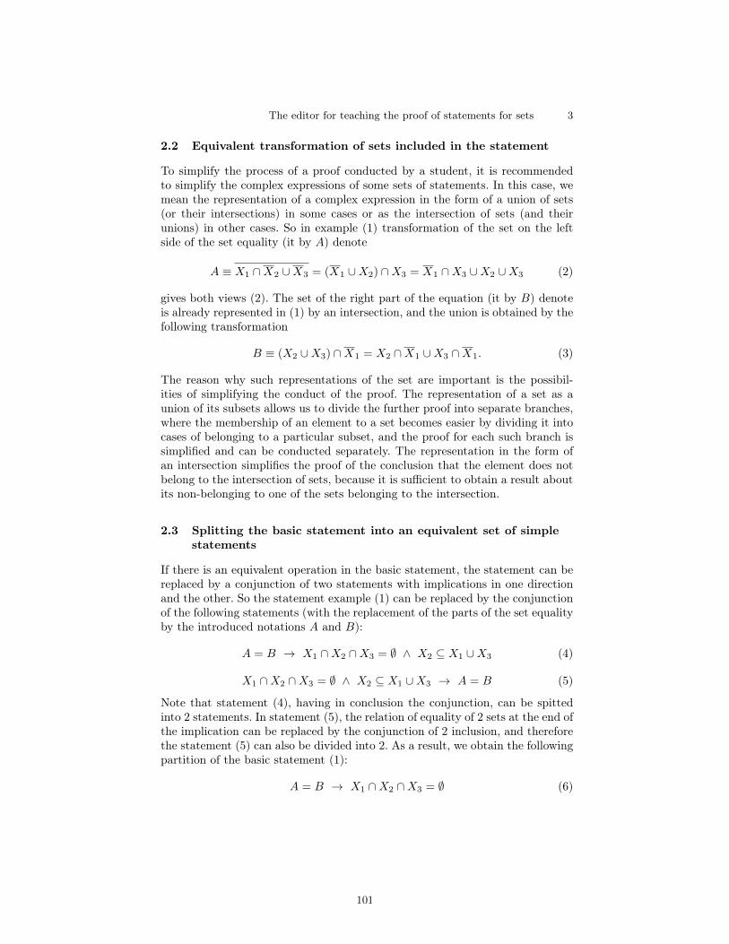
The editor for teaching the proof of statements for sets 3

2.2 Equivalent transformation of sets included in the statement

To simplify the process of a proof conducted by a student, it is recommendedto simplify the complex expressions of some sets of statements. In this case, wemean the representation of a complex expression in the form of a union of sets(or their intersections) in some cases or as the intersection of sets (and theirunions) in other cases. So in example (1) transformation of the set on the leftside of the set equality (it by A) denote

A ≡ X1 ∩X2 ∪X3 = (X1 ∪X2) ∩X3 = X1 ∩X3 ∪X2 ∪X3 (2)

gives both views (2). The set of the right part of the equation (it by B) denoteis already represented in (1) by an intersection, and the union is obtained by thefollowing transformation

B ≡ (X2 ∪X3) ∩X1 = X2 ∩X1 ∪X3 ∩X1. (3)

The reason why such representations of the set are important is the possibil-ities of simplifying the conduct of the proof. The representation of a set as aunion of its subsets allows us to divide the further proof into separate branches,where the membership of an element to a set becomes easier by dividing it intocases of belonging to a particular subset, and the proof for each such branch issimplified and can be conducted separately. The representation in the form ofan intersection simplifies the proof of the conclusion that the element does notbelong to the intersection of sets, because it is sufficient to obtain a result aboutits non-belonging to one of the sets belonging to the intersection.

2.3 Splitting the basic statement into an equivalent set of simplestatements

If there is an equivalent operation in the basic statement, the statement can bereplaced by a conjunction of two statements with implications in one directionand the other. So the statement example (1) can be replaced by the conjunctionof the following statements (with the replacement of the parts of the set equalityby the introduced notations A and B):

A = B → X1 ∩X2 ∩X3 = ∅ ∧ X2 ⊆ X1 ∪X3 (4)

X1 ∩X2 ∩X3 = ∅ ∧ X2 ⊆ X1 ∪X3 → A = B (5)

Note that statement (4), having in conclusion the conjunction, can be spittedinto 2 statements. In statement (5), the relation of equality of 2 sets at the end ofthe implication can be replaced by the conjunction of 2 inclusion, and thereforethe statement (5) can also be divided into 2. As a result, we obtain the followingpartition of the basic statement (1):

A = B → X1 ∩X2 ∩X3 = ∅ (6)

101

4 Vadim Rublev, Vladislav Bondarenko

A = B → X2 ⊆ X1 ∪X3 (7)

X1 ∩X2 ∩X3 = ∅ ∧ X2 ⊆ X1 ∪X3 → A ⊆ B (8)

X1 ∩X2 ∩X3 = ∅ ∧ X2 ⊆ X1 ∪X3 → B ⊆ A (9)

An example of reducing the proof of the basic statement (1) to the proof of 4simple statements (6)-(9) shows that this can be done in other cases of the basicstatements.

2.4 The choice of a method of proving a simple statement and theselection of the initial set of premises in it

In a simple statement, when performing the premises of the left part of theimplication, it is necessary to prove the truth of the right part of the implica-tion(call it a target statement). There are 2 methods of proof when the target isthe inclusion relation of sets:

– direct method when we prove for an arbitrary element of the universal set,that from the belonging of an element to the included set follows its belongingto the including set (call it a target conclusion), that is, the accuracy of theinclusion.

– indirectmethod, when we assume the opposite in the target statement(existsan element of the universal set that belongs to the included set of the targetrelation of the inclusion of sets, but does not belong to the including set) andby a consistent conclusion come to a contradiction with the conjunction ofpremises left part of the implication to this simple statement.

For example, in simple statements (7)-(9) both methods are possible. However,for statement (7) it is more rational to apply the method (perhaps indirect fewersteps of proof), and for statements (8)and (9) the direct method is more rational.

If the target statement is the equality of a set to an empty set or to a universalset, then only the indirect method is rational. In this case, the existence of itselement is opposite for an empty set, and the existence of an element that doesnot belong to this set is opposite for the equality of a certain set to a universalset. For a simple statement (6) you need to use an indirect method and showthe contradiction with the premises of the statement.

The proof of any method begins with sequential steps, each of which is basedon a premise. The initial premise in the direct method of proof is that an ar-bitrary element of the universal set belongs to the included set of the targetstatement. For example, for statement (8), the initial premiseis the expression ∀x : x ∈ A.

The initial premise in the indirect method of proof is the denial of the targetstatement, which is expressed by the existence of an element that contradictsthe target statement. For example, for (6), the initial statement premise is theexpression ∃x : x ∈ X1 ∩ X2 ∩ X3, and for (7) – statement ∃x : x ∈ X2, x /∈X1 ∪X3.

102

The editor for teaching the proof of statements for sets 5

In addition to the initial premise, conclusions can be based on assumptionsstatement related to the conditions (left side of the implication).The statementsystem prepares them as the initial set of premises, adding to it the initialpremise. Meanwhile

1) to the equality of sets (for example, C = D) there correspond 4 premises(in the example, x ∈ C → x ∈ D, x ∈ D → x ∈ C, x /∈ C → x /∈ D,x /∈ D → x /∈ C);

2) to the inclusion case (for example,X2 ⊆ X1∪X3) there correspond 2 premises(in the example, x ∈ X2 → x ∈ X1 ∪X3 and x /∈ X1 ∪X3 → x /∈ X2);

3) to the equality of a set to the empty set (for example, X1 ∩ X2 ∩ X3 = ∅)there correspond 1 premise (in the example, x /∈ X1 ∩X2 ∩X3);

4) and the equality of a set to the universal set (for example, X1∪X2∪X3 = U)also matches 1 premise (in the example, x ∈ X1 ∪X2 ∪X3).

For each elementary conclusion of the proof, if it is true, the system adds theconclusion as a premise to the set of premises of the proof or branch of the proof(more on that in the next section).

2.5 Definition of the elementary step of the proof

The proof is conducted with the help of a sequence of steps, at each of whichan elementary conclusion is drawn, based on the indicated premises for conclu-sion. For educational purposes, we limit ourselves to only elementary conclusionsbased on no more than 2 premises. For elementary conclusions, the followingideas are used:

1. If an element belongs to a certain set (for example, premises x ∈ C), theconclusion can be its belonging to any set, covering the set of the premises(in the example, the conclusion x ∈ C ∪D).

2. If an element belongs to two sets (for example, 2 premises x ∈ C and x ∈ D),the conclusion can be an element belonging to the intersection of these sets(in the example conclusion x ∈ C ∩D).

3. If an element belongs to a set (for example, x ∈ C ∩D), it belongs to eachpart of it (in the example , 2 conclusions x ∈ C and x ∈ D).

4. If an element belongs to a intersection of sets (for example, the premisex ∈ C), it does not belong to its complement (in the example the conclusionx /∈ C).

5. If an element does not belong to a set (for example, premise x /∈ C), itbelongs to its complement (in the example, the conclusion x ∈ C)).

6. If an element does not belong to two sets (for example, 2 premises x /∈ Cand x /∈ D), it does not belong to the union of these sets (in the examplethe conclusion x /∈ C ∪D).

7. If an element does not belong to a union of sets (for example, the premisex /∈ C ∪D), it does not belong to any of these union sets (in the example,the conclusion x /∈ C and the conclusion x /∈ D).

103

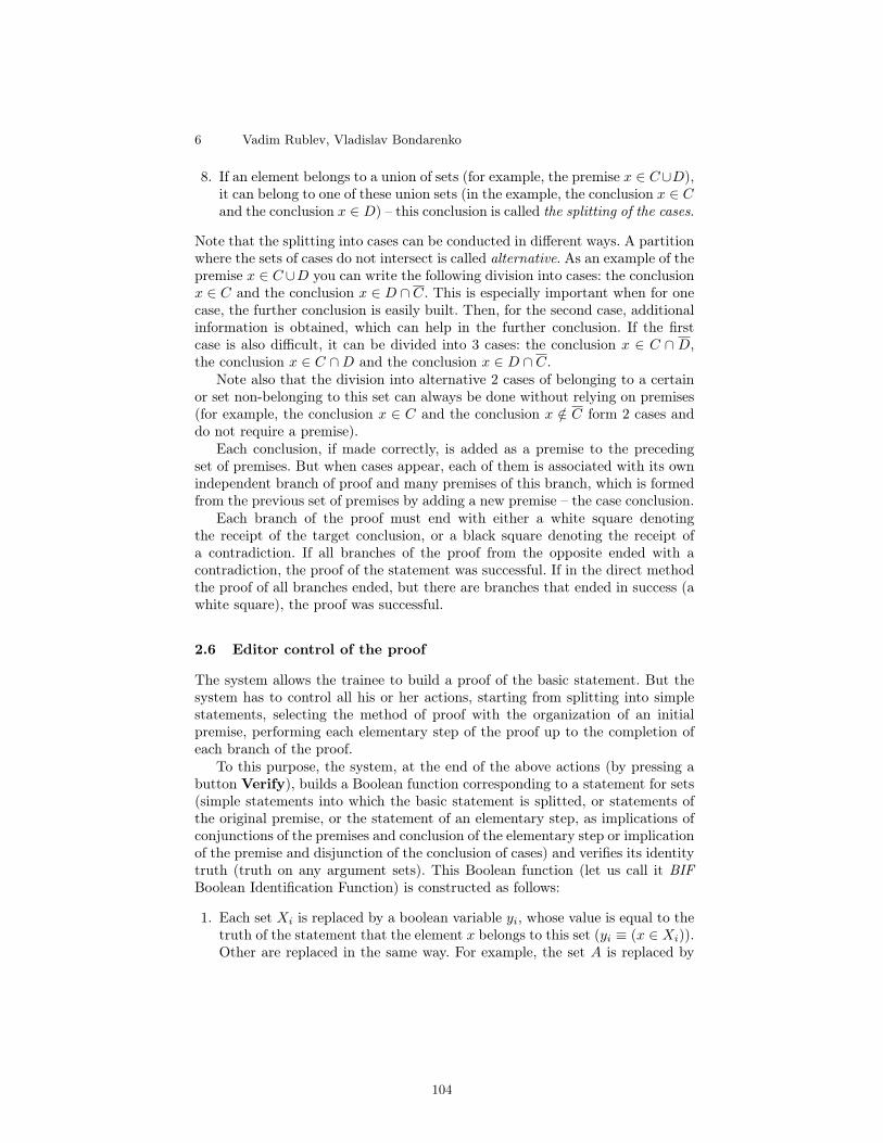
6 Vadim Rublev, Vladislav Bondarenko

8. If an element belongs to a union of sets (for example, the premise x ∈ C∪D),it can belong to one of these union sets (in the example, the conclusion x ∈ Cand the conclusion x ∈ D) – this conclusion is called the splitting of the cases.

Note that the splitting into cases can be conducted in different ways. A partitionwhere the sets of cases do not intersect is called alternative. As an example of thepremise x ∈ C∪D you can write the following division into cases: the conclusionx ∈ C and the conclusion x ∈ D ∩ C. This is especially important when for onecase, the further conclusion is easily built. Then, for the second case, additionalinformation is obtained, which can help in the further conclusion. If the firstcase is also difficult, it can be divided into 3 cases: the conclusion x ∈ C ∩ D,the conclusion x ∈ C ∩D and the conclusion x ∈ D ∩ C.

Note also that the division into alternative 2 cases of belonging to a certainor set non-belonging to this set can always be done without relying on premises(for example, the conclusion x ∈ C and the conclusion x /∈ C form 2 cases anddo not require a premise).

Each conclusion, if made correctly, is added as a premise to the precedingset of premises. But when cases appear, each of them is associated with its ownindependent branch of proof and many premises of this branch, which is formedfrom the previous set of premises by adding a new premise – the case conclusion.

Each branch of the proof must end with either a white square denotingthe receipt of the target conclusion, or a black square denoting the receipt ofa contradiction. If all branches of the proof from the opposite ended with acontradiction, the proof of the statement was successful. If in the direct methodthe proof of all branches ended, but there are branches that ended in success (awhite square), the proof was successful.

2.6 Editor control of the proof

The system allows the trainee to build a proof of the basic statement. But thesystem has to control all his or her actions, starting from splitting into simplestatements, selecting the method of proof with the organization of an initialpremise, performing each elementary step of the proof up to the completion ofeach branch of the proof.

To this purpose, the system, at the end of the above actions (by pressing abutton Verify), builds a Boolean function corresponding to a statement for sets(simple statements into which the basic statement is splitted, or statements ofthe original premise, or the statement of an elementary step, as implications ofconjunctions of the premises and conclusion of the elementary step or implicationof the premise and disjunction of the conclusion of cases) and verifies its identitytruth (truth on any argument sets). This Boolean function (let us call it BIFBoolean Identification Function) is constructed as follows:

1. Each set Xi is replaced by a boolean variable yi, whose value is equal to thetruth of the statement that the element x belongs to this set (yi ≡ (x ∈ Xi)).Other are replaced in the same way. For example, the set A is replaced by

104

The editor for teaching the proof of statements for sets 7

a boolean variable a, whose name is a lowercase letter, corresponding to theset name and its true value coincides with the value of the statement of thebelonging of an element x to this set, i.e. a ≡ (x ∈ A).

2. Operations on sets of complement, intersection and union are replaced ac-cordingly by operations of negation, conjunction and disjunction for the cor-responding subsets of statements.

3. The equality for sets is replaced by the equivalence operation of the corre-sponding statements.

4. The inclusion for sets is replaced by the operation of implication of thecorresponding statements.

5. The equality of a set to the empty set is replaced by the negation of thecorresponding statement for the set.

6. The equality of a set to the universal set is replaced by the correspondingstatement for the set.

So in the considered example (2) of identical representations of the set A weobtain the following BIF fa = (y1 ∧ y2 ∨ y3 ↔ (y1 ∨ y2) ∧ y3) ∧ (y1 ∧ y2 ∨ y3 ↔(y1 ∧ y3) ∨ (y2 ∧ y3)) and since it is identically true, then by the theorem onthe connection of expressions of the algebra of sets and the algebra of statementsand its consequences (see, for example [5]) the system confirms the correctnessof transformations of the set A.

Next, for a simple statement (6), the BIF will look as follows:

f6 ≡ (y1 ∧ y2 ∨ y3 ↔ (y2 ∨ y3) ∧ y1)→ y1 ∧ y2 ∧ y3.

Its identical truth also confirms the correctness of the simple statement (6).When conducting the proof from the contrary of this statement, the student

receives the initial premise. ∃x : x ∈ X1 ∩ X2 ∩ X3 from the negation of theproved statement X1 ∩X2 ∩X3 = ∅ and BIF for verification gets the followingexpression: fu1 ≡ y1 ∧ y2 ∧ y3 ↔ y1 ∧ y2 ∧ y3, and since it is identically true, theinitial premise is correctly built by the student.

From the received initial premise follows a conjunction of 3 elementary con-clusions. x ∈ X1 ∧ x ∈ X2 ∧ x ∈ X5, what is verified by the identical truth ofBIF of the function of implication of the function of premise and conjunction offunctions of elementary conclusions y1 ∧ y2 ∧ y3 → y1 ∧ y2 ∧ y3.

3 Editor interface for proving assertions for sets

The editor interface is a constructor. Using a dialog with a choice of actions(Fig. 1), the trainee chooses which elements he will need for further work. Suchelements will appear in the main program window (Fig. 2). Another single win-dow is the input toolbar (Fig. 3). The proof process is divided into several stages:

1. Initially, at launch, a dialog is called up with the choice of action (Fig. 1),where learner selects one of the items he needs for the proof.

2. “Enter the basic statement” creates a field for input.

105

8 Vadim Rublev, Vladislav Bondarenko

3. “Inputting identical transformations for some sets” (they are given the namesA and B create two input fields with buttons for checking the transforma-tions).

4. “Splitting the basic statement” creates a split number, an input field and avalidation button.

5. “The choice of the statement to be proved” creates a dialog window in whichthe previously entered splits of the basic statement are displayed.

6. “Entering the initial premise and step of proving” creates verify button andinput field.

After entering the text of the elementary conclusion or the initial premise intothe scheme of the proof, one or several buttons are displayed in the form of ared square, pressing one of them will form a field for entering the text of thenext elementary conclusion. The choice of an elementary conclusion of a whiteor black square, if correct, leads to the completion of the proof of the statementor its branch.

Fig. 1: Choose dialog

106

The editor for teaching the proof of statements for sets 9

Fig. 2: A window for entering the required statements and premises of evidence

107

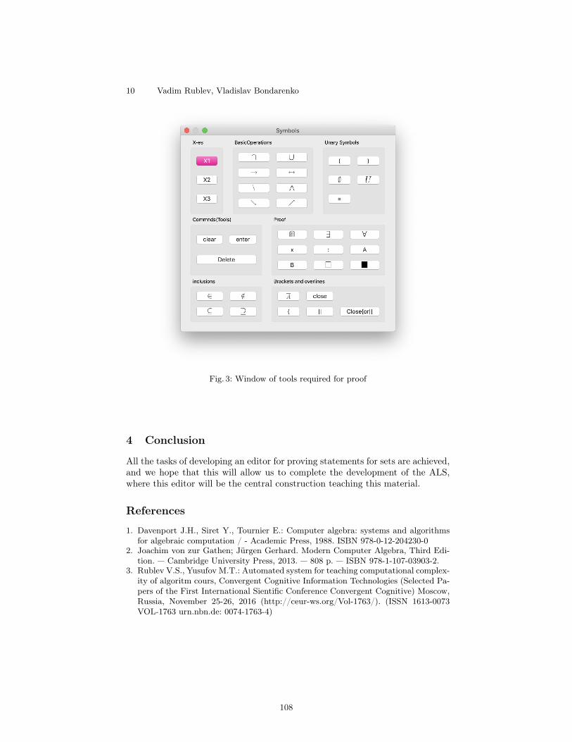
10 Vadim Rublev, Vladislav Bondarenko

Fig. 3: Window of tools required for proof

4 Conclusion

All the tasks of developing an editor for proving statements for sets are achieved,and we hope that this will allow us to complete the development of the ALS,where this editor will be the central construction teaching this material.

References

1. Davenport J.H., Siret Y., Tournier E.: Computer algebra: systems and algorithmsfor algebraic computation / - Academic Press, 1988. ISBN 978-0-12-204230-0

2. Joachim von zur Gathen; Jurgen Gerhard. Modern Computer Algebra, Third Edi-tion. — Cambridge University Press, 2013. — 808 p. — ISBN 978-1-107-03903-2.

3. Rublev V.S., Yusufov M.T.: Automated system for teaching computational complex-ity of algoritm cours, Convergent Cognitive Information Technologies (Selected Pa-pers of the First International Sientific Conference Convergent Cognitive) Moscow,Russia, November 25-26, 2016 (http://ceur-ws.org/Vol-1763/). (ISSN 1613-0073VOL-1763 urn.nbn.de: 0074-1763-4)

108

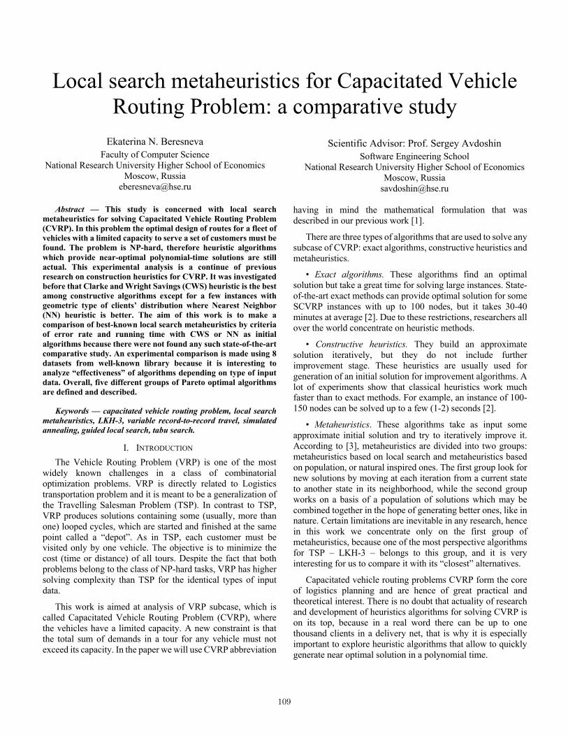
Local search metaheuristics for Capacitated Vehicle Routing Problem: a comparative study

Ekaterina N. Beresneva Faculty of Computer Science

National Research University Higher School of Economics Moscow, Russia

eberesneva@hse.ru

Scientific Advisor: Prof. Sergey Avdoshin Software Engineering School

National Research University Higher School of Economics Moscow, Russia

savdoshin@hse.ru

Abstract — This study is concerned with local search metaheuristics for solving Capacitated Vehicle Routing Problem (CVRP). In this problem the optimal design of routes for a fleet of vehicles with a limited capacity to serve a set of customers must be found. The problem is NP-hard, therefore heuristic algorithms which provide near-optimal polynomial-time solutions are still actual. This experimental analysis is a continue of previous research on construction heuristics for CVRP. It was investigated before that Clarke and Wright Savings (CWS) heuristic is the best among constructive algorithms except for a few instances with geometric type of clients’ distribution where Nearest Neighbor (NN) heuristic is better. The aim of this work is to make a comparison of best-known local search metaheuristics by criteria of error rate and running time with CWS or NN as initial algorithms because there were not found any such state-of-the-art comparative study. An experimental comparison is made using 8 datasets from well-known library because it is interesting to analyze “effectiveness” of algorithms depending on type of input data. Overall, five different groups of Pareto optimal algorithms are defined and described.

Keywords — capacitated vehicle routing problem, local search metaheuristics, LKH-3, variable record-to-record travel, simulated annealing, guided local search, tabu search.

I. INTRODUCTION The Vehicle Routing Problem (VRP) is one of the most

widely known challenges in a class of combinatorial optimization problems. VRP is directly related to Logistics transportation problem and it is meant to be a generalization of the Travelling Salesman Problem (TSP). In contrast to TSP, VRP produces solutions containing some (usually, more than one) looped cycles, which are started and finished at the same point called a “depot”. As in TSP, each customer must be visited only by one vehicle. The objective is to minimize the cost (time or distance) of all tours. Despite the fact that both problems belong to the class of NP-hard tasks, VRP has higher solving complexity than TSP for the identical types of input data.

This work is aimed at analysis of VRP subcase, which is called Capacitated Vehicle Routing Problem (CVRP), where the vehicles have a limited capacity. A new constraint is that the total sum of demands in a tour for any vehicle must not exceed its capacity. In the paper we will use CVRP abbreviation

having in mind the mathematical formulation that was described in our previous work [1].

There are three types of algorithms that are used to solve any subcase of CVRP: exact algorithms, constructive heuristics and metaheuristics.

• Exact algorithms. These algorithms find an optimal solution but take a great time for solving large instances. State-of-the-art exact methods can provide optimal solution for some SCVRP instances with up to 100 nodes, but it takes 30-40 minutes at average [2]. Due to these restrictions, researchers all over the world concentrate on heuristic methods.

• Constructive heuristics. They build an approximate solution iteratively, but they do not include further improvement stage. These heuristics are usually used for generation of an initial solution for improvement algorithms. A lot of experiments show that classical heuristics work much faster than to exact methods. For example, an instance of 100-150 nodes can be solved up to a few (1-2) seconds [2].

• Metaheuristics. These algorithms take as input some approximate initial solution and try to iteratively improve it. According to [3], metaheuristics are divided into two groups: metaheuristics based on local search and metaheuristics based on population, or natural inspired ones. The first group look for new solutions by moving at each iteration from a current state to another state in its neighborhood, while the second group works on a basis of a population of solutions which may be combined together in the hope of generating better ones, like in nature. Certain limitations are inevitable in any research, hence in this work we concentrate only on the first group of metaheuristics, because one of the most perspective algorithms for TSP – LKH-3 – belongs to this group, and it is very interesting for us to compare it with its “closest” alternatives.

Capacitated vehicle routing problems CVRP form the core of logistics planning and are hence of great practical and theoretical interest. There is no doubt that actuality of research and development of heuristics algorithms for solving CVRP is on its top, because in a real word there can be up to one thousand clients in a delivery net, that is why it is especially important to explore heuristic algorithms that allow to quickly generate near optimal solution in a polynomial time.

109

There are a lot of articles related to CVRP local search metaheuristics, but no works were found which compare improvement heuristics using the same input data of different types and sizes. We will compare these algorithms under criteria of quality, or error rate, and running time. Under the error rate we mean the percentage of difference in the obtained value of the solution with the optimal (or best-known) solution for the problem.

The aim of this work is to make a comparison of best-known local search metaheuristics by criteria of solution quality and running time with CWS or NN as initial algorithms as there were not found any such state-of-the-art comparative study. In addition, it is important to define sets of Pareto optimal metaheuristics for different types of input data.

The paper is structured as follows. In the second part, a general local search approach is described. After that, in the third section, some notes on a most popular local search metaheuristics are provided, including short description of chosen algorithms to be intercompared. The fourth part presents design of experiments on local search metaheuristics. of experimental results. The fifth and the sixth sections describe results of solution qualities and computing times of algorithms, respectively. The seventh part consists of definition of Pareto optimal metaheuristics and five such sets are presented. In the last part we summarize our findings and suggest areas for future work.

II. LOCAL SEARCH APPROACH Local search algorithms take as input some approximate

initial solution and try to iteratively upgrade it with local improvements. These changes can either improve a single route (intra-route optimization) or change more than one routes simultaneously in such a way that the overall solution is improved (inter-route optimization).

Intra-route and inter-route optimization strategies consist of different schemes, which are fully described in [5]. In this research we will use the most-known and simplest but still effective local improvement heuristics: 1-point move, 2-point move and 2-opt.

The set of all solutions that can be obtained by applying the local improvements on a solution 𝑠 is called the neighborhood 𝑁(𝑠). Of course, the bigger neighborhood is, the more likely it contains a new solution that can improve current one. However, to have large neighborhoods means to have inevitably higher computational complexity since more solutions need to be generated and evaluated [6]. At the same time, local search methods must deal with the problem of being stuck in a local optimum. Thus, a lot of methods to escaping the local optimum are applied, they will be described in the next section.

So, basically, local search approach consists of the following main steps:

1. Taking as input some initial solution 𝑠. 2. Generation of a neighborhood 𝑁(𝑠).

3. Selection of the best solution 𝑠∗ from 𝑁(𝑠) using some acceptance criteria.

4. Make a new 𝑠 equal to𝑠∗. 5. Checking for exceeding different limits. If stop criteria

is satisfied then terminate, otherwise continue with the step 2.

III. CVRP LOCAL SEARCH METAHEURISTICS Local search metaheuristics are used to solve a wide range

of combinatorial optimization problems. Among heuristic methods for solving TSP there is one, which is the best – it is local search metaheuristic, proposed by Lin, Kernighan and Helsgaun [7]. Also, local search algorithms are key part of most known methods for solving most subcases of VRP [3] [8] [9] [10] etc.

The most well-known schemes for solving CVRP that include local search steps are different variants of tabu search, forms of deterministic and simulated annealing, variable neighborhood search, guided local search [11]. Recently a new adoption of LKH for TSP called LKH-3 was proposed by one of the original authors, Helsgaun [12] . Also, in a recent study it was stated that improved version of record-to-record travel heuristic analyzed [13] is “… a well-performing metaheuristic”, which combines strategies of deterministic annealing, tabu search, variable neighborhood search and both intra-route and inter-route optimizations described later. It was proposed by Li and others [14].

Of course, there are a lot of other metaheuristics for finding CVRP solution, however it was decided to concentrate on a set of several reputed local search algorithms that were honorably mentioned in recent studies.

As it was stated earlier, for all metaheuristics an initial solution must be obtained. For most input problems Clarke and Wright Savings (CWS) heuristic [4] is used, which is the best among construction algorithms except for a few instances with geometric type of clients’ distribution. For these especial input files Nearest Neighbor (NN) heuristic is applied instead of CWS.

Thus, in this study we will intercompare following local search metaheuristics for solving classical CVRP.

A. A set of optimization operators (OPT) As it was stated above, in this research the most-known and

simplest local improvement heuristics are used. They are 1-point move, 2-point move and 2-opt.

In a tour of 𝑁 vertices 1-point move operator (or relocate heuristic) moves some vertex 𝑣(, 𝑖 ∈ 𝑁 after another vertex 𝑣,, 𝑗 ∈ 𝑁, 𝑖 ≠ 𝑗 at the same tour. Another 2-point move operator (or exchange heuristic) swaps locations of two different vertices 𝑣(, 𝑖 ∈ 𝑁 and 𝑣,, 𝑗 ∈ 𝑁, 𝑖 ≠ 𝑗. And the main idea of 2-opt heuristic is to remove two edges (𝑣(, 𝑣,), 𝑖, 𝑗 ∈ 𝑁 and (𝑣/, 𝑣0), 𝑥, 𝑦 ∈ 𝑁 from the solution and replace them with two new edges (𝑣(, 𝑣/) and (𝑣,, 𝑣0). It is important to note that

110

all mentioned operators can be applied for each of intra-optimization and inter-optimization as it is shown in Fig. 1.

Fig. 1. Intra-route 2-opt (above) in compare to intre-route 2-opt (below).

B. Guided local search (GLS) The guided local search metaheuristic is used to avoid local

minima. It was initially proposed by [15] and later applied to CVRP by [16]. According to [17], this method is memory-based as it determines and penalizes “ineffective” edges by increasing its cost to a new 𝑐∗4𝑣(, 𝑣,5 = 𝑐4𝑣(, 𝑣,5 +𝜆𝑝4𝑣(, 𝑣,5𝐿, where 𝑝4𝑣(, 𝑣,5 counts the number of penalties of edge 4𝑣(, 𝑣,5, 𝐿 is a proxy for the average cost of an edge, computed as the costs of the starting solution divided by the number of customers, and λ controls the impact of penalties (authors suggest to always set λ = 0.1).

C. Tabu search (TS) Tabu search originally was proposed by Glover and others

[18]. The main idea of TS is as follows. If some solutions in 𝑁(𝑠) cannot be improved for several iterations or they violate the rules, they are made forbidden (or tabu) in order to prevent being in a stack of local minimum. Such forbidden solutions are put into a tabu-list, so this heuristic is also memory-based like GLS. The duration that a solution remains tabu is called its tabu-tenure and it can vary over different intervals of time.

We use recent TS algorithm that provides good results described in [19] as it was stated in [5].

D. Simulated annealing (SA) This classical algorithm was developed in 1983 by [20]. It

is based on an analogy from the annealing process of solids, where a solid is heated to a high temperature and gradually cooled in order for it to crystallize in a low energy configuration [21]. In this research we used adopted version of SA for CVRP by [22]. In SA some solution 𝑠∗ from 𝑁(𝑠) at iteration 𝑖 is

chosen to be a new𝑠 = ;𝑠∗withprobability𝑃(𝑠, 𝑠∗, 𝑖)

𝑠withprobability1 − 𝑃(𝑠, 𝑠∗, 𝑖)

accordingly to the probabilistic function 𝑃(𝑠, 𝑠∗, 𝑖) =exp L− M(N)OM(N∗)

PQR ,where𝑓(𝑠)is a length of solution 𝑠, 𝑄( is an

element of an arbitrary decreasing, converging to zero, positive sequence, which specifies an analogue of the falling temperature in the crystal.

E. Lin-Kernighan-Helsgaun heuristic for CVRP (LKH-3) LKH-3 is proposed by Helsgaun in 2017 [12]. The

implementation of LKH-3 builds on the idea of transforming the problem into classical symmetric TSP. After that algorithm uses the principle of 2-opt algorithm and generalizes it. In this heuristic, the 𝑘-Opt, where 𝑘 = 2. . √𝑁YYYYYYYY, is applied, so the switches of two or more edges are made in order to improve the tour. This method is adaptive, so decision about how many edges should be replaced is taken at each step [7] [23].

This algorithm was not developed by us as original source code of LKH-3 is free of charge for academic and non-commercial use and can be downloaded at [24].

F. Variable record-to-record travel heuristic (VRTR) Li and others suggested a variable record-to-record travel

heuristic, which is based on classical record-to-record travel algorithm (RTR). RTR combines approaches of deterministic annealing (which is a variant of simulated annealing heuristic) and tabu search. The main differences between VRTR and RTR are as follows. Firstly, VRTR considers 1-point, 2-point and 2-opt moves not only within individual routes as RTR does, but also between them. Secondly, “VRTR uses a variable-length neighbor list that should help focus the algorithm on promising moves and speed up the search procedure” [14].

IV. DESIGN OF EXPERIMENTS All algorithms from section III were implemented as

sequential algorithms in C/C++, no multi-threading was explicitly utilized. They were executed on an Intel Core i5 clocked at 1.3GHz with 4 GB RAM running the macOS 10.14.3 operating system.

The computational testing of the solution methods for CVRP has been carried out by considering eight sets of test instances from the next well-known database [25]. Total number of instances in sets A, B, E, F, G, M, P, X is 211. All instances inside one set have its own characteristics and a way of generation: cluster-based / uniform / geometric distribution of clients, real-world / imitative cases etc. The integer Euclidean metric is used for all instances. The naming scheme and data format for each instance is described here [26]. Shortly, the first letter in names shows the name of used set, the figure after letter ‘n’ shows the number of nodes and the figure which stands after letter ‘k’ presents the number of vehicles.

Experiment starts with choice of a local search metaheuristic M from set OPT, GLS, SA, TS, LKH-3, VRTR. After one dataset D is selected from a list of all mentioned benchmark datasets, an instance file F from chosen dataset D is taken. Next, the following steps are repeated 51 times on instance F: chosen metaheuristic M is executed on a basis of initial solution obtained by CWS or NN (as it was explained in a previous chapter). During all iterations, except the first one, solution qualities ε[\(M, F) and computing times t[\(M, F) (in seconds) are calculated for algorithm M on test F. The first run is not taken into account in calculations because of specifity of C++

111

compiler. Solution quality (or percent above best-known, or gap) is calculated using the next formula [11]:

𝐹(𝑆a) − 𝐹bcd(𝑆)𝐹bcd(𝑆)

∙ 100%,

where 𝐹(𝑆a) is a length of obtained solution and 𝐹bcd(𝑆) is a length of optimal solution or best-known one.

Also we calculate minimal value εh[i(M, F)among all figures ε[\(M, F) and sample mean 𝑋Yd(M, F) =kla∑ 𝑡(d(M, F)la(dok among all figures t[\(M, F). And finally,

among all εh[i(M, F) from one dataset average sample mean 𝑋Yp(M, D) =

k|s|∑ εh[i(M, F) , ∀F ∈ D is calculated, which

shows average gap for algorithm M on dataset D. And among all 𝑋Yd(M, F) from one dataset average sample mean 𝑋Yd(M, D) =k|u|∑𝑋Yd(M, F) , ∀F ∈ D is calculated, which shows average

computing time of algorithm M on dataset D. |D| is a number of input files in dataset D.

The plan of experiment on local search metaheuristics is described in Fig. 2.

Input: local search metaheuristics, datasets 1: foreach local search metaheuristic M 2: foreach dataset D from datasets 3: foreach instance file F from D 4: for it ∈ 0…50 // number of runs 5: init_sol = run CWSorNN on F 6: final_sol = run M on F with init_sol 7: if (it != 0) // if not the first run 8: calculate ε[\(M, F), t[\(M, F) 9: calculate εh[i(M, F) 10: calculate th[i(M, F) 11: calculate thz(M, F) 12: calculate 𝑋Yd(M, F) 13: calculate 𝑠d(M, F) 14: calculate 𝑋Yp(M, D) // average gap on dataset 15: calculate 𝑋Yd(M, D) // average computing time

Fig. 2. Plan of experiment on constructive heuristics.

Each metaheuristic is subsequently launched on all instances from every mentioned dataset, so no input file is missed.

V. COMPUTATIONAL RESULTS ON SOLUTION QUALITY Results about the best (= minimal) solution qualities

εh[i(M, F) of metaheuristics available from experiments for set A are presented in Fig. 3. The horizontal axis represents the name of instance data. The vertical axis shows the solution quality. Results for other sets cannot be presented here as detailed as for set A, because of its size, but they are aggregated in Table 1, where average gaps 𝑋Yp(M, D) for all metaheuristics and all datasets are given. Figure 4 is a visual representation of this table. These general figures can show an approximate overall effectiveness of algorithms by criterion of solution quality. Analysis of Fig. 4 indicated a group of top-3 algorithms by criterion of solution quality: they are LKH-3, VRTR, SA. Let’s take a closer look at their results.

Fig. 3. Solution quality of local search metaheuristics, set A.

TABLE I. AVERAGE GAP 𝑋Yp(𝑀, 𝐷) IN THE DATASET, %.

Average gap 𝑋Yp(M, D) in the dataset

Local search metaheuristics CWS

or NN

OPT GLS TS SA LKH-3 VRTR

Set (

its si

ze)

A (26) 5,0% 4,5% 3,0% 2,1% 0,9% 0,2% 0,6% B (23) 4,4% 3,9% 3,1% 2,5% 1,0% 0,2% 0,6% E (11) 7,1% 5,3% 4,1% 3,6% 0,8% 0,4% 0,8% F (3) 4,4% 2,7% 3,3% 3,0% 1,8% 0,1% 1,9%

G (20) 11% 10% 8,1% 9,7% 5,2% 2,1% 2,4% M (4) 4,7% 2,8% 2,6% 2,1% 0,5% 0,2% 0,5% P (24) 8,0% 6,6% 3,5% 4,5% 0,7% 0,5% 0,9% X(100) 5,9% 5,4% 4,9% 4,0% 4,1% 2,0% 1,7%

Fig. 4. Average gap of local search metaheuristics in the datasets (%).

It is clearly seen that in 7 out of 8 sets LKH-3 produces solutions with the least (= the best) solution qualities. Experiment results that are not shown here because of their large size reveal that LKH-3 produces not the best solutions in:

3 input files out of 26 for set A (≈12%); 1 input files out of 23 for set B (≈4%); 2 input files out of 11 for set E (≈18%); 1 input files out of 3 for set F (≈33%); 6 input files out of 20 for set G (30%); 0 input files out of 4 for set M (0%); 6 input files out of 24 for set P (≈25%); 61 input files out of 100 for set X (61%);

Totally, LKH-3 was not the best in quality criterion for 80 input files out of 211 (≈38%). Only 6 times SA was the best, while all other times VRTR was “the winner”.

112

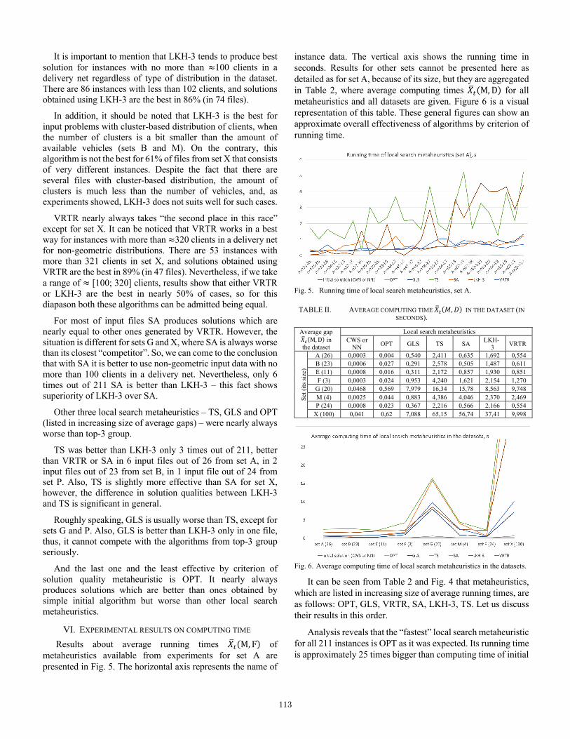
It is important to mention that LKH-3 tends to produce best solution for instances with no more than ≈100 clients in a delivery net regardless of type of distribution in the dataset. There are 86 instances with less than 102 clients, and solutions obtained using LKH-3 are the best in 86% (in 74 files).

In addition, it should be noted that LKH-3 is the best for input problems with cluster-based distribution of clients, when the number of clusters is a bit smaller than the amount of available vehicles (sets B and M). On the contrary, this algorithm is not the best for 61% of files from set X that consists of very different instances. Despite the fact that there are several files with cluster-based distribution, the amount of clusters is much less than the number of vehicles, and, as experiments showed, LKH-3 does not suits well for such cases.

VRTR nearly always takes “the second place in this race” except for set X. It can be noticed that VRTR works in a best way for instances with more than ≈320 clients in a delivery net for non-geometric distributions. There are 53 instances with more than 321 clients in set X, and solutions obtained using VRTR are the best in 89% (in 47 files). Nevertheless, if we take a range of ≈ [100; 320] clients, results show that either VRTR or LKH-3 are the best in nearly 50% of cases, so for this diapason both these algorithms can be admitted being equal.

For most of input files SA produces solutions which are nearly equal to other ones generated by VRTR. However, the situation is different for sets G and X, where SA is always worse than its closest “competitor”. So, we can come to the conclusion that with SA it is better to use non-geometric input data with no more than 100 clients in a delivery net. Nevertheless, only 6 times out of 211 SA is better than LKH-3 – this fact shows superiority of LKH-3 over SA.

Other three local search metaheuristics – TS, GLS and OPT (listed in increasing size of average gaps) – were nearly always worse than top-3 group.

TS was better than LKH-3 only 3 times out of 211, better than VRTR or SA in 6 input files out of 26 from set A, in 2 input files out of 23 from set B, in 1 input file out of 24 from set P. Also, TS is slightly more effective than SA for set X, however, the difference in solution qualities between LKH-3 and TS is significant in general.

Roughly speaking, GLS is usually worse than TS, except for sets G and P. Also, GLS is better than LKH-3 only in one file, thus, it cannot compete with the algorithms from top-3 group seriously.

And the last one and the least effective by criterion of solution quality metaheuristic is OPT. It nearly always produces solutions which are better than ones obtained by simple initial algorithm but worse than other local search metaheuristics.

VI. EXPERIMENTAL RESULTS ON COMPUTING TIME Results about average running times 𝑋Yd(M, F) of

metaheuristics available from experiments for set A are presented in Fig. 5. The horizontal axis represents the name of

instance data. The vertical axis shows the running time in seconds. Results for other sets cannot be presented here as detailed as for set A, because of its size, but they are aggregated in Table 2, where average computing times 𝑋Yd(M, D) for all metaheuristics and all datasets are given. Figure 6 is a visual representation of this table. These general figures can show an approximate overall effectiveness of algorithms by criterion of running time.

Fig. 5. Running time of local search metaheuristics, set A.

TABLE II. AVERAGE COMPUTING TIME 𝑋Yd(𝑀, 𝐷) IN THE DATASET (IN SECONDS).

Average gap 𝑋Yp(M, D) in the dataset

Local search metaheuristics CWS or

NN OPT GLS TS SA LKH-3 VRTR

Set (

its si

ze)

A (26) 0,0003 0,004 0,540 2,411 0,635 1,692 0,554 B (23) 0,0006 0,027 0,291 2,578 0,505 1,487 0,611 E (11) 0,0008 0,016 0,311 2,172 0,857 1,930 0,851 F (3) 0,0003 0,024 0,953 4,240 1,621 2,154 1,270

G (20) 0,0468 0,569 7,979 16,34 15,78 8,563 9,748 M (4) 0,0025 0,044 0,883 4,386 4,046 2,370 2,469 P (24) 0,0008 0,023 0,367 2,216 0,566 2,166 0,554

X (100) 0,041 0,62 7,088 65,15 56,74 37,41 9,998

Fig. 6. Average computing time of local search metaheuristics in the datasets.

It can be seen from Table 2 and Fig. 4 that metaheuristics, which are listed in increasing size of average running times, are as follows: OPT, GLS, VRTR, SA, LKH-3, TS. Let us discuss their results in this order.

Analysis reveals that the “fastest” local search metaheuristic for all 211 instances is OPT as it was expected. Its running time is approximately 25 times bigger than computing time of initial

113

algorithm, however, even for 1000 clients in a delivery net the maximum running time does not exceed 3 seconds.

Next algorithm is GLS, which is approximately 300 times slower than initial one. In sets B, E, F, P, M and X it nearly always (94%) ranks #2 just after OPT. Of course, there are cases when GLS works slightly slower than others, but the number of such situations is not very significant and the difference between obtained values does not exceed 1 second. However, in sets A and G GLS works with mixed results: computing times of GLS, SA, VRTR or LKH-3 (depending on dataset) are fluctuated and too close to each other, so it is impossible to find a leader.

Average computing time of VRTR steadily goes at the third plays, except for set G with geometric instances and several rare cases from other datasets. VRTR has smooth growth of speed, and no special aspects of its work are found apart from not very stable work with geometric-inspired instances.

Next one is SA. In comparison with VRTR, SA has bigger growth of speed and the plot of its running time is more fluctuated. In sets A, B, E, F and P this algorithm executes quicker than LKH-3 but slower than VRTR. However, in sets G, M and X it shows much worse effectivity, when the number of clients in a delivery net becomes more than 100. It means that SA is better to use for instances with up to one hundred delivery points.

LKH-3 is slower than other mentioned metaheuristics (except for TS) for all datasets apart from sets G, M and those instances from set X with 322 and more delivery points. The main unique feature of LKH-3 is its variability. Linear chart of running times of LKH-3 has a lot of drastic jumps and slumps. That is why this metaheuristic has not very positive computing time rate. Nevertheless, LKH-3 can work very quickly, especially when there are no more than 50-80 clients in a net.

Last one metaheuristic to be discussed concerning its computing time is TS. As LKH-3, linear chart of running times has a lot of drastic jumps and slumps. In average, this is the slowest algorithm in this group, however, in a third of cases it can compete with LKH-3 or SA but not very significant speeding up can be noticed.

VII. PARETO OPTIMAL LOCAL SEARCH METAHEURISTICS

The algorithm 𝑚a ∈ ℳ is Pareto optimal if (∀𝑚 ∈ ℳ) L(𝑚 ≠ 𝑚a) ⇒ 4𝑋Yp(𝑚,𝐷) > 𝑋Yp(𝑚a, 𝐷)5 ∨ 4𝑋Yd(𝑚,𝐷) > 𝑋Yd(𝑚a, 𝐷)5R Thus, our aim is to find a sets of Pareto optimal algorithms for different types of input data.

Figures from 5 to 14 are plotted using values from Table 1 and Table 2. The horizontal axis represents average computing time 𝑋Yd(M, D) in seconds. The vertical axis shows average solution quality 𝑋Yp(M, D).

Fig. 7. Average solution quality vs. average running time, set A.

Fig. 8. Average solution quality vs. average running time, set B.

Fig. 9. Average solution quality vs. average running time, set E.

Fig. 10. Average solution quality vs. average running time, set F.

114

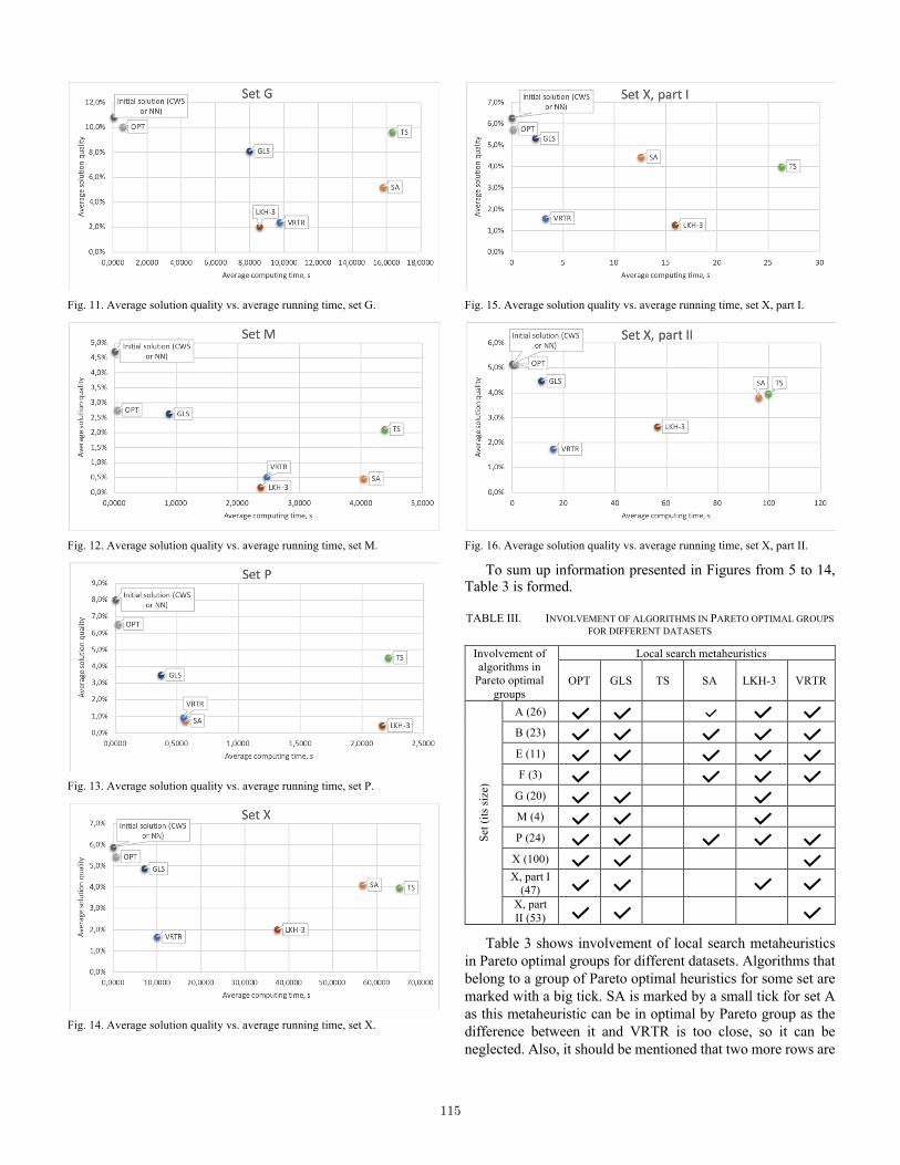
Fig. 11. Average solution quality vs. average running time, set G.

Fig. 12. Average solution quality vs. average running time, set M.

Fig. 13. Average solution quality vs. average running time, set P.

Fig. 14. Average solution quality vs. average running time, set X.

Fig. 15. Average solution quality vs. average running time, set X, part I.

Fig. 16. Average solution quality vs. average running time, set X, part II.

To sum up information presented in Figures from 5 to 14, Table 3 is formed.

TABLE III. INVOLVEMENT OF ALGORITHMS IN PARETO OPTIMAL GROUPS FOR DIFFERENT DATASETS

Involvement of algorithms in

Pareto optimal groups

Local search metaheuristics

OPT GLS TS SA LKH-3 VRTR

Set (

its si

ze)

A (26) B (23) E (11) F (3)

G (20)

M (4)

P (24) X (100) X, part I

(47) X, part II (53)

Table 3 shows involvement of local search metaheuristics in Pareto optimal groups for different datasets. Algorithms that belong to a group of Pareto optimal heuristics for some set are marked with a big tick. SA is marked by a small tick for set A as this metaheuristic can be in optimal by Pareto group as the difference between it and VRTR is too close, so it can be neglected. Also, it should be mentioned that two more rows are

115

added – they are “set X, part I” which consists of instances with up to 322 clients and “set X, part II” which is vice versa has instances with 322 and more delivery points inside input files. This division is connected with the big size of set X and with the fact that was described in section V – VRTR works in a best way for instances with more than ≈320 clients in a delivery net for non-geometric distributions but LKH-3 produces good results for instances with no more than ≈100 clients regardless of type of distribution in the dataset.

The following conclusions are made on a base of results from Table 3:

1. Sets A, B, E and P can be aggregated together because a group of Pareto optimal algorithms is the same for all these sets. We will name this aggregation as Group_1. It represents two different types of inputs. The first one is with clients’ coordinates and demands that are formed from a uniform distribution with some outlying cases. The second one is with nodes that are formed into clusters, and the number of clusters is equal or greater than number of available vehicles. Demands are also formed from a uniform distribution with some outlying cases. All input files from Group_1 have 101 clients in a delivery net as maximum.

2. Set F forms a second group Group_2 with only 3 instances obtained from real goods deliveries. Number of delivery points varies from 45 to 135.

3. Group_3 is formed of sets G and M that also have the same Pareto optimal metaheuristics. Number of delivery points varies from 100 to 483. Set G has instances with locations in a form of concentric squares, pointed stars and rays, while set M consists of only 4 input files with locations that are grouped into clusters, and the number of clusters is equal or smaller by 1 than number of available vehicles.

4. Group_4 is formed of the first part of set X. There are 47 instances in it, and the number of instances is up to 322 clients. Group_4 is a mix of input data types: it has different combinations of demand distribution (unitary demands, small/large values, small/large variance), depot positioning (central, eccentric, random) and customer positioning (practical cases, uniform distribution, cluster-based).

5. Group_5 is formed of the second part of set X. There are 53 instances in it, and the number of instances is from 322 to 1001 clients. Other characteristics of this group are the same as Group_4 has.

Above-mentioned conclusions are outlined in Table 4 with information about involvement of algorithms in Pareto optimal groups depending on types of input data. All algorithms are listed in increasing order of average computing times (from best to worst) and in decreasing order of average solution qualities (from worst to best).

TABLE IV. INVOLVEMENT OF ALGORITHMS IN PARETO OPTIMAL GROUPS DEPENDING ON TYPES OF INPUT DATA

Number of delivery points

Distribution of delivery points

Distribution of demands

Pareto optimal algorithms

Group_1 Up to 101

1. Uniform (with some outlying cases).

2. Cluster-based, the number of clusters is equal or greater than number of available vehicles.

Uniform (with some outlying cases)

OPT GLS SA VRTR LKH-3

Group_2 Up to 135

Real-world Real-world

OPT SA VRTR LKH-3

Group_3 From 100 to 483

1. Geometric (concentric squares, pointed stars and rays).

2. Cluster-based, the number of clusters is equal or smaller by 1 than number of available vehicles.

Constant or uniform

OPT GLS LKH-3

Group_4 From 100 to 322

Mixed Mixed OPT GLS VRTR LKH-3

Group_5 From 322 to 1001

Mixed Mixed OPT GLS VRTR

VIII. CONCLUSIONS

As it was expected, unfortunately, there is no one universal metaheuristic that takes the first places by both criteria of solution quality and running time. Overall, the next recommendations should be given to people who are interested in metaheuristics solving CVRP.

1. For uniform (with some outlying cases) or cluster-based distribution of clients’ locations, where the number of clusters is equal or greater than number of available vehicles it is better to apply Set of optimization operators, Guided local search, Simulated annealing, Variable record-to-record travel algorithm or Lin-Kernighan-Helsgaun heuristic for CVRP depending on desired solution quality and available time for calculations. Here and elsewhere the algorithms are listed in increasing order of average computing times (from best to worst) and in decreasing order of average solution qualities (from worst to best).

2. For real-world instances it is better to use following local search metaheuristics: Set of optimization operators, Simulated annealing, Variable record-to-record travel algorithm or Lin-Kernighan-Helsgaun heuristic for CVRP.

3. For geometric (with concentric squares, pointed stars and rays) or cluster-based distribution of clients’ locations, where the number of clusters is equal or smaller by 1 than number of available vehicles, it is better to apply Set of

116

optimization operators, Guided local search or Lin-Kernighan-Helsgaun heuristic for CVRP.

4. Finally, for mixed up combinations of demand distribution, depot positioning and customer positioning there are two recommendations. If there up to approximately 350 clients in a delivery net, it is better to use Set of optimization operators, Guided local search algorithm, Variable record-to-record travel algorithm or Lin-Kernighan-Helsgaun heuristic for CVRP. Otherwise, if there are nearly 320 delivery point and more then LKH-3 stops being so effective, so it is better to use following local search metaheuristics: Set of optimization operators, Guided local search algorithm or Variable record-to-record travelling algorithm.

Also experiments revealed absolute inefficiency of Tabu search as it is not in any of Pareto optimal groups.

In future we are planning to extend our study by conducting experiments using:

1. Population-based or nature-inspired metaheuristics as there are a lot of productive algorithms, too.

2. Other input data sets, including the most recent one with thousands of nodes in each instance. It is important to check local search metaheuristics on problems with extra-large dimensions to analyze their effectiveness.

REFERENCES

[1] E. Beresneva and S. Avdoshin, "Analysis of Mathematical Formulations of Capacitated Vehicle Routing Problem and Methods for their Solution," Trudy ISP RAN/Proc. ISP RAS, vol. 30, no. 3, pp. 233-250, 2018.

[2] K. Braekers, K. Ramaekers and I. Nieuwenhuyse, "The vehicle routing problem: State of the art classification and review," Computers & Industrial Engineering, vol. 99, pp. 300-313, 2016.

[3] B. Golden, S. Raghavan and E. Wasil, The vehicle routing problem: Latest advances and new challenges, New York: Springer, 2008.

[4] P. Toth and D. Vigo, Vehicle Routing Problems, Methods, and Applications, Philadelphia: SIAM, 2014.

[5] F. Arnold, M. Gendreau and K. Sorensen, "Efficiently solving very large-scale routing problems," Computers and Operations Research, vol. 107, pp. 32-42, 2019.

[6] K. Helsgaun, "An effective implementation of the Lin–Kernighan traveling salesman heuristic," EJOR, vol. 12, pp. 106-130, 2000.

[7] E. Zachariadis and C. Kiranoudis, "An open vehicle routing problem metaheuristic for examining wide solution neighborhoods," Computers & Operations Research, vol. 37, no. 4, pp. 712-723, 2010.

[8] E. Taillard, G. Laporte and M. Gendreau, "Vehicle routeing with multiple use of vehicles," Journal of the Operational Research Society, vol. 47, no. 8, p. 1065, 1996.

[9] S. Ropke and D. Pisinger, "An adaptive large neighborhood search heuristic for the pickup and delivery problem with time windows," Transportation Science, vol. 40, no. 4, p. 455–472, 2006.

[10] P. Toth and D. Vigo, "An overview of vehicle routing problems," in The Vehicle Routing Problem, SIAM, 2002.

[11] K. Helsgaun, "An Extension of the Lin-Kernighan-Helsgaun TSP Solver for Constrained Traveling Salesman and Vehicle Routing Problems," Roskilde University, 2017.

[12] P. Schittekat and K. Sorensen, "Deconstructing record-to-record travel for the capacitated vehicle routing problem," Operational Research and Management Science Letters, vol. 1, no. 1, pp. 17-27, 2018.

[13] F. Li, B. Golden and E. Wasil, "Very large-scale vehicle routing: new test problems, algorithms, and results," Computers & Operations Research, vol. 32, p. 1165–1179, 2005.

[14] G. Laporte and F. Demet, "Classical Heuristics for the Capacitated VRP," in The Vehicle Routing Problem, SIAM, 2002, pp. 109-128.

[15] C. Voudouris, E. Tsang and A. Alsheddy, "Guided local search," in Handbook of metaheuristics, 2010, pp. 321-361.

[16] D. Mester and O. Braysy, "Active-guided evolution strategies for large-scale capacitated vehicle routing problems," Computers & Operations Research, vol. 34, no. 10, p. 2964–2975, 2007.

[17] F. Arnold and K. Sorensen, "Knowledge-guided local search for the Vehicle Routing Problem," Computers and Operations Research, vol. 105, pp. 32-46, 2019.

[18] F. T. E. Glover, "A user’s guide to tabu search," Operations Research, vol. 41, no. 1, pp. 1-28, 1993.

[19] E. Zachariadis and C. Kiranoudis, "A strategy for reducing the computa- tional complexity of local search-based methods for the vehicle routing problem," Computers & Operations Research, vol. 37, p. 2089–2105, 2010.

[20] S. Kirkpatrick, C. Gelatt and M. Vecchi, "Optimization by simulated annealing," Science, vol. 220, no. 4598, p. 671– 680, 1983.

[21] NEO, "Simulated Annealing," [Online]. Available: http://neo.lcc.uma.es/vrp/solution-methods/metaheuristics/simulated-annealing/. [Accessed 27 02 2019].

[22] I. Osman, "Metastrategy simulated annealing and tabu search algorithms for the vehicle routing problem," Annals of Operations Research, vol. 41, pp. 421-451, 1993.

[23] S. Avdoshin and B. E.N., "The Metric Travelling Salesman Problem: The Experiment on Pareto-optimal Algorithms," Trudy ISP RAN/Proc. ISP RAS, vol. 29, no. 4, pp. 123-138, 2017.

[24] K. Helsgaun, "LKH-3," 2. [Online]. Available: http://akira.ruc.dk/~keld/research/LKH-3/. [Accessed 01 2019].

[25] I. Xavier, "CVRPLIB," [Online]. Available: http://vrp.atd-lab.inf.puc-rio.br/index.php/en/. [Accessed 09 05 2018].

[26] Heidelberg University, "TSPLIB," [Online]. Available: https://www.iwr.uni-heidelberg.de/groups/comopt/software/TSPLIB95/. [Accessed 09 05 2018].

117

118

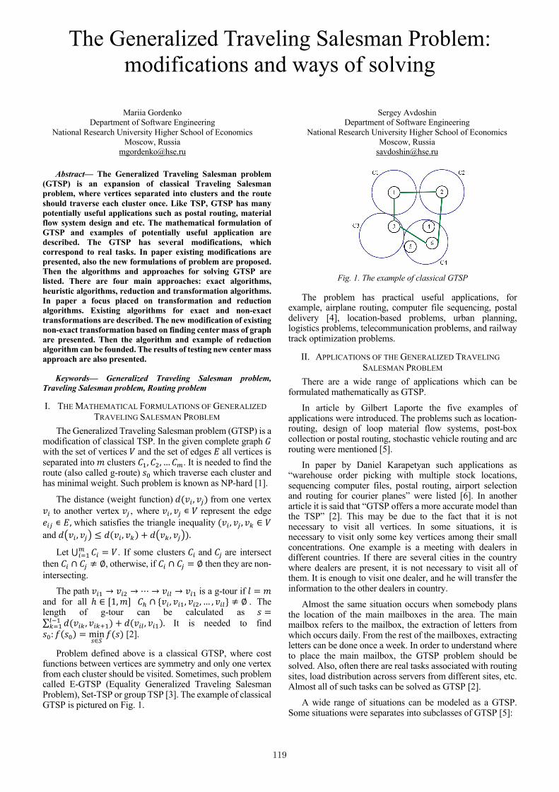
The Generalized Traveling Salesman Problem: modifications and ways of solving

Mariia Gordenko Department of Software Engineering

National Research University Higher School of Economics Moscow, Russia

mgordenko@hse.ru

Sergey Avdoshin Department of Software Engineering

National Research University Higher School of Economics Moscow, Russia

savdoshin@hse.ru

Abstract— The Generalized Traveling Salesman problem (GTSP) is an expansion of classical Traveling Salesman problem, where vertices separated into clusters and the route should traverse each cluster once. Like TSP, GTSP has many potentially useful applications such as postal routing, material flow system design and etc. The mathematical formulation of GTSP and examples of potentially useful application are described. The GTSP has several modifications, which correspond to real tasks. In paper existing modifications are presented, also the new formulations of problem are proposed. Then the algorithms and approaches for solving GTSP are listed. There are four main approaches: exact algorithms, heuristic algorithms, reduction and transformation algorithms. In paper a focus placed on transformation and reduction algorithms. Existing algorithms for exact and non-exact transformations are described. The new modification of existing non-exact transformation based on finding center mass of graph are presented. Then the algorithm and example of reduction algorithm can be founded. The results of testing new center mass approach are also presented.

Keywords— Generalized Traveling Salesman problem, Traveling Salesman problem, Routing problem

I. THE MATHEMATICAL FORMULATIONS OF GENERALIZED TRAVELING SALESMAN PROBLEM

The Generalized Traveling Salesman problem (GTSP) is a modification of classical TSP. In the given complete graph 𝐺 with the set of vertices 𝑉 and the set of edges 𝐸 all vertices is separated into 𝑚 clusters 𝐶&, 𝐶(, …𝐶*. It is needed to find the route (also called g-route) 𝑠, which traverse each cluster and has minimal weight. Such problem is known as NP-hard [1].

The distance (weight function) 𝑑(𝑣0, 𝑣1) from one vertex 𝑣0 to another vertex 𝑣1 , where 𝑣0, 𝑣1 ∊ 𝑉 represent the edge 𝑒01 ∊ 𝐸, which satisfies the triangle inequality (𝑣0, 𝑣1, 𝑣5 ∈ 𝑉 and 𝑑7𝑣0, 𝑣18 ≤ 𝑑(𝑣0, 𝑣5) + 𝑑7𝑣5, 𝑣18).

Let ⋃ 𝐶0 = 𝑉*0>& . If some clusters 𝐶0 and 𝐶1 are intersect

then 𝐶0 ∩ 𝐶1 ≠ ∅, otherwise, if 𝐶0 ∩ 𝐶1 = ∅ then they are non-intersecting.

The path 𝑣0& → 𝑣0( → ⋯ → 𝑣0D → 𝑣0& is a g-tour if 𝑙 = 𝑚 and for all ℎ ∈ [1,𝑚] 𝐶J ∩ 𝑣0, 𝑣0&, 𝑣0(, … , 𝑣0D ≠ ∅ . The length of g-tour can be calculated as 𝑠 =∑ 𝑑(𝑣05, 𝑣05N&)DO&5>& + 𝑑(𝑣0D, 𝑣0&). It is needed to find

𝑠,: 𝑓(𝑠,) = minU∈V

𝑓(𝑠) [2].

Problem defined above is a classical GTSP, where cost functions between vertices are symmetry and only one vertex from each cluster should be visited. Sometimes, such problem called E-GTSP (Equality Generalized Traveling Salesman Problem), Set-TSP or group TSP [3]. The example of classical GTSP is pictured on Fig. 1.

Fig. 1. The example of classical GTSP

The problem has practical useful applications, for example, airplane routing, computer file sequencing, postal delivery [4], location-based problems, urban planning, logistics problems, telecommunication problems, and railway track optimization problems.

II. APPLICATIONS OF THE GENERALIZED TRAVELING SALESMAN PROBLEM

There are a wide range of applications which can be formulated mathematically as GTSP.

In article by Gilbert Laporte the five examples of applications were introduced. The problems such as location-routing, design of loop material flow systems, post-box collection or postal routing, stochastic vehicle routing and arc routing were mentioned [5].

In paper by Daniel Karapetyan such applications as “warehouse order picking with multiple stock locations, sequencing computer files, postal routing, airport selection and routing for courier planes” were listed [6]. In another article it is said that “GTSP offers a more accurate model than the TSP” [2]. This may be due to the fact that it is not necessary to visit all vertices. In some situations, it is necessary to visit only some key vertices among their small concentrations. One example is a meeting with dealers in different countries. If there are several cities in the country where dealers are present, it is not necessary to visit all of them. It is enough to visit one dealer, and he will transfer the information to the other dealers in country.

Almost the same situation occurs when somebody plans the location of the main mailboxes in the area. The main mailbox refers to the mailbox, the extraction of letters from which occurs daily. From the rest of the mailboxes, extracting letters can be done once a week. In order to understand where to place the main mailbox, the GTSP problem should be solved. Also, often there are real tasks associated with routing sites, load distribution across servers from different sites, etc. Almost all of such tasks can be solved as GTSP [2].

A wide range of situations can be modeled as a GTSP. Some situations were separates into subclasses of GTSP [5]:

119

• The Covering Tour Problem; • Material Flow System Design; • Post-box collection; • Stochastic vehicle routing; • Arc routing.

III. THE TYPES OF THE GENERALIZED TRAVELING SALESMAN PROBLEM

Previously, the classical variant of GTSP was defined. However, there are real applications which require some modifications of classical GTSP. In this section all known types of GTSP are listed. The several new modifications of GTSP are proposed.

A. Generalized Traveling Salesman Problem with intersecting clusters It is a less-known modification of GTSP, which defined

in [7]. The definition of problem is similar to GTSP, but 𝐶&, 𝐶(, … , 𝐶* sets may intersect, so 𝐶0 ∩ 𝐶1 ≠ ∅ for some 𝑖, 𝑗 ∈ [1,𝑚] and 𝑖 ≠ 𝑗. The example is presented on Fig. 2. The vertex 𝑣Y lies in 𝐶Z and 𝐶[ cluster simultaneously.

Fig. 2. The example of GTSP with intersecting clusters

B. Asymmetric Generalized Traveling Salesman Problem (A-GTSP) If the distance function is asymmetry, so 𝑑7𝑣0, 𝑣18 ≠

𝑑7𝑣1, 𝑣08 for some 𝑣0, 𝑣1 ∊ 𝑉 , the problem called A-GTSP (Asymmetric Generalized Traveling Salesman Problem).

C. Generalized Traveling Salesman Problem with many vertices in clusters (Many-GTSP)

In various articles, there is a mention of the problem of GTSP, where in the route 𝑠 = 7𝑣0], 𝑣0^, . . . , 𝑣0_8, 𝑙 ∈ [𝑚, |𝑉|], where from each cluster more than one vertex can appear. However, algorithms that solve problem in this formulation were not found. There is an assumption that the problem is solved by classical methods with some modifications.

D. Dynamic Traveling Salesman (Dynamic GTSP) The less well-known, but potentially useful problem is a Dynamic Generalized Traveling Salesman Problem (Dynamic GTSP). It is a variant of Dynamic Routing Problems and Generalized Traveling Salesman Problems at the same time. The Dynamic GTSP is a problem, where new vertices are added or deleted during the traveling. This is the main difference from the classical GTSP [8]. In the research [8] four types of Dynamic GTSP were presented. There are very few works that are devoted to this problem. In [8] the multi-agent-based approach to modeling and solving dynamic generalized traveling salesman problem is given.

E. Multi-objective Generalized Traveling Salesman Problem (MO-GTSP)

This problem is also very similar to the classical GTSP problem. However, there is some expansion. In GTSP only one characteristic is assigned to the edge, but in MO-GTSP several characteristics (for example, time, cost) are attributed to each arc, which should be minimized together [9]. The example is presented on Fig. 3.

Fig. 3. The example of MO-GTSP with two functions to optimize:

cost and time

F. Clustered Traveling Salesman Problem It is an extension of TSP which has similarities with GTSP. All vertices are divided into non-intersecting clusters and solution consists of all vertices 𝑉, but vertices from one cluster should be traversed together. The example of problem and solution is presented on Fig. 4.

Fig. 4. The example of Clustered Traveling Salesman Problem

G. k-Generalized Traveling Salesman Problem (k-GTSP) Previously, k-GTSP was not defined. However, other routing problem (for example, Chinese Postman problem or Traveling Salesman problem) have “-k” definition, which are very different.

Fig. 5. The example of k-GTSP (k-GTSP with k salesmen). On

figure there are 2 salesman and 2 tours (green and red)

It is possible to imagine that more than one salesman will traverse the route. Moreover, the start vertex for each salesman may be different. If the 𝑘 salesman are defined, it is needed to find route with minimal weight 𝑠 = 𝑡& ∪ …∪ 𝑡5 , where 𝑡0 is route of 𝑖 salesman. For all 𝑖 ∈ [1,𝑚] |𝑠 ∩ 𝐶0| =1. The example is shown on Fig. 5. In future, I will call such problem as k-GTSP with 𝑘 salesmen. There is a similar

120

formulation for another routing problem k-CPP (k-Chinese Postman Problem) [10]. For TSP also was defined the k-TSP problem. The main idea to find the minimal weight cycle traverses exactly 𝑘 vertices without repetitions [11]. Such problem can be generalized for the GTSP. In given complete graph 𝐺 with the set of vertices 𝑉 and the set of edges 𝐸 it is needed to find minimal weight route 𝑠 traverses only 𝑘 clusters. The example is depicted on Fig. 6. Such problem will call k-GTSP with decreasing number of vertices.

Fig. 6. The example of k-GTSP with decreasing number of vertices

It should be mentioned that problem defined above may be practically useful. For example, on the map of clusters it is necessary to choose 𝑘 clusters such that the cost of traversing will be minimal. This can be useful, for example, if the supplier wants to choose the stores with minimal costs of deliver the goods. In the literature, another formulation of the 𝑘-problem can be found. Such problems are called finding the 𝑘 − best solutions and widely know for polynomial solvable problems. However, there is a 𝑘-TSP problem. The main idea consists of finding 𝑘 − best solutions. Such problem can be generalized to GTSP. It is needed to find the set of 𝑘 solutions with minimal weight. The example is shown on Fig. 7. In my future work I will call such problem as k-GTSP with k best solutions.

Fig. 7. The example of k-GTSP with k best solutions (3 solutions

are depicted)

IV. THE WAYS OF SOLVING THE GENERALIZED TRAVELING SALESMAN PROBLEM

The GTSP is NP-hard problem and exact solution is very time expensive because requires complete search of all possible variants. Even for small tasks (for example, 20 clusters) on a personal computer, calculating the optimal route can be very time consuming. After analyzing the sources, several groups of algorithms and approaches for solving GTSP can be distinguished:

• Exact algorithms (such as branch and bound, branch and cut algorithms, etc.);

• Heuristic algorithms (random-key genetic algorithm, mrOX genetic algorithm, BIO-inspired algorithms,

generalized nearest neighbor heuristic, memetic algorithm, 2-opt local search algorithm, generalized initialization, insertion and improvement heuristic, LKH heuristic, neighborhood heuristics, etc.);

• Algorithms for transforming GTSP into related problems (exact and non-exact transformations);

• Algorithms for reduction GTSP dimension. Below the description of transformation and reduction some algorithms are presented.

A. Transformation GTSP with intersecting clusters to GTSP with non-intersecting clusters (I-N transformation)

Suppose we are dealing with a GTSP with intersecting clusters, for some 𝑖, 𝑗 ∈ [1,𝑚] 𝐶0 ∩ 𝐶1 ≠ ∅ . Such type of GTSP instance 𝐺 can be transformed into 𝐺′ with non-intersecting clusters. The algorithm was mentioned by Y.N. Lien in [2]. The main idea of transformation is copying the vertices, which simultaneously lie in different clusters 𝑝 times (𝑝 is a number of clusters, where vertex lies). Let 𝑆hbe a set of clusters in which the 𝑣 vertex lies, 𝑞h = |𝑆h|. Then it is needed to find g-tour in 𝐺′. Between copies of each vertex it is needed to construct random route. After that from g-tour in 𝐺′ the g-tour in 𝐺 can be obtained by deleting from g-tour copies of vertices. The correctness of algorithm was proved [2]. The cost of g-tours in 𝐺 and 𝐺′ are similar [2]. If some vertex should be marked as start it marked as 𝑣, and placed into non-intersected special cluster 𝐶, . If there is no such restriction, then such a cluster is not allocated.

Fig. 8. The example of I-N transformation (g-tour is green, yellow

route is the route between duplicated vertices)

The example of algorithm’s working is presented. The Fig. 8, Table I and Table II show how the transformation is occurred.

TABLE I. I-N TRANSFORMATION. THE VERTEX DISTRIBUTION

𝑺𝟏 𝑺𝟐 𝑺𝟑 𝑺𝟒 𝑺𝟓 𝑺𝟔 𝑺𝟕 𝑺𝟖 𝑺𝟗 𝑺𝟏𝟎 𝑺𝟏𝟏 𝑺𝟏𝟐 𝑺𝟏𝟑

𝑪𝟏 𝑪𝟏 𝑪𝟏, 𝑪𝟑

𝑪𝟏, 𝑪𝟐, 𝑪𝟒

𝑪𝟐, 𝑪𝟒

𝑪𝟐, 𝑪𝟒 𝑪𝟑 𝑪𝟑 𝑪𝟑 𝑪𝟒 𝑪𝟒 𝑪𝟒 𝑪𝟐

𝒒𝒗 1 1 2 3 2 2 1 1 1 1 1 1 1

TABLE II. I-N TRANSFORMATION. THE VERTEX DISTRIBUTION INTO CLUSTERS

Cluster Vertices 𝑪𝟏 𝑣&, 𝑣(, 𝑣Z, 𝑣[ 𝑪𝟐 𝑣[, 𝑣Y, 𝑣x, 𝑣&Z 𝑪𝟑 𝑣Z, 𝑣y, 𝑣z, 𝑣 𝑪𝟒 𝑣Y, 𝑣x, 𝑣&,, 𝑣&&, 𝑣&(

121

B. Transformation GTSP with non-intersecting clusters into standard TSP) (S-N transformation)

The GTSP with non-intersecting clusters can be transformed into standard instance of TSP [2]. Suppose we are dealing with a GTSP with non-intersecting clusters, for all 𝑖, 𝑗 ∈ [1, |𝑉|] 𝐶0 ∩ 𝐶1 = ∅. It is needed to mark the start vertex as 𝑣, and put it in individual cluster 𝐶, . In related 𝐺| problem create 𝐶′ clusters, which consist of replicas of vertices:

• 𝑣, ∈ 𝐶, copies as 𝑎,,, and 𝑐,,, into 𝐶,′ cluster. • For all nodes from each clusters the three replicas

𝑎, 𝑏, 𝑐 should be created in 𝐺′ (see Fig. 9). • For each cluster vertex 𝑒 added.

After copying and doubling vertices transformation of edges are required. The edges transform in the following ways:

• In the cluster 𝐶, the 𝑐,,, vertex connects with 𝑎,,, by edge with zero cost.

• All vertex in each transformed cluster 𝐶0′ connect by edges with zero cost in the following way: 𝑎0,, →𝑏0,, → 𝑐0,, → 𝑎0,& → 𝑏0,& → 𝑐0,& → ⋯ → 𝑎0,|| →𝑏0,|| → 𝑐0,|| → 𝑎0,, . All 𝑏 vertex connects with corresponding 𝑎 vertex. All 𝑐 vertices connect with all 𝑒vertex in each cluster and 𝑒 vertex connects with all 𝑏 vertices in cluster by zero cost edges.

• All intercluster edges are copies with the same cost of traverse.

The 𝐺′′ problem is not presented on complete graph. After finding the solution on 𝐺′′ for transforming g-tour to 𝐺′ it is needed to remove incluster cycles in g-tour. The correctness of algorithm was proved [2].

Fig. 9. The example of S-N transformation [3]

C. T-Transformation of GTSP into A-TSP T-transformation doubles up the number of vertices [12, 13] and consists of the following steps:

• For every vertex in each cluster 𝑣1 ∈ 𝑉0, 𝑖 ∈ [1, 𝑘] define two vertices 𝑣1 (entering) and 𝑣1| (leaving). Each pair of such vertices is joined by an arc from 𝑣1 to 𝑣1| with very high cost.

• Join all 𝑣1 ∈ 𝑉0| vertices in increasing order and 𝑣1| ∈𝑉0| in decreasing order with zero cost.

• Edges between 𝑉0 copied with the same cost. The proof of correctness such transformation is given in [12]. The example of T-transformation is shown on Fig. 10

D. Noon-Bean transformation of GTSP into ATSP It is a way of transformation without adding any vertex. Here the cost of traversing is changed. The big constant M adds to each intercluster edges. It is guarantee that firstly the

all vertices into cluster would be traversed and then the route goes to another cluster. After such solution some vertices from tour should be deleted (after the first vertex of the cluster is met, the rest should be removed). Received route is the g-tour. The correctness, proof and some computational results on GTSPlib are presented in [14] and an example of transformation is presented in my previous research [15].

Fig. 10. The example of T-transformation

E. Spatial Transformation of GTSP to TSP GTSP can be solved in the following way [3]:

• From each cluster 𝑉0 the vertex 𝑣0 should be selected. • Calculate the Hamiltonian cycle in the subgraph 𝐺′,

constructed on the selected vertices from step 1. Step 1 and 2 doing until all possible options for selecting vertices are completed. Then the smallest route is selected. However, such solution requires a lot of processing power and memory, especially on large-scale problems. In article [3] the five different types of selecting vertices from clusters are shown:

1) E-Search E-Search is known as Euclidian-Search. The main idea of this method is constructing a line connecting the first and last vertex from the original data. After that, from each cluster select only one vertex which is closest to the line. Computational time is 𝑂(𝑉) [3]. The process of E-Search is shown on Fig. 11.

Fig. 11. The example of E-Search (yellow line - line between the

first and last vertices, red vertices were selected)

Fig. 12. R-Search example

2) R-Search R-Search is known as Radial-Search. It is needed for the first and last vertex in the original data find from each cluster radially the nearest vertices. So, there are 25TSP instance, it

122

is needed to solve both and select the best. Computational time is 𝑂(𝑉) of selecting 25 instances [3]. The process of R-Search is shown on Fig. 12.

3) RE-Search It is a combination of R-Search and E-Search. Firstly, it is needed to find two vertices most radially nearest to start and end vertex in the original data. Then, for selected vertices the E-Search applied. Computational time is 𝑂(𝑉) [3].

4) D-Search D-Search is known as Dijkstra-Search. The main idea of this method is constructing a route connecting the first and last vertex from the original data using Dijkstra algorithm. After that, from each cluster select only one vertex which is closest to the route. Computational time is 𝑂(𝑉() [3].

5) RD-Search It is a combination of R-Search and D-Search. Firstly, it is needed to find two vertices most radially nearest to start and end vertex in the original data. Then, for selected vertices the D-Search applied. Computational time is 𝑂(𝑉() [3]. The approaches presented above have advantages and disadvantages. One of the disadvantages is the strong dependence of the minimum route weight on chosen starting and ending vertices. I propose the following search method CM-Search based on finding vertices closest to the “center of mass”.

6) CM-Search CM-Search is a Center of Mass Search. The main idea of this method is to find the center of mass of the graph 𝐺 (let the mass of each vertex is equal). After that, from each cluster select only one vertex which is closest to the center mass. Computational time is 𝑂(𝑉). However, method also has a disadvantage. The situation where all vertices are concentrated in one place, but there are several vertices that are far away from them is possible. In this case, the center of mass is shifted, and non-optimal vertices can be selected. The example of bad case shown on Fig. 13. It can be seen that the selection 𝑣Z and 𝑣[ instead of 𝑣( and 𝑣Y is more optimal. One solution of such problem is to assign big mass to the vertices from the clusters with a larger number of vertices. This method is new and requires testing on test data.

Fig. 13. CM-Search (the star is the center of mass). Bad case.

F. The Reduction Algorithm for GTSP It is known that GTSP problems (real or, for example, from GTSPlib) have big size (several hundred of vertices). Some of vertices and edges between them are redundant. There is algorithm with running time 𝑂(𝑁Z) which can reduce size approximately to 10-15% [6]. Let 𝑛 = |𝑉| the number of vertices in graph 𝐺. If graph 𝐺 consists of 𝑚 clusters then only 𝑚 vertices should be traversed, another 𝑛 −𝑚 vertices are redundant. In article by

Gregory Gutin the definition of redundant vertex is presented. “Let 𝐶 be a cluster, |𝐶| > 1. We say that a vertex 𝑟 ∈ 𝐶 is redundant if for each pair 𝑥, 𝑦 of vertices from distinct clusters different from 𝐶 , there exists a vertex 𝑠 ∈ 𝐶\𝑟 such that 𝑑(𝑥, 𝑠) + 𝑑(𝑠, 𝑦) ≤ 𝑑(𝑥, 𝑟) + 𝑑(𝑟, 𝑦)” [6]. The example of GTSP with three clusters is defined in Table III (different colors match to different clusters). This example can be reduced. We can define differences table as shown in original research [6]. The differences can be calculated as 𝑑𝑖𝑠𝑡(𝑥, 𝑠) − 𝑑𝑖𝑠𝑡(𝑥. 𝑟). For the example from Table III the Differences table (Table IV) and Comparison distances table (Table V) can be calculated - 𝑑𝑖𝑠𝑡(𝑥, 𝑟) + 𝑑𝑖𝑠𝑡(𝑟, 𝑦) −𝑑𝑖𝑠𝑡(𝑥, 𝑠) − 𝑑𝑖𝑠𝑡(𝑠, 𝑦).

TABLE III. THE EXAMPLE OF GTSP PROBLEM

𝑣& 𝑣( 𝑣Z 𝑣[ 𝑣Y 𝑣x 𝑣y 𝑣z 𝑣& - 1 2 10 7 6 7 8 𝑣( 1 - 3 8 8 7 10 11 𝑣Z 2 3 - 11 10 7 6 5 𝑣[ 10 8 11 - 1 2 1 2 𝑣Y 7 8 10 1 - 1 3 1 𝑣x 6 7 7 2 1 - 2 1 𝑣y 7 10 6 1 3 2 - 2 𝑣z 6 11 5 2 1 1 2 -

TABLE IV. THE DIFFERENCES TABLE FOR 1 CLUSTER AND 𝑟 = 𝑣&

𝑠/𝑟 𝑣[ 𝑣Y 𝑣x 𝑣y 𝑣z 𝑣( 2 -1 -1 -3 -3 𝑣Z -1 -3 -1 1 3

TABLE V. THE TABLE FOR COMPARISON DISTANCE THROUGH 𝑟 = 𝑣& AND 𝑠

𝑠 = 𝑣( 𝑠 = 𝑣Z 𝑣[ → 𝑣U → 𝑣y -1 0 𝑣[ → 𝑣U → 𝑣z -1 2 𝑣Y → 𝑣U → 𝑣y -4 -2 𝑣Y → 𝑣U → 𝑣z -4 0 𝑣x → 𝑣U → 𝑣y -4 0 𝑣x → 𝑣U → 𝑣z -4 2

The Comparison distances in Table V shows that vertex 𝑟 = 𝑣& is not redundant. The same calculations may be done for vertex 𝑣(. The calculations shown in Table VI and Table VII.

TABLE VI. THE DIFFERENCES TABLE FOR 1 CLUSTER AND 𝑟 = 𝑣(

𝑠/𝑟 𝑣[ 𝑣Y 𝑣x 𝑣y 𝑣z 𝑣& -2 1 1 3 3 𝑣Z -3 -2 0 4 6

TABLE VII. THE TABLE FOR COMPARISON DISTANCE THROUGH 𝑟 = 𝑣( AND 𝑠

𝑣& 𝑣Z 𝑣[ → 𝑣U → 𝑣y 1 1 𝑣[ → 𝑣U → 𝑣z 1 3 𝑣Y → 𝑣U → 𝑣y 4 2 𝑣Y → 𝑣U → 𝑣z 4 4 𝑣x → 𝑣U → 𝑣y 4 4 𝑣x → 𝑣U → 𝑣z 4 6

The Comparison distances in Table VII shows that vertex 𝑟 = 𝑣( is redundant and can be removed. The transformed GTSP is presented in Table VIII.

123

After removing redundant vertices from GTSP the calculations should be done again. Again, perform the calculation for the vertex 𝑟 = 𝑣& (see Table IX and Table X).

TABLE VIII. THE EXAMPLE OF GTSP PROBLEM

𝑣& 𝑣Z 𝑣[ 𝑣Y 𝑣x 𝑣y 𝑣z 𝑣& - 2 10 7 6 7 8 𝑣Z 2 - 11 10 7 6 5 𝑣[ 10 11 - 1 2 1 2 𝑣Y 7 10 1 - 1 3 1 𝑣x 6 7 2 1 - 2 1 𝑣y 7 6 1 3 2 - 2 𝑣z 6 5 2 1 1 2 -

TABLE IX. THE DIFFERENCES TABLE FOR 1 CLUSTER AND 𝑟 = 𝑣&

𝑣[ 𝑣Y 𝑣x 𝑣y 𝑣z 𝑣Z -1 -3 -1 1 3

TABLE X. THE TABLE FOR COMPARISON DISTANCE THROUGH 𝑟 = 𝑣& AND 𝑠

𝑠/𝑟 𝑣Z 𝑣[ → 𝑣U → 𝑣y 0 𝑣[ → 𝑣U → 𝑣z 2 𝑣Y → 𝑣U → 𝑣y -2 𝑣Y → 𝑣U → 𝑣z 0 𝑣x → 𝑣U → 𝑣y 0 𝑣x → 𝑣U → 𝑣z 2

Nothing changes in Table IX and X, the vertex 𝑣& is not redundant. The reduction can be continued, but, further results of calculations showed that it is meaningless. In the same way, the reduction of number of edges can be done [6].

V. THE RESULTS OF COMPUTATIONAL EXPERIMENTS The transformation approach CM-Search E for spatial transformation of GTSP to TSP were tested on standard GTSPLib by D. Karapetyan [16]. The transformation algorithms were implemented in C++ and tested on a computer with 2,6 GHz Intel Core i5 processor. After CM-Search transformation the LKH-heuristic for finding solution were used [18]. In paper [3] was shown that the applying R-Search transformation on real-world dataset and solving transformed TSP gives the average error 8.8% (for five presented Searches it is the lowest). The main disadvantage of R-Search is computational time. The R-Search gives 2* variants and then each variant should be solved. The testing of CM-Search shows that the average error is 8.1%, and computational time (in average) reduced on 83% by reducing the dimension (compared to using the LKH algorithm on non-reduced problem).

VI. CONCLUSION In paper the existing modifications of GTSP were listed and described. Three new modifications which have real applications were proposed. In next research the methods for solving 𝑘 -GTSP with 𝑘 salesmen, 𝑘 -GTSP with 𝑘 best solutions and 𝑘-GTSP with decreasing number of vertices will be proposed.

Various approaches for solving the GTSP were presented. Particular attention is paid to the algorithms for reducing the dimension and transformation algorithms. The new transformation non-exact approach CM-Search for spatial transformation of GTSP to TSP were presented and tested. Testing shown that the CM-Search significantly reduces computation time with a permissible error.

REFERENCES [1] M. Gordenko and S. Avdoshin, "The mixed chinese postman

problem," Trudy Instituta sistemnogo programmirovaniya RAN, vol. 29, no. 4, 2017.

[2] Y. N. Lien, E. Ma and B. W. S. Wah, "Transformation of the Generalized Traveling-Salesman Problem into the Standard

Traveling-Salesman Problem," Information Sciences, Vols. 74 (1-2), pp. 177-189, 1993.

[3] M. Zia, Z. Cakir and D. Z. Seker, "Spatial Transformation of Equality–Generalized Travelling Salesman Problem to Travelling

Salesman Problem," ISPRS International Journal of Geo-Information, vol. 7, no. 3, p. 115, 2018.

[4] U. Palekar and G. Laporte, "Some applications of the clustered travelling salesman problem," Journal of the Operational Research

Society, vol. 53, no. 9, pp. 972-976, 2002. [5] G. Laporte, A.-V. Ardavan and C. Sriskandarajah, "Some

Applications of the Generalized Travelling Salesman Problem," The Journal of the Operational Research Society, vol. 12 (47), pp. 1461-

1467, December 1996. [6] G. Gutin and D. Karapetyan, "Generalized traveling salesman

problem reduction algorithms," arXiv preprint arXiv:0804.0735, 2008.

[7] E. Ma, B. W. -S. Wah and Yao-Nan Lien, "Transformation of the generalized traveling-salesman problem into the standard traveling-salesman problem," Information sciences, vol. 74, no. 1-2, pp. 177-

189. [8] A. Baykasoğlu and Z. D. U. Durmuşoğlu, "A multi-agent based

approach to modeling and solving dynamic generalized travelling salesman problem," Journal of Intelligent & Fuzzy Systems, vol. 31,

no. 1, pp. 77-90, 2016. [9] J. Pinxten, "Online Heuristic for the Multi-objective Generalized

Traveling Salesman Problem," Design, Automation & Test in Europe Conference & Exhibition (DATE), pp. 822-825, 2016.

[10] A. Osterhues and F. Mariak, "On variants of the k-Chinese Postman Problem," Operations Research and Wirtschaftsinformatik, vol. 30,

31 August 2005. [11] A. Horbach, "Combinatorial relaxation of the k-traveling salesman

problem," Manuskripte aus den Instituten für Betriebswirtschaftslehre der Universität Kiel, vol. 599, 2005.

[12] V. Dimitrijević and Z. Šarić, "An efficient transformation of the generalized traveling salesman problem into the traveling salesman problem on digraphs," Information Sciences, vol. 102, no. 1-4, pp.

105-110, 1997. [13] G. Laporte and F. Semet, "Computational evaluation of a

transformation procedure for the symmetric generalized traveling salesman problem," INFOR: Information Systems and Operational

Research, vol. 37, no. 2, pp. 114-120, 1999. [14] D. Ben-Arieh, G. Gutin, M. Penn, A. Yeo and A. Zverovitch,

"Transformations of Generalized ATSP into ATSP," Operations Research Letters, vol. 31, no. 5, pp. 357-365, 2003.

[15] M. Gordenko and S. Avdoshin, "Transformation of the Mixed Chinese Postman Problem in multigraph into the Asymmetric Travelling Salesman Problem," International Journal of Open

Information Technologies, vol. 5, no. 6, pp. 6-11, 2017. [16] D. Karapetyan, "GTSP Instances Library," [Online]. Available:

http://www.cs.nott.ac.uk/~pszdk/gtsp.html. [Accessed 21 March 2019].

124

Constructive heuristics for Capacitated Vehicle Routing Problem: a comparative study

Ekaterina N. Beresneva Faculty of Computer Science

National Research University Higher School of Economics Moscow, Russia

eberesneva@hse.ru

Scientific Advisor: Prof. Sergey Avdoshin Software Engineering School

National Research University Higher School of Economics Moscow, Russia

savdoshin@hse.ru

Abstract— Vehicle Routing Problem (VRP) is concerned with the optimal design of routes to be used by a fleet of vehicles to serve a set of customers. In this study we analyze constructive heuristics for a subcase of VRP, where the vehicles have a limited capacity – Capacitated Vehicle Routing Problem (CVRP). The problem is NP-hard, therefore heuristic algorithms which provide near- optimal polynomial-time solutions are still actual. The aim of this work is to make a comparison of constructive heuristics as there were not found any such classification. Finally, the leader by a criterion of quality is admitted being a Clarke and Wright Savings heuristic; however, this algorithm cannot find the solution for all used instances. This fact and other ones are discussed in the paper. Our future goal is to make an experimental comparison of the most common and state-of-the-art metaheuristics using well suited constructive heuristic to build a suboptimal solution.

Keywords— capacitated vehicle routing problem, mathematical formulation, classical heuristics, constructive heuristics.

I. INTRODUCTION The Vehicle Routing Problem (VRP) is one of the most

widely known questions in a class of combinatorial optimization problems. VRP is directly related to Logistics transportation problem and it is meant to be a generalization of the Travelling Salesman Problem (TSP). In contrast to TSP, VRP produces solutions containing some (usually, more than one) looped cycles, which are started and finished at the same point called “depot”. The objective is to minimize the cost (time or distance) for all tours. For the identical type of input data, VRP has higher solving complexity than TSP. Both problems belong to the class of NP-hard tasks.

This work is aimed at analysis of VRP subcase, which is called Capacitated Vehicle Routing Problem (Capacitated VRP, CVRP), where the vehicles have a limited capacity. It means that there is a physical restriction on transportation more than determined amount of weight for each machine. Capacitated vehicle routing problems form the core of logistics planning and are hence of great practical and theoretical interest.

There are three types of algorithms that are used to solve any subcase of CVRP:

• Exact algorithms. These algorithms find an optimal solution but take a great time for solving large instances. Such

methods include Branch-and-Bound, Branch-and-Cut, cutting plane, column generation, cut and solve, Branch-and-Cut-and-Price, Branch-and-Price, and dynamic programming techniques. It was shown in [1] that Branch-and-Bound algorithm was able to solve random CVRP instances with up to 300 customers and four vehicles within 1000 CPU seconds in 2002. However, according to the same source some real-world CVRP instances with up to 47 vertices only were successfully solved within 1000 CPU seconds. Current situation does not differ a lot. State-of-the-art exact methods can provide optimal solution for some SCVRP instances with up to 100 nodes, but it takes 30-40 minutes at average [2]. Due to these restrictions, researchers all over the world concentrate on heuristic methods.

• Classical heuristics. These algorithms build an approximate solution iteratively, but they do not include further improvement stage. Different scientific works reveal that, in comparison to exact methods, classical heuristics work much faster. For example, an instance of 100-150 nodes can be solved up to a few (1-2) seconds [2]. Heuristics are divided into two groups that include constructive heuristics and improvement heuristics.

• Metaheuristics. Such type of algorithms is also called a framework for building heuristics. According to [3], metaheuristics either explore the solution space by moving at each iteration from a solution to another solution in its neighbourhood (metaheuristics based on local search) or evolve a population of solutions which may be combined together in the hope of generating better ones (metaheuristics based on population, natural inspired).

Actuality of research and development of heuristics algorithms for solving VRP is on its top, because such approximate algorithms can produce near-optimal solutions in a polynomial time. It is especially important in real-world tasks when there are more than one hundred clients in a delivery net. Among the best-known algorithms for CVRP there are metaheuristic proposed by Pisinger and Ropke [4], Nagata and Braysy [5], and Vidal et al [6].

There are a lot of articles related to CVRP heuristics, but no works were found which compare solution quality, or gap, of classical heuristics using the same data bases. Solution quality is calculated as the percentage of difference in the obtained

125

value of the solution with the optimal (or best-known) solution for the problem.

It is important to analyze classical heuristics since constructive heuristics are usually used in order to provide an initial (suboptimal) solution to improvement methods and to metaheuristics that allow to iteratively get near optimal solutions. So, we will discuss only algorithms from the first group.

The paper is structured as follows. In the second part a mathematical formulation of CVRP is given. In the third section, some notes on a classification of most popular constructive heuristics are provided, including description of chosen algorithms. The fourth part consists of design of experiments and their results. And, finally, in the fifth part conclusions and future goals are given.

II. CLASSICAL CVRP MATHEMATICAL MODEL In the paper we will use CVRP abbreviation having in mind

the mathematical formulation that was described in a previous work of authors [7].

Let a complete weighted oriented graph 𝐺 =< 𝑉, 𝑉 ×𝑉 > is given. Let 𝐼 = 0, 1, … ,𝑁, where 𝑁 + 1 = |𝑉|. Graph vertices are indexed as 𝑖𝑛𝑑 = 𝑉 → 𝐼, (∀𝑣 ∈ 𝑉)(∀𝑤 ∈ 𝑉) 𝑣 ≠ 𝑤 ⟹ 𝑖𝑛𝑑(𝑣) ≠ 𝑖𝑛𝑑(𝑤). Thus, 𝑉 = 𝑣?, 𝑣@, … , 𝑣A is the set of vertices, here 𝑖 = 𝑖𝑛𝑑(𝑣B), 𝑖 ∈ 𝐼. Let 𝑣?be the depot, where vehicles are located, and 𝑣B be the destination points of a delivery, 𝑖 ≠ 0.

The distance between two vertices 𝑣B and 𝑣C is calculated using a distance function 𝑐E𝑣B, 𝑣CF. Here a real-valued function 𝑐(∙,∙) on 𝑉 × 𝑉 satisfies ∀𝑖, 𝑗, 𝑔 ∈ 𝐼 [8]:

1. 𝑐E𝑣B, 𝑣CF ≥ 0 (non-negativity axiom). 2. 𝑐E𝑣B, 𝑣CF = 0 if and only if 𝑣B = 𝑣C (identity axiom). 3. 𝑐E𝑣B, 𝑣CF = 𝑐E𝑣C, 𝑣BF (symmetry axiom). 4. 𝑐E𝑣B, 𝑣KF ≤ 𝑐E𝑣B, 𝑣CF + 𝑐E𝑣C, 𝑣KF (triangle inequality

axiom).

Each destination point 𝑣B, ∀𝑖 ∈ 𝐼, is associated with a known nonnegative demand, 𝑑B, to be delivered, and the depot has a fictitious demand 𝑑? = 0. The total demand of the set 𝑉′ ⊆ 𝑉 is calculated as 𝑑(𝑉′) = ∑ 𝑑BP

|QP|BPR@ .

Let 𝐾 be a number of available vehicles at the depot 𝑣?. Each vehicle has the same capacity – 𝐶. Let us assume that every vehicle may perform at most one route and 𝐾 ≥ 𝐾UBV, where 𝐾UBV is a minimal number of vehicles needed to serve all the customers due to restriction on 𝐶. Clearly, next condition must be fulfilled – (∀𝑣B ∈ 𝑉)𝑑B ≤ 𝐶,∀𝑖 ∈ 𝐼, which prohibits goods transportation that exceed maximum vehicle capacity.

Let introduce 𝑉? = 𝑣?,where 𝑣? ∈ 𝑉. Let us divide 𝑉 in 𝐾 + 1 sets: 𝑆 = 𝑉?, 𝑉@, … , 𝑉X, each subset, except for 𝑉?, represent a set of customers to be served for one vehicle. 𝑆YZZ = 𝑆 is a set of all possible partitions of 𝑉. Let 𝐽 = 0, 1, … , 𝐾 be a set that keeps indexes. Then (∀𝑗 ∈ 𝐽)\𝑉C\ ≥ 1. There should be no duplicates in any of

subsets from 𝑆:(∀𝑔 ∈ 𝐽)(∀𝑗 ∈ 𝐽)(𝑔 ≠ 𝑗 ⇒ 𝑉K ∩ 𝑉C = ∅). Also, all subsets from 𝑆 must form set 𝑉. Thus, 𝑉 = ⋃ 𝑉CX

CR? . In this notation, 𝑉?a = 𝑉? ∪ 𝑉a, ∀𝑘 ∈ 𝐽\0. It is obvious that 𝑑(𝑉ea) ≤ 𝐶.

Let introduce 𝑀a = 1,𝑁@ … ,𝑁a, 𝑁a = |𝑉a|,∑ 𝑁aXaR@ = 𝑁. Then let 𝑀?a = 0 ∪ 𝑀a. Let 𝐼a =

⋃ 𝑖|𝑖 = 𝑖𝑛𝑑(𝑣), ∀𝑣 ∈ 𝑉aXaR@ be a set of vertex indices from

𝑉a. Then 𝐼?a = 0 ∪ 𝐼a,∀𝑘 ∈ 𝐽\0.

Let 𝐻a = 𝑝a:𝑀?a → 𝐼?a|𝑝a(0) = 0&(∀𝑥 ∈ 𝑀?a)(∀𝑦 ∈ 𝑀?a)𝑥 ≠ 𝑦 ⟹ 𝑝a(𝑥) ≠ 𝑝a(𝑦) be a set of codes of all possible permutations ℎa = n𝑣op(?), 𝑣op(@), … , 𝑣opEApFqof 𝑉?a. These permutations represent all possible Hamiltonian cycles of graph 𝐺?a < 𝑉(?a), 𝑉(?a) × 𝑉(?a) >, ∀𝑘 ∈ 𝐽\0.

Weight of ℎa ∈ 𝐻a can be found according to the formula 1:

𝑓(ℎa) = 𝑐 n𝑣op(?), 𝑣opEApFq + s 𝑐E𝑣op(t), 𝑣op(tu@)FApv@

tR?

(1)

Let 𝑆′ be a set of 𝑉?@, 𝑉?w, … , 𝑉?X. In this notation the weight of 𝑆′ is calculated as 𝐹(𝑆y) = ∑ 𝑓(ℎa)aR@..Xzzzzz , ∀𝑘 ∈𝐽\0.

Overall, the formulation of CVRP is to find: 𝑆?: 𝐹(𝑆?) = min

~∈~𝐹(𝑆) (2)

III. CONSTRUCTIVE HEURISTICS In this section the most popular constructive heuristics are

described.

A. Sequential Insertion algorithm (SI) Sequential Insertion algorithm [9] constructs routes

subsequently, one after another.

In the first step, a new tour 𝑡𝑜𝑢𝑟a, 𝑘 ≤ 𝐾, is initialized with a random unrouted node 𝑣B, 𝑖 ≠ 0,and the depot 𝑣?. Thus, a tour (𝑣?, 𝑣B, 𝑣?) is obtained.

In the second step, another unrouted vertex 𝑣C, 𝑗 ≠ 0, is chosen, such that its incorporation in the current tour gives the least increase in a tour length and demand of a potential node 𝑣C does not exceed vehicle capacity. So, the next two formulae must be hold:

argmin∈ep,∈ep,∉ep

𝑐E𝑣Y, 𝑣CF + 𝑐E𝑣C, 𝑣Yu@F − 𝑐(𝑣Y, 𝑣Yu@);

𝐷ep + 𝑑C ≤ 𝐶, where 𝐷ep is a total demand of current 𝑡𝑜𝑢𝑟a.

If all conditions hold then this unrouted vertex 𝑣C, 𝑗 ≠ 0 is inserted in a tour 𝑡𝑜𝑢𝑟a between 𝑣Y and 𝑣Yu@.

The second step is repeated until no more unrouted vertex 𝑣C, 𝑗 ≠ 0, can be feasibly inserted. In this case a new tour 𝑡𝑜𝑢𝑟a, 𝑘 ≤ 𝐾, is initialized, and the procedure starts from the first step.

126

B. Improved Parallel Insertion algorithm (PI) Parallel Insertion Improved algorithm [10] builds routes

simultaneously. This method is a modification of Sequential Insertion algorithm.

In the first step, the minimum number 𝐾UBV of feasible routes is defined as 𝐾UBV = ∑ 𝑑BB∈|Q| /𝐶. All these routes 𝑡𝑜𝑢𝑟a ∈ 𝑇𝑜𝑢𝑟𝑠are initialized with 𝐾UBV different closest to 𝑣? unrouted nodes 𝑣B, 𝑖 ≠ 0. Thus, 𝐾UBV tours (𝑣?, 𝑣B, 𝑣?) are obtained.

In the second step, a random unrouted node 𝑣C, 𝑗 ≠ 0, is inserted in some route 𝑡𝑜𝑢𝑟a at its best insertion position. The next two conditions must be hold – incorporation of 𝑣C in this tour gives the least increase in a tour length among all other tours and demand of a potential node 𝑣C does not exceed vehicle capacity. So:

argmin∈ep,∈ep,∉ep

𝑐E𝑣Y, 𝑣CF + 𝑐E𝑣C, 𝑣Yu@F − 𝑐(𝑣Y, 𝑣Yu@);

𝐷ep + 𝑑C ≤ 𝐶, where 𝐷ep is a total demand of current 𝑡𝑜𝑢𝑟a.

If all conditions hold then this unrouted vertex 𝑣C, 𝑗 ≠ 0 is inserted in a tour 𝑡𝑜𝑢𝑟a between 𝑣Y and 𝑣Yu@.

The second step is repeated until no more unrouted vertex 𝑣C, 𝑗 ≠ 0, can be feasibly inserted in some route 𝑡𝑜𝑢𝑟a. In this case a new tour 𝑡𝑜𝑢𝑟a, 𝑘 ≤ 𝐾, is initialized as (𝑣?, 𝑣C, 𝑣?) and adds to set of all tours 𝑇𝑜𝑢𝑟𝑠, and the procedure continues.

C. Nearest Neighbour heuristic (NN) Nearest Neighbour heuristic constructs routes subsequently,

one after another, in a greedy way.

In the first step, an unrouted node 𝑣B, 𝑖 ≠ 0,which is closest to the depot 𝑣?, is chosen. A new open tour 𝑡𝑜𝑢𝑟a, 𝑘 ≤ 𝐾, is initialized with 𝑣B and 𝑣?. Thus, a tour (𝑣?, 𝑣B) is obtained.

In the second step, another unrouted vertex 𝑣C, 𝑗 ≠ 0, is chosen, which is the nearest to the last added vertex and a demand of a potential node 𝑣C does not exceed vehicle capacity. So, the next two formulae must be hold:

argmin∈ep,∉ep

𝑐E𝑣B, 𝑣CF;

𝐷ep + 𝑑C ≤ 𝐶, where 𝐷ep is a total demand of current 𝑡𝑜𝑢𝑟a.

If all conditions hold then this unrouted vertex 𝑣C is added in the end of 𝑡𝑜𝑢𝑟a after 𝑣B, and since that time it turns to be the last added vertex.

The second step is repeated until no more unrouted vertex 𝑣C, 𝑗 ≠ 0, can be feasibly inserted. In this case a new tour 𝑡𝑜𝑢𝑟a, 𝑘 ≤ 𝐾, is initialized, and the procedure starts from the first step.

D. Clarke and Wright Savings Heuristic (CWS) [9] In the first step, all vertices 𝑣B ∈ 𝑉, 𝑖 ≠ 0, must form |𝑉 − 1|

routes. Thus, |𝑉 − 1| tours (𝑣?, 𝑣B, 𝑣?) are obtained.

In the second step, ∀𝑣B ∈ 𝑉, ∀𝑣C ∈ 𝑉, 𝑖 ≠ 0, 𝑗 ≠ 0, 𝑖 ≠ 𝑗, saving 𝑠E𝑣B, 𝑣CF is calculated as 𝑠E𝑣B, 𝑣CF = 𝑐(𝑣B, 𝑣?) +𝑐E𝑣?, 𝑣CF − 𝑐(𝑣B, 𝑣C). All savings are put in a list of 𝑆, must be sorted in a non-increasing order.

In the third step, the first unused saving in a list is taken. Then, existence of two routes 𝑡𝑜𝑢𝑟 and 𝑡𝑜𝑢𝑟, 𝑥 ≠ 𝑦, having the next conditions, is checked:

there is an edge (𝑣B, 𝑣?) in route 𝑥 and edge (𝑣?, 𝑣C) in tour 𝑡𝑜𝑢𝑟;

𝐷e + 𝐷e ≤ 𝐶.

If there are such routes then 𝑡𝑜𝑢𝑟 and 𝑡𝑜𝑢𝑟 are combined by removing edges (𝑣B, 𝑣?), (𝑣?, 𝑣C) and introducing edge (𝑣B, 𝑣C). After that, despite of ability or absence these routes, the current saving is skipped and the next one in the list is checked.

The last step works until 𝐾 tours are left.

E. Variant of Clarke and Wright Savings Heuristic (CWS_2) Classical variant of Clarke and Wright Savings algorithm

forms good tours in the first part of its work mostly. However, it was noticed that it tends to produce less competitive tours towards the end because of periphery nodes addition. Thus, Yellow [11] and Gaskell [12] suggested improved form of savings calculation. It is 𝑠E𝑣B, 𝑣CF = 𝑐(𝑣B, 𝑣?) + 𝑐E𝑣?, 𝑣CF −𝜆𝑐(𝑣B, 𝑣C). Here 𝜆 is a parameter which responds for measuring the distance between the vertices to be joint. In one report [13] it was mentioned that the best value of 𝜆 is 0.4.

F. Two-phase methods Two-phase methods are based on the decomposition of the

CVRP solution process into two separate stages – clustering and routing. In the clustering stage, a partition of the customers into routes is made, and in the routing stage, the sequence of the customers on each subset is obtained.

1) Subgroup of Cluster-First-Route-Second heuristics In Cluster-First-Route-Second methods, nodes are first

partitioned into different subsets called clusters and then routes are determined by sequencing the customers within each subset.

a) Sweep This Cluster-First-Route-Second method can be applied

only for planar instances [9].

Clustering stage Let us define 𝑣B ∈ 𝑉 as 𝑣B = (𝑥B; 𝑦B), where 𝑥B and 𝑦B are

the Cartesian coordinates of point 𝑣B.

In the first step, new normalized vertices 𝑣By =(𝑥By; 𝑦B′) = (𝑥B − 𝑥?; 𝑦B − 𝑦?) are introduced, where the depot 𝑣?′ has new Cartesian coordinates (0; 0), ∀𝑖 ∈ |𝑉|.

127

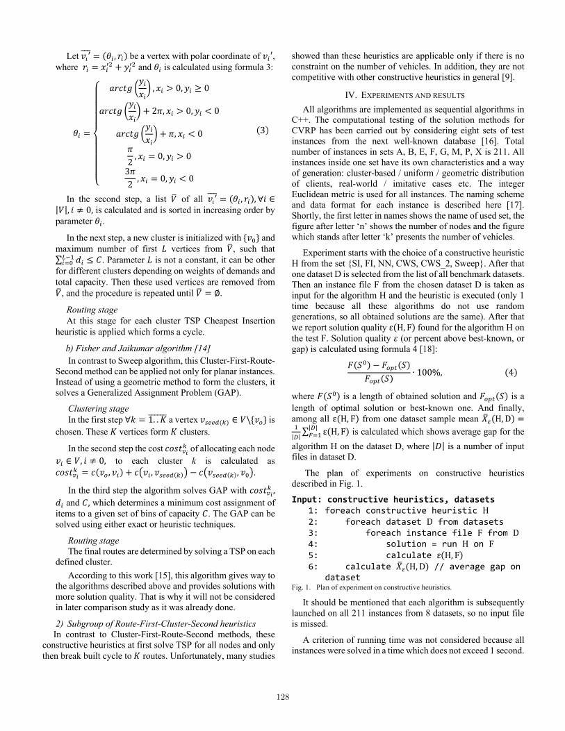
Let 𝑣′zzz = (𝜃B, 𝑟B) be a vertex with polar coordinate of 𝑣B′, where 𝑟B = 𝑥Byw + 𝑦Byw and 𝜃B is calculated using formula 3:

𝜃B =

⎩⎪⎪⎪⎨

⎪⎪⎪⎧ 𝑎𝑟𝑐𝑡𝑔 ¦

𝑦B𝑥B§ , 𝑥B > 0, 𝑦B ≥ 0

𝑎𝑟𝑐𝑡𝑔 ¦𝑦B𝑥B§ + 2𝜋, 𝑥B > 0, 𝑦B < 0

𝑎𝑟𝑐𝑡𝑔 ¦𝑦B𝑥B§ + 𝜋, 𝑥B < 0

𝜋2 , 𝑥B = 0, 𝑦B > 03𝜋2 , 𝑥B = 0, 𝑦B < 0

(3)

In the second step, a list 𝑉z of all 𝑣′zzz = (𝜃B, 𝑟B), ∀𝑖 ∈|𝑉|, 𝑖 ≠ 0, is calculated and is sorted in increasing order by parameter 𝜃B.

In the next step, a new cluster is initialized with 𝑣? and maximum number of first 𝐿 vertices from 𝑉z , such that ∑ 𝑑B«v@BR? ≤ 𝐶. Parameter 𝐿 is not a constant, it can be other

for different clusters depending on weights of demands and total capacity. Then these used vertices are removed from 𝑉z , and the procedure is repeated until 𝑉z = ∅.

Routing stage At this stage for each cluster TSP Cheapest Insertion

heuristic is applied which forms a cycle.

b) Fisher and Jaikumar algorithm [14] In contrast to Sweep algorithm, this Cluster-First-Route-

Second method can be applied not only for planar instances. Instead of using a geometric method to form the clusters, it solves a Generalized Assignment Problem (GAP).

Clustering stage In the first step ∀𝑘 = 1. . 𝐾zzzzzz a vertex 𝑣¬­­®(a) ∈ 𝑉\𝑣e is

chosen. These 𝐾 vertices form 𝐾 clusters.

In the second step the cost 𝑐𝑜𝑠𝑡a of allocating each node

𝑣B ∈ 𝑉, 𝑖 ≠ 0, to each cluster k is calculated as 𝑐𝑜𝑠𝑡

a = 𝑐(𝑣e, 𝑣B) + 𝑐E𝑣B, 𝑣¬­­®(a)F − 𝑐E𝑣¬­­®(a), 𝑣?F.

In the third step the algorithm solves GAP with 𝑐𝑜𝑠𝑡a ,

𝑑B and 𝐶, which determines a minimum cost assignment of items to a given set of bins of capacity 𝐶. The GAP can be solved using either exact or heuristic techniques.

Routing stage The final routes are determined by solving a TSP on each

defined cluster. According to this work [15], this algorithm gives way to

the algorithms described above and provides solutions with more solution quality. That is why it will not be considered in later comparison study as it was already done. 2) Subgroup of Route-First-Cluster-Second heuristics In contrast to Cluster-First-Route-Second methods, these

constructive heuristics at first solve TSP for all nodes and only then break built cycle to𝐾 routes. Unfortunately, many studies

showed than these heuristics are applicable only if there is no constraint on the number of vehicles. In addition, they are not competitive with other constructive heuristics in general [9].

IV. EXPERIMENTS AND RESULTS All algorithms are implemented as sequential algorithms in

C++. The computational testing of the solution methods for CVRP has been carried out by considering eight sets of test instances from the next well-known database [16]. Total number of instances in sets A, B, E, F, G, M, P, X is 211. All instances inside one set have its own characteristics and a way of generation: cluster-based / uniform / geometric distribution of clients, real-world / imitative cases etc. The integer Euclidean metric is used for all instances. The naming scheme and data format for each instance is described here [17]. Shortly, the first letter in names shows the name of used set, the figure after letter ‘n’ shows the number of nodes and the figure which stands after letter ‘k’ presents the number of vehicles.

Experiment starts with the choice of a constructive heuristic H from the set SI, FI, NN, CWS, CWS_2, Sweep. After that one dataset D is selected from the list of all benchmark datasets. Then an instance file F from the chosen dataset D is taken as input for the algorithm H and the heuristic is executed (only 1 time because all these algorithms do not use random generations, so all obtained solutions are the same). After that we report solution quality ε(H, F)found for the algorithm H on the test F. Solution quality 𝜀 (or percent above best-known, or gap) is calculated using formula 4 [18]:

𝐹(𝑆?) − 𝐹eo(𝑆)𝐹eo(𝑆)

∙ 100%, (4)

where 𝐹(𝑆?) is a length of obtained solution and 𝐹eo(𝑆) is a length of optimal solution or best-known one. And finally, among all ε(H, F) from one dataset sample mean 𝑋z¶(H, D) =@|¸|∑ ε(H, F)|¸|¹R@ is calculated which shows average gap for the

algorithm H on the dataset D, where |𝐷| is a number of input files in dataset D.

The plan of experiments on constructive heuristics described in Fig. 1.

Input: constructive heuristics, datasets 1: foreach constructive heuristic H 2: foreach dataset D from datasets 3: foreach instance file F from D 4: solution = run H on F 5: calculate ε(H, F) 6: calculate 𝑋z¶(H, D) // average gap on

dataset Fig. 1. Plan of experiment on constructive heuristics.

It should be mentioned that each algorithm is subsequently launched on all 211 instances from 8 datasets, so no input file is missed.

A criterion of running time was not considered because all instances were solved in a time which does not exceed 1 second.

128

It is thought to be insignificant in comparison with time-consuming metaheuristic work.

Figures 2, 3 and 4 represent the results of experiments conducted over algorithms using sets B, P and G of widely different types. The horizontal axis represents the name of instance data. The vertical axis shows the solution quality.

Fig. 2. Solution quality of constructive heuristics, set P.

Fig. 3. Solution quality of constructive heuristics, set P.

Fig. 4. Solution quality of constructive heuristics, set G.

Average gaps 𝑋z¶(H, D) of each algorithm on different data sets are presented in Table 1 and Figure 5. These general figures can show an approximate overall effectiveness of algorithms. On the basis of Table 1, all Figures 2, 3, 4, 5 and other results which cannot be shown here because of their large volume, it can be easily seen that CWS algorithm (its column is made bold in the table) is a leader for all input files, except some instances from dataset G. Its average gap varies from 3,4% till 11,0%.

The closest competitor is its variant CWS_2, which has average solution quality in a range [9,8%; 20,6%]. CWS_2 algorithm is able to construct the best solutions only for some instances in set B. In all other cases this algorithm nearly always takes second place and goes behind classical CWS.

TABLE I. AVERAGE GAPS OF ALL HEURISTICS FOR EVERY SET, %.

Average gap 𝑋z¶(H, D) in the dataset

Constructive heuristic

SI PI NN CWS CWS_2 Sweep

Set (

its si

ze)

A (26) 68,7% 33,2% 39,7% 5,0% 12,7% 40,2% B (23) 82,3% 34,0% 41,2% 4,3% 9,8% 31,7% E (11) 70,4% 30,0% 41,5% 6,4% 17,5% 36,4% F (3) 42,5% 48,5% 74,6% 4,4% 20,6% 71,9%

G (20) 24,8% 15,6% 16,3% 11,0% 18,4% 142,4% M (4) 83,0% 35,5% 44,6% 3,4% 12,0% 89,2% P (24) 66,0% 25,6% 32,2% 6,9% 11,3% 31,4%

X (100) 99,7% 23,3% 27,4% 5,9% 11,9% 82,9%

Fig. 5. Average gap of constructive heuristics in the datasets.

There is only one algorithm that have a problem with finding an answer to the given problems – it is Sweep. This heuristic is not able to construct a set of routes without exceeding the number of vehicles for some input files. All the others coped with the task – they are NN, SI, PI, CWS and CWS_2. Table 3 shows the percentage and the number of unsolved instances for all sets. In average, Sweep algorithm cannot solve the instance without over limit in more than 50% cases. It can be explained by the fact that the next vertex to be added is chosen by criteria of distance (polar angle, for real) but not the capacity.

TABLE II. PERCENTAGE OF UNSOLVED INSTANCES FOR EVERY SET, %.

Percentage of unsolved instances in

the set

Constructive heuristic

SI PI NN CWS CWS_2 Sweep

Set (

its si

ze)

A (26) 0% 0% 0% 0% 0% 69,0% B (23) 0% 0% 0% 0% 0% 50,0% E (11) 0% 0% 0% 0% 0% 43,5% F (3) 0% 0% 0% 0% 0% 63,6%

G (20) 0% 0% 0% 0% 0% 66,7% M (4) 0% 0% 0% 0% 0% 90,0% P (24) 0% 0% 0% 0% 0% 50,0%

X (100) 0% 0% 0% 0% 0% 58,3%

129

It was mentioned earlier that CWS is not a leader for some instances from dataset G. There are 8 instances when NN finds the best solutions but not CWS (Fig. 4). This interesting change of the leader is connected with the type of customers’ distribution – these instances have a form of rays going from the center. If we look at Fig. 6, where a solution for the instance is presented, we can see that the idea of nearest neighbor works here the best way.

Fig. 6. Solution for instance G-n200-k5.

V. CONCLUSIONS

Overall, the next recommendation should be given to the problem which has described variant of mathematical model of CVRP. In general, for all types of clients’ distribution the best algorithm to be applied is Clarke and Wright Savings, however, in case of having input data in form of concentric rays (like in Fig. 6) it is better to use Nearest Neighbor algorithm. Also, a few instances were solved best of all by Clarke and Wright Savings 2 algorithm, so it is important to have this algorithm in mind, however the difference between it and CWS is not very significant (no more than 1%).

One more conclusion is that it is unreasonable to use Sweep heuristic as it is not able to construct a set of routes without exceeding the number of vehicles for more than 50% of input files.

Finally, for our research it means that for all instances, except those 8 from set G, CWS heuristic will be used as initial algorithm for metaheuristic, otherwise – we will apply NN.

REFERENCES

[1] P. Toth and D. Vigo, "Branch-and-Bound algorithms for the capacitated VRP," in The Vehicle Routing Problem, Philadelphia, SIAM, 2002, pp. 29-51.

[2] K. Braekers, K. Ramaekers and I. Nieuwenhuyse, "The vehicle routing problem: State of the art classification and review," Computers & Industrial Engineering, vol. 99, pp. 300-313, 2016.

[3] B. Golden, S. Raghavan and E. Wasil, The vehicle routing problem: latest advances and new challenges, New York: Springer, 2008.

[4] P. Pisinger and S. Ropke, "A general heuristic for vehicle routing problems," Computers & Operations Research, vol. 34, no. 8, pp. 2403-2435, 2007.

[5] Y. Nagata and O. Braysy, "Edge assembly-based memetic algorithm for the capacitated vehicle routing problem," Networks, vol. 54, no. 4, pp. 205-215, 2009.

[6] T. Vidal, T. Crainic, M. Gendreau, N. Lahrichi and W. Rei, "A hybrid genetic algorithm for multi-depot and periodic vehicle routing problems," Operations Research, vol. 60, no. 3, pp. 611-624, 2012.

[7] E. Beresneva and S. Avdoshin, "Analysis of mathematical formulations of Capacitated Vehicle Routing Problem and methods for their solution," Trudy ISP RAN/Proc. ISP RAS, vol. 30, no. 3, pp. 233-250, 2018.

[8] M. Reed and B. Simon, Methods of modern mathematical physics, London: Academic Press, 1972.

[9] G. Laporte and F. Demet, "Classical heuristics for the Capacitated VRP," in The Vehicle Routing Problem, SIAM, 2002, pp. 109-128.

[10] G. Laporte, Y. Nobert and M. Desrochers, "Optimal routing under capacity and distance restrictions," Operations Research, vol. 33, no. 5, p. 1050–1073, 1985.

[11] P. Yellow, "A computational modification to the savings method of vehicle scheduling," Operational Research Quarterly, no. 21, pp. 281-283, 1970.

[12] T. Gaskell, "Bases for vehicle fleet scheduling," Operational Research Quarterly, no. 18, pp. 281-295, 1967.

[13] B. Golden, T. Magnanti and H. Nguyen, "Implementing vehicle routing algorithms," Networks, no. 7, pp. 113-148, 1977.

[14] M. L. Fisher and R. Jaikumar, "A generalized assignment heuristic for vehicle routing," Networks, vol. 11, no. 3, pp. 109-124, 1981.

[15] T. Sultana, M. Akhand and M. Rahman, "A variant Fisher and Jaikuamr algorithm to solve capacitated vehicle routing problem," The Proceedings of the 8th International Conference on Information Technology (ICIT), no. 1, pp. 710-716, 2017.

[16] I. Xavier, "CVRPLIB," [Online]. Available: http://vrp.atd-lab.inf.puc-rio.br/index.php/en/. [Accessed 09 05 2019].

[17] Heidelberg University, "TSPLIB," [Online]. Available: https://www.iwr.uni-heidelberg.de/groups/comopt/software/TSPLIB95/. [Accessed 09 05 2019].

[18] P. Toth and D. Vigo, "An overview of vehicle routing problems," in The Vehicle Routing Problem, SIAM, 2002.

130

Solving the Generalized Traveling Salesman using Ant Colony algorithm with improvement local

search procedures Anastasia Inkina

School of Software Engineering National Research University Higher School of Economics

Moscow, Russia aninkina@edu.hse.ru

Mariia Gordenko Department of Software Engineering

National Research University Higher School of Economics Moscow, Russia

mgordenko@hse.ru

Abstract— The paper presents the research in progress in Generalized Traveling Salesman problem (GTSP) solved with ant colony algorithm. Firstly, the overview of GTSP is presented. Next, the formulation of GTSP is written. The ant colony algorithm, also, is shown. Algorithms of local search, which can improve the solution obtained by Ant Colony algorithm are identified. Test plans for algorithms and current results are provided in the next section. In conclusion, there are plans for future research.

Keywords— Generalized Traveling Salesman problem, arc routing problem, local search algorithm, ant colony algorithm

I. INTRODUCTION The Generalized Traveling Salesman problem (GTSP) is a

routing problem. Most routing problem is NP-hard. In general, GTSP is NP-hard problem. The problem defined on graph and each vertex associate with cluster. It is needed to find the route with minimal weight, which traverse each cluster exactly once. It was shown, if the sequence of clusters visiting is defined that it is polynomial problem [1].

There are a lot of real-life problem, which can be solved as GTSP. For example, postal routing, airplane routing, finding optimal point for postal box and etc.

There are various algorithms for solving the GTSP. They can be divided into two big groups: exact algorithms and heuristic algorithms. Exact algorithms (such as branch-and-cut) give optimal solution, but, have exponential computational complexity, whereas, heuristic algorithms can solve GTSP in polynomial time with solution close to optimal.

In paper, the ant colony algorithm is described. The formulation on future experiments of ant colony algorithm for GTSP with using local search procedures (2-opt, 3-opt, tabu-search and etc.) are presented.

II. DEFENITION OF GENERALIZED TRAVELING SALESMAN PROBLEM

The Generalized Traveling Salesman problem is defined in complete graph 𝐺 = (𝑉, 𝐸).

Let 𝑉 be a set of vertices, |𝑉| = 𝑛; 𝐸 be a set of edges between vertices from 𝑉, |𝐸| = 𝑚.

Let 𝑒,- be an edge between 𝑣,, 𝑣- ∈ 𝑉. The weight 𝑑(𝑣,, 𝑣-) is a cost of traversing from 𝑣, to 𝑣- . If 𝑑2𝑣,, 𝑣-3 =𝑑(𝑣-, 𝑣,) for each vertex 𝑣,, 𝑣- ∈ 𝑉 then problem is defined as symmetric, otherwise, asymmetric. In paper, we work we symmetric GTSP.

All vertices are separated into 𝑘 clusters 𝐶6, 𝐶7, … , 𝐶9 , 𝐶6 ∪ 𝐶7 ∪ …∪ 𝐶9 = 𝑉. If 𝐶, ∩ 𝐶- = ∅ for all 𝑖 ≠

𝑗,where 𝑖, 𝑗 ∈ [1, 𝑘] then problem is called as GTSP with non-intersecting clusters. The problem with intersecting clusters can be presented as GTSP with non-intersecting clusters, it was shown in research by Lien [1].

It is needed to find the route 𝑔, which traverse each cluster exactly once and has minimal possible length. Let 𝑔 =2𝑣EF, 𝑣EG, … , 𝑣EH, 𝑣EF3, for each 𝑖 ∈ [1, 𝑘] | 𝐶, ∩I𝑣EF, 𝑣EG, … , 𝑣EH, 𝑣EFJ| = 1. The length 𝐿 =∑ 𝑑2𝑣EM, 𝑣EMNF3 + 𝑑 P𝑣EH, 𝑣E6Q9R6,S6 . If 𝐻 = 𝑔6, 𝑔7, … , it is

needed to find 𝑔W = min𝑔,,where 𝑔, ∈ 𝐻.

III. ANT COLONY ALGORITHM There is a nature-inspired metaheuristic such as

evolutionary algorithms (EA), particle swarm optimization (PSO), ant colony optimization algorithm (ACO). In research the ACO algorithm is described and tested (not all test implemented yet). It should be note, that the first mention of nature-inspired metaheuristic algorithms dates back to mid-2000.

The idea for using ACO for solving arc routing problem is not new. In previous research by Brezina Jr I. and Čičková Z. the ACO were used for solving Traveling Salesman problem [3]. In paper the impact of different parameters of algorithm on solution is shown. The computational results also were provided. The result for different amount of ant looks very interesting. If author uses 100 ants, then difference of solution from optimal is 17%. When the number of ants increases to 10000 the deference is falls to 0,83%.

In research by Camelia-M. Pintea, Petric a C. Pop, Camelia Chira how to apply ACO for solving GTSP were shown. However, for solving the GTSP authors choose parameters (𝑏 = 0.5, 𝑝 = 0.5, 𝑞` = 0.5, they will be defined) based on their experience. However, for such an algorithm, fine tuning parameters is very important and can improve the solution. This is the first task of the current research. The second task is trying to use for improving the solution various local search algorithms.

The ACO algorithm can be defined as follows (author calls it as Reinforcing Ant Colony System (RACS)) [3]:

• Let ℎ - the number of ants. It needed randomly put ℎ ants into vertices.

• In each iteration (𝑡 + 1) every ant should be moved into another unvisited vertex and update parameters, which characterize the solution.

131

• Let 𝜏,-(𝑡) is a trail intensity of 𝑒,- at 𝑡 time. Ant moved to the next vertex based on trail intensity and visibility of next vertex, calculates as 𝜂,- =

6eMf

.

• It should be note, that trail intensity reduced each time (the process called as evaporation). It is needed for stopping unbounded increasing of trial intensity. Let 𝑝 ∈ [0,1] be an evaporation rate.

• The selection of next vertex based on probability function:

𝑝,g9 (𝑡) =𝜏,g(𝑡)(𝜂,g(𝑡))h

∑ 𝜏,`(𝑡)(𝜂,`(𝑡))h`∈iMH

where 𝑏 – importance of edge weight in ant choice, 𝑝,g9 (𝑡) – is a probability for choosing next vertex 𝑢 ∈𝑉9, 𝐽,9 – is unvisited vertices for 𝑣, by ant 𝑘. • Let 𝑞 be a randomly chosen number from 0 to 1,

and 𝑞W is the rate of acceptance (temperature level). If 𝑞 > 𝑞W we choose vertex 𝑢, defined in previous stem, otherwise vertex should be chosen in following way:

𝑗 = 𝑎𝑟𝑔𝑚𝑖𝑛 P𝜏,g(𝑡)2𝜂,g(𝑡)3hQ , 𝑢 ∈ 𝐽,9

TABLE I. RESULTS OF ACO TESTING

Name Length Optimal Error rate Name Length Optimal Error rate Name Length Optimal Error rate

3burma14 1805 1805 0% 20rat99 587 497 18% 56a280 1395 1079 29%

4br17 31 31 0% 20rd100 4064 3650 11% 60pr299 31548 22615 40%

4gr17 1309 1309 0% 21eil101 273 249 10% 64lin318 27856 20765 34%

4ulysses16 4539 4539 0% 21lin105 8687 8213 6% 65rbg323 777 471 65%

5gr21 1765 1740 1% 22pr107 28868 27898 3% 72rbg358 985 693 42%

5gr24 353 334 6% 24gr120 3247 2769 17% 80rd400 8971 6361 41%

5ulysses22 5308 5307 0% 25pr124 41094 36605 12% 81rbg403 1460 1170 25%

6bayg29 757 707 7% 26bier127 86674 72418 20% 84fl417 12362 9651 28%

6bays29 827 822 1% 26ch130 3375 2828 19% 87gr431 133414 101946 31%

6fri26 518 481 8% 28gr137 44035 36417 21% 88pr439 75711 60099 26%

7ftv33 476 476 0% 28pr136 50651 42570 19% 89pcb442 30405 21657 40%

8ftv36 525 525 0% 29pr144 51339 45886 12% 89rbg443 1065 632 69%

8ftv38 538 511 5% 30ch150 3282 2750 19% 99d493 27488 20023 37%

9dantzig42 432 417 4% 30kroA150 13343 11018 21% 107ali535 178369 128639 39%

10att48 5645 5394 5% 30kroB150 16521 12196 35% 107att532 18612 13464 38%

10gr48 1924 1834 5% 31pr152 59826 51576 16% 107si535 18461 13502 37%

10hk48 6800 6386 6% 32u159 31938 22664 41% 113pa561 1489 1038 43%

11berlin52 4221 4040 4% 35si175 6832 5564 23% 115rat575 3287 2388 38%

11eil51 197 174 13% 39rat195 1061 854 24% 115u574 24324 16687 46%

12brazil58 16644 15332 9% 40d198 13479 10557 28% 131p654 33975 27428 24%

14st70 334 316 6% 40kroa200 18369 13406 37% 132d657 30933 22498 37%

16eil76 232 209 11% 40krob200 17391 13111 33% 134gr666 206406 163028 27%

16pr76 69540 64925 7% 41gr202 31809 23301 37% 145u724 22852 17272 32%

20gr96 33544 29440 14% 45ts225 78855 68340 15% 157rat783 4594 3262 41%

20kroA100 11238 9711 16% 45tsp225 2288 1612 42% 200dsj1000 12668019 9187884 38%

20kroB100 11529 10328 12% 46gr229 92661 71972 29% 201pr1002 162079 114311 42%

20kroC100 11283 9554 18% 46pr226 86880 64007 36% 207si1032 25100 22306 13%

20kroD100 10917 9450 16% 53gil262 1490 1013 47% 212u1060 150344 106007 42%

20kroE100 10759 9523 13% 53pr264 38080 29549 29% 217vm1084 182367 130704 40%

132

• After choosing the vertex the pheromone intensity trail should be updated 𝜏,-(𝑡 + 1) =(1 − 𝑝)𝜏,-(𝑡) +

Epq

, where 𝐿 – current best tour.

• After iteration the pheromone should be updated 𝜏,-(𝑡 + 1) = (1 − 𝑝)𝜏,-(𝑡) + 𝑝∆𝜏,-(𝑡).

After working of algorithm, we find sub-optimal solution 𝐿

LOCAL SEARCH IMPROVEMENT ALGORTIHMS The ants can find non-optimal solution and methods of

local search can be applied for improving solution after using ACO.

The following local search procedure can be applied:

• 2-opt heuristic. In current tour 𝑔 , two edges between vertices 𝑣,, 𝑣- and 𝑣9, 𝑣s should be removed and connected in another way. If obtained tour has lowest length, then 𝑔 is changed. It is repeated for all pair of vertices.

• 3-opt heuristic. The heuristic is similar to 2-opt, but in 3-opt three edges should be removed, and vertices should be reconnected and if possible, for 𝑔 tour more optimal solution should be assigned.

• tabu-search heuristic. It this method the neighborhood solution is used and check for optimality (if length is lower).

• Lin-Kernighan heuristic. It is a complex heuristic, which can be implemented by Keld Helsgaun [4].

• In future another local search improvement heuristics can be added.

IV. PLANS FOR EXPERIMENTS Experiments consists of two steps:

• Testing ACO algorithms with different parameters 𝑏, 𝑝, 𝑞W, 𝑘.

• Testing ACO with local search improvement heuristics.

The 𝑏, 𝑝, 𝑞W, 𝑘 firstly will be chosen in empirical way, after testing the results we be analyzed and method for improving and fine tune parameters will be chosen.

For testing ACO with local search improvement algorithms for each test the ACO will be applied and after that each local search algorithm will be done. Each test should be done 10 times and we write the resulting solution and its length, considering the deviation from the optimal result:

𝑒(𝐿) =𝐿 − 𝐿W𝐿W

where 𝐿 is current obtained length and 𝐿W is know best solution. For testing the GTSPLib by D. Karapetyan [16] will be used. The code of algorithms is written on C#.

V. CURRENT RESULTS In Table I the results of ACO algorithm are presented. For

testing the parameters 𝑏 = 1, 𝑝 = 1, 𝑞` = 1 were used. It can be seen that the average.

The next step find the dependence between parameters and results and then find the best parameters.

VI. CONCLUSION In research in progress the methods and plans for future research are presented. The methods are described, and the experiments are written.

In plan, find the optimal fine tuning of parameters for ACO and using them for testing ACO with local search heuristic.

REFERENCES

[1] C. M. Pintea, P. C. Pop и C. Chira, «The generalized traveling salesman problem solved with ant algorithms» Journal of Universal

Computer Science, #13, 7, pp. 1065-1075, 2007. [2] Y. N. Lien, E. Ma и B. W. S. Wah, «Transformation of the

Generalized Traveling-Salesman Problem into the Standard Traveling-Salesman Problem» Information Sciences, Т. 1/274 (1-2),

pp. 177-189, 1993. [3] J. I. Brezina и Z. Čičková, «Solving the travelling salesman problem

using the ant colony optimization» Management Information Systems, т. 6, 4, pp. 10-14, 2011.

[4] K. Helsgaun, «An extension of the Lin-Kernighan-Helsgaun TSP solver for constrained traveling salesman and vehicle routing

problems» Technical Report, Roskilde University, 2017. [5] D. Karapetyan, «GTSP Instances Library». Available:

http://www.cs.nott.ac.uk/~pszdk/gtsp.html.

133

V. M. Solovyev, A. S. Belousov. Administration of Virtual Data Processing Center overOpenFlow

УДК 004.75

ADMINISTRATION OF VIRTUAL DATA PROCESSING CENTEROVER OPENFLOW

V. M. Solovyev1, A. S. Belousov2

1Soloviev Vladimir Mikhailovich, Ph.D. in Technical Sciences, assistant professor of thedepartment of mathematical cybernetics and computer science, head of Centre of NewInformation Technologies in Volga Region, Saratov State University, svm@sgu.ru.2Belousov Aleksandr Aleksandrovich, Bachelor in Informatics and Computer Engineering,student of the Master’s Degree in Applied Mathematics and Computer Science at theSaratov State University for the faculty of Computer Science and Information Technologi,tortyt1@gmail.com.

Abstract: This paper researches the building principles and administration of virtual dataprocessing centers based on hyper-converged systems over OpenFlow. We provide theimplementation features of these virtual centers on the basis of software-defined networkingthat is managed by a dedicated controller (server). We suggest the graph administration modelof hyper-converged system resources compliant with required performance on one level andeconomic requirements on another level. Based on the proposed model, the implementationvariation of greedy control algorithm of virtual data processing center over OpenFlow wasexamined. This algorithm assigns the requests to physical resources by using of dedicated serversoftware. The advantages of such hyper-converged system model on performance issues wereoutlined, e.g., multi-threaded routing and security, elimination of the most current threats. Wesummarize the possibilities of transition to network infrastructure in these virtual data processingcenters. Such infrastructure is focused on data and using of blockchain technology providinghigh reliability and content protection.

Key words: Converged Infrastructure (CI), Hyper-converged Infrastructure (HCI), SoftwareDefined Networks (SDN), OpenFlow, Virtual Data Center (VDC), Service Level Agreement(SLA), Multi-Threaded Routing (MRT), Quality of Service (QoS), Data Oriented NetworkArchitecture (DONA), Blockchain.

Virtual data processing center (VDPC) refers to hyper-converged infrastructure (HCI)that allows us to create virtual machines, data warehouses, switchers and routers, andcommunication channels. The main task of VDPC is to accept a client connection (tenant1)and update it with the help of virtualization technology in network topology. The basis ofthe mechanism of VDPC resources administration refers to a model extended for HCI tasks[1]. The network topology in this model is represented by graph T = (C ∪ M ∪ K ∪ L),C is a plurality of computing nodes, M is a plurality of data warehouses, K is a pluralityof switching elements, L is a plurality of communication channels. Each of plurality has itsown vectors of scalar argument defined. This argument sets up the parameters: of computing

1A tenant represents the requests for virtual machines, data warehouses, switchers, routers, communicationchannels, and all virtual communication channels.

1134

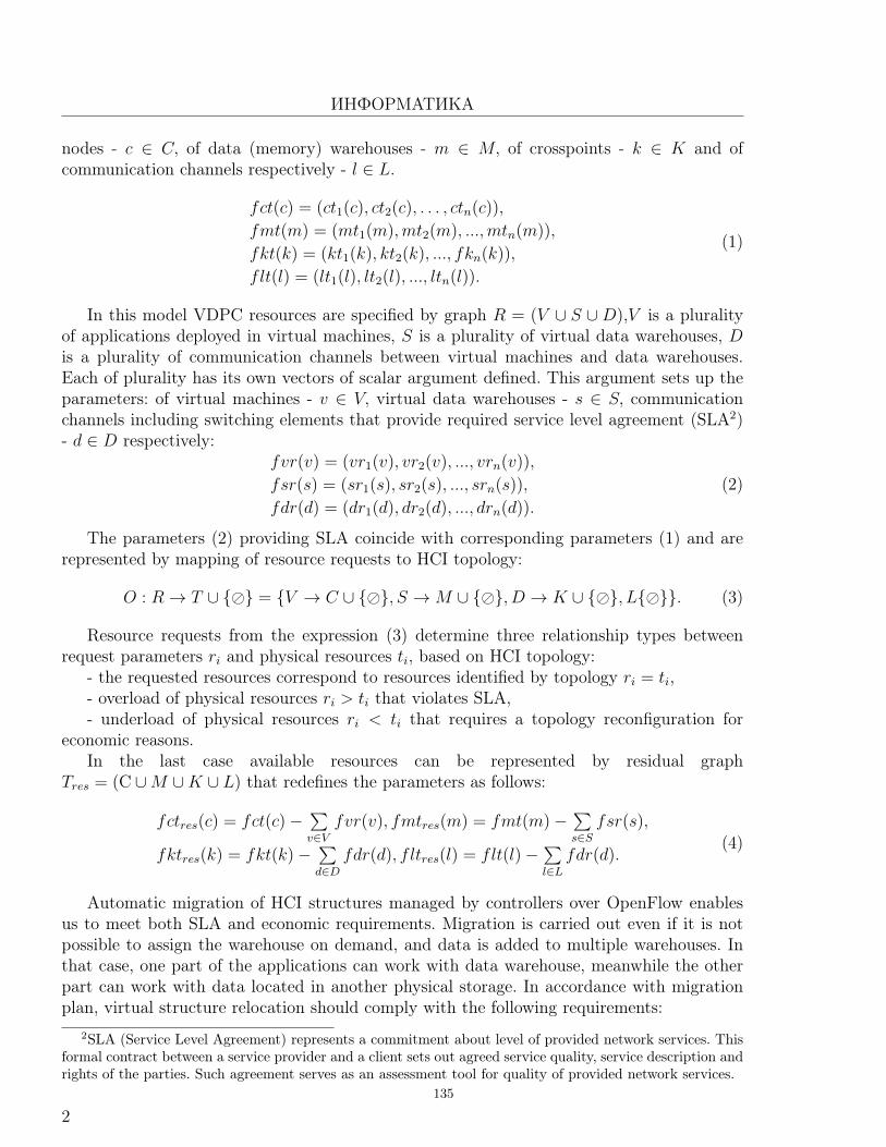
ИНФОРМАТИКА

nodes - c ∈ C, of data (memory) warehouses - m ∈ M, of crosspoints - k ∈ K and ofcommunication channels respectively - l ∈ L.

fct(c) = (ct1(c), ct2(c), . . . , ctn(c)),

fmt(m) = (mt1(m),mt2(m), ...,mtn(m)),

fkt(k) = (kt1(k), kt2(k), ..., fkn(k)),

f lt(l) = (lt1(l), lt2(l), ..., ltn(l)).

(1)

In this model VDPC resources are specified by graph R = (V ∪ S ∪D),V is a pluralityof applications deployed in virtual machines, S is a plurality of virtual data warehouses, Dis a plurality of communication channels between virtual machines and data warehouses.Each of plurality has its own vectors of scalar argument defined. This argument sets up theparameters: of virtual machines - v ∈ V, virtual data warehouses - s ∈ S, communicationchannels including switching elements that provide required service level agreement (SLA2)- d ∈ D respectively:

fvr(v) = (vr1(v), vr2(v), ..., vrn(v)),

fsr(s) = (sr1(s), sr2(s), ..., srn(s)),

fdr(d) = (dr1(d), dr2(d), ..., drn(d)).

(2)

The parameters (2) providing SLA coincide with corresponding parameters (1) and arerepresented by mapping of resource requests to HCI topology:

O : R→ T ∪ = V → C ∪ , S →M ∪ , D → K ∪ , L. (3)

Resource requests from the expression (3) determine three relationship types betweenrequest parameters ri and physical resources ti, based on HCI topology:

- the requested resources correspond to resources identified by topology ri = ti,- overload of physical resources ri > ti that violates SLA,- underload of physical resources ri < ti that requires a topology reconfiguration for

economic reasons.In the last case available resources can be represented by residual graph

Tres = (С ∪M ∪K ∪ L) that redefines the parameters as follows:

fctres(c) = fct(c)−∑v∈V

fvr(v), fmtres(m) = fmt(m)−∑s∈S

fsr(s),

fktres(k) = fkt(k)−∑d∈D

fdr(d), f ltres(l) = flt(l)−∑l∈L

fdr(d).(4)

Automatic migration of HCI structures managed by controllers over OpenFlow enablesus to meet both SLA and economic requirements. Migration is carried out even if it is notpossible to assign the warehouse on demand, and data is added to multiple warehouses. Inthat case, one part of the applications can work with data warehouse, meanwhile the otherpart can work with data located in another physical storage. In accordance with migrationplan, virtual structure relocation should comply with the following requirements:

2SLA (Service Level Agreement) represents a commitment about level of provided network services. Thisformal contract between a service provider and a client sets out agreed service quality, service description andrights of the parties. Such agreement serves as an assessment tool for quality of provided network services.

2135

V. M. Solovyev, A. S. Belousov. Administration of Virtual Data Processing Center overOpenFlow

- there is no SLA violation during relocation;- relocation is implemented at given time constraints. Automatic operation of controllers

enables us to achieve it.Input to migration is a plurality of incoming requests Z = Ri, a plurality of queried

requests W = Ri, a graph of remaining resources Tres, and time constraint on migration τ .During migration, a new node s′ and a virtual communication channel between nodes s ands′ are added to graph of re quested resources R.

The administration of VDPC over OpenFlow is based on a greedy algorithm3 of requestassignment to physical resources, with the use of controller (server) software. Expression (4)describes such a greedy algorithm. As an optimization criterion, the most compact allocationof request elements (2) is applied. A similar approach is widely used in data processing centersand by cloud providers [2, 3]. The quality of VDPC administration depends on selected greedycriteria: next request - KR, virtual node - KV , physical node - KC . Criteria KV and KC relyon cost function defined as a weighted sum of required parameters considering the resourcedeficit. This function represents as follows: d(i) = (

∑R

∑e∈R rr,i−

∑c∈C rc,i)/

∑R

∑e∈R re,i.

Then the cost function of an assignment of element e will appear as r(e) =∑n

i=l d(i)re,i. Inthis equation the selected element HCI is characterized by a vector of values of requiredresource parameters (re,1, re,2, . . . , re,n). To calculate the measure of the resource deficit,firstly, it is necessary to subtract the values of available physical resources for the requiredresource parameter from the common value of this resource parameter in all requests. Thenthe measure is calculated as a quotient of this difference by total sum of required resources.We can define the cost function as weighted sum of required resource parameters consideringthe resource deficit. According to criterion KV , the HCI virtual element with maximum costfunction is chosen. This allows us to assign primarily the most resource-deficient elementsand then assign all the other virtual elements. According to criterion KС, the HCI physicalelement with minimum cost function is chosen. By this, we can ensure maximal utilization(loading) of computing resources. According to criterion KС, the query with the maximumweighted sum of requested resources is chosen.

The general framework of administration algorithm will be as follows.

1. Scheduler4 analyses incoming requests of resources Z = Ri.

2. If plurality Ri /∈ is not empty, the program selects another request Ri accordingto greedy criterion KR. Otherwise, algorithm terminates its functioning.

3. Using the elements of request Ri, the program forms a plurality of virtual nodesU = V ∪ S. Where it is not possible to form a plurality of virtual nodes U , itproceeds to step 14.

4. Scheduler selects another element N from formed plurality of virtual nodes U on thebasis of greedy criterion KV . Then this element is placed in queue Q which containsthe elements awaiting an assignment.

3The greedy algorithm means optimization algorithm based on locally optimal decision that are made ateach stage. Whereby, we assume that the final decision will also prove optimal.

4Scheduler is a program (service) driven by controller software. The principal scheduler function is to startother programs.

3136

ИНФОРМАТИКА

5. Using the elements Ci, scheduler forms a plurality of physical nodes Ci /∈ . Itis possible to assign the element N to these nodes based on correct accomplishmentof mapping (3). Otherwise, if Ci ∈ , program calls the procedure of limitedenumeration.

6. The program selects a physical resource from the formed plurality of physical nodes onthe basis of greedy criterion KC . It redefines the values of physical resources parametersaccording to functions (4).

7. Scheduler selects all virtual channels Di that link element N to elements of request Ri

to be assigned.

8. Scheduler sorts a plurality of channels Di /∈ by value of the capacity in ascendingorder.

9. The program selects a virtual channel Li from a plurality of channels Di. It shouldensure the shortest route that links element N to elements of request Ri. Where it isnot possible to plot the route, it calls the procedure of virtual channel assignment ona physical resource. It redefines the values of physical resources according to functions(4).

10. Scheduler adds to queue Q the virtual nodes linked with N . By this, it follows the orderof virtual channels from sorted plurality Di. These channels connect the nodes.

11. Scheduler deletes N from U and Q.

12. If Q is not empty, program proceeds to step 4.

13. If U is not empty, program proceeds to step 3. Otherwise, if U is empty, programproceeds to step 1.

14. The program cancels all assignments of the elements of request Ri and removes therequest from a plurality Z = Ri. Then it proceeds to step 2.

This algorithm contains two procedures described in [2]. The first one is a procedure oflimited enumeration; the second one refers to a procedure of virtual channel assignment on aphysical resource. A scheduler calls the procedure of limited enumeration if it is not possibleto assign the next virtual node N from a plurality of requests to any physical resource. Thisprocedure analyses a subset of a plurality of physical nodes Ci from a graph of physicalresources. Specified enumeration depth determines the subset capacity; the quantity of viewedsubsets is limited. The program views only subsets whose total quantity of nodes’ remainingresources allows us to assign the current element N . The procedure ensures the execution ofstep 5 if the program changes (selects) the enumeration depth and quantity of viewed subsets.Scheduler calls the procedure of virtual channel assignment on a physical resource when it isnot possible to plot the route that links elementN to element of requestRi via virtual channel.The route searching mechanism is based on modified Dijkstra’s algorithm [4]. However, itcan include only switching elements and communication channels of physical network towhich ratios of mapping accuracy are applied (3). If it is not possible to assign a virtual

4137

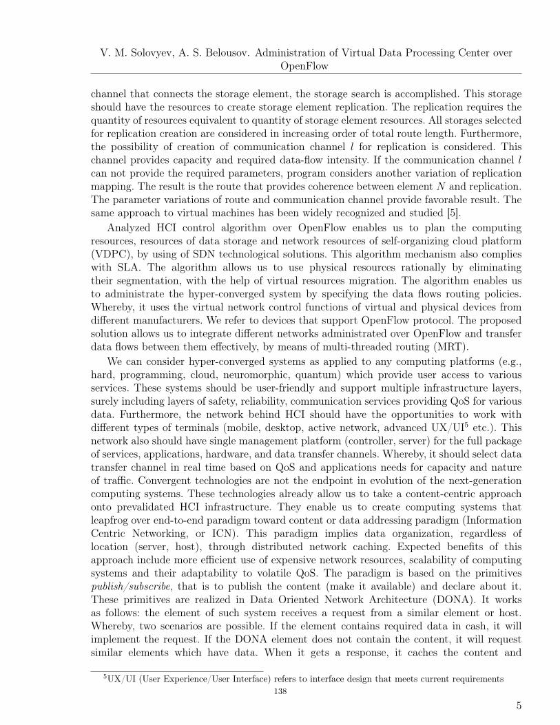
V. M. Solovyev, A. S. Belousov. Administration of Virtual Data Processing Center overOpenFlow

channel that connects the storage element, the storage search is accomplished. This storageshould have the resources to create storage element replication. The replication requires thequantity of resources equivalent to quantity of storage element resources. All storages selectedfor replication creation are considered in increasing order of total route length. Furthermore,the possibility of creation of communication channel l for replication is considered. Thischannel provides capacity and required data-flow intensity. If the communication channel lcan not provide the required parameters, program considers another variation of replicationmapping. The result is the route that provides coherence between element N and replication.The parameter variations of route and communication channel provide favorable result. Thesame approach to virtual machines has been widely recognized and studied [5].

Analyzed HCI control algorithm over OpenFlow enables us to plan the computingresources, resources of data storage and network resources of self-organizing cloud platform(VDPC), by using of SDN technological solutions. This algorithm mechanism also complieswith SLA. The algorithm allows us to use physical resources rationally by eliminatingtheir segmentation, with the help of virtual resources migration. The algorithm enables usto administrate the hyper-converged system by specifying the data flows routing policies.Whereby, it uses the virtual network control functions of virtual and physical devices fromdifferent manufacturers. We refer to devices that support OpenFlow protocol. The proposedsolution allows us to integrate different networks administrated over OpenFlow and transferdata flows between them effectively, by means of multi-threaded routing (MRT).

We can consider hyper-converged systems as applied to any computing platforms (e.g.,hard, programming, cloud, neuromorphic, quantum) which provide user access to variousservices. These systems should be user-friendly and support multiple infrastructure layers,surely including layers of safety, reliability, communication services providing QoS for variousdata. Furthermore, the network behind HCI should have the opportunities to work withdifferent types of terminals (mobile, desktop, active network, advanced UX/UI5 etc.). Thisnetwork also should have single management platform (controller, server) for the full packageof services, applications, hardware, and data transfer channels. Whereby, it should select datatransfer channel in real time based on QoS and applications needs for capacity and natureof traffic. Convergent technologies are not the endpoint in evolution of the next-generationcomputing systems. These technologies already allow us to take a content-centric approachonto prevalidated HCI infrastructure. They enable us to create computing systems thatleapfrog over end-to-end paradigm toward content or data addressing paradigm (InformationCentric Networking, or ICN). This paradigm implies data organization, regardless oflocation (server, host), through distributed network caching. Expected benefits of thisapproach include more efficient use of expensive network resources, scalability of computingsystems and their adaptability to volatile QoS. The paradigm is based on the primitivespublish/subscribe, that is to publish the content (make it available) and declare about it.These primitives are realized in Data Oriented Network Architecture (DONA). It worksas follows: the element of such system receives a request from a similar element or host.Whereby, two scenarios are possible. If the element contains required data in cash, it willimplement the request. If the DONA element does not contain the content, it will requestsimilar elements which have data. When it gets a response, it caches the content and

5UX/UI (User Experience/User Interface) refers to interface design that meets current requirements

5138

ИНФОРМАТИКА

implements the request. This universal mechanism is applicable to any protocol, forminga global single mechanism of caching and content delivery. In addition, this mechanism issupported by all network nodes and aimed at all users, not just ICN users. Such a networkensures content security, not security of its delivery. It relies on a content-based model anddraws on the concept of reputation, because the provider must sign the content, so userscan always define it. Data Oriented Network Architecture interacts well with blockchain6

technology that provides the high reliability of content storage and protection. Network entryis protected cryptographically. Unauthorized entry requires enormous computing resourcesproportional to the network size. It allows us to exclude human or machine error, missedoperations, unauthorized entry etc. In future, over the course of evolution, HCI will employother network technologies.References

1. By Charles Clos. A Study of Non-Blocking Switching Networks (Manuscriptreceived October 30, 1952). Accessed July 4, 2017, available athttp://ieeexplore.ieee.org/stamp/stamp.jsp?arnumber=6770468.

2. Zotov I. A., Kostenko V. A. Resource Allocation Algorithm in Data Centers with a UnifiedScheduler for Different Types of Resources, // Izvestiya Akademii Nauk. Teoriya i SistemiUpravleniya, 2015, 1, pp. 61-71.

3. Meng Xiaoqiao, Pappas Vasileios, Zhang Li. Improving the Scalability of Data CenterNetworks with Traffic-aware Virtual Machine Placement // IBM T.J. Watson ResearchCenter 19 Skyline Drive, Hawthorne, NY 10532. Accessed July 4, 2017, available athttp://ieeexplore.ieee.org/stamp/stamp.jsp?arnumber=5461930.

4. Cormen T. H., Leiserson C. E., Rivest R. L., Stein C. Introduction to Algorithms. CambridgeMA: MIT Press and McGrawHill, 2001. pp. 595–601.

5. Zhao Ming, Figueiredo Renato J. Experimental Study of Virtual Machine Migration inSupport of Reservation of Cluster Resources // Advanced Computing and Information SystemsLaboratory (ACIS) Electrical and Computer Engineering, University of Florida. Accessed July4, 2017, available at http://ieeexplore.ieee.org/stamp/stamp.jsp?arnumber=5483380.

6The revolutionary technology of blockchain was created by Satoshi Nakamoto. This technology helpsto allocate the digital content without its copying. Pertinently, it resembles a digital book whose data andtheir modifications are duplicated in network for several thousands of times and are regularly updated. Thisdistributed database without central storage node is stored in network. It provides its users the hosting,such as Google Docs during collective work. Each group of blockchain transactions is a block, and minersconduct the audit of them (digital content). Therefore, this technology operates with chain of blocks createdby complex cryptographic algorithms.

6139

A Survey of Smart Contract Safety andProgramming Languages

Alexey Tyurin∗, Ivan Tyulyandin†, Vladimir Maltsev‡, Iakov Kirilenko¶ and Daniil Berezun∥

Mathematics and Mechanics FacultySaint Petersburg State University

University Embankment, 7, 199034Saint Petersburg, Russia

∗a.tyurin@2016.spbu.ru, †i.tyulyandin@2015.spbu.ru, ‡v.maltsev@2016.spbu.ru,¶y.kirilenko@spbu.ru, ∥danya.berezun@gmail.com

Abstract—Blockchain technologies are gradually being foundan application in many areas, especially in FinTech. As a result,a lot of blockchain platforms have emerged with the support ofsmart contracts that are intended to automate party interactions.However, it has been shown that they are prone to attacks anderrors which lead to money loss. To date, there has been awide range of approaches for making smart contracts safer thatincluded analysis tools, reasoning models, and safer and morerigorous programming languages.

In this paper, we provide an overview of smart contractprogramming languages design principles, related vulnerabilities,and future research areas. The provided overview is meant tooutline the to date state of languages and to become a possiblebasis for future proceedings.

I. INTRODUCTION

Initially, blockchains were designed for cryptocurrencymanagement based on transactions. Further such systems in-volved smart contracts usage to enhance transactions, makingthem more sophisticated. This enabled to move part of anapplication logic into the blockchain, thus allowing to providecustomizable redeeming conditions [1], develop crowdfundingsystems [2], and other applications based on blockchain tech-nology [3]. Fundamentally smart contracts are programmableobjects beyond blockchain, intended to represent automatable1

and enforceable2 agreements [4].Since smart contracts are essentially programs that are

executed within blockchain and written in some programminglanguage, bugs and errors are possible. Erroneous transactionbehavior can lead to a financial damage. For example, a not-reentrancy of a function has caused $40 million loss [5].Moreover, due to the immutable nature of the blockchain, it isoften impossible to fix a contract with a bad3 behavior that isalready on the chain, i.e. contracts are irrevocably committed.One possible approach to detect such unwanted behaviors andminimize the number of vulnerabilities is to provide a way toformalize smart contracts properties and vulnerabilities. It will

1 “Automatable” rather than “automated” since parts of an agreement mayrequire some human input.

2 Enforceable either by law or by tamper-proof computer code.3 Here, by a “bad” contract behavior, we mean any behavior that is

unexpected or undesirable by the contract owner, caused by any reason.

help to specify vulnerabilities sources and facilitate reasoningabout smart contracts.

In [6] provided by IOHK research4, an ontology thatprovides a set of basic conceptual primitives is specified. Itcan be used to construct desired propositions about smartcontracts. It is not intended to be the only true ontology,rather the useful one. According to the ontology, blockchainbased smart contracts can be considered as computations overblockchain state, that include the changing over time stateitself as well as a transition function. And we will furtherrefer to modality properties as to relationships between states,possibility or necessity properties that should be maintainedthroughout transitions.

These concepts allow thinking about smart contract behaviorabstractedly over details. For example, consider a Deadline-dependent Transfer, a smart contract controlling propertytransfer between recipients5. Only Recipient 1 may transferthe Item during some time interval prior to the deadline, whileonly Recipient 2 may transfer the Item once deadline hasbeen passed. A modality property can be formulated in thefollowing way. There always should be a blockchain statewhere at least one system participant who controls the Item,being transferred, exists, i.e. the absence of dead states in theblockchain.

Unfulfillment of those properties in blockchain based smartcontracts may lead to money loss and malicious attacks. Forexample, a vulnerable sequence of smart contract library callsin PARITY wallet led to $150 million freezes on wallets [7].

State inconsistency and weaknesses may be caused bya number of different reasons such as blockchain-specificbehavior, execution environment bugs, a model of underlyingprogramming language that is not amenable to proof con-structions, non-intuitive representation of programs in lan-guages with good models, unintuitive semantics of underlyingprogramming language for people who lack programmingexperience etc [8]. Also, some modality properties may neverbe proved because of possible non-termination of a program,which basically depends on a certain programming language.

4 IOHK company is one of the main customers of research in peer-to-peernetworks. See https://iohk.io/about/ for details.

5Between users or other smart contracts

140

Thereby, to make smart contracts secure it is desirableto be able to specify the intended behavior and propertiesthat they should fulfill. These properties fulfillment can beprovided with machine-checkable proofs and facilitated withmore intuitive programming languages accompanied by toolsfor static analysis and formal verification to reduce the numberof errors.

To date, various approaches, languages, and tools have beenproposed: extensive type systems and various programmingparadigms [9], programming languages that have easilychecked termination conditions [10, 11], high-level languagesthat encourages safer programming via abstractions [12, 13],and intermediate and low-level languages that ease formalverification and compilers development [14–16].

Smart contract programming languages design is influencedby domain ontology, encountered vulnerabilities and ease ofreasoning about modality properties. So, in this paper, weconcentrate on the incorporation of known approaches usedin design and development of smart contracts programminglanguages, proceed through vulnerabilities and domain specificconcepts that have been considered during design process,provide a classification of current efforts, and emphasize topicsfor future research.

The paper is organized as follows. Section II provides ashort evaluation of similar works. Section III gives a briefsummary of blockchain architecture principles relevant to lan-guages and tools design. Section IV describes known vulnera-bilities of smart contracts, classifying them for future analysis.Section V provides a survey of smart contract programminglanguages and their design ideas and principles, according toknown vulnerabilities and blockchain architectures. In sec-tion VI we discuss possible research gaps and future work.Section VII concludes the paper.

II. RELATED WORK

Surely this paper is not the only one surveying smartcontract programming languages, and we are aware of a coupleof similar works.

So, [17] provides an overview of smart contracts program-ming languages, security properties, and verification methodsalong with some classification of them. However, despite agood coverage, the proposed survey is rather superficial ina sense that it describes languages through specification oftheir features, not going deep into design foundations that haveprovided the features.

Another work [18] gives an overview of some distributedledger systems, smart contracts languages, and technologiesthat might facilitate safety and performance, or make newapplications possible. The paper is not aimed entirely atlanguages, hence it leaves the description without design foun-dations and any classification according to whether desirableproperties or design principles.

[15] also contains some overview of existing languages andtheir features, but the survey is performed from the perspectiveof comparison between them and the language proposed in thepaper.

In contrast, this work is intended to enhance languagecoverage, provide foundations and intuition for reasoning,classification of languages, properties, and design fundamen-tals along with vulnerabilities that have influenced them.

III. BACKGROUND

Since smart contracts are computations on a blockchain,underlying blockchain protocol basically sets the path forlanguage and tools design. In this section, we review afew protocol details that influence further development oflanguages. Substantially there are two widespread blockchainarchitectures on top of which smart contracts are built todate — UTxO-based and account-based blockchains, thatallow stateless and stateful smart contracts respectively.

A. UTxO

Unspent transaction output, UTxO, model was introducedwith the emergence of BITCOIN blockchain. A typical BIT-COIN transaction contains a list of inputs that specifies thefunds that the transaction issuer can transfer and a list ofoutputs, that represent the way these funds are intended to betransferred. Each output can be used as an input for anothertransaction. For example, an issuer can set the amount ofcurrency for each output or specify conditions, under whicha possible receiver of funds can spend them, also they canspecify themselves as the receivers to get so-called change. Aset of UTxO consists of all transactions outputs that have notbeen yet used as inputs.

Redeeming conditions for transaction outputs in BITCOINare defined with programs written in BITCOIN SCRIPT [10].These programs describe properties that must be satisfied forthe redeemer to be able to use these transaction outputs astheir transaction inputs in order to spend the credits. Thespender should provide input values to each locking script ofreferenced outputs of previous transaction such that all scriptsevaluate to t r u e , e.g. they may provide their wallet addressand transaction signature to verify authority.

Such scripts are stored within transactions and are beingmaintained only during a transaction, thus they have no state.Further scripts have limited access to blockchain data andessentially they are pure stateless functions of transactiondata, i.e. of input parameters. Despite limitations, scriptsalong with transaction signatures can express complex re-deeming conditions such as multi-signature payments, depositproviding, escrow, and dispute mediation, access to externaldata using oracles, time-locks, payment channels, cross-chainatomic trades etc [19]. Throughout the paper, we regard thesescripts as stateless smart contracts.

B. Account-based blockchains

Account-based blockchains maintain an explicit statethroughout transactions. A state is a mapping between accountaddresses and balances. Within these blockchain systems, eachtransaction is a mapping between the states. Basically, thesesystems are transaction-based state machines.

141

ETHEREUM is an example of such a system [20]. InETHEREUM smart contracts are similar to users’ accounts ina sense that they have their own address and a balance. Smartcontracts are stored inside the blockchain and essentially thesecontracts are lists of functions that can be invoked throughusers’ transactions or other contracts messaging. These func-tions are defined with bytecode of the corresponding executionenvironment called Ethereum Virtual Machine, EVM. Sinceany smart contract has a balance, it is a stateful function of adata transaction (or a message) and blockchain state, in whichthe transaction takes place, so they can write to blockchainstate or read from it. Contracts state typically involves a storedamount of currency. However, in general, it can have arbitrarypersistent storage that is maintained throughout the transitionsof the blockchain.

C. Preventing the Denial-of-service attacks (DOS)

Despite the underlying blockchain model, smart contractsare computations that are replicated over blockchain viaconsensus protocol. To prevent DOS-attacks the number ofcomputations for every program representing a smart contractshould be restricted beforehand. Restriction mechanism de-pends on the underlying programming languages properties.One of the main properties in the context of smart contractsis halting, i.e. whether every program that has been writtenin it terminates or not. BITCOIN SCRIPT program alwaysterminates since language is not Turing-complete and it doesnot have loops, or recursion, or any other mechanism thatprovides infinite computations. However, the size of a programalso affects the performance of the system behind it. ThusBITCOIN SCRIPT programs are limited by the stack size andnumber of computationally heavy instructions, i.e. transactionsthat contain a script that does not satisfy restrictions arerejected.

For programs written in languages that do not guaranteeprogram termination, e.g. EVM bytecode, program executionis limited via a gas system. Gas is basically an amount ofcryptocurrency specified for contract execution. Fixed unitsof gas are charged to a miner for every instruction beingexecuted. If the specified amount of gas is expired, executionof the contract stops. Furthermore, EVM contracts also havea limited stack size.

IV. SMART CONTRACT WEAKNESS

In this section, programming language-level vulnerabilitiesthat may cause unfulfillment of modality properties and possi-ble mistakes are classified. It is worth to notice, that the mostcommon property arising in distributed systems is that resultsof computations should be deterministic. While many smartcontract programming languages have been designed with de-terminism in mind, sometimes general purpose programminglanguages are used for development [21]. A detailed overviewof potential risks of non-determinism and causes can be foundin [22].

We consider SOLIDITY language for stateful contracts, sinceit is the most popular smart contract programming languages

and generally it was one of the first languages that revealedsuch weaknesses, unfortunately on its own instance. Despiteoriginally being known as unsafe, the language is evolvingand to date its compiler is able to warn about code that mightmisbehave. However, Solidity has provided the foundation forthe design of other languages. The most famous errors thathave caused contracts failure are DAO [5] and PARITY [23].

SOLIDITY vulnerabilities are classified in the followingsubsections based on what level they occur on and the reasonsthat cause them. Code examples of the weaknesses could befound in [20, 24–28]. Possible attacks are discussed in [29].Also, it is worth to mention, that SOLIDITY is a Turing-complete language, meaning that in general fulfillment ofparticular modality properties can not be proved, even despiteguaranteed termination due to gas limit.

A. Block content manipulation

Block of transactions in blockchains is formed by one of theparticipants who have the ability to influence block content.Thus, careless blocks handling may cause a number of errors.

Front-Running (Transaction-ordering dependence): It is im-portant to be careful of transactions order. For example, Alicehas deployed contract with possibility to sell a product and seta price for it. Bob wants to buy the product, and Alice wantsto set a higher price. Let’s assume, they want to do it at thesame time. If Bob’s request is the first, Alice loses money. Inanother case, Bob’s transaction can be rejected, or Bob willspend more money than he expected.

Weak sources of randomness: Random values should bedeterministic for all nodes in the network due to consensusconsiderations. One way to get randomness is to use pseudo-random values. Variables of contract, even the private ones,meta-variables of a block, or a hash of a previous andnext block cannot be used as a source of entropy. In someblockchains (including ETHEREUM) it is possible to haveinfluence over these variables during the validation process. Apseudo-random value in smart contract code can be predictedby a malefactor. Precalculation can be done via code analysis.

B. Contract interaction

A smart contract should be able to interact with othercontracts. The following vulnerabilities appear due to the factthat smart contracts cannot rely on of each other’s behavior.

Unchecked return values for low-level calls: There arethree functions to send ether [30] from account to account inETHEREUM: send ( ) and c a l l ( ) that return f a l s e if an erroroccurs but the transaction execution continues, and t r a n s f e r( ) that rolls back the transaction in case of error. Low-level functions c a l l c o d e ( ) and d e l e g a t e c a l l ( ) behave inthe same way as functions send ( ) and c a l l ( ) . Thus handlingof f a l s e value of corresponding functions is needed to avoidundesirable behavior of contract. According to Luu et al. [31],27.9% of smart contracts in ETHEREUM blockchain do notcheck returned values.

142

Reentrancy: An external contract can call back functions ofa caller contract before the first invocation has finished. It canlead to undesirable recursive function interactions and allowthe callee contract to take over the control flow. The exampleof this vulnerability is a famous DAO smart contract [5].

Callstack bound: A failure may occur when an external callis made, but the program stack has reached its limit. Stackoverflow is possible in smart contract languages. In EVM callstack is limited to 1024 stack frames. If the exception is notproperly handled by a contract, the malefactor can use it toattack.

C. Resource limits

If the smart contract language is Turing-complete, there isa need in metering6 mechanism to prevent infinite execution.ETHEREUM charges a fee, named gas. Amount of gas isproportional to the number of executed commands by EVM.Every transaction in bounded with maximum amount of gasas well as blocks.

Infinite loops: Mistakes and misprints in operators usagemay keep contracts syntactically correct but strongly affecttheir logic. For example, writing =+ instead of += in a loop ter-minating condition may lead to unexpected program behaviorand even to an infinite loop. Moreover, in this case, excessivegas consumption may occur. It also includes situations whenthe number of memory addresses being used are significantlyincrease, e.g. when the number of elements in a map grows,it becomes too expensive to iterate over it.

D. Arithmetics

In SOLIDITY arithmetics is available on unsigned integersonly and the language does not provide any arithmetic op-erations check for correctness. This class of mistakes mostlyrefers to common programmer errors. In the case of smartcontracts, they may lead to a huge loss of assets. Thus, it iscommon to consider them as vulnerabilities in order to attractprogrammers attention.

Overflow and underflow: These vulnerabilities arise be-cause numbers can have a fixed size. In case of ETHEREUM,maximum value for u i n t ( u i n t 2 5 6 ) is 2256 − 1 and mini-mum — 0. A programmer has to manually checks overflowand underflow.

Floating points and precision: SOLIDITY does not havefixed and floating point types. Instead, a programmer has toemulate them via integers. All integer divisions are roundeddown. Careless handling of such operations may cause unex-pected program behavior.

E. Storage access

The following vulnerabilities are caused by negligent mem-ory usage and access.

Uninitialized storage pointer: Local structures, arrays, andmaps link to storage zero address by default. Using of theseobject without initialization will lead to overwriting whateveris in zero address.

6Metering is a way to limit and charge the execution of a smart contract.

Write to an arbitrary storage location: A smart contract canstore some data and wrong variable assignment can break it.SOLIDITY has reference types. Mistake with references canlead to internal state corruption. If an array index is out ofrange, the exception will be thrown, and the smart contractwill be reverted.

F. Internal control flow

This class of vulnerabilities is caused by a complex controlflow graph structure and an ability to manipulate it.

Using of inherited functions and variables: It is possible touse inheritance in smart-contracts languages with the object-oriented paradigm. SOLIDITY allows multiple inheritance. Ifseveral super-classes have a method or variable with the samename, their behavior in sub-class depends on the inheritanceorder. It could shadow previously defined values or functionsand lead to undesirable results.

Using of built-in functions: Programmers should be awareof using built-in functions and their behavior. E.g., someonewould like to use assertions to check program invariant.SOLIDITY a s s e r t ( ) function is intended for this purpose. Incase of failure, this method throws an exception and doesnot return the remaining gas. Thus, to check for changingvalues, such as input data, it is recommended to use r e q u i r e( ) statement which in the same case does transaction rollbackand returns remaining gas.

Using of deprecated functions: It is not clear what newcompiler versions do with deprecated functions. Therefore, itis not recommended to use these objects.

Locked assets: Contracts should provide a way to manageassets. Suppose in the example the contract has a method totake assets but does not have code to give them back. Dueto smart contract code immutability in blockchain history, itis impossible to upgrade or fix this contract. It will causeproperty loss.

G. Authorization

Authorization is a major part of a person identificationmechanism, designed to verify the permission for actions.Incorrect or insufficient authorization can lead to the followingvulnerabilities.

Incorrect initialization: When smart contract was deployedto a blockchain, it should be initialized. Often initializationcontains sensitive operations such as a setting contract’s owner.An error in this action may violate the logic of the smartcontract. In SOLIDITY, the constructor is a special function,which is called once to set contract’s state. In new SOLIDITYversions, constructors are denoted by a special keyword thatmade the definitions more obvious. But in earlier versions (lessthan 0.4.22) constructor is just a function with the same nameas the class has. Thus, a typo in constructors’ name makes it ausual function, which can be called by anybody since defaultmodifier for function is public.

143

Function default visibility: Incorrect access modifiers usageor a lack of them can lead to undesirable behavior. Forexample, calling the function that changes the contract ownerwith public access modifier allows everyone to become itsowner. Default modifier for SOLIDITY is p u b l i c . Thus, it isstrongly recommended to explicitly define visibility for allfunctions and variables.

V. SMART CONTRACT LANGUAGES

In this section, smart contract languages are consideredwith respect to their main features, paradigms, and commonproperties such as Turing-completeness, metering mechanism,reasoning, type system, code analyzers, etc. To reduce thenumber of subsections we have classified languages withrespect to their level of usage.

Low-level languages: These languages are designed fordirect execution by the underlying execution environment.Most concepts and principles of formal semantics, computa-tional model, metering, logic for reasoning about programs,and typing are often introduced on that level. Furthermore,to date, smart contracts are mostly stored on the blockchainin low-level bytecode, which imposes suitability considera-tions. Examples of such languages are BITCOIN-SCRIPT [10],EVM [32], MICHELSON [33].

High-level: Languages with the idea of making the writ-ing of contracts easier for developers via readability and saferhigh-level syntactic constructs enhanced by a type system thatprovides machine services abstractions. Safety aspect appearshere and refers to the languages ability to guarantee theintegrity of these abstractions and abstractions introduced bythe programmer using definitional facilities of the language. Ina safe language, such abstractions can be used abstractly whilein an unsafe language they cannot: in order to completelyunderstand how a program may (mis-) behave, it is necessaryto keep in mind all sorts of low-level details such as the layoutof data structures in memory and the order in which they willbe allocated by the compiler. [34]. The semantics of both levelsshould be considered here7 Examples of such languages areSOLIDITY [35], FLINT [12], and LIQUIDITY [36].

Intermediate-level: Languages that present a compromisebetween a high-level source and low-level target languages. Asa general rule, they are designed in order to simplify programverification or static analysis, relying on the computationmodel, type system, reasoning, semantics, etc. Furthermore,they allow unification of compilation, i.e. providing a languagethat can be compiled for different platforms. SCILLA [15] isan example of such a language.

It is also useful to emphasize some desirable language prop-erties that affect language design.

• Reasoning — language behavior model should allow tospecify modality properties and facilitate proving of their(un-) fulfillment. Underlying calculus model and typesystem are aimed at this.

7 Fundamentally safeness spreads to other levels since low-level languageis an abstraction of its implementation, e.g. a virtual machine.

• Safety — language abstractions should hold integrityproperty. Rigorous semantics promotes this.

• Expressivity — basically language should be expressiveto fit possible various range of use cases.

• Readability — language representation of a contract be-havior should be intuitive, i.e. be easy to inspect and writewith.

Every smart contract language has domain specific instruc-tions or/and types, e.g. cryptographic primitives, assets types,messaging instructions. So we will not emphasize this aspectmuch. Notable features and models of several languages withrespect to desirable properties are discussed below while asummary of a more expanded set of languages is presented inthe table on the Fig. 1.

A. Low-level languages

1) BITCOIN SCRIPT: is an untyped8 stack-based low-levellanguage for stateless smart contracts development in BITCOINand handles transaction verification process. It is intentionallynon-Turing-complete with the restricted instruction set wheresome opcodes are removed e.g. multiplication, division, stringsoperations, bitwise logic, due to possible overflow vulnerabil-ities and implementation bugs. Everything is allocated on thestack of limited size words while a program has access tosome transaction fields e.g. a hash of transaction data, timefield. Thus every program is a pure function of transactiondata, i.e. transactions are self-contained.

To our knowledge, BITCOIN SCRIPT has no formal seman-tics, which makes metering ad-hoc and does not enforce formalverification. Furthermore, its stack-based nature and bytecodemake smart contracts less auditable since only bytecode isstored inside transactions. Metering is performed via expensiveoperators counting and script size evaluation. However script’sinput is arbitrary, hence BITCOIN SCRIPT allows specifica-tion of redemption properties like signature checking, pay-to-public-key-hash, pay-to-script-hash, multisignature checking,and arbitrary data storage inside transactions [1, 10, 48].

2) SIMPLICITY: is designed for extending BITCOINSCRIPT capabilities. It is intended to enhance expressiveness,while enabling static analysis that allows to efficiently boundthe number of computations, maintaining BITCOIN SCRIPTdesign of self-contained transactions, and providing formal se-mantic to facilitate reasoning about programs. It is anticipatedto be used as a compilation target for high-level languagesand deployed to sidechains [49]. SIMPLICITY is a typed non-Turing-complete combinator-based language with terms basedon Gentzen’s sequent calculus. Every SIMPLICITY type isfinite: it contains finitely many values. Hence SIMPLICITYdoes not support recursive types and can express only finitaryfunctions.

The core of SIMPLICITY consists of nine combinatorsfor term construction with a corresponding denotational se-mantics. The language is formalized in COQ as well as a

8 More precisely stack operates with byte vectors, which can be interpreteddepending on opcode.

144

Language Level Currentstate

Project Paradigm / in-fluence

Analyzers Metering Turing-completeness Main features

Bamboo high-level alpha(experi-mental)

Ethereum functional EVM bytecodeanalyzers1

gassystem yes program behaves as a state

automata

BitcoinScript

low-level under de-velopment

Bitcoin stack-based,reverse-polish

no2 script size no Forth-like syntax, any pro-gram always terminates

Chaincode high-level stable HyperledgerFabric

generalpurposelanguages

no2 timeout yes GO, NODE.JS and JAVAextensions for smart con-tracts

EOSIO high-level stable EOS.IO object-oriented,staticallytyped

no2 boundsystem3

yes C++11 library

EVMbytecode low-level stable Ethereum stack-based EVM bytecode

analyzers1

gassystem yes well researched

Flint high-level alpha Ethereum contract-oriented, typesafe

EVM bytecodeanalyzers1

gassystem yes Swift-like syntax, safety

IELE low-level prototype Ethereum register-based tools generatedby K [37]

gassystem yes generated from formal

specification, LLVMIR-like syntax, safety

Ivy high-level prototype(experi-mental)

Bitcoin imperative no2 gassystem no can be compiled to Bit-

coin Script

Liquidity high-level under de-velopment

Tezos fully-typed,functional

underdevelopment

gassystem yes OClaml-like syntax, com-

piled to Michelson ac-cording to formal seman-tics, safety

LLL intermediate-level

under de-velopment

Ethereum stack-based EVM bytecodeanalyzers1

gassystem yes Lisp-like syntax, a wrap-

ping over EVM bytecode

Logikon high-level expe-rimental Ethereum logical-

functionalEVM bytecodeanalyzers1

gassystem yes translated to Yul

Michelson low-level under de-velopment

Tezos stack-based,strongly typed

Typechecksystem

gassystem yes programs can be verified

with Coq

Plutus(PlutusCore) high-level

(low-level)under de-velop

Cardano functional no2 gassystem yes Haskell-like syntax, for-

mal specification

Rholang high-level under de-velopment

RChain functional no2 rule reduc-tion system4

yes concurrent, Scala-likesyntax, based on rho-calculus

Scilla intermediate-level

under de-velopment

Zilliqa functional Scilla-checker gas system no5 embedded in Coq, formalspecification

Simplicity low-level under de-velopment

Bitcoin functional,combinator-based, typed

Bit Machine Bit Machinecell usage

no formal denotational andoperational semantics

Solidity high-level stable Ethereum staticallytyped, object-oriented

EVM bytecodeanalyzers1,SmartCheck [38],ZEUS [39],Solidity* [40]

gassystem yes JavaScript-like syntax,

popularity

SolidityX high-level beta Ethereum secure-oriented

EVM bytecodeanalyzers1

gassystem yes compiled to Solidity

Vyper high-level beta Ethereum imperative EVM bytecodeanalyzers1

gassystem no Python-like syntax, safety

Yul intermediate-level

under de-velopment

Ethereum object-oriented

EVM bytecodeanalyzers1

gassystem yes intermediate language for

future Solidity

Fig. 1. Smart contract languages1 Programs can be translated to EVM bytecode, and then OYENTE [31], SECURIFY [41], EVM* [40], KEVM [42], MYTHRIL [43], VANDAL [44], RATTLE [45],

MANTICORE [46] can be applied.2 To our knowledge there is no analyzer, which works with that smart contract language.3 Based on the amount of EOS tokens, more tokens — more computation power.4 Applying one reduction rule of rho-calculus [47] costs some value, paid by user.5 Any in-contract computation within a transition terminates, however non well-founded recursion in SCILLA can be implemented with contracts calling

themselves or via explicit continuations, i.e. blockchain level interaction. Loops constructs are planned to be implemented via well-founded recursivefunctions.

145

correctness of some functions built up from combinators, e.g.half-adder or SHA-256 function. Generally, the completeness,i.e. the notion that any function between SIMPLICITY typescan be expressed with combinators, is verified in COQ.

Further, operational semantics of SIMPLICITY is definedwithin the abstract machine called BIT MACHINE, intended toease bounding of the number of computations, i.e. metering.It is designed to crash at anything that resembles undefinedbehavior. BIT MACHINE is an abstract imperative machinewhich state consists of two non-empty stacks of data framesformed by an array of cells. The machine has a set ofinstructions that manipulate the two stacks and their dataframes, and corresponding operational semantics is definedby translating a SIMPLICITY expression into a sequence ofBIT MACHINE instructions. It allows computational resourcesmeasuring with respect to cells and frames, e.g. the numberof executed instructions, copied cells, maximum cells in bothstacks at the given point, the number of frames in both stacks.Operational semantics correctness and its correspondence tothe denotational semantics are verified in COQ. Furthermore,the set of core combinators can be extended for implementinga signature checking that requires transaction data, thus SIM-PLICITY programs can be built to implement the pay-to-scripthash scheme [50].

Summarizing, SIMPLICITY stateless nature and rather sim-ple functional semantics without recursion and unboundedloops facilitate equational reasoning, avoiding complex logic.It provides means for formal verification of programs aswell as static analysis more capable to effectively bound thenumber of computational resources. To date SIMPLICITY hasa HASKELL implementation under development [51].

3) EVM: is a bytecode language for Ethereum VirtualMachine. It is designed to support and execute arbitrarycomputations over ETHEREUM account-based blockchain, i.e.programs with loops and recursion.

EVM is a stack-based, Turing-complete machine of 256-bit words with memory model of word addressed byte array.The machine also has a persisted storage which is maintainedbetween transactions and is a part of the blockchain state. Itis a word-addressable word array. Program code is separatedfrom data. Access to and modification of data in different typesof memory is charged differently from storage — the mostexpensive to stack and memory being equally charged. Theformal execution model and the environment is specified inETHEREUM Yellow paper [32].

There are efforts on specifying formal semantics for EVMin OYENTE [31], F* [52], KEVM [42], and LEM [53] thatfocus on formal verification tools and detecting and avoidinginsecure features of EVM, e.g. delegatecall, overflows, unde-fined call/return. Also, the poor human-readability of bytecodeis a flaw. ETHEREUM includes many implementations ofEVM, e.g. in JAVA SCRIPT, C++, PYTHON, and a promisingWEBASSEMBLY implementation [54].

4) IELE: is a language defined within K-framework9 [14].It was designed to overcome EVM drawbacks with an idea ofcorrectness by construction and formal verification in mind.It is intended to be secure and human-readable and to serveas a compilation target for high-level languages, thus unifyingcompilers construction.

IELE is a register-based untyped10 language: instructionsoperate on and store their output in infinite number of virtualregisters and have access to a persistent storage — theunbounded sparse array of arbitrary-precision signed integers.The language implementation is generated from its formalspecification defined in K-framework, which provides genera-tion of verification tools, debugger, interpreter, model checker,etc. IELE has functions and defines a call/return conventionwhere a called function expects a specific number of parame-ters and returns a specific number of values or correspondingerror status.11 Furthermore, IELE avoids some insecure EVMfeatures, e.g. by introducing delegatecall functionality andmaintains arbitrary-precision arithmetic. Its operational seman-tics specifies contracts internal state, blockchain state, andtransition rules, i.e. contract’s code, intra-contract call stack,remaining gas, and the state of the local memory and virtualregisters, storage content, balances, etc. Thus IELE makesformal verification less tedious, enhances human-readability,eliminates undefined, and implementation-defined behaviors,i.e. it is considered to be safe12.

Gas costs for computation time are based on instructionsasymptotic and the gas cost for memory is based on peakmemory consumption. Gas model is designed to allow arbi-trarily large valued instructions and to avoid artificial limitson the size of data or call stacks while preserving the existinggoals of the EVM gas model. However, while arithmetics maycause overflows in EVM, in IELE it may cause out-of-gasexception, starting from some input size. Gas formulas arealso specified in K.

5) MICHELSON [33, 55]: is a typed stack-based languagedesigned to be on-chain code for stateful smart contracts inTEZOS. It is intended to be a more readable compilation targetand more amenable for formal verification.

A MICHELSON program supports high-level types (e.g.map, list, set, etc.) and receives an input stack with parametersand storage being pushed on. It evaluates to a result stack withan output value and new storage, or can fail. The language doesnot support closures in a sense that every functions has emptyenvironment. Messaging with other contracts is performedthrough passing a storage and not maintains the stack betweencalls. The types are predefined13 and monomorphic, further

9Framework used to produce implementation derived from formal specifi-cations, based on logic rules.

10 Arbitrary-precision signed integers is the main datatype.11For reference, in EVM caller sends an arbitrary byte stream containing

the call arguments values since functions are represented as a set of JUMPlabels.

12 IELE is stated to be the first real-world language, that is designed andimplemented using formal semantics, with a zero gap between the formalspecification and the implementation.

13 A programmer can not define their own types.

146

types of input, output, and storage of a contract are fixedand it is statically ensured that resulting storage type ispreserved. MICHELSON has a builtin type for cryptocurrencyand operations defined for this type are mandatory checkedfor underflow/overflow. Typing is done via types propagation.

Due to its computation model, MICHELSON has a straight-forward semantics, based on rewriting rules defined on stackand syntax. Also, it defines what is considered as well-typedstacks and the resulting outputs. MICHELSON is currentlyimplemented in OCAML via GADT with an interpreter de-fined corresponding to the semantics while leaving the typechecking to OCAML. It is anticipated to replace current im-plementation with a one verified with either COQ or F* [56].

6) PLUTUS CORE: is a typed language designed for use asa transaction validation language in UTxO-based blockchainsystems. Fundamentally it is eagerly-reduced higher-orderpolymorphic λ-calculus extended with iso-recursive types,higher kinds, and a library of basic types and functions, henceit has a straightforward operational semantics. The languageis meant to be a compilation target, since it is difficult to writeand read but it is intended to be formally verifiable in proof-assistants.

PLUTUS CORE program is a closed term, and its executionis performed by (possibly non-terminating) reduction of well-typed terms. All types can be normalized and normalizationprocess always terminates. Further, operations on types allowto deal with sized types, i.e. sized integers or bytestrings, thatallows them to be tracked in the type system to facilitatecharging for the appropriate amount of gas and detectingoverflows at the type level. The language has a specifiedabstract machine intended to be amenable for a verificationreference implementation. Moreover, PLUTUS CORE has itsformal specification defined in K [57, 58].

Transaction validation is performed similarly to BITCOINSCRIPT. Validation is successful if the PLUTUS CORE programreduces to a non-error value within an allotted number of steps.But it is more extended in a sense that a program has a read-only access to world state passed through a monad [59, 60].

PLUTUS CORE is an on-chain language for CARDANOblockchain and is embedded into HASKELL. Furthermore theblockchain system itself is implemented in HASKELL as wellas off-chain computations, e.g. wallets, it allows type checkingon the level of the interaction between off-chain applicationsand on-chain code.

B. High-level languages

1) SOLIDITY: is a very rich and expressive high-levelobject-oriented Turing-complete language [35] for writingsmart contracts for EVM with a syntax similar to JAVASCRIPTand C++. It has static types, inheritance, libraries, complexuser-defined types supporting, and other features. As a conse-quence, that causes its prevalence as well as a large numberof potential vulnerabilities (see section IV).

2) SOLIDITYX: is a high-level language [61] which com-piles to SOLIDITY. SOLIDITYX is a secure-oriented language,which means that it has a defense from some vulnerabilities

by default, for example, all access modifiers are private bydefault. However, SOLIDITYX is in beta development nowand it is not recommended to be used in production.

3) VYPER (aka VIPER): is a high-level language for im-plementing smart contracts for the EVM [13]. It is PYTHON3derived programming language. VYPER is an alternative toSOLIDITY that is aimed at code security, clarity, and unam-biguity, for example, it excludes constructions that can leadto misleading code. To achieve this VYPER does not supportmodifiers, class inheritance, inline assembly, function over-loading, operator overloading, recursive calling, infinite-lengthloops, binary fixed point. The language also leverages overflowchecking, array bounding, and limited state modification.

4) FLINT: is a high-level statically-typed contract-orientedlanguage aimed to write robust smart contracts on EVM [12].FLINT provides a mechanism to specify actors that can interactwith a contract, immutability by default, assets types, and safersemantics with overflows causing revert of a transaction andexplicit states.

5) BAMBOO: is a high-level language compiling to theEVM [62]. Its compiler is implemented in OCAML thusBAMBOO is well amenable to formal verification. BAMBOOcreates clarify state transitions and avoids reentrancy problemsby default. However, it does not support loops and assignmentsinto storage variables, except array elements, which improvesthe ability of contracts to be verified but complicates theirdevelopment.

6) LOGIKON: is a high-level logical-functional languagecompiled to YUL [63]. LOGIKON program represents a set oflogical constraints statically and formally verified.

7) IVY: is a language [64], designed to simplify program-ming of stateless smart contracts for BITCOIN. Compare toBITCOIN SCRIPT, in IVY program it is possible to use namedvariables, named clauses, domain-specific types, syntax sugarfor function calls.

8) LIQUIDITY: is a functional, statically and strongly typedlanguage, compiled down to MICHELSON. It has OCAMLsyntax and keeps safety guaranteed by MICHELSON, whileproviding high-level constraints. LIQUIDITY has a formalspecification of the compilation semantics[65] and supportsdecompilation back from MICHELSON, based on graph pro-duced by symbolic execution that is eventually transformedinto LIQUIDITY AST. This feature greatly enhances readability,since stack-based MICHELSON code is rather hard to inspectmanually.

9) CHAINCODE: is a smart contract program, written forHYPERLEDGER FABRIC [21] blockchain. CHAINCODE canbe developed with GO, NODE.JS or JAVA. The code shouldimplement a special interface to interact with the blockchainnetwork. Unlike ETHEREUM smart contracts, CHAINCODEdoes not have account address or associated assets, but thesmart contract can have a mapping of the real assets to theinternal state. CHAINCODE has similar conception to databasestored procedures. When a transaction is created, CHAINCODEis called to perform operations according to the transactiondata. Possible operations are: read, update or delete data,

147

stored in the ledger. Also, it is possible to invoke or readthe state of another CHAINCODE, if the caller has enoughpermissions.

C. Intermediate-level languages

1) YUL (JULIA or IULIA): is an intermediate lan-guage [66]. It can be compiled to a number of backends:EVM 1.0, EVM 1.5 and eWASM. It is planning to use YULas an intermediate language in the future versions of theSOLIDITY compiler. YUL can be used for "inline assembly"inside SOLIDITY.

2) RHOLANG: is a functional, concurrent, based on rho-calculus [47] language [67], used in project RCHAIN. Asmart contract in terms of RCHAIN is a process, whichhas persistent state, its own code, and associated address.Execution of code is done by applying the reduction rule ofrho-calculus. RHOLANG has behavioral types [68], reflection,reactive API, asynchronicity. Synchronization primitives forparallel execution of transactions are messages and channels.Messages are the way to communicate smart contracts witheach other, sending values through channels. A user has to paya cost in special tokens, named Phlogiston, to the node in thesystem for computational resources, These tokens will be usedfor executing smart contract’s code. Rate-limiting mechanismlooks like the gas system in ETHEREUM. Unlike EVM, wheregas metering is done on the VM level, manipulations onPhlogistons are injected in smart contract’s source code byRHOLANG compiler.

3) SCILLA: is intended to be an intermediate level languageas a translation target for high-level languages to facilitateprogram analysis and verification before compiling to exe-cutable bytecode. SCILLA is a typed language built on statefulsmart contracts, i.e. contracts that have a state representedwith a storage and that can communicate either with othercontracts via messages or with the off-chain world by raisingevents or with blockchain explicitly reading blockchain data.The language design is aimed to facilitate formal reasoningproviding clear and principled semantics.

Specifically, its semantics is based on communicating au-tomata that separate contract specific computations calledtransitions and blockchain-wide interactions, i.e. messagingwith other contracts, thus making transitions atomic. Atomicityis achieved through allowing only tail-calling communicationswhich eliminate reentrancy problems. However non-tail callsare needed for some computations e.g. passing and savingsome value back from the callee, it is implemented withexplicit continuations mechanism. Nevertheless, possible non-terminating execution can be caused by non well-foundedrecursion, which is going to be handled with gas usage.Further, SCILLA specifies pure, i.e. that change the state andimpure transitions and those reading blockchain data, e.g.block number with OCAML based syntax.

SCILLA has been shallow-embedded in COQ, specifyingsuch properties as contract terminology, contract state, andtransitions along with blockchain states, which allows proper-ties verification in isolation. So its design implies leveraging

of formal reasoning to prove different modality properties, e.g.safety14, liveness15 or termination for well-founded recursivefunctions. It is anticipated to enhance support for automatingthe proofs of safety/temporal properties.

4) LLL: is a Lisp-like language [69] for EVM. Mainpurpose of LLL is to provide a little bit higher level ofabstraction upon EVM bytecode, i.e. programmer has morehigh-level constructions to work with stack. Also languagehas more functionality over the base set of EVM opcodes,such as multiary operators (they can be applied to one ormore arguments, result of following code (+ 1 2 3 4 5) is15), including files, control structures, and macro definitions.LLL has an analog of variables, it makes automatic memorymanagement for saving values.

VI. DISCUSSION

We briefly described notable approaches for specification ofsmart contracts intended behavior and analysis of behavioralproperties. However, this survey is nevertheless incomplete.The area of blockchain and smart contracts is under ac-tive research. The community tries to apply different ap-proaches and ways in the area of smart contract languagesand their execution environments development. Some of themare Turing-completeness, paradigm (e.g. imperative, object-oriented, functional), level of abstraction, a way to limit codeexecution (metering systems such as ETHEREUM gas, timebounds, number of instructions) and a formal theory on whicha language is based.

In the rest of the section, we discuss contributions that havenot been classified in previous sections, propose aspects thatmay worth future researching and related work, and summarizepossible pros and cons of provided aspects.

Recall that most smart contracts in blockchains are irre-versible, i.e. they are hard to fix once they are deployed.One approach to mitigate this is a design pattern providedin [70, 71] that leverages using delegatecalls. It suggestsdeploying contracts with another dispatcher contract. Theincreased number of messages makes analysis and reasoningmore complicated, since dispatcher contracts should be robustand safe then. Another approach is platforms that allowupgradable contracts [72].

Arguable concept is the representation in which contractsare deployed to a blockchain. Most of the systems includedin our survey store on-chain code in a some low-level form.Such form hardens auditability, while also may serve asa uniform compilation target. That facilitates the develop-ment with different languages. There are platforms wherecontracts are stored as programs written in high-level safelanguages [72]. Another possible approach for this is a de-compilation from low-level byte code to more high level codelike in MICHELSON and LIQUIDITY case. However, to ourknowledge, only this couple of languages have formalizedsemantics of compilation, while none of the known works

14 These are invariants that hold through the lifetime of a contract, exposingthat nothing should go wrong.

15 Basically, it states that something should eventually happen.

148

provides the correctness of interpretation and interpretationafter compilation at all, i.e. the correctness of the compiler orthe commutativity of the implied diagram.

One more problem is a metering system for smart contracts,such as ETHEREUM gas and its analogues. Gas estimation isin general undecidable. It could be useful to find mechanismsto predict gas consumption. Improper estimation may leadto vulnerabilities (e.g. DoS-attacks), or to fails during codeexecution (e.g. ETHEREUM out-of-gas exception). Gas con-sumption depends on many factors such as memory usage andblockchain state. Various adaptive methods like type systemare already surveyed PLUTUS [58], rigorous semantics withasymptotic analysis as in IELE [14], or dynamic adjustment asadaptive gas cost mechanism in [73] may be promising, as wellas methods based on symbolic paths exploration and resourceanalysis [74, 75]. For example, PLUTUS design of unboundedintegers allows metering statically due to its type system,while unbounded integers in IELE allows only dynamic gasevaluation. One may apply techniques like RAML [76]. Gasreducing optimization are also worth considering. 16

Since smart contracts use cases are yet to be researched,it is undesirable to restrict either statefulness of contracts orTuring-completeness of languages they are written in. Thecompromise between an ability to run arbitrary computationson the blockchain and amenability to reasoning defines futureresearch topics. For instance, in [9] dependent types withinIDRIS language are leveraged for writing provable smartcontracts, that are compiled down to run on ETHEREUM.Languages based on models, which better describe interactionbetween contracts based on message passing may becomefuture research objectives, e.g. languages based on processcalculus [77]. Extensive type systems in such systems alsoworth researching, e.g. behavioral type systems or linear epis-temic ones [78]. Type annotating while writing a contract withsuch languages is often non-trivial as well as robust and safecontracts development in general. There are researches aimedat domains formalizing, e.g. finances and at the design ofsimpler languages that are embedded in some safe language foronly domain purposes [79]. Such domain specific languagestend to be visual to ease the development process for non-experts in programming. Approaches aimed at actors behaviorare as well interesting. There is a DSCP contracting protocolfor trading proposed in [80]. The protocol was verified usinggame theory and statistical models, such as Markov decisionprocesses.

There is still another point about properties to consider.It is modality properties formulating, an i.e. specification ofsuch a property a smart contract should satisfy. If the propertyunfulfillment can be proved, it would prevent some exploit, e.g.already mentioned DAO. Some such properties can be seen in[81]. It propose BITML — Bitcoin Modelling Language thatleverages process calculus to describe interactions betweenparticipants and generate BITCOIN transactions according to

16 Due to safety considerations, such optimization should be proven to besemantically equivalent. However we are not aware of any related results.

symbolic semantics. In [82] EVM is formalized in LEMfor modeling smart contracts behavior with some propertiesdefined.

To outline the discussion, it it worth to notice that manyresearches avoid the infrastructure around the language, i.e.development environments, testing and deployment tools, ex-tensive API libraries. However, these are essential componentsof successful development and a field for a plenty of practicalstudies, since to date only ETHEREUM has a rather completeinfrastructure.

VII. CONCLUSION

As smart contracts platforms are intended to reasonablyautomate the economy, smart contracts should be safe androbust. In this paper, we have presented an overview of ato date state of smart contract programming languages. Wehave classified weaknesses and vulnerabilities smart contractsare prone to. Languages calculus models, semantics, andtype systems have been surveyed as well as other propertiesaccording to reasoning, safety, expressiveness, and readability.At the end we have summarized related work and possiblefuture research topics.

REFERENCES

[1] Bitcoin contract. URL: https://en.bitcoin.it/wiki/Contract (Date:2019-01-30).

[2] Solidity-example-crowdfunding. URL: https://github.com/zupzup/solidity-example-crowdfunding (Date: 2019-01-30).

[3] D. Macrinici, C. Cartofeanu, and S. Gao, “Smart contract ap-plications within blockchain technology: A systematic mappingstudy,” Telematics and Informatics, vol. 35, no. 8, pp. 2337 –2354, 2018.

[4] C. D. Clack, V. A. Bakshi, and L. Braine, “Smart contract tem-plates: foundations, design landscape and research directions,”CoRR, vol. abs/1608.00771, 2016.

[5] A 50 million hack just showed that the dao wasall too human. URL: https://www.wired.com/2016/06/50-million-hack-just-showed-dao-human/ (Date: 2019-01-30).

[6] D. McAdams. An ontology for smart contracts.URL: https://cryptochainuni.com/wp-content/uploads/Darryl-McAdams-An-Ontology-for-Smart-Contracts.pdf(Date: 2019-02-07).

[7] N. Atzei, M. Bartoletti, and T. Cimoli, “A survey of attackson ethereum smart contracts sok,” in Proceedings of the 6thInternational Conference on Principles of Security and Trust -Volume 10204. New York, NY, USA: Springer-Verlag NewYork, Inc., 2017, pp. 164–186.

[8] G. Destefanis, A. Bracciali, R. Hierons, M. Marchesi, M. Ortu,and R. Tonelli, “Smart contracts vulnerabilities: A call forblockchain software engineering?” ResearchGate, 2018.

[9] Safer smart contracts through type-driven develop-ment. URL: https://publications.lib.chalmers.se/records/fulltext/234939/234939.pdf (Date: 2019-01-30).

[10] “Bitcoin script,” 2019-01-30. URL: https://en.bitcoin.it/wiki/Script

[11] R. O’Connor, “Simplicity: A new language for blockchains,”CoRR, vol. abs/1711.03028, 2017.

[12] Flint. URL: https://github.com/flintlang/flint (Date: 2019-01-30).

[13] Vyper. URL: https://github.com/ethereum/vyper (Date: 2019-01-29).

[14] T. Kasampalis, D. Guth, B. Moore, T. Serbanuta, V. Ser-banuta, D. Filaretti, G. Rosu, and R. Johnson, “Iele: An

149

intermediate-level blockchain language designed and imple-mented using formal semantics,” University of Illinois, Tech.Rep. http://hdl.handle.net/2142/100320, July 2018.

[15] I. Sergey, A. Kumar, and A. Hobor, “Scilla: a smart contractintermediate-level language,” CoRR, vol. abs/1801.00687, 2018.

[16] Plutus core specification. URL: https://github.com/input-output-hk/plutus/tree/master/plutus-core-spec (Date:2019-01-30).

[17] D. Harz and W. J. Knottenbelt, “Towards safer smart contracts:A survey of languages and verification methods,” CoRR, vol.abs/1809.09805, 2018.

[18] P. L. Seijas, S. Thompson, and D. McAdams, “Scripting smartcontracts for distributed ledger technology,” Cryptology ePrintArchive, Report 2016/1156, 2016, https://eprint.iacr.org/2016/1156.

[19] Contract. URL: https://en.bitcoin.it/wiki/Contract (Date: 2019-01-30).

[20] Ethereum contract security techniques and tips. URL: https://github.com/ethereum/wiki/wiki/Safety (Date: 2019-01-29).

[21] E. Androulaki, A. Barger, V. Bortnikov, C. Cachin, K. Chris-tidis, A. De Caro, D. Enyeart, C. Ferris, G. Laventman,Y. Manevich, S. Muralidharan, C. Murthy, B. Nguyen,M. Sethi, G. Singh, K. Smith, A. Sorniotti, C. Stathakopoulou,M. Vukolic, S. W. Cocco, and J. Yellick, “Hyperledger fabric: Adistributed operating system for permissioned blockchains,” inProceedings of the Thirteenth EuroSys Conference, ser. EuroSys’18. New York, NY, USA: ACM, 2018, pp. 30:1–30:15.

[22] K. Yamashita, Y. Nomura, E. Zhou, B. Pi, and S. Jun, “Po-tential risks of hyperledger fabric smart contracts,” in 2019IEEE International Workshop on Blockchain Oriented SoftwareEngineering (IWBOSE), 2019, pp. 1–10.

[23] 300m in cryptocurrency accidentally lost forever due tobug. URL: https://www.theguardian.com/technology/2017/nov/08/cryptocurrency-300m-dollars-stolen-bug-ether (Date: 2019-01-30).

[24] Smart contract weakness classification and test cases. URL:https://smartcontractsecurity.github.io/SWC-registry/ (Date:2019-01-29).

[25] Decentralized application security project. URL: https://dasp.co(Date: 2019-01-29).

[26] Security considerations. URL: https://solidity.readthedocs.io/en/latest/security-considerations.html (Date: 2019-01-29).

[27] Vulnerabilities description. URL: https://github.com/trailofbits/slither/wiki/Vulnerabilities-Description (Date: 2019-01-30).

[28] Smart contract weakness classification and test cases. URL:https://smartcontractsecurity.github.io/SWC-registry/ (Date:2019-01-22).

[29] N. Atzei, M. Bartoletti, and T. Cimoli, “A survey of attackson ethereum smart contracts sok,” in Proceedings of the 6thInternational Conference on Principles of Security and Trust -Volume 10204. New York, NY, USA: Springer-Verlag NewYork, Inc., 2017, pp. 164–186.

[30] Ether — the crypto-fuel for the ethereum network. URL:https://www.ethereum.org/ether (Date: 2019-01-30).

[31] L. Luu, D.-H. Chu, H. Olickel, P. Saxena, and A. Hobor,“Making smart contracts smarter,” in Proceedings of the 2016ACM SIGSAC Conference on Computer and CommunicationsSecurity, ser. CCS ’16. New York, NY, USA: ACM, 2016, pp.254–269.

[32] D. G. Wood. Ethereum: A secure decentralisedgeneralised transaction ledger. URL: https://ethereum.github.io/yellowpaper/paper.pdf (Date: 2019-01-31).

[33] Michelson language. URL: https://www.michelson-lang.com/(Date: 2019-01-31).

[34] B. C. Pierce, Types and Programming Languages, 1st ed. TheMIT Press, 2002.

[35] Solidity. URL: https://github.com/ethereum/solidity (Date:

2019-01-29).[36] Liquidity. URL: https://github.com/OCamlPro/liquidity (Date:

2019-01-29).[37] G. Rou and T. F. erbnut, “An overview of the k semantic

framework,” The Journal of Logic and Algebraic Programming,vol. 79, no. 6, pp. 397 – 434, 2010, membrane computing andprogramming.

[38] S. Tikhomirov, E. Voskresenskaya, I. Ivanitskiy, R. Takhaviev,E. Marchenko, and Y. Alexandrov, “Smartcheck: Static analysisof ethereum smart contracts,” in Proceedings of the 1st Interna-tional Workshop on Emerging Trends in Software Engineeringfor Blockchain, ser. WETSEB ’18. New York, NY, USA: ACM,2018, pp. 9–16.

[39] S. Kalra, S. Goel, M. Dhawan, and S. Sharma, “Zeus: Analyzingsafety of smart contracts,” 01 2018.

[40] K. Bhargavan, A. Delignat-Lavaud, C. Fournet, A. Gollamudi,G. Gonthier, N. Kobeissi, N. Kulatova, A. Rastogi, T. Sibut-Pinote, N. Swamy, and S. Zanella-Béguelin, “Formal verifica-tion of smart contracts: Short paper,” in Proceedings of the 2016ACM Workshop on Programming Languages and Analysis forSecurity, ser. PLAS ’16. New York, NY, USA: ACM, 2016,pp. 91–96.

[41] P. Tsankov, A. Dan, D. Drachsler-Cohen, A. Gervais, F. Bünzli,and M. Vechev, “Securify: Practical security analysis of smartcontracts,” in Proceedings of the 2018 ACM SIGSAC Conferenceon Computer and Communications Security, ser. CCS ’18. NewYork, NY, USA: ACM, 2018, pp. 67–82.

[42] E. Hildenbrandt, M. Saxena, X. Zhu, N. Rodrigues, P. Daian,D. Guth, B. Moore, Y. Zhang, D. Park, A. Stefanescu, andG. Rosu, “Kevm: A complete semantics of the ethereum virtualmachine,” in 2018 IEEE 31st Computer Security FoundationsSymposium. IEEE, 2018, pp. 204–217.

[43] Mythril. URL: https://github.com/ConsenSys/mythril-classic(Date: 2019-01-29).

[44] L. Brent, A. Jurisevic, M. Kong, E. Liu, F. Gauthier, V. Gramoli,R. Holz, and B. Scholz, “Vandal: A scalable security analysisframework for smart contracts,” CoRR, vol. abs/1809.03981,2018.

[45] Rattle. URL: https://github.com/trailofbits/rattle (Date: 2019-01-30).

[46] Manticore. URL: https://github.com/trailofbits/manticore (Date:2019-01-30).

[47] L. G. Meredith and M. Radestock, “A reflective higher-ordercalculus,” Electr. Notes Theor. Comput. Sci., vol. 141, pp. 49–67, 2005.

[48] Bitcoin weaknesses. URL: https://en.bitcoin.it/wiki/Weaknesses(Date: 2019-01-30).

[49] A. Back, M. Corallo, L. Dashjr, M. Friedenbach, G. Maxwell,A. Miller, A. Poelstra, J. Timón, and P. Wuille, “Enablingblockchain innovations with pegged sidechains,” 2014.

[50] Mediawiki. URL: https://github.com/bitcoin/bips/blob/master/bip-0016.mediawiki (Date: 2019-02-5).

[51] Simplicity. URL: https://github.com/ElementsProject/simplicity(Date: 2019-02-5).

[52] Grishchenko I., Maffei M., Schneidewind, C.: A semanticframework for the security analysis of ethereum smartcontracts - technical report (2018). URL: https://secpriv.tuwien.ac.at/tools/ethsemantics. (Date: 2019-01-30).

[53] Formalization of ethereum virtual machine in lem. URL:https://github.com/pirapira/eth-isabelle (Date: 2019-01-30).

[54] Ewasm: design overview and specification. URL: https://github.com/ewasm/design (Date: 2019-01-30).

[55] Michelson: the language of smart contracts in tezos. URL: http://www.liquidity-lang.org/doc/reference/michelson.html (Date:2019-01-30).

[56] Why michelson? URL: https://www.michelson-lang.com/

150

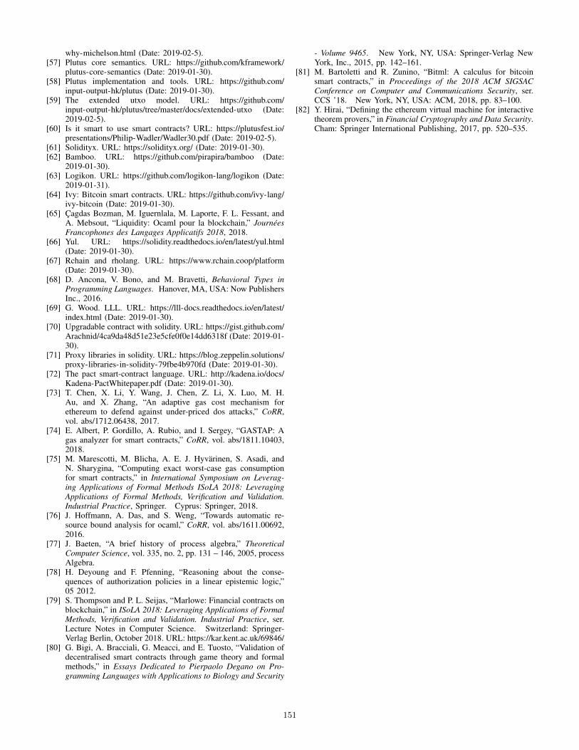
why-michelson.html (Date: 2019-02-5).[57] Plutus core semantics. URL: https://github.com/kframework/

plutus-core-semantics (Date: 2019-01-30).[58] Plutus implementation and tools. URL: https://github.com/

input-output-hk/plutus (Date: 2019-01-30).[59] The extended utxo model. URL: https://github.com/

input-output-hk/plutus/tree/master/docs/extended-utxo (Date:2019-02-5).

[60] Is it smart to use smart contracts? URL: https://plutusfest.io/presentations/Philip-Wadler/Wadler30.pdf (Date: 2019-02-5).

[61] Solidityx. URL: https://solidityx.org/ (Date: 2019-01-30).[62] Bamboo. URL: https://github.com/pirapira/bamboo (Date:

2019-01-30).[63] Logikon. URL: https://github.com/logikon-lang/logikon (Date:

2019-01-31).[64] Ivy: Bitcoin smart contracts. URL: https://github.com/ivy-lang/

ivy-bitcoin (Date: 2019-01-30).[65] Çagdas Bozman, M. Iguernlala, M. Laporte, F. L. Fessant, and

A. Mebsout, “Liquidity: Ocaml pour la blockchain,” JournéesFrancophones des Langages Applicatifs 2018, 2018.

[66] Yul. URL: https://solidity.readthedocs.io/en/latest/yul.html(Date: 2019-01-30).

[67] Rchain and rholang. URL: https://www.rchain.coop/platform(Date: 2019-01-30).

[68] D. Ancona, V. Bono, and M. Bravetti, Behavioral Types inProgramming Languages. Hanover, MA, USA: Now PublishersInc., 2016.

[69] G. Wood. LLL. URL: https://lll-docs.readthedocs.io/en/latest/index.html (Date: 2019-01-30).

[70] Upgradable contract with solidity. URL: https://gist.github.com/Arachnid/4ca9da48d51e23e5cfe0f0e14dd6318f (Date: 2019-01-30).

[71] Proxy libraries in solidity. URL: https://blog.zeppelin.solutions/proxy-libraries-in-solidity-79fbe4b970fd (Date: 2019-01-30).

[72] The pact smart-contract language. URL: http://kadena.io/docs/Kadena-PactWhitepaper.pdf (Date: 2019-01-30).

[73] T. Chen, X. Li, Y. Wang, J. Chen, Z. Li, X. Luo, M. H.Au, and X. Zhang, “An adaptive gas cost mechanism forethereum to defend against under-priced dos attacks,” CoRR,vol. abs/1712.06438, 2017.

[74] E. Albert, P. Gordillo, A. Rubio, and I. Sergey, “GASTAP: Agas analyzer for smart contracts,” CoRR, vol. abs/1811.10403,2018.

[75] M. Marescotti, M. Blicha, A. E. J. Hyvärinen, S. Asadi, andN. Sharygina, “Computing exact worst-case gas consumptionfor smart contracts,” in International Symposium on Leverag-ing Applications of Formal Methods ISoLA 2018: LeveragingApplications of Formal Methods, Verification and Validation.Industrial Practice, Springer. Cyprus: Springer, 2018.

[76] J. Hoffmann, A. Das, and S. Weng, “Towards automatic re-source bound analysis for ocaml,” CoRR, vol. abs/1611.00692,2016.

[77] J. Baeten, “A brief history of process algebra,” TheoreticalComputer Science, vol. 335, no. 2, pp. 131 – 146, 2005, processAlgebra.

[78] H. Deyoung and F. Pfenning, “Reasoning about the conse-quences of authorization policies in a linear epistemic logic,”05 2012.

[79] S. Thompson and P. L. Seijas, “Marlowe: Financial contracts onblockchain,” in ISoLA 2018: Leveraging Applications of FormalMethods, Verification and Validation. Industrial Practice, ser.Lecture Notes in Computer Science. Switzerland: Springer-Verlag Berlin, October 2018. URL: https://kar.kent.ac.uk/69846/

[80] G. Bigi, A. Bracciali, G. Meacci, and E. Tuosto, “Validation ofdecentralised smart contracts through game theory and formalmethods,” in Essays Dedicated to Pierpaolo Degano on Pro-gramming Languages with Applications to Biology and Security

- Volume 9465. New York, NY, USA: Springer-Verlag NewYork, Inc., 2015, pp. 142–161.

[81] M. Bartoletti and R. Zunino, “Bitml: A calculus for bitcoinsmart contracts,” in Proceedings of the 2018 ACM SIGSACConference on Computer and Communications Security, ser.CCS ’18. New York, NY, USA: ACM, 2018, pp. 83–100.

[82] Y. Hirai, “Defining the ethereum virtual machine for interactivetheorem provers,” in Financial Cryptography and Data Security.Cham: Springer International Publishing, 2017, pp. 520–535.

151

Ethereum Blockchain Analysis using Node2VecAleksander Salnikov

Higher School of EconomicsMoscow, Russia

salnikovsas@gmail.com

Evgenia SivetsHigher School of Economics

Moscow, Russiaevgeniasivets@gmail.com

Abstract—In this work we apply Node2Vec[19] to obtain struc-tural information from Ethereum network transaction graph[11],[12]. Given the large amount of data that is stored in theblockchain, we make use of the Google BigQuery service toextract only a small relevant subset of nodes and reconstructtransaction graph. After that the Node2Vec was used to embedthis graph into a high-dimensional vector space. The space ofembeddings is used to clusterize Ethereum addresses.

The Ethereum network was chosen thanks to the propertyof its addresses to represent a long-term entity, in contrast toBitcoin[1] and many other blockchains where it is not possibleto establish such relationship between entities (users, etc...) andaddresses[2], [3], [4], [5]. This makes us think of trying to classifyEthereum users according to their activity[6], [7], based solelyon the blockchain data.

I. INTRODUCTION

A. The purposes of blockchain data analysis overview

Blockchain technology has been becoming more and morepopular and complex recently. Simply speaking, blockchaincan be seen as a very specific type of database — a distributedledger. Because of blockchain being a public database thatanyone can write to (following a certain set of rules) andthe record will persist forever in its state, the blockchaindata, as a result, implicitly contains valuable financial andsocial information about its users. Which ultimately drawsattention of both data scientists and government regulators,giving a boost to developing blockchain analysis techniquesand motivating research teams to explore the data from manydifferent perspective.

The blockchain state has been conceptualized throughgraph-based data models, providing researchers with a richtoolbox of different approaches. Graph theory has been alreadysuccessfully applied to solve many practical and theoreticalnetwork-related problems, which, by the way, may explain thewide adoption of network mental model towards blockchainsas well. Much progress has been achieved in the field ofrandom graph analysis, so it was just a matter of time forthis ideas to make their way into blockchain state research.

The first widely adopted blockchain system was Bitcoin.Being designed to preserve privacy of its users, while pre-serving all information about every single transaction on thenetwork, it expectedly became a target for researches aimingto extract users’ private information from blockchain data. Ithas been shown that the blockchain data contains much moreprivate information that has been previously assumed and ledto deeper understanding of the privacy problem in distributed

systems. Despite not being ultimately private, Bitcoin is stillthe first and the most popular cryptocurrency in the world.

While some subsequent developments tried to challenge theuncovered privacy-related issues in order to archive the levelof privacy that Bitcoin initially expected to provide, othersfocused on exploring another unique properties of emergedtechnology. In particular, they enriched identity managementfunctionality: making the user to be represented as an on-network entity, capable of interacting with other entities —users or special kind of programs, living in the network, named”smart-contracts”. Ethereum appeared to be the first widely-adopted blockchain system that implemented these concepts,although formerly it was presented as a system for general-purpose distributed computations. Without a design decisionsaiming at achieving privacy, the Ethereum data explicitlycontains information about the sender and recipient for eachtransaction, making it more suitable for conducting research.

B. Ethereum network transaction graph model

For the purpose of our study, Ethereum network can berepresented as a directed graph, where nodes represent networkentities (addresses), whereas edges reflect transactions betweenthem.

Each edge of this graph has at least the following set ofattributes: transacted value and transaction time[13]. Over timenew edges may be added to the graph but cannot be removedor modified[20]. Accounting for both incoming value andoutgoing value that has been transacted to/from a particularnode determines the node’s balance at any particular momentof time.

Besides the financial transactions there are another kindof transactions related to smart-contract functionality thatEthereum provides. Smart-contract can be seen as applicationsthat are running inside the network and may enjoy the samesecurity guarantees that the ordinary transactions do. Theyfacilitate the exchange of messages between network entities,with each message being a transaction carrying arbitrary app-specific data[8], [10], [11], [9]. This opens up great opportu-nities for a further research.

C. Obtaining Data and Data-set preparation

We used Google’s BigQuery service to obtain only inter-esting subset of data through querying block-chain data withSQL. Google maintains the up-to-date complete Ethereumblock-chain data on their servers and provides a structural

152

query service to allow data scientists analyze the data withoutthe overhead of downloading gigabytes of data and keeping itup-to-date.

SQL allows to easily fetch required data. For example, toobtain every transaction that ever happened, we may write:

1 SELECT from_address, to_address, value2 FROM `bigquery-public-data

.crypto_ethereum.transactions`→

This query will return each transaction separately.For the sake of simplicity, we will bring individual transac-

tions into aggregated ones based on pair of sender and receiver.The corresponding query reads:

1 SELECT from_address, to_address,SUM(value)→

2 FROM `bigquery-public-data.crypto_ethereum.transactions`→

3 GROUP BY from_address, to_address

To obtain list of every address, involved in transactions wecan use the following query:

1 SELECT from_address2 FROM `bigquery-public-data.

crypto_ethereum.transactions`→

3 GROUP BY from_address4 UNION DISTINCT5 SELECT to_address6 FROM `bigquery-public-data.

crypto_ethereum.transactions`→

7 GROUP BY to_address

Using full Ethereum-addresses during the calculation stepwould require a huge amount of memory. Since the set ofnetwork addresses is fixed and known beforehand, we maymitigate this issue by enumerating them at the pre-processingstep and using integers as identifiers instead. The mapping(stored as a Python dictionary) can be easily used to resolvethe network address when needed.

Also there is some interest in transaction analysis thathappened over a specific period of time.

D. Nodes embedding

LetG = (V,E),

where V — the set of all network entities, E — a set ofaggregated transactions between them.

Our primary goal is to process this data using variousmachine learning algorithms in order to categorize them intodistinct groups according to the type of their activity on thenetwork.

Solving this problem directly on the graph model is avery hard task. Instead, one of the recent approaches – graph

embedding – suggests representing network vertices into alow-dimensional vector space [16]:

f : V → Rd,

chosen so that preserving information about network topologystructure[18]. Here d is the number of dimensions of our fea-ture representation. The above requirement can be expressed interms of maximizing the likelihood of network neighborhoodspreserving:

maxf

∑u∈V

logP (NS(u)|f(u)).

The objective can be efficiently optimized using stochasticgradient descent (SGD) [14]. The idea behind an embeddingis that the neighborhood (the context) of each node to muchextend determines the properties of the node itself.

Here we used the notion of node’s neighborhood [17],that must be clearly specified before we may continue. Moreformally, we have to define a sampling strategies.

Definition 1. For each node u ∈ V , its network neighborhoodNS(u) ⊂ V is generated through a neighborhood samplingstrategy S.

The simplest such strategies are, for instance, Breadth-firstSampling (BFS) and Depth-first Sampling (DFS), but beingdeterministic they represent single node’s neighborhood, fail-ing to preserve a complex structure of a node’s neighborhood.Instead, the node2vec approach, that we will work with, solvesthis by using randomized procedure to sample many differentneighborhoods for a single node.

E. Random Walks

For each node u, consider the following random walk ofthe fixed length ` with the following distribution [15]:

P (ci = x|ci−1 = v) =

πvx/Z if (v, x) ∈ E0 otherwise

Here Z is the normalizing constant, πvx is transition proba-bility between nodes v and x, defined as:

αpq(t, x) =

1/p if dtx = 0

1 if dtx = 1

1/q if dtx = 2

where dtx denotes the shortest path distance between nodes tand x.

The two parameters have the following meaning:

1) return parameter p — controls the likelihood of returningto the same node

2) in-out parameter q — defines if random walk should gotowards node t (when q > 1) or away from it (q < 1).

153

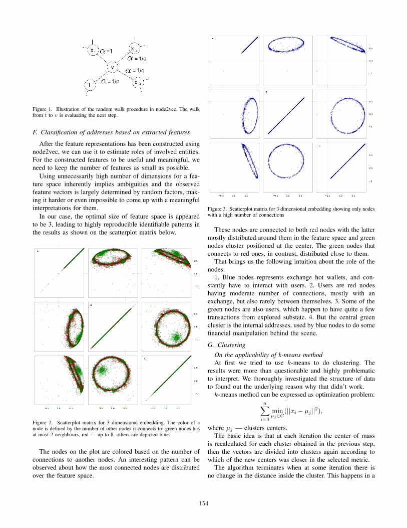
Figure 1. Illustration of the random walk procedure in node2vec. The walkfrom t to v is evaluating the next step.

F. Classification of addresses based on extracted features

After the feature representations has been constructed usingnode2vec, we can use it to estimate roles of involved entities.For the constructed features to be useful and meaningful, weneed to keep the number of features as small as possible.

Using unnecessarily high number of dimensions for a fea-ture space inherently implies ambiguities and the observedfeature vectors is largely determined by random factors, mak-ing it harder or even impossible to come up with a meaningfulinterpretations for them.

In our case, the optimal size of feature space is appearedto be 3, leading to highly reproducible identifiable patterns inthe results as shown on the scatterplot matrix below.

Figure 2. Scatterplot matrix for 3 dimensional embedding. The color of anode is defined by the number of other nodes it connects to: green nodes hasat most 2 neighbours, red — up to 8, others are depicted blue.

The nodes on the plot are colored based on the number ofconnections to another nodes. An interesting pattern can beobserved about how the most connected nodes are distributedover the feature space.

Figure 3. Scatterplot matrix for 3 dimensional embedding showing only nodeswith a high number of connections

These nodes are connected to both red nodes with the lattermostly distributed around them in the feature space and greennodes cluster positioned at the center, The green nodes thatconnects to red ones, in contrast, distributed close to them.

That brings us the following intuition about the role of thenodes:

1. Blue nodes represents exchange hot wallets, and con-stantly have to interact with users. 2. Users are red nodeshaving moderate number of connections, mostly with anexchange, but also rarely between themselves. 3. Some of thegreen nodes are also users, which happen to have quite a fewtransactions from explored substate. 4. But the central greencluster is the internal addresses, used by blue nodes to do somefinancial manipulation behind the scene.

G. Clustering

On the applicability of k-means methodAt first we tried to use k-means to do clustering. The

results were more than questionable and highly problematicto interpret. We thoroughly investigated the structure of datato found out the underlying reason why that didn’t work.k-means method can be expressed as optimization problem:

n∑i=0

minµj∈C

(||xi − µj ||2),

where µj — clusters centers.The basic idea is that at each iteration the center of mass

is recalculated for each cluster obtained in the previous step,then the vectors are divided into clusters again according towhich of the new centers was closer in the selected metric.

The algorithm terminates when at some iteration there isno change in the distance inside the cluster. This happens in a

154

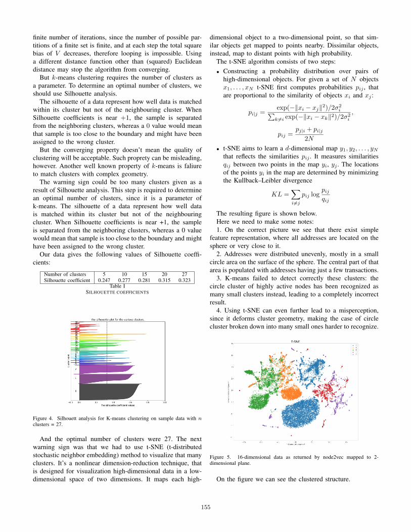
finite number of iterations, since the number of possible par-titions of a finite set is finite, and at each step the total squarebias of V decreases, therefore looping is impossible. Usinga different distance function other than (squared) Euclideandistance may stop the algorithm from converging.

But k-means clustering requires the number of clusters asa parameter. To determine an optimal number of clusters, weshould use Silhouette analysis.

The silhouette of a data represent how well data is matchedwithin its cluster but not of the neighbouring cluster. WhenSilhouette coefficients is near +1, the sample is separatedfrom the neighboring clusters, whereas a 0 value would meanthat sample is too close to the boundary and might have beenassigned to the wrong cluster.

But the converging property doesn’t mean the quality ofclustering will be acceptable. Such proprety can be misleading,however. Another well known property of k-means is faliureto match clusters with complex geometry.

The warning sign could be too many clusters given as aresult of Silhouette analysis. This step is required to determinean optimal number of clusters, since it is a parameter ofk-means. The silhouette of a data represent how well datais matched within its cluster but not of the neighbouringcluster. When Silhouette coefficients is near +1, the sampleis separated from the neighboring clusters, whereas a 0 valuewould mean that sample is too close to the boundary and mighthave been assigned to the wrong cluster.

Our data gives the following values of Silhouette coeffi-cients:

Number of clusters 5 10 15 20 27Silhouette coefficient 0.247 0.277 0.281 0.315 0.323

Table ISILHOUETTE COEFFICIENTS

Figure 4. Silhouett analysis for K-means clustering on sample data with nclusters = 27.

And the optimal number of clusters were 27. The nextwarning sign was that we had to use t-SNE (t-distributedstochastic neighbor embedding) method to visualize that manyclusters. It’s a nonlinear dimension-reduction technique, thatis designed for visualization high-dimensional data in a low-dimensional space of two dimensions. It maps each high-

dimensional object to a two-dimensional point, so that sim-ilar objects get mapped to points nearby. Dissimilar objects,instead, map to distant points with high probability.

The t-SNE algorithm consists of two steps:• Constructing a probability distribution over pairs of

high-dimensional objects. For given a set of N objectsx1, . . . , xN t-SNE first computes probabilities pij , thatare proportional to the similarity of objects xi and xj :

pi|j =exp(−‖xi − xj‖2)/2σ2

i∑k 6=i exp(−‖xi − xk‖2)/2σ2

i

,

pij =pj|i + pi|j

2N

• t-SNE aims to learn a d-dimensional map y1, y2, . . . , yNthat reflects the similarities pij . It measures similaritiesqij between two points in the map yi, yj . The locationsof the points yi in the map are determined by minimizingthe Kullback–Leibler divergence

KL =∑i 6=j

pij logpijqij

The resulting figure is shown below.Here we need to make some notes:1. On the correct picture we see that there exist simple

feature representation, where all addresses are located on thesphere or very close to it.

2. Addresses were distributed unevenly, mostly in a smallcircle area on the surface of the sphere. The central part of thatarea is populated with addresses having just a few transactions.

3. K-means failed to detect correctly these clusters: thecircle cluster of highly active nodes has been recognized asmany small clusters instead, leading to a completely incorrectresult.

4. Using t-SNE can even further lead to a misperception,since it deforms cluster geometry, making the case of circlecluster broken down into many small ones harder to recognize.

Figure 5. 16-dimensional data as returned by node2vec mapped to 2-dimensional plane.

On the figure we can see the clustered structure.

155

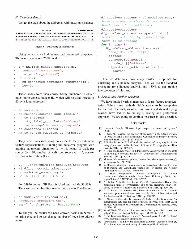
H. Technical details

We get the data about the addresses with maximum balance.

Figure 6. DataFrame of transactions

Using networkx we find the maximal connected component.The result was about 25000 nodes.

1 g = nx.from_pandas_edgelist(df,2 source="from_address",3 target="to_address")4 Gc = max(5 nx.connected_component_subgraphs(g),6 key=len)

These nodes were then consecutively numbered to obtainmuch more concise integer ID, which will be used instead of20-byte long addresses.

1 Gc_numbered =2 nx.relabel.convert_node_labels_\3 _to_integers(4 Gc, label_attribute="address",5 ordering="decreasing degree")6 df_connected_numbered =7 nx.to_pandas_edgelist(Gc_numbered)

They were processed using node2vec to learn continuousfeature representations. Running the node2vec program withtraining parameters dimention (d) = 16, length of walk persource (l) = 20, number of walks per source (r) = 5, contextsize for optimization (k) = 5:

1 ../../snap/examples/node2vec/node2vec2 -i:df_connected_numbered.csv3 -o:node2vec_embedding.txt4 -d:16 -l:20 -r:5 -k:5 -v

For 24936 nodes 1GB Ram is Used and real 0m31.538sThen we read embedding results into pandas DataFrame.

1 df_node2vec = pd.read_csv(2 "node2vec_embedding.txt",3 sep=" ", skiprows=1, header=None)

To analyse the results we need convert back numbered idto string type and so we change number of node into addressname.

1 df_node2vec_address = df_node2vec.copy()2 #create a new dataframe for renaming3 #back node ids to addresses

1 df_node2vec_address =2 df_node2vec_address.astype(0: str)3 #convert id to str type and change4 #node_id to address5 for i, line in6 df_node2vec_address.iterrows():7 node_id = int(line[0])8 address =9 Gc_numbered.nodes[

10 node_id]["address"]11 df_node2vec_address.at[i,0] =12 address

Then we determine how many clusters is optimal forclustering and silhouette analysis. Then we use the standardprocedure for silhouette analysis and t-SNE to get graphicinterpretation of clusters.

I. Results and Further research

We have studied various methods to learn feature represen-tation. While some methods didn’t appear to be acceptablefor the task, the analysis of arising issues and its underlyingreasons have led us to the rigid, scaling and performantapproach. We are going to continue research in this direction.

REFERENCES

[1] Nakamoto, Satoshi. ”Bitcoin: A peer-to-peer electronic cash system.”(2008).

[2] F. Reid, M. Harrigan, An analysis of anonymity in the bitcoin system,In: Proc. of IEEE Third International Conference on Privacy, Security,Risk and Trust, 2012, pp. 1318-1326.

[3] P. Koshy, D. Koshy, P. McDaniel, An analysis of anonymity in bitcoinusing p2p network traffic. In Proc. of Financial Cryptography and DataSecurity, 2014, pp. 469-485.

[4] A. Biryukov, D. Khovratovich, I. Pustogarov, Deanonymisation of clientsin bitcoin p2p network. In: Proc. of Computer and CommunicationsSecurity, 2014, pp. 15-29.

[5] Monero, Monero-secure, private, untraceable, (https://getmonero.org/),accessed on Jan. 21, 2018.

[6] V. Monaco, Identifying bitcoin users by transaction behavior, In: Proc.of Biometric and Surveillance Technology for Human and ActivityIdentification XII, 9457(2015):945704.

[7] C. Zhao, Graph-based forensic investigation of bitcointransactions, Master’s thesis, Iowa State University, 2014, doi:https://doi.org/10.31274/etd-180810-3797.

[8] A. Kosba, A. Miller, E. Shi, Z. Wen, C. Papamanthou, Hawk: Theblockchain model of cryptography and privacy-preserving smart con-tracts, In: Proc. of Security and Privacy (S&P), 2016, pp. 839-858.

[9] C. K. Frantz, M. Nowostawski, From institutions to code: Towardsautomated generation of smart contracts, In: Proc. of Foundations andApplications of Self* Systems, 2016, pp. 210-215.

[10] F. Zhang, E. Cecchetti, K. Croman, A. Juels, E. Shi, Town crier: Anauthenticated data feed for smart contracts, In: Proc. of the 2016 ACMSIGSAC Conference on Computer and Communications Security, 2016,pp. 270-282.

[11] Wood, Gavin. ”Ethereum: A secure decentralised generalised transactionledger.” Ethereum Project Yellow Paper 151 (2014): 1-32.

[12] ” The Ethereum Nodes Explorer”. Accessed April 28, 2018. https://www.ethernodes.org/network/1/nodes

[13] ”Etherchain - The Ethereum Blockchain Explorer”. Accessed April 28,2018. https://www.etherchain.org/charts/averageBlockUtilization

156

[14] B. Recht, C. Re, S. Wright, and F. Niu. Hogwild!: A lock-free approachto parallelizing stochastic gradient descent. In NIPS, 2011.

[15] L. Backstrom and J. Leskovec. Supervised random walks: predictingand recommending links in social networks. In WSDM, 2011.

[16] S. Cao, W. Lu, and Q. Xu. GraRep: Learning Graph Representationswith global structural information. In CIKM, 2015.

[17] L. A. Adamic and E. Adar. Friends and neighbors on the web. Socialnetworks, 25(3):211–230, 2003.

[18] S. Fortunato. Community detection in graphs. Physics Reports, 486(3-5):75 – 174, 2010.

[19] Grover, Aditya and Leskovec, Jure node2vec: Scalable feature learningfor networks 2016, Proceedings of the 22nd ACM SIGKDD internationalconference on Knowledge discovery and data mining

[20] Buterin, Vitalik and others A next-generation smart contract anddecentralized application platform

157

A Tool for Identification of Unusual Wallets onEthereum Platform

Mikhail Petrov1 Rostislav Yavorskiy2

National Research University Higher School of EconomicsMyasnitskaya 20, Moscow, Russia

mishanayrus@gmail.com1 ryavorsky@hse.ru2

Abstract. We present a tool for identifying the most suspicious Ethereumwallets by finding atypical vertices of the transactions graph. We inspectdifferent characteristics of the wallets and the transactions they wereinvolved in during a week. First, we identify ”typical” groups of nodes.Then the nodes which are far different from all these groups are consid-ered to be suspicious.

Keywords: Ethereum platform · cryptocurrency transactions · trans-actions graph.

1 Introduction

Anomaly detection is an area that has been receiving much attention in recentyears. It has a wide variety of applications, including fraud detection, networkintrusion detection, medical diagnosis and other fields. Usually research in thisarea is using attribute-value data as the medium from which anomalies are to beextracted. Some works are focused on anomaly detection in graph-based data. Inour paper we are going to combine these approaches for the goal of identificationof suspicios wallets in a cryptocurrency community.

1.1 Cryptocurrencies and Ether

The area of cryptocurrency is quite young. The first appearance of Ether, thetransactions graph of which will be analyzed in this article, appeared in 2013. Bynow the analysis of the Ether community has progressed very little. One can findquite many articles on the analysis and prediction of cryptocurrencies rates, butso far few research has been focused on the analysis of exchange communitiesfor the cryptocurrencies.

It is known that the semantics of transactions of blockchain systems can becaptured by a transaction graph, see e.g. [1]. Such a graph generally consists ofthe states and the transactions as transitions between the states, together withconditions for the consistency and validity of transactions.

Detailed overview of cryptocurrencies could be found in [4].

158

2 M. Petrov, R. Yavorskiy

1.2 Overview of anomaly detection methods

In [8] a comprehensive survey of recent anomaly detection systems and hybrid in-trusion detection systems is provided, and recent technological trends in anomalydetection are also discussed. In [2] existing techniques are grouped into differentcategories based on the underlying approach adopted by each technique. Foreach category key assumptions are identified, which are used by the techniquesto differentiate between normal and anomalous behavior. In [7] two techniquesfor graph-based anomaly detection are introduced. The authors suggest a newmethod for calculating the regularity of a graph, with applications to anomalydetection. Experimental results are provided which use both real-world networkintrusion data and artificially-created data. In [5] several information-theoreticmeasures, namely, entropy, conditional entropy, relative conditional entropy, in-formation gain, and information cost for anomaly detection are used.

1.3 Networks analysis

As it was already mentioned, see [7], some anomaly detection method use graph-based analysis. Besides standard graph analysis library networkx, we are alsousing statistical properties of social networks, see [3, 6].

1.4 Structure of the remaining text

The rest of the paper is organized as follows. Section 2 describes the data weworked with. Section 3 describes the methods we used to analyze transactiondata. Section 4 presents a description of how the points for the strangeness ratingwere calculated. Section 5 shows the top 5 vertices as a result of calculating thesuspiciousness rating with the rating values.

2 The data analyzed

In this paper data on all transactions for a week was downloaded using the openetherium API. Significant characteristics for the community analysis were cho-sen, and an ether exchange graph was constructed based on them. The verticesof this graph are the participants in the platform and also the edges are thetransactions between these participants. Further in the received graph, the char-acteristics of the vertices were calculated, clusters were found, and associativerules based on them were constructed. As a result, taking into account the dataon graph vertices, clustering, and associative rules, the suspiciousness rating ofvertices was constructed.

Since in this paper we were focused on identifying suspicious and untypicalmembers in the ether exchange community, only those characteristics that wereuseful for analyzing and constructing the graph were extracted from the set ofparameters.

159

A Tool for Identification of Unusual Wallets on Ethereum Platform 3

2.1 Ethereum API

Ethereum API provides information about each block, all transactions and everymembers of the network. JSON RPC API of the Ethereum platform currentlysupports four programming languages: C++, Go, Python, and Parity. Also thereis an option to access the data via web interface at https://etherscan.io, whichwe used.

For our study all transactions executed during a particular week have beendownloaded. That was done using the timestamp field of the blocks and themethod eth getBlockByNumber().

Totally information about 3,382,252 transactions were collected.

2.2 Format of Ethereum transaction data

All transactions were selected from each block and then the following four pa-rameters were saved for each transaction:

– address of the sender;– address of the receiver;– date and time of the transaction;– the amount of the internal currency (wei) that is transferred.

These characteristics of transactions allow us to construct the graph of an etherexchange. The vertices in this graph are the addresses of wallets which are eithersenders or receivers of these transactions, the edges correspond to the transac-tions themselves.

In this paper we analyze only total amount sent from node A to node B andignore details about the number of transactions and distribution of the amountbetween them.

In addition to the total volume transmitted between a pair of wallets, thefrequency of interactions between participants (the number of transactions sent)could be considered too.

2.3 Transactions graph

The resulting set of transaction on ether exchange was processed and presentedas a graph. The first step to getting the graph was renaming vertices, sinceaddresses do not make any sense. In order to save memory and more clarity,they were numbered with the help of natural numbers, and the dictionary withaddresses mapping in the vertex numbers was saved in the file.

Next, we summed the weights of the edges between identical pairs of senderand receiver, recorded the graph as an adjacency list with edge weights andthe total number of transactions between vertices. As a result, we obtainedan undirected graph with positive and negative edge weights. The graph has1,577,010 vertices and 4,963,980 edges. To analyze this graph we used networkx,a common library of the Python language. All further operations for calculatingthe various characteristics of the graph have been done with the help of thislibrary.

160

4 M. Petrov, R. Yavorskiy

3 Analysis

Our anomaly detection analysis consists of the following four parts:

1. Graph connectivity analysis. During this step we put off wallets forwhich too few information is available, so no meaningful analysis could beconducted for them.

2. Analysis of the vertex characteristics. Here we compute degree, cen-trality and containing k-core for each vertex of the transaction graph.

3. Cluster analysis. The clustering is performed based on the vectors obtainedin the previous section.

4. Association rules are used to find patterns that can be traced in thisgraph.

After each part all the vertices are ranged according to their suspiciousness,and then these ratings are merged into one.

3.1 Connectivity analysis

The next step was to analyze the connectivity components of the obtained graph.The graph has 35,628 connectivity components. These components can be di-vided into three groups:

– The main component of a large community. In this component there are1,474,024 vertices. Most likely, it is a graph of the interaction of people ofsome large service or exchange, but the exact meaning is not yet clear. Thiscomponent has the biggest interest for analysis and will continue to be thefirst in priority.

– The second type is a small groups of ten to a thousand people. Most likely,these groups are small companies in which payment occurs in the cryptocur-rency, or small communities that pay cryptocurrency for some services. Thisgroup also deserves attention for analysis, but to a lesser extent.

– The third class includes groups of up to ten people. These are some localexchanges of money, betting between people. This group has no interest foranalysis, since it does not contain any meaningful information.

As was mentioned above, the first group has the greatest interest for ana-lyzing, therefore it will be analyzed in the future. The remaining connectivitycomponents are stored in separate files and their analysis is possible in futurework.

3.2 Vertex Characteristics

Since the main purpose of the work is to distinguish atypical and suspiciousvertices, then we must determine the typical aspects of the obtained community.Taking into account that the received connectivity component can have multiplechains of elements with a degree equal to two, therefore the graph has many

161

A Tool for Identification of Unusual Wallets on Ethereum Platform 5

vertices that are just a link in the chain of transmission of the cryptocurrency, itwas decided to allocate the k-cores of the graph of this component. A k-core ofa graph G is a maximal subgraph of G in which all vertices have degree at leastk. To do this, we run a search of the value of k-cores from 1 to 50 and used themethod k core for each value. If the k-core was not found for the value of n, thenit will not be found for n + 1, since any k+1-core is also a k-core. Therefore, ifsuch a situation arises in searching the k-cores, then the search can be stopped.

The algorithm stopped at k equal to 15, which means that the k-kernels from1 to 14 were found. Since the sizes of k-cores beginning with k equal to 8 arealready sufficiently small and the 3-core is quite large, 4, 5, 6, and 7 core werechosen as an optimal from the point of view of time for analyzing the graph.Based on the selected k-cores we can calculate new characteristics of the vertices.Three kinds of centrality were calculated for each vertex in the core: betweennesscentrality, closeness centrality and degree centrality. Also we add vertex degreeas a characteristic. On the basis of the obtained data, we can form a vectorthat will describe the vertices of the graph (participants of the cryptocurrencycommunity), split each characteristic into groups of segments and create binaryvectors for deriving associative rules.

As a result, we obtained a 5-dimensional vector characterizing the verticesof the graph: 3 kinds of centralities; number of the k-core, which vertex belongs;degree of a vertex. Also, the dimensionality of these vectors could be increasedby adding distance to the hubs for each of the characteristics, but this operationis planned for the next stages of the work. The resulting vectors can be clusterednow.

3.3 Clustering

Based on the vectors obtained in the previous section, clustering is performedusing the standard k-means method. Since for this method it is necessary toinitially know the number of clusters we must first determine this number. Todetermine the optimal number of clusters all numbers from 0 to 200 in stepsof 10 were chosen, clustering was performed and the result were checked withSilhouette and the shoulder methods.

162

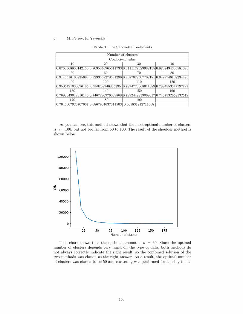
6 M. Petrov, R. Yavorskiy

Table 1. The Silhouette Coefficients

Number of clusters

Coefficient value

10 20 30 40

0.6768368853142156 0.7095846965311733 0.8111177029982155 0.8702494303581093

50 60 70 80

0.9146516160235698 0.9293358278581296 0.9387072507702181 0.9478746102234425

90 100 110 120

0.9505421030096185 0.950768946865395 0.7874773068611389 0.7884553347797727

130 140 150 160

0.7698049042610146 0.7467290976039868 0.7992449839069017 0.7467532658132512

170 180 190

0.7044007926707637 0.6867901637311503 0.665831212711668

As you can see, this method shows that the most optimal number of clustersis n = 100, but not too far from 50 to 100. The result of the shoulder method isshown below:

This chart shows that the optimal amount is n = 30. Since the optimalnumber of clusters depends very much on the type of data, both methods donot always correctly indicate the right result, so the combined solution of thetwo methods was chosen as the right answer. As a result, the optimal numberof clusters was chosen to be 50 and clustering was performed for it using the k-

163

A Tool for Identification of Unusual Wallets on Ethereum Platform 7

means method. Distribution of the cluster size can be seen in the figure number3:

It can be seen from the distribution diagram that one strongly dominant interms of the size of the elements cluster, two clusters slightly above the averagelevel, about 15 clusters of medium size and the other clusters of a very small sizewere obtained. These results will be used in the next chapter to build associativerules.

3.4 Association Rules

Now based on all of the characteristics of the community we can try to findpatterns that can be traced in this graph. For example, it may happen that ifthe vertex belongs to the 4-core, then its degree must necessarily be higher than7. To do this, it is necessary to generate binary vectors in which the elementat the i-th position will report whether this element belongs to a certain groupor not. Having formed such vectors, we can find patterns, but on first stepwe need to form the groups themselves. For this, it is necessary to analyzethe distribution of the characteristics of the vectors. To achieve this, we shouldconstruction distribution histograms for each of the characteristics. The first andthird graphs of distributions are strongly shifted to the left, and the thresholds

164

8 M. Petrov, R. Yavorskiy

between the groups are not visible, so we need to look at the left parts closer:

From the received observations it is possible to break each of the character-istics into ranges of values into which approximately equal number of elementswill fall. These ranges will also form groups for finding associative rules. Theresult is the following groups:

Table 2. Groups

Degree centrality Betweenness centrality Closenness centrality

0 < x ≤ 0.005 0 < x ≤ 0.0005 0 < x ≤ 0.2

0.005 < x ≤ 0.015 0.0005 < x ≤ 0.001 0.2 < x ≤ 0.3

0.015 < x 0.001 < x 0.3 < x ≤ 0.4

0.4 < x

Generation of binary vectors is now carried out. To search for associativerules we used the mlxtend library, which is the apriori method to search forfrequent sets of attributes, and then search for associative rules. In our scriptthe rules with a minimum support = 0.8 are taken so that the existing patternsare highly probable. As a result of the launch, two associative rules were found:

165

A Tool for Identification of Unusual Wallets on Ethereum Platform 9

Table 3. New rules table

Number Antecedants Consequents Antecedent support Consequent support

0 1 deg. cen. group 1 bet. cen. group 0.997946 0.994034

1 1 bet. cen. group 1 deg. cen. group 0.994034 0.997946

Support Confidence Lift Leverage Conviction

0.993876 0.995922 1.001899 0.001884 1.463008

0.993876 0.999841 1.001899 0.001884 12.922448

To get more associative rules, we need to decrease the support threshold, butthen there will be less probabilistic associative rules, which will contradict thegoal of finding typical signs of this community.

4 Top strangeness rating

Now, when there is a whole set of characteristics of the vertices (clusteringresults, clustered vectors, associative rules), we can start isolating their typicalvalues and finding all the values that will go beyond this framework. For eachovershoot of these boundaries points are entered, which will award the verticeswith these atypical characteristics. For each ”suspicious” characterization pointsfrom 1 to 100 will be given depending on the criticality. At the end, the promisedrating of the suspicious vertices of the community graph will be obtained.

Let’s start with the simplest - associative rules. Here everything is simple,because if a vector does not obey this rule, then it is atypical for this community.Here, the scores in the scores will be determined by the value of the support ofthe associative rule multiplied by one hundred.

The next will be the scoring of vertices whose vectors are too far from thecenter of their clusters. We can calculate the average distance to the center ofeach cluster and the variance. Accordingly, if the distance of the vector does notfall within the range of the mean ± variance, then this vector is atypical. Pointswill be calculated according to the following formula:

|mean− distance|differencemax

,

mean is the average distance to the center in the clusterdistance - the point to the center of a particular windbreaker

differencemax is the maximum difference between the average and thedistance from the vector to the center inside the cluster

Next will be scoring the vertices, whose characteristics of the vectors also gobeyond the limits of the mean ± variance. Here the same normalized formulawill be used, as well as with distances.

The last will be awarded for belonging to atypical small clusters. Since thesizes of some clusters reach even one, this clearly indicates the atypicality of

166

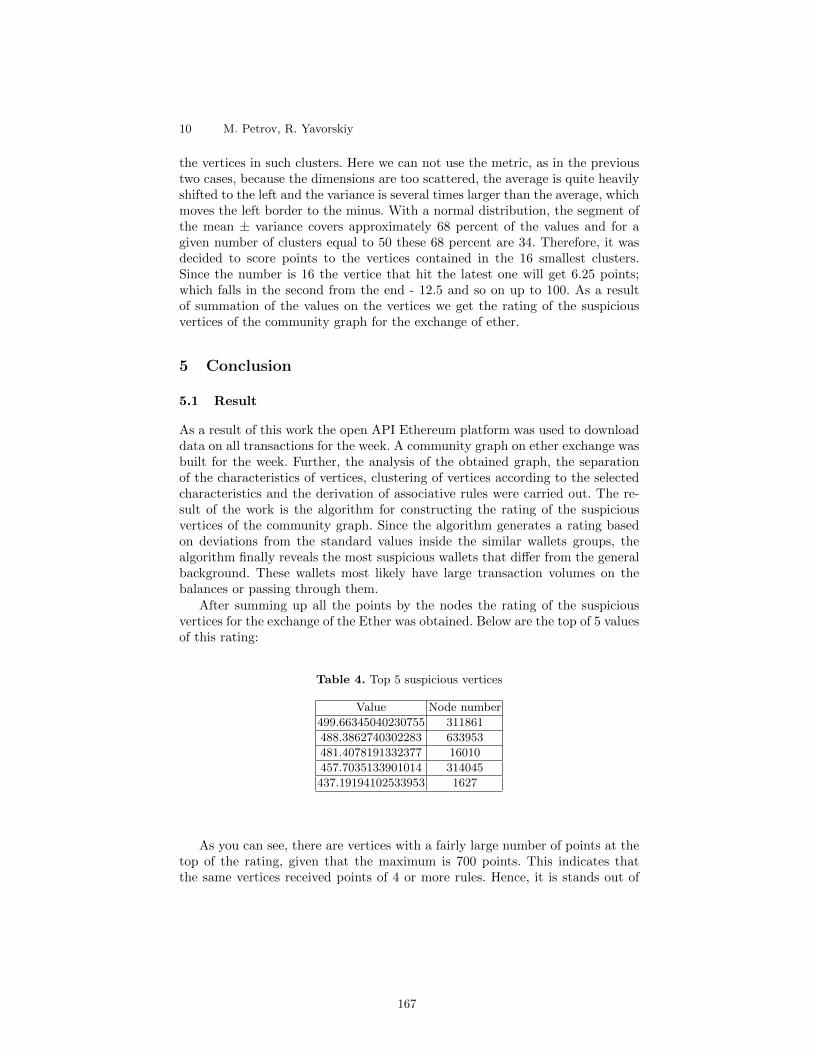
10 M. Petrov, R. Yavorskiy

the vertices in such clusters. Here we can not use the metric, as in the previoustwo cases, because the dimensions are too scattered, the average is quite heavilyshifted to the left and the variance is several times larger than the average, whichmoves the left border to the minus. With a normal distribution, the segment ofthe mean ± variance covers approximately 68 percent of the values and for agiven number of clusters equal to 50 these 68 percent are 34. Therefore, it wasdecided to score points to the vertices contained in the 16 smallest clusters.Since the number is 16 the vertice that hit the latest one will get 6.25 points;which falls in the second from the end - 12.5 and so on up to 100. As a resultof summation of the values on the vertices we get the rating of the suspiciousvertices of the community graph for the exchange of ether.

5 Conclusion

5.1 Result

As a result of this work the open API Ethereum platform was used to downloaddata on all transactions for the week. A community graph on ether exchange wasbuilt for the week. Further, the analysis of the obtained graph, the separationof the characteristics of vertices, clustering of vertices according to the selectedcharacteristics and the derivation of associative rules were carried out. The re-sult of the work is the algorithm for constructing the rating of the suspiciousvertices of the community graph. Since the algorithm generates a rating basedon deviations from the standard values inside the similar wallets groups, thealgorithm finally reveals the most suspicious wallets that differ from the generalbackground. These wallets most likely have large transaction volumes on thebalances or passing through them.

After summing up all the points by the nodes the rating of the suspiciousvertices for the exchange of the Ether was obtained. Below are the top of 5 valuesof this rating:

Table 4. Top 5 suspicious vertices

Value Node number

499.66345040230755 311861

488.3862740302283 633953

481.4078191332377 16010

457.7035133901014 314045

437.19194102533953 1627

As you can see, there are vertices with a fairly large number of points at thetop of the rating, given that the maximum is 700 points. This indicates thatthe same vertices received points of 4 or more rules. Hence, it is stands out of

167

A Tool for Identification of Unusual Wallets on Ethereum Platform 11

the general background immediately by several characteristics, which proves itsstrangeness.

References

1. Christian Cachin, AD Caro, Pedro Moreno-Sanchez, Bjorn Tackmann, and MarkoVukolic. The transaction graph for modeling blockchain semantics. Technical report,Cryptology ePrint Archive, Report 2017/1070, 2017.

2. Varun Chandola, Arindam Banerjee, and Vipin Kumar. Anomaly detection: Asurvey. ACM computing surveys (CSUR), 41(3):15, 2009.

3. Aric Hagberg, Pieter Swart, and Daniel S Chult. Exploring network structure,dynamics, and function using networkx. Technical report, Los Alamos NationalLab.(LANL), Los Alamos, NM (United States), 2008.

4. Jan Lansky. Possible state approaches to cryptocurrencies. Journal of SystemsIntegration, 9(1):19–31, 2018.

5. Wenke Lee and Dong Xiang. Information-theoretic measures for anomaly detection.In Security and Privacy, 2001. S&P 2001. Proceedings. 2001 IEEE Symposium on,pages 130–143. IEEE, 2001.

6. Mary McGlohon, Leman Akoglu, and Christos Faloutsos. Statistical properties ofsocial networks. In Social network data analytics, pages 17–42. Springer, 2011.

7. Caleb C Noble and Diane J Cook. Graph-based anomaly detection. In Proceedingsof the ninth ACM SIGKDD international conference on Knowledge discovery anddata mining, pages 631–636. ACM, 2003.

8. Animesh Patcha and Jung-Min Park. An overview of anomaly detection techniques:Existing solutions and latest technological trends. Computer networks, 51(12):3448–3470, 2007.

168

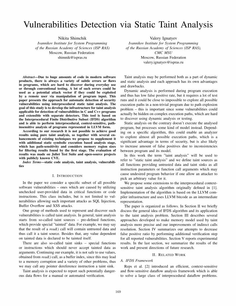
Vulnerabilities Detection via Static Taint AnalysisNikita Shimchik

Ivannikov Institute for System Programmingof the Russian Academy of Sciences (ISP RAS)

Moscow, Russian Federationshimnik@ispras.ru

Valery IgnatyevIvannikov Institute for System Programming

of the Russian Academy of Sciences (ISP RAS),CMC MSU

Moscow, Russian Federationvalery.ignatyev@ispras.ru

Abstract—Due to huge amounts of code in modern softwareproducts, there is always a variety of subtle errors or flawsin programs, which are hard to discover during everyday useor through conventional testing. A lot of such errors could beused as a potential attack vector if they could be exploitedby a remote user via manipulation of program input. Thispaper presents the approach for automatic detection of securityvulnerabilities using interprocedural static taint analysis. Thegoal of this study is to develop the infrastructure for taint analysisapplicable for detection of vulnerabilities in C and C++ programsand extensible with separate detectors. This tool is based onthe Interprocedural Finite Distributive Subset (IFDS) algorithmand is able to perform interprocedural, context-sensitive, path-insensitive analysis of programs represented in LLVM form.

According to our research it is not possible to achieve goodresults using pure taint analysis, so together with several en-hancements of existing techniques we propose to supplement itwith additional static symbolic execution based analysis stage,which has path-sensitivity and considers memory region sizesfor filtering results found by the first stage. The evaluation ofresults was made on Juliet Test Suite and open-source projectswith publicly known CVE.

Index Terms—static code analysis, taint analysis, vulnerabili-ties

I. INTRODUCTION

In the paper we consider a specific subset of all possiblesoftware vulnerabilities – ones which are caused by utilizingunchecked user-provided data in critical functions or codeinstructions. This class includes, but is not limited to vul-nerabilities allowing such important attacks as SQL Injection,Buffer Overflow and XSS attacks.

One group of methods used to represent and discover suchvulnerabilities is called taint analysis. In general, taint analysisstarts from so-called taint sources – pre-defined functions,which provide special ”tainted” data. For example, we may saythat the result of a read() call will contain untrusted data andthus call it a taint source. Besides that, any value dependenton tainted data is declared to be tainted itself.

There are also so-called taint sinks – special functionsor instructions which should never accept tainted data asarguments. Continuing our example, it is not safe to use values,obtained from read() call, as a buffer index, since this may leadto a memory corruption and a variety of other problems, thuswe may call any pointer dereference instruction a taint sink.

Taint analysis is expected to report such potentially danger-ous data flows for a manual or automated verification.

Taint analysis may be performed both as a part of dynamicand static analysis and each approach has its own advantagesand drawbacks.

Dynamic analysis is performed during program executionand thus has low false positive rate, but it requires a lot of testruns and it could be close to impossible to explore all possibleexecution paths in a non-trivial program due to path explosionproblem – this is important since some vulnerabilities couldactually be hidden on complex execution paths, which are hardto discover using dynamic analysis or testing.

Static analysis on the contrary doesn’t execute the analysedprogram, but processes some kind of model instead. Depend-ing on a specific algorithm, this could enable an analyzerto explore almost all possible execution paths, which is asignificant advantage in terms of security, but is also likelyto increase amount of false positives due to inconsistenciesbetween program and its model.

In this work the term ”taint analysis” will be used torefer to ”static taint analysis” and we define taint sources asall functions providing untrusted data and taint sinks as allinstruction parameters or function call arguments which maycause undesired program behavior if one allow an attacker topick an arbitrary value for it.

We propose some extensions to the interprocedural context-sensitive taint analysis algorithm originally defined in [1].Implementation of the algorithm is based on the LLVM com-piler infrastructure and uses LLVM bitcode as an intermediaterepresentation.

The paper is organized as follows. In Section II we brieflydiscuss the general idea of IFDS algorithm and its applicationto the taint analysis problem. Section III describes severalapproaches developed to make memory model used by taintanalysis more precise and our improvements of indirect callsresolution. Section IV summarizes our attempts to decreasefalse positive ratio by performing additional verification stepfor all reported vulnerabilities. Section V reports experimentalresults. In the last section, we summarize the results of thework and present directions of future research.

II. RELATED WORK

A. IFDS Framework

Reps et al. [2] introduced an efficient, context-sensitiveand flow-sensitive dataflow analysis framework which is ableto solve a large class of interprocedural dataflow problems.

169

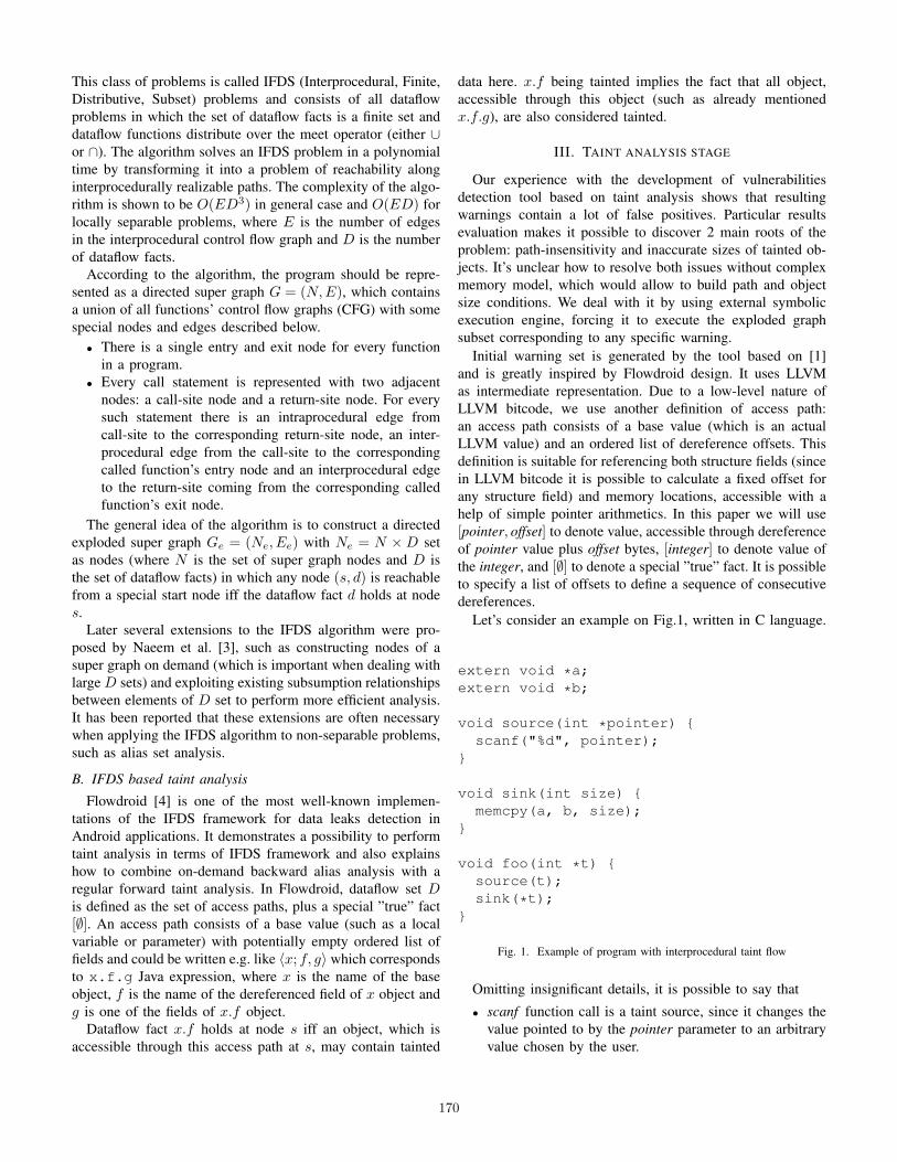
This class of problems is called IFDS (Interprocedural, Finite,Distributive, Subset) problems and consists of all dataflowproblems in which the set of dataflow facts is a finite set anddataflow functions distribute over the meet operator (either ∪or ∩). The algorithm solves an IFDS problem in a polynomialtime by transforming it into a problem of reachability alonginterprocedurally realizable paths. The complexity of the algo-rithm is shown to be O(ED3) in general case and O(ED) forlocally separable problems, where E is the number of edgesin the interprocedural control flow graph and D is the numberof dataflow facts.

According to the algorithm, the program should be repre-sented as a directed super graph G = (N,E), which containsa union of all functions’ control flow graphs (CFG) with somespecial nodes and edges described below.

• There is a single entry and exit node for every functionin a program.

• Every call statement is represented with two adjacentnodes: a call-site node and a return-site node. For everysuch statement there is an intraprocedural edge fromcall-site to the corresponding return-site node, an inter-procedural edge from the call-site to the correspondingcalled function’s entry node and an interprocedural edgeto the return-site coming from the corresponding calledfunction’s exit node.

The general idea of the algorithm is to construct a directedexploded super graph Ge = (Ne, Ee) with Ne = N ×D setas nodes (where N is the set of super graph nodes and D isthe set of dataflow facts) in which any node (s, d) is reachablefrom a special start node iff the dataflow fact d holds at nodes.

Later several extensions to the IFDS algorithm were pro-posed by Naeem et al. [3], such as constructing nodes of asuper graph on demand (which is important when dealing withlarge D sets) and exploiting existing subsumption relationshipsbetween elements of D set to perform more efficient analysis.It has been reported that these extensions are often necessarywhen applying the IFDS algorithm to non-separable problems,such as alias set analysis.

B. IFDS based taint analysis

Flowdroid [4] is one of the most well-known implemen-tations of the IFDS framework for data leaks detection inAndroid applications. It demonstrates a possibility to performtaint analysis in terms of IFDS framework and also explainshow to combine on-demand backward alias analysis with aregular forward taint analysis. In Flowdroid, dataflow set Dis defined as the set of access paths, plus a special ”true” fact[∅]. An access path consists of a base value (such as a localvariable or parameter) with potentially empty ordered list offields and could be written e.g. like 〈x; f, g〉 which correspondsto x.f.g Java expression, where x is the name of the baseobject, f is the name of the dereferenced field of x object andg is one of the fields of x.f object.

Dataflow fact x.f holds at node s iff an object, which isaccessible through this access path at s, may contain tainted

data here. x.f being tainted implies the fact that all object,accessible through this object (such as already mentionedx.f.g), are also considered tainted.

III. TAINT ANALYSIS STAGE

Our experience with the development of vulnerabilitiesdetection tool based on taint analysis shows that resultingwarnings contain a lot of false positives. Particular resultsevaluation makes it possible to discover 2 main roots of theproblem: path-insensitivity and inaccurate sizes of tainted ob-jects. It’s unclear how to resolve both issues without complexmemory model, which would allow to build path and objectsize conditions. We deal with it by using external symbolicexecution engine, forcing it to execute the exploded graphsubset corresponding to any specific warning.

Initial warning set is generated by the tool based on [1]and is greatly inspired by Flowdroid design. It uses LLVMas intermediate representation. Due to a low-level nature ofLLVM bitcode, we use another definition of access path:an access path consists of a base value (which is an actualLLVM value) and an ordered list of dereference offsets. Thisdefinition is suitable for referencing both structure fields (sincein LLVM bitcode it is possible to calculate a fixed offset forany structure field) and memory locations, accessible with ahelp of simple pointer arithmetics. In this paper we will use[pointer, offset] to denote value, accessible through dereferenceof pointer value plus offset bytes, [integer] to denote value ofthe integer, and [∅] to denote a special ”true” fact. It is possibleto specify a list of offsets to define a sequence of consecutivedereferences.

Let’s consider an example on Fig.1, written in C language.

extern void *a;extern void *b;

void source(int *pointer) scanf("%d", pointer);

void sink(int size) memcpy(a, b, size);

void foo(int *t) source(t);sink(*t);

Fig. 1. Example of program with interprocedural taint flow

Omitting insignificant details, it is possible to say that

• scanf function call is a taint source, since it changes thevalue pointed to by the pointer parameter to an arbitraryvalue chosen by the user.

170

• memcpy function call copies size bytes from the objectpointed to by b variable to the object pointed to by avariable. We may call it a taint sink, since it is dangerousto specify size values greater than actual size of objectspointed to by a or b.

• source function’s entry-to-exit subgraph can be sum-marized with the path edge (source-Entry, [∅]) →(source-Exit, [pointer, 0]), i.e. value of [pointer, 0] be-comes unconditionally tainted.

• sink function’s subgraph can be summarized with the pathedge (sink-Entry, [size])→ (Sink, [size]), i.e. tainted datawould reach a taint sink if the value of [size] is knownto be tainted at the entry of the sink function.

• foo function’s subgraph can be summarized as(foo-Entry, [∅])→ (source-callsite, [∅])→ (source-retsite, [t, 0])→ (sink-callsite, [t, 0])→ (Sink, [size]), i.e. tainted data unconditionally reachesa taint sink.

Unlike in known implementations and Flowdroid we don’tstore the whole exploded super graph, because it requires toomuch memory for regular industrial project with millions linesof code even if this graph is constructed on-demand. To solvethis issue another analysis mode was developed, which doesn’trequire exploded super graph edges to be constructed. Theexisting IFDS analysis engine was supplemented with functionsummaries (similar to [3]) and explicit taint traces, whichmakes it possible to show user where the tainted data originatefrom and how did it get to the taint sink without the need tostore the graph itself.

As we’ve noticed during analysis of selected open sourceprojects, the majority of taint sources is usually located”far” from each other in a program and thus their taintflow subgraphs are rarely intersecting. To decrease memoryconsumption, we have added an ability to run a separateanalysis for every taint source. Therefore, exploded graphnodes and summaries can be cleared, but the total analysistime could increase since parts of the program graph can bepotentially analyzed more than once.

The second significant difference with other implementa-tions is that each request for a set of aliases for any specifictainted value is handled in a separate local environment withits own IFDS solver and exploded super graph. The graphis cleared after the call and only the resulting aliases set ispreserved so that it could be reused both in main taint analysisand when calculating other aliases sets.

Remaining improvements are discussed in following sub-sections III-A and III-B with more details.

A. Unresolved function calls

When examining a call site we assume that it is triviallyeasy to determine the called function by the generated bitcode.Unfortunately, C and C++ programs contain calls, whosetargets couldn’t be determined until runtime. There are threemain sources of such unresolved calls, described below:

1) virtual functions;

2) external functions;3) indirect calls.

C++ virtual function is a member function declared withina base class and overridden by the method in the derivedclass. When performing a virtual call, the called function isdetermined by the actual type of the object and may varyin runtime. Such calls were already handled in the previousimplementation of the algorithm [1] by adding interproceduraledges to all possible overrides.

Another case of a call with unknown called function isan external call. There are two main kinds of external calls:library functions and system calls. In both cases the analyzedprogram doesn’t contain called functions’ definitions and thuswe cannot add any ”call-site to entry” and ”exit to return-site”edges to the call and has to rely on ”call-site to return-site”intraprocedural edge only.

By default we assume that an external function can changevalues of all its arguments, unless it contradicts with languagesemantics, so the corresponding facts are not propagatedfurther. We also assume that external function doesn’t changevalue of any global variable and leave it tainted. Usually suchassumptions lead to an undertainting and thus we’ve developedseveral ways to deal with this issue:

1) Since there is a limited number of system functionsand most of them are well-documented, it is possibleto create summaries (models) for most frequently usedones manually. Our tool also provides the list of externalfunctions encountered during analysis, which makesit possible for user to prepare summaries for them.It’s also possible to specify custom sources, sinks andpropagators using similar files in JSON format – thosesummaries are applied at ”call-site to return-site” edges.

2) For an open-source library it is possible to compileit into LLVM bitcode and then link it together withthe analyzed program’s representation using llvm-linkprogram, which is a part of LLVM infrastructure.

3) If some specific parameter of an external function hastype with const qualifier, which specifies that its valueshould remain unchanged after invocation, we derivea rule for propagating taint through the correspondingargument in every call of this function. Unfortunately,a lot of type-related information, including constancy,is lost during compilation, so we had to add severalmodifications to the Clang compiler in order to storethis information in the LLVM metadata.

Lastly, there is another type of calls where the memoryaddress of the called function is calculated at runtime – suchcalls are named indirect calls. It is possible to say that avirtual call is just a special case of such indirect call. Cdevelopers sometimes use indirect calls to simulate virtualcalls functionality available in C++ and thus it could beimportant to support such calls. For example, such techniqueis used in security-critical OpenSSL library.

We’ve evaluated several ways to handle indirect calls,described below. Firstly, we make the following assumptions

171

for an indirect call:(A) the indirect call is never used for invocation of any

external function, thus the analyzed program containsdefinitions for all possible candidate functions;

(B) the set of all possible candidates is completely deter-mined by the program itself, which means that for allpossible target function there is a path in the programwhere the address of the given target is taken andtransferred to the indirect call instruction.

If (A) is considered to be false, such indirect call isactually an external call and should be handled as appropriate,otherwise we can examine following approaches:

1) The naive approach is to take every function definitionwith compatible parameter types and consider as a can-didate. The problem of this approach is that all functionswith 0 parameters are indistinguishable and most func-tions with 1-2 parameters are divided into large clusters.If we also assume (B) to be true, this approach could beslightly improved by excluding functions, whose addresswas never explicitly taken in the program.

2) Another approach relies on the assumption that bothfunctions and variables in a program are usually namedaccording to their semantics. In this case it should bepossible to compare similarity between call instructionand different call candidates to choose the most likelycalled function. Unfortunately, the function and variablenames are virtually never plain equal and while it shouldbe possible to write an automated heuristic, its resultswould be unreliable due to lack of formal specifica-tions regarding naming. Such a heuristic would need toput ”encrypt string”, ”EncryptString”, ”EncryptUTF”,”encstr” names into the same similarity cluster, butdifferentiate between ”encrypt” and ”decrypt” functionnames. Common abbreviations, such as ”Context – ctx”and ”Source – src” may also pose a problem.Right now we use a semi-automated solution, where thenaive approach is used to generate a .txt file with ”ex-pression name” → ”called function names” mapping,which can be filtered by a user for further analysis runs.

3) Assuming both (A) and (B) are true, it should be possi-ble to implement an interprocedural backward-dataflowanalysis to find possible candidates for an arbitraryindirect call. We suppose that one of the problems ofsuch analysis is that its results are used to add missinginterprocedural edges to the super graph, but at the sametime they are dependent on the super graph structure,thus it should be performed as an iterative process. Wedon’t have a working implementation of this approachby now.

B. Memory model

As it was already mentioned in Section III, we use an accesspath based memory model with an access path defined as acombination of base value and an ordered list of dereferenceoffsets.

In the current implementation, offsets are represented witheither constant integers or a special λ-offset, which is used todenote an unknown offset. This λ-offset has a special behavior:given any pointer ptr and a constant offset a, access path[ptr, λ] is considered to be subsuming [ptr, a], i.e. the statementb = ptr[a] would propagate taint from either one of theseaccess paths to [b], but the statement ptr[a] = 0 wouldremove taint from the second one only.

Usage of arbitrary integer offsets instead of object fields inaccess paths, what is required to achieve complete support ofall C++ features, leads to an extremely large D set, whichhas a great impact on worst-case complexity of the algorithm.Thus it is necessary either to make sure that transfer functionswould work with a limited subset of D for any given program,or to limit path length in the exploded super graph.

While this special offset enables us to give a simpleand efficient representation for complex expressions likes->packet+len+left, where s->packet is a pointerand len and left are non-constant offsets, it inevitably leadsto an overtaint problem, because λ-offset doesn’t restrict theset of possible values and any two λ-offsets are considered tobe equal.

While it is possible to extend this model to achieve moreprecise analysis, it’s required to keep reasonable size of the Dset. We’ve evaluated following approaches:

1) A relatively simple extension of the model is to in-troduce ”unknown non-negative” offset λ+, which isincluded into ”unknown” λ-offset. Let us assume that aninstruction writes tainted data into a single element withunknown index of an array field of an object. As a resultthe whole object becomes tainted, because resultingaccess path will be equal to [this, offsetof(field) + λ] =[this, λ]. If the used index is nonnegative, because itcorresponds to an unsigned variable, it’s possible toachieve better precision, tainting only consequent partof the object with the help of λ+.This approach has allowed us to slightly decreaseamount of false positives on LibTIFF library, but ithasn’t proved to make any difference in other cases,since buffers are usually accessed via pointers and thissituation seems to be rather an exception.

2) The access path is the core of used memory model. It’spossible to use interval domain to get better granularityand precision. The model requires to define a numberof predicates, such as that one access path correspondsto the memory region included into region of anotheraccess path. Since AP construction and predicate cal-culation for interval domain is significantly slower andthe total number of created access paths (the size of theD set) grows significantly too, the total analysis timebecomes unacceptable.

3) We also tried to implement another extension of mem-ory model which uses symbolic expressions insteadof integer offsets in access path. But this approachrequires to gather constraints for these offsets usingLLVM-instructions which are usually ignored by the

172

IFDS engine, because values of these variables arenot tainted. Therefore it’s better to build a dedicatedsymbolic execution engine and integrate it with existingIFDS engine or to build taint analysis immediately onsymbolic execution [5]. Because of this we decided touse an existing symbolic execution tool as a secondanalysis stage.

4) We also considered using a region based memory model,similar to the one proposed in [6], since that would allowus to merge all aliases in a single data fact, insteadof propagating them independently. We don’t have aworking implementation of this approach.

IV. ANALYSIS RESULTS REFINEMENT STAGE

One of the likely reasons of false positives is the lackof path-sensitivity in the IFDS algorithm. Let’s consider amodified example based on a typical buffer overflow test fromthe Juliet Test Suite for C/C++ on Fig.2.

extern int globalFive;int data = -1;

if(globalFive == 5)fscanf(stdin, "%d", &data);

if(globalFive != 5)

int buffer[10] = 0 ;if (data >= 0)

buffer[data] = 1;

Fig. 2. Example for path insensitivity problem

There is a single taint source fscanf(data) and a single taintsink buffer[data]. Due to path-insensitivity of the algorithm,it reports a dangerous data flow between those instructions,but in reality there is no realizable path from source to sink,because that would require variable globalFive to be equal to5 and not to be equal to 5 at the same time.

There are different ways to solve this issue. We proposeperforming a two-stage analysis: the first step is done by arelatively fast and simple analyzer, which is able to detectmost errors in the program but also produces a high amount offalse positives and a second one is performed by a slower butmore precise path-sensitive analyzer, whose task is to confirmor reject reports from the first stage.

Similar two-staged approach, consisting of static and guideddynamic analysis was proposed for example in [7] [8]. Pre-liminary static analysis helps to avoid path explosion problemin dynamic analysis, since it is necessary to check only thoseexecution paths, which were already discovered by the firststage.

We propose an analogical combination of two static anal-yses: IFDS-based analysis and symbolic execution. Unlikebuilding taint analysis using static symbolic execution withoutIFDS framework, as we have already done for C# in [5],or as it is done for C and C++ in Svace [9], two-stagedapproach allows to deal with following issues. Every generalpurpose static analyzer is required to balance between analysisprecision and performance. We can enable very detailed andprecise analysis because it’s necessary to handle only minimalamount of possible dangerous paths, found by the previousstage. Hence states explosion problem together with conditionssimplification for analyzer with states merging are solved.

We decided to use an existing symbolic execution enginefor a second stage and the main requirement was that it shouldwork with program representation in LLVM bitcode format toease exchanging data between stages.

As an experiment, we consider a simpler form of reportconfirmation – a path confirmation. In this case the onlytask of the second analyzer is to confirm that the source-sink path is realizable and it doesn’t need to know anythingabout the vulnerability itself. Hereafter we plan to built moreprecise condition for each type of detected error. For example,considering usage of tainted data as an array index, we canensure proper sanitizing by building condition to check if theindex is out of bounds.

A. KLEE

KLEE [10] is a well-known open-source symbolic executionengine which is actively developed since 2008 and has morethan one hundred related publications [11].

It analyses programs in LLVM format and is able to mixboth concrete and symbolic execution. To enable symbolicexecution, the program should be explicitly annotated withspecial functions, which are used to mark symbolic valuesto be created, conditions to be checked etc. This should bedone either manually, or by linking the program with a specialimplementation of system libraries, such as uClibc [12].

We have tested a simple way to transfer information abouttaint sources and sinks in program to KLEE by instrumentingbitcode file with necessary special functions calls.

The path confirmation problem was modeled as follows:Every warning trace contains an ordered list of instructions

(tracepoints) in a program along the path from source to sink,which are important to demonstrate to user the taint flow. Forevery tracepoint except the last one corresponding to the sink,a special global variable tracepoint i j is created, where i isthe index number of the current report trace and j is an indexnumber of the tracepoint.

At the first tracepoint of every trace i we insert an LLVMinstruction, corresponding to the assignment

tracepoint_i_1 = 1;

At every other tracepoint j of the trace i we insert LLVMinstructions, corresponding to the code

if (tracepoint_i_(j-1))

173

tracepoint_i_j = 1;

At the sink we insert an equivalent of the code

if (tracepoint_i_(j-1))klee_report_error(...);

In this terms, the error would be reported iff KLEE hasfound a realizable path which visits all tracepoints of the tracein a proper order.

Unfortunately, while the concept seemed to be working forsimple test cases (and even there were some difficulties withexternal functions), the general idea has proved to be not soeasy to properly implement.

In particular, we encountered following issues:• KLEE doesn’t support memory regions with symbolic

size. It means that it’s necessary to explicitly specifysize for every input string and memory buffer, which isinappropriate for us. This problem is addressed in [13]

• KLEE as is can’t start analysis from an arbitrary point ofthe program. It is acceptable for tests generation, but it isnot very suitable for our purpose, since we are interestedin simulating of a relatively small subpath from sourceto sink. In addition many libraries don’t have any entrypoint at all. The problem is addressed in [14]

• By design KLEE uses program traversing strategy whichis aimed to increase code coverage. However, we werenot satisfied with the existing ”covering-new” heuristicand would need to implement another one for directedsymbolic execution similar to [15].

• By default, KLEE works on self-contained isolated pro-grams that don’t use any external code (e.g. C libraryfunctions), but in practice most programs use externalfunctions calls. To solve this issue, it is possible to linkthe program with the library or model representation orto automatically generate stub definitions for unknownfunctions.

After successful experiments on artificial tests, we’ve triedKLEE to automatically confirm our reports on the relativelysmall library LibTIFF, but we haven’t managed to find a wayto reach even the taint source.

As a conclusion, we’ve decided that it would be too hardto adapt this tool to our problem and it is better to use a purestatic analysis approach.

B. Svace

Svace [16] is a static analysis tool for bug detection de-veloped at the Institute for Systems Programming, RussianAcademy of Sciences. It supports analyzing program writtenin various programming languages, including C, C++, C# andJava.

Unlike the previous tool, it performs purely static analysis,which means that it doesn’t necessarily require a full modelof the analyzed program and is suitable to analyze librarieswithout executable files.

We started with creating a symbolic execution based checkerfor Svace, which analyses the modified LLVM bitcode file to

confirm the existence of a realizable source-sink path for tracesof warnings reported by the first stage.

For the proof of concept, report traces are represented in afollowing manner:

1) Temporarily we don’t use any tracepoints, other thanthe first corresponding to the source and the last onecorresponding to the sink.

2) All unique sources appearing in any reported source-sinkpair are sorted and enumerated. If tainted data from thesource haven’t reached any sink, such source is ignored.

3) For every source, a global variable source i tainted iscreated, where i is the source’s index number.

4) A special function calltaint_variable(source_i_tainted) isinserted after every source statement in the program totell the analyzer that the variable is tainted.

5) A special function callcheck_tainted(source_i_tainted) isinserted before every sink statement appearing ina source-sink pair, where i is the corresponding source’sindex number.

For every function containing either taint variable orcheck tainted call, a summary is created. Summary containsintraprocedural reachability condition of the correspondingsource or sink. Similar summaries are created for every callerfunction and contain conjunction of call reachability conditionand condition from the callee translated into the caller context.Error condition is equal to the conjunction of the currentpath condition, the source reachability condition and the sinkreachability condition. The resulting condition is passed to asolver for every function call, containing sink. If the resultingcondition is UNSAT checker classifies corresponding report asfalse positive.

Hereafter we plan to check the reachability condition of thewhole path or set of paths, instead of source to sink subpath.For example the entry point can be considered as the entryof nearest function containing source to sink path. We alsowant to filter out sanitized taints by checking correspondingsecurity conditions.

V. TESTING RESULTS

First of all, we performed empirical evaluation of some ofthe memory usage enhancements mentioned in Section III. Wehave launched analysis 4 times on libssl library from OpenSSLversion 1.0.1f with following configurations:

1) Baseline configuration, with most enhancements dis-abled

2) Default configuration3) Default configuration without separate sources analysis4) Default configuration with full exploded graph instead

of currently used taint tracesThis library contains 3 taint sources and was chosen for the

demonstration because it contains a well-known ”Heartbleed”(CVE-2014-0160) vulnerability, which was successfully foundby the analyzer. Also we have to mention the fact that baseline

174

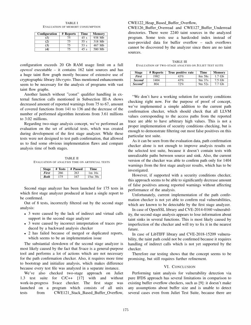
TABLE IEVALUATION OF MEMORY CONSUMPTION

Configuration # Reports Time Memory(1) 75 45 s 938 Mb(2) 75 55 s 318 Mb(3) 75 53 s 467 Mb(4) 75 45 s 580 Mb

configuration exceeds 20 Gb RAM usage limit on a fullopenssl executable – it contains 162 taint sources and hasa huge taint flow graph mostly because of extensive use ofcryptographic library libcrypto. Thus mentioned enhancementsseem to be necessary for the analysis of programs with vasttaint flow graphs.

Another launch without ”const” qualifier handling in ex-ternal function calls mentioned in Subsection III-A showsdecreased amount of reported warnings from 75 to 67, amountof covered functions from 141 to 136 and the decrease of thenumber of performed algorithm iterations from 3.61 millionsto 3.02 millions.

Regarding two-stage analysis concept, we’ve performed anevaluation on the set of artificial tests, which was createdduring development of the first stage analyzer. While thesetests were not designed to test path confirmation, that allowedus to find some obvious implementation flaws and compareanalysis time of both stages.

TABLE IIEVALUATION OF ANALYSIS TIME ON ARTIFICIAL TESTS

Stage # Tests # Passed TimeFirst 266 263 1m 16sBoth 175 167 15m 38s

Second stage analyzer has been launched for 175 tests inwhich first stage analyzer produced at least a single report tobe confirmed.

Out of 8 tests, incorrectly filtered out by the second stageanalysis:

• 3 were caused by the lack of indirect and virtual callssupport in the second stage analyzer

• 3 were caused by incorrect interpretation of traces pro-duced by a backward analysis checker

• 2 has failed because of merged or duplicated reports,which seems to be an implementation issue

The substantial slowdown of the second stage analyzer ismost likely caused by the fact that Svace is a general-purposetool and performs a lot of actions which are not necessaryfor the path confirmation checker. Also, it requires more timeto bootstrap and initialize analysis, which makes differencebecause every test file was analyzed in a separate instance.

We’ve also checked two-stage approach on Juliet1.3 test suite for C/C++ [17] with and withoutwork-in-progress Svace checker. The first stage waslaunched on a program which consists of all unixtests from CWE121 Stack Based Buffer Overflow,

CWE122 Heap Based Buffer Overflow,CWE126 Buffer Overread and CWE127 Buffer Underreaddirectories. There were 2240 taint sources in the analyzedprogram. Some tests use a hardcoded index instead ofuser-provided data for buffer overflow – such overflowscannot be discovered by the analyzer since there are no taintsources.

TABLE IIIEVALUATION OF TWO-STAGE ANALYSIS ON JULIET TEST SUITE

Stage # Reports True positive rate Time MemoryFirst 1982 43% 8m 58s 1.7 Gb

Second 1404 43% 9m 37s 7.5 GbSecond∗ 804 72% 9m 52s 7.7 Gb

∗We don’t have a working solution for security conditionschecking right now. For the purpose of proof of concept,we’ve implemented a simple addition to the current pathconfirmation checker, which should check that all LLVMvalues corresponding to the access paths from the reportedtrace are able to have arbitrary high values. This is not aproper implementation of security conditions checking, but isenough to demonstrate filtering out most false positives on thisparticular test suite.

As it can be seen from the evaluation data, path confirmationchecker alone is not enough to improve analysis results onthe selected test suite, because it doesn’t contain tests withunrealizable paths between source and sink. Also, the currentversion of the checker was able to confirm path only for 1404warnings from the first stage analyzer results, which has to beinvestigated.

However, if supported with a security conditions checker,this approach seems to be able to significantly decrease amountof false positives among reported warnings without affectingperformance of the analysis.

Unfortunately, current implementation of the path confir-mation checker is not yet able to confirm real vulnerabilities,which are known to be detectable by the first stage analyzer.

In case of OpenSSL library and CVE-2014-0160 vulnerabil-ity, the second stage analysis appears to lose information abouttaint sinks in several functions. This is most likely caused byimperfection of the checker and will try to fix it in the nearestfuture.

In case of LibTIFF library and CVE-2018-15209 vulnera-bility, the taint path could not be confirmed because it requireshandling of indirect calls which is not yet supported by thechecker.

Therefore our testing shows that the concept seems to bepromising, but still requires further refinement.

VI. CONCLUSION

Performing taint analysis for vulnerability detection viapure IFDS approach has several limitations in comparison toexisting buffer overflow checkers, such as [9]: it doesn’t makeany assumptions about buffer size and is unable to detectseveral cases even from Juliet Test Suite, because there are

175

no taint sources. For example, if a constant array index isused to access memory outside of array bounds. Moreover,considering error detection problem, pure static taint analysisgenerate too many alarms to be able to find few vulnerabilitiesuncaught in an industrial project. The majority of false alarmsare introduced by path-insensitivity and overtainting due toinconsistencies between a program and its memory model. Ourexperience shows that addons to simple and efficient memorymodel used by IFDS lead to unreasonable analysis slowdownand offer just a minimal results improvement. Therefore apostprocessing of results is required.

Proposed approach with two-staged analysis looks promis-ing, but requires a lot of enhancements to achieve industrial-level quality and there are no guaranties that it is even possible.

We are going to continue our research by developing othertypes of report confirmation in Svace infrastructure, sincedespite all listed limitations, the tool has a potential to discoverserious vulnerabilities, such as ”Heartbleed” in OpenSSL andCVE-2018-15209 in LibTIFF.

REFERENCES

[1] V. Koshelev, A. Izbyshev, and I. Dudina., “Interprocedural taint analysisfor LLVM-bitcode,” Trudy ISP RAN / Proc. ISP RAS, vol. 26, pp. 97–118, 2014, (in Russian).

[2] T. Reps, S. Horwitz, and M. Sagiv, “Precise interprocedural dataflowanalysis via graph reachability,” POPL ’95, pp. 49–61, 1995.

[3] N. A. Naeem, O. Lhotak, and J. Rodriguez, “Practical extensions to theIFDS algorithm,” Compiler Construction 2010, pp. 124–144, 2010.

[4] S. Arzt, S. Rasthofer, C. Fritz, A. Bartel, J. Klein, Y. L. Traon,D. Octeau, and P. McDaniel, “FlowDroid: precise context, flow, field,object-sensitive and lifecycle-aware taint analysis for android apps,”PLDI ’14, pp. 259–269, 2014.

[5] M. V. Belyaev, N. V. Shimchik, V. N. Ignatyev, and A. A. Belevantsev,“Comparative analysis of two approaches to static taint analysis,”Programming and Computer Software, vol. 44, no. 6, pp. 459–466, 2018.

[6] Z. Xu, T. Kremenek, and J. Zhang, “A memory model for staticanalysis of C programs,” Leveraging Applications of Formal Methods,Verification, and Validation, pp. 535–548, 2010.

[7] A. Y. Gerasimov, L. V. Kruglov, M. K. Ermakov, and S. P. Vartanov,“An approach of reachability determination for static analysis defectswith help of dynamic symbolic execution,” Trudy ISP RAN / Proc. ISPRAS, vol. 29, pp. 111–134, 2017, (in Russian).

[8] A. Y. Gerasimov, “Directed dynamic symbolic execution for staticanalysis warnings confirmation,” Programming and Computer Software,vol. 44, no. 5, pp. 316–323, 2018.

[9] I. A. Dudina and A. A. Belevantsev, “Using static symbolic execution todetect buffer overflows,” Programming and Computer Software, vol. 43,no. 5, pp. 277–288, 2017.

[10] C. Cadar, D. Dunbar, , and D. Engler, “KLEE: Unassisted and automaticgeneration of high-coverage tests for complex systems programs,” OSDI’08, pp. 209–224, 2008.

[11] Publications • KLEE. [Online]. Available:http://klee.github.io/publications/ [Accessed: 20-Mar-2019]

[12] klee/uclibc: KLEE’s version of uClibc. [Online]. Available:https://github.com/klee/klee-uclibc [Accessed: 2-Apr-2019]

[13] M. Simacek, “Symbolic-size memory allocation support for Klee,”Master’s thesis, Masaryk University, Faculty of Informatics, Brno,2018. [Online]. Available: https://is.muni.cz/th/mdedh/ [Accessed: 21-Mar-2019]

[14] D. A. Ramos and D. Engler, “Under-constrained symbolic execution:Correctness checking for real code,” Proceedings of USENIX SecuritySymposium ’15, pp. 49–64, 2015.

[15] P. D. Marinescu and C. Cadar, “KATCH: High-coverage testing ofsoftware patches,” Proc. of 9th Joint Mtg. on Foundations of SoftwareEngineering (FSE) ’13, pp. 235–245, 2013.

[16] V. P. Ivannikov, A. A. Belevantsev, A. E. Borodin, V. N. Ignatiev, D. M.Zhurikhin, and A. I. Avetisyan, “Static analyzer Svace for finding defectsin a source program code,” Programming and Computer Software,vol. 40, no. 5, pp. 265–275, 2014.

[17] Software assurance reference dataset. [Online]. Available:https://samate.nist.gov/SARD/testsuite.php [Accessed: 20-Mar-2019]

176

XXX-X-XXXX-XXXX-X/XX/$XX.00 ©20XX IEEE

C# parser for extracting cryptographic protocols

structure from source code

1st Ilya Pisarev

Information security departmen

Southern Federal University

Taganrog, Russian Federation

ilua.pisar@gmail.com

2nd Liudmila Babenko

Information security departmen

Southern Federal University

Taganrog, Russian Federation

lkbabenko@sfedu.ru

Abstract—Cryptographic protocols are the core of any secure

system. With the help of them, data is transmitted securely and

protected from third parties' negative impact. As a rule, a

cryptographic protocol is developed, analyzed using the means of

formal verification and, if it is safe, gets its implementation in the

programming language on which the system is developed.

However, in the practical implementation of a cryptographic

protocol, errors may occur due to the human factor, the

assumptions that are necessary for the possibility of

implementing the protocol, which entail undermining its security.

Thus, it turns out that the protocol itself was initially considered

to be safe, but its implementation is in fact not safe. In addition,

formal verification uses rather abstract concepts and does not

allow to fully analyze the protocol. This paper presents an

algorithm for analyzing the source code of the C# programming

language to extract the structure of cryptographic protocols. The

features of the implementation of protocols in practice are

described. The algorithm is based on the searching of important

code sections that contain cryptographic protocol-specific

constructions and finding of a variable chain transformations

from the state of sending or receiving messages to their initial

initialization, taking into account possible cryptographic

transformations, to compose a tree, from which a simplified

structure of a cryptographic protocol will be extracted. The

algorithm is implemented in the C# programming language using

the Roslyn parser. As an example, a cryptographic protocol is

presented that contains the basic operations and functions,

namely, asymmetric and symmetric encryption, hashing,

signature, random number generation, data concatenation. The

analyzer work is shown using this protocol as an example. The

future work is described.

Keywords—cryptographic protocols, C#, parser, verification,

tree, analysis, source code.

I. INTRODUCTION

The problem of verifying the security of cryptographic protocols is relevant nowadays despite the existence of a large number of already verified protocols. The need to use self-written protocols that use lightweight cryptography for IoT, mobile robots, as well as the imperfection of formal verification of protocols is a new challenge for verification methods, in particular, the possibility of verifying the security of cryptographic protocols implementation. The primary task in this matter is to extract the structure of the protocol from the

source code. At the moment there are works in which the problem of extracting an abstract model from the source code of programming languages C [1-3], Java [4-6], F# [7-12] is being considered. Most of them require a special programming style for the possibility of use these algorithms or the use of additional annotations in the source code. The paper proposes to analyze the source code of the C # programming language. There are no other works in which code analysis would be carried out, not involving the use of annotations or a special programming style.

II. CRYPTOGRAPHIC PROTOCOLS

Cryptographic protocols are a set of cryptographic algorithms and functions, with a correct combination of which is obtained a secure process of transferring messages between the parties. Protocol security is defined as complying with security requirements, the main of which are mutual authentication of the parties, protection against time attacks such as replay attacks, privacy and integrity of the transmitted data. Below is an example of a test protocol that does not have a special meaning, but contains all the basic cryptographic algorithms and functions: asymmetric and symmetric encryption, hashing, signature, random number generation.

1. A->B:

2. B->A:

3. A->B:

4. B->A:

5. A->B:

6. B->A:

At the beginning of this protocol, messages 1-3 use the Needham–Schroeder public key protocol (NSPK) [13] for mutual authentication of the parties. In message 3, in addition to the random number Nb, the key k is also transmitted for further communication between the parties using a symmetric cipher. In message 4, M2 data is transmitted, asymmetrically encrypted on partys' A public key, and some M1 data. All this is encrypted symmetrically using the key k, after which the data hash M1 is applied. In message 5, side A applies its M3 data to the previously sent data M1 and M2, encrypts all this symmetrically on key k, applies a signature and sends this

177

message to side B. In message 6, B sends A M3 data encrypted symmetrically on key k.

III. FEATURES OF THE CRYPTOGRAPHIC PROTOCOLS

IMPLEMENTATION

There are a number of problems with the implementation of cryptographic protocols. One of the problems is the dynamic size of messages. In the programming language, the transfer of messages between the parties is implemented using sockets. In this case, the party that receives the message must know in advance the size of the buffer to receive. For example, in the protocol described in the previous paragraph, in the first three messages random numbers and identifiers of the parties with a fixed length are used. In this case, everything is simple and at the reception of the message by the party, it will expect a previously calculated static message length. However, messages 4-6 use data M1, M2, M3, which may have different lengths. For example, in message 4, M1 data can be a video file, the length of which can vary from 1 MB to several GB. And the question is how to tell the receiving party the size of the receiving buffer. There are various options for how this can be done, for example, to add information about its length to the beginning of a message, to put a mark at the end of the message. Let us consider in more detail the option with the addition of information about the length of the message. This option involves the use of additional data before the main message, which will contain the size of the future message. An example of a message with additional size information is shown in Figure 1.

Buffer size Message

Figure 1 – Additional information about the size of the message

The receiving party in this case receives a fixed array of bytes, which contains the size of the message, after which the second portion takes the rest of the message knowing in advance its length.

A send: Buffer size, Message

B receive(4 bytes): Buffer size

B receive(Buffer size): Message

Since Message is usually encrypted and, in the context of a protocol, its transmission is protected, the question arises of how to protect information in Buffer size. All security requirements are important for us, except secrecy. To ensure them, you can, for example, use the signature of this area with timestamps. Thus, the transmission, for example, message 4, will have the following form when implementing the protocol:

B->A:

Another way is to get data into a fixed-length buffer until the buffer becomes empty. In this case, problems can also arise as shown in Figure 2.

Message part 1

Message part 2 Intruder’s part

Receive in buffer 1

Receive in buffer 2

Figure 2 – Intruders' attack on the addition of real data

The result is that the message will be received longer than necessary and in some implementations, in which further processing of the message by the receiving party is tied to the use of the message length, some data may be imperceptibly corrupted when decrypting and dividing the data into the message elements (random numbers, keys, etc.). In order to avoid this, various methods of controlling the length of a message are also used. Thus, some protocols are changed and supplemented during implementation, and for their initial analysis, for example, by means of formal verification this is not taken into account.

IV. SOURCE CODE ANALYSIS ALGORITHM

As an example for describing the operation of the algorithm, the previously considered protocol was taken and implemented in the C # programming language in the form of a client server application.

1. A->B:

2. B->A:

3. A->B:

4. B->A:

5. A->B:

6. B->A:

The analysis algorithm uses the C # Roslyn source code parser [14]. With it you can get the tree structure of the source code, and you can use filters. We need these filters:

1. InvocationExpressionSyntax - call expressions.

2. VariableDeclarationSyntax - declaration of variables.

3. AssignmentExpressionSyntax - an assignment expression.

4. IfStatementSyntax - statement with a condition statement.

Using filters, you can get the desired expression, after which you can view the tree structure of this expression. For example, using "AssignmentExpressionSyntax" we can find the expression "M1enc1 = RSA.Encrypt (M1, true)". The derived linear tree structure of the expression is shown in Figure 3.

Figure 3 – Tree structure of expression in a linear form.

178

The main purpose of using this parser is to find the transition from one variable to another. In this case, we are interested in the transition M1enc1 -> M1. This is achieved by searching for data such as "IdentifierName" together with the use of a black list of expressions. For example, it uses the call of the "Encrypt" method, as well as the previously declared object of the asymmetric encryption class "RSA", which are present in the black list, and M1enc1 and M1 that we need can be obtained from here, where the first element will be the variable to which the value will be assigned, and the rest of those that are lower and not included in the black list will be the new value assigned.

The algorithm is based on the definition of important code sections containing constructs specific to cryptographic protocols. Ultimately, the task is to find a chains of variables transformation from the state of sending or receiving messages (socket send/receive) to their initial initialization (static initialization, load from file, etc.), while taking into account possible cryptographic transformations (hash, encryption, etc.). In the course of building a chain, a tree is constructed, the nodes of which are variables with additional information about them, including data type definitions for the final leaves of the tree and cryptographic algorithms in the tree nodes. The tree structure allows you to describe all the chains of data transformations, since the data in the message is combined in various ways, the chains can be strongly branched and joined. Below is a fragment of the source code for the implementation of a part of the cryptographic protocol (messages 1-3) from participant A.

1

2

3

4

5

6

7

8

9

10

11

12

13

14

15

16

17

18

19

20

21

22

23

24

25

26

27

28

29

...

Socket socA =

new Socket(ipAddress.AddressFamily,

SocketType.Stream, ProtocolType.Tcp);

socA.Connect(remoteEP);

RNGCryptoServiceProvider rng = new

RNGCryptoServiceProvider();

byte[] A = new byte[] 132, 114 ;

byte[] B = new byte[] 15, 245 ;

byte[] Na = new byte[64];

rng.GetBytes(Na);

byte[] M1 = new byte[2 + 64];

Array.Copy(A, 0, M1, 0, A.Length);

Array.Copy(Na, 0, M1, 2, Na.Length);

//1

byte[] M1enc;

using (RSACryptoServiceProvider RSA =

new RSACryptoServiceProvider())

RSA.ImportParameters(

rsaPB.ExportParameters(false));

M1enc = RSA.Encrypt(M1, true);

30

31

32

33

34

35

36

37

38

39

40

41

42

43

44

45

46

47

48

49

50

51

52

53

54

55

56

57

58

59

60

61

62

63

64

65

66

67

68

69

70

socA.Send(M1enc);

//2

byte[] MGet2Encr = new byte[256];

socA.Receive(MGet2Encr);

byte[] MGet2;

using (RSACryptoServiceProvider RSA = new

RSACryptoServiceProvider())

RSA.ImportParameters(

rsaSA.ExportParameters(true));

MGet2 = RSA.Decrypt(MGet2Encr, true);

byte[] BFromServer = new byte[2];

byte[] NaGet = new byte[64];

Array.Copy(MGet2, 0, BFromServer, 0, 2);

Array.Copy(MGet2, 0, NaGet, 0, 64);

if (!NaGet.SequenceEqual(Na) &&

!B.SequenceEqual(BFromServer))

socA.Shutdown(SocketShutdown.Both);

socA.Close();

return;

byte[] Nb = new byte[64];

Array.Copy(MGet2, 64, Nb, 0, 64);

byte[] k = new byte[32 + 16];

rng.GetBytes(k);

byte[] M3 = new byte[0];

M3 = Nb.Concat(k).ToArray();

//3

byte[] M3enc;

using (RSACryptoServiceProvider RSA = new

RSACryptoServiceProvider())

RSA.ImportParameters(rsaPB.ExportParameters(false));

M3enc = RSA.Encrypt(M3, true);

socA.Send(M3enc);

...

First you need to define the declaration and initialization:

1. Objects of class Socket.

2. Class objects of the standard library cryptographic algorithms, such as the RSACryptoServiceProvider asymmetric encryption algorithm, the RNGCryptoServiceProvider random number generator, etc.

179

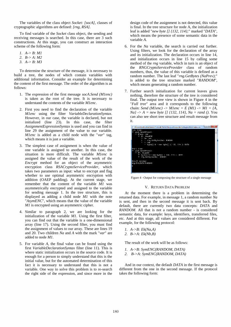
The variables of the class object Socket: [socA], classes of cryptographic algorithms are defined: [rng, RSA].

To find variable of the Socket class object, the sending and receiving messages is searched. In this case, there are 3 such constructions. At this stage, you can construct an interaction scheme of the following form:

1. A-> B: M1

2. B-> A: M2

3. A-> B: M3

To determine the structure of the message, it is necessary to

build a tree, the nodes of which contain variables with additional information. Consider an example for determining the content of the first message. The order of the algorithm is as follows:

1. The expression of the first message socA.Send (M1enc) is taken as the root of the tree. It is necessary to understand the contents of the variable M1enc.

2. First you need to find the declaration of the variable M1enc using the filter VariableDeclarationSyntax. However, in our case, the variable is declared, but not initialized (line 23). In this case, the filter AssignmentExpressionSyntax is used and you can find in line 29 the assignment of the value to our variable. M1enc is added as a child node with the "var" tag, which means it is just a variable.

3. The simplest case of assignment is when the value of one variable is assigned to another. In this case, the situation is more difficult. The variable M1enc is assigned the value of the result of the work of the Encrypt method for an object of the asymmetric encryption class RSACryptoServiceProvider, which takes two parameters as input: what to encrypt and flag whether to use optimal asymmetric encryption with addition (OAEP padding). At the current stage, we remember that the content of the variable M1 was asymmetrically encrypted and assigned to the variable for sending message 1. In the tree structure, this is displayed as adding a child node M1 with the note "AsymENC", which means that the value of the variable M1 is encrypted using an asymmetric cipher.

4. Similar to paragraph 2, we are looking for the initialization of the variable M1. Using the first filter, you can find out that the variable is a one-dimensional array (line 17). Using the second filter, you must find the assignment of values to our array. These are lines 19 and 20. Two children Na and A with the mark "var" are added to node M1.

5. For variable A, the final value can be found using the first VariableDeclarationSyntax filter (line 11). This is where static initialization occurs in the source code. It is enough for a person to simply understand that this is the initial value, but for the automated determination of this fact it is necessary to understand that this is not a variable. One way to solve this problem is to re-search the right side of the expression, and since more in the

design code of the assignment is not detected, this value is final. In the tree structure for node A, the initialization leaf is added "new byte [] 132, 114;" marked "DATA", which means the presence of some semantic data in the variable A.

6. For the Na variable, the search is carried out further. Using filters, we look for the declaration of the array and its initialization. The declaration occurs in line 14, and initialization occurs in line 15 by calling some method of the rng variable, which in turn is an object of the RNGCryptoServiceProvider class of random numbers, thus, the value of this variable is defined as a random number. The last leaf "rng.GetBytes (NaPrev);" is added to the tree structure marked "RANDOM", which means generating a random number.

7. Further search initialization for current leaves gives nothing, therefore the structure of the tree is considered final. The output tree view is shown in Figure 4 in the "Full tree" area and it corresponds to the following chain: Send (M1enc) -> M1enc = E (M1) -> M1 = A, Na -> A = new byte [] 132, 114, Na = rand (). You can also see short tree structure and result message from it.

Figure 4 –Output for composing the structure of a single message

V. RETURN DATA PROBLEM

At the moment there is a problem in determining the returned data. For example, in message 1, a random number Na is sent, and then in the second message it is sent back. By default, there are currently two data concepts: DATA and RANDOM. All that is not a random number - is considered semantic data, for example: keys, identifiers, transferred files, etc. And at this stage, all values are considered different. For example, for the following protocol:

1. A->B: Ek(Na,A)

2. B->A: Ek(Nb,B)

The result of the work will be as follows:

1. A->B: SymENC(RANDOM, DATA)

2. B->A: SymENC(RANDOM, DATA)

And in our context, the default DATA in the first message is different from the one in the second message. If the protocol takes the following form:

180

1. A->B: Ek(Na,A)

2. B->A: Ek(Nb,Na)

There is a problem. Na just comes back, and on the receiving side we need to understand that this is the same data. For example, when processing message 2 (lines 34-58), we can trace the separated parts. In line 50, the value of the random number Na is obtained, after which it is checked for coincidence with what was sent in line 52. Most often in the context of cryptographic protocols, returned values are used for mutual authentication. There can be 2 types: the return of the same number or the return of a function from this number. In both cases, the return value is checked for a match with the one sent earlier. In our case, this is line 53. However, another value is checked here — identifier B. In this case, one of the solutions to this problem would be to find the situation when the variable was sent, and then a value is checked for a match with this variable. In this case, you can assume that this is the case of the return value. However, there may be a number of problems, in particular, just the occurrence of an error in writing code, or simply the absence of such a check of the return value. At the moment, the abstract notion of the type of the RETURN variable is used. This means that a variable of this type was returned in the current message.

VI. PROTOCOL OUTPUT STRUCTURE

Using the algorithm presented in the preceding paragraphs, the complete output structure of the protocol is constructed according to the messages. It is obtained both in short form for formal verification, and in full form for dynamic verification. The full view contains the last variable, before serving in the cryptographic function, the names of the last variables and their initial initialization, for example, static in the code or loading data from a file. Dynamic analysis will be considered in further work and therefore the contents of the full protocol can be changed.

Short view:

1) A->B: AsymENC(DATA,RANDOM)

2) B->A: AsymENC(RETURN,RANDOM,DATA)

3) A->B: AsymENC(RETURN,RANDOM)

4) B->A: SymENC(DATA,AsymENC(DATA)),

HASH(DATA)

5) A->B: SymENC(RETURN,RETURN,DATA),

Sign(RETURN,RETURN,DATA)

6) B->A: SymENC(RETURN)

Full view:

1) A->B: AsymENC(DATA,RANDOM)

M1 | byte[] A = new byte[] 132, 114

| rng.GetBytes(Na)

2) A->B: AsymENC(RETURN,RANDOM,DATA)

M2 | socB.Receive(MGet1) |

rng.GetBytes(Nb) | byte[] B = new

byte[] 15, 245

3) A->B: AsymENC(RETURN,RANDOM)

M3 | socA.Receive(MGet2Encr) |

rng.GetBytes(k)

4) A->B: SymENC(DATA,AsymENC(DATA)),

HASH(DATA)

ForEncM4 | byte[] M1forSend =

File.ReadAllBytes("Mess1.txt") |

M2forSend | byte[] M2forSend =

File.ReadAllBytes("Mess2.txt") |

M1forSend | byte[] M1forSend =

File.ReadAllBytes("Mess1.txt")

5) A->B: SymENC(RETURN,RETURN,DATA),

Sign(RETURN,RETURN,DATA)

ConcatMess5 | socA.Receive(MGet4) |

socA.Receive(MGet4) | byte[] M3forSend

= File.ReadAllBytes("Mess3.txt") |

ConcatMess5 | socA.Receive(MGet4) |

socA.Receive(MGet4) | byte[] M3forSend

= File.ReadAllBytes("Mess3.txt")

6) A->B: SymENC(RETURN)

M3From5 | socB.Receive(MGet5)

VII. FUTURE WORK

Future work primarily includes a segmentation of DATA semantic data into classes:

1. Party identifiers

2. Keys

3. Timestamps

4. Authentication Codes

5. Data received from the user

It is also an important point to determine the ownership of a key by any of the parties in the case of asymmetric encryption, and to the list of parties in the case of symmetric encryption. Support for protocols involving more than two parties will also be needed. In addition, a complete solution to the problem of accurately determining the returned data is necessary to make it possible to build a complete structure of a cryptographic protocol and its further analysis using formal verification tools. After obtaining the structure of the cryptographic protocol, it is necessary to develop an algorithm for automated translation into the specification language of the most well-known protocol verification tools, such as Avispa [15], Scyther [16], ProVerif [17], and others. It is also necessary to improve the parser. At the moment, the structure can only be retrieved from areas of code where all functions for sending and receiving messages are combined into one block, for example, into the body of a function or class method. In the future, it is planned to improve the parser to work with complex code structures.

VIII. CONCLUSION

An algorithm was presented for analyzing the source code of the C # programming language for extracting the structure of cryptographic protocols, based on identifying important code sections that contain cryptographic protocol-specific constructions and determining the chain of variable

181

transformations from the sending or receiving status to their initial initialization, taking into account possible cryptographic transformations to compose a tree, from which it is possible to get simplified structure of a cryptographic protocol. An example of a protocol containing all cryptographic functions is given. The output structure of the cryptographic protocol is shown. For the further possibility of the application of formal verification of protocols and dynamic analysis, it is necessary to make an additional classification of semantic data, determine whether the keys belong to any party or parties, and also solve the problem with the returned values.

ACKNOWLEDGMENT

The work was supported by the Ministry of Education and Science of the Russian Federation grant 2.6264.2017/8.9.

REFERENCES

[1] Chaki S., Datta A. ASPIER: An automated framework for verifying security protocol implementations //Computer Security Foundations Symposium, 2009. CSF'09. 22nd IEEE. – IEEE, 2009. – С. 172-185.

[2] Goubault-Larrecq J., Parrennes F. Cryptographic protocol analysis on real C code //International Workshop on Verification, Model Checking, and Abstract Interpretation. – Springer, Berlin, Heidelberg, 2005. – С. 363-379.

[3] Goubault-Larrecq J., Parrennes F. Cryptographic protocol analysis on real C code. – Technical report, Laboratoire Spécification et Vérification, Report LSV-09-18, 2009.

[4] Jürjens J. Using interface specifications for verifying crypto-protocol implementations //Workshop on foundations of interface technologies (FIT). – 2008.

[5] Jürjens J. Automated security verification for crypto protocol implementations: Verifying the jessie project //Electronic Notes in Theoretical Computer Science. – 2009. – Т. 250. – . 1. – С. 123-136.

[6] O’Shea N. Using Elyjah to analyse Java implementations of cryptographic protocols //Joint Workshop on Foundations of Computer Security, Automated Reasoning for Security Protocol Analysis and Issues in the Theory of Security (FCS-ARSPA-WITS-2008). – 2008.

[7] Backes M., Maffei M., Unruh D. Computationally sound verification of source code //Proceedings of the 17th ACM conference on Computer and communications security. – ACM, 2010. – С. 387-398.

[8] Bhargavan K. et al. Cryptographically verified implementations for TLS //Proceedings of the 15th ACM conference on Computer and communications security. – ACM, 2008. – С. 459-468.

[9] Bhargavan K., Fournet C., Gordon A. D. Verified reference implementations of WS-Security protocols //International Workshop on Web Services and Formal Methods. – Springer, Berlin, Heidelberg, 2006. – С. 88-106.

[10] Bhargavan K. et al. Verified interoperable implementations of security protocols //ACM Transactions on Programming Languages and Systems (TOPLAS). – 2008. – Т. 31. – . 1. – С. 5.

[11] Bhargavan K. et al. Verified implementations of the information card federated identity-management protocol //Proceedings of the 2008 ACM symposium on Information, computer and communications security. – ACM, 2008. – С. 123-135.

[12] Bhargavan K. et al. Cryptographically verified implementations for TLS //Proceedings of the 15th ACM conference on Computer and communications security. – ACM, 2008. – С. 459-468.

[13] Needham R. M., Schroeder M. D. Using encryption for authentication in large networks of computers //Communications of the ACM. – 1978. – Т. 21. – . 12. – С. 993-999.

[14] Capek P., Kral E., Senkerik R. Towards an empirical analysis of. NET framework and C# language features' adoption //Computational Science and Computational Intelligence (CSCI), 2015 International Conference on. – IEEE, 2015. – С. 865-866.

[15] Viganò L. Automated security protocol analysis with the AVISPA tool //Electronic Notes in Theoretical Computer Science. – 2006. – Т. 155. – С. 61-86.

[16] Cremers C. J. F. The scyther tool: Verification, falsification, and analysis of security protocols //International Conference on Computer Aided Verification. – Springer, Berlin, Heidelberg, 2008. – С. 414-418.

[17] Küsters R., Truderung T. Using ProVerif to analyze protocols with Diffie-Hellman exponentiation //Computer Security Foundations Symposium, 2009. CSF'09. 22nd IEEE. – IEEE, 2009. – С. 157-171.

182

Fabless-companies data security

while using cloud services

Adelina Akhmedzianova

Kazan Federal University

Kazan,Russia iadelina.ah@gmail.com

Alexey Budyakov

Bauman Moscow State Technical

University

Moscow, Russia

alexbb@mail.ru

Sergey Svinarev

Rostov Law Institute of the Ministry of

Internal Affairs of the Russian

Federation

Rostov-on-Don, Russia squire@inbox.ru

Abstract—Cloud storage services like Google Drive and

Yandex.Disk are increasingly popular to store and transmitting

service information in corporate purposes, especially in fabless

companies, which do not have hardware and other resources for

sensitive data storage and exchange. These services allow

synchronizing and accessing data from multiple devices.

However, privacy of data stored in a cloud is a concern. To allow

data access from multiple devices, current solutions derive the

encryption keys solely from user-chosen passwords, which

result in low entropy keys. Moreover existing solutions do not

provide verification of the relevance of the data contained in the

cloud. In these terms, fabless companies need a more

appropriate solution. Method being developed has integration

with the Yandex.Disk cloud and intended to improve the

confidentiality of information stored in a cloud and consists of

user-side encryption, two-factor authentication scheme using

single-time passwords. Provision is made to ensure the

confidentiality of information during transmission to users not

having installed software. The resulting solution also can be

further used to create cross-platform software. Limitations of

considered scheme and further research are presented.

Keywords—cloud services, data security, encryption

I. INTRODUCTION

The high demand for using cloud storage services can be demonstrated by the example of fabless-companies. These companies are engaged in the development of semiconductor chips and other high-tech devices, so employees during their work process develop intellectual property objects – information in the limited-access category that have high economic value [1]. Many fabless-companies are small and it is widespread practice that engineers of the companies work remotely in collaboration, so there is the reason cloud storage services are preferable.

At present, cloud storage solutions like Google.Drive and Yandex.Disk are becoming more and more popular, bringing innovation not only in terms of minimizing the cost of resources but also in terms of optimization of company processes. These solutions are widely used for both personal purposes and corporate purposes for storage and transmission different types of data, including proprietary information.

Cloud services have a number of advantages like absence of need physical storages and opportunity to provide multiple access to files. However, security policy of cloud storages do not provide an appropriate level of data protection, including protection from cloud service providers themselves [2].

Currently some solutions partially solve the problem of providing security data storage in cloud services: Boxcyptor [3], CarotDAV [4], Mega [5]. These software applications are powerful tools for ensuring the confidentiality of data storage in the clouds, but most of them do not meet the requirements

in terms of easy access to the system, providing high level of data availability to multiple users, adaptability to the needs of the particular organization.

For example, the service [3] does not provide the relevance of files in the presence of multiple user access. Additionally, the encryption keys are generated only once when the user registers. The service [5] uses its own cloud storage and does not interact with other cloud storages.

The common disadvantages of existing solutions include the fact that they do not provide secure transmission of keys between users and the absence of version control – these tasks are completely left on the shoulders of users. Thus, the existing solutions in the field of data security in cloud services have a number of drawbacks, so they can not be used in organizations interested in providing the secure storage of processed data in cloud services – in particular, in fabless-companies.

This paper presents the approach to develop the software solution providing the security of data storage in the Yandex.Disk cloud storage service. The main part of paper divided into three sections. The first section presents the main requirements for the system. The second section describes the main functionalities of the system: two-factor authentication scheme, client-side encryption and directly interaction with cloud storage service directly by using API interface. In the third section is proposed the technique of generation and safe distribution of the encryption keys that takes into account the features of the scope of the system. In the last section, the limitations of the approach are described and options for the future work directions are proposed.

II. MATERIALS AND METHODS

A. Requirements

The main task of our system is to ensure the security of data stored in the cloud services. The most effective way to achieve this task is client-side encryption. However, client-side encryption additionally leads to the task of secure encryption key exchange between multiple users and task of secure transfer data to users who have no access to the system.

In order to design the solution it is necessary to define the main requirements that it must meet in order to be successful. An effective solution should meet the following requirements:

• providing convenient and effective tools to quickly

upload files from computer to cloud storage and download

files from cloud storage to a computer in safe mode;

• integration with cloud storage service using API

interface;

183

• ensuring the confidentiality of data (data encryption,

key generation and exchange) taking into account the features

of the scope of the system;

• ensuring the availability of data (including in relation

to people who have no access to the system);

• ensuring the relevance of data (confirmation of the

relevance of the file when it is loaded);

• providing an intuitive user interface;

• reducing the number of required actions from the user.

B. The basic functionality

Requirements from Section A allow to describe basic functionality of solution. In general, the solution can be used to perform the following scenarios:

1. Uploading a file to the cloud storage service;

2. Downloading a file from the cloud storage service;

3. Transfer a file to a person who has no access to the solution (but has the right to access the file).

Let’s describe each scenario more detailed.

Scenario 1. Uploading a file to the cloud storage service. In order to upload a new file to the cloud storage, firstly user has to be verified by entering a one-time password from his own token. After successful verification user should select the document needs to be uploaded. Then the solution generates an encryption key, encrypts the selected file and upload it directly to user’s folder in the cloud storage. If the user wants to update an existing file, in the solution will be additionally performed a comparison of the keys of both versions of file (normally they must be equal). After successful uploading the file to the file’s parameters will be added meta information about the last uploading. Fig.1 shows the conceptual scheme of the Scenario 1.

Fig.1. Conceptual scheme of Scenario 1 “Uploading a file to the cloud storage service”

Scenario 2. Downloading a file from the cloud storage service. In order to download file from the cloud storage, user must select the file has to be downloaded from the list of available files, provided by the solution. Then user has to be verified by entering a one-time password from his own token. Then in the solution is performing checking of the relevance of the file and, if it necessary, requests to get the latest version of this file are sent to users who have access to this file. Then user has to enter the encryption key, after which the document is decrypted. After successful downloading the file to the file’s parameters will be added meta information about the last downloading. Fig.2 shows the conceptual scheme of the Scenario 2.

Fig.2. Conceptual scheme of Scenario 2 “Downloading a file from the

cloud storage service”

Scenario 3. Transfer a file to a person who has no access to the system. In order to transfer a file to a legitimate person without an installed application, other user with access to the solution has to download the file according to Scenario 2 and sent this file via secure messenger.

The advantage of the solution is the fact that users do not interact with cloud storage service, but only with one solution. Interaction with cloud service is provided through Rest API interface, where the following methods are possible:

view a list of files in a user’s folders;

view and add meta information parameters of the file;

upload and download files.

Therefore, data processing takes place on the side of our solution, data storage – on the side of cloud service. The fragment of system sequence diagram, which shows the interaction between our solution and cloud storage service according to Scenario 1 “Uploading a file to the cloud storage service” is provided on Fig.3.

Fig.3. Sequence diagram for Scenario 2“Uploading the file to a cloud service”

C. Approach for data encryption

The task of providing the confidentiality of data is traditionally solved by the implementation of cryptographic algorithms. There is no need to separate the sender, who

184

applies encryption, and the receiver, who applies decryption of files, so it is advisable to use symmetric cryptographic algorithms in this case. DES is one such algorithm. DES is a block cipher operating on 64-bit blocks of plaintext using a 64-bit key [6].

In addition, to the implementation of the encryption, the solution according to the requirements should provide the secure transfer of encryption keys. Transferring method must be appropriate to the specifics of the scope of the solution: in the cloud data storage users should be able to instantly access all the files available in their cloud folders.

At the time, we consider two approaches to generate encryption keys: by hardware random number generator (Fig. 4) and by extracting bits from the image data (Fig. 5).

Fig.4. Example of one-time random number generator

Using image files as source files for a key generation has the advantage of improving the convenience in transferring encryption keys between users and implemented in different ways: generating encryption keys directly from the image or getting a key as result of converting the bits of the source file.

Method of generating encryption keys directly from the image, provided by the user, do not ensure a high degree of data confidentiality [7]. Image-keys distribute to users by uploading them into a cloud storage. Storing image-keys in a cloud service raises the probability of a brute-force attack.

More appropriate way to generate encryption key from the image as a result of some transformations. Currently the most popular method of hiding information in the media files is a steganography, the essence of which is to use files as a digital containers to hide data [8]. But using stenography methods in our solution leads to the complexity of the user interface and to the need for additional training in the rules of storage result images.

A modification of method of stenography is the reverse approach, when the encryption key is extracted from the source image by transformations without pre-treatment of this image. In order to generate the key from the source image we must set the sequence of positions. The encryption key consists of the bits standing in positions from a given sequence. In order to increase the resistance to attacks of this sequence should be non-trivial: for example, a sequence of positions of a fractal curve can be used (Fig.5).

If we define a set of positions in fractal curve, the bits from the original image located at these positions will make up the resulting encryption key. The most important limitation of the

proposed approach is the need to ensure the confidentiality of the solution source code.

Fig.5. Julia Set visualization

Advantages and disadvantages of considered two-factor authentication schemes will be investigated and compared to choose one for realization.

III. CONCLUSION

Nowadays privacy of data stored in a cloud services is a concern. The organizations interested in data security while using cloud storages (including fabless-companies) need such solution. This paper purposes an approach to the development of a solution providing security of data stored in the cloud services. The proposed approach has advantages over existing solutions. The approach ensures not only the implementation of the encryption functions but also the method of secure and convenient key generation and distribution. A system developed according to the described method will have an intuitive user interface. The number of actions required from the user is reduced because of direct interaction with cloud service by API interface. The main limitation of the approach is the need to protect program source code from unauthorized access and modification. The method proposed in this paper can be used as a basis for the development of a cross-platform application.

REFERENCES

[1] Jeorge S.Hurtarte, Evert A.Wolsheimer, Lisa M.Tafoya, “Understanding Fabless IC Technology”. Newnes, 2007, pp.25-32

[2] ‘Terms of Use of Yandex.Disk Service’, 2018. [Online]. Available: https://yandex.com/legal/disk_termsofuse/.

[3] ‘Boxcryptor. Encryption software to secure cloud files’, 2018. [Online]. Available: https://www.boxcryptor.com

[4] ‘WebDAV Client CarotDAV’, 2018. [Online]. Available: http://rei.to/carotdav_en.html.

[5] ‘MEGA’,2019. [Online]. Available: https://mega.nz.

[6] W.Stallings, “Cryptography and Network Security: Principles and Practice”, 6th ed. Prentice Hall Press Upper Saddle River, New Jersey: 2013, pp. 68-89.

[7] Omer A.Shqeer, “Judgment of Extracting Encryption Keys From Image Data”, IJCSNS vol.14, no.2, pp.116-119.

[8] S.Katzenbeisser, Fabien A.P.Petitcolas, “Information Hiding Techniques for Steganography and Digital Watermarking”. Boston: Artech House, 2000, pp.43-71.

[9] J.Sanders, E.Kandrot “CUDA by Example: an introduction to general-purpose GPU programming”. Addison-Wesley Professional,2010, pp.46-57.

185

Artificial Intelligence in Web Attacks Detecting

Maxim Gromov

Tomsk State University, 36, Lenin ave., Tomsk, 634050, Russia

maxim.leo.gromov@gmail.com

Svetlana Prokopenko Tomsk State University,

36, Lenin ave., Tomsk, 634050, Russia s.prokopenko@sibmail.com

Natalia Shabaldina Tomsk State University,

36, Lenin ave., Tomsk, 634050, Russia nataliamailbox@mail.ru

Alexander Sotnikov Tomsk State University,

36, Lenin ave., Tomsk, 634050, Russia sotnikhtc@gmail.com

Annotation – In this paper, the problem of web attacks

detecting is considered. We propose to use neural networks

to solve the problem. Such approach allows to pre-process

user data only once. Experimental results confirm the

feasibility of the application of artificial intelligence in web

attacks detection.

Index Terms – Web application, attack, neural network.

I. INTRODUCTION

EB APPLICATIONS are widely used. Users trust

web applications transfer, processing and storage

of personal and commercial data. Therefore security of

web applications is a hot topic. As a rule, web applications are verified and tested, in

particular, the security of applications is checked. But

even in this case, a valid user (who in fact has no

malicious intents) may accidentally enter data that

actually is an attack on the application. It happens due to

the fact that the variety of possible attacks is very large.

And at the moment of application development not all

attacks are known for developers.

Usually known types of attacks are considered for

testing of safety/security. But during exploitation, new

types of attacks dangerous for the application may appear. In this case, it becomes necessary to eliminate this

vulnerability of the application. It can be done, for

example, by adding of a new filter to the application

which detects such attacks.

The detection of web application vulnerabilities can be

done in different ways. There are mathematical

approaches based on automata equations and inequalities

solutions [1-5]. These approaches require the description

of a part of the program and all kinds of user data by

automata. Then the solutions of corresponding automata

equation or inequality describe possible attacks on this

web application. But these mathematical approaches are not general, because in some cases they can lead to

attacks’ skipping. In other cases the solutions include not

only attacks but also safe data [2].

Furthermore, there is a tool called Stranger [6, 7]. This

tool uses an attack pattern and a source code of a web

application and draws a conclusion whether the

application is vulnerable to the given attack.

Unfortunately, Stranger is applicable to programs written

in PHP ver. 3 or lower versions.

If new type of attacks appear and the application is

vulnerable to these attacks, new filters should be added to

the source code of the web application. These filters may

be implemented based on the PHP function

preg_replace. Filters indicate attacks and stop the

execution of the application, or modify user data. Such

user data modification should not lead to the loss of data

meaning but should remove the threat. During

exploitation, the web application is regularly upgraded

with new filters. So the web application source code is

regularly changed. To the best of our knowledge, there

are no other ways to protect web applications from new

vulnerabilities. Our paper is devoted to web attacks detection. For this

purpose we propose to exploit neural networks. Attack

detection is considered as a text classification process.

This approach requires only attack patterns and there is no

necessity in the source code of the application. Thus this

approach can be applied for web attacks detection on

applications that are developed in any programming

language. When new types of attacks appear, one only

needs to retrain the neural network.

II. PROBLEM STATEMENT

All modern web applications are interactive. Usually it

is assumed that users interact with the applications. The

user enters arbitrary data in specific fields. Since entered

data is processed by the application, it may be unsafe for

the application. User data can lead to database structure or

contents disruption, unauthorized access to data, etc.

To avoid situations described above, it is possible to act

in two ways. The first way is to analyze the source code

of a web application in order to detect and fix

vulnerabilities in the application. The second way is to

pre-process user data in order to detect and prevent possible attacks on the web application. Both cases

require the knowledge of the type of attacks.

Feasibility of neural networks to pre-process user data

is experimentally investigated in this paper.

III. THEORY

In this research, we consider a web application to be

vulnerable if it admits unauthorized access to data, their

modification, etc. Users interact with the web application

by issuing requests to the web server (via form fields or

W

186

2

URL requests). These requests contain transmitted users’

data. In this case, an attack is user data that is generated in

a special way.

The attack can be detected and neutralized using built-

in filters, for example, using the PHP preg_replace

function. Each type of attack should be described by a

regular expression, and the filter function should be called

for this expression (Fig. 1a).

Filter 1

Filter 2

Filter 3

Web-service

Data

User

ANN

Filter 1 Filter 2 Filter 3

Web-service

0

12

3

Data

User

a) b)

Fig. 1. Attacks’ filtering workflow. Classical approach (a), proposed

approach (b)

We propose another approach. The idea is to create a

function that detects an attack and determines attack’s

type. Neural network will be used for this purpose [8].

This approach allows to avoid multiple calls of the filtering function and call it with the desired regular

expression only once (Fig. 1b).

Since the considered problem is similar to the problem

of text messages classification, an appropriate neural

network structure is chosen (Fig. 2). The network includes

the following layers. The first one is embedding layer,

which is designed to map text strings to dense vectors.

Next layers are two recurrent layers LSTM (1) and LSTM

(2) for analyzing sequences and extracting key features

from dense vectors. The activation functions of the

recurrent layers are linear. Then dropout layer comes that

controls overfitting followed by dense layer. Dense layer is a classical features’ classification layer. An activation

function of the dense layer is sigmoid. Since this network

is used for classification problem, the function categorical

cross-entropy is used as a cost function during network

training.

The variety of possible attacks is large. Therefore we

consider only three types of classical attacks for

experiments: two types of SQL injections and one type of

XSS attacks.

An SQL injection is an injection of a malicious code

into an SQL request in order to gain unauthorized access to a database [9]. An XSS attack (cross-site scripting) is

an insertion of malicious code into the page being formed

[10]. For example, the malicious code can be written in

JavaScript.

The neural network needs to be trained before using.

The training set is formed as follows.

Three types of text strings were generated. The first

type of strings contains strings with SQL injections of the

kind OR 1=1. The second one contains strings of

common SQL injections. And the third type of strings

contains XSS attacks. In each case, the attacks were

masked by randomly generated text. We also generated

strings without attacks and strings that are similar to

attacks but are not attacks in fact.

string

Em

be

dd

ing

laye

r

maps words on dense vectors

LST

M(2

)-------------------------------LS

TM

(1)

analyses sequences

DR

OP

OU

T

to avoid overfitting

De

nse

0 – not dangerous1 – XSS attack, dangerous for the field 32 – SQL-injection of the kind ;‘OR 1= 1’, dangerous for the field 23 – common SQL-injection, dangerous for the fields 1 and 2

Fig. 2. Neural network structure

IV. EXPERIMENTAL RESULTS

A. An Example of a Web Application and Attacks

In order to develop attack patterns and to train the

neural network, we implemented user password change

web application. Moreover, we may not experiment with

real web applications since these experiments can lead to

data corruption stored and processed by the application.

The created web application is implemented using the

web server solution stack XAMPP [11]. The graphical

user interface of this application has a web form with

three fields, in which the user enters a login, an old-

password and a new-password.

The following two database queries are made in the

PHP part of the web application when transferring data

from the form to the web server:

SELECT pswrd FROM users WHERE login =

‘”.$login.”’;

UPDATE users SET pswrd =

‘”.$newpass.”’ WHERE login =

‘”.$login.”’;

For this web application, we consider various SQL

injections. An example of one of them is as follows.

Suppose that a user does not know the structure of

database queries, but knows names of tables. The user

wants to drop the table containing information about

logins and passwords. In order to drop the table, the user

types the following text in the new-password field:

'; drop table users; --

It implies the following database query:

UPDATE users SET pswrd = ‘’; drop

table users; -- ’ WHERE login =

‘”.$login.”’;

As a result of the malicious query, the table users is

dropped.

187

3

B. Experiments to Detect Web Attacks Using a Neural Network

To experiment on web attacks detecting using neural

network, the source code of the web application is not

required and the purpose of the application is not

essential. Therefore, similar to the experiments described

in the previous subsection, we consider a web application

with graphical user interface form containing three fields

(1, 2 and 3). Users type data to these fields. The web application processes data from the specified fields in

different ways. The method of data processing is essential

for the experiment. These fields are sensitive to the

attacks of different types.

The data from the first field is substituted as values of

variables in the logical expression for the WHERE

directive of the SQL query, for example,

SELECT * FROM users WHERE login =

'".$login."'

In the example above, the data from field 1 is

substituted for the $login variable.

Data from the second field is inserted into SQL query

of the general form.

Data from the third field is displayed unchanged in the

browser.

To detect and classify attacks, the neural network takes

user data string as an input, and returns a class number of

the string (Fig. 2):

0 denotes that the user data string does not contain an

attack;

1 denotes that the user data string contains an XSS

attack. The string is dangerous for the field 3;

2 denotes that the user data string contains an SQL

injection of the form ";‘ OR 1 = 1 ’". The string is

dangerous for the field 2;

3 denotes that the user data string contains an SQL

injection of the general form. The string is dangerous for

fields 1 and 2.

To train the neural network, the following training set

was generated:

– one million different strings with XSS attacks,

– one million different strings with the SQL injection of

the form ";‘ OR 1 = 1 ’";

– one million different strings with common SQL

injection.

Each attack was masked by random text data.

Moreover, strings that resemble attacks but are not

attacks were generated. For example, instead of the tag

<SCRIPT> a non-existent tag <ASCRIPT> was used,

etc. One million strings of pseudo-attacks for each type of

attacks were generated. Therefore, three millions of such

pseudo-attacks were generated.

Additionally, one million text strings with no attacks

and pseudo-attacks were generated.

Totally seven million text strings (data that user could

type in the fields of the web application form) were

generated. Each generated string was of the length 100

characters.

To train the neural network all string were shuffled. The

type of the string (SQL injections of the kind OR 1=1,

common SQL injection, XSS attack, and the string

without any attack) was kept with the corresponding

string. This information was used to train the network and

to assess the accuracy of recognition of the attack type.

The Keras over TensorFlow framework was used to

implement the neural network. For the experiments we

used the computer with the following parameters:

processor Intel Core i5-3470 3.2 GHz, 8 GB of RAM, 1

TB hard drive, video card GeForce GTX 650 Ti with

CUDA support, operating system Windows 7.

After training the network by 10% of an artificially

generated sample of seven million strings, the neural

network could classify the attacks with the accuracy of

99.97%.

V. CONCLUSION

In this paper, we considered the problem of web

application security. To the best of our knowledge the

only approach to solve the problem is to add new filters to

the source code of the application. Each filter should

detect specific attack and/or modify user data. In contrast

to this approach in the paper we suggested to perform

two-step pre-processing of user data to detect and filter an

attack on the web application.

At the first step an attack is detected and classified. At

the second step the user data is filtered by the appropriate

filter. Note that in the classical approach user data passes through several filters (Fig. 1a). It happens because it is

not known a priori whether the data contain an attack. The

type of the attack also is not known. In our approach, user

data passes through one filter (Fig. 1b), since the type of

attack was recognized at the first step.

As a future work, one could consider the problem of

embedding of a trained neural network into a web

application. In addition, it is interesting to investigate the

problem of neural network training on the fly.

ACKNOWLEDGMENT

This work was carried out with the financial support of

grant RNF No. 16-49-03012 "Reliability, security and

trust in systems used as services: scalable solutions for

effective analysis and management."

REFERENCES

[1] Anton V. Kolomeets, Natalia V. Shabaldina, Ekaterina V.

Darusenkova, Nina V. Yevtushenko. Using Models of Finite

Transition Systems for Checking Web-Service Security //18th

International Conference of Young Specialists on

Micro/Nanotechnologies and Electron Devices EDM 2017 :

proceedings Erlagol, 29 june - 3 july 2017. Novosibirsk: NSTU

publisher, 2017. P. 151-154.

[2] Shabaldina N., Yevtushenko N., Yu F. Towards checking

WEB-services security: using automata equations and inequalities //

Proceedings of the XII Conference Computer-aided technologies in

applied mathematics (ICAM 2018), June 4-8, 2018. P. 90

[3] P. Linz. An Introduction to Formal Languages and Automata,

Johnes & Barlett Learning, 2012

[4] L. Kari, “On language equations with invertible operations,”

Theoret. Comput. Sci. 132 (1994), L. Kari and G. Thierrin,

“Maximal and Minimal Solutions to Language Equations,” Journal

of computer and system sciences 53, (1996)

[5] B. A. Trahtenbrot, Ya. M.Barzdin: Finite automata (Behavior

and synthesis). Nauka, Moscow 1970 (in Russian).

188

4

[6] An Automata-based PHP String Analysis Tool.

https://vlab.cs.ucsb.edu/stranger/

[7] F. Yu, M. Alkhalaf, and T. Bultan. Stranger: An automata-

based string analysis tool for php. In TACAS, pages 154-157, 2010.

[8] Artificial neural network.

https://en.wikipedia.org/wiki/Artificial_neural_network

[9] SQL Injection Cheat Sheet.

https://www.netsparker.com/blog/web-security/sql-injection-cheat-

sheet/

[10] XSS Filter Evasion Cheat Sheet.

https://www.owasp.org/index.php/XSS_Filter_Evasion_Cheat_Shee

t

[11] XAMPP. https://www.apachefriends.org

189

SQLite RDBMS Extension for Data Indexing Using

B-tree Modifications

Anton Rigin1, Sergey Shershakov2

Faculty of Computer Science

National Research University – Higher School of Economics

Moscow, Russia 1amrigin@edu.hse.ru, 2sshershakov@hse.ru

The B-tree structure has several modifications which are, by

default, not supported in the popular open-source RDBMS

SQLite. In the scope of this work an extension for SQLite is

developed, based on some modifications of the B-tree structure.

The modifications of the base structure were developed as a C++

library. The library is connected to the SQLite using the C-C++

cross-language API. The SQLite extension also implements the

novel algorithm for selecting the best possible index structure (B-

tree or one of its modifications) for some table of a database.

Keywords—B-tree; data indexing; SQLite; DBMS; RDBMS;

multiway tree

I. INTRODUCTION

Last decades, the amount of data volume is growing substantially which exposes the well-known problem of big data [1].

Many companies and laboratories need to collect, store and process big data. There exist many algorithmic and software solutions to cope with these problems. One of these solutions is using indices which are usually represented by data structures such as hash tables and trees.

Using indices creates a new problem – when data are stored on slow carriers, it is more efficient to load data batches from a storage instead of splitting to individual elements. Multiway trees solve this problem. One type of them is a B-tree which was initially described by Bayer and McCreight in 1972 [2]. The B-tree also has several modifications. In this paper, the following B-tree modifications are considered: B+-tree [3], B*-tree [4] and B*+-tree (the latter is developed by the author of this paper data structure, which combines the main B+-tree and B*-tree features) [5].

This paper extends the research made in the framework of the term project [5].

One of the popular open-source relational database management systems (RDBMS) is SQLite [6]. It is used in mobile phones, computers and many other devices. However, this RDBMS does not support using B+-tree or B*-tree as data index structures by default.

The main goals of the work are the following:

• to add B-tree modifications such as B+-tree, B*-tree and B*+-tree to SQLite;

• to develop and implement an algorithm that would allow selecting the most appropriate indexing data structure (B-tree, B+-tree, B*-tree or B*+-tree) when a user manipulates a table.

The work includes linking of B-tree modifications from a C++ library (developed by the author of this work previously) to SQLite using a C-C++ cross-language API and developing an algorithm for selecting an indexing data structure.

The rest of the paper is organized as follows. Firstly, B-tree, B+-tree, B*-tree and B*+-tree are shortly described. After this, the SQLite, its indexing algorithms and extensions are presented. Then, the B-tree modifications C++ library and connecting it to the SQLite RDBMS is described. After this, our previous researches conducted using this library are presented. These researches have proved the main theoretical B-tree modifications complexity hypotheses and they show the abilities of this library. Then, the indexing approach, the methods for outputting the index representation and information and the development of algorithm of selecting the best index structure for table are discussed, after which the experiment conducted using the developed in this work SQLite extension is described. After this, the main points of the paper are summarized in conclusion and used references are presented.

II. B-TREE AND ITS MODIFICATIONS

A. B-tree

The B-tree is a multiway tree. It means that each node may contain more than one data key. Furthermore, each node except of the leaf nodes contains more than one pointer to the children nodes. If some node contains k keys than it contains exactly k + 1 pointers to the children nodes [2].

The B-tree depends on its important parameter which is called B-tree order. The B-tree order is such a number t that:

190

• for each non-root node, the following is true: t – 1 ≤ k ≤ 2t – 1, where k is the number of keys in the node [2];

• for root node in the non-empty tree the following is true: 1 ≤ k ≤ 2t – 1, where k is the number of keys in the node [2];

• for root node in the empty tree the following is true: k = 0, where k is the number of keys in the node [2].

B-tree operations complexities are the following (t is the tree order, n is the tree total keys count):

• for the searching operation: time complexity is O(tlogtn), memory usage is O(t) and disk operations count is O(logtn) [2];

• for the nodes split operation (the part of the insertion operation): time complexity is O(t), memory usage is O(t) and disk operations count is O(1) [2];

• for the insertion operation (includes the nodes split operation): time complexity is O(tlogtn), memory usage is O(tlogtn) for simple recursion and O(t) for tail recursion and disk operations count is O(logtn) [2];

• for the deletion operation: time complexity is O(tlogtn), memory usage is O(tlogtn) for simple recursion and O(t) for tail recursion and disk operations count is O(logtn) [2].

B-tree is usually used as the data index [2].

The example of B-tree is shown on the Fig. 1.

Fig. 1. The B-tree example, tree order t = 6.

B. B-tree Modifications

B+-tree is the B-tree modification in which only leaf nodes contain real keys (real data), other nodes contain router keys for searching real keys. Leaf nodes in B+-tree contain t ≤ k ≤ 2t keys, where t is the tree order, the rules for other nodes are the same as in B-tree [3]. Keys deletion in B+-tree is expected to be faster than in B-tree since it is always performed on the leaf nodes.

B*-tree is the B-tree modification in which each node (except of the root node) is filled at least by 2/3 not 1/2 [4]. Keys insertion in B*-tree is expected to be faster than in B-tree.

B*+-tree is the B-tree modification developed by the author of this paper which combines the main B+-tree and B*-tree features together. In this data structure only leaf nodes contain real keys (real data) as in B+-tree and each node (except of the root node) is filled at least by 2/3 as in B*-tree.

III. IMPLEMENTATION AND TOOLS

A. SQLite and Its Extensions

The SQLite is the popular open-source C-language library which implements the SQLite relational database management system (RDBMS) [6]. The SQLite default index algorithms are hash-table and B-tree. The SQLite does not implement B+-tree and B*-tree based indices.

Nevertheless, SQLite supports loading its extensions at run-time, which can add new functionality to the SQLite. For example, it can be a new index structure implementation. One of such extensions is the R-tree. The R-tree is a B-tree modification which allows to index geodata. It is loaded by the SQLite as the extension and delivered together with the SQLite RDBMS default build.

B. B-tree Modifications C++ Library

The B-tree modifications C++ library was developed by the author of this paper previously. It contains B-tree, B+-tree, B*-tree and B*+-tree implementations written in C++ [5].

In the current work this library is connected to the SQLite as the run-time loadable extension. For this goal the C-C++ cross-language API is implemented. It is possible to do using the extern “C” … C++ statement. The other tasks are to implement base SQLite extension’s methods and to use Makefiles to make this extension run-time loadable correctly. The extension provides module for creating virtual tables (tables which encapsulate callbacks instead of simple reading from database and writing to database) based on this module.

C. Research Conducted Using the Library

The B-tree modifications C++ library was previously used for conducting a research on the performance of multiway trees in the problem of structured data indexing by the author of this paper [5].

The CSV files with random content were generated for the indexing, with sizes of 25000, 50000, 75000, 100000 rows. The value of the first cell of each row was considered as a key (“name”) of the row and was saved in the tree together with the bytes offset of the row in the indexed CSV file. The charts of different dependencies were built using the Python 2.

The chart with the indexing time dependence on the tree order for a file where the “names” (keys) of the rows are uniformly distributed, with the size of 25000 rows is shown on the Fig. 2.

191

Fig. 2. The chart with the indexing time dependence on the tree order for a

file where the “names” (keys) of the rows are uniformly distributed, with

the size of 25000 rows.

According to this chart, B*-tree and B*+-tree have a better time performance on the keys insertion than B-tree and B+-tree, as expected. These results are confirmed by the experiments with other parameters (for example, on the larger files with different keys).

However, the better time performance of B*-tree and B*+-tree on the keys insertion has a cost of a larger memory usage as shown on the Fig. 3.

Fig. 3. The chart with the indexing memory usage dependence on the tree order for a file where all the “names” (keys) of the rows are equal, with

the size of 25000 rows.

Also, indexing using B*-tree or B*+-tree requires more disk operations than indexing using B-tree or B+-tree as shown on the Fig. 4.

Fig. 4. The chart with the indexing disk operations count dependence on the tree order for a file where all the “names” (keys) of the rows are

equal, with the size of 25000 rows.

The monotonous dependence of the keys searching on the tree order is not detected as shown on the Fig. 5.

Fig. 5. The chart with the index searching time dependence on the tree

order for a file where the “names” (keys) of the rows are uniformly

distributed, with the size of 25000 rows.

The B*-tree and B*+-tree require more memory during the keys searching than the B-tree and B+-tree as shown on the Fig. 6.

192

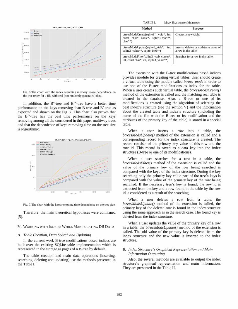
Fig. 6. The chart with the index searching memory usage dependence on

the tree order for a file with real (not randomly generated) data.

In addition, the B+-tree and B*+-tree have a better time performance on the keys removing than B-tree and B*-tree as expected and shown on the Fig. 7. This chart also proves that the B*+-tree has the best time performance on the keys removing among all the considered in this paper multiway trees and that the dependence of keys removing time on the tree size is logarithmic.

Fig. 7. The chart with the keys removing time dependence on the tree size.

Therefore, the main theoretical hypotheses were confirmed [5].

IV. WORKING WITH INDICES WHILE MANIPULATING DB DATA

A. Table Creation, Data Search and Updating

In the current work B-tree modifications based indices are built over the existing SQLite table implementation which is represented in the storage as pages of a B-tree by default.

The table creation and main data operations (inserting, searching, deleting and updating) use the methods presented in the Table I.

TABLE I. MAIN EXTENSION METHODS

Method Purpose

btreesModsCreate(sqlite3*, void*, int, const char* const*, sqlite3_vtab**, char**)

Creates a new table.

btreesModsUpdate(sqlite3_vtab*, int, sqlite3_value**, sqlite_int64*)

Inserts, deletes or updates a value of a row in the table.

btreesModsFilter(sqlite3_vtab_cursor*, int, const char*, int, sqlite3_value**)

Searches for a row in the table.

The extension with the B-tree modifications based indices provides module for creating virtual tables. User should create a virtual table using the module called btrees_mods in order to use one of the B-tree modifications as index for the table. When a user creates such virtual table, the btreesModsCreate() method of the extension is called and the matching real table is created in the database. Also, a B-tree or one of its modifications is created using the algorithm of selecting the best index’s structure (see the section V) and the information about the created table and index’s structure (including the name of the file with the B-tree or its modification and the attributes of the primary key of the table) is stored in a special table.

When a user inserts a row into a table, the btreesModsUpdate() method of the extension is called and a corresponding record for the index structure is created. The record consists of the primary key value of this row and the row id. This record is saved as a data key into the index structure (B-tree or one of its modifications).

When a user searches for a row in a table, the btreesModsFilter() method of the extension is called and the value of the primary key of the row being searched is compared with the keys of the index structure. During the key searching only the primary key value part of the tree’s keys is compared with the value of the primary key of the row being searched. If the necessary tree’s key is found, the row id is extracted from the key and a row found in the table by the row id is considered as a result of the searching.

When a user deletes a row from a table, the btreesModsUpdate() method of the extension is called, the primary key of the deleted row is found in the index structure using the same approach as in the search case. The found key is deleted from the index structure.

When a user updates the value of the primary key of a row in a table, the btreesModsUpdate() method of the extension is called. The old value of the primary key is deleted from the index structure and the new value is inserted to the index structure.

B. Index Structure’s Graphical Representation and Main

Information Outputting

Also, the several methods are available to output the index structure’s graphical representation and main information. They are presented in the Table II.

193

TABLE II. INDEX STRUCTURE’S INFORMATION AND GRAPHICAL

REPRESENTATION OUTPUTTING EXTENSION METHODS

Method Purpose

btreesModsVisualize(sqlite3_context*, int, sqlite3_value**)

Outputs the graphical representation of the table’s index structure (tree) into the GraphViz DOT file.

It is called after the SQL query such as SELECT btreesModsVisualize(“btt”, “btt.dot”);, where btt is the table name, btt.dot is the outputting GraphViz DOT file name.

btreesModsGetTreeOrder(sqlite3_context*, int, sqlite3_value**)

Outputs the order of the tree used as the table’s index structure.

It is called after the SQL query such as SELECT btreesModsGetTreeOrder(“btt” );, where btt is the table name.

btreesModsGetTreeType(sqlite3_context*, int, sqlite3_value**)

Outputs the type of the tree (1 – B-tree, 2 – B+-tree, 3 – B*-tree, 4 – B*+-tree) used as the table’s index structure.

It is called after the SQL query such as SELECT btreesModsGetTreeType(“btt” );, where btt is the table name.

C. SQLite Extension’s Usage Example

The developed in this work SQLite extension’s usage example is presented on the screenshot (Fig. 8).

Fig. 8. SQLite extension’s usage example.

V. ALGORITHM OF SELECTING THE BEST INDEX STRUCTURE

In this work an algorithm for selecting the best index structure for a table is developed and implemented in the following way.

The algorithm considers B-tree and its modifications (B+-tree, B*-tree and B*+-tree) for using as an index structure. The best index structure is defined by the step 6 of the algorithm.

The algorithm is executed at the start of each operation on the table (search, insertion, deletion or update of the table’s row) which uses the btrees_mods module. The algorithm consists of the following steps.

1. If the current total count of the operations on the tree is equal to 0 or more than 10000 or not a multiple of 1000, then exit the algorithm, otherwise go to step 2.

2. If the current count of the modifying operations on the tree (key insertions, key deletions) is less than 10 % of the current total count of the operations on the tree, then exit the algorithm, otherwise go to step 3.

3. If the current count of the key insertion operations is more than 90 % of the current count of the modifying operations on the tree, then select the B*-tree as the index structure and go to step 6, otherwise go to step 4.

4. If the current count of the key insertion operations is not less than 60 % of the current count of the modifying operations on the tree, then select the B*+-tree as the index structure and go to step 6, otherwise go to step 5.

5. Select the B+-tree as the index structure and go to step 6.

6. If the new index structure was selected in the steps 3 – 5, then rebuild the existing index structure into the new selected index structure (which is considered as the best index structure) saving all the data stored in the existing index structure.

The tree order of the B-trees and their modifications used in the SQLite extension developed in this work equals 100.

VI. EXPERIMENT CONDUCTED USING THE DEVELOPED SQLITE

EXTENSION

The experiment on the counting the empirical computational complexity is conducted using the developed in this work SQLite extension. The operations’ times were counted using the SQLiteStudio GUI manager [7]. The results are presented in the Table III.

TABLE III. EXPERIMENT RESULTS

Operation on the table Total execution time (ms)

Mean execution time per row (ms)

Table creation 21 -

First 500 rows insertion 9128 18.3

Next 500 rows insertion 9802 19.6

1001st row insertion (including the B-tree into the B*-tree rebuilding)

50 50

Next 499 rows insertion 9168 18.4

Last 500 rows insertion 8933 17.9

194

Operation on the table Total execution time (ms)

Mean execution time per row (ms)

First 500 rows deletion 9888 19.8

Next 500 rows deletion (including the B*-tree into the B*+-tree rebuilding)

9974 19.9

Next 500 rows deletion 9784 19.6

Last 500 rows deletion (including the B*+-tree into the B+-tree rebuilding)

9201 18.4

1000 rows insertion 18113 18.1

Next 4800 rows insertion (including the B+-tree into the B*+-tree rebuilding)

86465 18

According to the data in the Table III, the key insertion on the B*-tree is faster than on the B-tree as expected. The key deletion on the B+-tree and B*+-tree is faster than on the B-tree and B*-tree respectively. Also, the key insertion on the B*+-tree is slightly faster than on the B+-tree.

VII. CONCLUSION

The big data problem currently affects the world. There are many mathematical and software solutions for collecting, storing and processing big data including the data indexing. Many of the index data structures are tree-based ones such as B-tree and its modifications. B-tree is used as an index structure in many DBMSs including the popular open-source RDBMS SQLite. However, the SQLite does not support its modifications which may be more appropriate for some tasks than the original B-tree. In the current work this problem is elaborated.

Firstly, the B-tree modifications C++ library is connected to the SQLite as the extension using C-C++ cross-language API. After this, the algorithm of the best index selecting is developed and implemented and the experiment is conducted using the developed in this work SQLite extension.

This work tests new data indexing approaches using the SQLite as an example. The results of the work can be used by researchers and professors in this field and their students. The SQLite B-tree modifications extension can be used by all the developers who use this DBMS.

ACKNOWLEDGMENT

This work is supported by RFBR according to the Research project No. 18-37-00438 “mol_a”.

REFERENCES

[1] J. Manyika et al., “Big data: The next frontier for innovation, competition, and productivity,” McKinsey Global Institute, May 2011. Accessed: Jan. 20, 2019. [Online]. Available: https://www.mckinsey.com/~/media/McKinsey/Business%20Functions/McKinsey%20Digital/Our%20Insights/Big%20data%20The%20next%20frontier%20for%20innovation/MGI_big_data_exec_summary.ashx

[2] R. Bayer and E. McCreight, “Organization and maintenance of large ordered indexes,” Acta Informatica, vol. 1, no. 3, pp. 173 – 189, 1972.

[3] K. Pollari-Malmi. (2010). B+-trees [PDF paper]. Available: https://www.cs.helsinki.fi/u/mluukkai/tirak2010/B-tree.pdf

[4] “B*-tree.” NIST Dictionary of Algorithms and Data Structures. Available: https://xlinux.nist.gov/dads/HTML/bstartree.html (accessed Dec. 24, 2018).

[5] A. Rigin, “On the Performance of Multiway Trees in the Problem of Structured Data Indexing,” (in Russian), coursework, Dept. Soft. Eng., HSE, Moscow, Russia, 2018.

[6] “SQLite Home Page.” SQLite.org. Available: https://www.sqlite.org/ (accessed Jan. 20, 2019).

[7] “SQLiteStudio”. SQLiteStudio. Available: https://sqlitestudio.pl/ (accessed: Jan. 26, 2019).

195

Supporting evolutionary concepts to organize

information search in the Internet

1st Alexander Marenkov I nstitute YurInfor-MSU Moscow Malaya Pirogovskaya 5, Moscow,

119435, Russian Federation qwex-x@rambler.ru

2nd Senior Researcher Sergey Kosikov

I nstitute YurInfor-MSU Moscow Malaya Pirogovskaya 5, Moscow,

119435, Russian Federation

kosikov.v@gmail.com

3rd Candidate of Technical Sciences Larisa Ismailova

I nstitute YurInfor-MSU Moscow Malaya Pirogovskaya 5, Moscow,

119435, Russian Federation

lyu.ismailova@gmail.com

Abstract—Problem domain (PD), which are modeled in

information systems, are subject to changes; they have the

dynamics that must be taken into account when designing and

further using an information system. In this case, the arising

changes in the problem domain may not only affect the specific

data but change the content of the meta descriptions of the

problem domain. This instability is especially characteristic of

the information from the Internet. This requires additional

domain modeling tools and information system support for

saving the actual connection between the information system

and the problem domain.

The paper proposes an approach to modeling dynamic PD

based on the support of evolutionary concepts. It also considers

the possibility of using the approach to develop a prototype of a

system for supporting information search in the Internet and

processing the data found.

Keywords—concept, extension, intensional, problem domain,

domain dynamics

I. INTRODUCTION

When researching the PD one should adhere to the hypothesis, which forms the possibility of allocating

indivisible atomic objects, on the one hand, in this problem

domain, and the connections between these objects, on the

other hand. In its turn, the connected objects can form new

objects in the PD, and it is possible to include the connections

between objects themselves into the number of objects [4].

The dynamic nature of the PD requires a formalized

description of changes as a basis for developing tools. The

changes may be extensional (changing the scope of concepts

in the description of the problem domain) and intensional

(changing the content of the concepts, i.e., the researcher's

understanding of the problem domain).

The indicated above is characteristic of such an

information resource as the Internet, as well. Numerous

changes of concepts are seen in the Internet environment,

which today penetrate many spheres of human activity, be it

information gathering, training, communication, job, leisure,

etc. Constantly new information appears, the existing information is deleted or is affected by modifications.

Network pages are identified by a URL, which can be

considered as an individual identifier of the information page.

The change in the content of a page can both keep the

classification attributes of a page (extensional changes) and

lead to their change (intensional changes).

The changes may also be related to a modification of the

PD. This happens when the Internet user formulates

information queries. When the query is performed, a dynamic web page is created in accordance with its own classification

of resources. Different queries may classify the same Internet

resources into different classes according to the setting the

classifying characteristics.

The paper proposes an approach to the formalization of

variable classifications of objects based on the evolutionary

concept technique. An evolutionary concept is understood as

a concept supplied with a spectrum of its potential

transformations, keeping a given set of semantic characteristics of the concept. The paper discusses ways to

specify the general definition of the evolutionary concept

regarding the Internet.

II. THE TASK OF SUPPORTING EVOLUTIONARY CONCEPTS

Ensuring the work with evolutionary concepts is a critical

opportunity when developing information systems in

dynamic problem domains. For this reason, the task of

supporting evolutionary concepts for describing dynamic

objects is given a priority and is considered as the task to form

a set of tools that provide for the following:

representation of objects, allowing to account the dynamics of both extensions and intensions of the

introduced concepts;

ability to compute the assigning of objects bound to the

point of correlation;

ability to store descriptions of objects with the support

to linking with the object data about the nature of its

dynamics and extracting objects according to such

data.

The need to support the work in the Internet

environment makes additional requirements to the

developed tools. These requirements are as follows:

dynamic invocation to the address of the resource in

the Internet to check the validity of the link;

dynamic information retrieval by link and comparison

with a set of stored samples to determine the presence

of changes and define their nature;

196

construction and re-construction of the classification of

dynamic objects, including the case when modifying

the intentions of concepts in the problem domain.

It is feasible to solve the problem by combining the

expressive capabilities of semantic networks and applicative

computing systems. In this case, it seems possible to provide

a combination of the representation flexibility and the power

of computational tools enough to support evolutionary

concepts.

The possibility of using the approach to develop a

prototype of a system for supporting information search in the

Internet and processing the data found is under consideration.

III. REFERENCES

[1] Storing RDF at relational database. URL:

http://infolab.stanford.edu/~melnik/rdf/db.html [2] Current status of RDF, URL:

http://www.w3.org/standarts/techs/rdf#w3c_all

[3] Quillan M. R. Semantic memory // BOLT BERANEK AND

NEWMAN INC CAMBRIDGE MA. 1966. . SCIENTIFIC-2. [4] Wolfenhagen V. E. Logic. Lecture notes: the technique of reasoning.

Moscow. JurInfoR Center JSC, 2002. [5] Wolfengagen V. E., Ismailova L. Y., Kosikov S. V. The Presentation

of Evolutionary Concepts // First International Early Research Career

Enhancement School on Biologically Inspired Cognitive

Architectures. Springer, Cham, 2017. С. 113-125. [6] Wolfengagen, V. 2010. Semantic Modeling: Computational Models

of the Concepts // In Proceedings of the 2010 International

Conference on Computational Intelligence and Security (CIS '10).

IEEE Computer Society, Washington, DC, USA, 42-46.

DOI=10.1109/CIS.2010.16.

URL:http://dx.doi.org/10.1109/CIS.2010.16

197

XXX-X-XXXX-XXXX-X/XX/$XX.00 ©20XX IEEE

Deriving test suites with guaranteed fault coverage

against nondeterministic Finite State Machines with

timed guards and timeouts

Aleksandr Tvardovskii

National Research Tomsk State University

Tomsk, Russia

tvardal@mail.ru

Nina Yevtushenko

Ivannikov Institute for System Programming RAS

Moscow, Russia

evtushenko@ispras.ru

Abstract—The behavior of many information and control

systems nowadays is nondeterministic and depends on time

aspects. In this paper, we adapt classical FSM based test

derivation methods for initialized nondeterministic FSMs with

timed guards and timeouts (TFSMs). A proposed approach and

appropriate fault model are based on the FSM abstraction of the

given TFSM specification that can be used to describe the

behavior of a TFSM and allows to adapt classical FSM based

test derivation methods when deriving tests for TFSMs. We

study properties of such an abstraction for a nondeterministic

TFSM and justify that our method allows to derive test suites

with guaranteed fault coverage with respect to the defined fault

model.

Keywords—Finite State Machine, timeout, timed guard,

nondeterministic Timed Finite State Machine, test derivation

I. INTRODUCTION

Finite State Machines (FSMs) are widely used for analysis and synthesis of discrete event systems [1]. In particular, FSM based approaches can be effectively used when deriving test sequences for determining whether a given implementation considered as a “black box” conforms to its specification and a number of methods exist for deriving complete test suites with respect to various fault models [see, for example, 2-5] without the explicit enumeration of possible FSMs under test. Well-known W-method [2] and many its derivatives have been developed including those for FSMs with the nondeterministic behavior (see, for example, [4, 6]). Researchers often consider the case when the specification is a nondeterministic FSM, while an implementation FSM is deterministic and conforms to the specification if the implementation behavior is contained in that of the specification. In other words, the specification nondeterminism occurs according to the optionality of the informal requirements’ description and the behavior of a conforming implementation must not violate the specification.

Nowadays time aspects become very important when describing the behavior of digital and hybrid control systems, and, respectively, similar to automata [7] classical FSMs were extended with time variables [see, for example, 5, 8-12]. When the behavior of a system under test is described by a Timed Finite State Machine (TFSM), classical FSM-based methods have to be modified and extensions to the W-based methods are considered in the context of systems with timed constraints [8], [13]. In [10], Merayo et al. consider timed possibly nondeterministic FSMs where time elapsed when an output has to be produced after an input has been applied to the FSM under test is limited. The model also takes into account input timeouts at states. However, the authors do not consider test derivation; yet establish a number of

conformance relations. El-Fakih et al. [9] consider test derivation and assessment for FSMs with timed guards; such an FSM has a single clock that is reset at every transition. In the thesis by Zhigulin [12], a method is proposed for deriving complete test suites for FSMs with timeouts. The author considers a traditional fault domain assuming that the number of states of an implementation TFSM (Implementation Under Test, IUT) does not exceed that of the state reduced specification TFSM as well as the maximal finite timeout of the IUT does not exceed that of the specification. However, as we further show, two reduced TFSMs with timeouts can be equivalent but not isomorphic and this fact violates the main idea of W-based methods of checking the isomorphism or homomorphism between transitions of the specification and implementation under test. In [11], the authors show that the behavior of a deterministic TFSM can be adequately described by its FSM abstraction and this is a hint that a fault model can be derived based on such abstraction for which well elaborated FSM based methods with guaranteed fault coverage can be applied. Such a fault model is considered in [14] for deriving a complete test suite against deterministic TFSMs.

In this paper, we consider FSMs with timed guards, timeouts and output delays (TFSM) which generalize the TFSM model that has only timed guards or only input timeouts [10]. Moreover, in our case, a TFSM can be nondeterministic. Timed guards describe the system behavior depending on a time instance when an input is applied. If no input is applied until an (input) timeout expires then the system can spontaneously move to another state. An output delay describes a time for processing a given transition.

We propose a method for deriving a test suite with guaranteed fault coverage against a complete possibly nondeterministic specification FSM with timed guards, input timeouts and output delays with respect to the reduction relation assuming that an implementation TFSM under test is deterministic. The fault model and a procedure for deriving a complete test suite are based on the FSM abstraction of a given TFSM specification since according to [11], the behavior of a TFSM can be completely described by its corresponding (untimed) FSM abstraction.

The structure of the paper is as follows. Section 2 contains the preliminaries for classical and timed FSMs. It also contains the explanation how the behavior of a TFSM can be described using an appropriate FSM abstraction. In Section 3, existing test derivation methods for nondeterministic FSMs with respect to the reduction relation are considered. Section 4 contains the review of related works on test derivation against Timed FSM models. In Section 5, a method is proposed for deriving a complete test suite against a

198

nondeterministic FSM with timed guards and timeouts by determining an appropriate fault model based on the FSM abstraction of the given TFSM specification; the section also contains an example of a test derivation procedure. Section 6 concludes the paper.

II. PRELIMINARIES

This section contains basic definitions of classical Finite State Machines and Timed Finite State Machines as their extension. We also show how the behavior of a TFSM can be adequately described by the corresponding FSM abstraction and establish some useful properties of such FSM abstractions.

A. Finite State Machines

The model of a Finite State Machine (FSM) [1] is used for describing the behavior of a system that moves from state to state under input stimuli and produces a predefined output

response. Formally, an initialized FSM is a 5-tuple S = (S, I,

O, hS, s0) where S is a finite non-empty set of states with the designated initial state s0, I and O are input and output

alphabets, and hS (S I O S) is the transition

(behavior) relation. A transition (s, i, o, s) describes the situation when an input i is applied to S at the current state s.

In this case, the FSM moves to state s and produces the output (response) o. FSM S is nondeterministic [15] if for some

pair (s, i) S I, there can exist several pairs (o, s′) O

S such that (s, i, o, s′) hS; otherwise, the FSM is

deterministic. FSM S is complete if for each pair (s, i) S

I there exists (o, s′) ∈ O S such that (s, i, o, s′) hS; otherwise, the FSM is partial. FSM S is observable if for

every two transitions (s, i, o, s1), (s, i, o, s2) hS it holds that s1 = s2. In the following, we consider complete observable possibly nondeterministic FSM specifications, while an implementation is a complete deterministic FSM. A complete nondeterministic FSM is reduced if for every two different states, the sets of traces do not coincide. The unique reduced form exists for any complete nondeterministic FSM and can be derived similar to that for complete deterministic FSMs [15].

A trace or an Input/Output sequence /, written often as an I/O sequence, of the FSM S at state s is a sequence of consecutive input/output pairs starting at the state s. Given a

trace /, is the input projection of the trace (input

sequence) while is the corresponding output projection (output sequence), i.e., a possible output response of the

FSM when the sequence is applied at state s. Given a complete nondeterministic FSM, there can exist several output responses for an input sequence at a given state.

Given states s and p of complete FSMs S and P, state p is a reduction of s (written, p ≤ s) if the set of I/O sequences of FSM P at state p is contained in the set of I/O sequences of FSM S at state s. FSM P is a reduction of FSM S if the reduction relation holds between the initial states of the machines.

B. Timed Finite State Machines

A timed FSM (TFSM) is enriched with timed guards and timeouts [11]. The timed guards at a state have less time upper bounds than the timeout at the state (if any) and describe the behavior at a given state for inputs which arrive at different time instances. Correspondingly, an initialized TFSM is a 6-tuple S = (I, S, O, hS, ΔS, s0) where S is a finite non-empty

set of states with the designated initial state s0, I and O are

input and output alphabets, hS S I O S Z is the transition relation and ΔS is the timeout function. The

set is a set of input timed guards and Z is the set of output delays which are non-negative integers. The timeout

function is the function ΔS: S → S (N ) where N is the set of positive integers: for each state this function specifies the maximum time for waiting for an input. If no input is applied until an (input) timeout expires then the system can spontaneously move to another state. By definition, for each state of TFSM exactly one timeout is specified. An input timed

guard g describes the time domain when a transition can be executed and is given in the form of interval <min, max>

from [0; T), where < (, [, > ), ] and T is the input timeout at the current state. We also denote the largest finite boundary of timed guards and timeouts as BS. The transition

(s, i, o, s, g, d) S I O S Z means that TFSM S

being at state s accepts an input i applied at time t g measured from the initial moment or from the moment when TFSM S has produced the last output; the clock then is set to zero and S produces output o exactly after d time units. Given state s of TFSM S such that ΔS(s) = (s', T), if no input is applied before the timeout T expires, the TFSM S moves to

state s'. If ΔS(s) = (s', ) then s' = s, and this means that the TFSM can stay at state s indefinitely long waiting for an input.

Given TFSM S, S is a complete TFSM if the union of all input timed guards at any state s under every input i equals [0; T) when ΔS(s) = (s', T). In this paper, we consider only complete TFSMs and the question about the interpretation of undefined transitions in partial machines and their augmentation is out of the scope of this paper [16].

TFSM S is a deterministic TFSM if for each two

transitions (s, i, o1, s1, g1, d1), (s, i, o2, s2, g2, d2) hS, s1 s2, d1 d2 or o1 o2, it holds that g1 g2 = , otherwise, TFSM S is nondeterministic. In this paper, we consider the system specification as a complete observable possibly nondeterministic TFSM while the behavior of an implementation under test (IUT) is described by a complete deterministic TFSM. In other words, the specification describes a set of permissible possible behaviors and a conforming implementation must be one of them.

Example. Consider a TFSM S in Figure 1 with two states, one input and three outputs, where ΔS(a) = (b, 2), i.e., the

timeout at state a is 2. For state b, ΔS(b) = (b, ), and this loop is not shown in the figure. If input i is applied to the TFSM at state a at time instance 1 measured from the initial moment then S moves to state b producing output o2 after one time unit. However, if any input is not applied to TFSM until time value reaches 2 then S moves to state b using a timeout transition. At state b, TFSM S can wait for an input indefinitely long.

Fig. 1. Timed Finite State Machine S

199

A timed input is a pair (i, t) where i I and t is a real; a timed input (i, t) means that input i is applied to the TFSM at time instance t measured from the initial moment or from the moment when TFSM S has produced the last output. A timed

output is a pair (o, d) where o O and d is the output delay measured from the moment when an input has been applied. In order to determine the output response of the TFSM at state s to a timed input (i, t), state s', which is reached by the TFSM by timeout transitions at time instance t, is calculated first [12]. State s' is a state where TFSM moves from state s via

timeout transitions such that the maximum sum of all timeouts starting from state s is less than t. At the second step, a transition (or several transitions for nondeterministic

TFSM) (s', i, o, s'', g, d) such that t – g is considered. According to this transition, the machine produces the output (o, d) to a timed input (i, t) applied at state s and moves to the next state s''.

A sequence of timed inputs = (i1, t1) … (in, tn) is a timed

input sequence, a sequence of timed outputs = (o1, d1) … (on, dn) is a timed output sequence. The TFSM is initialized and the clock is equal to 0 at the initial moment. Given a timed input sequence (i1, t1) … (in, tn), an input i1 is applied when clock value is equal to t1; after applying the input the clock is set to 0 and the machine produces an output o1 when clock value is equal to d1. After producing the output o1 the clock is reset and the machine is waiting for another input i2 that is applied when clock value equals t2. After applying the input i2

the clock is set to 0 and the machine produces an output o2 when clock value is equal to d2. After producing the output o2

the clock is reset and the machine is waiting for another input

i3, etc. A sequence / = (i1, t1)/(o1, d1) … (in, tn)/(on, dn) of consecutive pairs of timed inputs and timed outputs starting at the state s is a timed I/O sequence or a timed trace of TFSM S at state s. Note that time of the first timed input in the sequence is counted from startup of the system at state s while time of all next inputs is counted from the time instance when a

previous output was produced. Similar to FSMs, is an

applied timed input sequence while is the corresponding

output response of the TFSM to sequence of applied inputs. Given a state of a complete nondeterministic TFSM, there can exist several output responses to a timed input sequence.

Similar to FSMs, the set of all timed traces at the initial state determines the behavior of an initialized TFSM.

Example. Consider TFSM S in Figure 1 again. If a timed input sequence (i. 2.5).(i, 0) is applied to S at state a then TFSM first moves to state b by timeout when clock value reaches 2. The clock is reset and output (o1, 2) or (o3, 2) is produced, the system moves back to state a and the clock is reset When the next input (i, 0) is immediately applied, the

TFSM moves either to state a with timed output (o3, 0) or to state b with timed output (o1, 1).

Given states s and p of complete TFSMs S and P, state p is a reduction of s (written, p ≤ s) if the set of timed I/O sequences of TFSM P at state p is contained in the set of timed I/O sequences of TFSM S at state s. TFSM P is a reduction of TFSM S if the reduction relation holds between the initial states of the machines.

C. FSM abstraction

The behavior of a TFSM can be adequately described using a classical FSM that is called the FSM abstraction of the TFSM and is derived similar to [11]; however, in [11], output delays are not considered.

Given a complete observable possibly nondeterministic

TFSM S = (S, I, O, S, ΔS, s0), the largest finite boundary of timed guards and timeouts BS and maximum output delay D, we derive the FSM abstraction of TFSM S as the FSM AS =

(SA, I I, OA, AS, s0) where SA = (s, 0), (s, (0, 1)), …, (s,

(BS – 1, BS)), (s, BS), (s, (BS, )): s S, OA = (o, 0), (o, 1),

…, (o, D): o O I. The input I is a special input of the FSM abstraction. Given state (s, tj), tj = 0, …, BS, of FSM

AS and input i, a transition ((s, tj), i, (o, d), (s, 0)) is a transition of the FSM abstraction AS if and only if there exists a transition

(s, i, o, s, gi, d) S such that tj gi. Given state (s, gj), gj =

(0, 1), …, (BS – 1, BS), (BS, ), of FSM AS and input i, a

transition ((s, gi), i, (o, d), (s, 0)) is a transition of AS if and

only if there exists a transition (s, i, o, s, g, d) S such that

gi g. In other words, transitions under input i I correspond to timed inputs (i, t) where t is ‘hidden’ as the second item of states of the FSM abstraction AS. Transitions under the special input I correspond to the clock change between non-integer and integer values, or to a timeout transition between states. Given state s such that ΔS(s) = (s',

T), transitions ((s, n), I, I, (s, (n, n + 1))) and ((s, (n – 1,

n)), I, I, (s, n)) are in the transition relation AS if and only

if n < T. Transition ((s, (n – 1, n)), I, I, (s, 0)) AS if and

only if n = T . In [11], it is shown that the FSM abstraction of complete and deterministic TFSM S is also complete and deterministic. In the same way, it can be shown that the FSM abstraction of a complete observable nondeterministic TFSM S is complete observable and nondeterministic.

Example. For a deterministic TFSM S in Figure 1 the corresponding FSM abstraction is shown in Figure 2. FSM abstraction AS has states (a, 0), (a, (0, 1)), (a, 1), (a, (1, 2)), (b,

0), (b, (0, )). Transitions ((a, 0), i, (o1, 1), (b, 0)) and ((a, 0), i, (o3, 0), (a, 0)) exist in FSM abstraction AS since TFSM S has transitions (a, i, o1, b, [0, 0], 1) and (a, i, o3, a, [0, 0], 0). FSM abstraction AS has transition ((a, (0, 1)), i, (o2, 1), (b, 0)) since TFSM S has transition (a, i, o2, b, (0, 2), 1). Transition ((a, 0),

Fig. 2. FSM abstraction AS of TFSM S (Figure 1)

200

I, I, (a, (0, 1))) of AS corresponds to clock change at state a from time instance 0 to the interval (0, 1).

A timed input sequence of TFSM S can be transformed

into a corresponding input sequence FSM of the FSM abstraction AS. In this case, each timed input (i, t) is replaced by sequence I.I … I.i of inputs of the FSM abstraction where the number of inputs I equals the number of clock transitions between a non-integer and integer values for the time duration t. At the same time the response of the FSM abstraction to sequence I.I.….I.i equals I.I.….I.(o, d), where the number of inputs I is the same as for the timed input (i, t) and (o, d) is the response of the TFSM to timed input (i, t). Thus, the output sequence of the FSM abstraction

FSM can be transformed into corresponding timed output

sequence by removing all outputs I. The following statement can be established.

Proposition 1. A timed trace / exists for TFSM S if and

only if there exists a trace FSM/FSM for the FSM abstraction AS.

Proposition 2. There exists a timed trace / at state s of a possibly nondeterministic TFSM S if and only if the FSM

abstraction AS has a trace FSM/FSM at state (s, 0).

Indeed, all the transitions under input I are deterministic and correspond to the clock change between integer and non-integer value and equal to increasing of timed variable while transitions at state (a, g) of abstraction under another input i corresponds to transitions of TFSM at state a at time (or timed interval) g.

Example. Consider TFSM S in Figure 1 and its FSM abstraction in Figure 2. Timed trace (i, 2.5)/(o1, 2).(i, 0)/(o3, 0) of TFSM S corresponds to trace I/I.I/I.I/I.I/I.I/I.i/(o1, 2).i/(o3, 0) of FSM abstraction AS, and vice versa.

According to Proposition 2, all the trace features of a TFSM are preserved for its FSM abstraction and thus, the set of reductions of a TFSM can be analyzed based on a set of reductions of a classical FSM. The following statement establishes necessary and sufficient conditions for two TFSM states to be in the reduction relation.

Proposition 3. State s of TFSM S is a reduction of state p of TFSM P if and only if state (s, 0) of the FSM abstraction AS is a reduction of state (p, 0) of FSM AP.

Thus, the conclusion about the reduction relation between two TFSMs can be drawn based on their FSM abstractions and there exist methods for checking the reduction relation between two FSM states or between two FSMs.

III. FAULT MODELS AND TEST SUITES

FSM based testing can be preset and adaptive. We first consider the preset testing where test cases are (timed) input sequences derived from the given TFSM specification to determine whether a given IUT, which is assumed to have the FSM behavior, conforms to the given specification. In this section, classical FSM based test derivation methods are adapted for test derivation against Timed FSMs.

In this paper, an implementation FSM P conforms to the specification if FSM P is a reduction of the specification FSM. In other words, an implementation FSM P conforms to the specification FSM if for each input sequence the output response of the FSM P is contained in the set of output

responses of the specification FSM to this input sequence. In

this case, the fault model FMmFSM = <S, ≤, m> is considered

where S is the specification that is a complete observable,

possibly nondeterministic FSM, ≤ is the reduction relation, m is the fault domain which contains each deterministic complete FSM with at most m states over the same input alphabet as the specification. Here we notice that differently from the paper [17] where only deterministic FSMs are considered, the specification can be nondeterministic and the conformance relation is not the equivalence but the reduction relation. Correspondingly, different transfer and separating sequences have to be used when deriving a test suite with guaranteed fault coverage.

A test suite is complete with respect to the FMmFSM = <S,

≤, m> if for each FSM P ∈ m such that P is not a reduction of S, the test suite has a sequence for which an output response of P is not in the set of output responses of S to this sequence.

A complete test suite with respect to FMmFSM can be

derived using an appropriate modification of the so-called state counting reduction (SCR) method for nondeterministic FSMs which was proposed in [6]; the proposed method is based on deterministically-transfer (d-transfer) and separating sequences. A state s is deterministically reachable (d-reachable) from the initial state of the FSM S if there exists an input sequence α such that for any output response β to α, the machine S moves from the initial state to state s when α is applied. In this case, α is a d-transfer sequence for state s. States s1 and s2 of an FSM S are separable if there exists an input sequence α such that the sets of output responses of the FSM at states s1 and s2 to α do not intersect; in this case, sequence α is called a separating sequence for states s1 and s2. If a sequence separates each pair of different states of the FSM S then this sequence is a separating sequence for FSM S. Again, differently from [17], not each input sequence is a d-transfer of the nondeterministic specification and separable states and separating sequences for the nondeterministic specification are defined in a different way according to [15].

If FSM S has a separating sequence and each state is d-reachable from the initial state, the procedure for deriving a

complete test suite w.r.t. the fault model FMnFSM = <S, ≤, n>

where n is the number of states of S, has the following steps:

1. A d-cover set of the FSM S is derived. This set contains a

d-transfer sequence for each state of the FSM S.

2. Each sequence of the d-cover set is appended with the

separating sequence of the FSM S and every input that

also is appended with the separating sequence .

If an adaptive test suite is derived, an adaptive distinguishing sequence can be used instead of a separating sequence while d-transfer sequences can be replaced by adaptive transfer sequences (if they exist). Adaptive distinguishing (separating) and d-transfer sequences can be shorter then preset, moreover, they exist more often.

An input sequence α is adaptive if the next input depends on the outputs of the FSM. Such an input sequence can be represented by an FSM called a test case [18]. At each state of a test case, either there are transitions for one input with all outputs or there are no transitions and in the latter case, a state is called terminal. Given a test case (TC) D for FSM S, an adaptive distinguishing sequence defined by DTC D is applied in the following way. If input i1 is defined at the initial state d0

201

of D then the first input i1 is applied to FSM S and DTC D moves to the i1o-successor d1 of state d0 if the output o is the response of S to the input i1. The next input to apply is the input defined at state d1, etc. The procedure terminates when a terminal state is reached.

A test case represents an adaptive separating sequence for states s1 and s2 of the FSM S if each input-output sequence from the initial to the terminal state of the test case is possible at most at one of states s1 or s2. In the former case, the state s1 is identified, while in the latter case it will be state s2. States s1 and s2 of the FSM S are adaptively separable if there is a test case that represents an adaptive separating sequence for states s1 and s2. In this case, the corresponding trace from the initial state to a terminal state of an adaptive separating test case allows to determine what was a state of the FSM S before the experiment.

If an adaptive sequence separates each pair of states of the FSM S, then such a sequence is an adaptive separating sequence for the FSM S.

A test case can also represent an adaptive sequence from the initial state of the FSM S to the state s if each input-output sequence of the test case from the initial to a terminal state is ended at state labeled by s [18, 19]. In this case, the state s is adaptively reachable from the initial state. The above steps for deriving a complete adaptive test suite are almost the same as for preset testing listed above; the only difference is that adaptive distinguishing sequences are used instead of separating sequences while using adaptive transfer sequences instead of d-transfer sequences.

If FSM S has no (adaptive) separating sequence or S has states which are not d-reachable from the initial state then a complete test suite cannot be derived using the above procedure. In this case, the so-called state counting (SCR) method should be applied [6].

Below, we describe the main steps of the general SCR-

method with respect to fault model FMmFSM = <S, ≤, m>.

1. Determine subset Sd of all d-reachable states and derive

d-cover of the FSM S which contains a d-transfer

sequence for each state of Sd.

2. Determine the set R = R1, R2, …, Rp of maximal subsets

of pairwise separable states; for each subset Rj R,

denote Rjd a subset of all d-reachable states of Rj. For

each subset Rj R, derive a distinguishing set Wj that

contains a separating sequence for each pair of different

states of Rj.

3. For each state sk of Sd, derive a set of input sequences Nk:

an input sequence Nk if for each I/O sequence / at

state sk, it holds that / traverses states of some Rj R

at least m - |Rjd| + 1 times and this does not hold for any

proper prefix of . Concatenate each prefix of sequence

with each sequence of the set Wj.

4. Concatenate each d-transfer sequence with each

sequence of each set Wj that was used at Step 3 when

terminating an input sequence of the set Nk, k = 1, …, p.

Here we notice that in general case, complete test suites derived by SCR method are much longer than for the case when the specification FSM has a separating sequence and the derivation method is much more complex. To minimize our

efforts for deriving a complete test suite w.r.t. the fault model

FMmFSM = <S, ≤, m>, the adaptive testing can be used instead

of the preset [18].

It is known that a test suite can be usually shorter if the specification FSM has a sequence, which separates every two states [6]. In this case set Wj contains only one separating

sequences and R = S. However, such a separating sequence does not always exist and thus, we are obliged to use a set of separating sequences for test derivation. Adaptive distinguishing (separating) sequences exist more often than the preset and are usually shorter, thus, adaptive distinguishing sequences can be preferable for test derivation. Anyway, using adaptive distinguishing sequences can increase the size of subsets of pairwise distinguishable states, and thus, sets Wj and the sets Nk of transfer input sequences, and correspondingly, minimize a complete test suite.

In the next section, we consider an existing approach for adaptation classical FSM based test derivation methods for Timed FSM.

IV. RELATED WORK ON TFSM BASED TESING

The problem of deriving a complete test suite against a nondeterministic FSM with timed guards with respect to reduction relation has been considered in [19]. The proposed approach is based on the FSM abstraction of TFSM but that abstraction is a bit different from that considered in the ‘Preliminaries’ section. In that case, one-to-one mapping between sets of states of TFSM and corresponding FSM abstraction has been established. The latter allows to inherit the above described steps for deriving a complete test with respect to the fault domain which contains each deterministic complete TFSMs with timed guards with at most m states over the same input alphabet as the specification TFSM S and the largest boundary BS for input timed guards. However, in general case, this approach cannot be applied for FSMs with time guards and timeouts since the one-to-one mapping between transitions of two state reduced equivalent TFSMs with timeouts not always can be established.

In [14], it is shown that initialized reduced deterministic TFSM specification and TFSM implementation with timeouts can be equivalent yet not isomorphic; moreover, they can have different number of states. The latter violates the main assumption of W-based methods about checking the correspondence between FSM transitions. As an example, consider TFSMs in Figure 3.

Fig. 3. Two reduced deterministic complete TFSMs R and Q

202

Each state in R and Q is reachable from the initial state and each two different states of each machine are not equivalent, i.e., both TFSMs are connected and state reduced. By direct inspection, one can assure that equivalent machines in Figure 3 have different number of states and thus, are not isomorphic.

On the other hand, according to Proposition 1, the necessary relationship holds between transitions of their FSM abstractions. For example, reduced forms of FSM abstractions of TFSMs R and Q (Figure 3) are isomorphic. FSM abstraction AR and its reduced form is shown in Figure 4. Thus, in order to derive a complete test suite for deterministic TFSMs, corresponding fault domain contains every TFSM P over the same input alphabet as S such that the reduced form of the FSM abstraction of P has at most m > 1 states. A similar approach can be applied for the test derivation against nondeterministic FSMs with timeouts and timed guards; in the next section, corresponding fault model and test derivation method are proposed.

V. TEST DERIVATION METHOD FOR NONDETERMINISTIC FSM

WITH TIMED GUARDS AND TIMEOUTS

In order to derive a test suite with guaranteed fault coverage for a nondeterministic TFSM we propose a fault model based on the FSM abstraction of the TFSM and apply the SCR-method.

Given a nondeterministic TFSM S with n states (Figure 1), two deterministic equivalent TFSM implementations R and Q (Figure 3) which are reductions of S can have different number of states. However, the reduced forms of their abstractions are isomorphic and are reductions of FSM abstraction AS. Another example in Figure 5 demonstrates that for nondeterministic TFSM Y there can exist a deterministic

TFSM Y with the same number of states and the boundary BS,

such that FSM abstraction AY has more states than AY.

Given a TFSM specification S, we consider the fault

model FMmTFSM = <S, ≤, m>, where S is the complete

nondeterministic observable TFSM specification, ≤ is the

reduction relation, m is the fault domain that contains each deterministic complete TFSM P over the same input alphabet as the specification such that the reduced form of its FSM abstraction AP has at most m > 1 states.

It can well happen that some timed FSMs with less states than the specification TFSM are not included into the fault

domain and vice versa a number of timed FSMs which have more states than the specification TFSM, are included into the fault domain.

Example. Consider TFSM specification S (Figure 1) with

two states. Fault domain m from fault model FMmTFSM = <S,

≤, m> contains TFSM R (Figure 3) with 3 states since the FSM abstraction AR has not more states than the FSM abstraction AS. At the same time, in Figure 5 the TFSM

specification Y and its non-conforming implementation Y are shown such that both TFSMs have three states and the finite

timed guards’ boundary two. However, the fault domain m

does not contain Y since the reduced form of its FSM abstraction has more states than AY. Thus, it can happen that nonconforming implementations with the same number of states as the specification TFSM can pass a complete test suite

with respect to <S, ≤, m>.

Fig. 5. TFSM Y and its non-conforming implementation Y

Note that the FSM abstraction of TFSM S can have non-separable states, i.e. the FSM abstraction can have a pair of states for which a separating sequence does not exist while the specification TFSM S has a separating sequence, i.e., all states of the TFSM S are pairwise separable. For example, TFSM S in Figure 1 has a separating sequence (i, 1) while the corresponding FSM abstraction AS has a pair of non-separable

Fig. 4. The FSM abstraction AR of TFSMs R (Figure 3) and its reduced forms

203

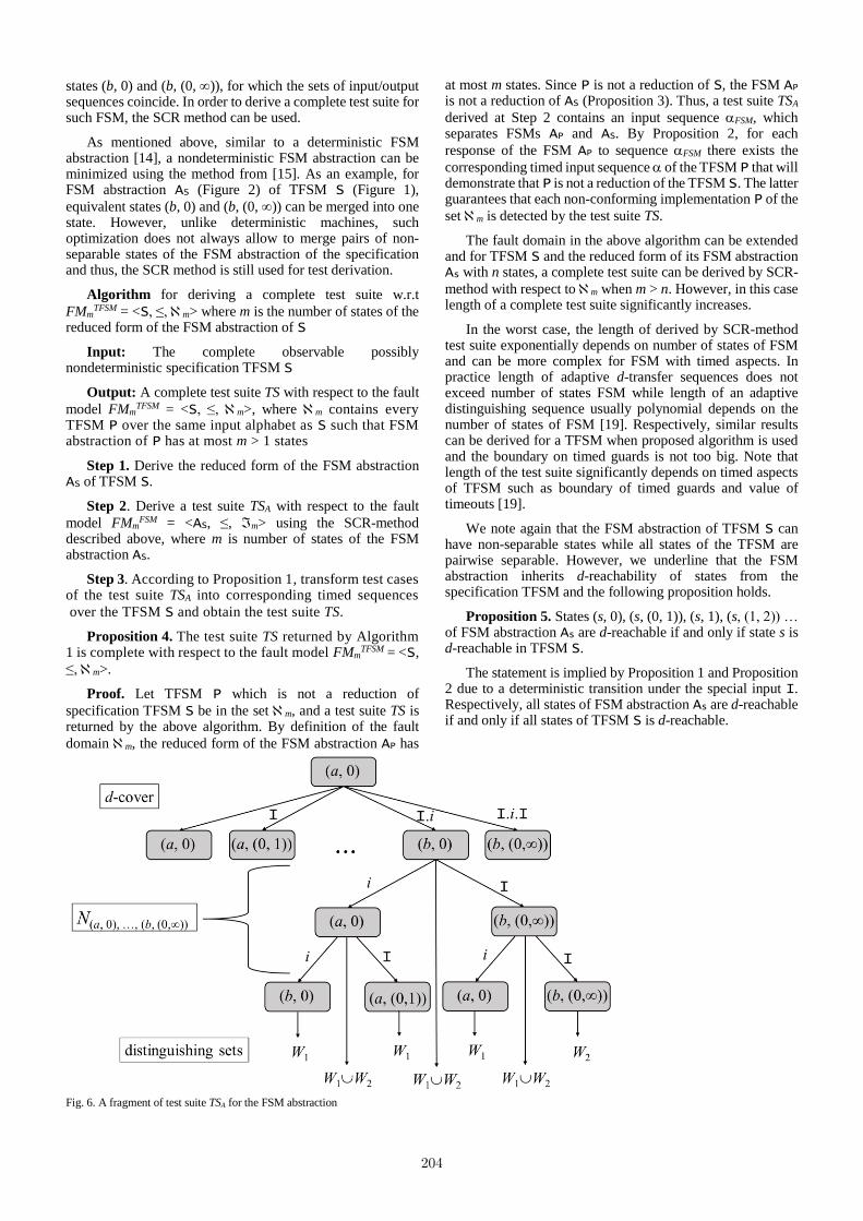
states (b, 0) and (b, (0, )), for which the sets of input/output sequences coincide. In order to derive a complete test suite for such FSM, the SCR method can be used.

As mentioned above, similar to a deterministic FSM abstraction [14], a nondeterministic FSM abstraction can be minimized using the method from [15]. As an example, for FSM abstraction AS (Figure 2) of TFSM S (Figure 1),

equivalent states (b, 0) and (b, (0, )) can be merged into one state. However, unlike deterministic machines, such optimization does not always allow to merge pairs of non-separable states of the FSM abstraction of the specification and thus, the SCR method is still used for test derivation.

Algorithm for deriving a complete test suite w.r.t

FMmTFSM = <S, ≤, m> where m is the number of states of the

reduced form of the FSM abstraction of S

Input: The complete observable possibly nondeterministic specification TFSM S

Output: A complete test suite TS with respect to the fault

model FMmTFSM = <S, ≤, m>, where m contains every

TFSM P over the same input alphabet as S such that FSM abstraction of P has at most m > 1 states

Step 1. Derive the reduced form of the FSM abstraction AS of TFSM S.

Step 2. Derive a test suite TSA with respect to the fault

model FMmFSM = <AS, ≤, m> using the SCR-method

described above, where m is number of states of the FSM abstraction AS.

Step 3. According to Proposition 1, transform test cases of the test suite TSA into corresponding timed sequences

over the TFSM S and obtain the test suite TS.

Proposition 4. The test suite TS returned by Algorithm 1 is complete with respect to the fault model FMm

TFSM = <S,

≤, m>.

Proof. Let TFSM P which is not a reduction of

specification TFSM S be in the set m, and a test suite TS is returned by the above algorithm. By definition of the fault

domain m, the reduced form of the FSM abstraction AP has

at most m states. Since P is not a reduction of S, the FSM AP is not a reduction of AS (Proposition 3). Thus, a test suite TSA

derived at Step 2 contains an input sequence FSM, which separates FSMs AP and AS. By Proposition 2, for each

response of the FSM AP to sequence FSM there exists the

corresponding timed input sequence of the TFSM P that will demonstrate that P is not a reduction of the TFSM S. The latter guarantees that each non-conforming implementation P of the

set m is detected by the test suite TS.

The fault domain in the above algorithm can be extended and for TFSM S and the reduced form of its FSM abstraction As with n states, a complete test suite can be derived by SCR-

method with respect to m when m > n. However, in this case length of a complete test suite significantly increases.

In the worst case, the length of derived by SCR-method test suite exponentially depends on number of states of FSM and can be more complex for FSM with timed aspects. In practice length of adaptive d-transfer sequences does not exceed number of states FSM while length of an adaptive distinguishing sequence usually polynomial depends on the number of states of FSM [19]. Respectively, similar results can be derived for a TFSM when proposed algorithm is used and the boundary on timed guards is not too big. Note that length of the test suite significantly depends on timed aspects of TFSM such as boundary of timed guards and value of timeouts [19].

We note again that the FSM abstraction of TFSM S can have non-separable states while all states of the TFSM are pairwise separable. However, we underline that the FSM abstraction inherits d-reachability of states from the specification TFSM and the following proposition holds.

Proposition 5. States (s, 0), (s, (0, 1)), (s, 1), (s, (1, 2)) … of FSM abstraction As are d-reachable if and only if state s is d-reachable in TFSM S.

The statement is implied by Proposition 1 and Proposition 2 due to a deterministic transition under the special input I. Respectively, all states of FSM abstraction As are d-reachable if and only if all states of TFSM S is d-reachable.

Fig. 6. A fragment of test suite TSA for the FSM abstraction

204

Example. Consider TFSM S in Figure 1 and its FSM abstraction AS in Figure 2. We derive a complete test suite

w.r.t. the fault model FM6TFSM = <S, ≤, 6>. For state (b, 0)

of AS there exists a d-transfer sequence I.i and respectively, state b of TFSM S has a timed d-transfer sequence (i, 0,5). Other states of FSM abstraction are d-reachable from states (a, 0) and (b, 0) by a sequence of I inputs. Thus, all states of AS are d-reachable from the initial state and for the FSM abstraction AS, Sd = (a, 0), (a, (0, 1)), (a, 1), (a, (1, 2)), (b, 0),

(b, (0, )).

Given FSM AS, we can also determine two maximal subsets of pairwise separable states R1 = (a, 0), (a, (0, 1)), (a, 1), (a, (1, 2)), (b, 0), R2 = (a, 0), (a, (0, 1)), (a, 1), (a, (1, 2)),

(b, (0, )) and corresponding distinguishing sets W1 = W2 = i, I.i, I.I.i. Note that R1 = R1d and R2 = R2d since all states of AS are d-reachable.

Consider state (b, 0) and the set N(b, 0) of input sequences derived at Step 3 of the SCR-method when a test suite is

derived with respect to the fault model <S, ≤, 6>. Input/Output sequences with the input projection of the set N(b,

0) should traverse states of some Rj at least 2 = 6 - 5 + 1 times while this does not hold for any proper prefix of the input sequence, and respectively, i.i is in the set N(b, 0) which traverses states (a, 0) and (b, 0) of R1. Other sequences at state (b, 0) are i.I (traverses (a, 0), (a, (0, 1))), I.i (traverses (b, (0,

)), (a, 0)), I.I (traverses (b, (0, )), (b, (0, ))) and thus,

N(b, 0) = i.i, i.I, I.i, I.I, i, I

A fragment of the tree that is obtained when deriving a test suite, is shown in Figure 6. One of test sequences of TSA is I.i.i.i.I.I.i and a corresponding timed input sequence of test TS is (i, 0,5).(i, 0).(i, 0).(i, 1) where (i, 0,5) is a d-transfer sequence and (i, 1) is a separating sequence from W1. Each sequence of the test suite is applied to TFSM implementation at the initial state. First input i is applied when clock is equal to 0,5; after applying the input the clock is set to 0 and the machine produces corresponding output when clock value is equal to 1 when an implementation is conforming. After producing the output o2 the clock is reset and the machine is waiting for the next input i that is immediately applied after resetting the clock. After applying this input the clock is reset again and the machine produces an output o1 or o3 when clock value is equal to 2. After producing any of outputs the clock is reset and the machine is waiting for a next input, etc.

VI. CONCLUSIONS

In this paper, we have proposed an approach for deriving complete test suites with respect to the reduction relation against nondeterministic Finite State Machines with timed guards and timeouts. Both, a proposed approach and a corresponding fault model are based on the FSM abstraction of machines with timed guards and timeouts and this allows inheriting the known FSM based SCR-method when deriving

test suites with guaranteed fault coverage for nondeterministic TFSMs.

ACKNOWLEDGMENT

This work is partly supported by RFBR project N 19-07-00327/19.

REFERENCES

[1] Gill A. Introduction to the Theory of Finite-State Machines, 272 p. 1964.

[2] Chow T.S. Test design modeled by finite-state machines. IEEE Trans. Software Eng., 1978, vol. 4, no. 3, pp. 178–187.

[3] Dorofeeva R., El-Fakih K., Maag S., Cavalli A., Yevtushenko N. FSM-based conformance testing methods: A survey annotated with experimental evaluation. Inf. Software Technol., 2010, vol. 52, pp. 1286–1297.

[4] Hierons R.M., Merayo M.G., Nunez M. Testing from a Stochastic Timed System with a Fault Model. Journal of Logic and Algebraic Programming, 2009, Vol. 72(8), pp. 98-115.

[5] Krichen M. and Tripakis S. Conformance testing for real-time systems. Formal Methods Syst. Des., 2009, vol. 34, no. 3, pp. 238–304.

[6] Petrenko A., Yevtushenko N. Conformance tests as checking experiments for partial nondeterministic FSM. In: Grieskamp, W., Weise, C. (eds.) FATES 2005, Springer, Heidelberg, 2006, LNCS, vol. 3997, pp. 118–133. doi:10.1007/11759744_9

[7] Alur R. and Dill D.L. A theory of timed automata. Theoretical Computer Science 126, 1994, pp. 183–235.

[8] Springintveld J., Vaandrager F., and D’Argenio P. Testing timed automata. Theor. Comput. Sci., 2001, vol. 254, nos. 1–2, pp. 225–257.

[9] El-Fakih K., Yevtushenko N., and Fouchal H., Testing timed finite state machines with guaranteed fault coverage. Proceedings of the 21st IFIP WG 6.1 International Conference on Testing of Software and Communication Systems and 9th International FATES Workshop, 2009, pp. 66–80.

[10] Merayo M.G., Nunez M., and Rodriguez I. Formal testing from timed finite state machines. Comput. Networks: Int. J. Comput. Telecommun. Networking, 2008, vol. 52, no. 2, p. 432–460.

[11] Bresolin D., El-Fakih K., Villa T., and Yevtushenko N. Deterministic timed finite state machines: Equivalence checking and expressive power, Int. Conf. GANDALF, 2014, pp. 203–216.

[12] Zhigulin M., Yevtushenko N., Maag S., Cavalli A. FSM-Based Test Derivation Strategies for Systems with Time-Outs. 11th International Conference On Quality Software, Madrid, 2011, pp. 141–150.

[13] En-Nouaary A., Dssouli R., Khendek F. Timed Wp-Method: Testing Real-Time Systems. IEEE TSE 28(11), 2002, 1023–1038.

[14] Tvardovskii A., El-Fakih K, Yevtushenko N. Deriving Tests with Guaranteed Fault Coverage for Finite State Machines with Timeouts. LNCS, 2018, Vol. 11146, pp. 149–154.

[15] Starke P. Abstract Automata / P. Starke // American Elsevier, 1972, 419 p.

[16] Villa T., Kam T., Brayton R.K., Sandgiovanni-Vincentelli A. Synthesis of Finite State machines: Logic Optimization, Springer, 1997, 520 p.

[17] Lee D., Yannakakis M. Principles and methods of testing finite state machines - a survey. Proceedings of the IEEE, 1996, Vol. 84(8), pp. 1090–1123.

[18] Yevtushenko N., El-Fakih K., and Ermakov A., On-the-fly construction of adaptive checking sequences for testing deterministic implementations of nondeterministic specifications. Lect. Notes Comput. Sci., 2016, vol. 9976, pp. 139–152.

[19] Tvardovskii A.S., Gromov M.L., El-Fakih Khaled, Evtushenko N.V. Testing Timed Nondeterministic Finite State Machines with the Guaranteed Fault Coverage. Automatic Control and Computer Sciences, 2017, Vol. 51, 7, pp. 724–730.

205

Simulating Petri Nets with Inhibitor and ResetArcs*

Pavel PertsukhovPAIS Lab, Faculty of Computer Science

National Research University Higher School of EconomicsMoscow, Russia

papertsukhov@edu.hse.ru

Alexey MitsyukPAIS Lab, Faculty of Computer Science

National Research University Higher School of EconomicsMoscow, Russiaamitsyuk@hse.ru

Abstract—Event logs of software systems are used to analysetheir behaviour and inter-component interaction. Artificial eventlogs with desirable specifics are needed to test algorithms sup-porting this type of analysis. Recent methods allow to generateartificial event logs by simulating ordinary Petri nets. In thispaper we present the algorithm generating event logs for Petrinets with inhibitor and reset arcs. Nets with inhibitor arcsare more expressive than ordinary Petri nets, and allow toconveniently model conditions in real-life software. Resets arecommon in real-life systems as well. This paper describes the netsimulation algorithm, and shows how it can be applied for eventlog generation.

Index Terms—Petri nets, inhibitor arcs, reset arcs, simulation,event logs

I. INTRODUCTION

Recently, process analytics evolved into an advanced fieldof computer-based technology. Automated methods have beencreated to find bottlenecks and inefficiencies in process modelsof information systems.

One particular technology that helps to automate processanalysis is process mining [1]. Experts in this technologyemploy algorithms and methods which use the records of asystem behaviour, which are called “event logs” or “systemlogs”. This information can be explored to discover a modelof how the real process behaves [1]. An existing process modelruns can be aligned to the records of an event log to checkif the model conforms to the real system behaviour [2]. Thefield also provides an expert with method to improve/repairprocesses and process models.

The process simulation methods are also applied in the fieldof process analytics [3].

Recently, it has been stated that process mining and si-mulation form “a match made in heaven” [4]. In particular,process model simulation can be applied to look in the futureof a process, and to test what-if alternative scenarios possiblebecause of process change. Moreover, the development of pro-cess mining algorithms is impossible without sample modelsand event logs with a suitable characteristics [1]. Sample eventlogs can be generated using the process model simulationmethods [5]–[8]. Process mining and simulation can also be

*This work is supported by the Basic Research Program at the NationalResearch University Higher School of Economics.

matched in other way. The results of process discovery andconformance checking can be applied to improve simulationmodels.

Various modelling formalisms are employed in the fieldof process analytics [1], [3]. Among them, the language ofPetri nets is one of the most well-established, well-researched,simple, and commonly-used modelling languages [9]. Lots ofprocess discovery and analysis techniques are based on thislanguage [1].

A strength of the Petri net language is that on top of simplydefined P/T-nets many extensions have been built. These arehigh-level Petri nets: Coloured Petri nets [10], Nested Petrinets [11], Object nets [12] etc. Method to simulate Petri netsof various types have been proposed in literature. However,for many types of Petri nets still there are no simulationtechniques/tools.

This paper presents an approach and a tool to simulatePetri nets with reset and inhibitor arcs. The addition of thesearc types improves the net expressiveness significantly. Thus,these nets are used when the process can not be (conveniently)modelled by P/T-nets.

This paper is organized as follows. Section II definesmodels and event logs. In Section III the main contributionis presented: algorithms to simulate Petri nets with inhibitorand reset arcs. These algorithms are implemented in the toolwhich is described in Section IV. Finally, Section V concludesthe paper.

II. PETRI NETS AND EVENT LOGS

In this section, we define process models and event logs.Let N denote the set of all non-negative integers, and N+ =N \ 0.

A. Ordinary Petri nets

Petri nets are directed bipartite graphs which allows formodelling and representation of processes in information sy-stems [13]. More formally, an ordinary Petri net is a tripleN = (P, T, F ), where P and T are two disjoint sets of placesand transitions, and F ⊆ (P ×T )∪ (T ×P ) is a flow relation.

As graphs, Petri nets have convenient visual representation.Fig. 1 shows an example model. Places are shown by circles,transitions are shown by boxes, the flow relation is depicted

206

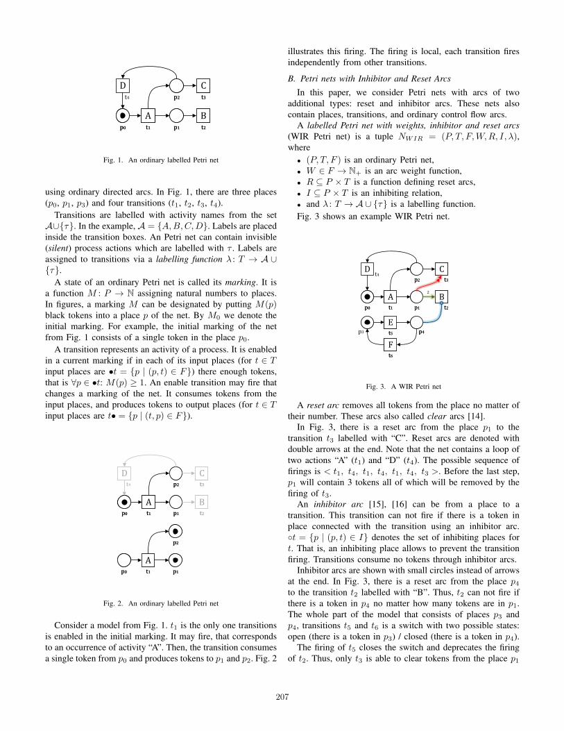
At1

At1 p1p1p0p0

Dt4 p2p2

Bt2

Bt2

Ct3

Ct3

Fig. 1. An ordinary labelled Petri net

using ordinary directed arcs. In Fig. 1, there are three places(p0, p1, p3) and four transitions (t1, t2, t3, t4).

Transitions are labelled with activity names from the setA∪τ. In the example, A = A,B,C,D. Labels are placedinside the transition boxes. An Petri net can contain invisible(silent) process actions which are labelled with τ . Labels areassigned to transitions via a labelling function λ : T → A ∪τ.

A state of an ordinary Petri net is called its marking. It isa function M : P → N assigning natural numbers to places.In figures, a marking M can be designated by putting M(p)black tokens into a place p of the net. By M0 we denote theinitial marking. For example, the initial marking of the netfrom Fig. 1 consists of a single token in the place p0.

A transition represents an activity of a process. It is enabledin a current marking if in each of its input places (for t ∈ Tinput places are •t = p | (p, t) ∈ F) there enough tokens,that is ∀p ∈ •t: M(p) ≥ 1. An enable transition may fire thatchanges a marking of the net. It consumes tokens from theinput places, and produces tokens to output places (for t ∈ Tinput places are t• = p | (t, p) ∈ F).

At1

At1 p1p1p0p0

Dt4 p2p2

Bt2

Bt2

Ct3

Ct3

At1

At1 p1p1p0p0

p2p2

Fig. 2. An ordinary labelled Petri net

Consider a model from Fig. 1. t1 is the only one transitionsis enabled in the initial marking. It may fire, that correspondsto an occurrence of activity “A”. Then, the transition consumesa single token from p0 and produces tokens to p1 and p2. Fig. 2

illustrates this firing. The firing is local, each transition firesindependently from other transitions.

B. Petri nets with Inhibitor and Reset Arcs

In this paper, we consider Petri nets with arcs of twoadditional types: reset and inhibitor arcs. These nets alsocontain places, transitions, and ordinary control flow arcs.

A labelled Petri net with weights, inhibitor and reset arcs(WIR Petri net) is a tuple NWIR = (P, T, F,W,R, I, λ),where• (P, T, F ) is an ordinary Petri net,• W ∈ F → N+ is an arc weight function,• R ⊆ P × T is a function defining reset arcs,• I ⊆ P × T is an inhibiting relation,• and λ : T → A∪ τ is a labelling function.Fig. 3 shows an example WIR Petri net.

At1

At1 p1p1p0p0

Dt4

p2p2

Bt2

Bt2

2

Ct3

Ct3

Et5

Et5 p4p4

Ft6

Ft6

p3

Fig. 3. A WIR Petri net

A reset arc removes all tokens from the place no matter oftheir number. These arcs also called clear arcs [14].

In Fig. 3, there is a reset arc from the place p1 to thetransition t3 labelled with “C”. Reset arcs are denoted withdouble arrows at the end. Note that the net contains a loop oftwo actions “A” (t1) and “D” (t4). The possible sequence offirings is < t1, t4, t1, t4, t1, t4, t3 >. Before the last step,p1 will contain 3 tokens all of which will be removed by thefiring of t3.

An inhibitor arc [15], [16] can be from a place to atransition. This transition can not fire if there is a token inplace connected with the transition using an inhibitor arc.t = p | (p, t) ∈ I denotes the set of inhibiting places fort. That is, an inhibiting place allows to prevent the transitionfiring. Transitions consume no tokens through inhibitor arcs.

Inhibitor arcs are shown with small circles instead of arrowsat the end. In Fig. 3, there is a reset arc from the place p4to the transition t2 labelled with “B”. Thus, t2 can not fire ifthere is a token in p4 no matter how many tokens are in p1.The whole part of the model that consists of places p3 andp4, transitions t5 and t6 is a switch with two possible states:open (there is a token in p3) / closed (there is a token in p4).

The firing of t5 closes the switch and deprecates the firingof t2. Thus, only t3 is able to clear tokens from the place p1

207

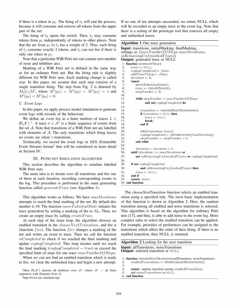
if there is a token in p2. The firing of t3 will end the process,because it will consume and remove all tokens from the upperpart of the net.

The firing of t6 opens the switch. Then, t2 may consumetokens from p1 independently of tokens in other places. Notethat the arc from p1 to t2 has a weight of 2. Thus, each firingof t2 consume exactly 2 tokens, and t2 can not fire if there isonly one token in p1.

Note that a particular WIR Petri net can contain zero numberof reset and inhibitor arcs.

Marking of a WIR Petri net is defined in the same wayas for an ordinary Petri net. But the firing rule is slightlydifferent for WIR Petri nets. Each marking change is calledstep. In this paper, we assume that each step consists of asingle transition firing. The step from Fig. 2 is denoted byM0[t1〉M ′, where M ′(p1) = M ′(p2) = M ′(p3) = 1 andM ′(p0) =M ′(p4) = 0.

C. Event Logs

In this paper, we apply process model simulation to generateevent logs with records of the behaviour.

We define an event log as a finite multiset of traces L ∈B(A∗) 1. A trace σ ∈ A∗ is a finite sequence of events fromthe set A. Note that transitions of a WIR Petri net are labelledwith elements of A. The only transitions which firing leavesno events are silent τ -transitions.

Technically, we record the event logs in XES (ExtensibleEvent Stream) format2 that will be considered in more detailin Section IV.

III. PETRI NET SIMULATION ALGORITHM

This section describes the algorithm to simulate labelledWIR Petri nets.

The main idea is to iterate over all transitions and fire oneof them at each iteration, recording corresponding events tothe log. This procedure is performed in the main generatingfunction called generateTrace (see Algorithm 1).

This algorithm works as follows. We have maxIterationsattempts to reach the final marking of the net. By default thisnumber is 10. The function moveToInitialState initiates thetrace generation by setting a marking of the to M0. Then, wecreate an empty trace by calling createTrace.

At each step of the main loop, the algorithm chooses anenabled transition in the chooseNextTransition, and fire it(function fire). The function fire changes a marking of thenet and writes an event to trace. Then we call the functionisCompleted to check if we reached the final marking andupdate replayCompleted. This loop iterates until we reachthe final marking (replayCompleted = true) or exceed thespecified limit of steps for one trace maxNumberOfSteps.

When we can not find an enabled transition which is readyto fire, we clear the unfinished trace and begin a new attempt.

1Here B(A∗) denotes all multisets over A∗, where A∗ — all finitesequences with elements from A.

2http://www.xes-standard.org/

If no one of ten attempts succeeded, we return NULL whichwill be recorded as an empty trace to the event log. Note thatthere is a setting of the prototype tool that removes all emptyand unfinished traces.

Algorithm 1 One trace generationInput: transitions, initialMarking, finalMarking,settings as maxNumberOfSteps,maxIterations,isRemovingUnfinishedTracesOutput: generated trace or NULL1: function GENERATETRACE2: trace← NULL;3: replayCompleted← false;4: addTraceToLog ← false;5: iteration← 0;6: repeat7: MOVETOINITIALSTATE();8: trace← CREATETRACE();9: stepNumber ← 0;

10:11: while stepNumber < maxNumberOfSteps

12: and not replayCompleted do13:14: transition← CHOOSENEXTTRANSITION();15: if transition = NULL then16: trace← NULL;17: break;18: end if19:20: FIRE(transition, trace);21: replayCompleted← ISCOMPLETED(finalMarking);22: stepNumber ← stepNumber + 1;23: end while24:25: iteration← iteration+ 1;26: until (iteration >= maxIterations or27: not isRemovingUnfinishedTraces or replayCompleted)28:29: if not replayCompleted

30: and isRemovingUnfinishedTraces then31: trace← NULL;32: end if33: return trace;34: end function

The chooseNextTransition function selects an enabled tran-sition using a specified rule. The most basic implementationof this function is shown in Algorithm 2. Here, the randomtransition among all enabled and noise transitions is selected.This algorithm is based on the algorithm for ordinary Petrinets [17], and thus, is able to add noise to the event log. Morecomplex rules to select the enabled transition can be applied.For example, priorities of preferences can be assigned to thetransitions which affect the order of their firing. If there is noenabled transition, then NULL is returned.

Algorithm 2 Looking for the next transitionInput: allTransitions, noiseTransitionsOutput: selected transition or NULL

1: function CHOOSENEXTTRANSITION(allTransitions, noiseTransitions)2: enabledTransitions← FINDENABLEDTRANSITIONS();3:4: return random transition among enabledTransitions5: and noiseTransitions or NULL;6: end function

208

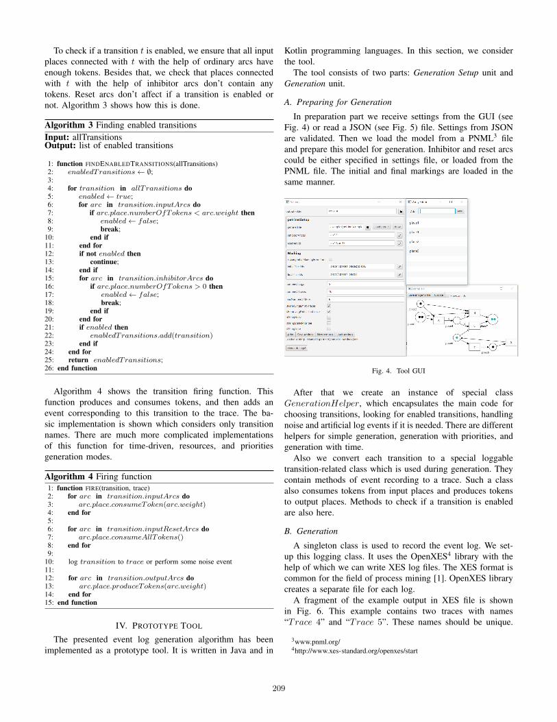
To check if a transition t is enabled, we ensure that all inputplaces connected with t with the help of ordinary arcs haveenough tokens. Besides that, we check that places connectedwith t with the help of inhibitor arcs don’t contain anytokens. Reset arcs don’t affect if a transition is enabled ornot. Algorithm 3 shows how this is done.

Algorithm 3 Finding enabled transitionsInput: allTransitionsOutput: list of enabled transitions

1: function FINDENABLEDTRANSITIONS(allTransitions)2: enabledTransitions← ∅;3:4: for transition in allT ransitions do5: enabled← true;6: for arc in transition.inputArcs do7: if arc.place.numberOfTokens < arc.weight then8: enabled← false;9: break;

10: end if11: end for12: if not enabled then13: continue;14: end if15: for arc in transition.inhibitorArcs do16: if arc.place.numberOfTokens > 0 then17: enabled← false;18: break;19: end if20: end for21: if enabled then22: enabledTransitions.add(transition)23: end if24: end for25: return enabledTransitions;26: end function

Algorithm 4 shows the transition firing function. Thisfunction produces and consumes tokens, and then adds anevent corresponding to this transition to the trace. The ba-sic implementation is shown which considers only transitionnames. There are much more complicated implementationsof this function for time-driven, resources, and prioritiesgeneration modes.

Algorithm 4 Firing function1: function FIRE(transition, trace)2: for arc in transition.inputArcs do3: arc.place.consumeToken(arc.weight)4: end for5:6: for arc in transition.inputResetArcs do7: arc.place.consumeAllTokens()8: end for9:

10: log transition to trace or perform some noise event11:12: for arc in transition.outputArcs do13: arc.place.produceTokens(arc.weight)14: end for15: end function

IV. PROTOTYPE TOOL

The presented event log generation algorithm has beenimplemented as a prototype tool. It is written in Java and in

Kotlin programming languages. In this section, we considerthe tool.

The tool consists of two parts: Generation Setup unit andGeneration unit.

A. Preparing for Generation

In preparation part we receive settings from the GUI (seeFig. 4) or read a JSON (see Fig. 5) file. Settings from JSONare validated. Then we load the model from a PNML3 fileand prepare this model for generation. Inhibitor and reset arcscould be either specified in settings file, or loaded from thePNML file. The initial and final markings are loaded in thesame manner.

Fig. 4. Tool GUI

After that we create an instance of special classGenerationHelper, which encapsulates the main code forchoosing transitions, looking for enabled transitions, handlingnoise and artificial log events if it is needed. There are differenthelpers for simple generation, generation with priorities, andgeneration with time.

Also we convert each transition to a special loggabletransition-related class which is used during generation. Theycontain methods of event recording to a trace. Such a classalso consumes tokens from input places and produces tokensto output places. Methods to check if a transition is enabledare also here.

B. Generation

A singleton class is used to record the event log. We set-up this logging class. It uses the OpenXES4 library with thehelp of which we can write XES log files. The XES format iscommon for the field of process mining [1]. OpenXES librarycreates a separate file for each log.

A fragment of the example output in XES file is shownin Fig. 6. This example contains two traces with names“Trace 4” and “Trace 5”. These names should be unique.

3www.pnml.org/4http://www.xes-standard.org/openxes/start

209

Fig. 5. Generation settings in JSON

Fig. 6. Fragment of XES file

The first trace is of the three events: “B”, “D”, and “D”. Notethat XES is XML-based, and is easy-to-read for a machine ora human.

Then we use a Generator class to launch the main genera-tion method (see Algorithm 1), passing a generationHelperto this class.

C. Tool Usage

Let us test our tool on the model from Fig. 7.The initial marking consists of the four tokens (shown as

black dots): one token lies in place2, one is in place5, and two

tokens are in place1. Our goal is to reach the final marking(shown as green dots): two tokens in place7, and one tokenin place6.

Fig. 7. Petri net used for log generation

Transition C is enabled only when place place6 is empty.C consumes 2 tokens from place4 and produces a token toplace7.

Transition B removes all tokens in places place1 andplace2. When fire this transition consumes 4 tokens fromplace4 and produces a token to place7. Thus, B can not firebefore A.

At each step either X or Y is enabled, so these transitionsmay produce a trace of any length.

We set-up our tool to remove unfinished traces and limitedmax number of steps to 10.

The result of the generation is shown in Fig. 8.Let us look at some trace, for example: 〈A,X,B, Y,C,X〉.

First fired transition was A, and it produced 6 tokens to place4.Then X fired. It consumed a token from place5 and producedone to place6. C can not fire in this marking. Thus, B fires.4 of 6 tokens was consumed from place4, and one token

Fig. 8. Resulting traces

210

produced to place7. Then Y fired and “opened” C. C has beenfired just after Y was fired, when a token has been removedfrom place6 . B and C were fired once each, and produced 2tokens in total to place7. place1 and place2 were cleared byB. The last event was X , which placed a token to place6. Atthe end of this run all tokens lie in the final marking.

V. CONCLUSIONS

In this paper, we have presented the algorithm to simulatea process model in the form of weighted labelled Petri netwith inhibitor and reset arcs. This algorithm can be applied togenerate event logs from the event log. Proposed algorithmcontinues the previous works on Petri net simulation withthe purpose of generating artificial event logs. The prototypeimplementation is based on Gena tool5.

We have plans for future work. Firstly, we plan to com-prehensively evaluate the proposed algorithm on artificial andreal-life process models. For now, we just tested it on samplemodels to check algorithm validity. Secondly, we also planto improve the prototype implementation and make it stableand usable. Thirdly, Gena is able to simulate timed processmodels, models with resources, data, add noise to an eventlog [8], [17]. Recently, an extension for Gena to simulatethe multi-agent system has been proposed [18]. We plan tomerge these extensions and the algorithm presented in thispaper. Then, it will be possible to simulate WIR Petri netswith time/resources, and data.

REFERENCES

[1] Wil M. P. van der Aalst, Process mining: Discovery, Conformance andEnhancement of Business Processes. Springer, 2011.

[2] J. Carmona, B. F. van Dongen, A. Solti, and M. Weidlich, ConformanceChecking - Relating Processes and Models. Springer, 2018.

[3] M. Weske, Business Process Management: Concepts, Languages, Archi-tectures. Springer, 2007.

[4] W. M. P. van der Aalst, “Process mining and simulation: a match madein heaven!,” in SummerSim, pp. 4:1–4:12, ACM, 2018.

[5] A. Burattin and A. Sperduti, “PLG: A framework for the generationof business process models and their execution logs,” in BusinessProcess Management Workshops, vol. 66 of Lecture Notes in BusinessInformation Processing, pp. 214–219, Springer, 2010.

[6] A. Burattin, “PLG2: multiperspective process randomization with onlineand offline simulations,” in BPM (Demos), vol. 1789 of CEUR WorkshopProceedings, pp. 1–6, CEUR-WS.org, 2016.

[7] T. Jouck and B. Depaire, “Ptandloggenerator: A generator for artificialevent data,” in BPM (Demos), vol. 1789 of CEUR Workshop Procee-dings, pp. 23–27, CEUR-WS.org, 2016.

[8] A. A. Mitsyuk, I. S. Shugurov, A. A. Kalenkova, and W. M. P. van derAalst, “Generating event logs for high-level process models,” SimulationModelling Practice and Theory, vol. 74, pp. 1–16, 2017.

[9] W. Reisig, Understanding Petri Nets - Modeling Techniques, AnalysisMethods, Case Studies. Springer, 2013.

[10] K. Jensen and L. M. Kristensen, Coloured Petri Nets - Modelling andValidation of Concurrent Systems. Springer, 2009.

[11] I. A. Lomazova, “Nested petri nets: Multi-level and recursive systems,”Fundam. Inform., vol. 47, no. 3-4, pp. 283–293, 2001.

[12] R. Valk, “Object petri nets: Using the nets-within-nets paradigm,” inLectures on Concurrency and Petri Nets, vol. 3098 of Lecture Notes inComputer Science, pp. 819–848, Springer, 2003.

[13] W. M. P. van der Aalst and K. M. van Hee, Workflow Management:Models, Methods, and Systems. MIT Press, 2002.

5https://pais.hse.ru/research/projects/gena

[14] C. Lakos and S. Christensen, “A general systematic approach to arcextensions for coloured petri nets,” in Application and Theory of PetriNets, vol. 815 of Lecture Notes in Computer Science, pp. 338–357,Springer, 1994.

[15] R. Janicki and M. Koutny, “Semantics of inhibitor nets,” Inf. Comput.,vol. 123, no. 1, pp. 1–16, 1995.

[16] H. C. M. Kleijn and M. Koutny, “Process semantics of p/t-nets withinhibitor arcs,” in ICATPN, pp. 261–281, 2000.

[17] I. S. Shugurov and A. A. Mitsyuk, “Generation of a Set of EventLogs with Noise,” in Proceedings of the 8th Spring/Summer YoungResearchers Colloquium on Software Engineering (SYRCoSE 2014),pp. 88–95, 2014.

[18] R. A. Nesterov, A. A. Mitsyuk, and I. A. Lomazova, “Simulatingbehavior of multi-agent systems with acyclic interactions of agents,”Proceedings of the Institute for System Programming, vol. 30, pp. 285–302, 2018.

211

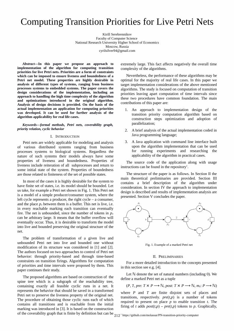
Computing Transition Priorities for Live Petri NetsKirill Serebrennikov

Faculty of Computer Science National Research University Higher School of Economics

Moscow, Russiacyrilsilver94@gmail.com

Abstract—In this paper we propose an approach toimplementation of the algorithm for computing transitionpriorities for live Petri nets. Priorities are a form of constraintswhich can be imposed to ensure liveness and boundedness of aPetri net model. These properties are highly desirable inanalysis of different types of systems, ranging from businessprocesses systems to embedded systems. The paper covers thedesign considerations of the implementation, including anapproach to handling the high time complexity of the algorithmand optimizations introduced in the original algorithm.Analysis of design decisions is provided. On the basis of theactual implementation an application for computing prioritieswas developed. It can be used for further analysis of thealgorithm applicability for real life cases.

Keywords—formal methods, Petri nets, coverability graph,priority relation, cyclic behavior

I. INTRODUCTION

Petri nets are widely applicable for modeling and analysisof various distributed systems ranging from businessprocesses systems to biological systems. Regardless thenature of such systems their models always have someproperties of liveness and boundedness. Properties ofliveness include reiteration of all subprocesses and return tosome initial state of the system. Properties of boundednessare those related to finiteness of the set of possible states.

In most of the cases it is highly desirable for the system tohave finite set of states, i.e. its model should be bounded. Letus take, for example a Petri net shown in Fig. 1. This Petri netis a model of a simple producer/consumer system, where theleft cycle represents a producer, the right cycle – a consumer,and the place p3 between them is a buffer. This net is live, i.e.in every reachable marking each transition can eventuallyfire. The net is unbounded, since the number of tokens in p3

can be arbitrary large. It means that the buffer overflow willeventually occur. Thus, it is desirable to transform the modelinto live and bounded preserving the original structure of thenet.

The problem of transformation of a given live andunbounded Petri net into live and bounded one withoutmodification of its structure was considered in [1] and [2].The authors focused on two approaches to control of Petri netbehavior: through priority-based and through time-basedconstraints on transition firings. Algorithms for computationof priorities and time intervals were proposed by them. Thispaper continues their study.

The proposed algorithms are based on construction of thespine tree which is a subgraph of the reachability tree,containing exactly all feasible cyclic runs in a net. Itrepresents the behavior that should be saved in a transformedPetri net to preserve the liveness property of the original net.The procedure of obtaining those cyclic runs each of whichcontains all transitions and is reachable from the initialmarking was introduced in [3]. It is based on the constructionof the coverability graph that is finite by definition but can be

extremely large. This fact affects negatively the overall timecomplexity of the algorithms.

Nevertheless, the performance of these algorithms may beoptimal for the majority of real life cases. In this paper wetarget implementation considerations of the above mentionedalgorithms. The study is focused on computation of transitionpriorities leaving apart computation of time intervals sincethese two procedures have common foundation. The maincontributions of this paper are:

1. An approach to implementation design of thetransition priority computation algorithm based onconstruction steps optimization and adoption ofparallelization;

2. A brief analysis of the actual implementation coded inJava programming language;

3. A Java application with command line interface builtupon the algorithm implementation that can be usedfor running experiments and researching theapplicability of the algorithm in practical cases.

The source code of the application along with usageinstructions can be found in the repository1.

The structure of the paper is as follows. In Section II themain theoretical preliminaries are provided. Section IIIcontains a brief description of the algorithm underconsideration. In section IV the approach to implementationdesign is described and results of implementation analysis arepresented. Section V concludes the paper.

II. PRELIMINARIES

For a more detailed introduction to the concepts presentedin this section see e.g. [4].

Let ℕ denote the set of natural numbers (including 0). Wedefine a marked Petri net as a tuple

(P, T, pre: T ⨯ P ⟶ ℕ, post: T ⨯ P ⟶ ℕ, m0: P ⟶ ℕ)

where P and T are finite disjoint sets of places andtransitions, respectively. pre(t,p) is a number of tokensrequired to present on place p to enable transition t. Thefiring of t adds post(t,p) – pre(t,p) tokens to p. Graphically,

1 https://github.com/molassar/PN-transition-priority-computer

Fig. 1. Example of a marked Petri net

212

places are denoted by circles and transitions by squares.There is a directed arc from p to t if pre(t,p) > 0. The arc isannotated with pre(t,p) if pre(t,p) > 1. Similarly, there is adirected arc from t to p if post(t,p) > 0. It is annotated withpost(t,p) if post(t,p) > 1. The pre-set of a transition t is the setof places p satisfying pre(t,p) > 0. The post-set of t is a set ofplaces p satisfying post(t,p) > 0. A marking of a net is amapping m: P ⟶ ℕ. The initial marking m0 is representedby m0(p) tokens on place p.

An initial run is a sequence of transition firings, startingwith the initial marking. Reachable markings are all thosemarkings which can be reached by the initial run. A cyclicrun is a finite run starting and ending at the same marking.

A reachability graph of a Petri net is a labeled directedgraph in which vertices correspond to reachable markings ofthe net. A directed edge from vertex v to vertex v' is labeledwith transition t which is enabled by marking m representedby v and leads to marking m' represented by v'.

A Petri net is bounded if, for each place p, the number oftokens on p does not exceed some fixed bound k , i.e. for∈ℕeach reachable marking m the following is true: m(p) ≤ k.Thus, a Petri net is bounded if and only if its reachabilitygraph is finite.

A marking m' strictly covers a marking m if and only iffor each place p ∈ P, m'(p) ≥ m(p) and m' ≠ m.

In case of unbounded nets coverability graphs providefinite information about behavior. The construction ofcoverability graph is based on the notion of the generalizedmarking which is formally a mapping: P ω, where⟶ ℕ ⋃ω denotes an arbitrary number of tokens on a place. Acoverability graph is defined constructively: it is constructedsuccessively like the reachability graph starting from theinitial marking. However, in case of the coverability graphwhen a marking m' represented by a current leave v' in thereachability graph strictly covers a marking m represented bya vertex v, lying on the path from the root to v', then incoverability graph the vertex v' gets a marking mw, wheremw(p) = ω, if m'(p) > m(p), and mw(p) = m'(p), if m'(p) =m(p). Fig. 2 shows a coverability graph of the exampleshown in Fig. 1.

The coverability net of a Petri net N = (P, T, pre, post, m0)is a new Petri net N' = (P', T', pre', post', m0') which isconstructed on the basis of a coverability graph (V, E, v0) ofthe original net. The transitions of N' are mapped to thetransitions of N by a labeling function λ': T' ⟶ T. Thecoverability net is formally defined as:

P' = V,

T' = E,

pre'((v', t, v''), v) = 1 if v = v',

pre'((v', t, v''), v) = 0 if v ≠ v',

post'((v', t, v''), v) = 1 if v = v'',

post'((v', t, v''), v) = 0 if v ≠ v'',

m0'(v) = 1 if v = v0,

m0'(v) = 0 if v ≠ v0,

λ'(v, t, v') = t.

The extended coverability net is the coverability net thatcontains additional places to capture the token count changefor ω-marked places of the original net. For each unboundedplace p in the original net a place p is added to the extendedcoverability net. If transition t is in the pre-set of p in theoriginal net N, then all transitions t' ∈ T' with λ'(t') = t are inthe pre-set of the added place p. Arc weights are taken intoaccount. The same holds for the post-sets of added places.The initial marking of added places coincides with the initialmarking of these places in the original net. Fig. 3demonstrates the extended coverability net constructed uponthe coverability graph shown in Fig. 2.

We define the set of all minimal feasible cyclic runstogether with prefixes leading to the cycles in a Petri net N as

C(N) = τσ | τσ* is an initial run in N,

τ does not include σ and

σ includes all transitions in N

where σ is a minimal feasible cyclic run in N and τ is a finiteinitial run leading to σ. A spine tree is a subgraph of areachability tree that contains exactly all runs from C(N). Thespine tree contains the behavior that should be saved incourse of transformation in order to keep a Petri net live. Forthe Petri net in Fig. 1 C(N) = babacd, babcad, babcda,babacbd, babcabd, babacbad. Thus, the spine tree of the nethas the construction as shown in Fig. 4.

A priority relation for a Petri net N is a partial order(T, ≪), i.e., the relation is reflexive, antisymmetric andtransitive. A priority relation ≪ can be specified by assigninga priority label π(t) ∈ ℕ to each transition t. Thus, t ≪ t' ifand only if π(t) < π(t'). A Petri net with priorities is a Petrinet together with a priority relation. In a Petri net withpriorities if Q is a set of all transitions enabled in a markingm then only transitions with the highest priority may fire.

Fig. 3. The extended coverability net of the Petri net of Fig. 1

Fig. 2. A coverability graph of the Petri net of Fig. 1

213

III. ALGORITHM OVERVIEW

Let N be a live and unbounded Petri net. The task is tocheck, if it is possible to transform this net into live andbounded by adding priorities to its transitions. To accomplishthe task we should find those transition priorities, whichexclude runs leading to unboundedness.

It is possible to distinguish two major stages in thealgorithm. The first is the search for cyclic runs in a Petri net.The presence of cyclic runs is a necessary condition forexistence of transition priorities for a given Petri net. On thesecond stage the spine tree is built with the cyclic runs foundon the previous stage forming its skeleton. The wholealgorithm has the following sequence of actions:

1. Given a Petri net build its coverability graph;

2. Given the coverability graph constructed on theprevious step build a coverability net;

3. Transform the coverability net into an extendedcoverability net;

4. Find behavioral cycles of the extended coverabilitynet;

5. If the set of cyclic runs computed on the previous stepis not empty build a spine tree in which the cyclic runsform the skeleton;

6. Given the spine tree build a spine-based coverabilitytree in which all leaves are colored in either red orgreen2;

7. Traverse the spine-based coverability tree. For eachnon-red node a with its incoming edge labeled aftertransition t1 if there exists a red sibling b with itsincoming edge labeled after transition t2 add ( t1, t2) tothe priority relation;

8. Assign priority labels to the transitions on the basis ofthe priority relation computed on the previous step.

The steps 1-4 form the first stage of the algorithm –search for cyclic runs. The procedure was introduced in [3].The second stage – computation of a priority relation throughspine tree construction – is represented by the steps 5-7. Itwas described in [1].

2 For the complete algorithm see [1]

IV. IMPLEMENTATION APPROACH

A. Cyclic Runs Search

The problem of the search for cyclic runs in a Petri netcan be reduced to the search for cyclic runs in its extendedcoverability net. The original algorithm for the cyclic runssearch is comprised of four steps. We have reduced thenumber of steps to two by optimizing the construction phasesof coverability and extended coverability nets.

The first step is the construction of a coverability graph.This step can not be avoided since the coverability graph isthe foundation for the rest of the algorithm. Since thecoverability graph can grow exponentially the overall timecomplexity of the algorithm is also exponential. We havechosen parallelization to target the problem. Theimplementation of coverability graph construction andtraversal steps was designed to be easily parallelized.

Listing 1 demonstrates the pseudocode of the algorithmfor building the coverability graph. Each node is processed inthe following way: the set of transitions is filtered to find thetransitions enabled by the marking corresponding to a node,then all the filtered transitions are fired to produce newgeneralized markings. Directed arcs are added from thevertex labeled by the marking of the node to the verticeslabeled by the produced generalized markings. New nodesare generated from the obtained markings for furtherprocessing. Processing of a node does not depend onprocessing of other nodes so this task can be scheduled inparallel. The actual implementation of the pseudocode hasthe time complexity

O(|V| * |T| * d(CG) * |P|)

where |V| is the number of vertices in a coverability graph, |T|- the cardinality of the transition set of a Petri net, d(CG) –depth of the coverability graph, i.e. the distance from theroot to the most distant vertex, and |P| - the cardinality of theset of places.

We have made two implementations of the algorithm:single-threaded and parallel. For the parallel implementationthe fork/join Java framework was used. It is based on the

Fig. 4. The spine tree of the Petri net of Fig. 1

Listing 1. Pseudocode of the algorithm for building the coverability graph

214

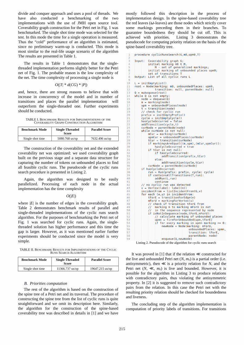
divide and conquer approach and uses a pool of threads. Wehave also conducted a benchmarking of the twoimplementations with the use of JMH open source tool.Coverability graph construction for the Petri net in Fig. 1 wasbenchmarked. The single shot time mode was selected for thetest. In this mode the time for a single operation is measured.Thus the “cold” performance of an algorithm is estimated,since no preliminary warm-up is conducted. This mode ismost similar to the real-life usage scenario of the algorithmThe results are presented in Table 1.

The results in Table 1 demonstrates that the single-threaded implementation performs slightly better for the Petrinet of Fig. 1. The probable reason is the low complexity ofthe net. The time complexity of processing a single node is

O(|T| * d(CG) * |P|)

and, hence, there are strong reasons to believe that withincrease in concurrency of the model and in number oftransitions and places the parallel implementation willoutperform the single-threaded one. Further experimentsshould be conducted.

TABLE I. BENCHMARK RESULTS FOR IMPLEMENTATIONS OF THECOVERABILITY GRAPH CONSTRUCTION ALGORITHM

Benchmark Mode Single-ThreadedScore

Parallel Score

Single shot time 5080.768 us/op 7632.496 us/op

The construction of the coverability net and the extendedcoverability net was optimized: we used coverability graphbuilt on the previous stage and a separate data structure forcapturing the number of tokens on unbounded places to findall feasible cyclic runs. The pseudocode of the cyclic runssearch procedure is presented in Listing 2.

Again, the algorithm was designed to be easilyparallelized. Processing of each node in the actualimplementation has the time complexity

O(|E|)

where |E| is the number of edges in the coverability graph.Table 2 demonstrates benchmark results of parallel andsingle-threaded implementations of the cyclic runs searchalgorithm. For the purposes of benchmarking the Petri net ofFig. 1 was searched for cyclic runs. Again, the single-threaded solution has higher performance and this time thegap is larger. However, as it was mentioned earlier furtherexperiments should be conducted since the model is verysimple.

TABLE II. BENCHMARK RESULTS FOR IMPLEMENTATIONS OF THE CYCLICRUNS SEARCH ALGORITHM

Benchmark Mode Single-ThreadedScore

Parallel Score

Single shot time 11366.737 us/op 19647.215 us/op

B. Priorities computation

The rest of the algorithm is based on the construction ofthe spine tree of a Petri net and its traversal. The procedure ofconstructing the spine tree from the list of cyclic runs is quitestraightforward and we omit its description here. Similarly,the algorithm for the construction of the spine-basedcoverability tree was described in details in [1] and we have

mostly followed this description in the process ofimplementation design. In the spine-based coverability treethe red leaves (ω-leaves) are those nodes which strictly coversome markings preceding them in their branches. Toguarantee boundedness they should be cut off. This isachieved with priorities. Listing 3 demonstrates thepseudocode for computing priority relation on the basis of thespine-based coverability tree.

It was proved in [1] that if the relation ≪ constructed forthe live and unbounded Petri net (N, m0) is a partial order (i.e.antisymmetric), then ≪ is a priority relation for N, and thePetri net (N, ≪, m0) is live and bounded. However, it ispossible for the algorithm in Listing 3 to produce relationswith contradictory pairs, thus violating the antisymmetricproperty. In [2] it is suggested to remove such contradictorypairs from the relation. In this case the Petri net with theresulting priority relation should be checked for boundednessand liveness.

The concluding step of the algorithm implementation iscomputation of priority labels of transitions. For transitions

Listing 2. Pseudocode of the algorithm for cyclic runs search

215

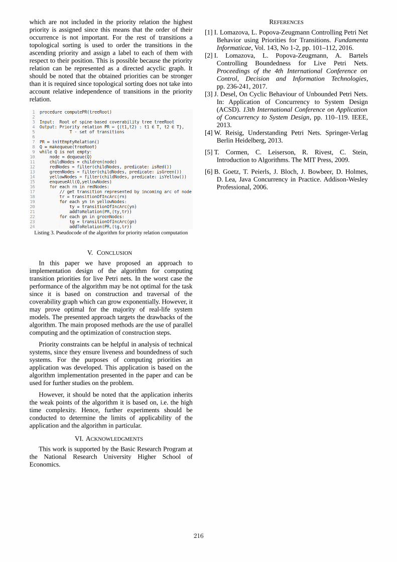
which are not included in the priority relation the highestpriority is assigned since this means that the order of theiroccurrence is not important. For the rest of transitions atopological sorting is used to order the transitions in theascending priority and assign a label to each of them withrespect to their position. This is possible because the priorityrelation can be represented as a directed acyclic graph. Itshould be noted that the obtained priorities can be strongerthan it is required since topological sorting does not take intoaccount relative independence of transitions in the priorityrelation.

V. CONCLUSION

In this paper we have proposed an approach toimplementation design of the algorithm for computingtransition priorities for live Petri nets. In the worst case theperformance of the algorithm may be not optimal for the tasksince it is based on construction and traversal of thecoverability graph which can grow exponentially. However, itmay prove optimal for the majority of real-life systemmodels. The presented approach targets the drawbacks of thealgorithm. The main proposed methods are the use of parallelcomputing and the optimization of construction steps.

Priority constraints can be helpful in analysis of technicalsystems, since they ensure liveness and boundedness of suchsystems. For the purposes of computing priorities anapplication was developed. This application is based on thealgorithm implementation presented in the paper and can beused for further studies on the problem.

However, it should be noted that the application inheritsthe weak points of the algorithm it is based on, i.e. the hightime complexity. Hence, further experiments should beconducted to determine the limits of applicability of theapplication and the algorithm in particular.

VI. ACKNOWLEDGMENTS

This work is supported by the Basic Research Program atthe National Research University Higher School ofEconomics.

REFERENCES

[1] I. Lomazova, L. Popova-Zeugmann Controlling Petri NetBehavior using Priorities for Transitions. FundamentaInformaticae, Vol. 143, No 1-2, pp. 101–112, 2016.

[2] I. Lomazova, L. Popova-Zeugmann, A. BartelsControlling Boundedness for Live Petri Nets.Proceedings of the 4th International Conference onControl, Decision and Information Technologies,pp. 236-241, 2017.

[3] J. Desel, On Cyclic Behaviour of Unbounded Petri Nets.In: Application of Concurrency to System Design(ACSD). 13th International Conference on Applicationof Concurrency to System Design, pp. 110–119. IEEE,2013.

[4] W. Reisig, Understanding Petri Nets. Springer-VerlagBerlin Heidelberg, 2013.

[5] T. Cormen, C. Leiserson, R. Rivest, C. Stein,Introduction to Algorithms. The MIT Press, 2009.

[6] B. Goetz, T. Peierls, J. Bloch, J. Bowbeer, D. Holmes,D. Lea, Java Concurrency in Practice. Addison-WesleyProfessional, 2006.

Listing 3. Pseudocode of the algorithm for priority relation computation

216

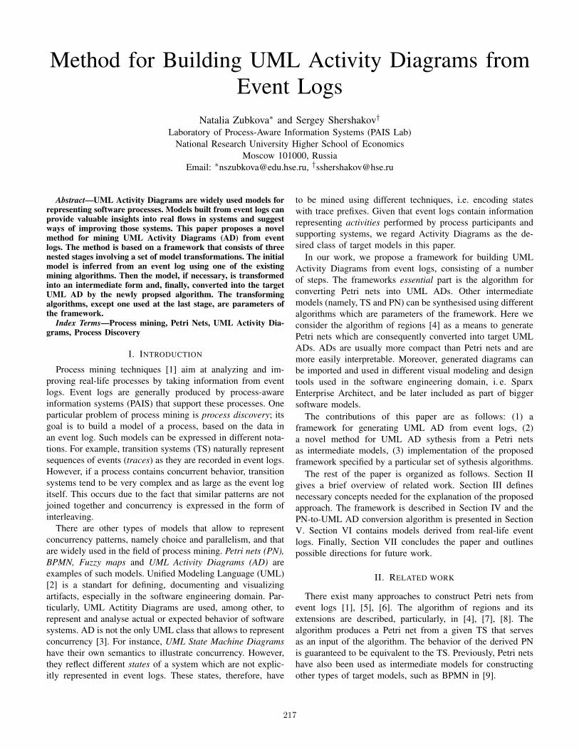
Method for Building UML Activity Diagrams fromEvent Logs

Natalia Zubkova∗ and Sergey Shershakov†Laboratory of Process-Aware Information Systems (PAIS Lab)

National Research University Higher School of EconomicsMoscow 101000, Russia

Email: ∗nszubkova@edu.hse.ru, †sshershakov@hse.ru

Abstract—UML Activity Diagrams are widely used models forrepresenting software processes. Models built from event logs canprovide valuable insights into real flows in systems and suggestways of improving those systems. This paper proposes a novelmethod for mining UML Activity Diagrams (AD) from eventlogs. The method is based on a framework that consists of threenested stages involving a set of model transformations. The initialmodel is inferred from an event log using one of the existingmining algorithms. Then the model, if necessary, is transformedinto an intermediate form and, finally, converted into the targetUML AD by the newly propsed algorithm. The transformingalgorithms, except one used at the last stage, are parameters ofthe framework.

Index Terms—Process mining, Petri Nets, UML Activity Dia-grams, Process Discovery

I. INTRODUCTION

Process mining techniques [1] aim at analyzing and im-proving real-life processes by taking information from eventlogs. Event logs are generally produced by process-awareinformation systems (PAIS) that support these processes. Oneparticular problem of process mining is process discovery; itsgoal is to build a model of a process, based on the data inan event log. Such models can be expressed in different nota-tions. For example, transition systems (TS) naturally representsequences of events (traces) as they are recorded in event logs.However, if a process contains concurrent behavior, transitionsystems tend to be very complex and as large as the event logitself. This occurs due to the fact that similar patterns are notjoined together and concurrency is expressed in the form ofinterleaving.

There are other types of models that allow to representconcurrency patterns, namely choice and parallelism, and thatare widely used in the field of process mining. Petri nets (PN),BPMN, Fuzzy maps and UML Activity Diagrams (AD) areexamples of such models. Unified Modeling Language (UML)[2] is a standart for defining, documenting and visualizingartifacts, especially in the software engineering domain. Par-ticularly, UML Actitity Diagrams are used, among other, torepresent and analyse actual or expected behavior of softwaresystems. AD is not the only UML class that allows to representconcurrency [3]. For instance, UML State Machine Diagramshave their own semantics to illustrate concurrency. However,they reflect different states of a system which are not explic-itly represented in event logs. These states, therefore, have

to be mined using different techniques, i.e. encoding stateswith trace prefixes. Given that event logs contain informationrepresenting activities performed by process participants andsupporting systems, we regard Activity Diagrams as the de-sired class of target models in this paper.

In our work, we propose a framework for building UMLActivity Diagrams from event logs, consisting of a numberof steps. The frameworks essential part is the algorithm forconverting Petri nets into UML ADs. Other intermediatemodels (namely, TS and PN) can be synthesised using differentalgorithms which are parameters of the framework. Here weconsider the algorithm of regions [4] as a means to generatePetri nets which are consequently converted into target UMLADs. ADs are usually more compact than Petri nets and aremore easily interpretable. Moreover, generated diagrams canbe imported and used in different visual modeling and designtools used in the software engineering domain, i. e. SparxEnterprise Architect, and be later included as part of biggersoftware models.

The contributions of this paper are as follows: (1) aframework for generating UML AD from event logs, (2)a novel method for UML AD sythesis from a Petri netsas intermediate models, (3) implementation of the proposedframework specified by a particular set of sythesis algorithms.

The rest of the paper is organized as follows. Section IIgives a brief overview of related work. Section III definesnecessary concepts needed for the explanation of the proposedapproach. The framework is described in Section IV and thePN-to-UML AD conversion algorithm is presented in SectionV. Section VI contains models derived from real-life eventlogs. Finally, Section VII concludes the paper and outlinespossible directions for future work.

II. RELATED WORK

There exist many approaches to construct Petri nets fromevent logs [1], [5], [6]. The algorithm of regions and itsextensions are described, particularly, in [4], [7], [8]. Thealgorithm produces a Petri net from a given TS that servesas an input of the algorithm. The behavior of the derived PNis guaranteed to be equivalent to the TS. Previously, Petri netshave also been used as intermediate models for constructingother types of target models, such as BPMN in [9].

217

The similarity between UML Activity Diagrams and Petrinets are studied in numerous works. Arlow et al. presentUML specification in application to Unified Process includingUML AD structural elements, and also mention that UMLAD are based on the Peti Net techniques [10]. In [11] authorsformalize AD semantics and compare them to semantics ofPetri Nets. There are many works dedicated to the transfor-mation of UML Activity Diagrams into Petri nets; the reversetransformation is studied scantily. In [12] the author describesan approach to translate UML AD into Petri nets. Agarwal[13] developed a method for transforming AD into Petri netsfor verification purposes. The author considers a set of UMLpatterns and indicates corresponding Petri net instances.

III. PRELIMINARIES

B(X) is the set of all multisets over some set X . For agiven set X , X+ is the set of all non-empty finite sequencesover X .

A. Trace, Event Log

Let Z be a set of activities. A trace is a finite sequenceσ = 〈a1, a2, ..., ai, ..., an〉 ∈ Z+.By σ(i) = ai we denote i-thelement. L ∈ B(Z+) , such that |L| > 0, is an event log. Here,|L| is the number of all traces.

B. Labeled Petri Net, Well-structured Labeled Petri Net

A labeled Petri net (PN) is a tuple PN = P, T, F, l,where P is a set of places, T is a set of transitions, P ∩T = ∅,F ⊆ (P × T ) ∪ (T × P ) is the flow relation, l is the labelingfunction l : T → Λ, and Λ is a set of labels. In process mining,labels of transition represent events.

Given p ∈ P , the set p• = y|(p, y) ∈ F is the postset ofp.

In this paper by Petri net we denote a well-structured Petrinet, i.e. a hierarcical Petri net that can be recursively dividedinto parts having single entry and exit points [14].

Fig. 1: An Activity Diagram example

C. UML Activity Diagram

A UML Activity Diagram is a tuple AD = N,E,NT,where• NT is a set of node typesNT = control, object, executable

• N is a set of nodes. n ∈ N : n = (λ, type), λ ∈Λ, type ∈ NT

• E is a set of edges. e ∈ E : e = (n1, n2), n1, n2 ∈ NSimilar definition was used in [15]. In this paper we mainlyfocus on the following elements of the UML AD (see Fig. 1):

1) A is a set of activity nodes, a ∈ A : a = (λ, executable)2) F is a set of parallel nodes, f ∈ F : f = (control)3) D is a set of decision nodes, d ∈ D : d = (control)4) init and final are initial and final nodes, both of type

control.UML decision nodes should be equipped with guards that

indicate the conditions under which the decision is made. Inthis paper, we regard non-deterministic Petri nets as interme-diate models1. The proposed conversion algorithm does notassume the presence of guard information in the event logand uses only the input Petri net. Thus, the produced ActivityDiagram is non-deterministic as well.

IV. FRAMEWORK

The proposed framework is illustrated in Fig. 2. The frame-work consists of a number of nested stages related to individ-ual steps of the proposed method. At every step a transforma-tion from one entity, event log or process model, into anotheris made. There exist numerous approaches to construct bothPetri nets and transition systems. Models obtained from thesame event log, but using different algorithms, represent thesame process. However, they vary in details that are usuallyrepresented by quality metrics [16]. Depending on the task,specific combinations of quality metrics can be considered.

The long path of the framework (I) includes first buildinga TS needed for the algorithm of regions. Here, varioustechniques for TS construction can be used, for instance,prefix tree sythesis [17], frequency based reduction [18], neuralapproach [19] etc. However, the TS synthesis can be bypassedand a Petri net can be generated directly from the event log (II).There are many algorithms for that, i. e. Inductive miner [14],α−algorithm [5], ILP-miner [20] and other. Finally, in III thegenerated Petri net is converted into a UML Activity Diagram.

A. Proposed implementation

In this paper we consider the full version of the frameworkwith the following parameters.

1) Prefix tree builder, unlimited window, for TS construc-tion.

2) The algorithm of regions for converting the TS into aPN.

3) The PN-to-UML AD converter described in the follow-ing section.

This following paragraph gives a brief overview of thealgorithms used in steps 1 and 2.

Prefix tree builder [17] is an algorithm for TS synthesis.Event logs usually do not explicitly contain states that areneeded for the construction of a transition system. A statefunction is introduced in order to infer such states. This

1There exists an extension to Petri nets that adds guards to its semantics.However, most of the process mining algorithms consider Petri nets withoutguards. Here we follow the same approach.

218

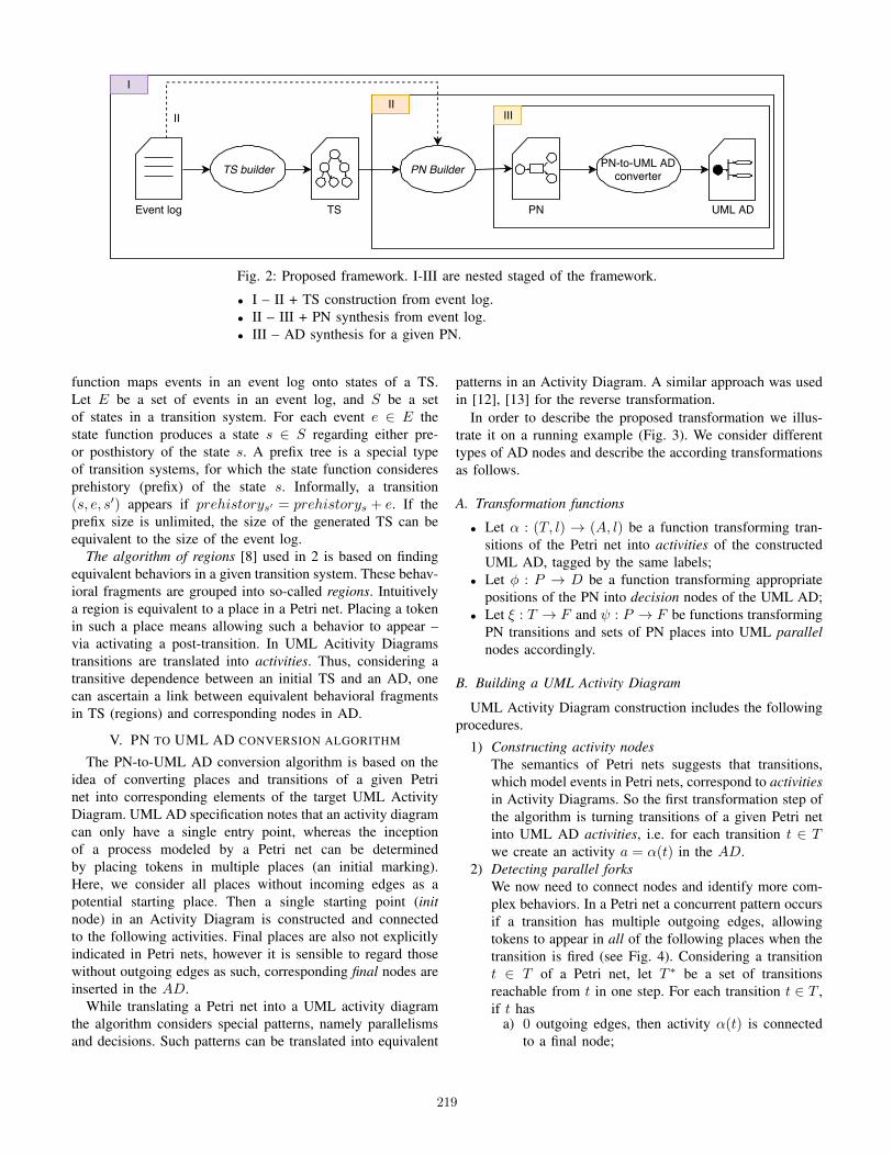
Event log

TS builder

TS

PN Builder

PN

PN-to-UML ADconverter

UML AD

IIIII

I

II

Fig. 2: Proposed framework. I-III are nested staged of the framework.

• I – II + TS construction from event log.• II – III + PN synthesis from event log.• III – AD synthesis for a given PN.

function maps events in an event log onto states of a TS.Let E be a set of events in an event log, and S be a setof states in a transition system. For each event e ∈ E thestate function produces a state s ∈ S regarding either pre-or posthistory of the state s. A prefix tree is a special typeof transition systems, for which the state function consideresprehistory (prefix) of the state s. Informally, a transition(s, e, s′) appears if prehistorys′ = prehistorys + e. If theprefix size is unlimited, the size of the generated TS can beequivalent to the size of the event log.

The algorithm of regions [8] used in 2 is based on findingequivalent behaviors in a given transition system. These behav-ioral fragments are grouped into so-called regions. Intuitivelya region is equivalent to a place in a Petri net. Placing a tokenin such a place means allowing such a behavior to appear –via activating a post-transition. In UML Acitivity Diagramstransitions are translated into activities. Thus, considering atransitive dependence between an initial TS and an AD, onecan ascertain a link between equivalent behavioral fragmentsin TS (regions) and corresponding nodes in AD.

V. PN TO UML AD CONVERSION ALGORITHM

The PN-to-UML AD conversion algorithm is based on theidea of converting places and transitions of a given Petrinet into corresponding elements of the target UML ActivityDiagram. UML AD specification notes that an activity diagramcan only have a single entry point, whereas the inceptionof a process modeled by a Petri net can be determinedby placing tokens in multiple places (an initial marking).Here, we consider all places without incoming edges as apotential starting place. Then a single starting point (initnode) in an Activity Diagram is constructed and connectedto the following activities. Final places are also not explicitlyindicated in Petri nets, however it is sensible to regard thosewithout outgoing edges as such, corresponding final nodes areinserted in the AD.

While translating a Petri net into a UML activity diagramthe algorithm considers special patterns, namely parallelismsand decisions. Such patterns can be translated into equivalent

patterns in an Activity Diagram. A similar approach was usedin [12], [13] for the reverse transformation.

In order to describe the proposed transformation we illus-trate it on a running example (Fig. 3). We consider differenttypes of AD nodes and describe the according transformationsas follows.

A. Transformation functions

• Let α : (T, l) → (A, l) be a function transforming tran-sitions of the Petri net into activities of the constructedUML AD, tagged by the same labels;

• Let φ : P → D be a function transforming appropriatepositions of the PN into decision nodes of the UML AD;

• Let ξ : T → F and ψ : P → F be functions transformingPN transitions and sets of PN places into UML parallelnodes accordingly.

B. Building a UML Activity Diagram

UML Activity Diagram construction includes the followingprocedures.

1) Constructing activity nodesThe semantics of Petri nets suggests that transitions,which model events in Petri nets, correspond to activitiesin Activity Diagrams. So the first transformation step ofthe algorithm is turning transitions of a given Petri netinto UML AD activities, i.e. for each transition t ∈ Twe create an activity a = α(t) in the AD.

2) Detecting parallel forksWe now need to connect nodes and identify more com-plex behaviors. In a Petri net a concurrent pattern occursif a transition has multiple outgoing edges, allowingtokens to appear in all of the following places when thetransition is fired (see Fig. 4). Considering a transitiont ∈ T of a Petri net, let T ∗ be a set of transitionsreachable from t in one step. For each transition t ∈ T ,if t has

a) 0 outgoing edges, then activity α(t) is connectedto a final node;

219

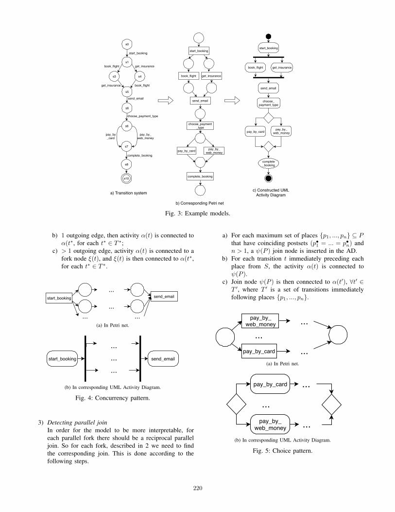
complete_booking

pay_by_card

start_booking

send_email

get_insurancebook_flight

choose_payment_type

pay_by_web_money

complete_booking

start_booking

book_flight get_insurance

send_email

choose_payment_type

pay_by_cardpay_by_

web_money

s0

s1

s5

s6

s6

s7

s8

s4s3

start_booking

book_flight

book_flight get_insurance

get_insurance

send_email

choose_payment_type

pay_by_card

pay_by_web_money

complete_booking

s10

b) Corresponding Petri net

a) Transition system c) Constructed UMLActivity Diagram

Fig. 3: Example models.

b) 1 outgoing edge, then activity α(t) is connected toα(t∗, for each t∗ ∈ T ∗;

c) > 1 outgoing edge, activity α(t) is connected to afork node ξ(t), and ξ(t) is then connected to α(t∗,for each t∗ ∈ T ∗.

start_booking send_email...

...... ...

(a) In Petri net.

...

...

...start_booking send_email

(b) In corresponding UML Activity Diagram.

Fig. 4: Concurrency pattern.

3) Detecting parallel joinIn order for the model to be more interpretable, foreach parallel fork there should be a reciprocal paralleljoin. So for each fork, described in 2 we need to findthe corresponding join. This is done according to thefollowing steps.

a) For each maximum set of places p1, ..., pn ⊆ Pthat have coinciding postsets (p•1 = ... = p•n) andn > 1, a ψ(P ) join node is inserted in the AD.

b) For each transition t immediately preceding eachplace from S, the activity α(t) is connected toψ(P ).

c) Join node ψ(P ) is then connected to α(t′), ∀t′ ∈T ′, where T ′ is a set of transitions immediatelyfollowing places p1, ..., pn.

pay_by_card

pay_by_ web_money

......

...

(a) In Petri net.

...

...

...pay_by_card

pay_by_web_money

(b) In corresponding UML Activity Diagram.

Fig. 5: Choice pattern.

220

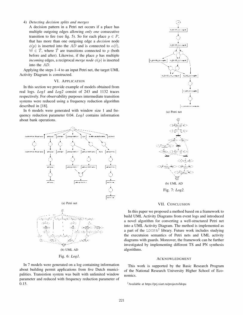
4) Detecting decision splits and mergesA decision pattern in a Petri net occurs if a place hasmultiple outgoing edges allowing only one consecutivetransition to fire (see fig. 5). So for each place p ∈ P ,that has more than one outgoing edge a decision nodeφ(p) is inserted into the AD and is connected to α(t),∀t ∈ T , where T are transitions connected to p (bothbefore and after). Likewise, if the place p has multipleincoming edges, a reciprocal merge node φ(p) is insertedinto the AD.

Applying the steps 1–4 to an input Petri net, the target UMLActivity Diagram is constructed.

VI. APPLICATION

In this section we provide example of models obtained fromreal logs. Log1 and Log2 consist of 243 and 1132 tracesrespectively. For observability purposes intermediate transitionsystems were reduced using a frequency reduction algorithmdescribed in [18].

In 6 models were generated with window size 1 and fre-quency reduction parameter 0.04. Log1 contains informationabout bank operations.

(a) Petri net

(b) UML AD

Fig. 6: Log1.

In 7 models were generated on a log containing informationabout building permit applications from five Dutch munici-palities. Transistion system was built with unlimited windowparameter and reduced with frequency reduction parameter of0.15.

(a) Petri net

(b) UML AD

Fig. 7: Log2.

VII. CONCLUSION

In this paper we proposed a method based on a framework tobuild UML Activity Diagrams from event logs and introduceda novel algorithm for converting a well-structured Petri netinto a UML Activity Diagram. The method is implemented asa part of the LDOPA2 library. Future work includes studyingthe executuion semantics of Petri nets and UML activitydiagrams with guards. Moreover, the framework can be furtherinvestigated by implementing different TS and PN synthesisalgorithms.

ACKNOWLEDGMENT

This work is supported by the Basic Research Programof the National Research University Higher School of Eco-nomics.

2Available at https://prj.xiart.ru/projects/ldopa

221

REFERENCES

[1] Wil Van der Aalst. Data Science in Action. In Process Mining, pages3–23. Springer, 2016.

[2] UML specification. https://www.omg.org/spec/UML/About-UML/. Ac-cessed: 2019-03-01.

[3] Concurrecy in UML. https://www.omg.org/ocup-2/documents/concurrency in uml version 2.6.pdf. Accessed: 2019-03-05.

[4] Josep Carmona, Jordi Cortadella, and Michael Kishinevsky. A Region-Based Algorithm for Discovering Petri Nets from Event Logs. volume5240, pages 358–373, 09 2008.

[5] Wil MP Van Der Aalst and Boudewijn F Van Dongen. Discovering PetriNets from Event Logs. In Transactions on Petri Nets and Other Modelsof Concurrency VII, pages 372–422. Springer, 2013.

[6] A Weijters, Wil M. P. Aalst, and Alves A K Medeiros. Process Miningwith the Heuristics Miner-algorithm, volume 166. 01 2006.

[7] Eric Badouel, Luca Bernardinello, and Philippe Darondeau. Polynomialalgorithms for the synthesis of bounded nets. In Colloquium on Treesin Algebra and Programming, pages 364–378. Springer, 1995.

[8] Jordi Cortadella, Michael Kishinevsky, Luciano Lavagno, and AlexandreYakovlev. Deriving Petri nets from finite transition systems. IEEEtransactions on computers, 47(8):859–882, 1998.

[9] Anna A. Kalenkova, Wil M. P. van der Aalst, Irina A. Lomazova, andVladimir A. Rubin. Process mining using bpmn: relating event logs andprocess models. Software & Systems Modeling, 16(4):1019–1048, Oct2017.

[10] Jim Arlow and Ila Neustadt. UML2 and the Unified Process: practicalobject-oriented analysis and design. Pearson Education, 2005.

[11] Rik Eshuis and Roel Wieringa. A comparison of Petri net and Activitydiagram variants. In Proc. of 2nd Int. Coll. on Petri Net Technologiesfor Modelling Communication Based Systems, volume 93, 2001.

[12] Dirk Fahland. Translating UML2 Activity diagrams to Petri nets. Berlin,Germany: Humboldt-Universitat zu Berlin, 2008.

[13] Bhawana Agarwal. Transformation of UML Activity diagrams into Petrinets for verification purposes. International Journal Of Engineering AndComputer Science, 2(3):798–805, 2013.

[14] Sander JJ Leemans, Dirk Fahland, and Wil MP van der Aalst. Discov-ering block-structured process models from event logs-a constructiveapproach. In International conference on applications and theory ofPetri nets and concurrency, pages 311–329. Springer, 2013.

[15] Kseniya Davydova and Sergei Shershakov. Mining hybrid uml modelsfrom event logs of soa systems. 29(4), 2017.

[16] Joos CAM Buijs, Boudewijn F Van Dongen, and Wil MP van Der Aalst.On the role of fitness, precision, generalization and simplicity in processdiscovery. In OTM Confederated International Conferences” On theMove to Meaningful Internet Systems”, pages 305–322. Springer, 2012.

[17] Wil MP Van der Aalst, Vladimir Rubin, HMW Verbeek, Boudewijn Fvan Dongen, Ekkart Kindler, and Christian W Gunther. Process mining:a two-step approach to balance between underfitting and overfitting.Software & Systems Modeling, 9(1):87, 2010.

[18] Sergey A Shershakov, Anna A Kalenkova, and Irina A Lomazova. Tran-sition systems reduction: balancing between precision and simplicity. InTransactions on Petri Nets and Other Models of Concurrency XII, pages119–139. Springer, 2017.

[19] Timofey Shunin, Natalia Zubkova, and Sergey Shershakov. Neuralapproach to the discovery problem in process mining. In Analysis of Im-ages, Social Networks and Texts, pages 261–273. Springer InternationalPublishing, 2018.

[20] Jan Martijn EM Van der Werf, Boudewijn F van Dongen, Cor AJHurkens, and Alexander Serebrenik. Process discovery using integerlinear programming. In International conference on applications andtheory of petri nets, pages 368–387. Springer, 2008.

222

XXX-X-XXXX-XXXX-X/XX/$XX.00 ©20XX IEEE

“Life” in Tensors: Implementing Cellular Automata

on Graphics Adapters

Shalyapina Natalia

National Research Tomsk State University

Tomsk, Russia

nat.shalyapina@gmail.com

Gromov Maxim

National Research Tomsk State University

Tomsk, Russia maxim.leo.gromov@gmail.com

Abstract— This paper presents an approach to the

description of cellular automata using tensors on the example

of the cellular automata of Conway's Game of Life. This

approach allows to attract various frameworks for organizing

scientific calculations on high-performance graphics adapter

processors, that is, to automatically build parallel software

implementations of cellular automata. In our work, we use the

Keras and TensorFlow frameworks to organize computations

on NVIDIA graphics adapters. Since these frameworks were

created to build neural networks, the functioning of the

cellular automata of Conway's Game of Life is described by a

specially constructed neural network. The resulting

acceleration from such a parallel implementation of the

cellular automata is estimated experimentally.

Keywords— Cellular automata, Conway's Game of Life,

tensor

I. INTRODUCTION

The use of automata in description of a dynamic systems’ behavior has been known for a long time. The key point of this approach to the description of systems is a representation of the object under study in the form of a discrete automatic device – automaton (State Machine or Transition System). Under the influence of input sequences (or external factors) an automaton changes its state and produces reactions. There are many types of such automata: the Moore and Mealy machines [1], the cellular automaton [2], and others. The knowledge of the features of the object under study can provide enough information to select the appropriate type of automaton for the object’s behavior description. In some cases, it is convenient to use an infinite model. But finite models are mostly common. In the latter case, the sets of states, input actions (or states of the environment), and output reactions are finite.

Our work deals with cellular automata (CA). The theory of cellular automata began to take shape quite a long time ago. The work of John von Neumann [3] might be considered as the first work of the cellular automata theory. Today, a large number of studies devoted to cellular automata are known [4, 5]. Note that a major part of these works is devoted to the simulating of spatially distributed systems in physics, chemistry, biology, etc. [6]. The goal of the simulation is to find the states of the cells of a CA after a predetermined number of CA cycles. The resulting set of states in some way characterizes the state of the process or object under study (fluid flow rate at individual points, concentration of substances, etc.). Thus, the task of

simulating a certain process or object by a cellular automaton can be divided into two subtasks. First, the researcher must select the parameters of the automaton (the dimension of the grid of cells, the shape of the cells, the type of neighborhood, etc.). And secondly, programmatically implement the behavior of the selected cellular automaton. Our work is focused on the second task – the software implementation of the cellular automaton.

In itself, the concept of a cellular automaton is quite simple and the idea of software implementation is obvious. However, the number of required calculations and the structure of these calculations suggest the use of modern supercomputers with a large number of cores and supporting large-block parallelism. In this case, the cell field of the automaton is divided into separate blocks. Processing of blocks is done in parallel and independently from each other. At the end of each processing cycle, the task of combining the processing results of each block arises. This problem was solved in [7] in the original way. The experimental study in [7] of the efficiency of parallelization was carried out on clusters with 32 and 768 processors. Despite the high effectiveness of this approach, it has some issues. First, this approach assumes that a researcher has an access to a cluster. Supercomputers are quite expensive and usually are the property of some collective access center [8]. Of course, after waiting a certain time in the queue, access to the cluster is possible. But another difficulty arises: a special skill is needed to write parallel programs in order to organize parallel sections of the program correctly. And this leads to the fact that it takes a certain number of experiments with the program to debug it before use. The latter means multiple times of waiting in a queue for a cluster, which, of course, delays the moment of launching true (not debugging) experiments with cellular automata.

We offer an alternative approach for software implementation of cellular automata, which is based on the use of modern graphics adapters. Modern graphics adapters are also well-organized supercomputers, consisting of several specialized computational cores and allowing execution of operations in parallel. Compared to clusters, graphics adapters are available for a wide range of users and we believe that their capabilities are enough to simulate cellular automata. The fact is that if we exclude extravagant and exotic examples of cellular automata, the process of modeling their behavior does not imply branching or return to the previous state. Exactly these restrictions are imposed on programs for graphics adapters. In addition, there are

223

special source development kits (frameworks) that can exploit multi-core graphics adapters and help a researcher quickly and efficiently create a software product, without being distracted by thinking about parallelizing data flows and control flows. In particular, such frameworks include Keras [9] and ThensorFlow [10].

In this paper, we demonstrate an approach for software implementation of cellular automata on graphics adapters. To do this, we use the well-known frameworks’ combination Keras-over-TensorFlow.

In order to use these tools, we propose to describe the set of states of an automaton cells’ by the main data structure used in these frameworks, namely, the tensor. Then we describe the process of evolution of the automaton in terms of tensor operations. Since Keras was developed as a tool for building (and learning) neural networks, a special neural network is built to implement the operations on tensors. The network takes as an input the tensor of the current set of states of the CA cells and builds the tensor of the subsequent set of states. A well-known cellular automaton, the Conway’s Game of Life, is used as a demonstration.

The work is structured as follows. Section II presents the

basic concepts and definitions concerning the theory of

cellular automata. Section III provides a description of the

game Conway’s Game of Life, its features and rules of

operation. Section IV is devoted to a detailed presentation of

the proposed approach for software implementation of

cellular automata on graphics adapters. The results of

computer experiments with the implementation of the

Conway’s Game of Life and comparison with the results of

a classical sequential implementation are presented in

Section V.

II. PRELIMINARIES

The Moore machine (finite, deterministic, fully defined)

is a 6-tuple 𝐴 = ⟨𝑆, , 𝐼, 𝑂, 𝜑, 𝜓⟩ , where S is the finite

nonempty set of states of the machine with a distinguished

initial state ∈ 𝑆, I is the finite set of input stimuli (input

signals), O is a finite set of output reactions (output signals),

𝜑: 𝑆 × 𝐼 → 𝑆 is a fully defined transition function,

𝜓: 𝑆 → 𝑂 is a fully defined function of output reactions. If

at some moment of time the Moore machine ⟨𝑆, , 𝐼, 𝑂, 𝜑, 𝜓⟩ is at the certain state 𝑠 ∈ 𝑆 and the input signal 𝑖 ∈ 𝐼 arrives,

then the machine changes its state to the state 𝑠′ = 𝜑 (𝑠, 𝑖),

and the signal 𝑜 = 𝜓 (𝑠′) appears at its output. The

machine starts its operation from the initial state with the

output signal 𝜓 (). It is important to note that originally

Moore defined the machine so that the output signal of the

machine is determined not by the final state of the transition,

but by the initial one (i.e. in the definition above instead of

𝑜 = 𝜓 (𝑠′) should be 𝑜 = 𝜓(𝑠) ). However, for our

purposes it is more convenient to use the definition we have

specified.

Let ℤ be the set of integers. Consider the set of all possible

integers pairs (𝑖, 𝑗) ∈ ℤ × ℤ . With each pair (𝑖, 𝑗) we

associate some finite set of pairs of integers 𝑁𝑖,𝑗 ⊆ ℤ × ℤ,

called the neighborhood of the pair (i, j). Pairs of Ni, j will be

called neighbors of the pair (i, j). The sets Ni, j must be such

that the following rule holds: if the pair (p, q) is the

neighbor of the pair (i, j), then the pair (p + k, q + l) is the

neighbor of the pair (i + k, j + l), where k and l are some

integers. Note that the cardinalities of all neighborhoods

coincide and the sets will have the same structure. For

convenience, we assume that all neighbors from Ni, j are

enumerated with integers from 1 to | Ni, j |, where | Ni, j | is

the cardinality of the set Ni, j. Then we can talk about the

first, second, etc. neighbor of some pair (i, j). If the pair (p,

q) is the n-th neighbor of the pair (i, j), then the pair (p + k,

q + l) is the n-th neighbor of the pair (i + k, j + l).

Consider the set of Moore machines of the form

𝐴𝑖,𝑗 = ⟨𝑆, 𝑖,𝑗 , 𝑆|𝑁𝑖,𝑗|, 𝑆, 𝜑, 𝜓⟩ such that 𝜓 (𝑠) = 𝑠 . Here i

and j are some integers, 𝐵𝑛 is the n-th Cartesian power of B.

The machines corresponding to the neighbors of the pair (i,

j) are called neighbors of the machine Ai, j. Neighboring

machines will be numbered as well as the corresponding

neighboring pairs (that is, the first neighbor, the second,

etc.). We specifically note that (i) for each machine Ai, j the

set of states is the same, i.e. S; (ii) for each machine Ai, j, the

set of output signals coincides with the set of states, that is,

also S; (iii) as an output signal, the machine gives its current

state; (iv) all machines have the same transition function and

the same function of output reaction; (v) as an input signal,

machines take tuples of states (of their neighbors), the

number of elements in the tuple coincides with the number

of neighbors, that is, equals | Ni, j |; (vi) machines differ only

in their initial states. Let at a given time moment the current

state of the first neighbor of the machine Ai, j is equal to s1,

the state of the second neighbor is s2, ..., the state of the n-th

neighbor is sn, where n = | Ni, j |. Then the tuple (s1, s2, ..., sn)

is the input signal of the machine Ai, j at this very moment.

All machines accept input signals, change their states and

provide output signals simultaneously and synchronously.

That is, some global clock signal is assumed.

The resulting set 𝐴𝑖,𝑗| (𝑖, 𝑗) ∈ ℤ × ℤ of the Moore

machines is called a two-dimensional synchronous cellular

automaton (or simply cellular automaton – CA). Each

individual Moore machine of this set will be called a cell.

The set of states of all cells the CA at a given time moment

will be called the global state of the cellular automaton at

this time moment.

The transition rules of cells from one state to another

(the function φ), the type of neighborhood of the cells (the

sets Ni, j), the number of different possible cell states (the set

S) define the whole variety of synchronous two-dimensional

cellular automata.

For clarity, one can draw cellular automata on the plane.

For this, the plane is covered with figures. Coverage can be

arbitrary, but of course, it is more convenient to do it in a

regular way. Classic covers are equal squares, equal

triangles and equal hexagons. The choice of one or another

method of covering the plane is dictated by the original

problem a CA is used for and the selected set of neighbors.

Next, the cover figures are assigned to the cells of the

cellular automaton in a regular manner. For example, let the

224

plane be covered with equal squares, so that each vertex of

each square is also the vertex of the other three squares of

the coverage (Fig. 1a). Choose the square of this coverage

randomly and associate it with the cell A0,0. Let the cell Ai,j

be associated with a certain square. Then we associate the

cell Ai + 1,j with the square on the right, the cell Ai - 1,j with the

square on the left, the cell Ai,j + 1 with the square above, and

the cell Ai,j - 1 with the square below (Fig. 1b). Cell states

will be represented by the color of the corresponding square

(Fig. 1c)

a)

b)

c)

Fig. 1. A CA represented on a plane covered by equal squares: a) the

coverage of the plane; b) association of the cells with the squares; c) colour

representation of cells’ states (for the case |𝑆| = 2 , «white» – state 0, «black» – state 1)

The resulting square based representation of a CA on a

plane is classical one. In our work we consider only this

representation.

For the square based representation of a CA, the

neighborhoods shown in Fig. 2 are the most common.

a)

b)

Fig. 2. The neighborhood (grey cells) of a cell (the black one) by а)

von Neumann, b) Moore

If a given cellular automaton models a process (for

example, heat transfer), then the various global initial states

𝑖,𝑗| (𝑖, 𝑗) ∈ ℤ × ℤ of the cellular automaton correspond to

different initial conditions of the process. According to the

definition of cellular automata introduced by us, the set of

cells in it is infinite. However, from the point of view of

practice, especially in the case of an implementation of a

cellular automaton, a set of cells have to be made finite. In

this case, some of the cells lack some neighbors. Therefore,

for them the set of neighbors and the transition function are

modified. Such modifications determine the boundary

conditions of the process being modeled.

III. CONWAY’S GAME OF LIFE

In the 70s of the 20th century, the English

mathematician John Conway proposed a cellular automaton

called the Conway’s Game of Life [l3].

The cells of this automaton are interpreted as biological

cells. The state “0” corresponds to the “dead” cell, and the

state “1” – “alive”. The game uses the Moore’s

neighborhood (Fig. 2b), i.e. each cell has 8 neighbors. The

rules for the transition of cells from one state to another are

as follows:

if a cell is “dead” and has three “alive” neighbors,

then it becomes “alive”;

− if a cell is “alive” and has two or three “alive”

neighbors, then it remains “alive”;

− if a cell is “alive” and has less than two or more

than three neighbors, then it becomes “dead”.

For the convenience of perception, the behavior of each

cell of the cellular automaton Conway’s Game of Life can

be illustrated using the transition graph (Fig. 3).

Fig. 3. Cell Transition Graph of the Conway’s Game of Life, where N is the number of “alive” neighbors

Despite the simplicity of the functioning of the

automaton, it is an object for numerous studies, since the

variation of the initial configuration leads to the appearance

of various images of its dynamics with interesting

properties. One of the most interesting among them are

moving groups of cells – gliders. Gliders not only oscillate

with a certain periodicity, but also move the space (plane).

Thus, as a result of experiments, it was established that on

the basis of gliders logical elements AND, OR, NOT can be

built. Therefore any other Boolean function can be

implemented. It was also proved that using the cellular

automata Conway’s Game of Life it is possible to emulate

the operation of a Turing machine [l3].

IV. FEATURES OF CONWAY’S GAME OF LIFE PARALLEL

IMPLEMENTATION

According to our definition, a set of states of a cell is

finite. It is obvious that, in this case, without loss of

generality, we can assume that the set of states is the set of

integers from 0 to |S| - 1, where |S| – is the cardinality of the

set of states. Therefore, the global state of the cellular

automaton can be represented as a matrix A. The element

Ai,j of this matrix is equal to the current state of the cell Ai,j.

We call the matrix A the matrix of the global state of the

cellular automaton. If there are no restrictions on the number

225

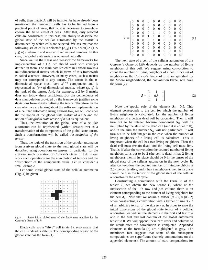
of cells, then matrix A will be infinite. As have already been

mentioned, the number of cells has to be limited from a

practical point of view, that is, it is necessary to somehow

choose the finite subset of cells. After that, only selected

cells are considered. In this case, the ability to describe the

global state of the cellular automaton by the matrix is

determined by which cells are selected. We assume that the

following set of cells is selected: 𝐴𝑖,𝑗| (1 ≤ 𝑖 ≤ 𝑚) ∧ (1 ≤

𝑗 ≤ 𝑛), where m and n – two fixed natural numbers. In this

case, the global state matrix is obtained naturally.

Since we use the Keras and TensorFlow frameworks for

implementation of a CA, we should work with concepts

defined in them. The main data structure in TensorFlow is a

multidimensional matrix which in terms of this framework

is called a tensor. However, in many cases, such a matrix

may not correspond to any tensor. The tensor in the n-

dimensional space must have np + q

components and is

represented as (p + q)-dimensional matrix, where (p, q) is

the rank of the tensor. And, for example, a 2 by 3 matrix

does not follow these restricions. But the convenience of

data manipulation provided by the framework justifies some

deviations from strictly defining the tensor. Therefore, in the

case when we are talking about the software implementation

of a cellular automaton using TensorFlow, we will consider

the the notion of the global state matrix of a CA and the

notion of the global state tensor of a CA as equivalent.

Thus, the evolution of the global state of a cellular

automaton can be represented (within TensorFlow) as a

transformation of the components of the global state tensor.

Such a transformation will be called the evolution of the

tensor.

Thus, the logic of the transition of the cellular automaton

from a given global state to the next global state will be

described using operations on tensors. In particular, for the

software implementation of Conway’s Game of Life in our

work such operations are the convolution of tensors and the

"restriction" of the components value. Let us consider a

small example.

Let some initial global state of the cellular automaton

(Fig. 4) be given.

Fig. 4. Some initial global state of the finite state machine for the

Conway’s Game of Life

Black cells are a “alive” cell (state 1), zero means that

the cell is “dead” (state 0). The corresponding tensor of the

global state has the form (1):

𝑻 =

[ 0000000000

0000000000

0000000000

0000100000

0001110000

0001000000

0000000000

0000000000

0000000000

0000000000]

The next state of a cell of the cellular automaton of the

Conway’s Game of Life depends on the number of living

neighbors of this cell. We suggest using convolution to

count the number of living neighbors of a cell. Since set of

neighbors in the Conway’s Game of Life are specified by

the Moore neighborhood, the convolution kernel will have

the form (2):

𝑺 = [1 1 11 0,5 11 1 1

]

Note the special role of the element S22 = 0,5. This

element corresponds to the cell for which the number of

living neighbors is calculated. Let the number of living

neighbors of a certain dead cell be calculated. Then it will

turn out to be integer because component S22 will be

multiplied by the state of the dead cell (and it is equal to 0),

and in the sum the number S22 will not participate. It will

turn out to be half-integer in the case when the number of

living neighbors of a living cell is calculated. This is

important when the cell has two living neighbors. Then the

dead cell must remain dead, and the living cell must live.

That is, if after the convolution the counted number of living

neighbors turns out to be 2 (the cell is dead, it has 2 living

neighbors), then in its place should be 0 in the tensor of the

global state of the cellular automaton in the next cycle. If,

after convolution, the counted number of living neighbors is

2.5 (the cell is alive, and it has 2 neighbors), then in its place

should be 1 in the tensor of the global state of the cellular

automaton in the next cycle.

Constructing a convolution with the kernel S of the

tensor T, we obtain the new tensor C, where at the

intersection of the i-th row and j-th column there is an

element corresponding to the number of living neighbors for

the cell Ai,j. Note that we obtain a tensor (m – 2) (n – 2)

when constructing a convolution with a kernel of size 3 3

of an arbitrary tensor of the size m n. In order to save the

initial dimensions of the global state tensor of a cellular

automaton, we will set the elements in the first and last row

and in the first and last column of the global automaton

tensor to 0. We will append these zero rows and columns to

the result after the convolution is completed. Appended

elements in the formula (3) are highlighted in gray. The

mentioned fact suggests that some of the subsequent

computations are superfluous (namely computations on the

appended elements). The amount of extra computations for

226

the global state tensor with dimensions m n will be (2m –

2) + (2n – 2). Then, the part of extra computations in the

amount of useful computations is (2𝑚−2)+(2𝑛−2)

(𝑚−1)(𝑛−1)= 𝑂( 1

𝑚+ 1

𝑛).

(3)

Taking into account the agreement on the half-integer

value of the number of living neighbors, the integer part of

the value of the tensor component C determines the number

of living neighbors of the cell, and the presence of the

fractional part means that the cell was alive in the previous

step.

According to the rules of the Conway’s Game of Life it

is necessary to transform the tensor C in order to determine

the global state of the cellular automaton in the next step.

Components with values in the range [2.5, 3.5] should take

the value 1 (cells are alive). The remaining components

should become 0 (cells are dead). Among the classical

operations on tensors there is no operation that would allow

to express the required transformation. However, the

frameworks used in our work (Keras and TensorFlow) were

created primarily for the problems of the theory of artificial

intelligence, namely, for implementing of neural networks.

The data flow in them is the flow of tensors (a tensor as an

input, a tensor as an output). Computational elements, that

change data, are layers of the neural network.

So, for example, in our case for the convolution we use a

two-dimensional convolution layer with the kernel S

(formula (2)). Any tool for neural network implementation

ought to have the special type of layers – activation layers

(layer of non-linear transformations). These layers calculate

activation functions (some non-linear functions) of each

element of the input tensor and put the result into the output

tensor. Keras and TensorFlow offer a standard set of non-

linear activation functions. In addition, it is possible to

create custom activation functions. We built our own

activation function based on a function from a standard set

of functions, called a Rectified Linear Unit (ReLU). The

function ReLU is defined as follows (formula (4)). Its graph

is shown in Figure 5:

𝑅𝑒𝐿𝑈 = 𝑚𝑎𝑥(0, 𝑥)

Fig. 5. Diagram of ReLU function

Taking into account the required transformation of the

components of the tensor C described above, we suggested

the function presented in (5):

δ = 𝑅𝑒𝐿𝑈(4(𝑥 − 2,125)) − 𝑅𝑒𝐿𝑈(4(𝑥 − 2,125)) −𝑅𝑒𝐿𝑈(4(𝑥 − 2,125)) + 𝑅𝑒𝐿𝑈(4(𝑥 − 2,125))

Fig. 6. Diagram of the transition function of the Conway’s Game of

Life

As a result of applying the function δ to each component

of the tensor C, the tensor of the global state of the cellular

automaton will take the following form (formula (6)).

𝑻′ =

[ 0000000000

0000000000

0000000000

0001110000

0001010000

0001000000

0000000000

0000000000

0000000000

0000000000]

Thus, the software implementation of the Conway’s

Game of Life using the frameworks Keras and TensorFlow

is a two-layer neural network. The first layer is

convolutional, with the kernel from formula (2). The second

layer is the activation layer with the activation function from

formula (5).

V. EXPERIMENTAL RESULTS

We have implemented the described approach for the

cellular automaton of the Conway’s Game of Life in the

Python.

Based on the frameworks Keras and TensorFlow, a two-

layer neural network was created. The first layer is

0

1

2

3

4

5

-5 -4 -3 -2 -1 0 1 2 3 4 5

y

x

012345

0 0,5 1 1,5 2 2,5 3 3,5 4 4,5 5 5,5 6 6,5 7 7,5 8

y

x

227

convolutional with the kernel of the form (2), the second

layer is the activation layer with the activation function of

the form (5). Naturally, network training is not required. We

set all parameters in advance. In this case, the neural

network is a way of presenting the necessary

transformations of the global state tensor of the cellular

automaton, which is provided by Keras + TensorFlow. The

resulting program was launched on a graphics adapter with

CUDA support. For comparison with the classical

implementation of the cellular automaton of the Conway’s

Game of Life on a uniprocessor system, we used the

implementation of [11].

R-pentamino [12] located in the middle of the field (Fig.

4) was used as the initial global state of the cellular

automaton of the Conway’s Game of Life in the

experiments.

We took a square game field (the matrix of the global

state of the cellular automaton) with dimensions m × m,

where m varied from 10 to 350 with the step 10. For each m,

we calculated 1000 subsequent global states of the cellular

automaton. The execution time was measured. The

calculations were repeated 10 times. Time was averaged. All

experiments were conducted on a computer with the

following characteristics: Intel Core i5-3470@3.2 GHz

processor, 8 GB RAM, Windows 7-x64 OS, GeForce GTX

650 Ti graphics adapter (1024 MB RAM, 928 MHz base

frequency, 768 CUDA cores).

Dependence diagrams of the program execution time on

the “length” of the square field side m of the game are

shown in Figures 7 and 8. We also built regressions. The

regression curves are shown in Figures 7 and 8 as well. A

second-degree polynomial was chosen as the regression

hypothesis.

Fig. 7. Results of experiments with a single-threaded implementation

Fig. 8. Results of experiments with CUDA (Keras+TensorFlow)

implementation

It can be noted that for small values of m, the execution

time of a single-threaded program is smaller than the

execution time of the multiprocessor (on the graphics

adapter) implementation proposed by us. However, as m

grows, the situation changes and the proposed

multiprocessor implementation begins to outperform the

classical single-threaded implementation. We associate this

with the overhead of transferring data from the computer’s

general RAM to the graphics adapter’s RAM and returning

the result from the graphics adapter’s memory to the

computer’s memory. When the dimensions of the game field

of the Conway’s Game of Life are small, the time of actual

calculations of the global states of the cellular automaton is

much less than the time of transmission of information. As

the field size grows, the computation time of the cellular

automaton state becomes significant, the data transfer time

is leveled, and the multiprocessor implementation on the

graphics adapter begins to significantly outrun the single-

threaded speed.

Obviously, the dependence of the execution time of

programs on the "length" m of the square field side of the

Conway’s Game of Life must be parabolic. With the growth

of m, the number of cells grows as m2, each cell needs to be

processed once per cycle. Therefore, operations of fixed

duration must be of the m2 order. According to the obtained

results we constructed regression polynomials of the second

degree. Regression curves are in good agreement with

experimental data (Fig. 7, 8). It may seem that for a

multithreaded implementation the dependency should be

different. However, we note that when the number of cells

becomes much more than the number of cores in a multi-

core system (in our case, the graphics adapter had 768

cores), then processing will be performed block by block:

first comes one block of 768 cells, then another, etc. Thus,

m2/K operations will be done, where K is the number of

cores, that is, also of the order of m2.

VI. CONCLUTIONS

In this paper, a tensor approach to the software

implementation of cellular automata is described and

programmatically implemented. The approach is focused on

launching programs on multi-core graphics adapters.

Programs are implemented in Python using the frameworks

Keras and TensorFlow. These frameworks allow

automatically generate and run multi-threaded programs on

multi-core graphics adapters. These frameworks were

created for the problems of the artificial neural networks

theory. The data flow is the flow of tensors, and the

converting nodes are the layers of the neural network.

Therefore, the proposed approach should be implemented

within these frameworks as some kind of neural network.

For the Conway’s Game of Life we proposed a two-layer

neural network with certain parameters.

The effectiveness of using the developed approach was

shown during a series of computer experiments. If the

number of cells in the automaton is equal to the number of

cores, then the maximum acceleration can be observed. If

228

the number of cells exceeds the number of cores, then the

parallel sections of the program are executed sequentially.

This means that with a very large size of the playing field

the type of dependence will be parabolic when using a

graphics adapter. The latter is confirmed by regression

analysis.

REFERENCES

[1] D. Harris and S. Harris. Digital Design and Computer Architecture.

Morgan Kaufmann, 2012. 721 p.

[2] T. Toffolli, N. Margolus. Cellular Automata Machines. MIT Press, 1987. 279 p.

[3] J. von Neumann Theory of Self-Reproducing Automata. University of Illinois Press, 1966. 403 p.

[4] O. Bandman. Simulation Spatial Dynamics by Probabilistic Cellular Automata. Lecture Notes in Computer Science, 2002, vol. 2493, 10–19 pp.

[5] G.G. Malinetski, M.E. Stepantsov Modelirovanie diffusionnykh protsessov s pomoshchyu kletochnykh avtomatov s okrestnostyu Margolusa (Modeling of Diffusion Processes by Cellular Automata with Margolus Neighborhood), Zhurnal vychislitelnoy matematiki i matematicheskoy phiziki (Comput. Math. Math. Phys.), 1998, vol. 38, No. 6, 1017–1021 pp. (in Russian).

[6] J.R. Weimar. Cellular Automata for Reaction-Diffusion Systems. Parallel Computing, 1999, vol. 23, No. 11, 1699–1715 pp.

[7] Y.G. Medvedev. Razrabotka i issledovanie trehmernoj kletochno-avtomatnoj modeli potoka vyazkoj zhidkosti (Development and Research of a Three-Dimensional Cellular Automaton Model of a Viscous Fluid Flow). PhD thesis, Novosibirsk, 2005, 108 p (in Russian).

[8] Vychislitelnyj klaster «SKIF Cyberia» (Computing Cluster «SKIF Cyberia»). URL: https://cyberia.tsu.ru (12.05.2019).

[9] Keras: the Python Deep Learning Library. URL: https://keras.io (12.05.2019).

[10] TensorFlow. URL: https://www.tensorflow.org (12.05.2019).

[11] Sozdanie igry «Zhizn'» na C++ (Implementation of the Game "Life" using С++) URL: https://code-live.ru/post/cpp-life-game (12.05.2019).

[12] M. Gardner The Fantastic Combinations of John Conway's New Solitaire Game "Life". Scientific American, 1970, vol. 223, no 4, 120–123 pp.

229

Modeling of angular stabilization system onprocessors with scalable architecture

Dmitry MelnichukDepartment of Mathematical Support of Computer and Information Systems

Saratov State UniversitySaratov, Russia

melnichukdv@sgu.ru

Abstract—A numerical simulation of the effect of typicalnonlinearities on the output vector functions of a nonlinearstabilization system of a moving control object is performed. Theefficiency of parallelization of computations in the implementa-tion of similar tasks is investigated on the example of clustersystems with Intel Xeon Phi coprocessors.

Index Terms—hybrid dynamical systems, processors with scal-able architectures

I. INTRODUCTION

Currently, cluster systems are widely used, in the nodesof which one or several processors with a large number ofcores are used. Examples include computing systems with newIntel Xeon processors with scalable architecture or computingsystems with Intel Xeon Phi coprocessors that are used asvirtual cluster nodes. Parallel computational architectures ofthis class are effective only when solving problems with asignificant parallelism resource. In this case, classes of mathe-matical models that are effectively implemented on Intel XeonPhi, will be effectively implemented on modern scalable IntelXeon architectures. For the problems of modeling of hybriddynamical systems (HDS) [1, 2] a significant resource of par-allelism is typical, since in this class of mathematical modelsthe (theoretically infinite-dimensional) phase space of controlobjects with space-distributed parameters is isolated. For dy-namic balancing of computational load on cluster systems, theMPI-MAP parallelization pattern was previously implemented[3]. The purpose of this work is to study the effectiveness ofthe software implementation on parallel computing systemsof the class of modeling problems of the influence of typicalnonlinearities and nonstationarity on the output vector functionof the HDS. As an example, we consider a similar [4] systemof angular stabilization of the movable control object (therocket taking into account the deformations of its body),but providing stabilization both with respect to the verticaldirection and with respect to the longitudinal axis.

II. PARALLEL ALGORITHMS FOR MODELING OF HYBRIDDYNAMICAL SYSTEMS

HDS are systems of ordinary differential equations andpartial differential equations connected by means of boundaryconditions and constraint’s conditions under appropriate initialconditions [1, 2]. HDS with piecewise continuous input vector

function x(t), x : R → RNx and continuous output vectorfunction y(t), y : R → RNy correspond to equations similarto [2, 4]

y = f(x,y,h,p,µ,µtt)

u = F(u,x,y, y,µ,µtt), r ∈ Ω

G(u,y,µ)|S = 0, S = ∂Ω; h =

∫S

H(u,µ)dS

y(0) = y0, u(r, 0) = u0(r)

(1)

Here r ∈ RNr are independent spatial coordinates ofindividual points of the object with space-distributed param-eters, Ω ⊂ RNr is an area occupied by an object withspace-distributed parameters, h : R → RNh , f : RNx ×RNy × RNh × RNp × RNµ × RNt → RNy , u(r, t), u :RNr × R → RNu are distributed output vector function,operators F : (RNr × R → RNu) × (R → RNx) × (R →RNy )× (R→ RNy )×RNµ×RNt → (RNr ×R→ RNu), G :(RNr×R→ RNu)×(R→ RNy )×RNµ → (RNr×R→ RNg ),H : (RNr × R → RNu) × RNµ → (R → RNh) correspondto partial differential equations, boundary conditions, andcoupling conditions; p ∈ RNp are feedback parameters; µ ∈RNµ are parameters of model nonlinearities; µt ∈ RNt areparameters characterizing the unsteadiness of the system fromthe point of view of the automatic control theory; the point atthe top indicates the time t differentiation. When µ = µt = 0HDS (1) becomes linear stationary. The main theorems onthe stability of linearized HDS are formulated and proved in[1, 2]. In work [4] on the basis of an asymptotic method ofmany scales the fact of stabilization of nonlinear HDS on thebasis of parametric synthesis on the linearized model is proved,and adaptive algorithms of parametric synthesis are offered.After parametric synthesis, numerical simulation of the effectof typical nonlinearities and unsteadiness on the output vectorfunction of a nonlinear HDS is performed (1). In this case, theinput vector function x(t) and the initial conditions y0, u0(r)are fixed, and the components of the vectors µ and µt changewith a fixed step within a parallelepiped. The element-by-element transformation of sequence (µj ,µtj ), j = 1, 2, 3, ...into a sequence of values characterizing the maximum andstandard deviations of function y(t;µj ,µtj ) from y(t; 0, 0) isparallelized

230

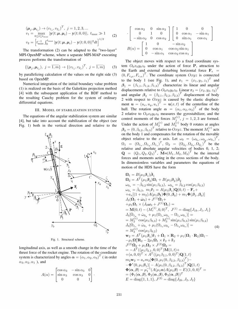
(µj ,µtj )→ (v1j , v2j )T, j = 1, 2, 3, ...

v1 = max0≤t≤tmax

|y(t;µ,µt)− y(t; 0, 0)|, tmax 1

v2 =[t−1max

∫ tmax

0|y(t;µ,µt)− y(t; 0, 0)|2dt

]1/2 (2)

The transformation (2) can be adapted to the ”two-layer”MPI-OpenMP scheme, where a separate MPI-MAP executingprocess performs the transformation of

(µj ,µtj ), j = 1,m → (v1j , v2j )T, j = 1,m (3)

by parallelizing calculation of the values on the right side (3)based on OpenMP.

Numerical integration of the initial boundary value problem(1) is realized on the basis of the Galerkins projection method[4] with the subsequent application of the BDF method tothe resulting Cauchy problem for the system of ordinarydifferential equations.

III. MODEL OF STABILIZATION SYSTEM

The equations of the angular stabilization system are similar[4], but take into account the stabilization of the object (seeFig. 1) both in the vertical direction and relative to the

Fig. 1. Structural scheme.

longitudinal axis, as well as a smooth change in the time of thethrust force of the rocket engine. The rotation of the coordinatesystem is characterized by angles α = (α1, α2, α3)

T ( in orderα3, α2, α1 ), and

A(α) =

cosα3 − sinα3 0sinα3 cosα3 0

0 0 1

·

·

cosα2 0 sinα2

0 1 0− sinα2 0 cosα2

1 0 00 cosα1 − sinα1

0 sinα1 cosα1

B(α) =

1 0 − sinα2

0 cosα1 cosα2 sinα1

0 − sinα1 cosα2 cosα1

The object moves with respect to a fixed coordinate sys-

tem O0x0y0z0 under the action of force P, attraction tothe Earth and external disturbing horizontal force Fe =(0, Fey0 , Fez0)

T . The coordinate system Oxyz is connectedto the body 1 (see Fig. 1), and r1 = (x1, y1, z1)

T andβ1 = (β1,1, β1,2, β1,3)

T characterize its linear and angulardisplacements relative to O0x0y0z0. Linear r2 = (x2, y2, z2)

T

and angular β2 = (β2,1, β2,2, β2,3)T displacement of body

2 with respect to Oxyz is caused by the elastic displace-ment u = (ux, uy, uz)

T= u(x, t) of the centerline of the

hull. The rotation angle α = (α1, α2, α3)T of the body

2 relative to O0x0y0z0 measures the gyrostabilizer, and thecontrol moments of the forces M (c)

j , j = 1, 2, 3 are formed.Under the action of M (c)

2 and M (c)3 body 0 rotates at angles

β0 = (0, β0,2, β0,3)T relative to Oxyz. The moment M (c)

1 actson the body 1 and compensates for the rotation of the movableobject relative to the x axis. Let ω0 = (ω0x , ω0y , ω0z )

T ,Ω1 = (Ω1x ,Ω1y ,Ω1z )

T , Ω2 = (Ω2ξ ,Ω2η ,Ω2ζ )T be the

relative and absolute angular velocities of bodies 0, 1, 2;Q = (Q1, Q2, Q3)

T , M=(M1,M2,M3)T be the internal

forces and moments acting in the cross sections of the body.In dimensionless variables and parameters the equations ofmotion of the HDS have the form

Ω1 = B(µ1β1)β1

Ω2 = AT (µ1β2)Ω1 +B(µ1β2)β2

ω0x = −β0,2 sin(µ1β0,3), ω0y = β0,2 cos(µ1β0,3)

ω0z = β0,3, m1r1 = A(µ1β1)Q(0, t)− Fe++ax[(1 +m2)A(µ1β1)Φ(0,β0) +m1Φ(β1,β0)]

J0(Ω1 + ω0) + J (1)Ω1++µ1Ω1 × (J0ω0 + J (1)Ω1) =

= M(0, t)− (M(1)c , 0, 0)T , J (1) = diagJ1k, J1, J1

J0[Ω1y + ω0y + µ1(Ω1zω0x − Ω1xω0z )] =

= M(c)2 cos(µ1β0,3) +M

(c)3 sin(µ1β0,3) sin(µ1β0,2)

J0[Ω1z + ω0z + µ1(Ω1xω0y − Ω1yω0x)] =

= M(c)3 cos(µ1β0,2)

w2 = AT (µ1β1)r1 + Ω1 ×R2 + µ1(Ω1 ·R2)Ω1−−µ1Ω

21R2 − 2µ1Ω1 × r2 + r2

J (2)Ω2 + µ1Ω2 × J (2)Ω2 == −AT ((µ1β2,1, 0, 0)T )M(1, t)++(a, 0, 0)T ×AT ((µ1β2,1, 0, 0)T )Q(1, t)

m2w2 = axm2[Φ(0, µ1(0, β2,2, β2,3)T

)−−Φ∗(0, µ1β1)]−A(µ1(0, β2,2, β2,3)

T)Q(1, t)

Φ(α,β) = µ−11 (A(µ1α)A(µ1β)− E)(1, 0, 0)T =

= (Φ1(α,β),Φ2(α,β),Φ3(α,β))T

E = diag1, 1, 1, J (2) = diagJ2k, J2, J2

(4)

231

R2 = (1 + a, 0, 0)T + µ1r2, Φ∗(α,β) == µ−1

1 (AT (µ1α)AT (µ1β)− E)(1, 0, 0)T == (Φ∗1(α,β),Φ∗2(α,β),Φ∗3(α,β))T

Φ∗∗(α,β) = µ−11 (A(µ1α)A(µ1β)− E)(0, 1, 0)

T=

= (Φ∗∗1 (α,β),Φ∗∗2 (α,β),Φ∗∗3 (α,β))T

α2 = −µ−11 arcsin(µ1Φ3(β2,β1))

α3 = 1µ1

arcsin µ1Φ2(β2,β1)cos(µ1α2)

α1 = − 1µ1

arcsinµ1Φ∗∗

3 (β2,β1)cos(µ1α2)

M(c)1 = S1[α1], f1(z) = tg z

M(c)3 = S3[α3]− p1β0,3 − p2µ

−12 f1(µ2β0,3)

M(c)2 = S2[α2]− p6β0,2 − p7µ

−12 f1(µ2β0,2)

S1[α] = µ−13 f2(µ3S(L)

1 [α])

S(L)1 [α] = p11dα/dt+ p12α, f2(z) = th z

S3[α] = µ−13 f2(µ3S(L)

3 [α])

S(L)3 [α] = p3dα/dt+ p4α+ p5

∫ t0α(ξ)dξ

S2[α] = µ−13 f2(µ3S(L)

2 [α])

S(L)2 [α] = p8dα/dt+ p9α+ p10

∫ t0α(ξ)dξ

u′x = [(1− µ21(u′y

2+ u′z

2))1/2 − 1]/µ1

L21 = µ1u′y, L31 = µ1u

′z

L11 = (1− L221 − L2

31)1/2

L33 = (1− L231)1/2, L12 = −L21/L33

L22 = L11/L33

L32 = 0, L13 = −L31L22, L23 = L31L12

κ1 = u′z(L12L′22 − L22L

′12)

κ2 = u′zL22L′11 − u′′yL23 − u′′zL33

κ3 = −u′yL′11/L33 + u′′yL22

uy + (AT (µ1β1)r1) · (0, 1, 0)T − (µ1Ω1xuz−−Ω1z (x+ µ1ux)) + µ1[(x+ µ1ux)Ω1x++µ1uzΩ1z ]Ω1y − µ2

1(Ω21x + Ω2

1z )uy++2µ1(Ω1x uz − Ω1z ux) == L21(Q′1 + µ1(κ2Q3 − κ3Q2))++L22(Q′2 − µ1(κ1Q3 − κ3Q1))++L23(Q′3 + µ1(κ1Q2 − κ2Q1))−−ax[Φ∗2(0,β1) + ((m2 + 1− x)u′y)′]

uz + (AT (µ1β1)r1) · (0, 0, 1)T + µ1Ω1xuy−−Ω1y (x+ µ1ux) + µ1[(x+ µ1ux)Ω1x++µ1uyΩ1y ]Ω1z − µ2

1(Ω21x + Ω2

1y )uz−−2µ1(Ω1x uy − Ω1y ux) == L31(Q′1 + µ1(κ2Q3 − κ3Q2))++L33(Q′3 + µ1(κ1Q2 − κ2Q1))−−ax[Φ∗3(0,β1) + ((m2 + 1− x)u′z)

′]Q′′1 − µ2

1(κ22 + κ2

3)Q1 == µ1−ax(m2 + 1− x)(κ2

2 + κ23)+

+κ′3Q2 − κ′2Q3 + 2κ3Q′2 − 2κ2Q

′3−

−µ1κ1(κ2Q2 + κ3Q3)− ((u′x)2 + (u′y)2 + (u′z)2)+

+(Ω1xL11 + Ω1yL21 + Ω1zL31)2−−(Ω2

1x + Ω21y + Ω2

1z )+

+2[L11(Ω1y u′z − Ω1z u

′y)− L21(Ω1x u

′z − Ω1z u

′x)+

+L31(Ω1x u′y − Ω1y u

′x)]

(5)

uy(0, t) = 0, u′y(0, t) = 0uy(1, t) = y2 − aΦ2(0,β2)u′y(1, t) = cos(µ1β2,2)µ−1

1 sin(µ1β2,3)uz(0, t) = 0, u′z(0, t) = 0uz(1, t) = z2 − aΦ3(0,β2)u′z(1, t) = −µ−1

1 sin(µ1β2,2)x2 = ux(1, t) + aΦ1(0,β2)Q′1(0, t) + µ1(κ2(0, t)Q3(0, t)− κ3(0, t)Q2(0, t)) == r1 ·A(µ1β1)(1, 0, 0)T + axΦ∗1(0,β1)Q′1(1, t) + µ1(κ2(1, t)Q3(1, t)− κ3(1, t)Q2(1, t)) == axΦ∗1(β2,β1) + µ1a(Ω2

2η + Ω22ζ

)+

+(1, 0, 0)T ·AT (µ1β2)w2

(6)

M1 = Ik

(β2,1 + γβ2,1 −

∫ 1

0κ1dx

)M2 = κ2 − γu′′z , M3 = κ3 + γu′′yQ2 = −M ′3 + µ1(κ2M1 − κ1M2)Q3 = M ′2 + µ1(κ3M1 − κ1M3)

(7)

β1(0) = β1(0) = β2(0) = β2(0) = β0,2(0) =

= β0,2(0) = β0,3(0) = β0,3(0) = r1(0) == r1(0) = y2(0) = y2(0) = z2(0) = z2(0) == uy(x, 0) = uy(x, 0) = uz(x, 0) = uz(x, 0) = 0

(8)

Here x(t) = (Fey0(t), Fez0(t))T and y(t) =

(β1,3(t), β2,3(t), β1,2(t), β2,2(t), β1,1(t), β2,1(t))T are input

and output vector functions, p = (p1, p2, ..., p12)T are

feedback parameters, (4) are ordinary differential equations,(5) are partial differential equations, (6) are boundaryconditions, (7) are constraints conditions, (8) are initialconditions. The set of parameters µ = (µ1, µ2, µ3)

T

characterizes typical nonlinearities, and the parameterµt = µ4, µ4 ≥ 0 characterizes a smooth change in thecharacteristic overload according to the law

ax(t) = a(min)x + (a(max)

x − a(min)x )e−µ4t,

t ≥ 0, a(min)x < ax ≤ a(max)

x

(9)

At µ = 0, the model equations are linearized and de-composed into three independent subsets corresponding tothe motion in the O0x0y0 and O0x0z0 planes (by virtue ofsymmetry, they pass into each other), as well as to the rotationrelative to the longitudinal axis. In this case, p5+j = pj ,j = 1, 5, correspond to the stabilization system in the verticaldirection, and p11, p12 correspond to the stabilization systemwith respect to the longitudinal axis.

IV. NUMERICAL SIMULATION RESULTS

In the numerical simulation of the output vector functionsof the nonlinear angular stabilization system, the componentsof the input vector function were given as Fey0(t) = 1(t),Fez0(t) = 1(t)−1(t−1), where 1(t) is the unit jump functionof Heaviside. For stabilization system with a set of parameters

232

J0 = 0.02,m1 = 0.3, J1 = 0.07,m2 = 0.2, J2 = 0.05,

a = 0.166667, a(min)x = 0.2, a(max)

x = 2, γ = 0.01,

J1k = 0.1, J2k = 0.05, Jk = 2, µ1 = 0.08, µ2 = 0.15,

µ3 = 0.055, µ4 = 0.05

(10)

the feedback parameters of the stabilization system in thedirection of vertical p1 = p6 = 6.347, p2 = p7 = 13.12,p3 = p8 = 17.59, p4 = p9 = 14.03, p5 = p10 = 5.951 werechosen on the basis of an adaptive algorithm of parametricsynthesis of the family of linearized models of HDS [4]. Sincethe stabilization of the object with respect to the longitudinalaxis is intended to compensate for the slow accumulationof errors due to nonlinear effects, the feedback parametersp11 = 0.04, p12 = 1 are selected in the central part of thestability region.

Figure 2 presents the results of numerical simulation of thecomponents β1,2 and β1,3 of the output vector functions of theoriginal nonlinear unsteady HDS (shown as a solid line) andits linear stationary analog at µ1 = µ2 = µ3 = µ4 = 0 (shownas a dashed line). The significant difference of the resultsis explained by the fact that the dimensionless overload axdecreases smoothly, with the decrease of ax in the consideredrange of overload changes in the linear stationary system,the attenuation of transients decreases, and the characteristicvalue of the output vector function increases. Nevertheless,parametric synthesis based on the linearized model allowsto stabilize the original nonlinear system in the vertical di-rection in the entire range of overloads. As follows fromthe results presented in Fig. 3, the selected values of thefeedback parameters p11 and p12 allow to stabilize the movablecontrol object with respect to the longitudinal axis, i.e. toallow compensate for the slow accumulation of errors dueto nonlinear effects. Fig. 4 shows the dependences of theparameters µ3 ∈ [0, 0.055] and µ4 ∈ [0, 0.05] at fixed µ1

and µ2 maximum v1 and standard v2 deviations (see (2)) ofthe output vector function of the nonlinear HDS on the outputvector function of the linearized HDS for tmax = 250. Asfollows from the data presented in Fig. 4, when changingthe overload according to (9) the greatest influence on theoutput vector function of the nonlinear HDS has parameterµ4, characterizing the unsteadiness of the system.

Similar data characterizing the efficiency of stabilizationwith respect to the vertical, longitudinal axis, as well as theinfluence of the parameters of nonlinearity and unsteadinesson the output functions of the stabilization system with pa-rameters

J0 = 0.00003,m1 = 0.0667, J1 = 0.00009728,m2 = 0.333,

J2 = 0.00345, a = 0.166667, ax = 1, γ = 0.01,

p1 = p6 = 4.098, p2 = p7 = 9.553, p3 = p8 = 7.687,

p4 = p9 = 7.714, p5 = p10 = 3.269, J1k = 0.002,

J2k = 0.005, J2 = 2, µ1 = 0.08, µ2 = 0.2,

µ3 = 0.04, µ4 = 0.05, p11 = 0.05, p12 = 1(11)

are shown in Fig. 5-7.

Fig. 2. Stabilization in the vertical direction.

Fig. 3. Stabilization with respect to the longitudinal axis.

Similarly to the previously discussed non-linear stabilizationsystem allows to compensate for errors in the entire range ofoverload (Fig. 5, 6). The greatest influence on the output vectorfunction of the nonlinear HDS has the parameter µ4, whichcharacterizes the unsteadiness of the system.

V. EFFICIENCY ANALYSIS OF PARALLEL ALGORITHMS

Consider the effectiveness of the implementation on com-puter systems with coprocessors Intel Xeon Phi parallel al-gorithm (2), (3) modeling the effect of typical nonlinearitiesand unsteadiness on the output functions of the HDS. Thedata corresponding to the modeling of a nonlinear stabiliza-tion system with parameters (10) are presented in Table I.The calculations were performed on a cluster of faculty ofComputer Science and Informational Technologies and VolgaRegion Center of New Information Technologies of SSU. Thefour-dimensional grid of change of parameters µ1, µ2, µ3, µ4

dimension 6×9×9×9 was used. As follows from the resultsshownin the Table I , in this case the use of a single Intel XeonPhi coprocessor is more efficient than the use of two quad-coreCPUs. The most profitable strategy of using coprocessors isparallelization based on OpenMP inside the coprocessor andparallelization based on MPI-MAP between coprocessors.

233

Fig. 4. Maximum and standard deviations.

Fig. 5. Stabilization in the vertical direction.

Fig. 6. Stabilization with respect to the longitudinal axis.

Similar data for the stabilization system with parametersfor the stabilization system with a set of parameters (11) arepresented in Table II. And in this case, using one Intel XeonPhi processor is more efficient than using two quad-core CPUs.The most profitable strategy for the use of coprocessors is the

TABLE ITIME OF MODELING THE IMPACT OF NONLINEARITIES, SEC.

Grid 6× 9× 9× 9Processor, serial/parallel Test 1 Test 2 Test 3 Test 4 Test 5Intel Xeon E5-2603 v2,serial

16411 16325 16470 16531 16314

2 processors Intel XeonE5-2603 v2, OpenMP

2480 2471 2501 2492 2485

Coprocessor Intel XeonPhi 5110P, OpenMP

1667 1635 1673 1649 1655

2 coprocessors IntelXeon Phi 5110P, MPI-MAP/OpenMP

1023 1015 1032 1008 1040

parallelization based on OpenMP within the coprocessor andparallelization based on MPI-MAP between the coprocessors.

TABLE IITIME OF MODELING THE IMPACT OF NONLINEARITIES, SEC.

Grid 6× 9× 9× 9Processor, serial/parallel Test 1 Test 2 Test 3 Test 4 Test 5Intel Xeon E5-2603 v2,serial

9637 9597 9645 9657 9675

2 processors Intel XeonE5-2603 v2, OpenMP

1443 1470 1430 1412 1467

Coprocessor Intel XeonPhi 5110P, OpenMP

1052 1042 1063 1037 1055

2 coprocessors IntelXeon Phi 5110P, MPI-MAP/OpenMP

703 699 710 707 705

Analogique evidence of the effectiveness of the imple-mentation of the parallel algorithm (2), (3) using a singleIntel Xeon Phi coprocessor (OpenMP) and two Intel XeonPhi coprocessors (MPI-MAP OpenMP) for a more detailed

234

Fig. 7. Maximum and standard deviations.

meshes, changing parameters µ1, µ2, µ3, µ4 are given in TableIII for stabilization system with parameters (10) and in TableIV for the stabilization system with parameters (11).

TABLE IIITIME OF MODELING THE IMPACT OF NONLINEARITIES, SEC.

Processor, serial/parallel Test 1 Test 2 Test 3 Test 4 Test 5Grid 6× 16× 16× 16

Coprocessor Intel XeonPhi 5110P, OpenMP

8953 9005 8934 8902 8985

2 coprocessors IntelXeon Phi 5110P, MPI-MAP/OpenMP

4726 4753 4715 4703 4744

Grid 12× 16× 16× 16Coprocessor Intel XeonPhi 5110P, OpenMP

18132 18243 18025 18187 18053

2 coprocessors IntelXeon Phi 5110P, MPI-MAP/OpenMP

9478 9529 9435 9501 9439

TABLE IVTIME OF MODELING THE IMPACT OF NONLINEARITIES, SEC.

Processor, serial/parallel Test 1 Test 2 Test 3 Test 4 Test 5Grid 6× 16× 16× 16

Coprocessor Intel XeonPhi 5110P, OpenMP

5671 5634 5654 5754 5698

2 coprocessors IntelXeon Phi 5110P, MPI-MAP/OpenMP

2988 2969 2967 3031 3002

Grid 12× 16× 16× 16Coprocessor Intel XeonPhi 5110P, OpenMP

11205 11278 11154 11174 11237

2 coprocessors IntelXeon Phi 5110P, MPI-MAP/OpenMP

5777 5809 5735 5741 5798

As follows from the Table III and IV results, with anincrease in the average number of nodes on the grid measure-ment, the multiplicative contribution to the acceleration of theMPI-MAP pattern quickly tends to the number of coprocessorsused.

VI. CONCLUSIONS

The proposed parallel algorithm is effective on clustersystems with nodes using processors with a large number ofcores. In particular, it is effective on cluster systems with IntelXeon Phi coprocessors.

REFERENCES

[1] Andreichenko D. K., Andreichenko K. P. On the theory of hybrid dynam-ical systems. Jour-nal of Computer and Systems Sciences International,2000, vol. 39, no. 3, pp. 383-398.

[2] Andreichenko D. K., Andreichenko K. P. Modelirovanie, analiz i sintezkombinirovannykh dinamicheskikh sistem. Uchebnoe posobie [Model-ing, analysis and synthesis of combined dynamical systems. Tutorial].Saratov, Rait-Ekspo Publ., 2013. 144 p. ISBN 978-5-4426-0018-6 (inRussian).

[3] Andreichenko D. K., Andreichenko K. P., Melnichuk D. V. PatternMPI-MAP i modeliro-vanie nelinejnyh kombinirovannyh dinamicheskihsistem [Pattern MPI-MAP and modeling of nonlinear hybrid dynam-ical systems] Problemy upravleniya, obrabotki i peredachi in-formacii[Problems of control, information processing and transmission]. Saratov,Rait-Ekspo Publ., 2015, vol.2, pp. 19-26. ISBN 978-5-4426-0049-0 (inRussian).

[4] Andreichenko D. K., Andreichenko K. P., Melnichuk D. V., PortenkoM. S. Adaptive Algorithm of Parametric Synthesis of Hybrid DynamicalSystems. Izv. Saratov Univ. (N. S.), Ser. Math. Mech. Inform., 2016, vol.16, iss. 4, pp. 465475 (in Russian). DOI: 10.18500/1816-9791-2016-16-4-465-475.

235