8

Gabriella Conti Department of Economics, University of Chicago Università di Napoli 'Federico II'

Stephen Pudney Institute for Social and Economic Research University of Essex

No. 2008-39 November 2008

ISE

R W

orkin

g P

aper S

eriesw

ww

.iser.essex.ac.uk

If you're happy and you know it, clap your hands! Survey design and the analysis of satisfaction

Non-technical summary

If you're happy and you know it, clap your hands!: Survey design and the analysis of satisfaction

The way you ask a question often affects the answer you get. This is just as true in survey research as it is in ordinary life. In recent years there has been a shift of interest in the policy debate from financial measures of well-being (income, wealth, etc.) to broader concepts of welfare (happiness, satisfaction, etc.) This is undoubtedly a good thing but it raises the question of how best to measure ill-defined concepts like satisfaction. The usual method in social science research is to use large-scale surveys, with questionnaires containing direct questions on satisfaction with various aspects of life, and work. Survey participants are then asked to locate their degree of satisfaction on a numerical scale from (say) 1 to 7. The British Household Panel Survey (BHPS) has been widely used for research on life and job satisfaction and, since its inception in 1991, there have been some significant changes in the way the satisfaction questions have been asked. In this paper, we ask whether the answers that people give to these questions have been influenced significantly by the way the questions are asked. We focus on two features of the BHPS. First, in 1992, there was an apparently minor change to the questions, which involved explanatory textual labels being added to more of the response categories numbered 1-7. Consequently, from 1992 onwards, interviewees were given a clearer explanation of what the response scale means. Second, from 1996, a self-completion paper questionnaire was added, so that we know both the answer that each individual gave in open interview and the much more private answer given in the self-completion questionnaire. There are six main conclusions: (1) The apparently minor re-design of the satisfaction questions in 1992 caused a very large change in the pattern of answers, particularly for women, who seem to respond better when the levels of satisfaction are given verbal as well as numerical meaning. (2) Oral interviews conducted by an interviewer tend to produce more positive reports of satisfaction than private self-completion questionnaires – the “let’s put on a good show for the interviewer” effect. (3) When children are present during the interview, adult interviewees tend to give still more positive responses – the “not in front of the children” effect. (4) The presence of the interviewee’s partner during the interview tends to depress the level of reported satisfaction – the “don’t show your partner how satisfied you are” effect, which we speculate may have something to do with the desire to maintain a strong bargaining position within the relationship. (5) These distortions of survey responses are important for research findings. For example, it is often reported by researchers that women’s job satisfaction is little affected by their hours and rate of pay. We cast doubt on this finding. When information from the more private self-completion questionnaire is used for the analysis, there is strong evidence that, like men, women’s degree of job satisfaction is influenced by both. (6) In future surveys asking about subjective well-being, happiness or satisfaction, it is important where possible to ask these questions by a suitably ‘private’ mode rather than by open oral interview.

If you’re happy and you know it, clap your hands!

Survey design and the analysis of satisfaction

Gabriella Conti

Department of Economics, University of Chicagoand

Universita di Napoli ‘Federico II’

Stephen Pudney

Institute for Social and Economic Research, University of Essex

November 2008

Abstract

Surveys differ in the way they measure satisfaction and happiness, so comparative researchfindings are vulnerable to distortion by survey design differences. We examine this using theBritish Household Panel Survey, exploiting its changes in question design and parallel useof different interview modes. We find significant biases in econometric results, particularlyfor gender differences in attitudes to the wage and hours of work. Results suggest that thecommon empirical finding that women care less than men about their wage and more abouttheir hours may be an artifact of survey design rather than a real behavioural difference.

Keywords: Satisfaction, measurement error, questionnaire design, BHPS

JEL codes: C23, C25, C81, J28

Contact: Steve Pudney, ISER, University of Essex, Wivenhoe Park, Colchester, CO4 3SQ,UK; tel. +44(0)1206-873789; email: spudney@essex.ac.uk

This work was supported by the Economic and Social Research Council through the MiSoC and ULSCresearch centres (award nos. RES518285001 and H562255004). We are grateful to Andrea Galeotti, AnnetteJackle, Peter Lynn, Stephen Jenkins and Nicole Watson for helpful comments.

1 Introduction

After years of extreme scepticism, many economists have accepted the value of research based

on direct observation of individual well-being or satisfaction as an alternative to the analysis

of market choices for the indirect revelation of underlying welfare. Although economists

are not unanimous in their welcome of this approach to welfare analysis, it amounts to a

profound change in the nature of economic research. However, economists have come late

to this type of analysis and sometimes do not show the caution that typifies much of the

sociological and psychological literature, particularly in relation to the survey measurement

process.

There are good reasons to be cautious, since there is evidence to suggest that the subjec-

tive assessments of satisfaction given by survey respondents are influenced by even apparently

trivial aspects of the survey design. This is particularly worrying, since there is no accepted

international standard for questions of this type and practice differs widely across surveys,

making comparative work problematic. Moreover, it is possible that different population

groups are influenced to different degrees by specific aspects of survey design, raising doubts

about the inferences that have been drawn about welfare differences between groups de-

fined by characteristics like gender and age. The economics literature is showing increasing

concern for these measurement issues (see Kristensen and Westergaard-Nielsen [2007] and

Krueger and Schkade [2008] for recent examples) and our aim in this paper is to contribute

to this strand of research by examining evidence generated as a by-product of a number of

past innovations in the design of the British Household Panel Survey (BHPS).

In this paper we exploit three innovations in question design and interview mode occurred

in the BHPS as “quasi-experiments” to analyze the effect of survey design features on re-

ported job satisfaction. We find strong evidence that apparently innocuous changes in survey

design lead to large distortions in reported job satisfaction. Women seem to be more affected

by these changes than men. They are more attracted by numerically-coded categories which

are also accompanied by textual labels - a phenomenon we name the gender-biased labeling

hypothesis.1 They also seem to be more affected by “social desirability” concerns during the

1Systematic gender differences are commonly found in the results of cognitive tests focusing on quanti-tative and verbal skills with test results skewed towards the former for males and the latter for females (seeHalpern [2000] for a review).

1

interview than when filling in the self-completion questionnaire. We are able to explain the

“part-time work puzzle” by Booth and Van Ours [2008] by simply noticing that the difference

in the effect of part-time work on reported job satisfaction is driven by the use of two differ-

ent questions - one asked by the interviewer, and the other reported in the self-completion

questionnaire. Finally, we estimate a latent factor model which explicitly incorporates these

design features and assesses quantitatively the extent of the bias.

The structure of the paper is as follows. We begin in section 2 by reviewing the relevant

aspects of survey design and the opportunities offered by the changing design of the BHPS.

In section 3 we consider the impact of an apparently minor aspect of the design of job

satisfaction questions: the use of textual labels as anchors for a subjective response scale,

the distortion of the distribution of responses caused by the lack of adequate labeling and its

impact on statistical models involving satisfaction variables. Section 4 exploits the existence

of two parallel BHPS questions on the same concept of overall job satisfaction to investigate

the impact of interview mode and context for a common set of respondents. Section 5

concludes.

2 Survey design: theory and practice

2.1 Survey design issues

Satisfaction and happiness are difficult subjects for survey research. The underlying concept

is ambiguous, so that phrasing of questions may be important. The lack of a natural scale for

measurement means that the method of framing, and explaining the meaning of, the range

of acceptable responses to survey participants is also important. Mood and interpersonal

interaction at the point of interview may have a transient influence on subjective assessments,

so that context and mode of interview also have a bearing on the outcome of the interview.

Some aspects of the interview process have been explored systematically, particularly the

design of allowable responses and the interview context.

Questions on satisfaction or happiness generally offer the respondent a number of dis-

crete, ordered categories which may be numbered and/or labeled with a textual description.

2

There is a great deal of rather mixed evidence on the appropriate number of response cat-

egories to offer respondents to subjective questions and a wide range of recommendations

exist, from two or three (Johnson et al. [1982]) to ten or more (Preston and Colman [2000]).

These recommendations are based on either internal group consistency measured by Cron-

bach’s α or on test-retest reliability. Weng [2004] has reviewed this literature and presented

further test-retest evidence, concluding in favour of a 7-point scale, as used in the BHPS.

Response labeling has also been the subject of experimental evaluation. From the point of

view of internal group consistency and test-retest reliability, textual labeling of every re-

sponse category has generally been found to be superior to the alternative in which only the

extreme categories are labeled (Weng [2004]). However, much less attention has been paid

to the possible distortions in the shape of the response distribution that may be induced

by inappropriate labeling and still less to the consequent biases that arise in the results of

conditional statistical modeling. We know little about the extent to which labeling influences

some population groups more than others.

There is a body of research on the effect of questionnaire structure and content, gener-

ally finding that respondents’ behaviour in answering attitudinal questions is vulnerable to

influence by ‘macro’ factors such as the perceived value of the survey, its relevance to the

interests of the respondent and the mood or moral position suggested by the immediately

preceding questions. These questionnaire context effects are well documented, particularly

for attitudinal, rather than strictly factual, questions (Tourangeau et al. [1991], Tourangeau

[1999]) and it is a weakness of the economic literature that little attention is usually paid to

questionnaire context when interpreting the results based on survey measures of satisfaction.

The context of the interview is also a potential influence on interview outcomes. The

psychology of survey response emphasises the role of self-image, harmonious social interaction

and the social acceptability of responses to questions on sensitive issues (Tourangeau et

al. [1991]). From an economic perspective, we could also add the incentive to maintain

bargaining power and credibility in the context of household decision-making, when interview

responses may be heard by other family members. Consequently, the personal characteristics

and behaviour of the interviewer and the presence of other individuals in the room during

interview are particularly important.

3

The mode of interview is an important influence on response for interviews which cover

sensitive issues like illicit behaviour, where computer-assisted self-interviewing (CASI) and

self-completion (SC) paper questionnaires are generally preferred to face-to-face interviewing

as a way of assuring a greater degree of confidentiality and inducing more truthful responses

(Aquilino [1997], Tourangeau and Smith [1996]). CASI is not normally used for questions

on general attitudes and subjective assessments of well-being, but these questions may be

rather sensitive for some respondents, particularly where the distribution of personal welfare

within the household is a contentious issue. For this reason, one might expect less distorted

responses from SC questionnaires than from face-to-face interviews.

It is no simple matter to understand the influence of survey design and context on the

outcome of survey-based research on satisfaction. An approach which underpins much of

the survey methods literature is the randomised trial, which randomly assigns survey par-

ticipants to treatment groups, each receiving different versions of the survey instrument or

different modes of delivery. This is often regarded as the ‘gold standard’ but it is open to

objection. Any small-scale trial explicitly designed as an experiment is necessarily quite

different from a routine wave of an established large-scale survey. Trials are generally sub-

ject to closer attention from survey managers, often use a special group of interviewers and

are temporary, rather than sustained, studies. They cannot be ‘double blind’ in any sense

and the extrapolation of their results to the practical situation of a large-scale continuing

survey is uncertain. In this paper we take a complementary approach based on the obser-

vational method, which entails observation and analysis of the effects of differences within,

and changes to, the design of an actual survey. While the lack of experimental control is

a disadvantage for the causal interpretation of observed effects, analysis of the same sur-

veys that are used for actual research avoids potentially invalid extrapolation of small-scale,

short-duration experiments.

2.2 The BHPS: some unnatural experiments

The BHPS is a nationally-representative annual household panel survey that began in the UK

in 1991. It has been the source of data for many well-known studies of life and job satisfaction,

including Clark and Oswald [1996], Clark [1997], Rose [2005], Taylor [2006] and Booth and

Van Ours [2008]. Each wave of the BHPS involves at least one visit to the household by

4

an interviewer, who conducts a face-to-face interview with each adult household member.

The BHPS offers two interesting opportunities for research on the influence of survey design

features. First, in 1992 there was a change in the labeling of response categories used on the

showcard for questions on job satisfaction. Second, a self-completion paper questionnaire

was introduced in 1996, covering a range of topics including satisfaction with various aspects

of life and essentially duplicating the overall job satisfaction question in the main interview.2

We consider each of these changes and attempt to draw from BHPS experience some

conclusions about the way that statistical inferences might be affected by question design,

interview and questionnaire context and interview mode.

3 Labeling of response categories: job satisfaction in

1991 and 1992

Following standard questions on the type of job, characteristics of the employer, hours of

work and travel to work arrangements, the BHPS interviewer asks seven questions on the

respondent’s satisfaction with specific aspects of his or her job: promotion prospects, to-

tal pay including overtime or bonuses, relations with supervisor or manager, job security,

ability to use own initiative, the work itself and hours of work (the questions on promotion

prospects, relations with supervisor/manager and use of initiative were discontinued from

1998 onwards). The exact question wording is given in Appendix 1B. Table 1 summarises

the showcards used in 1991 and 1992 onwards to indicate to respondents the 7-point scale of

permitted responses. In 1991 only three of the seven response categories were given textual

labels; since 1992 all have been labeled (note that the label for category 1 also changed).

2In 1999 there was a third change from pencil-and-paper interviewing (PAPI) to computer-assisted per-sonal interviewing (CAPI) (see Banks and Laurie [2000]). The latter introduced a laptop computer to improvecontrol over the interviewer’s question flow, wording and response checking. We found no significant impactof this change (details available from the authors on request).

5

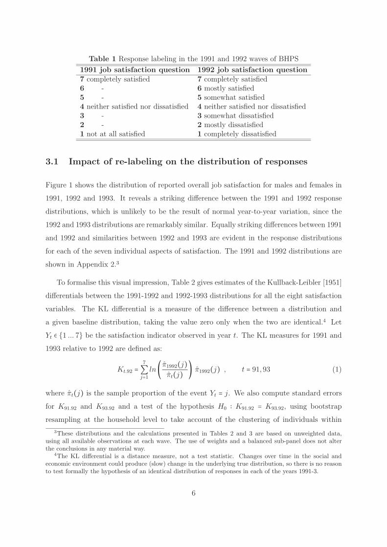
Table 1 Response labeling in the 1991 and 1992 waves of BHPS

1991 job satisfaction question 1992 job satisfaction question

7 completely satisfied 7 completely satisfied6 - 6 mostly satisfied5 - 5 somewhat satisfied4 neither satisfied nor dissatisfied 4 neither satisfied nor dissatisfied3 - 3 somewhat dissatisfied2 - 2 mostly dissatisfied1 not at all satisfied 1 completely dissatisfied

3.1 Impact of re-labeling on the distribution of responses

Figure 1 shows the distribution of reported overall job satisfaction for males and females in

1991, 1992 and 1993. It reveals a striking difference between the 1991 and 1992 response

distributions, which is unlikely to be the result of normal year-to-year variation, since the

1992 and 1993 distributions are remarkably similar. Equally striking differences between 1991

and 1992 and similarities between 1992 and 1993 are evident in the response distributions

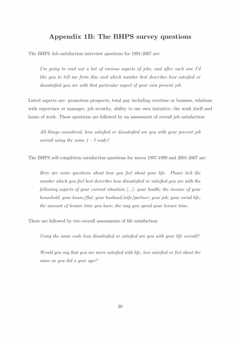
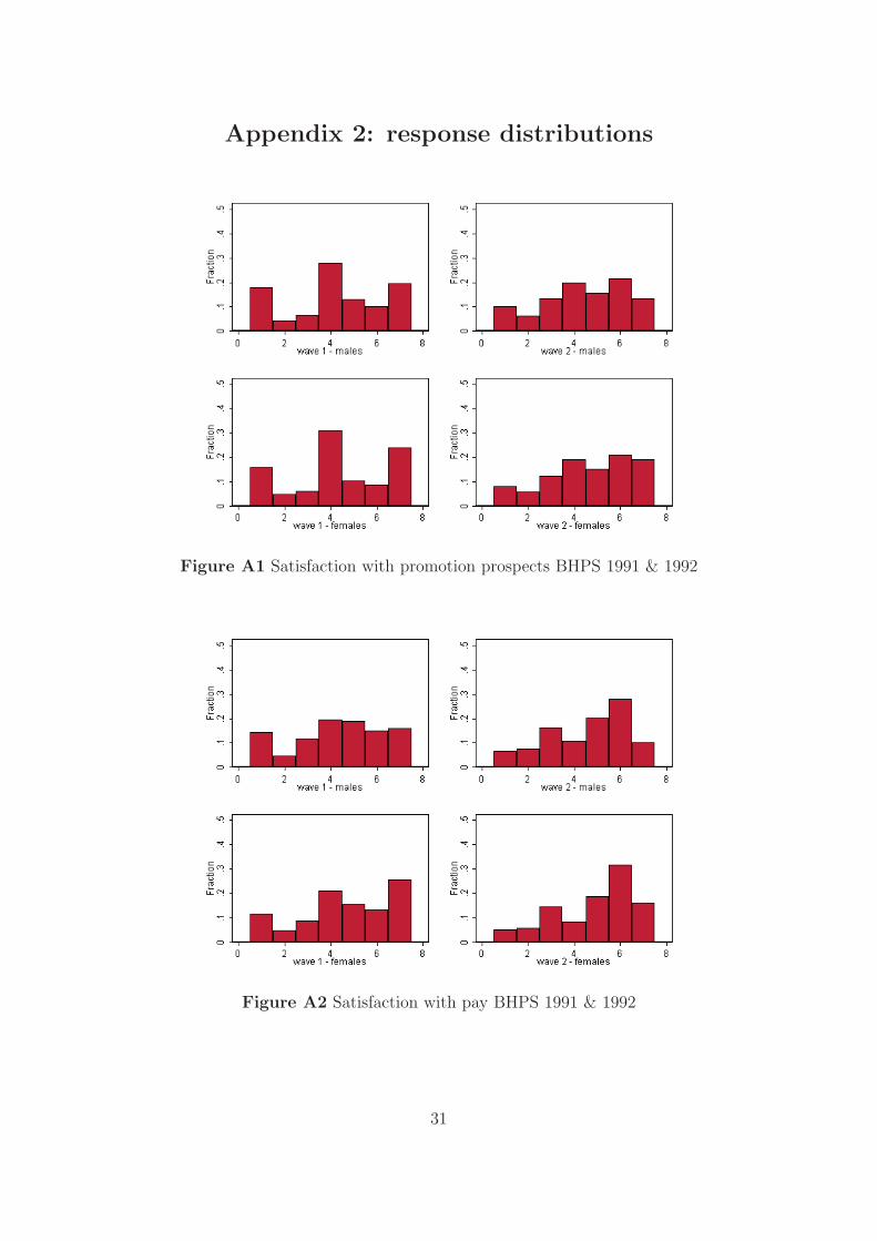
for each of the seven individual aspects of satisfaction. The 1991 and 1992 distributions are

shown in Appendix 2.3

To formalise this visual impression, Table 2 gives estimates of the Kullback-Leibler [1951]

differentials between the 1991-1992 and 1992-1993 distributions for all the eight satisfaction

variables. The KL differential is a measure of the difference between a distribution and

a given baseline distribution, taking the value zero only when the two are identical.4 Let

Yt ∈ {1 ... 7} be the satisfaction indicator observed in year t. The KL measures for 1991 and

1993 relative to 1992 are defined as:

Kt.92 =

7

∑j=1

ln( π1992(j)πt(j) ) π1992(j) , t = 91,93 (1)

where πt(j) is the sample proportion of the event Yt = j. We also compute standard errors

for K91.92 and K93.92 and a test of the hypothesis H0 ∶ K91.92 = K93.92, using bootstrap

resampling at the household level to take account of the clustering of individuals within

3These distributions and the calculations presented in Tables 2 and 3 are based on unweighted data,using all available observations at each wave. The use of weights and a balanced sub-panel does not alterthe conclusions in any material way.

4The KL differential is a distance measure, not a test statistic. Changes over time in the social andeconomic environment could produce (slow) change in the underlying true distribution, so there is no reasonto test formally the hypothesis of an identical distribution of responses in each of the years 1991-3.

6

Figure 1: Overall job satisfaction, 1991-1993 (full sample)

households. The result is very striking: there are large, highly significant differences between

the 1991 and 1992 distributions, but much smaller differences between the distributions for

the 1992 and 1993 waves, which used a common labeling scheme. There were, of course,

other differences between 1991 and 1992, notably that 1991 was the first wave of the BHPS,

so all respondents were new entrants to the panel and might conceivably have been affected

by panel conditioning in later waves. However, the change in the empirical distribution of

job satisfaction is clearly attributable to question design: the distortion obviously affects the

three labeled categories, with greater prominence for 1, 4 and 7 in 1991 than in later years.

Moreover, the response distributions for new entrants in later waves of the panel show no

such differences.

A second important conclusion is that there is substantially greater distortion in 1991

among the sample of female respondents than among males. This is consistent with the

gender-biased labeling hypothesis: that response categories which are labeled only numeri-

cally and not verbally are less unattractive to men than to women, on average.

7

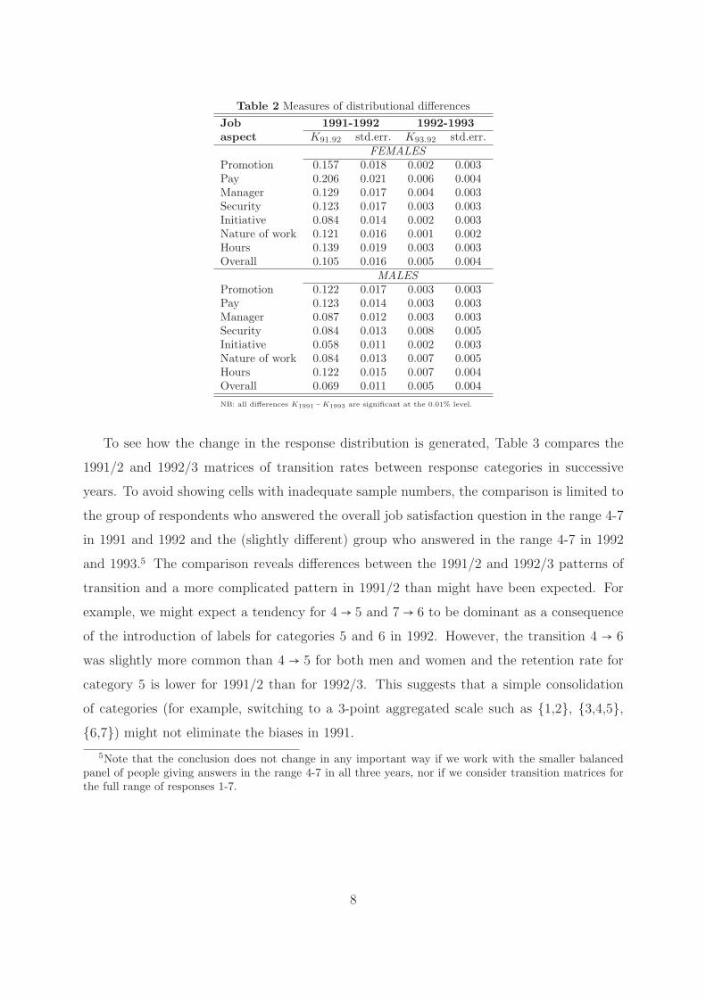
Table 2 Measures of distributional differences

Job 1991-1992 1992-1993aspect K91.92 std.err. K93.92 std.err.

FEMALESPromotion 0.157 0.018 0.002 0.003Pay 0.206 0.021 0.006 0.004Manager 0.129 0.017 0.004 0.003Security 0.123 0.017 0.003 0.003Initiative 0.084 0.014 0.002 0.003Nature of work 0.121 0.016 0.001 0.002Hours 0.139 0.019 0.003 0.003Overall 0.105 0.016 0.005 0.004

MALESPromotion 0.122 0.017 0.003 0.003Pay 0.123 0.014 0.003 0.003Manager 0.087 0.012 0.003 0.003Security 0.084 0.013 0.008 0.005Initiative 0.058 0.011 0.002 0.003Nature of work 0.084 0.013 0.007 0.005Hours 0.122 0.015 0.007 0.004Overall 0.069 0.011 0.005 0.004

NB: all differences K1991 −K1993 are significant at the 0.01% level.

To see how the change in the response distribution is generated, Table 3 compares the

1991/2 and 1992/3 matrices of transition rates between response categories in successive

years. To avoid showing cells with inadequate sample numbers, the comparison is limited to

the group of respondents who answered the overall job satisfaction question in the range 4-7

in 1991 and 1992 and the (slightly different) group who answered in the range 4-7 in 1992

and 1993.5 The comparison reveals differences between the 1991/2 and 1992/3 patterns of

transition and a more complicated pattern in 1991/2 than might have been expected. For

example, we might expect a tendency for 4→ 5 and 7→ 6 to be dominant as a consequence

of the introduction of labels for categories 5 and 6 in 1992. However, the transition 4 → 6

was slightly more common than 4 → 5 for both men and women and the retention rate for

category 5 is lower for 1991/2 than for 1992/3. This suggests that a simple consolidation

of categories (for example, switching to a 3-point aggregated scale such as {1,2}, {3,4,5},

{6,7}) might not eliminate the biases in 1991.

5Note that the conclusion does not change in any important way if we work with the smaller balancedpanel of people giving answers in the range 4-7 in all three years, nor if we consider transition matrices forthe full range of responses 1-7.

8

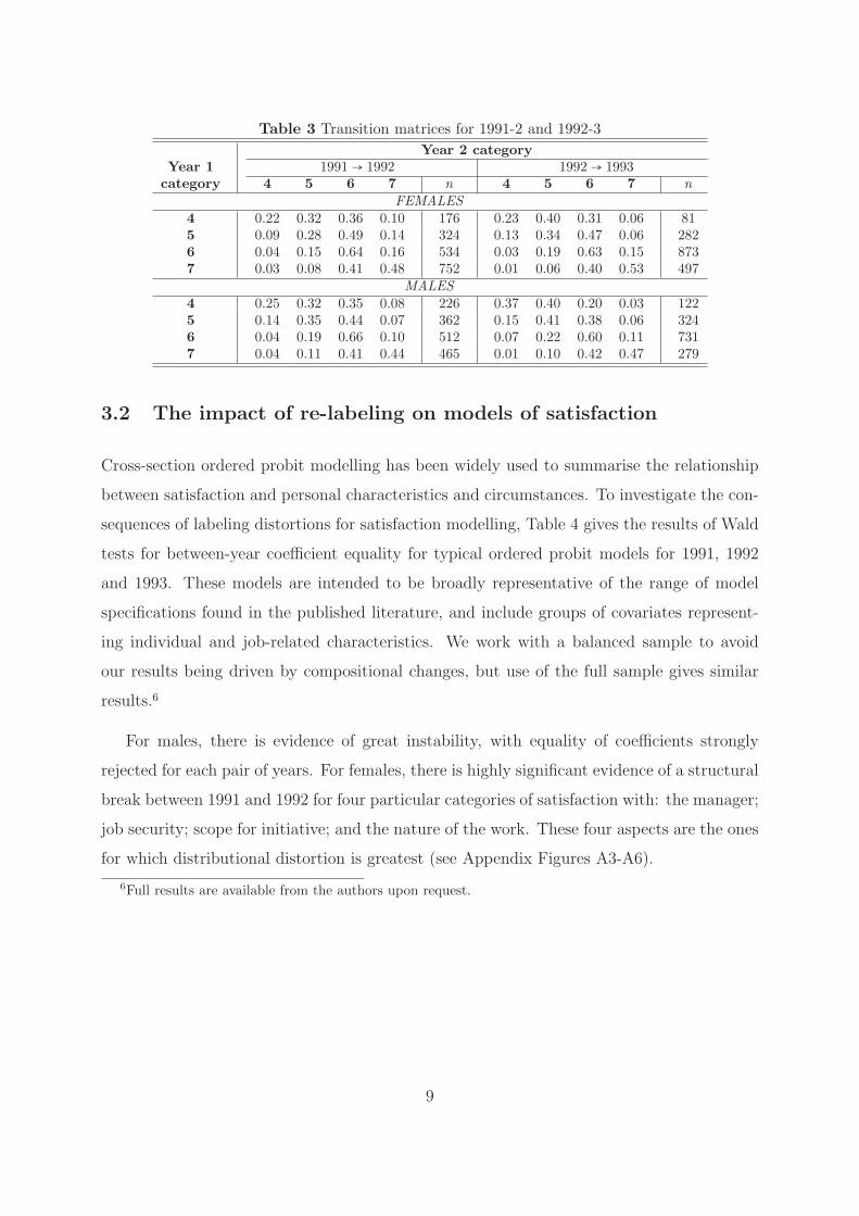
Table 3 Transition matrices for 1991-2 and 1992-3

Year 2 categoryYear 1 1991→ 1992 1992→ 1993

category 4 5 6 7 n 4 5 6 7 nFEMALES

4 0.22 0.32 0.36 0.10 176 0.23 0.40 0.31 0.06 815 0.09 0.28 0.49 0.14 324 0.13 0.34 0.47 0.06 2826 0.04 0.15 0.64 0.16 534 0.03 0.19 0.63 0.15 8737 0.03 0.08 0.41 0.48 752 0.01 0.06 0.40 0.53 497

MALES4 0.25 0.32 0.35 0.08 226 0.37 0.40 0.20 0.03 1225 0.14 0.35 0.44 0.07 362 0.15 0.41 0.38 0.06 3246 0.04 0.19 0.66 0.10 512 0.07 0.22 0.60 0.11 7317 0.04 0.11 0.41 0.44 465 0.01 0.10 0.42 0.47 279

3.2 The impact of re-labeling on models of satisfaction

Cross-section ordered probit modelling has been widely used to summarise the relationship

between satisfaction and personal characteristics and circumstances. To investigate the con-

sequences of labeling distortions for satisfaction modelling, Table 4 gives the results of Wald

tests for between-year coefficient equality for typical ordered probit models for 1991, 1992

and 1993. These models are intended to be broadly representative of the range of model

specifications found in the published literature, and include groups of covariates represent-

ing individual and job-related characteristics. We work with a balanced sample to avoid

our results being driven by compositional changes, but use of the full sample gives similar

results.6

For males, there is evidence of great instability, with equality of coefficients strongly

rejected for each pair of years. For females, there is highly significant evidence of a structural

break between 1991 and 1992 for four particular categories of satisfaction with: the manager;

job security; scope for initiative; and the nature of the work. These four aspects are the ones

for which distributional distortion is greatest (see Appendix Figures A3-A6).

6Full results are available from the authors upon request.

9

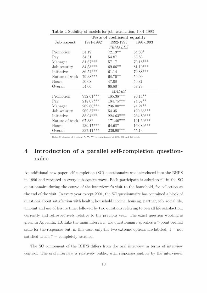
Table 4 Stability of models for job satisfaction, 1991-1993

Tests of coefficient equality

Job aspect 1991-1992 1992-1993 1991-1993FEMALES

Promotion 54.19 72.19** 64.80*Pay 34.31 54.87 53.83Manager 81.67*** 57.17 79.18***Job security 84.53*** 69.06** 81.10***Initiative 86.54*** 61.14 79.88***Nature of work 79.38*** 68.70** 59.99Hours 50.08 47.08 59.81Overall 54.06 66.80* 58.78

MALESPromotion 932.61*** 185.38*** 76.14**Pay 218.07*** 184.75*** 74.57**Manager 262.60*** 236.00*** 74.21**Job security 262.37*** 54.35 190.65***Initiative 88.94*** 224.63*** 264.89***Nature of work 67.38* 171.46*** 191.60***Hours 239.17*** 64.68* 163.80***Overall 337.11*** 236.90*** 55.13

Note: 51 degrees of freedom; *, **, *** ⇒ significance at 10%, 5% and 1% levels.

4 Introduction of a parallel self-completion question-

naire

An additional new paper self-completion (SC) questionnaire was introduced into the BHPS

in 1996 and repeated in every subsequent wave. Each participant is asked to fill in the SC

questionnaire during the course of the interviewer’s visit to the household, for collection at

the end of the visit. In every year except 2001, the SC questionnaire has contained a block of

questions about satisfaction with health, household income, housing, partner, job, social life,

amount and use of leisure time, followed by two questions referring to overall life satisfaction,

currently and retrospectively relative to the previous year. The exact question wording is

given in Appendix 1B. Like the main interview, the questionnaire specifies a 7-point ordinal

scale for the responses but, in this case, only the two extreme options are labeled: 1 = not

satisfied at all; 7 = completely satisfied.

The SC component of the BHPS differs from the oral interview in terms of interview

context. The oral interview is relatively public, with responses audible by the interviewer

10

and any other household members who happen to be in the room, whilst the SC question-

naire is completed in writing, with less open access to others. In addition to the differences

in question wording, response labeling and interview mode, the interview and SC questions

differ considerably in the context of the questionnaire. The interview job satisfaction ques-

tions are located in the employment section and preceded by simple factual questions about

job type, attributes of the employer, hours of work and travel-to-work. In contrast, the SC

satisfaction questions are preceded by questions on the respondent’s experience of anxiety

and other personal difficulties and then opinions on a series of ‘difficult’ issues such as gen-

der roles within the family, divorce, homosexuality, etc. This contextual difference makes it

impossible to distinguish conclusively between interview mode and questionnaire context as

the source of difference between the SC and interview patterns of satisfaction responses.

Around 64% of interviewees also complete a SC questionnaire. Much of our analysis is

necessarily conditional on the availability of both an interview and SC response. However,

this does not imply that selection bias is a problem. Selection would be an important issue

if we were aiming to analyse the difference between SC and interview responses that would

be observed if the SC response were hypothetically available for all interviewees. This is not

our aim: instead we are interested in the effects of using SC rather than interview data for

analysis, so we are by definition interested in the SC sample conditional on SC response.

4.1 The extent and correlates of discrepant response

Figure 2 plots the response distributions for the interview and SC job satisfaction questions

using pooled data for 1996-9 and 2001-5, restricting the sample to those individuals who

answered both questions. The two sample distributions are clearly different, for both genders.

In particular, the sample proportions for Y = 7 are nearly equal (0.095 and 0.144 for interview

for males and females respectively, and 0.104 and 0.138 for the SC) but the SC proportion of

Y = 1 observations is nearly double that of the interview (0.014 for the latter for both males

and females, but 0.027 for the SC). For other response categories, the interview response

distribution is right-shifted relative to the SC distribution, with, for example, the proportions

giving a response less than or equal to 4 being 21.3% and 15.9% for the interview, and 32.1%

and 31.1% for the SC, for males and females respectively (note again the larger shift for

women than for men). An interpretation of the difference between the interview and SC

11

Figure 2: Job satisfaction distributions for interview and SC respondents, by gender

response distributions is the combined effect of two processes: a tendency to give higher

responses in the interview setting than in the self-completion questionnaire as a result of

social pressure (Smith [1979]) and a tendency for the SC procedure to amplify the labeled

Y = 1 and Y = 7 categories relative to the other unlabeled categories.

Only 45% of respondents who answer both the SC and interview questions on job sat-

isfaction give the same response in both. Table 5 shows the distribution of discrepancies.

There is a definite tendency towards giving a 1-point higher response in the interview than

in the SC questionnaire. Sample proportions for these 1-point shifts are as high as 40%

and 53% for people at points 4 and 5 on the SC-scale. Respondents who classify themselves

towards the top of the job satisfaction scale are more likely to provide consistent answers

in the two different modes of interview. For example, 75.5% of the individuals who have

classified themselves on point 6 also report a similar answer to the interviewer. Instead, the

stability of self-reported job satisfaction is much lower for those at the lower end.

12

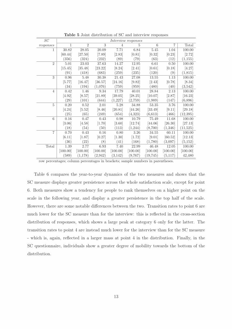
Table 5 Joint distribution of SC and interview responses

SC Interview responsesresponses 1 2 3 4 5 6 7 Total

1 30.82 28.05 20.09 7.71 6.84 5.45 1.04 100.00[60.44] [27.50] [7.89] [2.83] [0.81] [0.32] [0.23] [2.72](356) (324) (232) (89) (79) (63) (12) (1,155)

2 5.01 23.03 37.63 14.27 12.95 6.61 0.50 100.00[15.45] [35.48] [23.22] [8.24] [2.41] [0.61] [0.18] [4.27]

(91) (418) (683) (259) (235) (120) (9) (1,815)3 0.96 5.48 30.38 21.43 27.08 13.55 1.13 100.00

[5.77] [16.47] [36.57] [24.16] [9.82] [2.43] [0.78] [8.34](34) (194) (1,076) (759) (959) (480) (40) (3,542)

4 0.42 1.46 9.34 17.79 40.01 28.84 2.13 100.00[4.92] [8.57] [21.89] [39.05] [28.25] [10.07] [2.87] [16.23](29) (101) (644) (1,227) (2,759) (1,989) (147) (6,896)

5 0.20 0.52 2.01 5.28 34.88 53.35 3.76 100.00[4.24] [5.52] [8.46] [20.81] [44.26] [33.49] [9.11] [29.18](25) (65) (249) (654) (4,323) (6,613) (466) (12,395)

6 0.16 0.47 0.43 0.98 10.79 75.49 11.68 100.00[3.06] [4.58] [1.70] [3.60] [12.74] [44.06] [26.30] [27.13](18) (54) (50) (113) (1,244) (8,700) (1,346) (11,525)

7 0.70 0.43 0.16 0.80 3.26 34.55 60.11 100.00[6.11] [1.87] [0.27] [1.30] [1.72] [9.01] [60.52] [12.13](36) (22) (8) (41) (168) (1,780) (3,097) (5,152)

Total 1.39 2.77 6.93 7.40 22.99 46.48 12.05 100.00[100.00] [100.00] [100.00] [100.00] [100.00] [100.00] [100.00] [100.00]

(589) (1,178) (2,942) (3,142) (9,767) (19,745) (5,117) 42,480

row percentages; column percentages in brackets; sample numbers in parentheses.

Table 6 compares the year-to-year dynamics of the two measures and shows that the

SC measure displays greater persistence across the whole satisfaction scale, except for point

6. Both measures show a tendency for people to rank themselves on a higher point on the

scale in the following year, and display a greater persistence in the top half of the scale.

However, there are some notable differences between the two. Transition rates to point 6 are

much lower for the SC measure than for the interview: this is reflected in the cross-section

distribution of responses, which shows a large peak at category 6 only for the latter. The

transition rates to point 4 are instead much lower for the interview than for the SC measure

- which is, again, reflected in a larger mass at point 4 in the distribution. Finally, in the

SC questionnaire, individuals show a greater degree of mobility towards the bottom of the

distribution.

13

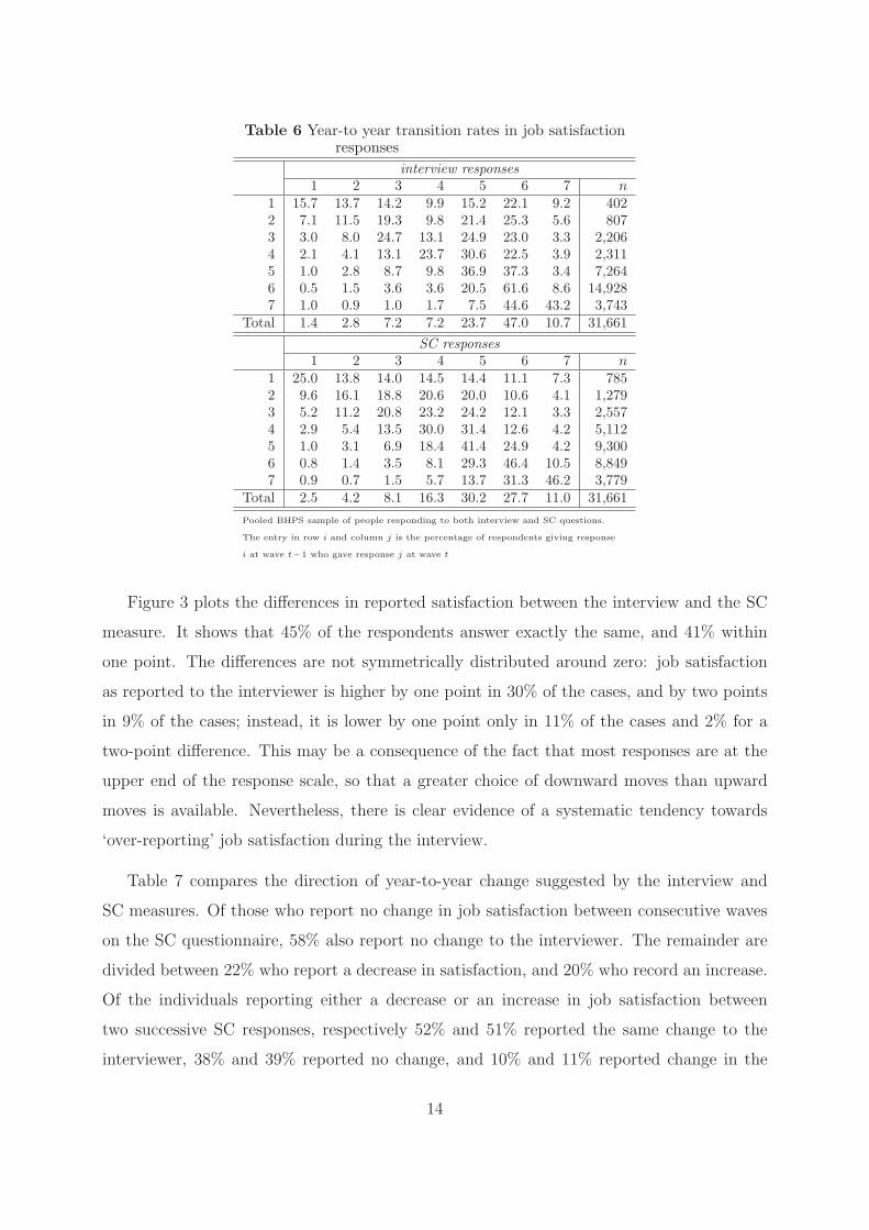
Table 6 Year-to year transition rates in job satisfactionresponses

interview responses1 2 3 4 5 6 7 n

1 15.7 13.7 14.2 9.9 15.2 22.1 9.2 4022 7.1 11.5 19.3 9.8 21.4 25.3 5.6 8073 3.0 8.0 24.7 13.1 24.9 23.0 3.3 2,2064 2.1 4.1 13.1 23.7 30.6 22.5 3.9 2,3115 1.0 2.8 8.7 9.8 36.9 37.3 3.4 7,2646 0.5 1.5 3.6 3.6 20.5 61.6 8.6 14,9287 1.0 0.9 1.0 1.7 7.5 44.6 43.2 3,743

Total 1.4 2.8 7.2 7.2 23.7 47.0 10.7 31,661

SC responses1 2 3 4 5 6 7 n

1 25.0 13.8 14.0 14.5 14.4 11.1 7.3 7852 9.6 16.1 18.8 20.6 20.0 10.6 4.1 1,2793 5.2 11.2 20.8 23.2 24.2 12.1 3.3 2,5574 2.9 5.4 13.5 30.0 31.4 12.6 4.2 5,1125 1.0 3.1 6.9 18.4 41.4 24.9 4.2 9,3006 0.8 1.4 3.5 8.1 29.3 46.4 10.5 8,8497 0.9 0.7 1.5 5.7 13.7 31.3 46.2 3,779

Total 2.5 4.2 8.1 16.3 30.2 27.7 11.0 31,661

Pooled BHPS sample of people responding to both interview and SC questions.

The entry in row i and column j is the percentage of respondents giving response

i at wave t − 1 who gave response j at wave t

Figure 3 plots the differences in reported satisfaction between the interview and the SC

measure. It shows that 45% of the respondents answer exactly the same, and 41% within

one point. The differences are not symmetrically distributed around zero: job satisfaction

as reported to the interviewer is higher by one point in 30% of the cases, and by two points

in 9% of the cases; instead, it is lower by one point only in 11% of the cases and 2% for a

two-point difference. This may be a consequence of the fact that most responses are at the

upper end of the response scale, so that a greater choice of downward moves than upward

moves is available. Nevertheless, there is clear evidence of a systematic tendency towards

‘over-reporting’ job satisfaction during the interview.

Table 7 compares the direction of year-to-year change suggested by the interview and

SC measures. Of those who report no change in job satisfaction between consecutive waves

on the SC questionnaire, 58% also report no change to the interviewer. The remainder are

divided between 22% who report a decrease in satisfaction, and 20% who record an increase.

Of the individuals reporting either a decrease or an increase in job satisfaction between

two successive SC responses, respectively 52% and 51% reported the same change to the

interviewer, 38% and 39% reported no change, and 10% and 11% reported change in the

14

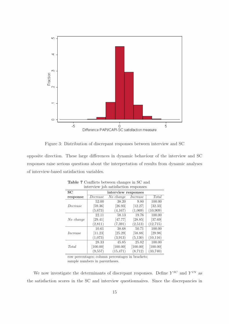
Figure 3: Distribution of discrepant responses between interview and SC

opposite direction. These large differences in dynamic behaviour of the interview and SC

responses raise serious questions about the interpretation of results from dynamic analyses

of interview-based satisfaction variables.

Table 7 Conflicts between changes in SC andinterview job satisfaction responses

SC interview responsesresponse Decrease No change Increase Total

52.00 38.20 9.80 100.00Decrease [59.36] [26.93] [12.27] [32.33]

(5,673) (4,167) (1,069) (10,909)22.11 58.13 19.76 100.00

No change [29.41] [47.77] [28.85] [37.69](2,811) (7,391) (2,513) (12,715)

10.61 38.68 50.71 100.00Increase [11.23] [25.29] [58.88] [29.98]

(1,073) (3,913) (5,130) (10,116)28.33 45.85 25.82 100.00

Total [100.00] [100.00] [100.00] [100.00](9,557) (15,471) (8,712) (33,740)

row percentages; column percentages in brackets;sample numbers in parentheses.

We now investigate the determinants of discrepant responses. Define Y SC and Y IN as

the satisfaction scores in the SC and interview questionnaires. Since the discrepancies in

15

reporting are highly asymmetric, we use a multinomial logit model to distinguish between

three states: Y SC> Y IN , Y SC

< Y IN and Y SC= Y IN to allow the covariates to have a

different impact on the probability of over-reporting and under-reporting in the interview

relative to the SC questionnaire.7 The no-discrepancy case is taken as the baseline state with

logit coefficients normalised to zero. Selected estimates (expressed as marginal effects) are

displayed in Table 8; full coefficient estimates are given in Table A3.1 in Appendix 3. For

economy of language, in discussing these results, we treat the SC responses as the reference

baseline, referring to over and under reporting in the interview relative to the SC.8

Significant ethnic differences emerge, with Indian males and females having an increased

probability of under-reporting their job satisfaction, while Indian women also have a smaller

probability of over-reporting in the interview. This underlines the importance of cultural

differences in the sensitivity to social influences in the interview context and may have impor-

tant implications for analyses of cross-national differences and ethnic differences in treatment

at work. The coefficients of variables related to marital status raise issues of strategic re-

porting behaviour related to credibility and bargaining power within the family. Married

men and respondents of both genders whose partner is present during the interview have a

significantly increased probability of under-reporting and (for males only) a reduced proba-

bility of over-reporting during the interview. Separated, divorced and widowed people have

an increased probability of over-reporting job satisfaction, compared to their never-married

counterparts. Men earning a higher wage have a lower probability of under-reporting, while

men working part-time have a higher probability of over-reporting. The non-profit sector

has been linked with high levels of job satisfaction in the research literature (Benz [2005]).

Here we find it to be associated with both a higher probability of over-reporting and a lower

probability of under-reporting for males, while no such effect appears for females. Individuals

working longer hours (both regular hours and overtime) are more likely to under-report and

less likely to over-report job satisfaction, regardless of their gender. These patterns clearly

suggest the existence of ‘social desirability’ influences on respondents in the face-to-face

interview situation.

7We have also estimated static and dynamic random effects probit models for the occurrence of Y SC≠

Y IN , giving similar results to those reported here. Details are available on request.8The marginal effects are calculated as ∂Pr(outcome∣x)/∂xj , for continuous x-variables and the corre-

sponding discrete difference for binary variables, where x is the point of sample means and the outcomes areSC < interview and SC > interview (SC=interview is the baseline category).

16

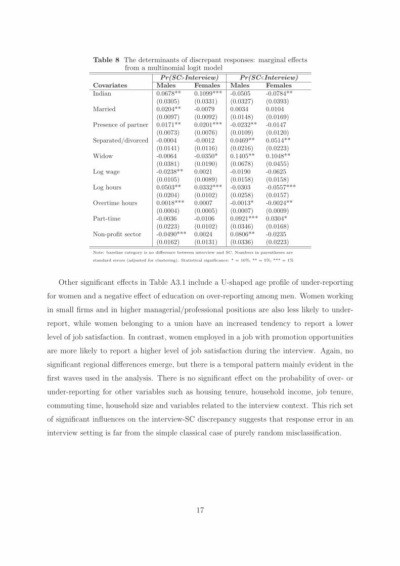
Table 8 The determinants of discrepant responses: marginal effectsfrom a multinomial logit model

Pr(SC>Interview) Pr(SC<Interview)Covariates Males Females Males FemalesIndian 0.0678** 0.1099*** -0.0505 -0.0784**

(0.0305) (0.0331) (0.0327) (0.0393)Married 0.0204** -0.0079 0.0034 0.0104

(0.0097) (0.0092) (0.0148) (0.0169)Presence of partner 0.0171** 0.0201*** -0.0232** -0.0147

(0.0073) (0.0076) (0.0109) (0.0120)Separated/divorced -0.0004 -0.0012 0.0469** 0.0514**

(0.0141) (0.0116) (0.0216) (0.0223)Widow -0.0064 -0.0350* 0.1405** 0.1048**

(0.0381) (0.0190) (0.0678) (0.0455)Log wage -0.0238** 0.0021 -0.0190 -0.0625

(0.0105) (0.0089) (0.0158) (0.0158)Log hours 0.0503** 0.0332*** -0.0303 -0.0557***

(0.0204) (0.0102) (0.0258) (0.0157)Overtime hours 0.0018*** 0.0007 -0.0013* -0.0024**

(0.0004) (0.0005) (0.0007) (0.0009)Part-time -0.0036 -0.0106 0.0921*** 0.0304*

(0.0223) (0.0102) (0.0346) (0.0168)Non-profit sector -0.0490*** 0.0024 0.0806** -0.0235

(0.0162) (0.0131) (0.0336) (0.0223)

Note: baseline category is no difference between interview and SC. Numbers in parentheses are

standard errors (adjusted for clustering). Statistical significance: * = 10%; ** = 5%; *** = 1%

Other significant effects in Table A3.1 include a U-shaped age profile of under-reporting

for women and a negative effect of education on over-reporting among men. Women working

in small firms and in higher managerial/professional positions are also less likely to under-

report, while women belonging to a union have an increased tendency to report a lower

level of job satisfaction. In contrast, women employed in a job with promotion opportunities

are more likely to report a higher level of job satisfaction during the interview. Again, no

significant regional differences emerge, but there is a temporal pattern mainly evident in the

first waves used in the analysis. There is no significant effect on the probability of over- or

under-reporting for other variables such as housing tenure, household income, job tenure,

commuting time, household size and variables related to the interview context. This rich set

of significant influences on the interview-SC discrepancy suggests that response error in an

interview setting is far from the simple classical case of purely random misclassification.

17

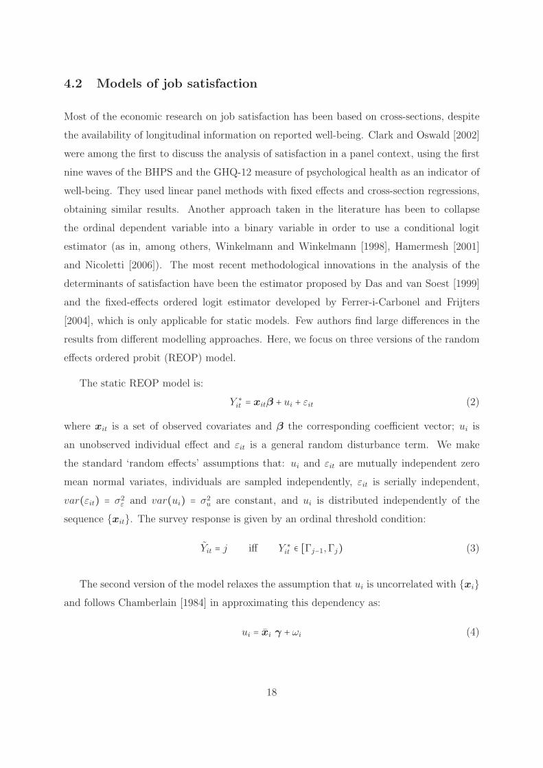
4.2 Models of job satisfaction

Most of the economic research on job satisfaction has been based on cross-sections, despite

the availability of longitudinal information on reported well-being. Clark and Oswald [2002]

were among the first to discuss the analysis of satisfaction in a panel context, using the first

nine waves of the BHPS and the GHQ-12 measure of psychological health as an indicator of

well-being. They used linear panel methods with fixed effects and cross-section regressions,

obtaining similar results. Another approach taken in the literature has been to collapse

the ordinal dependent variable into a binary variable in order to use a conditional logit

estimator (as in, among others, Winkelmann and Winkelmann [1998], Hamermesh [2001]

and Nicoletti [2006]). The most recent methodological innovations in the analysis of the

determinants of satisfaction have been the estimator proposed by Das and van Soest [1999]

and the fixed-effects ordered logit estimator developed by Ferrer-i-Carbonel and Frijters

[2004], which is only applicable for static models. Few authors find large differences in the

results from different modelling approaches. Here, we focus on three versions of the random

effects ordered probit (REOP) model.

The static REOP model is:

Y ∗it = xitβ + ui + εit (2)

where xit is a set of observed covariates and β the corresponding coefficient vector; ui is

an unobserved individual effect and εit is a general random disturbance term. We make

the standard ‘random effects’ assumptions that: ui and εit are mutually independent zero

mean normal variates, individuals are sampled independently, εit is serially independent,

var(εit) = σ2ε and var(ui) = σ2

u are constant, and ui is distributed independently of the

sequence {xit}. The survey response is given by an ordinal threshold condition:

Yit = j iff Y ∗it ∈ [Γj−1,Γj) (3)

The second version of the model relaxes the assumption that ui is uncorrelated with {xi}and follows Chamberlain [1984] in approximating this dependency as:

ui = xi γ + ωi (4)

18

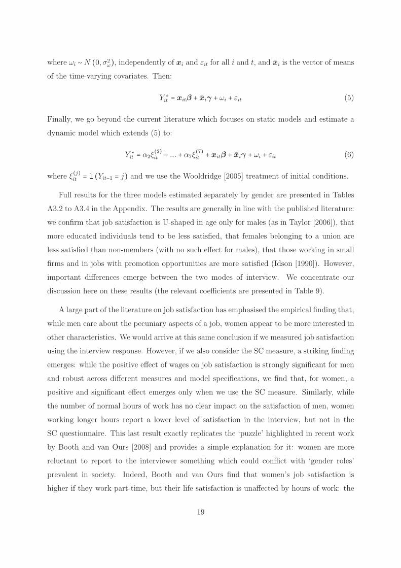
where ωi ∼ N (0, σ2ω), independently of xi and εit for all i and t, and xi is the vector of means

of the time-varying covariates. Then:

Y ∗it = xitβ + xiγ + ωi + εit (5)

Finally, we go beyond the current literature which focuses on static models and estimate a

dynamic model which extends (5) to:

Y ∗it = α2ξ(2)it + ... + α7ξ

(7)it +xitβ + xiγ + ωi + εit (6)

where ξ(j)it = (Yit−1 = j) and we use the Wooldridge [2005] treatment of initial conditions.

Full results for the three models estimated separately by gender are presented in Tables

A3.2 to A3.4 in the Appendix. The results are generally in line with the published literature:

we confirm that job satisfaction is U-shaped in age only for males (as in Taylor [2006]), that

more educated individuals tend to be less satisfied, that females belonging to a union are

less satisfied than non-members (with no such effect for males), that those working in small

firms and in jobs with promotion opportunities are more satisfied (Idson [1990]). However,

important differences emerge between the two modes of interview. We concentrate our

discussion here on these results (the relevant coefficients are presented in Table 9).

A large part of the literature on job satisfaction has emphasised the empirical finding that,

while men care about the pecuniary aspects of a job, women appear to be more interested in

other characteristics. We would arrive at this same conclusion if we measured job satisfaction

using the interview response. However, if we also consider the SC measure, a striking finding

emerges: while the positive effect of wages on job satisfaction is strongly significant for men

and robust across different measures and model specifications, we find that, for women, a

positive and significant effect emerges only when we use the SC measure. Similarly, while

the number of normal hours of work has no clear impact on the satisfaction of men, women

working longer hours report a lower level of satisfaction in the interview, but not in the

SC questionnaire. This last result exactly replicates the ‘puzzle’ highlighted in recent work

by Booth and van Ours [2008] and provides a simple explanation for it: women are more

reluctant to report to the interviewer something which could conflict with ‘gender roles’

prevalent in society. Indeed, Booth and van Ours find that women’s job satisfaction is

higher if they work part-time, but their life satisfaction is unaffected by hours of work: the

19

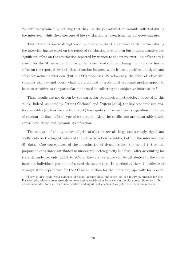
“puzzle” is explained by noticing that they use the job satisfaction variable collected during

the interview, while their measure of life satisfaction is taken from the SC questionnaire.

This interpretation is strengthened by observing that the presence of the partner during

the interview has no effect on the reported satisfaction level of men but it has a negative and

significant effect on the satisfaction reported by women to the interviewer - an effect that is

absent for the SC measure. Similarly, the presence of children during the interview has no

effect on the reported level of job satisfaction for men, while it has a positive and significant

effect for women’s interview (but not SC) responses. Paradoxically, the effect of ‘objective’

variables like pay and hours which are grounded in traditional economic models appear to

be most sensitive to the particular mode used in collecting the subjective information.9

These results are not driven by the particular econometric methodology adopted in this

study. Indeed, as noted by Ferrer-i-Carbonel and Frijters [2004], the key economic explana-

tory variables (such as income from work) have quite similar coefficients regardless of the use

of random- or fixed-effects type of estimators. Also, the coefficients are remarkably stable

across both static and dynamic specifications.

The analysis of the dynamics of job satisfaction reveals large and strongly significant

coefficients on the lagged values of the job satisfaction variables, both in the interview and

SC data. One consequence of the introduction of dynamics into the model is that the

proportion of variance attributed to unobserved heterogeneity is halved: after accounting for

state dependence, only 14.6% to 20% of the total variance can be attributed to the time-

invariant individual-specific unobserved characteristics. In particular, there is evidence of

stronger state dependence for the SC measure than for the interview, especially for women.

9There is also some weak evidence of ‘social acceptability’ influences on the interview process for men.For example, while women strongly express higher satisfaction from working in the non-profit sector in bothinterview modes, for men there is a positive and significant coefficient only for the interview measure.

20

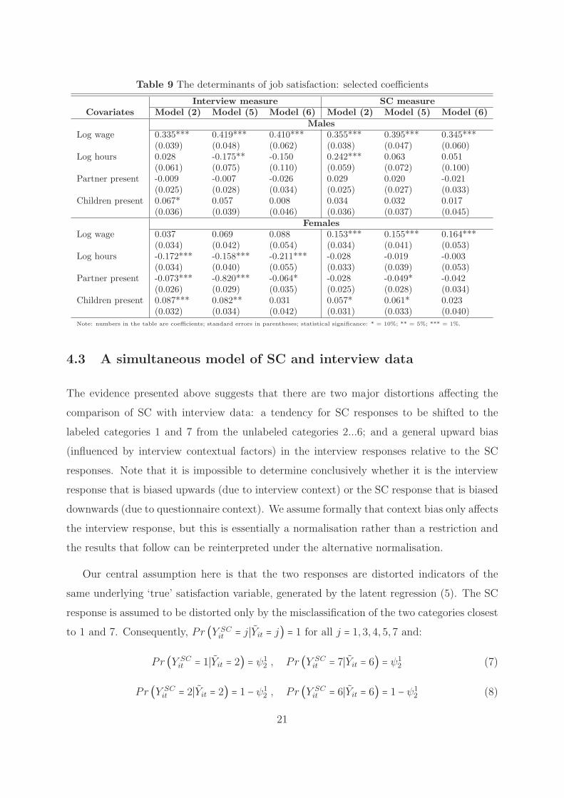
Table 9 The determinants of job satisfaction: selected coefficients

Interview measure SC measureCovariates Model (2) Model (5) Model (6) Model (2) Model (5) Model (6)

MalesLog wage 0.335*** 0.419*** 0.410*** 0.355*** 0.395*** 0.345***

(0.039) (0.048) (0.062) (0.038) (0.047) (0.060)Log hours 0.028 -0.175** -0.150 0.242*** 0.063 0.051

(0.061) (0.075) (0.110) (0.059) (0.072) (0.100)Partner present -0.009 -0.007 -0.026 0.029 0.020 -0.021

(0.025) (0.028) (0.034) (0.025) (0.027) (0.033)Children present 0.067* 0.057 0.008 0.034 0.032 0.017

(0.036) (0.039) (0.046) (0.036) (0.037) (0.045)Females

Log wage 0.037 0.069 0.088 0.153*** 0.155*** 0.164***(0.034) (0.042) (0.054) (0.034) (0.041) (0.053)

Log hours -0.172*** -0.158*** -0.211*** -0.028 -0.019 -0.003(0.034) (0.040) (0.055) (0.033) (0.039) (0.053)

Partner present -0.073*** -0.820*** -0.064* -0.028 -0.049* -0.042(0.026) (0.029) (0.035) (0.025) (0.028) (0.034)

Children present 0.087*** 0.082** 0.031 0.057* 0.061* 0.023(0.032) (0.034) (0.042) (0.031) (0.033) (0.040)

Note: numbers in the table are coefficients; standard errors in parentheses; statistical significance: * = 10%; ** = 5%; *** = 1%.

4.3 A simultaneous model of SC and interview data

The evidence presented above suggests that there are two major distortions affecting the

comparison of SC with interview data: a tendency for SC responses to be shifted to the

labeled categories 1 and 7 from the unlabeled categories 2...6; and a general upward bias

(influenced by interview contextual factors) in the interview responses relative to the SC

responses. Note that it is impossible to determine conclusively whether it is the interview

response that is biased upwards (due to interview context) or the SC response that is biased

downwards (due to questionnaire context). We assume formally that context bias only affects

the interview response, but this is essentially a normalisation rather than a restriction and

the results that follow can be reinterpreted under the alternative normalisation.

Our central assumption here is that the two responses are distorted indicators of the

same underlying ‘true’ satisfaction variable, generated by the latent regression (5). The SC

response is assumed to be distorted only by the misclassification of the two categories closest

to 1 and 7. Consequently, Pr (Y SCit = j∣Yit = j) = 1 for all j = 1,3,4,5,7 and:

Pr (Y SCit = 1∣Yit = 2) = ψ1

2 , P r (Y SCit = 7∣Yit = 6) = ψ1

2 (7)

Pr (Y SCit = 2∣Yit = 2) = 1 −ψ1

2 , P r (Y SCit = 6∣Yit = 6) = 1 −ψ1

2 (8)

21

where ψj

k ∈ [0,1] are fixed parameters.10

The interview response is assumed to be distorted instead by a general downward shift

in all the classification thresholds, so that (3) is replaced by:

Y INit = j iff Y ∗it ∈ [Γj−1 − dit,Γj − dit) (9)

where

dit =witδ + ηit (10)

The vector wit contains a set of variables which appear to be related to interview distortion:

the wage and hours variables, ethnicity dummies and six variables describing the interview

context; δ is the corresponding coefficient vector and ηit is a random deviation distributed,

independently of all other variables, as N(0, σ2η). The model is estimated by maximum like-

lihood (ML), with the individual effects ui integrated out using Gauss-Hermite quadrature.

The components of the model relating to reporting error (10) and (7) are summarised in

Table 10. Selected coefficients from the latent satisfaction equation (5) are given in Table

10, together with coefficients from a latent factor model with no allowance for systematic

misreporting, equivalent to the structure (5), (7)-(10) with the restrictions δ = 0 and ψj

k = 0

for j = 1,7 and k = 2, ...6. Full coefficient estimates can be found in Appendix 3.

Table 10 confirms the strong negative influence of the presence of a partner during the

interview and (for women only) a positive influence of the presence of a child. For women,

the distortion of interview responses relative to SC responses is significantly related to wages

and hours, with high-wage, long-hours women less prone to overstatement. The transfer of

probability mass from the Y = 6 to Y = 7 category and from Y = 2 to the Y = 1 in the SC

questionnaire emerges very clearly and we estimate a large variance of σ2η ≈ 1 for the random

component of the measurement error, dit, associated with the interview-based satisfaction

report, implying that joint ML estimation effectively assigns low weight to the interview data

relative to the SC data.

10In more general specifications, allowing transfers from Y = 3,4,5 to Y = 1,2, these additional transferprobabilities were estimated to lie on the boundary at 0 or to be insigificantly different from 0.

22

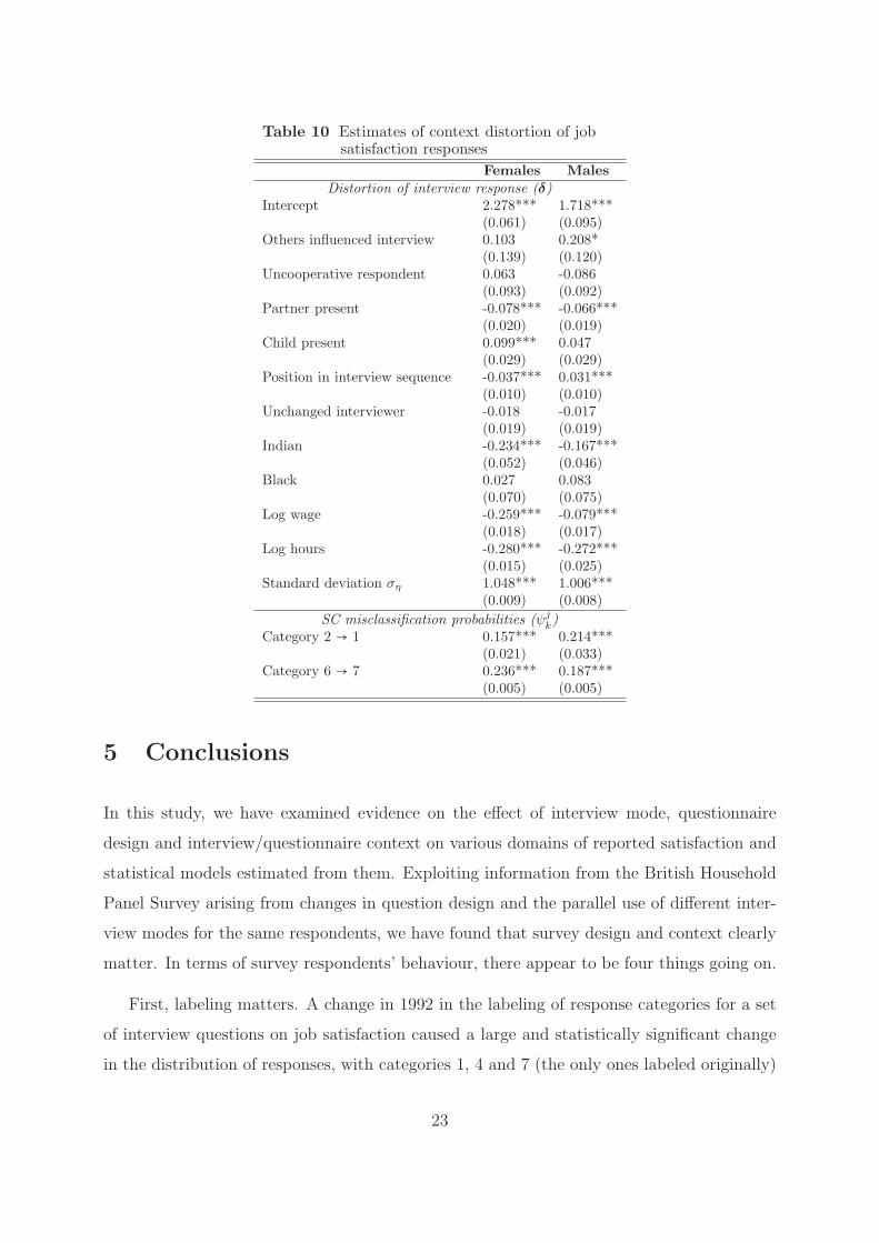
Table 10 Estimates of context distortion of jobsatisfaction responses

Females MalesDistortion of interview response (δ)

Intercept 2.278*** 1.718***(0.061) (0.095)

Others influenced interview 0.103 0.208*(0.139) (0.120)

Uncooperative respondent 0.063 -0.086(0.093) (0.092)

Partner present -0.078*** -0.066***(0.020) (0.019)

Child present 0.099*** 0.047(0.029) (0.029)

Position in interview sequence -0.037*** 0.031***(0.010) (0.010)

Unchanged interviewer -0.018 -0.017(0.019) (0.019)

Indian -0.234*** -0.167***(0.052) (0.046)

Black 0.027 0.083(0.070) (0.075)

Log wage -0.259*** -0.079***(0.018) (0.017)

Log hours -0.280*** -0.272***(0.015) (0.025)

Standard deviation ση 1.048*** 1.006***(0.009) (0.008)

SC misclassification probabilities (ψjk)

Category 2 → 1 0.157*** 0.214***(0.021) (0.033)

Category 6 → 7 0.236*** 0.187***(0.005) (0.005)

5 Conclusions

In this study, we have examined evidence on the effect of interview mode, questionnaire

design and interview/questionnaire context on various domains of reported satisfaction and

statistical models estimated from them. Exploiting information from the British Household

Panel Survey arising from changes in question design and the parallel use of different inter-

view modes for the same respondents, we have found that survey design and context clearly

matter. In terms of survey respondents’ behaviour, there appear to be four things going on.

First, labeling matters. A change in 1992 in the labeling of response categories for a set

of interview questions on job satisfaction caused a large and statistically significant change

in the distribution of responses, with categories 1, 4 and 7 (the only ones labeled originally)

23

becoming much less prominent in responses from 1992 onwards, when all response categories

were given textual labels. The distortion in 1991 relative to later years was especially strong

for women and could clearly be attributed to the change in question design, despite the

absence of an experimental comparison. The large distributional impact of this change in

questionnaire design also has a substantial impact on the nature of standard cross-section

ordinal models of job satisfaction.

Second, there appears to be a general “put on a good show” effect, causing a large bias

towards positive responses in open oral interviews, relative to more private interview modes

like the BHPS self-completion paper questionnaire. This bias is not uniform across individual

types. In particular, it appears to be less strong for high-wage women and this produces

a downward bias in interview-based estimates of the impact of the wage on women’s job

satisfaction. It thus provides an explanation for the common research finding that women

appear to care less than men about their level of pay.

Third, there is a “not in front of the children” effect, causing a further upward bias in

oral interview responses when children happen to be in the room during interview. This

effect is particularly strong for women.

Fourth, there is some evidence of a “don’t let your partner know how satisfied you are”

effect. The presence of a partner during the oral interview tends to depress the level of

response and this could be interpreted in terms of within-couple bargaining behaviour. Mar-

ital partners engage in bargaining over many aspects of individual and family life and they

may consequently have an incentive to overstate their personal sacrifice and understate their

achieved satisfaction, in order to maintain a strong bargaining position.

There are further important methodological conclusions to be drawn. Comparisons be-

tween surveys with different question designs and survey modes are clearly dangerous, so

international comparative work is unwise unless harmonised data sources can be used. For

future survey design work, it seems important to insulate questions on satisfaction as far as

possible from the micro-social influences that exist within the household and others intro-

duced from outside by the interviewer. This is particularly important if comparisons are to

be made between men and women. The most effective way of achieving this insulation is to

use survey instruments, such as self-completion paper questionnaires or computer-assisted

24

self interviewing (CASI), which avoid the public declaration of attitudes inherent in an oral

interview. It is also important that these instruments are carefully designed and use full

textual labeling of response categories. Until better designs do become available, it is im-

portant that researchers using satisfaction data are aware of design and context effects and

make some allowance for them when interpreting the results from statistical modelling.

References

[1] Akerlof, G.A., A.K. Rose and J.L. Yellen (1988), “Job switching and job satisfaction in

the US labor market”, Brookings Papers on Economic Activity, 2, 495-594.

[2] Aquilino, W. S. (1997), “Privacy effects on self-reported drug use: interactions with

survey mode and respondent characteristics”, in L. Harrison and A. Hughes (eds.) The

Validity of Self-Reported Drug Use: Improving the Accuracy of Survey Estimates, 383-

415, Rockville: National Institute on Drug Abuse, NIDA Research Monograph 167.

[3] Banks, R. and H. Laurie (2000), “From PAPI to CAPI: The case of the British Household

Panel Survey”, Social Science Computer Review, 18(4), 397-406.

[4] Benz, M. (2005), “Not for the profit, but for the satisfaction? - evidence on worker

well-being in non-profit firms”, Kyklos, 58(2), 155-176.

[5] Booth, A.L. and J.C. van Ours (2008), “Job satisfaction and family happiness: the part-

time work puzzle”, Economic Journal, 118, F77-F99.

[6] Chamberlain, G. (1984), “Panel data”, in Z. Griliches and M.D. Intriligator (eds.), Hand-

book of Econometrics, vol.2, Amsterdam: North Holland.

[7] Clark, A. and A. Oswald (1996), “Satisfaction and comparison income”, Journal of Public

Economics, 65, 359-381.

[8] Clark, A. (1997), “Job satisfaction and gender: Why are women so happy at work?”,

Labour Economics, 4, 341-372.

[9] Clark, A. and A. Oswald (2002), “Well-being in panels”, University of Warwick, mimeo.

25

[10] Das, M. and A. van Soest (1999), “A panel data model for subjective information on

household income growth”, Journal of Economic Behavior and Organization, 40, 409-426.

[11] Ferrer-i-Carbonel, A. and Frijters, P. (2004), “The effect of methodology on the deter-

minants of happiness”, Economic Journal, 114, 641-659.

[12] Freeman, R. (1978), “Job satisfaction as an economic variable”, American Economic

Review, 68, 135-142.

[13] Ghinetti, P. (2007), “The public-private job satisfaction differential in Italy”, Labour,

21(2),361-388.

[14] Halpern, D.F. (2000), Sex differences in cognitive abilities (3rd ed.), Mahwah, NJ: Erl-

baum.

[15] Hamermesh, D. (2001), “The changing distribution of job satisfaction”, Journal of Hu-

man Resources, 36, 1-30.

[16] Idson, T.L. (1990), “Establishment size, job satisfaction and the structure of work”,

Applied Economics, 22, 1007-1018.

[17] Johnson, S. M., P.C. Smith and S.M. Tucker (1982), “Response format of the Job

Descriptive Index: assessment of reliability and validity by the multitrait-multimethod

matrix”, Journal of Applied Psychology, 67, 500-505.

[18] Kaiser, L.C. (2002), “Job Satisfaction: A Comparison of Standard, NonStandard, and

Self-Employment Patterns across Europe with a Special Note to the Gender/Job Satis-

faction Paradox”, EPAG Working Paper no.27, Colchester: University of Essex.

[19] Kristensen, N. and N. Westergaard-Nielsen (2007), “Reliability of job satisfaction mea-

sures”, Journal of Happiness Studies, 8, 273-292.

[20] Krueger, A.B. and D.A. Schkade (2008), “The reliability of subjective well-being mea-

sures”, Journal of Public Economics, 92(8-9), 18331845.

[21] Kullback, S. and R.A. Leibler (1951), “On information and sufficiency”, Annals of

Mathematical Statistics, 22, 79-86.

26

[22] Levy-Garboua, L. and Montmarquette, C. (2004), “Reported job satisfaction: what

does it mean?”, Journal of Socio-Economics, 33, 135-151.

[23] Nicoletti, C. (2006), “Differences in Job Dissatisfaction across Europe”, ISER Working

Paper no.42, Colchester: University of Essex.

[24] Preston, C. C. and A.M. Colman (2000), “Optimal number of response categories in

rating scales: reliability, validity, discriminating power and respondent preferences”, Acta

Psychologica, 104(1), 1-15.

[25] Rose, M.J. (2005), “Job Satisfaction in Britain: Coping with Complexity”, British

Journal of Industrial Relations, 43(3), 455-467.

[26] Shields, M. and Wheatley-Price (2002), “Racial Harassment, Job Satisfaction and In-

tentions to Quit: Evidence from the British Nursing Profession”, Economica, 69, 295-26.

[27] Smith, T.W. (1979), “Happiness: Time Trends, Seasonal Variations, Intersurvey Differ-

ences, and Other Mysteries”, Social Psychology Quarterly, 42(1), 18-30.

[28] Souza-Puza, A. and Sousa-Pouza, A. A. (2000), “Well-being at work: a cross-national

analysis of the levels and determinants of job satisfaction”, Journal of Socio-Economics,

29(6), 517-538.

[29] Taylor, M. P. (2006), “Tell Me Why I Don’t Like Mondays: investigating calendar

effects on job satisfaction and well-being”, Journal of the Royal Statistical Society Series

A (Statistics in Society), 169, 127-142.

[30] Tourangeau, R. (1999), “Context effects on answers to attitude questions”, in M.G.

Sirken, D.J. Herrmann, S. Schechter, N. Schwarz, J.M. Tanur and R. Tourangeau (eds.),

Cognition and Survey Research, 111-131, New York: Wiley.

[31] Tourangeau, R., K.A. Rasinski and N. Bradburn (1991), “Measuring happiness in sur-

veys: a test of the subtraction hypothesis”, Public Opinion Quarterly, 55, 255-266.

[32] Tourangeau, R. and Smith, T. W. (1996). “Asking sensitive questions: the impact of

data collection mode, question format and question context”, Public Opinion Quarterly,

60, 275-304.

27

[33] Weng, L.-J. (2004), “Impact of the number of response categories and anchor labels on

coefficient alpha and test-retest reliability”, Educational and Psychological Measurement,

64, 956-972.

[34] Winkelmann, L. and R. Winkelmann (1998), “Why are the unemployed so unhappy?

Evidence from panel data”, Economica, 65, 1-15.

[35] Wooldridge, J.M. (2005), “Simple solutions to the initial conditions problem in dy-

namic, nonlinear panel data models with unobserved heterogeneity”, Journal of Applied

Econometrics, 20, 39-54.

[36] Wunder, C. and Schwarze, J. (2006), “Income inequality and job satisfaction of full-time

employees in Germany”, IZA Discussion Paper, no. 2084.

28

Appendix 1A: Survey design in practice

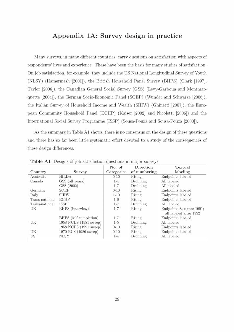
Many surveys, in many different countries, carry questions on satisfaction with aspects of

respondents’ lives and experience. These have been the basis for many studies of satisfaction.

On job satisfaction, for example, they include the US National Longitudinal Survey of Youth

(NLSY) (Hamermesh [2001]), the British Household Panel Survey (BHPS) (Clark [1997],

Taylor [2006]), the Canadian General Social Survey (GSS) (Levy-Garboua and Montmar-

quette [2004]), the German Socio-Economic Panel (SOEP) (Wunder and Schwarze [2006]),

the Italian Survey of Household Income and Wealth (SHIW) (Ghinetti [2007]), the Euro-

pean Community Household Panel (ECHP) (Kaiser [2002] and Nicoletti [2006]) and the

International Social Survey Programme (ISSP) (Sousa-Pouza and Sousa-Pouza [2000]).

As the summary in Table A1 shows, there is no consensus on the design of these questions

and there has so far been little systematic effort devoted to a study of the consequences of

these design differences.

Table A1 Designs of job satisfaction questions in major surveysNo. of Direction Textual

Country Survey Categories of numbering labelingAustralia HILDA 0-10 Rising Endpoints labeledCanada GSS (all years) 1-4 Declining All labeled

GSS (2002) 1-7 Declining All labeledGermany SOEP 0-10 Rising Endpoints labeledItaly SHIW 1-10 Rising Endpoints labeledTrans-national ECHP 1-6 Rising Endpoints labeledTrans-national ISSP 1-7 Declining All labeledUK BHPS (interview) 1-7 Rising Endpoints & centre 1991;

all labeled after 1992BHPS (self-completion) 1-7 Rising Endpoints labeled

UK 1958 NCDS (1981 sweep) 1-5 Declining All labeled1958 NCDS (1991 sweep) 0-10 Rising Endpoints labeled

UK 1970 BCS (1986 sweep) 0-10 Rising Endpoints labeledUS NLSY 1-4 Declining All labeled

29

Appendix 1B: The BHPS survey questions

The BHPS Job satisfaction interview questions for 1991-2007 are:

I’m going to read out a list of various aspects of jobs, and after each one I’d

like you to tell me from this card which number best describes how satisfied or

dissatisfied you are with that particular aspect of your own present job.

Listed aspects are: promotion prospects, total pay including overtime or bonuses, relations

with supervisor or manager, job security, ability to use own initiative, the work itself and

hours of work. These questions are followed by an assessment of overall job satisfaction:

All things considered, how satisfied or dissatisfied are you with your present job

overall using the same 1 - 7 scale?

The BHPS self-completion satisfaction questions for waves 1997-1999 and 2001-2007 are:

Here are some questions about how you feel about your life. Please tick the

number which you feel best describes how dissatisfied or satisfied you are with the

following aspects of your current situation [...]: your health; the income of your

household; your house/flat; your husband/wife/partner; your job; your social life;

the amount of leisure time you have; the way you spend your leisure time.

These are followed by two overall assessments of life satisfaction:

Using the same scale how dissatisfied or satisfied are you with your life overall?

Would you say that you are more satisfied with life, less satisfied or feel about the

same as you did a year ago?’

30

Appendix 2: response distributions

Figure A1 Satisfaction with promotion prospects BHPS 1991 & 1992

Figure A2 Satisfaction with pay BHPS 1991 & 1992

31

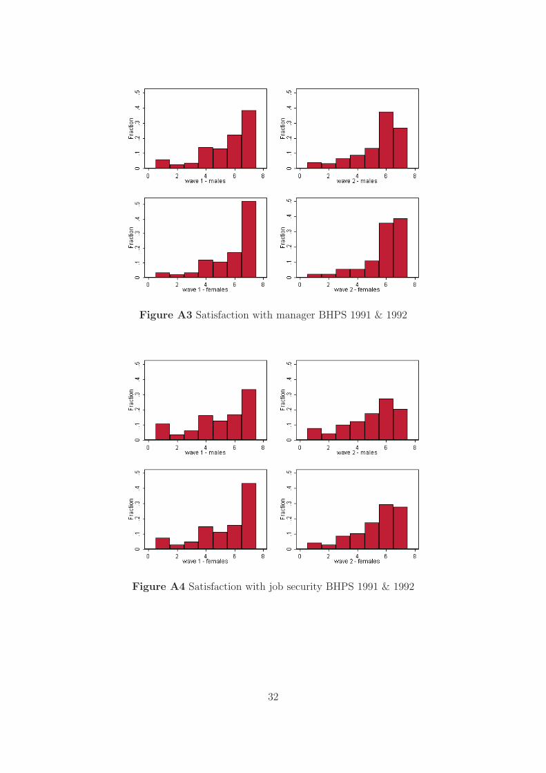
Figure A3 Satisfaction with manager BHPS 1991 & 1992

Figure A4 Satisfaction with job security BHPS 1991 & 1992

32

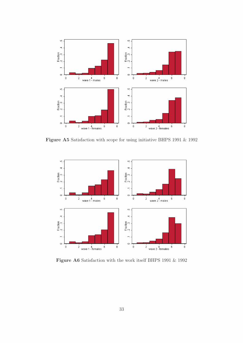
Figure A5 Satisfaction with scope for using initiative BHPS 1991 & 1992

Figure A6 Satisfaction with the work itself BHPS 1991 & 1992

33

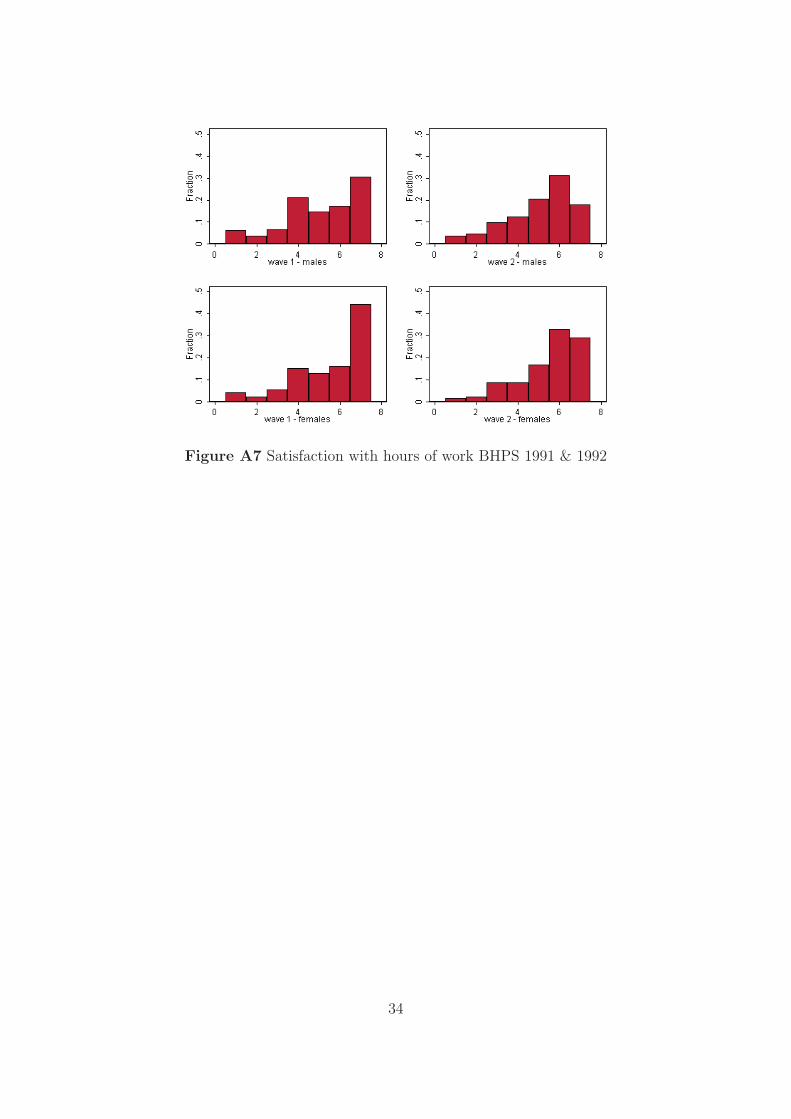
Figure A7 Satisfaction with hours of work BHPS 1991 & 1992

34

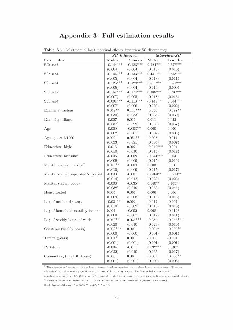
Appendix 3: Full estimation results

Table A3.1 Multinomial logit marginal effects: interview-SC discrepancy

SC>interview interview>SCCovariates Males Females Males FemalesSC: sat2 -0.144*** -0.126*** 0.524*** 0.557***

(0.004) (0.004) (0.015) (0.010)SC: sat3 -0.144*** -0.133*** 0.441*** 0.553***

(0.005) (0.004) (0.018) (0.011)SC: sat4 -0.125*** -0.128*** 0.511*** 0.651***

(0.005) (0.004) (0.016) (0.009)SC: sat5 -0.167*** -0.174*** 0.388*** 0.596***

(0.007) (0.005) (0.018) (0.013)SC: sat6 -0.091*** -0.118*** -0.148*** 0.064***

(0.007) (0.006) (0.020) (0.022)Ethnicity: Indian 0.068** 0.110*** -0.050 -0.078**

(0.030) (0.033) (0.033) (0.039)Ethnicity: Black -0.007 0.016 0.011 0.032

(0.037) (0.029) (0.055) (0.057)Age -0.000 -0.003** 0.000 0.000

(0.002) (0.001) (0.002) (0.003)Age squared/1000 0.002 0.051** -0.008 -0.014

(0.023) (0.021) (0.035) (0.037)Education: high1 -0.015 0.007 -0.040*** -0.004

(0.010) (0.010) (0.015) (0.017)Education: medium1 -0.006 -0.008 -0.044*** 0.004

(0.009) (0.009) (0.015) (0.016)Marital status: married2 0.020** -0.008 0.003 0.010

(0.010) (0.009) (0.015) (0.017)Marital status: separated/divorced -0.000 -0.001 0.0469** 0.0514**

(0.014) (0.012) (0.022) (0.022)Marital status: widow -0.006 -0.035* 0.140** 0.105**

(0.038) (0.019) (0.068) (0.045)House rented 0.005 0.006 0.006 0.006

(0.009) (0.008) (0.013) (0.013)Log of net hourly wage -0.024** 0.002 -0.019 -0.062

(0.010) (0.009) (0.016) (0.016)Log of household monthly income 0.001 -0.002 0.008 -0.019*

(0.009) (0.007) (0.012) (0.011)Log of weekly hours of work 0.050** 0.033*** -0.030 -0.056***

(0.020) (0.010) (0.026) (0.016)Overtime (weekly hours) 0.002*** 0.000 -0.001* -0.002**

(0.000) (0.000) (0.001) (0.001)Tenure (years) 0.001* 0.000 -0.000 -0.001

(0.001) (0.001) (0.001) (0.001)Part-time -0.004 -0.011 0.092*** 0.030*

(0.022) (0.010) (0.035) (0.017)Commuting time/10 (hours) 0.000 0.002 -0.001 -0.006**

(0.001) (0.001) (0.002) (0.003)1“High education” includes: first or higher degree, teaching qualification or other higher qualification. “Medium

education” includes: nursing qualification, A-level, O-level or equivalent. Baseline includes: commercial

qualifications (no O-levels), CSE grade 2-5 (Scottish grade 4-5), apprenticeship, other qualifications, no qualifications.

2 Baseline category is “never married”. Standard errors (in parentheses) are adjusted for clustering.

Statistical significance: * = 10%; ** = 5%; *** = 1%

35

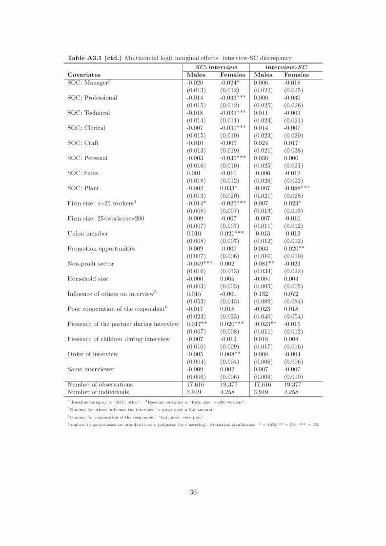
Table A3.1 (ctd.) Multinomial logit marginal effects: interview-SC discrepancy

SC>interview interview>SCCovariates Males Females Males FemalesSOC: Manager3 -0.020 -0.024* 0.006 -0.018

(0.013) (0.012) (0.022) (0.025)SOC: Professional -0.014 -0.033*** 0.000 -0.030

(0.015) (0.012) (0.025) (0.026)SOC: Technical -0.018 -0.033*** 0.011 -0.003

(0.014) (0.011) (0.024) (0.024)SOC: Clerical -0.007 -0.039*** 0.014 -0.007

(0.015) (0.010) (0.023) (0.020)SOC: Craft -0.010 -0.005 0.024 0.017

(0.013) (0.019) (0.021) (0.038)SOC: Personal -0.003 -0.036*** 0.036 0.000

(0.016) (0.010) (0.025) (0.021)SOC: Sales 0.001 -0.010 -0.006 -0.012

(0.018) (0.012) (0.026) (0.022)SOC: Plant -0.002 0.034* -0.007 -0.088***

(0.013) (0.020) (0.021) (0.028)Firm size: <=25 workers4 -0.014* -0.025*** 0.007 0.023*

(0.008) (0.007) (0.013) (0.013)Firm size: 25<workers<=200 -0.009 -0.007 -0.007 -0.010

(0.007) (0.007) (0.011) (0.012)Union member 0.010 0.021*** -0.013 -0.012

(0.008) (0.007) (0.012) (0.012)Promotion opportunities -0.009 -0.009 0.003 0.020**

(0.007) (0.006) (0.010) (0.010)Non-profit sector -0.049*** 0.002 0.081** -0.023

(0.016) (0.013) (0.034) (0.022)Household size -0.000 0.005 -0.004 0.004

(0.003) (0.003) (0.005) (0.005)Influence of others on interview5 0.015 -0.001 0.132 0.072

(0.053) (0.043) (0.089) (0.084)Poor cooperation of the respondent6 -0.017 0.018 -0.023 0.018

(0.023) (0.033) (0.040) (0.054)Presence of the partner during interview 0.017** 0.020*** -0.023** -0.015

(0.007) (0.008) (0.011) (0.012)Presence of children during interview -0.007 -0.012 0.018 0.004

(0.010) (0.009) (0.017) (0.016)Order of interview -0.005 0.008** 0.008 -0.004

(0.004) (0.004) (0.006) (0.006)Same interviewer -0.009 0.002 0.007 -0.007

(0.006) (0.006) (0.009) (0.010)Number of observations 17,616 19,377 17,616 19,377Number of individuals 3,949 4,258 3,949 4,2583 Baseline category is “SOC: other”. 4Baseline category is “Firm size: >=200 workers”.

5Dummy for others influence the interview “a great deal, a fair amount”.

6Dummy for cooperation of the respondent: “fair, poor, very poor”.

Numbers in parentheses are standard errors (adjusted for clustering). Statistical significance: * = 10%; ** = 5%; *** = 1%

36

Table A3.1 (ctd.) Multinomial logit marginal effects: interview-SC discrepancy

SC>interview interview>SCCovariates Males Females Males FemalesOuter London7 -0.004 0.016 -0.058* -0.010

(0.024) (0.020) (0.030) (0.037)South East -0.019 -0.004 -0.029 -0.006

(0.021) (0.016) (0.029) (0.033)South West -0.009 0.016 -0.047 -0.018

(0.023) (0.019) (0.031) (0.035)East Anglia -0.017 -0.005 -0.046 0.017

(0.024) (0.021) (0.036) (0.041)East Midlands -0.021 -0.010 -0.032 0.006

(0.021) (0.018) (0.032) (0.038)West Midlands Conurbation 0.003 0.007 -0.001 0.011

(0.028) (0.024) (0.041) (0.045)West Midlands -0.025 -0.027* -0.041 0.032

(0.022) (0.016) (0.034) (0.038)Greater Manchester 0.003 -0.000 -0.081** -0.040

(0.027) (0.020) (0.034) (0.039)Merseyside -0.022 -0.044** -0.071* -0.009

(0.027) (0.019) (0.041) (0.045)North West -0.004 0.032 -0.087*** -0.027

(0.025) (0.024) (0.032) (0.038)South Yorkshire -0.023 -0.007 -0.011 -0.028

(0.024) (0.022) (0.043) (0.044)West Yorkshire -0.048** -0.002 -0.035 0.037

(0.021) (0.022) (0.039) (0.045)Yorkshire & Humberside -0.023 -0.005 -0.018 0.013

(0.024) (0.023) (0.038) (0.042)Tyne & Wear 0.006 0.055* -0.065 -0.028

(0.032) (0.033) (0.044) (0.052)North -0.010 -0.012 -0.100*** 0.018

(0.025) (0.019) (0.033) (0.042)Wales -0.029 -0.004 -0.032 0.028

(0.023) (0.020) (0.036) (0.039)Scotland -0.007 0.014 -0.078*** -0.040

(0.023) (0.019) (0.030) (0.034)Wave 6 -0.032*** -0.032*** -0.000 -0.012

(0.011) (0.009) (0.018) (0.019)Wave 7 -0.021* -.0366*** -0.018 -0.005

(0.011) (0.009) (0.017) (0.018)Wave 8 0.027** -0.006 -0.069*** -0.068***

(0.013) (0.010) (0.017) (0.017)Wave 9 0.017 0.018* -0.021 -0.049***

(0.013) (0.011) (0.017) (0.017)Wave 10 0.003 -0.011 -0.023 -0.038**

(0.012) (0.010) (0.016) (0.017)Wave 12 -0.006 -0.006 -0.018 -0.007

(0.011) (0.010) (0.016) (0.018)Wave 13 0.037*** 0.006 -0.043*** -0.029

(0.013) (0.011) (0.016) (0.017)Wave 14 0.011 -0.013 -0.004 0.028

(0.012) (0.010) (0.017) (0.018)7 Baseline category is Inner London.

Numbers in parentheses are standard errors (adjusted for clustering). Statistical significance: * = 10%; ** = 5%; *** = 1%

37

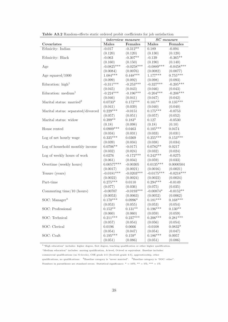
Table A3.2 Random-effects static ordered probit coefficients for job satisfaction

interview measure SC measureCovariates Males Females Males FemalesEthnicity: Indian -0.017 -0.312** 0.189 -0.094

(0.120) (0.120) (0.130) (0.120)Ethnicity: Black -0.063 -0.307** -0.139 -0.365**

(0.160) (0.150) (0.190) (0.140)Age -0.0825*** -0.0258*** -0.0889*** -0.0458***

(0.0084) (0.0076) (0.0082) (0.0077)Age squared/1000 1.084*** 0.448*** 1.177*** 0.755***

(0.099) (0.092) (0.098) (0.093)Education: high1 -0.311*** -0.253*** -0.327*** -0.205***

(0.045) (0.043) (0.046) (0.043)Education: medium1 -0.224*** -0.196*** -0.204*** -0.208***

(0.046) (0.041) (0.047) (0.042)Marital status: married2 0.0733* 0.172*** 0.101** 0.135***

(0.041) (0.039) (0.040) (0.040)Marital status: separated/divorced 0.229*** -0.0151 0.175*** -0.0753

(0.057) (0.051) (0.057) (0.052)Marital status: widow 0.399** 0.183* 0.127 -0.0530

(0.18) (0.098) (0.18) (0.10)House rented 0.0909*** 0.0463 0.105*** 0.0474

(0.034) (0.031) (0.033) (0.031)Log of net hourly wage 0.335*** 0.0369 0.355*** 0.153***

(0.039) (0.034) (0.038) (0.034)Log of household monthly income 0.0706** -0.0171 0.0782** 0.0217

(0.032) (0.024) (0.032) (0.024)Log of weekly hours of work 0.0276 -0.172*** 0.242*** -0.0275

(0.061) (0.034) (0.059) (0.033)Overtime (weekly hours) 0.00577*** -0.00305 0.0135*** 0.0000504

(0.0017) (0.0021) (0.0016) (0.0021)Tenure (years) -0.0181*** -0.0203*** -0.0175*** -0.0218***

(0.0022) (0.0024) (0.0022) (0.0024)Part-time 0.275*** 0.0110 0.294*** -0.0149

(0.077) (0.036) (0.075) (0.035)Commuting time/10 (hours) -0.00707 -0.0193*** -0.00874* -0.0152**

(0.0053) (0.0063) (0.0052) (0.0062)SOC: Manager3 0.170*** 0.0996* 0.181*** 0.168***

(0.053) (0.055) (0.053) (0.054)SOC: Professional 0.152** 0.131** 0.196*** 0.130**

(0.060) (0.060) (0.059) (0.059)SOC: Technical 0.211*** 0.237*** 0.206*** 0.281***

(0.057) (0.054) (0.056) (0.054)SOC: Clerical 0.0196 0.0666 -0.0108 0.0832*

(0.054) (0.047) (0.054) (0.047)SOC: Craft 0.195*** 0.159* 0.186*** 0.0957

(0.051) (0.086) (0.051) (0.086)1“High education” includes: higher degree, first degree, teaching qualification or other higher qualification.

“Medium education” includes: nursing qualification, A-level, O-level or equivalent. Baseline includes:

commercial qualifications (no O-levels), CSE grade 2-5 (Scottish grade 4-5), apprenticeship, other

qualifications, no qualifications. 2Baseline category is “never married”. 3Baseline category is “SOC: other”.

Numbers in parentheses are standard errors. Statistical significance: * = 10%; ** = 5%; *** = 1%

38

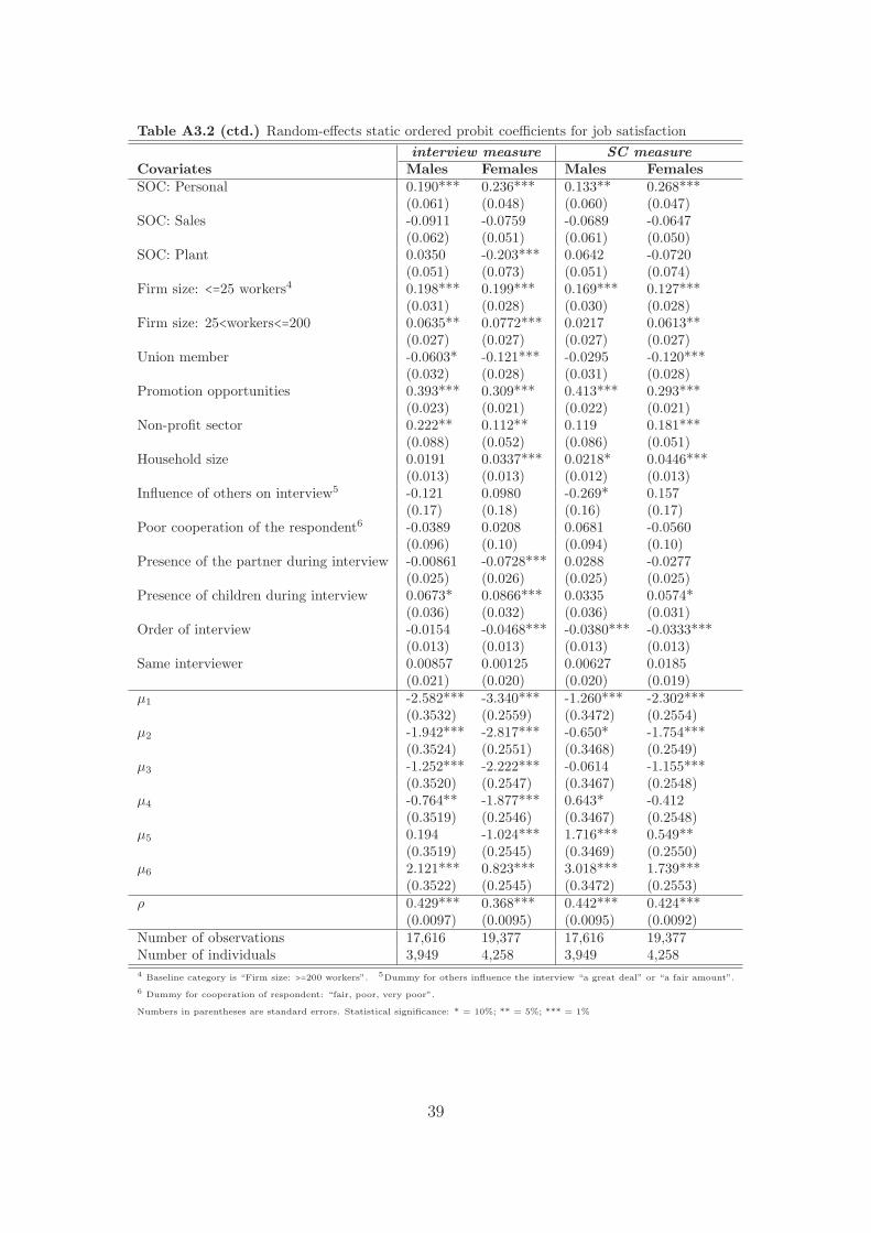
Table A3.2 (ctd.) Random-effects static ordered probit coefficients for job satisfaction

interview measure SC measureCovariates Males Females Males FemalesSOC: Personal 0.190*** 0.236*** 0.133** 0.268***

(0.061) (0.048) (0.060) (0.047)SOC: Sales -0.0911 -0.0759 -0.0689 -0.0647

(0.062) (0.051) (0.061) (0.050)SOC: Plant 0.0350 -0.203*** 0.0642 -0.0720

(0.051) (0.073) (0.051) (0.074)Firm size: <=25 workers4 0.198*** 0.199*** 0.169*** 0.127***

(0.031) (0.028) (0.030) (0.028)Firm size: 25<workers<=200 0.0635** 0.0772*** 0.0217 0.0613**

(0.027) (0.027) (0.027) (0.027)Union member -0.0603* -0.121*** -0.0295 -0.120***

(0.032) (0.028) (0.031) (0.028)Promotion opportunities 0.393*** 0.309*** 0.413*** 0.293***

(0.023) (0.021) (0.022) (0.021)Non-profit sector 0.222** 0.112** 0.119 0.181***

(0.088) (0.052) (0.086) (0.051)Household size 0.0191 0.0337*** 0.0218* 0.0446***

(0.013) (0.013) (0.012) (0.013)Influence of others on interview5 -0.121 0.0980 -0.269* 0.157

(0.17) (0.18) (0.16) (0.17)Poor cooperation of the respondent6 -0.0389 0.0208 0.0681 -0.0560

(0.096) (0.10) (0.094) (0.10)Presence of the partner during interview -0.00861 -0.0728*** 0.0288 -0.0277

(0.025) (0.026) (0.025) (0.025)Presence of children during interview 0.0673* 0.0866*** 0.0335 0.0574*

(0.036) (0.032) (0.036) (0.031)Order of interview -0.0154 -0.0468*** -0.0380*** -0.0333***

(0.013) (0.013) (0.013) (0.013)Same interviewer 0.00857 0.00125 0.00627 0.0185

(0.021) (0.020) (0.020) (0.019)µ1 -2.582*** -3.340*** -1.260*** -2.302***

(0.3532) (0.2559) (0.3472) (0.2554)µ2 -1.942*** -2.817*** -0.650* -1.754***

(0.3524) (0.2551) (0.3468) (0.2549)µ3 -1.252*** -2.222*** -0.0614 -1.155***

(0.3520) (0.2547) (0.3467) (0.2548)µ4 -0.764** -1.877*** 0.643* -0.412

(0.3519) (0.2546) (0.3467) (0.2548)µ5 0.194 -1.024*** 1.716*** 0.549**

(0.3519) (0.2545) (0.3469) (0.2550)µ6 2.121*** 0.823*** 3.018*** 1.739***

(0.3522) (0.2545) (0.3472) (0.2553)ρ 0.429*** 0.368*** 0.442*** 0.424***

(0.0097) (0.0095) (0.0095) (0.0092)Number of observations 17,616 19,377 17,616 19,377Number of individuals 3,949 4,258 3,949 4,2584 Baseline category is “Firm size: >=200 workers”. 5Dummy for others influence the interview “a great deal” or “a fair amount”.

6 Dummy for cooperation of respondent: “fair, poor, very poor”.

Numbers in parentheses are standard errors. Statistical significance: * = 10%; ** = 5%; *** = 1%

39

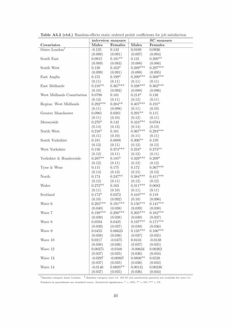
Table A3.2 (ctd.) Random-effects static ordered probit coefficients for job satisfaction

interview measure SC measureCovariates Males Females Males FemalesOuter London7 -0.135 0.142 0.0169 0.0936

(0.098) (0.091) (0.097) (0.094)South East 0.0915 0.181** 0.131 0.200**

(0.089) (0.083) (0.088) (0.086)South West 0.130 0.163* 0.289*** 0.297***

(0.099) (0.091) (0.098) (0.095)East Anglia 0.155 0.199* 0.299*** 0.308***

(0.11) (0.11) (0.11) (0.11)East Midlands 0.216** 0.367*** 0.338*** 0.362***

(0.10) (0.092) (0.098) (0.096)West Midlands Conurbation 0.0798 0.101 0.214* 0.138

(0.13) (0.11) (0.12) (0.11)Region: West Midlands 0.292*** 0.204** 0.407*** 0.191*

(0.11) (0.098) (0.11) (0.10)Greater Manchester 0.0961 0.0261 0.291** 0.115

(0.11) (0.10) (0.12) (0.11)Merseyside 0.270* 0.142 0.424*** 0.0784

(0.14) (0.13) (0.14) (0.13)North West 0.216* 0.161 0.367*** 0.294***

(0.11) (0.10) (0.11) (0.11)South Yorkshire 0.181 0.0888 0.306** 0.159

(0.13) (0.11) (0.12) (0.12)West Yorkshire 0.156 0.374*** 0.234* 0.273**

(0.12) (0.11) (0.12) (0.11)Yorkshire & Humberside 0.287** 0.185* 0.329*** 0.209*

(0.12) (0.11) (0.12) (0.12)Tyne & Wear 0.115 0.175 0.172 0.367***

(0.14) (0.13) (0.15) (0.13)North 0.174 0.247** 0.384*** 0.411***

(0.12) (0.11) (0.12) (0.12)Wales 0.272** 0.163 0.311*** 0.0682

(0.11) (0.10) (0.11) (0.11)Scotland 0.172* 0.0372 0.410*** 0.119

(0.10) (0.092) (0.10) (0.096)Wave 6 0.205*** 0.191*** 0.156*** 0.141***

(0.040) (0.038) (0.039) (0.038)Wave 7 0.198*** 0.200*** 0.205*** 0.162***

(0.039) (0.038) (0.038) (0.037)Wave 8 0.0594 0.0435 0.197*** 0.171***

(0.039) (0.037) (0.038) (0.036)Wave 9 0.0455 0.00623 0.135*** 0.106***

(0.038) (0.036) (0.037) (0.035)Wave 10 0.0217 -0.0475 0.0416 -0.0138

(0.038) (0.036) (0.037) (0.035)Wave 12 0.00371 -0.0168 -0.00634 0.00262

(0.037) (0.035) (0.036) (0.034)Wave 13 -0.0297 -0.00807 0.0806** 0.0528

(0.037) (0.035) (0.036) (0.034)Wave 14 -0.0146 0.0695** 0.00131 0.00236

(0.037) (0.035) (0.036) (0.034)7Baseline category Inner London. 8 Baseline category wave 15. NB SC job satisfaction question not available for wave 11.

Numbers in parentheses are standard errors. Statistical significance: * = 10%; ** = 5%; *** = 1%

40

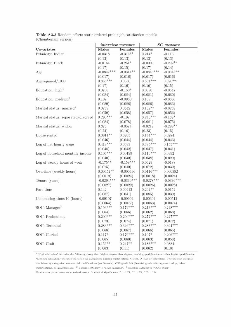
Table A3.3 Random-effects static ordered probit job satisfaction models(Chamberlain version)

interview measure SC measureCovariates Males Females Males FemalesEthnicity: Indian -0.0318 -0.315** 0.214* -0.113

(0.13) (0.13) (0.13) (0.13)Ethnicity: Black -0.0164 -0.251* -0.0909 -0.292**

(0.17) (0.15) (0.17) (0.14)Age -0.0847*** -0.0314** -0.0846*** -0.0348**

(0.017) (0.016) (0.017) (0.016)Age squared/1000 0.856*** 0.0636 0.864*** 0.326**

(0.17) (0.16) (0.16) (0.15)Education: high1 0.0708 -0.150* 0.0390 -0.0547

(0.084) (0.084) (0.081) (0.080)Education: medium1 0.102 -0.0980 0.109 -0.0660

(0.089) (0.086) (0.086) (0.083)Marital status: married2 0.0739 0.0542 0.132** -0.0259

(0.059) (0.058) (0.057) (0.056)Marital status: separated/divorced 0.290*** -0.107 0.246*** -0.138*

(0.084) (0.078) (0.081) (0.075)Marital status: widow 0.373 -0.0574 -0.0218 -0.299**

(0.24) (0.16) (0.23) (0.15)House rented 0.0911** 0.0205 0.144*** 0.0284

(0.046) (0.044) (0.044) (0.043)Log of net hourly wage 0.419*** 0.0693 0.395*** 0.155***

(0.048) (0.042) (0.047) (0.041)Log of household monthly income 0.106*** 0.00199 0.116*** 0.0392

(0.040) (0.030) (0.038) (0.029)Log of weekly hours of work -0.175** -0.158*** 0.0629 -0.0188

(0.075) (0.040) (0.072) (0.039)Overtime (weekly hours) 0.00452** -0.000496 0.0116*** 0.000582

(0.0019) (0.0024) (0.0018) (0.0024)Tenure (years) -0.0294*** -0.0330*** -0.0278*** -0.0336***

(0.0027) (0.0029) (0.0026) (0.0028)Part-time 0.142 0.00413 0.202** -0.0152

(0.087) (0.041) (0.085) (0.039)Commuting time/10 (hours) -0.00107 -0.00994 -0.00304 -0.00512

(0.0064) (0.0077) (0.0063) (0.0074)SOC: Manager3 0.193*** 0.174*** 0.213*** 0.248***

(0.064) (0.066) (0.062) (0.063)SOC: Professional 0.200*** 0.290*** 0.272*** 0.227***

(0.073) (0.074) (0.071) (0.072)SOC: Technical 0.283*** 0.346*** 0.283*** 0.394***

(0.068) (0.067) (0.066) (0.065)SOC: Clerical 0.117* 0.176*** 0.107* 0.206***

(0.065) (0.060) (0.063) (0.058)SOC: Craft 0.156** 0.247** 0.183*** 0.0884

(0.063) (0.11) (0.062) (0.10)1“High education” includes the following categories: higher degree, first degree, teaching qualification or other higher qualification.

“Medium education” includes the following categories: nursing qualification, A-level, O-level or equivalent. The baseline includes

the following categories: commercial qualifications (no O-levels), CSE grade 2-5 (Scottish grade 4-5), apprenticeship, other

qualifications, no qualifications. 2 Baseline category is “never married”. 3 Baseline category is “SOC: other”.

Numbers in parentheses are standard errors. Statistical significance: * = 10%; ** = 5%; *** = 1%

41

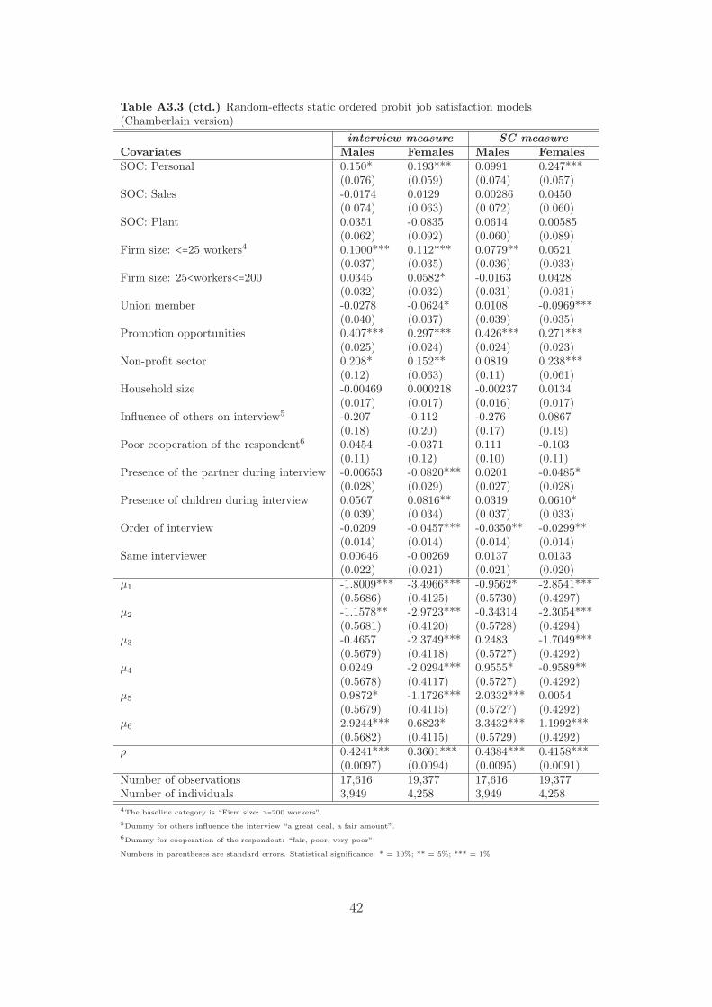
Table A3.3 (ctd.) Random-effects static ordered probit job satisfaction models(Chamberlain version)

interview measure SC measureCovariates Males Females Males FemalesSOC: Personal 0.150* 0.193*** 0.0991 0.247***

(0.076) (0.059) (0.074) (0.057)SOC: Sales -0.0174 0.0129 0.00286 0.0450

(0.074) (0.063) (0.072) (0.060)SOC: Plant 0.0351 -0.0835 0.0614 0.00585

(0.062) (0.092) (0.060) (0.089)Firm size: <=25 workers4 0.1000*** 0.112*** 0.0779** 0.0521

(0.037) (0.035) (0.036) (0.033)Firm size: 25<workers<=200 0.0345 0.0582* -0.0163 0.0428

(0.032) (0.032) (0.031) (0.031)Union member -0.0278 -0.0624* 0.0108 -0.0969***

(0.040) (0.037) (0.039) (0.035)Promotion opportunities 0.407*** 0.297*** 0.426*** 0.271***

(0.025) (0.024) (0.024) (0.023)Non-profit sector 0.208* 0.152** 0.0819 0.238***

(0.12) (0.063) (0.11) (0.061)Household size -0.00469 0.000218 -0.00237 0.0134

(0.017) (0.017) (0.016) (0.017)Influence of others on interview5 -0.207 -0.112 -0.276 0.0867

(0.18) (0.20) (0.17) (0.19)Poor cooperation of the respondent6 0.0454 -0.0371 0.111 -0.103

(0.11) (0.12) (0.10) (0.11)Presence of the partner during interview -0.00653 -0.0820*** 0.0201 -0.0485*

(0.028) (0.029) (0.027) (0.028)Presence of children during interview 0.0567 0.0816** 0.0319 0.0610*

(0.039) (0.034) (0.037) (0.033)Order of interview -0.0209 -0.0457*** -0.0350** -0.0299**

(0.014) (0.014) (0.014) (0.014)Same interviewer 0.00646 -0.00269 0.0137 0.0133

(0.022) (0.021) (0.021) (0.020)µ1 -1.8009*** -3.4966*** -0.9562* -2.8541***

(0.5686) (0.4125) (0.5730) (0.4297)µ2 -1.1578** -2.9723*** -0.34314 -2.3054***

(0.5681) (0.4120) (0.5728) (0.4294)µ3 -0.4657 -2.3749*** 0.2483 -1.7049***

(0.5679) (0.4118) (0.5727) (0.4292)µ4 0.0249 -2.0294*** 0.9555* -0.9589**

(0.5678) (0.4117) (0.5727) (0.4292)µ5 0.9872* -1.1726*** 2.0332*** 0.0054

(0.5679) (0.4115) (0.5727) (0.4292)µ6 2.9244*** 0.6823* 3.3432*** 1.1992***

(0.5682) (0.4115) (0.5729) (0.4292)ρ 0.4241*** 0.3601*** 0.4384*** 0.4158***

(0.0097) (0.0094) (0.0095) (0.0091)Number of observations 17,616 19,377 17,616 19,377Number of individuals 3,949 4,258 3,949 4,2584The baseline category is “Firm size: >=200 workers”.

5Dummy for others influence the interview “a great deal, a fair amount”.

6Dummy for cooperation of the respondent: “fair, poor, very poor”.

Numbers in parentheses are standard errors. Statistical significance: * = 10%; ** = 5%; *** = 1%

42

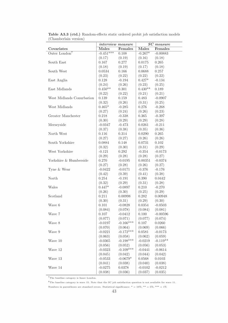
Table A3.3 (ctd.) Random-effects static ordered probit job satisfaction models(Chamberlain version)

interview measure SC measureCovariates Males Females Males FemalesOuter London7 -0.451*** 0.108 -0.267* -0.00883

(0.17) (0.19) (0.16) (0.18)South East 0.167 0.277 0.0175 0.265

(0.18) (0.19) (0.17) (0.18)South West 0.0534 0.166 0.0688 0.257

(0.23) (0.22) (0.22) (0.22)East Anglia 0.128 -0.194 0.427* -0.134

(0.24) (0.26) (0.23) (0.25)East Midlands 0.450** 0.301 0.430** 0.189

(0.22) (0.22) (0.21) (0.21)West Midlands Conurbation 0.139 0.159 0.483 -0.0907

(0.32) (0.26) (0.31) (0.25)West Midlands 0.465* -0.285 0.276 -0.268

(0.27) (0.24) (0.26) (0.23)Greater Manchester 0.218 -0.338 0.365 -0.397

(0.30) (0.29) (0.29) (0.28)Merseyside -0.0347 -0.473 0.0261 -0.211

(0.37) (0.38) (0.35) (0.36)North West 0.116 0.314 0.0290 0.265

(0.27) (0.27) (0.26) (0.26)South Yorkshire 0.0884 0.148 0.0731 0.102

(0.32) (0.30) (0.31) (0.29)West Yorkshire -0.121 0.292 -0.354 -0.0173

(0.29) (0.28) (0.28) (0.27)Yorkshire & Humberside 0.270 -0.0195 0.00351 -0.0374

(0.27) (0.28) (0.26) (0.27)Tyne & Wear -0.0422 -0.0171 -0.376 -0.176

(0.42) (0.39) (0.41) (0.38)North 0.254 -0.191 0.390 0.0442

(0.32) (0.29) (0.31) (0.28)Wales 0.447* -0.0897 0.210 -0.270

(0.26) (0.30) (0.25) (0.29)Scotland 0.211 0.00998 0.282 0.00948

(0.30) (0.31) (0.29) (0.30)Wave 6 0.101 -0.0828 0.0354 -0.0503

(0.084) (0.078) (0.084) (0.081)Wave 7 0.107 -0.0412 0.100 -0.00596

(0.077) (0.071) (0.077) (0.074)Wave 8 -0.0197 -0.166*** 0.107 0.0260

(0.070) (0.064) (0.069) (0.066)Wave 9 -0.0221 -0.172*** 0.0581 -0.0173

(0.063) (0.058) (0.062) (0.059)Wave 10 -0.0365 -0.198*** -0.0219 -0.119**

(0.056) (0.052) (0.056) (0.053)Wave 12 -0.0323 -0.109*** -0.0441 -0.0614

(0.045) (0.042) (0.044) (0.042)Wave 13 -0.0533 -0.0679* 0.0568 0.0103

(0.041) (0.038) (0.040) (0.038)Wave 14 -0.0275 0.0378 -0.0102 -0.0212

(0.038) (0.036) (0.037) (0.035)7The baseline category is Inner London.

8The baseline category is wave 15. Note that the SC job satisfaction question is not available for wave 11.

Numbers in parentheses are standard errors. Statistical significance: * = 10%; ** = 5%; *** = 1%

43

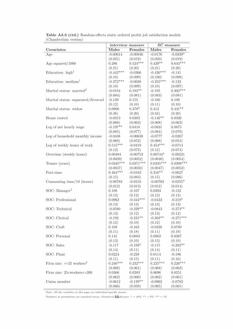
Table A3.3 (ctd.) Random-effects static ordered probit job satisfaction models(Chamberlain version)

interview measure SC measureCovariates Males Females Males FemalesAge -0.00614 -0.00846 -0.0176 -0.0339*

(0.021) (0.019) (0.020) (0.019)Age squared/1000 0.286 0.524*** 0.439** 0.643***

(0.21) (0.20) (0.21) (0.20)Education: high1 -0.442*** -0.0366 -0.430*** -0.141

(0.10) (0.099) (0.100) (0.098)Education: medium1 -0.372*** -0.0638 -0.355*** -0.133

(0.10) (0.099) (0.10) (0.097)Marital status: married2 -0.0184 0.182** -0.105 0.302***

(0.084) (0.081) (0.083) (0.081)Marital status: separated/divorced -0.139 0.155 -0.160 0.109

(0.12) (0.10) (0.11) (0.10)Marital status: widow 0.0908 0.378* 0.412 0.431**

(0.38) (0.20) (0.34) (0.20)House rented -0.0313 0.0383 -0.146** 0.0326

(0.068) (0.063) (0.068) (0.063)Log of net hourly wage -0.197** 0.0418 -0.0831 0.0875

(0.085) (0.077) (0.084) (0.079)Log of household monthly income -0.0438 -0.00638 -0.0777 -0.0267

(0.068) (0.052) (0.068) (0.054)Log of weekly hours of work 0.515*** -0.0419 0.454*** -0.0714

(0.12) (0.073) (0.12) (0.074)Overtime (weekly hours) 0.00484 -0.00753 0.00744* -0.00221

(0.0039) (0.0052) (0.0040) (0.0054)Tenure (years) 0.0345*** 0.0371*** 0.0335*** 0.0398***

(0.0047) (0.0050) (0.0047) (0.0052)Part-time 0.464*** -0.0183 0.316** -0.0627

(0.15) (0.083) (0.15) (0.086)Commuting time/10 (hours) -0.00783 -0.0210 -0.00762 -0.0255*

(0.012) (0.013) (0.012) (0.014)SOC: Manager3 0.108 -0.107 0.0393 -0.122

(0.12) (0.12) (0.12) (0.13)SOC: Professional 0.0962 -0.344*** -0.0433 -0.218*

(0.13) (0.13) (0.13) (0.13)SOC: Technical -0.0580 -0.229** -0.0843 -0.274**

(0.13) (0.12) (0.13) (0.12)SOC: Clerical -0.192 -0.231** -0.303** -0.271***

(0.12) (0.10) (0.12) (0.10)SOC: Craft 0.108 -0.163 -0.0338 0.0780

(0.11) (0.18) (0.11) (0.19)SOC: Personal 0.141 0.0883 0.0982 0.0387

(0.13) (0.10) (0.13) (0.10)SOC: Sales -0.117 -0.193* -0.115 -0.282**

(0.14) (0.11) (0.14) (0.11)SOC: Plant 0.0224 -0.228 0.0114 -0.196

(0.11) (0.15) (0.11) (0.16)Firm size: <=25 workers4 0.240*** 0.232*** 0.225*** 0.226***

(0.068) (0.061) (0.068) (0.062)Firm size: 25<workers<=200 0.0366 0.0283 0.0696 0.0251

(0.062) (0.060) (0.062) (0.061)Union member -0.0612 -0.139** -0.0962 -0.0782

(0.066) (0.059) (0.065) (0.061)

Note: All the variables on this page are individual-specific means.

Numbers in parentheses are standard errors. Statistical significance: * = 10%; ** = 5%; *** = 1%44

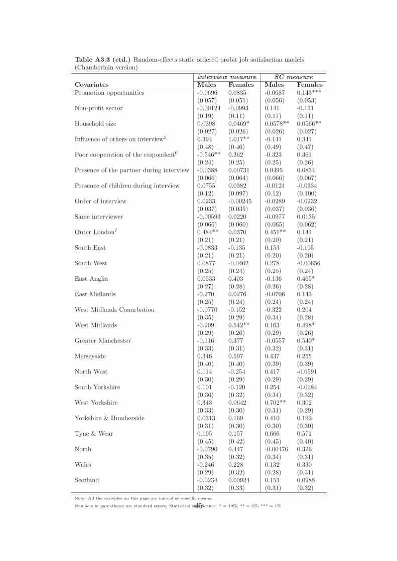
Table A3.3 (ctd.) Random-effects static ordered probit job satisfaction models(Chamberlain version)

interview measure SC measureCovariates Males Females Males FemalesPromotion opportunities -0.0696 0.0835 -0.0687 0.143***

(0.057) (0.051) (0.056) (0.053)Non-profit sector -0.00124 -0.0993 0.141 -0.131

(0.19) (0.11) (0.17) (0.11)Household size 0.0398 0.0469* 0.0578** 0.0566**

(0.027) (0.026) (0.026) (0.027)Influence of others on interview5 0.394 1.017** -0.141 0.341

(0.48) (0.46) (0.49) (0.47)Poor cooperation of the respondent6 -0.546** 0.362 -0.323 0.361

(0.24) (0.25) (0.25) (0.26)Presence of the partner during interview -0.0388 0.00731 0.0495 0.0834

(0.066) (0.064) (0.066) (0.067)Presence of children during interview 0.0755 0.0382 -0.0124 -0.0334

(0.12) (0.097) (0.12) (0.100)Order of interview 0.0233 -0.00245 -0.0289 -0.0232

(0.037) (0.035) (0.037) (0.036)Same interviewer -0.00593 0.0220 -0.0977 0.0135

(0.066) (0.060) (0.065) (0.062)Outer London7 0.484** 0.0370 0.451** 0.141

(0.21) (0.21) (0.20) (0.21)South East -0.0833 -0.135 0.153 -0.105

(0.21) (0.21) (0.20) (0.20)South West 0.0877 -0.0462 0.278 -0.00656

(0.25) (0.24) (0.25) (0.24)East Anglia 0.0533 0.403 -0.136 0.465*

(0.27) (0.28) (0.26) (0.28)East Midlands -0.270 0.0276 -0.0706 0.143

(0.25) (0.24) (0.24) (0.24)West Midlands Conurbation -0.0770 -0.152 -0.322 0.204

(0.35) (0.29) (0.34) (0.28)West Midlands -0.209 0.542** 0.163 0.498*

(0.29) (0.26) (0.29) (0.26)Greater Manchester -0.116 0.377 -0.0557 0.540*

(0.33) (0.31) (0.32) (0.31)Merseyside 0.346 0.597 0.437 0.255

(0.40) (0.40) (0.39) (0.39)North West 0.114 -0.254 0.417 -0.0591

(0.30) (0.29) (0.29) (0.29)South Yorkshire 0.101 -0.120 0.254 -0.0184

(0.36) (0.32) (0.34) (0.32)West Yorkshire 0.343 0.0642 0.702** 0.302

(0.33) (0.30) (0.31) (0.29)Yorkshire & Humberside 0.0313 0.169 0.410 0.192

(0.31) (0.30) (0.30) (0.30)Tyne & Wear 0.195 0.157 0.666 0.571

(0.45) (0.42) (0.45) (0.40)North -0.0790 0.447 -0.00476 0.326

(0.35) (0.32) (0.34) (0.31)Wales -0.246 0.228 0.132 0.330

(0.29) (0.32) (0.28) (0.31)Scotland -0.0234 0.00924 0.153 0.0988

(0.32) (0.33) (0.31) (0.32)

Note: All the variables on this page are individual-specific means.

Numbers in parentheses are standard errors. Statistical significance: * = 10%; ** = 5%; *** = 1%45

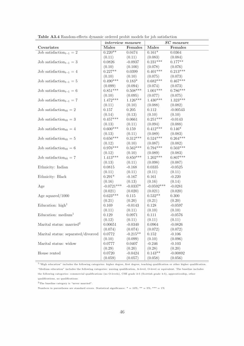
Table A3.4 Random-effects dynamic ordered probit models for job satisfaction

interview measure SC measureCovariates Males Females Males FemalesJob satisfactiont−1 = 2 0.220** 0.0474 0.161* 0.0364

(0.11) (0.11) (0.083) (0.084)Job satisfactiont−1 = 3 0.0826 -0.0937 0.231*** 0.177**

(0.10) (0.100) (0.078) (0.076)Job satisfactiont−1 = 4 0.227** 0.0399 0.401*** 0.213***

(0.10) (0.10) (0.075) (0.073)Job satisfactiont−1 = 5 0.490*** 0.183* 0.682*** 0.467***

(0.099) (0.094) (0.074) (0.073)Job satisfactiont−1 = 6 0.851*** 0.508*** 1.001*** 0.786***

(0.10) (0.095) (0.077) (0.075)Job satisfactiont−1 = 7 1.472*** 1.126*** 1.430*** 1.323***

(0.11) (0.10) (0.088) (0.082)Job satisfactiont0 = 2 0.157 0.205 0.112 -0.00543

(0.14) (0.13) (0.10) (0.10)Job satisfactiont0 = 3 0.457*** 0.0661 0.251*** -0.0143

(0.13) (0.11) (0.094) (0.088)Job satisfactiont0 = 4 0.600*** 0.159 0.412*** 0.146*

(0.13) (0.11) (0.089) (0.083)Job satisfactiont0 = 5 0.656*** 0.312*** 0.524*** 0.264***

(0.12) (0.10) (0.087) (0.082)Job satisfactiont0 = 6 0.976*** 0.562*** 0.794*** 0.503***

(0.12) (0.10) (0.089) (0.083)Job satisfactiont0 = 7 1.413*** 0.850*** 1.202*** 0.807***

(0.13) (0.11) (0.098) (0.087)Ethnicity: Indian 0.0815 -0.168 0.0335 -0.0525

(0.11) (0.11) (0.11) (0.11)Ethnicity: Black 0.291* -0.167 0.161 -0.220

(0.16) (0.13) (0.16) (0.14)Age -0.0721*** -0.0337* -0.0592*** -0.0281

(0.021) (0.020) (0.021) (0.020)Age squared/1000 0.623*** 0.115 0.532** 0.300

(0.21) (0.20) (0.21) (0.20)Education: high1 0.169 -0.0143 0.128 -0.0597

(0.11) (0.11) (0.10) (0.10)Education: medium1 0.129 0.0971 0.111 -0.0576

(0.12) (0.11) (0.11) (0.11)Marital status: married2 0.00651 -0.0340 0.0964 -0.0826

(0.074) (0.074) (0.072) (0.072)Marital status: separated/divorced 0.0772 -0.215** 0.152 -0.106

(0.10) (0.099) (0.10) (0.096)Marital status: widow 0.0777 0.0407 -0.246 -0.103

(0.29) (0.20) (0.28) (0.20)House rented 0.0720 -0.0424 0.143** -0.00892

(0.059) (0.057) (0.058) (0.056)1“High education” includes the following categories: higher degree, first degree, teaching qualification or other higher qualification.

“Medium education” includes the following categories: nursing qualification, A-level, O-level or equivalent. The baseline includes

the following categories: commercial qualifications (no O-levels), CSE grade 2-5 (Scottish grade 4-5), apprenticeship, other

qualifications, no qualifications.

2The baseline category is “never married”.

Numbers in parentheses are standard errors. Statistical significance: * = 10%; ** = 5%; *** = 1%

46

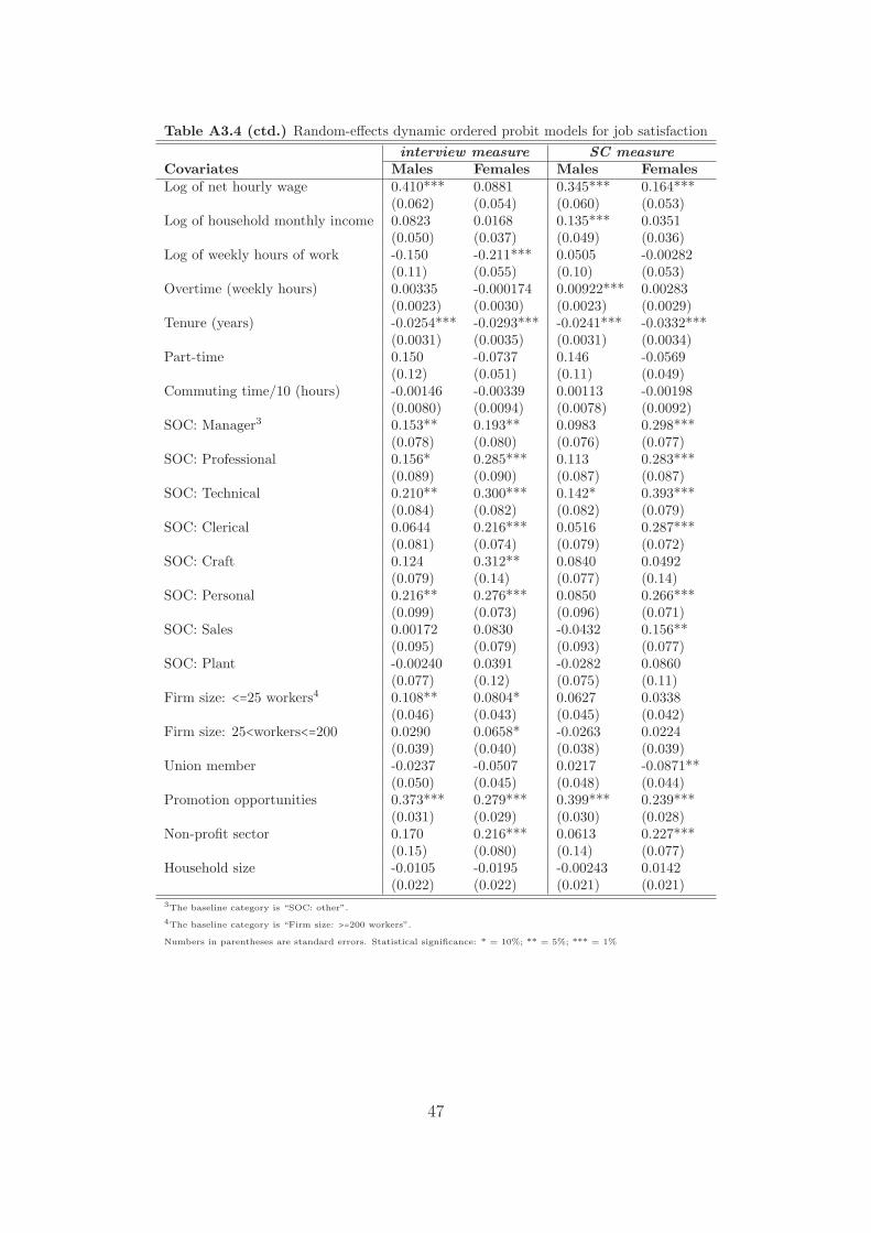
Table A3.4 (ctd.) Random-effects dynamic ordered probit models for job satisfaction

interview measure SC measureCovariates Males Females Males FemalesLog of net hourly wage 0.410*** 0.0881 0.345*** 0.164***

(0.062) (0.054) (0.060) (0.053)Log of household monthly income 0.0823 0.0168 0.135*** 0.0351

(0.050) (0.037) (0.049) (0.036)Log of weekly hours of work -0.150 -0.211*** 0.0505 -0.00282

(0.11) (0.055) (0.10) (0.053)Overtime (weekly hours) 0.00335 -0.000174 0.00922*** 0.00283

(0.0023) (0.0030) (0.0023) (0.0029)Tenure (years) -0.0254*** -0.0293*** -0.0241*** -0.0332***

(0.0031) (0.0035) (0.0031) (0.0034)Part-time 0.150 -0.0737 0.146 -0.0569

(0.12) (0.051) (0.11) (0.049)Commuting time/10 (hours) -0.00146 -0.00339 0.00113 -0.00198

(0.0080) (0.0094) (0.0078) (0.0092)SOC: Manager3 0.153** 0.193** 0.0983 0.298***

(0.078) (0.080) (0.076) (0.077)SOC: Professional 0.156* 0.285*** 0.113 0.283***

(0.089) (0.090) (0.087) (0.087)SOC: Technical 0.210** 0.300*** 0.142* 0.393***

(0.084) (0.082) (0.082) (0.079)SOC: Clerical 0.0644 0.216*** 0.0516 0.287***

(0.081) (0.074) (0.079) (0.072)SOC: Craft 0.124 0.312** 0.0840 0.0492

(0.079) (0.14) (0.077) (0.14)SOC: Personal 0.216** 0.276*** 0.0850 0.266***

(0.099) (0.073) (0.096) (0.071)SOC: Sales 0.00172 0.0830 -0.0432 0.156**

(0.095) (0.079) (0.093) (0.077)SOC: Plant -0.00240 0.0391 -0.0282 0.0860

(0.077) (0.12) (0.075) (0.11)Firm size: <=25 workers4 0.108** 0.0804* 0.0627 0.0338

(0.046) (0.043) (0.045) (0.042)Firm size: 25<workers<=200 0.0290 0.0658* -0.0263 0.0224

(0.039) (0.040) (0.038) (0.039)Union member -0.0237 -0.0507 0.0217 -0.0871**

(0.050) (0.045) (0.048) (0.044)Promotion opportunities 0.373*** 0.279*** 0.399*** 0.239***

(0.031) (0.029) (0.030) (0.028)Non-profit sector 0.170 0.216*** 0.0613 0.227***

(0.15) (0.080) (0.14) (0.077)Household size -0.0105 -0.0195 -0.00243 0.0142

(0.022) (0.022) (0.021) (0.021)3The baseline category is “SOC: other”.

4The baseline category is “Firm size: >=200 workers”.

Numbers in parentheses are standard errors. Statistical significance: * = 10%; ** = 5%; *** = 1%

47

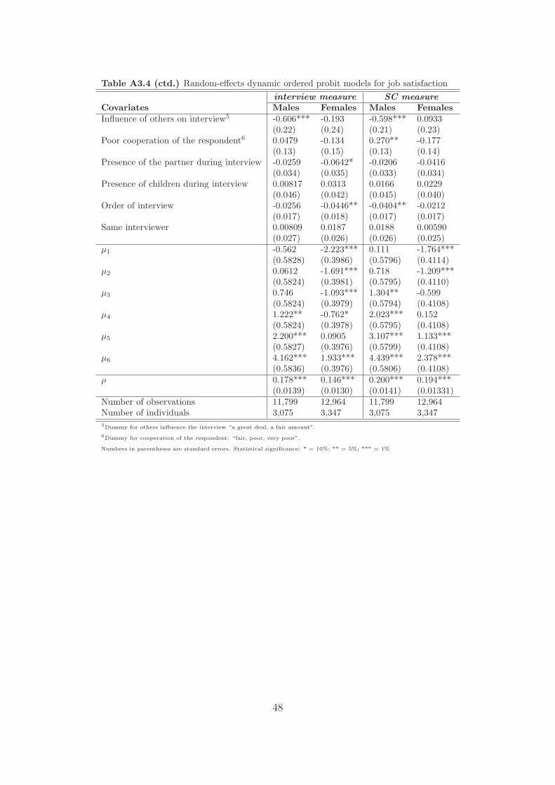
Table A3.4 (ctd.) Random-effects dynamic ordered probit models for job satisfaction

interview measure SC measureCovariates Males Females Males FemalesInfluence of others on interview5 -0.606*** -0.193 -0.598*** 0.0933

(0.22) (0.24) (0.21) (0.23)Poor cooperation of the respondent6 0.0479 -0.134 0.270** -0.177

(0.13) (0.15) (0.13) (0.14)Presence of the partner during interview -0.0259 -0.0642* -0.0206 -0.0416

(0.034) (0.035) (0.033) (0.034)Presence of children during interview 0.00817 0.0313 0.0166 0.0229

(0.046) (0.042) (0.045) (0.040)Order of interview -0.0256 -0.0446** -0.0404** -0.0212

(0.017) (0.018) (0.017) (0.017)Same interviewer 0.00809 0.0187 0.0188 0.00590

(0.027) (0.026) (0.026) (0.025)µ1 -0.562 -2.223*** 0.111 -1.764***

(0.5828) (0.3986) (0.5796) (0.4114)µ2 0.0612 -1.691*** 0.718 -1.209***

(0.5824) (0.3981) (0.5795) (0.4110)µ3 0.746 -1.093*** 1.304** -0.599

(0.5824) (0.3979) (0.5794) (0.4108)µ4 1.222** -0.762* 2.023*** 0.152

(0.5824) (0.3978) (0.5795) (0.4108)µ5 2.200*** 0.0905 3.107*** 1.133***

(0.5827) (0.3976) (0.5799) (0.4108)µ6 4.162*** 1.933*** 4.439*** 2.378***

(0.5836) (0.3976) (0.5806) (0.4108)ρ 0.178*** 0.146*** 0.200*** 0.194***

(0.0139) (0.0130) (0.0141) (0.01331)Number of observations 11,799 12,964 11,799 12,964Number of individuals 3,075 3,347 3,075 3,3475Dummy for others influence the interview “a great deal, a fair amount”.

6Dummy for cooperation of the respondent: “fair, poor, very poor”.

Numbers in parentheses are standard errors. Statistical significance: * = 10%; ** = 5%; *** = 1%

48

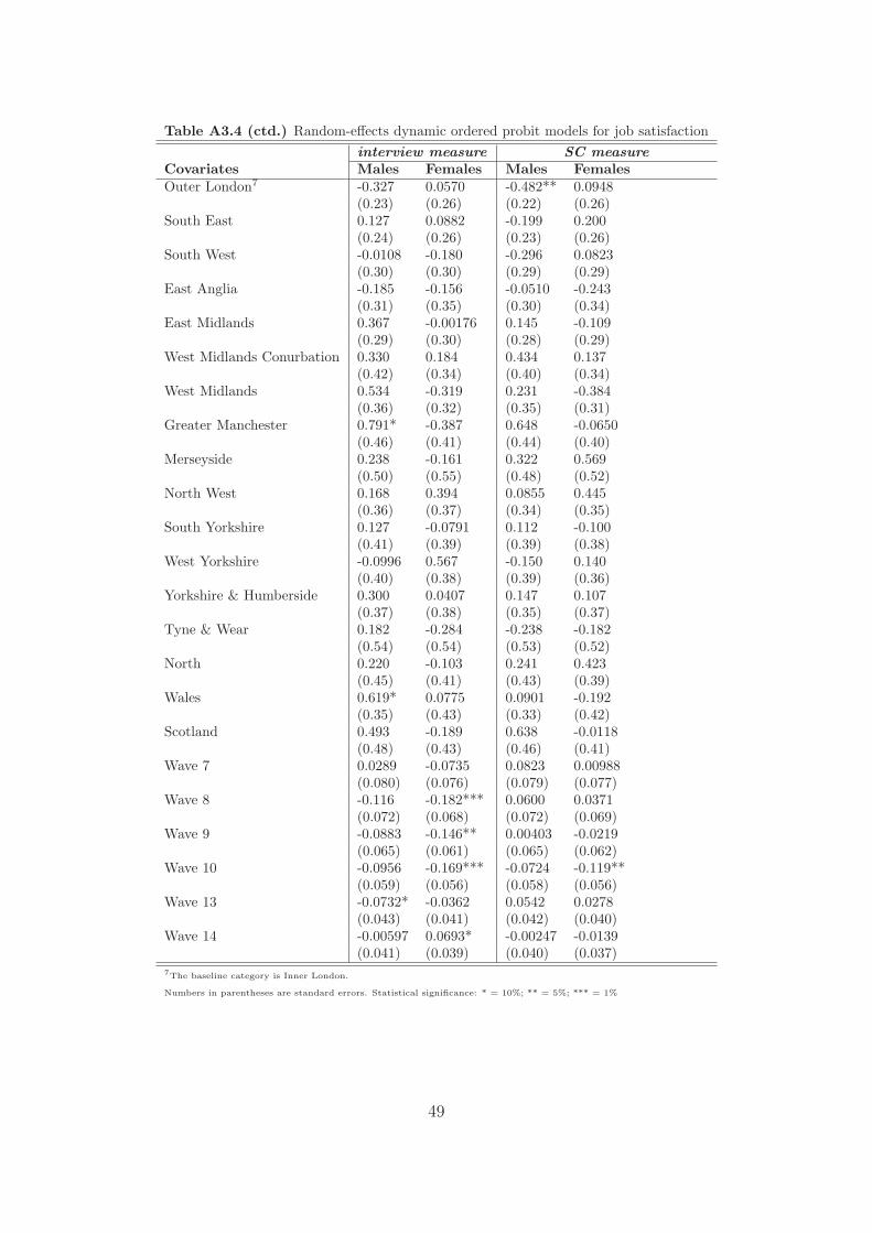
Table A3.4 (ctd.) Random-effects dynamic ordered probit models for job satisfaction

interview measure SC measureCovariates Males Females Males FemalesOuter London7 -0.327 0.0570 -0.482** 0.0948

(0.23) (0.26) (0.22) (0.26)South East 0.127 0.0882 -0.199 0.200

(0.24) (0.26) (0.23) (0.26)South West -0.0108 -0.180 -0.296 0.0823

(0.30) (0.30) (0.29) (0.29)East Anglia -0.185 -0.156 -0.0510 -0.243

(0.31) (0.35) (0.30) (0.34)East Midlands 0.367 -0.00176 0.145 -0.109

(0.29) (0.30) (0.28) (0.29)West Midlands Conurbation 0.330 0.184 0.434 0.137

(0.42) (0.34) (0.40) (0.34)West Midlands 0.534 -0.319 0.231 -0.384

(0.36) (0.32) (0.35) (0.31)Greater Manchester 0.791* -0.387 0.648 -0.0650

(0.46) (0.41) (0.44) (0.40)Merseyside 0.238 -0.161 0.322 0.569

(0.50) (0.55) (0.48) (0.52)North West 0.168 0.394 0.0855 0.445

(0.36) (0.37) (0.34) (0.35)South Yorkshire 0.127 -0.0791 0.112 -0.100

(0.41) (0.39) (0.39) (0.38)West Yorkshire -0.0996 0.567 -0.150 0.140

(0.40) (0.38) (0.39) (0.36)Yorkshire & Humberside 0.300 0.0407 0.147 0.107

(0.37) (0.38) (0.35) (0.37)Tyne & Wear 0.182 -0.284 -0.238 -0.182

(0.54) (0.54) (0.53) (0.52)North 0.220 -0.103 0.241 0.423

(0.45) (0.41) (0.43) (0.39)Wales 0.619* 0.0775 0.0901 -0.192

(0.35) (0.43) (0.33) (0.42)Scotland 0.493 -0.189 0.638 -0.0118

(0.48) (0.43) (0.46) (0.41)Wave 7 0.0289 -0.0735 0.0823 0.00988

(0.080) (0.076) (0.079) (0.077)Wave 8 -0.116 -0.182*** 0.0600 0.0371

(0.072) (0.068) (0.072) (0.069)Wave 9 -0.0883 -0.146** 0.00403 -0.0219

(0.065) (0.061) (0.065) (0.062)Wave 10 -0.0956 -0.169*** -0.0724 -0.119**

(0.059) (0.056) (0.058) (0.056)Wave 13 -0.0732* -0.0362 0.0542 0.0278

(0.043) (0.041) (0.042) (0.040)Wave 14 -0.00597 0.0693* -0.00247 -0.0139

(0.041) (0.039) (0.040) (0.037)7The baseline category is Inner London.

Numbers in parentheses are standard errors. Statistical significance: * = 10%; ** = 5%; *** = 1%

49

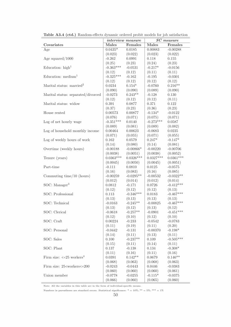
Table A3.4 (ctd.) Random-effects dynamic ordered probit models for job satisfaction

interview measure SC measureCovariates Males Females Males FemalesAge 0.0435* 0.0185 0.00883 -0.00288

(0.023) (0.022) (0.023) (0.022)Age squared/1000 -0.262 0.0991 0.118 0.155

(0.25) (0.23) (0.24) (0.23)Education: high1 -0.363*** -0.0531 -0.217* -0.0156

(0.12) (0.12) (0.11) (0.11)Education: medium1 -0.325*** -0.162 -0.195 -0.0301

(0.12) (0.12) (0.12) (0.12)Marital status: married2 0.0234 0.154* -0.0760 0.216**

(0.090) (0.090) (0.089) (0.090)Marital status: separated/divorced -0.0273 0.243** -0.128 0.130

(0.12) (0.12) (0.12) (0.11)Marital status: widow 0.391 0.0877 0.371 0.122

(0.37) (0.23) (0.36) (0.23)House rented 0.00573 0.00877 -0.134* -0.0122

(0.076) (0.071) (0.075) (0.071)Log of net hourly wage -0.351*** 0.0140 -0.273*** 0.0587

(0.089) (0.081) (0.089) (0.082)Log of household monthly income 0.00464 0.00623 -0.0683 0.0235

(0.071) (0.055) (0.071) (0.055)Log of weekly hours of work 0.162 0.0579 0.247* -0.147*

(0.14) (0.080) (0.14) (0.081)Overtime (weekly hours) -0.00188 -0.00866* -0.00220 -0.00706

(0.0038) (0.0051) (0.0038) (0.0052)Tenure (years) 0.0363*** 0.0326*** 0.0327*** 0.0361***

(0.0045) (0.0050) (0.0045) (0.0051)Part-time -0.111 0.0810 0.0125 -0.0575

(0.16) (0.083) (0.16) (0.085)Commuting time/10 (hours) -0.00259 -0.0295** -0.00532 -0.0322**

(0.012) (0.014) (0.012) (0.014)SOC: Manager3 0.0812 -0.171 0.0726 -0.412***

(0.12) (0.12) (0.12) (0.13)SOC: Professional 0.113 -0.346*** 0.0183 -0.467***

(0.13) (0.13) (0.13) (0.13)SOC: Technical -0.0163 -0.245** -0.00825 -0.467***

(0.13) (0.12) (0.13) (0.12)SOC: Clerical -0.0618 -0.257** -0.0901 -0.451***

(0.12) (0.10) (0.12) (0.10)SOC: Craft 0.00224 -0.233 -0.0542 -0.0783

(0.11) (0.19) (0.11) (0.20)SOC: Personal -0.0442 -0.131 -0.00370 -0.198*

(0.14) (0.11) (0.13) (0.11)SOC: Sales 0.100 -0.237** 0.109 -0.505***

(0.15) (0.11) (0.14) (0.11)SOC: Plant 0.137 -0.138 0.134 -0.308*

(0.11) (0.16) (0.11) (0.16)Firm size: <=25 workers4 0.0391 0.142** 0.0679 0.146**

(0.068) (0.063) (0.068) (0.063)Firm size: 25<workers<=200 -0.0243 -0.0443 0.0446 -0.0383

(0.060) (0.060) (0.060) (0.061)Union member -0.0778 -0.0255 -0.115* -0.0375

(0.066) (0.060) (0.065) (0.060)

Note: All the variables in this table are in the form of individual-specific means.

Numbers in parentheses are standard errors. Statistical significance: * = 10%; ** = 5%; *** = 1%

50

Table A3.4 (ctd.) Random-effects dynamic ordered probit models for job satisfaction

interview measure SC measureCovariates Males Females Males FemalesPromotion opportunities -0.217*** -0.0633 -0.213*** 0.0477

(0.054) (0.051) (0.054) (0.052)Non-profit sector 0.0893 -0.107 -0.00262 -0.108

(0.20) (0.11) (0.19) (0.11)Household size 0.0242 0.0231 0.0229 -0.00612

(0.028) (0.029) (0.028) (0.029)Influence of others on interview5 1.155** -0.156 0.202 0.185

(0.55) (0.55) (0.55) (0.56)Poor cooperation of the respondent6 -0.284 0.283 -0.419 0.0773

(0.28) (0.31) (0.28) (0.31)Presence of the partner during interview 0.0629 0.0229 0.00932 0.0498

(0.061) (0.061) (0.061) (0.063)Presence of children during interview -0.0384 -0.0602 0.121 0.0777

(0.11) (0.094) (0.11) (0.097)Order of interview 0.0252 0.0652* -0.00714 0.0546

(0.038) (0.036) (0.038) (0.037)Same interviewer 0.0288 -0.0352 0.0184 -0.0426

(0.071) (0.066) (0.071) (0.068)Outer London7 0.555** -0.132 0.676*** -0.126

(0.26) (0.28) (0.25) (0.28)South East 0.0508 -0.168 0.336 -0.199

(0.26) (0.28) (0.25) (0.27)South West 0.247 0.0833 0.544* -0.00108

(0.32) (0.31) (0.31) (0.31)East Anglia 0.438 0.112 0.296 0.354

(0.34) (0.36) (0.33) (0.36)East Midlands -0.0734 0.0390 0.0572 0.219

(0.31) (0.32) (0.30) (0.31)West Midlands Conurbation -0.342 -0.363 -0.423 -0.208

(0.44) (0.36) (0.42) (0.36)West Midlands -0.182 0.275 0.0519 0.408

(0.38) (0.33) (0.37) (0.33)Greater Manchester -0.583 0.138 -0.445 -0.0597

(0.48) (0.43) (0.46) (0.42)Merseyside 0.212 0.0838 0.172 -0.663

(0.52) (0.56) (0.50) (0.54)North West 0.0383 -0.555 0.171 -0.410

(0.38) (0.38) (0.37) (0.37)South Yorkshire 0.190 -0.0674 0.114 0.0649

(0.43) (0.41) (0.41) (0.40)West Yorkshire 0.388 -0.602 0.453 -0.0552

(0.43) (0.39) (0.41) (0.38)Yorkshire & Humberside -0.161 -0.135 0.00527 -0.0785

(0.39) (0.40) (0.38) (0.39)Tyne & Wear -0.0188 0.107 0.395 0.220

(0.55) (0.55) (0.55) (0.54)North 0.0337 0.0739 -0.0288 -0.322

(0.47) (0.42) (0.45) (0.41)Wales -0.371 -0.289 0.0972 0.0876

(0.37) (0.45) (0.36) (0.43)Scotland -0.240 0.0529 -0.413 -0.00392

(0.49) (0.44) (0.48) (0.43)

Note: All the variables in this table are in the form of individual-specific means.

Numbers in parentheses are standard errors. Statistical significance: * = 10%; ** = 5%; *** = 1%

51

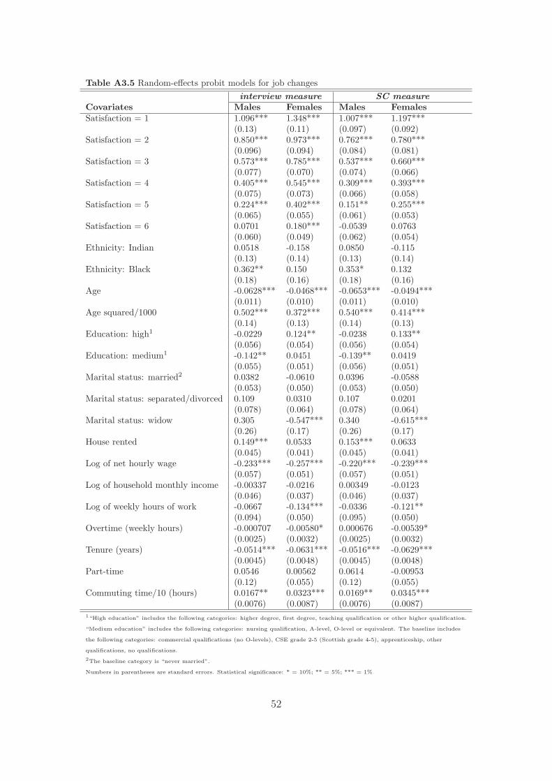
Table A3.5 Random-effects probit models for job changes

interview measure SC measureCovariates Males Females Males FemalesSatisfaction = 1 1.096*** 1.348*** 1.007*** 1.197***

(0.13) (0.11) (0.097) (0.092)Satisfaction = 2 0.850*** 0.973*** 0.762*** 0.780***

(0.096) (0.094) (0.084) (0.081)Satisfaction = 3 0.573*** 0.785*** 0.537*** 0.660***

(0.077) (0.070) (0.074) (0.066)Satisfaction = 4 0.405*** 0.545*** 0.309*** 0.393***

(0.075) (0.073) (0.066) (0.058)Satisfaction = 5 0.224*** 0.402*** 0.151** 0.255***

(0.065) (0.055) (0.061) (0.053)Satisfaction = 6 0.0701 0.180*** -0.0539 0.0763

(0.060) (0.049) (0.062) (0.054)Ethnicity: Indian 0.0518 -0.158 0.0850 -0.115

(0.13) (0.14) (0.13) (0.14)Ethnicity: Black 0.362** 0.150 0.353* 0.132

(0.18) (0.16) (0.18) (0.16)Age -0.0628*** -0.0468*** -0.0653*** -0.0494***

(0.011) (0.010) (0.011) (0.010)Age squared/1000 0.502*** 0.372*** 0.540*** 0.414***

(0.14) (0.13) (0.14) (0.13)Education: high1 -0.0229 0.124** -0.0238 0.133**

(0.056) (0.054) (0.056) (0.054)Education: medium1 -0.142** 0.0451 -0.139** 0.0419

(0.055) (0.051) (0.056) (0.051)Marital status: married2 0.0382 -0.0610 0.0396 -0.0588

(0.053) (0.050) (0.053) (0.050)Marital status: separated/divorced 0.109 0.0310 0.107 0.0201

(0.078) (0.064) (0.078) (0.064)Marital status: widow 0.305 -0.547*** 0.340 -0.615***

(0.26) (0.17) (0.26) (0.17)House rented 0.149*** 0.0533 0.153*** 0.0633

(0.045) (0.041) (0.045) (0.041)Log of net hourly wage -0.233*** -0.257*** -0.220*** -0.239***

(0.057) (0.051) (0.057) (0.051)Log of household monthly income -0.00337 -0.0216 0.00349 -0.0123

(0.046) (0.037) (0.046) (0.037)Log of weekly hours of work -0.0667 -0.134*** -0.0336 -0.121**

(0.094) (0.050) (0.095) (0.050)Overtime (weekly hours) -0.000707 -0.00580* 0.000676 -0.00539*

(0.0025) (0.0032) (0.0025) (0.0032)Tenure (years) -0.0514*** -0.0631*** -0.0516*** -0.0629***

(0.0045) (0.0048) (0.0045) (0.0048)Part-time 0.0546 0.00562 0.0614 -0.00953

(0.12) (0.055) (0.12) (0.055)Commuting time/10 (hours) 0.0167** 0.0323*** 0.0169** 0.0345***

(0.0076) (0.0087) (0.0076) (0.0087)1“High education” includes the following categories: higher degree, first degree, teaching qualification or other higher qualification.

“Medium education” includes the following categories: nursing qualification, A-level, O-level or equivalent. The baseline includes

the following categories: commercial qualifications (no O-levels), CSE grade 2-5 (Scottish grade 4-5), apprenticeship, other

qualifications, no qualifications.

2The baseline category is “never married”.

Numbers in parentheses are standard errors. Statistical significance: * = 10%; ** = 5%; *** = 1%

52

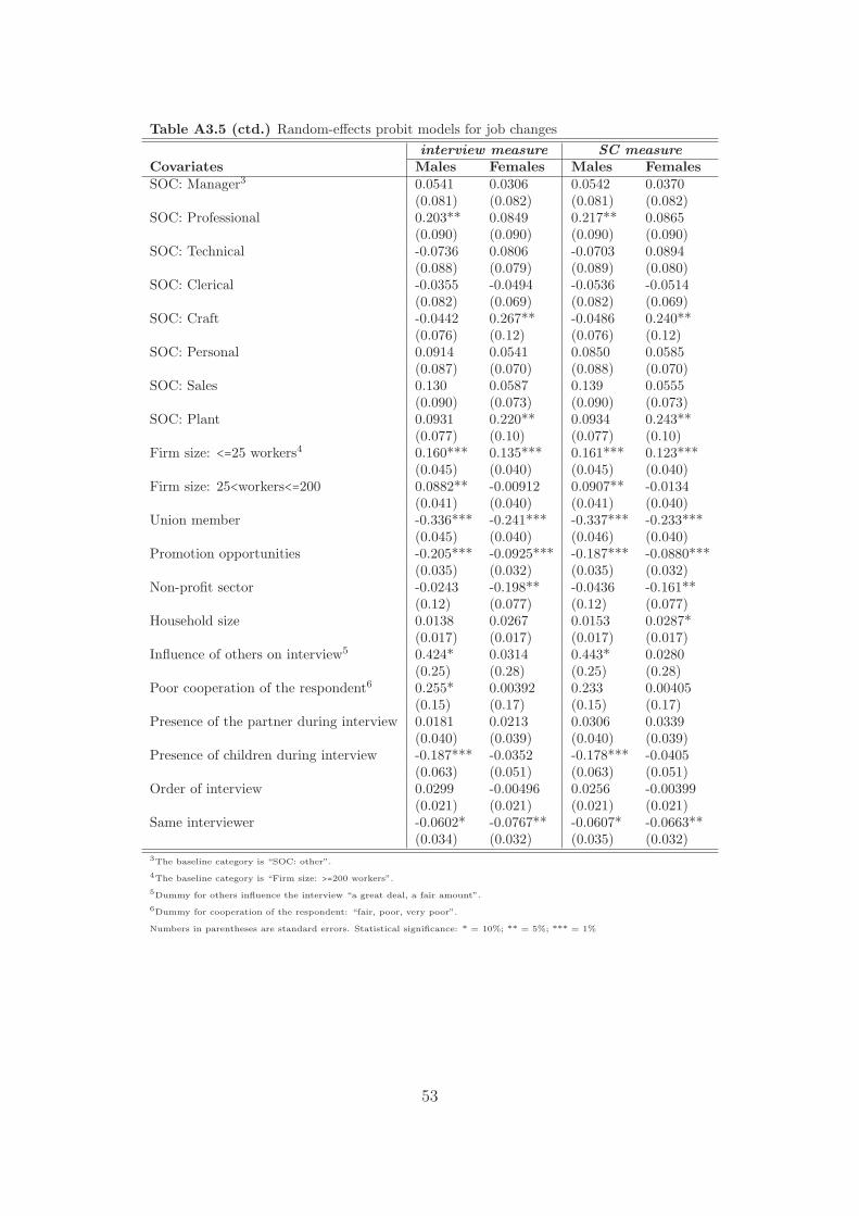
Table A3.5 (ctd.) Random-effects probit models for job changes

interview measure SC measureCovariates Males Females Males FemalesSOC: Manager3 0.0541 0.0306 0.0542 0.0370

(0.081) (0.082) (0.081) (0.082)SOC: Professional 0.203** 0.0849 0.217** 0.0865

(0.090) (0.090) (0.090) (0.090)SOC: Technical -0.0736 0.0806 -0.0703 0.0894

(0.088) (0.079) (0.089) (0.080)SOC: Clerical -0.0355 -0.0494 -0.0536 -0.0514

(0.082) (0.069) (0.082) (0.069)SOC: Craft -0.0442 0.267** -0.0486 0.240**

(0.076) (0.12) (0.076) (0.12)SOC: Personal 0.0914 0.0541 0.0850 0.0585

(0.087) (0.070) (0.088) (0.070)SOC: Sales 0.130 0.0587 0.139 0.0555

(0.090) (0.073) (0.090) (0.073)SOC: Plant 0.0931 0.220** 0.0934 0.243**

(0.077) (0.10) (0.077) (0.10)Firm size: <=25 workers4 0.160*** 0.135*** 0.161*** 0.123***

(0.045) (0.040) (0.045) (0.040)Firm size: 25<workers<=200 0.0882** -0.00912 0.0907** -0.0134

(0.041) (0.040) (0.041) (0.040)Union member -0.336*** -0.241*** -0.337*** -0.233***

(0.045) (0.040) (0.046) (0.040)Promotion opportunities -0.205*** -0.0925*** -0.187*** -0.0880***

(0.035) (0.032) (0.035) (0.032)Non-profit sector -0.0243 -0.198** -0.0436 -0.161**

(0.12) (0.077) (0.12) (0.077)Household size 0.0138 0.0267 0.0153 0.0287*

(0.017) (0.017) (0.017) (0.017)Influence of others on interview5 0.424* 0.0314 0.443* 0.0280

(0.25) (0.28) (0.25) (0.28)Poor cooperation of the respondent6 0.255* 0.00392 0.233 0.00405

(0.15) (0.17) (0.15) (0.17)Presence of the partner during interview 0.0181 0.0213 0.0306 0.0339

(0.040) (0.039) (0.040) (0.039)Presence of children during interview -0.187*** -0.0352 -0.178*** -0.0405

(0.063) (0.051) (0.063) (0.051)Order of interview 0.0299 -0.00496 0.0256 -0.00399

(0.021) (0.021) (0.021) (0.021)Same interviewer -0.0602* -0.0767** -0.0607* -0.0663**

(0.034) (0.032) (0.035) (0.032)3The baseline category is “SOC: other”.

4The baseline category is “Firm size: >=200 workers”.

5Dummy for others influence the interview “a great deal, a fair amount”.

6Dummy for cooperation of the respondent: “fair, poor, very poor”.

Numbers in parentheses are standard errors. Statistical significance: * = 10%; ** = 5%; *** = 1%

53

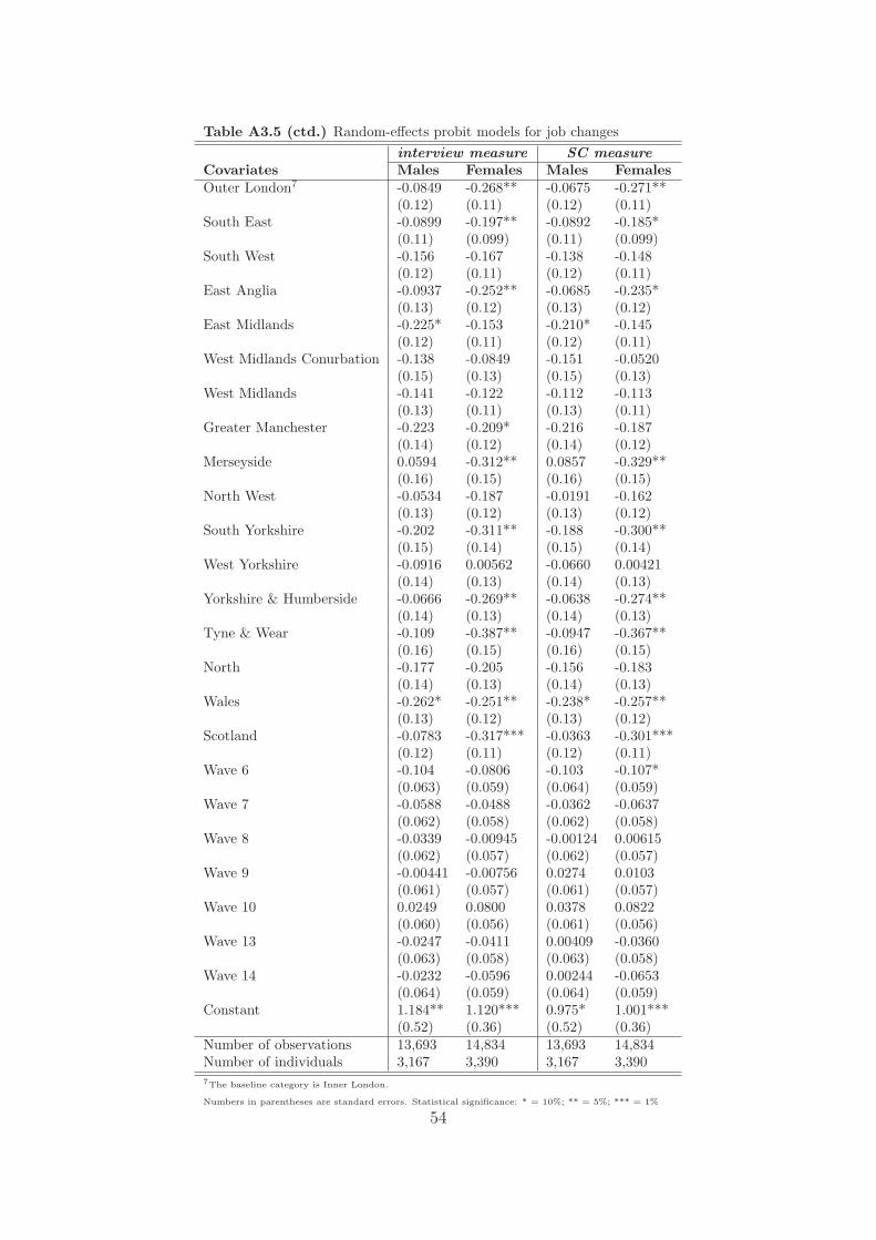
Table A3.5 (ctd.) Random-effects probit models for job changes

interview measure SC measureCovariates Males Females Males FemalesOuter London7 -0.0849 -0.268** -0.0675 -0.271**

(0.12) (0.11) (0.12) (0.11)South East -0.0899 -0.197** -0.0892 -0.185*

(0.11) (0.099) (0.11) (0.099)South West -0.156 -0.167 -0.138 -0.148

(0.12) (0.11) (0.12) (0.11)East Anglia -0.0937 -0.252** -0.0685 -0.235*

(0.13) (0.12) (0.13) (0.12)East Midlands -0.225* -0.153 -0.210* -0.145

(0.12) (0.11) (0.12) (0.11)West Midlands Conurbation -0.138 -0.0849 -0.151 -0.0520

(0.15) (0.13) (0.15) (0.13)West Midlands -0.141 -0.122 -0.112 -0.113

(0.13) (0.11) (0.13) (0.11)Greater Manchester -0.223 -0.209* -0.216 -0.187

(0.14) (0.12) (0.14) (0.12)Merseyside 0.0594 -0.312** 0.0857 -0.329**

(0.16) (0.15) (0.16) (0.15)North West -0.0534 -0.187 -0.0191 -0.162

(0.13) (0.12) (0.13) (0.12)South Yorkshire -0.202 -0.311** -0.188 -0.300**

(0.15) (0.14) (0.15) (0.14)West Yorkshire -0.0916 0.00562 -0.0660 0.00421

(0.14) (0.13) (0.14) (0.13)Yorkshire & Humberside -0.0666 -0.269** -0.0638 -0.274**

(0.14) (0.13) (0.14) (0.13)Tyne & Wear -0.109 -0.387** -0.0947 -0.367**

(0.16) (0.15) (0.16) (0.15)North -0.177 -0.205 -0.156 -0.183

(0.14) (0.13) (0.14) (0.13)Wales -0.262* -0.251** -0.238* -0.257**

(0.13) (0.12) (0.13) (0.12)Scotland -0.0783 -0.317*** -0.0363 -0.301***

(0.12) (0.11) (0.12) (0.11)Wave 6 -0.104 -0.0806 -0.103 -0.107*

(0.063) (0.059) (0.064) (0.059)Wave 7 -0.0588 -0.0488 -0.0362 -0.0637

(0.062) (0.058) (0.062) (0.058)Wave 8 -0.0339 -0.00945 -0.00124 0.00615

(0.062) (0.057) (0.062) (0.057)Wave 9 -0.00441 -0.00756 0.0274 0.0103

(0.061) (0.057) (0.061) (0.057)Wave 10 0.0249 0.0800 0.0378 0.0822

(0.060) (0.056) (0.061) (0.056)Wave 13 -0.0247 -0.0411 0.00409 -0.0360

(0.063) (0.058) (0.063) (0.058)Wave 14 -0.0232 -0.0596 0.00244 -0.0653

(0.064) (0.059) (0.064) (0.059)Constant 1.184** 1.120*** 0.975* 1.001***

(0.52) (0.36) (0.52) (0.36)Number of observations 13,693 14,834 13,693 14,834Number of individuals 3,167 3,390 3,167 3,3907The baseline category is Inner London.

Numbers in parentheses are standard errors. Statistical significance: * = 10%; ** = 5%; *** = 1%

54

Table A3.6 Random-effects latent factor modelsof interview and SC response

Covariates Females MalesEthnicity: Indian -0.2024 0.0867

(0.1694) (0.1544)Ethnicity: Black -0.4757 -0.2441

(0.2014) (0.2137)Age 0.0036 -0.1034

(0.0068) (0.0074)Age squared/1000 0.1375 1.3455

(0.0797) (0.0875)Education: high1 -0.2275 -0.2960

(0.0408) (0.0417)Education: medium1 -0.2145 -0.1903

(0.0401) (0.0433)Married2 0.0814 0.1382

(0.0399) (0.0394)Separated/divorced -0.1699 0.2522

(0.0524) (0.0553)Widower -0.0889 0.1242

(0.0979) (0.1997)House rented 0.0042 0.0808

(0.0297) (0.0314)Log wage 0.0852 0.4235

(0.0328) (0.0358)Log household income -0.0358 -0.0169

(0.0234) (0.0249)Log hours -0.0855 0.1609

(0.0282) (0.0523)Overtime (weekly hours) -0.0019 0.0137

(0.0020) (0.0015)Tenure (years) -0.0220 -0.0201

(0.0021) (0.0020)Part-time -0.0625 0.1734

(0.0322) (0.0601)Commuting time/10 (hours) -0.0174 -0.0113

(0.0058) (0.0047)1“High education” includes: higher degree, first degree, teaching

qualification or other higher qualification. “Medium education” includes

nursing qualification, A-level, O-level or equivalent. The baseline

includes: commercial qualifications (no O-levels), CSE grade 2-5

(Scottish grade 4-5), apprenticeship, other qualifications, no qualifications.

2The baseline category is “never married”.

55

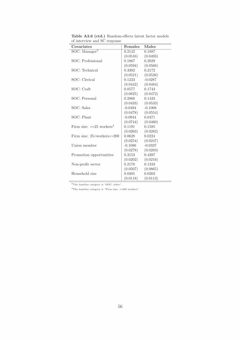
Table A3.6 (ctd.) Random-effects latent factor modelsof interview and SC response

Covariates Females MalesSOC: Manager3 0.2142 0.1887

(0.0516) (0.0493)SOC: Professional 0.1867 0.2029

(0.0594) (0.0568)SOC: Technical 0.3302 0.2172

(0.0521) (0.0526)SOC: Clerical 0.1223 -0.0287

(0.0442) (0.0484)SOC: Craft 0.0577 0.1743

(0.0825) (0.0472)SOC: Personal 0.2860 0.1433

(0.0433) (0.0533)SOC: Sales -0.0494 -0.1008

(0.0478) (0.0554)SOC: Plant -0.0944 0.0471

(0.0744) (0.0460)Firm size: <=25 workers4 0.1191 0.1585

(0.0263) (0.0282)Firm size: 25<workers<=200 0.0628 0.0224

(0.0254) (0.0247)Union member -0.1086 -0.0337

(0.0278) (0.0283)Promotion opportunities 0.3153 0.4397

(0.0202) (0.0216)Non-profit sector 0.2178 0.1333

(0.0507) (0.0865)Household size 0.0305 0.0203

(0.0118) (0.0113)3The baseline category is “SOC: other”.

4The baseline category is “Firm size: >=200 workers”.

56

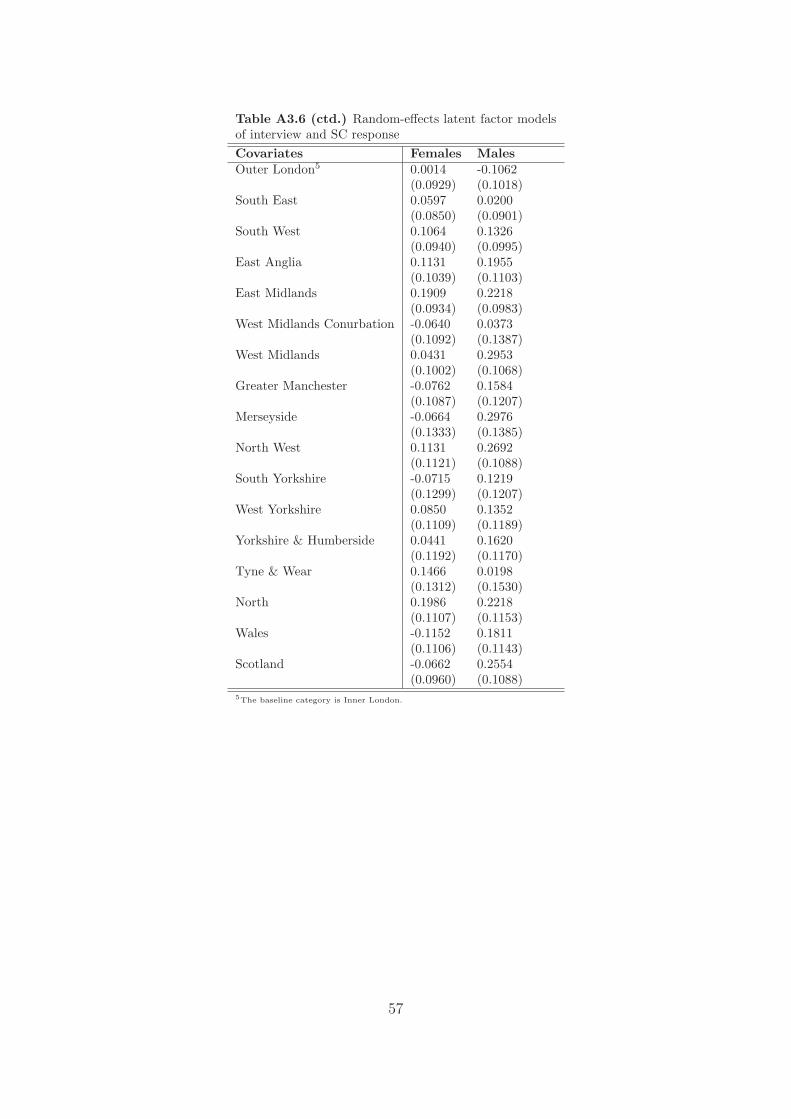
Table A3.6 (ctd.) Random-effects latent factor modelsof interview and SC response

Covariates Females MalesOuter London5 0.0014 -0.1062

(0.0929) (0.1018)South East 0.0597 0.0200

(0.0850) (0.0901)South West 0.1064 0.1326

(0.0940) (0.0995)East Anglia 0.1131 0.1955

(0.1039) (0.1103)East Midlands 0.1909 0.2218

(0.0934) (0.0983)West Midlands Conurbation -0.0640 0.0373

(0.1092) (0.1387)West Midlands 0.0431 0.2953

(0.1002) (0.1068)Greater Manchester -0.0762 0.1584

(0.1087) (0.1207)Merseyside -0.0664 0.2976

(0.1333) (0.1385)North West 0.1131 0.2692

(0.1121) (0.1088)South Yorkshire -0.0715 0.1219

(0.1299) (0.1207)West Yorkshire 0.0850 0.1352

(0.1109) (0.1189)Yorkshire & Humberside 0.0441 0.1620

(0.1192) (0.1170)Tyne & Wear 0.1466 0.0198

(0.1312) (0.1530)North 0.1986 0.2218

(0.1107) (0.1153)Wales -0.1152 0.1811

(0.1106) (0.1143)Scotland -0.0662 0.2554

(0.0960) (0.1088)5The baseline category is Inner London.

57

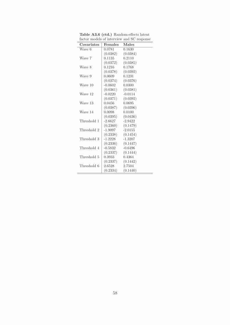
Table A3.6 (ctd.) Random-effects latentfactor models of interview and SC response

Covariates Females MalesWave 6 0.0781 0.1630

(0.0382) (0.0384)Wave 7 0.1135 0.2110

(0.0372) (0.0385)Wave 8 0.1216 0.1768

(0.0378) (0.0392)Wave 9 0.0609 0.1231

(0.0374) (0.0376)Wave 10 -0.0602 0.0300

(0.0361) (0.0381)Wave 12 -0.0220 -0.0114

(0.0371) (0.0392)Wave 13 0.0456 0.0695

(0.0387) (0.0396)Wave 14 0.0098 0.0100

(0.0395) (0.0436)Threshold 1 -2.6627 -2.9422

(0.2360) (0.1479)Threshold 2 -1.9097 -2.0155

(0.2338) (0.1454)Threshold 3 -1.2228 -1.3207

(0.2336) (0.1447)Threshold 4 -0.5832 -0.6496

(0.2337) (0.1444)Threshold 5 0.3933 0.4364

(0.2337) (0.1442)Threshold 6 2.6528 2.7504

(0.2334) (0.1440)

58

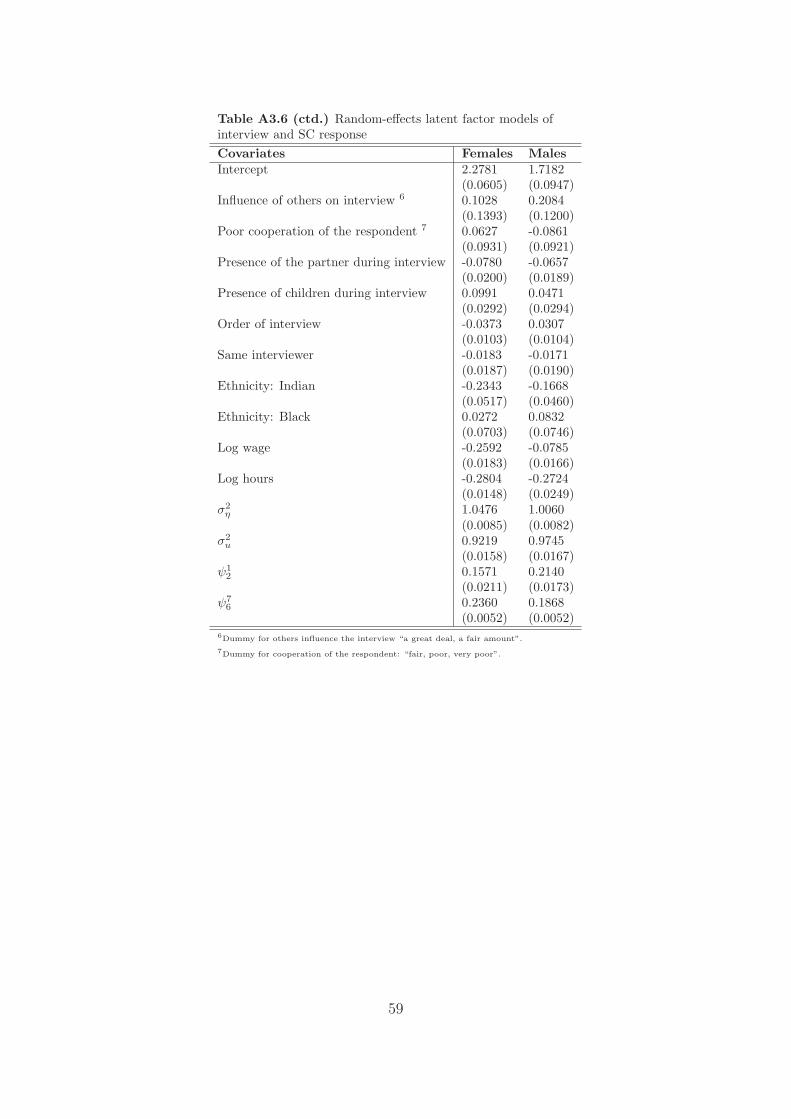
Table A3.6 (ctd.) Random-effects latent factor models ofinterview and SC response

Covariates Females MalesIntercept 2.2781 1.7182

(0.0605) (0.0947)Influence of others on interview 6 0.1028 0.2084

(0.1393) (0.1200)Poor cooperation of the respondent 7 0.0627 -0.0861

(0.0931) (0.0921)Presence of the partner during interview -0.0780 -0.0657

(0.0200) (0.0189)Presence of children during interview 0.0991 0.0471

(0.0292) (0.0294)Order of interview -0.0373 0.0307

(0.0103) (0.0104)Same interviewer -0.0183 -0.0171

(0.0187) (0.0190)Ethnicity: Indian -0.2343 -0.1668

(0.0517) (0.0460)Ethnicity: Black 0.0272 0.0832

(0.0703) (0.0746)Log wage -0.2592 -0.0785

(0.0183) (0.0166)Log hours -0.2804 -0.2724

(0.0148) (0.0249)σ2

η 1.0476 1.0060(0.0085) (0.0082)

σ2

u 0.9219 0.9745(0.0158) (0.0167)

ψ1

20.1571 0.2140(0.0211) (0.0173)

ψ7

60.2360 0.1868(0.0052) (0.0052)

6Dummy for others influence the interview “a great deal, a fair amount”.

7Dummy for cooperation of the respondent: “fair, poor, very poor”.

59