Surface-wave inversion using a direct search algorithm and its application to ambient vibration...

Near Surface Geophysics, 2004, 211-221

© 2004 European Association of Geoscientists & Engineers 211

Surface-wave inversion using a direct search algorithm andits application to ambient vibration measurements

M. Wathelet1, 2*, D. Jongmans1 and M. Ohrnberger3

1 LIRIGM, Université Joseph Fourier, BP 53, 38041 Grenoble cedex 9, France 2 GEOMAC, Université de Liège, 1 Chemin des Chevreuils, Bât. B52, 4000 Liège, Belgium3 Institut für Geowissenschaften der Universität Potsdam, POB 601553, D-14415 Potsdam, Germany

Received January 2004, revision accepted August 2004

ABSTRACTPassive recordings of seismic noise are increasingly used in earthquake engineering to measure insitu the shear-wave velocity profile at a given site. Ambient vibrations, which are assumed to bemainly composed of surface waves, can be used to determine the Rayleigh-wave dispersion curve,with the advantage of not requiring artificial sources. Due to the data uncertainties and the non-lin-earity of the problem itself, the solution of the dispersion-curve inversion is generally non-unique.Stochastic search methods such as the neighbourhood algorithm allow searches for minima of themisfit function by investigating the whole parameter space. Due to the limited number of parame-ters in surface-wave inversion, they constitute an attractive alternative to linearized methods. Anefficient tool using the neighbourhood algorithm was developed to invert the one-dimensional Vs

profile from passive or active source experiments. As the number of generated models is usuallyhigh in stochastic techniques, special attention was paid to the optimization of the forward compu-tations. Also, the possibility of inserting a priori information into the parametrization was intro-duced in the code.

This new numerical tool was successfully tested on synthetic data, with and without a priori infor-mation. We also present an application to real-array data measured at a site in Brussels (Belgium),the geology of which consists of about 115 m of sand and clay layers overlying a Palaeozoic base-ment. On this site, active and passive source data proved to be complementary and the methodallowed the retrieval of a Vs profile consistent with borehole data available at the same location.

is of major importance in earthquake engineering, and ambientvibrations measured by an array of vertical sensors are increas-ingly applied for determining Vs profiles (e.g. Horike 1985;Tokimatsu 1995; Ishida et al. 1998; Miyakoshi et al. 1998;Yamamoto 1998; Satoh et al. 2001; Scherbaum et al. 2003).

In a first step, the Rayleigh phase-velocity dispersion curve isderived from the processing of simultaneous ground-motionrecordings at various stations. The recording time is usuallygreater than or equal to half an hour and the number of stationsis generally between 6 and 10, depending upon the availableequipment (sensors, synchronized or multichannel stations) andtime (the set-up may take quite a long time for a large number ofsensors). The geometry of the station layout is not strictlyimposed by the processing method itself, but a circular shapeensures an equal response of the array for waves coming from allazimuths. The common approaches used to derive the dispersioncurve from the raw signals can be classified into two main fam-ilies: frequency–wavenumber (Lacoss et al. 1969; Capon 1969;Kvaerna and Ringdahl 1986; Ohrnberger 2001) and spatial auto-

INTRODUCTIONFor the majority of seismic prospecting methods, natural or cul-tural ambient vibrations constitute an undesired part of the signal,which has to be eliminated as much as possible. However, thenoise field is influenced by the subsurface structure and the use ofarray records of seismic noise has been recognized as a methodfor deriving the S-wave velocity profile at a given site (e.g. Aki1957; Asten 1978; Tokimatsu 1995). The hypothesis behind themethod is that ambient vibrations mainly consist of surfacewaves, whose dispersion characteristics depend primarily on thebody-wave velocities (Vp for compressional-wave velocities andVs for shear-wave velocities), the density and the thickness of thedifferent layers (Murphy and Shah 1988; Aki and Richards 2002).Noise energy depends upon the source locations and upon theimpedance contrast between the rocky basement and the overly-ing soft sediments (Chouet et al. 1998; Milana et al. 1996). Aknowledge of the shear-wave velocity (Vs) profile at a given site

* [email protected]

M. Wathelet, D. Jongmans and M. Ohrnberger212

© 2004 European Association of Geoscientists & Engineers, Near Surface Geophysics, 2004, 2, 211-221

correlation (Aki 1957; Roberts and Asten 2004). The first meth-ods are best suited for plane wavefields with a single dominantsource of noise but may be also used in more complex situations,averaging the apparent velocity over longer periods of time. Theoutput of a basic frequency–wavenumber processing consists ofsemblance maps which indicate the azimuth and the velocity (orslowness) of the waves travelling with the highest energy. Thegrid maps are obtained by shifting and stacking the recorded sig-nals over small time windows. The former class of methodsassumes stationary-wave arrivals both in time and space andhence an infinite number of simultaneous sources. Spatial auto-correlation methods are considered as more efficient by someauthors (e.g. Ohori et al. 2002), but the relative performances ofeach method have not been rigorously investigated so far. Here,we applied the frequency–wavenumber method which has beenwidely used (e.g. Asten and Henstridge 1984; Ohrnberger 2001).

At the second stage, the dispersion curve is inverted to obtainthe Vs (and eventually the Vp) vertical profile, as in the classicalactive-source methods (Stokoe et al. 1989; Malagnini et al.1995). Compared with these latter methods, noise-based tech-niques offer the following advantages (Satoh et al. 2001): (i)they can be easily applied in urban areas; (ii) they do not requireartificial seismic sources; (iii) they allow greater depths to bereached (from tens of metres to hundreds of metres according tothe array aperture and the noise-frequency content). Like all sur-face-wave methods, the geometry obtained is purely one-dimen-sional and is averaged within the array, implying that the tech-nique is not suitable when strong lateral variations are present.

The derivation of 1D S-wave velocity profiles from surface-wave dispersion curves is a classical inversion problem in geo-physics, usually solved using linearized methods (Nolet 1981;Tarantola 1987). In his computer program, Herrmann (1987)implemented a damped least-squares method that uses an analyt-ical formulation for derivatives and a starting model. At eachiteration, a better estimate of the model is calculated by lineariz-ing the problem and the best solution, minimizing a misfit func-tion, is obtained after a few iterations. If the misfit functionexhibits several minima, which is usually the case when uncer-tainties on the dispersion curve are high, the derivative-basedmethods give a single optimal model which strongly dependsupon the starting model. For active-source measurements, someauthors proposed inverting the complete waveforms or particularwavefield transforms (Yoshizawa and Kennett 2002; Forbriger2003) to get a better constraint on the solution. This is not appli-cable to ambient vibrations for which no information about thesource properties is available. In geophysics, a new class ofmethods, based on uniform pseudo-random sampling of aparameter space (Monte-Carlo type), has emerged during the last15 years: they are simulated annealing (Sen and Stoffa 1991),genetic algorithms (Lomax and Snieder 1994) and more recent-ly the neighbourhood algorithm developed by Sambridge (1999).The objective of these algorithms is to investigate the wholeparameter space, looking for good data-fitting sets of parameters.

In this work we have developed a new code using the neigh-bourhood algorithm for inverting dispersion curves. The soft-ware allows the inclusion of a priori information on the differentparameters and a major effort has been made to optimize thecomputation time at the different stages of inversion. In particu-lar, we have re-implemented the dispersion-curve computation inC++ language using Dunkin’s (1965) formalism. The code istested on synthetic cases as well as on one real data set, combin-ing ambient vibrations and active-source data. In both cases, therole of a priori information for constraining the solution isemphasized.

INVERSION METHODThe neighbourhood algorithm The neighbourhood algorithm is a stochastic direct-searchmethod for finding models of acceptable data fit inside a multi-dimensional parameter space (Sambridge 1999). For surface-wave inversion, the main parameters are the S-wave velocity, theP-wave velocity, the density and the thickness of each layer. Likeother direct-search methods, the neighbourhood algorithm gen-erates pseudo-random samples (one sample is one set of param-eters corresponding to one ground model) in the parameter spaceand the dispersion curves are computed (forward problem) for allthese models. The a priori density of probability is set as uni-form over the whole parameter space, the limits of which aredefined by the a priori ranges of all chosen parameters. Thecomparison of the computation results with the measured disper-sion curve provides one misfit value that indicates how far thegenerated model is from the true solution. The originality of theneighbourhood algorithm is to use previous samples for guidingthe search for improved models. Once the data misfit function isknown at all previous samples (forward computations), theneighbourhood algorithm provides a simple way of interpolatingan irregular distribution of points, making use of Voronoi geom-etry to find and investigate the most promising parts of theparameter space. For satisfactory investigation of the parameterspace, the number of dispersion-curve computations can be veryhigh (a few thousands to a few tens of thousands). The computa-tion time has then to be optimized in order to obtain an efficientdispersion-curve inversion tool. Compared to other stochasticsearch methods (genetic algorithm, simulating annealing) theneighbourhood algorithm has fewer tuning parameters (only 2)and seems to achieve comparable or better results (Sambridge1999). For poorly constrained parameters, the results may differwhen starting two separate inversions. Hence, the robustness ofthe final results is generally checked by running the same inver-sion several times with different random seeds, an integer valuethat initializes the pseudo-random generator.

Dispersion-curve computation (forward problem)The theoretical elastic computation of the dispersion curve for astack of horizontal and homogeneous layers has been studied byThomson (1950) and Haskell (1953) and has been modified by

Surface-wave inversion using a direct search algorithm 213


Dunkin (1965) and Knopoff (1964). Only the Rayleigh phasevelocities are considered here as the experimental dispersioncurve is generally obtained from processing the vertical compo-nents of noise. As ambient vibrations may contain waves travel-ling in all directions, Love dispersion-curve computationrequires the measurement of the two horizontal components andis much more difficult because records contain both Rayleighand Love waves.

The dispersion-curve computation was carefully designed inorder to reduce the computation time and to avoid misinterpreta-tion of the different modes in particular cases. Together with a re-writing of Dunkin’s (1965) formulae, we use an efficient rootsearch, based on the Lagrange polynomial and constructed byiteration with Neville’s method (Press et al. 1992). On a Pentium1.7 GHz, the code that we have developed is able to compute thefundamental-mode dispersion curve of a single layer over a half-space with 30 samples in 850 microseconds (more than 1000computations per second).

Parametrization of the modelThe parametrization of the model (i.e. choosing the number oflayers to invert) is not a straightforward problem. On the onehand, to avoid ill-posed problems, the number of parametersshould be as low as possible; on the other hand, the parametrizedmodel should include all possible classes of 1D structure able tomatch the complexity of the measured dispersion curve.Probably the best compromise is to start with the simplest modeland progressively add new layers if the data are not sufficientlymatched (Scherbaum et al. 2003). Obviously, the depth intervalof the chosen parametrization should be consistent with theavailable frequency range of the dispersion curve. Estimations ofthe penetration depth based on one-third of the wavelength(Tokimatsu 1995) are useful but probably too restrictive. We pre-fer a trial-and-error approach, starting with large parameterranges and focusing on the zones where the dispersion curve pro-vides information.

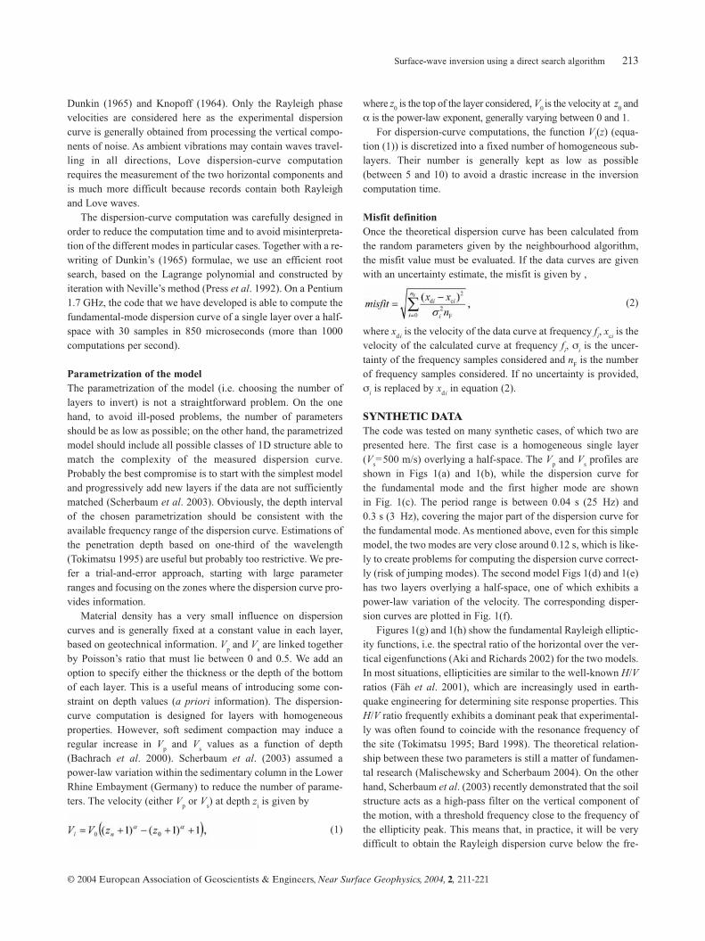
Material density has a very small influence on dispersioncurves and is generally fixed at a constant value in each layer,based on geotechnical information. Vp and Vs are linked togetherby Poisson’s ratio that must lie between 0 and 0.5. We add anoption to specify either the thickness or the depth of the bottomof each layer. This is a useful means of introducing some con-straint on depth values (a priori information). The dispersion-curve computation is designed for layers with homogeneousproperties. However, soft sediment compaction may induce aregular increase in Vp and Vs values as a function of depth(Bachrach et al. 2000). Scherbaum et al. (2003) assumed apower-law variation within the sedimentary column in the LowerRhine Embayment (Germany) to reduce the number of parame-ters. The velocity (either Vp or Vs) at depth zi is given by

(1)

where z0 is the top of the layer considered, V0 is the velocity at z0 andα is the power-law exponent, generally varying between 0 and 1.

For dispersion-curve computations, the function Vi(z) (equa-tion (1)) is discretized into a fixed number of homogeneous sub-layers. Their number is generally kept as low as possible(between 5 and 10) to avoid a drastic increase in the inversioncomputation time.

Misfit definitionOnce the theoretical dispersion curve has been calculated fromthe random parameters given by the neighbourhood algorithm,the misfit value must be evaluated. If the data curves are givenwith an uncertainty estimate, the misfit is given by ,

(2)

where xd i is the velocity of the data curve at frequency fi, xci is thevelocity of the calculated curve at frequency fi, σi is the uncer-tainty of the frequency samples considered and nF is the numberof frequency samples considered. If no uncertainty is provided,σi is replaced by xd i in equation (2).

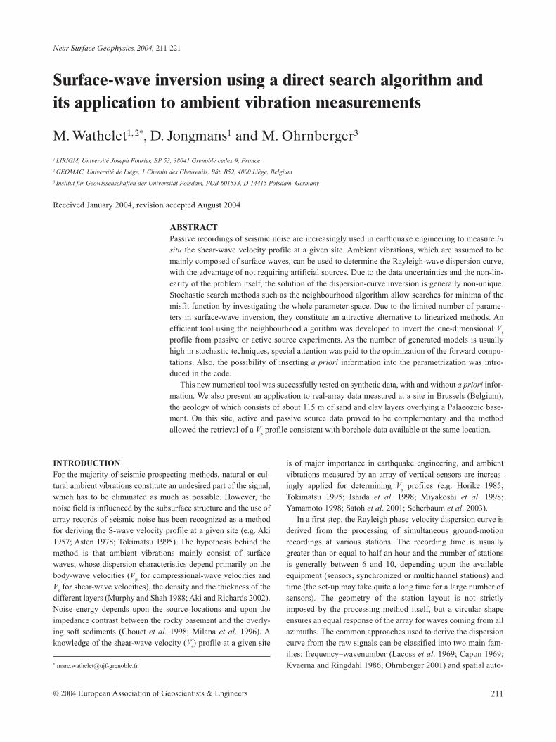
SYNTHETIC DATAThe code was tested on many synthetic cases, of which two arepresented here. The first case is a homogeneous single layer(Vs=500 m/s) overlying a half-space. The Vp and Vs profiles areshown in Figs 1(a) and 1(b), while the dispersion curve forthe fundamental mode and the first higher mode are shownin Fig. 1(c). The period range is between 0.04 s (25 Hz) and0.3 s (3 Hz), covering the major part of the dispersion curve forthe fundamental mode. As mentioned above, even for this simplemodel, the two modes are very close around 0.12 s, which is like-ly to create problems for computing the dispersion curve correct-ly (risk of jumping modes). The second model Figs 1(d) and 1(e)has two layers overlying a half-space, one of which exhibits apower-law variation of the velocity. The corresponding disper-sion curves are plotted in Fig. 1(f).

Figures 1(g) and 1(h) show the fundamental Rayleigh elliptic-ity functions, i.e. the spectral ratio of the horizontal over the ver-tical eigenfunctions (Aki and Richards 2002) for the two models.In most situations, ellipticities are similar to the well-known H/Vratios (Fäh et al. 2001), which are increasingly used in earth-quake engineering for determining site response properties. ThisH/V ratio frequently exhibits a dominant peak that experimental-ly was often found to coincide with the resonance frequency ofthe site (Tokimatsu 1995; Bard 1998). The theoretical relation-ship between these two parameters is still a matter of fundamen-tal research (Malischewsky and Scherbaum 2004). On the otherhand, Scherbaum et al. (2003) recently demonstrated that the soilstructure acts as a high-pass filter on the vertical component ofthe motion, with a threshold frequency close to the frequency ofthe ellipticity peak. This means that, in practice, it will be verydifficult to obtain the Rayleigh dispersion curve below the fre-

0 2000 4000Vp (m/s)

-40

-30

-20

-10

0

Dep

th (m

)

0 1000 2000Vs (m/s)

-40

-30

-20

-10

0

Dep

th (m

)

0.10 0.20Period (s)

0

400

800

1200

1600

Vel

ocit

y (m

/s)

0 2000 4000Vp (m/s)

-40

-30

-20

-10

0

Dep

th (m

)

0 1000 2000Vs (m/s)

-40

-30

-20

-10

0

Dep

th (m

)

0.10 0.20Period (s)

0

400

800

1200

1600

Vel

ocit

y (m

/s)

5 10 15 20 25Frequency (Hz)

-2

0

2

Log

10(E

llipt

icit

y)

5 10 15 20 25Frequency (Hz)

-0

1

2

3

4

Log

10(E

llipt

icit

y)

(a) (b) (c)

(d) (e) (f)

(g) (h)

0 2000 4000Vp (m/s)

0

10

20

30

40

Dep

th(m

)

0 1000 2000Vs (m/s)

0

10

20

30

40

Dep

th(m

)

0.10 0.20 0.30Period (s)

400

800

1200

1600

Vel

ocit

y(m

/s)

(a) (b) (c)

0 2000 4000Vp (m/s)

0

10

20

30

40

Dep

th(m

)

0 1000 2000Vs (m/s)

0

10

20

30

40

Dep

th(m

)

0.10 0.20 0.30Period (s)

400

800

1200

1600

Vel

ocit

y(m

/s)

(d) (e) (f)

Relative Misfit Value0.002 0.004 0.006 0.008 0.010 0.012

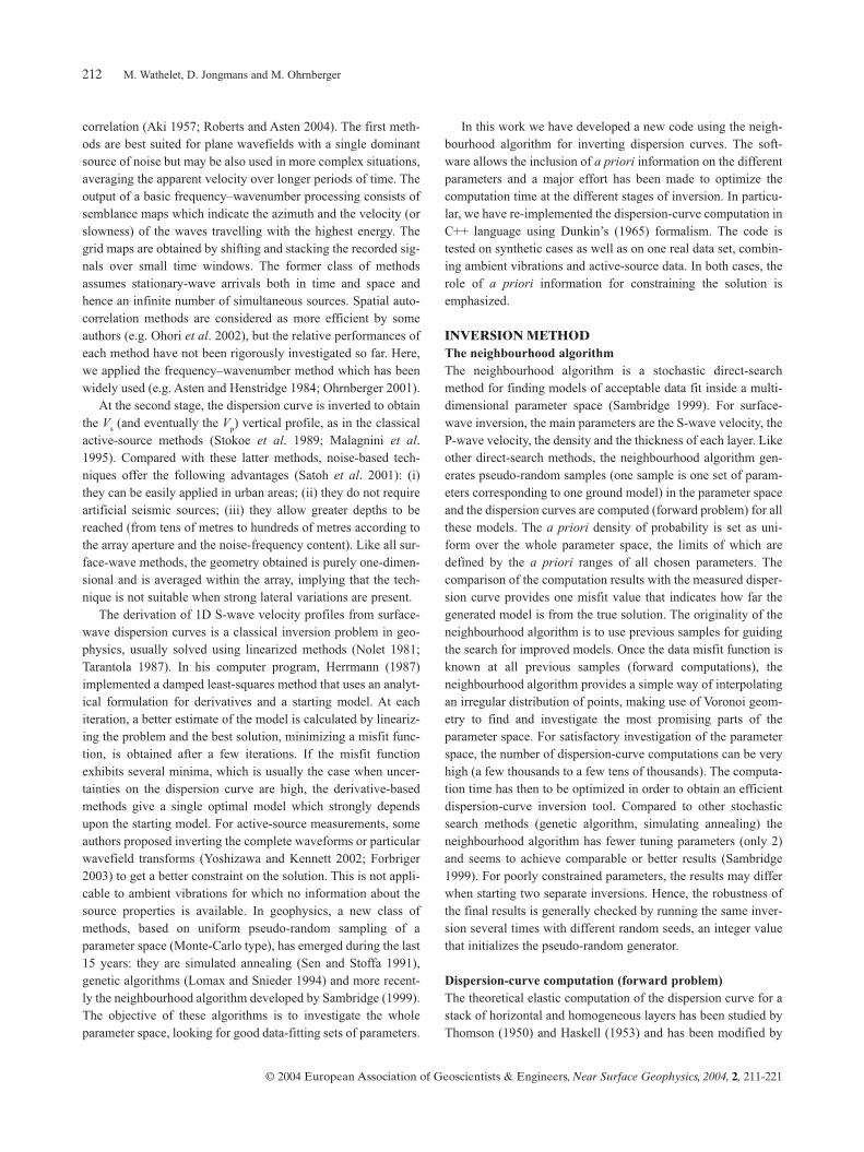
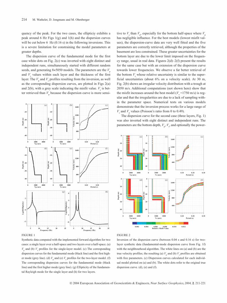
FIGURE 2

Inversion of the dispersion curve (between 0.04 s and 0.16 s) for two-

layer synthetic data (fundamental-mode dispersion curve from Fig. 1f)

with the neighbourhood algorithm. The white lines on (a) and (b) are the

true velocity profiles; the resulting (a) Vp and (b) Vs profiles are obtained

with free parameters. (c) Dispersion curves calculated for each individ-

ual model plotted on (a) and (b). The white dots refer to the original true

dispersion curve. (d), (e) and (f).



quency of the peak. For the two cases, the ellipticiy exhibits apeak around 6 Hz Figs 1(g) and 1(h) and the dispersion curveswill be cut below 6 Hz (0.16 s) in the following inversions. Thisis a severe limitation for constraining the model parameters atgreater depths.

The dispersion curve of the fundamental mode for the firstcase white dots on Fig. 2(c) was inverted with eight distinct andindependent runs, simultaneously started with different randomseeds, and generating 8×5050 models. The parameters are the Vp

and Vs values within each layer and the thickness of the firstlayer. The Vp and Vs profiles resulting from the inversion, as wellas the corresponding dispersion curves, are plotted in Figs 2(a)and 2(b), with a grey scale indicating the misfit value. Vs is bet-ter retrieved than Vp because the dispersion curve is more sensi-

tive to Vs than Vp, especially for the bottom half-space where Vp

has negligible influence. For the best models (lowest misfit val-ues), the dispersion-curve data are very well fitted and the fiveparameters are correctly retrieved, although the properties of thebasement are less constrained. These greater uncertainties for thebottom layer are due to the lower limit imposed on the frequen-cy range, usual in real data. Figures 2(d)–2(f) present the resultsfor the same case but with an extension of the dispersion curvetowards lower frequencies. We observe a far better retrieval ofthe bottom Vs whose relative uncertainty is similar to the super-ficial uncertainties (about 6% on a velocity scale). At 30 m, Fig. 2(b) shows an irregular velocity distribution with a trough at2050 m/s. Additional computations (not shown here) show thatthe misfit increases around the best model (Vs =1750 m/s) is reg-ular and that the irregularities are due to a lack of sampling with-in the parameter space. Numerical tests on various modelsdemonstrate that the inversion process works for a large range ofVs and Vp values (Poisson’s ratio from 0 to 0.49).

The dispersion curve for the second case (three layers, Fig. 1)was also inverted with eight distinct and independent runs. Theparameters are the bottom depth, Vp, Vs, and optionally the power-

FIGURE 1

Synthetic data computed with the implemented forward algorithm for two

cases: a single layer over a half-space and two layers over a half-space. (a)

Vp and (b) Vs profiles for the single-layer model. (c) The corresponding

dispersion curves for the fundamental mode (black line) and the first high-

er mode (grey line). (d) Vp and (e) Vs profiles for the two-layer model. (f)

The corresponding dispersion curves for the fundamental mode (black

line) and the first higher mode (grey line). (g) Ellipticity of the fundamen-

tal Rayleigh mode for the single layer and (h) for two layers.

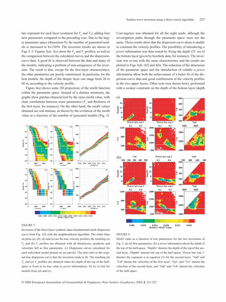
Convergence was obtained for all the eight seeds, although theinvestigation paths through the parameter space were not thesame. These results show that the dispersion curve alone is unableto constrain the velocity profiles. The possibility of introducing apriori information was then tested by fixing the depth (35 m) ofthe bottom layer (given by borehole data, for instance). The inver-sion was re-run with the same characteristics and the results areplotted in Figs 3(d)–3(f) and 4(b). The reduction of the dimensionof the parameter space and the introduction of reliable a prioriinformation allow both the achievement of a better fit of the dis-persion-curve data and good confinement of the velocity profilesin the two upper layers. Other tests (not shown here), performedwith a weaker constraint on the depth of the bottom layer (depth

law exponent for each layer (common for Vp and Vs), adding fournew parameters compared to the preceding case. Due to the larg-er parameter space (dimension 9), the number of generated mod-els is increased to 8×15050. The inversion results are shown inFigs 3–5. Figures 3(a)–3(c) show the Vp and Vs profiles, as well asthe comparison between the calculated curves and the dispersion-curve data. A good fit is observed between the data and many ofthe models, indicating a problem of non-uniqueness of the inver-sion. The result is that, except for the first-layer characteristics,the other parameters are poorly constrained. In particular, for thebest models, the depth of the deeper layer can range from 20 to60 m, according to the velocity profile.

Figure 4(a) shows some 2D projections of the misfit functionwithin the parameter space. Instead of a distinct minimum, thegraphs show patches characterized by the same misfit value, withclear correlations between some parameters (Vs and thickness ofthe first layer, for instance). On the other hand, the misfit valuesobtained are real minima, as shown by the evolution of the misfitvalue as a function of the number of generated models (Fig. 5).

0 2000 4000Vp (m/s)

-60

-50

-40

-30

-20

-10

0

Dep

th (m

)

0 1000 2000Vs (m/s)

-60

-50

-40

-30

-20

-10

0

Dep

th (m

)

0.04 0.06 0.08 0.10 0.12 0.14Period (s)

0

400

800

1200

1600

Vel

ocit

y (m

/s)

0 2000 4000Vp (m/s)

-60

-50

-40

-30

-20

-10

0

Dep

th (m

)

0 1000 2000Vs (m/s)

-60

-50

-40

-30

-20

-10

0

Dep

th (m

)

0.04 0.06 0.08 0.10 0.12 0.14Period (s)

0

400

800

1200

1600

Vel

ocit

y (m

/s)

(a) (b) (c)

(d) (e) (f)

Relative Misfit Value0.006 0.008 0.010 0.012 0.014 0.016 0.018 0.020 0.022 0.024 0.026

FIGURE 3

Inversion of the three-layer synthetic data (fundamental-mode dispersion

curve from Fig. 1(f) with the neighbourhood algorithm. The white lines

on plots (a), (b), (d) and (e) are the true velocity profiles; the resulting (a)

Vp and (b) Vs profiles are obtained with all thicknesses, gradients and

velocities left as free parameters. (c) Dispersion curves calculated for

each individual model plotted on (a) and (b). The dots refer to the origi-

nal true dispersion curve that the inversion tends to fit. The resulting (d)

Vp and (e) Vs profiles are obtained when the depth of the top of the half-

space is fixed at its true value (a priori information). (f) As (c) but for

models from (d) and (e).

FIGURE 4

Misfit value as a function of two parameters for the two inversions of

Fig. 3: (a) all free parameters; (b) a priori information about the depth of

the top of the half-space. ‘Depth1’ denotes the depth of the top of the sec-

ond layer, ‘Depth6’ denotes the top of the half-space, ‘Power law exp 1’

denotes the exponent α in equation (1) for the second layer, ‘Vp0’ and

‘Vs0’ denote the velocities of the first layer, ‘Vp1’ and ‘Vs1’ denote the

velocities of the second layer, and ‘Vp6’ and ‘Vs6’ denote the velocities

of the half-space.



4

8

12

16

Dep

th1

4

8

12

16

Dep

th1

100

200

300

400

500

Vs0

0.2 0.4

Power law exp 1

400

800

1200

Vs1

0.2 0.4

Power law exp 1

500

1000

1500

2000

Vp1

2000 4000

Vp6

1000

2000

3000

Vs6

100 200 300 400 500

Vs0

4

8

12

16

Dep

th1

0.2 0.4

Power law exp 1

4

8

12

16

Dep

th1

200 400 600 800

Vp0

100

200

300

400

500

Vs0

0.2 0.4

Power law exp 1

400

800

1200

Vs1

0.2 0.4

Power law exp 1

500

1000

1500

2000

Vp1

2000 4000

Vp6

1000

2000

3000

Vs6

(b)

Relative Misfit Value0.006 0.010 0.014 0.018 0.022 0.026

(a)



range between 32 m and 38 m), led to similar results. Looking atFig. 4(b), the introduction of the depth constraint permits a clearminimum to appear in the general shape of the misfit function.Also, good-fitting models with Vp values exceeding 4000 m/swere removed by the a priori information.

REAL DATAThe whole process of deriving velocity profiles from ambientvibration recordings was applied at a site located in the south ofBrussels, Belgium, inside the park of the Royal Observatory ofBelgium (50°47’56’’N-04°21’33’’E; Fig. 6(a). The topographyis almost flat and the soil structure mainly consists of a succes-sion of sand and clayey-sand horizontal layers overlying aPalaeozoic bedrock (the so-called Brabant Massif). The samestructure extends to the north-west towards the North Sea with aregular increase in the total thickness of the sediments corre-sponding to deepening of the Palaeozoic substratum (Nguyen et

0 4000 8000 12000Generated models

0.00

0.02

0.04

0.06

0.08

Min

imum

Mis

fit v

alue

-100 0 100West-East (m)

-100

0

100

Nor

th-S

outh

(m

)

(a)

(b)

(c)

FIGURE 5

Convergence history of the inversions of Figs 3(a)–3(c) and 4(a). The

parameter space representation has been constructed with eight inde-

pendent runs (distinct random seeds).

FIGURE 6

Location map for the real case, park of the Royal Observatory of Belgium in Uccle, Brussels (Belgium). (a) Regional map. (b) Site map including the

location of all the seismic stations. Six non-simultaneous arrays were recorded: ‘radius 130’ (large dark-grey circles), ‘radii 25-75-130’ (large light-grey

triangles), ‘radius 100’ (empty circles), ‘radius 50’ (empty squares) and ‘radius 25’ (crosses) (c) Borehole description.



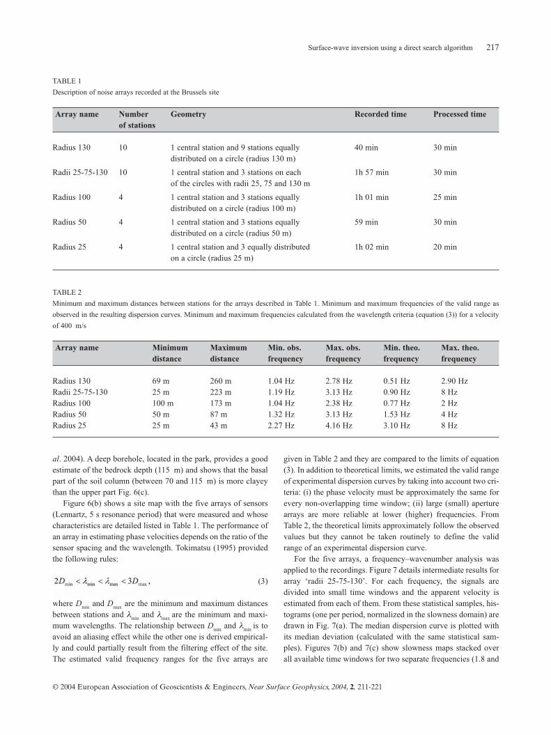
al. 2004). A deep borehole, located in the park, provides a goodestimate of the bedrock depth (115 m) and shows that the basalpart of the soil column (between 70 and 115 m) is more clayeythan the upper part Fig. 6(c).

Figure 6(b) shows a site map with the five arrays of sensors(Lennartz, 5 s resonance period) that were measured and whosecharacteristics are detailed listed in Table 1. The performance ofan array in estimating phase velocities depends on the ratio of thesensor spacing and the wavelength. Tokimatsu (1995) providedthe following rules:

(3)

where Dmin and Dmax are the minimum and maximum distancesbetween stations and λmin and λmax are the minimum and maxi-mum wavelengths. The relationship between Dmin and λmin is toavoid an aliasing effect while the other one is derived empirical-ly and could partially result from the filtering effect of the site.The estimated valid frequency ranges for the five arrays are

given in Table 2 and they are compared to the limits of equation(3). In addition to theoretical limits, we estimated the valid rangeof experimental dispersion curves by taking into account two cri-teria: (i) the phase velocity must be approximately the same forevery non-overlapping time window; (ii) large (small) aperturearrays are more reliable at lower (higher) frequencies. FromTable 2, the theoretical limits approximately follow the observedvalues but they cannot be taken routinely to define the validrange of an experimental dispersion curve.

For the five arrays, a frequency–wavenumber analysis wasapplied to the recordings. Figure 7 details intermediate results forarray ‘radii 25-75-130’. For each frequency, the signals aredivided into small time windows and the apparent velocity isestimated from each of them. From these statistical samples, his-tograms (one per period, normalized in the slowness domain) aredrawn in Fig. 7(a). The median dispersion curve is plotted withits median deviation (calculated with the same statistical sam-ples). Figures 7(b) and 7(c) show slowness maps stacked over all available time windows for two separate frequencies (1.8 and

TABLE 1

Description of noise arrays recorded at the Brussels site

Array name Number Geometry Recorded time Processed timeof stations

Radius 130 10 1 central station and 9 stations equally 40 min 30 mindistributed on a circle (radius 130 m)

Radii 25-75-130 10 1 central station and 3 stations on each 1h 57 min 30 minof the circles with radii 25, 75 and 130 m

Radius 100 4 1 central station and 3 stations equally 1h 01 min 25 mindistributed on a circle (radius 100 m)

Radius 50 4 1 central station and 3 stations equally 59 min 30 mindistributed on a circle (radius 50 m)

Radius 25 4 1 central station and 3 equally distributed 1h 02 min 20 minon a circle (radius 25 m)

TABLE 2

Minimum and maximum distances between stations for the arrays described in Table 1. Minimum and maximum frequencies of the valid range as

observed in the resulting dispersion curves. Minimum and maximum frequencies calculated from the wavelength criteria (equation (3)) for a velocity

of 400 m/s

Array name Minimum Maximum Min. obs. Max. obs. Min. theo. Max. theo.distance distance frequency frequency frequency frequency

Radius 130 69 m 260 m 1.04 Hz 2.78 Hz 0.51 Hz 2.90 HzRadii 25-75-130 25 m 223 m 1.19 Hz 3.13 Hz 0.90 Hz 8 HzRadius 100 100 m 173 m 1.04 Hz 2.38 Hz 0.77 Hz 2 HzRadius 50 50 m 87 m 1.32 Hz 3.13 Hz 1.53 Hz 4 HzRadius 25 25 m 43 m 2.27 Hz 4.16 Hz 3.10 Hz 8 Hz



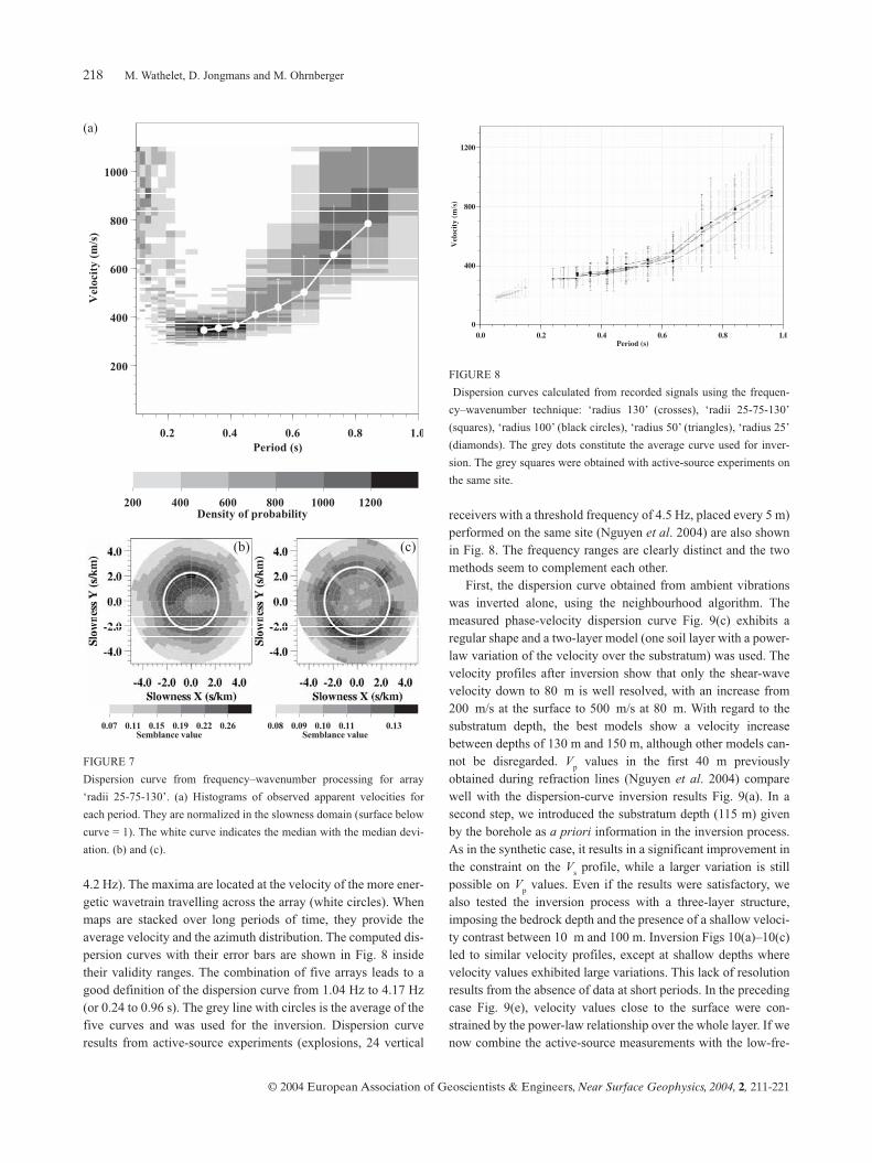
4.2 Hz). The maxima are located at the velocity of the more ener-getic wavetrain travelling across the array (white circles). Whenmaps are stacked over long periods of time, they provide theaverage velocity and the azimuth distribution. The computed dis-persion curves with their error bars are shown in Fig. 8 insidetheir validity ranges. The combination of five arrays leads to agood definition of the dispersion curve from 1.04 Hz to 4.17 Hz(or 0.24 to 0.96 s). The grey line with circles is the average of thefive curves and was used for the inversion. Dispersion curveresults from active-source experiments (explosions, 24 vertical

receivers with a threshold frequency of 4.5 Hz, placed every 5 m)performed on the same site (Nguyen et al. 2004) are also shownin Fig. 8. The frequency ranges are clearly distinct and the twomethods seem to complement each other.

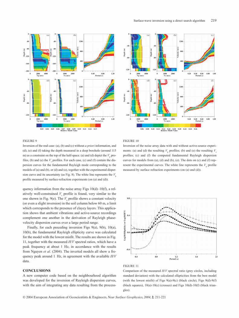
First, the dispersion curve obtained from ambient vibrationswas inverted alone, using the neighbourhood algorithm. Themeasured phase-velocity dispersion curve Fig. 9(c) exhibits aregular shape and a two-layer model (one soil layer with a power-law variation of the velocity over the substratum) was used. Thevelocity profiles after inversion show that only the shear-wavevelocity down to 80 m is well resolved, with an increase from200 m/s at the surface to 500 m/s at 80 m. With regard to thesubstratum depth, the best models show a velocity increasebetween depths of 130 m and 150 m, although other models can-not be disregarded. Vp values in the first 40 m previouslyobtained during refraction lines (Nguyen et al. 2004) comparewell with the dispersion-curve inversion results Fig. 9(a). In asecond step, we introduced the substratum depth (115 m) givenby the borehole as a priori information in the inversion process.As in the synthetic case, it results in a significant improvement inthe constraint on the Vs profile, while a larger variation is stillpossible on Vp values. Even if the results were satisfactory, wealso tested the inversion process with a three-layer structure,imposing the bedrock depth and the presence of a shallow veloci-ty contrast between 10 m and 100 m. Inversion Figs 10(a)–10(c)led to similar velocity profiles, except at shallow depths wherevelocity values exhibited large variations. This lack of resolutionresults from the absence of data at short periods. In the precedingcase Fig. 9(e), velocity values close to the surface were con-strained by the power-law relationship over the whole layer. If wenow combine the active-source measurements with the low-fre-

Density of probability200 400 600 800 1000 1200

0.2 0.4 0.6 0.8 1.0Period (s)

200

400

600

800

1000

Vel

ocit

y(m

/s)

Semblance value0.07 0.11 0.15 0.19 0.22 0.26

Semblance value0.08 0.09 0.10 0.11 0.13

(b) (c)

0.0 0.2 0.4 0.6 0.8 1.0Period (s)

0

400

800

1200

Vel

ocit

y (m

/s)

FIGURE 7

Dispersion curve from frequency–wavenumber processing for array

‘radii 25-75-130’. (a) Histograms of observed apparent velocities for

each period. They are normalized in the slowness domain (surface below

curve = 1). The white curve indicates the median with the median devi-

ation. (b) and (c).

FIGURE 8

Dispersion curves calculated from recorded signals using the frequen-

cy–wavenumber technique: ‘radius 130’ (crosses), ‘radii 25-75-130’

(squares), ‘radius 100’ (black circles), ‘radius 50’ (triangles), ‘radius 25’

(diamonds). The grey dots constitute the average curve used for inver-

sion. The grey squares were obtained with active-source experiments on

the same site.

(a)



quency information from the noise array Figs 10(d)–10(f), a rel-atively well-constrained Vs profile is found, very similar to theone shown in Fig. 9(e). The Vs profile shows a constant velocity(or even a slight inversion) in the soil column below 60 m, a limitwhich corresponds to the presence of clayey layers. This applica-tion shows that ambient vibrations and active-source recordingscomplement one another in the derivation of Rayleigh phase-velocity dispersion curves over a large period range.

Finally, for each preceding inversion Figs 9(a), 9(b), 10(a),10(b), the fundamental Rayleigh ellipticity curve was calculatedfor the model with the lowest misfit. The results are shown in Fig.11, together with the measured H/V spectral ratios, which have apeak frequency at about 1 Hz, in accordance with the resultsfrom Nguyen et al. (2004). The inverted models all show a fre-quency peak around 1 Hz, in agreement with the available H/Vdata.

CONCLUSIONSA new computer code based on the neighbourhood algorithmwas developed for the inversion of Rayleigh dispersion curves,with the aim of integrating any data resulting from the process-

0.4 0.8 1.2 1.6 2.0Period (s)

-0.4

0.0

0.4

0.8

Log

10(E

llipt

icit

y) o

r L

og10

(H/V

)

0 2000 4000Vp (m/s)

-200

-160

-120

-80

-40

0

Dep

th (m

)

0 1000 2000Vs (m/s)

-200

-160

-120

-80

-40

0

Dep

th (m

)

0.40 0.80 1.20Period (s)

0

400

800

1200

Vel

ocit

y (m

/s)

0 2000 4000Vp (m/s)

-120

-80

-40

0

Dep

th (m

)

0 1000 2000Vs (m/s)

-120

-80

-40

0

Dep

th (m

)

0.40 0.80 1.20Period (s)

0

400

800

1200

Vel

ocit

y (m

/s)

(a) (b) (c)

(d) (e) (f)


0 2000 4000Vp (m/s)

-120

-80

-40

0

Dep

th (m

)

0 1000 2000Vs (m/s)

-120

-80

-40

0

Dep

th (m

)

0.20 0.40 0.60 0.80 1.00Period (s)

0

400

800

1200

Vel

ocit

y (m

/s)

0 2000 4000Vp (m/s)

-120

-80

-40

0

Dep

th (m

)

0 1000 2000Vs (m/s)

-120

-80

-40

0

Dep

th (m

)

0.20 0.40 0.60 0.80 1.00Period (s)

0

400

800

1200

Vel

ocit

y (m

/s)

(a) (b) (c)

(d) (e) (f)


FIGURE 11

Comparison of the measured H/V spectral ratio (grey circles, including

standard deviation) with the calculated ellipticities from the best model

(with the lowest misfit) of Figs 9(a)-9(c) (black circle), Figs 9(d)-9(f)

(black squares), 10(a)-10(c) (crosses) and Figs 10(d)-10(f) (black trian-

gles).

FIGURE 9

Inversion of the real case: (a), (b) and (c) without a priori information, and

(d), (e) and (f) taking the depth measured in a deep borehole (around 115

m) as a constraint on the top of the half-space. (a) and (d) depict the Vp pro-

files, (b) and (e) the Vs profiles. For each case, (c) and (f) contain the dis-

persion curves for the fundamental Rayleigh mode corresponding to the

models of (a) and (b), or (d) and (e), together with the experimental disper-

sion curve and its uncertainty (as Fig. 8). The white line represents the Vp

profile measured by surface-refraction experiments (on (a) and (d)).

FIGURE 10

Inversion of the noise array data with and without active-source experi-

ments: (a) and (d) the resulting Vp profiles; (b) and (e) the resulting Vs

profiles; (c) and (f) the computed fundamental Rayleigh dispersion

curves for models from (a), (d) and (b), (e). The dots on (c) and (f) rep-

resent the experimental curves. The white line represents the Vp profile

measured by surface refraction experiments (on (a) and (d)).



ing of active-source experiments or ambient-noise recordings.Much effort was devoted to the optimization of the computationtime, particularly in the calculation of the dispersion curve, asthousands of models have to be computed. A flexible parame-trization, including a velocity variation inside the layers, hascontributed to the reduction in the number of parameters, allow-ing a better investigation of the parameter space with a direct-search algorithm such as the neighbourhood algorithm. The soft-ware was also designed to allow the introduction of a prioriinformation.

The method was successfully tested on several synthetic datasets, two of which have been presented here. These tests showedthe efficiency of the developed tool and the limits of the dispersion-curve inversion alone. The introduction of a priori informationwhen available is of major importance in constraining the solution.

The real-case analysis also proved the applicability and thereliability of the method. The introduction of borehole data(depth of the substratum) also considerably improved the results.

Combining active and passive seismic sources proved to bevery helpful at the Brussels site, allowing Vs values to be obtaineddown to the bedrock, located at more than 100 m depth. The inver-sion led to a velocity profile which agrees with the borehole log.

In the future, we plan to introduce into the inversion the peakfrequencies of the ellipticity, which were found to constrain thelayer thickness in the case of the single layer over a half-space(Scherbaum et al. 2003) and could supplement borehole datawhen they are not available.

ACKNOWLEDGEMENTSWe are grateful to Frank Scherbaum for sharing his experienceand his software for noise processing. Daniel Vollmer, HansHavenith, Thierry Camelbeek and the team of the RoyalObservatory of Belgium are acknowledged for their support dur-ing field experiments. We also thank M. Sambridge who allowsthe free distribution of his inversion code for research purposes.This study was made possible through the support of theSESAME European project (“Site EffectS assessment usingAMbient Excitation”, Project EVG1-CT-2000-00026).

REFERENCESAki K. 1957. Space and time spectra of stationary stochastic waves, with

special reference to microtremors. Bulletin of the EarthquakeResearch Institute 35, 415–456.

Aki K. and Richards P.G. 2002. Quantitative Seismology. 2nd edition,University Science Books.

Asten M.W. 1978. Geological control on the three-component spectra ofRayleigh-wave microseism. Bulletin of the Seismological Society ofAmerica 68, 1623–1636.

Asten M.W. and Henstridge J.D.1984. Array estimators and use of micro-seisms for reconnaissance of sedimentary basins. Geophysics 49,1828-1837.

Bachrach R., Dvorkin J. and Nur M.A. 2000. Seismic velocities andPoisson’s ratio of shallow unconsolidated sands. Geophysics 65,559–564.

Bard P.-Y. 1998. Microtremor measurements: A tool for site effect esti-mation? In: The Effect of Surface Geology on Seismic Motion (edsIrikura, Kudo, Osaka and Sasatani). Balkema.

Capon J. 1969. High-resolution frequency-wavenumber spectrum analy-sis. Proceedings of the IEEE 57, 1408–1418.

Chouet B., De Luca G., Milana G., Dawson P., Martini M. and Scarpa R.1998. Shallow velocity structure of Stromboli Volcano, Italy, derivedfrom small-aperture array measurements of strombolian tremor.Bulletin of the Seismological Society of America 88, 653–666.

Dunkin J.W. 1965. Computation of modal solutions in layered, elasticmedia at high frequencies. Bulletin of the Seismological Society ofAmerica 55, 335–358.

Fäh D., Kind F. and Giardini D. 2001. A theoretical investigation of ave-rage H/V ratios, Geophysical Journal International 145, 535–549.

Forbriger T. 2003. Inversion of shallow-seismic wavefields. Part 2:Infering subsurface properties from wavefield transforms.Geophysical Journal International 153, 735–752.

Haskell N.A. 1953. The dispersion of surface waves on a multi-layeredmedium. Bulletin of the Seismological Society of America 43, 17–34.

Herrmann R.B. 1987. Computer Programs in Seismology. St LouisUniversity.

Horike M. 1985. Inversion of phase velocity of long-periodmicrotremors to the S-wave-velocity structure down to the basementin urbanized areas. Journal of Physics of the Earth 33, 59–96.

Ishida H., Nozawa T. and Niwa M. 1998. Estimation of deep surfacestructure based on phase velocities and spectral ratios of long-periodmicrotremors. 2nd International Symposium on the Effect of SurfaceGeology on Seismic Motion, Yokohama, Japan, 2, pp. 697–704.

Knopoff L. 1964. A matrix method for elastic wave problems. Bulletin ofthe Seismological Society of America 54, 431–438.

Kvaerna T. and Ringdahl F. 1986. Stability of various fk-estimation tech-niques. In: Semiannual Technical Summary, 1 October 1985 – 31March 1986, NORSAR Scientific Report, 1-86/87, Kjeller, Norway,pp. 29–40.

Lacoss R.T., Kelly E.J. and Toksöz M.N. 1969. Estimation of seismicnoise structure using arrays. Geophysics 34, 21–38.

Lomax A.J. and Snieder R. 1994. Finding sets of acceptable solutionswith a genetic algorithm with application to surface wave group dis-persion in Europe. Geophysical Research Letters 21, 2617–2620.

Malagnini L., Herrmann R.B., Biella G. and de Franco R. 1995. Rayleighwaves in Quaternary alluvium from explosive sources: determinationof shear-wave velocity and Q structure. Bulletin of the SeismologicalSociety of America 85, 900–922.

Malischewsky P.G. and F. Scherbaum. 2004. Love’s formula and H/V-ratio (ellipticity) of Rayleigh waves, Wave Motion 40, 50–67

Milana G., Barba S., Del Pezzo E. and Zambonelli E. 1996. Site responsefrom ambient noise measurements: new perspectives from an arraystudy in Central Italy. Bulletin of the Seismological Society of America86, 320–328.

Miyakoshi K., Kagawa T. and Kinoshita S. 1998. Estimation of geologi-cal structures under the Kobe area using the array recordings ofmicrotremors. 2nd International Symposium on the Effect of SurfaceGeology on Seismic Motion, Yokohama, Japan, 2, pp. 691–696.

Murphy J.R. and Shah H.K. 1988. An analysis of the effects of site geol-ogy on the characteristics of near-field Rayleigh waves. Bulletin of theSeismological Society of America 78, 64–82.

Nguyen F., Van Rompaey G., Teerlynck H., van Camp M., Jongmans D.and Camelbeeck T. 2004. Use of microtremor measurement for assess-ing site effects in Northern Belgium interpretation of the observedintensity during the MS= 5.0 June 11 1938 earthquake. Journal ofSeismology 8, 41–56.

Nolet G. 1981. Linearized inversion of (teleseismic) data. In: TheSolution of the Inverse Problem in Geophysical Interpretation (ed. R.Cassinis), pp. 9–37. Plenum Press.



Ohori M., Nobata A. and Wakamatsu K. 2002. A comparison of ESACand FK methods of estimating phase velocity using arbitrarily shapedmicrotremor arrays. Bulletin of the Seismological Society of America92, 2323–2332.

Ohrnberger M. 2001. Continuous automatic classification of seismic sig-nals of volcanic origin at Mt Merapi, Java, Indonesia. Dissertation,University of Potsdam.

Press W.H., Teukolsky S.A., Vetterling W.T. and Flannery B.P. 1992.Numerical Recipes in Fortran, 2nd edition. Cambridge UniversityPress.

Roberts J.C. and Asten M.W. 2004. Resolving a velocity inversion at thegeotechnical scale using the microtremor (passive seismic) surveymethod. Exploration Geophysics 35, 14–18.

Sambridge M. 1999. Geophysical inversion with a neighbourhood algo-rithm I. Searching a parameter space. Geophysical JournalInternational 103, 4839–4878.

Satoh T., Kawase H. and Matsushima S.I. 2001. Differences between sitecharacteristics obtained from microtremors, S-waves, P-waves, andcodas. Bulletin of the Seismological Society of America 91, 313–334.

Scherbaum F., Hinzen K.-G. and Ohrnberger M. 2003. Determination ofshallow shear wave velocity profiles in the Cologne/Germany areausing ambient vibrations. Geophysical Journal International 152,597–612.

Sen M.K. and Stoffa P.L. 1991. Nonlinear one-dimensional seismicwaveform inversion using simulated annealing. Geophysics 56,1624–1638.

Stokoe K.H.II, Rix G.J. and Nazarian S. 1989. In situ seismic testingwith surface waves. Proceedings of the XII International Conferenceon Soil Mechanics and Foundation Engineering, pp. 331–334.

Tarantola A. 1987. Inverse Problem Theory. Elsevier Science PublishingCo.

Thomson W.T. 1950. Transmission of elastic waves through a stratifiedsolid medium. Journal of Applied Physics 21, 89–93.

Tokimatsu K. 1995. Geotechnical site characterization using surfacewaves. In: Earthquake Geotechnical Engineering (ed.Ishihara), pp.1333–1368. Balkema, Rotterdam.

Yamamoto H. 1998. An experiment for estimating S-wave velocity struc-ture from phase velocities of Love and Rayleigh waves inmicrotremors. 2nd International Symposium on the Effect of SurfaceGeology on Seismic Motion, Yokohama, Japan, 2, pp. 705–710.

Yoshizawa K. and Kennett B.L.N. 2002. Non-linear waveform inversionfor surface waves with a neighbourhood algorithm – application tomultimode dispersion measurements. Geophysical JournalInternational 149, 118–133.

Surface-wave inversion using a direct search algorithm and its application to ambient vibration...

Documents

Transcript of Surface-wave inversion using a direct search algorithm and its application to ambient vibration...