Supporting Top-K Keyword Search in XMLDatabases

Liang Jeff Chen, Yannis Papakonstantinou

Department of Computer Science and Engineering , UCSDLa Jolla, CA, US

{jeffchen,yannis}@cs.ucsd.edu

Abstract— Keyword search is considered to be an effectiveinformation discovery method for both structured and semi-structured data. In XML keyword search, query semanticsis based on the concept of Lowest Common Ancestor (LCA).However, naive LCA-based semantics leads to exponential com-putation and result size. In the literature, LCA-based semanticvariants (e.g., ELCA and SLCA) were proposed, which definea subset of all the LCAs as the results. While most existingwork focuses on algorithmic efficiency, top-K processing for XMLkeyword search is an important issue that has received verylittle attention. Existing algorithms focusing on efficiency aredesigned to optimize the semantic pruning and are incapable ofsupporting top-K processing. On the other hand, straightforwardapplications of top-K techniques from other areas (e.g., relationaldatabases) generate LCAs that may not be the results andunnecessarily expand efforts in the semantic pruning. In thispaper, we propose a series of join-based algorithms that combinethe semantic pruning and the top-K processing to support top-Kkeyword search in XML databases. The algorithms essentiallyreduce the keyword query evaluation to relational joins, andincorporate the idea of the top-K join from relational databases.Extensive experimental evaluations show the performance advan-tages of our algorithms.

I. INTRODUCTION

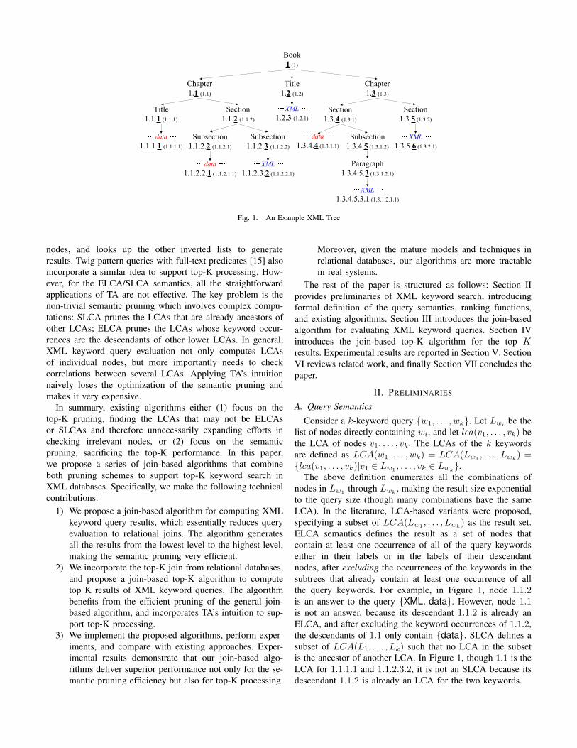
Keyword search is considered to be an effective informationdiscovery method for structured and semi-structured data[1], [2], [3], [4], [5], [6], [7]. It allows users without priorknowledge of schema and query languages to search. In XMLkeyword search, the results of a keyword query are no longerentire XML documents, but instead are XML elements thatcontain all the keywords. The intuition is that keywords maybe found over multiple elements. The LCA of these elementscontains all the keywords and thus can be a result. Considerthe keyword query {XML, data} over the XML documentof Figure 1. Nodes 1.1.2.2.1 and 1.1.2.3.2 contain the twokeywords, and node 1.1.2 is their lowest common ancestor.So the subtree rooted at 1.1.2 contains all the keywords andis expected to be the result.

The naive LCA-based semantics is straightforward, butleads to exponential computation and result size. Considertwo lists of nodes Lxml = {u1, u2, . . . , um} and Ldata ={v1, v2, . . . , vn} containing two keywords {XML} and {data}respectively. For any pair of ui, i ∈ [1,m] and vj , j ∈ [1, n],there exists an LCA for them in the XML tree. In other words,for this two-keyword query, the total number of the LCAs is

This research was supported by NSF IIS award 0713672

m × n. More generally, for the naive LCA-based semantics,the result size is exponential to the query size, though manypairs may share the same LCA.

The several LCA-based semantic variants that have beenproposed specify a subset of the m× n LCAs as the results.The most widely followed variants are ELCA [5], [8] andSLCA [6], [9], [10], [11], [12]. The algorithmic challengeof the semantic variants is to achieve the pruning withoutcomputing all the LCAs. Most existing work [5], [8], [6], [9],[11] focuses on this topic, addressing how to answer keywordqueries efficiently. The main idea is utilizing the documentorder of XML elements to pre-prune LCAs so that resultcandidate space is largely reduced.

While query semantics and algorithm efficiency have beenwidely discussed, top-K keyword search in XML databases isan important issue that very little work has concentrated on. Asis typical in the keyword search systems, a ranking functioncan be defined [5], [13] to assign to results ranking scores,and ranked results are returned to users. Top-K processingaims to compute the results with highest scores first so thatexecution can terminate earlier after the top K results havebeen generated.

Existing algorithms focusing on efficiency cannot provideeffective support for top-K processing. These algorithms sharesome common characteristics: inverted lists are sorted by thedocument order. At least one list is scanned sequentially.This behavior determines that results are generated in thedocument order, rather than the order of ranking scores. Allthe results must be generated in order to return the top Kresults. Essentially, these algorithms are designed to optimizethe semantic pruning, and are incapable of supporting top-Kprocessing.

Top-K processing is not a new problem, and has beenextensively studied in other areas, e.g., information retrievaland relational databases. Among the proposed algorithms,the Threshold Algorithm (TA) [14] is the most well-knowninstance. Given a set of ranked inputs and an aggregation func-tion that aggregates local scores from individual inputs, TAmatches results from individual inputs and computes a scorethreshold for unseen results. Generated results whose scoresare greater than the threshold are output without blocking.

A straightforward application of TA in XML keywordsearch appears in RDIL [5]. It iteratively reads new nodes fromone keyword list sorted by the ranking scores of individual

Book

1 (1)

Chapter

1.1 (1.1)

Title

1.2 (1.2)

Chapter

1.3 (1.3)

Title

1.1.1 (1.1.1)

Section

1.1.2 (1.1.2)

Subsection

1.1.2.2 (1.1.2.1)

Subsection

1.1.2.3 (1.1.2.2)

data

1.1.2.2.1 (1.1.2.1.1)

XML

1.1.2.3.2 (1.1.2.2.1)

XML

1.2.3 (1.2.1)

data

1.3.4.4 (1.3.1.1)

Section

1.3.4 (1.3.1)

Section

1.3.5 (1.3.2)

Subsection

1.3.4.5 (1.3.1.2)

XML

1.3.5.6 (1.3.2.1)

XML

1.3.4.5.3.1 (1.3.1.2.1.1)

Paragraph

1.3.4.5.3 (1.3.1.2.1)

data

1.1.1.1 (1.1.1.1)

Fig. 1. An Example XML Tree

nodes, and looks up the other inverted lists to generateresults. Twig pattern queries with full-text predicates [15] alsoincorporate a similar idea to support top-K processing. How-ever, for the ELCA/SLCA semantics, all the straightforwardapplications of TA are not effective. The key problem is thenon-trivial semantic pruning which involves complex compu-tations: SLCA prunes the LCAs that are already ancestors ofother LCAs; ELCA prunes the LCAs whose keyword occur-rences are the descendants of other lower LCAs. In general,XML keyword query evaluation not only computes LCAsof individual nodes, but more importantly needs to checkcorrelations between several LCAs. Applying TA’s intuitionnaively loses the optimization of the semantic pruning andmakes it very expensive.

In summary, existing algorithms either (1) focus on thetop-K pruning, finding the LCAs that may not be ELCAsor SLCAs and therefore unnecessarily expanding efforts inchecking irrelevant nodes, or (2) focus on the semanticpruning, sacrificing the top-K performance. In this paper,we propose a series of join-based algorithms that combineboth pruning schemes to support top-K keyword search inXML databases. Specifically, we make the following technicalcontributions:

1) We propose a join-based algorithm for computing XMLkeyword query results, which essentially reduces queryevaluation to relational joins. The algorithm generatesall the results from the lowest level to the highest level,making the semantic pruning very efficient.

2) We incorporate the top-K join from relational databases,and propose a join-based top-K algorithm to computetop K results of XML keyword queries. The algorithmbenefits from the efficient pruning of the general join-based algorithm, and incorporates TA’s intuition to sup-port top-K processing.

3) We implement the proposed algorithms, perform exper-iments, and compare with existing approaches. Exper-imental results demonstrate that our join-based algo-rithms deliver superior performance not only for the se-mantic pruning efficiency but also for top-K processing.

Moreover, given the mature models and techniques inrelational databases, our algorithms are more tractablein real systems.

The rest of the paper is structured as follows: Section IIprovides preliminaries of XML keyword search, introducingformal definition of the query semantics, ranking functions,and existing algorithms. Section III introduces the join-basedalgorithm for evaluating XML keyword queries. Section IVintroduces the join-based top-K algorithm for the top Kresults. Experimental results are reported in Section V. SectionVI reviews related work, and finally Section VII concludes thepaper.

II. PRELIMINARIES

A. Query Semantics

Consider a k-keyword query {w1, . . . , wk}. Let Lwi be thelist of nodes directly containing wi, and let lca(v1, . . . , vk) bethe LCA of nodes v1, . . . , vk. The LCAs of the k keywordsare defined as LCA(w1, . . . , wk) = LCA(Lw1 , . . . , Lwk

) ={lca(v1, . . . , vk)|v1 ∈ Lw1 , . . . , vk ∈ Lwk

}.The above definition enumerates all the combinations of

nodes in Lw1 through Lwk, making the result size exponential

to the query size (though many combinations have the sameLCA). In the literature, LCA-based variants were proposed,specifying a subset of LCA(Lw1 , . . . , Lwk

) as the result set.ELCA semantics defines the result as a set of nodes thatcontain at least one occurrence of all of the query keywordseither in their labels or in the labels of their descendantnodes, after excluding the occurrences of the keywords in thesubtrees that already contain at least one occurrence of allthe query keywords. For example, in Figure 1, node 1.1.2is an answer to the query {XML, data}. However, node 1.1is not an answer, because its descendant 1.1.2 is already anELCA, and after excluding the keyword occurrences of 1.1.2,the descendants of 1.1 only contain {data}. SLCA defines asubset of LCA(L1, . . . , Lk) such that no LCA in the subsetis the ancestor of another LCA. In Figure 1, though 1.1 is theLCA for 1.1.1.1 and 1.1.2.3.2, it is not an SLCA because itsdescendant 1.1.2 is already an LCA for the two keywords.

The pruning schemes of ELCA and SLCA are non-trivialand algorithmically complex. Given one combination of nodesv1 ∈ L1, . . . , vk ∈ Lk and their LCA u = lca(v1, . . . , vk),whether u is the result or not may be determined by anothercombination v

′1 ∈ L1, . . . , v

′k ∈ Lk: if u is the ancestor of

lca(v′1, . . . , v

′k), then u is not the SLCA; if u is the ancestor

of lca(v′1, . . . , v

′k) and ∃i such that vi = v

′i, then u is not

the ELCA. Efficient algorithms must optimize the semanticpruning to avoid not only enumerating all the combinationsbut also checking the correlations of all the LCAs in theLCA(L1, . . . , Lk) space.

B. Ranking Function

XML contains abundant textual contents and structure in-formation. How to rank XML keyword queries incorporatingboth of them is an interesting problem that has been studiedin the literature, e.g. [5], [13], [16], [17]. Since this paper onlyfocuses on the algorithmic perspective, in this subsection, weonly introduce one ranking function that is widely adopted inthe XML keyword search scenario. Notice that the algorithmswe propose in this paper are not restricted to this function.

The basic idea of ranking keyword query results is thatindividual nodes directly containing the keywords can beviewed as “documents”. Local ranking scores are given basedon the “documents”, and are propagated to their ELCA orSLCA. An aggregation function aggregates them into a globalscore which is the final ranking score of the result subtree.

Given a node v and a keyword w, g(v, w) is a function thatassigns to v a local ranking score. The function g can takemultiple factors into account (e.g., IR score that evaluates thecontent relevance and link-based score that evaluates the globalimportance of the node), and combine them in an arbitraryway.

Consider the k-keyword query {w1, . . . , wk}. Let vi, i =1, . . . , k, be an occurrence of wi at depth li, and let node u atdepth l̃ be the ELCA/SLCA of vi’s. Let F (·) be the functionthat combines g(vi, wi), i = 1, . . . , k, with damping factorsinto a score of u:

score(u) = F (I1, . . . , Ik),

where Ii = g(vi, wi) × d(li − l̃), i = 1, . . . , k, and d(·) is adecreasing function.

The combining function F (·) is expected to satisfy thefollowing property:

Monotonicity Let u and u′

be two ELCAs/SLCAs for thek-keyword query. If ∀i ∈ [1, k], Ii ≤ I

′i , then score(u) ≤

score(u′).

Monotonicity is the assumption on which most top-Kprocessing algorithms are based. It is also true for mostexisting ranking functions of XML keyword search. For easeof exposition, we simply assume that F (·) is the sum function,i.e., score(u) =

∑ki=1 g(vi, wi)× d(li − l̃).

The function d(·) decreases the score of the keyword occur-rence as its vertical distance to the ELCA/SLCA increases. Itreflects the intuition that compact subtrees are more importantbecause of the tighter relationship between keywords. Similar

intuition is also reflected in information retrieval [18]: forthe documents that contain all the keywords, if the keywordoccurrences in a document are within a short distance, thatdocument’s score tends to be higher than the documents whosekeyword occurrences are far away.

If the ELCA/SLCA contains more than one occurrences ofwj , i.e., vj

1, . . . , vjm, F (·) only takes the maximum score (after

applying the damping factor) of the occurrences as the input,i.e., max{g(vj

1, wj)× d(lj1 − l̃), . . . , g(vjm, wj)× d(ljm − l̃)}.

C. Existing Algorithms

Many algorithms were proposed to address how to evaluateXML keyword queries efficiently. The basic idea is utilizingthe document order of the nodes in the inverted lists tooptimize the semantic pruning. Specifically, nodes in the XMLtree are identified by Dewey id’s. All the Dewey id’s areshown within the parentheses in Figure 1. Then computing theLCA of two nodes reduces to computing the longest commonprefix of their Dewey id’s. The inverted lists L1, . . . , Lk areessentially joined to compute the prefixes of the Dewey id’sthat contain all the keywords.

Two types of algorithms were developed in the literature:stack-based algorithms [5], [10], [6] and index-based algo-rithms [6], [8], [11]. The stack-based algorithms follow theidea of the merge join in relational databases, and scan theDewey id’s from the smallest to the largest. They use a stack toonline merge all the Dewey id’s and simultaneously computethe longest prefixes that contain all the keywords. The index-based algorithms, on the other hand, follow the idea of theindex join. Given a node v containing one keyword, let ube the LCA for v and its closest nodes containing the otherkeywords. The main observation is that any ELCA/SLCAcontaining v cannot be lower than u. Thus, the algorithms lookup the inverted lists to locate v’s closest nodes containing theother keywords, and further compute the ELCA/SLCA.

RDIL in [5] were proposed to support top-K keyword searchin XML. It iteratively retrieves new nodes from one invertedlist sorted by the local score, and looks up indices of theother inverted lists to generate results. Essentially, it is verysimilar to the index-based algorithms. However, RDIL has twomajor problems. First, scanning nodes out of the documentorder loses the semantic pruning optimization, and has tocheck many irrelevant LCAs and their correlations. Second,retrieving nodes by the order of the local score may not leadto the results with high overall scores. Given a node containingone keyword, even if its local score is very high, if the prefixof its Dewey id containing the other keywords is very short,the global ranking score will be penalized a lot by the dampingfactor.

III. JOIN-BASED ALGORITHM

The goal of the join-based algorithms is to incorporate boththe semantic pruning and the top-K processing. We concentrateon the efficient semantic pruning in this section. We willfurther incorporate top-K ideas from relational databases inthe next section.

Ancestor-descendant relationships between LCAs are thekey for the semantic pruning of the ELCA/SLCA semantics:any LCA must check its descendant LCAs (if there areany). Existing algorithms utilize the order of the Dewey idto efficiently capture ancestor-descendant relationships, andconsequently force the processing order to be the documentorder. However, according to the query semantics, if LCAsat low levels are generated first, LCAs at high levels canbe pruned directly based on previously generated LCAs. Nodocument order needs to be enforced. In the following, wewill show how to get rid of the document order, meanwhileachieving the efficient semantic pruning.

A. Node Encoding

We first define a new encoding of nodes in the XML tree.Each node in the tree is assigned a number, called JDeweynumber, such that

1) the number is a unique identifier among all the nodes inthe same tree depth. In Figure 1, the JDewey numbersare underlined under the nodes’ tags.

2) for two nodes v1, v2 in the same level, if v1’s JDeweynumber is greater than v2, all the JDewey numbers ofthe children of v1 are greater than the children of v2. Forexample, consider two nodes v1(1.3.4) and v2(1.1.2) inFigure 1. Nodes v1 and v2 are in the same level and v1’sJDewey number (i.e., 4) is greater than v2 (i.e., 2). Soall the JDewey numbers of v1’s children (i.e., 4 and 5)are greater than v2’s children (i.e., 2 and 3).

Given the JDewey numbers of the nodes in the XML tree,the JDewey sequence of node v is a vector of JDewey numberson the path from the root to v. In Figure 1, the JDeweysequences are shown under the tags.

At first glance, the JDewey encoding is very similar to theDewey id. Their common feature is that ancestor-descendantrelationships are implicitly captured in the encoding. Themajor difference is how they uniquely identify a node in thetree. Let S denote a JDewey sequence and S(i) denote theith JDewey number in S. Two parameters, i and S(i), canuniquely identify the node, whereas the Dewey id requires thewhole vector.

The representation difference may result in different stor-ages of the inverted lists. Figure 2 shows the inverted listof {XML} in both encodings. Since individual numbers in aDewey id cannot identify nodes, in the inverted list, the wholeDewey id must be encoded into a sequence of bytes and storedintegrally. In contrast, JDewey sequences can be broken intoindividual numbers and the inverted list is stored by column,as shown in Figure 2(a). Here a column corresponds to a levelin the XML tree, and numbers in that column identify nodesat that level. In the next subsection, we will see how thiscolumn-oriented storage facilitates query evaluation.

With the JDewey sequences, the lca(·) operator no longerneeds to match the longest common prefix. Given two nodesv1, v2 and their corresponding JDewey sequences S1, S2, if iis the largest number such that S1(i) = S2(i) = N , then nodeN at level i is the LCA of v1 and v2.

23211

321

135431

6531

XML

(a) JDewey sequences

12211

121

112131

1231

XML

(b) Dewey id’s

Fig. 2. Inverted lists in two encodings

An important feature of the JDewey encoding is that num-bers in every column of an inverted list are sorted, if theinverted list is ordered by the JDewey sequence, as shown inFigure 2(a). More formally, the order of JDewey sequences isdefined as follows: S1 < S2 iff either (1) ∃j, S1(j) < S2(j),or (2) S1 is the prefix of S2.

Property 3.1: Given two JDewey sequences S1 and S2, ifS1 < S2, then ∀i ≤ min{|S1|, |S2|}, S1(i) ≤ S2(i).

Proof: By the definition of the JDewey order, either (1)S1 is the prefix of S2, or (2) ∃j, S1(j) < S2(j). For thefirst case, the above property is obviously true. For the secondcase S1(j) < S2(j), since S1(j) is the parent of S1(j+1) andS2(j) is the parent of S2(j + 1), by the second requirementof the JDewey number, S1(j + 1) < S2(j + 1). Similarly,since S1(j) is the child of S1(j− 1) and S2(j) is the child ofS2(j − 1), S1(j − 1) ≤ S2(j − 1) (otherwise, S1(j) > S2(j)which contradicts with the condition). By induction, ∀j ≤min{|S1|, |S2|}, S1(j) ≤ S2(j).

Now we briefly discuss how to maintain the JDewey en-coding. When nodes are removed from the XML tree, theirJDewey numbers and the corresponding JDewey sequencesare deleted. It is tricky when nodes are inserted into thetree, as the second requirement of the JDewey number mustbe satisfied. Consider inserting node v as a child of u. TheJDewey number assigned to v must be less than the nodesat the same level whose parents’ JDewey numbers are greaterthan u. Also it must be greater than the nodes at the same levelwhose parents’ JDewey numbers are less than u. To addressthis problem, extra spaces of the JDewey numbers are reservedfor u’s children. For example, in Figure 1, node 1.1.2 has twochildren. With 2 extra numbers reserved for 1.1.2, the JDeweynumber of the children of 1.3.4 is 6, instead of 4. Notice thatwhen all the reserved spaces of u are used, only a partial XMLtree needs to be re-encoded. In the example, if node 1.1.2runs out of space when new nodes are added as its children,only the subtree rooted at 1.1 needs to be re-encoded: update1.1’s JDewey number to be the largest number in the secondlevel, and then corresponding numbers can be chosen for itsdescendants.

Another concern of this new encoding is that it normallytakes more bytes to represent a JDewey sequence than aDewey id, because the JDewey number requires uniquenessamong all the nodes at the same level whereas the Deweyid’s number only requires uniqueness among its siblings. Inthe experimental section, we will show that with storageoptimization, the inverted index using the JDewey encoding

is around the same size as existing systems using Dewey id’s.

B. Pseudo Algorithm

Now we introduce a join-based algorithm, which reduceskeyword query evaluation to relational joins. For simplicity,we focus on the ELCA semantics in the following. We willbriefly mention how to evaluate the SLCA semantics later.

Consider two lists of nodes Lxml = {S11 , S1

2 , . . . , S1m}

and Ldata = {S21 , S2

2 , . . . , S2n} containing {XML} and

{data} respectively. Let l1m = max{|S11 |, . . . , |S1

m|}, l2m =max{|S2

1 |, . . . , |S2n|}, and lm = min{l1m, l2m}. For two lists

of JDewey numbers, Lxml(lm) = {S11(lm), . . . , S1

m(lm)} andLdata(lm) = {S2

1(lm), . . . , S2n(lm)}, if a JDewey number N

appears in both lists, then node N at level lm contains allthe keywords and is an LCA. In other words, Lxml(lm) onLdata(lm) computes the LCAs at level lm. In general, ∀l ≤ lm,Lxml(l) on Ldata(l) computes the LCAs at level l. Notice thatfor a pair S1

i ∈ Lxml, S2j ∈ Ldata, if S1

i (lm) = S2j (lm), then

∀l < lm, S1i (l) = S2

j (l). Thus, if S1i and S2

j are joined once,they should not be matched at higher levels.

According to the ELCA semantics, an ELCA should containat least one occurrence of all the keywords after excludingthe keyword occurrences of its descendant ELCAs. The LCAsgenerated by Lxml(lm) on Ldata(lm) are also ELCAs, becausethere cannot be any other LCAs lower than lm. For thematched pair S1

i (lm) = S2j (lm), since they are already the

occurrences of the generated ELCA and should not be theoccurrences of other higher ELCAs, S1

i and S2j should be

excluded from Lxml and Ldata in the following processing.Similarly, ∀l < lm, if some JDewey numbers are matchedthrough Lxml(l) on Ldata(l), their corresponding JDeweysequences should be excluded. Then, the LCAs generated byeach join are also ELCAs.

Input : Lxml = {S11 , . . . , S2

m}, Ldata = {S21 , . . . , S2

n}Output: Rmin{l1m,l2m}, . . . , R1, where Rl is a list of

ELCAs at level l

H1 ← ∅, the set of JDewey sequences that have beenerased from Lxml;H2 ← ∅, the set of JDewey sequences that have beenerased from Ldata;for l ← min{l1m, l2m} to 1 do

compute relational join Lxml(l) on Ldata(l) ;foreach pair S1

i (l) = S2j (l) do

if i /∈ H1 and j /∈ H2 thenRl ← Rl ∪ {S1

i (l)} ;H1 ← H1 ∪ {i} ;H2 ← H2 ∪ {j} ;

endend

endReturn Rl, l = min{l1m, l2m}, . . . , 1 if Rl is not empty ;

Algorithm 1: Join-based algorithm for computing ELCAs

Algorithm 1 shows the pseudo code for computing ELCAs.

In each iteration, the algorithm scans the two lists of JDeweynumbers and performs the join. The semantic pruning is doneby excluding matched JDewey sequences from the followingjoins. Since the processing is bottom up, the correctness ofthe semantics is guaranteed. In Section III-A, we mentionedthat the inverted lists are stored vertically. Thus, Algorithm 1is I/O optimized. Moreover, the algorithm does not read thewhole JDewey sequences from the disk at once. Note that thescan starts from l0 = min{l1m, l2m} (since it is obvious thatthere is no ELCA lower than l0). This would save disk I/Owhen the XML tree is deep and some keywords only appearat high levels.

Example 3.1: Consider the two-keyword query {XML,data}. The inverted lists are shown in Figure 3(a). Sincel1m = 6, l2m = 5, the join starts from the 5th column, i.e.,{2, 3} on {1}. Since no matched number is found, there is noELCA at this level. Then move to the next column, as shownin Figure 3(b), and join the next two lists of JDewey numbers,i.e., {3, 5, 6} on {1, 2, 4}. Again no ELCA is generated.In Figure 3(c), the join between {2, 3, 4, 5} and {1, 2, 4}finds matched numbers {2, 4}. So the nodes numbered 2and 4 at level 3 are the lowest ELCAs. Their correspondingJDewey sequences should also be erased from the followingprocessing, as shown in Figure 3(d) and Figure 3(e). Thisprocess repeats until it reaches the root level, and eventuallyidentifies the root as the last ELCA.

It must be explained that in the above example, number 1appears twice in Lxml(1), as shown in Figure 3(e). Two pairswould be matched if we follow the relational join semantics.The two numbers in Lxml(1) correspond to the two nodes(1.2.3 and 1.3.5.6) that are both occurrences of {XML}, andthe two matched pairs correspond to the same ELCA, i.e., theroot. Only one of them needs to be output. In other words, thejoins in our scenario follow the set semantics, instead of thebag.

For the queries with k > 2 keywords, the algorithmis the same, except that the initial value of l becomesmin{l1m, . . . , lkm} and at each level one join becomes k − 1joins.

C. Join Optimization

In this subsection, we discuss join optimizations in threeaspects: join algorithms, join ordering, and dynamic optimiza-tion.

Join algorithms. By Property 3.1, ∀l ∈ [1, min{l1m, l2m}],Lxml(l) and Ldata(l) are sorted. Both the merge join and theindex join are available for the join plan. For the index join,since each column is sorted, conceptually no additional indicesare required, though in practice sparse indices can be built overcolumns to improve efficiency.

Having the two join algorithms, the main-memory complex-ity of Algorithm 1 is given as follows. At each level, k − 1joins are performed, where k is the number of the keywords.For the merge join, the complexity is O(

∑kj=1 |Lj |); for the

index join, the complexity is O(k|L1| log |L|) where |L1| isthe size of the shortest list and |L| is the size of the longest

23211

321

135431

6531

1111

12211

4431

XML data

(a)

3211

321

5431

6531

1111

2211

4431

XML data

(b)

211

321

431

531

111

211

431

XML data

(c)

21

31

11

XML data

(d)

1

1

1

XML data

(e)

Fig. 3. An execution example of the join-based algorithm for ELCA

list. There are altogether min{l1m, . . . , lkm} columns. In theworst case, all the keywords appear in the lowest level. Thenmin{l1m, . . . , lkm} = d where d is the depth of the XML tree. Ifall the joins use the merge join, the overall complexity wouldbe O(d·∑k

j=1 |Lj |); if all the joins use the index join, the over-all complexity would be O(d · k|L1| log |L|). For comparison,the complexities for the stack-based algorithms and the index-based algorithms are O(d

∑ki=1 |Li|) and O(dk|L1| log |L|).

The join-based algorithm can leverage existing techniquesfrom relational databases to choose the right join algorithmfor queries with various frequencies.

Join ordering. The join order has an important impacton the join performance. A lot of efforts have been madein relational databases. In XML keyword search, the costmodel for the join is greatly simplified. First, since all thecolumns in the inverted lists are already sorted, the sort orderof intermediate results is also retained. Second, the join inour scenario follows the set semantics. In general, |Lxml(l) onLdata(l)| ≤ min{|Lxml(l)|, |Ldata(l)|}, whereas in RDBMS,in the worse case, result space can be the Cartesian productof the input relations.

The simplification of the cost model implies a simple yeteffective join ordering scheme for XML keyword search. Inour system, the join order is always the left-deep join, fromthe shortest inverted list to the longest inverted list.

Dynamic optimization. Besides query optimization at com-pile time, the query plan can also be optimized dynami-cally with accurate knowledge of run-time parameters. Inparticular, we focus on choosing join algorithms dynamically.Consider a three-keyword query {w1, w2, w3} and the joinorder (Lw1(l) on Lw2(l)) on Lw3(l). If the intermediate resultsize of the first join is orders of magnitude smaller than Lw3(l),the second join would choose the index join; otherwise, thesecond join would choose the merge join.

More importantly, the join-based algorithm provides an op-portunity to choose join algorithms in different contexts. Algo-rithm 1 processes nodes bottom up, and joins are performed foreach column. In the XML tree, different levels may correspondto different contexts and thus have different join selectivities.Consider the DBLP database where papers are organized byconferences. Paper elements contain information about title,authors, etc. Let w1={topk}, w2={rewriting} and w3={XML},and assume |Lw1 | < |Lw2 | < |Lw3 |. In intuition, keyword co-occurrences of {topk} and {rewriting} are few at paper levelbecause very few papers discuss these two topics at the sametime. However, at the conference level, their co-occurrences

become many because nearly all the database conferencescover these two topics. In general, keyword correlation is aconcept bound to specific contexts. The selection of the joinalgorithms should be context-aware. While it is hard to predictkeyword correlations in different contexts at compile time,with dynamic optimization, join algorithms can be chosen onthe fly. In this example, at the paper level, the second joinwill normally choose the index join because the result sizeof the first join is very small. Then at the conference level,it is likely that the second join will switch to the merge joinbecause the result size of the first join may be comparable to|Lw3 |.

For comparison, the best effort the existing systems canmake is choosing the stack-based or the index-based algo-rithms for individual keywords. Processing the entire Deweyid integrally loses the fine granularity to identify different con-texts, and therefore cannot achieve optimality in the execution.

D. Compression

Compression in relational databases improves the perfor-mance significantly. Most recently, [19], [20] revisit this topicin the context of column-oriented databases. In XML keywordsearch, since the inverted lists are stored vertically and all thecolumns are sorted, the same JDewey numbers are groupedtogether and stored consecutively, as demonstrated in Figure3(a). Two compression schemes in [19] are used in our systemto improve the performance. For the columns that contain alarge number of distinct values, e.g., Lxml(3) in Figure 3(a),the first entry of each disk block is the original JDewey numberand every subsequent value is the delta from the first JDeweynumber. For the columns that contain few distinct values,e.g., Lxml(1) in Figure 3(a), duplicate JDewey numbers arerepresented by triples (v, r, c) such that v is a JDewey number,r is the row number where v first appears, and c is the numberof times v repeats.

The two compression schemes are very effective in savingstorage for the column-oriented inverted lists. The reasonthe JDewey encoding requires more bytes than the Deweyencoding is the uniqueness requirement of the JDewey number.However, the first scheme only stores delta values within onedisk block, achieving a similar effect of the numbering schemeof the Dewey encoding (i.e., relative position among siblings).Furthermore, the second scheme compresses duplicate JDeweynumbers into one entry, leveraging the fact that word distribu-tion is usually biased in different contexts. Consider the aboveDBLP example. While {rewriting} rarely appears in network

conferences, it is a frequent term in database community.Therefore, in the inverted list of {rewriting}, for the columnthat corresponds to the conference level, the distribution ofthe JDewey numbers mainly concentrates on a few distinctvalues each of which corresponds to a database conference.After the compression, same conferences only appear onceand the number of triples stored is relatively small. In thetraditional Dewey id, although the number assigned to a node vrequires less bits for representation, this number has to appearin all the Dewey id’s of the descendants of v.

Column-oriented compression also improves the query eval-uation efficiency. Recall that duplicate numbers in a columnonly generate at most one result, as demonstrated in Figure3(e). The second compression scheme groups the same valuein indexing time and saves the online computation.

E. Range Checking

In Algorithm 1, the semantic pruning is done by erasingmatched JDewey sequences from the inverted lists. In thecompressed columns, a triple corresponds a range that theJDewey number spans. Thus, the semantic pruning can bebased on ranges rather than individual rows.

AK

B3

B2

B1

B4

column lcolumn l-1

(a)

AK

Bi

column l-1 column l

Bj

(b)

Fig. 4. A snapshot of range checking

Consider a snapshot shown in Figure 4(a), where Bj , j =1, . . . , 4 are four ranges of the JDewey sequences in Lxml(l)that have been matched. Ak is the range of a JDewey numberN in column l − 1 that can join with some number(s) in theother list Ldata(l − 1). According to the semantic pruning,since the JDewey sequences within B2 and B3 are the keywordoccurrences of other lower ELCAs, they should be excludedfrom Ak. In other words, if |Ak| > |B2|+|B3|, N is the ELCAthat contains the occurrence(s) of {XML} after the exclusion;otherwise, N is not the ELCA.

Given a range Ak in column l− 1, we only need to searchthe ranges within Ak in column l, and check their sizes. Noticethat the relationship between the ranges in column l and Ak iseither contained or disjoint. Cases in Figure 4(b) would neverhappen. This is because the JDewey numbers in Bi or Bj

have the same value and thus have the same parent. Ak eithercontains all of Bi and Bj or neither of them. Having thisproperty, the range checking is simply a binary search process(searching the ranges within Ak). When the join of columnl− 1 finishes, all the sequences within Ak are excluded fromLxml.

F. SLCA Evaluation

The SLCA semantics can also be evaluated through Algo-rithm 1. The only difference is that for two matched JDeweysequences S1

i (l) = S2j (l), the SLCA pruning erases not only

S1i from Lxml, but also S1

k such that ∃l0 < l, S1k(l0) = S1

i (l0),since S1

k(l0) corresponds to the nodes that are ancestors ofS1

i (l). With regard to the ranking checking, in Figure 4(a), allthe numbers within Ak are not SLCAs, regardless of whether|Ak| > |B2|+ |B3|.

IV. JOIN-BASED TOP-K ALGORITHM

The efficient semantic pruning proposed in the previoussection is the base for top-K keyword search. Without thedocument order enforcement, it is possible to apply the top-Kpruning to find top ranked results first. The join-based algo-rithm processes nodes bottom up, and individual scores canbe updated when propagated upwards. In such a progressiveway, the top-K pruning is able to dynamically choose the mostpromising nodes at each level, which makes the top-K pruningmore effective.

The join-based algorithm reduces XML keyword searchto relational joins. Intuitively, top-K keyword queries can beevaluated through top-K joins. In this section, we first reviewthe top-K join problem from relational databases, and thenpropose a join-based top-K algorithm to return the top Kresults.

A. Review of Top-K Join in RDBMS

The top-K join problem in relational databases has beenaddressed by [21], [22]. The basic idea of the algorithm isas follows: scan each relation by the descending order of itstuples’ ranking scores. Each time a new tuple is retrieved, jointhis tuple with all the tuples seen from other relations. At anytime, a threshold for all the unseen results can be computed.Generated results whose scores are greater than the thresholdare output without blocking.

Consider the following SQL query where the three relationsare already sorted by the scores, as shown in Figure 5.

SELECT R1.idFROM R1, R2, R3

WHERE R1.id = R2.id AND R2.id = R3.idORDER BY R1.score + R2.score + R3.scoreLIMIT K

The algorithm maintains a cursor for each relation, and scansthe relation by the order of the score. Figure 5 shows asnapshot of the execution. Solid pointers denote cursors’current positions. Three tuples from each relation have beenseen so far, and two results are generated. Next time whentuple (4, 0.5) from R1 is retrieved, the join between (4, 0.5)and the tuples seen from R2 and R3 is performed. Newlygenerated results are put into the result set.

Let si denote the score of the next tuple to be retrievedfrom Ri, and si

m denote the maximum score from Ri (in otherwords, the score of the first tuple of Ri). Then the scores of allthe unseen results are bound by max{(s1 + s2

m + s3m), (s1

m +

3

2

1

4

…

id

1.0

0.7

0.7

0.5

……

score

1

2

3

5

…

id

1.0

0.8

0.6

0.4

……

score

2

4

1

6

…

id

1.0

0.8

0.5

0.4

……

score

2

1

id

2.5

2.2

score

R1 R2

R3

s1

s2

s3

result set

3

4

id

1.0

R1

0.8

R2

0.6

R3

Tuples in bucket

Fig. 5. A snapshot of the relational top-K join

s2 + s3m), (s1

m + s2m + s3)} = max{2.5, 2.4, 2.4} = 2.5. The

score of the result tuple (2, 2.5) is no less than the threshold,and thus can be output, whereas (1, 2.2) is still blocked.

B. Top-K Star Join Algorithm

The top-K join algorithm in the literature is designed forgeneral join patterns. In XML keyword search, the join patternis only the star join, i.e., R1.a = R2.b = R3.c, instead ofthe sequence join, i.e., R1.a = R2.b1 AND R2.b2 = R3.c.Given the property of the star join, there is an opportunityfor further improvement. In the following, we propose a newtop-K algorithm which computes a tighter upper bound of theunseen results for the star join.

Consider a k-relation star join R1.id = R2.id = . . . =Rk.id. The algorithm works as follows: (1) maintain a cursorfor each relation, and let si be the score of the tuple rightafter the cursor in Ri. Each time retrieve one tuple ti fromRi. Ri is chosen in a round-robin way until the result sizereaches K. After that, Ri whose si is maximum is chosen. (2)Put ti into the hash bucket. If there is a matched tuple t0 inthe bucket, increment t0’s score by ti’s score. If t0 has beenmatched k−1 times (there is no match when it is put into thebucket first time), move it from the bucket to the result set.

The threshold of the unseen results for the star join iscomputed under two cases: (1) results whose id’s have notbeen seen in any relation; (2) results whose id’s have beenseen in some relation(s), but not all. In other words, their id’sreside in the bucket.• For case 1, their threshold is

∑ki=1 si.

• For case 2, the tuples in the bucket are grouped intogroups GP , P ⊂ {1, . . . , k}. All the tuples in GP havebeen seen in Rj , j ∈ P . Let ms(GP ) denote the maxi-mum score of the tuples in GP . Then the threshold of thetuples in GP is ms(GP ) +

∑j /∈P sj . The threshold of

all the tuples in the bucket is: maxP⊂{1,...,k}(ms(GP )+∑j /∈P sj).

Since ms(GP )+∑

j /∈P sj ≥ ∑i∈P si+

∑j /∈P sj =

∑mi si,

we only need to consider the threshold of case 2. Therefore,the threshold of all the unseen results is: maxP (ms(GP ) +∑

j /∈P sj), P ⊂ {1, . . . , k}.For comparison, the threshold of the unseen results for

the traditional top-K join algorithm is: maxi(si +∑

j 6=i sjm)

where i = 1, . . . , k. For any i ∈ [1, k], let P be the subsetof {1, . . . , k} such that i /∈ P , then ms(GP ) +

∑j /∈P sj

≤ ∑j∈P sj

m +∑

j /∈P sj ≤ si +∑

j 6=i sjm. Therefore, our

algorithm provides a tighter upper bound of the unseen resultsfor the star join. In Figure 5, if we use the new algorithm, twotuples are currently in the bucket, i.e., tuple 3 has been seenin R1 and R3, tuple 4 has been seen in R2, G{1,3} = (3, 1.0+0.6) = (3, 1.6) and G{2} = (4, 0.8), as shown in Figure 5. Ifthey can be results in the future, their scores would be boundby max{1.6+s2, 0.8+s1+s3} = max{2.0, 1.7} = 2.0. Thus,the second result (1, 2.2) can also be output without blocking.The tighter upper bound is attributed to the fact that the newalgorithm maintains the status of the partial results, i.e., thetuples that are partially joined within a subset of the relations.To compute the threshold of the partial results, only the scoresfrom the unjoined relations are estimated.

In the algorithm, the number of the groups in the bucket is2k−2 in the worst case, which seems exponential to the querysize (number of relations). However, notice that the numberof tuples maintained in the bucket is bound by the numberof tuples seen so far. Recall that each time a new tuple isretrieved, both the old and the new algorithms need to generateall the valid join combinations with the tuples seen fromother relations. Maintaining the pool of all the tuples alreadyretrieved is the requirement for both algorithms. Groupingwithin the bucket doesn’t increase the algorithm complexity.

C. Join-based Top-K Keyword Search

The idea of the join-based top-K algorithm for keywordsearch is sorting the inverted lists by the ranking score andusing the top-K star join algorithm as the join plan. The joinsare performed bottom up and the semantic pruning is achievedby the range checking. However, there exists a problem forsuch schemes. Consider two nodes v1, v2 that directly containthe keyword w. If v1 is at the level l1, v2 is at the levell2 and l1 > l2, given the fact that g(v1, w) > g(v2, w),the relationship between g(v1, w) × d(l1 − l2) and g(v2, w)is unknown before the computation and the comparison. InFigure 6, although the original score of the first JDeweysequence is greater than the second, in the 4th column, therelationship between 0.5×d(3) and 0.44 may be greater than,equal to, or less than, depending on how fast the originalscore decreases. This fact means that for Lxml, Lxml(l1) andLxml(l2) may have different orders of JDewey sequences withrespect to their ranking scores.

6531 0.44

1135431 0.5

Fig. 6. Two JDewey Sequences with ranking scores

To overcome this problem, JDewey sequences in Lxml aregrouped by their lengths, as shown in Figure 7. Within onegroup, ∀S1, S2, if score(S1(l)) > score(S2(l)), score(S1(l−l0)) > score(S2(l − l0)). In other words, there is an unique

order for JDewey sequences in one group. The number ofthe groups is at most the height of the XML tree. Thisscheme breaks Lxml into segments each of which is orderedby the local ranking scores. The complete order of a columncan be reconstructed by merging segments online. In theimplementation, the algorithm maintains a cursor for eachsegment. Recall that the top-K join algorithm only retrievesone JDewey number from the column at one time. So thealgorithm picks one JDewey number with the highest scorefrom all the cursors at each iteration.

23211

321

1135431

6531 1111

12211

4431

XML data

0.5

0.9

0.33

0.55

0.5

0.44

0.7

Fig. 7. JDewey sequences grouped by their lengths

Similar to the general join-based algorithm, the join-basedtop-K algorithm joins JDewey numbers by column. The onlydifference is that the top-K star join algorithm is used asthe join plan. The generated results whose ranking scores aregreater than the threshold of the unseen results are output with-out blocking. However, notice that the algorithm in Section IV-B is for one join and only computes the upper bound of theunseen results within the current column. Since ELCAs maybe generated by all the columns, we also need to computethe threshold of the unseen results in other columns. Moreprecisely, if we are currently performing the join of column l0,∀l < l0, we also need to compute the upper bound of ELCAsat level l. The upper bound of the ELCAs at level l can becomputed as

∑ki=1 si

m(l) where sim(l) is the maximum score

in Li(l) and k is the number of keywords. In practice, we donot need to compute all the columns. Instead, if (1) l < l0−1and (2) ∀i ∈ [1, k], @S ∈ Li such that |S| = l, then we canskip column l. This is because: if the above two conditions areboth true, ∀i ∈ [1, k], si

m(l) = sim(l + 1)× d(·) < si

m(l + 1).Therefore, the threshold of the unseen results in column l isalways less than the unseen results in column l + 1. On theother hand, if ∃S ∈ Li such that |S| = l, there may be nodamping factor for si

m(l) and thus the upper bound of thiscolumn must be computed.

Example 4.1: Consider again the query {XML, data}. Fig-ure 7 shows the two inverted lists and the original rankingscores of JDewey sequences. Assume the damping functionis d(∆l) = 0.9∆l. The joins for column 5 and 4 are firstperformed, and no result is generated. Figure 8(a) shows thestatus of the join for column 3. In the figure, two numbersfrom Lxml(3) (i.e., 2, 3) and Ldata(3) (i.e., 2, 4) have beenretrieved and put into the hash bucket. Number 2 is matchedand further moved into the result set. Its score is 0.73+0.41 =1.14. The threshold of the unseen results in column 3 is:max{ms(G{1}) + s2(3), ms(G{2}) + s1(3)} = max{0.7 +

0.3, 0.5+0.4} = 1. We also need to consider the unseen resultsin other columns, i.e., column 1 and column 2. Since bothLxml(1) and Ldata(1) do not contain sequence S such that|S| = 1, we only need to consider column 2. The maximumscores from Lxml(2) and Ldata(2) are 0.7 ∗ 0.9 = 0.63 and0.5 ∗ 0.9 = 0.45. So the threshold of the unseen results incolumn 2 is 0.63 + 0.45 = 1.08, which is also less than thenode 2’s score. Therefore, node 2 at level 3 can be output.

431

531

111

XML data

0.33

0.3

0.4

(a)

31

11

XML data

0.27

0.36

21 0.63

(b)

Fig. 8. A snapshot of the join-based top-K algorithm

When all the numbers in Lxml(3) and Ldata(3) are re-trieved, number 4 in column 3 is also matched and its score is0.33 + 0.5 = 0.88. However, it cannot be output at this point.As shown in Figure 8(b), the upper bound of the unseen resultsin column 2 is 0.63 + 0.27 = 0.9, which is greater than thenode 4’s score.

V. EXPERIMENTS

In this section, we experimentally evaluate the join-basedalgorithms on DBLP and XMark data sets, and compare themwith the stack-based [5] and the index-based [8] systems. Thesize of the DBLP document is 496MB. XMark is generatedwith factor 1.0 and the size of the document is 113MB.Considering the original DBLP XML tree is very shallow, wegroup the papers firstly by conference/journal names, and thenby years. Xcerse and Lucene are used to parse the XML treeand the textual contents. All the algorithms are implementedusing Java under JDK 5. Instead of using column-orienteddatabases, we store the inverted lists directly on the disk. Themain reason is that the number of the keywords is very large(more than 300,000 in DBLP) and most inverted lists arevery short. We also build sparse indices on the columns toimprove the efficiency of the index join. All the experimentsare performed on a Debian 2.40GHz PC with 1G memory.Similar to the previous technical discussion, we only focus onthe ELCA semantics in the following. Query execution timefor the SLCA semantics is around the same as the ELCAsemantics for any algorithm.

A. Index Size

Table I shows the index sizes of different algorithms, whereIL denotes the inverted lists and sparse denotes the sparseindices. As we can see, the JDewey encoding on which thejoin-based algorithms rely does not introduce much spaceoverhead (and even saves spaces for the DBLP data set).This is mainly due to the effectiveness of the compression,

TABLE IINDEX SIZES OF DIFFERENT ALGORITHMS

DBLP XMark

Join-based IL sparse IL sparse327MB 14MB 302MB 4MB

stack-based 392MB 267MBindex-based 2.1G 1.3G

Top-K Join IL sparse IL sparse394MB 14MB 351MB 4MB

RDIL IL B+-tree IL B+-tree392MB 446MB 267MB 252MB

as discussed in Section III-D. In the experiment, Dewey id’sare also compressed by the coding scheme proposed in [6].

The index size of the index-based algorithm is extremelylarge. This is because the implementation in [6], [8] uses asingle B-tree in BerkeleyDB. Each key entry in the B-tree is apair of a keyword and a Dewey Id. If the length of the invertedlist for a keyword is n, then this keyword occurs n times inthe B-tree, which costs a lot of space.

The lower half of Table I shows the index sizes of the twotop-K algorithms. In the top-K scenario, our algorithm has agreat advantage in terms of the index size. RDIL, as mentionedin Section II-C, builds additional B-trees on top of the invertedlists, which inevitably introduces much space overhead. Onthe other hand, the core operation of the join-based top-Kalgorithm is the hash join, and thus requires no additionalindex.

B. Query Performance for the Complete Result Set

We compare the query performance of the three algorithmsfor the ELCA semantics, varying both keyword frequenciesand the number of keywords. For each experiment, fortyqueries within each frequency range are randomly selected.The execution time in the figures is the average of the fortyqueries executed 5 times. Furthermore, all the experimentsare on hot cache. For the index-based algorithm in [8],BerkeleyDB provides an application-level cache mechanism.The stack-based and the join-based algorithm use the cacheprovided by the file system. Note that the sparse indices arefairly small, as shown in Table I, and are always cached inmain memory.

Experimental results are shown in Figures 9(a) – 9(d). Dueto the space limit, only results from DBLP are listed. Resultsfrom XMark are similar. In fact, query execution time mainlydepends on two factors: keyword frequencies and keywordcorrelations. We vary the number of keywords from 2 to 5.In all queries, the high frequency is fixed, i.e., 100k. Thelow frequency varies from 10 to 10k. As we can see fromthe figure, when the low frequency is extremely small (10 or100), the execution time of our algorithm and the index-basedalgorithm is in the same order of magnitude. However, whenthe low frequency goes beyond 1000, the difference is obvious,especially in Figure 9(d). For the queries in that range, our

algorithm already switches to the merge join. In fact, if weforce the query plan to use the index join, the performancecan be as bad as the index-based algorithm. The executiontime of the stack-based algorithm is always in the same orderof magnitude, regardless of the low frequency. This is becausethe stack-based algorithms need to scan all the input lists. Inconsequence, its execution time is bound by the keyword withthe highest frequency, which is fixed in the experiment.

We also evaluate the algorithms on keywords with thesame frequency, as shown in Figures 9(e) – 9(f). The stack-based algorithm then performs slightly better than the index-based algorithm, which can also be seen from their theoreticalcomplexities. In these experiments, the join-based algorithmperforms much better than the stack-based algorithm. This isattributed to several reasons: first, the dynamic optimizationchooses the join algorithms based on the size of intermediateresults and may not stick to the merge join, though the inputinverted lists are around the same size. Since the correlationsbetween randomly selected keywords are normally low, onlythe first join at each level chooses the merge join. Second, thestack-based algorithms push Dewey id’s from all the invertedlists into one stack. When pushing the Dewey id’s fromthe same inverted list into the stack, the algorithm matchestheir common prefixes and groups them online. For the join-based algorithm, this process is actually done by the secondcompression scheme in the indexing time which saves theonline computation.

C. Query Performance for the Top K Results

Now we evaluate the performance for the top K resultsand compare three algorithms: the join-based top-K algorithm,the general join-based algorithm that generates the completeresult set and RDIL. We first run the algorithms on queriesrandomly selected in the previous experiments. The resultis shown in Figure 10(a). Overall, the performance of thejoin-based top-K algorithm is worse than the general join-based algorithm. When the low frequency is very small (10 or100), it is even worse than RDIL. Interestingly, the executiontime of the join-based top-K algorithm decreases as the lowfrequency increases. All these observations are attributed tothe keyword correlations. Conceptually, the join-based top-Kalgorithm only performs well when the number of results isfairly large. For the keywords with low correlations, the totalnumber of results is very small, and the algorithm ends upwith scanning all the input lists. Since the high frequency isfixed in the experiment, the execution time is very large. Onthe other hand, RDIL is similar to the index-based algorithmsand can terminate when the shortest list is completely scanned.When the low frequency increases, the number of results alsoincreases. Therefore, it takes less time for the join-based top-Kalgorithm to find the top 10 results.

While randomly selected queries have low correlations, wemanually pick a set of queries such as {sensor, network} and{XML, keyword, search}, and run the three algorithms again.The results are reported in Figures 10(b) and 10(c). Overall,the join-based top-K algorithm is efficient. For most queries,

(a) Low Frequency: 10 (b) Low Frequency: 100 (c) Low Frequency: 1k

(d) Low Frequency: 10k (e) Same Frequency: 1k (f) Same Frequency: 10k

Fig. 9. Query performance for the complete result set

the algorithm terminates much earlier than the general join-based algorithm. This is very important in practice, becausethe keywords input by users normally have medium or highcorrelations. RDIL, on the other hand, is much less effectivein terms of top-K processing. The reasons were analyzed inSection II-C.

The results in Figure 10 imply that the join-based top-Kalgorithm and the join-based algorithm for complete resultsare complementary to each other. The factor that determinestheir relative performance is the keyword correlation, which isalso know as join cardinality in the relational join scenario.

D. Discussion on Hybrid Index

Since the algorithms for complete results and the top K re-sults have strengths in different directions, it is straightforwardto design a hybrid index where score indices are built on topof the inverted lists that are sorted by the JDewey sequence.While this approach increases the index size, it makes thethree join plans (the merge join, the index join, the top-Kjoin) all available. Whether to choose the top-K join or notwill be mainly based on join cardinality estimation: the top-K algorithm should only be used at the current level whenthe result size is estimated to be large. Moreover, the joinalgorithms are chosen based on columns and join cardinalityis re-estimated for different contexts.

Note that join cardinality estimation is a well-defined prob-lem that has been widely studied in the context of relationaldatabases. A hybrid algorithm is also proposed in [5], com-bining the stacked-based algorithm with RDIL. However, itscost model is unclear, which greatly limits its practical usage.

VI. RELATED WORK

Extensive work has been done in LCA-based XML keywordsearch [5], [6], [8], [10], [11], [9]. Most recently, much work

has been done in new problems in this area. For example,[23] studies query evaluation over virtual views of XML.The major difference with the LCA-based keyword searchis that given the view definition, the returned elements arefixed, whereas the returned results of the LCA-based semanticscan be arbitrary elements in XML tree. [10], [12] studythe problem of how to return results with more semantics.They firstly compute SLCAs using the index-based algorithm,and then further infer relevant results by analyzing matchedpatterns and XML structures.

Another set of work, e.g. [16], [17], [15], [9], [13], tries toextend XQuery with the full-text predicates, combining boththe IR ranking mechanism and the XML tree structure to im-prove search effectiveness. Keyword proximity search in XML[7], [24] shares many similarities with LCA-based keywordsearch. However, the semantic pruning is not considered intheir scenarios.

In addition to semi-structured data, there is also muchwork on keyword search over structured data. DISCOVER[3], DBXplorer [1] and BANKS [2] are the first three systemspresented to support keyword search in relational databases.Their query semantics is that results of keyword queriesare sets of tuples that contain all the keywords and can beconnected through primary keys and foreign keys. Later workfollows this semantics and further focuses on two aspects:efficiency [3] and effectiveness [4], [25]. The top-K processingissue is also studied [22], [25].

Top-K queries in relational databases have been studiedfor a couple of years. Existing work attacks the problemfrom different dimensions: monotonic ranking functions [14],[26], [27], [28], non-monotonic ranking functions [29], [25],existence of materialized views [30], [31], [32]. More relatedwork to our scenario is the top-K join problem [21], [22],

(a) Randomly selected 2-keyword queries (b) First set of manually selected queries (c) Second set of manually selected queries

Fig. 10. Query performance for top 10 results

which considers the traditional SQL join semantics. In thispaper, we convert keyword search into relational joins. Thereexists a good possibility to exploit more top-K processingtechniques from relational databases and apply them in XMLkeyword search.

VII. CONCLUSION

Top-K keyword search in XML is an important issue thathas yet received very little attention. Existing algorithms eitherfocus on efficiency, generating results in the document orderrather than the ranking order, or simply apply the top-Kintuition from other areas, making the query evaluation veryexpensive. In this paper, we proposed a series of algorithmsthat incorporate both the efficient semantic pruning and thetop-K processing to support top-K keyword search. We pre-sented a join-based algorithm that processes nodes bottom upand reduces keyword query evaluation into relational joins.Several optimizations were proposed to further improve itsefficiency. Then we incorporated the idea of the top-K joinfrom relational databases and proposed a join-based top-Kalgorithm to compute top K results. Extensive experimentalresults confirmed the advantages of our algorithms over pre-vious algorithms in both efficiency and top-K processing.

REFERENCES

[1] S. Agrawal, S. Chaudhuri, and G. Das, “Dbxplorer: A system forkeyword-based search over relational databases,” in ICDE, 2002, pp.5–16.

[2] G. Bhalotia, A. Hulgeri, C. Nakhe, S. Chakrabarti, and S. Sudarshan,“Keyword searching and browsing in databases using banks,” in ICDE,2002, pp. 431–440.

[3] V. Hristidis and Y. Papakonstantinou, “Discover: Keyword search inrelational databases,” in VLDB, 2002, pp. 670–681.

[4] F. Liu, C. T. Yu, W. Meng, and A. Chowdhury, “Effective keywordsearch in relational databases,” in SIGMOD Conference, 2006, pp. 563–574.

[5] L. Guo, F. Shao, C. Botev, and J. Shanmugasundaram, “Xrank: Rankedkeyword search over xml documents,” in SIGMOD Conference, 2003,pp. 16–27.

[6] Y. Xu and Y. Papakonstantinou, “Efficient keyword search for smallestlcas in xml databases,” in SIGMOD Conference, 2005, pp. 537–538.

[7] V. Hristidis, N. Koudas, Y. Papakonstantinou, and D. Srivastava, “Key-word proximity search in xml trees,” IEEE Trans. Knowl. Data Eng.,vol. 18, no. 4, pp. 525–539, 2006.

[8] Y. Xu and Y. Papakonstantinou, “Efficient lca based keyword search inxml data,” in EDBT, 2008, pp. 535–546.

[9] Y. Li, C. Yu, and H. V. Jagadish, “Schema-free xquery,” in VLDB, 2004,pp. 72–83.

[10] Z. Liu and Y. Chen, “Identifying meaningful return information for xmlkeyword search,” in SIGMOD Conference, 2007, pp. 329–340.

[11] C. Sun, C. Y. Chan, and A. K. Goenka, “Multiway slca-based keywordsearch in xml data,” in WWW, 2007, pp. 1043–1052.

[12] Z. Liu and Y. Chen, “Reasoning and identifying relevant matches forxml keyword search,” PVLDB, vol. 1, no. 1, pp. 921–932, 2008.

[13] S. Amer-Yahia and M. Lalmas, “Xml search: languages, inex andscoring,” SIGMOD Record, vol. 35, no. 4, pp. 16–23, 2006.

[14] R. Fagin, A. Lotem, and M. Naor, “Optimal aggregation algorithms formiddleware,” in PODS, 2001.

[15] M. Theobald, R. Schenkel, and G. Weikum, “An efficient and versatilequery engine for topx search,” in VLDB, 2005, pp. 625–636.

[16] S. Amer-Yahia, E. Curtmola, and A. Deutsch, “Flexible and efficientxml search with complex full-text predicates,” in SIGMOD Conference,2006, pp. 575–586.

[17] S. Amer-Yahia, C. Botev, and J. Shanmugasundaram, “Texquery: a full-text search extension to xquery,” in WWW, 2004, pp. 583–594.

[18] R. A. Baeza-Yates and B. A. Ribeiro-Neto, Modern Information Re-trieval. ACM Press / Addison-Wesley, 1999.

[19] M. Stonebraker, D. J. Abadi, A. Batkin, X. Chen, M. Cherniack,M. Ferreira, E. Lau, A. Lin, S. Madden, E. J. O’Neil, P. E. O’Neil,A. Rasin, N. Tran, and S. B. Zdonik, “C-store: A column-oriented dbms,”in VLDB, 2005, pp. 553–564.

[20] D. J. Abadi, S. Madden, and M. Ferreira, “Integrating compression andexecution in column-oriented database systems,” in SIGMOD Confer-ence, 2006, pp. 671–682.

[21] I. F. Ilyas, W. G. Aref, and A. K. Elmagarmid, “Supporting top-k joinqueries in relational databases,” in VLDB, 2003, pp. 754–765.

[22] V. Hristidis, L. Gravano, and Y. Papakonstantinou, “Efficient ir-stylekeyword search over relational databases,” in VLDB, 2003, pp. 850–861.

[23] F. Shao, L. Guo, C. Botev, A. Bhaskar, M. M. M. Chettiar, F. Y. 0002,and J. Shanmugasundaram, “Efficient keyword search over virtual xmlviews,” in VLDB, 2007, pp. 1057–1068.

[24] V. Hristidis, Y. Papakonstantinou, and A. Balmin, “Keyword proximitysearch on xml graphs,” in ICDE, 2003, pp. 367–378.

[25] Y. Luo, X. Lin, W. Wang, and X. Zhou, “Spark: top-k keyword queryin relational databases,” in SIGMOD Conference, 2007, pp. 115–126.

[26] K. C.-C. Chang and S. won Hwang, “Minimal probing: supportingexpensive predicates for top-k queries,” in SIGMOD Conference, 2002,pp. 346–357.

[27] H. Bast, D. Majumdar, R. Schenkel, M. Theobald, and G. Weikum, “Io-top-k: Index-access optimized top-k query processing,” in VLDB, 2006,pp. 475–486.

[28] N. Mamoulis, K. H. Cheng, M. L. Yiu, and D. W. Cheung, “Efficientaggregation of ranked inputs,” in ICDE, 2006, p. 72.

[29] D. Xin, J. Han, and K. C.-C. Chang, “Progressive and selective merge:computing top-k with ad-hoc ranking functions,” in SIGMOD Confer-ence, 2007, pp. 103–114.

[30] V. Hristidis, N. Koudas, and Y. Papakonstantinou, “Prefer: A system forthe efficient execution of multi-parametric ranked queries,” in SIGMODConference, 2001, pp. 259–270.

[31] G. Das, D. Gunopulos, N. Koudas, and D. Tsirogiannis, “Answeringtop-k queries using views,” in VLDB, 2006, pp. 451–462.

[32] N. Bansal, S. Guha, and N. Koudas, “Ad-hoc aggregations of rankedlists in the presence of hierarchies,” in SIGMOD Conference, 2008, pp.67–78.