
Subject Title: Engineering Drawing Class
108
ية الهندسة/ كلمىصلمعة ال جا[email protected] سي اسم التدري: د. ا حمدلد ابراهيم خاكترونيليىان البريد ا عن: Lectures of the Department of Mechanical Engineering Dr. Ahmed Khalid lecture Lecture sequences: Lecture Contents The major contents: 1- Introduction : (lines , section , views, dimension) 2- Tolerances and Fit 3- Fastening devices permanent fastening 4- Fastening devices temporary fastening 5- Simple assembly drawing 6- Assembly drawing Couplings 7- Assembly drawing Bearings 8- Assembly drawing Pipe joints 9- Assembly drawing Valves 10- Cams 11- Gears 12- Elements of machine parts 13- Drawing using Auto CAD 2D 14- Drawing using Auto CAD 3D Subject Title: Engineering Drawing Class: Second Class
-
Upload
khangminh22 -
Category
Documents
-
view
1 -
download
0
Transcript of Subject Title: Engineering Drawing Class

جامعة المىصل/ كلية الهندسة
[email protected] :عنىان البريد االليكتروني خالد ابراهيمحمد د. ا :اسم التدريسي
Lectures of the Department
of Mechanical Engineering
Dr. Ahmed Khalid lecture Lecture sequences:
Lecture
Contents
The major contents:
1- Introduction : (lines , section , views, dimension)
2- Tolerances and Fit
3- Fastening devices permanent fastening
4- Fastening devices temporary fastening
5- Simple assembly drawing
6- Assembly drawing Couplings
7- Assembly drawing Bearings
8- Assembly drawing Pipe joints
9- Assembly drawing Valves
10- Cams
11- Gears
12- Elements of machine parts
13- Drawing using Auto CAD 2D
14- Drawing using Auto CAD 3D
Subject Title: Engineering Drawing Class: Second Class

جامعة المىصل/ كلية الهندسة
[email protected] عنىان البريد االليكتروني خالد ابراهيمحمد ا د. التدريسي:اسم:
Introduction
1.1 Technical Drawing The technical drawings are widely used in engineering and technology. Whether it is
an aircraft engine or a part of car, the persons responsible for making it need accurate
and definitive information on all parts and on how they fit together. Some drawings
can be three dimensional, or two dimensional. The drawing can be done by
computer, or by hand. The designer and drafter have many options available to
present technical information.
1.2 Classification of Mechanical Drawings 1.2.1 Assembly Drawings :
An assembly drawing shows the complete drawing of a given machine, indicating
the relative positions of various components assembled together .As assembly
drawing should not be overcrowded with dimensions and dotted lines.
1.2.2 Part Drawings :
A part drawing illustrates the number of views of a single part of a machine required
to facilitate its manufacture. It should furnish all the dimensions. Limits and special
finishing processes such as heat treatment, honing, lapping, surface finish , etc.
1.2.3 Shop Drawings :
A shop drawing may be defined as the complete drawing of an object comprising the
number of drawings required to facilitate the fabrication of all the parts of the object
and their subsequent assembly into a complete product. A shop drawing will usually
include both the assembly drawing and the part drawings.
1.2.4 Drawings for Catalogues: In catalogues, only the outlines of assembly drawings are displayed for illustration
purposes.
1.2.5 Drawings for Instruction manuals:
These drawings generally consist of assembly drawings which are to be used when a
machine, shipped away in assembled condition, is knocked down in order to check
all the components before being re-assembled and installed elsewhere. These
drawings have each component numbered in such a way that they are readily
identified on the job.
1.2.6 Schematic Representation :
High level mechanization and automation which are the characteristics of modern
technology have resulted in complicated machinery, utilizing different combinations
of mechanical, electrical, pneumatic, and hydraulic transmission systems. It is very
difficult to understand the operating principles of these various devices merely from
the assembly drawings. In order to supplement these, schematic representation of the
unit is supplied to facilitate understanding of the operation principle of the elements
comprising the unit.
Schematic representation is the simplified illustration of a machine or of a
system, replacing all the elements by their respective conventional representations.
1.2.7 Patent Drawings :

جامعة المىصل/ كلية الهندسة
[email protected] عنىان البريد االليكتروني خالد ابراهيمحمد ا د. التدريسي:اسم:
Patent drawings come into existence when new designs are being invented. Patent
drawings must be schematically correct and must illustrate completely each feature
of the claimed invention.
Patent drawings are pictorial and self explanatory. They are not useful for
production purposes as they are not detailed as are shop drawings. The salient
features are numbered for reference to the specifications section of the patent
application for a complete description.
1.3 Principles of Drawing
1.3.1 Drawing sheet size: There are six standard size for drawing sheets. These sizes are given in Table (1-1).
These standard sizes help save paper and are also convenient for storing.
Table (1-1) Preferred sizes of drawing sheets
Drawing Sheet Size Size in millimeters Size in inches
A0 1189 x 841 46.81 x 33.11
A1 841 x 591 33.11 x 23.39
A2 594 x 420 23.39 x 16.55
A3 420 x 297 16.55 x 11.69
A4 297 x 210 11.69 x 8.27
A5 210 x 148 8.27 x 5.84
A6 148 x 105 5.84 x 4.13
However, the sizes available in the market may be different from those suggested so
the former may be used for classroom training.
1.3.2 Drawing Sheet Layout: The layout of a drawing sheet should, by the clarity and neatness of its appearance,
facilitate the reading of drawings. It should include sufficient margin from the edges
for filing and binding purposes. Fig.(1-1) is a typical layout of a drawing sheet size
A1.
جامعة المىصل/ كلية الهندسة
[email protected] عنىان البريد االليكتروني خالد ابراهيمحمد ا د. التدريسي:اسم:
Fig.1-1 Layout of a drawing sheet
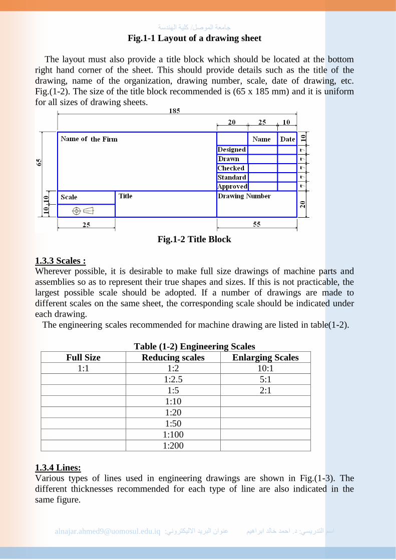
The layout must also provide a title block which should be located at the bottom
right hand corner of the sheet. This should provide details such as the title of the
drawing, name of the organization, drawing number, scale, date of drawing, etc.
Fig.(1-2). The size of the title block recommended is (65 x 185 mm) and it is uniform
for all sizes of drawing sheets.
Fig.1-2 Title Block
1.3.3 Scales : Wherever possible, it is desirable to make full size drawings of machine parts and
assemblies so as to represent their true shapes and sizes. If this is not practicable, the
largest possible scale should be adopted. If a number of drawings are made to
different scales on the same sheet, the corresponding scale should be indicated under
each drawing.
The engineering scales recommended for machine drawing are listed in table(1-2).
Table (1-2) Engineering Scales
Full Size Reducing scales Enlarging Scales
1:1 1:2 10:1
1:2.5 5:1
1:5 2:1
1:10
1:20
1:50
1:100
1:200
1.3.4 Lines:
Various types of lines used in engineering drawings are shown in Fig.(1-3). The
different thicknesses recommended for each type of line are also indicated in the
same figure.

جامعة المىصل/ كلية الهندسة
[email protected] عنىان البريد االليكتروني خالد ابراهيمحمد ا د. التدريسي:اسم:
Fig.(1-3) Types of lines
The use of various types of lines is indicated in figure(1-4).
Fig.(1-4)

جامعة المىصل/ كلية الهندسة
[email protected] عنىان البريد االليكتروني خالد ابراهيمحمد ا د. التدريسي:اسم:
1.3.5 Lettering :
Lettering is an important feature of engineering drawing. The main requirements for
lettering are legibility, uniformity, ease and rapidity of execution. Single stroke
letters meet these requirements and are universally used nowadays.
The expression "single stroke" means that the width of the straight or curved lines
that from the lettering is equal to that of the stroke of a pen or pencil.
Both the upright and slant types of letters and numerals are suitable for general
use. All these letters should be of capital type, except for abbreviations when lower
case letters are used. If the slant type is used, an inclination of approximately (75º) is
recommended. The inclination once decided should be uniformly maintained
throughout the drawing.
The recommended sizes (heights) of letters and numerals used for different
purposes are given in table(1-3).
Table (1-3) Recommended Sizes of letters and numbers
Item Size h, mm
Drawing number in title block and letters denoting cutting
plane section.
10,12
Title of the drawing 6,8
Sub-titles and headings 3,4,5,6
Notes such as legends, schedules, material list, dimensioning 3,4,5
Alteration on tries and the tolerances 2,3
They should be kept clear of the drawing lines . Uniformity in height and inclination
of lettering is assured by the use of guide lines and slope lines if necessary. Specimen
letters (capitals and lower case) and numerals are shown in Fig.(1-5).
Fig.(1-5)
1.4 Conventional Representation 1.4.1 Machine Components :
When the complete drawing of a machine component involves a lot of time or space,
its convention may be drawn in its place to represent the actual machine component.
Typical examples of conventional representation of various machine components are
shown in figures(1.6),(1-7)and(1-8).

جامعة المىصل/ كلية الهندسة
[email protected] عنىان البريد االليكتروني خالد ابراهيمحمد ا د. التدريسي:اسم:
Fig.(1-6) Conventional representation of various machine components
Fig.(1-7) Conventional representation of Spring
جامعة المىصل/ كلية الهندسة
[email protected] عنىان البريد االليكتروني خالد ابراهيمحمد ا د. التدريسي:اسم:
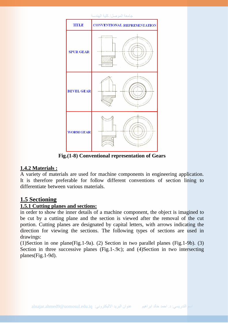
Fig.(1-8) Conventional representation of Gears
1.4.2 Materials : A variety of materials are used for machine components in engineering application.
It is therefore preferable for follow different conventions of section lining to
differentiate between various materials.
1.5 Sectioning 1.5.1 Cutting planes and sections:
in order to show the inner details of a machine component, the object is imagined to
be cut by a cutting plane and the section is viewed after the removal of the cut
portion. Cutting planes are designated by capital letters, with arrows indicating the
direction for viewing the sections. The following types of sections are used in
drawings:
(1)Section in one plane(Fig.1-9a). (2) Section in two parallel planes (Fig.1-9b). (3)
Section in three successive planes (Fig.1-.9c); and (4)Section in two intersecting
planes(Fig.1-9d).

جامعة المىصل/ كلية الهندسة
[email protected] عنىان البريد االليكتروني خالد ابراهيمحمد ا د. التدريسي:اسم:
Fig.(1-9)-(a)Section in one plane. (b)Section in two parallel planes.(c) Section in
three successive planes.(d) Section in two intersecting planes.
1.5.2 Hatching lines : For making the sections clear, hatching lines are drawn on the sectioned portion.
These lines are normally drawn at 45º to the axis or to the main outline of the
section. If a part which is adjacent to an already sectioned part is also to be sectioned.
The hatching lines are drawn at 45º but in the opposite direction to those on the part
sectioned earlier. If a third part, adjacent to the first two, is to be sectioned, hatching
lines are drawn with a different pitch or spacing. If the same part is undergoing
sectioning in different planes, section lines may be offset along the dividing line.
Spacing between the hatching lines should be uniform and should be chosen in
proportion to the size of the section.
1.5.3 Revolved and removed sections: Cross-sections may be revolved in place or removed for exposing the view with
minimum extra effort. A revolved section is shown in figure(1-10a) and a removed
section in figure(1-10b).

جامعة المىصل/ كلية الهندسة
[email protected] عنىان البريد االليكتروني خالد ابراهيمحمد ا د. التدريسي:اسم:
Fig.(1-10)-(a) Revolved section,(b) Removed section
1.5.4 Half sections :
A machine may be symmetrical about a horizontal line or about a vertical line. In
such cases, a full sectional view in unnecessary to show the inner details. Half of the
view about the line of symmetry may be shown in section figure(1.11a)is an example
of a half sectional view.
1.5.5 Local Sections : A local section is drawn when a full or half section is not needed to show the inner
details. Figure(1.11b) is an example of a local section.
Fig.(1-11)-(a)Half section,(b)Local section
1.5.6 Special cases :
When a section plane passes axially or longitudinally through certain machine
elements such as shafts, bolts, nuts, keys, pins, rivets, rods, ribs or webs, pulley arms,
etc., these should not be sectioned but should be shown in full as illustrated in
figures(1-12a)(1-12b)(1-12c)and(1-12d).

جامعة المىصل/ كلية الهندسة
[email protected] عنىان البريد االليكتروني خالد ابراهيمحمد ا د. التدريسي:اسم:
Fig.(1-12)Correct and incorrect drawings of (a) rivet in section.(b) pulley arms
in section. (c) pulley in section.(d)Webs in section.
1.5.7 Aligned sections:
Any part with an odd number of spokes, rids or holes will give an unsymmetrical and
misleading section if the principles of projection are strictly adhered to. In such cases
the unsymmetrically placed elements should be rotated into the plane of projection,
i.e., the plane of paper. The true and aligned sections of an armed pulley are
illustrated in figure (1-13).
Fig.(1-13) Actual and aligned sections of pulley arms
1.6 Dimensioning lines, symbols, figures and notes constitute the notation of dimensioning.
1.6.1 Principles of Dimensioning : The following are some of the basic principles of dimensioning:
1- Dimensions should be placed on the view which shows the relevant features most
clearly.
2- Dimensions marked in one view need not be repeated in another view.

جامعة المىصل/ كلية الهندسة
[email protected] عنىان البريد االليكتروني خالد ابراهيمحمد ا د. التدريسي:اسم:
3- As far as possible, dimensions should be placed outside the view as shown in
figure (1-14a).
4- Dimensions should be taken from visible outlines rather than from hidden lines as
shown in figure (1-14b).
5- Dimensions should be given from a base line, a center line of a hole, or a finished
surface. Dimensioning to a center line should be avoided except when the center line
passes through the center of a hole (figures 1-14c,1-14d and 1-14e).
Fig.(1-14)-(a) Dimension should be placed outside the view.(b)Dimension should
not be taken from hidden lines.(c)Location of the position of
holes.(d)Dimensioning to the center line of an object be avoided.(e)
Dimensioning to the center line of a hole is permitted.
6- The crossing of dimension lines should be avoided as far as possible.
7- If the space for dimensioning is insufficient, the arrow heads can be reversed as
shown in figure(1.15a), and the adjacent arrow heads may be replaced by a dot as
shown in figure(1-15b).

جامعة المىصل/ كلية الهندسة
[email protected] عنىان البريد االليكتروني خالد ابراهيمحمد ا د. التدريسي:اسم:
Fig.(1-15)-(a)Different way of dimensioning.(b)Use of dots in place of arrow
heads when the space for dimensioning is sufficient.
8- As far as possible, dimensions should be expressed in one unit, preferably in
millimeters. The symbol for the unit (mm) can therefore be dropped and a note can
be added starting that all dimensions of the drawing are in millimeters.
1.6.2 Execution of Dimension : Dimension lines and projection lines (extension line) should be drawn as continuous
thin lines. Projection lines should be drawn from the outline of the object and
extended slightly beyond the dimension line(Fig. 1-16).
Fig.(1-16)
The projection and dimension lines should not intersect other lines unless it is
unavoidable (Fig.1-17a). projection lines are to be drawn perpendicular to the outline
of the feature to be dimensioned. However, they can be drawn obliquely, but parallel
to each other in special cases such as on tapered features as shown in figure(1-17b).
Leaders (pointer lines) are continuous thin lines which are drawn from the notes and
figures to the features. These are to be terminated either by arrow heads or dots.
Arrow heads should always terminate at a line, whereas dots should be within the
جامعة المىصل/ كلية الهندسة
[email protected] عنىان البريد االليكتروني خالد ابراهيمحمد ا د. التدريسي:اسم:
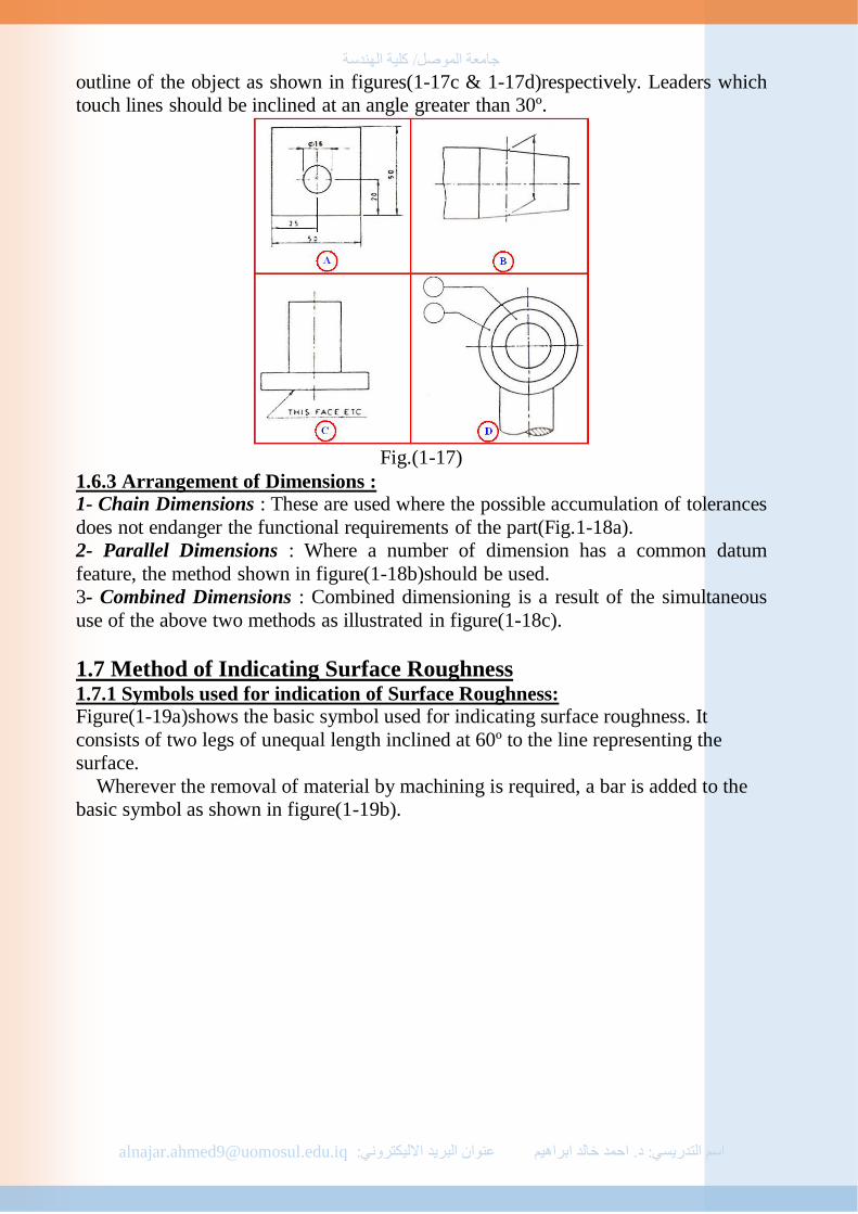
outline of the object as shown in figures(1-17c & 1-17d)respectively. Leaders which
touch lines should be inclined at an angle greater than 30º.
Fig.(1-17)
1.6.3 Arrangement of Dimensions : 1- Chain Dimensions : These are used where the possible accumulation of tolerances
does not endanger the functional requirements of the part(Fig.1-18a).
2- Parallel Dimensions : Where a number of dimension has a common datum
feature, the method shown in figure(1-18b)should be used.
3- Combined Dimensions : Combined dimensioning is a result of the simultaneous
use of the above two methods as illustrated in figure(1-18c).
1.7 Method of Indicating Surface Roughness 1.7.1 Symbols used for indication of Surface Roughness: Figure(1-19a)shows the basic symbol used for indicating surface roughness. It
consists of two legs of unequal length inclined at 60º to the line representing the
surface.
Wherever the removal of material by machining is required, a bar is added to the
basic symbol as shown in figure(1-19b).

جامعة المىصل/ كلية الهندسة
[email protected] عنىان البريد االليكتروني خالد ابراهيمحمد ا د. التدريسي:اسم:
Fig.(1-18)
When the removal of material is not allowed, a circle is add to the basic symbol as
shown in figure(1-19c).
If some special surface characteristics are to be indicated(for example a milled
surface)a line is added to the longer leg of the basic symbol as shown in figure(1-
19d).
Fig.(1-19)
1.7.2 Indication of surface Roughness :
The value defining the surface roughness in micrometers, or its corresponding grade,
is added to the symbols as shown in figure(1-20).
Fig.(1-20)

جامعة المىصل/ كلية الهندسة
[email protected] عنىان البريد االليكتروني خالد ابراهيمحمد ا د. التدريسي:اسم:
The standard roughness values in micrometers and the corresponding roughness
grade symbol are given in table(1-4).
Table(1-4) Roughness values and Roughness grade symbols
Roughness values in micrometers Roughness grade symbols
50 N12
25 N11
12.5 N10
6.3 N9
3.2 N8
1.6 N7
0.8 N6
0.4 N5
0.2 N4
0.1 N3
0.05 N2
0.025 N1
When it is necessary to specify the maximum and the minimum limits of the
surface roughness, both the value or the grades should be shown as in figure(1-21).
Fig.(1-21)
Figure(1-22) represent the general symbol of surface roughness for all surface
texture.
Fig.(1-22)
a : Roughness value Ra in micrometers or Roughness grade symbol N1 to N2.
b : Production method , treatment or coating.
c : Sampling length.
d : Direction of lay.
e : Machining allowance.
f : Other roughness values(in brackets).

جامعة المىصل/ كلية الهندسة
[email protected] عنىان البريد االليكتروني خالد ابراهيمحمد ا د. التدريسي:اسم:
Tolerances and Fits
2.1 Introduction This section, based on the International Standards Organization (ISO) system,
introduces the engineering concept of sizing parts before fitting them together to
achieve a desirable relative motion between them. Only more general applications
will be considered; tolerance of form and position.
In manufacture it is impossible to produce components to an exact size, even though
they may be classified as identical. Even in the most precise methods of production it
would be extremely difficult and costly to reproduce a diameter time after time so
that it is always within 0.01mm of a given basic size. However, industry does
demand that parts should be produced between a given maximum and minimum size.
The difference between these two sizes is called the tolerance which can be defined
as the amount of variation in size which is tolerance. A broad, generous tolerance is
cheaper to produce and maintain than a narrow, precise one. Hence one of the golden
rules of engineering design is “always specify as large a tolerance as is possible
without sacrificing quality”. There are a number of general definitions and terms
which are used, and these are described and illustrated below.
2.1.1 Shaft: A shaft is defined as a member which fits into another member(Fig.2-1). It may be
stationary or rotating. The popular concept is a rotating shaft in a bearing. However,
when speaking of tolerance, the term shaft can also apply to a member which has to
fit into a space between two restrictions, for example a pulley wheel which rotates
between two side plates in determining the clearance fit of the boss between the side
plates, the length of the pulley boss is regarded as the shaft.
Figure(2-1) Shaft fit to hole

جامعة المىصل/ كلية الهندسة
[email protected] عنىان البريد االليكتروني خالد ابراهيمحمد ا د. التدريسي:اسم:
2.1.2 Hole: A hole is defined as the member which houses or fits the shafts(Fig.2-1). It may be
stationary or rotating, for example a bearing in which a shaft rotates is a hole.
However, when speaking of tolerance, the term hole can also apply to the space
between two restrictions into which a member has to fit, for example the space
between two side plates in which a pulley rotates is regarded as a hole.
2.1.3 Basic size:
This is the size about which the limits of a particular fit are fixed(Fig.2-1). It is the
same for both shaft and hole. It is also called the nominal size.
2.1.4 Limits of size:
These are the extremes of size which are allowed for a dimension(Fig.2-1). Two
limits are possible: one the maximum allowable size and the other the minimum
allowable size.
:Deviation.1.5 2
This is the difference between the basic size and the actual size(Fig.2-1). The
extremes of deviations are referred to as the upper and lower deviations. Upper
deviations are designated in tables as ES for a hole and es for shaft. Lower deviations
are designated in tables as EI for a hole and ei for a shaft. The values given in
Tables(2.1) and (2.2) are the upper and lower deviations for both shafts and holes.
2.1.6 Tolerance: Tolerance is defined as the difference between the maximum and minimum limits of
size for a hole or shaft(Fig.2-1). It is also the difference between the upper and lower
deviations.
Fit .2 2 A fit may be defined as the relative motion which can exist between a shaft and hole
(as defined above) resulting from the final sizes which are achieved in their
manufacture. There are three classes of fit in common use: clearance, transition and
interference.
2.2.1 Clearance fit: This fit results when the shaft size is always less than the hole size for all possible
combinations within their tolerance ranges(Fig.(2-1a)). Relative motion between
shaft and hole is always possible.
The minimum clearance occurs at the maximum shaft size and the minimum hole
size.
The maximum clearance occurs at the minimum shaft size and the maximum hole
size.
Clearance fits range from coarse or very loose to close precision and locational. A
few possible combinations are given in Tables (2.1) and (2.2).
2.2.2 Transition fit: A pure transition fit occurs when the shaft and hole are exactly the same size(Fig.(2-
2b)). This fit is theoretically the boundary between clearance and interference and is
practically impossible to achieve, but by selective assembly or careful machining
methods, it can be approached within very fine limits.
جامعة المىصل/ كلية الهندسة
[email protected] عنىان البريد االليكتروني خالد ابراهيمحمد ا د. التدريسي:اسم:
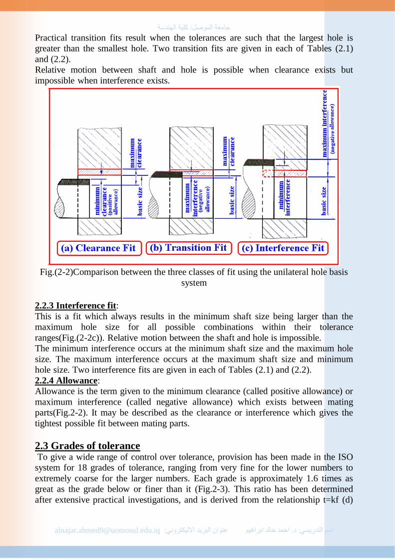
Practical transition fits result when the tolerances are such that the largest hole is
greater than the smallest hole. Two transition fits are given in each of Tables (2.1)
and (2.2).
Relative motion between shaft and hole is possible when clearance exists but
impossible when interference exists.
Fig.(2-2)Comparison between the three classes of fit using the unilateral hole basis
system
2.2.3 Interference fit:
This is a fit which always results in the minimum shaft size being larger than the
maximum hole size for all possible combinations within their tolerance
ranges(Fig.(2-2c)). Relative motion between the shaft and hole is impossible.
The minimum interference occurs at the minimum shaft size and the maximum hole
size. The maximum interference occurs at the maximum shaft size and minimum
hole size. Two interference fits are given in each of Tables (2.1) and (2.2).
2.2.4 Allowance:
Allowance is the term given to the minimum clearance (called positive allowance) or
maximum interference (called negative allowance) which exists between mating
parts(Fig.2-2). It may be described as the clearance or interference which gives the
tightest possible fit between mating parts.
2.3 Grades of tolerance
To give a wide range of control over tolerance, provision has been made in the ISO
system for 18 grades of tolerance, ranging from very fine for the lower numbers to
extremely coarse for the larger numbers. Each grade is approximately 1.6 times as
great as the grade below or finer than it (Fig.2-3). This ratio has been determined
after extensive practical investigations, and is derived from the relationship t=kf (d)

جامعة المىصل/ كلية الهندسة
[email protected] عنىان البريد االليكتروني خالد ابراهيمحمد ا د. التدريسي:اسم:
where t is the tolerance and is equal to a function of the diameter multiplied by the
constant k. different values of k are used to provide a series of tolerance grades for
various diameters. The 18 grades are designated, ITO1, ITO, IT1, IT2, up to IT16.
The letters IT (which stand for ISO series of tolerances) are omitted in tables and
also when designating fits. The numerical values of these grades of fit for all
diameters up to 3150 mm are given in AS 1654-Limits and Fits for Engineering.
Figure(2-4) illustrates graphically a comparison between some of the grades (IT5 to
IT13). The grades actually represent the size of the tolerance zone and this in turn
dictates the degree of accuracy of the machining process required to keep the size
within the specified tolerance. Low grades required precision or tool room machines
with highly skilled labor. Coarse grades are much easier to maintain, and require
cheaper machines and less skilled labor
Fig.(2-3) Practical use of international tolerance grade
Fig.(2-4) Comparison of some grade of tolerance
Tolerance symbols are used to specify the tolerances and fits for mating parts
(Fig.2-5). For the hole-basis system, the 50 indicates the diameter in millimeters; the
fundamental deviation for the hole is indicated by the capital letter H, and for shaft it
is indicated by the lowercase letter f. the numbers following the letters indicate this
IT grades. Note that the symbols for the hole and shaft are separated by the slash.
Tolerance symbols for a 50-mm-diameter hole may be given in several acceptable

جامعة المىصل/ كلية الهندسة
[email protected] عنىان البريد االليكتروني خالد ابراهيمحمد ا د. التدريسي:اسم:
forms (Fig.2-5). The values in parentheses are for reference only and may be
omitted.
These are designated by capital letters for holes and lower-case letters for shafts as
shown below.
Holes A,B,C,CD,D,E,EF,F,FG,G,H,JS,J,K,M,N,P,R,S,T,U,V,X,Y,Z,ZA,ZB,ZC
Shafts a,b,c,cd,d,e,ef,f,fg,g,h,js,j,k,m,n,p,r,s,t,u,v,x,y,z,za,zb,zc
Fig.(2-5) Acceptable Methods of giving tolerance symbols
These letters represent a wide range of tolerance zone positions varying from
above to below the basic size for both shafts and holes. Figures(2-6)and(2-7)
illustrate graphically these positions for a 10 mm shaft and hole respectively using a
grade 7 tolerance throughout.

جامعة المىصل/ كلية الهندسة
[email protected] عنىان البريد االليكتروني خالد ابراهيمحمد ا د. التدريسي:اسم:
The JS hole and js shaft tolerance zone positions are unlike the in that they provide
symmetrical bilateral tolerance and hence have no fundamental deviation. Stated
simply, this means that the tolerance zone is equally disposed above and below the
basic size for both shaft and hole.
It will also be noticed that the H hole, which is featured in Table(2.1) is the only
one which has the basic size at the lower limit. Also the h shaft is the only one which
has the basic size at the upper limit. These two fundamental deviations (zero for both
h shaft and H hole) enable a selection of fits to be made on either a hole basis or a
shaft basis.
2.4 The hole-basis system Fits are obtained by regarding the hole as standard with a zero fundamental deviation
(Fig.2-8) and varying the fundamental deviation of the shafts to suit. The 18 grades
of tolerance can still be applied to alter the size of the tolerance zones when required.
Table(2.1) is based on this system which is also known as a unilateral hole-basis

جامعة المىصل/ كلية الهندسة
[email protected] عنىان البريد االليكتروني خالد ابراهيمحمد ا د. التدريسي:اسم:
system because the disposition of the hole tolerance zones are all on the positive side
of the basic size.
2.5 The shaft-basis system Table(2.2) is based on this system. In this case the fundamental deviation of the
shaft, h, is zero, and the fits are obtained by varying the fundamental deviations of
the holes as well as applying the 18 grades of tolerance. it is a unilateral shaft-basis
system because the disposition of the shaft tolerance zones are all on the negative
side of the basic size.
Fig.(2-8) Use of fundamental deviation
Figure(2-9) illustrates five classes of fit using this system, ranging from clearance on
the left to interference on the right.
The hole-basis system is more commonly used because it is easier to produce
standard holes by drilling or reaming and then turn the shaft to suit the fit desired.
Measurements can also be made more quickly and accurately on shaft sizes than on
hole sizes.

جامعة المىصل/ كلية الهندسة
[email protected] عنىان البريد االليكتروني خالد ابراهيمحمد ا د. التدريسي:اسم:
Fig.(2-9) Five classes of fit using a shaft basis system
In some cases, however, a shaft-basis system may be desirable. For example, when a
driving shaft has a number of different parts fitted to it, it is preferable to give the
shaft a constant diameter and bore out the various parts to give the required fit for
each.
2.6 Designated of a fit A hole is designated by a capital letter followed by a number, for example H9. H is
the fundamental deviation, which indicates the position of the tolerance zone with
respect to the basic size (in this case it is zero). The figure(2-7) indicates the grad of
tolerance that is the size of the tolerance zone.
A shaft is designated in a similar way except that a lower case letter is used to
distinguish it from the hole, for example d10.
The whole fit is therefore designated as H9-d10 and if it were applied to, say, an 80
mm basic size the values of the tolerance limits would be
Hole +0.074 Shaft -0.1
0 -0,22
This can be checked from Table 1.19a. This table represents a selected variety of fits
out of many thousands of possible combinations. These are suitable for the general
engineering applications shown on the sheet. This data sheet covers all basic sizes up
to 500 mm.
A description of each of the ten types of fit represented on the data sheet follows.
H11-C11
This is a slack or coarse clearance fit which may be used where dirty conditions
prevail and ease of assembly and disassembly are essential, for example, agricultural
machinery, loose pulleys, very large shaft and assemblies.

جامعة المىصل/ كلية الهندسة
[email protected] عنىان البريد االليكتروني خالد ابراهيمحمد ا د. التدريسي:اسم:

جامعة المىصل/ كلية الهندسة
[email protected] عنىان البريد االليكتروني خالد ابراهيمحمد ا د. التدريسي:اسم:
جامعة المىصل/ كلية الهندسة
[email protected] عنىان البريد االليكتروني خالد ابراهيمحمد ا د. التدريسي:اسم:
H9-d10 This is a loose running fit suitable for idler gears and pulleys. It can be used as a
running fit for large bearing applications which are met in steel mills, large turbines,
heavy metal forming machinery and similar installations.
H9-e9
This is easy running fit which is applicable where an appreciable tolerance is
allowed. Applications include main bearings in IC engines, camshaft bearings, valve
rocker shafts and similar installations.
H8-f7 This is the fit usually selects for normal running conditions. It is suitable for most
applications requiring a reasonable quality fit which is economical and easy to
produce. Rotating shaft bearings, gears running on shafts, fits of components in
medium and light mechanisms and general light to medium engineering applications
are some of the uses of this class of fit.
H7-g6
This is a precision running or a location fit in which the clearance is small. It is only
recommended for precision running assemblies where light loads and large variations
in temperature are not encountered. It can also be used for spigot fits and other
locational non-running fits.
H7-h6
This is the average location or spigot fit used on non running assemblies. It usually
has a very small clearance associated with it, and is one of the closes possible
clearance fits.
H7-k6 This is a true transition fit, and on an average there will be no clearance found. It is
used where assembly and disassembly are required and no vibration or relative
movement can be tolerance, for example a gudgeon pin fitted into a piston, a hand
wheel keyed to a shaft, or similar applications.
H7-n6 This fit can give interference at one extreme and clearance at the other. However, on
average it is a heavy push fit and is used in applications where a tight assembly is
required.
H7-p6
This is a true interference fit used in pressing ferrous parts together. The amount of
interference is small, and assemblies may be dismantled and reassembled without
damaging the surfaces, particularly with dissimilar metals.

جامعة المىصل/ كلية الهندسة
[email protected] عنىان البريد االليكتروني خالد ابراهيمحمد ا د. التدريسي:اسم:
H7-s6 This is a heavy press fit used for permanent assembly of members. Pressing a part
usually results in the scoring of the surfaces, especially if similar metals are used.
Initial assembly may be achieved without damage to the surfaces by heating the hole
and shrinking it on to the shaft. Used on non-ferrous assemblies such as pressed in
bushes, sleeves, liners. Seats and the like.
2.7 Application of tolerance to dimensions Tolerance should be specified in the case where a dimension is critical to the proper
functioning or interchangeability of a component.
A tolerance can also be supplied to a dimension which can have an unusually large
variation in size.
2.8 General tolerance These are quoted in note form and apply when the same tolerance is applicable all
over the drawing or where different tolerances apply to various ranges of sizes or for
a particular type of member. The following examples illustrate the use of general
tolerances.
2.9 Individual tolerances For tolerancing individual linear dimensions one of the following methods may be
used. In some cases the fits are designated and values are taken from Table(2-1).
Method 1
This is specifying both limits of size and placing them above and below the
dimension line(Fig.2-10). It is the most foolproof method for general use.
Method 2 This is by specifying the basic size following by the limits of tolerance above and/or
below the basic size:
1.When the limits are equally disposed above and below the basic size (Fig.2-
11).
TOLERANCE EXCEPT WHERE
OTHERWISE STATED ±0.125
TOLERANCE EXCEPT WHERE
OTHERWISE STATED ON
DIMENSIONS
UP TO 75 ± 0.075
OVER 75 UP TO 100 ± 0.125
OVER 100 UP TO 200 ± 0.25
ON ANGLES ± 1º
TOLERANCE ON CAST
THICKNESSES ± 15%

جامعة المىصل/ كلية الهندسة
[email protected] عنىان البريد االليكتروني خالد ابراهيمحمد ا د. التدريسي:اسم:
2.When the limits are not equally disposed above and below the basic size; the
upper limit should always be shown in the upper position and lower limit in
the lower position (this applies to both shafts and holes, see Fig.(2-12).
2.10 Methods of dimensioning to avoiding accumulation of tolerance Chin dimensioning can result in tolerance accumulating to such an extent as to make
an overall tolerance impossible. This can be overcome by omitting one of the chains
of dimensions as shown in Figure (2-13).
Progressive dimensioning from a fixed datum ensures that accumulation of
tolerances will not occur. In Figure (2-14) this method is used in dimensioning all of
the vertical surfaces from the left hand end on the front view. Thus adjacent vertical
surfaces, such as X and Y, have a space between them which is influenced by two
toleranced dimensions. With chain dimensioning, this space would be controlled by
one dimension.

جامعة المىصل/ كلية الهندسة
[email protected] عنىان البريد االليكتروني خالد ابراهيمحمد ا د. التدريسي:اسم:
On the top view the positions of the holes are dimensioned by chain method using
the bottom edge and the left-hand end as initial reference or datum surfaces.
Whichever method is used will depend on the relationship of functional
dimensions and whether or not there are reference or datum surfaces from
which it is desirable to refer these functional dimensions.
2.11 Geometry tolerancing Linear tolerancing is concerned with the sizing of dimensions. It facilitates producing
elements of components (such as lengths, diameters, bores, recesses, keyways, etc.)
as economically as possible while ensuring that when the component is produced and
put to use it will be functional. However, linear tolerancing takes on account of
errors which may occur in the geometrical shape or form of the elements, and if such
errors are present on a component to an excessive degree it can be rendered useless.
For example, a shaft which may be within tolerance as far as the diameter dimension
is concerned is quite useless if it is not acceptably straight within its length. The
straightness of the shaft is a property imparted to it by the machining process
(lathing, grinding, etc.) which produced it.
2.12 Assembly of components (introduction) A mechanical assembly is a combination or “fitting together” of components
designed to perform a specific mechanical function. Each component has a finished
dimension which lies within a specified tolerance. Because of the range of finished
sizes allowable for each component, it follows that the overall dimension which
encloses the assembly must be a function of the accumulation of tolerances of the
individual components.
In the design of mechanical assemblies, great care must be taken to ensure that the
cumulative effect of assembled component tolerance is controlled to ensure
satisfactory operation of the product.
جامعة المىصل/ كلية الهندسة
[email protected] عنىان البريد االليكتروني خالد ابراهيمحمد ا د. التدريسي:اسم:
2.13 Types of assemblies Two types of component assemblies are possible, and irrespective of how involved
an assembly may appear, it can always be analyzed as one or the other of the
following types:
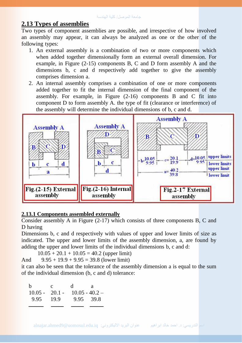
1. An external assembly is a combination of two or more components which
when added together dimensionally form an external overall dimension. For
example, in Figure (2-15) components B, C and D form assembly A and the
dimensions b, c and d respectively add together to give the assembly
comprises dimension a.
2. An internal assembly comprises a combination of one or more components
added together to fit the internal dimension of the final component of the
assembly. For example, in Figure (2-16) components B and C fit into
component D to form assembly A. the type of fit (clearance or interference) of
the assembly will determine the individual dimensions of b, c and d.
2.13.1 Components assembled externally Consider assembly A in Figure (2-17) which consists of three components B, C and
D having
Dimensions b, c and d respectively with values of upper and lower limits of size as
indicated. The upper and lower limits of the assembly dimension, a, are found by
adding the upper and lower limits of the individual dimensions b, c and d:
10.05 + 20.1 + 10.05 = 40.2 (upper limit)
And 9.95 + 19.9 + 9.95 = 39.8 (lower limit)
it can also be seen that the tolerance of the assembly dimension a is equal to the sum
of the individual dimension (b, c and d) tolerance:
b c d a
10.05 - 20.1 - 10.05 - 40.2 –
9.95 19.9 9.95 39.8
ــــــــــــ ـــــــــــ ـــــــــــ ـــــــــــــ

جامعة المىصل/ كلية الهندسة
[email protected] عنىان البريد االليكتروني خالد ابراهيمحمد ا د. التدريسي:اسم:
0.1 + 0.2 + 0.1 = 0.4 (assembly tolerance)
2.13.2Components assembled internally (case 1) Consider assembly A in Figure(2-18), which consists of three components B, C and
D having dimensions b, c and d respectively with values of upper and lower limits of
size as indicated. It is necessary to determine the maximum (upper) and minimum
(lower) limits of clearance between the three components.
The maximum combined sizes (lower limits) of components B and C from the
maximum opening size (upper limit) of D:
35.5 – (14.95 + 19.9) = 0.65 (upper limit)
The minimum clearance is found by subtracting the maximum combined sizes (upper
limits) of components B and C from the minimum opening size (lower limit) of D:
35.3 – (15.05 + 20.1) = 0.15 (lower limit)
in this cases a positive clearance always results for all possible sizes of the three
compo Of
Case 2
This is similar to case 1, but dimension d has reduced limits. It is necessary to
determine the maximum (upper) and minimum (lower) limits of clearance between
the three components of assembly A shown in Figure (19).
The maximum clearance is found by subtracting the minimum combined sizes (lower
limits) of components B and C from the maximum opening size (upper limit) of
opening D:
35.15 – (14.9 + 19.9) = 0.3 (upper limit)
The minimum clearance is found by subtracting the maximum combined sizes (upper
limits) of components B and C from the minimum opening size (lower limit) of
opening D:

جامعة المىصل/ كلية الهندسة
[email protected] عنىان البريد االليكتروني خالد ابراهيمحمد ا د. التدريسي:اسم:
34.85 – (15.05 + 20.1) = 0.3 (lower limit)
The lower limit of the clearance is negative, so in fact the fit in this case ranges from
0.3 clearances at one extreme to 0.3 interference at the other extreme.
Example
A rope sheave block assembly is shown in Figure (2-20). Two spacers of equal
widths and tolerance are required to give a maximum and minimum total clearance
of 1.50 and 0.50 mm respectively between the forked end, spacers and rope sheave.
Determine:
1. The upper and lower limit of size of each spacer.
2. The limits of size of the fit of the sheave and the spacers on the pin if a normal
running fit is required.
جامعة المىصل/ كلية الهندسة
[email protected] عنىان البريد االليكتروني خالد ابراهيمحمد ا د. التدريسي:اسم:
3. The fit of the non-ferrous bush in the sheave.
Let X = upper limit of each spacer.
Y = lower limit of each spacer.
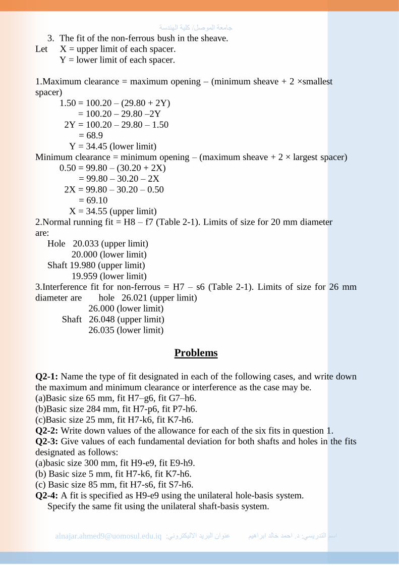
1.Maximum clearance = maximum opening – (minimum sheave + 2 ×smallest
spacer)
1.50 = 100.20 – (29.80 + 2Y)
= 100.20 – 29.80 –2Y
2Y = 100.20 – 29.80 – 1.50
= 68.9
Y = 34.45 (lower limit)
Minimum clearance = minimum opening – (maximum sheave + 2 × largest spacer)
0.50 = 99.80 – (30.20 + 2X)
= 99.80 – 30.20 – 2X
2X = 99.80 – 30.20 – 0.50
= 69.10
X = 34.55 (upper limit)
2.Normal running fit = H8 – f7 (Table 2-1). Limits of size for 20 mm diameter
are:
Hole 20.033 (upper limit)
20.000 (lower limit)
Shaft 19.980 (upper limit)
19.959 (lower limit)
3.Interference fit for non-ferrous = H7 – s6 (Table 2-1). Limits of size for 26 mm
diameter are hole 26.021 (upper limit)
26.000 (lower limit)
Shaft 26.048 (upper limit)
26.035 (lower limit)
Problems
Q2-1: Name the type of fit designated in each of the following cases, and write down
the maximum and minimum clearance or interference as the case may be.
(a)Basic size 65 mm, fit H7–g6, fit G7–h6.
(b)Basic size 284 mm, fit H7-p6, fit P7-h6.
(c)Basic size 25 mm, fit H7-k6, fit K7-h6.
Q2-2: Write down values of the allowance for each of the six fits in question 1.
Q2-3: Give values of each fundamental deviation for both shafts and holes in the fits
designated as follows:
(a)basic size 300 mm, fit H9-e9, fit E9-h9.
(b) Basic size 5 mm, fit H7-k6, fit K7-h6.
(c) Basic size 85 mm, fit H7-s6, fit S7-h6.
Q2-4: A fit is specified as H9-e9 using the unilateral hole-basis system.
Specify the same fit using the unilateral shaft-basis system.

جامعة المىصل/ كلية الهندسة
[email protected] عنىان البريد االليكتروني خالد ابراهيمحمد ا د. التدريسي:اسم:
Specify the same fit using the unilateral shaft-basis system.
Using a basic size of 100 mm, write down both limits of size for the shaft and
hole in each case.
Q2-5:A housing is to be board out for a 50 mm outside diameter roller bearing.
Name and designate the fit to be used, giving values for the upper and lower
limits of size of the housing.
Q2-6: (a)Make a fully dimensioned detailed drawing or sketch of the bush shown in
figure(2-21).The method of tolerancing should be consistent throughout. (Scale 2:1).
(b)Show separately the limits for the mating member in each case. What is the
maximum and minimum clearance or interference in each case?
Q2-7: Figure(2-22) shows a knuckle joint consisting of a fork, a rod and a 10 mm
diameter pin. The rod, which has a nominal width of (20mm), is to have a loose
clearance fit in the fork. The pin has a fit in the fork and rod designated by H7-g6.
(a)What are the values of the maximum and minimum clearances for the fit of the
rod into the fork?
(b)What are the limits of size for the pin and the pin holes in the rod and fork?
(c)What are the maximum and minimum amounts of relative lengthwise movement
between the fork and rod resulting from the tolerances for the pin and its associated
holes?
Q2-8: A (100mm) basic size shaft is to have the following five clearance fits located
within its length. It is desirable to turn the shaft to one diameter for reasons of
uniformity and ease of turning. What system can be used in order to accomplish this,
and within what limits can the shaft be turned in order to achieve all of the fits?
D10-h9, E9-h9, F8-h7, G7-h6, H7-h6
Q2-9: The pulley assembly shown in Figure (2-23) has various fits designated. Scale
off the correct basic sizes for these fits, determine both the hole and shaft limits in
each case, and insert your answers in the table provided.
Q2-10: Determine the maximum and minimum limits of size of the clearance X on
the dog clutch shown in figure(2-24).
Q2-11: The hole is assembled on the pin in figure(2-25). Determine:
(a)The maximum and minimum distance X.

جامعة المىصل/ كلية الهندسة
[email protected] عنىان البريد االليكتروني خالد ابراهيمحمد ا د. التدريسي:اسم:
(b)The maximum and minimum distance between surfaces A and B.

جامعة المىصل/ كلية الهندسة
[email protected] عنىان البريد االليكتروني خالد ابراهيمحمد ا د. التدريسي:اسم:
Fasteners
3.1 Introduction As a new product is developed, determining how to fasten it together is a major
consideration. The product must be assembled quickly, using standard, easily
available, low cost fasteners. The devices may be used to align one part to anther, or
may be used to transmit motion or force, as in a bolted drive-shaft flange. Many
considerations are required as to what kind, type and material of fastener is to be
used .
3.2 Classifications of Fasteners There are two major classifications of fasteners: Permanent and Temporary.
Permanent fasteners are used when parts will not be disassembled. Temporary
fasteners are used when the parts will be disassembled at some future time.
Permanent fastening methods include welding, brazing, stapling, nailing, gluing and
riveting .Temporary fasteners include screws, bolts, keys, and pins.
3.2.1 Temporary Fasteners:
Temporary fasteners are used when the parts will be disassembled at some future
time. Many temporary fasteners include threads in their design.
3.2.1.1 Threads : Threads are used for four different applications :
1. to fasten parts together, such as a nut and a bolt.
2. for fine adjustment between parts in relation to each other, such as the fine
adjusting screw on a surveyor's transit.
3. for fine measurement, such as a micrometer.
4. to transmit motion or power, such as an automatic screw threading attachment on a
lathe or a house jack.
3.2.1.2 Thread Terms :
Refer to (Fig.3-1) for the following terms.
Fig.(3-1) External thread and Internal thread
1.External thread : Threads located on the outside of a part, such as those on a bolt.
2.Internal thread : Threads located on the inside of a part, such as those on a nut.
3.Axis : A longitudinal center line of the thread.

جامعة المىصل/ كلية الهندسة
[email protected] عنىان البريد االليكتروني خالد ابراهيمحمد ا د. التدريسي:اسم:
4.Major diameter : the largest diameter of a screw thread, both external and internal
.
5.Minor diameter : The smallest diameter of a screw thread, both external and
internal .
6.Pitch diameter : The diameter of an imaginary diameter centrally located between
the major and the minor diameter.
7.Pitch : The distance from a point on a screw thread to a corresponding point on the
next thread, as measured parallel to the axis.
8.Root : the bottom point joining the sides of a thread.
9.Crest : The top point joining the sides of a thread.
10.Depth of thread : The distance between the crest and the root of the thread, as
measured at a right angle to the axis.
11.Angle of thread : The included angle between the sides of the thread.
12.Series of thread : A standard number of threads per inch (TPI) for each standard
diameter ,See (Fig.3-2).
Fig.(3-2) Standard number of threads per inch
13.Thread profiles : The profile (cross section)of the thread. (Fig.3-3) shows
various forms.
14.Right-hand thread : A thread that when viewed axially winds in a clockwise and
receding direction. Threads are always right-hand unless other wise specified. See
(Fig.3-4).
15.Left-hand thread : A thread that when viewed axially winds in a
counterclockwise and receding direction. All left-hand threads are designated L.H.
See (Fig.3-4).
16.Lead : the distance a threaded part moves axially, with respect to a fixed mating
part, in one complete revolution. See (Fig.3-5).

جامعة المىصل/ كلية الهندسة
[email protected] عنىان البريد االليكتروني خالد ابراهيمحمد ا د. التدريسي:اسم:
Fig.(3-3) Thread profiles
Fig.(3-4) Right hand thread and Left hand thread
17.Single thread : A thread having the thread form produced on only one helix of
the cylinder (Fig.3-5(a)). on a single thread, the lead and pitch are equivalent.
Fig.(3-5)(a) Single thread, & (b,c) Multiple thread
18.Multiple thread : A thread combination having the same form produced on two
or more helices of the cylinder (Fig.3-5(b,c)). for a multiple thread, the lead is an
integral multiple of the pitch; that is, on a double thread, lead is twice the pitch; on a

جامعة المىصل/ كلية الهندسة
[email protected] عنىان البريد االليكتروني خالد ابراهيمحمد ا د. التدريسي:اسم:
triple thread, lead is three times the pitch. A multiple thread permits a more rapid
advance without a coarser (larger) thread form.
3.2.1.3 Thread Representation : the top illustration of (Fig.3-6) shows a normal view of an external thread. To draw a
thread exactly as it will actually look takes too much drafting time. To help speed up
the drawing of threads, one of two basic systems is used and each is described and
illustrated. The schematic system of representing threads was developed
approximately in 1940, and is still used somewhat today. The simplified system of
representation threads was developed 15 years later, and is actually quicker and in
greater use today.
Fig.(3-6) Representation of external thread
3.2.1.3.1 Standard external thread representation : The most recent standard to illustrate external threads using either the schematic or
simplified system is illustrated in (Fig.3-6). 3.2.1.3.1.1 How to draw threads using the Schematic System :
Step 1: Refer to (Fig.3-7) lightly draw the major diameter, and locate the
approximate length of full threads.
Step 2: Lightly locate the minor diameter and draw the 45 ْ chamfered ends as
illustrated. Draw lines to represent the crest of the threads spaced approximately
equal to the pitch.
Step 3: Draw slightly thicker lines centered between the crest lines to the minor
diameter. These lines represent the root of the threads.
Step 4:Check all work and darken in notice the crest lines are thin black lines and the
root lines are thick black lines.

جامعة المىصل/ كلية الهندسة
[email protected] عنىان البريد االليكتروني خالد ابراهيمحمد ا د. التدريسي:اسم:
Fig.(3-7) drawing of external threads using the Schematic System
3.2.1.3.1.2 How to draw threads using the Simplified System :
Step 1: Refer to (Fig.3-8) lightly draw the major diameter, and locate the
approximate length of full threads.
Step 2: locate the minor diameter and draw the 45 ْ chamfered ends as illustrated.
Draw dash lines along the minor diameter. This represents the root of the threads.
Step 3: Check all work and darken in. The dash lines are thin black lines.

جامعة المىصل/ كلية الهندسة
[email protected] عنىان البريد االليكتروني خالد ابراهيمحمد ا د. التدريسي:اسم:
Fig.(3-8) drawing of external threads using the Simplified System
3.2.1.3.2 Standard internal thread representation : There are two major kinds of interior holes: Through holes and Blind holes. A
through hole as its name implies, goes completely through an object. A blind hole is
a hole that does not completely through an object. In the manufacture of a blind hole,
a tap drill must be drilled in to the part first, (Fig.3-9). To illustrate a tap drill, use the
(30 ْ -60 ْ ) triangle. This is not the actual angle of a drill point but is close enough
for illustration.
Fig.(3-9) Standard internal thread representation
جامعة المىصل/ كلية الهندسة
[email protected] عنىان البريد االليكتروني خالد ابراهيمحمد ا د. التدريسي:اسم:
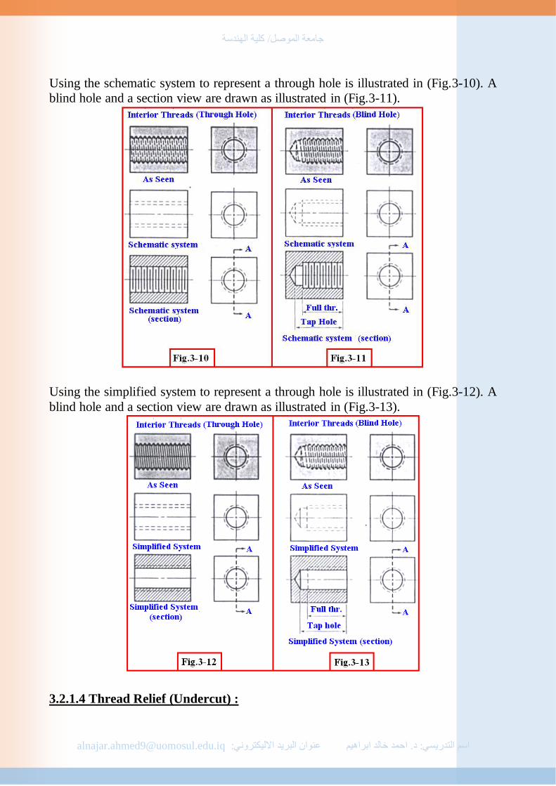
Using the schematic system to represent a through hole is illustrated in (Fig.3-10). A
blind hole and a section view are drawn as illustrated in (Fig.3-11).
Using the simplified system to represent a through hole is illustrated in (Fig.3-12). A
blind hole and a section view are drawn as illustrated in (Fig.3-13).
3.2.1.4 Thread Relief (Undercut) :

جامعة المىصل/ كلية الهندسة
[email protected] عنىان البريد االليكتروني خالد ابراهيمحمد ا د. التدريسي:اسم:
On exterior threads, it is impossible to make perfectly uniform threads up to a
shoulder; thus, the threads tend to run out, as illustrated in (Fig.3-14). where mating
parts must be held tightly against the shoulder, the last one or two threads must be
removed or relieved. This is usually done no farther than to the depth of the threads
so as not to weaken the fastener. The simplified system of the thread representation
is illustrated at the bottom of (Fig.3-14).
Full interior threads cannot be manufactured to the end of a blind hole. One way to
eliminate this problem is to call-off a thread relief or undercut, as illustrated in
(Fig.3-15). The bottom illustration is as it would be drawn by the drafter.
3.2.1.5 Screw, Bolt and Stud : (Fig.3-16) illustrates and describes a screw, a bolt, and a stud. A Screw is a threaded
fastener that does not use a nut and is screwed directly into a part.
Fig.3-16 Screw ,Bolt and Stud
A Bolt is a threaded fastener that passes directly through parts to hold them together,
and uses a nut to tighten or hold the parts together.
A Stud is a fastener that is a steel rod with threads at both ends. It is screwed into a
blind hole and holds other parts together by a nut on its free end. In general practice,

جامعة المىصل/ كلية الهندسة
[email protected] عنىان البريد االليكتروني خالد ابراهيمحمد ا د. التدريسي:اسم:
a stud has either fine threads at one end and coarse threads at the other, or class 3-fit
threads at one end and 2-fit threads at the other end.
The minimum full thread length for a screw or a stud is:
- In Steel: equal to the diameter.
- In Cast iron, Brass, Bronze: equal to 1.5 times the diameter.
- In Aluminum, Zinc, Plastic: equal to 2 times the diameter.
The clearance hole for holes up to (9mm) diameter is approximately 0.03 over size;
for large holes, 0.06 oversize.
3.2.1.6 Machine Screws : Machine screw size run from (0.3mm) to (20mm) in diameter. There are eight
standard head forms. Four major kinds are illustrated in (Fig.3-17). machine screw
are used for screwing into thin materials. Most machine screws are threaded within a
thread or two to the head. Although these are screws, machine screws sometimes
incorporate a hex-head nut to fasten parts together.
The length of a machine screw is measured from the bottom of the head to the end of
the screw (refer again to Fig.3-17).
3.2.1.7 Cap Screws : Cap screw sizes run from (6mm) and up. There are five standard head forms, (Fig.3-
18). A cap screw is usually used as a true screw, and it passes through a clearance
hole in one part and screws into another part.
3.2.1.8 How to draw Square and Hexagonal-head bolts :
Exact dimensions for square-and hex-head bolts are given in actual practice, they are
drawn using the proportions as given in (Fig.3-19) and (Fig.3-20). Notice that the
heads are shown in the profile so three surfaces

جامعة المىصل/ كلية الهندسة
[email protected] عنىان البريد االليكتروني خالد ابراهيمحمد ا د. التدريسي:اسم:
Fig.3-19 Step of drawing square head bolt
Fig.3-20 Step of drawing hexagonal head bolt

جامعة المىصل/ كلية الهندسة
[email protected] عنىان البريد االليكتروني خالد ابراهيمحمد ا د. التدريسي:اسم:
are seen in the front view. In the event a square- or hexagonal-head bolt must be
illustrated 90º, the proportions as illustrated in (Fig.3-21) are used.
Fig.3-21 Square and Hexagonal-head bolt
3.2.1.9 Nuts, Bolt and other fasteners in section : If the cutting plane passes through the axis of any fastener, the fastener is not
sectioned. It is treated exactly as a shaft and drawn exactly as it is viewed. Refer to
(Fig.3-22). 3.2.1.10 Thread Call-Offs: Although not all companies use the exact same call –offs for various fasteners, it is
important that all drafters within one company use the same method. One method
used to call-off fasteners is illustrated in (Fig.3-23). Regardless of which system is
used, the first line contains the fasteners general identification, type of head, and
classification. All threads are assumed to be right hand (R.H), unless otherwise
noted. If a thread is to be left hand (L.H), it is noted at the end of the second line.

جامعة المىصل/ كلية الهندسة
[email protected] عنىان البريد االليكتروني خالد ابراهيمحمد ا د. التدريسي:اسم:
3.2.1.11 washers : Washers provide a greater bearing surface under the fastener. This helps prevent a
nut, bolt or screw from pulling through the material.
3.2.1.11.1 Type of washers : There are five type of washer for different users .
1. Flat Washers: Used under the head of a bolt or nut to distribute the forces applied
when tightening. See (Fig.3-24a).
2.Lock washers: Lock washers place tension against a nut after tightening, to help
prevent the nut from loosening. See (Fig.3-24b).
3. External Tooth Lock Washers: Uses external teeth for locking and tension. See
(Fig.3-24C).
4. Internal Tooth Lock Washers: Uses internal teeth for locking and tension. Less
aggressive than external with a smaller outside diameter. See (Fig.3-24d).
5. Fender Washers: Used to distribute the forces applied when tightening. Fender
washers have a larger outside diameter than standard(Fig.3-24e). Available in 1 size
per diameter. The outside diameter is not as large as U.S. sizes, but larger than a
standard metric flat washer.
Fig.3-24 Type of Washers
3.2.1.12 Keys : A key is defined as a piece inserted between the joint of two parts to prevent
relative movement. In making machine drawings there is frequent occasion for
representing key fasteners, used to prevent the rotation of wheels, gears, etc., on their
shafts. A key is a piece of metal (Figure.3-25) placed so that part of it lies in a groove
, called the "key seat" cut in a shaft . The key then extends somewhat above the shaft
and fits into a "key way" cut in a hub. After assembly the key is partly in the shaft
and partly in the hub, locking the two together so that one cannot rotate without the
other.

جامعة المىصل/ كلية الهندسة
[email protected] عنىان البريد االليكتروني خالد ابراهيمحمد ا د. التدريسي:اسم:
Fig. 3-25 key nomenclature
3.2.1.12.1 Key Types : The three major kinds used in industry today : Saddle keys, Sunk keys and Round
keys.
(A) Saddle keys :
Saddle keys are of uniform width but tapering in thickness on one side. These are of
two types : Hollow Saddle keys and Flat Saddle keys(Fig.3-26).
1- Hollow Saddle Key: A hollow saddle key fits into the keyway provided in the hub
of the mounting, white its underside, which is hollow, fits on to the curved surface of
the shaft (Fig.3-26a).
2- Flat Saddle Key: This key is similar to the hollow saddle key except that the
underside of it is made into a flat surface which sits on the flat surface provided on
the shaft (Fig.3-26b).
Both types of saddle keys are suitable for light duty only. The flat variety is slightly
superior to the hollow type. Saddle keys are apt to slip around the shaft if used under
heavy loads.
When saddle keys with tapered top surfaces are used, the bottom surface of the
keyway cut in the hub of the mounting will also have to be tapered to suit the taper
provided on the key. The magnitude of the taper is usually 1:100. In such tapered
saddle keys, the underside can be made either hollow or flat.
(B) Sunk keys:
Sunk keys fit into the keyways provided in the hub of the mounting and in the shaft
as well. Generally half the thickness of the key fits into the

جامعة المىصل/ كلية الهندسة
[email protected] عنىان البريد االليكتروني خالد ابراهيمحمد ا د. التدريسي:اسم:
Fig.3-26(a) Hollow saddle key,(b)Flat saddle key.
shaft keyway and the remaining half in the hub keyway. Sunk keys are used for
heavy duty as the grip between the key and the shaft is positive.
Sunk keys may be broadly classified as : Taper keys, Parallel keys, Feather keys,
and Woodruff keys.
1- Taper Sunk Keys: Taper Sunk Keys are rectangular or square in cross section, uniform in width but
tapered in thickness(Fig.3-27). For easy assembly and removal of the joints, the
bigger end of the key is sometimes provided with a gib. (Fig.3-28) shows a key with
a gib head used for making a joint.
2- Parallel Sunk Keys:
Parallel sunk keys are of uniform cross section throughout their length. The cross
section can be either rectangular or square. The ends of the

جامعة المىصل/ كلية الهندسة
[email protected] عنىان البريد االليكتروني خالد ابراهيمحمد ا د. التدريسي:اسم:
Fig.3-27 Taper sunk key
keys may be either squared or rounded. Parallel keys are used when the mating part
or mounting is required to side along the shaft (Fig.3-29). Here the key is normally
fitted into the keyway provided on the shaft with the help of set screws.
Fig.3-28 Gib Head key Fig.3-29 Parallel Sunk key
3- Feather Keys: A feather keys is a particular kind of parallel key. It also is fitted to one member of
the pair and permits relative axial movement. It is usually fitted on to the hub of the
mounting but not on to the shaft. Feather keys are of four types: Peg feather key,
Single headed feather key, Double headed feather key and splines.
a- Peg Feather Key: In this, a projection known as a peg is provided on the key
which fits into a hole in the hub or the sliding member(Fig.3-30a).

جامعة المىصل/ كلية الهندسة
[email protected] عنىان البريد االليكتروني خالد ابراهيمحمد ا د. التدريسي:اسم:
b-Single headed feather key: In this, the key is provided with a head at one end. This
is screwed to the hub of mounting (Fig.3-30b).
c-Double headed feather key: In this, both ends of the key are provided with gib
heads, so that its axial movement in the hub is prevented. Hub and key move axially
as one unit(Fig.3-30c).
d- Splines: Splines are keys made as integral parts of the shaft. A shaft with keys or
splines is formed by cutting a number of uniform grooves equally spaced on the
surface of the shaft. The sliding part will also be provided with corresponding
keyways on its hub bone. Once the part is placed on the shaft, the splines facilitate
free axial movement and provide a positive drive as well (Fig.3-31).
Fig.3-30 Feather Key.(a) Peg feather key,(b)Single headed feather key,(c)
Double headed feather key
Fig.3-31 Splines key
4- Woodruff Keys: A woodruff key is a particular kind of sunk key in which the key is a part of a
segment of a circular disc of uniform thickness. Thus the width of the key is uniform
and its bottom surface, being circular, tilts easily in the recess provided in the shaft.

جامعة المىصل/ كلية الهندسة
[email protected] عنىان البريد االليكتروني خالد ابراهيمحمد ا د. التدريسي:اسم:
The recess is milled to the same curvature as the key(Fig.3-32). The following
proportions are usually used for Woodruff keys:
W=0.2D
R=0.4D
T=0.9R , where D is the diameter of the shaft.
Woodruff keys are generally used on tapered shafts of machine tools and
automobiles.
Fig. 3-32 Woodruff Key
(C) Round keys:
Round keys are of circular cross section and fit in the hole provided partly in the
shaft and partly in the hub. The key can have either uniform cross section throughout
its length or it can be tapered (Fig.3-33). The diameter of the round key may be taken
as (0.25D), where D is the diameter of the shaft.
D1=0.25D
Round keys are used in light duty work where the loads are not considerable.

جامعة المىصل/ كلية الهندسة
[email protected] عنىان البريد االليكتروني خالد ابراهيمحمد ا د. التدريسي:اسم:
Fig.3-33 Round key
3.2.1.12.2 Specification of Keys : Keys are specified by note or number , depending upon the type. Square and flat
keys are specified by a note giving the width, height, and length ; for example :
Width x thickness ( type of key )length of key
6 x 6 Square key 50 Lg
10x 8 Flat key 50 Lg
Plain taper stock keys are specified by giving the width, the height at the large end,
and the length. The height at large end is measured at the distance W (width) from
the large end. The taper is 1 to 96. for example,
9.5 x 9.5 x 38 Square Plain Taper Key
12.5 x 9.5 x 32 Flat Plain Taper Key
Gib head taper stock keys are specified by giving the same information, except for
name, as that given for square or flat taper keys (Fig.5); for example:
Width x Height x length of key( type of key ) ,and anther dimension from
Appendix
19x19x57 Square Gib-head Taper key
22.3x 15.8x63.5 Flat Gib-head Taper key
Pratt and Whitney keys are specified by number or latter ,and use appendix to
measure dimension . For example :
Pratt and Whitney key No.6 (using Appendix)
Woodruff keys are specified by number
Woodruff Key No.405 (using Appendix)
3.2.1.12.3 Classes of Fit : There are three classifications of fit :

جامعة المىصل/ كلية الهندسة
[email protected] عنىان البريد االليكتروني خالد ابراهيمحمد ا د. التدريسي:اسم:
- Class 1 : A side surface clearance fit obtained by using bar stock key and keyseat
tolerances .This is a relatively free fit.
- Class 2 : A possible side surface interference or side surface clearance fit obtained
by using bar stock key and keyseat tolerances . This is a relatively tight fit.
- Class 3 : A side surface interference fit obtained by interference fit tolerances .
This is a very tight fit and has not been generally standardized.

جامعة المىصل/ كلية الهندسة
[email protected] عنىان البريد االليكتروني خالد ابراهيمحمد ا د. التدريسي:اسم:
Welding
4.1 Permanent Fasteners Permanent fasteners are used when parts will not be disassembled. Permanent
fastening method include welding, brazing, stapling, nailing, gluing and riveting.
4.1.1 welding : Welding is the process of joining metal by heating a joint to a suitable temperature
with or without the application of pressure, and with or without the use of filler
material. Welding is used to permanently join assemblies when it will be
unnecessary to disassemble them for maintenance or other purposes. Some of the
advantages of welding over other methods of fastening are: simplified fabrication,
economy, increased strength and rigidity, ease of repair, creation of gas- and liquid-
tight joints and reduction in weight and /or size.
The welding processes, in their official groupings, are shown by Table (4.1) This
table also shows the letter designation for each process. The letter designation
assigned to the process can be used for identification on drawings, tables, etc.
Table (4.1) Welding processes and letter designation.
Group Welding Process Letter Designation
Arc welding Carbon Arc CAW
Flux Cored Arc FCAW
Gas Metal Arc GMAW
Gas Tungsten Arc GTAW
Plasma Arc PAW
Shielded Metal Arc SMAW
Stud Arc SW
Submerged Arc SAW
Brazing Diffusion Brazing DFB
Dip Brazing DB
Furnace Brazing FB
Induction Brazing IB
Infrared Brazing IRB
Resistance Brazing RB
Torch Brazing TB
Oxyfuel Gas Welding Oxyacetylene Welding OAW
Oxyhydrogen Welding OHW
Pressure Gas Welding PGW
Resistance Welding Flash Welding FW
High Frequency HFRW

جامعة المىصل/ كلية الهندسة
[email protected] عنىان البريد االليكتروني خالد ابراهيمحمد ا د. التدريسي:اسم:
Resistance
Percussion Welding PEW
Projection Welding RPW
Resistance-Seam Welding RSEW
Resistance-Spot Welding RSW
Upset Welding UW
Solid State Welding Cold Welding CW
Diffusion Welding DFW
Explosion Welding EXW
Forge Welding FOW
Friction Welding FRW
Hot Pressure Welding HPW
Roll Welding ROW
Ultrasonic Welding USW
Soldering Dip Soldering DS
Furnace Soldering FS
Induction Soldering IS
Infrared Soldering IRS
Iron Soldering INS
Resistance Soldering RS
Torch Soldering TS
Wave Soldering WS
Other Welding
Processes Electron Beam EBW
Electroslag ESW
Induction IW
Laser Beam LBW
Thermit TW
4.1.1.1 Types of Welded Joints :
Welds are made at the junction of the various pieces that make up the weldment. The
junctions of parts, or joints, are defined as the location where two or more numbers
are to be joined. Parts being joined to produce the weldment may be in the form of
rolled plate, sheet, shapes, pipes, castings, forgings, or billets. The five basic types of
welding joints are listed below, see (Fig.4-1).
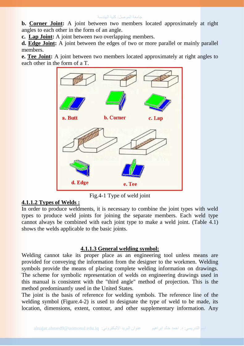
a. Butt Joint: A joint between two members lying approximately in the same plane.
جامعة المىصل/ كلية الهندسة
[email protected] عنىان البريد االليكتروني خالد ابراهيمحمد ا د. التدريسي:اسم:
b. Corner Joint: A joint between two members located approximately at right
angles to each other in the form of an angle.
c. Lap Joint: A joint between two overlapping members.
d. Edge Joint: A joint between the edges of two or more parallel or mainly parallel
members.
e. Tee Joint: A joint between two members located approximately at right angles to
each other in the form of a T.
Fig.4-1 Type of weld joint
4.1.1.2 Types of Welds :
In order to produce weldments, it is necessary to combine the joint types with weld
types to produce weld joints for joining the separate members. Each weld type
cannot always be combined with each joint type to make a weld joint. (Table 4.1)
shows the welds applicable to the basic joints.
4.1.1.3 General welding symbol:
Welding cannot take its proper place as an engineering tool unless means are
provided for conveying the information from the designer to the workmen. Welding
symbols provide the means of placing complete welding information on drawings.
The scheme for symbolic representation of welds on engineering drawings used in
this manual is consistent with the "third angle" method of projection. This is the
method predominantly used in the United States.
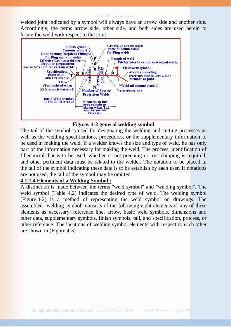
The joint is the basis of reference for welding symbols. The reference line of the
welding symbol (Figure.4-2) is used to designate the type of weld to be made, its
location, dimensions, extent, contour, and other supplementary information. Any
جامعة المىصل/ كلية الهندسة
[email protected] عنىان البريد االليكتروني خالد ابراهيمحمد ا د. التدريسي:اسم:
welded joint indicated by a symbol will always have an arrow side and another side.
Accordingly, the terms arrow side, other side, and both sides are used herein to
locate the weld with respect to the joint.
Figure. 4-2 general welding symbol
The tail of the symbol is used for designating the welding and cutting processes as
well as the welding specifications, procedures, or the supplementary information to
be used in making the weld. If a welder knows the size and type of weld, he has only
part of the information necessary for making the weld. The process, identification of
filler metal that is to be used, whether or not preening or root chipping is required,
and other pertinent data must be related to the welder. The notation to be placed in
the tail of the symbol indicating these data is to be establish by each user. If notations
are not used, the tail of the symbol may be omitted.
4.1.1.4 Elements of a Welding Symbol : A distinction is made between the terms "weld symbol" and "welding symbol". The
weld symbol (Table 4.2) indicates the desired type of weld. The welding symbol
(Figure.4-2) is a method of representing the weld symbol on drawings. The
assembled "welding symbol" consists of the following eight elements or any of these
elements as necessary: reference line, arrow, basic weld symbols, dimensions and
other data, supplementary symbols, finish symbols, tail, and specification, process, or
other reference. The locations of welding symbol elements with respect to each other
are shown in (Figure.4-3) .

جامعة المىصل/ كلية الهندسة
[email protected] عنىان البريد االليكتروني خالد ابراهيمحمد ا د. التدريسي:اسم:

جامعة المىصل/ كلية الهندسة
[email protected] عنىان البريد االليكتروني خالد ابراهيمحمد ا د. التدريسي:اسم:
Fig.4-3 locations of welding symbol
4.1.1. 5 Surface contour symbols : Contour symbols are used to indicate which of the three types of contours is desired
on the surface of the weld : flush, concave, or convex. Flush welds are those that are
smooth with the surface or flat across the hypotenuse of a fillet weld. A concave
contour is a weld that bulges inward with a curve, and a convex contour is one that
bulges outward with a curve (Table.4.4).
Table(4.4) Contour Surface symbols
In many cases, it is necessary to finish the weld by a supplementary process to
bring it to the desired contour. These processes may be added to the contour
symbols to specify their operations in finishing the welds. These processes and their
letter specifications are : chipping(C), grinding (G), hammering (H), machining (M),

جامعة المىصل/ كلية الهندسة
[email protected] عنىان البريد االليكتروني خالد ابراهيمحمد ا د. التدريسي:اسم:
rolling (R), and peening (P). Example of these contour symbols are given in Fig.(4-
4).
Fig.4-4 Symbol of finishing operation in welds
4.1.1.6 The structure of the welding symbol: Many symbols which may be added to drawings to specify different types of welds.
These symbols come from the A.W.S which has developed a system of standard
welding symbols that can be used on prints to describe the type of weld and the
weld's specifications.
A basic welding symbol has a reference line, a leader line, an arrow, an optional tail,
and welding information (Figure.4-5)
Fig. 4-5 Basic welding symbol
Reference line : the starting place for the welding symbol. The specifications for
how the weld is to be made will be based on the positioning of the other components
compared to the reference line.
Leader line : takes us to the arrow and can have a special use which will be
discussed later.
Arrow : points to the joint where the weld should be made.
Tail : the tail is optional and is where you can place information that has no
designated place on the welding symbol.

جامعة المىصل/ كلية الهندسة
[email protected] عنىان البريد االليكتروني خالد ابراهيمحمد ا د. التدريسي:اسم:
The Arrow points to the joint where the weld is to be made. The side of the joint that
the arrow points to is called the Arrow side. The opposite side of that joint is called
the Other side (Figure.4-6 ).
Figure.4-6 Arrow side and opposite side in welding symbol
Remember that the reference line is the starting point for all information about the
weld. You may use symbols around the reference line to specify welding on either
the arrow side or the other side. Any symbols below the reference line are
specifications for the arrow side regardless of whether the arrow is pointing up,
down, left, or right. Any symbols above the reference line are specifications for the
other side of the joint (Figure.4-7).
Fig.4-7 Specs for arrow and opposite side To complete the welding symbol, it is necessary to specify the type of weld. The
following are very common types of welds and are used for different purposes, often
for different types of mating surfaces(Table.4.4).
(Figure.4-8) show the example of a fillet weld to be made on the arrow side of the
joint. This is an example of how to apply these weld symbols to the welding symbol
as a whole.
Figure.4-8

جامعة المىصل/ كلية الهندسة
[email protected] عنىان البريد االليكتروني خالد ابراهيمحمد ا د. التدريسي:اسم:
This is a fillet weld to be made on the arrow side of the joint. Note how the
fillet weld symbol is below the reference line which indicates the arrow side of the
joint. In this case, the right side is the arrow side (Figure 4-8).
Below is a welding symbol that specifies two welds, one on either side of the
joint. The fillet weld (fillet weld symbol is below the reference line) is to be made on
the arrow side of the joint while the bevel weld (bevel weld symbol is above the
reference line) is to be made on the other side of the joint (Figure.4-9).
Fig.4-9
The tail may be used to specify the welding process by which the weld is supposed
to be made (Figure.4-10). Check out the (table.3.1)for a list of welding processes.
The following specifies a Gas Metal-Arc Welding process.
Figure.4-10
You may also specify the method by which the process is applies as shown in
(Figure.4-11 ).
Figure.4-11
The method may be (AU) for Automatic Welding, (MA) for manual welding, (ME)
for machine welding, or (SA) for semi-automatic welding.
A couple of common symbols on a welding symbol are the weld-all-around symbol
and the field weld symbol. The weld-all-around symbol is a circle around the
intersection reference line and the leader line (Figure.4-12).
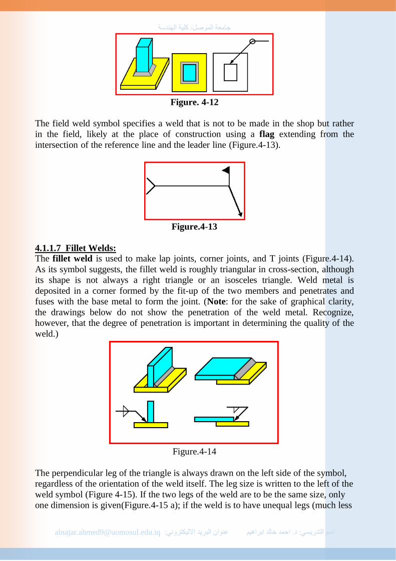
جامعة المىصل/ كلية الهندسة
[email protected] عنىان البريد االليكتروني خالد ابراهيمحمد ا د. التدريسي:اسم:
Figure. 4-12
The field weld symbol specifies a weld that is not to be made in the shop but rather
in the field, likely at the place of construction using a flag extending from the
intersection of the reference line and the leader line (Figure.4-13).
Figure.4-13
4.1.1.7 Fillet Welds: The fillet weld is used to make lap joints, corner joints, and T joints (Figure.4-14).
As its symbol suggests, the fillet weld is roughly triangular in cross-section, although
its shape is not always a right triangle or an isosceles triangle. Weld metal is
deposited in a corner formed by the fit-up of the two members and penetrates and
fuses with the base metal to form the joint. (Note: for the sake of graphical clarity,
the drawings below do not show the penetration of the weld metal. Recognize,
however, that the degree of penetration is important in determining the quality of the
weld.)
Figure.4-14
The perpendicular leg of the triangle is always drawn on the left side of the symbol,
regardless of the orientation of the weld itself. The leg size is written to the left of the
weld symbol (Figure 4-15). If the two legs of the weld are to be the same size, only
one dimension is given(Figure.4-15 a); if the weld is to have unequal legs (much less

جامعة المىصل/ كلية الهندسة
[email protected] عنىان البريد االليكتروني خالد ابراهيمحمد ا د. التدريسي:اسم:
common than the equal-legged weld), both dimensions are given and there is an
indication on the drawing as to which leg is longer (Figure.4-15-b).
Figure.4-15-a
Figure.4-15-b
The length of the weld is given to the right of the symbol (Figure.4-16). If no length
is given, then the weld is to be placed between specified dimension lines (if given) or
between those points where an abrupt change in the weld direction would occur (like
at the end of the plates in the example above).
Figure.4-16
For intermittent welds, the length of each portion of the weld and the spacing of the
welds are separated by a dash (length first, spacing second) and placed to the right of
the fillet weld symbol (Figure.4-17). the chain intermittent weld is a weld where
each weld is applied directly opposite to each other on opposite sides of the
joint(Fig.4-18a), and the staggered intermitted weld is similar to the chain
intermittent weld except the welds are staggered directly opposite each other on
opposite sides(Fig.4-18b) .

جامعة المىصل/ كلية الهندسة
[email protected] عنىان البريد االليكتروني خالد ابراهيمحمد ا د. التدريسي:اسم:
Figure.4-17
Fig.4-18
Notice that the spacing, or pitch, is not the clear space between the welds, but the
center-to-center (or end-to-end) distance.
4.1.1.8 Groove Welds:
The groove weld is commonly used to make edge-to-edge joints, although it is also
often used in corner joints, T joints, and joints between curved and flat pieces. As
suggested by the variety of groove weld symbols, there are many ways to make a
groove weld, the differences depending primarily on the geometry of the parts to be
joined and the preparation of their edges. Weld metal is deposited within the groove
and penetrates and fuses with the base metal to form the joint. (Note: for the sake of
graphical clarity, the drawings below generally do not show the penetration of the
weld metal. Recognize, however, that the degree of penetration is important in
determining the quality of the weld.)
4.1.1. 8.1 The various types of groove weld are:
1- Square groove weld :The Square groove weld(Figure.4-19), in which the
"groove" is created by either a tight fit or a slight separation of the edges. The
amount of separation, if any, is given on the weld symbol.

جامعة المىصل/ كلية الهندسة
[email protected] عنىان البريد االليكتروني خالد ابراهيمحمد ا د. التدريسي:اسم:
Figure.4-19
2- V-groove weld :The V-groove weld, in which the edges of both pieces are
chamfered, either singly or doubly, to create the groove. The angle of the V is given
on the weld symbol(Figure.4-20), as is the separation at the root opening (if any).
Figure.4-20
If the depth of the V is not the full thickness--or half the thickness in the case of a
double V--the depth is given to the left of the weld symbol (Figure.4-21).
Figure.4-21
If the penetration of the weld is to be greater than the depth of the groove, the depth
of the effective throat is given in parentheses after the depth of the V(Figure.4-22).

جامعة المىصل/ كلية الهندسة
[email protected] عنىان البريد االليكتروني خالد ابراهيمحمد ا د. التدريسي:اسم:
Figure. 4-22
3- bevel groove weld :The bevel groove weld, in which the edge of one of the
pieces is chamfered and the other is left square(Figure.4-23). The bevel symbol's
perpendicular line is always drawn on the left side, regardless of the orientation of
the weld itself. The arrow points toward the piece that is to be chamfered. This extra
significance is emphasized by a break in the arrow line. (The break is not necessary
if the designer has no preference as to which piece gets the edge treatment or if the
piece to receive the treatment should be
obvious to a qualified welder.) Angle and depth of edge treatment, effective throat,
and separation at the root are described using the methods discussed in the V-groove
section.
Figure. 4-23
4- U-groove weld: The U-groove weld, in which the edges of both pieces are given a
concave treatment(Figure.4-24). Depth of edge treatment, effective throat, and
separation at the root are described using the methods discussed in the V-groove
section.

جامعة المىصل/ كلية الهندسة
[email protected] عنىان البريد االليكتروني خالد ابراهيمحمد ا د. التدريسي:اسم:
Figure.4-24
5- J-groove weld: The J-groove weld, in which the edge of one of the pieces is
given a concave treatment and the other is left square (Figure.4-25). It is to the U-
groove weld what the bevel groove weld is to the V-groove weld. As with the bevel,
the perpendicular line is always drawn on the left side and the arrow (with a break, if
necessary) points to the piece that receives the edge treatment. Depth of edge
treatment, effective throat, and separation at the root are described using the methods
discussed in the V-groove section.
Figure.4-25
6- flare-V groove weld :The flare-V groove weld commonly used to join two
rounds or curved parts. The intended depth of the weld itself is given to the left of the
symbol, (Figure.4-26).
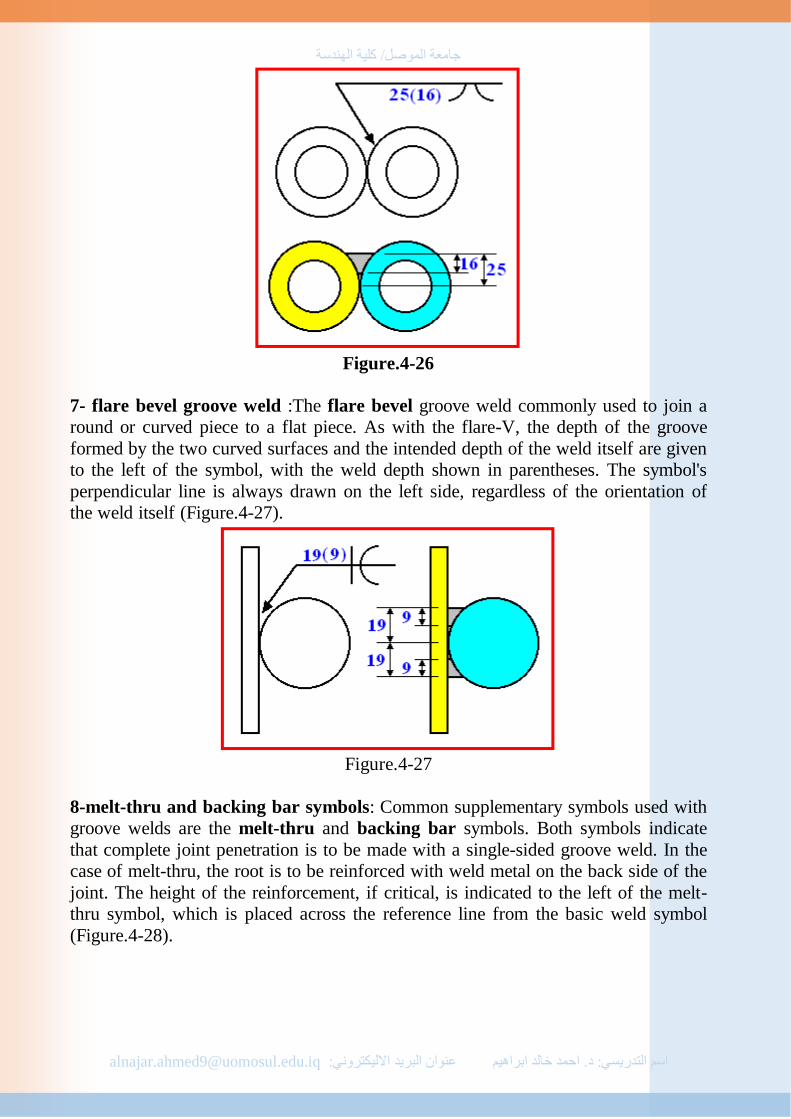
جامعة المىصل/ كلية الهندسة
[email protected] عنىان البريد االليكتروني خالد ابراهيمحمد ا د. التدريسي:اسم:
Figure.4-26
7- flare bevel groove weld :The flare bevel groove weld commonly used to join a
round or curved piece to a flat piece. As with the flare-V, the depth of the groove
formed by the two curved surfaces and the intended depth of the weld itself are given
to the left of the symbol, with the weld depth shown in parentheses. The symbol's
perpendicular line is always drawn on the left side, regardless of the orientation of
the weld itself (Figure.4-27).
Figure.4-27
8-melt-thru and backing bar symbols: Common supplementary symbols used with
groove welds are the melt-thru and backing bar symbols. Both symbols indicate
that complete joint penetration is to be made with a single-sided groove weld. In the
case of melt-thru, the root is to be reinforced with weld metal on the back side of the
joint. The height of the reinforcement, if critical, is indicated to the left of the melt-
thru symbol, which is placed across the reference line from the basic weld symbol
(Figure.4-28).

جامعة المىصل/ كلية الهندسة
[email protected] عنىان البريد االليكتروني خالد ابراهيمحمد ا د. التدريسي:اسم:
Figure.4-28
When a backing bar is used to achieve complete joint penetration, its symbol is
placed across the reference line from the basic weld symbol. If the bar is to be
removed after the weld is complete, an "R" is placed within the backing bar symbol.
The backing bar symbol has the same shape as the plug or slot weld symbol, but
context should always make the symbol's intention clear (Figure.4-29).
Figure.4-29
4.1.1.9 Plug and Slot Welds:
Plug welds and slot welds are used join overlapping members, one of which has
holes (round for plug welds, elongated for slot welds) in it. Weld metal is deposited
in the holes and penetrates and fuses with the base metal of the two members to form
the joint. (Note: for the sake of graphical clarity, the drawings below do not show the
penetration of the weld metal. Recognize, however, that the degree of penetration is
important in determining the quality of the weld.)
For plug welds, the diameter of each plug are given to the left of the symbol and the
plug-to-plug spacing (pitch) is given to the right. For slot welds, the width of each
slot is given to the left of the symbol (Figure.4-30), the length and pitch (separated
by a dash) are given to the right of the symbol, and a detail drawing is referenced in
the tail. The number of plugs or slots is given in parentheses above or below the weld
symbol. The arrow-side and other-side designations indicate which piece contains
the hole(s). If the hole is not to be completely filled with weld metal, the depth to
which it is to be filled is given within the weld symbol.

جامعة المىصل/ كلية الهندسة
[email protected] عنىان البريد االليكتروني خالد ابراهيمحمد ا د. التدريسي:اسم:
Figure.4-30
4.1.1.10 Resistance spot welds: a. General. Resistance spot weld symbols have no arrow or other side significance
in themselves, although supplementary symbols used in con-junction with them may
have such significance. Resistance spot weld symbols shall be centered on the
reference line. Dimensions may be shown on either side of the reference line.
b. Size of Resistance Spot Welds. Resistance spot welds are dimensioned by either
size or strength as follows:
(1) The size of resistance spot welds is designated as the diameter of the weld
expressed in millimeter and must be shown, with or without inch marks, to the left of
the weld symbol (fig. 4-31a).
Figure 4-31.Resistance Spot welding
(2) The strength of resistance spot welds is designated as the minimum acceptable
shear strength in pounds per spot and must be shown to the left of the weld symbol
(fig.4-31.b).

جامعة المىصل/ كلية الهندسة
[email protected] عنىان البريد االليكتروني خالد ابراهيمحمد ا د. التدريسي:اسم:
c. Spacing of Resistance Spot Welds. (1) The pitch of resistance spot welds shall be shown to the right of the weld symbol
(fig4-31.c).
(2) When the symbols are shown directly on the drawing, the spacing is shown by
using dimension lines.
(3) When resistance spot welding extends less than the distance between abrupt
changes in the direction of the welding or less than the full length of the joint, the
extent must be dimensioned (fig.4-31.e).
d. Number of Resistance Spot Welds. When a definite number of welds is desired
in a certain joint, the number must be shown in parentheses either above or below the
weld symbol (fig. 4-31.d).
e. Flush Resistance Spot Welding Joints. When the exposed surface of one
member of a resistance spot welded joint is to be flush, that surface shall be indicated
by adding the flush contour symbol to the weld symbol, (fig. 4-31.f).
4.1.1.11 Resistance seam welds:
a. General. (1) Resistance seam weld symbols have no arrow or other side significance in
themselves, although supplementary symbols used in injunction with them may have
such significance. Resistance seam weld symbols must be centered on the reference
line.
(2) Dimensions of resistance seam welds may be shown on either side of the
reference line.
b. Size of Resistance Seam Welds. Resistance seam welds must be dimensioned by
either size or strength as follows:
(1) The size of resistance seam welds must be designated as the width of the weld
expressed in millimeter and shall be shown, with or without inch marks, to the left of
the weld symbol (fig. 4-32.a).
جامعة المىصل/ كلية الهندسة
[email protected] عنىان البريد االليكتروني خالد ابراهيمحمد ا د. التدريسي:اسم:
Figure 4-32 Resistance Seam Welding
(2) The strength of resistance seam welds must be designated as the minimum
acceptable shear strength in pounds per linear inch and must be shown to the left of
the weld symbol (fig. 4-32.b).
c. Length of Resistance Seam Welds.
(1) The length of a resistance seam weld, when indicated on the welding symbol,
must be shown to the right of the welding symbol (fig. 4-32.c).
(2) When resistance seam welding extends for the full distance between abrupt
changes in the direction of the welding, no length dimension need be shown on the
welding symbol.
(3) When resistance seam welding extends less than the distance between abrupt
changes in the direction of the welding or less than the full length of the joint, the
extent must be dimensioned (fig. 4-32.d).
d. Pitch of Resistance Seam Welds. The pitch of intermittent resistance seam
welding shall be designated as the distance between centers of the weld increments
and must be shown to the right of the length dimension (fig. 4-32.e).
e. Termination of Intermittent Resistance Seam Welding. When intermittent
resistance seam welding is used by itself, the symbol indicates that increments are
located at the ends of the dimensioned length. When used between continuous
resistance seam welding, the symbol indicates that spaces equal to the pitch minus
the length of one increment are left at the ends of the dimensional length. Separate
symbols must be used for intermittent and continuous resistance seam welding when
the two are combined.
f. Flush Resistance Seam Welded Joints. When the exposed surface of one member
of a resistance seam welded joint is to be flush, that surface shall be indicated by
adding the flush contour symbol to the weld symbol, observing the usual location
significance (fig. 4-32.f).
4.1.1.12 Projection welds:
a. General.
(1) When using projection welding, the spot weld symbol must be used with the
projection welding process reference in the tail of the welding symbol. The spot weld
symbol must be centered on the reference line.
(2) Embossments on the arrow side member of a joint for projection welding shall be
indicated by placing the weld symbol on the side of the reference line toward the
reader (figure 4-33.a).

جامعة المىصل/ كلية الهندسة
[email protected] عنىان البريد االليكتروني خالد ابراهيمحمد ا د. التدريسي:اسم:
Figure 4-33
(3) Embossment on the other side member of a joint for projection welding shall be
indicated by placing the weld symbol on the -side of the reference line away from the
reader (Figure 4-33.b).
(4) Proportions of projections must be shown by a detail or other suitable means.
(5) Dimensions of projection welds must be shown on the same side of the reference
line as the weld symbol.
b. Size of Projection Welds.
(1) Projection welds must be dimensioned by strength. Circular projection welds may
be dimensioned by size.
(2) The size of circular projection welds shall be designated as the diameter of the
weld expressed in fractions or in millimeter and shall be shown, to the left of the
weld symbol (Figure.4-34.a).
Figure. 4-34
(3) The strength of projection welds shall be designated as the minimum acceptable
shear strength in pounds per weld and shall be shown to the left of the weld symbol
(Figure 4-34.b).
c. Spacing of Projection Welds. The pitch of projection welds shall be shown to the
right of the weld symbol (Figure 4-34.c).
d. Number of Projection Welds. When a definite number of projection welds is
desired in a certain joint, the number shall be shown in parentheses (Figure 4-34.d).
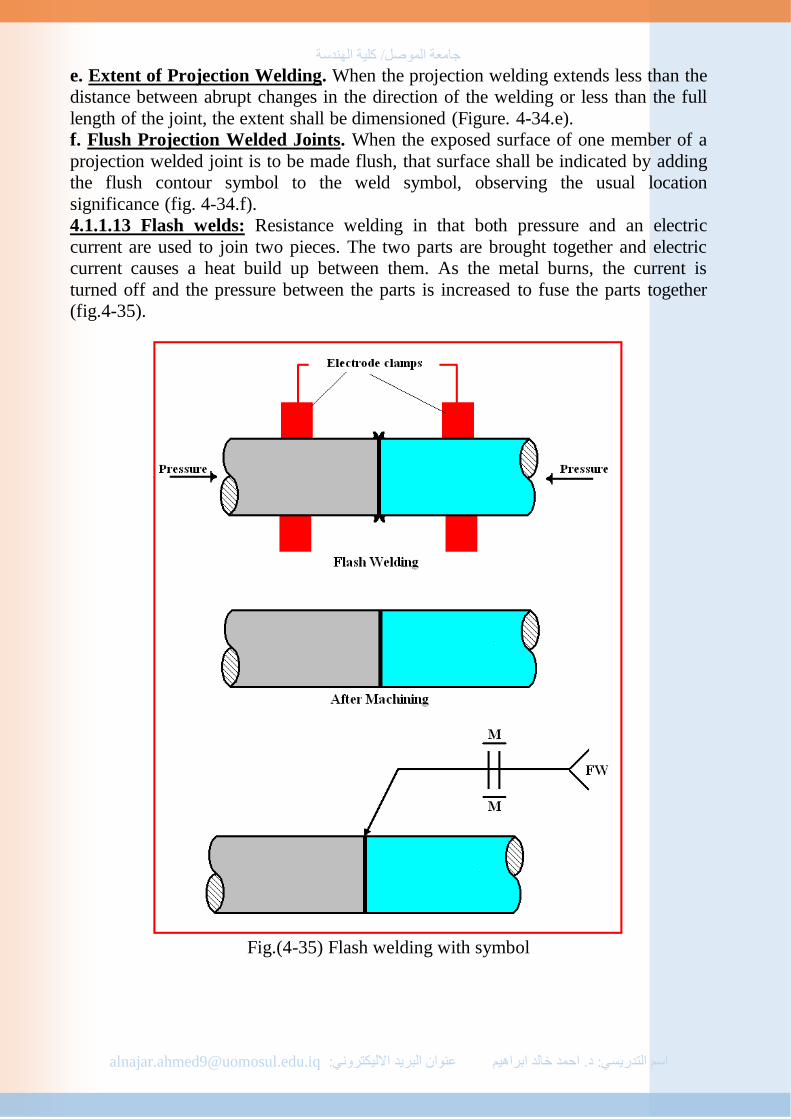
جامعة المىصل/ كلية الهندسة
[email protected] عنىان البريد االليكتروني خالد ابراهيمحمد ا د. التدريسي:اسم:
e. Extent of Projection Welding. When the projection welding extends less than the
distance between abrupt changes in the direction of the welding or less than the full
length of the joint, the extent shall be dimensioned (Figure. 4-34.e).
f. Flush Projection Welded Joints. When the exposed surface of one member of a
projection welded joint is to be made flush, that surface shall be indicated by adding
the flush contour symbol to the weld symbol, observing the usual location
significance (fig. 4-34.f).
4.1.1.13 Flash welds: Resistance welding in that both pressure and an electric
current are used to join two pieces. The two parts are brought together and electric
current causes a heat build up between them. As the metal burns, the current is
turned off and the pressure between the parts is increased to fuse the parts together
(fig.4-35).
Fig.(4-35) Flash welding with symbol

جامعة المىصل/ كلية الهندسة
[email protected] عنىان البريد االليكتروني خالد ابراهيمحمد ا د. التدريسي:اسم:
Graphical Method of Determining Cam Profiles
5.1 Cams A cam is machine part which has a surface or groove specially formed to impart an
unusual or angular motion to another machine part called a follower which presses
against and moves according to the rise and fall of the cam surface . the follower is
made to oscillate over specific distance called the stroke or displacement with a
predetermined motion governed by the design of the cam profile.
5.2 Types of cam There are tow general types of the cam distinguished by the direction of motion of
the follower to the cam axis [refer to Figure (5-1)].
1. Radial or disc cams in which the follower moves at right angles to the cam axis.
2. Cylindrical and end cams, in which the follower moves parallel to the cam axis.
Fig.5-1 Type of Cam
5.3 Applications

جامعة المىصل/ كلية الهندسة
[email protected] عنىان البريد االليكتروني خالد ابراهيمحمد ا د. التدريسي:اسم:
Basically, cams are used to translate the rotary motion of the a camshaft to the
straight line reciprocating motion of the follower. cams are used machine elements in
variety of applications including machine tools , motor cars .textile machinery and
other machines found in industry. On the turret automatic lathe for example disc
cams are used to move tool slides backwards and forwards in their guide ways. In the
motor car engine a well –known application is the camshaft on which a number of
cams raise and lower the inlet and exhaust valves via a push rod and lever system.
Figure (5-1) illustrates various configurations of cam and follower combinations.
5.4 Displacement Diagram Since the motion of the cam follower is of primary importance ,the followers rate of
speed and its various position during one revolution of the cam must be carefully
planned on a displacement diagram before the cam profile is constructed (see Figure
(5-2)).The displacement curve is plotted on the displacement diagram which is
essentially a rectangle , the base of which is essentially a rectangle the base of which
represents 360º or one revolution of the cam and the height of which represents the
total displacement or stroke of the follower .It must be remembered that because the
follower returns to its lowest position in every revolution of the cam . The
displacement curve should begin and end at the lowest position of the stroke.
Fig.5-2 Types of Cam and Follower motions
5.4.1 Type of Displacement Diagrams:
There are three types of motion commonly used in cam design :
1.Constant velocity or straight –line motion
2.Simple harmonic motion
3.Constant acceleration –deceleration or parabolic motion
5.4.1.1 Uniform or Constant Velocity Motion: is represented on the displacement
diagram (Fig.5-2a) by dividing the relevant section of the follower stoke and cam
revolution into the same number of equal parts . this means that for each part of the
cam revolution .the follower will rise or fall by equal amounts .
5.4.1.2 Simple Harmonic Motion is represented on the displacement diagram
(Fig.5-2b ) by drawing a semicircle on the relevant section of the follower stroke .
Dividing the semicircle into six equal parts. And projecting them horizontally to
intersect ordinates drawn from six equal division on that section of the cam
revolution over which harmonic motion is required .

جامعة المىصل/ كلية الهندسة
[email protected] عنىان البريد االليكتروني خالد ابراهيمحمد ا د. التدريسي:اسم:
Harmonic motion imparts a movement to the follower which commences from
zero gradually builds up to maximum speed halfway through the motion and then
slows down to zero during the second half of the motion .
5.4.1.3 Constant Acceleration –Deceleration or Parabolic Motion is represented
on the displacement diagram (Fig.5-2c) by dividing the relevant section of the
follower stroke into parts proportional to 1²,2²,3², etc(1,4,9, etc.) and projecting them
horizontally to intersect ordinates drawn from the same number of equal division on
that section of the cam revolution over which parabolic motion is required . As with
harmonic motion parabolic motion commences with zero follower movement
accelerates uniformly to a maximum velocity at halfway through the motion then
decelerates uniformly back to zero over the second half of the motion in each of the
above cases the motion may applied to either the rise or fall of the follower the curve
beginning at the bottom or top of the displacement diagram respectively and
progressing in the direction of the arrows.
Figure (5-3) illustrates a typical cam displacement diagram on which the three
types of motion (Fig.5-2) are utilized .The use of dwell periods are also shown .
Where for that section of the cam the follower is stationary within its stroke .the cam
profile for a dwell period is circular.
The constant velocity motion dashed line ad, may be modified to prevent abrupt
changes in the follower motion it is achieved by inserting radii at the beginning and
end of the motion to give curve ABCD.
The follower description of the follower motion relates to the displacement
diagram (Fig.5-3) commencing from the bottom of the stroke (point A). The follower
rises with modified constant velocity ( curve ABCD ) through half the stroke 60º
rotation of the cam . It then dwells (DE) for the next 30º rotation and finally
completes the rise ( curve EF ) with harmonic . the cam at this stage has completed
half a revolution 180º and the follower is at the top of its stroke . for the next 30º
revolution the follower dwells (FG) then falls with constant accelerates back to zero
speed in falling through the remainder of the stroke (curve
Fig.5-3 Cam displacement diagram with typical curves

جامعة المىصل/ كلية الهندسة
[email protected] عنىان البريد االليكتروني خالد ابراهيمحمد ا د. التدريسي:اسم:
HK ) the cam having rotated through further 60º to a total of 330º of the complete
revolution . for the remaining 30º of cam rotation the follower dwells (KL) after
which the next cam revolution commences . the motion of the follower is repeated
according to the displacement diagram .
5.5 construct a radial disc cam for wedge- shaped follower Construct a cam for a cam for wedge- shaped follower. Imparting to the follower
motion ;
(a) Upward stroke during 120º of cam rotation at constant velocity.
(b) Dwell for 60º of cam rotation .
(c) Fall to its original position through a further 120º rotation with simple harmonic
motion .
(d) Dwell for the remainder of the cams revolution.
the stroke of the follower is 20 mm and in line with the vertical axis of the camshaft.
The minimum radius of the cam is 10mm and its to rotate in a clockwise direction.
Draw a displacement diagram to a scale of the 15mm=90º cam rotation.
(1).Draw the center lines of the camshaft and the highest and lowest positions of the
follower (Fig.5-4).
(2). Draw the displacement diagram comprising the required motion.
(3). Project the constant velocity motion from the displacement diagram across to the
stroke position of the follower.
(4). Divide the first 120º rotation of the cam into six equal parts (20º each) and
describe radii from the constant velocity points to intersect these divisions in
sequence at point 1 to 6.
(5). Describe an arc from 6 to 7 (60º) representing the dwell at the top of the stroke.
(6).Project the harmonic motion from the displacement diagram across to the stroke
position of the follower.
Fig.(5-4)
7. Divide the next 120º of the cam rotation into six equal parts (20º each) and
describe radii from the harmonic motion points to intersect these division in
sequence at points 8 to 13 .
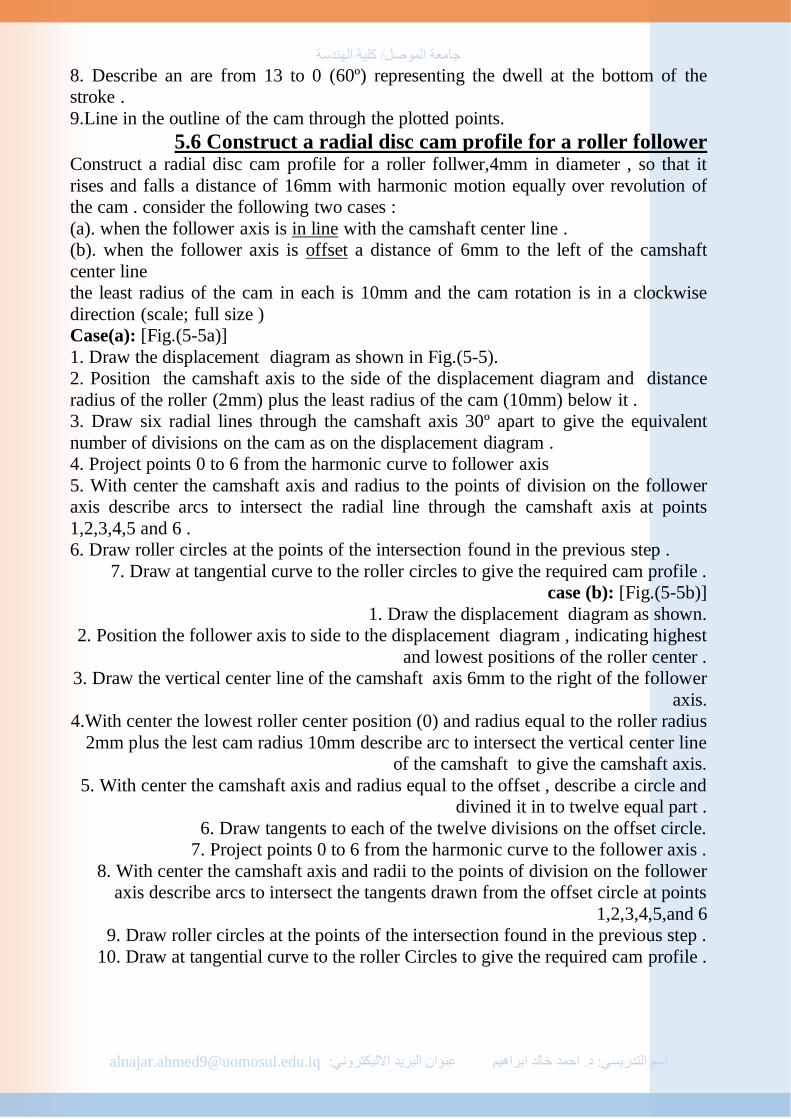
جامعة المىصل/ كلية الهندسة
[email protected] عنىان البريد االليكتروني خالد ابراهيمحمد ا د. التدريسي:اسم:
8. Describe an are from 13 to 0 (60º) representing the dwell at the bottom of the
stroke .
9.Line in the outline of the cam through the plotted points.
5.6 Construct a radial disc cam profile for a roller follower Construct a radial disc cam profile for a roller follwer,4mm in diameter , so that it
rises and falls a distance of 16mm with harmonic motion equally over revolution of
the cam . consider the following two cases :
(a). when the follower axis is in line with the camshaft center line .
(b). when the follower axis is offset a distance of 6mm to the left of the camshaft
center line
the least radius of the cam in each is 10mm and the cam rotation is in a clockwise
direction (scale; full size )
Case(a): [Fig.(5-5a)]
1. Draw the displacement diagram as shown in Fig.(5-5).
2. Position the camshaft axis to the side of the displacement diagram and distance
radius of the roller (2mm) plus the least radius of the cam (10mm) below it .
3. Draw six radial lines through the camshaft axis 30º apart to give the equivalent
number of divisions on the cam as on the displacement diagram .
4. Project points 0 to 6 from the harmonic curve to follower axis
5. With center the camshaft axis and radius to the points of division on the follower
axis describe arcs to intersect the radial line through the camshaft axis at points
1,2,3,4,5 and 6 .
6. Draw roller circles at the points of the intersection found in the previous step .
7. Draw at tangential curve to the roller circles to give the required cam profile .
case (b): [Fig.(5-5b)]
1. Draw the displacement diagram as shown.
2. Position the follower axis to side to the displacement diagram , indicating highest
and lowest positions of the roller center .
3. Draw the vertical center line of the camshaft axis 6mm to the right of the follower
axis.
4.With center the lowest roller center position (0) and radius equal to the roller radius
2mm plus the lest cam radius 10mm describe arc to intersect the vertical center line
of the camshaft to give the camshaft axis.
5. With center the camshaft axis and radius equal to the offset , describe a circle and
divined it in to twelve equal part .
6. Draw tangents to each of the twelve divisions on the offset circle.
7. Project points 0 to 6 from the harmonic curve to the follower axis .
8. With center the camshaft axis and radii to the points of division on the follower
axis describe arcs to intersect the tangents drawn from the offset circle at points
1,2,3,4,5,and 6
9. Draw roller circles at the points of the intersection found in the previous step .
10. Draw at tangential curve to the roller Circles to give the required cam profile .
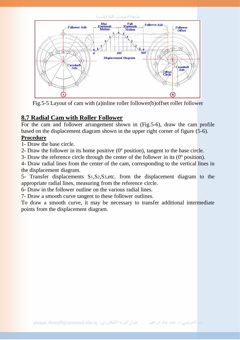
جامعة المىصل/ كلية الهندسة
[email protected] عنىان البريد االليكتروني خالد ابراهيمحمد ا د. التدريسي:اسم:
Fig.5-5 Layout of cam with (a)inline roller follower(b)offset roller follower
8.7 Radial Cam with Roller Follower For the cam and follower arrangement shown in (Fig.5-6), draw the cam profile
based on the displacement diagram shown in the upper right corner of figure (5-6). Procedure
1- Draw the base circle.
2- Draw the follower in its home positive (0º position), tangent to the base circle.
3- Draw the reference circle through the center of the follower in its (0º position).
4- Draw radial lines from the center of the cam, corresponding to the vertical lines in
the displacement diagram.
5- Transfer displacements S1,S2,S3,etc. from the displacement diagram to the
appropriate radial lines, measuring from the reference circle.
6- Draw in the follower outline on the various radial lines.
7- Draw a smooth curve tangent to these follower outlines.
To draw a smooth curve, it may be necessary to transfer additional intermediate
points from the displacement diagram.

جامعة المىصل/ كلية الهندسة
[email protected] عنىان البريد االليكتروني خالد ابراهيمحمد ا د. التدريسي:اسم:
Fig.(5-6) Radial cam with roller follower
5.8 Cam with offset Roller Follower For the cam and follow arrangement shown in figure (5-7), draw the cam profile
based on the displacement diagram shown in the upper right corner.
Procedure:
1- Draw the base circle.
2- Draw the follower in its home position (0º position), tangent to the base circle.
3- Draw the reference circle through the center of the follower in its home position.
4-Draw the offset circle tangent to the follower center line .
5- Divide the offset circle into a number of divisions corresponding to the division in
the displacement diagram , and number accordingly.
6- Draw tangents to the offset circle at each number .
7- Lay off the various displacements s1,s2,s3 ,etc along the appropriate tangent lines ,
measuring from the reference circle.
8- Draw in the follower outlines on the various tangent lines .
9- Draw a smooth curve tangent to these follower out lines .

جامعة المىصل/ كلية الهندسة
[email protected] عنىان البريد االليكتروني خالد ابراهيمحمد ا د. التدريسي:اسم:
Fig.(5-7) Cam with offset roller follower
5.9 Cam with Swinging Roller Follower for the cam-and –follower arrangement show in figure (5-8), draw the cam profile
based on the same displacement diagram used in the earlier examples .
procedure 1-Draw the base circle .
2-Draw the follower in its home position , tangent to the base circle .
3-Draw the reference circle through the center of the follower .
4-Locate points around the reference circle corresponding to the division in the
displacement diagram , and number accordingly .
5-Draw a pivot circle through the follower pivot .
6-Locate the pivot points around the pivot circle corresponding to each point on the
reference circle , and number accordingly.
7-From each of the pivot points , draw an are whose radius is equal to the length of
the follower arm .
8-At the zero position , draw the two extreme position of the follower lever by
laying off the are AB equal to the maximum displacement.
9-Lay off the various displacement S1,S2,S3 etc along this arc .
10-Rotate each of the points on are AB to its proper position around the cam profile .
11-Draw in the follower outline at each of the points just located .
12-Draw a smooth curve tangent to the follower out lines.

جامعة المىصل/ كلية الهندسة
[email protected] عنىان البريد االليكتروني خالد ابراهيمحمد ا د. التدريسي:اسم:
Fig.(5-8) Cam with swinging roller follower
8.10 Cam with translational flat –faced follower For the cam –and – follower arrangement shown in figure (5-9), draw the cam profile
based on the displacement diagram shown in the upper right corner of figure (5-9).
Procedure 1-Draw the base circle, which in this case also server as the reverence circle .
2-Draw the follower in its home position , tangent to the base circle .
3-Draw radial lines corresponding to the division in the displacement diagram and
number accordingly .
4-Draw in the follower out line on the various radial lines by laying off the
appropriate displacement and drawing lines perpendicular to he radial lines .
5-Draw a smooth curve tangent to the follower out lines.
Notice in the figure (5-9), that the tangent points usually fall at the midpoints of the
inner sides of the small triangles that are formed around the periphery of the cam .

جامعة المىصل/ كلية الهندسة
[email protected] عنىان البريد االليكتروني خالد ابراهيمحمد ا د. التدريسي:اسم:
Fig.(5-9) Cam with translating flat faced follower
5.11 Cam with swinging roller follower For the cam and follower arrangement shown in figure (5-10), draw the cam profile
based on the same displacement diagram as is used in the previous case.
Procedure
1- Draw the base circle, which in this case also serves as the reference circle.
2- Draw the follower in its home position, tangent to the base circle.
3- Draw radial lines corresponding to the divisions in the displacement diagram , and
number accordingly.
4- Draw a pivot circle through the follower pivot.
5- Locate the pivot points around the pivot circle, and number accordingly.
6- Locate the trace point on the flat face at an arbitrary radius R from the pivoted
point at zero position.
7- At the zero position, draw the two extreme positions of the follower lever by
laying off the arc AB equal to the maximum displacement.
8- Lay off the various displacements S1,S2,S3,etc. along this arc.
9- Locate the trace point 1" relative to the cam at the intersection of the arc of radius
R, centered at 1', and the arc of radius 01, centered at 0. Establish points 2",3", etc. in
a similar manner.

جامعة المىصل/ كلية الهندسة
[email protected] عنىان البريد االليكتروني خالد ابراهيمحمد ا د. التدريسي:اسم:
10- The first position of the flat follower face, relative to the cam, is the straight line
through point 1" that is tangent to the small circle of radius r , centered at point 1'.
Construct the successive positions of the follower face in a similar manner.
Fig.(5-10) Cam with Swinging flat faced follower
Problems
Q5-1: Fig.(5-11)shows the displacement diagram of radial disc cam using roller
follower. The center of follower is offset to the right of the cam shaft center. Draw
the radial cam profile, all dimension is clear in the figure.
Fig.(5-11) Problem 5-1
Q5-2:Fig.(5-12) shows the lowest position of roller follower. The center of
follower is offset to the left of the cam shaft center. The radial cam is rotate
clockwise at velocity (100 rev/min) and supported by rod (24mm)diameter.
Construct the displacement diagram and draw the cam profile (scale 1:1). The
required motion is
(a) Dwell at interval (0.05 sec).

جامعة المىصل/ كلية الهندسة
[email protected] عنىان البريد االليكتروني خالد ابراهيمحمد ا د. التدريسي:اسم:
(b) Rise (36mm) simple harmonic motion during (0.2 sec).
(c) Fall (12mm) constant velocity during (0.15 sec).
(d) Fall (42mm) acceleration and declaration during (0.2 sec).
Fig.(5-12)Problem 5-2
Q5-3: Construct the displacement diagram and draw the cam profile for given data
- Type of follower is roller (1.8 cm) diameter.
- The axis of follower is offset to the (1.6cm) right of cam shaft center.
- The stroke of follower (5.2 cm).
- The minimum radius of cam (4 cm).
- The required motion :
Angle of rotate cam Follower motion
From 0º to 30º
From 30º to 120º
From 120º to 150º
From 150º to 360º
Dwell
Rise simple harmonic motion
Dwell
Fall acceleration and declaration
Q8-4: Fig.(5-13) shows the cam profile contact with roller follower (28mm) in
diameter. Construct the displacement diagram of roller follower:
(a) the center of roller follower is in line with the center of cam shaft.
(b) the center of roller follower is offset to the right (18mm) of cam shaft center.
Q5-5: Is the same of (Q4) but using flat follower in this problem.

جامعة المىصل/ كلية الهندسة
[email protected] عنىان البريد االليكتروني خالد ابراهيمحمد ا د. التدريسي:اسم:
Fig.(5-13) Problem 5-4
Q5-6: Fig.(5-14) shows the displacement diagram of swinging roller follower and
lowest radius of cam . Draw the cam profile (scale 1:1).
Fig.(5-14) Problem 5-6
Q5-7: Figure (5-15) shows an oscillating roller ended follower, radius 125mm.
Determine the profile of a cam, centre O, which in revolving once causes the
follower to rise and fall through 30º about a mean horizontal position with uniform
angular velocity.
Fig.(5-15) Problem 5-7

جامعة المىصل/ كلية الهندسة
[email protected] عنىان البريد االليكتروني خالد ابراهيمحمد ا د. التدريسي:اسم:
Gears
6.1 Introduction Gears are toothed wheels that mesh together to transmit force and motion from one
gear to the next. They are linked together by teeth cut into their circumferences that
contact each other.
Gears are used for different applications: transfer rotary motion from one shaft to
another shaft. Gears can change direction of rotation, speed up or slow down
rotation, transmit rotational power (torque), and change rotary motion to straight line
motion.
There are various kinds of gears (Fig.6-1), each with their own function. Drafters
must be able to identify each kind of gear, know the various functions of each, and
be able to prepare working drawings of the various gears using correct terminology.
Fig.(6-1) kinds of gears
6.2 Classification of Gears Gears are an adaptation of rolling cylinders and cones, designed to ensure positive
motion. It is important to become familiar with the terms associated with gears, and
with basic proportions and formulas for calculation of parameters.
6.2.1 Basic types :
There are numerous variations
1. spur gear, The spur gear is the most commonly used gear (Fig.6-2.a). It is
cylindrical in form, with teeth that are cut straight across the face of the gear. All
teeth are parallel to the axis of the shaft. The spur gear is usually considered the
driven gear (transmitting power).
2. Pinion Gear : The pinion gear is exactly like a spur gear but it is usually smaller,
and has fewer teeth(Fig.6-2a). The pinion gear is normally considered the drive gear.

جامعة المىصل/ كلية الهندسة
[email protected] عنىان البريد االليكتروني خالد ابراهيمحمد ا د. التدريسي:اسم:
Fig.6-2(a)spur gear and Pinion gear (b)Rack gear
3.Rack Gear : The rack gear is a type of spur gear, but its teeth are in a straight line
or flat instead of in a cylindrical form (Fig.6-2b). The rack gear is used to transfer
circular motion into straight line motion.
4. Ring Gear : The ring gear is similar to the spur, pinion and rack gears except that
the teeth are internal (Fig.6-3).
5. Bevel Gear : A bevel gear is cone shaped in form with straight teeth that are on an
angle to the axis of the shaft (Fig.6-4). Bevel gears are used to transmit power and
motion between intersecting shafts that are at 90º to each other.
6. Angle Gear : The angle gear is similar to a bevel gear except that the angles are at
other than 90º to each other.
7. Miter Gear : The miter gear is exactly the same as a bevel gear, except that both
mating gears have the same number of teeth. The shafts are at 90º to each other.

جامعة المىصل/ كلية الهندسة
[email protected] عنىان البريد االليكتروني خالد ابراهيمحمد ا د. التدريسي:اسم:
8. Spiral Bevel Gear : Any bevel gears with curved teeth are called spiral bevel
gears(Fig.6-5).
9. Worm Gear : Worm gears are used to transmit power and motion at a 90º angle
between nonintersecting shafts(Fig.6-6). They are normally used as a speed reducer.
The worm gear is round like a wheel. The worm is shaped a screw with threads (or
teeth) wound around it. Because one full turn of the worm is required to advance the
worm gear one tooth, a high ratio speed reduction is achieved. The worm drives the
larger worm gear.
10. Helical Gears : Helical gears operate on parallel shafts and transmit rotary
motion in a manner identical to spur gears. The teeth have an involute shape but are
not parallel to their rotational axis (Fig.6-7). Helical gear sets can transmit heavy
loads at high speeds due to gradual engagement of the teeth and the smooth transfer
of load from one tooth to another.
11. Herringbone Gears : Since helical gear teeth are cut at angle to the axis of the
gear, a force is generated along the axis. To compensate for this force, left hand and
right hand teeth are combined (Fig.6-8). Large ships , for example, use herringbone
gears in the drive train between the turbine and the propeller.

جامعة المىصل/ كلية الهندسة
[email protected] عنىان البريد االليكتروني خالد ابراهيمحمد ا د. التدريسي:اسم:
6.2.2 Gear Teeth :
The teeth of gears are projections designed to fit into the tooth spaces of the mating
gear and contact mating teeth along a common line known as the pressure line
(Fig.6-9). The most common from for the tooth flank is the involute, and when it is
made in this form the gears are known as involute gears. The angle of the pressure
line determines the particular involute the flank will have. The ANSI has
standardized two pressure angle, 14½º and 20º. A composite 14½º tooth and a 20º
stud tooth are also used.
6.2.3 Gear Specification : The following definitions are generally applicable to all types of gears (Fig.6-9),
although they especially refer to spur gears. Wherever they differ for other gears, the
corresponding definitions are dealt with separately.
1- Pitch Circle Diameter (D): If the meshing gears are replaced by two imaginary
cylinders rolling on each other without slip and with the same speed as the gears, the
diameters of such imaginary cylinders (known as pitch cylinders) are known as pitch
circle diameters of the gears.
2- Pitch Point : This is the point of contact of the pitch circles of two mating gears.

جامعة المىصل/ كلية الهندسة
[email protected] عنىان البريد االليكتروني خالد ابراهيمحمد ا د. التدريسي:اسم:
Fig.6-9 Gear Specification
3- Centre Distance : This is the distance between the centers of the two mating gears
and is given by the equation,
2
pg DDC
where Dg = pitch circle diameter of the gear ,
Dp =pitch circle diameter of the pinion.
4- Circular Pitch (PC): This is the distance between a point on one tooth and a
corresponding point on the next tooth measured along the pitch circle circumference
of the gear. It is given by the equation,
N
DPC
where N is the number of teeth on the gear.
5- Module (m): Module is defined as the ratio of the pitch circle diameter to the
number of teeth on the gear. It is given by the equation, m=D/N.
Module is always expressed in mm. It is the main design parameter in fixing the
dimension of gear teeth and is always rounded up to the next higher value.
6- Tooth Face : This is the surface of the side of the tooth above the pitch cylinder.
7- Tooth Flank : This is the surface of the side of the tooth below the pitch cylinder.
8- Face Width (B): This is the width of the tooth face measured along the gear axis.
It can be taken as, B=2PC to 4 PC or 2πm to 4πm .
9- Crest :This is the outermost surface of the tooth.
10- Root: This is the bottom most surface of the tooth.
11- Thickness: This is the thickness of the tooth measured along the pitch circle.
جامعة المىصل/ كلية الهندسة
[email protected] عنىان البريد االليكتروني خالد ابراهيمحمد ا د. التدريسي:اسم:
12- Addendum (a): This is defined as the radial height of the tooth above the pitch
circle. It can be taken as, a=m .
13- Dedendum(d): This is defined as the radial depth of the tooth below the pitch
circle and can be taken as , d=(1+π/20)m.
14- Clearance (c): This is the difference between the dedendum and the addendum
of the gear tooth and is given by equation, c=d- a .
15- Addendum Circle : This is the circle passing though the crests of the gear teeth.
The diameter of this circle is given by the equation Da=D+2a.
16- Dedendum Circle : This is the circle passing through the roots of the gear teeth.
It is also known as root circle. The diameter of this circle is given by the equation ,
Dd = D-2d.
17- Fillet : This is the junction where the root of the tooth meets the bottom of the
tooth space. Fillet radius may be taken as, r=0.4m for spur and helical gears and
r=0.2m for bevel gears.
18- Whole Depth (dh): This is the total depth of the tooth from the crest to the root
and is given by the equation, dh = a+d.
19- Common Tangent : This is the common tangent to the pitch circles of the two
mating gears at the pitch point .
20- Common Normal : This is the common normal to the two tooth profiles at the
point of contact.
21- Pressure angle (φ): This is the angle made by the common normal and the
common tangent.
22- Base Circle : This is the circle from which the involute profile of the tooth is
generated. Base circle diameter is given by the equation,
Db=D cosφ .
6.3 Drawing of Tooth Profiles : Tooth profiles can be either of involute or cycloidal form. The involute form is used
extensively nowadays because of its advantage both from manufacturing as well as
operational points of view.
6.3.1 The involute curve: gears use the involute curve as the profile of their gear
teeth because of the involutes unique property of being able to transfer motion and
forces in a uniform manner.
6.3.1.1 How to construct an involute curve on a basic circle:
Method 1:An involute curve may be considered as the path traced by the end of a
string as it its unwound from a circle called a base circle. The principle of
constructing an involute is illustrated in (Fig.6-10a).
Step 1: The base circle is divided into equal divisions with radial lines from the
center. Tangents are drawn perpendicular to the radial lines on the arc.
Step 2: The chordal distance from 1 to 0 is used as the radius and 1 as the center to
find point 1 on the involute curve. The distance from 2 to newly found 1 is revolved
to the tangent line through 2 to locate a second point, and the process is continued.

جامعة المىصل/ كلية الهندسة
[email protected] عنىان البريد االليكتروني خالد ابراهيمحمد ا د. التدريسي:اسم:
Fig.(6-10a) Construct an Involute Curve
Method 2: Involute is the locus of a point situated on a straight line rolling on the
circumference of a circle. Figure (6-10b) shows the stages in the construction of an
involute tooth profile which are described as follows:
1- Draw vertical center line OP and describe an arc of the pitch circle with O as
center and OP as radius(equal to the pitch circle radius of the gear).
2- Draw a line, tangent to the pitch circle at P, the pitch point. This is the common
tangent.
3- Draw line of action AB through the pitch point making an angle equal to pressure
angle φ with the tangent line. In case of involute teeth, the line of action is the path
of the point of contact, which is a straight line passing through the pitch point. The
line of action makes an angle equal to the pressure angle with the common tangent. It
can also be observed from (Fig.6-9) that the line of action is tangent to the two base
circles of the involutes forming the tooth profiles of the gears under mesh.
4- From center O draw line OQ perpendicular to the line of action (Fig.6-10c).
5- Draw an arc of the base circle with center O and radius OQ.
6- Mark off a number of equidistant points on either side of Q,
viz.,5,4,3,2,1,Q,I,II,III,IV,V,etc., on the circumference of the base circle(Fig.6-10c).
7- Join these points to center O and then draw tangents to the base circle at all these
point.
8- On the tangent lines to the right of Q, mark off lengths equal to PQ minus the
corresponding segmental lengths from Q. For example, on the tangent line from 3,
mark off the length equal to PQ minus the segmental length Q3. On the tangent lines
to the left of Q, mark off lengths equal to PQ plus the corresponding segmental
lengths from Q. For example, on the tangent line from III, mark off the length equal
to PQ plus the segmental length QIII.
9- Join the points thus obtained by a smooth curve which is the required involute
profile of the tooth.
10- Mark off arc PR on the pitch circle equal to one fourth of the circular pitch.
11- Draw line of symmetry OR of the tooth(Fig.6-10d).
12- The profile drawn already forms only one half of the tooth surface. The other
half is symmetrical to this. Therefore the second half (which forms the left side
surface of the tooth)can be drawn by drawing a number of concentric circles and
marking off equal distances from line of symmetry OR as shown in the figure.

جامعة المىصل/ كلية الهندسة
[email protected] عنىان البريد االليكتروني خالد ابراهيمحمد ا د. التدريسي:اسم:
13- Draw the addendum circle.
14- Draw the dedendum circle.
15- draw the fillets. This completes the tooth profile.
Figure (6-10b,c,d)
6.4 Drawing of Toothed Gears :
6.4.1 Spur Gears : The spur gear is a circular gear with teeth cut around its circumference. Two mating
spur gears can transmit power from one shaft to another parallel shaft.
When the two meshing gears are unequal in diameter, the smaller gear is called
the pinion and the larger one is called the gear.
The following terms are used to describe the parts of a spur gear. Many of these
features are illustrated and labeled in (Fig.6-9). The corresponding formulas for each
feature are given in gear specification .
6.4.1.1 To Draw a Spur Gear: A conventional drawing of a spur gear is shown in
(Fig.6-11). The teeth need not be drawn since this is time consuming and
unnecessary.
To draw spur gear in any problem, calculate all the dimension of spur gear from
given data in problem, the module(m) , number of teeth(N) and shaft diameter(Ds):
before drawing we can calculate anther dimension to use in drawing
1- Pitch Circle Diameter (D) : D = m x N
2- Addendum Circle Diameter (Da) : Da =D + 2a = D + 2m
3- Dedendum Circle Diameter (Dd) : Dd = D – 2d or Dd =D-2(1.157)m
4-Face Width(B): B = 3 x Pc = 3x(πD/N)
5-Hub Diameter (Dh): Dh =1.5Ds to 2Ds , where Ds is shaft diameter.
6-Hub Length (L): L=B to 1.4B
7-Web Thickness(Tw): Tw = Pc =(πD/N)
8-Rim Thickness (Tr): Tr = a+d = m+(1.157)m

جامعة المىصل/ كلية الهندسة
[email protected] عنىان البريد االليكتروني خالد ابراهيمحمد ا د. التدريسي:اسم:
After calculation of all dimension of a spur gear, drawing the spur gear shown in
(Fig.6-11).
Fig.6-11 Conventional drawing of a spur gear
6.4.1.2 To Draw a Spur Gearing : The combination of two spur gears in mesh is
known as spur gearing. This is the most commonly used gearing in applications. The
same calculation in spur gear use in spur gearing in order to draw two spur gear in
mesh (Fig.6-12).
Fig.6-12 Conventional drawing of a spur gearing
6.4.2 To Draw a Rack Gear: (Fig.6-13) A rack is, theoretically, a spur gear
having an infinite pitch diameter. Therefore, compared with the mating gear, all
circular dimensions become linear. To draw the teeth of a standard involute rack by
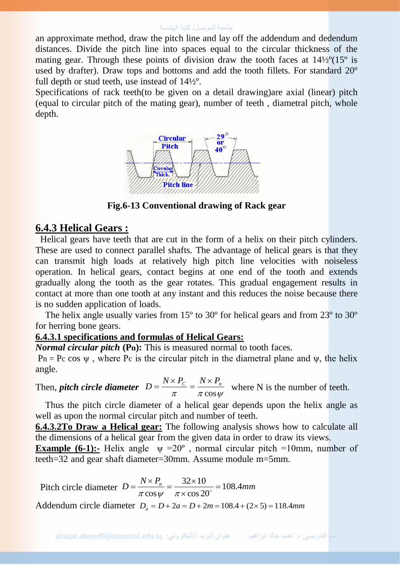
جامعة المىصل/ كلية الهندسة
[email protected] عنىان البريد االليكتروني خالد ابراهيمحمد ا د. التدريسي:اسم:
an approximate method, draw the pitch line and lay off the addendum and dedendum
distances. Divide the pitch line into spaces equal to the circular thickness of the
mating gear. Through these points of division draw the tooth faces at 14½º(15º is
used by drafter). Draw tops and bottoms and add the tooth fillets. For standard 20º
full depth or stud teeth, use instead of 14½º.
Specifications of rack teeth(to be given on a detail drawing)are axial (linear) pitch
(equal to circular pitch of the mating gear), number of teeth , diametral pitch, whole
depth.
Fig.6-13 Conventional drawing of Rack gear
6.4.3 Helical Gears : Helical gears have teeth that are cut in the form of a helix on their pitch cylinders.
These are used to connect parallel shafts. The advantage of helical gears is that they
can transmit high loads at relatively high pitch line velocities with noiseless
operation. In helical gears, contact begins at one end of the tooth and extends
gradually along the tooth as the gear rotates. This gradual engagement results in
contact at more than one tooth at any instant and this reduces the noise because there
is no sudden application of loads.
The helix angle usually varies from 15º to 30º for helical gears and from 23º to 30º
for herring bone gears.
6.4.3.1 specifications and formulas of Helical Gears: Normal circular pitch (Pn): This is measured normal to tooth faces.
Pn = Pc cos ψ , where Pc is the circular pitch in the diametral plane and ψ, the helix
angle.
Then, pitch circle diameter cos
nC PNPND
where N is the number of teeth.
Thus the pitch circle diameter of a helical gear depends upon the helix angle as
well as upon the normal circular pitch and number of teeth.
6.4.3.2To Draw a Helical gear: The following analysis shows how to calculate all
the dimensions of a helical gear from the given data in order to draw its views.
Example (6-1):- Helix angle ψ =20º , normal circular pitch =10mm, number of
teeth=32 and gear shaft diameter=30mm. Assume module m=5mm.
Pitch circle diameter mmPN
D n 4.10820cos
1032
cos
Addendum circle diameter mmmDaDDa 4.118)52(4.10822

جامعة المىصل/ كلية الهندسة
[email protected] عنىان البريد االليكتروني خالد ابراهيمحمد ا د. التدريسي:اسم:
Dedendum circle diameter mmmDdDDd 84.96)20
1(22
Gear width mmP
PB nC 32
20cos
103
cos33
Hub diameter Dh=1.5Ds to 2Ds , where Ds is the shaft diameter
Assume Dh=1.75 Ds .
Dh=1.75 x30=52.5mm
Hub length L= B to 1.4B
Assume L=1.2B
L=1.2x32=38.4mm
Web thickness mmP
PT nCW 6.10
20cos
10
cos
Rim thickness mmmmbaTr 785.105)20
14.31(5)
201(
The views of helical gear incorporating the above dimensions can be drawn similar
to the views explained below.
(Fig.6-14) shows the plain front view of a helical gear. In this the direction of helical
teeth is indicated by three thin continuous lines at an angle equal to the helix angle
(ψ). Regarding the other two views, there is practically no difference in
representation between the spur and helical gears as in (Fig.9-11).
6.4.3.3 Helical gearing: The combination of two helical gears in mesh in known as
helical gearing .This gearing works smoother than spur gearing.
The following analysis shows how to calculate all the dimensions of a helical
gearing from the given data in order to draw its views.
Example (6-2):- Helix angle =20º and the remaining data is the same as that given
for spur gearing.
calculation
The parameters calculated in the analysis of spur gearing can be used here also as
the data is the same. It is to be noted in helical gearing that a right hand helix will
mesh only with a left hand helix.
The views drawn for spur gearing in (Figure.6-12) will hold good in this case also,
except that the plain front view will be changed as indicated in (Figure.6-15).

جامعة المىصل/ كلية الهندسة
[email protected] عنىان البريد االليكتروني خالد ابراهيمحمد ا د. التدريسي:اسم:
6.4.4 Bevel Gears : Bevel gears may be classified as either of straight teeth or of curved teeth; only the
former is discussed here. Straight bevel gears are easy to design and economical to
produce. The teeth of the straight bevel gear are cut on a tapered blank which is a
right frustum of a cone. The cross-section of the blank gradually tapers from large
section at the outer edge to a small section at the inner edge. The apex of the cone
lies on the shaft axis and is called the vertex. Bevel gears may be used to transmit
power between shafts at practically any angle; only 90º type is discussed here. Figure
(6-16) illustrates the nomenclature for bevel gears.
1.Pitch Line: Pitch line is a straight line joining the vertex and a point on the outer
edge of any tooth at pitch circle radius.

جامعة المىصل/ كلية الهندسة
[email protected] عنىان البريد االليكتروني خالد ابراهيمحمد ا د. التدريسي:اسم:
2.Pitch Angle: Pitch angle is the angle between the pitch line and the axis of the
gear.
3.Pitch Cone Radius: This is the length of the pitch line.
4.Addendum: This is the height of the tooth from the pitch line at the outer edge.
5.Dedendum: This is the depth of the tooth below the pitch line at the outer edge.
The following analysis shows how to calculate all the dimensions of a bevel gear
from the given data in order to draw its views.
Figure (6-16) Conventional drawing of a Bevel gear
Example (6-3): Module m=5,number of teeth N=32, pitch angle =45º and shaft
diameter =40mm?
Calculation to draw bevel gear
Pitch circle diameter D = 32 x 5=160mm
Pitch cone radius mmx
DRc 2.113
45sin2
160
sin2
Circular pitch mmN
DPc 7.15
32
160
Face width mmRc
B 74.373
2.113
3
Addendum a = m =5mm
Dedendum mmmd 785.520
1
Hub diameter Dh=1.5Ds to 2Ds ,where Ds is the shaft diameter.
Assume Dh = 2Ds = 2x40 =80mm
Hub length L=B to 1.4B
Assume L=1.4B = 1.4 x 37.74 = 52.9mm
Rim thickness Tr = a+d = 10.785mm

جامعة المىصل/ كلية الهندسة
[email protected] عنىان البريد االليكتروني خالد ابراهيمحمد ا د. التدريسي:اسم:
The views of the bevel gear, in incorporating the above dimensions can be shown
similar to the views shown in figure(9-17).
Figure (6-17)
6.4.4.1 Bevel Gearing :
The combination of two bevel gears in mesh is known as bevel gearing. In case of a
single bevel gear, pitch cone angle can be given directly. But in case of bevel
gearing, the pitch cone angles of the pinion and gear are calculated, knowing the
shaft angle (α) , i.e., the angle between the axes of the intersecting shafts.
Pitch cone angle of pinion
g
p
p
s
p
g
sp
N
N
N
N
1
1
tan
)
cos
sin(tan
when αs=90º
Pitch cone angle of gear αg= αs – αp
The following analysis shows how to calculate all the dimension of a bevel
gearing from the given data in order to draw its views.
Example (6-4):- Draw the front view and sectional side view of a bevel gearing,
satisfying the following conditions: Shaft angle =90º, module m=5mm, number of
teeth on pinion Np=16, number of teeth on gear Ng=40, pinion shaft diameter
Dsp=20mm, Gear shaft diameter Dsg=40mm ?
Calculation to draw bevel gearing The parameters calculated in the analysis of spur gearing, can be used here also as
the data is the same. Additional calculations are as follows:
Pitch cone angle of pinion αp=tan¹־(Np/Ng)
αp=tan21.8=(16/40)¹־º
Pitch cone angle of gear αg= αs – αp =90º - 21.8º=68.2º

جامعة المىصل/ كلية الهندسة
[email protected] عنىان البريد االليكتروني خالد ابراهيمحمد ا د. التدريسي:اسم:
Dp=m x Np=5x16=80mm, Dg=m x Ng=5x40=200mm
Pitch cone radius Rc= (Dp/(2sinαp))=80/(2sin21.8)=107.71mm
B=Rc/3=35.9mm. a=m=5mm, d=(1+π/20)m=5.785mm, Tr=a+d=10.785mm ,
Dhg=1.5Dsg=60mm, Dhp=1.5Dsp=30mm
L=1.2B=1.2x35.9=43.08mm
The views of the bevel gearing satisfying the above dimensions can be drawn similar
to views shown in figure (6-18).
Fig.(6-18) Bevel gearing
6.4.5 Worm Gears : In worm gears, the driving member is essentially a screw known as "worm". It has a
trapezoidal thread. The driven member is a gear wheel known as the worm wheel.
The worm wheel is essentially a helical gear with teeth cut on a concave-shaped
periphery, i.e., the worm gear blank is throated on the periphery. This results in the
worm gear enveloping the worm. Worm gearing is usually used in speed reducer
units where large reductions are needed.
The worm may be either left handed or right handed with single or multiple start
threads. The following are commonly used terms relating to worm gears see figure
(6-19).
1-Axial Pitch :- This is the distance measured parallel to the axis of the worm
between corresponding points on two consecutive profiles. It is equal to the circular
pitch of the worm wheel.
2- Lead :- Lead of the worm is the distance that a point on the pitch circle of the
worm wheel will advance during one revolution of the worm. Thus in a single start
worm, the lead and pitch are the same, whereas in a double start worm, the lead is
equal to twice the pitch and so on.
3- Helix Angle (λ) :- The helix angle of the worm is the angle between a line
tangential to the thread at the pitch line and a plane perpendicular to the axis of the
worm and is given by the equation,

جامعة المىصل/ كلية الهندسة
[email protected] عنىان البريد االليكتروني خالد ابراهيمحمد ا د. التدريسي:اسم:
)(tan 1
Dw
lead where Dw is the pitch diameter of the worm.
4- Pressure Angle (φ):- This is the angle between a line tangent to the profile at the
pitch line and a line perpendicular to the axis of the worm measured in an axial
plane. For single and double start worms, a pressure angle (14½º) is recommended
and for triple and quadruple start worms, a pressure angle of 20º is recommended.
Figure (6-19) Worm and Worm wheel
5- Pitch Diameter of worm (Dw):- The worm must be strong enough to transmit the
desired load without excessive deflection. At the same time the diameter should be as
small as permissible with the necessary strength in order to minimize the rubbing
speed. The pitch diameter of the worm can be taken as (89.1
875.0C) Where C is the
centre distance in centimeters.
6- Length of Worm (Lw) :- This is the length of the threaded part of the worm
measured parallel to the axis.
7- Gear Ratio :- This is the ratio between the number of teeth on the worm wheel
and the number of starts on the worm.
6.4.5.1 To Draw a Worm and Worm Wheel : the following example shows how to
calculate all the dimensions of a worm and worm wheel from the given data in order
to draw their views.
Example(9-5) :- Number of starts on the worm = 2

جامعة المىصل/ كلية الهندسة
[email protected] عنىان البريد االليكتروني خالد ابراهيمحمد ا د. التدريسي:اسم:
Center Distance C = 200
Gear ratio = 40
Module m = 4 mm
Assume worm is integral with its shaft and worm wheel shaft diameter is 50mm.
Calculation -Number of teeth on worm wheel (Ng)=Gear ratio x Number of Starts on worm =
40x2=80
-Pitch circle diameter of worm wheel(Dg)=Ng x m =80x4=320mm.
-Pitch diameter of worm (Dw) = 2C-Dg = 2x200 - 320 =80 mm.
-Assume pressure angle of the worm thread is (14½º)and worm shaft diameter is
40mm.
-Assume addendum a=m=4 mm.
-Dedendum d=(1+π/20)m=(1+ π/20)x4=4.628 mm.
-Outside diameter of worm (Dow)=Dw+2a= 80+2x4=88 mm.
-Root diameter of worm (Drw)=Dw-2d = 80-2x4.628=70.744 mm
-Outside diameter of worm wheel (Dog)=Dg+0.9549PC=
320+0.9549x(πx320/80)=332 mm.
-Throat Diameter (Dtg)=Dg+2a=320+2x4=328 mm.
-Root diameter of worm wheel (Drg)=Dg-2d=320-2x4.628 =310.744 mm
-Face width of worm wheel (B)=2.38xPC+6mm, for single or double start worm, and
=2.15PC +5 mm for triple or quadruple start worm , so assume
B=2.38PC+6mm=2.38x(πx320/80)+6=36 mm.
-Worm thread length Lw=(Dog²-Dg²) 2
1
=(332²-320²) 2
1
=88.45 mm.
-Web thickness Tw=PC = πDg/Ng=πx 320/80=12.5mm.
-Rim thickness Tr=a+d = 8.628 mm.
Hub diameter Dhg=2xshaft diameter= 2x50 = 100mm.
Hub length L=1.4xB=1.4x36=50mm.
The views of the worm and worm wheel, incorporating the above dimensions, can be
drawn similar to the views shown in (Figure.9-19).
6.4.5.2 Worm Gearing: The combination of a worm wheel in mesh is known as
worm gearing, This gearing is of great use where large speed reductions, such as
40:1, 100:1,etc., are needed.
Utilizing the dimensions of the worm and worm wheel obtained from the data
and analysis in (9.5.3), the views of the worm gearing (the worm and worm wheel in
mesh) can be drawn similar to the views shown in figure (6-20).

جامعة المىصل/ كلية الهندسة
[email protected] عنىان البريد االليكتروني خالد ابراهيمحمد ا د. التدريسي:اسم:
Figure (6-20) Worm Gearing