�����������������

Citation: Riboldi, C.E.D.; Cacciola, S.;

Ceffa, L. Studying and Optimizing

the Take-Off Performance of

Three-surface Aircraft. Aerospace 2022,

9, 139. https://doi.org/10.3390/

aerospace9030139

Academic Editor: Haixin Chen

Received: 28 December 2021

Accepted: 28 February 2022

Published: 5 March 2022

Publisher’s Note: MDPI stays neutral

with regard to jurisdictional claims in

published maps and institutional affil-

iations.

Copyright: © 2022 by the authors.

Licensee MDPI, Basel, Switzerland.

This article is an open access article

distributed under the terms and

conditions of the Creative Commons

Attribution (CC BY) license (https://

creativecommons.org/licenses/by/

4.0/).

aerospace

Article

Studying and Optimizing the Take-Off Performance ofThree-Surface Aircraft

Carlo E. D. Riboldi *,† , Stefano Cacciola *,† and Lorenzo Ceffa †

Dipartimento di Scienze e Tecnologie Aerospaziali, Politecnico di Milano, Via La Masa 34, 20156 Milan, Italy;lorenzo.ceffa@mail.polimi.it* Correspondence: carlo.riboldi@polimi.it (C.E.D.R.); stefano.cacciola@polimi.it (S.C.)† These authors contributed equally to this work.

Abstract: In the quest for making aircraft more energy-efficient, configuration, and primarily thearrangement and quality of aerodynamic surfaces, play a relevant role. In a previous comparativestudy by the authors, it was shown how to obtain a significant increase in cruise performanceby adopting a three-surface configuration instead of a classical pure back-tailed design. In thispaper, an analysis of the same configurations in take-off is carried out, to assess through a faircomparison the potential effect of a three-surface one especially on take-off distance. Take-off ismathematically described by means of a sound analytic approach. Take-off distance is computed fora baseline two-surface aircraft, and in a later stage on a three-surface one. In addition to exploringthe performance, a numerical optimization is also deployed, so as to find the best use of bothconfigurations analyzed (i.e., baseline and three-surface) in take-off, and the corresponding topperformance. The quality of the optimum, as well as the practical realization of a control link betweenthe yoke and both control surfaces in the three-surface configuration, are analyzed in depth. Thepaper describes the advantage which can be attained by selecting a three-surface configuration, andproposes some remarks concerning the practical implementation of the maneuver to actually capturean optimal performance.

Keywords: three-surface aircraft; redundant longitudinal control; take-off; optimization; dynamicperformance; efficiency in flight

1. Introduction

Although reaching production only in rare instances, three-surface aircraft have beenaccurately studied, especially in comparison to more traditional configurations. Existingtechnical works on the matter are typically centered on aerodynamics, such as [1–4],structural or aero-elastic performance [5,6]. They invariably show that a three-surfaceaircraft is indeed feasible, while of course implying the need for some more sophisticationin aerodynamic and structural design, with respect to more standard configurations. Inparticular, difficulty in the design and performance prediction is due to the interactionbetween the canard and the wing. This interaction is not limited to the wake effect ofthe canard on the wing, but also on the upwash effect of the wing on the canard. Forhigh performance aircraft in canard or three-surface configurations (typically fighters), aclose aerodynamic coupling between surfaces prevents the use of standard design andperformance prediction techniques, thus complicating the assessment of advantages withrespect to more traditional configurations at a preliminary design level. Actually, in thosecases the mutual interaction among surfaces is such that the overall airflow cannot beconsidered as the perturbed result of a superimposition of those pertaining to each isolatedsurface, so that a preliminary characterization can typically be attempted only via CFD orwind tunnel testing. However, for larger (passenger) aircraft featuring a longer fuselageallowing for an increased longitudinal distance between aerodynamic surfaces, the lattercan be treated as aerodynamically decoupled, allowing one to deploy easier predictive

Aerospace 2022, 9, 139. https://doi.org/10.3390/aerospace9030139 https://www.mdpi.com/journal/aerospace

Aerospace 2022, 9, 139 2 of 22

models [1–4,7], so as to capture and assess potential pros and cons early in the designprocess (see Figure 1 for example designs).

Despite the chance of reducing trim drag being one of the major drivers pushingthe three-surface configuration, flight performance and dynamics of this type of aircrafthave been superficially investigated in technical works [7,8]. A systematic study of flightperformance for aircraft with this configuration has been presented only recently in [9].

Albeit limited to the longitudinal plane, the latter introduces a complete flight dy-namics model of a three-surface aircraft, including a control surface for both canard andhorizontal tail and accounting for the mutual aerodynamic interactions of surfaces in aloosely coupled geometry. The presence of two movable surfaces entails a redundancy inthe longitudinal control of the airplane, which was exploited to minimize the trim drag, i.e.,to find the combination of the motion of the two aforementioned surfaces associated to theminimum drag in cruise for any speed and altitude (and, hence, any lift coefficient). As amatter of fact, this possibility is one of the major reasons for adopting a three-surface config-uration. Clearly, such an approach cannot be featured by a standard two-surface airplane,which can only be optimized for a single lift coefficient. In addition to investigating thiseffect, the same cited work simultaneously shows how flying qualities are not degraded onthe novel three-surface configuration, nor an increase in pilot’s workload is expected on athree-surface aircraft with respect to a traditional one. These evidence definitely supportthat a three-surface configuration would be highly desirable in the design framework nowfaced especially by general aviation, where new designs are much constrained by energyperformance [10–14].

Figure 1. Examples of existing three-surface aircraft. (Left): Wren 460 [15]. (Right): Piaggio P180EVO [16].

Following in the same line, the present paper further explores the potential of three-surface configuration, by moving on to terminal maneuvers, and specifically to take-off.It is self-evident that improving take-off distance is associated to a higher level of safetyduring terminal conditions. Moreover, since a lower take-off distance would reduce thetime spent by the aircraft close to the ground, and consequently its footprint in termsof noise and chemical pollution [17], an increase in take-off performance would provideanother relevant potential advantage in today’s aircraft design framework.

Clearly, optimizing specific take-off performance indicators is not a new topic inliterature. For example, in [18], through a flexible multi-body modeling approach, acatapult-assisted take-off is optimized using as merit figures the ground clearance and theloads at wing root.

Moreover, in [19], a tool for simulating the main flying conditions is presented, with theaim of supporting preliminary airplane design activity. The tool is then used for optimizingtake-of and landing maneuvers of a standard civil airplane to find the trajectories associatedto minimum noise emissions.

Finally, reduction in take-off distance can be potentially achievable through innovativeconfigurations, involving blown wings and distributed electrical propulsion [20], or throughunconventional wing shapes designed to decrease the induced drag [21].

The goal of the approach presented in this paper is, however, to exploit a conceptoriginally proposed for a different scope, i.e., the three-surface aircraft with redundant

Aerospace 2022, 9, 139 3 of 22

longitudinal control, which was proposed to reduce the trim drag in cruise condition [9],for improving the performance in terminal maneuvers, with specific emphasis on take-offdistance. In fact, practice suggests that the chance to make use of an additional degree ofcontrol in the longitudinal plane—i.e., a deflectable canard, besides the usual tail elevator—may entail a change in how surfaces are managed in take-off. However, understandingwhat is the optimal use of the newly introduced canard control is not a trivial task, sincethe attainable take-off performance is bound also to a simultaneous action on the elevator,to take place at a given speed during the take-off run.

In order to systematically analyze the take-off maneuver and assess the performanceof a three-surfaced aircraft with respect to a standard, back-tailed configuration, a generalmodel for longitudinal dynamics in take-off will be introduced at first. In this model, thetake-off trajectory is obtained accounting for the motion in the vertical plane of an aircraftwith a tricycle undercarriage. Both the ground run, pitch-up, and airborne components oftake-off are accounted for, and the maneuver is concluded upon reaching a certain altitude,as per standard regulations for certification.

The model is then intensively used in a numerical optimization framework, to studythe minimal take-off length, obtained acting with a step of the elevator control (for atwo-surface aircraft), or a step of both the elevator and the canard additional control(for a three-surface aircraft). The action on control is imposed at a certain speed duringthe ground run, again considered as an optimization parameter. The choice of theseoptimization parameters has been carried out with the actual piloting technique in mind, soas to obtain an optimization result resembling a maneuver actually performed by a humanpilot. The investigation is carried out considering several physical constraints, in order toensure that a candidate optimal control trajectory is actually flyable.

The results will show that a significant improvement can be obtained in terms oftake-off length with a three-surface configuration with respect to what is obtained with atwo-surface one. A high degree of commonality between the two has been assumed, for animproved fairness of the comparison. An analysis of the respective take-off performancemaps will be presented, including a study on the effect of constraints.

The optimal analysis will be concluded, drawing some indications on the optimaluse of the canard and elevator control surfaces during take-off. The analysis of suchoptimal movement of the control surface will provide a further hint on the mutual settingbetween the canard and elevator, when it comes to mechanically linking both to the samemovement of the pilot’s control yoke. The robustness of the optimal performance withrespect to a different choice of the tuning of the mechanical link, possibly constrained byother requirements, will be assessed.

2. Flight Mechanics Models for a Three-Surface Aircraft in Take-Off

As stated in the introduction, the study of the take-off trajectory in the longitudinalplane is carried by developing a corresponding dynamic model. The aircraft is geometricallyconsidered as a rigid body with an extension in the 2D vertical plane. This means thatthe relative position of the landing gear, assumed tricycle, as well as those of the threeaerodynamic surfaces—canard (when present, i.e., not on two-surface aircraft), wing andhorizontal tail—with respect to the center of gravity are accurately modeled to resemblethe actual arrangement of the aircraft in a side view. For dynamics computation, aircraftmass and moment of inertia are lumped in the center of mass, and the latter is consideredas the measuring point for writing dynamic equilibrium equations.

2.1. Kinematics of the Take-Off Maneuver

The take-off maneuver is considered composed of three phases, namely the ground run,rotation and airborne phases. The first lasts since the standstill condition up to when oneof the wheel reaction forces is nullified, typically the front one. This marks the beginningof the rotation phase, where the aircraft is typically rotating around the contact point ofthat part of the undercarriage which is still on ground, and is not yet airborne. When all

Aerospace 2022, 9, 139 4 of 22

reaction forces on the wheels are nullified, the aircraft is airborne, and the correspondinglast phase of the maneuver is started.

The completion of the take-off maneuver is reached upon climbing to a given clearancefrom ground, as prescribed by regulations.

The take-off distance is a measure of performance obtained as the length of theprojection line on the ground of the trajectory of the aircraft center of gravity, from the initialstandstill position up to reaching the clearance needed to complete the take-off maneuver.

In consideration of a possible slope of the runway with respect to the horizon, threetwo-dimensional reference frames are introduced, for conveniently writing the equationsof motion and measuring the take-off distance. The horizon frame ((·)H) is centered in theinitial aircraft standstill point, and features the first axis (bH

x ) along the horizon (normalto gravity), and the second one (bH

z ) aligned with gravity and pointing upwards. Therunway frame ((·)R) is again centered in the standstill point, with the first axis (bR

x ) alongthe runway and pointing towards the take-off direction, and the second axis (bR

z ) normal tothe runway surface, pointing upward. The two frames are, therefore, made different by anon-null rotation of an angle ψ, measuring the slope angle of the runway with respect tothe horizontal, as in Figure 2.

𝒃𝑥𝑅

𝒃𝑧𝑅𝒃𝑧

𝐻

𝒃𝑥𝐻

horizon

𝜓

𝜓

Figure 2. Reference frames: horizon and runway. Definition of ψ.

The take-off distance, intended as the primary measure of performance of the aircraftin the take-off maneuver, is defined along the first axis of the runway frame, bR

x .The third reference frame adopted in the description is the body frame ((·)B), which

is attached to the aircraft, centered in the center of gravity (CG), with the first axis (bBx )

defined as the roll axis, and the third one (bBz ) defined as the yawing axis.

Similar to the aircraft in flight, pitch angle θ is defined between the longitudinal axisand the horizon (i.e., bB

x and bHx ). Due to the specific design of the undercarriage, to an

arbitrary choice of the roll axis of the aircraft, as well as the presence of a non-null runwayslope ψ, in standstill (initial) condition the pitch angle may be a non-null value θ(t0) = θ0.The time derivative of pitch, namely pitch rate, is defined as q = θ.

The position of CG in the horizon frame can be described by coordinates xH and zH ,whereas in the runway frame by xR and zR. Similarly, the intensity of the velocity vectorcan be defined as either

V =√(xH)2 + (zH)2 =

√(xR)2 + (zR)2. (1)

In this analysis, no wind speed relative to the ground has been considered (still airhypothesis), yielding a perfect equivalence of the velocity and airspeed vectors.

Climb angle γ is defined between the velocity vector and the horizon (bHx ), and may

be analytically described through the scalar components of the velocity vector of CG,respectively, xH and zH , as

γ = arctanzH

xH . (2)

Concerning the geometry of the aircraft, the thrust line has been considered potentiallymisaligned with respect to the roll axis by an angle φT , and displaced with respect to CGalong the bB

z axis by a value ζT . The value of the absolute (i.e., always positive) distancesbetween CG and the main and nose wheels can be defined as χmw and χnw along the bodyaxis bB

x .

Aerospace 2022, 9, 139 5 of 22

2.2. Dynamic Equilibrium in Take-Off2.2.1. Ground Run Phase

Considering the ground run, this can be analytically defined as a condition whereboth reaction forces on the main and nose wheels are non-null. In this condition, pitch rateq = 0, and climb angle γ = −ψ. Written in scalar components in the runway reference,momentum balance and angular momentum balance yield, respectively, the first two andthe third equations in the following system

mxR = T cos(α + φT)− D + W sin ψ− µRN ,

mzR = T sin(α + φT) + L−W cos ψ + RN = 0,

ICG,yy θ = MCG + ΓCG + PCG = 0,

(3)

where m is the mass and ICG,yy is the barycentric moment of inertia about the pitch axis,W is aircraft weight force. Quantities L, D, MCG represent the aerodynamic lift and dragforce components, and the barycentric pitching moment. Force T represents thrust, andΓCG its moment about CG. The reaction forces of the main and nose wheels are lumpedin the momentum balance equations, bearing the term RN as a reaction force normal tothe ground, and RT = µRN tangential to the ground, where µ is a friction coefficient.Conversely, in the angular momentum balance equation the moment of the reaction forcesis represented by PCG. Finally, α is the angle of attack, and represents the misalignmentbetween bB

x and bHX in this context.

In analytical terms, the components just introduced and appearing in balance equa-tions (Equation (3)) are defined as follows,

W = mg,

L =12

ρV2SCL,

D =12

ρV2SCD,

RN = RmwN + Rnw

N ,

MCG =12

ρV2ScCMCG ,

ΓCG = T cos(φT)ζT ,

PCG = −RmwN χmw + Rnw

N χnw,

(4)

where the reaction normal to the runway on the nose and main wheel are, respectively,Rnw

N and RmwN , g is gravity, ρ the density of air, S the area of the wing planform and c the

mean aerodynamic chord of the wing. Parameters CL, CD, and CMCG are the lift, drag,and pitching moment (barycentric) coefficients pertaining to the aircraft in ground run.These are obtained from the specific angle of attack α attained during the ground run, itselfa result of the incidences of the aerodynamic surfaces with respect to the fuselage, andof the misalignment between bB

x and the ground direction bRx . They are also functions

of the deflection of the controls δe of the elevator and δc of the canard (if available, ason a three-surface aircraft), which both assume increasing values in the model wheneverdeflected downwards. Furthermore, it should be remarked for practical purposes that thevalues of these coefficients pertain to a take-off configuration, i.e., typically with slats andflaps deployed, and not to a clean one, typically adopted for computations in cruise.

From Equations (3) and (4), it is possible to obtain expressions for the total, main wheeland nose wheel reaction forces, yielding

Aerospace 2022, 9, 139 6 of 22

RN = W cos ψ− T sin(α + φT)− L,

RmwN =

1χmw (MG + ΓG + Rnw

N χnw),

RnwN =

(RN −

1χmw (MCG + ΓG)

)(1 +

χnw

χmw

)−1.

(5)

The forces and moments acting on the aircraft according to the model just introducedare graphically summarized in the sketch presented in Figure 3.

roll axis

𝑹𝑁𝑛𝑤

𝑹𝑇𝑛𝑤𝑹𝑇

𝑚𝑤

𝑹𝑁𝑚𝑤

𝑻

𝑾

𝒃𝑥𝐵

𝜙𝑇

𝑫

𝑳

𝑴𝑪𝑮

Figure 3. Forces and moment acting on the aircraft (positive as portrayed).

Here, each action is portrayed as assumed positive in the model.

2.2.2. Rotation Phase

The rotation phase is triggered upon reaching a null value of the reaction force on oneof the wheels, typically the nose wheel, so that

RnwN = 0. (6)

The latter can be substituted in Equations (4) and (5), yielding simplifications in thedefinitions of RN and PCG.

The nullification of the reaction force on the nose wheel is accompanied by a rotationof the aircraft in the vertical plane, measured by a non-null pitch rate q. Considering anegligible motion of the CG normal to ground, i.e., a null zR, the value of γ shall be null byhypothesis, thus resulting in the equivalence q = α.

The equations of motion are formally the same as in Equation (3), with the onlyexception of the angular momentum balance (third equation) which does not equate tozero, since a rotational acceleration θ may be non-null in this phase.

2.2.3. Airborne Phase

The aircraft is airborne when all ground reaction forces reach zero. In accordance withusual flight dynamics performance analyses, the equations of motion in this phase can beconveniently written in the horizon frame, yielding in scalar components

mxH = T cos(θ + φT)− D cos γ− L sin γ

mzH = T sin(θ + φT) + L cos γ−W − D sin γ

ICG,yy θ = MCG + ΓCG.

(7)

Clearly, in this phase the aircraft is free to climb, and γ 6= 0 in general, where γ = θ − α.

2.2.4. Evaluation of the Take-Off Distance

The take-off distance, since it is bound to a minimum clearance with respect to theground, needs to be computed as the projection of the entire take-off trajectory on the bR

xaxis in the runway frame. Considering the ground run and rotation phases, the first scalarcomponent in Equation (3) can be integrated yielding the corresponding xR distance value

Aerospace 2022, 9, 139 7 of 22

directly. For the airborne phase, the corresponding contribution along bRx can be computed

applying the rotation {xR

zR

}=

[cos ψ − sin ψsin ψ cos ψ

]{xH

zH

}, (8)

fed with the result of the integration of Equation (7), and taking the first line ofthe result.

Thanks to Equation (8), it is possible to represent the position and orientation of anaircraft in take-off through an array composed of three scalars only, as

s =

xR

zR

θ

. (9)

The corresponding state array of the system is—as usual for a mechanical system—composed of s and its time derivative s, so that

x =

{ss

}. (10)

Similarly, an array of controls can be defined as u, which in general will be

u =

{δeδc

}. (11)

Clearly, for a two-surface aircraft the second scalar control in Equation (11) can betaken out of the formulation.

Based on the state and control arrays just introduced, the value of the take-off distanceDTO can be computed from the integral

DTO =∫ tt

0

(∫ t

0xR(x, u)dτ

)dt. (12)

As anticipated, the take-off maneuver is over upon reaching a certain clearance fromthe runway level, hereby defined as ht, and defined in the direction of bR

z . The final time ttappearing in Equation (12) corresponds to a condition when the aircraft has reached thethreshold clearance, or analytically zR = ht.

2.3. Aerodynamics Modeling

The equations of motion Equations (3) and (7), with definitions in (4) and (6) invariablyhold for virtually any aircraft which can be modeled from a lateral view with two compo-nents in the undercarriage, namely a main and a nose wheel. The difference between atwo-surface and a less conventional three-surface configuration impacts the model throughthe definition of the aerodynamic coefficients.

Considering both configurations, the following structure is adopted in this researchfor the lift, drag, and barycentric pitching moment

CL = CLα α + CLδeδe + CLδc

δc + CLq q + CL0 ,

CD = kC2L + CD0 ,

CMCG = CMCGαα + CMCGδe

δe + CMCGδcδc + CMCGq

q + CMCG0.

(13)

In Equation (13) the derivative of CLα and CMCGαrepresent sensitivities with respect to

the angle of attack α, CLδe, and CMCGδe

those with respect to the deflection of the tail elevatorδe, CLδc

, and CMCGδcthose with respect to the deflection of the canard control surface δc.

The sensitivities CLq and CMCGqrepresent stability derivatives with respect to the pitch rate

q. Coefficients CL0 , CD0 , k, and CMCG0do not depend on any variable.

Aerospace 2022, 9, 139 8 of 22

All coefficients are, in principle, functions not only of the general arrangement ofaerodynamics surfaces (two-surface vs. three-surface), but also of the features of the take-off configuration. In particular, with respect to typical clean aerodynamic configuration (e.g.,in cruise), in take-off an aircraft shall feature extracted landing gear, and a non-negligiblewing flap/slat deflection. However, for modeling purposes, it is common practice [22,23] tohave the effect of a change in the configuration with respect to the clean one act through aseparated additional effect independent of kinematics (i.e., α, q) or elevator/canard control(δe, δc), yielding:

CL0 = CcL0+ C f

L,

CD0 = CcD0

+ C fD0

+ ClgD0

,

CMCG0= Cc

MCG0+ C f

MCG0,

(14)

where superscript (·)c stands for clean configuration, whereas (·) f and (·)lg mark the flapand landing gear contributions.

Values of the aerodynamic coefficients in Equations (13) and (14) can be obtainedas functions of the aerodynamic properties of the wing, tail, canard, flap/slat system,and landing gear. These relationships can be obtained through semi-empirical models astypical in a design phase (specifically, standard estimation procedures by Roskam [22] andPamadi [23] have been adopted in the present research, where aerodynamic coefficientsare computed based on statistical regressions, for a basic geometrical sizing and assignedtwo-dimensional aerodynamic properties), from virtual (i.e., numerical) experiments, orfrom experiments typically in the wind tunnel.

The contributions to an aerodynamic coefficient by a given aircraft component on theaircraft (e.g., contributions to CLα by the wing, or by the tail) are then suitably merged, tobear a global value pertaining to the aircraft as a whole, as required to populated the modelin Equations (13) and (14) (see again the procedures proposed in [22,23]). Considering thecontributions of the wing and tail, the classical two-surface modeling adopted for flightdynamics computations can be adopted [23]. For a three-surface aircraft, a correspondingcomplete formulation has been developed and thoroughly shown in [9].

It should be remarked that the aerodynamic coefficients in the model representedby Equations (13) and (14) are considered constant assigned parameters in the presentresearch. In other words, once the configuration, including flap/slat deflection, is assigned,the values of all aerodynamic coefficients are known and constant for the duration ofthe take-off maneuver. Furthermore, considering transient effects, like the reduction inground effect when increasing the altitude, working with constant coefficients equatesto considering an average behavior of the aircraft during the maneuver. Where, on theone hand, this is a simplification, the comparisons carried out in this work, especiallyamong two-surface and three-surface aircraft, are carried out invariably adopting the samehypothesis, and are, therefore, fair.

Thrust Modeling

Since take-off is a maneuver associated with a significant change in velocity (and,consequently, in airspeed), it is important to account for the effect of a change in airspeedon the performance of the propulsion system. This is particularly true for propeller-drivenaircraft, since thrust is usually decreasing with speed in take-off, and failing to account forthat may produce an over-estimation of the take-off performance (i.e., an erroneously lowtake-off distance). At the level of detail of the flight mechanics model considered in thistext, it is possible to include a simple first-principle model to account for this variability,based on the assumption that the propulsive power available from the engine and propelleris constant with airspeed. As a result of that assumption, the available thrust T can bewritten as

T =

{T0, for V = 0

PbηP(ν)V , otherwise

, (15)

Aerospace 2022, 9, 139 9 of 22

where Pb is the shaft power of the engine, and ηP(ν) is the efficiency of the propeller, itselfa function of the advance ratio ν. In this work, ηP is considered independent of the windspeed, assumption clearly acceptable if the sole take-off is considered.

Take-off is usually carried out at a constant throttle setting, hence the latter is notconsidered as a control parameter.

3. Optimal Take-Off Performance

As stated in the introduction, the present research is focused on seeking the optimaltake-off performance attainable with a two-surface and a three-surface aircraft. By assess-ing the corresponding measurements of performance, the improvement provided by aconfiguration with respect to the other will be demonstrated. However, in order to producea fair and practically meaningful performance analysis, the optimal performance needs tobe studied accounting for a physically achievable take-off maneuver.

The meaning of this requirement is two-fold. Firstly, the maneuver should take intoaccount the need to control the aircraft in the longitudinal plane via a single stick control,even when considering a three-surface aircraft. In other words, even though the canardcontrol surface introduces a new independent control in the longitudinal plane (in fact,a redundant control), both controls on the longitudinal plane (i.e., both the elevator andcanard deflections) need to be linked to the same stick control. This implies that no timephase between the actuation of the two controls can be envisaged, or in other words, thatthe canard and tail need to move simultaneously. On the other hand, the relationshipbetween the motion of the two deflections on a three-surface aircraft, i.e., the elevator andcanard respective response to a motion of the stick, is not hypothesized a priori, and willbe instead an outcome of the present analysis. Secondly, the motion of the aircraft duringthe take-off maneuver is constrained by obvious clearance and, more generally, kinematiclimitations, so as to avoid for instance contacts of the fuselage with the runway (e.g., tailstrike issues), or excessive rotation rates. This type of limitation can be naturally applied inan optimal performance analysis, by means of properly-defined mathematical constraints.

In the next sub-section, the framework adopted for the optimal analysis of take-offperformance will be described in detail.

3.1. Measure of Performance and Structure of Control

The selected measure of performance for take-off is DTO, as defined in Equation (12),which is, therefore, promoted to objective function in the optimization. The reason has beenstated in the introduction, and is primarily bound to the general good correlation of thisparameter with a reduced noise and chemical footprint on ground. It is also an interestingflight performance parameter in its own respect.

It is apparent from Equation (12) that the take-off distance is a function of the controlaction u, in principle a continuous function of time.

A quasi-steady approach has been adopted for aerodynamics, wherein aerodynamiccoefficients are updated based on the instantaneous current condition of the aircraft.

In a numerical framework, considering a piece-wise constant representation of thecontrol action over the take-off maneuver on a velocity grid of arbitrary resolution andcomposed of N nodes, it is possible to assign the control action analytically by defining anarray of control velocities and a corresponding set of control values, so that

U =

V(t0)δe(t0)δc(t0)

V(t1)δe(t1)δc(t1)

...V(tt)δe(tt)δc(tt)

, (16)

where U is the numerical representation of u.For a two-surface aircraft, clearly δc is simply taken out of the formulation. Thinking to

the more complicated three-surface case, on account of the considerations just introduced(see the preliminary part of Section 3), a change in one of the controls should imply asimultaneous change in the other (time co-location effect). This is not a priori guaranteed

Aerospace 2022, 9, 139 10 of 22

by the numerical representation in Equation (16), where for each node the values of δe andδc should be related according to a bound modeling the mechanical link between the two.However, before imposing such a link, we make at this level a further hypothesis, whichsimplifies the problem while further increasing its practical meaning. Actually, consideringthat during a take-off maneuver, the manually operated aircraft stick is actuated typicallyonly once and only a certain amount—usually, the control column is pulled gently bya certain amount—the representation in Equation (16) is reduced to the following two-nodes one

U =

0

δe(t0)δc(t0)

V(t1)δe(t1)δc(t1)

, (17)

where a null value V(t0) = 0 has been further hypothesized, representing null velocityat the beginning of the take-off run. The representation in Equation (17) assumes thatthe control action in the take-off run can be described by a set of five parameters for athree-surface aircraft, namely the initial deflections δe(t0) and δc(t0), which are the valuesof the controls kept constant from a standstill condition up to a velocity V(t1), and a secondcouple of deflections δe(t1) and δc(t1), obtained step-wise action on the control columnat time t1. Clearly, for a two-surface aircraft, the representation in Equation (17) is evensimpler, since δc is taken out of the formulation, and consequently the set of parameters tobe assigned is reduced to three, namely V(t1), δe(t0), and δe(t1).

It can be pointed out that for a three-surface aircraft the simplification of the controlrepresentation hypothesized passing from Equation (16) to (17) offers a significant simplifi-cation in the design of a mechanical link between the elevator, the canard, and the motionof the control stick. Actually, for whatever choice of the four scalar parameters defining thecouples (δe(t0), δc(t0)) and (δe(t1), δc(t1)), it is possible to obtain a corresponding linearrelationship as

δc = aδe + b, (18)

which interpolates both conditions. This allows one to design a physically linear kinematiclink between both surfaces and the yoke, greatly simplifying the kinematic connectionsand general arrangement of the control line. The same would not be guaranteed a prioriwhen adopting a representation based on a number of nodes grater than two.

Based on the representation introduced in Equation (17), it is possible to set up anoptimal problem where DTO is expressed as a function of U instead of a generic u.

3.2. Free End-Time Problem and Definition of the Set of Optimization Parameters

For an assigned control, the evaluation of DTO is bound to the knowledge of tt, thefinal time of the take-off maneuver, corresponding to the following recursive definition

tt|zR(tt) =∫ tt

0

(∫ t

0zR(x, u)dτ

)dt = ht. (19)

It is possible to configure the optimal problem as a free end-time one. This canbe treated considering tt as an additional optimization parameter, such that time t isexpressed as

t = ttt∗, (20)

with t∗ defined as an arbitrary reference time value. The objective function can be corre-spondingly computed as

DTO =∫ 1

0

(∫ t∗

0x∗

R(x∗, u)dτ∗

)dt∗. (21)

In Equation (21), quantities x∗R

and x∗ are obtained by recurring to the mathemat-ical definition of the time derivatives with respect to a scaled time, which according toEquation (20) yields for a generic function f (t)

Aerospace 2022, 9, 139 11 of 22

d fdt

=d f

d(ttt∗)=

1tt

d fdt∗

d2 fdt2 =

d2 fd(ttt∗)2 =

1tt

2d2 fdt∗2

.(22)

Therefore, for the derivatives of the state array it is readily obtained that

x∗ = tt x, x∗ = t2t x, (23)

wherein the scalar x∗R

required for evaluating Equation (21) can be extracted.In order to close the free end-time problem, Equation (19) is promoted to an additional

constraint in the optimization.To conclude, adopting the representation of the control time function in Equation (17)

and defining the problem as a free end-time one, the set of optimization parameters to beconsidered for a two-surface aircraft can be defined as

p =

δe(t0)V(t1)δe(t1)

tt

, (24)

whereas for a three-surface aircraft

p =

δe(t0)δc(t0)V(t1)δe(t1)δc(t1)

tt

. (25)

Both sets are used to minimize for the respective aircraft architecture the take-offdistance, invariably defined as

DTO =∫ 1

0

(∫ t∗

0x∗

R(x∗, U)dτ∗

)dt∗, (26)

according to the same constraint on final time

zR(tt) =∫ tt

0

(∫ t

0zR(x, U)dτ

)dt = ht. (27)

From a numerical stand-point, the latter Equation (27) is managed by means of acouple of inequality constraints. In analytical terms, it is imposed that

zRlower ≤ zR(tt) ≤ zR

upper, (28)

where zRlower and zR

upper are chosen suitably close to ht. This eases convergence for thenumerical optimization method, at the price of a possible small inaccuracy on the finaldistance from ground to be reached.

3.2.1. Physical Constraints

As previously stated, a set of physical constraints need to be added to produce a phys-ically feasible take-off maneuver. In addition to the constraint in Equations (27) and (28),four more physical constraints are considered.

Aerospace 2022, 9, 139 12 of 22

1. Stall prevention. The practical means by which stall avoidance is pursued are two-fold. Firstly, the value of the lift coefficient is forced not to become too close to themaximum attainable, in order to avoid reaching the stall condition for instance inpresence of a disturbance in the angle of attack. Secondly, a safety speed of 120% ofthe stall value needs to be attained at the end of the take-off maneuver, as per standardregulations for certification. In analytic terms, these constraints read:

maxt

(CL(t)) ≤ k CLmax ,

V(tt) ≥ 1.2VS1 .(29)

A safety margin of k = 95% has been considered in the computations to follow.Notably, where a stall value for the entire aircraft can be computed based on themodels adopted, separate stall on each surface has not been considered explicitly incomputations. Instead, surfaces were checked a posteriori for stall in sample cases, toavoid considering non-physical maneuvers. Due to the relatively mild motion of thecontrol surfaces, and the generally slow maneuvers, no issue was ever found in thissense, at least in the scope of the present analysis.

2. Pitch rate and climb angle. These quantities are limited so as to avoid excessive loadfactors (pitch rate), as well as an excessively steep climb at the end of the take-offmaneuver, which is unusual in practice. In analytic terms,

maxt

(|q(t)|) ≤ qmax

γ(tt) ≤ γmax

(30)

3. Tail strike prevention. In order to avoid the tail hitting the ground in the rotationphase (tail strike), it is possible to include a constraint on the clearance of the potentialpoint of contact of the tail cone, in a direction normal to the ground surface. In analyticterms, when defining B the potential point of contact of the tail cone in a rotationaround the point of contact of the main wheel with the ground, the coordinate zR

Bshall measure its position in the runway reference. Despite the aircraft is not rotatingaround this point in the rotation phase, this is an acceptable approximation for thelevel of detail of the model considered in this research. Therefore, a constraint can bewritten as

zRB ≥ d, (31)

where d represents a minimum threshold for the clearance.4. Bounds for control sequence coherence. Recall from Equation (17) that the control

input is described through a sequence of values of δe and δc which are enforced uponreaching a certain speed, as in real field practice. In order to avoid an unrealisticsetting by the optimizer, the speed V(t1) is bound between zero and the take-offspeed. Similarly, for the elevator in a two-surface configuration, δe(t1) needs to bemore intensely negative than δe(t0), in accordance to practice (i.e., pulling on the yokeduring take-off, to trigger rotation). In analytic terms, this yields the following twobounds for optimization variables

0 ≤ V(t1) ≤ V(tt)

δe(t0) ≥ δe(t1).(32)

To explain this point better, it should be remarked that the constraint highlightedin Equation (32) has been included to stop a time-marching simulation in case the setcontrol pull-up airspeed V(t1) is not reached before actual lift-off. The idea behind it isthat a control pull-up (whatever its intensity within the prescribed bounds) would notsignificantly alter the resulting take-off distance if imposed after liftoff. Furthermore, atake-off maneuver requiring the pilot to change the control setting during or soon afterliftoff would be practically too difficult to implement, due to a possibly excessive workload

Aerospace 2022, 9, 139 13 of 22

in the phase following liftoff. This would produce results with an academic validity, butwith hardly interesting in practice. Concerning the second inequality in Equation (32) apush on the controls is not a realistic control strategy for obtaining a liftoff. Therefore, suchregulation approach was taken away a priori from the space of solutions.

The overall numerical scheme highlighted in this section is based on the computationof the take-off distance DTO. The latter can be carried out in practice via an adaptiveRunge-Kutta integration method.

4. Application to a General Aviation Aircraft

As stated in the introduction, a comparative analysis between the performance of aconventional two-surface aircraft and one with three-surface is of interest, to better under-stand whether the latter might produce an increase in take-off performance. This wouldcome besides the increase in cruise performance already demonstrated in [9]. In order to setup a fair comparison, a thorough performance assessment of a two-surface aircraft will beshown first on the data of a Diamond DA-42 [24], a light twin-propeller aircraft certified inCS-23 normal category. Not only will the global performance optimum be investigated, butalso the general behavior of the merit function, i.e., DTO, to better understand the qualityof the optimal solution and the behavior of the performance and constraints. Next, the per-formance of an equivalent three-surface aircraft will be evaluated, obtained guaranteeingthe same static margin and overall control volume of the baseline two-surface version [9].The details of the analysis will be shown in the respective subsections to follow.

4.1. Optimal Take-Off of Two-Surface Aircraft

The basic data of the DA-42 (see Figure 4) are reported in Table 1. In order to explore theDTO performance, a range of values for δe(t0), δe(t1) and V(t1) are considered. Furthermore,a set of constraining values are adopted to study the effect of all constraints defined inSection 3.2.1. These are shown in Table 2.

Figure 4. Diamond Aircraft DA-42 [24].

Table 1. Basic data for baseline two-surface aircraft. Geometrical positions are assigned from theforward tip of the fuselage, positive forward.

Parameter Symbol Value Unit

Take-off mass m 1900 kgWing surface Sw 16.29 m2

Tail surface St 2.35 m2

Center of gravity location xG −2.94 mMain gear location xmw −3.22 mBrake power Pb 247 kWFlap deflection (take-off) δ f 15 degTail clearance zR

B −0.39 m

Aerospace 2022, 9, 139 14 of 22

Table 2. Problem-relevant specifications, constraints, and boundaries.

Constraint Symbol Assumed Value Unit

Elevator excursion |δemax | 13 degTop control pull-up speed Vmax(t1) 50 m/sStall speed VS1 33.4 m/sMaximum lift coefficient CLmax 1.67 -Maximum climb angle γmax 15 degMaximum pitch rate qmax 10 deg/sMinimum tail clearance d 0.15 m

4.1.1. Parametric Analysis

Based on the modeling introduced above, the take-off distance DTO for a two-surfaceaircraft can be computed once the values of δe(t0), δe(t1), and V(t1) are assigned. Arepresentation via contour plots of the result, as a function of two quantities and for anassigned value of a third parameter, is shown in Figures 5 and 6. Respectively, in the formerthe assigned parameter is the pull-up speed V(t1), whereas in the latter the value of theinitial deflection δe(t0). In practice, these two parameters are V(t1) the speed for which thepilot imposes a change in the deflection of the elevator, and δe(t0) the initial value of theelevator deflection kept by the pilot from the start of the take-off run until reaching V(t1),according to the adopted model.

Figure 5. Take-off distance for a two-surface aircraft, as a function of δe(t0) and δe(t1), for differentassigned V(t1). (Left): V(t1) = 72 kn (37 m/s). (Right): V(t1) = 85 kn (44 m/s). Red area: tail strike.Purple area: excessive pitch rate. Cyan area: take-off before control pull-up. Grey area: two or moreconstraints violated.

Considering the plots in Figure 5, for a lower control pull-up speed (left) the effect ofthe initial control setting δe(t0) is almost null. For increasing the absolute values of the finalδe(t1), a decreasing (i.e., improving) value of DTO is obtained. However, the red area to thebottom of the plot is where the tail strike constraint is hit, thus limiting a further decreasein DTO.

For a higher control pull-up speed V(t1) (right plot), the effect of the initial elevatordeflection δe(t0) is more marked, showing for a higher value generally higher DTO results(to the right of the plot), culminating in the activation of the maximum pitch rate constraint(purple area) for more intense target deflections δe(t1) after the control pull-up. Thiscorresponds to physical conditions where the initial part of the take-off run is operatedpushing (instead of pulling as typical) on the control, with the effect of a tendency to keepthe aircraft below ht, resulting in a longer DTO. In other words, take-off is sought throughan increase in speed, rather than an increase in the angle of attack, bearing a longer distance.

Aerospace 2022, 9, 139 15 of 22

Conversely, for lower values of δe(t0) (left area of the plot), corresponding to a con-dition where the control is more intensely pulled towards the final target value since thebeginning of the take-off run, lower values of DTO might be achieved. However, the cyanarea is associated to a condition where the final speed of the maneuver, i.e., when ht isreached, is lower than V(t1), so that the take-off maneuver is complete without even pullingthe control at some point. This violates the constraint in Equation (32). For completeness,the grey areas in Figure 5 correspond to a simultaneous violation of two or more of theconsidered constraints.

A complementary analysis with respect to Figure 5 is presented in Figure 6.

Figure 6. Take-off distance for the two-surface aircraft, as a function of V(t1) and δe(t1), for differentassigned δe(t0). (Left): δe(t0) = −3 deg. (Right): δe(t0) = +5 deg. Red area: tail strike. Purplearea: excessive pitch rate. Cyan area: take-off before control pull-up. Grey area: two or moreconstraints violated.

Looking at the contour lines in both plots of Figure 6, two macro-regions can bespotted, corresponding to lower or higher values of V(t1). For lower values of V(t1), theeffect of the latter is rather limited, whereas a significant effect is obtained from a changein δe(t1). For both plots—i.e., for both considered initial values of δe(t0)—a low DTO isobtained on the border of the tail-strike constraint violation area (bottom left corner onthe plot).

For higher values of V(t1), a significant gradient with respect to the latter is observed.For a higher value of δe(t0) (right plot), DTO is increased in this area as a result of aprolonged pitch-down command on the elevator, which retards the take-off maneuver,producing higher take-off distances. Moreover, for excessively high control pull-up speeds,a change in elevator deflection produces an excessive pitch rate, represented by the purplestrip towards the top of the plot.

On the other hand, for a low, negative δe(t0) (left plot), it should be noted that thevalues to the left and to the right of the δe(t1) = −3 deg value on the horizontal axiscorrespond to the two sides of a limit condition, where pitch control keeps the same valueall along the take-off maneuver. To the left of this line, for higher values of V(t1) (top-leftpart of the plot), the solution in terms of DTO remains stable, but the cyan constraintviolation area indicates that the maneuver ends (i.e., final altitude is reached) before anyaction on the controls. This is similar to the scenario encountered on the right plot inFigure 5. Conversely, to the right of the line, a solution where a pull-down action on theelevator control is carried out is actually considered. This is obviously associated to aramp-up in the DTO performance, which is of little practical relevance.

Aerospace 2022, 9, 139 16 of 22

The plots in Figures 5 and 6, besides introducing a good deal of information, provideexamples of the rather articulated outcome of the performance analysis. They also provideelements for interpreting and forecasting the position of the global optimal solution.

4.1.2. Optimization

The optimal solution for a two-surface aircraft is obtained by minimizing the DTOfunction in Equation (26), subject to constraints in Equations (28)–(31), with optimizationparameters p defined in Equation (24), bounded as per Equation (32).

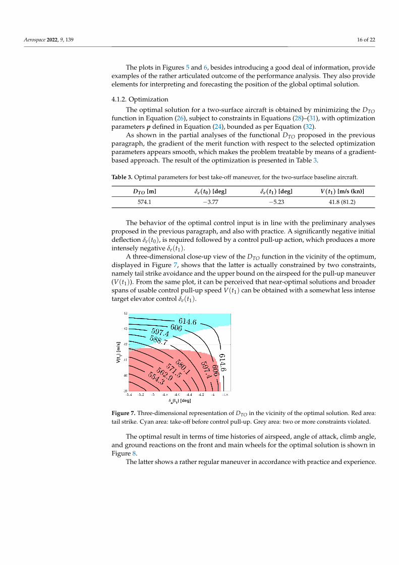
As shown in the partial analyses of the functional DTO proposed in the previousparagraph, the gradient of the merit function with respect to the selected optimizationparameters appears smooth, which makes the problem treatable by means of a gradient-based approach. The result of the optimization is presented in Table 3.

Table 3. Optimal parameters for best take-off maneuver, for the two-surface baseline aircraft.

DTO [m] δe(t0) [deg] δe(t1) [deg] V(t1) [m/s (kn)]

574.1 −3.77 −5.23 41.8 (81.2)

The behavior of the optimal control input is in line with the preliminary analysesproposed in the previous paragraph, and also with practice. A significantly negative initialdeflection δe(t0), is required followed by a control pull-up action, which produces a moreintensely negative δe(t1).

A three-dimensional close-up view of the DTO function in the vicinity of the optimum,displayed in Figure 7, shows that the latter is actually constrained by two constraints,namely tail strike avoidance and the upper bound on the airspeed for the pull-up maneuver(V(t1)). From the same plot, it can be perceived that near-optimal solutions and broaderspans of usable control pull-up speed V(t1) can be obtained with a somewhat less intensetarget elevator control δe(t1).

Figure 7. Three-dimensional representation of DTO in the vicinity of the optimal solution. Red area:tail strike. Cyan area: take-off before control pull-up. Grey area: two or more constraints violated.

The optimal result in terms of time histories of airspeed, angle of attack, climb angle,and ground reactions on the front and main wheels for the optimal solution is shown inFigure 8.

The latter shows a rather regular maneuver in accordance with practice and experience.

Aerospace 2022, 9, 139 17 of 22

Figure 8. Time histories of airspeed (top-left), angle of attack and climb angle (top-right), and groundreactions (bottom) for an optimal take-off run on the two-surface aircraft. Triangle markers indicatevalues associated to time instant t1.

4.2. Optimal Take-Off of Three-Surface Aircraft with Redundant Longitudinal Control

In order to provide an as fair as possible comparison to the two-surface aircraft, thusshowing the effect of just having a three-surface configuration instead of a standard two-surface, a new aircraft has been obtained from the baseline DA-42, adding a canard (seeFigure 9 for a comparison). The sizing of the new three-surface aircraft has been carried outbased on two considerations. Firstly, to keep the airborne stability and control performancesimilar to that of the reference DA-42, the static margin and the overall control volumehave been preserved, as described in detail in [9]. Correspondingly, the wing has beenrelocated backwards with respect to the baseline. Secondly, the landing gear of the newaircraft has been shifted backwards, in order to keep the same distance between the centerof gravity and the main landing gear as on the original DA-42. Concerning the tail clearancefor the activation of the tail-strike constraint, this has been set in order to preserve thesame maximum pitch angle of the DA-42 on ground. Basic data for the three-surfaceconfiguration are recalled in Table 4.

Figure 9. Comparison of the original planform of the DA-42 and the modified three-surface aircraft.

Aerospace 2022, 9, 139 18 of 22

Table 4. Basic features of three-surface configuration. Longitudinal distances positive forward.

Parameter Symbol Value Unit

Tail surface St 1.87 m2

Canard surface Sc 1.19 m2

Wing shift ∆xACw −0.70 mCenter of gravity shift ∆xG −0.34 m

The optimal problem solved for the three-surface aircraft is the same considered forthe original DA-42, with the only difference due to the set of parameters, which is thatreported in Equation (25) instead of Equation (24). Clearly, the larger number of parametersmakes the graphical exploration of the cost function DTO very impractical.

4.2.1. Example of Parameter Analysis of the Merit Function

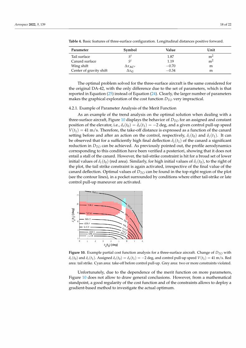
As an example of the trend analysis on the optimal solution when dealing with athree-surface aircraft, Figure 10 displays the behavior of DTO for an assigned and constantposition of the elevator, i.e., δe(t0) = δe(t1) = −2 deg, and a given control pull-up speedV(t1) = 41 m/s. Therefore, the take-off distance is expressed as a function of the canardsetting before and after an action on the control, respectively, δc(t0) and δc(t1). It canbe observed that for a sufficiently high final deflection δc(t1) of the canard a significantreduction in DTO can be achieved. As previously pointed out, the profile aerodynamicscorresponding to this condition have been verified a posteriori, showing that it does notentail a stall of the canard. However, the tail-strike constraint is hit for a broad set of lowerinitial values of δc(t0) (red area). Similarly, for high initial values of δc(t0), to the right ofthe plot, the tail strike constraint is again activated, irrespective of the final value of thecanard deflection. Optimal values of DTO can be found in the top-right region of the plot(see the contour lines), in a pocket surrounded by conditions where either tail-strike or latecontrol pull-up maneuver are activated.

Figure 10. Example partial cost function analysis for a three-surface aircraft. Change of DTO withδc(t0) and δc(t1). Assigned δe(t0) = δe(t1) = −2 deg, and control pull-up speed V(t1) = 41 m/s. Redarea: tail strike. Cyan area: take-off before control pull-up. Grey area: two or more constraints violated.

Unfortunately, due to the dependence of the merit function on more parameters,Figure 10 does not allow to draw general conclusions. However, from a mathematicalstandpoint, a good regularity of the cost function and of the constraints allows to deploy agradient-based method to investigate the actual optimum.

Aerospace 2022, 9, 139 19 of 22

4.2.2. Optimal Solution

In case an optimization is carried out based on the five optimization parameters inEquation (25), a solution featuring a roughly constant value of the canard deflection isobtained (similar to what can be seen in Figure 10). The quantitative solution is presentedin Table 5. This is interesting, since it shows that the use of the canard like a flap instead ofa continuously deflectable surface like a tail elevator, may be envisaged. Instead, a mildnegative deflection of the elevator is required, as expected.

Table 5. Parameters for optimal take-off for a three-surface aircraft.

DTO [m] δe(t0) [deg] δc(t0) [deg] δe(t1) [deg] δc(t1) [deg] V(t1) [m/s (kn)]

534.3 1.09 12.69 −0.68 12.99 40.3 (78.3)

The optimal solution for the original DA-42 baseline can be retrieved for comparisonin Table 3. It can be observed that a non-negligible 7% reduction in the optimal take-offdistance DTO is obtained by moving to a three-surface configuration.

4.2.3. Considerations on Control Linkage

The optimal values of canard and elevator deflection in Table 5 for the three-surface air-craft have been investigated considering the five optimization variables, and, in particular,the initial and final values of the elevator and canard deflection, as independent quantities.However, as explained in paragraph 3.1, the modeling adopted for this study allows toeffortlessly envisage a linear relationship between the deflections of the elevator and ca-nard, which would be easy to design and manufacture in the field. The ensuing linkagewould constrain both control surfaces to move as a result of a deflection of the control yoke,making the mathematical solution obtained from optimal analysis practically achievable.

Considering Equation (18), the values of a = −0.169 and b = 0.225 rad for the optimalsolution in Table 5.

A first consideration concerning this result is on its robustness. By performing ananalysis of the cost function distance DTO in the vicinity of the optimal solution, it canbe observed that the latter is—as expected—significantly constrained. This is shown inFigure 11, where on the left plot the values of δe(t0) and δe(t1) are presented on the axes,and V(t1) has been set at its optimal value, and on the right the V(t1) and δe(t1) are freeparameters, and δe(t0) has been set at the optimal value (clearly, δc is set according tothe linkage law, and its initial and final values are correspondingly not free parametersany more).

Figure 11. Take-off distance for the three-surface aircraft with optimal linkage, as a function ofδe(t0) and δe(t1) for optimal V(t1) (left), and as a function of δe(t1) and V(t1) for optimal δe(t0)

(right). Red area: tail strike. Cyan area: take-off before control pull-up. Grey area: two or moreconstraints violated.

Aerospace 2022, 9, 139 20 of 22

This suggests that the choice of this linkage might introduce a certain sensitivity fromthe actual choice of parameters in a take-off maneuver. In other words, if not deflecting theyoke of the right amount or at the right control pull-up speed, the resulting take-off mighteasily produce the violation of a constraint, which, physically speaking, might for instanceproduce a tail-strike.

This suggests, for practical purposes, choosing a slightly sub-optimal condition, i.e., asomewhat higher DTO and the corresponding set of five parameters. If on the one handthis would not ensure the feasibility of the globally optimal take-off maneuver, it wouldincrease on the other the robustness of the solution, increasing the practical safety of theactual maneuver, mathematically represented in particular by a less critical compliancewith respect to tail-strike and maximum pitch-rate constraints.

A second consideration stems from the results of the optimization of the linkage forcruise, proposed in [9]. The corresponding values of the coefficients in Equation (18) isa = 0.461 and b = 0.329 deg, which are significantly different from those obtained in thepresent study. When applied, the values just mentioned produce the optimal achievablecondition reported in Table 6, which, in particular, correspond to a DTO significantly abovethe optimal value shown in Table 5, and coincidentally closer to the value achievable witha two-surface aircraft (see Table 3).

Table 6. Parameters for optimal take-off, for a three-surface aircraft with control linkage tuned foroptimal cruise.

DTO [m] δe(t0) [deg] δc(t0) [deg] δe(t1) [deg] δc(t1) [deg] V(t1) [m/s (kn)]

588.7 −5.54 −2.21 −6.39 −2.61 41.3 (80.4)

This is not surprising, since the requirements which the synthesis of the cruise linkagehave been based upon do not correspond with those driving the analysis presented inthis paper. However, this shows that capturing both optimal working conditions in cruiseand take-off with a single linear linkage is not generally possible. An ensuing suggestionwhich may be obtained is that, for a practical implementation of a control on a three-surface aircraft, a linear mechanical control linkage may be adopted with a tuning wheelin it, capable of altering the linear linkage for different phases of the flight. Of course, aconceptually easier way to develop such a control would be that of departing from a directmechanical linkage, implementing an electronics-augmented system instead. In the latterscenario, a change in the linkage characteristics would be obtained by simply programming(i.e., scheduling) the coefficients of the linear link as a function of the flight phase. This maybe identified by an action of the pilot, switching to either a terminal phase or cruising mode.

5. Conclusions

In the present research, the increase in the take-off performance of a three-surfaceaircraft with respect to a two-surface one was investigated.

Despite a good deal of literature that exists regarding the topic of aerodynamics andaeroelasticity of canard and three-surfaces configurations, the specific behavior in terminalmaneuvers of such aircraft is not currently covered.

Furthermore, as opposed to the existing literature concerning take-off optimization,typically focused on providing means of improving take-off key indicators (e.g., loads,ground clearance, rolling distance and noise), this research tries to assess the advantageof an assigned (i.e., non-negotiable) three-surface configuration, shown to be capable ofsuccessfully reduce trim drag in cruise in prior research, also in a take-off maneuver.

An original description of take-off has been proposed starting from a classical lumped-coefficient approach. This is typical to flight mechanics, and allows to seamlessly cover bothtwo-surface and three-surface aircraft. After introducing a model for take-off dynamics,the take-off maneuver was modeled as a reaction to a prescribed time history of controls.The latter has been envisaged taking into account three desired features:

Aerospace 2022, 9, 139 21 of 22

• Simplicity of the time history, so as to allow a pilot to carry out the maneuver;• A minimal set of descriptive parameters, in order to reduce computational cost in an

optimal analysis;• A set of parameters compatible with the need to manufacture a linear linkage connect-

ing the elevator and canard surfaces.

An optimal analysis of the take-off performance was carried out at first on a baselinetwo-surface aircraft. For this case, a visual study of the cost function, identified in thetake-off distance DTO, was possible, thanks to the very reduced number of optimizationparameters.

Next, a qualitatively similar optimal analysis was carried out on a three-surface aircraft,obtained from the baseline in a way such to make the two equivalent in a stability andcontrol authority sense, both in flight and in take-off.

The simulation model, as well as the implementation of some constraints in theoptimization have allowed obtaining a streamlined algorithm, computationally manageablewithout difficulty and imposing irrelevant machine time overheads on standard commercialcomputers. This, in turn, makes the envisaged procedure a good asset in a preliminarydesign or performance verification phase.

The result of the optimal analysis on the three-surface aircraft has shown a 7% incre-ment in performance achievable by suitably making use of redundant control on the pitchaxis. No stall issues on the control surfaces have been encountered in the performanceanalysis phase, thanks to the generally mild deflections required for maneuvering. Theoptimal region is generally constrained by tail-strike or an excessively delayed pull-up, sothat liftoff takes place before an actual pull on the control yoke.

Interestingly, the optimal result in this configuration features a roughly constantvalue of the canard deflection during the maneuver, suggesting its use as a flap morethan of a control surface. A potential weak robustness of the optimal solution was found,meaning that the achievement of the global optimum would come only for a precise take-offmaneuver, and with the risk of incurring in physical limitations (such as tail-strike) incase of small deviation from it. This suggests to consistently drift in practice towards asub-optimal maneuver, granting a reduced advantage on take-off distance, with the plus ofa lower risk of accidents in case the pilot’s action on the controls were not perfect.

Finally, from the comparison of a possible structure of a linear linkage between thecanard and elevator stemming from the optimal solution, it was evidenced that a differ-ence exists with respect to what was obtained in cruise condition from previous studies.Although not surprising, this suggests that a single linear linkage cannot be designed to cap-ture optimum performance in both cruise and take-off, but instead a proper scheduling ofthe linkage should be envisaged, easier to obtain in an electronics-augmented control chain.

As a final consideration, despite being possibly less disruptive in terms of an increasein take-off performance with respect to technical solutions specifically targeting that goal(such as distributed electric propulsion or blown wings), a three-surface configuration canbe profitably employed to reduce the take-off length, besides optimizing cruise performance.Furthermore, this result is obtained without a substantial technological leap with respect tothe existing baseline, thus representing an easily achievable answer to the need for moreefficient and socially acceptable aircraft.

Author Contributions: C.E.D.R. and S.C. developed the original formulation and composed thepresent paper. L.C. contributed to the refinement of the formulation, and carried out the quantitativeanalyses. All authors participated equally within the development of the body of the work, withdiscussions and critical comments to the results. All authors have read and agreed to the publishedversion of the manuscript.

Funding: This research received no external funding.

Institutional Review Board Statement: Not applicable.

Informed Consent Statement: Not applicable.

Aerospace 2022, 9, 139 22 of 22

Data Availability Statement: All the data and the numerical tools used in this work may be obtainedby contacting the corresponding authors.

Conflicts of Interest: The authors declare no conflicts of interest.

References1. Agnew, J.; Hess, J. Benefits of aerodynamic interaction to the three-surface configuration. J. Aircr. 1980, 17, 823–827. [CrossRef]2. Kendall, E.R. The minimum induced drag, longitudinal trim and static longitudinal stability of two-surface and three-surface

airplanes. In Proceedings of the AIAA 2nd Applied Aerodynamics Conference, Seattle, WA, USA, 21–23 August 1984.3. Kendall, E.R. The theoretical minimum of induced drag of three-surface airplanes in trim. J. Aircr. 1985, 22, 847–854. [CrossRef]4. Kroo, I. A general approach to multiple lifting surface design and analysis. In Proceedings of the Aircraft Design Systems and

Operations Meeting, San Diego, CA, USA, 31 October–2 November 1984.5. Ricci, S.; Scotti, A.; Zanotti, D. Control of an all-movable foreplane for a three surface aircraft wind tunnel model. Mech. Syst.

Signal Process. 2006, 20, 1044–1066. [CrossRef]6. Mattaboni, M.; Quaranta, G.; Mantegazza, P. Active flutter suppression for a three-surface transport aircraft by recurrent neural

networks. J. Guid. Control Dyn. 2009, 32, 1295–1307. [CrossRef]7. Strohmeyer, D.; Seubert, R.; Heinze, W.; Osterheld, C.; Fornasier, L. Three surface aircraft—A concept for future transport aircraft.

In Proceedings of the 38th AIAA Aerospace Science Meeting and Exhibit, Reno, NV, USA, 1–3 January 2000.8. Gundlach, J. Designing Unmanned Aircraft Systems: A Comprehensive Approach, 2nd ed.; American Institute of Aeronautics and

Astronautics: Reston, VA, USA, 2012.9. Cacciola, S.; Riboldi, C.E.D.; Arnoldi, M. Three-surface model with redundant longitudinal control: Modeling, trim optimization

and control in a preliminary design perspective. Aerospace 2021, 8, 139. [CrossRef]10. Riboldi, C.E.D.; Gualdoni, F. An integrated approach to the preliminary weight sizing of small electric aircraft. Aerosp. Sci. Technol.

2016, 58, 134–149. [CrossRef]11. Riboldi, C.E.D. An optimal approach to the preliminary design of small hybrid-electric aircraft. Aerosp. Sci. Technol. 2018, 81,

14–31. [CrossRef]12. Riboldi, C.E.D. Energy optimal off-design power management for hybrid electric aircraft. Aerosp. Sci. Technol. 2019, 105, 1.

[CrossRef]13. Riboldi, C.E.D.; Trainelli, L.; Biondani, F. Structural batteries in aviation: A preliminary sizing methodology. J. Aerosp. Eng. 2020,

3, 040200311–040200315. [CrossRef]14. Trainelli, L.; Riboldi, C.E.; Rolando, A.; Salucci, F. Methodologies for the initial design studies of an innovative community-friendly

miniliner. IOP Conf. Ser. Mater. Sci. Eng. 2021, 1024, 0121091–0121098. [CrossRef]15. Peterson’s Performance Plus, Inc. 1465 S.E. 30th, Municipal Airport, El Dorado, KS 67042. 2021. Available online: www.katmai-

kenai.com (accessed on 23 February 2022).16. Piaggio Aerospace, Viale Generale Disegna, 1, 17038 Villanova d’Albenga Italy. 2021. Available online: www.piaggioaerospace.it/

(accessed on 23 February 2022).17. Riboldi, C.E.D.; Trainelli, L.; Rolando, A.; Mariani, L.; Salucci, F. Predicting the effect of electric and hybrid electric aviation on

acoustic pollution. Noise Mapp. 2020, 7, 35–56. [CrossRef]18. Del Carre, A.; Palacios, R. Simulation and optimization of takeoff maneuvers of very flexible aircraft. J. Aircr. 2020, 57, 1097–1110.

[CrossRef]19. De Marco, A.; Trifari, V.; Nicolosi, F.; Ruocco, M. A simulation-based performance analysis tool for aircraft design workflows.

Aerospace 2020, 7, 155. [CrossRef]20. Moore, K.R.; Ning, A. Takeoff and performance trade-offs of retrofit distributed electric propulsion for urban transport. J. Aircr.

2019, 56, 1880–1892. [CrossRef]21. Reddt, S.R.; Sobieczky, H.; Dulikravic, G.S.; Abdoli, A. Multi-element winglets: Multi-objective optimization of aerodynamic

shapes. J. Aircr. 2016, 53, 992–1000. [CrossRef]22. Roskam, J. Airplane Design; Roskam Aviation and Engineering Corporation: Ottawa, KS, USA, 1988.23. Pamadi, B.N. Performance, Stability, Dynamics and Control of Aircraft; American Institute of Aeronautics and Astronautics: Reston,

VA, USA, 1998.24. Diamond Aircraft; Diamond Aircraft Industries GmbH. N.A. Otto-Strasse 5, 2700 Wiener Neustadt, Austria. 2021. Available

online: www.diamondaircraft.com/ (accessed on 23 February 2022).