Strathprints Institutional Repository - CORE

Strathprints Institutional Repository

Borg, Matthew Karl and Macpherson, Graham and Reese, Jason (2010) Controllers forimposing continuum-to-molecular boundary conditions in arbitrary fluid flow geometries. MolecularSimulation, 36 (10). pp. 745-757. ISSN 0892-7022

Strathprints is designed to allow users to access the research output of the University of Strathclyde.Copyright c© and Moral Rights for the papers on this site are retained by the individual authorsand/or other copyright owners. You may not engage in further distribution of the material for anyprofitmaking activities or any commercial gain. You may freely distribute both the url (http://strathprints.strath.ac.uk/) and the content of this paper for research or study, educational, ornot-for-profit purposes without prior permission or charge.

Any correspondence concerning this service should be sent to Strathprints administrator:mailto:[email protected]

http://strathprints.strath.ac.uk/

brought to you by COREView metadata, citation and similar papers at core.ac.uk

provided by University of Strathclyde Institutional Repository

https://core.ac.uk/display/9030973?utm_source=pdf&utm_medium=banner&utm_campaign=pdf-decoration-v1



mailto:[email protected]


Controllers for imposing continuum-to-molecular boundary conditions in arbitrary fluid flowgeometries

Matthew K. Borga*, Graham B. Macphersonb and Jason M. Reesea

aDepartment of Mechanical Engineering, University of Strathclyde, Glasgow G1 1XJ, UK; bOpenCFD Ltd, 9 Albert Road, Caversham,Reading, Berkshire RG4 7AN, UK

(Received 6 October 2009; final version received 5 March 2010)

We present a new parallelised controller for steering an arbitrary geometric region of a molecular dynamics (MD) simulationtowards a desired thermodynamic and hydrodynamic state. We show that the controllers may be applied anywhere in thedomain to set accurately an initial MD state, or solely at boundary regions to prescribe non-periodic boundary conditions(PBCs) in MD simulations. The mean molecular structure and velocity autocorrelation function remain unchanged (whensampled a few molecular diameters away from the constrained region) when compared with those distributions measuredusing PBCs. To demonstrate the capability of our new controllers, we apply them as non-PBCs in parallel to a complex MDmixing nano-channel and in a hybrid MD continuum simulation with a complex coupling region. The controllermethodology is easily extendable to polyatomic MD fluids.

Keywords: molecular dynamics; hybrid MD continuum simulations; boundary conditions; nanofluidics; thermodynamicstate; controllers

1. Introduction

The use of periodic boundary conditions (PBCs) is typical

of molecular dynamics (MD) [1,2] simulations, as they

provide a conservative, efficient, simple and robust

implementation for studying systems at equilibrium.

Despite these advantages, however, many engineering

applications require a non-periodic alternative to control

continuum properties at a boundary region. Some

examples include MD systems with open boundaries,

such as fluid flows requiring inlet and outlet boundary

conditions, or non-equilibrium MD systems exhibiting

gradients of density and temperature across boundaries of

the domain. Additionally, an important class of examples

is hybrid MD continuum methods [3–7] that require

boundary conditions prescribed from a continuum solution

at the coupling interface.

Various methods for controlling continuum properties

have been proposed in the literature. Sun and Ebner [8]

proposed a 1D ‘piston’ at a boundary that forces molecules

into the bulk. At specified time intervals, the piston resets

to its original position and inserts molecules within the

dilute region so as to match the density. Methods for

changing density in the global MD domain also exist,

which require changing the volume of the domain and

rescaling all molecular positions [2]. The application of a

gravitational force to all molecules within the domain [9]

is a widely used technique to drive Poiseuille-type flow

configurations, but the channel centre velocity is typically

an outcome of the simulation rather than an input.

Furthermore, the method still relies mostly on the

application of PBCs, hence its usefulness still seems

limited. O’Connell and Thompson [3] and Nie et al. [4]

derived a constrained Lagrangian technique for imposing

momentum in hybrid simulations of liquids, while Flekkøy

et al. [5] and Delgado-Buscalioni and Coveney [6] instead

proposed flux exchange schemes between continuum and

MD formulations. Finally, concepts derived from control

theory are being established as plausible methods for

changing and converging the state of a fluid in MD

simulations. To the author’s knowledge, the feedback

control concept in MD was originally described by Li et al.

[10], and further exploited by Kotsalis et al. [11,12] for

controlling 1D density error gradients, next to non-

periodic planar boundaries.

Several issues surround the models proposed in the

literature. First, the use of global Cartesian coordinates for

imposing local perturbations on molecules precludes the

imposition of spatially varying properties in complex 3D

regions. Typically, control is applied to 1D boundary

regions in cuboid-geometry domains with target values that

are spatially uniform. Second, there is a lack of generality

and flexibility in the proposed models, such as the ability to

regulate the frequency of control, the applicability of

the models to both pure and multi-species fluids and the

relative ease of applying many controllers within an MD

simulation. Finally, it is sometimes unclear from the

publications whether the algorithms have been designed

and applied for parallel processing, an issue which is of

ISSN 0892-7022 print/ISSN 1029-0435 online

q 2010 Taylor & Francis

DOI: 10.1080/08927021003752812

http://www.informaworld.com

*Corresponding author. Email: [email protected]

Molecular Simulation

Vol. 36, No. 10, September 2010, 745–757

Downloaded By: [Reese, Jason] At: 09:01 16 October 2010

utmost importance in computationally intensive simu-

lations. These limitations, therefore, impede MD and

hybrid MD continuum simulations of more realistic

engineering applications.

In this paper, we present a new set of controller

algorithms for imposing density and velocity. These have

several unique features. The mesh is kept static, no moving

pistons are used nor is the simulation domain permitted

to expand or contract. Individual cells on the mesh are

utilised for localised control of continuum properties.

Parallelisation on distributed processors is achieved,

spatially varying flows are obtained and control is possible

in complex 3D regions. Moreover, non-periodic boundary

conditions (NPBCs) may be applied at generally complex

boundaries of MD simulations, or at the arbitrary shaped

interfaces of hybrid MD continuum simulations. In such

a hybrid scheme, the continuum finite-volume cells are

linked to the molecular cells via the controllers. In

addition, a feedback loop algorithm is implemented;

for density control, molecules are inserted or deleted

depending on the error between the measured and target

density within an arbitrary cell. For velocity control, an

external force is incorporated in the equations of motion of

molecules occupying the cell, which corresponds to the

velocity error relating the measured to target velocity

within the same cell. Finally, a flexible decoupled time

scheme is proposed on a per-controller basis so that

an arbitrary continuum property may be controlled at

frequencies appropriate to the time variations of the target

property dictated by the problem, and measured over

longer timescales to increase its statistical accuracy when

supplied in the feedback loop.

In this paper, our new control method is described

in Section 2, and test cases demonstrated in Section 3.

Conclusions are made in Section 4.

2. Method

We consider a domain of arbitrary geometry, defined by an

unstructured polyhedral mesh, typically used in finite-

volume computational fluid dynamics (CFD). The MD

fluid occupies the domain geometry and consists of point

masses (which we will refer to as ‘molecules’) that interact

through a pairwise potential U(rij), where rij ¼ jrijj and

rij ¼ ri 2 rj is the separation vector between a pair of

molecules (i, j). The standard shifted Lennard-Jones (LJ)

12-6 potential [2] is used:

UðrijÞ ¼41

rijs

� �2122

rijs

� �26� �

2 ULJðrcutÞ; rij # rcut;

0; rij . rcut;

8<:

ð1Þ

where s is the characteristic length scale, 1 is the

characteristic potential energy, rcut is the cut-off radius and

ULJðrcutÞ is the potential energy value at which the LJ

potential gets truncated.

The positions ri and velocities vi of molecules evolve

according to standard Newtonian dynamics

miai ¼ f i; ð2Þ

where ai ¼ €ri and mi are the molecule’s acceleration and

mass, respectively. The Verlet Leapfrog algorithm [2] is

used to integrate numerically the equations of motion, by a

numerical MD time step Dtm: update first the mid-step

velocity viðt þ Dtm=2Þ ¼ viðtÞ þ 1=2aiðtÞDtm and advance

the molecules to their new positions riðt þ DtmÞ ¼

riðtÞ þ viðt þ Dtm=2ÞDtm. Here, we use an efficient

tracking scheme [13] on molecules as they move within

the mesh. Molecules get transferred across processors as

they collide with interprocessor boundaries, and also a

molecule’s cell occupancy is updated as it moves from cell

to cell of the mesh. Next, we compute the intermolecular

force on all the molecules:

f i ¼XNmol

j¼1ð–iÞ

f ðrijÞrij

jrijj; ð3Þ

where f ðrijÞrij=jrijj ¼ 27UðrijÞ is the pair force potential

and Nmol is the number of molecules located within the

sphere of radius rcut, centred at ri. This step makes use of the

arbitrary interacting cells algorithm scheme [14], which is a

generalisation of the linked cells algorithm [1] for computing

intermolecular pair forces in complex meshes. The

acceleration is given by aiðt þ DtmÞ ¼ f i=mi. Finally,

we update the second-step velocity viðt þ DtmÞ ¼

viðt þ Dtm=2Þ þ ð1=2Þaiðt þ DtmÞDtm. The MD code

which we use, including the algorithms briefly mentioned

above, is implemented in OpenFOAM v. 1.6 (the open

source CFD toolbox; available online: www.openfoam.org),

which is open source and available to be downloaded freely

from OpenFOAM.

2.1 Controller methodology

Our general controller methodology is used to converge

continuum properties within individual cells of the mesh

(see Figure 1).

The methods for imposing non-equilibrium MD

proposed in the literature generally involve applying

additional perturbations (e.g. in the form of external forces

fexti ) to molecules by using global coordinates. An example

is a code that loops over all molecules in the domain and

applies control if the molecule’s position is within, say,

xmin # xi # xmax (e.g. [4]).

Instead, we consider applying external perturbations

locally using control cells, which is facilitated by the cell

occupancy data structure that gets updated every time step:

an arbitrary cell on the mesh stores an inexpensive link to

M.K. Borg et al.746


those molecules that are currently residing within. This

method introduces numerous benefits. First, control is

implemented by looping over molecules within the cell,

rather than over molecules within the system. Second, the

controlling zone (a group of control cells) can be any

arbitrary 3D shape, size and location within the simulation

domain. For example, the control zone could be selected as

the entire domain in order to converge to an initial MD

state, and thereafter solely as the boundary regions in order

to implement NPBCs. Third, spatially varying properties

may be imposed within MD simulations using this local

approach by specifying different target properties per

control cell. Finally, the controller code is parallelised,

since the MD mesh geometry is partitioned onto separate

processors based on the cells that comprise the mesh

(software package and libraries for sequential and parallel

graph partitioning, static mapping and sparse matrix block

ordering and sequential mesh and hypergraph partitioning;

available online: www.labri.fr/perso/pelegrin/scotch/).

Fields of target continuum properties are prescribed to

the state controller (see Figure 1). Each entry within a field

corresponds to an MD cell in the controlling zone: an

arbitrary control cell P ‘knows’ the required cell-centred

density, rreqP , velocity u

reqP and temperature T

reqP at any time

t of the simulation. Throughout the simulation, the fields

may either be uniform, or be altered by some form of

external function (temporally and/or spatially) or be

directly modified by the continuum solution in an

overlapping region if it is a hybrid simulation. In the

latter, the overlaying coupling region is identical to the MD

controlling zone: an arbitrary finite-volume CFD cell P0

corresponds to the MD control cell P in shape, size and

global coordinate.

2.1.1 Control functions

A simple closed-loop (negative feedback) control system

is implemented. The three functions of the control system

are defined as follows, see Figure 1:

(1) Sensor – measures the macroscopic property from a

zone cell P, using a bin-averaging technique.

(2) Error – computes the difference between the target

property in P 0 and the measured property in its

corresponding cell P, and converts it into a quantity

that is best suited for the actuation function. For

example, the change in density has to be converted

into a number of missing/extra molecules required

within the cell.

(3) Actuator – imposes the necessary control operations

on molecular variables occupying P, based on the

error signal.

2.1.2 Time scheme

We devise a flexible decoupled time scheme for

measurement and control of an arbitrary continuum

property within its controller architecture. The scheme

is decoupled because control and measurement of the

macroscopic property may occur at independent frequen-

cies and over different timescales.

Timescales relating to measurement include the

sampling time, Dts, which defines the time period between

cell-averaged samples, and the averaging time, Dtav, which

MD Mesh

Controlling zone

+–

Error Control cell, P

State controller

rPmeas (t) TP

meas (t) uPmeas (t)

rPreq (t) TP

req (t) uPreq(t)

Actuatorcontrol molecules

Sensormeasure properties

Target continuum fields

Correspondingcell, P ′

Figure 1. Schematic showing the operation of a generic controller using a cell-based approach.

Molecular Simulation 747


defines the time over which samples are accumulated and

time averaged. The relationship between them is the

number of samples:

S ¼Dtav

Dts: ð4Þ

Dtav is dependent on the cell size and property being

controlled [15], so that an accurate mean value is

computed.

Control is applied at well-defined time intervals, Dtcont.

Between controlling steps, no perturbations are imposed

within the control cells, so as to allow local equilibration

of the fluid after being exposed to the controller’s actions.

The frequency of control, and hence the strength of

coupling the measured property with the target, is

therefore dependent on the value chosen for Dtcont.

Control and measurement processes are effectively

linked, by a common time interval, Dt ¼ navDtav ¼

ncontDtcont, where nav and ncont are the number of averages

and number of control steps, respectively, that are

performed within the time interval. Practically, nav ¼ 1

so that Dt ¼ Dtav is the maximum possible averaging time

interval to reduce the statistical error of the measured

property. Therefore, a property measurement carried out

during the previous time interval Dt, is used to compute the

necessary controlling actions to take place over the nextDt.

A key benefit of our proposed time scheme is that

modification to Dtcont is permitted in order to change the

rate of control, without restricting Dtav and hence

affecting the accuracy of any measurement. We highlight

this as an essential requirement in the controller

methodology; poor sampling due to a small Dtav will

feed a noisy error signal to the actuator that may result in

an unstable diverging state.

The most challenging part of a decoupled time scheme

is the requirement that the controlling models distribute

alterations on molecular variables over a series of ncontcontrol time steps, as illustrated in Figure 2.

2.2 Density control

Density is controlled within an arbitrary control cell P,

using the following procedure:

(1) At a time t, compute the density error in P and

translate this into ‘molecules’ using the following

formula:

DNPðt! tnÞ ¼ NINT rreqP ðtnÞ2 rmeas

P ðtÞ� �

VP

� �; ð5Þ

where rmeasP ðtÞ is the measured cell density during the

previous time period (to ! t), rreqP ðtnÞ is the required

cell density at a later time (tn ¼ t þ Dt) and DNPðt!

tnÞ are the total number of molecules to control from

cell P during the next Dt. The NINT(x) function is

required to apply the nearest integer, since only whole

molecules may be introduced (DNP . 0) or removed

(DNP , 0). If rreqP ðtnÞ is not known at a time tn,

it may be extrapolated from old-time quantities:

rreqP ðtnÞ ¼ 2r

reqP ðtÞ2 r

reqP ðtoÞ.

(2) DNP is divided equally across the subsequent ncontcontrol steps:

DNPðtcontj Þ ¼

ceil DNP=ncont� �

; if DNP . 0;

floor DNP=ncont� �

; if DNP , 0;

8<:

ð6Þ

t # tcontj , tn, {j ¼ 1; 2; . . . ; ncont}, followed by a

residual correction to DNPðtcontj Þ at each control step,

so that the prescribed density is matched accurately

during ðt! tnÞ.

(3) At an arbitrary control step, tcontj , two types of mass

residuals are corrected. The number of molecules that

fail to be inserted or deleted in a previous control

step, dNfailP ðtcontj21 Þ, are added to DNPðt

contj Þ. Then, the

cumulative error resulting from the ceiling/flooring

functions in Equation (6) is checked:

∆tm = ∆ts ∆tcont

Control onmolecules

Measurementof property

Continuumproperty

(tn)

time

∆t = ∆tav

ttnto

+–

(to t)

(t nt )

ncont = 2

t2contt1

cont

Figure 2. Schematic showing the timeline for an MD simulation with control. Processes of measurement and control are decoupled, butlinked by a common time interval Dt.

M.K. Borg et al.748


If jDNPðtcontj Þ þ DNsuccess

P j . jDNPj,

Then modify DNPðtcontj Þ to:

DNPðtcontj Þ ¼ DNPðt! tnÞ2 DNsuccess

P ; ð7Þ

where DNsuccessP is the cumulative number of

molecules controlled within previous control steps.

Note that the terms DNfailP and DNsuccess

P are positive or

negative depending on whether DNP . 0 or

DNP , 0, respectively. Furthermore, DNsuccessP is

reset to zero after the whole time interval ðt! tnÞ,

while DNfailP is set to zero after every control step.

(4) Insertion and deletion processes are performed

immediately after the intermolecular force calcu-

lation step of the Leapfrog algorithm, and are

described separately below.

2.2.1 Inserting molecules

If DNP . 0, the actuation function inserts these whole

molecules sequentially into the cell P. During this process,

existing molecules that currently reside within the domain

remain fixed in space and time. The procedure for inserting

one molecule, i, is described.

(1) Search for an insertion site, ri, that ensures non-

overlapping molecules. We employ the USHER

algorithm [16], which performs a steepest-descent

iterative search in the potential energy landscape.

A site to insert a molecule is accepted if its potential

energy is equal to the average potential energy per

molecule within the cell, i.e.

UreqP ¼ kUilP ¼

XSk¼1

XNPðtkÞ

i¼1

1

2

XNmol

j¼1ð–iÞ

UðrijÞ

XSk¼1

NPðtkÞ

; ð8Þ

where NPðtkÞ is the number of molecules residing in P

at time tk.

(2) Create a molecule at ri, and update the acceleration

and potential energy of the surrounding molecules j,

within interaction range:

anj ¼ aoj 2f ðrijÞrij

mjjrijj; ð9Þ

Unj ¼ Uo

j þUðrijÞ

2: ð10Þ

(3) The initial velocity, vi, of the newly inserted molecule

is sampled randomly from a Maxwell–Boltzmann

distribution at the required temperature, TreqP , and

mean velocity, ureqP .

2.2.2 Deleting molecules

If DNP , 0, molecules may be deleted sequentially using

the reverse of the insertion process. Deletion is more

computationally efficient and also more successful than

insertion. Existing molecules within the cell are held fixed

in time and space as candidate molecules are deleted. The

process for deleting one molecule is described:

(1) Initially, select a candidate molecule i from a cell P,

using a criterion that maintains the potential energy of

the cell the same. We use a scheme that loops over all

molecules within cell P and chooses the molecule

with its potential energy closest to UreqP .

(2) Update the accelerations and potential energies of

surrounding molecules to account for the molecule

being deleted. These equations are similar to

Equations (10) and (9) but with the opposite signs

in front of the second terms on the RHS.

(3) Delete molecule i from cell P.

2.2.3 Multi-species control

Our density controller is designed to operate on both single-

andmulti-species fluid systems. For multi-species fluids, the

set-up consists of applying a density controller per species in

a common controlling zone, and providing the controllers

with the target partial densities within the control cells.

2.2.4 Parallelisation

The density controller is parallelised by allowing

processors to communicate during the control steps in

order to check for conflicts immediately after the insertion

site, and/or candidate molecules for deletion have been

identified on each processor. A conflict occurs if any two

or more designated molecules are within rcut. The conflict

is resolved by arbitrarily assigning a priority to each

processor. The processor with the highest priority proceeds

with the insertion/deletion of the molecule, while

processors of lower priority that detect a conflict terminate

their tries and reattempt them in the next try.

2.3 Velocity control

The convective velocity is controlled within P by the

following procedure:

(1) At time t, we compute the velocity error that is to be

imposed per control step:

DuPðtcontj Þ ¼

DuPðt! tnÞ

ncont

¼l

ncontureqP ðtnÞ2 umeas

P ðtÞ� �

; ð11Þ



where umeasP ðtÞ is the measured cell velocity at current

time t, ureqP ðtnÞ is the required cell velocity at a later

time ðtn ¼ t þ DtÞ and l=ncont ¼ Kp is the pro-

portional gain of the controller. The latter is a

modifiable parameter (typically l < 1 and

ncont < 25) that defines the rate at which the

velocities of molecules occupying cell P are

accelerated towards ureqP ðtnÞ. Similarly, if u

reqP ðtnÞ is

unknown at a time tn, it too may be extrapolated from

known quantities: ureqP ðtnÞ ¼ 2u

reqP ðtÞ2 u

reqP ðtoÞ.

(2) At each control step, we add an external force to the

equations of motion of all molecules i occupying cell

P, after the intermolecular force calculation step:

fexti ¼DuPðt

contj Þ

Dtmmi: ð12Þ

2.4 Temperature control

For temperature control, we implement the popular

thermostats [2] using a cell-based approach. In this

paper, we adopt the velocity scaling thermostat [2], which

scales molecular velocities based on the root of the ratio

between target and measured temperatures.

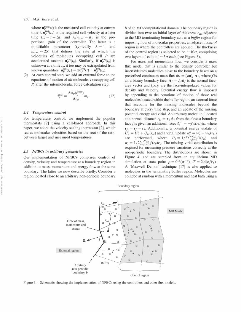
2.5 NPBCs in arbitrary geometries

Our implementation of NPBCs comprises control of

density, velocity and temperature at a boundary region in

addition to mass, momentum and energy flow at the same

boundary. The latter we now describe briefly. Consider a

region located close to an arbitrary non-periodic boundary

b of an MD computational domain. The boundary region is

divided into two: an initial layer of thickness rcut adjacent

to the MD terminating boundary acts as a buffer region for

imposing flow of molecular properties; an adjacent control

region is where the controllers are applied. The thickness

of the control region is selected to be ,10s, comprising

two layers of cells of ,5s each (see Figure 3).

For mass and momentum flow, we consider a mass

flux model that is similar to the density controller but

inserts/deletes molecules close to the boundary based on a

prescribed continuum mass flux _mf ¼ ðruÞf ·Af , where f is

an arbitrary boundary face, Af ¼ Af n̂f is the normal face-

area vector and ðruÞf are the face-interpolated values for

density and velocity. Potential energy flow is imposed

by appending to the equations of motion of those real

molecules located within the buffer region, an external force

that accounts for the missing molecules beyond the

boundary at every time step, and an update of the missing

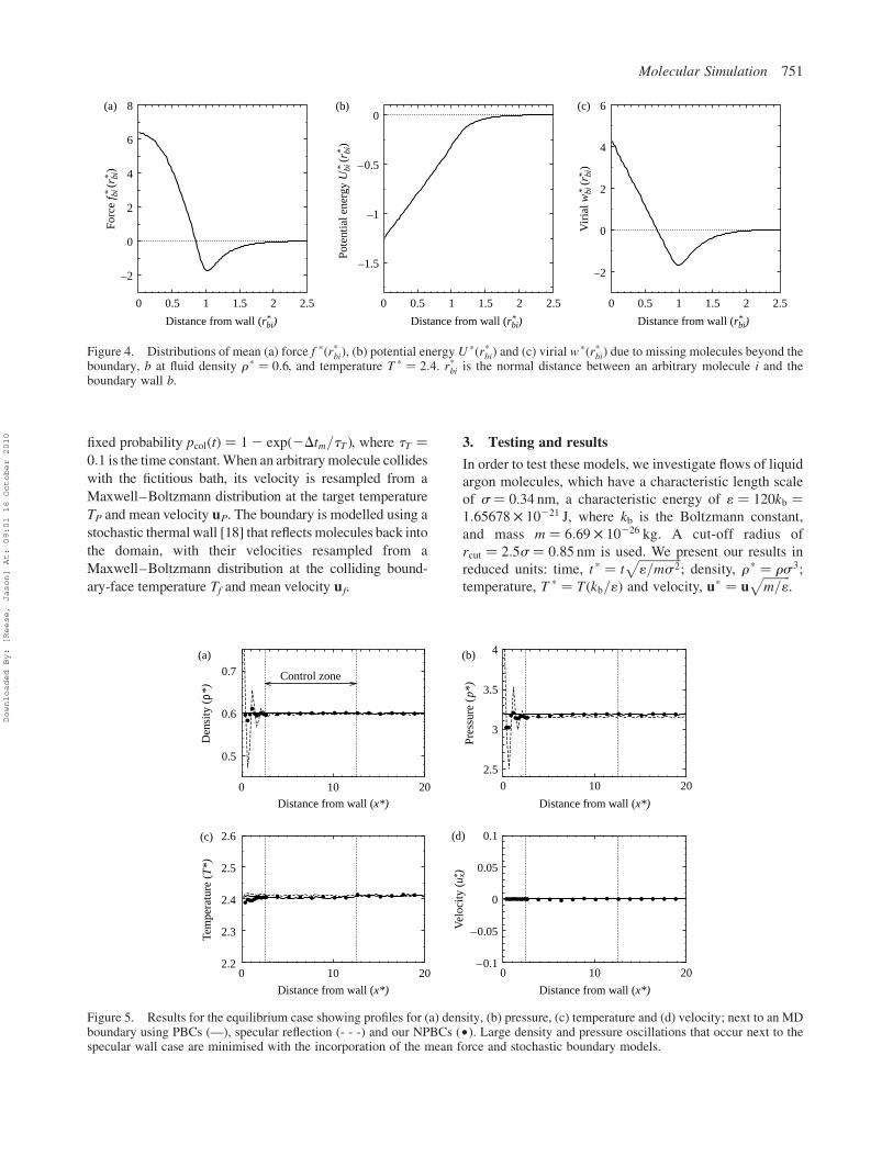
potential energy and virial. An arbitrary molecule i located

at a normal distance rbi ¼ rfi·n̂f from the closest boundary

face f is given an additional force fexti ¼ 2f biðrbiÞn̂f , where

rfi ¼ rf 2 ri. Additionally, a potential energy update of

Uni ¼ Uo

i þ UbiðrbiÞ and a virial update wni ¼ wo

i þ wbiðrbiÞ

are performed, where Ui ¼ 1=2PNmol

jð–iÞUðrijÞ and

wi ¼ 1=2PNmol

jð–iÞ f ðrijÞrij. The missing virial contribution is

required for measuring pressure variations correctly at the

non-periodic boundary. The distributions are shown in

Figure 4, and are sampled from an equilibrium MD

simulation at state point r ¼ 0:6ðs23Þ, T ¼ 2:4ð1=kbÞ.A ‘Maxwell Demon’ technique [17] is also applied to

molecules in the terminating buffer region. Molecules are

collided at random with a momentum and heat bath using a

Boundary region

i

nff

rcut

rcut

Flow of mass,momentum and

energy

MD Mesh

Arbitrarynon-periodicboundary, b

External region

Control region

Buffer

Figure 3. Schematic showing the implementation of NPBCs using the controllers and other flux models.

M.K. Borg et al.750


fixed probability pcolðtÞ ¼ 12 expð2Dtm=tT Þ, where tT ¼

0:1 is the time constant.When an arbitrarymolecule collides

with the fictitious bath, its velocity is resampled from a

Maxwell–Boltzmann distribution at the target temperature

TP and mean velocity uP. The boundary is modelled using a

stochastic thermal wall [18] that reflects molecules back into

the domain, with their velocities resampled from a

Maxwell–Boltzmann distribution at the colliding bound-

ary-face temperature Tf and mean velocity uf.

3. Testing and results

In order to test these models, we investigate flows of liquid

argon molecules, which have a characteristic length scale

of s ¼ 0.34 nm, a characteristic energy of 1 ¼ 120kb ¼

1:65678 £ 10221 J, where kb is the Boltzmann constant,

and mass m ¼ 6:69 £ 10226 kg. A cut-off radius of

rcut ¼ 2:5s ¼ 0:85 nm is used. We present our results in

reduced units: time, t * ¼ tffiffiffiffiffiffiffiffiffiffiffiffiffiffi1=ms2

p; density, r* ¼ rs3;

temperature, T * ¼ Tðkb=1Þ and velocity, u* ¼ uffiffiffiffiffiffiffiffiffim=1

p.

2.2

2.3

2.4

2.5

2.6

Tem

pera

ture

(T

*)

–0.1

–0.05

0

0.05

0.1

Vel

ocity

(u x

)

0.5

0.6

0.7

0 10 20

Den

sity

(ρ*

)

Distance from wall (x*)

0 10 20


0 10 20


0 10 20


Control zone

2.5

3

3.5

4

Pres

sure

(p*

)

(a)

(c) (d)

(b)

*

Figure 5. Results for the equilibrium case showing profiles for (a) density, (b) pressure, (c) temperature and (d) velocity; next to an MDboundary using PBCs (—), specular reflection (- - -) and our NPBCs (†). Large density and pressure oscillations that occur next to thespecular wall case are minimised with the incorporation of the mean force and stochastic boundary models.

–2

0

2

4

6

8

0 0.5 1 1.5 2 2.5

Forc

e f b

i (r b

i)

0 0.5 1 1.5 2 2.5 0 0.5 1 1.5 2 2.5

–1.5

–1

–0.5

0

Pote

ntia

l ene

rgy

Ubi

(rbi

)

–2

0

2

4

6

Vir

ial w

bi (r

bi)

(a) (b) (c)

Distance from wall (rbi)* Distance from wall (rbi)

* Distance from wall (rbi)*

*

**

***

Figure 4. Distributions of mean (a) force f *ðr*biÞ, (b) potential energy U*ðr*biÞ and (c) virial w

*ðr*biÞ due to missing molecules beyond theboundary, b at fluid density r * ¼ 0:6, and temperature T * ¼ 2:4. r*bi is the normal distance between an arbitrary molecule i and theboundary wall b.



0

1

2

3

4

5

6

7

8(a) (b)

0 0.5 1 1.5

VA

CF

<v*

(t*)

v*(0

)>

Time (t*)

0

0.5

1

1.5

2

1 1.5 2 2.5

RD

F g*

(rij)

Intermolecular distance (rij)*

*

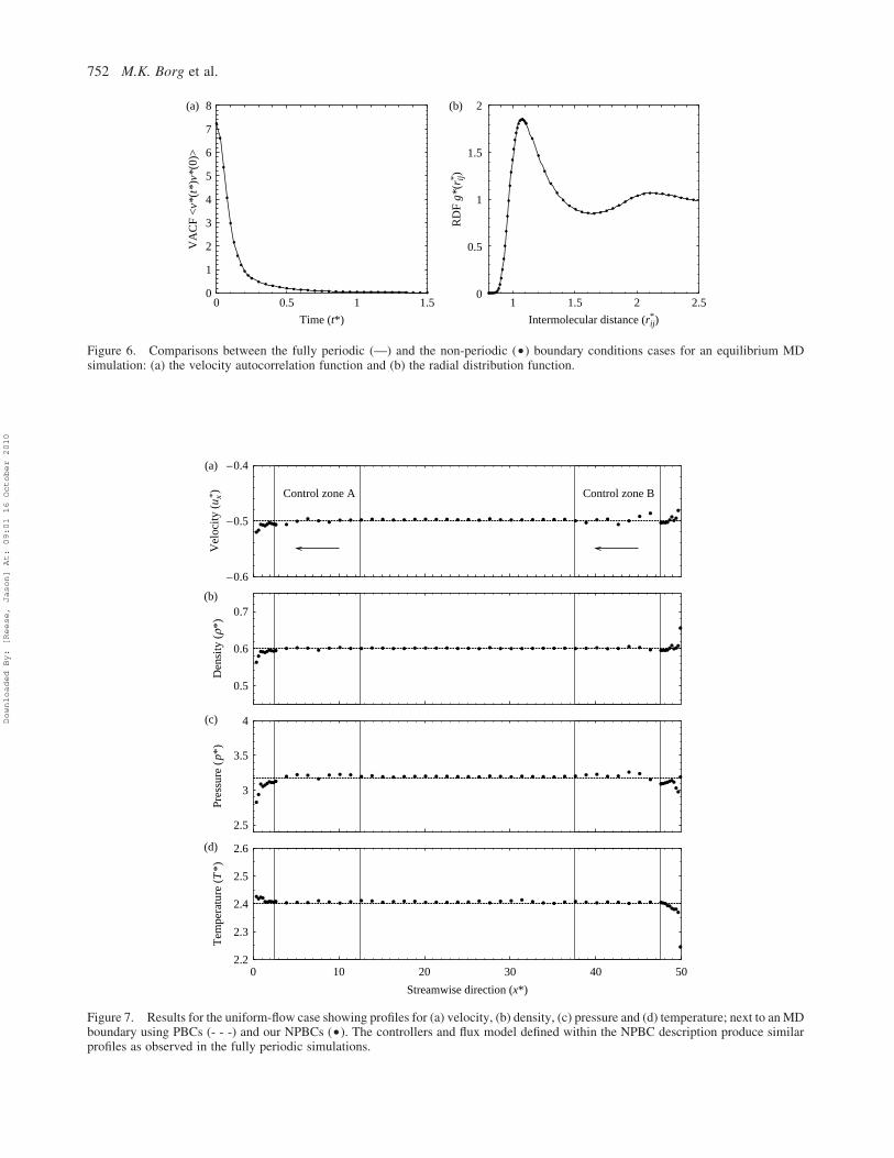
Figure 6. Comparisons between the fully periodic (—) and the non-periodic (†) boundary conditions cases for an equilibrium MDsimulation: (a) the velocity autocorrelation function and (b) the radial distribution function.

2.2

2.3

2.4

2.5

2.6

0 10 20 30 40 50

Streamwise direction (x*)

Tem

pera

ture

(T

*)Pr

essu

re (

p*)

Den

sity

(r*

)V

eloc

ity (

u x* )

2.5

3

3.5

4

0.5

0.6

0.7

–0.6

–0.5

–0.4(a)

(b)

(c)

(d)

Control zone A Control zone B

Figure 7. Results for the uniform-flow case showing profiles for (a) velocity, (b) density, (c) pressure and (d) temperature; next to anMDboundary using PBCs (- - -) and our NPBCs (†). The controllers and flux model defined within the NPBC description produce similarprofiles as observed in the fully periodic simulations.

M.K. Borg et al.752


3.1 Verification studies

3.1.1 Initial state for MD simulations

For the simulations that follow, and generally in most

of our MD simulations, we use our controllers to set an

accurate initial MD state. First, we use a pre-processing

utility [19] for generating initial lattice structures of

molecules in the domain mesh, based on input properties

such as density, temperature, bulk velocity and lattice

structure. Second, we run an MD simulation with the

controllers applied in all cells of the mesh in order to

converge the local fluid properties to the global targets.

Finally, the controllers are switched off and the MD

system is equilibrated.

3.1.2 Test of NPBCs: equilibrium and uniform flow MD

simulations

To simulate equilibrium and 1D uniform flow, we replace

PBCs in one direction of a cubic domain by our NPBCs.

We simulate a domain of dimensions ðx; y; zÞ ¼ ð50s; 20s;20sÞ, set at a state point (T * ¼ 2:4; r* ¼ 0:6), with two

independent NPBCs applied at x ¼ 0 and x ¼ 50s that

control this state point continually. In the equilibrium case,

velocity control is set to zero, u* ¼ ð0; 0; 0Þ. We then

compare density profiles of properties in the x-direction for

three separate cases: fully periodic, semi-periodic (only

reflective walls are applied) and our NPBCs. The results in

Figure 5 show that conformity is achieved in the control

region between the fully periodic case and the NPBCs that

employ the controllers. Also, the density oscillations that

occur due to the finite-size effects of the specular wall

boundary are largely rectified. Furthermore, we see that

the external perturbations imposed within the boundary

region do not influence the liquid structure or its dynamics.

Figure 6 shows a comparison of the radial distribution and

velocity autocorrelation functions from a region located in

the central part of the computational domain, for both fully

periodic and non-periodic cases.

In the uniform-flow case, a mean velocity of u* ¼

ð20:5; 0; 0Þ is applied at both boundaries of the previous

equilibrium case, and steady state is allowed to be reached.

We see in Figure 7 that our NPBCs effectively control the

state at the boundary even if the imposed flow rate is large.

3.2 Control of MD in a 3D complex-geometry mixingchannel

We now consider a microscale mixing channel of three-

inlet one-outlet design, taken from [20] (Figure 8 inset)

and reduce its scale to nanometres so that reasonable

mixing time scales may be simulated (Figure 8).

The nano mixer geometry is initially drawn in

Pro/ENGINEERw, a commercial computer-aided design

drawing application, and exported as a STEP format (.stp)

to GAMBITw (a meshing utility normally used for

FLUENTw CFD). The geometry is meshed using

hexahedral cells, and further exported in mesh format

(.msh) into OpenFOAM, where it is filled with LJ

molecules of two species. The two fluids are essentially

isotopes of argon that have identical properties but

different identification (id) number, so that mixing can be

observed and measured. The NPBCs in inlet A (Figure 8)

supply molecules of fluid I at a constant rate, u*A ¼ ð0; 0;0:25Þ, while inlets B1 and B2 supply molecules of fluid II

at the same rate: u*B1 ¼ ð0:07; 0; 0Þ, u*B2 ¼ ð20:07; 0; 0Þ.These velocities were selected based on the parameter

sensitivity guidelines for flow rate ratios described in [20].

Density and temperature at the inlets are set to r* ¼ 0:6and T * ¼ 2:4, respectively.

At the outlet C, no control is applied since the target

values of density, velocity and temperature are not known

a priori; the complex constrictions in the central part of the

domain and the boundary walls introduce compressibility

effects. So, instead we apply a new mass flux boundary

model that removes molecules of fluids I and II at a rate

computed from the error between the mean density within

the global system and a target density, r* ¼ 0:55.

Fluid I

Fluid II

A

B1 B2

C

5µm10nm

xy

z

Figure 8. The nano mixer MD case shown in its initial state.NPBCs are applied at all three inlets (A, B1, B2) and the outlet(C), depicted by the shaded regions. Note: only 10,000 randommolecules are shown of the,200,000 molecules that occupy thesimulation domain. Inset: an image of the original fabricatedmicroscale mixer taken from [20]; reproduced with permissionfrom copyright holder.



The channel wall boundary is 3D – no PBCs are

applied at all within this simulation. We model the outer

wall using an implicit isothermal stochastically reflective

boundary model that resamples velocities of colliding

molecules from a Maxwell–Boltzmann distribution at

a temperature of T * ¼ 2:4, and zero mean velocity, and

imposes the constraint ðvi·n̂f Þ # 0. In addition, potential

energy and external forces are also applied to molecules

near the boundary to take into effect the missing liquid–

wall molecular interactions. The applied mean force and

potential energy distributions (Figure 9) are sampled from

a small equilibrium MD simulation next to a face-centred

cubic MD wall lattice at a temperature of T * ¼ 2:4 and

density r* ¼ 0:8.The mixing-channel case is decomposed and solved on

eight processors for a duration of t * ¼ 2500. Results of

steady-state mixing are shown in Figures 10 and 11. The

partial densities of both fluids are sampled in a region close

to the outlet (Figure 11) and show that mixing occurs

throughout the width of the outlet channel. Mixing is more

complete in the central part of the channel; at the sides,

we see discrepancies of Dr < 0.03 relative to the mean

(target) partial density.

3.3 Hybrid continuum MD simulations with a complexcoupling region

We can further demonstrate the capabilities of our

controllers, and the NPBCs in which they operate, by

applying them in a complex coupling region of a hybrid

MD-CFD simulation. The case we choose is an isothermal

shear flow (Couette type) that has a complex protrusion in

the stationary wall (see Figure 12). The wall and adjacent

layer of liquid are modelled by MD, while the rest of the

domain and moving wall are simulated by CFD. The

sonicLiquidFlow solver already in OpenFOAM (the open

source CFD toolbox; available online: www.openfoam.org)

is used for the continuum subdomain; it models liquid flow

using the compressible Navier–Stokes equations. Amoving

wall velocity of u*w ¼ ð0:5; 0; 0Þ, with a no-slip boundary

condition, is applied to the top boundary of the domain, and

cyclic boundary conditions are applied in the other two

directions. At the molecular-continuum interface, a 3D

overlap region is present so that coupling between CFD

and MD formulations can occur at regular time intervals of

the simulation. The global mesh (see Figure 12(a)) is

segmented into two separate MD and CFD sub-meshes,

such that the coupling region is common to both sub-

meshes (see Figure 12(b)). This sub-meshing technique

ensures that the coupling region on both meshes are

identical.

The coupling region is made up of two sub-regions,

M ! C (molecular-to-continuum) and C ! M (conti-

nuum-to-molecular), in which velocity boundary con-

ditions are passed between CFD and MD formulations.

In the M ! C sub-region (on the MD mesh), velocity

fields are averaged from molecular data and are passed as

Dirichlet boundary conditions to the CFD mesh.

Similarly, in the C ! M sub-region (on the CFD mesh)

the convective velocity fields are passed as target fields to

the MD mesh. These fields are used by our NPBC

description, that is, via the controllers. Although no

density or temperature coupling is performed, controllers

are still applied in the C ! M region to fix the boundary

state to r* ¼ 0:6 and T * ¼ 1:8. Accurate coupling is

achieved by setting the viscosity (h ¼ 0:899ðffiffiffiffiffiffi1m

p=s2Þ)

and pressure (p ¼ 1:98ðs3=1Þ) of the CFD formulation to

match those sampled from an equilibrium MD simulation

at the desired state point. The viscosity is determined

using the Green–Kubo relationship [2], by averaging the

shear-stress autocorrelation function over 2 £ 106 MD

time steps.

0

10

20

30

(a) (b) (c)

0 0.5 1 1.5 2 2.5

Distance from wall (r*) Distance from wall (r*) Distance from wall (r*)

–1.2

–0.8

–0.4

0

0.4

0.8

1.2

1.6

0 0.5 1 1.5 2 2.5–5

0

5

10

15

20

25

30

35

0 0.5 1 1.5 2 2.5

f bi (

r bi)

**

Ubi

(rbi

)*

*

wbi

(rbi

)*

*

Figure 9. Distributions of mean (a) force, (b) potential energy and (c) virial sampled next to face-centred cubic wall in an equilibriumMD simulation at r * ¼ 0:8 and T * ¼ 2:4. Wall molecules are tethered in space and a harmonic spring potential is applied between atether point and its corresponding wall molecule, Uh ¼ 1=2Ksðri 2 rtethi Þ2, where Ks ¼ 150ð1=s 2Þ is the spring constant.

M.K. Borg et al.754


A coupling time framework is used that advances

the MD and CFD in a sequential manner by a common

coupling time interval Dtcoupling ¼ tCDtc ¼ tMDtm ¼

20ðffiffiffiffiffiffiffiffiffiffiffiffiffiffims2=1

pÞ:

(1) Advance continuum solution t! t þ Dtcoupling by

tC ¼ 200 time steps. MD waits.

(2) Apply C ! M BCs.

(3) Advance MD t! t þ Dtcoupling by tM ¼ 4000 time

steps. CFD waits.

(4) Apply M ! C BCs.

(5) Repeat the dual time-marching scheme until the end

of the simulation.

The hybrid and full MD simulations are each solved

in parallel on two processors, so that timings can be

compared. Steady-state results are shown in Figures 13

and 14, where general agreement of the velocity field is

observed between the full MD and hybrid MD-CFD

simulations. However, the hybrid simulation is approxi-

mately two times faster over the full MD simulation.

Speed-up may also be estimated from the term NFMmol=N

Hmol,

Figure 10. Mid-channel cross-sectional fields showing (a) theLagrangian field of molecules, (b) partial density for fluid I, (c)partial density for fluid II and (d) total velocity.

0

0.1

0.2

0.3

0.4

0.5

0.6

0.7

0.8

0 10 20 30 40 50 60

Den

sity

(ρ*

)

Outlet channel width (x*)

Fluid IFluid II

Fluid I + II

Figure 11. The linear partial-density distribution for both fluidstaken from a sampling region at the outlet of the mixer. Thefigure shows complete mixing in the middle part of the channel.

MD

N-S

Couplingregion

Continuum mesh, C Molecular mesh, M

Bufferregion

10 nmx

y

z

C M

M C

uw

NPBCs

(b) Coupling region

(a)

Figure 12. (a) Hybrid simulation domain of a shear flow with acomplex fixed-wall topology. (b) Schematic of the couplingregion between continuum and molecular subdomain meshes.M ! C and C ! M velocity boundary conditions are transferredbetween pairs of coupled cells, as shown in the two highlightedregions. C ! M coupling is achieved via the controllers.



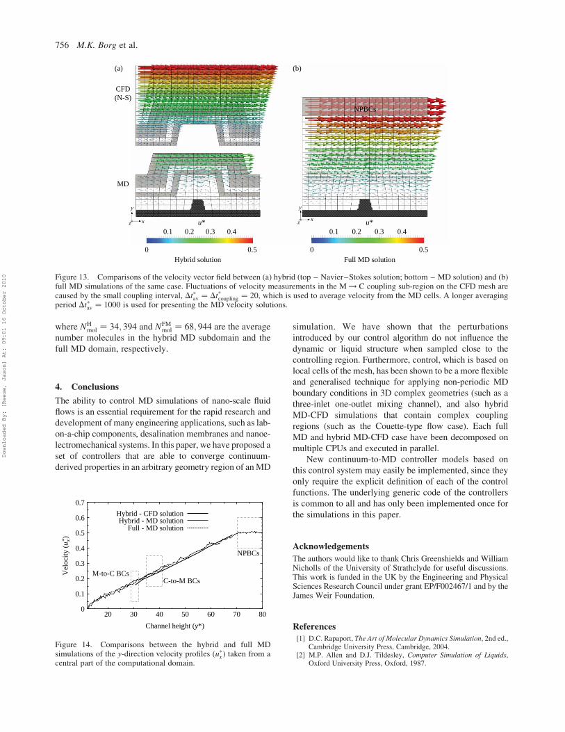
where NHmol ¼ 34; 394 and NFM

mol ¼ 68; 944 are the average

number molecules in the hybrid MD subdomain and the

full MD domain, respectively.

4. Conclusions

The ability to control MD simulations of nano-scale fluid

flows is an essential requirement for the rapid research and

development of many engineering applications, such as lab-

on-a-chip components, desalination membranes and nanoe-

lectromechanical systems. In this paper, we have proposed a

set of controllers that are able to converge continuum-

derived properties in an arbitrary geometry region of anMD

simulation. We have shown that the perturbations

introduced by our control algorithm do not influence the

dynamic or liquid structure when sampled close to the

controlling region. Furthermore, control, which is based on

local cells of the mesh, has been shown to be a more flexible

and generalised technique for applying non-periodic MD

boundary conditions in 3D complex geometries (such as a

three-inlet one-outlet mixing channel), and also hybrid

MD-CFD simulations that contain complex coupling

regions (such as the Couette-type flow case). Each full

MD and hybrid MD-CFD case have been decomposed on

multiple CPUs and executed in parallel.

New continuum-to-MD controller models based on

this control system may easily be implemented, since they

only require the explicit definition of each of the control

functions. The underlying generic code of the controllers

is common to all and has only been implemented once for

the simulations in this paper.

Acknowledgements

The authors would like to thank Chris Greenshields and WilliamNicholls of the University of Strathclyde for useful discussions.This work is funded in the UK by the Engineering and PhysicalSciences Research Council under grant EP/F002467/1 and by theJames Weir Foundation.

References

[1] D.C. Rapaport, The Art of Molecular Dynamics Simulation, 2nd ed.,Cambridge University Press, Cambridge, 2004.

[2] M.P. Allen and D.J. Tildesley, Computer Simulation of Liquids,Oxford University Press, Oxford, 1987.

CFD(N-S)

(a) (b)

MD

0.1 0.2 0.3 0.4 0.1 0.2 0.3 0.4

0.500.5Hybrid solution Full MD solution

NPBCs

u* u*

0

x

y

zx

y

z

Figure 13. Comparisons of the velocity vector field between (a) hybrid (top – Navier–Stokes solution; bottom – MD solution) and (b)full MD simulations of the same case. Fluctuations of velocity measurements in the M ! C coupling sub-region on the CFD mesh arecaused by the small coupling interval, Dt*av ¼ Dt*coupling ¼ 20, which is used to average velocity from the MD cells. A longer averagingperiod Dt*av ¼ 1000 is used for presenting the MD velocity solutions.

0

0.1

0.2

0.3

0.4

0.5

0.6

0.7

20 30 40 50 60 70 80

Vel

ocity

(u x

* )

Channel height (y*)

NPBCs

M-to-C BCsC-to-M BCs

Hybrid - CFD solutionHybrid - MD solution

Full - MD solution

Figure 14. Comparisons between the hybrid and full MDsimulations of the y-direction velocity profiles ðu*xÞ taken from acentral part of the computational domain.

M.K. Borg et al.756


[3] S.T. O’Connell and P.A. Thompson, Molecular dynamics-continuum hybrid computations: A tool for studying complex fluidflows, Phys. Rev. E 52 (1995), pp. R5792–R5795.

[4] X.B. Nie, S.Y. Chen, W. E, and M.O. Robbins, A continuum andmolecular dynamics hybrid method for micro- and nano-fluid flow,J. Fluid Mech. 500 (2004), pp. 55–64.

[5] E.G. Flekkøy, G. Wagner, and J. Feder, Hybrid model for combinedparticle and continuum dynamics, Europhys. Lett. 52 (2000),pp. 271–276.

[6] R. Delgado-Buscalioni and P.V. Coveney, Continuum-particlehybrid coupling for mass, momentum, and energy transfers inunsteady fluid flow, Phys. Rev. E 67 (2003), pp. 1–13, 046704.

[7] T. Werder, J.H. Walther, and P. Koumoutsakos, Hybrid atomistic-continuummethod for the simulation of dense fluid flows, J. Comput.Phys. 205 (2005), pp. 373–390.

[8] M. Sun and C. Ebner, Molecular-dynamics simulation ofcompressible fluid flow in two-dimensional channels, Phys. Rev. A46 (1992), pp. 4813–4818.

[9] J. Koplik, J.R. Banavar, and J.F. Willemsen,Molecular dynamics ofPoiseuille flow and moving contact lines, Phys. Rev. Lett. 60 (1988),

pp. 1282–1285.[10] J. Li, D. Liao, and S. Yip, Imposing field boundary conditions in MD

simulation of fluids: Optimal particle controller and buffer zonefeedback, Mat. Res. Soc. Symp. Proc. 538 (1998), pp. 473–478.

[11] E.M. Kotsalis, J.H. Walther, and P. Koumoutsakos, Control ofdensity fluctuations in atomistic-continuum simulations of denseliquids, Phys. Rev. E 76 (2007), 016709.

[12] E.M. Kotsalis, J.H. Walther, E. Kaxiras, and P. Koumoutsakos,A control algorithm for multiscale flow simulations of water, Phys.Rev. E 79 (2009), 045701.

[13] G.B. Macpherson, N. Nordin, and H.G. Weller, Particle tracking inunstructured, arbitrary polyhedral meshes for use in CFD andmolecular dynamics, Commun. Numer. Methods Eng. 25 (2009),pp. 263–273.

[14] G.B. Macpherson and J.M. Reese, Molecular dynamics in arbitrarygeometries: Parallel evaluation of pair forces, Mol. Simulat. 34(2008), pp. 97–115.

[15] N. Hadjiconstantinou, A. Garcia, M. Bazant, and G. He, Statisticalerror in particle simulations of hydrodynamic phenomena,J. Comput. Phys. 187 (2003), pp. 274–297.

[16] R. Delgado-Buscalioni and P.V. Coveney, USHER: An algorithmfor particle insertion in dense fluids, J. Chem. Phys. 119 (2003),pp. 978–987.

[17] N. Hadjiconstantinou and A. Patera, Heterogeneous atomistic-continuum methods for dense fluid systems, Int. J. Modern Phys. C 8(1997), pp. 967–976.

[18] G. Ciccotti and A. Tenenbaum, Canonical ensemble and non-equilibrium states by molecular dynamics, J. Stat. Phys. 23 (1980),pp. 767–772.

[19] G.B. Macpherson, M.K. Borg, and J.M. Reese, Generation of initialmolecular dynamics configurations in arbitrary geometries and inparallel, Mol. Simulat. 33 (2007), pp. 1199–1212.

[20] D.E. Hertzog, B. Ivorra, B. Mohammadi, O. Bakajin, and J.G.Santiago, Optimization of a microfluidic mixer for studying proteinfolding kinetics, J. Anal. Chem. 78 (2006), pp. 4299–4306.



Strathprints Institutional Repository - CORE

Documents

Transcript of Strathprints Institutional Repository - CORE