Strategic Behaviour in Power Wholesale Electricity Markets
246
ARENBERG DOCTORAL SCHOOL Faculty of Engineering Science Strategic Behaviour in Power Wholesale Electricity Markets Design, Implementation & Validation of an Agent-Based Simulation Platform Marijn Maenhoudt Dissertation presented in partial fulfillment of the requirements for the degree of Doctor in Engineering Science January 2014
-
Upload
khangminh22 -
Category
Documents
-
view
2 -
download
0
Transcript of Strategic Behaviour in Power Wholesale Electricity Markets

ARENBERG DOCTORAL SCHOOLFaculty of Engineering Science
Strategic Behaviour in PowerWholesale Electricity MarketsDesign, Implementation & Validation of anAgent-Based Simulation Platform
Marijn Maenhoudt
Dissertation presented in partialfulfillment of the requirements for the
degree of Doctor in EngineeringScience
January 2014


Strategic Behaviour in Power Wholesale ElectricityMarketsDesign, Implementation & Validation of an Agent-Based SimulationPlatform
Marijn MAENHOUDT
Supervisory Committee:Prof. dr. ir. J. Vandewalle, chairProf. dr. ir. G. Deconinck, supervisorProf. dr. ir. R. BelmansProf. dr. T. Holvoet
Prof. dr. L. Meeus(Vlerick Business School, Leuven, Belgium)
Prof. P. E. Morthorst(DTU-Risø, Roskilde, Denmark)
Dissertation presented in partialfulfillment of the requirements forthe degree of Doctorin Engineering Science
January 2014

© KU Leuven – Faculty of Engineering ScienceKasteelpark Arenberg 10, bus 2445, B-3001 Heverlee (LEUVEN) (Belgium)
Alle rechten voorbehouden. Niets uit deze uitgave mag worden vermenigvuldigden/of openbaar gemaakt worden door middel van druk, fotocopie, microfilm,elektronisch of op welke andere wijze ook zonder voorafgaande schriftelijketoestemming van de uitgever.
All rights reserved. No part of the publication may be reproduced in any formby print, photoprint, microfilm or any other means without written permissionfrom the publisher.
D/2014/7515/20ISBN 978-94-6018-796-4

Preface
I had a dream this day would come four years ago. Four long, intense andchallenging years ago. How the content of the dissertation you are holding wasestablished, did not fully correspond to what I imagined it would be. Thesepast four years had its ups and downs and its fair share of bumpy roads andheavy winds which prevented the completion of the ideal dissertation.
And that’s okay. It’s the failure to attain the perceived ideal that ultimatelydefines the unique content of this dissertation. It’s not easy, but by acceptingthe setbacks and handling them right, they can become a catalyst for profoundreinvention. The beauty is that trough disappointment, clarity can be gainedand with clarity comes conviction and true originality.
Besides praising my own efforts and congratulating myself with my achievements,I would like to thank the OPTIMATE consortium for serving as a discussionforum and for providing the necessary, timely feedback. Specifically, I would liketo thank Nicolas Biegala, Jean-Yves Bourmaud, François Beaude and AdrienAtaya from Réseau de Transport d’Électricité (RTE) for their technical advice,as well as Serge Galant, Athanase Vafeas and Tiziana Pagano from Technofi fororganising all OPTIMATE meetings and workshops.
I would also like to thank my colleagues and professors for maintaining anenvironment of excellence at ELECTA. Special thanks go to my promoter GeertDeconinck whose advice, active involvement and valid concerns helped shapingthe quality of both the content and the text of this dissertation. I would alsolike to thank Ronnie Belmans for his omnipresence, ”omni-availability”, humourand dedication to improve the textual quality of the dissertation. Lastly, Iwould like to thank Quynh Chi Trinh and Zhifeng Qiu for their involvement inthe OPTIMATE project, Benjamin Dupont, Frederik Geth and Stijn Vandaelfor their involvement in guiding master students and Patrik Buijs, Hakan Ergun,Wouter Labeeuw, Ariana Isabel Ramos Gutierrez, Hanspeter Höschle, Simon De
i

ii PREFACE
Rijcke, Samson Yemane Hadush, Arne van Stiphout, Carlos González de Miguel,Sandro Iacovella, Niels Leemput, Steven De Boeck, Pieter Tielens, WillemLeterme, Mar Martinez Diaz and Robert Heinrich Renner for their positiveattitude, responsible mind-set and amusing jests during the working day.
I would also like to thank Joost Vandewalle for acting as chairman, and LeonardoMeeus, Tom Holvoet and Poul Erik Morthorst for their involvement as academicjudicators. Without their comments, I would have a significantly lower workload during the Christmas period, but also a lower quality in terms of content.
Finally, I would also like to thank my family and friends for their support, trustand extraordinary awesomeness.

Abstract
Liberalising the European electricity industry did not naturally produce itsintended results. Network constraints, few dominant sellers in a relativelysmall market, complex market designs, price-inelastic consumers, reductions ingeneration capacity, unavailability of perfect information provided in real-time,and portfolio economics and technical characteristics induced the observedstrategic gaming behaviour of generators.
In order to understand the evolution of the electricity market, dynamic marketmodelling tools can be applied. Using such models, all stakeholders cangain insights on the sensitivity of market design parameters against potentialdisturbances or market imperfections, and take necessary actions to pro-activelyaddress them. How the state of an interconnected electrical system evolvesafter clearing the day-ahead market as organised under the European PowerExchange (PX) model, subject to strategic gaming behaviour has been studied.Presented contributions revolve around two research domains.
Firstly, a novel profit risk hedging offering strategy is presented. It submitsthe coordinated dispatch schedule of thermal, hydropower and renewable powerplants to the market operator. The generator pursues a total profit-maximisingobjective by simultaneously exercising physical and economic withholdingwhile explicitly taking into account underlying technical constraints and planteconomics. Price-responsive demand is realistically modelled by step-wisedecreasing curves. The consideration of portfolio flexibility to mitigate profitrisks is proven to yield higher total profit than alternative strategies.
Secondly, the offering strategy is integrated in a newly designed dynamicelectricity market model. Using multi-agent systems, each generator updatesits perception of the market environment by evaluating the performance ofhistoric decisions on its profit. Four learning and decision processes have beendesigned. The first determines the optimal renewable energy supply quantity to
iii

iv ABSTRACT
submit with hydropower as reserve, in order to minimise future self-balancingresponsibilities. The second determines whether to behave competitively orstrategically. The third determines the degree to which the generator canstrategically increase its profit. The last accounts for crossborder exchanges.
Results obtained by applying the model to case studies illustrate its validity.Consequently, by explicitly taking into account the most relevant market designparameters, the agent-based simulation platform is capable of answering researchquestions existing electricity market simulation tools cannot address.

Beknopte samenvatting
De transformatie van een vertikaal-geïntegreerde naar een geliberaliseerdeelektriciteitsmarkt resulteerde niet in het gewenste resultaat. Een beperktenetwerkcapaciteit, beperkte mededinging, een complexe marktstructuur, eenbeperkte vraagelasticiteit, een beperkte transparantie, en technische eneconomische beperkingen moedigen het strategisch gedrag van producenten aan.
Om de evolutie van de electriciteitsmarkt te onderzoeken kan gebruik gemaaktworden van dynamische marktsimulatoren. Zij laten belanghebbenden toeom de sensitiviteit van de marktstructuur te bepalen om zodoende de nodigestappen te ondernemen deze pro-actief aan te pakken. Hoe de toestand vanhet elektriciteitssysteem, na het sluiten van de day-ahead markt, evolueertten gevolge van een verandering in marktontwerp, rekening houdend methet winstmaximaliserend gedrag van producenten, wordt onderzocht. Dewetenschappelijke bijdragen situeren zich binnen twee onderzoeksdomeinen.
Ten eerste wordt een nieuwe biedstrategie voorgesteld. Zij biedt demarktoperator het gecoördineerde productieschema van thermische, waterkracht-en hernieuwbare eenheden aan. De producent maximaliseert hierbij zijn totalewinst door simultaan fysiek en economisch energie achter te houden, rekeninghoudend met de technische en economische beperkingen van de centrales in zijnportfolio. De vraagelasticiteit wordt realistisch gemodelleerd als een stapsgewijsdalende curve. De inachtneming van de flexibiliteit van het portfolio om deonzekerheid op de winst te beperken leidt tot een grotere winst ten opzichtevan alternatieve biedstrategieën.
Ten tweede wordt de biedstrategie geïntegreerd in een nieuw dynamischelektriciteitsmarktmodel. Gebruik makend van een multi-agent systeem, werktelke producent zijn perceptie over de markt bij op basis van de impact diehistorische beslissingen hadden op de uiteindelijke winst. Vier processen werdenhiervoor ontwikkeld. Het eerste bepaalt de optimale hoeveelheid hernieuwbare
v

vi BEKNOPTE SAMENVATTING
energie die aangeboden wordt aan de marktoperator, alsook de hoeveelheidwaterkracht die gereserveerd wordt voor zelf-balancering. Het tweede bepaalt ofde producent zich strategisch of competitief gaat gedragen. Het derde bepaaltin hoeverre de producent zijn winst strategisch kan verhogen. Als laatsteworden de grensoverschrijdende energieuitwisselingen bepaald. Omdat hetagent-gebaseerd model rekening houdt met de meest relevante parameters intermen van marktontwerp, is het mogelijk om onderzoeksvragen te beantwoordendie bestaande gelijkaardige modellen niet kunnen beantwoorden.

Contents
Abstract iii
Contents vii
List of Figures xiii
List of Tables xix
1 Introduction 1
1.1 Context and motivation . . . . . . . . . . . . . . . . . . . . . . . 1
1.1.1 Need for dynamic electricity market models . . . . . . . . 1
1.1.2 Importance of developing market rules and regulations . 3
1.2 Objective and scope . . . . . . . . . . . . . . . . . . . . . . . . 5
1.3 Outline and structure . . . . . . . . . . . . . . . . . . . . . . . 6
I Market Participant’s Offering Strategy 9
2 Restructured electricity market 11
2.1 Structure of liberalised electricity markets in mainland Europe 12
2.2 Market design options . . . . . . . . . . . . . . . . . . . . . . . 13
vii

viii CONTENTS
2.2.1 Domestic day-ahead markets . . . . . . . . . . . . . . . 13
2.2.2 Congestion management mechanisms . . . . . . . . . . . 15
2.2.3 Renewable support mechanisms . . . . . . . . . . . . . . 15
2.3 Behaviour of generators . . . . . . . . . . . . . . . . . . . . . . 16
2.3.1 Operating in the European electricity spot market . . . 16
2.3.2 Influence of the market structure and design . . . . . . 19
2.4 Conclusion and contribution . . . . . . . . . . . . . . . . . . . . 22
3 Unit commitment and economic dispatch 23
3.1 Introduction . . . . . . . . . . . . . . . . . . . . . . . . . . . . . 24
3.2 State-of-the-art . . . . . . . . . . . . . . . . . . . . . . . . . . . 26
3.2.1 Thermal power plant modelling . . . . . . . . . . . . . . 26
3.2.2 Hydropower plant modelling . . . . . . . . . . . . . . . 28
3.2.3 Wind and solar plant modelling . . . . . . . . . . . . . . 30
3.3 Model formulation . . . . . . . . . . . . . . . . . . . . . . . . . . 31
3.3.1 Objective function . . . . . . . . . . . . . . . . . . . . . . 31
3.3.2 Revenue calculation . . . . . . . . . . . . . . . . . . . . 32
3.3.3 Thermal plant constraints . . . . . . . . . . . . . . . . . 34
3.3.4 Hydropower plant constraints . . . . . . . . . . . . . . . 43
3.3.5 Wind and solar plant constraints . . . . . . . . . . . . . 45
3.4 Impact of the contributions of the model . . . . . . . . . . . . . 48
3.4.1 Dynamic gradient limits and hot stand-by phase . . . . 48
3.4.2 Gradient costs . . . . . . . . . . . . . . . . . . . . . . . 50
3.4.3 Coordinated dispatch . . . . . . . . . . . . . . . . . . . 53
3.5 Conclusion . . . . . . . . . . . . . . . . . . . . . . . . . . . . . 55
4 Offering Strategy 57
4.1 Introduction . . . . . . . . . . . . . . . . . . . . . . . . . . . . . 58

CONTENTS ix
4.2 State-of-the-art . . . . . . . . . . . . . . . . . . . . . . . . . . . 59
4.2.1 Literature overview . . . . . . . . . . . . . . . . . . . . . 59
4.2.2 Conclusion and contributions . . . . . . . . . . . . . . . . 61
4.3 Risk-constrained offering strategy . . . . . . . . . . . . . . . . . 62
4.3.1 Constructing price-quantity curves per market round . . 65
4.3.2 Determining complex price-quantity pairs . . . . . . . . . 71
4.4 Impact of the offering strategy . . . . . . . . . . . . . . . . . . 76
4.4.1 Perfectly competitive market . . . . . . . . . . . . . . . 77
4.4.2 Oligopolistic market . . . . . . . . . . . . . . . . . . . . 84
4.5 Conclusions . . . . . . . . . . . . . . . . . . . . . . . . . . . . . . 91
II Electricity Market Simulation Platform 93
5 Electricity market models 95
5.1 Introduction . . . . . . . . . . . . . . . . . . . . . . . . . . . . . 96
5.1.1 Game theory-based optimisation models . . . . . . . . . 96
5.1.2 Supply function equilibrium models . . . . . . . . . . . 97
5.1.3 Evolutionary models . . . . . . . . . . . . . . . . . . . . 98
5.1.4 Conclusive discussion . . . . . . . . . . . . . . . . . . . 99
5.2 Multi-agent systems . . . . . . . . . . . . . . . . . . . . . . . . 100
5.2.1 Methodology description . . . . . . . . . . . . . . . . . . 100
5.2.2 Agent-based electricity market models . . . . . . . . . . . 101
5.2.3 Electricity market complex adaptive system . . . . . . . . 101
5.2.4 Agent-based modelling of electricity systems wholesalepower market test bed . . . . . . . . . . . . . . . . . . . 102
5.2.5 PowerACE . . . . . . . . . . . . . . . . . . . . . . . . . 103
5.2.6 Comparison of electricity market modelling tools . . . . 103
x CONTENTS
5.3 Conclusion . . . . . . . . . . . . . . . . . . . . . . . . . . . . . 105
6 Agent-based electricity market model 107
6.1 Introduction . . . . . . . . . . . . . . . . . . . . . . . . . . . . . 108
6.2 Agent-based simulator . . . . . . . . . . . . . . . . . . . . . . . 110
6.2.1 Agent definitions . . . . . . . . . . . . . . . . . . . . . . 110
6.2.2 Bidding area agent . . . . . . . . . . . . . . . . . . . . . 113
6.2.3 Holding company . . . . . . . . . . . . . . . . . . . . . . 127
6.2.4 Agents’ interactions . . . . . . . . . . . . . . . . . . . . 129
6.3 Case study . . . . . . . . . . . . . . . . . . . . . . . . . . . . . . 131
6.3.1 Simulation setup . . . . . . . . . . . . . . . . . . . . . . . 131
6.3.2 Results . . . . . . . . . . . . . . . . . . . . . . . . . . . 133
6.3.3 Altering market design parameters . . . . . . . . . . . . 138
6.4 Conclusions . . . . . . . . . . . . . . . . . . . . . . . . . . . . . . 141
III Synthesis 143
7 Conclusions and recommendations 145
7.1 Summary, contributions and conclusions . . . . . . . . . . . . . 146
7.1.1 Summary per chapter . . . . . . . . . . . . . . . . . . . 146
7.1.2 Conclusions and contributions . . . . . . . . . . . . . . . 147
7.2 Practical impact . . . . . . . . . . . . . . . . . . . . . . . . . . 149
7.2.1 Future of the competitive OPTIMATE tool . . . . . . . 149
7.2.2 Impact of the agent-based simulator . . . . . . . . . . . 149
7.3 Model limitations . . . . . . . . . . . . . . . . . . . . . . . . . . 150
7.3.1 Behaviour of TSOs . . . . . . . . . . . . . . . . . . . . . 150
7.3.2 Intra-day and balancing markets . . . . . . . . . . . . . . 151

CONTENTS xi
7.3.3 Regulatory intervention . . . . . . . . . . . . . . . . . . 152
7.4 Recommended future work . . . . . . . . . . . . . . . . . . . . 152
7.4.1 Behaviour of bidding area agents . . . . . . . . . . . . . 152
7.4.2 Perimeter definition of the simulator . . . . . . . . . . . 153
7.4.3 Scenario generation . . . . . . . . . . . . . . . . . . . . 153
IV Appendices 155
A Market design parameter differences in Europe 157
B OPTIMATE project brochure 161
C Price evolution when behaving strategically 167
Bibliography 175
Curriculum vitae 197
List of publications 201


List of Figures
2.1 Aggregated supply and demand curve of the Iberian electricitymarket as emerged for the first market round on January, 1, 2012 18
2.2 Residual demand curve faced by a new entrant, as calculatedfrom figure 2.1 (shaded areas correspond) . . . . . . . . . . . . 18
2.3 Effect of complex pairs during the first market round of January,1, 2012 of the Iberian electricity market . . . . . . . . . . . . . . 21
3.1 Modelled revenue calculation . . . . . . . . . . . . . . . . . . . 32
3.2 Modelled operational phases of the thermal unit . . . . . . . . 36
3.3 Modelled dynamic gradient limits . . . . . . . . . . . . . . . . . 37
3.4 Modelled fixed gradient limits in literature . . . . . . . . . . . . 37
4.1 90% confidence interval of the price forecast distribution in theelectricity market of mainland Spain as calculated from January,1 to the March, 11, 2008 . . . . . . . . . . . . . . . . . . . . . . 63
4.2 Example of the target dispatch schedules for each residual demandcurve forecast in figure 4.1 . . . . . . . . . . . . . . . . . . . . . 63
4.3 90% confidence interval of the residual demand curve forecastdistribution at market round 22 in the electricity market ofmainland Spain as calculated from the 1st to 24th of January 2012 64
4.4 Detail of figure 4.3 with the anticipated supply quantity andanticipated market clearing price indicated . . . . . . . . . . . 64
xiii
xiv LIST OF FIGURES
4.5 Distribution of the emerging market clearing prices in the Iberianelectricity market as calculated from January, 1, to March, 11,2008 . . . . . . . . . . . . . . . . . . . . . . . . . . . . . . . . . 77
4.6 Comparative assessment of the performance of each offeringstrategy to obtain maximum profit after the market clearingmechanism, assuming a competitive market environment . . . . . 81
4.7 Change in profit against change in imbalances resulting frombeing accepted according to an infeasible dispatch schedule by theMarket Operator (MO) when pursuing the ”expected literaturebenchmark” benchmarked against the ”full literature benchmark”strategy, in a competitive market environment. . . . . . . . . . 83
4.8 Change in profit against change in imbalances resulting frombeing accepted according to an infeasible dispatch schedule bythe MO when pursuing the ”presented complex” benchmarkedagainst the ”full literature benchmark” strategy, in a competitivemarket environment. . . . . . . . . . . . . . . . . . . . . . . . . 84
4.9 Accepted, actual and optimal dispatch schedule when pursuingthe benchmark offering strategy, during the worst performingmarket session compared to the ”presented complex” strategy . 85
4.10 Accepted, actual and optimal dispatch schedule when pursuingthe ”presented complex” offering strategy using 7 price scenarios,during the best performing market session compared to thebenchmark strategy . . . . . . . . . . . . . . . . . . . . . . . . 85
4.11 Offer curves for each strategy, as submitted for hour 16, duringthe presented strategy’s best performing market session comparedto the benchmark strategy . . . . . . . . . . . . . . . . . . . . . 86
4.12 Change in profit against change in imbalances resulting frombeing accepted according to an infeasible dispatch schedule bythe MO when pursuing the ”presented simple” benchmarkedagainst the ”presented complex” strategy, in a competitive marketenvironment. . . . . . . . . . . . . . . . . . . . . . . . . . . . . 86
4.13 90% confidence interval of the residual demand curve forecastdistribution for market round 5, in the electricity market ofmainland Spain as calculated from January, 1 to March, 24, 2012 87

LIST OF FIGURES xv
4.14 90% confidence interval of the residual demand curve forecastdistribution for market round 20, in the electricity market ofmainland Spain as calculated from January, 1 to the March, 24,2012 . . . . . . . . . . . . . . . . . . . . . . . . . . . . . . . . . 88
4.15 Comparative assessment of the performance of each offeringstrategy to obtain maximum profit after the market clearingmechanism, assuming an oligopolistic market environment . . . 89
4.16 Change in profit against change in imbalances resulting frombeing accepted according to an infeasible dispatch schedule bythe MO when pursuing the ”expected literature benchmark”benchmarked against the ”full literature benchmark” strategy, ina oligopolistic market environment. . . . . . . . . . . . . . . . . 90
4.17 Change in profit against change in imbalances resulting frombeing accepted according to an infeasible dispatch schedule bythe MO when pursuing the ”presented complex” benchmarkedagainst the ”full literature benchmark” strategy, in a oligopolisticmarket environment . . . . . . . . . . . . . . . . . . . . . . . . . 91
6.1 Simplified class diagram of the agent-based simulator with theThermal power plant (Th), Run-of-River power plant (RoR),Pumped-Hydro Storage plant (PHS), Load (L), Photo-Voltaicpower plant (PV), Wind power plant (W) class types . . . . . . . 111
6.2 Example of mapping the European geographical environment tothe definition of clusters . . . . . . . . . . . . . . . . . . . . . . 112
6.3 Decision process for creating price-quantity pairs . . . . . . . . 115
6.4 Merging residual demand forecast scenarios with crossbordertrade scenarios . . . . . . . . . . . . . . . . . . . . . . . . . . . 117
6.5 Learning process for reinforcing the status . . . . . . . . . . . . 119
6.6 Decision process for selecting the status to pursue . . . . . . . . 120
6.7 Decision process for selecting residual demand curve forecastscenarios . . . . . . . . . . . . . . . . . . . . . . . . . . . . . . . 122
6.8 Example of reinforcing crossborder trade . . . . . . . . . . . . . 124
6.9 Evaluating export opportunities and import threats . . . . . . 125
6.10 Calculating the import threat and export opportunity price-quantity pair . . . . . . . . . . . . . . . . . . . . . . . . . . . . 126
xvi LIST OF FIGURES
6.11 Decision process for selecting the best-response crossborder tradescenarios . . . . . . . . . . . . . . . . . . . . . . . . . . . . . . . 127
6.12 Coordinating export opportunities and import threats . . . . . 128
6.13 Decisions and actions the bidding area agent must undertake, interms of the agent-based timeline . . . . . . . . . . . . . . . . . 130
6.14 Actions from the bidding area agent’s perspective . . . . . . . . 130
6.15 Demand per market round, per bus . . . . . . . . . . . . . . . . 132
6.16 Dynamic five-bus test system used to validate the AMES simulator132
6.17 State of the system in market round 5 when all bidding areaagents behave competitively . . . . . . . . . . . . . . . . . . . . 134
6.18 State of the system in market round 18 when all bidding areaagents behave competitively . . . . . . . . . . . . . . . . . . . . 134
6.19 State of the system in market round 18 when all bidding areaagents behave strategically . . . . . . . . . . . . . . . . . . . . . 136
6.20 State of the system in market round 5 when all bidding areaagents behave strategically . . . . . . . . . . . . . . . . . . . . . 137
6.21 State of the system in market round 18 when all biddingarea agents behave competitively in a Flow-Based (FB) marketcoupling environment . . . . . . . . . . . . . . . . . . . . . . . . 138
6.22 State of the system in market round 18 when all bidding areaagents behave strategically in a FB market coupling environment 139
6.23 State of the system in market round 18 when all biddingarea agents behave strategically with a market ceiling price ofe32.40/MWh in bidding area B . . . . . . . . . . . . . . . . . . . 141
C.1 Evolution of emerging market clearing prices in bidding area Awhen behaving strategically under net transfer capacity marketcoupling . . . . . . . . . . . . . . . . . . . . . . . . . . . . . . . 169
C.2 Evolution of emerging market clearing prices in bidding area Awhen behaving strategically under flow-based market coupling . 169
C.3 Evolution of emerging market clearing prices in bidding area Bwhen behaving strategically under net transfer capacity marketcoupling . . . . . . . . . . . . . . . . . . . . . . . . . . . . . . . 170

LIST OF FIGURES xvii
C.4 Evolution of emerging market clearing prices in bidding area Bwhen behaving strategically under flow-based market coupling . 170
C.5 Evolution of emerging market clearing prices in bidding area Cwhen behaving strategically under net transfer capacity marketcoupling . . . . . . . . . . . . . . . . . . . . . . . . . . . . . . . . 171
C.6 Evolution of emerging market clearing prices in bidding area Cwhen behaving strategically under flow-based market coupling . . 171
C.7 Evolution of emerging market clearing prices in bidding area Dwhen behaving strategically under net transfer capacity marketcoupling . . . . . . . . . . . . . . . . . . . . . . . . . . . . . . . 172
C.8 Evolution of emerging market clearing prices in bidding area Dwhen behaving strategically under flow-based market coupling . 172
C.9 Evolution of emerging market clearing prices in bidding area Ewhen behaving strategically under net transfer capacity marketcoupling . . . . . . . . . . . . . . . . . . . . . . . . . . . . . . . 173
C.10 Evolution of emerging market clearing prices in bidding area Ewhen behaving strategically under flow-based market coupling . 173


List of Tables
2.1 Market design parameters influencing generator’s behaviour . . 20
3.1 Price Data and Optimal Generation Schedule . . . . . . . . . . 49
3.2 Unit characteristics per plant type . . . . . . . . . . . . . . . . . 51
3.3 Residual demand curve characteristics and optimal oligopolisticdispatch schedule solutions per applied method . . . . . . . . . 52
3.4 Optimal dispatch schedule solutions per applied method, givenresidual demand curves shown in table 3.3 . . . . . . . . . . . . 54
4.1 Thermal Generation Portfolio Parameters . . . . . . . . . . . . 78
4.2 Downward profit risk, measured in terms of the percentage ofmaximum profit obtained in 90% of all cases . . . . . . . . . . . 81
4.3 Downward profit risk, measured in terms of the percentage ofmaximum profit obtained in 90% of all cases . . . . . . . . . . 89
5.1 Agents’ characteristics in three agent-based electricity marketmodelling tools . . . . . . . . . . . . . . . . . . . . . . . . . . . 104
6.1 Specialised subagents . . . . . . . . . . . . . . . . . . . . . . . . . 131
6.2 Branch characteristics . . . . . . . . . . . . . . . . . . . . . . . 133
6.3 Agents’ characteristics . . . . . . . . . . . . . . . . . . . . . . . 133
xix

xx LIST OF TABLES
6.4 Market clearing prices in case all agents behave competitively[e/MWh] . . . . . . . . . . . . . . . . . . . . . . . . . . . . . . 134
6.5 Market clearing prices in market round 18 in case all agentsbehave strategically . . . . . . . . . . . . . . . . . . . . . . . . 136
6.6 Market clearing prices in market round 5 in case all agents behavestrategically . . . . . . . . . . . . . . . . . . . . . . . . . . . . . 137
6.7 Market clearing prices in case all agents behave competitvelyunder FB market coupling . . . . . . . . . . . . . . . . . . . . . 138
6.8 Market clearing prices in case all agents behave strategicallyunder FB market coupling . . . . . . . . . . . . . . . . . . . . . 139
6.9 Market clearing prices in case all agents behave strategically witha market ceiling price of e32.40/MWh in bidding area B . . . . . 141
A.1 Summary of market design parameters for selected West-European bidding areas . . . . . . . . . . . . . . . . . . . . . . 159
A.2 Summary of market design parameters for selected Central-European bidding areas . . . . . . . . . . . . . . . . . . . . . . 159
A.3 Summary of market design parameters for selected North- andSouth-European bidding areas . . . . . . . . . . . . . . . . . . . 160

Glossary
bidding area A geographical area with common rules fororganised day-ahead and intra-day markets.Examples of bidding areas are Belgium, theNetherlands, Germany, the Iberian Peninsula.
centralised planner Calculates a plan based on information receivedfrom individual entities. The plan is fed back tothe entities as an instruction on how to behave.
competitive behaviour Behaviour in case no barriers to competition,such as infrastructure constraints or technicalgeneration constraints, are present. Competitivebehaviour approaches the behaviour of operatingat variable cost the less market power potentialthe market participant has.
control area A geographical area with common rules forbalancing service procurement and imbalancesettlements. Examples of control blocks areBelgium, the Netherlands, the Iberian Peninsula.
economic withholding Artificially pricing price-quantity pairs awayfrom actual cost levels.
future energy Hydropower the plant can discharge during thecurrent market session, on top of the plannedenergy. This additional hydropower is morevaluable than the water value.
xxi

xxii Glossary
gate closure time The deadline at which all price-quantity pairs forall market rounds in the market session have tobe submitted to the market operator by marketparticipants active in the bidding area.
generator A firm whose core operation consists in covertingone form of energy into electrical energy.
hybrid agent An agent attempting to balance reactive andpractive behaviour. Reactive behaviour respondsto changes in the environment without complexreasoning while proactive behaviour requiresmore complex learning methods.
market operator A special-purpose independent entity responsiblefor hosting the day-ahead and intra-dayelectricity market trading platform. It is chargedexclusively with clearing and settling wholesaletransactions (price-quantity pairs).
market power The ability of a firm to profitably maintain pricesabove competitive levels for a significant periodof time (Werden, 1996). These firms are referredto as price makers, others as price takers. Beinga price maker does not necessarily imply thatthe market power potential is actually exercised.
physical withholding Artificially removing capacity of efficient plantsfrom the market, resulting in the need forinefficient, more expensive plants to supply,thereby increasing the market clearing price.
planned energy Hydropower which is planned to be dischargedduring the current market session. This energyis priced at the water value and provides amaximum target discharge limit to ensure thelonger-term profitability of the plant.
price-quantity pair A market instrument indicating at which pricea generator (retail company, large consumer) iswilling to sell (buy) a certain energy quantity,in which market round. An inflexible minimumquantity is accompanied with a flexible quantityup to the pair’s maximum volume. Simple price-quantity pairs are valid for a single market round,complex pairs span multiple market rounds.
Glossary xxiii
residual energy Unused hydropower from previous marketsessions or the energy needed to be dischargedin order to avoid reaching the reservoir capacitylimit. Residual hydropower is less valuable thanthe hydropower the plant is expected to haveavailable during the market session.
retail company Electricity retailing is the final process inthe delivery of electricity from generation tothe consumer. Electricity retailers aggregatedemand from consumers to the wholesale market.
strategic gamingbehaviour
Behaviour resulting from a decrease in competi-tion because of a favourable location in the grid.It deviates from competitive behaviour as longas barriers to competition are instated. Strategicgaming behaviour approaches the behaviour ofa monopolist the more market power potentialthe market participant has.
transmission systemoperator
An entity entrusted with transporting energy inthe form of electrical power or gas on a nationalor regional level, using fixed infrastructure.

Acronyms
ACE Agent-based Computational Economics.AMES Agent-based Modelling of Electricity Systems
wholesale power market test bed.ARIMA Autoregressive Integrated Moving Average.
BA Bidding Area.BAA Bidding Area Agent.
CA Control Area.CAA Control Area Agent.CWE Central Western European.
ED Economic Dispatch.EMCAS Electricity Market Complex Adaptive System.
ENTSO-E the European Network of Transmission SystemOperators for Electricity.
FB Flow-Based.
GLPK GNU Linear Programming Kit.
L Load.LSE Load Serving Entity.
MILP Mixed-Integer Linear Problem.MO Market Operator.
NTC Net Transfer Capacity.
xxiv

Acronyms xxv
OMIE Operador del Mercado Ibérico de Energía.OPTIMATE Open Platform to Test Integration in new
MArkeT designs of massive intermittent Energysources dispersed in several regional powermarkets.
PCR Price Coupling of Regions.PHS Pumped-Hydro Storage plant.PV Photo-Voltaic power plant.PX Power Exchange.
RES Renewable Energy Sources.RoR Run-of-River power plant.RTE Réseau de Transport d’Électricité.
Th Thermal power plant.TSO Transmission System Operator.
UC Unit Commitment.
W Wind power plant.


List of Symbols
Binary Variables
L(b, t) Quantity of price-quantity pair b is partially met by thegenerator, i.e. marginal, at market round t. [-]
L(kt, i, t, r) Power level of operational zone r of thermal unit i of plantkt is fully used at market round t [-]
νD(kh, t) hydropower plant kh is generating electricity by dischargingwater at market round t [-]
νD(kt, i, t) Thermal unit i of plant kt decreases its power level frommarket round t to t+ 1 [-]
νP(kh, t) hydropower plant kh consumes energy by pumping waterat market round t [-]
νU(kt, i, t) Thermal unit i of plant kt increases its power level frommarket round t to t+ 1 [-]
ω(kr, t,m) Coordinated dispatch scenario m is pursued for renewableenergy source kr at market round t [-]
φD(kt, i, t) Thermal unit i of plant kt shuts down at market round t[-]
φD(kt, i, t) Thermal unit i of plant kt operates in its shut-down phaseat market round t [-]
φH(kt, i, t) Thermal unit i of plant kt operates in its hot stand-byphase at market round t [-]
xxvii

xxviii LIST OF SYMBOLS
φHD(kt, i, t) Thermal unit i of plant kt goes out of hot-standby atmarket round t [-]
φHS(kt, i, t) Thermal unit i of plant kt goes into hot stand-by at marketround t [-]
φP(kt, i, t) Thermal unit i of plant kt operates in its production phaseat market round t [-]
φS(kt, i, t) Thermal unit i of plant kt starts up at market round t [-]
φS(kt, i, t) Thermal unit i of plant kt operates in its start-up phaseat market round t [-]
ζ(kt, i, t) Thermal unit i of plant kt is operational [-]
Positive Continuous Variables
C(t) Total incurred cost for committing and dispatching theportfolio at market round t [e]
CD(kt, i, t) Anticipated shut-down cost of submitting the commitmentof thermal unit i of plant kt on the day-ahead market atmarket round t [e]
CD(kt, t) Aggregated anticipated shut-down cost of submitting thecommitment of thermal plant kt on the day-ahead marketat market round t [e]
CD(t) Aggregated anticipated shut-down cost of submitting thecommitment of the thermal plants in the portfolio on theday-ahead market, at market round t [e]
CG(t) Aggregated anticipated supplementary maintenance costof submitting the dispatch of the thermal plants in theportfolio on the day-ahead market, at market round t [e]
CH(t) Aggregated anticipated opportunity cost of submitting thedispatch of the hydropower plants in the portfolio on theday-ahead market, at market round t [e]
CP(kt, i, t) Anticipated operational generation cost of submitting thedispatch of thermal unit i of plant kt on the day-aheadmarket at market round t [e]
CP(kt, t) Aggregated anticipated operational generation cost ofsubmitting the dispatch of thermal plant kt on the day-ahead market at market round t [e]

LIST OF SYMBOLS xxix
CP(t) Aggregated anticipated operational generation cost ofsubmitting the dispatch of the thermal plants in theportfolio on the day-ahead market, at market round t[e]
CR(t) Aggregated anticipated cost of submitting the quantitiesof the renewable plants in the portfolio on the day-aheadmarket, at market round t [e]
CS(kt, i, t) Anticipated start-up cost of submitting the commitmentof thermal unit i of plant kt on the day-ahead market atmarket round t [e]
CS(kt, t) Aggregated anticipated start-up cost of submitting thecommitment of thermal plant kt on the day-ahead marketat market round t [e]
CS(t) Aggregated anticipated start-up cost of submitting thecommitment of the thermal plants in the portfolio on theday-ahead market, at market round t [e]
CG(kt, i, t) Anticipated supplementary maintenance cost of submittingthe dispatch of thermal unit i of plant kt on the day-aheadmarket, at market round t [e]
CG(kt, t) Aggregated anticipated supplementary maintenance costof submitting the dispatch of thermal plant kt on theday-ahead market, at market round t [e]
κD(kt, i, t) Maximum dynamically calculated downward gradient limitof thermal unit i of plant kt at market round t [MW/marketround]
κD(kt, i, t) Minimum dynamically calculated downward gradient limitof thermal unit i of plant kt at market round t [MW/marketround]
κU(kt, i, t) Maximum dynamically calculated upward gradient limit ofthermal unit i of plant kt at market round t [MW/marketround]
κU(kt, i, t) Minimum dynamically calculated upward gradient limit ofthermal unit i of plant kt at market round t [MW/marketround]

xxx LIST OF SYMBOLS
µ(t) Total anticipated day-ahead revenue obtained by submit-ting the coordinated dispatch of the portfolio on the day-ahead market, at market round t [e]
P(kt, i, t) Envisaged power level of unit i of thermal plant kt atmarket round t [MW]
P(kt, i, t, r) power level from operational zone r of thermal unit i ofplant kt at market round t [MW]
Q(b, t) Energy supplied by the generator to meet the demand ofprice-quantity pair b at market round t [MWh]
Q(k, t) Envisaged energy supply by plant k at market round t[MWh]
Q(kh, t) Envisaged energy supply by hydropower plant kh at marketround t [MWh]
Q(kr, t) Envisaged energy supply by renewable energy source kr atmarket round t [MWh]
Q(kt, i, t) Envisaged energy supply by thermal unit i of plant kt atmarket round t [MWh]
Q(kt, t) Aggregated envisaged energy supply by thermal plant ktat market round t [MWh]
Q(t) Total anticipated energy generation by the portfolio atmarket round t [MWh]
V(kh, t) Envisaged power level of residual energy by plant kh atmarket round t [MW]
Vr(kh, t) Withholding of the available residual power level ofhydropower plant kh at market round t [MW]
W(kh, t) Envisaged power level of planned energy by plant kh atmarket round t [MW]
Wr(kh, t) Withholding of the available planned power level ofhydropower plant kh at market round t [MW]
X(kh, t) Envisaged power level of future energy by plant kh atmarket round t [MW]
Xr(kh, t) Withholding of the available future power level of hy-dropower plant kh at market round t [MW]
LIST OF SYMBOLS xxxi
Y(kr, t) Envisaged power level of plant kr to submit to the day-ahead market at market round t [MW]
Zr(kh, t) Withholding of the available power consumption inputlevel of hydropower plant kh at market round t [MW]
Indices
b(t)(1 . . . B(t)) Price-quantity pair of the residual demand curve thegenerator faces at market round t, containing B(t) price-quantity pairs [-]
f(1 . . . F) The number of historic crossborder trade scenarios to bewithheld from the database of historical assessments [-]
i(1 . . . I(kt)) Unit of thermal plant kt containing a total of I(kt) units[-]
k(1 . . . K) Plant in the generator’s portfolio, consisting of K plants ofany plant type [-]
kh(1 . . . Kh) hydropower plant in the generator’s portfolio, consistingof Kh plants of the hydropower plant type [-]
kr(1 . . . Kr) Renewable energy source in the generator’s portfolio,consisting of Kr plants of the renewable energy sourcetype [-]
kt(1 . . . Kt) Thermal plant in the generator’s portfolio, consisting ofKt plants of the thermal plant type [-]
m(1 . . .M(kr) One of the M coordinated dispatch scenarios between thesubmitted power level of a renewable energy source andreserved hydropower [-]
n(1 . . . N) The number of anticipated residual demand curve scenariosto be applied to the scheduling problem [-]
n1(1 . . . N1) The number of historic residual demand curves to bewithheld from the residual demand curve distribution [-]
q(1 . . . Q) The subset of price-quantity pairs to be submitted to theMO. A price-quantity pair tuple representing the supplyof energy to the market by either one for each renewableenergy source, one for each unit of each thermal plant andone for each type of dispatched energy of each hydropowerplant [-]
xxxii LIST OF SYMBOLS
r(i(k))(1 . . . R) Allowed operational zone of unit i of plant k, able tooperate in R operational zones [-]
t(d)(1 . . . T(d)) Market round t in market session d containing T(d) marketrounds [-]
Parameters
α User-defined parameter which denotes the significance levelof the market clearing price forecast distribution per marketround, per agent [-]
β User-defined parameter which denotes the significance levelof the renewable injection forecast distribution per marketround, per agent [-]
CDD(kt, i, tu) Shut-down cost plus supplementary maintenance costincurred by thermal unit i of plant kt for shutting downafter an operational duration of tu [e]
CP0(kt, i) Sunk cost for dispatching thermal unit i of plant kt atmarket round t [e/market round]
CPH(kt, i) Sunk cost for operating thermal unit i of plant kt in thehot stand-by phase at market round t [e/market round]
CSU(kt, i, td) Start-up cost plus supplementary maintenance cost in-curred by thermal unit i of plant kt for starting up after aduration of inactivity td [e]
δ User-defined parameter which denotes the significance levelof the residual demand curve forecast distribution permarket round, per agent [-]
εP The price granularity imposed by the MO [e/MWh]
ηt(kt, i, r) Fuel cost of thermal unit i of plant kt at market round twhen operating in operational zone r [e/(MW * marketround)]
ηh,F(kh, d) Water value for the supply of future energy by hydropowerplant kh during market session d [e/MWh]
ηh,P(kh, d) Water value for the supply of planned energy by hy-dropower plant kh during market session d [e/MWh]
ηh,R(kh, d) Water value for the supply of residual energy by hydropowerplant kh during market session d [e/MWh]
LIST OF SYMBOLS xxxiii
ηh,Z(kh, d) Water value for the consumption of electricity to pumpwater by hydropower plant kh during market session d[e/MWh]
γ Market round granularity [hour/market round]
CGD(kt, i, t, tD∼) Supplementary maintenance cost incurred by thermal uniti of plant kt for ramping down at market round t, tD∼
market rounds after having ramped up [e]
CGU(kt, i, t, tU∼) Supplementary maintenance cost incurred by thermal uniti of plant kt for ramping up at market round t, tU∼ marketrounds after having ramped down [e]
H(kr, t) Maximum power level limit to be reserved from hydropowerplants at market round t in order to coordinate with thedispatch of renewable energy source kr [MW]
H(kr, t) Minimum power level limit to be reserved from hydropowerplants at market round t in order to coordinate with thedispatch of renewable energy source kr [MW]
κD(kt, i) Technical gradient of the predefined shut-down powertrajectory of thermal unit i of plant kt when operating inthe shut-down phase [MW/market round]
κPD(kt, i) Maximum technical downward gradient limit of thermalunit i of plant kt when operating in the production phase[MW/market round]
κPU(kt, i) Maximum technical upward gradient limit of thermal uniti of plant kt when operating in the production phase[MW/market round]
κU(kt, i) Technical gradient of the predefined start-up powertrajectory of thermal unit i of plant kt when operating inthe start-up phase [MW/market round]
λ(b, t) Price of price-quantity pair b at market round t [e/MWh]
λ(t) The market ceiling price imposed by the MO in the biddingarea [e/MWh]
λ(t) The market floor price imposed by the MO in the biddingarea [e/MWh]
λn(t) The anticipated residual demand curve, according toscenario n, at market round t [e/MWtime]
xxxiv LIST OF SYMBOLS
P(kt, i) Maximum stable power level of unit i of plant kt [MW]
P(kt, i) Minimum stable power level of unit i of plant kt [MW]
PD(kh) Maximum technical power level of hydropower plant kh[MW]
PD(kh) Minimum technical power level of hydropower plant kh[MW]
π(kr, t) Subsidies allocated to renewable energy source kr at marketround t [e/(MW * market round)]
Pµ(kr, t) Mean forecast power level of renewable energy source kr,at market round t [MW]
PP(kh) Maximum technical power consumption input level ofhydropower plant kh [MW]
PP(kh) Minimum technical power consumption input level ofhydropower plant kh [MW]
ψ(kt, i, r) Upper power level limit of operational zone r of thermalunit i of plant kt [MW]
ψ(kt, i, r) Lower power level limit of operational zone r of thermalunit i of plant kt [MW]
Pσ(kr, t) Standard deviation of the forecast power level of renewableenergy source kr, at market round t [MW]
Q(b, t) Maximum quantity to be met when supplying price-quantity pair b at market round t [MWh]
Q(b, t) Minimum quantity to be met in order to supply price-quantity pair b at market round t [MWh]
QF(kh, d) Available extra energy to be discharged during marketsession d by hydropower plant kh [MW * market round]
QP(kh, d) Available planned energy to be discharged during marketsession d by hydropower plant kh [MW * market round]
QR(kh, d) Available residual energy to be discharged during marketsession d by hydropower plant kh [MW * market round]
R(kr, t) Maximum allowed upward deviation from the expectedpower level of renewable energy source kr at market roundt [%]

LIST OF SYMBOLS xxxv
R(kr, t) Maximum allowed downward deviation from the expectedpower level of renewable energy source kr at market roundt [%]
ρc(kr, t,m) The expected balancing costs associated to renewableenergy source kr at market round t when pursuingcoordinated dispatch scenario m [e]
ρh(kr, t,m) The reserved power level of hydropower plant kr in scenariom [MW]
ρr(kr, t,m) The power level of renewable energy source kr in scenariom [MW]
τOFF(kt, i) Minimum duration thermal unit i of plant kt hasto be inactive before starting up without incurringsupplementary maintenance costs [market round]
τON(kt, i) Minimum duration thermal unit i of plant kt has tobe operational before shutting down without incurringsupplementary maintenance costs [market round]
tD≡(kt, i) Minimum duration for which the power level has tobe stable before ramping down after having ramped upin order to avoid supplementary maintenance costs forthermal unit i of plant kt [market round]
tU≡(kt, i) Minimum duration for which the power level has tobe stable before ramping up after having ramped downin order to avoid supplementary maintenance costs forthermal unit i of plant kt [market round]
Z(kh, t) Envisaged power consumption input level of plant kh atmarket round t [MW]


Chapter 1Introduction
The European electricity industry is constantly evolving in terms of networkinfrastructure, market operation and regulations. Electricity markets areconsidered of major importance in this context as they support an efficient useof existing resources while acting as a catalyst to combat future challenges.
Section 1.1 presents the motivation for designing, implementing and validating anagent-based dynamic electricity market simulation platform. It also provides themotivation to describe realistic behaviour of generators, exploiting opportunitiesfor strategic gaming behaviour and including inherent complexities of theelectricity market. Research objectives and the central research question arementioned in section 1.2. The outline and structure are discussed in section 1.3.
1.1 Context and motivation
1.1.1 Need for dynamic electricity market models
In 2007, the European Commission adopted the third package of legislativeproposals for electricity markets (European Commission, 2008). The packageconsists of a number of measures and proposals to complement existing rules:separating generation and supply from transmission networks (i.e. functionalunbundling), facilitating crossborder collaboration and trade, strengtheningnational regulators, and increasing market transparency (European Commission,2007a; European Commission, 2007b).
1
2 INTRODUCTION
The package should promote sustainability by stimulating energy efficiency andguaranteeing access to the energy market for smaller companies investing inrenewable energy. A competitive market is argued to ensure greater securityof supply by improving the conditions for investments in power plants andtransmission networks.
The third package complements the rules of the second Energy Package,which came into force in 2003, in an attempt of moving toward a singlecompetitive European market, and illustrates the overall experience withliberalising electricity markets: competitive results are not a natural productof liberalisation. In contrast, national electricity markets in Europe have gonethrough an evolutionary transition in terms of market design, each design theresult of incremental adjustments in market architecture and market rules inorder to gradually achieve a truly competitive electricity market. (Hogan, 2002).The third package is since complemented with further rules in order to facilitatethe free flow of electricity across Europe (European Commission, 2013b).
In order to understand the impact of different reform proposals on the operationof the market, dynamic market modelling tools can be applied. Even thoughsuch models do not forecast the future state of the market, they do evaluatewhether the market would operate and evolve as intended. Using such models,insights on the sensitivity of market design parameters against potential shocksor market imperfections could be generated and pro-actively addressed.
Also market participants benefit from applying dynamic market modelling tools.The evolution of the electricity market to an unfamiliar environment indeedposes two risks (Larsen & Bunn, 1999). Firstly, it results in a market whereall market participants have very little understanding of how it would operatein the short term. Secondly, the lack of historical data on the evolution of themarket hazes the long term evolution of the market.
From a Market Operator (MO) or Transmission System Operator (TSO) pointof view, such model complements insights on the impact of Flow-Based (FB)market coupling gained by external parallel test runs (CASC, 2014). Withthe anticipated increase of international electricity trade between Europeancountries and renewable power generation, the exchange of energy is expectedto grow as well. In order to efficiently exploit available interconnector capacities,FB market coupling on the day-ahead market is proposed as an efficient way todecrease average annual electricity prices and overall system operation costs.
Policy coordination — i.e. a common strategic view on security of Europeanenergy supply, efficient use of available resources and free international electricitytrade — are necessary in order to combat future challenges of economic growthand climate change (Capros & Mantzos, 2005).

CONTEXT AND MOTIVATION 3
1.1.2 Importance of developing market rules and regulations
1.1.2.1 Intentional strategic gaming behaviour
Liberalising electricity markets did not produce the expected competitive resultsdue to strategic gaming behaviour. Liberalising the British Electricity SpotMarket for example lead to an effective duopoly (Green & Newbery, 1992).Although a third generator was set to enter the market with base load productionplants to increase competition, the allowance of entry of only a single additionalsupplier was heavily criticised for being insufficient to encourage competitivebehaviour (Green, 1996). Divestiture initiatives resulting in at least five successorgenerators were argued to lead to lower levels of strategic gaming behaviour andelectricity prices. It would furthermore result in less inefficiencies than incurredat the time through generation capacity expansion.
The inadequacy of the England and Wales electricity market rules and structuregoverning its operation has been pointed out as culprit for its failure (Wolak& Patrick, 2001). It is argued that few major generators were presented withopportunities to earn revenue substantially in excess of their variable costs.The strategic use of market rules for their own advantage was supported byan analysis of four fiscal years of emerging market clearing prices, tradedenergy volumes and submitted price-quantity pairs to the MO. Empiricalresearch studying prices and volumes of bilateral contracts and the spotmarket supports the notion that changing the market design would increasecompetition (Herguera, 2000; Green, 1999; Wolfram, 1999).
Finally, the constrained physical electrical network facilitated the exercise ofmarket power in the British Electricity Spot Market (Cardell et al., 1997). Thefundamental concentration of generation ownership1 led to strong market poweran adequate market has to address (Joskow & Schmalensee, 1988; Schmalensee& Golub, 1984). From this perspective, the TSO has a key supporting rolewithin the operation of the electricity market in order to provide a foundation ofefficient pricing and low-barrier access (Hogan, 1998; Hogan, 2000). A marketin which the TSO overcomes the barriers posed by network constraints bymeans of coordinated dispatch was proposed (Singh et al., 1998). The efficientmanagement of costs associated with transmission constraints in such marketreinforces the need for market analysis with more realistic network models.
Intentionally taking advantage of few dominant sellers in a relatively smallmarket, infrastructure constraints, and the inadequacy of market designs torepresent the essential complexity in electricity systems was also observed inCalifornia (Borenstein et al., 2000; Hogan, 2003; Blumstein et al., 2002), Norway,
1An isolated market created by transmission bottlenecks.

4 INTRODUCTION
Australia and Canada2. Two major types of market power were distinguished:economic withholding and physical withholding (Lusan et al., 1999). Economicwithholding occurs when a generator inflates the market clearing price at whichthe supplied energy is sold above competitive price levels. When pursuingphysical withholding, a generator increases its profit by restricting energygenerated. The artificial supply scarcity increases the price which compensatesfor the decrease in volume sold if successfully exercised.
1.1.2.2 Inherent complexities of electricity trading
Intentional exercise of market power is however not the only cause of an inefficientuse of available resources. Firstly, to ensure the reliability of the electricitysystem, electrical energy consumed and generated have to match. Due to thestochastic nature of electricity consumption, energy demand cannot be perfectlypredicted at the time generators need to decide their Unit Commitment (UC)and Economic Dispatch (ED) schedules. Demand uncertainty introduces theexposure of a generator to profit risks. As risks always need to be offset byan adequate reward, it is a natural behaviour of a generator to cover them byshading its prices to higher-than-competitive levels.
Secondly, the portfolio’s technical and economic constraints prevent a generatorto continuously follow demand in the absence of economically viable short-term storage plants and as long as consumers are unable to respond to real-time prices. Additionally, available market instruments are not capable tofully reflect these underlying temporal complexities, leading to unintendeddispatch inefficiencies (Cramton, 2003). Both are impediments to theemergence of competitive market clearing prices, even if all generators behavecompetitively (Borenstein & Bushnell, 2000).
Finally, imperfect market information provided with delay prevents an efficientuse of available resources (Albuyeh & Kumar, 2003; Qiu, 2013). The publicationof real-time information is a prerequisite for a generator to efficiently controltheir portfolio consisting of geographically dispersed plants which simultaneouslyparticipate in multiple markets, organised in different time frames.
Thus, although the market clearing price is locally increased, an expensive plantmust run in order to ensure local electricity system stability, for the alternativeof forced load shedding induces a much higher cost (Jurewitz & Walther, 1997).Therefore the price increase can be seen as a temporary locational rent. Allowinggenerators to earn this rent in the short term promotes new local investmentsin the long term, thereby spurring an efficient use of resources.
2No symptoms of strategic gaming behaviour were found in the PJM or New York electricitymarket.

OBJECTIVE AND SCOPE 5
1.2 Objective and scope
In hindsight, the myriad problems related to observed behaviour of generatorscould have been anticipated given network constraints, few dominant sellers ina relatively small market, complex market designs, price-inelastic consumers,reductions in generation capacity, unavailability of perfect information providedin real-time, and portfolio economics and technical characteristics (Woo et al.,2003; Borenstein et al., 2008).
This does not mean the industry was better off remaining strictly regulated.Although the restructured electricity markets may be argued to be more costlyfor consumers than their regulated predecessors in the short term, liberalisationis indispensable for evolving to a more efficient long term market equilibrium.Indeed, maintaining reliable electricity grids without building lots of newtransmission lines and conventional power plants requires expansive and openelectricity markets and new forms of regulations.
The main research objectives of the work are summarised as:
• Designing, implementing and validating strategic gaming behaviour,exercised by generators while accurately taking into account competitors’and consumers’ behaviour, market design parameters, unavailability ofperfect information, and portfolio economics and technical characteristics
• Designing, implementing and validating an agent-based simulationplatform capable of assessing the robustness of a specific market designsubject to the strategic gaming behaviour of market participants
Hence, the central research question is formulated as
How would the state of an interconnected electrical system evolve after clearingthe day-ahead market as organised under the European Power Exchange (PX)
model, subject to strategic gaming behaviour?
Such a model can be applied to support policy decision making processesaiming at facilitating day-ahead crossborder trade between European countries,ensuring an efficient use of limited network capacity and massively integratingRenewable Energy Sources (RES). The availability of such a common platformwould facilitate the convergence towards an efficient European market.

6 INTRODUCTION
1.3 Outline and structure
The central research question is solved by addressing three lower level researchquestion categories.
Market participant’s offering strategy Which important market designs, instatedin European electricity markets, influence the behaviour of generators(chapter 2)? How are the inherent complexities of electricity tradingaccurately modelled and how is intentional strategic gaming behaviourformally described (chapters 3 and 4)?
Electricity market simulation platform Which modelling techniques are suitedto dynamically simulate the operation of the electricity market and whatare their limitations (chapters 5)? How to create a dynamic simulationmodel overcoming the limitations of alternative, existing ones (6)?
Synthesis What are the contributions, the practical relevance and limitationsof the deveoped dynamic simulation model? (chapter 7)
Part I presents the strategic gaming behaviour a generator pursues whensubmitting price-quantity pairs to the MO of the day-ahead market. Theoffering strategy integrates portfolio constraints and plant economics, modelsstrategic gaming behaviour by means of step-wise demand curves, and createsstep-wise discrete supply curves for various market designs parameters.
Chapter 2 introduces the market designs and structures which shape existingEuropean day-ahead electricity markets. By linking their effect on marketparticipants’ profit, the chapter provides the motivation to design, implementand validate a novel profit-maximising offering strategy.
Chapter 3 presents a novel coordinated UC and ED Mixed-Integer LinearProblem (MILP) model for finding the scheduling solution of a portfolioconsisting of thermal, hydropower and RES plants. The model approaches theproblem from the perspective of strategic and flexible dispatch as is requiredfrom a generator operating in a power system characterised by massive RESintegration. Profit of a generator is shown to increase in electricity systemswith medium to high price volatility.
Chapter 4 presents the novel profit risk hedging offering strategy. Both simpleand complex price-quantity pairs are created with the objective to mitigate theemergence of a significantly infeasible accepted dispatch schedule. While theoffering strategies found in literature mostly set prices of price-quantity pairsequal to competitive or expected price levels, the introduced offering strategy isshown to outperform the former when applied to a realistic market setup.

OUTLINE AND STRUCTURE 7
Part II presents the design of the developed agent-based model. Assessingits performance in an alternative, open-source short-term electricity marketmodelling tool indicates the presented agent-based simulator models the requiredcomplexity to provide a common framework to all stakeholders in order tofacilitate the convergence towards an efficient European target market design.
Chapter 5 presents the motivation for the design, implementation and validationof a novel simulation platform to dynamically simulate the operation of theEuropean electricity market. A review of the existing theoretical modellingframeworks indicates that a hybrid model — consisting of an evolutionary modelcomplemented by a detailed supply function equilibrium model — producesresults close to what has been observed in reality. A discussion of the propertiesof three recently developed large-scale Agent-based Computational Economics(ACE) models reveals the need to create a simulator whose methodology issupported by a sound theoretical framework in terms of generators’ strategiclearning behaviour, subject to relevant market design parameters.
Chapter 6 presents the large-scale ACE model for the operation of short termelectricity markets. The simulation tool advances the state-of-the-art in fiveways. Firstly, generators own a portfolio consisting of thermal, hydropower andRES plants. Secondly, both a transmission grid with limited capacity as well asprice-responsive demand can be modelled. Thirdly, generators pursue a totalprofit-maximisation objective by combining physical and economic withholdingstrategy while explicitly taking into account underlying technical constraintsand plant economics. Fourthly, each generator updates its strategic decisionsby evaluating (1) whether it is more profitable to behave competitively thanstrategically, (2) which crossborder exchange opportunities or threats exist,(3) which market power it potentially has and (4) which amount of renewablesupply should be submitted in the day-ahead market. Lastly, by explicitlytaking into account relevant market design parameters, the simulator is capableof answering research questions other than which pricing mechanism to impose.
Chapter 7 illustrates how the presented contributions address the central researchquestion. Since the research work extends the efforts KU Leuven carried out aswork package leader during the OPTIMATE project, its future practical impactis mentioned in addition to research recommendations.


Part I
Market Participant’s Offering Strategy
9


Chapter 2Restructured electricity
market
The evolution of day-ahead electricity market designs has been caused bydiscrepancies between the intended and actual operation of the market. Chapter1 introduces strategic gaming behaviour and the inherent complexity of theelectricity market as reasons why discrepancies occur. It also illustrates howadapting the market design and structure potentially mitigates unintendedbehaviour exercised by market participants.
Any change in market design influences the maximum profit a generator is able toobtain during each market session. A change in market design parameters hencetriggers a change in the behaviour of each affected generator. This chaptertherefore provides the motivation to design a generator’s profit-maximisingoffering strategy subject to the incumbent market design.
Section 2.1 presents an overview of the operation of a European electricitymarket. The instated market design parameters are discussed in section 2.2.Their influence on the generator’s behaviour is introduced in section 2.3. Theseparameters are expected to gain importance in the near future when consideringthe European commitment to enhance the competitive operation of the electricitymarket, to facilitate crossborder trade and to integrate Renewable EnergySources (RES). Finally, the conclusions of this chapter and their relevance tofollowing chapters are elaborated in section 2.4.
11

12 RESTRUCTURED ELECTRICITY MARKET
2.1 Structure of liberalised electricity markets inmainland Europe
More than two decades of global experience in restructuring electricity marketsresulted in the convergence to two categories of market frameworks, each oneevolved geographically in mainland Europe and the U.S.A. (Oksanen et al., 2009).Each market framework is affected by the market restructuring process, in turndepending on the technical conditions of the existing intra- and interregionaltransmission network, the degree of horizontal restructuring and privatisationof the electricity generation assets and the degree to which regulatory bodiessurveil the operation of the market.
Focusing on the European electricity market framework, a Market Operator(MO) operates the Power Exchange (PX) in each bidding area to set the day-ahead and intra-day market clearing price and traded energy volume. Generatorsand retail companies are allowed to sign bilateral agreements and tradercompanies are allowed to use financial markets for long-term settlements. Short-term settlements are the responsibility of the Transmission System Operator(TSO) in order to maintain a secure transmission system within its control area.The borders of the control area generally coincide with the ones of the biddingarea except for Germany, where the bidding area is divided in four control areas,and Italy where three bidding areas are allocated to a single control area.
Although long- and medium-term markets are expected to gain importance,electricity day-ahead spot markets remain the most relevant, given they areconsidered as a reference for all other transactions. In each European biddingarea, day-ahead spot market sessions are organised as a series of 24 hourlymarket rounds. Each market round is organised as a double-sided, uniformpriced, sealed-bid auction in which each participating generator and retailcompany submits a price-quantity curve. Each market participant is unawareof the price-quantity curves submitted by its competitors.
Each price-quantity curve is composed of multiple price-quantity pairs. Marketparticipants within a bidding area must submit price-quantity pairs to theresponsible PX before the market session’s gate closure time. The aggregateddemand curve is sorted in terms of decreasing price while the aggregated supplycurve is sorted in terms of increasing price. The emerging market clearingprice is obtained by optimising social welfare, by assigning transactions fromcompanies who supply electrical energy at low cost to consumers or retailerswho value the electrical energy the most. From the market clearing onward upto delivery time, the TSO is responsible to address network congestion and toensure reliability of the electricity system within its control area.

MARKET DESIGN OPTIONS 13
Physically interconnected bidding areas are economically connected throughan implicit market coupling mechanism in which a central coordination unitalgorithm calculates the available crossborder transmission capacities betweenthe coupled areas. Given the available capacities, price-quantity pairs betweenbidding areas are matched to maximise total social welfare in all involved biddingareas. Each MO consequently receives either the complete set of price-quantitypairs if price coupling is imposed, or only the exchanged volumes betweenbidding areas in case of volume coupling.
The market coupling process benefits bidding areas characterised by higher pricescompared to neighbouring bidding areas since it facilitates price convergence.The European Price Coupling of Regions (PCR) project is currently in fullprogress of implementation. Following the Trilateral Market Coupling betweenFrance, Belgium and the Netherlands, Germany and Denmark have joined toform the Central Western European (CWE) regional market coupling. Followingsimulation tests starting from August 2013, the Northwest Market Couplingis targeted to go live in November 2013 which then also includes the Balticcountries, Nordic countries and the U.K (ACER, 2011). The final objective isto couple all remaining European bidding areas by late 2014, albeit the projecthas been struck with delays.
2.2 Market design options
2.2.1 Domestic day-ahead markets
Despite similarities, significant differences in terms of design and structure of theelectricity market are observed across European bidding areas (Sánchez Mará,2010; Ockenfels et al., 2008).
Since the liberalisation of the electricity market in Europe, a variety of complexmarket designs have emerged. Market designs as implemented in Belgium,Germany, Denmark-Scandinavia-Estonia, the Iberian Peninsula, France,Switzerland, Italy and the Netherlands have recently been analysed (Barquínet al., 2010). Additionally the analysis provides expected evolutions for eachmarket design per geographical region. The content of the report is conciselydescribed to illustrate the differences in market designs in the European context.In general, three main design philosophies are identified: the Central-WesternEuropean, Southern European and the Nordic Platform philosophy (Weber &Schröder, 2010; Barquín et al., 2010; Rivero et al., 2011). A detailed overviewper country is included in appendix A.

14 RESTRUCTURED ELECTRICITY MARKET
The Central-Western European Platform philosophy is based on non-compulsoryenergy-only day-ahead and intra-day markets. Both markets require portfoliobidding: the disclosure of generation programmes of individual power plantswhen submitting price-quantity pairs is not obligatory. Market participantsmust however act as a Balancing Responsible Party in order to ensure theactual delivery of accepted energy volumes. Germany, Belgium, France, theNetherlands and continental Denmark are categorised under this philosophy.Each bidding area is characterised by a single price as redispatch costs to solveinternal congestion issues are socialised. Market clearing prices are typicallybounded between e−3000/MWh and e3000/MWh. The only exception isSwitzerland, which does not allow negative prices to emerge.
The Southern European Platform philosophy is based on energy price marketscomplemented with capacity payment markets. Unit bidding is mandatoryand typically requires price-quantity pairs to be submitted by physical powerplants in order to determine the specific network power injection and withdrawalpoints. Since unit bidding is instated, multiple1 intra-day markets are organiseddaily. Available instruments therefore require the representation of technicalplant characteristics. The market participant is still allowed to rearrange itsdispatch in over-the-counter markets. Negative prices are not permitted, whilepositive prices are tightly regulated, with an instated market ceiling price ofe180.3/MWh in the Iberian bidding area.
The Nordic Platform philosophy is based on energy-only day-ahead marketsconnected by market splitting and a continuous intra-day market. In bothmarkets, portfolio bidding is required because the high integration of hydropowergeneration capacity. Additionally, different zonal prices within a bidding areaarise in case security studies show a violation of internal transmission networkconstraints. Negative and positive prices are permitted to a smaller extent:prices are allowed to emerge between e−200/MWh and e2000/MWh.
Even though the Nordic, Central-West and Southern European region pricecoupling targets under the PCR flagship project already involve a degreeof convergence in market structure, the duration and timing of the marketsession, the granularity of the market rounds and when to organise the gateclosure times are still topics for discussion (Holttinen, 2005). After all, timedeterminants in power markets have been historically established for electricitysystems dominated by traditional generation facilities subject to intertemporalconstraints. The rapid transformation of the European electricity systemtowards one characterised by large-scale RES integration requires a trade-offbetween time determinants which reduce forecast error risk to those whichreduce operational risks.
1Currently six intra-day markets are organised.

MARKET DESIGN OPTIONS 15
2.2.2 Congestion management mechanisms
Two congestion management mechanisms exist in order to account for limitedtransmission network capacity between bidding areas: market coupling andmarket splitting. Both use Net Transfer Capacity (NTC) values calculated byeach TSO based on their knowledge of the transmission grid in their own controlarea, followed by a reconciliation process with neighbouring TSOs. Under amarket coupling scheme, social welfare is first optimised per bidding area beforeareas are coupled to maximise total welfare. Under a market splitting scheme,social welfare is first maximised over all involved bidding areas. From thisoptimal position, welfare is gradually reduced in order to alleviate violations ofthe transmission network capacity.
Besides the use of NTC market coupling, the innovative Flow-Based (FB)market coupling is proposed by the European Network of TransmissionSystem Operators for Electricity (ENTSO-E) to more clearly describe theinterdependency of commercial crossborder transactions between regionalbidding areas and the emerging physical power flows on all crossborderinterconnections. Although more complex calculations are required comparedto NTC, FB market coupling accounts for the netting of the induced power flowon each interconnector between neighbouring areas by evaluating the impact ofall crossborder transactions on the particular transmission line.
The FB market coupling mechanism therefore yields a more efficient useof the physical infrastructure, in turn facilitating crossborder trade andsupporting regional power market integration in a single pan-European electricitymarket (Kurzidem, 2010). This is especially true for bidding areas located in thehighly meshed Central and West European transmission network. In longitudinalsystems such as France-Spain or Sweden-Finland, FB market coupling ratherincreases market coupling complexity without providing significant advantages.
2.2.3 Renewable support mechanisms
Different RES support mechanisms spur different patterns of renewable invest-ments needed to increase the share of renewable supply (European Commission,2012; European Commission, 2012). Although many RES support mechanisms2
exist, even within the same bidding area, and although the same mechanismsdiffer in implementation details between control areas, three broad categoriesare discussed in accordance to the definitions used in the EC 2009/28directive: feed-in tariff, market premium and tradable green certificate scheme(European Parliament, 2009).
2Tax reductions or direct subsidies are for example also support mechanisms.
16 RESTRUCTURED ELECTRICITY MARKET
Feed-in tariffs prioritise RES access and dispatch over any other technology.Remuneration is independent of the market clearing price to guarantee anadequate return on investment within a price-volatile electricity market.Market premiums increase exposure to market clearing price volatility by onlyguaranteeing a supplementary price mark-up on top of the emerging marketclearing price for the supplied renewable energy during each market round.Dispatch and remuneration are therefore only partially guaranteed because thegenerator bears the RES injection forecast risk.
The tradable green certificates scheme remunerates the RES generator with greencertificates for each supplied unit of renewable energy. Each green certificateis obtained in addition to the revenue obtained by supplying the market withrenewable energy at the market clearing price. The price of each certificate isdetermined by a separate green certificates market in which the demand forcertificates is regulated by authorities by imposing minimum ownership volumeson all market participants.
Maturing renewable energy technologies and the increasing regulation needs ofthe TSOs gradually shift the goal of support mechanisms towards representingmore price elasticity. Although such a shift is seen between the price-inelasticfeed-in tariff scheme and the more price-elastic green certificate scheme, thefinal objective is to fully expose RES suppliers to the price-volatile electricitymarket (CEER, 2010). Some proposals, such as shortening the gate-closurehorizon, a reduction of the trading periods length and a shift of trading period,might increase overall market efficiency compared to the current situation withsupport schemes (CEER, 2010; Holttinen, 2005; Newbery, 2010).
2.3 Behaviour of generators
2.3.1 Operating in the European electricity spot market
In a liberalised electricity market, profit resulting from electricity trade is thedriving force behind all activities. Maximising profit day-ahead of deliverytime exposes generators to risks resulting from: (1) limited access to delayedinformation, (2) demand forecast uncertainty, (3) competitors’ behaviour, (4)RES power levels, (5) unexpected events such as outage of a thermal powerplant or transmission line, (6) the impact of previously made decisions in termsof bilateral contracts or long-term obligations towards large customers, (7) theimpact of concurrently organized auctions (e.g. ancillary services) or futureones (e.g. balancing markets), (8) operating constraints inherent to each typeof generation plant and (9) transmission constraints.

BEHAVIOUR OF GENERATORS 17
All uncertainties affect the actual emerging market clearing price in each marketround. Short-term, day-ahead price predictions typically exhibit white-noiseerrors ranging from 5% to 12%, severely harming the profit of the generator if itsdecisions do not adequately account for the price uncertainty range (Contreraset al., 2003; Delarue et al., 2010). Generators consequently face two complexproblems. They first need to decide the optimal dispatch schedule of eachgeneration technology in their portfolio and then they need to formulate thepreferred dispatch schedule as a set of price-quantity pairs so that this optimaldispatch schedule is accepted by the MO.
Although not all risks can be taken into account, the assumption that allmarket information is reflected by the market clearing price forecast is notsufficiently adequate to account for competitors’ behaviour. Especially inoligopolistic market settings the generator will rather use residual demandcurves to represent a relationship between its own portfolio power level and theemerging market clearing price (Berzal et al., 2001). Although each marketround is organised as a sealed-bid auction, market participants are still capableof discovering their own residual demand curve.
In case the MO only feedbacks the emerging market clearing price and acceptedvolumes to each market participant, each market round one discrete point ofthe residual demand curve is revealed. Since the frequency of change of theunderlying physical assets of competitors is much lower than the frequencyof feedback, the market participant is capable of predicting a distribution ofresidual demand curves (Portela et al., 2012; Sanchez, 2006). Alternatively, theresidual demand curve is directly deducted in case the aggregated demand andsupply curves are published in a pursue to enhance data transparency and pricesignal provision among market participants.
Figures 2.1 and 2.2 illustrate the subtraction of the aggregated demand curvewith the aggregated supply curve to obtain the residual demand curve a newentrant would face in the Iberian electricity market on January, 1, 2012. Onecan observe that demand is almost fully met by low-cost generation capacityas is typical for bidding areas characterised by a large integration of renewableenergy sources. Therefore, the residual demand curve has very limited potentialfor additional positive volumes to be supplied at profitable prices.
The residual demand curve is thus composed of both demand and supply price-quantity pairs. When supplying the residual demand curve, the generator eitherdispatches its portfolio to actually supply demand, or to push competing supplyprice-quantity pairs to a less favourable position in the merit order. Sincecompetitors strive to improve their position in the merit order, the above figuresonly present one specific outcome, depending on the pursued offering strategiesby each generator in the bidding area.

18 RESTRUCTURED ELECTRICITY MARKET
0 1 2 3 4 5 60
50
100
150
200
Volume [104 MWh]
Price
[e/M
Wh]
Figure 2.1: Aggregated supply and demand curve of the Iberian electricitymarket as emerged for the first market round on January, 1, 2012
−5 −4 −3 −2 −1 0 1 20
50
100
150
200
Volume [MWh]
Price
[e/M
Wh]
Figure 2.2: Residual demand curve faced by a new entrant, as calculated fromfigure 2.1 (shaded areas correspond)

BEHAVIOUR OF GENERATORS 19
Economic literature generally labels offering strategies deviating from submittingall available capacity at variable cost as strategic gaming behaviour. The marketparticipant is then said to exercise its market power potential. Economistsdefine market power as the ability to profitably steer the market price awayfrom its competitive level (Stoft, 2002). The exercise of market power in aliberalised market hence describes an expected response from generators tounilaterally increase their profit.
The legal definition alternatively defines market power as the ability to profitablysustain elevated prices through the unilateral restriction of supply by a dominantfirm or by the restriction of supply arising from the coordinated, collusiverestriction of supply decisions by multiple firms acting in a coordinatedfashion (Cramton, 2004). Competition authorities bear the responsibility tomitigate this fraudulent type of strategic gaming behaviour. The focus ofstrategic gaming behaviour is therefore limited to the economists’ definition byassuming perfectly functioning regulatory and governmental instances.
2.3.2 Influence of the market structure and design
An efficient market design provides incentives to satisfy current and futuredemand levels with a least-cost, reliable supply of electricity. The experiencesfrom the in chapter 1 described market failures highlight the importanceof understanding the preferences and constraints of market participants.Competitive theory has been proven unsatisfactory to describe realisticbehaviour under the same market structure and design (Weber, 2011). Moreover,strategic gaming behaviour is highly sensitive to the market design and structure.Table 2.1 lists potential influences of the market design and structure parametersmentioned in section 2.2 on market participants’ behaviour.
Firstly, timing issues are relevant when integrating RES in the operation of theelectricity market. Moving the gate closure time closer to the start of the marketsession is argued to lead to an increased use of the spot market which mightfoster liquidity and might attract new market participants. The improvementin renewable power level forecasts leads to a more accurate dispatch scheduleon their part. Consequently, the additional supply of renewable energy reducesincentives for exercising strategic gaming behaviour.
Reducing the duration between the gate closure time and the start of themarket session on the other hand leads to undesired operational consequencesfor traditional generation plants as they need sufficient preparation time forbeing committed and actively dispatched. A similar reasoning holds for reducingthe market round granularity and the duration of the market session.
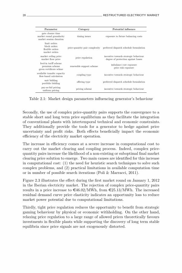
20 RESTRUCTURED ELECTRICITY MARKET
Parameter Category Potential influencegate closure time
timing issues exposure to future balancing costsmarket round granularitymarket session duration
limit orders
price-quantity pair complexity preferred dispatch schedule formulationblock ordersflexible ordersmarket orders
market ceiling price price regulation incentive towards strategic behaviourmarket floor price degree of protection against lossesfeed-in tariff scheme
renewable support scheme imbalance cost exposureprice risk exposurepremium scheme
green certificate schmeavailable transfer capacity coupling type incentive towards strategic behaviourflow-based calculation
unit bidding offering type preferred dispatch schedule formulationportfolio biddingpay-as-bid pricing pricing scheme incentive towards strategic behaviouruniform pricing
Table 2.1: Market design parameters influencing generator’s behaviour
Secondly, the use of complex price-quantity pairs supports the convergence to astable short and long term price equilibrium as they facilitate the integrationof conventional plants with intertemporal technical and economic constraints.They additionally provide the tools for a generator to hedge against priceuncertainty and profit risks. Both effects beneficially impact the economicefficiency of the electricity market operation.
The increase in efficiency comes at a severe increase in computational cost tocarry out the market clearing and coupling process. Indeed, complex price-quantity pairs increase the likelihood of a non-existing or suboptimal final marketclearing price solution to emerge. Two main causes are identified for this increasein computational cost: (1) the need for heuristic search techniques to solve suchcomplex problems, and (2) practical limitations in available computation timeor in number of possible search iterations (Poli & Marracci, 2011).
Figure 2.3 illustrates the effect during the first market round on January 1, 2012in the Iberian electricity market. The rejection of complex price-quantity pairsresults in a price increase to e46.02/MWh, from e25.13/MWh. The increasedresidual demand curve price elasticity indicates an opportunity loss to reducemarket power potential due to computational limitations.
Thirdly, tight price regulation reduces the opportunity to benefit from strategicgaming behaviour by physical or economic withholding. On the other hand,relaxing price regulation to a large range of allowed prices theoretically favoursinvestments in flexible plants while supporting the discovery of long term stableequilibria since price signals are not exogenously distorted.

BEHAVIOUR OF GENERATORS 21
0 5 · 10−2 0.1 0.15 0.2 0.25 0.3 0.35 0.4 0.45 0.50
10
20
30
40
50
Volume [104 MWh]
Price
[e/M
Wh]
submitted residual demand curveaccepted residual demand curve
Figure 2.3: Effect of complex pairs during the first market round of January, 1,2012 of the Iberian electricity market
Practical experience tends to confirm theory as low market ceiling pricesconstitute a price reference for generators at which price-quantity pairs shouldbe submitted. They are also argued to distort demand’s willingness to pay inthe event of capacity bottlenecks (Weber & Schröder, 2010). Similar argumentsare made regarding an insufficiently low market floor price from the perspectiveof investing in storage facilities or expressing true costs when facing a shut-downat high start-up costs.
Fourthly, from the perspective of renewable support schemes, the generatoronly anticipates price risk under the market premium or green certificatescheme. Under both schemes, RES would be dispatched at the negative priceof the market premium or the negative price of the price received on the greencertificate’s market. Consequently, prices are supposedly more volatile undera feed-in tariff scheme due to the guaranteed dispatch and lack of balancingresponsibility for the owners of RES. Although it is argued that investment inmore supply flexibility is attracted as a consequence, the level of investmenthas not been proven significant in practice (Barquín et al., 2010).
Fifthly, the target for future market design is a single price coupling, at least ona broad regional basis. In other words, one single matching algorithm determinesthe emerging market clearing prices and accepted price-quantity pairs in eachbidding area. However, even under such target market design, structural
22 RESTRUCTURED ELECTRICITY MARKET
congestions between bidding areas can be exploited by market participants toincrease market clearing prices locally. FB market coupling is being advocatedas a more efficient, less risk-averse method for allocating scarce transmissionline capacity compared to the NTC market coupling.
Lastly, regarding the offering type, portfolio bidding allows generators toreschedule the dispatch of plants in their portfolio based on the accepteddispatch schedule, therefore allowing a more efficient, least-cost dispatch. Unitbidding on the other hand facilitates transparency and therefore increasesregulatory influence, resulting in generators to be less tempted to exercisemarket power to the full extent of the available potential.
2.4 Conclusion and contribution
This chapter introduces existing designs and structures of day-ahead electricitymarkets developed over the past decades. The focus lies on the Europeanelectricity market framework organised as the PX model.
By comparing existing European electricity market designs, three broadcategories of parameters shaping the design and structure of a typical Europeanday-ahead electricity market are identified: domestic day-ahead market, marketcoupling mechanism and RES support schemes. In each category, the marketdesign parameters influence the strategic gaming behaviour of generators sinceeach parameter affects the maximum profit it can obtain during each marketsession, both during day-ahead and real-time.
Taking into account all uncertainties each market participant faces whenparticipating in the day-ahead electricity spot market, it is subject to significantprofit risks which have to be adequately accounted for. The generator is thusrequired to determine the price-quantity pairs which optimise its total profitafter being submitted to and accepted by the MO.
Consequently, this chapter provides the motivation to design, implement andvalidate strategic profit-maximising behaviour exhibited by a generator whencreating price-quantity pairs to submit to the MO during the day-aheadelectricity market. The designed behaviour has to account for the effect of thetarget market design parameters mentioned.
The design of generators’ strategic gaming behaviour is described in followingchapters. Chapter 3 covers the design, implementation and validation of theUnit Commitment (UC) and Economic Dispatch (ED) process, while chapter 4covers the design, implementation and validation of the offering strategy.

Chapter 3Unit Commitment and
Economic Dispatch
The liberalised electricity market requires generators to deploy their availablegeneration capacity under price uncertainty. This uncertainty gradually reduceswhen approaching the time of power delivery. Perfect anticipation to priceuncertainty is thus only achieved when a generator is capable of continuouslyadjusting the power level of the generation plants in its portfolio according toupdated, more accurate price forecasts.
The technologies in the generation portfolio are however not endlesslycontrollable or flexible. The decision on how to efficiently dispatch each planthas to be made well in advance of the actual time of power delivery. UnitCommitment (UC) and Economic Dispatch (ED), complemented by an adequateoffering strategy, manage the generator’s profit risk due to price uncertainty.
This chapter describes the scheduling problem faced by a generator owninga portfolio consisting of thermal, hydropower and renewable plants from theperspective of strategic and flexible dispatch. It optimises total profit givenresidual demand curves the generator faces in each market round of the marketsession. Technical constraints and plant economics are modelled for each planttype with a focus on modelling thermal plants because of their inflexibility andlarge presence in the EU271 electricity generation mix.
1Croatia joined the European Union in July, 2013. No EU28 statistics are yet available.
23
24 UNIT COMMITMENT AND ECONOMIC DISPATCH
This chapter presents incremental and innovative contributions to the state-of-the-art literature as it approaches the problem from the perspective offlexible dispatch. The approach and its contributions are derived from previouspublications (Maenhoudt & Deconinck, 2012; Maenhoudt & Deconinck, 2013a).
The first contribution is found in the presentation of a novel Mixed-IntegerLinear Problem (MILP) formulation which explicitly represents the formalconstraints of each of the different operational phases. Secondly, fixed thermalgradient limits and constraints concerned with modelling the thermal minimumstable power level duration before changing ramping direction, are relaxed.Instead, the gradient is dynamically calculated based on the power level and aviolation of the minimum stable power level duration is allowed at the expenseof incurring supplementary maintenance costs. Finally, the detailed model ofthe operation of thermal plants is complemented with hydropower plants andRenewable Energy Sources (RES). All mentioned plant types are modelled sothat they are able to cooperate in a coordinated manner in order to maximiseprofit subject to elastic demand and competitors’ behaviour.
The innovative contribution is found in deciding the strategic RES quantity tobe submitted to the Market Operator (MO) so that total profit is maximised.The decision reflects a trade-off between expected future balancing costs and thegained profit on the day-ahead market. Instead of assuming RES injection asnegative demand, the generator rather exploits the superior position of RES inthe merit order to influence day-ahead market prices at the cost of an increasedexpected balancing cost.
Validation cases are presented to illustrate the performance of the novel UCand ED formulation. Case studies are selected from literature based on theavailability of results to which obtained results are benchmarked. The threepresented case studies investigate the impact on profits from dynamicallycalculating the gradient limits, additionally incurring gradient costs anddispatching the portfolio in a coordinated manner.
3.1 Introduction
Three types of plants are distinguished in a typical generation portfolio: RES2,energy storage and thermal plants. RES are highly variable as significantdifferences in power levels, resulting from variations in weather conditions,occur. They only allow for limited control since, even with the installation
2Although renewable energy sources include biomass, geothermal, wind, solar andhydropower plants, this dissertation defines renewables in the narrow context of uncontrollable,stochastic energy sources such as wind and solar plants.
INTRODUCTION 25
of power electronics allowing for curtailment, the instantaneous power levelis stochastic and shows significant differences locally (Jónsson et al., 2010).Renewables are interesting from an economic perspective as their variable costsare practically non-existent.
The most economically relevant energy storage sources are hydropower plants.This generation technology is both flexible and controllable at a low variablecost. Its exploitation however is highly dependent on geographical requirementssuch as the presence of a river or a steep elevation, thereby drastically reducingits applicability (Yu et al., 2011). Their share in the generation technologymix is therefore limited except in bidding areas with an abundance of such atopography, such as in Nordic countries or the Alps.
Thermal plants such as nuclear or fossil fuel power plants are controllable. Eachthermal plant however is subject to intertemporal constraints, allowing for athermal flexibility spectrum ranging from very low to reasonably high flexibility.Generally, inflexible plants tend to cover base load demand while more flexibleones are used to cover mid load and peak demand. Typically, the variable cost3
of flexible thermal plants is smaller than that of inflexible ones.
Thermal plants are currently highly represented in the EU27 electricitygeneration mix. In 2010, their share of total available generation capacitywas 78.3%4 followed by an 11.9% share of hydropower plants and a 9.0% shareof RES5 (European Commission, 2012). Although new RES investments haveslowed in 2012, their share is expected to increase at the expense of thermalgeneration plants according to short-term predictions on the future compositionof the electricity generation mix in Europe (IEA, 2012).
Increasing the share of RES is led by policy instead of demand growth: Europeanelectricity consumption has not significantly changed over the past decade andis expected to decline slightly in the short to medium term. The massiveintegration of RES in the European electricity generation mix will thereforedemand greater flexibility on the supply side in order to ensure electricity systemreliability, even if real-time demand response or economically viable energystorage technologies are available in the medium term (Traber & Kemfert, 2011).
As demand-side flexibility is currently insufficient to cope with RES supplyfluctuations, electricity prices exhibit more volatile and complicated patternswith increased RES integration. Electricity prices often appear intractable, sothat many forecast tools predict the price distribution by taking into account adetailed definition of the physical system of generation and transmission, and
3Depending on the cost of CO2 emissions.427.4% nuclear, 24.7% solid and 2.6% liquid fossil fuels, and 23.6% gaseous fossil fuels.54.5% wind, 0.7% solar and 3.7% biomass; the remainder tidal wave and geothermal.
26 UNIT COMMITMENT AND ECONOMIC DISPATCH
the drivers of demand. More sophisticated statistical processes already providebetter price forecasts (Harris, 2006a), of which time series analysis (Nogaleset al., 2002; Contreras et al., 2003), neural networks (Mandal et al., 2007) andfuzzy regression models (Niimura & Nakashima, 2001) are the most popularones to accurately predict short-term market clearing prices.
Besides improvements in forecasting techniques, the utilisation efficiencyof generation plants is augmented by comprehensive UC and ED models.Considering the current and future European target electricity generationmix (European Commission, 2010; European Commission, 2012), thermalplants are modelled more in detail compared to hydropower and RES plants.The modelling scope of the latter is limited to wind and solar farms.
The scope is limited to the day-ahead spot market, i.e. no simultaneouslyorganized automatic generation control or reserve markets are modelled. Insteadit is assumed that arbitrage between markets has already taken place and thatits effects are integrated in the parametric input values (Frangioni et al., 2009).
3.2 State-of-the-art
3.2.1 Thermal power plant modelling
3.2.1.1 Literature overview
Long before liberalisation of the electricity market, a truncated heuristicmethod was used to minimise both generation and start-up costs, while fulfillingspinning reserves, load, and crew requirements (Pang & Chen, 1976). Technicalconstraints are limited to minimum and maximum power limits. The start-upand shut-down phase of the plant is not explicitly modelled but approximatedby a step function. The method only guarantees near optimal feasible schedulesdue to the enormous computational efforts.
Lagrangian relaxation has been widely applied to solve cost-based thermal UCproblems in which the generation and start-up costs are minimised subjectto load and spinning reserve requirements, minimum and maximum powerlimits, and the minimum up and down times (Merlin & Sandrin, 1983). Theproblem is formulated more in detail by imposing ramping limits and exponentialstart-up costs (Bard, 1988). Linear transmission constraints based on a directcurrent power flow model have also been included (Tseng et al., 1999). Finally,Lagrangian relaxation techniques to solve price-based UC formulations includingfuel and emission constraints are also proposed (Shahidehpour et al., 2002a).

STATE-OF-THE-ART 27
Lagrangian relaxation outperforms alternative methods in computation timewhen applied to large-scale scheduling problems, although the convergence to afeasible or optimal solution is not guaranteed (Borghetti et al., 2003; Zhai et al.,2002). Recent improvements in methodology however attempt to mitigate thesedisadvantages (Seki et al., 2010; Ongsakul & Petcharaks, 2004).
The widely applied MILP formulation guarantees convergence to an optimalscheduling solution and allows for explicitly formulating technical and economicconstraints. Expected wholesale and reserve market prices, generation costs, non-linear start-up and shut-down costs are incorporated in the profit-maximisingobjective function subject to capacity constraints, gradient limits and minimumup and down times (Arroyo & Conejo, 2000). Recently, the start-up andshut-down trajectories were formulated more in detail (Arroyo & Conejo,2004; Ostrowski et al., 2010). By focusing on computational efficiency, thenumber of constraints and their complexity has also been reduced (Carrion &Arroyo, 2006). The MILP formulation has also been applied to simultaneouslyconsidering energy, automatic generation control, and reserve markets (Arroyo& Conejo, 2002). The various thermal operating phases and regions can bemodelled (Simoglou et al., 2010; Simoglou et al., 2012). Increasing the size ofthe envisaged portfolio however exponentially increases the computation time.
Evolutionary methods are characterised by similar advantages and drawbacksas Lagrangian relaxation (Cheng et al., 2000). Only recently they have beenapplied as a stand-alone solution technique in large-scale scheduling problems,with promising results in terms of convergence speed (Ebrahimi et al., 2011;Damousis et al., 2004; Moghimi Hadji & Vahidi, 2012; Senjyu et al., 2005).Yet, convergence to a global optimum is not guaranteed. The optimality of thesolution is additionally highly sensitive to the selected learning parameters.
3.2.1.2 Conclusion and contributions
Considering the dominant share of thermal plants in the current and targetEU27 generation mix, their detailed representation cannot be avoided whenmodelling the scheduling problem. The above discussion additionally illustratesthat the MILP framework is better suited to represent the thermal plant’stechnical characteristics and economics.
Although convergence to an optimal scheduling solution is guaranteed whenusing such a framework, its convergence speed can pose a limitation whenapplying the scheduling problem to a realistically-sized portfolio. This drawbackcan however be mitigated by using increasingly more performant processingunits and the formulation of tight, computationally efficient MILP formulations.

28 UNIT COMMITMENT AND ECONOMIC DISPATCH
The operation of a thermal plant is mainly constrained by its maximum andminimum stable power limit, fixed gradient limit, fixed minimum up and downtime, fixed minimum stable power level duration and the predefined trajectoriesto be followed when starting up and shutting down. The total incurred costsare the result of non-linear generation costs, exponential start-up costs andexponential shut-down costs. Maintenance costs are not included in literature.
These dependencies can be modelled in detail to more accurately representthe thermal plant’s flexibility in an environment characterised by massive RESintegration. From this perspective, the assumption of predefined start-up andshut-down trajectories and fixed gradient limits restrict the representation ofthe plant’s actual operational ability. Additionally, similar to the dependencyof the start-up and shut-down cost on the duration the plant was respectivelyinactive or operational, a supplementary maintenance cost is also incurred incase the minimum stable power level duration is violated. Consequently, theassumption of a fixed minimum stable power level duration is not an accuraterepresentation of the actual operational ability of a thermal plant.
The state-of-the-art of thermal plant modelling is therefore advanced bydynamically calculating the gradient based on the power level and by allowingsupplementary maintenance costs to be incurred when violating the minimumstable power level duration constraints. Both novelties increase the flexibilityto dispatch the thermal plant in anticipation of forecast market clearing prices.In support of these contributions, a novel 0/1 MILP formulation is presentedin section 3.3 which explicitly represents each of the operational phases of thethermal plant, including the hot stand-by phase.
3.2.2 Hydropower plant modelling
3.2.2.1 Literature overview
Two types of hydropower plants are distinguished: pumped-hydro storage plantsand run-of-river plants. The former transforms potential energy held by thewater mass in its reservoir to electricity when discharging and vice versa whenpumping (Deane et al., 2010). Run-of-river plants transform the kinetic energyheld by the water mass in a river to electricity.
The run-of-river plant is in most cases complemented with a pondage, reducingexposure to river flow seasonality and making it possible to regulate the waterflow — and thus power level — to some extent. While the dispatch of pumped-hydro storage plants is driven by load balancing or price arbitrage, run-of-riverplants serve as peaking power or must run plants.

STATE-OF-THE-ART 29
Short-term management of the available water in the reservoir allows hydropowerplants to store and transfer energy to market rounds when its use is mostprofitable (Rangel, 2008). The majority of installed hydropower capacity in theEU27 are of the run-of-river plant type6 although this share is expected to risedue to its vast untapped potential (European Commission, 2013a).
Typically, both hydropower plant types are assumed not to be subject tointertemporal constraints (Ambec & Doucet, 2003). The water reservoirminimum and maximum capacity limits are important factors for the operationof the plant: in case the maximum capacity limit is reached, the plant dischargesin order to avoid spillage while water is treated as a scarce commodity in casethe minimum capacity limit is reached.
Water inflow is generally treated as deterministic although weather conditionsaffect the reservoir’s water inflow (Barroso et al., 2002). The scarcity of water ishence modelled as the opportunity cost of immediate water discharge comparedto storing it for future use. The cost increases when weather conditions are dryand is assumed known or forecasted based on historic data (Johnsen, 2001).
Hydropower depends on the turbine outflow and the head in the reservoir,which is in turn a function of the amount of water stored in the reservoir,the turbine outflow and spillage (Diniz & Maceira, 2008). The power levelof the hydropower plant is proportional to the turbine outflow rate and finalreservoir volumes and is guided by future cost functions or specific targetvalues obtained from long-term scheduling models. A multi-stage stochasticprogramming model better hedges against uncertainty of water inflows (Baslis& Bakirtzis, 2011). A compact MILP framework can be used to solve such ascheduling problem of cascaded run-of-river plants and pumped-hydro storageplants when pursuing a profit-maximisation objective. However, the requiredmodelling accuracy heavily depends on the specific hydropower plants addressedand their cascading topology.
In contrast to the previously-used models of self-replenishing hydro reservoirs,the pumping ability is explicitly taken into account when modelling pumped-hydro storage plants (Schill & Kemfert, 2011). A game-theoretic model has beenapplied to study the utilisation of storage under imperfect electricity marketconditions. Although it is argued that storage utilisation and storage-relatedwelfare effects depend on the storage owner and its ability to exert strategicgaming behaviour, no results could be obtained to support this claim whenapplying the model to the German power market.
6Although no distinction between the two types is made in the EU27 statistics, synthesisof data from various sources result in a 45 GW installed pumped-hydro storage capacity.Comparing with the EU27 statistics, this amounts to a current share of 32.1% of all hydropowerplants.

30 UNIT COMMITMENT AND ECONOMIC DISPATCH
3.2.2.2 Conclusion and contributions
Since the required modelling accuracy heavily depends on the specifichydropower portfolio topology addressed and their share in the current andtarget EU27 generation mix remains rather small compared to other generationtechnologies, a general model of hydropower plants is created. Besides theminimum and maximum capacity limits and the discharge or pumping limits,the minimum water inflow and the opportunity cost of water discharge areassumed to be readily obtained from long-term hydropower planning models orpreliminary weekly scheduling models. They are therefore assumed to be inputparameters to the short-term UC and ED.
The constraints which guide final reservoir volumes towards a future costfunction or specific target value restrict the flexible operation of the hydropowerplant. This assumption is hence relaxed in order for the generator to deviatefrom its planned dispatch schedule in case it is more profitable to do so. A rangeof future cost functions and specific target values is therefore included in theproblem formulation. Similar to the opportunity cost of water, these parametricvalues are assumed to be decided exogenously by medium- to long-term models.
3.2.3 Wind and solar plant modelling
3.2.3.1 Literature overview
Fluctuating intermittent generation characteristics are dealt with in literature bytwo approaches: storage and risk minimisation. The former converts renewableenergy to a different form that can be stored and used when desired viae.g. compressed air facilities, plug-in electrical vehicles or pumped-hydrostorage plants (Castronuovo & Peas Lopes, 2004; Brown et al., 2008). Thelatter calculates the day-ahead submitted renewable energy source quantityby minimising the expected costs of imbalance charges during the imbalancesettlement by the Transmission System Operator (TSO) (Matevosyan & Soder,2006). No distinction is made between the different types of intermittentgeneration technologies.
The former approach envisages electricity storage as a strategy for integratinglarge amounts of RES into the electricity system (Barton & Infield, 2004).Nevertheless, storage capacity in electricity markets with imperfect competitionis not fully utilised so that social welfare is not maximised (Schill & Kemfert,2009). A stochastic MILP framework generally provides similar solutions as itsdeterministic counterpart (Tuohy & O’Malley, 2011; Meibom et al., 2011).
MODEL FORMULATION 31
Renewable energy sources are generally modelled as negative demand while itsintegration is mostly assumed within a wind feed-in scheme and approachedfrom the perspective of maximising system level efficiency. These analysestypically assume RES dispatch priority over conventional plants. In case RESactively participates in the market, such as under the premium scheme orgreen quota scheme, their back-up and balancing capabilities should be takeninto account during the UC and ED problem formulation by each generatorindividually: a coordinated dispatch with other available generation technologiesin the generator’s portfolio indeed results in a reduction of imbalance chargescompared to the uncoordinated dispatch (Garcia-Gonzalez et al., 2008).
3.2.3.2 Conclusion and contributions
The combination of using storage and minimising imbalance risk when handlingthe dispatch of RES during the UC and ED model is innovative. The dispatchof RES is coordinated with flexible hydropower plants in order to maximiseprofit subject to elastic demand and competitors’ behaviour. At the same time,risk towards future balancing costs is reduced by calculating the expected costof balancing requirements for each coordinated RES and hydropower portfoliodispatch. Consequently total profit is maximised as a trade-off between theexpected future balancing cost and the additional gained profit on the day-aheadmarket. This novel modelling approach is innovative as the generator is capableto partially reserve hydropower capacity to profit from high balancing prices onreal-time markets or during the imbalance settlement with the TSO.
3.3 Model formulation
3.3.1 Objective function
The deregulated electricity market shifted the objective function of a generatorfrom an obligation to economically supply demand towards a profit-driven freechoice to supply paying customers (Shahidehpour et al., 2002a). The latterobjective is formally represented by
T∑t=1
(µ(t) − C(t)
)(3.1)Maximise
C(t) = CP(t) + CS(t) + CD(t) + CG(t) + CH(t) + CR(t)with
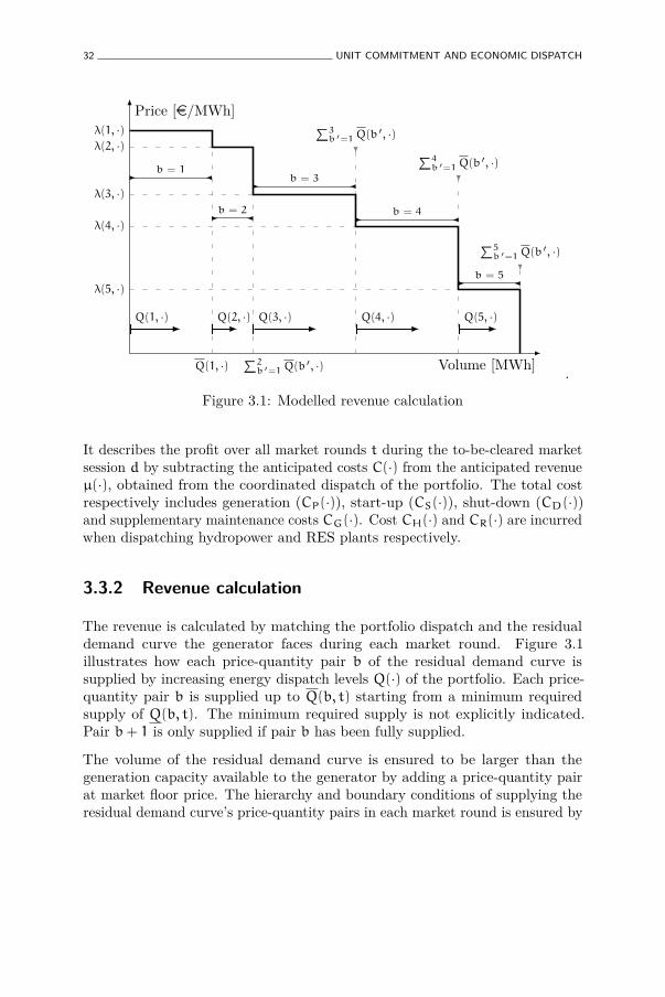
32 UNIT COMMITMENT AND ECONOMIC DISPATCH
Price [e/MWh]
Volume [MWh]Q(1, ·)∑2b ′=1Q(b ′, ·)
∑3b ′=1Q(b ′, ·) ∑4
b ′=1Q(b ′, ·)
∑5b ′=1Q(b ′, ·)
λ(1, ·)λ(2, ·)
λ(3, ·)
λ(4, ·)
λ(5, ·)
Q(1, ·) Q(2, ·) Q(3, ·) Q(4, ·) Q(5, ·)
b = 1
b = 2
b = 3
b = 4
b = 5
.
Figure 3.1: Modelled revenue calculation
It describes the profit over all market rounds t during the to-be-cleared marketsession d by subtracting the anticipated costs C(·) from the anticipated revenueµ(·), obtained from the coordinated dispatch of the portfolio. The total costrespectively includes generation (CP(·)), start-up (CS(·)), shut-down (CD(·))and supplementary maintenance costs CG(·). Cost CH(·) and CR(·) are incurredwhen dispatching hydropower and RES plants respectively.
3.3.2 Revenue calculation
The revenue is calculated by matching the portfolio dispatch and the residualdemand curve the generator faces during each market round. Figure 3.1illustrates how each price-quantity pair b of the residual demand curve issupplied by increasing energy dispatch levels Q(·) of the portfolio. Each price-quantity pair b is supplied up to Q(b, t) starting from a minimum requiredsupply of Q(b, t). The minimum required supply is not explicitly indicated.Pair b+ 1 is only supplied if pair b has been fully supplied.
The volume of the residual demand curve is ensured to be larger than thegeneration capacity available to the generator by adding a price-quantity pairat market floor price. The hierarchy and boundary conditions of supplying theresidual demand curve’s price-quantity pairs in each market round is ensured by

MODEL FORMULATION 33
Q(t) =
B∑b=1
(Q(b, t) + L(b, t) ∗
( b−1∑b ′=1
Q(b ′, t)))
(3.2)
Q(b, t) ≥ L(b, t) ∗Q(b, t) (3.3)
Q(b, t) ≤ L(b, t) ∗Q(b, t) (3.4)
B∑b=1
L(b, t) = 1 (3.5)
Price-quantity pairs are supplied according to decreasing price levels so thatonly one pair is partially supplied. This marginal price-quantity pair is indicatedby variable L(·) and sets the maximum anticipated market clearing price. Therevenue is subsequently calculated by multiplying the portfolio dispatch levelwith the price λ(·) of the marginal price-quantity pair:
µ(t) =
B∑b=1
([Q(b, t) +
(L(b, t) ∗
b−1∑b ′=1
Q(b ′, t))]∗ λ(b, t)
)(3.6)
This revenue is referred to as the maximum anticipated revenue under bothuniform and pay-as-bid pricing scheme. It is attained only when complementedwith a perfect offering strategy.
The total supplied energy is obtained by
Q(t) =
K∑k=1
Q(k, t) (3.7)
Q(kt, t) =
I(kt)∑i=1
Q(kt, i, t)with
Q(kt, i, t) = γ ∗ P(kt, i, t) ∃kt ⊂ k
Q(kh, t) = γ ∗ (V(kh, t) +W(kh, t) + X(kh, t) − Z(kh, t)) ∃kh ⊂ k
Q(kr, t) = γ ∗ Y(kr, t) ∃kr ⊂ k

34 UNIT COMMITMENT AND ECONOMIC DISPATCH
The supplied energy is obtained by multiplying the power level of each plant kat each market round with market round granularity γ. Pumping of hydropowerplants consumes power and is subtracted from the total power generation.
3.3.3 Thermal plant constraints
3.3.3.1 Units’ Operational Phases
Besides the start-up (φS(·)), shut-down (φD(·)) and production (φP(·)) phase,also the hot stand-by phase (φH(·)) is modelled as an operational phase of athermal plant. During hot stand-by, fuel is consumed to keep the unit’s coreat high temperature without generating power. In contrast to shutting down,hot stand-by avoids start-up costs and a violation of the minimum duration ofinactivity at the expense of supplementary fuel consumption costs.
The hot stand-by phase is entered after the shut-down phase, while the start-up phase is initiated once exiting hot stand-by. The transition between alloperational phase is hence modelled by
φS(kt, i, t− 1) ≤ φS(kt, i, t) + φP(kt, i, t) + φH(kt, i, t) (3.8)
φS(kt, i, t− 1) ≤ φS(kt, i, t) + φP(kt, i, t) (3.9)
φD(kt, i, t) ≤ φD(kt, i, t− 1) + φP(kt, i, t− 1) + φH(kt, i, t− 1) (3.10)
φD(kt, i, t− 1) ≤ φD(kt, i, t) + φD(kt, i, t) (3.11)
φD(kt, i, t) ≤ φP(kt, i, t− 1) + φD(kt, i, t− 1) (3.12)
φP(kt, i, t− 1) ≤φP(kt, i, t) + φD(kt, i, t)
+ φD(kt, i, t) + φH(kt, i, t)(3.13)
φP(kt, i, t− 1) + φS(kt, i, t− 1) + φS(kt, i, t− 1) ≥ φP(kt, i, t) (3.14)
φHD(kt, i, t) ≤ φS(kt, i, t) + φP(kt, i, t) (3.15)
φHS(kt, i, t) ≤ φD(kt, i, t) + φP(kt, i, t) (3.16)
φHS(kt, i, t− 1) − φHD(kt, i, t) = φH(kt, i, t) − φH(kt, i, t− 1) (3.17)

MODEL FORMULATION 35
The start-up phase is initiated by a start-up moment (φS(·)) and leads to theproduction phase. The shut-down phase is entered from the production phaseand is terminated by the shut-down moment (φD(·)) or by entering the hotstand-by phase. The hot stand-by phase has a hot stand-by initiation (φHS(·))and termination (φHD(·)) moment coinciding either with the start-up momentor shut-down moment. The production phase is initiated after having startedup or after having completed the start-up phase. The production phase isterminated by shutting down or by entering the hot stand-by phase.
Mutually exclusive phases and moments are prevented to co-exist by
φS(kt, i, t− 1) + φD(kt, i, t) ≤ 1 (3.18)
φS(kt, i, t) + φD(kt, i, t) ≤ 1 (3.19)
φHS(kt, i, t− 1) + φHD(kt, i, t) ≤ 1 (3.20)
ζ(kt, i, t) = φS(kt, i, t) + φD(kt, i, t) + φP(kt, i, t) + φH(kt, i, t) (3.21)
φS(kt, i, t− 1) − φD(kt, i, t) = ζ(kt, i, t) − ζ(kt, i, t− 1) (3.22)
A thermal unit operating in any of the operational phases is consideredoperational while, in the other case, it is considered inactive. Any operationalphase starts with a start-up moment and ends with a shut-down moment.Whether or not a unit is operational is denoted by ζ(·).
Finally, phases are related to the minimum and maximum power level by
P(kt, i, t) − (P(kt, i) ∗ ζ(kt, i, t)) ≥
−P(kt,i) ∗ (ζ(kt, i, t) − φP(kt, i, t))(3.23)
P(kt, i, t) − (P(kt, i)∗ζ(kt, i, t)) ≤
(P(kt, i) − P(kt,i)) ∗ φP(kt, i, t) − (P(kt, i) ∗ φH(kt, i, t))(3.24)
No generation is allowed during hot stand-by, even though the unit is consideredoperational. The start-up and shut-down phase bridge the unstable power levelrange between zero and the minimum power level. The plant operates in thestable power level range between the minimum and maximum power level.
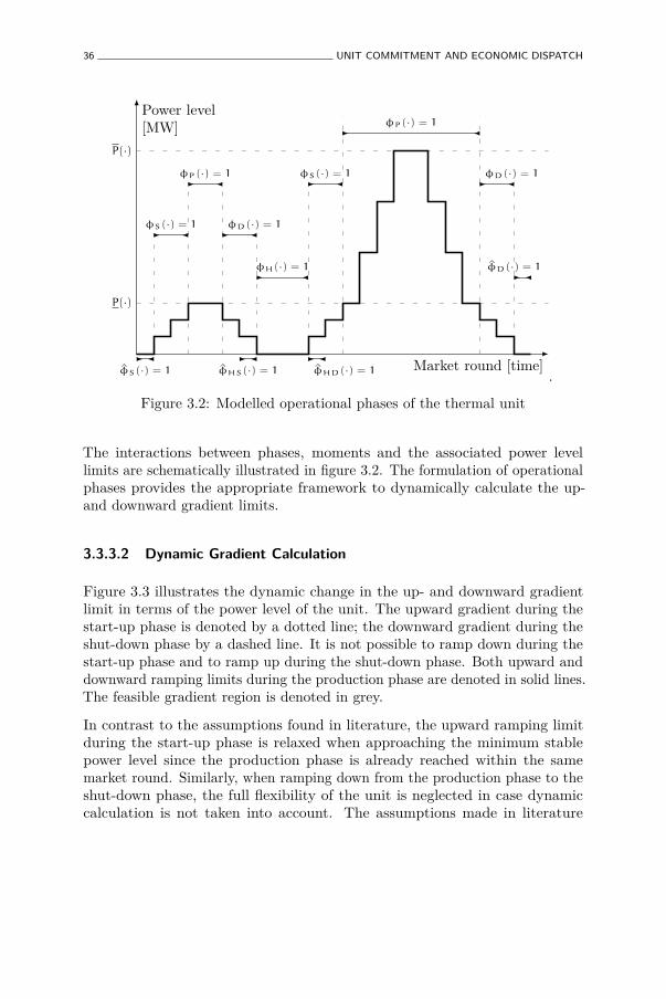
36 UNIT COMMITMENT AND ECONOMIC DISPATCH
Power level[MW]
P(·)
P(·)
Market round [time]
φP(·) = 1
φS(·) = 1 φD(·) = 1
φS(·) = 1 φD(·) = 1
φP(·) = 1
φH(·) = 1
φS(·) = 1 φHS(·) = 1 φHD(·) = 1
φD(·) = 1
.
Figure 3.2: Modelled operational phases of the thermal unit
The interactions between phases, moments and the associated power levellimits are schematically illustrated in figure 3.2. The formulation of operationalphases provides the appropriate framework to dynamically calculate the up-and downward gradient limits.
3.3.3.2 Dynamic Gradient Calculation
Figure 3.3 illustrates the dynamic change in the up- and downward gradientlimit in terms of the power level of the unit. The upward gradient during thestart-up phase is denoted by a dotted line; the downward gradient during theshut-down phase by a dashed line. It is not possible to ramp down during thestart-up phase and to ramp up during the shut-down phase. Both upward anddownward ramping limits during the production phase are denoted in solid lines.The feasible gradient region is denoted in grey.
In contrast to the assumptions found in literature, the upward ramping limitduring the start-up phase is relaxed when approaching the minimum stablepower level since the production phase is already reached within the samemarket round. Similarly, when ramping down from the production phase to theshut-down phase, the full flexibility of the unit is neglected in case dynamiccalculation is not taken into account. The assumptions made in literature
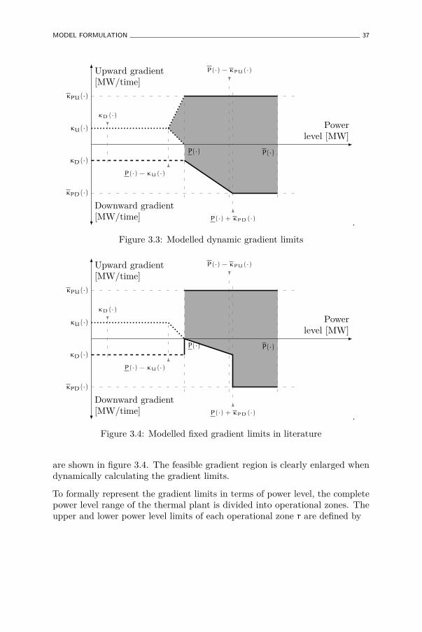
MODEL FORMULATION 37
κPU(·)
κPD(·)
κD(·)
κU(·)
Upward gradient[MW/time]
Downward gradient[MW/time]
P(·)P(·)
P(·) − κU(·)
κD(·)
P(·) + κPD(·)
Powerlevel [MW]
P(·) − κPU(·)
.
Figure 3.3: Modelled dynamic gradient limits
κPU(·)
κPD(·)
κD(·)
κU(·)
Upward gradient[MW/time]
Downward gradient[MW/time]
P(·)P(·)
P(·) − κU(·)
κD(·)
P(·) + κPD(·)
Powerlevel [MW]
P(·) − κPU(·)
.
Figure 3.4: Modelled fixed gradient limits in literature
are shown in figure 3.4. The feasible gradient region is clearly enlarged whendynamically calculating the gradient limits.
To formally represent the gradient limits in terms of power level, the completepower level range of the thermal plant is divided into operational zones. Theupper and lower power level limits of each operational zone r are defined by
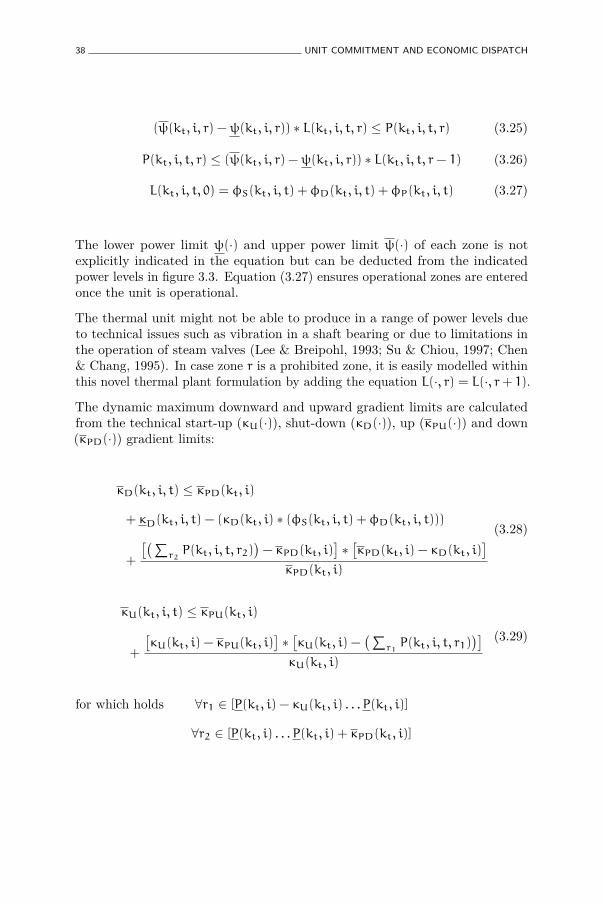
38 UNIT COMMITMENT AND ECONOMIC DISPATCH
(ψ(kt, i, r) −ψ(kt, i, r)) ∗ L(kt, i, t, r) ≤ P(kt, i, t, r) (3.25)
P(kt, i, t, r) ≤ (ψ(kt, i, r) −ψ(kt, i, r)) ∗ L(kt, i, t, r− 1) (3.26)
L(kt, i, t, 0) = φS(kt, i, t) + φD(kt, i, t) + φP(kt, i, t) (3.27)
The lower power limit ψ(·) and upper power limit ψ(·) of each zone is notexplicitly indicated in the equation but can be deducted from the indicatedpower levels in figure 3.3. Equation (3.27) ensures operational zones are enteredonce the unit is operational.
The thermal unit might not be able to produce in a range of power levels dueto technical issues such as vibration in a shaft bearing or due to limitations inthe operation of steam valves (Lee & Breipohl, 1993; Su & Chiou, 1997; Chen& Chang, 1995). In case zone r is a prohibited zone, it is easily modelled withinthis novel thermal plant formulation by adding the equation L(·, r) = L(·, r+ 1).
The dynamic maximum downward and upward gradient limits are calculatedfrom the technical start-up (κU(·)), shut-down (κD(·)), up (κPU(·)) and down(κPD(·)) gradient limits:
κD(kt, i, t) ≤ κPD(kt, i)
+ κD(kt, i, t) − (κD(kt, i) ∗ (φS(kt, i, t) + φD(kt, i, t)))
+
[(∑r2P(kt, i, t, r2)
)− κPD(kt, i)
]∗[κPD(kt, i) − κD(kt, i)
]κPD(kt, i)
(3.28)
κU(kt, i, t) ≤ κPU(kt, i)
+
[κU(kt, i) − κPU(kt, i)
]∗[κU(kt, i) −
(∑r1P(kt, i, t, r1)
)]κU(kt, i)
(3.29)
∀r1 ∈ [P(kt, i) − κU(kt, i) . . . P(kt, i)]for which holds
∀r2 ∈ [P(kt, i) . . . P(kt, i) + κPD(kt, i)]

MODEL FORMULATION 39
The minimum up- and downward gradient limits during the start-up and shut-down phase are modelled by
κU(kt, i, t) ≥ −(∑
r3P(kt, i, t, r3)
)+ κU(kt, i) ∗ (φS(kt, i, t) + φS(kt, i, t) + φHS(kt, i, t))
(3.30)
κD(kt, i, t) ≥(∑
r4P(kt, i, t, r4)
)−(κD(kt,i, t) ∗ (1− φD(kt, i, t))
) (3.31)
∀r3 ∈ [P(kt, i) − κU(kt, i) . . . P(kt, i)]for which holds
∀r4 ∈ [0 . . . κD(kt, i, t)]
All equations model the gradient as represented in figure 3.3. Consistency isensured by
κU(kt, i, t) ≤ κU(kt, i) ∗ (1− φD(kt, i, t)) (3.32)
κU(kt, i, t) ≥ κU(kt, i, t) (3.33)
κD(kt, i, t) ≥ κD(kt, i, t) (3.34)
An upward gradient during the shut-down phase is eliminated while ensuringthe minimum gradient limit is always lower than the maximum one. The powerlevel of each operational zone is aggregated to the power level of the unit by
P(kt, i, t) =
R∑r=1
P(kt, i, t, r) (3.35)
The dynamic maximum and minimum upward and downward gradient limitsare linked to the maximum and minimum allowed change in power level by

40 UNIT COMMITMENT AND ECONOMIC DISPATCH
P(kt, i, t) ≤ P(kt, i, t− 1) + κU(kt, i, t− 1) − κD(kt, i, t− 1) (3.36)
P(kt, i, t) ≥ P(kt, i, t− 1) + κD(kt, i, t− 1) − κU(kt, i, t− 1) (3.37)
The change in supplied energy is obtained by applying the market roundgranularity as introduced in equation (3.7).
3.3.3.3 Gradient Costs
In contrast to assumptions in literature, the minimum stable power level durationcan be violated at the expense of incurring supplementary maintenance costs.A profit-maximising generator would violate the minimum stable power levelduration if the cost for increased flexibility is offset by the gain of profitablysupplying the market at a larger quantity. Hence, the assumption of a fixedminimum stable power level duration is insufficient when modelling strategicgaming behaviour in a liberalised market environment.
The gradient cost is dependent on the up- (νU(·)) or downward (νD(·)) rampingdirection, and the minimum stable power level duration t·≡(·):
CG(kt, i, t) ≥
CGU(kt, i, t, tU∼) ∗ (νU(kt, i, t) + νD(kt, i, t− tU∼) − 1)(3.38)
CG(kt, i, t) ≥
CGD(kt, i, t, tD∼) ∗ (νD(kt, i, t) + νU(kt, i, t− tD∼) − 1)(3.39)
tU∼ = 1 . . . tU≡(kt, i)for which holds
tD∼ = 1 . . . tD≡(kt, i)
The gradient cost per unit is aggregated on a portfolio level by
CG(t) =
K∑k=1
CG(kt, t) =
I(k)∑i(k)=1
CG(kt, i, t) (3.40)
MODEL FORMULATION 41
Supplementary costs are allowed to be different when ramping up after havingramped down than when ramping down after having ramped up.
Consistency regarding the ramping direction ν·(·) is achieved by
φS(kt, i, t) + φS(kt, i, t) + φHD(kt, i, t− 1) ≤ νU(kt, i, t) (3.41)
νU(kt, i, t) ≤ φS(kt, i, t) + φP(kt, i, t)
+ φS(kt, i, t) + φHD(kt, i, t− 1)(3.42)
φD(kt, i, t) ≤ νD(kt, i, t) (3.43)
νD(kt, i, t) ≤ φD(kt, i, t) + φP(kt, i, t) (3.44)
νU(kt, i, t) + νD(kt, i, t) ≤ 1 (3.45)
Ramping upward is enforced during the start-up phase and after terminatingthe hot stand-by phase. No such obligation is instated to ramp up during theproduction phase. Similarly, ramping down is mandatory during the shut-downphase but optional during the production phase. A unit is prohibited to rampup and down during the same market round.
3.3.3.4 Generation, start-up and shut-down costs
The generation cost is represented by
CP(kt, i, t) =
R∑r=1
(P(kt, i, t, r) ∗ ηt(kt, i, r)
)+(CP0(kt, i) ∗ (ζ(kt, i, t) − φH(kt, i, t))
)+(CPH(kt, i) ∗ φH(kt, i, t)
)(3.46)
It takes into account sunk operating costs (CP0(·)) and fuel consumption costsfor operating during hot stand-by (CPH(·)).

42 UNIT COMMITMENT AND ECONOMIC DISPATCH
The fuel consumption in any other operational phase exhibits a quadraticfunction in terms of the unit’s power level. In order to maintain a linearformulation, the fuel cost curve is linearly interpolated by using linear costslopes (ηt(·)). Each linear cost slope is defined per operational zone r. Themodular formulation of operational zones makes it easy to add zones in orderto accurately represent the quadratic shape of the fuel cost curve.
Start-up and shut-down costs depend on the temperature of the unit’s core,resembling an exponential curve before reaching an equilibrium after a timeperiod denoted by the minimum operational duration τON(·) and minimuminactive duration τOFF(·). Even though an explicit constraint is mostly instatedin literature to prevent starting up or shutting down before the respectiveminimum duration has been reached, these minimum durations can be violatedat the expense of incurring supplementary maintenance costs.
The total cost when starting up or shutting down a thermal unit is calculted by
CS(kt, i, t) ≥[φS(kt, i, t) −
t−1∑t ′=t−td
ζ(kt, i, t′)]∗ CSU(kt, i, td) (3.47)
CD(kt, i, t) ≥ CDD(kt, i, tu)∗
[φD(kt, i, t) −
t−1∑t ′=t−tu
(1− ζ(kt, i, t′))] (3.48)
∀td ∈ [1 . . . τOFF(kt, i)]for which holds
∀tu ∈ [1 . . . τON(kt, i)]
The exponential shape of both cost functions is interpolated per market roundby the step-wise functions CSU(·) and CDD(·). All unit costs are aggregatedon a portfolio level using
CP(t) =
K∑k=1
CP(kt, t) =
I(k)∑i=1
CP(kt, i, t) (3.49)
CS(t) =
K∑k=1
CS(kt, t) =
I(k)∑i=1
CS(kt, i, t) (3.50)
MODEL FORMULATION 43
CD(t) =
K∑k=1
CD(kt, t) =
I(k)∑i=1
CD(kt, i, t) (3.51)
3.3.4 Hydropower plant constraints
3.3.4.1 Target discharge levels
Each hydropower plant has a specific maximum target discharge level permarket session in order to preserve the long-term profitability of the plant dueto stochastic inflow levels. In contrast to discussed literature, three categoriesof discharges are considered: planned, residual and future energy.
Planned energy (QP(·)) is the actual discharge capacity planned during themarket session. Residual energy (QR(·)) is the cumulative unused dischargepotential from previous market sessions while future energy (QF(·)) relates toenergy capacity allocated to the next market session. Each of the dischargecategories are input parameters to the short-term UC and ED, but areexogenously obtained from a medium-term planning tool (Doquet et al., 2008).
The maximum allocated discharge level during the market session, for eachdischarge category, is described by
T∑t=1
(V(kh, t) + Vr(kh, t)) ∗ γ ≤ QR(kh, d) (3.52)
T∑t=1
(W(kh, t) +Wr(kh, t)) ∗ γ ≤ QP(kh, d) +T∑t=1
(Z(kh, t) ∗ γ) (3.53)
T∑t=1
(X(kh, t) + Xr(kh, t)) ∗ γ ≤ QF(kh, d) (3.54)
No constraints are formulated to force a target dispatch schedule to be followed:the hydropower plant is allowed to deviate from the planned energy dischargedepending on whether such deviation would result in the most profitable set ofmaximum anticipated market clearing prices. Thus, in contrast to alternativemodels found in literature, the hydropower plant is not obliged to reach apredetermined water reservoir level at the end of the market session.

44 UNIT COMMITMENT AND ECONOMIC DISPATCH
Profitability differs between each discharge category. Planned energy is onlysupplied to the market in case the market clearing price exceeds the watervalue during the market session. Residual energy is available in case not allplanned energy has been dispatched during previous market sessions or in casethe reservoir level threatens to reach its maximum capacity.
The cost of residual energy is therefore lower than the water value but nevernegative. Dispatching future energy poses an additional risk as it reduces theplanned dispatch level during future market sessions. Hence, the associated costis higher than the water value. The water value for each discharge category isretrieved from an exogenous medium-term planning model.
The generator is also capable of reserving part of the total available dischargecapacity. Reserved hydropower is not submitted to the MO on the day-aheadmarket, but withheld to support future balancing requirements. The reservationof hydropower must however comply with the short-term discharge levels.
3.3.4.2 Technical capacity limits
The minimum and maximum technical discharge limits are enforced by
V(kh, t) + Vr(kh, t) +W(kh, t) +Wr(kh, t)
+ X(kh, t) + Xr(kh, t) ≤ νD(kh, t) ∗ PD(kh)(3.55)
V(kh, t) + Vr(kh, t) +W(kh, t) +Wr(kh, t)
+ X(kh, t) + Xr(kh, t) ≥ νD(kh, t) ∗ PD(kh)(3.56)
The amount of water to be pumped is limited by
Z(kh, t) + Zr(kh, t) ≤ νP(kh, t) ∗ PP(kh) (3.57)
Z(kh, t) + Zr(kh, t) ≥ νP(kh, t) ∗ PP(kh) (3.58)
Finally, simultaneously pumping and discharging is prohibited by
νP(kh, t) + νD(kh, t) ≤ 1 (3.59)

MODEL FORMULATION 45
The minimum and maximum reservoir limits are implicitly enforced by reducingor increasing the maximum discharge levels per discharge category, or bychanging the associated water values. Since these parameters are determinedby a medium-term planning model, their creation is not further discussed.
3.3.4.3 Dispatching cost
The cost for dispatching the hydropower plant is embedded in the water valueassociated to each type of energy. Water values are exogenously calculatedbased on the typical characteristics of the hydropower plant, the state of itsreservoir level and the expected day-ahead market clearing price over a limitedhorizon of future market sessions, commonly 1 year. The dispatching cost ofthe hydropower plant in each market round is therefore fully described by
CH(t) = (γ ∗ V(kh, t) ∗ ηh,R(kh, d)) + (γ ∗W(kh, t) ∗ ηh,P(kh, d))
+ (γ ∗ X(kh, t) ∗ ηh,F(kh, d)) − (γ ∗ Z(kh, t) ∗ ηh,Z(kh, d))(3.60)
3.3.5 Wind and solar plant constraints
In case the feed-in tariff scheme is imposed, the generator does not submit price-quantity pairs to supply renewable energy to the day-ahead market. Rather, anyRES plant is considered as must-run. The TSO is subsequently responsible formaximising the injection of renewable energy subject to transmission constraints.In this case, renewable energy can be considered as a negative demand shift,thereby eliminating the need for its representation in the UC and ED model.
In case the incumbent support scheme allows RES participation on the day-ahead market, as is the case under e.g. the green quota and premium scheme,the generator already needs to submit a renewable quantity to the MO in orderto avoid excessive balancing costs due to the associated uncertainty on theplant’s actual power level at delivery time. Hence, the RES quantity to submithas to be taken into account in the UC and ED model.
3.3.5.1 Allowed quantity range
In contrast to conventionally submiting the expected RES power level, the RESquantity to submit is selected from an allowed range using the mean (Pµ(·))and standard deviation (Pσ(·)) of the RES dispatch forecast:

46 UNIT COMMITMENT AND ECONOMIC DISPATCH
Y(kr, t) ≤ Pµ(kr, t) + R(kr, t) ∗ Pσ(kr, t) (3.61)
Y(kr, t) ≥ Pµ(kr, t) − R(kr, t) ∗ Pσ(kr, t) (3.62)
Parameters R(·) and R(·) indicate the up- and downward risk in the form of thestatistical standard score.
The approach maximises the day-ahead profit subject to the submitted RESquantity, the dispatching cost of the remaining plants in the portfolio andthe emerging market clearing price in function of the portfolio dispatch level.Consequently, coordinated dispatch flexibility between the RES plant and thetemporally constrained thermal plants in the portfolio, is facilitated.
In case the generator additionally owns hydropower plants, discharge or pumpingcapacity can be reserved for future self-balancing requirements. The reservationof hydropower is linked to the RES forecast uncertainty by H(·) and H(·):
Vr(kh, t) +Wr(kh, t) + Xr(kh, t) − Zr(kh, t)
≤Kr∑kr=1
(H(kr, t) ∗ Pσ(kr, t))(3.63)
Vr(kh, t) +Wr(kh, t) + Xr(kh, t) − Zr(kh, t)
≥−
Kr∑kr=1
(H(kr, t) ∗ Pσ(kr, t))(3.64)
In case prices of intra-day markets, real-time markets or imbalance charges afterthe imbalance settlement can be adequately forecasted, above equations arecomplemented with information on which future balancing costs to expect, giventhe coordinated dispatch of hydropower plants and the RES plant. For thispurposeM scenarios of submitting RES quantity ρr(·) and reserving hydropowerρh(·) are evaluated in terms of expected future balancing cost.
The expected future balancing cost associated to each scenario m is exogenouslycalculated using stochastic optimisation taking into account the RES forecastuncertainty, the water value of energy reserved, and estimations of intra-dayand real-time liquidity. They are estimated using either historic experience, oragent-based models to account for strategic gaming behaviour (Trinh, 2013).

MODEL FORMULATION 47
By introducing the expected future balancing cost when dispatching the RESplant, a trade-off between maximising day-ahead profit and minimising theexpected cost of future balancing requirements is achieved. Hence, objectivefunction (3.1) maximises total expected profit. The expected cost for futurebalancing requirements can be negative, e.g. because of strategic gamingbehaviour, indicating a profit can be gained on intra-day and real-time markets.
Each scenario m representing a decision ω(·) on the submitted RES quantity(ρr(·)) and the reserved amount of hydropower (ρh(·)) for all RES farms, isintegrated by
Y(kr, t) −
M(kr)∑m=1
ω(kr, t,m) ∗ ρr(kr, t,m) = 0 (3.65)
Kh∑kh=1
(Vr(kh, t) +Wr(kh, t) + Xr(kh, t))
−
Kr∑kr=1
M(kr)∑m=1
ω(kr, t,m) ∗ ρh(kr, t,m) = 0
(3.66)
Only one scenario can be pursued per RES plant:
M(kr)∑m=1
ω(kr, t,m) = 1 (3.67)
3.3.5.2 Dispatching cost
The total RES dispatching cost equals the expected future balancing cost ρc(·)minus existing subsidies (π(·)), corresponding to e.g. the received premium orthe price of green certificates depending on the instated RES support scheme.The operational cost for a RES plant is considered negligible:
CR(t) =
M∑m=1
(ρc(kr, t,m) ∗ω(kr, t,m)) − π(kr, t) ∗ Y(kr, t) (3.68)

48 UNIT COMMITMENT AND ECONOMIC DISPATCH
3.4 Impact of the contributions of the model
Following case studies assess the performance of the presented UC and ED model.Results are compared with results retrieved from literature to quantitativelyposition the presented model to alternative ones. Benchmarking with literaturemoreover increases model credibility. The simulation setup of each of thethree seperate case studies retrieved assesses the impact of each contribution inisolation from the other in order to facilitate the interpretation of results.
All presented cases were implemented in GAMS 23.9.3 and solved with CPLEXon a 2.27 GHz processor (Rosenthal, 2012).
3.4.1 Dynamic gradient limits and hot stand-by phase
To assess the impact of dynamically calculating the gradient limit, the resultsof the presented model are compared with results retrieved from a benchmarkcase study assuming fixed gradient limits (Arroyo & Conejo, 2004). The casestudy encompasses a single thermal plant consisting of a single unit, owned bya generator active in a perfectly competitive market environment. Since lowprices encourage a shut-down and start-up of the plant, dynamically calculatingthe gradient limits is expected to facilitate this process and to significantlyimpact the final profit. An hourly market round granularity is assumed.
The generation cost is linear with a fuel cost of e38/MWh. Sunk operatingcost are equal to e100/h. The shut-down cost is independent of the operationalduration and equals e56. Similarly, the cost incurred at start-up equals e850.Supplementary maintenance costs are not considered.
The gradient limit during the start-up phase is 38 MW/h, during the shut-downphase 40 MW/h. The maximum technical power level is 294 MW. The minimumstable power level equals 112 MW. The maximum ramp-up and ramp-downrates during the production phase are 60 MW/h and 50 MW/h respectively.
Both the start-up and shut-down phase lasts 3 hours. Minimum operationaland inactive durations are 3 hours. The unit has already been operating for 11hours and produces 170 MW during the last hours of the previous day.
The residual demand curve in each market round consists of a single price-quantity pair priced at λ(1, t). Hourly prices are denoted in table 3.1.
During market rounds 1 to 8, prices are lower than the plant’s fuel cost, providingan incentive to shut down the plant. From market round 8 onward, a significantjump in prices is observed, giving the incentive to the generator to restart

IMPACT OF THE CONTRIBUTIONS OF THE MODEL 49
Hour λ(1, t)λ(1, t)λ(1, t) Benchmark Presented[e/MWh] [MW] [MW]
1 26.950 120 1202 25.817 112 78.43 22.209 70 38.44 21.219 30 05 19.668 0 06 19.800 0 07 24.167 0 388 26.950 37 769 40.700 75 115.210 44.110 112 175.211 45.177 172 235.212 47.025 232 29413 47.773 292 29414 46.200 294 29415 44.033 294 29416 44.550 294 29417 46.200 294 29418 48.950 294 29419 48.840 294 29420 45.100 294 29421 43.252 294 29422 44.000 244 24423 44.000 194 19424 25.850 144 144
Table 3.1: Price Data and Optimal Generation Schedule
the plant as soon as the minimum inactive duration time has passed. A localmaximum of e47.773/MWh is reached in market round 13, leading to a trade-offbetween reducing the power level to avoid supplying at a loss and increasingthe power level to benefit from supplying at highly profitable prices.
By dynamically calculating the gradient limit, this trade-off is expected tobe relaxed, resulting in a more efficient dispatch. Table 3.1 also illustratesthe scheduling solution obtained from the presented model together with thesolution calculated by the benchmark model (Arroyo & Conejo, 2004).
The difference in results between both models is found during market rounds 2to 12. During the shut-down process as well as the start-up process, the plantis observed to ramp faster when applying the presented model because gradientlimits are dynamically calculated. Indeed, the plant’s ramping process frommarket round 1 to round 2 only lasts 9.6 minutes considering the maximumdownward gradient limit in the production phase. While the benchmark modelimplicitly requires the plant to halt its ramping process when the minimumstable power level is reached, the presented model allows the plant to enter theshut-down phase for the remaining 50.4 minutes.

50 UNIT COMMITMENT AND ECONOMIC DISPATCH
The plant therefore ramps down faster during unprofitable market rounds 1 to5, thereby reducing the incurred loss. Moreover, by reaching the shut-downmoment one market round earlier, the plant is already able to start up at marketround 7. Adding the increased flexibility during start-up, the plant reaches itsmaximum power level two profitable market rounds earlier than the benchmarkmodel, hence increasing its revenue.
The resulting profit achieved when using the presented model equals e19.39kcompared to a profit of e16.77k without applying dynamic gradient calculation,equivalent to a profit increase of 15.6%. The profit increases further when thepossibility of a hot stand-by phase is taken into account. Assigning the sunkoperating cost as the cost for operating in the hot stand-by phase increasesthe profit to e20.26k, equivalent to an increase of 20.8%, as expensive start-upcosts during market round 7 are avoided.
3.4.2 Gradient costs
To study the impact of supplementary gradient costs, the case study presentedin reference (de la Torre et al., 2002) is selected. Since the envisaged generatorowns a realistically-sized portfolio of 40 thermal units dispersed over 7 plantswith varying technical characteristics, supplementary maintenance costs areexpected to be incurred in exchange for increased portfolio dispatch flexibility.
Unit characteristics between plants are based on the 1996 IEEE RTS teststandard (Grigg et al., 1999). Table 3.2 illustrates the properties of each unit.Four operational zones approximate the non-linear fuel cost curve. The start-upcost is considered independent of the duration the unit is inactive. Finally,the gradient cost is assumed to be exponentially decreasing in terms of thestable duration, for both ramping directions. The maximum supplementarymaintenance cost is assumed to equal the start-up cost; its minimum equals10% of the start-up cost.
Although only a relevant case study assuming an oligopolistic environment hasbeen found in literature, the inclusion of gradient costs is also valuable for agenerator operating in a competitive environment. Dispatch flexibility in anoligopolistic environment is expected to result in higher prices during marketrounds in which technical constraints prevent the generator from fully exploitingits market power potential, while, in a competitive environment, dispatchflexibility is expected to allow for a more cost-efficient portfolio dispatch. Theimpact on profit in both environments is however expected to be small due tothe incurment of high supplementary maintenance costs relative to the smalltemporary advantage, but is expected to increase with increasing price volatilityor market power potential differences between market rounds.
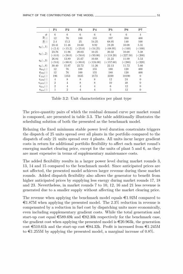
IMPACT OF THE CONTRIBUTIONS OF THE MODEL 51
P1 P2 P3 P4 P5 P6 P7# 6 6 6 6 6 6 4
P(·) 12 76 100 155 197 350 400P(·) 2.4 15.2 25 54.25 68.95 140 100
ηt(·, 1)23.41 11.46 18.60 9.92 19.20 10.08 5.31(<2.4) (<15.2) (<25.0) (<54.25) (<68.95) (<140) (<100)
ηt(·, 2)23.76 11.96 20.03 10.25 20.32 10.68 5.38(<6.0) (<38.0) (<50.0) (<93.00) (<118.20) (<227.50) (<200)
ηt(·, 3)26.84 13.89 21.67 10.68 21.22 11.09 5.53(<9.6) (<60.8) (<80.0) (<124.00) (<157.60) (<280) (<320)
ηt(·, 4) 30.40 15.97 22.72 11.26 22.13 11.72 5.66κPU(·) 12 76 100 155 180 120 400κPD(·) 12 76 100 155 180 120 400CSU(·) 196 1353 1635 2173 2239 10190 0τON(·) 4 8 8 8 12 24 0τOFF(·) 2 4 8 8 10 48 0τD≡(·) 2 4 4 4 6 12 0τU≡(·) 1 2 4 4 5 12 0
Table 3.2: Unit characteristics per plant type
The price-quantity pairs of which the residual demand curve per market roundis composed, are presented in table 3.3. The table additionally illustrates thescheduling solution of both the presented as the benchmark model.
Relaxing the fixed minimum stable power level duration constraints triggersthe dispatch of 25 units spread over all plants in the portfolio compared to thedispatch of only 21 units spread over 4 plants. All units incur larger gradientcosts in return for additional portfolio flexibility to affect each market round’semerging market clearing price, except for the units of plant 5 and 6, as theyare most expensive in terms of supplementary maintenance costs.
The added flexibility results in a larger power level during market rounds 3,13, 14 and 15 compared to the benchmark model. Since anticipated prices arenot affected, the presented model achieves larger revenue during these marketrounds. Added dispatch flexibility also allows the generator to benefit fromhigher anticipated prices by supplying less energy during market rounds 17, 18and 23. Nevertheless, in market rounds 7 to 10, 12, 16 and 21 less revenue isgenerated due to a smaller supply without affecting the market clearing price.
The revenue when applying the benchmark model equals e1.92M compared toe1.87M when applying the presented model. The 2.3% reduction in revenue iscompensated by a reduction in fuel cost by dispatching units more economically,even including supplementary gradient costs. While the total generation andstart-up cost equal e589.69k and e82.30k respectively for the benchmark case,the gradient cost when applying the presented model is e20.963k, the generationcost e510.61k and the start-up cost e84.32k. Profit is increased from e1.245Mto e1.255M by applying the presented model, a marginal increase of 0.8%.

52 UNIT COMMITMENT AND ECONOMIC DISPATCH
Hou
rBlock
1Block
2Block
3Block
4So
lution
perplan
t,withgrad
ient
cost
[MW
h]So
lution
perplan
t,fix
eddu
ration
s[M
Wh]
PQ
PQ
PQ
PQ
P1
P2
P3
P4
P5
P6
P7
P1
P2
P3
P4
P5
P6
P7
115
2000
1020
005
2000
020
0091
.232
5.5
840.0
400.0
91.2
325.5
840.0
400.0
215
2000
1215
0010
3000
550
091
.272
8.5
68.9
1011
.416
00.0
91.2
930.0
878.8
1600
.03
1822
5015
750
1540
0012
1000
212.8
829.3
68.9
1011
.416
00.0
91.2
930.0
878.8
1600
.04
2017
5015
1750
1012
5010
250
91.2
728.5
68.9
1011
.416
00.0
91.2
930.0
878.8
1600
.05
2312
5018
2250
1217
5010
750
152.0
724.0
12.6
1011
.416
00.0
91.2
930.0
878.8
1600
.06
3030
0020
500
1525
012
500
91.2
724.0
12.6
1011
.411
60.8
91.2
930.0
878.8
1100
.07
3315
0025
1250
2212
5020
750
152.0
728.5
12.6
1491
.113
00.0
91.2
930.0
1378
.816
00.0
834
1800
2714
0022
550
2047
591
.232
5.5
12.6
1491
.112
79.4
91.2
930.0
1378
.880
0.0
935
1750
3275
030
750
1520
0091
.242
6.3
12.6
1491
.112
28.6
91.2
930.0
1378
.885
0.0
1034
2500
3225
0028
500
1750
045
6.0
93.0
12.6
1870
.716
00.0
456.0
930.0
1450
.016
00.0
1134
1650
3311
0030
900
1895
015
2.0
25.0
426.3
12.6
1870
.711
63.4
456.0
930.0
1450
.081
4.0
1235
1500
3315
0031
1300
1820
002.4
262.3
25.0
527.0
12.6
1870
.716
00.0
456.0
930.0
1450
.014
64.0
1330
2250
2814
5027
2000
2275
012
.045
6.0
100.0
814.1
12.6
1870
.716
00.0
456.0
930.0
1450
.016
00.0
1427
4000
2715
0027
2500
12.0
456.0
100.0
814.1
12.6
1870
.716
00.0
456.0
930.0
1450
.016
00.0
1530
2700
2717
502.4
456.0
25.0
713.3
12.6
1640
.716
00.0
456.0
930.0
1450
.016
00.0
1634
2000
3015
0029
250
2850
2.4
197.6
511.8
1500
.715
37.4
456.0
930.0
1450
.091
4.0
1736
1600
3390
031
900
2812
502.4
197.6
356.8
1360
.714
82.5
456.0
930.0
1450
.016
00.0
1833
1250
3225
025
250
1875
015
.219
4.1
890.7
400.0
1450
.030
0.0
1933
2000
2975
018
200
1850
015
.229
4.8
840.0
1600
.014
50.0
1300
.020
3319
0025
600
1814
0010
550
15.2
294.8
840.0
750.0
1450
.045
0.0
2130
1500
2214
5018
500
76.0
294.8
840.0
1600
.014
50.0
1500
.022
2695
018
1500
1575
015
.284
0.0
1594
.814
50.0
1000
.023
2110
5016
550
1290
015
.284
0.0
744.8
1450
.010
50.0
2416
1100
1211
5015
.284
0.0
1394
.814
50.0
800.0
Table3.3:
Residua
ldem
andcu
rvecharacteris
ticsan
dop
timal
oligop
olist
icdispatch
sche
dule
solutio
nspe
rap
plied
metho
d
IMPACT OF THE CONTRIBUTIONS OF THE MODEL 53
The observed profit increase can thus be considered negligible for an oligopolisticgenerator to provide an incentive to violate the minimum stable power levelduration. The results nevertheless illustrate the capability of a generator toprovide dispatch flexibility, which is especially interesting from the perspectiveof system reliability. Gradient costs might therefore gain importance wheninter-market round price volatility is high, as is generally the case for a powersystem characterised by a massive RES integration.
3.4.3 Coordinated dispatch
No publication covering the coordinated dispatch between thermal, hydropowerand RES plants in an oligopolistic environment has been found. The residualdemand curves and thermal characteristics of the previous case study are hencecomplemented with a hydropower and RES plant. In order to reduce portfolioflexibility, thermal plant 7 is omitted. The hydropower plant has a daily plannedenergy of 3000 MWh at a water value of e25/MWh and a maximum dischargelimit of 200 MW. Maintenance costs are omitted.
In order not to clutter the validation case with imbalance cost data associatedto each coordinated dispatch scenarios m, the submitted RES quantity isconsidered to be able to deviate from the expected energy injection level, up-and downwardly, as long as the reservation level of hydropower minimally coversthe increase in expected imbalance.
The expected imbalance is calculated from its half-folded normal imbalancedistribution while the associated imbalance cost equals the operating cost fordispatching the reserved hydropower. Intra-day and real-time prices are hencenot explicitly considered so the impact of shorter term markets on the optimalday-ahead scheduling solution can however not be generalised.
Although in reality the expected imbalance cost would be integrated to assess theeconomic benefit in intra-day and real-time markets for deviating the submittedRES quantity from the forecast, this approach is sufficient to validate thepresented model since both coordinated and uncoordinated approach yield thesame imbalance risk.
The total profit when applying coordinated dispatch equals e1.18M comparedto a profit of e1.13M. The 4.24% increase in profit is obtained because thecoordinated dispatch generally achieves either higher market clearing prices,or a larger amount of supply at equal market clearing prices, during the mostprofitable market rounds of the market session. Deviating from submittingthe mean RES quantity hence increases the portfolio flexibility to manipulatemarket clearing prices without affecting expected future balancing costs.

54 UNIT COMMITMENT AND ECONOMIC DISPATCH
Hou
rSo
lution
perplan
t,coordina
teddispatch
[MW
h]So
lution
perplan
t,un
coordina
teddispatch
[MW
h]P1
P2
P3
P4
P5
P6
HW
P1
P2
P3
P4
P5
P6
HW
132
5.5
1380
.032
5.5
1200
.02
340
1615
.014
.458
5.6
1400
.03
340
1800
.070
.093
0.0
200.0
1800
.04
91.2
340
840.0
452.0
14.4
930.0
840.0
400.0
591
.234
084
0.0
1170
.093
0.0
869.6
1000
.06
14.4
91.2
340
840.0
133.6
1380
.093
0.0
869.6
0.4
1200
.07
340
840.0
320.0
930.0
869.6
320.0
814
.415
061
8.8
840.0
137.0
1121
.014
.491
.293
0.0
869.6
200.0
950.0
915
061
8.8
840.0
1.2
890.0
91.2
930.0
413.7
869.6
100.5
845.0
1014
.491
.215
061
8.8
840.0
123.0
1260
.091
.293
0.0
413.7
869.6
200.0
1050
.011
91.2
150
618.8
840.0
1950
.091
.232
5.5
413.7
869.6
1950
.012
256.3
150
930
413.7
840.0
68.0
342.0
14.4
456
325.5
413.7
869.6
200.0
300.0
1325
6.3
930
413.7
840.0
1260
.072
.045
615
0.0
325.5
413.7
869.6
200.0
1260
.014
14.4
429.9
930
413.7
840.0
1372
.072
.045
615
0.0
325.5
413.7
869.6
200.0
1290
.015
429.9
930
413.7
850.0
50.4
1776
.072
.045
615
0.0
325.5
413.7
869.6
200.0
1600
.016
91.2
400
413.7
850.0
1995
.014
.445
615
0.0
325.5
869.6
34.5
1900
.017
325.5
413.7
850.0
6.8
904.0
72.0
91.2
150.0
869.6
200.0
760.0
1885
0.0
1600
.014
.486
9.6
1600
.019
850.0
100.0
1800
.014
.486
9.6
66.0
1800
.020
14.4
850.0
172.0
766.0
49.2
91.2
869.6
200.0
690.0
2185
0.0
1197
.014
.491
.232
5.5
869.6
1050
.022
850.0
1600
.091
.241
0.0
840.0
1600
.023
875.0
725.0
410.0
640.0
2432
5.5
1384
.554
0.0
600.0
500.0
Table3.4:
Optim
aldispatch
sche
dule
solutio
nspe
rap
pliedmetho
d,givenresid
uald
eman
dcu
rves
show
nin
table3.3

CONCLUSION 55
3.5 Conclusion
A novel coordinated UC and ED MILP model of a portfolio consisting of thermal,hydropower and RES plants is presented. Profits generated by the portfolioare optimised subject to residual demand curves the generator faces in eachmarket round of the market session. Technical constraints and plant economicsare modelled for each plant type although thermal plants are modelled morein detail because of their inflexibility and their dominant share in the EU27electricity generation technology mix.
The scheduling problem is approached from the perspective of strategicand flexible dispatch, as required by a generator in an electricity systemcharacterised with massive RES integration. Several contributions to literaturehave consequently been made. Firstly, the dispatch flexibility of thermal plantshas been accurately modelled: fixed thermal gradient limits have been replacedby a dynamic gradient calculation and the fixed thermal minimum stable powerlevel durations before changing ramping direction can now be violated at theexpense of incurring supplementary maintenance costs.
Secondly, a RES quantity deviating from the expected RES supply is strategicallysubmitted to the MO on the day-ahead market. In contrast to submittingthe expected supply of RES plants as negative demand or envisaging acollaboration scheme between hydropower and RES plants with the sole objectiveof minimising imbalance costs, the presented model envisages such collaborationscheme in coexistence with the dispatch of the inflexible thermal portfolio tomaximise total profit. The RES quantity are determined as a trade-off betweenthe expected future self-balancing cost and the additional gained profit on theday-ahead market from influencing the emerging market clearing price.
Results from applying the model to case studies retrieved from literature showthat modelling the flexible dispatch augments the profit of a generator, especiallyin electricity systems with medium to high price volatility. Since the massiveintegration of RES is expected to increase price volatility, modelling the flexibledispatch of a typical portfolio will further gain in importance. Because themodel relaxes the assumptions and constraints existing models incorporate,the obtained profit will at least be equal or higher than the one obtained byapplying these alternative models. The use of the presented UC and ED problemformulation throughout the dissertation to solve the scheduling problem is hencelegitimate from the perspective of flexible and strategic dispatch.

Chapter 4Offering Strategy
Generators deploy their available generation capacity under uncertain pricesignals when operating in the electricity market. Price uncertainty is graduallyreduced close to the actual time of delivery. Perfect anticipation to uncertaintyis thus only achieved if a generator is capable of continuously adjusting thepower level of generation plants in its portfolio according to updated forecasts.
The different technologies in the portfolio are however not endlessly controllableand flexible. As such, the decision on how to efficiently dispatch each planthas to be made well in advance of the actual time of power delivery. As seenin chapter 3, Unit Commitment (UC) and Economic Dispatch (ED) modelsare well suited as a decision support tool to maximise the profit of a generator.Without a complementary offering strategy however, the uncertainty of futureprofit risk is not adequately managed.
This chapter presents a novel offering strategy the generator should pursuewhen participating in the day-ahead spot market as organised under the PowerExchange (PX) model. The offering strategy aggregates optimal target dispatchschedules, calculated from residual demand curve forecast confidence intervals,to create a coordinated set of price-quantity pairs to submit to the MarketOperator (MO) so that the feedback of an infeasible accepted dispatch scheduleis mitigated when the actually emerging residual demand curves deviate fromthe anticipated ones used in the UC and ED model. The method hence aims atobtaining the maximum attainable profit during the market session, i.e. theprofit obtained under perfect knowledge of emerging residual demand curves.
57

58 OFFERING STRATEGY
This chapter is based on references (Maenhoudt & Deconinck, 2013b; Maenhoudt& Deconinck, 2013c) and containts three innovative contributions.
Firstly, a novel profit risk hedging offering strategy is presented. In contrastto expected profit maximisation used in literature, the presented offeringstrategy succeeds in maximising each market session’s profit while mitigating theassociated risk due to residual demand curve uncertainty. The offering strategyadditionally mitigates imbalances arising from being accepted by the MO tosupply the market according to an infeasible day-ahead dispatch schedule, hencemitigating exposure to undesired future balancing requirements. This scheduleresults from the coordinated dispatch of thermal and hydropower plants, andRenewable Energy Sources (RES).
Secondly, the offering strategy explicitly represents the technical flexibility ofeach plant in the portfolio in both price and quantity. Moreover, the strategy isnot limited to the creation of price-quantity pairs which are valid for a singlemarket round. The method advances the state-of-the-art in offering strategiesby creating complex price-quantity pairs spanning multiple market rounds forhandling significant deviations from anticipated residual demand curves. Theimpact of creating such complex price-quantity pairs on profit risk is assessedand illustrates a well-performing strategy under imperfect knowledge of the realresidual demand curve distribution.
Thirdly, the performance of the offering strategy is benchmarked againstalternative offering strategies in a realistic market environment. Data areobtained from the electricity market of mainland Spain, characterised by a largeinstalled capacity of RES plants. The realistic data are complemented witha realistic market clearing process which mimics the mechanism as currentlyimplemented in the Central Western European (CWE) region. The strategy isbenchmarked against both competitive offering strategies found in literatureand against a recently presented oligopolistic strategy. A comparative analysisillustrates the robustness of the presented offering strategy compared to thealternative ones. This allows the method to approximate the maximumattainable profit during the market session at low computational cost.
4.1 Introduction
The price of electricity is the motivation behind all activities of a generatorin a liberalised market. Based on price forecasts for each market round of thenext market session, each generator performs a price-based UC and ED tomaximise its profit. Maximising profit day-ahead of power delivery time exposesgenerators to risk resulting from (1) limited access to delayed information, (2)

STATE-OF-THE-ART 59
demand forecast uncertainty, (3) competitors’ behaviour, (4) RES forecast errors,(5) unexpected events such as outages of thermal power plant or transmissionlines, (6) the impact of previously made decisions in terms of bilateral contractsor long-term obligations towards large customers, (7) impact of concurrentlyorganised auctions (e.g. ancillary services) or future ones (e.g. balancingmarkets), (8) operating constraints inherent to each type of power plant and(9) transmission constraints.
All mentioned uncertainties affect the actual emerging market clearing price ineach market round. Short term price predictions typically exhibit white-noiseerrors ranging from 5% to 12%, severely harming the profit of the generator if itsresponse to above-mentioned risk is not adequately accounted for when creatingprice-quantity pairs (Contreras et al., 2003; Delarue et al., 2010). Stochastic UCand ED models have therefore been developed in order to calculate the targetdispatch schedule which maximises the expected profit under profit risk (David,1993; Baillo et al., 2004; Simoglou et al., 2010; Plazas et al., 2005; Conejoet al., 2002). The target dispatch schedule is then translated according to theavailable market instruments, typically restricted to price-quantity pairs permarket round. Besides offering the single target dispatch schedule at a singlefixed price, either equalling the variable generation cost or the expected marketclearing price, literature proposes few alternative offering strategies.
4.2 State-of-the-art
4.2.1 Literature overview
Two broad categories of stochastic UC and ED models are identified: either auser-defined risk factor is included in the objective function, or expected profitis maximised given the likelihood of occurrence of a set of price scenarios orprice confidence intervals (Xu & Baldick, 2007; Barroso et al., 2011).
The profit risk factor mostly consists of a user-defined risk tolerance parametermultiplied by the variance of the normally distributed price forecast (Yamin &Shahidehpour, 2004; Ni et al., 2004). This parameter determines the risk levelthe generator is willing to expose itself to. Results obtained by this approachare proven to be highly sensitive to the value of this parameter. To mitigateresult sensitivity, conditional value-at-risk has been proposed to replace theprice variance as profit risk component in the objective function (Jabr, 2005).Although results are proven to be more robust, they are also proven to bemore conservative and less optimal. Using conditional value-at-risk is thereforeargued to be more suited to manage medium to long term market risks.
60 OFFERING STRATEGY
Price scenario trees are commonly combined with the real options model, ormore recently with the conditional value-at-risk method, to determine a trade-off between allocating power generation to weekly forward contracts and theshort-term day-ahead spot market (Denton et al., 2003; Garces & Conejo,2010). Short-term models rather use Monte Carlo simulations to tackle profitrisk (Gountis & Bakirtzis, 2004). Due to the computational intensity of allmethods involving price scenarios, a trade-off is required between the amount ofgenerated price scenarios and the level of detail at which technical constraintsare modelled. The approach is for the same reason only applicable when acompetitive market environment is envisaged since the price is the only stochasticvariable for which scenario trees are necessary. In an oligopolistic environment,scenario trees need to be created for the price, volume and number of price-quantity pairs, thereby rendering the problem computationally intractable.
Besides deploying heuristic or iterative solution techniques such as geneticalgorithms (Azadeh et al., 2012), fuzzy logic (Attaviriyanupap et al., 2004;Yamin, 2005), control theory (Syothert & MacLeod, 2000) or partical swarmoptimisation (Chaturvedi et al., 2009; Zhang et al., 2010) to reduce computationtime or to enlarge the approach’s scope to an oligopolistic market environment,computational complexity is also reduced by confining price scenarios toconfidence intervals (Conejo et al., 2002; Baringo & Conejo, 2011). Bothapproaches however come at the expense of the results being sensitive, eitherto the choice of evolutionary input parameters or the choice of the confidenceinterval (Boonchuay & Ongsakul, 2011).
All described approaches generally have the same effect on the creation ofprice-quantity pairs: they conserve the submitted supply quantity in order toreduce the generator’s exposure to profit risk. Indeed, when participating in aperfectly competitive market environment in which uniform pricing is imposed,reducing the supply quantity reduces profit risk at the expense of incurringan opportunity cost for not submitting the whole supply capacity. From theperspective of an oligopoly, the reduction of market participant’s profit riskcannot be deducted from reducing the supply quantity alone.
The resulting conservative dispatch schedule is then submitted per marketround at a single fixed price either equalling the variable generation costor the expected market clearing price. Literature proposes few alternativepricing strategies (Borenstein et al., 2002; Bushnell & Saravia, 2002; Wolfram,1999; Joskow & Kahn, 2001; Mansur, 2001) even though it is more and moreargued that this literature benchmark of pricing price-quantity pairs cannot beconsidered the norm for a realistic offering strategy (Cramton, 2004). Such apricing strategy is rather argued not to mitigate profit risk.

STATE-OF-THE-ART 61
4.2.2 Conclusion and contributions
Although the discussed approaches provide a framework to maximise expectedprofit in the presence of profit risk, the offering strategy either fails to accuratelyrepresent technical constraints and plant economics, its results are highlysensitive to selected input parameters or the formulation is computationallyintensive due to the need for dense scenario trees in order to make informeddecisions. The approaches moreover unrealistically assume a perfectly knownprice distribution and assume computationally-friendly piece-wise linear curvesto be submitted to the MO. These offering strategies consequently cannot begeneralised to be applied in real power markets (von der Fehr & Harbord, 1993;Wen & David, 2001; Fleten & Kristoffersen, 2007).
Maximising expected profit as objective generally produces rather conservativedispatch schedules. Downward price risk indeed poses significantly higher profitrisk compared to the opportunity cost when prices are higher than expected.As a consequence, by integrating profit risk anticipation in the UC and EDproblem formulation, the described approaches reduce the supply quantity tobe submitted to the MO in favour of reduced exposure to downward profit risk.
All of the discussed offering strategy approaches hence yield a trade-off, whetheror not user-defined, between two conflicting objectives: maximising profit versusminimising profit risk. These objectives are however not necessarily conflicting:in case prices are lower than expected, the incurred loss in revenue and costassociated to future balancing requirements depend on the flexibility of theplants in the portfolio to adjust their power levels according to the dispatchschedule resulting from the rejection of price-quantity pairs. Integrating theflexibility of the portfolio to adjust its dispatch schedule to market clearingprices should allow the generator to both hedge itself against downward pricerisk and to pursue profit-maximising opportunities in case emerging marketclearing prices are higher than expected. An effective pricing strategy whichcomplements the UC and ED scheduling solution is therefore argued to bebetter suited to mitigate profit risk.
This chapter presents a novel offering strategy which represents the dispatchflexibility of the plants in the portfolio to adjust their power level to emergingmarket clearing prices. The offering strategy mitigates imbalances between thetarget and accepted dispatch schedule due to residual demand curve uncertainty.The generator then avoids either being contractually obliged to supply at aloss, being forced to balance its position using secondary markets, or sufferingan opportunity cost in the face of profitable market clearing prices. All threeeffects are persistent over time and lead to a reduction in total profit and anincrease in profit risk (Lind & Plott, 1991).

62 OFFERING STRATEGY
4.3 Risk-constrained offering strategy
The offering strategy assumes the availability of N target dispatch schedulesspanning the next market session. Each target dispatch schedule n is obtainedby solving a price-based UC and ED of which the general form equals:
T∑t=1
(λ∗n(t) ∗Qn(t) − Cn(t)) (4.1)Maximise
f(Qn(t)) ≤ A(t)subject to
g(Qn(t)) = B(t)
λ∗n(t) = λn(t)|(Qn(t)=Q∗n(t))with
The scheduling problem optimises the generator’s profit on a portfolio levelgiven residual demand curve forecast scenario λn(t) and total cost functionCn(t) for dispatching the portfolio according to dispatch schedule Qn(t). Asa result, all plants’ and units’ optimal target dispatch schedules Q∗n(kt, i, t),Q∗n(kh, t) and Q∗n(kr, t) to be submitted for each market round t are obtained.The resulting anticipated market clearing price equals λ∗n(t). Since the offeringstrategy aims at representing the dispatch flexibility of the portfolio, targetdispatch schedules are assumed to be obtained by solving the presented UCand ED problem formulation (chapter 3). Technical and economic constraintsare represented using the short-hand notation f(·), g(·), A(t) and B(t).
Each residual demand curve forecast scenario n throughout the market sessionis derived from the residual demand curve forecast distributions in each marketround t by assuming the emergence of all residual demand curves correspondingto the same percentile of each residual demand curve forecast distributionper market round. Figure 4.1 illustrates the scenario generation in case threeperfectly competitive residual demand curve forecast scenarios correspondingto the 5%, 50% and 95% percentile are anticipated. The figure is obtained bycalculating the distribution of emerging market clearing prices in the electricitymarket of mainland Spain during the first 71 days of 2008.
Figure 4.2 illustrates the associated target dispatch schedules. For illustrativepurposes, figures 4.3 and 4.4 show the forecast confidence interval in case anoligopolistic market environment is assumed, as observed in market round 22 ofthe electricity market of mainland Spain on January, 24, 2012.

RISK-CONSTRAINED OFFERING STRATEGY 63
2 4 6 8 10 12 14 16 18 20 22 2420
40
60
80
100
Market Round [hour]
MarketClearingPrice
[e/M
Wh]
5% percentile50% percentile95% percentile
Figure 4.1: 90% confidence interval of the price forecast distribution in theelectricity market of mainland Spain as calculated from January, 1 to the March,11, 2008
0 2 4 6 8 10 12 14 16 18 20 22 240
2
4
6
8
10
12
Market Round [hour]
Power
Produ
ctionLe
vel[103MW
]
5% percentile
50% percentile
95% percentile
Figure 4.2: Example of the target dispatch schedules for each residual demandcurve forecast in figure 4.1

64 OFFERING STRATEGY
−4 −3 −2 −1 0 1 2 3 40
50
100
150
200
Supplied energy [104 MWh]
Anticipated
marketclearing
price[e/M
Wh]
Figure 4.3: 90% confidence interval of the residual demand curve forecastdistribution at market round 22 in the electricity market of mainland Spain ascalculated from the 1st to 24th of January 2012
0 0.2 0.4 0.6 0.8 1 1.2 1.4 1.6 1.80
20
40
60
λ∗1(·)
λ∗2(·)
λ∗3(·)
Supplied energy [104 MWh]
Anticipated
marketclearing
price[e/M
Wh]
Figure 4.4: Detail of figure 4.3 with the anticipated supply quantity andanticipated market clearing price indicated

RISK-CONSTRAINED OFFERING STRATEGY 65
Simple price-quantity pairs are created in order to handle profit risk due toresidual demand curve uncertainty within the residual demand curve confidenceinterval marked by anticipated residual demand curve forecast scenarios λ1(t)and λN(t). Complex price-quantity pairs spanning multiple market rounds areformulated in order to mitigate profit risk in case the actual residual demandcurve emerges outside the residual demand curve forecast confidence interval.
The creation of the set of simple and complex price-quantity pairs is elaboratedin the remainder of this section. To aid readability, the formal representationof a price-quantity pair is denoted as
{QO,n
(q), QO,n(q), λO,n(q), tStart, tEnd} (4.2)
in which QO,n
(q) corresponds to the indivisible part of the price-quantity pairwhich at least needs to be supplied when accepted and QO,n(q) equals to themaximum volume submitted at price λO,n(q). The created price-quantity pairis valid from market round tStart to market round tEnd. In case a price-quantitypair is valid for a single market round, tStart equals tEnd. The creation of suchprice-quantity pair type is discussed first.
4.3.1 Constructing price-quantity curves per market round
4.3.1.1 Pricing the quantities of the first residual demand curve scenario
The target dispatch schedule proposes the generator to supply the market withQ∗1(t) at a maximum anticipated price λ∗1(t). Price λ∗1(t) therefore poses anupper bound on λO,1(q) of any price-quantity pair q contributing to supplyQ∗1(t), even if the price of the price-quantity pair causes the generator to produceat a loss during market round t. In fact, as the target dispatch schedule isoptimal, limiting the price of the price-quantity pair to λ∗1(t) keeps the likelihoodof this loss being compensated in following, more profitable, market roundsconsistent with the likelihood of emerging prices to exceed the ones denotedby the residual demand curve forecast distribution. The likelihood of beingrejected by the MO in market round t, which in turn results in an infeasibleaccepted dispatch schedule and associated losses, is consequently reduced.
The lower limit of the price at which the price-quantity pair is submitted, isdetermined by the actual cost for dispatching the portfolio to supply Q∗1(t).Since the dispatching cost differs between plant types and individual plants,
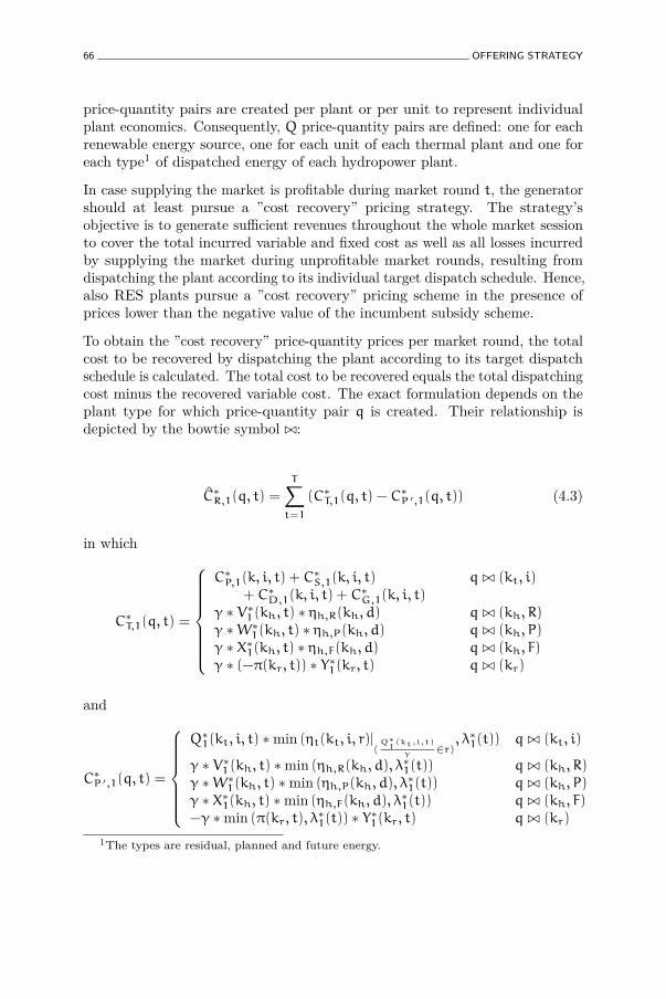
66 OFFERING STRATEGY
price-quantity pairs are created per plant or per unit to represent individualplant economics. Consequently, Q price-quantity pairs are defined: one for eachrenewable energy source, one for each unit of each thermal plant and one foreach type1 of dispatched energy of each hydropower plant.
In case supplying the market is profitable during market round t, the generatorshould at least pursue a ”cost recovery” pricing strategy. The strategy’sobjective is to generate sufficient revenues throughout the whole market sessionto cover the total incurred variable and fixed cost as well as all losses incurredby supplying the market during unprofitable market rounds, resulting fromdispatching the plant according to its individual target dispatch schedule. Hence,also RES plants pursue a ”cost recovery” pricing scheme in the presence ofprices lower than the negative value of the incumbent subsidy scheme.
To obtain the ”cost recovery” price-quantity prices per market round, the totalcost to be recovered by dispatching the plant according to its target dispatchschedule is calculated. The total cost to be recovered equals the total dispatchingcost minus the recovered variable cost. The exact formulation depends on theplant type for which price-quantity pair q is created. Their relationship isdepicted by the bowtie symbol ./:
C∗R,1(q, t) =
T∑t=1
(C∗T,1(q, t) − C∗P ′,1(q, t)) (4.3)
in which
C∗T,1(q, t) =
C∗P,1(k, i, t) + C∗S,1(k, i, t) q ./ (kt, i)
+ C∗D,1(k, i, t) + C∗G,1(k, i, t)
γ ∗ V∗1(kh, t) ∗ ηh,R(kh, d) q ./ (kh, R)γ ∗W∗1(kh, t) ∗ ηh,P(kh, d) q ./ (kh, P)γ ∗ X∗1(kh, t) ∗ ηh,F(kh, d) q ./ (kh, F)γ ∗ (−π(kr, t)) ∗ Y∗1(kr, t) q ./ (kr)
and
C∗P ′,1(q, t) =
Q∗1(kt, i, t) ∗min (ηt(kt, i, r)|(Q∗1(kt,i,t)
γ∈r), λ∗1(t)) q ./ (kt, i)
γ ∗ V∗1(kh, t) ∗min (ηh,R(kh, d), λ∗1(t)) q ./ (kh, R)γ ∗W∗1(kh, t) ∗min (ηh,P(kh, d), λ∗1(t)) q ./ (kh, P)γ ∗ X∗1(kh, t) ∗min (ηh,F(kh, d), λ∗1(t)) q ./ (kh, F)−γ ∗min (π(kr, t), λ∗1(t)) ∗ Y∗1(kr, t) q ./ (kr)
1The types are residual, planned and future energy.

RISK-CONSTRAINED OFFERING STRATEGY 67
Increasing the price of the price-quantity pair increases the likelihood of the price-quantity pair being rejected. This risk is ideally kept as small as possible over allprofitable market rounds. The total cost to be recovered C∗R,1(q, t) is thereforedistributed proportionally to the yield between the maximum anticipated priceassociated to residual demand curve scenario 1 and the variable generation cost.The ”cost recovery” price mark-up is obtained by
C∗R,1(q, t) = α ∗ (λ∗1(t) − η(q)) + η(q) (4.4)
α =C∗R,1(q, t)∑T
t=1 ((λ∗1(t) − η(q)) ∗Q∗1(q, t))
(4.5)with
η(q) =
ηt(kt, i, r)|
(Q∗n(kt,i,t)
γ∈r)
q ./ (kt, i)
ηh,R(kh, d) q ./ (kh, R)ηh,P(kh, d) q ./ (kh, P)ηh,F(kh, d) q ./ (kh, F)−π(kr, t) q ./ (kr)
in which
Q∗1(q, t) =
Q∗1(kt, i, t) q ./ (kt, i)γ ∗ V∗1(kh, t) q ./ (kh, R)γ ∗W∗1(kh, t) q ./ (kh, P)γ ∗ X∗1(kh, t) q ./ (kh, F)γ ∗ (Y∗1(kr, t)) q ./ (kr)
and
The final ”cost recovery” price C∗R,1(q, t) at each individual profitable marketround t is then obtained by adding the variable generation cost to the ”costrecovery” price mark-up. The ”cost recovery” price at unprofitable marketrounds is consistent with the maximum anticipated price associated to residualdemand curve forecast scenario 1 and equals λ∗1(t).
Hence, a lower and upper bound on the price for each price-quantity paircreated to supply Q∗1(t) to the market, are defined. A risk-averse generatortends to decide the final price of the price-quantity pair equal to the lower bound,ensuring its cost recovery, while a risk-minded generator tends to choose a priceequal to the upper bound, thereby actively attempting to set the emergingmarket clearing price. Any risk behaviour is applicable as they are all consistentwith the likelihood of emerging prices to exceed those denoted by the residualdemand curve scenario.

68 OFFERING STRATEGY
The formal representation of the resulting price-quantity pair is given by
{QO,1
(q), QO,1(q), λO,1(q), tStart, tEnd} (4.6)
QO,1
(q) =
Q∗1(q, t) (1); q ./ (kt, i)Q∗1(q, t) (2); q ./ (kh, ·)∆Q∗1(q, t) (3); q ./ (kh, ·)0 otherwise
in which
QO,1(q) = Q∗1(q, t)
λO,1(q) ∈ [C∗R,1(q, t) . . . λ∗1(t)]
tStart = tEnd = t
Q∗1(q, t) ≤ γ ∗ P(kt, i) (1)with
∆Q∗1(q, t) ≥ Q∗1(q, t) (2)
∆Q∗1(q, t) < Q∗1(q, t);∆Q
∗1(q, t) > 0 (3)
∆Q∗1(q, t) = γ ∗ PD(kh) −q−1∑q ′=1
[Q∗1(q′, t)]|q ′./(kh,·)and
The maximum quantity to submit to the MO equals the target dispatch schedulewhile the minimum quantity depends on minimum technical limits to supplyenergy during market round t. As such, the indivisible part of price-quantitypairs associated with a thermal unit explicitly represents the start-up trajectoryin case the thermal plant starts up, the shut-down trajectory when shuttingdown, or the minimum stable power level in case it operates in its productionphase. Price-quantity pairs associated to a hydropower plant type explicitlyrepresent the plant’s minimum technical capacity limits. No technical limitsare represented if the price-quantity pair is associated with a RES plant.
Since the risk behaviour of the generator depends on the environment it operatesin, which in turn should be represented by the shape of the residual demandcurve, the generator is expected to randomly select the price of the price-quantity pair from the uniform price distribution defined between the previously-calculated lower and upper price limits.
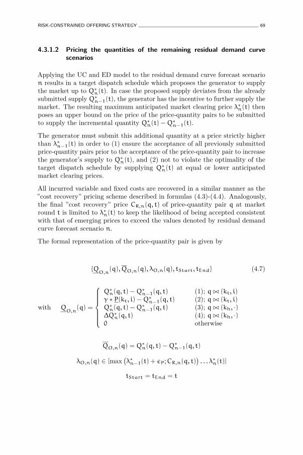
RISK-CONSTRAINED OFFERING STRATEGY 69
4.3.1.2 Pricing the quantities of the remaining residual demand curvescenarios
Applying the UC and ED model to the residual demand curve forecast scenarion results in a target dispatch schedule which proposes the generator to supplythe market up to Q∗n(t). In case the proposed supply deviates from the alreadysubmitted supply Q∗n−1(t), the generator has the incentive to further supply themarket. The resulting maximum anticipated market clearing price λ∗n(t) thenposes an upper bound on the price of the price-quantity pairs to be submittedto supply the incremental quantity Q∗n(t) −Q∗n−1(t).
The generator must submit this additional quantity at a price strictly higherthan λ∗n−1(t) in order to (1) ensure the acceptance of all previously submittedprice-quantity pairs prior to the acceptance of the price-quantity pair to increasethe generator’s supply to Q∗n(t), and (2) not to violate the optimality of thetarget dispatch schedule by supplying Q∗n(t) at equal or lower anticipatedmarket clearing prices.
All incurred variable and fixed costs are recovered in a similar manner as the”cost recovery” pricing scheme described in formulas (4.3)-(4.4). Analogously,the final ”cost recovery” price CR,n(q, t) of price-quantity pair q at marketround t is limited to λ∗n(t) to keep the likelihood of being accepted consistentwith that of emerging prices to exceed the values denoted by residual demandcurve forecast scenario n.
The formal representation of the price-quantity pair is given by
{QO,n
(q), QO,n(q), λO,n(q), tStart, tEnd} (4.7)
QO,n
(q) =
Q∗n(q, t) −Q
∗n−1(q, t) (1); q ./ (kt, i)
γ ∗ P(kt, i) −Q∗n−1(q, t) (2); q ./ (kt, i)Q∗n(q, t) −Q
∗n−1(q, t) (3); q ./ (kh, ·)
∆Q∗n(q, t) (4); q ./ (kh, ·)0 otherwise
with
QO,n(q) = Q∗n(q, t) −Q
∗n−1(q, t)
λO,n(q) ∈ [max(λ∗n−1(t) + εP ;CR,n(q, t)
). . . λ∗n(t)]
tStart = tEnd = t

70 OFFERING STRATEGY
Q∗n(q, t) < γ ∗ P(kt, i) (1)and
Q∗n(q, t) ≥ γ ∗ P(kt, i); Q∗n−1(q, t) < γ ∗ P(kt, i) (2)
∆Q∗n(q, t) ≥ Q∗n(q, t) (3)
∆Q∗n(q, t) < Q∗n(q, t); ∆Q∗n(q, t) > 0 (4)
∆Q∗n(q, t) = γ ∗ PD(kh) −q−1∑q ′=1
[Q∗n(q′, t)]|q ′./(kh,·)
The minimum quantity to be supplied depends on whether the minimumtechnical limits to supply energy during market round t have already been takeninto account by previously created price-quantity pairs. Price-quantity pairsare created according to this representation for all remaining residual demandcurve forecast scenarios and each market round in the market session. This stepof the offering strategy is hence iterated T ∗ (N− 1) times. Price-quantity pairsare only created in case QO,n(q) > 0.
4.3.1.3 Pricing remaining portfolio capacity
Generators are obliged to submit the complete available generation capacity ofthermal plants to the MO to ensure sufficient market liquidity, guaranteeingan efficient operation of the electricity market. In case a thermal unit has notbeen dispatched at full capacity according to target dispatch schedule Q∗N(t),the remaining capacity γ ∗ P −Q∗N(t) thus still needs to be submitted. Thisrequirement is obviously not applicable to hydropower and RES plants becauseof reservoir energy level limitations respectively controllability issues.
The price at which to submit the remaining capacity is bounded downwardby λ∗N(t) since the excess capacity is not supposed to actually be dispatchedaccording to target dispatch schedule N. Since no more residual demand forecastscenarios are available to determine the upper bound of the price at which theprice-quantity pair can be submitted, only the practical price limit equal to themarket ceiling price is binding. As previously noted, technical limits have to betaken into account when creating the price-quantity pair.
The formal representation is given by
{QO,N+1
(q), QO,N+1(q), λO,N+1(q), tStart, tEnd} (4.8)

RISK-CONSTRAINED OFFERING STRATEGY 71
in which
QO,N+1
(t) =
{γ ∗ P(kt, i) −Q∗N(q, t) (1); q ./ (kt, i)0 otherwise; q ./ (kt, i)
QO,n(t) = P(kt, i) −Q∗N(q, t)
λO,n(t) ∈ [max (λN(t) + εP ;CR,N(q, t)) . . . λ(t)]
tStart,n = tEnd,n = t
Q∗N(q, t) ≤ γ ∗ P(kt, i) (1)with
4.3.2 Determining complex price-quantity pairs
Price-quantity pairs per market round reflect the generator’s anticipation toprice deviations within the residual demand curve forecast confidence intervalmarked by λ∗1(t) and λ∗N(t). On the other hand, in case emerging residualdemand curves in individual market rounds are significantly perturbed dueto e.g. an unanticipated deviation from renewable energy injection levels orthe inadequacy of the residual demand curve forecast distribution to grasp theunderlying uncertainties in competitors’ behaviour, price-quantity pairs mightbe rejected even though the plants in the portfolio do not have the technicalcapabilities to resolve the resulting infeasible dispatch schedule. The generatorsubsequently faces expensive balancing requirements.
In order to address the lack of intertemporal technical flexibility, complexprice-quantity pairs spanning multiple subsequent market rounds are created.Since thermal units are least flexible and therefore more prone to an infeasibledispatch schedule caused by a rejection of associated price-quantity pairs, theiroperational risk is hedged by creating complex price-quantity pairs. Thisassumption is consistent with the modelling assumptions in chapter 3, sinceonly thermal units have modelled intertemporal constraints.
The downward price risk faced by an operational thermal unit is mitigatedby calculating the opportunity cost for shutting down operational units whenanticipated market clearing prices are lower than λ∗1(t). Upward price risks aremitigated by starting up an idle thermal unit in order to increase profit in casemarket clearing prices are higher than λ∗N(t). Hedging against both risks iselaborated in section 4.3.2.1 and 4.3.2.2 respectively. No exogenous constraintson the size, type or amount of price-quantity pairs are imposed.

72 OFFERING STRATEGY
4.3.2.1 Hedging against Downward Price Risk
Downward price risks are hedged by defining a complex price-quantity pair tokeep the unit operational during multiple subsequent market rounds, even atunprofitable anticipated prices, in order to avoid more expensive start-up costs.However, in case the complex price-quantity pair is rejected, the unit has tobe able to ramp down to zero to shut down and to ramp up again during allmarket rounds for which the complex price-quantity pair is defined, in order toavoid being systematically positively imbalanced.
A price-quantity pair is created in case it covers an operational duration frommarket round tStart to tEnd included, as long as this duration satisfies thethermal unit’s technical ramping flexibility during each operational phase, itsminimum stable power level duration and minimum inactive duration. Thetime it takes the thermal unit to ramp down from and up to its target dispatchschedule is denoted by
tEnd − tStart + 1 =τPD(kt, i) + τPU(kt, i) + τD(kt, i)
+ τU(kt, i) + τOFF(kt, i) + τ′U(kt, i) + τ
′D(kt, i)
(4.9)
τPD(kt, i) =Q∗n(q, tStart − 1) − P(kt, i)
κPD(kt, i)with
τPU(kt, i) =Q∗n(q, tEnd + 1) − P(kt, i)
κPU
τD(kt, i) =P(kt, i)
κD(kt, i)
τU(kt, i) =P(kt, i)
κU(kt, i)
The first and second term denote the time it takes the unit to ramp downto and ramp up from the minimum stable power level without violating theplant’s commitment to supply the market according to its optimal dispatchschedule before tStart and after tEnd as calculated by the UC and ED model.The third and fourth term denote the duration of the shut-down and start-uppower trajectory. Thirdly, τ ′U(kt, i) and τ ′D(kt, i) denote the time needed tomaintain a stable power level duration after tStart and before tEnd respectively.Finally, the minimum time needed to start up after the shut-down moment isτOFF(kt, i).

RISK-CONSTRAINED OFFERING STRATEGY 73
Any complex price-quantity pair spanning a lower number of market roundsprevents the unit to fully ramp down in case the complex pair is rejected dueto its limited technical flexibility. Although supplementary gradient costs canbe incurred in order to reduce the market round span over which the complexprice-quantity pair is defined, this possibility is no longer relevant during thisstep of the offering strategy. Indeed, the creation of complex price-quantity pairsis aimed at reducing the likelihood of a rejection of individual price-quantitypairs per market round rather than to provide dispatch flexibility to obtain alarger profit. Results obtained in chapter 3 support this reasoning.
Since a downward price risk is envisaged, the complex price-quantity pair isdefined to cover all subsequent market rounds in which the average anticipatedemerging clearing prices are lowest. Hence, the residual demand curve forecastscenario for which complex price-quantity pairs are created, corresponds to theone with the lowest average anticipated emerging clearing prices which triggerthe dispatch of the unit over market rounds tStart to tEnd included. Duringthe remainder of this section, this residual demand curve forecast scenario isreferred to as scenario n. In case no such forecast scenario exists, no complexprice-quantity pairs are created.
To determine the price and quantity of the complex price-quantity pair, theopportunity cost related to an acceptation and a rejection of the thermal unitto supply the market are compared. In case of a rejection, an expected costCrej(q) is faced by the generator in order to ramp down from its power level attStart and ramp up to its power level at tEnd:
Crej(q) =
tS,2∑t ′=tS,1
CP(kt, i, t) +
tE,1∑t ′=tS,2
CS(kt, i, t)
+
tE,2∑t ′=tE,1
CP(kt, i, t)
(4.10)
tS,1 = tStart + τ′D(kt, i)in which
tS,2 = tStart + τ′D(kt, i) + τPD(kt, i)
tE,1 = tEnd − τ ′U(kt, i) − τPD(kt, i)
tE,2 = tEnd − τ ′D(kt, i)

74 OFFERING STRATEGY
In case the complex price-quantity pair is accepted, the incurred cost Cacc(q)equals the total incurred generation cost minus the revenue obtained forsupplying the market with QO,n(q) at a minimum averaged renumerationλO,n(q). The incurred cost when accepted is given by
Cacc(q) = QO,n(q) ∗tEnd∑
t ′=tStart
(CP(kt, i, t) − λO,n(q)) (4.11)
The complex price-quantity pair has to be accepted when Cacc(q) < Crej(q).The resulting relationship between λO,n(q) and QO,n(q) allows the generator tosubmit increasing quantities at increasing price-quantity prices. The generatorcan thus theoretically create complex price-quantity pairs covering downwardprice risk for the individual power tranches of which the full power level perunit is composed. Practically however, exogenous constraints on the size, typeor amount of price-quantity pairs limit the number of complex pairs in order tostill be able to solve the market clearing problem.
The minimum quantity of each created complex price-quantity pair has to be atleast equal to the minimum stable power level P(kt, i) in order to avoid beingaccepted to operate in the unstable start-up or shut-down phase. The maximumquantity is limited by the minimum power level obtained from the schedulingsolution associated to residual demand curve forecast scenario n, from tStartto tEnd included. Any larger quantity would indeed violate the optimal targetdispatch schedule, thereby reducing the exercised market power potential.
Finally, the complex price-quantity pair is priced higher than the averagedanticipated prices according to residual demand curve forecast scenario n− 1,or the market floor price in case n = 1. Similarly, the upper bound is set bythe average of anticipated prices according to residual demand curve forecastscenario n. The complex price-quantity pairs are
{QO,n
(q), QO,n(q), λO,n(q), tStart, tEnd} (4.12)
QO,n(q) ∈ [P(kt, i),tEndmin
t=tStartQ∗n(kt, i, t)]in which
QO,n
(q) = QO,n(q)
λO,n(q) = max (λopp(q), λn−1(t) + εP)
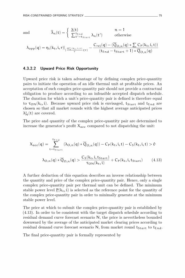
RISK-CONSTRAINED OFFERING STRATEGY 75
λn(t) =
{λ(t) n = 1∑tEndt ′=tStart
λn(t′) otherwiseand
λopp(q) = ηt(kt, i, r)|(Q∗n(kt,i,t)
γ∈r)
−Crej(q) − (QO,n(q) ∗
∑CP(kt, i, t))
(tEnd − tStart + 1) ∗QO,n(q)
4.3.2.2 Upward Price Risk Opportunity
Upward price risk is taken advantage of by defining complex price-quantitypairs to initiate the operation of an idle thermal unit at profitable prices. Anacceptation of such complex price-quantity pair should not provide a contractualobligation to produce according to an infeasible accepted dispatch schedule.The duration for which a unit’s price-quantity pair is defined is therefore equalto τON(kt, i). Because upward price risk is envisaged, tStart and tEnd arechosen so that all market rounds with the highest average anticipated pricesλ∗N(t) are covered.
The price and quantity of the complex price-quantity pair are determined toincrease the generator’s profit Xacc compared to not dispatching the unit:
Xacc(q) =
tEnd∑t=tStart
(λO,n(q) ∗QO,n(q)) − CP(kt, i, t) − CS(kt, i, t) > 0
λO,n(q) ∗QO,n(q) >CS(kt, i, tStart)
τON(kt, i)+ CP(kt, i, tStart) (4.13)
A further deduction of this equation describes an inverse relationship betweenthe quantity and price of the complex price-quantity pair. Hence, only a singlecomplex price-quantity pair per thermal unit can be defined. The minimumstable power level P(kt, i) is selected as the reference point for the quantity ofthe complex price-quantity pair in order to minimally generate at the minimumstable power level.
The price at which to submit the complex price-quantity pair is established by(4.13). In order to be consistent with the target dispatch schedule according toresidual demand curve forecast scenario N, the price is nevertheless boundeddownward by the average of the anticipated market clearing prices according toresidual demand curve forecast scenario N, from market round tStart to tEnd.
The final price-quantity pair is formally represented by

76 OFFERING STRATEGY
{QO,n
(q), QO,n(q), λO,n(q), tStart, tEnd} (4.14)
QO,n(q) = P(kt, i)with
QO,n
(q) = QO,n(q)
λO,n(q) = max (λopp(q), λN(t) + εP)
λn(t) =
{λ(t) n = 1∑tEndt ′=tStart
(λn(t′)) otherwisein which
λopp(q) =CS(kt, i, tStart)
QO,n(q) ∗ τON(kt, i)+CP(kt, i, tStart)
QO,n(q)
Note that the complex price-quantity pairs partially replace the price-quantitypairs defined to comply with the obligation to submit the complete thermalcapacity to the MO.
4.4 Impact of the offering strategy
The performance of the offering strategy is assessed in both a competitive andoligopolistic environment. The presented strategies are compared with onescommonly applied in literature in order to deduct objective conclusions. Thesimulation setup of each of the two seperate case studies retrieved assessesthe impact of the presented strategy in isolation from the others in order tofacilitate the interpretation of results.
Since the presented offering strategy explicitly incorporates portfolio flexibility,it is expected to attain a significantly larger profit and smaller imbalance afterday-ahead market clearing. The degree in which profit increases and imbalancesdecrease is expected to be larger in the competitive environment as, in contrastto the oligopolistic one, quantity is not considered a stochastic variable.
The use of realistic residual demand curves and a portfolio covering the fullrelevant range of technical flexibility and plant economics justifies the deductionof general conclusions rather than case-specific ones.

IMPACT OF THE OFFERING STRATEGY 77
2 4 6 8 10 12 14 16 18 20 22 2420
40
60
80
100
Market Round [hour]
MarketClearingPrice
[e/M
Wh]
emerging prices
Figure 4.5: Distribution of the emerging market clearing prices in the Iberianelectricity market as calculated from January, 1, to March, 11, 2008
4.4.1 Perfectly competitive market
4.4.1.1 Simulation setup and data generation
The simulation setup is based on realistic data corresponding to the timehorizon retrieved from reference (Lagarto et al., 2012). Market clearing pricesare obtained from the website of the MO Operador del Mercado Ibérico deEnergía (OMIE) in the Iberian electricity market or the electricity market frommainland Spain if market splitting occurred (OMIE, 2013). Since this casestudy aims at assessing the performance of the presented offering strategy ina competitive market environment, the residual demand curves are modelledas a single price-quantity pair of which the price equals the emerging marketclearing price and the maximum quantity can be assumed infinite.
The case mimics the offering problem faced by a fictitious generator enteringthe electricity market. The generator has to submit price-quantity pairs tothe MO in order to be able to supply the market during the market sessionorganised on the 12th of March 2008 (Lagarto et al., 2012). The actual priceuncertainty faced by the generator is illustrated in figure 4.5 and is calculatedbased on historical market clearing prices from January, 1, 2008 to March, 11,2008. The full black line denotes the actual market clearing price on the 12th ofMarch and is fully described by the created price distribution.
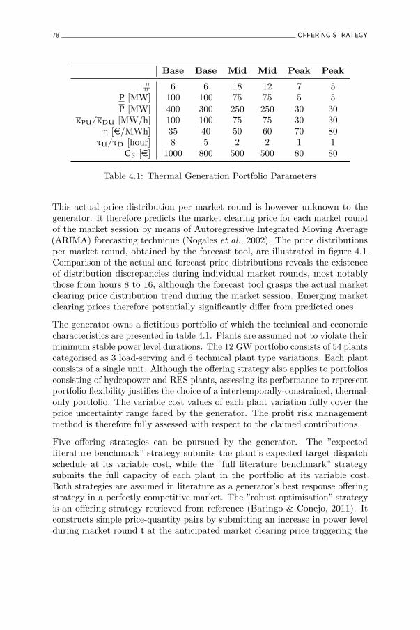
78 OFFERING STRATEGY
Base Base Mid Mid Peak Peak# 6 6 18 12 7 5
P [MW] 100 100 75 75 5 5P [MW] 400 300 250 250 30 30
κPU/κDU [MW/h] 100 100 75 75 30 30η [e/MWh] 35 40 50 60 70 80τU/τD [hour] 8 5 2 2 1 1
CS [e] 1000 800 500 500 80 80
Table 4.1: Thermal Generation Portfolio Parameters
This actual price distribution per market round is however unknown to thegenerator. It therefore predicts the market clearing price for each market roundof the market session by means of Autoregressive Integrated Moving Average(ARIMA) forecasting technique (Nogales et al., 2002). The price distributionsper market round, obtained by the forecast tool, are illustrated in figure 4.1.Comparison of the actual and forecast price distributions reveals the existenceof distribution discrepancies during individual market rounds, most notablythose from hours 8 to 16, although the forecast tool grasps the actual marketclearing price distribution trend during the market session. Emerging marketclearing prices therefore potentially significantly differ from predicted ones.
The generator owns a fictitious portfolio of which the technical and economiccharacteristics are presented in table 4.1. Plants are assumed not to violate theirminimum stable power level durations. The 12 GW portfolio consists of 54 plantscategorised as 3 load-serving and 6 technical plant type variations. Each plantconsists of a single unit. Although the offering strategy also applies to portfoliosconsisting of hydropower and RES plants, assessing its performance to representportfolio flexibility justifies the choice of a intertemporally-constrained, thermal-only portfolio. The variable cost values of each plant variation fully cover theprice uncertainty range faced by the generator. The profit risk managementmethod is therefore fully assessed with respect to the claimed contributions.
Five offering strategies can be pursued by the generator. The ”expectedliterature benchmark” strategy submits the plant’s expected target dispatchschedule at its variable cost, while the ”full literature benchmark” strategysubmits the full capacity of each plant in the portfolio at its variable cost.Both strategies are assumed in literature as a generator’s best response offeringstrategy in a perfectly competitive market. The ”robust optimisation” strategyis an offering strategy retrieved from reference (Baringo & Conejo, 2011). Itconstructs simple price-quantity pairs by submitting an increase in power levelduring market round t at the anticipated market clearing price triggering the
IMPACT OF THE OFFERING STRATEGY 79
additional quantity to be supplied. The approach corresponds to a recentdevelopment in offering strategy formulation and is considered optimal in anoligopolistic market environment. Finally, the ”presented simple” and ”presentedcomplex” offering strategy respectively correspond to the presented offeringstrategy with and without the creation of complex price-quantity pairs.
Two key performance indicators are identified to objectively assess theperformance of all offering strategies given the envisaged market environment:the relative profit gap and the strategy’s future balancing cost.
Firstly, the obtained profit when pursuing an offering strategy is benchmarkedagainst the maximum attainable profit during each market session. It iscalculated by subtracting the cost for generating the actual dispatch schedulefrom the revenue. The actual dispatch schedule PP(t) is obtained by performinga cost-based UC given the accepted portfolio dispatch schedule PA(t). Revenueis calculated by multiplying the emerging market clearing price λ∗(t) with theminimum of the accepted and the actual power level since the generator isonly rewarded for the contracted levels. The maximum profit is obtained bycalculating the optimal dispatch schedule PI(t) under perfect knowledge of themarket clearing prices. This formally corresponds to
∑Tt=t0
((λ∗(t) ∗min (PA(t), PP(t))) − C(PP(t)))∑Tt=t0
((λ∗(t) ∗ PI(t)) − CI(t))(4.1)
Secondly, the change in obtained profit between two offering strategies iscompared to the change in total daily imbalance between accepted and actualdispatch schedules. This indicator allows the deduction of relevant conclusionson the future balancing requirements caused by pursuing each offering strategy.Four possible outcomes are observed. In case the profit increases while the dailyimbalances increase, the cost related to the increase in imbalance should be offsetby the increase in profit. As such, the metric serves as an upper bound for futurebalancing costs to justify the use of the offering strategy. Similarly, a lower boundof balancing costs is obtained when profit and imbalances both decrease. In theelectricity market of mainland Spain2 upward imbalance prices are typicallysituated between e35/MWh and e55/MWh. Downward imbalance prices aretypically found in the range between e15/MWh and e30/MWh (REE, 2013).An increase in profit and a decrease in imbalance illustrates the superiority ofthe applied offering strategy and vice versa. The imbalance is calculated as
2The Iberian electricity market is split in case of congested transmission lines. Whenmarket results deviate between Portugal and mainland Spain, results of the latter are used inthis case study.

80 OFFERING STRATEGY
T∑t=t0
|PA(t) − PP(t)| (4.2)
The performance and robustness of each strategy are assessed for 100 differentemerging market clearing price outcomes. These outcomes have been calculatedfrom the covariance matrix between the price distributions of each market round(figure 4.5). Since each offering strategy creates price-quantity pairs based onthe price forecast distribution, 100 market sessions are simulated in which anidentical set of price-quantity pairs is matched to different emerging marketclearing price outcomes. The performance and robustness of the offering strategyis as such statistically assessed given an imperfectly known price distributionand a variety of plant types.
The problem formulation per market session consists of 36 variable groups and 72constraint groups. For the envisaged portfolio, this leads to a model containing44034 discrete and 52129 continuous variables, and 451723 constraints. Theoffering problem is solved in 4.7 minutes for each price forecast scenario, usingthe GNU Linear Programming Kit (GLPK) solver in C++ (Makhorin, 2012),on a machine with a 2.83GHz processor and 3.84GB RAM memory.
4.4.1.2 Results
Figure 4.6 illustrates the distribution of the obtained profit relative to themaximum attainable profit per market session over all 100 market outcomes.The data is plotted in boxplot format in order to visualise the median profitvalue and the associated uncertainty. The ”full literature benchmark” (LF)and ”expected literature benchmark” strategy (LE) only offer according to theprice scenario of the price forecast distribution at the 50% percentile, whilethe remaining strategies use more than one price scenario. The amount ofused price scenarios is denoted by the number in brackets. All price scenariosare determined by dividing the 90% confidence interval of the price forecastdistribution uniformly in smaller confidence intervals for each offering strategy.
The presented strategy, both with and without complex price-quantity pairs,provide a higher median and mean profit than any of the alternative literaturebenchmark strategies. While the mean profit equals e484.36k and e466.07kfor both benchmark strategies, mean profit equals e491.77k to e495.14k whenpursuing the ”presented simple” (PS), and e504.34k to e505.79k when applyingthe ”presented complex” (PC) strategy. The mean performance of the ”fullliterature benchmark” strategy (89.4%) outperforms the one of the ”expected
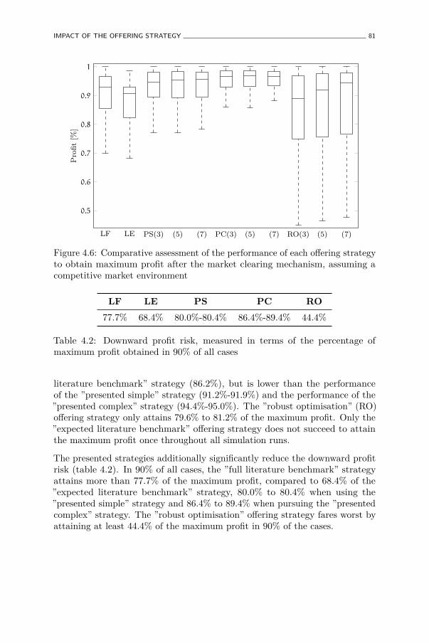
IMPACT OF THE OFFERING STRATEGY 81
0.5
0.6
0.7
0.8
0.9
1
LF LE PS(3) (5) (7) PC(3) (5) (7) RO(3) (5) (7)
Profit
[%]
Figure 4.6: Comparative assessment of the performance of each offering strategyto obtain maximum profit after the market clearing mechanism, assuming acompetitive market environment
LF LE PS PC RO77.7% 68.4% 80.0%-80.4% 86.4%-89.4% 44.4%
Table 4.2: Downward profit risk, measured in terms of the percentage ofmaximum profit obtained in 90% of all cases
literature benchmark” strategy (86.2%), but is lower than the performanceof the ”presented simple” strategy (91.2%-91.9%) and the performance of the”presented complex” strategy (94.4%-95.0%). The ”robust optimisation” (RO)offering strategy only attains 79.6% to 81.2% of the maximum profit. Only the”expected literature benchmark” offering strategy does not succeed to attainthe maximum profit once throughout all simulation runs.
The presented strategies additionally significantly reduce the downward profitrisk (table 4.2). In 90% of all cases, the ”full literature benchmark” strategyattains more than 77.7% of the maximum profit, compared to 68.4% of the”expected literature benchmark” strategy, 80.0% to 80.4% when using the”presented simple” strategy and 86.4% to 89.4% when pursuing the ”presentedcomplex” strategy. The ”robust optimisation” offering strategy fares worst byattaining at least 44.4% of the maximum profit in 90% of the cases.
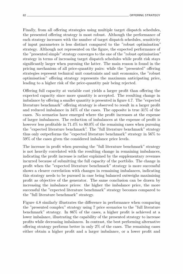
82 OFFERING STRATEGY
Finally, from all offering strategies using multiple target dispatch schedules,the presented offering strategy is most robust. Although the performance ofeach strategy increases with the number of target dispatch schedules, sensitivityof input parameters is less distinct compared to the ”robust optimisation”strategy. Although not represented on the figure, the expected performance ofthe ”presented simple” strategy converges to the one of the ”robust optimisation”strategy in terms of increasing target dispatch schedules while profit risk stayssignificantly larger when pursuing the latter. The main reason is found in thepricing mechanism of all price-quantity pairs: while the ”presented” offeringstrategies represent technical unit constraints and unit economics, the ”robustoptimisation” offering strategy represents the maximum anticipating price,leading to a higher risk of the price-quantity pair being rejected.
Offering full capacity at variable cost yields a larger profit than offering theexpected capacity since more quantity is accepted. The resulting change inimbalance by offering a smaller quantity is presented in figure 4.7. The ”expectedliterature benchmark” offering strategy is observed to result in a larger profitand reduced imbalance in 34% of the cases. The opposite is true 31% of thecases. No scenarios have emerged where the profit increases at the expenseof larger imbalances. The reduction of imbalances at the expense of profit ishowever less profitable in 71.4% to 80.0% of the remaining cases when pursuingthe ”expected literature benchmark”. The ”full literature benchmark” strategythus only outperforms the ”expected literature benchmark” strategy in 56% to59% of the cases given the considered imbalance price levels.
The increase in profit when pursuing the ”full literature benchmark” strategyis not heavily correlated with the resulting change in remaining imbalances,indicating the profit increase is rather explained by the supplementary revenuesincurred because of submitting the full capacity of the portfolio. The change inprofit when the ”expected literature benchmark” strategy is more successfulshows a clearer correlation with changes in remaining imbalances, indicatingthis strategy needs to be pursued in case being balanced outweighs maximisingprofit as objective of the generator. The same conclusion can be drawn byincreasing the imbalance prices: the higher the imbalance price, the moresuccessful the ”expected literature benchmark” strategy becomes compared tothe ”full literature benchmark” strategy.
Figure 4.8 similarly illustrates the difference in performance when comparingthe ”presented complex” strategy using 7 price scenarios to the ”full literaturebenchmark” strategy. In 86% of the cases, a higher profit is achieved at alower imbalance, illustrating the capability of the presented strategy to increaseprofits while decreasing imbalances. In contrast, the best performing alternativeoffering strategy performs better in only 2% of the cases. The remaining caseseither obtain a higher profit and a larger imbalance, or a lower profit and
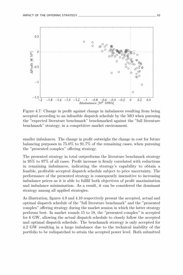
IMPACT OF THE OFFERING STRATEGY 83
−2 −1.8 −1.6 −1.4 −1.2 −1 −0.8 −0.6 −0.4 −0.2 0 0.2 0.4−1.5
−1
−0.5
0
0.5
∆Imbalance [104 MWh]
∆Profit
[e106]
Figure 4.7: Change in profit against change in imbalances resulting from beingaccepted according to an infeasible dispatch schedule by the MO when pursuingthe ”expected literature benchmark” benchmarked against the ”full literaturebenchmark” strategy, in a competitive market environment.
smaller imbalances. The change in profit outweighs the change in cost for futurebalancing purposes in 75.0% to 91.7% of the remaining cases, when pursuingthe ”presented complex” offering strategy.
The presented strategy in total outperforms the literature benchmark strategyin 95% to 97% of all cases. Profit increase is firmly correlated with reductionsin remaining imbalances, indicating the strategy’s capability to obtain afeasible, profitable accepted dispatch schedule subject to price uncertainty. Theperformance of the presented strategy is consequently insensitive to increasingimbalance prices as it is able to fullfil both objectives of profit maximisationand imbalance minimisation. As a result, it can be considered the dominantstrategy among all applied strategies.
As illustration, figures 4.9 and 4.10 respectively present the accepted, actual andoptimal dispatch schedule of the ”full literature benchmark” and the ”presentedcomplex” offering strategy during the market session in which the latter strategyperforms best. In market rounds 15 to 18, the ”presented complex” is acceptedfor 6 GW, allowing the actual dispatch schedule to closely follow the acceptedand optimal dispatch schedule. The benchmark strategy is only accepted for4.2 GW resulting in a large imbalance due to the technical inability of theportfolio to be redispatched to attain the accepted power level. Both submitted

84 OFFERING STRATEGY
−2 −1.8 −1.6 −1.4 −1.2 −1 −0.8 −0.6 −0.4 −0.2 0 0.2 0.4−1.5
−1
−0.5
0
0.5
∆Imbalance [104 MWh]
∆Profit
[e106]
Figure 4.8: Change in profit against change in imbalances resulting from beingaccepted according to an infeasible dispatch schedule by the MO when pursuingthe ”presented complex” benchmarked against the ”full literature benchmark”strategy, in a competitive market environment.
price-quantity curves in hour 16 are presented in figure 4.11, illustrating thebase power plants’ complex price-quantity pair creation below variable cost tomitigate deviations from the optimal dispatch schedule.
Finally, figure 4.12 compares the performance of the ”presented simple” with”presented complex” offering strategy. The beneficial impact of creating complexprice-quantity pairs is clearly observed in 68% of all cases. Both offeringstrategies show the same performance in all other cases.
4.4.2 Oligopolistic market
4.4.2.1 Simulation setup and data generation
Data of the first 84 market sessions in 2012 (from January, 1 to March, 24,2012) organised by the Iberian electricity market operator have been gatheredto obtain a similar time horizon as retrieved from the competitive case (OMIE,2013). In case market splitting occurs between mainland Spain and Portugalbecause of congested transmission lines, market results from mainland Spain are

IMPACT OF THE OFFERING STRATEGY 85
0 2 4 6 8 10 12 14 16 18 20 22 244
6
8
10
12
Market Round [hour]
Power
Produ
ctionLe
vel[103MW
]
acceptedactualoptimal
Figure 4.9: Accepted, actual and optimal dispatch schedule when pursuingthe benchmark offering strategy, during the worst performing market sessioncompared to the ”presented complex” strategy
0 2 4 6 8 10 12 14 16 18 20 22 244
6
8
10
12
Market Round [hour]
Power
Produ
ctionLe
vel[103MW
]
acceptedactualoptimal
Figure 4.10: Accepted, actual and optimal dispatch schedule when pursuing the”presented complex” offering strategy using 7 price scenarios, during the bestperforming market session compared to the benchmark strategy
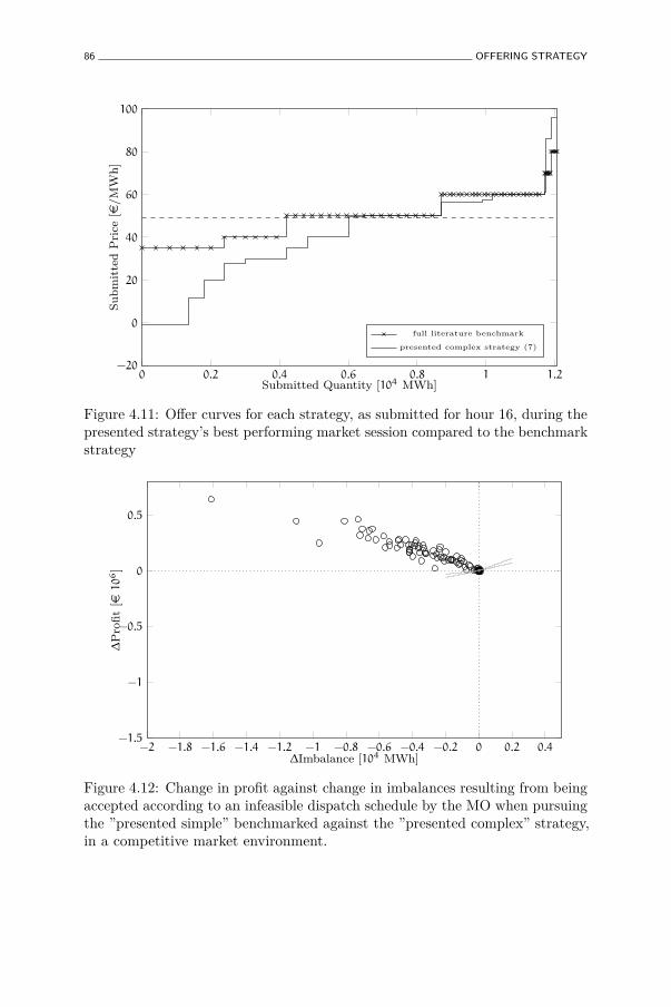
86 OFFERING STRATEGY
0 0.2 0.4 0.6 0.8 1 1.2−20
0
20
40
60
80
100
Submitted Quantity [104 MWh]
Subm
itted
Price
[e/M
Wh]
full literature benchmark
presented complex strategy (7)
Figure 4.11: Offer curves for each strategy, as submitted for hour 16, during thepresented strategy’s best performing market session compared to the benchmarkstrategy
−2 −1.8 −1.6 −1.4 −1.2 −1 −0.8 −0.6 −0.4 −0.2 0 0.2 0.4−1.5
−1
−0.5
0
0.5
∆Imbalance [104 MWh]
∆Profit
[e106]
Figure 4.12: Change in profit against change in imbalances resulting from beingaccepted according to an infeasible dispatch schedule by the MO when pursuingthe ”presented simple” benchmarked against the ”presented complex” strategy,in a competitive market environment.
IMPACT OF THE OFFERING STRATEGY 87
0 0.2 0.4 0.6 0.8 1 1.2 1.4 1.6 1.8 20
20
40
60
80
Supplied energy [104 MWh]
Anticipated
marketclearing
price[e/M
Wh] 5% percentile
50% percentile95% percentile
Figure 4.13: 90% confidence interval of the residual demand curve forecastdistribution for market round 5, in the electricity market of mainland Spain ascalculated from January, 1 to March, 24, 2012
used. Crossborder exchanges are implicitly represented by the residual demandcurve.
The residual demand curve forecast distribution is calculated from the first 24market sessions, of which the 90% residual demand curve confidence interval isillustrated for market round 5, 20 and 22 in figures 4.13, 4.14 and 4.4 respectively.The residual demand curves for each market round in the remaining 60 marketsessions are unknown to the generator and used to assess each offering strategyin terms of the indicators introduced in section 4.4.1. The portfolio owned bythe generator is considered equivalent to the one presented in table 4.1.
The problem formulation is equivalent to the one described in 4.4.1, consistingof 36 variable and 72 constraint groups per market session. The exact numberof variables and equations depends on the number of price-quantity pairs out ofwhich each residual demand curve is composed. Generally, the offering problemis more complex so that the GLPK solver takes 27 minutes to solve the offeringproblem on a machine with a 2.83GHz processor and 3.84GB RAM memory.

88 OFFERING STRATEGY
0 0.2 0.4 0.6 0.8 1 1.2 1.4 1.6 1.8 20
20
40
60
80
Supplied energy [104 MWh]
Anticipated
marketclearing
price[e/M
Wh] 5% percentile
50% percentile95% percentile
Figure 4.14: 90% confidence interval of the residual demand curve forecastdistribution for market round 20, in the electricity market of mainland Spain ascalculated from January, 1 to the March, 24, 2012
4.4.2.2 Results
Figure 4.15 ilustrates the distribution of the obtained profit relative to themaximum attainable profit per market round over all 60 market outcomes.Comparison with figure 4.6 reveals all strategies to underperform due tothe additional uncertainty in terms of supply quantity. The ”full literaturebenchmark” strategy (41.1%) performs worse compared to ”expected literaturebenchmark” strategy (47.9%). The ”presented simple” offering strategy performsaround 58.3%-59.7% while the ”presented complex” strategy performs bestby attaining 65.6%-73.2% of the maximum obtainable profit. The ”robustoptimisation” strategy performs worst with a ratio of only 8.9%-17.0%.
Only the strategies presented in section 4.3 never lead to a loss. The capabilityof these strategies to reduce downward profit risk is confirmed when looking atthe minimum profit obtained in 90% of all cases (table 4.3). The ”presentedcomplex” strategy obtains at least 41.3%-46.8% of the maximum attainableprofit, while this performance declines when looking at the ”presented simple”(37.6%-39.0%), the ”expected literature benchmark” (19.9%), the ”full literaturebenchmark” (16.9%) and the ”robust optimisation” strategy (-50.0%-36.8%).
Although the performance increases with a larger number of residual demandcurve forecast scenarios, the results of each offering strategy can be considered

IMPACT OF THE OFFERING STRATEGY 89
−1
−0.5
0
0.5
1
LF LE PS(3) (5) (7) PC(3) (5) (7) RO(3) (5) (7)
Profit
[%]
Figure 4.15: Comparative assessment of the performance of each offering strategyto obtain maximum profit after the market clearing mechanism, assuming anoligopolistic market environment
LF LE PS PC RO16.9% 19.9% 37.6%-39.0% 41.3%-46.8% -50.0%-39.8%
Table 4.3: Downward profit risk, measured in terms of the percentage ofmaximum profit obtained in 90% of all cases
robust in terms of the user-defined parameters.
Submitting expected power levels at variable cost obtains a larger profit thansubmitting the full capacity because the MO only partially rejects a price-quantity pair thanks to the price-elastic residual demand curve, thereby reducingdownward imbalance risks due to the rejection. Figure 4.16 illustrates the changein profit and imbalance by offering according to the former strategy compared tothe latter. In 55.0% of all cases, a larger profit is obtained while also obtaininga more balanced position when offering according to the ”expected literaturebenchmark” strategy. In 11.7% the ”expected literature benchmark” strategyobtains a lower profit while obtaining a less balanced position.
Assuming the same imbalance prices as in section 4.4.1.2, the ”expected literaturebenchmark” strategy outperforms the ”full literature benchmark” strategy in76.7% of all cases. Although the ”expected literature benchmark” strategy

90 OFFERING STRATEGY
−0.8 −0.6 −0.4 −0.2 0 0.2 0.4 0.6−0.2
0
0.2
0.4
0.6
∆Imbalance [104 MWh]
∆Profit
[e106]
Figure 4.16: Change in profit against change in imbalances resulting from beingaccepted according to an infeasible dispatch schedule by the MO when pursuingthe ”expected literature benchmark” benchmarked against the ”full literaturebenchmark” strategy, in a oligopolistic market environment.
results in lower remaining imbalances in 83.3% of all cases, no clear correlation isobserved with changes in profit. Both strategies thus focus on different objectives:the ”expected literature benchmark” strategy reduces remaining imbalanceswhile the ”full literature benchmark” strategy aims at increasing revenues.The residual demand curve’s inverse relationship between supplied quantityand emerging market clearing prices mitigates the success rate of the latterstrategy, giving more incentives to generators to pursue the ”expected literaturebenchmark” strategy. This incentive increases with increasing imbalance prices.
Figure 4.17 compares the ”presented complex” strategy using 3 price scenariosand the ”full literature benchmark” strategy. In 86.7% of the cases, a largerprofit is achieved at a lower remaining imbalance while only 5% of all casesexhibits a smaller profit at a higher remaining imbalance. The increase in profitoutweighs the cost for balancing in 91.7% of all cases. Profit increase is largelycorrelated with reductions in remaining imbalances, indicating the presentedoffering strategy is also capable of obtaining a feasible, accepted dispatchschedule under residual demand curve uncertainty. The effect is neverthelessless outspoken compared to the results under a competitive market setup.

CONCLUSIONS 91
−0.8 −0.6 −0.4 −0.2 0 0.2 0.4 0.6−0.2
0
0.2
0.4
0.6
∆Imbalance [104 MWh]
∆Profit
[e106]
Figure 4.17: Change in profit against change in imbalances resulting from beingaccepted according to an infeasible dispatch schedule by the MO when pursuingthe ”presented complex” benchmarked against the ”full literature benchmark”strategy, in a oligopolistic market environment
4.5 Conclusions
This chapter describes a novel profit risk hedging offering strategy the generatorcould pursue when participating in the day-ahead spot market as organisedunder the European PX model. Simple price-quantity pairs defined per marketround, and complex price-quantity pairs spanning multiple market rounds arecreated with the objective to mitigate the emergence of an infeasible accepteddispatch schedule. The performance of the offering strategy is benchmarkedagainst alternative offering strategies in a realistic market environment.
The presented offering strategy succeeds in increasing profits obtained duringthe market session while mitigating up- and downward profit risks. Compared tostrategies applied in literature, in a perfectly competitive market environment,the presented strategy outperforms in 95% to 97% of all scenarios. Since allscenarios have been generated based on data obtained from the Iberian MO,the performance rate is representative for a system with moderate to high pricevolatility, as characterised by medium to large RES integration.
This performance rate is largely insensitive to the cost associated to futurebalancing requirements as profit is increased while imbalances are reduced in

92 OFFERING STRATEGY
more than 80% of all cases. Creating complex price-quantity pairs results in anincrease in performance in 68% of all scenarios. As such, even though perfectlycompetitive market conditions are assumed, deviating the price of price-quantitypairs away from the variable generation costs is a rational offering strategy.
The presented strategy moreover attains higher profits in an oligopolisticenvironment as the presented strategy outperforms the second best performingalternative strategy in 91.7% of all cases. Again, scenarios are representative fora system characterised by medium to large RES integration. The correlationbetween increasing profit and decreasing remaining imbalances indicates thecapability of the presented offering strategy to obtain a profitable and feasibleaccepted dispatch schedule after market clearing. Moreover, the offering strategysuccessfully hedges against profit risk since it is the only strategy which avoidssupplying the market at a loss during simulations.
This case study therefore shows profit is increased, and profit risk reduced, byrepresenting the flexibility of the portfolio through the price-quantity pairs.The offering strategy attains more than 90% of the maximum profit using thelowest number of price scenarios. The performance only increases 0.7% in casethe number of price scenarios is doubled, illustrating the method’s robustnessand computational efficiency, even in case the actual price distribution is notperfectly represented by the forecast price distribution. Since the number ofprice scenarios is the method’s sole user-defined input parameter, the methodis argued to illustrate a lower sensitivity to input parameters compared toalternative methods. Consequently, even though a price taker power producerdoes not have market power potential to alter the market clearing price toits own advantage, deviating the offer price away from the variable cost is arational strategy to hedge against profit risks.

Part II
Electricity Market Simulation Platform
93


Chapter 5Electricity market models
Regulatory intervention is currently based on ex-post indicators which measurethe exercise of market power. Whether market power potential is exercisedis deducted by comparing market prices or companies’ market share obtainedby market simulations with actually observed ones (Joskow & Kahn, 2001), orby calculating key indices such as the Lerner index, pivotal supplier analysis,price discovery, concentration ratio or the Hirschmann-Herfindahl index (de laFuente & Junco, 2011; Porter et al., 2008). These indices are however not 100%conclusive on whether market power potential is exercised as their value isheavily dependent on the definition of the market they investigate.
The reactive nature of corrective regulatory action results in increaseduncertainty for market participants in terms of market design evolution. Theaction’s effect is moreover unproven as it might simply conceal the causeof suboptimal market performance in the short term rather than effectivelyeliminating it in the long term. Regulators therefore seek ways to establisheffective and transparent market rules consistent with short and long termcompetitive market results, while minimising further interventions. More reliabletools to monitor market power are thus necessary (Helman & Hobbs, 2010).
Ex-ante market simulation techniques on the other hand require assumptionson actions of generators, the transmission network properties and demandcharacteristics, among others. The sensitivity of simulation results to the selectedassumptions and the lack of a common framework to address them are importantfactors why regulatory authorities are sceptical towards the application of ex-ante simulation techniques to specific regulatory purposes (Neuhoff et al., 2005).
95
96 ELECTRICITY MARKET MODELS
Nevertheless, ex-ante simulation tools are able to give information on thedynamics of price convergence while ex-post measurements only assess a staticsituation. Representing the dynamics of generators to flexibly adapt their energysupply to changing market and regulatory conditions is critical when evaluatingelectricity markets, especially since electricity is not storable, demand is ratherinelastic and transport requires a physical link (Borenstein, 2000).
This chapter provides the motivation to create a novel agent-based electricitymarket model. Besides providing an introductory overview and comparison ofrecent electricity market modelling trends, three recently developed agent-basedelectricity market models are discussed. Their strengths and limitations arecompared and the impact of the assumptions on the results are highlighted.The content of this chapter is based on references (Maenhoudt & Deconinck,2010a; Maenhoudt & Deconinck, 2010b).
5.1 Introduction
Three categories of electricity market models are identified in recent literature:game theory-based optimisation, supply function equilibrium and evolutionarymodels (Ventosa et al., 2005; Zhang, 2010). Each type is briefly discussed below.
5.1.1 Game theory-based optimisation models
Game theory-based optimisation models focus on the difficult and detailed profit-maximisation problem for a single firm competing in the electricity market. Theymaximise the profit of a generator facing an exogenous price or an exogenousresidual demand curve in order to explore relevant aspects of the market designand regulations. They have been widely applied because of their numericaltractability (Hobbs, 2001; Wietze et al., 2006; Pritchard, 2002). They aretherefore well documented in literature and can easily be solved by powerfuland well-known optimisation algorithms, such as for example the Mixed-IntegerLinear Problem (MILP) framework.
Unfortunately, the simple algebraic mathematical framework is not capable ofmodelling the level of complexity required when handling the complete electricitysystem, thereby limiting its scalability, scope and applicability as decisionsupport tool for designing market rules and protocols. As such, perfect andcomplete information on competitors’ cost functions and strategies, unlimitednetwork capacity and a perfectly known utility function are typical assumptions.

INTRODUCTION 97
Additionally, the demand function faced by all generators should be continuouslydifferentiable (Orbay, 2009). Besides heavily reducing the number of marketdesign features that can be evaluated, such models also quickly lead to non-convex feasible regions. Non-existent or non-unique equilibrium solutions existas a result, which leads to significant differences in results under slightly differentassumptions (Neuhoff et al., 2005; Hobbs & Pang, 2007).
Another drawback is the ability of a generator to only offer one singleprice-quantity pair. Depending on the choice of the strategic variable,two important subcategories of game theory-based optimisation models aredistinguished. The Cournot model applies to tight market conditions asgenerators strategically optimize the quota, while the Bertrand submodel appliesto intensely competitive market conditions as generators optimise in termsof price. The Cournot competition model has been widely applied to betterunderstand the influence of individual market design options on the performanceof electricity markets (Bushnell et al., 2004; Yao et al., 2007). Although theBertrand and Cournot models have recently been integrated to form a morerealistic hybrid model, the above-mentioned disadvantages of game theory-basedoptimisation models remain valid (Edenhofer et al., 2010).
Alternative subcategories do exist. The Stackelberg leadership model for examplemodels sequential competition in terms of quota between generators. Theapplication of this model is justified if one generator has a major advantageover its competitors. This is especially true in recently deregulated electricitymarkets when labelling the incumbent as Stackelberg leader and new entrantsas followers (Harris, 2006b).
5.1.2 Supply function equilibrium models
Equilibrium models perceive the electricity market as a static, non-cooperativegame in which two or more market participants have the objective to maximisetheir individual profit subject to quasi-perfect knowledge of the equilibriumstrategy or best-response functions of all other competitors (Forshner & Shy,2009). The assumption that each participant has complete information or areasonable estimate of competitors’ costs, strategies and pay-off functions, maybe valid in small systems with a small number of competitors, but cannothold when considering a large amount of participants. Equilibrium models alsoassume the existence of a market equilibrium at which no market participantcan profitably affect the market clearing price by changing its own strategy giventhe strategies employed by its rivals. Both oligopolistic and competitive marketscan be modelled. The equilibrium state of the former is called Cournot-Nash,the latter Walras-Nash equilibrium.

98 ELECTRICITY MARKET MODELS
Equilibrium models using both price and quota as strategic variables arecategorised as supply function equilibrium models (Klemperer & Meyer, 1989).They basically extend traditional game-theoretic optimisation models with theconjectural variations approach (Vives, 2001). Representing the beliefs of agenerator concerning how the total energy supply from its rivals changes interms of market clearing prices, allows generators to behave strategically onboth price and quota, in contrast to the one-dimensional strategic actions whenapplying game theory-based optimisation models (Day et al., 2002). Differentdegrees of competitive intensity can be modelled by defining different assumedsupply responses. Actual responses are not necessary equal to the assumedresponses by other generators.
The mathematical theory of bargaining for market power has been extensivelyused thanks to its mathematical tractability (Shahidehpour et al., 2002b).Extending the model to include continuous linear supply and demand functionshowever transforms the simple mathematical framework into a set of differentialequations, thereby rendering the model numerically intractable (García et al.,2002). The assumption of continuous demand and supply functions itself doesnot fully match with reality as Power Exchanges (PXs) only accept step-wisefunctions from both suppliers and consumers. Moreover, since the results ofequilibrium models are highly sensitive to the representation of the demandand supply functions, the outcome of these models can radically differ fromreality (Fabra et al., 2006). For instance, studies applying the supply functionequilibrium model to analyse the effect of divestiture in the England and Walesspot market have repeatedly and consistently underestimated the subsequentremaining potential of market power (Green & Newbery, 1992; Green, 1996).
Matching supply function equilibrium models to the practical requirements ofPXs produced inconclusive results (Hortacsu & Puller, 2004). Nevertheless,the approach is capable of representing how the transmission network perturbsthe efficient operation of the electricity market by allowing market participantsto anticipate the effect of the dispatch schedule of one of the plants in theirportfolio on the whole network (Barquin & Vazquez, 2008). Consequently,supply function equilibrium models can be considered more appropriate thangame theory-based optimisation models to be applied to realistic cases.
5.1.3 Evolutionary models
Evolutionary models allow market participants to independently formulate best-response actions based on observed historic information and their currentperception of the environment. Historic information contains the marketparticipant’s observations on how its former actions affect the environment
INTRODUCTION 99
it operates in, and therefore also its objective function. The goal of applying anevolutionary model is to gradually adjust behavioural parameters in order todetermine which actions are most probably the best response in which situations.The model hence allows for a better understanding of the underlying marketdynamics from the point of view of a market participant.
The absence of equilibrium constraints might prevent evolutionary modelsto reach an optimal solution. The choice of individual market participants’learning capabilities, among other assumptions, plays a significant role in thisdrawback. For instance, an individual memory of historic performances ratherleads towards a Nash-Cournot equilibrium (Bergin & Bernhardt, 2004), whileinstating a collective memory under the same setup tends to converge to aNash-Walras equilibrium (Alós-Ferrer, 2004). Another example: applying theQ-learning mechanism results in more collective solutions in contrast to a trial-and-error or imitation learning method (Waltman & Kaymak, 2008). As such,even though an evolutionary model has the flexibility, scalability and capabilityto adequately represent the complexities of an electricity system, its results aresubject to scepticism if embedded assumptions are not clearly communicated.
Despite this drawback, supply function equilibrium models have been shown tosignificantly underestimate the effect of market power potential while the resultsobtained from evolutionary models have been shown to be more in line withwhat has been observed in reality (Day & Bunn, 2001). Consequently, beforepractically applying dynamic electricity market models, extensive validationstudies to assess the impact of assumptions on the results should be undertakenbefore relevant conclusions can be drawn.
5.1.4 Conclusive discussion
The complex and detailed offering problem the generator faces to createprice-quantity pairs can be perceived as a static game. Hence, it has to becomplemented with an evolutionary model in order for the generator to updateits perception of the environment and to decide which actions are most likelyto successfully maximise its profit. The resulting hybrid model thus benefitsfrom properties such as flexibility, scalability, capability of representing thecomplexities of the electricity system and moderate numerical tractability.
The hybrid model can be applied to evaluate the operation of the electricitymarket and to understand the underlying market dynamics. The choice onhow to represent market participants’ interactions is crucial since scepticismtowards modelling assumptions are the most significant drawback of evolutionarymodels. Multi-agent systems and genetic algorithms are evolutionary models
100 ELECTRICITY MARKET MODELS
with the most academic support1. Since genetic algorithms are search heuristics,combining the natural mechanisms of inheritance, crossover, mutation andselection, multi-agent systems are argued to be more transparent in terms ofassumption scrutiny. Genetic algorithms are moreover better suited to modelthe evolution of a population rather than the evolution of the individualsthemselves (Safarzyńska & Bergh, 2010; Zhang et al., 2009).
5.2 Multi-agent systems
5.2.1 Methodology description
A multi-agent system is a bottom-up modelling approach to represent a systemin which a global system property is determined by the complex and repeatedinteractions of numerous computing elements, denoted as agents (Wooldridge,2009). Situated in a dynamic environment, agents are capable of decidingautonomously, during simulation run-time, which actions need to be undertakenin order to meet its design objectives. For this purpose, agents learn from historicexperiences as each action differently affects the environment. Since the agent’saction does not have a deterministic outcome, perceiving what effect its actionshad on the environment rather allows it to assess the likelihood of achievingits objectives if the action is pursued under similar conditions (Uhrmacher& Weyns, 2009). System convergence is expected during simulation runtime,although the agents’ decisions and interactions can differ between simulationruns, leading to different system equilibrium states.
The effect on the system resulting from the collective actions of all agents isargued to grasp the dynamic state of real world systems without explicitlyconstricting it to predefined system equilibrium states. Multi-agent systemshave therefore steadily gained popularity as an approach to model strategicgaming behaviour in the electricity market (Ventosa et al., 2005; Sueyoshi &Tadiparthi, 2008; Veit et al., 2009). Each individual generator is modelledas an agent with the objective to compete for generation services at a pricedetermined by decisions of competing generators, consumers and market rules.
Despite increasing contributions, no common protocol for the design andvalidation of multi-agent models has been developed. Four key concepts havebeen identified (Michel et al., 2009). Firstly, an agent is autonomous as it actson its own initiative; these actions are shaped by the agent’s local knowledgeabout its competences and resources. Secondly, the agent acts with other agents
1Simulation based on human behaviour and interactions is omitted as these studies aremore situated in the broader concept of experimental economics

MULTI-AGENT SYSTEMS 101
located in the environment: only when the agent is an element of a society,a complex system behaviour can emerge; the role the agent plays within thissociety determines the actions it can perform to achieve its goal. Thirdly,the emergent behaviour cannot manifest itself without agent interaction: localinteractions produce organised patterns of activities such as cooperation, conflictor competition. Lastly, the agent is situated within an environment, definingthe conditions the agent finds itself in.
5.2.2 Agent-based electricity market models
Economies are a suitable application for multi-agent systems as they are complexand dynamic systems characterised by the presence of a large number ofparticipants that engage repeatedly in local interactions which result in asystem-wide emergent behaviour. These emergent effects are perceived byall market participants, subsequently adjusting their behaviour accordingly.The application of multi-agent systems to simulate economies is labelled asAgent-based Computational Economics (ACE) (Tesfatsion, 2006).
Generators, Transmission System Operators (TSOs), Market Operators (MOs),consumers and regulators are agents within the liberalised electricity market.Considering the generator, it is subject to transmission constraints and localdemand response. Agents have extensive databases of historical performancesto anticipate future market conditions.
Three ACE agent-based models are discussed: the Electricity Market ComplexAdaptive System (EMCAS), the Agent-based Modelling of Electricity Systemswholesale power market test bed (AMES) and the PowerACE model. Thesemodels are considered to be more comprehensive compared to alternativeones (Praca et al., 2003; Weidlich & Veit, 2008).
5.2.3 Electricity market complex adaptive system
The commercially available EMCAS model is developed by Argonne NationalLaboratory (Conzelmann, 2008). This model includes generators as strategicreasoning agents and models all other market participants as agents withoutreasoning capabilities or with static behaviour. The time span of the modelstretches from year-ahead until real-time decision making.
The generator has the possibility to follow three offering strategies: a generationcost, a physical withholding and an economic withholding strategy. Thegenerator acts competitively — only submitting one price-quantity pair permarket round to supply its full generation capacity at variable costs — when

102 ELECTRICITY MARKET MODELS
pursuing the generation cost strategy. When pursuing the physical withholdingstrategy, the generator tries to predict the expected system reserve. Whenthis reserve falls below a user-defined threshold value, the generator reducesits supply in an attempt to increase the market clearing price. The economicwithholding strategy finally lets the generator increase (decrease) the price of itsprice-quantity pair proportionally to the price of that submitted on the previousday in case it was accepted (rejected) (Androcec et al., 2010).
Two types of learning techniques are implemented when using the physicalwithholding or economic withholding approach. Using the observation learningtechnique, the agent proportionally changes the quota or price of its price-quantity pair in line with the previously observed effects on the market clearingprice and its own profit. Periodically, the agent switches to the exploration-basedlearning technique in which it changes the price or quota pseudo-randomly inorder to obtain more information from the environment than it would receivewhen only using the observation learning technique. The actual decisions aremade by taking into account a user-defined risk tolerance parameter.
The EMCAS model has been applied to power markets situated in the IberianPeninsula, Western and Eastern Europe (Fekete et al., 2009) and the MidwesternUnited States (Conzelmann et al., 2005).
5.2.4 Agent-based modelling of electricity systems wholesalepower market test bed
The AMES model is a non-commercial, open-source tool developed to increaseinsights in the complex dynamics of electricity markets, developed by theEconomics Department of the Iowa State University (Tesfatsion, 2013). Themodel includes generators as strategic reasoning agents and treats other marketparticipants as passive. The time span of the model is short-term.
The generator chooses a linear supply price-quantity curve for each hour ofthe day at the beginning of the daily simulation. The strategic action of theagent consists in deciding the optimal slope and ordinate of the supply curve.The submitted curve must have higher or equal reported costs than its ownvariable fuel cost. By increasing or decreasing the slope or ordinate, the agentstrategically seeks to increase its daily net earnings.
At the end of each day, stochastic reinforcement learning is used to update theprobability of success assigned to each supply price-quantity curve in its actiondomain. Stochastic reinforcement learning increases or decreases the likelihoodof success of each action corresponding to the expected reward.

MULTI-AGENT SYSTEMS 103
The AMES simulator has been applied to a nodal representation of Central West-ern Europe (Zhu et al., 2011) and interesting academic case studies (Hongyan& Tesfatsion, 2009a; Hongyan & Tesfatsion, 2009b).
5.2.5 PowerACE
PowerACE is a software tool to model the electricity market and emissionmarkets in Germany. It incorporates generators, load serving entities, electricitytraders, MOs, certificate traders and consumer agents.
The generators behave strategically by optimising price-quantity pairs on theday-ahead and balancing market. To determine the price-quantity pair on theday-ahead market, a user-defined range of both prices and quota is determined.This continuous range is discretised in a number of values specified by the user.Each price-quantity pair is then created by combining the discrete price andquota values. Only one price-quantity pair is created per unit and hour.
Using modified Erev-Roth reinforcement learning, the agent updates the successprobabilities of each pre-defined price-quantity pair. A user-defined parameterensures the gradual convergence towards a dominant action but is howevershown to significantly affect final simulation results if somewhat altered. Thesame approach and learning method is used for creating the price-quantity pairson the balancing power market (Weidlich, 2007).
PowerACE has been applied to investigate the interplay between electricityand emission markets. Recently, demand response from plug-in hybrid electricvehicles has been integrated in the model (Dallinger & Wietschel, 2012).
5.2.6 Comparison of electricity market modelling tools
Although not all models are accurately described in literature, each model’sembedded assumptions can be identified. An overview of the three discussedmodels and their assumptions are listed in table 5.1. Four categories of limitingassumptions are identified which can be improved in order to mitigate criticismand scepticism towards an ACE model.
Firstly, underlying technical characteristics and plant economics are notaccurately represented through the action domain of the active generator.Each generator randomly chooses the price and quota of the price-quantity pairrather than creating them based on the capability and flexibility of the plantsof its portfolio. Consequently, the generator is subject to significant profit riskswhen pursuing its actions, which is unrealistic.

104 ELECTRICITY MARKET MODELS
AM
ES
EM
CA
SP
ower
AC
E
Objectiv
eMax
imiseda
y-ah
ead
profi
tMax
imiseda
y-ah
eadprofi
tMax
imiseda
y-ah
eadprofi
tan
dim
balanc
eprofi
tex-post
Action
Dom
ain
Selectsasupp
lycurve,
stric
tlyhigh
erthan
the
varia
blecost
curve,
from
auser-define
dda
taba
seof
linearsupp
lycurves
Ran
domly
deviatingthequ
otaaw
ayfrom
theplan
t’scapa
city
isallowed
incase
the
system
reserverequ
irementis
lower
than
auser-defi
nedthresholdlevel.
The
price
isincreasedfrom
varia
blecost
byim
posing
auser-defi
nedpricemark-up
relativ
eto
thepreviously
subm
itted
price-qu
antit
ypa
ir.
Selectsasing
leuser-defi
ned
price-qu
antit
ypa
irpe
rplan
t
Learning
Process
Stocha
stic
reinforcem
ent
basedon
day-ah
eadprofi
t
Mainlyexploration-ba
sed,
butalso
observation-ba
sedin
case
ofph
ysical
with
holding
Stocha
stic
reinforcem
ent
learning
basedon
day-ah
ead
profi
tan
don
theba
lancing
marketprofi
t
Design
optio
nsPric
ingsche
mes
Pric
ingsche
mes
Pric
ingsche
mes
and
rene
wab
lesupp
ortsche
mes
Scop
eNospecific
Regiona
lly(C
roatia,B
eNeL
ux,t
heMidwest(U
S))
German
y
Other
Perfectde
man
dforecast
Nocomplex
instruments
Nocomplex
instruments
Nocomplex
instruments
Table5.1:
Agents’
characteris
ticsin
threeagent-ba
sedelectricity
marketmod
ellin
gtools

CONCLUSION 105
Secondly, each model can only be applied to a static environment in whichthe generators face exactly the same demand profile each day. Applying eachmodel to dynamic games is not straightforward since the duration for reachingconvergence during such a static game is not negligible. As illustration, on thesimple 5-bus system, AMES needs more than 50 iterations before converging.In order for the model to be applied to a dynamic environment, convergencemust be reached after only a few iterations.
Thirdly, only one-dimensional or discrete strategies can be pursued by thegenerator. The pursued strategy is moreover selected by the user before theactual simulation run. A more realistic strategy allows the generator to chooseits pursued strategy from a continuous action domain.
Lastly, none of the models is suited to assess the impact of market designparameters on the behaviour of the market participants. The many studiesconducted with each of the described models implicitly assume an approximationof the current day-ahead market design. Consequently, only the effect of apay-as-bid pricing compared to a uniform pricing scheme can be investigated.The models are therefore not suited to aid the discussion towards a future targetelectricity market design.
5.3 Conclusion
This chapter presents the motivation for the design, implementation andvalidation of a novel tool to dynamically simulate the European electricitymarket. Modelling the electricity market ex-ante indeed reveals the impact themarket participants’ actions, transmission network properties and demandelasticity has on the market dynamics leading to market clearing priceconvergence. Consequently, it is argued to lead to more effective and transparentmarket rules compared to static ex-post measurement techniques.
A review of the existing modelling frameworks indicates that a hybrid model,consisting of an evolutionary model complemented by a detailed supply functionequilibrium model produces results close to what has been observed in reality.Moreover, a hybrid model is flexible, scalable, numerically tractable and capableto represent the complexities of the electricity system. Although a widediversity of evolutionary models are available in literature, the multi-agentsystem methodology seems to be better suited to model individual behaviour.
Three recently developed large-scale ACE models are discussed. The discussionclarifies why regulatory authorities are sceptical of using ex-ante simulationmodels to support long-term policy decisions. Firstly, assumptions on the

106 ELECTRICITY MARKET MODELS
generators’ strategies, action domain and underlying technical constraints andportfolio economics are required. Secondly, no theoretical framework exists todetermine the optimal strategy to pursue during future market sessions. Thirdly,the speed at which the action domain is adapted towards the best-responsestrategies limits the applicability of each model to dynamic market environments.Fourthly, existing simulators are only capable of modelling the impact of thepricing scheme on the pursued actions of market participants and are thereforeinadequate to support the decision making towards the creation of the Europeanelectricity market’s target design.
Considering the limitations in existing models, chapter 6 proposes a noveldesign of an ACE model. The supply function equilibrium model has alreadybeen introduced in part I. The design of the agent-based model complementingthe supply function equilibrium model is presented in chapter 6. Embeddedassumptions are made transparent and their potential impact on final results ismade clear. Case studies are presented to illustrate the validity of the model.

Chapter 6Agent-based electricity
market model
Without an adequate framework of rules and protocols to manage the operationof a liberalised electricity market, dramatically different results than the expectedones emerge. Simulation tools mimicking the behaviour of generators have beenproven to realistically reproduce observed strategic gaming behaviour. Giventhe discussion of relevant and recently developed electricity market simulatorsin chapter 5 however, there is a need for a dynamic electricity market modelsimulating strategic gaming behaviour exercised by a generator while takinginto account specific market design parameters.
This chapter presents a newly developed numerical agent-based simulationplatform. It models the operation of the short-term day-ahead electricitymarket. Generators are modelled as hybrid agents while Transmission SystemOperators (TSOs) and Market Operators (MOs) are modelled more as centralisedplanners without learning capabilities. Retailers or large industrial consumersare modelled as agents with pre-defined actions, without learning capabilities.Generators are capable of creating price-quantity pairs to maximise their profitunder uncertainty. The simple and complex price-quantity pairs are submittedto the MO before gate closure time. The frequent organisation of the marketallows each agent to gradually explore its action domain thanks to its ability todynamically learn from the feedback received from the MO.
107

108 AGENT-BASED ELECTRICITY MARKET MODEL
Besides the contribution of designing, implementing and validating the agent-based simulation platform, as discussed in section 6.2, the performance ofthe model is benchmarked against the open-source Agent-based Modelling ofElectricity Systems wholesale power market test bed (AMES) in section 6.3.Benchmarking is carried out by applying the presented agent-based simulationplatform to a dynamic 5-bus test case scenario, in both a competitive andstrategic setup. The impact of altering market design parameters on thebehaviour of generators — and subsequently the state of the power system —is assessed to illustrate the applicability of the simulator as a decision supporttool to investigate the robustness of future target market designs.
This chapter reflects the content of references (Maenhoudt et al., 2011;Maenhoudt, 2012b; Maenhoudt, 2012a; Maenhoudt et al., 2012), created duringthe OPTIMATE project. Also reference (Maenhoudt, 2013), written after theofficial end of the project, is integrated. .
6.1 Introduction
The presented agent-based simulator has been developed by the KU Leuvenfollowing its research work as work package leader during the OPTIMATEproject1. The collaborative research and demonstration project was co-funded bythe European Community’s 7th Framework Programme under grant agreementFP7-239456-optimate over the period October 2009 to December 2012. Theconsortium combined the practical experience of five TSOs2 with the theoreticalknowledge of six academic institutions3.
The project aimed at developing a numerical test platform to analyse andto validate new market designs which facilitate the integration of RenewableEnergy Sources (RES) dispersed in multiple bidding areas. For this purpose asimulation platform was developed to support the simulation of interconnectedpower systems, interacting with electricity markets. The final objective wasto support the assessment of new electricity market design parameters to helpreaching the 2020 EU27 targets and to recommend promising technical andregulatory solutions moving towards a ”virtual single European transmissiongrid” as well as regional balancing processes, considering the zonal diversity ofmarket features and of generation mixes (OPTIMATE, 2009).
1Open Platform to Test Integration in new MArkeT designs of massive intermittent Energysources dispersed in several regional power markets (OPTIMATE)
2Elia, TransnetBW, REE, RTE and 50Hz3KU Leuven, ARMINES, DTU, University of Madrid-Comillas, University of Manchester
and EUI

INTRODUCTION 109
The project resulted, in 2013, in the commercial exploitation of the OPTIMATEprototype simulation tool subject to competitive behaviour of generators(appendix B). Within the project, the author was responsible for designing,implementing, testing and validating the competitive behaviour of generators asindicated by the yellow modules in the schematic representation of the sequentialplatform architecture on the third page of the appendix. Hence, the author wasalso heavily involved in the general design of the whole day-ahead process.
Although the competitive simulator already contributes to the state-of-the-artin dynamic electricity market simulation tools, two major shortcomings canbe identified when considering the ’Bids & Offers to Market’ and the ’FinalProgram’ modules4. Firstly, each generator creates price-quantity pairs bymeans of price forecast distributions. As indicated in part I, not forecastingthe residual demand curve distribution significantly increases profit risk andreduces profits. Especially from the perspective of the project’s objectives, thisshortcoming can be considered a major drawback since history has shown thatthe assumption of suboptimal behaviour leads to the creation of a market designwhich itself might induce undesired strategic gaming behaviour.
Secondly, and closely related to the first drawback, generators do not dynamicallylearn from their experiences. Instead, ex-post learning adapts the user-definedreference input parameters5 to the actually emerging market outcomes. Theseadjustments ensure consistency between the actions the TSO takes related torequired reserves and available transmission capacity, and those by generatorsrelated to the creation of price-quantity pairs. Learning is thus primarily usedto ensure convergence in behaviour rather than to encourage diversity whenapplying the competitive simulator.
Lastly, the simulator assumes all individual European exchanges to be perfectlycoordinated in terms of market round granularity, market session granularityand gate closure time. This assumption is not only an approximation of realityas can be deducted from chapter 2, it also represents a modelling limitation tosimulate promising future target market designs which propose an alterationfrom current market designs in terms of market round granularity, marketsession granularity and gate closure time.
The agent-based simulator presented in this chapter enhances the competitivesimulator with a multi-agent system in order to introduce strategic gamingbehaviour and in order to eliminate granularity and timing limitations.
4The ”Bids & Offers to Market” module determines the price-quantity pairs to submit tothe MO. The ”Final Program” module determines the least-cost dispatch schedule subject tothe accepted dispatch schedule, as received from the MO. See part I for details.
5Reference input parameters cover forecasts and reference dispatch schedules among othersand are calculated by running the ANTARES tool which has been developed by RTE (Doquet,2007; Doquet et al., 2008).

110 AGENT-BASED ELECTRICITY MARKET MODEL
6.2 Agent-based simulator
6.2.1 Agent definitions
The diverse participants in the electricity market are represented as agents. Eachagent has its own set of objectives, decision-making rules, action domain andbehavioural pattern. Further, agents draw on an array of historical informationand projected data. Figure 6.1 schematically illustrates all agents in an electricitymarket in terms of a simplified class diagram.
A cluster corresponds to a physical region in which the transmission networkcan be considered a copper plate during a user-defined percentage of the year.Clusters are interconnected by a transmission network consisting of individualbranches. In each cluster, generation assets or loads, further referred to asequipment, are located. The generation assets are subdivided in the five powerplant types introduced in chapter 3.
Areas are a combination of clusters. The set of clusters in which equipmentcompete to be accepted by the MO to supply the day-ahead or intra-day marketis denoted as bidding area (BA). The set of clusters in which the imbalancesettlement is decided, is called a control area (CA). Figure 6.2 illustrates howEuropean bidding and control areas are mapped to the cluster definition. Thetransmission lines are considered to be congested for at least 5% of the year.
The holding agent is a parent company controlling the management andoperations of corporations owning generation assets or loads. These corporationsare defined along the two introduced areas. The bidding area agent (BAA) isresponsible for managing all equipment within a single bidding area. It is incharge of creating price-quantity pairs to supply the day-ahead and intra-daymarket. The control area agent (CAA) on the other hand is responsible forall equipment within a single control area. Its objective is hence to minimiseimbalance costs, given the former actions of the bidding area agent and theactual real-time situation. Because the scope while designing and implementingthe agent-based simulator is limited to the day-ahead market, the design andimplementation of cognitive agents is limited to the bidding area agent.
Large industrial consumers and retail companies only own electricity consumingequipment or loads. They are modelled as bidding area agents without learningcapabilities and pre-defined default actions: they do not adapt their price-quantity demand curve based on perceptions of the actions of generators. Thedemand profile and dispatch schedule of load equipment are given as user inputbefore clearing the market session. The design allows the definition of hybridagents owning both generation as well as consumption equipment.

AGENT-BASED SIMULATOR 111
agent
geography
plant
1*
1 *
1
*
1
*
1
1
1
1
1
*
1 *12
1
*
Holding
BAA CAA
TSOMO
Organiser
CABA
Area Cluster Branch
Equipment
Th
PHS
RoRWPV
L
Figure 6.1: Simplified class diagram of the agent-based simulator with theThermal power plant (Th), Run-of-River power plant (RoR), Pumped-HydroStorage plant (PHS), Load (L), Photo-Voltaic power plant (PV), Wind powerplant (W) class types
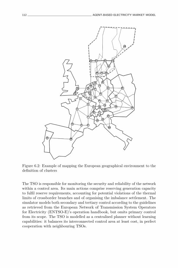
112 AGENT-BASED ELECTRICITY MARKET MODEL
Figure 6.2: Example of mapping the European geographical environment to thedefinition of clusters
The TSO is responsible for monitoring the security and reliability of the networkwithin a control area. Its main actions comprise reserving generation capacityto fulfil reserve requirements, accounting for potential violations of the thermallimits of crossborder branches and of organising the imbalance settlement. Thesimulator models both secondary and tertiary control according to the guidelinesas retrieved from the European Network of Transmission System Operatorsfor Electricity (ENTSO-E)’s operation handbook, but omits primary controlfrom its scope. The TSO is modelled as a centralised planner without learningcapabilities: it balances its interconnected control area at least cost, in perfectcooperation with neighbouring TSOs.
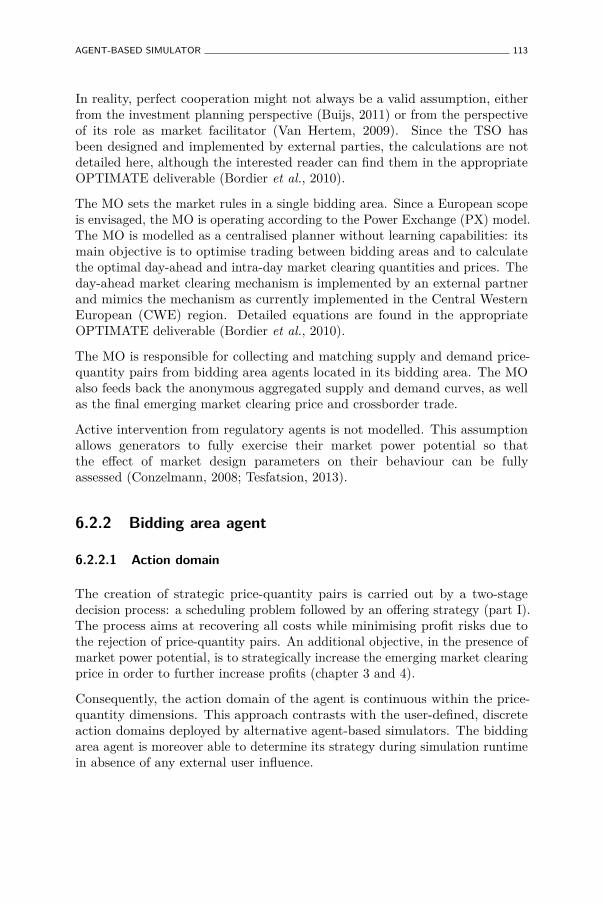
AGENT-BASED SIMULATOR 113
In reality, perfect cooperation might not always be a valid assumption, eitherfrom the investment planning perspective (Buijs, 2011) or from the perspectiveof its role as market facilitator (Van Hertem, 2009). Since the TSO hasbeen designed and implemented by external parties, the calculations are notdetailed here, although the interested reader can find them in the appropriateOPTIMATE deliverable (Bordier et al., 2010).
The MO sets the market rules in a single bidding area. Since a European scopeis envisaged, the MO is operating according to the Power Exchange (PX) model.The MO is modelled as a centralised planner without learning capabilities: itsmain objective is to optimise trading between bidding areas and to calculatethe optimal day-ahead and intra-day market clearing quantities and prices. Theday-ahead market clearing mechanism is implemented by an external partnerand mimics the mechanism as currently implemented in the Central WesternEuropean (CWE) region. Detailed equations are found in the appropriateOPTIMATE deliverable (Bordier et al., 2010).
The MO is responsible for collecting and matching supply and demand price-quantity pairs from bidding area agents located in its bidding area. The MOalso feeds back the anonymous aggregated supply and demand curves, as wellas the final emerging market clearing price and crossborder trade.
Active intervention from regulatory agents is not modelled. This assumptionallows generators to fully exercise their market power potential so thatthe effect of market design parameters on their behaviour can be fullyassessed (Conzelmann, 2008; Tesfatsion, 2013).
6.2.2 Bidding area agent
6.2.2.1 Action domain
The creation of strategic price-quantity pairs is carried out by a two-stagedecision process: a scheduling problem followed by an offering strategy (part I).The process aims at recovering all costs while minimising profit risks due tothe rejection of price-quantity pairs. An additional objective, in the presence ofmarket power potential, is to strategically increase the emerging market clearingprice in order to further increase profits (chapter 3 and 4).
Consequently, the action domain of the agent is continuous within the price-quantity dimensions. This approach contrasts with the user-defined, discreteaction domains deployed by alternative agent-based simulators. The biddingarea agent is moreover able to determine its strategy during simulation runtimein absence of any external user influence.

114 AGENT-BASED ELECTRICITY MARKET MODEL
Figure 6.3 illustrates the decision process from the perspective of the biddingarea agent. Four types of input data need to be available to the bidding areaagent: the plants in its portfolio, the strategy for submitting the renewableenergy supply, whether behaving strategically is more favourable compared tobehaving competitively and the degree to which it can increase its profit bysubmitting price-quantity pairs strategically. The latter three decisions aremade for each individual market round in the market session.
Firstly, the technical characteristics and plant economics of all equipment ownedby the bidding area agent are known at the beginning of each simulation. Thecharacteristics of the portfolio owned by its competitors is not known. Thesimulator allows for dynamically defining the equipment owned per bidding areaagent to simulate investments or divestments made during simulation runtime.Deciding whether it is appropriate to invest or divest in a specific plant ishowever not part of the scope of the simulator.
Secondly, the initial limits between which the RES energy supply per marketround should be submitted is user-defined at the beginning of the simulation.The user then opts for either fixing these limits during simulation runtime, orto allow individual bidding area agents to gradually adapt them over time tomaximise their total profit. In case the bidding area agent additionally ownshydropower plants, this decision also incorporates how much hydropower toreserve in order to minimise future self-balancing requirements (section 6.2.2.2).
Thirdly, the decision on whether to approach a future market roundcompetitively or strategically is determined during simulation runtime exceptwhen the user specifically enables the option to simulate a competitive-onlyenvironment. All bidding area agents in the geographical scope then solelyadjust the price of all price-quantity pairs to account for profit risk. Althoughnot equal to the definition of behaving competitively, as found in many existingmodels, the results found in section 4.4.1 illustrate the proposed competitivebehaviour to outperform alternative competitive offering strategies.
When competition is not enforced by the user, the bidding area agent learns itsstatus during simulation runtime based on past experiences (section 6.2.2.3).Approaching a future market round strategically, the agent maximises its profit,while reducing profit risk, by complementing the physical withholding andeconomic withholding strategy in order to deviate the emerging market clearingprice away from competitive levels. This behaviour is consistent with the resultsfound in section 4.4.2 and actually observed behaviour in chapter 2.
Lastly, the degree to which the bidding area agent can increase its profitby strategically submitting price-quantity pairs, is learned during simulationruntime. By interpreting the impact of its offering strategy on the decisions of

AGENT-BASED SIMULATOR 115
Sta
tus
RE
S li
mits
Eq
uip
men
t
Det
erm
ine
opti
mal
dis
pat
ch s
ched
ule
Det
erm
ine
the
qu
ota
tosu
bm
it a
nd
th
e p
rice
Sta
tus
Sta
tus
RE
S li
mits
Ren
ewab
le q
uot
asu
bm
issi
on s
trat
egy
Res
idu
al d
eman
dcu
rves
for
sce
nar
io n
Tar
get d
ispa
tch
sche
dule
Tar
get d
ispa
tch
sche
dule
Tar
get
dis
pat
chsc
hed
ule
s 1.
.N
Sta
rt
n =
= N
?
n =
0
++
n
Pri
ce-q
uot
a p
airs
En
dye
s
no
Figu
re6.3:
Decision
processforcreatin
gprice-qu
antit
ypa
irs

116 AGENT-BASED ELECTRICITY MARKET MODEL
competitors during historic market sessions, the bidding area agent composes aresidual demand curve forecast distribution from which it draws a user-specifiedamount of step-wise residual demand curve forecast scenarios. The degree towhich the agent can behave strategically is determined by the elasticity of theresidual demand curve forecast scenarios. The amount of residual demand curveforecast scenarios N remains static during simulation runtime, since resultspresented in section 4.4 are largely insensitive to the number of residual demandcurve forecast scenarios, under both a competitive and oligopolistic marketenvironment (section 6.2.2.4).
Since only the residual demand curve distribution emerging in the biddingarea agent’s own bidding area is learned, the bidding area agent still needs toaccount for crossborder trade. This effect is learned over time (section 6.2.2.5).Consequently, the N residual demand curve forecast scenarios are obtainedby merging N1 residual demand curve forecast scenarios from the distributionobserved in the agent’s own bidding area with F crossborder trade scenarios asobserved between the agent’s own bidding area and interconnected ones. Theprocess is depicted in figure 6.4.
6.2.2.2 Learning the strategy for submitting the renewable energy supply
The proposed method to decide the supply of each renewable energy sourceto the day-ahead market depends on the ability of the bidding area agent toforecast intra-day and real-time market clearing prices, to forecast intra-day andreal-time market liquidity and to forecast imbalance settlement prices. Giventhese values, the bidding area agent stochastically calculates the expected costassociated to submitting a renewable quantity to the MO. These costs aresubsequently fed to the Unit Commitment (UC) and Economic Dispatch (ED)problem to determine which renewable quantity should be submitted in orderto maximise total profit. The more accurate the estimation of these parameters,the better-performing the stochastic optimisation becomes.
Due to the numerical instability and lack of validation of intra-day, real-time and imbalance settlement parameters as received from the externallydeveloped OPTIMATE modules, the stochastic optimisation is not activatedduring simulation. Additionally, the dynamic learning of parameters R(kr, t),R(kr, t), H(kr, t) and H(kr, t) used in equations (3.61)-(3.64) is not activatedalthough it has been designed and implemented.
Consequently, parameters R(kr, t), R(kr, t), H(kr, t) and H(kr, t) are user-defined in the current version of the agent-based simulator. Their valuesremain static during simulation runtime.

AGENT-BASED SIMULATOR 117
Inse
rt c
ross
bor
der
pri
ce-q
uot
a p
airs
Res
idu
al d
eman
dcu
rve
for
scen
ario
n1
Sta
rt
n1
==
N1
?
n1
= 0
++
n1
Res
idu
al d
eman
dcu
rve
for
scen
ario
n
En
d
Cro
ssb
ord
er e
ner
gyex
chan
ge s
cen
ario
f
++
f
f =
= F
?ye
s
no
no
yes
f =
0
Figu
re6.4:
Merging
resid
uald
eman
dforecast
scen
arioswith
crossborde
rtrad
escen
arios

118 AGENT-BASED ELECTRICITY MARKET MODEL
6.2.2.3 Learning whether to behave strategically
Figure 6.5 illustrates the process carried out by the bidding area agent toevaluate whether the status decision was justified. After receiving feedback fromthe MO, the bidding area agent performs a ”what-if” analysis to find out whatthe market clearing price would have been if it would have submitted price-quantity pairs under the assumption of behaving competitively or strategicallyduring all market rounds. The ”what-if” analysis is carried out by matchingthe hypothetically submitted price-quantity pairs with the actually emergedresidual demand curve. Although this matching process might not resemble thematching algorithm used by the MO, relevant conclusions are drawn.
The matching results in three comparable profit values: actually emerging profitobtained by the pursued offering strategy, hypothetically emerging profit if thebidding area agent would have acted strategically during all market rounds, andhypothetically emerging profit the bidding area agent would have received if itacted competitively during all market rounds.
In case the profit that would have been obtained if the competitive set ofprice-quantity pairs were submitted, is larger than the actually obtained profit,competitive behaviour is reinforced for all market rounds in which the biddingarea agent behaved strategically. Indeed, the evaluation suggests the biddingarea agent has incurred higher losses by behaving strategically during thesemarket rounds. Analogously, in case the profit resulting from submitting thestrategic set of price-quantity pairs is higher than actually obtained, strategicgaming behaviour is reinforced for all market rounds in which the bidding areaagent behaved competitively. Lastly, in case the obtained profit is maximum,no status is reinforced. In case the obtained profit is minimum, both thecompetitive and strategic gaming behaviour are equally reinforced to preventpremature convergence.
Each status reinforcement is stored in a database along with the value of theemerging market clearing price, the injected renewable energy and the marketround type. The emerging market clearing price determines which plants areeligible for dispatch, the market round type indicates the effect of intertemporalconstraints on the dispatch schedule as submitted by competitors and theinjected renewable energy influences both competition and prices by reducingthe participation per segment of conventional generation plant (Sensfuß et al.,2008). All three interdependent values affect the status behaviour to pursue.
Historic status reinforcements are considered to give insights in which behaviourto pursue during future market rounds. Figure 6.6 illustrates the status decisionprocess for future market rounds. Firstly, the database with historic statusreinforcements is processed to retrieve all relevant historic reinforcements. The

AGENT-BASED SIMULATOR 119
Sta
rt
yes
Em
ergi
ng s
uppl
y &
dem
and
curv
es
Pric
e-qu
ota
pairs
ass
umin
gco
mpe
titiv
e be
havi
our
t =
0
++
t
Mat
ch p
rice
-qu
ota
pai
rs w
ith
his
tori
c re
sid
ual
dem
and
cu
rve
t =
= T
?
Per
form
leas
t-co
st u
nit
com
mit
men
t an
d e
con
omic
dis
pat
ch
no
yes
Em
ergi
ng s
uppl
y &
dem
and
curv
es
Pric
e-qu
ota
pairs
ass
umin
gst
rate
gic
beha
viou
r
t =
0
++
t
Mat
ch p
rice
-qu
ota
pai
rs w
ith
his
tori
c re
sid
ual
dem
and
cu
rve
t =
= T
?
Per
form
leas
t-co
st u
nit
com
mit
men
t an
d e
con
omic
dis
pat
ch
no
Pric
e-qu
ota
pairs
ass
umin
gco
mpe
titiv
e be
havi
our
Pri
ce-q
uot
a p
airs
ass
um
ing
com
pet
itiv
e b
ehav
iou
r
Em
ergi
ng s
uppl
y &
dem
and
curv
esE
mer
gin
g su
pp
ly &
dem
and
curv
esE
mer
ging
sup
ply
& d
eman
dcu
rves
Em
ergi
ng
sup
ply
& d
eman
dcu
rves
Pric
e-qu
ota
pairs
ass
umin
gst
rate
gic
beha
viou
rP
rice
-qu
ota
pai
rs a
ssu
min
gst
rate
gic
beh
avio
ur
Pro
fit
wh
en b
ehav
ing
com
pet
itiv
ely
Pro
fit
wh
en b
ehav
ing
com
pet
itiv
ely
Com
par
e p
rofi
t an
d r
ein
forc
est
atu
sE
nd
Sta
tus
dec
isio
ns
per
mar
ket
rou
nd
Figu
re6.5:
Learning
processforreinforcingthestatus

120 AGENT-BASED ELECTRICITY MARKET MODEL
Start
Status ==competitive
Perform statisticalhypothesis testing
Draw statusdecision from
status distribution
Minimum threshold ofinstances satisfied ?
End
StatusreinforcementsStatusreinforcementsHistoric status
reinforcement
All history tested ?
no
yes
no yes
Status decision
Figure 6.6: Decision process for selecting the status to pursue
bidding area agent is assumed to use a standard statistical hypothesis testingtechnique to determine whether historic information is relevant: if the historicmarket clearing price is not rejected by the future market round’s price forecastdistribution at a 100α% significance level, if the historic renewable energyinjection level is not rejected by the future market round’s renewable injectionforecast distribution at a 100β% significance level, and if the historic marketround type equals the market round type of the future market round, thehistoric status reinforcement is considered relevant. The values of α and β areuser-defined per bidding area agent.
Once all relevant historic status reinforcements have been retrieved, the binomialstatus forecast distribution is built by the bidding area agent. According to theproperties of this distribution, the decision on which status to pursue during

AGENT-BASED SIMULATOR 121
the future market round is randomly drawn. In order for the distribution to besufficiently accurate before guiding the decisions of the bidding area agent, itmust be minimally composed of a user-defined number of instances. In orderfor the bidding area agent to flexibly adapt its behaviour, older instances areomitted. All parameters are user-defined per bidding area agent.
6.2.2.4 Learning the residual demand curve scenarios
The bidding area agent receives information from the MO on its accepteddispatch schedule and the emerged market clearing price per market round.This information is stored in a database from which the bidding area agentretrieves relevant historically observed residual demand curves when facing theproblem of creating a residual demand curve forecast distribution for a futuremarket round (figure 6.7).
Although many MOs already anonymously feedback the aggregated supply anddemand curves, even without feedback, the assumption is still justified. Theportfolio dispatch level and emerging market clearing price reveal a single pointof the residual demand forecast distribution. More than two decades of marketexperience justify the assumption that generators have sufficient data availableto create such residual demand forecast distribution (Baker & Bresnahan, 1988).To save computation time while running each simulation and because it is moreand more common in reality, the supply and demand curves are consideredpublished by the MO to all bidding area agents active in the area.
Each stored residual demand curve is accompanied by the value of the emergingmarket clearing price, the renewable energy supply and the market round type.Similar to the approach used in 6.2.2.3, the emerging market clearing pricedetermines which competing plants are eligible for dispatch, the market roundtype indicates the effect of intertemporal constraints on the dispatch scheduleas submitted by competitors and the injected renewable energy influences bothcompetition and prices by reducing the participation per segment of conventionalgeneration plant (Sensfuß et al., 2008).
Historic residual demand curves are considered similar to the future anticipatedresidual demand curve in case (1) the historic market clearing price is notrejected by the price forecast distribution at a 100α% significance level, (2)the historic renewable energy injection level is not rejected by the renewableinjection forecast distribution at a 100β% significance level and (3) the historicmarket round type equals the market round type of the future market round.The values of α and β are user-defined. Although more complex classificationtechniques could be implemented to more accurately determine similar residualdemand curves, this would come at a higher computation cost.
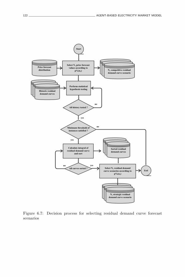
122 AGENT-BASED ELECTRICITY MARKET MODEL
Start
Perform statisticalhypothesis testing
Minimum threshold ofinstances satisfied ?
End
StatusreinforcementsStatus
reinforcementsHistoric residualdemand curves
All history tested ?
no
yes
yes
no
All curves sorted ?
Calculate integral ofresidual demand curve
and sort
Sorted residualdemand curves
Select N1 residual demandcurve scenarios according to
p%(n1)
no yes
Select N1 price forecastvalues according to
p%(n1)
Price forecastdistribution
N1 competitive residualdemand curve scenarioN1 competitive residual
demand curve scenarioN1 competitive residualdemand curve scenario
N1 competitiveresidual demand curve
scenario
N1 competitiveresidual demand curve
scenarioN1 strategic residual
demand curve scenario
Figure 6.7: Decision process for selecting residual demand curve forecastscenarios

AGENT-BASED SIMULATOR 123
The residual demand forecast distribution consequently consists of all relevantresidual demand curves. In order to be sufficiently accurate before guiding thedecisions of the agent, the distribution has to be composed of a user-definedminimum number of residual demand curve instances. Similarly, in order forthe agent to have a recent distribution available, more historic instances areremoved from the residual demand curve forecast distribution in favour of recentones. This minimum threshold parameter is user-defined.
Once all similar residual demand curves have been selected, the residual demandcurve forecast distribution is determined. The N1 residual demand curveforecast scenarios are drawn from a 100δ% confidence interval of this distributionaccording to selected percentile values, as denoted by
p%(n1) =1− δ
2+ (n1 ∗
δ
N1 − 1) (6.1)
All mentioned parameters are user-defined. Since each residual demand forecastscenario represents an opportunity for gaining revenue, the relevant historicresidual demand curves are sorted according to their integral value. The integralof the curve is taken up to the maximum available capacity of all equipmentin the portfolio of the bidding area agent since the remainder of the residualdemand curve is irrelevant in terms of revenue.
6.2.2.5 Accounting for crossborder trade
The bidding area agent receives, from the MO, information on the emergedmarket clearing price in its own bidding area per market round. Market clearingprices from other bidding areas in the geographical scope of the simulatorare also publicly available. Based on this information, it is able to assess thecrossborder trade from its own perspective. The goal when accounting forcrossborder trade is therefore not to estimate how much power is exchangedbetween bidding areas, but rather to estimate how much potential the biddingarea agent itself has to export or how much import threat it is subject to, asonly these parameters affect its action domain.
Considering one branch connecting two neighbouring bidding areas, the exportopportunity or import threat is revealed by assessing the difference in quantitybetween the hypothetical isolated bidding area and the actually emerginginterconnected case. Data on the emerging case is obtained from the feedbackon emerging market clearing prices, the hypothetical one from feedback of thesupply and demand curves published by the MO.

124 AGENT-BASED ELECTRICITY MARKET MODEL
Price [e/MWh] Price [e/MWh]
λ′
1(·)
λ′
2(·) λ(·)
Quantity[MWh]
Quantity[MWh]
00
.
Figure 6.8: Example of reinforcing crossborder trade
For instance, consider the residual demand curves in figure 6.8. The residualdemand curve on the left belongs to the bidding area further denoted as firstbidding area; the one on the right belongs to the second bidding area. Twocompeting bidding area agents are active, one in each bidding area. Bothbidding areas are assumed to be coupled by a transmission line with unlimitedcapacity and the portfolio is assumed to have no dispatching costs. Theseassumptions are only meant for simplification without loss of generality. Theshaded regions indicate the anticipated revenue by each bidding area agent.
The difference in emerging market clearing price between the hypothetical case(λ ′(·)) and the actually emerging one (λ(·)) reveals whether there is a potentialexport opportunity or import threat. In case the price in the hypothetical caseis lower than or equal to the actually emerging one, it is in the best interest ofthe bidding area agent to continue its participation in exporting. By increasingits supply, it could attain a larger volume of sold energy, while the emergingmarket clearing price in its own bidding area increases up to the market clearingprice as emerged in the neighbouring bidding area. Exporting therefore has abeneficial impact on its profit.
The full export opportunity of the bidding area agent is deducted from theobserved residual demand curves. The bidding area agent in the second biddingarea perceives it has a potentially unexplored export opportunity since theactually emerging price equals the hypothetical one. By assessing at whichhypothetical exports the hypothetical price λ ′(·) emerges, the bidding area agentdetermines the possible range of export opportunities (figure 6.9). This rangecorresponds to any possible export. The reinforced export value is uniformly

AGENT-BASED SIMULATOR 125
Price [e/MWh] Price [e/MWh]
λ′
1(·)
λ′
2(·) λ(·)
Quantity[MWh]
Quantity[MWh]
00
.
Figure 6.9: Evaluating export opportunities and import threats
drawn from this range as the export opportunity the bidding area agent canexpect. The price associated to the export opportunity is set at the marketclearing price of the neighbouring bidding area.
In case the price in the hypothetical case is higher than the actually emergingone, it is in the best interest of the bidding area agent to avoid engaging intocompetition with bidding area agents located in neighbouring bidding areas.Although this action results in less volume of energy sold, the resulting congestionof transmission lines connecting its own bidding area with the exporting oneswould maintain a higher-than-competitive market clearing price. Congestionleads to a dominant local market position which in turn increases market powerpotential, offsetting the loss from reducing its supply. In case this response failsto offset the loss, the bidding area agent reconsiders whether strategic gamingbehaviour leads to higher profits (section 6.2.2.3).
By assessing at which hypothetical imports the actual price λ(·) emerges, thebidding area agent determines the possible range of import threats. The importthreat reinforcement is randomly drawn from this range. The price associatedto the import threat is set at the market clearing price of the own bidding area.
This process (figure 6.10) is carried out for each branch connecting the agent’sbidding area. All reinforcements are aggregated to obtain a crossborder importor export price-quantity curve which is stored in a database together with theemerging market clearing price in the agent’s own bidding area, the injectedrenewable energy and the market round type.

126 AGENT-BASED ELECTRICITY MARKET MODEL
Start
Difference > 0 ?
Calculate hypothetical price
Calculate range of exportopportunities
Subtract hypothetical pricewith emerging price
Calculate range of importthreats
Draw reinforcement fromuniform distribution
Draw reinforcement fromuniform distribution
Supply anddemand curves
Acceptedprice-quota pairs
Crossborder exchangereinforcement
End
yes no
Figure 6.10: Calculating the import threat and export opportunity price-quantity pair
Historic crossborder trade assessments are considered to shed light on futurecrossborder trade if the historic market clearing price is not rejected by the priceforecast distribution at a 100α% significance level, the historic renewable energyinjection level is not rejected by the renewable injection forecast distributionat a 100β% significance level and the historic market round type equals themarket round type of the future market round. In order for the distributionto be sufficiently accurate when guiding the decisions of the agent, it must becomposed of a minimum threshold of reinforcements. In order for the biddingarea agent to flexibly adapt its behaviour, more historic instances are omittedwhen creating the distribution.
Once all relevant crossborder import or export assessments have been selected,the crossborder trade forecast distribution is built by the bidding area agent(figure 6.11). The F crossborder trade scenarios are drawn from a 100δ%confidence interval of this distribution according to selected percentile valuesdenoted by

AGENT-BASED SIMULATOR 127
Start
Perform statisticalhypothesis testing
Minimum threshold ofinstances satisfied ?
End
Status reinforcementsStatus reinforcementsHistoric crossborder
exchange reinforcements
All history tested ?
no
yes
yes
no
All reinforcements sorted ?
Calculate netcrossborder quota and
sort
Sorted crossborderexchange quota
Select F crossborder exchangescenarios according to p%(f)
no yes
N1 competitiveresidual demand curve
scenario
N1 competitiveresidual demand curve
scenarioF strategic residual
demand curve scenario
Figure 6.11: Decision process for selecting the best-response crossborder tradescenarios
p%(f) =1− δ
2+ (f ∗ δ
F− 1) (6.2)
6.2.3 Holding company
The holding coordinates the actions of its bidding area agents and control areaagents in order to maximise the total profit on the holding level. Since thescope of strategic gaming behaviour is limited to the day-ahead market, onlythe discussion of the coordination between bidding area agents is relevant.
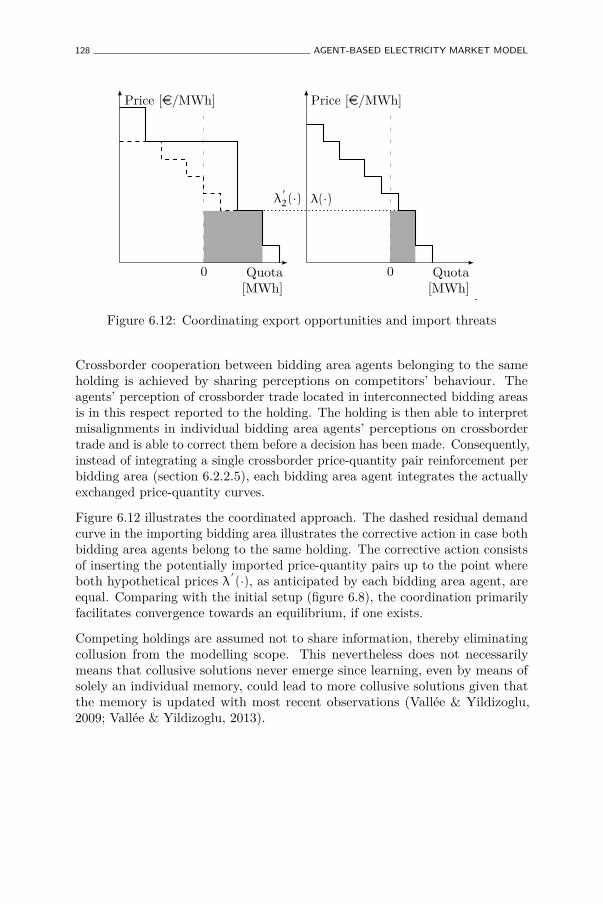
128 AGENT-BASED ELECTRICITY MARKET MODEL
Price [e/MWh] Price [e/MWh]
λ′
2(·) λ(·)
Quota[MWh]
Quota[MWh]
00
.
Figure 6.12: Coordinating export opportunities and import threats
Crossborder cooperation between bidding area agents belonging to the sameholding is achieved by sharing perceptions on competitors’ behaviour. Theagents’ perception of crossborder trade located in interconnected bidding areasis in this respect reported to the holding. The holding is then able to interpretmisalignments in individual bidding area agents’ perceptions on crossbordertrade and is able to correct them before a decision has been made. Consequently,instead of integrating a single crossborder price-quantity pair reinforcement perbidding area (section 6.2.2.5), each bidding area agent integrates the actuallyexchanged price-quantity curves.
Figure 6.12 illustrates the coordinated approach. The dashed residual demandcurve in the importing bidding area illustrates the corrective action in case bothbidding area agents belong to the same holding. The corrective action consistsof inserting the potentially imported price-quantity pairs up to the point whereboth hypothetical prices λ ′(·), as anticipated by each bidding area agent, areequal. Comparing with the initial setup (figure 6.8), the coordination primarilyfacilitates convergence towards an equilibrium, if one exists.
Competing holdings are assumed not to share information, thereby eliminatingcollusion from the modelling scope. This nevertheless does not necessarilymeans that collusive solutions never emerge since learning, even by means ofsolely an individual memory, could lead to more collusive solutions given thatthe memory is updated with most recent observations (Vallée & Yildizoglu,2009; Vallée & Yildizoglu, 2013).

AGENT-BASED SIMULATOR 129
6.2.4 Agents’ interactions
Before the start of each simulation, a timeline consisting of a sequence of marketrounds is created for each bidding area. Market rounds are aggregated in marketsessions with gate closure times denoted in number of market rounds beforethe starting time of the first market round belonging to the market session.Although the implementation allows each market session to be different fromothers within the timeline, the current timeline creation assumes all sessions tobe identical in terms of gate closure times and in terms of number of marketrounds, is in line with common practice. Since each bidding area has its owntimeline, market sessions between areas can still differ in properties.
The timeline is the driver of market events and agents’ actions. Instead ofimplementing a central sequencing algorithm as in the modularly developedcompetitive OPTIMATE simulator, processes can be carried out in parallelwith each other in the agent-based simulator. Such a design has the advantageof reducing the gap between modelling assumptions and reality. For example,the latter design allows forecasts to be gradually updated during simulationruntime, while the former assumes the most recent forecast to be availablebefore initiating subsequent modules. Depending on the time it takes for futuredecision and calculation processes to be finished, the gate closure time mightbe reached before the updated price-quantity pairs could be calculated. Theresulting heterogeneous beliefs could lead to an inefficient creation of price-quantity pairs, which might lead to a suboptimal market coupling solutionwhich does not accurately reflect underlying market forces (Qiu, 2013).
Figure 6.13 illustrates which actions and decisions the bidding area agent shouldundertake during simulation runtime. From a day-ahead perspective, only onehard deadline has to be complied with by the bidding area agent: the gateclosure time of the day-ahead market session (B). Feedback is received fromthe MO after the day-ahead (C) and intra-day (D) market clearing. After theactual time of delivery (E), information on the imbalance settlement is obtainedfrom the TSO. This design facilitates scalability and maintenance.
Each of the events trigger the actions of the bidding area agent (figure 6.14).Once an event triggers the action, the bidding area agent creates one of thespecialised subagents (table 6.1). Consequently, the bidding area agent isexempted from performing computationally intensive tasks. All subagentsare created per market round in the market session except for the subagentsresponsible for creating the price-quantity pairs the bidding area agent has tosubmit to the MO.

130 AGENT-BASED ELECTRICITY MARKET MODEL
A
Update Forecasts
B
Decide renewableenergy supply
Decide degree tostrategically increase
profit
Decide import threator export opportunity
Unit commitment and economic dispatch
Offering strategy
C
Gather day-ahead feedback from market operator
Evaluate strategicdecision
Evaluate crossborderdecision
D
Gather intra-day feedback from market operator
E
Gather real-time feedback from transmission systemoperator
Evaluate renewableenergy supply
decision
A
Figure 6.13: Decisions and actions the bidding area agent must undertake, interms of the agent-based timeline
event
createreturnreceived
baa:Bidding Area Agent
subAgent:SubAgent
Figure 6.14: Actions from the bidding area agent’s perspective

CASE STUDY 131
Name Description
RdcCalculator Calculates the actual residual demand curveXbExchangeDecider Decides F crossborder trade price-quantity pair
PriceDecider Decides the pairs’ price to submitRdcScenarioDecider Decides N1 residual demand curve forecast scenariosQuantityDecider Decides the pairs’ quantity to submitStatusDecider Decides whether to behave strategically
XbExchangeEvaluator Reinforces crossborder trade assessmentsStatusEvaluator Reinforces the status decisions
Table 6.1: Specialised subagents
6.3 Case study
6.3.1 Simulation setup
The case study is retrieved from the published tests carried out to validate theAMES simulator (Hongyan & Tesfatsion, 2009a; Li et al., 2009). Although thecase study originates from studying the impact of financial transmission rights,the existence of network constraints and a load pocket renders the case alsouseful to study the effects of strategic gaming behaviour (ISO New England,2002). Study cases applied to alternative dynamic electricity market simulationtools — such as e.g. Electricity Market Complex Adaptive System (EMCAS)or PowerACE — did not contain sufficient data to be accurately reproducedand have therefore not been applied to the presented simulation tool. Thesepractical limitations have been raised in literature (Weidlich & Veit, 2008).
The case study depicts a dynamic 5-bus system in which five generators andthree utilities operate (figure 6.16). The reactances of the transmission linesand portfolio characteristics are illustrated in tables 6.2 and 6.3 respectively.Although thermal plant types were envisaged in AMES, the presented agent-based simulator models them as hydropower plants with infinite reservoir levelsbecause of the lack of intertemporal constraints and start-up costs. Demand istaken from (Shahidehpour et al., 2002c) and represented in figure 6.15.
Three case studies are conducted. The first studies the competitive outcomeand compares the results with these from the AMES simulator. The secondinvestigates strategic gaming behaviour. The third illustrates how changesin market design affect the behaviour of generators. Although not a realisticrepresentation of a real power system, all case studies provide insights on thevalidity and applicability of the agent-based model as a policy support tool.

132 AGENT-BASED ELECTRICITY MARKET MODEL
2 4 6 8 10 12 14 16 18 20 22 24
200
300
400
Market Round [hour]
Power
[MW
]
Utility 1Utility 2Utility 3
Figure 6.15: Demand per market round, per bus
ED
A C
B
0.0297W
0.0064W
0.0304W
0.0281W0.0108W
0.0297W
Brighton
Sundance
Utility 3
Alta
Park City
Utility 1
Solitude
Utility 2
Figure 6.16: Dynamic five-bus test system used to validate the AMES simulator

CASE STUDY 133
Area 1 Area 2 Capacity [MW] Reactance [Ohm]
A B 250 0.0281A D 150 0.0304A E 400 0.0064B C 350 0.0108C D 240 0.0297D E 240 0.0297
Table 6.2: Branch characteristics
Agent Bidding area Capacity [MW] Water value [e/MWh]
Alta A 110 14.55Park City A 100 15.60LSE1 B 400 NA
Solitude C 520 30.20LSE2 C 350 NA
Sundance D 200 32.40LSE3 D 350 NA
Brighton E 600 14.20
Table 6.3: Agents’ characteristics
6.3.2 Results
6.3.2.1 Competitive behaviour
Assuming all bidding area agents behave competitively, the market clearingprices per market round converge to the values in table 6.4 for each marketround during the market session. Figures 6.17 and 6.18 illustrate the state ofthe power system during low and high demand respectively. In both situations,the transmission lines E-D, A-D and A-B are congested.
During all market rounds, independent on whether demand is low or high, thecongestion of transmission lines A-D and A-B prevent bidding area agents Altaand Park City from dispatching their more efficient plants at full capacity. Asa result, bidding area agent Solitude is the price-setting generator in areas B, Cand D, as can be seen from the emerging market clearing prices. These resultsare in line with the results obtained by the AMES simulator.

134 AGENT-BASED ELECTRICITY MARKET MODEL
ED
A C
B
240MW
360MW
150MW
250MW37.16MW
184.89MW
600MW
0MW
205.11MW
40MW
0MW
287.16MW
98.40MW
246.13MW
Figure 6.17: State of the system in market round 5 when all bidding area agentsbehave competitively
ED
A C
B
240MW
360MW
150MW
250MW198.62MW
69.56MW
600MW
0MW
320.44MW
40MW
0MW
448.62MW
513.59MW
384.53MW
Figure 6.18: State of the system in market round 18 when all bidding areaagents behave competitively
A B C D E
14.55 30.20 30.20 30.20 14.55
Table 6.4: Market clearing prices in case all agents behave competitively[e/MWh]

CASE STUDY 135
6.3.2.2 Strategic behaviour
When allowing strategic gaming behaviour using the AMES simulator, theresulting market clearing prices in areas B, C, D and E are slightly higher thanthe ones obtained in the competitive setup in each market round. However,market power is only exercised significantly in market round 18, with a tenfoldprice increase in areas B and C, and a threefold in area D. The AMES simulatoralso indicates a decrease in market clearing price in area A down to negativelevels (Hongyan & Tesfatsion, 2009a; Li et al., 2009).
When applying the presented agent-based simulator, strategic gaming behaviourleads to a convergence in the system state. Explorative behaviour of allagents however deviates emerging prices away from their equilibrium whichin turn might trigger a temporary price battle. The study’s limited demandelasticity moreover exacerbates these price variations originating from therandom economic withholding behaviour (section 4.3).
Since the case study investigates the effect of strategic gaming behaviouron the state of the system, an in-depth discussion on the evolution of themarket clearing prices is omitted. Figures representing the price evolutionwhen behaving strategically are included in appendix C. Considering the aboveproperties of the simulator, bidding areas in which large price variations areconsistent over time, are undergoing the exercise of market power.
The identified equilibrium system state during the market round with highestdemand is given in figure 6.19, while table 6.5 illustrates the emerging marketclearing prices. Since the absolute price values themselves only provide asnapshot of the whole simulation run, the range of emerging values is denotedinstead, in order to deduct relevant conclusions.
When behaving competitively, agent Solitude has a dominant position thanksto a constrained transmission grid. It is expected to exert its market powerwhen behaving strategically. This behaviour is indeed observed when comparingfigures 6.19 and 6.18: agent Solitude reduces its supply by 170.44 MW. Onlyagent Sundance is capable of filling the resulting supply gap, since more efficientcompetitors are restricted in terms of supply by transmission constraints. Marketclearing prices in areas B, C and D are thus determined by a leader-followerrelationship between Solitude and Sundance, in which Solitude sets the price.
The physical withholding strategy is explained by the imposed market ceilingprice, equalling e3000/MWh, and the demand in area C, which is larger thanthe capacity of transmission line D-C. During simulation, agent Solitude prefersto congest transmission line D-C in order to prevent Sundance to impose animplicit price barrier. Indeed, if Solitude prices its price-quantity pairs higher

136 AGENT-BASED ELECTRICITY MARKET MODEL
ED
A C
B
240MW
360MW
150MW
250MW198.62MW
240MW
600MW
170.44MW
320.44MW
40MW
0MW
448.62MW
343.15MW
384.53MW
Figure 6.19: State of the system in market round 18 when all bidding areaagents behave strategically
A B C D E
15.60 ≥30.40 ≥30.40 32.40 15.60
Table 6.5: Market clearing prices in market round 18 in case all agents behavestrategically
than the variable cost of Sundance without pursuing the physical withholdingstrategy, the MO would reject the price-quantity pairs at the expense of grantingSundance dispatch. By pursuing the physical withholding strategy, Solitudecan price its price-quantity pairs at any price.
Agent Sundance cannot exercise a similar strategy to increase the marketclearing price in its own bidding area. Since area D only serves as a transit zoneto supply B and C, it faces competition from Alta, Park City and Brighton. Dueto its variable cost, it is the least efficient market participant. Consequently,agent Sundance has no choice but to behave competitively.
Agent Brighton’s full capacity is always accepted as it is the most efficient marketplayer. Alta is the second most efficient supplier but nevertheless exercisesphysical withholding due to a transmission capacity bottleneck between areas Aand B. Both players try to explore their strategic opportunities independently.Agent Brighton observes no benefit from pursuing physical withholding whileagent Alta observes that it does not benefit from pursuing physical withholdingas well as from trying to export to more profitable bidding areas.

CASE STUDY 137
ED
A C
B
240MW
360MW
150MW
250MW37.16MW
240MW
600MW
55.11MW
205.11MW
40MW
0MW
287.16MW
43.29MW
246.13MW
Figure 6.20: State of the system in market round 5 when all bidding area agentsbehave strategically
A B C D E
15.60 ≥32.40 ≥32.40 ≥32.40 15.60
Table 6.6: Market clearing prices in market round 5 in case all agents behavestrategically
Accidentally, synchronised exploration from agents Brighton and Alta triggersthe acceptation of Park City to supply the market. Consequently, marketclearing prices in areas A and E are set by the expensive plant owned by ParkCity, allowing Brighton and Alta to benefit from higher prices. The simulatordoes not explicitly model collusion, however, the leader-follower relationship inwhich the follower sets the price, clearly signals collusion opportunities betweenBrighton, Alta and Park City.
As conclusion for market round 18, the market participants setting the priceare the two identified leaders: Solitude and Brighton-Alta. The former obtainsits market power thanks to its unique position in the electricity grid, while thelatter only obtains market power when colluding with Park City.
The identified equilibrium system state during the market round with lowestdemand is shown in figure 6.20, while table 6.6 illustrates the emerging marketclearing prices. Compared with the system state when behaving competitively(figure 6.17), signals Solitude applying the same offering strategy as duringmarket rounds with higher demand.

138 AGENT-BASED ELECTRICITY MARKET MODEL
ED
A C
B
212.12MW
313.15MW
0MW
313.15MW135.47MW
0MW
525.27MW
108.32MW
320.44MW
0MW
0MW
448.62MW
520MW
384.53MW
Figure 6.21: State of the system in market round 18 when all bidding areaagents behave competitively in a Flow-Based (FB) market coupling environment
A B C D E
14.55 14.55 30.20 32.40 14.20
Table 6.7: Market clearing prices in case all agents behave competitvely underFB market coupling
In contrast to the results obtained by applying the AMES simulator, significantmarket power is not only limited to market round 18 but actually occurs inall market rounds. This result is confirmed by interpreting any steady-statesolution of the system and assessing the resulting profit increase compared toan alternative offering strategy. Additionally, no negative market clearing pricesoccur in bidding area E, in line with expectations. The agent-based simulatorhence successfully converges to the optimal offering strategy.
6.3.3 Altering market design parameters
6.3.3.1 Towards flow-based market coupling
Figure 6.21 illustrates the equilibrium system state subject to competitivebehaviour when imposing FB market coupling. Since the highest benefit interms of social welfare is achieved by supplying bidding area B with powersupplied by the most efficient supplier Brighton, FB market coupling aims at

CASE STUDY 139
ED
A C
B
120.44MW
363.21MW
0MW
363.21MW0MW
0MW
483.65MW
200MW
320.44MW
0MW
0MW
363.21MW
384.53MW
384.53MW
Figure 6.22: State of the system in market round 18 when all bidding areaagents behave strategically in a FB market coupling environment
A B C D E
14.55 3000.00 ≥32.40 32.40 ≤14.55
Table 6.8: Market clearing prices in case all agents behave strategically underFB market coupling
exploiting the full capacity of lines E-A and A-B. The capacity of line A-B isincreased to 313.15 MW, from 250 MW when imposing Net Transfer Capacity(NTC) market coupling. As side effect however, no power is transported on lineA-D. The resulting market clearing prices are shown in table 6.7.
Competitive behaviour is not the dominant strategy for agent Solitude to pursue.The market clearing price in bidding area B is indeed lower than the variablecost of agent Solitude, which supplies bidding area B by 135.47 MW. Runningthe agent-based simulator with strategic gaming behaviour hence results inagent Solitude to restrict its supply. Physical withholding from bidding areaagent Solitude forces the FB market coupling mechanism to partially sheddemand from Load Serving Entity (LSE) B in order to optimise the socialwelfare of the whole geographical scope (figure 6.22). The FB market couplingmechanism on the other hand increases the supply from bidding area E to Bvia transmission lines E-A and A-D even further, compared to the competitivecase, by increasing the capacity from transmission line E-A to 363.21 MW atthe cost of reducing the capacity of transmission line E-D to 120.44 MW.

140 AGENT-BASED ELECTRICITY MARKET MODEL
This reduction benefits agent Sundance as it is rewarded the dispatch of its fullcapacity in order to satisfy residual demand in bidding area D. Consequently,no generation capacity is available to compete with agent Solitude, grantingthe latter the opportunity to become a monopolist in bidding area C.
This test case hence illustrates that the implementation of a measure to increaseoverall social welfare could lead to unintended results in case no ex-anteassessment of its effects in a non-competitive environment has been carried out.The resulting market clearing prices are given in table 6.8, their evolution inappendix C. Comparison with the evolution of the prices under NTC marketcoupling reveals that the envisaged geographical scope does not clearly benefitfrom implementing a different market coupling mechanism. In contrast, theinability of the whole system to supply total demand, even though sufficientgeneration capacity is installed and the unfulfilled demand is priced at themarket ceiling price, rather suggests damaging effects.
6.3.3.2 Imposing market ceiling prices
Another regulatory corrective action consists of reducing the market ceilingprice to more competitive levels. Prices in neighbouring bidding areas indicatethe market ceiling price could be reduced to e32.40/MWh, still higher than anyemerging market clearing price observed when competitive behaviour is assumedand equal to the variable cost of the most inefficient plant in the system. Allother bidding areas maintain the original market ceiling price.
Applying strategic gaming behaviour, the equilibrium system state presented infigure 6.23 and the market clearing prices presented in table 6.9 are reached.
The difference in market ceiling price between areas B and C significantlyreduces the incentive for agent Solitude to strategically supply area B. Instead,agent Solitude’s profit is only increased by behaving almost fully competitively.Indeed, since transmission lines C-B and D-C are not congested — as Sundanceis never profitably dispatched — creating a local monopoly in bidding area Cis not a viable strategy for agent Solitude to pursue. Indeed, in case Solitudewould reduce its supply, the market clearing mechanism is obliged to shed loadin bidding area B at, from Solitude’s perspective, profitable prices.
Hence, this case study illustrates that lowering the market ceiling price mightbe a good regulatory intervention to enforce competitive market clearing pricesin the envisaged environment. The agent-based simulator does however nottake into account any long term inefficiencies caused by artificially removingthe symptom of market power instead of providing a structural solution.
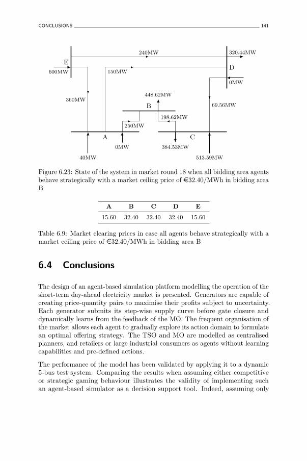
CONCLUSIONS 141
ED
A C
B
240MW
360MW
150MW
250MW198.62MW
69.56MW
600MW
0MW
320.44MW
40MW
0MW
448.62MW
513.59MW
384.53MW
Figure 6.23: State of the system in market round 18 when all bidding area agentsbehave strategically with a market ceiling price of e32.40/MWh in bidding areaB
A B C D E
15.60 32.40 32.40 32.40 15.60
Table 6.9: Market clearing prices in case all agents behave strategically with amarket ceiling price of e32.40/MWh in bidding area B
6.4 Conclusions
The design of an agent-based simulation platform modelling the operation of theshort-term day-ahead electricity market is presented. Generators are capable ofcreating price-quantity pairs to maximise their profits subject to uncertainty.Each generator submits its step-wise supply curve before gate closure anddynamically learns from the feedback of the MO. The frequent organisation ofthe market allows each agent to gradually explore its action domain to formulatean optimal offering strategy. The TSO and MO are modelled as centralisedplanners, and retailers or large industrial consumers as agents without learningcapabilities and pre-defined actions.
The performance of the model has been validated by applying it to a dynamic5-bus test system. Comparing the results when assuming either competitiveor strategic gaming behaviour illustrates the validity of implementing suchan agent-based simulator as a decision support tool. Indeed, assuming only

142 AGENT-BASED ELECTRICITY MARKET MODEL
competitive behaviour results in a system state equilibrium which significantlydeviates from the system state when assuming strategic gaming behaviour. Casestudies illustrating how the state of an interconnected electrical system changesas a result of an alteration in day-ahead market design, show the capability ofthe agent-based simulator to be used as a common framework to facilitate theconvergence towards an efficient European target market design.

Part III
Synthesis
143


Chapter 7Conclusions and
recommendations
A dynamic electricity market model capable of assessing the robustness of marketdesigns subject to strategic gaming behaviour, has been designed, implementedand validated. It can be applied to support policy desicion making processesaiming at facilitating day-ahead cross-border trade between European countries,ensuring an efficient use of the limited network capacity and massively integratingRenewable Energy Sources (RES) in the grid. Such common platform facilitatesthe convergence towards an efficient European market, currently difficult dueto the involvement of many stakeholders with conflicting interests and the longterm uncertain consequences in case a design decision is taken.
This chapter provides a synthesis of the presented work and addresses its centralresearch question. Section 7.1 summarises the added value of each chapter inaddressing the research questions and lists their contributions. The importanceof each contribution from the perspective of the central research question isclarified. Section 7.2 presents the practical impact of the research, both in termsof the short-term future of the competitive simulator developed during theOPTIMATE1 project and in terms of how the presented agent-based simulatoraffects the commercialisation of the OPTIMATE simulator. Limitations arediscussed in section 7.3 and recommended future work in section 7.4.
1Open Platform to Test Integration in new MArkeT designs of massive intermittent Energysources dispersed in several regional power markets (OPTIMATE)
145

146 CONCLUSIONS AND RECOMMENDATIONS
7.1 Summary, contributions and conclusions
7.1.1 Summary per chapter
Chapter 1 introduces the motivation for researching how the market designaffects the state of an interconnected electrical system after clearing the day-ahead market, as organised under the European Power Exchange (PX) model,given that generators do not necessarily behave competitively. The unanticipatedresults encountered after the liberalisation of the electricity market at the end ofthe 20th century indeed debunk the assumption that electricity markets naturallyproduce competitive results. The failure to create competitive electricity marketshas been attributed to network constraints, few dominant sellers in a relativelysmall market, market designs that encourage strategic gaming behaviour, price-inelastic consumers, reductions in generation capacity, unavailability of perfectinformation provided in real-time, and a lack of transparent market instrumentsto express technical constraints and portfolio economics.
All causes mentioned of inefficient use of available resources are an input tothe decision making process of market participants. Since a liberalised marketchanges the objective of generators from an obligation to supply demand atleast cost to a choice to supply demand profitably, chapter 2 presents importantcurrent and target market design parameters influencing the profit-maximisingbehaviour of a generator. Market design parameters impact the generator’sbehaviour on three domains: its domestic market environment, influences bycross-border exchanges and RES supply uncertainty. Integrating the identifiedmarket design parameters when designing the profit-maximising behaviour of agenerator ensures the practical applicability of the offering strategy.
The strategic gaming behaviour of a generator is formally described as a two-step process. The generator first calculates the portfolio’s scheduling solutionby means of a price-based Unit Commitment (UC) and Economic Dispatch(ED) problem formulation (chapter 3). In the second step, the schedulingsolution is translated to a set of price-quantity pairs (chapter 4). The offeringstrategy is approached from the perspective of strategic and flexible dispatch,as required from a generator in an electricity system characterised by massiveRES integration. Modelling the flexible dispatch is shown to augment theprofit of a generator in electricity systems with medium to high price volatility.The offering strategy presented outperforms alternative strategies in both acompetitive and an oligopolistic environment by successfully hedging profit risks.Since massive RES integration is expected to increase price volatility, modellingthe flexible dispatch further gains importance, rendering the presented strategymore dominant to pursue compared to the introduced alternative ones.

SUMMARY, CONTRIBUTIONS AND CONCLUSIONS 147
The offering strategy itself is categorised as a supply function equilibrium model.In order to dynamically simulate the operation of an electricity market, it mustbe complemented by an evolutionary model. Chapter 5 presents the motivationfor selecting multi-agent systems to model the evolution of the behaviour ofindividuals within a population. It also indicates the criticism such models areprone to. Although the assumption on the generator’s strategy, action domainand underlying technical constraints and portfolio economics has been addressedin chapters 2, 3 and 4, the learning and decision process of exogenous influenceson profit needs to be addressed (chapter 6).
As a result, the presented agent-based simulation platform models the operationof the short-term day-ahead electricity market in which each generator graduallyexplores its best-response actions thanks to the repetitive organisation of themarket. The platform’s performance in terms of final result and convergencespeed has been validated by applying it to a dynamic five bus system in orderto test how the market design affects the state of an interconnected electricalsystem after clearing the day-ahead market, as organised under the EuropeanPX model, given that generators do not necessarily behave competitively.
7.1.2 Conclusions and contributions
Two decades of deregulation, gaining experience, and reforms were neededto gradually adapt the initially instated market designs — introduced afterthe transformation of the electricity system from a monopolistic environmentto a liberalised one — in order to mitigate unanticipated emergent strategicgaming behaviour. In the European context, this resulted in a variety of co-existing, complex market designs. Currently, a new transformation around threepolicy pillars is in progress: integrating RES, maintaining system reliabilityand security, and creating a pan-European market to guarantee affordableelectricity prices. Keeping the early experiences after liberalisation in mind,how generators could behave strategically in such future electricity system needsto be studied. This research question is addressed in part I.
In order to detect potential unanticipated emergent strategic gaming behaviourex-ante, a hybrid model consisting of an evolutionary model complementedby a detailed supply function equilibrium model is designed, implementedand validated. Such hybrid model is argued to produce results close tothe observations in reality. How the market design affects the state of aninterconnected electrical system after clearing the day-ahead market, given thatgenerators do not necessarily behave competitively, cannot be investigated withexisting tools. Part II addresses the lack of such dynamic simulation tool.
The state-of-the-art is advanced in five domains:
148 CONCLUSIONS AND RECOMMENDATIONS
1. Generators own a portfolio consisting of thermal, hydropower and RESplants. In comparison, existing models threat either only thermal plantsor a combination of RES and hydropower plants. This contribution ispresented in chapter 3 presenting a novel coordinated UC and ED Mixed-Integer Linear Problem (MILP) model of a global, modern portfolio.
2. Both a transmission grid with limited capacity as well as price-responsivedemand is modelled. As shown in chapter 3, the price-responsive demandis realistically modelled as step-wise decreasing curves. The influence ofthe limited transmission grid has been validated in chapter 6.
3. Generators pursue a total profit-maximisation objective by simultaneouslyexercising the physical and economic withholding strategy while explicitlytaking into account underlying technical constraints and plant economics.The scheduling problem has been validated in chapter 3, while the novelprofit risk hedging offering strategy is validated in chapter 4. Theconsideration of portfolio flexibility to mitigate profit risks is proven toyield a higher total profit when benchmarked against alternative strategies.
4. Each generator updates its perception on which it supports its strategicdecisions by evaluating the performance of historic decisions on its profit.Four learning and decision processes have been designed along the threedimensions identified in chapter 2: domestic market environment, influenceof crossborder exchanges on profit and RES supply uncertainty. The designof each learning and decision process is presented in chapter 6.
5. By explicitly taking into account relvant market design parameters, theagent-based simulation platform is capable of anwering research questionsexisting electricity market simulation tools cannot address. Importantmarket design parameters have been identified in chapter 2, while chapter5 illustrates the limitation of alternative dynamic electricity marketsimulators to only simulate how the pricing scheme affects the stateof an interconnected electrical system after clearing the day-ahead market.
The above-mentioned contributions result in the development of a new dynamicagent-based electricity market model. Although the model does not address thequestion which market design is optimal, it does address how robust a specificmarket design is subject to strategic gaming behaviour.
Considering the coming transformation of the electricity system, all stakeholdersare in need of such common simulation platform in order to facilitate theconvergence in terms of policy decisions aiming at (1) facilitating cross-borderexchanges between European countries in the day-ahead, intra-day and balancingmarkets, (2) ensuring an efficient use of the limited network capacity and (3)massively integrating RES.
PRACTICAL IMPACT 149
7.2 Practical impact
7.2.1 Future of the competitive OPTIMATE tool
Since its release in spring 2013, the competitive simulator developed duringthe OPTIMATE project is being made commercially available in its prototypeform for European Transmission System Operators (TSOs), regulators, publicentities, and research units. Although Réseau de Transport d’Électricité (RTE)is conducting the exploitation, the developed modules ’Bids & Offers to Market’and ’Final Program’ are still owned by KU Leuven.
Access to the simulation platform can be purchased on an annual basis. Alicense to access the web platform costs e1.7k per year and includes technicaluser support and access to relevant documentation. Once a license is obtained,the user is granted access to the online simulation platform where it can definecustom scenarios and visually interpret the final results.
In order to enable both experienced users and beginners to start using thesimulation platform, training sessions are regulary scheduled. Their goal is toget acquainted with the functional aspects of the tool as well as to understandthe platform’s results. Group studies are also conducted on topics selected bythe participants in order to facilitate user discussions on market design. Thecommercialisation of the tool is still ongoing and is likely to lead to a faster,more modular version of the platform by mid 2015.
The simulation platform has already received widespread interest from theEuropean Network of Transmission System Operators for Electricity (ENTSO-E), individual TSOs and national administrations of Energy. The simulator isalso deployed within the EU-FP7 project GARPUR, whose objective is to design,develop, and assess new system reliability criteria and management processeswhile maximising social welfare, with the aim to progressive implementationover the coming decades at a pan-European level.
7.2.2 Impact of the agent-based simulator
Although the competitive OPTIMATE simulator already represented abreakthrough in terms of electricity market modelling, the results obtained bythe presented agent-based dynamic electricity market model show significantdifferences. These differences in results originate not only from the implementedstrategic gaming behaviour, but also from the differently implementedcompetitive behaviour (chapter 4).
150 CONCLUSIONS AND RECOMMENDATIONS
OPTIMATE aimed at developing a simulation tool to provide a commonlyagreed upon modelling framework in order to facilitate the collaboration anddiscussion between policy makers and other stakeholders. Since the agent-basedsimulation platform reveals more information on the robustness of marketdesigns than simply assuming competitive behaviour, discussions are ongoingbetween KU Leuven and RTE to transfer the exploitation rights of the presentedagent-based simulation platform. The agent-based simulation platform will thenbe available to users of the OPTIMATE tool.
7.3 Model limitations
Although the model is able to grasp aspects of the complexity of the electricitymarket, assumptions are made which impact the model’s results and theconclusions that can be drawn. The limitations mentioned should be taken intoaccount when interpreting the outcome of the model.
7.3.1 Behaviour of TSOs
The TSO carries out three main tasks: short run management of networkexternalities2, coordination of neighbouring TSOs for cross-border trade, andlong term management of network investments (Rious et al., 2008). The firsttwo tasks are most important within the scope of the energy market.
Network externalities are handled by reserving generation capacity for redispatchpurposes or by counter trading3, coordination of cross-border trade by imposinglimits which are considered constraints during market coupling. These securitynorms are however not stable due to the nature of power flows and variable linecapacity limits. The congestion signal is a variable, complex and non-transparentconstraint and may be easily manipulated for monetary purposes. The TSO maye.g. favour a simple market splitting or reduce cross-border trade over costlycounter-trading to solve an internal congestion (Glachant & Pignon, 2005), orover-estimate the amount of reserve requirements it needs. This behaviour inturn creates incentive misalignment and affects the coordination between TSOs,who already rely on incomplete and asymmetric information.
2Network externalities mainly consist of congestion and losses, but can e.g. also includevoltage constraints.
3Counter-trading refers to the voluntary adjustment market, in which generators submitprice-quantity pairs to the TSO in order to deviate from their dispatch schedules resultingfrom the day-ahead market.
MODEL LIMITATIONS 151
Although no evidence of such behaviour has been observed in practice, thecurrent modelling assumption of perfectly coordinated TSOs, who base theirdecisions on complete and symmetric data as if they do not have a financialstake, is an ideal behaviour (Vandezande et al., 2008). Although such behaviourmight be expected in practise because TSOs are strictly regulated, lack oftransparency and confidentiality of information render accurate monitoringdifficult. Consequently, although the behaviour of TSOs generally tends towardsthe ideal, strategic gaming behaviour cannot be ruled out in complex caseswhere such behaviour leads to significantly lower costs. Such cases are morelikely to occur in an environment characterised by massive RES integrationso that the results of the model will over-estimate the efficient utilisation ofresources and the degree of price convergence, and under-estimate the level ofstrategic gaming behaviour of market participants.
7.3.2 Intra-day and balancing markets
The scope of strategic gaming behaviour of market participants is limitedto the operation of the day-ahead spot market, given they are consideredas a reference for all other transactions. No strategic gaming behaviour ismodelled in simulataneously organised automatic generation control, reserve orcapacity markets, nor are intra-day and balancing markets modelled. Instead,intertemporal arbitrage is assumed to already have been carried out.
This arbitrage can however increase strategic gaming behaviour. From thisrespect, the arbitrage between the day-ahead and balancing market can be highlyprofitable. Enron’s4 ”Richochet” strategy for example consisted of scheduling anexport in day-ahead and then re-importing the power in real time to arbitragebetween the day-ahead and real-time markets (California ISO, 2002).
Other strategies include the ”Fat Boy” strategy, designed to sell power in thereal-time market at the imbalance price by submitting a balanced scheduleto the day-ahead market, consisting of the intended supply and a fictionaldemand. When this demand does not occur in real time, the supply is sold asan imbalance. The imbalance price was guaranteed not to be zero since otherTSOs rarely needed to decrement resources due to chronic underschedulingby other market participants. The ”Get Shorty” strategy consists of sellingancillary services in the day-ahead market to buy them in the real-time market.
The incentive to pursue these strategies is greatly reduced by instating forwardload scheduling, 10-minutes settlement periods, and the establishment of capacity
4Enron Corporation was an energy, commodities, and services company based in Houston,Texas and is a well-known example of willful corporate fraud. Their trading strategies haveplayed a major role in creating the California electricity crisis.

152 CONCLUSIONS AND RECOMMENDATIONS
obligations on load and generation, among others. Although increased regulatoryintervention also limit such strategic gaming behaviour, one must bear in mindthat intertemporal arbitrage strategies are not explicitly reflected by the model’sresults. This limitation gains in importance in case prices for balancing andspot prices are largely disconnected. As generators are observed to undersupplythe higher the day-ahead price when exercising strategic gaming behaviour,structurally biased imbalances will occur, reinforcing the importance of thislimitation (Möller et al., 2011; Vandezande et al., 2010).
7.3.3 Regulatory intervention
Regulatory intervention is currently only taken into account in the form of aspecific market design topology at the beginning of each simulation run. Duringsimulation, no regulatory influence is assumed, allowing generators to fullyexploit their strategic gaming behaviour. The model can therefore be applied toinvestigate how an electricity market could operate and evolve in the short-term,but not to determine how the electricity market will operate and evolve. Themodel is a dynamic simulation tool, not a prediction tool. Observations inreality will generally show a significantly lower exercise of market power thanksto the threat of regulatory intervention counteracting the profit-maximisinginterests of generators if it exploits its full market power potential.
7.4 Recommended future work
7.4.1 Behaviour of bidding area agents
The presented agent-based simulator models strategic gaming behaviourof generators. Besides their actions, decisions made by market operators,transmission system operators, regulators, financial institutions and retailcompanies or large consumers affect the outcome of the market. Modelling thestrategic actions of retail companies or large consumers is most relevant as itenables the simulator to assess unintended consequences of increased consumerempowerment. Representing behaviour of the Market Operator (MO) and TSOis however also interesting as the simulator is capable of testing different marketclearing mechanisms or new system reliability criteria respectively.
Secondly, the decisions of the generator — and therefore the convergence rateto an equilibrium state — are influenced by the implemented learning anddecision process. Although the currently implemented learning and decisionprocess rapidly and correctly identifies equilibrium system states, more realistic
RECOMMENDED FUTURE WORK 153
evolutions in market clearing prices could be obtained by adding additionallearning loops, e.g. to estimate the probability density function of all historicallyaccepted price-quantity pair prices, or by adding more advanced learning anddecision processes, such as neural networks or fuzzy logic.
7.4.2 Perimeter definition of the simulator
The scope of the current simulator can firstly be broadened along the dimensionof the market term. Altough strategic gaming behaviour in more short termmarkets such as the intra-day and real-time markets are derived from thedecisions made in the day-ahead market, it could also drive the decisions madeduring the day-ahead market. Examples of such strategies are the infamous”inc/dec” and ”Death Star” games in which a generator artificially congeststhe transmission grid and is subsequently remunerated for removing the falsecongestion during real-time markets (Navarro & Shames, 2003).
Similarly, long term contracts are suspected to increase short-term marketpower by limiting opportunities for market entry. On the other hand, long-termcontracts can provide efficient solutions to support investments in differentgeneration technologies with high capital intensity (Glachant et al., 2011).Modelling potential strategic gaming behaviour on the long-term market couldtherefore provide the simulation tool the ability to assess the trade-off betweenlong- and short-term market efficiency.
The scope can also be broadened along the market type dimension. Besidesenergy markets, a mature wholesale market additionally consists of capacitymarkets, infrastructure capacity markets and emission markets .
7.4.3 Scenario generation
The agent-based simulator has been applied to academically interestingvalidation cases. Within the OPTIMATE project, access-restricted data onthe European power system has been gathered. The competitive OPTIMATEsimulator has therefore already been applied to a realistic representation of theCentral Western European (CWE) region. Consequently, once the agent-basedsimulator has been integrated on OPTIMATE’s servers, these realistic scenarioscan be assessed by the agent-based simulator.


Part IV
Appendices
155


Appendix AMarket design parameter
differences in Europe
157

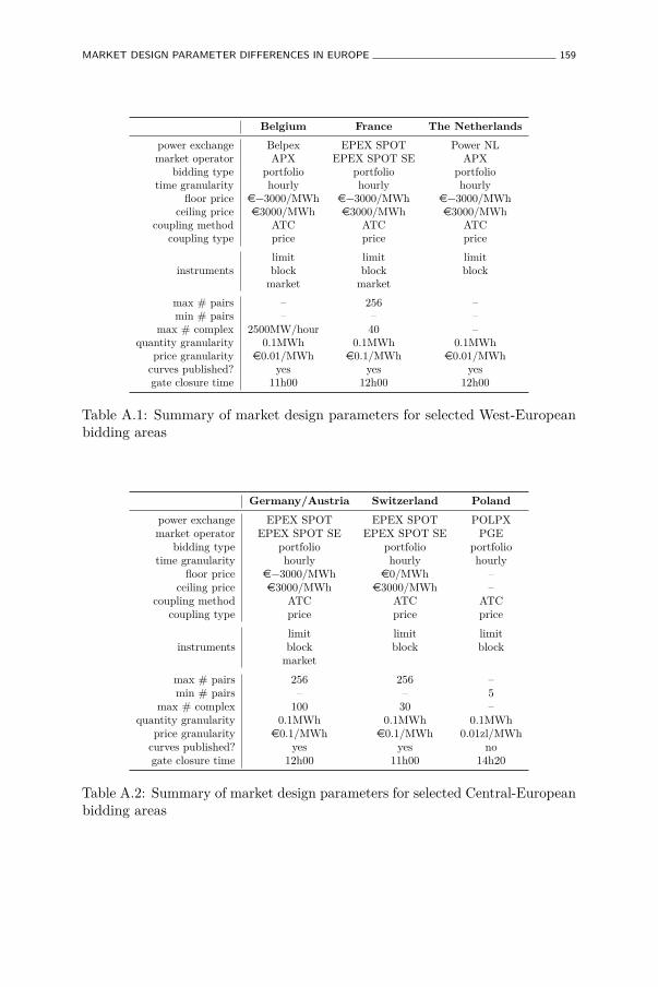
MARKET DESIGN PARAMETER DIFFERENCES IN EUROPE 159
Belgium France The Netherlandspower exchange Belpex EPEX SPOT Power NLmarket operator APX EPEX SPOT SE APX
bidding type portfolio portfolio portfoliotime granularity hourly hourly hourly
floor price e−3000/MWh e−3000/MWh e−3000/MWhceiling price e3000/MWh e3000/MWh e3000/MWh
coupling method ATC ATC ATCcoupling type price price price
instrumentslimit limit limitblock block blockmarket market
max # pairs – 256 –min # pairs – – –
max # complex 2500MW/hour 40 –quantity granularity 0.1MWh 0.1MWh 0.1MWh
price granularity e0.01/MWh e0.1/MWh e0.01/MWhcurves published? yes yes yesgate closure time 11h00 12h00 12h00
Table A.1: Summary of market design parameters for selected West-Europeanbidding areas
Germany/Austria Switzerland Polandpower exchange EPEX SPOT EPEX SPOT POLPXmarket operator EPEX SPOT SE EPEX SPOT SE PGE
bidding type portfolio portfolio portfoliotime granularity hourly hourly hourly
floor price e−3000/MWh e0/MWh –ceiling price e3000/MWh e3000/MWh –
coupling method ATC ATC ATCcoupling type price price price
instrumentslimit limit limitblock block blockmarket
max # pairs 256 256 –min # pairs – – 5
max # complex 100 30 –quantity granularity 0.1MWh 0.1MWh 0.1MWh
price granularity e0.1/MWh e0.1/MWh 0.01zl/MWhcurves published? yes yes nogate closure time 12h00 11h00 14h20
Table A.2: Summary of market design parameters for selected Central-Europeanbidding areas

160 MARKET DESIGN PARAMETER DIFFERENCES IN EUROPE
Denmark/Nordic Iberian Peninsula Italypower exchange Elspot MIBEL MGPmarket operator Nord Pool Spot AS OMI GME
bidding type portfolio unit unittime granularity hourly hourly hourly
floor price e−200/MWh e0/MWh e0/MWhceiling price e2000/MWh e180.3/MWh 3000
coupling method ATC ATC ATCcoupling type price / volume price price
instrumentslimit limit limitblock block blockflexible
max # pairs 64 25/unit –min # pairs – – –
max # complex 50 – –quantity granularity 0.1MWh 1MWh 0.001MWh
price granularity e0.1/MWh (1kr/MWh)) e0.01/MWh e0.01/MWhcurves published? yes yesgate closure time 10h00 11h00 9h15
Table A.3: Summary of market design parameters for selected North- andSouth-European bidding areas

Appendix BOPTIMATE project
brochure
161


An Open simulAtiOn plAtfOrm tO testintegrAtiOn in mArket design Of mAssive intermittent energymOdelling shOrt-term electricity mArkets And systems
OptimAte models european processes from day ahead to real time to:
— Assess future electricity market designs— Analyse the impact of massive variable
generation integration
the goal:
— Improving economic efficiency — ensuring security of supply— Achieving sustainable development in
europe

research units(uk)
Denmark
Belgium germany
coorDinator france
technical Directorfrance
Belgium germany
france
spain italy
spain
1 cOOrdinAtOr5 trAnsmissiOn system OperAtOrs6 reseArch units
three main studies achieved within the project:— cross-border capacity management— day-ahead, intra-day and balancing designs — renewable support schemes
plAtfOrm OptiOns
market design variants: 40tsO operation modes: 30Actors strategy variants: 10scenario variants: unlimited
dAy-AheAd prOcess
OptimAte ex-pOst feedbAck
OptimAte web Access
intrA-dAy prOcess reAl-time prOcess
dAily iterAtiOn
decisiOns mAdefOr the next eight hOurs
( 16x1/2 hOur)
decisiOns mAdefOr the current
1/2 hOur Only
reserverequirements
cAsecOnfigurAtiOn
cAsemOnitOring
web Access tO Outputs
scenAriOdescriptiOn indicAtOrs
imbAlAnce & settlements
finAl prOgrAm
intrA-dAy iterAtiOn
mArket cOupling
bAlAncing
mArketcOupling
crOss-bOrderlimits tO mArket bAlAncing
bids & OfferstO mArket cOngestiOn
remOvAl
in
out
leArning by dOing
OperAtiOns trAnsmissiOn system OperAtOrs
pOwer exchAnges
mArket plAyers
uniteD kingDom
platform architecture

plAtfOrm AvAilAble by end Of 2012!
graphical outputs display
tsOs, regulAtOrs And AcAdemics cAn rely On OptimAte tO Assist them On the fOllOwing issues
— How do different variable feed-in regimes affect system efficiency and security of supply ?— Will flow-based market coupling outperform ATC coupling ?— How do various balancing schemes impact DA, ID and RT processes ?— How to best mitigate market power ?

Appendix CPrice evolution whenbehaving strategically
167


PRICE EVOLUTION WHEN BEHAVING STRATEGICALLY 169
0 200 400 600 800 1,000 1,2000
1,000
2,000
3,000
Simulation run [market round]
Price
[e/M
Wh]
Figure C.1: Evolution of emerging market clearing prices in bidding area Awhen behaving strategically under net transfer capacity market coupling
0 200 400 600 800 1,000 1,2000
1,000
2,000
3,000
Simulation run [market round]
Price
[e/M
Wh]
Figure C.2: Evolution of emerging market clearing prices in bidding area Awhen behaving strategically under flow-based market coupling

170 PRICE EVOLUTION WHEN BEHAVING STRATEGICALLY
0 200 400 600 800 1,000 1,2000
1,000
2,000
3,000
Simulation run [market round]
Price
[e/M
Wh]
Figure C.3: Evolution of emerging market clearing prices in bidding area Bwhen behaving strategically under net transfer capacity market coupling
0 200 400 600 800 1,000 1,2000
1,000
2,000
3,000
Simulation run [market round]
Price
[e/M
Wh]
Figure C.4: Evolution of emerging market clearing prices in bidding area Bwhen behaving strategically under flow-based market coupling

PRICE EVOLUTION WHEN BEHAVING STRATEGICALLY 171
0 200 400 600 800 1,000 1,2000
1,000
2,000
3,000
Simulation run [market round]
Price
[e/M
Wh]
Figure C.5: Evolution of emerging market clearing prices in bidding area Cwhen behaving strategically under net transfer capacity market coupling
0 200 400 600 800 1,000 1,2000
1,000
2,000
3,000
Simulation run [market round]
Price
[e/M
Wh]
Figure C.6: Evolution of emerging market clearing prices in bidding area Cwhen behaving strategically under flow-based market coupling

172 PRICE EVOLUTION WHEN BEHAVING STRATEGICALLY
0 200 400 600 800 1,000 1,2000
1,000
2,000
3,000
Simulation run [market round]
Price
[e/M
Wh]
Figure C.7: Evolution of emerging market clearing prices in bidding area Dwhen behaving strategically under net transfer capacity market coupling
0 200 400 600 800 1,000 1,2000
1,000
2,000
3,000
Simulation run [market round]
Price
[e/M
Wh]
Figure C.8: Evolution of emerging market clearing prices in bidding area Dwhen behaving strategically under flow-based market coupling

PRICE EVOLUTION WHEN BEHAVING STRATEGICALLY 173
0 200 400 600 800 1,000 1,2000
1,000
2,000
3,000
Simulation run [market round]
Price
[e/M
Wh]
Figure C.9: Evolution of emerging market clearing prices in bidding area Ewhen behaving strategically under net transfer capacity market coupling
0 200 400 600 800 1,000 1,2000
1,000
2,000
3,000
Simulation run [market round]
Price
[e/M
Wh]
Figure C.10: Evolution of emerging market clearing prices in bidding area Ewhen behaving strategically under flow-based market coupling


Bibliography
ACER. (2011, Oct). Cross-regional roadmap for day-ahead marketcoupling. Technical report. Agency for the Cooperation of EnergyRegulators. http://www.acer.europa.eu/Electricity/Regional_initia-tives/Cross_Regional_Roadmaps/Documents/Final%20version%20Cross-regional%20road%20map%20Market%20Coupling.ppt [Last accessed January2014].
Albuyeh, F. & Kumar, J. (2003). Decision support tools for marketparticipants. IEEE Transactions on Power Systems, 18(2), pages 512–516.
Alós-Ferrer, Carlos. (2004). Cournot versus Walras in dynamic oligopolieswith memory. International Journal of Industrial Organization, 22(2), pages193–217.
Ambec, Stefan & Doucet, Joseph A. (2003). Decentralizing hydropower production. Canadian Journal of Economics / Revue canadienned’Economique, 36(3), pages 587–607.
Androcec, I. & Jakasa, T. & Krajcar, S. (2010). Modeling of generationand supply competitiveness in regional cross-border electricity trading. 6 pagesof: 7th International Conference on the European Energy Market (EEM10).
Arroyo, J.M. & Conejo, A.J. (2000). Optimal response of a thermal unitto an electricity spot market. IEEE Transactions on Power Systems, 15(3),pages 1098–1104.
Arroyo, J.M. & Conejo, A.J. (2002). Optimal response of a power generatorto energy, AGC, and reserve pool-based markets. IEEE Transactions on PowerSystems, 17(2), pages 404–410.
175
176 BIBLIOGRAPHY
Arroyo, J.M. & Conejo, A.J. (2004). Modeling of start-up and shut-downpower trajectories of thermal units. IEEE Transactions on Power Systems,19(3), pages 1562–1568.
Attaviriyanupap, P. & Kita, H. & Tanaka, E. & Hasegawa, J. (2004).A fuzzy-optimization approach to dynamic economic dispatch consideringuncertainties. IEEE Transactions on Power Systems, 19(3), pages 1299–1307.
Azadeh, A. & Ghaderi, S. F. & Pourvalikhan Nokhandan, B. &Sheikhalishahi, M. (2012). A new genetic algorithm approach for optimizingbidding strategy viewpoint of profit maximization of a generation company.Expert Systems with Applications, 39(1), pages 1565–1574.
Baillo, A. & Ventosa, M. & Rivier, M. & Ramos, A. (2004). Optimaloffering strategies for generation companies operating in electricity spotmarkets. IEEE Transactions on Power Systems, 19(2), pages 745–753.
Baker, Jonathan B. & Bresnahan, Timothy F. (1988). Estimating theresidual demand curve facing a single firm. International Journal of IndustrialOrganization, 6(3), pages 283–300.
Bard, Joanthan F. (1988). Short-term scheduling of thermal-electricgenerators using Lagrangian Relaxation. Operations Research, 36(5), pages756–766.
Baringo, L. & Conejo, A.J. (2011). Offering strategy via robustoptimization. IEEE Transactions on Power Systems, 26(3), pages 1418–1425.
Barquin, J. & Vazquez, M. (2008). Cournot equilibrium calculation inpower networks: an optimization approach with price response computation.IEEE Transactions on Power Systems, 23(2), pages 317–326.
Barquín, Julián & Rouco, Luis & Rivero, Enrique. (2010, Jul).Current designs and expected evolutions of day-ahead, intra-day and balancingmarket/mechanisms in europe. Technical report. Commillas PontificalUniversity. Deliverable D2.2, D3.3.1, D3.3.2, D3.2 of the OPTIMATE project,http://www.optimate-platform.eu/downloads/index.html [Last accessed Jan-uary 2014].
Barroso, Luiz Augusto N. & Fampa, Márcia H. C. & Kelman, Rafael& Pereira, Mario V. F. & Lino, Priscila. (2002). Market power issuesin bid-based hydrothermal dispatch. Annals of Operations Research, 117(4).
Barroso, Luiz Augusto N. & Street, A. & Granville, S. & Pereira,M.V. (2011). Offering strategies and simulation of multi-item iterative auctionsof energy contracts. IEEE Transactions on Power Systems, 26(4), pages 1917–1928.

BIBLIOGRAPHY 177
Barton, J.P. & Infield, D.G. (2004). Energy storage and its use withintermittent renewable energy. IEEE Transactions on Energy Conversion,19(2), pages 441–448.
Baslis, C.G. & Bakirtzis, A.G. (2011). Mid-term stochastic scheduling ofa price-maker hydro producer with pumped storage. IEEE Transactions onPower Systems, 26(4), pages 1856–1865.
Bergin, James & Bernhardt, Dan. (2004). Comparative learning dynamics.International Economic Review, 45(2), pages 431–465.
Berzal, D. & de la Fuente, J.I. & Gomez, T. (2001, Sep). Buildinggeneration supply curves under uncertainty in residual demand curves for theday-ahead electricity market. 6 pages of: IEEE Power Tech Proceedings, vol.1.
Blumstein, Carl & Friedman, LeeS. & Green, Richard. (2002).The history of electricity restructuring in California. Journal of Industry,Competition and Trade, 2(1), pages 1566–1679.
Boonchuay, Chanwit & Ongsakul, Weerakorn. (2011). Optimal riskybidding strategy for a generating company by self-organising hierarchicalparticle swarm optimisation. Energy Conversion and Management, 52(2),pages 1047–1053.
Bordier, Marc & Maïzi, Nadia & Bellini, Robert & Marmorat,Jean Paul & Roy, Valérie & Thomas, Johann & Maenhoudt, Marijn& Coulondre, Jean-Marie. (2010, Oct). Day-ahead module functionaldescription. Technical report. ARMINES, University of Leuven and RTE.Deliverable D1.3 of the OPTIMATE project.
Borenstein, Severin. (2000). Understanding competitive pricing and marketpower in wholesale electricity markets. The Electricity Journal, 13(6).
Borenstein, Severin & Bushnell, James. (2000). Electricity restructuring:deregulation or reregulation? Regulation, 23(2), pages 46–52.
Borenstein, Severin & Bushnell, James & Wolak, Frank. (2000, Sep).Diagnosing market power in California’s restructured wholesale electricitymarket. Technical report 7868. National Bureau of Economic Research.http://www.nber.org/papers/w7868 [Last accessed January 2014].
Borenstein, Severin & Bushnell, James B. & Wolak, Frank A.(2002). Measuring market inefficiencies in California’s restructured wholesaleelectricity market. The American Economic Review, 92(5), pages 1376–1405.

178 BIBLIOGRAPHY
Borenstein, Severin & Bushnell, James & Knittel, Christopher R.& Wolfram, Catherin. (2008). Inefficiencies and market power in financialarbitrage: a study of California’s electricity markets. The Journal of IndustrialEconomics, 56(2), pages 347–378.
Borghetti, A. & Frangioni, A. & Lacalandra, F. & Nucci, C.A.(2003). Lagrangian heuristics based on disaggregated bundle methods forhydrothermal unit commitment. IEEE Transactions on Power Systems, 18(1),pages 313–323.
Brown, P.D. & Peas Lopes, J.A. & Matos, M.A. (2008). Optimizationof pumped storage capacity in an isolated power system with large renewablepenetration. IEEE Transactions on Power Systems, 23(2), pages 523–531.
Buijs, Patrick. (2011, Dec). Transmission investments: concepts forEuropean collaboration in planning and financing. Ph.D. thesis, KU Leuven.https://lirias.kuleuven.be/handle/123456789/321137 [Last accessed January2014].
Bushnell, James & Mansur, Erin T. & Saravia, Celeste. (2004, Mar).Market structure and competition: a cross-market analysis of u.s. electricityderegulation. Technical report. Center for the Study of Energy Markets, UCBerkeley. www.ucei.berkeley.edu/PDF/csemwp126.pdf [Last accessed January2014].
Bushnell, Jim & Saravia, Celeste. (2002, May). An empiricalassessment of the competitiveness of the New England electricity mar-ket. Working paper 101, University of California Energy Institute.http://escholarship.org/uc/item/8913v4bk [Last accessed January 2014].
Capros, Pantelis & Mantzos, Leonidas. (2005, May). Long-termscenarios for strategic energy policy of the EU. Technical report. E3MLab, Institute of Communication and Computer Systems, National TechnicalUniversity of Athens. http://www.sessa.eu.com/documents/wp/D44.1-Capros.pdf [Last accessed January 2014].
Cardell, Judith B. & Hitt, Carrie Cullen & Hogan, William W.(1997). Market power and strategic interaction in electricity networks. Resourceand Energy Economics, 19(1–2), pages 109–137.
Carrion, M. & Arroyo, J.M. (2006). A computationally efficient mixed-integer linear formulation for the thermal unit commitment problem. Ieeetransactions on power systems, 21(3), pages 1371–1378.

BIBLIOGRAPHY 179
CASC. (2014, Jan). Publication CWE flow-based external par-allel run. http://www.casc.eu/en/Resource-center/CWE-Flow-Based-MC/Publication-CWE-Flow-based-External-parallel-run [Last accessed Jan-uary 2014].
Castronuovo, E.D. & Peas Lopes, J.A. (2004). On the optimizationof the daily operation of a wind-hydro power plant. IEEE Transactions onPower Systems, 19(3), pages 1599–1606.
CEER. (2010, Jul). Regulatory aspects of the integration of wind generationin european electricity markets. Technical report. Council of European EnergyRegulators. http://www.energy-regulators.eu/portal/page/portal/EER_-HOME/EER_PUBLICATIONS/CEER_PAPERS/Electricity/2010/C10-SDE-16-03_CEER%20wind%20conclusions%20paper_7-July-2010.pdf [Lastaccessed January 2014].
Chaturvedi, Krishna Teerth & Pandit, Manjaree & Srivastava,Laxmi. (2009). Particle swarm optimization with time varying accelerationcoefficients for non-convex economic power dispatch. International Journal ofElectrical Power & Energy Systems, 31(6), pages 249–257.
Chen, Po-Hung & Chang, Hong-Chan. (1995). Large-scale economicdispatch by genetic algorithm. IEEE Transactions on Power Systems, 10(4),pages 1919–1926.
Cheng, Chuan-Ping & Liu, Chih-Wen & Liu, Chun-Chang. (2000).Unit commitment by Lagrangian Relaxation and Genetic Algorithms. IEEETransactions on Power Systems, 15(2), pages 707–714.
Conejo, A.J. & Nogales, F.J. & Arroyo, J.M. (2002). Price-taker biddingstrategy under price uncertainty. IEEE Transactions on Power Systems, 17(4),pages 1081–1088.
Contreras, J. & Espinola, R. & Nogales, F.J. & Conejo, A.J. (2003).ARIMA models to predict next-day electricity prices. IEEE Transactions onPower Systems, 18(3), pages 1014–1020.
Conzelmann, G. (2008, Jun). Electricity market complex adaptivesystem (EMCAS). http://www.dis.anl.gov/projects/emcas.html [Last accessedJanuary 2014].
Conzelmann, Guenter & Boyd, Gale & Koritarov, Vladimir &Veselka, Tom. (2005, Jun). Multi-agent power market simulation usingEMCAS. Pages 2829–2834 of: IEEE Power Engineering Society GeneralMeeting.
180 BIBLIOGRAPHY
Cramton, P. (2003, Jan). Electricity market design: the good, the bad, andthe ugly. 8 pages of: Proceedings of the 36th Annual Hawaii InternationalConference on System Sciences (HICSS03).
Cramton, Peter. (2004, Jan). Competitive bidding behavior in uniform-priceauction markets. 12 pages of: Hawaii International Conference on System Sci-ences (HICSS04). http://www.cramton.umd.edu/papers2000-2004/cramton-bidding-behavior-in-electricity-markets-hawaii.pdf [Last accessed January2014].
Dallinger, David & Wietschel, Martin. (2012). Grid integration ofintermittent renewable energy sources using price-responsive plug-in electricvehicles. Renewable and Sustainable Energy Reviews, 16(5), pages 3370–3382.
Damousis, I.G. & Bakirtzis, A.G. & Dokopoulos, P.S. (2004). A solutionto the unit commitment problem using integer-coded genetic algorithm. IEEETransactions on Power Systems, 19(2), pages 1165–1172.
David, A.K. (1993). Competitive bidding in electricity supply. IEE Proceedingsof Generation, Transmission and Distribution, 140(5), pages 421–426.
Day, ChristopherJ. & Bunn, DerekW. (2001). Divestiture of generationassets in the electricity pool of England and Wales: a computational approachto analyzing market power. Journal of Regulatory Economics, 19(2), pages123–141.
Day, C.J. & Hobbs, B.F. & Pang, Jong-Shi. (2002). Oligopolisticcompetition in power networks: a conjectured supply function approach. IEEETransactions on Power Systems, 17(3), pages 597–607.
de la Fuente, José Ignacio & Junco, Paula. (2011, Jul). Paper analysisof measures to ensure robustness and economic efficiency of the expected realperformance of TSO-driven balancing markets. Technical report. Red Eléctricade España. Deliverable D2.4 of the OPTIMATE project.
de la Torre, S. & Arroyo, J.M. & Conejo, A.J. & Contreras, J.(2002). Price maker self-scheduling in a pool-based electricity market: a mixed-integer lp approach. IEEE Transactions on Power Systems, 17(4), pages1037–1042.
Deane, J.P. & Gallachóir, B.P. Ó & McKeogh, E.J. (2010). Techno-economic review of existing and new pumped hydro energy storage plant.Renewable and Sustainable Energy Reviews, 14(4), pages 1293–1302.
Delarue, Erik & Van Den Bosch, Pieterjan & D’haeseleer, William.(2010). Effect of the accuracy of price forecasting on profit in a price-basedunit commitment. Electric Power Systems Research, 80(10), pages 1306–1313.
BIBLIOGRAPHY 181
Denton, M. & Palmer, A. & Masiello, R. & Skantze, P. (2003).Managing market risk in energy. IEEE Transactions on Power Systems, 18(2),pages 494–502.
Diniz, A.L. & Maceira, M.E.P. (2008). A four-dimensional model of hydrogeneration for the short-term hydrothermal dispatch problem considering headand spillage effects. IEEE Transactions on Power Systems, 23(3), pages1298–1308.
Doquet, Michel. (2007, Jul). Use of a stochastic process to sample windpower curves in planning studies. Pages 663–670 of: 2007 IEEE LausannePower Tech.
Doquet, Michel & Mornot, E. & Verrier, F. & Gonzalez, R. &Lepy, S. (2008). A new tool for adequacy reporting of electric systems:ANTARES. In: International Council for Large Electric Systems (CIGRE).paper C1-305.
Ebrahimi, J. & Hosseinian, S.H. & Gharehpetian, G.B. (2011). Unitcommitment problem solution using shuffled frog leaping algorithm. IEEETransactions on Power Systems, 26(2), pages 573–581.
Edenhofer, O. & Knopf, B. & Barker, T. & Baumstark, L. &Bellevrat, E. & Chateau, B. & Criqui, P. & Isaac, M. & Kitous,A. & Kypreos, S. & others. (2010). The economics of low stabilization:model comparison of mitigation strategies and costs. The Energy Journal,31(1), pages 11–48.
Fabra, Natalia & von der Fehr, Nils-Henrik & Harbord, David.(2006). Designing electricity auctions: uniform, discriminatory and Vickrey.The RAND Journal of Economics, 37(1), pages 23–46.
Fekete, K. & Knezevic, G. & Nikolovski, S. & Slipac, G. (2009, Jun).Influence of cross-border energy trading on prices of electricity in Croatia.6 pages of: 6th International Conference on the European Energy Market(EEM09).
Fleten, Stein-Erik & Kristoffersen, Trine Krogh. (2007). Stochasticprogramming for optimizing bidding strategies of a nordic hydropower producer.European Journal of Operational Research, 181(2), pages 916–928.
Forshner, Zivan & Shy, Oz. (2009). Constant best-response functions:interpreting Cournot. International Journal of Business and Economics, 8(1),pages 1–6.

182 BIBLIOGRAPHY
Frangioni, A. & Gentile, C. & Lacalandra, F. (2009). Tighterapproximated MILP formulations for unit commitment problems. IEEETransactions on Power Systems, 24(1), pages 105–113.
Garces, L.P. & Conejo, A.J. (2010). Weekly self-scheduling, forwardcontracting, and offering strategy for a producer. IEEE Transactions onPower Systems, 25(2), pages 657–666.
García, A. & Ventosa, M. & Rivier, M. & Ramos, A. & Relaño,G. (2002, Jun). Fitting electricity market models. a conjectural variationsapproach. 8 pages of: 14th Power Systems Computation Conference (PSCC02),vol. 4. http://www.iit.upcomillas.es/aramos/papers/PSCCSeville_s12p03.pdf[Last accessed January 2014].
Garcia-Gonzalez, J. & de la Muela, R.M.R. & Santos, L.M. &Gonzalez, A.M. (2008). Stochastic joint optimization of wind generationand pumped-storage units in an electricity market. IEEE Transactions onPower Systems, 23(2), pages 460–468.
Glachant, J. M. & Finon, D. & De Hauteclocque, A. (2011).Competition, Contracts and Electricity Markets: A New Perspective. TheLoyola De Palacio Series on European Energy Policy. Edward Elgar. ISBN:978-1849804790.
Glachant, Jean-Michel & Pignon, Virginie. (2005). Nordic congestion’sarrangement as a model for Europe? Physical constraints vs. economicincentives. Utilities Policy, 13(2), pages 153–162.
Gountis, V.P. & Bakirtzis, A.G. (2004). Bidding strategies for electricityproducers in a competitive electricity marketplace. IEEE Transactions onPower Systems, 19(1), pages 356–365.
Green, Richard. (1996). Increasing competition in the British electricityspot market. The Journal of Industrial Economics, 44(2), pages 205–216.
Green, Richard. (1999). The electricity contract market in England andWales. The Journal of Industrial Economics, 47(1), pages 107–124.
Green, Richard J. & Newbery, David M. (1992). Competition in theBritish electricity spot market. Journal of Political Economy, 100(5), pages929–953.
Grigg, C. & Wong, P. & Albrecht, P. & Allan, R. & Bhavaraju, M.& Billinton, R. & Chen, Q. & Fong, C. & Haddad, S. & Kuruganty,S. & Li, W. & Mukerji, R. & Patton, D. & Rau, N. & Reppen, D.& Schneider, A. & Shahidehpour, M. & Singh, C. (1999). The IEEE

BIBLIOGRAPHY 183
reliability test system - 1996. IEEE Transactions on Power Systems, 14(3),pages 1010–1020.
Harris, C. (2006a). Electricity markets: pricing, structures and economics.Finance Series, vol. 328. John Wiley & Sons. ISBN: 978-0-470-01158-4. Pages295–327.
Harris, C. (2006b). Electricity markets: pricing, structures and economics.Finance Series, vol. 328. John Wiley & Sons. ISBN: 978-0-470-01158-4. Pages436–448.
Helman, U. & Hobbs, B.F. (2010). Large-scale market power modeling:analysis of the U.S. Eastern interconnection and regulatory applications. IEEETransactions on Power Systems, 25(3), pages 1434–1448.
Herguera, Iñigo. (2000). Bilateral contracts and the spot market forelectricity: some observations on the British and the NordPool experiences.Utilities Policy, 9(2), pages 73–80.
Hobbs, B.E. (2001). Linear complementarity models of Nash-Cournotcompetition in bilateral and POOLCO power markets. IEEE Transactions onPower Systems, 16(2), pages 194–202.
Hobbs, Benjamin F. & Pang, J. S. (2007). Nash-Cournot equilibriain electric power markets with piecewise linear demand functions and jointconstraints. Operations Research, 55(1), pages 113–127.
Hogan, W. W. (1998, Dec). Competitive electricity market design:a wholesale primer. www.hks.harvard.edu/fs/whogan/empr1298.pdf [Lastaccessed January 2014].
Hogan, William W. (2000, May). Regional transmission organizations:millenium order on designing market institutions for electric network systems.Technical report. Center for Business and Government, Harvard University.www.hks.harvard.edu/fs/whogan/hjp0500a.pdf [Last accessed January 2014].
Hogan, William W. (2002). Electricity market restructuring: reforms ofreforms. Journal of Regulatory Economics, 21(Jan), pages 103–132.
Hogan, William W. (2003, Oct). Successful market design (SMD) andfailure diagnosis: blackouts and lampposts in regulating electricity markets.Technical report. Center for Business and Government, Harvard University.www.hks.harvard.edu/fs/whogan/Hogan_RPP_100903.pdf [Last accessedJanuary 2014].
Holttinen, H. (2005). Optimal electricity market for wind power. EnergyPolicy, 33(16), pages 2052–2063.
184 BIBLIOGRAPHY
Hongyan, Li & Tesfatsion, Leigh. (2009a, Jul). The AMES wholesalepower market test bed: a computational laboratory for research, teaching, andtraining. 8 pages of: Power and Energy Society IEEE Proceedings.
Hongyan, Li & Tesfatsion, Leigh. (2009b). Capacity withholding inrestructured wholesale power markets: an agent-based test bed study. 11pages of: Power Systems Conference and Exposition (PSCE09).
Hortacsu, Ali & Puller, Steven L. (2004, Mar). Testing strategic modelsof firm behavior in restructured electricity markets: a case study of ERCOT.Technical report. Center of Study of Energy Markets (CSEM), University of Cal-ifornia, Energy Institute. http://www.ucei.berkeley.edu/PDF/csemwp125.pdf[Last accessed January 2014].
IEA. (2012). World energy outlook (WEO). Technical report. InternationalEnergy Agency. http://www.polsci.chula.ac.th/pitch/ep13/weo12.pdf [Lastaccessed January 2014].
Jabr, R.A. (2005). Robust self-scheduling under price uncertainty usingConditional Value-at-Risk. IEEE Transactions on Power Systems, 20(4),pages 1852–1858.
Jónsson, Tryggvi & Pinson, Pierre & Madsen, Henrik. (2010). Onthe market impact of wind energy forecasts. Energy Economics, 32(2), pages313–320.
Johnsen, T.A. (2001). Hydropower generation and storage, transmissioncontraints and market power. Utilities Policy, 10(2), pages 63–73.
Joskow, P. & Kahn, E. (2001, Mar). A quantitative analysisof pricing behavior in California’s wholesale electricity market duringsummer 2000. Technical report. National Bureau of Economic Research.http://www.nber.org/papers/w8157.pdf [Last accessed January 2014].
Joskow, Paul L. & Schmalensee, Richard. (1988). Markets for power:an analysis of electrical utility deregulation. MIT Press Books. The MIT Press.
Jurewitz, John L. & Walther, Robin J. (1997). Must-run generation:can we mix regulation and competition successfully? The Electricity Journal,10(10), pages 44–55.
Kitzing, Lena & Schroeder, Sascha Thorsten & Morthorst,Poul Erik & Maenhoudt, Marijn & Glachant, Jean-Michel &Saguan, Marcelo & Rivero, Enrique. (2012, Nov). Analysis and synthesisof the results of the simulations. Technical report. DTU (Technical Universityof Denmark). Deliverable D6.1 of the OPTIMATE project.

BIBLIOGRAPHY 185
Klemperer, Paul D. & Meyer, Margaret A. (1989). Supply functionequilibria in oligopoly under uncertainty. Econometrica, 57(6), pages 1243–1277.
Kurzidem, Martin Johann. (2010, Mar). Analysis of flow-basedmarket coupling in oligopolistic power markets. Ph.D. thesis, ETHZurich. http://www.eeh.ee.ethz.ch/uploads/tx_ethpublications/Kurzidem_-diss.pdf [Last accessed January 2014].
Lagarto, J. & de Sousa, J. & Martins, A. & Ferrao, P. (2012, May).Price forecasting in the day-ahead iberian electricity market using a conjecturalvariations ARIMA model. 7 pages of: 9th International Conference on theEuropean Energy Market (eem12).
Larsen, E. R. & Bunn, D. W. (1999). Deregulation in electricity:understanding strategic and regulatory risk. The Journal of the OperationalResearch Society, 50(4), pages 337–344.
Lee, F.N. & Breipohl, A.M. (1993). Reserve constrained economic dispatchwith prohibited operating zones. IEEE Transactions on Power Systems, 8(1),pages 246–254.
Li, Hongyan & Sun, Junjie & Tesfatsion, Leigh S. (2009, Jun).Separation and volatility of locational marginal prices in restructured wholesalepower markets. Technical report. Iowa State University, Department ofEconomics. www.econ.iastate.edu/tesfatsi/LMPSeparationVolatility.LST.pdf[Last accessed January 2014].
Lind, Barry & Plott, Charles R. (1991). The winner’s curse: experimentswith buyers and with sellers. American Economic Review, 81(1), pages 335–346.
Lusan, D.A. & Yu, Z. & Sparrow, F.T. (1999, Jan). Market gaming andmarket power mitigation in deregulated electricity markets. Pages 839–843 of:IEEE Power Engineering Society Winter Meeting, vol. 2.
Maenhoudt, M. & Deconinck, G. (2010a, Jun). Agent-based modelling asa tool for testing electric power market designs. 5 pages of: 7th InternationalConference on the European Energy Market (EEM10).
Maenhoudt, M. & Deconinck, G. (2010b, Mar). Agent-based modellingas a tool for testing electric power market designs. 5 pages of: 5th YoungResearcher Symposium.
Maenhoudt, Marijn. (2012a, Jun). Report on the different research questionsand/or assumptions. Technical report. University of Leuven. Deliverable D5.3of the OPTIMATE project.
186 BIBLIOGRAPHY
Maenhoudt, Marijn. (2012b, Jun). Report on the implemented agent-based model. Technical report. University of Leuven. Deliverable D5.2 of theOPTIMATE project.
Maenhoudt, Marijn. (2013, Feb). Effects of agent behaviour on selectedcase study scenarios. Technical report. University of Leuven. Deliverable D5.5of the OPTIMATE project.
Maenhoudt, Marijn & Deconinck, Geert. (2012, May). Detailedmodelling of thermal units from a price taker’s perspective. 8 pages of:9th International Conference on the European Energy Market (EEM12).http://ieeexplore.ieee.org/xpls/abs_all.jsp?arnumber=6254741 [Last accessedJanuary 2014].
Maenhoudt, Marijn & Deconinck, Geert. (2013a, Sep). The effectof maintenance costs on the flexible dispatch of thermal units. 8 pagesof: 48th Universities Power Engineering Conference (UPEC2013), vol. 48.https://lirias.kuleuven.be/handle/123456789/410674 [Last accessed January2014].
Maenhoudt, Marijn & Deconinck, Geert. (2013b, Sep). A novel offeringstrategy to reduce profit risk. 8 pages of: 48th Universities Power EngineeringConference (upec2013). https://lirias.kuleuven.be/handle/123456789/410675[Last accessed January 2014].
Maenhoudt, Marijn & Deconinck, Geert. (2013c). Strategic offeringto maximize day-ahead profit by hedging against an infeasible market clearingresult. Accepted to be published in IEEE Transactions on Power Systems.
Maenhoudt, Marijn & Trinh, Quynh Chi & Qiu, Zhifeng &Deconinck, Geert. (2011, Sep). Report on model descriptions with agents,rationales, data and tuning parameter values to consider. Technical report.University of Leuven. Deliverable D5.1 of the OPTIMATE project.
Maenhoudt, Marijn & Trinh, Quynh Chi & Qiu, Zhifeng. (2012,Oct). Synthesis of the results obtained. Technical report. University of Leuven.Deliverable D5.4 of the OPTIMATE project.
Makhorin, Andrew. (2012, Jun). GNU linear programming kit.http://www.gnu.org/software/glpk/ [Last accessed January 2014].
Mandal, P. & Senjyu, T. & Urasaki, N. & Funabashi, T. &Srivastava, A.K. (2007). A novel approach to forecast electricity pricefor PJM using neural network and similar days method. IEEE Transactionson Power Systems, 22(4), pages 2058–2065.
BIBLIOGRAPHY 187
Mansur, Erin. (2001). Pricing behavior in the initial summer of therestructured pjm wholesale electricity market. University of California EnergyInstitute.
Matevosyan, J. & Soder, L. (2006). Minimization of imbalance cost tradingwind power on the short-term power market. IEEE Transactions on PowerSystems, 21(3), pages 1396–1404.
California ISO. (2002, Oct). Analysis of trading and schedulingstrategies described in Enron memos. Technical report. Department ofMarket Analysis. http://www.hks.harvard.edu/hepg/Papers/CAISO_en-ron.trading.analysis_10-4-02.pdf [Last accessed January 2014].
European Commission. (2007a). Proposal for a Directive ofthe European Parliament and of the Council amending Directive2003/54/EC concerning common rules for the internal market inelectricity. Technical report. European Commission. http://eur-lex.europa.eu/LexUriServ/LexUriServ.do?uri=COM:2007:0528:FIN:EN:PDF[Last accessed January 2014].
European Commission. (2007b). Proposal for a Regulation of theEuropean Parliament and of the Council Amending Regulation (EC)No 1228/2003 on conditions for access to the network for cross-borderexchanges in electricity. Technical report. European Commission. http://eur-lex.europa.eu/LexUriServ/LexUriServ.do?uri=COM:2007:0531:FIN:EN:PDF[Last accessed January 2014].
European Commission. (2008). Energising Europe: a real market with securesupply. Technical report. European Commission. http://europa.eu/rapid/press-release_IP-07-1361_en.pdf [Last accessed January 2014].
European Commission. (2010). Energy 2020, astrategy for competitive, sustainable and secure energy.Technical report. European Commission. http://eur-lex.europa.eu/LexUriServ/LexUriServ.do?uri=COM:2010:2020:FIN:EN:PDF[Last accessed January 2014].
European Commission. (2012). Country factsheets — EU 27 memberstates. Technical report. Statistics and Market Observatory for En-ergy. http://ec.europa.eu/energy/observatory/countries/doc/2012-country-factsheets.pdf [Last accessed January 2014].
European Commission. (2012). Energy roadmap 2050. Technicalreport. Publications Office of the European Union. http://eur-lex.europa.eu/LexUriServ/LexUriServ.do?uri=COM:2011:0885:FIN:EN:PDF[Last accessed January 2014].
188 BIBLIOGRAPHY
European Commission. (2013a). Assessing Europe’s potentialpumped hydropower storage. Technical report. European Commission.http://ec.europa.eu/dgs/jrc/downloads/jrc_20130503_assessment_euro-pean_phs_potential.pdf [Last accessed January 2014].
European Commission. (2013b). Commission Decision of 21 Au-gust 2013 on the establishment of the annual priority lists for thedevelopment of network codes and guidelines for 2014. Techni-cal report. European Commission. http://new.eur-lex.europa.eu/legal-content/EN/TXT/?uri=uriserv:OJ.L_.2013.224.01.0014.01.ENG [Last ac-cessed January 2014].
European Parliament. (2009, Apr). Directive 2009/28/EC of theEuropean Parliament and of the Council of 23 April 2009 on thepromotion of the use of energy from renewable sources and amending andsubsequently repealing directives 2001/77/EC and 2003/30/EC. http://eur-lex.europa.eu/LexUriServ/LexUriServ.do?uri=OJ:L:2009:140:0016:0062:EN:PDF [Last accessed January 2014].
ISO New England. (2002, Jan). Financial transmission rights: auctionexample. http://www.newengland-rto.org/markets/othrmkts_data/ftr/ tech_-sessions/manual_06_ftr_auction_example_presentation.pdf [Last accessedJanuary 2014].
Meibom, P. & Barth, R. & Hasche, B. & Brand, H. & Weber, C. &O’Malley, M. (2011). Stochastic optimization model to study the operationalimpacts of high wind penetrations in Ireland. IEEE Transactions on PowerSystems, 26(3), pages 1367–1379.
Merlin, A. & Sandrin, P. (1983). A new method for unit commitment atElectricité de France. IEEE Transactions on Power Apparatus and Systems,102(5), pages 1218–1225.
Michel, F. & Ferber, Jacques & Drogoul, A. (2009). Multi-agentsystems and simulations: a survey from the agent community’s perspective.CRC Press. Chapter 1.
Moghimi Hadji, M. & Vahidi, B. (2012). A solution to the unit commitmentproblem using imperialistic competition algorithm. IEEE Transactions onPower Systems, 27(1), pages 117–124.
Möller, Christoph & Rachev, Svetlozar T. & Fabozzi, Frank J.(2011). Balancing energy strategies in electricity portfolio management. EnergyEconomics, 33(1), pages 2–11.
BIBLIOGRAPHY 189
Navarro, Peter & Shames, Michael. (2003). Aftershocks — and essentiallessons — from the California electricity debacle. The Electricity Journal,16(4), pages 24–30.
Neuhoff, Karsten & Barquin, Julian & Boots, Maroeska G. &Ehrenmann, Andreas & Hobbs, Benjamin F. & Rijkers, Fieke A.M. &Vázquez, Miguel. (2005). Network-constrained Cournot models of liberalizedelectricity markets: the devil is in the details. Energy Economics, 27(3), pages495–525.
Newbery, David. (2010). Market design for a large share of wind power.Energy Policy, 38(7), pages 3131–3134.
Ni, E. & Luh, P.B. & Rourke, S. (2004). Optimal integrated generationbidding and scheduling with risk management under a deregulated powermarket. IEEE Transactions on Power Systems, 19(1), pages 600–609.
Niimura, T. & Nakashima, T. (2001). Deregulated electricity market datarepresentation by fuzzy regression models. IEEE Transactions on Systems,Man, and Cybernetics, Part C: Applications and Reviews, 31(3), pages 320–326.
Nogales, F.J. & Contreras, J. & Conejo, A.J. & Espinola, R.(2002). Forecasting next-day electricity prices by time series models. IEEETransactions on Power Systems, 17(2), pages 342–348.
Ockenfels, Axel & Grimm, Veronika & Zoettl, Gregor. (2008, Mar).Strommarktdesign: Preisbildungsmechanismus im Auktionsverfahren für Strom-stundenkontrakte an der EEX (English translation of the report). Technical re-port. University of Cologne. http://cdn.eex.com/document/38615/gutachten_-eex_ockenfels_e.pdf [Last accessed January 2014].
Oksanen, M. & Karjalainen, R. & Viljainen, S. & Kuleshov, D.(2009, May). Electricity markets in Russia, the US, and Europe (EEM09). 7pages of: 6th International Conference on the European Energy Market.
OMIE. (2013, Nov). Market results. http://www.omie.es/files/flash/ResultadosMercado.swf [Last accessed January 2014].
Ongsakul, W. & Petcharaks, N. (2004). Unit commitment by enhancedadaptive lagrangian relaxation. IEEE Transactions on Power Systems, 19(1),pages 620–628.
OPTIMATE. (2009). a numerical simulation platform. http://www.optimate-platform.eu/ [Online; accessed November 2013].
190 BIBLIOGRAPHY
Orbay, Hakan. (2009). Computing Cournot equilibrium throughmaximization over prices. Economics Letters, 105(1), pages 71–73.
Ostrowski, J. & Anjos, M.F. & Vannelli, A. (2010, May). Tight mixed-integer linear programming formulations for generator self-scheduling. 4pages of: 23rd Canadian Conference on Electrical and Computer Engineering(CCECE10).
Pang, C.K. & Chen, H.C. (1976). Optimal short-term thermal unitcommitment. IEEE Transactions on Power Apparatus and Systems, 95(4),pages 1336–1346.
Plazas, M.A. & Conejo, A.J. & Prieto, F.J. (2005). Multimarket optimalbidding for a power producer. IEEE Transactions on Power Systems, 20(4),pages 2041–2050.
Poli, Davide & Marracci, Mirko. (2011). Clearing procedures for day-ahead Italian electricity market: are complex bids really required. InternationalJournal of Energy, 5(3), pages 70–77.
Portela, J. & Muñoz, A. & Alonso, E. (2012, Jun).Day-ahead residual demand curve forecasting in electricitymarkets. In: 32nd International Symposium on Forecasting.www.forecasters.org/proceedings12/PORTELAJOSEISF2012.pdf [Lastaccessed January 2014].
Porter, David C. & Tanggaard, Carsten & Weaver, Daniel G. &Yu, Wei. (2008). Dispersed trading and the prevention of market failure: thecase of the Copenhagen stock exchange. European Financial Management,14(2), pages 243–267.
Praca, I. & Ramos, C. & Vale, Z. & Cordeiro, M. (2003). MASCEM:a multiagent system that simulates competitive electricity markets. IEEEIntelligent Systems, 18(6), pages 54–60.
Pritchard, G. (2002). The must-run dispatch auction in an electricitymarket. Energy Economics, 24(3), pages 199–216.
Qiu, Zhifeng. (2013, Aug). Computational game theory applied in electricitymarket — games played with heterogeneous beliefs. Ph.D. thesis, KU Leuven.https://lirias.kuleuven.be/handle/123456789/410996 [Last accessed January2014].
Rangel, Luiz Fernando. (2008). Competition policy and regulation inhydro-dominated electricity markets. Energy Policy, 36(4), pages 1292–1302.
BIBLIOGRAPHY 191
REE. (2013, Feb). MIBEL imbalances management process.http://www.esios.ree.es/web-publica/ [Last accessed January 2014].
Rious, Vincent & Glachant, Jean-Michel & Perez, Yannick &Dessante, Philippe. (2008). The diversity of design of TSOs. Energy Policy,36(9), pages 3323–3332.
Rivero, E. & Barquín, J. & Rouco, L. (2011, May). European balancingmarkets. Pages 333–338 of: 8th International Conference on the EuropeanEnergy Market (EEM11),.
Rosenthal, Richard E. (2012, Jan). GAMS —a user’s guide. GAMS Development Corporation.http://www.gams.com/dd/docs/bigdocs/GAMSUsersGuide.pdf [Lastaccessed January 2014].
Safarzyńska, Karolina & Bergh, Jeroen C.J.M. (2010). Evolutionarymodels in economics: a survey of methods and building blocks. Journal ofEvolutionary Economics, 20(3), pages 329–373.
Sanchez, I. (2006). Short-term prediction of wind energy production.International Journal of Forecasting, 22(1), pages 43–56.
Sánchez Mará, Néstor. (2010, Jul). Day-ahead electricity market: proposalsto adapt complex conditions in OMEL. M.Phil. thesis, Universidad PontificaComillas. www.iit.upcomillas.es/docs/TM-10-014.pdf [Last accessed January2014].
Schill, W. & Kemfert, C. (2009, Aug). Strategic storage and fluctuatingwind power in a game-theoretic electricity market model with imperfectcompetition. In: 10th International Association for Energy Economics Euro-pean Conference (IAEE). http://www.aaee.at/2009-IAEE/uploads/fullpaper_-iaee09/P_562_Schill_Wolf-Peter_31-Aug-2009,%2012:27.pdf [Last accessedJanuary 2014].
Schill, Wolf-Peter & Kemfert, Claudia. (2011). Modeling strategicelectricity storage: the case of pumped hydro storage in Germany. Energy,32(3), pages 59–88.
Schmalensee, Richard & Golub, Bennett W. (1984). Estimatingeffective concentration in deregulated wholesale electricity markets. TheRAND Journal of Economics, 15(1), pages 12–26.
Seki, T. & Yamashita, N. & Kawamoto, K. (2010). New local searchmethods for improving the Lagrangian-Relaxation-based unit commitmentsolution. IEEE Transactions on Power Systems, 25(1), pages 272–283.

192 BIBLIOGRAPHY
Senjyu, T. & Saber, A.Y. & Miyagi, T. & Shimabukuro, K. &Urasaki, N. & Funabashi, T. (2005). Fast technique for unit commitmentby genetic algorithm based on unit clustering. IEE Proceedings of Generation,Transmission and Distribution, 152(5), pages 705–713.
Sensfuß, Frank & Ragwitz, Mario & Genoese, Massimo. (2008). Themerit-order effect: a detailed analysis of the price effect of renewable electricitygeneration on spot market prices in Germany. Energy Policy, 36(8), pages3086–3094.
Shahidehpour, M. & Yamin, H. & Li, Zuyi. (2002a). Market operations inelectric power systems: forecasting, scheduling, and risk management. edition1. Wiley-IEEE Press. ISBN: 978-0-471-44337-7. Pages 115–160.
Shahidehpour, M. & Yamin, H. & Li, Z. (2002b). Market operations inelectric power systems: forecasting, scheduling, and risk management. edition1. Wiley-IEEE Press. ISBN: 978-0-471-44337-7. Pages 191–230.
Shahidehpour, M. & Yamin, H. & Li, Z. (2002c). Market operations inelectric power systems: forecasting, scheduling, and risk management. edition1. Wiley-IEEE Press. ISBN: 978-0-471-44337-7. Pages 296–297.
Simoglou, C. K. & Biskas, P. N. & Bakirtzis, A. G. (2012). Optimalself-scheduling of thermal units during commissioning. IEEE Transactions onPower Systems, 27(1), pages 181–188.
Simoglou, C.K. & Biskas, P.N. & Bakirtzis, A.G. (2010). Optimalself-scheduling of a thermal producer in short-term electricity markets byMILP. IEEE Transactions on Power Systems, 25(4), pages 1965–1977.
Singh, H. & Hao, S. & Papalexopoulos, A. (1998). Transmissioncongestion management in competitive electricity markets. IEEE Transactionson Power Systems, 13(2), pages 672–680.
Stoft, Steven. (2002). Power System Economics: Designing Markets forElectricity. Wiley-IEEE Press. ISBN: 978-0-471-15040-4. Pages 316–373.
Su, Ching-Tzong & Chiou, Gwo-Jen. (1997). A fast-computation Hopfieldmethod to economic dispatch of power systems. IEEE Transactions on PowerSystems, 12(4), pages 1759–1764.
Sueyoshi, Toshiyuki & Tadiparthi, Gopalakrishna R. (2008). Anagent-based decision support system for wholesale electricity market. DecisionSupport Systems, 44(2), pages 425–446.
Syothert, A. & MacLeod, I. (2000). Competitive bidding as a controlproblem. IEEE Transactions on Power Systems, 15(1), pages 88–94.

BIBLIOGRAPHY 193
Tesfatsion, Leigh. (2006). Agent-based computational economics: aconstructive approach to economic theory. Handbook of ComputationalEconomics, vol. 2. Elsevier. Pages 831–880.
Tesfatsion, Leigh. (2013, Jul). The AMES wholesalepower market test bed: a free open-source computationallaboratory for the agent-based modeling of electricity systems.http://www2.econ.iastate.edu/tesfatsi/AMESMarketHome.htm [Lastaccessed January 2014].
Traber, Thure & Kemfert, Claudia. (2011). Gone with the wind? –—electricity market prices and incentives to invest in thermal power plants underincreasing wind energy supply. Energy Economics, 33(2), pages 249–256.
Trinh, Quynh Chi. (2013, Dec). Balancing market designs for marketpower mitigation in interrelated electricity markets. Ph.D. thesis, KU Leuven.https://lirias.kuleuven.be/handle/123456789/425179 [Last accessed January2014].
Tseng, Chung-Li & Oren, Shmuel S. & Cheng, Carol S. & an Li,Chao & Svoboda, Alva J. & Johnson, Raymond B. (1999). Atransmission-constrained unit commitment method in power system scheduling.Decision Support Systems, 24(3–4), pages 297–310.
Tuohy, A. & O’Malley, M. (2011). Pumped storage in systems with veryhigh wind penetration. Energy Policy, 39(4), pages 1965–1974.
Uhrmacher, Adelinde M. & Weyns, Danny. (2009). Multi-agent systems:simulation and applications (computational analysis, synthesis, and design ofdynamic systems. CRC Press. ISBN: 978-1420070231.
Vallée, Thomas & Yildizoglu, Murat. (2009). Convergence in the finiteCournot oligopoly with social and individual learning. Journal of EconomicBehavior & Organization, 72(2), pages 670–690.
Vallée, Thomas & Yildizoglu, Murat. (2013). Can they beat the Cournotequilibrium? learning with memory and convergence to equilibria in a Cournotoligopoly. Computational Economics, 41(4).
Van Hertem, Dirk. (2009, Jan). The use of power flow con-trolling devices in the liberalized market. Ph.D. thesis, KU Leuven.https://lirias.kuleuven.be/handle/1979/2047 [Last accessed January 2014].
Vandezande, Leen & Meeus, Leonardo & Belmans, Ronnie. (2008).The next step in the Central Western European electricity market: cross-border balancing. Revue e: revue d’électricité et d’électronique industrielle,

194 BIBLIOGRAPHY
124(1), pages 19–24. https://lirias.kuleuven.be/handle/123456789/183562[Last accessed January 2014].
Vandezande, Leen & Meeus, Leonardo & Belmans, Ronnie & Saguan,Marcelo & Glachant, Jean-Michel. (2010). Well-functioning balancingmarkets: a prerequisite for wind power integration. Energy Policy, 38(7),pages 3146–3154.
Veit, Daniel J. & Weidlich, Anke & Krafft, Jacob A. (2009). An agent-based analysis of the German electricity market with transmission capacityconstraints. Energy Policy, 37(10), pages 4132–4144.
Ventosa, Mariano & Baíllo, Álvaro & Ramos, Andrés & Rivier,Michel. (2005). Electricity market modeling trends. Energy Policy, 33(7),pages 897–913.
Vives, Xavier. (2001). Oligopoly pricing: old ideas and new tools. The MITPress. ISBN: 0-262-22060-1.
von der Fehr, Nils-Henrik Morch & Harbord, David. (1993). Spotmarket competition in the UK electricity industry. The Economic Journal,103(418), pages 531–546.
Waltman, Ludo & Kaymak, Uzay. (2008). Q-learning agents in a Cournotoligopoly model. Journal of Economic Dynamics and Control, 32(10), pages3275–3293.
Weber, Alexander. (2011, Jun). Review of biases expected fromstakeholder behaviour in day-ahead/intra-day markets. Technical report. EnBWTransportnetze AG. Deliverable D3.6, D3.7 of the OPTIMATE project.
Weber, Alexander & Schröder, Sascha T. (2010, Mar). Proposalsof new variants for day-ahead, intra-day and balancing markets/mechanismsin Europe. Technical report. EnBW Transportnetze AG and Riso DTU.Deliverable D2.3, D3.4, D3.5 of the OPTIMATE project, http://www.optimate-platform.eu/downloads/index.html [Last accessed January 2014].
Weidlich, Anke. (2007, Oct). PowerAce. http://www.powerace.de/engl/[Last accessed January 2014].
Weidlich, Anke & Veit, Daniel. (2008). A critical survey of agent-basedwholesale electricity market models. Energy Economics, 30(4), pages 1728–1759.
Wen, Fushuan & David, A.K. (2001). Optimal bidding strategies andmodeling of imperfect information among competitive generators. IEEETransactions on Power Systems, 16(1), pages 15–21.

BIBLIOGRAPHY 195
Werden, G. J. (1996). The economist’s view: identifying market power inelectric generation. Public Utilities Fortnightly, 134(4), pages 16–21.
Wietze, Lise & Vincent, Linderhof & Onno, Kuik & Claudia,Kemfert & Robert, Östling & Thomas, Heinzow. (2006). A gametheoretic model of the Northwestern european electricity market –— Marketpower and the environment. Energy Policy, 34(15), pages 2123–2136.
Wolak, Frank A. & Patrick, Robert H. (2001, Apr). The impact ofmarket rules and market structure on the price determination process in theEngland and Wales electricity market. Technical report. National Bureauof Economic Research. http://www.nber.org/papers/w8248 [Last accessedJanuary 2014].
Wolfram, Catherine D. (1999). Measuring duopoly power in the Britishelectricity spot market. The American Economic Review, 89(4), pages 805–826.
Woo, Chi-Keung & Lloyd, Debra & Tishler, Asher. (2003). Electricitymarket reform failures: UK, Norway, Alberta and California. Energy Policy,31(11), pages 1103–1115.
Wooldridge, Michael. (2009). An introduction to multi-agent systems.edition 2. Wiley. ISBN: 978-0-470-51946-2.
Xu, Lin & Baldick, R. (2007). Transmission-constrained residual demandderivative in electricity markets. IEEE Transactions on Power Systems, 22(4),pages 1563–1573.
Yamin, H.Y. (2005). Fuzzy self-scheduling for GenCos. Ieee transactions onpower systems, 20(1), pages 503–505.
Yamin, H.Y. & Shahidehpour, S.M. (2004). Risk and profit in self-scheduling for GenCos. IEEE Transactions on Power Systems, 19(4), pages2104–2106.
Yao, Jian & Oren, Shmuel S. & Adler, Ilan. (2007). Two-settlementelectricity markets with price caps and Cournot generation firms. EuropeanJournal of Operational Research, 181(3), pages 1279–1296.
Yu, T. & Wang, Y.M. & Ye, W.J. & Zhou, B. & Chan, K.W.(2011). Stochastic optimal generation command dispatch based on improvedhierarchical reinforcement learning approach. Generation, TransmissionDistribution, IET, 5(8), pages 789–797.
Zhai, Qiaozhu & Guan, Xiaohong & Cui, Jian. (2002). Unit commitmentwith identical units successive subproblem solving method based on LagrangianRelaxation. IEEE Transactions on Power Systems, 17(4), pages 1250–1257.

196 BIBLIOGRAPHY
Zhang, Jianhuan & Wang, Yingxin & Wang, Rui & Hou, Guolian.(2010, Jul). Bidding strategy based on adaptive particle swarm optimizationfor electricity market. Pages 3207–3210 of: 8th World Congress on IntelligentControl and Automation (WCICA).
Zhang, S.X. & Chung, C.Y. & Wong, K.P. & Chen, H. (2009). Analyzingtwo-settlement electricity market equilibrium by coevolutionary computationapproach. IEEE Transactions on Power Systems, 24(3), pages 1155–1164.
Zhang, X.P. (2010). Restructured electric power systems: analysis ofelectricity markets with equilibrium models. Vol. 43. Wiley-IEEE Press. ISBN:978-0-470-26064-7.
Zhu, Shiguang & Rious, Vincent & Barbieri, Galileo & Pérez,Yannick. (2011, Aug). Analysing the market power in a nodal representationof the Central Western Europe by the agent-based modeling of electrictiysystem. Pages 308–314 of: 17th Power Systems Computation Conference.

Curriculum vitae
197


. M M ://..//
W E
P October 2009 — December 2013*E University of Leuven, ESAT - ELECTA Leuven, BelgiumJ T Ph.D
Developing an agent-based simulator to assess the robustness of differentmarket designs in a non-competitive environment with a high penetrationof renewable energy sources. is research is carried out within the M€4.2EU’s Seventh Framework Programme for Research (FP7), OPTIMATE, ofwhich this research managed k€500.e research is integrated in the OPTIMATE simulator (www.optimate-platform.eu) and has received interest from regulatory bodies, TSOs, aca-demics and utilities.
P July 2009 — October 2009E Mobelife NV Leuven, BelgiumJ T Junior Research Engineer
Conducting pioneer research to explore cutting-edge shoulder implant tech-nology.Reviewed literature on state-of-the-art shoulder implant technology to buildup experience within the company from scratch. Prepared documents andpresentations in order to provide a starting point for applying for researchfunding.
P October 2008 — April 2009E Packo Inox Brugge, BelgiumJ T Production/Project Engineer
Managing the production process and production crew for creating solutionsfor the food, pharmaceutical and agricultural industry.e stainless steel scrap flow has been mapped and standardized, provid-ing a starting point to evaluate and implement waste-reduction solutions.e packaging and transportation facility has been reorganized to facilitatemonitoring incomplete packets.
E
P December 2011 — December 2011D Master of Business Administration (MBA)
U Escuela Superior de Administración y Dirección de Empresas (ESADE)Barcelona, SpainIntroductory course on Business Strategy, Entrepreneurship, Marketing, Fi-nance, Intellectual Property and Project Pitching.
K A · H · B B @ . . T ( + )

P September 2007 — June 2008D Master in Industrial Management — Energy, Safety and Environment
U University of Leuven Leuven, Belgiumesis: ”Life cycle analysis of punching machines from an energy perspec-tive”, June 2008, KU Leuven library.
P September 2002 — June 2007D Master of Applied Science in Mechanical and Electrical Engineering
U University of Leuven Leuven, Belgiumesis: ”Automatische Dialectdetectie, Vergelijking en Classificatie vanDialecten” (”Automatic Detection of Flemish Dialects through Classifica-tion”), KU Leuven library [online June 2007].
K A · H · B B @ . . T ( + )

List of publications
201


LIST OF PUBLICATIONS 203
Journal articles
Maenhoudt, Marijn & Deconinck, Geert. (2013). Strategic offering to maximizeday-ahead profit by hedging against an infeasible market clearing result.Accepted to be published in IEEE Transactions on Power Systems.
Conference proceedings
Maenhoudt, M. & Deconinck, G. (2010, Jun). Agent-based modelling as atool for testing electric power market designs. 5 pages of: 7th InternationalConference on the European Energy Market (EEM10).
Maenhoudt, M. & Deconinck, G. (2010, Mar). Agent-based modelling as a toolfor testing electric power market designs. 5 pages of: 5th Young ResearcherSymposium.
Maenhoudt, Marijn & Deconinck, Geert. (2012, May). Detailed mod-elling of thermal units from a price taker’s perspective. 8 pages of:9th International Conference on the European Energy Market (EEM12).http://ieeexplore.ieee.org/xpls/abs_all.jsp?arnumber=6254741 [Last accessedJanuary 2014].
Maenhoudt, Marijn & Deconinck, Geert. (2013, Sep). The effect ofmaintenance costs on the flexible dispatch of thermal units. 8 pagesof: 48th Universities Power Engineering Conference (UPEC2013), vol. 48.https://lirias.kuleuven.be/handle/123456789/410674 [Last accessed January2014].
Maenhoudt, Marijn & Deconinck, Geert. (2013, Sep). A novel offering strategyto reduce profit risk. 8 pages of: 48th Universities Power Engineering Conference(upec2013). https://lirias.kuleuven.be/handle/123456789/410675 [Last accessedJanuary 2014].
Project deliverables
Bordier, Marc & Maïzi, Nadia & Bellini, Robert & Marmorat, Jean Paul &Roy, Valérie & Thomas, Johann & Maenhoudt, Marijn & Coulondre, Jean-Marie. (2010, Oct). Day-ahead module functional description. Technical report.

204 LIST OF PUBLICATIONS
ARMINES, University of Leuven and RTE. Deliverable D1.3 of the OPTIMATEproject.
Maenhoudt, Marijn & Trinh, Quynh Chi & Qiu, Zhifeng & Deconinck, Geert.(2011, Sep). Report on model descriptions with agents, rationales, data andtuning parameter values to consider. Technical report. University of Leuven.Deliverable D5.1 of the OPTIMATE project.
Maenhoudt, Marijn. (2012, Jun). Report on the implemented agent-basedmodel. Technical report. University of Leuven. Deliverable D5.2 of theOPTIMATE project.
Maenhoudt, Marijn. (2012, Jun). Report on the different research questionsand/or assumptions. Technical report. University of Leuven. Deliverable D5.3of the OPTIMATE project.
Maenhoudt, Marijn & Trinh, Quynh Chi & Qiu, Zhifeng. (2012, Oct). Synthesisof the results obtained. Technical report. University of Leuven. DeliverableD5.4 of the OPTIMATE project.
Maenhoudt, Marijn. (2013, Feb). Effects of agent behaviour on selected casestudy scenarios. Technical report. University of Leuven. Deliverable D5.5 ofthe OPTIMATE project.
Kitzing, Lena & Schroeder, Sascha Thorsten & Morthorst, Poul Erik &Maenhoudt, Marijn & Glachant, Jean-Michel & Saguan, Marcelo & Rivero,Enrique. (2012, Nov). Analysis and synthesis of the results of the simulations.Technical report. DTU (Technical University of Denmark). Deliverable D6.1 ofthe OPTIMATE project.


FACULTY OF ENGINEERING SCIENCEDEPARTMENT OF ELECTRICAL ENGINEERING
ESAT-ELECTAKasteelpark Arenberg 10, bus 2445
B-3001 Heverlee (LEUVEN)[email protected]
http://www.esat.kuleuven.be/electa/