Stock liquidity and investment opportunities: New evidence from FTSE 100 index deletions

Financial Management • Autumn 2006 • pages 35 - 51

Stock Liquidity andInvestment Opportunities:

Evidence from Index AdditionsJohn R. Becker-Blease and Donna L. Paul*

1For theory and empirical tests of a liquidity premium in stock returns, see, among others, Amihud and Mendelson(1986; 1989), Easley and O’Hara (2004), Haugen and Baker (1996), Brennan and Subrahmanyam (1996), andChordia, Subrahmanyam, and Anshuman (2001).

We examine the relation between stock liquidity and investment opportunities in a sample offirms experiencing an exogenous liquidity shock. We find a positive relation between changesin capital expenditures and changes in stock liquidity, indicating that stock liquidity influencescorporate investment decisions. This relation is robust to alternative measures of growthopportunities, and is consistent with a liquidity premium in equity returns. That is, anincrease in liquidity effectively expands the set of positive NPV projects because it reducesthe cost of capital. The results suggest that liquidity-enhancing events benefit shareholdersby increasing the pool of viable growth opportunities.

Finance theory suggests that liquidity is a priced factor in expected asset returns becauseinvestors demand compensation for expected trading difficulty. In this context, Amihud andMendelson (1986, 1988) argue that increases in stock liquidity will be positively related to firmvalue, because assets in place are discounted at a lower cost of capital when stock liquidityimproves. However, it is difficult to test this theory because expected returns are not directlyobservable. Several researchers address this problem by using realized returns as a proxy forexpected returns and find evidence consistent with theoretical predictions.1

In this article, we investigate the liquidity premium hypothesis from a different perspective.Myers (1977) argues that firm value is comprised of both assets in place and valuable investmentopportunities. If required equity returns, and thus the cost of capital, is lowered as a result of anincrease in stock liquidity, one would expect, at the margin, an expansion in the investmentopportunity set. We test whether investment opportunities are increasing in stock liquidity, andthus provide a relatively unexplored implication of the liquidity premium hypothesis.

We conduct our analysis on firms that are added to the Standard and Poor’s 500 Index (S&P500) between January 1980 and December 2000. This sample is well suited for testing the relationbetween stock liquidity and investment opportunities for two reasons. First, the evidenceindicates that on average, firms added to the index experience a significant permanent increasein stock liquidity (see, for example, Hegde and McDermott, 2003; Chordia, 2002). Second, thepost-listing increase in liquidity is an exogenous event, in the sense that firms do not self-selectinto the S&P 500. Rather, Standard and Poor’s selects index candidates based on publicinformation, including market capitalization, industry grouping, stock liquidity, and fundamental

The authors thank an anonymous referee, Bill Christie (the Editor), Jennifer Bethel, Jeff Brookman, John Chalmers,Diane Del Guercio, Michael Goldstein, Jarrad Harford, Laurie Krigman, Rick Sias, Erik Sirri, and seminar participantsat Washington State University for their helpful comments and suggestions. The authors were formerly at theUniversity of New Hampshire and Babson College, respectively.

*John R. Becker-Blease is an Assistant Professor of Finance at Washington State University, Vancouver, WA. Donna L.Paul is an Assistant Professor of Finance at Washington State University, Pullman, WA.

Financial Management • Autumn 200636

analysis.2 Thus, our empirical tests are not likely to be biased by unobservable firmcharacteristics that determine an endogenous decision to enhance stock liquidity.

In the empirical analysis, we first confirm the liquidity improvement following index inclusiondocumented in other studies. We then test the hypothesis that an increase in stock liquidityexpands the viable investment opportunity set. Using realized capital expenditures as a proxyfor growth opportunities, we find significant abnormal increases in this variable followingindex addition. Consistent with our hypothesis, these changes in capital expenditures arepositively related to changes in stock liquidity, and persist when we control for pre-additioninvestment opportunities, stock returns, capital expenditure momentum, and financial slack, aswell as post-addition changes in the information environment and internally generated funds.We find similar relations between stock liquidity and growth opportunities when we usealternative, ex ante, measures of growth prospects, such as research and development spending,book-to-market, and analysts’ long-term growth forecasts.

This article complements an emerging body of empirical literature that explicitly examineslinks between corporate finance and the market microstructure of a firm’s stock. These studiesinclude evidence that investment banking fees for seasoned equity offers are lower for firmswith greater stock liquidity (Butler, Grullon, and Weston, 2005), that firms with lower stockliquidity are more likely to pay dividends (Banerjee, Gatchev, and Spindt, 2005), and thatstock liquidity interacts with debt policy (Lipson and Mortal, 2004, and Lesmond, O’Connor,and Senbet, 2003). We contribute to this literature by providing insight into how frictions ina firm’s trading environment can constrain its investment opportunities. Our evidencesupports the recommendations of Amihud and Mendelson (1988) that corporate managersshould be aware of and seek to improve stock liquidity as they pursue the objective ofmaximizing shareholder wealth.

The article is organized as follows. Section I describes the data and study design, SectionII contains univariate evidence of changes in stock liquidity and capital expenditures, andSection III contains multivariate tests of changes in capital expenditures on changes instock liquidity. Section IV reports results of additional tests, and Section V concludes.

I. Data

We draw our sample from firms added to the S&P 500 index because of existing evidence of anincrease in stock liquidity associated with index addition. To identify abnormal changes in investmentopportunities following index addition, we also collect data for a matched control sample.

A. Sample Selection and Descriptive Statistics

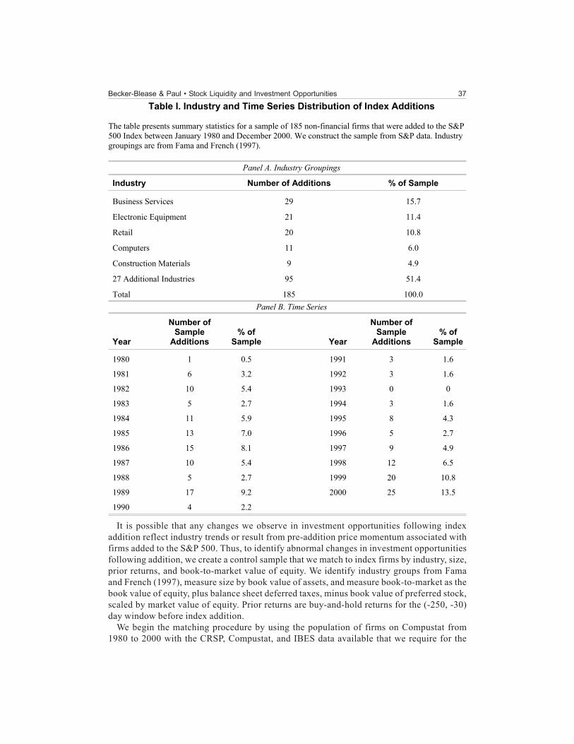
We begin the sample selection process by identifying non-financial firms that are added tothe S&P 500 between January 1980 and December 2000, using data obtained from Standard &Poor’s. The final sample comprises 185 firms that we are able to match with control firmsusing the procedure described later in this section. Table I, Panel A, reports the distributionof industries represented by nine or more sample firms. There are 32 total industries, withBusiness Services, Electronic Equipment, and Retail having the highest representation. PanelB reports the time series of index additions. It indicates active periods of index additionsfrom 1984-1987 and 1998-2000, which reflect general trends in industry consolidation of non-financial firms.

2S&P 500 Fact Sheet: http://www2.standardandpoors.com/spf/pdf/index/500factsheet.pdf.

Becker-Blease & Paul • Stock Liquidity and Investment Opportunities 37

Table I. Industry and Time Series Distribution of Index Additions

The table presents summary statistics for a sample of 185 non-financial firms that were added to the S&P 500 Index between January 1980 and December 2000. We construct the sample from S&P data. Industry groupings are from Fama and French (1997).

Panel A. Industry Groupings

Industry Number of Additions % of Sample

Business Services 29 15.7

Electronic Equipment 21 11.4

Retail 20 10.8

Computers 11 6.0

Construction Materials 9 4.9

27 Additional Industries 95 51.4

Total 185 100.0 Panel B. Time Series

Year

Number of Sample

Additions % of

Sample Year

Number of Sample

Additions % of

Sample

1980 1 0.5 1991 3 1.6

1981 6 3.2 1992 3 1.6

1982 10 5.4 1993 0 0

1983 5 2.7 1994 3 1.6

1984 11 5.9 1995 8 4.3

1985 13 7.0 1996 5 2.7

1986 15 8.1 1997 9 4.9

1987 10 5.4 1998 12 6.5

1988 5 2.7 1999 20 10.8

1989 17 9.2 2000 25 13.5

1990 4 2.2 It is possible that any changes we observe in investment opportunities following index

addition reflect industry trends or result from pre-addition price momentum associated withfirms added to the S&P 500. Thus, to identify abnormal changes in investment opportunitiesfollowing addition, we create a control sample that we match to index firms by industry, size,prior returns, and book-to-market value of equity. We identify industry groups from Famaand French (1997), measure size by book value of assets, and measure book-to-market as thebook value of equity, plus balance sheet deferred taxes, minus book value of preferred stock,scaled by market value of equity. Prior returns are buy-and-hold returns for the (-250, -30)day window before index addition.

We begin the matching procedure by using the population of firms on Compustat from1980 to 2000 with the CRSP, Compustat, and IBES data available that we require for the


analysis. Next, to ensure that firms are not candidates for matching in the years that they arein our sample of index additions, we delete observations for index firms in the year of, andthree years before and after, their addition year. From this pool of potential matches, weidentify the group of firms in the same Fama and French (1997) industry grouping with totalassets and book-to-market within 40% of the sample firm, and delete firms that do not havepotential matches after this screen. Finally, we select the firm with the closest prior stockreturn match, yielding 185 pairs of sample and control firms.

We note that the 40% matching band is wider than conventional 20% matching bands. AsHegde and McDermott (2003) show, S&P 500 firms are, on average, positive momentumstocks. This price run-up makes it difficult to find industry peers of similar size and priorreturns. The industry match is necessary to ensure that any changes in investmentopportunities we observe are firm-specific, and not due to overall changes in industry growthopportunities. Thus, to minimize the distance in prior returns between sample and controlfirms in the same industry, we expand the match bands for size and book-to-market.

Table II contains descriptive statistics for sample and control firms in the fiscal yearbefore index addition. Results in the table indicate that in spite of efforts to match on sizeand prior returns, there are significant differences between sample and control firms forthese variables. The median paired difference (sample minus control) is $81.4 million forbook value of assets, and 8.8% for prior returns, both significant at the 1% level. However,differences for book-to-market equity, R&D spending, and cash are not significantly differentfrom zero. In light of this evidence of significant differences between some firms and theirmatches, we include pre-addition differences in all the match variables as controls in themultivariate analysis.

The remaining variables in Table II are financial leverage, EBITDA, and return on assets.Financial leverage is long-term debt scaled by book value of assets, EBITDA is earningsbefore interest, taxes, depreciation, and amortization, and return on assets is EBITDA scaledby total assets. The table shows that sample firms have better operating performance in theyear before addition compared to the matched control firms. This evidence, together withthe results for size and prior returns, supports the prevailing opinion that index candidatesare industry leaders.

B. Proxies for Investment Opportunities and Stock Liquidity

If firms experience an increase in their investment opportunity set, which we cannot observe,we expect the increase to translate into increased capital expenditures, which we can observe.Capital expenditures reflect managerial efforts to exploit current investment opportunities.Thus, similar to Denis (1994) and Pilotte (1992), we use changes in capital expenditures as anex post proxy for changes in investment opportunities.

We define the measurement periods for capital expenditures as follows. The pre-addition (e-1) period is from the end of the fiscal year before addition, and the post-addition (e+1) measureis from the end of the fiscal year following the addition year. We refer to the change from e-1 toe+1 as a one-year change. Growth opportunities may need more than one year to be realized incapital expenditures, so we also evaluate changes for a three-year period surrounding indexaddition. The three-year change in capital expenditures is the average of the three fiscal yearsfollowing addition minus the average for the three fiscal years before addition.

There is sample attrition during the second and third fiscal years following addition, primarilydue to acquisitions. To preserve sample size for the analysis that requires three-year measures,we compute the two-year average change in capital expenditures for cases in which either the


Table II. Descriptive Statistics The table presents descriptive statistics for 185 non-financial firms that were added to the S&P 500 Index between January 1980 and December 2000, and 185 control firms matched on industry, size, book-to-market equity, and stock returns in the year prior to addition. Total Assets is Compustat item #6, Sales is Compustat item #12, Book/Market Value of Equity is book value of equity, plus balance sheet deferred taxes, minus book value of preferred stock, scaled by market value of equity. R&D is Compustat item #46 and Cash is Compustat item #1. Long-Term Debt is Compustat item #9, EBITDA is Compustat item #13, and Return on Assets is EBITDA scaled by Total Assets. Cumulative stock return is the raw return for the (-250, -30) day window before index addition. With the exception of cumulative returns, we calculate all values at the end of the fiscal year preceding addition. Mean (Median) Paired Differences are the mean (median) difference between the matched sample and control pairs, with p-values from t-tests (Wilcoxon Signed Rank tests) that the paired difference is zero.

Sample Control Paired

Difference p-value Total Assets ($MM) 1,892.76

(956.66) 1,793.60

(936.55) 99.16

(81.38) 0.099

(0.000)

Book to Market Value of Equity

0.445 (0.324)

0.434 (0.323)

0.011 (-0.005)

0.238 (0.845)

R&D / Sales (%) 4.06 (0.00)

5.71 (0.00)

-1.65 (0.00)

0.259 (0.844)

Cash / Total Assets (%) 16.98 (9.10)

15.45 (9.25)

0.73 (0.14)

0.604 (0.783)

Long-Term Debt / Total Assets (%)

16.16 (14.97)

19.25 (15.59)

-3.09 (-0.88)

0.031 (0.101)

EBITDA ($MM) 291.83 (185.16)

268.70 (172.65)

24.45 (27.27)

0.214 (0.002)

Return on Assets (%) 19.59 (19.44)

18.10 (18.89)

1.48 (1.30)

0.040 (0.066)

Cumulative Stock Return (%) 0.606 (0.310)

0.279 (0.172)

0.328 (0.088)

0.000 (0.000)

sample or control firm is missing Year 3 data, and compute the one-year change for pairsmissing Year 2 data. We treat missing observations in the pre-addition period in the same way.The results are qualitatively similar if we delete firms with missing observations.

We construct three proxies for stock liquidity using CRSP data. The first is the illiquidityratio, which Amihud (2002) uses as a proxy for the price impact of a trade. The illiquidity ratiois the average of the ratio of daily absolute return to the daily volume in dollars.

(1)


where Rid is the return on stock i on day d, VOLDid is the corresponding daily volume indollars, and Di is the number of days with data available for stock i during the pre- and post-addition measurement periods.

The two additional liquidity proxies are volume and share turnover. Volume is the naturallog of the average of daily number of shares traded times closing price. Turnover is monthlynumber of shares traded divided by the number of shares outstanding, and we divide Nasdaqtrading volume by two to correct for the upward bias in volume in dealer markets. In measuringthe liquidity proxies, we exclude the event month and the two months surrounding it. Thus,if the event month is m, we begin measuring pre-addition liquidity in month m-2, andmeasurement of post-addition liquidity in month m+2. One-, two-, and three-year levelscorrespond to data for 12, 24, and 36 months surrounding the event months. We follow thesame method as we did for capital expenditures for sample or control firms with missing Year3 or Year 2 data, and for missing observations in the pre-addition period.

II. Changes in Stock Liquidity and Capital Expenditures

In this section, we examine overall changes in stock liquidity and capital expenditures forsample firms following their addition to the S&P 500.

A. Changes in Stock Liquidity

Table III contains levels and changes for liquidity proxies in the three years followingindex addition, compared to the three years before addition. Columns (1) and (2) show thatby all measures of liquidity, sample firms have higher pre-addition liquidity than do controlfirms. We also note that the mean pre-listing illiquidity ratio of 0.217 is lower than the averageof 0.337 reported in Amihud (2002) for NYSE stocks over the period 1963-1996. This evidenceof higher pre-listing liquidity is not surprising, given Standard and Poor’s stated intent ofselecting firms with high liquidity as candidates for index inclusion.

The post-addition levels and changes in the liquidity proxies in Columns (3) through (6) ofTable III are consistent with results from earlier studies that index addition is a liquidity-enhancing event. Although there is a general improvement in liquidity for both sample andcontrol firms, the increase in liquidity is significantly higher for sample firms. Column (5)shows significant positive median one-year changes in paired differences of -0.009 for theilliquidity ratio, 0.403 for volume, and 0.011 for turnover. The changes for three-year averagesin Column (6) are also positive and highly significant, indicating that the relative liquidityimprovement persists for at least three years subsequent to index addition.

B. Changes in Capital Expenditures

Table IV contains changes in capital expenditures for the one- and three-year periodsfollowing index addition, compared to the year before addition. We scale capital expendituresby total assets in the pre-addition fiscal year to provide meaningful comparisons of changesfollowing addition. Column (3) contains capital expenditures for the year before addition andshows mean (median) capital spending of 9.24% (7.85%) of total assets for sample firmscompared to 9.8% (8.02%) for control firms, with paired differences that are not significantlydifferent from zero. Columns (1) and (2) show that this statistically insignificant differencebetween sample and control firms is also present in the two earlier fiscal years. Thus, it isunlikely that the changes documented in the table represent pre-existing momentum in capital

Becker-Blease & Paul • Stock Liquidity and Investment Opportunities 41Table III. Changes in Stock Liquidity

The table presents mean (median) liquidity changes following the addition of 185 non-financial firms to the S&P 500 Index between January 1980 and December 2000. We match control firms on industry, size, book-to-market equity, and stock returns in the year prior to addition. We measure liquidity as the average of the absolute value of the daily return divided by the daily volume in dollars multiplied by 106 (Illiquidity Ratio), the average of daily number of shares traded times closing price (Volume), and monthly share volume divided by shares outstanding (Turnover Ratio). These measures exclude data from the event month and the two months surrounding it. For example, e-3, e-2, and e-1 refer to liquidity measured between months 37 to 26, 25 to 14, and 13 to two preceding the event month, respectively. Liquidity difference is the mean [median] difference between each sample and control firm. We measure the average levels of liquidity (Columns 1 and 4 as the three-year average pre-addition (e-1_3) and post-addition (e+1_3). If a firm delists prior to the third year, or lacks sufficient data in the pre-period, we substitute the two- or one-year averages. We conduct t-tests (Wilcoxon sign rank tests) that the mean (median) paired difference or change is equal to zero.

Panel A. Illiquidity Ratio

(1)

e-1_3 (2) e-1

(3) e+1

(4) e+1_3

(5) e-1 to e+1

(6) e-1_3 to e+1_3

Sample 0.217 0.056

0.150 0.031

0.068 0.021

0.076 0.023

-0.082*** -0.007***

-0.141***

-0.022*** Control 0.457

0.078 0.411 0.053

0.307 0.065

0.507 0.091

-0.104 -0.001

0.050 -0.006*

Difference -0.240*** (-0.008)***

-0.261*** (-0.010)***

-0.239*** (-0.023)***

-0.431*** (-0.028)***

-0.022

(-0.009)*** -0.191**

(-0.022)***

Panel B. Volume

(1)

e-1_3 (2) e-1

(3) e+1

(4) e+1_3

(5) e-1 to e+1

(6) e-1_3 to e+1_3

Sample 15.587 (15.522)

15.868 (15.723)

16.353 (16.036)

16.450 (16.255)

0.484*** (0.496)***

0.863*** (0.840)***

Control 15.087 (15.086)

15.255 (15.125)

15.265 (15.198)

15.354 (15.182)

0.027 (0.047)

0.294*** (0.328)***

Difference 0.531*** (0.426)***

0.632*** (0.482)***

1.087*** (0.856)***

1.096*** (0.947)***

0.456*** (0.403)***

0.573*** (0.527)***

Panel C. Turnover Ratio

(1)

e-1_3 (2) e-1

(3) e+1

(4) e+1_3

(5) e-1 to e+1

(6) e-1_3 to e+1_3

Sample 0.141 (0.071)

0.144 (0.077)

0.181 (0.092)

0.183 (0.100)

0.037*** (0.013)***

0.042*** (0.015)***

Control 0.117 (0.074)

0.125 (0.080)

0.135 (0.076)

0.134 (0.085)

0.011*

(0.003)** 0.017**

(0.006)*** Difference 0.023**

(0.009)** 0.019*

(0.006)* 0.046***

(0.020)*** 0.048***

(0.018)*** 0.026***

(0.011)*** 0.025**

(0.008)*** ***Significant at the 0.01 level. **Significant at the 0.05 level. *Significant at the 0.10 level.


(1

)

e-3

(2)

e-2

(3)

e-1

(4) e

(5)

e+1

(6)

e+2

(7)

e+3

(8)

e-1_

3

(9)

e+1_

3

(10)

e-1

to e

(11)

e to

e+1

(12)

e-1

to e

+1

(13)

e-1_

3 to

e+1

_3

Samp

le 6.6

73

(5.62

1)

[183

]

7.782

(6

.620)

[1

85]

9.242

(7

.849)

[1

85]

12.41

1 (1

0.408

) [1

85]

16.76

4 (1

2.297

) [1

85]

16.95

4 (1

1.542

) [1

83]

16.81

2 (1

0.245

) [1

73]

7.898

(7

.235)

[1

85]

16.90

6 (1

1.327

) [1

85]

3.

170**

*

(2.0

96)**

*

[185

]

4.

352**

*

(1.0

66)**

*

[185

]

7.52

2***

(3.2

88)**

*

[185

]

7.

645**

*

(3.3

49)**

*

[185

] Co

ntrol

6.741

(5

.636)

[1

81]

7.384

(6

.111)

[1

85]

9.800

(8

.024)

[1

85]

10.58

5 (8

.676)

[1

85]

10.82

3 (7

.495)

[1

85]

10.72

5 (8

.108)

[1

77]

11.52

6 (8

.161)

[1

64]

8.040

(6

.317)

[1

85]

10.85

0 (8

.405)

[1

85]

0.785

*

(0.27

0)**

[185

]

0.238

(-0

.416)

*

[185

]

1.023

(-0

.135)

[1

85]

1.050

*

(0.34

6)

[185

] Di

ff.

0.042

(0

.421)

[1

79]

0.398

(0

.303)

[1

85]

-0.55

8 (-0

.055)

[1

85]

1.8

26**

(2.0

46)**

*

[185

]

5.9

41**

*

(3.6

54)**

*

[185

]

6.

199**

*

(3.1

86)**

*

[173

]

5.9

02**

*

(2.2

96)**

*

[152

]

-0.14

2 (-0

.413)

[1

85]

6.05

62**

*

(3.48

49)**

*

[185

]

2.

385**

*

(1.3

72)**

*

[185

]

4.

115**

*

(1.5

97)**

*

[185

]

6.

499**

*

(3.3

92)**

*

[185

]

6.

615**

*

(3.3

43)**

*

[185

] **

*Sign

ifica

nt at

the 0.

01 le

vel.

**S

ignifi

cant

at the

0.05

leve

l.

*Sign

ifica

nt at

the 0.

10 le

vel.

Tabl

e IV

. Cha

nges

in C

apita

l Exp

endi

ture

s

The

tabl

e sh

ows t

he m

ean

(med

ian)

cha

nges

in c

apita

l exp

endi

ture

s fol

low

ing

the

addi

tion

of 1

85 n

on-fi

nanc

ial f

irms t

o th

e S&

P 50

0 In

dex

betw

een

Janu

ary

1980

and

Dec

embe

r 200

0. W

e m

atch

con

trol f

irms o

n in

dustr

y, si

ze, b

ook-

to-m

arke

t equ

ity, a

nd st

ock

retu

rns i

n th

e ye

ar p

rior t

o ad

ditio

n. T

he ta

ble

cont

ains

leve

ls an

ddi

ffere

nces

bet

wee

n sa

mpl

e and

cont

rol f

irms’

capi

tal e

xpen

ditu

res (

Com

pusta

t ite

m #

30) s

cale

d by

tota

l ass

ets (

Com

pusta

t ite

m #

6) at

e-1

(the f

iscal

yea

r pre

cedi

ngin

dex

addi

tion)

in th

e yea

rs su

rroun

ding

inde

x ad

ditio

n. W

e mea

sure

the a

vera

ge le

vels

of li

quid

ity (C

olum

ns 8

and

9) as

the t

hree

-yea

r ave

rage

pre

-add

ition

(e-1

_3)

and

post-

addi

tion

(e_1

+3).

If a

firm

del

ists b

efor

e th

ree

year

s, or

lack

s suf

ficie

nt d

ata

in th

e pr

e-pe

riod,

we

subs

titut

e th

e tw

o- o

r one

-yea

r ave

rage

s. W

e co

nduc

t t-

tests

(Wilc

oxon

sign

rank

tests

) tha

t the

mea

n (m

edia

n) p

aire

d di

ffere

nce

or c

hang

e is

equa

l to

zero

. Num

ber o

f obs

erva

tions

is in

[bra

cket

s].


expenditures that continues following addition. However, we do control for the pre-additiongrowth rate in capital expenditures in the multivariate analysis.

Column (12) of Table IV shows that from the fiscal year before index addition through theyear following addition, sample firms have significant mean (median) increases in capitalexpenditures of 7.52% (3.29%). Control firms do not have significant increases in capitalexpenditures during this period. The significant mean (median) change of 6.5% (3.39%) inthe paired differences indicates abnormal growth in capital expenditures for sample firms.

For further comparison, we check the population of Compustat firms during our sampleperiod. The median one-year change in capital expenditures is 0.57%, and the median changefor sample firms falls near the 85th percentile of this population. This finding suggests thatthe increase for sample firms is a material shift in capital investments.

To further investigate the timing and pattern of changes in capital expenditures, we includeadditional yearly data in Table IV. Columns (1) through (3) show that both sample and controlfirms have similar, albeit modest, increases in capital expenditures for each of the three fiscalyears preceding index addition. Columns (3), (4), and (10) show that from the fiscal yearbefore addition to the year of addition, sample firms increase capital spending at a significantlyhigher rate than do control firms, indicating that the shift in capital spending begins in theyear of index addition for some firms. Columns (4), (5), and (11) show an even greater abnormalincrease in capital spending by sample firms from the year of addition to the year followingaddition. This increase stabilizes after the first fiscal year following addition, as shown inColumns (5), (6), and (7), and also by the similarity in the magnitude of one year changes andaverage three-year changes in Columns (12) and (13).

We draw two conclusions from the evidence in Table IV. First, the capital spending patternsfor sample and control firms in the three fiscal years preceding index addition do not suggestthat Standard and Poor’s chooses firms that are pursuing aggressive internal expansion.This result allays any concerns that the post-addition changes that we observe merelyreflect Standard and Poor’s selection criteria. Second, the evidence indicates that the shift incapital spending that follows index addition occurs fairly quickly, and that spendingmomentum ends by the first fiscal year following addition.

III. Stock Liquidity and Capital Expenditures

We hypothesize that, if liquidity is a priced factor in equity returns, corporate managerswill perceive an increased set of viable investments following a liquidity enhancing shock,and increase capital investment intensity. We test this relation by estimating OLS coefficientsfor changes in capital expenditures on changes in stock liquidity. All levels in the regressionsare paired differences (sample minus control) and all changes are changes in paireddifferences. The liquidity variables are transformed to natural logs for the regressions.

The regressions include the variables we used to create the matched control sample,namely firm size (natural log of total assets), book-to-market equity, and prior returns. Weinclude these variables because, in spite of our attempt to match on these dimensions, theunivariate statistics in Table II indicate some differences between the samples on the matchvariables. We include additional variables to control for their likely effect on changes incapital expenditures. Capital expenditure growth controls for the effect of capital spendingmomentum on changes in expectations for future growth, and is measured as the three-yearaverage growth as of the fiscal year before addition. Control variables for access to capitalare pre-addition cash, financial leverage, ROA growth, and post-addition change in operating


income and earnings forecast dispersion. Financial leverage is long-term debt scaled bybook value of assets. ROA is EBITDA scaled by book value of assets, and ROA growth isfrom three years before addition to the year preceding addition. Post-addition change inoperating income is EBITDA in the fiscal year following addition minus EBITDA in the fiscalyear before addition, scaled by pre-addition total assets.

To control for the effect of changes in the information environment, we include changes inearnings forecast dispersion. We do so because, as investor attention increases followingindex addition, it is possible for information asymmetry to decrease, resulting in improvedmarket conditions for external capital issues (Myers and Majluf, 1984). In such cases, firmscould increase capital spending on projects that were viable before addition, but shelvedbecause of capital raising constraints. Dispersion is the standard deviation of analysts’earnings forecasts on IBES, deflated by stock price five days before the earningsannouncement date.

Table V contains OLS coefficient estimates for one-year change in capital expenditures onone-year change in stock liquidity. We estimate a model for each of the three liquidity proxies:the illiquidity ratio in Model (1), volume in Model (2), and share turnover in Model (3). In allthree models, the proxies for stock liquidity have significant coefficients in the predicteddirection. Abnormal changes in capital expenditures are increasing in volume and shareturnover, and are decreasing in the illiquidity ratio.

The evidence in the table is consistent with the hypothesis that corporate managersrespond to improvements in stock liquidity (and corresponding declines in the cost of capital)by increasing capital investment intensity. The coefficient estimates indicate that, holdingother variables constant, a 1% improvement in liquidity is associated with increases incapital expenditures ranging from 0.04 percentage points in Model (1) to 0.11 percentagepoints in Model (3). We consider these effects to be important, since the univariate evidencein Column (3) of Table IV indicates that the pre-addition level of capital expenditures (sampleminus control firm) is -0.558 percentage points. When we compare the coefficient estimatesfor the liquidity proxies with the positive and significant coefficients for change in operatingincome, we find that the partial effect of liquidity changes on capital spending is roughlyone-quarter to one-half of the partial effect of changes in income.

The results also show a significant positive coefficient on change in operating income,suggesting that internally generated capital is an important source of financing for capitalspending. The pre-listing difference in cash is significant in Model (3), suggesting that pre-addition cash stockpiles partially fund changes in capital spending. However, this result isnot robust to other specifications of the liquidity proxy in Models (1) and (2). In addition, thestatistically insignificant coefficients on financial leverage indicate that pre-addition debtlevels are unrelated to changes in capital spending. Overall, the evidence on these financingvariables suggests that abnormal changes in operating income are relatively more importantthan is pre-existing capital structure in explaining abnormal changes in capital expenditures.

We also test whether the positive relation between changes in capital expenditures andchanges in stock liquidity persist over a longer time horizon following the index additionevent by estimating the model in Table V for three-year changes. The three-year change incapital expenditures is measured as the average of the three fiscal years following additionminus the average for the three fiscal years before addition (Column 13 of Table IV). Three-year changes in liquidity are measured for the 36 months surrounding the event month(Column 6 of Table III). The results of the regression (not reported in a table) indicate thatthe positive relation between changes in capital expenditures and changes in stock liquidityobtains for this longer post-event window. Except for share turnover, the coefficients on the


Table V. OLS Coefficients for Changes in Capital Expenditures on Changes in Stock Liquidity

The table presents the regression coefficient estimates for the relation between stock liquidity and capital expenditures. The sample consists of non-financial firms added to the S&P 500 index between January 1980 and December 2000. All differences described in the table are paired differences between each sample firm and a control firm matched on industry, size, book-to-market equity, and stock returns in the year prior to addition. The dependent variable, Change in Capital Expenditures, is the change in the difference for capital expenditures for the fiscal year following addition minus the fiscal year before addition. We scale capital expenditures by total assets at the fiscal year-end prior to addition. The illiquidity ratio is the natural log of the average of the absolute value of the daily return divided by the daily volume in dollars. Change in Illiquidity Ratio is the change in the difference for the 12-month period following index addition compared to the 12-month period before index addition, excluding the event month and the two months surrounding it. Volume is the natural log of the average of daily volume multiplied by closing price. Share Turnover is the natural log of monthly number of shares traded divided by the number of shares outstanding. We compute change in volume and change in share turnover in the same way as the change in the illiquidity ratio. Book-to-Market is the difference in the ratio of book value of equity, plus balance sheet deferred taxes, minus book value of preferred stock, to the market value of equity in the fiscal year preceding the index addition year. Log (Total Assets) is the difference in the log of Compustat item #6 in the fiscal year preceding the index addition year. Capital expenditure growth rate is the difference in the three-year growth rate of capital expenditures (Compustat item #30), from the four fiscal years preceding addition to one year prior to addition. Log (Cash) is the difference in the log of Compustat item #1 for the fiscal year preceding index addition. Debt/Total Assets is the difference in the ratio of long-term debt (Compustat item #9) to total assets for the fiscal year preceding index addition. ROA Growth Rate is the difference in the growth rate in ROA from three fiscal years preceding addition to one year preceding addition. Prior Stock Return is the difference in the cumulative raw return for (-250, -30) days prior to index addition. Change in Operating Income is the change in the difference between sample and control firms in the level of EBITDA (Compustat item #13) in the year subsequent to addition minus the year preceding addition, scaled by total assets preceding addition. Change in Earnings Forecast Dispersion is the change in the difference in standard deviation of analysts’ forecasts scaled by the firm’s stock price five days prior to the earnings announcement from the fiscal year preceding index inclusion to the fiscal year subsequent to inclusion. (1) (2) (3) Change in Illiquidity Ratio -0.0402***

(0.0141)

Change in Volume 0.0529***

(0.0161)

Change in Share Turnover 0.1055***

0.0267 Log (Total Assets) 0.0030

(0.0543) 0.0014

(0.0535) -0.0165 0.0522

Book-to-Market 0.0357 (0.0989)

-0.0048 (0.0555)

0.0160 0.0966

Capital Expenditure Growth Rate -0.0061 (0.0070)

-0.0058 (0.0071)

-0.0060 0.0068

Log (Cash) 0.0054 (0.0078)

0.0085 (0.0078)

0.0156**

0.0078 Debt/Total Assets 0.0057

(0.0678) 0.0162

(0.0675) 0.0525 0.0655

ROA Growth Rate 0.2201 (0.1504)

0.1690 (0.1521)

0.1569 0.1481


Table V. OLS Coefficients for Changes in Capital Expenditures on Changes in Stock Liquidity (Continued)

(1) (2) (3) Prior Stock Return -0.0002

(0.0020) -0.0004 (0.0020)

-0.0005 0.0020

Change in Operating Income 0.1561**

(0.0688) 0.1356*

(0.0696) 0.1934***

0.0631 Change in Earnings Forecast Dispersion -0.2070

(0.7654) -0.3266 (0.7598)

-0.5608 0.7488

Intercept 0.0336 (0.0250)

0.0360 (0.0246)

0.0482**

0.0234 N 185 185 185 F-statistic 2.65 2.93 3.48 p-value of model 0.005 0.002 0.000 Adjusted R2 8.31 9.62 11.92 ***Significant at the 0.01 level. **Significant at the 0.05 level. *Significant at the 0.10 level.

liquidity proxies are in the predicted direction and significant at the 1% level.

The results indicate that changes in stock liquidity are positively related to changes incapital expenditures following an exogenous liquidity-enhancing shock. Our interpretationof this evidence is that as the liquidity premium in expected returns decreases, there is anincrease in investment opportunities at the margin, and the set of viable investmentopportunities expands.

IV. Additional Tests

We perform two sets of robustness tests in this section. First, we estimate the model usingalternative proxies for investment opportunities. Second, we estimate the model for thesubset of 127 sample firms that are matched to control firms on the same trading venue tocheck whether differences in the way trading volume is recorded for Nasdaq versus NYSE/AMEX stocks influence the results reported above.

A. Alternative Proxies for Investment Opportunities

We consider three alternative proxies for investment opportunities: research anddevelopment expenditures, book-to-market equity, and analysts’ long-term growth forecasts.In contrast to capital expenditures, these proxies reflect expectations, rather than realizations.To test whether they are also increasing in stock liquidity, we conduct additional OLSanalyses of changes in these variables on changes in stock liquidity.

1. Research and Development Expenditure

Empirical evidence shows that R&D expenditures represent a firm’s investment in futuregrowth (e.g., Eberhart, Maxwell, and Siddique, 2004), and in this sense can be a proxy for thefirm’s investment opportunity set. We collect R&D expenditures for the same time periods ascapital expenditures, that is, the fiscal year before addition, and the fiscal year following the


addition year. To preserve sample size, we follow the standard practice of replacing missingvalues of R&D with zero. We then estimate the model in Table V, replacing change in capitalexpenditures with change in R&D spending scaled by sales for the dependent variable.

Table VI presents OLS coefficients for change in R&D on change in liquidity. We findsignificant coefficients in the predicted direction for all three liquidity proxies. These resultsgenerally support the hypothesis that changes in investment opportunities, as measured byR&D spending, are increasing in changes in stock liquidity. The coefficients on the liquidityvariables are comparable in magnitude to the coefficient sizes in the capital expenditureregressions, indicating that the change in liquidity has similar effects on changes in bothR&D spending and capital spending.

Other variables enter the model with significance. The positive coefficients on pre-additioncash levels and financial leverage indicate that relative to their industry peers, firms withgreater pre-addition cash stockpiles and financial leverage are more likely to have abnormalincreases in R&D spending. We also note a negative, significant coefficient on pre-additionROA growth in all three models, indicating that firms with relatively higher pre-additiongrowth are less likely to have abnormal increases in growth opportunities.

2. Book-to-Market Value of Equity

The second alternative proxy for investment opportunities is the book-to-market value ofequity. It is generally agreed that high book-to-market denotes a low-growth (value) stock, andlow book-to-market denotes a high-growth (glamour) stock. Thus, a decrease in book-to-market is consistent with an increase in growth opportunities. We estimate regression modelssimilar to those in Table V for capital expenditures, but using the one-year change in the paireddifference of the book-to-market as the dependent variable. Changes in the book-to-market aremeasured for the same time period as changes in capital expenditures. Untabulated resultsshow a significant, positive coefficient on change in the illiquidity ratio, a significant negativecoefficient on volume, and an insignificant negative coefficient on turnover.

These results are consistent with an increase in investment opportunities as liquidityincreases. However, Hegde and McDermott (2003) find a positive relation between changesin stock liquidity and index addition announcement returns, indicating that the increase instock prices upon addition is related to changes in liquidity. In light of their evidence, wenote that our tests cannot distinguish whether the negative relation between changes instock liquidity and changes in book-to-market indicates increased investment opportunities,or merely a higher valuation of current investments due to a lower discount rate. Nonetheless,together with the evidence for capital expenditures and R&D spending, the results for book-to-market lend support to the hypothesis that investment opportunities are increasing instock liquidity.

3. Analysts’ Long-Term Growth Forecasts

We use analysts’ long-term growth forecasts as a third alternative proxy for growthopportunities. We collect forecasts for three- to five-year growth in earnings from IBES, andmeasure levels and changes in these long-term growth forecasts as follows. The pre-additiongrowth estimate is the median forecast from one full quarter before the quarter of addition,and the post-addition estimate is the median forecast from the first fiscal-year-end forecastsmade at least one full quarter after addition.

To test whether analysts update their long-term growth forecasts as stock liquidity changes,we estimate OLS coefficients for changes in these growth forecasts on changes in stockliquidity, and the other independent variables in Tables V and VI. The results provide additional


Table VI. OLS Coefficients for Changes in R&D Expenditures on Changes in Stock Liquidity

The table presents regression coefficient estimates for the relation between stock liquidity and research and development expenditures. The sample consists of non-financial firms added to the S&P 500 index between January 1980 and December 2000. All differences described below are paired differences between each sample firm and a control firm matched on industry, size, book-to-market equity, and stock returns in the year prior to addition. The dependent variable, Change in R&D expenditures is the change in the difference for research and development expenditures for the fiscal year following addition minus the fiscal year before addition. We scale R&D expenditures by sales at the fiscal year-end prior to addition. The Illiquidity Ratio is the natural log of the average of the absolute value of the daily return divided by the daily volume in dollars. Change in Illiquidity Ratio is the change in the difference for the 12-month period following index addition compared to the 12-month period before index addition, excluding the event month and the two months surrounding it. Volume is the natural log of the average of daily volume multiplied by closing price. Share Turnover is the natural log of monthly number of shares traded divided by the number of shares outstanding. Change in Volume and Change in Share Turnover are computed in the same way as the change in the illiquidity ratio. Book-to-market is the difference in the ratio of book value of equity, plus balance sheet deferred taxes, minus book value of preferred stock, to the market value of equity in the fiscal year preceding index addition year. Log (Total Assets) is the difference in the log of Compustat item #6 in the fiscal year preceding index addition year. Capital Expenditure Growth Rate is the difference in the three-year growth rate of capital expenditures (Compustat item #30), from four fiscal years preceding addition to one year prior to addition. Log (Cash) is the difference in the log of Compustat item #1 for the fiscal year preceding index addition. Debt/Total Assets is the difference in the ratio of long-term debt (Compustat item #9) to total assets for the fiscal preceding index addition. ROA Growth Rate is the difference in the growth rate in ROA from three fiscal years preceding addition to one year preceding addition. Prior Stock Return is the difference in the cumulative raw return for (-250, -30) days prior to index addition. Change in Operating Income is the change in the difference between sample and control firms in the level of EBITDA (Compustat item #13) in the year subsequent to addition minus the year preceding addition, scaled by total assets preceding addition. Change in Earnings Forecast Dispersion is the change in the difference in standard deviation of analysts’ forecasts scaled by the firm’s stock price five days prior to the earnings announcement from the fiscal year preceding index inclusion to the fiscal year subsequent to inclusion. Standard errors appear below coefficient estimates. (1) (2) (3) Change in Illiquidity Ratio -0.0528**

0.0236

Change in Volume 0.0383*

0.0215

Change in Share Turnover 0.0773*

0.0458 Log (Total Assets) -0.0620

0.0905 -0.0806 0.0911

-0.0898 0.0894

Book-to-Market -0.1440 0.1649

-0.1428 0.1692

-0.1610 0.1655

Capital Expenditure Growth Rate 0.0057 0.0117

0.0052 0.0118

0.0051 0.0117

Log (Cash) 0.0243*

0.0129 0.0280**

0.0131 0.0335**

0.0133 Debt/Total Assets 0.3057***

0.1130 0.3190***

0.1143 0.3523***

0.1122 ROA Growth Rate -0.5588**

0.2509 -0.5802**

0.2551 -0.6003**

0.2538 Prior Stock Return 0.0011

0.0033 0.0009 0.0034

0.0008 0.0034

Becker-Blease & Paul • Stock Liquidity and Investment Opportunities 49 Table VI. OLS Coefficients for Changes in R&D Expenditures on Changes in

Stock Liquidity (Continued)

(1) (2) (3) Change in Operating Income -0.2065*

0.1148 -0.1829 0.1180

-0.1462 0.1081

Change in Earnings Forecast Dispersion -0.4711 1.2767

-0.6469 1.2897

-0.7986 1.2826

Intercept 0.0273 0.0418

0.0415 0.0415

0.0507 0.0401

N 185 185 185 F-statistic 2.37 2.03 2.27 p-value of model 0.011 0.033 0.016 Adjusted R2 7.02 5.38 5.61 ***Significant at the 0.01 level. **Significant at the 0.05 level. *Significant at the 0.10 level.

support for the hypothesis that changes in stock liquidity influence the firm’s investmentopportunity set. There is a negative, significant coefficient on the illiquidity ratio, a positive,significant coefficient on volume, and a positive but insignificant coefficient on turnover.

B. Samples Matched on Trading Venue

In our analysis, we follow the standard practice of dividing Nasdaq volume by two tocorrect for the upward bias in trading volume due to double counting of dealer trades.However, because Nasdaq volume is not necessarily biased up by a factor of two in allcases, it is possible that inconsistent treatment of sample and control pairs across tradingvenues influences the results.

To check for any effect of differences in trading characteristics, we re-estimate theregression models in Table V for the subsample of 127 firms that have the same tradingvenue as their matched control firm. The Table V results for the full sample persist for thissubsample of firms. The coefficients on all three liquidity proxies are in the predicted directionand significant at the 5% level or better.

We also estimate the model for the subsample of 95 sample firms traded on NYSE or Amexthat are matched to firms on the same trading venue. For this subsample, the coefficients onthe three liquidity proxies are also significant and in the predicted direction.

V. Conclusion

In this article, we investigate the liquidity premium hypothesis by testing whetherinvestment opportunities are increasing in stock liquidity. Amihud and Mendelson (1986)demonstrate that an improvement in stock liquidity decreases the firm’s cost of capital. Weargue that this not only increases the value of assets in place, as Amihud and Mendelson(1988) show, but also increases the firm’s set of viable investment opportunities. This isbecause, with a lower cost of capital, managers are likely to accept projects that previouslyhad negative net present values. Thus, we hypothesize that an improvement in stock liquidityresults in increased growth opportunities.


Our sample comprises firms that are newly added to the S&P 500 list because there isevidence that these firms experience an overall increase in stock liquidity following indexinclusion. In addition, because the liquidity shock is exogenous, our tests are unlikely to bebiased by unobservable characteristics of firms that exert effort to increase stock liquidity.

In the empirical analysis, we test the hypothesis that investment opportunities areincreasing in stock liquidity by regressing abnormal changes in capital expenditures onabnormal changes in stock liquidity. We define abnormal changes as post-addition changesin paired differences between each sample firm and a control firm matched on industry, size,book-to-market, and prior returns.

We find that, relative to their industry peers, newly added firms have abnormal increasesin capital expenditures, and that these changes in capital expenditures are positively relatedto changes in stock liquidity. This finding is consistent with the hypothesis that growthopportunities are increasing in stock liquidity. We find similar relations for alternative proxiesfor investment opportunities, such as R&D spending, book-to-market, and analysts’ long-termgrowth forecasts. The results are robust to the inclusion of variables that are likely to explainchanges in growth opportunities, such as availability of cash, pre-addition capital expendituremomentum, pre-addition price momentum, and post-addition changes in cash flows.

Our results suggest an increase in the investment opportunity set as stock liquidityimproves, and provide additional evidence on the benefits of liquid securities. We concludethat stock liquidity is important to corporate managers and shareholders because the tradingenvironment of a stock influences corporate investment decisions.

References

Amihud, Y., 2002, “Illiquidity and Stock Returns: Cross-Section and Time-Series Effects,” Journal ofFinancial Markets 5, 31-56.

Amihud, Y. and H. Mendelson, 1986, “Asset Pricing and the Bid-Ask Spread,” Journal of Financial Economics17, 223-249.

Amihud, Y. and H. Mendelson, 1988, “Liquidity and Asset Prices: Financial Management Implications,”Financial Management 17, 5-15.

Amihud, Y. and H. Mendelson, 1989, “The Effects of Beta, Bid-Ask Spread, Residual Risk and Size on StockReturns,” Journal of Finance 44, 479-486.

Banerjee, S., V. Gatchev, and P. Spindt, 2005, “Stock Market Liquidity and Firm Dividend Policy,” Journalof Financial and Quantitative Analysis (Forthcoming).

Brennan, M. and A. Subrahmanyam, 1996, “Market Microstructure and Asset Pricing; On the Compensationof Illiquidity in Stock Returns,” Journal of Financial Economics 41, 441-464.

Butler, A.W., G. Grullon, and J.P. Weston, 2005, “Stock Market Liquidity and The Cost of Issuing Equity,”Journal of Financial and Quantitative Analysis 40, 331-348.

Chordia, T., A. Subrahmanyam, and V. R. Anshuman, 2001, “Trading Activity and Expected Stock Returns,”Journal of Financial Economics 59, 3-32.

Becker-Blease & Paul • Stock Liquidity and Investment Opportunities 51Chordia, T., 2002, “Liquidity and Returns: The Impact of Inclusion into the S&P 500 Index,” Emory

University Working Paper.

Denis, D.J., 1994, “Investment Opportunities and the Market Reaction to Equity Offerings,” Journal ofFinancial and Quantitative Analysis 29, 159-176.

Easley, D. and M. O’Hara, 2004, “Information and the Cost of Capital,” Journal of Finance 59, 1553-1583.

Eberhart A., W.F. Maxwell, and A.R. Siddique, 2004, “An Examination of Long-Term Abnormal StockReturns and Operating Performance Following R&D Increases,” Journal of Finance 59, 623-650.

Fama, E.F. and K.R. French, 1997, “Industry Costs of Equity,” Journal of Financial Economics 43, 153-193.

Haugen, R.A. and N.L. Baker, 1996, “Commonality in the Determinants of Expected Stock Returns,”Journal of Financial Economics 41, 401-439.

Hegde, S.P. and J.B. McDermott, 2003, “The Liquidity Effects of Revisions to the S&P 500 Index: AnEmpirical Analysis,” Journal of Financial Markets 6, 413-459.

Lesmond, D.A., P. O’Connor, and L. W. Senbet, 2003, “Leverage Recapitalizations and Liquidity,” TulaneUniversity Working Paper.

Lipson, M.L. and S. Mortal, 2004, “Capital Structure Decisions and Equity Market Liquidity,” Universityof Missouri Working Paper.

Myers, S.C., 1977, “Determinants of Corporate Borrowing,” Journal of Financial Economics 5, 147-175.

Myers, S.C. and N.S. Majluf, 1984, “Corporate Financing and Investment Decisions When Firms HaveInformation that Investors Do Not Have,” Journal of Financial Economics 13, 187-221.

Pilotte, E., 1992, “Growth Opportunities and the Stock Price Response to New Financing,” Journal ofBusiness 65, 371-394.

Stock liquidity and investment opportunities: New evidence from FTSE 100 index deletions

Documents

Transcript of Stock liquidity and investment opportunities: New evidence from FTSE 100 index deletions