E C O L O G I C A L E C O N O M I C S 6 0 ( 2 0 0 6 ) 2 0 4 – 2 1 5

ava i l ab l e a t www.sc i enced i rec t . com

www.e l sev i e r. com/ l oca te /eco l econ

ANALYSIS

Stochastic frontier analysis of total factor productivity in theoffshore oil and gas industry

Shunsuke Managi a,⁎, James J. Opaluch b, Di Jin c, Thomas A. Grigalunas b

a Faculty of Business Administration, International Graduate School of Social Sciences, Yokohama National University,79-4, Tokiwadai, Hodogaya-ku, Yokohama 240-8501, Japanb Department of Environmental and Natural Resource Economics, University of Rhode Island, Kingston, RI 02881, USAc Marine Policy Center, Woods Hole Oceanographic Institution, Woods Hole, MA 02543, USA

A R T I C L E I N F O

⁎ Corresponding author. Tel.: +81 45 339 3720E-mail addr ess: managi@ ynu.ac.jp (S. Man

0921-8009/$ - see front matter © 2005 Elsevidoi:10.1016/j.eco lecon.2005.11.028

A B S T R A C T

Article history:Received 4 August 2003Received in revised form20 November 2005Accepted 22 November 2005Available online 23 January 2006

We examine the impact of technological change on oil and gas exploration, developmentand production in the Gulf of Mexico over the past five decades. We analyze the effect oftechnological change on the production frontier using a unique field-level data set covering1947 through 1998. We then develop estimates of the growth in total factor productivity(TFP) in the industry at the regional level from 1976 to 1995. To address the unique featuresof this marine resource industry, we include in our models some key geological variablessuch as water depth and field size. In addition, the results reveal that environmentalregulation had a significantly negative impact on offshore production, although suchimpact has been diminishing over time.

© 2005 Elsevier B.V. All rights reserved.

Keywords:Technological changeProductivityStochastic frontier analysisEnvironmental regulationOffshore oil and gas industry

JEL classification:D24Q32L71

1. Introduction

The offshore oil and gas industry has played a significant rolein energy supply in the United States. Since 1947 in the Gulf ofMexico, as one of the first large-scale offshore productionareas in theworld, the share of offshore production in the totaldomestic production has been increasing. In 2001, Federaloffshore oil and gas production accounted for 26.3% and 24.3%of total U.S. production, respectively (U.S. Department ofInterior, 2001). Oil and gas production in the Gulf, our study

; fax: +81 45 339 3707.agi).

er B.V. All rights reserved

region, accounted for 88% and 99% of the total U.S. offshoreproduction in 1997, respectively (U.S. Department of theInterior, 1997). Contrary to earlier predictions of decliningproduction due to resource depletion (Walls, 1994), the outputfrom the Gulf of Mexico has increased in recent years.

Offshore oil and gas operations take place in a much moredifficult natural environment than onshore operations. Gen-erally, the long run path of offshore oil and gas production isthe net result of two opposing forces: forces that reduce costsby technological change, and forces that increase costs by

.

1 Typically, EPA regulations have taken effect several years laterin the Western Gulf of Mexico, where most U.S. offshore oil andgas installations are concentrated, than in other areas of the OCS.

205E C O L O G I C A L E C O N O M I C S 6 0 ( 2 0 0 6 ) 2 0 4 – 2 1 5

cumulative depletion and the associated decline in resourceaccessibility such as exploitation moving to fields that aremore remote, deeper and smaller. In the past five decades,offshore operations in the Gulf of Mexico expanded first alongthe coast in shallow waters, and then extended into deepwaters. The continued development and production in theregion has depended heavily on technological innovation.

The purpose of this study is to examine the role techno-logical change in conjunction with environmental regulationhas played in the offshore industry. We first analyze the effectof technological change on the production frontier using aunique field-level data set, and we then develop estimate ofthe growth in total factor productivity (TFP) in the industry atthe regional level.

Introductions to offshore technologies can be found inmany studies (e.g., Massachusetts Institute of Technology,1973; Giuliano, 1981; Farrow et al., 1990; Bohi, 1997). Severalrecent technological innovations have had significant impacton the offshore industry. Three-dimensional (3D) seismictechnology became available in the mid-1980s and has beenwidely used since 1992 (U.S. Department of the Interior, 1996).The higher-quality images from 3D seismology greatly im-proved the ability to locate new hydrocarbon deposits, todetermine the characteristics of reservoirs for optimal devel-opment, and to help determine the best approach forproducing from a reservoir. The new technology has substan-tially increased the success rate of both exploratory anddevelopment wells, which has led to reductions in the numberof wells drilled for a deposit as well as in exploration anddevelopment cost.

Horizontal drilling technology has developed rapidlysince the late 1980s. The technology involves a steerabledownhole motor assembly and a “measurement-while-drilling” package. With horizontal drilling technology, dril-lers are capable of guiding a drillstring that can deviate at allangles from vertical. Thus, the wellbore intersects thereservoir from the side rather than from above (U.S.Department of Energy, 1993). Horizontal drilling has beenwidely used offshore to reach deposits far away from fixedplatforms, by that increasing access to dis tant reserves andlowering the cost of production.

Deep-water technology encompasses two production sys-tems: tension leg platforms (TLPs) and subsea completions.TLPs float above the offshore field and are anchored to the seafloor by hollow steel tubes. TLPs have been used in severaldeep-water fields in the Gulf of Mexico. Although deep-watertechnologies are mostly used for offshore development andproduction, they provide a driving force for explorations indeep waters.

There has been a growing literature on technological changeandpetroleumexplorationanddevelopment. Ina studyofnaturalgasexplorationanddiscovery intheU.S. lower48states,ClevelandandKaufmann (1997) foundthatdepletioneffectshadoutweighedtechnological improvements from1943 to1991. By contrast, Fagan(1997) found that technological change had offset resourcedepletion in her analysis of onshore and offshore oil discoverycosts from 27 large U.S. oil producers over the 1977–1994 periods.Cuddington and Moss (2001) have reached the same conclusionfrom their analysis of the cost of finding additional petroleumreserves (cost of exploration and development) from 1967 to 1990.

Jin et al. (1998) developed a framework for the estimation oftotal factor productivity (TFP) in the offshore oil and gasindustry. Their model extends conventional TFP measure-ment by accounting for the effects of increasing water depthand declining field size. They applied themodel using regionaldata in Gulf of Mexico and developed preliminary estimatesfor TFP change from 1976 to 1995. The results suggest thatproductivity change in the offshore industry has beenremarkable.

In a separate study using our field-level data on productionand Data Envelopment Analysis (DEA), we found that theeffect of technological progress dominated that of resourcedepletion in production from fields (Managi et al., 2004a).Statistical relevance of results, however, is not provided. Weobtain similar conclusion using the discovery of new fieldsthat the effect of technological progress dominated that ofresource depletion in discovery process from fields (Managi etal., 2005a). Inefficiency in field-level activity, however, is notconsidered. In this study, we consider the inefficiency in field-level production and analyze the impact of technology and theother relevant variables statistically.

We also consider the effect of environmental regulationson field-level production frontier as well as on regional-levelproductivity measurement (Barbera and McConnell, 1990).Several studies have examined how the oil and gas industryresponds to changes in environmental regulations in theliterature. Kunce et al. (2004), for example, examines how theoil and gas industry responds to changes in environmentaland land use regulations pertaining to drilling. A simulationmodel for Wyoming shows that drilling and future productionare sensitive to changes in costs associated with environmen-tal and land use regulations.

Since the 1970s, the offshore oil and gas industry has beensubject to multiple environmental regulations. Under theCleanWater Act of 1972, the Environmental Protection Agency(EPA) first limited the disposal of free oil in drilling muds andissued effluent discharge standards based on existing tech-nologies in 1975. Standards for toxic and nonconventionalpollutants in effluent discharges and drilling muds wereadded in 1986, along with limits on oil and grease in producedwater. In 1993, discharge standards were revised and expand-ed to cover drilling fluids and cuttings; produced water; deckdrain age; treatment, completion and workover fluids; anddomestic and sanitary wastes for most of the OCS (outercontinental shelf). These standards were extended to theWestern Gulf of Mexico portion of the OCS in 1998–1999.1 Inaddition, under the Clean Air Act, the national ambient airquality standards first became applicable tomost of the OCS in1990. The standards became applicable to the Western Gulf ofMexico in 1993.

The paper is organized as follows. Section 2 presents themethods of our stochastic frontier analysis and TFP assess-ment. Empirical data used in the study are described inSection 3. We discuss the results in Section 4. Conclusions aresummarized in Section 5.

Fig. 1 –Polar representation of multiple outputs.

206 E C O L O G I C A L E C O N O M I C S 6 0 ( 2 0 0 6 ) 2 0 4 – 2 1 5

2. Methods

The offshore oil and gas industry is a nonrenewable resourceindustry and its production is affected by resource stock size(e.g., oil and gas reserves) and quality (e.g., field size andreservoir type). Unlike onshore production, the offshoreindustry must develop new offshore production technologiesto accommodate increasing water depth as shallow waterresources are depleted. In fact, offshore oil and gas productionat any given time is conditioned on certain marine geologicaland technical factors. For example, without the recent deep-water technologies, production from deep-water fields wouldnot have occurred. Finally, the industry must comply withrelevant environmental regulations. Thus, for the offshore oiland gas industry, a general production function may bespecified as (see Appendix A for derivation of production inexploration–extraction model):

yt ¼ F xt;D;S;Rt;Et;tð Þ ð1Þ

where yt is the vector of outputs (i.e., oil and gas) at time t, xt isthe vector of factor inputs (e.g., drillings and platforms), D isthe water depth, S is the field size, Rt is the depletion throughtime t, E is the stringency of environmental regulations,2 and tis time. The above specification extends the classical produc-tion function (Solow, 1957) by explicitly including attributevariables D, S, R and E. The extension is essential for the studyof the offshore oil and gas industry.

Generally, Eq. (1) is valid for data at the disaggregate fieldlevel and the aggregate regional level. We will first examinethe field-level production using a stochastic frontier model3

and then estimate changes in TFP at the regional level usingan aggregate model.4

The stochastic frontier production function was initiallydeveloped by Aigner et al. (1977) and Meeusen and van denBroeck (1977). Battese and Coelli (1992) present a stochasticfrontier model for unbalanced panel data with fixed effects.The effects are assumed to be distributed as truncated normalrandom variables, and also permitted to vary systematicallywith time. Löthgren (1997) extend the stochastic frontieranalysis by introducing a stochastic ray frontier model toaccommodate the case of multiple outputs.

In our study, we have two outputs, oil and gas. FollowingLöthgren, we obtain a scalar valued representation of themultiple output technology by using a polar coordinaterepresentation of the output vector (y) as follows:

y ¼ idmðhÞ ð2Þ

where ι is the Eulidean norm (length) of the output vector y, mis a function representing output mix, and θ is the polar

2 See Stijn et al. (2002) for the literature review of stochasticfrontier analysis in pollution control.3 Although stochastic frontier models have been used for

measuring technological change, the results are usually sensitiveto parameterization (see Hjalmarsson et al., 1996). In the study,we will not estimate technological change using the stochasticfrontier model.4 Some cost data are available only in aggregated level and

therefore we utilize the cost elasticity information to estimateTFP.

coordinate angle.5 Fig. 1 illustrates the polar coordinaterepresentation in the two-output case.

The stochastic ray frontier production function model canbe specified as:

i ¼ f ðx;hÞexpðv� uÞ ð3Þ

where v and u form the composite error term in a standardstochastic frontier model, where u is a truncated randomvariable capturing inefficiency in production and v is a normalerror term representing measurement error. Our specificationof (3) is:

lniit ¼ aþ blnxit þ ghit þ vit � uit ð4Þ

where i is the field index and t (=1,…, T) is time (i.e., year). ιit isthe normof field i at time t, xit is a vector of the inputs (x) and θitis an output angles. vit is the random noise term, indepen-dently and identically distributed as N(0,σv

2). uit accounts fortechnological inefficiency in production, defined as uiexp(−η(t−T)) with ui being a non-negative randomvariable truncated at0, and independently and identically distributed as N(μ,σu

2). α,β, γ, and η are the parameters to be estimated.

In our field-level analysis, we use cumulative values forfactor inputs (elements of x) and outputs (y), because for theabove technology definition, it is more appropriate to expressthe production relationship on cumulative terms for a nonre-newable industry. For example, for a field, the production at t isdetermined by cumulative inputs (e.g., drilling) up to t−1.

We have two outputs: cumulative oil production in barrelsand cumulative gas production in thousand cubic feet. Weexamine a number of input/explanatory variables (i.e., ele-ments of vector x). The effects of technological change arecaptured by three technical variables. Tech is the cumulativeweighted technological innovation index as described below.6

5 For detailed description of the method and calculation of θ, seeLöthgren (1997).6 Alternative indexes of technologies are technological change

index estimated in Data Envelopment Analysis or StochasticFrontier Analysis. These are, however, measures of shifts in aproduction frontier. If we employ either of them, it is less relevantstructural model since we measure the production frontier usingthe one measure of the frontiers. See Managi (2002) for the resultsusing frontier techniques as a proxy for Tech.

207E C O L O G I C A L E C O N O M I C S 6 0 ( 2 0 0 6 ) 2 0 4 – 2 1 5

The variable horizontalexp represents the extent to whichhorizontal/directional drilling is used in exploratory wells, andis defined as the ratio of cumulative drilling distance to thecorresponding vertical depth. A higher ratio reflects greaterdegree of horizontal/directional drilling in the field. Similarly,horizontaldev represents the level of horizontal drilling indevelopment wells. The expected signs of these threetechnical variables are positive, since technological changeleads to increases in output.

Inmost empirical analyses, the effect of technological levelis usually examined by including a time-trend or dummyvariables in regression models.7 Moss (1993) and Cuddingtonand Moss (2001) construct a technology index based oncounting specific technological diffusions in the exploration–development sector of the oil and gas industry (i.e., thenumber of technological innovations adopted by the industry)from 1947 to 1990. For their index, Cuddington and Moss treatall innovations the same and do not differentiate technolog-ical innovations in terms of their impacts on productivityimprovements in the industry. In this study, we construct analternative technology index as follows. First, we extend theMoss (1993) index from 1991 to 1998. Specifically, we collectinformation from Oil and Gas Journal and Hart's PetroleumEngineer International (formerly Petroleum Engineer International)to construct our technology index following the methodologydescribed by Moss (1993).8 Examples of major innovations inthe 1990s include 3D seismic data acquisition, and horizontaldrilling.9 We then use data from the National PetroleumCouncil (NPC 1995) to weight each innovation.10 The NPC datacontain survey results of firms' rankings of short and long-term impacts of specific technologies on the industry. Ourtechnological innovation index covers the exploration–devel-opment–production stage and is constructed as

Techt ¼Xt

t¼t0

Xi

wit � Nit: ð5Þ

where Techt is the cumulative weighted technological inno-vation index at time t; wit is the weight for innovations intechnology category i at time t; Nit is the number oftechnological innovations in technology category i at time t.As noted, N covers all exploration–development–productionstage innovations.

We consider five conventional factor input variables: thecumulative number of exploratory and development wells upto t−1 (well); the cumulative average drilling distance (in ft)per exploratory well (drillexp), calculated as the cumulative

7 See Fagan (1997) for example.8 This rule consists of four steps: (i) gathering information on

relevant technologies; (ii) sorting collected materials by categoryof technology; (iii) compiling a chronology of technologicaldevelopments for each category of technology; and (iv) datingthe technological innovations. See Managi et al. (in press) for thevalidity of this index.9 See Managi (2002) for a precise description of post-1990

innovations and Moss (1993) for pre-1990 innovations.10 For example, innovation in horizontal drilling is consideredmore significant than innovation in depth mapping. Thus,horizontal drilling gets higher weight than depth mapping. Theweights are normalized to sum to one. For specific calculation ofweights, see Managi (2002).

drilling distance divided by the cumulative number of wells;the cumulative average drilling distance (in ft) per develop-ment well (drilldev); the number of platforms (platform); andplatform size, measured as average number of slots perplatform for the field (platform size). Positive signs areexpected for these variables capturing drilling and productioninputs.

To account for specific field characteristics, we includeseveral geophysical variables: the remaining reserves in thefield at t−1 in million BOE (barrel of oil equivalent), the fieldsize in million BOE, water depth of a field in ft, the averageporosity of reservoirs in the field, measured in percent termsand the volume of untreated produced water in barrels.11 Theexpected signs for reserves, field size, and porosity arepositive, since larger reserve size is generally associated withhigher production, and higher porosity implies greater flowrate lower production cost. The expected sign forwater depth isnegative, as exploration, development and production offields tent to be more costly in deeper waters. The expectedsign for produced water is negative, as additional inputs areneeded to reduce water production for a field at a particularpoint in time. Finally, production is adversely affected by thestringency of environmental regulations governing offshoreoil and gas operations. Wemeasure environmental stringencyas the estimated environmental compliance cost in dollars perunit of oil and gas production.

Although the production function (1) provides a nicedescription of how outputs are affected by conventionalinputs (e.g., capital and labor) and other factors, it is notconvenient for the measurement of total factor productivity(TFP). We examine instead the cost function to estimate thechange in TFP in the offshore industry at the regional levelfollowing Denny et al. (1981) and Jin et al. (1998). Assumingthat firms in the industry minimize cost, duality theorysuggests that for any well-behaved production function (1),there exists a cost function that provides an equivalentdescription of the technology (e.g., Fuss and McFadden,1978). We write the conditional cost function as:

C ¼ g w1; N ;wn;Yo;Yg;D;S:E;Q;t� � ð6Þ

where wi (i=1, …, n) is the price of factor input i, Yo and Yg areoutput quantities of oil and gas, D is the water depth, S is thefield size, E is the effect of environmental regulation followingGollop and Roberts (1983), Q is pollution discharge (e.g.,produced water and oil spills), and t is time. The term“conditional” is used to indicate that the cost is conditionedon a fixed set of attributes (e.g., field size).

Generally, for a given technology, production cost is relatedinversely to stock size (Pindyck, 1978) and positively tocumulative discovery (Livernois and Uhler, 1987a,b). Theaverage field size in a region decreases as cumulativediscovery rises and it generally implies a decline in the stock

11 We follow the usual convention in environmental economicsof treating pollution emissions as an input to production (e.g.Baumol and Oates, 1988; Cropper and Oates, 1992). Thus, areduction (increase) in untreated produced water, with all otherinputs and outputs held fixed, represents an increase (decreasein productivity.

,

)

208 E C O L O G I C A L E C O N O M I C S 6 0 ( 2 0 0 6 ) 2 0 4 – 2 1 5

size. In this study, we use the average field size (S) in the regionto represent the stock factor and ∂C/∂Sb0.

The offshore industry must develop new productiontechnologies to accommodate increasing water depth asshallow water resources are depleted. Offshore oil and gasproduction at any given time is conditioned on certainmarine geophysical and technical factors. We use averagewater depth (D) of all active fields at t in the region torepresent the physical and technical factors of the industry.For a given technology, cost increases with water depth andtherefore ∂C/∂DN0.

Offshore oil and gas exploration and production are subjectto environmental regulations (Jin and Grigalunas, 1993a,b;American Petroleum Institute, 1995). As noted, these regula-tions have been designed to control the discharge of drillingwastes and produced water. We use variable E to denoteregulatory intensity (Gollop and Roberts, 1983) and, all elseequal, the cost increases with more stringent regulation, i.e.,∂C/∂EN0.

Productivity measures should account for external effects(Barbera and McConnell, 1990). For example, a reduction inpollution from offshore oil could result in an increase inproductivity of commercial fisheries. Thus, with all otherinputs and outputs held fixed, a reduction (increase) in waterpollution represents an increase (decrease) in productivity.Wefollow the usual convention in environmental economics oftreating pollution emissions (Q) as an input to production (e.g.,Baumol and Oates, 1988; Cropper and Oates, 1992). Generally,∂C/∂QN0.

Following Jin et al. (1998), we define TFP as the shift in thecost function (g) in the study. Differentiating Eq. (6) withrespect to time (t) we obtain

ACAt

¼Xi

AgAwi

dwi

dtþXj

AgAYj

dYj

dtþ AgAD

dDdt

þ AgAS

dSdt

þ AgAE

dEdt

þ AgAQ

dQdt

þ AgAt

ð7Þ

where j=(o, g). Dividing through by C and applying Shephard'slemma (∂g/∂wi=Xi) yields:

C�C¼

Xi

wiXi

Cw�iwi

þXj

eCYj

Y�jYj

þ eCDD�Dþ eCS

S�Sþ eCE

E�E� eCQ

Q�Q

þ 1CAgAt

ð8Þ

where ε is the cost (C) elasticity with respect to relevantexplanatory variables. In deriving Eq. (8), we treat water depth(D), field size (S), and environmental regulation (E) asexogenous. However, pollution discharge (Q) is consideredendogenous like other factor inputs.12 Thus, we have anegative sign for the last term in Eq. (8).

Since C ¼ Pi wiXi, we have

Xi

wiXi

Cw�iwi

� C�C¼ �

Xi

wiXi

CX�iXi

ð9Þ

In the study, we define TFP as the shift in the cost function(g). Substituting Eq. (9) into Eq. (8) and rearranging, we have an

12 Similarly, Q may be viewed as an output with negative shadowprice (i.e., environmental damage).

expression for the proportional rate of shift in the costfunction (1/C)(∂g/∂t).

� 1CAgAt

¼Xj

eCYj

Y�jYj

�Xi

wiXi

CX�iXi

þ eCDD�Dþ eCS

S�Sþ eCE

E�E� eCQ

Q�Q

ð10Þ

Assuming that the firms in the offshore industry engage inmarginal cost pricing (∂C/∂Yj=pj) and denoting R ¼ P

j piYj, Eq.(10) becomes

� 1CAgAt

¼Xj

eCYj

Xj

pjYj

RY�jYj

�Xi

wiXi

CX�iXi

þ eCDD�Dþ eCS

S�S

þ eCEE�E� eCQ

QQ

ð11Þ

The conventional definition of proportional change in TFP(Jorgenson and Griliches, 1967) is

A�A

¼Xj

pjYj

RY�jYj

�Xi

wiXi

CX�iXi

ð12Þ

where (A˙/A) is the conventional definition of proportionalchange in TFP (Jorgenson and Griliches, 1967). Thus, if the costfunction exhibits constant returns to scale (

Pj eCYj ¼ 1) with

respect to factor inputs, Eq. (11) can be rewritten as

� 1CAgAt

¼ A�Aþ eCD

D�Dþ eCS

S�Sþ eCE

E�E� eCQ

Q�Q: ð13Þ

We know that the average water depth and the stringencyof environmental regulations have been increasing whileaverage field size has been decreasing over time. SinceεCDN0, εCSb0, εCEN0, and εCQN0, the second, third and fourthterms on the right hand side of (13) are positive. If environ-mental discharge decreases over time, the last term is alsopositive. Eq. (13) suggests that in the case of offshore oil andgas, the conventional measure of TFP change (A˙/A) willunderestimate the level of technological change by excludingthe effects of water depth, field size and environmentalregulations.

For empirical estimation, the Tornqvist approximation for(A˙/A) is:

lnAðtÞ

Aðt� 1Þ� �

¼ 12

Xj

sYj ðtÞ þ sYj ðt� 1Þh i

lnYjðtÞ

Yjðt� 1Þ

" #

� 12

Xi

sXi ðtÞ þ sXi ðt� 1Þ� �ln

XiðtÞXiðt� 1Þ

� �

with

sYj ¼pjYjXj

pjYj; sXi ¼

wiXiXi

wiXið14Þ

where t is discrete time (year), Xi is the quantity of factor inputi (i.e., wells and platforms), Yj (j=oil or gas) is the quantity ofoutput j, pj is the output price of Yj, and sXi

and sYjare cost and

revenue shares. A general discussion of the standard methodfor growth accounting in its continuous time (Divisia index)form and in discrete time (Tornqvist) approximations can befound in Jorgenson and Griliches (1967), Christensen andJorgenson (1995), and Hulten (1986). A more detailed discus-sion of Tornqvist and other index numbers can be found inDiewert (1976, 1978, 1992) and Fisher (1922).

209E C O L O G I C A L E C O N O M I C S 6 0 ( 2 0 0 6 ) 2 0 4 – 2 1 5

We develop estimates of TFP change at the regional levelusing Eqs. (13) and (14). The approach has two majoradvantages. First, it captures the full effect in TFP changefrom offshore exploration, development and production in theentire region over a long period of time. Also, it involves onlyrelatively simple computation.13 However, the approach has itlimitations. Most importantly, we are unable to developprecise empirical TFP estimates using Eq. (13), since theelasticities (ε) cannot be accurately measured due to lack ofrelevant data. We will use sensitivity analysis to partiallycompensate this problem.

15 The four categories are conventional pollutants, non-conven-tional organic pollutants, non-conventional metal pollutants, andradionuclides. Conventional pollutants include oil and grease,and TSS. Non-conventional organic pollutants include benzene,benzo(a)pyrene, chlorobenzene, di-n-butylphthalate, ethylben-zene, n-alkanes, naphthalene, p-chloro-m-cresol, phenol, ster-anes, toluene, triterpanes, total xylenes, 2-butanone, and 2,4-dimethylphenol. Non-conventional metal pollutants include

3. Data

Our study region is the Gulf of Mexico. Offshore exploration–development–production data used in the analysis areobtained from the U.S. Department of the Interior, MineralsManagement Service (MMS), Gulf of Mexico OCS RegionalOffice. Specifically, we develop our project database using fiveMMS data files:

(1) Production data, including monthly oil, gas, and producedwater outputs from every well in the Gulf of Mexico overthe period from 1947 to 1998. The data include a total of5,064,843 monthly observations for 28,946 productionwells.

(2) Borehole data describing drilling activity of each of 37,075wells drilled from 1947 to 1998.

(3) Platform data with information on each of 5997 platforms,including substructures, from 1947 to 1998.

(4) Field reserve data including oil and gas reserve sizesand discovery year of each of 957 fields from 1947 to1997.

(5) Reservoir-level porosity information from 1974 to 2000.This data includes a total of 15,939 porosity measurementsfrom 390 fields (see Appendix B).

Thus, the project database is comprised of well-level datafor oil output, gas output, produced water output, and thequantity of fluid injected, and field-level data for the numberof exploration wells drilled, total drilling distance of explora-tion wells, total vertical distance of exploration wells, numberof development wells drilled, total drilling distance ofdevelopment wells, total vertical distance of developmentwells, number of platforms, total number of slots, totalnumber of slots drilled, water depth, oil reserves, gas reserves,original proved oil and gas combined reserves in BOE,discovery year, and porosity.14

Althoughwe havewell-level production data, the well levelis not a good unit formeasuring technological efficiency due tospillover effects across wells within a given field. Rather, thefield level is a more appropriate unit for measuring techno-logical efficiency. For this reason the relevant variables were

14 Detailed description of these data files can be found at http://www.gomr.mms.gov.

13 By contrast, other methods such as DEA require much moreintensive computation.

extracted from these MMS data files and merged by year andfield. On average there are 370 fields operating in anyparticular year, and a total of 18,117 observations from 1947to 1998.

In addition to our field-level exploration–production dataset, we developed separate data set for environmentalvariables (E and Q). The environmental emission data setincludes data of 33 different types of water pollutants in fourcategories from EPA15 as well as data of oil spills from theCoast Guard. To measure the level of environmental regula-tory stringency over time, we use estimates of environmentalcompliance costs associated with preventing water pollutionand oil spills. The compliance costs are based on ex anteestimates, since we do not have the ex post cost studies.16 Thecompliance cost estimates are compiled from relevant regu-latory announcements published in various issues of theFederal Register and from relevant EPA documents (e.g., EPA,1985, 1993).

To construct the Tornqvist input indexes (see Eq. (14)), wecompile costs associated with drilling and platforms (wi).Offshore drilling cost data from 1955 to 1996 were collectedfrom various issues of the Joint Association Survey on DrillingCosts (JAS) published by the American Petroleum Institute. TheJAS data were grouped into nine depth intervals in each of theoffshore areas in the Gulf of Mexico (e.g., offshore Louisianaand offshore Texas). Our drilling data set has a total of 1,943observations. We used the Engineering News Record (ENR, 2000)Construction Cost Index to covert costs in different years into2000 dollars. The operating costs for platforms in the Gulf arefrom the U.S. Department of Energy's Costs and Indices forDomestic Oil and Gas Field Equipment and Production Operations(various issues from 1977 to 1996).

To improve precision, the regional-level input index isbased on disaggregate data. For drilling activities, we firstcalculate the regional total number of wells by seven differentdrilling depth intervals, and then use the correspondingaverage depth in each interval group to calculate the drillingcost per well for each group using a cost function estimatedusing the above drilling cost data. For platforms, we processthe data in 12 groups by platform size (i.e., slots) and waterdepth. The water depth (D) and field size (S) index arecalculated as the weighted average water depth and fieldsize across all producing fields for each year, and the weightfor a field is the revenue share of that field.

alminum, arsenic, barium, boron, cadmium, copper, iron, lead,manganese, mercury, nickel, silver, titanium and zinc. Radio-nuclides include Radium 226 and Radium 228.16 Harrington et al. (2000) examined ex ante versus ex post costestimates of environmental regulations, and concluded that forEPA and OSHA rules, ex ante estimates of unit pollution reductioncost were often accurate.

210 E C O L O G I C A L E C O N O M I C S 6 0 ( 2 0 0 6 ) 2 0 4 – 2 1 5

4. Results

For the field-level analysis, we estimate our stochastic frontiermodel with three separate specifications. The first specifica-tion is for the entire data set from 1947 to 1998. Since data forstringency of environmental regulations are not availablebefore 1968, we assess the effect of environmental regulationson offshore operation in the second specification using aseparate data set including the stringency variable from 1968to 1998, andwe compare themodel resultswith versuswithoutthe environmental variables by applying the initial specifica-tion to the data for 1968–1998. All the specifications areestimatedusing the Frontier Version 4.1 software (Coelli, 1994).

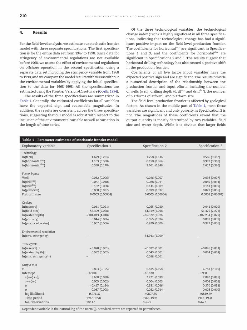
The results of the three specifications are summarized inTable 1. Generally, the estimated coefficients for all variableshave the expected sign and reasonable magnitudes. Inaddition, the results are consistent across the three specifica-tions, suggesting that our model is robust with respect to theinclusion of the environmental variable as well as variation inthe length of time series.

Table 1 – Parameter estimates of stochastic frontier model

Explanatory variable Specification 1

Technologyln(tech) 1.629 (0.204)ln(horizontalexp) 1.163 (0.380)ln(horizontaldev) 0.350 (0.178)

Factor inputsWell 0.032 (0.006)ln(drillexp) 0.087 (0.010)ln(drilldev) 0.182 (0.008)ln(platform) 0.060 (0.037)Platform size 0.0003 (0.00004)

Geologyln(reserve) 0.041 (0.021)ln(field size) 56.309 (2.058)ln(water depth) −104.013 (4.048)ln(porosity) 0.044 (0.036)ln(produced water) 0.967 (0.006)

Environmental regulationln(env. stringency) –

Time effectsln(reserve) · t −0.028 (0.001)ln(water depth) · t 0.052 (0.002)ln(env. stringency) · t –

Output mixθ 5.803 (0.155)Intercept −17.009σs2=σv

2 +σu2 8.650 (0.098)

γ=σu2/σs

2 0.005 (0.002)μ −0.417 (0.164)η 0.067 (0.008)log likelihood −45276.37Time period 1947–1998No. observations 18117

Dependent variable is the natural log of the norm (ι). Standard errors are

Of the three technological variables, the technologicalchange index (Tech) is highly significant in all three specifica-tions, indicating that technological change has had a signif-icant positive impact on the field-level production frontier.The coefficients for horizontalexp are significant in Specifica-tions 1 and 3, and the coefficients for horizontaldev aresignificant in Specifications 2 and 3. The results suggest thathorizontal drilling technology has also caused a positive shiftin the production frontier.

Coefficients of all five factor input variables have theexpected positive sign and are significant. The results providea numerical description of the relationship between theproduction frontier and input efforts, including the numberof wells (well), drilling depth (drillexp and drilldev), the numberof platforms (platform), and platform size.

The field-level production frontier is affected by geologicalfactors. As shown in the middle part of Table 1, most thesevariables are significant and only porosity in Specification 2 isnot. The magnitudes of these coefficients reveal that theoutput quantity is mostly determined by two variables: fieldsize and water depth. While it is obvious that larger fields

Specification 2 Specification 3

1.258 (0.146) 0.566 (0.467)0.150 (0.364) 0.993 (0.360)2.661 (0.346) 2.617 (0.320)

0.026 (0.007) 0.036 (0.007)0.088 (0.011) 0.089 (0.011)0.144 (0.009) 0.141 (0.009)0.099 (0.037) 0.072 (0.036)

0.0003 (0.00004) 0.0003 (0.00004)

0.055 (0.020) 0.041 (0.020)64.319 (1.098) 51.375 (2.273)

−85.372 (1.026) −107.234 (1.029)0.055 (0.034) 0.059 (0.033)0.970 (0.006) 0.977 (0.006)

−54.943 (1.009) –

−0.032 (0.001) −0.026 (0.001)0.043 (0.001) 0.054 (0.001)0.028 (0.001) –

6.815 (0.158) 6.784 (0.160)−16.630 −9.980

7.771 (0.099) 7.820 (0.085)0.004 (0.003) 0.004 (0.002)0.351 (0.046) 0.370 (0.091)0.032 (0.014) 0.026 (0.010)

−40807.35 −40839.291968–1998 1968–199816677 16677

reported in parentheses.

17 For example, for a large field (280 million barrels oil equiva-lent), drilling cost and production operating cost account for over75% of the total cost associated with the entire explorationdevelopment and production process (Lewin and Associates1985).18 See Managi et al. (2004b) for another filed level econometricanalysis and the forecasting of oil and gas production.

211E C O L O G I C A L E C O N O M I C S 6 0 ( 2 0 0 6 ) 2 0 4 – 2 1 5

producemore, it is somewhat surprising to see the magnitudeof the negative impact of water depth on the productionfrontier. The challenge posed by water depth is indeedsubstantial. Generally, we expect potential of larger produc-tion is available in deep-water areas. Our results show that, onaverage, it is not true in our study periods. This might bebecause industry focused on production from large filed indeep water and little attention is paid to small and averagefield size fields. We model produced water, a byproduct ofpetroleum production, on the input side. Although the volumeof produced water from a field is influenced by the geologicaltype of its reservoirs and the age of the field, our resultssuggest that, on average, the quantities of producedwater andpetroleum output are positively related.

The offshore oil and gas industry has been subject to notonly challenging marine conditions but also increasingenvironmental regulations (see Managi et al., 2005b). Toestimate associated production frontier shift, we include ameasure of the stringency of environmental regulations inSpecification 2 (see Table 1). The significantly negativecoefficient implies that environmental regulation has indeedhad a measurable impact on productivity of the offshore oiland gas industry.

We include three time interaction terms with reserves (i.e.,remaining stock in a field), water depth, and environmentalstringency in our model, respectively, to examine how thesefactors change over time (t). The corresponding coefficientsare all significant. The time interaction term is negative forreserves, suggesting that the positive effect of remainingresource stock on field-level production has been decliningover time, which suggest that new technologies allow one tomore efficiently exploit small fields. The time interactionterms are positive for water depth and environmentalstringency. The former shows that the negative impacts ofwater depth and environmental regulations on the productionfrontier have been diminishing (becoming less negative) overtime due to technological change, including less “structural”components of technological change, such as learning bydoing.

The positive sign of the parameter capturing the time-varying effect (η) indicates that efficiency at the field level hasincreased over time, which is likely due to the learning bydoing in the Gulf of Mexico (Managi et al., 2004a). Finally, theestimated polar angle θ is positive and significant. The resultsuggests that when the frontier output mix is changed bysubstituting gas production for oil production, the increase ingas production is greater than the corresponding decrease inoil production, as measured in BOE.

In summary, the results of our field-level analysis indicatethat the effect of technological change on the offshore oil andgas industry was substantial over the study period from 1947to 1995. Similarly, environmental regulation also had asignificant impact on offshore production. Next, we attemptto measure the magnitude of the technological change in theoffshore industry.

As noted in Eq. (14), the computation of the Tornqvistindexes involves the costs (wi) of relevant factor inputs (Xi). Wehave relatively complete cost data for drilling and platformsfrom 1976 to 1995. Thus, our TFP assessment is carried out forthis period. Also, we include two factor input variables: the

total number of exploratory and development wells, and thenumber of platforms. These two variables capture the bulk ofexploration, development, and production efforts. Costsassociated with drilling and platforms are the two mostsignificant cost components in the offshore industry.17

We first calculate the conventional TFP using Eq. (13). Ourresults indicate that from 1976 to 1995, the average annualgrowth in output (i.e., oil and gas) was 1.30%,while the averagegrowth in inputs (i.e., wells and platforms) was 1.75%. Thus,the conventional TFP, or net result of depletion and techno-logical change, decreased on average 0.45% per year in thestudy period. The result suggests that, at the aggregateregional level and in the entire exploration–development–production process, the effect of technological change wasunable to offset completely the effect of resource depletionfrom 1976 to 1995.18

Since the offshore oil and gas industry is a resourceindustry, it is necessary to make adjustments to theconventional TFP estimates (see Eq. (13)) with respect toresource conditions (e.g., field size and water depth). Wedevelop the adjustments as in Eq. (13). We first estimate theadjusted TFP change by accounting for the depletion effects.Over the 1976–1995 study period and across all active fields ineach year, average field size (S) declined at an average rate of14.62% per year, and average water depth (D) rose, onaverage, 0.62% per year. As shown in Eq. (6), the impacts ofthese two indexes on TFP estimate depend on thecorresponding cost elasticities (εCS and εCD). However, weare unable to develop estimates of these elasticities in thestudy for lack of relevant data. Instead, we utilize sensitivityanalysis to explore the range of the adjusted TFP. In thesensitivity analysis, we vary both εCS and εCD from 0.4 to 1.2(see the discussion in Jin et al., 1998). The results of averageannual TFP growth adjusted for field size and water depth arepresented in Table 2.

The adjusted average annual TFP growth ranges from5.64% to 17.82%, depending on the values of the costelasticities. Generally, if the cost elasticities are larger, thecorresponding TFP growth estimates will be higher. Al-though we cannot develop a point estimate, the resultsclearly show that true TFP growth in the offshore industry issignificantly higher, when the effects of field size and waterdepth are accounted for (using Eq. (13)), than conventionalmeasurement.

During the study period, our environmental regulatoryintensity index (E) rose, on average, 6.27% per year and ourpollution discharge index (Q) declined at an average rate of11.56% per year. Again, since we do not have necessary datato estimate relevant cost elasticities (εCE and εCQ), we employsensitivity analysis to examine a wide range of possiblevalues (0.01–0.1). Table 3 summaries the resulting estimatesof average annual TFP growth, adjusted for water depth,

,,

Table 2 – Average annual TFP growth (%) in the Gulf ofMexico offshore oil and gas industry (1976–1995), adjustedfor water depth and field size

εCD

0.4 5.64 8.56 11.48 14.41 17.330.6 5.76 8.68 11.61 14.53 17.450.8 5.88 8.81 11.73 14.65 17.581.0 6.01 8.93 11.85 14.78 17.701.2 6.13 9.05 11.98 14.90 17.82

εCS 0.4 0.6 0.8 1.0 1.2

εCS is the cost elasticity with respect to field size and εCD is the costelasticity with respect to water depth.

212 E C O L O G I C A L E C O N O M I C S 6 0 ( 2 0 0 6 ) 2 0 4 – 2 1 5

field size, stringency of environmental regulations andpollution discharges (oil spills and produced waters). In thecalculation, we set the cost elasticities for both water depth(εCD) and field size (εCS) at 0.8 (e.g., Fagan, 1997; Jin et al.,1998).

As shown in Table 3, accounting for stringency ofenvironmental regulations and pollution discharge leads toeven greater adjusted TFP growth estimates. In our base case,the adjusted TFP growth is 11.73% (see Table 2 with εCD=ε-CS=0.8), the fully adjusted TFP growth ranges from 16.03% to54.70% as the value of the cost elasticities (εCE and εCQ) varyfrom 0.01 to 0.1. The results further enhance our findings andclearly show that the true TFP growth, accounting for waterdepth, field size, environmental regulation, and pollutiondischarge, is well above the conventional measure. The paceof productivity improvement in the offshore oil and gasindustry has been truly remarkable compared to standardproductivity measurement.

5. Conclusions

Offshore oil and gas operations in the Gulf of Mexico haveplayed an important role in energy supply in the United States.In the past five decades, the offshore industry expanded firstalong the coast in shallow waters, and then extended intodeep waters. Contrary to earlier predictions of decliningproduction due to resource depletion (Walls, 1994), the output

Table 3 – Average annual TFP percentage growth in the Gulf of Mwater depth, field size, environmental regulation, and pollution

εCE 0.01 0.02 0.03 0.04 0.05

εCQ0.01 16.03 16.09 16.16 16.23 16.300.02 20.25 20.32 20.39 20.46 20.530.03 24.48 24.55 24.62 24.69 24.760.04 28.71 28.78 28.85 28.92 28.980.05 32.94 33.01 33.08 33.14 33.210.06 37.17 37.24 37.30 37.37 37.440.07 41.40 41.47 41.53 41.60 41.670.08 45.63 45.69 45.76 45.83 45.900.09 49.85 49.92 49.99 50.06 50.130.10 54.08 54.15 54.22 54.29 54.35

εCE is the cost elasticity with respect to environmental regulatory intensi

from the region has increased in recent years (U.S. Depart-ment of Interior, 2000). The continued development andproduction in the region has depended heavily on technolog-ical innovations.

In the study, we examine the role technological change hasplayed in the offshore industry. We first analyze the effect ofpollution discharge (e.g., produced water and oil spill),technological change on the production frontier using aunique field-level data set covering 1947 through 1998, andwe then develop estimates of the growth in total factorproductivity (TFP) in the industry at the regional level from1976 to 1995.

Results of our stochastic frontier model suggest that theeffect of technological change on the offshore oil and gasindustry at the field level was substantial over the studyperiod from 1947 to 1998. Because of technological progress,the negative effect of resource depletion on field-levelproduction frontier has been declining over time. Similarly,the negative impact of water depth on the production frontierhas been falling. The results reveal that environmentalregulation had a significantly negative impact on offshoreproduction, although such impact has been diminishing overtime due to technological change and improvement inmanagement. Finally, the stochastic frontier analysis showthat the production efficiency at the field level has beendecreasing, which is likely due to the depletion of reserves andresulting expansion of exploration and production in deepwaters.

To measure the magnitude of technological progress, wedevelop estimates of the growth in TFP in the offshoreindustry in the Gulf of Mexico region. Our results indicatethat the conventional TFP decreased on average 0.45% peryear from 1976 to 1995, implying that at the aggregateregional level and in the entire exploration–development–production process, the effect of technological change wasunable to offset completely the effect of resource depletionin this period. However, adjusted for field size and waterdepth, the average annual change in TFP grew at least 5.64%.Although we cannot provide a point estimate for lack ofdata, the results clearly show that true TFP growth in theoffshore industry is significantly higher, when depletioneffects associated with field size and water depth areaccounted for. Also, the adjusted TFP growth estimates will

exico offshore oil and gas industry (1976–1995), adjusted fordischarge

0.06 0.07 0.08 0.09 0.10

16.37 16.44 16.50 16.57 16.6420.60 20.66 20.73 20.80 20.8724.82 24.89 24.96 25.03 25.1029.05 29.12 29.19 29.26 29.3233.28 33.35 33.42 33.49 33.5537.51 37.58 37.65 37.71 37.7841.74 41.81 41.87 41.94 42.0145.97 46.03 46.10 46.17 46.2450.19 50.26 50.33 50.40 50.4754.42 54.49 54.56 54.63 54.70

ty and εCQ is the cost elasticity with respect to pollution discharge.

Table A2 – Stage II estimates

Dependent variable Porosity Standarderror

Independent variable Estimated coefficient

Intercept −134.649 ⁎ 68.843ln(oil reserve) 0.554 ⁎ 0.335ln(gas reserve) 2.409 ⁎⁎⁎ 0.41542ln(water depth) 15.145 ⁎ 7.91355ln(5Yr exp drill) 1.05296 ⁎⁎⁎ 0.22748IMR 5.11798 ⁎⁎ 1.753R2 0. 206Adjusted R2 0.196

213E C O L O G I C A L E C O N O M I C S 6 0 ( 2 0 0 6 ) 2 0 4 – 2 1 5

be higher if the cost elasticities with respect to water depthor field size are larger.

In addition to water depth and field size, accounting forenvironmental regulatory stringency and pollution dischargeleads to further increase in the estimates of adjusted TFPgrowth. For our sensitivity analysis, the low-end estimate ofthe fully adjusted TFP growth is 16.03%, and the actual growthmay be much greater, depending on the values of the costelasticities. In general, our results at both the field level andthe regional level are consistent, and they clearly show thatthe pace of technological progress in the offshore oil and gasindustry has been truly remarkable.

The variable 5Yr exp drill is cumulative drilling feet of explorationwells in the field for first 5 years following discovery. 50% of totaldrilling is completed on an average of 5.2 years; therefore, wechoose 5 years, based on the assumption that MMS has data forlarge fields. IMR=Inverse Mills Ratio.⁎ Significant at 10% level.⁎⁎ Significant at 5% level.⁎⁎⁎ Significant at 1% level.

Acknowledgements

The authors thank four anonymous referees for helpfulcomments. This research was funded by the United StatesEnvironmental Protection Agency STAR grant program (GrantNumber Grant Number R826610-01) and the Rhode IslandAgricultural Experiment Station (AES Number 5034). Theresults and conclusions of this paper do not necessaryrepresent the views of the funding agencies.

Appendix A. Nonrenewable resource model andenvironmental regulations

Our empirical econometric equation of oil and gas productionin this study is base on a dynamic profit-maximizingframework for nonrenewable resource industry (see Deacon,1993; Krautkreamer, 1998; Kunce et al., 2004 for review in theliterature). We use simplified version of exploration–extrac-tion aggregated model (e.g., Livernois and Uhler, 1987a,b).Hypothetical competitive firm makes optimal extraction andexploration decisionwith respect to reserves over one ormanydeposits in each aggregated field. The firm faces exogenousprices, is assumed to have complete property rights, and isassumed to maximize the present value of profits fromexploration and extraction operations. Especially, followingassumptions are utilized for our empirical specification. First,production cost function is assumed to have a log–logrelationship to variables including factor inputs, technology,geological factors, and environmental regulations applied toproduction. Second, nonrenewable resource is extracted froma fixed stock of homogeneous quality. Solving present valueHamiltonian and after some tedious calculations, oil and gasproduction is shown to have a log–log relationship to variablesin Eq. (1).

Table A1 – Stage I probit estimates

Independentvariable

Estimatedcoefficient

Standarderror

Intercept 811.234 ⁎ 65.866Discovery year −106.926 ⁎ 8.679Log likelihood −543.8820313

Dependent variable=1 if porosity observed; 0 otherwise.⁎ Significant at the 1% level.

Several studies have examined how the oil and gasindustry responds to changes in environmental regulations(e.g., Stollery, 1985; Jin and Grigalunas, 1993a; Denison et al.,1995; Kunce et al., 2004). Ideally, the model needs toconsider the effects of the regulations to all stages of oiland gas operations: exploration, development, and produc-tion (see Jin and Grigalunas, 1993a). Empirically, however, itis difficult to obtain the data of the regulations. Forexample, recent study by Kunce et al. (2004) studies theenvironmental regulations pertaining to drilling. The drillingfluids, drill cuttings, deck drainage, well treatment fluids,proposal sand, and sanitary and domestic wastes are alsoimportant factors in the regulations in addition to theenvironmental regulations applied to production. We onlyconsider the compliance cost of the regulations applied toproduction since these data is not available in field level.This may not be a terrible assumption since there is moreregulation on production side than drilling (see EPA, 1976,1985, 1993, 1999; Managi, 2002 for detailed history of theregulations).

Appendix B. Missing data estimation

Complete data for porosity is available for only 390 fields out of933 fields, with more data available in more recent years. Weuse a two-step estimation procedure to correct for censoring ofobservations (Heckman, 1979; Greene, 1981). Tables A1 and A2contains estimation results from these regression models. Inthe first stage results, Probit is applied to determine thelikelihood that a porosity measure is missing, and discoveryyear is the explanatory variable. Porosity is the dependentvariable in the second stage, and the explanatory variables areoil reserves in the field, gas reserves in the field, water depthand the number of exploratory wells drilled in the first fiveyears following discovery of the field. Results for second stageindicate that higher porosity values tend to be found in largerreservoirs, in reservoirs in which more drilling occurs and indeeper-water fields (Table A2).

214 E C O L O G I C A L E C O N O M I C S 6 0 ( 2 0 0 6 ) 2 0 4 – 2 1 5

R E F E R E N C E S

Aigner, D.J., Lovell, C.A.K., Schmidt, P., 1977. Formulation andestimation of stochastic frontier production function models.Journal of Econometrics 6, 21–37.

American Petroleum Institute, 1995. Potential Impact of Environ-mental Regulations on the Oil and Gas Exploration andProduction Industry. API, Washington, DC. March.

American Petroleum Institute. Independent Petroleum Associa-tion of America, and Mid-Continent Oil and Gas Association.various years. Joint Association Survey on Drilling Costs. API,Washington, DC.

Barbera, A.J., McConnell, V.D., 1990. The impact of environmentalregulations on industry productivity: direct and indirecteffects. Journal of Environmental Economics and Management18 (1), 50–65.

Battese, G.E., Coelli, T.J., 1992. Frontier production functions,technical efficiency and panel data: with application topaddy farmers in India. Journal of Productivity Analysis 3,153–169.

Baumol, W.J., Oates, W.E., 1988. The Theory of EnvironmentalPolicy, 2nd edition. Cambridge University Press, Cambridge.

Bohi, D.R., 1997. Changing Productivity of Petroleum Explorationand Development in the U.S. Draft Report. Resources For TheFuture, Washington, DC. January.

Christensen, L.R., Jorgenson, D.W., 1995. Measuring economicperformance in the private sector. In: Jorgenson, D.W. (Ed.),Productivity Volume 1: Postwar U.S. Economic Growth. MITPress.

Cleveland, C.J., Kaufmann, R., 1997. Natural gas in the U.S.: how farcan technology stretch the resource base? The Energy Journal18 (2), 89–108.

Coelli, T.J., 1994. A Guide to FRONTIER Version 4.1: A ComputerProgram for Stochastic Frontier and Cost Function Estimation.Department of Econometrics, University of New England,Armidale.

Cropper, Maureen L., Oates, Wallace E., 1992. Environmentaleconomics: a survey. Journal of Economic Literature 30 (2),675–740.

Cuddington, J.T., Moss, D.L., 2001. Technical change, depletion andthe U.S. petroleum industry: a new approach to measurementand estimation. American Economic Review 91 (4), 1135–1148.

Deacon, R., 1993. Taxation, depletion, and welfare: a simulationstudy of the U.S. petroleum resource. Journal of EnvironmentalEconomics and Management 24 (2), 159–187.

Denison, D., Crocker, T., Briand, G., 1995. The impact of environ-mental controls on petroleum exploration, development, andextraction. In: Shojai, S. (Ed.), The New Global Oil Market:Understanding Energy Issues in the World Economy. PraegerPublishers, Wesport.

Denny, M., Fuss, M., Waverman, L., 1981. The measurement andinterpretation of total factor productivity in regulated indus-tries, with an application to canadian telecommunications. In:Cowing, T.G., Stevenson, R.E. (Eds.), Productivity Measurementin Regulated Industries. Academic Press, New York.

Diewert, W.E., 1976. Exact and superlative index numbers. Journalof Econometrics 4, 115–145.

Diewert, W.E., 1978. Superlative index numbers and consistency inaggregation. Econometrica 46 (4), 883–900.

Diewert, W.E., 1992. The measurement of productivity. Bulletin ofEconomic Research 44 (3), 163–198.

Engineering News Record [ENR], 2000. ENR market trends, ENRIndex Review, Construction Cost Index. Engineering NewsRecord.

Fagan, M.N., 1997. Resource depletion and technical change:effects on U.S. crude oil finding costs from 1977 to 1994. TheEnergy Journal 18 (4), 91–105.

Farrow, R.S., Broadus, J.M., Grigalunas, T.A., Hoagland, P.,Opaluch, J.J., 1990. Managing the Outer Continental ShelfLands: Ocean of Controversy. Taylor and Francis, New York.

Fisher, I., 1922. The Making of Index Numbers. Houghton MifflinCompany, Boston.

Fuss, Melvin, McFadden, Daniel, 1978. Production Economics: ADual Approach to Theory and Applications. North-Holland,Amsterdam.

Giuliano, F.A., 1981. Introduction to Oil and Gas Technology,Second edition. International Human Resources DevelopmentCorporation, Boston, MA.

Gollop, F.M., Roberts, M.J., 1983. Environmental regulations andproductivity growth: the case of fossil-fueled electric powergeneration. Journal of Political Economy 91 (4), 654–674.

Greene, William, 1981. Sample selection bias as a specificationerror: comment. Econometrica 49 (3), 795–798.

Harrington,Winston, Morgenstern, Richard D., Nelson, Peter, 2000.On the accuracy of regulatory cost estimates. Journal of PolicyAnalysis and Management 19 (2), 297–322.

Heckman, James, 1979. Sample selection bias as a specificationerror. Econometrica 47 (1), 153–161.

Hjalmarsson, Lennart, Kumbhakar, Subal C., Heshmati, Almas,1996. DEA, DFA and SFA: a comparison. Journal of ProductivityAnalysis 7 (2–3), 303–327.

Hulten, C.R., 1986. Productivity change, capital utilization, andthe sources of efficiency growth. Journal of Econometrics 33,31–50.

Jin, D., Grigalunas, T.A., 1993a. Environmental compliance andenergy exploration and production: application to offshore oiland gas. Land Economics 69 (1), 82–97.

Jin, Di, Grigalunas, T.A., 1993b. Environmental compliance andoptimal oil and gas exploitation. Natural Resource Modeling 7(4), 331–352.

Jin, Di, Kite-Powell, H., Schumacher, M., 1998. Total FactorProductivity Change in the Offshore Oil and Gas Industry.Woods Hole Oceanographic Institution Working Paper.

Jorgenson, D.W., Griliches, Z., 1967. The explanation of produc-tivity change. Review of Economic Studies 34 (3), 249–280.

Krautkreamer, J.A., 1998. Nonrenewable resource scarcity. Journalof Economic Literature 36, 2065–2107.

Kunce, M., Gerking, S., Morgan, W., 2004. Environmental and landuse regulation in nonrenewable resource industries: implica-tions from the Wyoming checkerboard. Land Economics 80 (1),76–94.

Lewin and Associates, Inc., 1985. Replacement Costs of DomesticCrude Oil. vol. 1–2. DOE/FE30014-1. Prepared for U.S. Dept. ofEnergy, Washington, D.C.

Livernois, J., Uhler, R.S., 1987a. Extraction costs and the economicsof nonrenewable resources. Journal of Political Economy 95,195–203.

Livernois, J.R., Uhler, R.S., 1987b. Extraction costs and theeconomics of nonrenewable resources. Journal of PoliticalEconomy 95 (1), 195–203.

Löthgren, Mickael, 1997. Generalized stochastic frontier produc-tion models. Economics Letters 57 (3), 255–259.

Managi, Shunsuke, 2002. Technological change, depletion andenvironmental policy in offshore oil and gas industry. PhDdiss., University of Rhode Island.

Managi, S., Opaluch, J.J., Jin, D., Grigalunas, T.A., 2004a.Technological change and depletion in offshore oil and gas.Journal of Environmental Economics and Management 47 (2),388–409.

Managi, S., Opaluch, J.J., Jin, D., Grigalunas, T.A., 2004b. Forecastingenergy supply and pollution from the offshore oil and gasindustry. Marine Resource Economics 19 (3), 307–332.

Managi, S., Opaluch, J.J., Jin, D., Grigalunas, T.A., 2005a. Techno-logical change and petroleum exploration in the Gulf ofMexico. Energy Policy 33 (5), 619–632.

215E C O L O G I C A L E C O N O M I C S 6 0 ( 2 0 0 6 ) 2 0 4 – 2 1 5

Managi, S., Opaluch, J.J., Jin, D., Grigalunas, T.A., 2005b. Environ-mental regulations and technological change in the offshoreoil and gas industry. Land Economics 81 (2), 303–319.

Managi, S., Opaluch, J.J., Jin, J.J., Grigalunas, T.A., in press.Alternative innovation indexes in the offshore oil and gasindustry. Applied Economics Letters.

Massachusetts Institute of Technology, 1973. The Georges BankPetroleum Study: Summary, vol. 1–2. Offshore Oil Task Group,Cambridge, MA.

Meeusen, W., van den Broeck, J., 1977. Efficiency estimation fromCobb–Douglas production functions with composed error.International Economic Review 18, 435–444.

Moss, D.L., 1993. Measuring technical change in the petroleumindustry: a new approach to assessing its effect on explorationand development. National Economic Research Associations,Working Paper Number 20.

Pindyck, R.S., 1978. The optimal exploration and production ofnonrenewable resources. Journal of Political Economy 86 (5),841–861.

Solow, R.M., 1957. Technical progress and the aggregate produc-tion function. Review of Economics and Statistics 39, 312–320.

Stijn, R., Lovell, C.A.K., Thijssen, G., 2002. Analysis of environ-mental efficiency variation. American Journal of AgriculturalEconomics 84 (4), 1054–1065.

Stollery, K., 1985. Environmental controls in extractive industries.Land Economics 61, 136–144.

U.S. Department of Energy, 1993. Drilling Sideways: A Review ofHorizontal Well Technology and Its Domestic Application.DOE/EIA/TR-0565. Energy Information Administration,Washington, DC.

U.S. Department of Interior, 2000. Mineral Revenue Collections.Washington, DC.: U.S. Minerals Management Service.

U.S. Department of Interior, 2001. Technical Information Man-agement System (TIMS) Database. U.S. Mineral ManagementService (MMS).

U.S. Department of the Interior, 1996. Offshore Statistics SecondQuarter. Minerals Management Services, Operations andSafety Management, Herndon, VA.

U.S. Department of the Interior, 1997. Federal Offshore Statistics:1995. OCS Report MMS 97-0007. Minerals Management Ser-vices, Operations and Safety Management, Herndon, VA.

U.S. Environmental Protection Agency, 1976. Development Docu-ment for Interim Final Effluent Limitations Guidelines andNew Source Performance Standards for the Oil and GasExtraction Point Source Category. Environmental ProtectionAgency, Washington, DC.

U.S. Environmental Protection Agency, 1985. Economic ImpactAnalysis of Proposed Effluent Limitations and Standards forthe Offshore Oil and Gas Industry. Environmental ProtectionAgency, Washington, DC.

U.S. Environmental Protection Agency, 1993. Economic ImpactAnalysis of Final Effluent Limitations Guidelines and Stan-dards for the Offshore Oil and Gas Industry. EnvironmentalProtection Agency, Washington, DC.

U.S. Environmental Protection Agency, 1999. EnvironmentalAssessment of Proposed Effluent Limitations Guidelines andstandards for Synthetic-Based Drilling Fluids and other Non-Aqueous Fluids in the Oil and Gas Extraction Point SourceCategory. Environmental Protection Agency, Washington, DC.

Walls, M.A., 1994. Using a ‘Hybrid’ approach to model oil and gassupply: a case study of the Gulf of Mexico outer continentalshelf. Land Economics 70 (1), 1–19.