a c t a o e c o l o g i c a 3 3 ( 2 0 0 8 ) 2 8 0 – 2 9 0

ava i lab le a t www.sc iencedi rec t .com

journa l homepage : www.e lsev ie r . com/ loca te /ac toec

Original article

Stochastic approach to determine spatial patternsof lizard community on a desert island

Crystian Sadiel Venegas-Barrera1, Enrique Morales-Bojorquez*, Gustavo Arnaud

Centro de Investigaciones Biologicas del Noroeste (CIBNOR), Mar Bermejo 195, Col. Playa Palo de Santa Rita, La Paz, B.C.S. 23090, Mexico

a r t i c l e i n f o

Article history:

Received 23 May 2007

Accepted 30 November 2007

Published online 18 April 2008

Keywords:

Spatial dependence

Markov models

Numerical dominance

Species richness

Spatial arrangement

Nearby samples

* Corresponding author. Tel.: þ52 612 123 84E-mail address: emorales@cibnor.mx (E.

1 Present address: Laboratorio de Ecologıa Ede Mexico, Instituto Literario 100, 50000, Tol1146-609X/$ – see front matter ª 2008 Elsevidoi:10.1016/j.actao.2008.01.002

a b s t r a c t

One of the principal sources of error in identifying spatial arrangements is autocorrelation,

since nearby points in space tend to have more similar values than would be expected by

random change. When a Markovian approach is used, spatial arrangements can be mea-

sured as a transition probability between occupied and empty spaces in samples that are

spatially dependent. We applied a model that incorporates first-order Markov chains to an-

alyse spatial arrangement of numerical dominance, richness, and abundance on a lizard

community at different spatial and temporal scales. We hypothesized that if a spatial de-

pendence on abundance and richness exists in a diurnal desert community, then the Mar-

kov chains can predict the spatial arrangement. We found that each pair of values was

dependent only on its immediate predecessor segment. In this sense, we found interge-

neric differences at temporal and spatial scales of recurrence estimates. Also, in desert

scrub, species show higher spatial aggregation and had lower species richness than at

the island level; the inverse pattern occurred on rocky hillsides. At the species level, Uta

stansburiana is the most abundant species in desert scrub, while Sauromalus slevini is the

most abundant species on rocky hillsides. This report attempts to understand, using Mar-

kovian spatial models, the effect of nearby samples on local abundance and richness on

different scales and over several seasons.

ª 2008 Elsevier Masson SAS. All rights reserved.

1. Introduction segregation, habitat selection, and territoriality (Legendre,

The spatial arrangement of several species in a community is

not homogeneous because limiting factors that affect abun-

dance and distribution change spatially and species tend to

respond differentially to environmental heterogeneity. Gener-

ally, species predominate in habitats where conditions are

suitable, and are rare in unfavourable habitats (Kneitel

and Chase, 2004). Therefore, spatial elements play a funda-

mental role in most ecological processes, including spatial

84x3351; fax: þ52 612 125Morales-Bojorquez).volutiva, Centro de Invesuca, Mexico.er Masson SAS. All rights

1993; Bevers and Flather, 1999). Patterns based on spatial ar-

rangements are a first approximation for analysing the effect

of biotic, that is, inter- or intraspecific interactions and abiotic

environmental variations, such as, temperature, pH, topogra-

phy, and soil on species. One of the principal sources of error

in identifying spatial arrangements is autocorrelation, since

nearby points tend to have more similar values than would

be expected by random change (Lichstein et al., 2002). When

a Markovian approach is used, spatial arrangements can be

3625.

tigaciones en Recursos Bioticos, Universidad Autonoma del Estado

reserved.

a c t a o e c o l o g i c a 3 3 ( 2 0 0 8 ) 2 8 0 – 2 9 0 281

measured as a transition probability between occupied and

empty spaces in samples that are spatially dependent.

A first-order Markov chain is a stochastic model in which

the future development of a system is dependent on the pres-

ent state of the system and is independent of the way in which

that state has developed (Formacion and Saila, 1994).

In ecology, Markov chains have been used principally in

temporal succession of ecological states (Tanner et al., 1996;

Wootton, 2001a; Hill et al., 2004), time of recovery and restora-

tion of forests (Orloci and Orloci, 1988; Hall et al., 1991; Tucker

and Anand, 2004), patterns of change in parental stock and re-

cruitment in fisheries (Roshchild and Mullen, 1985), estimates

of bird populations (Wileyto et al., 1994), and anthropogenic

impact on marine mammals (Lusseau, 2003). Markov chains

spatial models have been used to predict sequences of egg-

laying in butterflies (Root and Kareiva, 1984), ontogenic

change in habitat preference of cotton rats (Kincaid and

Cameron, 1985), movements of Canada geese (Hestbeck

et al., 1991), and spatial inhibition by allelopathy in plants

(Kenkel, 1993). These studies highlight the potential of Markov

chains in the study of population dynamics and importance of

proximity neighbourhoods in the state of system. However,

rarely has it been used to explore spatial changes in richness,

abundance, or dominance of species at a community scale,

despite the utility of that approach to analyse spatial depen-

dence between near samples and calculate the average dis-

tance between ecological states.

The advantages of Markov chains are that: (1) such models

are relatively easy to derive from continuous data; (2) the

model does not require deep insight into the mechanisms of

dynamic change; (3) the basic transition matrix summarizes

essential parameters of dynamic change in a systems in

a way that few others models achieve; and (4) a model has

much potential for identifying recent history in dynamic com-

munities and population dynamics (Formacion and Saila,

1994). These characteristics are ideal for calculating spatial ar-

rangement of species. Additionally, Markov chains can be

used to estimate the probability of any state of abundance or

richness occur in the space, assuming that it is dependent

on the preceding area. We assumed that: (1) contagious bio-

logical process that affect local abundance of individual spe-

cies are spatially dependent (Legendre, 1993), i.e. conditions

of growth, survival, and reproduction tend to be similar at

nearby sites, (2) well-selected habitats provide high fitness po-

tential (Railsback et al., 2003), (3) individuals in a population do

not show a random distribution, i.e. occurrence of an individ-

ual does not affect the presence of others, and (4) species with

similar adaptations will tend to occur together at the same

sites (Bell, 2001). In this study, we developed models that in-

corporate first-order Markov chains to analyse spatial changes

in states of numerical dominance (more abundant species by

unit area), richness (number of species by unit area), and

abundance of one lizard community on Isla Coronados in

the Gulf of California. We chose diurnal lizard species on

Isla Coronados because they are conspicuous, abundant, and

represent one of the four islands in Gulf of California with

high richness (ten species). We hypothesized that, if a pattern

of abundance and richness exist in a desert community, then

Markov chains can predict the spatial arrangement. If we

knew the sequences of presence-occurrence, richness, and

abundance of species, then we can estimate the average dis-

tance before we again observe the same species (recurrence)

and rate of change between species without the necessity of

evaluating the spatial structure of habitats. We predicted

high probabilities of replacement between species with simi-

lar habitat requirements as species with different require-

ments. Also, we can compare the numerical dominance and

richness at two spatial scales (island and landscape) to ana-

lyse the effect of scale on the estimation of spatial arrange-

ment. Finally, we calculated the spatial arrangement for

more abundant species on two landscapes.

2. Materials and methods

2.1. Study area

Isla Coronados is a volcanic, land bridge island (26�0801500 N,

111�160500 W) located w10 km northeast of Loreto, B.C.S.,

Mexico and w3 km from the closest shore of the Baja Califor-

nia Peninsula (Fig. 1). The climate is hot and arid in summer

(mean July temperature 33 �C) and warm in winter (mean Jan-

uary temperature 16 �C). Summer precipitation comes from

convectional storms on the Peninsula (average 190 mm/year)

(Grismer, 1994). Four types of habitats occur on Isla Coronado;

rocky hillsides, desert scrubland, a coastal zone, and a transi-

tion zone between rocky hillsides and desert scrub (Venegas,

2003). On rocky hillsides, approximately 45% of the surface is

covered with rocks (ranging in diameter from 20 to 100 cm),

15% is bare soil (includes fallen leaves, soil, and gravel

<2 cm), and 40% is covered with vegetation (Jatropha cuneata,

Euphorbia magdalenae, and Simmondsia chinensis). In desert

scrub, approximately 7% are rocks (<10 cm diameter), 38% is

bare soil, and 55% is covered with vegetation (principally Fou-

quieria diguetii, Gossypium harknessii, Hibiscus denudatus, and

Jatropha cuneata). The coastal zone has a ground surface that

is 5% rock (<10 cm diameter), 65% bare soil, and 30% covered

with vegetation (principally Salicornia virginica, Maytenus phyl-

lanthoides, and Atriplex barclayana). The transition habitat is

characterized by 30% rocks (5–50 cm diameter), 17% bare

soil, and 53% vegetation (Jatropha cuneata, Hibiscus denudatus,

Euphorbia magdalenae, and Lycium sp.).

2.2. Species

Isla Coronados is one of four islands in the Gulf of California

with a largest number of diurnal lizard species (Grismer,

2002). Of the ten species in the study area, four are ground-

dwelling species: desert iguana (Dipsosaurus dorsalis), zebra-

tailed lizard (Callisaurus draconoides), side-blotched lizard (Uta

stanburiana), and orange-throated whiptail (Aspidoscelis hyper-

ythra) and six are rock dwellers: slevin’s chuckwalla (Sauroma-

lus slevini), black-tailed brush lizard (Urosaurus nigricaudus),

central Baja California banded rock lizard (Petrosaurus repens),

granite spiny lizard (Sceloporus orcutti), western whiptail

(A. tigris), and Baja California spiny lizard (S. zosteromus)

(Grismer, 2002). Diurnal desert lizard species show different

sizes of home range, exhibit varying territoriality, and differ-

ent kinds of foraging behaviour (Pough et al., 2004). The foli-

vores, D. dorsalis and S. slevini, have a small home range,

Fig. 1 – Study area on Isla Coronado in the Gulf of California, off the east coast of the Baja California Peninsula. Transects and

principal habitats are shown.

a c t a o e c o l o g i c a 3 3 ( 2 0 0 8 ) 2 8 0 – 2 9 0282

where size tends to increase as the patchiness of food in-

creases, and defend polygynous territories (Kwiatkowski and

Sullivan, 2002). Phrynosomatidae species, genus Callisarus,

Uta, Urosaurus, Sceloporus, and Petrosaurus, commonly sit and

wait to prey on mobile prey and defend a small home range

(ambush, Pough et al., 2004). Finally, Teiidae species, Aspido-

scelis, are active predators that mostly feed on cryptic or

slow-moving prey, have larger home ranges with a high over-

lap with neighbours, but with very little overlap of their core

areas where they obtain most of their food (Eifler and Eifler,

1998). We assumed that changes in spatial distribution are

the result of availability of resources and reproductive events

that affect the size of the home range; therefore, the distance

between states of numerical dominance, richness, and abun-

dance depend on seasonality.

2.3. Data collection

Patterned annual activity of desert lizard species varies, which

affects the frequency of sightings. For example, Aspidoscelis

hyperythra and A. tigris are more abundant in warm months

(May–July), Dipsosaurus dorsalis and Sauromalus slevini are

a c t a o e c o l o g i c a 3 3 ( 2 0 0 8 ) 2 8 0 – 2 9 0 283

sighted more frequently after summer rainfall (September–

October), while Sceloporus spp. and Petrosaurus repens prefer

months with temperatures below 25 �C (November–Decem-

ber). We chose May, September, and November to evaluate

the frequency of sighting lizard species. We delimited homo-

geneous areas (landscape units) based on interpretations of

aerial photographs (scale 1:75,000) and prepared four perma-

nent transects (3 to 9.8 km long and 6 m wide) for censuses

of the four habitats in 2004 in four days in May, September,

and November (Fig 1). The 6-m width was close to the limit

of identifying species by sight. Transects were divided into

25-m segments because GPS resolution was 6–15 m with

MapInfo 5.0 software (MapInfo, New York). We analysed

data at two levels, island and landscape, for dominance, rich-

ness, and abundance of diurnal lizard species. At the island

level, 862 segments (21,745 m) were evaluated during each

sampling period, distributed among the four habitats. At the

landscape level, we evaluated only the two principal land-

scapes, rocky hillsides with 328 segments (8200 m) and desert

scrubland with 224 segments (5600 m). We sighted 446 lizards

in May, 691 in September, and 330 in November. Transects

were sampled from 08:00 to 14:00 h and again from 16:00 to

18:00 h because most of species have bimodal daily activity.

Observations were not taken at 14:00 to 16:00 h during the hot-

test time of day when most species reduce their activity

(Grismer, 2002). The species and the GPS-defined location of

every sighting were recorded.

2.4. Model

First-order Markovian models are based on probabilities of

transition from one state to another after a one-distance

step (segment), which depends only on the previous state

(Formacion and Saila, 1994; Wootton, 2001a; Hill et al., 2004).

We assumed that the population is closed during the month

of the survey, without loss or gain of individuals. Wootton

(2001b) found that the application of second-order Markov

chains showed similar results as first-order Markov chains;

therefore, we assumed that the present state of systems

only depend on the previous sample. We employed three

kinds of information: (1) numerical dominance, most abun-

dant species by segment and ecological states are the species

and empty segments; (2) richness or number of species by seg-

ment and states are the number of species and empty seg-

ments; and (3) abundance or number of lizards by species

and states are the number of lizards and empty segment.

For example, for numerical dominance, let the lizard’s com-

munity be sampled at regular intervals, and let there be a re-

cord of the state observed at each sampling.

We defined a state ‘i’ at segment ‘s’ of the lizard commu-

nity to mean that species ‘i’ is the dominate species present

in the lizard community at segment ‘f’, and let there be ‘m’

species that dominate the lizard community at one segment

or another on segments under study (Roshchild and Mullen,

1985). Let the one-step transition probability ‘piw’ be defined

as: Piw ¼ the probability that the dominant species in the lizard

communities is species w, given that the dominant species in

the lizard community during the immediately preceding seg-

ment was species i.

The matrix of one-step transition probabilities for all the m

states of the lizard community is given by:

P ¼

��������

Pii Piw Pim

Piw Pww Pwm

. . .Pim Pmw Pmm

��������

where Pii ¼ the dominant species in the lizard community

from one segment to the next remains Species i and Piw ¼ the

predominant species in the lizard community changes from

one segment dominated by Species i to Species w, where

isw. When the matrix is post-multiplied by vector w(f), repre-

senting the composition of states at segment s, according to

Equation 1,

Wðfþ 1Þ ¼ PwðfÞ; (1)

the resulting vector w(f þ 1) describes the composition of the

lizard’s community at segment s þ 1. The previous equation

can be used iteratively to simulate the composition of the

community over an area. The resulting vector is the steady

states probability ‘wi’, which means that the probability that

the lizard’s community will be in a particular state is indepen-

dent of its initial state (Hill et al., 2004). This is a relatively

simple model, in which probability distribution of the

model-states stabilizes after a given number of model steps

(Tucker and Anand, 2004). This property makes the model

ideal for presenting spatial pattern dominance.

We tested three Markovian assumptions of models. (1)

Transition probabilities are constant and depend only on pre-

vious states. We hypothesized that if each transition probabil-

ity was independent of the previous state, then we would

expect ‘n/y’, where ‘y’ is defined like a number of segments be-

tween a pair of states (cells), where ‘n’ is the total number of

segments, and ‘y’ is the total number of cells. The chi-square

criterion (P < 0.05) was used to test this hypothesis (Roshchild

and Mullen, 1985). (2) Irreducibility implies that every state is

possibly recurrent, that is, having occurred once, there is

a non-zero probability that it will occur again. (3) When ergo-

dicity, a recurrent state within a finite class of communicating

states, is not periodic, it means that a class of communicating

states need only contain at least one member i with piis0.

2.5. Parameters

Replacement Analysis (P) is the probability that a randomly-

selected point in a stationary lizard community is replaced

by a different species. This probability is the average of the

stationary distribution of the probability of replacement, de-

fined as:

P ¼ wið1� Pii � PeiÞ=wi; (2)

where wi is the stationary frequency of species i, and e is in an

empty state (Hill et al., 2004).

Expected turnover segments (E) measure the number of

segments in which a point changes state (Hill et al., 2004).

The turnover segments of species i is the distance that a point

changes to state j, defined as:

E ¼ di ¼ 1=ð1� PiiÞ: (3)

Recurrence segments (R) is a point in any state that will

eventually leave this state and then return to it after some

a c t a o e c o l o g i c a 3 3 ( 2 0 0 8 ) 2 8 0 – 2 9 0284

number of segments (Hill et al., 2004). A recurrence segment of

state i is the average distance elapsing between points leaving

state i and returning to it, defined as:

R ¼ qi ¼ ð1�wiÞ=wið1� PiiÞ: (4)

We analysed three spatial levels. (a) Island, which describes

spatial segregation between species and richness in all seg-

ments evaluated during the three months of sampling. We

expected high probabilities of replacement between species

with similar habitat requirements as species with different re-

quirements. We calculated the steady-state probabilities of

numerical dominance and richness for the three months,

since the species had different annual activity cycles (Grismer,

2002). We expected seasonal variations. To test this hypothe-

sis, we used the G test at P < 0.05 (Sokal and Rohlf, 1981). (b)

Landscape, which describes the properties of species with

similar habitat requirements. We analysed only the species

in the rocky hillside and flatland desert scrubland landscapes

in September because the largest number of lizards occur at

this time. We expected lower rates of replacement, turnover,

and distance of recurrence than at the island level. We used

the G test at P < 0.05. (c) Species, which describes the spatial

pattern of the most abundant species at the landscape level.

The estimates illustrate a potential use of Markov chains in

spatial arrangement studies because each species responds

differently to habitat and will show differences as distance be-

tween lizards.

3. Results

3.1. Island level

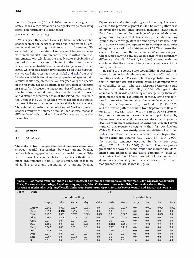
The matrix of transition probabilities of numerical dominance

showed spatial segregation between ground-dwelling

and rock-dwelling species because the transition probabilities

tend to have lower values between species with different

niche requirements (Table 1). For example, the probability

of finding a segment dominated by a ground-dwelling

Table 1 – Estimated transition matrix P for numerical dominanUsta, Uta stansburiana; Ahyp, Aspidoscelis hyperythra; Cdra, CaUrosaurus nigricaudus; Atig, Aspidoscelis tigris; Prep, Petrosauru

From State

Ground-dwelling

Empty Ddor Usta Ahyp Cd

Empty 0.663 0.059 0.129 0.061 0.

Ddor 0.353 0.318 0.235 0.094 0.

Usta 0.452 0.075 0.377 0.075 0.

Ahyp 0.364 0.309 0.073 0.2 0.

Cdra 0.0 0.0 1.0 0.0 0.

Ssle 0.636 0.0 0.0 0.03 0.

Unig 0.667 0.03 0.03 0.0 0.

Atig 0.556 0.0 0.0 0.0 0.

Prep 0.0 0.0 0.0 0.0 0.

Sorc 0.667 0.0 0.333 0.0 0.

Szos 0.0 0.0 0.0 0.0 0.

Dipsosaurus dorsalis after sighting a rock-dwelling Sauromalus

slevini in the previous segment is 0.0. The same pattern was

observed for several other species, including lower values

than those estimated for transition of species of the same

group. We observed that transition probabilities among

ground-dwellers are greater than among rock-dwellers (Table

2). We used a simple assumption where our expected number

of segments by cell in all matrices was 7.09. This means that

every cell could have the same value. When we analysed

this assumption with a chi-square test, there was a significant

difference (c2 ¼ 173, d.f. ¼ 120, P < 0.001). Consequently, we

concluded that the number of transitions by cell was not uni-

formly distributed.

In Table 2, the steady-state probabilities of seasonal var-

iations in numerical dominance and richness of lizard com-

munities are shown. For example, these probabilities mean

that in summer Uta stansburiana could be dominant with

a probability of 0.17, whereas Sceloporus zosteromus could

be dominant with a probability of 0.001. Changes in the

abundance of lizards and the space occupied by them de-

pend on the season. The estimate of steady-state probabili-

ties for numerical dominance at the island level is lower in

May than in September (Gtest ¼ 42.8, d.f. ¼ 10, P < 0.001)

and the inverse pattern occurred from September to Novem-

ber (Gtest ¼ 790, d.f. ¼ 10, P < 0.001) (Table 2). During Septem-

ber, more segments were occupied, principally by

Dipsosaurus dorsalis and Sauromalus slevini, and ground-

dwellers were more abundant, showing the expected lower

turnover and recurrence segments than for rock-dwellers

(Table 3). The richness steady-state probabilities of occupied

states (more than one species) in September are higher than

during spring and autumn (Gtest ¼ 25.7, d.f. ¼ 3, P ¼ 0.004);

the opposite tendency occurred in the empty state

(Gtest ¼ 175, d.f. ¼ 3, P < 0.001) (Table 2). The steady-state

probabilities showed seasonal variations in numerical dom-

inance and richness of the lizard community (Table 2).

September had the highest level of richness; numerical

dominance was most dynamic between seasons. The transi-

tion probabilities are shown in Fig. 2a.

ce at insular level in summer. Ddor, Dipsosaurus dorsalis;llisaurus draconoides; Ssle, Sauromalus slevini; Unig,s repens; Sorc, Sceloporus orcutti; and Szos, S. zosteromus.

To

Rock-dwelling

ra Ssle Unig Atig Prep Sorc Szos

0 0.041 0.039 0.0 0.002 0.004 0.002

0 0.0 0.0 0.0 0.0 0.0 0.0

007 0.0 0.007 0.0 0.0 0.007 0.0

0 0.018 0.018 0.018 0.0 0.0 0.0

0 0.0 0.0 0.0 0.0 0.0 0.0

0 0.212 0.091 0.0 0.03 0.0 0.0

0 0.061 0.212 0.0 0.0 0.0 0.0

0 0.333 0.111 0.0 0.0 0.0 0.0

0 0.0 0.5 0.5 0.0 0.0 0.0

0 0.0 0.0 0.0 0.0 0.0 0.0

0 0.0 0.0 1.0 0.0 0.0 0.0

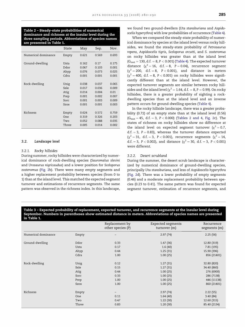
Table 2 – Steady-state probabilities of numericaldominance and richness at the insular level during thethree sampling periods. Abbreviations of species namesare presented in Table 1.

State May Sep. Nov.

Numerical dominance Empty 0.621 0.569 0.693

Ground-dwelling Usta 0.162 0.17 0.175

Ddor 0.067 0.103 0.001

Ahyp 0.076 0.073 0.025

Cdra 0.001 0.001 0.001

Rock-dwelling Unig 0.038 0.037 0.065

Ssle 0.017 0.036 0.009

Atig 0.014 0.004 0.01

Prep 0.001 0.002 0.007

Sorc 0.001 0.003 0.009

Szos 0.001 0.001 0.003

Richness Empty 0.624 0.572 0.759

One 0.319 0.326 0.203

Two 0.052 0.088 0.035

Three 0.005 0.014 0.002

a c t a o e c o l o g i c a 3 3 ( 2 0 0 8 ) 2 8 0 – 2 9 0 285

3.2. Landscape level

3.2.1. Rocky hillsidesDuring summer, rocky hillsides were characterized by numer-

ical dominance of rock-dwelling species (Sauromalus slevini

and Urosaurus nigricaudus) and a lower position for Sceloporus

zosteromus (Fig. 2b). There were many empty segments and

a higher replacement probability between species (from 0 to

1) than at the island level. This matched the expected segment

turnover and estimations of recurrence segments. The same

pattern was observed in the richness index. In this landscape,

Table 3 – Expected probability of replacement, expected turnovSeptember. Numbers in parentheses show estimated distancein Table 1.

Replacementother species

Numerical dominance Empty –

Ground-dwelling Ddor 0.33

Usta 0.17

Ahyp 0.44

Cdra 1.00

Rock-dwelling Unig 0.12

Ssle 0.15

Atig 0.44

Sorc 0.33

Prep 1.00

Szos 1.00

Richness Empty –

One 0.11

Two 0.47

Three 0.83

we found two ground-dwellers (Uta stansburiana and Aspido-

scelis hyperythra) with low probabilities of occurrence (Table 4).

When we compared the steady-state probability of numer-

ical dominance by species at the island level versus rocky hill-

sides, we found the steady-state probability of Petrosaurus

repens, Aspidoscelis tigris, Sceloporus orcutti, and S. zosteromus

on rocky hillsides was greater than at the island level

(Gtest ¼ 130, d.f. ¼ 8, P < 0.001) (Table 4). The expected turnover

distance (c2 ¼ 16, d.f. ¼ 8, P ¼ 0.04), recurrence segment

(c2 ¼ 200, d.f. ¼ 8, P < 0.001), and distance in meters

(c2 ¼ 400, d.f. ¼ 8, P < 0.001) on rocky hillsides were signifi-

cantly different than at the island level. However, the

expected turnover segments are similar between rocky hill-

sides and the island level (c2 ¼ 1.64, d.f. ¼ 8, P ¼ 0.99). On rocky

hillsides, there is a greater probability of sighting a rock-

dwelling species than at the island level and an inverse

pattern occurs for ground-dwelling species (Table 4).

In the rocky hillside landscape, there was a greater proba-

bility (0.72) of an empty state than at the island level (0.56)

(Gtest ¼ 45, d.f. ¼ 3, P < 0.000) (Tables 2 and 4, Fig. 2c). The

states of richness on rocky hillsides show no difference at

the island level on expected segment turnover (c2 ¼ 0.7,

d.f. ¼ 3, P ¼ 0.83), whereas the turnover distance expected

(c2 ¼ 31, d.f. ¼ 3, P < 0.001), recurrence segments (c2 ¼ 14,

d.f. ¼ 3, P < 0.002), and distance (c2 ¼ 30, d.f. ¼ 3, P < 0.001)

were different.

3.2.2. Desert scrublandDuring the summer, the desert scrub landscape is character-

ized by numerical dominance of ground-dwelling species,

principally Uta stansburiana, and less of Aspidoscelis hyperythra

(Fig. 2d). There was a lower probability of empty segments

(0.46) and a moderate replacement probability between spe-

cies (0.23 to 0.41). The same pattern was found for expected

segment turnover, estimation of recurrence segments, and

er, and recurrence segments at the insular level duringin meters. Abbreviations of species names are presented

by(P)

Expected segmentsturnover (m)

Recurrencesegments (m)

2.97 (74) 2.25 (56)

1.47 (36) 12.80 (319)

1.6 (40) 7.81 (195)

1.25 (31) 15.90 (396)

1.00 (25) 856 (21401)

1.27 (31) 32.80 (820)

1.27 (31) 34.40 (860)

1.00 (25) 276 (6900)

1.00 (25) 286 (7138)

1.00 (25) 446 (11138)

1.00 (25) 860 (21401)

2.97 (74) 2.22 (55)

1.64 (40) 3.40 (84)

1.22 (30) 12.60 (315)

1.20 (30) 85.40 (2134)

Fig. 2 – Diagram of transition probabilities of: (a) richness at the insular level, (b) numerical dominance; and (c) richness in

rocky hillsides, (d) numerical dominance, and (e) richness in desert scrub.

a c t a o e c o l o g i c a 3 3 ( 2 0 0 8 ) 2 8 0 – 2 9 0286

richness index. In this landscape, we did not find rock-

dwelling species (Table 4).

Steady-state probabilities for numerical dominance in des-

ert scrub differ significantly from the island level (Gtest ¼ 15,

d.f. ¼ 3, P ¼ 0.001). In desert scrubland, Uta stansburiana had

a steady-state probability of 0.23 as a dominant species and

Aspidoscelis hyperytrhus has a steady-state probability of 0.11.

Comparing expected segments and distance turnover, we

did not find significant statistical differences between desert

scrubland and the island level (c2 ¼ 0.54, d.f. ¼ 3, P ¼ 0.96;

c2 ¼ 7.9, d.f. ¼ 3, P ¼ 0.09). We found lower expected recur-

rence segments and distance for richness states within desert

scrubland than at the island level (c2 ¼ 7.9, d.f. ¼ 3, P ¼ 0.04;

c2 ¼ 80, d.f. ¼ 8, P ¼ 0.001). In this landscape, there were less

empty segments than at the island level (Gtest ¼ 8.6, d.f. ¼ 3,

P ¼ 0.035, see Tables 2 and 4, Fig. 2e). Number of species by

segment in desert scrubland were no different than at the is-

land level, as in the case for expected segment turnover and

distance (c2 ¼ 0.27, d.f. ¼ 3, P ¼ 0.96; c2 ¼ 5.16, d.f. ¼ 3,

P ¼ 0.16). However, recurrence segments and distance were

different (c2 ¼ 8, d.f. ¼ 3, P ¼ 0.04; c2 ¼ 30, d.f. ¼ 3, P ¼ 0.001).

3.3. Species level

This analysis was made for the most abundant species in both

landscapes. They were defined according to estimates of

steady-state probabilities that are >0.095; the value among

species ranged from 0.003 to 0.235 (Table 4); therefore, we

selected five species (Table 5). Table 5 shows that recurrence

for empty segments is, on average, between 1.2 to 1.8 seg-

ments (from 30 m to 45 m) for all species. When a species is

sighted in a segment, we expect to sight it again within 4.7

to 27.7 segments (117 to 692 m), depending on the species.

The state with four lizards per segment varied from 111 to

115 (2787 to 2890 m). Some species were absent from this

state, with different combinations of this description applying

to states, as shown in Table 5. According to these results, Uta

stansburiana had the most individuals by segment and the

shortest recurrence segment in the desert scrublands. On

rocky hillsides, Sauromalus slevini had more members by seg-

ment and Urosaurus nigricaudus had the shortest recurrence

segments and distances.

4. Discussion

Markov chains predict the most probable state of a system and

it depends only on the previous state of system before an

elapsed interval of time or space (Formacion and Saila,

1994). In temporal models, Markov chains can predict behav-

iour, dominance, or ecological succession, while spatial

models have been used to explain movements of animals. In

this sense, Hestbeck et al., 1991 noted that Markov chains

are not strictly appropriate for projected equilibrium regional

abundance of Canada geese; however, Markov chains are use-

ful for the study of population dynamics. Root and Kareiva

Table 4 – Expected probability during September of steady states, replacement, expected turnover, and recurrence segmentsfor numerical dominance and richness for numerical dominance and richness at the landscape level. Numbers inparentheses indicate estimated distance in meters. Abbreviations of species names are presented in Table 1.

Landscape Model State Steadystates

Replacement byother species (P)

Expected segmentsturnover (m)

Recurrencesegments (m)

Rocky hillside Numerical dominance Empty 0.720 – 4.18 (104) 1.62 (40)

Ssle 0.097 0.63 1.28 (32) 11.90 (297)

Unig 0.095 0.68 1.29 (32) 12.30 (307)

Ahyp 0.024 0.75 1.00 (25) 40.30 (1007)

Atig 0.024 0.63 1.00 (25) 40.30 (1007)

Usta 0.024 0.33 2.00 (50) 80.30 (2007)

Prep 0.006 0.00 1.00 (25) 164 (4100)

Sorc 0.006 1.00 1.00 (25) 164 (4100)

Szos 0.003 0.00 1.00 (25) 330 (8250)

Richness Empty 0.720 – 4.18 (104) 1.63 (40)

One 0.240 0.04 1.44 (36) 4.53 (113)

Two 0.034 0.50 1.11 (27) 31.50 (787)

Three 0.006 1.00 1.00 (25) 154 (3850)

Desert scrub Numerical dominance Empty 0.460 – 2.20 (55) 2.58 (64)

Usta 0.235 0.23 1.410 (35) 4.57 (114)

Ddor 0.190 0.34 1.66 (41) 6.99 (174)

Ahyp 0.115 0.41 1.23 (30) 9.71 (242)

Richness Empty 0.570 – 2.10 (74) 2.07 (51)

One 0.330 0.11 1.60 (40) 2.58 (64)

Two 0.090 0.48 1.20 (30) 11.50 (287)

Three 0.010 1.00 1.00 (25) 233 (5833)

a c t a o e c o l o g i c a 3 3 ( 2 0 0 8 ) 2 8 0 – 2 9 0 287

(1984) suggested that a flight sequence of cabbage butterflies

was Markovian. Kenkel (1993) demonstrated that individual

plant performance is determined in part by proximity of

neighbourhood, i.e. spatially dependent. Finally, Kincaid and

Cameron (1985) found that movements of cotton rats Sismodus

hispidus between habitats follow a Markovian pattern and

were dependent on age. Results in this study are similar to re-

sults reported in seasonal modelsdpreceding samples can

predict the state of the system (Wootton, 2001a,b; Hill et al.,

2004).

Transition probabilities of numerical dominance and rich-

ness at the island, landscape, and species levels can be used to

compress data into a few predictive quantities. Transition

Table 5 – Recurrence segments for the most abundant species inNumbers in parentheses indicate estimated distance in meters

State

Desert scru

Usta Ddor

Number of lizards/segment

0 1.6 (40) 1.7 (45)

1 4.7 (117) 8.5 (212)

2 7.5 (187) 18.4 (460)

3 58.7 (1467) 43.2 (1080)

4 115.6 (2890) –

Number expected for cell 9.5 14.6

d.f. 24 15

c2 81 75

P 0.00001 0.00001

probabilities, steady-state probabilities, replacement analysis,

expected turnover, and recurrence show different useful

information of the characteristics of spatial arrangement of

the lizard community. These include: (1) a view of the possible

interactions between species and their environment without

deeper evaluation (in the form of transition probabilities),

the interactions occurring in areas where growth, survival,

and reproduction are suitable for maintaining population dy-

namics in the absence of immigration (Pulliam, 2000)dalso,

dominance and spatial recurrence change, depending on avail-

ability of resources and habitat use where some species tend to

be dominant in certain areas and rare in other; (2) an index

of dominance and richness (steady-states probabilities);

desert scrub and rocky hillside landscapes. –, not recorded.. Abbreviations of species names are presented in Table 1.

Recurrence segments (m)

b Rocky hillside

Ahyp Unig Ssle

1.6 (40) 1.2 (30) 1.8 (45)

9.7 (242) 10.5 (262) 27.7 (692)

36.5 (912) 41.7 (1043) 116 (2900)

74.0 (1850) – 176 (4400)

111.5 (2787) – –

9 19 11.1

24 8 15

81 60 73

0.00001 0.00001 0.00001

a c t a o e c o l o g i c a 3 3 ( 2 0 0 8 ) 2 8 0 – 2 9 0288

(3) importance of seasonal activity and scale in the spatial dispo-

sition of species; (4) an estimate of spatial change in dominance

and richness (replacement and turnover segments); and (5)

observation of abundance of individual species (recurrence

segments). Also, since we include four different kinds of habi-

tats, we can analyse effect of transition probabilities between

pairs of species among diverse environmental conditions.

The results of the island and landscape models provide

some interesting insights into the importance of seasonal

change in the spatial arrangement of lizard species. Four

main results were found. (1) In contrast to sedentary species

(Hill et al., 2004), season influenced the estimates of parame-

ters of numerical dominance and richness that can be

explained by interspecific differences in periods of activity,

thermal preferences, or foraging behaviour. For example, Dip-

sosaurus dorsalis is active in warmer months and reduces its

activity at temperatures below 25 �C (Muth, 1980) as do Petro-

saurus repens and Sceloporus orcutti (Grismer, 1994). (2) There

were higher transition probabilities within a habitat group

(ground-dwelling or rock-dwelling) than between species.

This spatial segregation could reflect choice of different mi-

croclimates, reflecting physiological tolerance or choice of dif-

ferent vegetation (Pianka, 1982; Vitt, 1991). (3) Since steady-

state probabilities, expected turnover, and recurrence seg-

ments were lower at the island than the landscape level, it is

necessary to select the appropriate scale for evaluation in sur-

vey methods to obtain a more realistic estimate of abundance

and richness of species (Collins and Glenn, 1995; Bradbury

et al., 2001). In this case, the island level was used to contrast

species with different niche requirements and the landscape

level to analyse species with similar niche requirement. (4)

We found lower probabilities of steady states for rock-dwell-

ing species at the island level and rocky hillsides than species

in the desert scrubland.

We found that Uta stansburiana will probability become the

dominant species at the island level and in the desert scrub-

land and Urosaurus nigricaudus will continue to be the domi-

nant species on rocky hillsides. In contrast, Sceloporus

zosteromus and Petrosaurus repens have the lowest probabilities

to become dominant species at the island level and in the

rocky hillside landscape. Our results seem to be consistent

with observations about generalist species tending to achieve

dominance (Formacion and Saila, 1994; Brown et al., 1995).

According to Hanski and Gyllenberg, 1997, generalist species,

such as U. stansburiana, or species using broad resources are

common and widely distributed; whereas specialist species,

such as P. repens, are narrowly distributed.

We found that three species co-exist in high abundance

and low recurrence in segments of the desert scrubland, while

eight species are present in low abundance and high recur-

rence in segments of rocky hillside. This result is consistent

with the models of He and Legendre (2002) and Kneitel and

Chase (2004) that higher species richness in a sampling area

occurs if the species are spatially more regularly distributed

in the community, while high spatial aggregation of individ-

uals of a species result in lower species richness in a study

area. When environmental factors or resources are spatially

variable, different species find suitable microhabitats in dif-

ferent localities and co-exist regionally (Morris, 1990; He and

Legendre, 2002).

At the species level in desert scrubland, Aspidoscelis hyper-

ythus had the highest number of recurrence segments for their

states of abundance, possibly because this species actively

forages (Pianka, 1982) and defends a mobile territory from

other conspecifics (Eifler and Eifler, 1998). Uta stansburiana is

a passive, general predator, using broad spatial resources by

sitting and waiting (Grismer, 2002), which could explain its

high abundance and low recurrence in this landscape. On

the rocky hillside, Sauromalus slevini is the rock-dwelling spe-

cies with more lizards per segment, possibly because the

males protect their polygynous territories (Kwiatkowski and

Sullivan, 2002). In general, inter- and intraspecific differences

in abundance depend on spatially-fixed environmental varia-

tions and seasonal environmental variations (Ives and

Klopfer, 1997; Pulliam, 2000). In lizards, abundance autocorre-

lation can result from social organization (Glinsky and Krekor-

ian, 1985; Eifler and Eifler, 1998), foraging mode (Pianka, 1982),

mating systems (Sinervo et al., 2001; Kwiatkowski and Sulli-

van, 2002), or food resources (Vitt, 1991).

Our estimates of first-order Markovian chains are domi-

nated by empty segments and these probably play a funda-

mental role in inter- and intraspecific interactions. Gilpin

and Hanski, 1991 proposed that unoccupied, but habitable,

areas may also be important in the dynamics of the spatial

structure of populations. In this sense, populations may be-

come locally extinct, even in perfectly suitable habitats, and

the delay between extinction and re-colonization should leave

some fraction of suitable habitats unoccupied at any given

time (Thomas and Kunin, 1999). Patches and travelling waves

can be produced when populations are influenced by densities

of neighbouring populations (Sinervo et al., 2001), where spa-

tial-temporal patterns occur because local dispersal of indi-

viduals link the dynamics of adjacent areas (Morris, 1990;

Johnson, 2000).

Legendre (1993) explained that spatial structuring is an im-

portant component of ecosystems, where heterogeneity is

functional, and not the result of some random, noise-generat-

ing process. Because the spatial pattern in the desert lizard

community is variable, with spatial patterns that change sea-

sonally (Vitt, 1991; Case, 2002; Grismer, 2002), we quantified

the probability that a random sighting of a lizard at an insular

and landscape level in different periods of year. To predict

spatial behaviour in biological communities, it was necessary

to quantify the complete distribution of probabilities that

describe movements and sightings along all possible land-

scapes and seasons (Bradbury et al., 2001). If the dynamics of

movement are even moderately complex, it is not possible

to describe complete sight probability of movement in conve-

nient, closed forms, such as those found by other researchers

(Yoccoz et al., 2001; MacKenzie et al., 2003). We need to know

not only what physical boundaries delineate lizard species,

but also to show how rapidly the components of a species

mix change within those boundaries.

In conclusion, we could establish a model where each pair

of values was dependent only upon its immediate predecessor

segment. According to Liebhold and Gurevitch, 2002, spatial

dependence of ecological data has typically been a problem

that can reduce a field observer’s capacity to understand the

spatial pattern of the population or community. This effort

illustrates how first-order Markovian spatial chains may be

a c t a o e c o l o g i c a 3 3 ( 2 0 0 8 ) 2 8 0 – 2 9 0 289

used to examine spatial dependence of abundance and rich-

ness at different scales and seasons. However, understanding

how neighbouring elements affect each other or how they af-

fect a process is quite different from classical ecological

concerns for the structure and function of discrete communi-

ties, populations, or ecosystems (Pickett and Cadenasso, 1995).

Acknowledgements

We thank Abelino Cota, Franco Cota, Israel Guerrero, and

Armando Tejas for assistance with fieldwork. This research

was supported by grants from Consejo Nacional de la Ciencia

y Tecnologıa (CONACYT) and Fondo Mexicano para la Conser-

vacion de la Naturaleza (FMCN). Thanks are extended to one

anonymous reviewer who made useful comments and sug-

gestions to improve the manuscript.

r e f e r e n c e s

Bell, G., 2001. Neutral macroecology. Science 293, 2413–2418.Bevers, M., Flather, C.H., 1999. The distribution and abundance of

population limited at multiple spatial scales. J. Anim. Ecol. 68,976–987.

Bradbury, R.B., Payne, R.J.H., Wilson, J.D., Krebs, J.B., 2001.Predicting population responses to resource management.Trends Ecol. Evol. 16, 440–445.

Brown, J., Mehlman, D., Stevens, G.C., 1995. Spatial variation inabundance. Ecology 76, 2028–2043.

Case, T.J., 2002. Ecology of reptiles. In: Case, T.J., Cody, M.C. (Eds.),New Island Biogeography in the Sea of Cortez. OxfordUniversity Press, New York, pp. 221–270.

Collins, S., Glenn, S., 1995. Effects of organismal and distancescaling on analysis of species distribution and abundance.Ecol. Appl. 7, 543–551.

Eifler, D.A., Eifler, M.A., 1998. Foraging behavior and spacingpatterns of the lizard Cnemidophorus uniparens. J. Herpetol. 1,24–33.

Formacion, S.P., Saila, S.B., 1994. Markov chain properties totemporal dominance changes in a Philippine pelagic fishery.Fish. Res. 19, 241–256.

Gilpin, M.E., Hanski, I., 1991. Metapopulation Dynamics: Empiricaland Theoretical Investigations. Academic Press, London.

Glinsky, T.H., Krekorian, C., 1985. Individual recognition in free-living adult male desert iguanas, Dipsosaurus dorsalis.J. Herpetol. 19, 541–554.

Grismer, L.L., 1994. The origin and evolution of the peninsularherpetofauna of Baja California, Mexico. Herpet. Nat. Hist. 1,51–106.

Grismer, L.L., 2002. Amphibians and Reptiles of Baja California, ItsPacific Islands, and the Islands in the Sea of Cortes. Universityof California Press, Berkeley.

Hanski, I., Gyllenberg, M., 1997. Uniting two general patterns inthe distribution of species. Science 275, 397–400.

Hall, F.G., Botkin, D.B., Strebel, D.E., Woods, K.D., Goetz, S.J., 1991.Large-scale patterns of forest succession as determined byremote sensing. Ecology 72, 628–640.

He, F., Legendre, P., 2002. Species diversity pattern derived fromspecies-area models. Ecology 83, 1185–1198.

Hestbeck, J.B., Nichols, J.D., Malecki, R.A., 1991. Estimates ofmovement and sites fidelity using mark-resight data ofwintering Canada Geese. Ecology 72, 523–533.

Hill, M.F., Witman, J.D., Caswell, H., 2004. Markov chain analysisof succession in rocky subtidal community. Am. Nat. 164,E46–E61.

Ives, A.R., Klopfer, E.D., 1997. Spatial variation in abundance createdby stochastic temporal variation. Ecology 78, 1907–1913.

Johnson, M.P., 2000. Scale of density dependence as an alternativeto local dispersal in spatial ecology. J. Anim. Ecol. 69, 536–540.

Kenkel, N.C., 1993. Modeling Markovian dependence inpopulations of Aralia nudicaulis. Ecology 74, 1700–1708.

Kincaid, M.B., Cameron, G.N., 1985. Interactions of cotton ratswith a patchy environment: dietary responses and habitatselection. Ecology 66, 1769–1783.

Kneitel, J.M., Chase, J.M., 2004. Trade-offs in community ecology:linking spatial scales and species coexistence. Ecol. Lett. 7,69–80.

Kwiatkowski, A.A., Sullivan, B.K., 2002. Mating system structureand population density in a polygynous lizards, Sauromalusobesus (¼ater). Inter. Soc. Behav. Ecol. 2, 201–208.

Legendre, P., 1993. Spatial autocorrelation: trouble or newparadigm. Ecology 73, 1659–1673.

Lichstein, J.M., Simons, T.R., Shriner, S.A., Franzreb, K.E., 2002.Spatial autocorrelation and autoregressive models in ecology.Ecol. Monogr. 72, 445–463.

Liebhold, A.M., Gurevitch, J., 2002. Integrating the statisticalanalysis of spatial data in ecology. Ecography 25, 553–557.

Lusseau, D., 2003. Effects of tour boats on the behaviour ofbottlenose dolphins: using Markov chain to modelanthropogenic impacts. Conserv. Ecol. 17, 1785–1793.

MacKenzie, D.I., Nichols, J.D., Hines, J.E., Knutson, M.G.,Franklin, A.A., 2003. Estimating site occupancy, colonization,and local extinction when a species in detected imperfectly.Ecology 84, 2200–2207.

Morris, D.W., 1990. Temporal variation, habitat selection andcommunity structure. Oikos 59, 303–312.

Muth, A., 1980. Physiological ecology of desert iguana (Dipsosurusdorsalis) eggs: temperature and water relations. Ecology 61,1335–1343.

Orloci, L., Orloci, M., 1988. On recovery, Markov chains, andcanonical analysis. Ecology 69, 1260–1265.

Pianka, E.R., 1982. Niche relations of desert lizards. In: Cody, M.,Diamond, J. (Eds.), Ecology and Evolution of Communities.Harvard University Press, Cambridge, MA, pp. 292–314.

Pickett, S.T.A., Cadenasso, M.L., 1995. Landscape ecology: spatialheterogeneity in ecological systems. Science 269, 331–334.

Pough, F., Andrews, R., Cadle, J., Crump, M., Savitsky, A., Wells, K.,2004. Herpetology. Pearson Prentice Hall, New Jersey.

Pulliam, H.R., 2000. On the relationship between niche anddistribution. Ecol. Lett. 3, 349–361.

Railsback, S.F., Stauffer, H.B., Harvey, B.C., 2003. What can habitatpreference models tell us? test using a virtual troutpopulation. Ecol. Appl. 13, 1580–1594.

Roshchild, R.S., Mullen, A.J., 1985. The information content ofstock-and-recruitment data and its non-parametricclassification. J. Cons. Int. Explor. Mer. 42, 116–124.

Root, R.B., Kareiva, P.M., 1984. The search resources by cabbagebutterflies (Pieris rapae) ecological consequences andadaptative significance of Markovian movements in a patchyenvironment. Ecology 65, 147–168.

Sokal, R.R., Rohlf, F.J.R., 1981. Biometry, second ed. Freeman, SanFrancisco, CA.

Sinervo, B., Svensson, E., Comendant, T., 2001. Condition genotype-by-environment interaction, and correlational selection inlizards life-history morphs. Evolution 10, 2053–2069.

Tanner, J.E., Hughes, T.P., Connell, J.H., 1996. The role of history incommunity dynamics: a modelling approach. Ecology 77,108–117.

Thomas, C.D., Kunin, W.E., 1999. The spatial structure ofpopulations. J. Anim. Ecol. 68, 647–657.

a c t a o e c o l o g i c a 3 3 ( 2 0 0 8 ) 2 8 0 – 2 9 0290

Tucker, B., Anand, C.M., 2004. The applications of Markov modelsin recovery and restoration. Int. J. Ecol. Environ. Sci. 30,131–140.

Venegas, B.C.S., 2003. Abundancia, distribucion y nicho de laslagartijas diurnas de Isla Coronados, Baja California Sur,Mexico. Master’s Thesis. Centro de Investigaciones Biologicasdel Noroeste, La Paz, B.C.S., Mexico.

Vitt, L.J., 1991. Desert reptile communities. In: Polis, G.A. (Ed.), TheEcology of Desert Communities. University of Arizona Press,Tucson, pp. 249–277.

Wileyto, E.P., Ewens, W.J., Mullen, M.A., 1994. Markov-recapturepopulation estimates: a tool for improving interpretations oftrapping experiments. Ecology 75, 1109–1117.

Wootton, J.T., 2001a. Prediction in complex communities: analysisof empirically derived Markov models. Ecology 82, 580–598.

Wootton, J.T., 2001b. Causes of species diversity differences:a comparative analysis of Markov models. Ecol. Lett. 4, 46–56.

Yoccoz, N.G., Nichols, J.D., Boulinier, T., 2001. Monitoring ofbiological diversity in space and time. Trends Ecol. Evol. 16,446–453.