Management of Environmental Quality: An International JournalEmerald Article: Statistical methods for analysis of seasonal modifications in the salt marshes of the Venice lagoonM. Camuffo, F. Benvenuto, M. Marani Abbadessa, L. Modenese, A. Marani

Article information:

To cite this document: M. Camuffo, F. Benvenuto, M. Marani Abbadessa, L. Modenese, A. Marani, (2006),"Statistical methods for analysis of seasonal modifications in the salt marshes of the Venice lagoon", Management of Environmental Quality: An International Journal, Vol. 17 Iss: 3 pp. 323 - 338

Permanent link to this document: http://dx.doi.org/10.1108/14777830610658737

Downloaded on: 31-10-2012

References: This document contains references to 29 other documents

To copy this document: permissions@emeraldinsight.com

Access to this document was granted through an Emerald subscription provided by UNIVERSITA CA FOSCARI DI VENEZIA

For Authors: If you would like to write for this, or any other Emerald publication, then please use our Emerald for Authors service. Information about how to choose which publication to write for and submission guidelines are available for all. Please visit www.emeraldinsight.com/authors for more information.

About Emerald www.emeraldinsight.comWith over forty years' experience, Emerald Group Publishing is a leading independent publisher of global research with impact in business, society, public policy and education. In total, Emerald publishes over 275 journals and more than 130 book series, as well as an extensive range of online products and services. Emerald is both COUNTER 3 and TRANSFER compliant. The organization is a partner of the Committee on Publication Ethics (COPE) and also works with Portico and the LOCKSS initiative for digital archive preservation.

*Related content and download information correct at time of download.

Statistical methods for analysis ofseasonal modifications in the saltmarshes of the Venice lagoon

M. Camuffo, F. Benvenuto, M. Marani Abbadessa, L. Modeneseand A. Marani

Department of Environmental Sciences, Venezia, Italy

Abstract

Purpose – To define synthetic indices of changes of vegetation coverage on salt marshes of theVenice lagoon that might be used to model changes of the entire basin.

Design/methodology/approach – Remote sensing data from the satellite sensor QuickBird wereprocessed to retrieve vegetation coverage in different seasons, i.e. different phenological stages of thehalophytic vegetation. These changes have been described by means of landscape metrics (LSM’s) andstatistical moments.

Findings – LSM’s selected have been useful to describe the dominant shapes of vegetation coverage,while the low variations occurred were only partially explained. The first four statistical momentshave been only partially functional to the description of temporal variation of the patches.

Practical implications – These indicators, whose performances have been evaluated by the presentwork, could be used to detect larger variations on longer period and on wider spatial scale. In this wayit could also be possible to easily detect the effects of changes on the hydrodynamic regime that mayoccur in relation with new projected interventions on the Venice lagoon.

Originality/value – This approach has never been applied to salt marshes of the Venice lagoon. Theremote sensing data, in particular LSM’s and statistical moments applied together, might be valuabletools to detect shape changes in the delicate environment of salt marshes and suggest possibleremedies for problems of managing the Venice lagoon.

Keywords Salts, Water, Italy, Statistical analysis, Environmental management, Aquatic biology

Paper type Case study

IntroductionCoastal wetland areas, such as lagoons and estuaries, are complex and delicateenvironments subject to rapid morphological and ecological evolution, often inresponse to strong anthropogenic pressure. In recent years the combined ecological andeconomic importance of these dynamic environments has focused attention onmonitoring and forecasting change in these natural coastal deposits.

The Venice lagoon (Northern Italy, Figure 1) is a representative example (Maraniet al., 2004). It has been deeply modified over several centuries through the diversion ofthe main rivers which used to flow into the lagoon to the sea, the dredging of artificialchannels, and the construction of jetties at the three inlets. The resulting changes have

The current issue and full text archive of this journal is available at

www.emeraldinsight.com/1477-7835.htm

The authors thank Sistema Informativo of Consorzio Venezia Nuova for giving us aerialorthorectified photos of the Venice lagoon. They also thank Pamela Berry for her invaluable help inimproving the English of our manuscript and the anonymous referees for their very usefulcomments and suggestions. This research was supported by the European Research Project TidalInlets Dynamics and Environment – Tide, EVK3-CT-2001-00064, www.istitutoveneto.it/tide).

Analysis ofseasonal

modifications

323

Management of EnvironmentalQuality: An International Journal

Vol. 17 No. 3, 2006pp. 323-338

q Emerald Group Publishing Limited1477-7835

DOI 10.1108/14777830610658737

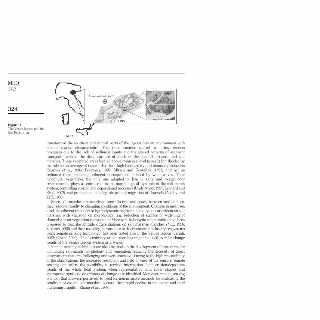
transformed the southern and central parts of the lagoon into an environment withdistinct marine characteristics. This transformation caused by diffuse erosionprocesses due to the lack of sediment inputs and the altered patterns of sedimenttransport involved the disappearance of much of the channel network and saltmarshes. These vegetated areas located above mean sea level (a.m.s.l.) but flooded bythe tide on an average of twice a day, host high biodiversity and biomass production(Scarton et al., 1996; Boorman, 1999; Mitsch and Gosselink, 1993) and act assediment traps, reducing sediment re-suspension induced by wind waves. Theirhalophytic vegetation, the only one adapted to live in salty and oxygen-poorenvironments, plays a central role in the morphological dynamic of the salt marshsystem, controlling erosion and depositional processes (Underwood, 1997; Leonard andReed, 2002), soil production, stability, shape, and migration of channels (Ashley andZeff, 1988).

Since, salt marshes are transition zones (in time and space) between land and sea,they respond rapidly to changing conditions of the environment. Changes in mean sealevel, in sediment transport or hydrodynamic regime punctually appear evident on saltmarshes: with variation on morphology (e.g. reduction of surface or widening ofchannels) or on vegetation composition. Moreover, halophytic communities have beenproposed to describe altitude differentiations on salt marshes (Sanchez et al., 1996;Silvestri, 2000) and their usability, as variables to discriminate and classify ecosystemsusing remote sensing technology, has been tested also in the Venice lagoon (Ceriali,2002; Cibien, 1999). This sensitivity of salt marshes might be used to infer changetrends of the Venice lagoon system as a whole.

Remote sensing techniques are ideal methods to the development of procedures formonitoring salt-marsh morphology and vegetation, reducing the necessity of directobservations that are challenging and work-intensive. Owing to the high repeatabilityof the observations, the increased resolution and field of view of the sensors, remotesensing data offers the possibility to retrieve information about erosion/depositiontrends of the whole tidal system, when representative land cover classes andappropriate synthetic descriptors of changes are identified. Moreover, remote sensingis a tool that answers positively to need for non-invasive methods for evaluating thecondition of coastal salt marshes, because their rapid decline in the extent and theirincreasing fragility (Zhang et al., 1997).

Figure 1.The Venice lagoon and theSan Felice area

MEQ17,3

324

Many studies have already been done in order to test new approaches to infer long termprocesses from scaling relationship and spatial patterns (Belyea and Lancaster, 2002;Aitkenhead et al., 2004; Paruelo and Tomasel, 1997). Spatial analysis provides valuableinsight into the developmental processes operating at particular sites. Then comparativeanalysis in salt marshes complexes would provide valuable insight into how physicalfactors influence the landscape dynamics of patterned salt marshes.

Thus, this paper explores the possibility of properly describing the most relevantpatterns of the salt marsh landscape, and subsequently of discriminating seasonalchanges of salt marsh coverage integrating the use of multispectral data and theapplication of several indices to describe these variations and, hopefully, the dynamicsof the factors that determine them.

Data and preprocessingThis study describes quantitative observations of selected areas using remotesensing and field observations performed during the European Research ProjectTIDE (acknowledgments). Three QuickBird (www.digitalglobe.com/product/basic_imagery.shtml) satellite images were used to observe seasonal (andtemporal) changes in the environment. This system offers a very high spatialresolution indispensable to study salt marsh areas: from 2.8 m, in the multispectralimage, to 0.70 m in the panchromatic one. On the other hand, the spectral resolutionis sufficient to discriminate the main end members present on salt marshes offeringthree bands on the visible (450-520 nm; 520-600 nm; 630-690 nm) and one on the nearinfrared (760-900 nm).

We obtained seasonal data in two different years (2002-2003) and with widedifferences in tide level:

16 May 2002 tidal level 2 16 cm m.s.l.

10 February 2003 tidal level 2 24 cm m.s.l.

25 July 2003 tidal level þ 08 cm m.s.l.

10 October 2003 tidal level þ 60 cm m.s.l.

At the same time, as the satellite flays over the salt-marshes recording an image (imageacquisition), more than 90 patches in the study area were perimetrated by a DifferentialGeographic Position System, to define the regions of interest (ROIs) of the selectedclasses on each of these images. These observations have confirmed the similarity inthe vegetation situation between May 2002 and May 2003, thus in our work we wereable to enhance differences due to seasonality of vegetation and different tidal levels,leaving out the different years of images recording.

There has also been a satellite acquisition in October 2003 but the very high tidelevel, 60 cm a.m.s.l., that determined the submersion of the studied salt marshes,prevented its use in the present study. Thus, only data recorded on May 2002,February and July 2003 have been processed.

The QuickBird images were first radiometrically corrected and converted in reflectancedata by atmospheric correction using the 6S model (Vermote et al., 1997), on the basis ofsun photometer-derived atmospheric optical thickness supplied by the Venice Instituteof the Italian Consiglio Nazionale delle Ricerche (data available on the web-site of

Analysis ofseasonal

modifications

325

the International Research Network AERONET: http://aeronet.gsfc.nasa.gov).After this phase, images were georeferenced to the Gauss-Boaga coordinate systemusing about 70 ground control points, both registered on field and derived fromorthorectified aerial photos (0.16 m resolution). Data geocoding was performed using thefirst order polynomial model and nearest-neighbours re-sampling method with a rootmean square error less than 0.6 pixel for all images.

The three images were also co-registered and areas outside the study site weremasked out to avoid a useless increase of the computational time.

The investigated areaThe study area selected is a complex of salt marshes named San Felice salt marsh(Figure 1 and Plate 1). It is located in the northern part of the Venice lagoon(semi-diurnal tidal regime with average maximum tidal excursion of 1 m) and its totalarea is 1.02 km2. San Felice salt marsh degrades from the main channels down to a bigcentral depression and has an average elevation of about 0.30 m (a.m.s.l.).

The great anthropogenic interventions that occurred in the lagoon, until now, hadjust partially disturbed the salt marshes of our study. Their relative stability hasallowed us to establish a differentiation of micro-unevenness and sedimentologiccharacteristics of the substrate and thus an organized vegetational order. It is thereforereasonable to control the actual shapes in order to estimate the evolutionary tendencies,also in relation to plans that could induce important alterations in the area. The controlmust obviously be distributed in the space and in the time and it cannot be limited topunctual measures, even if numerous, therefore remote sensing techniques appear to bethe appropriate instrument in such context.

Plate 1.An overview of the SanFelice salt marsh

MEQ17,3

326

MethodsPost-classification comparison involves independently produced spectral classificationfollowed by a pixel-by-pixel comparison to detect change in cover type (Coppin et al.,2004) often showing only two classes: changed and unchanged areas.

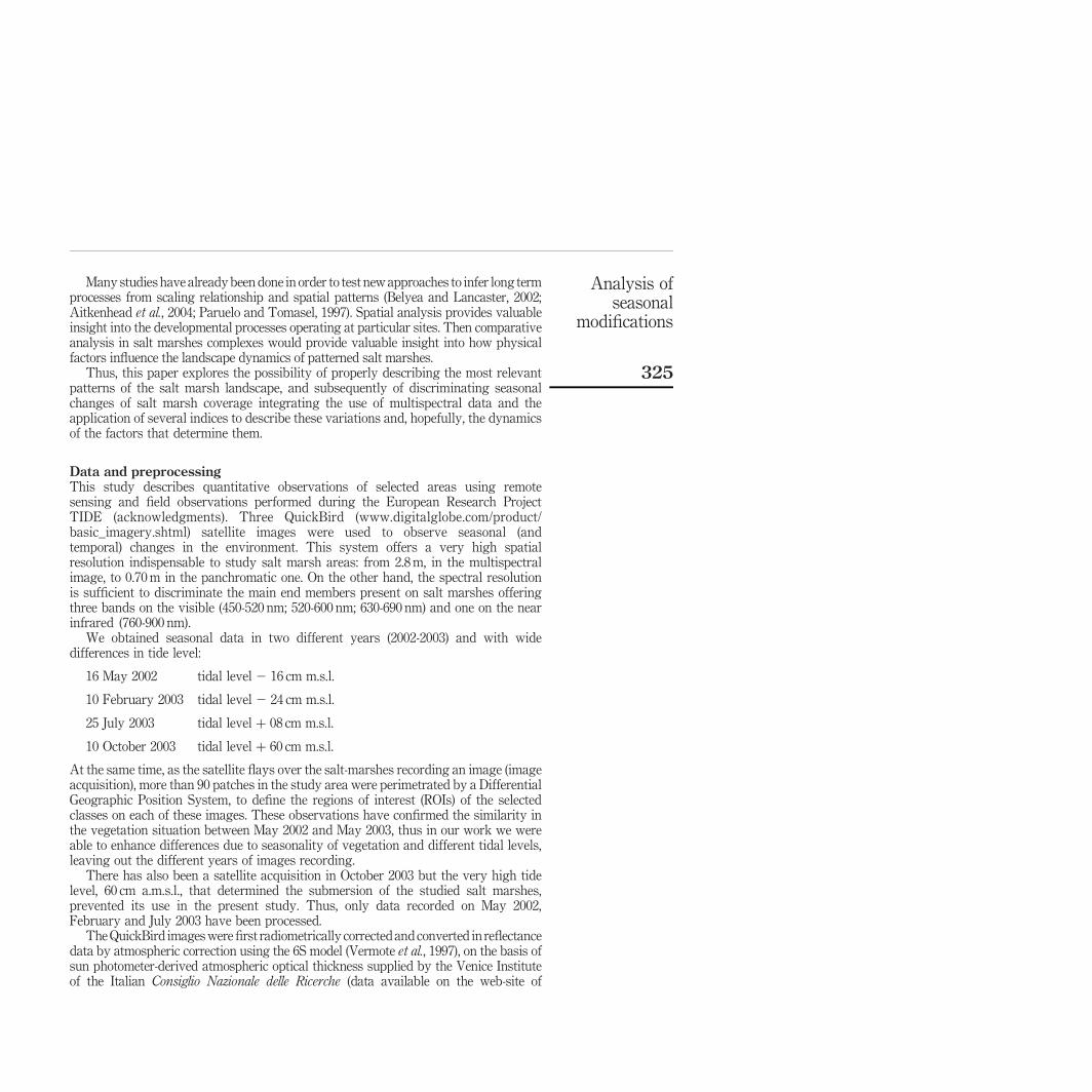
This study was focused on changes between individual classes, particularly among“soil” “water” and “vegetation” and on the changes in their spatial distributions. Thus, ithas been decided to integrate post-classification comparisons with a statistical analysisof the three classes in the three periods in which images were registered. The imageswere classified using data of classes coverage, collected on field delimiting areas ofinterest of each class by a differential GPS, applying the supervised algorithm SpectralAngle Mapper (Kruse et al., 1993) as implemented on the commercial software ENVI(Figure 2). A subset of the pixels defined by the ROI was used to test the accuracy of theclassifications that resulted higher than 90 per cent for all the processed images.

In order to define and describe the constitutive elements of a landscape, thelandscape ecology’s methodology and some statistical indicators have been adopted:both of them can help to investigate the mechanisms of salt marsh evolution. From theoperative point of view, this has been done both with the freeware software Fragstat3.3 (McGarigal and Marks, 1994) and with a Fortan code written to determine clustersfor each class and to calculate statistical moments.

The basic elements of the landscape structure are the patches of the ecosystemsdefined by Riitters et al. (1995) as an aggregation of adjacent pixels (considering theeight pixels nearest to a fixed one) belonging to the same class. Different configurationand composition of landscape elements can indicate an ecosystem evolution, assumingthat the ecological processes interact with the landscape structures and are influencedby their configuration (Forman, 1995; Sondergrath and Schroder, 2002; Vulleumier andPrelaz-Droux, 2002).The quantitative description of the landscape structures can bedone by many landscape metrics (LSM). We used the LSM introduced by Gustafson(1998). The performance of several metrics among them has been tested for the presentstudy but only five have been employed because they better allowed the extraction ofspecific characteristics of the salt marshes. In Appendix 1 they are briefly summarized.

Moreover, the use of statistical moments computed with respects of pixel spatialcoordinates of the patches can contribute to determine synthetic indicators of formand disposition. Moments are constants characterising a spatial data distribution.Numerous algorithms and techniques use them for pattern recognition, objectsidentification, image coding, and reconstruction. Moment-based methods oftenyield features from an image that are invariant to translation, scaling, and rotation(Liao and Pawlak, 1996; Reiss, 1991; Teague, 1980). It is well known that, in principle,most of the image information can be recaptured by using a sufficiently large number

Figure 2.Classification results of

the salt marsh of SanFelice: water in black,

vegetated areas in greyand bare soil areas in

white

Analysis ofseasonal

modifications

327

of a particular set of image moments: the question is how well an image can becharacterized and reconstructed by a small finite set of its moments or, equivalently,how many different moments must be computed to distinguish significantly differentpatterns (Cho-Huak and Roland, 1988). In the present study the geometric momentshave been considered because they are the more suited to our focused goals.

In order to investigate only the geometrical variations of patches along the time andalso to facilitate the interpretation of the results, we computed only the former fourcentral moments, the ones used most in statistics. We calculated them with respect tospatial coordinates of the pixels of patches considering separately both X- and Y-axis.The four former moments practically used in this work are summarized in Appendix 2.To calculate them we developed a Fortran code.

Analysis and results of the inter seasonal comparisonThe basic surface in every image was the squared pixel with 2.8 m side. The classescomposing the landscape considered in the present study were water (present in smallchannels locally named ghebi and salt pans), vegetation, and soil. The decision to useonly three classes is due to the necessity to define a procedure in order to highlightchanges even if the detected period is too short to determine strong variations. Thus,we selected these macro-classes that have significant changes with the seasons and thetide level. Further work will analyse the changes occurring on patches of differenthalophytic species.

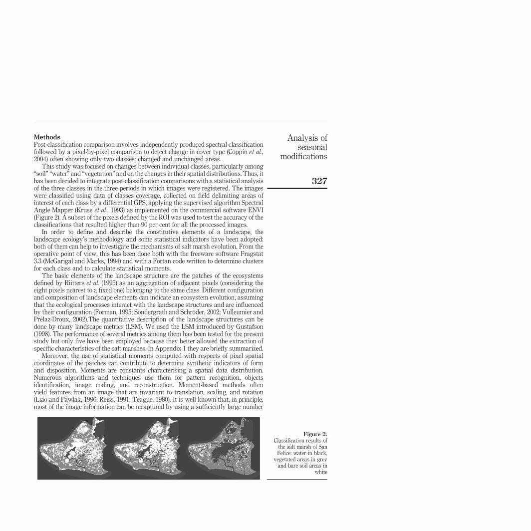
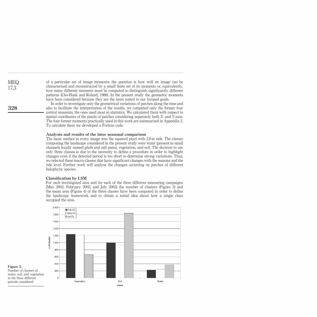
Classification by LSMFor each investigated area and for each of the three different measuring campaigns(May 2002, February 2003, and July 2003) the number of clusters (Figure 3) andthe mean area (Figure 4) of the three classes have been computed in order to definethe landscape framework and to obtain a initial idea about how a single classoccupied the area.

Figure 3.Number of clusters ofwater, soil, and vegetationin the three differentperiods considered

MEQ17,3

328

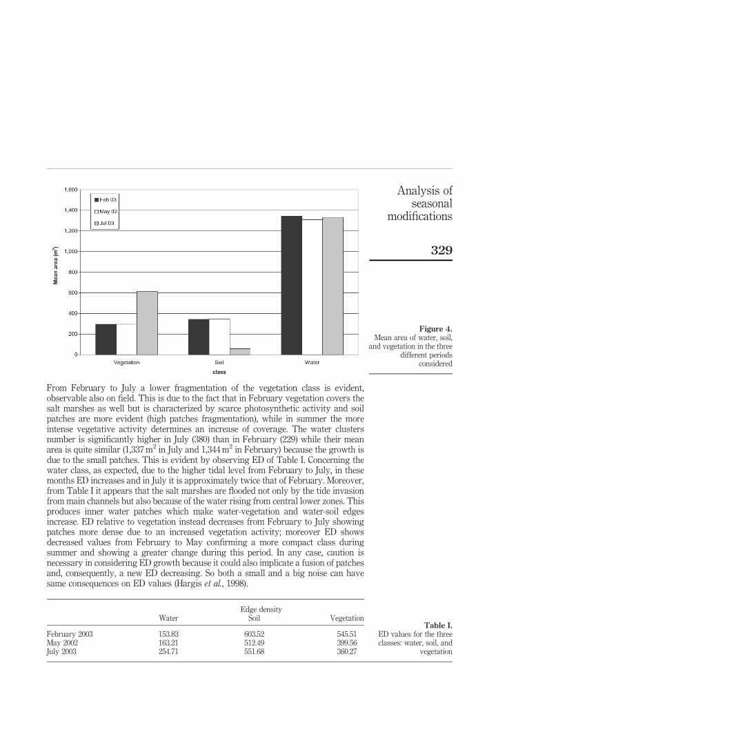
From February to July a lower fragmentation of the vegetation class is evident,observable also on field. This is due to the fact that in February vegetation covers thesalt marshes as well but is characterized by scarce photosynthetic activity and soilpatches are more evident (high patches fragmentation), while in summer the moreintense vegetative activity determines an increase of coverage. The water clustersnumber is significantly higher in July (380) than in February (229) while their meanarea is quite similar (1,337 m2 in July and 1,344 m2 in February) because the growth isdue to the small patches. This is evident by observing ED of Table I. Concerning thewater class, as expected, due to the higher tidal level from February to July, in thesemonths ED increases and in July it is approximately twice that of February. Moreover,from Table I it appears that the salt marshes are flooded not only by the tide invasionfrom main channels but also because of the water rising from central lower zones. Thisproduces inner water patches which make water-vegetation and water-soil edgesincrease. ED relative to vegetation instead decreases from February to July showingpatches more dense due to an increased vegetation activity; moreover ED showsdecreased values from February to May confirming a more compact class duringsummer and showing a greater change during this period. In any case, caution isnecessary in considering ED growth because it could also implicate a fusion of patchesand, consequently, a new ED decreasing. So both a small and a big noise can havesame consequences on ED values (Hargis et al., 1998).

Figure 4.Mean area of water, soil,

and vegetation in the threedifferent periods

considered

Edge densityWater Soil Vegetation

February 2003 153.83 603.52 545.51May 2002 163.21 512.49 399.56July 2003 254.71 551.68 360.27

Table I.ED values for the threeclasses: water, soil, and

vegetation

Analysis ofseasonal

modifications

329

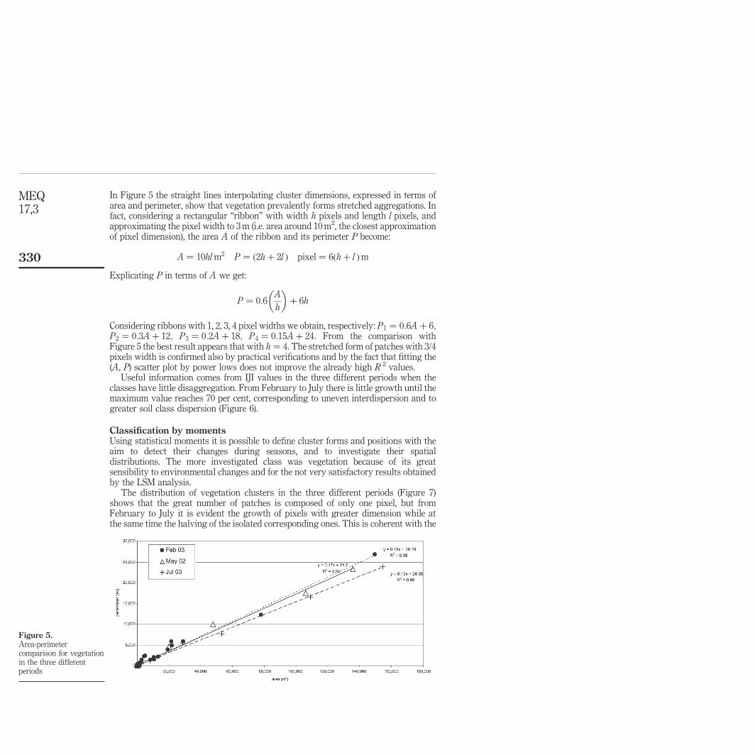
In Figure 5 the straight lines interpolating cluster dimensions, expressed in terms ofarea and perimeter, show that vegetation prevalently forms stretched aggregations. Infact, considering a rectangular “ribbon” with width h pixels and length l pixels, andapproximating the pixel width to 3 m (i.e. area around 10 m2, the closest approximationof pixel dimension), the area A of the ribbon and its perimeter P become:

A ¼ 10hl m2 P ¼ ð2hþ 2l Þ pixel ¼ 6ðhþ l Þm

Explicating P in terms of A we get:

P ¼ 0:6A

h

� �þ 6h

Considering ribbons with 1, 2, 3, 4 pixel widths we obtain, respectively: P1 ¼ 0:6Aþ 6;P2 ¼ 0:3Aþ 12; P3 ¼ 0:2Aþ 18; P4 ¼ 0:15Aþ 24: From the comparison withFigure 5 the best result appears that with h ¼ 4. The stretched form of patches with 3/4pixels width is confirmed also by practical verifications and by the fact that fitting the(A, P) scatter plot by power lows does not improve the already high R 2 values.

Useful information comes from IJI values in the three different periods when theclasses have little disaggregation. From February to July there is little growth until themaximum value reaches 70 per cent, corresponding to uneven interdispersion and togreater soil class dispersion (Figure 6).

Classification by momentsUsing statistical moments it is possible to define cluster forms and positions with theaim to detect their changes during seasons, and to investigate their spatialdistributions. The more investigated class was vegetation because of its greatsensibility to environmental changes and for the not very satisfactory results obtainedby the LSM analysis.

The distribution of vegetation clusters in the three different periods (Figure 7)shows that the great number of patches is composed of only one pixel, but fromFebruary to July it is evident the growth of pixels with greater dimension while atthe same time the halving of the isolated corresponding ones. This is coherent with the

Figure 5.Area-perimetercomparison for vegetationin the three differentperiods

MEQ17,3

330

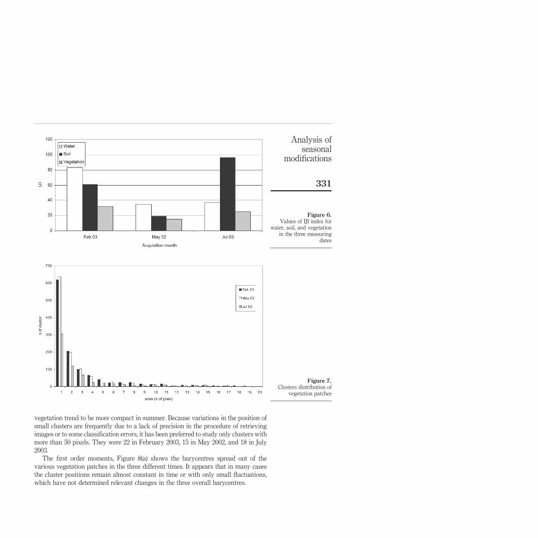
vegetation trend to be more compact in summer. Because variations in the position ofsmall clusters are frequently due to a lack of precision in the procedure of retrievingimages or to some classification errors, it has been preferred to study only clusters withmore than 50 pixels. They were 22 in February 2003, 15 in May 2002, and 18 in July2003.

The first order moments, Figure 8(a) shows the barycentres spread out of thevarious vegetation patches in the three different times. It appears that in many casesthe cluster positions remain almost constant in time or with only small fluctuations,which have not determined relevant changes in the three overall barycentres.

Figure 6.Values of IJI index for

water, soil, and vegetationin the three measuring

dates

Figure 7.Clusters distribution of

vegetation patches

Analysis ofseasonal

modifications

331

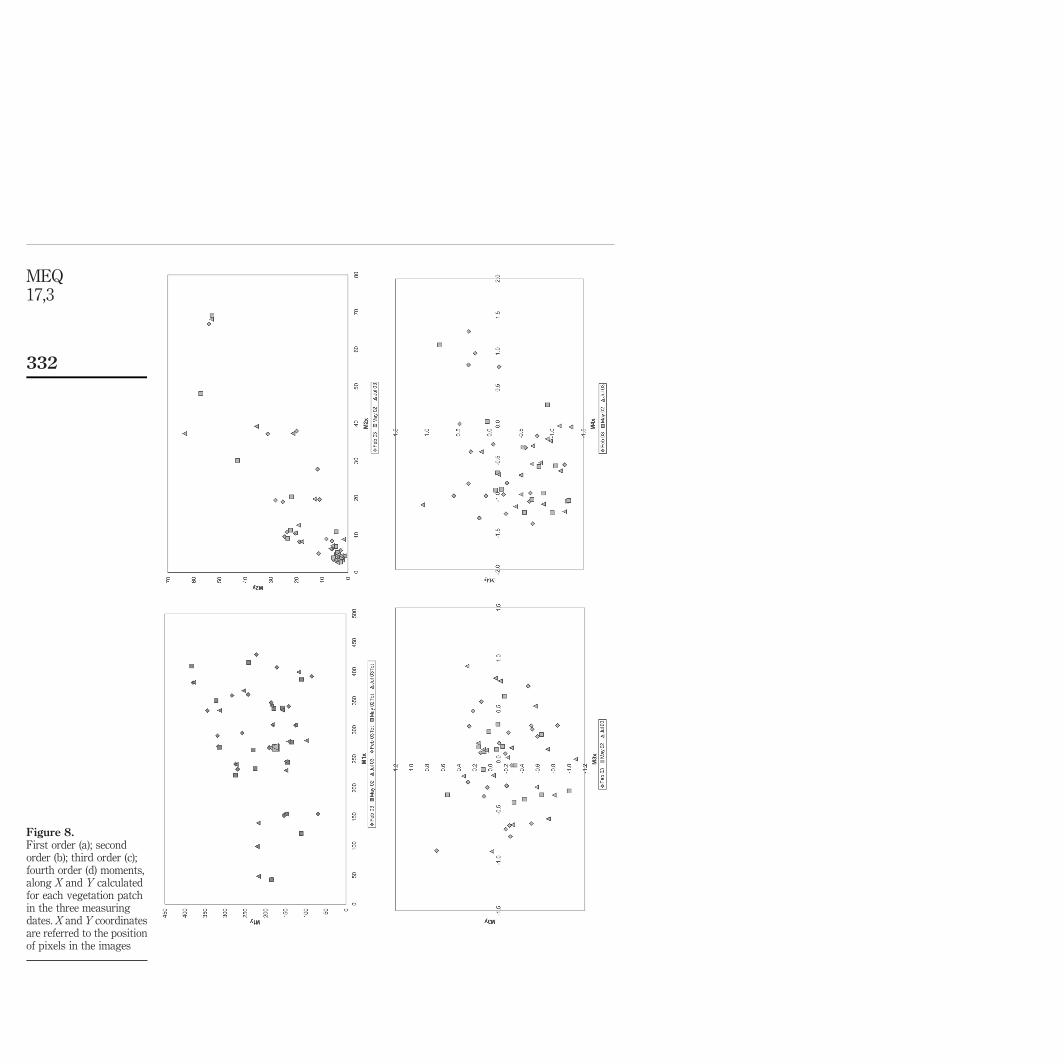
Figure 8.First order (a); secondorder (b); third order (c);fourth order (d) moments,along X and Y calculatedfor each vegetation patchin the three measuringdates. X and Y coordinatesare referred to the positionof pixels in the images

MEQ17,3

332

The variance of the clusters (Figure 8(b)), i.e. second order moments, shows thatdispersions in X direction (axis west-east) and Y (axis south-north) are quite similar.Observing the third order moments of Figure 8(c), it appears that they are evenlydistributed around zero in both X and Y direction in all the three seasons, with only apartial concentration of negative values in the Y direction, so different seasons do notseem to have different behaviours concerning vegetation distribution deviations fromsymmetry.

Also the fourth order moments of Figure 8(d) are very close to zero but moreconcentrated in the third quadrant, especially the clusters resulting from theclassification of QuickBird images of May 2002 and July 2003 (Table II). Thus, adistribution of pixel coordinates fundamentally platicurtic appears. This means thatpatches with more than 50 pixels are characterised a by a flat shape both in X and in Y.

Observing more carefully the three wider (in terms of dimension) clusters ofvegetation for each of the images, as it is possible to observe by Table III it appears thatthe former two clusters take up quite similar surfaces, whereas the third one in Februaryis around half of those of May and July. Analysed in a whole overview the former fourmoments, Table IV shows that the wider cluster remains constant in the three seasonswith only small differences in the asymmetry and in the more or less flat form. As clusterdimensions become smaller, differences among the seasons growth and, in particular,the February’s patches differ more from those of May and July. Beginning with thesecond cluster, the one in February differs more with respect both to the barycentrelatitude and to the less spread out. From the third patch there are so many differencesthat it is difficult to be sure to always compare the same cluster.

ConclusionsThe analysis of cluster compositions and spatial distribution in three different seasons(May 2002, February and July 2003) resulted in a clearer comprehension of factors havingmore influence, respectively, in the three different dates and also to find synthetic indexesdescribing the present situation. This study indeed has shown the possibility of usingsome aggregated indexes characterising the texture of a landscape. The methodologyused was focused to detect temporal variations of vegetation: only those on seasonal scaleresulted relevant (i.e. between winter and summer). In fact the data set available has

I quadrant(per cent)

II quadrant(per cent)

III quadrant(per cent)

IV quadrant(per cent)

February 2003 20 25 50 5May 2002 13 0 80 7July 2003 0 12 88 0

Table II.Percentages of vegetation

clusters in the fourquadrants with regard toFigure 8(d), for each of the

three seasons

Area (No. of pixel)F 2003 M 2002 J 2003

19,092.00 17,317.00 19,723.009,963.00 13,554.00 13,905.003,714.00 6,071.00 6,774.00

Table III.Areas of the three wider

clusters in the threedifferent measuring dates

Analysis ofseasonal

modifications

333

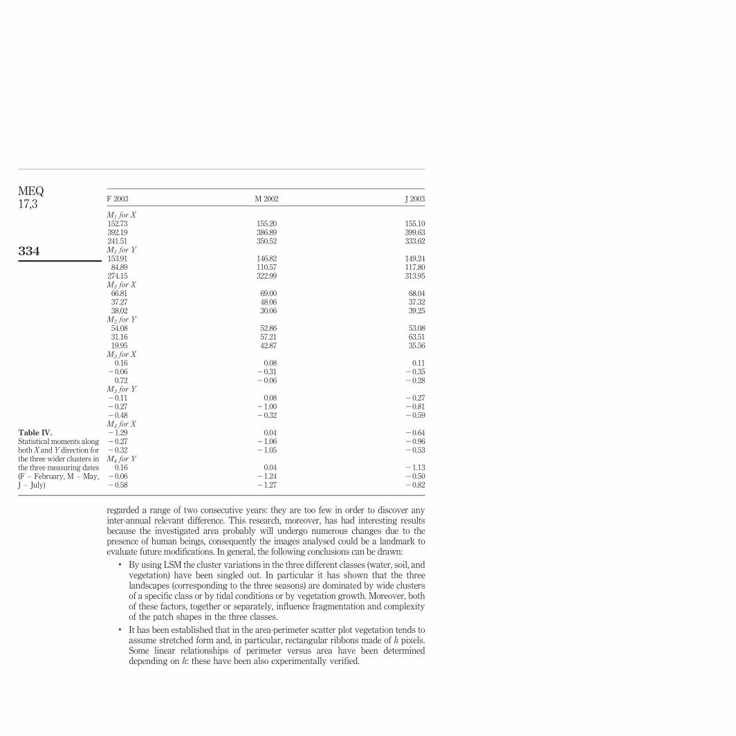
regarded a range of two consecutive years: they are too few in order to discover anyinter-annual relevant difference. This research, moreover, has had interesting resultsbecause the investigated area probably will undergo numerous changes due to thepresence of human beings, consequently the images analysed could be a landmark toevaluate future modifications. In general, the following conclusions can be drawn:

. By using LSM the cluster variations in the three different classes (water, soil, andvegetation) have been singled out. In particular it has shown that the threelandscapes (corresponding to the three seasons) are dominated by wide clustersof a specific class or by tidal conditions or by vegetation growth. Moreover, bothof these factors, together or separately, influence fragmentation and complexityof the patch shapes in the three classes.

. It has been established that in the area-perimeter scatter plot vegetation tends toassume stretched form and, in particular, rectangular ribbons made of h pixels.Some linear relationships of perimeter versus area have been determineddepending on h: these have been also experimentally verified.

F 2003 M 2002 J 2003

M1 for X152.73 155.20 155.10392.19 386.89 399.63241.51 350.52 333.62M1 for Y153.91 146.82 149.2484.89 110.57 117.80

274.15 322.99 313.95M2 for X

66.81 69.00 68.0437.27 48.06 37.3238.02 30.06 39.25

M2 for Y54.08 52.86 53.0831.16 57.21 63.5119.95 42.87 35.56

M3 for X0.16 0.08 0.11

20.06 20.31 20.350.72 20.06 20.28

M3 for Y20.11 0.08 20.2720.27 21.00 20.8120.48 20.32 20.59M4 for X21.29 0.04 20.6420.27 21.06 20.9620.32 21.05 20.53M4 for Y

0.16 0.04 21.1320.06 21.24 20.5020.58 21.27 20.82

Table IV.Statistical moments alongboth X and Y direction forthe three wider clusters inthe three measuring dates(F – February, M – May,J – July)

MEQ17,3

334

. Analysing clusters with more than 50 pixels by means of the former fourstatistical moments it has been established that fluctuations of patches aroundtheir barycentre do not vary too much.

. With respect to it, there is no significant dispersion or asymmetry neither alongX- nor Y-axis, even if in February patches resulted in more compact form alongthe latitude than along the longitude.

. Analysing the former three bigger clusters, only the first one remains almostconstant during the different seasons. The remaining two are similar enoughonly between May and July. In February, meanwhile, due to more fragmentationclusters are undoubtedly different.

. For what concerns the second order moments, the average of the standarddeviation in the three different months are almost the same for each seasonconsidered. Moreover, the regression analysis of Mx

2 versus My2 denotes a linear

dependence of the standard deviations along the two axes.. By the present study we pointed out that a small number (four) of moments are

adequate enough to characterize certain patterns of a set such as patterns ofvegetation in the lagoon of Venice. It is important to remember that the finedetails can be recreated only by including higher order moments which are, onthe other hand, both more vulnerable to noise and computationally heavy.

The present study is only a first approach aimed to investigate seasonal modificationsin salt marshes in the Venice lagoon. Much more data are necessary to obtain deeperinsight into their behaviour and to reach a more accurate description. New data will becollected in the future and other approaches of research are actually in progress inorder to better describe salt marsh evolution.

References

Aitkenhead, M.J., Mustard, M.J. and McDonald, A.J.S. (2004), “Using neural networks to predictspatial structure in ecological systems”, Ecological Modelling, Vol. 179, pp. 393-403.

Ashley, G. and Zeff, M. (1988), “Tidal channel classification for a low-mesotidal salt marsh”,Marine Geology, Vol. 82, pp. 17-32.

Belyea, L.R. and Lancaster, J. (2002), “Inferring landscape dynamics of bog pools from scalingrelationship and spatial patterns”, Journal of Ecology, Vol. 90, pp. 223-34.

Boorman, L.A. (1999), “Salt marshes: present functioning and future change”, Mangroves andSalt Marshes, Vol. 3, pp. 227-41.

Ceriali, A. (2002), “Telerilevamento delle dinamiche di barena”, degree thesis on EnvironmentalSciences, University Ca’ Foscari of Venice, Venezia.

Cho-Huak, T. and Roland, T.C. (1988), “On image analysis by the methods of moments”, IEEETransactions on Pattern Analysis and Machine Intelligence, Vol. 10 No. 4, pp. 496-513.

Cibien, M.T. (1999), “Correzione atmosferica di immagini Mivis sulla Laguna di Venezia”, degreethesis on Environmental Sciences, University Ca’ Foscari of Venice, Venizia.

Coppin, P., Jonckheere, J., Nackaerts, K. and Muys, B. (2004), “Digital change detection methodsin ecosystem monitoring: a review”, International Journal of Remote Sensing, Vol. 25,pp. 1565-96.

Forman, R.T.T. (1995), Land Mosaics: The Ecology of Landascapes and Regions, CambridgeUniversity Press, Cambridge.

Analysis ofseasonal

modifications

335

Gustafson, E.J. (1998), “Quantifying landscape spatial pattern: what is the state of the art?”,Ecosystems, Vol. 1, pp. 143-56.

Hargis, C.D., Bissonete, J.A. and David, L. (1998), “The behaviour of landscape metrics commonlyused in the study of habitat fragmentation”, Landscape Ecology, Vol. 13, pp. 167-86.

Kruse, F.A., Lefkoff, A.B., Boardman, J.B., Heidebrecht, K.B., Shapiro, A.T., Barloon, P.J. and Goetz,A.F.H. (1993), “The spectral image processing system (SIPS) – interactive visualization andanalysis of imaging spectrometer data”, Remote Sensing of Environment, Vol. 44, pp. 145-63.

Leonard, L.A. and Reed, D.J. (2002), “Hydrodynamics and sediment transport through tidalmarsh canopies”, Journal of Coastal Research, ICS 2002 Proceedings, pp. 459-69.

Liao, X.S. and Pawlak, M. (1996), “On image analysis by moments”, IEEE Transactions onPattern Analysis and Machine Intelligence, Vol. 18 No. 3, pp. 254-66.

McGarigal, K. and Marks, B.J. (1994), “FRAGSTATS: spatial pattern analysis program forquantifying landscape structure”, USDA Forest Service General Technical ReportPNW-GTR-351, Oregon State University, Forest Science Department, Cornvallis, OR.

Marani, M., Lanzoni, S., Silvestri, S. and Rinaldo, A. (2004), “Tidal landforms, patterns ofhalophytic vegetation and the fate of the Lagoon of Venice”, Journal of Marine Systems,Vol. 51, pp. 191-210.

Mitsch, J.W. and Gosselink, J.G. (1993), Wetlands, Van Nostrand Reinhold, New York, NY.

Paruelo, J.M. and Tomasel, F. (1997), “Prediction of functional characteristics of ecosystems: acomparison of artificial neural networks and regression models”, Ecological Modelling,Vol. 98, pp. 173-86.

Reiss, T.H. (1991), “The revised fundamental theorem of moment invariants”, IEEE Transactionson Pattern Analysis and Machine Intelligence, Vol. 13 No. 8, pp. 830-4.

Riitters, K.H., O’Neil, R.V., Hunsaker, C.T., Wickham, J.D., Yankee, D.H., Timmins, S.P., Jones,K.B. and Jackson, B.L. (1995), “A factor analysis of landscape pattern and structuremetrics”, Landscape Ecology, Vol. 10, pp. 23-39.

Sanchez, J.M., Izco, J. and Medrano, M. (1996), “Relationships between vegetation zonation andaltitude in a salt-marsh system in northwest Spain”, Journal of Vegetation Science, Vol. 7,pp. 695-702.

Scarton, F., Perco, F. and Borella, S. (1996), “The importance of protecting lagoon habitats forbird life”, Quaderni Trimestrali Consorzio Venezia Nuova (Venezia), Vol. 4.

Silvestri, S. (2000), “La vegetazione alofila quale indicatore morfologico degli ambienti a marea”,PhD thesis, University of Padova.

Sondergrath, D. and Schroder, B. (2002), “Population dynamics and habitat connectivity affectingthe spatial spread of population – a simulation study”, Landscape Ecology, Vol. 17, pp. 57-70.

Teague, M. (1980), “Image analysis via the general theory of moments”, I. J. Opt. Soc. Amer.,Vol. 70 No. 8, pp. 920-30.

Underwood, G.J.C. (1997), “Microalgal colonisation in a saltmarsh restoration scheme”, EstuarineCoastal and Shelf Science, Vol. 44, pp. 471-81.

Vermote, E.F., Tanre, D., Deuze, J.L., Herman, M. and Morerette, J.J. (1997), “Second simulation ofthe satellite signal in the solar spectrum, 6S: an overview”, IEEE Trans. on Geoscience andRemote Sensing, Vol. 35, pp. 675-86.

Vulleumier, S. and Prelaz-Droux, R. (2002), “Map of ecological networks for landscape planning”,Landscape and Urban Planning, Vol. 58, pp. 157-70.

Zhang, M., Ustin, S.L., Rejmankova, E. and Sanderson, E.W. (1997), “Monitoring pacific coast saltmarshes using remote sensing”, Ecological Applications, Vol. 7 No. 3, pp. 1039-53.

MEQ17,3

336

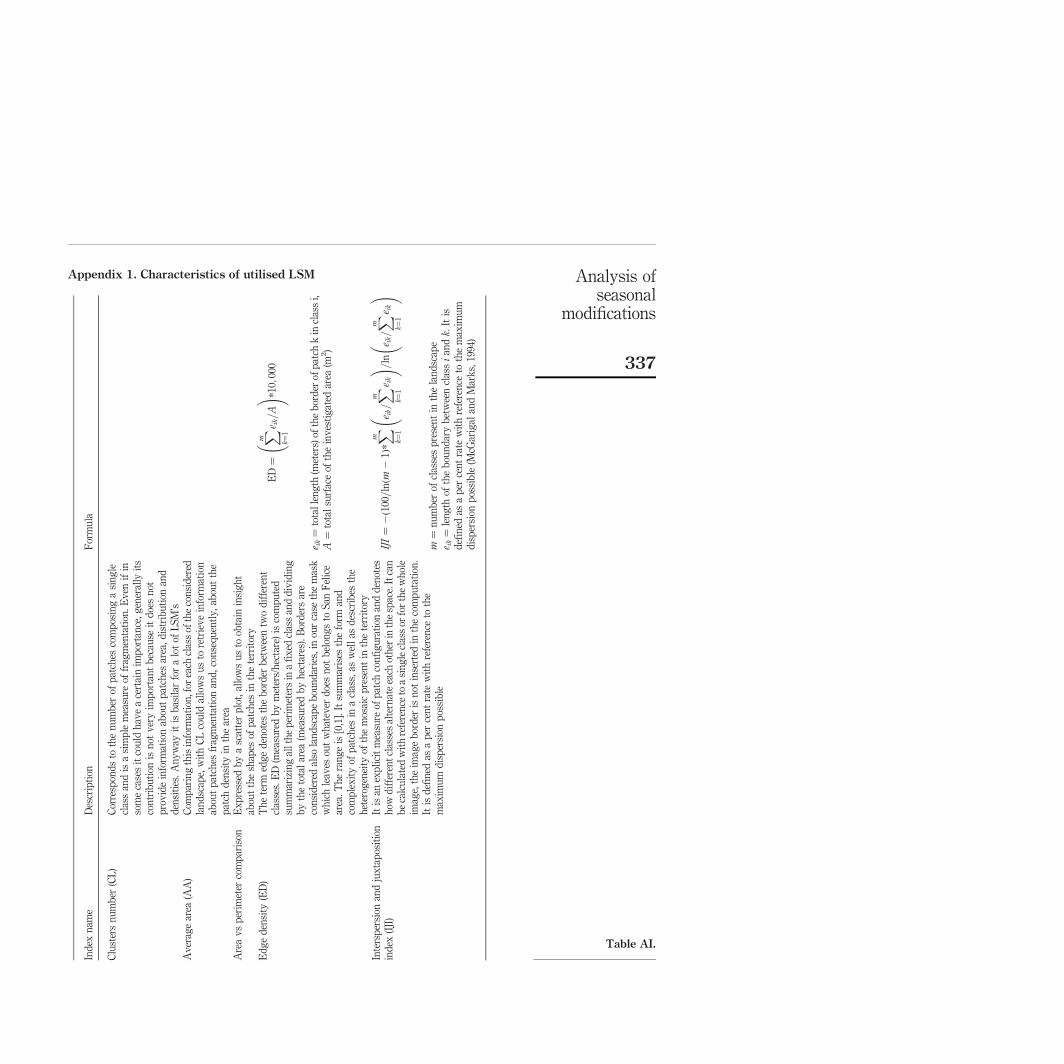
Appendix 1. Characteristics of utilised LSM

Ind

exn

ame

Des

crip

tion

For

mu

la

Clu

ster

sn

um

ber

(CL

)C

orre

spon

ds

toth

en

um

ber

ofp

atch

esco

mp

osin

ga

sin

gle

clas

san

dis

asi

mp

lem

easu

reof

frag

men

tati

on.

Ev

enif

inso

me

case

sit

cou

ldh

ave

ace

rtai

nim

por

tan

ce,g

ener

ally

its

con

trib

uti

onis

not

ver

yim

por

tan

tb

ecau

seit

doe

sn

otp

rov

ide

info

rmat

ion

abou

tp

atch

esar

ea,

dis

trib

uti

onan

dd

ensi

ties

.A

ny

way

itis

bas

ilar

for

alo

tof

LS

M’s

Av

erag

ear

ea(A

A)

Com

par

ing

this

info

rmat

ion

,for

each

clas

sof

the

con

sid

ered

lan

dsc

ape,

wit

hC

Lco

uld

allo

ws

us

tore

trie

ve

info

rmat

ion

abou

tp

atch

esfr

agm

enta

tion

and

,co

nse

qu

entl

y,

abou

tth

ep

atch

den

sity

inth

ear

eaA

rea

vs

per

imet

erco

mp

aris

onE

xp

ress

edb

ya

scat

ter

plo

t,al

low

su

sto

obta

inin

sig

ht

abou

tth

esh

apes

ofp

atch

esin

the

terr

itor

yE

dg

ed

ensi

ty(E

D)

Th

ete

rmed

ge

den

otes

the

bor

der

bet

wee

ntw

od

iffe

ren

tcl

asse

s.E

D(m

easu

red

by

met

ers/

hec

tare

)is

com

pu

ted

sum

mar

izin

gal

lth

ep

erim

eter

sin

afi

xed

clas

san

dd

ivid

ing

by

the

tota

lar

ea(m

easu

red

by

hec

tare

s).

Bor

der

sar

eco

nsi

der

edal

sola

nd

scap

eb

oun

dar

ies,

inou

rca

seth

em

ask

wh

ich

leav

esou

tw

hat

ever

doe

sn

otb

elon

gs

toS

anF

elic

ear

ea.

Th

era

ng

eis

[0,1

].It

sum

mar

ises

the

form

and

com

ple

xit

yof

pat

ches

ina

clas

s,as

wel

las

des

crib

esth

eh

eter

ogen

eity

ofth

em

osai

cp

rese

nt

inth

ete

rrit

ory

ED¼

Xm k¼1

e ik=A

! *1

0;00

0

e ik¼

tota

lle

ng

th(m

eter

s)of

the

bor

der

ofp

atch

kin

clas

si,

A¼

tota

lsu

rfac

eof

the

inv

esti

gat

edar

ea(m

2)

Inte

rsp

ersi

onan

dju

xta

pos

itio

nin

dex

(IJI

)It

isan

exp

lici

tm

easu

reof

pat

chco

nfi

gu

rati

onan

dd

enot

esh

owd

iffe

ren

tcl

asse

sal

tern

ate

each

oth

erin

the

spac

e.It

can

be

calc

ula

ted

wit

hre

fere

nce

toa

sin

gle

clas

sor

for

the

wh

ole

imag

e,th

eim

age

bor

der

isn

otin

sert

edin

the

com

pu

tati

on.

Itis

defi

ned

asa

per

cen

tra

tew

ith

refe

ren

ceto

the

max

imu

md

isp

ersi

onp

ossi

ble

IJI¼

2ð1

00=

lnðm

21Þ

*Xm k¼1

e ik=Xm k¼

1

e ik

! =

lne ik=Xm k¼

1

e ik

!

m¼

nu

mb

erof

clas

ses

pre

sen

tin

the

lan

dsc

ape

e ik¼

len

gth

ofth

eb

oun

dar

yb

etw

een

clas

si

andk.

Itis

defi

ned

asa

per

cen

tra

tew

ith

refe

ren

ceto

the

max

imu

md

isp

ersi

onp

ossi

ble

(McG

arig

alan

dM

ark

s,19

94)

Table AI.

Analysis ofseasonal

modifications

337

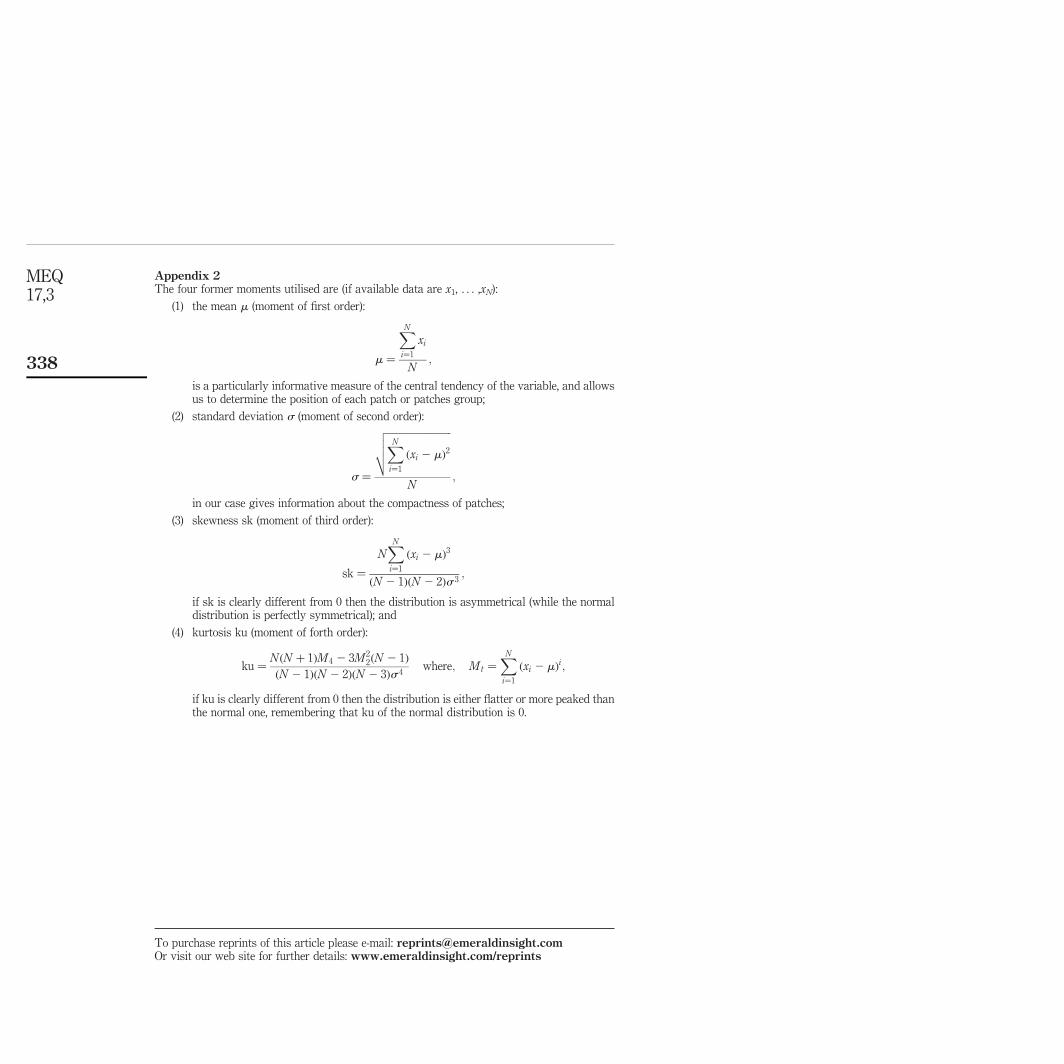
Appendix 2The four former moments utilised are (if available data are x1, . . . ,xN):

(1) the mean m (moment of first order):

m ¼

XNi¼1

xi

N;

is a particularly informative measure of the central tendency of the variable, and allowsus to determine the position of each patch or patches group;

(2) standard deviation s (moment of second order):

s ¼

ffiffiffiffiffiffiffiffiffiffiffiffiffiffiffiffiffiffiffiffiffiffiffiffiffiffiXNi¼1

ðxi 2 mÞ2

vuutN

;

in our case gives information about the compactness of patches;

(3) skewness sk (moment of third order):

sk ¼

NXNi¼1

ðxi 2 mÞ3

ðN 2 1ÞðN 2 2Þs 3;

if sk is clearly different from 0 then the distribution is asymmetrical (while the normaldistribution is perfectly symmetrical); and

(4) kurtosis ku (moment of forth order):

ku ¼NðN þ 1ÞM 4 2 3M 2

2ðN 2 1Þ

ðN 2 1ÞðN 2 2ÞðN 2 3Þs 4where; Mt ¼

XNi¼1

ðxi 2 mÞi;

if ku is clearly different from 0 then the distribution is either flatter or more peaked thanthe normal one, remembering that ku of the normal distribution is 0.

MEQ17,3

338

To purchase reprints of this article please e-mail: reprints@emeraldinsight.comOr visit our web site for further details: www.emeraldinsight.com/reprints