International Journal of

Geo-Information

Article

Station-Free Bike Rebalancing Analysis: Scale,Modeling, and Computational Challenges

Xueting Jin and Daoqin Tong *

School of Geographical Sciences and Urban Planning, Arizona State University, 975 S Myrtle Ave,Tempe, AZ 85281, USA; xjin50@asu.edu* Correspondence: daoqin.tong@asu.edu

Received: 17 September 2020; Accepted: 18 November 2020; Published: 19 November 2020 �����������������

Abstract: In the past few years, station-free bike sharing systems (SFBSSs) have been adopted inmany cities worldwide. Different from conventional station-based bike sharing systems (SBBSSs)that rely upon fixed bike stations, SFBSSs allow users the flexibility to locate a bike nearby andpark it at any appropriate site after use. With no fixed bike stations, the spatial extent/scale usedto evaluate bike shortage/surplus in an SFBSS has been rather arbitrary in existing studies. On theone hand, a balanced status using large areas may contain multiple local bike shortage/surplus sites,leading to a less effective rebalancing design. On the other hand, an imbalance evaluation conductedin small areas may not be meaningful or necessary, while significantly increasing the computationalcomplexity. In this study, we examine the impacts of analysis scale on the SFBSS imbalance evaluationand the associated rebalancing design. In particular, we develop a spatial optimization model tostrategically optimize bike rebalancing in an SFBSS. We also propose a region decomposition methodto solve large-sized bike rebalancing problems that are constructed based on fine analysis scales.We apply the approach to study the SFBSS in downtown Beijing. The empirical study shows thatimbalance evaluation results and optimal rebalancing design can vary substantially with analysisscale. According to the optimal rebalancing results, bike repositioning tends to take place amongneighboring areas. Based on the empirical study, we would recommend 800 m and 100/200 mas the suitable scale for designing operator-based and user-based rebalancing plans, respectively.Computational results show that the region decomposition method can be used to solve problemsthat cannot be handled by existing commercial optimization software. This study provides importantinsights into effective bike-share rebalancing strategies and urban bike transportation planning.

Keywords: station-free bike sharing system; rebalance; scale; optimization

1. Introduction

Bike sharing systems (BSSs) are an important component in today’s urban transportationsystem [1,2]. As a more sustainable mode of transportation, bike-sharing has the potential to reducecar usage, solve the first/last mile problem, and contribute to the local retail sales [3–5]. The history ofbike sharing can be traced back to the 1960s when the concept was first introduced in Amsterdam,Netherlands [6]. Over the past decades, bike sharing systems have evolved through multiple generations.Early generations involved no prior registration and failed, as many bikes were vandalized or turnedinto private use [6,7]. Starting from 1995, prior registration has been required. A registered customercan rent and return a bicycle at a number of fixed bike stations. These systems are also known asstation-based bike sharing systems (SBBSSs) [8] and have been successfully deployed in multiplecities around the world. Leveraged by the recent advanced technologies such as smart phones, GPS,and integrated payment systems, the newest generation of bike sharing involves having no fixed bikestations. Without docking stations, the station-free bike sharing systems (SFBSSs) provide users the

ISPRS Int. J. Geo-Inf. 2020, 9, 691; doi:10.3390/ijgi9110691 www.mdpi.com/journal/ijgi

ISPRS Int. J. Geo-Inf. 2020, 9, 691 2 of 16

flexibility to use a smart phone app to locate a bike nearby and park it at any appropriate place afteruse. Due to the high flexibility and convenience, SFBSSs have gained considerable popularity over thepast few years and have been widely adopted in many countries, including China, United Kingdom,Singapore, the United States, and the Netherlands [9]. It was estimated that in 2018, 16 to 18 millionstation-free bikes were in use worldwide, compared to 3.7 million station-based bikes [10].

A balanced status refers to the situation when bike supply meets bike demand. Both station-freeand station-based bike sharing systems frequently suffer from the spatiotemporal fluctuations ofdemand, leading to the imbalance problem. Without timely rebalancing efforts, the imbalance problemmay substantially degrade the system performance. For an SBBSS, the imbalance problem may lead tozero inventories at some stations and no space for parking at others. As a result, rentals and returns maybe only possible at a limited number of stations, leaving many areas/demands un- or under-served [11].For an SFBSS, the imbalance problem is more serious. While unmet demands remain, no restriction onwhere a user can pick up or park a bike may lead to bikes piling up and blocking city sidewalks.

Many studies have been conducted to assess the imbalance status of an SBBSS and designthe associated rebalancing strategy [12–16]. While the imbalance evaluation in an SBBSS is ratherstraightforward [17,18], due to the lack of fixed stations in an SFBSS, there is no clearly defined spatialscale or geographical areas to evaluate bike inventories, assess the imbalance status, and perform thesubsequent rebalancing analysis. Existing studies have explored various analysis scales, including trafficanalysis zones and regular grids of various sizes [19–22]. The selection of these analysis scaleshas been rather arbitrary. There has been no discussion on the suitable scale needed to evaluateand address the imbalance issue in an SFBSS. On the one hand, a balanced status evaluatedusing large areas (e.g., 10 × 10 km grids) may contain multiple local bike shortage/surplus sites,which can significantly compromise the system performance. On the other hand, analysis conductedusing small areas (e.g., 10 × 10 m grids) may greatly add to computational burden. Therefore,analysis scale, modeling/analysis, and computational requirements are related, and selection ofthe appropriate analysis scale is essential for the imbalance assessment of an SFBSS and the followingrebalancing analysis.

2. Literature Review

Recently, a number of studies have examined bike sharing systems by focusing on two areas [23–26].The first area concerns identifying the factors affecting bike sharing demand, and these factors includesocio-economic status, built environment, traffic infrastructure, air quality, and weather [27–29].The second area focuses on the imbalance issue of a bike sharing system and the associated rebalancingstrategies. In this study, we are mainly interested in the latter.

To solve the imbalance issue in a bike-sharing system, various rebalancing strategies have beendeveloped. Table 1 provides a summary of the recent literature on these rebalancing strategies.In particular, user-based and operator-based methods are the two major types of rebalancingstrategies [8,12,30]. In a user-based rebalancing strategy, incentives in the form of a bonus voucheror discount are often used to encourage users to move bikes from surplus areas to shortage areas.For example, in 2008, the bike sharing system Vélib’ in Paris launched a discount pricing strategy [31] tomotivate users to return bikes to uphill stations. A pricing strategy was developed by Chemla et al. [32]to incentivize users to return bikes to the least loaded stations nearby, and a dynamic online pricingincentive strategy was proposed by Pfrommer et al. [33] to motivate users to choose alternative locationsto pick up or return bikes. However, depending on users’ participation, user-based rebalancing maynot be sufficient to achieve the system level self-rebalancing [30]. Hence, user-based rebalancingstrategies are often used as a supplement to operator-based ones. These two types of strategies canbe combined to help reduce rebalancing costs [33]. Currently, most existing bike-sharing systems(e.g., Mobike and Ofo in China) employ operator-based rebalancing strategies [8].

ISPRS Int. J. Geo-Inf. 2020, 9, 691 3 of 16

Table 1. Summary of literature on bike rebalancing strategies.

Research Article Bike SharingSystem

Type ofRebalancing

StrategyObjective Study Unit Number

of Units

Chemla et al. [12] Station-based Operator-based Complete rebalance Station 100

Raviv et al. [34] Station-based Operator-based Minimize (a) total unmet demand,(b) total operating cost Station 60

Ho and Szeto [35] Station-based Operator-based Minimize total penalties Station 400

Alvarez-Valdes et al. [36] Station-based Operator-based Minimize unsatisfied demand Station 28

Gaspero et al. [37] Station-based Operator-based Maximize expected future bikedemands Station 92

Pal and Zhang [8] Station-based Operator-based Minimize the operation time ofrebalancing vehicle fleets Station 476

Schuijbroek et al. [38] Station-based Operator-based

Minimize (a) the deviation from agiven target inventory level,

(b) the number of (un)loadingoperations, (c) total work time

Station 135

Dell’Amico et al. [39] Station-based Operator-based Minimize total cost Station 116

Chemla et al. [32] Station-based User-based Minimize imbalance amount Station 20 to 250

Pfrommer et al. [40] Station-based Operator-basedand User-based Minimize unsatisfied demand Station 354

Pan et al. [19] Station-free User-based Minimize cost Grid/square –

Ji et al. [41] Station-free User-basedExamine the influences of

acceptable walking distance anduser’s cooperative factor

Grid/hexagonwith side

length of 100 m1185

Zhai et al. [21] Station-free Operator-based Minimize travel cost Grid/square 20 to 1100

A few studies have focused on developing efficient operator-based rebalancing methods. In anoperator-based rebalancing operation, a fleet of vehicles are often sent to move bikes from site to site.Among others, spatial optimization methods [42] have been widely used to determine the numberof relocation vehicles and the associated routes for performing the rebalancing operation [8,34,38,39].All the studies included in Table 1 are based on optimization methods except for Ji et al. [41].These problems have often been formulated using mixed integer programming (MIP) [34,38]. Some ofthese studies integrated GIS into classic location models, including the p-median problem and thecoverage location problems, to achieve the optimal rebalancing design [8,18]. A range of objectives/goalshave been examined in the bike rebalancing design. These objectives include minimizing costs,varying from travel costs to the overall rebalancing costs (including travel, trucks, loading and unloadingcosts), and maximizing the system level balance evaluated using different metrics (e.g., minimal absolutedeviation from the target number of bikes) (also see Table 1). While some studies focused on a singleobjective [35,43], a few studies considered multiple goals simultaneously [44,45].

As shown in Table 1, existing bike rebalancing models are mainly station-based and have beenconstructed to address the imbalance issue of an SBBSS. In an SBBSS, stations are the analysis unitsused to perform the imbalance evaluation and the subsequent rebalancing analysis. In an SFBSS,if we divide a region into a set of sub-areas and treat each sub-area as a “station”, we can apply astation-based rebalancing model to solve the imbalance issue in an SFBSS. In fact, traffic analysiszones [20] and regular grids [19,21,41] have already been used to conduct the imbalance assessment forSFBSSs. Although traffic analysis zones (TAZs) are widely used in transportation planning, they aredelineated largely based on motorized traffic and are generally too coarse to capture the variationof bike supply and demand given the short distance that bike users are normally willing to walk toaccess bikes. As for the grid-based approaches, the selection of grid size has been either arbitrary orunspecified [19,21,41]. To the best of our knowledge, there have been no studies exploring the impactsof analysis scale on the imbalance evaluation and the associated rebalancing design in an SFBSS.Scale can be critical in an SFBSS study: A balanced status at a large scale may contain multiple localbike shortage/surplus sites, and as a result, the rebalancing strategy designed based on a large scale

ISPRS Int. J. Geo-Inf. 2020, 9, 691 4 of 16

might not solve the imbalance issue completely. In contrast, analysis conducted using fine scales mayencounter computational challenges, and a scale that is too fine (such as 1 m) might not be necessary oreven meaningful.

Table 1 also summarizes the number of analysis units (i.e., sub-areas/grids in an SFBSS or stationsin an SBBSS) used in current bike rebalancing studies, ranging from 28 to 1185. Since a rebalancingproblem can be computationally intractable when a large number of analysis units are involved,many studies focused on small cities/areas or used a coarse scale [19,21]. For example, the modelproposed by Chemla et al. [32] was unable to simulate the user-based rebalancing process for morethan 250 stations because of the large problem size. Focusing on small areas or using coarse scaleanalysis units may provide limited insights into effective rebalancing strategies for a large urban area.

Therefore, identifying the appropriate analysis scale and designing efficient and effective bikerebalancing strategies are needed for SFBSSs in large cities. In this study, we aim to fill in the researchgaps by focusing on two important questions: (1) how scale impacts the imbalance evaluation ofan SFBSS and the associated rebalancing design, and (2) how to deal with computational challengesfor large sized rebalancing problems. We develop a spatial optimization model to strategicallyoptimize bike rebalancing efforts. We also propose a region decomposition method to solve large-sizedproblems that are constructed based on fine analysis scales. We apply the approach to study theSFBSS in downtown Beijing. Based on the empirical study, we discuss the strengths and weaknessesassociated with alternative analysis scales and make recommendations on scale choice for differentrebalancing strategies.

3. Methodology

3.1. Study Area and Data

Our study area consists of six districts in central Beijing: Dongcheng, Xicheng, Chaoyang, Haidian,Fengtai, and Shijingshan. Beijing, the capital of China, is among the few cities that first adopted SFBSSsin 2015. According to the Beijing Municipal Commission of Transport, in the second half of 2018,the average daily shared bike usage in Beijing was 1.3 million with the majority clustered in our studyarea. We use a trip level bike usage dataset in this study. The dataset was obtained from Mobike,a major station-free bike sharing company in China. The dataset contains the information on order ID,bike ID, user ID, start time, start location, and end location. We use the bike trip data on Wednesday,10 May 2017 as a typical weekday to illustrate our method. We assume a daily rebalancing cycle byevaluating the bike pickups and returns in an area within a day.

3.2. Alternative Scales and Data Preprocessing

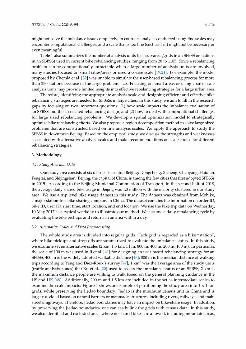
The whole study area is divided into regular grids. Each grid is regarded as a bike “station”,where bike pickups and drop-offs are summarized to evaluate the imbalance status. In this study,we examine seven alternative scales (2 km, 1.5 km, 1 km, 800 m, 400 m, 200 m, 100 m). In particular,the scale of 100 m was used in Ji et al. [41] for designing an user-based rebalancing strategy for anSFBSS; 400 m is the widely adopted walkable distance [46]; 800 m is the median distance of walkingtrips according to Yang and Diez-Roux’s survey [47]; 1 km2 was the average area of the study units(traffic analysis zones) that Xu et al. [20] used to assess the imbalance status of an SFBSS; 2 km isthe maximum distance people are willing to walk based on the general planning guidance in theUS and UK [48]. Additionally, 200 m and 1.5 km are included in the set as intermediate scales toexamine the scale impacts. Figure 1 shows an example of partitioning the study area into 1 × 1 kmgrids, while preserving the Jiedao boundary. Jiedao is the minimum census unit in China and islargely divided based on natural barriers or manmade structures, including rivers, railways, and mainstreets/highways. Therefore, Jiedao boundaries may have an impact on bike-share usage. In addition,by preserving the Jiedao boundaries, one can easily link the grids with census data. In this study,we also identified and excluded areas where no shared bikes are allowed, including mountain areas,

ISPRS Int. J. Geo-Inf. 2020, 9, 691 5 of 16

nature reserve areas, and parks. Within each grid, we count the bike pickups and returns based onthe bike start and end locations in a day. Then, bike shortage/surplus is computed by comparing thepickup and return amounts: a bike shortage/surplus area is an area where bike pickups are more/lessthan bike returns. In this study, we also introduce a shortage/surplus lower bound and upper bound toallow an SFBSS to deviate slightly from the perfect balance status.

ISPRS Int. J. Geo-Inf. 2020, 9, x FOR PEER REVIEW 5 of 16

400 m is the widely adopted walkable distance [46]; 800 m is the median distance of walking trips according to Yang and Diez-Roux’s survey [47]; 1 km2 was the average area of the study units (traffic analysis zones) that Xu et al. [20] used to assess the imbalance status of an SFBSS; 2 km is the maximum distance people are willing to walk based on the general planning guidance in the US and UK [48]. Additionally, 200 m and 1.5 km are included in the set as intermediate scales to examine the scale impacts. Figure 1 shows an example of partitioning the study area into 1 x1 km grids, while preserving the Jiedao boundary. Jiedao is the minimum census unit in China and is largely divided based on natural barriers or manmade structures, including rivers, railways, and main streets/highways. Therefore, Jiedao boundaries may have an impact on bike-share usage. In addition, by preserving the Jiedao boundaries, one can easily link the grids with census data. In this study, we also identified and excluded areas where no shared bikes are allowed, including mountain areas, nature reserve areas, and parks. Within each grid, we count the bike pickups and returns based on the bike start and end locations in a day. Then, bike shortage/surplus is computed by comparing the pickup and return amounts: a bike shortage/surplus area is an area where bike pickups are more/less than bike returns. In this study, we also introduce a shortage/surplus lower bound and upper bound to allow an SFBSS to deviate slightly from the perfect balance status.

Figure 1. An example of partitioning the study area into regular grids (1 x1 km).

3.3. Bike-Share Rebalancing Flow Model

In this study, we introduce a bike-share rebalancing flow model to strategically optimize bike rebalancing efforts. When addressing the imbalance issue, the model aims to identify the optimal bike repositioning with the minimal overall bike repositioning distance. In the model, we do not confine ourselves to a specific rebalancing strategy, user-based or operator-based. Therefore, the goal of this model is neither designing the optimal route for vehicles to redistribute bikes nor developing a pricing strategy to incentivize users to engage in the rebalancing efforts. This strategic analysis will help design the specific rebalancing strategies needed to solve the imbalance issue in an SFBSS.

In the model, we set a lower bound L and an upper bound U on the rebalancing ratio to allow an SFBSS to deviate slightly from the complete balance status. For an area with a certain amount of bike shortage/surplus, a complete rebalancing involves shipping in/out bikes that have the same amount of shortage/surplus. In this model, L and U specify the minimum and maximum percentage of imbalanced bikes that need to be shipped in/out to achieve a balance status. If we set L = 0.9 and U = 1.1, for an area with surplus imbalance of 100, the number of bikes that need to be shipped out during the rebalancing process should be more than or equal to 90 but cannot exceed 110. For a complete rebalancing operation, one can set L and U to be 1. Consider the following notation (Table 2):

Figure 1. An example of partitioning the study area into regular grids (1 km × 1 km).

3.3. Bike-Share Rebalancing Flow Model

In this study, we introduce a bike-share rebalancing flow model to strategically optimize bikerebalancing efforts. When addressing the imbalance issue, the model aims to identify the optimalbike repositioning with the minimal overall bike repositioning distance. In the model, we do notconfine ourselves to a specific rebalancing strategy, user-based or operator-based. Therefore, the goalof this model is neither designing the optimal route for vehicles to redistribute bikes nor developing apricing strategy to incentivize users to engage in the rebalancing efforts. This strategic analysis willhelp design the specific rebalancing strategies needed to solve the imbalance issue in an SFBSS.

In the model, we set a lower bound L and an upper bound U on the rebalancing ratio to allowan SFBSS to deviate slightly from the complete balance status. For an area with a certain amountof bike shortage/surplus, a complete rebalancing involves shipping in/out bikes that have the sameamount of shortage/surplus. In this model, L and U specify the minimum and maximum percentageof imbalanced bikes that need to be shipped in/out to achieve a balance status. If we set L = 0.9 andU = 1.1, for an area with surplus imbalance of 100, the number of bikes that need to be shipped outduring the rebalancing process should be more than or equal to 90 but cannot exceed 110. For acomplete rebalancing operation, one can set L and U to be 1. Consider the following notation (Table 2):

ISPRS Int. J. Geo-Inf. 2020, 9, 691 6 of 16

Table 2. Notation summary.

Notation Description

Parameter

L Lower bound of the rebalancing ratioU Upper bound of the rebalancing ratioP Set of areas with surplus imbalanceN Set of areas with shortage imbalanceZ Set of areas prohibiting shared bikesi, j Index of areasAi Imbalance amount of area idi j Distance between area i and area j

Variable Xi j Number of bikes relocated from area i to area j

The bike-share rebalancing flow model is formulated as:

Min∑

i∑

jXi j ∗ di j (1)

S.T. ∑jXi j −

∑jX ji ≥ L ∗Ai ∀ i ∈ P

(2)∑j

Xi j −∑

j

X ji ≤ U ∗Ai ∀ i ∈ P (3)

∑j

X ji −∑

j

Xi j ≥ L ∗Ai ∀ i ∈ N (4)

∑j

X ji −∑

j

Xi j ≤ U ∗Ai ∀ i ∈ N (5)

Xi j = 0 ∀ i, j ∈ Z (6)

Xi j ∈ non− negative Integers ∀ i, j (7)

In the objective function (1), we aim to minimize the overall travel distance of repositioned bikes.Constraints (2) and (3) ensure that for all areas with bike surplus the net rebalancing outflow is morethan the lower bound but does not exceed the upper bound. Constraints (4) and (5) specify that forall areas with bike shortage, the net rebalancing inflow is more than the lower bound but does notexceed the upper bound. Constraints (6) ensure no rebalancing flows for areas prohibiting sharedbikes. Constraints (7) impose a positive integer restriction on the amount of bikes to be repositioned.In our experimental study, we use the rectilinear distance metric to evaluate the overall travel distance:

di j =∣∣∣ai − a j

∣∣∣+ ∣∣∣bi − b j∣∣∣ (8)

where, ai is the x-coordinate of the centroid of area i, bi is the y-coordinate of the centroid of area i.In many urban areas, high-density roads and intersections make travel distance close to the rectilineardistance [49]. In addition, roads in many parts of downtown Beijing show the grid pattern, which makesrectilinear distance a reasonable metric for measuring travel distance [50].

3.4. Region Decomposition Approach

As discussed earlier, rebalancing models constructed using fine scales are generally challengingto solve. Consider that people often use shared bikes to travel a short distance. For example,bike-sharing trips in China are 1.5 km on average (http://global.chinadaily.com.cn/). For a large area,there may exist multiple sub-regions where bike-sharing trips mainly stay within a single sub-region.Given this, we develop a heuristic by decomposing a large region into multiple self-containedsub-regions to reduce the problem size. Figure 2 shows the workflow of the heuristic. First, the entire

ISPRS Int. J. Geo-Inf. 2020, 9, 691 7 of 16

region is divided into several sub-regions at a relatively coarse scale. Then the imbalance status foreach sub-region is evaluated. If the sub-region meets the balance criterion, the sub-region is consideredas a self-contained sub-region. If there exists a sub-region that is not self-contained, an alternativeregion division is needed until all the resultant sub-regions are self-contained. Then, each sub-region isfurther divided into finer grids (i.e., analysis scale), and based on the finer scale, the imbalance statusis evaluated. Finally, the bike-sharing rebalancing flow model is implemented to obtain the optimalsolution for each sub-region.

ISPRS Int. J. Geo-Inf. 2020, 9, x FOR PEER REVIEW 7 of 16

alternative region division is needed until all the resultant sub-regions are self-contained. Then, each sub-region is further divided into finer grids (i.e., analysis scale), and based on the finer scale, the imbalance status is evaluated. Finally, the bike-sharing rebalancing flow model is implemented to obtain the optimal solution for each sub-region.

Figure 2. Workflow of the region decomposition approach.

In our case study, the computational experiments are carried out on a workstation powered by an Intel Core i7 CPU with a total RAM of 16 GB running a 64-bit operating system. Problem instances with analysis scales of 800 m and coarser are solved directly using the commercial optimization software CPLEX. Problems with finer scales are too large to be solved directly using CPLEX. For these problems, the region decomposition heuristic is applied. In the heuristic, the entire study area is divided into 14 sub-regions using the 10 × 10 km grids, while preserving the district boundaries (see Figure 3). These sub-regions have an average area of 98 km2. To examine whether these sub-regions are self-contained, we calculate the ratio of the shortage/surplus amount to the daily bike usage. If the absolute value of the ratio is less than 10%, the sub-region is considered self-contained. Then, each self-contained sub-region is further partitioned based on the analysis scale (e.g., 100, 200, and 400 m). Figure 3 shows the self-contained sub-regions derived in the case study along with the surplus/shortage evaluation conducted at the 200 m scale.

Figure 2. Workflow of the region decomposition approach.

In our case study, the computational experiments are carried out on a workstation powered by anIntel Core i7 CPU with a total RAM of 16 GB running a 64-bit operating system. Problem instanceswith analysis scales of 800 m and coarser are solved directly using the commercial optimizationsoftware CPLEX. Problems with finer scales are too large to be solved directly using CPLEX. For theseproblems, the region decomposition heuristic is applied. In the heuristic, the entire study area isdivided into 14 sub-regions using the 10 × 10 km grids, while preserving the district boundaries(see Figure 3). These sub-regions have an average area of 98 km2. To examine whether these sub-regionsare self-contained, we calculate the ratio of the shortage/surplus amount to the daily bike usage.If the absolute value of the ratio is less than 10%, the sub-region is considered self-contained. Then,each self-contained sub-region is further partitioned based on the analysis scale (e.g., 100, 200,and 400 m). Figure 3 shows the self-contained sub-regions derived in the case study along with thesurplus/shortage evaluation conducted at the 200 m scale.

ISPRS Int. J. Geo-Inf. 2020, 9, 691 8 of 16ISPRS Int. J. Geo-Inf. 2020, 9, x FOR PEER REVIEW 8 of 16

Figure 3. An example of sub-region division.

4. Results

4.1. Imbalance Assessment Across Scales

Table 3 provides a summary of the bike imbalance analysis in downtown Beijing. In addition to the seven scales discussed previously, we include two coarse scales, 10 km and 5 km, to provide the imbalance assessment at extreme large scales. With the grid size decreasing from 10 km to 100 m, the number of grids increases substantially. Columns “Maximum Surplus” and “Maximum Shortage” record the maximum bike surplus and shortage at each scale, respectively. Table 3 shows that while the maximum surplus and shortage appear to be relatively consistent across scale, the total imbalance increases substantially when fine grids are used. For example, when scale changes from 5 km to 200 m, the maximum surplus and shortage remain similar, but the total imbalance increases more than 17 times. This suggests that an imbalance assessment conducted at a large scale may dismiss many local imbalanced sites. Column “Imbalanced Grids” reports the total amount of grids with the surplus/shortage more than the 10% of the daily usage. Column “Percentage of Imbalanced Grids” computes the percentage of the imbalanced grids using the 10% imbalance threshold. In general, the percentage of imbalanced grids first increases, reaches the maximum at the 800 m scale, and then decreases when finer scales are used. This also suggests that a coarse scale analysis may ignore many local imbalance sites. When scale is extremely coarse (10 km in this case study), the entire system is balanced. We note that at a very fine scale, although more imbalanced local sites are identified, many grids are found to be sites with no bike inventory/usage. For example, our data show that there are 106,719 grids (about 75%) with no bike usage when the analysis is conducted at the 100 m scale.

Figure 3. An example of sub-region division.

4. Results

4.1. Imbalance Assessment Across Scales

Table 3 provides a summary of the bike imbalance analysis in downtown Beijing. In additionto the seven scales discussed previously, we include two coarse scales, 10 km and 5 km, to providethe imbalance assessment at extreme large scales. With the grid size decreasing from 10 km to 100 m,the number of grids increases substantially. Columns “Maximum Surplus” and “Maximum Shortage”record the maximum bike surplus and shortage at each scale, respectively. Table 3 shows that whilethe maximum surplus and shortage appear to be relatively consistent across scale, the total imbalanceincreases substantially when fine grids are used. For example, when scale changes from 5 km to200 m, the maximum surplus and shortage remain similar, but the total imbalance increases morethan 17 times. This suggests that an imbalance assessment conducted at a large scale may dismissmany local imbalanced sites. Column “Imbalanced Grids” reports the total amount of grids with thesurplus/shortage more than the 10% of the daily usage. Column “Percentage of Imbalanced Grids”computes the percentage of the imbalanced grids using the 10% imbalance threshold. In general,the percentage of imbalanced grids first increases, reaches the maximum at the 800 m scale, and thendecreases when finer scales are used. This also suggests that a coarse scale analysis may ignore manylocal imbalance sites. When scale is extremely coarse (10 km in this case study), the entire systemis balanced. We note that at a very fine scale, although more imbalanced local sites are identified,many grids are found to be sites with no bike inventory/usage. For example, our data show that thereare 106,719 grids (about 75%) with no bike usage when the analysis is conducted at the 100 m scale.

ISPRS Int. J. Geo-Inf. 2020, 9, 691 9 of 16

Table 3. Imbalance assessment based on different scales.

Scale (m) Numberof Grids

MaxSurplus

MaxShortage

TotalImbalance

ImbalancedGrids

Percentage ofImbalanced Grids

10,000 14 293 279 1364 0 0%5000 63 363 227 5648 10 15.87%2000 381 460 484 19,602 185 48.56%1500 662 418 403 25,789 375 56.65%1000 1470 367 473 35,974 856 58.23%800 2297 367 316 42,996 1375 59.86%400 9476 363 302 65,788 5004 52.81%200 36,284 332 154 96,029 14,029 38.66%100 138,475 304 148 113,618 24,446 17.65%

Figure 4 shows that imbalanced areas identified at a scale may change when an alternative scale isused. For example, at the 10 km scale, the northwestern grid (circled in Figure 4a) has bike surplus.At the 5 km scale, bike surplus is found to be concentrated in the northeastern corner of the area.If we continue decreasing the scale to 2 km, we start to find local bike shortage and surplus at sitesthat are considered to be balanced at the 5 km scale. A similar pattern is also observed when wefurther decrease the analysis scale. In general, when coarse grids are used to perform the imbalanceassessment, local surplus and shortage tend to cancel out, leading to an overall more imbalanced status.

ISPRS Int. J. Geo-Inf. 2020, 9, x FOR PEER REVIEW 9 of 16

Table 3. Imbalance assessment based on different scales.

Scale (m)

Number of Grids

Max Surplus

Max Shortage

Total Imbalance

Imbalanced Grids

Percentage of Imbalanced

Grids 10,000 14 293 279 1364 0 0% 5000 63 363 227 5648 10 15.87% 2000 381 460 484 19,602 185 48.56% 1500 662 418 403 25,789 375 56.65% 1000 1470 367 473 35,974 856 58.23% 800 2297 367 316 42,996 1375 59.86% 400 9476 363 302 65,788 5004 52.81% 200 36,284 332 154 96,029 14,029 38.66% 100 138,475 304 148 113,618 24,446 17.65%

Figure 3 shows that imbalanced areas identified at a scale may change when an alternative scale is used. For example, at the 10 km scale, the northwestern grid (circled in Figure 4a) has bike surplus. At the 5 km scale, bike surplus is found to be concentrated in the northeastern corner of the area. If we continue decreasing the scale to 2 km, we start to find local bike shortage and surplus at sites that are considered to be balanced at the 5 km scale. A similar pattern is also observed when we further decrease the analysis scale. In general, when coarse grids are used to perform the imbalance assessment, local surplus and shortage tend to cancel out, leading to an overall more imbalanced status.

Figure 4. Imbalanced site identification at different scales: (a) 10 km × 10 km, (b) 5 km × 5 km, (c) 2 km × 2 km, (d) 1.5 km × 1.5 km, (e) 1 km × 1 km, (f) 800 m × 800 m, (g) 400 m × 400 m, (h) 200 m × 200 m, and (i) 100 m × 100 m.

Figure 4. Imbalanced site identification at different scales: (a) 10 km × 10 km, (b) 5 km × 5 km,(c) 2 km × 2 km, (d) 1.5 km × 1.5 km, (e) 1 km × 1 km, (f) 800 m × 800 m, (g) 400 m × 400 m,(h) 200 m × 200 m, and (i) 100 m × 100 m.

ISPRS Int. J. Geo-Inf. 2020, 9, 691 10 of 16

4.2. Rebalancing Results at Different Scales

Table 4 provides a summary of the rebalancing results at different scales. For the rebalancing ratio,we set the lower bound L = 0.9 and upper bound U = 1.1. We exclude the scales of 5 km and 10 kmwhen solving the rebalancing problem, as these two scales are too coarse. Table 4 shows that whenfiner scales are used, although the number of bikes repositioned increases, the travel distance per bikedecreases with an overall average close to the scale used in the analysis. For example, at the 2 km scale,repositioned bikes need to travel slightly more than 2 km compared to the average bike travel distanceof 100 m at the 100 m scale. Column “Objective” reports the total distance that repositioned bikes needto travel during the rebalancing process. When scale decreases from 2 km to 1 km, the total traveldistance increases. This is because the rate of increase in the amount of bikes repositioned is slightlyhigher than the rate of decrease in the average bike travel distance. When the scale keeps decreasingfrom 1 km to 100 m, although more bikes need to be repositioned, the overall travel distance decreases.This is because the average bike travel distance decreases substantially at fine scales. For example,when scale decreases from 1 km to 100 m, the number of bikes repositioned increases about 4 times,whereas the average bike travel distance decrease by 13 times. Column “OD pairs” reports the numberof origin–destination grid pairs involved in the bike repositioning process. Table 4 shows that the totalamount of OD pairs increases when fine analysis scales are used. This is reasonable given that theoverall amount of imbalanced grids increases with finer scales (also see Table 3). Column “Averagebikes repositioned per OD pair” summarizes the average number of bikes repositioned between anOD grid pair. Results show that it decreases with finer scales; at the 100 m scale, on average only aboutthree bikes are associated with a repositioning flow.

Table 4. Rebalancing results at different scales (L = 0.9; U = 1.1).

Scale (m) Numberof Grids Objective (m) Bikes

RepositionedAverage Bike

Travel Distance (m) OD PairsAverage BikesRepositionedPer OD Pair

2000 381 23,264,185 9898 2350 322 311500 662 24,940,431 13,294 1876 533 251000 1469 25,504,588 19,146 1332 1135 17800 2297 25,450,894 23,176 1098 1705 14400 8715 25,338,955 52,358 484 5375 10200 34,670 18,757,073 82,756 227 15,588 5100 104,066 9,321,226 92,990 100 28,610 3

Figure 5 maps the rebalancing flows at the 200 m scale. As Figure 5 shows, most rebalancing flowsoccur among neighboring grids. Grids with surplus imbalance tend to be the origin of rebalancingflows, and grids with shortage imbalance are more likely to be the destination of rebalancing flows.We also notice that there are in/out flows in some grids that already meet the balance criterion.Such flows are often used to help neighboring grids to achieve the balance status. Some grids servethe “transfer” purpose. Rather than directly redistributing bikes from a bike surplus grid to a bikeshortage grid, these grids receive bikes from bike surplus areas and redistribute some to one/multiplebike shortage areas. Since the rectilinear distance is used in the empirical study, the “transfer” doesnot increase the overall reposition distance but leads to a decrease in the average bike travel distance.Including these “transfers” may have the potential to reduce the overall cost by introducing “hubs”in the operator-based rebalancing operation and provide the flexibility for users to engage in one ormultiple segments of the rebalancing flows in a user-based rebalancing process.

ISPRS Int. J. Geo-Inf. 2020, 9, 691 11 of 16ISPRS Int. J. Geo-Inf. 2020, 9, x FOR PEER REVIEW 11 of 16

Figure 5. Rebalancing flows at the 200 m scale.

Figure 6 shows the frequency distribution of bike repositioning distances when the scale of 200 m is used in the analysis. According to the figure, around 71% of the repositioned bikes travel from 200 to 300 m, and 99% of the repositioned bikes travel less than 500 m. Figure 7 shows the frequency distribution of the amount of repositioned bikes associated with each rebalancing flow. According to Figure 7, 75% of the rebalancing flows contain one to five bikes, and 99% of the flows involve fewer than 35 bikes. A similar pattern can also be found at other scales: 1) rebalancing travel tends to concentrate on neighboring grids; 2) the average travel distance of repositioned bikes is similar to the analysis scale; 3) the number of repositioned bikes on each rebalancing flow tends to be small.

Figure 6. Frequency distribution of bike travel distance at the 200 m scale.

Figure 5. Rebalancing flows at the 200 m scale.

Figure 6 shows the frequency distribution of bike repositioning distances when the scale of 200 mis used in the analysis. According to the figure, around 71% of the repositioned bikes travel from 200to 300 m, and 99% of the repositioned bikes travel less than 500 m. Figure 7 shows the frequencydistribution of the amount of repositioned bikes associated with each rebalancing flow. According toFigure 7, 75% of the rebalancing flows contain one to five bikes, and 99% of the flows involve fewerthan 35 bikes. A similar pattern can also be found at other scales: (1) rebalancing travel tends toconcentrate on neighboring grids; (2) the average travel distance of repositioned bikes is similar to theanalysis scale; (3) the number of repositioned bikes on each rebalancing flow tends to be small.

1

Figure 6. Frequency distribution of bike travel distance at the 200 m scale.

ISPRS Int. J. Geo-Inf. 2020, 9, 691 12 of 16

1

Figure 7. Frequency distribution of repositioned bikes on a rebalancing flow at the 200 m scale.

Table 5 presents the time needed for solving all the problem instances. Problem instances withthe scale of 800 m or coarser are solved optimally using CPLEX. For these problems, the overallsolution time increases when finer scales are used. For example, the time needed for solving therebalancing model increases from 14 s to more than 3 min, when scale decreases from 2 km to 800 m.Problem instances with the scale of 400 m or finer are solved using the region decomposition heuristic.In general, problem solution time also increases when finer scales are used. For example, the overallcomputation time increases from 13 min to more than 2 h when scale decreases from 400 m to 100 m.To assess the quality of a solution obtained using the region decomposition heuristic, we also applythe region decomposition heuristic to solve the problem instance with the analysis scale of 800 m.The solution given by the region decomposition heuristic is about 4% worse than the optimal solution.

Table 5. Summary of problem solution time.

Scale (m) Number of Grids Solution Approach Time (second)

2000 381 Exact 131500 662 Exact 171000 1469 Exact 88800 2297 Exact 195400 8715 Region Decomposition Heuristic 787200 34,670 Region Decomposition Heuristic 3486100 104,066 Region Decomposition Heuristic 8143

5. Discussion

Scale is critical in the imbalance evaluation and rebalancing design of an SFBSS. Analysis conductedbased on large scales (e.g., 1 km or coarser) provides a regional picture of the imbalance status andis computational efficient. From the operator-based rebalancing point of view, a large-scale analysishelps a strategic rebalancing planning. A rebalancing strategy based on a large-scale analysis usuallyinvolves repositioning fewer bikes and a consequent smaller fleet size and less costs associated withbike loading and unloading. However, given that large-scale analysis may miss many local imbalancesites, the effectiveness of a rebalancing operation based on a large-scale analysis may be compromised.In addition, a large-scale analysis might be less helpful for designing a user-based rebalancing approach,because users are unlikely to walk long distances to participate in the rebalancing process.

ISPRS Int. J. Geo-Inf. 2020, 9, 691 13 of 16

Analysis using small scales (e.g., 100, 200 m) identifies a large amount of bikes that need to berepositioned. For an operator-based rebalancing approach, repositioning a large amount of bikeswould require high costs for bike loading and unloading. However, given that imbalance sites canbe more accurately identified when fine analysis scales are used, an operator-based rebalancingstrategy designed based on fine scales will be more effective than that using a coarse scale. Small scaleanalysis also provides valuable insights into the design of effective user-based rebalancing strategies.Our empirical results suggest that many local bike surplus and shortage can be addressed by movingbikes between neighboring areas. For example, at the 200 m scale the majority of rebalancing tripswould involve a bike repositioning of less than 300 m. In this case, incentives might be effective forusers to help rebalance the system.

Based on the empirical study, we would recommend 800 m as the suitable scale for designingoperator-based rebalancing strategies. At the 800 m scale, the percentage of imbalanced bikes reaches themaximum. It suggests that at this scale many local imbalance sites are identified without introducingtoo many non-relevant areas. In addition, at the scale of 800 m, the rebalancing problem size isreasonable and solving the rebalancing problem is efficient, making it possible to design real-timedynamic rebalancing strategies. Furthermore, even if local shortage/surplus sites exist within an 800 mgrid, considering that 800 m is the median distance of walking trips [47], it is acceptable for many usersto walk from a local shortage site to a local surplus site to pick up a bike.

As for user-based rebalancing strategies, we would recommend fine scales, such as 100 and 200 m,as the analysis unit. At the 100 m scale, the empirical study suggests that a lot of rebalancing could beachieved within a very short repositioning distance (100 m on average). In this case, consumers do notneed to walk far and will be highly motivated to participate in the rebalancing process. Our study alsoshows that on average only a few bikes need to be redistributed between an OD pair, so in most cases,a small number of users are needed to help move bikes between two specific sites. At the fine scale,many sites could serve as the transfer “stations”, which allows users the flexibility to participate in oneor multiple segments of rebalancing trips.

In general, large-sized rebalancing problems present problem–solution challenges. In this study,we introduce the region decomposition heuristic to solve large-sized problem instances. The empiricalstudy shows that the heuristic can be used to solve problems that cannot be handled by existingcommercial optimization software. We note that the heuristic solution quality highly relies uponthe delineation of “self-contained” sub-regions. In the empirical study, we use a random approachto delineate these sub-regions, and solutions generated by the heuristic are slightly worse than theoptimal solution. Future study can focus on developing strategies to identify effective self-containedsub-regions and the associated scale to improve solution quality.

It should be acknowledged that this study has some limitations. First, similar to many existingmethods, in an SFBSS, we partition a region into a number of sub-areas and treat each sub-area as a“station” with all bikes inside the same sub-area aggregated at the center of the sub-area. Such anapproach might be problematic when the analysis units/sub-areas are large, as bikes inside a sub-areaare more likely to be far from the center of a sub-area. Second, in the rebalancing model, we allow anSFBSS to deviate slightly from the complete balance status by introducing a rebalancing upper boundand lower bound. In the empirical study, we examine a lower bound of 0.9 and an upper bound of 1.1.Future work should examine whether and how varying upper/lower bounds affect the appropriatescale selection in the SFBSS rebalancing analysis.

6. Conclusions

SFBSSs have been widely adopted in many cities around the world. However, allowing usersto pick up/drop off bikes at numerous sites in an SFBSS causes the bike imbalance issue in an SFBSS.The imbalance issue cannot only suppress potential demand in areas of low supply but also causes bikemess in areas of excess supply. With no fixed bike stations, previous studies have adopted arbitraryanalysis units for analyzing an SFBSS. This study examines the impacts of scale on the imbalance

ISPRS Int. J. Geo-Inf. 2020, 9, 691 14 of 16

evaluation of an SFBSS and the associated rebalancing strategy design. A spatial optimization modelis developed to perform the rebalancing strategically along with a heuristic to solve large-sizedproblems. The empirical study in downtown Beijing shows that imbalance evaluation results can varysubstantially with scale. Imbalance assessment at a large scale cannot only miss many local imbalancesites but also fail to accurate identify the location where imbalance occurs. As for the rebalancing efforts,bike repositioning tends to take place among neighboring areas. Recommendations on the scale choiceare provided for the two major rebalancing strategies. Research results provide important insights intosustainable bike transportation planning. Insights can also be gained from this study to help solve theimbalance issue in other shared mobility systems, including car-sharing and scooter-sharing systems.

Author Contributions: Conceptualization, Daoqin Tong; data curation, Xueting Jin; formal analysis, Xueting Jin;methodology, Xueting Jin and Daoqin Tong; supervision, Daoqin Tong; visualization, Xueting Jin; writing—originaldraft, Xueting Jin; writing—review and editing, Daoqin Tong. All authors have read and agreed to the publishedversion of the manuscript.

Funding: This research received no external funding.

Conflicts of Interest: The authors declare no conflict of interest.

References

1. Midgley, P. The role of smart bike-sharing systems in urban mobility. In Journeys Sharing Urban TransportSolutions; LTA Academy: Singapore, 2009; pp. 23–31.

2. Jiang, Q.; Ou, S.-J.; Wei, W. Why Shared Bikes of Free-Floating Systems Were Parked Out of Order?A Preliminary Study based on Factor Analysis. Sustainability 2019, 11, 3287. [CrossRef]

3. Büttner, J.; Mlasowsky, H.; Birkholz, T.; Gröper, D.; Fernández, A.C.; Emberger, G.; Petersen, T.; Robèrt, M.;Vila, S.S.; Reth, P.; et al. Optimizing Bike Sharing in European Cities—A Handbook; Obis Project; Intelligent EnergyEurope: Brussels, Belgium, 2011.

4. Rojas-Rueda, D.; de Nazelle, A.; Teixido, O.; Nieuwenhuijsen, M.J. Replacing car trips by increasing bike andpublic transport in the greater Barcelona metropolitan area: A health impact assessment study. Environ. Int.2012, 49, 100–109. [CrossRef]

5. Buehler, R.; Hamre, A. Business and Bikeshare User Perceptions of the Economic Benefits of Capital Bikeshare.Transp. Res. Rec. 2015, 2520, 100–111. [CrossRef]

6. DeMaio, P. Bike-sharing: History, Impacts, Models of Provision, and Future. J. Public Transp. 2009, 12, 3.[CrossRef]

7. Nielsen, B. The Bicycle in Denmark: Present Use and Future Potential; Ministry of Transport: Copenhagen,Demark, 1993.

8. Pal, A.; Zhang, Y. Free-floating bike sharing: Solving real-life large-scale static rebalancing problems.Transp. Res. Part C Emerg. Technol. 2017, 80, 92–116. [CrossRef]

9. Shen, Y.; Zhang, X.; Zhao, J. Understanding the usage of dockless bike sharing in Singapore. Int. J. Sustain. Transp.2018, 12, 686–700. [CrossRef]

10. Schmidt, C. Active travel for all? The surge in public bike-sharing programs. Environ. Health Perspect. 2018,126, 082001. [CrossRef]

11. Nair, R.; Miller-Hooks, E. Fleet Management for Vehicle Sharing Operations. Transp. Sci. 2011, 45, 524–540.[CrossRef]

12. Chemla, D.; Meunier, F.; Calvo, R.W. Bike sharing systems: Solving the static rebalancing problem. Discret. Opt.2013, 10, 120–146. [CrossRef]

13. O’Mahony, E.; Shmoys, D.B. Data Analysis and Optimization for (Citi) Bike Sharing. In Proceedings of the29th AAAI Conference on Artificial Intelligence, Austin, TX, USA, 25–30 January 2015.

14. Liu, J.; Sun, L.; Chen, W.; Xiong, H. Rebalancing Bike Sharing Systems: A Multi-source Data SmartOptimization. In Proceedings of the 22nd ACM SIGKDD International Conference on Knowledge Discoveryand Data Mining, San Francisco, CA, USA, 13–17 August 2016; Volume 10, pp. 1005–1014.

15. Fricker, C.; Gast, N. Incentives and redistribution in homogeneous bike-sharing systems with stations offinite capacity. EURO J. Transp. Logist. 2016, 5, 261–291. [CrossRef]

ISPRS Int. J. Geo-Inf. 2020, 9, 691 15 of 16

16. Li, Y.; Zheng, Y.; Yang, Q. Dynamic bike reposition: A spatio-temporal reinforcement learning approach.In Proceedings of the 24th ACM SIGKDD International Conference on Knowledge Discovery and DataMining, London, UK, 19–23 August 2018; pp. 1724–1733.

17. Bulhões, T.; Subramanian, A.; Erdogan, G.; Laporte, G. The static bike relocation problem with multiplevehicles and visits. Eur. J. Oper. Res. 2018, 264, 508–523. [CrossRef]

18. Chiariotti, F.; Pielli, C.; Zanella, A.; Zorzi, M. A Dynamic Approach to Rebalancing Bike-Sharing Systems.Sensors 2018, 18, 512. [CrossRef] [PubMed]

19. Pan, L.; Cai, Q.P.; Fang, Z.X.; Tang, P.Z.; Huang, L.B. A Deep Reinforcement Learning Framework forRebalancing Dockless Bike Sharing Systems. In Proceedings of the AAAI Conference on Artificial Intelligence,27 January–1 February 2019, Honolulu, HI, USA; Volume 33, pp. 1393–1400. [CrossRef]

20. Xu, C.; Ji, J.; Liu, P. The station-free sharing bike demand forecasting with a deep learning approach andlarge-scale datasets. Transp. Res. Part C Emerg. Technol. 2018, 95, 47–60. [CrossRef]

21. Zhai, Y.; Liu, J.; Du, J.; Wu, H. Fleet Size and Rebalancing Analysis of Dockless Bike-Sharing Stations Basedon Markov Chain. ISPRS Int. J. Geo Inf. 2019, 8, 334. [CrossRef]

22. Xing, Y.; Wang, K.; Lu, J. Exploring travel patterns and trip purposes of dockless bike-sharing by analyzingmassive bike-sharing data in Shanghai, China. J. Transp. Geogr. 2020, 87, 102787. [CrossRef]

23. Beecham, R.; Wood, J. Exploring gendered cycling behaviours within a large-scale behavioural data-set.Transp. Plan. Technol. 2014, 37, 83–97. [CrossRef]

24. Fishman, E.; Washington, S.; Haworth, N.; Watson, A. Factors influencing bike share membership: An analysisof Melbourne and Brisbane. Transp. Res. Part A 2015, 71, 17–30. [CrossRef]

25. Yang, H.; Xie, K.; Ozbay, K.; Ma, Y.; Wang, Z. Use of Deep Learning to Predict Daily Usage of Bike SharingSystems. Transp. Res. Rec. J. Transp. Res. Board 2018, 2672, 92–102. [CrossRef]

26. Zhou, Y.; Wang, L.; Zhong, R.; Tan, Y. A Markov Chain Based Demand Prediction Model for Stations in BikeSharing Systems. Math. Probl. Eng. 2018, 2018, 1–8. [CrossRef]

27. Li, H.; Wang, Q.; Shi, W.; Deng, Z.; Wang, H. Residential clustering and spatial access to public services inShanghai. Habitat Int. 2015, 46, 119–129. [CrossRef]

28. Zhang, Y.; Thomas, T.; Brussel, M.; van Maarseveen, M. Exploring the impact of built environment factors onthe use of public bikes at bike stations: Case study in Zhongshan, China. J. Transp. Geogr. 2017, 58, 59–70.[CrossRef]

29. El-Assi, W.; Salah Mahmoud, M.; Nurul Habib, K. Effects of built environment and weather on bike sharingdemand: A station level analysis of commercial bike sharing in Toronto. Transportation 2017, 44, 589–613.[CrossRef]

30. Caggiani, L.; Ottomanelli, M. A Dynamic Simulation based Model for Optimal Fleet Repositioning inBike-sharing Systems. Proc. Soc. Behav. Sci. 2013, 87, 203–210. [CrossRef]

31. Vélib’. Le Bonus V’+ Sera en Service dans une Centaine de Stations Vélib’ dès le 14 Juin. 2008. Available online:http://www.velib.paris.fr/ (accessed on 15 October 2020).

32. Chemla, D.; Meunier, F.; Pradeau, T.; Calvo, R.W. Self-Service Bike Sharing Systems: Simulation, Repositioning,Pricing; Technical Report hal-00824078; Centre d’Enseignement et de Recherche en Mathématiques etCalcul Scientifique–CERMICS, Laboratoire d’Informatique de Paris-Nord–LIPN, Parallélisme, Réseaux,Systèmes d’information, Modélisation–PRISM 2013: Aachen, Germany, 2013.

33. Müller, J.; Schmöller, S.; Giesel, F. Identifying Users and Use of (Electric-) Free-Floating Carsharing inBerlin and Munich. In Proceedings of the 2015 IEEE 18th International Conference, Las Palmas, Spain,15–18 September 2015; pp. 2568–2573.

34. Raviv, T.; Tzur, M.; Forma, I.A. Static repositioning in a bike-sharing system: Models and solution approaches.EURO J. Transp. Logist. 2013, 2, 187–229. [CrossRef]

35. Ho, S.; Szeto, W. Solving a static repositioning problem in bike-sharing systems using iterated tabu search.Transp. Res. Part E Logist. Transp. Rev. 2014, 69, 180–198. [CrossRef]

36. Alvarez-Valdes, R.; Belenguer, J.M.; Benavent, E.; Bermudez, J.D.; Muoz, F.; Vercher, E.; Verdejo, F.Optimizing the level of service quality of a bikesharing system. Omega 2016, 62, 163–175. [CrossRef]

37. Gaspero, D.; Andrea, R.; Tommaso, U. Balancing bike sharing systems with constraint programming.Constraints 2015, 21, 318–348. [CrossRef]

38. Schuijbroek, J.; Hampshire, R.; van Hoeve, W.J. Inventory rebalancing and vehicle routing in bike sharingsystems. Eur. J. Oper. Res. 2017, 257, 992–1004. [CrossRef]

ISPRS Int. J. Geo-Inf. 2020, 9, 691 16 of 16

39. Dell’Amico, M.; Hadjicostantinou, E.; Iori, M.; Novellani, S. The Bike Sharing Rebalancing Problem:Mathematical Formulations and Benchmark Instances. Omega 2014, 45, 7–19.

40. Pfrommer, J.; Warrington, J.; Schildbach, G.; Morari, M. Dynamic vehicle redistribution and online priceincentives in shared mobility systems. IEEE Trans. Intell. Transp. Syst. 2014, 15, 1567–1578. [CrossRef]

41. Ji, Y.; Jin, X.; Ma, X.; Zhang, S. How Does Dockless Bike-Sharing System Behave by Incentivizing Users toParticipate in Rebalancing? IEEE Access 2020, 8, 58889–58897. [CrossRef]

42. Tong, D.; Murray, A. Spatial Optimization in Geography. Ann. Assoc. Am. Geogr. 2012, 102, 1290–1309.[CrossRef]

43. Contardo, C.; Morency, C.; Rousseau, L.-M. Balancing a Dynamic Public Bike-Sharing System; Technical Report;CIRRELT: Montreal, QC, Canada, 2012.

44. Caggiani, L.; Ottomanelli, M. A Modular Soft Computing Based Method for Vehicles Repositioning inBike-shating Systems. Transp. Res. Proc. 2012, 10, 364–373.

45. Szeto, W.Y.; Liu, Y.; Ho, S.C. Chemical Reaction Optimization for Solving a Static Multi-vehicle Bike RepositionProblem. Transport. Res. Part B Methodol. 2016, 109, 176–211. [CrossRef]

46. Atash, F. Redesigning suburbia for walking and transit: Emerging concepts. J. Urban Plan. Dev. 1994, 120,48–57. [CrossRef]

47. Yang, Y.; Diez-Roux, A.V. Walking distance by trip purpose and population subgroups. Am. J. Prev. Med.2012, 43, 11–19. [CrossRef]

48. Mátrai, T.; Tóth, J. Comparative assessment of public bike sharing systems. Transp. Res. Proc. 2016, 14,2344–2351. [CrossRef]

49. O’brien, O.; Cheshire, J.; Batty, M. Mining bicycle sharing data for generating insights into sustainabletransport systems. J. Transp. Geogr. 2014, 34, 262–273. [CrossRef]

50. Miyagawa, M. Distribution of the difference between distances to the first and second nearest facilities(ISOLDE XII). J. Oper. Res. Soc. Jpn. 2013, 56, 167–176. [CrossRef]

Publisher’s Note: MDPI stays neutral with regard to jurisdictional claims in published maps and institutionalaffiliations.

© 2020 by the authors. Licensee MDPI, Basel, Switzerland. This article is an open accessarticle distributed under the terms and conditions of the Creative Commons Attribution(CC BY) license (http://creativecommons.org/licenses/by/4.0/).