State Route 11 Toll Road and East Otay Mesa Port of Entry
95
San Diego Association of Governments California Department of Transportation, District 11 State Route 11 Toll Road and East Otay Mesa Port of Entry Financial Feasibility Study Final Report December 21, 2006
-
Upload
khangminh22 -
Category
Documents
-
view
0 -
download
0
Transcript of State Route 11 Toll Road and East Otay Mesa Port of Entry

San Diego Association of Governments California Department of Transportation, District 11
State Route 11 Toll Road and East Otay Mesa Port of Entry
Financial Feasibility Study Final Report December 21, 2006
San Diego Association of Governments California Department of Transportation, District 11
State Route 11 Toll Road and East Otay Mesa Port of Entry
Financial Feasibility Study
Final Report
Prepared By:
HDR|HLB DECISION ECONOMICS INC. 8403 Colesville Road, Suite 910
Silver Spring, MD 20910
December 21, 2006
HDR|HLB DECISION ECONOMICS INC. Table of Contents • i
TABLE OF CONTENTS
List of Figures.............................................................................................................................................iii
List of Tables..............................................................................................................................................iv
Executive Summary....................................................................................................................................vi
Chapter 1: Introduction ............................................................................................................................1
Chapter 2: Project Description and Study Area .......................................................................................4 2.1 Description of Border Area.........................................................................................................4 2.2 Border Crossings.........................................................................................................................5
2.2.1 Passenger Vehicle Crossings ..................................................................................................5 2.2.2 Truck Crossings......................................................................................................................5
2.3 Description of S.R. 11 and the EOM POE .................................................................................6 2.4 Market Areas...............................................................................................................................6
Chapter 3: Analytical Models...................................................................................................................8 3.1 Border Crossing Model...............................................................................................................8 3.2 Port of Entry Diversion and Toll Share Model...........................................................................9 3.3 Toll Revenue Model .................................................................................................................12 3.4 Financial Model ........................................................................................................................13
Chapter 4: Risk Analysis Variables........................................................................................................14 4.1 Population .................................................................................................................................14 4.2 Additional Variables for Forecasting Border Crossings...........................................................21 4.3 Border Crossing Market Segments ...........................................................................................22 4.4 Value of Time ...........................................................................................................................24 4.5 Waiting Times...........................................................................................................................26 4.6 Driving Times to the EOM POE...............................................................................................28 4.7 Infrastructure Assumptions.......................................................................................................29 4.8 S.R. 11 and EOM POE Traffic Ramp-Up.................................................................................30 4.9 Data for Scenario Analysis .......................................................................................................30
4.9.1 Summary of Baseline Assumptions for Revenue Scenarios.................................................30 4.9.2 Revenue Scenarios................................................................................................................31 4.9.3 Revenue Risk Factors ...........................................................................................................32 4.9.4 Project Cost Scenarios ..........................................................................................................33
Chapter 5: Summary of Findings ...........................................................................................................34 5.1 Border Crossing Forecasts ........................................................................................................34 5.2 EOM POE Transaction Forecasts .............................................................................................36 5.3 Toll Revenue Forecast ..............................................................................................................38 5.4 Toll Rates..................................................................................................................................42 5.5 Results for Revenue Scenarios .................................................................................................42 5.6 Risk Analysis of Debt Service Coverage..................................................................................43 5.7 Assessment of the Investors Market .........................................................................................56
Chapter 6: Conclusions ..........................................................................................................................59
Appendix 1: Supplementary Data Tables and Graphs .............................................................................61 A. U.S. Real GDP and San Diego Real GRP.....................................................................................61
HDR|HLB DECISION ECONOMICS INC. Table of Contents • ii
B. Assumptions about Existing POE Operations and Use ................................................................62 C. Assumptions about Peak Periods ..................................................................................................62 D. Waiting times at OM: Commercial Vehicles................................................................................63 E. Waiting times at OM: Passenger Vehicles....................................................................................64 F. Waiting times at SY: Passenger Vehicles .....................................................................................65 G. Expected Waiting times at SY and OM (Survey Data) ................................................................66 H. Summary of Border Crossing Surveys..........................................................................................67
Appendix 2: RAP Primer..........................................................................................................................68
Appendix 3: Panelist Inputs .....................................................................................................................73
Appendix 4: Assessment of S.R. 11 as a Toll Road in Light of Standard Rating Criteria.......................79
Appendix 5: Reading DSCR Probability Tables ......................................................................................81
Appendix 6: Sample of Existing Toll Border Crossings ..........................................................................82
Appendix 7: Notes From Discussion with MBIA ....................................................................................83
References and Data Sources ....................................................................................................................84

HDR|HLB DECISION ECONOMICS INC. List of Figures • iii
LIST OF FIGURES
Figure 1: Risk Analysis Process Overview ................................................................................................3 Figure 2: Map of S.R. 11 ............................................................................................................................4 Figure 3: U.S. Market Areas.......................................................................................................................7 Figure 4: Mexican Market Areas................................................................................................................7 Figure 5: Structure and Logic Diagram for Border Crossing Demand Forecast........................................8 Figure 6: Structure and Logic Diagram for Toll Share Estimation..........................................................10 Figure 7: Diversion Model Equations .......................................................................................................11 Figure 8: Structure and Logic Diagram for Toll Revenue Forecasting....................................................12 Figure 9: Border Crossing Forecast of Passenger Vehicles at OM..........................................................34 Figure 10: Border Crossing Forecast of Passenger Vehicles at SY .........................................................35 Figure 11: Border Crossing Forecast of Trucks at OM............................................................................36 Figure 12: Border Crossing Forecast of Passenger Vehicles at EOM .....................................................37 Figure 13: Border Crossing Forecast of Trucks at EOM .........................................................................38 Figure 14: Annual Passenger Vehicle Revenue .......................................................................................39 Figure 15: Annual Truck Revenue ...........................................................................................................40 Figure 16: Total Annual Revenue at EOM...............................................................................................41 Figure 17: Reading DSCR Probability Tables .........................................................................................81
HDR|HLB DECISION ECONOMICS INC. List of Tables • iv
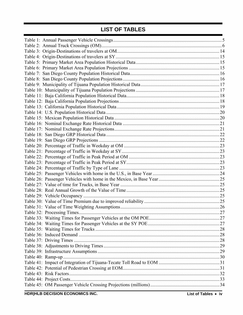
LIST OF TABLES
Table 1: Annual Passenger Vehicle Crossings...........................................................................................5 Table 2: Annual Truck Crossings (OM).....................................................................................................6 Table 3: Origin-Destinations of travelers at OM......................................................................................14 Table 4: Origin-Destinations of travelers at SY.......................................................................................15 Table 5: Primary Market Area Population Historical Data......................................................................15 Table 6: Primary Market Area Population Projections ............................................................................15 Table 7: San Diego County Population Historical Data...........................................................................16 Table 8: San Diego County Population Projections .................................................................................16 Table 9: Municipality of Tijuana Population Historical Data..................................................................17 Table 10: Municipality of Tijuana Population Projections ......................................................................17 Table 11: Baja California Population Historical Data..............................................................................18 Table 12: Baja California Population Projections....................................................................................18 Table 13: California Population Historical Data......................................................................................19 Table 14: U.S. Population Historical Data ...............................................................................................20 Table 15: Mexican Population Historical Data ........................................................................................20 Table 16: Nominal Exchange Rate Historical Data .................................................................................21 Table 17: Nominal Exchange Rate Projections........................................................................................21 Table 18: San Diego GRP Historical Data ...............................................................................................22 Table 19: San Diego GRP Projections .....................................................................................................22 Table 20: Percentage of Traffic in Weekday at OM ................................................................................23 Table 21: Percentage of Traffic in Weekday at SY..................................................................................23 Table 22: Percentage of Traffic in Peak Period at OM ............................................................................23 Table 23: Percentage of Traffic in Peak Period at SY..............................................................................23 Table 24: Percentage of Traffic by Type of Lane ....................................................................................23 Table 25: Passenger Vehicles with home in the U.S., in Base Year ........................................................24 Table 26: Passenger Vehicles with home in the Mexico, in Base Year ...................................................25 Table 27: Value of time for Trucks, in Base Year ...................................................................................25 Table 28: Real Annual Growth of the Value of Time ..............................................................................25 Table 29: Vehicle Occupancy ..................................................................................................................25 Table 30: Value of Time Premium due to improved reliability ...............................................................25 Table 31: Value of Time Weighting Assumptions...................................................................................26 Table 32: Processing Times......................................................................................................................27 Table 33: Waiting Times for Passenger Vehicles at the OM POE...........................................................27 Table 34: Waiting Times for Passenger Vehicles at the SY POE............................................................27 Table 35: Waiting Times for Trucks ........................................................................................................28 Table 36: Induced Demand ......................................................................................................................28 Table 37: Driving Times ..........................................................................................................................28 Table 38: Adjustments to Driving Times .................................................................................................29 Table 39: Infrastructure Assumptions ......................................................................................................29 Table 40: Ramp-up ...................................................................................................................................30 Table 41: Impact of Integration of Tijuana-Tecate Toll Road to EOM ...................................................31 Table 42: Potential of Pedestrian Crossing at EOM.................................................................................31 Table 43: Risk Factors..............................................................................................................................32 Table 44: Project Costs.............................................................................................................................33 Table 45: OM Passenger Vehicle Crossing Projections (millions)..........................................................34
HDR|HLB DECISION ECONOMICS INC. List of Tables • V
Table 46: SY Passenger Vehicle Crossing Projections (millions) ...........................................................35 Table 47: OM Truck Crossing Projections (millions)..............................................................................36 Table 48: EOM POE Passenger Vehicle Crossing Projections (millions) ................................................37 Table 49: EOM POE Truck Transaction Projections (millions) ..............................................................38 Table 50: Passenger Vehicle Revenue Projections (millions)...................................................................39 Table 51: Truck Revenue Projections (millions) .....................................................................................40 Table 52: EOM Total Revenue Projections (millions).............................................................................41 Table 53: Total Annual Revenue (millions) – by vehicle type and lane type ..........................................41 Table 54: Average Toll Rate – Passenger Vehicles .................................................................................42 Table 55: Average Toll Rate – Trucks .....................................................................................................42 Table 56: Summary of Revenue Results for Revenue Scenarios ..............................................................42 Table 57: Debt Service Coverage Estimation of Baseline Cost Estimation.............................................44 Table 58: Debt Service Coverage Estimation (S.R. 11 Capital and O&M Costs, with $50M Grant) .....45 Table 59: Alternate Cost Scenario (Total S.R. 11 Costs and POE Capital Costs, with $300M Grant) ...46 Table 60: Alternate Cost Scenario (Total S.R. 11 Costs and POE Capital Costs, with $400M Grant) ...47 Table 61: Alternate Cost Scenario (Total S.R. 11 Costs, POE Capital Costs, and O&M Costs after
2044, with $400M Grant) ..................................................................................................................48 Table 62: Alternate Revenue Scenario (Total S.R. 11 Costs, Integration with Tijuana – Tecate Toll
Road) .................................................................................................................................................49 Table 63: Alternate Revenue Scenario (Total S.R. 11 Costs, Tolled Pedestrian Crossing at EOM).......50 Table 64: Alternate Revenue Scenario (Total S.R. 11 Costs, EOM Designed for Trucks Only) ............51 Table 65: Alternate Revenue Scenario (Total S.R. 11 Costs, Risk of Punta Colonet Opening in 2020)..52 Table 66: Alternate Revenue Scenario (Total S.R. 11 Costs, Risk of Expanded Mass Transit at
Existing Facilities).............................................................................................................................53 Table 67: Alternate Revenue Scenario (Total S.R. 11 Costs, Risk of Increased Border Security)..........54 Table 68: Alternate Revenue Scenario (Total S.R. 11 Costs, Risk of U.S. Compliance with NAFTA
Truck Rules) ......................................................................................................................................55 Table 69: Indicative DSCR Ranges for Toll Road Securitization Transactions ......................................57 Table 70: Expected S.R. 11 and EOM POE Credit Ratings and Needs for Public Co-Investments........58
HDR|HLB DECISION ECONOMICS INC. Executive Summary •
vi
EXECUTIVE SUMMARY
Background Trade between the U.S. and Mexico fuels economic growth on regional and national levels. Investments in border infrastructure attempt to keep pace with U.S. import demand but with partial success. New demands for improved security extend average processing times and exacerbate waiting times at the port of entries. Problems are particularly acute in the San Diego-Tijuana region, since San Ysidro is the busiest land crossing in the world in terms of numbers of people processed. Waiting times at existing facilities routinely can last over an hour for passenger vehicles, and truck drivers have logged four hours in line.
Budget constraints at the federal level have limited its ability to contribute to border infrastructure needs. Where funds are available, long lead times are required between project design and allocation. In this context, innovative financing mechanisms such as public-private partnerships can play an important role. Infrastructure investments that can generate revenue - and even an attractive return on investment - become potential examples of win-win solutions.
While local resources are also constrained, the demand for generating public benefits from investments can sometimes drive action to unlock funds. In this regard, it can become very important to understand the implications of investment levels on the size and distribution of public benefits.
Project Summary
The San Diego Association of Governments (SANDAG) has retained HDR|HLB Decision Economics Inc. (HDR|HLB) to assess whether the proposed State Route (S.R.) 11 and East Otay Mesa (EOM) Port of Entry (POE) could be financed as toll facilities. In this effort, HDR|HLB has developed traffic, revenue, cost and financial risk models--approaches that have been extensively used in other toll road feasibility analysis for capital markets (rating agencies, bond insurers, etc).
Development of S.R. 11 and the EOM POE would help reduce long wait times at nearby POEs. These facilities have limited options for expanding capacity to meet current demand. As population and economic development drive future demand, wait times would increase accordingly. A new POE in the San Diego-Tijuana region will relieve this pressure and can achieve reductions in wait times for all persons crossing the border.
Study Approach The primary focus of this study is whether the S.R. 11 and EOM POE project is a good candidate to attract private investment. To answer this question, HDR|HLB investigated whether the necessary conditions for a “successful” toll facility are met; evaluated the facility in light of standard credit rating criteria for toll facilities; analyzed the impact of potential revenue and cost scenarios; and assessed the investor market.
The traffic and revenue forecast analysis is built around transparency. An expert panel, convened by HDR|HLB, SANDAG, and the California Department of Transportation (Caltrans) thoroughly reviewed the models, verified data accuracy, assessed reasonability of assumptions and suggested revisions, as necessary. In all cases, key assumptions on the drivers of traffic and revenue are characterized with a risk

HDR|HLB DECISION ECONOMICS INC. Executive Summary •
vii
profile and uncertainty. Analytical models incorporate these uncertainties to ultimately provide a probability of achieving the necessary debt service coverage levels over time.
Findings Principal financial findings are contained in Table ES-1. This table summarizes debt service coverage ratios (DSCR) for a series of cost scenarios with baseline revenues. The baseline cost scenario includes only capital and operation and maintenance (O&M) costs for S.R. 11. Additional cost scenarios assess the grant level requirements necessary to achieve a solid financial rating while including the cost of additional project elements.
Regarding baseline costs, passenger vehicles and trucks transaction growth and a high demand for the lower waiting times at the EOM POE appear to produce the revenues that are necessary to limit debt service coverage risk to only a few years. With a $50 million grant (17% of the total capital cost), the revenues achieve a high likelihood of success and reasonably likelihood of an investment grade rating. To achieve the same investment grade rating, the capital grant requirement rises substantially to $400 million if project revenues are intended to cover S.R. 11 capital and O&M costs and also the EOM POE capital cost (Scenario C-1). The grant amount is over 60% of the total capital cost. If the EOM POE O&M costs (including personnel) are added to the project budget, the debt service coverage simply cannot be met. Only if O&M costs for the first thirty years are covered by an external source and with the same $400 million capital grant can the project achieve a reasonable credit rating Scenario C-3. The cumulative shortfall in O&M costs over this period is approximately $1 billion in current year dollars.
Table ES-1: Expected S.R. 11 and EOM POE Credit Ratings and Needs for Public Co-Investments (In Millions of 2012 Dollars)
Scenario Total
Capital Costs
Annual O&M Costs
Capital Grant
Likelihood of
"Success" 1
Likelihood of Investment
Grade Rating2 Cost Scenarios
Baseline Scenario $0 S.R.-11 Capital and O&M Costs 0% >90% 75% - 80%
$50
$294.5 $0.42
17% >95% 80% - 85%
Scenario C-1 $300 S.R.-11 Capital and O&M Costs, plus POE Capital Costs 45% >80% 65% - 70%
$400
$660.4 $0.42
61% >95% 80% - 85%
Scenario C-2 $400 S.R.-11 Capital and O&M Costs, plus POE Capital and O&M Costs
$660.4 $37.02 61% <5% <5%
Scenario C-3 $400 S.R.-11 Capital and O&M Costs, plus POE Capital and O&M Costs after 30 years
$660.4 $37.02 61% >90% 75% - 80%
Note: (1) Major bond insurers (with AAA ratings) would prefer to insure projects with a 99 percent probability that the DSCR (the first percentile) is 1.0 or higher. This level of analysis is limited to an upper probability bound of 95%. Exact determination at the 99% level may be required by the major bond insurers. (2) Major bond insurers (with AAA ratings) consider a DSCR of 1.25 to be the minimum level for an investment grade rating of BBB.

HDR|HLB DECISION ECONOMICS INC. Executive Summary •
viii
Strengths, weaknesses, and an assessment of the investor market can be summarized as follows:
Strengths
• EOM and S.R. 11 would be an alternative border crossing to increasingly congested Otay Mesa (OM) and San Ysidro (SY) facilities.
• New facilities would offer dramatic travel time savings for users.
• Travelers continuing to use the free POEs would experience small reductions in wait times, but if aggregated would amount to a sizable public benefit.
• Over the next several decades, population growth in the region – especially in Mexico, would lead to success of the toll facilities.
Weaknesses
• Estimated construction and operational costs for S.R. 11 and EOM are quite expensive.
• As with most toll road start-ups, a financing plan with relatively low obligations in early years of operations (e.g., principal repayments starting a few years after opening) would be needed to be viable.
Investor Market assessment
• The analysis reveals that S.R. 11 and EOM POE would require at least $400 million in external funds to pay for all construction costs. This level of funding is however insufficient to cover the EOM POE O&M costs until the facility has been operating for 30 years.
• Integration with the Mexican toll road would lower the total cost burden somewhat, but not enough to pay for the annual O&M shortfall at the EOM POE.
Next Steps Given the need for public participation, some additional analyses may be needed. These include an assessment of economic benefits and distributional welfare effects on the region (i.e. an assessment of whether the rate of return from the social perspective warrants the local public investments in the project). In addition, conducting a due diligence and risk-based assessment of estimated construction and O&M costs of S.R. 11 and the EOM POE may identify mitigation strategies for reducing risks. Also, a more complete financial analysis could broaden the scope of study to explore the potential of non-toll revenues (e.g. development fees) to reduce grant needs and to explore mechanisms for alleviating shortfalls in O&M costs.
HDR|HLB DECISION ECONOMICS INC. S.R. 11 and East Otay Mesa POE Financial Feasibility • 1
CHAPTER 1: INTRODUCTION
State Route (S.R.) 11 is a proposed road connecting S.R. 905 and S.R. 125 to the San Diego and Tijuana international border. S.R. 11 would terminate at the proposed East Otay Mesa (EOM) port of entry (POE). The San Diego Association of Governments (SANDAG) has contracted HDR|HLB Decision Economics Inc. (HDR|HLB) to prepare a financial feasibility study of developing S.R. 11 and the POE as tolled facilities.
The EOM POE would be located approximately two miles east of the Otay Mesa (OM) POE and eight miles east of the San Ysidro (SY) POE, two local existing POEs. This road and new POE would further the increasing interconnections between the rapidly growing populations and economic centers on both sides of the border.
Development of S.R. 11 and the EOM POE would reduce long wait times currently observed at the OM and SY border crossings. These facilities have limited options for expanding capacity to meet current demand. As population and economic development drive future demand, wait times are expected to increase accordingly. A new POE in the San Diego-Tijuana region will relieve this pressure, and depending on the how its toll system is operated, can achieve reductions in wait times for all persons.
S.R. 11 and the EOM POE would be developed as integrated facilities. Passenger vehicles and trucks crossing the border at EOM would pay a toll before joining S.R. 11. S.R. 11 would begin just after exiting the POE and provide interchanges for local border traffic and others traveling further north. Traffic using S.R. 11 without crossing the border would be assumed to pay a different toll amount that is proportional to its service.1
Note that S.R. 11 and the EOM POE are necessarily coupled project components. Neither facility is reasonably attractive without the other. Complicating this relationship is that these facilities are typically owned, operated and funded by separate institutions, local and state government (or private) and federal government. While this relationship may imply complexities for financial feasibility, this study does not delve into this matter but focuses only on levels of revenue and costs.
This report discusses the process and assumptions in forecasting cross border traffic and revenue from these proposed facilities. The financial feasibility of the several revenue and cost scenarios is evaluated to determine the conditions which lead to acceptable risks as perceived by the financial community.
The baseline scenario is designed for the toll revenue to be applied to the total capital and operation and maintenance (O&M) costs of S.R. 11 only. The additional scenarios are defined as:
Alternative 1:
– Toll revenue applied to baseline plus POE capital cost
Alternative 2:
– Toll revenue applied to baseline plus POE capital and O&M costs
1 Traffic and revenues for local S.R. 11 road use were not examined in this analysis. These revenues are likely to be small and, according to a previous study, only marginally able to generate revenues sufficient to cover costs.

HDR|HLB DECISION ECONOMICS INC. S.R. 11 and East Otay Mesa POE Financial Feasibility • 2
Alternative 3:
– Demand for EOM POE increases with Tijuana-Tecate toll road integration
Alternative 4:
– EOM POE offers bus rapid transit service for pedestrians
Alternative 5:
– EOM POE is designed for trucks only
Other alternatives are examined based on other risk factors of the project.
Overall, the study addresses several components including an:
Investigation of whether the necessary conditions for a “successful” toll facility are met (sufficient traffic/toll revenues and adequate capital at a reasonable cost);
Evaluation of the facility in light of standard credit rating criteria for toll facilities (i.e. evaluate potential risk and the likelihood of an “investment-grade” rating);
Evaluation of how alterations in the operation configurations might impact its “performance”;
Assessment of the investor market; and
Technical and managerial recommendations.
Six major steps are involved in completing this analysis. These steps include:
1. Research and analyze regional socio-economic projections;
2. Review data from SANDAG including previous relevant reports;
3. Develop a simplified risk analysis travel demand and toll revenue forecasting model;
4. Conduct a Risk Analysis Process (RAP) session;
5. Update risk analysis assumptions and run Monte Carlo simulations to generate initial traffic, revenue, and debt service coverage ratio (DSCR) projections;
6. Report and document simulation results.
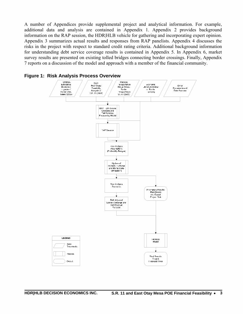
Figure 1 illustrates how these steps are linked in a structure and logic diagram.
The organization of the report begins with a description of the border area, the historical border crossings, and a description of S.R. 11 and the EOM POE. The next section discusses the methodological framework for the models used in this analysis: the border crossing forecast model, the POE and toll road diversion model, toll revenue model, and the financial model. The forecasting assumptions of the risk analysis variables used in these models are presented in the fourth section. The results of these models are described in the fifth section and the conclusions and recommendations are discussed in the sixth section.
HDR|HLB DECISION ECONOMICS INC. S.R. 11 and East Otay Mesa POE Financial Feasibility • 3
A number of Appendices provide supplemental project and analytical information. For example, additional data and analysis are contained in Appendix 1. Appendix 2 provides background information on the RAP session, the HDR|HLB vehicle for gathering and incorporating expert opinion. Appendix 3 summarizes actual results and responses from RAP panelists. Appendix 4 discusses the risks in the project with respect to standard credit rating criteria. Additional background information for understanding debt service coverage results is contained in Appendix 5. In Appendix 6, market survey results are presented on existing tolled bridges connecting border crossings. Finally, Appendix 7 reports on a discussion of the model and approach with a member of the financial community.
Figure 1: Risk Analysis Process Overview
HDR|HLB DECISION ECONOMICS INC. S.R. 11 and East Otay Mesa POE Financial Feasibility • 4
CHAPTER 2: PROJECT DESCRIPTION AND STUDY AREA
The study area for the scope of this financial feasibility report includes the San Diego-Tijuana border area, the existing POEs of OM and SY, and the proposed EOM facility.
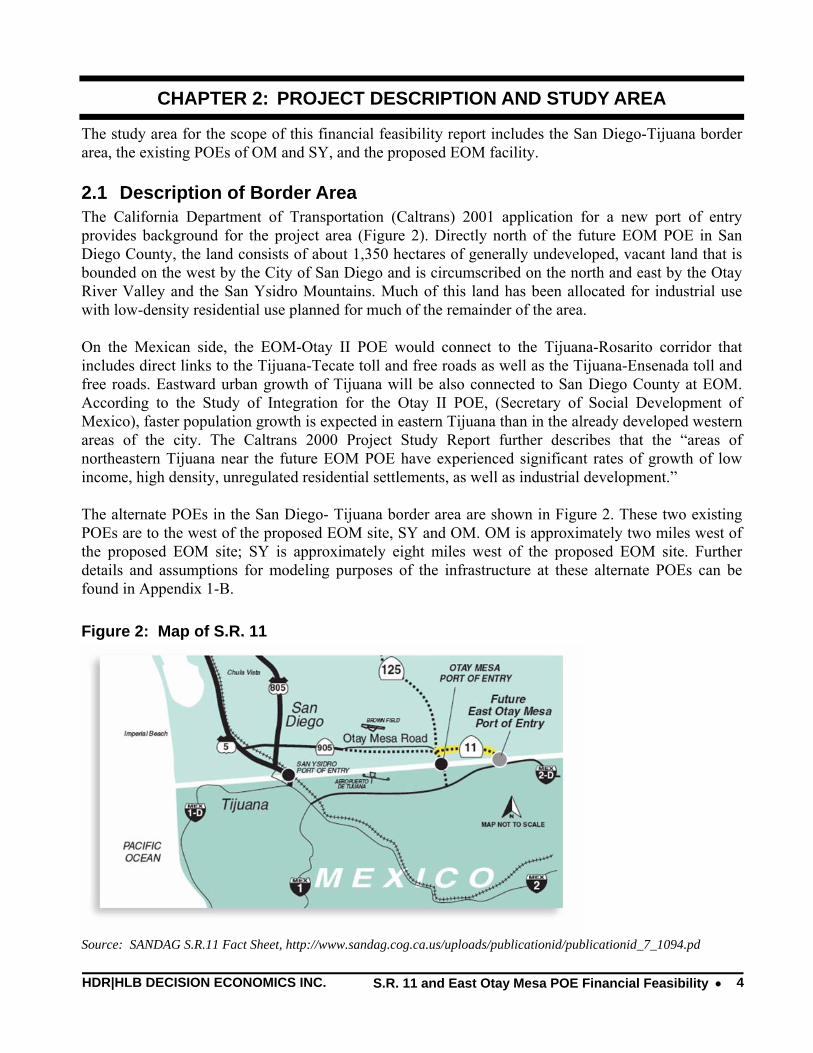
2.1 Description of Border Area The California Department of Transportation (Caltrans) 2001 application for a new port of entry provides background for the project area (Figure 2). Directly north of the future EOM POE in San Diego County, the land consists of about 1,350 hectares of generally undeveloped, vacant land that is bounded on the west by the City of San Diego and is circumscribed on the north and east by the Otay River Valley and the San Ysidro Mountains. Much of this land has been allocated for industrial use with low-density residential use planned for much of the remainder of the area. On the Mexican side, the EOM-Otay II POE would connect to the Tijuana-Rosarito corridor that includes direct links to the Tijuana-Tecate toll and free roads as well as the Tijuana-Ensenada toll and free roads. Eastward urban growth of Tijuana will be also connected to San Diego County at EOM. According to the Study of Integration for the Otay II POE, (Secretary of Social Development of Mexico), faster population growth is expected in eastern Tijuana than in the already developed western areas of the city. The Caltrans 2000 Project Study Report further describes that the “areas of northeastern Tijuana near the future EOM POE have experienced significant rates of growth of low income, high density, unregulated residential settlements, as well as industrial development.” The alternate POEs in the San Diego- Tijuana border area are shown in Figure 2. These two existing POEs are to the west of the proposed EOM site, SY and OM. OM is approximately two miles west of the proposed EOM site; SY is approximately eight miles west of the proposed EOM site. Further details and assumptions for modeling purposes of the infrastructure at these alternate POEs can be found in Appendix 1-B.
Figure 2: Map of S.R. 11
Source: SANDAG S.R.11 Fact Sheet, http://www.sandag.cog.ca.us/uploads/publicationid/publicationid_7_1094.pd
HDR|HLB DECISION ECONOMICS INC. S.R. 11 and East Otay Mesa POE Financial Feasibility • 5
Another POE, Tecate, is located approximately 25 miles further east of the proposed EOM site. This POE is much smaller and less frequently used. Because total border crossings at Tecate are relatively low, insignificant levels of revenue could be generated from crossings diverted to the EOM POE. Tecate is not modeled as an alternative POE but instead is assessed in one of the revenue scenarios.
2.2 Border Crossings This section presents data on border crossings by passenger vehicles at the SY and OM POEs and trucks at OM. Trucks were permitted to cross at SY until 1992.
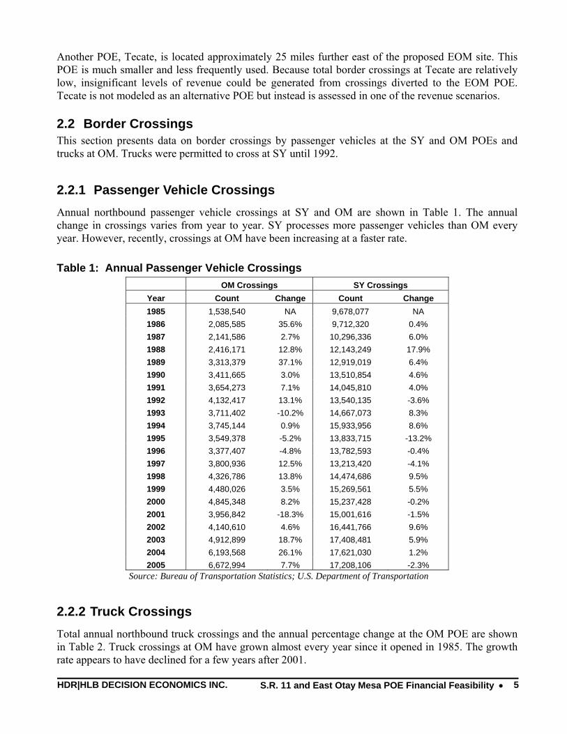
2.2.1 Passenger Vehicle Crossings Annual northbound passenger vehicle crossings at SY and OM are shown in Table 1. The annual change in crossings varies from year to year. SY processes more passenger vehicles than OM every year. However, recently, crossings at OM have been increasing at a faster rate.
Table 1: Annual Passenger Vehicle Crossings OM Crossings SY Crossings
Year Count Change Count Change 1985 1,538,540 NA 9,678,077 NA 1986 2,085,585 35.6% 9,712,320 0.4% 1987 2,141,586 2.7% 10,296,336 6.0% 1988 2,416,171 12.8% 12,143,249 17.9% 1989 3,313,379 37.1% 12,919,019 6.4% 1990 3,411,665 3.0% 13,510,854 4.6% 1991 3,654,273 7.1% 14,045,810 4.0% 1992 4,132,417 13.1% 13,540,135 -3.6% 1993 3,711,402 -10.2% 14,667,073 8.3% 1994 3,745,144 0.9% 15,933,956 8.6% 1995 3,549,378 -5.2% 13,833,715 -13.2% 1996 3,377,407 -4.8% 13,782,593 -0.4% 1997 3,800,936 12.5% 13,213,420 -4.1% 1998 4,326,786 13.8% 14,474,686 9.5% 1999 4,480,026 3.5% 15,269,561 5.5% 2000 4,845,348 8.2% 15,237,428 -0.2% 2001 3,956,842 -18.3% 15,001,616 -1.5% 2002 4,140,610 4.6% 16,441,766 9.6% 2003 4,912,899 18.7% 17,408,481 5.9% 2004 6,193,568 26.1% 17,621,030 1.2% 2005 6,672,994 7.7% 17,208,106 -2.3%
Source: Bureau of Transportation Statistics; U.S. Department of Transportation
2.2.2 Truck Crossings Total annual northbound truck crossings and the annual percentage change at the OM POE are shown in Table 2. Truck crossings at OM have grown almost every year since it opened in 1985. The growth rate appears to have declined for a few years after 2001.

HDR|HLB DECISION ECONOMICS INC. S.R. 11 and East Otay Mesa POE Financial Feasibility • 6
Table 2: Annual Truck Crossings (OM) Year Count Change Year Count Change 1985 88,426 NA 1996 530,704 19.1% 1986 145,039 64.0% 1997 567,715 7.0% 1987 207,405 43.0% 1998 606,384 6.8% 1988 235,545 13.6% 1999 646,587 6.6% 1989 275,057 16.8% 2000 688,340 6.5% 1990 216,185 -21.4% 2001 708,446 2.9% 1991 315,650 46.0% 2002 731,291 3.2% 1992 374,141 18.5% 2003 697,152 -4.7% 1993 384,615 2.8% 2004 726,164 4.2% 1994 439,654 14.3% 2005 730,253 0.6% 1995 445,770 1.4%
Source: Bureau of Transportation Statistics; U.S. Department of Transportation
2.3 Description of S.R. 11 and the EOM POE Northbound passenger vehicles and trucks would follow similar inspection procedures at the EOM POE as they would at SY or OM. EOM would perform primary inspections through U.S. Customs and U.S. Secondary Inspections. Trucks would first stop at the U.S. Commercial Import Station. From there, required trucks would be routed on a commercial vehicle bypass road to the Otay Mesa POE Commercial Vehicle Enforcement Facility (CVEF) or to a new facility located at the EOM POE. The northbound travelers crossing the border at EOM will continue on S.R. 11 towards its junction with S.R. 125 and S.R. 905. There are also two local interchanges described in the Caltrans September 2000 Project Study Report at Enrico Fermi Road and the future extension of local roads.
Two alignments are currently being considered for S.R. 11. The Caltrans 2000 Project Study Report describes the central alignment requiring 70 hectares of right of way and impacting 14 parcels for S.R. 11. The central alignment would include a 4.7 km section of four-lane freeway with two local interchanges and a two-lane truck bypass road between EOM and the OM CVEF. The western alignment requires approximately 60 hectares of right of way and will impact 13 parcels. The western alignment would include a 4.1 km section of four-lane freeway with two local interchanges and an over crossing and a two-lane truck bypass road to the OM CVEF.
2.4 Market Areas This analysis has incorporated influences on crossings at the existing POEs from the U.S. and Mexico at several regional levels. On the U.S. side, four market areas are considered (shown in Figure 3). The two focal areas are located within San Diego County and consist of:
U.S. primary market area (PMA), comprising the sub-regional areas of South Bay, Sweetwater, Jamul, Chula Vista, and National City; and
U.S. Secondary Market Area consists of San Diego County excluding the PMA.
Two other areas include California (excluding San Diego County) and the U.S. (excluding California).

HDR|HLB DECISION ECONOMICS INC. S.R. 11 and East Otay Mesa POE Financial Feasibility • 7
Figure 3: U.S. Market Areas
On the Mexican side, three market areas are considered (shown in Figure 4). The Municipality of Tijuana comprises the Mexican PMA. A secondary market area consists of the State of Baja California (excluding Tijuana). The third market area in Mexico consists of the entire country, excluding Baja California.
Figure 4: Mexican Market Areas
Tijuana
Baja California
Secondary Market Area
Primary Market Area
HDR|HLB DECISION ECONOMICS INC. S.R. 11 and East Otay Mesa POE Financial Feasibility • 8
CHAPTER 3: ANALYTICAL MODELS
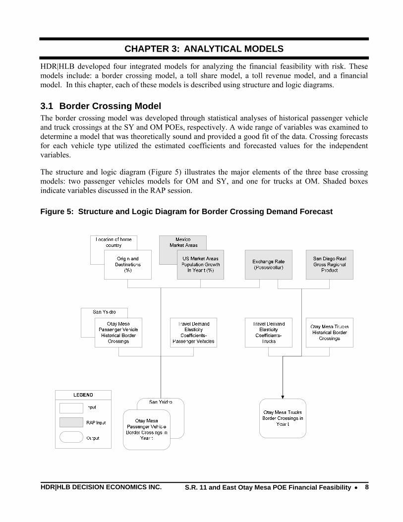
HDR|HLB developed four integrated models for analyzing the financial feasibility with risk. These models include: a border crossing model, a toll share model, a toll revenue model, and a financial model. In this chapter, each of these models is described using structure and logic diagrams. 3.1 Border Crossing Model The border crossing model was developed through statistical analyses of historical passenger vehicle and truck crossings at the SY and OM POEs, respectively. A wide range of variables was examined to determine a model that was theoretically sound and provided a good fit of the data. Crossing forecasts for each vehicle type utilized the estimated coefficients and forecasted values for the independent variables.
The structure and logic diagram (Figure 5) illustrates the major elements of the three base crossing models: two passenger vehicles models for OM and SY, and one for trucks at OM. Shaded boxes indicate variables discussed in the RAP session.
Figure 5: Structure and Logic Diagram for Border Crossing Demand Forecast

HDR|HLB DECISION ECONOMICS INC. S.R. 11 and East Otay Mesa POE Financial Feasibility • 9
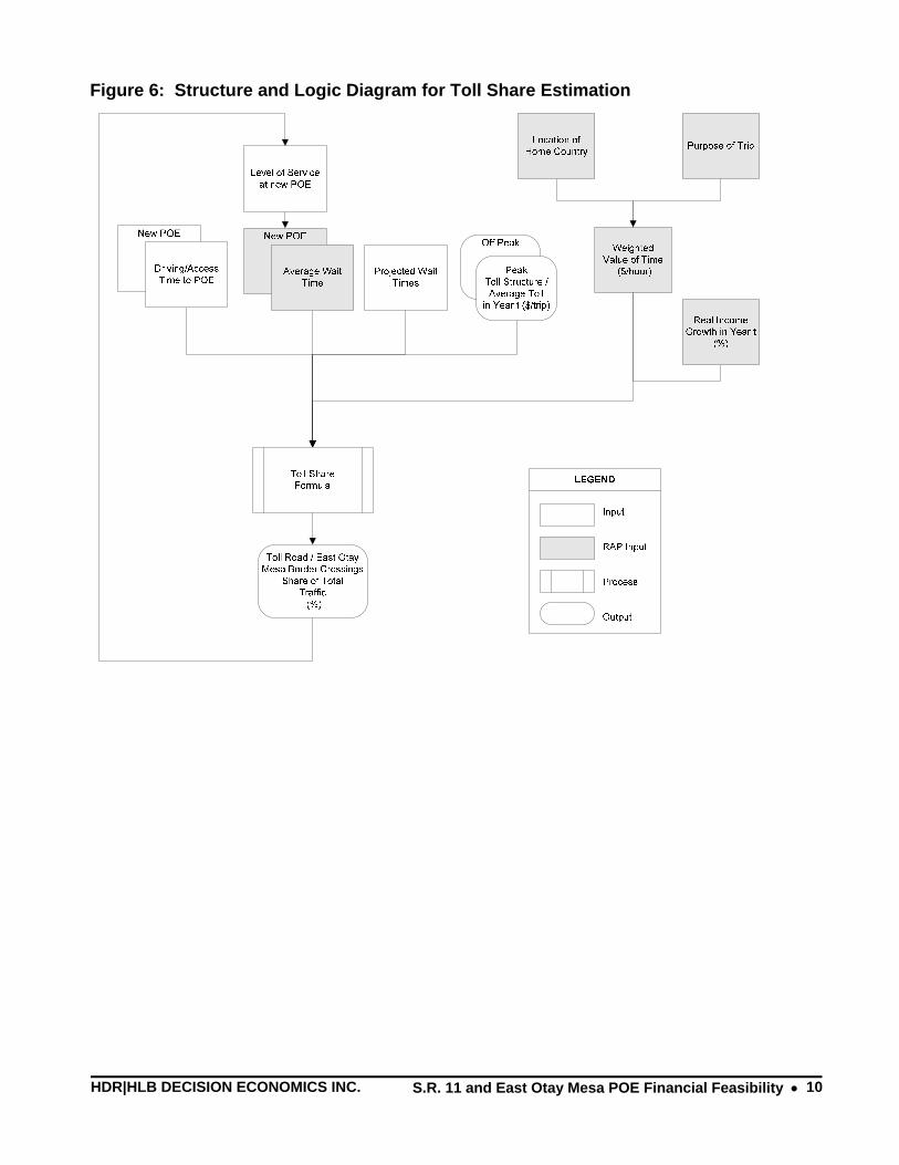
3.2 Port of Entry Diversion and Toll Share Model HDR|HLB’s model for estimating traffic diversion from existing POEs to the EOM POE was developed specially for this project. Conventional toll diversion models were not applied in this project because the task involved disentangling the interrelationships between toll rates, maximum waiting times at the EOM POE and traffic diversion to the EOM POE. The final model builds on a theory of convergence of travel time options for different border crossing locations. For example, at a given toll rate, travelers are assumed to be indifferent between waiting at an existing facility or paying the toll, driving the extra distance and incurring a shorter wait time at EOM. With some proportion of travelers choosing EOM, waiting times at the existing facilities are reduced proportional to the number of lanes at the new facility.
Figure 6 illustrates the major elements of the model. The model accounts for additional costs of the toll, and driving distance to the new POE. Value of time, weighted by location of home country and purpose of trip, contribute to the likelihood of going to the new POE. RAP variables are shown in shaded cells. Baseline waiting times are derived from RAP panelists and U.S. Customs and Border Protection (CBP) data. Annual increases in baseline waiting times are computed from increases in total crossing volumes. Because it is expected that CBP will undertake infrastructural and operational steps to reduce waiting times, waiting times grow at a smaller rate than that of crossings.
Induced demand represents additional border crossings that are created due to the reduction in waiting times at existing facilities, after traffic is .diverted to the EOM POE. The model incorporates induced demand by assuming that reduction in waiting times at existing facility is partially returned to original levels, at a rate determined by an elasticity of induced demand. The model also assumes that some of the new travelers will be diverted to the new POE at the same diversion rate as current users. The resulting induced demand diversion to EOM is a relatively minor level of volume. This volume however represents upward pressure on the toll rate. The final toll rate for all vehicles incorporates original and induced demand for the lower waiting times at EOM.
Several key equations are involved in solving the toll diversion model. Figure 7 lists a set of equations for solving truck and passenger vehicle diversion from OM. The model for passenger vehicles is more complex because vehicles are diverted from two facilities, each of which has its own distance to the EOM POE and weighted value of time (as determined by a person’s purpose of trip and location of home, respectively). Separate models of toll diversion are developed for individual cases including: Passenger Vehicles: Normal and SENTRI lanes; Trucks: Normal and FAST; peak and off-peak periods; and, weekend and weekday periods.2 Toll rates and diversion levels are principal outputs of the models.
2 SENTRI (Secure Electronic Network for Travelers Rapid Inspection) and FAST (Free and Secure Trade) are programs offered to pre-approved passengers, importers, carriers, and registered drivers that result in quicker clearance across the border.
HDR|HLB DECISION ECONOMICS INC. S.R. 11 and East Otay Mesa POE Financial Feasibility • 10
Figure 6: Structure and Logic Diagram for Toll Share Estimation

HDR|HLB DECISION ECONOMICS INC. S.R. 11 and East Otay Mesa POE Financial Feasibility • 11
Figure 7: Diversion Model Equations
Truck Model Equations to Solve for Toll Rate and Diversion
1. WE = LO/LE (ŴO – WO)
2. WO = WE + DO + T/V
3. T = V (WO – WE – DO)
4. DVE = WELE / ŴOLO
Passenger Vehicle Model Equations to Solve for Toll Rate and Diversion
5. WE = LO/LE (ŴO – WO) + LS/LE (ŴS – WS)
6. WO = WE + DO + T/VO
7. WS = WE + DS + T/VS
8. T = VS (WS –WE – DS ) = VO (WO –WE – DO )
9. DVE = WELE / [ ŴOLO + ŴSLS ]
Where:
Subscripts: O = Otay Mesa, E = proposed East Otay Mesa, S = San Ysidro
W = Waiting Times; Ŵ = Existing Waiting Time
L = Number of operating lanes
T = Toll rate
D = Driving time difference between existing and new POE
V = Value of time (weighted by purpose of trip, location (country) of home)
DV = Toll Diversion rate

HDR|HLB DECISION ECONOMICS INC. S.R. 11 and East Otay Mesa POE Financial Feasibility • 12
3.3 Toll Revenue Model The toll revenue model developed by HDR|HLB is relatively straightforward. Figure 8 illustrates the major elements including the analytical dimensions (weekend/weekday period, type of lane, peak/off-peak period); RAP variables (shaded boxes); and additional model features such as ramp-up, risk factors, and revenue scenarios.
Figure 8: Structure and Logic Diagram for Toll Revenue Forecasting
HDR|HLB DECISION ECONOMICS INC. S.R. 11 and East Otay Mesa POE Financial Feasibility • 13
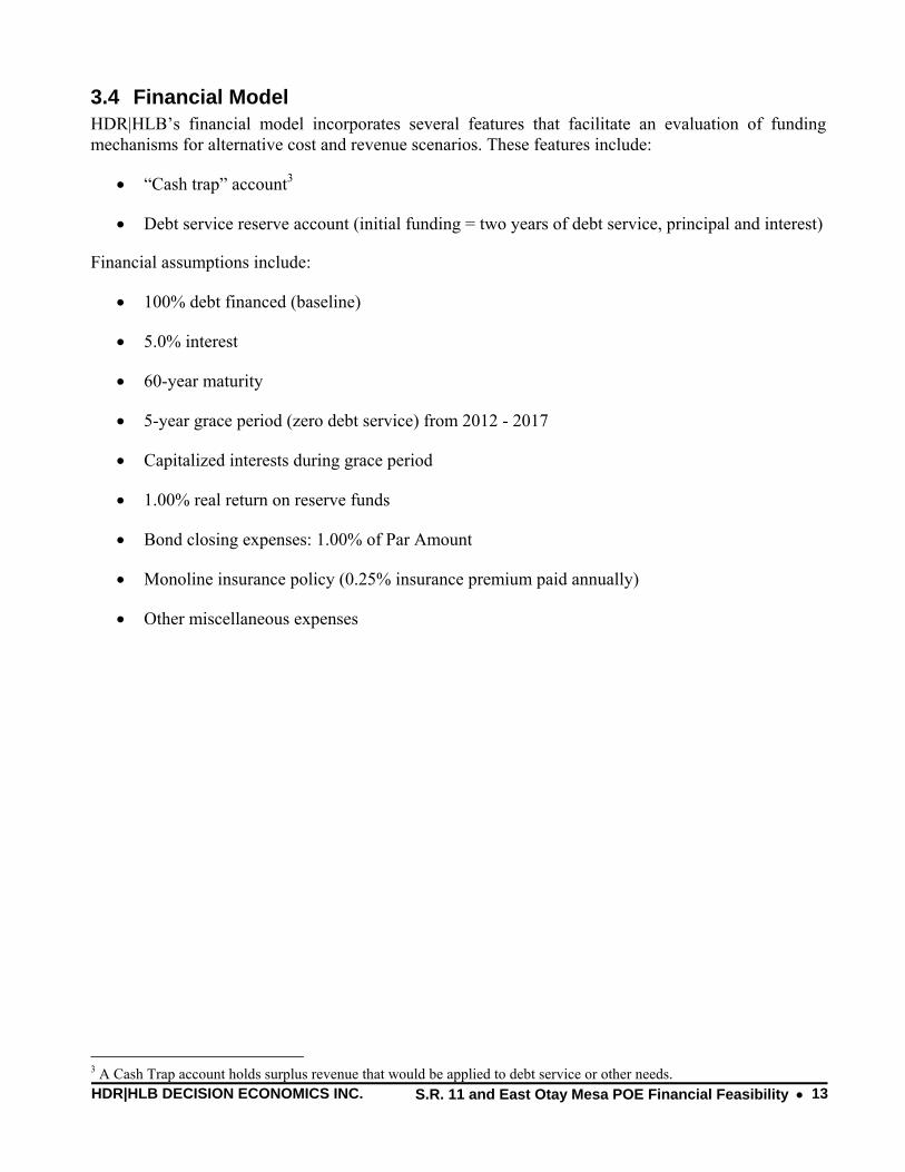
3.4 Financial Model HDR|HLB’s financial model incorporates several features that facilitate an evaluation of funding mechanisms for alternative cost and revenue scenarios. These features include:
• “Cash trap” account3
• Debt service reserve account (initial funding = two years of debt service, principal and interest)
Financial assumptions include:
• 100% debt financed (baseline)
• 5.0% interest
• 60-year maturity
• 5-year grace period (zero debt service) from 2012 - 2017
• Capitalized interests during grace period
• 1.00% real return on reserve funds
• Bond closing expenses: 1.00% of Par Amount
• Monoline insurance policy (0.25% insurance premium paid annually)
• Other miscellaneous expenses
3 A Cash Trap account holds surplus revenue that would be applied to debt service or other needs.
HDR|HLB DECISION ECONOMICS INC. S.R. 11 and East Otay Mesa POE Financial Feasibility • 14
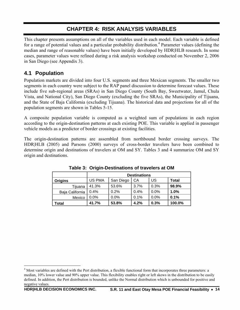
CHAPTER 4: RISK ANALYSIS VARIABLES
This chapter presents assumptions on all of the variables used in each model. Each variable is defined for a range of potential values and a particular probability distribution.4 Parameter values (defining the median and range of reasonable values) have been initially developed by HDR|HLB research. In some cases, parameter values were refined during a risk analysis workshop conducted on November 2, 2006 in San Diego (see Appendix 3).
4.1 Population Population markets are divided into four U.S. segments and three Mexican segments. The smaller two segments in each country were subject to the RAP panel discussion to determine forecast values. These include five sub-regional areas (SRAs) in San Diego County (South Bay, Sweetwater, Jamul, Chula Vista, and National City), San Diego County (excluding the five SRAs), the Municipality of Tijuana, and the State of Baja California (excluding Tijuana). The historical data and projections for all of the population segments are shown in Tables 5-15.
A composite population variable is computed as a weighted sum of populations in each region according to the origin-destination patterns at each existing POE. This variable is applied in passenger vehicle models as a predictor of border crossings at existing facilities.
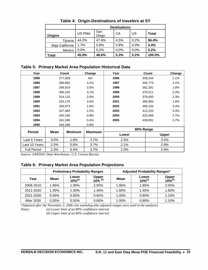
The origin-destination patterns are assembled from northbound border crossing surveys. The HDR|HLB (2005) and Parsons (2000) surveys of cross-border travelers have been combined to determine origin and destinations of travelers at OM and SY. Tables 3 and 4 summarize OM and SY origin and destinations.
Table 3: Origin-Destinations of travelers at OM Destinations Origins US PMA San Diego CA US Total
Tijuana 41.3% 53.6% 3.7% 0.3% 98.9% Baja California 0.4% 0.2% 0.4% 0.0% 1.0%
Mexico 0.0% 0.0% 0.1% 0.0% 0.1% Total 41.7% 53.8% 4.2% 0.3% 100.0%
4 Most variables are defined with the Pert distribution, a flexible functional form that incorporates three parameters: a median, 10% lower value and 90% upper value. This flexibility enables right or left skews in the distribution to be easily defined. In addition, the Pert distribution is bounded, unlike the Normal distribution which is unbounded for positive and negative values.
HDR|HLB DECISION ECONOMICS INC. S.R. 11 and East Otay Mesa POE Financial Feasibility • 15
Table 4: Origin-Destinations of travelers at SY Destinations
Origins US PMA San Diego CA US Total
Tijuana 44.2% 47.6% 4.5% 0.2% 96.4% Baja California 1.7% 0.8% 0.8% 0.0% 3.4%
Mexico 0.0% 0.2% 0.0% 0.0% 0.2% Total 45.9% 48.6% 5.3% 0.2% 100.0%
Table 5: Primary Market Area Population Historical Data Year Count Change Year Count Change 1985 277,909 NA 1996 348,244 1.1% 1986 286,850 3.2% 1997 355,773 2.2% 1987 296,919 3.5% 1998 362,281 1.8% 1988 306,155 3.1% 1999 370,511 2.3% 1989 314,115 2.6% 2000 379,000 2.3% 1990 325,170 3.5% 2001 385,993 1.8% 1991 330,973 1.8% 2002 399,152 3.4% 1992 337,483 2.0% 2003 412,220 3.3% 1993 340,190 0.8% 2004 423,483 2.7% 1994 341,596 0.4% 2005 439,091 3.7% 1995 344,288 0.8%
80% Range Period Mean Minimum Maximum
Lower Upper Last 5 Years 3.0% 1.8% 3.7% 2.5% 3.5%
Last 10 Years 2.5% 0.8% 3.7% 2.1% 2.9% Full Period 2.3% 0.4% 3.7% 2.0% 2.6%
Source: SANDAG Data Warehouse; U.S. Census Bureau
Table 6: Primary Market Area Population Projections Preliminary Probability Ranges Adjusted Probability Ranges*
Year Mean Lower 10%(a)
Upper 10% (b) Mean Lower
10%(a) Upper 10%(b)
2006-2010 1.95% 1.90% 2.00% 1.95% 1.95% 2.05% 2011-2020 1.35% 1.30% 1.40% 1.50% 1.40% 1.60% 2021-2030 0.55% 0.50% 0.60% 1.00% 0.90% 1.10% After 2030 0.55% 0.50% 0.60% 1.00% 0.90% 1.10%
*Adjusted after the November 2, 2006 risk workshop (the adjusted ranges were used in the analysis) Notes: (a) Lower limit of an 80% confidence interval (b) Upper limit of an 80% confidence interval
HDR|HLB DECISION ECONOMICS INC. S.R. 11 and East Otay Mesa POE Financial Feasibility • 16
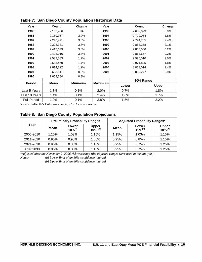
Table 7: San Diego County Population Historical Data Year Count Change Year Count Change 1985 2,102,486 NA 1996 2,682,093 0.9% 1986 2,169,957 3.2% 1997 2,729,054 1.8% 1987 2,248,471 3.6% 1998 2,794,785 2.4% 1988 2,328,331 3.6% 1999 2,853,258 2.1% 1989 2,417,639 3.8% 2000 2,858,000 0.2% 1990 2,498,016 3.3% 2001 2,863,657 0.2% 1991 2,539,583 1.7% 2002 2,920,010 2.0% 1992 2,583,470 1.7% 2003 2,971,805 1.8% 1993 2,614,222 1.2% 2004 3,013,014 1.4% 1994 2,638,511 0.9% 2005 3,039,277 0.9% 1995 2,658,584 0.8%
80% Range Period Mean Minimum Maximum
Lower Upper Last 5 Years 1.3% 0.1% 2.0% 0.7% 1.8% Last 10 Years 1.4% 0.1% 2.4% 1.0% 1.7%
Full Period 1.9% 0.1% 3.8% 1.5% 2.2% Source: SANDAG Data Warehouse; U.S. Census Bureau
Table 8: San Diego County Population Projections Preliminary Probability Ranges Adjusted Probability Ranges*
Year Mean Lower
10%(a) Upper 10% (b) Mean Lower
10%(a) Upper 10%(b)
2006-2010 1.15% 1.03% 1.15% 1.15% 1.03% 1.15% 2011-2020 0.95% 0.90% 1.05% 0.95% 0.85% 1.15% 2021-2030 0.95% 0.85% 1.10% 0.95% 0.75% 1.25% After 2030 0.95% 0.85% 1.10% 0.95% 0.75% 1.25%
*Adjusted after the November 2, 2006 risk workshop (the adjusted ranges were used in the analysis) Notes: (a) Lower limit of an 80% confidence interval (b) Upper limit of an 80% confidence interval

HDR|HLB DECISION ECONOMICS INC. S.R. 11 and East Otay Mesa POE Financial Feasibility • 17
Table 9: Municipality of Tijuana Population Historical Data
Year Count Average Annual Growth Rate (%)
1970 341,000 NA
1980 462,000 3.1%
1990 747,381 4.9%
1995 991,592 5.8%
2000 1,210,820 4.1%
2005 1,410,700 3.1%
80% Range Period Mean Minimum Maximum
Lower Upper Last 5 Years 3.10% 2.92% 3.76% 2.90% 3.31%
Last 10 Years 3.59% 2.92% 5.18% 3.28% 3.90% Full Period 4.33% 2.92% 6.54% 4.03% 4.63%
Sources: Institute for Regional Studies of the Californias (1970 and 1980 estimates); Instituto Nacional de Estadística, Geografía e Informática (1990, 1995, 2000, and 2005 estimates)
Table 10: Municipality of Tijuana Population Projections Preliminary Probability Ranges Adjusted Probability Ranges*
Mean Lower
10%(a) Upper 10% (b) Mean Lower
10%(a) Upper 10%(b)
2006-2010 2.70% 2.30% 4.10% 3.50% 2.63% 4.38% 2011-2020 2.20% 2.10% 2.30% 1.84% 1.38% 2.30% 2021-2030 1.65% 1.50% 1.80% 1.41% 1.06% 1.76% After 2030 1.65% 1.50% 1.80% 1.52% 1.14% 1.90%
*Adjusted after the November 2, 2006 risk workshop (the adjusted ranges were used in the analysis) Notes: (a) Lower limit of an 80% confidence interval (b) Upper limit of an 80% confidence interval
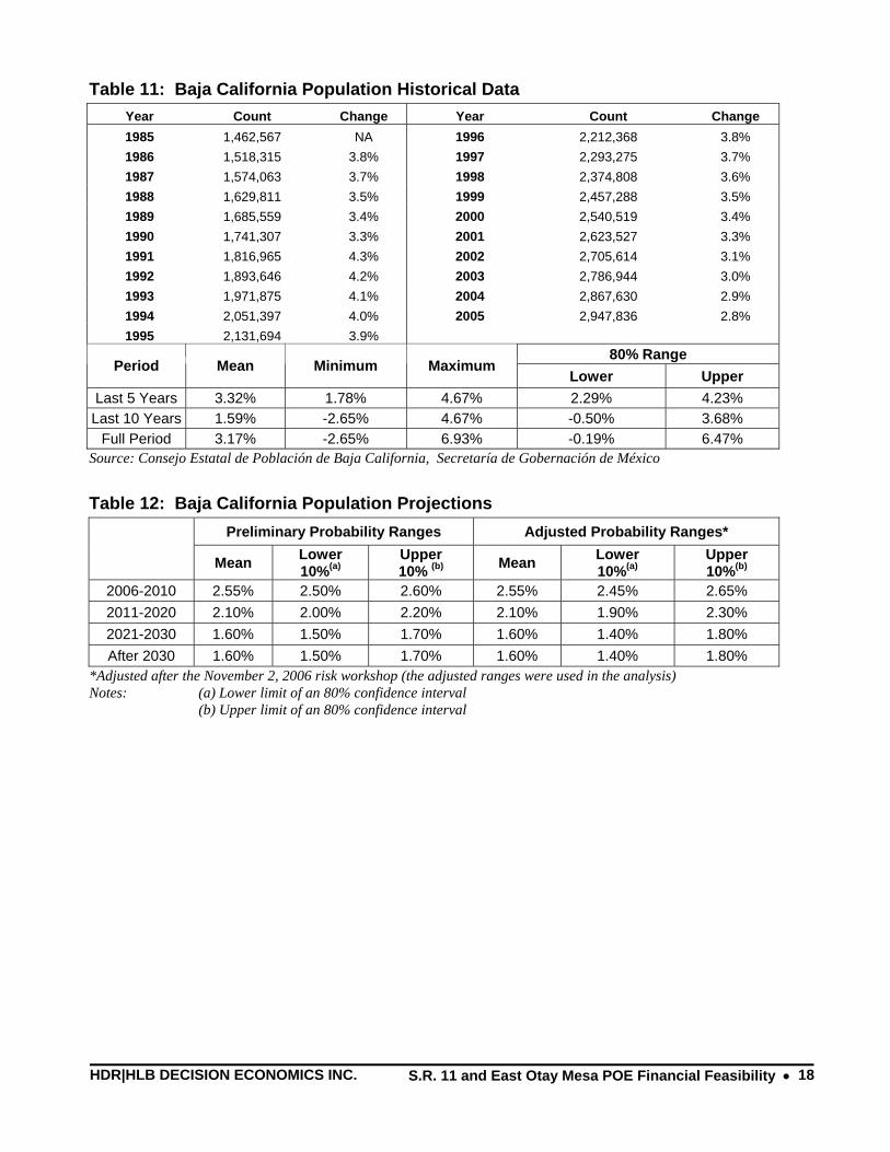
HDR|HLB DECISION ECONOMICS INC. S.R. 11 and East Otay Mesa POE Financial Feasibility • 18
Table 11: Baja California Population Historical Data Year Count Change Year Count Change 1985 1,462,567 NA 1996 2,212,368 3.8% 1986 1,518,315 3.8% 1997 2,293,275 3.7% 1987 1,574,063 3.7% 1998 2,374,808 3.6% 1988 1,629,811 3.5% 1999 2,457,288 3.5% 1989 1,685,559 3.4% 2000 2,540,519 3.4% 1990 1,741,307 3.3% 2001 2,623,527 3.3% 1991 1,816,965 4.3% 2002 2,705,614 3.1% 1992 1,893,646 4.2% 2003 2,786,944 3.0% 1993 1,971,875 4.1% 2004 2,867,630 2.9% 1994 2,051,397 4.0% 2005 2,947,836 2.8% 1995 2,131,694 3.9%
80% Range Period Mean Minimum Maximum
Lower Upper Last 5 Years 3.32% 1.78% 4.67% 2.29% 4.23% Last 10 Years 1.59% -2.65% 4.67% -0.50% 3.68%
Full Period 3.17% -2.65% 6.93% -0.19% 6.47% Source: Consejo Estatal de Población de Baja California, Secretaría de Gobernación de México
Table 12: Baja California Population Projections Preliminary Probability Ranges Adjusted Probability Ranges*
Mean Lower
10%(a) Upper 10% (b) Mean Lower
10%(a) Upper 10%(b)
2006-2010 2.55% 2.50% 2.60% 2.55% 2.45% 2.65% 2011-2020 2.10% 2.00% 2.20% 2.10% 1.90% 2.30% 2021-2030 1.60% 1.50% 1.70% 1.60% 1.40% 1.80% After 2030 1.60% 1.50% 1.70% 1.60% 1.40% 1.80%
*Adjusted after the November 2, 2006 risk workshop (the adjusted ranges were used in the analysis) Notes: (a) Lower limit of an 80% confidence interval (b) Upper limit of an 80% confidence interval
HDR|HLB DECISION ECONOMICS INC. S.R. 11 and East Otay Mesa POE Financial Feasibility • 19
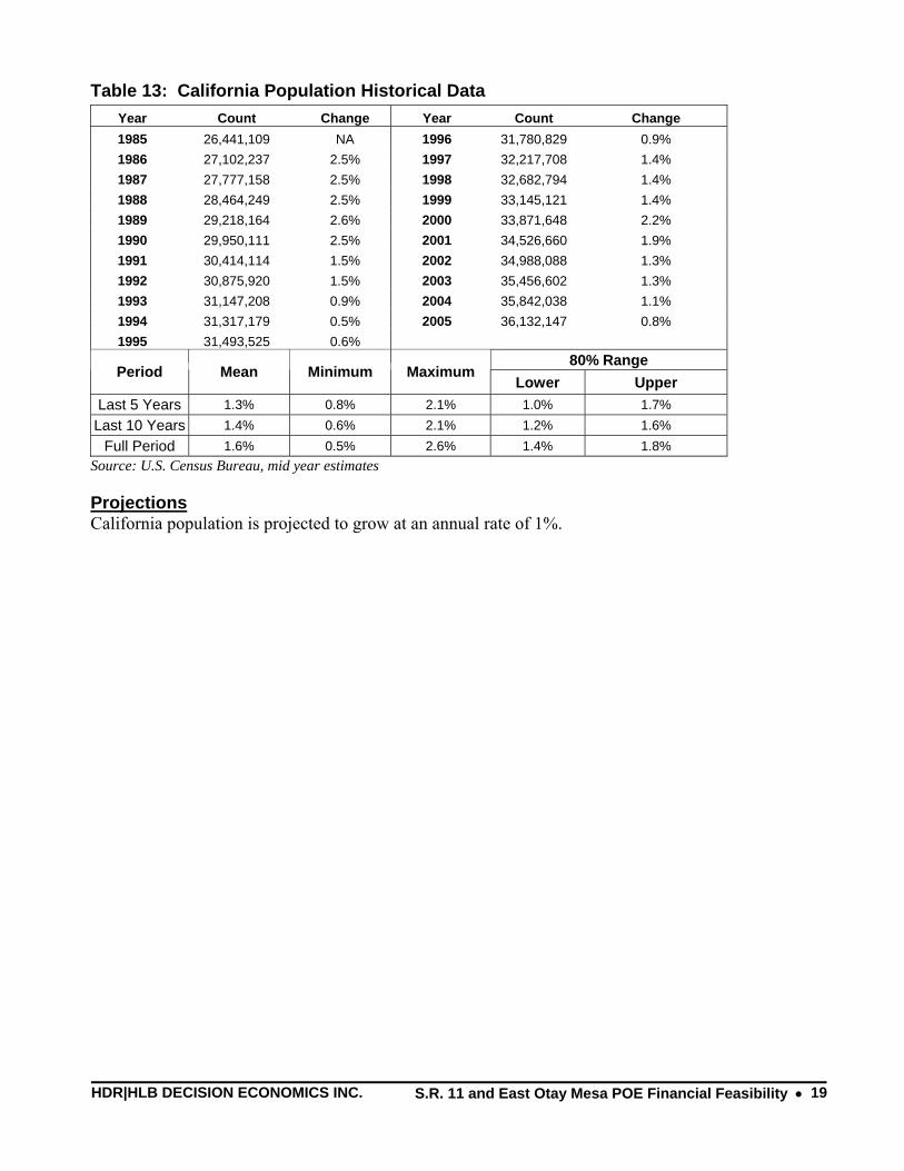
Table 13: California Population Historical Data Year Count Change Year Count Change 1985 26,441,109 NA 1996 31,780,829 0.9% 1986 27,102,237 2.5% 1997 32,217,708 1.4% 1987 27,777,158 2.5% 1998 32,682,794 1.4% 1988 28,464,249 2.5% 1999 33,145,121 1.4% 1989 29,218,164 2.6% 2000 33,871,648 2.2% 1990 29,950,111 2.5% 2001 34,526,660 1.9% 1991 30,414,114 1.5% 2002 34,988,088 1.3% 1992 30,875,920 1.5% 2003 35,456,602 1.3% 1993 31,147,208 0.9% 2004 35,842,038 1.1% 1994 31,317,179 0.5% 2005 36,132,147 0.8% 1995 31,493,525 0.6%
80% Range Period Mean Minimum Maximum
Lower Upper Last 5 Years 1.3% 0.8% 2.1% 1.0% 1.7%
Last 10 Years 1.4% 0.6% 2.1% 1.2% 1.6% Full Period 1.6% 0.5% 2.6% 1.4% 1.8%
Source: U.S. Census Bureau, mid year estimates
Projections California population is projected to grow at an annual rate of 1%.

HDR|HLB DECISION ECONOMICS INC. S.R. 11 and East Otay Mesa POE Financial Feasibility • 20
Table 14: U.S. Population Historical Data Year Count Change Year Count Change 1985 237,923,795 NA 1996 268,582,017 1.2% 1986 240,132,887 0.9% 1997 271,818,977 1.2% 1987 242,288,918 0.9% 1998 275,040,082 1.2% 1988 244,498,982 0.9% 1999 278,195,745 1.1% 1989 246,819,230 0.9% 2000 281,421,906 1.2% 1990 248,709,873 0.8% 2001 285,107,923 1.3% 1991 251,955,245 1.3% 2002 287,984,799 1.0% 1992 255,585,733 1.4% 2003 290,850,005 1.0% 1993 259,068,338 1.4% 2004 293,656,842 1.0% 1994 262,318,037 1.3% 2005 296,410,404 0.9% 1995 265,471,847 1.2%
80% Range Period Mean Minimum Maximum
Lower Upper Last 5 Years 1.0% 0.9% 1.3% 0.9% 1.1%
Last 10 Years 1.1% 0.9% 1.3% 1.1% 1.2% Full Period 1.1% 0.8% 1.4% 1.1% 1.2%
Source: U.S. Census Bureau, mid year estimates
Projections The U.S. population is projected to grow at approximately 0.8% annually.
Table 15: Mexican Population Historical Data Year Count Change Year Count Change 1985 76,767,225 NA 1996 94,398,579 1.6% 1986 78,442,430 2.2% 1997 95,895,146 1.6% 1987 80,122,492 2.1% 1998 97,325,063 1.5% 1988 81,781,816 2.1% 1999 98,616,905 1.3% 1989 83,366,836 1.9% 2000 99,926,620 1.3% 1990 84,913,652 1.9% 2001 101,246,961 1.3% 1991 86,488,032 1.9% 2002 102,479,927 1.2% 1992 88,111,030 1.9% 2003 103,718,062 1.2% 1993 89,749,141 1.9% 2004 104,959,594 1.2% 1994 91,337,896 1.8% 2005 105,909,000 0.9% 1995 92,880,353 1.7%
80% Range Period Mean Minimum Maximum
Lower Upper Last 5 Years 1.2% 0.9% 1.3% 1.1% 1.3%
Last 10 Years 1.3% 0.9% 1.7% 1.2% 1.4% Full Period 1.6% 0.9% 2.2% 1.5% 1.7%
Source: U.S. Census Bureau, International Database
Projections The population of Mexico is projected to grow at approximately 1.2% annually in the near future, until 2020. After 2020, the growth rate is projected to be 0.8% annually.
HDR|HLB DECISION ECONOMICS INC. S.R. 11 and East Otay Mesa POE Financial Feasibility • 21
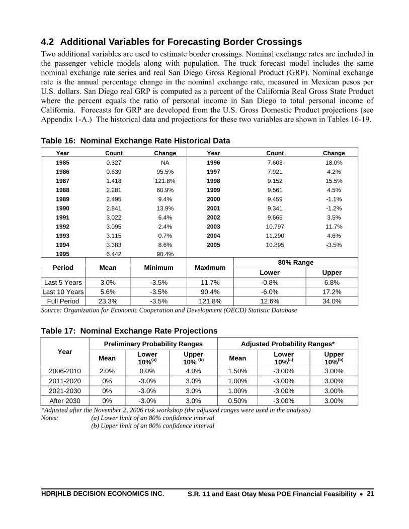
4.2 Additional Variables for Forecasting Border Crossings Two additional variables are used to estimate border crossings. Nominal exchange rates are included in the passenger vehicle models along with population. The truck forecast model includes the same nominal exchange rate series and real San Diego Gross Regional Product (GRP). Nominal exchange rate is the annual percentage change in the nominal exchange rate, measured in Mexican pesos per U.S. dollars. San Diego real GRP is computed as a percent of the California Real Gross State Product where the percent equals the ratio of personal income in San Diego to total personal income of California. Forecasts for GRP are developed from the U.S. Gross Domestic Product projections (see Appendix 1-A.) The historical data and projections for these two variables are shown in Tables 16-19.
Table 16: Nominal Exchange Rate Historical Data Year Count Change Year Count Change 1985 0.327 NA 1996 7.603 18.0% 1986 0.639 95.5% 1997 7.921 4.2% 1987 1.418 121.8% 1998 9.152 15.5% 1988 2.281 60.9% 1999 9.561 4.5% 1989 2.495 9.4% 2000 9.459 -1.1% 1990 2.841 13.9% 2001 9.341 -1.2% 1991 3.022 6.4% 2002 9.665 3.5% 1992 3.095 2.4% 2003 10.797 11.7% 1993 3.115 0.7% 2004 11.290 4.6% 1994 3.383 8.6% 2005 10.895 -3.5% 1995 6.442 90.4%
80% Range Period Mean Minimum Maximum
Lower Upper Last 5 Years 3.0% -3.5% 11.7% -0.8% 6.8%
Last 10 Years 5.6% -3.5% 90.4% -6.0% 17.2% Full Period 23.3% -3.5% 121.8% 12.6% 34.0%
Source: Organization for Economic Cooperation and Development (OECD) Statistic Database
Table 17: Nominal Exchange Rate Projections Preliminary Probability Ranges Adjusted Probability Ranges*
Year Mean Lower
10%(a) Upper 10% (b) Mean Lower
10%(a) Upper 10%(b)
2006-2010 2.0% 0.0% 4.0% 1.50% -3.00% 3.00% 2011-2020 0% -3.0% 3.0% 1.00% -3.00% 3.00% 2021-2030 0% -3.0% 3.0% 1.00% -3.00% 3.00% After 2030 0% -3.0% 3.0% 0.50% -3.00% 3.00%
*Adjusted after the November 2, 2006 risk workshop (the adjusted ranges were used in the analysis) Notes: (a) Lower limit of an 80% confidence interval (b) Upper limit of an 80% confidence interval

HDR|HLB DECISION ECONOMICS INC. S.R. 11 and East Otay Mesa POE Financial Feasibility • 22
Table 18: San Diego GRP Historical Data Year Count Change Year Count Change 1990 77,246 NA 1998 92,355 8.0% 1991 76,447 -1.0% 1999 101,011 9.4% 1992 76,081 -0.5% 2000 108,040 7.0% 1993 75,442 -0.8% 2001 109,522 1.4% 1994 76,158 0.9% 2002 113,902 4.0% 1995 78,314 2.8% 2003 117,747 3.4% 1996 81,887 4.6% 2004 124,405 5.7% 1997 85,529 4.4% 2005 130,293 4.7%
80% Range Period Mean Minimum Maximum
Lower Upper Last 5 Years 3.8% 1.4% 7.0% 2.5% 5.1%
Last 10 Years 5.2% 1.4% 9.4% 4.2% 6.3% Full Period 3.6% -1.0% 9.4% 2.5% 4.7%
Sources: San Diego Chamber of Commerce; Bureau of Economic Analysis, U.S. Department of Commerce
Table 19: San Diego GRP Projections Preliminary Probability Ranges Adjusted Probability Ranges*
Year Mean Lower
10%(a) Upper 10% (b) Mean Lower
10%(a) Upper 10%(b)
2006-2010 4.5% 4.4% 4.6% 3.80% 3.70% 3.90% 2011-2020 4.1% 4.0% 4.2% 3.30% 3.10% 3.50% 2021-2030 4.1% 3.9% 4.3% 3.30% 3.10% 3.50% After 2030 4.1% 3.9% 4.3% 3.30% 3.10% 3.50%
*Adjusted after the November 2, 2006 risk workshop (the adjusted ranges were used in the analysis) Notes: (a) Lower limit of an 80% confidence interval (b) Upper limit of an 80% confidence interval
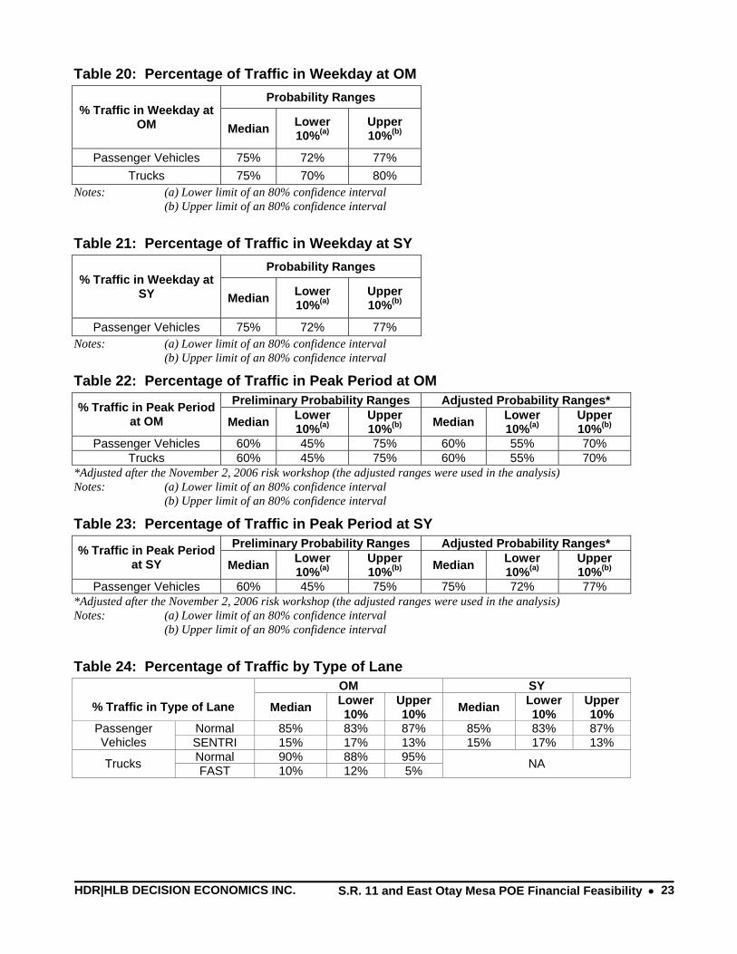
4.3 Border Crossing Market Segments In developing toll revenue projections, the total border crossings at OM and SY are divided into the segments of time and the type of lane. For example, assumptions are made on the percent of travelers crossing during weekday and weekend days (Tables 20-21) and peak and off-peak periods (Tables 22-23). A third market segmentation involves delineating the percentage of passenger vehicles and trucks using normal or SENTRI/FAST lanes (Table 24). A characterization of peak times based on an analysis of wait times and number of lanes open is provided in Appendix 1-C.
HDR|HLB DECISION ECONOMICS INC. S.R. 11 and East Otay Mesa POE Financial Feasibility • 23
Table 20: Percentage of Traffic in Weekday at OM Probability Ranges
% Traffic in Weekday at OM Median Lower
10%(a) Upper 10%(b)
Passenger Vehicles 75% 72% 77% Trucks 75% 70% 80%
Notes: (a) Lower limit of an 80% confidence interval (b) Upper limit of an 80% confidence interval
Table 21: Percentage of Traffic in Weekday at SY Probability Ranges
% Traffic in Weekday at SY Median Lower
10%(a) Upper 10%(b)
Passenger Vehicles 75% 72% 77% Notes: (a) Lower limit of an 80% confidence interval (b) Upper limit of an 80% confidence interval
Table 22: Percentage of Traffic in Peak Period at OM Preliminary Probability Ranges Adjusted Probability Ranges* % Traffic in Peak Period
at OM Median Lower 10%(a)
Upper 10%(b) Median Lower
10%(a) Upper 10%(b)
Passenger Vehicles 60% 45% 75% 60% 55% 70% Trucks 60% 45% 75% 60% 55% 70%
*Adjusted after the November 2, 2006 risk workshop (the adjusted ranges were used in the analysis) Notes: (a) Lower limit of an 80% confidence interval (b) Upper limit of an 80% confidence interval
Table 23: Percentage of Traffic in Peak Period at SY Preliminary Probability Ranges Adjusted Probability Ranges* % Traffic in Peak Period
at SY Median Lower 10%(a)
Upper 10%(b) Median Lower
10%(a) Upper 10%(b)
Passenger Vehicles 60% 45% 75% 75% 72% 77% *Adjusted after the November 2, 2006 risk workshop (the adjusted ranges were used in the analysis) Notes: (a) Lower limit of an 80% confidence interval (b) Upper limit of an 80% confidence interval
Table 24: Percentage of Traffic by Type of Lane OM SY
% Traffic in Type of Lane Median Lower 10%
Upper 10% Median Lower
10% Upper 10%
Normal 85% 83% 87% 85% 83% 87% Passenger Vehicles SENTRI 15% 17% 13% 15% 17% 13%
Normal 90% 88% 95% Trucks FAST 10% 12% 5% NA
HDR|HLB DECISION ECONOMICS INC. S.R. 11 and East Otay Mesa POE Financial Feasibility • 24
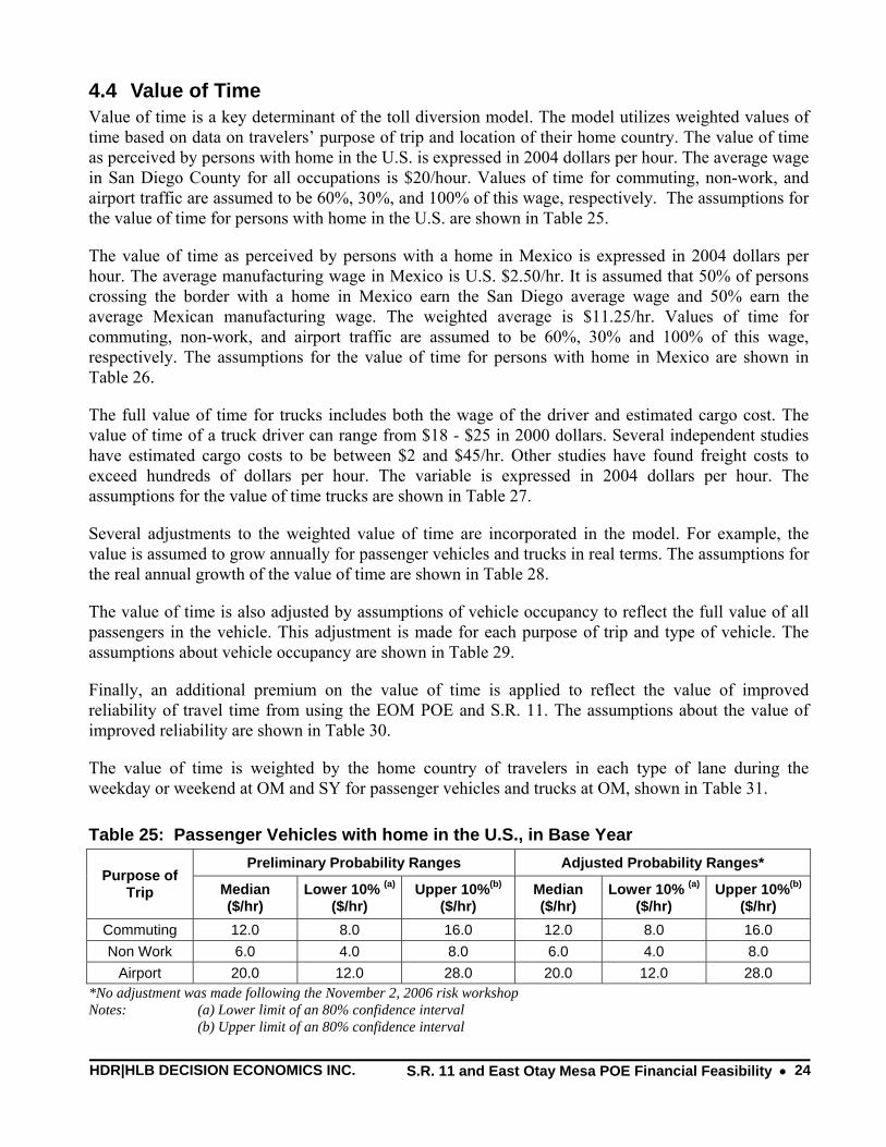
4.4 Value of Time Value of time is a key determinant of the toll diversion model. The model utilizes weighted values of time based on data on travelers’ purpose of trip and location of their home country. The value of time as perceived by persons with home in the U.S. is expressed in 2004 dollars per hour. The average wage in San Diego County for all occupations is $20/hour. Values of time for commuting, non-work, and airport traffic are assumed to be 60%, 30%, and 100% of this wage, respectively. The assumptions for the value of time for persons with home in the U.S. are shown in Table 25.
The value of time as perceived by persons with a home in Mexico is expressed in 2004 dollars per hour. The average manufacturing wage in Mexico is U.S. $2.50/hr. It is assumed that 50% of persons crossing the border with a home in Mexico earn the San Diego average wage and 50% earn the average Mexican manufacturing wage. The weighted average is $11.25/hr. Values of time for commuting, non-work, and airport traffic are assumed to be 60%, 30% and 100% of this wage, respectively. The assumptions for the value of time for persons with home in Mexico are shown in Table 26.
The full value of time for trucks includes both the wage of the driver and estimated cargo cost. The value of time of a truck driver can range from $18 - $25 in 2000 dollars. Several independent studies have estimated cargo costs to be between $2 and $45/hr. Other studies have found freight costs to exceed hundreds of dollars per hour. The variable is expressed in 2004 dollars per hour. The assumptions for the value of time trucks are shown in Table 27.
Several adjustments to the weighted value of time are incorporated in the model. For example, the value is assumed to grow annually for passenger vehicles and trucks in real terms. The assumptions for the real annual growth of the value of time are shown in Table 28.
The value of time is also adjusted by assumptions of vehicle occupancy to reflect the full value of all passengers in the vehicle. This adjustment is made for each purpose of trip and type of vehicle. The assumptions about vehicle occupancy are shown in Table 29.
Finally, an additional premium on the value of time is applied to reflect the value of improved reliability of travel time from using the EOM POE and S.R. 11. The assumptions about the value of improved reliability are shown in Table 30.
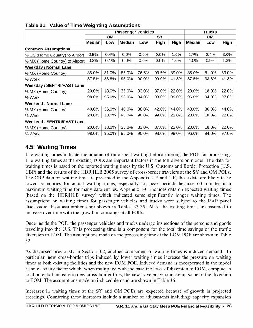
The value of time is weighted by the home country of travelers in each type of lane during the weekday or weekend at OM and SY for passenger vehicles and trucks at OM, shown in Table 31.
Table 25: Passenger Vehicles with home in the U.S., in Base Year Preliminary Probability Ranges Adjusted Probability Ranges*
Purpose of Trip Median
($/hr) Lower 10% (a)
($/hr) Upper 10%(b)
($/hr) Median ($/hr)
Lower 10% (a) ($/hr)
Upper 10%(b) ($/hr)
Commuting 12.0 8.0 16.0 12.0 8.0 16.0 Non Work 6.0 4.0 8.0 6.0 4.0 8.0
Airport 20.0 12.0 28.0 20.0 12.0 28.0 *No adjustment was made following the November 2, 2006 risk workshop Notes: (a) Lower limit of an 80% confidence interval (b) Upper limit of an 80% confidence interval

HDR|HLB DECISION ECONOMICS INC. S.R. 11 and East Otay Mesa POE Financial Feasibility • 25
Table 26: Passenger Vehicles with home in the Mexico, in Base Year Preliminary Probability Ranges Adjusted Probability Ranges*
Purpose of Trip Median
($/hr) Lower 10% (a)
($/hr) Upper 10%t(b)
($/hr) Median ($/hr)
Lower 10% (a) ($/hr)
Upper 10%(b) ($/hr)
Commuting 6.7 4.4 8.9 6.73 4.48 8.97 Non Work 3.4 2.2 4.5 3.36 2.24 4.48
Airport 11.25 6.7 15.7 11.21 6.73 15.69 *Adjusted after the November 2, 2006 risk workshop (the adjusted ranges were used in the analysis) Notes: (a) Lower limit of an 80% confidence interval (b) Upper limit of an 80% confidence interval
Table 27: Value of time for Trucks, in Base Year Preliminary Probability Ranges Adjusted Probability Ranges* Country of
Origin Median ($/hr)
Lower 10% (a) ($/hr)
Upper 10% (b) ($/hr)
Median ($/hr)
Lower 10% (a) ($/hr)
Upper 10% (b)
($/hr) US 45.0 30.0 60.0 45.0 30.0 60.0
Mexico 45.0 30.0 60.0 22.5 15.0 30.0 *Adjusted after the November 2, 2006 risk workshop (the adjusted ranges were used in the analysis) Notes: (a) Lower limit of an 80% confidence interval (b) Upper limit of an 80% confidence interval
Table 28: Real Annual Growth of the Value of Time Preliminary Probability Ranges Adjusted Probability Ranges*
Variable Median Lower 10%(a)
Upper 10%(b) Median Lower
10%(a) Upper 10%(b)
US 1.0% 0.5% 1.25% 1.0% 0.75% 1.25% Passenger Vehicles Mexico 1.0% 0.5% 1.25% 1.0% 0.75% 1.25%
US 1.0% 0.5% 1.25% 0.50% 0.38% 0.63% Trucks
Mexico 1.0% 0.5% 1.25% 0.50% 0.38% 0.63% *Adjusted after the November 2, 2006 risk workshop (the adjusted ranges were used in the analysis) Notes: (a) Lower limit of an 80% confidence interval (b) Upper limit of an 80% confidence interval
Table 29: Vehicle Occupancy Median
Airport 1.67 Commuting 1.35 Passenger Vehicles Non Work 1.67
Trucks 1.12
Table 30: Value of Time Premium due to improved reliability
Median Lower 10%(a)
Upper 10%(b)
Additional Premium on Value of Time – Passenger Vehicles and Trucks .20 .10 .30
Notes: (a) Lower limit of an 80% confidence interval (b) Upper limit of an 80% confidence interval
HDR|HLB DECISION ECONOMICS INC. S.R. 11 and East Otay Mesa POE Financial Feasibility • 26
Table 31: Value of Time Weighting Assumptions Passenger Vehicles Trucks
OM SY OM Median Low Median Low High High Median Low High
Common Assumptions
% US (Home Country) to Airport 0.5% 0.4% 0.0% 0.0% 0.0% 1.0% 2.7% 2.4% 3.0% % MX (Home Country) to Airport 0.3% 0.1% 0.0% 0.0% 0.0% 1.0% 1.0% 0.9% 1.3% Weekday / Normal Lane
% MX (Home Country) 85.0% 81.0% 85.0% 76.5% 93.5% 89.0% 85.0% 81.0% 89.0% % Work 37.5% 33.8% 95.0% 90.0% 99.0% 41.3% 37.5% 33.8% 41.3% Weekday / SENTRI/FAST Lane
% MX (Home Country) 20.0% 18.0% 35.0% 33.0% 37.0% 22.0% 20.0% 18.0% 22.0% % Work 98.0% 95.0% 95.0% 94.0% 98.0% 99.0% 96.0% 94.0% 97.0% Weekend / Normal Lane
% MX (Home Country) 40.0% 36.0% 40.0% 38.0% 42.0% 44.0% 40.0% 36.0% 44.0% % Work 20.0% 18.0% 95.0% 90.0% 99.0% 22.0% 20.0% 18.0% 22.0% Weekend / SENTRI/FAST Lane
% MX (Home Country) 20.0% 18.0% 35.0% 33.0% 37.0% 22.0% 20.0% 18.0% 22.0% % Work 98.0% 95.0% 95.0% 90.0% 98.0% 99.0% 96.0% 94.0% 97.0% 4.5 Waiting Times The waiting times indicate the amount of time spent waiting before entering the POE for processing. The waiting times at the existing POEs are important factors in the toll diversion model. The data for waiting times is based on the reported waiting times by the U.S. Customs and Border Protection (U.S. CBP) and the results of the HDR|HLB 2005 survey of cross-border travelers at the SY and OM POEs. The CBP data on waiting times is presented in the Appendix 1-E and 1-F; these data are likely to be lower boundaries for actual waiting times, especially for peak periods because 60 minutes is a maximum waiting time for many data entries. Appendix 1-G includes data on expected waiting times (based on the HDR|HLB survey) which indicated some significantly longer waiting times. The assumptions on waiting times for passenger vehicles and trucks were subject to the RAP panel discussion; these assumptions are shown in Tables 33-35. Also, the waiting times are assumed to increase over time with the growth in crossings at all POEs.
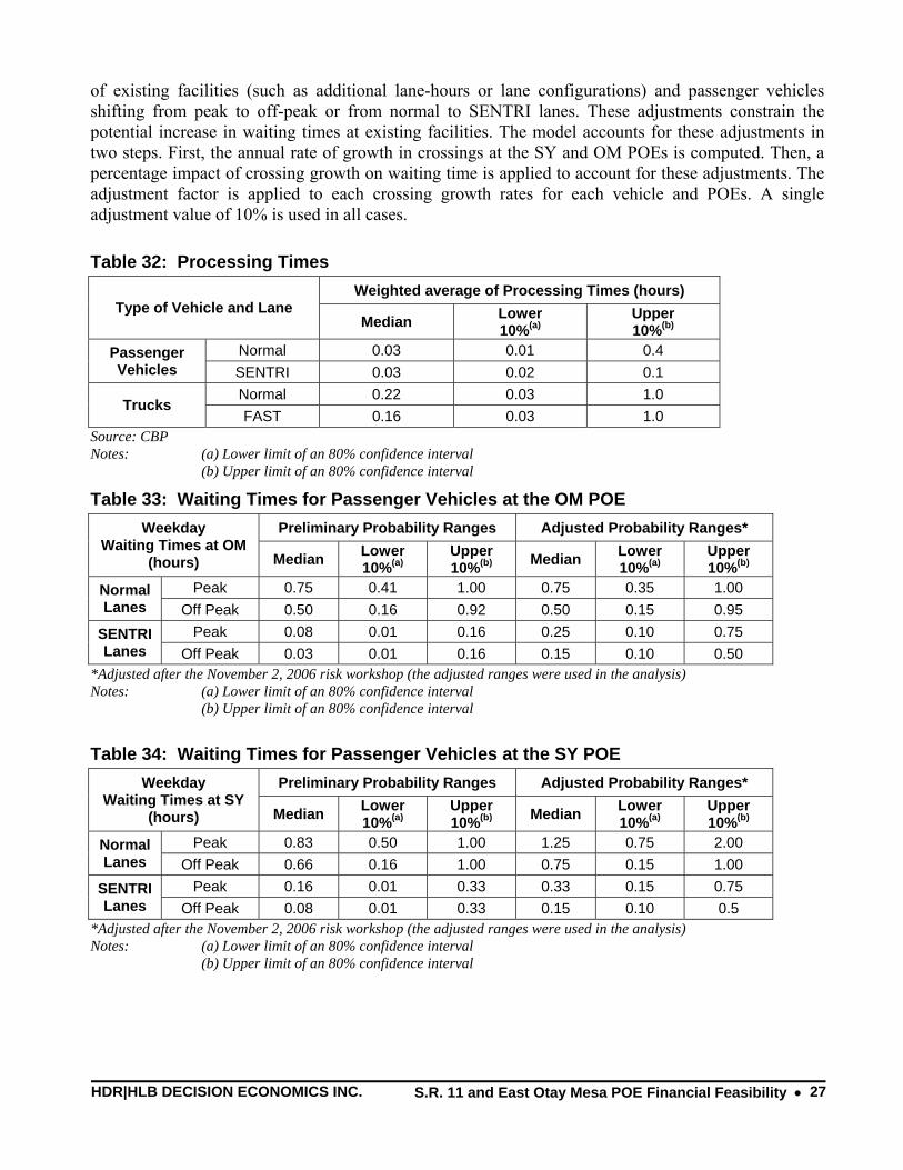
Once inside the POE, the passenger vehicles and trucks undergo inspections of the persons and goods traveling into the U.S. This processing time is a component for the total time savings of the traffic diversion to EOM. The assumptions made on the processing time at the EOM POE are shown in Table 32.
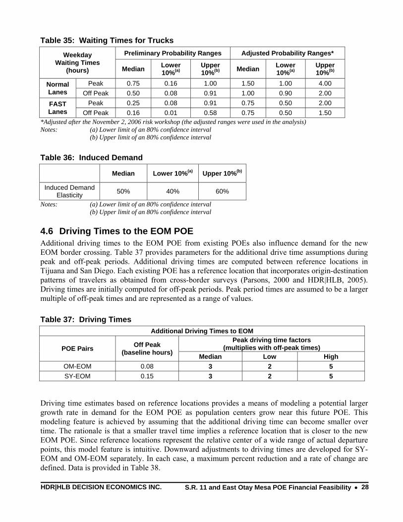
As discussed previously in Section 3.2, another component of waiting times is induced demand. In particular, new cross-border trips induced by lower waiting times increase the pressure on waiting times at both existing facilities and the new EOM POE. Induced demand is incorporated in the model as an elasticity factor which, when multiplied with the baseline level of diversion to EOM, computes a total potential increase in new cross-border trips, the new travelers who make up some of the diversion to EOM. The assumptions made on induced demand are shown in Table 36.
Increases in waiting times at the SY and OM POEs are expected because of growth in projected crossings. Countering these increases include a number of adjustments including: capacity expansion
HDR|HLB DECISION ECONOMICS INC. S.R. 11 and East Otay Mesa POE Financial Feasibility • 27
of existing facilities (such as additional lane-hours or lane configurations) and passenger vehicles shifting from peak to off-peak or from normal to SENTRI lanes. These adjustments constrain the potential increase in waiting times at existing facilities. The model accounts for these adjustments in two steps. First, the annual rate of growth in crossings at the SY and OM POEs is computed. Then, a percentage impact of crossing growth on waiting time is applied to account for these adjustments. The adjustment factor is applied to each crossing growth rates for each vehicle and POEs. A single adjustment value of 10% is used in all cases.
Table 32: Processing Times Weighted average of Processing Times (hours)
Type of Vehicle and Lane Median Lower
10%(a) Upper 10%(b)
Normal 0.03 0.01 0.4 Passenger Vehicles SENTRI 0.03 0.02 0.1
Normal 0.22 0.03 1.0 Trucks
FAST 0.16 0.03 1.0 Source: CBP Notes: (a) Lower limit of an 80% confidence interval (b) Upper limit of an 80% confidence interval
Table 33: Waiting Times for Passenger Vehicles at the OM POE Preliminary Probability Ranges Adjusted Probability Ranges* Weekday
Waiting Times at OM (hours) Median Lower
10%(a) Upper 10%(b) Median Lower
10%(a) Upper 10%(b)
Peak 0.75 0.41 1.00 0.75 0.35 1.00 Normal Lanes Off Peak 0.50 0.16 0.92 0.50 0.15 0.95
Peak 0.08 0.01 0.16 0.25 0.10 0.75 SENTRI Lanes Off Peak 0.03 0.01 0.16 0.15 0.10 0.50
*Adjusted after the November 2, 2006 risk workshop (the adjusted ranges were used in the analysis) Notes: (a) Lower limit of an 80% confidence interval (b) Upper limit of an 80% confidence interval
Table 34: Waiting Times for Passenger Vehicles at the SY POE Preliminary Probability Ranges Adjusted Probability Ranges* Weekday
Waiting Times at SY (hours) Median Lower
10%(a) Upper 10%(b) Median Lower
10%(a) Upper 10%(b)
Peak 0.83 0.50 1.00 1.25 0.75 2.00 Normal Lanes Off Peak 0.66 0.16 1.00 0.75 0.15 1.00
Peak 0.16 0.01 0.33 0.33 0.15 0.75 SENTRI Lanes Off Peak 0.08 0.01 0.33 0.15 0.10 0.5
*Adjusted after the November 2, 2006 risk workshop (the adjusted ranges were used in the analysis) Notes: (a) Lower limit of an 80% confidence interval (b) Upper limit of an 80% confidence interval
HDR|HLB DECISION ECONOMICS INC. S.R. 11 and East Otay Mesa POE Financial Feasibility • 28
Table 35: Waiting Times for Trucks Preliminary Probability Ranges Adjusted Probability Ranges* Weekday
Waiting Times (hours) Median Lower
10%(a) Upper 10%(b) Median Lower
10%(a) Upper 10%(b)
Peak 0.75 0.16 1.00 1.50 1.00 4.00 Normal Lanes Off Peak 0.50 0.08 0.91 1.00 0.90 2.00
Peak 0.25 0.08 0.91 0.75 0.50 2.00 FAST Lanes Off Peak 0.16 0.01 0.58 0.75 0.50 1.50
*Adjusted after the November 2, 2006 risk workshop (the adjusted ranges were used in the analysis) Notes: (a) Lower limit of an 80% confidence interval (b) Upper limit of an 80% confidence interval
Table 36: Induced Demand
Median Lower 10%(a) Upper 10%(b)
Induced Demand Elasticity 50% 40% 60%
Notes: (a) Lower limit of an 80% confidence interval (b) Upper limit of an 80% confidence interval
4.6 Driving Times to the EOM POE Additional driving times to the EOM POE from existing POEs also influence demand for the new EOM border crossing. Table 37 provides parameters for the additional drive time assumptions during peak and off-peak periods. Additional driving times are computed between reference locations in Tijuana and San Diego. Each existing POE has a reference location that incorporates origin-destination patterns of travelers as obtained from cross-border surveys (Parsons, 2000 and HDR|HLB, 2005). Driving times are initially computed for off-peak periods. Peak period times are assumed to be a larger multiple of off-peak times and are represented as a range of values.
Table 37: Driving Times Additional Driving Times to EOM
Peak driving time factors (multiplies with off-peak times) POE Pairs Off Peak
(baseline hours) Median Low High OM-EOM 0.08 3 2 5 SY-EOM 0.15 3 2 5
Driving time estimates based on reference locations provides a means of modeling a potential larger growth rate in demand for the EOM POE as population centers grow near this future POE. This modeling feature is achieved by assuming that the additional driving time can become smaller over time. The rationale is that a smaller travel time implies a reference location that is closer to the new EOM POE. Since reference locations represent the relative center of a wide range of actual departure points, this model feature is intuitive. Downward adjustments to driving times are developed for SY-EOM and OM-EOM separately. In each case, a maximum percent reduction and a rate of change are defined. Data is provided in Table 38.

HDR|HLB DECISION ECONOMICS INC. S.R. 11 and East Otay Mesa POE Financial Feasibility • 29
Table 38: Adjustments to Driving Times Adjustments to Driving Times to Account for Population Growth in East and Northeast Tijuana
Annual rate of change in driving time POE Pairs
Median Low High Maximum % reduction in driving
time
OM-EOM 2.0% 0.0% 5.0% 40% SY-EOM 1.0% 0.0% 5.0% 30%
4.7 Infrastructure Assumptions Another variable in the POE diversion and toll share model is the number of lanes open at the existing POEs and at EOM. The number lanes open for each type of lane currently varies at the existing POEs by weekday and weekend and time of day. Information on this variation was obtained from a SANDAG dataset that was originally produced by CBP. Further details about the infrastructure at the existing POEs and at EOM can be found in Appendix 1-G. The assumptions made on the number lanes open at the existing POEs and at EOM are shown in Table 39.
Table 39: Infrastructure Assumptions OM SY EOM
Med
ian
Low
Hig
h
Med
ian
Low
Hig
h
Med
ian
Low
Hig
h
Passenger Vehicles Weekday Normal Lanes
Peak 8 6 9 19 16 22 8 6 9 Off Peak 6 2 8 16 4 19 6 2 8
Weekday SENTRI Lanes Peak 1 1 1 3 0 4 1 1 1 Off Peak 1 1 1 2 0 3 1 1 1
Weekend Normal Lanes Peak 9 6 9 20 16 22 9 6 9 Off Peak 6 4 8 14 4 19 6 4 8
Weekend SENTRI Lanes Peak 1 1 1 3 0 4 1 1 1 Off Peak 1 1 1 2 0 3 1 1 1
Trucks Weekday Normal Lanes
Peak 7 5 9 7 5 9 Off Peak 6 5 8 6 5 8
Weekday FAST Lanes Peak 1 1 1 1 1 1 Off Peak 1 1 1 1 1 1
Weekend Normal Lanes Peak 6 6 9 6 6 9 Off Peak 5 1 6 5 1 6
Weekend FAST Lanes Peak 1 1 1 1 1 1 Off Peak 1 1 1
1 1 1

HDR|HLB DECISION ECONOMICS INC. S.R. 11 and East Otay Mesa POE Financial Feasibility • 30
4.8 S.R. 11 and EOM POE Traffic Ramp-Up These variables, shown in Table 40, describe the changes on S.R. 11 and border crossing traffic at EOM in the opening year and immediately thereafter. It shows how fast the maximum potential use of the facility (for a given set of socioeconomic conditions) would be reached, and represents the time needed for the community to become aware of the toll road and its potential benefits (in terms of time savings, access, safety, etc).
Table 40: Ramp-up
Preliminary Probability Ranges Adjusted Probability Ranges*
Variable Median Lower
10%(a) Upper 10%(b) Median Lower
10%(a) Upper 10%(b)
% of Projected Total at Opening 50% 40% 60% 60% 50% 70% Passenger Vehicles Ramp-up Period
(years to steady state) 36 24 48 2.00 1.00 4.50
% of Projected Total at Opening 50% 40% 60% 60% 50% 70% Trucks
Ramp-up Period (years to steady state) 36 24 48 2.00 0.50 2.50
*Adjusted after the November 2, 2006 risk workshop (the adjusted ranges were used in the analysis) Notes: (a) Lower limit of an 80% confidence interval (b) Upper limit of an 80% confidence interval
4.9 Data for Scenario Analysis
4.9.1 Summary of Baseline Assumptions for Revenue Scenarios The following list briefly reviews the major assumptions in the baseline analysis. Some of these assumptions will be modified in the revenue and cost scenarios.
Alternative POEs: OM and SY Capacity (numbers / types of lanes):
– Current capacity at existing POEs5 – New POE is assumed to have nine passenger vehicle lanes (including one SENTRI),
and nine truck lanes (including one FAST) Origin-Destinations of persons crossing border
– Apply results from border crossing surveys in 2000 and 2005 Process
– POE to process passenger vehicles and trucks (no pedestrian) – Estimates of processing times were made available by U.S. Customs and Border
Protection Facility
– S.R. 11 Capital and O&M costs only – No toll facility on the Mexican side
Wait Time – EOM provides a twenty minute wait time for normal lanes (truck and passenger
vehicles) and FAST lanes – SENTRI provides a six minute wait time
5 See Appendix 1-B for details of capacity at existing POEs.

HDR|HLB DECISION ECONOMICS INC. S.R. 11 and East Otay Mesa POE Financial Feasibility • 31
4.9.2 Revenue Scenarios Several alternate revenue scenarios have been modeled for this project. Two scenarios include variables that were discussed by RAP panelists. One of these scenarios assesses the seamless interconnection of S.R. 11 with the Tijuana-Tecate toll road in Mexico. The Tijuana-Tecate Toll Road currently ends approximately two miles south of the possible site of the EOM-Otay II POE. A direct connection from this toll road is in planning stages. The assumptions on the impact of the integration of the Tijuana-Tecate toll road to EOM are shown in Table 41.
The second revenue scenario considers the potential shift of people from passenger vehicles to crossing the border as pedestrians and then utilizing a potential bus rapid transit at the EOM POE. For these scenarios, additional variables have been defined including the opening year and total impact on revenue. The assumptions on the impact of the pedestrian crossing at EOM are shown in Table 42.
A third scenario would assess revenue impacts if EOM were designed only for trucks. Such a facility would provide service for 16 normal and two FAST lanes. No passenger vehicles would be permitted. This scenario is modeled the same as the baseline revenue but with the new numbers of lanes. Assumptions on waiting times at existing facilities and level of service at new facility are unchanged.
Table 41: Impact of Integration of Tijuana-Tecate Toll Road to EOM Preliminary Probability Ranges Adjusted Probability Ranges*
Variable Median Lower
10%(a) Upper 10%(b) Median Lower
10%(a) Upper 10%(b)
Opening Year 2020 2015 2025 2015 2015 2015
Impact on Passenger Vehicle Diversion 10% 5% 15% 7% 5% 10%
Impact on Truck Diversion 10% 5% 15% 10% 5% 15%
*Adjusted after the November 2, 2006 risk workshop (the adjusted ranges were used in the analysis) Notes: (a) Lower limit of an 80% confidence interval (b) Upper limit of an 80% confidence interval Additional assumptions for modeling this scenario include:
• Integration of roads generates additional diversion from the Tecate POE • Growth at the Tecate POE is similar to that at the OM and SY POEs • Toll rates are assumed to be unchanged because increased volumes are relatively low
Table 42: Potential of Pedestrian Crossing at EOM Preliminary Probability Ranges Adjusted Probability Ranges*
Variable Median Lower
10%(a) Upper 10%(b) Median Lower
10%(a) Upper 10%(b)
Opening Year 2020 2015 2025 2015 2015 2015
Impact on S.R. 11/ EOM Vehicle Use -4% -1% -6%
Diversion to pedestrian modes 20% 10% 30%
*Adjusted after the November 2, 2006 risk workshop (the adjusted ranges were used in the analysis) Notes: (a) Lower limit of an 80% confidence interval (b) Upper limit of an 80% confidence interval
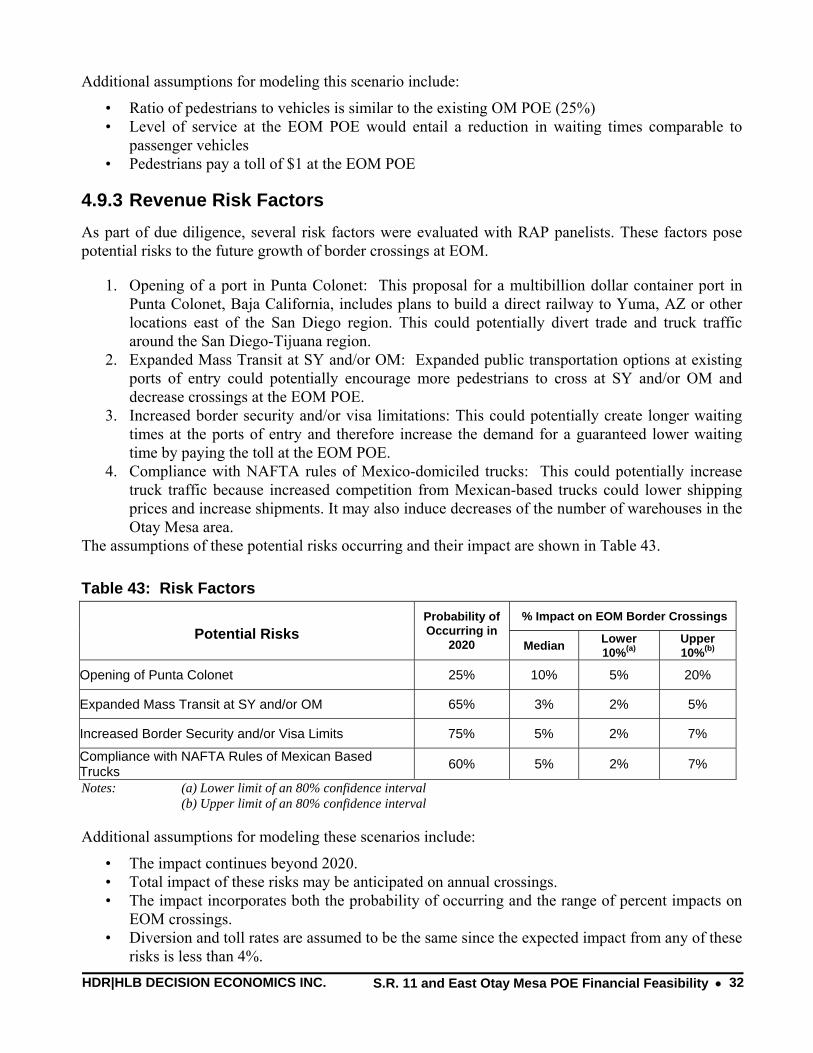
HDR|HLB DECISION ECONOMICS INC. S.R. 11 and East Otay Mesa POE Financial Feasibility • 32
Additional assumptions for modeling this scenario include:
• Ratio of pedestrians to vehicles is similar to the existing OM POE (25%) • Level of service at the EOM POE would entail a reduction in waiting times comparable to
passenger vehicles • Pedestrians pay a toll of $1 at the EOM POE
4.9.3 Revenue Risk Factors As part of due diligence, several risk factors were evaluated with RAP panelists. These factors pose potential risks to the future growth of border crossings at EOM.
1. Opening of a port in Punta Colonet: This proposal for a multibillion dollar container port in Punta Colonet, Baja California, includes plans to build a direct railway to Yuma, AZ or other locations east of the San Diego region. This could potentially divert trade and truck traffic around the San Diego-Tijuana region.
2. Expanded Mass Transit at SY and/or OM: Expanded public transportation options at existing ports of entry could potentially encourage more pedestrians to cross at SY and/or OM and decrease crossings at the EOM POE.
3. Increased border security and/or visa limitations: This could potentially create longer waiting times at the ports of entry and therefore increase the demand for a guaranteed lower waiting time by paying the toll at the EOM POE.
4. Compliance with NAFTA rules of Mexico-domiciled trucks: This could potentially increase truck traffic because increased competition from Mexican-based trucks could lower shipping prices and increase shipments. It may also induce decreases of the number of warehouses in the Otay Mesa area.
The assumptions of these potential risks occurring and their impact are shown in Table 43.
Table 43: Risk Factors % Impact on EOM Border Crossings
Potential Risks
Probability of Occurring in
2020 Median Lower 10%(a)
Upper 10%(b)
Opening of Punta Colonet 25% 10% 5% 20%
Expanded Mass Transit at SY and/or OM 65% 3% 2% 5%
Increased Border Security and/or Visa Limits 75% 5% 2% 7%
Compliance with NAFTA Rules of Mexican Based Trucks 60% 5% 2% 7%
Notes: (a) Lower limit of an 80% confidence interval (b) Upper limit of an 80% confidence interval
Additional assumptions for modeling these scenarios include:
• The impact continues beyond 2020. • Total impact of these risks may be anticipated on annual crossings. • The impact incorporates both the probability of occurring and the range of percent impacts on
EOM crossings. • Diversion and toll rates are assumed to be the same since the expected impact from any of these
risks is less than 4%.
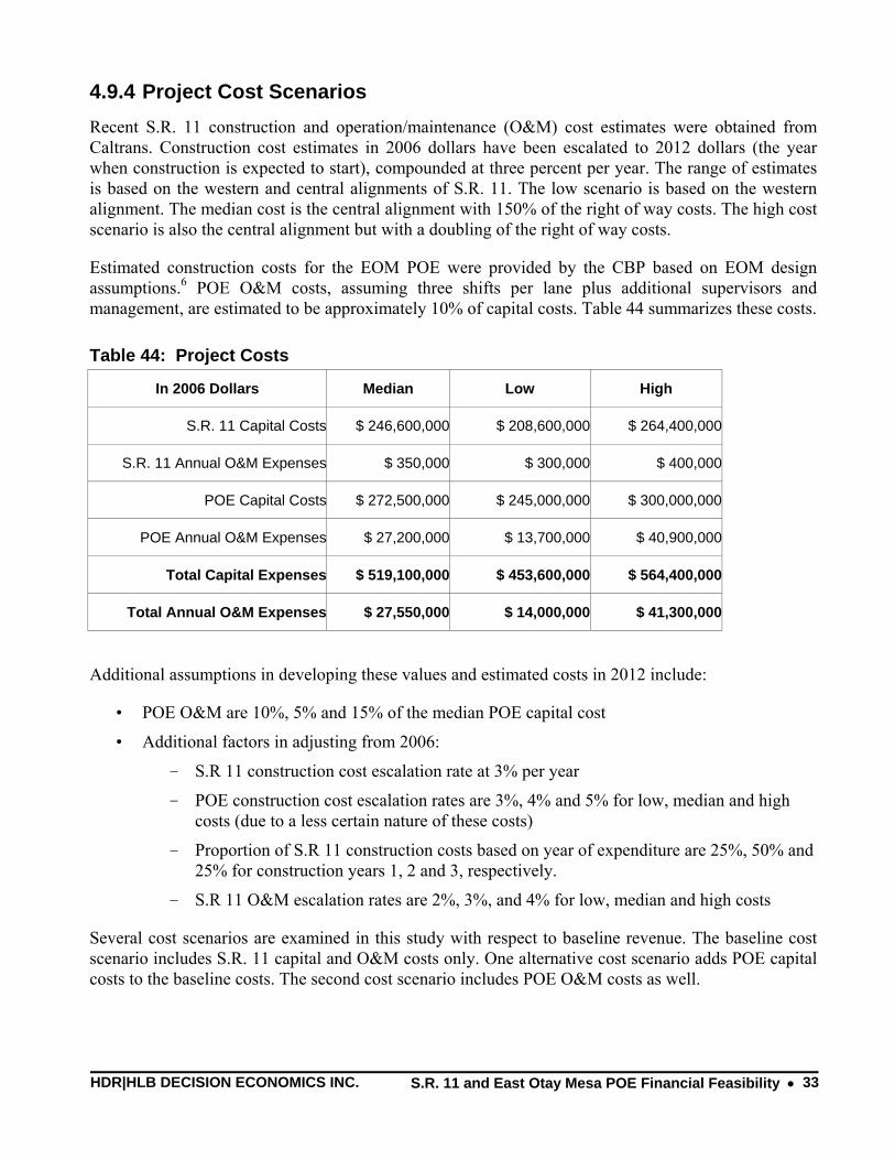
HDR|HLB DECISION ECONOMICS INC. S.R. 11 and East Otay Mesa POE Financial Feasibility • 33
4.9.4 Project Cost Scenarios Recent S.R. 11 construction and operation/maintenance (O&M) cost estimates were obtained from Caltrans. Construction cost estimates in 2006 dollars have been escalated to 2012 dollars (the year when construction is expected to start), compounded at three percent per year. The range of estimates is based on the western and central alignments of S.R. 11. The low scenario is based on the western alignment. The median cost is the central alignment with 150% of the right of way costs. The high cost scenario is also the central alignment but with a doubling of the right of way costs.
Estimated construction costs for the EOM POE were provided by the CBP based on EOM design assumptions.6 POE O&M costs, assuming three shifts per lane plus additional supervisors and management, are estimated to be approximately 10% of capital costs. Table 44 summarizes these costs.
Table 44: Project Costs
In 2006 Dollars Median Low High
S.R. 11 Capital Costs $ 246,600,000 $ 208,600,000 $ 264,400,000
S.R. 11 Annual O&M Expenses $ 350,000 $ 300,000 $ 400,000
POE Capital Costs $ 272,500,000 $ 245,000,000 $ 300,000,000
POE Annual O&M Expenses $ 27,200,000 $ 13,700,000 $ 40,900,000
Total Capital Expenses $ 519,100,000 $ 453,600,000 $ 564,400,000
Total Annual O&M Expenses $ 27,550,000 $ 14,000,000 $ 41,300,000
Additional assumptions in developing these values and estimated costs in 2012 include:
• POE O&M are 10%, 5% and 15% of the median POE capital cost
• Additional factors in adjusting from 2006:
- S.R 11 construction cost escalation rate at 3% per year
- POE construction cost escalation rates are 3%, 4% and 5% for low, median and high costs (due to a less certain nature of these costs)
- Proportion of S.R 11 construction costs based on year of expenditure are 25%, 50% and 25% for construction years 1, 2 and 3, respectively.
- S.R 11 O&M escalation rates are 2%, 3%, and 4% for low, median and high costs
Several cost scenarios are examined in this study with respect to baseline revenue. The baseline cost scenario includes S.R. 11 capital and O&M costs only. One alternative cost scenario adds POE capital costs to the baseline costs. The second cost scenario includes POE O&M costs as well.
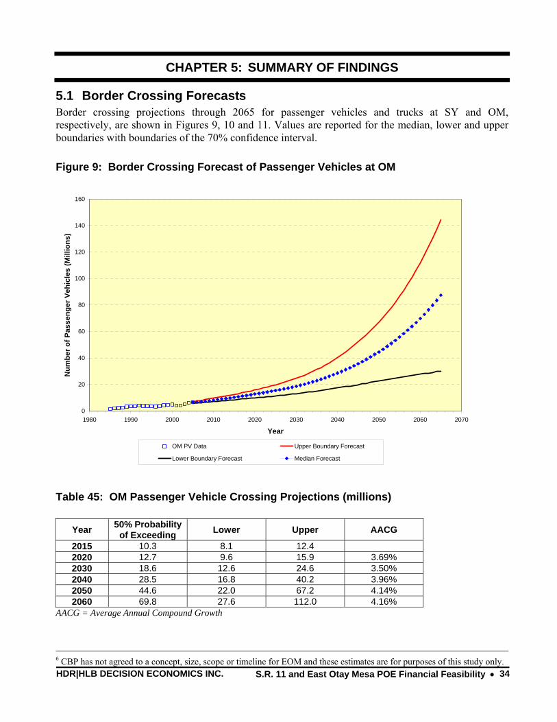
HDR|HLB DECISION ECONOMICS INC. S.R. 11 and East Otay Mesa POE Financial Feasibility • 34
CHAPTER 5: SUMMARY OF FINDINGS
5.1 Border Crossing Forecasts Border crossing projections through 2065 for passenger vehicles and trucks at SY and OM, respectively, are shown in Figures 9, 10 and 11. Values are reported for the median, lower and upper boundaries with boundaries of the 70% confidence interval.
Figure 9: Border Crossing Forecast of Passenger Vehicles at OM
0
20
40
60
80
100
120
140
160
1980 1990 2000 2010 2020 2030 2040 2050 2060 2070
Year
Num
ber o
f Pas
seng
er V
ehic
les
(Mill
ions
)
OM PV Data Upper Boundary Forecast
Lower Boundary Forecast Median Forecast
Table 45: OM Passenger Vehicle Crossing Projections (millions)
Year 50% Probability of Exceeding Lower Upper AACG
2015 10.3 8.1 12.4 2020 12.7 9.6 15.9 3.69% 2030 18.6 12.6 24.6 3.50% 2040 28.5 16.8 40.2 3.96% 2050 44.6 22.0 67.2 4.14% 2060 69.8 27.6 112.0 4.16%
AACG = Average Annual Compound Growth
6 CBP has not agreed to a concept, size, scope or timeline for EOM and these estimates are for purposes of this study only.
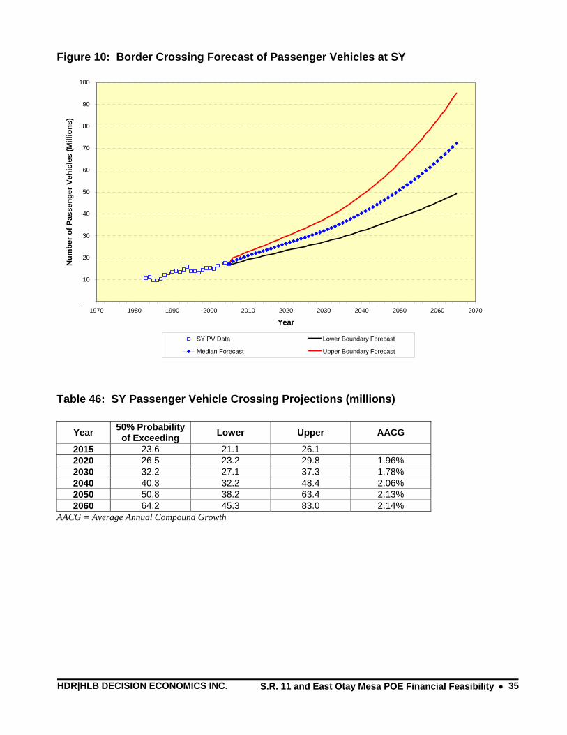
HDR|HLB DECISION ECONOMICS INC. S.R. 11 and East Otay Mesa POE Financial Feasibility • 35
Figure 10: Border Crossing Forecast of Passenger Vehicles at SY
-
10
20
30
40
50
60
70
80
90
100
1970 1980 1990 2000 2010 2020 2030 2040 2050 2060 2070
Year
Num
ber o
f Pas
seng
er V
ehic
les
(Mill
ions
)
SY PV Data Lower Boundary Forecast
Median Forecast Upper Boundary Forecast
Table 46: SY Passenger Vehicle Crossing Projections (millions)
Year 50% Probability of Exceeding Lower Upper AACG
2015 23.6 21.1 26.1 2020 26.5 23.2 29.8 1.96% 2030 32.2 27.1 37.3 1.78% 2040 40.3 32.2 48.4 2.06% 2050 50.8 38.2 63.4 2.13% 2060 64.2 45.3 83.0 2.14%
AACG = Average Annual Compound Growth
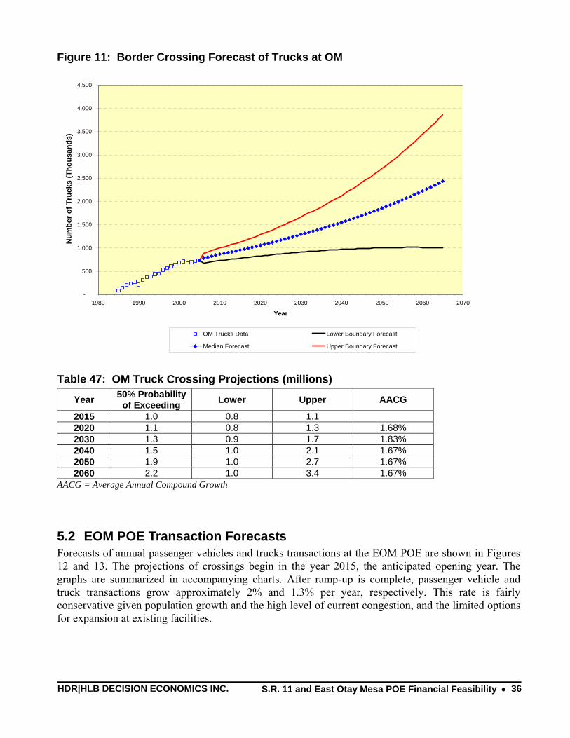
HDR|HLB DECISION ECONOMICS INC. S.R. 11 and East Otay Mesa POE Financial Feasibility • 36
Figure 11: Border Crossing Forecast of Trucks at OM
-
500
1,000
1,500
2,000
2,500
3,000
3,500
4,000
4,500
1980 1990 2000 2010 2020 2030 2040 2050 2060 2070
Year
Num
ber o
f Tru
cks
(Tho
usan
ds)
OM Trucks Data Lower Boundary Forecast
Median Forecast Upper Boundary Forecast
Table 47: OM Truck Crossing Projections (millions)
Year 50% Probability of Exceeding Lower Upper AACG
2015 1.0 0.8 1.1 2020 1.1 0.8 1.3 1.68% 2030 1.3 0.9 1.7 1.83% 2040 1.5 1.0 2.1 1.67% 2050 1.9 1.0 2.7 1.67% 2060 2.2 1.0 3.4 1.67%
AACG = Average Annual Compound Growth
5.2 EOM POE Transaction Forecasts Forecasts of annual passenger vehicles and trucks transactions at the EOM POE are shown in Figures 12 and 13. The projections of crossings begin in the year 2015, the anticipated opening year. The graphs are summarized in accompanying charts. After ramp-up is complete, passenger vehicle and truck transactions grow approximately 2% and 1.3% per year, respectively. This rate is fairly conservative given population growth and the high level of current congestion, and the limited options for expansion at existing facilities.
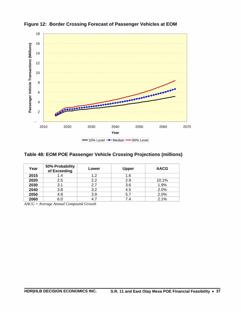
HDR|HLB DECISION ECONOMICS INC. S.R. 11 and East Otay Mesa POE Financial Feasibility • 37
Figure 12: Border Crossing Forecast of Passenger Vehicles at EOM
Table 48: EOM POE Passenger Vehicle Crossing Projections (millions)
Year 50% Probability of Exceeding Lower Upper AACG
2015 1.4 1.2 1.6 2020 2.5 2.2 2.9 10.1% 2030 3.1 2.7 3.6 1.9% 2040 3.8 3.2 4.5 2.0% 2050 4.8 3.9 5.7 2.0% 2060 6.0 4.7 7.4 2.1%
AACG = Average Annual Compound Growth
-
2
4
6
8
10
12
14
16
18
2010 2020 2030 2040 2050 2060 2070
Year
Pass
enge
r Veh
icle
Tra
nsac
tions
(Mill
ions
)
10% Level Median 90% Level
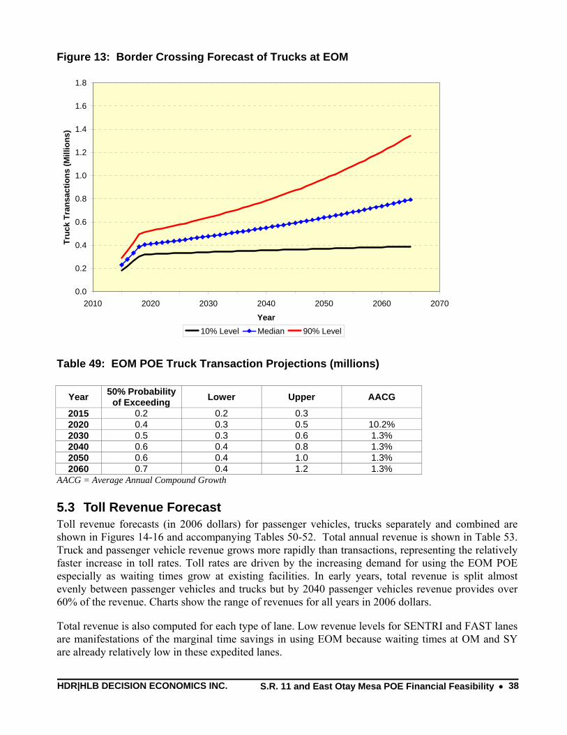
HDR|HLB DECISION ECONOMICS INC. S.R. 11 and East Otay Mesa POE Financial Feasibility • 38
Figure 13: Border Crossing Forecast of Trucks at EOM
Table 49: EOM POE Truck Transaction Projections (millions)
Year 50% Probability of Exceeding Lower Upper AACG
2015 0.2 0.2 0.3 2020 0.4 0.3 0.5 10.2% 2030 0.5 0.3 0.6 1.3% 2040 0.6 0.4 0.8 1.3% 2050 0.6 0.4 1.0 1.3% 2060 0.7 0.4 1.2 1.3%
AACG = Average Annual Compound Growth
5.3 Toll Revenue Forecast Toll revenue forecasts (in 2006 dollars) for passenger vehicles, trucks separately and combined are shown in Figures 14-16 and accompanying Tables 50-52. Total annual revenue is shown in Table 53. Truck and passenger vehicle revenue grows more rapidly than transactions, representing the relatively faster increase in toll rates. Toll rates are driven by the increasing demand for using the EOM POE especially as waiting times grow at existing facilities. In early years, total revenue is split almost evenly between passenger vehicles and trucks but by 2040 passenger vehicles revenue provides over 60% of the revenue. Charts show the range of revenues for all years in 2006 dollars.
Total revenue is also computed for each type of lane. Low revenue levels for SENTRI and FAST lanes are manifestations of the marginal time savings in using EOM because waiting times at OM and SY are already relatively low in these expedited lanes.
0.0
0.2
0.4
0.6
0.8
1.0
1.2
1.4
1.6
1.8
2010 2020 2030 2040 2050 2060 2070
Year
Truc
k Tr
ansa
ctio
ns (M
illio
ns)
10% Level Median 90% Level

HDR|HLB DECISION ECONOMICS INC. S.R. 11 and East Otay Mesa POE Financial Feasibility • 39
Figure 14: Annual Passenger Vehicle Revenue
Table 50: Passenger Vehicle Revenue Projections (millions)
Year 50% Probability of Exceeding Lower Upper AACG
2015 $4.7 $3.5 $5.9 2020 $9.0 $6.7 $11.2 11.4% 2030 $12.4 $9.3 $15.5 3.0% 2040 $17.1 $12.7 $21.8 3.0% 2050 $23.5 $17.2 $30.6 2.9% 2060 $32.4 $23.1 $43.3 3.0%
AACG = Average Annual Compound Growth
$0
$10
$20
$30
$40
$50
$60
$70
$80
$90
$100
2010 2020 2030 2040 2050 2060 2070
Year
Pass
enge
r Veh
icle
Rev
enue
(Mill
ions
)
10% Level Median 90% Level
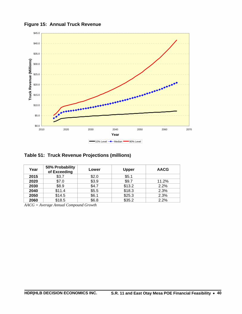
HDR|HLB DECISION ECONOMICS INC. S.R. 11 and East Otay Mesa POE Financial Feasibility • 40
Figure 15: Annual Truck Revenue
$0.0
$5.0
$10.0
$15.0
$20.0
$25.0
$30.0
$35.0
$40.0
$45.0
2010 2020 2030 2040 2050 2060 2070
Year
Truc
k R
even
ue (M
illio
ns)
10% Level Median 90% Level
Table 51: Truck Revenue Projections (millions)
Year 50% Probability of Exceeding Lower Upper AACG
2015 $3.7 $2.0 $5.1 2020 $7.0 $3.9 $9.7 11.2% 2030 $8.9 $4.7 $13.2 2.2% 2040 $11.4 $5.5 $18.3 2.3% 2050 $14.5 $6.1 $25.3 2.3% 2060 $18.5 $6.8 $35.2 2.2%
AACG = Average Annual Compound Growth
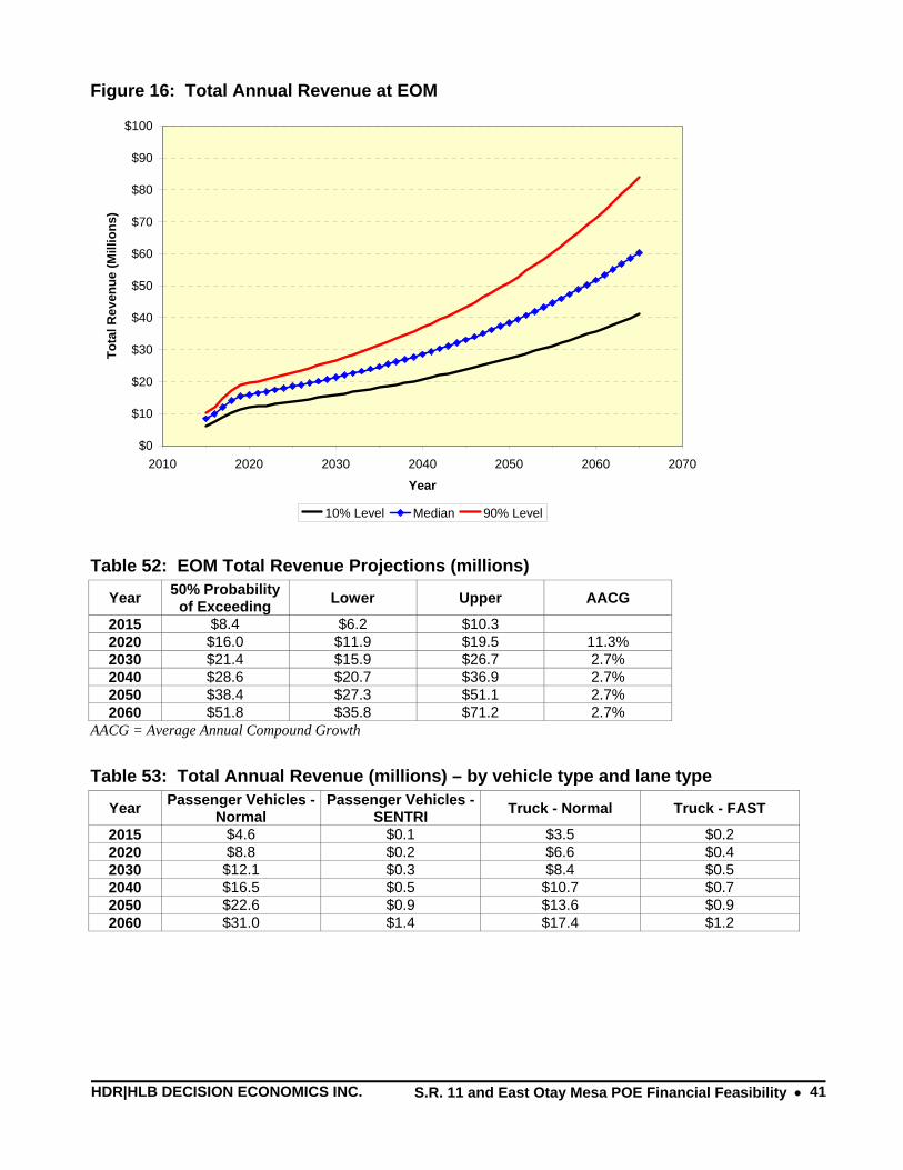
HDR|HLB DECISION ECONOMICS INC. S.R. 11 and East Otay Mesa POE Financial Feasibility • 41
Figure 16: Total Annual Revenue at EOM
Table 52: EOM Total Revenue Projections (millions)
Year 50% Probability of Exceeding Lower Upper AACG
2015 $8.4 $6.2 $10.3 2020 $16.0 $11.9 $19.5 11.3% 2030 $21.4 $15.9 $26.7 2.7% 2040 $28.6 $20.7 $36.9 2.7% 2050 $38.4 $27.3 $51.1 2.7% 2060 $51.8 $35.8 $71.2 2.7%
AACG = Average Annual Compound Growth
Table 53: Total Annual Revenue (millions) – by vehicle type and lane type
Year Passenger Vehicles - Normal
Passenger Vehicles -SENTRI Truck - Normal Truck - FAST
2015 $4.6 $0.1 $3.5 $0.2 2020 $8.8 $0.2 $6.6 $0.4 2030 $12.1 $0.3 $8.4 $0.5 2040 $16.5 $0.5 $10.7 $0.7 2050 $22.6 $0.9 $13.6 $0.9 2060 $31.0 $1.4 $17.4 $1.2
$0
$10
$20
$30
$40
$50
$60
$70
$80
$90
$100
2010 2020 2030 2040 2050 2060 2070
Year
Tota
l Rev
enue
(Mill
ions
)
10% Level Median 90% Level
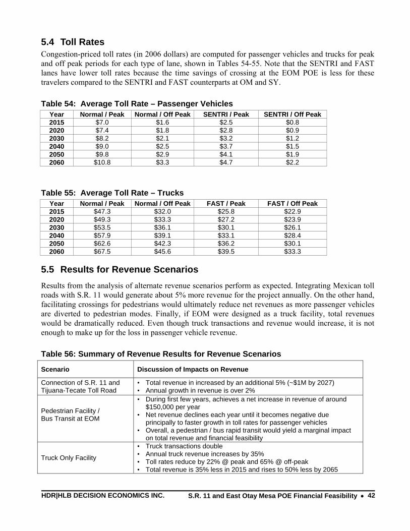
HDR|HLB DECISION ECONOMICS INC. S.R. 11 and East Otay Mesa POE Financial Feasibility • 42
5.4 Toll Rates Congestion-priced toll rates (in 2006 dollars) are computed for passenger vehicles and trucks for peak and off peak periods for each type of lane, shown in Tables 54-55. Note that the SENTRI and FAST lanes have lower toll rates because the time savings of crossing at the EOM POE is less for these travelers compared to the SENTRI and FAST counterparts at OM and SY.
Table 54: Average Toll Rate – Passenger Vehicles Year Normal / Peak Normal / Off Peak SENTRI / Peak SENTRI / Off Peak 2015 $7.0 $1.6 $2.5 $0.8 2020 $7.4 $1.8 $2.8 $0.9 2030 $8.2 $2.1 $3.2 $1.2 2040 $9.0 $2.5 $3.7 $1.5 2050 $9.8 $2.9 $4.1 $1.9 2060 $10.8 $3.3 $4.7 $2.2
Table 55: Average Toll Rate – Trucks Year Normal / Peak Normal / Off Peak FAST / Peak FAST / Off Peak 2015 $47.3 $32.0 $25.8 $22.9 2020 $49.3 $33.3 $27.2 $23.9 2030 $53.5 $36.1 $30.1 $26.1 2040 $57.9 $39.1 $33.1 $28.4 2050 $62.6 $42.3 $36.2 $30.1 2060 $67.5 $45.6 $39.5 $33.3
5.5 Results for Revenue Scenarios Results from the analysis of alternate revenue scenarios perform as expected. Integrating Mexican toll roads with S.R. 11 would generate about 5% more revenue for the project annually. On the other hand, facilitating crossings for pedestrians would ultimately reduce net revenues as more passenger vehicles are diverted to pedestrian modes. Finally, if EOM were designed as a truck facility, total revenues would be dramatically reduced. Even though truck transactions and revenue would increase, it is not enough to make up for the loss in passenger vehicle revenue.
Table 56: Summary of Revenue Results for Revenue Scenarios
Scenario Discussion of Impacts on Revenue
Connection of S.R. 11 and Tijuana-Tecate Toll Road
• Total revenue in increased by an additional 5% (~$1M by 2027) • Annual growth in revenue is over 2%
Pedestrian Facility / Bus Transit at EOM
• During first few years, achieves a net increase in revenue of around $150,000 per year
• Net revenue declines each year until it becomes negative due principally to faster growth in toll rates for passenger vehicles
• Overall, a pedestrian / bus rapid transit would yield a marginal impact on total revenue and financial feasibility
Truck Only Facility
• Truck transactions double • Annual truck revenue increases by 35% • Toll rates reduce by 22% @ peak and 65% @ off-peak • Total revenue is 35% less in 2015 and rises to 50% less by 2065
HDR|HLB DECISION ECONOMICS INC. S.R. 11 and East Otay Mesa POE Financial Feasibility • 43
5.6 Risk Analysis of Debt Service Coverage Debt service coverage (DSC) is usually expressed as a ratio of cash flow available to meet annual interest and principal payments on debt, including sinking funds payments. The formula is:
DSCR = Cash Flow Available for Debt Service
Debt Requirements (Principal and Interest Payments of Outstanding Debt)
DSCR results are shown in tables that represent DSCR values along a probability distribution ranging from 5% to 95% for a number of years. The individual DSCR cells in the table are color-coded for DSCR values below 1.0, and between 1.0 and 1.1. Any DSCR value falling below 1.0 represents insufficient cash flow to service outstanding debt obligations. The credit rating agency Fitch, for example, looks for a minimum DSCR of 1.25 for it to bestow an investment grade bond rating. Appendix 5 provides additional guidelines to help read the DSCR probability tables.
HDR|HLB’s risk analysis of the debt service coverage ratio for the baseline cost and revenue scenario is provided in Table 57. The baseline cost estimation of the project presents some down-side risks in the early years, with a likelihood of default (debt payment obligations exceeding revenue available for debt service, or debt service coverage ratio less than 1.0) of about 95 percent. Baseline results can be compared against cost scenarios (including various levels of external financial support) in Tables 58-61. DSCR results for alternate revenue scenarios and risk factors are shown in Tables 62-64 and Tables 65-68, respectively. These results are summarized and discussed in the next section. Note that the tables begin in year 2017 on the basis of the assumption that there is a five-year grace period following the start of construction in year 2012. In all cases, it is assumed that revenue increases with inflation at 3% annually.
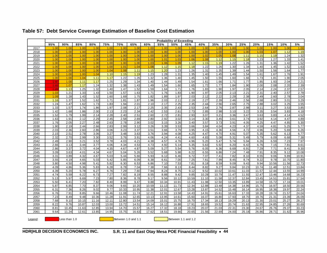
HDR|HLB DECISION ECONOMICS INC. S.R. 11 and East Otay Mesa POE Financial Feasibility • 44
Table 57: Debt Service Coverage Estimation of Baseline Cost Estimation
Probability of Exceeding95% 90% 85% 80% 75% 70% 65% 60% 55% 50% 45% 40% 35% 30% 25% 20% 15% 10% 5%
2017 1.00 1.00 1.00 1.00 1.00 1.00 1.00 1.00 1.00 1.00 1.00 1.00 1.00 1.00 1.00 1.00 1.00 1.00 1.002018 1.00 1.00 1.00 1.00 1.00 1.00 1.00 1.00 1.00 1.00 1.00 1.00 1.00 1.00 1.00 1.03 1.07 1.12 1.192019 1.00 1.00 1.00 1.00 1.00 1.00 1.00 1.00 1.00 1.00 1.00 1.02 1.05 1.08 1.11 1.15 1.19 1.24 1.322020 1.00 1.00 1.00 1.00 1.00 1.00 1.00 1.00 1.01 1.03 1.06 1.08 1.12 1.15 1.18 1.23 1.27 1.33 1.412021 1.00 1.00 1.00 1.00 1.00 1.00 1.00 1.03 1.06 1.09 1.12 1.15 1.19 1.22 1.26 1.31 1.36 1.42 1.522022 1.00 1.00 1.00 1.00 1.00 1.01 1.04 1.08 1.12 1.15 1.18 1.22 1.26 1.30 1.34 1.40 1.45 1.52 1.632023 1.00 1.00 1.00 1.00 1.04 1.08 1.11 1.15 1.20 1.23 1.26 1.31 1.35 1.39 1.44 1.50 1.56 1.64 1.772024 1.00 1.00 1.00 1.04 1.10 1.15 1.19 1.23 1.28 1.31 1.35 1.40 1.45 1.49 1.54 1.61 1.67 1.76 1.912025 1.00 1.00 1.04 1.11 1.17 1.22 1.26 1.32 1.36 1.40 1.45 1.50 1.55 1.60 1.66 1.73 1.81 1.90 2.052026 0.92 1.00 1.11 1.17 1.25 1.29 1.34 1.40 1.44 1.49 1.54 1.61 1.66 1.71 1.77 1.85 1.93 2.04 2.212027 0.93 1.07 1.17 1.24 1.32 1.38 1.43 1.49 1.54 1.60 1.65 1.72 1.77 1.84 1.90 2.00 2.08 2.20 2.392028 0.99 1.13 1.25 1.32 1.40 1.47 1.52 1.59 1.64 1.71 1.76 1.83 1.90 1.97 2.05 2.14 2.24 2.37 2.572029 1.03 1.21 1.33 1.43 1.50 1.57 1.63 1.71 1.76 1.83 1.90 1.97 2.05 2.13 2.21 2.31 2.40 2.57 2.782030 1.09 1.28 1.43 1.52 1.60 1.69 1.75 1.82 1.89 1.97 2.03 2.12 2.22 2.29 2.38 2.49 2.60 2.78 3.042031 1.16 1.37 1.52 1.62 1.71 1.81 1.87 1.96 2.03 2.11 2.19 2.27 2.39 2.46 2.56 2.68 2.80 3.01 3.292032 1.24 1.47 1.62 1.73 1.83 1.94 2.01 2.10 2.17 2.25 2.35 2.44 2.56 2.65 2.75 2.88 3.02 3.25 3.552033 1.33 1.57 1.74 1.86 1.97 2.08 2.17 2.25 2.35 2.43 2.53 2.64 2.76 2.87 2.98 3.11 3.27 3.53 3.852034 1.42 1.68 1.86 2.00 2.13 2.23 2.34 2.42 2.53 2.61 2.73 2.85 2.98 3.10 3.22 3.35 3.54 3.83 4.182035 1.52 1.79 1.99 2.14 2.28 2.40 2.51 2.60 2.72 2.81 2.93 3.07 3.21 3.36 3.47 3.63 3.83 4.14 4.522036 1.63 1.91 2.12 2.29 2.45 2.58 2.69 2.80 2.92 3.02 3.14 3.30 3.45 3.61 3.74 3.92 4.14 4.47 4.892037 1.76 2.05 2.27 2.48 2.63 2.78 2.90 3.02 3.15 3.26 3.40 3.57 3.73 3.91 4.05 4.25 4.47 4.85 5.302038 1.90 2.19 2.44 2.66 2.83 2.99 3.12 3.26 3.39 3.53 3.66 3.84 4.04 4.23 4.37 4.59 4.81 5.25 5.772039 2.03 2.36 2.60 2.86 3.06 3.23 3.37 3.51 3.66 3.79 3.95 4.15 4.36 4.56 4.72 4.96 5.20 5.69 6.262040 2.15 2.51 2.78 3.06 3.27 3.48 3.63 3.76 3.94 4.08 4.25 4.47 4.70 4.91 5.07 5.35 5.62 6.13 6.772041 2.32 2.70 2.99 3.30 3.52 3.76 3.91 4.06 4.24 4.41 4.60 4.83 5.08 5.31 5.49 5.79 6.09 6.68 7.382042 2.49 2.90 3.21 3.52 3.78 4.03 4.21 4.38 4.57 4.76 4.96 5.20 5.47 5.74 5.94 6.26 6.59 7.23 7.972043 2.66 3.13 3.44 3.77 4.06 4.34 4.53 4.73 4.92 5.14 5.35 5.63 5.92 6.20 6.42 6.76 7.15 7.81 8.612044 2.86 3.37 3.72 4.04 4.35 4.67 4.87 5.09 5.27 5.54 5.76 6.05 6.36 6.69 6.91 7.29 7.71 8.41 9.302045 3.09 3.63 4.01 4.34 4.67 5.04 5.26 5.52 5.68 5.98 6.22 6.55 6.86 7.24 7.48 7.91 8.35 9.12 10.082046 3.31 3.89 4.32 4.67 5.03 5.44 5.66 5.93 6.12 6.46 6.72 7.07 7.41 7.82 8.10 8.55 9.06 9.89 10.912047 3.55 4.19 4.65 5.03 5.42 5.85 6.09 6.38 6.61 7.00 7.25 7.61 7.99 8.45 8.74 9.22 9.78 10.70 11.802048 3.80 4.50 4.98 5.41 5.82 6.30 6.53 6.86 7.10 7.53 7.81 8.18 8.59 9.09 9.43 9.94 10.56 11.56 12.732049 4.09 4.86 5.36 5.83 6.28 6.78 7.04 7.38 7.66 8.13 8.44 8.82 9.27 9.84 10.23 10.74 11.48 12.51 13.842050 4.39 5.20 5.78 6.27 6.76 7.29 7.60 7.94 8.24 8.75 9.12 9.52 10.02 10.61 11.03 11.57 12.44 13.55 14.992051 4.74 5.59 6.22 6.73 7.27 7.82 8.19 8.55 8.88 9.42 9.85 10.28 10.79 11.47 11.93 12.47 13.46 14.68 16.232052 5.13 5.97 6.69 7.23 7.80 8.36 8.78 9.17 9.56 10.12 10.59 11.10 11.58 12.37 12.84 13.45 14.51 15.81 17.542053 5.50 6.41 7.20 7.82 8.40 8.99 9.47 9.88 10.34 10.91 11.43 11.98 12.50 13.35 13.89 14.58 15.72 17.16 19.012054 5.87 6.85 7.70 8.37 9.06 9.65 10.20 10.59 11.13 11.73 12.34 12.88 13.48 14.38 14.96 15.75 16.97 18.50 20.562055 6.31 7.36 8.26 9.02 9.77 10.33 10.95 11.38 12.01 12.67 13.28 13.87 14.52 15.48 16.14 16.95 18.36 19.97 22.242056 6.76 7.91 8.85 9.66 10.46 11.08 11.74 12.21 12.91 13.58 14.43 14.91 15.61 16.63 17.33 18.28 19.74 21.57 24.042057 7.23 8.49 9.48 10.36 11.28 11.91 12.65 13.13 13.95 14.61 15.60 16.07 16.80 17.93 18.70 19.76 21.31 23.39 26.092058 7.68 9.10 10.15 11.16 12.11 12.80 13.54 14.09 15.01 15.75 16.70 17.34 18.13 19.29 20.13 21.30 23.01 25.27 28.272059 8.22 9.76 10.87 12.03 13.00 13.72 14.51 15.14 16.12 16.88 17.91 18.65 19.52 20.74 21.63 22.95 24.85 27.26 30.692060 8.81 10.45 11.63 12.85 13.94 14.70 15.57 16.27 17.32 18.18 19.23 20.07 21.03 22.31 23.30 24.67 26.76 29.37 33.232061 9.64 11.24 12.61 13.85 14.95 15.75 16.63 17.62 18.51 19.66 20.65 21.56 22.69 24.00 25.18 26.86 28.71 31.62 35.96
Legend: Less than 1.0 Between 1.0 and 1.1 Between 1.1 and 1.2

HDR|HLB DECISION ECONOMICS INC. S.R. 11 and East Otay Mesa POE Financial Feasibility • 45
Table 58: Debt Service Coverage Estimation (S.R. 11 Capital and O&M Costs, with $50M Grant)
Probability of Exceeding95% 90% 85% 80% 75% 70% 65% 60% 55% 50% 45% 40% 35% 30% 25% 20% 15% 10% 5%
2017 1.00 1.00 1.00 1.00 1.00 1.00 1.00 1.00 1.00 1.00 1.00 1.00 1.00 1.00 1.00 1.01 1.05 1.09 1.142018 1.00 1.00 1.00 1.00 1.00 1.00 1.00 1.00 1.00 1.03 1.05 1.08 1.11 1.14 1.17 1.20 1.25 1.31 1.382019 1.00 1.00 1.00 1.00 1.00 1.02 1.05 1.08 1.11 1.14 1.17 1.21 1.24 1.28 1.31 1.35 1.41 1.47 1.562020 1.00 1.00 1.00 1.00 1.04 1.08 1.11 1.15 1.19 1.22 1.26 1.29 1.33 1.37 1.40 1.45 1.51 1.58 1.682021 1.00 1.00 1.00 1.05 1.10 1.14 1.18 1.22 1.26 1.30 1.34 1.37 1.42 1.46 1.50 1.55 1.62 1.71 1.802022 1.00 1.00 1.05 1.11 1.16 1.21 1.25 1.29 1.34 1.38 1.42 1.46 1.51 1.55 1.59 1.66 1.73 1.83 1.942023 1.00 1.01 1.12 1.18 1.24 1.29 1.34 1.38 1.43 1.49 1.53 1.57 1.62 1.67 1.72 1.79 1.87 1.98 2.112024 1.00 1.07 1.19 1.26 1.31 1.38 1.43 1.48 1.54 1.60 1.64 1.69 1.74 1.79 1.85 1.93 2.01 2.14 2.282025 1.00 1.14 1.26 1.35 1.40 1.47 1.53 1.58 1.65 1.71 1.75 1.81 1.88 1.93 2.00 2.08 2.17 2.30 2.472026 1.00 1.20 1.33 1.43 1.49 1.56 1.62 1.68 1.76 1.83 1.88 1.93 2.01 2.07 2.15 2.23 2.33 2.47 2.662027 1.00 1.28 1.42 1.52 1.59 1.67 1.74 1.81 1.88 1.97 2.01 2.08 2.16 2.22 2.31 2.41 2.51 2.67 2.882028 1.05 1.36 1.52 1.62 1.70 1.78 1.86 1.93 2.02 2.11 2.16 2.22 2.32 2.39 2.48 2.59 2.70 2.88 3.102029 1.13 1.46 1.62 1.73 1.82 1.90 2.00 2.08 2.17 2.27 2.33 2.40 2.50 2.58 2.68 2.80 2.92 3.12 3.382030 1.21 1.55 1.74 1.84 1.95 2.04 2.14 2.22 2.33 2.44 2.51 2.58 2.69 2.77 2.90 3.02 3.14 3.37 3.672031 1.29 1.67 1.86 1.98 2.08 2.19 2.29 2.40 2.51 2.63 2.70 2.78 2.90 2.99 3.13 3.27 3.39 3.65 4.002032 1.36 1.78 1.98 2.11 2.23 2.35 2.46 2.58 2.70 2.82 2.90 3.00 3.12 3.21 3.36 3.53 3.66 3.95 4.322033 1.47 1.90 2.13 2.25 2.39 2.53 2.65 2.79 2.91 3.03 3.14 3.23 3.38 3.48 3.66 3.82 3.98 4.29 4.702034 1.57 2.04 2.28 2.42 2.57 2.71 2.84 3.00 3.14 3.26 3.38 3.49 3.64 3.75 3.96 4.11 4.32 4.63 5.092035 1.69 2.17 2.44 2.61 2.76 2.91 3.05 3.22 3.37 3.51 3.64 3.78 3.92 4.05 4.27 4.43 4.69 5.02 5.522036 1.82 2.32 2.61 2.79 2.95 3.13 3.29 3.47 3.62 3.78 3.92 4.07 4.22 4.37 4.59 4.77 5.06 5.44 5.972037 1.95 2.50 2.81 2.99 3.17 3.37 3.54 3.74 3.92 4.08 4.23 4.40 4.57 4.73 4.97 5.17 5.50 5.90 6.492038 2.10 2.70 3.01 3.21 3.40 3.62 3.81 4.03 4.20 4.39 4.58 4.73 4.92 5.10 5.35 5.60 5.98 6.38 7.062039 2.27 2.88 3.24 3.45 3.65 3.89 4.11 4.34 4.52 4.73 4.93 5.12 5.31 5.51 5.78 6.05 6.49 6.90 7.672040 2.44 3.13 3.47 3.70 3.92 4.17 4.42 4.65 4.86 5.09 5.30 5.53 5.71 5.92 6.22 6.55 7.00 7.43 8.302041 2.64 3.37 3.74 3.97 4.22 4.50 4.75 5.03 5.26 5.48 5.72 5.98 6.17 6.40 6.72 7.08 7.58 8.07 9.012042 2.84 3.60 4.01 4.26 4.54 4.84 5.12 5.41 5.67 5.92 6.19 6.44 6.67 6.91 7.27 7.65 8.19 8.72 9.762043 3.06 3.89 4.31 4.59 4.88 5.21 5.52 5.80 6.09 6.37 6.68 6.95 7.20 7.45 7.85 8.25 8.82 9.43 10.572044 3.30 4.14 4.62 4.93 5.23 5.58 5.93 6.22 6.55 6.85 7.20 7.46 7.74 8.05 8.46 8.90 9.52 10.21 11.422045 3.55 4.45 4.97 5.29 5.63 6.00 6.40 6.71 7.05 7.40 7.76 8.09 8.36 8.73 9.14 9.65 10.29 11.08 12.382046 3.84 4.79 5.34 5.69 6.06 6.45 6.88 7.24 7.60 7.98 8.38 8.73 9.03 9.43 9.84 10.41 11.13 12.00 13.392047 4.13 5.11 5.75 6.11 6.49 6.94 7.40 7.77 8.17 8.59 9.02 9.40 9.72 10.16 10.61 11.25 12.03 12.92 14.532048 4.42 5.43 6.16 6.55 6.96 7.42 7.91 8.35 8.78 9.23 9.73 10.07 10.46 10.91 11.44 12.12 13.01 13.92 15.702049 4.77 5.85 6.62 7.07 7.51 8.00 8.49 9.00 9.46 9.96 10.48 10.86 11.33 11.79 12.36 13.12 14.13 15.12 17.082050 5.11 6.29 7.11 7.56 8.09 8.58 9.13 9.67 10.18 10.72 11.28 11.71 12.22 12.71 13.32 14.20 15.20 16.33 18.452051 5.50 6.74 7.62 8.14 8.69 9.23 9.85 10.38 10.93 11.55 12.10 12.60 13.17 13.65 14.36 15.35 16.45 17.62 20.082052 5.87 7.19 8.12 8.70 9.29 9.91 10.56 11.18 11.72 12.42 13.00 13.54 14.18 14.69 15.47 16.55 17.77 18.99 21.802053 6.40 7.74 8.70 9.41 9.99 10.66 11.36 12.00 12.61 13.35 14.00 14.60 15.27 15.81 16.69 17.92 19.23 20.55 23.622054 6.85 8.27 9.31 10.07 10.73 11.44 12.23 12.87 13.57 14.38 15.06 15.73 16.46 17.07 17.97 19.34 20.74 22.19 25.542055 7.34 8.95 9.99 10.81 11.48 12.27 13.11 13.87 14.60 15.44 16.17 16.98 17.68 18.40 19.39 20.87 22.42 23.98 27.612056 7.92 9.59 10.73 11.55 12.32 13.14 14.04 14.92 15.71 16.54 17.34 18.26 19.02 19.81 20.85 22.45 24.13 25.92 29.792057 8.57 10.26 11.50 12.39 13.22 14.13 15.06 16.02 16.87 17.85 18.68 19.71 20.50 21.32 22.41 24.24 26.10 28.09 32.242058 9.25 10.98 12.27 13.32 14.18 15.13 16.13 17.20 18.14 19.16 20.04 21.23 22.10 22.94 24.16 26.10 28.30 30.36 34.822059 9.94 11.79 13.16 14.23 15.19 16.20 17.34 18.46 19.55 20.57 21.54 22.74 23.89 24.64 25.98 28.10 30.57 32.76 37.572060 10.67 12.64 14.14 15.22 16.26 17.34 18.52 19.77 20.97 22.11 23.05 24.39 25.62 26.47 27.97 30.24 32.93 35.23 40.392061 11.34 13.60 15.05 16.51 17.61 18.71 19.95 21.23 22.53 23.78 24.78 25.94 27.46 28.53 30.31 32.51 35.37 38.29 44.16
Legend: Less than 1.0 Between 1.0 and 1.1 Between 1.1 and 1.2
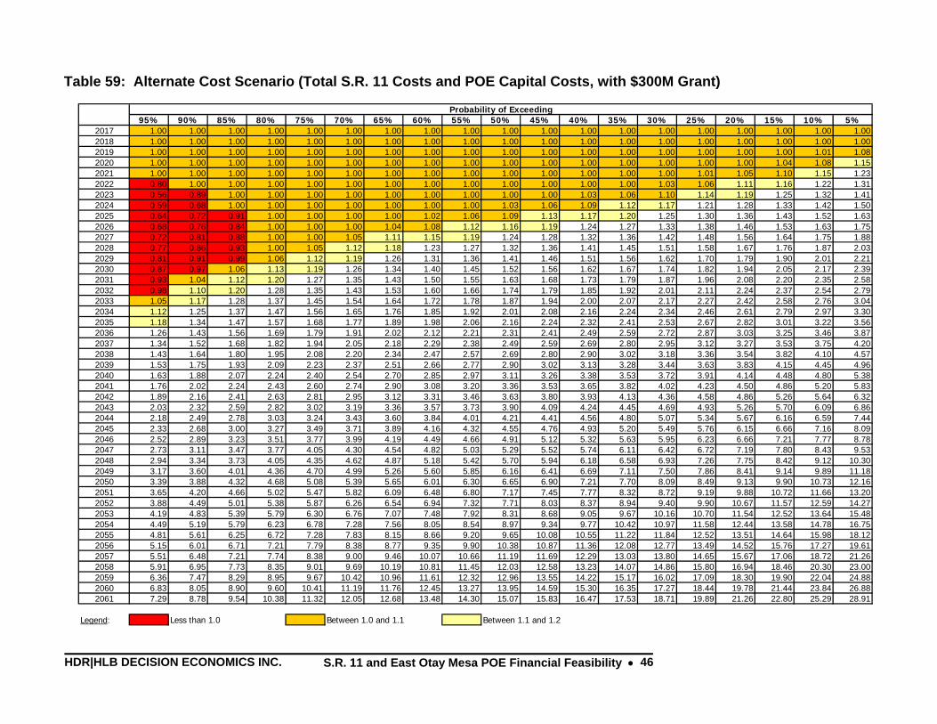
HDR|HLB DECISION ECONOMICS INC. S.R. 11 and East Otay Mesa POE Financial Feasibility • 46
Table 59: Alternate Cost Scenario (Total S.R. 11 Costs and POE Capital Costs, with $300M Grant)
Probability of Exceeding95% 90% 85% 80% 75% 70% 65% 60% 55% 50% 45% 40% 35% 30% 25% 20% 15% 10% 5%
2017 1.00 1.00 1.00 1.00 1.00 1.00 1.00 1.00 1.00 1.00 1.00 1.00 1.00 1.00 1.00 1.00 1.00 1.00 1.002018 1.00 1.00 1.00 1.00 1.00 1.00 1.00 1.00 1.00 1.00 1.00 1.00 1.00 1.00 1.00 1.00 1.00 1.00 1.002019 1.00 1.00 1.00 1.00 1.00 1.00 1.00 1.00 1.00 1.00 1.00 1.00 1.00 1.00 1.00 1.00 1.00 1.01 1.082020 1.00 1.00 1.00 1.00 1.00 1.00 1.00 1.00 1.00 1.00 1.00 1.00 1.00 1.00 1.00 1.00 1.04 1.08 1.152021 1.00 1.00 1.00 1.00 1.00 1.00 1.00 1.00 1.00 1.00 1.00 1.00 1.00 1.00 1.01 1.05 1.10 1.15 1.232022 0.80 1.00 1.00 1.00 1.00 1.00 1.00 1.00 1.00 1.00 1.00 1.00 1.00 1.03 1.06 1.11 1.16 1.22 1.312023 0.56 0.89 1.00 1.00 1.00 1.00 1.00 1.00 1.00 1.00 1.00 1.03 1.06 1.10 1.14 1.19 1.25 1.32 1.412024 0.59 0.68 1.00 1.00 1.00 1.00 1.00 1.00 1.00 1.03 1.06 1.09 1.12 1.17 1.21 1.28 1.33 1.42 1.502025 0.64 0.72 0.91 1.00 1.00 1.00 1.00 1.02 1.06 1.09 1.13 1.17 1.20 1.25 1.30 1.36 1.43 1.52 1.632026 0.68 0.76 0.84 1.00 1.00 1.00 1.04 1.08 1.12 1.16 1.19 1.24 1.27 1.33 1.38 1.46 1.53 1.63 1.752027 0.72 0.81 0.88 1.00 1.00 1.05 1.11 1.15 1.19 1.24 1.28 1.32 1.36 1.42 1.48 1.56 1.64 1.75 1.882028 0.77 0.86 0.93 1.00 1.05 1.12 1.18 1.23 1.27 1.32 1.36 1.41 1.45 1.51 1.58 1.67 1.76 1.87 2.032029 0.81 0.91 0.99 1.06 1.12 1.19 1.26 1.31 1.36 1.41 1.46 1.51 1.56 1.62 1.70 1.79 1.90 2.01 2.212030 0.87 0.97 1.06 1.13 1.19 1.26 1.34 1.40 1.45 1.52 1.56 1.62 1.67 1.74 1.82 1.94 2.05 2.17 2.392031 0.93 1.04 1.12 1.20 1.27 1.35 1.43 1.50 1.55 1.63 1.68 1.73 1.79 1.87 1.96 2.08 2.20 2.35 2.582032 0.98 1.10 1.20 1.28 1.35 1.43 1.53 1.60 1.66 1.74 1.79 1.85 1.92 2.01 2.11 2.24 2.37 2.54 2.792033 1.05 1.17 1.28 1.37 1.45 1.54 1.64 1.72 1.78 1.87 1.94 2.00 2.07 2.17 2.27 2.42 2.58 2.76 3.042034 1.12 1.25 1.37 1.47 1.56 1.65 1.76 1.85 1.92 2.01 2.08 2.16 2.24 2.34 2.46 2.61 2.79 2.97 3.302035 1.18 1.34 1.47 1.57 1.68 1.77 1.89 1.98 2.06 2.16 2.24 2.32 2.41 2.53 2.67 2.82 3.01 3.22 3.562036 1.26 1.43 1.56 1.69 1.79 1.91 2.02 2.12 2.21 2.31 2.41 2.49 2.59 2.72 2.87 3.03 3.25 3.46 3.872037 1.34 1.52 1.68 1.82 1.94 2.05 2.18 2.29 2.38 2.49 2.59 2.69 2.80 2.95 3.12 3.27 3.53 3.75 4.202038 1.43 1.64 1.80 1.95 2.08 2.20 2.34 2.47 2.57 2.69 2.80 2.90 3.02 3.18 3.36 3.54 3.82 4.10 4.572039 1.53 1.75 1.93 2.09 2.23 2.37 2.51 2.66 2.77 2.90 3.02 3.13 3.28 3.44 3.63 3.83 4.15 4.45 4.962040 1.63 1.88 2.07 2.24 2.40 2.54 2.70 2.85 2.97 3.11 3.26 3.38 3.53 3.72 3.91 4.14 4.48 4.80 5.382041 1.76 2.02 2.24 2.43 2.60 2.74 2.90 3.08 3.20 3.36 3.53 3.65 3.82 4.02 4.23 4.50 4.86 5.20 5.832042 1.89 2.16 2.41 2.63 2.81 2.95 3.12 3.31 3.46 3.63 3.80 3.93 4.13 4.36 4.58 4.86 5.26 5.64 6.322043 2.03 2.32 2.59 2.82 3.02 3.19 3.36 3.57 3.73 3.90 4.09 4.24 4.45 4.69 4.93 5.26 5.70 6.09 6.862044 2.18 2.49 2.78 3.03 3.24 3.43 3.60 3.84 4.01 4.21 4.41 4.56 4.80 5.07 5.34 5.67 6.16 6.59 7.442045 2.33 2.68 3.00 3.27 3.49 3.71 3.89 4.16 4.32 4.55 4.76 4.93 5.20 5.49 5.76 6.15 6.66 7.16 8.092046 2.52 2.89 3.23 3.51 3.77 3.99 4.19 4.49 4.66 4.91 5.12 5.32 5.63 5.95 6.23 6.66 7.21 7.77 8.782047 2.73 3.11 3.47 3.77 4.05 4.30 4.54 4.82 5.03 5.29 5.52 5.74 6.11 6.42 6.72 7.19 7.80 8.43 9.532048 2.94 3.34 3.73 4.05 4.35 4.62 4.87 5.18 5.42 5.70 5.94 6.18 6.58 6.93 7.26 7.75 8.42 9.12 10.302049 3.17 3.60 4.01 4.36 4.70 4.99 5.26 5.60 5.85 6.16 6.41 6.69 7.11 7.50 7.86 8.41 9.14 9.89 11.182050 3.39 3.88 4.32 4.68 5.08 5.39 5.65 6.01 6.30 6.65 6.90 7.21 7.70 8.09 8.49 9.13 9.90 10.73 12.162051 3.65 4.20 4.66 5.02 5.47 5.82 6.09 6.48 6.80 7.17 7.45 7.77 8.32 8.72 9.19 9.88 10.72 11.66 13.202052 3.88 4.49 5.01 5.38 5.87 6.26 6.54 6.94 7.32 7.71 8.03 8.37 8.94 9.40 9.90 10.67 11.57 12.59 14.272053 4.19 4.83 5.39 5.79 6.30 6.76 7.07 7.48 7.92 8.31 8.68 9.05 9.67 10.16 10.70 11.54 12.52 13.64 15.482054 4.49 5.19 5.79 6.23 6.78 7.28 7.56 8.05 8.54 8.97 9.34 9.77 10.42 10.97 11.58 12.44 13.58 14.78 16.752055 4.81 5.61 6.25 6.72 7.28 7.83 8.15 8.66 9.20 9.65 10.08 10.55 11.22 11.84 12.52 13.51 14.64 15.98 18.122056 5.15 6.01 6.71 7.21 7.79 8.38 8.77 9.35 9.90 10.38 10.87 11.36 12.08 12.77 13.49 14.52 15.76 17.27 19.612057 5.51 6.48 7.21 7.74 8.38 9.00 9.46 10.07 10.66 11.19 11.69 12.29 13.03 13.80 14.65 15.67 17.06 18.72 21.262058 5.91 6.95 7.73 8.35 9.01 9.69 10.19 10.81 11.45 12.03 12.58 13.23 14.07 14.86 15.80 16.94 18.46 20.30 23.002059 6.36 7.47 8.29 8.95 9.67 10.42 10.96 11.61 12.32 12.96 13.55 14.22 15.17 16.02 17.09 18.30 19.90 22.04 24.882060 6.83 8.05 8.90 9.60 10.41 11.19 11.76 12.45 13.27 13.95 14.59 15.30 16.35 17.27 18.44 19.78 21.44 23.84 26.882061 7.29 8.78 9.54 10.38 11.32 12.05 12.68 13.48 14.30 15.07 15.83 16.47 17.53 18.71 19.89 21.26 22.80 25.29 28.91
Legend: Less than 1.0 Between 1.0 and 1.1 Between 1.1 and 1.2

HDR|HLB DECISION ECONOMICS INC. S.R. 11 and East Otay Mesa POE Financial Feasibility • 47
Table 60: Alternate Cost Scenario (Total S.R. 11 Costs and POE Capital Costs, with $400M Grant)
Probability of Exceeding95% 90% 85% 80% 75% 70% 65% 60% 55% 50% 45% 40% 35% 30% 25% 20% 15% 10% 5%
2017 1.00 1.00 1.00 1.00 1.00 1.00 1.00 1.00 1.00 1.00 1.00 1.00 1.00 1.00 1.00 1.00 1.03 1.07 1.142018 1.00 1.00 1.00 1.00 1.00 1.00 1.00 1.00 1.00 1.00 1.03 1.06 1.09 1.12 1.15 1.19 1.23 1.28 1.362019 1.00 1.00 1.00 1.00 1.00 1.00 1.02 1.05 1.09 1.11 1.15 1.18 1.22 1.26 1.29 1.33 1.38 1.43 1.542020 1.00 1.00 1.00 1.00 1.00 1.05 1.08 1.12 1.16 1.19 1.23 1.26 1.30 1.35 1.38 1.42 1.48 1.54 1.662021 1.00 1.00 1.00 1.00 1.05 1.11 1.15 1.19 1.23 1.26 1.31 1.35 1.39 1.44 1.48 1.52 1.59 1.65 1.792022 1.00 1.00 1.00 1.05 1.11 1.17 1.21 1.26 1.30 1.34 1.39 1.43 1.47 1.52 1.57 1.62 1.69 1.77 1.922023 1.00 1.00 1.05 1.12 1.18 1.25 1.30 1.35 1.40 1.44 1.49 1.54 1.59 1.64 1.70 1.76 1.83 1.92 2.082024 1.00 1.02 1.11 1.20 1.26 1.34 1.39 1.44 1.49 1.54 1.60 1.65 1.71 1.77 1.83 1.89 1.97 2.07 2.252025 1.00 1.08 1.18 1.28 1.35 1.43 1.49 1.54 1.60 1.65 1.71 1.77 1.83 1.90 1.97 2.03 2.13 2.24 2.432026 1.00 1.14 1.25 1.35 1.43 1.51 1.59 1.64 1.71 1.76 1.83 1.89 1.96 2.03 2.11 2.18 2.28 2.41 2.622027 1.05 1.21 1.33 1.44 1.53 1.61 1.70 1.77 1.83 1.88 1.96 2.03 2.11 2.18 2.27 2.35 2.47 2.61 2.832028 1.11 1.30 1.41 1.53 1.63 1.72 1.81 1.89 1.96 2.02 2.10 2.17 2.26 2.35 2.44 2.53 2.66 2.81 3.062029 1.18 1.38 1.51 1.65 1.75 1.84 1.94 2.03 2.11 2.18 2.26 2.34 2.43 2.53 2.63 2.74 2.88 3.04 3.332030 1.25 1.48 1.61 1.75 1.87 1.98 2.09 2.18 2.26 2.34 2.42 2.53 2.61 2.72 2.84 2.95 3.12 3.29 3.602031 1.35 1.57 1.72 1.87 2.01 2.12 2.24 2.34 2.43 2.53 2.61 2.71 2.81 2.94 3.06 3.19 3.38 3.56 3.902032 1.43 1.67 1.84 2.00 2.15 2.28 2.40 2.50 2.61 2.71 2.80 2.91 3.02 3.16 3.30 3.44 3.65 3.86 4.232033 1.53 1.80 1.98 2.16 2.32 2.45 2.59 2.70 2.82 2.92 3.04 3.14 3.27 3.40 3.58 3.73 3.95 4.17 4.602034 1.63 1.91 2.13 2.32 2.49 2.64 2.78 2.90 3.04 3.14 3.26 3.38 3.53 3.68 3.86 4.03 4.28 4.52 4.992035 1.75 2.04 2.28 2.49 2.68 2.83 3.00 3.12 3.27 3.38 3.51 3.64 3.81 3.97 4.17 4.37 4.62 4.90 5.422036 1.87 2.17 2.44 2.67 2.87 3.04 3.21 3.35 3.52 3.64 3.77 3.92 4.09 4.28 4.50 4.71 4.99 5.31 5.872037 2.02 2.34 2.62 2.88 3.10 3.27 3.47 3.62 3.79 3.93 4.08 4.24 4.44 4.64 4.89 5.12 5.41 5.76 6.432038 2.17 2.49 2.82 3.11 3.32 3.51 3.74 3.89 4.08 4.23 4.38 4.56 4.79 5.01 5.28 5.53 5.85 6.24 6.922039 2.32 2.66 3.02 3.34 3.57 3.76 4.01 4.21 4.40 4.54 4.74 4.93 5.16 5.42 5.70 5.98 6.33 6.74 7.492040 2.50 2.84 3.22 3.57 3.82 4.06 4.31 4.52 4.72 4.88 5.10 5.31 5.56 5.84 6.14 6.45 6.84 7.27 8.152041 2.68 3.07 3.49 3.83 4.13 4.38 4.64 4.87 5.09 5.29 5.53 5.73 6.02 6.33 6.64 7.00 7.41 7.90 8.842042 2.86 3.30 3.74 4.09 4.45 4.72 4.98 5.25 5.48 5.69 5.96 6.18 6.49 6.83 7.17 7.56 8.02 8.56 9.592043 3.07 3.55 4.03 4.40 4.77 5.06 5.35 5.66 5.90 6.13 6.42 6.66 7.00 7.38 7.73 8.18 8.67 9.27 10.352044 3.28 3.80 4.31 4.71 5.12 5.45 5.73 6.09 6.33 6.61 6.89 7.16 7.53 7.93 8.38 8.84 9.35 10.03 11.212045 3.55 4.08 4.63 5.08 5.51 5.87 6.18 6.57 6.83 7.15 7.45 7.73 8.14 8.57 9.07 9.59 10.12 10.87 12.152046 3.83 4.37 4.98 5.44 5.91 6.31 6.65 7.05 7.35 7.70 8.03 8.35 8.76 9.24 9.79 10.33 10.93 11.76 13.142047 4.14 4.69 5.36 5.85 6.38 6.76 7.15 7.58 7.92 8.30 8.65 9.00 9.45 9.98 10.56 11.19 11.80 12.76 14.232048 4.42 5.03 5.78 6.26 6.83 7.25 7.67 8.11 8.50 8.90 9.30 9.66 10.19 10.77 11.39 12.07 12.71 13.77 15.442049 4.75 5.40 6.22 6.72 7.33 7.80 8.25 8.74 9.17 9.61 10.01 10.42 11.02 11.66 12.33 13.07 13.78 14.89 16.682050 5.11 5.79 6.67 7.20 7.89 8.38 8.85 9.37 9.88 10.34 10.79 11.26 11.88 12.58 13.29 14.13 14.86 16.11 17.992051 5.48 6.24 7.17 7.73 8.46 9.01 9.56 10.09 10.62 11.13 11.61 12.14 12.81 13.58 14.37 15.27 16.03 17.40 19.502052 5.84 6.71 7.68 8.28 9.05 9.68 10.23 10.86 11.43 12.02 12.50 13.07 13.81 14.61 15.50 16.47 17.25 18.79 21.092053 6.29 7.20 8.24 8.95 9.75 10.39 11.02 11.71 12.34 12.92 13.47 14.08 14.94 15.80 16.69 17.77 18.64 20.36 22.892054 6.70 7.71 8.87 9.65 10.47 11.17 11.79 12.60 13.27 13.88 14.49 15.19 16.11 17.02 18.00 19.18 20.11 21.95 24.792055 7.17 8.24 9.48 10.35 11.25 11.97 12.64 13.49 14.30 14.90 15.56 16.32 17.36 18.28 19.37 20.67 21.76 23.68 26.832056 7.67 8.82 10.15 11.04 12.01 12.82 13.57 14.45 15.36 15.94 16.76 17.54 18.64 19.68 20.86 22.21 23.51 25.59 28.912057 8.22 9.52 10.89 11.88 12.83 13.80 14.61 15.50 16.53 17.27 18.09 18.94 20.10 21.25 22.48 24.05 25.48 27.65 31.262058 8.82 10.16 11.70 12.75 13.74 14.82 15.78 16.63 17.79 18.54 19.49 20.36 21.64 22.94 24.24 25.93 27.53 29.79 33.742059 9.48 10.93 12.54 13.70 14.80 15.89 16.92 17.79 19.11 19.91 20.97 21.89 23.32 24.72 26.09 27.97 29.70 32.21 36.532060 10.20 11.83 13.42 14.66 15.87 17.02 18.09 19.11 20.48 21.46 22.55 23.53 25.02 26.56 28.09 30.10 32.01 34.81 39.532061 11.21 12.86 14.31 15.67 17.05 18.12 19.43 20.38 21.71 22.78 24.16 25.42 27.01 28.49 30.32 32.18 34.42 37.43 42.35
Legend: Less than 1.0 Between 1.0 and 1.1 Between 1.1 and 1.2
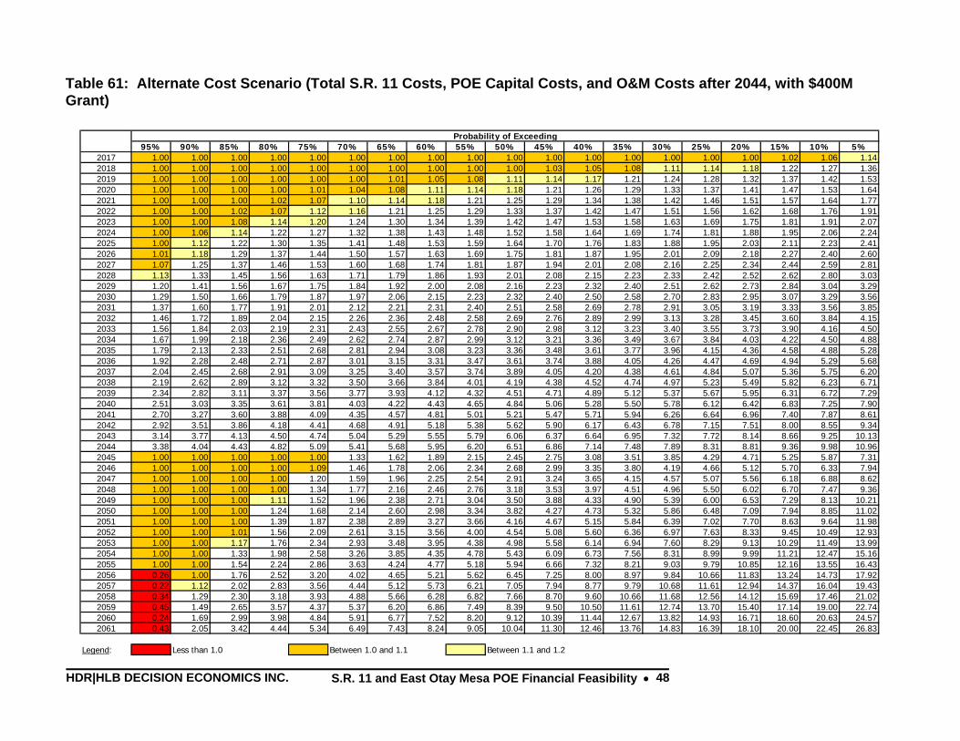
HDR|HLB DECISION ECONOMICS INC. S.R. 11 and East Otay Mesa POE Financial Feasibility • 48
Table 61: Alternate Cost Scenario (Total S.R. 11 Costs, POE Capital Costs, and O&M Costs after 2044, with $400M Grant)
Probability of Exceeding95% 90% 85% 80% 75% 70% 65% 60% 55% 50% 45% 40% 35% 30% 25% 20% 15% 10% 5%
2017 1.00 1.00 1.00 1.00 1.00 1.00 1.00 1.00 1.00 1.00 1.00 1.00 1.00 1.00 1.00 1.00 1.02 1.06 1.142018 1.00 1.00 1.00 1.00 1.00 1.00 1.00 1.00 1.00 1.00 1.03 1.05 1.08 1.11 1.14 1.18 1.22 1.27 1.362019 1.00 1.00 1.00 1.00 1.00 1.00 1.01 1.05 1.08 1.11 1.14 1.17 1.21 1.24 1.28 1.32 1.37 1.42 1.532020 1.00 1.00 1.00 1.00 1.01 1.04 1.08 1.11 1.14 1.18 1.21 1.26 1.29 1.33 1.37 1.41 1.47 1.53 1.642021 1.00 1.00 1.00 1.02 1.07 1.10 1.14 1.18 1.21 1.25 1.29 1.34 1.38 1.42 1.46 1.51 1.57 1.64 1.772022 1.00 1.00 1.02 1.07 1.12 1.16 1.21 1.25 1.29 1.33 1.37 1.42 1.47 1.51 1.56 1.62 1.68 1.76 1.912023 1.00 1.00 1.08 1.14 1.20 1.24 1.30 1.34 1.39 1.42 1.47 1.53 1.58 1.63 1.69 1.75 1.81 1.91 2.072024 1.00 1.06 1.14 1.22 1.27 1.32 1.38 1.43 1.48 1.52 1.58 1.64 1.69 1.74 1.81 1.88 1.95 2.06 2.242025 1.00 1.12 1.22 1.30 1.35 1.41 1.48 1.53 1.59 1.64 1.70 1.76 1.83 1.88 1.95 2.03 2.11 2.23 2.412026 1.01 1.18 1.29 1.37 1.44 1.50 1.57 1.63 1.69 1.75 1.81 1.87 1.95 2.01 2.09 2.18 2.27 2.40 2.602027 1.07 1.25 1.37 1.46 1.53 1.60 1.68 1.74 1.81 1.87 1.94 2.01 2.08 2.16 2.25 2.34 2.44 2.59 2.812028 1.13 1.33 1.45 1.56 1.63 1.71 1.79 1.86 1.93 2.01 2.08 2.15 2.23 2.33 2.42 2.52 2.62 2.80 3.032029 1.20 1.41 1.56 1.67 1.75 1.84 1.92 2.00 2.08 2.16 2.23 2.32 2.40 2.51 2.62 2.73 2.84 3.04 3.292030 1.29 1.50 1.66 1.79 1.87 1.97 2.06 2.15 2.23 2.32 2.40 2.50 2.58 2.70 2.83 2.95 3.07 3.29 3.562031 1.37 1.60 1.77 1.91 2.01 2.12 2.21 2.31 2.40 2.51 2.58 2.69 2.78 2.91 3.05 3.19 3.33 3.56 3.852032 1.46 1.72 1.89 2.04 2.15 2.26 2.36 2.48 2.58 2.69 2.76 2.89 2.99 3.13 3.28 3.45 3.60 3.84 4.152033 1.56 1.84 2.03 2.19 2.31 2.43 2.55 2.67 2.78 2.90 2.98 3.12 3.23 3.40 3.55 3.73 3.90 4.16 4.502034 1.67 1.99 2.18 2.36 2.49 2.62 2.74 2.87 2.99 3.12 3.21 3.36 3.49 3.67 3.84 4.03 4.22 4.50 4.882035 1.79 2.13 2.33 2.51 2.68 2.81 2.94 3.08 3.23 3.36 3.48 3.61 3.77 3.96 4.15 4.36 4.58 4.88 5.282036 1.92 2.28 2.48 2.71 2.87 3.01 3.15 3.31 3.47 3.61 3.74 3.88 4.05 4.26 4.47 4.69 4.94 5.29 5.682037 2.04 2.45 2.68 2.91 3.09 3.25 3.40 3.57 3.74 3.89 4.05 4.20 4.38 4.61 4.84 5.07 5.36 5.75 6.202038 2.19 2.62 2.89 3.12 3.32 3.50 3.66 3.84 4.01 4.19 4.38 4.52 4.74 4.97 5.23 5.49 5.82 6.23 6.712039 2.34 2.82 3.11 3.37 3.56 3.77 3.93 4.12 4.32 4.51 4.71 4.89 5.12 5.37 5.67 5.95 6.31 6.72 7.292040 2.51 3.03 3.35 3.61 3.81 4.03 4.22 4.43 4.65 4.84 5.06 5.28 5.50 5.78 6.12 6.42 6.83 7.25 7.902041 2.70 3.27 3.60 3.88 4.09 4.35 4.57 4.81 5.01 5.21 5.47 5.71 5.94 6.26 6.64 6.96 7.40 7.87 8.612042 2.92 3.51 3.86 4.18 4.41 4.68 4.91 5.18 5.38 5.62 5.90 6.17 6.43 6.78 7.15 7.51 8.00 8.55 9.342043 3.14 3.77 4.13 4.50 4.74 5.04 5.29 5.55 5.79 6.06 6.37 6.64 6.95 7.32 7.72 8.14 8.66 9.25 10.132044 3.38 4.04 4.43 4.82 5.09 5.41 5.68 5.95 6.20 6.51 6.86 7.14 7.48 7.89 8.31 8.81 9.36 9.98 10.962045 1.00 1.00 1.00 1.00 1.00 1.33 1.62 1.89 2.15 2.45 2.75 3.08 3.51 3.85 4.29 4.71 5.25 5.87 7.312046 1.00 1.00 1.00 1.00 1.09 1.46 1.78 2.06 2.34 2.68 2.99 3.35 3.80 4.19 4.66 5.12 5.70 6.33 7.942047 1.00 1.00 1.00 1.00 1.20 1.59 1.96 2.25 2.54 2.91 3.24 3.65 4.15 4.57 5.07 5.56 6.18 6.88 8.622048 1.00 1.00 1.00 1.00 1.34 1.77 2.16 2.46 2.76 3.18 3.53 3.97 4.51 4.96 5.50 6.02 6.70 7.47 9.362049 1.00 1.00 1.00 1.11 1.52 1.96 2.38 2.71 3.04 3.50 3.88 4.33 4.90 5.39 6.00 6.53 7.29 8.13 10.212050 1.00 1.00 1.00 1.24 1.68 2.14 2.60 2.98 3.34 3.82 4.27 4.73 5.32 5.86 6.48 7.09 7.94 8.85 11.022051 1.00 1.00 1.00 1.39 1.87 2.38 2.89 3.27 3.66 4.16 4.67 5.15 5.84 6.39 7.02 7.70 8.63 9.64 11.982052 1.00 1.00 1.01 1.56 2.09 2.61 3.15 3.56 4.00 4.54 5.08 5.60 6.36 6.97 7.63 8.33 9.45 10.49 12.932053 1.00 1.00 1.17 1.76 2.34 2.93 3.48 3.95 4.38 4.98 5.58 6.14 6.94 7.60 8.29 9.13 10.29 11.49 13.992054 1.00 1.00 1.33 1.98 2.58 3.26 3.85 4.35 4.78 5.43 6.09 6.73 7.56 8.31 8.99 9.99 11.21 12.47 15.162055 1.00 1.00 1.54 2.24 2.86 3.63 4.24 4.77 5.18 5.94 6.66 7.32 8.21 9.03 9.79 10.85 12.16 13.55 16.432056 0.26 1.00 1.76 2.52 3.20 4.02 4.65 5.21 5.62 6.45 7.25 8.00 8.97 9.84 10.66 11.83 13.24 14.73 17.922057 0.22 1.12 2.02 2.83 3.56 4.44 5.12 5.73 6.21 7.05 7.94 8.77 9.79 10.68 11.61 12.94 14.37 16.04 19.432058 0.34 1.29 2.30 3.18 3.93 4.88 5.66 6.28 6.82 7.66 8.70 9.60 10.66 11.68 12.56 14.12 15.69 17.46 21.022059 0.45 1.49 2.65 3.57 4.37 5.37 6.20 6.86 7.49 8.39 9.50 10.50 11.61 12.74 13.70 15.40 17.14 19.00 22.742060 0.24 1.69 2.99 3.98 4.84 5.91 6.77 7.52 8.20 9.12 10.39 11.44 12.67 13.82 14.93 16.71 18.60 20.63 24.572061 0.43 2.05 3.42 4.44 5.34 6.49 7.43 8.24 9.05 10.04 11.30 12.46 13.76 14.83 16.39 18.10 20.00 22.45 26.83
Legend: Less than 1.0 Between 1.0 and 1.1 Between 1.1 and 1.2
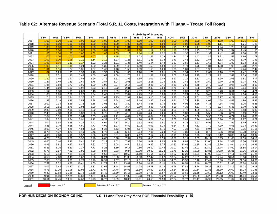
HDR|HLB DECISION ECONOMICS INC. S.R. 11 and East Otay Mesa POE Financial Feasibility • 49
Table 62: Alternate Revenue Scenario (Total S.R. 11 Costs, Integration with Tijuana – Tecate Toll Road)
Probability of Exceeding95% 90% 85% 80% 75% 70% 65% 60% 55% 50% 45% 40% 35% 30% 25% 20% 15% 10% 5%
2017 1.00 1.00 1.00 1.00 1.00 1.00 1.00 1.00 1.00 1.00 1.00 1.00 1.00 1.00 1.00 1.00 1.00 1.01 1.072018 1.00 1.00 1.00 1.00 1.00 1.00 1.00 1.00 1.00 1.00 1.00 1.00 1.02 1.05 1.08 1.11 1.16 1.21 1.292019 1.00 1.00 1.00 1.00 1.00 1.00 1.00 1.01 1.03 1.06 1.08 1.11 1.14 1.17 1.20 1.24 1.29 1.36 1.432020 1.00 1.00 1.00 1.00 1.00 1.01 1.03 1.07 1.10 1.12 1.15 1.18 1.22 1.25 1.28 1.33 1.37 1.45 1.552021 1.00 1.00 1.00 1.00 1.02 1.06 1.09 1.13 1.16 1.19 1.22 1.26 1.30 1.33 1.37 1.42 1.47 1.56 1.662022 1.00 1.00 1.00 1.04 1.07 1.12 1.15 1.19 1.23 1.26 1.29 1.34 1.38 1.42 1.46 1.51 1.57 1.66 1.782023 1.00 1.00 1.05 1.11 1.14 1.19 1.23 1.28 1.31 1.35 1.38 1.43 1.48 1.52 1.57 1.63 1.69 1.79 1.932024 1.00 1.04 1.11 1.17 1.22 1.26 1.31 1.36 1.40 1.44 1.48 1.53 1.59 1.63 1.68 1.74 1.82 1.93 2.082025 1.00 1.11 1.18 1.24 1.30 1.35 1.39 1.45 1.50 1.53 1.58 1.64 1.71 1.75 1.81 1.88 1.95 2.08 2.252026 1.01 1.16 1.24 1.31 1.37 1.43 1.48 1.55 1.59 1.63 1.69 1.75 1.81 1.87 1.93 2.01 2.10 2.24 2.422027 1.07 1.23 1.33 1.39 1.46 1.53 1.58 1.65 1.70 1.75 1.81 1.88 1.94 2.01 2.07 2.16 2.26 2.42 2.612028 1.13 1.31 1.41 1.48 1.55 1.63 1.68 1.76 1.81 1.87 1.93 2.02 2.08 2.15 2.22 2.31 2.43 2.59 2.832029 1.20 1.40 1.50 1.58 1.66 1.75 1.81 1.88 1.95 2.01 2.08 2.17 2.25 2.32 2.40 2.50 2.63 2.81 3.072030 1.27 1.49 1.61 1.69 1.78 1.87 1.94 2.01 2.08 2.15 2.25 2.33 2.41 2.49 2.59 2.70 2.85 3.04 3.322031 1.36 1.58 1.72 1.80 1.90 1.99 2.07 2.15 2.23 2.31 2.41 2.51 2.59 2.68 2.79 2.92 3.08 3.28 3.592032 1.44 1.69 1.83 1.92 2.03 2.13 2.22 2.31 2.39 2.48 2.58 2.70 2.78 2.88 2.99 3.14 3.32 3.54 3.882033 1.54 1.80 1.95 2.06 2.18 2.29 2.39 2.49 2.57 2.67 2.78 2.91 3.00 3.11 3.23 3.40 3.61 3.84 4.212034 1.63 1.93 2.09 2.20 2.34 2.45 2.57 2.67 2.75 2.88 3.00 3.13 3.24 3.34 3.49 3.67 3.92 4.16 4.582035 1.74 2.05 2.24 2.37 2.51 2.63 2.75 2.87 2.96 3.10 3.23 3.37 3.49 3.61 3.76 3.97 4.22 4.49 4.972036 1.86 2.19 2.39 2.54 2.68 2.82 2.94 3.06 3.19 3.32 3.48 3.61 3.75 3.88 4.05 4.28 4.56 4.86 5.392037 2.00 2.34 2.56 2.72 2.88 3.03 3.17 3.30 3.44 3.58 3.75 3.89 4.06 4.19 4.38 4.64 4.95 5.26 5.852038 2.15 2.51 2.76 2.94 3.09 3.26 3.42 3.54 3.69 3.87 4.03 4.20 4.38 4.53 4.73 5.04 5.36 5.70 6.312039 2.30 2.69 2.96 3.16 3.32 3.50 3.67 3.81 3.97 4.17 4.34 4.53 4.72 4.89 5.10 5.44 5.78 6.18 6.832040 2.45 2.88 3.16 3.38 3.56 3.75 3.92 4.10 4.26 4.48 4.66 4.85 5.08 5.26 5.50 5.86 6.24 6.69 7.392041 2.64 3.09 3.39 3.64 3.83 4.04 4.21 4.42 4.59 4.84 5.03 5.24 5.47 5.68 5.96 6.35 6.77 7.28 8.062042 2.84 3.32 3.64 3.91 4.12 4.32 4.53 4.77 4.94 5.22 5.41 5.65 5.88 6.14 6.43 6.86 7.33 7.87 8.772043 3.04 3.54 3.89 4.19 4.42 4.64 4.87 5.14 5.32 5.62 5.81 6.08 6.32 6.63 6.95 7.41 7.92 8.49 9.542044 3.25 3.79 4.18 4.50 4.73 4.99 5.23 5.52 5.72 6.03 6.26 6.54 6.78 7.12 7.49 7.99 8.56 9.18 10.332045 3.50 4.07 4.48 4.84 5.08 5.38 5.63 5.95 6.17 6.51 6.75 7.07 7.33 7.71 8.07 8.64 9.29 9.95 11.182046 3.76 4.37 4.79 5.19 5.46 5.79 6.05 6.40 6.64 7.01 7.28 7.61 7.89 8.30 8.72 9.36 10.01 10.78 12.082047 4.03 4.68 5.16 5.57 5.86 6.20 6.51 6.88 7.17 7.54 7.81 8.19 8.51 8.93 9.39 10.12 10.85 11.64 13.072048 4.28 5.05 5.56 5.96 6.26 6.66 6.98 7.37 7.69 8.10 8.39 8.79 9.11 9.59 10.14 10.95 11.68 12.53 14.162049 4.60 5.40 5.96 6.41 6.72 7.17 7.52 7.93 8.30 8.69 9.06 9.49 9.82 10.34 11.00 11.84 12.63 13.50 15.412050 4.95 5.81 6.37 6.87 7.22 7.70 8.08 8.54 8.92 9.37 9.75 10.22 10.62 11.15 11.88 12.76 13.64 14.63 16.692051 5.33 6.25 6.81 7.37 7.73 8.28 8.69 9.17 9.60 10.10 10.49 10.97 11.41 12.01 12.80 13.74 14.69 15.85 18.142052 5.73 6.67 7.29 7.90 8.28 8.87 9.33 9.84 10.30 10.80 11.28 11.78 12.29 12.90 13.81 14.80 15.81 17.06 19.582053 6.18 7.14 7.84 8.48 8.89 9.52 10.07 10.59 11.10 11.64 12.15 12.67 13.23 13.91 14.93 15.97 17.11 18.49 21.242054 6.59 7.63 8.40 9.07 9.56 10.24 10.83 11.36 11.93 12.47 13.07 13.64 14.27 15.01 16.14 17.24 18.51 19.98 23.022055 7.08 8.15 9.00 9.73 10.26 10.99 11.67 12.18 12.81 13.37 14.04 14.65 15.36 16.18 17.41 18.60 19.95 21.56 24.882056 7.59 8.72 9.62 10.41 11.00 11.77 12.51 13.07 13.74 14.37 15.10 15.74 16.51 17.40 18.75 20.02 21.45 23.24 26.912057 8.09 9.42 10.32 11.17 11.82 12.65 13.44 14.03 14.78 15.48 16.28 16.96 17.81 18.74 20.27 21.62 23.16 25.23 29.182058 8.73 10.10 11.08 11.96 12.72 13.54 14.48 15.05 15.89 16.62 17.52 18.24 19.20 20.14 21.81 23.30 25.00 27.28 31.482059 9.32 10.83 11.88 12.78 13.68 14.49 15.59 16.15 17.08 17.86 18.87 19.65 20.62 21.65 23.50 25.12 26.99 29.49 33.912060 9.91 11.59 12.71 13.68 14.64 15.50 16.71 17.37 18.33 19.12 20.22 21.07 22.12 23.29 25.23 26.98 29.00 31.84 36.562061 10.61 12.45 13.67 14.68 15.73 16.78 17.89 18.80 19.81 20.58 21.58 22.64 23.77 25.17 26.99 29.05 31.32 34.29 39.69
Legend: Less than 1.0 Between 1.0 and 1.1 Between 1.1 and 1.2
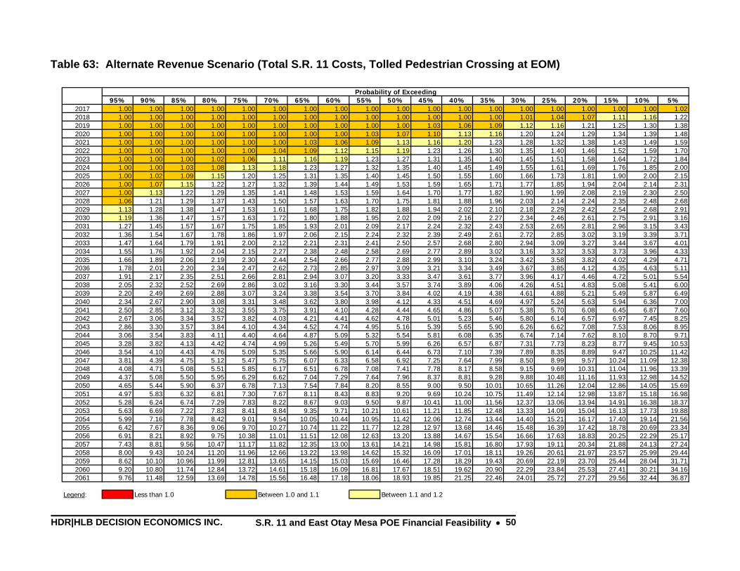
HDR|HLB DECISION ECONOMICS INC. S.R. 11 and East Otay Mesa POE Financial Feasibility • 50
Table 63: Alternate Revenue Scenario (Total S.R. 11 Costs, Tolled Pedestrian Crossing at EOM)
Probability of Exceeding95% 90% 85% 80% 75% 70% 65% 60% 55% 50% 45% 40% 35% 30% 25% 20% 15% 10% 5%
2017 1.00 1.00 1.00 1.00 1.00 1.00 1.00 1.00 1.00 1.00 1.00 1.00 1.00 1.00 1.00 1.00 1.00 1.00 1.022018 1.00 1.00 1.00 1.00 1.00 1.00 1.00 1.00 1.00 1.00 1.00 1.00 1.00 1.01 1.04 1.07 1.11 1.16 1.222019 1.00 1.00 1.00 1.00 1.00 1.00 1.00 1.00 1.00 1.00 1.03 1.06 1.09 1.12 1.16 1.21 1.25 1.30 1.382020 1.00 1.00 1.00 1.00 1.00 1.00 1.00 1.00 1.03 1.07 1.10 1.13 1.16 1.20 1.24 1.29 1.34 1.39 1.482021 1.00 1.00 1.00 1.00 1.00 1.00 1.03 1.06 1.09 1.13 1.16 1.20 1.23 1.28 1.32 1.38 1.43 1.49 1.592022 1.00 1.00 1.00 1.00 1.00 1.04 1.09 1.12 1.15 1.19 1.23 1.26 1.30 1.35 1.40 1.46 1.52 1.59 1.702023 1.00 1.00 1.00 1.02 1.06 1.11 1.16 1.19 1.23 1.27 1.31 1.35 1.40 1.45 1.51 1.58 1.64 1.72 1.842024 1.00 1.00 1.03 1.08 1.13 1.18 1.23 1.27 1.32 1.35 1.40 1.45 1.49 1.55 1.61 1.69 1.76 1.85 2.002025 1.00 1.02 1.09 1.15 1.20 1.25 1.31 1.35 1.40 1.45 1.50 1.55 1.60 1.66 1.73 1.81 1.90 2.00 2.152026 1.00 1.07 1.15 1.22 1.27 1.32 1.39 1.44 1.49 1.53 1.59 1.65 1.71 1.77 1.85 1.94 2.04 2.14 2.312027 1.00 1.13 1.22 1.29 1.35 1.41 1.48 1.53 1.59 1.64 1.70 1.77 1.82 1.90 1.99 2.08 2.19 2.30 2.502028 1.06 1.21 1.29 1.37 1.43 1.50 1.57 1.63 1.70 1.75 1.81 1.88 1.96 2.03 2.14 2.24 2.35 2.48 2.682029 1.13 1.28 1.38 1.47 1.53 1.61 1.68 1.75 1.82 1.88 1.94 2.02 2.10 2.18 2.29 2.42 2.54 2.68 2.912030 1.19 1.36 1.47 1.57 1.63 1.72 1.80 1.88 1.95 2.02 2.09 2.16 2.27 2.34 2.46 2.61 2.75 2.91 3.162031 1.27 1.45 1.57 1.67 1.75 1.85 1.93 2.01 2.09 2.17 2.24 2.32 2.43 2.53 2.65 2.81 2.96 3.15 3.432032 1.36 1.54 1.67 1.78 1.86 1.97 2.06 2.15 2.24 2.32 2.39 2.49 2.61 2.72 2.85 3.02 3.19 3.39 3.712033 1.47 1.64 1.79 1.91 2.00 2.12 2.21 2.31 2.41 2.50 2.57 2.68 2.80 2.94 3.09 3.27 3.44 3.67 4.012034 1.55 1.76 1.92 2.04 2.15 2.27 2.38 2.48 2.58 2.69 2.77 2.89 3.02 3.16 3.32 3.53 3.73 3.96 4.332035 1.66 1.89 2.06 2.19 2.30 2.44 2.54 2.66 2.77 2.88 2.99 3.10 3.24 3.42 3.58 3.82 4.02 4.29 4.712036 1.78 2.01 2.20 2.34 2.47 2.62 2.73 2.85 2.97 3.09 3.21 3.34 3.49 3.67 3.85 4.12 4.35 4.63 5.112037 1.91 2.17 2.35 2.51 2.66 2.81 2.94 3.07 3.20 3.33 3.47 3.61 3.77 3.96 4.17 4.46 4.72 5.01 5.542038 2.05 2.32 2.52 2.69 2.86 3.02 3.16 3.30 3.44 3.57 3.74 3.89 4.06 4.26 4.51 4.83 5.08 5.41 6.002039 2.20 2.49 2.69 2.88 3.07 3.24 3.38 3.54 3.70 3.84 4.02 4.19 4.38 4.61 4.88 5.21 5.49 5.87 6.492040 2.34 2.67 2.90 3.08 3.31 3.48 3.62 3.80 3.98 4.12 4.33 4.51 4.69 4.97 5.24 5.63 5.94 6.36 7.002041 2.50 2.85 3.12 3.32 3.55 3.75 3.91 4.10 4.28 4.44 4.65 4.86 5.07 5.38 5.70 6.08 6.45 6.87 7.602042 2.67 3.06 3.34 3.57 3.82 4.03 4.21 4.41 4.62 4.78 5.01 5.23 5.46 5.80 6.14 6.57 6.97 7.45 8.252043 2.86 3.30 3.57 3.84 4.10 4.34 4.52 4.74 4.95 5.16 5.39 5.65 5.90 6.26 6.62 7.08 7.53 8.06 8.952044 3.06 3.54 3.83 4.11 4.40 4.64 4.87 5.09 5.32 5.54 5.81 6.08 6.35 6.74 7.14 7.62 8.10 8.70 9.712045 3.28 3.82 4.13 4.42 4.74 4.99 5.26 5.49 5.70 5.99 6.26 6.57 6.87 7.31 7.73 8.23 8.77 9.45 10.532046 3.54 4.10 4.43 4.76 5.09 5.35 5.66 5.90 6.14 6.44 6.73 7.10 7.39 7.89 8.35 8.89 9.47 10.25 11.422047 3.81 4.39 4.75 5.12 5.47 5.75 6.07 6.33 6.58 6.92 7.25 7.64 7.99 8.50 8.99 9.57 10.24 11.09 12.382048 4.08 4.71 5.08 5.51 5.85 6.17 6.51 6.78 7.08 7.41 7.78 8.17 8.58 9.15 9.69 10.31 11.04 11.96 13.392049 4.37 5.08 5.50 5.95 6.29 6.62 7.04 7.29 7.64 7.96 8.37 8.81 9.28 9.88 10.48 11.16 11.93 12.98 14.522050 4.65 5.44 5.90 6.37 6.78 7.13 7.54 7.84 8.20 8.55 9.00 9.50 10.01 10.65 11.26 12.04 12.86 14.05 15.692051 4.97 5.83 6.32 6.81 7.30 7.67 8.11 8.43 8.83 9.20 9.69 10.24 10.75 11.49 12.14 12.98 13.87 15.18 16.982052 5.28 6.24 6.74 7.29 7.83 8.22 8.67 9.03 9.50 9.87 10.41 11.00 11.56 12.37 13.06 13.94 14.91 16.38 18.372053 5.63 6.69 7.22 7.83 8.41 8.84 9.35 9.71 10.21 10.61 11.21 11.85 12.48 13.33 14.09 15.04 16.13 17.73 19.882054 5.99 7.16 7.78 8.42 9.01 9.54 10.05 10.44 10.95 11.42 12.06 12.74 13.44 14.40 15.21 16.17 17.40 19.14 21.562055 6.42 7.67 8.36 9.06 9.70 10.27 10.74 11.22 11.77 12.28 12.97 13.68 14.46 15.48 16.39 17.42 18.78 20.69 23.342056 6.91 8.21 8.92 9.75 10.38 11.01 11.51 12.08 12.63 13.20 13.88 14.67 15.54 16.66 17.63 18.83 20.25 22.29 25.172057 7.43 8.81 9.56 10.47 11.17 11.82 12.35 13.00 13.61 14.21 14.98 15.81 16.80 17.93 19.11 20.34 21.88 24.13 27.242058 8.00 9.43 10.24 11.20 11.96 12.66 13.22 13.98 14.62 15.32 16.09 17.01 18.11 19.26 20.61 21.97 23.57 25.99 29.442059 8.62 10.10 10.96 11.99 12.81 13.65 14.15 15.03 15.69 16.46 17.28 18.29 19.43 20.69 22.19 23.70 25.44 28.04 31.712060 9.20 10.80 11.74 12.84 13.72 14.61 15.18 16.09 16.81 17.67 18.51 19.62 20.90 22.29 23.84 25.53 27.41 30.21 34.162061 9.76 11.48 12.59 13.69 14.78 15.56 16.48 17.18 18.06 18.93 19.85 21.25 22.46 24.01 25.72 27.27 29.56 32.44 36.87
Legend: Less than 1.0 Between 1.0 and 1.1 Between 1.1 and 1.2
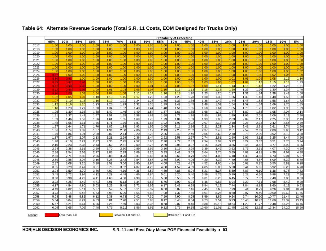
HDR|HLB DECISION ECONOMICS INC. S.R. 11 and East Otay Mesa POE Financial Feasibility • 51
Table 64: Alternate Revenue Scenario (Total S.R. 11 Costs, EOM Designed for Trucks Only)
Probability of Exceeding95% 90% 85% 80% 75% 70% 65% 60% 55% 50% 45% 40% 35% 30% 25% 20% 15% 10% 5%
2017 1.00 1.00 1.00 1.00 1.00 1.00 1.00 1.00 1.00 1.00 1.00 1.00 1.00 1.00 1.00 1.00 1.00 1.00 1.002018 1.00 1.00 1.00 1.00 1.00 1.00 1.00 1.00 1.00 1.00 1.00 1.00 1.00 1.00 1.00 1.00 1.00 1.00 1.002019 1.00 1.00 1.00 1.00 1.00 1.00 1.00 1.00 1.00 1.00 1.00 1.00 1.00 1.00 1.00 1.00 1.00 1.00 1.002020 1.00 1.00 1.00 1.00 1.00 1.00 1.00 1.00 1.00 1.00 1.00 1.00 1.00 1.00 1.00 1.00 1.00 1.00 1.002021 1.00 1.00 1.00 1.00 1.00 1.00 1.00 1.00 1.00 1.00 1.00 1.00 1.00 1.00 1.00 1.00 1.00 1.00 1.002022 1.00 1.00 1.00 1.00 1.00 1.00 1.00 1.00 1.00 1.00 1.00 1.00 1.00 1.00 1.00 1.00 1.00 1.00 1.002023 1.00 1.00 1.00 1.00 1.00 1.00 1.00 1.00 1.00 1.00 1.00 1.00 1.00 1.00 1.00 1.00 1.00 1.00 1.002024 1.00 1.00 1.00 1.00 1.00 1.00 1.00 1.00 1.00 1.00 1.00 1.00 1.00 1.00 1.00 1.00 1.00 1.00 1.022025 0.87 1.00 1.00 1.00 1.00 1.00 1.00 1.00 1.00 1.00 1.00 1.00 1.00 1.00 1.00 1.00 1.02 1.05 1.092026 0.80 0.91 1.00 1.00 1.00 1.00 1.00 1.00 1.00 1.00 1.00 1.00 1.00 1.01 1.03 1.06 1.08 1.12 1.162027 0.83 0.87 0.94 1.00 1.00 1.00 1.00 1.00 1.00 1.00 1.01 1.03 1.05 1.07 1.09 1.12 1.15 1.18 1.232028 0.87 0.90 0.93 1.00 1.00 1.00 1.00 1.01 1.04 1.05 1.07 1.09 1.11 1.13 1.15 1.18 1.22 1.26 1.312029 0.92 0.95 0.98 1.00 1.01 1.03 1.05 1.07 1.10 1.11 1.13 1.15 1.18 1.20 1.23 1.26 1.30 1.34 1.402030 0.96 1.00 1.02 1.04 1.07 1.08 1.11 1.14 1.16 1.18 1.20 1.23 1.25 1.27 1.31 1.34 1.38 1.43 1.502031 1.02 1.05 1.07 1.10 1.13 1.15 1.17 1.20 1.23 1.25 1.28 1.30 1.33 1.36 1.39 1.43 1.48 1.53 1.602032 1.07 1.10 1.13 1.16 1.19 1.21 1.24 1.28 1.30 1.33 1.36 1.38 1.42 1.44 1.48 1.53 1.58 1.64 1.722033 1.12 1.16 1.20 1.23 1.26 1.29 1.32 1.36 1.39 1.42 1.45 1.48 1.51 1.54 1.59 1.64 1.69 1.76 1.852034 1.18 1.23 1.27 1.30 1.34 1.37 1.40 1.44 1.48 1.51 1.55 1.58 1.61 1.65 1.70 1.75 1.82 1.90 1.992035 1.25 1.30 1.35 1.38 1.42 1.46 1.49 1.54 1.57 1.61 1.65 1.68 1.72 1.77 1.82 1.88 1.95 2.04 2.142036 1.31 1.37 1.42 1.47 1.51 1.55 1.58 1.63 1.68 1.72 1.76 1.80 1.84 1.89 1.95 2.01 2.09 2.19 2.302037 1.39 1.46 1.52 1.56 1.61 1.65 1.69 1.75 1.79 1.84 1.89 1.93 1.98 2.03 2.09 2.17 2.25 2.36 2.492038 1.48 1.55 1.61 1.66 1.71 1.76 1.81 1.86 1.92 1.97 2.02 2.07 2.12 2.18 2.25 2.33 2.42 2.54 2.692039 1.57 1.64 1.71 1.76 1.82 1.88 1.93 1.99 2.05 2.11 2.16 2.21 2.28 2.34 2.41 2.51 2.61 2.74 2.902040 1.66 1.74 1.82 1.87 1.94 2.00 2.06 2.12 2.19 2.25 2.32 2.37 2.43 2.51 2.59 2.69 2.80 2.96 3.122041 1.76 1.86 1.94 2.00 2.07 2.14 2.20 2.28 2.35 2.42 2.49 2.55 2.62 2.70 2.78 2.90 3.02 3.19 3.382042 1.87 1.97 2.07 2.13 2.21 2.29 2.36 2.44 2.52 2.58 2.67 2.74 2.81 2.90 2.99 3.12 3.25 3.44 3.662043 1.98 2.10 2.21 2.27 2.36 2.45 2.52 2.60 2.70 2.77 2.87 2.94 3.02 3.12 3.22 3.37 3.51 3.70 3.942044 2.10 2.23 2.35 2.43 2.52 2.61 2.69 2.78 2.89 2.96 3.07 3.15 3.24 3.35 3.46 3.62 3.77 3.99 4.252045 2.24 2.38 2.51 2.60 2.70 2.80 2.89 2.99 3.10 3.19 3.29 3.39 3.49 3.62 3.73 3.91 4.07 4.30 4.602046 2.38 2.54 2.68 2.77 2.88 2.99 3.09 3.20 3.33 3.41 3.53 3.64 3.75 3.89 4.02 4.21 4.39 4.64 4.982047 2.53 2.71 2.86 2.96 3.08 3.20 3.31 3.43 3.56 3.66 3.79 3.91 4.03 4.18 4.33 4.53 4.73 5.01 5.372048 2.69 2.88 3.04 3.16 3.28 3.42 3.54 3.67 3.80 3.92 4.06 4.20 4.32 4.49 4.65 4.87 5.09 5.39 5.792049 2.87 3.08 3.25 3.38 3.52 3.66 3.80 3.94 4.08 4.22 4.37 4.52 4.65 4.84 5.02 5.25 5.50 5.82 6.282050 3.05 3.29 3.47 3.61 3.76 3.92 4.07 4.22 4.38 4.52 4.69 4.85 5.00 5.20 5.41 5.66 5.92 6.28 6.782051 3.24 3.50 3.70 3.86 4.02 4.19 4.36 4.52 4.69 4.85 5.04 5.21 5.37 5.59 5.83 6.10 6.38 6.78 7.322052 3.45 3.72 3.94 4.12 4.29 4.48 4.66 4.84 5.01 5.20 5.40 5.59 5.76 5.99 6.27 6.56 6.88 7.29 7.882053 3.68 3.98 4.22 4.41 4.60 4.80 4.99 5.19 5.38 5.58 5.82 6.01 6.20 6.45 6.77 7.07 7.40 7.88 8.532054 3.92 4.25 4.49 4.71 4.91 5.13 5.34 5.56 5.76 5.99 6.24 6.46 6.66 6.94 7.29 7.61 7.98 8.49 9.202055 4.17 4.54 4.80 5.03 5.25 5.49 5.72 5.96 6.17 6.43 6.69 6.94 7.15 7.44 7.84 8.18 8.60 9.15 9.932056 4.43 4.82 5.11 5.37 5.59 5.87 6.11 6.37 6.60 6.87 7.16 7.45 7.68 7.99 8.41 8.79 9.26 9.84 10.702057 4.73 5.14 5.46 5.73 5.98 6.29 6.55 6.83 7.08 7.37 7.69 8.01 8.26 8.60 9.07 9.49 10.00 10.62 11.552058 5.03 5.48 5.82 6.12 6.38 6.73 7.02 7.30 7.59 7.90 8.25 8.59 8.86 9.24 9.74 10.20 10.77 11.44 12.462059 5.34 5.84 6.21 6.53 6.81 7.20 7.51 7.83 8.12 8.48 8.84 9.23 9.51 9.93 10.46 10.97 11.60 12.32 13.432060 5.67 6.21 6.61 6.96 7.26 7.69 8.03 8.36 8.68 9.07 9.46 9.88 10.18 10.64 11.22 11.77 12.48 13.26 14.462061 6.09 6.65 7.09 7.48 7.79 8.21 8.56 8.92 9.32 9.76 10.15 10.60 11.01 11.45 12.07 12.62 13.34 14.20 15.60
Legend: Less than 1.0 Between 1.0 and 1.1 Between 1.1 and 1.2

HDR|HLB DECISION ECONOMICS INC. S.R. 11 and East Otay Mesa POE Financial Feasibility • 52
Table 65: Alternate Revenue Scenario (Total S.R. 11 Costs, Risk of Punta Colonet Opening in 2020)
Probability of Exceeding95% 90% 85% 80% 75% 70% 65% 60% 55% 50% 45% 40% 35% 30% 25% 20% 15% 10% 5%
2017 1.00 1.00 1.00 1.00 1.00 1.00 1.00 1.00 1.00 1.00 1.00 1.00 1.00 1.00 1.00 1.00 1.00 1.00 1.002018 1.00 1.00 1.00 1.00 1.00 1.00 1.00 1.00 1.00 1.00 1.00 1.00 1.00 1.00 1.00 1.00 1.04 1.09 1.152019 1.00 1.00 1.00 1.00 1.00 1.00 1.00 1.00 1.00 1.00 1.00 1.00 1.02 1.05 1.08 1.11 1.16 1.21 1.302020 1.00 1.00 1.00 1.00 1.00 1.00 1.00 1.00 1.00 1.00 1.02 1.06 1.09 1.12 1.15 1.19 1.24 1.30 1.392021 1.00 1.00 1.00 1.00 1.00 1.00 1.00 1.00 1.02 1.05 1.08 1.12 1.15 1.19 1.22 1.27 1.32 1.39 1.492022 1.00 1.00 1.00 1.00 1.00 1.00 1.01 1.04 1.07 1.11 1.14 1.18 1.22 1.26 1.30 1.35 1.40 1.48 1.592023 1.00 1.00 1.00 1.00 1.00 1.03 1.08 1.11 1.15 1.18 1.22 1.26 1.31 1.35 1.40 1.45 1.51 1.60 1.722024 1.00 1.00 1.00 1.01 1.06 1.10 1.14 1.18 1.22 1.26 1.31 1.35 1.40 1.45 1.50 1.55 1.63 1.72 1.862025 0.99 1.00 1.01 1.07 1.12 1.17 1.22 1.26 1.30 1.35 1.40 1.45 1.50 1.55 1.60 1.66 1.75 1.85 2.012026 0.90 1.00 1.05 1.13 1.19 1.24 1.29 1.34 1.38 1.43 1.48 1.54 1.60 1.66 1.71 1.78 1.88 1.99 2.152027 0.91 1.02 1.12 1.20 1.26 1.32 1.37 1.43 1.48 1.53 1.59 1.65 1.71 1.77 1.84 1.91 2.02 2.14 2.332028 0.97 1.08 1.18 1.27 1.34 1.40 1.46 1.52 1.57 1.64 1.69 1.77 1.83 1.90 1.97 2.05 2.17 2.30 2.512029 1.01 1.15 1.26 1.36 1.43 1.50 1.56 1.62 1.69 1.76 1.82 1.90 1.97 2.05 2.12 2.21 2.34 2.49 2.732030 1.09 1.23 1.34 1.45 1.53 1.60 1.67 1.74 1.81 1.88 1.95 2.04 2.13 2.21 2.29 2.39 2.52 2.69 2.952031 1.16 1.31 1.43 1.54 1.64 1.72 1.79 1.86 1.94 2.02 2.10 2.19 2.28 2.37 2.47 2.57 2.72 2.90 3.202032 1.23 1.39 1.52 1.64 1.75 1.84 1.91 2.00 2.08 2.17 2.25 2.35 2.45 2.54 2.65 2.77 2.94 3.12 3.462033 1.32 1.49 1.63 1.76 1.88 1.97 2.06 2.14 2.23 2.34 2.43 2.54 2.65 2.75 2.88 3.00 3.18 3.38 3.752034 1.41 1.59 1.75 1.88 2.02 2.12 2.21 2.31 2.40 2.51 2.61 2.73 2.85 2.97 3.11 3.24 3.44 3.68 4.052035 1.50 1.69 1.87 2.02 2.16 2.27 2.37 2.48 2.59 2.71 2.82 2.94 3.07 3.20 3.35 3.50 3.72 3.98 4.392036 1.61 1.81 2.00 2.16 2.31 2.43 2.54 2.66 2.78 2.91 3.03 3.17 3.31 3.45 3.61 3.77 4.01 4.29 4.742037 1.72 1.95 2.15 2.32 2.48 2.61 2.74 2.87 2.99 3.14 3.27 3.42 3.57 3.73 3.91 4.09 4.34 4.65 5.142038 1.84 2.09 2.31 2.48 2.67 2.81 2.95 3.09 3.22 3.38 3.52 3.69 3.85 4.02 4.23 4.42 4.69 5.04 5.582039 1.97 2.25 2.48 2.67 2.86 3.01 3.17 3.32 3.47 3.64 3.79 3.99 4.16 4.34 4.55 4.77 5.07 5.45 6.042040 2.11 2.41 2.65 2.85 3.06 3.23 3.40 3.57 3.73 3.92 4.08 4.28 4.48 4.67 4.90 5.14 5.47 5.88 6.522041 2.26 2.59 2.85 3.07 3.29 3.49 3.67 3.85 4.03 4.24 4.41 4.63 4.84 5.06 5.31 5.56 5.93 6.37 7.072042 2.42 2.78 3.06 3.31 3.52 3.77 3.94 4.14 4.34 4.57 4.75 5.00 5.22 5.46 5.74 6.02 6.42 6.90 7.652043 2.59 2.99 3.30 3.56 3.78 4.06 4.25 4.46 4.69 4.92 5.13 5.39 5.62 5.91 6.21 6.49 6.94 7.47 8.272044 2.79 3.21 3.53 3.82 4.06 4.35 4.55 4.79 5.04 5.28 5.52 5.79 6.05 6.36 6.70 6.99 7.48 8.06 8.952045 3.01 3.46 3.80 4.11 4.37 4.69 4.91 5.17 5.45 5.71 5.97 6.25 6.53 6.86 7.24 7.59 8.09 8.72 9.702046 3.24 3.71 4.08 4.43 4.70 5.04 5.28 5.57 5.87 6.15 6.43 6.74 7.04 7.40 7.81 8.21 8.76 9.45 10.502047 3.46 3.99 4.38 4.76 5.06 5.42 5.68 6.00 6.34 6.62 6.92 7.28 7.59 8.01 8.43 8.87 9.47 10.24 11.402048 3.70 4.28 4.67 5.09 5.43 5.81 6.09 6.46 6.80 7.12 7.44 7.82 8.18 8.63 9.07 9.56 10.21 11.04 12.352049 3.97 4.60 5.03 5.47 5.85 6.24 6.57 6.96 7.34 7.69 8.04 8.45 8.83 9.32 9.79 10.36 11.05 11.96 13.432050 4.25 4.94 5.40 5.86 6.28 6.70 7.08 7.48 7.89 8.30 8.68 9.10 9.53 10.06 10.57 11.19 11.95 12.95 14.542051 4.54 5.31 5.81 6.30 6.75 7.20 7.61 8.05 8.49 8.93 9.35 9.80 10.27 10.84 11.41 12.08 12.94 13.99 15.682052 4.88 5.69 6.24 6.77 7.27 7.70 8.17 8.65 9.13 9.58 10.06 10.56 11.05 11.65 12.27 13.04 13.96 15.08 16.942053 5.24 6.12 6.73 7.29 7.83 8.31 8.80 9.32 9.83 10.32 10.85 11.42 11.93 12.55 13.27 14.12 15.11 16.28 18.382054 5.63 6.57 7.24 7.84 8.41 8.95 9.47 10.01 10.59 11.10 11.69 12.28 12.86 13.51 14.32 15.24 16.33 17.56 19.882055 6.07 7.05 7.78 8.42 9.02 9.61 10.19 10.75 11.41 11.94 12.59 13.23 13.83 14.56 15.44 16.46 17.65 18.96 21.512056 6.50 7.56 8.35 9.05 9.68 10.30 10.93 11.53 12.24 12.85 13.52 14.22 14.88 15.61 16.62 17.71 19.02 20.43 23.202057 6.97 8.11 8.97 9.73 10.40 11.06 11.76 12.40 13.17 13.84 14.59 15.37 16.04 16.87 17.94 19.14 20.57 22.06 25.102058 7.47 8.74 9.62 10.42 11.18 11.86 12.64 13.31 14.18 14.87 15.72 16.56 17.28 18.16 19.36 20.66 22.17 23.79 27.182059 8.01 9.36 10.35 11.15 11.97 12.74 13.59 14.33 15.21 15.98 16.87 17.80 18.60 19.53 20.88 22.29 23.93 25.66 29.422060 8.60 10.01 11.05 11.94 12.83 13.68 14.54 15.39 16.29 17.18 18.10 19.12 20.05 21.01 22.48 24.03 25.80 27.74 31.742061 9.28 10.77 11.79 12.91 13.74 14.83 15.67 16.54 17.56 18.53 19.47 20.57 21.54 22.71 24.09 25.96 27.69 30.08 34.40
Legend: Less than 1.0 Between 1.0 and 1.1 Between 1.1 and 1.2
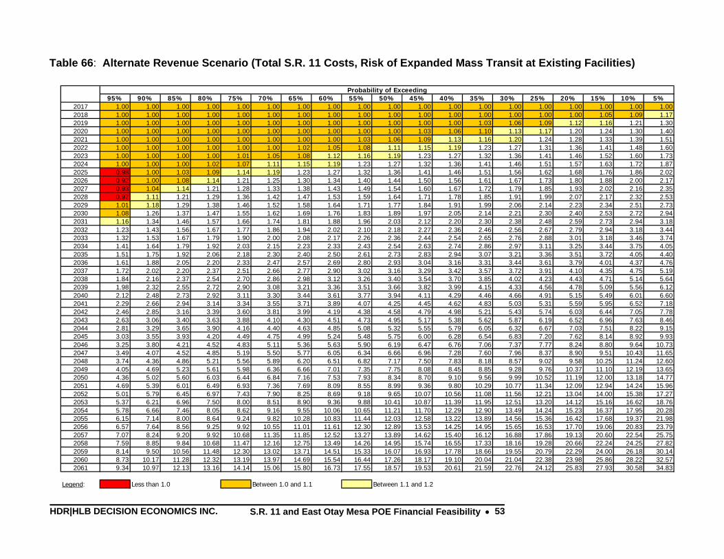
HDR|HLB DECISION ECONOMICS INC. S.R. 11 and East Otay Mesa POE Financial Feasibility • 53
Table 66: Alternate Revenue Scenario (Total S.R. 11 Costs, Risk of Expanded Mass Transit at Existing Facilities)
Probability of Exceeding95% 90% 85% 80% 75% 70% 65% 60% 55% 50% 45% 40% 35% 30% 25% 20% 15% 10% 5%
2017 1.00 1.00 1.00 1.00 1.00 1.00 1.00 1.00 1.00 1.00 1.00 1.00 1.00 1.00 1.00 1.00 1.00 1.00 1.002018 1.00 1.00 1.00 1.00 1.00 1.00 1.00 1.00 1.00 1.00 1.00 1.00 1.00 1.00 1.00 1.00 1.05 1.09 1.172019 1.00 1.00 1.00 1.00 1.00 1.00 1.00 1.00 1.00 1.00 1.00 1.00 1.03 1.06 1.09 1.12 1.16 1.21 1.302020 1.00 1.00 1.00 1.00 1.00 1.00 1.00 1.00 1.00 1.00 1.03 1.06 1.10 1.13 1.17 1.20 1.24 1.30 1.402021 1.00 1.00 1.00 1.00 1.00 1.00 1.00 1.00 1.03 1.06 1.09 1.13 1.16 1.20 1.24 1.28 1.33 1.39 1.512022 1.00 1.00 1.00 1.00 1.00 1.00 1.02 1.05 1.08 1.11 1.15 1.19 1.23 1.27 1.31 1.36 1.41 1.48 1.602023 1.00 1.00 1.00 1.00 1.01 1.05 1.08 1.12 1.16 1.19 1.23 1.27 1.32 1.36 1.41 1.46 1.52 1.60 1.732024 1.00 1.00 1.00 1.02 1.07 1.11 1.15 1.19 1.23 1.27 1.32 1.36 1.41 1.46 1.51 1.57 1.63 1.72 1.872025 0.98 1.00 1.03 1.09 1.14 1.19 1.23 1.27 1.32 1.36 1.41 1.46 1.51 1.56 1.62 1.68 1.76 1.86 2.022026 0.92 1.00 1.08 1.14 1.21 1.25 1.30 1.34 1.40 1.44 1.50 1.56 1.61 1.67 1.73 1.80 1.88 2.00 2.172027 0.93 1.04 1.14 1.21 1.28 1.33 1.38 1.43 1.49 1.54 1.60 1.67 1.72 1.79 1.85 1.93 2.02 2.16 2.352028 0.97 1.11 1.21 1.29 1.36 1.42 1.47 1.53 1.59 1.64 1.71 1.78 1.85 1.91 1.99 2.07 2.17 2.32 2.532029 1.01 1.18 1.29 1.38 1.46 1.52 1.58 1.64 1.71 1.77 1.84 1.91 1.99 2.06 2.14 2.23 2.34 2.51 2.732030 1.08 1.26 1.37 1.47 1.55 1.62 1.69 1.76 1.83 1.89 1.97 2.05 2.14 2.21 2.30 2.40 2.53 2.72 2.942031 1.16 1.34 1.46 1.57 1.66 1.74 1.81 1.88 1.96 2.03 2.12 2.20 2.30 2.38 2.48 2.59 2.73 2.94 3.182032 1.23 1.43 1.56 1.67 1.77 1.86 1.94 2.02 2.10 2.18 2.27 2.36 2.46 2.56 2.67 2.79 2.94 3.18 3.442033 1.32 1.53 1.67 1.79 1.90 2.00 2.08 2.17 2.26 2.36 2.44 2.54 2.65 2.76 2.88 3.01 3.18 3.46 3.742034 1.41 1.64 1.79 1.92 2.03 2.15 2.23 2.33 2.43 2.54 2.63 2.74 2.86 2.97 3.11 3.25 3.44 3.75 4.052035 1.51 1.75 1.92 2.06 2.18 2.30 2.40 2.50 2.61 2.73 2.83 2.94 3.07 3.21 3.36 3.51 3.72 4.05 4.402036 1.61 1.88 2.05 2.20 2.33 2.47 2.57 2.69 2.80 2.93 3.04 3.16 3.31 3.44 3.61 3.79 4.01 4.37 4.762037 1.72 2.02 2.20 2.37 2.51 2.66 2.77 2.90 3.02 3.16 3.29 3.42 3.57 3.72 3.91 4.10 4.35 4.75 5.192038 1.84 2.16 2.37 2.54 2.70 2.86 2.98 3.12 3.26 3.40 3.54 3.70 3.85 4.02 4.23 4.43 4.71 5.14 5.642039 1.98 2.32 2.55 2.72 2.90 3.08 3.21 3.36 3.51 3.66 3.82 3.99 4.15 4.33 4.56 4.78 5.09 5.56 6.122040 2.12 2.48 2.73 2.92 3.11 3.30 3.44 3.61 3.77 3.94 4.11 4.29 4.46 4.66 4.91 5.15 5.49 6.01 6.602041 2.29 2.66 2.94 3.14 3.34 3.55 3.71 3.89 4.07 4.25 4.45 4.62 4.83 5.03 5.31 5.59 5.95 6.52 7.182042 2.46 2.85 3.16 3.39 3.60 3.81 3.99 4.19 4.38 4.58 4.79 4.98 5.21 5.43 5.74 6.03 6.44 7.05 7.782043 2.63 3.06 3.40 3.63 3.88 4.10 4.30 4.51 4.73 4.95 5.17 5.38 5.62 5.87 6.19 6.52 6.96 7.63 8.462044 2.81 3.29 3.65 3.90 4.16 4.40 4.63 4.85 5.08 5.32 5.55 5.79 6.05 6.32 6.67 7.03 7.51 8.22 9.152045 3.03 3.55 3.93 4.20 4.49 4.75 4.99 5.24 5.48 5.75 6.00 6.28 6.54 6.83 7.20 7.62 8.14 8.92 9.932046 3.25 3.80 4.21 4.52 4.83 5.11 5.36 5.63 5.90 6.19 6.47 6.76 7.06 7.37 7.77 8.24 8.80 9.64 10.732047 3.49 4.07 4.52 4.85 5.19 5.50 5.77 6.05 6.34 6.66 6.96 7.28 7.60 7.96 8.37 8.90 9.51 10.43 11.652048 3.74 4.36 4.86 5.21 5.56 5.89 6.20 6.51 6.82 7.17 7.50 7.83 8.18 8.57 9.02 9.58 10.25 11.24 12.602049 4.05 4.69 5.23 5.61 5.98 6.36 6.66 7.01 7.35 7.75 8.08 8.45 8.85 9.28 9.76 10.37 11.10 12.19 13.652050 4.36 5.02 5.60 6.03 6.44 6.84 7.16 7.53 7.93 8.34 8.70 9.10 9.56 9.99 10.52 11.19 12.00 13.18 14.772051 4.69 5.39 6.01 6.49 6.93 7.36 7.69 8.09 8.55 8.99 9.36 9.80 10.29 10.77 11.34 12.09 12.94 14.24 15.962052 5.01 5.79 6.45 6.97 7.43 7.90 8.25 8.69 9.18 9.65 10.07 10.56 11.08 11.56 12.21 13.04 14.00 15.38 17.272053 5.37 6.21 6.96 7.50 8.00 8.51 8.90 9.36 9.88 10.41 10.87 11.39 11.95 12.51 13.20 14.12 15.16 16.62 18.762054 5.78 6.66 7.46 8.05 8.62 9.16 9.55 10.06 10.65 11.21 11.70 12.29 12.90 13.49 14.24 15.23 16.37 17.95 20.282055 6.15 7.14 8.00 8.64 9.24 9.82 10.28 10.83 11.44 12.03 12.58 13.22 13.89 14.56 15.36 16.42 17.68 19.37 21.982056 6.57 7.64 8.56 9.25 9.92 10.55 11.01 11.61 12.30 12.89 13.53 14.25 14.95 15.65 16.53 17.70 19.06 20.83 23.792057 7.07 8.24 9.20 9.92 10.68 11.35 11.85 12.52 13.27 13.89 14.62 15.40 16.12 16.88 17.86 19.13 20.60 22.54 25.752058 7.59 8.85 9.84 10.68 11.47 12.16 12.75 13.49 14.26 14.95 15.74 16.55 17.33 18.16 19.28 20.66 22.24 24.25 27.822059 8.14 9.50 10.56 11.48 12.30 13.02 13.71 14.51 15.33 16.07 16.93 17.78 18.66 19.55 20.79 22.29 24.00 26.18 30.142060 8.73 10.17 11.28 12.32 13.19 13.97 14.69 15.54 16.44 17.26 18.17 19.10 20.04 21.04 22.38 23.98 25.86 28.22 32.572061 9.34 10.97 12.13 13.16 14.14 15.06 15.80 16.73 17.55 18.57 19.53 20.61 21.59 22.76 24.12 25.83 27.93 30.58 34.83
Legend: Less than 1.0 Between 1.0 and 1.1 Between 1.1 and 1.2
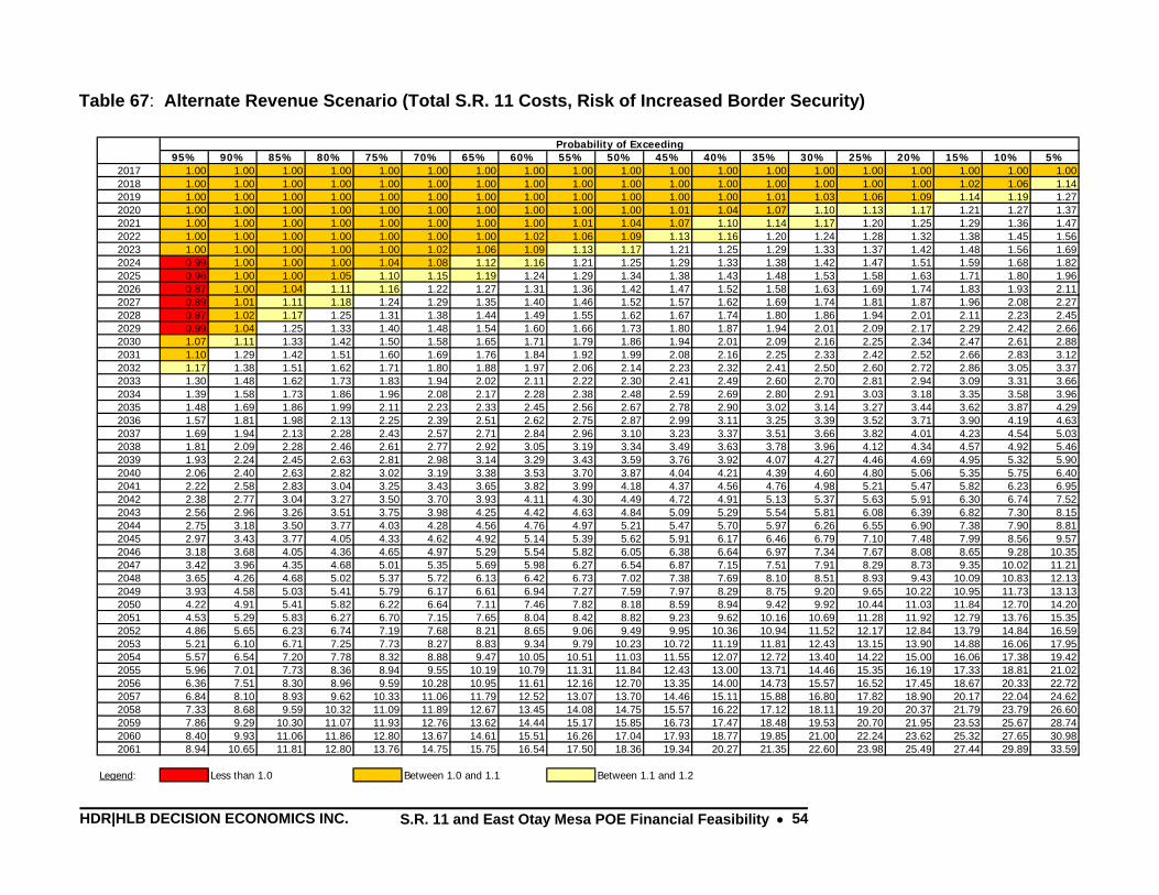
HDR|HLB DECISION ECONOMICS INC. S.R. 11 and East Otay Mesa POE Financial Feasibility • 54
Table 67: Alternate Revenue Scenario (Total S.R. 11 Costs, Risk of Increased Border Security)
Probability of Exceeding95% 90% 85% 80% 75% 70% 65% 60% 55% 50% 45% 40% 35% 30% 25% 20% 15% 10% 5%
2017 1.00 1.00 1.00 1.00 1.00 1.00 1.00 1.00 1.00 1.00 1.00 1.00 1.00 1.00 1.00 1.00 1.00 1.00 1.002018 1.00 1.00 1.00 1.00 1.00 1.00 1.00 1.00 1.00 1.00 1.00 1.00 1.00 1.00 1.00 1.00 1.02 1.06 1.142019 1.00 1.00 1.00 1.00 1.00 1.00 1.00 1.00 1.00 1.00 1.00 1.00 1.01 1.03 1.06 1.09 1.14 1.19 1.272020 1.00 1.00 1.00 1.00 1.00 1.00 1.00 1.00 1.00 1.00 1.01 1.04 1.07 1.10 1.13 1.17 1.21 1.27 1.372021 1.00 1.00 1.00 1.00 1.00 1.00 1.00 1.00 1.01 1.04 1.07 1.10 1.14 1.17 1.20 1.25 1.29 1.36 1.472022 1.00 1.00 1.00 1.00 1.00 1.00 1.00 1.02 1.06 1.09 1.13 1.16 1.20 1.24 1.28 1.32 1.38 1.45 1.562023 1.00 1.00 1.00 1.00 1.00 1.02 1.06 1.09 1.13 1.17 1.21 1.25 1.29 1.33 1.37 1.42 1.48 1.56 1.692024 0.99 1.00 1.00 1.00 1.04 1.08 1.12 1.16 1.21 1.25 1.29 1.33 1.38 1.42 1.47 1.51 1.59 1.68 1.822025 0.96 1.00 1.00 1.05 1.10 1.15 1.19 1.24 1.29 1.34 1.38 1.43 1.48 1.53 1.58 1.63 1.71 1.80 1.962026 0.87 1.00 1.04 1.11 1.16 1.22 1.27 1.31 1.36 1.42 1.47 1.52 1.58 1.63 1.69 1.74 1.83 1.93 2.112027 0.89 1.01 1.11 1.18 1.24 1.29 1.35 1.40 1.46 1.52 1.57 1.62 1.69 1.74 1.81 1.87 1.96 2.08 2.272028 0.97 1.02 1.17 1.25 1.31 1.38 1.44 1.49 1.55 1.62 1.67 1.74 1.80 1.86 1.94 2.01 2.11 2.23 2.452029 0.99 1.04 1.25 1.33 1.40 1.48 1.54 1.60 1.66 1.73 1.80 1.87 1.94 2.01 2.09 2.17 2.29 2.42 2.662030 1.07 1.11 1.33 1.42 1.50 1.58 1.65 1.71 1.79 1.86 1.94 2.01 2.09 2.16 2.25 2.34 2.47 2.61 2.882031 1.10 1.29 1.42 1.51 1.60 1.69 1.76 1.84 1.92 1.99 2.08 2.16 2.25 2.33 2.42 2.52 2.66 2.83 3.122032 1.17 1.38 1.51 1.62 1.71 1.80 1.88 1.97 2.06 2.14 2.23 2.32 2.41 2.50 2.60 2.72 2.86 3.05 3.372033 1.30 1.48 1.62 1.73 1.83 1.94 2.02 2.11 2.22 2.30 2.41 2.49 2.60 2.70 2.81 2.94 3.09 3.31 3.662034 1.39 1.58 1.73 1.86 1.96 2.08 2.17 2.28 2.38 2.48 2.59 2.69 2.80 2.91 3.03 3.18 3.35 3.58 3.962035 1.48 1.69 1.86 1.99 2.11 2.23 2.33 2.45 2.56 2.67 2.78 2.90 3.02 3.14 3.27 3.44 3.62 3.87 4.292036 1.57 1.81 1.98 2.13 2.25 2.39 2.51 2.62 2.75 2.87 2.99 3.11 3.25 3.39 3.52 3.71 3.90 4.19 4.632037 1.69 1.94 2.13 2.28 2.43 2.57 2.71 2.84 2.96 3.10 3.23 3.37 3.51 3.66 3.82 4.01 4.23 4.54 5.032038 1.81 2.09 2.28 2.46 2.61 2.77 2.92 3.05 3.19 3.34 3.49 3.63 3.78 3.96 4.12 4.34 4.57 4.92 5.462039 1.93 2.24 2.45 2.63 2.81 2.98 3.14 3.29 3.43 3.59 3.76 3.92 4.07 4.27 4.46 4.69 4.95 5.32 5.902040 2.06 2.40 2.63 2.82 3.02 3.19 3.38 3.53 3.70 3.87 4.04 4.21 4.39 4.60 4.80 5.06 5.35 5.75 6.402041 2.22 2.58 2.83 3.04 3.25 3.43 3.65 3.82 3.99 4.18 4.37 4.56 4.76 4.98 5.21 5.47 5.82 6.23 6.952042 2.38 2.77 3.04 3.27 3.50 3.70 3.93 4.11 4.30 4.49 4.72 4.91 5.13 5.37 5.63 5.91 6.30 6.74 7.522043 2.56 2.96 3.26 3.51 3.75 3.98 4.25 4.42 4.63 4.84 5.09 5.29 5.54 5.81 6.08 6.39 6.82 7.30 8.152044 2.75 3.18 3.50 3.77 4.03 4.28 4.56 4.76 4.97 5.21 5.47 5.70 5.97 6.26 6.55 6.90 7.38 7.90 8.812045 2.97 3.43 3.77 4.05 4.33 4.62 4.92 5.14 5.39 5.62 5.91 6.17 6.46 6.79 7.10 7.48 7.99 8.56 9.572046 3.18 3.68 4.05 4.36 4.65 4.97 5.29 5.54 5.82 6.05 6.38 6.64 6.97 7.34 7.67 8.08 8.65 9.28 10.352047 3.42 3.96 4.35 4.68 5.01 5.35 5.69 5.98 6.27 6.54 6.87 7.15 7.51 7.91 8.29 8.73 9.35 10.02 11.212048 3.65 4.26 4.68 5.02 5.37 5.72 6.13 6.42 6.73 7.02 7.38 7.69 8.10 8.51 8.93 9.43 10.09 10.83 12.132049 3.93 4.58 5.03 5.41 5.79 6.17 6.61 6.94 7.27 7.59 7.97 8.29 8.75 9.20 9.65 10.22 10.95 11.73 13.132050 4.22 4.91 5.41 5.82 6.22 6.64 7.11 7.46 7.82 8.18 8.59 8.94 9.42 9.92 10.44 11.03 11.84 12.70 14.202051 4.53 5.29 5.83 6.27 6.70 7.15 7.65 8.04 8.42 8.82 9.23 9.62 10.16 10.69 11.28 11.92 12.79 13.76 15.352052 4.86 5.65 6.23 6.74 7.19 7.68 8.21 8.65 9.06 9.49 9.95 10.36 10.94 11.52 12.17 12.84 13.79 14.84 16.592053 5.21 6.10 6.71 7.25 7.73 8.27 8.83 9.34 9.79 10.23 10.72 11.19 11.81 12.43 13.15 13.90 14.88 16.06 17.952054 5.57 6.54 7.20 7.78 8.32 8.88 9.47 10.05 10.51 11.03 11.55 12.07 12.72 13.40 14.22 15.00 16.06 17.38 19.422055 5.96 7.01 7.73 8.36 8.94 9.55 10.19 10.79 11.31 11.84 12.43 13.00 13.71 14.46 15.35 16.19 17.33 18.81 21.022056 6.36 7.51 8.30 8.96 9.59 10.28 10.95 11.61 12.16 12.70 13.35 14.00 14.73 15.57 16.52 17.45 18.67 20.33 22.722057 6.84 8.10 8.93 9.62 10.33 11.06 11.79 12.52 13.07 13.70 14.46 15.11 15.88 16.80 17.82 18.90 20.17 22.04 24.622058 7.33 8.68 9.59 10.32 11.09 11.89 12.67 13.45 14.08 14.75 15.57 16.22 17.12 18.11 19.20 20.37 21.79 23.79 26.602059 7.86 9.29 10.30 11.07 11.93 12.76 13.62 14.44 15.17 15.85 16.73 17.47 18.48 19.53 20.70 21.95 23.53 25.67 28.742060 8.40 9.93 11.06 11.86 12.80 13.67 14.61 15.51 16.26 17.04 17.93 18.77 19.85 21.00 22.24 23.62 25.32 27.65 30.982061 8.94 10.65 11.81 12.80 13.76 14.75 15.75 16.54 17.50 18.36 19.34 20.27 21.35 22.60 23.98 25.49 27.44 29.89 33.59
Legend: Less than 1.0 Between 1.0 and 1.1 Between 1.1 and 1.2
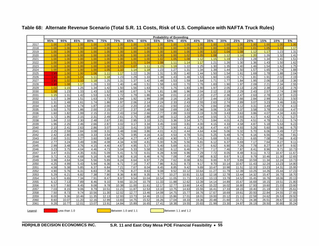
HDR|HLB DECISION ECONOMICS INC. S.R. 11 and East Otay Mesa POE Financial Feasibility • 55
Table 68: Alternate Revenue Scenario (Total S.R. 11 Costs, Risk of U.S. Compliance with NAFTA Truck Rules)
Probability of Exceeding95% 90% 85% 80% 75% 70% 65% 60% 55% 50% 45% 40% 35% 30% 25% 20% 15% 10% 5%
2017 1.00 1.00 1.00 1.00 1.00 1.00 1.00 1.00 1.00 1.00 1.00 1.00 1.00 1.00 1.00 1.00 1.00 1.00 1.002018 1.00 1.00 1.00 1.00 1.00 1.00 1.00 1.00 1.00 1.00 1.00 1.00 1.00 1.00 1.00 1.01 1.05 1.10 1.172019 1.00 1.00 1.00 1.00 1.00 1.00 1.00 1.00 1.00 1.00 1.00 1.00 1.02 1.04 1.08 1.12 1.17 1.23 1.312020 1.00 1.00 1.00 1.00 1.00 1.00 1.00 1.00 1.00 1.00 1.02 1.05 1.08 1.12 1.16 1.20 1.26 1.32 1.412021 1.00 1.00 1.00 1.00 1.00 1.00 1.00 1.00 1.02 1.05 1.08 1.12 1.15 1.19 1.23 1.28 1.34 1.41 1.512022 1.00 1.00 1.00 1.00 1.00 1.00 1.01 1.04 1.08 1.11 1.14 1.17 1.21 1.26 1.30 1.36 1.43 1.50 1.622023 1.00 1.00 1.00 1.00 1.00 1.03 1.07 1.11 1.15 1.19 1.22 1.25 1.30 1.35 1.40 1.46 1.54 1.62 1.752024 1.00 1.00 1.00 1.00 1.05 1.10 1.14 1.18 1.23 1.27 1.31 1.34 1.39 1.44 1.50 1.57 1.65 1.74 1.882025 0.99 1.00 1.00 1.06 1.11 1.17 1.22 1.26 1.31 1.35 1.40 1.44 1.50 1.54 1.61 1.69 1.78 1.88 2.042026 0.91 1.00 1.04 1.11 1.18 1.23 1.29 1.33 1.38 1.43 1.48 1.53 1.60 1.65 1.71 1.81 1.91 2.02 2.192027 0.95 1.02 1.10 1.18 1.25 1.31 1.37 1.42 1.48 1.53 1.59 1.64 1.71 1.77 1.84 1.95 2.06 2.18 2.362028 0.98 1.08 1.17 1.26 1.33 1.40 1.46 1.51 1.58 1.63 1.70 1.76 1.83 1.90 1.97 2.09 2.21 2.34 2.552029 1.02 1.15 1.25 1.34 1.42 1.50 1.56 1.63 1.70 1.75 1.83 1.90 1.97 2.05 2.13 2.26 2.38 2.53 2.762030 1.08 1.23 1.33 1.43 1.52 1.60 1.67 1.74 1.81 1.88 1.96 2.04 2.12 2.19 2.29 2.43 2.57 2.74 2.992031 1.15 1.31 1.42 1.53 1.62 1.72 1.79 1.86 1.94 2.01 2.10 2.20 2.27 2.36 2.47 2.63 2.78 2.97 3.232032 1.22 1.39 1.51 1.63 1.73 1.84 1.92 1.99 2.08 2.16 2.26 2.37 2.44 2.53 2.66 2.84 2.99 3.21 3.502033 1.31 1.48 1.61 1.74 1.86 1.97 2.06 2.14 2.24 2.33 2.43 2.55 2.63 2.74 2.89 3.07 3.23 3.46 3.812034 1.40 1.59 1.74 1.87 2.00 2.12 2.20 2.30 2.41 2.50 2.62 2.75 2.84 2.96 3.12 3.31 3.49 3.73 4.132035 1.50 1.70 1.86 2.00 2.15 2.27 2.37 2.48 2.59 2.69 2.82 2.96 3.06 3.19 3.37 3.58 3.78 4.03 4.472036 1.60 1.82 1.99 2.15 2.31 2.43 2.54 2.66 2.77 2.89 3.03 3.19 3.29 3.43 3.63 3.86 4.07 4.34 4.812037 1.72 1.95 2.15 2.31 2.49 2.61 2.75 2.88 2.98 3.12 3.28 3.44 3.55 3.71 3.93 4.17 4.42 4.71 5.272038 1.84 2.10 2.30 2.48 2.67 2.81 2.95 3.10 3.21 3.36 3.54 3.71 3.84 4.01 4.25 4.51 4.78 5.11 5.742039 1.96 2.25 2.46 2.66 2.87 3.02 3.17 3.34 3.45 3.63 3.81 4.00 4.15 4.33 4.58 4.87 5.18 5.53 6.232040 2.10 2.41 2.63 2.86 3.07 3.23 3.41 3.59 3.72 3.90 4.11 4.30 4.47 4.67 4.93 5.26 5.60 5.96 6.752041 2.25 2.59 2.84 3.08 3.31 3.48 3.66 3.86 4.01 4.21 4.44 4.64 4.84 5.06 5.32 5.70 6.06 6.49 7.272042 2.42 2.80 3.06 3.33 3.54 3.75 3.95 4.16 4.32 4.53 4.78 5.01 5.25 5.48 5.74 6.16 6.56 7.06 7.812043 2.60 3.01 3.27 3.60 3.80 4.04 4.27 4.47 4.65 4.90 5.17 5.41 5.69 5.91 6.21 6.65 7.08 7.66 8.432044 2.77 3.24 3.49 3.86 4.08 4.34 4.59 4.81 5.00 5.26 5.56 5.81 6.12 6.37 6.69 7.17 7.64 8.27 9.112045 2.99 3.48 3.76 4.15 4.40 4.67 4.95 5.17 5.40 5.69 6.01 6.27 6.62 6.90 7.26 7.78 8.27 8.97 9.922046 3.23 3.75 4.04 4.46 4.73 5.04 5.33 5.58 5.82 6.12 6.46 6.77 7.17 7.46 7.87 8.41 8.96 9.71 10.732047 3.47 4.01 4.35 4.81 5.09 5.41 5.73 6.01 6.28 6.59 6.96 7.29 7.72 8.05 8.48 9.11 9.72 10.47 11.672048 3.71 4.31 4.68 5.16 5.48 5.80 6.16 6.46 6.76 7.08 7.49 7.88 8.32 8.67 9.13 9.79 10.46 11.30 12.652049 3.98 4.64 5.04 5.56 5.89 6.24 6.64 6.97 7.29 7.62 8.08 8.51 9.00 9.37 9.89 10.59 11.34 12.24 13.732050 4.25 4.99 5.43 5.94 6.36 6.71 7.14 7.47 7.86 8.21 8.73 9.17 9.70 10.14 10.67 11.43 12.24 13.23 14.802051 4.58 5.38 5.85 6.37 6.84 7.21 7.67 8.04 8.45 8.85 9.42 9.89 10.47 10.98 11.51 12.33 13.23 14.31 15.952052 4.90 5.76 6.31 6.83 7.36 7.76 8.27 8.63 9.08 9.52 10.12 10.64 11.27 11.79 12.39 13.25 14.26 15.44 17.232053 5.29 6.21 6.82 7.38 7.90 8.36 8.90 9.35 9.77 10.27 10.91 11.53 12.18 12.78 13.44 14.32 15.47 16.70 18.702054 5.67 6.65 7.34 7.91 8.47 8.97 9.54 10.04 10.54 11.05 11.71 12.43 13.13 13.79 14.52 15.45 16.76 18.06 20.132055 6.12 7.13 7.89 8.46 9.10 9.66 10.24 10.79 11.33 11.88 12.62 13.39 14.14 14.89 15.67 16.69 18.15 19.51 21.802056 6.57 7.60 8.45 9.08 9.78 10.38 11.00 11.61 12.17 12.77 13.60 14.42 15.22 16.02 16.80 17.93 19.60 21.03 23.602057 7.03 8.15 9.06 9.79 10.51 11.21 11.87 12.53 13.10 13.75 14.63 15.55 16.41 17.33 18.15 19.40 21.19 22.72 25.612058 7.50 8.73 9.74 10.56 11.30 12.02 12.77 13.46 14.08 14.75 15.77 16.76 17.67 18.69 19.61 20.93 22.84 24.55 27.652059 8.00 9.36 10.46 11.35 12.13 12.93 13.73 14.46 15.11 15.86 17.01 18.01 19.00 20.12 21.11 22.58 24.62 26.53 29.922060 8.60 10.07 11.20 12.16 12.99 13.83 14.75 15.52 16.26 17.04 18.33 19.36 20.48 21.60 22.71 24.38 26.51 28.67 32.332061 9.28 10.77 12.01 13.07 13.91 14.84 15.89 16.65 17.41 18.38 19.55 20.83 21.99 23.30 24.87 26.19 28.50 30.80 35.24
Legend: Less than 1.0 Between 1.0 and 1.1 Between 1.1 and 1.2

HDR|HLB DECISION ECONOMICS INC. S.R. 11 and East Otay Mesa POE Financial Feasibility •
56
5.7 Assessment of the Investors Market Assessing the investor market implies the need for information about the supply and cost of private equity and debt for toll road financing. The key driver of supply and cost of capital is credit rating. If the project fails to obtain an investment-grade rating, the large institutional investors (the pension funds, fireman's funds, etc.) are generally not permitted to participate (due to a high risk exposure). It is the institutional investors that hold at least two thirds of most traditionally financed toll roads. Thus, the absence of an investment grade rating might lock this project out of the market. However, if the road is rated investment-grade, the market for toll road revenue bond securities is mature and, while taken aback by recent problems of under-performance, still plentiful. Investment grade toll roads also attract private equity. Examples include Route 407 in Toronto, Canada, and S.R. 125 in California.
Furthermore, if the proposed toll road is in a jurisdiction with Public-Private Partnership enabling legislation, the public sector can, if it chooses, share in the investment cost (through tax-financed sources, such as general obligation bonds, self-help taxes, federal grants and TIFIA credit support). In so doing, the public sector can “elevate” a road with a marginal or even below investment grade rating to the investment grade level, thereby giving rise to a plentiful supply of efficiently priced private capital.
Potential for Public-Private Partnership
The appropriate means of approaching a combined public and private opportunity is through the vehicle known as Public-Private Partnering (PPP). To assess the specific form that such a partnership might take, the following questions need to be addressed:
Is the prospective enterprise likely to generate significant private benefits?
Does the required investment exhibit a high enough degree of financial risk to indicate that private capital alone would be insufficient to finance it?
Would some degree of public involvement encourage private participation?
The public sector is expected to be a significant beneficiary, mainly because the toll road would benefit the region through:
Improved traffic flows;
Reduced highway congestion;
Increased industrial productivity and competitiveness due to improved access;
Improved transportation safety; and
Improved air quality and reduced greenhouse gas emissions.
The public sector can encourage and facilitate the success of the private investment through measures such as:
Ensuring that the zoning around the toll area attracts investment such as warehousing, assembly, and general manufacturing plants;
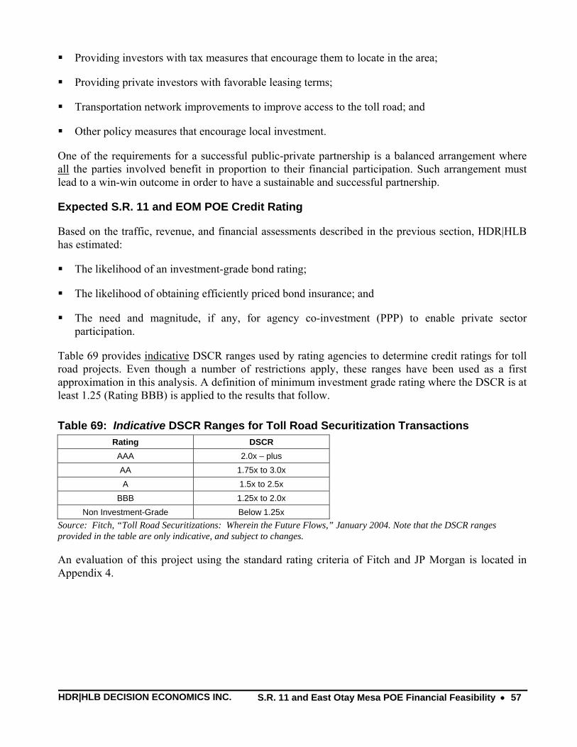
HDR|HLB DECISION ECONOMICS INC. S.R. 11 and East Otay Mesa POE Financial Feasibility •
57
Providing investors with tax measures that encourage them to locate in the area;
Providing private investors with favorable leasing terms;
Transportation network improvements to improve access to the toll road; and
Other policy measures that encourage local investment.
One of the requirements for a successful public-private partnership is a balanced arrangement where all the parties involved benefit in proportion to their financial participation. Such arrangement must lead to a win-win outcome in order to have a sustainable and successful partnership.
Expected S.R. 11 and EOM POE Credit Rating
Based on the traffic, revenue, and financial assessments described in the previous section, HDR|HLB has estimated:
The likelihood of an investment-grade bond rating;
The likelihood of obtaining efficiently priced bond insurance; and
The need and magnitude, if any, for agency co-investment (PPP) to enable private sector participation.
Table 69 provides indicative DSCR ranges used by rating agencies to determine credit ratings for toll road projects. Even though a number of restrictions apply, these ranges have been used as a first approximation in this analysis. A definition of minimum investment grade rating where the DSCR is at least 1.25 (Rating BBB) is applied to the results that follow.
Table 69: Indicative DSCR Ranges for Toll Road Securitization Transactions Rating DSCR
AAA 2.0x – plus AA 1.75x to 3.0x A 1.5x to 2.5x
BBB 1.25x to 2.0x Non Investment-Grade Below 1.25x
Source: Fitch, “Toll Road Securitizations: Wherein the Future Flows,” January 2004. Note that the DSCR ranges provided in the table are only indicative, and subject to changes.
An evaluation of this project using the standard rating criteria of Fitch and JP Morgan is located in Appendix 4.

HDR|HLB DECISION ECONOMICS INC. S.R. 11 and East Otay Mesa POE Financial Feasibility •
58
Table 70: Expected S.R. 11 and EOM POE Credit Ratings and Needs for Public Co-Investments (In Millions of 2012 Dollars)
Scenario Total
Capital Costs
Annual O&M Costs
Capital Grant
Likelihood of
"Success" 1
Likelihood of Investment
Grade Rating2
Cost Scenarios Baseline Scenario $0 S.R.-11 Capital and O&M Costs 0%
>90% 75% - 80%
$50
$294.5 $0.42
17% >95% 80% - 85%
Scenario C-1 $300 S.R.-11 Capital and O&M Costs, plus POE Capital Costs 45%
>80% 65% - 70%
$400
$660.4 $0.42
61% >95% 80% - 85%
Scenario C-2 $400 S.R.-11 Capital and O&M Costs, plus POE Capital and O&M Costs
$660.4 $37.02 61%
<5% <5%
Scenario C-3 $400 S.R.-11 Capital and O&M Costs, plus POE Capital and O&M Costs after 30 years
$660.4 $37.02 61%
>90% 75% - 80%
Revenue Scenarios (with Baseline Cost) Scenario R-1 $0 Integration of Mexican Toll Road
$294.5 $0.42 0%
>95% 80% - 85%
Scenario R-2 $0 Pedestrian crossing at EOM
$294.5 $0.42 0%
>95% 80% - 85%
Scenario R-3 $0 Truck only service at EOM
$294.5 $0.42 0%
>80% 65% - 70%
Risk Factor Scenarios (with Baseline Cost) Scenario RF-1 $0 Opening of Punta Colonet
$294.5 $0.42 0%
>90% 75% - 80%
Scenario RF-2 $0 Expanded Mass Transit at Existing Facilities
$294.5 $0.42 0%
>90% 75% - 80%
Scenario RF-3 $0 Increased Border Security
$294.5 $0.42 0%
>90% 75% - 80%
Scenario RF-4 $0 Truck Compliance with NAFTA
$294.5 $0.42 0%
>90% 75% - 80%
Note: (1) Major bond insurers (with AAA ratings) would prefer to insure projects with a 99% probability that the DSCR (the first percentile) is 1.0 or higher. This level of analysis is limited to an upper probability bound of 95%. Exact determination at the 99% level may be required by the major bond insurers. (2) Major bond insurers (with AAA ratings) consider a DSCR of 1.25 to be the minimum level for an investment grade rating of BBB.
HDR|HLB DECISION ECONOMICS INC. S.R. 11 and East Otay Mesa POE Financial Feasibility •
59
CHAPTER 6: CONCLUSIONS
The main conclusion of this analysis is that, given the existing level of uncertainty surrounding key assumptions, the S.R. 11 toll road is a potentially good investment provided that there are sufficient external resources to cover the capital and O&M costs of EOM. With traditional debt finance, minor default risks may occur in early years. Its potential would be enhanced by integration with Mexican toll roads, an outcome that most experts consider likely.
S.R. 11 however cannot be considered without EOM. Accordingly, as indicated in the core of the report, public participation would be necessary to attract sufficient private capital and finance construction and management of EOM. A grant or other financing mechanism with back-loaded debt service/repayments is needed (possibly low-interest loan from the Transportation Infrastructure Finance and Innovation Act or TIFIA).
Strengths, weaknesses, and an assessment of the investor market can be summarized as follows:
Strengths
• EOM and S.R. 11 would be an alternative border crossing to increasingly congested OM and SY facilities.
• New facilities would offer dramatic travel time savings for users.
• Travelers continuing to use the free POEs would experience small reductions in wait times, but if aggregated would amount to a sizable public benefit.
• Over the next several decades, population growth in the region – especially in Mexico, would lead to success of the toll facilities.
Weaknesses
• Estimated construction and operational costs for S.R. 11 and EOM are quite expensive.
• As with most toll road start-ups, a financing plan with relatively low obligations in early years of operations (e.g., principal repayments starting a few years after opening) would be needed to be viable.
Investor Market assessment
• The analysis reveals that S.R. 11 and EOM POE would require at least $400 million in external funds to pay for all construction costs. This level of funding is however insufficient to cover the EOM POE O&M costs until the facility has been operating for 30 years.
• Integration with the Mexican toll road would lower the total cost burden somewhat, but not enough to pay for the annual O&M shortfall at the EOM POE.
HDR|HLB DECISION ECONOMICS INC. S.R. 11 and East Otay Mesa POE Financial Feasibility •
60
Conclusions
• S.R. 11 and the EOM POE meet the criteria for a successful toll road project that are:7
a. The new EOM POE and toll road relieve congestion at the existing SY and OM POEs in an already developed border region;
b. It provides a quicker and more convenient connection between existing and planned pockets of residential and commercial development; and
c. The time savings from taking the toll road more than compensates the users for paying the toll.
• While S.R. 11 and EOM may generate substantial traffic and toll revenues, public contributions would be necessary to generate private investment interest.
Next Steps Given the need for public participation, some additional analyses may be needed. These include an assessment of economic benefits and distributional welfare effects on the region (i.e. an assessment of whether the rate of return from the social perspective warrants the local public investments in the project). In addition, conducting a due diligence and risk-based assessment of estimated construction and O&M costs of S.R. 11 and the EOM POE may identify mitigation strategies for reducing risks. Also, a more complete financial analysis could broaden the scope of study to explore the potential of non-toll revenues (e.g. development fees) to reduce grant needs and to explore mechanisms for alleviating short falls in O&M costs.
7 Source: William Streeter and Katherine McManus, “Challenges of Start-Up Toll Roads,” Project Finance Special Report, Fitch, June 9, 1999

HDR|HLB DECISION ECONOMICS INC. S.R. 11 and East Otay Mesa POE Financial Feasibility •
61
APPENDIX 1: SUPPLEMENTARY DATA TABLES AND GRAPHS
A. U.S. Real GDP and San Diego Real GRP Data Source: San Diego Chamber of Commerce; Bureau of Economic Analysis, U.S. Department of Commerce; Congressional Budget Office (CBO) Economic Projections for 2006 to 2016.
Historical Data
Year Change in US GDP
Change in SD GRP
Difference (Change in SD GRP – Change in US GDP)
1990 1.9% 1.4% -0.5% 1991 -0.2% -0.5% -0.3% 1992 3.3% -1.1% -4.4% 1993 2.7% -0.8% -3.5% 1994 4.0% 1.5% -2.5% 1995 2.5% 2.6% 0.1% 1996 3.7% 4.1% 0.4% 1997 4.5% 6.5% 2.0% 1998 4.2% 8.0% 3.8% 1999 4.5% 9.4% 4.9% 2000 3.7% 7.0% 3.3% 2001 0.8% 1.4% 0.6% 2002 1.6% 4.0% 2.4% 2003 2.5% 3.4% 0.9% 2004 3.9% 5.7% 1.8% 2005 3.2% 4.7% 1.5%
Average difference 2001-2005 1.4%
CBO's Year By Year Projections for Fiscal Years
2006-2016 CBO Projections + 1.4%
Year Projections San Diego GRP Projections 2006 3.4% 4.8% 2007 3.2% 4.6% 2008 3.1% 4.5% 2009 3.1% 4.5% 2010 3.1% 4.5% 2011 2.8% 4.2% 2012 2.7% 4.1% 2013 2.7% 4.1% 2014 2.6% 4.0% 2015 2.6% 4.0% 2016 2.5% 3.9%

HDR|HLB DECISION ECONOMICS INC. S.R. 11 and East Otay Mesa POE Financial Feasibility •
62
B. Assumptions about Existing POE Operations and Use Data Source: U.S. Customs and Border Protection (CBP) and SANDAG.
This chart indicates the numbers of lanes and hours of operation for the existing and proposed point of entry at EOM.
Existing POEs New POE
Type of Lane OM SY EOM
Total Autos 8 24 8 SENTRI able 1 4 1 Trucks 8 NA 8 FAST 1 NA 1
Hours of operation Autos 24 hours / 7 days 24 hours / 7 days same as OM SENTRI able 5:00 AM-8:00 PM / Weekdays 4:00 AM-12:00 AM / 7 days Trucks 6:00 AM-8:00 PM / Weekdays 9:00 AM-5:00 PM / Weekends
C. Assumptions about Peak Periods This chart provides results of an assessment of peak periods on weekdays and weekends for all existing POE based on the numbers of lanes open and the waiting time (WT). Hourly CBP data for 6 months (April – September, 2006) were used in determining peak periods.
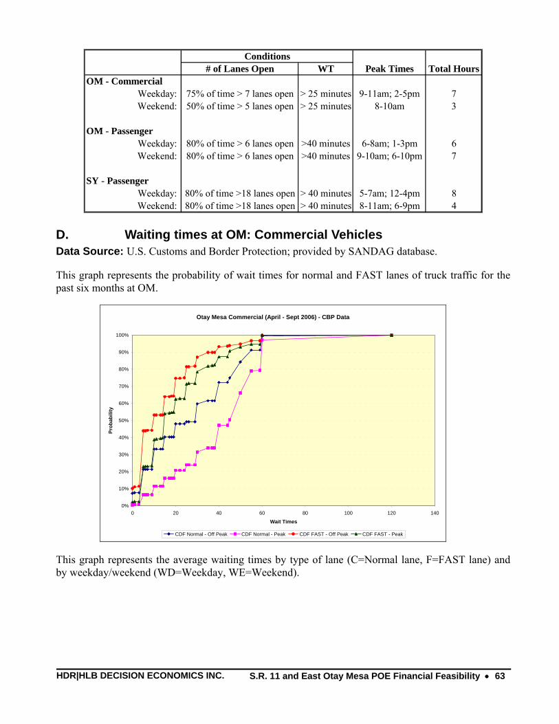
HDR|HLB DECISION ECONOMICS INC. S.R. 11 and East Otay Mesa POE Financial Feasibility •
63
# of Lanes Open WT Peak Times Total HoursOM - Commercial
Weekday: 75% of time > 7 lanes open > 25 minutes 9-11am; 2-5pm 7Weekend: 50% of time > 5 lanes open > 25 minutes 8-10am 3
OM - PassengerWeekday: 80% of time > 6 lanes open >40 minutes 6-8am; 1-3pm 6Weekend: 80% of time > 6 lanes open >40 minutes 9-10am; 6-10pm 7
SY - PassengerWeekday: 80% of time >18 lanes open > 40 minutes 5-7am; 12-4pm 8Weekend: 80% of time >18 lanes open > 40 minutes 8-11am; 6-9pm 4
Conditions
D. Waiting times at OM: Commercial Vehicles Data Source: U.S. Customs and Border Protection; provided by SANDAG database.
This graph represents the probability of wait times for normal and FAST lanes of truck traffic for the past six months at OM.
Otay Mesa Commercial (April - Sept 2006) - CBP Data
0%
10%
20%
30%
40%
50%
60%
70%
80%
90%
100%
0 20 40 60 80 100 120 140
Wait Times
Prob
abili
ty
CDF Normal - Off Peak CDF Normal - Peak CDF FAST - Off Peak CDF FAST - Peak
This graph represents the average waiting times by type of lane (C=Normal lane, F=FAST lane) and by weekday/weekend (WD=Weekday, WE=Weekend).
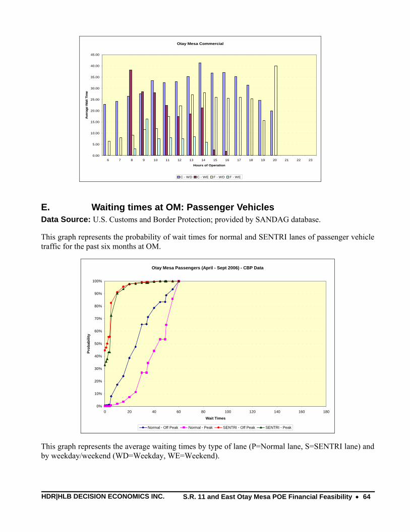
HDR|HLB DECISION ECONOMICS INC. S.R. 11 and East Otay Mesa POE Financial Feasibility •
64
Otay Mesa Commercial
0.00
5.00
10.00
15.00
20.00
25.00
30.00
35.00
40.00
45.00
6 7 8 9 10 11 12 13 14 15 16 17 18 19 20 21 22 23
Hours of Operation
Ave
rage
Wai
t Tim
e
C - WD C - WE F - WD F - WE
E. Waiting times at OM: Passenger Vehicles Data Source: U.S. Customs and Border Protection; provided by SANDAG database.
This graph represents the probability of wait times for normal and SENTRI lanes of passenger vehicle traffic for the past six months at OM.
Otay Mesa Passengers (April - Sept 2006) - CBP Data
0%
10%
20%
30%
40%
50%
60%
70%
80%
90%
100%
0 20 40 60 80 100 120 140 160 180
Wait Times
Prob
abili
ty
Normal - Off Peak Normal - Peak SENTRI - Off Peak SENTRI - Peak
This graph represents the average waiting times by type of lane (P=Normal lane, S=SENTRI lane) and by weekday/weekend (WD=Weekday, WE=Weekend).
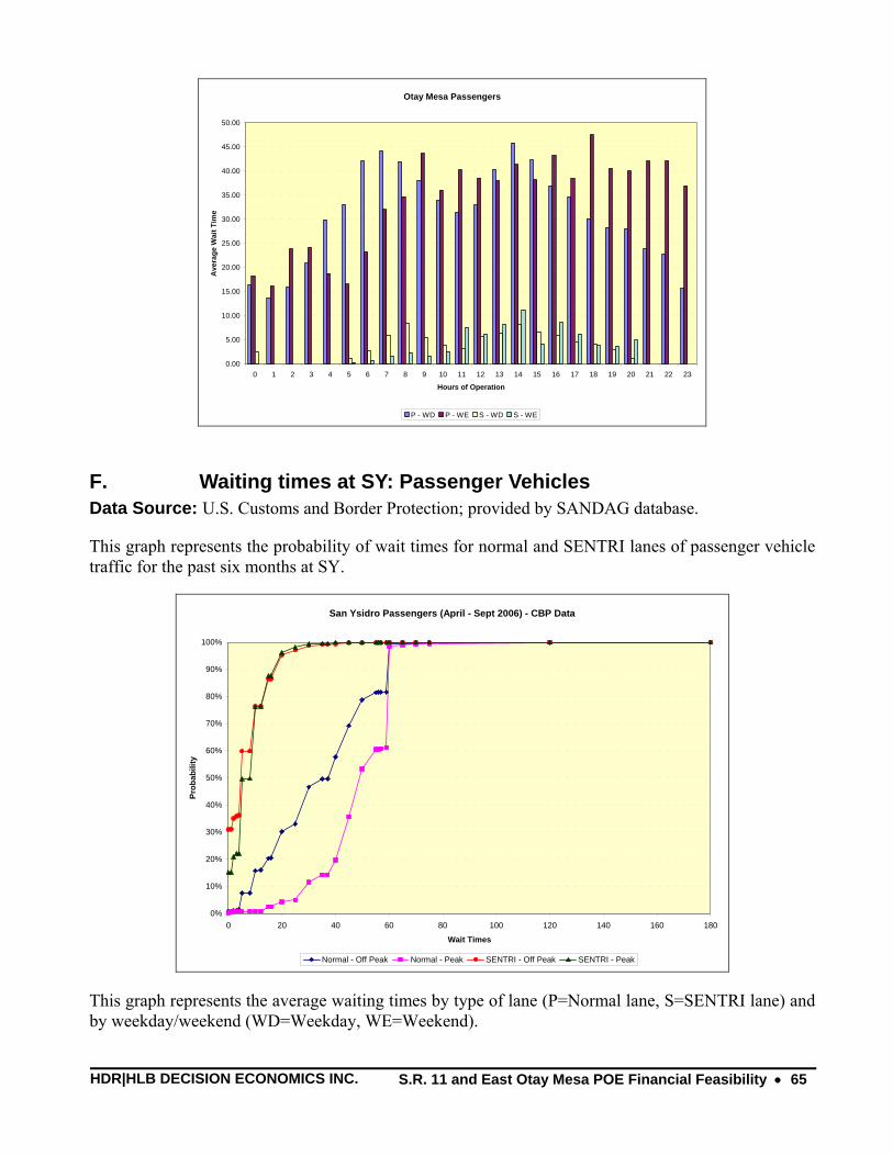
HDR|HLB DECISION ECONOMICS INC. S.R. 11 and East Otay Mesa POE Financial Feasibility •
65
Otay Mesa Passengers
0.00
5.00
10.00
15.00
20.00
25.00
30.00
35.00
40.00
45.00
50.00
0 1 2 3 4 5 6 7 8 9 10 11 12 13 14 15 16 17 18 19 20 21 22 23
Hours of Operation
Ave
rage
Wai
t Tim
e
P - WD P - WE S - WD S - WE
F. Waiting times at SY: Passenger Vehicles Data Source: U.S. Customs and Border Protection; provided by SANDAG database.
This graph represents the probability of wait times for normal and SENTRI lanes of passenger vehicle traffic for the past six months at SY.
San Ysidro Passengers (April - Sept 2006) - CBP Data
0%
10%
20%
30%
40%
50%
60%
70%
80%
90%
100%
0 20 40 60 80 100 120 140 160 180
Wait Times
Prob
abili
ty
Normal - Off Peak Normal - Peak SENTRI - Off Peak SENTRI - Peak
This graph represents the average waiting times by type of lane (P=Normal lane, S=SENTRI lane) and by weekday/weekend (WD=Weekday, WE=Weekend).

HDR|HLB DECISION ECONOMICS INC. S.R. 11 and East Otay Mesa POE Financial Feasibility •
66
San Ysidro Passengers
0.00
5.00
10.00
15.00
20.00
25.00
30.00
35.00
40.00
45.00
50.00
0 1 2 3 4 5 6 7 8 9 10 11 12 13 14 15 16 17 18 19 20 21 22 23
Hours of Operation
Ave
rage
Wai
t Tim
e
P - WD P - WE S - WD S - WE
G. Expected Waiting times at SY and OM (Survey Data) Data Source: HDR|HLB Decision Economics Inc. (2005). Surveys were conducted of random passenger vehicles waiting to cross the border. Their actual waiting time is unknown.
This graph represents expected waiting times for peak and off-peak periods in normal lanes.
Expected Peak and Off-Peak Wait Times in Normal Lanes at San Ysidro and Otay Mesa
0%
5%
10%
15%
20%
25%
30%
35%
0 1 4 5 10 12 15 20 25 30 35 40 45 50 60 63 65 70 75 80 90 100 105 120 150 180 195 240
Expected Wait Times
Prop
ortio
n of
Res
pond
ents
/ Pa
ssen
ger V
ehic
les
San Ysidro - Off Peak San Ysidro - Peak Otay Mesa - Off Peak Otay Mesa - Peak
This graph represents expected waiting times for peak and off-peak periods in SENTRI lanes.
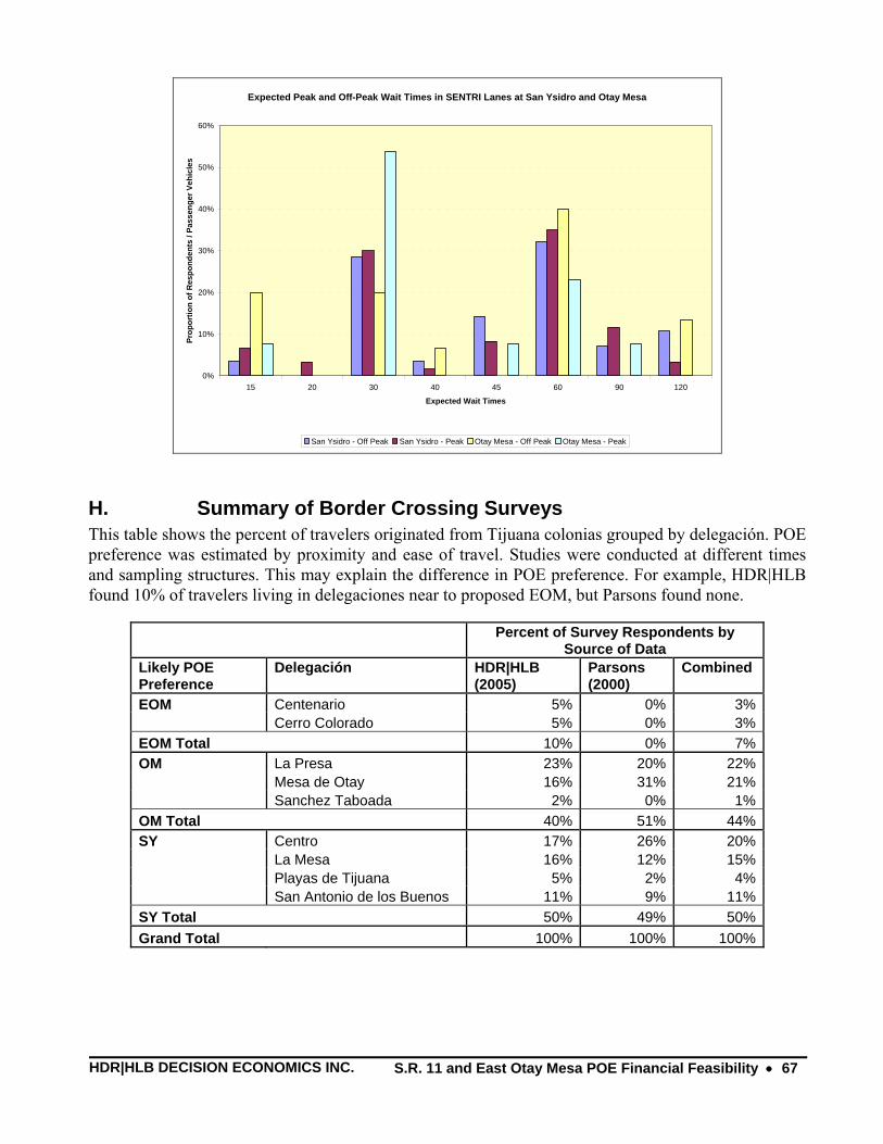
HDR|HLB DECISION ECONOMICS INC. S.R. 11 and East Otay Mesa POE Financial Feasibility •
67
Expected Peak and Off-Peak Wait Times in SENTRI Lanes at San Ysidro and Otay Mesa
0%
10%
20%
30%
40%
50%
60%
15 20 30 40 45 60 90 120
Expected Wait Times
Prop
ortio
n of
Res
pond
ents
/ Pa
ssen
ger V
ehic
les
San Ysidro - Off Peak San Ysidro - Peak Otay Mesa - Off Peak Otay Mesa - Peak
H. Summary of Border Crossing Surveys This table shows the percent of travelers originated from Tijuana colonias grouped by delegación. POE preference was estimated by proximity and ease of travel. Studies were conducted at different times and sampling structures. This may explain the difference in POE preference. For example, HDR|HLB found 10% of travelers living in delegaciones near to proposed EOM, but Parsons found none.
Percent of Survey Respondents by
Source of Data Likely POE Preference
Delegación HDR|HLB (2005)
Parsons (2000)
Combined
EOM Centenario 5% 0% 3% Cerro Colorado 5% 0% 3%EOM Total 10% 0% 7%OM La Presa 23% 20% 22% Mesa de Otay 16% 31% 21% Sanchez Taboada 2% 0% 1%OM Total 40% 51% 44%SY Centro 17% 26% 20% La Mesa 16% 12% 15% Playas de Tijuana 5% 2% 4% San Antonio de los Buenos 11% 9% 11%SY Total 50% 49% 50%Grand Total 100% 100% 100%
HDR|HLB DECISION ECONOMICS INC. S.R. 11 and East Otay Mesa POE Financial Feasibility •
68
APPENDIX 2: RAP PRIMER
Economic forecasts traditionally take the form of a single “expected outcome” supplemented with alternative scenarios. The limitation of a forecast with a single expected outcome is clear -- while it may provide the single best statistical estimate, it offers no information about the range of other possible outcomes and their associated probabilities. The problem becomes acute when uncertainty surrounding the forecast’s underlying assumptions is material.
A common approach is to create “high case” and “low case” scenarios to bracket the central estimate. This scenario approach can exacerbate the problem of dealing with risk because it gives no indication of likelihood associated with the alternative outcomes. The commonly reported “high case” may assume that most underlying assumptions deviate in the same direction from their expected value, and likewise for the “low case.” In reality, the likelihood that all underlying factors shift in the same direction simultaneously is just as remote as that of everything turning out as expected.
Another common approach to providing added perspective on reality is “sensitivity analysis.” Key forecast assumptions are varied one at a time in order to assess their relative impact on the expected outcome. A problem here is that the assumptions are often varied by arbitrary amounts. A more serious concern with this approach is that, in the real world, assumptions do not veer from actual outcomes one at a time. It is the impact of simultaneous differences between assumptions and actual outcomes that is needed to provide a realistic perspective on the riskiness of a forecast.
Risk Analysis provides a way around the problems outlined above. It helps avoid the lack of perspective in “high” and “low” cases by measuring the probability or “odds” that an outcome will actually materialize. This is accomplished by attaching ranges (probability distributions) to the forecasts of each input variable. The approach allows all inputs to be varied simultaneously within their distributions, thus avoiding the problems inherent in conventional sensitivity analysis. The approach also recognizes interrelationships between variables and their associated probability distributions.
The Risk Analysis Process involves four steps:
Step 1. Define the structure and logic of the forecasting problem;
Step 2. Assign estimates and ranges (probability distributions) to each variable and forecasting coefficient in the forecasting structure and logic;
Step 3. Engage experts and stakeholders in assessment of model and assumption risks (the “RAP Session”); and
Step 4. Issue forecast risk analysis.
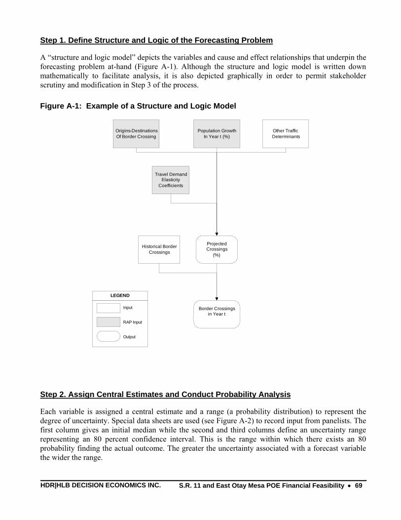
HDR|HLB DECISION ECONOMICS INC. S.R. 11 and East Otay Mesa POE Financial Feasibility •
69
Step 1. Define Structure and Logic of the Forecasting Problem
A “structure and logic model” depicts the variables and cause and effect relationships that underpin the forecasting problem at-hand (Figure A-1). Although the structure and logic model is written down mathematically to facilitate analysis, it is also depicted graphically in order to permit stakeholder scrutiny and modification in Step 3 of the process.
Figure A-1: Example of a Structure and Logic Model
Population Growth In Year t (%)
Other Traffic Determinants
Travel Demand Elasticity
Coefficients
Projected Crossings
(%)
Historical Border Crossings
Input
RAP Input
Output
LEGEND
Border Crossingsin Year t
Origins-Destinations Of Border Crossing
Step 2. Assign Central Estimates and Conduct Probability Analysis
Each variable is assigned a central estimate and a range (a probability distribution) to represent the degree of uncertainty. Special data sheets are used (see Figure A-2) to record input from panelists. The first column gives an initial median while the second and third columns define an uncertainty range representing an 80 percent confidence interval. This is the range within which there exists an 80 probability finding the actual outcome. The greater the uncertainty associated with a forecast variable the wider the range.
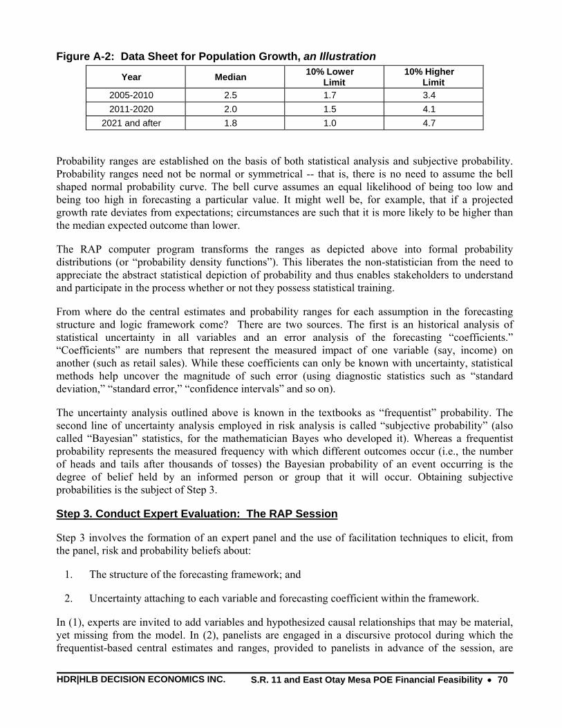
HDR|HLB DECISION ECONOMICS INC. S.R. 11 and East Otay Mesa POE Financial Feasibility •
70
Figure A-2: Data Sheet for Population Growth, an Illustration
Year Median 10% Lower Limit
10% Higher Limit
2005-2010 2.5 1.7 3.4 2011-2020 2.0 1.5 4.1
2021 and after 1.8 1.0 4.7
Probability ranges are established on the basis of both statistical analysis and subjective probability. Probability ranges need not be normal or symmetrical -- that is, there is no need to assume the bell shaped normal probability curve. The bell curve assumes an equal likelihood of being too low and being too high in forecasting a particular value. It might well be, for example, that if a projected growth rate deviates from expectations; circumstances are such that it is more likely to be higher than the median expected outcome than lower.
The RAP computer program transforms the ranges as depicted above into formal probability distributions (or “probability density functions”). This liberates the non-statistician from the need to appreciate the abstract statistical depiction of probability and thus enables stakeholders to understand and participate in the process whether or not they possess statistical training.
From where do the central estimates and probability ranges for each assumption in the forecasting structure and logic framework come? There are two sources. The first is an historical analysis of statistical uncertainty in all variables and an error analysis of the forecasting “coefficients.” “Coefficients” are numbers that represent the measured impact of one variable (say, income) on another (such as retail sales). While these coefficients can only be known with uncertainty, statistical methods help uncover the magnitude of such error (using diagnostic statistics such as “standard deviation,” “standard error,” “confidence intervals” and so on).
The uncertainty analysis outlined above is known in the textbooks as “frequentist” probability. The second line of uncertainty analysis employed in risk analysis is called “subjective probability” (also called “Bayesian” statistics, for the mathematician Bayes who developed it). Whereas a frequentist probability represents the measured frequency with which different outcomes occur (i.e., the number of heads and tails after thousands of tosses) the Bayesian probability of an event occurring is the degree of belief held by an informed person or group that it will occur. Obtaining subjective probabilities is the subject of Step 3.
Step 3. Conduct Expert Evaluation: The RAP Session
Step 3 involves the formation of an expert panel and the use of facilitation techniques to elicit, from the panel, risk and probability beliefs about:
1. The structure of the forecasting framework; and
2. Uncertainty attaching to each variable and forecasting coefficient within the framework.
In (1), experts are invited to add variables and hypothesized causal relationships that may be material, yet missing from the model. In (2), panelists are engaged in a discursive protocol during which the frequentist-based central estimates and ranges, provided to panelists in advance of the session, are
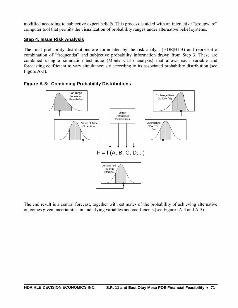
HDR|HLB DECISION ECONOMICS INC. S.R. 11 and East Otay Mesa POE Financial Feasibility •
71
modified according to subjective expert beliefs. This process is aided with an interactive “groupware” computer tool that permits the visualization of probability ranges under alternative belief systems.
Step 4. Issue Risk Analysis
The final probability distributions are formulated by the risk analyst (HDR|HLB) and represent a combination of “frequentist” and subjective probability information drawn from Step 3. These are combined using a simulation technique (Monte Carlo analysis) that allows each variable and forecasting coefficient to vary simultaneously according to its associated probability distribution (see Figure A-3).
Figure A-3: Combining Probability Distributions
F = f (A, B, C, D, ..)
Exchange Rate Outlook (%)
San DiegoPopulation Growth (%)
Diversion to New POE
(%)
Value of Time($ per hour)
Annual Toll Revenue($Million)
Jointly Determined Probabilities
The end result is a central forecast, together with estimates of the probability of achieving alternative outcomes given uncertainties in underlying variables and coefficients (see Figures A-4 and A-5).
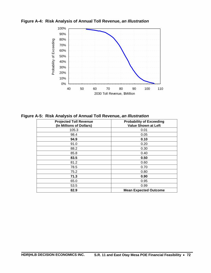
HDR|HLB DECISION ECONOMICS INC. S.R. 11 and East Otay Mesa POE Financial Feasibility •
72
Figure A-4: Risk Analysis of Annual Toll Revenue, an Illustration
0%10%
20%30%
40%50%
60%70%
80%90%
100%
40 50 60 70 80 90 100 1102030 Toll Revenue, $Million
Pro
babi
lity
of E
xcee
ding
Figure A-5: Risk Analysis of Annual Toll Revenue, an Illustration Projected Toll Revenue (In Millions of Dollars)
Probability of Exceeding Value Shown at Left
105.3 0.01 98.4 0.05 94.9 0.10 91.0 0.20 88.2 0.30 85.8 0.40 83.5 0.50 81.2 0.60 78.5 0.70 75.2 0.80 71.3 0.90 65.0 0.95 53.5 0.99 82.9 Mean Expected Outcome

HDR|HLB DECISION ECONOMICS INC. S.R. 11 and East Otay Mesa POE Financial Feasibility •
73
APPENDIX 3: PANELIST INPUTS
On November 2, 2006, a risk analysis workshop was held in San Diego, to discuss the forecasting process and gather inputs both on the forecasting models as well as on the key variables driving the forecasts. The panel consisted of local professionals representing both the public and the private sectors including Federal Highway Administration (FHWA), California Department of Transportation (Caltrans), and San Diego Association of Governments (SANDAG).
A summary of panelist inputs for the following variables is provided on the next pages:
Population growth in primary market area, %
Population growth in San Diego County, %
Population growth in Tijuana, %
Population growth in Baja California, %
Nominal exchange rate outlook, %
San Diego Real Gross Regional Product growth, %
Value of time for passenger vehicles and trucks ($ per hour, and % growth in real terms)
Waiting Times for passenger vehicles and trucks
Percentage of traffic in peak period
S.R. 11 traffic ramp-up: opening year level and years to steady state
Impact of Tijuana-Tecate Toll Road for passenger vehicles and trucks
Potential of pedestrian crossings at EOM
Other risks to border crossings
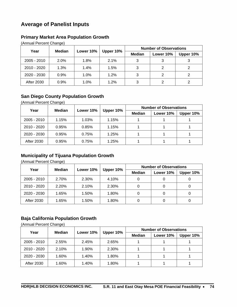
HDR|HLB DECISION ECONOMICS INC. S.R. 11 and East Otay Mesa POE Financial Feasibility •
74
Average of Panelist Inputs
Primary Market Area Population Growth (Annual Percent Change)
Number of Observations Year Median Lower 10% Upper 10%
Median Lower 10% Upper 10% 2005 - 2010 2.0% 1.8% 2.1% 3 3 3
2010 - 2020 1.3% 1.4% 1.5% 3 2 2
2020 - 2030 0.9% 1.0% 1.2% 3 2 2
After 2030 0.9% 1.0% 1.2% 3 2 2
San Diego County Population Growth (Annual Percent Change)
Number of Observations Year Median Lower 10% Upper 10%
Median Lower 10% Upper 10% 2005 - 2010 1.15% 1.03% 1.15% 1 1 1
2010 - 2020 0.95% 0.85% 1.15% 1 1 1
2020 - 2030 0.95% 0.75% 1.25% 1 1 1
After 2030 0.95% 0.75% 1.25% 1 1 1
Municipality of Tijuana Population Growth (Annual Percent Change)
Number of Observations Year Median Lower 10% Upper 10%
Median Lower 10% Upper 10% 2005 - 2010 2.70% 2.30% 4.10% 0 0 0
2010 - 2020 2.20% 2.10% 2.30% 0 0 0
2020 - 2030 1.65% 1.50% 1.80% 0 0 0
After 2030 1.65% 1.50% 1.80% 0 0 0
Baja California Population Growth (Annual Percent Change)
Number of Observations Year Median Lower 10% Upper 10%
Median Lower 10% Upper 10% 2005 - 2010 2.55% 2.45% 2.65% 1 1 1
2010 - 2020 2.10% 1.90% 2.30% 1 1 1
2020 - 2030 1.60% 1.40% 1.80% 1 1 1
After 2030 1.60% 1.40% 1.80% 1 1 1
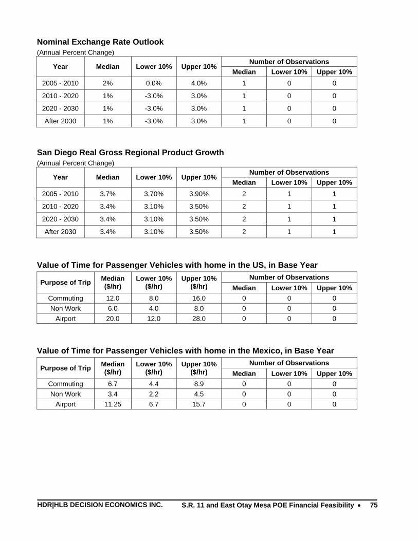
HDR|HLB DECISION ECONOMICS INC. S.R. 11 and East Otay Mesa POE Financial Feasibility •
75
Nominal Exchange Rate Outlook (Annual Percent Change)
Number of Observations Year Median Lower 10% Upper 10%
Median Lower 10% Upper 10% 2005 - 2010 2% 0.0% 4.0% 1 0 0
2010 - 2020 1% -3.0% 3.0% 1 0 0
2020 - 2030 1% -3.0% 3.0% 1 0 0
After 2030 1% -3.0% 3.0% 1 0 0
San Diego Real Gross Regional Product Growth (Annual Percent Change)
Number of Observations Year Median Lower 10% Upper 10%
Median Lower 10% Upper 10% 2005 - 2010 3.7% 3.70% 3.90% 2 1 1
2010 - 2020 3.4% 3.10% 3.50% 2 1 1
2020 - 2030 3.4% 3.10% 3.50% 2 1 1
After 2030 3.4% 3.10% 3.50% 2 1 1
Value of Time for Passenger Vehicles with home in the US, in Base Year Number of Observations
Purpose of Trip Median ($/hr)
Lower 10% ($/hr)
Upper 10% ($/hr) Median Lower 10% Upper 10%
Commuting 12.0 8.0 16.0 0 0 0 Non Work 6.0 4.0 8.0 0 0 0
Airport 20.0 12.0 28.0 0 0 0
Value of Time for Passenger Vehicles with home in the Mexico, in Base Year Number of Observations
Purpose of Trip Median ($/hr)
Lower 10% ($/hr)
Upper 10% ($/hr) Median Lower 10% Upper 10%
Commuting 6.7 4.4 8.9 0 0 0 Non Work 3.4 2.2 4.5 0 0 0
Airport 11.25 6.7 15.7 0 0 0
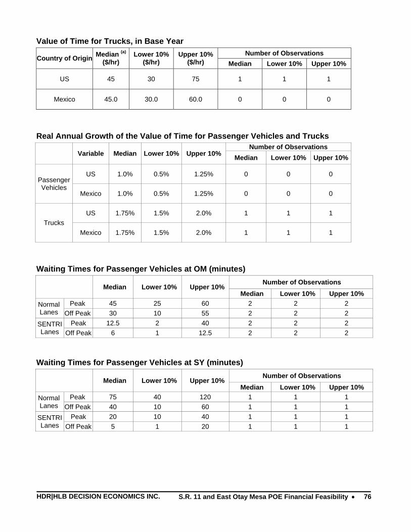
HDR|HLB DECISION ECONOMICS INC. S.R. 11 and East Otay Mesa POE Financial Feasibility •
76
Value of Time for Trucks, in Base Year Number of Observations
Country of Origin Median (a) ($/hr)
Lower 10% ($/hr)
Upper 10% ($/hr) Median Lower 10% Upper 10%
US 45 30 75 1 1 1
Mexico 45.0 30.0 60.0 0 0 0
Real Annual Growth of the Value of Time for Passenger Vehicles and Trucks Number of Observations
Variable Median Lower 10% Upper 10% Median Lower 10% Upper 10%
US 1.0% 0.5% 1.25% 0 0 0 Passenger Vehicles
Mexico 1.0% 0.5% 1.25% 0 0 0
US 1.75% 1.5% 2.0% 1 1 1 Trucks
Mexico 1.75% 1.5% 2.0% 1 1 1
Waiting Times for Passenger Vehicles at OM (minutes) Number of Observations
Median Lower 10% Upper 10% Median Lower 10% Upper 10%
Peak 45 25 60 2 2 2 Normal Lanes Off Peak 30 10 55 2 2 2
Peak 12.5 2 40 2 2 2 SENTRI Lanes Off Peak 6 1 12.5 2 2 2
Waiting Times for Passenger Vehicles at SY (minutes) Number of Observations
Median Lower 10% Upper 10% Median Lower 10% Upper 10%
Peak 75 40 120 1 1 1 Normal Lanes Off Peak 40 10 60 1 1 1
Peak 20 10 40 1 1 1 SENTRI Lanes Off Peak 5 1 20 1 1 1

HDR|HLB DECISION ECONOMICS INC. S.R. 11 and East Otay Mesa POE Financial Feasibility •
77
Waiting Times for Trucks at OM (minutes) Number of Observations
Median Lower 10% Upper 10% Median Lower 10% Upper 10%
Peak 120 90 200 1 1 1 Normal Lanes Off Peak 60 50 120 1 1 1
Peak 15 5 55 0 0 0 SENTRI Lanes Off Peak 10 1 35 0 0 0
S.R. 11 and EOM Traffic Ramp-up
Number of Observations Variable Median Lower 10% Upper 10%
Median Lower 10% Upper 10%
Opening Year Traffic Level 54% 37% 56% 5 4 4
Ramp-up Period (years to steady state) 2 0.9 2.3 4 3 3
Percentage of Traffic in Peak Period
OM SY Number of Observations % Traffic in Peak Period Median Lower
10% Upper 10% Median Lower
10% Upper 10% Median Lower
10% Upper 10%
Passenger Vehicles 60% 45% 75% 60% 45% 75% 1 1 1
Trucks 60% 45% 75% NA 1 1 1
Impact of Integration of Tijuana-Tecate Toll Road to New POE
Number of Observations Variable Median Lower 10% Upper 10%
Median Lower 10%
Upper 10%
Opening Year 2015 2014 2025 2 2 2
Impact on S.R. 11/EOM Vehicle Use 15% 10% 20% 2 2 2

HDR|HLB DECISION ECONOMICS INC. S.R. 11 and East Otay Mesa POE Financial Feasibility •
78
Potential of Pedestrian Crossing at EOM
Number of Observations Variable Median Lower 10% Upper 10%
Median Lower 10%
Upper 10%
Opening Year 2020 2015 2025 0 0 0
Impact on S.R. 11/EOM Vehicle Use -3% -0.5% -5% 1 1 1
Additional Uncertainty in Border Crossing at EOM % Impact on EOM Border
Crossings Number of Observations
Potential Risks Probability
of Occurring Median Lower
10% Upper 10%
Probability of
Occurring Median Lower
10% Upper 10%
Opening of Punta Colonet 27.4% 10% 5% 20% 5 1 1 1
Expanded Mass Transit at SY and/or OM
65% 5% 3% 2% 4 1 1 1
Increased Border Security and/or Visa Limits
75% 5% 2% 7% 3 1 1 1
Compliance with NAFTA Rules of Mexican Based Trucks
60% 5% 3% 7% 4 1 1 1
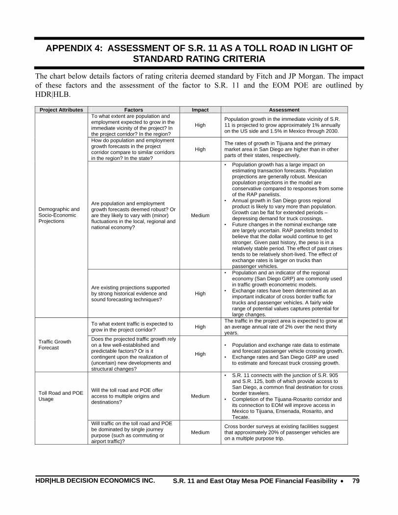
HDR|HLB DECISION ECONOMICS INC. S.R. 11 and East Otay Mesa POE Financial Feasibility •
79
APPENDIX 4: ASSESSMENT OF S.R. 11 AS A TOLL ROAD IN LIGHT OF STANDARD RATING CRITERIA
The chart below details factors of rating criteria deemed standard by Fitch and JP Morgan. The impact of these factors and the assessment of the factor to S.R. 11 and the EOM POE are outlined by HDR|HLB.
Project Attributes Factors Impact Assessment To what extent are population and employment expected to grow in the immediate vicinity of the project? In the project corridor? In the region?
High Population growth in the immediate vicinity of S.R. 11 is projected to grow approximately 1% annually on the US side and 1.5% in Mexico through 2030.
How do population and employment growth forecasts in the project corridor compare to similar corridors in the region? In the state?
High The rates of growth in Tijuana and the primary market area in San Diego are higher than in other parts of their states, respectively.
Are population and employment growth forecasts deemed robust? Or are they likely to vary with (minor) fluctuations in the local, regional and national economy?
Medium
• Population growth has a large impact on estimating transaction forecasts. Population projections are generally robust. Mexican population projections in the model are conservative compared to responses from some of the RAP panelists.
• Annual growth in San Diego gross regional product is likely to vary more than population. Growth can be flat for extended periods – depressing demand for truck crossings.
• Future changes in the nominal exchange rate are largely uncertain. RAP panelists tended to believe that the dollar would continue to get stronger. Given past history, the peso is in a relatively stable period. The effect of past crises tends to be relatively short-lived. The effect of exchange rates is larger on trucks than passenger vehicles.
Demographic and Socio-Economic Projections
Are existing projections supported by strong historical evidence and sound forecasting techniques?
High
• Population and an indicator of the regional economy (San Diego GRP) are commonly used in traffic growth econometric models.
• Exchange rates have been determined as an important indicator of cross border traffic for trucks and passenger vehicles. A fairly wide range of potential values captures potential for large changes.
To what extent traffic is expected to grow in the project corridor? High
The traffic in the project area is expected to grow at an average annual rate of 2% over the next thirty years.
Traffic Growth Forecast
Does the projected traffic growth rely on a few well-established and predictable factors? Or is it contingent upon the realization of (uncertain) new developments and structural changes?
High
• Population and exchange rate data to estimate and forecast passenger vehicle crossing growth.
• Exchange rates and San Diego GRP are used to estimate and forecast truck crossing growth.
Will the toll road and POE offer access to multiple origins and destinations?
Medium
• S.R. 11 connects with the junction of S.R. 905 and S.R. 125, both of which provide access to San Diego, a common final destination for cross border travelers.
• Completion of the Tijuana-Rosarito corridor and its connection to EOM will improve access in Mexico to Tijuana, Ensenada, Rosarito, and Tecate.
Toll Road and POE Usage
Will traffic on the toll road and POE be dominated by single journey purpose (such as commuting or airport traffic)?
Medium Cross border surveys at existing facilities suggest that approximately 20% of passenger vehicles are on a multiple purpose trip.
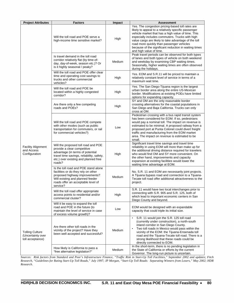
HDR|HLB DECISION ECONOMICS INC. S.R. 11 and East Otay Mesa POE Financial Feasibility •
80
Project Attributes Factors Impact Assessment
Will the toll road and POE serve a high-income time sensitive market? High
Yes. The congestion pricing-based toll rates are likely to appeal to a relatively specific passenger vehicle market that has a high value of time. This especially includes commuters. Trucks with high value cargo are likely to take advantage of the toll road more quickly than passenger vehicles because of the significant reduction in waiting times and high value of time.
Is travel demand in the toll road corridor relatively flat (by time-of-day, day-of-week, season etc.)? Or is it highly seasonal / peaky?
Medium
Peak travel periods can be observed for both types of lanes and both types of vehicle on both weekend and weekday by examining CBP waiting times. Seasonally, higher waiting times are often observed during the holidays.
Will the toll road and POE offer clear time and operating cost savings to trucks and other commercial vehicles?
High Yes. EOM and S.R.11 will be priced to maintain a relatively constant level of service in terms of a maximum wait time.
Will the toll road and POE be located within a highly congested corridor?
High
Yes. The San Diego-Tijuana region is the largest urban border area along the entire US-Mexican border. Modifications at existing POEs have limited options for expanding capacity.
Are there only a few competing roads and POEs? High
SY and OM are the only reasonable border crossing alternatives for the coastal populations in San Diego and Baja California. Trucks can only cross at OM.
Will the toll road and POE compete with other modes (such as public transportation for commuters, or rail for commercial vehicles?)
Low
Pedestrian crossing with a bus rapid transit system has been considered for EOM. If so, pedestrians would pay a nominal toll. The impact on revenue is estimated to be minimal. A proposed railway from a proposed port at Punta Colonet could divert freight traffic and manufacturing from the EOM market area. The impact on revenue is estimated to be small.
Will the proposed toll road and POE provide a clear competitive advantage (in terms of potential travel time savings, reliability, safety, etc.) over existing and planned free roads?
High
Significant travel time savings and travel time reliability in using EOM will more than make up for the additional driving distance required for travelers who would find OM and SY more convenient. On the other hand, improvements and capacity expansion at existing facilities would lower the waiting time advantage at EOM.
Is the toll road and POE stand alone facilities or do they rely on other proposed highway improvements? Will existing and planned feeder roads offer an acceptable level of service?
Medium
No. S.R. 11 and EOM are necessarily joint projects. A Tijuana bypass road and connection to a Tijuana-Tecate toll road offer additional attractiveness to the project.
Will the toll road offer appropriate access points to residential and/or commercial cluster?
High
S.R. 11 would have two local interchanges prior to connecting with S.R. 905 and S.R. 125, both of which lead to important economic centers in San Diego County and beyond.
Facility Alignment and Access Configuration
Will it be easy to expand the toll road and POE in the future (to maintain the level of service in case of excess volume growth)?
Low EOM would be designed with an expandable capacity that could triple its initial size.
Are there other toll roads in the vicinity of the project? Have they been well accepted and successful?
Medium
• S.R. 11 would join the S.R. 125 toll road (currently under construction), a north-south inland corridor in San Diego County.
• Two toll roads in Mexico would pass within the vicinity of the EOM: the Tijuana-Ensenada toll road and the Tijuana-Tecate toll road. There is a strong likelihood that these roads could be directly connected to EOM.
Tolling Culture (Uncertainty over toll acceptance)
How likely is California to pass a “free alternative legislation?” Medium
In the short-term, there is no pending legislation in the State of California or efforts by the current Governor. The long-run picture is uncertain.
Sources: Risk factors from Standard and Poor’s Infrastructure Finance, “Traffic Risk in Start-Up Toll Facilities,” September 2002 and updates; Fitch Research, “Guidelines for Rating Start-Up Toll Roads,” July 1997; JP Morgan, “Start-Up Toll Roads: Separating Winners from Losers,” May 2002; HDR Research.

HDR|HLB DECISION ECONOMICS INC. S.R. 11 and East Otay Mesa POE Financial Feasibility •
81
APPENDIX 5: READING DSCR PROBABILITY TABLES
This appendix explains, through an example, how the Debt Service Coverage Ratio (DSCR) probability tables presented in this report should be interpreted.
The tables provide, for each fiscal year, a decumulative probability distribution for the simulated DSCR. The distribution is summarized through twenty-one percentiles or probability levels, ranging from left to right, from 99% (99% probability of exceeding) to 1% (1% of exceeding).
In the example below, Monte Carlo simulation results indicate that:
In fiscal year 2008, there is a 75% chance that the DSCR will exceed 1.67 (upper text box); from the neighboring cells (on the same row), it appears that there is less than a 1% percent chance that the DSCR will fall below 1.59 in that year.
In fiscal year 2020 (lower text box), the DSCR will exceed 1.17 with a 95% probability. In other words, there is less than 5% chance that the DSCR will be less than 1.17.
Figure 17: Reading DSCR Probability Tables
Fiscal year There is a 75% probability that DSCR in fiscal year 2008 will be at least 1.67.
Probability of exceeding the DSCR values shown in the associated column
There is a 95% probability that DSCR in fiscal year 2020 will be at least 1.17.

HDR|HLB DECISION ECONOMICS INC. S.R. 11 and East Otay Mesa POE Financial Feasibility •
82
APPENDIX 6: SAMPLE OF EXISTING TOLL BORDER CROSSINGS
The chart below summarizes other existing toll bridges that connect POEs.
Toll Rates
U.S. - Mexico PV Commercial
Eagle Pass, TX-Piedras Negras $2.00 $7.00/2 axle; $3.00 per additional axle
Laredo, TX-Nuevo Laredo Bridge System
$3.00 $2.75 per axle
Brownsville, TX-Matamoros $2.00 $2.00/ 2 axle; $2 per additional axle
McAllen, TX-Hidalgo $2.00 $4.00/ 2 axle; $2 per additional axle
Pharr, TX to Reynosa, MX $2.00 $5.00/ 2 axle; $2 per additional axle
U.S. - Canada
Ambassador Bridge $3.25 $3.00/ 2 axle; $2.25 per additional axle
Detroit Windsor Tunnel $3.50 $3.50 plus $0.03 per 100 lbs gross weight
Peace Bridge $5.00 $5.00/ 2 axle; $3 per additional axle Sources:http://www.cityoflaredo.com/bridgesys/Bridgesystem.htm,http://expressbridge.com/bmsite.tolls.html, http://www.mcallen.net/bridge/#,http://www.cityofpharr.com/index.asp?NID=218,www.ambassadorbridge.com/an_overview_toll_rates_usf.html,http://www.dwtunnel.com/rate.html,http://www.peacebridge.com/ntr.php,http://www.cityofeaglepass.com/bridge/home.htm
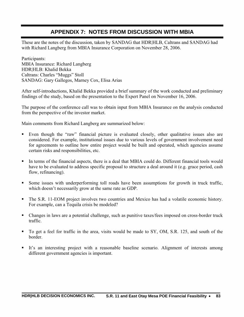
HDR|HLB DECISION ECONOMICS INC. S.R. 11 and East Otay Mesa POE Financial Feasibility •
83
APPENDIX 7: NOTES FROM DISCUSSION WITH MBIA
These are the notes of the discussion, taken by SANDAG that HDR|HLB, Caltrans and SANDAG had with Richard Langberg from MBIA Insurance Corporation on November 28, 2006. Participants: MBIA Insurance: Richard Langberg HDR|HLB: Khalid Bekka Caltrans: Charles “Muggs” Stoll SANDAG: Gary Gallegos, Marney Cox, Elisa Arias After self-introductions, Khalid Bekka provided a brief summary of the work conducted and preliminary findings of the study, based on the presentation to the Expert Panel on November 16, 2006. The purpose of the conference call was to obtain input from MBIA Insurance on the analysis conducted from the perspective of the investor market. Main comments from Richard Langberg are summarized below: Even though the “raw” financial picture is evaluated closely, other qualitative issues also are
considered. For example, institutional issues due to various levels of government involvement need for agreements to outline how entire project would be built and operated, which agencies assume certain risks and responsibilities, etc.
In terms of the financial aspects, there is a deal that MBIA could do. Different financial tools would
have to be evaluated to address specific proposal to structure a deal around it (e.g. grace period, cash flow, refinancing).
Some issues with underperforming toll roads have been assumptions for growth in truck traffic,
which doesn’t necessarily grow at the same rate as GDP. The S.R. 11-EOM project involves two countries and Mexico has had a volatile economic history.
For example, can a Tequila crisis be modeled? Changes in laws are a potential challenge, such as punitive taxes/fees imposed on cross-border truck
traffic. To get a feel for traffic in the area, visits would be made to SY, OM, S.R. 125, and south of the
border. It’s an interesting project with a reasonable baseline scenario. Alignment of interests among
different government agencies is important.
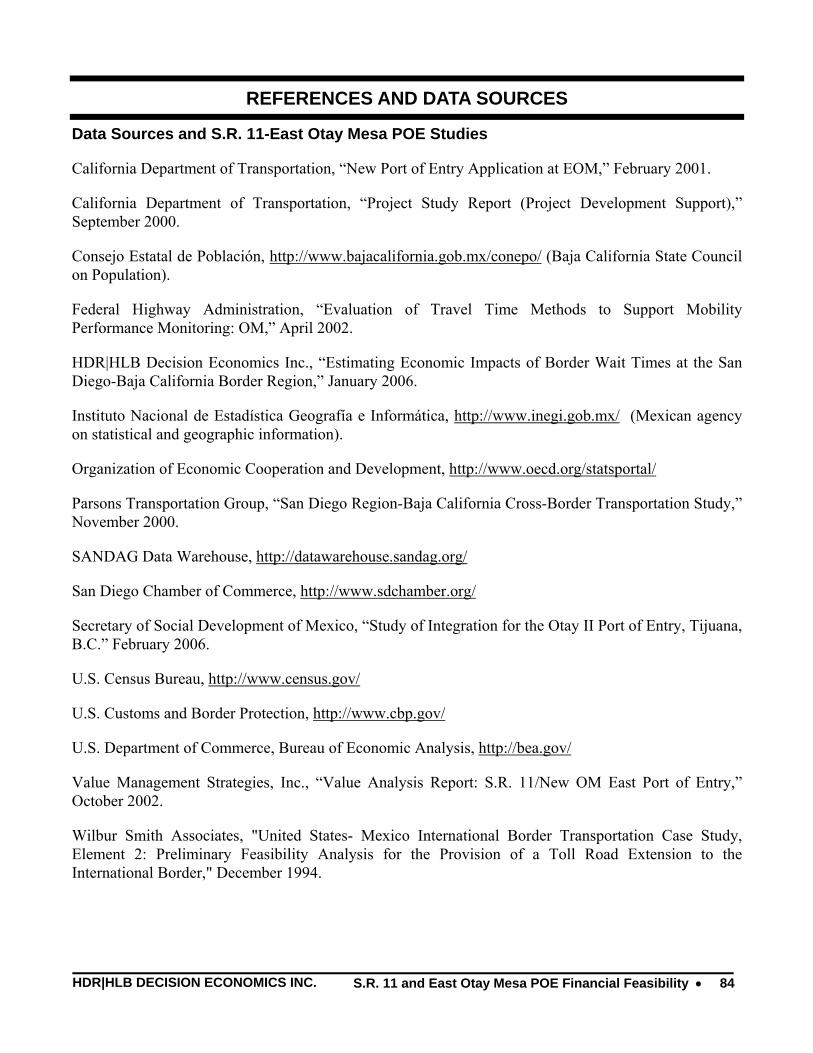
HDR|HLB DECISION ECONOMICS INC. S.R. 11 and East Otay Mesa POE Financial Feasibility •
84
REFERENCES AND DATA SOURCES
Data Sources and S.R. 11-East Otay Mesa POE Studies
California Department of Transportation, “New Port of Entry Application at EOM,” February 2001.
California Department of Transportation, “Project Study Report (Project Development Support),” September 2000.
Consejo Estatal de Población, http://www.bajacalifornia.gob.mx/conepo/ (Baja California State Council on Population).
Federal Highway Administration, “Evaluation of Travel Time Methods to Support Mobility Performance Monitoring: OM,” April 2002.
HDR|HLB Decision Economics Inc., “Estimating Economic Impacts of Border Wait Times at the San Diego-Baja California Border Region,” January 2006.
Instituto Nacional de Estadística Geografía e Informática, http://www.inegi.gob.mx/ (Mexican agency on statistical and geographic information).
Organization of Economic Cooperation and Development, http://www.oecd.org/statsportal/
Parsons Transportation Group, “San Diego Region-Baja California Cross-Border Transportation Study,” November 2000.
SANDAG Data Warehouse, http://datawarehouse.sandag.org/
San Diego Chamber of Commerce, http://www.sdchamber.org/
Secretary of Social Development of Mexico, “Study of Integration for the Otay II Port of Entry, Tijuana, B.C.” February 2006.
U.S. Census Bureau, http://www.census.gov/
U.S. Customs and Border Protection, http://www.cbp.gov/
U.S. Department of Commerce, Bureau of Economic Analysis, http://bea.gov/
Value Management Strategies, Inc., “Value Analysis Report: S.R. 11/New OM East Port of Entry,” October 2002.
Wilbur Smith Associates, "United States- Mexico International Border Transportation Case Study, Element 2: Preliminary Feasibility Analysis for the Provision of a Toll Road Extension to the International Border," December 1994.

HDR|HLB DECISION ECONOMICS INC. S.R. 11 and East Otay Mesa POE Financial Feasibility •
85
Financial Literature
Bain, R. & M. Wilkins. “Infrastructure Finance: Traffic Risks in Start-Up Toll Facilities” S&P. September 2002.
Bain, R. J.W. Plantagie. “Traffic Forecasting Risk: Study Update 2003” S&P. November 2003.
Bain, R., J.W. Plantagie. “Traffic Forecasting Risk: Study Update 2004” S&P. October 2004.
Bozzo, A. “Guidelines for Rating Start-Up Toll Roads” Fitch. July 1997.
Forsgren, K., J.E. Hecht, T. Doud, M. Wilkins. “The Toll Road Sector: Smooth Conditions Overall but Watch for Caution Flags” S&P. October 1999.
Forsgren, K., L. MacDonald. “Public Finance Criteria: Toll Roads and Bridge Revenue Bonds” S&P. October 2004.
George, C., S. Trommer, M. McDermott. “The Continuing Search for Bliss: Flexible Toll Road Structure” Fitch. October 2004.
George, C., Scott Trommer, M. McDermott, C. Lewis. “Stability in the U.S. Toll Road Sector: A Function of Management” Fitch. April 2005.
George, C., W. Streeter, S. Trommer. “Bliss, Heartburn, and Toll Road Forecasts” Fitch. November 2003.
“Infrastructure and Public Finance Ratings: Public Private Partnerships, Global Credit Survey 2005” S&P. May 2005.
Lutereau, P., L. Gremone. “Talca-Chillan Sociedad Concesionaria S.A” S&P. August 2005.
Monnier, L., C. George, G. Zurita, M. Hermans, & W. Streeter. “The Global Toll Road Credit Landscape” Fitch. May 2005.
Streeter, W., C. George, S. Trommer. “Redefining Toll Roads: An American Challenge” Fitch. March 2003.
Streeter, W., K. McManus. “Challenges to Start-up Toll Roads” Fitch. June 1999.
Streeter, W., M. Hermans, B. McCarthy, K. Stephenson, L. Monnier, P. Kolotas, M. Osako. “Toll Road Securitization: Wherein the Future Flows” Fitch. January 2004.
Woodel, C., W. Montrone. “S&P Introduction to Public Finance Criteria” S&P. November 2002.