Standing Swells Surveyed Showing Surprisingly Stable Solutionsfor the Lorenz ’96 Model

Morgan R. Frank1, Lewis Mitchell2, Christopher M. Danforth3

Computational Story Lab, Department of Mathematics and Statistics, Vermont Complex Systems Center, Vermont Advanced Computing Core,

University of Vermont, Burlington, Vermont1mrfrank@uvm.edu, 2lmitchell@uvm.edu, 3cdanfort@uvm.edu

December 23, 2013

The Lorenz ’96 model is an adjustable dimensionsystem of ODEs exhibiting chaotic behavior repre-sentative of dynamics observed in the Earth’s atmo-sphere. In the present study, we characterize statisticalproperties of the chaotic dynamics while varying thedegrees of freedom and the forcing. Tuning the dimen-sionality of the system, we find regions of parameterspace with surprising stability in the form of stand-ing waves traveling amongst the slow oscillators. Theboundaries of these stable regions fluctuate regularlywith the number of slow oscillators. These resultsdemonstrate hidden order in the Lorenz ’96 system,strengthening the evidence for its role as a hallmarkrepresentative of nonlinear dynamical behavior.

1 IntroductionModern society often depends on accurate weather fore-casting for daily planning, efficient air-travel, and disas-ter preparation [1]. Predicting the future state of phys-ical systems, such as the atmosphere, proves to be dif-ficult; chaotic systems exhibit sensitive dependence oninitial conditions, meaning that small errors in any stateapproximation will lead to exponential error growth [2].Furthermore, weather prediction requires the use of com-putationally expensive numerical models for representingthe atmosphere. Most scientists trying to advance cur-rent predictive techniques can not afford to run these real-world weather models. To this end, computationally man-ageable “simple models” are used instead to represent in-teresting atmospheric characteristics while reducing theoverall computation costs.

Scientists have long wrestled with chaotic behaviorlimiting the predictability of weather in the Earth’s at-mosphere [3–7]. In the case of atmospheric predictions,toy models exhibiting exponential error growth provide

an ideal environment for basic research in predictability.Edward Lorenz, one of the great pioneers in predictabilityresearch, introduced the following I-dimensional modelwhich exhibits chaotic behavior when subject to sufficientforcing

dxi

dt= xi−1(xi+1− xi−2)− xi +F (1)

where i = 1,2, . . . , I and F is the forcing parameter. Eachxi can be thought of as some atmospheric quantity, e.g.temperature, evenly distributed about a given latitude ofthe globe, hence there is a modularity in the indexing thatis described by xi+I = xi−I = xi.

In an effort to produce a more realistic growth rate ofthe large-scale errors, Lorenz went on to introduce a multiscale model by coupling two systems similar to the modelin equation (1), but differing in time scales. The equationsfor the Lorenz ’96 model [8] are given as

dxi

dt= xi−1(xi+1− xi−2)− xi +F− hc

b

J

∑j=1

y( j,i) (2)

dy( j,i)

dt= cby( j+1,i)(y( j−1,i)−y( j+2,i))−cy( j,i)+

hcb

xi (3)

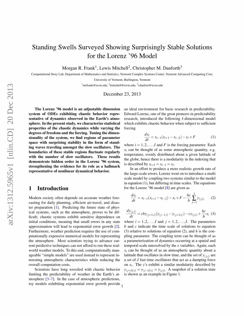
where i = 1,2, . . . , I and j = 1,2, . . . ,J. The parametersb and c indicate the time scale of solutions to equation(3) relative to solutions of equation (2), and h is the cou-pling parameter. The coupling term can be thought of asa parameterization of dynamics occurring at a spatial andtemporal scale unresolved by the x variables. Again, eachxi can be thought of as an atmospheric quantity about alatitude that oscillates in slow time, and the set of y( j,i) area set of J fast time oscillators that act as a damping forceon xi. The y’s exhibit a similar modularity described byy( j+IJ,i) = y( j−IJ,i) = y( j,i). A snapshot of a solution stateis shown as an example in Figure 1.

1

arX

iv:1

312.

5965

v1 [

nlin

.CD

] 2

0 D

ec 2

013

A

10

20

30

40

30

210

60

240

90

270

120

300

150

330

180 0

I=30, J=5, F=14

Slow Osc.Fast Osc.

B

Figure 1. (A) A visual representation for the coupling of the fast and slow time systems in the Lorenz ’96 model. There are I = 10 slowlarge amplitude oscillators, each of which are coupled to J = 3 fast small amplitude oscillators. The slow oscillators are arranged in a circlerepresenting a given latitude. (B) An example snapshot from an actual trajectory with I = 30, J = 5, and F = 14. The blue dots representthe slow oscillators, and the green represents the flow of information among the fast oscillators. See Figure 5 for further examples and amore detailed explanation.

This system has been used to represent weather relateddynamics in several previous studies as a low-dimensionalmodel of atmospheric dynamics [9–12]. There are manyadvantages to using the Lorenz ’96 model. A primary ad-vantage is that the model allows for flexibility in parame-ter tuning to achieve varying relative levels of nonlinear-ity, coupling of timescales, and spatial degrees of free-dom. Unless otherwise noted, we fix the time scaling pa-rameters b = c = 10 and the coupling parameter h = 1 forthe remainder of this study. These parameter choices areconsistent with the literature in terms of producing chaoticdynamics quantitatively similar to those observed in theatmosphere [13]. We vary I, J, and F to explore differentspatial degrees of freedom and different levels of nonlin-earity in the system dynamics.

In this study, we characterize the parameter space ofthe Lorenz ’96 system revealing patterns of order andchaos in the system. We discuss our methods in Section 2.In Section 3 and 4, we provide our results along with evi-dence for stability in the Lorenz ’96 model in the form ofstanding waves traveling around the slow oscillators. Wediscuss the implications of our findings in Section 4.

2 MethodsWe examine the Lorenz ’96 model for forcings F ∈ [1,18],and integer spatial dimensions I ∈ [4,50] and J ∈ [0,50].For each choice of F , I, and J, we integrate the Lorenz’96 model with a randomly selected initial condition inthe basin of attraction for the system attractor. We usethe Runge-Kutta method of order-4 [14] with a time stepof .001 to integrate the initial point along its trajectory.Initially, we iterate the point 500 time units without per-forming any analysis so that the trajectory is allowed toapproach the attractor; thus transient activity will be ig-nored. From here, we integrate an additional 500 timeunits for analysis. Results were insensitive to increases inintegration time, specific choices of initial condition, anddecreases in time step. Examples of stable and chaotictrajectories are shown in Figure 2.

We use the largest Lyapunov exponent, the percentageof positive Lyapunov exponents, and the normalized Lya-punov dimension to characterize the nonlinearity of thesystem. We approximate the Lyapunov exponent for the

2

−200

20

−20

0

20−10

0

10

20

X1

X2

X3

A

−200

20

−20

0

20−10

0

10

20

X1

X2

X3

B

0 5 10−10

−5

0

5

10

15

Time

X1

C

0 5 10−10

−5

0

5

10

15

Time

X1

D

0 1 2 3 4 5 60

1

2

3

4x 10

5

Frequency (Hz)

Pow

er

E

0 1 2 3 4 5 60

1

2

3

4x 10

5

Frequency (Hz)

Pow

er

F

Figure 2. Two example trajectories of the Lorenz ’96 model, alongwith periodograms for the corresponding trajectories of the slowoscillators. (A, C, & E) I = 4, J = 8, and F = 14. We observe a fairlyregular trajectory. The periodogram for this system supports this byshowing that only a few isolated frequencies have significant power.(B, D, & F) I = 10, J = 5, and F = 14. We observe an irregular tra-jectory. The periodogram exhibits some power at many frequencies.

ith dimension of the slow modes X along the trajectory ~vas

Li(v)≈1

∆timetotal

N

∑n=1

ln(| f (~v(n)i )|) (4)

where N is the number of iterations, ~v(n)i is the ith coor-dinate of the trajectory at the nth iterate, ∆timetotal is thetotal model time, and f is the stretch factor measured fromthe trajectories of an I-dimensional ensemble near a pointon the trajectory over a unit time step. This calculationcan be thought of as an average of the natural-log of thestretching/shrinking dynamics of the system acting on anensemble of points very near to the trajectory over time.The Lyapunov dimension is given by

L = D+1

|LD+1(~v)|

D

∑d=1

Ld(~v) (5)

where D is the largest whole number such that∑

Dd=1 Ld(~v)≥ 0. This calculation yields an approximation

of the slow mode attractor fractal dimension. In general,

the fractal dimension compared to the number of slowmode dimensions in the model (namely I) provides a rea-sonable measure of the nonlinearity in the system whichwe can subsequently compare to the dynamics resultingfrom different parameter choices [15].

From the one-dimensional time series in Figure 2, wesee examples of the dynamics exhibited by the slow vari-ables X (x1 is a representative example of X). We alsomeasure nonlinearity by looking at the frequency spec-trum for the trajectories of individual slow oscillators.Given a time series, the frequency spectrum can be ap-proximated using the fourier transform [16, 17]. Chaoticsystems typically exhibit power at a large number of fre-quencies, while stable systems will exhibit power at only asmall number of frequencies. Furthermore, the frequencyspectrum illuminates which frequencies the X variableswill tend to exhibit.

Lorenz suggested that the slow oscillators representmeasurements of some atmospheric quantity about agiven latitude [8]. With this in mind, it is meaningful tovisualize the system accordingly. Different from the im-ages provided in Figure 2, we will visualize states for allof the slow oscillators during a given trajectory as pointsevenly spaced around a circle centered at the origin, wherethe origin represents the lowest value (xmin) obtained byany of the slow oscillators along their respective trajec-tories. Each point’s distance from the origin is given byxi’s current value minus xmin. Treating the points in polar-coordinates (r,θ), where r is the oscillator’s distance fromxmin and θ indicates the subscript of the oscillator, we fit acubic spline to the shifted slow oscillator values to obtainapproximations for the flow of the atmospheric quantitybetween the slow oscillators. For clarity, the slow oscilla-tors’ radial positions (θ) remain fixed, while their distancefrom the origin varies over the course of the trajectory (seeFig. 1B). Note that this method of visualization allows usto observe all of the slow oscillators at once for any stateon a trajectory. A similar method is performed to repre-sent the activity of the fast oscillators in the same plot (theouter ring).

3 Results

It is common in the literature referencing the Lorenz ’96model to see the parameters I, J, and F chosen to en-sure that the system exhibits sufficient amounts of chaosto make the prediction problem interesting. For example,it is well-known that F > 6 will usually result in a weaklychaotic system for reasonable choices of I and J [9, 13].

3

I

J

Largest Lyapunov Exponent (F=8)

5 10 15 20 25 30 35 40 45 500

5

10

15

20

25

30

35

40

45

50

−1

−0.5

0

0.5

1

1.5

2

2.5

3

3.5

I

J

Largest Lyapunov Exponent (F=10)

5 10 15 20 25 30 35 40 45 500

5

10

15

20

25

30

35

40

45

50

−1

−0.5

0

0.5

1

1.5

2

2.5

3

3.5

I

J

Largest Lyapunov Exponent (F=12)

5 10 15 20 25 30 35 40 45 500

5

10

15

20

25

30

35

40

45

50

−1

−0.5

0

0.5

1

1.5

2

2.5

3

3.5

I

J

Largest Lyapunov Exponent (F=14)

5 10 15 20 25 30 35 40 45 500

5

10

15

20

25

30

35

40

45

50

−1

−0.5

0

0.5

1

1.5

2

2.5

3

3.5

I

J

% Positive Lyapunov Exponent (F=8)

5 10 15 20 25 30 35 40 45 500

5

10

15

20

25

30

35

40

45

50

0

0.2

0.4

0.6

0.8

1

I

J

% Positive Lyapunov Exponent (F=10)

5 10 15 20 25 30 35 40 45 500

5

10

15

20

25

30

35

40

45

50

0

0.2

0.4

0.6

0.8

1

I

J

% Positive Lyapunov Exponent (F=12)

5 10 15 20 25 30 35 40 45 500

5

10

15

20

25

30

35

40

45

50

0

0.2

0.4

0.6

0.8

1

I

J

% Positive Lyapunov Exponent (F=14)

5 10 15 20 25 30 35 40 45 500

5

10

15

20

25

30

35

40

45

50

0

0.2

0.4

0.6

0.8

1

I

J

Lyapunov Dimension/I (F=8)

5 10 15 20 25 30 35 40 45 500

5

10

15

20

25

30

35

40

45

50

0

0.2

0.4

0.6

0.8

1

I

J

Lyapunov Dimension/I (F=10)

5 10 15 20 25 30 35 40 45 500

5

10

15

20

25

30

35

40

45

50

0

0.2

0.4

0.6

0.8

1

I

JLyapunov Dimension/I (F=12)

5 10 15 20 25 30 35 40 45 500

5

10

15

20

25

30

35

40

45

50

0

0.2

0.4

0.6

0.8

1

I

J

Lyapunov Dimension/I (F=14)

5 10 15 20 25 30 35 40 45 500

5

10

15

20

25

30

35

40

45

50

0

0.2

0.4

0.6

0.8

1

Figure 3. For these plots, the axes represent integer values of the model dimensions I (slow) and J (fast). Each cell in the resulting plotrepresents a single integration with 500 unit time steps (or 106 iterations) of the Lorenz ’96 model. Note that these images are insensitiveto changes in initial condition. (Far Left Column) F = 8. (Center Left Column) F = 10. (Center Right Column) F = 12. (Far RightColumn) F = 14. (Top Row) The largest Lyapunov exponent. (Middle Row) The percent of positive Lyapunov exponents. (Bottom Row)The normalized Lyapunov dimension.

Beyond this, I = 8 and J = 4 for a total of 40 oscilla-tors is a popular choice, so much so that it is commonlyknown as the “Lorenz 40-variable” model [18]. Gener-alizing from these standards, we explore the parameterspace for I, J, and F systematically and characterize theresulting dynamical systems.

We first measure the largest Lyapunov exponent forseveral choices of I, J, and F in Figure 3 (top row). Weobserve that the lower portion of the plots (i.e. small J) ex-hibit strong, positive largest Lyapunov exponents (red &yellow regions). As J is increased, we observe the emer-gence of greatly reduced largest Lyapunov exponent (blueregions). This region of reduced chaotic activity returnsto a region of increased largest Lyapunov exponent as wecontinue to increment J. Furthermore, we observe that thetop and bottom borders of the blue regions oscillate withincreasing I. The blue region of reduced chaos appears

to occur at larger values of J as F is increased, while therange of the blue regions remain fairly constant in J.

We observe the percentage of positive Lyapunov ex-ponents in the middle row of Figure 3. Green vertical win-dows of increased percentage of positive Lyapunov expo-nents correspond to the peaks of the blue regions observedin the largest Lyapunov exponent plots. Interestingly, wefind that as we continue to increment J beyond these greenvertical strips, the percentage of positive Lyapunov expo-nents sharply declines.

The normalized Lyapunov dimension is shown in thebottom row of Figure 3. Here, we observe green andyellow vertical striations representing regions of reducedfractal dimensionality relative to the high fractal dimen-sionality red regions around them. These unstable dimen-sion striations

4

I

Fre

quen

cy (

Hz)

J=15 (F=8)

4 10 15 20 25 30 35 40 45 50

1

2

3

4

Log1

0(P

ower

)1

2

3

4

5

6

I

Fre

quen

cy (

Hz)

J=15 (F=10)

4 10 15 20 25 30 35 40 45 50

1

2

3

4

Log1

0(P

ower

)

1

2

3

4

5

6

I

Fre

quen

cy (

Hz)

J=15 (F=12)

4 10 15 20 25 30 35 40 45 50

1

2

3

4

Log1

0(P

ower

)

1.5

2

2.5

3

3.5

4

4.5

5

5.5

6

I

Fre

quen

cy (

Hz)

J=15 (F=14)

4 10 15 20 25 30 35 40 45 50

1

2

3

4

Log1

0(P

ower

)

2

2.5

3

3.5

4

4.5

5

5.5

6

I

Fre

quen

cy (

Hz)

J=10 (F=12)

4 10 15 20 25 30 35 40 45 50

1

2

3

4

Log1

0(P

ower

)

1.5

2

2.5

3

3.5

4

4.5

5

5.5

6

I

Fre

quen

cy (

Hz)

J=15 (F=12)

4 10 15 20 25 30 35 40 45 50

1

2

3

4

Log1

0(P

ower

)

1.5

2

2.5

3

3.5

4

4.5

5

5.5

6

I

Fre

quen

cy (

Hz)

J=20 (F=12)

4 10 15 20 25 30 35 40 45 50

1

2

3

4

Log1

0(P

ower

)

1.5

2

2.5

3

3.5

4

4.5

5

5.5

6

I

Fre

quen

cy (

Hz)

J=25 (F=12)

4 10 15 20 25 30 35 40 45 50

1

2

3

4

Log1

0(P

ower

)

1

2

3

4

5

6

Figure 4. For these plots, the x-axis represents choices of I, the y-axis represents different frequencies, and the color represents the powerspectrum of the trajectory of a slow oscillator at the corresponding parameter choice. (Top Row) J = 15 while F ∈ [8,10,12,14]. (BottomRow) F = 12 while J ∈ [10,15,20,25].

are in locations corresponding to the observed regions ofreduced largest Lyapunov exponent, and the vertical stria-tions of increased percentage of positive Lyapunov expo-nents. A periodicity in I is again apparent here.

We are surprised by these regions of reduced chaoticactivity and endeavor to explore them using a frequencyspectrum analysis. To this end, we examine frequencyspectrum bifurcation diagrams representing slices throughI-J space with a fixed F [17]. Some of these slices are pre-sented in Figure 4. We fix J = 15 and increase the forcingF moving from left-to-right along the top row of Figure 4.Along the bottom row of Figure 4, We fix F = 12 while in-creasing the number of fast variables J moving from left-to-right.

Examining the top row of Figure 4 for 8 ≤ F ≤ 12,we find increased power at many frequencies for mostchoices of I, but, interestingly, we also observe periodicwindows in the frequency spectrum bifurcation diagramwhere power is organized into just two different frequen-cies. Furthermore, these periodic windows of reducedspectral dispersion correspond to choices of I that resultedin stable behavior in Figure 3. We observe that whenF ≥ 14 there is power at many frequencies for I ≥ 6 andperiodic windows do not exist. This observation corre-sponds to the rise of the blue region of reduced largestLyapunov exponent as F is increased (Figure 3).

We look at the frequency spectrum bifurcation dia-gram in the bottom row of Figure 4 by fixing F = 12and varying J. Figure 3 suggests that we will observereduced largest Lyapunov exponent for 10 ≤ I ≤ 35 formost choices of I, and this is reflected in Figure 4 whenwe observe power at many frequencies for J = 10. Wetake steps through this region of reduced chaotic activ-ity as we increase J, and again find periodic windows inthe frequency spectrum bifurcation diagram, where largeamounts of power are only found at a finite number ofdifferent frequencies. Again these windows of reducedspectral activity occur at I values corresponding to peaksin the blue regions from Figure 3. Furthermore, we seeevidence that increasing J may have similar effects as re-ducing F .

Through further analysis of the frequency bifurcationspectrum diagrams, we observe that in general frequen-cies between one and two have more power, suggestingthat slow oscillators tend to exhibit these frequencies evenfor parameter choices resulting in chaotic dynamics. Wefind more interesting frequency behavior in the many win-dows of organized spectral activity, where the dominantand subdominant frequencies, namely the frequency withthe most power and the frequency with the second mostpower, appear to oscillate as a function of I. For J = 20and J = 25 in the bottom row of Figure 4, we see that

5

5

10

15

30

210

60

240

90

270

120

300

150

330

180 0

I=21, J=30, F=12, Time=0.80

Slow Osc.Fast Osc.

A

5

10

15

30

210

60

240

90

270

120

300

150

330

180 0

I=21, J=30, F=12, Time=1.00

Slow Osc.Fast Osc.

5

10

15

30

210

60

240

90

270

120

300

150

330

180 0

I=21, J=30, F=12, Time=1.20

Slow Osc.Fast Osc.

5

10

15

30

210

60

240

90

270

120

300

150

330

180 0

I=21, J=30, F=12, Time=1.40

Slow Osc.Fast Osc.

→ → →

5

10

15

30

210

60

240

90

270

120

300

150

330

180 0

I=10, J=25, F=14

Slow Osc.Fast Osc.

B

5

10

15

30

210

60

240

90

270

120

300

150

330

180 0

I=15, J=25, F=14

Slow Osc.Fast Osc.

5

10

15

30

210

60

240

90

270

120

300

150

330

180 0

I=20, J=25, F=14

Slow Osc.Fast Osc.

5

10

15

30

210

60

240

90

270

120

300

150

330

180 0

I=25, J=25, F=14

Slow Osc.Fast Osc.

5

10

15

30

210

60

240

90

270

120

300

150

330

180 0

I=30, J=25, F=14

Slow Osc.Fast Osc.

5

10

15

30

210

60

240

90

270

120

300

150

330

180 0

I=35, J=25, F=14

Slow Osc.Fast Osc.

5

10

15

30

210

60

240

90

270

120

300

150

330

180 0

I=43, J=25, F=14

Slow Osc.Fast Osc.

5

10

15

30

210

60

240

90

270

120

300

150

330

180 0

I=48, J=25, F=14

Slow Osc.Fast Osc.

10

20

30

40

30

210

60

240

90

270

120

300

150

330

180 0

I=30, J=5, F=14

Slow Osc.Fast Osc.

Figure 5. (A) For I = 21, J = 30, and F = 12, we plot the trajectories of the slow oscillators. This parameter choice yields a stable attractoras indicated by four snapshots of the standing waves, which travel clockwise around the ring of slow modes. (B) We show differentparameter choices yielding different numbers of standing waves (from 2-9). The plot in the bottom right corner represents a snapshot of atrajectory on a chaotic attractor and shows much more irregularity than the standing waves. Animations of these time series can be foundat http://www.uvm.edu/storylab/share/papers/frank2014a/L96Stability.avi

6

the dominant and subdominant frequencies fluctuate ev-ery fifth or sixth increment as we increase I. Also, thefluctuations become less severe as I approaches 50.

The frequency spectrum bifurcation diagrams showus that several parameter choices constrain the slow os-cillators to two distinct frequencies. This suggests thatwe should see a strong regularity in the time series forthese parameter choices. In Figure 5, we provide examplesnapshots of stable attractors, which resemble rose-plotsin polar coordinates, and a chaotic attractor with a strong,positive largest Lyapunov exponent, which resembles anamoeba (bottom right). Each petal of the stable attractorsis in fact a standing wave traveling around the slow os-cillators over time as shown by Figure 5A. We see thatthe oscillations of the stable attractors show signs of be-ing comprised of two frequencies, as individual slow os-

cillators seem to achieve both a relative local maximumand a global maximum. Furthermore, as we increase Iwe see additional petals added to the stable attractor. IfI is chosen so that it falls between two windows of in-creased spectral organization, then we see the dynamicsattempt to add an additional petal, but this petal will dis-sipate over time in a repeating process that prevents thetrajectory from stabilizing. We propose a simple functiondescribing the stable behavior in the Appendix.

We have provided evidence that stability emergesamongst regions of chaos in parameter space for theLorenz ’96 system, and that there appears to be a rela-tionship between the usual bifurcation parameter, F , andthe parameters controlling the dimension of the system, I& J. Figure 6 shows a few bifurcation diagrams where I,the number of slow oscillators, is used as a bifurcation

0 10 20 30 40 50−10

−5

0

5

10

15

Time

X1

A

0 10 20 30 40 50−4

−2

0

2

4

6

8

Time

X1

B

I

max

(X1)

J=10, F=8

15 25 35 45

0

3

5

8

10

log 10

Pro

babi

lity

−3.5

−3

−2.5

−2

−1.5C

I

max

(X1)

J=15, F=10

15 25 35 45

−0

2

5

7

10

12

log 10

Pro

babi

lity

−3.5

−3

−2.5

−2

−1.5D

I

max

(X1)

J=15, F=12

15 25 35 45

−3

−1

2

4

7

9

12

14

log 10

Pro

babi

lity

−3.5

−3

−2.5

−2

−1.5E

I

max

(X1)

J=20, F=14

15 25 35 45

−4

−1

1

4

6

9

11

14

16

log 10

Pro

babi

lity

−3.5

−3

−2.5

−2

−1.5F

F

max

(X1)

I=20, J=10

4 6 8 10 12 14−10

−5

0

5

10

15

log 10

Pro

babi

lity

−3.5

−3

−2.5

−2

−1.5

−1

−0.5

0

G

F

max

(X1)

I=20, J=30

4 6 8 10 12 14−4

−2

0

2

4

6

8

log 10

Pro

babi

lity

−3.5

−3

−2.5

−2

−1.5

−1

−0.5

0

H

F

max

(X1)

I=40, J=10

4 6 8 10 12 14−11

−6

−1

4

9

14

19

log 10

Pro

babi

lity

−3.5

−3

−2.5

−2

−1.5

−1

−0.5

0

I

F

max

(X1)

I=40, J=30

4 6 8 10 12 14123456789

10

log 10

Pro

babi

lity

−3.5

−3

−2.5

−2

−1.5

−1

−0.5

0

J

Figure 6. In the top row (A & B), we show two example trajectories representative of I = 20, J = 10, F = 12 and I = 20, J = 30, F = 12,respectively. Black circles indicate local maxima of the trajectories. These time series are example trajectories taken from the bifurcationdiagrams; panel A corresponds to the dashed line in panel G, and panel B corresponds to the dashed line in panel H. In the middle row(C-F), we provide bifurcation diagrams for several choices of J and F while I is varied as the bifurcation parameter. The y-axis indicatesthe values of the x1 local maxima. Note that ranges of the y-axes are different for each figure. The x-axis represents different choices of F

in the bottom row (G-J) for a few choices of I and J. We observe both windows of stability and windows of chaos.

7

I

h

5 10 15 20 25 30 35 40 45 500

0.1

0.2

0.3

0.4

0.5

0.6

0.7

0.8

0.9

1

max

. L.E

.

0.5

1

1.5

2

2.5

3

Figure 7. We examine the largest Lyapunov exponent as we vary I

on the x-axis and h, the coupling parameter, on the y-axis. J is fixedto be 50. We find a pattern similar to the ones observed in Figure 3.

parameter. These bifurcation diagrams display clearlywhere regions of stability and chaos can be found as wetune I. Furthermore, we again observe evidence of theregularity in the trajectories of the slow oscillators forparameter choices leading to stability since the values ofthe local maxima of the slow oscillators in such regionsare roughly constant across each bifurcation diagram.

Thinking of the dimensional parameters I and J asphysical parameters, we provide bifurcation diagrams fordifferent choices of I, J, and F , along with two represen-tative ~x variable trajectories, in Figure 6. Figures 6A, 6Bare example trajectories corresponding to the dashed linesin figures 6G, 6H, respectively. The dots in these timeseries indicate local maxima of the trajectories [3]. Figure6A demonstrates that values of the local maxima can fluc-tuate wildly, while figure 6B shows a parameter choicefor which local maxima tend towards only two differentvalues. The middle row of Figure 6 (panels C-F) exhibitswindows of both stable and chaotic dynamics as a func-tion of the dimensional parameter I. We again observewindows of stability and chaos in panels G-J where F , aphysical parameter, is tuned as the bifurcation parameterfor several choices of I and J. For a fixed I, increasing Jseems to condense the dynamics, constraining them to theenvelope of values observed.

Figure 7 allows us to relate the effects of varying thedimensional parameter J to varying the physical couplingparameter h. We vary I from 4 to 50 and vary h from 0 to1 while holding fixed J = 50 (note that h = 1 in all pre-vious figures, consistent with the literature). We observea pattern reminiscent of those observed in the top row ofFigure 3, which suggests that the parameters h and J mayhave an analogous effect on the system.

4 Discussion

The Lorenz ’96 model is a popular choice for atmosphericscientists attempting to improve prediction techniques.This is largely due to the reduction in degrees of freedomoffered by the Lorenz ’96 system in comparison to moresophisticated models used to make real-world weatherpredictions. Despite this simplification, the Lorenz ’96model is known for being a computationally manageablemodel that exhibits tunable levels of chaos, making it anappropriate tool for testing prediction techniques. How-ever, our inspection of parameter space reveals regionsof unexpected structural stability. In matters of complex-ity, it is common to assume that adding simple agents willonly lead to more complexity, but in the case of the Lorenz’96 model we see that there exists a bounded range of Jwhich organizes the dynamics and results in a dampeningof system-wide chaos.

We attempt to explain the observed regions of stabil-ity by inspecting the equations for the Lorenz ’96 system.Considering equation (2), the sum of the fast oscillatorscoupled with a given slow oscillator has a dampening ef-fect on the velocity of the slow oscillator, while we alsofind that the slow oscillator provides positive feedbackto the fast oscillators to which it is coupled in equation(3). Therefore, since each slow oscillator has many fastoscillators coupled with it, we expect any excitement ofthe slow oscillator to be quickly damped away by the fastoscillators. We find evidence of this in Figure 5, wherepeaks in the trajectories of the slow oscillators (pointson the inner circle) correspond to increased activity inthe fast oscillators coupled with it (the radially adjacentregion in the outer circle). If one continues to increaseJ beyond the observed regions of stability, then the in-creasingly chaotic dynamics observed in Figure 3 may bea result of increased apparent forcing. The magnitude ofthe sum of the fast oscillators for a given slow oscillatormay be large enough to act as a driving force for the dy-namics of the slow oscillator (see equation (2)).

To test this theory, Figure 7 shows the largest Lya-punov exponents as we vary I and h, the coupling param-eter, while holding J fixed at 50. Recalling equation (2),we see that reducing h dampens the sum of the fast os-cillators coupled to each slow oscillator. We observe thatFigure 7 exhibits a similar pattern to Figure 3, support-ing the claim that reducing the sum of the fast oscillatorsleads to the stable behavior we observe.

The frequency spectrum bifurcation diagrams in Fig-ure 4 reveal that the parameter choices for reduced chaoticactivity in Figure 3 yield surprisingly regular stable attrac-tors with slow oscillators whose trajectories are comprised

8

of only two frequencies. In fact, so long as the choicesof I, J, and F are such that the Lorenz ’96 system is inone of the stable regions of parameter space, the trajec-tories of any slow oscillator exhibits approximately thesame dynamics since the dominant and subdominant fre-quencies for stable attractors lie between 1-2, and 2.5-3,respectively, as seen in the frequency spectrum bifurca-tion diagrams in Figure 4. Indeed, the local maxima ofthe trajectories of the slow oscillators remain roughlyconstant across parameter choices leading to stability asshown in Figure 6. For a given choice of F and J, as Iis increased from one stable region in parameter space tothe next, we observe the addition of a petal, or a wave, tothe attractor. When I lies in between regions of stabilityin parameter space, we observe attractors that periodi-cally try to grow an additional petal that will eventuallydissipate over time. These interesting attractor behaviorsappear to occur periodically as a function of I.

AcknowledgementsWe would like to thank the Mathematics and Climate Re-search Network, the Vermont Complex Systems Center,and the Vermont Advance Computing Core for funding.Author ContributionsC.M.D., M.R.F, and L.M. designed the research.M.R.F. and C.M.D. prepared the figures and wrote themanuscript. M.R.F., L.M., and C.M.D analyzed the dataand reviewed the manuscript.Competing Financial InterestsThe authors declare no competing financial interests.

References

[1] R. A. Kerr. Weather Forecasts Slowly Clearing Up.Science 9 November 2012: Vol. 338 no. 6108 pp.734-737 DOI: 10.1126/science.338.6108.734

[2] J. A. Yorke. Chaos: An Introduction to DynamicalSystems. American Institute of Physics. ISSN: 0031-9228. http://dx.doi.org/10.1063/1.882006

[3] Lorenz, Edward N., 1963: Deterministic NonperiodicFlow. J. Atmos. Sci., 20, 130.141.

[4] E. N. Lorenz. The predictability of a flow whichpossesses many scales of motion. Tellus XXI, 289(1968).

[5] Farmer, J. D., and J. J. Sidorowich. PredictingChaotic Time Series. Phys. Rev. Lett. 59(8) (1987):845-848.

[6] C. M. Danforth, J. A. Yorke. 2006. Making Forecastsfor Chaotic Physical Processes. Physical Review Let-ters, 96, 144102.

[7] E.N. Lorenz, K.A. Emanuel, Optimal sites for sup-plementary weather observations: simulation with asmall model, J. Atmos. Sci. 55 (1998) 399414.

[8] E.N. Lorenz, Predictability A problem partly solved,in: ECMWF Seminar Proceedings on Predictability,Reading, United Kingdom, ECMWF, 1996, pp. 118.

[9] D. S. Wilks, Effects of Stochastic Parametrizations inthe Lorenz 96 System, Quart. J. Roy. Meteo. Soc. 131(2005) 389407.

[10] D. Orrell, Role of the Metric in Forecast ErrorGrowth: How Chaotic is the Weather?, Tellus 54A(2002) 350362.

[11] C. M. Danforth, E. Kalnay, Using Singular ValueDecomposition to Parameterize State-DependentModel Errors, J. Atmos. Sci. 65 (2008) 14671478.

[12] R. Lieb-Lappen, C. M. Danforth. 2012. AggressiveShadowing of a Low-Dimensional Model of Atmo-spheric Dynamics. Physica D. Volume 241, Issue 6,Pages 637648.

[13] A. Karimi, M. R. Paul. Extensive Chaos in theLorenz-96 Model. Chaos 20, 043105 (2010).

[14] R. England. Error estimates for Runga-Kutta typesolutions to systems of ordinary differential equa-tions. The Computer Journal (1969) 12 (2): 166-170.doi: 10.1093/comjnl/12.2.166

[15] J. Kaplan, J. Yorke, Chaotic behavior of multidimen-sional difference equations, in: H.-O. Peitgen, H.-O. Walther (Eds.), Functional Differential Equationsand Approximations of Fixed Points, Lecture Notesin Mathematics,. vol. 730, Springer, Berlin, 1979, pp.228-237.

[16] D. Orrell, 2003. Model Error and Predictability overDifferent Timescales in the Lorenz ’96 Systems. . J.Atmos. Sci., 60, 2219.2228.

[17] D. Orrell, L. A. Smith. Visualizing Bifurcations inHigh Dimensional Systems: The Spectral BifurcationDiagram. International Journal of Bifurcation andChaos, Vol. 13, No. 10 (2003) 3015-3027

[18] H. Li, E. Kalnay, T. Myoshi, C. M. Danforth. 2009.Accounting for Model Errors in Ensemble Data As-similation. Monthly Weather Review. 137, No. 10,3407-3419. doi:10.1175/2009MWR2766.1

9

5 Appendix

5.1 Modelling the Stable BehaviorWe attempt to further understand the stable behavior observed in the Lorenz 96 model by proposing a simple function.We model the normalized magnitude of a standing wave among the slow modes (as observed in Figure 5) with N(≈I/5) waves at time t using

r(θ, t) =sin

(N(θ+2π f · t)

)+1

2.

where f is the frequency of a representative slow mode. The frequency of the slow mode can be obtained by lookingat the dominant frequency from the spectra illustrated in Figure 4 (a function of I and F). Scaling f by the frequencyof sine (2π) and by the number of waves (N) will yield the desired angular velocity for the standing waves resultingfrom the model. Example waves resulting from the model at t = 0 are presented in the figure below.

0.2

0.4

0.6

0.8

1

30

210

60

240

90

270

120

300

150

330

180 0

(sin(2θ)+1)/2

0.2

0.4

0.6

0.8

1

30

210

60

240

90

270

120

300

150

330

180 0

(sin(3θ)+1)/2

0.2

0.4

0.6

0.8

1

30

210

60

240

90

270

120

300

150

330

180 0

(sin(4θ)+1)/2

0.2

0.4

0.6

0.8

1

30

210

60

240

90

270

120

300

150

330

180 0

(sin(5θ)+1)/2

0.2

0.4

0.6

0.8

1

30

210

60

240

90

270

120

300

150

330

180 0

(sin(6θ)+1)/2

0.2

0.4

0.6

0.8

1

30

210

60

240

90

270

120

300

150

330

180 0

(sin(7θ)+1)/2

0.2

0.4

0.6

0.8

1

30

210

60

240

90

270

120

300

150

330

180 0

(sin(8θ)+1)/2

0.2

0.4

0.6

0.8

1

30

210

60

240

90

270

120

300

150

330

180 0

(sin(9θ)+1)/2

Figure 8. Example trajectories from the model for stable behavior. We examine the results from the model for t = 0 with N ∈{2,3,4,5,6,7,8,9}.The resulting trajectories are comparable to the stable trajectories shown in Figure 5.

10