Studies in Computational Intelligence 605

Stan MatwinJan Mielniczuk Editors

Challenges in Computational Statistics and Data Mining

www.ebook3000.com

Studies in Computational Intelligence

Volume 605

Series editor

Janusz Kacprzyk, Polish Academy of Sciences, Warsaw, Polande-mail: kacprzyk@ibspan.waw.pl

www.ebook3000.com

About this Series

The series “Studies in Computational Intelligence” (SCI) publishes newdevelopments and advances in the various areas of computational intelligence—quickly and with a high quality. The intent is to cover the theory, applications, anddesign methods of computational intelligence, as embedded in the fields ofengineering, computer science, physics and life sciences, as well as themethodologies behind them. The series contains monographs, lecture notes andedited volumes in computational intelligence spanning the areas of neuralnetworks, connectionist systems, genetic algorithms, evolutionary computation,artificial intelligence, cellular automata, self-organizing systems, soft computing,fuzzy systems, and hybrid intelligent systems. Of particular value to both thecontributors and the readership are the short publication timeframe and the world-wide distribution, which enable both wide and rapid dissemination of researchoutput.

More information about this series at http://www.springer.com/series/7092

www.ebook3000.com

Stan Matwin • Jan MielniczukEditors

Challenges in ComputationalStatistics and Data Mining

123

www.ebook3000.com

EditorsStan MatwinFaculty of Computer ScienceDalhousie UniversityHalifax, NSCanada

Jan MielniczukInstitute of Computer SciencePolish Academy of SciencesWarsawPoland

and

Warsaw University of TechnologyWarsawPoland

ISSN 1860-949X ISSN 1860-9503 (electronic)Studies in Computational IntelligenceISBN 978-3-319-18780-8 ISBN 978-3-319-18781-5 (eBook)DOI 10.1007/978-3-319-18781-5

Library of Congress Control Number: 2015940970

Springer Cham Heidelberg New York Dordrecht London© Springer International Publishing Switzerland 2016This work is subject to copyright. All rights are reserved by the Publisher, whether the whole or partof the material is concerned, specifically the rights of translation, reprinting, reuse of illustrations,recitation, broadcasting, reproduction on microfilms or in any other physical way, and transmissionor information storage and retrieval, electronic adaptation, computer software, or by similar or dissimilarmethodology now known or hereafter developed.The use of general descriptive names, registered names, trademarks, service marks, etc. in thispublication does not imply, even in the absence of a specific statement, that such names are exempt fromthe relevant protective laws and regulations and therefore free for general use.The publisher, the authors and the editors are safe to assume that the advice and information in thisbook are believed to be true and accurate at the date of publication. Neither the publisher nor theauthors or the editors give a warranty, express or implied, with respect to the material contained herein orfor any errors or omissions that may have been made.

Printed on acid-free paper

Springer International Publishing AG Switzerland is part of Springer Science+Business Media(www.springer.com)

www.ebook3000.com

Preface

This volume contains 19 research papers belonging, roughly speaking, to the areasof computational statistics, data mining, and their applications. Those papers, allwritten specifically for this volume, are their authors’ contributions to honour andcelebrate Professor Jacek Koronacki on the occcasion of his 70th birthday. Thevolume is the brain-child of Janusz Kacprzyk, who has managed to convey hisenthusiasm for the idea of producing this book to us, its editors. Books related andoften interconnected topics, represent in a way Jacek Koronacki’s research interestsand their evolution. They also clearly indicate how close the areas of computationalstatistics and data mining are.

Mohammad Reza Bonyadi and Zbigniew Michalewicz in their article“Evolutionary Computation for Real-world Problems” describe their experience inapplying Evolutionary Algorithms tools to real-life optimization problems. Inparticular, they discuss the issues of the so-called multi-component problems, theinvestigation of the feasible and the infeasible parts of the search space, and thesearch bottlenecks.

Susanne Bornelöv and Jan Komorowski “Selection of Significant Features UsingMonte Carlo Feature Selection” address the issue of significant features detection inMonte Carlo Feature Selection method. They propose an alternative way of iden-tifying relevant features based on approximation of permutation p-values by normalp-values and they compare its performance with the performance of built-inselection method.

In his contribution, Łukasz Dębowski “Estimation of Entropy from SubwordComplexity” explores possibilities of estimating block entropy of stationary ergodicprocess by means of word complexity i.e. approximating function f(k|w) which for agiven string w yields the number of distinct substrings of length k. He constructstwo estimates and shows that the first one works well only for iid processes withuniform marginals and the second one is applicable for much broader class of so-called properly skewed processes. The second estimator is used to corroborateHilberg’s hypothesis for block length no larger than 10.

Maik Döring, László Györfi and Harro Walk “Exact Rate of Convergence ofKernel-Based Classification Rule” study a problem in nonparametric classification

v

www.ebook3000.com

concerning excess error probability for kernel classifier and introduce its decompo-sition into estimation error and approximation error. The general formula is providedfor the approximation and, under a weak margin condition, its tight version.

Michał Dramiński in his exposition “ADX Algorithm for SupervisedClassification” discusses a final version of rule-based classifier ADX. It summa-rizes several years of the author’s research. It is shown in experiments that inductivemethods may work better or on par with popular classifiers such as Random Forestsor Support Vector Machines.

Olgierd Hryniewicz “Process Inspection by Attributes Using Predicted Data”studies an interesting model of quality control when instead of observing quality ofinspected items directly one predicts it using values of predictors which are easilymeasured. Popular data mining tools such as linear classifiers and decision trees areemployed in this context to decide whether and when to stop the productionprocess.

Szymon Jaroszewicz and Łukasz Zaniewicz “Székely Regularization for UpliftModeling” study a variant of uplift modeling method which is an approach to assessthe causal effect of an applied treatment. The considered modification consists inincorporating Székely regularization into SVM criterion function with the aim toreduce bias introduced by biased treatment assignment. They demonstrate experi-mentally that indeed such regularization decreases the bias.

Janusz Kacprzyk and Sławomir Zadrożny devote their paper “CompoundBipolar Queries: A Step Towards an Enhanced Human Consistency and HumanFriendliness” to the problem of querying of databases in natural language. Theauthors propose to handle the inherent imprecision of natural language using aspecific fuzzy set approach, known as compound bipolar queries, to expressimprecise linguistic quantifiers. Such queries combine negative and positiveinformation, representing required and desired conditions of the query.

Miłosz Kadziński, Roman Słowiński, and Marcin Szeląg in their paper“Dominance-Based Rough Set Approach to Multiple Criteria Ranking withSorting-Specific Preference Information” present an algorithm that learns ranking ofa set of instances from a set of pairs that represent user’s preferences of one instanceover another. Unlike most learning-to-rank algorithms, the proposed approach ishighly interactive, and the user has the opportunity to observe the effect of theirpreferences on the final ranking. The algorithm is extended to become a multiplecriteria decision aiding method which incorporates the ordinal intensity of prefer-ence, using a rough-set approach.

Marek Kimmel “On Things Not Seen” argues in his contribution that frequentlyin biological modeling some statistical observations are indicative of phenomenawhich logically should exist but for which the evidence is thought missing. Theclaim is supported by insightful discussion of three examples concerning evolution,genetics, and cancer.

Mieczysław Kłopotek, Sławomir Wierzchoń, Robert Kłopotek and ElżbietaKłopotek in “Network Capacity Bound for Personalized Bipartite PageRank” startfrom a simplification of a theorem for personalized random walk in an unimodalgraph which is fundamental to clustering of its nodes. Then they introduce a novel

vi Preface

www.ebook3000.com

notion of Bipartite PageRank and generalize the theorem for unimodal graphs tothis setting.

Marzena Kryszkiewicz devotes her article “Dependence Factor as a RuleEvaluation Measure” to the presentation and discussion of a new evaluation mea-sure for evaluation of associations rules. In particular, she shows how the depen-dence factor realizes the requirements for interestingness measures postulated byPiatetsky-Shapiro, and how it addresses some of the shortcomings of the classicalcertainty factor measure.

Adam Krzyżak “Recent Results on Nonparametric Quantile Estimation in aSimulation Model” considers a problem of quantile estimation of the randomvariable m(X) where X has a given density by means of importance sampling usinga regression estimate of m. It is shown that such yields a quantile estimator with abetter asymptotic properties than the classical one. Similar results are valid whenrecursive Robbins-Monro importance sampling is employed.

The contribution of Błażej Miasojedov, Wojciech Niemiro, Jan Palczewski, andWojciech Rejchel in “Adaptive Monte Carlo Maximum Likelihood” deal withapproximation to the maximum likelihood estimator in models with intractableconstants by adaptive Monte Carlo method. Adaptive importance sampling and anew algorithm which uses resampling and MCMC is investigated. Among others,asymptotic results, such that consistency and asymptotic law of the approximativeML estimators of the parameter are proved.

Jan Mielniczuk and Paweł Teisseyre in “What do We Choose When We Err?Model Selection and Testing for Misspecified Logistic Regression Revisited”consider common modeling situation of fitting logistic model when the actualresponse function is different from logistic one and provide conditions under whichGeneralized Information Criterion is consistent for set t* of the predictors pertainingto the Kullback-Leibler projection of true model t. The interplay between t and t* isalso discussed.

Mirosław Pawlak in his contribution “Semiparametric Inference in Identificationof Block-Oriented Systems” gives a broad overview of semiparametric statisticalmethods used for identification in a subclass of nonlinear-dynamic systems calledblock oriented systems. They are jointly parametrized by finite-dimensionalparameters and an infinite-dimensional set of nonlinear functional characteristics.He shows that using semiparametric approach classical nonparametric estimates areamenable to the incorporation of constraints and avoid high-dimensionality/high-complexity problems.

Marina Sokolova and Stan Matwin in their article “Personal Privacy Protectionin Time of Big Data” look at some aspects of data privacy in the context of big dataanalytics. They categorize different sources of personal health information andemphasize the potential of Big Data techniques for linking of these various sources.Among others, the authors discuss the timely topic of inadvertent disclosure ofpersonal health information by people participating in social networks discussions.

Jerzy Stefanowski in his article “Dealing with Data Difficulty Factors whileLearning from Imbalanced Data” provides a thorough review of the approaches tolearning classifiers in the situation when one of the classes is severely

Preface vii

www.ebook3000.com

underrepresented, resulting in a skewed, or imbalanced distribution. The articlepresents all the existing methods and discusses their advantages and shortcomings,and recommends their applicability depending on the specific characteristics of theimbalanced learning task.

In his article James Thompson “Data Based Modeling” builds a strong case for adata-based modeling using two examples: one concerning portfolio managementand second being the analysis of hugely inadequate action of American healthservice to stop AIDS epidemic. The main tool in the analysis of the first example isan algorithm called MaxMedian Rule developed by the author and L. Baggett.

We are very happy that we were able to collect in this volume so many contri-butions intimately intertwined with Jacek’s research and his scientific interests.Indeed, he is one of the authors of Monte Carlo Feature Selection system which isdiscussed here and widely contributed to nonparametric curve estimation and clas-sification (subject of Döring et al. and Krzyżak’s paper). He started his career withresearch in optimization and stochastic approximation—the themes being addressedin Bonyadi and Michalewicz as well as in Miasojedow et al. papers. He held long-lasting interests in Statistical Process Control discussed by Hryniewicz. He also has,as the contributors to this volume and his colleagues fromRice University, Thompsonand Kimmel, keen interests in methodology of science and stochastic modeling.

Jacek Koronacki has been not only very active in research but also has gener-ously contributed his time to the Polish and international research communities. Hehas been active in the International Organization of Standardization and in theEuropean Regional Committee of the Bernoulli Society. He has been and is alongtime director of Institute of Computer Science of Polish Academy of Sciencesin Warsaw. Administrative work has not prevented him from being an activeresearcher, which he continues up to now. He holds unabated interests in newdevelopments of computational statistics and data mining (one of the editors vividlyrecalls learning about Székely distance, also appearing in one of the contributedpapers here, from him). He has co-authored (with Jan Ćwik) the first Polish text-book in statistical Machine Learning. He exerts profound influence on the Polishdata mining community by his research, teaching, sharing of his knowledge, ref-ereeing, editorial work, and by exercising his very high professional standards. Hisfriendliness and sense of humour are appreciated by all his colleagues and col-laborators. In recognition of all his achievements and contributions, we join theauthors of all the articles in this volume in dedicating to him this book as anexpression of our gratitude. Thank you, Jacku; dziękujemy.

We would like to thank all the authors who contributed to this endeavor, and theSpringer editorial team for perfect editing of the volume.

Ottawa, Warsaw, March 2015 Stan MatwinJan Mielniczuk

viii Preface

www.ebook3000.com

Contents

Evolutionary Computation for Real-World Problems . . . . . . . . . . . . . 1Mohammad Reza Bonyadi and Zbigniew Michalewicz

Selection of Significant Features Using Monte CarloFeature Selection . . . . . . . . . . . . . . . . . . . . . . . . . . . . . . . . . . . . . . . . 25Susanne Bornelöv and Jan Komorowski

ADX Algorithm for Supervised Classification . . . . . . . . . . . . . . . . . . . 39Michał Dramiński

Estimation of Entropy from Subword Complexity . . . . . . . . . . . . . . . . 53Łukasz Dębowski

Exact Rate of Convergence of Kernel-Based Classification Rule. . . . . . 71Maik Döring, László Györfi and Harro Walk

Compound Bipolar Queries: A Step Towards an EnhancedHuman Consistency and Human Friendliness . . . . . . . . . . . . . . . . . . . 93Janusz Kacprzyk and Sławomir Zadrożny

Process Inspection by Attributes Using Predicted Data . . . . . . . . . . . . 113Olgierd Hryniewicz

Székely Regularization for Uplift Modeling . . . . . . . . . . . . . . . . . . . . . 135Szymon Jaroszewicz and Łukasz Zaniewicz

Dominance-Based Rough Set Approach to Multiple CriteriaRanking with Sorting-Specific Preference Information . . . . . . . . . . . . 155Miłosz Kadziński, Roman Słowiński and Marcin Szeląg

ix

On Things Not Seen . . . . . . . . . . . . . . . . . . . . . . . . . . . . . . . . . . . . . 173Marek Kimmel

Network Capacity Bound for Personalized Bipartite PageRank . . . . . . 189Mieczysław A. Kłopotek, Sławomir T. Wierzchoń,Robert A. Kłopotek and Elżbieta A. Kłopotek

Dependence Factor as a Rule Evaluation Measure . . . . . . . . . . . . . . . 205Marzena Kryszkiewicz

Recent Results on Nonparametric Quantile Estimationin a Simulation Model . . . . . . . . . . . . . . . . . . . . . . . . . . . . . . . . . . . . 225Adam Krzyżak

Adaptive Monte Carlo Maximum Likelihood . . . . . . . . . . . . . . . . . . . 247Błażej Miasojedow, Wojciech Niemiro, Jan Palczewskiand Wojciech Rejchel

What Do We Choose When We Err? Model Selectionand Testing for Misspecified Logistic Regression Revisited . . . . . . . . . 271Jan Mielniczuk and Paweł Teisseyre

Semiparametric Inference in Identificationof Block-Oriented Systems . . . . . . . . . . . . . . . . . . . . . . . . . . . . . . . . . 297Mirosław Pawlak

Dealing with Data Difficulty Factors While Learningfrom Imbalanced Data . . . . . . . . . . . . . . . . . . . . . . . . . . . . . . . . . . . . 333Jerzy Stefanowski

Personal Privacy Protection in Time of Big Data. . . . . . . . . . . . . . . . . 365Marina Sokolova and Stan Matwin

Data Based Modeling. . . . . . . . . . . . . . . . . . . . . . . . . . . . . . . . . . . . . 381James R. Thompson

x Contents

Evolutionary Computation for Real-WorldProblems

Mohammad Reza Bonyadi and Zbigniew Michalewicz

Abstract In this paper we discuss three topics that are present in the area of real-world optimization, but are often neglected in academic research in evolutionarycomputation community. First, problems that are a combination of several inter-acting sub-problems (so-called multi-component problems) are common in manyreal-world applications and they deserve better attention of research community.Second, research on optimisation algorithms that focus the search on the edges offeasible regions of the search space is important as high quality solutions usuallyare the boundary points between feasible and infeasible parts of the search space inmany real-world problems. Third, finding bottlenecks and best possible investmentin real-world processes are important topics that are also of interest in real-worldoptimization. In this chapter we discuss application opportunities for evolutionarycomputation methods in these three areas.

1 Introduction

The Evolutionary Computation (EC) community over the last 30 years has spent alot of effort to design optimization methods (specifically Evolutionary Algorithms,EAs) that are well-suited for hard problems—problems where other methods usually

M.R. Bonyadi (B) · Z. MichalewiczOptimisation and Logistics, The University of Adelaide, Adelaide, Australiae-mail: mrbonyadi@cs.adelaide.edu.au

Z. MichalewiczInstitute of Computer Science, Polish Academy of Sciences, Warsaw, Polande-mail: zbyszek@cs.adelaide.edu.auurl: http://cs.adelaide.edu.au/∼optlog/

Z. MichalewiczPolish-Japanese Institute of Information Technology, Warsaw, Poland

Z. MichalewiczChief of Science, Complexica, Adelaide, Australia

© Springer International Publishing Switzerland 2016S. Matwin and J. Mielniczuk (eds.), Challenges in Computational Statisticsand Data Mining, Studies in Computational Intelligence 605,DOI 10.1007/978-3-319-18781-5_1

1

2 M.R. Bonyadi and Z. Michalewicz

fail [36]. As most real-world problems1 are very hard and complex, with nonlineari-ties and discontinuities, complex constraints and business rules, possibly conflictingobjectives, noise and uncertainty, it seems there is a great opportunity for EAs to beused in this area.

Some researchers investigated features of real-world problems that served as rea-sons for difficulties of EAs when applied to particular problems. For example, in[53] the authors identified several such reasons, including premature convergence,ruggedness, causality, deceptiveness, neutrality, epistasis, and robustness, that makeoptimization problems hard to solve. It seems that these reasons are either related tothe landscape of the problem (such as ruggedness and deceptiveness) or the optimizeritself (like premature convergence and robustness) and they are not focusing on thenature of the problem. In [38], a few main reasons behind the hardness of real-worldproblems were discussed; that included: the size of the problem, presence of noise,multi-objectivity, and presence of constraints. Apart from these studies on featuresrelated to the real-world optimization, there have been EC conferences (e.g. GECCO,IEEE CEC, PPSN) during the past three decades that have had special sessions on“real-world applications”. The aim of these sessions was to investigate the potentialsof EC methods in solving real-world optimization problems.

Consequently, most of the features discussed in the previous paragraph have beencaptured in optimization benchmark problems (many of these benchmark problemscan be found in OR-library2). As an example, the size of benchmark problemshas been increased during the last decades and new benchmarks with larger prob-lems have appeared: knapsack problems (KP) with 2,500 items or traveling salesmanproblems (TSP) with more than 10,000 cities, to name a few. Noisy environmentshave been already defined [3, 22, 43] in the field of optimization, in both continuousand combinatorial optimization domain (mainly from the operations research field),see [3] for a brief review on robust optimization. Noise has been considered for bothconstraints and objective functions of optimization problems and some studies havebeen conducted on the performance of evolutionary optimization algorithms withexistence of noise; for example, stochastic TSP or stochastic vehicle routing prob-lem (VRP). We refer the reader to [22] for performance evaluation of evolutionaryalgorithms when the objective function is noisy. Recently, some challenges to dealwith continuous space optimization problems with noisy constraints were discussedand some benchmarks were designed [43]. Presence of constraints has been alsocaptured in benchmark problems where one can generate different problems withdifferent constraints, for example Constrained VRP, (CVRP). Thus, the expectationis, after capturing all of these pitfalls and addressing them (at least some of them),EC optimization methods should be effective in solving real-world problems.

However, after over 30 years of research, tens of thousands of papers written onEvolutionary Algorithms, dedicated conferences (e.g. GECCO, IEEE CEC, PPSN),

1By real-world problems we mean problems which are found in some business/industry on daily(regular) basis. See [36] for a discussion on different interpretations of the term “real-worldproblems”.2Available at: http://people.brunel.ac.uk/~mastjjb/jeb/info.html.

Evolutionary Computation for Real-World Problems 3

dedicated journals (e.g. Evolutionary Computation Journal, IEEE Transactions onEvolutionary Computation), special sessions and special tracks on most AI-relatedconferences, special sessions on real-world applications, etc., still it is not that easyto find EC-based applications in real-world, especially in real-world supply chainindustries.

There are several reasons for this mismatch between the efforts of hundreds ofresearchers who have been making substantial contribution to the field of Evolution-ary Computation over many years and the number of real-world applications whichare based on concepts of Evolutionary Algorithms—these are discussed in detail in[37]. In this paper we summarize our recent efforts (over the last two years) to closethe gap between research activities and practice; these efforts include three researchdirections:

• Studying multi-component problems [7]• Investigating boundaries between feasible and infeasible parts of the search space[5]

• Examining bottlenecks [11].

The paper is based on our four earlier papers [5, 7, 9, 11] and is organized as fol-lows. We start with presenting two real-world problems (Sect. 2) so the connectionbetween presented research directions and real-world problems is apparent. Sec-tions3–5 summarize our current research on studying multi-component problems,investigating boundaries between feasible and infeasible parts of the search space,and examining bottlenecks, respectively. Section6 concludes the paper.

2 Example Supply Chains

In this section we explain two real-world problems in the field of supply chainmanagement. We refer to these two examples further in the paper.

Transportation of water tank The first example relates to optimization of the trans-portation of water tanks [21]. An Australian company produces water tanks withdifferent sizes based on some orders coming from its customers. The number ofcustomers per month is approximately 10,000; these customers are in different loca-tions, called stations. Each customer orders a water tank with specific characteristics(including size) and expects to receive it within a period of time (usually within1month). These water tanks are carried to the stations for delivery by a fleet oftrucks that is operated by the water tank company. These trucks have different char-acteristics and some of them are equipped with trailers. The company proceeds inthe following way. A subset of orders is selected and assigned to a truck and thedelivery is scheduled in a limited period of time. Because the tanks are empty and ofdifferent sizes they might be packed inside each other in order to maximize trucksload in a trip. A bundled tank must be unbundled at special sites, called bases, beforethe tank delivery to stations. Note that there might exist several bases close to the

4 M.R. Bonyadi and Z. Michalewicz

stations where the tanks are going to be delivered and selecting different bases affectsthe best overall achievable solution. When the tanks are unbundled at a base, onlysome of them fit in the truck as they require more space. The truck is loaded witha subset of these tanks and deliver them to their corresponding stations for delivery.The remaining tanks are kept in the base until the truck gets back and loads themagain to continue the delivery process.

The aim of the optimizer is to divide all tanks ordered by customers into subsetsthat are bundled and loaded in trucks (possibly with trailers) for delivery. Also, theoptimizer needs to determine an exact routing for bases and stations for unbundlingand delivery activities. The objective is to maximize the profit of the delivery at theend of the time period. This total profit is proportional to the ratio between the totalprices of delivered tanks to the total distance that the truck travels.

Each of the mentioned procedures in the tank delivery problem (subset selection,base selection, and delivery routing, and bundling) is just one component of theproblem and finding a solution for each component in isolation does not lead us tothe optimal solution of the whole problem. As an example, if the subset selectionof the orders is solved optimally (the best subset of tanks is selected in a way thatthe price of the tanks for delivery is maximized), there is no guarantee that thereexist a feasible bundling such that this subset fits in a truck. Also, by selecting tankswithout considering the location of stations and bases, the best achievable solutionscan still have a low quality, e.g. there might be a station that needs a very expensivetank but it is very far from the base, which actually makes delivery very costly. Onthe other hand, it is impossible to select the best routing for stations before selectingtanks without selection of tanks, the best solution (lowest possible tour distance) isto deliver nothing. Thus, solving each sub-problem in isolation does not necessarilylead us to the overall optimal solution.

Note also that in this particular case there are many additional considerations thatmust be taken into account for any successful application. These include schedulingof drivers (who often have different qualifications), fatigue factors and labor laws,traffic patterns on the roads, feasibility of trucks for particular segments of roads,and maintenance schedule of the trucks.

Mine to port operation The second example relates to optimizing supply-chainoperations of a mining company: from mines to ports [31, 32]. Usually in mine toport operations, themining company is supposed to satisfy customer orders to providepredefined amounts of products (the raw material is dig up in mines) by a particulardue date (the product must be ready for loading in a particular port). A port containsa huge area, called stockyard, several places to berth the ships, called berths, and awaiting area for the ships. The stockyard contains some stockpiles that are single-product storage units with some capacity (mixing of products in stockpiles is notallowed). Ships arrive in ports (time of arrival is often approximate, due to weatherconditions) to take specified products and transport them to the customers. The shipswait in the waiting area until the port manager assigns them to a particular berth.Ships apply a cost penalty, called demurrage, for each time unit while it is waitingto be berthed since its arrival. There are a few ship loaders that are assigned to each

Evolutionary Computation for Real-World Problems 5

berthed ship to load it with demanded products. The ship loaders take products fromappropriate stockpiles and load them to the ships. Note that, different ships havedifferent product demands that can be found in more than one stockpile, so thatscheduling different ship loaders and selecting different stockpiles result in differentamount of time to fulfill the ships demand. The goal of the mine owner is to providesufficient amounts of each product type to the stockyard. However, it is also in theinterest of the mine owner to minimize costs associated with early (or late) delivery,where these are estimated with respect to the (scheduled) arrival of the ship. Becausemines are usually far from ports, the mining company has a number of trains thatare used to transport products from a mine to the port. To operate trains, there is arail network that is (usually) rented by the mining company so that trains can travelbetween mines and ports. The owner of the rail network sets some constraints forthe operation of trains for each mining company, e.g. the number of passing trainsper day through each junction (called clusters) in the network is a constant (set bythe rail network owner) for each mine company.

There is a number of train dumpers that are scheduled to unload the productsfrom the trains (when they arrive at port) and put them in the stockpiles. The minecompany schedules trains and loads them at mine sites with appropriate materialand sends them to the port while respecting all constraints (the train schedulingprocedure). Also, scheduling train dumpers to unload the trains and put the unloadedproducts in appropriate stockpiles (the unload scheduling procedure), scheduling theships to berth (this called berthing procedure), and scheduling the ship loaders totake products from appropriate stockpiles and load the ships (the loader schedulingprocedure) are the other tasks for the mine company. The aim is to schedule the shipsand fill them with the required products (ship demands) so that the total demurrageapplied by all ships is minimized in a given time horizon.

Again, each of the aforementioned procedures (train scheduling, unload schedul-ing, berthing, and loader scheduling) is one component of the problem. Of courseeach of these components is a hard problem to solve by its own. Apart from thecomplication in each component, solving each component in isolation does not leadus to an overall solution for the whole problem. As an example, scheduling trainsto optimality (bringing as much product as possible from mine to port) might resultin insufficient available capacity in the stockyard or even lack of adequate productsfor the ships that arrive unexpectedly early. That is to say, ship arrival times haveuncertainty associated with them (e.g. due to seasonal variation in weather condi-tions), but costs are independent of this uncertainty. Also, the best plan for dumpingproducts from trains and storing them in the stockyard might result in a low qualityplan for the ship loaders and result in too much movement to load a ship.

Note that, in the real-world case, there were some other considerations in theproblem such as seasonal factor (the factor of constriction of the coal), hatch plan ofships (each product should be loaded in different parts of the ship to keep the balanceof the vessel), availability of the drivers of the ship loaders, switching times betweenchanging the loading product, dynamic sized stockpiles, etc.

Both problems illustrate the main issues discussed in the remaining sections ofthis document, as (1) they consist of several inter-connected components, (2) their

6 M.R. Bonyadi and Z. Michalewicz

boundaries between feasible and infeasible areas of the search space deserve carefulexamination, and (3) in both problems, the concept of bottleneck is applicable.

3 Multi-component Problems

There are thousands of research papers addressing traveling salesman problems, jobshop and other scheduling problems, transportation problems, inventory problems,stock cutting problems, packing problems, various logistic problems, to name but afew. While most of these problems are NP-hard and clearly deserve research efforts,it is not exactly what the real-world community needs. Let us explain.

Most companies run complex operations and they need solutions for problemsof high complexity with several components (i.e. multi-component problems; recallexamples presented in Sect. 2). In fact, real-world problems usually involve severalsmaller sub-problems (several components) that interact with each other and com-panies are after a solution for the whole problem that takes all components intoaccount rather than only focusing on one of the components. For example, the is-sue of scheduling production lines (e.g. maximizing the efficiency or minimizing thecost) has direct relationshipswith inventory costs, stock-safety levels, replenishmentsstrategies, transportation costs, delivery-in-full-on-time (DIFOT) to customers, etc.,so it should not be considered in isolation. Moreover, optimizing one componentof the operation may have negative impact on upstream and/or downstream activi-ties. These days businesses usually need “global solutions” for their operations, notcomponent solutions. This was recognized over 30 years ago by Operations Re-search (OR) community; in [1] there is a clear statement: Problems require holistictreatment. They cannot be treated effectively by decomposing them analytically intoseparate problems to which optimal solutions are sought. However, there are veryfew research efforts which aim in that direction mainly due to the lack of appro-priate benchmarks or test cases availability. It is also much harder to work with acompany on such global level as the delivery of successful software solution usu-ally involves many other (apart from optimization) skills, from understanding thecompanys internal processes to complex software engineering issues.

Recently a new benchmark problem called the traveling thief problem (TTP) wasintroduced [7] as an attempt to provide an abstraction of multi-component problemswith dependency among components. The main idea behind TTP was to combinetwo problems and generate a new problemwhich contains two components. The TSPand KP were combined because both of these problems were investigated for manyyears in the field of optimization (including mathematics, operations research, andcomputer science). TTP was defined as a thief who is going to steal m items fromn cities and the distance of the cities (d (i, j) the distance between cities i and j),the profit of each item (pi ), and the weight of the items (wi ) are given. The thief iscarrying a limited-capacity knapsack (maximum capacity W ) to collect the stolenitems. The problem is asked for the best plan for the thief to visit all cities exactly once(traveling salesman problem, TSP) and pick the items (knapsack problem, KP) from

Evolutionary Computation for Real-World Problems 7

these cities in a way that its total benefit is maximized. Tomake the two sub-problemsdependent, it was assumed that the speed of the thief is affected by the current weightof the knapsack (Wc) so that the more item the thief picks, the slower he can run. Afunction v : R → R is given which maps the current weight of the knapsack to thespeed of thief. Clearly, v (0) is the maximum speed of the thief (empty knapsack)and v (W ) is the minimum speed of the thief (full knapsack). Also, it was assumedthat the thief should pay some of the profit by the time he completes the tour (e.g.rent of the knapsack, r ). The total amount that should be paid is a function of thetour time. The total profit of the thief is then calculated by

B = P − r × T

where B is the total benefit, P is the aggregation of the profits of the picked items,and T is the total tour time.

Generating a solution for KP or TSP in TTP is possible without being aware of thecurrent solution for the other component. In addition, each solution for TSP impactsthe best quality that can be achieved in the KP component because of the impacton the pay back that is a function of travel time. Moreover, each solution for theKP component impacts the tour time for TSP as different items impact the speed oftravel differently due to the variability of weights of items. Some test problems weregenerated for TTP and some simple heuristic methods have been also applied to theproblem [44].

Note that for a given instance of TSP and KP different values of r and functionsf result in different instances of TTPs that might be harder or easier to solve. Asan example, for small values of r (relative to P), the value of r × T has a smallcontribution to the value of B. In an extreme case, when r = 0, the contributionof r × T is zero, which means that the best solution for a given TTP is equivalentto the best solution of the KP component, hence, there is no need to solve the TSPcomponent at all. Also, by increasing the value of r (relative to P), the contributionof r × T becomes larger. In fact, if the value of r is very large then the impact of Pon B becomes negligible, which means that the optimum solution of the TTP is veryclose to the optimum solution of the given TSP (see Fig. 1).

Fig. 1 Impact of the rentrate r on the TTP. For r = 0,the TTP solution isequivalent to the solution ofKP, while for larger r theTTP solutions become closerto the solutions of TSP

KP

TSP

r

TTP

8 M.R. Bonyadi and Z. Michalewicz

0

1

Dependency

Fig. 2 How dependency between components is affected by speed (function v). When v does not

drop significantly for different weights of picked items (∣∣∣v(W )−v(0)

W

∣∣∣ is small), the two problems can

be decomposed and solved separately. The value Dependency = 1 represents the two componentsare dependent while Dependency = 0 shows that two components are not dependent

The same analysis can be done for the function v. In fact, for a given TSP and KPdifferent function v can result in different instances of TTPs that, as before, might beharder or easier. Let us assume that v is a decreasing function, i.e. picking items withpositive weight causes drop or no change in the value of v. For a given list of items

and cities, if picking an item does not affect the speed of the travel (i.e.∣∣∣v(W )−v(0)

W

∣∣∣

is zero) significantly then the optimal solution of the TTP is the composition ofthe optimal solution of KP and TSP when they are solved separately. The reason is

that, with this setting (∣∣∣v(W )−v(0)

W

∣∣∣ is zero), picking more items does not change the

time of the travel. As the value of∣∣∣v(W )−v(0)

W

∣∣∣ grows, the TSP and KP become more

dependent (picking items have more significant impact on the travel time); see Fig. 2.

As the value of∣∣∣v(W )−v(0)

W

∣∣∣ grows, the speed of the travel drops more significantly

by picking more items that in fact reduces the value of B significantly. In an extreme

case, if∣∣∣v(W )−v(0)

W

∣∣∣ is infinitely large then it would be better not to pick any item

(the solution for KP is to pick no item) and only solve the TSP part as efficiently aspossible. This has been also discussed in [10].

Recently, we generated some test instances for TTP and made them available[44] so that other researchers can also work along this path. The instance set con-tains 9,720 problems with different number of cities and items. The specification ofthe tour was taken from existing TSP problems in OR-Library. Also, we proposedthree algorithms to solve those instances: one heuristic, one random search with lo-cal improvement, and one simple evolutionary algorithm. Results indicated that theevolutionary algorithm outperforms other methods to solve these instances. Thesetest sets were also used in a competition in CEC2014 where participants were askedto come up with their algorithms to solve the instances. Two popular approachesemerged: combining different solvers for each sub-problem and creating one systemfor the overall problem.

Evolutionary Computation for Real-World Problems 9

Problems that require the combination of solvers for different sub-problems, onecan find different approaches in the literature. First, in bi-level-optimization (and inthe more general multi-level-optimization), one component is considered the domi-nant one (with a particular solver associated to it), and every now and then the othercomponent(s) are solved to near-optimality or at least to the best extent possible byother solvers. In its relaxed form, let us call it “round-robin optimization”, the opti-mization focus (read: CPU time) is passed around between the different solvers forthe subcomponents. For example, this approach is taken in [27], where two heuristicsare applied alternatingly to a supply-chain problem, where the components are (1)a dynamic lot sizing problem and (2) a pickup and delivery problem with time win-dows. However, in neither set-up did the optimization on the involved componentscommence in parallel by the solvers.

A possible approach tomulti-component problemswith presence of dependenciesis based on the cooperative coevolution: a type of multi-population Evolutionary Al-gorithm [45]. Coevolution is a simultaneous evolution of several genetically isolatedsubpopulations of individuals that exist in a common ecosystem. Each subpopula-tion is called species and mate only within its species. In EC, coevolution can beof three types: competitive, cooperative, and symbiosis. In competitive coevolution,multiple species coevolve separately in such a way that fitness of individual fromone species is assigned based on how good it competes against individuals from theother species. One of the early examples of competitive coevolution is the work byHillis [20], where he applied a competitive predator-prey model to the evolution ofsorting networks. Rosin and Belew [47] used the competitive model of coevolutionto solve number of game learning problems including Tic-Tac-Toe, Nim and smallversion of Go. Cooperative coevolution uses divide and conquer strategy: all parts ofthe problem evolve separately; fitness of individual of particular species is assignedbased on the degree of collaboration with individuals of other species. It seems thatcooperative coevolution is a natural fit for multi-component problems with presenceof dependencies. Individuals in each subpopulationmay correspond to potential solu-tions for particular component, with its own evaluation function, whereas the globalevaluation function would include dependencies between components. Symbiosis isanother coevolutionary process that is based on living together of organisms of dif-ferent species. Although this type appears to represent a more effective mechanismfor automatic hierarchical models [19], it has not been studied in detail in the ECliterature.

Additionally, feature-based analysis might be helpful to provide new insights andhelp in the design of better algorithms for multi-component problems. Analyzingstatistical feature of classical combinatorial optimization problems and their relationto problem difficulty has gained an increasing attention in recent years [52]. Classicalalgorithms for the TSP and their success depending on features of the given inputhave been studied in [34, 41, 51] and similar analysis can be carried out for theknapsack problem. Furthermore, there are different problem classes of the knapsackproblem which differ in their hardness for popular algorithms [33]. Understandingthe features of the underlying sub-problems and how the features of interactionsin a multi-component problem determine the success of different algorithms is an

10 M.R. Bonyadi and Z. Michalewicz

interesting topic for future researchwhichwould guide the development and selectionof good algorithms for multi-component problems.

In the field of machine learning, the idea of using multiple algorithms to solve aproblem in a betterway has been used for decades. For example, ensemblemethods—such as boosting, bagging, and stacking—use multiple learning algorithms to searchthe hypothesis space in different ways. In the end, the predictive performance ofthe combined hypotheses is typically better than the performances achieved by theconstituent approaches.

Interestingly, transferring this idea into the optimization domain is not straightfor-ward. While we have a large number of optimizers at our disposal, they are typicallynot general-purpose optimizers, but very specific and highly optimized for a partic-ular class of problems, e.g., for the knapsack problem or the travelling salespersonproblem.

4 Boundaries Between Feasible and Infeasible Partsof the Search Space

A constrained optimization problem (COP) is formulated as follows:

find x ∈ F ⊆ S ⊆ RD such that

⎧

⎨

⎩

f (x) ≤ f (y) for all y ∈ F (a)gi (x) ≤ 0 for i = 1 to q (b)hi (x) = 0 for i = q + 1 to m (c)

(1)

where f , gi , and hi are real-valued functions on the search space S, q is the numberof inequalities, and m − q is the number of equalities. The set of all feasible pointswhich satisfy constraints (b) and (c) are denoted by F [39]. The equality constraintsare usually replaced by |hi (x)| − σ ≤ 0 where σ is a small value (normally set to10−4) [6]. Thus, a COP is formulated as

find x ∈ F ⊆ S ⊆ RD such that

{

f (x) ≤ f (y) for all y ∈ F (a)gi (x) ≤ 0 for i = 1 to m (b)

(2)

where gi (x) = |hi (x)| − σ for all i ∈ {q + 1, . . . , m}. Hereafter, the term COPrefers to this formulation.

The constraint gi (x) is called active at the point x if the value of gi (x) is zero.Also, if gi (x) < 0 then gi (x) is called inactive at x . Obviously, if x is feasible andat least one of the constraints is active at x , then x is on the boundary of the feasibleand infeasible areas of the search space.

In many real-world COPs it is highly probable that some constraints are active atoptimum points [49], i.e. some optimum points are on the edge of feasibility. Thereason is that constraints in real-world problems often represent some limitations of

Evolutionary Computation for Real-World Problems 11

resources. Clearly, it is beneficial to make use of some resources as much as possible,whichmeans constraints are active at quality solutions. Presence of active constraintsat the optimum points causes difficulty for many optimization algorithms to locateoptimal solution [50]. Thus, it might be beneficial if the algorithm is able to focusthe search on the edge of feasibility for quality solutions.

So it is assumed that there exists at least one active constraint at the optimum solu-tion of COPs. We proposed [5] a new function, called Subset Constraints BoundaryNarrower (SCBN), that enabled the search methods to focus on the boundary offeasibility with an adjustable thickness rather than the whole search space. SCBNis actually a function (with a parameter ε for thickness) that, for a point x , its valueis smaller than zero if and only if x is feasible and the value of at least one of theconstraints in a given subset of all constraint of the COP at the point x is withina predefined boundary with a specific thickness. By using SCBN in any COP, thefeasible area of the COP is limited to the boundary of feasible area defined by SCBN,so that the search algorithms can only focus on the boundary. Some other extensionsof SCBN are proposed that are useful in different situations. SCBN and its extensionsare used in a particle swarm optimization (PSO) algorithm with a simple constrainthandling method to assess if they are performing properly in narrowing the searchon the boundaries.

A COP can be rewritten by combining all inequality constraints to form only oneinequality constraint. In fact, any COP can be formulated as follows:

find x ∈ F ⊆ S ⊆ RD such that

{

f (x) ≤ f (y) for all y ∈ F (a)M (x) ≤ 0 (b)

(3)

where M (x) is a function that combines all constraints gi (x) into one function. Thefunction M (x) can be defined in many different ways. The surfaces that are definedby different instances of M (x)might be different. The inequality 3(b) should capturethe feasible area of the search space. However, by using problem specific knowledge,one can also define M (x) in a way that the area that is captured by M (x) ≤ 0 onlyrefers to a sub-space of the whole feasible area where high quality solutions mightbe found. In this case, the search algorithm can focus only on the captured areawhich is smaller than the whole feasible area and make the search more effective. Afrequently-used [29, 48] instance of M (x) is a function K (x)

K (x) =m

∑

i=1

max {gi (x) , 0} (4)

Clearly, the value of K (x) is non-negative. K (x) is zero if and only if x isfeasible. Also, if K (x) > 0, the value of K (x) represents the maximum violationvalue (called the constraint violation value).

As in many real-world COPs, there is at least one active constraint near the globalbest solution of COPs [49], some researchers developed operators to enable search

12 M.R. Bonyadi and Z. Michalewicz

methods to focus the search on the edges of feasibility. GENOCOP (GEnetic algo-rithm for Numerical Optimization for Constrained Optimization) [35] was probablythe first genetic algorithm variant that applied boundary search operators for dealingwith COPs. Indeed, GENOCOP had three mutations and three crossovers operatorsand one of these mutation operators was a boundary mutation which could generatea random point on the boundary of the feasible area. Experiments showed that thepresence of this operator caused significant improvement in GENOCOP for findingoptimum for problems which their optimum solution is on the boundary of feasibleand infeasible area [35].

A specific COP was investigated in [40] and a specific crossover operator, calledgeometric crossover, was proposed to deal with that COP. The COP was defined asfollows:

f (x) =∣∣∣∣∣

∑Di=1 cos4(xi )−2

∏Di=1 cos2(xi )

√∑D

i=1 i x2i

∣∣∣∣∣

g1 (x) = 0.75 −D∏

i=1xi ≤ 0

g2 (x) =D∑

i=1xi − 0.75D ≤ 0

(5)

where 0 ≤ xi ≤ 10 for all i . Earlier experiments [23] shown that the value of thefirst constraint (g1 (x)) is very close to zero at the best known feasible solution forthis COP. The geometric crossover was designed as xnew, j = √

x1,i x2, j , where xi, j

is the value of the j th dimension of the i th parent, and xnew, j is the value of the j thdimension of the new individual. By using this crossover, if g1 (x1) = g1 (x2) = 0,then g1 (xnew) = 0 (the crossover is closed under g1 (x)). It was shown that an evolu-tionary algorithm that uses this crossover ismuchmore effective than an evolutionaryalgorithmwhich uses other crossover operators in dealing with this COP. In addition,another crossover operator was also designed [40], called sphere crossover, that was

closed under the constraint g (x) =D∑

i=1x2i − 1. In the sphere crossover, the value of

the new offspring was generated by xnew, j =√

αx21, j + (1 − α) x22, j , where xi, j is

the value of the j th dimension of the i th parent, and both parents x1 and x2 are ong (x). This operator could be used if g (x) is the constraint in a COP and it is activeon the optimal solution.

In [50] several different crossover operators closed under g (x) =D∑

i=1x2i −1 were

discussed. These crossovers operators included repair, sphere (explained above),curve, and plane operators. In the repair operator, each generated solution was nor-malized and then moved to the surface of g (x). In this case, any crossover andmutation could be used to generate offspring; however, the resulting offspring ismoved (repaired) to the surface of g (x). The curve operator was designed in a waythat it could generate points on the geodesic curves, curves with minimum length on

Evolutionary Computation for Real-World Problems 13

a surface, on g (x). The plane operator was based on the selection of a plane whichcontains both parents and crosses the surface of g (x). Any point on this intersectionis actually on the surface of the g (x) as well. These operators were incorporated intoseveral optimization methods such as GA and Evolutionary Strategy (ES) and theresults of applying these methods to two COPs were compared.

A variant of evolutionary algorithm for optimization of awater distribution systemwas proposed [54]. The main argument was that the method should be able to makeuse of information on the edge between infeasible and feasible area to be effective insolving the water distribution system problem. The proposed approach was based onan adapting penalty factor in order to guide the search towards the boundary of thefeasible search space. The penalty factor was changed according to the percentage ofthe feasibility of the individuals in the population in such a way that there are alwayssome infeasible solutions in the population. In this case, crossover can make use ofthese infeasible and feasible individuals to generate solutions on the boundary offeasible region.

In [28] a boundary search operator was adopted from [35] and added to an antcolony optimization (ACO) method. The boundary search was based on the fact thatthe line segment that connects two points x and y, where one of these points areinfeasible and the other one is feasible, crosses the boundary of feasibility. A binarysearch can be used to search along this line segment to find a point on the boundaryof feasibility. Thus, any pair of points (x , y), where one of them is infeasible andthe other is feasible, represents a point on the boundary of feasibility. These pointswere moved by an ACO during the run. Experiments showed that the algorithm iseffective in locating optimal solutions that are on the boundary of feasibility.

In [5] we generalized the definition of edges of feasible and infeasible spaceby introducing thickness of the edges. We also introduced a formulation that, forany given COP, it could generate another COP that the feasible area of the lattercorresponds to the edges of feasibility of the former COP. Assume that for a givenCOP, it is known that at least one of the constraints in the set {gi∈Ω (x)} is active atthe optimum solution and the remaining constraints are satisfied at x , where Ω ⊆{1, 2, . . . , m}. We defined HΩ,ε (x) as follows:

HΩ,ε (x) = max

{∣∣∣∣maxi∈Ω

{gi (x)} + ε

∣∣∣∣− ε, max

i /∈Ω{gi (x)}

}

(6)

where ε is a positive value. Obviously, HΩ,ε (x) ≤ 0 if and only if at least one ofthe constraints in the subset Ω is active and the others are satisfied. The reason is

that, the component

∣∣∣∣maxi∈Ω

{gi (x)} + ε

∣∣∣∣− ε is negative if x is feasible and at least

one of gi∈Ω (x) is active. Also, the component maxi /∈Ω

{gi (x)} ensures that the rest

of constraints are satisfied. Note that active constraints are considered to have avalue between 0 and −2ε, i.e., the value of 2ε represents the thickness of the edges.This formulation can restrict the feasible search space to only the edges so thatoptimization algorithms are enforced to search the edges. Also, it enabled the user to

14 M.R. Bonyadi and Z. Michalewicz

provide a list of active constraints so that expert knowledge can help the optimizerto converge faster to better solutions.

Clearly methodologies that focuses the search on the edges of feasible area arebeneficial for optimization in real-world. As an example, in the mining problemdescribed in Sect. 2, it is very likely that using all of the trucks, trains, shiploaders, andtrain dumpers to the highest capacity is beneficial for increasing throughput. Thus,at least one of these constraints (resources) is active, which means that searchingthe edges of feasible areas of the search space very likely leads us to high qualitysolutions.

5 Bottlenecks

Usually real-world optimization problems contain constraints in their formulation.The definition of constraints in management sciences is anything that limits a systemfrom achieving higher performance versus its goal [17]. In the previous section weprovided general formulation of a COP. As discussed in the previous section, it isbelieved that the optimal solution of most real-world optimization problems is foundon the edge of a feasible area of the search space of the problem [49]. This belief isnot limited to computer science, but it is also found in operational research (linearprogramming, LP) [12] and management sciences (theory of constraints, TOC) [30,46] articles. The reason behind this belief is that, in real-world optimization problems,constraints usually represent limitations of availability of resources. As it is usuallybeneficial to utilize the resources as much as possible to achieve a high-qualitysolution (in terms of the objective value, f ), it is expected that the optimal solution isa point where a subset of these resources is used as much as possible, i.e., gi (x∗) = 0for some i and a particular high-quality x∗ in the general formulation of COPs [5].Thus, the best feasible point is usually located where the value of these constraintsachieves their maximum values (0 in the general formulation). The constraints thatare active at the optimum solution can be thought of as bottlenecks that constrain theachievement of a better objective value [13, 30].

Decision makers in industries usually use some tools, known as decision supportsystems (DSS) [24], as a guidance for their decisions in different areas of theirsystems. Probably themost important areas that decisionmakers need guidance fromDSS are: (1) optimizing schedules of resources to gain more benefit (accomplishedby an optimizer in DSS), (2) identifying bottlenecks (accomplished by analyzingconstraints in DSS), and (3) determining the best ways for future investments toimprove their profits (accomplished by an analysis for removing bottlenecks,3 knownas what-if analysis in DSS). Such support tools are more readily available than one

3The term removing a bottleneck refers to the investment in the resources related to that bottleneckto prevent those resources from constraining the problem solver to achieve better objective values.

Evolutionary Computation for Real-World Problems 15

might initially think: for example, the widespread desktop application MicrosoftExcel provides these via an add-in.4

Identification of bottlenecks and the best way of investment is at least as valuableas the optimization in many real-world problems from an industrial point of viewbecause [18]:An hour lost at a bottleneck is an hour lost for the entire system. An hoursaved at a non-bottleneck is a mirage. Industries are not only after finding the bestschedules of the resources in their systems (optimizing the objective function), butthey are also after understanding the tradeoffs between various possible investmentsand potential benefits.

During the past 30 years, evolutionary computation methodologies have providedappropriate tools as optimizers for decisionmakers to optimize their schedules. How-ever, the last two areas (identifying bottlenecks and removing them) that are neededin DSSs seem to have remained untouched by EC methodologies while it has beenan active research area in management and operations research.

There have been some earlier studies on identifying and removing bottlenecks[14, 16, 25, 30]. These studies, however, have assumed only linear constraints andthey have related bottlenecks only to one specific property of resources (usuallythe availability of resources). Further, they have not provided appropriate tools toguide decision makers in finding the best ways of investments in their system so thattheir profits are maximized by removing the bottlenecks. In our recent work [11],we investigated the most frequently used bottleneck removing analysis (so-calledaverage shadow prices) and identified its limitations. We argued that the root ofthese limitations can be found in the interpretation of constraints and the definitionof bottlenecks. We proposed a more comprehensive definition for bottlenecks thatnot only leads us to design a more comprehensive model for determining the bestinvestment in the system, but also addresses all mentioned limitations. Because thenew model was multi-objective and might lead to the formulation of non-linearobjective functions/constraints, evolutionary algorithms have a good potential to besuccessful on this proposed model. In fact, by applying multi-objective evolutionaryalgorithms to the proposed model, the solutions found represent points that optimizethe objective function and the way of investment with different budgets at the sametime.

Let us start with providing some background information on linear programming,the concept of shadow price, and bottlenecks in general. A Linear Programming (LP)problem is a special case of COP, where f (x) and gi (x) are linear functions:

find x such that z = max cT x subject to Ax ≤ bT (7)

where A is a m × d dimensional matrix known as coefficients matrix, m is thenumber of constraints, d is the number of dimensions, c is a d-dimensional vector,b is a m-dimensional vector known as Right Hand Side (RHS), x ∈ R

d , and x ≥ 0.

4http://tinyurl.com/msexceldss, last accessed 29th March 2014.

16 M.R. Bonyadi and Z. Michalewicz

The shadow price (SP) for the i th constraint of this problem is the value of z whenbi is increased by one unit. This in fact refers to the best achievable solution if theRHS of the i th constraint was larger, i.e., there were more available resources of thetype i [26].

The concept of SP in Integer Linear Programming (ILP) is different from theone in LP [13]. The definition for ILP is similar to the definition of LP, except thatx ∈ Z

d . In ILP, the concept of Average Shadow Price (ASP) was introduced [25].Let us define the perturbation function zi (w) as follows:

find x such that zi (w) = max cT x subject to ai x ≤ bi + w ak x ≤ bk ∀k �= i (8)

where ai is the i th row of thematrix A and x ≥ 0. Then, the ASP for the i th constraint

is defined by AS Pi = supw>0

{(zi (w)−zi (0))

w

}

. AS Pi represents that if adding one unit

of the resource i costs p and p < AS Pi , then it is beneficial (the total profit isincreased) to buy w units of this resource. This information is very valuable for thedecision maker as it is helpful for removing bottlenecks. Although the value of AS Pi

refers to “buying” new resources, it is possible to similarly define a selling shadowprice [25].

Several extensions of this ASP definition exist. For example, a set of resources isconsidered in [15] rather than only one resource at a time. There, it was also shownthat ASP can be used in mixed integer LP (MILP) problems.

Now, let us take a step back from the definition of ASP in the context of ILP,and let us see how it fits into a bigger picture of resources and bottlenecks. As wementioned earlier, constraints usually model availability of resources and limit theoptimizers to achieve the best possible solution which maximizes (minimizes) theobjective function [26, 30, 46]. Although finding the best solution with the currentresources is valuable for decision makers, it is also valuable to explore opportunitiesto improve solutions by adding more resources (e.g., purchasing new equipment)[25]. In fact, industries are seeking the most efficient way of investment (removingthe bottlenecks) so that their profit is improved the most.

Let us assume that the decision maker has the option of providing some additionalresource of type i at a price p. It is clearly valuable if the problem solver can determineif adding a unit of this resource can be beneficial in terms of improving the bestachievable objective value. It is not necessarily the case that adding a new resourceof the type i improves the best achievable objective value. As an example, considerthere are some trucks that load products into some trains for transportation. It mightbe the case that adding a new train does not provide any opportunity for gaining extrabenefit because the current number of trucks is too low and they cannot fill the trainsin time. In this case, we can say that the number of trucks is a bottleneck. Althoughit is easy to define bottleneck intuitively, it is not trivial to define this term in general.

There are a few different definitions for bottlenecks. These definitions are cate-gorized into five groups in [13]: (i) capacity based definitions, (ii) critical path baseddefinitions, (iii) structure based definitions, (iv) algorithm based definitions, and (v)system performance based definitions. It was claimed that none of these definitions

Evolutionary Computation for Real-World Problems 17

was comprehensive and some examples were provided to support this claim. Also,a new definition was proposed which was claimed to be the most comprehensivedefinition for a bottleneck: “a set of constraints with positive average shadow price”[13]. In fact, the average shadow price in a linear and integer linear program can beconsidered as a measure for bottlenecks in a system [30].

Although ASP can be useful in determining the bottlenecks in a system, it hassome limitations when it comes to removing bottlenecks. In this section, we discusssome limitations of removing bottlenecks based on ASP.

Obviously, the concept of ASP has been only defined for LP and MILP, but notfor problems with non-linear objective functions and constraints. Thus, using theconcept of ASP prevents us from identifying and removing bottlenecks in a non-linear system.

Let us consider the following simple problem5 (the problem is extremely simpleand it has been only given as an example to clarify limitations of the previous defini-tions): in a mine operation, there are 19 trucks and two trains. Trucks are used to filltrains with some products and trains are used to transport products to a destination.The rate of the operation for each truck is 100 tonnes/h (tph) and the capacity of eachtrain is 2,000 tonnes. What is the maximum tonnage that can be loaded to the trainsin 1 h? The ILP model for this problem is given by:

find x and y s.t. z = max {2000y} subject to (9)

g1 : 2000y − 100x ≤ 0, g2 : x ≤ 19, g3 : y ≤ 2

where x ≥ 0 is the number of trucks and y ≥ 0 is the number of loaded trains (ycan be a floating point value which refers to partially loaded trains). The constraintg1 limits the amount of products loaded by the trucks into the trains (trucks cannotoverload the trains). The solution is obviously y = 0.95 and x = 0.19 with objectivevalue 1,900. We also calculated the value of ASP for all three constraints:

• ASP for g1 is 1: by adding one unit to the first constraint (2000y − 100x ≤ 0becomes 2000y − 100x ≤ 1) the objective value increases by 1,

• ASP for g2 is 100: by adding 1 unit to the second constraint (x ≤ 19 becomesx ≤ 20) the objective value increases by 100,

• ASP for g3 is 0: by adding 1 unit to the second constraint (y ≤ 2 becomes y ≤ 3)the objective value does not increase.

Accordingly, thefirst and second constraints are bottlenecks as their correspondingASPs are positive. Thus, it would be beneficial if investments are concentrated onadding one unit to the first or second constraint to improve the objective value.

5We have made several such industry-inspired stories and benchmarks available: http://cs.adelaide.edu.au/~optlog/research/bottleneck-stories.htm.

18 M.R. Bonyadi and Z. Michalewicz

Adding one unit to the first constraint is meaningless from the practical point ofview. In fact, adding one unit to RHS of the constraint g1 means that the amount ofproducts that is loaded into the trains can exceed the trains’ capacities by one ton,which is not justifiable. In the above example, there is another option for the decisionmaker to achieve a better solution: if it is possible to improve the operation rate ofthe trucks to 101 tph, the best achievable solution is improved to 1,919 tons. Thus, itis clear that the bottleneck might be a specification of a resource (the operation rateof trucks in our example) that is expressed by a value in the coefficients matrix andnot necessarily RHS.

Thus, it is clear that ASP only gives information about the impact of changingRHS in a constraint, while the bottleneck might be a value in the coefficient matrix.The commonly used ASP, which only gives information about the impact of chang-ing RHS in a constraint, cannot identify such bottlenecks. Figure3 illustrates thislimitation.

The value of ASP represents only the effects of changing the value of RHS of theconstraints (Fig. 3, left) on the objective value while it does not give any informationabout the effects the values in the coefficients matrix might have on the objectivevalue (constraint g1 in Fig. 3, right). However, as we are show in our example, it ispossible to change the values in the coefficient matrix to make investments in orderto remove bottlenecks.

The value of ASP does not provide any information about the best strategy ofselecting bottlenecks to remove. In fact, it only provides information about the benefitof elevating the RHS in each constraint and does not say anything about the order ofsignificance of the bottlenecks. It remains the task of the decision maker to comparedifferent scenarios (also known aswhat-if analysis). For example, from amanagerialpoint of view, it is important to answer the following question: is adding one unit tothe first constraint (if possible) better than adding one unit to the second constraint(purchase a new truck)? Note that in real-world problems, there might be many

Fig. 3 x and y are number of trucks and number of trains respectively, gray gradient indicationof objective value (the lighter the better), shaded area feasible area, g1, g2, g3 are constraints, thewhite point is the best feasible point

Evolutionary Computation for Real-World Problems 19

resources and constraints, and a manual analysis of different scenarios might beprohibitively time consuming. Thus, a smart strategy is needed to find the best set ofto-be-removed bottlenecks in order to gain maximum profit with lowest investment.In summary, the limitations of identifying bottlenecks using ASP are:

• Limitation 1: ASP is only applicable if objective and constraints are linear.• Limitation 2: ASP does not evaluate changes in the coefficients matrix (the matrixA) and it is only limited to RHS.

• Limitation 3: ASP does not provide information about the strategy for investmentin resources, and the decision maker has to manually conduct analyses to find thebest investment strategy.

In order to resolve the limitations of ASP we proposed a new definition for bottle-necks and a new formulation for investment [11]. We defined bottlenecks as follows:A bottleneck is a modifiable specification of resources that by changing its value,the best achievable performance of the system is improved. Note that this definitionis a generalization of the definition of bottleneck in [13]: a set of constraints withpositive average shadow price is defined as a bottleneck. In fact, the definition in[13] concentrated on RHS only (it is just about the average shadow price) and itconsiders a bottleneck as a set of constraints. Conversely, our definition is based onany modifiable coefficient in the constraints (from capacity, to rates, or availability)and it introduces each specification of resources as a potential bottleneck.

Also, in order to determine the best possible investment to a system, we defineda Bottleneck COP (BCOP) for any COP as follows:

find x and l s.t. z ={

max f (x, l)min B (l)

subject to gi (x, li ) ≤ 0 for all i (10)

where l is a vector (l might contain continuous or discrete values) which contains lifor all i and B (l) is a function that calculates the cost of modified specifications ofresources coded in the vector l. For any COP, we can define a corresponding BCOPand by solving the BCOP, the plan for investment is determined.

The identification of bottlenecks and their removal are important topics in real-world optimization. As it was mentioned earlier, locating bottlenecks and finding thebest possible investment is of a great importance in large industries. For example,in the mining process described in Sect. 2 not only the number of trucks, trains, orother resources can constitute a bottleneck, but also the operation rate of any ofthese resources can also constitute a bottleneck. Given the expenses for removingany of these bottlenecks, one can use the model in Eq.10 to identify the best way ofinvestment to grow the operations and make the most benefit. This area has remaineduntouched by the EC community, while there are many opportunities to apply EC-based methodologies to deal with bottlenecks and investments.

20 M.R. Bonyadi and Z. Michalewicz

6 Discussion and Future Directions

Clearly, all three research directions (multi-component problems, edge of feasibility,and bottlenecks and investment) are relevant for solving real-world problems.

First, as it was mentioned earlier, an optimal solution for each component doesnot guarantee global optimality, so that a solution that represents the global optimumdoes not necessarily contain good schedules for each component in isolation [36].The reason lies on the dependency among components. In fact, because of depen-dency, even if the best solvers for each component are designed and applied to solveeach component in isolation, it is not useful in many real-world cases—the wholeproblem with dependency should be treated without decomposition of the compo-nents. Note that, decomposing problems that are not dependent on each other can beactually valuable as it makes the problem easier to solve. However, this decomposi-tion should be done carefully to keep the problem unchanged. Of course complexityof decomposing multi-component problems is related to the components dependen-cies. For example, one can define a simple dependency between KP and TSP in aTTP problem that makes the problems decomposable or make them tighten togetherso that they are not easily decomposable.

Looking at dependencies among components, the lack of abstract problems thatreflect this characteristic is obvious in the current benchmarks. In fact, real-worldsupply chain optimization problems are a combination ofmany smaller sub-problemsdependent on each other in a network while benchmark problems are singular. Be-cause global optimality is in interest in multi-component problems, singular bench-mark problems cannot assess quality of methods which are going to be used formulti-component real-world problems with the presence of dependency.

Multi-component problems pose new challenges for the theoretical investigationsof evolutionary computation methods. The computational complexity analysis ofevolutionary computation is playing a major role in this field [2, 42]. Results havebeen obtained formanyNP-hard combinatorial optimization problems from the areasof covering, cutting, scheduling, and packing. We expect that the computationalcomplexity analysis can provide new rigorous insights into the interactions betweendifferent components of multi-component problems. As an example, we consideragain the TTP problem. Computational complexity results for the two underlyingproblems (KP and TSP) have been obtained in recent years. Building on these results,the computational complexity analysis can help to understand when the interactionsbetween KP and TSP make the optimization process harder.

Second, there has been some experimental evidence that showed the importance ofsearching the boundaries of feasible and infeasible areas in a constraint optimizationproblem (COP) [40, 49, 50]. This boundary is defined as: the points that are feasibleand the value of at least one of the constraints is zero for them. In [5] three newinstances (called Constraint Boundary Narrower, CBN, Subset CBN, SCBN, and Allin a subset CBN, ACBN) for the constraint violation function were proposed whichwere able to reduce the feasible area to only boundaries of the feasible area. In theSCBN (ACBN), it is possible to select a subset of constraints and limit the boundaries

Evolutionary Computation for Real-World Problems 21

where at least one of these constraints (all of these constraints) is (are) active. Thethickness of the boundaries was adjustable in the proposed method by a parameter(ε). Experiments showed that changing the value of ε influences the performance ofthe algorithm. In fact, a smaller value of ε causes limiting the feasible area to narrowerboundaries, which makes finding the feasible areas harder. However, although it isharder to find the feasible areas (narrower boundaries), improving the final solutionsis easier once the correct boundary was found. Thus, as a potential future work, onecan design an adaptive method so that the search begins by exploring the feasiblearea and later concentrates on the boundaries.

Finally, a new definition for bottlenecks and a newmodel to guide decisionmakersto make the most profitable investment on their system should assist in narrowingthe gap between what is being considered in academia and industry. Our definitionfor bottlenecks and model for investment overcomes several of the drawbacks of themodel that is based on average shadow prices:

• It can work with non-linear constraints and objectives.• It offers changes to the coefficient matrix.• It can provide a guide towards optimal investments.

This more general model can form the basis for more comprehensive analyti-cal tools as well as improved optimization algorithms. In particular for the latterapplication, we conjecture that nature-inspired approaches are adequate, due to themulti-objective formulation of the problem and its non-linearity.

Bottlenecks are ubiquitous and companies make significant efforts to eliminatethem to the best extent possible. To the best of our knowledge, however, there seemsto be very little published research on approaches to identify bottlenecks research onoptimal investment strategies in the presence of bottlenecks seems to be even non-existent. In the future, we will push this research further, in order to improve decisionsupport systems. If bottlenecks can be identified efficiently, then this information canbe easily shown to the decisionmaker,whocan then subsequently use this informationin a manual optimization process.

There is also another research direction recently introduced to address real-worldoptimization problems that is locating disjoint feasible regions in a search space [4,8].6 It has been argued that the feasible area in constrained optimization problemsmight have an irregular shape and might contain many disjoint regions. Thus, it isbeneficial if an optimization algorithm can locate these regions as much as possibleso that the probability of finding the region that contain the best feasible solution isincreased. The problem of locating many disjoint feasible regions can be viewed asniching in multi-modal optimization [4].

6we have excluded this topic from this chapter because of the lack of space.

22 M.R. Bonyadi and Z. Michalewicz

References

1. Ackoff RL (1979) The future of operational research is past. J Oper Res Soc 53(3):93–104.ISSN 0160–5682

2. Auger A, Doerr B (2011) Theory of randomized search heuristics: foundations and recentdevelopments, vol 1. World Scientific. ISBN 9814282669

3. Bertsimas D, Brown DB, Caramanis C (2011) Theory and applications of robust optimization.SIAM Rev 53(3):464–501. ISSN 0036–1445

4. Bonyadi MR, Michalewicz Z (2014) Locating potentially disjoint feasible regions of a searchspace with a particle swarm optimizer, book section to appear. Springer, New York

5. Bonyadi MR, Michalewicz Z (2014) On the edge of feasibility: a case study of the particleswarm optimizer. In: Congress on evolutionary computation, IEEE, pp 3059–3066

6. Bonyadi MR, Li X, Michalewicz Z (2013) A hybrid particle swarm with velocity mutationfor constraint optimization problems. In: Genetic and evolutionary computation conference,ACM, pp 1–8. doi:10.1145/2463372.2463378

7. Bonyadi MR, Michalewicz Z, Barone L (2013) The travelling thief problem: the first step inthe transition from theoretical problems to realistic problems. In: Congress on evolutionarycomputation, IEEE

8. Bonyadi MR, Li X, Michalewicz Z (2014) A hybrid particle swarm with a time-adaptivetopology for constrained optimization. Swarm Evol Comput 18:22–37. doi:10.1016/j.swevo.2014.06.001

9. Bonyadi MR, Michalewicz Z, Neumann F, Wagner M (2014) Evolutionary computation formulti-component problems: opportunities and future directions. Frontiers in Robotics and AI,Computational Intelligence, under review, 2014

10. Bonyadi MR, Michalewicz Z, Przybyek MR, Wierzbicki A (2014) Socially inspired algo-rithms for the travelling thief problem. In: Genetic and evolutionary computation conference(GECCO), ACM

11. Bonyadi MR, Michalewicz Z, Wagner M (2014) Beyond the edge of feasibility: analysis ofbottlenecks. In: International conference on simulated evolution and learning (SEAL), volumeTo appear, Springer

12. Charnes A, Cooper WW (1957) Management models and industrial applications of linearprogramming. Manag Sci 4(1):38–91. ISSN 0025–1909

13. Chatterjee A, Mukherjee S (2006) Unified concept of bottleneck. Report, Indian Institute ofManagement Ahmedabad, Research and Publication Department

14. Cho S, Kim S (1992) Average shadow prices in mathematical programming. J Optim TheoryAppl 74(1):57–74

15. Crema A (1995) Average shadow price in a mixed integer linear programming problem. Eur JOper Res 85(3):625–635. ISSN 0377–2217

16. Frieze A (1975) Bottleneck linear programming. Oper Res Q 26(4):871–87417. Goldratt EM (1990) Theory of constraints. North River, Croton-on-Hudson18. Goldratt EM, Cox J (1993) The goal: a process of ongoing improvement. Gower, Aldershot19. Heywood MI, Lichodzijewski P (2010) Symbiogenesis as a mechanism for building complex

adaptive systems: a review. In: Applications of evolutionary computation, Springer, pp 51–6020. Hillis WD (1990) Co-evolving parasites improve simulated evolution as an optimization pro-

cedure. Phys D: Nonlinear Phenom 42(1):228–234. ISSN 0167–278921. JacobStolkAMZM,Mann I (2013)Combining vehicle routing andpacking for optimal delivery

schedules of water tanks. OR Insight 26(3):167190. doi:10.1057/ori.2013.122. Jin Y, Branke J (2005) Evolutionary optimization in uncertain environments-a survey. IEEE

Trans Evol Comput 9(3):303–317. ISSN 1089–778X23. Keane A (1994) Genetic algoritm digest. ftp://ftp.cse.msu.edu/pub/GA/gadigest/v8n16.txt24. Keen PG (1981) Value analysis: justifying decision support systems. MIS Q 5:1–15. ISSN

0276–778325. Kim S, Cho S-C (1988) A shadow price in integer programming for management decision. Eur

J Oper Res 37(3):328–335. ISSN 0377–2217

Evolutionary Computation for Real-World Problems 23

26. Koopmans TC (1977) Concepts of optimality and their uses. Am Econ Rev 67:261–274. ISSN0002–8282

27. LauHC,SongY (2002)Combining twoheuristics to solve a supply chain optimization problem.Eur Conf Artif Intell 15:581–585

28. Leguizamon G, Coello CAC (2009) Boundary search for constrained numerical optimizationproblems with an algorithm inspired by the ant colony metaphor. IEEE Trans Evol Comput13(2):350–368. ISSN 1089–778X

29. Li X, Bonyadi MR, Michalewicz Z, Barone L (2013) Solving a real-world wheat blendingproblem using a hybrid evolutionary algorithm. In: Congress on evolutionary computation,IEEE, pp 2665–2671. ISBN 1479904538

30. Luebbe R, Finch B (1992) Theory of constraints and linear programming: a comparison. Int JProd Res 30(6):1471–1478. ISSN 0020–7543

31. Maksud Ibrahimov SSZM, Mohais A (2012) Evolutionary approaches for supply chain opti-misation part 1. Int J Intell Comput Cybern 5(4):444–472

32. Maksud Ibrahimov SSZM, Mohais A (2012) Evolutionary approaches for supply chain opti-misation part 2. Int J Intell Comput Cybern 5(4):473–499

33. Martello S, Toth P (1990) Knapsack problems: algorithms and computer implementations.Wiley, Chichester

34. MersmannO,Bischl B, TrautmannH,WagnerM,Bossek J, NeumannF (2013)Anovel feature-based approach to characterize algorithm performance for the traveling salesperson problem.Ann Math Artif Intell 1–32. ISSN 1012–2443

35. Michalewicz Z (1992) Genetic algorithms + data structures = evolution programs. Springer.ISBN 3540606769

36. Michalewicz Z (2012) Quo vadis, evolutionary computation? Adv Comput Intell 98–12137. Michalewicz Z (2012) Ubiquity symposium: evolutionary computation and the processes

of life: the emperor is naked: evolutionary algorithms for real-world applications. Ubiquity,2012(November):3

38. Michalewicz Z, Fogel D (2004) How to solve it: modern heuristics. Springer, New York. ISBN3540224947

39. Michalewicz Z, Schoenauer M (1996) Evolutionary algorithms for constrained parameter op-timization problems. Evol Comput 4(1):1–32. ISSN 1063–6560

40. Michalewicz Z, Nazhiyath G, Michalewicz M (1996) A note on usefulness of geometricalcrossover for numerical optimization problems. In: Fifth annual conference on evolutionaryprogramming, Citeseer, p 305312

41. NallaperumaS,WagnerM,NeumannF,Bischl B,MersmannO, TrautmannH (2013)A feature-based comparison of local search and the christofides algorithm for the travelling salespersonproblem. In: Proceedings of the twelfth workshop on foundations of genetic algorithms XII,ACM, pp 147–160. ISBN 1450319904

42. Neumann F, Witt C (2012) Bioinspired computation in combinatorial optimization: algorithmsand their computational complexity. In: Proceedings of the fourteenth international conferenceon Genetic and evolutionary computation conference companion, ACM, pp 1035–1058. ISBN1450311784

43. Nguyen T, Yao X (2012) Continuous dynamic constrained optimisation-the challenges. IEEETrans Evol Comput 16(6):769–786. ISSN 1089–778X

44. Polyakovskiy S,BonyadiMR,WagnerM,MichalewiczZ,NeumannF (2014)A comprehensivebenchmark set and heuristics for the travelling thief problem. In: Genetic and evolutionary com-putation conference (GECCO), ACM. ISBN 978-1-4503-2662-9/14/07. doi:10.1145/2576768.2598249

45. Potter M, De Jong K (1994) A cooperative coevolutionary approach to function optimization.In: Parallel problem solving from nature, Springer, Berlin Heidelberg, pp 249–257. doi:10.1007/3-540-58484-6269

46. Rahman S-U (1998) Theory of constraints: a review of the philosophy and its applications. IntJ Oper Prod Manage 18(4):336–355. ISSN 0144–3577

24 M.R. Bonyadi and Z. Michalewicz

47. Rosin CD, Belew RK (1995) Methods for competitive co-evolution: finding opponents worthbeating. In: ICGA, pp 373–381

48. Runarsson T, YaoX (2000) Stochastic ranking for constrained evolutionary optimization. IEEETrans Evol Comput 4(3):284–294. ISSN 1089–778X

49. Schoenauer M, Michalewicz Z (1996) Evolutionary computation at the edge of feasibility. In:Parallel problem solving from nature PPSN IV, pp 245–254

50. SchoenauerM,Michalewicz Z (1997) Boundary operators for constrained parameter optimiza-tion problems. In: ICGA, pp 322–32

51. Smith-Miles K, van Hemert J, Lim XY (2010) Understanding TSP difficulty by learning fromevolved instances, Springer, pp 266–280. ISBN 3642137997

52. Smith-Miles K, Baatar D,Wreford B, Lewis R (2014) Towards objectivemeasures of algorithmperformance across instance space. Comput Oper Res 45:12–24. ISSN 0305–0548

53. Weise T, Zapf M, Chiong R, Nebro A (2009) Why is optimization difficult? Nature-inspiredalgorithms for optimisation, pp 1–50

54. Wu ZY, Simpson AR (2002) A self-adaptive boundary search genetic algorithm and its appli-cation to water distribution systems. J Hydraul Res 40(2):191–203. ISSN 0022–1686

Selection of Significant Features UsingMonte Carlo Feature Selection

Susanne Bornelöv and Jan Komorowski

Abstract Feature selection methods identify subsets of features in large datasets.Such methods have become popular in data-intensive areas, and performing featureselection prior tomodel constructionmay reduce the computational cost and improvethe model quality. Monte Carlo Feature Selection (MCFS) is a feature selectionmethod aimed at finding features to use for classification. Here we suggest a strategyusing a z-test to compute the significance of a feature using MCFS. We have usedsimulated data with both informative and random features, and compared the z-testwith a permutation test and a test implemented into the MCFS software. The z-testhad a higher agreement with the permutation test compared with the built-in test.Furthermore, it avoided a bias related to the distribution of feature values that mayhave affected the built-in test. In conclusion, the suggested method has the potentialto improve feature selection using MCFS.

Keywords Feature selection · MCFS · Monte Carlo · Feature significance ·Classification

1 Introduction

With the growth of large datasets in areas such as bioinformatics, computationalchemistry, and text recognition, limitations in the computational resources may forceus to restrict the analysis to a subset of the data. Feature selection methods reduce the

S. Bornelöv · J. Komorowski (B)Department of Cell and Molecular Biology, Science for Life Laboratory,Uppsala University, Uppsala, Swedene-mail: jan.komorowski@icm.uu.se

S. BornelövDepartment of Medical Biochemistry and Microbiology, Uppsala University, Uppsala, Swedene-mail: susanne.bornelov@imbim.uu.se

J. KomorowskiInstitute of Computer Science, Polish Academy of Sciences, Warsaw, Poland

© Springer International Publishing Switzerland 2016S. Matwin and J. Mielniczuk (eds.), Challenges in Computational Statisticsand Data Mining, Studies in Computational Intelligence 605,DOI 10.1007/978-3-319-18781-5_2

25

26 S. Bornelöv and J. Komorowski

data by selecting a subset of the features. An assumption in feature selection is thatlarge datasets contain some redundant or non-informative features. If successfullyremoving those, both the speed of the model training, the performance, and theinterpretation of the model may be improved [1].

There are several feature selection methods available. For a review of featureselection techniques used in bioinformatics, see Saeys et al. [2]. Some methods areunivariate and consider one feature at a time; others include feature interactions tovarious degrees. In this paperwehave studiedMonteCarlo Feature Selection (MCFS)[3]. MCFS focuses on selecting features to be used for classification. The use ofMCFS was originally illustrated by selecting genes with importance for leukemiaand lymphoma [3], and it was later used to study e.g. HIV-1 by selecting residues inthe amino acid sequence of reverse transcriptase with importance for drug resistance[4, 5]. Furthermore, MCFS may be used to rank the features based on their relativeimportance score. Thus, MCFS may be applied even on smaller datasets if the aimis to rank the features by their impact on the outcome (see e.g. [6–8]).

MCFS is a multivariate feature selection method based on random sampling ofthe original features. Each sample is used to construct a number of decision trees.Each feature is then given a score—relative importance (RI)—according to how itperforms in the decision trees. Thus, the selection of a feature is explicitly based onhow the feature contributes to classification.

One question is how to efficiently interpret the RI of a feature. If MCFS is usedto select a subset suitable for classification, a strategy may be to select the x high-est ranked features [6]. However, a stronger statistical basis for making the cutoffwould be preferred, particularly, when MCFS is used to determine which featuressignificantly influence the outcome.

TheMCFSalgorithm is implemented in the dmLab software available at [9]. Thereis a statistical test on the significance of a feature implemented in the software. Thestrategy of the test is to perform a number of permutations of the decision column,and in each permutation save the highest RI observed for any feature. Thereafter,the test compares the RI of each feature in the original data to the 95% confidenceinterval of the mean of the best RI scores [5].

Here, we suggest a different methodology that tests each feature separately to itsown set of controls. We show that this methodology leads to more accurate resultsand allows us to identify the most significant feature even when they do not have thehighest RI. Furthermore, by testing each feature separately, we avoid biases relatedto the distribution of feature values. Our suggested methodology is supported byexperiments using simulated data.

In conclusion, we have provided a methodology for computing the significance ofa feature using MCFS. We have shown that this methodology improves the currentlyused statistical test, and discussed the implications of using alternative methods.

Selection of Significant Features Using Monte Carlo Feature Selection 27

2 Materials and Methods

2.1 Monte Carlo Feature Selection

The MCFS algorithm is based on extensive use of decision trees. The general ideais to select s subsets of the original d features, each with a random selection of mfeatures. Each such subset is divided into a training and test set with 2/3 and 1/3 of theobjects, respectively. This division is repeated t times, and a decision tree classifieris trained on each training set. In all, st decision trees are trained and evaluated ontheir respective test set. An overview of the methodology is shown in Fig. 1.

Each feature is scored according to how it performs in these classifiers by a scorecalled relative importance (RI). The RI of a feature g was defined by Draminskiet al. [3] as

RIg = 1

Mg

st∑

τ=1

(wAccτ )u

∑

ng(τ )

IG(ng(τ ))

(no.in ng(τ )

no.in τ

)v

(1)

where s is the number of subsets and t is the number of splits for each subset. Mg isthe number of times the attribute g was present in the training set used to construct adecision tree. For each tree τ the weighted accuracy wAcc is calculated as the meansensitivity over all decision classes, using

wAcc = 1

c

c∑

i=1

nii

ni1 + ni2 + · · · + nic(2)

where c is the number of decision classes and ni j is the number of objects from classi that were classified to class j .

Furthermore, for each ng(τ ) (a node n in decision tree τ that uses attribute g) theinformation gain (IG) of ng(τ ) and the fraction of the number of training set objectsin (no.in) ng(τ ) compared to the number of objects in the tree root is computed.There are two weighting factors u and v that determine the importance of the wAccand the number of objects in the node.

Fig. 1 Overview of theMCFS procedure.Reproduced from Draminskiet al. [3]

28 S. Bornelöv and J. Komorowski

2.2 Construction of Datasets

To apply MCFS and to compute the significance of the features, we constructeddatasets with 120 numerical and 120 binary features. For each type of features, 20were correlated to the decision and 100 were uncorrelated. The decision class wasdefined to be binary (0 or 1) with equal frequency of both decisions. The number ofsimulated objects was set to either 100 or 1,000. Thus, for each object the decisionclass value was randomly drawn from the discrete uniform distribution [0,1] prior togenerating the attribute values. Detailed description of the attributes is provided inthe following sections. To verify that the features with an expected correlation to thedecision indeed were correlated, the Pearson correlation between each non-randomfeature and the decision was computed after the data generation (Table1).

Numerical Uncorrelated Features: RandNum0 to RandNum99. The values of anumerical uncorrelated feature (RandNumi , 0 ≤ i ≤ 99) were randomly drawn fromthe discrete uniform distribution [1, i +1]. Thus, the indices defined the range of

Table 1 Pearson correlation between each correlated feature and the decision. Presented for bothdatasets (100 objects and 1,000 objects) separately

i 100 objects 1,000 objects

Numi Bini Numi Bini

0 0.74 0.96 0.74 0.95

1 0.72 0.94 0.65 0.91

2 0.58 0.86 0.63 0.87

3 0.66 0.84 0.50 0.81

4 0.50 0.77 0.50 0.78

5 0.53 0.73 0.47 0.69

6 0.19 0.60 0.43 0.66

7 0.39 0.64 0.41 0.64

8 0.34 0.56 0.35 0.60

9 0.28 0.54 0.35 0.55

10 0.38 0.39 0.28 0.46

11 0.22 0.41 0.29 0.41

12 0.18 0.33 0.23 0.45

13 0.21 0.30 0.20 0.31

14 0.29 0.33 0.14 0.32

15 0.18 0.19 0.16 0.32

16 0.15 0.31 0.16 0.18

17 –0.01 0.01 0.07 0.14

18 0.08 0.07 0.07 0.15

19 –0.06 –0.02 –0.03 0.05

Selection of Significant Features Using Monte Carlo Feature Selection 29

possible values, which allowed us to test whether the number of possible values fora feature influenced its ranking.

Numerical Correlated Features: Num0 to Num19. The values of a numerical cor-related feature (Numi , 0≤ i≤ 19) were defined using the following algorithm: Let Xbe a random variable from the continuous uniform distribution (0,1). If X > (i+1)/21the value was selected randomly from the binomial distribution B(6, 0.5) if Deci-sion=0, and from B(6, 0.5)+3 if Decision=1. Otherwise, if X ≤ (i +1)/21, the valuewas selected randomly from the uniform distribution [0, 9]. Thus, low values wereindicative ofDecision=0 and high values ofDecision=1, with a noise level indicatedby the feature index.

Binary Uncorrelated Features: RandBin0 to RandBin99. The values of a binaryuncorrelated feature (RandBini , 0 ≤ i ≤ 99) were defined using the following algo-rithm: Let X be a random variable from the continuous uniform distribution (0,1). IfX > (i+1)/101 the value is 1, otherwise it is 0.

Thus, features with low indices will have ones in excess, features with middleindices will have more even distribution of ones and zeroes, and those with highindices will have zeroes in excess.

Binary Correlated Features: Bin0 to Bin19. The values of a binary correlatedfeature (Bini , 0 ≤ i ≤ 19) were defined using the following algorithm: Let X1 be arandom variable from the continuous uniform distribution (0,1). If X1 > (i +1)/21,the value is equal to the decision. Otherwise it is assigned by drawing another randomvariable X2 from the continuous uniform distribution (0,1). If X2 > (i +1)/21, thevalue is 1, otherwise it is 0.

2.3 Performing the Experiments

The experiments were performed using the dmLab software version 1.85.We appliedthe rule-of-thumb to set the number of features selected in each subset to

√d, where

d is the total number of features. Thus using 240 features, we used m = √240 ≈

15. The number of subsets was set to s = 3,000 for the permutation runs and s =100,000 for the original data. The number of trees trained in each subset was set to t= 5 and the number of permutation test runs was set to cutPointRuns = 10,000. Theweighting parameters were set to u = 0 and v = 1.

There were two main arguments for using a higher number of subsets on theoriginal data. Firstly, ranking of the features in the original data is the most crucialpart of the experiment. Therefore, it is generally motivated to focus more of thecomputational resources onto this step. Secondly, both the z-test and the built-in testrequire the rankings of the original data to be stable,which is obtained by constructinga high number of subsets.

Setting u = 0 will omit the decision tree accuracy from the calculation of RIs.Indeed, using model performance as a selection criteria may be counter-productive

30 S. Bornelöv and J. Komorowski

[10], and our experience is that the inclusion of the accuracy in the calculation of theRI overestimates the importance of all features in the original data compared to thepermuted ones. This effect is expected, since the accuracy on the original data willreflect the most predictive features, whereas on the permuted data it will only reflectrandom variation of the decision trees.

2.4 Selection of Significant Features

In this section we present different strategies to estimate the p-value of the RI of afeature using a permutation test, either alone or in combination with additional tests.Using a traditional permutation test requires thousands of permutations to yieldefficient estimates of small p-values. Thus, alternative tests performing a smallernumber of permutations and using these to estimate the underlying distribution maysave computational time. The test that is built-in into dmLab employs this strategyand performs a t-test comparing the best RIs obtained during the permutation runsto the RI of a feature on the original data. Here we suggest another approach usinga z-test to compute the p-value by estimating a normal distribution for each featureseparately.

During the permutation test the number of permutations, N , was set to 10,000 toobtain sufficient resolution of the p-values. The permutation test p-values were thenused as a gold standard to evaluate the build-in test and the suggested z-test. For thesetests a substantially smaller number of permutations are needed. Consequently, weused only the 100 first permutation runs to estimate the p-values using the built-inand the z-test.

Using a Permutation Test to Select Significant Features. A permutation test maybe applied to compute an approximation of the empirical p-value of a RI. The nullhypothesis is that the RI calculated on the real data is no better than the RIs com-puted for the permutated data. The empirical p-value approximates the probabilityof observing a test statistics at least as extreme as the observed value, assuming thatthe null hypothesis is true. Typically, a significance level, such as 0.05, is definedand attributes associated with p-values below this level are considered significantlyinformative.

Theoretically, the true permutation test p-value of RI = x that was measured fora feature g would be

ptrue(RIg = x) =

Nall∑

i=1I(RI i

g ≥ x)

Nall(3)

where I is the indicator function taking value 1 if the condition ismet, and 0 otherwise.RIi

g is the RI of the attribute g in permutation iand N all denotes the total number ofpossible permutations. However, since N all may be extremely large, only a limited

Selection of Significant Features Using Monte Carlo Feature Selection 31

number of permutations are commonly performed. Furthermore, pseudo-counts areadded to avoid p-values of zero, which are theoretically impossible since at least onepossible permutation has to be identical to the original data. Thus, an approximationof the permutation test p-value is commonly applied,which is based on the N numberof permutations with N � Nall using the following expression

p(RIg = x) =1 +

N∑

i=1I(RI i

g ≥ x)

N + 1(4)

Using a z-Test to Select Significant Features. By performing N permutations, eachfeature receives N estimates of its relative importance on non-informative data. If N> 30 and the RIs are normally distributed, the distribution mean μg and standarddeviation σ g of a feature g may be estimated from the data as

μg = 1

N

N∑

i=1

RI ig (5)

and

σg =√√√√

1

N − 1

N∑

i=1

(RI ig − μg)2 (6)

where RIig is the RI of attribute g in permutation i .

Thus, the z-score of the RI for a feature g on the original data, RIg = x , may becomputed as

z = (x − μg)/σg. (7)

A z-test can be applied to calculate the p-value associated to a particular z-score.Since no feature is expected to perform significantly worse on the original datacompared with the permuted one, an upper-tail p-value was computed.

Using the Built-in Test to Select Significant Features. To compare our results,we also used the combined permutation test implemented in the dmLab software.This test is also based on N permutations of the decision, and using each suchpermuted dataset, the whole MCFS procedure is repeated and the RI of each featureis computed. As opposed to the previous strategies, only the highest RI from eachpermuted dataset (RImax) is used, independently of which feature it is based on.Thus, N such RImax values are generated and used to estimate the parameters μmaxand σmax applying

μmax = 1

N

N∑

i=1

RI imax (8)

32 S. Bornelöv and J. Komorowski

and

σmax =√√√√

1

N − 1

N∑

i=1

(RI imax − μmax)2. (9)

A t-statistic is then computed per feature g as

T = (xg − μmax)/(σmax/√

N ) (10)

and the two-sided p-value associated to the t-statistics is obtained.

3 Results

3.1 Results of Simulation Study

We applied MCFS to the datasets with 100 and 1,000 objects. Table2 summarizesthe results after MCFS using 100 objects. The RI of each feature is reported, as wellas the estimated RI mean and standard deviation on the permuted data. The 10,000RIs computed for each feature on the permuted data were approximately bell shaped,occasionally displaying a bias towards either of the distribution tails. The p-valueswere calculated using the z-test and the permutation test as described in Sect. 2.4.Additionally, an overall RI threshold at the 0.05 significance level was estimated to0.0787 using the built-in method in dmLab.

Using both the z-test and the permutation test Num0-Num5, Num7-Num8, Num10,Bin0- Bin11, Bin14, and Bin16 were significant at the 0.05 level. Using the built-int-test combining all features, the Bin10-Bin11, Bin14, and Bin16 were not identified assignificant since their RIwas below 0.0787. Note thatBin16 was significant accordingto the z-test and the permutation test, although it had a lower RI than Num9 that wasnot significant using any of the tests.

A notable association between the ranking of the random binary features and theirindices was observed (Fig. 2a), where features with intermediate indices were rankedhigher than those with low or high indices. Since the random binary features with lowor high indices were defined to have an excess of ones or zeroes, respectively, thiscorresponds to a weak preference for features with a uniform distribution of values.However, no relation between the value range of a feature and its relative importancewas observed, consistent with previously reported results [11], although the variationof the RIs increased slightly with the value range (Fig. 2b). Both the binary andnumeric features were scored according to their expected relevance (Fig. 2c, d).

Since the data was randomly generated simulating only 100 objects, the exact sizeof the effect for a feature may differ slightly from the expectation. Thus, we repeatedthe same methodology with a sample size of 1,000 objects instead. The results areshown in Table3. This time, Bin0-Bin15 and Num0-Num13 were selected using z-test

Selection of Significant Features Using Monte Carlo Feature Selection 33

Table 2 Results of MCFS on simulated data with 100 objects. Significant features and the threehighest ranked non-significant features of each type are shown. The features are ranked accordingto their RI. Grayed lines denote non-significant features

and permutation test. The threshold using the built-in test was 0.0352, which in thiscase identified the same features.

The relation between the RI scores and the indices of the features is shown inFig. 3. There is a substantial decrease in the noise compared with using 100 objects.

34 S. Bornelöv and J. Komorowski

Fig. 2 Relation between attribute indices and RI using a dataset with 100 objects. Shown for a, brandom and c, d informative features of both a, c binary and b, d numeric type. Note that the y-axisscale varies from panel to panel

3.2 Comparison of p-Values

In order to determine how accurate the p-values obtained through the z-test were,we compared them with the permutation test p-values (Fig. 4a). Furthermore, wecomputed p-values based on the built-in method, and compared to the permutationtest p-values (Fig. 4b).

The p-values estimated using the z-test were closely following the ones obtainedby permutation test, whereas the built-in method failed to efficiently model the em-pirical p-values, although the built-in method identified almost as many significantfeatures as the z-test. Essentially, the p-values obtained by applying the built-inmethod were always equal to either 0 or 1. We speculate that the assumption ofcomparing two means results in a biased downward estimate of the variance of thedata.

4 Discussion

We have used simulated data to evaluate the application of a z-test to identifyingfeatures significant for classification using MCFS. The data was designed in such

Selection of Significant Features Using Monte Carlo Feature Selection 35

Table 3 Results of MCFS on simulated data with 1,000 objects. Significant features and the threehighest ranked non-significant features of each type are shown. The features are ranked accordingto their RI. Grayed lines denote non-significant features

36 S. Bornelöv and J. Komorowski

Fig. 3 Relation between attribute indices and RI using a dataset with 1,000 objects. Shown for a,b random and c, d informative features of both a, c binary and b, d numeric type. Note that they-axis scale varies from panel to panel

Fig. 4 Agreement between the permutation test and a p-values obtained from z-test, or b p-valuescomputed using the build-in strategy (showing upper-tail p-values). Calculated for the 100 objectsdataset

a way that the influence of the distribution and domain of feature values could beevaluated. We have shown that the RI of a feature depends on its distribution ofvalues across the objects. Features with more evenly distributed values tend to gethigher RI scores. This is likely caused by the inclusion of the information gain in thecalculation of the RI and may cause trouble if the RIs of all features are assumed tofollow the same distribution.

Selection of Significant Features Using Monte Carlo Feature Selection 37

The built-in test in the dmLab software assumes that the RI of all features derivefrom the same distribution, which may bias the estimate of the feature significances,essentially preventing some features from reaching significance if other—more fa-vorably distributed—features are present in the data. In this study we suggest thateach feature should be evaluated individually, using its own null model.

We have shown that a z-test efficiently estimates the correct p-value as validatedby a permutation test, whereas applying the built-in strategy combining a t-test witha permutation test failed to detect some significant features and to estimate the “true”p-values obtained by the permutation test. The built-in-strategy treats the RI com-puted on the original data as a mean instead of a single observation, which mayunderestimate the sample variation.

It should be noted that since the true standard deviation and mean of the featureRIs on the permuted data is not known, at least 30 permutations have to be performedto convincingly estimate the distribution parameters from the observed data in orderto apply a z-test. This puts a lower limit on the number of permutations that can berun to estimate the feature significances. The z-test requires the RIs measured forthe permuted data to be approximately normally distributed. Almost all features inour study had a bell shaped distribution, but sometimes with an elongated tail in onedirection. Such a tail may lead to an overestimation of the variance in the permuteddata, underestimating the significance of a feature. However, we did not observe anysuch effect.

Since the features are scored according to how they participate in decision treeclassifiers, non-informative features will generally not be selected when there areinformative features in the same subset. Thus, the more informative features that arepresent in the data, the lower the non-informative features are scored. We do notexpect this effect to significantly affect the estimated p-values of the informativefeatures, but the, comparably, non-informative ones will get very poor p-values,which may explain why many features obtained p-values close to 1 using both thepermutation test and the z-test.

Although this methodology is efficient at detecting informative features, the mostsignificant features may not necessarily be the best features to use for classification.The effect size of a feature may be more important than its significance, and both theRI and the p-value should be considered when selecting features for classification.

5 Conclusions

MCFS is a reliable method for feature selection that is able to identify significantfeatures, even with small effects. In this study we showed that features with moreevenly distributed values tend to receive higher RIs than features with an unevendistribution. To avoid biasing the selection towards such features, each feature shouldbe tested for significance separately. We have shown that a z-test is an efficientmethod to estimate the significance of a feature and that these p-values have a strongagreement with p-values obtained through a traditional permutation test.

38 S. Bornelöv and J. Komorowski

Acknowledgments We wish to thank the reviewers for insightful comments that helped improvethis paper. The authors were in part supported by an ESSENCE grant, by Uppsala University andby the Institute of Computer Science, Polish Academy of Sciences.

References

1. Guyon I, Elisseeff A (2003) An introduction to variable and feature selection. J. Mach. Learn.Res. 3:1157–1182

2. Saeys Y, Inza I, Larranaga P (2007) A review of feature selection techniques in bioinformatics.Bioinformatics 23:2507–2517

3. Draminski M, Rada-Iglesias A, Enroth S, Wadelius C, Koronacki J, Komorowski J (2008)Monte Carlo feature selection for supervised classification. Bioinformatics 24:110–117

4. Kierczak M, Ginalski K, Draminski M, Koronacki J, Rudnicki W, Komorowski J (2009) Arough set-based model of HIV-1 reverse transcriptase resistome. Bioinform. Biol. Insights3:109–127

5. Draminski M, Kierczak M, Koronacki J, Komorowski J (2010) Monte Carlo feature selectionand interdependency discovery in supervised classification. Stud Comput Intell 263:371–385

6. Enroth S, Bornelöv S, Wadelius C, Komorowski J (2012) Combinations of histone modifica-tions mark exon inclusion levels. PLoS ONE 7:e29911

7. Bornelöv S, Sääf A, Melen E, Bergström A, Moghadam BT, Pulkkinen V, Acevedo N, PietrasCO, Ege M, Braun-Fahrlander C, Riedler J, Doekes G, Kabesch M, van Hage M, Kere J,Scheynius A, Söderhäll C, Pershagen G, Komorowski J (2013) Rule-based models of the inter-play betweengenetic and environmental factors inChildhoodAllergy. PLoSONE8(11):e80080

8. Kruczyk M, Zetterberg H, Hansson O, Rolstad S, Minthon L, Wallin A, Blennow K, Ko-morowski J, Andersson M (2012) Monte Carlo feature selection and rule-based models topredict Alzheimer’s disease in mild cognitive impairment. J Neural Transm 119:821–831

9. http://www.ipipan.eu/staff/m.draminski/files/dmLab185.zip10. Van AHT, Saeys Y,Wehenkel L, Geurts P (2012) Statistical interpretation of machine learning-

based feature importance scores for biomarker discovery. Bioinformatics 28:1766–177411. Draminski M, Kierczak M, Nowak-Brzezinska A, Koronacki J, Komorowski J (2011) The

Monte Carlo feature selection and interdependency discovery is unbiased, vol 40, pp 199–211.Systems Research Institute, Polish Academy of Sciences

ADX Algorithm for Supervised Classification

Michał Draminski

Abstract In this paper, a final version of the rule based classifier (ADX) is presented.ADX is an algorithm for inductive learning and for later classification of objects. Asis typical for rule systems, knowledge representation is easy to understand by ahuman. The advantage of ADX algorithm is that rules are not too complicated andfor most real datasets learning time increases linearly with the size of a dataset. Thenovel elements in this work are the following: a new method for selection of thefinal ruleset in ADX and the classification mechanism. The algorithm’s performanceis illustrated by a series of experiments performed on a suitably designed set ofartificial data.

1 Introduction

Atpresentwehave a lot of different classificationmethods.Themost popularmethodsare those based on distance or dissimilarity measure (e.g. kNN [6, 10]), hierarchicalmethods (e.g. CART [3] and C4.5 [18, 19]), probabilistic methods (e.g. Bayessianclassifier), logic systems based on rough sets or classification rules (LEM2, MLEM2[12, 17, 20], AQ [14, 15], CN2 [4]), and neural nets. Prediction quality of each clas-sifier depends on a problem. After good preparation of input data (feature extractionand selection, discretization if needed, events selection) and optimization of classi-fier parameters, different classification techniques often give comparable results. Forvery large datasets a ‘perfect’ classifier should not need separate feature selectionprocess and is fast enough (learning time is a logarithmic or linear function of size ofthe dataset). Additionally, a classifier should generalize knowledge after the learningprocess. The ADX algorithm was designed to meet all these criteria and hopefully,it is not just one more classifier but also a good candidate to deal with very largedatasets.

M. Draminski (B)

Institute of Computer Science, Polish Academy of Sciences,Jana Kazimierza 5, 01-248 Warsaw, Polande-mail: mdramins@ipipan.waw.pl

© Springer International Publishing Switzerland 2016S. Matwin and J. Mielniczuk (eds.), Challenges in Computational Statisticsand Data Mining, Studies in Computational Intelligence 605,DOI 10.1007/978-3-319-18781-5_3

39

40 M. Draminski

2 Definitions

Let D denote a database. Each row in a database is an event/object e, what meansthat D is a set of events. Let |D| denote the number of events in D. Each column indatabase D corresponds to one attribute of events. Attribute can be nominal such ascolor (e.g., possible values of color are: green, red, etc.) or ordered such as heightrepresented by an ordered set of values/levels (e.g., small, medium and high), ornumerical such as height and weight measured, respectively, in inches and pounds.Attributes describe events in D. All possible combinations of values of attributesdescribing an event form a domain.We assume that D also includes a special attributecalled decision attribute d which determines class of each event. Thus, class di is avalue of nominal attribute d from a finite set di = {d1, . . . , dm},m < ∞.

Selector s is an expression that describes set of events by imposing some conditionon values one attribute. For example: color = blue; or weight > 80. Each simpleselector consists of a name of attribute, its single value and an operator relating thetwo. Advanced/complex selector can include a list of nominal or ordered values (e.g.color = [blue, red]) or a range of numeric values (e.g. weight = (70; 80]). Eachcomplex selector can be written as a set of simple selectors suitably combined intoone selector: color = [blue, red] is equivalent to color = blue OR color = red,weight = (70; 80] is equivalent to weight > 70 AND weight ≤ 80. Selectors which allows any value for the attribute is called universal/general and will bepresented as attribute = ∗ (e.g. color = ∗ denotes any color).

Let complex c denote a set of selectors and let length n of the complex denotethe number of selectors (simple or advanced) contained in the complex. For examplecomplex c = 〈s1, s2, s3〉, has length 3 (where s j , j = {1, 2, 3}, is a selector). Acomplex is understood as a conjunction of selectors.

Coverage of selector s, cov(s) is the number |Ds | of events that satisfy conditionin s divided by |D|. Coverage of c, cov(c) is the number |Dc| of events that satisfycomplex c divided by |D|.

cov(s) = |Ds ||D| , cov(c) = |Dc|

|D| (1)

For a given class di , positive set Ddi ,p is the set of events whose decision attributehas the value corresponding to this class. Accordingly, during creation of rules, fora given class di , all events that belong to di are called positive, all other events arecalled negative Ddi,n . For a given class, positive coverage pcovdi of a given complexc is the coverage on the subset of events which belong to the considered class di .Negative coverage ncovdi of the complex c is the coverage on the subset of eventswhose class is different from the considered class di , thus

pcovdi (c) = |Dcdi ,p|

|Ddi ,p| , ncovdi (c) = |Dcdi ,n

||Ddi ,n| (2)

ADX Algorithm for Supervised Classification 41

pcovdi (s) = |Dsdi ,p|

|Ddi ,p| , ncovdi (s) = |Dsdi ,n

||Ddi ,n| (3)

where Dcdi,p denotes the set of positive events for class di , covered by complex c.

Analogically, Dcdi,n

denotes the set of negative events for class di , covered by c, andDs

di,p, Dsdi,n

have the suitable meaning for selector s. Clearly Dcdi,p ∪ Dc

di,n= Dc.

Note that for any di :

cov(s) = |Dsdi ,p| + |Ds

di ,n|

|D| , cov(c) = |Dcdi ,p| + |Dc

di ,n|

|D| , (4)

The probability of positive class occurrence for complex c is given by Eq. (5).

probdi ,p(c) = |Dcdi ,p|

|Dcdi ,p| + |Dc

di ,n| (5)

By definition, strong rules characterize classes uniquely, and hence their negativecoverage ncov is equal to 0. If a complex has ncov > 0 and pcov > ncov for agiven class di it still characterizes this class but with some probability lesser than1. This probability is usually called confidence or consistency of a rule. Confidencefor any strong rule equals 1. A set of complexes, understood as disjunction of thecomplexes, that characterizes one class with positive confidence is called a ruleset.A set of rulesets that characterizes all classes with positive levels of confidence iscalled a ruleset family.

3 The ADX Algorithm—Creation of a Ruleset for One Class

Let us begin with a loose description of the algorithm. The idea of the ADX (Apriori–Decision rules eXtraction) algorithm is based on the observation that conjunction ofselectors cannot have a larger cov than minimal cov for each of these selectors. Themain goal of the algorithm is to find the best ruleset (the set of complexes such thateach of them has a possibly large pcov and a possibly small ncov for each of theclasses). The rules are built by an iteration process. In each iteration, we lengthencomplexes of high quality by one selector. Quality measure is based on pcov andncov and roughly speaking it is high if pcov is high and ncov is low. After creatingall the rulesets, classification can be done bymeasuring similarity of a new unlabeledevent to each ruleset. The ruleset which is most similar to the considered event willbe chosen as a classifier’s decision. We allow ambiguities, noise, and missing valuesin input data.

The ADX algorithm does not try to create very long and complicated rules withncov = 0 (strong rules). The idea is to create a set of rather simple rules with possiblylarge pcov and possibly small ncov. Sometimes a set of strong rules can perform

42 M. Draminski

badly during later prediction (e.g. for noisy data), and therefore ADX does not treatstrong rules in any special way. In the algorithm, there is no need to truncate the rulesfinally obtained since theway they are constructedmakes them possibly simple, shortand general. We assume in the sequel that input data are discretized beforehand, andhence that the ADX works on nominal values. However, a very good discretizationtechnique as proposed by Fayyad and Irani [9] is implemented into ADX.

3.1 First Step—Finding Selectors Base

For a given class and for each value of each attribute in D, the algorithm finds pcovand ncov. It means that in the first step, the algorithm builds a set of contingencytables for all attributes (excluding d). The set of all simple selectors thus obtained, tobe termed selectors base, can be sorted by quality measure Q which combines pcovand ncov (definition of Q will be given later).

3.2 Second Step—Creation of Complexes Set

We can say that the selectors base is a set of complexes with length 1. Longercomplexes are created via an iteration process. Each iteration consists of:

• Creation of candidates (each of them being 1 simple selector longer than selectorsin the previous iteration).

• Estimation of candidates’ quality.• Deleting useless complexes.• Selection of parents set.• Checking if stop criteria have been reached.

Creation of Candidates Complexes whose quality has not been estimated yet arecalled candidates. Creation of such complexes with length 2 is very simple. Theseare all possible selectors’ pairs excluding pairs where both selectors are based onthe same attribute. Notice that complex (length 2) c1 = 〈s1, s2〉 equals c2 = 〈s2, s1〉,because each complex consists of conjunction of selectors. There is an importantissue about creation of complexes longer than 2. To create a new complex candidateof length n + 1, the algorithm uses two complexes shorter by 1, which can be calledparents. Parent complexes need to have common part of length n − 1 (where ndenotes length of parents complexes). For example complex c1 = 〈s1, s2, s3〉 andc2 = 〈s2, s3, s5〉 can be used to create c3 = 〈s1, s2, s3, s5〉. Creation of complexeswith length 2 is based on simple selectors. Complexes with length 3 are based onselected parents complexes with length 2 and so on.

ADX Algorithm for Supervised Classification 43

Evaluation of Candidates’ Quality After creation of the candidates set there is aneed to separately evaluate quality of each newly created complex. During the eval-uation process, for each complex candidate there is calculated positive and negativecoverage (pcov and ncov) on the training set. Based on these coverages, the qualitymeasure Q1 is calculated and is used to evaluate complexes’ usability.

Q1 = (pcov − ncov)(1 − ncov) (6)

Deleting Useless Candidates Complexes that do not cover any positive event(pcov = 0) are deleted (to save the memory) during this step. Such complexesdo not describe a class and are useless for next steps. However the rest of the com-plexes, including those that will not be used for creation of new candidates, are storedfor future final selection step.

Selection of Parents Within this step, ADX selects complexes as parents fromwhich, next candidates (longer by 1) are created. The size of parents set is definedby parameter search Beam and selection of parents is based on measure Q1 (higheris better). If the number of complexes which have the same (and the highest) valueof Q1 is larger than search Beam then exactly search Beam parents are selected atrandom. Complexes which were not selected to be parents in the next iteration, arestored to be used for final selection process. While parameter search Beam controlsthe scope of exploration, it affects the learning time. With search Beam increas-ing the scope of exploration increases, but unfortunately, learning time grows too.Loosely speaking, search Beam should be set in such away that possibly best resultsbe obtained within acceptable time. Its default value is set to 50.

In this phase, selection of complexes with ncov = 0 as parents is allowed. Exper-iments have shown that it leads to building longer complexes which can play positiverole during the classification process (the ruleset proves more specific).

Stop Criteria Creation of candidates has two possible stop criteria. According tothe first criterion, creation of new candidates is stopped when complex length equalsthe number of attributes (without decision attribute). Creation of the ruleset has to befinished because each single selector in complex must describe a different attribute(complex cannot be any longer).

According to the second criterion, the algorithm is stopped when the set of newcandidates is empty (if there are no parents that have common part of n − 1 lengthand new candidates cannot be created).

3.3 Third Step—Merging of Complexes

In this step, the number of created and evaluated complexes is decreased and theirquality improved. If some complexes are based on the same attribute set and only oneselector has different value, then it is possible to merge such complexes. Merginginduces creation of new selectors and removal of those merged. This new selector

44 M. Draminski

is a disjunction of values of the corresponding base selectors. For example: 〈A =1, B = 3,C = 4〉 ⊕ 〈A = 1, B = 3,C = 7〉 =⇒ 〈A = 1, B = 3,C = [4, 7]〉,where new selector is C = [4, 7]. For the resulting complex pcov and ncov are thesums of corresponding coverages of removed complex.

3.4 Fourth Step—Final Selection of the Ruleset

The final selection step is critical for the ruleset creation and is similar to truncation ofa tree—essentially it has the same effect. From the entire set of stored rules we haveto select themost appropriate subset that can be used in later successful classification.

In this phase, from the entire set of complexes, maximally f inal Beam (a numbernot larger than fixed value of this parameter) of complexes is selected. Selection isbased on prediction ability of already selected rules. First of all, all the complexesdiscovered so far are sorted by quality measure Q2 (7). The measure Q2 is similarto Q1 but is more focused on complexes with lower ncov.

Q2 = (pcov − ncov)(1 − ncov)2 (7)

In order to describe final selection process, a measure Qr of prediction ability ofa ruleset has to be introduced.

Qr = (S p − Sn)(1 − Sn) (8)

whereS p =

∑

e∈Dp

S(e) (9)

Sn =∑

e∈Dn

S(e) (10)

and S(e) is measure of event e, to be defined in the next section.The idea of measure Qr is to estimate prediction ability of a ruleset on a given

subset of events. Factor S p denotes the sum of scores over all positive events in thesubset. Loosely speaking score S(e) of the event e expresses the level of belongingto the given ruleset. Analogously, factor Sn is calculated only for negative eventsfrom the selected training subset.

After sorting all the complexes we can start from the complex with the highestQ2, and add complexes, one by one, to the temporary final ruleset. If measure Qr

calculated for the entire temporary ruleset does not decrease, the temporarily addedrule joins the final ruleset. If not the rule is removed from the temporary ruleset andthe next rule from the ranking (with slightly lower Q2) is temporarily added. If thetraining set is very large to speed up the final selection process we can estimate Qr

ADX Algorithm for Supervised Classification 45

on a randomly selected subset of training events. The size of the selected subset isdefined by parameter max Events For Selection.

Measure Qr has high value if rules contained in temporary ruleset have possiblyhigh score for all positive events in the subset data and possibly low score for negativeevents in the same subset. Generally speaking, the selection of rules to the final rulesetis based on optimization of successful reclassification of events from the trainingsubset.

Notice that the number and quality of selected rules have high impact on speedand quality of later classification. Therefore maximal number of rules in the finalruleset (parameter f inal Beam) can be set larger than its default value for extremelylarge and complicated data. However, for some datasets, if Qr cannot be increasedby adding next complexes, the size of the final ruleset can be smaller than defaultf inal Beam value (e.g. if 1 rule in a given ruleset is sufficient to successfully predictthe class). The default setting for f inal Beam is 50.

4 Classification of New Events

During the classification process the system calculates the set of scores Sdi (e)whichdescribes strength of evidence of the considered event e belonging to class di .

1.

Sdi (e) =

⎧

⎪⎨

⎪⎩

S′di(e) =

∑

j probdi ,p(rj

di(e))

|rdi (e)|pdi (e)

pdiif ∃S′

d1(e),S′

d2(e)S

′d1(e) = S′

d2(e) = max(S′

di(e))

where:

• rdi (e)—denotes the set of rules/complexes from class di that cover an event e• pdi (e)—denotes the sum of pcovdi of rules that cover an event e• pdi—denotes the sum of pcovdi of rules from class di

• probdi ,p(rj

di(e))—denotes probability of class occurrence under condition that

rule/complex r jdicovers the event e

For each class, the system calculates separate score value. Class di that has max-imal value of a calculated index Sdi (e) provides the final decision. Score S′

di(e)

represents average probability of rules (from one ruleset) that cover the event. Ifmaximal value of S′

di(e) is related to more than one class (e.g. if the event is covered

by only strong rules S′d1(e) = S′

d2(e) = 1), the score Sdi (e) is calculated based on

suitable sums of pcovdi . In this case the score is equal to the fraction of the sumof pcovdi (e) of rules that cover the event and the sum of pcovdi of all rules in theruleset created for class di . If Sdi (e) still gives no result (e.g. the score for d1 equalsto score for d2) then the event is randomly classified based on frequency distributionof considered classes. However this situation in extremely rare.

46 M. Draminski

Factors pcovdi (c) and probdi ,p(c) are calculated and stored for all complexesfrom the final set. If an event is covered by a rule, the system uses suitable factor thathave been found during the learning process and based on that Sdi (e) and S′

di(e) are

calculated.In previous papers [7, 8] some different indices have been proposed but after

series of experiments Sdi (e) has proven to be most stable in giving best predictionresults and the ADX algorithm uses Sdi (e) (as a default) to calculate score.

5 Experiments

5.1 Artificial Data

In order to check prediction ability of the proposed classifier special syntheticdata were prepared. Based on R environment [21] 4 data sets were preparedk = 800, 4000, 8000, 16000 and each data set contained k events split into twoequal size classes.

The data contained 3 attributes: 2 numerical(x, y) that describe location in 2Dspace and the third one—decision attribute that determines the class: blue, red. Forthe class blue values of x and y were generated with normal distribution (mean = 0.5and stdev = 0.1). The class red is based on 4 similar normal distributions (each ofthem contained n

8 of events) with stdev = 0.1 and placed in the space in such a wayas to surround class blue (see Fig. 1).

The ruleset built on all events of the dataset with k = 800 is the following:

#Rules for decision = blue

#Complex Size: 2

x=(0.25748622;0.35888457] and y=(-Infinity;0.7059473]p:0.087

n: 0.002 q: 0.0847 pr: 0.9722

Fig. 1 Result of ADX crossvalidation, dataset n = 800,•—correctly classified red,◦—correctly classified blue,�—incorrectly classifiedblue, �—incorrectlyclassified red

0.0 0.5 1.0

0.2

0.4

0.6

0.8

1.0

1.2

x

y

ADX Algorithm for Supervised Classification 47

x=(0.35888457;0.6413076] and y=(-Infinity;0.7059473] p: 0.832

n: 0.012 q: 0.8097 pr: 0.9852

x=(0.6413076;0.7087706] and y=(-Infinity;0.7059473] p: 0.054

n: 0.002 q: 0.0523 pr: 0.9565

x=(0.7087706;0.7711703] and y=(-Infinity;0.7059473] p: 0.014

n: 0.002 q: 0.0124 pr: 0.8571

#Rules for decision = red

#Complex Size: 1

x=(-Infinity;0.25748622]p: 0.340 n: 0.002 q: 0.3366 pr:0.9927

x=(0.7711703;Infinity] p: 0.302 n: 0.0 q: 0.3025 pr: 1.0

y=(0.7059473;Infinity] p: 0.492 n: 0.007 q: 0.4813 pr: 0.9850

#Complex Size: 2

x=(0.25748622;0.35888457] and y=(0.7059473;Infinity] p: 0.072

n: 0.0 q: 0.0724 pr: 1.0

x=(0.6413076;0.7087706] and y=(0.7059473;Infinity] p: 0.052

n: 0.0 q: 0.0524 pr: 1.0

x=(0.7087706;0.7711703] and y=(0.7059473;Infinity] p: 0.072

n: 0.0 q: 0.0724 pr: 1.0

x=(0.7711703;Infinity] and y=(-Infinity;0.7059473] p: 0.242

n: 0.0 q: 0.2425 pr: 1.0

Values: p, n denote pcov and ncov, q quality Q1 of the rule and pr probabilityof positive class occurrence.

Results of 3 fold cross validation (average accuracy calculated for 10 repetitions)processed on 4 datasets of different sizes are summarized in Table1. The ADX clas-sifier was implemented in JAVA 1.6 and experiments were run on standard PC (Pen-tium IV 3.2GHz, 4GBRAM) runningWinXP. All other algorithms came fromWeka[22] ver. 3.4.11 and were run under R (library RWeka) with their default settings.The SVM(SMO) classifier was run under slightly changed parameters (C = 5.0,

Table 1 Average accuracy and processing time of a single 3-fold cv

k J48 1-NN NaiveBayes RandomForest SVM ADX

800 97.9 96.8 96.7 97.6 94.8 97.4

Time[s] 0.19 0.37 0.14 0.51 0.74 0.08

4000 97.6 97.0 96.0 97.3 97.3 97.3

Time[s] 0.62 3.08 0.31 2.14 22.38 0.44

8000 97.7 97.0 96.6 97.2 97.4 98.0

Time[s] 1.3 12.3 0.5 5.1 91.95 1.16

16000 97.6 96.7 96.3 NaN 97.4 97.8

Time[s] 2.9 56.9 1.4 32.3 438.9 3.74

48 M. Draminski

Table 2 Average accuracy and processing time of a single 3-fold cv (added noisy attributes)

k J48 1-NN NaiveBayes RandomForest SVM ADX

800 97.4 56.8 95.7 94.3 67.5 97.3

Time[s] 0.9 1.9 0.6 2.4 23 0.36

4000 97.1 54.2 95.9 97.0 89.6 97.3

Time[s] 5.9 33.3 3.2 16.2 4314 4.05

8000 97.1 56.7 96.5 97.4 95.4 98.0

Time[s] 13.7 122.2 6.4 36.9 11015 13.69

16000 97.1 55.8 96.3 97.4 96.8 97.8

Time[s] 30.2 438.2 12.5 82.4 29046 50.21

exponent = 2.0, lower OrderT erms = true) because for the specified classifica-tion problem linear polynomial kernel has to be used.

Prediction accuracies for almost all algorithms are very high and also similar toeach other. Time needed to process 3 fold cross validation is more diversified andADX compared to others techniques seems to be very effective. Figure1 presentsresults of one cross validation realization (data set k = 800).

For the second set of experiments each of previous datasets contained additionally30 new randomly generated attributes (each with uniform distribution from the range[0; 1]). The intention of such addition was to examine if ADX is sensitive to noninformative attributes and what kind of impact these attributes can have on createdrules. Table2 presents results of experiments that were processed in the same way aspreviously. The SVM weka implementation is not efficient when it deals with manynon informative attributes and it can be easily noticed comparing presented cv times.

Noisy attributes badly affected only on the performance 1-NN classifier. It is nosurprise because k-NNuses all attributes tomeasure the distance andwithout sensiblefeature selection k-NN leads to low prediction quality. For the ADX classifier resultsdid not change and rules are based only on informative x and y attributes. For thegiven set of experiments the ADX was also one of the fastest classifiers.

5.2 Real Data

The second set of experiments has performed on real data, most often from [16].For the experiments, the author used also a few commercial datasets that cannot bepublished, but the results of the classification can showdifferences between classifiers(Table3).

The dataset ‘frauds’ contains fraudulent transactions of reward receiving in loyaltyprogram VITAY of PKN ORLEN (PKN ORLEN is the biggest oil company incentral Europe). The number of fraudulent transactions is 3072. The dataset ‘Clients’contains customer profiles that are divided into 6 classes. The smallest class contains

ADX Algorithm for Supervised Classification 49

Table 3 Real datasets used for classification experiment

Dataset Events Attributes Classes Source

Alizadehdata 62 4026 3 [2]

Golubdata 38 7129 2 [11]

Frauds 15123 33 2 PKN Orlen

Mushroom 8123 22 2 [16]

Iris 150 4 3 [16]

AbaloneData 4177 8 3 [16]

Soybean 683 35 19 [16]

Tic_tac_toe 958 9 2 [16]

Hypothyroid 3772 30 4 [16]

Ionosphere 351 35 2 [16]

Splice.asx 3190 61 3 [16]

Vote 435 17 2 [16]

Zoo 101 18 7 [16]

Clients 16920 59 6 real Polska

919 profiles and the largest contains 7598 profiles. Each customer is described bya set of demographic features (e.g. sex, age etc.) as well as by behavioral featuresbased on transaction history (e.g. mobility, loyalty etc.).

For each of the datasets 3-fold cv was used 10 times of. The average result of10 cross validations is given in Table4. Classifiers: NaiveBayes (NB), C4.5 (J48),SVM(SMO), kNN (IBk) implemented inWEKAver. 3.4.11,were run on their defaultparameters (kNN: 1-NN, linear kernel in SVM). Implementation of ADX, done inJAVA 1.6, was run on its default parameters too. The factor wAcc is the well knownweighted/balanced accuracy which is sensitive to problems where classes are highlyunbalanced. Time given in the table is the average time of a single 3-fold crossvalidation process.

Classification quality (see Table4) of the ADX implementation is comparable tothat achieved by popular effective classifiers and for themost datasets theADX is oneof the best classifiers. However there are a few datasets where default parameters ofADXdid not lead to the highest performance. However, by applying slightly differentmethod for final selection of rules for ‘tic_tac_toe’ we can achieve average wAcc =0.985, for ‘Soybean’ average wAcc = 0.864 and for ‘zoo’ average wAcc = 0.811.

The time needed for processing a single cross validation proces is much morediversified. Great scalability of ADX can be noticed especially for large datasets. Forthe dataset ‘frauds’ and ‘Clients’ average cv time equals to several/tens of secondsin comparison to hundreds/thousands of seconds for other classifiers. In the caseof smaller datasets the ADX algorithm is still one of the fastest techniques but thedifference is not such significant.

50 M. Draminski

Table 4 Results of classification of real datasets

Dataset ADX J48 1-NN SVM NB

AlizadehAcc(wAcc)

94.8(89) 83.7(72.2) 97.7(95.5) 99.8(99.6) 89.4(77)

AlizadehCV[s]

0.77 1.44 1.68 1.15 1.21

GolubAcc(wAcc)

87.4(79.3) 83.9(82) 87.9(81.5) 92.9(87.7) 92.6(87.3)

Golub CV[s] 0.7 1.2 1.2 1.5 1

fraudsAcc(wAcc)

85.7(74.4) 86.7(76.8) 83.5(76.2) 86.3(73.7) 47.9(64.3)

frauds CV[s] 6.4 24.6 831.9 196.5 2.9

mushroomAcc(wAcc)

98.6(98.5) 100(100) 100(100) 100(100) 95.4(95.3)

mushroomCV[s]

2.3 0.3 139.1 19 0.2

irisAcc(wAcc)

93.2(93.2) 94.1(94.1) 95(95) 96.4(96.4) 95.5(95.5)

iris CV[s] 0.01 0.01 0.02 1.93 0.01

abaloneAcc(wAcc)

52.4(52) 52.7(52.7) 50.1(50.2) 54.5(53.1) 51.9(53.7)

abalone CV[s] 1.64 1.46 16.42 1.24 0.25

soybeamAcc(wAcc)

81.9(86.4) 88.9(86.5) 90.9(91.9) 92.5(95.3) 90.6(91.8)

soybeamCV[s]

2.3 0.1 1.4 121 1.4

tic_tacAcc(wAcc)

76.9(71) 83.3(79.7) 97.5(96.4) 98.3(97.6) 70.9(64)

tic_tac CV[s] 0.16 0.05 0.85 1.22 0.02

hypothyroidAcc(wAcc)

97.7(67.3) 99.5(72.4) 91.5(43.7) 93.6(38.3) 95.3(53.3)

hypothyroidCV[s]

2.2 0.4 38.8 17.4 0.3

ionosphereAcc(wAcc)

87.3(87.8) 89.7(87.7) 86.4(82) 87.9(84.2) 82.7(83.5)

ionosphereCV[s]

0.2 0.25 0.47 0.32 0.06

splice.asxAcc(wAcc)

86.1(85.7) 93.4(93.4) 73.4(78.9) 73.4(79) 95.3(94.8)

splice.asxCV[s]

1.9 0.5 51.8 54.4 0.2

voteAcc(wAcc)

94.1(94.2) 95.7(95.5) 92.2(92.6) 95.7(95.8) 90.1(90.4)

vote CV[s] 0.2 0.03 0.31 0.13 0.01

(continued)

ADX Algorithm for Supervised Classification 51

Table 4 (continued)

Dataset ADX J48 1-NN SVM NB

zooAcc(wAcc)

83.8(72.8) 93.4(85.5) 95(89.9) 95.2(88.1) 95(91)

zoo CV[s] 0.16 0.01 0.06 1.43 0.01

ClientsAcc(wAcc)

81.6(73.6) 89.6(85.5) 76.2(68.6) 87(83) 76.1(68.5)

Clients CV[s] 31 50 1739 483 1759

6 Conclusions

In the process of optimization of classifier’s parameters the speed of learning andtesting is very important. Today, in practice, we deal with huge amount of dataand even the data sample often contains thousands of events. Therefore, if varioustechniques have comparable classification quality, the scalability of classifier inmanypractical applications is the most important. The ADX algorithm gives comparableresults of classification to the well known popular classification techniques but itsscalability is much better.

The general idea of combining single selectors to lengthen the rules in ADXis very similar to lengthen itemsets in Apriori algorithm [1], but ADX producesclassification rules and uses combination of pcov and ncov to estimate rules quality.The quality Q of the rules is used to select a fixed number of best complexes (parents)to build complexes candidates. This solution has positive influence on efficiency ofalgorithms because it limits the number of possible candidates to be created. It alsohelps to create rules that do not need post pruning because high quality complexstill can cover some of negative events. The main idea of specialization of rulesto increase their quality is commonly used in many algorithms that are based onsequential covering schema (e.g. AQ, LEM2, CN2, RIPPER [5] etc.). Creation ofmany rules by combining simple selectors is in some sense analogous to creation ofspline functions in MARS (Multivariate Adaptive Regression Splines Model [13])by combining basis functions. However, the ADX algorithm is a new rule classifieralgorithm that is fast and highly efficient, what makes it very attractive consideringlarge datasets.

References

1. Agrawal R, Srikant R (1994) Fast algorithms for mining association rules. In: Proceedings ofthe 20th international conference on very large databases, Santiago, Chile

2. Alizadeh AA, Eisen MB, Davis RE, Ma C, Lossos IS, Rosenwald A, Boldrick JC, Sabet H,Tran T, Yu X, Powell JI, Yang L, Marti GE, Moore T, Hudso J Jr, Lu L, Lewis DB, TibshiraniR, Sherlock G, Chan WC, Greiner TC, Weisenburger DD, Armitage JO, Warnke R, Levy R,

52 M. Draminski

Wilson W, Grever MR, Byrd JC, Botstein D, Brown PO, Staudt LM (2000) Distinct types ofdiffuse large B-cell Lymphoma identified by expression profiling. Nature 403:503–511

3. Breiman L, Friedman JH, Olshen RA, Stone CJ (1984) Classification and regression trees.Wadsworth International Group, Monterey

4. Clarc P, Niblett T (1989) The CN2 induction algorithm. Mach. Learn. 3:261–2835. CohenW (1995) Fast effective rule induction. In: Machine learning: proceedings of the twelfth

international conference, Lake Tahoe, California6. Cover TM,Hart PE (1967)Nearest neighbor pattern classification. IEEETrans. Inform. Theory,

IT-13(1):21277. Draminski M (2004) ADX Algorithm: a brief description of a rule based classifier. In: Pro-

ceedings of the new trends in intelligent information processing and web mining IIS’2004symposium. Springer, Zakopane, Poland

8. Draminski M (2005) Description and practical application of rule based classifier ADX, pro-ceedings of the first Warsaw International Seminar on intelligent systems, WISIS (2004). In:Dramiski M, Grzegorzewski P, Trojanowski K, Zadrozny S (eds) Issues in intelligent systems.Models and techniques. ISBN 83-87674-91-5, Exit 2005

9. Fayyad UM, Irani KB (1992) On the handling of continuous-valued attributes in decision treegeneration. Mach. Learn. 8:87–102

10. Fix E, Hodges JL (1951) Discriminatory analysis nonparametric discrimination: Consistencyproperties, Project 21–49-004, Report no. 4, USAF School of Aviation Medicine, RandolphField, pp 261–279

11. Golub TR, Slonim DK, Tamayo P, Huard C, Gaasenbeek M, Mesirov JP, Coller H, Loh M,Downing JR, Caligiuri MA, Bloomfield CD, Lander ES (1999) Molecular classification ofCancer: class discovery and class prediction by gene expression monitoring. Science 286:531–537

12. Grzymala-Busse JW (2003)MLEM2-Discretization during rule induction, intelligent informa-tion processing andwebmining. In: Proceedings of the international IIS:IIPWM’03 conferenceheld in Zakopane, Poland

13. Hastie T, Tibshirani R, Friedman J (2001) Elements of statistical learning: data mining, infer-ence and prediction. Springer, New York

14. Kaufman KA, Michalski RS (1999) Learning from inconsistent and noisy data: the AQ18approach. In: Proceedings of the eleventh international symposium on methodologies for intel-ligent systems (ISMIS’99), Warsaw, pp 411–419

15. Michalski RS, Kaufman KA (2001) The AQ19 system for machine learning and pattern dis-covery: a general description and user’s guide, reports of the machine learning and inferencelaboratory, MLI 01–2. George Mason University, Fairfax

16. Newman DJ, Hettich S, Blake CL, Merz CJ (1998) UCI Repository of machine learning data-bases. University of California, Department of Information and Computer Science, Irvine,http://www.ics.uci.edu/mlearn/MLRepository.html

17. Pawlak Z (1991) Rough sets: theoretical aspects of reasoning about data. Kluwer AcademicPublishing, Dordrecht

18. Quinlan JR (1993) C4.5: Programs for machine learning. Morgan Kaufmann19. Quinlan JR (1986) Induction of decision trees. Machine learning 1:81–10620. Stefanowski J (1998) On rough set based approaches to induction of decision rules. In:

Polkowski L, Skowron A (eds) Rough sets in data mining and knowledge discovery, Physica-Verlag, pp 500–529

21. The R project for statistical computing. http://www.r-project.org/22. Wittenn IH, Eibe F (2005)Weka 3: datamining software in Java, datamining: practicalmachine

learning tools and techniques, 2nd edn. Morgan Kaufmann, San Francisco

Estimation of Entropy from SubwordComplexity

Łukasz Debowski

Abstract Subword complexity is a function that describes how many different sub-strings of a given length are contained in a given string. In this paper, two estimatorsof block entropy are proposed, based on the profile of subword complexity. The firstestimator works well only for IID processes with uniform probabilities. The secondestimator provides a lower bound of block entropy for any strictly stationary processwith the distributions of blocks skewed towards less probable values. Using this esti-mator, some estimates of block entropy for natural language are obtained, confirmingearlier hypotheses.

Keywords Subword complexity · Block entropy · IID processes · Naturallanguage · Large number of rare events

1 Introduction

The present paper concerns estimation of block entropy of a stationary process fromsubword complexity of a sample drawn from this process. The basic concepts areas follows. Fix X as a finite set of characters, called alphabet. Let (Xi )i∈Z be a(strictly) stationary process on a probability space (Ω,J , P), where Xi : Ω → X

and the blocks are denoted Xlk = (Xi )

li=k with probabilities P(w) := P(X |w|

1 =w). Function H(k) := E

[− log P(Xk1)

]

is called block entropy. It is nonnegative,growing, and concave [3, 4]. Let λ denote the empty string. Elements of set X∗ ={λ}∪⋃

n∈NXn are called finite strings. For a given stringw ∈ X

∗, substrings ofw arefinite blocks of consecutive characters of w. By f (k|w) we will denote the numberof distinct substrings of length k of string w. Function f (k|w) is called subwordcomplexity [13, 19, 25, 28].

Ł. Debowski (B)

Institute of Computer Science, Polish Academy of Sciences,Ul. Jana Kazimierza 5, 01-248 Warszawa, Polande-mail: ldebowsk@ipipan.waw.pl

© Springer International Publishing Switzerland 2016S. Matwin and J. Mielniczuk (eds.), Challenges in Computational Statisticsand Data Mining, Studies in Computational Intelligence 605,DOI 10.1007/978-3-319-18781-5_4

53

54 Ł. Debowski

We are interested how to estimate block entropy H(k) given subword complexityf (k|Xn

1 ). Estimating block entropy from a finite sample Xn1 is nontrivial since there

are (cardX)k different blocks of length k so we cannot obtain sufficiently goodestimates of individual probabilities of these blocks for (cardX)k > n. We expect,however, that this result may be improved for a stationary ergodic process, sinceby the Shannon-McMillan-Breiman theorem [1], there are roughly only exp(H(k))

different substrings of length k that appear with substantial frequency in realization(Xi )i∈Z. Hence it might be possible to obtain reliable estimates of block entropyfor exp(H(k)) ≤ n. Here we will show that some estimates of this kind could beobtained via subword complexity.

Estimating block entropy for relatively long blocks drawn from a discrete sta-tionary process has not been much investigated by mathematicians. What makes thestudied topic difficult is the necessity of doing statistical inference in the domain oflarge number of rare events (LNRE), cf. [21], and under unknown type of dependencein the process, except for the assumption of strict stationarity. These conditions maypreclude usage of standard statistical techniques of improving estimators such assmoothing or aggregation [5, 24]. In the mathematical literature, there are more pub-lications on entropy estimation in the context of entropy rate, e.g., [22, 29, 31, 32], ordifferential entropy, e.g., [16, 20]. The idea of estimating block entropy for relativelylong blocks has been pursued, however, by physicists in some appliedworks concern-ing the entropy of natural language and DNA [10–12, 26]. Subword complexity wasalso used to compute topological entropy ofDNA, a somewhat different concept [23].

In fact, the subject of this paper can bemotivated by the following applied problem.In the early days of information theory, Shannon [27] made a famous experimentwith human subjects and produced estimates of conditional entropy, equal to H(k +1) − H(k), for texts in natural language for block lengths in range k ∈ [1, 100].Many years later, Hilberg [17] reanalyzed these data and, for the considered k, hefound the approximate relationship

H(k) ≈ Akβ + hk (1)

with entropy rate h ≈ 0 and exponent β ≈ 1/2. Moreover, he conjectured thatrelationship (1) may be extrapolated for much larger k, such as k being the length ofa book. There are some rational arguments that such relationshipmay hold indeed [6]but more experimental support is required. Hence, whereas experiments with humansubjects are costly and may be loaded with large errors, there is some need for apurely statistical procedure of estimating block entropy for relatively large blocks.

Approaches to the concerned problem proposed so far were quite heuristic. Forexample, Ebeling and Pöschel [10] implemented the following scheme. First, letn(s|w) be the number of occurrences of substring s in a string w. For a sample Xn

1 ,let us consider this naive estimator of entropy,

Hest(k) = −∑

w∈Xk

n(w|Xn1 )

n − k + 1log

n(w|Xn1 )

n − k + 1. (2)

Estimation of Entropy from Subword Complexity 55

The estimator is strongly biased. In particular, Hest(k) ≤ log(n − k + 1). The biasof Hest(k) was corrected in this way. For a Bernoulli process, the expectation ofestimator Hest(k) can be approximated as

E Hest(k) ≈

⎧

⎪⎪⎨

⎪⎪⎩

H(k) − 1

2exp H(k)n−k+1 ,

exp H(k)

n − k + 1� 1 ,

log(n − k + 1) − log(2)n − k + 1

exp H(k),

exp H(k)

n − k + 1 1 ,

(3)

whereas the value of E Hest(k) for k between these two regimes can be approximatedby a Padé approximant. Hence, given an observed value of Hest(k) and assumingthat it is equal E Hest(k) and falls between the two regimes, H(k) was estimated byinverting the Padé approximant. The estimates obtained in [10] suggest that blockentropy for texts in natural language satisfies Hilberg’s hypothesis (1) for k ≤ 25.Onemay doubt, however, whether the obtained estimates can be trusted. First, naturallanguage is not a Bernoulli process and, second, using the Padé approximant insteadof a rigorously derived expression introduces unknown errors, which can explodewhen inverting the approximant.

Consequently, in this paper we will pursue some new mathematically rigorousideas of estimating block entropy from subword complexity. We propose two simpleestimators of block entropy. The first estimator works well only in the simple caseof IID processes with uniform probabilities. Thus we propose a second estimator,which works for any stationary process for which the distribution of strings of agiven length is asymmetric and skewed towards less probable values. It should benoted that this estimator yields a lower bound of entropy, in contrast to estimatorsbased on universal source coding, such as the Lempel-Ziv code, which provide anupper bound of entropy [7, 9, 31, 32]. Using the second estimator, we also estimateblock entropy for texts in natural language, confirming Hilberg’s hypothesis (1) fork ≤ 10. We believe that this result might be substantially improved. We supposethat subword complexity conveys enough information about block entropy for blocklengths smaller than or equal themaximal repetition. For natural language, this wouldallow to estimate entropy for k ≤ 100 [8].

2 Theoretical Results

Our starting point will be formulae for average subword complexity of strings drawnfrom some stochastic processes. A few such formulae have been given in [14, 18,19]. We will derive a weaker but a more general bound. First of all, let us recall,cf. [25], that function f (k|Xn

1 ) for a fixed sample Xn1 is unimodal and k for which

f (k|Xn1 ) attains its maximum is called the maximal repetition. For k greater than the

maximal repetitionwe have f (k|Xn1 ) = n−k+1. If wewant to have a nondecreasing

function of k, which is often more convenient, we may consider f (k|Xn+k−11 ). Now

56 Ł. Debowski

let us observe that f (k|Xn+k−11 ) ≤ min

[

(cardX)k, n]

[19]. For a stationary processthis bound can be strengthened in this way.

Theorem 1 For a stationary process (Xi )i∈Z we have

E f (k|Xn+k−11 ) ≤ Snk :=

∑

w∈Xk

min [1, n P(w)] . (4)

Remark Obviously, Snk ≤ min[

(cardX)k, n]

.

Proof We have

f (k|Xn+k−11 ) =

∑

w∈Xk

1

{n−1∑

i=0

1{

Xi+ki+1 = w

}

≥ 1

}

.

Hence by Markov inequality,

E f (k|Xn+k−11 ) =

∑

w∈Xk

P

(n−1∑

i=0

1{

Xi+ki+1 = w

}

≥ 1

)

≤∑

w∈Xk

min

[

1, En−1∑

i=0

1{

Xi+ki+1 = w

}]

=∑

w∈Xk

min [1, n P(w)] .

For independent random variables, bound (4) can be strengthened again. Letok( f (k)) denote a term that divided by f (k) vanishes in infinity, i.e., limk→∞ ok ( f (k))

f (k)= 0 [15, Chap. 9].

Theorem 2 ([14, Theorem 2.1]) For a sequence of independent identically distrib-uted (IID) random variables (Xi )i∈Z we have

E f (k|Xn+k−11 ) + on(1)ok(1) = Snk :=

∑

w∈Xk

(

1 − (1 − P(w))n)

. (5)

Remark We also have

Snk =∑

w∈Xk

P(w)

n−1∑

i=0

(1 − P(w))i ≤ Snk .

Formula (5) is remarkable. It states that the expectation of subword complexity foran IID process is asymptotically such as if each substringw were drawn n times withreplacement with probability P(w). Correlations among overlaps of a given string

Estimation of Entropy from Subword Complexity 57

asymptotically cancel out on average [14]. Function Snk is also known in the analysisof large number of rare events (LNRE) [21], developed to investigate Zipf’s law inquantitative linguistics [2, 30].

For the sake of further reasoning it is convenient to rewrite quantities Snk and Snk

as expectations of certain functions of block probability. For x > 0, let us define

g(x) := min [x, 1] , (6)

gn(x) := x

(

1 −(

1 − 1

nx

)n)

. (7)

We also introduce

g(x) := limn→∞ gn(x) = x

(

1 − exp

(

−1

x

))

. (8)

Then we obtain

Snk

n= E g

(

1

n P(Xk1)

)

, (9)

Snk

n= E gn

(

1

n P(Xk1)

)

≈ E g

(

1

n P(Xk1)

)

, (10)

where the last formula holds for sufficiently large n (looking at the graphs of gn andg, for say n ≥ 20).

Usually probability of a block decreases exponentially with the increasing blocklength. Thus it is convenient to rewrite formulae (9) and (10) further, using minuslog-probability Yk = − log P(Xk

1). The expectation of this random variable equals,by definition, block entropy E Yk = H(k). In contrast, we obtain

Snk

n= E σ(Yk − log n) , (11)

Snk

n= E σn(Yk − log n) ≈ E σ(Yk − log n) , (12)

where σ(y) := g(exp(y)), σn(y) := gn(exp(y)), and σ(y) := g(exp(y)).Apparently, formulae (4) and (5) combined with (11) and (12) could be used for

estimating block entropy of a process. In fact, we have the following proposition:

58 Ł. Debowski

Theorem 3 For a stationary ergodic process (Xi )i∈Z, we have

Snk

n= σ (H(k) + ok(k) − log n) + ok(1) , (13)

Snk

n= σn (H(k) + ok(k) − log n) + ok(1) (14)

≈ σ (H(k) + ok(k) − log n) + ok(1) . (15)

Proof By the Shannon-McMillan-Breiman theorem (asymptotic equipartition prop-erty), for a stationary ergodic process, the difference Yk − H(k) is of order ok(k)withprobability 1− ok(1) [1]. Since functions σ(x) and σn(x) increase in the considereddomain and take values in range [0, 1], then the claims follow from formulae (11)and (12) respectively.

Simulations performed in the next section suggest that for a large class ofprocesses, observed subword complexity f (k|Xn

1 ) is practically equal to its expecta-tion. Hence if n is large and the term ok(k) in inequality (15) is negligible, Theorems2 and 3 suggest the following estimation procedure for block entropy of IID proceses.First, we compute the subword complexity for a sufficiently large sample Xn

1 and,secondly, we apply some inverse function to obtain an estimate of entropy. Namely,by (5) and (15), we obtain the following estimate of block entropy H(k),

H (1)est (k) := log(n − k + 1) + σ−1

(f (k|Xn

1 )

n − k + 1

)

. (16)

Formula (16) is applicable only to sufficiently small k, which stems from usingsample Xn

1 rather than Xn+k−11 . Consequently, this substitution introduces an error

that grows with k and explodes at maximal repetition. As we have mentioned, for kgreater than the maximal repetition we have f (k|Xn

1 ) = n − k + 1, which implies

H (1)est (k) = ∞, since limx→1 σ−1(x) = ∞. For k smaller than themaximal repetition,

we have H (1)est (k) < ∞.

Estimator H (1)est (k) resembles in spirit inverting Padé approximant proposed by

Ebeling and Pöschel [10]. Quality of this estimator will be tested empirically forBernoulli processes in the next section. In fact, formula (16) works very well foruniform probabilities of characters. Then terms ok(k) and ok(1) in inequality (15)vanish. Thus we can estimate entropy of relatively large blocks, for which only atiny fraction of typical blocks can be observed in the sample. Unfortunately, thisestimator works so good only for uniform probabilities of characters. The term ok(k)

in inequality (15) is not negligible for nonuniform probabilities of characters. Themore nonuniform the probabilities are, the larger the term ok(k) is. The sign of thisterm also varies. It is systematically positive for small k and systematically negativefor large k. Hence reliable estimation of entropy via formula (16) is impossible ingeneral. This suggests that the approach of [10] cannot be trusted, either.

Estimation of Entropy from Subword Complexity 59

The persistent error of formula (16) comes from the fact that the asymptoticequipartition is truly only an asymptotic property. Nowwewill show how to improvethe estimates of block entropy for quite a general stationary process. We will showthat terms ok(k) and ok(1) in equality (13) may become negligible for Snk/n closeto 1/2. Introduce the Heaviside function

θ(y) =

⎧

⎪⎨

⎪⎩

0 y < 0 ,

1/2 y = 0 ,

1 y > 0 .

(17)

In particular, E θ(Yk − B) is a decreasing function of B. Thus we can define M(k),the median of minus log-probability Yk of block Xk

1, as

M(k) := sup {B : E θ(Yk − B) ≥ 1/2} . (18)

Theorem 4 For any C > 0 we have

Snk

n≥ 1 + exp(−C)

2=⇒ M(k) ≥ log n − C , (19)

Snk

n<

1

2=⇒ M(k) ≤ log n . (20)

Proof First, we have σ(y) ≤ (1 − exp(−C))θ(y + C) + exp(−C). Thus

Snk/n = E σ(Yk − log n) ≤ (1 − exp(−C)) E θ(Yk − log n + C) + exp(−C) .

Hence if Snk/n ≥ (1 + exp(−C))/2 then E θ(Yk − log n + C) ≥ 1/2 and conse-quently M(k) ≥ log n − C . As for the converse, σ(y) ≥ θ(y). Thus

Snk/n = E σ(Yk − log n) ≥ E θ(Yk − log n + C) .

Hence if Snk/n < 1/2 then E θ(Yk − log n) < 1/2 and consequently M(k) ≤ log n.

In the second step we can compare the median and the block entropy.

Theorem 5 For a stationary ergodic process (Xi )i∈Z, we have

M(k) = H(k) + ok(k) . (21)

Proof The claim follows by the mentioned Shannon-McMillan-Breiman theorem.Namely, the difference Yk − H(k) is of order ok(k)with probability 1−ok(1). Hencethe difference M(k) − H(k) must be of order ok(k) as well.

60 Ł. Debowski

A stronger inequality may hold for a large subclass of processes. Namely, wesuppose that the distribution of strings of a fixed length is skewed towards lessprobable values. This means that the distribution of minus log-probability Yk isright-skewed. Consequently, those processes satisfy this condition:

Definition 1 A stationary process (Xi )i∈Z is called properly skewed if for all k ≥ 1we have

H(k) ≥ M(k) . (22)

Assuming that the variance of subword complexity is small, formulae (22), (19),and (4) can be used to provide a simple lower bound of block entropy for properlyskewed processes. The recipe is as follows. First, to increase precision, we extendfunctions s(k) of natural numbers, such as subword complexity f (k|Xn

1 ) and blockentropy H(k), to real arguments by linear interpolation. Namely, for r = qk + (1−q)(k − 1), where q ∈ (0, 1), we will put s(r) := qs(k) + (1− q)s(k − 1). Then weapply this procedure.

1. Choose a C > 0 and let S := (1 + exp(−C))/2.2. Compute s(k) := f (k|Xn

1 )/(n − k + 1) for growing k until the least k is foundsuch that s(k) ≥ S. Denote this k as k1 and let k2 := k1 − 1.

3. Define

k∗ := (S − s(k2)) k1 + (s(k1) − S) k2s(k1) − s(k2)

. (23)

(We have s(k∗) = S).4. Estimate the block entropy H(k∗) as

H (2)est (k

∗) := log(n − k∗ + 1) − C. (24)

5. If needed, estimate entropy rate h = limk→∞ H(k)/k as

h(2)est = H (2)

est (k∗)/k∗. (25)

For a fixed sample size n, the above procedure yields an estimate of block entropyH(k) but only for a single block length k = k∗. Thus to compute the estimates ofblock entropy H(k) for varying k, we have to apply the above procedure for varyingn. So extended procedure is quite computationally intensive and resembles bakinga cake from which we eat only a cherry put on the top of it. By Theorems 1 and 4we conjecture that estimator H (2)

est (k∗) with a large probability gives a lower bound

of block entropy H(k∗) for properly skewed processes. The exact quality of thisbound remains, however, unknown, because we do not know the typical differencebetween subword complexity and function Snk . Judging from the experiments withBernoulli processes described in the next section, this difference should be small butit is only our conjecture. Moreover, it is an open question whether k∗ tends to infinity

Estimation of Entropy from Subword Complexity 61

for growing n and whether estimator h(2)est is consistent, i.e., whether h(2)

est − h tends

to 0 for n → ∞. That the estimator H (2)est (k

∗) yields only a lower bound of blockentropy is not a great problem in principle since, if some upper bound is needed, itcan be computed using a universal code, such as the Lempel-Ziv code [31, 32].

3 Simulations for Bernoulli Processes

In this section we will investigate subword complexity and block entropy for a fewsamples drawn fromBernoulli processes. The Bernoulli(p) process is an IID processover a binary alphabet X = {0, 1} where P(Xi = 1) = p and P(Xi = 0) = 1 − p.We have generated five samples Xn

1 of length n = 50000 drawn from Bernoulli(p)

processes, where p = 0.1, 0.2, 0.3, 0.4, 0.5. Subsequently, the empirical subwordcomplexities f (k|Xn

1 ) have been computed for k smaller than the maximal repetitionandplotted inFig. 1 togetherwith the expectation Snk computed from the approximateformula

Snk

n=

k∑

s=0

(k

s

)

ps(1 − p)k−sgn

(p−s(1 − p)−k+s

n

)

(26)

≈k

∑

s=0

qk(s)gn

(p−s(1 − p)−k+s

n

)

, (27)

where

qk(s) =exp

(

− (p−s/k)2kp(1−p)

)

∑kr=0 exp

(

− (p−r/k)2kp(1−p)

) . (28)

As we can see in Fig. 1, both the variance of f (k|Xn1 ) and the error term on(1)ok(1)

in formula (5) are negligible since even for a single sample Xn1 , subword complexity

f (k|Xn1 ) is practically equal to its expectation. We suppose that this property holds

also for stochastic processes with some dependence and thus estimation of entropyfrom empirical subword complexity may be a promising idea.

Thus let us move on to estimation of entropy. For the Bernoulli(p) process wehave block entropy H(k) = hk, where the entropy rate is

h = −p log p − (1 − p) log(1 − p) . (29)

In Fig. 2, we compare block entropy H(k) and estimator H (1)est (k) given by formula

(16). Only for p close to 0.5 estimator H (1)est (k) provides a good estimate of block

entropy H(k), for block lengths smaller than roughly 25. Let us note that there are 225

62 Ł. Debowski

p = 0.1

0

10000

20000

30000

40000

50000

60000

0 20 40 60 80 100 120

subw

ord

com

plex

ity

block length

empiricaltheoretical

p = 0.2

0

10000

20000

30000

40000

50000

60000

0 5 10 15 20 25 30 35 40 45 50

subw

ord

com

plex

ity

block lengthp = 0.3

0

10000

20000

30000

40000

50000

60000

0 5 10 15 20 25 30 35 40

subw

ord

com

plex

ity

block length

p = 0.4

0

10000

20000

30000

40000

50000

60000

0 5 10 15 20 25 30

subw

ord

com

plex

ity

block lengthp = 0.5

0

10000

20000

30000

40000

50000

60000

0 5 10 15 20 25 30

subw

ord

com

plex

ity

block length

empiricaltheoretical

empiricaltheoretical

empiricaltheoretical

empiricaltheoretical

Fig. 1 Subword complexity as a function of block length for samples Xn1 drawn from Bernoulli(p)

processes, where n = 50000 and p = 0.1, 0.2, 0.3, 0.4, 0.5. Pluses are the empirical data f (k|Xn1 ).

Crosses are values Snk (practically the same data points)

different blocks of length 25. This number is three orders ofmagnitude larger than theconsidered sample length (n = 50000). In this sample we may hence observe only atiny fraction of the allowed blocks and yet via formula (16) we can arrive at a goodestimate of block entropy. Unfortunately, the estimates H (1)

est (k) become very poor forstrongly nonuniform probabilities. As we can see in Fig. 2, the sign of the differencebetween H(k) and H (1)

est (k) varies. Moreover, whereas H(k) = hk grows linearly,

the shape of function H (1)est (k) is much less regular, partly it resembles a hyperbolic

function kβ , where β ∈ (0, 1), partly it looks linear, and it is not necessarily concave.

Estimation of Entropy from Subword Complexity 63

p = 0.1

0

5

10

15

20

25

30

35

40

45

50

0 20 40 60 80 100 120

entr

opy

block length

from subword complexitytheoretical

p = 0.2

0

5

10

15

20

25

30

35

40

45

50

0 5 10 15 20 25 30 35 40 45 50

entr

opy

block lengthp = 0.3

0

5

10

15

20

25

30

35

40

45

50

0 5 10 15 20 25 30 35 40

entr

opy

block length

p = 0.4

0

5

10

15

20

25

30

35

40

45

50

0 5 10 15 20 25 30

entr

opy

block lengthp = 0.5

0

5

10

15

20

25

30

35

40

45

50

0 5 10 15 20 25 30

entr

opy

block length

from subword complexitytheoretical

from subword complexitytheoretical

from subword complexitytheoretical

from subword complexitytheoretical

Fig. 2 Entropy as a function of block length for Bernoulli(p) processes, where p =0.1, 0.2, 0.3, 0.4, 0.5. Crosses are the true values H(k) = hk. Squares are estimates (16) for samplesXn1 of length n = 50000

(Whereas true block entropy H(k) is concave [4]). Hence function H (1)est (k) cannot

provide a reliable estimate of block entropy in general.To illuminate the source of this phenomenon, in Fig. 3, empirical subword com-

plexity f (k|Xn1 ) has been contrasted with function

fpred(k|Xn1 ) := (n − k + 1)σ (H(k) − log(n − k + 1)) , (30)

64 Ł. Debowski

p = 0.1

0

10000

20000

30000

40000

50000

60000

0 20 40 60 80 100 120

subw

ord

com

plex

ity

block length

empiricalfrom entropy

p = 0.2

0

10000

20000

30000

40000

50000

60000

0 5 10 15 20 25 30 35 40 45 50

subw

ord

com

plex

ity

block lengthp = 0.3

0

10000

20000

30000

40000

50000

60000

0 5 10 15 20 25 30 35 40

subw

ord

com

plex

ity

block length

p = 0.4

0

10000

20000

30000

40000

50000

60000

0 5 10 15 20 25 30

subw

ord

com

plex

ity

block lengthp = 0.5

0

10000

20000

30000

40000

50000

60000

0 5 10 15 20 25 30

subw

ord

com

plex

ity

block length

empiricalfrom entropy

empiricalfrom entropy

empiricalfrom entropy

empiricalfrom entropy

Fig. 3 Subword complexity as a function of block length for samples Xn1 drawn from Bernoulli(p)

processes, where n = 50000 and p = 0.1, 0.2, 0.3, 0.4, 0.5. Squares are the empirical dataf (k|Xn

1 ). Crosses are values (30)

which should equal f (k|Xn1 ) if the term ok(k) in inequality (15) is negligible, n is

large, and the variance of subword complexity is small. Whereas we have checkedthat the variance of f (k|Xn

1 ) is small indeed, the observed difference between theempirical subword complexity and function fpred(k|Xn

1 ) must be attributed to theterm ok(k) in inequality (15). As we can see in Fig. 3, the term ok(k) vanishesfor uniform probabilities (p = 0.5) but its absolute value grows when parameter pdiverges from 0.5 and can become quite substantial. The term ok(k) is systematically

Estimation of Entropy from Subword Complexity 65

positive for small block lengths and systematically negative for large block lengthsbut it vanishes for f (k|Xn

1 ) ≈ n/2.As we have explained in the previous section, the last observation can be used

to derive estimators H (2)est (k) and h(2)

est given in formulae (24) and (25). Now we willcheck how these estimators work. The distribution of log-probability of blocks isapproximately symmetric for Bernoulli processes, so these processes are probablyproperly skewed and consequently estimators H (2)

est (k) and h(2)est should be smaller

than the true values. Our simulation confirms this hypothesis. We have generatedfive samples Xm

1 of length m = 70000 drawn from Bernoulli(p) processes, wherep = 0.1, 0.2, 0.3, 0.4, 0.5. For each of these samples we have computed estimatorH (2)est (k) for C = 2 and subsamples Xn

1 of length n = 2 j , where j = 1, 2, 3, . . . andn ≤ m. The results are shown in Fig. 4. As we can see in the plots, the differencebetween H(k) and H (2)

est (k) is almost constant and close to C = 2. Additionally,in Fig. 5, we present the estimates of entropy rate for Bernoulli processes given byestimator h(2)

est for C = 2 and a sample of length n = 50000. They are quite rough butconsistently provide a lower bound as well. For the considered sample, the relativeerror ranges from 17% for uniform probabilities (p = 0.5) to 20% for p = 0.05.Thus we may say that the performance of estimators H (2)

est (k) and h(2)est is good, at

least for Bernoulli processes.

4 Texts in Natural Language

In the previous section, we have checked that the block entropy estimator H (2)est (k)

given by formula (24) returns quite good estimates for Bernoulli processes and per-sistently provides a lower bound of the true block entropy. Hence in this section, wewould like to apply this estimator to some real data such as texts in natural language.As we have mentioned, there were some attempts to estimate block entropy for textsin natural language from frequencies of blocks [10–12]. These attempts were quiteheuristic, whereas now we have an estimator of block entropy that may work forsome class of processes.

Let us recall that estimator H (2)est (k) works under the assumption that the process

is properly skewed, which holds e.g. if the distribution of strings of a fixed lengthis skewed towards less probable values. In fact, in texts in natural language, theempirical distribution of orthographic words, which are strings of varying length, ishighly skewed in the required direction, as described by Zipf’s law [30]. Hence wemay suppose that the hypothetical process of generating texts in natural language isalso properly skewed. Consequently, estimator H (2)

est (k) applied to natural languagedata should be smaller than the true block entropy.

Having this in mind, let us make some experiment with natural language data. Inthe following, we will analyze three texts in English: First Folio/35 Plays byWilliamShakespeare (4, 500, 500 characters),Gulliver’s Travels by Jonathan Swift (579, 438

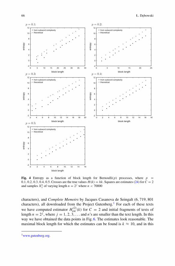
66 Ł. Debowski

p = 0.1

-2

0

2

4

6

8

10

12

0 5 10 15 20 25 30 35 40

entr

opy

block length

from subword complexitytheoretical

from subword complexitytheoretical

from subword complexitytheoretical

from subword complexitytheoretical

from subword complexitytheoretical

p = 0.2

-2

0

2

4

6

8

10

12

0 5 10 15 20 25

entr

opy

block lengthp = 0.3

-2

0

2

4

6

8

10

12

2 4 6 8 10 12 14 16 18 20

entr

opy

block length

p = 0.4

-2

0

2

4

6

8

10

12

0 2 4 6 8 10 12 14 16 18

entr

opy

block lengthp = 0.5

-2

0

2

4

6

8

10

12

0 2 4 6 8 10 12 14 16

entr

opy

block length

Fig. 4 Entropy as a function of block length for Bernoulli(p) processes, where p =0.1, 0.2, 0.3, 0.4, 0.5. Crosses are the true values H(k) = hk. Squares are estimates (24) for C = 2and samples Xn

1 of varying length n = 2 j where n < 70000

characters), and Complete Memoirs by Jacques Casanova de Seingalt (6, 719, 801characters), all downloaded from the Project Gutenberg.1 For each of these textswe have computed estimator H (2)

est (k) for C = 2 and initial fragments of texts oflength n = 2 j , where j = 1, 2, 3, . . . and n’s are smaller than the text length. In thisway we have obtained the data points in Fig. 6. The estimates look reasonable. Themaximal block length for which the estimates can be found is k ≈ 10, and in this

1www.gutenberg.org.

Estimation of Entropy from Subword Complexity 67

Fig. 5 Entropy rate h forBernoulli(p) processes as afunction of parameter p.Crosses are the true values,given by formula (29).Squares are the estimatesgiven by formula (25) forC = 2 and samples Xn

1 oflength n = 50000

0

0.2

0.4

0.6

0.8

1

0 0.1 0.2 0.3 0.4 0.5

entr

opy

rate

probability

theoreticalfrom subword complexity

Fig. 6 Estimates of blockentropy obtained throughestimator (24) for C = 2.Crosses relate to FirstFolio/35 Plays by WilliamShakespeare, squares relateto Gulliver’s Travels byJonathan Swift, and starsrelate to Complete Memoirsby Jacques Casanova deSeingalt. The regressionfunctions are models (31)with C = 2 and theremaining parameters givenin Table1

0

5

10

15

20

0 2 4 6 8 10 12

entr

opy

block length

ShakespeareSwift

Casanova de Seingalt

case we obtain H (2)est (k) ≈ 12.5 nats, which is less than the upper bound estimate

of H(10)/10 ≈ 1.5 nats per character by Shannon [27]. Our data also corroborateHilberg’s hypothesis. Namely, using nonlinear least squares, we have fitted model

H (2)est (k) = Akβ − C, (31)

where C was chosen as 2, and we have obtained quite a good fit. The values ofparameters A and β with their standard errors are given in Table1.

To verify Hilberg’s hypothesis for k ≥ 10 we need much larger data, such asbalanced corpora of texts. The size of modern text corpora is of order n = 109

characters. If relationship (1) persists in so large data, then we could obtain estimatesof entropy H(k) for block lengths k ≤ 20. This is still quite far from the range of datapoints k ∈ [1, 100] considered by Shannon in his experiment with human subjects[27]. But we hope that estimator H (2)

est (k) can be improved to be applicable also to

68 Ł. Debowski

Table 1 The fitted parameters of model (1). The values after ± are standard errors

Text A β

First Folio/35 Plays byWilliam Shakespeare

3.57 ± 0.05 0.652 ± 0.007

Gulliver’s Travels by JonathanSwift

3.56 ± 0.07 0.608 ± 0.012

Complete Memoirs by JacquesCasanova de Seingalt

3.60 ± 0.15 0.602 ± 0.021

so large block lengths. As we have shown, for the Bernoulli model with uniformprobabilities, subword complexity may convey information about block entropy forblock lengths smaller than or equal the maximal repetition. For many texts in naturallanguage, the maximal repetition is of order 100 or greater [8]. Hence we hope that,using an improved entropy estimator, we may get reasonable estimates of blockentropy H(k) for k ≤ 100.

5 Conclusion

In this paper we have considered some newmethods of estimating block entropy. Theidea is to base inference on empirical subword complexity—a function that counts thenumber of distinct substrings of a given length in the sample. In an entangled form,the expectation of subword complexity carries information about the probabilitydistribution of blocks of a given length fromwhich information about block entropiescan be extracted in some cases.

We have proposed two estimators of block entropy. The first estimator has beendesigned for IID processes but it has appeared that it works well only in the trivialcase of uniform probabilities. Thus we have proposed a second estimator, whichworks for any properly skewed stationary process. This assumption is satisfied ifthe distribution of strings of a given length is skewed towards less probable values.It is remarkable that the second estimator with a large probability provides a lowerbound of entropy, in contrast to estimators based on source coding, which give anupper bound of entropy. We stress that consistency of the second estimator remainsan open problem.

Moreover, using the second estimator, we have estimated block entropy for textsin natural language and we have confirmed earlier estimates as well as Hilberg’shypothesis for block lengths k ≤ 10. Further research is needed to provide an esti-mator for larger block lengths.We hope that subword complexity carries informationabout block entropy for block lengths smaller than or equal the maximal repetition,which would allow to estimate entropy for k ≤ 100 in the case of natural language.

Estimation of Entropy from Subword Complexity 69

References

1. Algoet PH, Cover TM (1988) A sandwich proof of the Shannon-McMillan-Breiman theorem.Ann. Probab. 16:899–909

2. Baayen, H (2001) Word frequency distributions. Kluwer Academic Publishers, Dordrecht3. Cover TM, Thomas JA (1991) Elements of information theory. Wiley, New York4. Crutchfield JP, Feldman DP (2003) Regularities unseen, randomness observed: the entropy

convergence hierarchy. Chaos 15:25–545. DillonWR, Goldstein M (1984) Multivariate analysis: methods and appplications. Wiley, New

York6. Debowski Ł (2011) On the vocabulary of grammar-based codes and the logical consistency of

texts. IEEE Trans. Inform. Theor. 57:4589–45997. Debowski Ł (2013) A preadapted universal switch distribution for testing Hilberg’s conjecture

(2013). http://arxiv.org/abs/1310.85118. Debowski Ł (2014) Maximal repetitions in written texts: finite energy hypothesis vs. strong

Hilberg conjecture (2014). http://www.ipipan.waw.pl/~ldebowsk/9. Debowski Ł (2014) A new universal code helps to distinguish natural language from random

texts (2014). http://www.ipipan.waw.pl/~ldebowsk/10. EbelingW, Pöschel T (1994) Entropy and long-range correlations in literary English. Europhys.

Lett. 26:241–24611. EbelingW,Nicolis G (1991) Entropy of symbolic sequences: the role of correlations. Europhys.

Lett. 14:191–19612. EbelingW, Nicolis G (1992) Word frequency and entropy of symbolic sequences: a dynamical

perspective. Chaos Sol. Fract. 2:635–65013. Ferenczi S (1999) Complexity of sequences and dynamical systems. Discr. Math. 206:145–15414. Gheorghiciuc I, Ward MD (2007) On correlation polynomials and subword complexity. Discr.

Math. Theo. Comp. Sci. AH, 1–1815. Graham RL, Knuth DE, Patashnik O (1994) Concrete mathematics, a foundation for computer

science. Addison-Wiley, New York16. Hall P, Morton SC (1993) On the estimation of entropy. Ann. Inst. Statist. Math. 45:69–8817. Hilberg W (1990) Der bekannte Grenzwert der redundanzfreien Information in Texten—eine

Fehlinterpretation der Shannonschen Experimente? Frequenz 44:243–24818. Ivanko EE (2008) Exact approximation of average subword complexity of finite randomwords

over finite alphabet. Trud. Inst. Mat. Meh. UrO RAN 14(4):185–18919. Janson S, Lonardi S, SzpankowskiW (2004) On average sequence complexity. Theor. Comput.

Sci. 326:213–22720. Joe H (1989) Estimation of entropy and other functionals of a multivariate density. Ann. Inst.

Statist. Math. 41:683–69721. Khmaladze E (1988) The statistical analysis of large number of rare events, Technical Report

MS-R8804. Centrum voor Wiskunde en Informatica, Amsterdam22. Kontoyiannis I, Algoet PH, SuhovYM,WynerAJ (1998)Nonparametric entropy estimation for

stationary processes and random fields, with applications to English text. IEEE Trans. Inform.Theor. 44:1319–1327

23. Koslicki D (2011) Topological entropy of DNA sequences. Bioinformatics 27:1061–106724. Krzanowski W (2000) Principles of multivariate analysis. Oxford University Press, Oxford25. de Luca A (1999) On the combinatorics of finite words. Theor. Comput. Sci. 218:13–3926. Schmitt AO, Herzel H, Ebeling W (1993) A new method to calculate higher-order entropies

from finite samples. Europhys. Lett. 23:303–30927. Shannon C (1951) Prediction and entropy of printed English. Bell Syst. Tech. J. 30:50–6428. Vogel H (2013) On the shape of subword complexity sequences of finite words (2013).

http://arxiv.org/abs/1309.344129. Wyner AD, Ziv J (1989) Some asymptotic properties of entropy of a stationary ergodic data

source with applications to data compression. IEEE Trans. Inform. Theor. 35:1250–1258

70 Ł. Debowski

30. Zipf GK (1935) The Psycho-Biology of language: an introduction to Dynamic Philology.Houghton Mifflin, Boston

31. Ziv J, Lempel A (1977) A universal algorithm for sequential data compression. IEEE Trans.Inform. Theor. 23:337–343

32. Ziv J, Lempel A (1978) Compression of individual sequences via variable-rate coding. IEEETrans. Inform. Theor. 24:530–536

Exact Rate of Convergenceof Kernel-Based Classification Rule

Maik Döring, László Györfi and Harro Walk

Abstract A binary classification problem is considered, where the posteriori proba-bility is estimated by the nonparametric kernel regression estimate with naive kernel.The excess error probability of the corresponding plug-in decision classification ruleaccording to the error probability of the Bayes decision is studied such that the excesserror probability is decomposed into approximation and estimation error. A generalformula is derived for the approximation error. Under a weak margin condition andvarious smoothness conditions, tight upper bounds are presented on the approxima-tion error. By a Berry-Esseen type central limit theorem a general expression for theestimation error is shown.

Keywords Lower bound · Upper bound · Classification error probability · Kernelrule · Margin condition

AMS Classification 62G10

This work was supported in part by the National Development Agency (NFÜ, Hungary) aspart of the project Introduction of Cognitive Methods for UAV Collision Avoidance UsingMillimeter Wave Radar, (grant no.: KMR-12-1-2012-0008).

M. DöringInstitute of Applied Mathematics and Statistics, University of Hohenheim,Schloss Hohenheim, 70599 Stuttgart, Germanye-mail: maik.doering@uni-hohenheim.de

L. Györfi (B)

Department of Computer Science and Information Theory,Budapest University of Technology and Economics,Magyar Tudósok Körútja 2., Budapest 1117, Hungarye-mail: gyorfi@cs.bme.hu

H. WalkDepartment of Mathematics, University of Stuttgart,Pfaffenwaldring 57, 70569 Stuttgart, Germanye-mail: walk@mathematik.uni-stuttgart.de

© Springer International Publishing Switzerland 2016S. Matwin and J. Mielniczuk (eds.), Challenges in Computational Statisticsand Data Mining, Studies in Computational Intelligence 605,DOI 10.1007/978-3-319-18781-5_5

71

72 M. Döring et al.

1 Introduction

We consider a binary classification problem. Using a kernel estimator for the posteri-ori probability, the asymptotics of the error probability is examined of the correspond-ing plug-in classification rule. In this paper lower and upper bounds are presentedon the rate of convergence of the classification error probability.

Let the feature vector X take values in Rd such that its distribution is denoted

by μ and let the label Y be binary valued. If g is an arbitrary decision function, thenits error probability is denoted by

L(g) = P{g(X) �= Y}.

The Bayes decision g∗ minimizes the error probability. It follows that

g∗(x) ={

1 if η(x) > 1/20 otherwise,

where the posteriori probability η is given by

η(x) = P{Y = 1 | X = x}.

Let the corresponding error probability be

L∗ = P{g∗(X) �= Y}.

PutD(x) = 2η(x) − 1,

then the Bayes decision has the following equivalent form:

g∗(x) ={

1 if D(x) > 00 otherwise.

In the standardmodel of pattern recognition,we are given training labeled samples,which are independent and identically copies of (X, Y): (X1, Y1), . . . , (Xn, Yn). Basedon these labeled samples, one can estimate the regression function D by Dn, and thecorresponding plug-in classification rule gn derived from Dn is defined by

gn(x) ={

1 if Dn(x) > 00 otherwise.

In the following our focus lies on the rate of convergence of the excess errorprobabilityE{L(gn)} − L∗. In Sect. 2margin conditions are discussed,whichmeasurehow fast the regression function D crosses the decision boundary. A nonparametric

Exact Rate of Convergence of Kernel-Based Classification Rule 73

kernel regression estimate of D is introduced and a decomposition of the excess errorprobability into approximation and estimation error is considered in Sect. 3. Tightupper bounds on the approximation error are shown in Sect. 4 depending on marginand smoothness conditions on D. By a Berry-Esseen type central limit theorema general expression for the estimation error is derived in Sect. 5. Finally, someconclusions are given.

2 Margin Conditions

Given the plug-in classification rule gn derived from Dn it follows

E{L(gn)} − L∗ ≤ E{|D(X) − Dn(X)|}

(cf. Theorem 2.2 in Devroye et al. [3]). Therefore we may get an upper bound on therate of convergence of the excess error probability E{L(gn)} − L∗ via the L1 rate ofconvergence of the corresponding regression estimation.

However, according to Sect. 6.7 in Devroye et al. [3], the classification is easierthan L1 regression function estimation, since the rate of convergence of the errorprobability depends on the behavior of the function D in the neighborhood of thedecision boundary

B0 = {x; D(x) = 0}. (1)

This phenomenon has been discovered by Mammen and Tsybakov [10], Tsybakov[13], who formulated the (strong) margin condition:

• The strong margin condition. Assume that for all 0 < t ≤ 1,

P {|D(X)| ≤ t} ≤ ctα, (2)

where α > 0 and c > 0.

Kohler and Krzyzak [7] introduced the weak margin condition:

• The weak margin condition. Assume that for all 0 < t ≤ 1,

E{

I{|D(X)|≤t}|D(X)|} ≤ ct1+α, (3)

where I denotes the indicator function.

Obviously, the strong margin condition implies the weak margin condition:

E{

I{|D(X)|≤t}|D(X)|} ≤ E{

I{|D(X)|≤t}t} = tP {|D(X)| ≤ t} ≤ ct · tα.

The difference between the strong and weak margin condition is that, for the strongmargin condition, the event

74 M. Döring et al.

{D(X) = 0}

counts. One can weaken the strong margin condition (2) such that we require

P {0 < |D(X)| ≤ t} ≤ ctα. (4)

Obviously, (4) implies (3). Under some mild conditions we have that α = 1.(Cf. Lemma 2.) The margin conditions measure how fast the probability of at-neighborhood of the decision boundary increases with t. A large value of α corre-sponds to a small probability of the neighborhood of the decision boundary, whichmeans that the probability for events far away of the decision boundary is high.Therefore, a classifier can make the right decision more easily, hence one can expectsmaller errors for larger values of α.

Recently, Audibert and Tsybakov [1] proved that if the plug-in classifier g hasbeen derived from the regression estimate D and if D satisfies the strong margincondition, then

L(g) − L∗ ≤(∫

(D(x) − D(x))2μ(dx)

) 1+α2+α

. (5)

It is easy to see that (5) holds even under weak margin condition: we have that

L(g) − L∗ = E{

I{g(X) �=g∗(X)}|D(X)|} (6)

(cf. Theorem 2.2 in Devroye et al. [3]). Let sign(x) = 1 for x > 0 and sign(x) = −1for x ≤ 0. For fixed tn > 0,

L(g) − L∗ = E

{

I{sign D(X) �=sign D(X),|D(X)|≤tn}|D(X)|}

+E

{

I{sign D(X) �=sign D(X),|D(X)|>tn}|D(X)|}

≤ E{

I{|D(X)|≤tn}|D(X)|}

+E

{

I{sign D(X) �=sign D(X),|D(X)−D(X)|>tn}|D(X) − D(X)|}

,

therefore the weak margin condition implies that

L(g) − L∗ ≤ ct1+αn + tnE

{

I{|D(X)−D(X)|>tn}|D(X) − D(X)|

tn

}

≤ ct1+αn + tnE

{

|D(X) − D(X)|2t2n

}

.

Exact Rate of Convergence of Kernel-Based Classification Rule 75

For the choice

tn =(

E

{

|D(X) − D(X)|2}) 1

2+α

we get (5).For bounding the error probability, assume, for example, that D satisfies the Lip-

schitz condition: for any x, z ∈ Rd

|D(x) − D(z)| ≤ C‖x − z‖.

If D is Lipschitz continuous and X is bounded then there are regression estimatessuch that ∫

(Dn(x) − D(x))2μ(dx) ≤ c21n− 2d+2 ,

therefore (5) means that

L(g) − L∗ ≤(

c21n− 2d+2

) 1+α2+α =

(

c1+α1 n− 1+α

d+2

) 22+α

.

Kohler and Krzyzak [7] proved that for the standard plug-in classification rules(partitioning, kernel, nearest neighbor) and for weak margin condition we get thatthe order of the upper bound can be smaller:

n− 1+αd+2 .

The main aim of this paper is to show tight upper bounds on the excess errorprobability E{L(gn)} − L∗ of the kernel classification rule gn.

3 Kernel Classification

We fix x ∈ Rd , and, for an h > 0, let the (naive) kernel estimate of D(x) be

Dn,h(x) = 1

n

n∑

i=1

(2Yi − 1)I{Xi∈Sx,h}/μ(Sx,h),

where Sx,h denotes the sphere centered at x with radius h. Notice thatDn,h is not a trueestimate, because its denominator contains the unknown distribution μ. However,the corresponding plug-in classification rule defined below depends only on the signof Dn,h(x), and so μ doesn’t count. The (naive) kernel classification rule is

gn,h(x) ={

1 if Dn,h(x) > 00 otherwise,

76 M. Döring et al.

(cf. Devroye [2], Devroye and Wagner [4], Krzyzak [8], Krzyzak and Pawlak [9]).If D is Lipschitz continuous and X is bounded then, for the L1 error, one has that

E{|D(X) − Dn,h(X)|} ≤ c2h + c3√nhd

,

(cf. Györfi et al. [5]), so for the choice

h = n− 1d+2 , (7)

the L1 upper bound implies that

E{L(gn,h)} − L∗ ≤ c4n− 1d+2 .

Because of (6), we have that the excess error probability of any plug-in classifi-cation rule has the following decomposition:

E{L(gn,h)} − L∗ = E

{∫

{sign Dn,h(x) �=sign D(x)}|D(x)|μ(dx)

}

= In,h + Jn,h,

where

In,h = E

{∫

{sign Dh(x)=sign Dn,h(x) �=sign D(x)}|D(x)|μ(dx)

}

and

Jn,h = E

{∫

{sign Dn,h(x) �=sign D(x)=sign Dh(x)}|D(x)|μ(dx)

}

with Dh(x) = E{Dn,h(x)}. In,h is called approximation error, while Jn,h is the esti-mation error.

4 Approximation Error

First we consider the approximation error. The following proposition means that thelower bound of the approximation error is approximately the half of the upper bound.Further, it shows that the bounds of the approximation error are mainly determinedby the bandwidth h.

Proposition 1(1

2+ o(1)

)

Ih ≤ In,h ≤ Ih,

Exact Rate of Convergence of Kernel-Based Classification Rule 77

where

Ih =∫

{sign Dh(x) �=sign D(x)}|D(x)|μ(dx).

Proof The upper bound is obvious. The lower bound follows from the central limittheorem, since

E

{∫

{0≥Dh(x),Dn,h(x)≤0<D(x)}|D(x)|μ(dx)

}

=∫

{Dh(x)≤0<D(x)}|D(x)|P{Dn,h(x) ≤ 0}μ(dx)

=∫

{Dh(x)≤0<D(x)}|D(x)|P{Dn,h(x) − Dh(x) ≤ −Dh(x)}μ(dx)

≥∫

{Dh(x)≤0<D(x)}|D(x)|P{Dn,h(x) − Dh(x) ≤ 0}μ(dx)

≥∫

{Dh(x)≤0<D(x)}|D(x)|

(1

2+ o(1)

)

μ(dx),

where o(1) is uniform in x. This can be seen, for example, using the Berry-Esseeninequality as in the proof of Proposition 2 below. The handling of remaining integralis analogous.

Kohler and Krzyzak [7] bounded the rate of convergence of the excess errorprobability assuming that D satisfies the weak margin condition and the Lipschitzcondition. Further they assume that X has a density which is bounded away fromzero:

f (x) ≥ c′ > 0 (8)

They proved that

E{L(gn,h)} − L∗ ≤ c5h1+α + c6nhd

(9)

such that, for the choice (7),

E{L(gn,h)} − L∗ ≤ c7n− 1+αd+2 .

In (9) the approximation error is upper bounded by c5h1+α . Next we show how itfollows from Proposition 1. Denote by

B0,h ={

x;minz∈B0

‖x − z‖ ≤ h

}

the h-neighborhood of the decision boundaryB0 defined by (1). Letλ be the Lebesguemeasure and let M∗(B0) be the outer surface (Minkowski content) of the decision

78 M. Döring et al.

boundary B0 defined by

M∗(B0) = limh↓0

λ(B0,h \ B0)

h.

Lemma 1 If D satisfies the weak margin condition and the Lipschitz condition, then

Ih ≤ c8h1+α.

If D satisfies the Lipschitz condition, the density f of X exists, it is bounded by fmax

and M∗(B0) is finite, thenIh ≤ c9h2.

Proof If x /∈ B0,h thensign Dh(x) = sign D(x).

Therefore

Ih =∫

{sign Dh(x) �=sign D(x)}|D(x)|μ(dx)

=∫

{sign Dh(x) �=sign D(x),x∈B0,h}|D(x)|μ(dx).

For any fixed x ∈ B0,h, there is a zx ∈ B0 such that ‖x − zx‖ ≤ h, which togetherwith the Lipschitz condition implies that

|D(x)| = |D(x) − D(zx)| ≤ Ch.

Thus, by the weak margin condition

Ih ≤∫

{|D(x)|≤Ch,x∈B0,h}|D(x)|μ(dx)

≤∫

{|D(x)|≤Ch}|D(x)|μ(dx)

≤ c(Ch)1+α.

Concerning the second half of the lemma, we have that

Ih ≤∫

{|D(x)|≤Ch,x∈B0,h}|D(x)|μ(dx)

≤ Ch∫

{0<|D(x)|,x∈B0,h}1μ(dx)

Exact Rate of Convergence of Kernel-Based Classification Rule 79

= Chμ{B0,h \ B0}≤ Chfmaxλ{B0,h \ B0}≤ Cc10h2.

The technique of the second half of the previous proof implies that α = 1.

Lemma 2 Let D satisfies the lower Lipschitz inequality at B0, which means a c∗ > 0exists, such that for all t ∈ [0, 1] and

x /∈ B0,c∗t

it follows|D(x)| > t.

If the density f of X exists, it is bounded by fmax, and the outer surface M∗(B0) isfinite, then the weak margin condition holds with α = 1.

Proof We verify (4) with α = 1.

P {0 < |D(X)| ≤ t}= P

{

0 < |D(X)| ≤ t, X ∈ B0,c∗t \ B0} + P

{

0 < |D(X)| ≤ t, X /∈ B0,c∗t}

≤ P{

X ∈ B0,c∗t \ B0} + P {0 < |D(X)| ≤ t, t < |D(X)|}

≤ c10c∗t.

Hall and Kang [6] investigated the bandwidth choice. They assumed that condi-tional densities exist, which are bounded away from zero. Under twice differentiableconditional densities, they proved that

E{L(gn,h)} − L∗ ≤ c11h4 + o

(1

nhd

)

. (10)

In (10) the approximation error is upper bounded by c11h4. Next we show how itfollows from Proposition 1.

Let us introduce some notations:

p+ := P{Y = 1}, p− := P{Y = 0}

Assume that the density f of X exists. Let the conditional densities f+ and f− bedefined by

P{X ∈ A | Y = 1} =∫

Af+(x) dx

and

P{X ∈ A | Y = 0} =∫

Af−(x) dx.

80 M. Döring et al.

Thenf (x) = p+ · f+(x) + p− · f−(x)

and

D(x) = f (x)

f (x),

wheref (x) := p+ · f+(x) − p− · f−(x).

Moreover,

f+(x) = f (x) · (1 + D(x))

2p+, f−(x) = f (x) · (

1 − D(x))

2p−.

Lemma 3 Assume that f is two-times differentiable with bounded second orderpartial derivatives. If D satisfies the weak margin condition and the density f isbounded below by fmin, then

Ih ≤ c12h2(1+α).

Proof Let Hf be the Hessian-matrix of f . Then the conditions of the lemma implythat

sup0≤t≤1

∣∣(x − z)T Hf

(

x + t(z − x))

(x − z)∣∣ ≤ c13‖x − z‖2 (11)

with 0 < c13 < ∞. We have the decomposition

Dh(x) =∫

Sx,hD(z)μ(dz)

μ(Sx,h)

=∫

Sx,h

f (z)f (z) f (z)dz

μ(Sx,h)

=∫

Sx,h

(

f (z) − f (x))

dz

μ(Sx,h)+ f (x)λ(Sx,h)

μ(Sx,h)

=∫

Sx,h

(

f (z) − f (x))

dz

μ(Sx,h)+ D(x)

f (x)λ(Sx,h)

μ(Sx,h).

The second order Taylor expansion

f (z) − f (x) = (z − x)T ∇ f (x) + (z − x)T Hf (xz)(z − x)/2

with xz ∈ Sx,h implies that

Exact Rate of Convergence of Kernel-Based Classification Rule 81

Dh(x)

=∫

Sx,h

(

(z − x)T ∇ f (x) + (z − x)T Hf (xz)(z − x)/2)

dz

μ(Sx,h)+ D(x)

f (x)λ(Sx,h)

μ(Sx,h)

=∫

Sx,h(z − x)T Hf (xz)(z − x)/2 dz

μ(Sx,h)+ D(x)

f (x)λ(Sx,h)

μ(Sx,h).

Therefore, from (11) we get that

Dh(x) ≥ −c13h2λ(Sx,h)/2

μ(Sx,h)+ D(x)

f (x)λ(Sx,h)

μ(Sx,h).

Thus, for D(x) ≥ 0 > Dh(x), we have

|D(x)| ≤ c13h2

2f (x)≤ c13h2

2fmin.

The same inequality holds for D(x) < 0 ≤ Dh(x). From the weak margin conditionwe get

Ih =∫

{

sign(

Dh(x))

�=sign(

D(x))

,x∈B0,h

} |D(x)|μ(dx)

≤∫

{

|D(x)|≤ c13h2

2fmin

} |D(x)|μ(dx)

≤ c12h2(1+α).

Under the assumption of Lemma 2 we have that the weak margin condition holdswith α = 1. Hence by Lemma 3 and Proposition 1 we get that the approximationerror In,h is upper bounded by a multiple of h4.

The question left is that whether the upper bounds in Lemmas 1 and 3 are tight.Consider some examples, where α = 1 and Ih can be calculated showing that theorder of the lower bounds have the order of the upper bounds.

Example 1 Assume that f is the uniform density on [−1, 1]d . Let h < 1, β ≥ 1,a > 0, b > 0, a + b < 1. Choose

p+ = 1

2+ b

4(β + 1)

andD(x) = ax1 + bxβ

1 · I(0,1](x1),

82 M. Döring et al.

where x = (x1, . . . , xd). Then

f (x) = ax1 + bxβ1 · I(0,1](x1)2d

· I[−1,1]d (x)

f+(x) = 1 + ax1 + bxβ1 · I(0,1](x1)

2d+1p+· I[−1,1]d (x)

f−(x) = 1 − ax1 − bxβ1 · I(0,1](x1)

2d+1p−· I[−1,1]d (x).

One can check that D satisfies the weak margin condition with α = 1. If x1 > 0 thensign Dh(x) = sign D(x). Let Vd be the volume of the d-dimensional unit sphere, i.e.Vd = πd/2/�(d/2 + 1). For −h < x1 ≤ 0

∫

Sx,h

D(x) μ(dx) =∫

Sx,h

ax1 + a(z1 − x1) + bzβ1 · I(0,1](z1)

2d· I[−1,1]d (z) dz

= aVd

2dhdx1+

∫ x1+h

x1−h

a(z1 − x1) + bzβ1 ·I(0,1](z1)

2dVd−1

(

h2 − (z1 − x1)2)(d−1)/2

dz1

= aVd

2dhdx1 + bVd−1

2d

∫ x1+h

0zβ1

(

h2 − (z1 − x1)2)(d−1)/2

dz1

≤ aVd

2dhdx1 + bVd−1

2dhd−1

∫ x1+h

0zβ1 dz1

≤ hd−1

2d

(

aVdhx1 + bVd−1

β + 1hβ+1

)

.

And we have a lower bound by

∫

Sx,h

D(x)μ(dx) = aVd

2dhdx1 + bVd−1

2d

∫ x1+h

0zβ1

(

h2 − (z1 − x1)2)(d−1)/2

dz1

= aVd

2dhdx1 + bVd−1

2d

∫ h

0I(−x1,∞)(z1)(z1 + x1)

β(

h2 − z21)(d−1)/2

dz1

= aVd

2dhdx1 + bVd−1

2d

∫ h

0

(

I(0,∞)(z1)zβ1

(

h2 − z21)(d−1)/2

+ x1I(−x1,∞)(z1)β(z1 + x1)β−1(h2 − z21

)(d−1)/2)

dz1

≥ aVd

2dhdx1 + bVd−1

2d

∫ h

0

(

zβ1

(

h2 − z21)(d−1)/2 + x1β zβ−1

1 hd−1)

dz1

Exact Rate of Convergence of Kernel-Based Classification Rule 83

≥ aVd

2dhdx1 + bVd−1

2d

(∫ h/2

0zβ1

(

h2 − (h/2)2)(d−1)/2

dz1

+∫ h

h/2(h/2)β−1z1

(

h2 − z21)(d−1)/2

dz1 + x1hd)

= aVd

2dhdx1 + bVd−1

2d

( 1

β + 1(h/2)β+1(h2 − (h/2)2

)(d−1)/2

+ (h/2)β−1(h2 − (h/2)2)(d+1)/2 1

d + 1+ x1hd

)

= hd−1

2d

(

(aVd + bVd−1)hx1 + bVd−1( (3/4)(d−1)/2

(β + 1)2β+1 + (3/4)(d+1)/2

(d + 1)2β−1

)

hβ+1)

.

For the notations

c14 = bVd−1

aVd + bVd−1

( (3/4)(d−1)/2

(β + 1)2β+1 + (3/4)(d+1)/2

(d + 1)2β−1

)

c15 = bVd−1

aVd · (β + 1)

we get that

−c14hβ < x1 =⇒ Dh(x) > 0 =⇒ −c15 · hβ < x1

Therefore

Ih =∫

{sign Dh(x) �=sign D(x)}|D(x)| μ(dx)

≥∫ 0

−c14·hβ

∫

[−1,1]d−1− a

2dx1 d(x2, . . . xd) dx1 = ac214

4· h2β

Analogously

ac2144

· h2β ≤ Ih ≤ ac2154

· h2β

• If β = 1, then D, f , f+ and f− are Lipschitz continuous and

Ih ≥ c16h2.

• If β = 1+ ε/2 for ε > 0, then D, f , f+ and f− are continuously differentiable and

Ih ≥ c17h2+ε .

84 M. Döring et al.

• If β = 2 + ε/2 for ε > 0, then D, f , f+ and f− are two times continuouslydifferentiable and

Ih ≥ c18h4+ε .

5 Estimation Error

Next we consider the estimation error. Introduce the notations

Nx,h = μ(Sx,h)Dh(x)2

1 − μ(Sx,h)Dh(x)2

andRx,h = c19

√

μ(Sx,h)(1 − μ(Sx,h)Dh(x)2)3

with a universal constant c19 > 0. Put

Jn,h =∫

{sign Dh(x)=sign D(x)}|D(x)|Φ

(

−√

n · Nx,h

)

μ(dx),

where Φ stands for the standard Gaussian distribution function.

Proposition 2 We have that

|Jn,h − Jn,h| ≤∫

{sign Dh(x)=sign D(x)}Rx,h · |D(x)|√

n + n2N3/2x,h

μ(dx).

Put ε > 0. If the density of X exists then, for h small enough,

∫

{sign Dh(x)=sign D(x)}|D(x)|Φ

(

−√

(1 + ε)n · μ(Sx,h)|Dh(x)|)

μ(dx)

≤ Jn,h

=∫

{sign Dh(x)=sign D(x)}|D(x)|Φ

(

−√

n · μ(Sx,h)|Dh(x)|)

μ(dx),

and∫

{sign Dh(x)=sign D(x)}Rx,h · |D(x)|√

n + n2N3/2x,h

μ(dx)

≤∫

{sign Dh(x)=sign D(x)}2c19 · |D(x)|

√

nμ(Sx,h)(1 + (√

n · μ(Sx,h)|Dh(x)|)3)μ(dx)

Exact Rate of Convergence of Kernel-Based Classification Rule 85

with a universal constant c19 > 0.

Proof First we show the following: For fixed x and h, under 0 < Dh(x) we have that

|P{Dn,h(x) ≤ 0} − Φ(

−√

n · Nx,h

)

| ≤ Rx,h√n + n2N3/2

x,h

,

which implies the first half of the proposition. (The case Dh(x) ≤ 0 and Dn,h(x) > 0is completely analogous.) Introduce the notation

Zi = −(2Yi − 1)I{Xi∈Sx,h}.

Then

P{Dn,h(x) ≤ 0} = P

{n

∑

i=1

Zi ≥ 0

}

= P

{∑ni=1(Zi − E{Zi})√

nVar(Z1)≥ −

√nE{Z1}√Var(Z1)

}

.

Because of

Var(Z1) = E{|Z1|2} − (E{Z1})2 = μ(Sx,h) − μ(Sx,h)2Dh(x)

2

and by 0 < Dh(x) we have that

E{Z1}√Var(Z1)

= −√

μ(Sx,h)Dh(x)√

1 − μ(Sx,h)Dh(x)2= −√

Nx,h

Therefore the central limit theorem for the probability P{Dn,h(x) ≤ 0} implies that

P{Dn,h(x) ≤ 0} = P

{

−∑n

i=1(Zi − E{Zi})√nVar(Z1)

≤ −√

nNx,h

}

≈ Φ(

−√

nNx,h

)

.

Notice that it is only an approximation. In order to make bounds out of the normalapproximation, we refer to Berry-Esseen type central limit theorem (see Theorem14 in Petrov [12]). Thus,

∣∣∣P{Dn,h(x) ≤ 0} − Φ

(

−√

nNx,h

)∣∣∣ ≤

c19E{|Z1|3}

Var(Z1)3/2√n

(

1 + (√

nNx,h)3

) ,

with the universal constant 30.84 ≥ c19 > 0 (cf.Michel [11]).Because of E{|Z1|3} =μ(Sx,h) we get that

86 M. Döring et al.

c19E{|Z1|3}

Var(Z1)3/2= c19

μ(Sx,h)1/2(

1 − μ(Sx,h)Dh(x)2)3/2 = Rx,h,

hence

∣∣∣P{Dn,h(x) ≤ 0} − Φ

(

−√

nNx,h

)∣∣∣ ≤ Rx,h√

n(1 + (n · Nx,h)3/2).

Concerning the second half of the proposition notice that if the density of X existsthen

Rx,h ≤ 2c19√

μ(Sx,h),

and, for any ε > 0,

μ(Sx,h)Dh(x)2 ≤ Nx,h ≤ (1 + ε)μ(Sx,h)Dh(x)

2

if h is small enough.

Next we show that the upper bound of the error term in the second half in

Proposition 2 is of order o(

1nhd

n

)

.

Lemma 4 Assume that

limn→∞ hn = 0 and lim

n→∞ nhdn = ∞, (12)

and that there is a c > 0 such that sign Dh(x) = sign D(x) implies |Dh(x)| ≥ c|D(x)|.If X has a density f with bounded support then

An :=∫

{sign Dhn (x)=sign D(x)}|D(x)|

√

nμ(Sx,hn)(1 + (√

nμ(Sx,hn)|Dhn(x)|)3)μ(dx)

= o

(1

nhdn

)

. (13)

Proof Let B be the bounded support of f . Then f (x) > 0 on B and f (x) = 0 on Bc.Introduce the notation

fn(x) = μ(Sx,hn)

λ(Sx,hn),

where λ stands for the Lebesgue measure. Under the conditions of the lemma wehave that

Exact Rate of Convergence of Kernel-Based Classification Rule 87

An ≤∫ |D(x)|

√

nμ(Sx,hn)(1 + (√

nμ(Sx,hn)c|D(x)|)3)μ(dx)

=∫ |D(x)|

√

nλ(Sx,hn)fn(x)(1 + (√

nλ(Sx,hn)fn(x)c|D(x)|)3)μ(dx)

=∫

1

fn(x)

1

cnλ(Sx,hn)

√

nλ(Sx,hn)fn(x)c|D(x)|1 + (

√

nλ(Sx,hn)fn(x)c|D(x)|)3μ(dx)

= 1

cnhdnVd

∫

B

f (x)

fn(x)rn(x)dx

with

rn(x) =√

nλ(Sx,hn)fn(x)c|D(x)|1 + (

√

nλ(Sx,hn)fn(x)c|D(x)|)3 .

Thus, we have to show that

∫

B

f (x)

fn(x)rn(x)dx → 0.

By theLebesgue density theorem fn(x) → f (x) and therefore fn(x)/f (x) → 1λ—a.e.on B, and so rn(x) → 0 λ—a.e. on B. Moreover, this convergence is dominated:

rn(x) ≤ max0≤u

u

1 + u3=: rmax.

Thus, ∫

Brn(x)dx → 0.

Apply the decomposition

∫

B

f (x)

fn(x)rn(x)dx ≤

∫

B

∣∣∣∣

f (x)

fn(x)− 1

∣∣∣∣rn(x)dx +

∫

Brn(x)dx

≤ rmax

∫

B

∣∣∣∣

f (x)

fn(x)− 1

∣∣∣∣dx + o(1).

In order to prove

∫

B

∣∣∣∣

f (x)

fn(x)− 1

∣∣∣∣dx → 0 (14)

we refer to the Riesz-Vitali-Scheffé theorem, according to which (14) is satisfied if

f

fn≥ 0,

88 M. Döring et al.

f

fn→ 1 λ—a.e. on B,

and∫

B

f (x)

fn(x)dx →

∫

B1 dx = λ(B). (15)

Thus, it remains to show (15). By the generalized Lebesgue density theorem (cf.Lemma 24.5 in Györfi et al. [5]), for each μ-integrable function m

∫

B

∣∣∣∣∣

∫

Sx,hnm(z)μ(dz)

μ(Sx,hn)− m(x)

∣∣∣∣∣μ(dx) → 0.

Therefore∫

B

∫

Sx,hnm(z)μ(dz)

μ(Sx,hn)μ(dx) →

∫

Bm(x)μ(dx).

Choose

m(x) = 1

f (x), x ∈ B.

Then

∫

B

f (x)

fn(x)dx =

∫

B

∫

Sx,hnm(z)μ(dz)

μ(Sx,hn)μ(dx) →

∫

Bm(x)μ(dx) =

∫

B1 dx = λ(B),

and the lemma is proved.

As we already mentioned, using Hoeffding and Bernstein inequalities Kohler andKrzyzak [7] proved that under the condition (8) we have

Jn,hn ≤ c6nhd

n(16)

with c6 < ∞.We believe that applying Proposition 2 the condition (8) can be weakened such

that the following conjecture holds: If X is bounded and it has a density then wehave (16).

Because of Lemma 4, this conjecture means that

∫

{sign Dh(x)=sign D(x)}|D(x)|Φ

(

−√

nμ(Sx,hn)|Dhn(x)|)

μ(dx) ≤ c6nhd

n. (17)

Concerning a possible way to prove (17) we may apply the covering argument of(5.1) in Györfi et al. [5], which says that for bounded X,

Exact Rate of Convergence of Kernel-Based Classification Rule 89

∫1

μ(Sx,hn)μ(dx) ≤ c20

hdn

.

The bounded support of X can be covered by spheres Sxj,hn/2, j = 1, . . . , Mn suchthat Mn ≤ c21/hd

n . Let

S′x,hn

= Sx,hn ∩ {z : sign Dhn(z) = sign D(z)}.

If x ∈ S′xj,hn/2

then S′xj,hn/2

⊆ S′x,hn

. For (17),

∫

{sign Dhn (x)=sign D(x)}|D(x)|Φ

(

−√

nμ(Sx,hn)|Dhn(x)|)

μ(dx)

≤Mn∑

j=1

∫

S′xj ,hn/2

|D(x)|Φ(

−√

nμ(Sx,hn)|Dhn(x)|)

μ(dx)

≤Mn∑

j=1

∫

S′xj ,hn/2

|D(x)|Φ(

−√

nμ(Sxj,hn/2)|Dhn(x)|)

μ(dx)

≤ 1

n

Mn∑

j=1

∫

S′xj ,hn/2

n|D(x)|e−nμ(Sxj ,hn/2)|Dhn (x)|2/2μ(dx)

≤ 1

n

Mn∑

j=1

∫

S′xj ,hn/2

n|D(x)|e−nμ(Sxj ,hn/2)c2|D(x)|2/2μ(dx),

where the last inequality follows by the assumptions of Lemma 4. If

supj

∫

S′xj ,hn/2

n|D(x)|e−nμ(Sxj ,hn/2)c2|D(x)|2/2μ(dx) < ∞

then∫

{sign Dh(x)=sign D(x)}|D(x)|Φ

(

−√

nμ(Sx,hn)|Dhn(x)|)

μ(dx) ≤ c22Mn

n≤ c6

nhdn.

Example 2 Notice that the upper bound in (16) is tight. As in the Example 1, if μ isthe uniform distribution and

D(x) = x1,

then sign Dhn(x) = sign D(x) and |Dhn(x)| = |D(x)| for hn < 1/2 and |x1| < 1/2.Thus

90 M. Döring et al.

Jn,hn

≥∫

{sign Dhn (x)=sign D(x)}|D(x)|Φ

(

−√

(1 + ε)nμ(Sx,hn)|Dhn(x)|)

μ(dx)

≥∫ 1/2

0zΦ

(

−√

(1 + ε)Vdnhdn2

−dz

)

dz

= 1

(1 + ε)Vdnhdn2

−d

∫√

(1+ε)Vdnhdn2

−d/2

0uΦ (−u) du

= 1

(1 + ε)Vdnhdn2−d

(∫ ∞

0uΦ (−u) du + o(1)

)

≥ c23nhd

n,

with 0 < c23. Hall and Kang [6] proved that if X has a density, bounded from aboveand from below then

Jn,hn = o

(1

nhdn

)

,

which contradicts the lower bound c23nhd

n.

In general, we conjecture the following: If X has a density, which is bounded byfmax, then

c24nhd

n≤ Jn,hn

with 0 < c24. This conjecture is supported by the fact that

μ(Sx,hn) ≤ fmaxVdhdn .

Therefore∫

{sign Dhn (x)=sign D(x)}|D(x)|Φ

(

−√

(1 + ε)nμ(Sx,hn)|Dhn(x)|)

μ(dx)

≥∫

{sign Dhn (x)=sign D(x)}|D(x)|Φ

(

−√

(1 + ε)nfmaxVdhdn |Dhn(x)|

)

μ(dx).

6 Conclusion

We presented tight upper bounds for the rate of convergence of the error probabilityof kernel classification rule. Decomposing the excess error probability into the sumof approximation and estimation error, we derived approximate formulas both forapproximation error and estimation error.

Exact Rate of Convergence of Kernel-Based Classification Rule 91

Under weak margin condition with α and Lipschitz condition on the regressionfunctionD, Kohler and Krzyzak [7] showed that the approximation error In,h is upperbounded by c5hα+1. If, in addition, the conditional densities are twice continuouslydifferentiable, then we proved that In,h ≤ c12h2(α+1). Furthermore, we present anexample, according to which these upper bounds are tight. Under the assumptionthat the Minkowski content of the decision boundary is finite and the lower Lipschitzinequality holds, the weak margin condition holds with α = 1. Hence we get theupper bound In,h ≤ c11h4 as in Hall and Kang [6] as a special case.

If X has a lower bounded density, then Kohler and Krzyzak proved the upperbound on the estimation error: Jn,h ≤ c6/(nhd). We show that this upper bound istight, too.

References

1. Audibert J-Y, Tsybakov AB (2007) Fast learning rates for plug-in classifiers, Ann Stat 35:608–633

2. Devroye L (1981) On the almost everywhere convergence of nonparametric regression functionestimates. Ann Stat 9:1310–1319

3. Devroye L, Györfi L, Lugosi G (1996) A probabilistic theory of pattern recognition. Springer,New York

4. Devroye L, Wagner TJ (1980) Distribution-free consistency results in nonparametric discrim-ination and regression function estimation. Ann Stat 8:231–239

5. Györfi L, Kohler M, Krzyzak A, Walk H (2002) A distribution-free theory of nonparametricregression. Springer, New York

6. Hall P,KangK (2005)Bandwidth choice for nonparametric classification.AnnStat 33:284–3067. KohlerM,KrzyzakA (2007)On the rate of convergence of local averaging plug-in classification

rules under a margin condition. IEEE Trans Inf Theory 53:1735–17428. Krzyzak A (1986) The rates of convergence of kernel regression estimates and classification

rules. IEEE Trans Inf Theory IT-32:668–6799. Krzyzak A, Pawlak M (1984) Distribution-free consistency of a nonparametric kernel regres-

sion estimate and classification. IEEE Trans Inf Theory IT-30:78–8110. Mammen E, Tsybakov AB (1999) Smooth discrimination analysis. Ann Stat 27:1808–182911. Michel R (1981) On the constant in the non-uniform version of the Berry-Esseen theorem. Z

Wahrsch Verw Gebiete 55:109–11712. Petrov VV (1975) Sums of independent random variables. Springer, Berlin13. TsybakovAB (2004)Optimal aggregation of classifiers in statistical learning. Ann Stat 32:135–

166

Compound Bipolar Queries:A Step Towards an Enhanced HumanConsistency and Human Friendliness

Janusz Kacprzyk and Sławomir Zadrozny

Abstract Database querying is a basic capability to make use of databases that areomnipresent and huge. A crucial problem is how to make possible for an ordinaryhuman user to properly express his intentions and preferences as to what should besearched for. As natural language, with its inherent imprecision, is the only fullynatural human means of communication and articulation, this makes difficult the useof traditional binary logic based querying tools. Fuzzy logic can come to the res-cue, notably using fuzzy logic with linguistic quantifiers. Such queries, proposed byKacprzyk and Ziółkowski [24], Kacprzyk et al. [25], have offered much in this con-text, and will also be used here. While looking for further solutions in this direction,the concept of a bipolar query has been proposed by Dubois and Prade [13], followedby a fuzzy bipolar query due to Zadrozny [36] (cf. Zadrozny and Kacprzyk [40])involving negative and positive information, notably meant as required and desiredconditions. A natural solution consisting in combining these two ideas was proposedconceptually byKacprzyk andZadrozny [22], and termed a compound bipolar query.In this paper we further extend this concept mainly by exploring some additionalaggregation related aspects of bipolar queries which include fuzzy queries with lin-guistic quantifiers.

To Professor Jacek Koronacki, a great researcher and scholar, and a long time friend, for hiswise support and inspiration.

J. Kacprzyk (B) · S. ZadroznySystems Research Institute, Polish Academy of Sciences, Warsaw, Polande-mail: kacprzyk@ibspan.waw.pl

S. Zadroznye-mail: Slawomir.Zadrozny@ibspan.waw.pl

J. KacprzykWIT—Warsaw School of Information Technology, Warsaw, Poland

© Springer International Publishing Switzerland 2016S. Matwin and J. Mielniczuk (eds.), Challenges in Computational Statisticsand Data Mining, Studies in Computational Intelligence 605,DOI 10.1007/978-3-319-18781-5_6

93

94 J. Kacprzyk and S. Zadrozny

1 Introduction

The purpose of this short note is to discuss some possible approaches, within the lineof research we have been active in for many years, to the very essence of flexiblequerying, that is retrieving from (possibly large) numerical databases informationwhich the human agent really wants to find. The human agent is assumed to be anaverage user, not a database specialist, and for him or her the only natural way ofarticulation of his or her intentions or needs, but also preferences (i.e. which recordis good and which is not), is by using natural language a characteristic feature ofwhich is an inherent imprecision and vagueness.

Needless to say that the use of natural language per se is a great difficulty to thetraditional database querying systems and languages but this is not all. Namely, the“normal”, or average human users think—as the human beings do—about a moresophisticated and complex concepts corresponding to what they want to retrieve.For instance, they may prefer to speak about a “good financial standing” rather thanabout, for instance, “yearly income is much more than USD xx” and “loans in banksare negligible” etc.

However, those concepts, being consistent for humans, are difficult to representformally through some commands of a querying language, notably the SQL. Theproblem is clearly not an inherent imprecision of terms like a “high income” becausethey can be represented by using fuzzy logic, and this has been known since the late1960s (cf. a survey in Galindo [18]). The very problem is a proper representation ofthe very meaning of those concepts which are at a higher level of abstraction likea “good financial standing”. Clearly, a proper representation should involve someaggregation of satisfaction values from the fulfillment of some conditions on someattributes but it is not clear which type of aggregation should be employed. The usualAND-type aggregation (and its relatedOR-type) has been dealt with in the traditionalfuzzy querying literature by just using the minimum (or a t-norm) or maximum (oran s-norm) but this was not enough.

The first step towards a more realistic and human consistent approach to therepresentation of more complex concepts in flexible (fuzzy) querying was proposedin the mid-1986 by Kacprzyk and Ziółkowski [24], followed by Kacprzyk et al. [25]in which the concept of a database query with a fuzzy linguistic quantifier has beenintroduced.

The idea of query with a linguistic quantifier is as follows. For clarity we willquote here an example from the real world application for which these queries havebeen initially proposed at the International Institute for Applied Systems Analysisin Laxenburg, Austria. The queries have been supposed to be employed in databasequerying to be used in a decision support system for regional authorities responsi-ble for, among other issues, water quality. Those top level people, unfamiliar withdatabases, have—while being interviewed during the development of a conceptualsolution and architecture of that decision support system—expressed interest mainlyin highly aggregated and sophisticated concepts like “dangerous water pollution”.After some discussion it has turned out that their human perception of the very

Compound Bipolar Queries … 95

meaning of such concepts has been that, for instance, “most of the important waterpollution indicators have considerably exceeded limits”, with the linguistic quantifier“most” considered to be very important.

It is easy to see that meaning of that complex term, “dangerous water pollution”,equated with the above linguistically quantified statement, has been a challenge,mostly because of the occurrence of the linguistic quantifier “most” that has beenoutside of the scope of the traditional logic, and its very essencewas even not the sameas the essence of the generalized quantifiers (cf. Mostowski [29] or Lindström [28]).Luckily enough, Zadeh’s [35] fuzzy logic based calculus of linguistically quantifiedpropositions makes it possible to determine the degrees of truth of such linguisticallyquantified statements. A very important capability has therefore been made availableby fuzzy querying with linguistic quantifiers.

However, as powerful as fuzzy queries with linguistic quantifiers can be, theyhave not been in a position to express all fine shades of meaning of real humanintentions as to what they really want to retrieve. Among many possible steps in thiscontext, one in which we have been active for years (cf. Zadrozny [36], Zadroznyand Kacprzyk [40], Zadrozny et al. [37], just to name a few) has been the concept ofa bipolar query.

The very essence of a bipolar query can be best shown on the following simpleexample of looking for a “good” apartment in a database of a real estate agency.Suppose that a customer comes to an agent and, when asked about what he or shewants to find, responds that he or she is interested in the purchasing of a “good apart-ment”. As such a general intention cannot be directly related to database attributesand used by the agent to search the database, the customer is again asked what he orshe means by a good apartment. The response may often be that he or she looks foran “inexpensive apartment” and possibly, “close to public transportation”. Notice,however, that this is still far from the traditional pattern of queries because “andpossibly” is certainly not equivalent to the classical conjunction.

The above type of a database query may be viewed as a reflection of the so calledbipolarity. Namely, there is a sound evidence, resulting from many experiments insocial and cognitive sciences, that a human being is usually considering both positiveand negative information while making a judgment or decision. This positive andnegative information is then somehow aggregated yielding an overall judgment. Theway this aggregation is carried out may be more or less explicit but in general it maytake different forms, depending on the task, context, emotional involvement etc. Inthe literature, often a special interpretation of the positive and negative informationis assumed which assigns higher importance to the latter but in a rather subtle way.Basically, considered in the database querying context, the latter implies mandatoryrequirements, as negative information is treated as corresponding to what must notoccur, and the former implies optional requirements, as positive information is treatedas concerning what is preferable, if possible. This bipolarity should therefore bereflected in database queries.

In our context, formal and algorithmic attempts at the formalization of bipolarityin judgments and evidence are crucial, and for us in particular those based on fuzzylogic and possibility theory the roots of which constitute fundamental works by

96 J. Kacprzyk and S. Zadrozny

Dubois and Prade and their collaborators, to name just a few: Benferhat et al. [4] orDubois and Prade [14–16].

There are many aspects of bipolarity to be taken into account, cf. Zadrozny et al.[37]. First, various models of bipolarity may be adopted, notably the use of a properscale to describe the phenomenon. Basically, two such models (scales) are usuallyconsidered: bipolar univariate and unipolar bivariate, cf. Grabisch et al. [19]. Theformer assumes one scale with three main levels of, respectively, negative, neutraland positive evaluation, gradually changing, while the latter model assumes twomore or less independent scales which separately account for a positive and negativeevaluation. Usually, the intervals [−1, 1] and [0, 1] are used to represent the scalesin the respective models of bipolarity. We will use the unipolar bivariate scales tohandle bipolarity.

It is easy to see that bipolarity triggers a qualitatively different character of bipolarevaluations. In flexible querying, a crucial problem is how to use them to order theresulting set of tuples. Basically, one should aggregate them and obtain an overallevaluation of each tuple against a bipolar query but, in general, it is not clear how todo this.

Here we study a special case when positive and negative conditions may be inter-preted in terms of desired and required conditions. Then, their aggregation mayproceed as proposed for the crisp case by Lacroix and Lavency [26]. We follow thisapproach, adapt it to the fuzzy case and study its properties and possible implemen-tations.

Basically, a prototypical example of a bipolar query considered in this paper is

C and possibly P (1)

exemplified by

find a house which is inexpensive and possibly close to public transportation

The main problem is to find a proper aggregation method to reflect the very trickyand non-conventional aggregation operator “…and possibly,…”. In our analyseswe will adopt our approach to that aggregation (cf. Zadrozny [36], Zadrozny andKacprzyk [38, 40]), De Tré et al. [11, 12]) that is basically an extension of theclassic Lacroix and Lavency [26] (nonfuzzy) approach to queries with preferences.

The bipolar queries as in the example given under (1) dowell serve their purpose asa means for a much more human consistent way of expressing what the human beingmay want to retrieve (which house to find) but clearly represent a simple situation,like a first approximation, of how real intentions and preferences are formulated bythe human being.

In addition to the choice of amodel of bipolarity, asmentioned earlier, one has alsoto decide how to combine bipolar evaluations of elementary conditions comprisingthe whole query and how to order query results with respect to bipolar evaluations.

The first approach may be traced to the seminal work of Lacroix and Lavency [26]on queries with preferences composed of two types of conditions: those which arerequired to be met and those which are just desired to be met. Such a query may be

Compound Bipolar Queries … 97

exemplified as follows: “Find houses cheaper than USD 500K and located not morethan five blocks from a railway station”. Data not satisfying the former condition(i.e., houses more expensive than USD 500K) are readily rejected, while the dissat-isfaction of the latter condition (i.e., located farther than five blocks from the station)may be acceptable provided there do not exist houses satisfying both conditionssimultaneously. Thus the former conditions may be treated as providing negativeinformation, related to the mandatory requirements pointing out which features ofdata makes them totally uninteresting to the user. The latter conditions may be seenas providing positive information, related to the optional requirements pointing outwhich features of data make them really interesting to the user. In that approach weadopt the unipolar bivariate model of bipolarity, and we basically assume that thebipolarity appears on the level of the whole query. Our main concern is clearly howto combine (aggregate) both the negative and positive evaluations to obtain a totalevaluation on a traditional unipolar univariate scale that would provide simple meansfor ordering the results of the query.

The introduction of a bipolar query has been a huge step forward towards a higherhuman consistency and human friendliness of flexible (fuzzy) query but it has notsolved all problems.

Basically, though a bipolar query reflects the way the human beings perceive howtheir real intention as to what is sought is formalized, the two parts of a bipolarquery, in its simple form concern real attributes in the database, e.g., the “price” and“distance to a railway station”. Such an approach is justified because many formalproperties can be formulated and proved (cf. the recent Zadrozny andKacprzyk’s [40]paper). This involvement of real database attributes may be, however, too strong alimitation in many real situations—cf. Kacprzyk and Zadrozny [22, 23].

Namely, in most cases, a customer looking for a house or apartment uses in thebeginning much more general form of his or her intention, by stating, if we stay inthe real estate context, for instance

find a house that is affordable and possibly well located

which can be considered a zero (highest) level query formulation (intention/preference)—cf. Kacprzyk and Zadrozny [22].

Then, if a real (human) estate agent is involved, then he or she would certainlyask to elaborate on the mandatory/necessary (later on referred to as: required) andoptional/possible (later on referred to as: desired) conditions. And then, for instance,the customer states

• for the required condition (“an affordable house”), I mean

find a house that is inexpensive and possibly in a modern building

• for the desired condition (“well located”), I mean

find a house that is in an affluent part of the town and possibly close to a recreational area

and these can be viewed as the first level query formulations (intentions/preferences).One can clearly continue in the same manner and obtain, by asking the customer

to further elaborate on his or her intentions, for instance

98 J. Kacprzyk and S. Zadrozny

• for the first level required condition, in the required part, i.e. “inexpensive”

find a house that has a low price and possibly a good bank loan offer

• for the first level required condition, in the desired part, i.e. “modern building”

find a house that is in a building with an intelligent energy management and possibly withfast lifts

• for the first level optional formulation, in the required part, i.e. “an affluent part ofthe town”

find a house that is in a quiet zone and possibly is close to the business district

• for the first level desired formulation, in the desired part, i.e. “close to a recreationalarea”

find a house that is close to a park and possibly close to a lake

and, obviously, one can continue in the similarway by further extending the particularparts of the queries.

This is an example of what can happen if the customer is inclined to stay withinthe bipolar query context, that is, if his intentions at consecutive levels can be bestexpressed by bipolar queries.

This need not always be the case.Our point of departure is here again that those imprecisely specified desired and

required conditions are clearly not directly related to the particular attributes in thedatabase, so that they cannot directly be employed for querying. Usually, those con-ditionsmay adequately be represented by some aggregation of conditions on attributevalues. For instance, such an aggregation can proceed by using a linguistic quantifierdriven aggregation via Zadeh’s [35] calculus of linguistically quantified propositions.To be more specific, combination of the desired and required condition may itself bea condition of a fuzzy query. For convenience, we will present this new extensionin terms of our fuzzy querying interface, FQUERY for Access, which supports anextended version of SQL, cf. Kacprzyk and Zadrozny [20, 21] and Bosc and Pivert[6] in the sense that, first, it supports linguistic terms in queries exemplified by fuzzyvalues such as “inexpensive” and fuzzy relations (fuzzy comparison operators) suchas “much less than” as in the following SQL query

SELECT *FROM apartmentWHERE (price IS inexpensive) AND

(distance to bus stop ISmuchlessthan 4 blocks)

(2)

So, to best express the customer’s intention, we can use in the required and desiredconditions of the source bipolar query linguistic quantifiers such as “most”, “almostall” etc. which play the role of flexible aggregation operators. This leads to theconcept of a bipolar fuzzy query with a linguistic quantifier.

Compound Bipolar Queries … 99

Therefore, staying for clarity in the real estate context, we have the followingsituation

• we assume a bipolar query of the general type

C and possibly P (3)

in which we have

– a required conditionC , exemplified in the real estate case considered by “afford-able”,

– a desired condition P , exemplified in the real estate case by “well located”,

• we assume that the required and desired conditions involve a linguistic quanti-fier driven aggregation of some partial conditions (which directly correspond toattributes in a real estate database in question!).

This boils down to the determination of a degree of truth of a linguistically quan-tified proposition in the sense of Zadeh [35].

For instance, suppose that

• the required condition “affordable” is defined as follows

Q of conditions among {ci }i=1,...,nC are to be satisfied (4)

where nC is the number of conditions in C , exemplified by

Most of conditions among ‘price IS inexpensive, bank loan IS easy to get, bank interest ISnot much higher than x%, …’ are to be satisfied

• the desired condition “conveniently located” is defined as follows

Q of conditions among {pi }i=1,...,n P are to be satisfied (5)

where n P is the number of conditions in P , exemplified by

Most of conditions among ‘distance to railroad station IS short, distance to bus stop IS muchless than 5 blocks, number of buses at stop IS high, …’ are to be satisfied

Therefore, in the new so called compound bipolar queries proposed Kacprzykand Zadrozny [23] we have a traditional bipolar query, denoted as (C, P), in whichboth C and P are fuzzy queries themselves, namely, fuzzy queries with linguisticquantifiers.

We will now present first a more detailed exposition of the compound fuzzyquery proposed. We will start with a brief summary of the essence of fuzzy querieswith linguistic quantifiers and then of bipolar queries in Sects. 2 and 3, respectively.Finally,wewill present the essence of our newproposal combining the bipolar querieswith queries with linguistic quantifiers.

100 J. Kacprzyk and S. Zadrozny

2 Queries with Linguistic Quantifiers

We assume that the linguistic quantifiers are meant in the sense of Zadeh, and canbe handled by two basic calculi: Zadeh’s original calculus based on fuzzy logic andby using Yager’s OWA operators. We will show the use of the former.

Zadeh’s calculus of linguistically quantified propositions concerns natural lan-guage type expressions like

“Most Swedes are tall” (6)

where “Most” is an example of a linguistic quantifier.Other examples include “almostall”, “much more than 50%” etc. These are examples of so-called relative quantifierswe are interested in.

A linguistically quantified proposition exemplified by (6) may be written as

Qx A(x) (7)

where Q denotes a linguistic quantifier (e.g.,most), X = {x} is a universe of discourse(e.g., a set of Swedes), and A(x) is a predicate corresponding to a certain property(e.g., of being tall).

The problem is to compute the truth value of (7). First, Q is equated with a fuzzyset defined in [0, 1], and we assume that Q is a regular nondecreasing quantifier,such that

y1 ≤ y2 ⇒ μQ(y1) ≤ μQ(y2); μQ(0) = 0; μQ(1) = 1 (8)

where the particular y ∈ [0, 1] correspond to proportions of elements with propertyA and μQ(y) is the degree to which a given proportion matches the semantics of Q.For example, Q = “most” might be given as

μQ(y) =⎧

⎨

⎩

1 for y > 0.82y − 0.6 for 0.3 ≤ y ≤ 0.80 for y < 0.3

(9)

The predicate A is modeled by an appropriate fuzzy set A defined in X with itsmembership function μA.

Compound Bipolar Queries … 101

Formally, the truth degree of (7) is computed using the following formula

Truth(Qx A(x)) = μQ(1

n

n∑

i=1

μA(xi )) (10)

where n is the cardinality of X .In the case of linguistically quantified statements with importance, exemplified

by “Most (Q) of young (B) Swedes are tall (A)”, written generally as

Q Bx A(x) (11)

where Q denotes a linguistic quantifier (e.g.,most), X = {x} is a universe of discourse(e.g., a set of Swedes), B(x) denotes importance of the particular x’s, and A(x) is apredicate corresponding to a certain property (e.g., of being tall), we have

Truth(Q Bx A(x)) = μQ(

∑ni=1 μB(xi ) ∧ μA(xi )

∑ni=1 μB(xi )

)

where “∧” is the minimum but may be replaced by a t-norm, if appropriate.To find Truth(Qx A(x)) and Truth(Q Bx A(x)) one can also use Yager’s ordered

weighted averaging (OWA) operators defined as follows. Let W ∈ [0, 1]m, W =[w1, . . . , wm],∑m

i=1 wi = 1 be a weight vector. Then the OWA operator of dimen-sion m and weight vector W is a function OW : [0, 1]m −→ [0, 1] such that

OW (a1, . . . , am) = W ◦ B =m

∑

i=1

wi bi (12)

where bi is i th largest element among ai ’s and B = [b1, . . . , bm]; ◦ denotes thescalar product.

The OWA operators generalize many widely used aggregation operators. Inparticular one obtains the maximum, minimum and average operators assumingW = [1, 0, . . . , 0, 0], W = [0, 0, . . . , 0, 1] and W = [ 1

m , 1m , . . . , 1

m , 1m ], respec-

tively.The OWA operators may be used to model linguistic quantifiers. Assume that Q

is a regular non-decreasing linguistic quantifier in the sense of Zadeh (8). Then theweight vector of the corresponding OWAoperator is defined byYager [30] as follows

wi = μQ

(i

m

)

− μQ

(i − 1

m

)

, i = 1, . . . , m (13)

Then, we can easily find the corresponding truth values of linguistically quantifiedstatements.

Since the purpose of this paper is to introduce a new class of compound bipo-lar queries involving as a required and desired condition a query with linguistic

102 J. Kacprzyk and S. Zadrozny

quantifiers, we will only assume that the truth value of a linguistically quantifiedproposition representing the query is calculated by using some method, and the typeof the method (mainly Zadeh’s [35] calculus of linguistically quantified propositionsor Yager’s [30] OWA operators) does not matter for our further considerations.

The fuzzy linguistic quantifiers may occur in various clauses of the SQL queryand we will follow the approach adopted in our FQUERY for Access package, cf.Kacprzyk and Zadrozny [20, 21], i.e., they will be used as operators aggregatingconditions in the WHERE clause. For example, with “most” defined by (9), the inter-pretation of that aggregation may be

“Most of the predicates {Ai }i=1,...,n are satisfied” (14)

for any number, n, of predicates.Therefore, we have formal means to define and implement queries with fuzzy

linguistic quantifiers, denoted for simplicity as

• Qx A(x) for the query with a linguistic quantifier of type (7), the truth value ofwhich is given by (4), i.e.

Truth(Qx P(x)) = μQ(1

n

n∑

i=1

μP (xi ))

• Q Bx A(x) for the query with a linguistic quantifier of type (11), the truth valueof which is given by (12), i.e.

Truth(Q Bx P(x))

= μQ(

∑ni=1 μB(xi ) ∧ μP (xi )

∑ni=1 μB(xi )

)

where “∧” is the minimum but may be replaced by another t-norm.

3 Bipolar Fuzzy Database Queries

Nowwe will briefly show the concept of a bipolar fuzzy query as meant in this paperand discuss some properties and related aspects that will be of relevance for thispaper, referring the reader to our other publications for details, notably Zadroznyand Kacprzyk [40].

As we have already mentioned, a query is to be meant as a condition expressingwhat the user is looking for, and the response to a query is a list of tuples satisfyingthis condition(s). For simplicity we assume just for now that we have simple, atomicconditions with constraints on the values of the attributes characterizing a givenrelation (table), and these atomic conditions are connected using the logical connec-

Compound Bipolar Queries … 103

tives of the conjunction, disjunction and negation; notice that we do not consider fornow the use of linguistic quantifiers as proposed by Kacprzyk and Ziołkowski [24],Kacprzyk et al. [25]; and they will be introduced into the bipolar queries later in thispaper.

Basically, such a simple fuzzy query concerning attribute X using a linguisticterm modeled by fuzzy set A may be denoted as

X is A (15)

where X in (15)may denote the attributeprice, while the fuzzy set A may representthe linguistic term “low”.

A unipolar scale is clearly associated with (15) as μA(x) denotes the degree towhich a given attribute value is compatible with the meaning of a given linguisticterm and hence the degree towhich this value satisfies the query condition. Therefore,this is a unipolar fuzzy querying approach.

Bipolarity in (fuzzy) database querying is essentiallymeant as the incorporation ofnegative and positive assessments/evaluations of data. In our real estate context, for acustomer the location near a railroad station may be welcome (a positive assessment)while its highprice is discouraging (a negative assessment). Evenmore, the placementnear a stationmay be attractive (positively assessed) due to a commuting convenienceand at the same time unattractive (negatively assessed) due to, e.g., the noise andsocial environment.

The first aspect, as already mentioned in the Introduction, that is crucial is relatedto a proper scale for expressing the bipolarity. An effective and efficient solution is toemploy two types of scales (cf. Grabisch et al. [19]) bipolar univariate and unipolarbivariate. In the former, an assessment is expressed as a number from [−1, 1], whichis divided into three parts expressing the negative (<0), neutral (0) and positive (>0)assessments, respectively. In the latter, the positive and negative assessments areexpressed separately on two unipolar scales with values from [0, 1]. In our case itwill be more convenient to use two separate unipolar scales what is effective andefficient; cf. for instance Yorke [34] for some psychological justifications.

Another important aspect is the level of data to which assessments are applied.They can refer to: the values of the particular attribute domains, and to the wholetuples (cf. [12]).

Bipolar queries have been first conceptualized in the context of fuzzy logic andusing its tools and techniques by Dubois and Prade [13] (cf. Dubois and Prade [14]for a comprehensive exposition) and their basic idea is to distinguish two types ofquery conditions which are related to the (flexible) constraints representing what isrequired (this, or better to say its negation, corresponds to the negative condition)and what is merely desired (this directly corresponds to the positive condition).Thus, in Dubois and Prade’s approach there is no symmetry between negative andpositive evaluations: the former are treated as more important. This is clear, in fact bytheir very semantics. This is confirmed by the original Dubois and Prade’s strategyto generate an answer to such a query which may be briefly stated as “first select(with respect to the negative condition) and then order (with respect to the positive

104 J. Kacprzyk and S. Zadrozny

condition)”. To implement this strategy for fuzzy conditions, Dubois and Prade [13,14, 16] propose to employ the lexicographic order of the tuples represented by vectorsof two degrees of matching of the negative and positive conditions. This is clearly alegitimate, yet conceptually simple and effective and efficient solution.

Research on bipolar queries in the sense adopted in this paper was triggered bythe seminal paper of Lacroix and Lavency [26] who proposed the use of a querywith two categories of conditions (similarly to the approach of Dubois and Prade,mentioned above): C which is required (mandatory), and P which expresses justmere preferences (desires). Such a query obviously involves bivariate unipolar scalewith the negative evaluation corresponding to not satisfying the required conditionC , and positive evaluation corresponding directly to satisfying the desired conditionP . Thus, concerning the very interpretation of negative and positive evaluations itis the same approach which was later adopted by Dubois and Prade in the abovementioned works, as well as by current authors in virtually all their works on bipolarqueries.

The crucial aspect of the semantics of Lacroix and Lavency’s approach is relatedto the “and possibly” operator in (1). Such an aggregation operator has been laterproposed independently by Dubois and Prade in default reasoning and earlier byYager [31, 32] in multicriteria decision making with so-called possibilistically qual-ified criteria which should be satisfied unless they interfere with the satisfaction ofother criteria. This is in fact the essence of the aggregation operator “and possibly”as proposed by Lacroix and Lavency. This concept was also applied by Bordognaand Pasi [5] in information retrieval.

Lacroix and Lavency [26] consider only the case of crisp conditions C and P sothat a bipolar query (C, P)may be processed using the “first select usingC then orderusing P” strategy, i.e., the answer to the bipolar query (C, P) is obtained by, first,finding tuples satisfying C and, second, choosing from among them those satisfyingP , if any. Such a very meaning was also assumed while fuzzifying the Lacroix andLavency approach, notably in Zadrozny [36], and Zadrozny and Kacprzyk [38], andis used also here. As to other approaches, cf. Bosc and Pivert [7, 8], Dubois andPrade [14] or Lietard et al. [27].

Suppose that queries are addressed to a set of tuples T = {t j } (a relation). Thenegative and positive assessments defining a bipolar query are identified with thepredicates (fuzzy sets) that represent them, denoted as C and P , respectively (thenegative assessment corresponds to the complement of C). For a tuple t ∈ T , C(t)and P(t) denote either that t satisfies the respective condition (in crisp case) or adegree of this satisfaction, in a fuzzy case. Therefore, the whole bipolar query isdenoted, as mentioned earlier, by (C, P).

Lacroix and Lavency’s [26] aggregation of C and P in “C and possibly P”proceeds as follows. A tuple t belongs to the answer set of a query (1) if it satisfiesthe (crisp) condition given by

C(t) and possibly P(t) ≡ C(t) ∧ ∃s(C(s) ∧ P(s)) ⇒ P(t)

Compound Bipolar Queries … 105

Notice that if there is no conflict between P and C with respect to the content of adatabase, i.e., there are tuples satisfying both of them, then the query collapses toC ∧ P , where ∧ is the minimum (i.e. the conventional “and”) while if there are notuples satisfying both P and C , then the query collapses to C . Thus, clearly, in thisinterpretation of the bipolar query, the matching degree of a tuple t depends not onlyon t , but also on the whole set of tuples T which implies serious difficulties as thenon-conventional “and possibly” aggregation cannot proceed via just the use of thevalues of the arguments.

The crucial issue is how to interpret the non-standard “and possibly” aggregationoperator in the fuzzy context. We proposed three different ways to derive the logicalformulas expressing the matching degree of a bipolar query with the “and possibly”operator (cf. Zadrozny and Kacprzyk [40]). Two of them rely on the treating the“and possibly” operator as a special case of the Chomicki’s winnow operator [10,40]. These three ways are the following

• by a direct fuzzification of (16):

C(t) and possibly P(t) ≡ C(t) ∧ (∃s (C(s) ∧ P(s)) ⇒ P(t)) (16)

• by a direct fuzzification of the winnow operator (cf. [10]):

C(t) and possibly P(t) ≡ C(t) ∧ ¬∃s ((C(s) ∧ P(s) ∧ ¬P(t))) (17)

• by using our fuzzy version of the winnow operator (cf. Zadrozny and Kacprzyk[40]):

C(t) and possibly P(t) ≡ C(t) ∧ ∀s (C(s) ⇒ (¬P(s) ∨ P(t))) (18)

In the classical Boolean logic all these three formulas are equivalent but thisis not true in the context of fuzzy (multivalued) logic where different versions ofthe the conjunction and disjunction may be obtained using various t-norms andt-conorms, respectively [17]. We will consider the so-called De Morgan Triples(∧,∨,¬) that comprise of a t-norm ∧, a t-conorm ∨ and a negation ¬, where¬(x ∨ y) = ¬x ∧ ¬y holds. The following three De Morgan Triples are of a specialimportance in fuzzy logic [17]: (∧min,∨max ,¬), (∧Π,∨Π,¬), (∧W ,∨W ,¬), calledin what follows, respectively, the MinMax, Π and W triples, and the particular t-norms and t-conorms are

t − normsx ∧min y = min(x, y) minimumx ∧Π y = x · y productx ∧W y = max(0, x + y − 1) Łukasiewicz

t − conormsx ∨max y = max(x, y) maximumx ∨Π y = x + y − x · y probabilistic sumx ∨W y = min(1, x + y) Łukasiewicz

106 J. Kacprzyk and S. Zadrozny

and ¬ in all the above De Morgan Triples is ¬x = 1 − x .In fuzzy logic, the universal and existential quantifier are meant, for the finite

universes, to correspond to the maximum and minimum operators, respectively.One can consider two implication operators related to the given DeMorgan Triple

(∧,∨,¬), the so-called S-implications

x →S−∨ y = ¬x ∨ y (19)

and R-implicationsx →R−∧ y = sup{z : x ∧ z ≤ y} (20)

Thus, for the particular De Morgan Triples, we obtain the following R-implicationoperators

x →R−min y ={

1 for x ≤ yy for x > y

x →R−Π y ={

1 for x = 0min{1, y

x } for x �= 0

x →R−W y = min(1 − x + y, 1)

and the following S-implication operators

x →S−max y = max(1 − x, y)

x →S−Π y = 1 − x + x · y

x →S−W y = min(1 − x + y, 1)

Basically, in a series of our papers (cf. Zadrozny and Kacprzyk [39]), whichculminated in Zadrozny and Kacprzyk [40], we analyzed in detail many aspectsrelated to the choice of one of the formulas (16)–(18) to represent the bipolar queriesand an appropriate modeling of the logical connectives occurring therein, i.e., thechoice of one of the De Morgan Triples.

These are just some examples of more relevant properties that may be useful forthe modeling of bipolar queries. For more information, we refer the reader to ourrecent paper [40].

Now, we will proceed to the very topic of this paper, namely the presentation ofa new concept of compound bipolar queries combining traditional bipolar querieswith queries with fuzzy linguistic quantifiers.

Compound Bipolar Queries … 107

4 Compound Bipolar Queries: A Synergistic Combinationof Bipolar Queries and Queries with Fuzzy LinguisticQuantifiers

In the discussion of the very essence and main properties of bipolar queries we haveassumed up to now a simple, general form of a bipolar query, denoted by (C, P),meant as “C and possibly P”. As we have already mentioned, the particular C’s andP’s can take on a more sophisticated form, namely can themselves be fuzzy querieswith linguistics quantifiers. This gives rise to a new concept of a compound bipolarquery proposed here as outlined in the Introduction.

Since the paper is meant to propose this new concept, and due to a lack of space,wewill only present in a simple and illustrativeway somemore relevant formulationspresented for the new compound bipolar queries. For clarity, we will strongly relateour discussion to the motivating example of real estate, and this will certainly notlimit the generality.

For convenience of the reader, and clarity of presentation, let us repeat now thereal estate example mentioned in the Introduction. Moreover, we will only use theapproachbasedonadirect fuzzificationof (16), i.e. of the sourceLacroix andLavencylogical formulation of bipolar queries.

Our source bipolar query is

find a house which is affordable and possibly well located

which is written as [cf. due to (1)]

C and possibly P (21)

and, due to (16), we have

C(t) and possibly P(t) ≡ C(t) ∧ (∃s (C(s) ∧ P(s)) ⇒ P(t))

The two types of conditions that exist in (21) are

• a required condition C , exemplified in the real estate case considered by “afford-able”,

• a desired condition P , exemplified in the real estate case by “well located”.

We assume that the required and desired conditions involve a linguistic quantifierdriven aggregation of some partial conditions (which directly correspond to attributesin a real estate database in question!), that is, correspond themselves to queries withfuzzy linguistic quantifiers.

For instance, in our real estate context

• the required condition “affordable” may be defined as (22), that is

Q of conditions among {ci }i=1,...,nC are to be satisfied. (22)

108 J. Kacprzyk and S. Zadrozny

where nC is the number of conditions in C , exemplified by

Most of conditions among ‘price IS inexpensive, bank loan IS easy to get, bank interest ISnot much higher than X%, …’ are to be satisfied

• the desired condition “well located” may be defined as follows (cf. (5))

Q of conditions among {pi }i=1,...,n P are to be satisfied. (23)

where n P is the number of conditions in P , exemplified by

Most of conditions among ‘distance to railroad station IS short, distance to bus stop ISmuch less than 5 blocks, number of buses at stop IS high, …’ are to be satisfied

The truth values of (22) and (23) are calculated due to—obviously assuming aregular nondecreasing quantifier (8)—as

• for the required condition C

Truth(Qici (t)) = μQ(1

nC

nC∑

i=1

μci (t)) (24)

where nC is the cardinality of the set of required conditions,• for the desired condition P

Truth(Qipi (t)) = μQ(1

n P

n P∑

i=1

μpi (t) P(xi )) (25)

where n P is the cardinality of the set of desired conditions.

Now, as we havementioned, wewill only use the approach based on a direct fuzzi-fication of the source Lacroix and Lavency logical formulation of bipolar queries,i.e. (16).

Our query (C, P) can therefore be written as [cf. (1)]

C and possibly P (26)

which, since C and P are queries (conditions) with fuzzy linguistic quantifiers, i.e.C(t) ≡ Q1 ci (t) and P(t) ≡ Q2 pi (t), respectively, can further be written forsimplicity as

Q1ci and possibly Q2 pi (27)

which in turn implies due to (16)

Compound Bipolar Queries … 109

Q1 ci (t) and possibly Q2 pi (t)

≡ Q1ci (t) ∧ ((∃s Q1ci (s) ∧ Q2 pi (s)) ⇒ Q2 pi (t))(28)

We have limited our analysis, for simplicity, to C and P constituting queries withfuzzy linguistic quantifiers that are represented by linguistically quantified propo-sitions without importance. One can clearly consider the case with importance, i.e.(11) with the truth value of the linguistically quantified proposition with importancecalculated due to (12). Then, we only need to replace in (28) the respective truthvalues of P and C by those calculated due to (12).

5 Concluding Remarks

We have further elaborated on the concept of a compound bipolar query whichwe introduced conceptually in Kacprzyk and Zadrozny [22]. This new query typecombines the concept of a bipolar query proposed byDubois andPrade [13], followedby a fuzzy bipolar query due to Zadrozny [36] (cf. Zadrozny and Kacprzyk [40]),involving negative and positive information, notably meant as required and desiredconditions with the concept of a query with fuzzy linguistic quantifiers proposed byKacprzyk and Ziółkowski [24], and Kacprzyk et al. [25]. We show a new quality thatcan be gained by such a combination, and illustrate our arguments and approach onan easily comprehensible real estate example.

Acknowledgments This work was partially supported by the National Centre for Research (NCN)under Grant No. UMO-2012/05/B/ST6/03068.

References

1. Benferhat S, DuboisD,Kaci S, PradeH (2002) Bipolar representation and fusion of preferenceson the possibilistic logic framework. In: Proceedings of the 8th international conference onprinciples and knowledge representation and reasoning (KR-02), Morgan Kaufmann, pp 421–448

2. Benferhat S, Dubois D, Kaci S, Prade H (2002) Bipolar possibilistic representations. In: Pro-ceedings of the 18th conference in uncertainty in artificial intelligence, Morgan Kaufmann, pp45–52

3. Benferhat S, Dubois D, Kaci S, Prade H (2006) Bipolar possibility theory in preference mod-eling: representation, fusion and optimal solutions. Inf Fusion 7:135–150

4. Benferhat S, Dubois D, Kaci S, Prade H (2008) Modeling positive and negative information inpossibility theory. Int J Intell Syst 23:1094–1118

5. Bordogna G, Pasi G (1995) Linguistic aggregation operators of selection criteria in fuzzyinformation retrieval. Int J Intell Syst 10(2):233–248

6. Bosc P, Pivert O (1995) SQLf: a relational database language for fuzzy querying. IEEE TransFuzzy Syst 3(1):1–17

110 J. Kacprzyk and S. Zadrozny

7. Bosc P, Pivert O (1992) Discriminated answers and databases: fuzzy sets as a unifying expres-sionmeans. In: Proceedings of the IEEE international conference on fuzzy systems, pp 745–752

8. Bosc P, Pivert O (1993) An approach for a hierarchical aggregation of fuzzy predicates. In:Proceedings 2nd IEEE international conference on fuzzy systems, pp 1231–1236

9. BoscP, PivertO,MokhtariA,LietardL (2010)Extending relational algebra to handle bipolarity.In: Proceedings of the 2010 ACM symposium on applied computing (SAC), ACM, pp 1718–1722

10. Chomicki J (2002) Querying with intrinsic preferences. LNCS 2287:34–5111. De Tré G, Zadrozny S, Bronselaer A (2010) Handling bipolarity in elementary queries to

possibilistic databases. IEEE Trans Fuzzy Sets 18(3):599–61212. De Tré G, Zadrozny S, Matthe T, Kacprzyk J, Bronselaer A (2009) Dealing with positive and

negative query criteria in fuzzy database querying. LNCS 5822:593–60413. Dubois D, Prade H (2002) Bipolarity in flexible querying. LNCS 2522:174–18214. Dubois D, Prade H Handling bipolar queries in fuzzy information processing, vol. 18, pp

97–11415. Dubois D, Prade H (2008) An introduction to bipolar representations of information and pref-

erence. Int J Intell Syst 23:866–87716. Dubois D, Prade H (2009) An overview of the asymmetric bipolar representation of positive

and negative information in possibility theory. Fuzzy Sets and Syst 160:1355–136617. Fodor J, Roubens M (1994) Fuzzy preference modelling and multicriteria decision support.

Kluwer Academic Publishers, Dordrecht18. Galindo J (ed) (2008) Handbook of research on fuzzy information processing in databases.

Information Science Reference, New York19. Grabisch M, Greco S, Pirlot M (2008) Bipolar and bivariate models in multicriteria decision

analysis: descriptive and constructive approaches. Int J Intell Syst 23:930–96920. Kacprzyk J, Zadrozny S (2001) Computing with words in intelligent database querying: stand-

alone and internet-based applications. Inf Sci 134(1–4):71–10921. Kacprzyk J, Zadrozny S (1995) FQUERY for access: fuzzy querying for a windows-based

DBMS. In: Bosc P, Kacprzyk J (eds) Fuzziness in database management systems. Physica-Verlag, Heidelberg, pp 415–433

22. Kacprzyk J, Zadrozny S (2013) Hierarchical bipolar fuzzy queries: towards more human con-sistent flexible queries, professor of FUZ-IEEE’2013, Hyderabad, India, IEEE Explore, pp1–8

23. Kacprzyk J, Zadrozny S (2013) Compound bipolar queries: combining bipolar queries andqueries with fuzzy linguistic quantifiers. In: Proceedings of EUSFLAT-2013, Atlantis Press,pp 848–855

24. Kacprzyk J, Ziołkowski (1986) A Database queries with fuzzy linguistic quantifiers. IEEETrans Syst Man Cybern 16:474–479

25. Kacprzyk J, Ziółkowski A, Zadrozny S (1989) FQuery III+: a “human consistent” databasequerying system based on fuzzy logic with linguistic quantifiers. Inf Syst 6:443–453

26. Lacroix M, Lavency P (1987) Preferences: putting more knowledge into queries. In: Proceed-ings of the 13 international conference on very large databases, Brighton, pp 217–225

27. Lietard L, Rocacher D, Bosc P (2009) On the extension of SQL to fuzzy bipolar conditions. InProceedings of the NAFIPS-2009, pp 1–6

28. Lindström P (1966) First-order predicate logic with generalized quantifiers. Theoria 32:186–195

29. Mostowski A (1957) On a generalization of quantifiers. Fundam Math 44:12–3630. Yager RR (1988) On ordered weighted averaging operators in multi-criteria decision making.

IEEE Trans Syst Man Cybern 18:183–19031. Yager R (1992) Higher structures in multi-criteria decision making. Int J Man-Mach Stud

36:553–57032. Yager R (1996) Fuzzy logic in the formulation of decision functions from linguistic specifica-

tions. Kybernetes 25(4):119–130

Compound Bipolar Queries … 111

33. Yager RR, Kacprzyk J (1997) The ordered weighted averaging operators: theory and applica-tions. Kluwer, Norwell

34. Yorke M Bipolarity or not? Some conceptual problems related to bipolar rating. Br Educ ResJ 27(2):171–186

35. Zadeh LA (1983) A computational approach to fuzzy quantifiers in natural languages. ComputMath Appl 9:149–184

36. Zadrozny S (2005) Bipolar queries revisited. In: LNAI 3558, pp 387–39837. Zadrozny S, De Tré G, Kacprzyk J (2010) Remarks on various aspects of bipolarity in database

querying. In: Proceedings of the DEXA’10, international workshops, IEEE computer society,pp 323–327

38. Zadrozny S, Kacprzyk J (2006) Bipolar queries and queries with preferences. In: Proceedingsof the DEXA’06, pp 415–419

39. Zadrozny S, Kacprzyk J (2007) Bipolar queries using various interpretations of logical con-nectives. In: LNCS 4529, pp 181–190

40. Zadrozny S, Kacprzyk J (2012) Bipolar queries: an aggregation operator focused perspective.Fuzzy Sets Syst 196:69–81

Process Inspection by AttributesUsing Predicted Data

Olgierd Hryniewicz

Abstract SPC procedures for process inspection by attributes are usually designedunder the assumption of directly observed quality data. However, in many practicalcases this direct observations are very costly or even hardly possible. For example, inthe production of pharmaceuticals costly and time consuming chemical analyses arerequired for the determination of product’s quality even in the simplest case whenwe have to decide whether the inspected product conforms to quality requirements.The situation is evenmore difficultwhen quality tests are destructive and long-lasting,as it is in the case of reliability testing. In such situations we try to predict the actualquality of inspected items using the values of predictors whose values are easilymeasured. In the paper we consider a situation when traditional prediction modelsbased on the assumption of the multivariate normal distribution cannot be applied.Instead, for prediction purposes we propose to use some techniques known from datamining. In this study, which has an introductory character, and is mainly based onthe results of computer simulations, we show how the usage of popular data miningtechniques, such as binary regression, linear discrimination analysis, and decisiontrees may influence the results of process inspection.

1 Introduction

The majority of popular Statistical Process Control (SPC) tools have been designedunder the assumption that the observed quality characteristics are independent, andusually normally distributed. Only few SPC procedures, such as the T2 control chart,introduced by Hotelling in the 1947, were designed for the statistical inspection ofprocesses described by multivariate data, see [6]. However, in modern productionprocesses many process characteristics can be measured simultaneously, and veryoften the assumption of the multivariate normality of their observed values simplydoes not hold. Recently, in the works like [8, 12–14] some new techniques have been

O. Hryniewicz (B)

Systems Research Institute, Newelska 6, 01-447 Warsaw, Polande-mail: hryniewi@ibspan.waw.pl

© Springer International Publishing Switzerland 2016S. Matwin and J. Mielniczuk (eds.), Challenges in Computational Statisticsand Data Mining, Studies in Computational Intelligence 605,DOI 10.1007/978-3-319-18781-5_7

113

114 O. Hryniewicz

proposed for dealing with interdependent statistical quality data. They are mainlybased on the so called profile data. In this approach a regression-type model thatdescribes the relationship between the quality characteristic of interest and someother explanatory variables is built. Then, control charts are used for the control ofstability of the parameters (profiles) of such regression models. These methods canbe used for the analysis of different dependencies of a regression type, both linear andnon-linear. However, in practically all cases the proposed models have been obtainedunder the assumption of the normality of measured characteristics. Moreover, it isassumed that all important quality characteristics of interest are directly measurable.

Automation of contemporary production processes allows for measurements ofimportant parameters of produced items. When specification limits are set for thevalues of these measurements one can say that 100% quality inspection has beenimplemented for this process. However, in many cases actual quality characteristicsof interest cannot be measured during a process. For example, in the productionof pharmaceuticals costly and time consuming chemical analyses are required forthe determination of product’s quality even in the simplest case when we have todecide whether the inspected product conforms to quality requirements. In such andsimilar cases 100% inspection is hardly feasible. The same is when the measurementprocedure is disruptive as in the case of the measurement of breaking strength. Themost difficult, and practically impossible to implement, are measurements which areboth disruptive and long-lasting. For example, [5] considered the case when the mostimportant quality characteristic is the lifetime of a produced object. In all these casesa direct inspection of quality characteristics of interest is practically impossible. Onecan think, however, about an indirect inspection of such characteristics. In such acase we should measure other easily measurable characteristics, and use obtainedvalues for the prediction of the unobserved values of the quality characteristic ofinterest.

The problemof an indirect inspection of important quality characteristics attractedattention of relatively few authors for the last more than fifty years. According to themost popular approach, introduced in a series of papers by Owen and collaborators,see [9], a multivariate probability distribution of the random vector (Z, X1, . . . , Xk)

is built, where Z is the quality characteristic of interest, and X1, . . . , Xk are the char-acteristics which are directly measurable in a production process. In all these papersit was assumed that the vector (Z, X1, . . . , Xk) is described by the multivariate (usu-ally bivariate) normal (Gaussian) distribution describing (Z, X1, . . . , Xk). Anotherapproach is based on the assumption that the relation between the predicted randomvariable Z and the explanatory variables X1, . . . , Xk is described by a certain (usu-ally linear) regression model. Also in this case the normality assumption about Z isusually used in practice. In both cases there is a direct link of the proposed methodsto the multivariate SPC tools mentioned in the first paragraph of this section.

Unfortunately, the models mentioned above are of rather limited applicabilitywhen the actual multivariate probability distribution of (Z, X1, . . . , Xk) is differentfrom the normal (Gaussian) one, and when the number of predictors (explanatoryvariables) X1, . . . , Xk is not small. In order to cope with this problem [5] has pro-posed to use the data miningmethodology. In his proposal the simplest case when the

Process Inspection by Attributes Using Predicted Data 115

random variable Z is described by the Bernoulli distribution is considered. In sucha case a classifier (e.g. linear classifier, decision tree or artificial neural net-work) is built using training data consisted of the limited number of observations(Z, X1, . . . , Xk), and this classifier is used in the inspection process for “labeling”the produced items. In statistical quality control this type of inspection is named “byattributes”. One can think, however, about the application of this methodology for amore general setting when the variable Z is real-valued. In such a case one can usesuch data mining methods as e.g. regression trees for the prediction of its unobservedvalues.

Classifiers used in the inspection process are usually built using small amount ofdata, named training data. Thus, the results of classification are not error-free. Whatis more important, however, that the relation between the results of classification andthe actual level of the quality characteristic of interest may be quite complicated.Therefore, there is a need to investigate the impact the quality of the classificationprocedures on the efficiency of SPC procedures used in production processes. Thisproblem was first approached in [5]. In this paper we extend his results and considera more general model of the process inspection.

The remaining part of this paper is organized as follows. In Sect. 2 we describean assumed mathematical model of the inspection process and discuss the problemof the prediction of directly unobserved quality characteristics using data miningtechniques. In Sect. 3 we describe a simulation model used for the evaluation ofthree prediction algorithms, namely theBinaryRegression, theLinearDiscriminationAnalysis (LDA) and the Classification Decision Tree Quinlan’s C4.5 algorithm. InSect. 4 the performance of these algorithms is evaluated in terms of prediction errorsfor both non-shifted and shifted process levels. Then, in Sect. 5, we compare theefficiency of the considered prediction algorithms for two types of 100% processinspectionmethods. Some conclusions and indication for a future work are presentedin the last section of the paper.

2 Mathematical Model of a Process with Predicted Valuesof Quality Characteristics

A general mathematical model of a process with predicted values of quality char-acteristics is a simple one. Let Z1, . . . , Zp be p quality characteristics whose valuesare not directly observed using measurement tools available for process operators.Their values should be predicted using observations X1, . . . , Xk of k predictors. Itcan be done if we assume their common probability distribution, i.e. the probabilitydistribution of a vector (Z1, . . . , Zp, X1, . . . , Xk). According to the famous Sklar’stheorem this distribution is univocally described by a (p + k)-dimensional copula,and marginal probability distributions of Z1, . . . , Zp and X1, . . . , Xk . Unfortunately,this general model is hardly applicable in practice. Therefore, we need to propose amodel that is simpler and more easy for practical interpretation. One of such possiblesimple models was proposed in [5]. This model has a hierarchical 3-level structure.

116 O. Hryniewicz

On the top level there is a one-dimensional real-value quality characteristic T . How-ever, for purpose of quality inspection we are not interested in the values of T , butin the values of a binary (attribute) variable defined as

Zt ={

0 , T ≥ t1 , T < t

(1)

This model has a direct interpretation when items produced in the monitoredprocess are considered as either conforming or nonconforming to certain qualityrequirements. In his paper [5] considers a process where the life-time of produceditems is the actual quality characteristic of interest. However, we can never identifyits precise probability distribution. Instead, we can identify the probability distribu-tion of a random variable T describing the results of an accelerated life test (ALT)or even a highly accelerated life-time test (HALT). Basing on previously accumu-lated experience we assume that items whose predicted life-time T which would beobserved in the ALT test is smaller than a certain value t are potentially less reliable,and can be considered as nonconforming. Thus, one can believe that the inferenceabout the values of Zt is more robust to uncertainties related to the unknown relation-ship between the actual life-time and the predicted value of the life-time that wouldbe observed in the accelerated life-time tests.

The first level of our model describes the predictors X1, . . . , Xk . In order to makeit simpler for future simulations we assume that consecutive pairs of predictors(Xi, Xi+1), i = 1, . . . , k−1are describedby k−1copulasCi(Fi(Xi), Fi+1(Xi+1)), i =1, . . . , k − 1, where F1(X1), . . . , Fk(Xk) are the cumulative probability functions ofthe marginal distribution of the predictors. In our model we have to assume the typeof the proposed copulas, and the strength of dependence between the pairs of ran-dom variables whose joint two-dimensional probability distributions are describedby these copulas. Pearson’s coefficient of correlation r is often used for this purpose.However, its applicability is limited to the case of the classical multivariate normaldistribution, or—in certain circumstances—to the case of the multivariate ellipticdistributions (for more information see [2]). When dependent random variables can-not be described by such a model, and it is a usual case when the predicted variable isthe life-time, a non-parametric measures of dependence should be used. In our modelwe propose to use Kendall’s coefficient of association τ defined, in its populationversion in terms of copulas, as (see [7])

τ(X, Y) = 4∫ ∫

[0,1]2C(u, v)dC(u, v) − 1. (2)

Numerical comparisons of the values of Pearson’s r, Kendall’s τ , and Spearman’sρ presented in [4] show that the usage of Pearson’s r in the analysis of reliabilitydata may lead to wrong conclusions, and Kendall’s τ is in this case a much bettermeasure of dependence.

In order to have a more realistic model for simulation purposes [5] proposedto use an in-between second level of latent variables HX1, . . . , HXk . Each hidden

Process Inspection by Attributes Using Predicted Data 117

variable HXi is associated with the predictor variable Xi and its fictitious realizationsare measured at the same scale as the predicted random variable T . The dependencebetween HXi and Xi is described by the copula CHi(FHi(HXi), Fi(Xi)). Moreover, weassume that there exists a certain linear relationship between the expected value ofHXi and the expected value of Xi. This assumption is needed if we want to model theeffects of the shifts in the expected values of the predictors on the expected value ofthe predicted variable T which is related to the hidden variables by a certain, possiblynonlinear, function

T = f (HX1, . . . , HXk). (3)

The probability distribution of T , and hence the probability distribution of Zt ,can be observed only in specially designed experiments. In practice, however, wecan observe only their predicted values T ′ and Z ′

t , respectively. As in productionprocesses we are mainly interested in the binary classification of produced items forprediction purposes we may use several, say s, classifiers, K1, . . . , Ks, each of theform

Z ′t = K(X1, . . . , Xk) (4)

In practical applications one can choose only one appropriate classifier or anensamble of classifiers with a predetermined decision rule (e.g. majority voting).

3 Process Inspection

Statistical methods for process inspection have been successfully used in industrialpractice since the works of Shewhart in 1920s. They usually have a form of controlcharts that allow to visualize the results of measurements of random samples takenfrom the inspected process. In contemporary production processes, however, all pro-duced may be inspected automatically, and the observed values of measured qualitycharacteristics have a form of respective time series.

The main aim of statistical process control (SPC) is to keep the process undercontrol. From amathematical point of view it means that the probability distributionsof the quality characteristics of interest should be stable in time. In practice it isrequired that their expected values and variances should be constant in time. Shiftsin the expected values (in one or both directions) and the increase of variance areconsidered as the signs of the process deterioration, and appropriate correction actionsshould be taken in order to make the process stable.

From a statistical point of view SPC processes can be viewed as the proceduresfor the detection of a change-point of a process. Since the introduction of sequentialstatistical methods (late 1940s and early 1950s) many statistical procedures relatedto the change-point problem have been proposed, both in classical and Bayesiansetting. A good overview of basic methods can be found in the book [1], availableon the internet. The most useful methods have been implemented in commercialsoftware packages, and in recently developed R package changepoint available at

118 O. Hryniewicz

the repository CRAN. Recently, the problem of the change-point detection has alsoattracted attention of the Artificial Intelligence community (e.g., see [15]).

Despite the abundance of good methods for the change-point detection practi-tioners in industry prefer to use old and very simple methods such as, e.g., controlcharts. Even if a production process is 100% inspected the results of inspection canbe analyzed and visualized using a well-known control charts. The CUSUM controlchart seems to be the most appropriate chart for this purpose. However, for somepractitioners it looks as too complicated and not easy for interpretation. Therefore,in this study we consider two simpler approaches used in practice.

In the first approach the process is divided into consecutive segments of the con-stant length of n elements. In the second approach only the last n produced items aretaken into account, so the inspection process uses a kind of a sliding window of thewidth n. The results of such inspection are analyzed on a (usually virtual) controlchart. In the first case it is a classical Shewhart control chart. In the second case it isa Moving Average (MAV) chart with a Shewhart-like control limits. In both cases analarm signal is generated if the observed value of the fraction nonconforming fallsbeyond the control limits calculated from the data taken from a process which is ina stable state.

In the case of the inspection by attributes the control limits of the Shewhart chartare calculated from a simple formula

CLSh = p ± 3

√

p(1 − p)

n, (5)

where p is the fraction of nonconforming items, estimated from a process data. Inthe case of the MAV chart the consecutive values displayed on the chart are stronglycorrelated. Therefore, for the construction of theMAV control chart with a Shewhart-type (i.e., three sigma) control limits we have to estimate not only the value of p, butthe value of its standard deviation σp as well. If we estimate these values the controllimits of the MAV chart are given by

CLMAV = p ± 3σp. (6)

One has to note, that the construction of the Shewhart control chart is easier from apractical point of view. When we calculate the value of p we do not need to retain theoriginal data, and we can use this value for the design of control charts for segmentsof a different size. In the case of the MAV control chart we have to recalculatefrom the original data the value of σp if we want to change the width of a slidingwindow.

Process Inspection by Attributes Using Predicted Data 119

4 Process Simulation

The general model described in Sect. 3 does not allow, due to its complexity, to inferabout important characteristics of the inspection process. A large computer simula-tion program that can be used for the Monte Carlo evaluation of many characteristicswhich are important to practitioners has been developed. In the current version theprogram implements the model described in Sects. 3 and 4 for only four predictors.Moreover, this implementation is somewhat restricted as some of its important fea-tures are typical for the case when reliability characteristics of produced items haveto be predicted in the inspection process.

The simulationprogramconsists of threemodules. Firstmodule generates a streamof data points, i.e. the values of predictors, the value of the unobservedoutput variable,and the class associated with this value. The second module builds classification(prediction) algorithms, and computes the predicted class of the output variableusing the values of predictors as its input. The third module simulates the process ofinspection, i.e. building and operating a control chart.

In the first module of the simulation program the probability distributions of pre-dictors defined by a user on the first level of the model can be chosen from a set offive distributions: uniform, normal, exponential, Weibull, and log-normal. Each ofthese distributions is represented either as a two-parameter parameter single distrib-ution or as a mixture of two such distributions. This second option enables a user tomodel more complex distributions such as, e.g., bimodal ones. For the second levelof the model a user can choose the probability distributions of the hidden variablesfrom a set of distributions which are typically used for the description of reliabilitydata (i.e., defined on the positive part of the real line): exponential, Weibull, andlog-normal. The dependence between the pairs of predictors, and between predictorsand associated hidden variables can be described by the following copulas: indepen-dent, normal, Clayton, Gumbel, Frank, and Fairlie-Gumbel-Morgenstern (FGM).The detailed description of these copulas can be found, e.g., in [7]. The strength ofthis dependence is defined by the value of Kendall’s coefficient of association τ . Theexpected values of the distributions of the hidden variables in this simulation modeldepend in a linear way on the expected values of its related predictors. Finally, onthe third level, hidden random variables are transformed to the final random variableT . The relation between the hidden variables and T is strongly non-linear, and isdescribed by operators of a “min-max” type.

Several types of classifiers (several linear regression models, two Linear Discrim-inant Analysis procedures, and one decision tree classifier) have been implementedin the second module of the simulation program. The classifiers are built using sam-ples of size nt of training data consisted of the vectors of the values of predictors(x1, x2, x3, x4), and the actual value of the assigned class. In this paper we con-sider only three of them which represent three different general approaches to theclassification problem.

The first considered classifier is a simple binary linear regression. We label theconsidered classes by 0 and 1, respectively, and consider these labels as real numbers,

120 O. Hryniewicz

treating them as observations of a real dependent variable in the linear regressionmodel of the following form:

R = w1 ∗ X1 + w2 ∗ X2 + w3 ∗ X3 + w4 ∗ X4 + w0, (7)

where R is the predicted class of an item described by explanatory variablesX1, X2, X3, X4, andw1, w2, w3, w4, w0 are respective coefficients of regression equa-tion estimated from a training set of nt elements. The value of R estimated from (7)is a real number, so an additional requirement is needed for the final classification(e.g. if R < 0, 5 an item is classified as belonging to the class 0, and to the class 1otherwise). The only advantage of this naive method is its simplicity. In the prob-lem of binary classification the logistic regression is definitely a better choice, butthe classical linear regression is implemented in all spreadsheets, such as, e.g., MSExcel. For this reason we have chosen this classifier as the easiest to implement inpractice.

The next classifier implements the algorithm of the Linear Discriminant Analy-sis (LDA) introduced by Fisher, and described in many textbooks on multivariatestatistical analysis and data mining (see, e.g. [3]). In this method statistical data areprojected on a certain hyperplane estimated from the training data. New data pointswhich are closer to the mean value of the projected on this hyperplane training datarepresenting the class 0 than to the mean value of training data representing theremaining class 1 are classified to the class 0. Otherwise, they are classified to theclass 1. The equation of the hyperplane is given by the following formula:

L = y1 ∗ X1 + y2 ∗ X2 + y3 ∗ X3 + y4 ∗ X4 + y0, (8)

where L is the value of the transformed data point calculated using the values of theexplanatory variables X1, X2, X3, X4, and y1, y2, y3, y4, y0 are respective coefficientsof the LDA equation estimated from a training set of nt elements. If ZL denote thedecision point, a new item is classified to the class 0 if L ≤ ZL , and to the class 1otherwise. In our simulation we implemented the classical method of the calculationof ZL , and this point is just the average of the mean values of the transformed datapoints from the training set that belonged to the class 0 and the class 1, respectively.The calculation of the LDA equation (8) is not so simple. However, it can be doneusing basic versions of many statistical packages such as SPSS, STATISTICA, etc.Therefore,wehave implemented this classifier in order to representmethods availablein basic versions of professional statistical packages of general purpose.

The third considered classifier is based on the implementation of the one of themost popular datamining classification algorithms, namely the classification decisiontree (CDT) algorithm C4.5 introduced by [10], and described in many textbooks ondata mining, such as, e.g., [11]. In our simulations we used its version (known asJ48) implemented in the WEKA software, available from the University of Waikato,Hamilton, New Zealand, under the GNU license. The decision tree is constructedusing “IF..THEN..ELSE” rules, deducted from the training data. In this paper forthe description of the CDT classifier we use the notation of the MS Excel function

Process Inspection by Attributes Using Predicted Data 121

IF(lt, t, f ), where lt is a logical condition (e.g.C < 50), t is the actionwhen lt = true,and f is the action when lt = false. The actions t and f can be defined as thecombinations of other IF functions, or—finally—as the assignments of classes tothe considered items.

The third module of the program is dedicated to the simulation of a productionprocess. The simulated process is described by twomathematicalmodels. Firstmodeldescribes the process in the so called Phase I when it is considered as being undercontrol. Second model represents a process that has been deteriorated, and is consid-ered as not being under control. Each simulation run begins with the simulation of asample of nd items which are used for the estimation of the parameters of the inspec-tion procedure (Shewhart control charts or MAV control charts). Separate controlcharts are designed for actual and predicted (using different classifiers) data. Next,n − 1 items (we call them historical data) are simulated using a first model in orderto represent the process before its possible transition to the possible out of controlstate. This additional sample is needed if we want to simulate theMAV control chart.After the historical data have been generated we start to simulate consecutive itemsusing either the first model (for the analysis of process’ behavior when it is undercontrol) or the second model (for the analysis of process’ behavior when it is outof control). The first item generated in this way forms, together with the historicaldata, the first sample whose fraction of nonconforming items (actual and predictedusing different classifiers) is compared with the control lines of the respective con-trol charts. If the value of one (or more) of these fractions falls beyond the controllimit of the respective control chart an alarm signal is generated. Consecutive itemsare generated until the moment when the alarm signals have been observed on allconsidered control charts. Note, that for the MAV chart decisions are taken after thegeneration of each consecutive item. In contrast to the MAV chart, for the Shewhartchart decisions are taken after the generation of consecutive segments of n items.

In order to evaluate statistical properties of the simulated inspection processes wehave to repeat the simulation process NR times. In the context of 100% inspectionthe most important characteristic of the inspection process is its Time to Signal (TS).By the Time to Signal we understand the number of inspected items between themoment of process deterioration and the alarm signal. The data obtained from NR

simulation runs let us to analyze the probability distributions of TS, and to computethe estimated values of important characteristics such as its average value (ATS),median, standard deviation, and skewness.

The simulation program described above can be run using different settings ofparameters. In the paper by [5] only one particular setting was used.We have decidedto continue thiswork using the same setting of parameters. This allows us not to repeatsome interesting findings that have been already described in [5]. In the model usedin the simulation experiments described in this paper the random predictor X1 isdistributed according to the normal distribution, X2 has the exponential distribution,X3 is distributed according to the log-normal distribution, and X4 has the Weibulldistribution. The dependence between X1 and X2 has been described by the Clay-ton copula with τ = 0, 8. The joint distribution of X2 and X3 is described by thenormal copula with τ = −0, 8 (Notice that this is bivariate “normal” distribution,

122 O. Hryniewicz

but with non-normal marginals!), and the joint distribution of X3 and X4 has beendescribed by the Frank copula with τ = 0, 8. The hidden variable HX1 is describedby the log-normal distribution, and its joint probability distribution with X1 has beendescribed by the normal copula with τ = −0, 8. The joint distribution of HX2 andX2 has been described by the Frank copula with τ = 0, 9, and the marginal distri-bution of HX2 is assumed to be the exponential. The joint model of HX3 and X3 issimilar, but the copula describing the dependence in this case is the Gumbel cop-ula. Finally, the hidden variable HD is described by the Weibull distribution, and itsjoint probability distribution with D has been described by the Clayton copula withτ = −0, 8. The random variable T that describes the life time has been defined asT = min[max(HX1, HX2), min(HX3, HX4)]. The parameters of the aforementioneddistributions have been found experimentally in such a way, that the items belong-ing to class 1 have the values of T smaller than 5, and to class 0 otherwise. More-over, the relation between the predictors X1, X2, X3, X4 and their hidden counterpartsHX1, HX2, HX3, HX4 is such that a shift in the expected value of each observed vari-able, measured in terms of its standard deviation, results with the similar shift ofthe expected value of its hidden counterpart, measured in terms of its own standarddeviation.

Theoretically, classifiers can be built using training data for each production run.However, the collection of training data is usually very costly (it requires, e.g., mak-ing long-lasting destructive tests), and the same classifier can be used for severalproduction runs. In our experiment we have decided to use ten sets of classifiers.Each of these sets consisted of classifiers designed using the same training data setof nt = 100 elements. Note that in the datamining community this size of the trainingdata is considered as small, and usually insufficient. However, in production realitythis is often the upper limit for the number of elements which can be used for theexperimental building of the prediction model.

The coefficients of the regression equation (7) are presented for the consideredten data sets in Table1. Those coefficients that have been indicated by the regressionstatistical tool as statistically non-significant have been printed in this Table in italics.However,we have to remember that in the calculation of the significance of regressioncoefficient it is assumed that observed data are distributed according to the normalprobability distribution. In our case it is obviously not true, so in our classificationexperiment we have used full regression equations.

Just a first look at Table1 reveals that the estimated regression equation (7) maybe completely different, depending on the chosen training data set. However, somegeneral pattern is visible: only explanatory variableX2 (represented by the coefficientw2) is significant for all regression lines. On the other hand, the explanatory variableX3 (represented by the coefficient w3) seems to be of no practical importance in theclassification process.

A similar comparison of the decision model parameters in the LDA case is pre-sented in Table2. In this case we cannot say about statistical significance of theparameters of the decision rule. However, the general impression is the same as inthe case of the regression algorithm. The particular models look completely differentdepending on the training data set. However, in all the cases the explanatory variable

Process Inspection by Attributes Using Predicted Data 123

Table 1 Regression model—different sets of training data

Dataset w1 w2 w3 w4 w5

Set 1 −0.133 −0.034 −0.0001 −0.026 3.036

Set 2 0.010 −0.039 0.0001 −0.033 2.321

Set 3 0.144 −0.033 <0.0001 0.0002 1.359

Set 4 −0.194 −0.034 −0.0005 −0.019 3.396

Set 5 −0.346 −0.021 −0.0006 0.002 3.763

Set 6 0.073 −0.047 <0.0001 −0.023 2.058

Set 7 −0.142 −0.040 −0.0004 −0.0008 3.019

Set 8 0.109 −0.038 <0.0001 −0.001 1.611

Set 9 −0.346 −0.039 0.0002 −0.034 4.054

Set 10 −0.002 −0.018 −0.0005 0.042 1.745

Table 2 Linear discrimination analysis—different sets of training data

Dataset y1 y2 y3 y4 y0 Midpoint

Set 1 0.687 0.174 0.001 0.133 −6.338 0.628

Set 2 −0.045 0.178 −0.001 0.151 −2.710 −0.014

Set 3 −0.646 0.148 <0.0005 −0.001 1.663 0.464

Set 4 0.880 0.152 0.002 0.087 −7.499 0.585

Set 5 1.500 0.091 0.003 −0.008 −9.121 0.254

Set 6 −0.342 0.219 <0.0005 0.107 −1.399 0.706

Set 7 0.703 0.196 0.002 0.037 −6.044 0.784

Set 8 −0.501 0.173 <0.0005 0.006 0.636 0.629

Set 9 1.458 0.127 0.001 0.143 −10.048 0.344

Set 10 0.008 0.087 0.002 −0.206 0.272 0.771

X3 seems to have no effect (very low values of the coefficient describing this variable)on the classification.

Finally, let us considered different decision rules estimated for theCDT algorithm.Because of a completely different structure of decision rules presented in Table3 wecannot compare directly these rules with the rules described by Eqs. (7)–(8). Theyalso look completely different for different training data sets, but in nearly all cases(except for the Set 9) decision are predominantly (and in two cases exclusively) basedon the value of the explanatory variable X3. One can notice that the weights assignedto the explanatory variables in the CDT algorithm are nearly exactly opposite tothe weights assigned in the classification models (7)–(8). In order to explain thisshocking difference one should take into account that both the linear regressionand the LDA procedures are based on the assumption of the linear dependence andnormality. Hryniewicz [5] shows the example of training data from which it is clearthat in the considered model the dependence between the random variable T and the

124 O. Hryniewicz

Table 3 Decision trees—different sets of training data

Dataset Decision rule

Set 1 IF(X3 <= 70,0181; IF(X3 <= 56,1124; 1; IF(X3 <= 63,2962; 2; 1)); IF(X4 <=16,4381; 2; IF(X1 <= 4,3509; 2; 1)))

Set 2 IF(X3 <= 56,4865; 1; IF(X4 <= 17,3301; 2; IF(X1 <= 4,0217; 2; 1)))Set 3 IF(X3 <= 73,6148; IF(X3 <= 57,1355; 1; IF(X1 <= 5,0876; 2; IF(X4 <=

4,497; 2; 1))); IF(X4 <= 17,3499; 2; 1))Set 4 IF(X3 <= 70,2191; 1; IF(X4 <= 15,9098; 2; 1))Set 5 IF(X3 <= 73,1584; 1; (IF(X4 <= 17,0516; (IF(X3 <= 87,8921; (IF(X4 <=

5,0679; 2; 1)); 2)); 1)))Set 6 IF(X3 <= 60,3912; 1; IF(X4 <= 16,3504; 2; 1))Set 7 IF(X3 <= 71,8184; 1; 2)Set 8 IF(X3 <= 71,4456; 1; (IF(X3 <= 983,0929; 2; (IF(X4 <= 18,8213; 2; 1)))))Set 9 IF(X2 <= 14,7339; (IF(X4 <= 16,7482; (IF(X4 <= 4,527; 1; 2)); 1)); 1)Set 10 IF(X3 <= 60,5044; 1; 2)

explanatory variables X3 and X4 is definitely not linear, but also non-monotonic. Thisdependence cannot be captured by the measures of linear correlation in the linearmodels (7)–(8). Moreover, this example shows that the explanatory potential of thesetwo variables is seemingly much greater than the potential of the variables X1 andX2. We will discuss this problem in the next section of this paper.

In the experiment we used a different coding of the observed classes ((2,1) insteadof (0,1)), and this feature is reflected in the values of coefficients presented Tables1and 2, and the description of rules presented in Table3. However, this change doesnot influence the properties of the considered classifiers.

In our simulation experiment we have simulated NR runs of the inspected process.Each of the ten sets of classifiers was used a random number of times NR,j, j =1, . . . , 10 having the same expectation NR/10. The joint probability distribution ofNR,1, . . . , NR,10 was multinomial with parameter NR, and with all probabilities equalto 1/10.

5 Simulation Experiments—Selected Results

5.1 General Remarks

Theproblemof process inspectionusingpredictedbinary attribute data canbedecom-posed into the following subproblems of great practical importance:

• Accuracy of classifiers in the presence of strongly non-linear dependence andnon-normal measurement data;

• Influence of imperfect classification on observed process quality levels;• Effectiveness of different inspection policies based on the predicted attributes.

Process Inspection by Attributes Using Predicted Data 125

Each of these problems should be subdivided into parts. First, when the processdata are generated by the same model as the data used for the design of classifiers.Second, when these two types of data are generated by different mechanisms. Thesecond of these problems is seldom considered by the data mining community whereit is usually assumed that the model discovered from training data is the same as themodel that describes future data. In the area of statistical process control (SPC) thisassumption may not hold, as we may face processes (or parts of them) which, bydefinition, are described by models different from those discovered from the trainingdata.

The problems mentioned above have been analyzed using the results of manysimulation experiments. In the following subsections we will present only a partof these results which seems to us the most interesting. It is important to notice,however, that all of the presented here results have been obtained for one modelof the process, described in Sect. 4. Therefore their interpretation should be ratherof qualitative character. They should be considered rather as the signalization ofimportant problems than already established solutions.

5.2 Accuracy of Classifiers

There exist many methods that can be used for the evaluation of the quality ofclassifiers. Some of them are simple and natural, some others (e.g. the methodsbased on the analysis of the ROC characteristic) are much more complicated, andmore difficult to interpret. In this research we have decided to use five simple tocalculate qualitymeasures of classifiers: Accuracy, Sensitivity, Precision, Specificity,and the F1 index. Definitions of these measures can be found in every book on datamining, and in the Internet (Wikipedia). The results presented below have beenobtained from 1000 simulation runs. In each simulation run a sample of 5000 itemswas generated, and evaluated by one set of classifiers taken randomly from 10 setsdescribed in Sect. 4. Therefore, the results presented below represent averages takenon the population of ten different sets of classifiers.

In Tables4, 5, 6, 7 and 8we distinguish nine cases. The case labeled Sh0 representsthe situation when both the training set and the evaluation set are generated fromthe same model. In the SPC context it means that the inspected process is undercontrol. The cases labeled ShXim-05s represent the situation when the evaluation setwas generated by the the model for which the expected value of the predictor Xi hasbeen shifted by −0, 5σ , where σ is the standard deviation of Xi. Similarly, the caseslabeled ShXip-05s represent the situation when the evaluation set was generated bythe the model for which the expected value of the predictor Xi has been shifted by+0, 5σ . In these tables RegBin stands for the binary regression classifier, LDA standsfor the LDA classifier, and C4.5 stands for Quinlan’s decision tree C4.5 classifier.

In the 45 comparisons (5 indices times 9 types of processes) the decision tree C4.5classifier was the best 27 times. Moreover, for 9 types of processes it has dominatedthe remaining classifiers 7 times, and in neither of these types it was dominated by

126 O. Hryniewicz

Table 4 Average accuracy of implemented classifiers

Process RegBin LDA C4.5

Sh0 0.861 0.858 0.910

ShX1m-05s 0.860 0.863 0.910

ShX1p-05s 0.858 0.846 0.910

ShX2m-05s 0.839 0.861 0.911

ShX2p-05s 0.869 0.842 0.909

ShX3m-05s 0.828 0.853 0.667

ShX3p-05s 0.866 0.844 0.861

ShX4m-05s 0.845 0.848 0.892

ShX4p-05s 0.866 0.846 0.834

Table 5 Average sensitivity of implemented classifiers

Process RegBin LDA C4.5

Sh0 0.548 0.718 0.830

ShX1m-05s 0.520 0.686 0.821

ShX1p-05s 0.564 0.736 0.838

ShX2m-05s 0.407 0.595 0.830

ShX2p-05s 0.626 0.786 0.832

ShX3m-05s 0.468 0.647 0.943

ShX3p-05s 0.594 0.764 0.519

ShX4m-05s 0.500 0.653 0.712

ShX4p-05s 0.586 0.765 0.838

Table 6 Average precision of implemented classifiers

Process RegBin LDA C4.5

Sh0 0.859 0.733 0.829

ShX1m-05s 0.877 0.760 0.836

ShX1p-05s 0.844 0.711 0.824

ShX2m-05s 0.912 0.818 0.829

ShX2p-05s 0.800 0.667 0.828

ShX3m-05s 0.934 0.846 0.495

ShX3p-05s 0.795 0.661 0.857

ShX4m-05s 0.878 0.764 0.882

ShX4p-05s 0.832 0.695 0.655

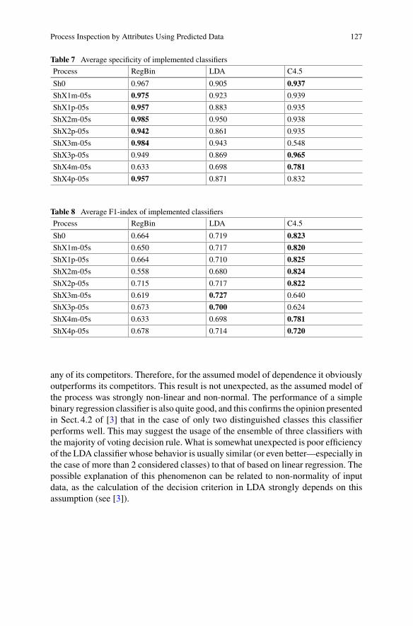
Process Inspection by Attributes Using Predicted Data 127

Table 7 Average specificity of implemented classifiers

Process RegBin LDA C4.5

Sh0 0.967 0.905 0.937

ShX1m-05s 0.975 0.923 0.939

ShX1p-05s 0.957 0.883 0.935

ShX2m-05s 0.985 0.950 0.938

ShX2p-05s 0.942 0.861 0.935

ShX3m-05s 0.984 0.943 0.548

ShX3p-05s 0.949 0.869 0.965

ShX4m-05s 0.633 0.698 0.781

ShX4p-05s 0.957 0.871 0.832

Table 8 Average F1-index of implemented classifiers

Process RegBin LDA C4.5

Sh0 0.664 0.719 0.823

ShX1m-05s 0.650 0.717 0.820

ShX1p-05s 0.664 0.710 0.825

ShX2m-05s 0.558 0.680 0.824

ShX2p-05s 0.715 0.717 0.822

ShX3m-05s 0.619 0.727 0.640

ShX3p-05s 0.673 0.700 0.624

ShX4m-05s 0.633 0.698 0.781

ShX4p-05s 0.678 0.714 0.720

any of its competitors. Therefore, for the assumed model of dependence it obviouslyoutperforms its competitors. This result is not unexpected, as the assumed model ofthe process was strongly non-linear and non-normal. The performance of a simplebinary regression classifier is also quite good, and this confirms the opinion presentedin Sect. 4.2 of [3] that in the case of only two distinguished classes this classifierperforms well. This may suggest the usage of the ensemble of three classifiers withthe majority of voting decision rule. What is somewhat unexpected is poor efficiencyof the LDA classifier whose behavior is usually similar (or even better—especially inthe case of more than 2 considered classes) to that of based on linear regression. Thepossible explanation of this phenomenon can be related to non-normality of inputdata, as the calculation of the decision criterion in LDA strongly depends on thisassumption (see [3]).

128 O. Hryniewicz

5.3 Process Quality Levels for Predicted Observations

The accuracy of the considered classifiers is, as it is seen from the results presentedin Sect. 5.2, far from being perfect. Therefore, the observed process quality levels,expressed in terms of the fraction of nonconforming items, may be quite differentfrom the actual one. In Table9 we show the estimates of the fraction nonconformingp estimated from samples of 1000 elements. The entries of Table9 represent theaverages obtained over the population of the considered ten sets of classifiers in1000 simulation runs. The column labeled Actual represents the values obtained ifthe actual values of the quality characteristic were directly observed.

From Table9 one can immediately see that in many cases the observed levels ofprocess’ quality are different from the actual ones. This is due to erroneous resultsof classification where we can distinguish two cases: erroneous classification ofnonconforming items as conforming (false positives), and erroneous classificationof conforming items as nonconforming (false negatives). This problemwas discussedin details in [5]. When the fraction of false positives is larger than the fraction offalse negatives is larger, then the observed process’ quality level will be smaller thanthe actual one, and vice versa. Classification errors of both types should be avoided,but their consequences could be different. When the observed process’ quality levelis smaller than the actual one, and it is always the case when the binary regressionclassifier is used, nonconforming items (e.g., potentially unreliable) pass qualityinspection. When consequences of non-detecting nonconforming items are seriousthis situation should be avoided. On the other hand, if the observed process’ qualitylevel is larger than the actual one we face losses incurred by the false rejection ofgood items.

The comparison of observed and actual quality levels yields only partial infor-mation about the efficiency of inspection. Consider, for example the case when thepercentages of false positives and false negatives are large but equal. In this case theobserved and the actual quality levels will be the same, but economic consequences

Table 9 Observed values of the fraction nonconforming p

Process Actual RegBin LDA C4.5

Sh0 0.252 0.163 0.252 0.257

ShX1m-05s 0.253 0.151 0.232 0.253

ShX1p-05s 0.252 0.178 0.275 0.260

ShX2m-05s 0.252 0.114 0.188 0.256

ShX2p-05s 0.253 0.208 0.303 0.259

ShX3m-05s 0.303 0.153 0.236 0.601

ShX3p-05s 0.234 0.178 0.280 0.148

ShX4m-05s 0.270 0.155 0.170 0.229

ShX4p-05s 0.244 0.176 0.284 0.331

Process Inspection by Attributes Using Predicted Data 129

for the process’ owner may be disastrous. Therefore, we should look for other fea-tures which could help us in distinguishing between “good” and “bad” classifiers.One has to note, however, than the terms “good” and “bad” are strongly context-dependent. Let us consider how the performance of classifiers influences the abilityof the inspection process to detect process’ disruptions. From Table9 we see thatshifts in the expected values of two predictors, X1 and X2, practically do not changethe actual fraction nonconforming. However, the observed fractions of nonconform-ing items are changing quite significantly when RegBin and LDA classifiers areused for prediction purposes. The consequences of this situation can be detrimen-tal, either due to the increasing rate of false alarms (when the observed fraction ofnonconforming items increases) or the increasing fraction of accepted nonconform-ing items (when the observed fraction of nonconforming items decreases). Anotherdangerous situation we observe in the case of the shift in the expected value of theexplanatory variable X4. For all considered classifiers the observed fractions of non-conforming items are changing but in the exactly opposite direction that the changeof the actual value of this quality characteristic.

A more complex situation is noticed when the shift in the expected value of thepredictor X3 is observed, as it can be seen from Fig. 1.

When this expected value decreases the actual fraction of nonconforming itemssignificantly increases. This phenomenon cannot be detected when RegBin and LDAclassifiers are used, but is even amplified when we use the C4.5 classifier for predic-tion purposes. Therefore, when this classifier is used, the deterioration of the processwill be quickly detected. However, as “free lunches” do not exist, we have to payin this case for the increased fraction of false positives when the actual fraction ofnonconforming items is decreasing. A more detailed explanation of this problem canbe found in [5].

While discussing the consequences of the usage of the C4.5 classifier one canthink if the analysis of popular measures of the quality of classification may be

Fig. 1 Observed fraction nonconforming in the presence of shift in X3 (multiples of σ )

130 O. Hryniewicz

Fig. 2 Values of F1-index in the presence of shift in X3 (multiples of σ )

useful. On Fig. 2 we see how the value of the popular F1-index changes with thechange of the expected value of X3, and thus with the change of the actual fractionof nonconforming items. We see that for processes being in “in-control” or “nearlyin-control” state the decision tree C4.5 classifier visibly outperforms its competitors.However, in the presence of large (both positive and negative) shifts in the expectedvalue of X3 the situation is quite different. When we try to interpret the consequencesof this “bad” performancewe can find that in the case of negative shifts this erroneousbehavior is even useful, and in the case of positive shifts the negative consequencesare quite improbable (processes usually do not improve spontaneously their quality).Therefore, the analysis of the measures of the quality of classification should beaccompanied by the analysis of the consequences of incorrect classification.

5.4 Properties of Inspection Policies

The main goal of the research described in this paper is to develop an efficientinspection procedure for a production process when the quality of produced itemsis observed indirectly. When classical SPC tools, such as control charts, are usedthere are two main questions to be answered. First, how to design the chosen controlchart. Second, what is the ability of this chart to detect process’ deterioration. In theproblem considered in this paper we have to add a third question about the influenceof the quality of used classifiers on the effectiveness of process’ inspection.

In the classical SPC the effectiveness of a control chart is measured by its AverageRun Length (ARL) defined as the average number of samples taken between theoccurrence of deterioration and the alarm or as the average number of samples takenbetween consecutive alarms when the process is under control. When we use SPCprocedures for the analysis of the results of 100% inspection we have to use the

Process Inspection by Attributes Using Predicted Data 131

Average Time to Signal (ATS) characteristic. ATS in this case is defined as theaverage number of items produced between the occurrence of deterioration and thealarm or as the average number of items produced between consecutive alarms whenthe process is under control.

When quality of produced items is evaluated by attributes (either conforming ornonconforming) Shewhart p-charts with one-sided (upper) control limits are usuallyused. Charts with two-sided control limits are used only when we want to detectimprovements of the process (e.g.when the input rawmaterial is changed to a newandsupposedly better one). In our experiments we have considered both types of controlcharts. However, for reasons explained in the previous section (actual deteriorationof a process can be signaled as its “improvement”—see the case of the X4 predictor)we have decided to suggest the usage of two-sided control charts.

Let us consider the application of the Shewhart control chart for the processinspection. First, let us consider the case when the inspected process is under control.In Table10 we present the values of ATS (usually denoted ATS0) for different sizesof samples (segments of the process). The parameters of the control chart have beencalculated using the estimated value of the fraction of nonconforming items estimatedfrom the sample of 1000 elements taken from a stable process.In the column labeled“Actual” we present the values of ATS of the chart for the actual, but not observed,values of the quality characteristic.

The similar values for the MAV control chart are presented in Table11.The results presented inTables10 and11 are strikingly different, but this difference

is not difficult to explain. In the case of the Shewhart control chart decisions are takenafter observing a sample of n elements. Thus, the value of, e.g., ATS0 = 30000 whenthe sample size is, e.g., equal to 100 means that on average 300 samples are evaluatedbefore the alarm (This is the value of ARL!). In the case of the MAV control chartthe decision is taken after each produced item. Thus, the value of ATS is the same asthe value of ARL. It means that the “waiting time” in terms of the number of takendecisions is in the case of theMAV chart much larger than in the case of the Shewhartchart, but the relationship between the respective values of the average time to signal(ATS) is just opposite.

Note that in the case of a stable inspected process each alarm is a false one.Therefore, we should prefer larger sample sizes n in order to have these alarms notso frequently. This can be achieved by the widening of distance between control

Table 10 Average time to signal ATS0—Shewhart chart

Sample size Actual RegBin LDA C4.5

100 31119 34055 32883 31526

200 48194 50710 50338 49556

300 65289 73189 71630 64340

400 75432 77902 78753 70359

500 93990 92629 92638 86232

132 O. Hryniewicz

Table 11 Average time to signal ATS0—MAV chart

Sample size Actual RegBin LDA C4.5

100 4158 4700 4091 4201

200 6593 7317 6314 6742

300 8715 9596 8431 8486

400 10828 11004 10650 10037

500 12221 11513 12521 11761

Table 12 Average time to signal ATS (shifted process)—Shewhart chart

Sample size Actual RegBin LDA C4.5

100 3359 39669 27618 2935

200 3204 50710 37381 4592

300 4008 63318 40791 5699

400 3140 60572 43864 6781

500 2835 68963 45039 11445

Table 13 Average time to signal ATS (shifted process)—MAV chart

Sample size Actual RegBin LDA C4.5

100 638 5247 3837 501

200 815 6349 4879 562

300 782 8746 5382 729

400 905 9864 6430 657

500 744 10234 6284 2030

limits on a chart. The effect of such a change may be, unfortunately, detrimental ifwe want to detect the deterioration of the inspected process as quickly as possible.In Tables12 and 13 we present the values of ATS when the expected value of theexplanatory variable (predictor) X3 is shifted downwards by 0, 5σ . From the secondcolumn of the Table9 we see that this shift results in the increase of the fractionnonconforming by 20%. This a really severe deterioration of the process and shouldbe detectes as quickly as possible.

From the analysis of simulation results presented in Tables10, 11, 12 and 13 wesee that the inspection is effective only in the case when the decision tree classifierC4.5 is used for the prediction of quality of inspected items. When the LDA clas-sifier is used the inspection process allows to detect deterioration but with visiblysmaller efficiency. The binary regression RegBin classifier is in the considered casecompletely ineffective. From the analysis of Tables4, 5, 6, 7 and 8 we see that inthe considered case the decision tree C4.5 classifier in comparison to its competi-tors is characterized by a larger value of Sensitivity and smaller values of Precisionand Specificity. The same is when we compare the LDA and the RegBin classi-

Process Inspection by Attributes Using Predicted Data 133

fiers. This behavior of classifiers can be explained by noting that high sensitivity andlow precision and specificity describe the situation when the observed percentage ofnonconforming items is larger than the actual one. Therefore, in the case of processdeterioration the probability of alarm increases, and the value of ATS decreases.One should note, however, that in the case of a stable (under control) process theobserved value of the fraction of nonconforming items is also larger than the actualone. This phenomenon results with a somewhat misleading information about theactual process level, but does not inflict the probability of false alarm (and the ATS0value), as the control limits are designed on the basis on observed but not actualvalues of the fraction of nonconforming items.

All the results described in this paper represent averages calculated with respectto different sets of classifiers. From more detailed results, presented in [5] for thecase of the inspection based on the Shewhart p-chart, one can find that depending onthe instance of the training set alarms may be triggered when the actual impact ofshifts in explanatory variables on actual quality is negligible, and—vice versa—maynot be triggered when it is needed. This behavior strongly depends upon the type of aclassifier, and its parameters estimated from a training data. Moreover, In this paperwe assumed that alarms are triggered by crossing either the lower or the upper controllimit. When only the upper control limit of the control chart is active, the respectivevalues of the ATS are much larger, especially in the case of no-shift or when the shiftin the explanatory variable has a small effect on the quality variable of interest. Thesituation is even worse when the deterioration of the process is accompanied withlowering of the observed fraction of nonconforming items, as it is the case in theupwards shift of the explanatory variable X4. In such a case such deterioration maybe never noticed using considered statistical methods.

6 Conclusions

The results presented in this paper add important information to that already given in[5]. However, this information is still of a very preliminary character, as the resultsfrom simulation experiments represent only one particular model of a process. Theyconfirm the findings presented in [5] that in the case of non-normal distributionsof quality characteristics, non-linear dependencies between observable (explana-tory), and not directly observable (only predicted!) values quality characteristics ofprocesses the inspection procedures based on control charts may be not effective.The most popular classifiers that are used for prediction purposes may not performwell, and their performance is difficult to be predicted in advance. Further researchis needed with the aim to find ensambles of classifiers that can be more effective thansingle classifiers in finding process’ deterioration. Such ensambles have to be robustto the change of the model of data used in their design.

134 O. Hryniewicz

References

1. Basseville M, Nikiforov IV (1993) Detection of abrupt changes: theory and applications.Prentice-Hall, Englewood Cliffs

2. Embrechts P, Lindskog F, McNeil A (2003) Modelling dependence with copulas and applica-tions to risk management. In: Rachev S (ed) Handbook of heavy tailed distributions in finance,Chapter 8. Elsevier, Amsterdam, pp 329–384

3. Hastie T, Tibshirani R, Friedman J (2008) The elements of statistical learning. data mining,inference, and prediction, 2nd edn. Springer, New York

4. Hryniewicz O, Karpinski J (2014) Prediction of reliability—pitfalls of using Pearson’s corre-lation. Eksploatacja i Niezawodnosc—Maintenance Reliab 16:472–483

5. Hryniewicz O (2015) SPC of processes with predicted data—application of the data miningmethodology, In: Knoth S, SchmidW (eds) Frontiers in statistical quality control—12, PhysicaVerlag, Heidelberg, pp 219–235

6. Montgomery DC (2011) Introduction to statistical quality control, 6th edn. Wiley, New York7. Nelsen RB (2006) An introduction to copulas, 2nd edn. Springer, New York8. Noorsana R, Saghaei A, Amiri A (2011) Statistical analysis of profile monitoring. Wiley,

Hoboken9. Owen DN, Su YH (1977) Screening based on normal variables. Technometrics 19:65–6810. Quinlan JR (1993) C4.5: programs for machine learning. Morgan Kaufmann, Los Altos11. Witten IH, Frank E, Hall MA (2011) Data mining. practical machine learning tools and tech-

niques, 3rd edn. Elsevier, Amsterdam12. Woodall WH, Spitzner DJ, Montgomery DC, Gupta S (2004) Using control charts to monitor

process and product profiles. J Qual Techn 36:309–32013. Wang YT, Huwang L (2012) On the monitoring of simple linear berkson profiles. Qual Rel

Engin Int 28:949–96514. Xu L, Wang S, Peng Y et al (2012) The monitoring of linear profiles with a GLR control chart.

J Qual Techn 44:348–36215. YamadaM, Kimura A, Naya F, Sawada H (2013) Change-point detection with feature selection

in high-dimensional time-series data. In: Proceedings of the 23rd International Joint. Confer-ence on Artificial Intelligence, Beijing, pp 1827–1833

Székely Regularization for Uplift Modeling

Szymon Jaroszewicz and Łukasz Zaniewicz

Abstract Uplift modeling is a subfield of machine learning concerned with pre-dicting the causal effect of an action at the level of individuals. This is achieved byusing two training sets: treatment, containing objects which have been subjected toan action and control, containing objects onwhich the action has not been performed.An uplift model then predicts the difference between conditional success probabil-ities in both groups. Uplift modeling is best applied to training sets obtained fromrandomized controlled trials, but such experiments are not always possible, in whichcase treatment assignment is often biased. In this paper we present a modificationof Uplift Support Vector Machines which makes them less sensitive to such a bias.This is achieved by including in the model formulation an additional term whichpenalizes models which score treatment and control groups differently. We call thetechnique Székely regularization since it is based on the energy distance proposedby Székely and Rizzo. Optimization algorithm based on stochastic gradient descenttechniques has also been developed. We demonstrate experimentally that the pro-posed regularization term does indeed produce uplift models which are less sensitiveto biased treatment assignment.

1 Introduction

The aim of conventional classification methods is to predict the class membershipprobabilities of new objects’ based on a given training dataset. In practice, however,usually a more important question is how this probability changes as a result of someaction.Modeling this particular change (or difference) is the scope of uplift modeling.In contrast to traditional response modeling, uplift approach uses two training sets:

S. Jaroszewicz (B) · Ł. ZaniewiczInstitute of Computer Science, Polish Academy of Sciences, Warsaw, Polande-mail: s.jaroszewicz@ipipan.waw.pl

Ł. Zaniewicze-mail: l.zaniewicz@phd.ipipan.waw.pl

S. JaroszewiczNational Institute of Telecommunications, Warsaw, Poland

© Springer International Publishing Switzerland 2016S. Matwin and J. Mielniczuk (eds.), Challenges in Computational Statisticsand Data Mining, Studies in Computational Intelligence 605,DOI 10.1007/978-3-319-18781-5_8

135

136 S. Jaroszewicz and Ł. Zaniewicz

treatment dataset with data on objects on which a particular action was taken, andcontrol with data on untreated cases.

Probably the most intuitive example of utility of uplift modeling is a direct mar-keting campaign for a certain product. It is easy to see that we can divide customersinto four groups:

1. Customers who purchased the product because they were targeted and would nothave purchased otherwise.

2. Customers who would have purchased the product regardless of whether theywere targeted or not.

3. Customers who would not have purchased the product regardless of whether theywere targeted or not.

4. Customers who were going to purchase the product, but were annoyed by theaction and, as a result, changed their mind.

In the first group the action is clearly beneficial, and in the fourth clearly detrimental.In the second and third groups the action has no real effect and those two groups can infact be aggregated into a single neutral group. Similar problems arise in personalizedmedicine where a treatment may bring recovery from a disease, but the patient mayalso be exposed to dangerous side effects.

In contrast, traditional classification models are only able to distinguish twogroups: those who respond (after, not necessarily because of the action) and thosewho do not. In many real world situations, this distinction does not correspond to theproblem actually being solved.

1.1 Biased Treatment Assignment Problem

A very important aspect of uplift modeling is how the cases are assigned to treat-ment and control groups. The best scenario is a randomized controlled experiment,where the assignment is random and does not depend on the features of the cases.Unfortunately, such an experiment is not always possible (e.g. for ethical or financialreasons) or only historical data may be available where, for example, the treatmentwas applied to patients which a doctor considered most suitable.

If treatment assignment was not random and biased then the effect of the actioncannot, usually, be estimated directly. Consider, for example, a medical treatmentwith potentially serious side effects. The doctor might then decide not to apply it topatients in severe condition who will thus be placed in the control group. However,such cases are also more likely not to recover from the disease making the controlgroup outcomes look worse and the treatment more effective than it is in reality.

In this paper we present Uplift Support Vector Machines originally proposedin [22] with an additional penalty term, whichwe call Székely regularizer. As a result,we obtain uplift models which are additionally forced to make similar predictionson the treatment and control groups, thus helping to reduce the effect of treatmentassignment bias.

Székely Regularization for Uplift Modeling 137

The additional regularizer is based on so called energy distance between proba-bility distributions proposed by Székely and Rizzo [6, 18, 19]. The distance has theproperty that it is zero if and only if the distributions are identical, it can thus be usedto enforce similar distributions of model scores in the treatment and control groups.

2 Related Work

Uplift modeling has received relatively little attention in the literature. The first papermentioning it explicitly was [10] where decision trees designed specifically for thatproblem were discussed. More details on the method were later presented in [11].

A trivial approach to uplift modeling uses two probabilistic classifiers, one builton the treatment dataset, the other on control, whose predicted probabilities are thensubtracted. The approach may however suffer from a serious drawback: both modelswill focus on predicting class probabilities in both groups and ignore the (usuallymuch weaker) differences between them. A good example can be found in [11].Therefore, most research in uplift modeling has been concerned with approacheswhich model the conditional difference in success probabilities directly.

Many such approaches are based on adaptations of decision trees. For example,in [11] uplift trees have been proposed which are based on a statistical test of successrate differences after the split and in [15, 16] trees based on information theoreticaldivergences between treatment and control class probabilities. Ensembles of deci-sion trees have been described in [2]; a more thorough analysis of various types ofensembles in the uplift setting can be found in [17].

Regression based techniques can be found for example in [4], where a classvariable transformation is presented which allows for converting uplift modelingproblems into classification problems. Similar techniques have been discussed in thestatistical literature [12, 21].

In [22] Uplift Support Vector Machines have been proposed which allow forexplicit identification of cases for which the action is positive, neutral and negative.Themodel is described in the next section.Another type of uplift SVMswas proposedin [8] and is based on direct maximization of the area under the uplift curve.

Good overviews of uplift modeling can be found in [11] and in [16]. Proceduresfor correcting treatment assignment bias will be discussed in Sect. 5.3.

2.1 Uplift Support Vector Machines

Let us first introduce some notation. Vectors will be denotedwith boldface, lowercaseletters, x, w. A dataset is a collection of records (xi , yi ) where xi is the i th featurevector and yi ∈ {−1, 1} the class value for the i th record. The outcome 1 is consideredthe successful or desired outcome. The superscript T will be used to denote termsrelated to the treatment group and the superscript C terms related to the control. For

138 S. Jaroszewicz and Ł. Zaniewicz

example, the treatment training dataset is DT = {(xTi , yT

i ) : i = 1, . . . , nT } and thecontrol training set is DC = {(xC

i , yCi ) : i = 1, . . . , nC }.

We now discuss in more details the Uplift Support Vector Machines presentedin [22] which we will use as the starting point for further developments. The machineis based on two separating hyperplanes

H1 : 〈w, x〉 − b1 = 0, H2 : 〈w, x〉 − b2 = 0.

The model predictions are made according to the following formula:

M(x) =

⎧

⎪⎨

⎪⎩

+1 if 〈w, x〉 > b1 and 〈w, x〉 > b2,

0 if 〈w, x〉 ≤ b1 and 〈w, x〉 > b2,

−1 if 〈w, x〉 ≤ b1 and 〈w, x〉 ≤ b2,

(1)

that is, the model classifies the effect of the action on a point x as positive (+1),negative (−1), or neutral (0). A graphical interpreation of themodel is shown in Fig. 1(taken from [22]). The hyperplane H1 separates positive and neutral predictions andthe hyperplane H2 separates neutral and negative predictions.

H1

H2T+

ξi,1C+

ξi,2

T+C−

T+

ξi,1ξi2

T−ξi,2

ξi,1

C+

+1

0

− 1

Fig. 1 The Uplift SVM optimization problem. Example points belonging to the positive class inthe treatment and control groups are marked respectively with T+ and C+. Analogous notation isused for points in the negative class. The figure shows penalties incurred by points with respect tothe two hyperplanes of the USVM. Positive sides of hyperplanes are indicated by small arrows atthe right ends of lines in the image. Red solid arrows denote the penalties incurred by points whichlie on the wrong side of a single hyperplane, blue dashed arrows denote additional penalties forbeing misclassified also by the second hyperplane

Székely Regularization for Uplift Modeling 139

Let us now formulate the optimization task which allows for finding the model’sparameters w, b1, b2. We will use DT+ = {(xi , yi ) ∈ DT : yi = +1} to denote datapoints belonging to the positive class in the treatment group and DT− = {(xi , yi ) ∈DT : yi = −1} to denote points in that group belonging to the negative class.Analogous notation is used for points in the control group.1

The version presented here is slightly different than that given in [22]: the softmargin penalties are averaged separately over the treatment and control groups. Asa result both groups have the same impact on the optimized risk. The optimizationproblem is to find weights w maximizing the function R(w) defined as

R(w) = 1

2〈w, w〉 + C1

nT

∑

DT+

ξi,1 + C2

nT

∑

DT−

ξi,1 + C2

nT

∑

DT+

ξi,2 + C1

nT

∑

DT−

ξi,2

+ C1

nC

∑

DC−

ξi,1 + C2

nC

∑

DC+

ξi,1 + C2

nC

∑

DC−

ξi,2 + C1

nC

∑

DC+

ξi,2, (2)

subject to constraints

〈w, xi 〉 − b1 ≥ +1 − ξi,1, for all (xi , yi ) ∈ DT+ ∪ DC−,

〈w, xi 〉 − b1 ≤ −1 + ξi,1, for all (xi , yi ) ∈ DT− ∪ DC+,

〈w, xi 〉 − b2 ≥ +1 − ξi,2, for all (xi , yi ) ∈ DT+ ∪ DC−,

〈w, xi 〉 − b2 ≤ −1 + ξi,2, for all (xi , yi ) ∈ DT− ∪ DC+,

ξi, j ≥ 0, for all i = 1, . . . , n, j ∈ {1, 2}.

Note that the model has two penalty coefficients, C1 and C2. The properties ofthe model are given in detail in [22], here we only review the main results withoutproofs, which easily carry over to the modified formulation given in this paper. First,the model is valid iff b1 ≥ b2, this is the case when C2 ≥ C1 which puts a constrainton the values of C1 and C2. The role of the coefficient C1 is the same as in classicalSVMs. From Fig. 1 it is clear that the coefficientC2 determines the additional penaltyfor points which are on the wrong side of both hyperplanes (e.g. a treatment pointwith negative outcome which is classified as positive). It turns out that the ratioC2/C1 determines the proportion of neutral predictions. For C1 = C2 no points areclassified as neutral and for a sufficiently large value of C2/C1 almost all points are.

In the following sections we will add an additional penalty term to (2) which willforce similar model behavior in the treatment and control groups.

1The values of the class variable should not be confused with model predictions defined in (1). Forexample, a model prediction of +1 means that we expect the class variable to take the value of +1if the action is performed (yT = +1) and to take the value of −1 if the action is not performed(yC = −1).

140 S. Jaroszewicz and Ł. Zaniewicz

3 Székely Regularized Support Vector Machines

One way to view an uplift model is as a function which maps feature vectors into theset {−1, 0,+1}. The value is interpreted as a decision on whether the action appliedto a given case will be beneficial, neutral, or detrimental. Another approach is for themodel to return a score: a real number being an increasing function of the predictedprobability that the action will be beneficial. In this paper we are going to define ourUplift Support Vector Machines using the discrete prediction model but for testingand regularization purposes we will use the linear score 〈w, x〉.

3.1 Distribution of Scores in Controlled RandomizedExperiments

Let us now state an important property of score based uplift models used in controlledrandomized experiments. Let Ms be an uplift model returning a score and Ms(x) thescore returned by the model for a specific instance x. When the feature vector x ispicked at random from a population distribution, then Ms(x) is a random variable.Suppose xT is picked at random from the treatment population and xC from thecontrol population. In a randomized controlled trial xT and xC follow the samedistributions and therefore Ms(xT ) and Ms(xC ) are random variables following thesame distributions. If the treatment assignment is not random, the distributions ofxT and xC differ and so may those of Ms(xT ) and Ms(xC ).

In this paper we will use this property to obtain models which are less sensitiveto treatment assignment bias. This will be achieved by adding a regularization termpenalizing models which yield different score distributions in the treatment andcontrol training sets.

3.2 The Energy Distance

In this paper we make use the concept of energy distance (also called E-statistic)e(α) proposed in 2005 by Székely and Rizzo [6, 18–20]. Initially this concept wasintroduced as a measure of distance between clusters, but it is in fact a general astatistical distance between two or more probability distributions. The name comesfrom the fact that it was first derived from physics; later Székely applied this conceptto statistics.

Let A = {a1, a2, . . . an1}, B = {b1, b2, . . . bn2} be two nonempty sets of pointsin Rd . Formally, e(α)(A, B) is defined as

Székely Regularization for Uplift Modeling 141

e(α)(A, B) = n1n2

n1 + n2

[2

n1n2

n1∑

i=1

n2∑

j=1

‖ai − b j‖α

− 1

n21

n1∑

i=1

n1∑

j=1

‖ai − a j‖α − 1

n22

n2∑

i=1

n2∑

j=1

‖bi − b j‖α

]

, (3)

where ‖ · ‖ is the Euclidean norm and α is parameter that influences the behavior ofthe distance. If α = 2 then the distance is equal to zero iff the means of A and Bare equal. The case α ∈ (0, 2) is more interesting, since the distance is then equalto zero iff the sets A and B are equal. Moreover, if A and B are random samplesand α ∈ (0, 2), then, as the size of A and B grows to infinity, the distance betweenthem tends to zero iff A and B are drawn from the same distribution (for α = 2the distributions from which they are drawn only need to have equal means). Thisproperty is important for the task the distance will be used for in this paper. Noticealso that for d = 1 the Euclidean norms reduce to absolute values.

3.3 Model Formulation

We modify the risk function of Uplift Support Vector Machines by adding an extraterm responsible for penalizing the difference in score distributions in the treatmentand control groups. We call this term the Székely regularization term. The risk func-tion of the regularized USVMs is

R(w) = 1

2〈w, w〉 + C1

nT

∑

DT+

ξi,1 + C2

nT

∑

DT−

ξi,1 + C2

nT

∑

DT+

ξi,2 + C1

nT

∑

DT−

ξi,2

+ C1

nC

∑

DC−

ξi,1 + C2

nC

∑

DC+

ξi,1 + C2

nC

∑

DC−

ξi,2 + C1

nC

∑

DC+

ξi,2

+ C3S(DT , DC , w). (4)

The risk is optimized subject to the same constraints as the risk given in (2). Above,S(DT , DC , w) is the Székely regularizer given by

S(DT , DC , w) = 2

nT nC

nT∑

i=1

nC∑

j=1

|〈w, xTi 〉 − 〈w, xC

j 〉|α

− 1

(nT )2

nT∑

i=1

nT∑

j=1

|〈w, xTi 〉 − 〈w, xT

j 〉|α

142 S. Jaroszewicz and Ł. Zaniewicz

− 1

(nC )2

nC∑

i=1

nC∑

j=1

|〈w, xCi 〉 − 〈w, xC

j 〉|α. (5)

Note that 〈w, xi 〉 is the score assigned by the model to a data record xi , and (5) is thusthe energy distance (3) applied to the sets of scores assigned by the model to recordsin the treatment and control groups. Due to the properties of the energy distance theterm will penalize models for which distributions of scores in both groups differ.

The factor C3 determines the strength of the penalty. The fraction nT nC

nT +nC from (3) isabsorbed into C3 for the ease of exposition.

Let us now discuss the choice of α. Since we want to guarantee equal scoredistributions we need α ∈ (0, 2) [19]. However for α < 1 the function S exhibitsstrong non-convexity and is thus more difficult to optimize. We should, therefore,chooseα from the interval [1, 2).We found values close to 1 towork better in practicebut for α = 1 the function S is not differentiable. We thus settled for α = 1.1 whichgives good properties and a smoother function to optimize. Note, however, that Smay not be convex even for α ∈ [1, 2).

4 Optimization

We now describe the method used to optimize (4) subject to the constraints specifiedbelow (2). As a first step we rewrite the problem as an unconstrained optimizationproblem using the hinge loss:

R(w) =1

2〈w, w〉

+ C1

nT

∑

DT+

h(yTi (〈w, xT

i 〉 − b1)) + C2

nT

∑

DT+

h(yTi (〈w, xT

i 〉 − b2))

+ C2

nT

∑

DT−

h(yTi (〈w, xT

i 〉 − b1)) + C1

nT

∑

DT−

h(yTi (〈w, xT

i 〉 − b2))

+ C2

nC

∑

DC+

h(−yCi (〈w, xC

i 〉 − b1)) + C1

nC

∑

DC+

h(−yCi (〈w, xC

i 〉 − b2))

+ C1

nC

∑

DC−

h(−yCi (〈w, xC

i 〉 − b1)) + C2

nC

∑

DC−

h(−yCi (〈w, xC

i 〉 − b2))

+ C3S(DT , DC , w), (6)

where h is the hinge loss function given by

h(q) = max{0, 1 − q}.

Székely Regularization for Uplift Modeling 143

We are going to use the Averaged Stochastic Gradient Descent algorithm [9] inorder to optimize (4). The reason is that the algorithm is fast, stable and works wellwith non-smooth functions. Note that in our optimization problem the derivatives ofthe target function are not guaranteed to exist so methods such as conjugate gradientdescent are not applicable.

In order to optimize the expression given in (6) we first need to compute itssubgradient (since R(w) is not everywhere differentiable there are values of w forwhich the gradient does not exist). Note that the subgradient of the hinge loss h(q)

is

∂h(q)

∂q=

⎧

⎪⎨

⎪⎩

−1 if q < 1,

any value in [−1, 0] if q = 1,

0 if q > 1.

Since for q = 1 any value in [−1, 0] can be picked we will simply set

∂h(q)

∂q= −1[1−q>0]. (7)

We can now give the expression for the subgradient of the minimized risk given in (6)

∂ R(w)

∂w=

w − C1

nT

∑

DT+

1[

1−yTi (〈w,xT

i 〉−b1)>0]xT

i yTi − C2

nT

∑

DT+

1[

1−yTi (〈w,xT

i 〉−b2)>0]xT

i yTi

− C2

nT

∑

DT−

1[

1−yTi (〈w,xT

i 〉−b1)>0]xT

i yTi − C1

nT

∑

DT−

1[

1−yTi (〈w,xT

i 〉−b2)>0]xT

i yTi

+ C2

nC

∑

DC+

1[

1+yCi (〈w,xC

i 〉−b1)>0]xC

i yCi + C1

nC

∑

DC+

1[

1+yCi (〈w,xC

i 〉−b2)>0]xC

i yCi

+ C1

nC

∑

DC−

1[

1+yCi (〈w,xC

i 〉−b1)>0]xC

i yCi + C2

nC

∑

DC−

1[

1+yCi (〈w,xC

i 〉−b2)>0]xC

i yCi

+ C3∂S(DT , DC , w)

∂w, (8)

where

∂S(DT , DC , w)

∂w

= 2

nT nC

nT∑

i=1

nC∑

j=1

α|〈w, xTi − xC

j 〉|α−1sgn(〈w, xTi − xC

j 〉)(xTi − xC

j )

144 S. Jaroszewicz and Ł. Zaniewicz

− 1

(nT )2

nT∑

i=1

nT∑

j=1

α|〈w, xTi − xT

j 〉|α−1sgn(〈w, xTi − xT

j 〉)(xTi − xT

j )

− 1

(nC )2

nC∑

i=1

nC∑

j=1

α|〈w, xCi − xC

j 〉|α−1sgn(〈w, xCi − xC

j 〉)(xCi − xC

j ). (9)

4.1 Averaged Stochastic Gradient Descent Algorithmfor Székely Regularized USMVs

The Stochastic Gradient Descent algorithm typically works by picking random dat-apoints, computing the contribution of those points to the gradient and updatingcurrent weights with a decreasing update coefficient.

Notice, however, that each term in the Székely regularizer given in (5) operateson a pair of treatment datapoints and a pair of control datapoints. In order to apply astochastic optimization algorithm to the problem we thus take, at each iteration, fourrandomly selected records, two from the treatment training set and two from control.The weight update is then computed based on four training points instead of one.

The algorithm is given in Fig. 2. The expressions ∂l(w, xTi , yT

i )/∂w and∂S(xT

i , xTj , xC

k , xCl , yT

i , yTj , yC

k , yCl , w)/∂w used in the algorithm will be given

below. Notice that in step 10 we take the average of the weight vectors wt obtainedduring all steps of the algorithm. This is the so called Polyak-Ruppert averaging [1,7, 9] which improves the convergence properties of the algorithm.

In order to provide the expressions for ∂l/∂w and ∂S/∂w used in the algorithm, aswell as to prove its convergence, we first need to compute the subgradient of the targetrisk function (9) for each random sample. Sincewe are dealingwith pairs of treatment

1. w0 = 02. For t ← 1, 2, . . .3. Draw two samples (xT

i , yTi ), (xT

j , yTj ) uniformly at random from DT

4. Draw two samples (xCk , yC

k ), (xCl , yC

l ) uniformly at random from DC

5. g ← wt−1 + 12

∂l(wt−1,xTi ,yT

i )∂wt−1

+ 12

∂l(wt−1,xTj ,yT

j )∂wt−1

6. g ← g + 12

∂l(wt−1,xCk ,yC

k )∂wt−1

+ 12

∂l(wt−1,xCl ,yC

l )∂wt−1

7. g ← g + C3∂S(xT

i ,xTj ,xC

k ,xCl ,yT

i ,yTj ,yC

k ,yCl ,wt−1)

∂wt−1

8. γt ← 1√t

9. wt ← wt−1 − γtg10. wa ← 1

t

∑tt′=1 wt′

11. If converged:12. Return wa

Fig. 2 The Averaged Stochastic Gradient descent algorithm for Székely regularized uplift supportvector machines

Székely Regularization for Uplift Modeling 145

and control points, each sample will involve four data records: xTi , xT

j , xCk , xC

l and

their corresponding class values yTi , yT

j , yCk , yC

l . The subgradient of the risk for thegiven sample is given by the following equation

∂ R(xTi , xT

j , xCk , xC

l , yTi , yT

j , yCk , yC

l , w)

∂w

= w + 1

2

∂l(w, xTi , yT

i )

∂w+ 1

2

∂l(w, xTj , yT

j )

∂w

+ 1

2

∂l(w, xCk , yC

k )

∂w+ 1

2

∂l(w, xCl , yC

l )

∂w

+ C3∂S(xT

i , xTj , xC

k , xCl , yT

i , yTj , yC

k , yCl , w)

∂w, (10)

where the parts resulting from differentiating the hinge loss are

∂l(w, x, y)

∂w

= xy ·

⎧

⎪⎪⎪⎨

⎪⎪⎪⎩

−C11[1−y(〈w,x〉−b1)>0] − C21[1−y(〈w,x〉−b2)>0] if (x, y) ∈ DT+−C21[1−y(〈w,x〉−b1)>0] − C11[1−y(〈w,x〉−b2)>0] if (x, y) ∈ DT−C11[1+y(〈w,x〉−b1)>0] + C21[1+y(〈w,x〉−b2)>0] if (x, y) ∈ DC−C21[1+y(〈w,x〉−b1)>0] + C11[1+y(〈w,x〉−b2)>0] if (x, y) ∈ DC+

(11)

and the part for the subgradient of the Székely regularizer is

∂S(xTi , xT

j , xCk , xC

l , yTi , yT

j , yCk , yC

l , w)

∂w

= α

2

[|〈w, xTi − xC

k 〉|α−1sgn(〈w, xTi − xC

k 〉)(xTi − xC

k )

+ |〈w, xTi − xC

l 〉|α−1sgn(〈w, xTi − xC

l 〉)(xTi − xC

l )

+ |〈w, xTj − xC

k 〉|α−1sgn(〈w, xTj − xC

k 〉)(xTj − xC

k )

+ |〈w, xTj − xC

l 〉|α−1sgn(〈w, xTj − xC

l 〉)(xTj − xC

l )]

− α|〈w, xTi − xT

j 〉|α−1sgn(〈w, xTi − xT

j 〉)(xTi − xT

j )

− α|〈w, xCk − xC

l 〉|α−1sgn(〈w, xCk − xC

l 〉)(xCk − xC

l ).

A necessary condition for the Stochastic Gradient Descent algorithm to converge isthat the expectation (taken over the randomly sampled vectors) of the subgradient (10)be equal to the subgradient computed on the full dataset given in (8). Since in thealgorithm given in Fig. 2 we are using four randomly sampled data points we needto take the expectation over all of them.

146 S. Jaroszewicz and Ł. Zaniewicz

We will denote the expectation over (xTi , yT

i ) by ETi [·], analogous notation will

be used for expectations over records in the control group. Notice that, since therecords in the stochastic optimization algorithm are chosen uniformly at random, wehave

ETi [ f (xT

i , yTi )] = 1

nT

nT∑

i=1

f (xTi , yT

i ), ECk [ f (xC

i , yCi )] = 1

nC

nC∑

i=1

f (xCi , yC

i ).

(12)Further, denote by E[·] the expectation over all four randomly chosen samples(xT

i , yTi ), (xT

j , yTj ), (xC

k , yCk ), (xC

l , yCl ), i.e.

E[·] = ETi E

Tj E

Ck E

Cl [·].

Let us now compute, term by term, the expectation of the subgradient given in (10).Clearly Ew = w. Also, using (11) and (12) we get

E∂l(w, xT

i , yTi )

∂w= E

Ti

∂l(w, xTi , yT

i )

∂w

= − 1

nT

nT∑

i=1

xTi yT

i

⎧

⎪⎪⎪⎪⎨

⎪⎪⎪⎪⎩

C11[

1−yTi (〈w,xT

i 〉−b1)>0]

+ C21[

1−yTi (〈w,xT

i 〉−b2)>0] if (xT

i , yTi ) ∈ DT+

C21[

1−yTi (〈w,xT

i 〉−b1)>0]

+ C11[

1−yTi (〈w,xT

i 〉−b2)>0] if (xT

i , yTi ) ∈ DT−

= −C1

nT

∑

DT+

1[

1−yTi (〈w,xi 〉−b1)>0

]xTi yT

i − C2

nT

∑

DT+

1[

1−yTi (〈w,xi 〉−b2)>0

]xTi yT

i

− C2

nT

∑

DT−

1[

1−yTi (〈w,xT

i 〉−b1)>0]xT

i yTi − C1

nT

∑

DT−

1[

1−yTi (〈w,xT

i 〉−b2)>0]xT

i yTi .

We now move to computing the expectation of the subgradient of the Székely regu-larizer. Note that

E|〈w, xTi − xC

k 〉|α−1sgn(〈w, xTi − xC

k 〉)(xTi − xC

k )

= ETi E

Ck |〈w, xT

i − xCk 〉|α−1sgn(〈w, xT

i − xCk 〉)(xT

i − xCk )

= 1

nT nC

nT∑

i=1

nC∑

k=1

|〈w, xTi − xC

k 〉|α−1sgn(〈w, xTi − xC

k 〉)(xTi − xC

k ).

By symmetry, the three other pairs of treatment and control points lead to the sameexpected value. Similarly

Székely Regularization for Uplift Modeling 147

E|〈w, xTi − xT

j 〉|α−1sgn(〈w, xTi − xT

j 〉)(xTi − xT

j )

= 1

(nT )2

nT∑

i=1

nT∑

j=1

|〈w, xTi − xT

j 〉|α−1sgn(〈w, xTi − xT

j 〉)(xTi − xT

j ).

The expression for the pair of control points is analogous. Finally we get

E

∂S(xTi , xT

j , xCk , xC

l , yTi , yT

j , yCk , yC

l , w)

∂w

= 2α1

nT nC

nT∑

i=1

nC∑

k=1

|〈w, xTi − xC

k 〉|α−1sgn(〈w, xTi − xC

k 〉)(xTi − xC

k )

− α1

(nT )2

nT∑

i=1

nT∑

j=1

|〈w, xTi − xT

j 〉|α−1sgn(〈w, xTi − xT

j 〉)(xTi − xT

j )

− α1

(nC )2

nC∑

i=1

nC∑

j=1

|〈w, xCi − xC

j 〉|α−1sgn(〈w, xCi − xC

j 〉)(xCi − xC

j ).

Combining the above results we get exactly the subgradient of the risk whichis minimized by Székely regularized Uplift Support Vector Machines given in (8)and (9).

Therefore the necessary condition for convergence is satisfied. For sufficiency, letus examine the properties of the optimization problem (6). Notice first, that althoughthe term 1

2 〈w, w〉 is strongly convex and the remaining terms are convex, the Székelypenalty term is not. Therefore the optimized function need not be convex and wecannot guarantee global convergence. Suppose that there exists a bound D such that‖w∗‖ ≤ D and ‖wt‖ ≤ D for all iteration steps t . Note that the risk function isLipschitz continuous on any closed region of the parameter space. It follows thatthe subgradient of R is bounded throughout the algorithm and the convergence is

guaranteed based on results given in [7, Sect. 11.0] for γt = Ct− 12 . The constant C

was chosen to be 1 in our implementation.Let us now briefly comment on the existence of the bound D. Without additional

assumptions we cannot formally guarantee that at every iteration we have ‖wt‖ ≤ D.To obtain such guarantees, an extra step can be added to Algorithm 2, which, aftereach iteration, projects wt onto a ball of some radius D [7]. In practice we saw noconvergence problems and the extra step was not necessary.

If we make an additional assumption that the Székely penalty S is locally convexaround the minimum we can guarantee fast convergence rates. Since 1

2 〈w, w〉 isstrongly convex and a sum of a convex and a strongly convex function is stronglyconvex, the risk R(w) given in (6) becomes strongly convex. The convergence rate

is then O(t−1) for γt = Ct− 12 following the results in [1, Theorem 3]. The constant

C was chosen to be 1 in our implementation.

148 S. Jaroszewicz and Ł. Zaniewicz

Note that the step size used guarantees convergence for non strongly convexfunctions and fast convergence for strongly convex ones.

5 Experimental Evaluation

In this section we will present an experimental evaluation of the proposed approach.We begin with a general discussion on evaluating uplift models, then describe ourapproach to testing under treatment assignment bias, and finally present the resultsof experiments.

5.1 Evaluating Uplift Models

Evaluating uplift models is more difficult than evaluating traditional classifiers. Foreach case we only know the outcome after the action was applied or when the actionwas not taken, never both. Therefore, we cannot decide whether specific cases havebeen correctly classified or not. This is known as the fundamental problem of causalinference [3].

Let us now discuss so called uplift curves used to graphically analyze the perfor-mance of uplift models. One type of curves used to assess standard classifiers arelift curves (also known as cumulative gains curves or cumulative accuracy profiles),where the x axis corresponds to the number of cases targeted and the y axis to thenumber of successes captured by the model. An uplift curve is computed by sub-tracting the lift curve obtained on the control test set from the lift curve obtained onthe treatment test set. Both curves are generated using the same uplift model. Thenumber of successes on the y axes is expressed as a percentage of the total populationwhich guarantees that the curves can be meaningfully subtracted.

The interpretation of the uplift curve is as follows: on the x axis we choose thepercentage of the population on which the action is to be performed and on the y axiswe read the difference between the success rates in the treatment and control groups.The value at x = 100% gives the gain in success probability from treating the wholepopulation. A diagonal line corresponds to random selection. The Area Under theUplift Curve (AUUC) can be used as a simple summary. In this paper we subtractthe area under the diagonal line from this value in order to obtain more meaningfulnumbers. More details on evaluating uplift models and on uplift curves can be foundin [11, 15].

Since there are now two test sets (treatment and control) procedures such ascrossvalidation are performed independently on them. In this paper we use ten timesten-fold crossvalidation to obtain the uplift curves.

Székely Regularization for Uplift Modeling 149

5.2 The Right Heart Catheterization Dataset

The right heart catheterization dataset [5] contains data about 5735 patients admittedto hospitals in serious condition. 2184 of them were subjected to the right heartcatheterization procedure (RHC) and constitute the treatment group; the remaining3551 did not receive the procedure and are the controls. The data does not comefrom a randomized study, the application of RHC was decided based on patients’condition, so the group selection is biased, in fact, it was done retrospectively basedon historical data. Because of this characteristics, as well as its relatively large size,the dataset is ideal to test our algorithm.

The class variable was the attribute Death denoting patient death during thefirst 180 days after hospital admission. Patient survival was considered the positiveoutcome. To avoid information leaks we removed other outcome related variablessuch as date of death or date of last contact.

The predictive attributes describe various characteristics of the patient such as age,sex, education, income, medical insurance, the disease the patient suffers from. Alsopresent are results of diagnostics performed at admission such as blood pressure,temperature, results of blood tests, and various scores describing the severity ofpatient’s condition.

5.3 Testing Methodology—Correcting Group Selection Bias

Testing the performance of themodelswas, however,more challenging than in case ofrandomized controlled trials. As discussed in Sect. 5.1 testing uplift models is basedon an assumption that groups of treatment and control records with similar scoresare indeed similar. Unfortunately, this is usually not the case for biased treatmentselection.

In order to test the model’s predictions we thus had to correct the bias in the testsets. In practice, such corrections are typically achieved using so called propensityscores [14]. A propensity score is the probability that a given patient, described bya feature vector x, will be assigned to the treatment group. There are several wayspropensity scores can be used to correct for nonrandom group assignment. In thispaper we are going to use inverse probability of treatment weighting (IPTW) [13].

The IPTW method assigns to each treatment group record a weight inverselyproportional to the probability that a record with those characteristics is selected fortreatment. This way, cases to which treatment is applied disproportionately often aregiven lower weights and underrepresented cases higher weights. The control grouprecords are, analogously, given weights proportional to the inverse of the probabilitythat a record with a given feature vector is not given the treatment. Note that for arandomized controlled trial all records within a group receive equal weights.

To summarize, our testing procedure works as follows: we build a model withnonrandom treatment assignment using the Székely penalty term to correct for the

150 S. Jaroszewicz and Ł. Zaniewicz

Fig. 3 ROC curve for thepropensity score model

bias, then we test the model on treatment and control test sets on which the bias hasbeen corrected using the inverse probability of treatment weighting. Since differentbias correction procedures are used for model construction and testing, we believethat it is less likely that the estimated model performance is a result of an uncorrectedtreatment assignment bias.

In order to use the IPTWprocedure one needs to know the probability of treatmentassignment conditional on patients’ characteristics. Unfortunately, this probability isusually unknown and needs to be estimated. Here, we use a logistic regression modeltrained on full data before crossvalidation splits. The ROC curve for the model isshown in Fig. 3 (area under the ROC curve is 0.686). It can be seen that the modelis able to predict reasonably well whether a given patient will receive the RHCprocedure. One can conclude that treatment assignment is indeed seriously biased.

5.4 Experimental Results

We will now present the experimental results. Figure4 shows uplift curves drawnfor several values of the Székely penalty coefficient C3. All experiments were per-formed for C1 = C2 = 1, only the value of C3 was changed. Ten times ten-foldcrossvalidation was used to obtain the curves. The curves are drawn based on dataweighted using inverse probability of treatment weighting (IPTW) to correct treat-ment assignment bias. More detailed data on areas under the uplift curves are givenin the second row of Table1.

Overall the treatment is not effective and the application of the right heart catheter-ization procedure seems to decrease patients chances of survival. This is in line withthe findings presented in [5].

Székely Regularization for Uplift Modeling 151

Fig. 4 Uplift curves forUplift SVM models withdifferent Székely penaltycoefficients

Table 1 The influence of the Székely penalty coefficient C3 on the area under the uplift curve andthe differences between scores in the treatment and control groups

C3 penalty coef-ficient

0 0.01 0.1 1 10 100

AUUC 0.1505 0.1511 0.1559 0.2030 0.4035 0.0727

Differencebetween scoremeans

0.1051 0.1050 0.1036 0.0839 0.0202 0.004

Kolmogorov-Smirnov statistic

0.3436 0.3433 0.3411 0.3026 0.1103 0.0320

It can be seen that without the Székely correction (C3 = 0) the curve follows thediagonal line corresponding to a model assigning treatment at random, except forthe 20% of highest scored cases for which RHC does indeed bring improvement insurvival rate over random selection.

With increasing values of the Székely penalty coefficient C3, the area under theuplift curve is steadily increasing, up to C3 = 100 where the performance rapidlydrops. This shows that the application of the Székely penalty does indeed improvemodel performance under treatment assignment bias.

The best performance is achieved forC3 = 10, and Fig. 4 shows that this particularmodel achieves good performance over awide range of scores, bringing improvementover random selection for about 75% of the population. The area under the upliftcurve is more than two and a half times better than for the unregularized model.

The drop in performance for very high value of the regularization parameter istypical for regularized models in general: too high a penalty leads to the modelignoring the data and focusing only on the regularization term.

To further analyze the effect of the Székely penalty on model behavior we ana-lyze the distributions ofmodel scores in treatment and control groups. Figure5 shows

152 S. Jaroszewicz and Ł. Zaniewicz

Fig. 5 Empirical cumulative distribution functions of scores in the treatment and control groupsfor various Székely regularization coefficient values

the empirical cumulative distribution functions of model score distributions in thetreatment and control groups for various strength of the Székely regularization term.The charts were obtained on a single repetition of the ten fold crossvalidation. Addi-tionally, we computed two types of statistics summarizing the discrepancies: thedifference between score means in the two groups and the Kolmogorov-Smirnovstatistic, i.e. the maximum difference between the empirical cumulative distributionfunctions of the two groups. The summary statistics are given in the third and fourthrows of Table1 and are shown graphically in Fig. 6.

It can be seen that for the unregularized model, the distributions of scores inboth groups differ significantly. The score means differ by about 0.1, which is afairly large value since the scores range roughly from −0.5 to 0.5. The value of theKolmogorov-Smirnov statistic is almost 0.35.

When the Székely penalty increases, the distributions become closer to each other.For C3 = 0.01 and C3 = 0.1 the decrease is tiny but noticeable and is accompaniedby a tiny but noticeable improvement in the area under the uplift curve.WhenC3 = 1the score distributions already come much closer to each other with the differencebetween means decreasing to about 0.084; at the same time AUUC increased byabout 35%with respect to the unregularized model. A further tenfold increase of thepenalty coefficient makes the distributions very similar; the difference in means isjust 0.02 and the Kolmogorov-Smirnov statistic just 0.11. The AUUC is 2.68 timeshigher than for the unregularized model.

A further tenfold increase in the value of C3 makes the score distributions in thetreatment and control groups practically identical, however the regularization is toostrong and the model no longer correctly predicts for whom the RHC procedure isbeneficial. In fact its predictions are not better than random assignments.

Székely Regularization for Uplift Modeling 153

Fig. 6 Statistics summarizing the differences between score distributions in the treatment andcontrol groups for various Székely regularization coefficient values

Let us now summarize our experimental findings. First, it was shown that theunregularized model behaves poorly after treatment assignment bias correction isapplied. Moreover, it produces significantly different scores in the treatment andcontrol groups likely modeling not the real causal impact of the action but the differ-ences in group assignment. As the Székely penalty term increased, the differencesbetween scores the model assigns to treatment and control records became muchsmaller, accompanied by large improvements in model performance. One can thusconclude that using the Székely penalty term does indeed reduce model’s suscepti-bility to treatment assignment bias, proving the main claim of the paper.

6 Conclusions

We have presented a regularization method which corrects the behavior of upliftmodels under nonrandomized treatment assignment. The approach is based on anenergy distance proposed by Székely and Rizzo which offers a practical way ofensuring similarity ofmodel scores in the treatment and control datasets. Experimentsperformed on the right heart catheterization dataset confirm the usefulness of theproposed approach.

Acknowledgments This work was supported by Research Grant no. N N516 414938 of the Pol-ish Ministry of Science and Higher Education (Ministerstwo Nauki i Szkolnictwa Wyzszego) fromresearch funds for the period 2010–2014. Ł.Z. was co-funded by the EuropeanUnion from resources

154 S. Jaroszewicz and Ł. Zaniewicz

of the European Social Fund. Project POKL ‘Information technologies: Research and their inter-disciplinary applications’, Agreement UDA-POKL.04.01.01-00-051/10-00.

References

1. Bach F, Moulines E (2011) Non-asymptotic analysis of stochastic approximation algorithmsfor machine learning. In: Proceedings of advances in neural information processing systems24 (NIPS 2011)

2. Guelman L, Guillén M, Pérez-Marín AM (2012) Random forests for uplift modeling: an insur-ance customer retention case. In: Modeling and simulation in engineering, economics andmanagement. Lecture notes in business information processing (LNBIP), vol 115. Springer,pp. 123–133

3. Holland PW (1986) Statistics and causal inference. J Am Stat Assoc 81(396):945–9604. Jaskowski M, Jaroszewicz S (2012) Uplift modeling for clinical trial data. In: ICML 2012

workshop on machine learning for clinical data analysis, Edinburgh, June 20125. Jr Connors AF, Speroff T, Dawson NV et al (1996) The effectiveness of right heart catheteri-

zation in the initial care of critically ill patients. JAMA 276(11):889–8976. Koronacki J, Cwik J (2008) Statystyczne systemy uczace sie. Exit, Warsaw (In Polish)7. Kushner HJ, Yin GG (2003) Stochastic approximation and recursive algorithms and applica-

tions. Springer8. Kuusisto F, Costa VS, Nassif H, Burnside E, Page D, Shavlik J (2014) Support vector machines

for differential prediction. In: ECML-PKDD9. Polyak BT, Juditsky AB (1992) Acceleration of stochastic approximation by averaging. SIAM

J Control Optim 30(4):838–85510. Radcliffe NJ, Surry PD (1999) Differential response analysis: Modeling true response by iso-

lating the effect of a single action. In: Proceedings of credit scoring and credit control VI.Credit Research Centre, University of Edinburgh Management School

11. Radcliffe NJ, Surry PD (2011) Real-world uplift modellingwith significance-based uplift trees.Portrait Technical Report TR-2011-1, Stochastic Solutions

12. Robins J, Rotnitzky A (2004) Estimation of treatment effects in randomised trials with non-compliance and a dichotomous outcome using structural mean models. Biometrika 91(4):763–783

13. Rosenbaum PR (1987) Model-based direct adjustment. J Am Stat Assoc 82(398):387–39414. Rosenbaum PR, Rubin DB (1983) The central role of the propensity score in observational

studies for causal effects. Biometrika 70(1):41–5515. Rzepakowski P, Jaroszewicz S (2010) Decision trees for uplift modeling. In: Proceedings of the

10th IEEE international conference on data mining (ICDM), Sydney, Australia, pp. 441–450Dec 2010

16. Rzepakowski P, Jaroszewicz S (2012) Decision trees for uplift modeling with single and mul-tiple treatments. Knowl Inf Syst 32:303–327 August

17. Sołtys M, Jaroszewicz S, Rzepakowski P (2014) Ensemble methods for uplift modeling. Datamining and knowledge discovery, pp. 1–29 (online first)

18. Szekely GJ, Rizzo ML (2004) Testing for equal distributions in high dimension. Interstat, Nov2004

19. Szekely GJ, Rizzo ML (2005) Hierarchical clustering via joint between-within distances:extending ward’s minimum variance method. J Classif 22(2):151–183

20. Szekely GJ, Rizzo ML, Bakirov NK (2007) Measuring and testing dependence by correlationof distances. Ann Stat 35(6):2769–2794

21. Vansteelandt S, Goetghebeur E (2003) Causal inference with generalized structural mean mod-els. J R Stat Soc B 65(4):817–835

22. Zaniewicz L, Jaroszewicz S (2013) Support vector machines for uplift modeling. In: The firstIEEE ICDM workshop on causal discovery (CD 2013), Dallas, Dec 2013

Dominance-Based Rough Set Approachto Multiple Criteria Ranking withSorting-Specific Preference Information

Miłosz Kadzinski, Roman Słowinski and Marcin Szelag

Abstract Anovel multiple criteria decision aidingmethod is proposed, that deliversa recommendation characteristic for ranking problems but employs preference infor-mation typical for sorting problems. The method belongs to the category of ordinalregression methods: it starts with preference information provided by the DecisionMaker (DM) in terms of decision examples, and then builds a preference modelthat reproduces these exemplary decisions. The ordinal regression is analogous toinductive learning of a model that is true in the closed world of data where it comesfrom. The sorting examples show an assignment of some alternatives to pre-definedand ordered quality classes. Although this preference information is purely ordinal,the number of quality classes separating two assigned alternatives is meaningfulfor an ordinal intensity of preference. Using an adaptation of the Dominance-basedRough Set Approach (DRSA), the method builds from this information a decisionrule preference model. This model is then applied on a considered set of alterna-tives to finally rank them from the best to the worst. The decision rule preferencemodel resulting from DRSA is able to represent the preference information aboutthe ordinal intensity of preference without converting this information into a cardinalscale. Moreover, the decision rules can be interpreted straightforwardly by the DM,facilitating her understanding of the feedback between the preference informationand the preference model. An illustrative case study performed in this paper supportsthis claim.

Keywords Decision analysis · Preference learning · Ranking · Dominance-basedrough set approach · Decision rules · Assignment examples

M. Kadzinski · R. Słowinski (B) · M. SzelagInstitute of Computing Science, Poznan University of Technology, 60-965 Poznan, Polande-mail: roman.slowinski@cs.put.poznan.pl

M. Kadzinskie-mail: milosz.kadzinski@cs.put.poznan.pl

M. Szelage-mail: marcin.szelag@cs.put.poznan.pl

R. SłowinskiSystems Research Institute, Polish Academy of Sciences, 01-447 Warsaw, Poland

© Springer International Publishing Switzerland 2016S. Matwin and J. Mielniczuk (eds.), Challenges in Computational Statisticsand Data Mining, Studies in Computational Intelligence 605,DOI 10.1007/978-3-319-18781-5_9

155

156 M. Kadzinski et al.

1 Introduction

Decision problems considered in Multiple Criteria Decision Aiding (MCDA) con-cern a set of alternatives evaluated on a consistent family of criteria. MCDA givesthe decision makers some tools and methods for structuring the problem, prefer-ence handling, and carrying forward the process of decision making. Taking intoaccount the type of expected results, the term decision can be interpreted in differentways. Generally, in MCDA we distinguish three types of decision problems: choice,ranking, and sorting.

In choice problems, one aims at selecting a small subset of potentially best al-ternatives. In ranking problems, alternatives should be ordered from the best to theworst. Finally, the sorting problem is about assigning the alternatives to some pre-defined and ordered classes. When considering multiple conflicting criteria, arrivingat a recommendation for each type of decision problems requires the use of someparticular decision aiding method [19].

Each MCDA method is distinguished by the type of admitted preference infor-mation, ways of constructing and exploiting the preference model, and techniquesused to work out a recommendation. Usually, these methods are designed for dealingwith either ranking and choice or sorting (ordinal classification) problems.

In this paper, we introduce a novel MCDA method that delivers recommendationcharacteristic for ranking problems but makes use of preference information that istypical for sorting problems. This method employs an adaptation of the Dominance-based Rough Set Approach (DRSA) (see [8, 11, 12, 21, 22]). Given the preferenceinformation in terms of class assignments (sorting) of some reference alternatives,it builds a decision rule preference model. This model is then applied on a set ofalternatives to be ranked, yielding a recommendation in terms of a weak order ofthese alternatives.

The method proposed belongs to the category of ordinal regression methods thatstart with preference information provided by the Decision Maker (DM) in termsof decision examples, and then build a mathematical model that replicates theseexemplary decisions. For this ability, the model is called DM’s preference model.

The motivation behind the proposed approach to multiple criteria ranking istwofold:

• the preference information provided by the DM in terms of sorting examplespermits to express the intensity of preference between alternatives in a purelyordinal way, such that intensity of preference of a over b is comparable to that of cover d only if the interval of classes between the assignment of a and b includes oris included in the interval of c and d; otherwise the intensities are non-comparable;

• the decision rule preference model resulting from DRSA is able to express thepreference relation with the above meaning of the ordinal intensity without anytransformation of the input preference information; moreover, the decision rulescan be interpreted straightforwardly by the DM, facilitating her understanding ofthe feedback between the preference information and the preference model.

Dominance-Based Rough Set Approach to Multiple Criteria Ranking … 157

Let us comment on thesemotivations inmore detail. First, let us observe that whenthe final aim is to construct a ranking of all considered alternatives, the preferenceinformation has often the form of pairwise comparisons of some or all consideredalternatives. This is quite natural, because position of each alternative in the rankingdepends on result of its comparison with other alternatives. These pairwise com-parisons often admit a multi-graded preference relation, expressing an intensity ofpreference.

For example, in the Analytical Hierarchy Process [20], the DM is supposed tocompare pairwise all considered alternatives and express the intensity of preferenceon a pre-defined cardinal ratio scale. In the MACBETH method [1], all pairs ofalternatives are assigned to some ordered classes of preference intensity and, finally,a cardinal intensity scale concordant with these assignments is computed. Some othermethods do not require more from the DM than an ordinal expression of preferenceintensity, like “a is preferred to b at least as strongly as c is preferred to d”, and obtainin consequence a single-graded quaternary relation in the set of pairs of alternatives;this is the case of the GRIP method [7], which builds a set of general additivevalue functions that replicate the ordinal preference information, and provides at theoutput necessary and possible quaternary relations that contribute to construction ofnecessary and possible rankings, respectively.All abovemethods use a value functionpreference model. Observe that rankings established by a value function permit tospeak about intensity of preference between alternatives in the ranking, as the scaleof the value function is an interval scale.

MCDA methods that use outranking relation preference model do not considerintensity of preference either in the input preference information, or in the resultingranking, which has an ordinal character.

Methods based on logical representation of preferences in terms of monotonicdecision rules, like DRSA, are able to process preference information with specifiedintensity of preference [8]. In this case, the pairwise comparisons of some referencealternatives get a degree of intensity of preference assigned by theDM.These degreesare linearly ordered, so that DRSA can approximate upward and downward unions ofthe degrees. Decision rules induced from these approximations suggest assignmentof a pair of alternatives to a preference relation having at least or at most a specifieddegree of intensity. Application of these rules on a set of alternatives leads to a fuzzypreference graph, whose exploitation with a weighted fuzzy net flow score procedureleads to a final ranking. A difference of positions in this ranking does not have themeaning of intensity of preference, which is similar to rankings obtained by methodsusing as preference model an outranking relation.

Experience indicates, however, that answering the questions about the intensityof preference between two alternatives in cardinal terms requires too big cognitiveeffort on the part of the DM. Facilitating the DM’s elicitation of the intensity ofpreference for pairwise comparisons is thus the first motivation of this paper. Themethod proposed in this paper permits the DM to express the intensity of preferencebetween reference alternatives in a purely ordinal way, as assignments of alterna-tives to pre-defined and ordered quality classes. The order of these classes has nocardinal meaning, so that the number of classes separating two assigned alternatives

158 M. Kadzinski et al.

is not meaningful for intensity of preference. The only comparison of intensities ofpreference is possible when an interval of classes for alternatives a, b includes or isincluded in the interval of classes for alternatives c, d; precisely, the following eightsituations of comparability for intensities of preference may occur:

• (a, b) � (c, d) if a � b, c � d, and the interval of classes for a, b includes theinterval of classes for c, d;

• (a, b) � (c, d) if a � b, c � d, and the interval of classes for a, b includes theinterval of classes for c, d;

• (a, b) � (c, d) if a � b, c � d, and the interval of classes for a, b is included inthe interval of classes for c, d;

• (a, b) � (c, d) if a � b, c � d, and the interval of classes for a, b is included inthe interval of classes for c, d;

• (a, b) � (c, d) if a � b, c � d, and the interval of classes for a, b includes theinterval of classes for c, d;

• (a, b) � (c, d) if a � b, c � d, and the interval of classes for a, b includes theinterval of classes for c, d;

• (a, b) � (c, d) if a � b, c � d, and the interval of classes for a, b is included inthe interval of classes for c, d;

• (a, b) � (c, d) if a � b, c � d, and the interval of classes for a, b is included inthe interval of classes for c, d.

The second motivation is related to the choice of the preference model type. Wechose the logical preference model in terms of monotonic decision rules. This is be-cause axiomatic analysis of all three preference model types leads to the conclusionthat decision rules, as they are defined in DRSA, are the only aggregation operatorsthat give account ofmost complex interactions among criteria, are non-compensatory,accept ordinal evaluation scales and do not convert ordinal evaluations into cardinalones [14]. Rules identify values that drive DM’s decisions—each rule is a scenarioof a causal relationship between evaluations on a subset of criteria and a compre-hensive judgment. They are also easily interpretable by users who trust proposedrecommendations more [13].

In this introduction, we should also refer to ranking methods based on preferencelearning in a way proposed by Machine Learning (ML) [10]. In ML, this task isknown as “learning to rank” and also involves learning of a preference model frompairwise comparisons of some alternatives (called items in ML) [5, 9, 18]. Precisely,the pairwise comparisons are provided by users (DMs) as lists of items with somepartial order between items in each list. This information is called the training data.Machine preference learning consists in discovering a model that predicts preferencefor a new set of items (or the input set of items considered in a different context) sothat the produced ranking is statistically “similar” to the order provided as the trainingdata. In this approach, learning is traditionally achieved by minimizing an empiricalestimate of an assumed loss function on rankings [6]. Learning to rank emergedto address application needs in areas such as information retrieval, Internet-relatedapplications, and bio-informatics. Indeed, ranking is at the core of document retrieval,collaborative filtering, or computational advertising. In recommender systems, a

Dominance-Based Rough Set Approach to Multiple Criteria Ranking … 159

ranked list of related items should be recommended to a user who has shown interestin some other items. In computational biology, one ranks candidate structures inprotein structure prediction problem, whereas in proteomics there is a need for theidentification of frequent top scoring peptides.

MCDA and machine preference learning show many similarities, however, thereare also striking differences between them [4]. In particular, MCDA stimulates theDM to interact with the method by incrementally enriching the preference infor-mation and observing its consequences on the recommended rankings. This featurereveals a specific aspect of learning adopted in MCDAwhich contrasts with ML ori-ented towards preference discovery without interaction with the DM. For the purposeof this article, we should also stress that neither in MCDA nor in machine preferencelearning, the ordinal intensity of preference has been considered in the way explainedabove as the first motivation.

The paper is organized as follows. In Sect. 2, we define notation and basic conceptsrelated to the preference information and approximated sets of pairs of alternatives.Induction of decision rules from rough approximations is described in Sect. 3. Ap-plication of decision rules on a set of alternatives is a subject of Sect. 4. In Sect. 5,exploitation of a preference graph resulting from application of decision rules is pre-sented together with the end result in form of a weak order on the set of alternatives.In Sect. 6, an illustrative example shows how the proposed method can be applied ina hypothetical case study. The final section includes summary and conclusions.

2 Notation and Basic Concepts

We shall use the following notation:

• A = {x, y, . . .}—a finite set of alternatives to be ranked;• C1, C2, . . . , C p—p predefined preference-ordered classes, where Ch+1 is pre-ferred to Ch , h = 1, . . . , p −1; moreover, H = {1, . . . , p} denotes the set of classindices;

• AR = {a, b, . . .}—afinite set ofm reference alternatives, onwhich theDMacceptsto express holistic preferences, such that each reference alternative is assigned toone of the classes C1, C2, . . . , C p; we assume that AR ⊆ A;

• B = AR × AR ;• G = {g1, g2, . . . , g j , . . . , gn}—a finite set of n evaluation criteria with ordinal orcardinal scales; without loss of generality, we assume that all criteria are of gaintype, i.e., the greater the criterion value, the better.

A criterion with the cardinal scale is called a cardinal criterion; the set of allcardinal criteria is denoted by G N ⊆ G, whileJG N denotes their indices. A criterionwith the ordinal scale is called an ordinal criterion; the set of all ordinal criteria isdenoted by G O ⊆ G, while JG O denotes their indices. Moreover, G N ∪ G O = Gand G N ∩ G O = ∅. For the sake of simplicity, we assume that for each cardinalcriterion g j ∈ G N , intensity of preference of a over b is defined as the difference of

160 M. Kadzinski et al.

evaluations, i.e., it is equal toΔ j (a, b) = g j (a)−g j (b). In case of criterion g j ∈ G O

with an ordinal scale, one can only establish an order of evaluations g j (a), a ∈ A.

Preference information. We assume that the DM provides a set of assignmentexamples, each one consisting of a reference alternative a ∈ AR and its assignmentClDM (a) = Ci , 1 ≤ i ≤ p.

Dominance relation for pairs of alternatives. The pair of alternatives (a, b) ∈ Bdominates pair (c, d) ∈ B with respect to set of criteriaG, denoted by (a, b)D2(c, d),if and only if (iff):

• for all g j ∈ G N , Δ j (a, b) ≥ Δ j (c, d), where Δ j (a, b) = g j (a) − g j (b);• for all g j ∈ G O , g j (a) ≥ g j (c) and g j (b) ≤ g j (d).

Dominance relation D2 is a partial weak order on B. If (a, b)D2(c, d), one expectsthat not ClDM (c) ≥ ClDM (a) and ClDM (d) ≤ ClDM (b), with at least one of theserelations being strict. Violation of this principle is considered as an inconsistencywith respect to dominance relation D2 on B and the order imposed on consideredclasses.

Granules of knowledge. The set of pairs of alternatives dominating (a, b) ∈ B,D+2 (a, b), is called the dominating set or positive dominance cone:

D+2 (a, b) = {(c, d) ∈ B : (c, d)D2(a, b)}. (1)

The set of pairs of alternatives dominated by (a, b), D−2 (a, b), is called the dominated

set or negative dominance cone:

D−2 (a, b) = {(c, d) ∈ B : (a, b)D2(c, d)}. (2)

Approximated sets of pairs of alternatives. Since classes C1, . . . , C p arepreference-ordered, when comparing two reference alternatives a, b ∈ AR , wherea ∈ Ci and b ∈ C j , 1 ≤ i, j ≤ p, three possibilities may arise:

• i = j , which means that a is indiscernible with b,• i > j , which means that a is preferred to b,• i < j , which means that b is preferred to a.

Notice that the comparison of two reference alternatives has an ordinal characteronly. In consequence, given two pairs of reference alternatives (a, b), (c, d) ∈ B,one can compare them with respect to preference only if the interval of classes towhich a, b belong includes (or is included in) the interval of classes to which c, dbelong. Specifically, if ClDM (a) ≥ ClDM (c) and ClDM (b) ≤ ClDM (d), then a ispreferred to b at least as much as c is preferred to d (c is preferred to d at most asmuch as a is preferred to b). Otherwise, these pairs are incomparable.

Let us consider the following set of pairs of alternatives

Si, j = {(a, b) ∈ B : ClDM (a) = Ci and ClDM (b) = C j }, (3)

Dominance-Based Rough Set Approach to Multiple Criteria Ranking … 161

where 1 ≤ i, j ≤ p. It includes pairs of alternatives with the same preference of thefirst alternative over the second one.

Using definition (3), one can define the following unions of sets:

S�(i, j) =⋃

k≥i,l≤ j

Sk,l; (4)

S�(i, j) =⋃

k≤i,l≥ j

Sk,l , (5)

where 1 ≤ i, j, k, l ≤ p. Union S�(i, j) is a set composed of pairs of referencealternatives (a, b) such that a is preferred to b at least as much as c is preferredto d, where (c, d) ∈ Si, j . Analogously, union S�(i, j) is a set composed of pairs ofreference alternatives (a, b) such that a is preferred to b at most as much as c ispreferred to d, where (c, d) ∈ Si, j .

Notice that the above unions are binary relations, thus, the expressions (a, b) ∈S�(i, j) and aS�(i, j)b can be used alternatively.Moreover, the unions are related in thefollowing way: S�(i, j) ⊇ S�(k,l) if and only if i ≤ k and j ≥ l, for all i, j, k, l ∈ H ;analogously, S�(i, j) ⊇ S�(k,l) if and only if i ≥ k and j ≤ l, for all i, j, k, l ∈ H .Thus, there exist two lattices of unions S�(i, j) and S�(i, j), respectively, ordered byweak inclusion relation. These lattices can be depicted by Hasse diagrams.

Figure1 presents Hasse diagram of lattice of unions S�(i, j), while Fig. 2 presentsHasse diagram of lattice of unions S�(i, j), 1 ≤ i, j ≤ 4; in both diagrams arcs showthe direction of inclusion, i.e., an arc leading from union U1 to U2 marks inclusionU1 ⊆ U2. For example, in case of union S�(3,2):

S�(3,2) ⊇ S�(3,1) ⊇ S�(4,1) and

S�(3,2) ⊇ S�(4,2) ⊇ S�(4,1).

Fig. 1 Hasse diagram of the lattice of unions S�(i, j) for 1 ≤ i, j ≤ 4

162 M. Kadzinski et al.

Fig. 2 Hasse diagram of the lattice of unions S�(i, j) for 1 ≤ i, j ≤ 4

Moreover, in case of union S�(2,2):

S�(2,2) ⊇ S�(1,2) ⊇ S�(1,3) ⊇ S�(1,4) and

S�(2,2) ⊇ S�(2,3) ⊇ S�(1,3) ⊇ S�(1,4) and

S�(2,2) ⊇ S�(2,3) ⊇ S�(2,4) ⊇ S�(1,4).

Rough approximations. We approximate unions S�(i, j) using positive dominancecones D+

2 (·, ·), and unions S�(i, j) using negative dominance cones D−2 (·, ·). The

lower and upper approximations of S�(i, j) and S�(i, j) are defined, respectively, as:

S�(i, j) = {(a, b) ∈ S�(i, j) : D+2 (a, b) ∩ (S�(i−1, j) ∪ S�(i, j+1)) = ∅}; (6)

S�(i, j) = {(a, b) ∈ B : D−2 (a, b) ∩ S�(i, j) �= ∅}; (7)

S�(i, j) = {(a, b) ∈ S�(i, j) : D−2 (a, b) ∩ (S�(i, j−1) ∪ S�(i+1, j)) = ∅}; (8)

S�(i, j) = {(a, b) ∈ B : D+2 (a, b) ∩ S�(i, j) �= ∅}, (9)

where 1 ≤ i, j ≤ p.Finally, the boundaries of S�(i, j) and S�(i, j) are defined, respectively, as:

Bn(S�(i, j)) = S�(i, j) \ S�(i, j), (10)

Bn(S�(i, j)) = S�(i, j) \ S�(i, j). (11)

Let us explain the idea underlying definitions of S�(i, j) and S�(i, j). On one hand,S�(i, j) contains pairs of reference alternatives (a, b) ∈ B which are not dominatedby any pair of reference alternatives (c, d) ∈ B such that the class of c is worse(worse or equal) than that of a and the class of d is better or equal (better) than that

Dominance-Based Rough Set Approach to Multiple Criteria Ranking … 163

of b. For example, the lower approximation of S�(3,2) contains pairs of referencealternatives (a, b)which are not dominated by any pair (c, d) belonging to S�(2,2) orS�(3,3). On the other hand, S�(i, j) contains pairs of reference alternatives (a, b) ∈ Bwhich dominate at least one pair of reference alternatives (c, d) belonging to S�(i, j).

3 Induction of Decision Rules

We assume that a preference model of the DM is a set of minimal decision rules,being statements of the type: “if premise, then conclusion” that represent a formof dependency between the condition part and the decision part. The premise of arule is a conjunction of elementary conditions concerning individual criteria, and thedecision part of a rule suggests that a pair of alternatives covered by the rule shouldbe assigned to particular union S�(i, j) or S�(i, j), 1 ≤ i, j ≤ p. We say that a pairof alternatives is covered by a decision rule if it matches the premise of the rule.On the other hand, a pair of alternatives supports a decision rule if it matches bothpremise and conclusion of the rule. Although we can distinguish certain, possible,and approximate rules, in this paper we will focus on the certain rules only.

In order to induce certain decision rules with conclusion x S�(i, j)y or x S�(i, j)y,1 ≤ i, j ≤ p, one needs to consider:

• positive examples, i.e., consistent pairs of reference alternatives concordant withgiven conclusion (pairs of reference alternatives from the lower approximationS�(i, j) or S�(i, j), respectively), and

• negative examples, i.e., pairs of reference alternatives contained in S�(i−1, j) ∪S�(i, j+1) or S�(i, j−1) ∪ S�(i+1, j), respectively.

Observe that sets of positive and negative examples do not make partition of B.Apart from both types of examples, B includes also so-called neutral examples, i.e.,pairs of reference alternatives that belong to B \ (S�(i, j) ∪ S�(i−1, j) ∪ S�(i, j+1)) orB \ (S�(i, j) ∪ S�(i, j−1) ∪ S�(i+1, j)), respectively. These examples are not taken intoaccount during rule induction.

In the following, when defining the syntax of decision rules, instead of conciseconclusion x S�(i, j)y, we employ the equivalent expression ClDM (x) ≥ Ci andClDM (y) ≤ C j , which is more informative for the DM. For the same reason, insteadof conclusion x S�(i, j)y, we use the expression ClDM (x) ≤ Ci and ClDM (y) ≥ C j .

We distinguish two types of decision rules:

• “at least” decision rules, with the following syntax:

if Δ j1(x, y) ≥ δ j1 and . . . and Δ jv (x, y) ≥ δ jv and . . . and g jv+1(x) ≥ r jv+1

and g jv+1(y) ≤ s jv+1 and . . . and g jz (x) ≥ r jz and g jz (y) ≤ s jz

then ClDM (x) ≥ Ci and ClDM (y) ≤ C j ,

164 M. Kadzinski et al.

• “at most” decision rules, with the following syntax:

if Δ j1(x, y) ≤ δ j1 and . . . and Δ jv (x, y) ≤ δ jv and . . . and g jv+1(x) ≤ r jv+1

and g jv+1(y) ≥ s jv+1 and . . . and g jz (x) ≤ r jz and g jz (y) ≥ s jz

then ClDM (x) ≤ Ci and ClDM (y) ≥ C j ,

where δ jk ∈ {g jk (a) − g jk (b) : (a, b) ∈ B} ⊆ , for jk ∈ { j1, . . . , jv} ⊆ JG N ;(r jk , s jk ) ∈ {(g jk (a), g jk (b)) : (a, b) ∈ B} ⊆ × , for jk ∈ { jv+1, . . . , jz} ⊆ JG O .For instance, considering ranking of cars, a decision rule could be “if car x hasmaximum speed at least 25km/h greater than car y (cardinal criterion), and car xhas comfort at least 3 while car y has comfort at most 2 (ordinal criterion), then carx is assigned to class at least C3 while car y is assigned to class at most C1”, wherevalues 2 and 3 code ordinal evaluations ‘medium’ and ‘good’, respectively.

The sets of “at least” and “at most” decision rules with the above syntax can beinduced using one of the well-known rule induction algorithms, e.g., VC-DomLEMalgorithm [2, 3], DomLEM algorithm [15, 23] or LEM2 algorithm [16, 17].

4 Application of Decision Rules

After induction of decision rules, the next step of the proposed methodology formultiple criteria ranking is the application of induced rules on set A. This applicationyields a preference structure on set A. Each pair of alternatives (x, y) ∈ A × A canbe covered by some decision rules suggesting assignment to relations S�(i, j) and/orto relations S�(i, j), 1 ≤ i, j ≤ p. It can be also not covered by any rule. In order torepresent these situations, we introduce the following binary relations on A:

S�(i, j) = {(x, y) ∈ A × A : ∃ r ∈ RS�(i, j) such that r covers (x, y)}, (12)

S�(i, j) = {(x, y) ∈ A × A : ∃ r ∈ RS�(i, j) such that r covers (x, y)}, (13)

where 1 ≤ i, j ≤ p and RS�(i, j) denotes set of rules with conclusion ClDM (x) ≥Ci and ClDM (y) ≤ C j . Notice that S�(i, j) andS�(i, j) are twodifferent relations. Thefirst one (see Definition (4)) is defined on set AR and concerns class assignmentsof reference alternatives, while the second one, introduced above, is defined onset A and concerns coverage by induced decision rules.

The preference structure on A, composed of relations S�(i, j) and S�(i, j), 1 ≤

i, j ≤ p, can be represented by a preference graph. It is a directed multigraph G.Each vertex (node) vx of the preference graph corresponds to exactly one alternativex ∈ A. One can distinguish in G two types of arcs: S�(i, j)-arcs and S�(i, j)-arcs. Forexample, given p = 4, the preference graph features an S�(4,1)-arc from vertex vx tovy iff xS�(4,1)y. G is a multigraph since for any pair of alternatives (x, y) ∈ A × Athere may be more than one arc from vertex vx to vertex vy . A final recommendation

Dominance-Based Rough Set Approach to Multiple Criteria Ranking … 165

for the multiple criteria ranking problem at hand, in terms of a complete weak orderof all alternatives belonging to set A, can be obtained upon a suitable exploitation ofthe preference graph.

5 Exploitation of the Preference Graph

For the purpose of exploitation of the preference graph we employ the WeightedFuzzy Net Flow Score (WFNFS) procedure described in [8]. As proved in [8], thisprocedure ensures that the obtained ranking contains dominance relation on set A,i.e., if alternative a dominates b with respect to set of criteria G, then a is going tobe ranked not lower than b. Since relations given by (12) and (13) are crisp, in thefollowing we describe a simplified version of this procedure that we call WeightedNet Flow Score (WNFS) procedure.

Let [] denote the Iverson bracket function defined as:

[P] ={

1 if P is true,0 otherwise.

(14)

In order to exploit a preference graph resulting from application of decision ruleson set A, we employ scoring function N F S : A → defined as

N F S(x) = ∑

y∈A\{x}

(∑

1≤ j≤i≤pw�(i, j)

([xS�(i, j)y] − [yS�(i, j)x])

− ∑

1≤i≤ j≤pw�(i, j)

([xS�(i, j)y] − [yS�(i, j)x]))

,(15)

where weights w�(i, j), for i ≥ j , and weights w�(i, j), for i ≤ j , are by defaultequal to one but can be set different by the DM, e.g., in order to express greaterimportance of preference between alternatives from more distant classes. For eachalternative x ∈ A, N F S(x) takes into account two types of arguments in favor ofx (i.e., existence of y ∈ A \ {x} such that xS�(i, j)y, and existence of y ∈ A \ {x}such that yS�(i, j)x) and two types of arguments in disfavor of x (i.e., existence ofy ∈ A \ {x} such that yS�(i, j)x , and existence of y ∈ A \ {x} such that xS�(i, j)y). Inthe following, we will also use the notions of strength andweakness of an alternative,with respect to S�(i, j) and S�(i, j). For instance, the strength of x ∈ A with respect toS

�(i, j) is the value∑

y∈A\{x}∑

1≤ j≤i≤p w�(i, j)[xS�(i, j)y], while the weakness ofx ∈ A with respect to S

�(i, j) is the value∑

y∈A\{x}∑

1≤i≤ j≤p w�(i, j)[xS�(i, j)y].Notice that if we put weightsw�(i, j) andw�(i, j) on respective arcs of the consideredpreference graph, then calculation of N F S(x) is equivalent to the calculation ofa kind of net flow of vertex vx of this graph, where positive and negative inflowsand outflows are considered. Function NFS induces a weak order on A, which is asolution of the considered multiple criteria ranking problem.

166 M. Kadzinski et al.

6 Illustrative Example

In this section, we illustrate the use of the presented method by considering real-world data concerning 13 Polish research units (group of joint evaluation, calledSI3MU). The units are evaluated on the following three gain-type criteria:

• scientific activity (g1) including scientific publications in international journalsand number of patents; the evaluation reflects an average number of points gainedby a single researcher of the unit;

• scientific potential (g2) including the ability to grant scientific degrees, numberof professor titles obtained by researchers of this unit in the evaluation period, aswell as prestigious memberships of the researchers; all achievements are scoredand these scores are summed up to get an evaluation;

• material effects of unit’s activities (g3) representing money acquired from grantsor cooperation with industry.

The performances of the 13 considered research units (denoted by a to m) are givenin Table1. The objective of the study is to order the units from the best to theworst. Although the aim consists in delivering a ranking, we will employ preferenceinformation which is specific for multiple criteria sorting problems.

Assignment examples. The preference information consists of exemplary class as-signments for 6 randomly chosen reference units (these are distinguished with anon-empty entry in Table1 (column Ref.)). There are 2 units assigned to each of thethree considered classes Cl1–Cl3 (with Cl3 being the best class). The assignmentexamples are derived from the original classification provided by the PolishMinistryof Science and Higher Education in 2014. Our aim is to “learn” a rule preferencemodel on the 6 assignment examples, and apply this model on the whole set of 13units in order to rank them.

Rough approximations. The provided 6 assignment examples entail considerationof 36 pairs of reference alternatives. It turns out that there is no inconsistency withrespect to dominance relation D2 on the set of these pairs and the order imposed onconsidered classes. The lower approximations for selected unions S�(i, j) and S�(i, j),1 ≤ i, j ≤ 3, are presented in Table2. Obviously, in this case they are equal to upperapproximations.

Minimal sets of decision rules. To induce decision rules from the lower approxi-mations given in Table2, we used a heuristic algorithm of a sequential covering type(inspired by LEM2). When selecting conditions for inclusion in a decision rule, wepreferred these conditions that allowed to cover maximal number of positive exam-ples, and then, to break possible ties, conditions which allowed to cover minimalnumber of negative examples. The resulting minimal sets of decision rules for se-lected unions are listed in Table3. Each of them consists of just a single decision rulewith at most two conditions.

Dominance-Based Rough Set Approach to Multiple Criteria Ranking … 167

Table 1 Research units’ performances and class assignments for reference units (column Ref.)

Unit g1 g2 g3 Ref.

a 29.41 127 270.93 Cl3b 30.57 122 280.14 −c 31.34 283 122.78 Cl3d 46.46 117 34.44 Cl2e 15.99 50 155.55 −f 20.08 108 47.43 Cl2g 17.03 60 61.12 −h 23.65 150 27.22 −i 9.54 109 50.65 −j 11.41 106 28.39 Cl1k 10.98 2 13.28 Cl1l 9.66 0 11.69 −m 4.16 2 1.35 −

Table 2 Lower approximations for selected unions S�(i, j), S�(i, j), 1 ≤ i, j ≤ 3

S�(3,1) = {(a, j), (a, k), (c, j), (c, k)}S�(3,2) = {(a, j), (a, k), (c, j), (c, k), (a, d), (a, f ), (c, d), (c, f )}S�(2,1) = {(a, j), (a, k), (c, j), (c, k), (d, j), (d, k), ( f, j), ( f, k)}S�(3,3) = {(a, j), (a, k), (c, j), (c, k), (a, d), (a, f ), (c, d), (c, f ), (a, a), (a, c), (c, a), (c, c)}S�(2,2) = {(a, j), (a, k), (c, j), (c, k), (a, d),(a, f ), (c, d),(c, f ), (d, j),(d, k), ( f, j), ( f, k),

(d, d), (d, f ), ( f, d), ( f, f )}S�(1,1) = {(a, j), (a, k), (c, j), (c, k), (d, j), (d, k), ( f, j), ( f, k), ( j, j), ( j, k), (k, j), (k, k)}S�(1,3) = {( j, a), (k, a), ( j, c), (k, c)}S�(2,3) = {( j, a), (k, a), ( j, c), (k, c), (d, a), ( f, a), (d, c), ( f, c)}S�(1,2) = {( j, a), (k, a), ( j, c), (k, c), ( j, d), (k, d), ( j, f ), (k, f )}S�(3,3) = {( j, a), (k, a), ( j, c), (k, c), (d, a), ( f, a), (d, c), ( f, c)(a, a), (a, c), (c, a), (c, c)}S�(2,2) = {( j, a), (k, a), ( j, c), (k, c), (d, a), ( f, a), (d, c), ( f, c), ( j, d), (k, d), ( j, f ), (k, f ),

(d, d), (d, f ), ( f, d), ( f, f )}S�(1,1) = {( j, a), (k, a), ( j, c), (k, c), ( j, d), (k, d), ( j, f ), (k, f ), ( j, j), ( j, k), (k, j), (k, k)}

Weights of arcs in the preference graph. To compute the score N F S(x) of eachunit x ∈ A, we employed the weights w�(i, j) and w�(i, j) given in Table4. Theseweights were chosen to be symmetric, i.e., w�(i, j) = w�( j,i). Moreover, they wereset so that to express:

• greater importance of preference between units from more distant classes, e.g.,w�(3,1) = 6 > w�(3,2) = 3 > w�(3,3) = 1;

168 M. Kadzinski et al.

Table 3 Minimal sets of decision rules induced from lower approximations of selected unionsS�(i, j), S�(i, j), 1 ≤ i, j ≤ 3

Appr. Rule

S�(3,1) if Δ1(x, y) ≥ 18.0 and Δ3(x, y) ≥ 94.39 then Cl(x) ≥ C3 and Cl(y) ≤ C1

S�(3,2) if Δ2(x, y) ≥ 10.0 and Δ3(x, y) ≥ 75.35 then Cl(x) ≥ C3 and Cl(y) ≤ C2

S�(2,1) if Δ1(x, y) ≥ 8.67 and Δ3(x, y) ≥ 6.05 then Cl(x) ≥ C2 and Cl(y) ≤ C1

S�(3,3) if Δ1(x, y) ≥ −156.0 and Δ3(x, y) ≥ −148.15 then Cl(x) ≥ C3 and Cl(y) ≤ C3

S�(2,2) if Δ1(x, y) ≥ −12.99 and Δ3(x, y) ≥ −9.0 then Cl(x) ≥ C2 and Cl(y) ≤ C2

S�(1,1) if Δ1(x, y) ≥ −0.43 then Cl(x) ≥ C1 and Cl(y) ≤ C1

S�(1,3) if Δ1(x, y) ≤ −18.0 and Δ3(x, y) ≤ −94.39 then Cl(x) ≤ C1 and Cl(y) ≥ C3

S�(2,3) if Δ2(x, y) ≤ −10.0 and Δ3(x, y) ≤ −75.35 then Cl(x) ≤ C2 and Cl(y) ≥ C3

S�(1,2) if Δ1(x, y) ≤ −8.67 and Δ3(x, y) ≤ −6.05 then Cl(x) ≤ C1 and Cl(y) ≥ C2

S�(3,3) if Δ1(x, y) ≤ 156.0 and Δ3(x, y) ≤ 148.15 then Cl(x) ≤ C3 and Cl(y) ≥ C3

S�(2,2) if Δ1(x, y) ≤ 12.99 and Δ3(x, y) ≤ 9.0 then Cl(x) ≤ C2 and Cl(y) ≥ C2

S�(1,1) if Δ1(x, y) ≤ 0.43 then Cl(x) ≤ C1 and Cl(y) ≥ C1

Table 4 Weights of arcs in the preference graph

w�(3,1) w�(3,2) w�(2,1) w�(1,1) w�(2,2) w�(3,3)

6 3 3 1 1 1

w�(1,3) w�(2,3) w�(1,2) w�(1,1) w�(2,2) w�(3,3)

6 3 3 1 1 1

• equal importance of preference for pairs of units for which the class difference isthe same, e.g., w�(3,2) = w�(2,1) = 3.

Ranking. In Table5, we show the result of application of the induced decision ruleson set A, and aggregation of the resulting relations S�(i, j) and S�(i, j) using scoringfunction N F S with the weights provided in Table4. The obtained ranking is uniquefor the induced set of decision rules and adopted weights. For clarity, for each re-search unit we additionally decompose its comprehensive score into the strength andweakness derived from both S

�(i, j) and S�(i, j). The final ranking (see Table5, col-

umn Rank(x)) reproduces the preference order derived from assignments examples,i.e., all reference units assigned to class Clh+1 are ranked better than these assignedto class Clh , for h = 1, 2. Moreover, when compared with the original classificationof the Polish Ministry of Science and Higher Education, all units judged as the best(worst) ones by the Ministry, i.e., a to c ( j to m), attain clearly positive (negative)scores in our procedure.

Dominance-Based Rough Set Approach to Multiple Criteria Ranking … 169

Table 5 Final scores (column N F S(x)) and ranks (column Rank(x)) of research units (for eachunit, we provide its strength and weakness reflected in N F S(x), both with respect to S

�(i, j) andS

�(i, j))

Unit (x) S�(i, j)

S�(i, j) N F S(x) Rank(x) Ref.

Strength Weakness Strength Weakness

a 116 10 117 10 213 1 Cl3b 113 9 114 8 210 2 −c 100 8 100 9 183 3 Cl3d 41 28 45 30 28 4 Cl2e 39 37 41 35 8 5 −f 37 46 38 45 −16 7 Cl2g 27 42 29 41 −27 8 −h 35 31 35 34 5 6 −i 26 54 22 59 −63 9 −j 23 72 21 75 −103 10 Cl1k 16 85 18 84 −135 11 Cl1l 15 86 16 86 −141 12 −m 13 93 13 93 −160 13 −

7 Summary and Conclusions

We presented a new method for multiple criteria ranking problem, characterized bythe following features:

• the preference information provided by the DM has the form of sorting examples,i.e., assignments of some reference alternatives to pre-defined and ordered qualityclasses,

• the intensity of preference between any two alternatives is considered as purelyordinal, i.e., the number of quality classes separating two assigned alternatives isnot meaningful for intensity of preference,

• the intensity of preference for pairs of quality classes can be represented by alattice depicted by Hasse diagram, i.e., one can say that intensity of preferencefor a pair of alternatives is greater than that of another pair, only if the interval ofclasses for the first pair includes that of the second pair,

• the method employs the decision rule preference model—the rules are inducedfrom rough approximations of unions of preference intensity relations, withoutconverting the ordinal input preference information into cardinal one,

• the set of rules is an easy to read summary of scenarios of causal relationshipsbetween evaluations of pairs of reference alternatives on a subset of criteria and acomprehensive judgment,

170 M. Kadzinski et al.

• application of decision rules on a considered set of alternatives leads to a preferencegraph—its exploitation using the weighted net flow score procedure results in alinear ranking.

In conclusion, one can observe that the proposedmethod doeswhat was promised:starting from an ordinal preference information about intensity of preference on asubset of alternatives, it builds an intelligible preference model being compatiblewith the input preference information, and applies this model on the whole set ofconsidered alternatives to finally rank them from the best to the worst. An illustrativecase study performed at the end of this paper supports this claim.

Acknowledgments The first author acknowledges financial support from the National ScienceCenter (grant no. DEC-2013/11/D/ST6/03056). The third author declares that he is a scholarshipholder within the 2012/2013 project “Scholarship support for Ph.D. students specializing in ma-jors strategic for Wielkopolska’s development”, Sub-measure 8.2.2 of Human Capital OperationalProgramme, co-financed by European Union under the European Social Fund.

References

1. Bana eCostaCA,Vansnick J-C (1994)MACBETH: an interactive path towards the constructionof cardinal value functions. Int Trans Oper Res 1(4):387–500

2. Błaszczynski J, Słowinski R, Szelag M (2010) Probabilistic rough set approaches to ordinalclassification with monotonicity constraints. In: Hüllermeier E, Kruse R, Hoffmann F (eds)IPMU 2010. Lecture notes in artificial intelligence, vol 6178. Springer, Berlin, pp 99–108

3. Błaszczynski J, Słowinski R, Szelag M (2011) Sequential covering rule induction algorithmfor variable consistency rough set approaches. Inf Sci 181:987–1002

4. Corrente S, Greco S, Kadzinski M, Słowinski R (2013) Robust ordinal regression in preferencelearning and ranking. Mach Learn 93:381–422

5. Dembczynski K, Kotłowski W, Słowinski R, Szelag M (2010) Learning of rule ensembles formultiple attribute ranking problems. In: Fürnkranz J, Hüllermeier E (eds) Preference learning.Springer, Berlin, pp 217–247

6. Doumpos M, Zopounidis C (2012) Preference disaggregation and statistical learning for mul-ticriteria decision support: a review. Eur J Oper Res 209(3):203–214

7. Figueira J, Greco S, Słowinski R (2009) Building a set of additive value functions representinga reference preorder and intensities of preference: gripmethod. Eur J Oper Res 195(2):460–486

8. Fortemps P, Greco S, Słowinski R (2008) Multicriteria decision support using rules that repre-sent rough-graded preference relations. Eur J Oper Res 188(1):206–223

9. Fürnkranz J, Hüllermeier E (2003) Pairwise preference learning and ranking. In: Lavrac N,Gamberger D, Todorovski L, Blockeel H (eds) Proceedings of the European conference onmachine learning (ECML 2003). Lecture notes in artificial intelligence, vol 2837. Springer, pp145–156

10. Fürnkranz J, Hüllermeier E (eds) (2010) Preference learning. Springer, Berlin11. Greco S, Matarazzo B, Słowinski R (1999) Rough approximation of a preference relation by

dominance relations. Eur J Oper Res 117:63–8312. GrecoS,MatarazzoB, Słowinski R (2001)Rough sets theory formulticriteria decision analysis.

Eur J Oper Res 129(1):1–4713. Greco S, Matarazzo B, Słowinski R (2005) Decision rule approach. In: Figueira J, Greco S,

Ehrgott M (eds) Multiple criteria decision analysis: state of the art surveys. Chap. 13. Springer,New York, pp 507–562

Dominance-Based Rough Set Approach to Multiple Criteria Ranking … 171

14. Greco S, Matarazzo B, Słowinski R (2005) Preference representation by means of conjointmeasurement and decision rule model. In: Bouyssou D, Jacquet-Lagrèze E, Perny P, SłowinskiR, Vanderpooten D, Vincke P (eds) Aiding decisions with multiple criteria—essays in honorof Bernard Roy. Kluwer, Boston, pp 263–313

15. Greco S, Matarazzo B, Słowinski R, Stefanowski J (2001) An algorithm for induction ofdecision rules consistent with the dominance principle. In: Ziarko W, Yao YY (eds) Roughsets and current trends in computing 2001. Lecture notes in artificial intelligence, vol 2005.Springer, Berlin, pp 304–313

16. Grzymała-Busse JW (1992) LERS—a system for learning from examples based on rough sets.In: Słowinski R (ed) Intelligent decision support. Handbook of Applications and Advances ofthe Rough Sets Theory. Kluwer, Dordrecht, pp 3–18

17. Grzymała-Busse JW (1997) A new version of the rule induction system LERS. FundamentaInformaticae 31(1):27–39

18. Liu T-Y (2011) Learning to rank for information retrieval. Springer, Berlin19. Roy B, Słowinski R (2013) Questions guiding the choice of a multicriteria decision aiding

method. EURO J Decis Process 1(1):69–9720. Saaty T (1980) The analytic hierarchy process. McGraw Hill, New York21. Słowinski R, Greco S, Matarazzo B (2009) Rough sets in decision making. In: Meyers RA (ed)

Encyclopedia of complexity and systems science. Springer, New York, pp 7753–778622. Słowinski R, Greco R, Matarazzo B (2014) Rough set based decision support. In: Burke EK,

Kendall G (eds) Search methodologies: introductory tutorials in optimization and decisionsupport techniques, Chap. 19, 2nd edn. Springer, New York, pp 557–609

23. Stefanowski J (2001) Algorytmy indukcji reguł decyzyjnych w odkrywaniu wiedzy. Rozprawy,vol 361. Wydawnictwo Politechniki Poznanskiej

On Things Not Seen

Marek Kimmel

Abstract Some statistical observations are frequently dismissed as “marginal” oreven “oddities” but are far from such. On the contrary, they provide insights thatlead to a better understanding of mechanisms which logically should exist but forwhich evidence is missing. We consider three case studies of probabilistic modelsin evolution, genetics and cancer. First, ascertainment bias in evolutionary genetics,arising when comparison between two or more species is based on genetic markersdiscovered in one of these species. Second, quasistationarity, i.e., probabilistic equi-libria arising conditionally on non-absorption. Since evolution is also the history ofextinctions (which are absorptions), this is a valid field of study. Third, inferenceconcerning unobservable events in cancer, such as the appearance of the first malig-nant cell, or the first micrometastasis. The topic is vital for public health of agingsocieties. We try to adhere to mathematical rigor, but avoid professional jargon, withemphasis on the wider context.

1 Introduction

This essay attempts to persuade the Reader that statistical observations that may bedismissed as “marginal” or even “oddities” are far from such. On the contrary, theyprovide insights that lead to a better understanding of mechanisms which logicallyshould exist but for which evidence is (and likely has to be) missing. To remainfocused, we adhere to probabilistic models in evolution, genetics and cancer, disci-plines in which the author claims expertise. The paper includes three case studies.First, ascertainment bias in evolutionary genetics, arising when comparison betweentwo or more species is based on genetic markers discovered in one of these species.

M. Kimmel (B)Department of Statistics, Rice University, 6100 Main Street, Houston, TX 77005, USAe-mail: kimmel@rice.edu

M. KimmelSystems Engineering Group, Silesian University of Technology,Akademicka 16, 44-100 Gliwice, Poland

© Springer International Publishing Switzerland 2016S. Matwin and J. Mielniczuk (eds.), Challenges in Computational Statisticsand Data Mining, Studies in Computational Intelligence 605,DOI 10.1007/978-3-319-18781-5_10

173

174 M. Kimmel

Second, quasistationarity, i.e., probabilistic equilibria arising conditionally on non-absorption. Since evolution is the history of extinctions (which are absorptions), thisis a valid field of study. Third, inference concerning unobservable events in cancer,such as the appearance of the first malignant cell, or the first micrometastasis. Thetopic is vital for public health, particularly in aging societies. We try to adhere tomathematical rigor wherever needed and to provide references. Discussion concernsthe wider context and philosophical implications.

2 Ascertainment Bias in Evolutionary Genetics

It has been observed that in evolutionary comparisons of Species 1 and 2, it iseasy to err by using markers that were discovered in Species 1 and then sampled(“typed”) in Species 1 and 2. Genetic markers have to exhibit among-individualvariation to be useful and therefore if a marker is discovered in Species 1, then onthe average it is more variable in Species 1 than in Species 2. Variability of markersserves as a proxy for the rate of nucleotide substitution, which in turn may be aproxy for the rate of evolution. For this reason, if Species 1 and 2 descend from acommon ancestral species, such as Human and Chimpanzee, andmarkers discoveredin Species 1 (Human, for example) are employed, then we may deduce that Humanhas been evolving faster than its sister species Chimpanzee, when in fact it has not[2, 7, 23]. One remedy for this effect (being a form of the ascertainment bias) is toalso use markers discovered in Species 2 and compare the outcomes in both cases.However, how to analyze such data and what inferences might be drawn? Li andKimmel [19] demonstrate that this is quite complicated and that conclusions may befar from obvious.

2.1 Microsatellite DNA and Divergence of Human andChimpanzee

Microsatellite loci are stretches of repeated DNAmotifs of length of 2–6 nucleotides.An example is a triplet repeat (motif of length 3) with allele length X = 4 (motifrepeated 4 times)

· · · |ACG|ACG|ACG|ACG| · · · .

Mutations in such loci usually have the form of expansions or contractions occurringat a high rate, ν ∼ 10−3–10−4 per generation. More specifically,

X −→ X + U (1)

whereU is an integer-valued random variable, at times constituting a Poisson processwith intensity ν. Mutations in this StepwiseMutationModel (SMM),mathematically

On Things Not Seen 175

form an unrestricted random walk (see e.g., [9]). Microsatellites are highly abun-dant in the genome. They are also highly polymorphic (variable). Applications ofmicrosatellites include: forensics (identification), mapping (locating genes), and evo-lutionary studies.

A microsatellite locus can be considered to have a denumerable set of allelesindexed by integers. Two statistics can summarize the variability at a microsatellitelocus in a sample of n chromosomes: The estimator of the genetic variance

V /2 =n

∑

i=1

(

Xi − X)2

/ (n − 1) , (2)

where Xi = Xi (t) is the length of the allele in the i th chromosome in the sampleand X is the mean of the Xi

V (t) = E(V ) = E[(Xi − X j )2], (3)

and Xi and X j are exchangeable random variables representing the lengths of twoalleles from the population [17]; and the estimator of homozygosity

P0 = (nK

∑

k=1

p2k − 1)/(n − 1), (4)

where pk denotes the relative frequency of allele k in the sample

Fig. 1 Evolutionary history of a locus in two species. Demographic scenario employed in themathematical model and simuPOP simulations. Notation: N0, N1, and N2, effective sizes of theancestral, cognate, and noncognate populations, respectively; X0, X1, and X2, increments of allelesizes due to mutations in the ancestral allele, in chromosome 1 and in chromosome 2, respectively.From Ref. [19]

176 M. Kimmel

P0(t) = E(P0) = Pr[Xi (t) = X j (t)]. (5)

Random variables Xi are exchangeable but not independent.Li and Kimmel [19] considered evolutionary history of a locus in two species.

They employed the following demographic scenario in the mathematical model andsimuPOP [20] simulations (Fig. 1). At time t before present (time is counted inreverse direction), a microsatellite locus is born in an ancestral species. At time t0,the ancestral species splits into species 1 (called cognate) and species 2 (called non-cognate). Notation: N0, N1, and N2, are effective lengths of the ancestral, cognate,and non-cognate populations, respectively; X0, X1, and X2 are increments of allelelengths due to mutations in the ancestral allele, in chromosome 1 sampled at time 0(present) from cognate population 1 and in chromosome 2, sampled from the non-cognate population 2.

2.2 Ascertainment Bias versus Drift and Mutation

In the random walk-like SMM model of mutation, a good measure of variability ata microsatellite locus is the length (repeat count) in a randomly sampled individual.Let us suppose that we discover a sequence of short motif repeats in the cognatespecies 1 and if its number of repeats Y1 is greater or equal the threshold value x ,we retain this microsatellite (we say we discovered it). Then we find a homologousmicrosatellite in species 2, i.e., microsatellite which is located in the same genomicregion (technically, flanked by sequences of sufficient similarity), provided suchmicrosatellite can be found. We take samples of microsatellite lengths from species1 and 2, and consider their lengths to be realizations of random variables Y ′

1 and Y2,respectively. We then consider the difference

D = E[Y ′1|Y1 ≥ x] − E[Y2|Y1 ≥ x].

Other things being equal, D is a manifestation of the ascertainment bias and is likelyto be positive. However, things may not be entirely equal. For example, if species1 has a lower mutation rate than species 2, then its microsatellites will tend to havelower maximum length, which may reduce D. On the other hand, if, say, species 2consistently has had a smaller population size, then genetic drift might have removedsome of the variants and now species 2 microsatellites will have lower maximumlength,whichmay inflate D. Li andKimmel [19] carried out analytical and simulationstudies of D under wide range of parameter values and obtained very good agreementof both techniques (Fig. 2). Briefly, as explained already, the observed difference Din allele lengths may be positive or negative depending on relative mutation rates andpopulation sizes in the species 0 (ancestral), 1, and 2. In conclusion, mutation rateand demography may amplify or reverse the sampling (ascertainment) bias. Othereffects were studied by different researchers. For example, Vowles and Amos [23]underscore the effects of upper bounds of repeat counts. An exhaustive discussion isfound in Ref. [19].

On Things Not Seen 177

(a)

Fig. 2 Observed difference D in allele sizes may be positive or negative. Comparison of simuPOPsimulations with computations based on Eq. (15). a Values of D for the basic parameter valuesb0 = b1 = b2 = b = 0.55, ν0 = ν1 = ν = 0.0001, t0 = 2 × 105 generations, and t = 5 × 105

generations, with the effective sizes of all populations concurrently varying from 2×104 to 4×105

individuals and with mutation rates ν2 varying from ν to 5ν. b Values of D for the basic parametervalues b0 = b1 = b2 = b = 0.55, ν0 = ν2 = ν = 0.0001, t0 = 2 × 105 generations, andt = 5 × 105 generations, with the effective sizes of all populations concurrently varying from2× 104 to 4× 105 individuals and with mutation rates ν1 varying from ν to 5ν (assuming 20 yearsper generation). From Ref. [19]

2.3 Hominid Slowdown and Microsatellite Statistics

Li and Kimmel [19] considered evidence for and against the so-called hominid slow-down (as discussed e.g., in Bronham et al. 1996), the observation that as the great apesbecome closer to theHuman lineage, their nucleotide substitution rates (rates of pointmutations in the genome) decrease. Consistent with this, Human and Human ances-tors are expected to have slower substitution rates than Chimpanzee and its ancestors(following the divergence from the common ancestral species about 7 million yearsago). Is this also true of microsatellite loci? Different molecular mechanisms shapethese two types of mutations. Nucleotide substitutions result from random errors inDNA replication, which then may not be repaired, but also may lead to dysfunc-tional proteins which will be eliminated from the population by natural selection(as discussed e.g., in [10]). Microsatellite mutations, as explained already, resultfrom replicase slippage. Most microsatellites are located in noncoding regions andtherefore are considered selectively neutral.

The study [19] involves a reconstruction of the past demography of Human andits ancestors as well as hypothetical demography of Chimpanzee and its ancestors,includingmigrations of Human from its ancestral African territory and resulting pop-ulation growth interrupted by recent glaciations and other events. Without getting

178 M. Kimmel

into technical details, the conclusion is that microsatellite mutation rate is likely tobe higher in Human than in Chimpanzee. It is interesting to observe that also theregulatory sites in the genome usually have the form of simple repeats (albeit inter-rupted) and vary quite considerably among species of mammals (as reviewed e.g.,in Ref. [13]). It is possible to further hypothesize that evolution in higher mammalschose the path of regulation of gene expression as opposed to modification of theamino acid sequences in proteins; possible reason being that these latter might betoo slow.

3 Quasistationarity in Genome Evolution

Let us consider an effect which is important if extinctions are indeed common inevolution. Suppose that a proliferating population has a random component of suchnature that it leads any lineage to extinction with probability 1. On the other hand,proliferation is sufficiently fast to make up for extinction so that the non-extinctpart may persist indefinitely. The long-term distribution of types of individuals inthe population conditional on non-extinction, if such distribution exists, is calledthe quasistationary distribution. Quasistationarity in a more general sense has beenstudied by mathematicians for a long time; relevant literature has been collected byPollet [21]. Here we will limit ourselves to an example from cell biology concerninggene amplification, based on an experiment pioneered by Schimke [22], with math-ematical model developed by Kimmel and Axelrod [15] and then generalized byKimmel [14] and Bansaye [3]. Let us notice that extinction causes information aboutevolution of the population to be scrambled. Therefore, if quasistationary distribu-tions are interpreted as if they were ordinary stationary distributions, the conclusionsmay be paradoxical or misleading.

3.1 Gene Amplification in Cancer and Schimke’s Experiments

One of the prevalent types of rearrangements in human cancer genome is gene ampli-fication, i.e., increase of the number of gene copies in cells beyond the usual diploidcomplement. Some examples have been provided by [1], but the phenomenon is quitecommon, usually appearing under the guise of copy number variation (CNV; Fig. 3).

Classical experiments demonstrating gene amplification and its connection withdrug resistance have been carried out in Schimke [22]. The gist of the experimentaldata can be described as follows. After passaging surviving cultured cells to everincreasing levels of metothrexate (MTX) over the period of the order of 10 Msec =5 month, it was possible to evolve cells that were resistant to extremely high dosesof MTX (Fig. 4). When the cells were put back into no MTX medium, they wereobserved to lose resistance within about 100 cell doublings (some cultures did not,but we sweep these under the rug for now).

On Things Not Seen 179

Fig. 3 Cytogenetics of gene amplification. Amplified DNA can be present in various forms includ-ing double minutes. A two-chromosome genome is depicted (top of the figure). Examples of arrayCGH copy number profiles (bottom left; plotted as the normalized log2 ratio) are shown with cor-responding FISH pictures (bottom right) of the cells using BAC clones from the region of theamplicon indicated by the red and green arrows. Many red and green signals can be seen in thedouble minutes in a methotrexate-resistant human cell line. From Ref. [1]

Fig. 4 Loss of resistance inSchimke’s experiments.Cells resistant to MTX areexposed to nonselectiveconditions. Some cell lineslose resistance completely(circles), while other onlypartially (squares andtriangles). From Ref. [5]

180 M. Kimmel

Schimke discovered, using techniques available at that time, that the highly resis-tant cell had, besides the usual chromosomes, small extrachromosomal DNA ele-ments roughly dicentric (he named them the “double minute chromosomes” or DMfor short) that contained extra copies of the dihydrofolate reductase (DHFR) gene,that confers resistance to MTX [1]. It became clear that the increased resistance wasdue to amplification of the DHFR gene. But how did the amplified copies get there?Clearly a supercritical process of gene copy proliferation was at play. However, howdid the cells know to multiply gene copies? The ghost of Lamarck knocked at thedoor.

3.2 Probabilists to Rescue

Fortunately for the common sense, Kimmel and Axelrod [15] conceived an ideaconsistent with the neo-Darwinian paradigm (despite appearances, this sentence isnot necessarily an oxymoron). The hypothesis can be stated as follows:

• Increased resistance is correlatedwith increased numbers of gene copies on doubleminute chromosomes (DM).

• The number of DHFR genes on double minutes in a cell may increase or decreaseat each cell division. This is because double minutes do not have centromeres,which are required to faithfully segregate chromosomes into progeny cells.

• The process of DM proliferation in cells is subcritical, since the DM do not effi-ciently replicate. Therefore cells grown in the absence of the drug gradually loseresistance to the drug, by losing extra gene copies.

The following model has been constructed by Kimmel and Axelrod [15].

• Galton-Watson process of gene amplification and deamplification in a randomlychosen line of descent (Fig. 5).

– Double minute chromosomes replicate irregularly– Upon cell division, DMs are asymmetrically assigned to progeny cells.

• The process is subcritical, i.e., the average number of DMs at division is less thantwice that number assigned to the cell at birth. This is consistent with imperfectreplication and segregation of DMs.

Hypotheses of the model explain why, under nonselective conditions, the numberof DMs per cell decreases which causes gradual loss of resistance (Fig. 5). In otherwords, zero is an absorbing state for the number of DMs. However, under selectiveconditions, only the cells with nonzero DM count survive. Therefore, conditionallyon nonabsorption (non-extinction of the DMs), according to the Yaglom theorem forsubcritical branching processes, the number of DMs per cell converges in distributionto a quasistationary distribution.

Specifically, suppose that proliferation ofDMs fromone cell generation to another,in a randomly selected ancestry line of cells is described by a Galton-Watson branch-

On Things Not Seen 181

Fig. 5 A simplified view of gene amplification and deamplification process. Each cell with at leastone gene copy can give rise to 2 progeny cells, each of which with probability b has amplified(doubled) count of DM gene copies, with probability d has deamplified (halved) count, or withprobability 1 − b − d, the same number. Halving of a single DM results in 0 DMs. Histogram atthe bottom shows the resulting distribution of gene copies per cell in the fourth generation. FromRef. [15]

ing process with the number of “progeny” of a DM is a nonnegative integer randomvariable with generic probability generating function (pgf) f (s), under the usualconditional independence hypotheses. As already noticed, this process is subcritical,i.e., m = f ′(1−) < 1. Let Zn denote the number of DMs in generation n and letfn(s) denote the pgf of Zn .

Yaglom Theorem (see e.g., Theorem 4 in Kimmel and Axelrod [16]) If m < 1,then P[Zn = j |Zn > 0] converges, as n → ∞ to a probability function whose pgfB(s) satisfies the equation

B[ f (s)] = mB(s) + (1 − m).

Also,

1 − fn(0) ∼ mn

B′(1−), n → ∞.

Yaglom limit is also an example of a quasistationary distribution, sayμ(x), whichin a general Markov chain can be defined via the following condition

μ(x) =∑

y≥1 μ(y)Py[X (t) = x]∑

y≥1 μ(y)Py[X (t) �= 0] ,

where Py[X (t) = x] is the transition probability matrix.

182 M. Kimmel

Let us suppose now that cell population has been transferred toMTX-freemediumat generation n = N . Based on the Yaglom Theorem, the fraction of resistant cellsdecreases roughly geometrically

1 − fn(0) ∼ mn−N

B′(1−), n > N ,

while {Zn|Zn > 0} remains unchanged. Moreover, if 2m > 1, then the net growthof the resistant population is observed also at the selection phase (n ≤ N ).

Loss of DMs in non-selective conditions has been visualized experimentally [5].Population distribution of numbers of copies per cell can be estimated by flow cytom-etry. Proportion of cells with amplified genes decreases with time (Fig. 6). Shape ofthe distribution of gene copy number in the subpopulation of cells with amplifiedgenes appears unchanged as resistance is gradually lost.

Fig. 6 Loss of resistance visualized by flowcytometry. Population distribution of numbers of copiesper cell can be estimated by flow cytometry. Proportion of cells with amplified genes decreases withtime. Shape of the distribution of gene copy number in the subpopulation of cells with amplifiedgenes appears unchanged as resistance is gradually lost. From Ref. [5]

On Things Not Seen 183

An important finding is that if 2m > 1, i.e., if absorption is not too fast, then cellproliferation outweighs the loss of cell caused by the selective agent (MTX) and theresistant subpopulation grows in absolute numbers also under selective conditions(when n ≤ N ; details in the original paper and the book).

A more general mathematical model of replication of “small particles” within“large particles” and of their asymmetric division (“Branching within branching”)has been developed by Kimmel [14] and followed up by Bansaye [3]. It is interestingto notice that quasistationary distributions are likely to generate much heterogeneity.An example is provided by large fluctuations of the critical Galton-Watson processbefore extinction; see Wu and Kimmel [24].

3.3 Quasistationarity and Molecular Evolution

An observation can be made that trends observed in molecular evolution can be mis-leading, if they are taken at their face value andwithout an attempt to understand theirunderlying “mechanistic” structure. It may be concluded, looking at the evolutionof resistance in cells exposed to MTX that there exists something in the MTX thatliterally leads to an increase of the number of DM copies. So, gene amplificationis “induced” by MTX. Only after it is logically deduced that DMs have to undergoreplication and segregation and assuming that both these processes are less orderlyin DMs than in the “normal” large chromosomes, the conclusion concerning the truenature of the process (selection superimposed on subcritical branching) follows bythe laws of population genetics.

4 Unobservables in Cancer

Early detection of cancer by mass screening of at risk individuals remains one of themost contentious issues in public health. We will mainly use lung cancer (LC) as anexample. The idea is to identify the “at risk” population (smokers in the LC case), andthen to apply an “early detection” procedure (CT-scan in the LC case), periodically,among the members of the “at risk” population. By treating the early (and implicitly,curable) cases discovered this way, a much higher cure rate is assured than that ofspontaneously appearing symptomatic cases. Is this reasoning correct? Two typesof arguments have been used to question the philosophy just described. On onehand, part of the early detection may constitute overdiagnosis. Briefly, by the effectknown from the renewal theory, a detection device with less than perfect sensitivity,placed at a fixed point in time and confronted with examined cases “flowing in time”,preferentially detects cases of longer duration, i.e. those for which the asymptomaticearly disease is more protracted. This effect is known as the length-biased sampling(discussion in Ref. [12]). Its extreme form, called overdiagnosis, causes detection ofcases that are so slow that they might show only at autopsy, or cases which look

184 M. Kimmel

like cancer but do not progress at all. Overdiagnosis, if it were frequent, wouldinvalidate early detection: a large number of “early non-cancers” would be foundand unnecessarily treated, causing increased morbidity and perisurgical mortality,without much or any reduction in LC death count.

On the other hand, the following scenario is possible, which also may invalidatescreening for early detection, although for an opposite reason. If it happens that LCproduces micrometastases, which are present when the primary tumor is of submil-limeter size, then detection of even 2–3mm tumors (achievable using CT) is futile,since the micrometastases progress and kill the patient whether the primary tumorhas been detected or not.

How to determine if screening reduces number of LC deaths? The orthodox bio-statistics approach is “empirical”. It consists of designing a two-arm RCT (screenedversus non-screened high risk individuals) and comparing numbers of LC deathsin the two arms. This methodology is statistically sound, but it may be consideredunethical. Patients in the control arm are denied potentially life-saving procedures.Those in the screened arm do not necessarily take advantage of the current state-of-art technology. Two sources of reduced contrast are: noncompliance in the screenedarm and/or “voluntary” screening in the control arm. It has been claimed that theresults of the Mayo Lung Project (MLP) 1967–1981 trial, which influenced recom-mendations not to screen for LC by chest X ray were simply due to lack of power todemonstrate mortality reduction by 5–10% which might be achievable using X rayscreening [12]. Finally, the National Lung Screening Trial (NLST) in the USA, inwhich around 50,000 smokers took part, demonstrated that a series of three annualscreenings followed by treatment of detected cases reduced mortality by about 20%.It has to be noted, that predictions of similar magnitude reduction obtained usingmodeling [18] have been almost universally disregarded by the medical community.

The NLST has left as many questions unanswered as it did answer. One of them isthe choice of the “best” high-risk group for LC screening. Given limited resources,how to allocate them to subgroups of screenees so that the efficacy of amass screeningprogram is maximized. Even if the meaning of the term “efficacy” is clarified, it isstill unknown who should be screened. Are these the heaviest smokers, the smokerswho have smoked for the longest period of time, individuals with family history oflung cancer, or those with impaired DNA-repair capacity [11]? At what age doesit make sense to start screening and how often should the individuals be screened?Answers to these questions require knowledge of the natural course of disease, whichis exactly what is not observable (Fig. 7).

Arguably, modeling can help. If a model of carcinogenesis, tumor growth and pro-gression (i.e., nodal and distant metastases) is constructed and validated and modelsof early detection and post-detection follow-up are added to it, then various scenariosof screening can be tested in silico. Another use of modeling is less utilitarian, butequally important. It can be called the inverse problem: How much is it possibleto say about the course of cancer based on snapshots including the disease charac-teristics at detection? To what extent is the size of the primary tumor predictive ofthe progression of the disease? In [6] some inferences of this type have been made(Fig. 8).

On Things Not Seen 185

Fig. 7 Time lines of cancer progression and detection

Fig. 8 Distributions of occult nodal and distant metastases in the simulated lung cancer patients(1988–1999) with stage N0M0, N1M0 and M1 stratified by tumor size. *TS, Primary tumor size(cm) in diameter **In SEER data, 7208 were N0M1, which is 9.7% of 74109 that had N and Mstaged. This stage is not modeled. From Ref. [6]

Figure8 depicts distributions of undetected (so-called occult) nodal and distantmetastases in the simulated lung cancer patients, fitting demographic and smokingpatterns of theSEERdatabase 1988–1999, detectedwith stageN0M0,N1M0andM1,stratified by primary tumor size. N0 and N1 correspond to the absence and presenceof lymph node metastasis, and M0 and M1 to the absence and presence of distantmetastasis, respectively. In other words, modeling allows to estimate how many oflung cancers detected as belonging to a given category, in reality belong to different,prognostically less favorable, categories. The results show some unexpected trends.The most important are the three top rows of Fig. 8, which concern tumors detectedwithout nodal or distant metastases (N0M0). These tumors, on the face of things,

186 M. Kimmel

offer best prognosis. Model predictions confirm this intuition, up to a point. Indeedup to the primary tumor size of about 1cm, more than 50% of apparent N0M0tumors are indeed N0M0. If they are detected at larger sizes, then only a minorityare truly N0M0, and the rest have occult metastases. So, if these tumors below 1cmare removed, there is a good chance the patient is cured. But, surprisingly, there isanother turning point. At sizes above 2.5–3cm, again majority of tumors are N0M0.Similar, though not as distinctive trend is present when we consider tumors detectedas N1M0. Therefore, if a very large tumor is discovered without apparent nodal anddistant metastasis and it is resectable, then the suggestion is that it might be resectedfor cure.

The explanation for this peculiar pattern is that if the rates of growth and pro-gression (metastasizing) of tumors are distributed, then detection is “cutting outwindows” in the distributions, through which the tumor population is observed. Inthe large primary tumor size category with no metastases observed, we deal withthe fast growing, slowly metastasizing subset. Other subpopulations simply presentwith metastasis when the primary tumor is large, become symptomatic and quicklyprogress to death. So, active detection leads to biased TNM distributions, with thebias sometimes being non-intuitive.

Mathematical models of the NLST trial predicted its outcome in two publications,one in 2004 [18] and the other in 2011 ([8]; submitted for publication before theNLST outcomewas announced), using two different modeling approaches. As statedalready, at that time these papers were universally ignored.

5 Discussion

What is the role and use of statistics as a profession (science?) and of statisticiansas professionals (scientists?). In minds of other scientists (physicists, biologists orphysicians) statistics is mainly perhaps a useful, but strictly confirmatory field. Whatis expected of a collaborating statistician is the “p-value” or the sample size neededto obtain a given “power” of a test as required by the funding agencies. However,one may reflect on how many useful and deep scientific concepts and techniquesare statistical in nature. Some of them have been revolutionary. We may list somewith biological applications: Fluctuation Analysis (FA) in cell biology, Moolgavkar-Knudson (M-K) model of carcinogenesis, Wright-Fisher (W-F) model in populationgenetics, Capture-Recapture (C-R) method in ecology, Maximum Likelihood (ML)and Least Squares (LS) methods in molecular phylogenetics, and other. However, letus notice that these methods are based on models that include structural features ofthe biological nature of the phenomenon in question. Some of these are unobserv-able, such as mutations in cells in FA, stage transition times in M-K, segregationof chromosomes to progeny in W-F, collections of individuals in C-R and ancestralnodes in phylogenetics.

On Things Not Seen 187

Arguably, statistics is most useful, when it considers phenomena in a “gray zone”such as inference on the unseens, i.e., processes that we believe are real, but whichcannot be directly observed. Three phases of scientific inquiry, are usually present:

1. Initially, when there is little or no data; the unseens are not suspected to exist,2. Existence of the unseens is revealed through progress in data collection and

logical analysis,3. Further progress may lead to resolution of the unseen by a reductionist approach.

Examples considered in the essay involve analyses in Phase 2. Each involves unseensthat may become observable at some time. Also, each required construction of a newmodel based on inferred biology of the process. In addition, each of the examplesincludes a statistical sampling mechanism, which introduces a bias (we may call itthe ascertainment bias). The role of the model is among other, to understand andcounter the bias. Arguably, this is the true purpose of statistical analysis.

References

1. Albertson DG (2006) Gene amplification in cancer. Trends Genet 22:447–4552. AmosW et al (2003) Directional evolution of size coupledwith ascertainment bias for variation

in drosophila microsatellites. Mol Biol Evol 20:660–6623. Bercu B, Blandin V (2014) Limit theorems for bifurcating integer-valued autoregressive

processes. Statistical inference for stochastic processes, pp 1–354. Bromham L, Rambaut A, Harvey PH (1996) Determinants of rate variation in mammalian

DNA sequence evolution. J Mol Evol 43:610–6215. BrownPC,Beverley SM, SchimkeRT (1981)Relationship of amplified dihydrofolate reductase

genes to double minute chromosomes in unstably resistant mouse fibroblast cell lines. Mol CellBiol 1:1077–1083

6. ChenX et al (2014)Modeling the natural history and detection of lung cancer based on smokingbehavior. PloS one 9(4):e93430

7. Cooper G, Rubinsztein DC, Amos W (1998) Ascertainment bias cannot entirely accountfor human microsatellites being longer than their chimpanzee homologues. Hum Mol Genet7:1425–1429

8. Foy M et al (2011) Modeling the mortality reduction due to computed tomography screeningfor lung cancer. Cancer 117(12):2703–2708

9. Goldstein DB, Schlotterer C (1999) Microsatellites: evolution and applications, pp 1–36810. Gorlov IP, Kimmel M, Amos CI (2006) Strength of the purifying selection against different

categories of the point mutations in the coding regions of the human genome. HumMol Genet15:1143–1150

11. Gorlova OY et al (2003) Genetic susceptibility for lung cancer: interactions with gender andsmoking history and impact on early detection policies. Hum Hered 56:139–145

12. Gorlova OY, Kimmel M, Henschke C (2001) Modeling of long-term screening for lung carci-noma. Cancer 92:1531–1540

13. Iwanaszko M, Brasier AR, Kimmel M (2012) The dependence of expression of NF-κB-dependent genes: statistics and evolutionary conservation of control sequences in the promoterand in the 3’ UTR. BMC Genomics 13:182

14. KimmelM (1997) Quasistationarity in a branchingmodel of division-within-division. In: Clas-sical and modern branching processes (Minneapolis, MN, 1994), pp 157–164. Springer, NewYork. IMA Vol Math Appl 84

188 M. Kimmel

15. Kimmel M, Axelrod DE (1990) Mathematical models of gene amplification with applicationsto cellular drug resistance and tumorigenicity. Genetics 125:633–644

16. Kimmel M, Axelrod DE (2015) Branching processes in biology (2nd edn, extended). Springer,Heidelberg

17. KimmelMet al (1996)Dynamics of repeat polymorphisms under a forward-backwardmutationmodel: within-and between-population variability at microsatellite loci. Genetics 143:549–555

18. KimmelM,GorlovaOY,HenschkeCI (2004)Modeling lung cancer screening.Recent advancesin quantitative methods in cancer and human health risk assessment, pp 161–175

19. Li B, Kimmel M (2013) Factors influencing ascertainment bias of microsatellite allele sizes:impact on estimates of mutation rates. Genetics 195:563–572

20. Peng B, Kimmel M (2005) simuPOP: a forward-time population genetics simulation environ-ment. Bioinformatics 21:3686–3687

21. Pollett PK (2014) Quasi-stationary distributions: a bibliography. http://www.maths.uq.edu.au/~pkp/papers/qsds/qsds.pdf

22. Schimke RT (ed) (1982) Gene amplification, vol 317. Cold Spring Harbor Laboratory, NewYork

23. Vowles EJ, Amos W (2006) Quantifying ascertainment bias and species-specific length dif-ferences in human and chimpanzee microsatellites using genome sequences. Mol Biol Evol23:598–607

24. Wu X, Kimmel M (2010) A note on the path to extinction of critical Markov branchingprocesses. Statist Probab Lett 80:263–269

Network Capacity Bound for PersonalizedBipartite PageRank

Mieczysław A. Kłopotek, Sławomir T. Wierzchon, Robert A. Kłopotekand Elzbieta A. Kłopotek

Abstract In this paper a novel notion of Bipartite PageRank is introduced andlimits of authority flow in bipartite graphs are investigated. As a starting point wesimplify the proof of a theorem on personalized random walk in unimodal graphsthat is fundamental to graph nodes clustering. As a consequence we generalize thistheorem to bipartite graphs.

Keywords Bipartite graphs · Social networks · PageRank

1 Introduction

The notion of the PageRank as ameasure of importance of aweb pagewas introducedin [11]. Since then a large flow of publications on this topic emerged, starting withmethods of computation [2] and numerous applications (Webpage ranking, client andseller ranking, clustering, classification of web pages, word sense disambiguation,spam detection, detection of dead pages etc.) and variations (personalized PageRank,topical PageRank, Ranking with Back-step, Query-Dependent PageRank etc.), [7].

This is an extended version of the paper presented at the AI2012 Conference, Sept. 20th, 2012,Warsaw, Poland.

M.A. Kłopotek (B) · S.T. WierzchonInstitute of Computer Science of Polish Academy of Sciences, Warszawa, Polande-mail: klopotek@ipipan.waw.pl

R.A. KłopotekInternational PhD. Programme at ICS PAS, Warszawa, Poland

M.A. KłopotekInstitute of Computer Science of Natural and Human Sciences University, Siedlce, Poland

E.A. Kłopotekm-Bank, Warszawa, Poland

© Springer International Publishing Switzerland 2016S. Matwin and J. Mielniczuk (eds.), Challenges in Computational Statisticsand Data Mining, Studies in Computational Intelligence 605,DOI 10.1007/978-3-319-18781-5_11

189

190 M.A. Kłopotek et al.

Fig. 1 An unoriented network

In this paper our attention is focused on a certain aspect of personalized PageRank,related to its usage as a way to cluster nodes of an undirected graph1 (see Fig. 1).While a number of algorithms has been developed based on PageRank variationswith the concept that a group of pages forms a cluster when it is unlikely to be leftby a random walker, the fundamental theorem on this issue seems to have quite acomplex proof—see e.g. [3, Lemma 2].

In this paper we will make an attempt to simplify it (Sect. 2) and further we willgeneralize it to bipartite graphs (Sect. 3).

Our interest in bipartite graphs arouse due to the fact that such graphs are of par-ticular interests in a number of application domains where the relationships betweenobjects may be conveniently represented in the form of a graph. The success storyof PageRank prompts the researchers to apply it also to those graphs e.g. describingmutual evaluations of students and lecturers [9], reviewers andmovies in amovie rec-ommender systems, or authors and papers in scientific literature or queries and URLsin query logs [4], or performing image tagging [1]. However, these attempts seemto be somehow counterproductive because the PageRank was explicitly designedto remove periodicity from the graph structure, whereas the bipartite graphs haveexplicitly this kind of structure. Therefore a suitable generalization of PageRank tosuch structures is needed in order to retain both advantages of the bipartite graphrepresentation and those of PageRank. This paper can be seen as a contribution in

1An unoriented graph may serve as the representation of relationships spanned by a network offriends, telecommunication infrastructure or street network of a city, etc.

Network Capacity Bound for Personalized Bipartite PageRank 191

this direction. Please note that Theorem 4 in [10] states that “PageRank’s algorithmwill not work on bipartire graphs”. We provide a method allowing to overcome thisinconvenience.

2 Unimodal PageRank

Let us restrict to one of the many interpretations of PageRank as the probability(“in the limit”) that a knowledgeable but mindless random walker (see Fig. 2) willencounter a given Web page. Knowledgeable because he knows the addresses of allthe web pages. Mindless because he chooses a next page to visit without payingattention to any hints on its contents. So upon entering a particular web page, if ithas no outgoing links, the walker jumps to any Web page with uniform probability.If there are outgoing links, he chooses with uniform probability one of the outgoinglinks and goes to the selected web page, unless he gets bored. If he gets bored(which may happen with a fixed probability ζ on any page), he jumps to any webpage with uniform probability. Thus ζ is referred to as teleportation probabilityor dumping factor. This variant of PageRank shall be called traditional uniformPageRank. Careful analysis of its properties with particular emphasis on the caseζ → 1 can be found in [5].

At the other extremewe can consider amindless page-u-fan randomwalkerwho isdoing exactly the same, but in case of a jump out of boredom he does not jump to anypage, but to the page u. A page ranking obtained in this way is called single-page

Fig. 2 Random walker interpretation of PageRank

192 M.A. Kłopotek et al.

Fig. 3 A preferred group of pages of a random walker

personalized PageRank. Its applications to classification of the users of a socialnetwork site into groups are discussed e.g. in [6].

There is an interesting relationship between the knowledgeable and the page-fan walkers: if there exists one page-fan for each web page then the traditionaluniform PageRank vector of the knowledgeable walker is the average of single-pagepersonalized PageRank vectors of all these one page-fan walkers (Fig. 3).

Also there are plenty possibilities of other mindless walkers between these twoextremes. For example once the walker is bored, he can jump to a page from a set Uwith a uniform probability or with probability proportional to the out-degree of thepages from this set. A detailed treatment of these topics can be found e.g. in [8] towhich unacquainted reader is warmly referred.

In any of the cases the PageRank is interpreted as the probability “in the limit”of a random walker reaching a web page. This probability can be considered as akind of “authority” of the page. We can assign also to the edges the probability thata walker will pass this edge. The probabilities assigned to edges can be viewed as a“flow of authority”.

So let us introduce some notation. By r wewill denote a (column) vector of ranks:r j will mean the PageRank of page j . All elements of r are non-negative and theirsum equals 1.

Let P = [pi j ] be a matrix such that if there is a link from page j to page i , thenpi, j = 1

outdeg( j) , where outdeg( j) is the out-degree of node j .2 In other words, P iscolumn-stochastic matrix satisfying

∑

i pi j = 1 for each column j . If a node had an

2 For some versions of PageRank, like TrustRank pi, j would differ from 1outdeg( j) giving preferences

to some outgoing links over others. We are not interested in such considerations here.

Network Capacity Bound for Personalized Bipartite PageRank 193

out-degree equal 0, then prior to construction of P the node is replaced by one withedges outgoing to all other nodes of the network.

Under these circumstances we have

r = (1 − ζ) · P · r + ζ · s (1)

where s is the so-called “initial” probability distribution (i.e. a column vector withnon-negative elements summing up to 1) that is also interpreted as a vector of Webpage preferences.

For a knowledgeable walker (case of traditional uniform PageRank) for eachnode j of the network s j = 1

|N | , where |N | is the cardinality of the set of nodes Nconstituting the network. For a page-u-fan (single-page personalized PageRank) wehave su = 1, and s j = 0 for any other page j �= u.

Let us introduce now multipage uniform personalized PageRank. It correspondsto a random walker that once he is bored, he jumps to any of the pages from a set Uwith uniform probability—one may say the walker is a uniform-set-U -fan. we get

s j =⎧

⎨

⎩

1

|U | if j ∈ U

0 otherwise, j = 1, . . . |N |

In this paper we will be interested in multipage hub-oriented personalized PageR-ank. It corresponds to a random walker that, once bored, jumps to any of the pagesfrom a setU with probability proportional to its out-degree—one may say the walkeris a hub-oriented-set-U -fan.

s j =⎧

⎨

⎩

outdeg( j)∑

k∈U outdeg(k)if j ∈ U

0 otherwise, j = 1, . . . |N | (2)

Instead of looking at a random walker or at authority flow “in the limit”, we canlook at the Web as a pipe-net through which the authority is flowing in discrete timesteps, starting from the initial distribution defined by some r(0) vector.

In single time step a fraction ζ of the authority of a node j flows into so-calledsuper-node, and the fraction 1−ζ

outdeg( j) is sent from this node to each of its childrenin the graph. After the super-node has received authorities from all the nodes, itredistributes the authority to all the nodes in fractions defined in the vector s. Weassume that the authority circulates lossless (we have a kind of a closed loop here).

Beside this, as was proven in many papers, we have to do here with a self-stabilizing process (under some conditions). Starting with any stochastic vector r(0)

and applying the operation

r(n+1) = (1 − ζ) · P · r(n) + ζ · s

194 M.A. Kłopotek et al.

the series {r(n)}will converge to r, the dominating eigenvector3 of the matrix P fromEq. (1) (i.e. r is the eigenvector corresponding to the maximal eigenvalue λ = 1 ofthe matrix P).

Subsequently let us consider only connected graphs (one-component graphs) withsymmetric links, i.e. undirected graphs. An unoriented edge between nodes meansthat there are oriented edges in both directions. Hence for each node j the relation-ships between in- and out-degrees are:

indeg( j) = outdeg( j) = deg( j)

Let us pose the question: how is the PageRank ofU -set pages related to the PageRankof other pages (that is those pages where there are no jumps out of being bored)?

First, let us note some obvious cases.

(a) Assume that ζ = 0, that is the random walker does not get bored. Let K =∑

j∈N deg( j) denote the number of outgoing edges of the whole undirectednetwork (K is twice as large as the number of unoriented edges of the network).Then for each j : r j = deg( j)

K , which is proved easily when one looks at thenetwork as a network of channels through which the authority flows from onenode to the other. Because the super-node does not play any role, and with theabove-mentioned r each channel is filled with the same amount of authority 1

K ,that is in each bi-directional channel the flow is compensated. Hence such aPageRank vector remains stable—it is the fixed point of Eq. (1). Note that self-stabilizing is not guaranteed here.

(b) On the other extreme, if ζ = 1 (only jumps through super-node) then r = s(stability guaranteed).

Let us note that for ζ > 0 the authority accumulated by the super-node equalsexactly ζ. Particularly, this amount of the authority is redistributed to all the “fan”pages U ⊂ N .

Let us discuss now a hub-oriented-set-U -fan defined in Eq. (2). Assume for amoment that the set U is identical with N , and that at a time-point t the authoritydistribution is

r (t)j = deg( j)

K(3)

Consider the next moment t + 1. Authority flew from the node j to the super-nodeamounting to ζ deg( j)

K , and into each (outgoing) link (1 − ζ) 1K . The very same node

j gets from the super-node authority amounting to ζ deg( j)K , and from each (ingoing)

link (1− ζ) 1K . Hence r(t+1) = r(t) so the r(t) defined in Eq. (3) is our solution of the

Eq. (1).For nonzero ζ the stabilization is guaranteed.Let us now turn to the situation where U is only a proper subset of N , and let us

ask: “How much authority from outside of U can flow into U via super-node at the

3Called also principal eigenvector.

Network Capacity Bound for Personalized Bipartite PageRank 195

point of stability?” Let us denote by po the total mass of authority contained in allthe nodes outside of U . Then our question concerns the quantity poζ. Note that thisis the same amount of authority that leaves U via links outgoing from this set to itscomplement (as a net balance). It is claimed that, see e.g. [3]:

Theorem 1 For the multipage hub-oriented personalized PageRank we have

poζ ≤ (1 − ζ)|∂(U )|V ol(U )

where ∂(U ) is the set of edges leading from U to the nodes outside of U (the so-called “edge boundary of U”), hence |∂(U )| is the cardinality of the boundary,and V ol(U ), called volume or capacity of U, is the sum of out-degrees of all nodesfrom U.

Before starting the proof let us stress the importance of this theorem for the task ofclustering. Some clustering algorithms assume that the set U is a good cluster if theamount of authority poζ leaving it via outgoing links is low. But this theorem statesthat this is not the full story. If you take a bigger subgraph then a chance of authorityleaving it will be reduced no matter how the internal structure looks like. So in factthe cluster value should be considered with respect to this natural limitation—“theworst case” of internal link structure and not just the absolute value.

Proof The idea of the proof is as follows:

1. We want to find a vector rb of authorities such that if r(t) ≤ rb at a time point t ,then this inequality is true for any t ′ > t .

2. Then we shall show that such a vector r(t) of authorities really exists, for whichr(t) ≤ rb holds.

3. Next we shall demonstrate that starting with any initial conditions the vectorr(t) ≤ rb is reachable.

4. The proof finishes when we show that the limiting vector rb allows us to concludethat the claim of the theorem is valid.

ad.1. To find the distribution r(t′) for t ′ > t we state that if in none of the links the

passing amount of authority will exceed

γ = (1 − ζ)1

∑

k∈U deg(k)

then at any later time point t ′ > t the inequality r (t′)

j ≤ r (t)j holds at any node j ∈ U .To justify this statement note that if a node j �∈ U gets via links l j,1, . . . , l j,deg( j)

the authority amounting to

al j,1 ≤ γ, . . . , al j,deg( j) ≤ γ

196 M.A. Kłopotek et al.

then it accumulates

a j =deg( j)∑

k=1

a j,k ≤ γ · deg( j)

of total authority, and in the next time step the following amount of authority flowsout through each of these links:

(1 − ζ)a j

deg( j)≤ γ(1 − ζ) ≤ γ

If a node j ∈ U gets via incoming links l j,1, . . . , l j,deg( j) the authority amountingto al j,1 ≤ γ, . . . , al j,deg( j) ≤ γ then, due to the authority obtained from the super-node

equal to b j = ζ deg( j)∑

k∈U deg(k) = deg( j)γ ζ1−ζ , in the next step through each link the

authority amounting to

(1 − ζ)a j

deg( j)+ (1 − ζ)

b j

deg( j)≤ γ(1 − ζ) + γ

ζ

1 − ζ(1 − ζ)

= γ(1 − ζ) + γζ = γ

flows out.So if already at time point t the authority flowing out through any link from any

node did not exceed γ (they were equal to it or to zero), then this property will hold(by induction) forever. This phenomenon is illustrated on Fig. 4. Here U is a sub-set consisting of 10 nodes randomly chosen from the graph representing karatenetwork, [12]. Left panel shows the number of entries of the vector r satisfying thecondition r(t

′) ≤ rb. As we see, at iteration t = 9 the vector rb is reached and forany t > 9 the inequality is satisfied. The difference rb − r(t) is shown on the rightpanel.

0 5 10 15 20 25 30 35 4010

15

20

25

30

35

iterations0 20 40 60 80 100 120

100

101

iterations

Fig. 4 Illustration of the fact that r(t′) ≤ rb for any t ′ > t (see text for the description)

Network Capacity Bound for Personalized Bipartite PageRank 197

ad.2. Assume the following value of the PageRank vector at time t :

r fj =

⎧

⎨

⎩

deg( j)∑

k∈U deg(k)if j ∈ U

0 otherwise(4)

It is easily seen that the amount outflowing through each edge of each node in Uamounts exactly to γ = (1 − ζ) 1∑

k∈U deg(k) , while for the other nodes it is zero and0 < γ. Hence there exists in fact a configuration for which the starting conditionsare matched.

Note also that such a reasoning supports our conviction that Eq. (4) can be truefor t = 0 only. In subsequent steps the authority assigned to the nodes form the setU flows to the remaining nodes.

ad.3. Imagine now that instead of injecting into an empty network at the first momentthe whole amount of authority r f , we inject at time t = 0 a fraction ζr f , at timet = 1 (1 − ζ)ζr f , and in general, at time t = i a fraction (1 − ζ)iζr f . Then atmoment t = i in each edge no more authority than γζ

∑ij=0(1 − ζ)i will flow so

that in the limit γ will not be exceeded. But this is exactly what happens with anarbitrary initial vector r injected into the network at time t . Whatever its nature, ζportion of it is injected via the supernode proportionally to r f at time point 0, and soon, so that in the limit the initial authority vector plays no role at all. So the favoritesituation will be reached in the end.

ad.4. Now it remains to show that the condition mentioned in step 1 of the proofreally matches the thesis of the theorem.

Let us notice first that, due to the closed loop of authority circulation, the amountof authority flowing into U from the nodes belonging to the set U = N\U must beidentical with the amount flowing out of U to the nodes in U .

But from U only that portion of authority flows out that flows out through theboundary of U because no authority leaves U via super-node (it returns from thereimmediately). As at most the amount γ∂(U ) leaves U , then

poζ ≤ γ∂(U ) = (1 − ζ)∑

k∈U deg(k)∂(U ) = (1 − ζ)

∂(U )

V ol(U ) �

Let us note in passing that ∂(U )V ol(U )

is known as conductance in case that V ol(U ) ≤0.5V ol(N ). Otherwise the denominator of conductance would be equal to V ol(N )−V ol(U ) (difference between the capacity of the whole network and the set U ).

Observe also, that po, as the amount of the authority assigned to the nodes formingthe set U , can be expressed as r(U ) = 1− r(U ). Denoting by c(U ) the conductanceof U we obtain another form of the theorem

r(U ) ≥ 1 − ζ

ζc(U ) (5)

198 M.A. Kłopotek et al.

Finally, let us note that the assumption of the hub-oriented random walk is animportant one because the above theorem is not valid for other choices of the distri-bution s. To show this consider a numerical example. Let U has the form U ′ ∪ {u}where U ′ is a clique (complete sub-graph) consisting of 1000 nodes and u is a nodehaving two neighbors: one belongs to the clique U ′ and the second is a node outsidethe clique. Assume further that only one node from U ′ has a link to a node outsidethe clique. Thus the volume of U is V ol(U ) = 1000 × 999 + 1 + 2 = 999,003.Suppose that ζ = 1/2. Would the theorem be true also for multipage personalizeduniform random walker then one would have: po · 0.5 ≤ (1 − 0.5) 2

999,003 which

means po ≤ 2999,003 . But as each node of U gets from the super-node authority

amounting to 0.51.001 , including the degree 2 node u, and thereafter, from this u node

half of the authority would go outside of U , then po ≥ 0.251.001 , which is an immediate

contradiction.

3 Bipartite PageRank

Some non-directed graphs occurring e.g. in social networks are in a natural waybipartite graphs. Thus there exist nodes of two modalities and meaningful linksmay occur only between nodes of distinct modalities (e.g. authors and their papers,communities and their members, clients and items (or products) purchased by them,Fig. 5).

Some literature exists already for such networks attempting to adapt PageRankto the specific nature of bipartite graphs, e.g. [4]. Whatever investigations wereperformed, apparently no generalization of Theorem 1 was obtained.

One seemingly obvious choice would be to use the unimodal PageRank, like itwas done in papers [1, 9], because a bipartite graph is in fact a graph. But this would

Fig. 5 An example of a bipartite graph

Network Capacity Bound for Personalized Bipartite PageRank 199

be conceptually wrong because the nature of the super-node would cause authorityflowing between nodes of the same modality which is prohibited by the definition ofthese networks.

Therefore in this paper we intend to close this conceptual gap and will introducea novel approach to Bipartite PageRank and will extend the Theorem 1 to this case.

So let us consider the flow of authority in a bipartite network with two distinctsuper-nodes: one collecting the authority from items and passing them to clients, andthe other the authority from clients and passing them to items.

rp = (1 − ζcp) · Pcp · rc + ζcp · sp (6)

rc = (1 − ζ pc) · Ppc · rp + ζ pc · sc (7)

The following notation is used in these formulas

• rp, rc, sp, and sc are stochastic vectors, i.e. the non-negative elements of thesevectors sum to 1;

• the elements of matrix Pcp are: if there is a link from page j in the set of Clientsto a page i in the set of I tems, then pcp

i j = 1deg( j) , otherwise pcp

i j = 0;• the elements of matrix Ppc are: if there is a link from page j in the set of I temsto page i in the set of Clients, then p pc

i j = 1deg( j) , and otherwise p pc

i j = 0;• ζcp ∈ [0, 1] is the boredom factor when jumping from Clients to Items;• ζ pc ∈ [0, 1] is the boredom factor when jumping from Items to Clients.

Definition 1 The solutions rp and rc of equation system (6) and (7) will be calleditem-oriented and client-oriented bipartite PageRanks, resp.

Again we assume that we have sets of preferred clients and items and we areinterested in the outflow of authority towards the other items and clients.

Subsequently we will study first the flow of authority in some special cases toproceed to formulation of limiting theorems.

Let us assume first that

ζ pc = ζcp = 0

i.e. that the super-nodes have no impact.Let K = ∑

j∈Clients deg( j) = ∑

j∈I tems deg( j) mean the number of edgesleaving one of the modalities. Let us consider a situation in which the amount ofauthority in each node j ∈ Clients is rc

j = deg( j)K , and that r p

j = deg( j)K for any

j ∈ I tems. Because through each link the same amount of 1K authority will flow

out, within each bidirectional link the amounts passed cancel out each other. So ther’s defined this way are a fixed point (and solution) of the Eqs. (6) and (7).

For the other extreme, when ζcp = ζ pc = 1 one obtains that rp = sp, rc = sc.In analogy to the traditional PageRank let us note at this point that for ζcp, ζ pc > 0

the “fan”-nodes of both the modalities (the sets of them being denoted with U p for

200 M.A. Kłopotek et al.

Fig. 6 Two sets of preferred nodes in a bipartite graph

items and U c for clients), will obtain in each time step from the super-nodes theamount of authority equal to ζ pc for clients and ζ pc for products, resp.

Let us now think about a fan of the group of nodes U p,U c who prefers thehubs, and assume first that U p = I tems,U c = Clients. Assume further that atthe moment t we have the following state of authority distribution: node j containsrc/p

j (t) = deg( j)K (meaning same formula for r p and rc). Let us consider now the

moment t + 1. From the product node j to the first super-node the authority ζ pc deg( j)K

flows, and into each outgoing link (1− ζ pc) 1K is passed. On the other hand the client

node j obtains from the same super-node authority ζ pc indeg( j)K , while from each

ingoing link (1 − ζ pc) 1K what means that rc(t + 1) = rc(t). In an analogous way

we can show that rp(t + 1) = rp(t). So a solution to the system of Eqs. (6) and (7)is found.

Let us now turn to the case when U p,U c are only proper subsets (or at least oneof them) of Items and Clients, resp (Fig. 6). We shall be interested in the net amountof authority leaving each U p,U c to the nodes belonging to other modality via theoutgoing links. This is equivalent to the amount of authority coming from the othernodes via supernodes to the sets U p,U c.

Applying techniques similar to the uni-modal case we can prove the theoremanalogous to Theorem 1.

Theorem 2 For the preferential personalized bipartite PageRank we have

pc,oζcp ≤ (1 − ζ pc)

|∂(U p

U c )|min(V ol(U p), V ol(U c))

and

pp,oζpc ≤ (1 − ζcp)

|∂(U c

U p )|min(V ol(U p), V ol(U c))

Network Capacity Bound for Personalized Bipartite PageRank 201

where

• pc,o is the sum of authorities from the set Clients\U c,• pp,o is the sum of authorities from the set I tems\U p,• ∂(U c

U p ) is the set of edges outgoing from Uc into nodes from I tems\U p (that is“fan’s border” of U c),

• ∂(U p

U c ) is the set of edges outgoing from U p into nodes from Clients\U c (that is“fan’s border” of U p),

• V ol(U c) is the sum of degrees of all nodes from U c (capacity of U c)• V ol(U p) is the sum of degrees of all nodes from U p (capacity of U p). �

Proof We have a painful surprise this time. In general we cannot define a useful stateof authority of nodes, analogous to that of traditional PageRank from the previoussection, so that in both directions between U p and U c nodes the same amount ofauthority would flow. This is due to the fact that in general capacities of U c and U p

may differ. Therefore a broader generalization is required.To find such a generalization let us reconsider the way how we can limit the flow

of authority in a single “channel” (link from one node to the other). The amount ofauthority passed consists of two parts: a variable one being a share of the authorityat the feeding end of the channel and a fixed one coming from a super-node. So,by increasing the variable part we come to the point that the receiving end gets lessauthority than this node fed into the channel—this is because of increased “evapo-ration” to the supernode.

Let us seek the amount of authority d being an upper bound on authority residingin a node per its incidental link such that if this limitation is obeyed in a given step,it is also obeyed in the subsequent ones. So let i be a client node of degree deg(i)and j be a product node of degree deg( j). This means that the amount of authorityat i shall not exceed d · deg(i) and d · deg( j) at j . In the next step node i gets theauthority of no more than ζ pc deg(i)

∑

v∈Uc deg(v) + deg(i) · d · (1 − ζ pc). Node j gets the

authority of no more than ζcp deg( j)∑

v∈U p deg(v) + deg( j) · d · (1− ζcp). We are interestedif the following holds:

d · deg(i) ≥ ζ pc deg(i)∑

v∈U c deg(v)+ deg(i) · d · (1 − ζ pc)

d · deg( j) ≥ ζcp deg( j)∑

v∈U p deg(v)+ deg( j) · d · (1 − ζcp)

This may be simplified to

d ≥ ζ pc 1∑

v∈U c deg(v)+ d · (1 − ζ pc)

202 M.A. Kłopotek et al.

d ≥ ζcp 1∑

v∈U p deg(v)+ d · (1 − ζcp)

Hence:

d · ζ pc ≥ ζ pc 1∑

v∈U c deg(v), d · ζcp ≥ ζcp 1

∑

v∈U p deg(v)

And finally:

d ≥ 1∑

v∈U c deg(v), d ≥ 1

∑

v∈U p deg(v)

So if we denote V ol(U p) = ∑

v∈U p deg(v) and V ol(U c) = ∑

v∈U c deg(v) weget finally

d = max

(1

V ol(U p),

1

V ol(U c)

)

= 1

min(V ol(U p), V ol(U c))

Let us notice first that, due to the closed loop of authority circulation, the amountof authority flowing into U c from the nodes belonging to the set U p = I tems\U p

must be identical with the amount flowing out of U p to the nodes in U c. The sameholds when we interchange the indices p and c.

But from U p only that portion of authority flows out to U c that flows out throughthe boundary of U p because no authority leaves the tandem U p,U c via super-nodes(it returns from there immediately). As the amount d(1− ζ pc)∂(U p

U c ) leaves at mostthe U p through outlinks not going into U c, then

pc,oζcp ≤ d(1 − ζ pc)

∣∣∣∂(

U p

U c)

∣∣∣ = (1 − ζ pc)

1

min(V ol(U p), V ol(U c))

∣∣∣∂(

U p

U c)

∣∣∣

For the flow from U c to U p we have analogous derivation.Let us now consider the issue if the flow d is obtainable in the links by specially

initializing the authorities of the nodes of the network. Assume that each node j ofU p was initialized to deg( j)

V ol(U p)and each node i of U c was initialized to deg(i)

V ol(U c)and

the remaining nodes are zero which is a valid initialization as the sum over nodes ineach modality is equal 1. Under these circumstances the authority of each node perlink is 1

V ol(U c)for U c nodes and 1

V ol(U p)for U p nodes which is precisely what we

need.The last part of the proof is to show that this advantegous condition will be

achieved in the limit and here we just can repeat the respective fragment of the proofof the preceding theorem. Again of course ζ ′s must be non-zero. �

Note by the way that the convergence is achieved in an analogous way as donefor the HITS (consult e.g. [8, Chap. 11]).

Network Capacity Bound for Personalized Bipartite PageRank 203

4 Concluding Remarks

In this paper we have introduced a novel approach to the concept of bipartite PageRank and have proposed limits for the flow of authority in a bipartite graph.

These limits can be used for example when verifying validity of clusters in suchgraphs. It is quite common to assume that the better the cluster the less authorityflows out of it when treating the cluster as the set on which a fan concentrates whilea personalized PageRank is computed. The theorem says that the outgoing authorityhas a natural upper limit dropping with the growth of the size of the sub-network sothat the outgoing authority cluster validity criterion cannot be used because it willgenerate meaningless large clusters. So a proper validity criterion should make acorrection related to the established limits in order to be of practical use.

In fact, this should be combined with a bootstrapping approach: an outgoingauthority should be compared with randomly generated structures of the clusternetwork to find out if this outgoing authority for a given structure is likely to differfrom a random structure.

To justify this remark note that the primary state-of-the-art mistake of the state-of-the-art-clustering algorithms is the lack of any verification if the discovered structureof clusters is really a new piece of knowledge or just an artifact of large scaled randomprocesses. This affects also the numerous graph clustering algorithms. Therefore wepropose in particular the following:

(1) significance of the clusters should be tested, and(2) quality of the clusters should be tested.

The significance should be tested using Monte Carlo method as follows: For acluster, count the number of edges in it. Next create random graphs over the setof cluster nodes of the same size in terms of the number of edges, according tosome randomprocess (requesting e.g. connectivity). For the original graph, substitutethe cluster with the newly generated random graph and compute the personalizedPageRank. Repeat this a number of times and count the share of random graphs forwhich the amount of out-flowing authority from the cluster is lower than for theoriginal graph. If it is lower than say 5%, the cluster is significant.

For significant clusters compute the quotient of outgoing authority with the the-oretical limits. The best clusters are those with the lowest quotient.

As a further research direction it is obvious that finding tighter limits is needed,or a proof that the found limits are the lowest ones possible. This would improve theevaluation of e.g. cluster quality.

Acknowledgments This research has been supported by the Polish State budget scientific researchfunds.

204 M.A. Kłopotek et al.

References

1. Bauckhage C (2008) Image tagging using pagerank over bipartite graphs. In: Proceedings ofthe 30th DAGM symposium on pattern recognition, pp 426–435. Springer, Berlin, Heidelberg.doi:10.1007/978-3-540-69321-5_43

2. Berkhin P (2005) A survey on PageRank computing. Internet Math 2:73–1203. Chung F (2011) Pagerank as a discrete Green’s function. In: Ji L (ed) Geometry and analysis, I,

Advanced lectures in mathematics (ALM), vol 17, pp 285–302. International Press of Boston,Boston

4. Deng H, LyuMR, King I (2009) A generalized co-hits algorithm and its application to bipartitegraphs. In: Proceedings of the 15th ACM SIGKDD international conference on knowledgediscovery and data mining, KDD’09, pp 239–248. ACM, New York, NY, USA, Paris, June28-July 1 2009 doi:10.1145/1557019.1557051

5. Frahm K, Georgeot B, Shepelyansky D (2011) Universal emergence of PageRank. J Phys AMath Theor 44:465101. doi:10.1088/1751-8113/44/46/465101

6. Garcia E, Pedroche F, Romance M (2013) On the localization of the personalized PageRankof complex networks. Linear Algebra Appl 439:640–652

7. Langville AN (2005) An annotated bibliography of papers about Markov chains and informa-tion retrieval. http://www.cofc.edu/langvillea/bibtexpractice.pdf

8. Langville AN, Meyer CD (2006) Google’s PageRank and beyond: the science of search enginerankings. Princeton University Press, Princeton

9. Link S (2011) Eigenvalue-based bipartite ranking. Bachelorarbeit/bachelor thesis. http://www.pms.ifi.lmu.de/publikationen/#PA_Stephan.Link

10. Meghabghab G, Kandel A (2008) Search engines, link analysis, and user’s web behavior. Aunifying web mining approach, Studies in computational intelligence, vol 99. Springer, NewYork

11. Page L, Brin S, Motwani R,Winograd T (1999) The PageRank citation ranking: bringing orderto the web. Technical Report 1999–66, Stanford InfoLab. http://ilpubs.stanford.edu:8090/422/

12. Zachary W (1977) An information flow model for conflict and fission in small groups. JAnthropol Res 33:452–473

Dependence Factor as a Rule EvaluationMeasure

Marzena Kryszkiewicz

Abstract Certainty factor and lift are known evaluation measures of associationrules. Nevertheless, they do not guarantee accurate evaluation of the strength ofdependence between rule’s constituents. In particular, even if there is a strongestpossible positive or negative dependence between rule’s constituents X and Y , thesemeasures may reach values quite close to the values indicating independence of Xand Y . Recently, we have proposed a new measure called a dependence factor toovercome this drawback. Unlike in the case of the certainty factor, when definingthe dependence factor, we took into account the fact that for a given rule X → Y ,the minimal conditional probability of the occurrence of Y given X may be greaterthan 0, while its maximal possible value may less than 1. In this paper, we firstrecall definitions and properties of all the three measures. Then, we examine thedependence factor from the point of view of an interestingness measure as well aswe examine the relationship among the dependence factor for X and Y with thosefor X and Y , X and Y , as well as X and Y , respectively. As a result, we obtain anumber of new properties of the dependence factor.

1 Introduction

Certainty factor and lift are known measures of association rules. The former measurewas offered in the expert system Mycin [9], while the latter is widely implemented inboth commercial and non-commercial data mining systems [2]. Nevertheless, theydo not guarantee accurate evaluation of the strength of dependence between rule’sconstituents. In particular, even if there is a strongest possible positive or negativedependence between rule’s constituents X and Y , these measures may reach valuesquite close to the values indicating independence of X and Y . This might suggestthat one deals with a weak dependence, while in fact the dependence is strong. In [4],

M. Kryszkiewicz (B)

Institute of Computer Science, Warsaw University of Technology,Nowowiejska 15/19, 00-665 Warsaw, Polande-mail: mkr@ii.pw.edu.pl

© Springer International Publishing Switzerland 2016S. Matwin and J. Mielniczuk (eds.), Challenges in Computational Statisticsand Data Mining, Studies in Computational Intelligence 605,DOI 10.1007/978-3-319-18781-5_12

205

206 M. Kryszkiewicz

we proposed a new measure called a dependence factor to overcome this drawback.Unlike in the case of the certainty factor, when defining the dependence factor, wetook into account the fact that for a given rule X → Y , the minimal conditionalprobability of the occurrence of Y given X may be greater than 0, while its maximalpossible value may less than 1. The dependence factor always takes value 1 if adependence is strongest possible positive, whereas for a strongest possible negativedependence, it always takes value –1; in the case of independence, it takes value 0.

In [4], we have focused on examining properties of the dependence factor as a mea-sure of dependence between rule’s constituents/events. Our new main contribution inthis paper is: (1) the examination of the dependence factor as an interestingness mea-sure with respect to the interestingness postulates formulated by Piatetsky-Shapiroin [7], and (2) the derivation of the relationship among the dependence factor for Xand Y , with those for X and Y , X and Y , as well as X and Y , respectively.

Our paper has the following layout. In Sect. 2, we briefly recall basic notionsof association rules, their basic measures (support, confidence) as well as lift andcertainty factor. In Sect. 3, we recall maximal and minimal values of examined mea-sures in the case when probabilities of rule’s constituents are fixed, as shown in [4]. InSect. 4, we recall the definition and properties of the dependence factor after [4]. Ournew contribution is presented in Sects. 5 and 6. In Sect. 5, we examine the usefulnessof the dependence factor as an interestingness measure, while in Sect. 6, we identifythe relationship between the dependence factors for events and their complements.Section 7 concludes our work.

2 Basic Notions and Properties

In this section, we recall the notion of association rules after [1].

Definition 1 Let I = {i1, i2, . . . , im} be a set of distinct literals, called items (e.g.products, features, symptoms). Any subset X of the set I is called an itemset. Atransaction database is denoted by D and is defined as a set of itemsets. Eachitemset T in D is a transaction. An association rule is an expression associating twoitemsets:

X → Y, where Ø �= Y ⊆ I and X ⊆ I\Y.

Itemsets and association rules are typically characterized by support and confi-dence, which are simple statistical parameters.

Definition 2 Support of an itemset X is denoted by sup(X) and is defined as thenumber of transactions in D that contain X ; that is

sup(X) = |{T ∈ D |X ⊆ T }|.

Support of a rule X → Y is denoted by sup(X → Y ) and is defined as the supportof X ∪ Y ; that is,

Dependence Factor as a Rule Evaluation Measure 207

sup(X → Y ) = sup(X ∪ Y ).

Clearly, the probability of the event that itemset X occurs in a transaction equalssup(X)/|D |, while the probability of the event that both X and Y occur in a transactionequals sup(X ∪ Y )/|D|. In the remainder, the former probability will be denoted byP(X), while the latter by P(XY).

Definition 3 The confidence of an association rule X → Y is denoted by conf (X →Y ) and is defined as the conditional probability that Y occurs in a transaction providedX occurs in the transaction; that is:

conf(X → Y ) = sup(X → Y )

sup(X)= P(XY )

P(X).

A large amount of research was devoted to strong association rules understoodas those association rules the supports and confidences of which exceed user-definedsupport threshold and confidence threshold, respectively. However, it has been arguedin the literature that these two measures are not sufficient to express different interest-ingness, usefulness or unexpectedness aspects of association rules [3, 5–8, 10–12].In fact, a number of such measures of association rules was proposed (see e.g. [3,5–8, 10–12]. Among them very popular measures are lift [2] and certainty factor[9].

Definition 4 The lift of an association rule X → Y is denoted by lift(X → Y )

and is defined as the ratio of the conditional probability of the occurrence of Y in atransaction given X occurs there to the probability of the occurrence of Y ; that is:

lift(X → Y ) = con f (X → Y )

P(Y ).

Lift may be also defined in an equivalent way in terms of probabilities only:

Property 1

lift(X → Y ) = P(XY )

P(X) × P(Y ).

Definition 5 The certainty factor of an association rule X → Y is denoted bycf(X → Y ) and is defined as the degree to which the probability of the occurrenceof Y in a transaction can change when X occurs there as follows:

c f (X → Y ) =

⎧

⎪⎨

⎪⎩

con f (X→Y )−P(Y )1−P(Y )

if con f (X → Y ) > P(Y ),0 if con f (X → Y ) = P(Y ),− P(Y )−con f (X→Y )

P(Y )−0 if con f (X → Y ) < P(Y ).

The definition of the certainty factor is based on the assumption that the probabilityof the occurrence of Y in a transaction given X occurs there (conf (X → Y )) can

208 M. Kryszkiewicz

0 P(Y ) conf(X→Y) 1 0 conf(X→Y ) P(Y ) 1

Fig. 1 Calculating the absolute value of the certainty factor as the ratio of the lengths of respectiveintervals when conf (X → Y ) > P(Y ) (on the left-hand side) and when conf (X → Y ) < P(Y )

(on the right-hand side)

be increased from P(Y ) up to 1 and decreased from P(Y ) down to 0. In Fig. 1, wevisualize the meaning of the absolute value of the certainty factor as the ratio of thelengths of respective intervals.

As shown in Property 2, the certainty factor can be expressed equivalently in termsof unconditional probabilities (by multiplying the numerator and denominator of theformula in Definition 5 by P(X)) or lift (by dividing the numerator and denominatorof the original cf formula by P(Y )).

Property 2

(a) c f (X → Y ) =

⎧

⎪⎨

⎪⎩

P(XY )−P(X)×P(Y )P(X)−P(X)×P(Y )

if P(XY ) > P(X) × P(Y ),

0 if P(XY ) = P(X) × P(Y ),

− P(X)×P(Y )−P(XY )P(X)×P(Y )−0 if P(XY ) < P(X) × P(Y ).

(b) c f (X → Y ) =

⎧

⎪⎪⎨

⎪⎪⎩

li f t (X→Y )−11

P(Y )−1

if li f t (X → Y ) > 1,

0 if li f t (X → Y ) = 1,

− 1−li f t (X→Y )1−0 if li f t (X → Y ) < 1.

Both lift and certainty factor are related to the notion of (in)dependence of events,where two events are treated as independent if the product of the probabilities of theiroccurrences equals the probability that the two events co-occur. Otherwise, they areregarded as dependent. Note that this notion of dependence does not indicate whichevent is a reason of the other. However, it allows formulating whether the dependencebetween events is positive or negative in the case when the events are dependent oneach other.

Definition 6 X and Y are:

• independent if P(XY) = P(X) × P(Y ),• dependent positively if P(XY) > P(X) × P(Y ),• dependent negatively if P(XY) < P(X) × P(Y ).

In Table 1, we provide equivalent conditions in terms of P , conf , lift and cf forindependence, positive dependence and negative dependence, respectively, betweentwo itemsets.

In general, one may distinguish between symmetric (two direction) measures ofassociation rules and asymmetric (one direction) ones.

Dependence Factor as a Rule Evaluation Measure 209

Table 1 Conditions for independence, positive dependence and negative dependence

(In)dependence (In)dependencecondition

Equivalent conditions interms of measures forX → Y

Equivalent conditions interms of measures forY → X

Y and X are dependentpositively

P(XY) >P(X) × P(Y )

conf (X → Y ) > P(Y )

lift(X → Y ) > 1cf (X → Y ) > 0

conf (Y → X) > P(X)

lift(Y → X) > 1cf (Y → X) > 0

Y and Xare independent P(XY) =P(X) × P(Y )

conf (X → Y ) = P(Y )

lift(X → Y ) = 1cf(X → Y ) = 0

conf (Y → X) = P(X)

lift(Y → X) = 1cf(Y → X) = 0

Y and Xare dependentnegatively

P(XY) <P(X) × P(Y )

conf (X → Y ) < P(Y )

lift(X → Y ) < 1cf(X → Y ) < 0

conf (Y → X) < P(X)

lift(Y → X) < 1cf(Y → X) < 0

Definition 7 A measure m is called symmetric (two direction) if m(X → Y ) =m(Y → X) for any X and Y. Otherwise, it is called an asymmetric (one direction)measure.

Property 3

(a) conf(X → Y ) = conf(Y → X) is not guaranteed to hold.(b) lift(X → Y ) = lift(Y → X).(c) cf(X → Y ) = cf(Y → X) is not guaranteed to hold if conf(X → Y ) > P(Y ).(d) cf(X → Y ) = cf(Y → X) if conf(X → Y ) ≤ P(Y ).

As follows from Property 3, conf is an asymmetric measure and lift is a symmetricmeasure. On the other hand, we observe that strangely cf has a mixed nature—asymmetric for positive dependences and symmetric for negative dependences andindependences. This observation provoked us to revisit the definition of cf and topropose its modification in [4]. When defining the dependence factor there, we tookinto account the fact that in some circumstances it may be infeasible to increasethe probability of the occurrence of Y in a transaction under the presence of X(conf (X → Y )) from P(Y ) up to 1 as well as it may be infeasible to decrease it fromP(Y ) down to 0.

3 Maximal and Minimal Values of Rule Measures

In this section, we first recall global maximal and minimal values of rule measures(Table 2). Next, following [4], we recall maximal and minimal values of rule measuresfor given values of P(X) and P(Y ).

In the remainder of the paper, we denote maximal probability and minimal probabilityof the co-occurrence of X and Y given P(X) and P(Y ) are fixed by max_P(XY |P(X),P(Y ))

and min_P(XY |P(X),P(Y )), respectively. Analogously, maximal confidence and minimal

210 M. Kryszkiewicz

Table 2 Global maximal and minimal values of rule measures

Measure Max Min

P(XY) 1 0

conf (X → Y ) 1 0

lift(X → Y ) ∞ 0

cf(X → Y ) 1 if Y depends on X positively −1 if Y depends on Xnegatively

confidence (maximal lift, minimal lift, maximal certainty factor, minimal certainty factor)of X → Y given P(X) and P(Y ) are fixed are denoted by max_conf (X → Y |P(X),P(Y ))

and min_conf (X → Y |P(X),P(Y )) (max_lift(X → Y |P(X),P(Y )), min_lift(X →Y |P(X),P(Y )), max_cf (X → Y |P(X),P(Y )), min_cf (X → Y |P(X),P(Y )), respectively.

Property 4

(a) max_conf (X → Y |P(X),P(Y)) = max_P(XY |P(X),P(Y))P(X)

(b) min_conf (X → Y |P(X),P(Y)) = min_P(XY |P(X),P(Y))P(X)

(c) max_lift(X → Y |P(X),P(Y)) = max_conf (XY |P(X),P(Y))P(Y) = max_P(XY |P(X),P(Y))

P(X)×P(Y)

(d) min_lift(X → Y |P(X),P(Y)) = min_conf (XY |P(X),P(Y))P(Y) = min_P(XY |P(X),P(Y))

P(X)×P(Y)

(e) max_cf (X → Y |P(X),P(Y)) = max_conf (X→Y |P(X),P(Y))−P(Y)1−P(Y)

= max_P(XY |P(X),P(Y ))−P(X)×P(Y )

P(X)−P(X)×P(Y )= max_li f t (XY |P(X),P(Y ))−1

1P(Y )

−1

(f) min_cf(X → Y |P(X),P(Y )) = − P(Y )−min_con f (X→Y |P(X),P(Y ))

P(Y )−0

= − P(X)×P(Y )−min_P(XY |P(X),P(Y ))

P(X)×P(Y )−0 = − 1−min_li f t (XY |P(X),P(Y ))

1−0

In Proposition 1, we show how to calculate min_P(XY |P(X),P(Y )) and max_P(XY |P(X),P(Y )).We note that neither max_P(XY |P(X),P(Y )) necessarily equals 1 nor min_P(XY |P(X),P(Y ))

necessarily equals 0. Figure 2 illustrates this.

Proposition 1

(a) max_P(XY |P(X),P(Y )) = min{P(X), P(Y )}(b) min_P(XY |P(X),P(Y )) =

{

0 if P(X) + P(Y ) ≤ 1P(X) + P(Y ) − 1 if P(X) + P(Y ) > 1

= max{0, P(X) + P(Y ) − 1}The next proposition follows from Property 4 and Proposition 1.

Proposition 2

(a) max_conf (X → Y |P(X),P(Y )) = min{P(X),P(Y )}P(X)

={

1 if P(X) ≤ P(Y ),P(Y )P(X)

if P(Y ) < P(X).

Dependence Factor as a Rule Evaluation Measure 211

X Y X Y X Yx x x xx x x xx x x x

x xx x x x x

(a) (b) (c)

Fig. 2 a max_P(XY |P(X),P(Y )) = min{P(X), P(Y )} = min{ 3

6 ,26

} = 26 . b

min_P(XY |P(X),P(Y )) = 0 if P(X) + P(Y ) ≤ 1. c min_P(XY |P(X),P(Y )) = P(X) + P(Y ) − 1 =56 + 4

6 − 1 = 36 if P(X) + P(Y ) > 1

(b) min_conf (X → Y |P(X),P(Y )) = max{0,P(X)+P(Y )−1}P(X)

={

0 if P(X) + P(Y ) ≤ 1,P(X)+P(Y )−1

P(X)if P(X) + P(Y ) > 1.

(c) max_lift(X → Y |P(X),P(Y )) = min{P(X),P(Y )}P(X)×P(Y )

= 1max{P(X),P(Y )} .

(d) min_lift(X → Y |P(X),P(Y )) = max{0,P(X)+P(Y )−1}P(X)×P(Y )

={

0 if P(X) + P(Y ) ≤ 1,P(X)+P(Y )−1

P(X)×P(Y )if P(X) + P(Y ) > 1.

(e) max_cf (X → Y |P(X),P(Y )) = min{P(X),P(Y )}−P(X)×P(Y )P(X)−P(X)×P(Y )

=1

max{P(X),P(Y )}−11

P(Y )−1

=⎧

⎨

⎩

1 if P(X) ≤ P(Y ),1

P(X)−1

1P(Y )

−1if P(X) > P(Y ).

(f) min_cf (X → Y |P(X),P(Y )) = − P(X)×P(Y )−max{0,P(X)+P(Y )−1}P(X)×P(Y )−0

= max{0,P(X)+P(Y )−1}P(X)×P(Y )

− 1 ={ −1 if P(X) + P(Y ) ≤ 1

P(X)+P(Y )−1P(X)×P(Y )

− 1 if P(X) + P(Y ) > 1.

In Table 3, we summarize real achievable maximal and minimal values of P(XY),conf (X → Y ), lift(X → Y ) and cf(X → Y ) for given values of P(X) and P(Y ).

4 Dependence Factor

In this section, we recall the definition of the dependence factor of a rule X → Y ,which we offered in [4] as a modification of the certainty factor. Unlike the certaintyfactor, it is based on real maximal and minimal values of conf (X → Y ) for givenvalues of P(X) and P(Y ). Then we present the properties of this measure.

212 M. Kryszkiewicz

Table 3 Real achievable maximal and minimal values of P(XY), conf (X → Y ), lift(X → Y ) andcf(X → Y ) for given values of P(X) and P(Y )

Measure Max for given values of P(X) andP(Y )

Min for given values of P(X) andP(Y )

P(XY) min {P(X), P(Y )} max {0, P(X) + P(Y ) − 1}conf (X → Y )

min{P(X),P(Y )}P(X)

max{0,P(X)+P(Y )−1}P(X)

lift(X → Y )min{P(X),P(Y )}

P(X)×P(Y )max{0,P(X)+P(Y )−1}

P(X)×P(Y )

cf(X → Y )min{P(X),P(Y )}−P(X)×P(Y )

P(X)−P(X)×P(Y )if Y

depends on X positively− P(X)×P(Y )−max{0,P(X)+P(Y )−1}

P(X)×P(Y )−0 ifY depends on X negatively

Definition 8 The dependence factor of X → Y is denoted by df(X → Y ) and isdefined as the ratio of the actual change of the probability of the occurrence of Y ina transaction given X occurs there to its maximal feasible change as follows:

d f (X → Y ) =

⎧

⎪⎨

⎪⎩

con f (X→Y )−P(Y )max_con f (X→Y | P(X ), P(Y ))−P(Y )

if con f (X → Y ) > P(Y ),

0 if con f (X → Y ) = P(Y ),− P(Y )−con f (X→Y )

P(Y )−min_con f (X→Y |P(X ), P(Y ))if con f (X → Y ) < P(Y ).

The dependence factor not only determines by how much the probability of theoccurrence of Y in a transaction changes under the presence of X with respect to byhow much it could have changed, but also it determines by how much the probabilityof the occurrence of X and Y in a transaction differs from the probability of theircommon occurrence under independence assumption with respect to by how muchit could have been different (see Proposition 3a). In addition, the dependence factordetermines by how much the value of the lift of a rule X → Y differs from the value1 (that is, from the value indicating independence of rule’s constituents in terms ofthe lift measure) with respect to by how much it could have been be different (seeProposition 3b).

Proposition 3

(a) d f (X → Y ) =

⎧

⎪⎨

⎪⎩

P(XY )−P(X)×P(Y )max_P(XY |P(X),P(Y ))−P(X)×P(Y )

if P(XY ) > P(X) × P(Y ),

0 if P(XY ) = P(X) × P(Y ),− P(X)×P(Y )−P(XY )

P(X)×P(Y )−min_P(XY |P(X),P(Y ))if P(XY ) < P(X) × P(Y ).

(b) d f (X → Y ) =

⎧

⎪⎨

⎪⎩

li f t (X→Y )−1max_li f t (X→Y |P(X),P(Y ))−1 if li f t (X → Y ) > 1,0 if li f t (X → Y ) = 1,− 1−li f t (X→Y )

1−min_li f t (X→Y |P(X),P(Y ))if li f t (X → Y ) < 1.

Theorem 1

(a) If P(XY) > P(X) × P(Y ), then df(X → Y ) ∈ (0, 1].(b) If P(XY) = P(X) × P(Y ), then df(X → Y ) = 0.(c) If P(XY) < P(X) × P(Y ), then df(X → Y ) ∈ [−1, 0).

Proof Follows from Proposition 3a. �

Dependence Factor as a Rule Evaluation Measure 213

Table 4 Maximal and minimal values of df(X → Y ) for any given values of P(X) and P(Y )

Measure Max for any given values ofP(X) and P(Y )

Min for any given values ofP(X) and P(Y )

df(X → Y ) 1 if X and Y are dependentpositively

–1if X and Y are dependentnegatively

As follows from Proposition 3a, the dependence factor is a symmetric measure.

Theorem 2 df(X → Y ) = df (Y → X).

Based on Proposition 1 and 3a, we will express the dependence factor df(X → Y )

in terms of P(XY), P(X) and P(Y ), which will be useful for examining propertiesof this measure.

Theorem 3

d f (X → Y ) =

⎧

⎪⎨

⎪⎩

P(XY )−P(X)×P(Y )min{P(X),P(Y )}−P(X)×P(Y )

if P(XY ) > P(X) × P(Y ),0 if P(XY ) = P(X) × P(Y ),− P(X)×P(Y )−P(XY )

P(X)×P(Y )−max{0,P(X)+P(Y )−1} if P(XY ) < P(X) × P(Y ).

One may easily note that df(X → Y ) reaches 1 when P(XY) is maximal for givenvalues of P(X) and P(Y ); that is, when P(XY) = min {P(X), P(Y )} or, in otherwords, when the dependence between X and Y is strongest possible positive forgiven values of P(X) and P(Y ). Analogously, df(X → Y ) reaches –1 when P(XY)is minimal for given values of P(X) and P(Y ); that is, when P(XY) = max {0, P(X)+P(Y ) − 1} or, in other words, when the dependence between X and Y is strongestpossible negative for these probability values (Table 4).

Based on Theorem 3 and Property 2a, one may derive relations between thedependence factor and the certainty factor as follows:

Theorem 4

(a) df (X → Y ) ≥ cf (X → Y ) if P(XY) > P(X) × P(Y ),(b) df (X → Y ) = cf (X → Y ) = 0 if P(XY) = P(X) × P(Y ),(c) df (X → Y ) ≤ cf (X → Y ) if P(XY) < P(X) × P(Y ),(d) df (X → Y ) = max{cf (X → Y ), cf (Y → X)} if P(XY) > P(X) × P(Y ),(e) df (X → Y ) = cf (X → Y ) if P(XY) < P(X) × P(Y )

and P(X) + P(Y ) < 1,(f) df (X → Y ) < cf (X → Y ) if P(XY) < P(X) × P(Y )

and P(X) + P(Y ) > 1.

Tables 5–6 illustrate the findings expressed as Theorem 4. In particular, Table 5 showsvalues of lift(X → Y ), cf(X → Y ) and df(X → Y ) for P(X) = 0.6 and P(Y ) = 0.3;that is, in the case when P(X) + P(Y ) ≤ 1. For these values of P(X) and P(Y ),the maximal possible value for P(XY) equals min {P(X), P(Y )} = 0.3. The fact of

214 M. Kryszkiewicz

Table 5 Comparison of values of lift(X → Y ), cf(X → Y ) and df(X → Y ) whenP(X) + P(Y ) ≤ 1

P(X) P(Y ) P(XY) P(X) ×P(Y )

lift(X →Y )

cf(X →Y )

cf(Y →X)

df (X →Y ) =df (Y →X)

0.60 0.30 0.30 0.18 1.67 0.29 1.00 1.00

0.60 0.30 0.25 0.18 1.39 0.17 0.58 0.58

0.60 0.30 0.20 0.18 1.11 0.05 0.17 0.17

0.60 0.30 0.18 0.18 1.00 0.00 0.00 0.00

0.60 0.30 0.15 0.18 0.83 –0.17 –0.17 –0.17

0.60 0.30 0.10 0.18 0.56 –0.44 –0.44 –0.44

0.60 0.30 0.00 0.18 0.00 –1.00 –1.00 –1.00

Table 6 Comparison of values of lift(X → Y ), cf(X → Y ) and df(X → Y ) whenP(X) + P(Y ) > 1

P(X) P(Y ) P(XY) P(X) ×P(Y )

lift(X →Y )

cf(X →Y )

cf(Y →X)

df (X →Y ) =df (Y →X)

0.80 0.60 0.60 0.48 1.25 0.38 1.00 1.00

0.80 0.60 0.55 0.48 1.15 0.22 0.58 0.58

0.80 0.60 0.50 0.48 1.04 0.06 0.17 0.17

0.80 0.60 0.48 0.48 1.00 0.00 0.00 0.00

0.80 0.60 0.45 0.48 0.94 –0.06 –0.06 –0.37

0.80 0.60 0.40 0.48 0.83 –0.17 –0.17 –1.00

reaching the maximal possible value by P(XY) for the given values of P(X) andP(Y ) is reflected by the value of df(X → Y ) = 1, which means that the dependencebetween X and Y is strongest possible positive. On the other hand, cf(X → Y )

= 0.29 does not reflect this fact. In general, the real dependence of Y on X maybe underestimated when expressed in terms of cf(X → Y ). Also the value 1.67 oflift(X → Y ) itself does not reflect the strong positive dependence between X and Yin the considered case in the view that the lift may reach very large values (close toinfinity) in general.Table 6 shows values of lift(X → Y ), cf(X → Y ) and df(X → Y ) for P(X) = 0.8and P(Y ) = 0.6; that is, in the case when P(X) + P(Y ) > 1. For these values ofP(X) and P(Y ), the minimal possible value of P(XY) equals P(X) + P(Y ) − 1 =0.4. Then the dependence between X and Y is strongest possible negative. This isreflected by the value of df(X → Y ) = −1. On the other hand, cf(X → Y ) = –0.17does not reflect this fact by itself. Also the value 0.83 of lift(X → Y ) itself does notreflect the strong negative dependence between X and Y as it is positioned closer tothe value 1 characteristic for independence rather than to the value 0.

Dependence Factor as a Rule Evaluation Measure 215

5 Dependence Factor as an Interestingness Measure

In [7], Piatetsky-Shapiro postulated that a good interestingness measure of an asso-ciation rules X → Y should fulfill the following conditions:

1. be equal to 0 if X and Y are independent; that is, if P(XY) = P(X) × P(Y ),2. be increasing with respect to P(XY) given P(X) and P(Y ) are fixed,3. be decreasing with respect to P(X) given P(XY) and P(Y ) are fixed or be

decreasing with respect to P(Y ) given P(XY) and P(X) are fixed.

According to [7], the following rule interest measure ri(X → Y ) = |D |×[P(XY)−P(X)× P(Y )] fulfills the above postulates. Nevertheless, we notice that this measuredoes not always satisfy the third postulate. Beneath we present the case in which theri measure violates this postulate:

Let P(Y ) = 0. Then, P(XY) = 0. In this case, ri(X → Y ) = 0 for each value ofP(X) in the interval [0, 1]. Thus, ri(X → Y ) is not guaranteed to be decreasing withrespect to P(X) given P(XY) and P(Y ) are fixed. Analogically, we would derivethat ri(X → Y ) = 0 for each value of P(Y ) in the interval [0, 1] if P(X) = 0. So,ri(X → Y ) is not guaranteed to be decreasing with respect to P(X) given P(XY)and P(Y ) are fixed. As a result, ri(X → Y ) does not fulfill the third postulate ifP(X) or P(Y ) equals 0.

In fact, the novelty(X → Y )measure, which was defined in [5] as [P(XY)–P(X)×P(Y )], violates the third postulate in the same way as ri(X → Y ).

Now, we will focus on examining if the dependence factor fulfills the postulatesof rule interestingness. We start with formulating the properties of probabilities ofevents which will be useful in our examination.

Proposition 4

(a) If P(X) = 0 or P(Y ) = 0 or P(X) = 1 or P(Y ) = 1, then P(XY) =P(X) × P(Y ).

(b) If P(XY) �= P(X) × P(Y ), then P(X), P(Y ) ∈ (0, 1).

Proof Ad (a) Trivial.

Ad (b) Follows from Proposition 4a. �

Theorem 5 Let X → Y be an association rule.

(a) df(X → Y ) = 0 iff P(XY) = P(X) × P(Y ).(b) df is increasing with respect to P(XY) given P(X) and P(Y ) are fixed.(c) df is non-increasing with respect to P(X) given P(XY) and P(Y ) are fixed. In

addition, df is decreasing with respect to P(X) given P(XY) and P(Y ) are fixed,P(Y ) /∈ {0, P(XY), 1} and P(XY) �= 0.

(d) df is non-increasing with respect to P(Y ) given P(XY) and P(X) are fixed.In addition, df is decreasing with respect to P(Y ) given P(XY) and P(X) arefixed,P(X) /∈ {0, P(XY), 1} and P(XY) �= 0.

216 M. Kryszkiewicz

Proof Ad (a, b) Follow trivially from Theorems 1 and 3.

Ad (c) Let us first determine the derivative df ′(X → Y ) of df(X → Y ) as a functionof variable P(X) based on Theorem 3 in all possible cases when P(XY) �= P(X) ×P(Y ). We will use the fact that in such cases P(X), P(Y ) ∈ (0, 1) (by Proposition4b).

Case P(XY) > P(X) × P(Y ) and min{P(X), P(Y )} = P(X).Then P(XY) > P(X) × P(Y ) > 0 anddf ′(X → Y ) = P(XY )×(1−P(Y ))

(P(X)−P(X)×P(Y ))2 < 0.

Case P(XY) > P(X) × P(Y ) and min{P(X), P(Y )} = P(Y ).Thendf ′(X → Y ) = P(Y )×(P(XY )−P(Y ))

(P(Y )−P(X)×P(Y ))2 .

Hence:

• If P(XY) = P(Y ), then df ′(X → Y ) = 0.• If P(XY) �= P(Y ), then P(XY) < P(Y ), so df ′(X → Y ) < 0.

Case P(XY) < P(X) × P(Y ) and max{0, P(X) + P(Y ) − 1} = 0.Thendf ′(X → Y ) = P XY×(P(Y )

(P(X)×P(Y ))2 .

Hence:

• If P(XY) = 0, then df ′(X → Y ) = 0.• If P(XY) �= 0, then df ′(X → Y ) < 0.

Case P(XY) < P(X)× P(Y ) and max{0, P(X)+ P(Y )− 1} = P(X)+ P(Y )− 1.Thendf ′(X → Y ) = (1−P(Y ))×(P(XY )−P(Y ))

(P(X)×P(Y )−(P(X)+P(Y )−1))2 = (1−P(Y ))×(P(XY )−P(Y ))

((1−P(X))×(1−P(Y )))2.

Hence:

• If P(XY) = P(Y ), then df ′(X → Y ) = 0.• If P(XY) �= P(Y ), then P(XY) < P(Y ), so df ′(X → Y ) < 0.

Now, let us consider the case when P(XY) = P(X)× P(Y ) and P(Y ) ∈ (0, 1). ThenP(X) may take only one value, namely P(XY )

P(Y ).

Finally, we note that for P(Y ) = 0 as well as for P(Y ) = 1, P(XY) = P(X)× P(Y )

(by Proposition 4a), and so, df(X → Y ) = 0 for each value of P(X) in the interval[0, 1].

Thus, df is a non-increasing function with respect to P(X) given P(XY) and P(Y )

are fixed. However, if P(Y ) /∈ {0, P(XY), 1} and P(XY) �= 0, then df is a decreasingfunction with respect to P(X) given P(XY) and P(Y ) are fixed.Ad (d) Analogous to the proof of Theorem 5c. �Corollary 1 df(X → Y ) fulfills the first and second Piatetsky-Shapiro postulates.In addition, it fulfills the third Piatetsky-Shapiro postulate if P(Y ) /∈ {0, P(XY), 1}and P(XY) �= 0 or if P(X) /∈ {0, P(XY), 1} and P(XY) �= 0.

Proof By Theorem 5. �

Dependence Factor as a Rule Evaluation Measure 217

6 Dependence Factors for Events and Their Complements

In this section, we examine the relationship between the dependence factors forevents and their complements. We start with determining extreme values of jointprobabilities of events and their complements. Next, we prove that the characterof the (in)dependence between X and Y determines uniquely the character of the(in)dependence between X and Y, X and Y , as well as X and Y , respectively. Even-tually, we derive the relationship among the dependence factor for X and Y , withthose for X and Y, X and Y , as well as X and Y , respectively.

Proposition 5

(a) max_P(XY |P(X),P(Y )) = 1 iff P(X) = P(Y ) = 1.(b) min_P(XY |P(X),P(Y )) = 0 iff P(X) + P(Y ) ≤ 1.(c) P(X) + P(Y ) ≤ 1 iff (1 − P(X)) + (1 − P(Y )) ≥ 1 iff P(X) + P(Y ) ≥ 1.

Proof Ad (a) Follows from Proposition 1a.Ad (b) Follows from Proposition 1b.Ad (c) Trivial. �

Proposition 6

(a) max_P(X Y |P(X),P(Y )) = min{P(X), P(Y )} = min{1 − P(X),

1 − P(Y )} = 1 − max{P(X), P(Y )}(b) min_P(X Y |P(X),P(Y )) = max{0, P(X) + P(Y ) − 1} =

max{0, (1 − P(X)) + (1 − P(Y )) − 1} = max{0, 1 − P(X) − P(Y )}(c) max_P(XY |P(X),P(Y )) = min{P(X), P(Y )} = min{P(X), 1 − P(Y )}(d) min_P(XY |P(X),P(Y )) = max{0, P(X) + P(Y ) − 1} =

max{0, P(X) + (1 − P(Y )) − 1} = max{0, P(X) − P(Y )}(e) max_P(XY |P(X),P(Y )) = min{P(X), P(Y )} = min{1 − P(X), P(Y )}(f) min_P(XY |P(X),P(Y )) = max{0, P(X) + P(Y ) − 1} =

max{0, (1 − P(X)) + P(Y ) − 1} = max{0, P(Y ) − P(X)}Proof Ad (a, c, e) Follows from Proposition 1a, saying that max_P(VZ|P(V ),P(Z)) =min{P(V ), P(Z)}.Ad (b, d, f) Follows Proposition 1b, saying that min_P(VZ|P(V ),P(Z)) = max{0,P(V ) + P(Z) − 1}. �

Lemma 1

(a) P(XY) > P(X)× P(Y ) iff P(X Y ) > P(X)× P(Y ) iff P(XY ) < P(X)× P(Y )

iff P(XY ) < P(X) × P(Y ).(b) P(XY) = P(X)× P(Y ) iff P(X Y ) = P(X)× P(Y ) iff P(XY ) = P(X)× P(Y )

iff P(XY ) = P(X) × P(Y ).(c) P(XY) < P(X)× P(Y ) iff P(X Y ) < P(X)× P(Y ) iff P(XY ) > P(X)× P(Y )

iff P(XY ) > P(X) × P(Y ).

Proof We will proof the proposition using the following equations:

218 M. Kryszkiewicz

• P(X) = 1 − P(X), P(Y ) = 1 − P(Y ),• P(XY ) = P(Y ) − P(XY), P(XY ) = P(X) − P(XY),• P(X Y ) = P(X) − P(XY ) = 1 − P(X) − P(Y ) + P(XY).

Ad (a)

• P(X Y ) > P(X)×P(Y ) iff 1−P(X)−P(Y )+P(XY) > (1−P(X))×(1−P(Y ))

iff P(XY) > P(X) × P(Y ).• P(XY ) < P(X)× P(Y ) iff P(X)− P(XY) < P(X)× (1 − P(Y )) iff P(XY) >

P(X) × P(Y ).• P(XY ) < P(X)× P(Y ) iff P(Y )− P(XY) < (1 − P(X))× P(Y ) iff P(XY) >

P(X) × P(Y ).

Ad (b, c) Analogous to the proof of Lemma 1a. �

Proposition 7

(a) X and Y are dependent positively iff X and Y are dependent positively iff X andY are dependent negatively iff X and Y are dependent negatively.

(b) X and Y are independent iff X and Y are independent iff X and Y are independentiff X and Y are independent.

(c) X and Y are dependent negatively iff X and Y are dependent negatively iff Xand Y are dependent positively iff X and Y are dependent positively.

Proof Follows from Lemma 1. �

Lemma 2 (Proof in Appendix)

(a) df (X → Y ) = df (X → Y )

(b) df (X → Y ) = df (X → Y )

(c) df (X → Y ) = −df (X → Y )

Theorem 6 follows immediately from Lemma 2.

Theorem 6

df(X → Y ) = df (X → Y ) = −df (X → Y ) = −df (X → Y ).

Corollary 2

(a) df (X → Y ) reaches maximum iff df (X → Y ) reaches maximum iff df (X → Y )

reaches minimum iff df (X → Y ) reaches minimum.(b) df (X → Y ) reaches minimum iff df (X → Y ) reaches minimum iff df (X → Y )

reaches maximum iff df (X → Y ) reaches maximum.

Dependence Factor as a Rule Evaluation Measure 219

7 Conclusions

In [4], we have offered the dependence factor as a new measure for evaluating thestrength of dependence between rules’ constituents. Unlike in the case of the certaintyfactor, when defining the dependence factor, we took into account the fact that for agiven rule X → Y , the minimal conditional probability of the occurrence of Y givenX may be greater than 0, while its maximal possible value may less than 1. df(X →Y ) always reaches 1 when the dependence between X and Y is strongest possiblepositive, –1 when the dependence between X and Y is strongest possible negative,and 0 if X and Y are independent. Unlike the dependence factor, the certainty factoritself as well as lift are misleading in expressing the strength of the dependence.In particular, if there is strongest possible positive dependence between X and Y ,cf(X → Y ) is not guaranteed to reach its global maximum value 1 (in fact, itsvalue can be quite close to 0 that suggests independence). On the other hand, ifthere is strongest possible negative dependence between X and Y , cf(X → Y ) is notguaranteed to reach its global minimum value –1 (in fact, its value can be quite closeto 0). Similarly, lift may reach values close to the value 1 (that means independencein terms of this measure) even in the cases when the dependence between X andY is strongest possible positive or strongest possible negative. Thus, we find thedependence factor more accurate measure of a rule constituents’ dependence thanthe certainty factor and lift.

In this paper, we have: (1) examined the dependence factor as an interesting-ness measure with respect to the interestingness postulates formulated by Piatetsky-Shapiro in [7], and (2) derived the relationship among the dependence factor for X andY with those for X and Y, X and Y , as well as X and Y , respectively. We have provedthat the dependence factor df(X → Y ) fulfills all Piatetsky-Shapiro interestingnesspostulates if P(Y ) /∈ {0, P(XY), 1} and P(XY) �= 0 or if P(X) /∈ {0, P(XY), 1}and P(XY) �= 0. Otherwise, it fulfills the first two postulates entirely and the thirdpostulate partially as df(X → Y ) is a non-increasing function rather than decreasingwith respect to the marginal probability of an event given the joint probability and themarginal probability of the other event are fixed. On the other hand, it can be observedthat several interestingness measures of association rules proposed and/or discussedin the literature does not fulfill all interestingness postulates from [7], including therule interest ri [7] and novelty [5], which violate the third postulate for zero marginalprobabilities.

In this paper, we have found that the character of the (in)dependence between Xand Y determines uniquely the character (positive/negative) of the (in)dependencebetween X and Y, X and Y , as well as X and Y , respectively. We have also foundthat the absolute value of the dependence factors is the same for events and theircomplements. We find this result justified as the marginal and joint probabilities ofevents and all their complements depend uniquely on the triple of the probabilities〈P(X), P(Y ), P(XY)〉.Acknowledgments We wish to thank an anonymous reviewer for constructive comments, whichinfluenced the final version of this paper positively.

220 M. Kryszkiewicz

Appendix

Proof of Lemma 2In the proof, we will use the following equations:

• P(X) = 1 − P(X), P(Y ) = 1 − P(Y ),• P(XY ) = P(Y ) − P(XY ), P(XY ) = P(X) − P(XY ),

• P(X Y ) = P(X) − P(XY ) = 1 − P(X) − P(Y ) + P(XY).

Ad (a)

Case P(X Y ) > P(X) × P(Y ):This case is equivalent to the case when P(XY) > P(X)× P(Y ) (by Lemma 1a).

Then:d f (X → Y ) = /* by Proposition 3a */

= P(X Y ) − P(X) × P(Y )

max _P(X Y |P(X),P(Y )) − P(X) × P(Y )= /* by Proposition 6a */

= (1 − P(X) − P(Y ) + P(XY )) − (1 − P(X)) × (1 − P(Y ))

(1 − max{P(X), P(Y )}) − (1 − P(X)) × (1 − P(Y ))

= P(XY ) − P(X) × P(Y )

min{P(X), P(Y )} − P(X) × P(Y )= /* by Theorem 3 */

= d f (X → Y ).

Case P(X Y ) = P(X) × P(Y ):This case is equivalent to the case when P(XY ) = P(X) × P(Y ) (by Lemma

1b). Then:df (X → Y ) = /* by Proposition 3a */

= 0 = /* by Proposition 3a */

= df (X → Y ).

Case P(X Y ) < P(X) × P(Y ) and P(X) + P(Y ) ≤ 1:This case is equivalent to the case when P(XY) < P(X)× P(Y ) (by Lemma 1c)

and P(X) + P(Y ) ≥ 1 (by Proposition 5c). Then:df (X → Y ) = /* by Proposition 3a */

− P(X) × P(Y ) − P(X Y )

P(X) × P(Y ) − min _P(X Y |P(X),P(Y ))= /* by Proposition 6b */

= − (1 − P(X)) × (1 − P(Y )) − 1(−P(X) − P(Y ) + P(XY ))

(1 − P(X)) × (1 − P(Y )) − max{0, 1 − P(X), P(Y )}= − P(X) × P(Y ) − P(XY )

(1 − P(X) − P(Y ) + P(X) × P(Y )) − (0)

= − P(X) × P(Y ) − P(XY )

(P(X) × P(Y ) − (P(X) + P(Y ) − 1)

Dependence Factor as a Rule Evaluation Measure 221

= − P(X) × P(Y ) − P(XY )

P(X) × P(Y ) − max{0, P(X) + P(Y ) − 1} = /* by Theorem 3 */

= d f (X → Y ).

Case P(X Y ) < P(X) × P(Y ) and P(X) + P(Y ) > 1:This case is equivalent to the case when P(XY ) < P(X)× P(Y ) (by Lemma 1c)

and P(X) + P(Y ) < 1 (by Proposition 5c). Then:d f (X → Y ) = /* by Proposition 3a */

= − P(X) × P(Y ) − P(X Y )

P(X) × P(Y ) − min _P(X Y |P(X),P(Y ))/* by Proposition 6b */

= − (1 − P(X)) × (1 − P(Y )) − (1 − P(X) − P(Y ) + P(XY ))

(1 − P(X)) × (1 − P(Y )) − max{0, 1 − P(X), P(Y )}= − P(X) × P(Y ) − P(XY )

(1 − P(X) − P(Y ) + P(X) × P(Y )) − (1 − P(X) − P(Y ))

= − P(X) × P(Y ) − P(XY )

(P(X) × P(Y ) − 0

= − P(X) × P(Y ) − P(XY )

(P(X) × P(Y ) − max{0, P(X) + P(Y ) − 1} = /* by Theorem 3 */

= d f (X → Y ).

Ad (b)The proof is analogous to the proof of Lemma 1a.

Ad (c)

Case P(XY ) > P(X) × P(Y ) and P(X) ≤ P(Y ):This case is equivalent to the case when P(XY ) < P(X)× P(Y ) (by Lemma 1c)

and P(X) ≤ 1 − P(Y ). Then:d f (X → Y ) = /* by Proposition 3a */

= P(XY ) − P(X) × P(Y )

max _P(XY |P(X),P(Y )) − P(X) × P(Y )= /* by Proposition 6c */

= (P(X) − P(XY )) − P(X) × (1 − P(Y ))

min{P(X), 1 − P(Y )} − P(X) × (1 − P(Y ))

= P(X) × P(Y ) − P(XY )

P(X) × P(Y ) − 0

= P(X) × P(Y ) − P(XY )

P(X) × P(Y ) − max{0, P(X) + P(Y ) − 1} = /* by Theorem 3 */

= −d f (X → Y ).

222 M. Kryszkiewicz

Case P(XY ) > P(X) × P(Y ) and P(X) > P(Y ).This case is equivalent to the case when P(XY ) < P(X)× P(Y ) (by Lemma 1c)

and P(X) > 1 − P(Y ). Then:d f (X → Y ) = /* by Proposition 3a */

= P(XY ) − P(X) × P(Y )

max_P(XY |P(X),P(Y )) − P(X) × P(Y )= /* by Proposition 6c */

= (P(X) − P(XY )) − P(X) × (1 − P(Y ))

min{P(X), 1 − P(Y )} − P(X) × (1 − P(Y ))

= P(X) × P(Y ) − P(XY )

(1 − P(Y )) − P(X) × (1 − P(Y ))

= P(X) × P(Y ) − P(XY )

P(X) × P(Y ) − max{0, P(X) + P(Y ) − 1} = /* by Theorem 3 */

= −d f (X → Y ).

Case P(XY ) = P(X) × P(Y ):This case is equivalent to the case when P(XY ) = P(X) × P(Y ) (by Lemma

1b). Then:d f (X → Y ) = /* by Proposition 3a */

= 0 = /* by Proposition 3a */

= −d f (X → Y ).

Case P(XY ) < P(X) × P(Y ) and P(X) + P(Y ) ≤ 1.This case is equivalent to the case when P(XY ) > P(X)× P(Y ) (by Lemma 1a)

and P(X) ≤ P(Y ). Then:d f (X → Y ) = /* by Proposition 3a */

= − P(X) × P(Y ) − P(XY )

P(X) × P(Y ) − min _P(XY |P(X),P(Y ))= /* by Proposition 6d */

= − P(X) × (1 − P(Y )) − (P(X) − P(XY ))

P(X) × (1 − P(Y )) − max{0, P(X) − P(Y )}= − P(XY ) − P(X) × P(Y )

(P(X) − P(X) × P(Y )) − (0)

= − P(XY ) − P(X) × P(Y )

min{P(X), P(Y )} − P(X) × P(Y )= /* by Theorem 3 */

= −d f (X → Y ).

Case P(XY ) < P(X) × P(Y ) and P(X) + P(Y ) > 1.This case is equivalent to the case when P(XY ) > P(X)× P(Y ) (by Lemma 1a)

and P(X) > P(Y ). Then:d f (X → Y ) = /* by Proposition 3a */

Dependence Factor as a Rule Evaluation Measure 223

= − P(X) × P(Y ) − P(XY )

P(X) × P(Y ) − min _P(XY |P(X),P(Y ))= /* by Proposition 6d */

= − P(X) × (1 − P(Y )) − (P(X) − P(XY ))

P(X) × (1 − P(Y )) − max{0, P(X) − P(Y )}= − P(XY ) − P(X) × P(Y )

P(X) × (1 − P(Y )) − (P(X) − P(Y ))

= − P(XY ) − P(X) × P(Y )

P(Y ) − P(X) × P(Y )

= − P(XY ) − P(X) × P(Y )

min{P(X), P(Y )} − P(X) × P(Y )= /* by Theorem 3 */

= −d f (X → Y ). �

References

1. Agrawal R, Imielinski T, Swami AN (1993) Mining association rules between sets of itemsin large databases. In: ACM SIGMOD international conference on management of data, pp207–216

2. Brin S, Motwani R, Ullman JD, Tsur S (1997) Dynamic itemset counting and implication rulesfor market basket data. In: ACM SIGMOD 1997 international conference on management ofdata, pp 255–264

3. Hilderman RJ, Hamilton HJ (2001) Evaluation of interestingness measures for ranking discov-ered knowledge. LNCS 2035:247–259

4. Kryszkiewicz M (2015) Dependence factor for association rules. In: Proceedings of ACIIDS2015, part II LNAI, vol 9012, pp 135–145, Springer, New York

5. Lavrac N, Flach P, Zupan B (1999) Rule evaluation measures: a unifying view. In: Proceedingsof ILP-1999. LNAI, vol 1634, pp 174–185. Springer, New York

6. Lenca P, Meyer P, Vaillant B, Lallich S (2008) On selecting interestingness measures forassociation rules: user oriented description and multiple criteria decision aid. In: Europeanjournal of operational research, vol 184, pp 610–626. Elsevier, France

7. Piatetsky-Shapiro G (1991) Discovery, analysis, and presentation of strong rules. Knowledgediscovery in databases, pp 229–248. AAAI/MIT Press, Cambridge

8. Sheikh LM, Tanveer B, Hamdani SMA (2004) Interesting measures for mining associationrules. In: Proceedings of INMIC 2004, IEEE

9. Shortliffe E, Buchanan B (1975) A model of inexact reasoning in medicine. Math Biosci23:351–379

10. Silberschatz A, Tuzhilin A (1995) On subjective measures of interestingness in knowledgediscovery. Proc KDD 1995:275–281

11. Suzuki E (2008) Pitfalls for categorizations of objective interestingness measures for rulediscovery. In: Statistical implicative analysis: theory and applications, pp 383–395. Springer,New York

12. Suzuki E (2009) Interestingness measures—limits, desiderata, and recent results. In:QIMIE/PAKDD

Recent Results on NonparametricQuantile Estimation in a Simulation Model

Adam Krzyzak

Abstract We present recent results on nonparametric estimation of a quantile ofdistribution of Y given by a simulation model Y = m(X), where m : Rd → R is afunction which is costly to compute and X is aRd -valued random variable with givendensity. We argue that importance sampling quantile estimate of m(X), based on asuitable estimate mn of m achieves better rate of convergence than the estimate basedon order statistics alone. Similar results are given for Robbins-Monro type recursiveimportance sampling and for quantile estimation based on surrogate model.

1 Introduction

In this paper we consider simulation model of a complex system described by

Y = m(X),

where X is aRd -valued random variable with density f : Rd → R and m : Rd → R

is an unknown function whose values may be computed at arbitrarily chosen designpoints, incurring however high computation costs. Let

G(y) = P{Y ≤ y} = P{m(X) ≤ y} (1)

be the cumulative distribution function (cdf) of Y . For α ∈ (0, 1) we are interestedin estimating quantiles of the form

qα = inf{y ∈ R : G(y) ≥ α}

A. Krzyzak (B)Department of Computer Science and Software Engineering, Concordia University,1455 De Maisonneuve Blvd. West, Montreal, QC H3G 1M8, Canadae-mail: krzyzak@cs.concordia.ca

© Springer International Publishing Switzerland 2016S. Matwin and J. Mielniczuk (eds.), Challenges in Computational Statisticsand Data Mining, Studies in Computational Intelligence 605,DOI 10.1007/978-3-319-18781-5_13

225

226 A. Krzyzak

using at most n evaluations of the function m. Here we assume that the density f ofX is known.

A simple idea is to estimate qα using an i.i.d. sample X1, . . . , Xn of X and tocompute the empirical cdf

Gm(X),n(y) = 1

n

n∑

i=1

I{m(Xi )≤y} (2)

and to use the corresponding plug-in estimate

qα,n = inf{y ∈ R : Gm(X),n(y) ≥ α}. (3)

Set Yi = m(Xi ) (i = 1, . . . , n) and let Y1:n, . . . , Yn:n be the order statistics ofY1, . . . , Yn , i.e., Y1:n, . . . , Yn:n is a permutation of Y1, . . . , Yn such that

Y1:n ≤ · · · ≤ Yn:n .

Since

qα,n = Y�nα�:n

is in fact an order statistic, the properties of this estimate can be studied using theresults from order statistics. In particular Theorem 8.5.1 in Arnold et al. [1] impliesthat in case that m(X) has a density g which is continuous and positive at qα we have

√n · g(qα) · Y�nα�:n − qα√

α · (1 − α)→ N (0, 1) in distribution.

This implies

P{

|qα,n − qα| >cn√

n

}

→ 0 (n → ∞) (4)

whenever cn → ∞ (n → ∞).In this paper we present a survey of our recent results on application of nonpara-

metric techniques to estimating qα , which lead to faster convergence rates than (4).In particular we will discuss

• nonparametric quantile estimation using importance sampling• recursive quantile estimation using Robbins-Monro type importance sampling• nonparametric quantile estimation based on surrogate model.

Throughout this paper we use the following notation: N, N0, Z and R are the setsof positive integers, nonnegative integers, integers and real numbers, respectively.For a real number z we denote by z� and �z� the largest integer less than or equal toz and the smallest integer larger than or equal to z, respectively. ‖x‖ is the Euclidean

Recent Results on Nonparametric Quantile Estimation in a Simulation Model 227

norm of x ∈ Rd , and the diameter of a set A ⊆ R

d is denoted by

diam(A) = sup {‖x − z‖ : x, z ∈ A} .

For f : Rd → R and A ⊆ Rd we set

‖ f ‖∞,A = supx∈A

| f (x)|.

Let p = k + s for some k ∈ N0 and 0 < s ≤ 1, and let C > 0. A functionm : Rd → R is called (p, C)-smooth, if for every α = (α1, . . . , αd) ∈ N

d0 with

∑dj=1 α j = k the partial derivative ∂k m

∂xα11 ...∂x

αdd

exists and satisfies

∣∣∣∣

∂km

∂xα11 . . . ∂xαd

d

(x) − ∂km

∂xα11 . . . ∂xαd

d

(z)

∣∣∣∣≤ C · ‖x − z‖s

for all x, z ∈ Rd .

For nonnegative random variables Xn and Yn we say that Xn = OP(Yn) if

limc→∞ lim sup

n→∞P(Xn > c · Yn) = 0.

The paper is organized as follows. In Sect. 2 we introduce importance samplingand apply it to quantile estimation. Quantile estimation by recursive procedure ofRobbins-Monro type importance sampling is discussed in Sect. 3 and Monte Carlosurrogate quantile estimates are considered in Sect. 4.

2 Nonparametric Quantile Estimation Using ImportanceSampling

In this section we apply importance sampling (IS) to obtain an estimate of qα whichconverges faster to qα than order statistics. Our presentation is based on Kohleret al. [31] where more detailed treatment of the problem at hand is given. Given asequence of independent and identically distributed random variables X, X1, X2, . . .

and a function φ : Rd → R the standard approach to estimating Eφ(X) is to usesample averages

1

n

n∑

i=1

φ(Xi ).

The goal of importance sampling is to improve estimation of Eφ(X), by using a newrandom variable Z with a density h satisfying for all x ∈ R

d

228 A. Krzyzak

φ(x) · f (x) �= 0 ⇒ h(x) �= 0

and generating an i.i.d. sequence Z , Z1, Z2, . . . which is then used to estimate

E{φ(X)} = E{

φ(Z) · f (Z)

h(Z)

}

by1

n

n∑

i=1

φ(Zi ) · f (Zi )

h(Zi ), (5)

whereas we assume that 00 = 0. We choose h such that the variance of (5) is small

(see for instance Sect. 4.6 in Glasserman [18], Neddermayer [38] and the literaturecited therein).

Quantile estimation using importance sampling has been considered by Can-namela et al. [6], Egloff and Leippold [16] and Morio [35]. The authors proposednew estimates in variousmodels, however only Egloff and Leippold [16] investigatedconsistency of their method. None of the papers analyzed the rates of convergence.

As m is costly to evaluate we replace it by a surrogate function which is cheapto evaluate at arbitrary points and we use important sampling to sample it usingof cluster properties of the distribution of X . Such surrogate functions have beenconsidered in context of quadratic response surfaces by Kim and Na [25] and Dasand Zheng [8], in context of support vector machines by Hurtado [23], Deheeger andLemaire [10] and Bourinet et al. [5], in context of neural networks by Papadrakakisand Lagaros [40], and in context of kriging and related concepts by Santner et al.[45] (see Sects. 3.3 and 3.4 with further references therein), Kaymaz [24] and Bichonet al. [4].No theoretical results concerning the rates of convergence of the investigatedestimates have been provided in the papers cited above.

Oakley [39] and Dubourg et al. [15] use the kriging approximation method, withpragmatic devices, the latter authors for the related, but simpler problemof estimatingthe distribution function value of m(X) at 0 (i.e., estimation of a failure rate, here0 instead of a general real y without loss of generality). They assume parametricmodel with m that is a realization of a Gaussian distributed random function. On thebasis of a set of pairs (x1, y1), . . . , (xn, yn) of moderate size n, with design vectorsxi suitably chosen and yi = m(xi ), by the Bayes principle a posterior distribution form is obtained, with posterior mean function m∗, which interpolates m at the designpoints x1, . . . , xn . According to this posterior distribution a new realization functionis chosen with cheap evaluations on a large set of randomly chosen design vectors.This yields more information on the original estimation problem including someuseful additional design points and the procedure is repeated. Refer to [15, 39] formore details.

In Kohler et al. [31] a new importance sampling quantile estimate is proposedand its rates of convergence are analyzed. It is done in a completely nonparametriccontext imposing mild smoothness assumption on m (the structure of m is unknown)

Recent Results on Nonparametric Quantile Estimation in a Simulation Model 229

in view of good approximation by a surrogate function. The basic idea is to use aninitial estimate of the quantile based on the order statistics of samples of m(X) inorder to determine an interval [an, bn] containing the quantile. Then we constructan estimate mn of m and restrict f to the inverse image m−1

n ([an, bn]) of [an, bn]to construct a new random variable Z enabling us to sample only from the regionimportant for the computation of the quantile. Our final estimate of the quantile isthen defined as an order statistic of m(Z), where the level of the order statistics takesinto account that we sample only from a part of the original density f . Under suitableassumptions on the smoothness of m and on the tails of f we are able to show that

this estimate achieves the rate of convergence of order log1.5 nn .

2.1 Definition of the Estimate

Let n = n1 + n2 + n3 where n1 = n1(n) = n/3� = n2 = n2(n) and n3 =n3(n) = n − n1 − n2. We use n1 evaluations of m to generate an initial estimate ofqα , n2 evaluations of m to construct an approximation of m, and we use n3 additionalevaluations of m to improve our initial estimate of qα .

Let qα,n1 be the quantile estimate based on order statistics introduced in Sect. 1.In order to improve it by importance sampling, we will use additional observations(x1, m(x1)), …, (xn2 , m(xn2)) of m at points x1, . . . , xn2 ∈ R

d and use an estimate

mn(·) = mn(·, (x1, m(x1)), . . . , (xn2 , m(xn2))) : Rd → R

of m : Rd → R. Both will be specified later. Let Kn = [−ln, ln]d for some ln > 0such that ln → ∞ as n → ∞ and assume that the supremum norm error of mn onKn is bounded by βn > 0, i.e.,

‖mn − m‖∞,Kn := supx∈Kn

|mn(x) − m(x)| ≤ βn . (6)

Set

an = qα,n1 − 2 · log n√n

− 2 · βn and bn = qα,n1 + 2 · log n√n

+ βn,

where both quantities depend (via qα,n1 ) on the data

dn1 = {

(X1, m(X1)), . . . , (Xn1 , m(Xn1))}

.

Next we replace X by a random variable Z with the density

h(x) = c2 · (I{x∈Kn : an≤mn(x)≤bn} + I{x /∈Kn}) · f (x)

230 A. Krzyzak

where

c2 =(∫

Rd

(

I{x∈Kn : an≤mn(x)≤bn} + I{x /∈Kn})

f (x)dx

)−1

= 1

1 − γ1 − γ2.

Here

γ1 = P{X ∈ Kn, mn(X) < an|dn1} =∫

Rd1Kn(x) · 1{x :mn(x)<an} · f(x)dx

and

γ2 = P{X ∈ Kn, mn(X) > bn|dn1} =∫

Rd1Kn(x) · 1{x :mn(x)>bn} · f(x)dx

can be computed exactly for given f and mn . A realization of random variable Z canbe constructed by a rejectionmethod:Wegenerate independent realizations of X untilwe observe a realization x which satisfies either x ∈ [−ln, ln]d and an ≤ mn(x) ≤ bn

or x /∈ [−ln, ln]d , which we then use as the realization of our Zn . In our applicationbelow we approximate them by the suitable Riemann sums. Observe that an andbn depend on dn1 and therefore the density h and the distribution of Z are randomquantities. Furthermore on the event

{

|qα,n1 − qα| ≤ log n√n

}

we have that∫

Rd

(

I{x∈Kn : an≤mn(x)≤bn } + I{x /∈Kn})

f (x)dx ≥ P{

qα − log n√n

≤ m(X) ≤ qα + log n√n

}

> 0,

(7)provided, e.g., the density of m(X) is positive and continuous at qα . Hence outside ofan event whose probability tends to zero for n → ∞ the constant c2 and the densityh are in this case well defined. A key Lemma 1 below relates the quantile qα to thequantile of m(Z) (for the proof refer to [31]).

Lemma 1 Assume that (6) holds, m(X) has a density which is continuous andpositive at qα and let Z be a random variable defined as above. Furthermore set

α = α − γ1

1 − γ1 − γ2

and

qm(Z),α = inf{y ∈ R : P{m(Z) ≤ y|dn1} ≥ α}

Recent Results on Nonparametric Quantile Estimation in a Simulation Model 231

wheredn1 = {(X1, m(X1)), . . . , (Xn1 , m(Xn1)}. Then we have with probability tend-ing to one for n → ∞ that

qα = qm(Z),α .

Let Z , Z1, Z2, …be independent and identically distributed and set

Gm(Z),n3(y) = 1

n3

n3∑

i=1

I{m(Zi )≤y}.

We estimate qα (which is outside of an event whose probability tends to zero forn → ∞ according to Lemma 1 equal to qm(Z),α) by

qm(Z),α,n3 = inf{

y ∈ R : Gm(Z),n3(y) ≥ α}

= inf

{

y ∈ R : Gm(Z),n3(y) ≥ α − γ1

1 − γ1 − γ2

}

.

As before we have that qm(Z),α,n3 is an order statistic of m(Z1), …, m(Zn3):

qm(Z),α,n3 = m(Z)�α·n3�:n3 .

we approximate m by the spline estimate mn introduced below. We use well-knownresults from spline theory to show that if we choose the design points z1, …, zn

equidistantly in Kn = [−ln, ln]d , then a properly defined spline approximation of a(p, C)-smooth function achieves the rate of convergence l p

n /n p/d .In order to define the spline approximation, we introduce polynomial splines,

i.e., sets of piecewise polynomials satisfying a global smoothness condition, and acorresponding B-spline basis consisting of basis functions with compact support asfollows:

Choose K ∈ N and M ∈ N0, and set uk = k · ln/K (k ∈ Z). For k ∈ Z letBk,M : R → R be the univariate B-spline of degree M with knot sequence (uk)k∈Zand support supp(Bk,M ) = [uk, uk+M+1]. In case M = 0 B-spline Bk,0 is theindicator function of the interval [uk, uk+1), and for M = 1 we have

Bk,1(x) =

⎧

⎪⎨

⎪⎩

x−ukuk+1−uk

, uk ≤ x ≤ uk+1,uk+2−x

uk+2−uk+1, uk+1 < x ≤ uk+2,

0 , elsewhere,

(so-called hat-function). The general recursive definition of Bk,M can be found, e.g.,in de Boor [9], or in Sect. 14.1 of Györfi et al. [21]. These B-splines are basis func-tions of sets of univariate piecewise polynomials of degree M , where the piecewisepolynomials are globally (M − 1)-times continuously differentiable and where theM th derivatives of the functions have jump points only at the knots ul (l ∈ Z).

232 A. Krzyzak

Fork = (k1, . . . , kd) ∈ Zd wedefine the tensor product B-spline Bk,M : Rd → R

by

Bk,M (x (1), . . . , x (d)) = Bk1,M (x (1)) · . . . · Bkd ,M (x (d)) (x (1), . . . , x (d) ∈ R).

With these functions we define SK ,M as the set of all linear combinations of allthose tensor product B-splines above, whose support has nonempty intersection withKn = [−ln, ln]d , i.e., we set

SK ,M =⎧

⎨

⎩

∑

k∈{−K−M,−K−M+1,...,K−1}d

ak · Bk,M : ak ∈ R

⎫

⎬

⎭.

It can be shown by using standard arguments from spline theory, that the functionsinSK ,M are in each component (M − 1)-times continuously differentiable and thatthey are equal to a (multivariate) polynomial of degree less than or equal to M (ineach component) on each rectangle

[uk1 , uk1+1) × · · · × [ukd , ukd+1) (k = (k1, . . . , kd) ∈ Zd), (8)

and that they vanish outside the set

[

−ln − M · lnK

, ln + M · lnK

]d

.

Next we define spline approximations using so-called quasi interpolants: For a con-tinuous function m : Rd → R we define an approximating spline by

(Qm)(x) =∑

k∈{−K−M,−K−M+1,...,K−1}d

Qkm · Bk,M

whereQkm =

∑

j∈{0,1,...,M}d

ak,j · m(tk1, j1 , . . . , tkd , jd )

for some ak,j ∈ R defined below and some suitably chosen points tk, j ∈ supp(Bk,M )

= [k · ln/K , (k + M + 1) · ln/K ]. It can be shown that if we set

tk, j = k · lnK

+ j

M· ln

K( j ∈ {0, . . . , M}, k ∈ {−K ,−K + 1, . . . , K − 1})

and

tk, j = −ln + j

M· ln

K( j ∈ {0, . . . , M}, k ∈ {−K −M,−K −M +1, . . . ,−K −1}),

Recent Results on Nonparametric Quantile Estimation in a Simulation Model 233

then there exist coefficients ak,j (which can be computed by solving a linear equationsystem), such that

|Qk f | ≤ c3 · ‖ f ‖∞,[uk1 ,uk1+M+1]×···×[ukd ,ukd +M+1] (9)

for any k ∈ Zd , any continuous f : Rd → R and some universal constant c1, and

such that Q reproduces polynomials of degree M or less (in each component) onKn = [−ln, ln]d , i.e., for any multivariate polynomial p : Rd → R of degree M orless in each component we have

(Qp)(x) = p(x) (x ∈ Kn) (10)

(cf., e.g., Theorems 14.4 and 15.2 in [21]).Next we define our estimate mn as a quasi interpolant. We fix the degree M ∈ N

and set

K =⌊

n1/d2 � − 1

2M

⌋

,

where we assume that n2 ≥ (2M + 1)d . Furthermore we choose x1, . . . , xn2 suchthat all of the (2M · K + 1)d points of the form

(j1

M · K· ln, . . . ,

jdM · K

· ln

)

( j1, . . . , jd ∈ {−M · K ,−M · K + 1, . . . , M · K })

are contained in {x1, . . . , xn2}, which is possible since (2M · K + 1)d ≤ n2. Thenwe define

mn(x) = (Qm)(x),

where Qm is the above defined quasi interpolant satisfying (17) and (19). The com-putation of Qm requires only function values of m at the points x1,…, xn2 and hencemn is well defined.

It follows from spline theory (cf., e.g., proof of Theorem 1 in Kohler [29]) that ifm is (p, C)-smooth for some 0 < p ≤ M + 1 then the above quasi interpolant mn

satisfies for some constant c4 > 0

‖mn − m‖∞,Kn := supx∈Kn

|mn(x) − m(x)| ≤ c4 · l pn

n p/d2

, (11)

i.e., (6) is satisfied with βn = c4 · l pn /n p/d

2 .

234 A. Krzyzak

2.2 Main Results

The following theorem presents the rate of convergence result for the quantile esti-mate using a general estimate of m.

Theorem 1 Assume that X is a Rd-valued random variable which has a density

with respect to the Lebesgue measure. Let m : Rd → R be a measurable function.Assume that m(X) has a density g with respect to the Lebesgue measure and letα ∈ (0, 1). Assume that the density g of m(X) is positive at qα and continuous on R.

Let the estimate qZ ,α,n of qα be defined as in Sect.2.1 with βn = log n√n

and assume

that regression estimate mn satisfies (6). Furthermore assume that

P{X /∈ Kn} = O

(√

log(n)√n

)

(12)

Then

|qm(Z),α,n3 − qα| = OP

(

log1.5(n)

n

)

.

The proof is given in [31] and is omitted. For m estimated by the spline estimatefrom the previous section we get the following result.

Corollary 1 Assume that X is a Rd-valued random variable which has a density

with respect to the Lebesgue measure. Let m : Rd → R be a (p, C)-smooth functionfor some p > d/2. Assume that m(X) has a density g with respect to the Lebesguemeasure. Let α ∈ (0, 1) and let qα be the α-quantile of m(X). Assume that the densityg of m(X) is positive at qα and continuous on R.

Let mn be the spline estimate from Sect.2.1 with M ≥ p − 1 and define theestimate qZ ,α,n of qα as in Sect.2.1 with βn = log n√

nand ln = log n. Furthermore

assume that

P{||X || ≥ log n} = O

(√

log(n)√n

)

. (13)

Then

|qm(Z),α,n3 − qα| = OP

(

log1.5(n)

n

)

.

It follows from Markov inequality that (13) is satisfied whenever

E{

exp

(1

2· ‖X‖

)}

< ∞.

If (13) does not hold it is possible to change the definition of ln in Corollary 1 to getan (maybemodified) assertion under a weaker tail condition. It is possible to improve

Recent Results on Nonparametric Quantile Estimation in a Simulation Model 235

the factor log1.5(n) in Corollary 1, provided one changes the definition of an and bn .More precisely, let (γn)n be a monotonically increasing sequence of positive realvalues which tends to infinity and assume

P{||X || ≥ log n} = O

(√γn√n

)

.

Set

an = qα,n1 −√

γn√n

and bn = qα,n1 +√

γn√n

.

By applying (4) in the proof of Theorem 1 it is possible to show that under theassumptions of Corollary 1 the estimate based on the above modified values of an

and bn satisfies

|qm(Z),α,n − qα| = OP

(γn

n

)

.

3 Recursive Quantile Estimation Using Robbins-MonroType Importance Sampling

Here we summarize our results on recursive quantile estimation using Robbins-Monro importance sampling. For full account we refer the reader to Kohler et al.[30]. In this section we use ideas from Kohler et al. [30] and importance samplingcombinedwith an approximation of the underlying functionm in order to improve therate of convergence of our recursive estimate of the quantile. Let Y be a real-valuedrandom variable with cumulative distribution function (cdf) G(y) = P{Y ≤ y}. Weare interested in estimating quantiles of Y of level α ∈ (0, 1), which can be definedas any value between

qlowerα = inf{y ∈ R : G(y) ≥ α} and qupper

α = sup{y ∈ R : G(y) ≤ α}.

We assume that Y has a bounded density g with respect to the Lebesgue-Borel-measure which is positive in a neighborhood of qupper

α , which implies that thereexists a uniquely determined quantile qα = qupper

α = qlowerα . Let Y , Y1, Y2, …be

independent and identically distributed. Given Y1, …, Yn , we are interested in esti-mates qn,α = qn,α(Y1, . . . , Yn) of qα with the property that the error qn,α − qα

converges quickly towards zero in probability as n → ∞.A simple estimate of qα is given by order statistics. Let Y1:n, . . . , Yn:n be the order

statistics of Y1, . . . , Yn , i.e., Y1:n, . . . , Yn:n is a permutation of Y1, . . . , Yn such thatY1:n ≤ . . . ≤ Yn:n . Then we can estimate qα by

qα,n = Y�nα�:n .

Note that qα,n satisfies (4).

236 A. Krzyzak

In order to compute the above estimate one needs to sort the given data Y1, …,Yn in increasing order, which requires an amount of time of order n · log(n) and anamount of space of order n (the latter one in order to save all values of the data pointssimultaneously). In case that one wants to compute a quantile estimate for a verylarge sample size, a recursive estimate might be more appropriate. Such a recursiveestimate can be computed by applying the Robbins-Monro procedure to estimate theroot of G(z) − α. In its most simple form one starts here with an arbitrary randomvariable Z1, e.g., Z1 = 0, and defines the quantile estimate Zn recursively via

Zn+1 = Zn − Dn

n· (I{Yn≤Zn} − α

)

(14)

for some suitable sequence Dn ≥ 0. The Robbins-Monro procedure was originallyproposed by Robbins andMonro [43] and further developed and investigated as wellas applied in many different situations, cf., e.g., the monographs Benveniste et al.[3], Ljung et al. [33], Chen [7] and Kushner and Yin [32], and the literature citedtherein. Refined versions of the above simple Robbins-Monro estimate achieve thesame rate of convergence as in (4) and (4), explicitly in Tierney [49] and Holst [22]by additional use of a recursive estimate of g(qα) or, for g Hölder continuous at qα ,as a consequence of general results on averaged Robbins-Monro estimates due toRuppert [44] and Polyak and Juditsky [41].

Consider again simulation model (1), where random variable Y is given byY = m(X) for some known measurable function m : R

d → R and some Rd -

valued random variable X . We want to use an importance sampling variant of therecursive estimate (14) based on a suitably defined approximation mn of m. In casethat the functionm is p-times continuously differentiable and that X satisfies a properexponential moment condition we show that this importance sampling variant of therecursive estimate achieves up to some logarithmic factor a rate of convergence oforder n−1/2−p/(2d) for 0 < p ≤ d.

3.1 Main Result

We combine a Robbins-Monro estimate with importance sampling in order toimprove the rate of convergence. Here we assume that our data is given by Y = m(X)

for some knownmeasurable functionm : Rd → R and someRd -valued randomvari-able X with known distribution μ. We assume that we have available a deterministicapproximation mn of m which satisfies

‖mn − m‖∞,[−ln ,ln ]d ≤ logp+1(n) · n−p/d (15)

for sufficiently large n for some 0 < p ≤ d, where ln = log(n). Set

mn = mn − logp+1(n) · n−p/d .

Recent Results on Nonparametric Quantile Estimation in a Simulation Model 237

Then we have‖mn − m‖∞,[−ln ,ln ]d ≤ 2 · logp+1(n) · n−p/d (16)

andmn(x) ≤ m(x) for all x ∈ [−ln, ln]d (17)

for sufficiently large n (more precisely, for n ≥ n0, where n0 ∈ N is some unknownpositive deterministic integer).

We recursively define a sequence of estimates Zn of qα . We start by choosing anarbitrary (w.l.o.g. deterministic) Z1, e.g., Z1 = 0. After having constructed alreadyZ1, …, Zn , we choose a random variable X (I S)

n such that X (I S)n has the distribution

Hn(B) = μ(({x ∈ [−ln, ln]d : mn(x) ≤ Zn} ∪ ([−ln, ln]d)c

) ∩ B)

Gn(Zn)(B ∈ Bd)

where Bd is the set of all Borel sets in Rd and where

Gn(z) = μ(

{x ∈ [−ln, ln]d : mn(x) ≤ z} ∪ ([−ln, ln]d)c)

. (18)

By construction, the distribution Hn has the Radon-Nikodym derivative (conditionalon Zn)

d Hn

dμ(x) = I{mn(x)≤Zn} · I{x∈[−ln ,ln ]d } + I{x /∈[−ln ,ln ]d }

Gn(Zn).

A realization of such a random variable can be constructed using a rejection method:we generate independent realizations of X until we observe a realization x whichsatisfies either x ∈ [−ln, ln]d and mn(x) ≤ Zn or x /∈ [−ln, ln]d , which we thenuse as the realization of our X (I S)

n .Next we choose i.i.d. random variables Xn,1, Xn,2, …, Xn,n distributed as X ,

which are independent of all other random variables constructed or used until thispoint and we set

Zn+1 = Zn − Dn

n·(

I{m(X (I S)n )≤Zn} · Gn(Zn) − α

)

, (19)

where Dn = log2(n) and

Gn(z) = 1

n

n∑

i=1

(

I{mn(Xn,i )≤z,Xn,i ∈[−ln ,ln ]d } + I{Xn,i /∈[−ln ,ln ]d })

(z ∈ R).

The main result below is an upper bound on the error of this quantile estimate.

Theorem 2 Let X, X1,1, X2,1, X2,2, X3,1, X3,2, X3,3, …be independent and iden-tically distributed R

d-valued random variables and let m : Rd → R be a

238 A. Krzyzak

measurable function. Let α ∈ (0, 1) and let qα be the α-quantile of Y = m(X).Assume that Y = m(X) has a bounded density g with respect to the Lebesgue-Borelmeasure which is bounded away from zero in a neighborhood of qα . Define X (I S)

n asabove, where mn satisfies (16) and (17) for some 0 < p ≤ d, and let q(I S)

α,n = Zn

be the Robbins-Monro importance sampling quantile estimate defined above withDn = log2(n). Then

P{

X /∈ [− log(n), log(n)]d}

> 0 (n ∈ N) and E{e‖X‖} < ∞ (20)

imply

q(I S)α,n → qα a.s. and

∣∣∣q(I S)

α,n − qα

∣∣∣ = OP

(

log3+p/2(n) · n−1/2−p/(2d))

.

The proof can be found in [30] and is omitted.

Remark 1 The construction of an approximation mn which satisfies (15) in caseof a (p, C)—smooth function m can be obtained, e.g., by spline approximation ofthe function m using n points in [− log(n), log(n)]d (cf., e.g., Kohler et al. [31]),which can be either chosen equidistantly in [− log(n), log(n)]d or can be definedrecursively such that we reuse for computation of mn+1 evaluations of m used forcomputation of mn . Thus as in the case importance sampling algorithm discussedin Kohler et al. [31], our algorithm achieves the faster rate of convergence than theestimate based on order statistics, but it requires less space to be computed than theorder statistics or the estimate in Kohler et al. [31].

4 Nonparametric Quantile Estimation Based on SurrogateModel

In this section we present quantile estimates based on a surrogate model. Theseestimates achieve under suitable conditions better rates of convergence than the onesbased on order statistics (see (4)). For in-depth discussion we refer the reader to Ensset al. [17]. The basic idea is to first construct an estimatemn ofm and then to estimatethe quantile qm(X),α by a Monte Carlo estimate of the quantile qmn(X),α , where

qmn(X),α = inf{

y ∈ R : PX {x ∈ Rd : mn(x) ≤ y} ≥ α

}

.

Themain result presented in Theorem 3 below concerns the error of thisMonte Carloestimate. We show that if the local error of mn is small in areas where m(x) is closeto qm(X),α , i.e., if for some small δn > 0

Recent Results on Nonparametric Quantile Estimation in a Simulation Model 239

|mn(x) − m(x)| ≤ δn

2+ 1

2· |m(x) − qm(X),α| for PX -almost all x,

then the error of the Monte Carlo estimate q(MC)mn(X),Nn ,α of qm(X),α is small, i.e.,

∣∣∣q

(MC)mn(X),Nn ,α − qm(X),α

∣∣∣ = OP

(

δn + 1√Nn

)

,

where Nn is the sample size of the Monte Carlo estimate. We use this result toanalyze the rate of convergence of two different estimates, whereas the error of mn

is globally small for the first estimate but only locally small for the second estimate.We show in particular that if m is (p, C)-smooth, i.e., if m is p-times continuouslydifferentiable (see the exact definition below), then the first estimate achieves (up tosome logarithmic factor) a rate of convergence of order n−p/d (as compared to therate n−1/2 of the order statistics estimate above), but the second one achieves (againup to some logarithmic factor) the rate of order n−2p/d .

In order to construct the surrogate mn any kind of nonparametric regression esti-mate can be used. Possible choices include kernel regression estimate (cf., e.g.,Nadaraya [36, 37], Watson [50]), Devroye and Wagner [11], Stone [46, 47] orDevroye and Krzyzak [13]), partitioning regression estimate (cf., e.g., Györfi [20] orBeirlant and Györfi [2]), nearest neighbor regression estimate (cf., e.g., Devroye [12]or Devroye et al. [14]), orthogonal series regression estimate (cf., e.g., Rafajłowicz[42] or Greblicki and Pawlak [19]), least squares estimates (cf., e.g., Lugosi andZeger [34] or Kohler [27]) or smoothing spline estimates (cf., e.g., Wahba [51] orKohler and Krzyzak [28]). For survey of quantile regression we refer the reader toYu et al. [52], Takeuchi et al. [48] and Koenker [26].

The idea of estimating the distribution of a random variable m(X) by the dis-tribution of mn(X), where mn is a suitable surrogate (or estimate) of m, has beenconsidered in a number of papers, see for example the discussion on applications ofsurrogate models in Sect. 2.

Various versions of importance sampling algorithms using surrogate models havebeen used in Dubourg et al. [15] and in Kohler et al. [31], whereas in the latter articletheoretical results have also been provided.

4.1 A General Error Bound

Let X , X1, X2, …be independent and identically distributed random variables. Inthis section we consider a general Monte Carlo surrogate quantile estimate definedas follows: First data

(x1, m(x1)), . . . , (xn, m(xn))

240 A. Krzyzak

is used to construct an estimate

mn(·) = mn(·, (x1, m(x1)), . . . , (xn, m(xn))) : Rd → R

of m. Here xi = Xi is one possible choice for the values of x1, …, xn ∈ Rd , but not

the only one (see the next two sections below). Then Xn+1, …, Xn+Nn are used todefine a Monte Carlo estimate of the α-quantile of mn(X) by

q(MC)mn(X),Nn ,α = inf

{

y ∈ R : G(MC)mn(X),Nn

(y) ≥ α}

,

where

G(MC)mn(X),Nn

(y) = 1

Nn

Nn∑

i=1

I{mn(Xn+i )≤y}.

Intuitively it is clear that the error of mn will influence the error of the above quantileestimate. Our main result states that for the error of the above quantile estimate it isnot important that the local error of mn is small in areas where m is far away fromthe quantile to be estimated.

Theorem 3 Let X be an Rd-valued random variable, let m : Rd → R be a measur-

able function and let α ∈ (0, 1). Define the Monte Carlo surrogate quantile estimateq(MC)

mn(X),Nn ,α of qm(X),α as above and let q(MC)m(X),Nn ,α be the Monte Carlo quantile

estimate of qm(X),α based on m(Xn+1), …, m(Xn+Nn ), i.e.,

q(MC)m(X),Nn ,α = inf

{

y ∈ R : G(MC)m(X),Nn

(y) ≥ α}

,

where

G(MC)m(X),Nn

(y) = 1

Nn

Nn∑

i=1

I{m(Xn+i )≤y}.

For n ∈ N let δn > 0 be such that the estimate mn satisfies

|mn(Xn+i ) − m(Xn+i )| ≤ δn

2+ 1

2· |qm(X),α − m(Xn+i )| for all i ∈ {1, . . . Nn}.

(21)Then we have

∣∣∣q

(MC)mn(X),Nn ,α − qm(X),α

∣∣∣ ≤ δn + 2 ·

∣∣∣q

(MC)m(X),Nn ,α − qm(X),α

∣∣∣ .

For the proof of Theorem 3 we refer the reader to [17]. We immediately concludefrom (4).

Corollary 2 Let X be an Rd -valued random variable, let m : R

d → R be ameasurable function and let α ∈ (0, 1). Assume that m(X) has a density which

Recent Results on Nonparametric Quantile Estimation in a Simulation Model 241

is continuous and positive at qm(X),α . Define the Monte Carlo surrogate quantile

estimate q(MC)mn(X),Nn ,α of qm(X),α as above. For n ∈ N let δn > 0 be such that the

estimate mn satisfies (21) with probability one. Then

∣∣∣q

(MC)mn(X),Nn ,α − qm(X),α

∣∣∣ = OP

(

δn + 1√Nn

)

Remark 2 If

|mn(x) − m(x)| ≤ δn

2+ 1

2· |m(x) − qm(X),α| for PX -almost all x, (22)

then (21) holds with probability one.

Remark 3 Condition (21) is in particular satisfied if we choose

δn = 2 · ‖mn − m‖∞,supp(PX ),

so Corollary 2 implies

∣∣∣q

(MC)mn(X),Nn ,α − qm(X),α

∣∣∣ = OP

(

‖mn − m‖∞,supp(PX ) + 1√Nn

)

. (23)

Remark 4 If the support of X is unbounded, it might be difficult to construct esti-mates for which the error is uniformly small on the whole support as requested inRemark 2. But under suitable assumptions on the tails of X it suffices to approximatem on a compact set. Indeed, let βn > 0 be such that

Nn · P{X /∈ [−βn, βn]d} → 0 (n → ∞).

Then it follows from Theorem 3 that in this case

∣∣∣q

(MC)mn(X),Nn ,α − qm(X),α

∣∣∣ = OP

(

‖mn − m‖∞,supp(PX )∩[−An ,An ]d + 1√Nn

)

.

4.2 A Surrogate Quantile Estimate Based on a Non-adaptivelyChosen Surrogate

In this section we choose mn as a non-adaptively chosen spline approximand in thedefinition of our Monte Carlo surrogate quantile estimate.

To do this, we choose α > 0 and set βn = log(n)α and we define a splineapproximand which approximates m on [−βn, βn]d . To this end we use polynomialsplines defined in Sect. 2 as follows.

242 A. Krzyzak

Choose K ∈ N and M ∈ N0, and set uk = k · βn/K (k ∈ Z). For k ∈ Z letBk,M : R → R be the univariate B-spline of degree M with knot sequence (ul)l∈Zand support supp(Bk,M ) = [uk, uk+M+1]. For more details on spline constructionrefer to Sect. 2.

Define SK ,M as the set of all linear combinations of all those tensor productB-splines, where the support has nonempty intersection with [−βn, βn]d , i.e., we set

SK ,M =⎧

⎨

⎩

∑

k∈{−K−M,−K−M+1,...,K−1}d

ak · Bk,M : ak ∈ R

⎫

⎬

⎭.

It can be shown by using standard arguments from spline theory, that the functions inSK ,M are in each component (M − 1)-times continuously differentiable, that theyare equal to a (multivariate) polynomial of degree less than or equal to M (in eachcomponent) on each rectangle

[uk1 , uk1+1) × · · · × [ukd , ukd+1) (k = (k1, . . . , kd) ∈ Zd), (24)

and that they vanish outside of the set

[

βn − M · βn

K, βn + M · βn

K

]d

.

Next we define spline approximands using so-called quasi interpolands: For a func-tion m : [−βn, βn]d → R we define an approximating spline by

(Qm)(x) =∑

k∈{−K−M,−K−M+1,...,K−1}d

Qkm · Bk,M

whereQkm =

∑

j∈{0,1,...,M}d

ak,j · m(tk1, j1 , . . . , tkd , jd )

for some ak,j ∈ R defined below and for suitably chosen points tk, j ∈ supp(Bk,M )∩[−βn, βn]. It can be shown that if we set

tk, j = k

K· βn + j

K · M· βn = k · M + j

K · M· βn ( j ∈ {0, . . . , M}, k ∈ {−K , . . . , K − 1})

and

tk, j = −βn + j

K · M( j ∈ {0, . . . , M}, k ∈ {−K − M,−K − M + 1, . . . ,−K − 1}),

Recent Results on Nonparametric Quantile Estimation in a Simulation Model 243

then there exist coefficients ak,j (which can be computed by solving a linear equationsystem), such that

|Qk f | ≤ c1 · ‖ f ‖∞,[uk1 ,uk1+M+1]×···×[ukd ,ukd +M+1] (25)

for any k ∈ {−M,−M + 1, . . . , K − 1}d , any f : [−βn, βn]d → R and someuniversal constant c1, and such that Q reproduces polynomials of degree M or less (ineach component) on [−βn, βn]d , i.e., for any multivariate polynomial p : Rd → R

of degree M or less (in each component) we have

(Qp)(x) = p(x) (x ∈ [−βn, βn]d) (26)

(cf., e.g., Theorems 14.4 and 15.2 in Györfi et al. [21]).Next we define our estimate mn as a quasi interpoland. We fix the degree M ∈ N

and set

K = Kn =⌊n1/d� − 1

2 · M

⌋

.

Furthermore we choose x1, . . . , xn such that all of the (2 · M · K + 1)d points of theform(

j1M · K

· An, . . . ,jd

M · K· An

)

( j1, . . . , jd ∈ {−M ·K ,−M ·K +1, . . . , M ·K })

are contained in {x1, . . . , xn}, which is possible since (2 · M · K + 1)d ≤ n. Thenwe define

mn(x) = (Qm)(x),

where Qm is the above defined quasi interpoland satisfying (25) and (26). Thecomputation of Qm requires only function values of m at the points x1, …, xn , i.e.,the estimate depends on the data

(x1, m(x1)), . . . , (xn, m(xn)),

and hence mn is well defined.

Theorem 4 Let X be an Rd -valued random variable, let m : Rd → R be a mea-

surable function and let α ∈ (0, 1). Assume that m(X) has a density which is con-tinuous and positive at qα and that m is (p, C)-smooth for some p > 0 and someC > 0. Define the Monte Carlo surrogate quantile estimate q(MC)

mn(X),Nn ,α of qm(X),α

as in Sect.4.1, where mn is the spline approximand defined above with parameterM ≥ p − 1.

Assume furthermore that

Nn · P{X /∈ [− log(n)α, log(n)α]d} → 0 (n → ∞). (27)

244 A. Krzyzak

Then∣∣∣q

(MC)mn(X),Nn ,α − qm(X),α

∣∣∣ = OP

(log(n)α·p

n p/d+ 1√

Nn

)

.

In particular, if we set Nn = �n2p/d/ log(n)2·α·p� then we get

∣∣∣q

(MC)mn(X),Nn ,α − qm(X),α

∣∣∣ = OP

(log(n)α·p

n p/d

)

.

It follows fromTheorem 4 that in case thatm be (p, C)-smooth for some p > d/2or some p > d, respectively, and that

n2·p/d · P{X /∈ [− log(n)α, log(n)α]} → 0 (n → ∞),

then the aboveMonteCarlo surrogate quantile estimate achieves a rate of convergencebetter than n−1/2 or n−1, respectively. It follows fromMarkov inequality that (27) isfor instance satisfied if

E{exp(X)} < ∞ andNn

nα→ 0 (n → ∞).

For in-depth discussion of the surrogate quantile estimate based on a non-adaptively and adaptively chosen surrogate the reader is referred to Enss et al. [17].

5 Conclusions

In the paper we discussed recent results on nonparametric quantile estimation usingimportance sampling, Robbins-Monro type importance sampling and surrogatemod-els. We also dealt with nonparametric maximum quantile estimation. The problemsdiscussed have both theoretical flavor and are important in applications. Furtherresearch on these problems is conducted.

Acknowledgments The author would like to thank his co-authors and acknowledge the supportfrom the Natural Sciences and Engineering Research Council of Canada.

References

1. Arnold BC, Balakrishnan N, Nagaraja HN (1992) A first course in order statistics. Wiley, NewYork

2. Beirlant J, Györfi L (1998) On the asymptotic L2-error in partitioning regression estimation. JStat Plan Inference 71:93–107

3. BenvenisteA,MétivierM,Priouret P (1990)Adaptive algorithms and stochastic approximation.Springer, New York

Recent Results on Nonparametric Quantile Estimation in a Simulation Model 245

4. Bichon B, Eldred M, Swiler M, Mahadevan S, McFarland J (2008) Efficient global reliabilityanalysis for nonlinear implicit performance functions. AIAA J 46:2459–2468

5. Bourinet JM, Deheeger F, LemaireM (2011) Assessing small failure probabilities by combinedsubset simulation and support vector machines. Struct Saf 33:343–353

6. Cannamela C, Garnier J, Iooss B (2008) Controlled stratification for quantile estimation. AnnAppl Stat 2(4):1554–1580

7. Chen H-F (2002) Stochastic approximation and its applications. Kluwer Academic Publishers,Boston

8. Das PK, Zheng Y (2000) Cumulative formation of response surface and its use in reliabilityanalysis. Probab Eng Mech 15:309–315

9. de Boor C (1978) A practical guide to splines. Springer, New York10. Deheeger F, Lemaire M (2010) Support vector machines for efficient subset simulations:

2SMART method. In: Proceedings of the 10th international conference on applications ofstatistics and probability in civil engineering (ICASP10), Tokyo, Japan

11. Devroye L, Wagner TJ (1980) Distribution-free consistency results in nonparametric discrim-ination and regression function estimation. Ann Stat 8:231–239

12. Devroye L (1982) Necessary and sufficient conditions for the almost everywhere convergenceof nearest neighbor regression function estimates. Zeitschrift für Wahrscheinlichkeitstheorieund verwandte Gebiete 61:467–481

13. Devroye L, Krzyzak A (1989) An equivalence theorem for L1 convergence of the kernelregression estimate. J Stat Plan Inference 23:71–82

14. Devroye L, Györfi L, Krzyzak A, Lugosi G (1994) On the strong universal consistency ofnearest neighbor regression function estimates. Ann Stat 22:1371–1385

15. Dubourg V, Sudret B, Deheeger F (2013)Metamodel-based importance sampling for structuralreliability analysis. Probab Eng Mech 33:47–57

16. Egloff D, LeippoldM (2010) Quantile estimation with adaptive importance sampling. Ann Stat38(2):1244–1278

17. Enss GC, Kohler M, Krzyzak A, Platz R (2014) Nonparametric quantile estimation based onsurrogate models. Submitted for publication

18. Glasserman P (2004) Monte Carlo methods in financial engineering. Springer, New York19. Greblicki W, Pawlak M (1985) Fourier and Hermite series estimates of regression functions.

Ann Inst Stat Math 37:443–45420. GyörfiL (1981)Recent results on nonparametric regression estimate andmultiple classification.

Probl Control Inf Theory 10:43–5221. Györfi L, Kohler M, Krzyzak A, Walk H (2002) A distribution-free theory of nonparametric

regression. Springer series in statistics. Springer, New York22. Holst U (1987) Recursive estimation of quantiles using recursive kernel density estimators.

Seq Anal: Des Methods Appl 6(3):219–23723. Hurtado J (2004) Structural reliability—statistical learning perspectives, Lecture notes in

applied and computational mechanics, vol 17. Springer, New York24. Kaymaz I (2005) Application of Kriging method to structural reliability problems. Struct Saf

27:133–15125. Kim SH, Na SW (1997) Response surface method using vector projected sampling points.

Struct Saf 19:3–1926. Koenker R (2005) Quantile regression. Cambridge University Press, New York27. Kohler M (2000) Inequalities for uniform deviations of averages from expectations with appli-

cations to nonparametric regression. J Stat Plan Inference 89:1–2328. Kohler M, Krzyzak A (2001) Nonparametric regression estimation using penalized least

squares. IEEE Trans Inf Theory 47:3054–305829. Kohler M (2014) Optimal global rates of convergence for noiseless regression estimation

problems with adaptively chosen design. J Multivar Anal 132:197–20830. KohlerM,KrzyzakA,WalkH (2014)Nonparametric recursive quantile estimation. Stat Probab

Lett 93:102–107

246 A. Krzyzak

31. Kohler M, Krzyzak A, Tent R, Walk H (2014) Nonparametric quantile estimation using impor-tance sampling. Submitted for publication

32. Kushner HJ, YinG (2003) Stochastic approximation and recursive algorithms and applications,2nd edn. Springer, New York

33. Ljung L, Pflug G, Walk H (1992) Stochastic approximation and optimization of random sys-tems. Birkhäuser Verlag, Basel

34. Lugosi G, Zeger K (1995) Nonparametric estimation via empirical risk minimization. IEEETrans Inf Theory 41:677–687

35. Morio J (2012) Extreme quantile estimationwith nonparametric adaptive importance sampling.Simul Model Pract Theory 27:76–89

36. Nadaraya EA (1964) On estimating regression. Theory Probab Appl 9:141–14237. Nadaraya EA (1970) Remarks on nonparametric estimates for density functions and regression

curves. Theory Probab Appl 15:134–13738. Neddermeyer JC (2009) Computationally efficient nonparametric importance sampling. J Am

Stat Assoc 104(486):788–80239. Oakley J (2004) Estimating percentiles of uncertain computer code outputs. J R Stat Soc: Ser

C (Appl Stat) 53(1):83–9340. Papadrakakis M, Lagaros N (2002) Reliability-based structural optimization using neural net-

works and Monte Carlo simulation. Comput Methods Appl Mech Eng 191:3491–350741. Polyak BT, Juditsky AB (2002) Acceleration of stochastic approximation by averaging. SIAM

J Control Optim 30(4):838–85542. Rafajłowicz E (1987) Nonparametric orthogonal series estimators of regression: a class attain-

ing the optimal convergence rate in L2. Stat Probab Lett 5:219–22443. RobbinsH,Monro S (1951)A stochastic approximationmethod. AnnMath Stat 22(3):400–40744. RuppertD (1991)Stochastic approximation. In:GoshBK,SenPK(eds)Handbookof sequential

analysis, Ch. 22. Marcel Dekker, New York, pp 503–52945. Santner TJ, Williams BJ, Notz WI (2003) The design and analysis of computer experiments.

Springer, New York46. Stone CJ (1977) Consistent nonparametric regression. Ann Stat 5:595–64547. Stone CJ (1982) Optimal global rates of convergence for nonparametric regression. Ann Stat

10:1040–105348. Takeuchi I, Le QV, Sears TD, Smola AJ (2006) Nonparametric quantile estimation. J Mach

Learn Res 7:1231–126449. Tierney L (1983) A space-efficient recursive procedure for estimating a quantile of an unknown

distribution. SIAM J Sci Stat Comput 4(4):706–71150. Watson GS (1964) Smooth regression analysis. Sankhya Ser A 26:359–37251. Wahba G (1990) Spline models for observational data. SIAM, Philadelphia52. Yu K, Lu Z, Stander J (2003) Quantile regression: application and current research areas. J R

Stat Soc, Ser D 52:331–350

Adaptive Monte Carlo MaximumLikelihood

Błazej Miasojedow, Wojciech Niemiro, Jan Palczewskiand Wojciech Rejchel

Abstract We consider Monte Carlo approximations to the maximum likelihoodestimator in models with intractable norming constants. This paper deals with adap-tiveMonte Carlo algorithms, which adjust control parameters in the course of simula-tion.We examine asymptotics of adaptive importance sampling and a new algorithm,which uses resampling and MCMC. This algorithm is designed to reduce problemswith degeneracy of importanceweights.Our analysis is based onmartingale limit the-orems.We also describe how adaptive maximization algorithms of Newton-Raphsontype can be combined with the resampling techniques. The paper includes resultsof a small scale simulation study in which we compare the performance of adaptiveand non-adaptive Monte Carlo maximum likelihood algorithms.

Keywords Maximum likelihood · Importance sampling · Adaptation · MCMC ·Resampling

B. Miasojedow · W. Niemiro (B)Faculty of Mathematics, Informatics and Mechanics,, University of Warsaw,Warsaw, Polande-mail: W.Niemiro@mimuw.edu.pl

B. Miasojedowe-mail: W.Miasojedow@mimuw.edu.pl

J. PalczewskiSchool of Mathematics, University of Leeds, Leeds, UKe-mail: J.Palczewski@leeds.ac.uk

W. Niemiro · W. RejchelFaculty of Mathematics and Computer Science, Nicolaus Copernicus University, Torun, Polande-mail: wrejchel@gmail.com

© Springer International Publishing Switzerland 2016S. Matwin and J. Mielniczuk (eds.), Challenges in Computational Statisticsand Data Mining, Studies in Computational Intelligence 605,DOI 10.1007/978-3-319-18781-5_14

247

248 B. Miasojedow et al.

1 Introduction

Maximum likelihood (ML) is a well-known and often used method in estimation ofparameters in statistical models. However, for many complex models exact calcula-tion of such estimators is very difficult or impossible. Such problems arise if con-sidered densities are known only up to intractable norming constants, for instance inMarkov random fields or spatial statistics. The wide range of applications of modelswith unknown norming constants is discussed e.g. in [10].Methods proposed to over-come the problems with computing ML estimates in such models include, amongothers, maximum pseudolikelihood [2], “coding method” [9] and Monte Carlo max-imum likelihood (MCML) [5, 9, 15, 17]. In our paper we focus on MCML.

In influential papers [4, 5] the authors prove consistency and asymptotic normalityofMCML estimators. To improve the performance ofMCML, one can adjust controlparameters in the course of simulation. This leads to adaptive MCML algorithms.We generalize the results of the last mentioned papers first to an adaptive version ofimportance sampling and then to a more complicated adaptive algorithm which usesresampling andMarkov chain Monte Carlo (MCMC) [7]. Our analysis is asymptoticand it is based on the martingale structure of the estimates. The main motivatingexamples are the autologistic model (with or without covariates) and its applicationsto spatial statistics as described e.g. in [9] and the autonormal model [11].

2 Adaptive Importance Sampling

Denote by fθ , θ ∈ Θ , a family of unnormalized densities on space Y . A dominatingmeasure with respect to which these densities are defined is denoted for simplicityby dy. Let yobs be an observation. We intend to find the maximizer θ� of the log-likelihood

�(θ) = log fθ (yobs) − log c(θ),

where c(θ) is the normalizing constant.We consider the situationwhere this constant,

c(θ) =∫

Yfθ (y)dy,

is unknown and numerically intractable. It is approximated with Monte Carlo sim-ulation, resulting in

�m(θ) = log fθ (yobs) − log cm(θ), (2.1)

where cm(θ) is a Monte Carlo (MC) estimate of c(θ). The classical importancesampling (IS) estimate is of the form

Adaptive Monte Carlo Maximum Likelihood 249

cm(θ) = 1

m

m∑

j=1

fθ (Y j )

h(Y j ), (2.2)

where Y1, . . . , Ym are i.i.d. samples from an instrumental density h. Clearly, anoptimal choice of h depends on themaximizer θ� of �, sowe should be able to improveour initial guess about h while the simulation progresses. This is the idea behindadaptive importance sampling (AIS). A discussion on the choice of instrumentaldensity is deferred to subsequent subsections. Let us describe an adaptive algorithmin the following form, suitable for further generalizations. Consider a parametricfamily hψ , ψ ∈ Ψ of instrumental densities.

Algorithm AdapIS

1. Set an initial value of ψ1, m = 1, c0(θ) ≡ 0.2. Draw Ym ∼ hψm .3. Update the approximation of c(θ):

cm(θ) = m − 1

mcm−1(θ) + 1

m

fθ (Ym)

hψm (Ym).

4. Update ψ : choose ψm+1 based on the history of thesimulation.

5. m = m + 1; go to 2.

At the output of this algorithm we obtain an AIS estimate

cm(θ) = 1

m

m∑

j=1

fθ (Y j )

hψ j (Y j ). (2.3)

The samples Y j are neither independent nor have the same distribution. However(2.3) has a nice martingale structure. If we put

Fm = σ{

Y j , ψ j : j ≤ m}

thenψm+1 isFm-measurable. Thewell-knownproperty of unbiasedness of IS impliesthat

E

(fθ (Ym+1)

hψm+1(Ym+1)

∣∣∣Fm

)

= c(θ). (2.4)

In other words, fθ (Ym)/hψm (Ym)−c(θ) aremartingale differences (MGD), for everyfixed θ .

250 B. Miasojedow et al.

2.1 Hypo-convergence of �m and Consistency of θm

In this subsection we make the following assumptions.

Assumption 1 For any θ ∈ Θ

supψ

∫fθ (y)2

hψ(y)dy < ∞.

Assumption 2 The mapping θ �→ fθ (y) is continuous for each fixed y.

Assumption 1 implies that for any θ , there is a constant Mθ < ∞ such that for all j ,

E

((fθ (Y j )

hψ j (Y j )

)2∣∣∣∣F j−1

)

≤ Mθ , a.s.,

because Y j ∼ hψ j . Note that Assumption 1 is trivially true if the mapping y �→fθ (y)/hψ(y) is uniformly bounded for θ ∈ Θ , ψ ∈ Ψ . Recall also that

m(cm(θ) − c(θ)) =m

∑

j=1

( fθ (Y j )

hψ j (Y j )− c(θ)

)

is a zero-meanmartingale. UnderAssumption 1, for a fixed θ ∈ Θ , we have cm(θ) →c(θ) a.s. by the SLLN for martingales (see Theorem A.2, Appendix A), so �m(θ) →�(θ) a.s. This is, however, insufficient to guarantee the convergence of maximumlikelihood estimates θm (maximizers of �m) to θ�. Under our assumptions we canprove hypo-convergence of the log-likelihood approximations.

Definition 1 A sequence of functions gm epi-converges to g if for any x we have

supB∈N (x)

lim supm→∞

infy∈B

gm(y) ≤ g(x),

supB∈N (x)

lim infm→∞ inf

y∈Bgm(y) ≥ g(x),

where N (x) is a family of all (open) neighbourhoods of x .A sequence of functions gm hypo-converges to g if (−gm) epi-converges to (−g).

An equivalent definition of epi-convergence is in the following theorem:

Theorem 1 ([14, Proposition 7.2]) gm epi-converges to g iff at every point x

lim supm→∞

gm(xm) ≤ g(x), for some sequence xm → x,

lim infm→∞ gm(xm) ≥ g(x), for every sequence xm → x .

Adaptive Monte Carlo Maximum Likelihood 251

As a corollary to this theorem comes the proposition that will be used to proveconvergence of θm , the maximizer of �m , to θ� (see, also, [1, Theorem 1.10]).

Proposition 1 Assume that gm epi-converges to g, xm → x and gm(xm)− inf gm →0. Then g(x) = inf y g(y) = limm→∞ gm(xm).

Proof (We will use Theorem 1 many times.) Let ym be a sequence converging to xand such that lim supm→∞ gm(ym) ≤ g(x) (such sequence ym exists). This impliesthat lim supm→∞ inf gm ≤ g(x). On the other hand, g(x) ≤ lim infm→∞ gm(xm) =lim infm→∞ inf gm , where the equality follows from the second assumption on xm .Summarizing, g(x) = limm→∞ inf gm = limm→∞ gm(xm). In particular, inf g ≤limm→∞ inf gm .

Take any ε > 0 and let xε be such that g(xε) ≤ inf g+ ε. There exists a sequenceym converging to xε such that g(xε) ≥ lim supm→∞ gm(ym) ≥ lim supm→∞ inf gm ,hence limm→∞ inf gm ≤ inf g+ ε. By arbitrariness of ε > 0 we obtain limm→∞ infgm ≤ inf g. This completes the proof.

Theorem 2 If Assumptions 1 and 2 are satisfied, then �m hypo-converges to � almostsurely.

Proof The proof is similar to the proof of Theorem 1 in [4]. We have to prove thatcm epi-converges to c. Fix θ ∈ Θ .

Step 1: For any B ∈ N (θ), we have

lim infm→∞ inf

ϕ∈Bcm(ϕ) ≥

∫

infϕ∈B

fϕ(y)dy =: c(B). (2.5)

Indeed,

infϕ∈B

cm(φ) = infϕ∈B

1

m

m∑

j=1

fϕ(Y j )

hψ j (Y j )≥ 1

m

m∑

j=1

infϕ∈B

fϕ(Y j )

hψ j (Y j )

= 1

m

m∑

j=1

(

infϕ∈B

fϕ(Y j )

hψ j (Y j )− c(B)

)

+ c(B).

The sum is that of martingale differences, so assuming that there is M < ∞ suchthat

supjE

((

infϕ∈B

fϕ(Y j )

hψ j (Y j )− c(B)

)2∣∣∣∣F j−1

)

≤ M

252 B. Miasojedow et al.

the SLLN implies (2.5). We have the following estimates:

E

((

infϕ∈B

fϕ(Y j )

hψ j (Y j )− c(B)

)2∣∣∣∣F j−1

)

= Var

(

infϕ∈B

fϕ(Y j )

hψ j (Y j )

∣∣∣∣F j−1

)

≤ E

((

infϕ∈B

fϕ(Y j )

hψ j (Y j )

)2∣∣∣∣F j−1

)

≤ E

(( fθ (Y j )

hψ j (Y j )

)2∣∣∣∣F j−1

)

≤ Mθ ,

where the last inequality is by Assumption 1.Step 2: We shall prove that supB∈N (θ) lim infm→∞ infϕ∈B cm(φ) ≥ c(θ).The left-hand side is bounded from below by supB∈N (θ) c(B). Further, we have

supB∈N (θ)

c(B) ≥ limδ↓0 c(B(θ, δ)) =

∫

limδ↓0 inf

ϕ∈B(θ,δ)fϕ(y)dy =

∫

fθ (y)dy = c(θ),

where the first equality follows from the dominated convergence theorem (the dom-inator is fθ ) and the last—from the Assumption 2.

Step 3: We have

supB∈N (θ)

lim supm→∞

infϕ∈B

cm(ϕ) ≤ supB∈N (θ)

infϕ∈B

lim supm→∞

cm(ϕ) = supB∈N (θ)

infϕ∈B

c(ϕ) ≤ c(θ).

Hence, supB∈N (θ) lim supm→∞ infϕ∈B cm(ϕ) ≤ c(θ).

Note that almost sure convergence in the next Proposition corresponds to therandomness introduced by AdapIS and yobs is fixed throughout this paper.

Proposition 2 If Assumptions 1 and 2 hold, θ� is the unique maximizer of � andsequence (θm) (where θm maximizes �m) is almost surely bounded then θm → θ�

almost surely.

Proof As we have already mentioned, by SLLN for martingales, �m(θ) → �(θ),pointwise. Hypo-convergence of �m to � implies, by Proposition 1, that the maxi-mizers of �m have accumulation points that are the maximizers of �. If � has a uniquemaximizer θ� then any convergent subsequence of θm , maximizers of �m , convergesto θ�. The conclusion follows immediately.

Of course, it is not easy to show boundedness of θm in concrete examples. In thenext section we will prove consistency of θm in models where log-likelihoods andtheir estimates are concave.

2.2 Central Limit Theorem for Adaptive Importance Sampling

Let θm be a maximizer of �m , i.e. the AIS estimate of the likelihood given by (2.1)with (2.3). We assume that θ� is a unique maximizer of �. For asymptotic normalityof θm , we will need the following assumptions.

Adaptive Monte Carlo Maximum Likelihood 253

Assumption 3 First and second order derivatives of fθ with respect to θ (denotedby ∇ fθ and ∇2 fθ ) exist in a neighbourhood of θ� and we have

∇c(θ) =∫

∇ fθ (y)dy, ∇2c(θ) =∫

∇2 fθ (y)dy.

Assumption 4 θm = θ� + Op(1/√

m).

Assumption 5 Matrix D = ∇2�(θ�) is negative definite.

Assumption 6 For every y, function ψ �→ hψ(y) is continuous and hψ(y) > 0.

Assumption 7 For some ψ� we have ψm → ψ� almost surely.

Assumption 8 There exists a nonnegative function g such that∫

g(y)dy < ∞ andthe inequalities

supψ

fθ�(y)2+α

hψ(y)1+α≤ g(y), sup

ψ

|∇ fθ�(y)|2+α

hψ(y)1+α≤ g(y),

supψ

‖∇2 fθ�(y)‖1+α

hψ(y)α≤ g(y)

are fulfilled for some α > 0 and also for α = 0.

Assumption 9 Functions ∇2�m(θ) are asymptotically stochastically equicontionu-ous at θ�, i.e. for every ε > 0 there exists δ > 0 such that

lim supm→∞

P

(

sup|θ−θ�|≤δ

‖∇2�m(θ) − ∇2�m(θ�)‖ > ε

)

= 0.

Let us begin with some comments on these assumptions and note simple facts whichfollow from them. Assumption 3 is a standard regularity condition. It implies that amartingale property similar to (2.4) holds also for the gradients and hessians:

E

( ∇ fθ (Ym+1)

hψm+1(Ym+1)

∣∣∣Fm

)

= ∇c(θ), E

( ∇2 fθ (Ym+1)

hψm+1(Ym+1)

∣∣∣Fm

)

= ∇2c(θ). (2.6)

Assumption 4 stipulates square root consistency of θm . It is automatically fulfilled if�m is concave, in particular for exponential families. Assumption 7 combined with6 is a “diminishing adaptation” condition. It may be ensured by an appropriatelyspecifying step 4 of AdapIS. The next assumptions are not easy to verify in general,but they are satisfied for exponential families on finite spaces, in particular for our“motivating example”: autologistic model. Let us also note that our Assumption 9plays a similar role to Assumption (f) in [4, Theorem 7].

254 B. Miasojedow et al.

Assumption 8 together with (2.4) and (2.6) allows us to apply SLLN formartingales in a formgiven inTheoremA.2,AppendixA. Indeed, fθ� (Ym)/hψm (Ym)−c(θ�),∇ fθ�(Ym)/hψm (Ym)−∇c(θ�) and∇2 fθ�(Ym)/hψm (Ym)−∇2c(θ�) areMGDswith bounded moments of order 1 + α > 1. It follows that, almost surely,

cm(θ�) → c(θ�), ∇ cm(θ�) → ∇c(θ�), ∇2cm(θ�) → ∇2c(θ�). (2.7)

Now we are in a position to state the main result of this section.

Theorem 3 If Assumptions 3–9 hold then

√m

(

θm − θ�

)

→ N (0, D−1V D−1) in distribution,

where D = ∇2�(θ�) and

V = 1

c(θ�)2VARY∼hψ�

[∇ fθ�(Y )

hψ�(Y )− ∇c(θ�)

c(θ�)

fθ�(Y )

hψ�(Y )

]

,

where ψ� is defined in Assumption 7.

Proof It is well-known (see [12, Theorem VII.5]) that we need to prove

√m∇�m(θ�)

d−→ N (0, V ) (2.8)

and that for every M > 0, the following holds:

sup|θ−θ�|≤M/

√m

m∣∣∣�m(θ) − �m(θ�)

− (θ − θ�)�∇�m(θ�) − 1

2(θ − θ�)

�D(θ − θ�)

∣∣∣

p−→ 0.

(2.9)

First we show (2.8). Since ∇�m(θ) = ∇ fθ (yobs)/ fθ (yobs) − ∇ cm(θ)/cm(θ) and∇�(θ�) = ∇ fθ�(yobs)/ fθ�(yobs) − ∇c(θ�)/c(θ�) = 0, we obtain that

∇�m(θ�) = ∇c(θ�)

c(θ�)− ∇ cm(θ�)

cm(θ�)=

∇c(θ�)

c(θ�)cm(θ�) − ∇ cm(θ�)

cm(θ�). (2.10)

The denominator in the above expression converges to c(θ�) in probability, by (2.7).In view of Slutski’s theorem, to prove (2.8) it is enough to show asymptotic normalityof the numerator. We can write

∇c(θ�)

c(θ�)cm(θ�) − ∇ cm(θ�) = − 1

m

m∑

j=1

ξ j ,

Adaptive Monte Carlo Maximum Likelihood 255

where we use the notation

ξ j = ∇ fθ�(Y j )

hψ j (Y j )− ∇c(θ�)

c(θ�)

fθ�(Y j )

hψ j (Y j ).

Now note that ξ j are martingale differences by (2.4) and (2.6). Moreover,

E

(

ξ jξTj |F j−1

)

=∫

(

∇ fθ�(y)

hψ j (y)− ∇c(θ�)

c(θ�)

fθ�(y)

hψ j (y)

)

(

∇ fθ�(y)

hψ j (y)− ∇c(θ�)

c(θ�)

fθ�(y)

hψ j (y)

)

�hψ j (y)dy,

so Assumptions 6 and 7 via dominated convergence and Assumption 8 (with α = 0in the exponent) entail

E

(

ξ jξTj |F j−1

)a.s.−−→ c(θ�)

2V .

Now we use Assumption 8 (with α > 0 in the exponent) to infer the Lyapunov-typecondition

E

(

|ξ j |2+α|F j−1

)

≤ const ·∫

g(y)dy < ∞.

The last two displayed formulas are sufficient for a martingale CLT (Theorem A.1,Appendix A). We conclude that

1√m

m∑

j=1

ξ jξ j� d−→ N (0, c(θ�)

2V ),

hence the proof of (2.8) is complete.Now we proceed to a proof of (2.9). By Taylor expansion,

�m(θ) − �m(θ�) − (θ − θ�)�∇�m(θ�) = 1

2(θ − θ�)

�∇2�m(θ)(θ − θ�)

for some θ ∈ [θ, θ�]. Consequently, the LHS of (2.9) is

≤ sup|θ−θ�|≤M/

√m

θ∈[θ,θ�]

m

∣∣∣∣

1

2(θ − θ�)

� (

∇2�m(θ) − ∇2�(θ�))

(θ − θ�)

∣∣∣∣

≤ M2

2sup

|θ−θ�|≤M/√

m

∥∥∥∇2�m(θ) − ∇2�(θ�)

∥∥∥

≤ M2

2sup

|θ−θ�|≤M/√

m

∥∥∥∇2�m(θ) − ∇2�m(θ�)

∥∥∥ + M2

2

∥∥∥∇2�m(θ�) − ∇2�(θ�)

∥∥∥ .

256 B. Miasojedow et al.

The first term above goes to zero in probability by Assumption 9. The second termalso goes to zero because

∇2�m(θ�) − ∇2�(θ�) = ∇2 log c(θ�) − ∇2 log cm(θ�)

= ∇2c(θ�)

c(θ�)− ∇c(θ�)

c(θ�)

∇c(θ�)�

c(θ�)− ∇2cm(θ�)

cm(θ�)+ ∇ cm(θ�)

cm(θ�)

∇ cm(θ�)�

cm(θ�)

p−→ 0,

in view of (2.7). Therefore (2.9) holds and the proof is complete.

2.3 Optimal Importance Distribution

We advocate adaptation to improve the choice of instrumental distribution h. Butwhich h is the best? If we use (non-adaptive) importance sampling with instrumentaldistribution h then themaximizer θm of theMC likelihood approximation has asymp-

totic normal distribution, namely√

m(

θm − θ�

)d−→ N (0, D−1V D−1), (m → ∞)

with

V = 1

c(θ�)2VARY∼h

[∇ fθ�(Y )

h(Y )− ∇c(θ�)

c(θ�)

fθ�(Y )

h(Y )

]

.

This fact is well-known [4] and is a special case of Theorem 3. Since the asymptoticdistribution is multidimensional its dispersion can be measured in various ways,e.g., though the determinant, the maximum eigenvalue or the trace of the covariancematrix. We examine the trace which equals to the asymptotic mean square error ofthe MCML approximation (the asymptotic bias is nil). Notice that

c(θ�)2V = VARY∼h

η(Y )

h(Y )= EY∼h

η(Y )η(Y )�

h(Y )2=

∫η(y)η(y)�

h(y)dy,

where

η(y) = ∇ fθ�(y) − ∇c(θ�)

c(θ�)fθ�(y).

Since tr[

D−1η(y)η(y)�D−1] = (D−1η(y))� D−1η(y) = |D−1η(y)|2, the mini-

mization of tr(D−1V D−1) is equivalent to

∫ |D−1η(y)|2h(y)

dy → min,

Adaptive Monte Carlo Maximum Likelihood 257

subject to h ≥ 0 and∫

h = 1. By Schwarz inequality we have

∫ |D−1η(y)|2h(y)

dy =∫ ( |D−1η(y)|√

h(y)

)2

dy∫ (√

h(y))2

dy

≥(∫ |D−1η(y)|√

h(y)

√

h(y)dy

)2

=(∫

|D−1η(y)|dy

)2

,

with equality only for h(y) ∝ |D−1η(y)|. The optimum choice of h is therefore

h�(y) ∝∣∣∣∣D−1

(

∇ fθ�(y) − ∇c(θ�)

c(θ�)fθ�(y)

)∣∣∣∣. (2.11)

Unfortunately, this optimality result is chiefly of theoretical importance, because itis not clear how to sample from h� and how to compute the norming constant forthis distribution. This might well be even more difficult than computing c(θ).

The following example shows some intuitive meaning of (2.11). It is a purely “toyexample” because the simple analitical formulas exist for c(θ) and θ� while MC isconsidered only for illustration.

Example 1 Consider a binomial distribution onY = {0, 1, . . . , n} given by πθ (y) =(n

y

)

py(1− p)n−y . Parametrize the model with the log-odds-ratio θ = log p/(1− p),

absorb the(n

y

)

factor into the measure dy to get the standard exponential family formwith

fθ (y) = eθy and c(θ) =n

∑

y=0

(n

y

)

eθy = (1 + eθ )n .

Taking into account the facts that ∇c(θ�)/c(θ�) = yobs and ∇ fθ (y) = yeθy weobtain that (2.11) becomes h�(y) ∝ |y − yobs|eθy (factor D−1 is a scalar so canbe omitted). In other words, the optimum instrumental distribution for AIS MCML,expressed in terms of p = eθ /(1 + eθ ) is

PY∼h� (Y = y) ∝(

n

y

)

|y − yobs|py(1 − p)n−y .

3 Generalized Adaptive Scheme

Importance sampling, even in its adaptive version (AIS), suffers from the degeneracyof weights. To compute the importance weights fθ (Ym)/hψm (Ym) we have to knownorming constants for every hψm (or at least their ratios). This requirement severlyrestricts our choice of the family of instrumental densities hψ . Available instrumentaldensities are far from h� and far from fθ /c(θ). Consequently the weights tend to

258 B. Miasojedow et al.

degenerate (most of them are practically zero, while a few are very large). Thiseffectively makes AIS in its basic form impractical. To obtain practically applicablealgorithms, we can generalize AIS as follows. In the same situation as in Sect. 2,instead of the AIS estimate given by (2.3), we consider a more general Monte Carloestimate of c(θ) of the form

cm(θ) = 1

m

m∑

j=1

d(θ, ψ j ), (3.1)

where the summands d(θ, ψ j ) are computed by an MC method to be specified later.For now let us just assume that this method depends on a control parameter ψ whichmay change at each step. A general adaptive algorithm is the following:

Algorithm AdapMCML

1. Set an initial value of ψ1, m = 1, c0(θ) ≡ 0.2. Compute an “incremental estimate” d(θ, ψm).3. Update the approximation of cm(θ):

cm(θ) = m − 1

mcm−1(θ) + 1

md(θ, ψm).

4. Update ψ : choose ψm+1 based on the history of thesimulation.

5. m = m + 1; go to 2.

AdapIS in Sect. 2 is a special case of AdapMCML which is obtained by lettingd(θ, ψm) = fθ (Ym)/hψm (Ym).

3.1 Variance Reduction Via Resampling and MCMC

The key property of the AIS exploited in Sect. 2 is the martingale structure impliedby (2.4) and (2.6). The main asymptotic results generalize if given ψ , the estimatesof c(θ) and its derivatives are conditionally unbiased. We propose an algorithmfor computing d in (3.1) which has the unbiasedness property and is more effi-cient than simple AIS. To some extent it is a remedy for the problem of weightdegeneracy and reduces the variance of Monte Carlo approximations. As before,consider a family of “instrumental densities” hψ . Assume they are properly nor-malized (

∫

hψ = 1) and the control parameter ψ belongs the same space as theparameter of interest θ (Ψ = Θ). Further assume that for every ψ we have at ourdisposal a Markov kernel Pψ on Y which preserves distribution πψ = fψ/c(ψ), i.e.fψ(y)dy = ∫

fψ(y′)Pψ(y′, dy)dy′. Let us fix ψ. This is a setup in which we canapply the following importance sampling-resampling algorithm ISReMC:

Adaptive Monte Carlo Maximum Likelihood 259

Algorithm ISReMC

1. Sample Y1, . . . , Yl ∼ hψ .

2. Compute the importance weights Wi = w(Yi ) = fψ(Yi )

hψ(Yi )and put

W• = ∑li=1 Wi .

3. Sample Y �1 , . . . , Y �

r ∼ ∑li=1 δYi (·)Wi/W• [Discrete distribution

with mass Wi/W• at point Yi ].4. For k = 1, . . . , r generate a Markov chain trajectory,

starting from Y �k and using kernel Pψ :

Y �k = Y 0

k , Y 1k , . . . , Y s

k , Y s+1k , . . . , Y s+n

k .

Compute d(θ, ψ) given by

d(θ, ψ) = W•l

1

r

r∑

k=1

1

n

s+n∑

u=s+1

fθ (Y uk )

fψ(Y uk )

. (3.2)

This algorithm combines the idea of resampling (borrowed from sequential MC;steps 2 and 3) with computing ergodic averages in multistart MCMC (step 4; noticethat s is a burn-in and n is the actual used sample size for a singleMCMCrun, repeatedr times). More details about ISReMC are in [7]. In our context it is sufficient to notethe following key property of this algorithm.

Lemma 1 If d(θ, ψ) is the output of IReMC then for every θ and every ψ ,

Ed(θ, ψ) = c(θ).

If Assumption 3 holds then also

E∇d(θ, ψ) = ∇c(θ), E∇2d(θ, ψ) = ∇2c(θ).

Proof We can express function c(θ) and its derivatives as “unnormalized expecta-tions” with respect to the probability distribution with density πψ = fψ/c(ψ):

c(θ) = EY∼πψ

fθ (Y )

fψ(Y )c(ψ),

∇c(θ) = EY∼πψ

∇ fθ (Y )

fψ(Y )c(ψ), ∇2c(θ) = EY∼πψ

∇2 fθ (Y )

fψ(Y )c(ψ).

260 B. Miasojedow et al.

Let us focus on Ed(θ, ψ). Write

a(y) = E

(

1

n

s+n∑

u=s+1

fθ (Y u)

fψ(Y u)

∣∣∣∣Y 0 = y

)

(3.3)

for the expectation of a single MCMC estimate started at Y 0 = y. Kernel Pψ

preserves πψ by assumption, therefore EY∼πψ a(Y ) = EY∼πψ fθ (Y )/ fψ(Y ) =c(θ)/c(ψ). Put differently,

∫

a(y) fψ(y)dy = c(θ).We make a simple observation that

E

(

d(θ, ψ)∣∣Y1, . . . , Yl , Y �

1 , . . . , Y �r

)

= W•l

1

r

r∑

k=1

a(Y �k ).

This conditional expectation takes into account only randomness of the MCMCestimate in step 4 of the algorithm. Now we consecutively “drop the conditions”:

E

(

d(θ, ψ)∣∣Y1, . . . , Yl

)

= W•l

l∑

i=1

a(Yi )Wi

W•= 1

l

l∑

i=1

a(Yi )Wi .

The expectation above takes into account the randomness of the resampling in step3. Finally, since Yi ∼ hψ in step 1, we have

Ed(θ, ψ) = Ea(Yi )Wi = EY∼hψ a(Y )fψ(Y )

hψ(Y )

=∫

a(y) fψ(y)dy = c(θ).

This ends the proof for d. Exactly the same argument applies to ∇d and ∇2d .

We can embed the unbiased estimators produced by ISReMC in our generaladaptive scheme AdapMCML. At each step m of the adaptive algorithm, we havea new control parameter ψm . We generate a sample from hψm , compute weights,resample and run MCMC using ψm . Note that the whole sampling scheme at stagem (including computation of weights) depends on ψm but not on θ . In the adaptivealgorithm random variable ψm+1 is Fm measurable, where Fm is the history ofsimulation up to stage m. Therefore the sequence of incremental estimates d(θ, ψm)

satisfies, for every θ ∈ Θ ,

E(d(θ, ψm+1)|Fm) = c(θ). (3.4)

Adaptive Monte Carlo Maximum Likelihood 261

Moreover, first and second derivatives exist and

E(∇d(θ, ψm+1)|Fm) = ∇c(θ), E(∇2d(θ, ψm+1)|Fm) = ∇2c(θ). (3.5)

Formulas (3.4) and (3.5) are analogues of (2.4) and (2.6).

3.2 Asymptotics of Adaptive MCML

In this subsection we restrict our considerations to exponential families on finitespaces. This will allow us to prove main results without formulating complicatedtechnical assumptions (integrability conditions analoguous to Assumption 8 wouldbe cumbersome and difficult to verify). Some models with important applications,such as autologistic one, satisfy the assumptions below.

Assumption 10 Let

fθ (y) = exp[θ�t (y)],

where t (y) ∈ Rd is the vector of sufficient statistics and θ ∈ Θ = R

d . Assume thaty belongs to a finite space Y .

Now, since Y is finite (although possibly very large),

c(θ) =∑

y

exp[θ�t (y)].

Note that Assumption 3 is automatically satisfied.

Assumption 11 Control parameters ψ belong to a compact set Ψ ⊂ Rd .

We consider algorithm AdapMCML with incremental estimates d produced byISReMC. The likelihood ratio in (3.2) and its derivatives assume the following form:

fθ (Y )

fψ(Y )= exp[(θ − ψ)�t (Y )],

∇ fθ (Y )

fψ(Y )= t (Y ) exp[(θ − ψ)�t (Y )],

∇2 fθ (Y )

fψ(Y )= t (Y )t (Y )� exp[(θ − ψ)�t (Y )]

(3.6)

(the derivatives are with respect to θ , with ψ fixed). Assumptions 11 and 10 togetherwith Assumption 6 imply that d(θ, ψ j ) are uniformly bounded, if θ belongs to acompact set. Indeed, the importance weights Wi in (3.2) are uniformly bounded

262 B. Miasojedow et al.

by Assumptions 6 and 11. Formula (3.6) shows that the ratios fθ (y)/ fψ j (y) =exp[(θ − ψ j )

�t (y)] are also uniformly bounded for ψ j and θ belonging to boundedsets. Since the statistics t (y) are bounded, the same argument shows that ∇d(θ, ψ j )

and ∇2d(θ, ψ j ) are uniformly bounded, too.For exponential families, log c(θ) and log cm(θ) are convex functions. It is a well

known property of exponential family that ∇2 log c(θ) = VARY∼πθ t (Y ) and thus itis a nonnegative definite matrix. A closer look at cm(θ) reveals that ∇2 log cm(θ) isalso a variance-covariance matrix with respect to some discrete distribution. Indeed,it is enough to note that cm(θ) is of the form

cm(θ) =∑

j,k,u

exp[θ�t j,k,u]a j,k,u,

for some t j,k,u ∈ Rd and a j,k,u > 0 (although if ISReMC within AdapMCML is

used to produce cm(θ) then t j,k,u and a j,k,u are quite complicated random variablesdepending on ψ j ).

Let θm be a maximizer of �m(θ) = θ�t (yobs) − log cm(θ) and assume that θ� isthe unique maximizer of �(θ) = θ�t (yobs) − log c(θ).

Proposition 3 If Assumptions 6, 10 and 11 hold, then θm → θ� almost surely.

Proof Boundedness of d(θ, ψm) for a fixed θ together with (3.4) implies thatd(θ, ψm) − c(θ) is a bounded sequence of martingale differences. It satisfies theassumptions of SLLN for martingales in Appendix A. Therefore cm(θ) → c(θ).Consequently, we also have �m(θ) → �(θ), pointwise. Pointwise convergence ofconvex functions implies uniform convergence on compact sets [13, Theorem 10.8].The conclusion follows immediately.

Theorem 4 If Assumptions 5–7, 10 and 11 hold, then

√m(θm − θ�) → N (0, D−1V D−1) in distribution,

where D = ∇2�(θ�) and

V = 1

c(θ�)2VAR

[

∇d(θ�, ψ�) − ∇c(θ�)

c(θ�)d(θ�, ψ�)

]

,

where d(θ�, ψ�) is a result of the IS/Resampling algorithm ISReMC, described inthe previous subsection, with ψ = ψ� and θ = θ�.

Note that d(θ�, ψ�) is a purely imaginary object, being a result of an algorithminitialized at a “limiting instrumental parameter”ψ� and evaluated at the “trueMLE”θ�, both unknown. It is introduced only to concisely describe the variance/covariancematrix V . Note also that ∇c(θ�)/c(θ�) is equal to t (yobs), the observed value of thesufficient statistic.

Adaptive Monte Carlo Maximum Likelihood 263

Proof (of Theorem 4) The proof is similar to that of Theorem 3, so we will not repeatall the details. The key argument is again based onSLLNandCLT formartingales (seeAppendix A). In the present situation we have more complicated estimators d(θ, ψ j )

than in Theorem 3. They are now given by (3.2). On the other hand, we work underthe assumption that fθ is an exponential family on a finite state spaceY . This impliesthat conditions (3.4) and (3.5) are fulfilled and the martingale differences therein areuniformly bounded (for any fixed θ and also for θ running through a compact set).Concavity of �m(θ) and �(θ) further simplifies the argumentation.

As in the proof of Theorem 3, we claim that (2.8) and (2.9) hold. The first ofthese conditions, (2.8), is justified exactly in the same way: by applying the CLT tothe numerator and SLLN to the denominator of (2.10). Now, we consider martingaledifferences given by

ξ j = ∇d(θ�, ψ j ) − ∇c(θ�)

c(θ�)d(θ�, ψ j ).

It follows from the discussion preceding the theorem that ξ j are uniformly bounded,so the CLT can be applied. Similarly, SLLN can be applied to d(θ�, ψ j ) − c(θ�).

Assumption (9) holds because third order derivatives of log cm(θ) are uniformlybounded in the neighbourhood of θ�. This allows us to infer condition (2.9) in thesame way as in the proof of Theorem 3.

Note also that we do not need Assumption 4. To deduce the conclusion of thetheorem from (2.9) we have to know that θm is square-root consistent. But thisfollows from the facts that �m(θ) is concave and the maximizer of the quadraticfunction−(θ−θ�)

�∇�m(θ�)− 12 (θ−θ�)

� D(θ−θ�) in (2.9) is square-root consistentby (2.8).

4 Simulation Results

In a series of small scale simulation experiments, we compare two algorithms. Thefirst one, used as a “Benchmark” is a non-adaptive MCML. The other is AdapMCMLwhich uses ISReMC estimators, as described in Sect. 3. Synthetic data used in ourstudy are generated from autologistic model, described below. Both algorithms useGibbs Sampler (GS) as an MCMC subroutine and both use Newton-Raphson itera-tions to maximize MC log-likelihood approximations.

4.1 Non-adaptive and Adaptive Newton-Raphson-TypeAlgorithms

Well-knownNewton-Raphson (NR)method in our context updates points θm approx-imating maximum of the log-likelihood as follows:

264 B. Miasojedow et al.

θm+1 = θm + ∇2�m(θm)−1∇�m(θm),

where �m is given by (2.1).Non-adaptive algorithms are obtained when some fixed value of the “instrumen-

tal parameter” is used to produce MC samples. Below we recall a basic version ofsuch an algorithm, proposed be Geyer [4] and examined e.g. in [9]. If we consideran exponenial family given by Assumption 10, then �m(θ) = θ�t (yobs)− log cm(θ).Let ψ be fixed and Y0, Y1, . . . , Ys, . . . , Ys+m be samples approximately drawn fromdistribution πψ ∝ fψ . In practice an MCMC method is applied to produce suchsamples, s stands for a burn-in. In all our experiments the MCMCmethod is a deter-ministic scan Gibbs Sampler (GS). Now, we let

cm(θ) ∝ 1

m

s+m∑

u=s+1

exp[(θ − ψ)�t (Yu)].

Consequently, if ωu(θ) = exp[(θ − ψ)�t (Yu)] and ω•(θ) = ∑s+mu=s+1 ωu(θ), then

the derivatives of the log-likelihood are expressed via weighted moments,

∇�m(θ) = t (yobs) − t (Y ), t (Y ) = 1

ω•(θ)

s+m∑

u=s+1

ωu(θ)t (Yu),

∇2�m(θ) = − 1

ω•(θ)

s+m∑

u=s+1

ωu(θ)(t (Yu − t (Y ))(t (Yu) − t (Y ))�.

The adaptive algorithm uses cm(θ) given by (3.1), with summands d(θ, ψ j )

computed byISReMC, exactly as described in Sect. 3. TheMCMCmethod imbeddedin ISReMC is GS, the same as in the non-adaptive algorithm. Importance samplingdistribution hψ in steps 1 and 2 of ISReMC is pseudo-likelihood, described byformula (4.1) in the next subsection. Computation of ψm+1 in step 4 of AdapMCMLuses one NR iteration: ψm+1 = ψm +∇2�m(ψm)−1∇�m(ψm), where �m is given by(2.1) with cm produced by AdapMCML.

4.2 Methodology of Simulations

For our experiments we have chosen the autologistic model, one of chief motivatingexamples for MCML. It is given by a probability distribution on Y = {0, 1}d×d

proportional to

fθ (y) = exp

(

θ0∑

r

y(r) + θ1∑

r∼s

y(r)y(s)

)

,

Adaptive Monte Carlo Maximum Likelihood 265

Table 1 Sufficient statistics, maximum log-likelihood andMPL estimate for example with d = 10

Statistic T ML θ� Log-Lik �(θ�) MPL θ

(59, 74) (−1.21, 0.75) −15.889991 (−1.07, 0.66)

Table 2 Sufficient statistics, maximum log-likelihood and MPL estimate for example with d = 15

Statistic T ML θ� Log-Lik �(θ�) MPL θ

(142, 180) (−0.46, 0.43) 12.080011 (−0.57, 0.54)

where r ∼ s means that two points r and s in the d × d lattice are neighbours. Thepseudo-likelihood hψ is given by

hψ(y) ∝∏

r

exp

(

θ0y(r) + θ1∑

s:r∼s

y(r)y(s)obs

)

. (4.1)

In our study we considered lattices of dimension d = 10 and d = 15. The valuesof sufficient statistics T = (∑

r y(r),∑

r∼s y(r)y(s))

, exact ML estimators θ� andmaxima of the log-likelihoods are in the Tables1 and 2. We report results of severalrepeated runs of a “benchmark” non-adaptive algorithm and our adaptive algorithm.The initial points are (1) the maximum pseudo-likelihood (MPL) estimate, denotedby θ (also included in the tables) and (2) point (0, 0). Number of runs is 100 ford = 10 and 25 for d = 15. Below we describe the parameters and results of thesesimulations. Note that we have chosen parameters for both algorithms in such a waywhich allows for a “fair comparison”, that is the amount of computations and numberof required samples are similar for the benchmark and adaptive algorithms.

For d = 10: In benchmark MCML, we used 1000 burn-in and 39,000 col-lected realisations of the Gibbs sampler; then 20 iterations of Newton-Raphson wereapplied. AdapMCML had 20 iterations; parameters within ISReMC were l = 1000,r = 1, s = 100, n = 900.

The results are shown in Figs. 1 and 2.For d = 15: In benchmark MCML, we used 10,000 burn-in and 290,000 col-

lected realisations of the Gibbs sampler; then 10 iterations of Newton-Raphson wereapplied. AdapMCML had 10 iterations; parameters within ISReMC were l =10,000,r = 1, s = 1000, n =19,000.

The results are shown in Figs. 3 and 4. The benchmark algorithm started from 0for d = 15 failed, so only the results for the adaptive algorithm are given in the rightparts of Figs. 3 and 4.

266 B. Miasojedow et al.

Fig. 1 Log-likelihood at the output of MCML algorithms; d = 10; 100 runs

Fig. 2 Output of MCML algorithms; d = 10; 100 repetitions

Adaptive Monte Carlo Maximum Likelihood 267

Fig. 3 Log-likelihood at the output of MCML algorithms; d = 15; 25 repetitions

Fig. 4 Output of MCML algorithms; d = 15; 25 repetitions

268 B. Miasojedow et al.

4.3 Conclusions

The results of our simulations allow to draw only some preliminary conclusions,because the range of experiments was limited. However, some general conclusionscan be rather safely formulated. The performance of the benchmark, non-adaptivealgorithm crucially depends on the choice of starting point. It yields quite satisfactoryresults, if started sufficiently close tho themaximum likelihood, for example from themaximum pseudo-likelihood estimate. Our adaptive algorithm is much more robustand stable in this respect. If started from a good initial point, it may give slightlyworse results than the benchmark, but still is satisfactory (see Fig. 2). However,when the maximum pseudo-likelihood estimate is not that close to the maximumlikelihood point, the adaptive algorithm yields an estimate with a lower variance (seeFig. 2). When started at a point distant from the maximum likelihood, such as 0, itworks much better than a non-adaptive algorithm. Thus the algorithm proposed inour paper can be considered as more universal and robust alternative to a standardMCML estimator.

Finally let us remark that there are several possibilities of improving our adaptivealgorithm. Some heuristically justified modifications seem to converge faster and bemore stable than the basic version which we described. Modifications can exploit theidea of resampling in a different way and reweigh past samples in subsequent steps.Algorithms based on stochastic approximation, for example such as that proposed in[16], can probably be improved by using Newton-Raphson method instead of simplegradient descent. However, theoretical analysis of suchmodified algorithms becomesmore difficult and rigorous theorems about them are not available yet. This is whywe decided not to include these modified algorithms in this paper. Further researchis needed to bridge a gap between practice and theory of MCML.

Acknowledgments This work was partially supported by Polish National Science Center No. NN201 608 740.

Appendix A: Martingale Limit Theorems

For completeness, we cite the following martingale central limit theorem (CLT):

Theorem A.1 ([8, Theorem 2.5]) Let Xn = ξ1 + · · · + ξn be a mean-zero (vectorvalued) martingale. If there exists a symmetric positive definite matrix V such that

1

n

n∑

j=1

E

(

ξ jξTj |F j−1

) p−→ V, (A.1)

Adaptive Monte Carlo Maximum Likelihood 269

1

n

n∑

j=1

E

(

ξ jξTj 1|ξ j |>ε

√n |F j−1

) p−→ 0 for each ε > 0, (A.2)

then

Xn√n

d−→ N (0, V ).

The Lindeberg condition (A.2) can be replaced by a stronger Lyapunov condition

1

n

n∑

j=1

E

(

|ξ j |2+α|F j−1

)

≤ M for some α > 0 and M < ∞. (A.3)

A simple consequence of [6, Theorem 2.18] (see also [3]) is the following stronglaw of large numbers (SLLN).

Theorem A.2 Let Xn = ξ1 + · · · + ξn be a mean-zero martingale. If

supjE

(

|ξ j |1+α|F j−1

)

≤ M for some α > 0 and M < ∞

thenXn

na.s.−−→ 0.

References

1. Attouch H (1984) Variational convergence of functions and operators. Pitman, Boston2. Besag J (1974) Spatial interaction and the statistical analysis of lattice systems. J R Stat Soc B

36:192–2363. Chow YS (1967) On a strong law of large numbers for martingales. Ann Math Stat 38:6104. Geyer CJ (1994) On the convergence of Monte Carlo maximum likelihood calculations. J R

Stat Soc B 56:261–2745. Geyer CJ, Thompson EA (1992) Constrained Monte Carlo maximum likelihood for dependent

data. J R Stat Soc B 54:657–6996. Hall P, Heyde CC (1980) Martinagale limit theory and its application. Academic Press, New

York7. Miasojedow B, Niemiro W (2014) Debiasing MCMC via importance sampling-resampling. In

preparation8. Helland IS (1982) Central limit theorems for martingales with discrete or continuous time.

Scand J Stat 9:79–949. Huffer FW, Wu H (1998) Markov chain Monte Carlo for autologistic regression models with

application to the distribution of plant species. Biometrics 54:509–52410. Møller BJ, Pettitt AN, Reeves R, BerthelsenKK (2006) An efficientMarkov chainMonte Carlo

method for distributions with intractable normalising constants. Biometrika 93:451–45811. Pettitt AN, Weir IS, Hart AG (2002) A conditional autoregressive Gaussian process for irreg-

ularly spaced multivariate data with application to modelling large sets of binary data. StatComput 12:353–367

270 B. Miasojedow et al.

12. Pollard D (1984) Convergence of stochastic processes. Springer, New York13. Rockafellar RT (1970) Convex analysis. Princeton University Press, Princeton14. Rockafellar TJ, Wets RJ-B (2009) Variational analysis, 3rd edn. Springer, New York15. Wu H, Huffer FW (1997) Modeling the distribution of plant species using the autologistic

regression model. Environ Ecol Stat 4:49–6416. Younes L (1988) Estimation and annealing for Gibbsian fields. Annales de l’I H P sec B

24(2):269–29417. ZalewskaM,NiemiroW, Samolinski B (2010)MCMC imputation in autologisticmodel.Monte

Carlo Methods Appl 16:421–438

What Do We Choose When We Err? ModelSelection and Testing for MisspecifiedLogistic Regression Revisited

Jan Mielniczuk and Paweł Teisseyre

Abstract The problem of fitting logistic regression to binary model allowing formissppecification of the response function is reconsidered. We introduce two-stageprocedure which consists first in ordering predictors with respect to deviances ofthe models with the predictor in question omitted and then choosing the minimizerof Generalized Information Criterion in the resulting nested family of models. Thisallows for large number of potential predictors to be considered in contrast to anexhaustivemethod.We prove that the procedure consistently choosesmodel t∗ whichis the closest in the averaged Kullback-Leibler sense to the true binary model t . Wethen consider interplay between t and t∗ and prove that for monotone response func-tion when there is genuine dependence of response on predictors, t∗ is necessarilynonempty. This implies consistency of a deviance test of significance under misspec-ification. For a class of distributions of predictors, including normal family, Rudd’sresult asserts that t∗ = t . Numerical experiments reveal that for normally distrib-uted predictors probability of correct selection and power of deviance test dependmonotonically on Rudd’s proportionality constant η.

Keywords Incorrect model specification · Variable selection · Logistic regression

J. Mielniczuk (B)

Faculty of Mathematics and Information Science, Warsaw University of Technology,Koszykowa 75, 00-662 Warsaw, Polande-mail: miel@ipipan.waw.pl

J. Mielniczuk · P. TeisseyreInstitute of Computer Science, Polish Academy of Sciences, Jana Kazimierza 5,01-248 Warsaw, Polande-mail: teisseyrep@ipipan.waw.plurl: http://www.ipipan.waw.pl

© Springer International Publishing Switzerland 2016S. Matwin and J. Mielniczuk (eds.), Challenges in Computational Statisticsand Data Mining, Studies in Computational Intelligence 605,DOI 10.1007/978-3-319-18781-5_15

271

272 J. Mielniczuk and P. Teisseyre

1 Introduction

We consider a general binary regression model in which responses y ∈ {0, 1} arerelated to explanatory variables x = (1, x1, . . . , x p)

′ ∈ R p+1 by the equation

P(y = 1|x) = q(x′β), (1)

where vector β = (β0, β1, . . . , βp)′ is an unknown vector of parameters and q :

R → (0, 1) is a certain unknown response function. To the data pertaining to (1) wefit the logistic regression model i.e. we postulate that the posterior probability thaty = 1 given x is of the form

p(x′γ) = exp(x′γ)/[1 + exp(x′γ)], (2)

where γ ∈ R p+1 is a parameter. Ourmain interest here is the situationwhen the logis-tic model is misspecified i.e. p �= q. Let t = {0} ∪ {1 ≤ k ≤ p : βk �= 0} be the truemodel i.e. consisting of indices of nonzero coefficients corresponding to true predic-tors and of the intercept denoted by 0. Our taskmay be either to identifymodel t whenincorrectly specified model (2) is fitted or, less ambitiously, to verify whether t con-tains indices corresponding to predictors i.e. whether response depends on predictorsat all. The situation of incorrect model specification is of importance because of obvi-ous reasons as in real applications usually we have no prior knowledge about datageneration process and, moreover, goodness-of-fit checks may yield inconclusiveresults. Thus investigating to what extent selection and testing procedures are resis-tant to response function misspecification is of interest. This is especially relevantwith large number of possible features and sparsity when selecting true predictors isa challenge in itself and is further exacerbated by possible model misspecification.Moreover, some data generation mechanisms lead directly to misspecified logisticmodel. As an example we mention [6] who consider the case of logistic model wheneach response is mislabeled with a certain fixed probability.

In the paper we consider selection procedures specially designed for large pscenario which use Generalized Information Criterion (GIC). This criterion encom-passes, for specific choices of parameters, such widely used criteria as Akaike Infor-mation Criterion (AIC) and Bayesian Information Criterion (BIC). AIC is known tooverestimate the dimension of the true model (see e.g. [4]) whereas BIC in the caseof correctly specified linear model with fixed p is consistent [7]. There are manymodifications of AIC and BIC which among others are motivated by the phenom-enon that for large p depending on the sample size BIC also choses too large numberof variables. We mention in particular modified BIC [3, 23], Extended BIC (EBIC)which consists in adding a term proportional to log p to BIC [8, 9] and Risk InflationCriterion [15]. Qian and Field [20] consider GIC and proved its consistency undercorrect specification. In this line of research [9] propose minimization of EBIC overall possible subsets variables of sizes not larger than k when k is some sufficientlylarge number. However, this approach becomes computationally prohibitive for even

What Do We Choose When We Err? … 273

moderate k. Other important approach is based on l1-penalized loglikelihood andits extensions and modifications such as Elastic Net (see [24]) and SCAD [14]. It isknown that l1-penalization leads to cancelation of some coefficients and thus can beconsidered as model selection method. For discussion of other approaches we referto [5, 10, 17] and references there.

The aims of the paper are twofold. We first introduce two-step modification ofa procedure based on GIC, the minimizer of which over the family of all possiblemodels is used as a selector of relevant variables. In the casewhen number of possiblepredictors is large such an approach is practically unfeasible due to high computa-tional cost of calculating GIC for all possible subsets. This is a reason, likely theonly one, why these methods are not frequently used and sequential greedy methodsare applied in practice. However, greedy methods lack theoretical underpinning andit is known that they may miss true predictors. We thus propose a specific two-stagegreedy method which consists in first ranking the predictors according to residualdeviances of the models containing all variables but the considered one. Then in thesecond stageGIC isminimized over the nested family ofmodels pertaining to increas-ing sets of the most important variables. We prove that such procedure picks withprobability tending to 1 the logistic model t∗ which minimizes averaged Kullback-Leibler distance from the binary model (1). This is to the best of our knowledgethe first formal result on the consistency of greedy selection procedure for logisticregression even in the case when p = q. As a by-product we obtain the knownresult concerning behaviour of GIC optimized over the family of all models due to[22]. As in their paper the very general framework is considered for which stringentassumptions are needed we note that it is possible to prove the result under muchweaker conditions (cf. their Proposition 4.2 (i), (ii) and Theorem 2 below). In viewof the result the nature of the interplay between t∗ and t becomes relevant. However,it seems that the problem, despite its importance, has failed to attract much attention.Addressing this question, admittedly partially, is the second aim of the paper. Wediscuss Rudd’s (1983) result in this context which states that for certain distribu-tions of predictors β∗ = ηβ for some η ∈ R, where β∗ which minimizes averagedKullback-Leibler distance from the binary model to logistic regressions. This obvi-ously implies that t∗ = t if η �= 0. As our main result in this direction we prove inTheorem 4 if t contains genuine regressors so does t∗ provided that q is monotoneand not constant. This implies in particular that in such a case significance test forregressors constructed under logistic model is consistent under misspecification. Wealso discuss the relevance of proved results in practice by investigating probability ofcorrect model selection for two-stage procedure and power of test of significance formoderate sample sizes. In particular, we empirically verify that, surprisingly, mis-specification of the model may lead to larger probabilities of correct selection andpositive selection rate than for correct specification and stress the importance of theproportionality constant η in this context. Namely, it turns out that this phenomenonoccurs mostly in the cases when η > 1. Moreover, we established that probability ofcorrect selection and power of deviance test depend monotonically on η.

274 J. Mielniczuk and P. Teisseyre

Generalization to the case when p is large in comparison to n is left for furtherstudy. As the fitting of the full model in the first stage of the procedure excludes itsapplication when p > n an initial screening of variables which is commonly donein applications (see e.g. [9]) would be necessary.

The paper is structured as follows. Section2 contains preliminaries, in Sect. 3we introduce and prove consistency of two-step greedy GIC procedure. Interplaybetween t and t∗ is discussed in Sect. 4 together with its consequence for consis-tency of deviance test under misspecification. In Sect. 5 we describe our numericalexperiments and Appendix contains proofs of auxiliary lemmas.

2 Preliminaries

Observe that the first coordinate ofβ in (1) corresponds to the intercept and remainingcoefficients to genuine predictors which are assumed to be random variables. Weassume that β is uniquely defined. The data consists of n observations (yi , xi )whichare generated independently from distribution Px,y such that conditional distributionPy|x is given by Eq. (1) and distribution of attribute vector x is (p + 1)-dimensionalwith first coordinate equal to 1. We consider the case when x is random since in thissituation behaviour of β∗ of maximum likelihood estimator β for incorrect modelspecification can be more easily described (cf. definition (6) below, see however [13]for analogous development for deterministic predictors).

As a first remark note that as distribution Px,y which satisfies (1) with parametersq and β satisfies also (1) for parameters q and cβ + α where c > 0 and q(s) =q((s − α)/c). It follows that when q is unknown only the direction of the vectorβ = (β1, . . . , βp)

′ may be possibly recovered.LetX be n×(p+1) designmatrix with rows x1, . . . , xn andY = (y1, . . . , yn)′ be

a response vector. Under the logistic regressionmodel, the conditional log-likelihoodfunction for the parameter γ ∈ R p+1 is

l(γ, Y|X) =n

∑

i=1

{yi log[p(x′iγ)] + (1 − yi ) log[1 − p(x′

iγ)]}

=n

∑

i=1

{yi x′iγ − log[1 + exp(x′

iγ)]}.

Note that we can alternatively view l(γ, Y|X) defined above as an empirical riskcorresponding to the logistic loss. Define also the score function for the parameterγ ∈ R p+1

sn(γ) = ∂l(γ, Y|X)

∂γ=

n∑

i=1

[yi − p(x′iγ)]xi = X′(Y − p(γ)), (3)

What Do We Choose When We Err? … 275

where p(γ) = (p(x′1γ), . . . , p(x′

nγ))′. The negative Hessian matrix will be denotedby

Jn(γ) = −∂l2(γ, Y|X)

∂γ∂γ′ =n

∑

i=1

{p(x′iγ)[1 − p(x′

iγ)]}xi x′i = X′Π(γ)X, (4)

whereΠ(γ) = diag{p(x′1γ)(1− p(x′

1γ)), . . . , p(x′

nγ)(1− p(x′nγ))}. Under assump-

tion E(x2k ) < ∞, for k = 1, . . . , p it follows from the Law of Large Numbers that

n−1 Jn(γ)P−→ Ex{xx′ p(x′γ)[1 − p(x′γ)]} =: J (γ). (5)

Observe that in the case of incorrect model specification cov[sn(γ)|x1, . . . , xn] =∑n

i=1{q(x′iγ)[1− q(x′

iγ)]}xi x′

i is not equal to negative Hessian Jn(γ) as in the caseof correct model specification when p(·) = q(·).

The maximum likelihood estimator (ML) β of parameter β is defined to be

β = arg maxγ∈R p+1

l(γ, Y|X).

Moreover defineβ∗ = arg min

γ∈R p+1E{Δx[q(x′β), p(x′γ)]},

where

Δx[q(x′β), p(x′γ)] = q(x′β) logq(x′β)

p(x′γ)+ [1 − q(x′β)] log 1 − q(x′β)

1 − p(x′γ)

is the Kulback-Leibler distance from the true Bernoulli distribution with the parame-ter q(x′β) to the postulated one with the parameter p(x′γ). Thus β∗ is the parametercorresponding to the logistic model closest to binary model with respect to Kullback-Leibler divergence. It follows from [16] that

βP−→ β∗ (6)

Using the fact that ∂p(x′γ)/∂γ = p(x′γ)[1 − p(x′γ)]x it is easy to see that

E[∂Δx[q(x′β), p(x′γ)]

∂γ

]

= E[−q(x′β)x + p(x′γ)x]

and

E[∂2Δx[q(x′β), p(x′γ)]

∂γγ′

]

= E{p(x′γ)[1 − p(x′γ)]xx′}

276 J. Mielniczuk and P. Teisseyre

is positive-semidefinite. Thus from the first of the above equations we have

E[q(x′β)x] = E[p(x′β∗)x] = E(yx). (7)

Note that as the first coordinate of x is equal one which corresponds to intercept, thepertaining equation is

E[q(x′β)] = E[p(x′β∗)] = E(y). (8)

Using (3) and (7) we obtain

cov{E[sn(β∗)|x1, . . . xn]} = nE{xx′[q(x′β) − p(x′β∗)]2}− nE{x[q(x′β) − p(x′β∗)]}{E{x[q(x′β) − p(x′β∗)]}}′

= nE{xx′[q(x′β) − p(x′β∗)]2}.

We also have

E{cov[sn(β∗)|x1, . . . , xn]} = nE{xx′q(x′β)[1 − q(x′β)]}.

Let Kn(γ) = cov[sn(γ)] be covariance matrix of score function sn(γ). From abovefacts we have

n−1Kn(β∗)= E

{

xx′{q(x′β)[1 − q(x′β)] + [q(x′β) − p(x′β∗)]2}}

=: K (β∗). (9)

The form of Kn(β∗) will be used in the proof of Lemma 2. From (6) it is also easy

to see thatβ∗ = arg min

γ∈R p+1E{−l(γ, Y|X)}.

It follows from [19] that β∗ exists provided 0 < q(β ′x) < 1 almost everywherewith respect to Px and is unique provided E ||x|| < ∞. In the following we willalways assume that β∗ exists and is unique. In the case of correct specification, whenp(·) = q(·) we have β∗ = β. In general β∗ may be different from β. The mostimmediate example is when q(s) = p(−s) which corresponds to logistic modelwith switched classes. In this case β∗ = −β. Li and Duan [19], p. 1019 give anexample when supports of β and β∗ are disjoint for a loss different than logistic. Lett∗ = {0} ∪ {1 ≤ k ≤ p : β∗

k �= 0}. In Sect. 4 we discuss the relationships betweenβ and β∗ as well as between t and t∗ in more detail. In Sect. 3 we give conditionsunder which set t∗ is identified consistently. Under certain assumptions we can alsohave t∗ = t and thus identification of set t is possible.

Let us discuss the notation used in this paper. Let m ⊆ f := {0, 1, . . . , p} beany subset of variable indices and |m| be its cardinality. Each subset m is associ-ated with a model with explanatory variables corresponding to this subset. In the

What Do We Choose When We Err? … 277

following f stands for the full model containing all available variables and by nullwe denote model containing only intercept (indexed by 0). We denote by βm amaximum likelihood estimator calculated for model m and by β∗

m the minimizerof averaged Kullback-Leibler divergence when only predictors belonging to m areconsidered. Thus β∗ = β∗

f . Moreover, β∗(m) stands for β∗ restricted to m. Depend-ing on the context these vectors will be considered as |m|-dimensional or as their(p+1)-dimensional versions augmented by zeros.We need the following fact statingthat when m ⊇ t∗ then β∗

m is obtained by restricting β∗ to m.

Lemma 1 Let m ⊇ t∗ and assume β∗ is unique. Then β∗m = β∗(m).

Proof The following inequalities hold

E{Δx[q(x′β), p(x′mβ∗

m)]} ≥ E{Δx[q(x′β), p(x′β∗)]}= E{Δx[q(x′β), p(x′

mβ∗(m))]}.

From the definition of projection the above inequality is actually equality and fromthe uniqueness the assertion follows.

3 Consistency of Two-Step Greedy GIC Procedure

We consider the following model selection criterion

G I C(m) = −2l(βm, Y|X) + an|m|,

where m is a given submodel containing |m| variables, βm is a maximum likelihoodestimator calculated for model m (augmented by zeros to p-dimensional vector) andan is penalty. Observe that an = log(n) corresponds to Bayesian Information Crite-rion and an = 2 corresponds to Akaike Information Criterion. GIC was considerede.g. by [22]. We would like to select a model which minimizes G I C over a family

M := {{0} ∪ s : s ⊆ {1, . . . , p}},

i.e. the family of all submodels of f containing intercept. Denote the correspondingselector by t∗. As M consists of 2p models and determination of t∗ requires cal-culation of GIC for all of them this becomes computationally unfeasible for largep. In order to restrict the space of models over which the optimal value of criterionfunction is sought we propose the following two-stage procedure.

Step 1. The covariates {1, . . . , p} are ordered with respect to the residual deviances

D f \{i1} f ≥ D f \{i2} f ≥ · · · ≥ D f \{i p} f .

278 J. Mielniczuk and P. Teisseyre

Step 2. The considered model selection criterion G I C is minimized over a family

Mnested := {{0}, {0} ∪ {i1}, {0} ∪ {i1, i2}, . . . , {0} ∪ {i1, i2, . . . , i p}}.

We define t∗gr as the minimizer of GIC over Mnested. The intuition behind the firststep of the procedure is that by omitting the true regressors from the model their cor-responding residual deviances are increased significantly more than when spuriousones are omitted. Thus the first step may be considered as screening of the familyM and reducing it to Mnested by whittling away elements likely to be redundant.

The following assumption will be imposed on Px and penalization constants an

(A1) J (β∗) is positive definite matrix.(A2) E(x2k ) < ∞, for k = 1, . . . , p.(A3) an → ∞ and an/n is nonincreasing and tends to 0 as n → ∞.

The main result of this section is the consistency of the greedy procedure definedabove.

Theorem 1 Under assumptions (A1)–(A3) greedy selector t∗gr is consistent i.e.P(t∗gr = t∗) → 1 when n → ∞.

The following two results which are of independent interest constitute the proof ofTheorem1. The first result asserts consistency of t∗. This is conclusion of Proposition4.2 (i) and (iii) in [22]. However, as the framework in the last paper is very general,it is possible to prove the assertions there under much milder assumptions withoutassuming e.g. that loglikelihood satisfies weak law of large numbers uniformly in β

and similar assumption on Jn . Theorem 3 states that after performing the first stepof the procedure relevant regressors will precede the spurious ones with probabilitytending to 1. Consistency of GIC in the almost sure sense was proved by [20] fordeterministic regressors under some extra conditions.

Theorem 2 Assume (A1)–(A3). Then t∗ is consistent i.e.

P(t∗ = t∗) = P[ minm∈M,m �=t∗

G I C(m) > G I C(t∗)] → 1.

Consider two models j and k and denote by

Dnjk = 2[l(βk, Y|X) − l(β j , Y|X)] (10)

deviance of the model k from the model j .

Theorem 3 Assume conditions (A1)–(A2). Then for all i ∈ t∗ \ {0} and j �∈ t∗ \ {0}we have

P[D f \{i} f > D f \{ j} f ] → 1, as n → ∞.

Proof (Theorem 1) As the number of predictors is finite and does not depend on nthe assertion in Theorem 3 implies that with probability tending to one model t∗ willbe included inMnested. This in view of Theorem 2 yields the proof of Theorem 1.

What Do We Choose When We Err? … 279

The following lemmas will be used to prove Theorem 2. Define sequence

d2n = min{[ max

1≤i≤n||xi ||2]−1, [ min

k∈t∗,1≤k≤p(1/2)β∗

k ]2}. (11)

Remark 1 It follows fromLemma 6 that under assumptions (A2) and (A3) if t∗\0 �=∅ we have nd2

n/anP−→ ∞.

Two lemmas below are pivotal in proving Theorem 2. The proofs are in the appendix.

Lemma 2 Let c ⊇ m ⊇ t∗. Assume (A1)–(A2). Then Dmc = OP (1).

Lemma 3 Let w �⊇ t∗ and c ⊇ t∗. Assume (A1)–(A2). Then P(Dwc > α1nd2n ) → 1

as n → ∞, for some α1 > 0.

Proof (Theorem 3) It follows from Lemma 3 that for i ∈ t we have P[Dnf \{i} f >

α1nd2n ] → 1, for α1 > 0 and by Remark 1 nd2

nP−→ ∞. By Lemma 2 we have that

D f \{ j} f = OP (1) for j ∈ t∗, which end the proof.

Proof (Theorem 2) Consider first the case t∗ = {0} ∪ m, m �= ∅. We have to showthat for all models m ∈ M such that m �= t∗

P[−2l(β t∗ , Y|X) + |t∗|an < −2l(βm, Y|X) + |m|an] → 1,

as n → ∞ which is equivalent to P[Dmt∗ > an(|t∗| − |m|)] → 1. In the case of

m �⊇ t∗ this follows directly from Lemma 3 and nd2n/an

P−→ ∞. Consider the caseof m ⊃ t∗. By Lemma 2 Dmt∗ = OP (1). This ends the first part of the proof in viewof an(|t∗| − |m|) → −∞. For t∗ = {0} we only consider the case m ⊃ t∗ and theassertion P[Dmt∗ > an(1 − |m|)] → 1 follows again from Lemma 2.

4 Interplay Between t and t∗

In view of the results of the previous section t∗ can be consistently selected by two-stepGICprocedure.Aswewant to choose t not t∗, the problemwhat is the connectionbetween these two sets naturally arises. First we study the problem whether it ispossible that t∗ is {0} whereas t does contain genuine regressors. Fortunately, theanswer under some mild conditions on the distribution Px,y , including monotonicityof response function q, is negative.We proceed by reexpressing the fact that t∗ = {0}in terms of conditional expectations and then showing that the obtained conditionfor monotone q can be satisfied only in the case when y and x are independent.

Let β = (β1, . . . , βp), β∗ = (β∗

1 , . . . , β∗p) and x = (x1, . . . , x p). The first

proposition (proved in the appendix) gives the simple equivalent condition for t∗ ={0}.

280 J. Mielniczuk and P. Teisseyre

Proposition 1 E(x|y = 1) = E(x|y = 0) if and only t∗ = {0}.Let f (x|y = 1) and f (x|y = 0) be the density functions of x in classes y = 1 andy = 0, respectively and denote by F(x|y = 1) and F(x|y = 0) the correspond-ing probability distribution functions. Note that the above proposition in particularimplies that in the logistic model for which expectations of x in both classes areequal we necessarily have β = 0. The second proposition asserts that this is true fora general binary model under mild conditions. Thus in view of the last propositionunder these conditions t∗ = {0} is equivalent to t = {0}.Proposition 2 Assume that q is monotone and densities f (x|y = 1), f (x|y = 0)exist. Then E(x|y = 1) = E(x|y = 0) implies f (x|y = 1) = f (x|y = 0) a.e., i.e.y and x are independent.

Proof Define h(x) as the density ratio of f (x|y = 1) and f (x|y = 0). Observethat as

h(x) = f (x|y = 1)

f (x|y = 0)= P(y = 0)

P(y = 1)

q(β0 + x′β)

1 − q(β0 + x′β)(12)

we have that h(x) = w(x′β) and w is monotone.Consider first the case p = 1. It follows from the monotone likelihood ratio

property (see [18], Lemma 2, Sect. 3) that since h(x) is monotone then conditionaldistributions F(x|y = 1) and F(x|y = 0) are ordered and as their expectations areequal this implies F(x|y = 1) = F(x|y = 0) and thus the conclusion for p = 1.

For p > 1 assume without loss of generality that β1 �= 0 and consider thetransformation z = (z1, . . . , z p) = (β

′x, x2, . . . , x p)

′. Denote by f (z|y = 1) andf (z|y = 0) densities of z in both classes. It is easy to see that we have

f (z|y = 1) = β−11 f

(

(z1 − β2z2 − · · · − βpz p)/β1, z2, . . . , z p∣∣ y = 1),

f (z|y = 0) = β−11 f

(

(z1 − β2z2 − · · · − βpz p)/β1, z2, . . . , z p∣∣ y = 0)

and

f (z|y = 1)

f (z|y = 0)= w

(

β′((z1 − β2z2, . . . , βpz p)/β1, z2, . . . , z p)

)

= w(z1). (13)

It follows from (13) that marginal densities f1(z1|y = 1), f1(z1|y = 0) satisfyf1(z1|y = 1)/ f1(z1|y = 0) = w(z1) and the first part of the proof yields f1(z1|y =1) = f1(z1|y = 0).

What Do We Choose When We Err? … 281

Thus we have for fixed z1

f (z|y = 1)

f (z|y = 0)= f (z2, . . . , z p|z1, y = 1) f1(z1|y = 1)

f (z2, . . . , z p|z1, y = 0) f1(z1|y = 0)

= f (z2, . . . , z p|z1, y = 1)

f (z2, . . . , z p|z1, y = 0)= w(z1),

which implies that for any z1 we have f (z2, . . . , z p|z1, y = 1) = f (z2, . . . , z p|z1,y = 0) and thus f (z|y = 1) = f (z|y = 0) and consequently f (x|y = 1) =f (x|y = 0) which ends the proof.

Observe now that in view of (12) if f (x|y = 1) = f (x|y = 0) then q(β0 + x′β) isconstant and thus β = 0 if 1, x1, . . . , x p are linearly independent with probability 1i.e. x′b = b0 a.e. implies that b = 0 (or equivalently that Σx > 0). Thus we obtain

Theorem 4 If q is monotone and not constant and 1, x1, . . . , x p are linearly inde-

pendent with probability 1 then t∗ = {0} is equivalent to t = {0} or, β∗ �= 0 is

equivalent to β �= 0.

Now we address the question when t = t∗. The following theorem has been provedin [21], see also [19] for a simple proof based on generalized Jensen inequality.

Theorem 5 Assume that β∗ is uniquely defined and there exist θ0, θ1 ∈ R p suchthat

(R) E(x|x′β = z) = θ0 + θ1z.

Then β∗ = ηβ, for some η ∈ R.

It is well known that Rudd’s condition (R) is satisfied for eliptically contoured distri-butions. In particular multivariate normal distribution satisfies this property (see e.g.[19], Remark 2.2). The case when η �= 0 plays an important role as it follows fromthe assertion of Theorem 5 that then t∗ = t . Note that in many statistical problemswe want to consistently estimate the direction of vector β and not its length. This istrue for many classification methods when we look for direction such that projectionon this direction will give maximal separation of classes. Theorem 4 implies thatunder its conditions η in the assertion of Theorem 5 is not equal zero. Thus we canstate

Corollary 1 Assume (A1)–(A3), (R) and conditions of Theorem 4. Then

P(t∗gr = t) → 1

i.e. two-stage greedy G I C is consistent for t .

Proof Under (R) it follows from Theorem 5 that β∗ = ηβ and as q is monotone and

not constant it follows from Theorem 4 that η �= 0 and thus t = t∗. This implies theassertion in view of Theorem 2.

282 J. Mielniczuk and P. Teisseyre

In thenext sectionbymeansof numerical experimentswewill indicate thatmagnitudeof η plays an important role for probability of correct selection. In particular we willpresent examples showing that when regressors are jointly normal and thus Ruud’scondition is satisfied, probability of correct selection of t by two-step greedy GICcan be significantly larger under misspecification than under correct specification.

The analogous result to Corollary 1 follows for t∗ when G I C is minimized overthe whole family of 2p models.

The important consequence of Theorem 4 is that power of significance test willincrease to 1 when there is dependence of y on x even when logistic model ismisspecified and critical region is constructed for such model. Namely, considersignificance test for H0 : β = 0 with critical region

C1−α = {Dnull,t∗gr> χ2

|t∗gr |−1,1−α} (14)

where χ2k,1−α is quantile of order 1−α of chi-squared distribution with k degrees of

freedom. Observe that if p = q it follows from Theorem 2 and [12] that under nullhypothesis P(C1−α|H0) → α what explains the exact form of the threshold of therejection region when the logistic model is fitted. We have

Corollary 2 Assume that conditions of Theorem 4 are satisfied and β �= 0. Considertest of H0 : β = 0 against H1 : β �= 0 with critical region C1−α defined in (14).Then the test is consistent i.e. P(Dnull,t∗gr

∈ C1−α|H1) → 1.

Observe that if β∗ �= 0 then in view of Remark 1 nd2

n → ∞. Then the main results

and Lemma 3 imply that when β∗ �= 0 P[Dnull,t∗gr

> χ2|t∗gr |−1,1−α

] → 1 for any

α > 0 and the test is consistent. But in view of Theorem 4 β∗ �= 0 is implied by

β �= 0.

5 Numerical Experiments

In this section we study how the incorrect model specification affects the modelselection and testing procedures, in particular how it influences probability of correctmodel selection, positive selection rate, false discovery rate and power of a test ofsignificance. In the case when attributes are normally distributed we investigate howthese measures depend on proportionality constant η appearing in Rudd’s theorem.

Recall that t denotes the minimal true model. Convention that β t is subvector ofβ corresponding to t is used throughout. We consider the following list of models.

(M1) t = {10}, βt = 0.2,(M2) t = {2, 4, 5}, β t = (1, 1, 1)′,(M3) t = {1, 2}, β t = (0.5, 0.7)′,(M4) t = {1, 2}, β t = (0.3, 0.5)′,(M5) t = {1, . . . , 8}, β t = (0.2, 0.3, 0.4, 0.5, 0.6, 0.7, 0.8, 0.9)′.

What Do We Choose When We Err? … 283

Models (M3)–(M5) above are considered in [9]. The number of all potential attributesis initially set to be p = 15 so the proportion of relevant variables varies from6.66% (for model M1) to 53.33% (for model M5). Recall that q(·) denotes a trueresponse function, i.e. for a given x, y is generated from Bernoulli distribution withsuccess probability q(x′β). The logistic model defined in (2) is fitted. Let FN (0,1)(·)denote distribution function of standard normal random variable and FCauchy(u,v)(·)distribution function of Cauchy distribution with location u and scale v. In the caseof incorrect model specification, the following response functions are considered:

q1(s) = FN (0,1)(s) (Probit model),

q2(s) =

⎧

⎪⎨

⎪⎩

FN (0,1)(s) for FN (0,1)(s) ∈ (0.1, 0.8)

0.1 for FN (0,1)(s) ≤ 0.1

0.8 for FN (0,1)(s) ≥ 0.8,

q3(s) =

⎧

⎪⎨

⎪⎩

FN (0,1)(s) for FN (0,1)(s) ∈ (0.2, 0.7)

0.2 for FN (0,1)(s) ≤ 0.2

0.7 for FN (0,1)(s) ≥ 0.7,

q4(s) ={

FN (0,1)(s) for |s| > 1

0.5 + 0.5 cos[4π FN (0,1)(s)]FN (0,1)(s) for |s| ≤ 1,

q5(s) = FCauchy(0,1)(s),

q6(s) = FCauchy(0,2)(s),

Studied response functions are shown in Fig. 1. Dashed line there corresponds tofitted logistic response function p(·).

We consider two distributions of attributes, in both cases attributes are assumed tobe independent. In the first scenario x j have N (0, 1) distribution and in the second x j

are generated from Gaussian mixture 0.95N (0, 1) + 0.05N (5, 1). Thus in the firstcase condition (R) of Theorem 5 is satisfied. This implies β

∗ = ηβ, for some η ∈ R.One of our main goals is to investigate how the value of η affects the performanceof model selection and testing procedures.

Recall that although Rudd’s condition is a property of distribution of predictorsand β it follows from definition of β∗ that η depends on the model as well ason misspecified response q(·). Table1 shows values of estimated proportionalityconstant η, denoted by η. To calculate η, for each variable k ∈ t , the value βk/βk ,where β is based on n = 106 observations is computed and then the values areaveraged over all attributes. The first column corresponds to η = 1 and it allowsto gauge the variability of η. Note also that the smallest value of η equal 0.52 andthe second largest (equal 1.74) are obtained for the model M2 and responses q6 andq1, respectively. It follows that in the first case estimated β is on average two timessmaller than the true one and around 1.7 times larger in the second case. Observe alsothat when β and β are approximately proportional, for q(s) such that q(s) > p(s)for s > 0 we can expect that β > β as we try to match q(x′

iβ) with p(x′i β).

284 J. Mielniczuk and P. Teisseyre

q1(s)

s

Pos

terio

r pr

obab

ility

q2(s)

s

Pos

terio

r pr

obab

ility

q3(s)

s

Pos

terio

r pr

obab

ility

q4(s)

s

Pos

terio

r pr

obab

ility

q5(s)

s

Pos

terio

r pr

obab

ility

−3 −2 −1 0 1 2 3

−3 −2 −1 0 1 2 3 −3 −2 −1 0 1 2 3−3 −2 −1 0 1 2 3

−3 −2 −1 0 1 2 3−3 −2 −1 0 1 2 3

0.0

0.2

0.4

0.6

0.8

1.0

0.0

0.2

0.4

0.6

0.8

1.0

0.0

0.2

0.4

0.6

0.8

1.0

0.0

0.2

0.4

0.6

0.8

1.0

0.0

0.2

0.4

0.6

0.8

1.0

0.0

0.2

0.4

0.6

0.8

1.0

q6(s)

s

Pos

terio

r pr

obab

ility

Fig. 1 Responses functions. Dashed line corresponds to fitted logit model p(·)

Table 1 Values of η for considered models

Model p(·) q1(·) q2(·) q3(·) q4(·) q5(·) q6(·)M1 0.988 1.642 1.591 1.591 0.788 1.241 0.651

M2 1.005 1.741 0.863 0.537 1.735 0.874 0.522

M3 0.993 1.681 1.352 0.968 1.524 1.045 0.580

M4 1.005 1.644 1.510 1.236 1.293 1.140 0.610

M5 1.013 1.779 0.897 0.552 1.724 0.879 0.532

This results in η > 1. Thus as expected for q1, η is greater than 1, whereas for q6 itis smaller than 1.

It is noted in [2] (Sect. 4.2) that the probit function can be approximated by thescaled logit function as q1(s) ≈ p(a ·s), where the scaling constant a = √

8/π ≈ 1.6is chosen so that the derivatives of the two curves are equal for s = 0. Observe thatconstant a is very close to η calculated for q1 (see Table1).

What Do We Choose When We Err? … 285

In order to select the final model we use the two-step greedy procedure withBayesian Information Criterion (BIC) described in Sect. 3. All fitted models includeintercept.

Let t∗ denote the model selected by a given selection criterion. As the measuresof performance we use the following indices:

• probability of correct model selection (CS): P(t∗ = t),• positive selection rate (PSR): E(|t∗ ∩ t |/|t |),• false discovery rate (FDR): E(|t∗ \ t |/|t∗|),• power of significance test (POWER): P(Dnull,t∗ ∈ C1−α|H1), where C1−α iscritical region and H1 corresponds tomodelsM1–M5.Levelα = 0.05was adoptedthroughout.

Empirical versions of the above measures are calculated and the results are averagedover 200 simulations. In the case of difficult models containing several predictorswith small contributions CS can be close to zero and thus PSR and FDR are muchmore revealing measures of effectiveness. Observe that PSR is an average fractionof correctly chosen variables with respect to all significant ones whereas FDR mea-sures a fraction of false positives (selected variables which are not significant) withrespect to all chosen variables. Thus PSR = 1 means that all significant variablesare included in the chosen model whereas FDR = 0 corresponds to the case whenno spurious covariates are present in the final model. Instead of using critical regionbased on asymptotic distribution defined in (14) for which the significance level usu-ally significantly exceeded assumed one, Monte Carlo critical value is calculated.For a given n and p 10000 datasets from null model are generated, for each one t∗and Dnull,t∗ is computed and this yields distribution of Dnull,t∗ . The critical value isdefined as empirical quantile of order (1 − α) for Dnull,t∗ .

Table2 shows the results for n = 200. The highlighted values are maximal valuein row (minimal values in case of FDR) and the last column pertains to maximalstandard deviation in row. Observe that the type of response function influencesgreatly all considered measures of performance. Values of POWER are mostly largerthan CS as detection of at least one significant variable usually leads to rejection ofthe null hypothesis. The most significant differences are observed for model M5 forwhich it is difficult to identify all significant variables as some coefficients are closeto zero but it is much easier to reject the null model. However, when there is only onesignificant variable in the model, the opposite may be true as it happens for modelM1. Note also that CS, PSR and POWER are usually large for large η. To make thispoint more clear Fig. 2 shows the dependence of CS, PSR, POWER on η. Model M1is not considered for this graph as it contains only one significant predictor. In thecase of CS, PSR and POWER monotone dependence is evident. However FDR isunaffected by the value of η which is understandable in view of its definition.

Table3 shows the results for n = 200 when attributes x j are generated fromGaussian mixture 0.95N (0, 1) + 0.05N (5, 1). Observe that the greatest impact ofthe change of x on CS occurs for truncated probit responses q2 and q3 for whichin the case of M2–M5 CS drops dramatically. The change affects also PSR but to alesser extent.

286 J. Mielniczuk and P. Teisseyre

Table 2 CS, PSR, FDR and POWER for x j ∼ N (0, 1) with n = 200, p = 15

Model p(·) q1(·) q2(·) q3(·) q4(·) q5(·) q6(·) max sd

M1 CS 0.100 0.410 0.410 0.400 0.070 0.190 0.060 0.035

PSR 0.170 0.530 0.530 0.520 0.110 0.300 0.080 0.036

FDR 0.218 0.198 0.198 0.198 0.142 0.234 0.243 0.030

POWER 0.080 0.200 0.200 0.200 0.110 0.120 0.040 0.028

M2 CS 0.820 0.760 0.850 0.550 0.770 0.870 0.590 0.035

PSR 1.000 1.000 1.000 0.860 1.000 1.000 0.867 0.016

FDR 0.050 0.072 0.040 0.051 0.061 0.038 0.064 0.011

POWER 1.000 1.000 1.000 0.970 1.000 1.000 0.970 0.012

M3 CS 0.680 0.790 0.760 0.670 0.680 0.660 0.250 0.034

PSR 0.920 0.995 0.975 0.910 0.985 0.940 0.590 0.023

FDR 0.068 0.073 0.082 0.060 0.103 0.095 0.087 0.013

POWER 0.980 1.000 1.000 0.950 1.000 0.990 0.550 0.035

M4 CS 0.300 0.700 0.680 0.440 0.380 0.380 0.050 0.035

PSR 0.650 0.940 0.920 0.795 0.740 0.765 0.310 0.023

FDR 0.130 0.078 0.073 0.113 0.140 0.103 0.153 0.021

POWER 0.700 1.000 0.990 0.890 0.870 0.830 0.290 0.033

M5 CS 0.000 0.090 0.010 0.000 0.110 0.000 0.000 0.022

PSR 0.647 0.821 0.601 0.391 0.815 0.595 0.372 0.012

FDR 0.033 0.031 0.034 0.047 0.024 0.038 0.068 0.010

POWER 1.000 1.000 1.000 0.950 1.000 1.000 0.930 0.018

To investigate this effect further we consider the probit function truncated at levelsc and 1 − c

q7(s) =

⎧

⎪⎨

⎪⎩

FN (0,1)(s) for FN (0,1)(s) ∈ (c, 1 − c)

0.2 for FN (0,1)(s) ≤ c

0.7 for FN (0,1)(s) ≥ 1 − c,

which is a generalization of q2 and q3. Figure7 shows howparameter c influencesCS,PSR and FDR when the response is generated from q7 and attributes are generatedfrom Gaussian mixture 0.95N (0, 1) + 0.05N (5, 1).

To illustrate the result concerning the consistency of greedy two-stepmodel selec-tion procedure stated in Corollary 1 we made an experiment in which dependencyon n is investigated. Figures3 and 4 show considered measures of performance withrespect to n for models M4 and M5. Somehow unexpectedly in some situations theresults for incorrect model specification are better than for the correct specification,e.g. for model (M4) CS is larger for q1, q2 and q4 than for q(·) = p(·) (cf. Fig. 3).The results for q6 are usually significantly worse than for p, which is related to thefact that η for this response is small (see again Table1). Observe also that the typeof response function clearly affects the PSRs whereas FDRs are similar in all cases.

What Do We Choose When We Err? … 287

0.0 0.5 1.0 1.5

η

CS

M2M3M4M5

0.0 0.5 1.0 1.5

η

PS

R

M2M3M4M5

0.0 0.5 1.0 1.5

η

FD

R

M2M3M4M5

0.0 0.5 1.0 1.5

0.0

0.2

0.4

0.6

0.8

1.0

η

PO

WE

R

0.0

0.2

0.4

0.6

0.8

1.0

0.0

0.2

0.4

0.6

0.8

1.0

0.0

0.2

0.4

0.6

0.8

1.0

M2M3M4M5

Fig. 2 CS, PSR, FDR, POWER versus η for n = 200, p = 15. Each point corresponds to differentresponse function

Figure5 shows how the power of the test of significance for the selectedmodel andfor the full model depends on the value of coefficient corresponding to the relevantvariable in model M1. We see that for both correct and incorrect specification thepower for selected model is slightly larger than for the full model for sufficientlylarge value of coefficient β10. The difference is seen for smaller values of β in caseof misspecification.

Finally we analysed how the number of potential attributes p influences the per-formance measures. The results shown in Fig. 6 for model M1 and n = 500 indicatethat FDR increases significantly when spurious variables are added to the model. Atthe same time CS decreases when p increases, however, PSR is largely unaffected.

In conclusion we have established that when predictors are normal quality ofmodel selection and power of the deviance test depend on the magnitude of Rudd’sconstant η. When η > 1 one can expect better results than for correct specification.Moreover, values of CS, PSR and POWER depend monotonically on η.

288 J. Mielniczuk and P. Teisseyre

Table 3 CS, PSR, FDR and POWER for x j ∼ 0.95N (0, 1) + 0.05N (5, 1) with n = 200, p = 15

Model p(·) q1(·) q2(·) q3(·) q4(·) q5(·) q6(·) max sd

M1 CS 0.140 0.540 0.490 0.370 0.270 0.220 0.060 0.036

PSR 0.220 0.700 0.670 0.490 0.330 0.320 0.110 0.036

FDR 0.403 0.263 0.270 0.233 0.452 0.344 0.245 0.034

POWER 0.220 0.460 0.450 0.240 0.340 0.260 0.090 0.035

M2 CS 0.790 0.730 0.180 0.050 0.780 0.720 0.350 0.034

PSR 0.993 1.000 0.943 0.573 1.000 0.977 0.777 0.021

FDR 0.052 0.070 0.278 0.227 0.056 0.084 0.094 0.016

POWER 1.000 1.000 0.990 0.740 1.000 1.000 0.980 0.031

M3 CS 0.600 0.740 0.140 0.090 0.700 0.440 0.140 0.035

PSR 0.925 1.000 0.915 0.725 0.990 0.855 0.600 0.021

FDR 0.103 0.095 0.338 0.283 0.106 0.169 0.163 0.019

POWER 1.000 1.000 0.990 0.840 1.000 1.000 0.790 0.029

M4 CS 0.330 0.670 0.120 0.040 0.410 0.210 0.010 0.035

PSR 0.690 0.920 0.700 0.620 0.800 0.685 0.385 0.020

FDR 0.148 0.077 0.235 0.230 0.127 0.147 0.248 0.027

POWER 0.950 1.000 0.930 0.760 1.000 0.890 0.460 0.035

M5 CS 0.010 0.140 0.000 0.000 0.070 0.000 0.000 0.025

PSR 0.641 0.834 0.338 0.194 0.792 0.573 0.324 0.011

FDR 0.013 0.020 0.188 0.185 0.017 0.034 0.054 0.015

POWER 1.000 1.000 0.970 0.720 1.000 1.000 0.960 0.032

In addition to tests on simulated data we performed an experiment on real data.We used Indian Liver Patient Dataset publicly available at UCI Machine LearningRepository [1]. This data set contains 10 predictors: age, gender, total Bilirubin,direct Bilirubin, total proteins, albumin, A/G ratio, SGPT, SGOT and Alkphos. Thebinary response indicates whether the patient has a liver disease or not. Our aimwas to use real explanatory variables describing the patients to generate an artificialresponse from different response functions. This can mimic the situation in whichthe liver disease cases follow some unknown distribution depending on explanatoryvariables listed above. We applied the following procedure. Predictors chosen bystepwise backward selection using BIC were considered. Estimators pertaining to3 chosen variables (1st-age, 4th-direct Bilirubin and 6th-albumin) are treated asnew true parameters corresponding to significant variables whereas the remainingvariables are treated as not significant ones. Having the new parameter β and vectorsof explanatory variables x1, . . . , xn in the data we generate new y1, . . . , yn usingconsidered response functions p, q1, . . . , q6.

Table 4 shows fraction of simulations in which the given variable was selectedto the final model when the two-step procedure was applied. Note that this measureis less restrictive than CS used in previous experiments. Observe that the choice ofresponse function affects the probabilities, e.g. direct Bilirubin is chosen in 80%

What Do We Choose When We Err? … 289

CS

200 400 600 800 1000

0.0

0.2

0.4

0.6

0.6

0.6

0.6

0.8

1.0

0.0

0.2

0.4

0.8

1.0

0.0

0.2

0.4

0.8

1.0

0.0

0.2

0.4

0.8

1.0

n200 400 600 800 1000

n

200 400 600 800 1000

n200 400 600 800 1000

n

PS

R

FD

R

PO

WE

Rpq1q2q3q4q5q6

Fig. 3 CS, PSR, FDR, POWER versus n for model (M4), p = 15. Note change of the scalefor FDR

200 400 600 800 1000

n

CS

200 400 600 800 1000

n

200 400 600 800 1000

n200 400 600 800 1000

n

PS

R

FD

R

0.0

0.2

0.4

0.6

0.8

1.0

0.0

0.2

0.4

0.6

0.8

1.0

0.0

0.2

0.4

0.6

0.8

1.0

0.0

0.2

0.4

0.6

0.8

1.0

PO

WE

R

Fig. 4 CS, PSR, FDR, POWER versus n for model (M5), p = 15. Note change of the scalefor FDR

290 J. Mielniczuk and P. Teisseyre

0.2 0.4 0.6 0.8 1.0

0.0

0.2

0.4

0.6

0.8

1.0

β10

Pow

er

power for selected modelpower for full model

pq1

Fig. 5 Power versus β10 for selected model and full model, with n = 200, p = 15

simulations for correct specification and only in 12% simulations for q3. The sig-nificant variables are most often chosen to the final model for p and q1. It is seenthat direct Bilirubin is less likely to be selected in the case of most of the consideredresponse functions (Fig. 7).

p

CS

pq1q2q3q4q5q6

20 40 60 80 100 120 14020 40 60 80 100 120 140p

p20 40 60 80 100 120 14020 40 60 80 100 120 140

p

PS

R

FD

R

0.0

0.2

0.4

0.6

0.8

1.0

0.0

0.2

0.4

0.6

0.8

1.0

0.0

0.2

0.4

0.6

0.8

1.0

0.0

0.2

0.4

0.6

0.8

1.0

PO

WE

R

Fig. 6 CS, PSR, FDR, POWER versus p for model M1 with n = 500

What Do We Choose When We Err? … 291

Table 4 Probabilities of selecting variables to the final model for Indian liver patient dataset

Relevantvariable

β p q1 q2 q3 q4 q5 q6

1 −0.02 0.95 1.00 1.00 0.88 0.87 0.95 0.62

0 0.00 0.12 0.13 0.20 0.11 0.09 0.09 0.11

0 0.00 0.23 0.23 0.16 0.07 0.18 0.19 0.27

1 −0.67 0.80 0.77 0.36 0.12 0.30 0.60 0.63

0 0.00 0.11 0.15 0.26 0.08 0.17 0.10 0.17

1 −0.02 1.00 1.00 0.44 0.10 0.95 0.84 0.72

0 0.00 0.17 0.17 0.27 0.05 0.09 0.22 0.19

0 0.00 0.23 0.16 0.13 0.01 0.08 0.15 0.16

0 0.00 0.28 0.15 0.06 0.02 0.08 0.18 0.17

0 0.00 0.22 0.14 0.06 0.04 0.10 0.16 0.12

0.0

0.2

0.4

0.6

0.8

1.0

c

CS

M1M2M3M4M5

c

PS

R

M1M2M3M4M5

0.0

0.4

0.8

0.0

0.4

0.8

c

FD

R

0.05 0.1 0.15 0.2 0.25 0.3 0.35 0.40.05 0.1 0.15 0.2 0.25 0.3 0.35 0.4

0.05 0.1 0.15 0.2 0.25 0.3 0.35 0.4

M1M2M3M4M5

Fig. 7 CS, PSR, FDR versus c for q7, x j ∼ 0.95N (0, 1) + 0.05N (5, 1), n = 200 and p = 15

Appendix A: Auxiliary Lemmas

This section contains some auxiliary facts used in the proofs. The following theoremstates the asymptotic normality of maximum likelihood estimator.

Theorem 6 Assume (A1) and (A2). Then

√n(β − β∗) d−→ N (0, J−1(β∗)K (β∗)J−1(β∗))

where J and K are defined in (5) and (9), respectively.

The above Theorem is stated in [11] (Theorem 3.1) and in [16] ((2.10) and Sect. 5B).

292 J. Mielniczuk and P. Teisseyre

Lemma 4 Assume that max1≤i≤n |x′i (

γ − β)| ≤ C for some C > 0 and someγ ∈ R p+1. Then for any c ∈ R p+1

exp(−3C)c′ Jn(β)c ≤ c′ Jn(γ)c ≤ exp(3C)c′ Jn(β)c, a.e.

Proof It suffices to show that for i = 1, . . . , n

exp(−3C)p(x′iβ)[1−p(x′

iβ)] ≤ p(x′iγ)[1−p(x′

iγ)] ≤ exp(3C)p(x′iβ)[1−p(x′

iβ)].

Observe that for γ such that maxi≤n |x′i (

γ − β)| ≤ C there is

p(x′iγ)[1 − p(x′

iγ)]

p(x′iβ)[1 − p(x′

iβ)] = ex′i (

γ−β)

[

1 + ex′i β

1 + ex′iγ

]2

≥ e−C

[

e−x′i β + 1

e−x′i β + eC

]2

≥ e−3C .

(15)By replacing β and γ in (15) we obtain the upper bound for c′ Jn(γ)c.

Lemma 5 Assume (A1) and (A2). Then l(β, Y|X) − l(β∗, Y|X) = OP (1).

Proof Using Taylor expansion we have for some β belonging to the line segmentjoining β and β∗

l(β, Y|X) − l(β∗, Y|X) = √n(β − β∗)′[Jn(β)/n]√n(β − β∗)/2, (16)

Define set An = {γ : ||γ − β∗|| ≤ sn}, where sn is an arbitrary sequence such thatns2n → 0. Using Schwarz and Markov inequalities we have for any C > 0

P[maxi≤i≤n

|x′i (γ − β∗)| > C] ≤ P[ max

1≤i≤n||xi ||sn > C]

≤ n maxi≤i≤n

P[||xi || > Cs−1n ] ≤ C−2ns2n E(||x||2) → 0.

Thus using Lemma 4 the quadratic form in (16) is bounded with probability tendingto 1 from above by

exp(3C)√

n(β − β∗)′[Jn(β∗)/n]√n(β − β∗)/2,

which is OP (1) as√

n(β − β∗) = OP (1) in view of Theorem 6 and n−1 Jn(β∗) P−→J (β∗).

What Do We Choose When We Err? … 293

A.1 Proof of Lemma 2

As β∗m = β∗

c we have for c ⊇ m ⊇ t∗

l(βc, Y|X) − l(βm , Y|X) = [l(βc, Y|X) − l(β∗c , Y|X)] + [l(β∗

m , Y|X) − l(βm |X, Y)],

which is OP (1) in view of Remark 1 and Lemma 5.

A.2 Proof of Lemma 3

The difference l(βc, Y|X) − l(βw, Y|X) can be written as

[l(βc, Y|X) − l(β∗, Y|X)] + [l(β∗, Y|X) − l(βw|X, Y)]. (17)

It follows from Lemma 5 and Remark 1 that the first term in (17) is OP (1). We willshow that the probability that the second term in (17) is greater or equal α1nd2

n , forsome α1 > 0 tends to 1. Define set An = {γ : ||γ − β∗|| ≤ dn}. Using the Schwarzinequality we have

supγ∈An

maxi≤n

|x′i (γ − β∗)| < max

1≤i≤n||xi ||dn ≤ 1, (18)

with probability one. Define Hn(γ) = l(β∗, Y|X) − l(γ, Y|X). Note that H(γ) isconvex and H(β∗) = 0. For any incorrect model w, in view of definition (11)of dn , we have βw /∈ An for sufficiently large n. Thus it suffices to show thatP(infγ∈∂ An Hn(γ) > α1nd2

n ) → 1, as n → ∞, for some α1 > 0. Using Taylorexpansion for some γ belonging to the line segment joining γ and β∗

l(γ, Y|X) − l(β∗, Y|X) = (γ − β∗)′sn(β∗) − (γ − β∗)′ Jn(γ)(γ − β∗)/2

and the last convergence is implied by

P[ supγ∈∂ An

(γ − β∗)′sn(β∗) > inf

γ∈∂ An(γ − β∗)′ Jn(γ)(γ − β∗)/2 − α1nd2

n ] → 0. (19)

It follows from Lemma 4 and (18) that for γ ∈ An

(γ − β∗)′ Jn(γ)(γ − β∗) ≥ e−3(γ − β∗)′ Jn(β∗)(γ − β∗). (20)

Let τ = exp(−3)/2.Using (20), the probability in (19) can be bounded fromabove by

294 J. Mielniczuk and P. Teisseyre

P[ supγ∈∂ An

(γ − β)′sn(β) > τd2nλmin(Jn(β)) − α1nd2

n ]+ P[ inf

γ∈∂ An(γ − β)′ Jn(γ)(γ − β)/2 < τd2

nλmin(Jn(β))]. (21)

Let λ−1 = λmin(J (β))/2. Assuming α1 < λ−

1 τ , the first probability in (21) can bebounded by

P[dn||sn(β)|| > τnd2nλ−

1 − α1nd2n ] + P[λmin(Jn(β)) < λ−

1 n]≤ P[||sn(β)|| > (τλ−

1 − α1)n1/2a1/2

n ]+ P[ndn < n1/2a1/2

n ] + P[λmin(Jn(β)) < λ−1 n]. (22)

Consider the first probability in (22). Note that sn(β∗) is a random vector withzero mean and the covariance matrix Kn(β∗). Using Markov’s inequality, the factthat cov[sn(β

∗)] = nK (β∗) and taking α1 < λ−τ it can be bounded from above by

tr{cov[sn(β∗)]}

(τλ− − α1)2n2d2n

= tr [Kn(β∗)]

(τλ− − α1)2n2d2n

≤ nκp

(τλ− − α1)2n2d2n

(23)

≤ κp

(τλ− − α1)2an→ 0,

where the last convergence follows from an → ∞.The convergence to zero of the second probability in (22) follows from nd2

n/anP−→

∞. As eigenvalues of a matrix are continuous functions of its entries, we have

λmin(n−1 Jn(β∗)) P−→ λmin(J (β∗)). Thus the convergence to zero of the third prob-ability in (22) follows from the fact that in view of (A1) matrix J (β∗) is positivedefinite. The second term in (21) is bounded from above by

P[ infγ∈∂ An

(γ − β)′ Jn(γ)(γ − β)/2 < τd2nλmin(Jn(β))]

≤ P[ infγ∈∂ An

(γ − β)′[Jn(γ) − 2τ Jn(β)](γ − β)/2

+ 2τd2nλmin(Jn(β))/2 < τd2

nλmin(Jn(β))]≤ P[ inf

γ∈∂ An(γ − β)′[Jn(γ) − 2τ Jn(β)](γ − β)/2 < 0] → 0,

where the last convergence follows from Lemma 4 and (18).

Lemma 6 Assume (A2) and (A3). Then we have maxi≤n ||xi ||2an/nP−→ 0.

Proof Using Markov inequality, (A2) and (A3) we have that ||xn||2an/nP−→ 0.

We show that this implies the conclusion. Denote gn := max1≤i≤n ||xi ||2an/n andhn := ||xn||2an/n. Define sequence nk such that n1 = 1 and nk+1 = min{n >

nk : maxi≤n ||xi ||2 > maxi≤nk ||xi ||2} (if such nk+1 does not exist put nk+1 = nk).Without loss of generality we assume that for A = {nk → ∞} we have P(A) = 1

What Do We Choose When We Err? … 295

as on Ac the conclusion is trivially satisfied. Observe that gnk = hnk and hnk

P−→ 0

as a subsequence of hnP−→ 0 and thus also gnk

P−→ 0. This implies that for anyε > 0 there exists n0 ∈ N such that for nk > n0 we have P[|gnk | ≤ ε] ≥ 1 − ε.As for n ∈ (nk, nk+1) gn ≤ gnk since an/n is nonincreasing we have that if n ≥ n0

P[|gn| ≤ ε] ≥ 1 − ε i.e. gnP−→ 0.

A.3 Proof of Proposition 1

Assume first that β∗ = 0 and note that this implies p(β0 + x′β∗

) = p(β0) = C ∈(0, 1). From (8) we have

P(y = 1) = E(y) = E[E(y|x)] = E[q(β0 + x′β)] = E[p(β∗0 + x′β∗

)] = C. (24)

Using (24) and (7) we get

E(xy) = E{E[xy|x]} = E{xE[y|x]} = E[xq(β0 + x′β)] (25)

= E[x p(β∗0 + x′β∗

)] = E(x)C.

From (24) we also have

E(xy) = ExI {y = 1} = E(x|y = 1)P(y = 1) = E(x|y = 1)C.

Comparing the last equation and right-side term in (25) we obtain E(x|y = 1) =E x = E(x|y = 0). Assume now E(x|y = 1) = E(x|y = 0) which implies as beforethat that E(x|y = 1) = E(x). Thus

E(xy) = E(x|y = 1)E(y) = E(x)E(y). (26)

Since (β∗0 , β

∗) is unique it suffices to show that (7) and (8) are satisfied for β

∗ = 0and β∗

0 such that Ep(β∗0 ) = P(Y = 1). This easily follows from (26).

References

1. Bache K, LichmanM (2013) UCI machine learning repository. University of California, Irvine2. Bishop CM (2006) Pattern recognition and machine learning. Springer, New York3. Bogdan M, Doerge R, Ghosh J (2004) Modifying the Schwarz Bayesian Information Criterion

to locate multiple interacting quantitative trait loci. Genetics 167:989–9994. Bozdogan H (1987) Model selection and Akaike’s information criterion (AIC): the general

theory and its analitycal extensions. Psychometrika 52:345–3705. Burnham K, Anderson D (2002) Model selection and multimodel inference. A practical

information-theoretic approach. Springer, New York

296 J. Mielniczuk and P. Teisseyre

6. Carroll R, Pederson S (1993) On robustness in the logistic regression model. J R Stat Soc B55:693–706

7. Casella G,Giron J,MartinezM,Moreno E (2009) Consistency of Bayes procedures for variableselection. Ann Stat 37:1207–1228

8. Chen J, Chen Z (2008) Extended Bayesian Information Criteria for model selection with largemodel spaces. Biometrika 95:759–771

9. Chen J, Chen Z (2012) Extended BIC for small-n-large-p sparse glm. Statistica Sinica 22:555–574

10. Claeskens G, Hjort N (2008) Model selection and model averaging. Cambridge UniversityPress, Cambridge

11. Czado C, Santner T (1992) The effect of link misspecification on binary regression inference.J Stat Plann Infer 33:213–231

12. Fahrmeir L (1987) Asymptotic testing theory for generalized linear models. Statistics 1:65–7613. Fahrmeir L (1990) Maximum likelihood estimation in misspecified generalized linear models.

Statistics 4:487–50214. Fan J, Li R (2001) Variable selection via nonconcave penalized likelihood and its oracle prop-

erties. J Am Stat Stat Assoc 96:1348–136015. Foster D, George E (1994) The risk inflation criterion for multiple regression. Ann Stat 22:

1947–197516. Hjort N, Pollard D (1993) Asymptotics for minimisers of convex processes. Unpublished

manuscript17. Konishi S, Kitagawa G (2008) Information criteria and statistical modeling. Springer,

New York18. Lehmann E (1959) Testing statistical hypotheses. Wiley, New York19. Li K, DuanN (1991) Slicing regression: a link-free regressionmethod. Ann Stat 19(2):505–53020. Qian G, Field C (2002) Law of iterated logarithm and consistent model selection criterion in

logistic regression. Stat Probab Lett 56:101–11221. Ruud P (1983) Sufficient conditions for the consistency of maximum likelihood estimation

despite misspecification of distribution in multinomial discrete choice models. Econometrica51(1):225–228

22. Sin C, White H (1996) Information criteria for selecting possibly misspecified parametricmodels. J Econometrics 71:207–225

23. Zak-Szatkowska M, Bogdan M (2011) Modified versions of Baysian Information Criterion forsparse generalized linear models. Comput Stat Data Anal 5:2908–2924

24. Zou H, Hastie T (2005) Regularization and variable selection via the elastic net. J R Stat SocB 67(2):301–320

Semiparametric Inference in Identificationof Block-Oriented Systems

Mirosław Pawlak

Abstract In this paper,we give the semiparametric statistics perspective on the prob-lemof identification of a class of nonlinear dynamic systems.Wepresent a frameworkfor identification of the so-called block-oriented systems that can be represented byfinite-dimensional parameters and an infinite-dimensional set of nonlinear charac-teristics that run typically through a nonparametric class of univariate functions. Weconsider systems which are expressible exactly in this form and the case when theyare approximative models. In the latter case, we derive projections, that is, solutionswhich minimize the mean L2 error. The chief benefit of such an approach is to makeclassical nonparametric estimates amenable to the incorporation of constraints andable to overcome the celebrated curse of dimensionality and system complexity.The developed methodology is explained by examining semiparametric versions ofpopular block-oriented structures, i.e., Hammerstein, Wiener, and parallel systems.

1 Introduction

The aim of system identification is to build a mathematical model of a class ofdynamic systems from observed input-output data. This is a well-examined subjectin the field of theoretical and applied automatic control, signal processing as well asprocess dynamics. The comprehensive overviewof classical andmodern system iden-tification theory and its applications can be found in [2, 17, 21, 31]. There, the com-mon approach to identification of dynamic systems is based on parametric modelsand the corresponding identification algorithms rely on the classical theory of max-imum likelihood and prediction error. In contrast, modern statistics, machine learn-ing and econometrics offer a large class of estimation techniques where parametric

M. Pawlak (B)

Department of Electrical and Computer Engineering, University of Manitoba,Winnipeg, MB R3T5V6, Canadae-mail: Miroslaw.Pawlak@umanitoba.ca

© Springer International Publishing Switzerland 2016S. Matwin and J. Mielniczuk (eds.), Challenges in Computational Statisticsand Data Mining, Studies in Computational Intelligence 605,DOI 10.1007/978-3-319-18781-5_16

297

298 M. Pawlak

assumption is not required [6, 9, 15, 16, 18–20, 30]. This includes strategies rangingfrom fully nonparametric algorithms to a more restrictive semiparametric inference.Surprisingly until recently, there has been a little influence of this powerful method-ology on system identification. In [29] the machine learning theory approach hasbeen applied to the parametric identification problem for linear systems with infinitememory having the fading memory property. In [26] an overview of recent con-tributions on the use of the regularization and RKHS (Reproducing Kernel HilbertSpace) theories in the context of identification of linear systems is presented. In [13]the statistical nonparametric estimation theory has been fully utilized and extendedto identification of large class of nonlinear dynamic systems. Various nonparametricmethods have been examined including classical Nadaraya–Watson kernel estimates,estimates employing orthogonal series expansions and the nonparametric version ofstochastic approximation. The extension of the nonparametric function estimationsetting to system identification is often non-trivial as in this case the functional rela-tionship between observed signals and the unknown characteristics is in the indirectform. This type of hidden information regarding the unknown functions yields oftento the lack of uniqueness and requires solving some indirect (inverse) estimationproblems. Furthermore, the observed data do not often meet the mixing dependencecondition, the assumption commonly assumed in the nonparametric/semiparametricstatistical inference.

In this paper we focus on a class of dynamic nonlinear systems, often referred toas block-oriented, that find numerous applications in control engineering, chemicaldynamics and biomedical systems [11]. Block-oriented nonlinear systems are rep-resented by a certain composition of linear dynamical and nonlinear static models.Hence, a block-oriented system is defined by the pair (λ, m(•)), where λ definesinfinite-dimensional parameter representing impulse response sequences of lineardynamical subsystems, whereas m(•) is a vector of nonparametric multidimensionalfunctions describing nonlinear elements. In the parametric identification approach toblock-oriented systems one assumes that both λ and m(•) are known up to unknownfinite dimensional parameters, i.e., λ = λ(ϑ) and m(•) = m(•; ζ ) for ϑ , ζ beingfinite dimensional unknown parameters. There are numerous identification algo-rithms for estimating ϑ , ζ representing specific block-oriented systems, see [10, 11]for an overview of the subject. Although such methods are quite accurate, it is wellknown, however, that parametricmodels carry a risk of incorrect model specification.On the other hand, in the nonparametric setting λ and m(•) are completely unspeci-fied and therefore the corresponding nonparametric block-oriented system does notsuffer from risk of misspecification. Nevertheless, since nonparametric estimationalgorithmsmake virtually no assumptions about the form of (λ, m(•)) they tend to beslower to converge to the true characteristics of a block-oriented system than correctlyspecified parametric algorithms. Moreover, the convergence rate of nonparametricmethods is inversely proportional to the dimensionality of input and interconnectingsignals. This is commonly referred to as the “curse of dimensionality”. Nonparamet-ric methods have attracted a great deal of attention in statistics and econometrics,see [20, 30] for an overview of the subject. The number of texts on nonparametric

Semiparametric Inference in Identification of Block-Oriented Systems 299

algorithms tailored to the needs of engineering and system identification in particularis much smaller, see [13, 19] for recent contributions.

In practice, we can accept intermediate models which lie between parametric andfully nonparametric cases. For this so called semiparametric models we specify aparametric form for some part of the model but we do not require the paramet-ric assumption for the remaining parts of the model. Hence, the nonparametricdescription (λ, m(•)) of the system is now replaced by (θ, g(•)), where θ is a finitedimensional vector and g(•) is a set of nonparametric nonlinearities being typi-cally univariate functions. The parameter θ represents characteristics of all lineardynamical subsystems and low-dimensional approximations of multivariate nonlin-earities. The fundamental issue is to characterize the accuracy of approximation of(λ, m(•)) by the selected semiparametric model (θ, g(•)). This challenging problemwill be addressed in this paper in some specific cases. Once such characterizationis resolved, we can make use of this low complexity semiparametric representationto design practical identification algorithms that share the efficiency of parametricmodelling while preserving the high flexibility of the nonparametric case. In fact, inmany situations we are able to identify linear and nonlinear parts of a block-orientedsystem under much weaker conditions on the system characteristics and underlyingprobability distributions.

A semiparametric inference is based on the concept of blending together para-metric and nonparametric estimation methods. The basic idea is to first examine theparametric part of the block-oriented structure as if all nonparametric parts wereknown. To eliminate the dependence of a parametric fitting criterion on the charac-teristics of the nonparametric parts, we form pilot nonparametric estimates of thecharacteristics being indexed by a finite-dimensional vector of the admissible valueof the parameter. Then, this is used to establish a parametric fitting criterion (suchas least squares) with random functions representing all estimated nonparametriccharacteristics. The resulting parameter estimates are employed to form final non-parametric estimates of the nonlinear characteristics. As a result of this interchange,we need some data resampling schemes in order to achieve some statistical indepen-dence between the estimators of parametric and nonparametric parts of the system.This improves the efficiency of the estimates and facilitates the mathematical analy-sis immensely. In Sect. 2 we examine sufficient conditions for the convergence ofour identification algorithms for a general class of semiparametric block-orientedsystems. This general theory is illustrated (Sect. 3) in the case of semiparametric ver-sions of Hammerstein systems,Wiener system, and parallel connections.We show inthis context that the semiparametric strategy leads to consistent estimates of (θ, g(•))

with optimal rates which are independent of the input signal dimensionality. Theseresults are also verified in some simulation studies.

An overview of the theory and applications of semiparametric inference in statis-tics and econometrics can be found in [15, 20, 28, 34].

300 M. Pawlak

2 Nonparametric and Semiparametric Inference

The modern nonparametric inference provides a plethora of estimation methodsallowing us to recover system characteristics with the minimum knowledge abouttheir functional forms. This includes classical methods like k−nearest neighbours,kernel and series estimators. On the other hand, sparse basis functions, regularizationtechniques, support vector machines, and boosting methods define modern machinelearning alternatives [16, 18, 23].

For a given set of training data DN = {(X1, Y1), . . . , (XN , YN )} taken at the inputand output of a certain system, a generic nonparametric estimate of a regressionfunction m(x) = E{Yt |Xt = x} can be written as

m N (x) =N∑

t=1

αt Yt K(x, Xt ), (1)

where K(x, v) is a kernel function and {αt } is a weight sequence. For the clas-sical kernel estimate {αt } plays role of the normalizing sequence, i.e., αt =(∑N

i=1 K(x, Xi ))−1 for each t , where K(x, v) is the kernel of the convolution type,

i.e., K(x, v) = K(x − v). On the other hand, in support vector kernel machines, {αt }is selected by the optimization algorithm defined by the maximal-margin separa-tion principle and the kernel function is of the inner product type (Mercer’s kernels)K(x, v) = ∑l φl(x)φl(v). In order to achieve the desired consistency property, i.e.,that m N (x) tends to m(x) as N → ∞, the kernel function must be tuned locally. Thiscan be achieved by introducing the concept of smoothing parameters that control thesize of local information that is employed in the estimation process. For instance, inthe kernel estimate we use Kb(x − v) = b−dK((x − v)/b), for x, v ∈ Rd , where bis a positive number, usually called the bandwidth.

The consistency is the desirable property and ismet bymost classical nonparamet-ric techniques. Some modern techniques like support vector machines are not localsince they use the entire training data in the design process. This can be partiallyovercome by using the properly regularized kernels.

A serious limitation in the use of nonparametric estimators is the fact that theyare prone to the dimensionality of observed signals as well as the smoothness ofestimated characteristics [9, 20, 30]. To illustrate this point, let us consider thefollowing multiple-input, single-output (MISO), nonlinear autoregressive model oforder p:

Yn = m(Yn−1, Yn−2, . . . , Yn−p, Un) + Zn, (2)

where Un ∈ Rd is the input signal, Zn is noise process, and m(•, •) is a (p + d)—dimensional function. It is clear that m(•, •) is a regression function of Yn on the pastoutputs Yn−1, Yn−2, . . . , Yn−p and the current input Un . Thus, it is a straightforwardtask to form a multivariate nonparametric regression estimate such as the one in(1), where the signal Xt ∈ R p+d is defined as Xt = (Yt−1, Yt−2, . . . , Yt−p, Ut ).The convergence analysis, [9, 20], of such an estimate will strongly depend on thestability conditions of the nonlinear recursive difference equation:

Semiparametric Inference in Identification of Block-Oriented Systems 301

yn = m(yn−1, yn−2, . . . , yn−p, un).

With this respect, a fading-memory type assumption along with the Lipschitz conti-nuity ofm(•, •) seem to be sufficient for the consistency of nonparametric regressionestimates. Hence, for m(•, •) being a Lipschitz continuous function the best possible

rate can be OP

(

N− 12+p+d

)

, where OP (•) denotes the convergence in probability.

For the second order system p = 2 and two-dimensional input this gives a very slowrate of OP (N−1/6). This apparent curse of dimensionality also exists in the case ofthe MISO Hammerstein system which will be examined in the next section.

To overcome this problemone can consider to approximate the regression functionm(x) = E{Yt |Xt = x}, x ∈ Rq , by some low-dimensional structures.We are lookingfor a parsimonious semiparametric alternative which can be represented by a finite-dimensional parameter and a set of single-variable nonlinearities. The following isa simple semiparametric model for m(x):

μ(x) = g(θT x), (3)

where the function g(•) and the parameter θ ∈ Rq are unknown and must be esti-mated. We note that g(•) is a single variable function and thus the curse of dimen-sionality for the model μ(x) is removed. The model μ(x) is not uniquely defined. Infact if g(•) is linear then we cannot identify θ . Moreover, the scaling of the vector θ

does not influence the values of g(•) if we rescale g(•) accordingly. Hence, we needto normalize θ either by setting one of the coefficients of θ to one, e.g., θ1 = 1 or byimposing the restriction ||θ || = 1. We will call the set of all such normalized valuesof θ as Θ .

In system identification the vector of covariates Xt can be decomposed as Xt =(Ut , Vt ), where Ut ∈ Rd has the interpretation of the input signal and Vt ∈ R p

defines the past values of the output signal. Then we can propose a few alternativesto the model in (3), e.g.,

μ(u, v) = ρT v + g(γ T u), (4)

where ρ ∈ R p and γ ∈ Rd are unknown parameters. This semiparametric modelapplied in (2) would result in a partially linear nonlinear system of the form

Yn = ρ1Yn−1 + ρ2Yn−2 + · · · + ρpYn−p + g(γ T Un) + Zn . (5)

The statistical inference for the model in (3), i.e., estimation of (θ, g(•)) requiresthe characterization of the “true” characteristics (θ∗, g∗(•)). This can be done byfinding the optimal L2 projection of the original system onto the model defined in(3). Hence, we wish to minimize the risk function

Q(θ, g(•)) = E{(Yt − g(θT Xt ))2} (6)

302 M. Pawlak

with respect to θ ∈ Θ and g(•) such that E{g2(θT Xt ))} < ∞. The minimizer ofQ(θ, g(•)) will be denoted as (θ∗, g∗(•)). Since the minimization of Q(θ, g(•)) isequivalent to the minimization of E{(Yt − g(θT Xt ))

2|Xt }. This is the L2 projectionand for a given θ ∈ Θ the solution is g(w; θ) = E{Yt |θT Xt = w}. This is just aregression function of Yt on θT Xt , i.e., the best predictor of the output signal Yt bythe projection of Xt onto the direction defined by the vector θ . Plugging this choiceinto Q(θ, g(•)), i.e., calculating Q(θ, g(•; θ)) we can readily obtain the followingscore function

Q(θ) = E{(Yt − g(θT Xt ; θ)2} = E{(var(Yt |θT Xt )}. (7)

The minimizer of Q(θ) with respect to θ ∈ Θ defines the optimal θ∗ and conse-quently the corresponding optimal nonlinearity g∗(w) = g(w; θ∗). This yields theminimal risk Q∗

sp = Q(θ∗) for the pre-selected semiparametric model. It is clearthat this risk is larger than the Bayes risk Q∗ corresponding to the fully nonpara-metric approach. On the other hand, Q∗

sp is smaller than the risk Q∗p corresponding

to the parametric choice. Hence, we have the following relationship between theaforementioned modelling strategies

Q∗ ≤ Q∗sp ≤ Q∗

p.

It should be noted, however, that these inequalities only hold for the limit case, i.e., ifthe training sample size is infinite. In a practical finite sample size situation, there isno preferable modelling approach that gives the smallest generalized identificationerror.

In the semiparametric case characterized by (7), it is difficult to determine anexplicit formula for the projection g(w; θ) and then to find θ∗ minimizing the riskin (7). It is clear that the smoothness and shape of g(w; θ) is controlled by thesmoothness of m(x) and the conditional distribution of Xt given θT Xt . To shedsome light on this issue let us consider a simple example.

Example 1. Let Yt = m(Ut , Ut−1) + Zt be the nonlinear autoregressive regressionmodelwithm(x1, x2) = x1x2. Assume that {Ut } is zeromean unit variance stationaryGaussian process with the correlation function E{Ut+τUt } = ρ(τ). Let us alsodenote ρ = ρ(1). The noise process {Zt } is assumed to be a stationary processwith zero mean and unit variance being, moreover, independent of {Ut }. We wishto determine the best L2 approximation of the system Yt = UtUt−1 + Zt by asemiparametric model of the form g(Ut + θUt−1). The aforementioned discussionreveals that first we have to determine the projection g(w; θ) = E{Yt |Ut + θUt−1 =w} and next to find the optimal θ∗ by minimizing the risk Q(θ) = E{var(Yt |Ut +θUt−1)}. To do so, let us first note that the random vector (Ut−1, Ut + θUt−1) hasthe bivariate Gaussian distribution with zero mean and covariance matrix

(

1 ρ + θ

ρ + θ 1 + θ2 + 2θρ

)

.

Semiparametric Inference in Identification of Block-Oriented Systems 303

This fact and some algebra yield

g(w; θ) = a(θ)w2 + b(θ), (8)

where a(θ) = (ρ + θ(1 − θ))/(1 + θ2 + 2θρ) and b(θ) = −θ(1 − ρ2))/(1 + θ2 +2θρ). Further algebra leads also to an explicit formula for the projection error Q(θ)

for a given θ . In Fig. 1we depict Q(θ) as a function of θ for the value of the correlationcoefficient ρ equal to 0, 0.4, 0.8. The dependence of Q(θ) on negative values of ρ isjust a mirror reflection of the curves shown in Fig. 1. Interestingly, we observe that inthe case ofρ = 0wehave twovalues of θ minimizing Q(θ), i.e., θ∗ = ±1/

√3.When

|ρ| is increasing, the optimal θ is unique and is slowly decreasing from θ∗ = 0.577for ρ = 0 to θ∗ = 0.505 for ρ = 0.9. On the hand, the value of the minimal errorQ(θ∗) is decreasing fast from Q(θ∗) = 0.75 for ρ = 0 to Q(θ∗) = 0.067 forρ = 0.9. Figure2 shows the optimal nonlinearities g∗(w) = g(w; θ∗) correspondingto the values ρ = 0, 0.4, 0.8. It is worth noting that g∗(w) for ρ = 0 is smallerthan g∗(w) for any ρ > 0. Similar relationships hold for ρ < 0. Thus, we canconclude that the best approximation (for ρ = 0) of the system Yt = UtUt−1 + Zt

by the class of semiparametric models {g(Ut + θUt−1) : θ ∈ Θ} is the model

Yt = g∗(Ut + θ∗Ut−1) + Zt , where θ∗ = ±1/√3 and g∗(w) = ±

√3−14 w2 ∓

√34 . In

the case when, e.g., ρ = 0.5 we obtain θ∗ = 0.532 and g∗(w) = 0.412w2 − 0.219.We should also observe that our semiparametricmodel represents theWiener cascadesystem with the impulse response (1, θ∗) and the nonlinearity g∗(w), see Sect. 3for further discussion on Wiener systems. The fact that the correlation reduces thevalue of the projection error Q(θ) can be interpreted as follows. With an increasingcorrelation between input variables the bivariate function m(Ut , Ut−1) = UtUt−1behaves like a function of a single variable. In fact, from (8) we have that b(θ) → 0as |ρ| → 1.

Thus far, we have discussed the preliminary aspects of the semiparametric infer-ence concerning the characterization of the optimal characteristics (θ∗, g∗(•)) of themodel in (3). Next, we wish to set up estimators of θ∗ and g∗(w). If the regression

Fig. 1 The projection errorQ(θ) versus θ for the valuesof the correlation coefficientρ = 0, 0.4, 0.8

2 1 0 1 20.0

0.5

1.0

1.5

2.0

2.5

ρ = 0

ρ = 0.4

ρ = 0.8

304 M. Pawlak

Fig. 2 The optimalnonlinearity g�(w) for thevalues of the correlationcoefficient ρ = 0, 0.4, 0.8

4 2 0 2 4

0

2

4

6

8

10

12

ρ = 0

ρ=

0.4

ρ = 0.8

function g(w; θ) = E{Yt |θT Xt = w}, θ ∈ Θ is assumed to be known, then, dueto (7), an obvious estimator of θ∗ would be a minimizer of the following empiricalcounterpart of Q(θ):

QN (θ) = N−1N∑

t=1

(Yt − g(θT Xt ; θ))2. (9)

Since g(w; θ) is unknown, this is not a feasible estimator. We can, however, estimatethe regression function g(w; θ) by some standard nonparametric methods like kernelalgorithms, see (1). Let g(w; θ) denote a nonparametric estimate of g(w; θ). As aconcrete choice we use the classical kernel estimate

g(w; θ) =N∑

t=1

Yt K ((w − θT Xt )/b)/

N∑

l=1

K ((w − θT Xl)/b), (10)

where b is the bandwidth parameter that controls the accuracy of the estimate.In the limit any reasonable nonparametric estimate g(w; θ) is expected to tend to

g(w; θ)which, in turn, satisfies the restriction g(w; θ∗) = g∗(w). Hence, substitutingg(w; θ) in (9) by g(w; θ) we can obtain the following criterion depending solelyon θ :

QN (θ) = N−1N∑

t=1

(Yt − g(θT Xt ; θ))2. (11)

It is now natural to define an estimate θ of θ∗ as the minimizer of QN (θ), i.e.,

θ = argminθ∈Θ

QN (θ). (12)

This approach may lead to an effective estimator of θ∗ subject to some limitations.First, as we have already noted, we should be able to estimate the projection g(w; θ)

Semiparametric Inference in Identification of Block-Oriented Systems 305

for a given θ . In the context of block-oriented systems, the difficulty of this stepdepends on the complexity of the studied nonlinear system, i.e., whether nonlinearcomponents can be easily estimated as if the parametric part of the system wereknown. This is due to the fact that some intermediate signals in block-orientedsystems are not measured. Nevertheless, in the next section we will demonstratethat effective identification algorithms are feasible for semiparametric versions ofHammerstein, Wiener and parallel systems. Second, we must minimize the criterionQN (θ) which may be an expensive task mostly if θ is highly dimensional and ifthe gradient vector of QN (θ) is difficult to evaluate. To partially overcome thesecomputational difficulties we can use the following generic iterative algorithm:

Step 1: Select an initial θ (old) and set g(w; θ (old)).Step 2: Minimize the criterion

QN (θ) = N−1N∑

t=1

(Yt − g(θT Xt ; θ(old)))2 (13)

with respect to θ and use the obtained value θ (new) to update g(w; θ), i.e., go toStep 1 in order to get g(w; θ(new)).Step 3: Iterate between the above two steps until a certain stopping rule is satisfied.

Note that in the above algorithm the criterion QN (θ) has a weaker dependenceon θ than the original criterion QN (θ). In fact, in QN (θ) the estimate g(w; θ) of theprojection g(w; θ) is already specified.

Concerning the recovery of the model optimal nonlinearity g∗(•) we can use theestimate θ and plug it back into our pilot estimate g(w; θ) to obtain g(w; θ ). Thiscan define a nonparametric estimate of g∗(•). Nevertheless, one can use any othernonparametric estimate g(•; θ) with θ replaced by θ . Yet another important issue isthe problem of selecting a smoothing parameter, like the bandwidth b in the kernelestimate in (10), which tunes nonparametric estimates g(•; θ) and g(•). The formerestimate is used as a preliminary estimator of the projection g(•; θ) so that θ∗ can beestimated in the process of minimizing QN (θ) in (11). On the other hand, the latterestimate is used as a final estimate of g∗(•). Hence, we may be forced to select twoseparate smoothing parameters. The one for g(•; θ), and the other for g(•). This canbe done by augmenting the definition of QN (θ) in (11) by adding the smoothingparameter as a variable in QN (θ). Hence, we define QN (θ, b) and then minimizeQN (θ, b) simultaneously with respect to θ and b. The bandwidth obtained in thisprocess is by no means good for selecting the estimate θ . Whether this is the properchoice for the accurate estimation of g(•) is not quite clear, see [14] for the affir-mative answer to this controversy in the context of the classical regression problemfrom i.i.d. data.

In order to establish consistency properties of the aforementioned estimates wefirst need to establish that the criterion QN (θ) in (11) tends (P) as N → ∞ tothe limit criterion Q(θ) in (7) for a given θ ∈ Θ . This holds under fairly generalconditions due to the law of large numbers. Furthermore, as we have already argued

306 M. Pawlak

we identify the optimal θ∗ with the minimum of Q(θ). Note, however, that QN (θ) isnot a convex function of θ and therefore need not achieve a unique minimum. This,however, is of no serious importance for the consistency since we may weaken ourrequirement on the minimizer θ of QN (θ) and define θ as any estimator that nearlyminimizes QN (θ), i.e.,

QN (θ) ≤ infθ∈Θ

QN (θ) + δN , (14)

for any random sequence δN , such that δN → 0(P), see [28]. It is clear that (14)implies that QN (θ) ≤ QN (θ∗) + δN and this is sufficient for the convergence of θ

defined in (14) to θ∗.Since θ depends on the whole mapping θ → QN (θ), the convergence of θ to

θ∗ requires uniform consistency of the corresponding criterion function, i.e., we

need supθ∈Θ

∣∣∣QN (θ) − Q(θ)

∣∣∣ → 0(P). This uniform convergence is the essential

step in proving the convergence of θ to θ∗. This can be established by using formaltechniques for verifying whether the following class of functions

{(y − g(w; θ))2 : θ ∈ Θ}

satisfies a uniform law of large numbers that is often referred to as the Glivienko-Cantelli property [28]. This along with the assumption that the limit criterion Q(θ)

is a continuous function on the compact set Θ ⊂ Rq , such that θ∗ ∈ Θ , imply thatfor any sequence of estimators θ that satisfy (14) we have

θ → θ∗ as N → ∞(P).

A related issue of interest pertaining to a given estimate is the rate of convergence,i.e., how fast the estimate tends to the true characteristic. Under the differentiabilitycondition of the mapping θ → (• − g(•; θ))2 we can consider the problem of theconvergence rate.Hence, if Q(θ) admits the second-order Taylor expansion at θ = θ∗then for θ defined in (14) with NδN → 0(P), we have

θ = θ∗ + OP (N−1/2). (15)

This is the usual parametric rate of convergence.Since θ → θ∗ then it is reasonable to expect that the estimate g(•; θ ) converges

to g(•; θ∗) = g∗(•). The following decomposition will facilitate this claim

g(•; θ ) − g∗(•) = {g(•; θ ) − g(•; θ∗)}+ {g(•; θ∗) − g∗(•)}. (16)

The convergence (P) of the second term to zero in the above decomposition repre-sents a classical problem in nonparametric estimation. The difficulty of establishingthis convergence depends on the nature of the dependence between random signals

Semiparametric Inference in Identification of Block-Oriented Systems 307

within the underlying system. Concerning the first term in (16) we can apply thelinearization technique, i.e.,

g(•; θ ) − g(•; θ∗) ={

∂

∂θg(•; θ)|θ=θ∗

}T

(θ − θ∗)

+ oP (‖θ − θ∗‖).

To show the convergence (P) of the first term to zero it suffices to prove that thederivative has a finite limit (P). This fact can be directly verified for a specificestimate g(•; θ) of g(•; θ). Hence, the statistical accuracy of g(•; θ ) is determinedby the second term of the decomposition in (16). It is well known that the commonnonparametric estimates reveal the rate g(•; θ∗) = g∗(•)+ OP (N−β), where 1/3 ≤β < 1 depends on the smoothness of g∗(•), see [13, 20, 30]. Thus, we obtain

g(•; θ ) = g∗(•) + OP (N−β). (17)

For instance, if g∗(•) is the Lipschitz continuous function and g(•; θ ) is the ker-nel nonparametric estimate then (17) holds with β = 1/3. For twice differentiablenonlinearities, this takes place with β = 2/5.

The criterion QN (θ) in (11) utilizes the same data to form the pilot nonparametricestimate g(w; θ) and to define QN (θ). This is not generally a good strategy and someform of resampling scheme should be applied in order to separate measurements intothe testing data (used to form QN (θ)) and training sequence (used for forming theestimate g(w; θ)). Such separation will facilitate not only the mathematical analysisof the estimation algorithms but also gives a desirable separation of parametric andnonparametric estimation problems, which allows one to evaluate parametric andnonparametric estimates more precisely. One such a strategy would be the leave-one-out method which modifies QN (θ) as follows

QN (θ) = N−1N∑

t=1

(Yt − gt (θT Xt ; θ))2, (18)

where gt (w; θ) is the version of the estimate g(w; θ) with the training data pair(Xt , Yt ) omitted from calculation. For instance, in the case of the kernel estimate in(10) this takes the form

gt (w; θ) =N∑

i �=t

Yi K ((w − θT Xi )/b)/

N∑

l �=t

K ((w − θT Xl)/b).

Yet another efficient resampling scheme is based on the partition strategy whichreorganizes a set of training data DN into two non overlapping subsets that aredependent as weakly as possible. Hence, we define two non overlapping subsets T1,T2 of the training set DN such that T1 is used to estimate the projection g(w; θ)

308 M. Pawlak

whereas T2 is used as a testing sequence to form the least-squares criterion QN (θ)

in (11). There are various strategies to split the data for the efficient estimation ofθ∗ and g∗(•). The machine learning principle says the testing sequence T2 shouldconsist (if it is feasible) of independent observations, whereas the training sequenceT1 can be quite arbitrary [6].

3 Semiparametric Block-Oriented Systems

In this section,wewill illustrate the semiparametricmethodologydeveloped inSect. 2by examining a few concrete cases of block-oriented systems. This includes popularHammerstein, Wiener, and parallel structures.

3.1 Semiparametric Hammerstein Systems

Let us begin with the multiple-input, single-output (MISO) Hammerstein systemwhich is depicted in in Figure 3. This is a cascade system consisting of a nonlinearcharacteristicm(·) followedby a linear dynamic subsystemwith the impulse responsefunction {λn}. Only the input Un and output Yn signals are measured, the otherintermediate signals are not available. The fully nonparametric Hammerstein systemis given by the following input-output relationship:

Yn = Λ(z)Vn + H(z)en,

Vn = m(Un), (19)

where Λ(z) is a causal transfer function defined as Λ(z) = ∑∞i=0 λi z−i , with z−1

being the backward-shift operator, i.e., Λ(z)Vn =∑∞i=0 λi Vn−i .

Moreover,∑∞

i=0 |λi | < ∞ and Λ(z) is stable, i.e., Λ(z) has poles within the unitcircle. The noise transfer function, H(z) = ∑∞

i=0 hi z−i satisfies∑∞

i=0 |hi | < ∞and has both poles and zeros within the unit circle. The latter requirement is imposingthe assumption that the noise model is stable and inversely stable, see [21]. The inputnoise process {en} is white with a finite variance.

Fig. 3 MISO Hammersteinsystem

m(•)Un Vn

Λ(z)

en

+

H(z)

Yn

Zn

Semiparametric Inference in Identification of Block-Oriented Systems 309

The system in in Fig. 3 is excited by the d-dimensional inputUn , which is assumedto be a sequence of i.i.d. random vectors. The output of the linear dynamic subsys-tem is corrupted by an additive noise Zn being independent of {Un}. The systemnonlinearity m(•) is a nonparametric measurable function defined on Rd such thatE |m(Un)| < ∞.

It is known, see [13], that if Λ(∞) = 1 and E{m(Un)} = 0 then m(u) =E{Yn|Un = u}. This fact holds for any correlated noise process. This key identityallows us to recoverm(•) by applying nonparametric regression estimates such thosedefined in (1). The technical obstacles include the fact that the internal signal Vn isnot measured and that the output process {Yn} need not be of mixing type. In fact, letYn = 0.5Yn−1 + m(Un) be the Hammerstein system with the AR(1) linear processand the nonlinearity being m(u) = 1 for u ≥ 0 and m(u) = 0 otherwise. Then, usingthe result proved in [1] we can conclude that {Yn} is not strongly-mixing.

Let m N (•) be a nonparametric regression function estimate based on the train-ing data DN = {(U1, Y1), . . . , (UN , YN )}. It can be demonstrated (under commonsmoothing conditions on m(u)) that for a large class of nonparametric regressionestimates, see [13], we have

m N (u) = m(u) + OP

(

N−2/(d+4))

. (20)

Hence, the estimates suffer the curse of dimensionality since the rate of convergencegets slower as d increases. It is alsoworth noting that the linear part of the systemΛ(z)can be recovered via the correlation method independently on the form of the systemnonlinearity and the noise structure, see [13]. This defines a fully nonparametricidentification strategy for the MISO Hammerstein system. The statistical accuracy,however, of such estimation algorithms is rather low due to the generality of theproblem.

Inmany practical situations and due to the inherent complexity of the nonparamet-ric Hammerstein system it is sufficient if we resort to the following semiparametricalternative of (19) (see Fig. 4)

Yn = Λ(z; λ)Vn + H(z; λ)en,

Vn = g(γ T Un), (21)

whereΛ(z; λ) and H(z; λ) are parametrized rational transfer functions. The functiong(•) and the d—dimensional parameter γ define the one-dimensional semiparamet-

Fig. 4 SemiparametricMISO Hammerstein model

Un Vn

en

+Yn

γ g(•)Wn

Zn

Λ(z; λ)

H(z; λ)

310 M. Pawlak

ric approximation of m(•) which was already introduced in Sect. 2, see (3). Note theclass of dynamical systems represented by the rational transfer functions covers awide range of linear autoregressive and moving average processes.

Hence, the semiparametric model in (21) is characterised by the pair (θ, g(•)),where θ = (λ, γ ). Since the identifiability of the model requires that Λ(∞; λ) =1 and γ1 = 1, therefore we can define the parameter space as Θ = {(λ, γ ) :Λ(∞; λ) = 1, γ1 = 1}, such that Θ is a compact subset of R p+d , where p is thedimensionality of λ. In order to develop constructive identification algorithms let usdefine the concept of the true Hammerstein system corresponding to (21). We mayassume without loss of generality that the true system is in the form as in (21) andthis will be denoted by the asterisk sign, i.e., the true system is defined as

Yn = Λ(z; λ∗)Vn + H(z; λ∗)en,

Vn = g∗(γ ∗T Un), (22)

where it is natural to expect that θ∗ ∈ Θ .Since the dependence of Yn on Vn is linear then we can recall, see [21], that a

one-step ahead prediction error for a given θ ∈ Θ is given by

εn(θ) = H−1(z; λ)[

Yn − Λ(z; λ)Vn(γ )]

, (23)

where Vn(γ ) is the counterpart of the true signal Vn corresponding to the valueγ . Under our normalization we note that for a given γ T Un the best L2 pre-dictor of Vn(γ ) is the regression E{Vn(γ )|γ T Un} = E{Yn|γ T Un}. Hence, letg(w; γ ) = E{Yn|γ T Un = w} be the regression function predicting the unobservedsignal Vn(γ ). It is worth noting that g(w; γ ∗) = g∗(w).All these considerations leadto the following form of (23)

εn(θ) = H−1(z; λ)[

Yn − Λ(z; λ)g(γ T Un; γ )]

. (24)

Reasoning now as in Sect. 2 we can readily form the score function for estimating θ∗

QN (θ) = N−1N∑

n=1

ε2n(θ).

This is a direct counterpart of the criterion defined in (9). As we have already notedthe regression g(w; γ ) is unknown but can be directly estimated by nonparametricregression estimates. For example, we use the kernel method, see (10),

g(w; γ ) =N∑

t=1

Yt K ((w − γ T Ut )/b)/

N∑

l=1

K ((w − γ T Ul)/b). (25)

Semiparametric Inference in Identification of Block-Oriented Systems 311

Using this or any other nonparametric regression estimate in QN (θ) we can formthe practical score function for estimating θ∗

QN (θ) = N−1N∑

n=1

ε2n(θ), (26)

where εn(θ) is the version of (24) with g(γ T Un; γ ) replaced by g(γ T Un; γ ). Theminimizer of QN (θ) = QN (λ, γ ) defines an estimate (λ, γ ) of (λ∗, γ ∗). Followingthe reasoning from Sect. 2 we can show that (λ, γ ) tends (P) to (λ∗, γ ∗). Further-more, under additional mild conditions we can find that (λ, γ ) is converging withthe optimal OP (N−1/2) rate.

Let us assume that the linear subsystem of the Hammerstein structure is of thefinite impulse response type of order p (FIR(p)), i.e., Λ(z; λ∗) = 1 +∑p

i=1 λ∗i z−i

[9, 21]. Then we can estimate Λ(z; λ∗) (independently of g∗(•) and γ ∗) via thecorrelation method, see [13]. In fact, for a given function η : Rd → R such thatEη(Un) = 0 and E{η(Un)g∗(Wn)} �= 0 we have the following estimate of λ∗

λt = N−1∑N−ti=1 Yt+iη(Ui )

N−1∑N

i=1 Yiη(Ui ), t = 1, . . . , p.

This applied in (26) gives the simplified least squares criterion for selecting γ

QN (γ ) = N−1N∑

i=p+1

(

Yi −p∑

t=0

λt g(

γ T Ui−t ; γ))2

. (27)

Once the parametric part of the Hammerstein system is obtained one can define thefollowing nonparametric estimate for the system nonlinearity

g(w) = g(w; γ ),

where g(w; γ ) is any nonparametric consistent estimate of g(w; γ ) and γ is theminimizer of QN (λ, γ ).

Recalling the arguments given in Sect. 2 we can conclude that if g∗(w) is twicedifferentiable and if we select the bandwidth as b = cN−1/5 then we have

g(w) = g∗(w) + OP (N−2/5).

This rate is independent of the dimensionality of the input signal and it is known to beoptimal [30]. This should be contrasted with the nonparametric Hammerstein systemidentification accuracy, see (20). The bandwidth choice is critical for the precision

312 M. Pawlak

of the kernel estimate. The choice b = cN−1/5 is only asymptotically optimal and inpractice one would like to specify b depending on the data at hand. One possibilityas we have already pointed out, would be to extend the criterion QN (θ) in (26) andinclude b into theminimization process. Hence, wewould have themodified criterionQN (θ, b).

It is worth noting that in the above two-step scheme the estimate g(w; γ ) in (26)and the criterion function QN (θ) share the same training data. This is usually not therecommended strategy since it may lead to estimates with unacceptably large vari-ance. Indeed, some resampling schemes would be useful here which would partitionthe training data into the testing and training sequences. The former should be used toform the criterion QN (λ, γ ), whereas the latter to obtain the nonparametric estimateg(w; γ ). The aforementioned concepts are illustrated in the following simulationexample, see also [24] for further details.

Example 2. In our simulation example, the d-dimensional input signal Un is gen-erated according to uncorrelated Gaussian distribution Nd(0, σ 2I). We assumethat the actual system can be exactly represented by the semiparametric model,

with the characteristics γ = (

cos(θ), sin(θ)/√

d − 1, . . . , sin(θ)/√

d − 1)T

andg(w) = 0.7 arctan(βw). Note that with this parameterization ||γ || = 1. The truevalue of γ corresponds to θ∗ = π/4. The slope parameter β defining g(w) is changedin some experiments. Note that the large β defines the nonlinearity with a very rapidchange at w = 0. The FIR(3) linear subsystem is used with the transfer functionΛ∗(z) = 1 + 0.8z−1 − 0.6z−2 + 0.4z−3. The noise Zt is N (0, 0.1). In our simula-tion examples we generate L different independent training sets and determine ourestimates γ and g(·) described in this section. The local linear kernel estimate withthe kernel function K (w) = (1− w2)2, |w| ≤ 1 was employed. In implementing thekernel estimate, the window length b was selected simultaneously with the choice ofγ . Furthermore, in the partition resampling strategy the size of the training subset isset to 55% of the complete training data of the size n = 150. It is also worth notingthat the optimal b needed for estimating a preliminary regression estimate g(w; γ ),has been observed to be different than that required for the final estimate g(w).

Figure5a shows the mean squared error (MSE) of γ versus the parameter β.Figure5b gives the identical dependence for the mean integrated squared error(MISE) of g(·). In both figures we have d = 2. We observe a little influence ofthe complexity of the nonlinearity g(w) on the accuracy of the estimating γ . Thisis not the case for estimating g(w). Clearly, a faster changing function is harder toestimate than the one that changes slowly. Figure6a, b show the influence of theinput dimensionality on the accuracy of γ and g(·). The slope parameter is set toβ = 2. As d varies from d = 2 to d = 10 we observe a very little change in the errorvalues. This supports the observation that the semiparametric approach may behavefavorably in high dimensions.

Semiparametric Inference in Identification of Block-Oriented Systems 313

Fig. 5 a M SE(γ ) versus the slope parameter β; b MISE(g) versus the slope parameter β; n = 150,d = 2

Fig. 6 a M SE(γ ) versus the input dimensionality d; b M I SE(g) versus the input dimensionalityd; n = 150, β = 2

3.2 Semiparameric Wiener Systems

In this section, we will illustrate the semiparametric methodology developed inSect. 2 by the examination of the constrained Wiener system. The system is shownin Fig. 7 and is characterized by the pair (λ∗, m∗(•)), where λ∗ ∈ R p+1 is the vector

Fig. 7 SemiparametricWiener system

Zn

YnUn Wnm∗(•){λ∗

i , 0 ≤ i ≤ p}

314 M. Pawlak

representing the true impulse response function of the linear subsystem, whereasm∗(•) is a function representing the nonlinear characteristic. TheWiener system canbe viewed as the inverse cascade connection to the Hammerstein system examined inthe previous section, see [13, 25] for algorithms for nonparametric identification ofWiener systems. Thus,we have the following time-domain input–output relationship:

⎧

⎪⎨

⎪⎩

Wn =p∑

l=0

λ∗l Un−l

Yn = m∗(Wn) + Zn

, (28)

where the order p of the dynamic FIR(p) type subsystem is assumed to be known.The tandem nature of theWiener system yields the scaling effect, that is, one can onlyestimate λ∗ up to a multiplicative constant. Let us consider a Wiener system withthe characteristics m∗(w) = m∗(w/c) and λ∗ = cλ∗, c being an arbitrary nonzeroconstant. Then it is easy to see that the new system is indistinguishable from theoriginal one. Thus, in order to get around this identifiability problem we need somenormalization of the sequence λ∗ = {λ∗

l , 0 ≤ l ≤ p}. A simple normalization is toassume that λ0 = 1.

To proceed further, it is necessary to introduce the space Λ of all admissibleimpulse response functions λ = {λl , 0 ≤ l ≤ p} of order p which satisfy thenormalization constraint λ0 = 1. Hence, let Λ = {λ ∈ R p+1 : λ0 = 1} such thatλ∗ ∈ Λ. By virtue of the semiparametric methodology of Sect. 2, we first wish tocharacterize the system nonlinearity for a given λ ∈ Λ. Hence, let

Wn(λ) =p∑

l=0

λl Un−l , (29)

be the interconnecting signal of the Wiener system corresponding to λ ∈ Λ. Conse-quently, the following regression function

m(w; λ) = E{Yn|Wn(λ) = w}, (30)

plays the role of the best approximate of m∗(w) for a given λ ∈ Λ. It is clearthat Wn(λ∗) = Wn and m(w; λ∗) = m∗(w). The smoothness of m(w; λ) playsan important role in the statistical analysis of our identification algorithms. Sincem(w; λ) = E{m∗(Wn)|Wn(λ) = w}, the smoothness of m(w; λ) is controlled by thesmoothness of m∗(w) and the conditional distribution of Wn on Wn(λ).

Example 1 To illustrate the dependence of m(w; λ) on m∗(w) in terms of smooth-ness, let {Un} be an i.i.d sequence with a normal distribution N (0, σ 2). Then, denot-ing by φ(•) the N (0, 1) density and after some algebra we have,

m(w; λ) =∫ ∞

−∞m∗(μ(λ)w + vσ(λ))φ(v)dv, (31)

Semiparametric Inference in Identification of Block-Oriented Systems 315

where

μ(λ) = λT λ∗

‖λ‖2 , σ 2(λ) = σ 2[

‖λ∗‖2 − (λT λ∗)2

‖λ‖2]

.

In Fig. 8 we plot m(w; λ) in (31) as a function of w with λ = (1, λ1)T , λ∗ =(1, 1)T , σ 2 = 1, and the discontinuous nonlinearity m∗(w) = sgn(w). Values λ1 =−0.9, 0, 0.9 are used. Note that the value λ1 = 0 indicates that there is no dynamicalsubsystem in theWiener system. The continuity of m(w; λ) is apparent. In Fig. 9, weplot m(w; λ) versus λ for a few selected values of w, that is, w = −1,−0.1, 0.1, 1.The sensitivity of m(w; λ) with respect to λ is small for points which lie far from thepoint of discontinuity w = 0. On the other hand, we observe a great influence of λ

at the points which are close to the discontinuity.

In general, we have that

m(w; λ) =∫ ∞

−∞m∗(z) f (z|w; λ)dz,

Fig. 8 The regressionfunction m(w; λ) in (31)versus w, with λ = (1, λ1)T ,λ∗ = (1, 1)T ,m∗(w) = sgn(w). Valuesλ1 = −0.9, 0, 0.9

-4 -2 0 2 4-1

-0.5

0

0.5

1

λ1 = 0

λ1 = −0.9

λ1 = 0.9

Fig. 9 The regressionfunction m(w; λ) in (31)versus λ1, withλ = (1, λ1)T , λ∗ = (1, 1)T ,m∗(w) = sgn(w). Valuesw = −1,−0.1, 0.1, 1

0 0.5 1 1.5 2

-1

-0.5

0

0.5

1

w = −0.1

w = 0.1

w = −1

w = 1

316 M. Pawlak

where f (z|w; λ) is the conditional probability density function of Wn on Wn(λ).Then recalling the result in [22] (Proposition 6.1.1) we can infer that m(w; λ) iscontinuous if

w →∫

Af (z|w; λ)dz (32)

is lower semicontinuous for every measurable set A. We say that the function h :R → R is lower semicontinuous if lim inf z→x h(z) ≥ h(x), x ∈ R. Note that theclass of lower semicontinuous functions admits some discontinues functions.

Our principal goal is to recover the pair (λ∗, m∗(•)) from the the training set

DN = {(U1, Y1), . . . , (UN , YN )}, (33)

where {Ui } is a stationary sequence of random variables with the marginal densityfunction fU (•). Owing to the semiparametric methodology discussed in Sect. 2, wefirst must estimate the regression function m(w; λ). This can easily be done usingany previously studied regression estimates applied to synthetic data parametrizedby λ:

{(Wp+1(λ), Yp+1), . . . , (WN (λ), YN )}. (34)

This yields an estimate m(w; λ), which allows one to define a predictive error as afunction of only the linear subsystem characteristic λ. Then, we can write the scorefunction as follows:

QN (λ) = N−1N∑

j=p+1

(Y j − m(W j (λ); λ))2. (35)

The strategy of estimating λ∗ is now based on the minimization of QN (λ).

Identification Algorithms The criterion Qn(λ) in (35) uses the same data to formthe pilot estimate m(w; λ) and to define Qn(λ). This is not generally a good strategyand some form of resampling scheme should be applied in order to separate thedata into the testing and training sequences. Hence, consider the partition strategythat reorganizes a set of training data DN into two non-overlapping subsets that arestatistically independent. Owing to the fact that the observations Yn and Yn+p+1 arestatistically independent, we define T1 as the subset of training set DN consistingof n1 observations after deleting the first p data points due to the memory effect.Similarly let T2 be the remaining part of DN separated from T1 by the distance oflength p. By construction we note that T1 and T2 are independent random subsetsof DN . This is the useful property that allows us to design efficient estimates of λ∗,m(w; λ), and consequently m∗(•). We use the subset T1 to estimate the regressionfunction m(w; λ) whereas T2 is used as a testing sequence to form the least-squares

Semiparametric Inference in Identification of Block-Oriented Systems 317

p n1 p n2

T1 T2

Fig. 10 The partition of the training set DN into independent subsets T1 and T2

criterion to recover the impulse response sequence λ∗. Also, let I1 and I2 denote theindices of data points {(Ui , Yi ), 1 ≤ i ≤ N }which belong to T1 and T2, respectively.Figure10 shows an example of the partition of T into T1 and T2. Here we haven2 = N − 2p − n1.

It is clear that there other possible partitions of a training data set. In fact, themachine learning theory principle says the testing sequence T2 should consists ofindependent observations, whereas the training sequence T1 can be arbitrary [5, 6]. Inour situation this strategy can be easily realized by choosing the testing observationsthat are p + 1 positions apart from each other.

The Nadaraya–Watson regression estimate applied to the subset T1 takes the fol-lowing form:

m(w; λ) =∑

j∈I1 Y j K(

w−W j (λ)

b

)

∑

j∈I1 K(

w−W j (λ)

b

) , (36)

for a given λ ∈ Λ.This pilot estimate ofm(w; λ) can now be used to form the least-squares approach

to recover the impulse response λ∗ of the Wiener system. Thus, the least-squaresversion of the criterion function in (35) confined to the data set T2 takes the followingform

QN (λ) = 1

n2

∑

i∈I2

{Yi − m(Wi (λ); λ)}2. (37)

A natural estimate of λ∗ is the following minimizer of QN (λ):

λ = argminλ∈Λ

QN (λ). (38)

Once the estimate λ is obtained, one can define the following estimate of the nonlinearcharacteristic m∗(•) of the Wiener system

m(w) = m(w; λ). (39)

It is clear that the criterion QN (λ) need not possess a unique minimum and,moreover, an efficient procedure to find the minimum of QN (λ) is required. This can

318 M. Pawlak

be partially overcome by applying the iterative algorithm introduced Sect. 2, see (13).This requires determining for a given λ(old) the minimum of the partially specifiedscore function,

QN (λ) = 1

n2

∑

i∈I2

{

Yi − m(

Wi (λ); λ(old))}2

. (40)

There are various ways to refine the above procedure by, e.g., employing somepreliminary estimate of λ∗, rather than selecting an arbitrary λ(old) at the initial step.In fact, assuming that the input signal {Un} is a stationary zero-mean white Gaussianprocess and then by a direct algebra we can show that

E{YnUn−r } = αλ∗r ,

for r = 1, 2, . . . , p and where the constant α is well defined assuming thatE |W0m∗(W0)| < ∞. Since λ∗

0 = 1 we can recover λ∗r by the following correla-

tion estimate

λr = N−1∑Nj=r+1 U j−r Y j

N−1∑N

j=1 U j Y j, r = 1, . . . , p.

It is worth noting that this is a consistent estimate of λ∗r provided that the input signal

is a stationary white Gaussian process. If the input process is at least close to beingGaussian, we can still choose λr as the initial value λ

(old)r in the aforementioned

iterative algorithm. This may drastically reduce the number of iterations required inthe algorithm.

The algorithm uses a kernel estimate which, in turn, needs the selection of thebandwidth parameter b. Due to the splitting strategy, our criterion QN (λ) or itssimplified form QN (λ) are already in the form of a predictive error, and we canincorporate the bandwidth into the definition of our criterion. Hence, we can use

QN (λ; b) = 1

n2

∑

i∈I2

{

Yi − m(

Wi (λ); λ(old))}2

as the criterion for selecting both λ and b.

Convergence Analysis This section is concerned with the convergence analysis ofthe identification algorithms λ and m(•) proposed in (38) and (39), respectively. Wewill employ the basic methodology established in Sect. 2.

Let fW (•) and fW (•; λ) be marginal density functions of random processes {Wn}and {Wn(λ)}, respectively. Note that fW (•) and fW (•; λ) always exist since theyare obtained by the (p + 1)-fold convolution of the scaled version of fU (•)—theprobability density function of the input process. In the subsequent sections of thischapter we give sufficient conditions for the convergence of λ and m(•).

Semiparametric Inference in Identification of Block-Oriented Systems 319

A. Parametric Estimation

Owing to the results in Sect. 2, we can extend a definition of the least-squares estimateto a class of minimizers that nearly minimize QN (λ), i.e.,

QN (λ) ≤ infλ∈Λ

QN (λ) + εN , (41)

for any random sequence {εN } such that εNN→ 0, (P). As we have already noted,

(41) implies that QN (λ) ≤ QN (λ∗) + εN and this is sufficient for the convergenceof λ in (41) to λ∗.

Let us begin with the observation that due to the independence of the sample setsT1 and T2 we have,

Q(λ) = E{QN (λ)|T1} = E{(Yt − m(Wt (λ); λ))2|T1}, (42)

where (Wt (λ), Yt ) is a random vector, which is independent of T1. The definition ofm(w; λ) in (30) and the fact that the noise is independent of {Yn} yield:

Q(λ) = E Z2t + E{(m(Wt (λ); λ) − m∗(Wt ))

2}+ E{(m(Wt (λ); λ) − m(Wt (λ); λ))2|T1}. (43)

The last term in the above decomposition represents the integrated squared errorbetween the kernel estimate m(w; λ) and the regression function m(w; λ). We caneasily show that under the standard assumptions on the kernel function and thebandwidth sequence {bN } (see Assumptions A4 and A5 listed below), the last termin (43) tends (P) to zero. Since, moreover, QN (λ) converges (P) to its average Q(λ)

for every λ ∈ Λ, then we may conclude that:

QN (λ)N→ Q(λ), (P) for every λ ∈ Λ, (44)

where,Q(λ) = E Z2

t + E{(m(Wt (λ); λ) − m∗(Wt ))2}. (45)

This asymptotic criterion can be now used to characterize the true impulse responsefunction λ∗. In fact, since Q(λ∗) = E Z2

t , we have Q(λ∗) ≤ Q(λ), λ ∈ Λ. Never-theless, λ∗ need not be a unique minimum of Q(λ). Indeed, the second term in (45)is equal to zero for such λ values which belong to the following set:

S = {λ ∈ Λ : P{m∗(Wt ) = E(m∗(Wt )|Wt (λ))} = 1}. (46)

This set defines all possible values minimizing Q(λ) and it is clear that λ∗ ∈ S. Theproperty P{m∗(Wt ) = E(m∗(Wt )|Wt (λ))} = 1 may hold for other λ values, but thishappens in very rare cases. Note, however, that S = R p+1 if m∗(•) is a constantfunction. Excluding this singular situation we may certainly assume that Q(λ) has

320 M. Pawlak

the unique global minimum at λ∗. This assumption will be applied throughout ourconvergence considerations.

The following formal assumptions are required for consistency:

A1 Let the density fU (•) of the input process be a continuous function boundedaway from zero on some small neighborhood of the point u = 0.

A2 Let m∗(•) be a non-constant continuous function defined on the support of therandom process {Wn} such that E |m∗(Wn)|2 < ∞.

A3 Let the space Λ = {λ ∈ R p+1 : λ0 = 1} of all admissible impulse responsefunctions be a compact subset of R p+1.

A4 Let the kernel function K (•) be continuous and satisfy the following restriction:

k11[−r,r ](w) ≤ K (w) ≤ k21[−R,R](w),

for some positive constants r ≤ R, k1 ≤ k2.A5 Let the smoothing sequence {bN } be such that bN → 0 and NbN → 0 as

N → ∞.

The kernel function satisfying Assumption A4 is called a boxed kernel and thereis a large class of kernels that may be categorized as such.

The following theorem gives sufficient conditions for the convergence of theidentification algorithm defined in (41) to the true impulse response function λ∗.

Theorem 1 Let λ be any estimate defined in (41) and let λ∗ be a unique minimizerof the limit criterion Q(λ). Suppose that Assumptions A1–A5 hold. Then we have,

λN→ λ∗, (P).

The critical part in proving this theorem is to show the uniform convergence ofQN (λ) to its average Q(λ), that is, that,

supλ∈Λ

|QN (λ) − Q(λ)| → 0, (P) as N → ∞.

Such a property is often called a Glivienko–Cantelli property. This is the property ofa set of functions,

{(Y − m(W (λ); λ))2 : λ ∈ Λ}, (47)

which defines the criterion QN (λ).If stronger requirements are imposed on (47), for example, that the nonlinearity

m∗(•) and the noise process {Zn} are bounded, then the set in (47) defines theVapnik–Chervonenkis class. This allows one to show the following exponential inequality:

P

{

supλ∈Λ

|QN (λ) − Q(λ)| ≥ δ|T1}

≤ c(N )e−αn2δ2 , (48)

Semiparametric Inference in Identification of Block-Oriented Systems 321

for every δ > 0 and some α > 0. The sequence c(N ) is known to not grow fasterthan a polynomial in N . It is worth noting that bound (48) holds uniformly overall training sequences T1 of size n1. The important consequence of this is that theaccuracy of the estimate λ does not depend critically on the training sequence T1.Hence, the training sequence can be quite arbitrary, whereas the testing part T2 ofthe training set should be as independent as possible [5, 6].

The result of Theorem1 combinedwith the further technical argumentsmentionedbriefly in Sect. 2 allow us to evaluate the rate of convergence of the estimate λ. Thisis summarized in the following theorem.

Theorem 2 Let all the assumptions of Theorem 1 be satisfied. Let the derivativeK (1)(•) of the kernel function exist and be bounded. Suppose that fU (•) and m∗(•)

have two continuous, bounded derivatives. Then for any sequence of estimators λ

that satisfy (41) with nεNN→ 0(P) and such that λ

N→ λ∗(P) we have

λ = λ∗ + OP (N−1/2).

This result shows that the semiparametric least-squares estimation method canreach the usual

√N parametric rate of convergence. Nevertheless, additional smooth-

ness conditions on the input density and system nonlinearity are required. On thecontrary, the correlation type estimators of λ∗ can reach the

√N ratewithout virtually

any assumptions on the nonlinearity and the system memory. The critical assump-tion, however, is that the input signal is Gaussian [13]. See, however, [12, 25] foralternative nonparametric identification algorithms of Wiener systems without theassumption of Gaussianity.

B. Nonparametric Estimation

The estimate λ of the linear subsystem found in the preceding section allows one todefine an estimate of m(•) as in (39), that is, m(•) = m(•; λ), where m(•; λ) is thekernel estimate defined in (36). The first step in proving the consistency result form(•) is to apply the decomposition in (16). The convergence of the second term inthis decomposition

m(•; λ∗) − m∗(•)N→ 0, (P), (49)

represents the classical problem in nonparametric estimation. In our case the outputprocess is p-dependent, that is, the random variables Yi and Y j are independentas long as |i − j | > p. Then the proof of (49) results from the fact that for anyp-dependent random process {ξi } such that E{ξi } = 0 and Eξ2i < ∞ we have

E

⎛

⎝

N∑

j=1

ξ j

⎞

⎠

2

≤ (p + 1)N∑

j=1

Eξ2j . (50)

322 M. Pawlak

Concerning the first term in (16), note that we wish to apply the linearization tech-nique with respect to λ − λ∗. To do so, let us write the kernel estimate m(w; λ) in(36) as follows:

m(w; λ) = r(w; λ)

f (w; λ), (51)

where

r(w; λ) = n−11 b−1

∑

j∈I1

Y j K

(w − W j (λ)

b

)

and

f (w; λ) = n−11 b−1

∑

j∈I1

K

(w − W j (λ)

b

)

.

Note that f (w; λ) is the kernel estimate of the density function f (w; λ), whereasm(w; λ) is the kernel estimate of m(w; λ) f (w; λ).

Now using (51) and recalling that W j (λ∗) = W j , we can express the derivative

of m(w; λ∗) with respect to W j , j ∈ I1 as follows:

D j (w) = n−11 b−2K (1)

(w − W j

b

)

· r(w; λ∗) − Y j f (w; λ∗)f 2(w; λ∗)

, (52)

where r(w; λ∗), f (w; λ∗) are defined as in (51) with λ = λ∗. Next, let us note that

W j (λ) − W j (λ∗) =

p∑

t=1

(λt − λ∗t )U j−t , j ∈ I1.

Then we can approximate m(w) − m(w; λ∗) by the first term of Taylor’s formula,

∑

j∈I1

D j (w)(W j (λ) − W j (λ∗)) =

p∑

t=1

(λt − λ∗t )At,n(w),

whereAt,N (w) =

∑

j∈I1

D j (w)U j−t ,

for 1 ≤ t ≤ p.

Since, by Theorem 1, we have that λt − λ∗t

N→ 0(P), it is sufficient to show thatthe stochastic term At,N (w) tends (P) to a finite function as N → ∞. Let us notethat by the standard technical considerations we can show that f (w; λ∗) and r(w; λ∗)converge (P) to fW (w) and m∗(w) fW (w), respectively. By this and (52), we see thatthe term At,N (w) is determined by the following two expressions:

Semiparametric Inference in Identification of Block-Oriented Systems 323

J1(w) = n−11 b−2

∑

j∈I1

K (1)(

w − W j

b

)

U j−t ,

J2(w) = n−11 b−2

∑

j∈I1

K (1)(

w − W j

b

)

Y jU j−t .

It suffices to examine the term J2(w). Let us start by noting that

J2(w) = ∂

∂wJ2(w), (53)

where

J2(w) = n−11 b−1

∑

j∈I1

K

(w − W j

b

)

Y j X j−t .

It can be shown by using (50) that

J2(w)N→ m∗(w)a(w), (P), (54)

where a(w) is some finite function. The convergence (P) of J2(w) implies the con-vergence (P) of the derivative due to the general result presented in [35]. Thus, by(53) and (54) we obtain

J2(w)N→ ∂

∂w{m∗(w)a(w)}, (P).

The aforementioned discussion explains themain steps used to prove the convergenceof the estimate m(w) defined in (39) to the true nonlinearity m∗(w). Note that thelinearization technique requires some differentiability conditions both on the systemcharacteristics and the kernel function. Hence, we need the following additionalformal assumptions:

A6 Let fU (•) have a bounded and continuous derivative.A7 Let m∗(•) have a bounded and continuous derivative.A8 Let the derivative K (1)(•) of the kernel function exist and be bounded.

All these considerations lead to the following convergence result for the nonlinearsubsystem identification algorithm.

Theorem 3 Let m(•) = m(•; λ), where m(•; λ) is the kernel regression estimatedefined in (36). Let all of the assumptions of Theorem 1 hold. If, further, AssumptionsA6–A8 are satisfied, then we have

m(w) → m∗(w), (P), as N → ∞

at every point w ∈ R where fW (w) > 0.

324 M. Pawlak

The conditions imposed in Theorem 3 are by no means the weakest possible andit may be conjectured that the convergence holds at a point where fW (w) and m∗(w)

are continuous.In the proof of Theorem 3, we have already shown that m(w) − m(w, λ∗) is of

order,p∑

t=1

(λt − λt ) At,N (w),

where At,N (w)N→ At (w)(P), some finite function At (w). Then, due to Theorem 2,

we have that

m(w) − m∗(w) = {m(w; λ∗) − m∗(w)} + OP (N−1/2). (55)

Hence, the rate of convergence of m(w) to m∗(w) depends merely on the speed atwhich the first term on the right-hand side of (55) tends to zero. This is, however,an usual problem in nonparametric estimation. Indeed, the rate is controlled by thesmoothness of the nonlinearity m∗(w) and density fW (•). Note that the smoothnessof fW (•) can be inferred by the smoothness of fU (•). Since we have assumedthat fU (•) and m∗(•) have two continuous bounded derivatives, then by standardanalysis we may readily obtain that m(w; λ∗)−m∗(w) = OP (N−2/5), provided thatthe kernel function is even and the bandwidth b is selected as b(N ) = aN−1/5, somepositive constant a. Consequently, we come to the following theorem.

Theorem 4 Let all the assumptions of Theorems 2 and 3 be satisfied. Suppose thatthe kernel function is even. Then we have

m(w) = m∗(w) + OP (N−2/5).

Extensions Thus far, we have examined the one channel Wiener system with afinite memory and the univariate nonlinearity. We have employed the semiparamet-ric approach to identify the parametric and nonparametric parts of the system. Thisstrategy can be further extended to other types ofWiener systems. Amongmany pos-sible alternatives we single out a multichannel model with separate dynamical partsand a common nonlinearity. A two-channel version of this particular class of Wienersystems is shown in Fig. 11. This model is important since the celebrated result due toBoyd and Chua [3] assures that any time-invariant nonlinear system, which satisfiesthe so-called fading memory property, can be approximated by a nonlinear moving-average operator having the structure depicted in Fig. 11. In the statistical settingthe fading memory assumption results in a certain type of physical/predictive datadependence such that two input signals which are close in the recent past, but notnecessarily close in the remote past, yield present outputs that are close. A similarconcept of dependence has been introduced in [32], see also [33].

Semiparametric Inference in Identification of Block-Oriented Systems 325

Fig. 11 The generalizedtwo-channel Wiener model

Zn

Yn

W1,n

W2,n

{λ∗1,i, 0 ≤ i ≤ p}

{λ∗2,i, 0 ≤ i ≤ p}

m∗(•, •)Un

Themodel in Fig. 11 can be easily identifiedwithin the semiparametric frameworkexamined in Sect. 2. Hence, without loss of generality, let us consider the followingtwo-channel system

Yn = m∗⎛

⎝

p∑

i=0

λ∗1,i Un−i ,

p∑

j=0

λ∗2, j Un− j

⎞

⎠+ Zn, (56)

where λ∗1 = {λ∗

1,i , 0 ≤ i ≤ p} and λ∗2 = {λ∗

2,i , 0 ≤ i ≤ p} are unknown parametersand m∗(•, •) is the unknown nonlinearity.

The first important issue, similar to that studied for the single inputWiener model,is whether the parameter λ∗ = (λ∗

1, λ∗2) ∈ Rs , s = 2p + 2, is identifiable. The

previous normalization λ1,0 = λ2,0 = 1 is not sufficient in this case; we mustfurther restrict a class of admissible impulse response sequences and nonlinearities.Concerning the parameter space of all admissible impulse response functions weassume that λ ∈ Λ ⊂ Rs for Λ being a compact subset of Rs , where λ = (λ1, λ2).

In general, we can only identify a linear subspace spanned by (λ∗1, λ

∗2). To be able

to identify the individual parameters we can assume that λ∗1 and λ∗

2 are not collinear.Furthermore, assume that m∗(•, •) is not a constant function and that the derivativesof m∗(w1, w2) with respect to each of the variables are not linearly dependent. Thisassures us that the nonlinearity is sufficiently far from being constant and linear.

The solution of the identification problem for the model (56) is now straightfor-ward. Indeed, we can follow the ideas developed in the previous section starting withan important concept of the optimal predictor of the output signal for a given λ ∈ Λ,

m(w1, w2; λ) = E{Yn|W1,n(λ1) = w1, W2,n(λ2) = w2}, (57)

where W1,n(λ1) = ∑pi=0 λ1,iUn−i and W2,n(λ2) = ∑p

j=0 λ2, jUn− j . We havethe obvious constraints W1,n(λ∗

1) = W1,n , W2,n(λ∗2) = W2,n and m(•, •; λ∗) =

m∗(•, •). Next, using the partition strategy of the training set shown in Fig. 10, theregression function m(w1, w2; λ) can be estimated by the two-dimensional versionof the kernel estimate m(w1, w2; λ) for a given λ = (λ1, λ2) ∈ Λ. This allows us toobtain the least-squares score function estimate λ of λ∗ having the

√N convergence

property. The corresponding estimate of m∗(w1, w2) is m(w1, w2) = m(w1, w2; λ).Then the reasoning leading to the results of Theorems 3 and 4 readily yields,

m(w1, w2) = m∗(w1, w2) + OP (N−1/3), (58)

326 M. Pawlak

where fU (•) and m∗(•, •) are twice continuously differentiable. The rate in (58)needs the proper choice of the bandwidth parameter b(N ) of the following formb(N ) = aN−1/6, for some positive constant a. Note that the rate in (58) is slowerthat that for the one channel Wiener system, see Theorem 4. This is due to the factthat we are estimating a bivariate function for which the rate is slower than for anunivariate one. Further restriction of m∗(w1, w2) to the class of additive functions ofthe form m1(w1) + m2(w2) would yield the identification algorithm with the one-dimensional rate OP (N−2/5), see [13] for some results regarding identification ofadditive systems.

3.3 Semiparametric Parallel Systems

In this section we make use of the semiparametric methodology in the context of theparallel system with a single (without loss of generality) input and a finite memorylinear subsystem.Hence, the system shown in Fig. 12 is assumed to be the true systemwith the following input-output description:

Yn = m∗(Un) +p∑

j=0

λ∗jUn− j + Zn . (59)

The identifiability condition for this system is that λ∗0 = 1. Hence, let Λ = {λ ∈

R p+1 : λ0 = 1} be a set of all admissible parameters that is assumed to be thecompact subset of R p+1.

As we have already discussed, the semiparametric least squares strategy beginswith the elimination of the nonlinear characteristic from the optimization process.To this end let,

Wn(λ) =p∑

j=0

λ jUn− j , (60)

be the output of the linear subsystem for a given λ ∈ Λ. Clearly Wn(λ∗) = Wn .

Fig. 12 Semiparametricnonlinear parallel model

Yn

ZnWn{λ∗

i , 0 ≤ i ≤ p}

m∗(•)

Un

Semiparametric Inference in Identification of Block-Oriented Systems 327

Next, we form the required projection

m(u; λ) = E{Yn − Wn(λ)|Un = u} (61)

such that m(u; λ∗) = m∗(u). In fact, noting that

m(u; λ) = m∗(u) +p∑

j=0

(λ∗j − λ j ) E{Un− j |Un = u},

we can confirm that m(u; λ∗) = m∗(u).For a given training set DN = {(U1, Y1), . . . , (UN , YN )} we can easily form a

nonparametric estimate of the regression function m(u; λ). Hence let,

m(u; λ) =∑N

t=p+1(Yt − Wt (λ))K(

u−Utb

)

∑Nt=1 K

(u−Ut

b

) , (62)

be the kernel regression estimate of m(u; λ).The mean-squared criterion for estimating λ∗ can now be defined as follows:

QN (λ) = N−1N∑

t=p+1

(

Yt − m(Ut ; λ) − Wt (λ))2

. (63)

The minimizer of the prediction error QN (λ) defines an estimate λ of λ∗. As soonas λ is determined we can estimate m∗(u) by the two-stage process, i.e., we have,

m(u) = m(u; λ). (64)

Thus far we have used the same data for estimating the pilot regression estimatem(u; λ) and the criterion function Qn(λ). This may lead to consistent estimates butthe mathematical analysis of such algorithms is lengthy. In Sect. 3.2 we suggestedthe partition resampling scheme which gives a desirable separation of the trainingand testing data sets and reduces the mathematical complications. This strategy canbe easily applied here, i.e., we can use a subset of DN to derive the kernel estimate in(62) and then utilize the remaining part of DN for computing the criterion functionQN (λ).

For estimates of λ and m(u) obtained as outlined above, we can follow the argu-ments given in Sect. 2 and show that λ → λ∗(P) and consequently m(u; λ) →m(u; λ∗) = m∗(u)(P).

Theminimization procedure required to obtain λ can be involved due to the highlynonlinear nature of QN (λ). A reduced complexity algorithm can be developed basedon the general iterative scheme described in Sect. 2, see (13). Hence, for a givenλ(old), set m(u; λ(old)). Then we form the modified criterion,

328 M. Pawlak

QN (λ) = N−1N∑

t=p+1

(

Yt − m(Ut ; λ(old)) − Wt (λ))2

, (65)

and findλ(new) = argmin

λ∈ΛQN (λ).

Next, we use λ(new) to get m(u; λ(new)) and iterate the above process until the criterionQN (λ) does not change significantly. It is worth noting that Wt (λ) in (65) is a linearfunction of λ and therefore we can explicitly find λ(new) that minimizes QN (λ).

We shouldnote that the above algorithmcanworkwith thedependent input process{Un}. However, if {Un} is a sequence of i.i.d. random variables, then the correlationmethod provides the following explicit solution for recovering λ∗. In fact, we have

λ∗j = cov(Yn, Un− j )

var(U0); j = 1, . . . , p.

Note also thatm∗(u) = E{Yn|Un = u} − u.

which allowsus to recoverm∗(u). Empirical counterparts of cov(Yn, Un− j ), var(U0),and the regression function E{Yn|Un = u} define the estimates of the system charac-teristics. Although these are explicit estimates, they are often difficult to generalizein more complex cases. On the other hand, the semiparametric approach can easilybe extended to a large class of interconnected complex systems.

4 Concluding Remarks

In this paper we have described the unified framework for identification of systemsthat can be represented or approximated by the infinite dimensional parameter anda set of univariate nonparametric functions. The parametric part of this paradigm isrepresenting linear dynamic subsystems of the nonlinear model as well as projectionson the low-dimensional subspaces. The latter case is essential for reducing the curseof dimensionality. The developed methodology is illustrated in the context of pop-ular block-oriented systems. We have argued that the semiparametric inference canoffer an attractive strategy for identification of large scale composite systems whereone faces an inherent problem of dimensionality and model complexity. In fact, thesemiparametric paradigm allows us to project the original systemonto some parsimo-nious alternative. The semiparametric version of the least squares method employedin this paper determines such a projection via an optimization procedure. We haveexamined a class of semiparametric dynamic systems characterized by functions of

Semiparametric Inference in Identification of Block-Oriented Systems 329

single variable and finite dimensional projection parameters. The model in (3) is animportant example of this class. The following is the natural generalization of theapproximation in (3)

μ(x) =L∑

l=1

gl(θTl x), (66)

where now we wish to specify the univariate functions {gl(•), 1 ≤ l ≤ L} and theparameters {θl , 1 ≤ l ≤ L}. Often one also needs to estimate the degree L of thisapproximation network. The approximation properties of (66) has been examinedin [7]. It is worth noting the nonlinear characteristic in Example 1 of Sect. 2, i.e.,m(x1, x1) = x1x2, can be exactly reproduced by the network in (66). In fact, we have

x1x2 = 1

4(x1 + x2)

2 − 1

4(x1 − x2)

2.

This corresponds to (66) with g1(w) = 14w2, g2(w) = − 1

4w2 and θ1 = (1, 1)T ,θ2 = (1,−1)T .

Semiparametric models have been extensively examined in the econometric liter-ature, see [15, 20, 34]. There, they have been introduced as more flexible extensionof the standard linear regression model and popular models include partial linearand multiple-index models. These are static models and this paper can be viewedas the generalization of these models to dynamic nonlinear block-oriented systems.In fact, the partially linear models fall into the category of parallel models, whereasmultiple-index models correspond to Hammerstein/Wiener connections. Semipara-metric models have recently been introduced in the nonlinear time series literature[9, 27]. Some preliminary results on semiparametric inference in system identifica-tion are reported in [8, 13].

In the approximation theory the model in (3) has been recently examined, see [4]and the references cited therein, as the one-dimensional approximation to functionsof many variables. The problem of learning of such approximations from a finitenumber of point queries has been studied. The accuracy of such approximationsdepends on the smoothness of g(•) and the sparsity of the vector θ ∈ Rq .

There are numerous ways to refine the results of this paper. First of all, one canconsider a more robust version the least-square criterion with a general class of lossfunction. This would lead to the semiparametric alternative of M-estimation [28]. Asa result, we could examine semiparametric counterparts ofmaximum-likelihood esti-mation and some penalized M-estimators. The latter would allow us to incorporatesome shape constraints like convexity and monotonicity of underlying characteris-tics. The extension of the semiparametric strategy to continuous-time systems wouldbe an interesting problem for future research. The issue of identification of highlydimensional dynamic systems modelled by semiparametric structures with somesparsity constraints could be another area of interest. On the more technical side, thequestion of finding semiparametric efficient estimators of the parametric componentof a semiparametric block-oriented model remains an open issue, see [28] for thebasic theory of semiparametric efficiency.

330 M. Pawlak

Acknowledgments The author wishes to thank Mount First for assistance. We would also like tothank the referee for his valuable comments and corrections.

References

1. Andrews DWK (1984) Non-strong mixing autoregressive process. J Appl Probab 21:930–9342. Billings S (2013) Nonlinear system identification. Wiley, New York3. Boyd S, Chua L (1985) Fading memory and the problem of approximating nonlinear operators

with Volterra series. IEEE Trans Circuits Syst 32:1150–11614. CohenA,Daubechies I,DeVoreR,KerkyacharianG, PicardD (2012)Capturing ridge functions

in high dimensions from point queries. Contr Approx 35:225–2435. Devroye L (1988) Automatic pattern recognition: a study of the probability of error. IEEE

Trans Pattern Anal Mach Intell 10:530–5436. Devroye L, Györfi L, Lugosi G (1996) A probabilistic theory of pattern recogntion. Springer,

New York7. Diaconis P, Shahshahani M (1984) On nonlinear functions of linear combinations. SIAM J Sci

Comput 5(1):175–1918. EspinozoM,Suyken JAK,DeMoorB (2005)Kernel based partially linearmodels andnonlinear

identification. IEEE Trans Autom Contr 50:1602–16069. Fan J, Yao Q (2003) Nonlinear time series: nonparametric and parametric methods. Springer,

New York10. Giannakis GB, Serpendin E (2001) A bibliography on nonlinear system identification. Sig

Process 81:533–58011. Giri F, Bai EW (eds) (2010) Block-oriented nonlinear system identification. Springer, New

York12. Greblicki W (2010) Nonparametric input density-free estimation of nonlinearity in Wiener

systems. IEEE Trans Inform Theory 56:3575–358013. Greblicki W, Pawlak M (2008) Nonparametric system identification. Cambridge University

Press, Cambridge14. Härdle W, Hall P, Ichimura H (1993) Optimal smoothing in single-index models. Ann Stat

21:157–17815. HärdleW,MüllerM, Sperlich S,WerwatzA (2004)Nonparametric and semiparametricmodels.

Springer, New York16. Hastie T, Tibshirani R, Friedman J (2009) The elements of statistical learning. Springer, New

York17. Isermann R, Munchhof M (2011) Identification of dynamic systems: an introduction with

applications. Springer, New York18. Koronacki J, Cwik J (2008) Statystyczne systemy uczace sie (in Polish). Exit, Warsaw19. Kvam PH, Vidakovic B (2007) Nonparametric statistics with applications to science and engi-

neering. Wiley, New York20. Li Q, Racine JS (2007) Nonparametric econometrics. Princeton University Press, Princeton21. Ljung L (1999) System identification: theory for the user. Prentice-Hall, Englewood Cliffs22. Meyn SP, Tweedie RL (1993) Markov chain and stochastic stability. Springer, New York23. Mohri M, Rostamizadeh A, Talwalker A (2012) Foundations of machine learning. The MIT

Press, Cambridge24. Pawlak M, Lv J (2014) On nonparametric identification of MISO Hammerstein systems25. Pawlak M, Hasiewicz Z, Wachel P (2007) On nonparametric identification of Wiener systems.

IEEE Trans Signal Process 55:482–49226. Pillonetto G, Dinuzzo F, Che T, De Nicolao G, Ljung L (2014) Kernel methods in system

identification, machine learning and function estimation: a survey. Automatica 50:657–682

Semiparametric Inference in Identification of Block-Oriented Systems 331

27. Saart P, Gao J, Kim NH (2014) Semiparametric methods in nonlinear time series: a selectivereview. J Nonparametric Stat 26:141–169

28. van der Vaart AW (1998) Asymptotic statistics. Cambridge University Press, Cambridge29. Vidyasagar M, Karandikar RL (2008) A learning theory approach to system identification and

stochastic adaptive control. J Process Contr 18:421–43030. Wasserman L (2006) All of nonparametric statistics. Springer, New York31. Westwick D, Kearney R (2003) Identification of nonlinear physiological systems. Wiley, New

York32. Wu WB (2005) Nonlinear system theory: another look at dependence. Proc Nat Acad Sci

102:14150–1415433. WuWB,Mielniczuk J (2010) A new look at measuring dependence. In: Doukham P et al. (eds)

Dependence in probability and statistics. Springer, New York, pp 123–14234. Yatchev A (2003) Semiparametric regression for the applied econometrician. Cambridge Uni-

versity Press, Cambridge35. Yatracos Y (1989) On the estimation of the derivative of a function with the derivative of an

estimate. J Multivar Anal 28:172–175

Dealing with Data Difficulty Factors WhileLearning from Imbalanced Data

Jerzy Stefanowski

Abstract Learning from imbalanced data is still one of challenging tasks inmachinelearning and data mining. We discuss the following data difficulty factors whichdeteriorate classification performance: decomposition of the minority class into raresub-concepts, overlapping of classes and distinguishing different types of examples.New experimental studies showing the influence of these factors on classifiers arepresented. The paper also includes critical discussions of methods for their identifi-cation in real world data. Finally, open research issues are stated.

1 Introduction

Data mining and machine learning have shown tremendous progress in last decadesand have become ones of the main sub-fields of computer sciences. The supervisedlearning of object classification is one of the most common tasks considered both intheory and practice. Discovered classification knowledge is often used as a classifierto predict class labels for unclassified, new instances. This task has been intensivelystudied and a large number of approaches, based on different principles, have beenalready introduced; for some reviews the reader can consult, e.g. [4, 49].

Nevertheless many real world problems still reveal difficulties for learning accu-rate classifiers and require new solutions. One of these challenges is learning fromimbalanced data,where at least one of the target classes contains amuch smaller num-ber of examples than the other classes. This class is usually referred to as theminorityclass, while the remaining classes are denoted asmajority ones. For instance, in med-ical problems the number of patients requiring special attention is much smaller thanthe number of patients who do not need it. Class imbalances have been also observedin many other application domains such as fraud detection in telephone calls orcredit cards transactions, bank risk analysis, technical diagnostics, network intrusiondetection, image recognition, detecting specific astronomical objects in sky surveys,

J. Stefanowski (B)

Institute of Computing Science, Poznan University of Technology, 60-965 Poznan, Polande-mail: jerzy.stefanowski@cs.put.poznan.pl

© Springer International Publishing Switzerland 2016S. Matwin and J. Mielniczuk (eds.), Challenges in Computational Statisticsand Data Mining, Studies in Computational Intelligence 605,DOI 10.1007/978-3-319-18781-5_17

333

334 J. Stefanowski

text categorization, information filtering; for some reviews see, e.g., [10, 18, 29, 30,72].

In all those problems, the correct recognition of the minority class is of key impor-tance. For instance, in a medical diagnosis a failure in recognizing an illness and notassigning a proper treatment to a patient is much more dangerous than misdiagnos-ing a healthy person, whose diagnosis may be verified by additional examinations.Although focusing attention on a critical class and considering misclassificationerrors are similar to cost sensitive learning [16], dealing with imbalanced classes isnot the same, as the costs of misclassifications are rather unknown in advance [50].Even if they could be somehow approximated, they may be different for particularinstances of the given class.

The standard classifiers do not work sufficiently well with imbalanced data [29,30, 41, 74]. They mainly concentrate on larger classes and often fail to classify suffi-ciently accurately minority class examples. For instance, [45] describes an informa-tion retrieval system, where the minority class contained only 0.2% of all examples.Although all considered classifiers achieved the overall accuracy close to 100%,they were useless because they failed to deliver requested documents from thisclass. While this degradation of classification performance has been known earlierfrom applications, improving classifiers for imbalanced data has received a growingresearch interest in the last decade and a number of specialized methods have beenproposed, for their review see, e.g., [10, 18, 29, 30].

Although several specialized methods exist, the identification of conditions fortheir efficient use is still an open researchproblem. It is also related tomore fundamen-tal issues of better understanding the nature of the imbalance data and key propertiesof its underlying distribution which makes this problem too difficult to be handled.

Note that many authors introducing their new method usually carry out its exper-imental evaluation over some data sets and show its better performance than somereference methods. However, these evaluations are usually quite limited and authorsdo not ask the above mentioned questions on data characteristics. In more compre-hensive comparative studies, as [2, 70], data sets are categorized with respect to theglobal ratio between imbalanced classes or the size of the minority class only. Nev-ertheless, it seems that these numbers do not sufficiently explain differences betweenclassification performance of the compared methods. For instance, for some data setseven with a high imbalance ratio, the minority class can be sufficiently recognizedby many standard classifiers.

Some researchers claim that the global imbalance ratio is not a problem itself andit may not be the main source of difficulties for learning classifiers. Following relatedworks [22, 34, 37, 47, 60] and earlier studies of Stefanowski et al. [52, 53, 55, 65]weclaim that other, as we call them, data difficulty factors, referring to characteristicsof minority class distributions, are also influential. They include:

• decomposition of the minority class into many rare sub-concepts—also known assmall disjuncts [32, 34, 36, 67, 73],

• an effect of too strong overlapping between the classes,• a presence of too many minority examples inside the majority class region.

Dealing with Data Difficulty Factors While Learning from Imbalanced Data 335

When these data difficulty factors occur together with class imbalance, they mayseriously hinder the recognition of the minority class, see e.g. a study [47, 64].Moreover, in earlier paper of Stefanowski et al. we have proposed to capture someof these data difficulty factors by considering the local characteristics of learningexamples from the minority class [53, 55].

We claim that the studies on data difficulty factors are still not sufficiently devel-oped and even well known among machine learning or data mining communities.Furthermore, most of these studies have been carried out on special synthetic datawith assumed distributions of the minority class, while good identification of thesefactors in the real data sets is not easy and it poses still open questions and requiresnew solutions.

The aim of this paper is to survey the main current research on the above men-tioned data difficulty factors including our own new experimental results. We willpresent consequences of these data factors on the classification performance. Then,we critically discuss current methods for their identification and put open questionson the directions of their future developments. Finally, we will claim that the properanalyzing of these data factors could be the basis for developing new specializedalgorithms for imbalanced data.

The paper is organized as follows. Section2 summarizes related pre-processingmethods and evaluation issues. Difficulties caused by a fragmentation of theminorityclass into rare sub-concept are described in Sect. 3. It is followed by a discussion ofclass overlapping in Sect. 4. Then, the novel view of types of minority examples, themethod for their identification in real world data sets, its experimental evaluation arepresented. The final section concludes the paper.

2 Pre-processing Methods for Class Imbalances

Methods addressing class imbalances are usually categorized into two groups:

• Data level methods—these are classifier-independent methods that rely on trans-forming the original data distribution of classes into the better one for learningclassifiers, e.g., by re-sampling or focused filtering some examples.

• Algorithmic level methods—they involve modifications of the algorithm.

In this paper we do not intend to provide a comprehensive review of all proposedmethods and rather will briefly present the selected data level methods only as theywill be considered in further experiments. The comprehensive reviews can be foundin, e.g., [10, 18, 29, 30, 52, 66, 72].

The methods on the algorithmic level include the following sub-categories: adap-tations to cost-sensitive learning, changing of internal algorithm bias (either in searchstrategies, evaluation criteria or classification strategies), generalizations of ensem-bles or one-class learning. On the other hand, methods on data level modify imbal-anced data to provide the class distribution more appropriated for learning classi-fiers. Many of these proposed methods offer a more balanced distribution of classes.

336 J. Stefanowski

In general, changing the class distribution towards a more balanced one improvesthe performance for most data sets and classifiers [29]. We describe the best wellknown pre-processing methods below.

2.1 Random Re-sampling and Informed Pre-processing

The most popular re-sampling methods are random over-sampling which replicatesexamples from the minority class, and random under-sampling which randomlyeliminates examples from the majority classes until a required degree of balancebetween class cardinalities is reached. However, several authors showed the simplerandom re-sampling methods were not sufficiently good at improving recognition ofimbalanced classes. Random under-sampling may potentially remove some impor-tant examples and simple over-sampling may also lead to overfitting [11, 42]. Therecent research focuses on particular examples, taking into account information abouttheir distribution in the attribute space [29].

Kubat and Matwin claim in [42] that characteristics of mutual positions of exam-ples is a source of difficulty for learning from imbalanced data, see also their moreapplied study [43]. They introduced one-side-sampling method (OSS), which filtersthe majority classes in a focused way [42]. It is based on distinguishing differenttypes of learning examples: safe examples, borderline (located near the decisionboundary) and noisy examples. They propose to use Tomek links (two nearest exam-ples having different labels) to identify and delete the borderline and noisy examplesfrom majority classes.

Then, the Nearest Cleaning Rule (NCR) method is introduced in [44] and it isbased on the focused removal of examples from the majority class. It applies theedited nearest neighbour rule (ENNR) to the majority classes [75]. ENNR first looksfor a specific number of nearest neighbours ([44] recommends using 3 neighbours)of the “seed” example, re-classifies it with them and then removes these majorityexamples, which cause the wrong re-classification. Experiments have shown thatNCR outperforms OSS [44].

The best well know informative sampling method is the Synthetic Minority Over-sampling Technique (SMOTE) [11]. It is also based on the k nearest neighbourhood,however it exploits it to selectively over-sample the minority class by creating newsynthetic examples. It considers each minority class example as a “seed” and findsits k-nearest neighbours also from the minority class. Then, according to the user-defined over-sampling ratio—or , SMOTE randomly selects or of these k neighboursand randomly introduces new examples along the lines connecting the seed examplewith these selected neighbours. It generate artificial examples for both qualitativeand quantitative attribute.

Some of the assumptions behind SMOTE could still be questioned. First, usingthe same over-sampling ratio to all minority examplesmay be doubtful for some data.Several researchers claim that unsafe examples are more liable to be misclassified,while safe examples located inside the class regions are easier to be learned and do

Dealing with Data Difficulty Factors While Learning from Imbalanced Data 337

not require such a strong over-sampling.What is more important, SMOTEmay over-generalize the minority class as it blindly over-samples the attribute space withoutconsidering the distribution of neighbours from the majority class. To overcomesuch limitations several generalizations of SMOTEhavebeen recently introduced; forreviews see [48, 62]. They usually follow one of the two directions: (1) an integrationof standard SMOTE with an extra post-processing step or (2) a modification of aninternal sampling strategy.

Thefirst solution is to integrate SMOTEwith a post-processing phase includingfil-tering the most harmful examples. For instance, using ENNR after SMOTE performsquite well with tree classifiers [2] and rules [52]. Yet a more elaborated approachis presented in [62], where an additional bagging ensemble is used to identify themost misclassified examples and iteratively remove them if it improves evaluationmeasures. The other group of more “internal” extensions includes two general solu-tions. The first generalizations over-sample some types of minority examples only.For instance, in Borderline-SMOTE only the borderline examples could be seeds forover-sampling [27]. The other generalizations attempt to modify localizations forintroducing the new synthetic examples. In Safe Level SMOTE and LN-SMOTE thedistribution of local sub-areas around the seed example and its selected neighbourare analysed and the new example is generated closer to a safer one [48].

Hybrid methods combine of over-sampling with cleaning difficult examples.Besides a simple integration of SMOTE with either ENN or Tomek links [68] othermore complex methods offer sophisticated internal combinations of different oper-ations, e.g. by using evolutionary algorithms to optimize some parameters, as thebalancing ratio, combinations of over-sampling versus under-sampling amount, seee.g. [21, 71].

SPIDER is another hybrid method that selectively filters out harmful examplesfrom the majority class and amplifies the difficult minority examples [65]. In the firststage it applies ENNR to distinguish between safe and unsafe examples (dependinghow k neighbours reclassify the given “seed” example). For the majority class—outliers or the neighbours which misclassify the seed minority example are eitherremoved or relabeled. The remaining unsafe minority examples are additionallyreplicated depending on the number of majority neighbours.

Note that in all the above mentioned methods k nearest neighbourhood is oftencalculated with the HVDM metric (Heterogeneous Value Difference Metric) [75].Recall that it aggregates normalized distances for both continuous and qualitativeattributes, however it uses the Stanfil and Valtz value difference metric for qualitativeattributes.

Many generalizations of ensembles are based on integrating re-sampling to mod-ify contents of training samples in bagging or boosting. For instance, SMOTE-Boostis an integration of SMOTEwith classical AdaBoost to focus successive classifiers onthe minority class [10]. Another representative is IIvotes, where SPIDER is addedto Breiman’s importance sampling of bootstraps [6]. Other extensions of baggingre-balance the class distribution inside each bootstrap sample into fully balanced

338 J. Stefanowski

ones, by either simple random over-sampling of the minority examples, or byunder-sampling the majority class—for their review and experimental comparisonsee [7, 19].

2.2 Evaluation Issues

Imbalanced data constitutes a challenge not only when constructing a classifier, butalso when evaluating its performance. Indeed, an overall classification accuracy isnot the best criterion characterizing performance of a classifier as it is biased towardthe majority classes. A good recognition of the minority is more preferred, thus aclassifier should be characterized rather by other specialized measures, e.g. by itssensitivity and specificity for the minority class.

Both these and other similar measures are defined with the confusion matrix fortwo class only, where typically the class label of the minority class is called positiveand the class label of themajority class is negative [29, 35]. Even if data containsmoremajority classes the classifier performance on these classes are usually aggregatedinto one negative class.

The sensitivity (also called a True-Positive Rate or Recall of the minority class) isdefined as the ratio of correctly recognized examples from the minority class whilethe specificity is the ratio of correctly excluded examples from themajority classes (ina case of binary classification the specificity of the minority class is the recall of themajority class). More attention is usually given to sensitivity than to specificity [24].However, in general there is trade-off between these two measures, i.e., improvingthe sensitivity too much may lead to deterioration of specificity at the same time—see experimental results in [25]. Thus, some measures summarizing both pointsof view are considered. One of them is G-mean [42], calculated as a geometricmean of sensitivity and specificity. Its key idea is to maximise the recognition ofeach of minority and majority classes while keeping these accuracies balanced. Animportant, useful property of theG-mean is that it is independent of the distribution ofexamples between classes. An alternative criterion aggregating precision and recallfor the minority class is F-measure; for a deeper discussion of its properties see e.g.[29]. Other less frequently used measures are nicely reviewed in [38].

Several authors also use the ROC (Receiver Operating Characteristics) curveanalysis in case of scoring classifiers. A ROC curve is a graphical plot of a truepositive rate (sensitivity) as a function of false positive rate (1-specificity) alongdifferent threshold values characterizing the performance of the studied classifier[35]. The quality of the classifier performance is reflected by the area under a ROCcurve (so called AUC measure) [10, 35, 38]. Although AUC is a very popular tool,some researchers have discussed some limitations, e.g. in the case of highly skeweddata sets it could lead to an overoptimistic estimation of the algorithm’s performance[28]. Thus, other proposals include Precision Recall Curves or other special costcurves (see their review in [13, 29]).

Dealing with Data Difficulty Factors While Learning from Imbalanced Data 339

3 Nature of Imbalanced Data

A data set is considered imbalanced when it is characterized by an unequal distribu-tion between classes. N. Japkowicz refers it to the between-class imbalance [33]. Itis evaluated by the global class imbalance ratio IR. Assume that the data set D con-tains n learning examples assigned to two classes: the minority class MK with Nmin

representatives and the majority class W K having Nmaj examples. Depending on theliterature sources, IR is usually expressed as either Nmaj/Nmin or the percentage ofNmin in the total number of examples n.

There is no unique opinion about the threshold for the degree of such imbalancebetween the class cardinalities to establish data to be imbalanced. Some researchershave studied the data setswhere one classwas several times smaller than other classes,while others have considered more severe imbalance ratios as, e.g., with IR = 10/1,100/1 or even greater. Without showing a precise threshold value for this ratio, werepeat after [72] that the problem is associated with lack of data (absolute rarity), i.e.the number of examples in the rare (minority) class is too small to recognize properlythe regularities in the data.

Although this description implies binary (two-class) problems, data with manymajority classes are often aggregated into one global majority class—which is a caseconsidered in this paper. However, note that some authors also consider multi-classdata sets, where imbalances may exist between various classes.

The imbalance of a learning data set can be either intrinsic (in the sense thatit is a direct result of the nature of the data space) or extrinsic (caused by reasonsexternal to the data space). Extrinsic imbalances can be caused by too high costsof acquiring the examples from the minority class, e.g. due to economic or privacyreasons [72] or comes from technical time or storage factors. For instance, He et al.give in [29] examples of learning from continuous balanced data stream where dueto technical sporadic interruptions in transmissions of some sub-blocks inside theanalyzed stream would become an extrinsic imbalanced data set.

Gary Weiss also discusses problems of data rarity and distinguishes betweenrelative imbalance and absolute rarity. In the former case, the data set contains toosmall minority class. However, if it is possible to collect/sample more examples andto increase the total size of data while keeping the same global imbalance ratio, it mayhappen that the absolute cardinality of the minority class will not be rare anymoreand it may be easier to be learned [72].

On the other hand, some studies have shown that for even highly imbalanced datathe minority class can be sufficiently accurately learned by all standard algorithms[2]. Examples of such popular UCI benchmark data sets are new-thyroid orvehicle—see their experimental analysis in [52]. Indeed one can image binaryclass distributions which could be linearly separated with not so much disturbancefrom even high imbalances assuming that the minority class does not represent anabsolute rarity. In case of a clear separation the minority class boundary could beeasily approximated by many algorithms.

340 J. Stefanowski

Fig. 1 MDS visualization ofclass distribution in ecoliimbalanced data

Distributions of real world imbalance data usually are not similar to the aboveexamples. For instance, Napierala in her attempts to visualize imbalanced data witheither multi-dimensional scaling or non-linear projections [52] to low dimensional(2 or 3 variables) has showed such distributions as presented in Fig. 1. One can noticethat in ecoli data both classes are not separated, instead they seriously overlap. Theconsistent region belonging solely to the minority class is rather very small—mostexamples lie in a mixed region between the classes. Another observation is presenceof small sub-groups of the minority class, having sometimes few instances only.

Furthermore, well known comprehensive experimental studies where many spe-cialized approaches over large collections of imbalanced data show that simplydiscussing the global imbalance ratio does not sufficiently explain differences ofclassification performance of these approaches [22, 37, 47, 53, 64].

All these results lead us to conclude that the global imbalance ratio is not theonly, and possibly not the main, data factor that hinders deterioration of learningclassifiers. As some researchers claims one should rather consider data set complexitywhich should be more influential. Data complexity can be understood as the difficultproperties distribution of examples from both classes in the attribute space. It is notparticularly surprising that it shows a crucial impact on learning, as one could expectthat data complexity should affect learning also in balanced domains. However, whendata complexity occurs together with the class imbalance data difficulty factors, thedeterioration of classification performance is amplified and it affects mostly (orsometimes only) the minority class.

The term “data complexity” can comprise different data distribution patterns. Upto now, the researchers have distinguished several data difficulty factorswhich hinderlearning in imbalanced domains, such as: decomposing the minority class into raresub-concepts, overlapping, and presence of outliers, rare instances or noise. We willdiscuss their role in the next sections.

Dealing with Data Difficulty Factors While Learning from Imbalanced Data 341

4 Decomposition of the Minority Class

4.1 Rare Sub-concepts and Small Disjuncts

Nearly all research on data difficulty factors were carried out by experimental stud-ies with synthetic data. The most well known and inspiring studies are research ofNathalie Japkowicz and her co-operators. They focused on within-class imbalance,i.e. target concepts (classes) were decomposed into several sub-concepts [33, 37].To check howmuch increasing the level of such a decomposition could influence theclassification performance, they carried our many experiments with specially gener-ated data. They controlled three parameters: the size of the training set, the imbalanceratio, and so called degree of concept complexity (understood as a decomposition ofthe class into a number of sub-concepts). Two classes were considered—theminorityversus the majority class. In their first experiments each data set was generated overa one-dimension interval. Depending on the concept complexity, the input intervalwas divided into a number of sub-intervals of the same size (up to five), each asso-ciated with a different class label. Following similar assumptions, in further studiesthey generated additional data sets in five-dimensional space, where an occurrenceof classes was modeled by separate clusters.

Decision tree (C4.5) and multi layered perceptron neural networks (MLP) werelearned from these data sets. The results of their experimental evaluation showedthat imbalance ratio did not cause the degradation of classifiers’ performance asmuch as increasing the degree of complexity (the number of sub-intervals). Theworst classification results were obtained for the highest decomposition of classes (5sub-intervals), in particular if they contained too small number of examples. On theother hand, in much larger data, where sub-clusters were represented by a reasonablenumber of examples, the imbalance ratio alone did not decrease the classificationperformance as much [37].

According to Japkowicz [33], if such imbalanced sub-concepts contain quite asmall number of minority class examples, then the deterioration of classificationperformance is associated with the problem of so called small disjuncts—which wasoriginally introduced by Holte et al. in standard (balanced) learning of symbolicclassifiers [32]. Briefly speaking, a classifier learns a concept by generating disjunctforms (e.g. rules of tree) to describe it. Small disjuncts are these parts of the learnedclassifier which cover a too small number of examples [32, 67, 72]. It has beenobserved in the empirical studies that small disjuncts contribute to the classificationerror more than larger disjuncts. In case of fragmented concepts (in particular inthe minority class) the presence of small disjunct arises [29]. The impact of smalldisjuncts was also further studied by other researchers, see e.g. [59, 73]. In par-ticular, additional experiments with applying other classifiers on the artificial dataconstructed in the similar way as [34] showed that decision trees were the most sen-sitive to the small disjuncts, then the next was multi layered perceptron, and supportvector machines were the less sensitive to them.

342 J. Stefanowski

Fig. 2 Clover data set

Fig. 3 Paw data set

Stefanowski studied in [64] more complicated decision boundaries in two dimen-sional, numerical data. First data sets, called sub-clus, contained rectangles defin-ing the minority class distributions. All these sub-rectangles are surrounded by theuniformly distributed examples from the majority class. Figure2 represents the nextshape, called a clover, a more difficult, non-linear setting, where theminority classresembles a flower with elliptic petals (here 3 sub-concepts—petals). The examplesof majority class were uniformly distributed in all the free parts. Similarly to earlierJapkowicz et al. research [37] , the size of data was changed (from 200 to 1200 exam-ples) and the imbalance ratio changed from fully balanced IR = 1 till more highlyimbalanced IR = 9. The minority class was also stepwise decomposed from 2 to 6sub-parts. Finally, other non-linear shapes of the minority class sub-concepts werepresented in paw data, see Fig. 3.

Three algorithms: k–nearest neighbor (k-NN), decision tree (J4.8)—and rule(JRIP)–based classifiers were considered. Representative results of the sensitivity

Dealing with Data Difficulty Factors While Learning from Imbalanced Data 343

Table 1 Sensitivity of k-NN classifier with respect to decomposing the minority class into sub-concepts and changing other parameters of sub-class data

Number ofsub-clusters

IR = 5 IR = 9

600 400 200 600 400 200

2 0.82 0.8 0.78 0.78 0.76 0.45

3 0.78 0.72 0.70 0.66 0.74 0.25

4 0.75 0.70 0.68 0.64 0.50 0.15

5 0.73 0.68 0.42 0.58 0.45 0.11

6 0.64 0.62 0.36 0.42 0.32 0.10

Table 2 Sensitivity of a tree classifier with respect to decomposing the minority class into sub-concepts and changing imbalance IR

Number of sub-clustersversus IR

600 400

3 5 7 9 3 5 7 9

2 0.92 0.92 0.83 0.80 0.94 0.85 0.82 0.80

3 0.90 0.85 0.80 0.78 0.84 0.78 0.72 0.70

4 0.85 0.80 0.78 0.74 0.82 0.75 0.68 0.60

5 0.75 0.35 0.24 0.06 0.14 0.10 0 0

6 0.22 0.10 0 0 0.06 0 0 0

Data size –600 and 400 examples

measure are shown in Table1 for k-NN classifier and in Table2 for decision trees.One can notice that while changing the size of the data—larger number 600 and400 did not influence so much as 200 ones. The highest decrease of evaluation mea-sures (also for G-mean) was observed for increasing the number of sub-regions ofthe minority class combined with decreasing the size of a data set—for all sizesof data it degraded the performance of a classifier much more than increasing theimbalanced ratio. The tree and rule classifiers showed the similar performance. Thedegradation of performance was larger if the decision boundary became non-lineareven for larger data set. It is illustrated in Table2 by results for tree classifier andclover data. The stepwise growth of the number of sub-regions (from 2 to 6) inclover shape decreases much more the sensitivity measure than stepwise increaseof the class imbalance ratio (from 3 to 9).

4.2 Dealing with Small Disjuncts

As a consequence of this research special approaches to handle the problem of smalldisjuncts were proposed in [34, 37]. They are based on specialized over-sampling

344 J. Stefanowski

of the minority class, sometimes also the majority class, with respect to inflate smalldisjuncts. The most well known proposal is cluster-based over-sampling [37]. Itsidea is to consider not only the between class imbalance but also the within-classimbalance (imbalance between discovered sub-clusters of each class) and to over-sample the data set by improving these two types of imbalances simultaneously.More precisely, the approach workflow is the following:

1. Apply a clustering algorithm to examples from each class separately. In this way,one discovers Cmin clusters in Nmin examples from the minority class MK andCmaj clusters in Nmaj examples from the majority class W K .

2. Inside the majority class all the clustersCmaj, except the largest one, are randomlyoversampled so as to get exactly the same number of examples as inside the largestcluster. In this way the current size of the majority class increases from Nmaj toMaxmaj.

3. In the minority class, each cluster is randomly over-sampled until it will containMaxmaj/Cmin examples, where Cmin is the number of clusters inside the minorityclass.

As the over-sampled data set will finally contain the same number of examples andall sub-clusters will also be of the same size, the authors claim that no between-classandnowithin-class imbalances remain inside the transformeddata. They successfullyapplied this approach to several artificial data as well as to 2 real world problems ofletter recognition [36] and text classification [57]. In these applications they appliedk-means clustering algorithm, although they did not give precise hints how to tunean appropriate k value.

SimilarlyBorowski [8] considered this pre-processing in text categorization of twolarger collection of documents. The first collection was Reuters 21578 and its subset,called MadApte,1 where 9603 documents constituted a training set (the minorityclass—corn—contained 181 examples) while 3299 ones were used a testing set.The other collection was OHSUMED containing text summaries restricted to sub-parts from 23 cardiovascular diseases.2 The training set contained 10,000 summaries(the minority class—CO1 disease—has 423 documents) while the testing setswas build on 10,000 summaries. In both collections NLP techniques were appliedto extract around 5000 terms in a vector space representation. Then features wereselected to around a fewhundred by using chi-square and entropy gain filters. Tables3and 4 summarize the main classification results of using different pre-processingmethods with the following classifiers: Naive Bayes (abbreviated as NB), k-nearestneighbour (k-NN), logistic regression (Reg-Log) support vector machines (SVM).For cluster over-sampling we tested 6 values k = 4, . . . , 10—the best values were 6and 7 depending on data. SMOTE was applied with 5 neighbours and testing over-sampling ratios or between 100 and 1000% (with a step 100)—the best ratio was400. Note that the cluster over-sampling improved both G-mean and F-measure.However, these improvements were not as high as those achieved by using SMOTE.

1Reuters data is at http://www.daviddlewis.com/resources/testcollections/reuters21578/.2OSHSUMED available at http://ir.ohsu.edu/ohsumed/ohsumed.html.

Dealing with Data Difficulty Factors While Learning from Imbalanced Data 345

Table 3 Applying cluster over-sampling and SMOTE to Reuters data

Method Classifiers Evaluation measure

NB k-NN Reg-Log SVM

Cluster-oversample 0.42 0.41 0.49 0.45 F

0.77 0.71 0.77 0.69 G-mean

SMOTE 0.38 0.46 0.47 0.46 F

0.88 0.83 0.90 0.91 G-mean

No pre-processing 0.0 0.34 0.18 0.4 F

0.0 0.56 0.33 0.59 G-mean

Table 4 Applying cluster over-sampling and SMOTE to Oshumed data

Method Classifiers Evaluation measure

NB k-NN Reg-Log SVM

Cluster-oversample 0.46 0.40 0.48 0.43 F

0.72 0.64 0.71 0.68 G-mean

SMOTE 0.34 0.41 0.47 0.49 F

0.81 0.77 0.83 0.82 G-mean

No pre-processing 0.13 0.38 0.34 0.46 F

0.27 0.61 0.51 0.65 G-mean

A quite similar conclusion was reached by another study of Napierala et al. [55]with synthetic data sets—subclass, clover and paw—which were affectedby different amounts of disturbance (increasing amount of overlapping and rareexamples—this type of examples is further defined in Sect. 6.1). The representativeresults are presented in Table5 where base denotes using a classifier without anypre-processing, RO is a simple random over-sampling, CO—cluster over-sampling,NCR—nearest cleaning rule, and the last column refers to SMOTE.While analyzingthese results one can notice that cluster over-sampling is competitive with othermethods for data sets containing the minority class without any perturbations. Then,the more complex, overlapped and affected shapes of the minority class sub-parts,the better are other pre-processing methods as SMOTE and SPIDER.

Yet another approach to deal with the above-mentioned within class decompo-sition was presented in [26]. Gumkowski and Stefanowski proposed to use a twophase approach including: (1) clustering and (2) constructing a hierarchical classi-fiers. More precisely,

1. Use a clustering algorithm to identify sub-concepts of the minority class.2. Construct Voronoi diagram sub-regions around centroids of the identified minor-

ity class clusters; Assign also majority class examples to these sub-regions fol-lowing the distance to the nearest centroid of the minority class cluster.

346 J. Stefanowski

Table 5 G-mean for synthetic data sets with varying degrees of the disturbance ratio

Data set Pre-processing method

Base RO CO NCR SPIDER SMOTE

subclus-0 0.937 0.937 0.948 0.925 0.929 0.938

subclus-30 0.733 0.724 0.724 0.702 0.715 0.712

subclus-50 0.559 0.565 0.602 0.664 0.621 0.704

subclus-70 0.407 0.442 0.469 0.596 0.578 0.541

clover-0 0.739 0.742 0.761 0.778 0.791 0.738

clover-30 0.636 0.637 0.651 0.722 0.676 0.665

clover-50 0.506 0.554 0.549 0.696 0.607 0.601

clover-70 0.418 0.465 0.489 0.658 0.568 0.571

paw-0 0.904 0.913 0.918 0.918 0.902 0.968

paw-30 0.763 0.776 0.771 0.785 0.778 0.833

paw-50 0.657 0.686 0.686 0.752 0.712 0.786

paw-70 0.508 0.582 0.569 0.718 0.651 0.718

Table 6 G-mean performance of the hierarchical classifiers with cluster analysis (HC) against astandard decision tree (J4.8)

Data Classifier Sensitivity F G-mean

paw-0 treeJ48 0.855 0.968 0.713

HC 0.940 0.975 0.844

paw-separ treeJ48 0.98 0.925 0.739

HC 0.961 0.946 0.864

paw-overlap treeJ48 0.0 0.0 0.0

HC 0.741 0.81 0.614

paw-outliers treeJ48 0.0 0.0 0.0

HC 0.86 0.89 0.729

3. Learn separate classifiers from learning examples (from both classes) located ineach sub-region.

4. Built the arbiter for the set of classifiers—i.e. for a new instance, find to whichVoronoi region it belongs and use its classifier to make a final decision.

This approach was implemented in WEKA with X-means clustering algorithmand J4.8 decision trees and its resulting classifier will be further abbreviated as HC.X-means is a kind of wrapper around running k-means with different k. The resultingclustering is chosen with respect to optimizing BIC criterion [51].

In Table6 we show results of using this approach with J4.8 trees over severalversions of the synthetic data set paw. We used it as it models three different sub-concepts inside the minority class (see its idea in Fig. 3). The first data, called paw-0is just a version illustrated in this figure without any disturbance. In this construction

Dealing with Data Difficulty Factors While Learning from Imbalanced Data 347

two sub-concepts are quite close to each other, so may mislead the clustering algo-rithm (X-means has a tendency to propose 2 clusters instead of three clusters). There-fore, we constructed a versionwithmore separated clusters (moving clusters away)—this is called paw-separ. Then, we additionally disturbed minority class shapesby introducing overlapping (paw-overlap) and moving more minority examplesinside the majority class as outliers.

In case of these synthetic data sets paw, where sub-parts are relatively well sep-arated, this algorithm can divide the space into three sub-areas and the hierarchicalclassifierHC improves slightly the sensitivity and othermeasures comparing to usinga single, standard tree. The improvements are a bit higher for paw-0, with moredifficult separation. For more disturbed data paws with overlapping and outliersthe standard trees deteriorates its performance while the HC classifier maintainsits good performance—although values of evaluation measures are smaller than incleaner shapes. However, we can conclude that in all cases the proposed approachimproves evaluation measures.

4.3 Open Issues

Although the idea of identifying and dealingwith small disjuncts sounds quite appeal-ing, several open issues remain critical if one needs to analyse real-world data sets.Note that most of the above discussed studies have been carried out with specialsynthetic data while for real ones the underlying distribution of the minority class isunknown and it is not easy to approximate (or even to guess) the possible numberand structure of sub-concepts.

Up to now most researchers have used clustering algorithms to find these sub-concepts. Other, quite rare studies concern analyzing classification or associationrules, mainly their evaluation measures as coverage or similar ones, to distinguishbetween small and large disjuncts.

For clustering nearly all authors applied k-means algorithm. The main problem isto tune k number of searched clusters. However, other problems include dealing withnon-spherical, complex shapes of clusters, an influence of overlapping, noise or out-liers. It is also not obvious which clustering evaluation criteria should be consideredas the most common ones were proposed for standard unsupervised framework [49].Here, one deals with at least partly supervised and imbalanced case where one hasto distinguish between minority and majority examples inside clusters. Even if clus-tering algorithms are applied separately to each class the algorithm may improperlyagglomerate smaller sub-parts of the minority into too large ones (see experienceswith paw data in [26]).

Tuning clustering algorithm parameters in the wrapper framework is also non-trivial. First, it refers to choosing an appropriate quality criterion. Some authorspropose to consider tuning clustering together with learning the final classifier andevaluate the integrated approach with special imbalance measures (as e.g. G-mean,AUC). To avoid possible over-fitting it is necessary to use an extra validation set or

348 J. Stefanowski

an internal cross validation inside the training set. This was a case in experimentalstudies as [8, 61]. However, one should take into account that the data set may behighly imbalanced and it may be difficult, or even impossible, to select a sufficientnumber of minority examples inside learning, validation and test parts. Perhaps newsolutions of partly informed bootstrap sampling could be developed. One should alsoremember that scanning too many k may be too time consuming or even not realistic.

Nevertheless, k-means may not be the best algorithm to be used in this context, inparticular for more complex distributions of the minority class which we will discussin further sections. Besides non-linear and complex decision shapes of clusters, over-lapping many minority examples could be either singletons like outliers or rare cases(a kind of pairs or triples). Additional experiments with real data sets showed thatapproaches such as clustering or building hierarchical classifiers are not effective forsuch difficult data sets [26, 55].Moving toward density based clustering algorithms isone of the solutions. They can distinguish between core instances (creating clusters)and noisy ones (referring to outliers or rare cases). However tuning parameters ofDBSCANorOPTICS is also not an easy task even in a classical unsupervised version[17]. The current heuristics do not take into account a distinction between minorityand majority examples but treat them in the same unsupervised way. Some recentproposals of working with DBSCAN try to look for new heuristics [58]. However,we think that it is necessary to develop a new family of semi-supervised densityalgorithms which take into account labels of examples while constructing neighbourclusters. Finally as imbalanced data sets usually contain minority class outliers newapproaches for their detection are still necessary.

5 Overlapping Between Minority and Majority Classes

Researchers also study different difficulty factors characterizing imbalanced data.An overlapping between minority and majority classes is one of them. Althoughmany previous studies in classical machine learning have shown that overlapping ofdifferent classes deteriorates the total classification accuracy, its influences on theminority class is thoroughly examined. As the minority class is under-represented inthe data set, it will be more likely under-represented also in the overlapping region.As a result, the algorithms may shift the decision boundary too close to the minorityclass, in the worst case treating the whole overlapping area as belonging to themajority class definition.

5.1 Experimental Studies

Prati et al. started more systematic studies on the role of overlapping [60]. Theygenerated artificial data sets where the minority and the majority class were repre-sented by two clusters in five dimensional space (examples where generated aroundcentroids following the Gaussian distribution). Two parameters were investigated:

Dealing with Data Difficulty Factors While Learning from Imbalanced Data 349

the imbalance ratio, and the distance between centroids—so classes could be movedfrom clear separation to high overlapping. For the C4.5 classifier they showed thatincreasing the overlapping ratio was more responsible for decreasing AUC resultsthan decreasing cardinality of the minority class.

Then, an influence of increasing overlapping was more precisely examined in[22]. Garcia et al. generated two-dimensional data sets with two classes separatedby a line orthogonal to one of the axis. They assumed a fixed size of data andchanged the overlapping amount for a given imbalance ratio and vice versa. Results ofexperiments with 6 different classifiers showed that increasing overlapping degradedtheir performance more (with respect to minority class) than changing the imbalanceratio. Moreover, in the other experiments they fixed the amount of overlapping andchanged the distribution of the minority examples by increasing their number in theoverlapping area. Again the results confirmed that increasing the local imbalanceratio and the size of the overlapping area were more influential than changing theoverall imbalance ratio. However, these factors influenced performance of particularclassifiers in a different way. For instance k—nearest neighbor classifier was themost sensitive to changes in the local imbalance region. Naive Bayes, MLP andJ4.8 worked better in the dense overlapping region. These conclusions have beenlater verified in additional experiments (focusing on performance of k-NN and otherevaluation measures), see [23]. One of their conclusions was that when overlappingregions increased, the more local classifiers—like k-NN with smaller values of k—performed better with recognition of the minority class.

The other study in [14] focused on the effects of overlapping and class imbal-ance on support vector machines (SVM). The authors showed that when the overlaplevel was high, it was unlikely that collecting more training data would produce amore accurate classifier. They also observed that the performance of SVM decreasedgradually with the increasing imbalance ratio and overlapping, and that there wasa sudden drop when the imbalance ratio equaled to 20% and the overlapping levelexceeded 60%, regardless of the training set size.

Prati et al. have recently come back to studying the overlapping in class imbal-ance [3]. Comparing to their previous work [60] they investigated the usefulness offive different re-sampling methods on the same difficult artificial data sets: popu-lar random-over sampling, random under-sampling, Nearest Cleaning Rule (NCR)[44], SMOTE and SMOTE + ENN [11]. Their main conclusion was that appropriatebalancing of training data usually led to a performance improvement of C4.5 clas-sifiers for highly imbalanced data sets with highly overlapped classes. However, theimprovements depend on the particular pre-processing method and the overlappingdegree. For the highest degree of overlapping it was not clear which method was thebest (NCR worked there quite well). Results for other overlapping degrees showedthat over-sampling methods in general, and SMOTE-based methods in particular,were more effective than under-sampling. Then, the data cleaning step used in theSMOTE + ENN seemed to be especially suitable in situations having a higher degreeof overlapping.

Finally, we come back to our studies [39, 64] where the effect of overlapping wasstudied together with other factors such as decomposition of the minority class into

350 J. Stefanowski

Table 7 Influence of overlapping on the sensitivity of the tree classifier learned from subclass data

Number ofsub-clusters

IR = 5 IR = 9

0% 10% 20% 0% 10% 20%

3 0.96 0.91 0.85 0.94 0.9 0.75

4 0.96 0.89 0.78 0.94 0.87 0.74

5 0.96 0.87 0.76 0.90 0.81 0.66

6 0.94 0.84 0.74 0.88 0.68 0.38

Overlapping is expressed by % of borderline examples from the minority class. Total number ofexamples –800

smaller sub-concepts and more complicated non-linear borders. The k-NN, rules(MODLEM [63]) and J4.8 decision tree classifier were applied to a collection ofspecially generated artificial data sets sub-class, clover (described in the previoussection). Table7 shows influence of stepwise increase of the amount overlappingon the tree classifier. The degree of overlapping is measured as a percentage of thesize of the minority class. It was observed that stepwise increase of overlappingmore strongly decrease the sensitivity. For instance, let us analyse the first column(%)—the sensitivity changes from 0.96 to 0.94. While for any of the number of sub-clusters the sensitivity decreases in range of nearly 0.2 (see, e.g. 4 sub-clusters, thesensitivity decreases from 0.96 to 0.78). The similar tendency can be observed forrule and k-NN classifiers.

The influence of overlapping on specialized pre-processing was also studiedin [55]. The tree and rule classifiers (J4.8 and MODLEM) were integrated withstandard random over-sampling, cluster over-sampling, nearest cleaning rule andSPIDER. All these methods were applied to artificial data sets as sub-clus,clover and alsomore complicated versions of paw data. The results clearly showedthat all methods of pre-processing improved the sensitivity of both classifiers. How-ever, simpler random over-sampling and cluster over-sampling performed compara-bly on all non-disturbed data sets.While onmore difficult sets (disturbance over 30%)both NCR and SPIDER methods were clearly better than there over-samplingmethods.

5.2 Detecting Overlapping in Real World Data Sets

Note that the data difficulty factors, as overlapping, were examined using mostlyartificial data sets [22, 60, 64], in which the data distribution was given a priori andthe degree of each factor could be precisely controlled by augmenting or diminishingthe degree of overlapping [22, 60] as well as the number and cardinality of smalldisjuncts [36, 37]. Moreover, the data sets were usually two-dimensional.

Dealing with Data Difficulty Factors While Learning from Imbalanced Data 351

The difficult issue is to analyse data factors in real-world imbalanced data setswhere the natural underlying distribution of minority examples is unknown and hasto discovered or at least approximated. Although some researchers published widecomprehensive experimental studies with several popular UCI benchmark data—see e.g. [2, 19, 40, 70], nearly all of them are just comparative experiments ofusing different standard classifiers [47, 59, 70], ensembles [7, 19] or pre-processingmethods [2]. The authors have mainly tried to identify general differences of studiedalgorithms, quite often without a deeper analysis of hidden data characteristics, orreferred to averaged values of these data factors which were easier to be calculatedas the total number of minority examples or the global imbalance ratio.

There is not so much research on direct evaluation of overlapping in the real worlddata sets. For example, in [14] (concerning the effects of overlapping and imbalanceon the SVM classifier), the authors propose to estimate the degree of overlappingin real-world data sets by measuring a number of support vectors which can beremoved from the classifier without deteriorating the classification accuracy. In thenext chapter we will present a simpler and intuitive method based on analyzing localcharacteristics of minority examples.

6 Types of Minority Examples with Respectto Their Local Characteristics

6.1 Motivations

The first paper discussing different types of minority examples is [42] where Kubatand Matwin have distinguished between safe, borderline and noisy examples. Bor-derline examples are located in the area surrounding class boundaries, where theminority and majority classes overlap. However, they are not only located in theoverlapping zone (discussed in the previous section) as they could also be difficultexamples located in specific sub-areas near highly non-linear decision boundaries.Safe examples are placed in relatively homogeneous areas with respect to the classlabel. So, they are inside typical clear parts of target concepts, which located fur-ther from the decision boundary between classes. By noisy examples they understandindividuals from one class occurring in safe areas of the other class. However, authorsapplied this term to majority class individuals inside the minority class and proposedto remove them from the training set [42].

Here we share these authors’ opinions saying that as the minority class is oftenunder-represented in the data, one should be careful with the similar treatment ofthe singletons from the minority class and rather not recognizing them as noise.Moreover, it is worth to stress that the typical understanding of noisy examples inmachine learning corresponds to a kind of data imperfections or errors (see e.g. [20,62, 69])which come fromeither randomerrors in descriptions of examples or fromaninappropriate description language. Researchers usually distinguish between class

352 J. Stefanowski

noise (errors with assigning a correct class label to a given example) or attributenoise (erroneous attribute values which could lead to wrong decisions, in particular,if such an example is located too close to decision boundaries) [9]. The typicalapproaches to deal with such noisy examples include: (1) identification of suspiciousexamples and eliminating or correcting them (e.g., by using edited approaches for k-nearest neighbour classifiers) or (2) omitting them during the learning phase to solveoverfitting phenomena (e.g., by pruning in decision trees or rules). These approachesmay improve the total classification accuracy in the standard learning perspective,see e.g. [9, 20].

However, the role of noisy examples in imbalanced data has not been deeplystudied yet. Some authors randomly injected changes of class labels or attributevalues to noise free data [1, 62, 69]. In such a way in [1, 69] effectiveness ofstandard techniques for handling class noise was evaluated. These two independentexperimental results showed that all learning algorithms were sensitive to noise inthe minority examples, however some of them, such as Naive Bayes and k—nearestneighbor classifiers, were often more robust than more complex learners, such assupport vector machines or Random Forests. In more recent our studies [62], theauthors introduced both class noise and attribute noise, by either changing the classlabel or the attribute values, respectively. The comparison concerned the SMOTEpre-processing method and its several extensions. It showed that SMOTE was sensitiveto the noisy data and its extensions which also clean noise introduced by SMOTE,were necessary. In particular, the new proposed specialized noise filter added aspost-processing to SMOTE, called SMOTE-IPF, can deal with some of these noisyexamples [62].

Napierala and Stefanowski in their papers [52–55] claimed that one should bevery careful with directly transferring standard methods for dealing with noise todifficultminority class examples, as it may lead to removal or relabel too high numberof minority examples, or to prune too many elements of classifiers mainly for theminority class. This claim is also consistent with research of Koshgoftar et al. [69]which also stated that in the class imbalance setting, using standard approaches forhandling noise “can be catastrophic”. The study in [9] also showed that when thereis an abundance of data, it is better to detect properly “bad data” at the expense ofthrowing away “good data”, while in case when the data are rare, more conservativefilters are better.

What is even more important—the noisy examples are often misclassified withsingletons playing a role of outliers. Note that the outlier is just an untypical exam-ple not coming from erroneous measurements. As the minority class can be under-represented in the data, the minority class singletons located in the majority classareas can be outliers, representing a rare but valid sub-concept of which no otherrepresentatives could be collected for training. A quite similar opinion was expressede.g. in [42], where the authors suggested that minority examples should not beremoved as they are too rare to be wasted, even considering the danger that some ofthem are noisy. In [76], which concerns the detection of noise in balanced data sets,the authors suggest to be cautious when performing automatic noise correction, as itmay lead to ignoring outliers which is “questionable, especially when the users are

Dealing with Data Difficulty Factors While Learning from Imbalanced Data 353

very serious with their data”. In our opinion, the minority class examples conformto this case.

We claim that the minority and majority distant examples should be treated in adifferent way. Majority examples located inside the minority class regions are morelikely to be a true noise and they could be candidates for removing or relabeling. Ingeneral, noisymajority examples are undesired as they can cause additional fragmen-tation of the minority class and can increase the difficulties in learning its definition.On the other hand, minority examples considered as outliers should be rather kept inthe learning set and properly treated by next pre-processing methods or specializedalgorithms for imbalanced data.

Moreover, it is worth to distinguish yet another type of so-called rare examples.These are pairs or triples of minority class examples, located inside the majorityclass region, which are distant from the decision boundary so they are not borderlineexamples, and at the same time are not pure singletons. The role of these exampleshas been preliminarily studied in the experiments with special artificial data sets [55,64]. It has been shown that rare examples significantly degraded the performance ofclassifiers. Additionally, various pre-processing methods performed differently onsuch rare examples. Finally, works on graphical visualizations of real-world imbal-anced data sets [53] have shown existence of such types of examples. The reader canalso analyse Fig. 1 where the minority class contains mainly unsafe examples: manyborderline, pairs or triples of rare small “islands” and many outliers.

Napierala and Stefanowski in their earlier research [53, 55] claimed that many ofconsidered data difficulty factors could be linked to the distinguishing the followingtypes of examples forming the minority class distribution:

• safe examples• borderline examples• rare examples• outliers

They also claimed that distinguishing these types of examples can be useful tofocus attention on difficulties of the minority class distributions, to support inter-pretations of differences in the performance of classifiers or specialized methodsapplied to imbalanced data as well as to develop new specialized algorithms. In thenext subsection we will briefly discuss some of these issues.

6.2 Identification of Example Types

Distinguishing four types of examples refers to most of previously discussed datadifficulty factors. If the minority class distribution will contain mainly unsafe exam-ples, it could indicate that the minority class does not constitute a whole conceptbut is affected by different disturbances. Although one cannot directly discover sub-concepts, it is possible to indirectly show possible decomposition. A larger number

354 J. Stefanowski

of borderline examples will directly approximate overlapping difficulty factors. Fur-thermore, rare examples and outliers also express data difficulty discussed in theprevious sub-section. Finally, it should be stressed that authors of related worksfocus rather on studying single data factors and usually do not consider several datafactors occurring together. What is even more important to notice, they usually car-ried out their experiments with artificially generated data, where given perturbationswere introduced to assumed data distribution, and rarely attempt to transfer suchstudies to real world methods.

Therefore, while considering our distinguishing of four types of examples, theresearch open issue is—how does one can automatically and possibly simply iden-tify these example type in real world data sets (with unknown underlying classdistributions).

Note that the visualisation projectionmethods—discussed in [52]—could confirmthe occurrence of different types of examples in some real-world data sets but theycannot be directly applied in the real-world settings. First of all, they cannot be usedfor very large data sets, as the visualisation of thousands of points would be difficultto read. Secondly, the projection to two dimensions may not always be feasible, asthe data set may be intrinsically characterized by more dimensions.

Furthermore, as we attempt to stress in earlier sections, it is practically easy todirectlymeasure only the simplest data characteristics as the global imbalanced ratio,data size, etc. while other more influential data factors are rather difficult to preciselyestimate in real world, not trivial data sets. Some of already proposed methods mayrather very roughly indicate the presenceof the givendata factors. For instance, in [14](concerning the effects of overlapping and imbalance on the support vector machineclassifier), the authors proposed to approximate the possible amount of overlappingin real-world data sets by measuring a number of support vectors which can beremoved from the classifier without deteriorating the classification accuracy. Othermethods for identification of unsafe or noisy examples are based on an extensiveusing cross-validated ensembles, bagging and boosting. However, their parametersare not easy to tune. Moreover, not all instances misclassified by ensembles may benoisy examples as some of them could be rather difficult but valid examples.

Therefore, Napierala and Stefanowski have looked for new simple techniqueswhich should more directly identify the difficult types of example distributions inimbalanced data. Moreover, they could be more intuitive for user with respect toprinciples and rules of their parametrization.

The proposed method origins from the hypotheses [53] on role of the mutualpositions of the learning examples in the attribute space and the idea of assessing thetype of example by analyzing class labels of the other examples in its local neigh-bourhood. By a term local we understand that one should focus on the processingcharacteristics of the nearest examples due to the possible sparse decompositionof the minority class into rather rare sub-concepts with non-linear decision bound-aries. Considering a larger size of the neighbourhood may not reflect the underlyingdistribution of the minority class.

In general, such a neighbourhood of the minority class example could be modeledin different ways. In further considerations we will use an analysis of the class labels

Dealing with Data Difficulty Factors While Learning from Imbalanced Data 355

among k-nearest neighbours [52, 53]. An alternative approach to model the localneighbourhood with kernel functions has been recently presented in [52]—however,its experimental evaluation has given similar conclusions as to data characteristics.

Constructing the k—neighbourhood involves decisions on choosing the value ofk and the distance function. In our previous considerations we have followed resultsof analyzing different distance metrics [46] and chose the HVDM metric (Hetero-geneous Value Difference Metric) [75]. Its main advantage for mixed attributes isthat it aggregates normalized distances for qualitative and quantitative attributes. Inparticular, comparing to other metrics HVDMprovides more appropriate handling ofqualitative attributes as instead of simple value matching, as it makes use of the classinformation to compute attribute value conditional probabilities by using a Stanfiland Valtz value difference metric for nominal attributes [75]. Tuning k value shouldbe done more carefully. In general, different values may be considered dependingon the data set characteristic. Values smaller than 5, e.g. k = 3, may poorly distin-guish the nature of examples, especially if one wants to assign them to four types.Too high values, on the other hand, would be inconsistent with the assumption ofthe locality of the method and not useful while dealing with complex, non-linearand fragmented distributions of the minority class. In this paper we do not solve theproblem of an automatic tuning this value with respect to complexity of the minorityclass distribution and its difficulty factors, leaving it for future research.

Experiments from [52] over many UCI data sets have showed that choosing k =5, 7, 9 and 11 values has led to quite similar categorizations of data with respect toproportions of theminority class types. Belowwewill show assigning types minorityclass for the smallest k values.

Depending on the number of examples from the majority class in the local neigh-bourhood of the given minority class example, we can evaluate whether this examplecould be safe or unsafe (difficult) to be learned. If all, or nearly all, its neighboursbelong the minority class, this example is treated as the safe example, otherwise it isone of unsafe types. For instance, in case of k = 5 the type of example x is definedas follows:

• if 5 or 4 of its neighbours belong to the same class as x, it is treated as a safeexample;

• if the numbers of neighbours from both classes are similar (proportions 3:2 or2:3)—it is a borderline example;

• if it has only one neighbour with the same label (1:4) it is a rare example;• if all neighbours come from the opposite class (0:5)—it is an outlier.

Similar interpretations can be extended for larger values of k. For instance, in caseof k = 7 and the neighbourhood distribution 7:0 or 6:1 or 5:2—a safe example; 4:3or 3:4—a borderline example; again the number of neighbours from both classes areapproximately the same; 2:5 or 1:6—a rare example; and 0:7—an outlier. Such aninterpretation can be extended for larger neighbourhoods and even tuning bandwidthin kernels—see such an analysis in [52].

The analysis of this neighbourhood has been applied in experiments with UCIimbalanced real-world data sets [52, 53]. The results of labeling types of minority

356 J. Stefanowski

class examples are presented inTable8.Note thatmanydata sets contain rather a smallnumber of safe minority examples. The exceptions are three data sets composed ofalmost only safe examples: flags, breast-w, car. On the other hand, thereare data sets such as cleveland, balance-scale or solar-flare, whichdo not contain any safe examples. We carried out a similar neighbourhood analysisfor themajority classes andmade a contrary observation—nearly all data sets containmainly safemajority examples (e.g.yeast: 98.5%,ecoli: 91.7%) and sometimesa limited number of borderline examples (e.g. balance-scale: 84.5% safe and15.6% borderline examples).What is evenmore important, nearly all data sets do notcontain any majority outliers and at most 2% of rare examples. These results showthat outliers and rare examples can constitute an important part of theminority class—there are some data sets where they even prevail in the minority class. Therefore, oneshould be cautious with considering all of them as noise and applying noise-handlingmethods such as relabeling or removing these examples from the learning set.

6.3 Influence of Example Types on Classification Performance

The results of labeling the minority class examples can also be used to categorizedata sets. depending on the dominating type of examples from the minority class.Only in abdominal-pain, acl, new-thyroid and vehicle data sets,safe minority examples prevail. Therefore, we can treat these 4 data sets as repre-sentatives of safe data sets. In the next category the borderline examples dominatein the distribution of the minority class. As could be observed in Table8, even indata sets with clean borders a considerable amount of examples (up to 36%) canbe labeled as borderline ones. So, the percentage of borderline examples must beeven higher to represent some overlapping between classes. We could treat a data setas a borderline data set if it contains more than 50% of borderline examples—forinstance these arecredit-g, ecoli, haberman, hepatitis. Additionaldata sets—as car and scrotal-pain—are located somewhere between safe andborderline categories. As the amount of safe examples is too low, they are mostlyinside the borderline category. Then, several data sets contain many rare examples.Although they are not as numerous as borderline examples, they constitute even 20–30% of the minority class. The rare category includes haberman (also assigned toborderline category), cmc, breast-cancer, cleveland, glass, hsvand abalone data sets, which have at least 20% of rare examples. Other data setscontain less than 10% of these examples. Finally, some data sets contain a relativelyhigh number of outlier examples—sometimes more than a half of the whole minorityclass. We can assign the data set to outlier category if more than 20% of examplesare labeled as outliers.

In previous studies [52, 53] we compared different learning algorithms and shownthat distinguishing these data characteristics is co-related with differentiating differ-ences in the performance of classifiers. First, for the safe data nearly all comparedsingle classifiers (SVM,RBF, k-NN, J4.8 decision trees or PART rules) perform quitewell with respect to sensitivity, F-measure or G-mean. The larger differentiation of

Dealing with Data Difficulty Factors While Learning from Imbalanced Data 357

Table 8 Labeling minorityexamples expressed as apercentage of each type ofexamples occurring in thisclass

Data set Safe Border Rare Outlier

abdominal_pain 61.39 23.76 6.93 7.92

balance-scale 0.00 0.00 8.16 91.84

breast-cancer 21.18 38.82 27.06 12.94

breast-w 91.29 7.88 0.00 0.83

bupa 20.69 76.55 0.00 2.76

car 47.83 47.83 0.00 4.35

cleveland 0.00 45.71 8.57 45.71

cmc 13.81 53.15 14.41 18.62

credit-g 15.67 61.33 12.33 10.67

ecoli 28.57 54.29 2.86 14.29

flags 100.00 0.00 0.00 0.00

haberman 4.94 61.73 18.52 14.81

hepatitis 18.75 62.50 6.25 12.50

hsv 0.00 0.00 28.57 71.43

ionosphere 44.44 30.95 11.90 12.70

new-thyroid 68.57 31.43 0.00 0.00

pima 29.85 56.34 5.22 8.58

postoperative 0.00 41.67 29.17 29.17

scrotal_pain 50.85 33.90 10.17 5.08

solar-flareF 2.33 41.86 16.28 39.53

transfusion 18.54 47.19 11.24 23.03

vehicle 74.37 24.62 0.00 1.01

yeast-ME2 5.88 47.06 7.84 39.22

classifiers occurs for more unsafe data sets. For instance, SVM and RBF classifierswork much better for safe category, while rare or outlier data strongly deterioratetheir classification performance. Rare and especially outlier examples are extremelydifficult to recognize. PART, J48 and sometimes 1NN may classify them but at avery low level. On the other hand, SVM and RBF fail to classify minority examplesin these data sets.

Similar analysis has been carried out for the most representative pre-processingapproaches, showing that the competence area of each method depends on the datadifficulty level, based on the types of minority class examples [56]. Again in the caseof safe data there are no significant differences between the compared methods—even random over-sampling works quite accurate. However, for borderline datasets Nearest Cleaning Rules performs best. On the other hand, SMOTE [11] andSPIDER [65], which can add new examples to the data, have proved to be moresuitable for rare and outlier data sets.

For more details on the competence of each studied single classifier and pre-processing methods see [52]. Moreover, our results often confirm the results of therelated works conducted on artificial data sets, see [2, 23, 55].

358 J. Stefanowski

Finally, yet another analysis for different generalizations of bagging ensemblesspecialized for class imbalances, have been carried out in our recent papers [5, 7]. Forsafe data sets nearly all bagging extensions for imbalanced data achieve similar highperformance. The strong differences between classifiers occur for the most difficultdata distributions with a limited number of safe minority examples. Furthermore, thebest improvements of all evaluation measures for Roughly Balanced Bagging andNearest Balanced Bagging are observed for the most unsafe data sets with many rareexamples and outliers [5].

7 Final Remarks and Open Research Challenges

This paper concerns problems of learning classifiers from imbalanced data. Althoughmany specialized methods have been introduced, it is still a challenging problem.Weclaim that besides developing new algorithms for improving classifiers, it is moreinteresting to askmore general research questions on the nature of the class imbalanceproblem, properties of an underlying distribution of the minority class in data, andits influence on performance of various classifiers and pre-processing methods.

Themain aimof this study is to discuss the data difficulty factorswhich correspondto sources of difficulties in recognizing the minority class. Following the literaturesurvey and own studies we have focused our attention on the following factors:

• decomposition of the minority class into rare sub-concepts,• overlapping of classes and borderline examples,• distinguishing different types of the minority examples.

For each difficulty factor we have discussed its influence of classification perfor-mance and details of its practical identification in real data sets. The main lessonfrom various experiments is that these factors are more influential than the globalimbalance ratio or the absolute size of the minority class which have been more oftenconsidered in the related literature up to now.

Our experiments with synthetics data have clearly showed that increasing datacomplexity (understood as decomposition of the minority class into many sub-parts) decreased evaluation measures more than changing the imbalance ratio orthe absolute size of the class. We have also showed that combining the minorityclass decomposition with non-linear decision boundaries and overlapping makes thelearning task extremely difficult. However, as it has been discussed and showedon several illustrative examples, identification of sub-clusters (corresponding tosmall disjuncts) in real world data, e.g. by clustering algorithms, is still an openresearch challenge. In particular, it is not obvious how to tune algorithm parameters(e.g. a number of expected clusters in k-mean) and to deal with complex shapes oroutliers. We think that developing a new kind of a semi-supervised density basedalgorithm (where it is necessary to deal with presence of minority versus majorityexamples inside clusters) could be a promising research direction. Similar limitations

Dealing with Data Difficulty Factors While Learning from Imbalanced Data 359

are manifested by current methods for identification of overlapping minority andmajority class distributions.

The other novel contributions are distinguishing different types of minority exam-ples and proposing a new method for their identification in real world data sets. Thisidentification method is based on analyzing class distribution inside the local k-neighbourhood of the minority examples. It can also approximate many discusseddata difficulty factors, except discovering small disjuncts. Its experimental evaluationhas led us to several novel observations with respect to earlier studies on imbalanceddata. First, analyzing types of examples in many UCI imbalanced data sets hasshowed that safe examples are uncommon in most of the imbalanced data. Theyrather contain all types of examples, but in different proportions. Depending on thedominating type of identified minority examples, the considered data sets could becategorized as: safe, border, rare or outlier. Borderline examples appear in most ofthe data sets and often constitute more than a half of the minority class.We could alsoobserve that rare and outlier examples are not only extremely difficult for most ofthe learning methods, but they are often quite numerous in the imbalanced data sets.

Our other comparative experiments have showed that the classifier performancecould be related to the above mentioned categories of data. First, for the safe datanearly all compared single classifiers perform quite well. The larger differentiationoccurs for more unsafe data set. For instance, support vector machines and RBFneural networks work much better for safe data category, while rare or outlier datastrongly deteriorate their classification performance. On the other hand, unpruneddecision trees and k-NN classifiers work better for more unsafe data sets. Similaranalysis has been carried out for the most representative pre-processing approaches,showing that the competence area of each method also depends on the data difficultylevel; Formore details see [52]. The other experiments for different generalizations ofbagging ensembles for class imbalances, have been carried out in the recent paper [7].

We also claim that the appropriate treatment of these factors, in particular typesof minority example, within new proposals of either pre-processing or classifiers,should lead to improving their classification performance. Although it is not insidethe scope of this paper, we mention that such research has already been undertakenand resulted in proposing: informed pre-processing method LN-SMOTE [48], ruleinduction algorithm BRACID [54] and nearest neighbour generalization of bagging,called NBBag [5].

On the other hand, several topics still remain open issues for future research.Besides already mentioned semi-supervised clustering for detecting small disjuncts,one could look for a more flexible method of tuning k in the local neighborhoodmethod for identification of types of examples with respect to the given data set;studying differences between outliers and real noise; detecting singleton examplesin empty spaces (which is an absolute rarity different to the situation of single exam-ples surrounded by k-neighbours from opposite classes), developing a new methodfor dealing with such examples, re-considering k-neighbourhood methods in highlydimensional spaces, studying different over-sampling with respect to identified dif-ferent characteristics of sub-areas of data. Finally, it is worth to consider mutli-classimbalanced problems, where at least two smaller classes are particularly interesting

360 J. Stefanowski

to experts and they prefer to improve their recognition separately and do not allow toaggregate them together. Although some authors have already attempted to decom-pose this problem into one-against all or pairwise coupling classifiers, we think itwould be more beneficial to look for another framework with unequal costs of mis-classifications between classes.

Acknowledgments The research was funded by the the Polish National Science Center, grantno. DEC-2013/11/B/ST6/00963. Close co-operation with Krystyna Napierala in research on typesof examples is also acknowledged.

References

1. Anyfantis D, KaragiannopoulosM, Kotsiantis S, Pintelas P (2007) Robustness of learning tech-niques in handling class noise in imbalanced datasets. In: Proceedings of the IFIP conferenceon artificial intelligence applications and innovations, pp 21–28

2. Batista G, Prati R, Monard M (2004) A study of the behavior of several methods for balancingmachine learning training data. ACM SIGKDD Explor Newsl 6(1):20–29

3. BatistaG,PratiR,MonardM(2005)Balancing strategies and class overlapping. In: Proceedingsof the IDA 2005, LNCS vol 3646, pp 24–35, Springer

4. Bishop Ch (2006) Pattern recognition andmachine learning. Information science and statistics.Springer, New York

5. Błaszczynski J, Stefanowski J (2015) Neighbourhood sampling in bagging for imbalanceddata. Neurocomputing 150(Part B):529–542

6. Błaszczynski J, Deckert M, Stefanowski J, Wilk Sz (2010) Integrating selective pre-processingof imbalanced data with Ivotes ensemble. In: Proceedings of the 7th international conferenceRSCTC 2010, LNAI vol 6086, pp 148–157, Springer

7. Błaszczynski J, Stefanowski J, Idkowiak L (2013) Extending bagging for imbalanced data. In:Proceedings of the 8th CORES 2013, Springer Series on Advances in Intelligent Systems andComputing, vol 226, pp 269–278

8. Borowski J (2014) Constructing data representations and classification of imbalanced textdocuments. Master Thesis, Poznan University of Technology (supervised by Stefanowski J.)

9. Brodley CE, FriedlM (1999) A: Identifying mislabeled training data. J Artif Intell Res 11:131–167

10. Chawla N (2005) Data mining for imbalanced datasets: an overview. In: Maimon O, Rokach L(eds) The data mining and knowledge discovery handbook, pp 853–867, Springer, New York

11. ChawlaN,BowyerK,Hall L,KegelmeyerW(2002) SMOTE: syntheticminority over-samplingtechnique. J Artif Intell Res 16:341–378

12. Cost S, Salzberg S (1993) A weighted nearest neighbor algorithm for learning with symbolicfeatures. Mach Learn J 10(1):1213–1228

13. Davis J, Goadrich M (2006) The relationship between Precision- Recall and ROC curves. In:Proceedings of the international conference on machine learning ICML, pp 233–240

14. Denil M, Trappenberg T (2011) A characterization of the combined effects of overlap andimbalance on the SVM classifier. In: Proceedings of CoRR conference, pp 1–10

15. Drummond C, Holte R (2006) Cost curves: an improved method for visualizing classifierperformance. Mach Learn J 65(1):95–130

16. Elklan C (2001) The foundations of cost-sensitive learning. In: Proceedings of the internationaljoint conference on artificial intelligence IJCAI-01, pp 63–66

17. Ester M, Kriegel H, Sander J, Xu X (1996) A density-based algorithm for discovering clustersin large spatial databases. In: Proceedings of the international conference KDD’96, pp 226–231

Dealing with Data Difficulty Factors While Learning from Imbalanced Data 361

18. Fernandez A, Garcia S, Herrera F (2011) Addressing the classification with imbalanced data:open problems and new challenges on class distribution. In: Proceedings of the HAIS confer-ence (part. 1), pp 1–10

19. GalarM, FernandezA, Barrenechea E, BustinceH,Herrera F (2011)A review on ensembles forthe class imbalance problem: bagging-, boosting-, and hybrid-based approaches. IEEE TransSyst Man Cybern Part C: Appl Rev 99:1–22

20. Gamberger D, Boskovic R, Lavrac N, Groselj C (1999) Experiments with noise filtering ina medical domain. In: Proceedings of the 16th international conference on machine learningICML’99, pp 143–151

21. Garcia S, Herrera F (2009) Evolutionary undersampling for classification with imbalanceddatasets: proposals and taxonomy. Evol Comput 17(3):275–306

22. Garcia V, Sanchez JS, Mollineda RA (2007) An empirical study of the behaviour of classifierson imbalanced and overlapped data sets. In: Proceedings of progress in pattern recognition,image analysis and applications 2007, LNCS, vol 4756, pp 397–406, Springer

23. Garcia V, Mollineda R, Sanchez JS (2008) On the k-nn performance in a challenging scenarioof imbalance and overlapping. Pattern Anal Appl 11(3–4):269–280

24. Grzymala-Busse JW,GoodwinLK,Grzymala-BusseW,ZhengX (2000)An approach to imbal-anced data sets based on changing rule strength. In: Proceeding of learning from imbalanceddata sets, AAAI workshop at the 17th conference on AI, pp 69–74

25. Grzymala-Busse JW, Stefanowski J, Wilk S (2005) A comparison of two approaches to datamining from imbalanced data. J Intell Manufact 16(6):565–574

26. Gumkowski M (2014) Using cluster analysis to classification of imbalanced data. MasterThesis, Poznan University of Technology (supervised by Stefanowski J.)

27. Han H, Wang W, Mao B (2005) Borderline-SMOTE: a new over-sampling method in imbal-anced data sets learning. In: Proceedings of the ICIC, LNCS vol 3644, pp 878–887, Springer

28. Hand D (2009) Measuring classifier performance. A coherent alternative to the area under theROC curve. Mach Learn J 42:203–231

29. He H, Garcia E (2009) Learning from imbalanced data. IEEE Trans Data Knowl Eng21(9):1263–1284

30. He H, Ma Y (eds) (2013) Imbalanced learning. Foundations, algorithms and applications.IEEE—Wiley

31. Hido S, Kashima H (2009) Roughly balanced bagging for imbalance data. Stat Anal Data Min2(5–6):412–426

32. Holte C, Acker LE, Porter BW (1989) Concept Learning and the problem of small disjuncts.In: Proceedings of the 11th IJCAI conference, pp 813–818

33. Japkowicz N (2001) Concept-learning in the presence of between-class and within-class imbal-ances. In: Proceedings of the Canadian conference on AI, pp 67–77

34. Japkowicz N (2003) Class imbalance: are we focusing on the right issue? In: Proceedings ofthe II workshop on learning from imbalanced data sets, ICML conference, pp 17–23:

35. Japkowicz N, Mohak S (2011) Evaluating learning algorithms: a classification perspective.Cambridge University Press, Cambridge

36. Japkowicz N, Stephen S (2002) Class imbalance problem: a systematic study. Intell Data AnalJ 6(5):429–450

37. Jo T, Japkowicz N (2004) Class Imbalances versus small disjuncts. ACM SIGKDD ExplorNewsl 6(1):40–49

38. Japkowicz N (2013) Assessment metrics for imbalanced learning. In: He H, Ma Y (eds) Imbal-anced learning. foundations, algorithms and applications. IEEE—Wiley, pp 187–206

39. Kaluzny K (2009) Analysis of class decomposition in imbalanced data. Master Thesis (super-vised by J. Stefanowski), Poznan University of Technology

40. Khoshgoftaar T,VanHulse J,NapolitanoA (2011)Comparing boosting and bagging techniqueswith noisy and imbalanced data. IEEE Trans Syst Man Cybern-Part A 41(3):552–568

41. Krawczyk B, Wozniak M, Schaefer G (2014) Cost-sensitive decision tree ensembles for effec-tive imbalanced classification. Appl Soft Comput 14:544–562

362 J. Stefanowski

42. KubatM,Matwin S (1997)Addressing the curse of imbalanced training sets: one-side selection.In: Proceedings of the 14th international conference onmachine learning ICML-97, pp 179–186

43. Kubat M, Holte R, Matwin S (1998) Machine learning for the detection of oil spills in radarimages. Mach Learn J 30:195–215

44. Laurikkala J (2001) Improving identification of difficult small classes by balancing class dis-tribution. Technical Report A-2001-2, University of Tampere

45. Lewis D, Catlett J (1994) Heterogeneous uncertainty sampling for supervised learning. In:Proceedings of 11th international conference on machine learning, pp 148–156

46. Lumijarvi J, Laurikkala J, JuholaM (2004) A comparison of different heterogeneous proximityfunctions and Euclidean distance. Stud Health Technol Inform 107(Part 2):1362–1366

47. Lopez V, Fernandez A, Garcia S, Palade V, Herrera F (2014) An Insight into classification withimbalanced data: empirical results and current trends on using data intrinsic characteristics.Inform Sci 257:113–141

48. Maciejewski T, Stefanowski J (2011) Local neighbourhood extension of SMOTE for miningimbalanced data. In: Proceedings of the IEEE symposium on computational intelligence anddata mining, pp 104–111

49. Maimon O, Rokach L (eds) (2005) The data mining and knowledge discovery handbook,Springer, New York

50. Maloof M (2003) Learning when data sets are imbalanced and when costs are unequal andunknown. In: Proceedings of the II workshop on learning from imbalanced data sets, ICMLconference

51. MooreA, PellegD (2000)X-means: extending k-meanswith efficient estimation of the numbersof clusters. In: Proceedings of the 17th ICML, pp 727–734

52. Napierala K (2013) Improving rule classifiers for imbalanced data. Ph.D. Thesis. Poznan Uni-versity of Technology

53. Napierala K, Stefanowski J (2012) The influence of minority class distribution on learningfrom imbalance data. In: Proceedings of the 7th conference HAIS 2012, LNAI vol 7209, pp139–150, Springer

54. Napierala K, Stefanowski J (2012) BRACID: a comprehensive approach to learning rules fromimbalanced data. J Intell Inform Syst 39(2):335–373

55. Napierala K, Stefanowski J, Wilk Sz (2010) Learning from imbalanced data in presence ofnoisy and borderline examples. In: Proceedings of 7th international conference RSCTC 2010,LNAI vol 6086, pp 158–167, Springer

56. Napierala K, Stefanowski J, Trzcielinska M (2014) Local characteristics of minority examplesin pre-processing of imbalanced data. In: Proceedings of the ISMIS 2014, pp 123–132

57. Nickerson A, Japkowicz N, Milios E (2001) Using unsupervised learning to guide re-samplingin imbalanced data sets. In: Proceedings of the 8th international workshop on artificial intelli-gence and statistics, pp 261–265

58. Niemann U, Spiliopoulou M, Volzke, H, Kuhn JP (2014) Subpopulation discovery in epidemi-ological data with subspace clustering. Found Comput Decis Sci 39(4)

59. Prati R, Gustavo E, Batista G,MonardM (2004) Learning with class skews and small disjuncts.In: Proceedings of the SBIA 2004, LNAI vol 3171, pp 296–306, Springer

60. Prati R, Batista G, Monard M (2004) Class imbalance versus class overlapping: an analysis ofa learning system behavior. In: Proceedings 3rd mexican international conference on artificialintelligence, pp 312–321

61. Parinaz S, Victor H, Matwin S (2014) Learning from imbalanced data using ensemble methodsand cluster-based undersampling. In: Electronic Proceedings of the NFMCP 2014 workshopat ECML-PKDD 2014, Nancy

62. Saez JA, Luengo J, Stefanowski J, Herrera F (2015) Addressing the noisy and borderlineexamples problem in classification with imbalanced datasets via a class noise filtering method-based re-sampling technique. Inform Sci 291:184–203

63. Stefanowski J (2007) On combined classifiers, rule induction and rough sets. Trans Rough Sets6:329–350

Dealing with Data Difficulty Factors While Learning from Imbalanced Data 363

64. Stefanowski J (2013) Overlapping, rare examples and class decomposition in learning classi-fiers from imbalanced data. In: Ramanna S, Jain LC, Howlett RJ (eds) Emerging paradigms inmachine learning, pp 277–306

65. Stefanowski J, Wilk Sz (2008) Selective pre-processing of imbalanced data for improvingclassification performance. In: Proceedings of the 10th international confernace DaWaK 2008.LNCS vol 5182, pp 283–292, Springer

66. Stefanowski J, Wilk Sz (2009) Extending rule-based classifiers to improve recognition ofimbalanced classes. In: Ras ZW, Dardzinska A (eds) Advances in data management, Studiesin computational intelligence, vol 223, pp 131–154, Springer

67. Ting K (1997) The problem of small disjuncts. Its remedy in decision trees. In: Proceedings ofthe 10th Canadian conference on AI, pp 91–97

68. Tomek I (1976) Two modifications of CNN. IEEE Trans Syst Man Commun 6:769–77269. Van Hulse J, Khoshgoftarr T (2009) Knowledge discovery from imbalanced and noisy data.

Data Knowl Eng 68:1513–154270. Van Hulse J, Khoshgoftarr T, Napolitano A (2007) Experimental perspectives on learning from

imbalanced data. In: Proceedings of ICML, pp 935–94271. Verbiest N, Ramentol E, Cornelis C, Herrera F (2012) Improving SMOTE with fuzzy rough

prototype selection to detect noise in imbalanced classification data. In: Proceedings of theinternational conference IBERAMIA, pp 169–178

72. Weiss GM (2004) Mining with rarity: a unifying framework. ACM SIGKDD Explor Newsl6(1):7–19

73. Weiss GM, Hirsh H (2000) A quantitative study of small disjuncts. In: Proceedings of the 17thnational conference on artificial intelligence—AAAI00, pp 665–670

74. Weiss GM, Provost F (2003) Learning when training data are costly: the efect of class distrib-ution on tree induction. J Artif Intell Res 19:315–354

75. Wilson DR, Martinez TR (1997) Improved heterogeneous distance functions. J Artif Intell Res6:1–34

76. Zhu X, Wu X, Yang Y (2014) Error detection and impact-sensitive instance ranking in noisydata sets. In: Proceeding of the 19th national conference on AI, AAAI’04

Personal Privacy Protection in Timeof Big Data

Marina Sokolova and Stan Matwin

Abstract Personal privacy protection increasingly becomes a story of privacyprotection in electronic data format. Personal privacy protection also becomesa showcase of advantages and challenges of Big Data phenomenon. Accumulation ofmassive data volumes combined with development of intelligent Data Mining algo-rithms allows more data being analysed and linked. Unintended consequences of BigData analytics include increasing risks of discovery new information about individ-uals. There are several approaches to protect privacy of individuals in the largeS.Matwin data sets, privacy-preserving Data Mining being an example. In this paper,we discuss content-aware prevention of data leaks. We concentrate on protection ofpersonal health information (PHI), arguably the most vulnerable type of personalinformation. This paper discusses the applied methods and challenges which arisewhen we want to hold health information private. PHI leak prevention on the Weband on online social networks is our case study.

1 Introduction

Personal privacy protection increasingly becomes a story of privacy protection inelectronic data. Personal privacy protection also becomes a showcase of advantagesand challenges of Big Data phenomenon. Accumulation of massive data volumes of

M. SokolovaSchool of Electrical Engineering and Computer Science, University of Ottawa,Ottawa, Canadae-mail: sokolova@uottawa.ca

M. Sokolova · S. MatwinInstitute for Big Data Analytics, Dalhousie University, Dalhousie, Canada

S. Matwin (B)

Institute of Computer Science, Polish Academy of Sciences, Warsaw, Polande-mail: stan@cs.dal.ca

M. SokolovaFaculty of Medicine, University of Ottawa, Ottawa, Canada

© Springer International Publishing Switzerland 2016S. Matwin and J. Mielniczuk (eds.), Challenges in Computational Statisticsand Data Mining, Studies in Computational Intelligence 605,DOI 10.1007/978-3-319-18781-5_18

365

366 M. Sokolova and S. Matwin

Table 1 PHI sources and data formats

Organizations Individuals

Main PHIsources

PHI dataformats

Example Main PHIsources

PHI dataformats

Example

ElectronicHealth Record

Structured andsemistructured

Race:CaucasGender:FemAge: 3yrDiag_1:250.83Readmit: NO

Onlinecommunities

Unstructured I have a familyhistory ofAlzheimer’sdisease. I haveseen what itdoes and itssadness is apart of my life

personal information (finances, health care, retail) combined with development ofintelligent Data Mining algorithms allows personal data being analysed and linkedin an innovative, but not always positive, way. Unintended consequences of Big Dataanalytics include increasing risks of discovering more information about individualsthan was originally expected to be disclosed. For example, cross-site informationaggregation can harvest information and link profiles on different social networkingsites. By comparing the attributes from those profiles, individual profiles can belinked with high confidence. Furthermore, the attribute values can be used in theWeb search to get other profiles of the individual [13].

As more data accumulates in various sources, large data breaches and inadvertentdata leaks are becoming common: 2,164 incidents were reported in 2013,1 a recordnumber so far. Such incidents also expose a growing number of individual records,with 822 mln. records exposed in 2013. 48.5% of all breaches had happened in US,5.5%—in UK, 2.7%—in Canada, whereas other countries accounted for a smallernumber of the incidents. 99% of disclosed data was in electronic format. Further,we consider only data in the electronic format.

Responding to the public demand, data mining and machine learning researchcommunities became involved in individual’s privacy protection through Privacy-Preserving Data Mining, i.e., methods that perform data mining tasks in a way thatstrives to preserve privacy. The methods help to protect organizational and personalprivacy in malicious breaches or inadvertent data leaks.

In this paper, we discuss content-aware prevention of inadvertent data leaks. Weuse protection of personal health information (PHI) as our on-going example. PHIrefers to combination of personal information of an individual (e.g., date of birth)and information about one’s health (e.g., diagnosis). PHI can be distributed by orga-nizations and individuals alike; Table1 provides data examples. All existing PHIprotection methods are based on analysis of the data’s content and as such they pro-vide a comprehensive example for our study. Further in the paper, we provide moredetails on Data Leak Prevention (DLP) and PHI methods and techniques used to

1 https://www.riskbasedsecurity.com/reports/2013-DataBreachQuickView.pdf.

Personal Privacy Protection in Time of Big Data 367

safeguard data and information, and on challenges faced while solving the DLP andPHI protection problems. PHI leak detection on the Web and in online communi-ties provides us with case studies of DLP applications, which has not yet been wellstudied. We discuss the problem challenges and suggest possible approaches to itssolution. Discussion of future work and recommendations conclude the paper.

2 Principles of Data Security

Before we start a discussion of tools dedicated to content-aware DLP, we want topoint out that basic good practices in personal data protection should start with sys-tematic utilization of standard computer security techniques. These basic precautionsapply to both data privacy breaches by malicious attackers, and to privacy violationsby inadvertent disclosure (most often, human error). In particular, the followingprinciples, if consistently reinforced across organizations, would be purposeful:

• compulsory encryption of all at rest data. This will protect against hacker attacksharvesting inactive data (e.g. the Target attack in 2013 and Home Depot attackin 2014 would likely be less significant if the data was encrypted; re-occurringattacks on E-commercewebsites resulting in theft of credit card informationwouldbecome inconsequential if data from past transactions were encrypted for storage).

• acknowledged tracing of private data access by authorized personnel. This would,to a large extent, avoid intentional privacy breaches internal to the organization.The approach has been used successfully in health care environments in majorglobal centres to protect health-related data of recognized celebrities.

• education. In particular, sensitizing personnel with access to personal data aboutthe dangers of placing this data in email, USBmemory keys, laptops taken outsidethe organization and other Internet of Things devices.

We suggest that only after an organization is satisfied with ensuring the basic level ofprotection, described above and easily auditable, it should implement more targetedDLP techniques, particularly those meant to protect privacy in data made availablefor secondary use.

3 Data Leaks

There are many possible dimensions of data leaks. Leaks can be inadvertent ormalicious, caused by insiders, third parties, or outsiders. Data can be in motion (e.g.,traversing a network), at rest (e.g., stored on a computer for future use) or in use(e.g., processed on selected nodes of a network, but not traversing it at the moment).Most of our discussion involves data at rest. We will note when data in motion orin use are considered. In this study, we discuss prevention of inadvertent leaks. The

368 M. Sokolova and S. Matwin

leaks, unfortunately, had become expected as sharing the data among many insidersand outside service providers became the norm [7]. In 2013, more than 500 majordata leaks were inadvertent. 66.4% of inadvertent leaks have known causes; amongthose, information is disclosed on Web in 16.7% and through email—in 14.7%.

With 10% of cost savings per patient from adoption of electronic medical/healthrecords (EHR) [12], we observe the rising use of electronic data capture tools inclinical research. Large electronic repositories of personal health information (PHI)are being built up. For instance, in Ontario, Canada, the use of electronic medicalrecords was doubled in 2006–20122; in Europe, UK has the biggest EHR market,with $2.1bn in projected spending by the end of 2015.3 We expect that the volume ofPHI will grow with acceleration of home-delivered health care programs which arebased on development of Internet of Things and the corresponding concept of WearYour Own Device (WYOD) [26]. Heart monitoring implants and wearable sensorsto detect falls are examples of biosensing devices used in home care.

PHI is in demand by academia and government agencies. The fast and wide-ranging acceptance of EHR guarantees its frequent secondary use, i.e. any use whichdiffers from the original purpose of the data gathering. Data custodians (e.g., hospi-tals, doctor offices, government agencies)must assure its confidentiality and integrityand adhere to privacy and security rules, while making data available for secondaryuse. Integrating privacy protection in the EHR design can be a powerful tool [6], butmight not be sufficient if used by its own.

Large medical data breaches and inadvertent disclosure are becoming common,substantially increasing concerns about data leaks. Survey of 43 US companies hasshown that there are some distinct consequences of a data breach in health care.4 Inthis industry more than others, customers notified of a data breach are more likelyto discontinue association with companies that failed to secure sensitive data aboutthem.While the average customer turnover due to a data breach was generally 3.6%,customer turnover in financial services due to a data breach—5.5%, in health careit was a much higher—6.5%. And the cost of a health care breach, at $282 perrecord, was more than twice as high as that of the average retail breach at $131 perrecord (ibid.). The survey also showed that 44% of data breaches occurred due toexternal causes involving third parties to whom the data has been transferred. PHIhas leaked from health care providers, through documents sent by employees andmedical students [11]. Data with insufficiently removed personal information cantoo cause PHI breaches [16].

Concerns about PHI leaks cause a moral retribution: patients may withhold infor-mation from a healthcare provider because of concerns over with whom the infor-mation might be shared, or how it might be used. The PHI breaches are potent legalissues, as PHI protection acts have been enabled by governments: Health Insurance

2https://www.infoway-inforoute.ca/index.php/news-media/2012-news-releases/use-of-electronic-medical-records-doubled-over-six-years.3http://www.computerweekly.com/news/2240215175/UK-shows-biggest-take-up-of-electronic-Health-records-in-Europe.4http://www.networkworld.com/news/2009/020209-data-breach.html.

Personal Privacy Protection in Time of Big Data 369

Portability and Accountability Act, often known as HIPAA (US),5 Personal HealthInformation Protection Act, or PHIPA (Ontario, Canada),6 Data Protection Direc-tive, or Directive 95/46/EC (EU).7 It is thus imperative to have a global knowledgeof best protocols and systems that protect privacy and confidentiality in data.

4 Personal Health Information: Definitions and Concepts

Personal Health Information (PHI) is a frequently used term usually defined througha set of meta-categories related to a person and his/her health conditions. The choiceand number of meta-categories varies. For example, PHI is viewed as personallyidentifiable information (names, dates of birth and death, address, family relation)coupled with the health information about the person (diagnosis, prescriptions, med-ical procedure) [19]. In [10], PHI is identified through three meta-categories: exactpersonal identifiers (name, date of birth), quasi-identifiers (race, location) and sensi-tive health information (diagnosis, treatment). Studies by [29] have shown that ref-erences to health care providers (hospital, clinic) and professionals (doctors, nurses)frequently appeared in EHRs and revealed patient’s health; thus such referencesshould be considered as PHI. The Health Insurance Portability and AccountabilityAct (HIPAA) defines PHI in the most specific terms. It protects 18 PHI categories,e.g., geolocation, health plan beneficiary number. We list the categories in Table2.

PHI can be stored and transferred in structured, semi-structured and unstructuredtext format. The former examples include pharmacy and admission records, thelatter examples—free-text parts of patient’s electronic medical records and letters,respectively. Health care organizations aremain producers of PHI, and their networksand data bases are the major PHI depositories. PHI can be found on many onlineforums and social networks [8].

Data sharing and the secondary use of data are beneficial for patients, medicalspecialists, researchers in various domains and health care administration. At thesame time, privacy laws mandate that individual’s consent is obtained before the PHIdata is shared. Obtaining the consent has been shown to lead to population selectionbias [9]. To avoid pitfalls of both PHI disclosure and the consent request, data cango through a modification process, in which removal, alteration of generalization ofpersonally identifiable information makes it difficult to identify a person from data.Such process is called anonymization. When patient records are anonymized, healthcare organizations are able to share such data without seeking preliminary patient’sconsent.

5http://www.hhs.gov/ocr/privacy/index.html.6http://www.e-laws.gov.on.ca/html/statutes/english/elaws_statutes_04p03_e.htm.7http://eurlex.europa.eu/LexUriServ/LexUriServ.do?uri=CELEX:31995L0046:EN:HTML.

370 M. Sokolova and S. Matwin

Table 2 Health information protected by the Health Insurance Portability and Accountability Act

1. Names 10. Account numbers

2. All geographical subdivisions smaller than aState, including street address, city, county,precinct, zip code, and their equivalentgeocodes, except for the initial three digits of azip code

11. Certificate/license numbers

3. Dates (other than year) for dates directlyrelated to an individual, including birth date,admission date, discharge date, date of death;and all ages over 89

12. Vehicle identifiers and serial numbers,including license plate numbers

4. Phone numbers 13. Device identifiers and serial numbers

5. Fax numbers 14. Web Uniform Resource Locators (URLs)

6. Electronic mail addresses 15. Internet Protocol (IP) address numbers

7. Social Security numbers 16. Biometric identifiers, including finger,retinal and voice prints

8. Medical record numbers 17. Full face photographic images and anycom- parable images

9. Health plan beneficiary numbers 18. Any other unique identifying number,characteristic, or code

Three major types of data attributes are considered when anonymization is dis-cussed [10]:

• explicit identifiers allow direct linking of an instance to a person (e.g., a cellularphone number or a drivers license number to its holder);

• quasi-identifiers, possibly combined with other attributes, may lead to otherdata sources and result in unique identification of a person; quasi-identifiers areoften dates (birth, death, admission), locations (postal codes, hospital names, andregions), race, ethnicity, languages spoken, aboriginal status, and gender;

• non-identifying attributes are those for which there is no known inference linkingto an explicit identifier.

Although all explicit identifiers are usually removed from the data as part of datapreprocessing, this action may not be sufficient for privacy protection and otheranonymization actions are required. For quasi-identifiers de-identification optionsare time-dependent, as algorithm’s design is based on data sources and possiblelinkage of the day. At the same time, new attributes and data sources that can leadto a linkage to explicitly identifying attributes are constantly being engineered, thus,there will never be certainty about future de-identification as being shown in genomicdata anonymization [14].

Commonly used Data Mining anonymization approaches may be categorized inthe following groups:

Personal Privacy Protection in Time of Big Data 371

Table 3 Comparison of k-anonymity, de-identification and differential privacy methods withrespect to data format and data size

Suitable data format Data size required for performance

Structured Unstructured Semi-structured

Singlerecord

Data set Twodata sets

k-anonymity Yes No No No Yes No

(text)De-identification

No Yes Yes Yes Yes No

Differentialprivacy

Yes No No No Yes Yes

1. k-anonymization. This approach stipulates that each record in a data set is similarto at least another k-1 records on the potentially identifying variables.

2. de-identification commonly refers to retrieval and extraction of PHI terms fromsemi-structured and unstructured texts.

3. differential privacy ensures that adding or removing a single dataset item doesnot substantially influence the outcome of data analysis.

The methods are evaluated through the information loss they incur and their effi-ciency. Applicability of those methods considerably varies. In Table3 we exemplifydata formats and data sizes necessary for each method.

5 Content-Aware Data Leak Prevention

Content-aware data leak prevention is the most technologically challenging partof data leak prevention. From the technology perspective, the methods discussedhere belong to the field of Privacy-Preserving Data Mining; for survey refer to [16].Content analysis of data is criticalwhen two conflicting forces are at play: necessity toshare the data and obligation to protect information the data holds. With the increaseof secondary use of EHR (i.e., necessity to share) and the growing awareness ofindividual’s privacy protection (i.e., obligation to protect), PHI leak prevention isa primary example of content-dependent leak prevention technology. Finances andsecurity are other popular fields for deployment of content-aware information leakprevention tools. Such tools are deployed in banks, financial companies, government,i.e. organizations that keep and process sensitive and confidential information [28].

In a commonly used practice, DLP technologies monitor communications ornetworks to detect PHI leaks. When a leak is detected the affected individual ororganization is notified, at which point they can take remedial action. DLP caneither prevent a PHI leak or detect it after it happens. Some methods, applied tostructured and unstructured data, remove explicit identifiers [27]. However, severalwell-popularized cases had shown that such removal may be insufficient for de-identification [16]. The majority of k-anonymity algorithms, which are applied to

372 M. Sokolova and S. Matwin

structured data sets, use generalization and suppression. Generalization reduces thevalue of attribute in precision or abstraction, at the same time reducing utility ofthe data. Suppression replaces a record’s value on an attribute with a missing value(this is called cell suppression), or in extreme cases a whole record is removed fromthe data set. Suppressing patient identifiable information may be insufficient whenorganizations disclose patient information, devoid of the sensitive information, toother agencies, e.g., DNA records transfer to publicly available data banks. In thecase of distributed data, patients’ organization-visit patterns, or trails, can re-identifyrecords to the identities from which they were derived.

While processing unstructured, free-form text data, tools apply Natural Lan-guage Processing, InformationExtraction, andMachineLearningmethods to enforcesafer data management [17, 18]. Typically, a text de-identification method is eitherdesigned for one type of documents, e.g. discharge summaries, or a collection of doc-uments coming from one health care facility. De-identification tasks apply NamedEntity Recognition to identify, and possibly transform, personal information (names,age, location) [29]. Performance of algorithms is usually measured in numbers ofindividual term recognition. The reported metrics are F-score, Recall, and Precision[20]. Let us exemplify on the results of de-identification of nurse notes, i.e. shortfree-form texts, which contain abbreviations and professional terminology [21]. StatDe-id, an open-source de-identification tool, uses rules in search personal informa-tion. It can also use area-customised dictionaries (local person names, geographic andhealth care provider names). When the dictionaries are used, the overall Precision is74.9%.When the dictionaries are not used, the overall Precision decreases to 72.5%.Performance substantially varies on identification of separate term categories. Forperson names, the use of the customized dictionaries is adverse: Precision = 73.1%without the dictionaries and 72.5%—with them. Locations, in contrast, considerablybenefit from the use of the dictionaries: Precision increases from 84.0 to 92.2%whenthe local information is available, Recall—from 37.0 to 97.0%. Unfortunately, theseresults are considerably lower than manual de-identification, where the averagedPrecision = 98.0% (ibid.).

Development of new de-identification algorithms is constrained by limited accessto training textual data. At that time, i2b2 data is the only set of clinical notes availablefor research.8 Building such data is labor- and cost-consuming, as every sentenceneeds to be manually examined and anonymized. Use of advanced NLP methodscan remedy the training data bottleneck as suggested in [5]. The researchers useddistributional similarity for acquiring lexical information fromnotes typed by generalpractitioners. Lexical acquisition from ‘sensitive’ text enables effective processing ofmuch larger datasets and, perhaps, will lead to construction of repository of trainingdata.

Some techniques suggest that data holders securely collaborate through a thirdparty: health care organizations keep all sensitive information in an encrypted stateuntil the third party certifies that the data to be disclosed satisfies a formal dataprotection model [15]. It is important to note that those techniques are designed and

8https://www.i2b2.org/NLP/DataSets/Main.php.

Personal Privacy Protection in Time of Big Data 373

applied to the data at rest. There is a general lack of tools which can detect andde-identify PHI in data sets in motion and in use. As with general DLP, differentmethods and tools may be required to safe-guard data in motion, at rest and in use.For the data in motion, if DLP is deployed to monitor email then a PHI alert canbe generated before the email is sent. Early work in this area has been done byone of the authors [1, 3, 4]. This work investigated some of the issues related toprivacy in an organizational setting, and proposed an approach based on informationextraction and email content analysis in terms of compliance or non-compliancewith organizational privacy rules. The approach emphasized a Role-based AccessControl (RBAC) approach to checking compliance with privacy rules, as well as theneed for ontologies which are needed to represent the roles and access privileges inan organization. A prototype has been developed in the university domain, wheredifferent agents (students, professors, administrative staff) have access to differentinformation and can only communicate selected information to other agents. Theprototype was based on a the real guidelines regarding Privacy Policy on the releaseof student information. For instance, student marks in a course C, accessible toadministrative staff, can bemailed only to professors who teachC. Student’s personalinformation cannot be emailed to other students or professors, etc.

For the data at rest, if DLP is used to monitor PHI leaks on the Internet (e.g., onpeer-to-peer file sharing networks or onweb sites), then the alerts pertain to leaks thathave already occurred, at which point the affected individual or data custodian canattempt to contain the damage and stop further leaks. Other common shortcomingsof the existing tools are:

• they apply to data sets built by health care providers; so far, few teams are activelyinvolved in PHI leak prevention outside of health care providers’ data sets.

• although patient records may provide information collected during multiple visits(this is called longitudinal data), there are currently techniques for the deiden-tification of numerical longitudinal medical and health records [24], but thereare no longitudinal de-identification techniques for textual data; current text de-identification methods are designed for the cross-sectional data which is collectedby observing patients at the same point of time or disregarding time differences.

6 PHI Leak Prevention on the Web

Emergence of the user-friendly Web 2.0 technologies imposed new challenges onDLP methods, due to increased volumes of data and an exponential increase in thenumber of data contributors. As online media becomes the main medium for theposting and exchange of information, analysis of this online data can contribute tostudies of the general public’s opinions on health-related matters. It has been shownthat significant volumes of PHI can be found on the Web hubs (e.g., microblogs,online forums, social networks). Currently, 19–28% of Internet users participatein online health discussions. Surveys of medical forum participants revealed that

374 M. Sokolova and S. Matwin

personal testimonials attract attention of up to 49% of participants, whereas only25% of participants are motivated by scientific and practical content [2]. A 2011survey of the US population estimated that 59% of all adults have looked online forinformation about health topics such as a specific disease or treatment.9

Texts which host both PII and health information (PHI texts) are not analyzedregardingwhether detectedPHI is self-disclosedor publishedby apresumably trustedconfidant. For example, a dedicated web site YourPrivacy separately considers PII inweb posts, whereas health information is viewed within the scope of doctor-patientcommunication.10 A few studies which analyzed information disseminated by healthcare professionals did not focus on PHI leaks, nor they analyzed large volumes oftexts, thus do not have sufficient generalization power.

Indiscrimination between self-disclosure and confidentiality breaches means thatPHI may remain on the Web, even when it has been detected due to the absence ofrules prohibiting its self-disclosure. At the same time, the Web-posted informationis freely available to 40% of the world population, i.e. reaching 3 billion web usersworld-wide.11 A concerned individual might not be aware about the PHI leak beforethe situation becomes harmful. For health care organizations, a timely detection ofposted patient’s PHI can prevent a breach of professional conduct. It can avert apossible negative impact for the company hosting the web site. Examples of hostcompanies include such industry giants as Google, which hosts health discussiongroups, and Yahoo!, which hosts health and wellness groups. Detection of the Web-posted PHI, thus, may prevent leaks in which legal and financial repercussions canbe severe. Albeit hosting companies claim non-responsibility for displayed contents,courts may and do disagree.12

Identification of PHI leaks can be done by combining efforts of Natural LanguageProcessing (NLP), Machine Learning (ML) and Software Engineering (SE), as it isoften done with Web mining in general. Detection results must be delivered quickly.Efficiency is important, especially when health information is not innocuous (e.g.,HIV, SARS, Ebola). Wemust make sensitive information unavailable as soon as pos-sible. To that end, all relevant texts should be found and passed formanual processing.(People do not always agree on sensitivity assessment, so inter-judge agreement maybe not all that high. We cannot definitely say that 100% recall is indeed required.)Manual processing requires that false positives be as rare as possible, lest humancontrol become lax with time.

There is another challenge: outside online medical communities, only a smallpercentage of text could have sensitive PHI information [25]. The learning algorithm,therefore, bases its decision on highly imbalanced input data, and the balance canchange with time. Furthermore, possible inferences from publicly available datacan have unintended consequences. To detect such consequences, security systemsmay use external knowledge repositories (e.g., Wikipedia, electronic dictionaries).

9http://pewinternet.org/Reports/2011/Social-Life-of-Health-Info.aspx.10http://www.yourprivacy.co.uk/.11http://www.internetlivestats.com/internet-users/.12http://en.wikipedia.org/wiki/District_of_Columbia_v.Heller.

Personal Privacy Protection in Time of Big Data 375

Access to the additional information requires NLP- and ML-enhanced tools whichare capable of extracting new knowledge from previously unseen data [8]. The last,but not the least, challenge is caused by stream-like data arrival. A continuous,steadfast current of information brings in unpredictability of content and context ofindividual data units. To detect PHI leak, a system has to process vast amount of un-predetermined information. To prevent adverse consequences, the detection shouldhappen in the shortest possible time interval. Both requirements make the task ofthe Web-posted PHI leak prevention being computationally and methodologicallycomplicated.

For a “smart” solution of seemingly intractable technological problem,weproposeto concentrate on characteristics of PHI texts, instead. Each PHI file can be identifiedwith a large, but restricted number of characteristics (e.g., names, addresses, diseases,drugs). We hypothesize that the PHI text detection can be compared to rare eventdetection. Those are extremely infrequent events whose characteristics make themor their consequences highly valuable. Such events appear with extreme scarcity andare hard to predict, although they are expected eventually to appear. The detectionprocedure can be based on finding distinguishable characteristics of the event. Fordetecting the Web-posted PHI, the proposed strategy is three-fold:

• develop, or adapt, a search algorithm which effectively seeks texts with a highpotential of PHI (e.g., documents distributed by health organizations and health-care employees, lectures, presentations); the algorithm should effectively and effi-ciently discharge unrelated and irrelevant information;

• construct a set of the characteristics that can provide a high accuracy of PHI textdetection; the sought after characteristics are syntactic and semantic indicatorsof PII and PHI in a text; for PII, we consider soft regular expressions for familyrelations, person’s introductions, age-identifying events and dates, etc.; for PHI,we suggest the identification of term collocations in knowledge sources, used byhealth care organizations;

• apply named entity recognition through the use of specialized dictionaries; thesedictionaries should contain information that is relevant for the given geographicarea; note that geographic parameters are the most prominent pointers in person’sidentification.

7 PHL Leak Prevention in Online Communities

On the Web, most of PHI is disclosed through online communities. Despite the sen-sitive nature of PHI, participants do not always understand the risks of its onlinedisclosure [30]. For example, a survey of participants from a popular forum PatientsLike Me has found that 84% of participants were comfortable with sharing theirmedical data with other participants, and 20% with the whole world [31]. This isa potentially dangerous behaviour, as while participants may be in control of theirmessages, they cannot control the use of modern text analysis methodologies by third

376 M. Sokolova and S. Matwin

parties. By the means of Information Retrieval, Information Extraction, and NaturalLanguage Processing, PHI can be harvested from the messages and further usedto impinge with the privacy of the individuals. Three common tendencies illustratethis. First, online utilities facilitating the search of registered users: almost 50% ofdisease-focused online communities had a tool performing such search. The mostfrequent user-searching queries were gender, age, username, geographic area, anddisease [23]. Second, entice of disclosure of PHI: all medical forums encourageparticipants to share their experience of illness and seek advice from other partici-pants. Such personal testimonials attract the attention of up to 49% of participants[2]. Third, PHI-related marketing: 25% of surveyed disease-focused networks wereselling health-related products, includingmedical devices, parapharmaceutical prod-ucts, and over-the-counter drugs and supplements [22]. Although online communi-ties have developed and implemented policies which include the use of self-selectednicknames and editing of messages with unique identifiers (e.g., contact informa-tion, last names can be altered or removed), strong concerns have been expressedthat such policies are not sufficient to protect the forum content, i.e., user messages.Additionally, many social media outlets gather and store participants’ demographicand habitual information, records of past and future treatments, some outlets publishan aggregated statistics of participants [22].

To improve safety of this public space, we propose to develop evidence-basedguidelines that help online users to avoid excessive PHI disclosure in online posts.One approach to alleviate some privacy-related problems is to protect PHI at thedata origin or at the earliest opportunity before posting it. This approach is effectivewhen the data origin venues are known and their numbers are limited, thus can bepossibly tractable, e.g. messages posted on a given medical forum. However, it maynot work in the distributed environment of online communities which enables userswithmultitude of platforms to postmessages, either as amember of the group or as anindividual. For example, from 41 social networks focusing on diseases, 14 networksclaimed to be present as a group on at least one other social network (ibid.).

We propose to focus on those aspects of online privacy that are more directlyat the user’s control, i.e., privacy protection in user-written text. For instance, ourguidelines will inform the users about potentially hazardous effects of disclosingpersonal identifiable information (e.g., full name, age), geographic personal pointers(e.g., home address, work location) and health information (e.g., diagnosis, healthcare unit). To achieve this goal, Social Mining technology can be used. It consists ofthe following steps: (i) identify online communities’ characteristics that promote anexcessive disclosure of PHI; (ii) determine the extent of problem, by investigating theproportion of users that excessively reveal PHI; and (iii) identify the demographicsof the users that excessively reveal PHI. Necessity of such guidelines can be seenfrom an example of online text:

Message 1: [user’s name] My brother Jim Smith …Message 2: [user’s name] “toss a few prayers up for my brother’s roomie John

Doe who in icu with a compound fracture of the knee”.Combined, both messages explicitly identify a person (John Doe who lives with

Jim Smith) andhis current health condition (a compound fracture of the knee treated in

Personal Privacy Protection in Time of Big Data 377

ICU). The informationmakes the public aware that the said John Doe, being admittedto the hospital for a supposedly long time, neither currently lives at homenor is presentat work. The person and health status link is dangerously excessive, e.g., the homecan be targeted and vandalized during the absence of the residents. To prevent thisexcessive disclosure, our guidelines will inform users that “Personally identifiableinformation identifies a person among other individuals and usually consists of aperson’s given and family names and points to a location of the said person eitherthrough a home address or geographic relations (e.g., the name of the employer)”.Two other guidelines could educate users on the steps to be taken to prevent themessage from being over-informative:

• “Avoid linking the name of the person and his/her diagnosis with the health careorganization”. Aware of this guideline, users would instead write “toss a fewprayers up for my brother’s roomie who has a compound fracture of the knee”.

• “Avoid linking the name of the person and his/her physical geographic location”.Aware of this guideline, users would instead write “toss a few prayers up for JohnDoe who has a compound fracture of the knee”.

By being informedwhat constitutes personally identifiable information, users will beaware of potential dangers of posting given and family names and geographic pointerof a person. After being guided on how to avoid an inadvertent disclosure of privateinformation and personally identifiable information, users will not jeopardize theirsafety and will improve security of their adobes. The users will also be sensitized towhat information they can post about others, thus, reducing the chances of inadvertentconfidentiality breaches.

8 Final Remarks and Future Work

This paper summarizes some of the existing challenges in privacy protection withinrealms of Big Data, when personal information of individuals can be found, cross-examined and aggregated frommanydifferent data sources.Wehave discussedmeritsof content-aware prevention of inadvertent data leaks and its application to protectionof personal health information. We have illustrated that successful implementationof leak prevention methods relies on solution of several Data Mining problems. Inthis paper, we have proposed pro-active content-aware prevention of personal healthinformation leaks which can work well in online communities.

So far, the early attempts at solutions are developed. If robust leak preventionmethods are to be built in order to avoid harmful privacy violation incidents, thereis a strong need to work on a number of important issues. We outline some of theissues below, and welcome a discussion on others.

• One of such issues is the detection of personally identifying information andhealth information in multi-modal data, e.g., data containing text and images, web

378 M. Sokolova and S. Matwin

page data combining text, images and web site links, and potential inference fromexternal web site links, e.g., Wikipedia.

• Another issue concerns data anonymization specifically in the healthcare context.What original data properties should be preserved, guaranteeing the quality andutility of data for secondary data use (e.g. research)? What quasiidentifiers shouldbe changed and how (for example, postal code can be changed in a differentway depending on the country). What are the appropriate techniques, especiallyfor longitudinal data? Techniques such as random name and address substitution,use of non-existing names and addresses are popular now, but were they properlyassessed?What are the criteria andmeasures of successful anonymization, leadingto measures of degree of privacy protection?

• This leads us to system development, testing, and deployment issues. They includethe challenges of combining Software Engineering,Machine Learning andNaturalLanguage Processing components and obtaining efficient, scalable systems. Thereare all-important issues of system testing and evaluation of systems performanceand user-acceptance: training and testing, failure detection, applicability of per-formance measures, e.g., efficiency, effectiveness, robustness, accuracy, precision,and generalization of results.

• Finally, there are important non-technical issues that need to be addressed for anyproposed technical solution. They include such questions as where does responsi-bility shift from data custodian to the PHI DLP system creators? What are respon-sibilities of third parties, e.g., secondary data users? How to train and sensitizeusers of the DLP systems?

We hypothesize that solution of the following problems is important for futuredevelopment of Privacy-preserving Data Mining methods:

• Balancing individual privacy and collective privacy within shared data; for exam-ple, in the same hospital data, privacy concerns can be different for patients diag-nosed with “good” disease and those who are diagnosed with “bad” disease.

• Estimating feasibility of personalized privacy; we can start with looking into twoquestions: personal pros and cons can andwill changewith time—how to deal withold data sets? can existing techniques generalize well from personalized records?

• Search for measures and metrics assessing algorithm’s performance in privacyprotection.

As for immediate PPDM tasks, we suggest to build repository of data sets, similarto UCI and develop a tool kit similar toWEKA.We believe that these are socially andeconomically important research areas, worthy of attention of the privacy researchcommunity.

References

1. Armour Q, Elazmeh W, Nour El-Kadri N, Japkowicz N, Matwin S (2005) Privacy complianceenforcement in Email. Adv Artif Intell 18:194–204 (Springer)

Personal Privacy Protection in Time of Big Data 379

2. Balicco L, Paganelli C (2011) Access to health information: going from professional to publicpractices. In: 4th International conference on information systems and economic intelligence,p 135

3. Boufaden N, Elazmeh W, Ma Y, Matwin S, El-Kadri N, Japkowicz N (2005) PEEP- an infor-mation extraction base approach for privacy protection in Email. CEAS

4. Boufaden N, ElazmehW,Matwin S, Japkowicz N (2005) PEEP- privacy enforcement in Emailproject. In: Third annual conference on privacy, security and trust, pp 257–260

5. Carroll J, Koeling R, Puri S (2012) Lexical acquisition for clinical text mining using distribu-tional similarity. In: Computational linguistics and intelligent text processing. Springer, NewYork, pp 232–246

6. Cavoukian A, Alvarez A (2012) Embedding privacy into the design of EHRs to enable multiplefunctionalities—Win/Win. Canada Health Infoway

7. Davenport T, McNeill D (2014) Analytics in healthcare and the life sciences. InternationalInstitute for Analytics

8. Ghazinour K, Sokolova M, Matwin S (2013) Detecting health-related privacy leaks in socialnetworks using text mining tools. Adv Artif Intell 26:25–39 (Springer)

9. Harris A, Teschke K (2008) Personal privacy and public health: potential impacts of privacylegislation on health research in Canada. Can J Public Health 99:293–296

10. Jafer Y, Matwin S, Sokolova M (2014) Task oriented privacy preserving data publishing usingfeature selection. Adv Artif Intell 27:143–154 (Springer)

11. Johnson E (2009) Data hemorrhages in the health-care sector. In: Financial cryptography anddata security, Springer, pp 71–89

12. Kazley A, Simpson A, Simpson K, Teufel R (2014) Association of electronic health recordswith cost savings in a national sample. Am J Manag Care 183–190

13. Li F, Zou X, Liu P, Chan J (2011) New threats to health data privacy. BMC Bioinf. doi:10.1186/1471-2105-12-S12-S7

14. MalinB (2005)An evaluation of the current state of genomic data privacy protection technologyand a roadmap for the future. J Am Med Inform Assoc 12:28–34

15. Malin B (2010) Secure construction of k-unlinkable patient records from distributed providers.Artif Intell Med 48:29–41

16. Matwin S, Szapiro T (2010) Data privacy: from technology to economics. In: J Koronacki et al(eds) Advances in machine learning II. Springer, New York, pp 43–74

17. McCoy A, Wright A, Eysenbach G, Malin B, Patterson E, Xu H et al (2013) State of the artin clinical informatics: evidence and examples. In: IMIA Yearbook of Medical Informatics, pp1–8

18. Meystre S, Friedlin F, South B, Shen S, Samore M (2010) Automatic de-identification oftextual documents in the electronic health record: a review of recent research. BMC Med ResMethodol. doi:10.1186/1471-2288-10-70

19. Mitiku T, Tu K (2008) ICES report: using data from electronic medical records: theory versuspractice. Healthc Q 11(2):23–25

20. Muqun L, Carrell D, Aberdeen J, Hirschman L, Malin B (2014) De-identification of clinicalnarratives through writing complexity measures. Int J Med Inform 83(10):750–767

21. Neamatullah I, Douglass M, Lehman L, Reisner A, Villarroel M, Long W et al (2008) Auto-mated de-identification of free-text medical records. Med Inform Decis Mak 8(32):24–32

22. Orizio G, Schulz P, Gasparotti C, Caimi L (2010) The world of e-patients: a content analysisof online social networks focusing on diseases. Telemed J E Health 16(10):1060–1066

23. Richter J, Becker A, Schalis H, Koch T, Willers R, Specker C et al (2011) An ask-the-expertservice on a rheumatology web site: who are the users and what did they look for? ArthritisCare Res 63(4):604–611

24. Sehatkar M (2014) Towards a privacy preserving framework for publishing longitudinal data(Ph.D. thesis). University of Ottawa

25. Sokolova M, El Emam K, Arbuckle L, Neri E, Rose S, Jonker E (2012) P2P Watch: personalhealth information detection in peer-to-peer file sharing networks. J Med Internet Res. http://dx.doi.org/10.2196/jmir.1898

380 M. Sokolova and S. Matwin

26. Swan M (2012) Sensor Mania! the internet of things, wearable computing, objective metrics,and the quantified self 2.0. J Sens Actuator Netw 1(3):217–253

27. Sweeney L (2006) Protecting job seekers from identity theft. IEEE Internet Comput 10(2):74–78

28. Tahboub R, Saleh Y (2014) Data leakage/loss prevention systems. Comput Appl Inform Syst1–6 (IEEE)

29. Uzuner O, Luo Y, Szolovits P (2007) Evaluating the state-of-the-art in automatic de-indentification. J Am Med Inform Assoc 14(5):550–563

30. Van der Velden M, El Emam K (2012) Not all my friends need to know: a qualitative study ofteenage patients, privacy and social media. J Am Med Inform Assoc 20(1):16–24

31. Wicks P, Massagli M, Frost J, Brownstein C, Okun S, Vaughan T et al (2010) Sharing healthdata for better outcomes on PatientsLikeMe. J Med Internet Res. http://dx.doi.org/10.2196/jmir.1549

Data Based Modeling

James R. Thompson

Abstract Statisticians spend a great deal of time coming up with tests that arefrequently useless in practice and then proving the asymptotic optimality of thetests under the assumption of conditions that do not actually exist. There is anotherapproach: we can use the data to build models. This is the goal of Tukey’s“Exploratory Data Analysis.” In this paper I will be examining alternatives to theNeoclassical Analysis of the stock market, the dominant view still in schools ofbusiness, data notwithstanding. Then I will give a brief analysis of the breakdown ofAmerica’s public health service in stopping the progression of the AIDS epidemicand demonstrate that simply closing down the gay bathhouses would have preventedAIDS from progressing from an endemic to a full blown epidemic which has alreadykilled more Americans than died in the two world wars.

Keywords Capital market line · Simugram · Maxmedian · AIDS

1 The Introduction

There is a tendency for mathematicians and statisticians (including “applied” ones)to believe that in the vast literature of theoretical tools, there must be one appropriateto the problem at hand. This is generally not the case. This fact has been emphasizedby Marian Rejewski, who cracked the Enigma code used by the German armedforces, and most sophisticatedly by the German Navy. Dr. Rejewski was not justa theoretical mathematician, but one who had four years of statistical training atGottingen. Given the task in 1931, he tried the rich panolpy of techniques he hadlearnt to no effect. Bydgoszcz, where he attended high school was part of the Germanchunk of partitioned Poland. So as a cadet in high school he learned much about theeccentricities used inmilitary and naval German reports. For example, memos startedwith a line beginning with “Von” followed by a second line starting with “Zu”. Then

J.R. Thompson (B)

Department of Statistics, Rice University, Houston, TX 77251-1892, USAe-mail: thomp@rice.edu

© Springer International Publishing Switzerland 2016S. Matwin and J. Mielniczuk (eds.), Challenges in Computational Statisticsand Data Mining, Studies in Computational Intelligence 605,DOI 10.1007/978-3-319-18781-5_19

381

382 J.R. Thompson

turning linguist and cultural sociologist, Rejewski built up a template of forms thatmust be used in military discourse. At the end of the day, he had reduced the numberof feasible combinations in Enigma from 1092 to a manageable 100,000. Every timethe code was changed by the Germans, using a few dozen cypher clerks, the Rejewskiteam could come up with the settings used in the new format in a week or so. (Itshould be noted in passing that the submarine codes could only be changed whensubmarines were docking at German occupied ports and that the SS never departedfrom the original settings of 1932).

The British have always minimized the fact that it was the Poles who crackedEnigma. However, Rejewski and his crew saved the British from a starvation-inducedpeace with the Nazis. Rejewski’s filtering “bombe” was the first digital computerand the coding is correctly viewed as proto-Unix. It is usually the case that realworld problems require stepping outside the standard tool boxes of mathematics andstatistics.

2 If Only the Market Were a Martingale (But It Is Not)

One way to express the Weak Form of the Efficient Market Hypothesis is to requirethat stocks have martingale structure, i.e., for a stock S(t), the expected value at anyfuture time t + r is S(t). In other words, a stock which has been going up for the last10 sessions is no more worthy an investment than a stock which has gone down forthe last 10 sessions. This is counterintuitive, but has been the basis of several NobelPrizes in Economics. One of these belongs to William Sharpe for his Capital MarketTheory [1, 2].

If we may assume that investors behave in a manner consistent with the EfficientMarket Hypothesis, then certain statements may be made about the nature of capitalmarkets as a whole. Before a complete statement of capital market theory may beadvanced, however, certain additional assumptions must be presented:

1. The μ and σ of a portfolio adequately describe it for the purpose of investordecision making [U = f (σ,μ)].

2. Investors can borrow and lend as much as they want at the riskless rate of interest.3. All investors have the same expectations regarding the future, the same portfolios

available to them, and the same time horizon.4. Taxes, transactions costs, inflation, and changes in interest rates may be ignored.

Under the above assumptions, all investors will have identical opportunity sets,borrowing and lending rates (rL = rB) and, thus, identical optimal borrowing-lending portfolios, say X (see Fig. 1).

The borrowing-lending line for the market as whole is called the Capital MarketLine. The “market portfolio” (X ) employed is the total universe of available securitiesweighted by their total stock value relative to all the stocks in the market universe(called the market portfolio) by the reasoning given above. The CML is linear and itrepresents the combination of a risky portfolio (X ) and a riskless security (a T−Bill).

Data Based Modeling 383

Fig. 1 The capital marketline

rL =rB

µ

X

One use made of the CML is that its slope provides the so-called market price ofrisk, or, that amount of increased return required by market conditions to justify theacceptance of an increment to risk, that is

slope = μ(X) − r

σ(X).

The simple difference μ(X) − r is called the equity premium, or the expected returndifferential for investing in risky equities rather than riskless debt.

This very elegant result of Sharpe indicates that one simply cannot do better thaninvest along the Sharpe Superefficient Frontier (CML). Of course, if one wishes toinvest on “autopilot” there are ways to do so. John Bogle has effectively and non-mathematically argued [3] that the value of investment counsellors is, in general, notworth their fees. Many years ago, he founded the Vanguard S&P 500 fund (amongothers) which maintains a portfolio balanced according to the market cap values ofeach of the members of the Standard and Poor selected basket of top 500 stocks.Thus the weight of investment in the i ′th stock would be

wi = Vi

ΣVj(1)

where Vi is the total market value of all the stocks in company i . Interestingly,Bogle’s strategy is actually very close to the “total market index fund” suggested byNobel laureate William Sharpe. However, Thompson et al. [4] took a backlook at50,000 randomly selected portfolios from the 1,000 largest market cap stocks overa period of 40 years. They discovered that over over half lie above the CML. How ithas been that EMH enthusiasts apparently failed to crunch the numbers is a matterof conjecture. Nor is this result surprising, since the Standard and Poor Index fundover this period has averaged an annual return of somewhat in excess of 10% whileBuffett’s Berkshire-Hathaway has delivered over 20% (Fig. 2).

When we see that randomnly selected portfolios frequently lie above the Cap-ital Market Line, we are tempted to see what happens when we make a selectionbased on equal weights of, for example, the Standard and Poor 100. We shall also

384 J.R. Thompson

Fig. 2 Randomly selected portfolios beating the super efficient frontier portfolios

Fig. 3 Market cap weight versus equal weight

demonstrate the results of Thompson’s patented Simugram portfolio selectionalgorithm [5]. Space does not permit a discussion of this algorithm. Suffice it tosay that though quite different from the fundamental analysis of Buffet, it achievesroughly the same results. During the economic shocks caused by the market collapseof 2008–2009, both the Simugram and the analysis of Buffett proved themselvesnonrobust against massive intervention of the Federal Reserve Bank to save the largebanks. (Now that QE3 has ended, Simugram appears to be working again).

We show such a comparison in Fig. 3.

Data Based Modeling 385

3 “Everyman’s” MaxMedian Rule for PortfolioManagement

If index funds, such as Vanguard’s S&P 500 are popular (and with some justificationthey are), this is partly due to the fact that over several decades the market capweighted portfolio of stocks in the S&P 500 of John Bogle (which is slightly differentthat a totalmarket fund) has small operataing fees, currently, less than0.1%comparedto fund management rates typically around 40 times that of Vanguard. And, withdividends thrown in, it produces around a 10% return. Many people prefer large capindex funds like those of Vanguard and Fidelity. The results of managed funds havenot been encouraging overall, although those dealing with people like Peter Lynchand Warren Buffet have done generally well. John Bogle probably did not build hisVanguard funds because of any great faith in fatwahs coming down from the EMHprofessors at the University of Chicago. Rather, he was arguing that investors werepaying too much for the “wisdom” of the fund managers. There is little question thatJohn Bogle has benefited greatly the middle class investor community.

That being said,we have shown earlier thatmarket capweighted funds do no better(actually worse) than those selected by random choice. It might, then, be argued thatthere are nonrandom strategies which the individual investor could use to his/heradvantage. For example if one had invested in the stocks with equal weight in theS&P 100 over the last 40 years rather than by weighting according to market cap, hewould have experienced a significantly higher annual growth (our backtest revealed asmuch as a 5% per year difference in favor of the equal weighted portolio).We remindthe reader that the S&P 100 universe has been selected by fundamental analysis fromthe S&P 500 according to fundamental analysis and balance.Moreover, the downsidelosses in bad years would have been less than with a market cap weighted fund. Itwould be nice if we could come up with a strategy which kept only 20 stocks in theportfolio. If one is into managing ones own portfolio, it would appear that Baggettand Thompson [6] did about as well with their MaxMedian Rule as the equal weightof the S&P 100 using a portfolio size of only 20 stocks. I am harking back to the oldmorality play of “Everyman” where the poor average citizen moving through life islargely abandoned by friends and advisors except for Knowledge who assures him“Everyman, I will accompany you and be your guide.”

The MaxMedian Rule [6] of Baggett and Thompson, given below, is easy to useand appears to beat the Index, on the average, by up to an annual multiplier of 1.05,an amount which is additionally enhanced by the power of compound interest. Notethat (1.15/1.10)45 = 7.4, a handy bonus to one who retires after 45 years. A purposeof the MaxMedian Rule was to provide individual investors with a tool which theycould use and modify without the necessity of massive computing. Students in myclasses have developed their own paradigms, such as the MaxMean Rule. In orderto use such rules, one need only purchase for a very modest one time fee the Yahoobase hquotes program from hquotes.com. (The author owns no portion of the hquotescompany).

386 J.R. Thompson

Fig. 4 A comparison ofthree investment strategies

The MaxMedian Rule

1. For the 500 stocks in the S&P 500 look back at the daily returns S( j, t) for thepreceding year

2. Compute the day to day ratios r( j, t) = S( j, t)/S( j, t − 1)3. Sort these for the year’s trading days4. Discard all r values equal to one5. Look in the 500 medians of the ratios6. Invest equally in the 20 stocks with the largest medians7. Hold for one year, then liquidate.

In Fig. 4 we examine the results of putting one present value dollar into play inthree different investments: 5% yielding T-Bill, S&P 500 Index Fund, MaxMedianRule. First, we shall do the investment simply without avoiding the intermediatetaxing structure. The assumptions are that interest income is taxed at 35%; capitalgains and dividends are taxed at 15%; and inflation is 2%. As we see, the T-Billinvested dollar is barely holding its one dollar value over time. The consequencesof such an investment strategy are disastrous as a vehicle for retirement. On theother hand, after 40 years, the S&P 500 Index Fund dollar has grown to 11 presentvalue dollars. The MaxMedian Rule dollar has grown to 55 present value dollars.Our investigations indicate that the MaxMedian Rule performs about as well as anequal weighted S&P 100 portfolio, though the latter has somewhat less downside inbad years. Of course, it is difficult for the individual investor to buy into a no loadequal weight S&P 100 index fund. So far as the author knows, none currently exist,though equal weighted S&P 500 index funds do (the management fees seem to be

Data Based Modeling 387

in the 0.50% range). For reasons not yet clear to the author, the advantage of theequal weight S&P index fund is only 2% greater than that of the market cap weightS&P 500. Even so, when one looks at the compounded advantage over 40 years, itappears to be roughly a factor of two. It is interesting to note that the bogus Ponzischeme of Maidoff claimed returns which appear to be legally attainable either bythe MaxMedian Rule or the equal weight S&P 100 rule. This leads the author to theconclusion that most of the moguls of finance and the Federal Reserve Bank havevery limited data analytical skills or even motivation to look at market data.

3.1 Investing in a 401-k

Money invested in a 401-k plan avoids all taxes until the money is withdrawn, atwhich time it is taxed at the current level of tax on ordinary income. In Table1, wedemonstrate the results of adding an annual inflation adjusted $5,000 addition to a401k for 40 years, using different assumptions of annual inflation rates. ($5,000 isvery modest but that sum can be easily adjusted.) All values are in current valuedollars.

We recall that when these dollars are withdrawn, taxes must be paid. So, in com-puting the annual cost of living, one should figure in the tax burden. Let us supposethe cost of living including taxes for a family of two is $70,000 beyond SocialSecurity retirement checks. We realize that the 401-k portion which has not beenwithdrawn will continue to grow (though the additions from salary will have ceasedupon retirement). Even for the unrealistically low inflation rate of 2% the situation isnot encouraging for the investor in T-bills. Both the S&P Index holder and the MaxMedian holder will be in reasonable shape. For the inflation rate of 5%, the T-billholder is in real trouble. The situation for the Index Fund holder is also risky. Theholder in the MaxMedian Rule portfolio appears to be in reasonable shape. Now, byhistorical standards, 5% inflation is high for the USA. On the other hand, we observethat the decline of the dollar against the Euro during the Bush Administration wasas high as 8% per year.

Hence, realistically, 8% could be a possibility to the inflation rate for the futurein the United States. In such a case, of the four strategies considered, only the returnavailable from theMaxMedian Rule leaves the family in reasonable shape. Currently,even the Euro is inflation-stressed due to the social welfare excesses of some of the

Table 1 40 year end results of three 401-k strategies

Inflation 2% 3% 5% 8%

T-Bill 447,229 292,238 190,552 110,197

S&P Index 1,228,978 924,158 560,356 254,777

MaxMedian 4,660,901 3,385,738 1,806,669 735,977

388 J.R. Thompson

Eurozone members. From a societal standpoint, it is not necessary that an individualinvestor achieve spectacular returns. What is required is effectiveness, robustness,transparency, and simplicity of use so that the returns will be commensurate withthe normal goals of families: education of children, comfortable retirement, etc.Furthermore, it is within the power of the federal government to bring the economyto such a passwhere even the prudent cannotmake do. The history ofmodern societiesshows that high rates of inflation cannot be sustained without some sort of revolution,such as thatwhich occurred at the end of theWeimarRepublic. Unscrupulous bankersencourage indebtedness on the unwary, taking their profits at the front end and leavingsociety as a whole to pick up the bill. Naturally, as a scientist, I would hope that theempirical rules such as theMaxMedian approach of Baggett and Thompson will leadto fundamental insights about the market and the economy more generally. Caveat:The MaxMedian Rule is freeware not quality assured or extensively tested. If youuse it, remember what you paid for it. The goal of the MaxMedian Rule is to enablethe individual investor to develop his or her own portfolios without the assistanceof generally overpriced and underachieving investment fund managers. The investorgets to use all sorts of readily available information in public libraries, e.g., InvestorsBusiness Daily. Indeed, many private investors will subscribe to IBD as well as toother periodicals. Obviously, even if a stock is recommended by theMaxMedian rule(or any rule) and there is valuable knowledge, such as that the company representedby the stock is under significant legal attack for patent infringement, oil spills, etc.,exclusion of the stock from the portfolio might be indicated. The bargain brokerageFidelity provides abundant free information for its clients and generally charges lessthan 8 dollars per trade.

Obviously, onemight choose rather aMaxMean rule or aMax 60 Percentile rule oran equal weight Index rule. The MaxMedian was selected to minimize the optimismcaused by the long right hand tails of the log normal curves of stock progression.MaxMean is therefore more risky. There are many which might be tested by a fortyyear backtest. My goal is not to push the MaxMedian Rule or the MaxMean Rule orthe equal weight S&P 100 rule or any rule, but rather allow the intelligent investor toinvest without paying vast sums to overpriced and frequently clueless MBAs. If, atthe end of the day, the investor chooses to invest in market cap based index funds, thatis suboptimal but not ridiculous. What is ridiculous is not to work hard to understandas much as practicable about investment. This chapter is a very good start. It has tobe observed that at this time in history, investment in US Treasury Bills or bank cdswould appear to be close to suicidal. Both the Federal Reserve and the investmentbanks are doing the Americanmiddle class no good service. 0.1% return on TreasuryBills is akin to theft, and what some of the investment banks do is akin to robbery.By lowering the interest rate to nearly zero, the Federal Reserve has damaged thesavings of the average citizen and laid the groundwork for future high inflation. Theprudent investor is wise to invest in stocks rather than in bonds.

I havenomagic riskless formula for getting rich.Rather, I shall offer someopinionsabout alternatives to things such as buying T-Bills. Investing in market cap indexfunds is certainly suboptimal. However, it is robustness and transparency rather thanoptimality which should be the goal of the prudent investor. It should be remembered

Data Based Modeling 389

that most investment funds do charge the investor a fair amount of his/her basicinvestmentwhatever be the results. TheEMHis untrue anddoes not justify investmentin a market cap weighted index fund. However, the fact is that, with the exception ofsuch gurus asWarren Buffett and Peter Lynch, the wisdom of the professional marketforecaster seldom justifies the premium of the guru’s charge. There are very specialmomentum based programs (on one of which the author holds a patent), in which theinvestor might do well. However, if one simply manages one’s own account, usingMaxMean or MaxMean within an IRA, it would seem to be better than trusting ingurus who have failed again and again. Berksire-Hathaway has proved to be overthe years a vehicle which produces better than 20% return. For any strategy that theinvestor is considering, backtesting for, say, 40 years, is a very good idea. That isnot easy to achieve with equal weight funds, since they have not been around verylong. Baggett and Thompson had to go back using raw S&P 100 data to assess thepotential of an S&P 100 equal weight fund. If Bernie Maidoff had set up such a fund,he might well have been able to give his investors the 15% return he promised butdid not deliver.

The United States government has been forcing commercial banks to grant mort-gage loans to persons unlikely to be able to repay them, and its willingness to allowcommercial banks to engage in speculative derivative sales, is the driving force behindthe market collapse of the late Bush Administration and the Obama Administration.Just the war cost part of the current crisis due to what Nobel Laureate Joseph Stiglitzhas described as something beyond a three trillion dollar war in the Middle Easthas damaged both Berkshire-Hathaway’s and other investment strategies. To survivein the current market situation, one must be agile indeed. Stiglitz keeps upping hisestimates of the cost of America’s war in the Middle East. Anecdotally, I have seenestimates as high as six trillion dollars. If we realize that the cost of running the entireUS Federal government is around three trillion dollars per year, then we can see whata large effect Bush’s war of choice has had on our country’s aggregate debt. Thisfact alone would indicate that a future damqging inflation is all but certain. To someextent, investing in the stock market could be viewed as a hedge against inflation.

In the next section, we will examine another cause of denigration and instabilityin the economy, the failure of the Centers for Disease Control to prevent the AIDSendemic from becoming an AIDS epidemic.

4 AIDS: A New Epidemic for America

In 1983, I was investigating the common practice of using stochastic models in deal-ing with various aspects of diseases. Rather than considering a branching processmodel for the progression of a contagious disease, it is better to use differentialequation models of the mean trace of susceptibles and infectives. At this time thedisease had infected only a few hundred in the United States and was still some-times referred to as GRIDS (Gay Related Immunodeficiency Syndrome). The morepolitically correct name of AIDS soon replaced it.

390 J.R. Thompson

Even at the very early stage of an observed United States AIDS epidemic, severalmatters appeared clear to me:

• The disease favored the homosexual male community and outbreaks seemed mostnoticeable in areas with sociologically identifiable gay communities.

• The disease was also killing (generally rather quickly) people with acutehemophilia.

• Given the virologist’s maxim that there are no new diseases, AIDS in the UnitedStates had been identified starting around 1980 because of some sociologicalchange. A disease endemic under earlier norms, it had blossomed into an epi-demic due to a change in society.

At the time, which was before the HIV virus had been isolated and identified,there was a great deal of commentary both in the popular press and in the medicalliterature (including that of the Centers for Disease Control) to the effect that AIDSwas a new disease. Those statements were not only false but were also potentiallyharmful. First of all, from a practical virological standpoint, a new disease mighthave as a practical implication genetic engineering by a hostile foreign power. Thiswas a time of high tension in the Cold War, and such an allegation had the potentialfor causing serious ramifications at the level of national defense.

Secondly, treating an unknown disease as a new disease essentially removes thepossibility of stopping the epidemic sociologically by simply seeking out and remov-ing (or lessening) the cause(s) that resulted in the endemic being driven over theepidemiological threshold.

For example, if somehow a disease (say, the Lunar Pox) has been introducedfrom the moon via the bringin in of moon rocks by American astronauts, that is anentirely differentmatter than, say, amysterious outbreak of dysentery in St. Louis. Fordysentery in St. Louis, we check food and water supplies, and quickly look for “theusual suspects”—unrefrigerated meat, leakage of toxins into the water supply, andso on. Given proper resources, eliminating the epidemic should be straightforward.

For the Lunar Pox, there are no usual suspects. We cannot, by reverting to somesociological status quo ante, solve our problem. We can only look for a bacteriumor virus and try for a cure or vaccine. The age-old way of eliminating an epidemicby sociological means is difficult—perhaps impossible.

In 1982, it was already clear that the United States public health establishmentwas essentially treating AIDS as though it were the Lunar Pox. The epidemic was atlevels hardly worthy of the name in Western Europe, but it was growing. Each of theEuropean countries was following classical sociological protocols for dealing with avenereal disease. These all involved somemeasure of defacilitating contacts betweeninfectives and susceptibles. The French demanded bright lighting in gay “make-out”areas. Periodic arrests of transvestite prostitutes in the Bois de Boulogne were widelypublicized. The Swedes took much more draconian steps, mild in comparison withthose of the Cubans. The Americans took no significant sociological steps at all.

However, as though following the Lunar Pox strategy, the Americans outdid therest of the world inmoney thrown at research related to AIDS. Some of this was spent

Data Based Modeling 391

on isolating the unknown virus. However, it was the French, spending pennies to theAmericans’ dollars, at the Pasteur Institute who first isolated HIV. In the intervening30 years since isolation of the virus, no effective vaccine or cure has been produced.

4.1 Why Was the AIDS Epidemic so Much More Prevalentin America Than in Other First World Countries?

Although the popular press in the early 1980s talked of AIDS as being a new diseaseprudence and experience indicated that it was not. Just as new species of animalshave not been noted during human history, the odds for a sudden appearance (absentgenetic engineering) of a new virus are not good. My own discussions with pathol-ogists with some years of experience gave anecdotal cases of young Anglo maleswho had presented with Kaposi’s sarcoma at times going back to early days in thepathologists’ careers. This pathology, previously seldom seen in persons of North-ern European extraction, now widely associated with AIDS, was at the time simplynoted as isolated and unexplained. Indeed, a few years after the discovery of the HIVvirus, HIV was discovered in decades old refrigerated human blood samples fromboth Africa and America.

Although it was clear that AIDS was not a new disease, as an epidemic it hadnever been recorded as such. Because some early cases were from the Congo, therewas an assumption by many that the disease might have its origins there. Recordkeeping in the Congo was not and is not very good. But Belgian colonial troops hadbeen located in that region for many years. Any venereal disease acquired in theCongo should have been vectored into Europe in the 19th century. But no AIDS-likedisease had been noted. It would appear, then, that AIDSwas not contracted easily asis the case, say, with syphilis. Somehow, the appearance of AIDS as an epidemic inthe 1980s, and not previously, might be connected with higher rates of promiscuoussexual activity made possible by the relative affluence of the times.

Then there was the matter of the selective appearance of AIDS in the Americanhomosexual community. If the disease required virus in some quantity for effectivetransmission (the swift progression of the disease in hemophiliacs plus the lack ofnotice of AIDS in earlier times gave clues that such might be the case), then theprofiles in Figs. 5 and 6 give some idea of why the epidemic seemed to be centeredin the American homosexual community. If passive to active transmission is muchless likely than active to passive, then clearly the homosexual transmission patternsfacilitate the disease more than the heterosexual ones.

Fig. 5 Heterosexualtransmission of AIDs Low Chance

Transmission

Male FemaleOf Further

392 J.R. Thompson

Active

Passive

Active

Passive Passive

Active

Fig. 6 Homosexual transmission of AIDs

One important consideration that seemed to have escaped attentionwas the appear-ance of the epidemic in 1980 instead of 10 years earlier. Gay lifestyles had begun tobe tolerated by law enforcement authorities in the major urban centers of Americaby the late 1960s. If homosexuality was the facilitating behavior of the epidemic,then why no epidemic before 1980? Of course, believers in the “new disease” theorycould simply claim that the causative agent was not present until around 1980. Inthe popular history of the early American AIDS epidemic, And the Band PlayedOn, Randy Shilts points at a gay flight attendant from Quebec as a candidate for“patient zero.” But this “Lunar Pox” theory was not a position that any responsibleepidemiologist could take (and, indeed, as pointed out, later investigations revealedHIV samples in human blood going back into the 1940s).

What accounts for the significant time differential between civil tolerance ofhomosexual behavior prior to 1970 and the appearance of the AIDS epidemic in the1980s? Were there some other sociological changes that had taken place in the late1970s that might have driven the endemic over the epidemiological threshold?

It should be noted that in 1983, data were skimpy and incomplete. As is frequentlythe casewith epidemics, decisions need to bemade at the early stageswhen one needsto work on the basis of skimpy data, analogy with other historical epidemics, and amodel constructed on the best information available.

I remember in 1983 thinking back to the earlier American polio epidemic thathad produced little in the way of sociological intervention and less in the way ofmodels to explain the progress of the disease. Although polio epidemics had beennoted for some years (the first noticed epidemic occurred around the time of WorldWar I in Stockholm), the American public health service had indeed treated it likethe “Lunar Pox.” That is, they discarded sociological intervention based on pastexperience of transmission pathways and relied on the appearance of vaccines atany moment. They had been somewhat lucky, since Dr. Jonas Salk started testinghis vaccine in 1952 (certainly they were luckier than the thousands who had diedand the tens of thousands who had been permanently crippled). But basing policy onhope and virological research was a dangerous policy (how dangerous we are stilllearning as we face the reality of 650,000 Americans dead by 2011 from AIDS). Iam unable to find the official CDC death count in America as of the end of 2014, buta senior statistician colleague from CDC reckons that 700,000 is not unreasonable.

Although some evangelical clergymen inveighed against the epidemic as divineretribution on homosexuals, the function of epidemiologists is to use their God-givenwits to stop epidemics. In 1983, virtually nothing was being done except to wait forvirological miracles.

Data Based Modeling 393

One possible candidate was the turning of a blind eye by authorities to the gaybathhouses that started in the late 1970s. These were places where gays could engagein high frequency anonymous sexual contact. By the late 1970s they were allowedto operate without regulation in the major metropolitan centers of America. Myinitial intuition was that the key was the total average contact rate among the targetpopulation.Was themarginal increase in the contact rate facilitated by the bathhousessufficient to drive the endemic across the epidemiological threshold? It did not seemlikely. Reports were that most gays seldom (many, never) frequented the bathhouses.

In the matter of the present AIDS epidemic in the United States, a great deal ofmoney is being spent. However, practically nothing in the way of steps for stop-ping the transmission of the disease is being done (beyond education in the use ofcondoms). Indeed, powerful voices in the Congress speak against any sort of gov-ernment intervention. On April 13, 1982, Congressman Henry Waxman [7] statedin a meeting of his Subcommittee on Health and the Environment, “I intend to fightany effort by anyone at any level to make public health policy regarding Kaposi’ssarcoma or any other disease on the basis of his or her personal prejudices regardingother people’s sexual preferences or life styles.” (It is significant that RepresentativeWaxman has been one of the most strident voices in the fight to stop smoking andglobal warming, considering rigorous measures acceptable to end these threats tohuman health.)

In light of Congressman Waxman’s warnings, it would have taken brave publichealth officials to close the gay bathhouses. We recall how Louis Pasteur had beenthreatened with the guillotine if he insisted on proceeding with his rabies vaccineand people died as a result. He proceeded with the testings, starting on himself.There were no Louis Pasteurs at the CDC. The Centers for Disease Control havebroad discretionary powers and its members have military uniforms to indicate theirauthority. They have no tenure, however. The Director of the CDC could have closedthe bathhouses, but that would have been an act of courage which could have endedhis career. Of all the players in the United States AIDS epidemic, CongressmanWaxman may be more responsible than any other for what has turned out to be adeath tally exceeding any of America’s wars, including its most lethal, the AmericanWar Between the States (aka the Civil War).

5 The Effect of the Gay Bathhouses

But perhaps my intuitions were wrong. Perhaps it was not only the total averagecontact rate that was important, but a skewing of contact rates, with the presenceof a high activity subpopulation (the bathhouse customers) somehow driving theepidemic. It was worth a modeling try.

The model developed in [8] considered the situation in which there are two sub-populations: the majority, less sexually active, and a minority with greater activitythan that of the majority. We use the subscript “1” to denote the majority portionof the target (gay) population, and the subscript “2” to denote the minority portion.

394 J.R. Thompson

The latter subpopulation, constituting fraction p of the target population, will betaken to have a contact rate τ times the rate k of the majority subpopulation. Thefollowing differential equations model the growth of the number of susceptibles Xi

and infectives Yi in subpopulation i (i = 1, 2).

dY1

dt= kαX1(Y1 + τY2)

X1 + Y1 + τ (Y2 + X2)− (γ + μ)Y1,

dY2

dt= kατ X2(Y1 + τY2)

X1 + Y1 + τ (Y2 + X2)− (γ + μ)Y2, (2)

d X1

dt= − kαX1(Y1 + τY2)

X1 + Y1 + τ (Y2 + X2)+ (1 − p)λ − μX1,

d X2

dt= − kατ X2(Y1 + τY2)

X1 + Y1 + τ (Y2 + X2)+ pλ − μX2.

where

k = number of contacts per month,α = probability of contact causing AIDS,λ = immigration rate into the population,μ = emigration rate from the population,γ = marginal emigration rate from the population due

to sickness and death.

In Thompson [8], it was noted that if we started with 1,000 infectives in a targetpopulation with kα = 0.05, τ = 1, a susceptible population of 3,000,000 and thebest guesses then available (μ = 1/(15× 12) = 0.00556, γ = 0.1, λ = 16,666) forthe other parameters, the disease advanced as shown in Table2.

Next, a situation was considered in which the overall contact rate was the sameas in Table2, but it was skewed with the more sexually active subpopulation 2 (ofsize 10%) having contact rates 16 times those of the less active population.

Even though the overall average contact rate in Tables2 and 3 is the same(kα)overall = 0.05, the situation is dramatically different in the two cases. Here,it seemed, was a prima facie explanation as to how AIDS was pushed over the

Table 2 Extrapolated AIDS cases: kα = 0.05, τ = 1

Year Cumulative deaths Fraction infective

1 1751 0.00034

2 2650 0.00018

3 3112 0.00009

4 3349 0.00005

5 3571 0.00002

10 3594 0.000001

Data Based Modeling 395

Table 3 Extrapolated AIDS cases: kα = 0.02, τ = 16, p = 0.10

Year Cumulative deaths Fraction infective

1 2,184 0.0007

2 6,536 0.0020

3 20,583 0.0067

4 64,157 0.0197

5 170,030 0.0421

10 855,839 0.0229

15 1,056,571 0.0122

20 1,269,362 0.0182

threshold to a full-blown epidemic in the United States: a small but sexually veryactive subpopulation.

This was the way things stood in 1984 when I presented my AIDS paper at thesummer meetings of the Society for Computer Simulation in Vancouver. It hardlycreated a stir among the mainly pharmacokinetic audience who attended the talk.And, frankly, at the time I did not think too much about it because I supposed thatprobably even as the paper was being written, the “powers that be” were shuttingdown the bathhouses. The deaths at the time were numbered in the hundreds, andI did not suppose that things would be allowed to proceed much longer withoutsociological intervention. Unfortunately, I was mistaken.

In November 1986, the First International Conference on Population Dynamicstook place at the University of Mississippi where there were some of the best bio-mathematical modelers from Europe and the United States. I presented my AIDSresults [9], somewhat updated, at a plenary session. By this time, I was alreadyalarmed by the progress of the disease (over 40,000 cases diagnosed and the bath-houses still open). The bottom line of the talk had become more shrill: namely, everymonth delayed in shutting down the bathhouses in the United States would resultin thousands of deaths. The reaction of the audience this time was concern, partlybecause the prognosis seemed rather chilling, partly because the argument was sim-ple to follow and seemed to lack holes, and partly because it was clear that somethingwas pretty much the matter if things had gone so far off track.

After the talk, the well-known Polish probabilist Robert Bartoszynski, with whomI had carried out a lengthy modeling investigation of breast cancer and melanoma(at the Curie-Sklodowska Institute in Poland and at Rice), took me aside and askedwhether I did not feel unsafe making such claims. “Who,” I asked, “will these claimsmake unhappy”? “The homosexuals,” said Bartoszynski. “No, Robert,” I said, “Iam trying to save their lives. It will be the public health establishment who will beoffended.”

And so it has been in the intervening years. I have given AIDS talks beforeaudiences with significant gay attendance in San Francisco, Houston, Washington,and other locales without any gay person expressing offense. Indeed, in his 1997

396 J.R. Thompson

book [10], Gabriel Rotello, one of the leaders of the American gay community, notonly acknowledges the validity of my model but also constructs a survival plan forgay society in which the bathhouses have no place.

5.1 A More Detailed Look at the Model

A threshold investigation of the two-activity population model (2) is appropriatehere. Even today, let alone in the mid-1980s, there was no chance that one wouldhave reliable estimates for all the parameters k, α, γ, μ, λ, p, τ . Happily, one ofthe techniques sometimes available to the modeler is the opportunity to expressthe problem in such a form that most of the parameters will cancel out. For thepresent case, we will attempt to determine the kα value necessary to sustain theepidemic when the number of infectives is very small. For this epidemic in its earlystages one can manage to get a picture of the bathhouse effect using only a fewparameters: namely, the proportion p of the target population which is sexually veryactive and the activity multiplier τ .

For Y1 = Y2 = 0 the equilibrium values for X1 and X2 are (1 − p)(λ/μ) andp(λ/μ), respectively. Expanding the right-hand sides of (2) in a Maclaurin series,we have (using lower case symbols for the perturbations from 0)

dy1dt

=[

kα(1 − p)

1 − p + τ p− (γ + μ)

]

y1 + kα(1 − p)τ

1 − p + τ py2

dy2dt

= kατ p

1 − p + τ py1 +

[kατ2 p

1 − p + τ p− (γ + μ)

]

y2.

Summing then gives

dy1dt

+ dy2dt

= [kα − (γ + μ)] y1 + [kατ − (γ + μ)] y2.

In the early stages of the epidemic,

dy1/dt

dy2/dt= (1 − p)

pτ.

That is to say, the new infectives will be generated proportionately to their relativenumerosity in the initial susceptible pool times their relative activity levels. So,assuming a negligible number of initial infectives, we have

y1 = (1 − p)

pτy2.

Data Based Modeling 397

Substituting in the expression for dy1/dt + dy2/dt , we see that for the epidemic tobe sustained, we must have

kα >(1 + μ)(1 − p + τ p)

1 − p + pτ2(γ + μ). (3)

Accordingly we define the heterogeneous threshold via

khetα = (1 + μ)(1 − p + τ p)

1 − p + pτ2(γ + μ).

Now, in the homogeneous contact case (i.e., τ = 1), we note that for the epidemicnot to be sustained, the condition in Eq. (4) must hold.

kα < (γ + μ). (4)

Accordingly we define the homogeneous threshold by

khomα = (γ + μ).

For the heterogeneous contact case with khet, the average contact rate is given by

kaveα = pτ (khetα) + (1 − p)(khetα) = (1 + μ)(1 − p + τ p)

1 − p + pτ2(γ + μ).

Dividing the sustaining value khomα by the sustaining value kaveα for the heteroge-neous contact case then produces

Q = 1 − p + τ2 p

(1 − p + τ p)2.

Notice that we have been able here to reduce the parameters necessary for con-sideration from seven to two. This is fairly typical for model-based approaches: thedimensionality of the parameter space may be reducible in answering specific ques-tions. Figure7 shows a plot of this “enhancement factor” Q as a function of τ . Notethat the addition of heterogeneity to the transmission picture has roughly the sameeffect as if all members of the target population had more than doubled their con-tact rate. Remember that the picture has been corrected to discount any increase inthe overall contact rate which occurred as a result of adding heterogeneity. In otherwords, the enhancement factor is totally a result of heterogeneity. It is this hetero-geneity effect which I have maintained (since 1984) to be the cause of AIDS gettingover the threshold of sustainability in the United States. Data from the CDC onAIDShave been other than easy to find. Concerning the first fifteen years of the epidemic,Dr. Rachel MacKenzie of the WHO was kind enough to give me the data. Gratefulthough I was for that data, I know there was some displeasure from theWHO that she

398 J.R. Thompson

0

0.5

1

1.5

2

2.5

3

3.5

1 2 3 4 5 6 7 8 9 10

p = .05

p = .10

p = .20

Q

Fig. 7 Effect of a high activity subpopulation

had done so, and after 1995 the data appeared on the internet very irregularlywith twoand three year gaps between data postings. Since the United States was contributingmost of the money for AIDS conferences, grants and other activities, I can under-stand the reluctance of the WHO to give out information which showed how badlythe Americans were doing compared to the rest of the First World. Transparency isgenerally assumed in scientific research, but that assumption is unfortunately wrongin some of the most important situations. Suffice it to say that during the 15 yearsof WHO data I was presented, the United States had 10 times the AIDS rate per100,000 of the UK, 8 times that of Netherlands, 7 times that of Denmark, 4 timesthat of Canada, and 3.5 times that of France. One can understand the embarrass-ment of the American CDC. I regret to say that AIDS goes largely unmentioned andunnoticed by the American media and such agencies as the NIH, the PHS, and theNCI. Benjamin Franklin once said: “Experience keeps a hard school and a fool willlearn by none other.” What about those who continue failed policies ad infinitum? Ibelieve Albert Einstein called them insane.

Sometimes establishment inertia trumps facts. When I started my crusade againstthe bathhouses, there were two in Houston. Now, within 5miles of the TexasMedicalCenter, there are 17. One of these adjoins the hotel Rice frequently uses to houseits visitors. Vancouver, which had no bathhouses when I gave my first AIDS lecturethere, nowhas 3.As somemay remember if they attended the recent nationalmeetingsof the ASA held in Vancouver, the Gay Pride Parade there has floats from the majorCanadian banks and from the University of British Columbia School of Medicine.Gay bathhouses are popping up in several European cities as well. The AmericanAIDS establishment has the pretence of having drugs which can make an AIDSsufferer as treatable as a diabetic. That these drugs are dangerous and over timefrequently produce pain so severe tht users eventually opt for cessation of treatmentis not much spoken about.

Data Based Modeling 399

6 Conclusions

Data analysis to a purpose is generally messy. If I think back on the very manyconsulting jobs I have done over the years, very few were solvavable unless onewent outside the box of classical statistical tools into other disciplines and murkywaters. Indeed, the honoree of this Festschrift Jacek Koronacki is a good example tous all of not taking the easy way out. During martial law, I offered him a tenured postat Rice. I cautioned him that in the unlikely event the Red Army ever left Poland, thenext administration would be full of unsavory holdovers from the junior ranks of theParty posing as Jeffersonian reformers. Jacek left Rice, nevertheless, with his wife,daughter and unborn son. He said he could not think of abandoning Poland and hiscolleagues. It would be ignoble to do so. He would return to Poland with his familyand hope God would provide. I have to say that though I was correct in my prophecy,Jacek chose the right path.

References

1. Sharpe, WE (1964) Capital asset prices: a theory of market equilibrium under conditions ofrisk. J Finance 19:425–442

2. Sharpe William E (2000) Portfolio theory and capital markets. McGraw Hill, New York3. Bogle JC (1999) Common sense and mutual funds: new imperatives for the intelligent investor.

Wiley, New York4. Thompson JR, Baggett LS, Wojciechowski WC, Williams EE (2006) Nobels for nonsense. J

Post Keynesian Econ Fall 3–185. Thompson, JR (2010) Methods and apparatus for determining a return distribution for an

investment portfolio. US Patent 7,720,738 B2, 18 May 20106. Baggett LS, Thompson JR (2007) Every man’s maxmedian rule for portfolio management. In:

Proceedings of the 13th army conference on applied statistics7. Shilts R (1987) And the band played on: politics, people, and the AIDS epidemic. St. Martin’s

Press, New York, p 1448. Thompson JR (1984) Deterministic versus stochastic modeling in neoplasia. In: Proceedings of

the 1984 computer simulation conference, society for computer simulation, San Diego, 1984,pp 822–825

9. Thompson JR (1998) The united states AIDS epidemic in first world context. In: Arino O,Axelrod D, Kimmel M (eds) Advances in mathematical population dynamics: molecules, cellsand man. World Scientific Publishing Company, Singapore, pp 345–354

10. Rotello G (1997) Sexual ecology: AIDS and the destiny of Gay men. Dutton, New York, pp85−89