Euphytica (2006) 149: 343–352

DOI: 10.1007/s10681-006-9086-7 C© Springer 2006

Stability of performance in lentil (Lens culinaris Medik) genotypes in Iran

Mehdi Mohebodini, Hamid Dehghani∗ & Sayyed Hossain SabaghpourTarbiat Modares University(∗author for correspondence: e-mail: dehghanr@modares.ac.ir)

Received 29 May 2005; accepted 27 December 2005

Key words: lentil, genotype by environment interaction, Lens culinaris, stability, yield, correlation

Summary

The development of genotypes, which can be adapted to a wide range of diversified environment, is the ultimategoal of plant breeders in a crop improvement program. In this study, several stability methods were used to evaluatethe genotype by environment interaction (GE) in 11 lentil (Lens culinaris Medik) genotypes. The genotypes wereevaluated for grain yield at 4 different locations for 3 years in semi arid areas of Iran. The testing locations havedifferent climatic and edaphic conditions providing the conditions necessary for the assessment of stability. Acombined analysis of variance, stability statistics, rank correlations among stability statistics and yield stabilitystatistic were determined. Significant differences were detected between genotypes and their GE interactions.Different univariate stability parameters were used to determine stability of the studied genotypes. The level ofassociation among the parameters was assessed using Spearman’s rank correlation. The different stability statisticswhich measured the different aspects of stability was substantiated by rank correlation coefficient. Rank-correlationcoefficients between yield and some stability parameters were highly significant. Genotypes mean yield (Mean) wassignificantly correlated to the Lin and Binns stability parameter PI (r = 0.93∗∗) and desirability index Di (r = 0.89∗∗).A principal component analysis based on rank correlation matrix was performed for grouping the different stabilityparameters studied. In conclusion, based on most stability parameters, the genotypes G2, G5 and G9 were found tobe the most stable. Results from rank correlation and principal component analysis showed that the stability variance(σ 2

i ) was strongly correlated with Wricke’s ecovalance, stability parameters of Plaisted and Peterson, and Plaisted.

Introduction

Lentil (Lens culinaris Medik) is traditionally grown asa rain fed crop, except in Sudan and Egypt, where itis grown under supplemental irrigation. Its seed is richsource of protein (up to 28%) for human consumption,and its straw is a valuable animal feed in Iran. Thecrop is adapted to less favorable environments, whereit is predominantly grown in winter in regions wherethe annual average rainfall ranges between 300 and400 mm (Sarker et al., 2003).

The development of varieties which can be adaptedto a wide range of environments is the ultimate goalof plant breeders in a crop improvement program. Alow level of interaction with unpredictable variablessuch as adverse weather conditions would give more

uniform and stable yields, whereas a high level of in-teraction with a controllable variable such as fertilizerapplication is desirable. The adaptability of a varietyin diverse environments is usually tested by the degreeof its interaction with the conditions under which it isplanted. A variety or genotype is considered to be moreadaptive or stable if it has a high mean yield but a lowdegree of fluctuation in yielding ability when grownin diverse environments. The knowledge of genotypeby environment interaction (GE) and stability of geno-types across environments is essential for breeding pro-gram. Some genotypes are adapted to a broad rangeof environmental conditions, while others are morelimited in their potential distribution. Some genotypesthat have similar performance regardless of the pro-ductivity level of the environment, and there are others

344

whose performance is directly related to the produc-tivity potential of the environment, clearly indicatingthe importance of stability analysis. Genotype by en-vironment interaction creates problems in identifyingsuperior genotypes (Allard and Bradshaw, 1964). Cropperformance depends on the genotype, environmentand their interaction. To select broadly adapted and sta-ble genotypes, information dealing with adaptation ofvariety and stability over environments (locations andyears) is important. Identification of stable genotypesthat show the least GE interaction is an important con-sideration in sites with noticeable environmental fluc-tuations. Under these conditions, the performance testof genotypes over a series of environments gives in-formation on genotype-environment interactions, butdoes not give measure the stability and adaptability ofvarieties. Stability of yield refers to the ability of agenotype to avoid substantial fluctuations in yield overa range of environments (Heinrich et al., 1983).

The concept of stability has been defined in morethan a few ways and several biometrical methods, in-cluding univariate and multivariate ones have been de-veloped to assess stability (Lin et al., 1986; Westcott,1986; Becker and Leon, 1988; Crossa, 1990). Althoughseveral models for the statistical measurement of thestability have been proposed, each of which reflectsdifferent aspects of stability and no single method canadequately explain cultivar performance across envi-ronments. Regression technique was first discussed byYates and Cochran (1938) and later by Finaly andWilkinson (1963) to measure stability and then wasimproved by Eberhart and Russell (1966). Perkins andJinks (1968) reported that regression coefficient (βi )is similar to Finlay and Wilkinson’s (1963) regressioncoefficient (bi ) except the observed values that are ad-justed for location effects before the regression. Twostability parameters similar to those of Eberhart andRussell (1966) were also proposed by Tai (1971) anda coefficient of determination (R2) was proposed byPinthus (1973). Regression coefficient (bi ), deviationfrom regression (S2

ii) and coefficient of determination(R2) have been the most widely used in stability pa-rameters which use three selection indices as selectioncriteria to identify stable varieties (Eberhart Russell,1966).

Some other univariate stability parameters are:environmental variance (S2

xi) (Roemer, 1917 citedin Becker & Leon, 1988), desirability index (Di )(Hernandez et al., 1993), superiority index (PI) (Lin andBinns, 1988), Plaisted and Peterson’s (1959) mean vari-ance component for a pair-wise genotype-environment

interaction (θi ), Plaisted’s (1960) variance compo-nent for GE interaction (θi ), Wricke’s (1962) ecova-lence (Wi

2), Shukla’s (1972) stability variance (θi2),

Francis and Kanenberg’s (1978) coefficient of vari-ability (CVi ), Freeman and Perkins (1971) stabilitymethod, Hanson’s (1970) genotypic stability (D2

i ).Stability indices allow researchers to identify

widely adapted genotypes for using in breeding pro-grams and help improving recommendations to thegrowers. The stability parameters were studied in grainlegumes to measure phenotypic stability but it is stillvery important information that should be available forthe lentil varieties. In Iran, the information pertainingto GE for lentil content is limited. Therefore presentstudy evaluates some genotypes of lentil for their yieldstability under different agro-climatic conditions andcompares the stability parameters that are used in geno-type by environment interactions analysis.

Materials and methods

The nine selected lentil genotypes, FLIP 97-1L (G1),FLIP 82-1L (G2), FLIP 92-15L (G3), FLIP 96-9L (G4),FLIP 92-12L (G5), FLIP 96-4L (G6), ILL 7946 (G7),ILL6037 (G8) and ILL 6199 (G9), and two standardcheck cultivars, ‘Kermanshah’ (G10) and ‘Gachsaran’(G11), were evaluated for three years (2002–2004).Randomized complete block design with four replica-tions were used at four different locations, Kerman-shah, Ardabil, Zanjan and Maragheh which are therepresentative areas of different lentil growing envi-ronments in semi-arid areas of Iran. A detailed descrip-tion of these localities is given in Table 1. Appropri-ate pesticides were used to control weeds, disease andinsects. Fertilizers were applied prior to ploughing atthe recommended rates of 8, 3 and 8 kg/1000 m2 forN, P2O5 and K2O, respectively. The fertilizer rate andother cultural practices were as per recommendation forthe respective locations. Plot size was 4 m2 (4 m long,4 rows, 0.25 m between adjacent rows). Plants werespaced 2 cm apart within rows. Seed yield was mea-sured at physiological maturity at 12.5% seed moisturecontent. The area harvested was 1.75 m2 and the unitof harvested yield was kg ha−1.

Combined analysis of variance was performed for12 environments (i.e. four different locations and threeyears). Bartlett’s test was also performed to assess thehomogeneity of variances prior to combine analyses.Fifteen stability statistics were applied to the data

345

Table 1. Description of the experimental sites and their overall agro-climatic conditions, like total annual rain fall and

average minimum and maximum temperature

Mean seasonal∗temp in◦C

Trial sites Location Altitude (m) Rain fall (mm) Soil type Min Max

Kermanshah 34 ◦19′ N 47 ◦07′ E 1322 472 Cambisols 12.1 30.5

Ardabil 38 ◦15′ N 48 ◦17′ E 1314 325 Solonchaks 6.2 20.3

Zanjan 36 ◦41′ N 48 ◦27′ E 1663 314 Regosols 9.4 23.85

Maragheh 37 ◦24′ N 47 ◦16′ E 1476 360 Regosols 11.3 25.1

∗Growing season includes months from April to July.

chosen so that they cover a wide range of philoso-phies in stability analysis. The method of Finlay andWilkinson (1963) was used for the estimated regres-sion coefficient (bi ) to measure the stability and relativeadaptability. Eberhart and Russell (1966) generalizedthis concept by calculating the deviations of the regres-sion coefficients from unity. According to the Eberhartand Russell (1966) model, regression coefficients ap-proximating one coupled with (S2

di) of zero indicateaverage stability. When this is associated with highmean yield, genotypes have general adaptability andwhen associated with low mean yield, genotypes arepoorly adapted to all environments. Regression valuesabove one describe genotypes with higher sensitivity toenvironmental change and greater specificity of adapt-ability to high yielding environments. Regression co-efficients below one provide a measurement of greaterresistance to environmental change, and therefore in-creasing the specificity of adaptability to low yieldingenvironments.

The stability of grain yield was calculated by re-gression the mean yields of individual genotypes onenvironmental index. Coefficient of determination (R2)as suggested by Pinthus (1973) was also computed. Agenotype with the maximum coefficient of determina-tion is considered to be stable. Regression coefficient(βi ) for each genotype was determined in accordancewith Perkins and Jinks (1968). In this method, a geno-type with minimum regression coefficient under dif-ferent environments is considered to be stable. The pa-rameters of α and λ as proposed by Tai (1971) was alsocalculated. In this procedure the principle of structuralrelationship analysis, the genotype by environmentalinteraction effect of a variety was partitioned into twocomponents. These were the linear response to envi-ronmental effects and the deviation from the linear re-sponse. The linear response to environmental effects

was measured by statistic (αi ) and the deviation fromthe linear response was measured by another statistic(λi ). A perfectly stable genotype had (αi , λi ) = (−1,1),and a genotype with average stability had (αi , λi ) =(0,1).

Environmental variance (S2xi) of genotypes detects

all deviations from the mean (Roemer, 1917 cited inBecker and Leon, 1988). A genotype with minimumvariance under different environments was consideredto be stable. Hernandez et al. (1993) proposed A desir-ability index (Di ) that would combine both yield andregression coefficient. Genotypes were identified as de-sirable if they had high Di values. Superiority measure(PI) was defined as the distance mean square betweenthe cultivar’s response and the maximum response overlocations (Lin and Binns, 1988). A low value of PI in-dicates high relative stability. Mean variance compo-nent for a pair-wise GE interaction (θi ) as proposedby Plaisted and Peterson (1959) was computed. Thisstability statistic measures a variety’s contribution tothe GE interaction and was computed from a total ofq (q−1)/2 pair-wise analyses. In each analysis, the GEvariance component was estimated. The lower θi indi-cates the more stable the genotype. The GE variancecomponent stability statistics (θi ) is the GE variancecomponent of the experiment with variety i deleted(Plaisted, 1960). The higher θi indicates the more sta-ble the genotype. Ecovalence (W 2

i ) as suggested byWricke (1962) was computed to further describe sta-bility. The GE interaction effect for genotype i, squaredand summed across all environments, is the stabilitymeasure for genotype i. A low ecovalence (W 2

i ) valueindicates high relative stability. An unbiased estimateusing stability variance (σ 2

i ) of genotypes was deter-mined according to Shukla (1972). The stability wasmeasured by combining use of coefficient of varia-tion (CVi ) and mean yield (Francis and Kannenberg,

346

1978). The coefficient of variation was plotted againstthe mean yield across environments for every genotype.Genotypes with a low CV and high yield were regardedas most desirable. A stable genotype was defined asone with bi = 1 and S2

d = 0 (Freeman and Perkins,1971). The genotypic stability (D2

i ) was found on theregression analysis since it uses the minimum slopefrom Eberhart and Russell’s analysis (Hanson, 1970).The concepts of relative genotypic stability as the mea-sure of homeostasis and comparative genotypic stabil-ity measure as the proximity between two genotypes(Hanson, 1970). The stable genotypes have lower D2

i

value. These methods for stability analysis were alsoused. Ranks were assigned to genotypes for each stabil-ity parameter and simple correlation coefficients usingSpearman’s rank correlation which were calculated onthe ranks to measure the relationship between the pa-rameters. Principal component (PC) analysis methodwas used for the grouping of stability statistics. All sta-tistical analyses were carried out using SAS version6.12 (1996) and GENSTAT version 7.1 (2003).

Results and discussion

The results of the combined analysis of variance forgrain yield of eleven genotypes in lentil are pre-sented in Table 2. The differences among genotypesfor grain yield were significant (P < 0.01). Sim-ilarly, highly significant differences were observedamong the environments for grain yield. This revealsthat these environments represented arrange of agro-climatic conditions of the country to assess the perfor-mance and the stability of the genotypes. The highlysignificant differences of GE interaction for grain yieldindicate the differential response of genotypes to en-vironments. Since the interaction was significant, the

Table 2. Combined analysis of variance for grain yield

of 11 lentil genotypes tested across 12 environments

(i.e. four locations and three years) in Iran

Source df Mean square

Environments(E) 11 1716831.70∗∗

R/E 36 21886.78∗∗

Genotypes (G) 10 184722.96∗∗

G × E 110 69195.13∗∗

Error 360 9575.27

∗∗Significant at the 0.01 probability level.

mean grain yield of genotypes was subjected to statisti-cal analysis. The mean performance and the estimatesof stability parameters are given in Table 3. The meangrain yield of all genotypes across environments wasranged from 520.9 kg ha−1 to 755.8 kg ha−1 and grandmean grain yield was 652.4 kg ha−1. The genotypes ofG5, G1, G2, G10, and G3 had above the grand meangrain yield while the rest had lower values than meangrain yield.

The performance test of genotypes analysis over aseries of environments in a combined analysis of vari-ance showed information on the GE interactions but noindications on the measurements of stability of individ-ual genotypes were noted. Hence, the linear regressionslope (Finlay and Wilkinson, 1963), and the linear re-gression coefficient and deviation from linear regres-sion (Eberhart and Russell, 1966) were proposed asparameters to estimate stability. Regression coefficientfor the eleven genotypes examined was ranged from0.59 to 1.39.

Corresponding to Eberhart and Russell’s (1966)method, the genotypes G2, G11 and G1 had bi valuesnear 1.0 and low S2

di , indicating an average stabilityover environments. The genotypes of G7, G5 and G10,had larger bi values, indicating greater sensitivity toenvironmental change. They were relatively suitable infavorable environments.

When the method of Finlay and Wilkinson (1963)was used, the genotypes G1, G6 and G11 had bi val-ues close to 1. Therefore, they were equally adaptedto good and poor locations. The genotypes of G7, G5and G10 had large bi values; thus they had low stabilityin all environments. The genotypes of G4, G3 and G9had low bi values; hence, they had high stability in allenvironments.

In line with Pinthus’s (1973) approach, the geno-types G5, G10 and G2 with higher coefficient of deter-mination were considered to be stable while genotypesG4, G3 and G6 with lower coefficient of determinationwere considered to be stable. According to Perkins andJinks’s (1968) model, the genotypes G11, G6 and G1with minimum regression coefficient and minimum de-viation from regression were considered to be stable. Inreference to Tai’s (1971) stability parameters (αi , λi ),the genotypes G5, G7 and G2 were stable because thesegenotypes were near to (αi , λi ) = (−1,1). By using theS2

xi (Roemer, 1917 cited in Becker and Leon, 1988), thegenotypes G9, G3 and G4 with minimum variance un-der different environments were considered to be stableand the genotypes G7, G5 and G10 were considered tobe unstable. Hernandez et al. (1993) desirability index

347

Tabl

e3.

Mea

ng

rain

yie

ld(k

gh

a−1)

(ME

AN

)an

des

tim

ates

of

stab

ilit

yp

aram

eter

sfo

rle

nti

ly

ield

so

f1

1g

eno

typ

este

sted

in1

2(i

.e.th

ree

yea

rsin

fou

rsi

tes)

env

iro

nm

ents

Gen

oty

pe

nu

mb

er

LS

D

Met

ho

d1

23

45

67

89

10

11

Mea

n(0

.05

)

ME

AN

70

7.3

b6

92

.6b

68

2.8

b5

20

.8d

75

5.8

a6

12

.1c

62

9.4

c6

32

.7c

62

4.2

c6

86

.6b

63

1.6

c6

52

.43

9.2

W2

i1

67

34

89

02

20

16

44

53

24

02

38

17

18

21

20

27

11

29

61

77

17

88

59

10

85

92

14

68

12

13

56

36

S2 xi5

24

58

55

08

12

57

10

28

97

08

46

93

52

42

79

70

47

62

43

02

08

29

77

19

74

53

55

CV

32

34

23

33

39

37

49

39

23

40

34

σi2

16

67

28

10

21

63

51

24

77

11

71

69

20

60

13

09

86

17

95

11

01

44

14

39

01

31

49

P5

91

70

17

13

16

01

68

72

20

66

11

72

40

18

78

52

34

58

17

59

21

40

79

15

99

01

54

31

P6

01

73

61

18

21

81

73

94

16

55

21

73

12

16

96

91

59

30

17

23

41

80

14

17

59

01

77

14

D2 i

23

10

39

19

72

21

10

90

96

16

85

70

37

85

79

25

18

13

50

76

50

28

26

71

54

12

33

30

09

51

80

35

7

lpha

−0.0

20

.1−0

.36

−0.4

10

.39

−0.0

60

.40

.09

−0.3

60

.32

−0.0

7

λ6

.98

3.5

84

.48

74

.48

8.3

99

.48

7.3

12

.18

4.2

95

.55

PI

16

78

71

76

61

23

43

47

38

65

11

10

14

47

39

35

76

83

86

72

37

03

22

30

11

33

98

9

MS

P5

18

33

70

77

79

91

64

78

57

09

14

10

09

26

91

29

33

93

27

80

49

79

87

R2

0.7

10

.85

0.6

10

.47

0.8

80

.65

0.7

80

.74

0.7

60

.87

0.7

3

S2

d1

67

13

85

86

10

81

71

68

57

10

81

62

00

93

22

80

01

75

25

53

09

10

33

51

33

10

b0

.97

1.1

0.6

40

.59

st1

.38

st0

.93

1.3

9st

1.1

0.6

41

.31

0.9

2

PJ

−0.0

30

.1−0

.36

−0.4

10

.38

−0.0

70

.39

0.1

−0.3

60

.31

−0.0

8

MS

PJ

57

68

16

01

54

22

65

22

47

00

86

79

65

74

91

99

93

36

83

12

17

36

18

05

70

49

63

6

HE

R8

58

86

47

83

61

39

71

75

78

46

80

47

24

89

17

75

FR

EE

.99

1.0

60

.76

0.5

1.1

10

.09

1.4

1.1

60

.67

1.4

41

.02

MS

FR

28

54

31

26

78

14

69

61

17

72

21

53

82

42

88

28

51

44

03

17

17

44

81

62

62

30

01

2

ME

AN

=M

ean

gra

iny

ield

;W

2 i=W

rick

e’s

ecova

len

ce;

S2 xi=

Env

iro

nm

enta

lva

rian

ce;

CV

=C

oef

fici

ent

of

vari

atio

n;θ i

2=S

hu

kla

’sst

abil

ity

vari

ance

;P

59

=P

lais

ted

and

Pet

erso

n’s

stab

ilit

yp

aram

eter

;P

60

=P

lais

ted

’sst

abil

ity

par

amet

er;

D2

iH

anso

n’s

gen

oty

pic

stab

ilit

y;α

,λ

=T

ai’s

stab

ilit

yp

aram

eter

s;P

I=

Lin

and

Bin

ns

sup

erio

rity

mea

sure

;M

SP

=M

ean

squ

ares

inL

inan

dB

inn

s;r2

=C

oef

fici

ent

of

det

erm

inat

ion

;b

=R

egre

ssio

nco

effi

cien

t;S2 d

=D

evia

tio

nfr

om

the

reg

ress

ion

;P

J=

Per

kin

san

dJi

nk

sre

gre

ssio

nco

effi

cien

t;M

SP

J=

Dev

iati

on

fro

mth

ere

gre

ssio

nin

Per

kin

san

dJi

nk

sm

eth

od

;H

ER

=d

esir

abil

ity

ind

ex;

FR

EE

=re

gre

ssio

nco

effi

cien

tin

Fre

eman

and

Per

kin

sm

eth

od

;M

SF

R=

Dev

iati

on

fro

mth

e

reg

ress

ion

inF

reem

anan

dP

erk

ins

met

ho

d;

∗ Sig

nifi

can

tat

the

0.0

5p

rob

abil

ity

level

;L

SD

=L

east

sig

nifi

can

td

iffe

ren

ce.

348

revealed that the genotypes G5, G10 and G2 with highDi values were stable genotypes and the genotypes G4,G9 and G6 with low Di values were unstable genotypes.In keeping with Lin and Binns’s (1988) stability param-eter (PI), the genotypes G5, G2 and G1 with low PI val-ues indicated high relative stability and these genotypesalso had high grain yield. In relation to this method, thegenotypes G4, G6 and G8 with high PI value indicatelow relative stability. When the stability parameter ofPlaisted and Peterson (1959) was used, indicated thatthe genotypes G2, G9 and G11 had lower θi and stablegenotypes. The stability parameter of (θi showed sameresult with Plaisted and Peterson’s (1959) parameter.In this method, stable genotypes had higher θi .

In keeping Wricke’s (1962) stability parameter W 2i ,

the genotypes G2, G9 and G11 with lower ecovalance(W 2

i ) were considered to be stable. The stability vari-ance (σ 2

i ) revealed that the genotypes G2, G9 andG11 had the smallest variance across the environ-ments, while the genotypes G7, G4 and G6 had thelargest σ 2

i . The genotypes G2, G9 and G11 were sta-ble while the genotypes G7, G4 and G6 were unstable.In line with Francis and Kannenberg’s (1978) stabil-ity parameter (CVi ), the genotypes G9, G3 and G1were considered to be stable genotypes. These geno-types had a low CVi and high yield. In Freeman andPerkins’s (1971) method, regression coefficient for theeleven genotypes ranged from 0.50–1.44. By using thismethod, the genotypes G2, G1 and G11 had an av-erage stability in all environments. The genotypes ofG10, G7 and G8 had large bi values, that indicatinggreater sensitivity to environmental change and suit-able in favorable environments. By using the Hanson’s(1970) stability parameter (D2

i ) was revealed that thegenotypes G9, G3 and G4 with lower D2

i were stablegenotypes.

Table 4 shows the ranking of the 11 lentil geno-types, after applying the methods of stability analysis.Rank-correlation coefficient between yield and somestability parameters were significant (P < 0.01; Ta-ble 5). The means of genotype yield (MEAN) werecorrelated to the stability parameter PI (r = 0.93∗∗)and desirability index (r = 0.89∗∗). Ecovalence (W 2

i ),stability variance (σi

2), stability parameter of θi andstability parameter of θi were highly correlated (r =1∗∗), which indicated that one of these four param-eters could be used as a substitute for the others inGE interaction study of lentil. Environmental vari-ance (S2

xi) had significant positive correlation with theCVi (r = 0.90∗∗), but had a negative correlationwith both stability parameters of TAI (r = −0.64∗)

Table 4. Ranks of the 11 lentil genotypes after yield data from 12

environments were analyzed for GE interaction and stability using

different univariate methods

Genotype number

Method 1 2 3 4 5 6 7 8 9 10 11

MEAN 2 3 5 11 1 10 8 6 9 4 7

W 2i 6 1 5 10 7 9 11 8 2 4 3

S2xi 6 7 2 3 10 5 11 8 1 9 4

CV 3 6 2 4 8 7 11 9 1 10 5

σi2 6 1 5 10 7 9 11 8 2 4 3

P59 6 1 5 10 7 9 11 8 2 4 3

P60 6 1 5 10 7 9 11 8 2 4 3

D2i 6 5 2 3 10 7 11 8 1 9 4

TAI 9 3 4 11 1 6 2 8 10 5 7

PI 3 2 5 11 1 10 7 9 8 4 6

R2 8 3 10 11 1 9 4 6 5 2 7

EBER 3 1 8 10 7 9 11 4 5 6 2

FINL 1 4.5 7.5 11 9 2 10 4.5 7.5 6 3

PJ 3 4 7 11 9 2 10 5 6 8 1

FREE 2 1 7 10 4 5 9 6 8 11 3

HER 4 3 7 11 1 9 5 6 10 2 8

and coefficient of determination (r = −0.69∗). Rank-correlation coefficients between coefficient of varia-tion (CV) and genotypic stability (D2i) were signif-icant (r = 0.91∗∗).The stability parameter of Eber-hart and Russell (1966) had significantly correlatedwith parameters of ecovalence (r = 0.78∗∗), stabil-ity variance (σi

2) (r = 0.78∗∗), stability parameter θi

(r = 0.78∗∗) and stability parameter of Plaisted (1960)(r = 0.78∗∗). Desirability index (Di ) was positively cor-relation with Tai’s (1971) stability parameter (r = 0.7∗),PI (r = 0.85∗∗) and R2 (r = 0.76∗∗) and was negativelycorrelation with environmental variance (r =−0.78∗∗).Tai’s (1971) stability parameters and PI were correlated(r = 0.60∗). The stability parameter of bi had correlatedwith both Perkins and Jinks’s (1968) stability param-eter (r = 0.93∗∗) and Freeman and Perkins’s (1971)stability parameter (r = 0.64∗). Eberhart and Russell s(1966) stability parameter had significantly correlatedwith Finlay and Wilkinson’s (1963) stability parameter(r = 0.63∗), Perkins and Jinks’s (1968) stability param-eter (r = 0.67∗) and Freeman and Perkins’s (1971) sta-bility parameter (r = 0.68∗). The PI and R2 parameterswere significantly correlated (r = 0.61∗). Also Perkinsand Jinks’s (1968) stability parameter was significantlycorrelated with Freeman and Perkins’s (1971) stabilityparameter (r = 0.7∗).

349

Table 5. Rank correlation coefficients between mean grain yields and stability parameters for lentil based on 12 genotypes grown in 12 environments

(i.e. three years in four locations)

Parameter Mean W 2i S2

xi CV σi2 P59 P60 D2

i TAI PI R2 EBE FINL PJ FREE

W 2i 0.38

S2xi −0.46 0.33

CV −0.12 0.42 0.9∗∗

σi2 0.38 1∗∗ 0.33 0.42

P59 0.38 1∗∗ 0.33 0.42 1∗∗

P60 0.38 1∗∗ 0.33 0.42 1∗∗ 1∗∗

D2i −0.33 0.48 0.96∗∗ 0.91∗∗ 0.48 0.48 0.48

TAI 0.50 0.00 −0.64∗ −0.54 0.00 0.00 0.00 −0.59

PI 0.93∗∗ 0.5 −0.4 −0.06 0.5 0.5 0.5 −0.25 0.60∗

R2 0.55 0.30 −0.69∗ −0.55 0.30 0.30 0.30 −0.58 0.6 0.61∗

EBER 0.5 0.78∗∗ 0.09 0.23 0.78∗∗ 0.78∗∗ 0.78∗∗ 0.23 −0.13 0.46 0.25

FINL 0.24 0.33 0.08 0.11 0.33 0.33 0.33 0.03 −0.17 0.14 −0.12 0.63∗

PJ 0.27 0.44 0.26 0.24 0.44 0.44 0.44 0.22 −0.18 0.06 −.17 0.67∗ 0.93∗∗

FREE 0.5 0.37 −0.01 0.20 0.37 0.37 0.37 0.05 0.17 0.49 0.06 0.68∗ 0.64∗ 0.7∗

HER 0.89∗∗ 0.17 −0.78∗∗ −0.52 0.17 0.17 0.17 −0.67 0.7∗ 0.85∗∗ 0.76∗∗ 0.27 0.09 −0.1 0.27

∗’∗∗ Significantly rank correlated at the 0.05 and 0.01 probability level, respectively; MEAN=Mean grain yield; W 2i =Wricke’s ecovalence;

σ 2xi =Environmental variance; CV=Coefficient of variation; σi

2=Shukla’s stability variance; P59=Plaisted and Peterson’s stability parameter;

P60=Plaisted’s stability parameter; D2i Hanson’s genotypic stability; TAI=Tai’s stability method; PI=Lin and Binns superiority measure; r2 =

Coefficient of determination; EBER = Eberhart and Russell’s stability method; FINL=Finlay and Wilkinson’s stability method; PJ=Perkins and

Jinks stability method; FREE=Freeman and Perkinz stability method; HER=desirability index.

Each on of the mentioned parameters produced agenotype order (Table 4). The rank correlation matrixwas calculated and a PC analysis based on this rankcorrelation matrix was performed. Table 6 shows theloading of the first two principal components of ranksof stability, which these accounted for 75.5 percent ofthe variance of the original variables. The PCA1 vs.PCA2 are illustrated in Figure 1. When both axes wereconsidered simultaneously, three groups (Figure 1). canbe defined as follows.

Group 1: TAI, R2, HER, PI, MEAN.Group 2: FREE, FINL, PJ, EBER, W 2

i , σi2, P59,

and P60.Group 3: CVi , D2

i , S2xi.

Group 1 include the Tai’s (1971) stability parame-ter, Pinthus’s (1973) stability parameter, Hernandezet al. (1993) stability parameter, Lin and Binns’s(1988) stability parameter and mean grain yield.Mean grain yield was included in the group 1 sug-gesting G1 comprised those methods where yieldhad the main influence on the ranking across envi-ronments. Lin and Binns (1988) proposed PI as ameasurement of genotypic performance, in a pos-sible attempt to integrate both yield and stability.

Figure 1 shows that PI is strongly related withMEAN. Based on PI, favor selection for yield, asFlores (1993 & 1998) was found. The stability pa-rameters of Tai (1971), Hernandez et al. (1993) andPinthus (1973) are also related with MEAN. Basedon these parameters, favor selection for yield andare related to dynamic concept of stability. In thedynamic concept of stability, for each environmentthe performance of a stable genotype correspondscompletely to the estimated level or the prediction.In the dynamic concept of stability, it was not re-quired that the genotypic response to environmen-tal conditions should be equal for all genotypes(Becker and Leon, 1988). Thus, stable genotypesaccording to these parameters recommended forregions in Iran where growing conditions arefavorable.Group 2 includeing the stability variance (σi

2) wasstrongly correlated with W 2

i , θi , σi , and the stabilitypararmeters of Freeman and Perkins (1971), Finlayand Wilkinson (1963), Perkins and Jinks (1968)and Eberhart and Russell’s (1966). As the group2 was intermediate between group 1 and group3, it consists of the parameters of methods thatwere influenced simultaneously by both yield and

350

Figure 1. Biplot of first two-principle component for different stability parameters.

Table 6. First two principal components loadings of ranks

obtained from different stability parameters

Principal component axis

Method PC1 PC2

MEAN 0.553 0.685

W 2i 0.940 −0.099

S2xi 0.232 −0.937

CV 0.402 −0.763

σi2 0.940 −0.099

P59 0.940 −0.099

P60 0.940 −0.099

D2i 0.369 −0.868

TAI 0.033 0.798

PI 0.616 0.663

R2 0.281 0.798

EBER 0.896 0.020

FINL 0.552 −0.080

PJ 0.619 −0.239

FREE 0.636 0.128

HER 0.296 0.925

% of variance accounted for 42 33.60

stability simultaneously. It was noted the introducedgenotypes according to these methods showed anaverage stability. However, these genotypes may not

be as good as the responsive ones under favorableconditions.Group 3 includes the Roemer (Roemer, 1917 citedin Becker and Leon, 1988), Hanson’s (1970) andFrancis and Kannenberg’s (1978) stability param-eters. These stability parameters, which were notgenerally associated with yield level, were mea-sured independently for crop yield. These param-eters identified as static concept of stability. In thestatic concept of stability, a genotype which show-ing a constant performance in all environments doesnot necessarily respond to improved growing con-ditions with increased yield. Therefore, stable geno-types according to these methods recommended forregions where growing conditions are unfavorable.

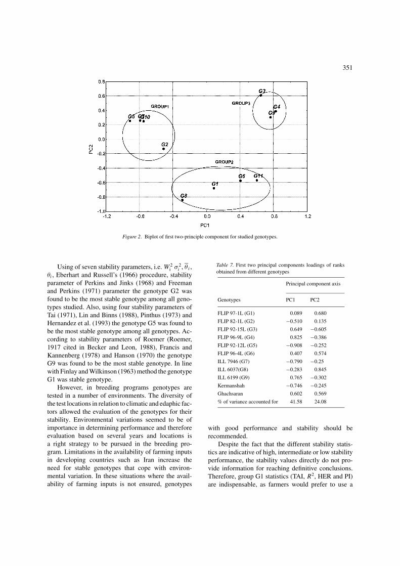
The PC analysis was performed for the ranks ofgenotypes obtained from different stability meth-ods. The results showed that the first two PCs ex-plained 65.5% of variance in data set (Table 7). ThePC1 axes divided the genotypes into two groups,in which group 1 contained high yield genotypessuch as G2 and G5, and group 2 and 3 includedlow yield genotypes such as G4 and G6 (Figure 2).According to two PCs, all genotypes can be clas-sified into three groups. Group 1 contained G2,G5, G7 and G10, group 2 included G1, G6, G8and G11, as group 3 consisted of G3, G4, and G9genotypes.

351

Figure 2. Biplot of first two-principle component for studied genotypes.

Using of seven stability parameters, i.e. W 2i σ 2

i , θ i ,θi , Eberhart and Russell’s (1966) procedure, stabilityparameter of Perkins and Jinks (1968) and Freemanand Perkins (1971) parameter the genotype G2 wasfound to be the most stable genotype among all geno-types studied. Also, using four stability parameters ofTai (1971), Lin and Binns (1988), Pinthus (1973) andHernandez et al. (1993) the genotype G5 was found tobe the most stable genotype among all genotypes. Ac-cording to stability parameters of Roemer (Roemer,1917 cited in Becker and Leon, 1988), Francis andKannenberg (1978) and Hanson (1970) the genotypeG9 was found to be the most stable genotype. In linewith Finlay and Wilkinson (1963) method the genotypeG1 was stable genotype.

However, in breeding programs genotypes aretested in a number of environments. The diversity ofthe test locations in relation to climatic and edaphic fac-tors allowed the evaluation of the genotypes for theirstability. Environmental variations seemed to be ofimportance in determining performance and thereforeevaluation based on several years and locations isa right strategy to be pursued in the breeding pro-gram. Limitations in the availability of farming inputsin developing countries such as Iran increase theneed for stable genotypes that cope with environ-mental variation. In these situations where the avail-ability of farming inputs is not ensured, genotypes

Table 7. First two principal components loadings of ranks

obtained from different genotypes

Principal component axis

Genotypes PC1 PC2

FLIP 97-1L (G1) 0.089 0.680

FLIP 82-1L (G2) −0.510 0.135

FLIP 92-15L (G3) 0.649 −0.605

FLIP 96-9L (G4) 0.825 −0.386

FLIP 92-12L (G5) −0.908 −0.252

FLIP 96-4L (G6) 0.407 0.574

ILL 7946 (G7) −0.790 −0.25

ILL 6037(G8) −0.283 0.845

ILL 6199 (G9) 0.765 −0.302

Kermanshah −0.746 −0.245

Ghachsaran 0.602 0.569

% of variance accounted for 41.58 24.08

with good performance and stability should berecommended.

Despite the fact that the different stability statis-tics are indicative of high, intermediate or low stabilityperformance, the stability values directly do not pro-vide information for reaching definitive conclusions.Therefore, group G1 statistics (TAI, R2, HER and PI)are indispensable, as farmers would prefer to use a

352

high-yielding cultivar that performs consistently fromyear to year or season to season. Selection of genotypesfor stability is needed in different environments, wherethe environment is variable and unpredictable. There-fore, genotype evaluation under variable environmentsand adoption of simultaneous selection for yield andstability is the most valuable selection index that canbe used in any plant breeding programs special in lentilbreeding programs.

In conclusion, several of stability statistics that havebeen employed in this study quantified stability ofgenotypes with respect to yield, stability and both ofthem. Both yield and stability of performance shouldbe considered simultaneously to exploit the useful ef-fect of GE interaction and to make selection of thegenotypes more precise and refined.

Though, adaptation is one of the traits they vary inassortment genotype and selection can thus be made touse the trait to develop cultivars adapted to poor andfavorable conditions. The stability and wide adaptationwere of vital importance in Iran where fluctuations ingrowing conditions are very high. The main limitationof landraces is low yielding. Therefore, by exploitingthe good adaptation and stability of these genotypes,it would be possible to develop high yield and well-adapted genotypes.

References

Allard, R.W. & A.D. Bradshaw, 1964. Implications of genotype en-

vironment interactions. Crop Sci 4: 503–508.

Becker, H.C. & J. Leon, 1988. Stability analysis in plant breeding.

Plant Breed 101: 1–23.

Crossa, J., 1990. Statistical analyses of multilocation trials. Adv

Agron 44: 55–85.

Eberhart, S.A. & W.A. Russell, 1966. Stability parameters for com-

paring varieties. Crop Sci 6: 36–40.

Finlay, K.W. & G.N. Wilkinson, 1963. The analysis of adaptation in

plant-breeding programme. Aust J Agric Res 14: 742–754.

Flores, F., M.T. Moreno & J.I. Cubero, 1998. A comparison of

univariate and multivariate methods to analyze environments.

Euphytica 31: 645–656.

Francis, T.R. & L.W. Kannenberg, 1978. Yield stability studies in

short-season maize. I. A descriptive method for grouping geno-

types. Can J Plant Sci 58: 1029–1034.

Freeman, G.H. & J.M. Perkins, 1971. Environmental and genotype-

environmental components of variability VIII. Relations between

genotypes grown in different environments and measures of these

environments. Heredity 27: 15–23.

GENSTAT 7 Committee, 2003. GENSTAT 7 releases 1 Reference

Manual. Clarendon Press, Oxford, UK.

Hanson, W.D., 1970. Genotypic stability. Theor Appl Genet 40: 226–

231.

Heinrich, G.M., C.A. Francis & J.D. Eastin, 1983. Stability of grain

sorghum yield components across diverse environments. Crop Sci

23: 209–212.

Hernandez, C.M. J. Crossa & A. Castillo, 1993. The area under the

function: An index for selecting desirable genotypes. Theor Appl

Genet 87: 409–415.

Lin, C.S. & M.R.Binns, 1988. A method of analysing cultivar ×location × year experiments: A new stability parameter. Theor

Appl Genet 76: 425–430.

Lin, C.S. M.R. Binns & L.P. Lefkovitch, 1986. Stability analysis:

Where do we stand? Crop Sci 26: 894–900.

Perkins, J.M. & J.L. Jinks, 1968. Environmental and genotype

environmental components of variability. Heredity 23: 523–

535.

Pinthus, J.M., 1973. Estimate of genotype value: A proposed method.

Euphitica 22: 121–123.

Plaisted, R.L. & L.C.A. Peterson, 1959. Technique for evaluating the

ability of selections and yield consistency in different locations

or seasons. Am Potato J 36: 381–385.

Plaisted, R.L.,1960. A shorter method of evaluating the ability of

selection to yield consistently over seasons. Am Potato J 37: 166–

172.

SAS institute, 1996. SAS/STAT User’s Guide, Second Edition. SAS

institute Inc., Cary, NC.

Sarker, A., W. Erskine & M. Singh, 2003. Regression models for

lentil seed and straw yields in Near East. Agricultural and Forest

Meteorology 116: 61–72.

Shukla, G.K., 1972. Some statistical aspects of partitioning

genotype-environmental components of variability. Heredity 29:

237–245.

Tai, G.C.C., 1971. Genotype stability analysis and its application to

potato regional trials. Crop Sci 11: 184–190.

Westcott, B., 1986. Some methods of analysing genotype-

environment interaction. Heredity 56: 243–253.

Wricke, G., 1962. Uber eine Methode zur Erfassung der okologischen

Streubreite in Eldversuchen. Z Pflanzenzucht 47: 92–96.

Yates, F. & W.G. Cochran, 1938. The analysis of groups of experi-

ments. J Agric Sci, Camb 28: 556–580.