Stability of gas pressure regulators

Applied Mathematical Modelling 32 (2008) 61–82

www.elsevier.com/locate/apm

Stability of gas pressure regulators

Naci Zafer a,*, Greg R. Luecke b,1

a Department of Mechanical Engineering, Eskisehir Osmangazi University, Makine Muhendisligi Bolumu,

26480 Bati Meselik, Eskisehir, Turkeyb Department of Mechanical Engineering, Iowa State University, Ames, IA 50010, USA

Received 1 May 2005; received in revised form 1 June 2006; accepted 2 November 2006Available online 3 January 2007

Abstract

Gas pressure regulators are widely used in both commercial and residential applications to control the operational pres-sure of the gas. One common problem in these systems is the tendency for the regulating apparatus to vibrate in an unsta-ble manner during operation. These vibrations tend to cause an auditory hum in the unit, which may cause fatigue damageand failure if left unchecked. This work investigates the stability characteristics of a specific type of hardware and showsthe cause of the vibration and possible design modifications that eliminate the unstable vibration modes. A dynamic modelof a typical pressure regulator is developed, and a linearized model is then used to investigate the sensitivity of the mostimportant governing parameters. The values of the design parameters are optimized using root locus techniques, and thedesign trade-offs are discussed.� 2006 Elsevier Inc. All rights reserved.

Keywords: Dynamics; Modeling; Stability; Vibrations; Pressure regulator

1. Introduction

Gas regulators are devices that maintain constant output pressure regardless of the variations in the inputpressure or the output flow. They range from simple, single-stage [1,2] to more complex, multi-stage [3,4], butthe principle of operation [5] is the same in all. High pressure gas flows through an orifice in the valve and thepressure energy in the gas is converted to heat and flow at the lower, regulated, pressure. The orifice faces amovable disk that regulates the amount of gas flow. A flexible diaphragm is attached to the disk by means of amechanical linkage. The diaphragm covers a chamber such that one side of the diaphragm is exposed to atmo-spheric pressure and the other is exposed to the regulated pressure. When the regulated pressure is too high,the diaphragm and linkage move the disk to close the orifice. When the regulated pressure is too low, the diskis moved to open the orifice and allow more gas pressure and flow into the regulator. On the opposite side ofthe diaphragm, an upper chamber houses a wire coil spring and a calibration screw. The screw compresses the

0307-904X/$ - see front matter � 2006 Elsevier Inc. All rights reserved.

doi:10.1016/j.apm.2006.11.003

* Corresponding author. Tel.: +90 222 239 3750x3387; fax: +90 222 239 3613/229 0535.E-mail addresses: [email protected] (N. Zafer), [email protected] (G.R. Luecke).

1 Tel.: +1 515 294 5916; fax: +1 515 294 3261.

mailto:[email protected]

mailto:[email protected]

62 N. Zafer, G.R. Luecke / Applied Mathematical Modelling 32 (2008) 61–82

spring, which changes the steady state force on the diaphragm, allowing for the adjustment of the regulatedpressure set point. If the regulated gas pressure rises above the safe operational pressure, an internal reliefvalve is opened to vent the excess gas through the upper chamber and into the atmosphere to prevent the dan-ger of high pressure gas at the regulator outlet.

Little information is published regarding these devices, due to concerns over proprietary information. Onereported study concerning high-pressure regulators is done by Kakulka et al. [6]. The regulator studied was apiston pressure-sensing unit that had a conical poppet valve that regulates the gas flow. The dynamic effects ofrestrictive orifices and the upstream and downstream volumes were addressed in the modeling and analysis.However, the source of the oscillations in the downstream exiting area, as well as the damping and the frictioneffects in the physical system, were left out. Several researchers have, on the other hand, addressed theunwanted oscillations and noise. Waxman et al. [7] eliminates the noisy oscillations with the implementationof a dead-band achieved by two micro switches. The design includes a stepping motor activated with the signalfrom a differential pressure transducer. Baumann [8] proposes a much less expensive solution, the use of a sta-tic pressure reducing plate with multiple holes. Ng [9] compares the effectiveness and cost of several methodsthat reduce or minimize the noise. Ng [10] addresses pressure regulators for liquids and names cavitations, thedamage caused by continuous formation and collapse of microscopic bubbles, to be the cause of hydrody-namic noise. Cavitations produce noise, vibration, and even cause significant damage. Ng states that theuse of quiet valves, or an orifice with multiple holes are not the solutions to this problem, since they are expen-sive and the small passages are most likely to be plugged by solid particles in the flow. Dyck [11] states that alarger restrictive orifice improves flow performance, but a small one makes the system more stable and is lesssensitive to downstream pressure fluctuations. Liptak [12] gives an equation for the offset in the regulated pres-sure with changing flow and shows that any decrease in this offset pressure decreases the stability of the reg-ulator, resulting in a noisy regulator with oscillatory pressure cycling. To stabilize the system he suggests usinglarger downstream pipe, a more restrictive flow from orifice to the lower chamber, straight lengths of pipeupstream and downstream. He also points out that maintaining gas flow at less than sonic velocities and elim-inating changes in flow directions would reduce the noise. It is obvious that these changes are very restrictivefrom the design and installation perspective, and are not guaranteed to stabilize the system.

In this study, we develop a comprehensive dynamical model for a gas pressure regulator from first principlesin order to gain a better understanding of its behavior. We first model an existing regulator and use empiricaldata as necessary to identify parameter values for the model. Using a linearized version of this model, we inves-tigate the effects of parameter variations using classical root-locus techniques. Our motivation is to design a toolthat allows for the identification of the most influential system parameters on the stability of the system, and toallow an assessment of any effects that changes in these parameters have on stabilization of the regulator.

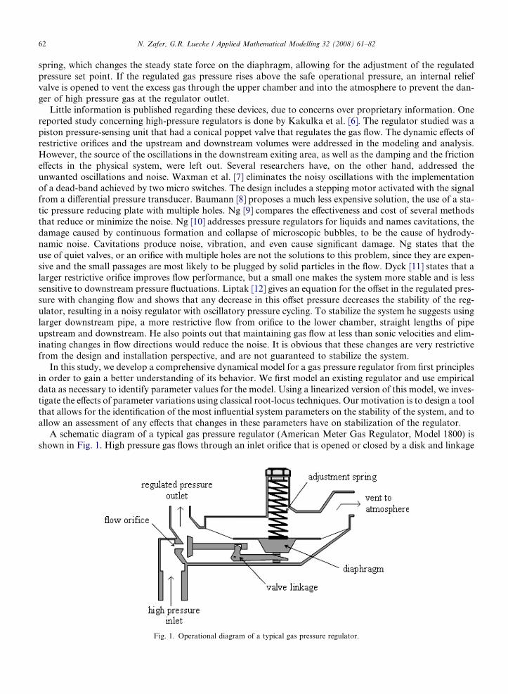
A schematic diagram of a typical gas pressure regulator (American Meter Gas Regulator, Model 1800) isshown in Fig. 1. High pressure gas flows through an inlet orifice that is opened or closed by a disk and linkage

Fig. 1. Operational diagram of a typical gas pressure regulator.

Fig. 2. Pressure regulator schematic.

N. Zafer, G.R. Luecke / Applied Mathematical Modelling 32 (2008) 61–82 63

attached to a diaphragm. The diaphragm moves in response to the balance between pressure inside the reg-ulator body and the adjustment spring force. As the regulated pressure increases, the disk closes to restrictthe incoming gas. When the regulated pressure is too low, the disk opens to allow more gas into the body cav-ity. The stability of the system depends on the amount of damping in the system, and much of the dampingcomes from flow restrictions within the regulator. In order to develop our model, we define three control vol-umes that are used in the dynamic analysis, identified in Fig. 2: the body chamber, the upper chamber and thelower chamber. Each control volume is characterized by pressure, volume, and the density as a function oftime. For the purpose of this analysis, these control volumes are used to track the mass flow through thesystem.

2. Gas dynamics governing equations

Modeling of operation of the gas pressure regulator is based on the physical behavior of compressible fluidflow. The modeling in this work uses the fundamental principles of ideal compressible flow, the principle ofconservation of mass, and well-known expressions for flow through orifices [13,14]. For the development ofthe pressure regulator model, we assume that the operating fluid is a perfect gas. Kinetic theory is then usedto express the state of a particular control volume according to the ideal gas equation:

PV ¼ mRT ; ð1Þ

where P is the pressure, V is volume, m is mass, R is a gas constant, T is temperature. Assuming the process isadiabatic and reversible, the second law of thermodynamics provides a relationship between the pressure andthe density of the fluid:

Pqk¼ Constant: ð2Þ


By considering the time differentials of Eqs. (1) and (2) together with the definition of density, one can easilyshow that

1

k

_PPþ

_VV¼ _m

m; ð3Þ

where k is the specific heat ratio, and

_m ¼ qQ; m ¼ qV : ð4Þ
Because the density for a fixed operational flow rate is constant, volumetric flow rate will be used, rather thanthe more conventional mass flow rate. Eq. (3) provides a basis for analysis and modeling of the pressure reg-ulator and describes the relationship between pressure, volume, and the mass flow for a particular controlvolume.
2.1. Lower chamber

Applying Eqs. (3) and (4) to the lower chamber, we get

1

kL

_P L

P L

þ_V L

V L

¼ �QL

V L

:

Note that the minus sign indicates that our convention of the direction of positive flow, QL, is out of the cav-ity. The motion of the diaphragm is related to change in volume by

_V L ¼ � _xdAd;

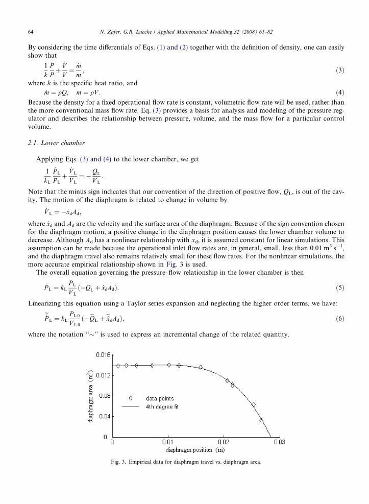
where _xd and Ad are the velocity and the surface area of the diaphragm. Because of the sign convention chosenfor the diaphragm motion, a positive change in the diaphragm position causes the lower chamber volume todecrease. Although Ad has a nonlinear relationship with xd, it is assumed constant for linear simulations. Thisassumption can be made because the operational inlet flow rates are, in general, small, less than 0.01 m3 s�1,and the diaphragm travel also remains relatively small for these flow rates. For the nonlinear simulations, themore accurate empirical relationship shown in Fig. 3 is used.

The overall equation governing the pressure–flow relationship in the lower chamber is then

_P L ¼ kLP L

V L

ð�QL þ _xdAdÞ: ð5Þ

Linearizing this equation using a Taylor series expansion and neglecting the higher order terms, we have:
e_P L ¼ kL
P L 0

V L 0

ð�eQL þ e_xdAdÞ; ð6Þ

where the notation ‘‘�’’ is used to express an incremental change of the related quantity.

Fig. 3. Empirical data for diaphragm travel vs. diaphragm area.


2.2. Upper chamber

A similar analysis for the upper chamber yields the differential equation governing the change in the pres-sure of the upper chamber:

1

kU

_P U

P U

þ_V U

V U

¼ QU

V U

;

where _V U ¼ _xdAd. The overall equation governing the pressure–flow in the upper chamber and the linearizedform are then

_P U ¼ kUP U

V U

ðQU � _xdAdÞ; ð7Þ

e_P U ¼ kU

P U 0

V U 0

ðeQU � e_xdAdÞ: ð8Þ

2.3. Body chamber

Although the flow out of the regulator is not steady, the gas pressure in the connected lower chamber andbody chamber cavities fluctuates as the regulator moves to equilibrium. For a compressible gas, these fluctu-ations also compress the gas and change the density of the fluid. However, the changes in density in thesechambers is small compared with the change density as the fluid moves from the high-pressure inlet to thelower pressure, regulated, body pressure. We can account for this change in density with an expansion ratio.Solving Eq. (3) for the body chamber using the outlet pressure gives:

1

kout

_P out

P out

¼ _mbody

mbody

:

Note that there is no change in volume for the body chamber, so that _V body ¼ 0 and the mass balance for thebody chamber in Fig. 1 is obtained by summing the mass flow rates in and out of this chamber.

_mbody ¼ _min � _mout þ _mL:

Substituting _m ¼ qQ in this equation for each of the control volumes, it follows that

Qbody ¼ jQin � Qout þ QL;

where Qin is the inlet flow-rate, and the expansion ratio

j ¼ qin

qbody

is used to account for the change in density of the inlet gas to that of the outlet gas. Again, note that qbody =qout = qL is assumed because the differences in pressure are small compared to the difference in pressurebetween these and the inlet pressure. Combining these equations gives the outlet pressure as a function ofthe flow crossing the control boundary:

1

kout

_P out

P out

¼ jQin � Qout þ QL

V body

;

_P out ¼ kout

P out

V body

ðjQin � Qout þ QLÞ:ð9Þ

Using a Taylor series expansion, we also obtain the linear, incremental, equation:

e_P out ¼ kout

P out0

V body0

ðjeQ in � eQout þ eQLÞ: ð10Þ


2.4. Flow governing equations

Fluid enters and exits the gas regulator through three flow holes, the inlet valve, the outlet orifice, andthrough the relief valve on the top of the upper chamber, each of these flow components contributes to thedynamic response characteristics of the overall regulator.

Because the pressure drop is very large from the inlet pressure through the orifice, the sonic, or critical, flowinto the regulator is proportional to the throat area [16], or the plunger travel. This provides a linear relation-ship between the flow into the regulator and the effective flow area between the orifice and the disk. This effec-tive area is dependent on the annular distance between the face of the disk and the orifice and the specificgeometry of both the disk and orifice, but is more or less constant in a specific valve.

Qin ¼ Cinxp; ð11Þ

where the constant Cin is obtained from empirical data shown in Fig. 4. This equation is already linear, and theincremental representation is:
eQin ¼ Cin~xp: ð12Þ
Flow in or out of the upper chamber occurs through a relief cap with a small vent hole. Generally, the upperchamber relief cap ventilation hole regulates flow during smaller adjustments of the diaphragm, and a spring-loaded relief plate prevents pressure build-up during large diaphragm motions or in the event of a rupture ofthe diaphragm. Using the assumption of a small orifice area when compared to the upper chamber cross sec-tional area, the flow through the ventilation hole in the upper chamber is expressed with the well-knownsquare root relationship

QU ¼ �CUt

ffiffiffiffiffiffiffiffiffiffiffiffiffiffiffiffiffiffiffiffiffiP U � P atm

p; ð13Þ

where CUt is the nonlinear flow coefficient. With Patm assumed constant, this equation is linearized usingTaylor series expansion to yield
eQU ¼ �CU
eP U; ð14Þ

with CU ¼ CUt

2ffiffiffiffiffiffiffiffiffiffiffiffiffiffiffiP U 0�P atmp .

Note that for values of PU close to the atmospheric pressure, or eP U close to zero, the linearized flow coef-ficient CU gets large and leads to large flows in response to small pressure changes to maintain the equilibriumconditions. Theoretically, this square-root relationship leads to an infinite slope of the pressure–flow curve,and this is borne out by the experimental data for flow through the upper chamber orifice at various pressuredifferences, shown in Fig. 5. However, as the pressure difference gets very small, this theoretical square-root

Fig. 4. Empirical data defining flow into the regulator as a function of the plunger travel.

Fig. 5. Empirical data for the upper chamber defining pressure as a function of the flow.


relationship breaks down and leads to a linear relationship with a very high gain. For the modeling in thiswork, the empirical data depicted in Fig. 5 is used to get the flow coefficient for the nonlinear square-rootmodel, CUt. For the linear model, CU is the slope of the curve in Fig. 5, and with low flow rates, CU willbe very large.

Flow out of the regulator is modeled using the assumption that the outlet orifice area is variable, whichaffects the gas pressure in the regulator body. This approach assumes that the flow demand to the regulatoris not separated from the body by additional dynamics from subsequent piping, and that the changes in flowdemand can be modeled as a variable orifice area at the regulator outlet. Using this approach, the flow out ofthe orifice is:

Qout ¼ ACd

ffiffiffiffiffiffiffiffiffiffiffiffiffiffiffiffiffiffiffiffiffiffiP out � P atm

p; ð15Þ

where ‘‘A’’ represents the variable area or demand from downstream. Linearization of this flow relationshipabout an equilibrium state has a slightly different result, because the pressure difference between the outlet andthe atmosphere never goes to zero. The outlet flow is a function of two variables, the pressure drop,(Pout � Patm), and the flow area, A. This linearization leads to

Qout ¼ Qout0 þo ACd


p� �oA

��P out¼P out0A¼A0

ðA� A0Þ þo ACd


p� �oP out

��P out¼P out0A¼A0

ðP out � P out0Þ

or
eQout ¼ C10eA þ C20
eP out; ð16Þ
where C10 ¼ Qout0
A0, C20 ¼

A20C2

d

2Qout0. While we continue to use empirical data to find typical value for the discharge

coefficient, Cd, in Eq. (15), for a given equilibrium condition the linear model uses the constant coefficients inEq. (16).

The flow into and out of the lower chamber is a complex function of the flow of gas through the regulatorand the shape of the flow cavity. The classical square-root relationship shown in Eq. (15) does not do a goodjob of describing the pressure–flow relationships found for regulators experimentally. Fig. 6 shows a typicalrelationship for the lower chamber and body chamber pressures at various steady state flow conditions. Thisdata indicates that the lower chamber pressure is lower than the outlet pressure in the body of the regulator.This is known as the ‘‘boost effect’’ and is caused by the venturi effect of the dynamic flow through the valvebody. In practice, this boost effect is carefully designed into the regulator as a means of obtaining constantregulation pressure over a wide range of flows, but using a model such as that in Eq. (15) means that thereshould always be flow from the lower chamber into the body. Since the lower chamber is a fixed volume atsteady state flow, this clearly cannot happen. Multiple flow paths, the dynamics of the fluid, and the geometryof internal obstructions make it difficult to develop an effective analytic model, but one approach is to imagine

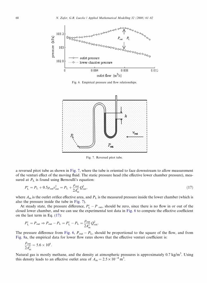
Fig. 6. Empirical pressure and flow relationships.

Fig. 7. Reversed pitot tube.


a reversed pitot tube as shown in Fig. 7, where the tube is oriented to face downstream to allow measurementof the venturi effect of the moving fluid. The static pressure head (the effective lower chamber pressure), mea-sured at PL is found using Bernoulli’s equation:

P �L ¼ P L þ 0:5qoutv2out ¼ P L þ

qout

2A2m

Q2out; ð17Þ

where Am is the outlet orifice effective area, and PL is the measured pressure inside the lower chamber (which isalso the pressure inside the tube in Fig. 7).

At steady state, the pressure difference, P �L � P out, should be zero, since there is no flow in or out of theclosed lower chamber, and we can use the experimental test data in Fig. 6 to compute the effective coefficienton the last term in Eq. (17):

P �L ¼ P out ) P out � P L ¼ P �L � P L ¼qout

2A2m

Q2out:

The pressure difference from Fig. 6, Pout � PL, should be proportional to the square of the flow, and fromFig. 8a, the empirical data for lower flow rates shows that the effective venturi coefficient is:

qout

2A2m

¼ 5:6� 106:

Natural gas is mostly methane, and the density at atmospheric pressures is approximately 0.7 kg/m3. Usingthis density leads to an effective outlet area of Am = 2.5 · 10�4 m3.

Fig. 8. Pressure difference between lower chamber and body chamber for various flow rates.


In our model, we used a maximum 3/4 in. (0.019 m) diameter outlet orifice (hardware outlet diameter) andfor this the actual area is 2.8502 · 10�4 m3. Although the flow path for the actual body chamber is more com-plex than any standard nozzle, it is well understood that flow though an orifice generates a vena contracta suchthat the effective flow area is smaller than the actual hole size. Comparing the flow area from the test data withthe actual hardware hole size indicates that we need to use a coefficient for the area contraction of 0.877. Thisvalue for the flow coefficient due to the effect of vena contracta corresponds well to typical published valuesbetween 0.73 and 0.97, depending on the shape of the opening [17].

For our linear model, Eq. (17) becomes

eP �L ¼ eP L þeQout

KL

ð18Þ

with KL ¼ A2m

qoutQout0, representing the boost factor. Fig. 8b shows the experimental pressure difference along with

a linear least-fit approximation of the constant, KL leading to 2.3 · 10�5.Also shown in Fig. 8b is a cubic least-square regression for the effective pressure that is used in the full non-

linear model. Note that the linear approximation compares favorably with the nonlinear experimental data upto about 0.007 m3 s�1. In simulation, this model of the boost effect resulted in a satisfactory response for boththe linear model and the nonlinear model at both low and moderate flow rates (as illustrated later in Section3). At very high flow rates, the venturi effect begins to fall off, and for the nonlinear model a cubic regression isused to develop a more accurate representation of the pressure–flow relationship. This polynomial has beenimplemented as the function for P �L, the fictitious equivalent pressure of the lower chamber:

P �L ¼ P L þ f ðQoutÞ: ð19Þ

The resulting model output for steady state conditions is shown for both the linear model and the nonlinearmodels in Fig. 8b. Using this effective pressure in the lower chamber, the flow between the body and the lowerchamber is then

QL ¼ CdL

ffiffiffiffiffiffiffiffiffiffiffiffiffiffiffiffiffiffiffiP �L � P out

p: ð20Þ

In order to determine the flow coefficient, a test was performed by removing the diaphragm and pumping airfrom the lower chamber and out through the valve body. This data is shown in Fig. 9a for flow from the lowerchamber to the valve body chamber for a particular valve, and this substantiates the use of Eq. (19) in themodel. The data was taken by removing the diaphragm and just flowing air from the lower chamber out ofthe body, with no venturi effects. The discharge coefficient for Eq. (20) was found by plotting (PL � Pout)vs. Q2

L, as shown in Fig. 9b, and finding the square root of the slope. The value of the nonlinear dischargecoefficient used in simulations is CdL = 5.5 · 10�4.

Fig. 9. Pressure–flow relationship between the lower chamber and the body chamber.


We can linearize Eq. (21) as

QL ¼ QL0 þo CdL


p� �oP �L

�� P �L¼P �

L0P out¼P out0

ðP �L � P �L0Þ þo ACd


p� �oP out

�� P�L¼P�

L0P out¼P out0

ðP out � P out0Þ þ h:o:t;

� QL0 þ1

2CdL

ffiffiffiffiffiffiffiffiffiffiffiffiffiffiffiffiffiffiffiffiffiffiP �L0 � P out0

p ðP �L � P �L0Þ � ðP out � P out0Þ� �

:

Defining CL ¼ 1

2CdL

ffiffiffiffiffiffiffiffiffiffiffiffiffiffiffiP �

L0�P out0

p and using eP �L ¼ eP L þeQ out

KL, we develop a linear flow model for lower chamber:

eQL ¼ CLðeP �L � eP outÞ ¼ CLeP L þ

eQout

KL

� eP out

!: ð21Þ

The linearized discharge coefficient, CL, is slope of the line in Fig. 9a at the particular flow rate of interest.

2.5. Mechanical system governing equations

The mechanical parts of the system also contribute to the dynamic response of the system. The gas pressureregulator is represented with a simplified model as shown in Fig. 10. Free body diagrams are given in Fig. 11.A simple dynamic analysis of the free body diagrams leads to

Fig. 10. Pressure regulator.

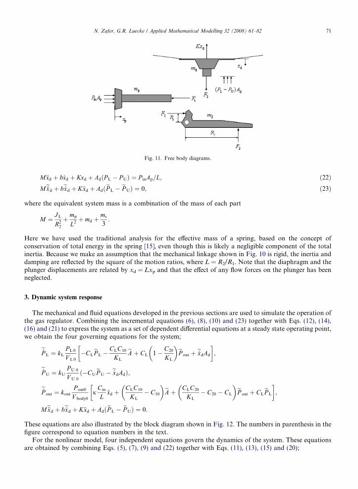
Fig. 11. Free body diagrams.


M€xd þ b _xd þ Kxd þ AdðP L � P UÞ ¼ P inAp=L; ð22ÞMe€xd þ be_xd þ K~xd þ AdðeP L � eP UÞ ¼ 0; ð23Þ

where the equivalent system mass is a combination of the mass of each part

M ¼ J L

R22

þ mp

L2þ md þ

ms

3:

Here we have used the traditional analysis for the effective mass of a spring, based on the concept ofconservation of total energy in the spring [15], even though this is likely a negligible component of the totalinertia. Because we make an assumption that the mechanical linkage shown in Fig. 10 is rigid, the inertia anddamping are reflected by the square of the motion ratios, where L = R2/R1. Note that the diaphragm and theplunger displacements are related by xd = Lxp and that the effect of any flow forces on the plunger has beenneglected.

3. Dynamic system response

The mechanical and fluid equations developed in the previous sections are used to simulate the operation ofthe gas regulator. Combining the incremental equations (6), (8), (10) and (23) together with Eqs. (12), (14),(16) and (21) to express the system as a set of dependent differential equations at a steady state operating point,we obtain the four governing equations for the system;

e_P L ¼ kL

P L 0

V L 0

�CLeP L �

CLC10

KL

eA þ CL 1� C20

KL

� eP out þ e_xdAd

�;

e_P U ¼ kU

P U 0

V U 0

ð�CUeP U � e_xdAdÞ;

e_P out ¼ kout

P out0

V body0

jCin

L~xd þ

CLC10

KL

� C10

� eA þ CLC20

KL

� C20 � CL

� eP out þ CLeP L

�;

Me€xd þ be_xd þ K~xd þ AdðeP L � eP UÞ ¼ 0:

These equations are also illustrated by the block diagram shown in Fig. 12. The numbers in parenthesis in thefigure correspond to equation numbers in the text.

For the nonlinear model, four independent equations govern the dynamics of the system. These equationsare obtained by combining Eqs. (5), (7), (9) and (22) together with Eqs. (11), (13), (15) and (20);

Fig. 12. System block diagram.


_P L ¼ kLP L

V L

_xdAd � CdL


p� ;

_P U ¼ �kUP U

V U

_xdAd þ CUt

ffiffiffiffiffiffiffiffiffiffiffiffiffiffiffiffiffiffiffiffiffiP U � P atm

p� ;

_P out ¼ kout

P out

V body

jCin

Lxd � ACd


pþ CdL


p� ;

M€xd þ b _xd þ Kxd þ AdðP L � P UÞ ¼ P inAp=Lþ F c:

Here, P �L is the equivalent pressure of the lower chamber described by Eq. (17) for the pitot, or by Eq. (19) forthe cubic fit approaches. Lower and upper chamber volumes may be approximated by VL = VL0 � Adxd andVU = VU0 + Adxd, where initial diaphragm position is xd0 ¼ L

CinQin0 ¼ L

Cin

Qout0

qNLand Ad is a function of xd de-

scribed in Fig. 3. Because xd0 5 0, a force to initially calibrate the regulator is required. This is done by addingthe term Fc = Kxd0 + Ad(PL 0 � PU 0) � PinAp/L into the mechanical system equation.

The simulation is used to verify the basic operational characteristics of the system, including the timeresponse and the stability of the regulator. The full nonlinear model is used to validate the overall operationof the regulator, including the transient response to large and small changes in outlet flow rates and steadystate pressure and flow conditions. Our main objective is to show that the simulations operate in a reasonableway in response to normal inputs, and in a manner consistent with observed behavior of the physical gas reg-ulator. Fig. 13 shows the simulation results for the steady state outlet pressure as a function of the outlet flowrate. The three modeling approaches are compared with the empirical data, and it is clear that there is a dif-ference in the steady state response using the linear and nonlinear models, particularly at higher flow rates.Fig. 13 also shows the input values used to test the models: a small flow demand of 0.001 m3 s�1 and largerdemands of 0.0065, 0.0071, 0.0092 and 0.0098 m3 s�1, along with the outlet orifice areas used to generate theseflows. First, the linear model will be compared to the nonlinear simulations to show that the linear model isvalid for small amplitude response about an equilibrium point. Next, using the linear model, we will apply thepowerful root locus techniques to investigate the effects of changes in various parameters on the systemresponse and stability.

Fig. 14 shows the time response of both the linear and the nonlinear models to a small step input in flowdemand, corresponding to case I in Fig. 13. The initial outlet flow rate was set to Qout0 = 3.9329 · 10�4 m3 s�1

and the step change for the outlet orifice area was taken as eA ¼ 1:5355� 10�5 m2. Note that the suddenchange in the outlet valve orifice area causes the pressure to drop, and then come back to the steady state.The sudden change first causes a drop in the regulated pressure, which is then restored as the plunger movesto a new steady state location. The small steady state errors are caused by the differences in the model assump-

Fig. 13. Outlet pressure and flow relationships: (I) A = 3.2258 · 10�5 m2; (II) A = 2.7493 · 10�4 m2; (III) A = 3.013 · 10�4 m2; (IV)A = 3.93 · 10�4 m2; (V) A = 4.2344 · 10�4 m2.

Fig. 14. Time response to step change in outlet area, A = 3.2258 · 10�5 m2.


tions, and while there are differences in the amplitude of the oscillations, the frequencies and settling timesmatch well.

Operational data for typical gas regulators show that the hardware has a tendency to exhibit dynamicallyunstable behavior under certain operating conditions. This instability causes the regulator to vibrate, or hum,although the gross operation of the regulator is not affected. Indeed, one major problem with this dynamicinstability is that the causal observer may become alarmed by the noise, requiring replacement of the unstableregulator. One common factor of instability is the coupling of the upper chamber with a large volume dis-charge tube for venting purposes. While changes in many other factors, including temperature, flow, andatmospheric pressure, affect the unstable response, empirical evidence indicates that it is possible to tune thisdischarge volume to induce the unstable behavior regardless of other factors.

In order to establish the conditions for the regulator to hum, we studied the time response of the regulatorwith an upper chamber volume about four times larger than the nominal value of the actual hardware,VU0 = 0.0025 m3, and the time response is shown in Fig. 15. This condition caused instability in both the non-linear and the linear model. The time response of both the linear and the nonlinear models at these large upperchamber initial volumes predict the frequency of oscillation at about <133 Hz. Fig. 15b also shows that thefrequency is the same for both the linear and nonlinear models, although there is a phase difference betweenthem. This phase difference is caused by a very small difference in frequency between the nonlinear models andthe linear model, which adds up over many cycles. The small lag gets larger if the initial displacement from theequilibrium is made larger [18].

Fig. 16 shows the time response of the regulator models for large and small inputs at the intermediate flowrates of cases II and III in Fig. 13. In the center plot, there are two step changes in the flow demand, a largechange at time = 0 corresponding to an initial outlet flow area of A0 = 1.6903 · 10�5 m2 and changing to

Fig. 15. Regulator response with large upper chamber volume, A = 3.2258 · 10�5 m2.

Fig. 16. Time response to step changes in outlet area, VU0 = 6 · 10�4 m3 (nominal value).


A = 2.7493 · 10�4 m2, and a small change at time = 1.0 corresponding to a change in outlet flow area from thesteady state at A0 = 2.7493 · 10�4 m2 and changing to A = 3.013 · 10�4 m2 thereafter. The flow rate settles toa steady state of Qout = 0.0065 m3 s�1 during the first second, and to Qout = 0.0071 m3 s�1 by the end of thesimulation. Because the step change for the first second is quite large, only the nonlinear models are used in thesimulation. Once the steady state is reached, the flow and pressure values are used to update the linear modelparameters and the response of the linear and nonlinear models are compared for the small amplitude input,shown in the zoomed portion on the right of Fig. 16. Thus, both the nonlinear and the linear model are com-pared after the step at 1 s in the simulation. For small amplitude inputs, the linear model dynamics closelymatch the nonlinear model simulations, although there are steady state errors predicted by Fig. 13.

This same set of large and small inputs is shown in Fig. 17, but in this case, with a large upper chamber vol-ume VU0 = 6 · 10�3 m3. Again, the initial, large step input is only simulated using the nonlinear models, andthe linear model is compared to the nonlinear responses for the small step input at 1.5 s. In this case, the linearmodel response still follows the nonlinear dynamics, although for both linear and nonlinear cases we see thatthe increase in the upper chamber volume has the effect of slowing the settling time of the regulator.

Fig. 18 shows the time response of the regulator for very high flow rates corresponding to cases IV and Vfrom Fig. 13. These step changes in the outlet orifice area from A0 = 1.6903 · 10�5 m2 to A = 3.93 · 10�4 m2

in the first 1 s and A = 3.93 · 10�4 m2 to A = 4.2344 · 10�4 m2 at 1.5 s correspond to steady state flow rates ofQout = 0.0092 m3 s�1 and to Qout = 0.0098 m3 s�1 respectively. Again, the steady state values of the nonlinear

Fig. 17. Time response to step changes in outlet area, VU0 = 6 · 10�3 m3.

Fig. 18. Time response to step changes in outlet area, VU0 = 6 · 10�4 m3 (nominal value).


model after the first large step input are used update the linear model parameters. Thus, both the nonlinearand the linear models are compared in the second part of the simulation, shown in the right of the figure. Notethat during the initial response for the large step input, the system is very under damped, as shown by theoscillations in the left-hand portion of Fig. 18. For the smaller input at the higher flow rate, however, thedynamics show considerably more damping, indicating that higher flow rates tend to stabilize the system.Fig. 19 shows the response for this same set of inputs with the larger upper chamber volume, VU0 =6 · 10�3 m3. Here again, it is clear that the higher flow rates tend to stabilize the system response.

These simulations show that the mathematical models of the gas regulator produce reasonable response tochanges in flow demands. The dynamic instability seen in real regulators for small flow rates can be repro-duced in the simulations by increasing the upper chamber volume, which is also true for regulators in actualoperation. The linear model closely matches the nonlinear model close to equilibrium positions and for smallinputs. We will now use linear analysis methods to identify design parameters that have an effect on the sta-bility of the system.

4. Linear system analysis

In order to understand the effects of various parameters on the stability of the system, an analysis of thelinear system has been examined in the form of a root locus diagram for several parameters. This method

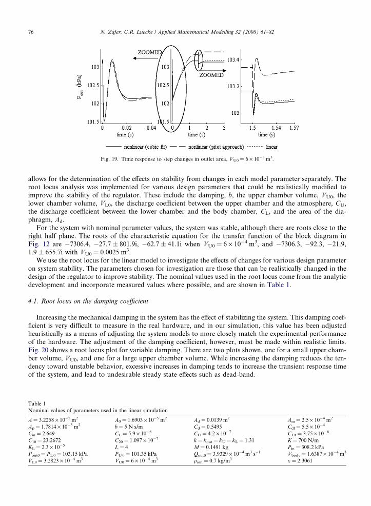
Fig. 19. Time response to step changes in outlet area, VU0 = 6 · 10�3 m3.


allows for the determination of the effects on stability from changes in each model parameter separately. Theroot locus analysis was implemented for various design parameters that could be realistically modified toimprove the stability of the regulator. These include the damping, b, the upper chamber volume, VU0, thelower chamber volume, VL0, the discharge coefficient between the upper chamber and the atmosphere, CU,the discharge coefficient between the lower chamber and the body chamber, CL, and the area of the dia-phragm, Ad.

For the system with nominal parameter values, the system was stable, although there are roots close to theright half plane. The roots of the characteristic equation for the transfer function of the block diagram inFig. 12 are �7306.4, �27.7 ± 801.9i, �62.7 ± 41.1i when VU0 = 6 · 10�4 m3, and �7306.3, �92.3, �21.9,1.9 ± 655.7i with VU0 = 0.0025 m3.

We use the root locus for the linear model to investigate the effects of changes for various design parameteron system stability. The parameters chosen for investigation are those that can be realistically changed in thedesign of the regulator to improve stability. The nominal values used in the root locus come from the analyticdevelopment and incorporate measured values where possible, and are shown in Table 1.

4.1. Root locus on the damping coefficient

Increasing the mechanical damping in the system has the effect of stabilizing the system. This damping coef-ficient is very difficult to measure in the real hardware, and in our simulation, this value has been adjustedheuristically as a means of adjusting the system models to more closely match the experimental performanceof the hardware. The adjustment of the damping coefficient, however, must be made within realistic limits.Fig. 20 shows a root locus plot for variable damping. There are two plots shown, one for a small upper cham-ber volume, VU0, and one for a large upper chamber volume. While increasing the damping reduces the ten-dency toward unstable behavior, excessive increases in damping tends to increase the transient response timeof the system, and lead to undesirable steady state effects such as dead-band.

Table 1Nominal values of parameters used in the linear simulation

A = 3.2258 · 10�5 m2 A0 = 1.6903 · 10�5 m2 Ad = 0.0139 m2 Am = 2.5 · 10�4 m2

Ap = 1.7814 · 10�5 m2 b = 5 N s/m Cd = 0.5495 Cdl = 5.5 · 10�4

Cin = 2.649 CL = 5.9 · 10�6 CU = 4.2 · 10�7 CUt = 3.75 · 10�6

C10 = 23.2672 C20 = 1.097 · 10�7 k = kout = kU = kL = 1.31 K = 700 N/mKL = 2.3 · 10�5 L = 4 M = 0.1491 kg Pin = 308.2 kPaPout0 = PL 0 = 103.15 kPa PU 0 = 101.35 kPa Qout0 = 3.9329 · 10�4 m3 s�1 Vbody = 1.6387 · 10�4 m3

VL0 = 3.2823 · 10�4 m3 VU0 = 6 · 10�4 m3 qout = 0.7 kg/m3 j = 2.3061

Fig. 20. Root locus for the variable b with two values of VU0; h: b = 5 N s/m.


Changes in the upper chamber volume also affect the stability of the regulator. As this volume decreases, thesystem becomes more stable, as shown for the root positions when the damping b = 5 N s/m. At the larger vol-ume, the system is unstable and at the smaller volume, the system is stable. This corresponds with known designgoals, where the upper chamber volume must be large enough to accommodate the diaphragm diameter andtravel, but is designed to be as small as possible. In addition, the oscillatory ‘‘hum’’ can often be induced by sim-ply attaching a larger volume pipe to the vent discharge valve, effectively increasing the upper chamber volume.

4.2. Root locus on the diaphragm area

Another parameter that is a candidate for design change is the diaphragm area. The root locus for Ad,shown in Fig. 21, shows some interesting trends. While the root locus shows that the diaphragm could bemade very small and result in stable performance of the regulator, this size diaphragm is not large enoughto counteract plunger flow forces or even allow mechanical connections necessary for the physical hardware.

The remaining locus indicates that diaphragm area cannot be chosen smaller than 0.0084 m2 in order to retainstability. Larger diaphragm areas, on the other hand, improve the response time of the system, although in theextreme, these roots also become under damped. However, because changes in diaphragm area usually implychanges in lower and upper chamber volumes, care must be taken when implementing a larger diaphragm.

4.3. Root locus on the upper chamber initial volume

The physical conditions surrounding the onset of instability include a large volume or pipe attached to theupper chamber. Often, just attaching a vent hose, common in Europe where the regulators are installed

Fig. 21. Root locus on Ad; e: Ad = 0.0139 m2 (nominal), r: Ad = 0.0084 m2.


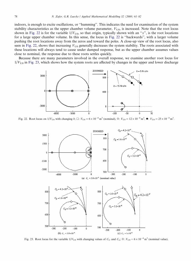
indoors, is enough to excite oscillations, or ‘‘humming’’. This indicates the need for examination of the systemstability characteristics as the upper chamber volume parameter, VU0, is increased. Note that the root locusshown in Fig. 22 is for the variable 1/VU0, so that origin, typically shown with an ‘‘x’’, is the root locationsfor a large upper chamber volume. In this sense, the locus in Fig. 22 is ‘‘backwards’’, with a larger volumepushing the root locations away from the zeros and toward the poles. A close-up view of the root locus, alsoseen in Fig. 22, shows that increasing VU0 generally decreases the system stability. The roots associated withthese locations will always tend to cause under damped response, but as the upper chamber assumes valuesclose to nominal, the response due to these roots settles quickly.

Because there are many parameters involved in the overall response, we examine another root locus for1/VU0 in Fig. 23, which shows how the system roots are affected by changes in the upper and lower discharge

Fig. 22. Root locus on 1/VU0 with changing b; h: VU0 = 6 · 10�4 m3 (nominal), �: VU0 = 12 · 10�4 m3, r: VU0 = 25 · 10�4 m3.

Fig. 23. Root locus for the variable 1/VU0 with changing values of CU and CL; �: VU0 = 6 · 10�4 m3 (nominal value).


coefficients. These coefficients are mainly a function of the hole sizes of the cap in the upper chamber, a designparameter that is relatively easy to change. The nominal values of all parameters except VU0 and CU are usedin Fig. 23a, where we see that increasing the upper chamber discharge coefficient, corresponding to increasingthe size of the vent hole, improves stability for small upper chamber volumes but does not substantially affectstability when these volumes get large. As the lower discharge coefficient is decreased, shown in Fig. 23b and c,the entire locus tends to move away from the imaginary axis, with an associated improvement in stability. Aspointed out in Fig. 22, reducing the initial size of the upper chamber still does improve the behavior of thesystem, but pipe and venting installations in the field will always tend to increase this volume and drive thesystem toward instability. Most importantly, the lower values of CL move the root locus entirely into the sta-ble region. This indicates that lowering the value of CL, by reducing the associated flow area between the lowerchamber and the valve body by at least a factor of two, will enhance system stability over a wide range ofupper chamber volume values.

4.4. Root locus on the lower chamber initial volume

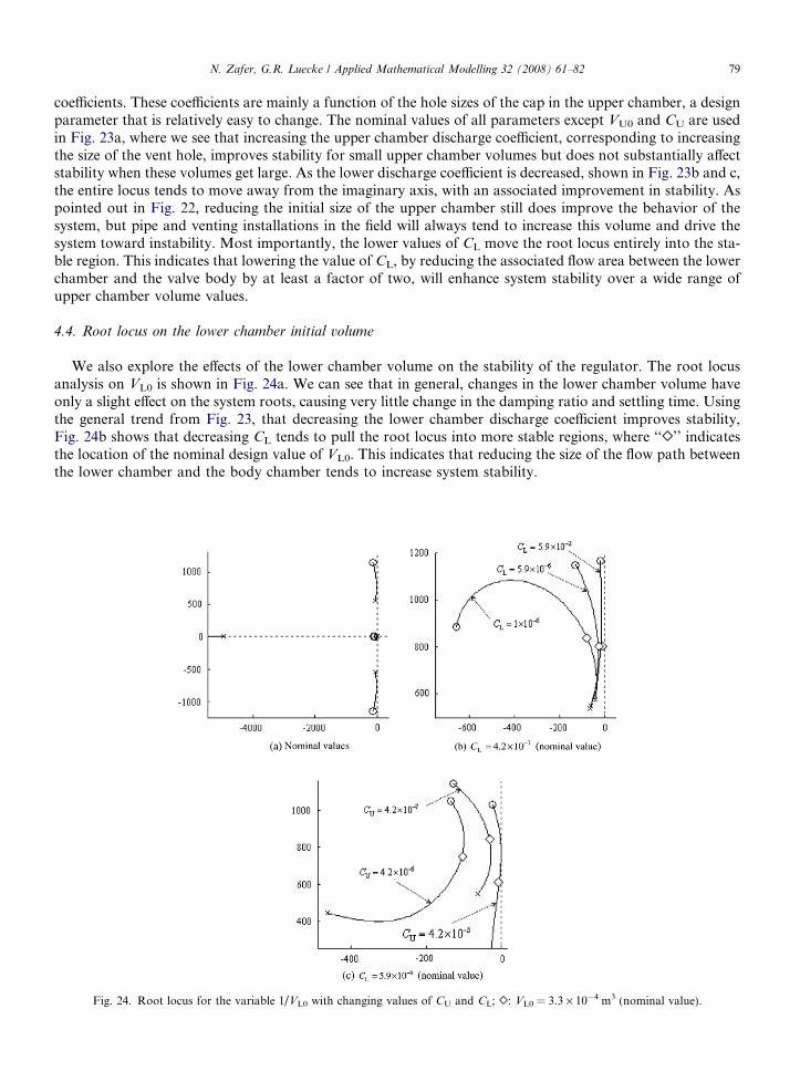
We also explore the effects of the lower chamber volume on the stability of the regulator. The root locusanalysis on VL0 is shown in Fig. 24a. We can see that in general, changes in the lower chamber volume haveonly a slight effect on the system roots, causing very little change in the damping ratio and settling time. Usingthe general trend from Fig. 23, that decreasing the lower chamber discharge coefficient improves stability,Fig. 24b shows that decreasing CL tends to pull the root locus into more stable regions, where ‘‘�’’ indicatesthe location of the nominal design value of VL0. This indicates that reducing the size of the flow path betweenthe lower chamber and the body chamber tends to increase system stability.

Fig. 24. Root locus for the variable 1/VL0 with changing values of CU and CL; �: VL0 = 3.3 · 10�4 m3 (nominal value).


Fig. 23 also indicates that increasing the upper discharge coefficient, CU, may improve stability, Fig. 24cshows the locus with a the nominal value of CL, but with a range of values for CU, as the lower chamber vol-ume, VL0, is changed. As the upper chamber discharge coefficient is increased by a factor of ten, the locusmoves toward instability. It is natural to try decreasing the value of CU, but this change also pushes the locustoward instability.

4.5. Root locus on the upper chamber discharge coefficient

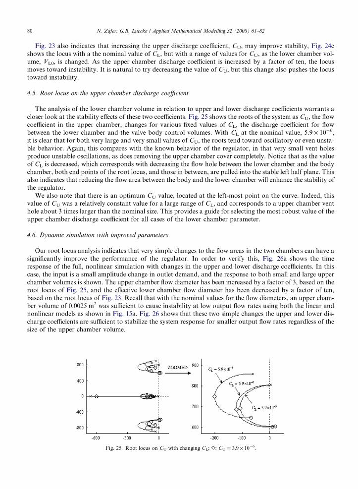
The analysis of the lower chamber volume in relation to upper and lower discharge coefficients warrants acloser look at the stability effects of these two coefficients. Fig. 25 shows the roots of the system as CU, the flowcoefficient in the upper chamber, changes for various fixed values of CL, the discharge coefficient for flowbetween the lower chamber and the valve body control volumes. With CL at the nominal value, 5.9 · 10�6,it is clear that for both very large and very small values of CU, the roots tend toward oscillatory or even unsta-ble behavior. Again, this compares with the known behavior of the regulator, in that very small vent holesproduce unstable oscillations, as does removing the upper chamber cover completely. Notice that as the valueof CL is decreased, which corresponds with decreasing the flow hole between the lower chamber and the bodychamber, both end points of the root locus, and those in between, are pulled into the stable left half plane. Thisalso indicates that reducing the flow area between the body and the lower chamber will enhance the stability ofthe regulator.

We also note that there is an optimum CU value, located at the left-most point on the curve. Indeed, thisvalue of CU was a relatively constant value for a large range of CL, and corresponds to a upper chamber venthole about 3 times larger than the nominal size. This provides a guide for selecting the most robust value of theupper chamber discharge coefficient for all cases of the lower chamber parameter.

4.6. Dynamic simulation with improved parameters

Our root locus analysis indicates that very simple changes to the flow areas in the two chambers can have asignificantly improve the performance of the regulator. In order to verify this, Fig. 26a shows the timeresponse of the full, nonlinear simulation with changes in the upper and lower discharge coefficients. In thiscase, the input is a small amplitude change in outlet demand, and the response to both small and large upperchamber volumes is shown. The upper chamber flow diameter has been increased by a factor of 3, based on theroot locus of Fig. 25, and the effective lower chamber flow diameter has been decreased by a factor of ten,based on the root locus of Fig. 23. Recall that with the nominal values for the flow diameters, an upper cham-ber volume of 0.0025 m2 was sufficient to cause instability at low output flow rates using both the linear andnonlinear models as shown in Fig. 15a. Fig. 26 shows that these two simple changes the upper and lower dis-charge coefficients are sufficient to stabilize the system response for smaller output flow rates regardless of thesize of the upper chamber volume.

Fig. 25. Root locus on CU with changing CL; �: CU = 3.9 · 10�6.

Fig. 26. Time response with changes in the upper and lower flow paths.


Larger output flow rates tend to stabilize the system as shown in Figs. 17–19. However, even at the low flowrates and with the larger upper chamber volumes, the changes in the two flow coefficients stabilize the oper-ation of the regulator as shown if the response of Fig. 26a. Although both of these design changes(CUt = 3.375 · 10�5, Cdl = 5.5 · 10�6) are very easy to implement in hardware, care must be taken to allowfor sufficient flow capability through the two chambers and out of the upper chamber vent hole in case theinlet flow orifice from the high pressure gas is stuck open, either though debris or mechanical failure. As notedearlier, the upper chamber vent is often a dual stage, spring loaded plate with a small discharge hole specif-ically for this reason.

5. Results and conclusion

This study establishes methodology to accurately model and analyze the behavior of self-regulating highpressure gas regulators. The model used has been developed from first principles to couple the mechanicaland fluid system dynamics. A linear version of the model has also been developed to allow the applicationof root locus techniques to study the stability of the system with changes in various design parameters.

Estimation of important parameters, such as damping and discharge coefficients, was based on availablesteady state empirical data. Both the linear and nonlinear models produce transient and steady state responsesthat compared favorably with the expected behavior of the typical gas regulator. Small errors in the steadystate response of the model can be attributed to the simplifying assumptions in the gas dynamics involved withthe venturi effect of the flowing gas. Transient response characteristics of the linear model match the nonlinearmodel for small amplitude inputs, although there are significant differences in steady state values for largeamplitude inputs.

One of the main reasons for the development of this model was the fact that these types of regulators tendto vibrate or hum when the relief port is connected to an extended pipe and the flow rate is kept small. Thisphenomenon was simulated as an increase in the upper chamber cavity on the regulator. Simulation resultssupport the loss of stability with an increase in this volume, indicating that the model provided an accuraterepresentation of the hardware.

In order to gain insight into the possibility of stabilizing the system through redesign, root locus techniqueswere used on the linear model to predict the effects of changes in various design parameters on the systemresponse and to identify the most influential system parameters. Physical parameters that were shown to havea significant effect on stability include the damping coefficient, the diaphragm area, and upper and lowerchamber volumes. Added damping, however, is difficult to control when relying on friction, may require add-ing hardware for accurate control, and increases the system dead-band and response time. Physical limitationson size restrict the effectiveness of changes in the sizes of the chamber volumes and the diaphragm area.

The effect of the size of the flow paths from the upper and lower chambers was also seen to have a signif-icant effect on the system stability. Using the root locus approach, we find that reducing the size of the flow


path between the regulator body and the lower chamber provides a distinct improvement in stability. In addi-tion, we show that there is an optimum size for the discharge hole on the upper chamber. We use the root locustechniques to show that decreasing the effective diameter of the lower chamber flow path by a factor of 10 andincreasing the diameter of the upper chamber flow path by about three times theoretically improves the sta-bility of the regulator. While there are limits on the allowable sizes for these holes, based on the discharge flowthat must be allowed in the case of catastrophic failure of the regulator, we show that using these changes inthe nonlinear simulation eliminates the vibration and hum and provides satisfactory performance of theregulator.

Acknowledgement

The authors are grateful to the anonymous referee for the insightful comments and suggestions whichhelped greatly improve the quality of this paper.

References

[1] R. Mooney, Pilot-loaded regulators: what you need to know, Gas Industr. (1989) 31–33.[2] R. Brasilow, The basics of gas regulators, Weld. Des. Fabric. (1989) 61–65.[3] A. Krigman, Guide to selecting pressure regulators, InTech (1984) 51–65.[4] E. Gill, Air-loaded regulators, the smart control valve alternative, InTech (1990) 21–22.[5] S.J. Bailey, Pressure controls 1987: sensing art challenges old technologies, Contr. Eng. (1987) 80–85.[6] D.J. Kukulka, A. Benzoni, J.C. Mallendorf, Digital simulation of a pneumatic pressure regulator, Simulation (1994) 252–266.[7] M. Waxman, H.A. Davis, B. Everhart, Automated pressure regulator, Rev. Sci. Instrum. (1984) 1467–1470.[8] H.D. Bauman, Reduce pressure quietly and safely, Chem. Eng. (1992) 138–142.[9] W.K. Ng, Measuring and reducing control valve noise pollution, I&CS (1994) 59–69.

[10] W.K. Ng, Control valve noise, ISA Trans. 33 (1994) 275–286.[11] R.I.J. Dyck, Residential gas regulators, Pipeline Gas J. (1988) 30–33.[12] B.G. Liptak, Pressure regulators, Chem. Eng. (1987) 69–76.[13] M.H. Aksel, O.C. Eralp, Gas Dynamics, Prentice-Hall, Englewood Cliffs, NJ, 1994.[14] C.A. Carmichael, Gas regulators work by equalizing opposing forces, Pipeline Gas Industr. (1996) 29–32.[15] W.H. Seto, Theory and Practice of Mechanical Vibrations, McGraw-Hill Book Co., New York, 1964.[16] B.T. Miralles, Preliminary considerations in the use of industrial sonic nozzles, Flow Meas. Instrum. 11 (2000) 345–350.[17] B.B. Shannak, L. Friedel, M. Alhusein, Prediction of single- and two-phase flow contraction through a sharp-edged short orifice,

Chem. Eng. Technol. 22 (10) (1999) 865–870.[18] N. Aggarwal, N. Verma, P. Arun, Simple pendulum revisited, Eur. J. Phys. 26 (2005) 517–523.

Stability of gas pressure regulators

Documents

Transcript of Stability of gas pressure regulators