^ßt^vö t- DO-U^o - DTIC

UNITED STATES AIR FORCE

SUMMER RESEARCH PROGRAM -- 1997

HIGH SCHOOL APPRENTICESHIP FINAL REPORTS

VOLUME 13

PHILLIPS LABORATORY

RESEARCH & DEVELOPMENT LABORATORIES

5800 Upiander Way

Culver City, CA 90230-6608

Program Director, RDL Program Manager, AFOSR Gary Moore Major Linda Steel-Goodwin

Program Manager, RDL Program Administrator, RDL Scott Licoscos Johnetta Thompson

Program Administrator Rebecca Kelly-Clemmons

Submitted to:

AIR FORCE OFFICE OF SCIENTIFIC RESEARCH

Boiling Air Force Base

Washington, D.C.

December 1997

^ßt^vö t- DO-U^o

REPORT DOCUMENTATION PAGE Form Approved

Public reporting burden for tris collection of information is estimated to average 1 hour per response, including the time for reviewing instructions, sei the collection of information. Sand comments regarding this burden estimate or any other aspect of this collection of infrcmation, including sug| Operations end Reports, 1216 Jefferson Davis Highway, Suite 1204, Arfngton, VA 22202-4302, and to the tftfice of Management end Budget, Par*

1. AGENCY USE ONLY (Leave blank) 2. REPORT DATE

December, 1997

3. REPO

AFRL-SR-BL-TR-00- reviewing formation

4. TITLE AND SUBTITLE

1997 Summer Research Program (SRP), High School Apprenticeship Program (HSAP), Final Reports, Volume 13, Phillips Laboratory

6. AUTHOR(S)

Gary Moore

7. PERFORMING ORGANIZATION NAME(S) AND ADDRESS(ES)

Research & Development Laboratories (RDL) 5800 Uplander Way Culver City, CA 90230-6608

S. SPONSORING/MONITORING AGENCY NAME(S) AND ADDRESS(ES)

Air Force Office of Scientific Research (AFOSR) 801 N. Randolph St. Arlington, VA 22203-1977

5. FUNDING NUMBERS

F49620-93-C-0063

8. PERFORMING ORGANIZATION REPORT NUMBER

10. SPONSORING/MONITORING AGENCY REPORT NUMBER

11. SUPPLEMENTARY NOTES

12a. DISTRIBUTION AVAILABILITY STATEMENT

Approved for Public Release 12b. DISTRIBUTION CODE

13. ABSTRACT (Maximum 200 words)

The United States Air Force Summer Research Program (USAF-SRP) is designed to introduce university, college, and technical institute faculty members, graduate students, and high school students to Air Force research. This is accomplished by the faculty members (Summer Faculty Research Program, (SFRP)), graduate students (Graduate Student Research Program (GSRP)), and high school students (High School Apprenticeship Program (HSAP)) being selected on a nationally advertised competitive basis during the summer intersession period to perform research at Air Force Research Laboratory (AFRL) Technical Directorates, Air Force Air Logistics Centers (ALC), and other AF Laboratories. This volume consists of a program overview, program management statistics, and the final technical reports from the HSAP participants at the Phillips Laboratory.

14. SUBJECT TERMS

Air Force Research, Air Force, Engineering, Laboratories, Reports, Summer, Universities, Faculty, Graduate Student, High School Student

17. SECURITY CLASSIFICATION OF REPORT

Unclassified

18. SECURITY CLASSIFICATION OF THIS PAGE

Unclassified

19. SECURITY CLASSIFICATION OF ABSTRACT

Unclassified

15. NUMBER OF PAGES

16. PRICE CODE

20. LIMITATION OF ABSTRACT

UL Standard Form 298 (Rev. 2-89) (EG) Prescribed by ANSI Std. 239.18 Designed using Perform Pro, WHS/DIOR, Oct 94

PREFACE

Reports in this volume are numbered consecutively beginning with number 1. Each report is paginated with the report number followed by consecutive page numbers, e.g., 1-1, 1-2, 1-3; 2-1, 2-2, 2-3.

This document is one of a set of 16 volumes describing the 1997 AFOSR Summer Research Program. The following volumes comprise the set:

VOLUME TITLE

1 Program Management Report

Summer Faculty Research Program (SFRP) Reports

2A&2B Armstrong Laboratory

3A&3B Phillips Laboratory

4A&4B Rome Laboratory

5A , 5B & 5C Wright Laboratory

6 Arnold Engineering Development Center, United States Air Force Academy and

Air T rtcriotiro Ppnfprc

Graduate Student Research Program (GSRP) Reports

7A & 7B Armstrong Laboratory

8 Phillips Laboratory

9 Rome Laboratory

10A & 10B Wright Laboratory

11 Arnold Engineering Development Center, United States Air Force Academy,

Wilford Hall Medical Center and Air Logistics Centers

High School Apprenticeship Program (HSAP) Reports

12A & 12B Armstrong Laboratory

13 Phillips Laboratory

14 Rome Laboratory

15A, 15B & 15C Wright Laboratory

16 Arnold Engineering Development Center

HSAP FINAL REPORT TABLE OF CONTENTS i-xiv

1. INTRODUCTION 1

2. PARTICIPATION IN THE SUMMER RESEARCH PROGRAM 2

3. RECRUITING AND SELECTION 3

4. SITE VISITS 4

5. HBCU/MI PARTICIPATION 4

6. SRP FUNDING SOURCES

7. COMPENSATION FOR PARTICIPATIONS 5

8. CONTENTS OF THE 1995 REPORT 6

5

APPENDICIES:

A. PROGRAM STATISTICAL SUMMARY A-1

B. SRP EVALUATION RESPONSES B-l

HSAP FINAL REPORTS

SRP Final Report Table of Contents

University/Institution Armstrong Laboratory ithor Report Title Directorate Vol-Page andiL Black AL/HRA 12- 1

Red Mountain High School, Mesa , AZ

(ümberly K Blazer AL/CFHV 12- 2 Oakwood High School, Dayton , OH Repeatability Evaluation of Night Vision Goggles for Geomentric Measurements

risten R Bonnema AL/CFHI 12- 3 Wayne High School, Huber Heights , OH The Effects of Individual Differences and team processes on Team Member schema similarity and taskP

ivid M Brogan AL/OERS 12 - 4 Robert E. Lee High School, San Antonio . TX The use of 3-Dimensional modeling in the widespread Dissemination of complex scientific data

atthew S Caspers AL/CFTF 12- 5 MacArthur High School, San Antonio , TX A Study of the 39-40 Hz Signal to determine an index of Gravitational induced loss of Consciousness

lizabeth M Cobb AL/CFBA 12- 6 Belmont High School, Dayton , OH A Study fo Pitch and Contact Associated with the Opening and Closing of Vaocal Cords

indaE Cortina AL/AOH 12- 7 Theodore Roosevelt High School, San Antonio , TX The Effect of Hyperbaric Oxygenation on the Mitotic Div of Prostate Cancer Cells

lariaAEvans AL/OEAO 12- 8 John Jay High School, San Antonio , TX Mercury Analysis By Cold Vapor By Atomic Ahsortion

aniel L Hardmeyer AL/AOC 12 - 9 James Madison High School, San Antonio. TX Neuropsychological Examinations For Pilots

lafisa Islam AL/OET 12- 10 Centerville High School. Centerville , OH Effects of timed exposure to Dibromobenzene on /arachidonic acid levels in skin using a methyl Este

tathleenSKao ALOERB 12- 11 Keystone School, San Antonio , TX Effects of Brain Temperature ofn Fatigue in Rats Due to Maziaml Exercise and Radio Frequency Radiati


University/institution Armstrong Laboratory . „.;,, Directorate vol-Page Author Report Title . _ i — — — —

7 MTomm AL/OEAO I2" 12 Lauren M Lamm

Kevstone School, San Antonio , TX Analyses of Metal Concentrations By Flame Atomic Absorption Spectroscopy

Evan D Large

Jason L Law

Shaun M Little

Katie E Lorenz

AL/HRGO — 12' 13

Northwestern High School, Springfield , OH ABDAR Remote Engineering

AL/CFT —— 12_ 14

Oliver Wendell Holmes High , San Antonio , TX

AL/HRCC 12' 15

Floresville High School, Floresville , TX The role of Microsoft's direct* 3 software development Kit in the rapid development of high

fidelity

AL/CFHP

Chaminade-Julienne High School, Dayton , OH Visual Acutiy between 6 and 60 Meters

12- 16

AL/CF 12- 17 Darby M Mahan

Tippecanoe High School, Tipp City , OH

_ 12- 18

12- 19

Priscilla M Medina AL/EQP - PSJ High School, Port Saint Joe , FL A Look into the Air Force's Computer Department

Mark T Meiners AL/HRA Dobson High , Mesa, AZ A Study of Accuracy and Response Time in Tests of Spatial Ability

« -ITH/TII«- AL/OERS l2" 20 David J Miller

Texas Acadeim of Mathematics , Denton , TX An Analysis of Radiofrequency Radiation Induced Temperature gradients in the Rat Brain

Joseph RMoate AL/EQM — 12' " Rutherford High School, PANAMA CITY , FL

AT /CFTF — ■ l2" 22

Shannon J Murphy AU/ur

Kevstone School, San Antonio , TX An"Investigation of The Precision of the El-Mar Fixation Analysis Software Technology

u


ithor University/Institution Report Title

Armstrong Laboratory Directorate

itrina A Navalta AL/OEAO Health Careers High School, San Antonio, TX Metals Analysis by Atomic Absorption Using A Graphite Furnace

Vol-Page

12- 23

iristine P Pan AL/HRCC Health Careers High School, San Antonio , TX Spinning a Web

12- 24

avitha K Reddy AL/CFBE

Miami Valley School, Dayton , OH Study of factors Influencing Injun- Potential Associated with Emergency Egress

12- 25

ritha K Reddy

ster I Resendiz

AL/CFBA 12- 26

Miami Valley School, Dayton , OH A Study of the Methodology Used In An Experiment Testing The Effect of Localizing Auditory Signals O

AL/CFTF William Howard Taft High School, San Antonio , TX A study of the shifts in scene perception memory

12- 27

manda M Scheidt AL/OET Wayne High School, Huber Heights , OH

12- 28

achel A Sharp AL/AOEL William Howard Taft High School, San Antonio , TX A study of the Analysis of Urinary Benzodiazepines Using Enzyme Hydrolysis

12- 29

ames E Sovel AL/EQA Rutherford High School, PANAMA CITY , FL

12- 30

jirtis J Sparks AL/HRGO Xenia High School, Xenia , OH ABDR:Remote Engineering Requests

12- 31

.auren M Spencer AL/EQL Rutherford High School, PANAMA CITY , FL Alternative Training Agents Laboratory-Scale Work

12- 32

Tyler W Standage AL/HRA Gilbert High School, Gilbert, AZ A Study of Accuracy and Response time in tests of Spatial Ability

12- 33

in


Author Univer s i ty/ Ins ti tu ti on Report Title

Armstrong Laboratory Directorate ^^ Vol-Page

Rachel J Strickland AL/EQP 12- 34

A. Crawford Moselv High School , Lynn Haven , FL the Process ofd Technical Publicaatinn/Documentation Via Electronic Media For the Armstrong

Laborato

Lvdia R Strickland AL/EQL 12- 35

A Crawford Moselv High School, Lynn Haven , FL Anaerobic Degradatin Products of Toluene and Laboratory MSDS Management

Kellv C Todd AL/AOH

Theodore Roosevelt High School, San Antonio , TX The Effect of Hyperbaric Oxygenation on the Mitotic Div of Prostate Cancer Cells

12- 36

Tammy L Venema AL/CFBS

Stebbins High School, Dayton , OH Cerebral hemoclynamic Response to a Squat-Stand at IG

12- 37

Mai P Vilimpoc AL/CFHP 12- 38

Beavercreek High School, Dayton , OH A Study of Psycho-Physiological Effects on Brainwave Activity During Varying levels of Activity

Elizabeth A Walker AL/AOH 12- 39

Theodore Roosevelt High School, San Antonio , TX The Effect of Hyperbaric Osygenation on the Mitotic Div of Prostate Cancer CeUs

Nathan L Wright AL/CFBV

Dayton Christian High School, Dayton , OH CG and MOI Study of Human and Manikin Segments

12- 40

Muchieh A Yu AL/AOE

Theodore Roosevelt High School, San Antonio , TX Detection of Clostridium Difficile Toxins by Polymerase Chain Reaction

12- 41

IV


University/Institution Phillips Laboratory ithor Report Title Directorate Vol-Page TulvRBIundell PLiRKO 13- 1

Rosamond High School, Rosamond , CA Engineering Assistant

lauren A Ferguson PL/LIMI 13- 2 Moriarity High School, Moriarity , NM Experimental Validation of Three-Dimensiona! Reconstruction of Inhomogeneity Images in turbid Media

ricaSGerken PUI.JDD _ 13- 3 Manzano High School, Albuquerque. NM Chaotic Dynamics in a Nd:YAG laser

gan BKba

aul G Loftsgard

awn R Miller

Lmy W Mok

PL/GPOS 13- 4 Chelmsford High School, North Chelra>ford , MA

PL/RKS 13- 5

Quartz Hill High School, Quartz Hill. CA A Study on Optical Patemation

PL/VTV —— 13- 6 Manzano High School, Albuquerque .NM A Study of Space Structure's Isolation

PL/GPID 13- 7

Newton North High Sch( ol, Newtonriuc , MA A study of the Effect of f jel Sulfur Content on the Production of Aerosols in Aircraft Exhaust Plum

Martin P Morales PL/RKS _ 13- 8 Palmdale High School, Palmdale , CA the Separations and Reacrions of Cyclohexyl Poss Compounds

bavidD Parker PL/RK» 13" 9

Boron High School, Boron , CA Intranet Web Page, Design and Development

Kimberly A Robinson PL/WSQA 13- 10 Sandia High School, Alluqucrquc , NM Scientific Visualization methods at the Center for Plasma Theory and Computation

Michael P Schoenfeld PL/VTV 13- 11 NewMexico Military Ins., Roswell, NM Study of the Effect of Heat Flow on tie Performance of an Alkali Metal Thermal-to-Electric Converter


Author

Thomas J Shea

University/Institution

Report Title

Phillips Laboratory Directorate

PL/RKS

Vol-Page

13- 12

Tehachapi High School, Tehachapi, CA A study of the Characterization of reduced Toxichy Monoporopellants

Carl W Steinbach

Nhi T Tran

PL/GPAB 13- 13

Lincoln-Sudbury Regional High , Sudbury , MA A Study of the Interrelation of Cloud Thickness and Cloud Liquid Water Content in Maritime

Stratocum

PL/LEMS 13- 14

Manzano High School, Albuquerque , NM Optically Addressed Spatial Light Modulators as real-time Holographic Media

Jeremy L White

Joanne Wu

Aaron Zimmerman

PL/WSAT 13- 15

Sandia High School, Albuquerque , NM Constructing a Computer Model of the Space Shuttle and The Effects of Lassers on Materials in

Space

PL/GPAB 13- 16

Newton North High School, Newtomille , MA Development of Algorithms to Objectively Forecast Present Weather and Surface VisibibtyBy

Means fo

PL/WSAT 13- 17

Sandia High School, Albuquerque , NM ID ASS ADDITIONS

VI


thor istine A Angell

University/Institution

Report Title

Rome Laboratory Directorate

RL/C3CA

Camden High School, Camden , NY HTML Computer Language

Vol-Page

14- 1

efan M Enjem RL/IRAE

Whitesboro Senior High School, Marcy , NY Writiing World-Wide Web (WWW) Pages

14- 2

red S Feldman RL/ERDR

Rome Free Academy , Rome , NY AFOSR SUMMER 1997 INTERNSHIP

14- 3

Duglas M Feldmann RL/OCSS

Oncida Senior High School, Oneida , NY Examination of the neaarest-neighbor rule in voice pattern Classification

14- 4

atrick X Fitzgerald RL/IRDS

Holland Patent High School, Holland Patent, NY The Multi-Temporal Trainable Dclay(MTTD) neural Network Architecture

14- 5

aniel E Grabski RL/ERDA

Holland Patent High School, Holland Patent, NY RF Module Life Test System Design

14- 6

andra L Jablonka RL/ERST

Oneida Senior High School, Oneida , NY Antenna Patten Measurements Using Infrared Imaging Techniques

14- 7

:olin M Kinsella RL/C3CA

Oneida Senior High School, Oneida , NY A Study of Genetic Algorithms

14- 8

Vlatthew A Miling RL/ERST

WS Senior High School, Verona , NY A Study of Hostile Electromagnetic Environments within Multichip Modules

14- 9

Francis P Ruiz RL/ERDD

Rome Free Academy , Rome , NY

14- 10

Roshan P Shah RL/C3CA

Camden High School, Camden. NY Multi-Paradigmatic Programming: Intergrating Prolog and Visual Basic

14- 11

Vll


Author Brian B Tuch

Brian S Walsh

University/Institution Report Title

Rome Laboratory Directorate Vol-Page

RL/IRAA — —

New Hartford Senior High School, New Hartford , NY A Study of the Application, Uses, and Performance of Spread Spectrum Technology in Digital

Signal Pr

RL/IRDS _

Whitesboro High School, Whitesboro, NY Web based Computer Programming

14- 12

14- 13

David A Young RLERDR 14- 14

Rome Free Academy , Rome , NY Reproducing the Copper/Gold Eutectic Curve Using Computer Simulations

Vlll


University/Institution Wright Laboratory Ithor Report Title Directorate Vol-Page_ chaelCAustin " WL/AASE 15- 1

Fairborn High School, Fairborn , OH System Administration

uravKBedi WL/MLBP 15- 2 Wayne High School, Huber Heights , OH Synthesis & Characterization of Melt Intercalated Nanocomposites

bstalWBhagat WL/MLPJ 15- 3 Davton Christian High School, Dayton . OH A Studv of the Effects of Varying Pulse Width and Duty Cycle On Polymer Dispersed

^rgaretABruns WL/»0R 15"4

Dbde High School, New Lebanon , OH Surface Structure and Optical Properties of a Sensitive Snake Infared Detector

[annonM Campbell WL/POTF _ 15- 5 Carroll High School, Dayton , OH Window Design for Laser Vclocimetere Data Aquisition

kcioB Castro WL/AACF 15- 6 Belmont High School, Dayton , OH

konRCaudill WL/POOX 15- 7 Fairborn High School, Fairborn , OH 2 Photonlonization and Disassociate Attachment of Eletrons To Excited Molcules

krnardoVCavour WL/FIBT 15- 8 Fairmont High School, Kettering , OH High School Appentice Program Accomplishments

hristopherR Clark WL/MNGA 15- 9 Niceville Senior High School, Niceville , FL Neural Networks & Digital Image Processing

Laron Davis WL/MNMF 15- 10 Niceville Senior High School, Niceville , FL Electronic Studies of Polypyrrole Films Grown on Semiconductor Wafer»

kbbieL Dressler WL/POSL 15- 11 Centerville High School, Centerville , OH Traction Models

IX


Author Molly M Flanagan

University/Institution Report Title

Wright Laboratory Directorate

WL/POTF Chaminade-Julienne Hi«;h School, Dayton , OH

Vol-Page

15- 12

Landon W Frvmire Laurel Hill High School, Laurel Hill, FL Technical Report Library User's Manual

WL/MNAV 15- 13

Allison D Gadd Carroll High School, Diiyton , OH

WL/FIVS 15- 14

Matthew A Gerding WL/MLPO

Fairborn High School, Fairborn , OH The Study of the Electro-Optic Coefficients of DR-1 and Dans

15- 15

Jon M Graham WL/DOR

Carroll High School, Riverside , OH The Flight Dynuics Lab

15-16

Trenton Hamilton WL/MNM Rocky Bayou Christian School, Niceville , FL Cast Ductile Iron (CDI) (A Controlled Fragmentation Study)

15- 17

Neil Harrison WL/MNM IS" 18

Ft Walton Beach High SC , Ft Walton BEACH , FL Comparison of Experimental Penetration Data with Various Penetration Prediction Methodologies

Angela C Helm WX/AACT 15- 19

Carroll High School, Dayton , OH

Anna S Hill WL/POTF

Carroll High School, Dayton , OH Window design for Laser velocimeter Data Aquisition

15- 20

Erek A Kasse WL/MLBT 15- 21

Bellbrook High School, Bellbrook , OH Friction and Solid Lubricants

Maria Lee WL/AAST

Wayne High School, Huber Heights , OH the Database Design for a Configuration Mnagcment Library

15- 11


University/Institution Wright Laboratory ithor Report Title Directorate Vol-Page olle«ALefevre WL/DOR 15-23

Lehman High School, Sidney , OH the Effect of Chain Lengths on Bond Orders and Geometry in Simple CyaninesO

bhnPLightle WL/FIGC 15- 24 Tippecanoe High School, Tipp City , OH A Study of two methods for Predicting fin Center of Pressure position

lexanderRLippert WL/MNMF 15- 25 Choctawhatchee High School, Ft Walton BEACH , FL Nanoparticle Doped Organic Electronic Junction Devices

[areas W Mac Nealy WL/AACA 15- 26 Chaminade-Juliennc High School, Dayton , OH Web Page Design to Display Infrared Imagery

lonathan S Mah WL/AASH 15- 27 Centerville High School, Centerville , OH The Integration of Circuit synthesis and Schematic Programs Using Prolog, ad Evaluatation of a Graph

>avid Mandel WL/MNM 15- 28 Niceville Senior High School, Niceville , FL Terminal Ballistics Data Acquisition & Analysis

licbde V Manuel WL/MNM 15- 29 Crestview High School, Crestview , FL The Mechanical & Metallurgical Characterization of Liquid Phase Sintered Tungsten Alloyw

,ori M Marshall WL/DOR 15-30 Carroll High School, Dayton , OH A Study of Chemical Vapor Depositiion and Pulse Laser Deposition

Terraice J McGregor WL/FTVS 15- 31 Fairborn High School, Fairborn , OH Chain Armor Ballistic Testing : Establishing the Ballistic Limit

Oebw-ah S Mills

Rxaa M Moore

WL/DOR 15-32 West Liberty-Dalem Jr./Sr. High School, W est Liberty , OH A Summer at Wright Patterson Air Force Base

WL/MLPJ 15- 33 Centerville High School. Centerville , OH Studies in Computational Chemistry and Biomimetics

XI


Author Jeremv M Mount

Universi ty/Ins ti tuti on Report Title

Wright Laboratory Directorate

WL/FHB

Bellbrook High School, Bellbrook , OH

Vol-Page

15- 34

John D Murchison WL/MNSA

Ft Walton Beach High SC , Ft Walton BEACH , FL Methodology for the Creation of a Randomized Shot-Line Generator

15- 35

Disha J Patel WL/AACT

Fairmont High School, Kettering , OH

15- 36

Neill W Perry WL/MNGS 15- 37

Crestview High School, Crestview , FL Empirical Characterization of Mid-Infrared Photodetectors for a Dual-Wavelength Ladar System

Kathleen A Pirog WL/MNGA

Niceville Senior High School, Niceville , FL The Implications of Photomodcler on the Generation of 3D Models

15- 38

Nathan A Power WL/AAOP

Heritage Christian School, Xenia , OH The World Wide Web and Hyper Text Markup Language

15- 39

Shaun G Power WL/AACI

Heritage Christian School, Xenia , OH

15- 40

Josh J Pressnell WL/AACN

Fairmont High School, Kettering, OH A Studv n Internet Programming and World Wide Web Publishing

15- 41

WL/POOS Stephanie M Puterbaugh Beavercreek High School, Dayton , OH Initial Experimental evaluation of an Axial Groove Heat Pipe for Aircraft Applications

15- 42

Matthew R Rabe WL/POSC 15- 43

Carroll High School, Dayton , OH

Kristan M Raymond WL/MNSE 15- 44

Ft Walton Beach High SC , Ft Walton BEACH . FL Immersion Corrosion Testing of Tungsten Heavy-Metal Alloys

Xll


University/Institution Wright Laboratory fcuthor Report Title Directorate Voi-Page David SRevill WL/MNGA 15- 45

Choctawhatchce High Sc hool, Ft Walton BEACH , FL Verification of State of Chemical Equations & Generation of Textures for Phenomenology Modeling

Harris T Schneiderman WL/FEMC 15- 46 Miami Valley School, Dayton , OH A Study of the capabilities of computational fluid dynamics technology to simulate the flight perfor

Nicole L Speelman WL/MLTM 15- 47 Stebbins High School, Dayton , OH Development and Application of Materials Characterization web Site

Kari D Sutherland WL/MLPJ 15- 48 Dayton Christian High School, Dayton , OH A Study of the Effects of the Performance of Polymer Dispersed Liquid Crystal Holographic Gratings w

Christine M Task WL/MLIM 15- 49 Stebbins High School, Dayton , OH

Rebecca M Thien WL/DOR 15-50 Chaminade-Juliennc Hi«;h School, Dayton , OH A Study of the Corrosion Resistencc of Sol-Gels

Jonathan D Tidwell WL/MNM 15- 51 Rocky Bayou Christian School, Niceville , FL Data Reduction for Blast Arena Lethality Enhancement

Robert LTodd WL/MLLI 15- 52 Carroll High School, Dayton , OH The Characterization of A Scud Fragment

Elizabeth A Walker WL//MNA 15- 53 Niceville Senior High School, Niceville , FL Concept vs RealityrDeveloping a Theoretical Sequencing Program for Shock Induced Combustion

Darren C Wells WL/DOR 15-54 Bellbrook High School, Bellbrook , OH A Studv of the Tension and Shear Strength of Bidircctonal Epoxy-Resin Composites

Tuan P Yang WL/MNM 15- 56 Choctawhatchce High School, Ft Walton BEACH , FL Thermal Characterization of the 1,3,3-Trinitroazetidinc (ADNAZ) Binary Mixture

mi


Author Karllee R Barton

University/Institution Report Title _

Arnold Engineering Development Center Directorate Vol-Page

AEDC Coffee County Central High , Manchester , TN A Math Mode« of the Flow Characteristics of The J4 gaseous Nitrogen Repress Systems

16- 1

Jason G Bradford AEDC Franklin County Senior High School, Winchester, TN Design of A Serchable Data Retreving Web Based Page

16- 2

James R Brandon AEDC

Coffee Countv Central High , Manchester . TN

16- 3

Barbara E King AEDC Franklin County Senior High School, Winchester, TN Assessment of Microwave Horn Antenna Radiation Pattern

16- 4

Kaitrin T Mahar AEDC Coffee County Central High , Manchester, TN Analysis of DWSG Characterizations

16- 5

Steven W Marlowe AEDC Franklin County Senior High School, Winchester, TN Writing a Cost Estimate Program Using The Java Programming Language

16- 6

Michael R Munn AEDC Coffee County Central High , Manchester. TN Construction of a Graphical User Interface for the Thermally Perfect Gas Code

16- 7

Jason A Myers AEDC Coffee County Central High , Manchester. TN Intranet Development Problem with Powerpoint

16- 8

James P Nichols AEDC

Tullahoma High School, Tullahoma , TN Assessment of Reflecting Microwave Horn Data Within A Plasma

16- 9

James M Perryman AEDC Shelbyville Central High School, Shelbyviüe, TN Computer Manipulation of Raman Spcctroscopy Test

16- 10

Kristin A Pierce AEDC Coffee County Central High , Manchester. TN Evaluation of Arc Heater Performance and Operational Stability

16- 11

nv


University/Institution Arnold Engineering Development Center »thor ReT>ort Title Directorate Vol-page

iniel M Thompson AEDC 16" U

Staelbyville Central High School, Shelbyvillc , TN Maintenance of Facilities

Imes R Williamson AEDC — 16- 13 Franklin County Senior High School, Winchester , TN Access Conversions

XV

1. INTRODUCTION

The Summer Research Program (SRP), sponsored by the Air Force Office of Scientific Research (AFOSR), offers paid opportunities for university faculty, graduate students, and high school students to conduct research in U.S. Air Force research laboratories nationwide during the summer.

Introduced by AFOSR in 1978, this innovative program is based on the concept of teaming academic researchers with Air Force scientists in the same disciplines using laboratory facilities and equipment not often available at associates' institutions.

The Summer Faculty Research Program (SFRP) is open annually to approximately 150 faculty members with at least two years of teaching and/or research experience in accredited U.S. colleges, universities, or technical institutions. SFRP associates must be either U.S. citizens or permanent

residents.

The Graduate Student Research Program (GSRP) is open annually to approximately 100 graduate students holding a bachelor's or a master's degree; GSRP associates must be U.S. citizens enrolled full time at an accredited institution.

The High School Apprentice Program (HSAP) annually selects about 125 high school students located within a twenty mile commuting distance of participating Air Force laboratories.

AFOSR also offers its research associates an opportunity, under the Summer Research Extension Program (SREP), to continue their AFOSR-sponsored research at their home institutions through the award of research grants. In 1994 the maximum amount of each grant was increased from $20,000 to $25,000, and the number of AFOSR-sponsored grants decreased from 75 to 60. A separate annual report is compiled on the SREP.

The numbers of projected summer research participants in each of the three categories and SREP "grants" are usually increased through direct sponsorship by participating laboratories.

AFOSR's SRP has well served its objectives of building critical links between Air Force research laboratories and the academic community, opening avenues of communications and forging new research relationships between Air Force and academic technical experts in areas of national interest, and strengthening the nation's efforts to sustain careers in science and engineering. The success of the SRP can be gauged from its growth from inception (see Table 1) and from the favorable responses the 1997 participants expressed in end-of-tour SRP evaluations (Appendix B).

AFOSR contracts for administration of the SRP by civilian contractors. The contract was first awarded to Research & Development Laboratories (RDL) in September 1990. After completion of the

1990 contract, RDL (in 1993) won the recompetition for the basic year and four 1-year options.

2. PARTICIPATION IN THE SUMMER RESEARCH PROGRAM

The SRP began with faculty associates in 1979; graduate students were added in 1982 and high school students in 1986. The following table shows the number of associates in the program each year.

YEAR SRP Participation, by Year TOTAL

SFRP GSRP HSAP

1979 70 70

1980 87 87

1981 87 87

1982 91 17 108

1983 101 53 154

1984 152 84 236

1985 154 92 246

1986 158 100 42 300

1987 159 101 73 333

1988 153 107 101 361

1989 168 102 103 373

1990 165 121 132 418

1991 170 142 132 444

1992 185 121 159 464

1993 187 117 136 440

1994 192 117 133 442

1995 190 115 137 442

1996 188 109 138 435

1997 148 98 140 427

Beginning in 1993, due to budget cuts, some of the laboratories weren't able to afford to fund as many associates as in previous years. Since then, the number of funded positions has remained fairly constant at a slightly lower level.

3. RECRUITING AND SELECTION

The SRP is conducted on a nationally advertised and competitive-selection basis. The advertising for faculty and graduate students consisted primarily of the mailing of 8,000 52-page SRP brochures to chairpersons of departments relevant to AFOSR research and to administrators of grants in accredited universities, colleges, and technical institutions. Historically Black Colleges and Universities (HBCUs) and Minority Institutions (Mis) were included. Brochures also went to all participating USAF laboratories, the previous year's participants, and numerous individual requesters (over 1000

annually).

RDL placed advertisements in the following publications: Black Issues in Higher Education, Winds of Change, and IEEE Spectrum. Because no participants list either Physics Today or Chemical & Engineering News as being their source of learning about the program for the past several years, advertisements in these magazines were dropped, and the funds were used to cover increases in brochure printing costs.

High school applicants can participate only in laboratories located no more than 20 miles from their residence. Tailored brochures on the HSAP were sent to the head counselors of 180 high schools in the vicinity of participating laboratories, with instructions for publicizing the program in their schools. High school students selected to serve at Wright Laboratory's Armament Directorate (Eglin Air Force

Base, Florida) serve eleven weeks as opposed to the eight weeks normally worked by high school students at all other participating laboratories.

Each SFRP or GSRP applicant is given a first, second, and third choice of laboratory. High school students who have more than one laboratory or directorate near their homes are also given first, second, and third choices.

Laboratories make their selections and prioritize their nominees. AFOSR then determines the number to be funded at each laboratory and approves laboratories' selections.

Subsequently, laboratories use their own funds to sponsor additional candidates. Some selectees do not accept the appointment, so alternate candidates are chosen. This multi-step selection procedure results in some candidates being notified of their acceptance after scheduled deadlines. The total applicants and participants for 1997 are shown in this table.

1997 Applicants and Participants

PARTICIPANT CATEGORY

TOTAL APPLICANTS

SELECTEES DECLPNDMG SELECTEES

SFRP 490 188 32

(HBCU/MD (0) (0) (0) GSRP 202 98 9

(HBCU/MI) (0) (0) (0)

HSAP 433 140 14

TOTAL 1125 426 55

4. SITE VISITS

During June and July of 1997, representatives of both AFOSR/NI and RDL visited each participating laboratory to provide briefings, answer questions, and resolve problems for both laboratory personnel and participants. The objective was to ensure that the SRP would be as constructive as possible for all participants. Both SRP participants and RDL representatives found these visits beneficial. At many of the laboratories, this was the only opportunity for all participants to meet at one time to share their experiences and exchange ideas.

5. HISTORICALLY BLACK COLLEGES AND UNIVERSITIES AND MINORITY INSTITUTIONS (HBCU/MIs)

Before 1993, an RDL program representative visited from seven to ten different HBCU/MIs annually to promote interest in the SRP among the faculty and graduate students. These efforts were marginally effective, yielding a doubling of HBCI/MI applicants. In an effort to achieve AFOSR's goal of 10% of all applicants and selectees being HBCU/MI qualified, the RDL team decided to try other avenues of approach to increase the number of qualified applicants. Through the combined efforts of the AFOSR Program Office at Boiling AFB and RDL, two very active minority groups were found, HACU (Hispanic American Colleges and Universities) and AISES (American Indian Science and Engineering Society). RDL is in communication with representatives of each of these organizations on a monthly basis to keep up with the their activities and special events. Both organizations have widely-distributed magazines/quarterlies in which RDL placed ads.

Since 1994 the number of both SFRP and GSRP HBCU/MI applicants and participants has increased ten-fold, from about two dozen SFRP applicants and a half dozen selectees to over 100 applicants and two dozen selectees, and a half-dozen GSRP applicants and two or three selectees to 18 applicants and 7 or 8 selectees. Since 1993, the SFRP had a two-fold applicant increase and a two-fold selectee increase. Since 1993, the GSRP had a three-fold applicant increase and a three to four-fold increase in selectees.

In addition to RDL's special recruiting efforts, AFOSR attempts each year to obtain additional funding or use leftover funding from cancellations the past year to fund HBCU/MI associates. This year, 5 HBCU/MI SFRPs declined after they were selected (and there was no one qualified to replace them with). The following table records HBCU/MI participation in this program.

SRP HBCU/MI Participation, By Year

YEAR SFRP GSRP

Applicants Participants Applicants Participants

1985 76 23 15 11

1986 70 18 20 10

1987 82 32 32 10

1988 53 17 23 14

1989 39 15 13 4

1990 43 14 17 3

1991 42 13 8 5

1992 70 13 9 5

1993 60 13 6 2

1994 90 16 11 6

1995 90 21 20 8

1996 119 27 18 7

6. SRP FUNDING SOURCES

Fundin- sources for the 1997 SRP were the AFOSR-provided slots for the basic contract and laboratory funds. Funding sources by category for the 1997 SRP selected participants are shown here.

1997 SRP FUNDING CATEGORY SFRP GSRP HSAP

AFOSR Basic Allocation Funds 141 89 123

USAF Laboratory Funds 48 9 17

HBCU/MI By AFOSR (Using Procured Addn'l Funds)

0 0 N/A

TOTAL 9 98 140

7.

SFRP - 188 were selected, but thirty two canceled too late to be replaced. GSRP - 98 were selected, but nine canceled too late to be replaced. HSAP - 140 were selected, but fourteen canceled too late to be replaced.

COMPENSATION FOR PARTICIPANTS

Compensation for SRP participants, per five-day work week, is shown in this table.

1997 SRP Associate Compensation

PARTICIPANT CATEGORY 1991 1992 1993 1994 1995 1996 1997

Faculty Members $690 $718 $740 $740 S740 $770 $770

Graduate Student (Master's Degree)

$425 $442 $455 $455 S455 $470 $470

Graduate Student (Bachelor's Degree)

$365 $380 $391 $391 S391 $400 $400

High School Student (First Year)

$200 $200 $200 $200 S200 $200 $200

High School Student (Subsequent Years)

$240 $240 $240 $240 S240 $240 $240

The program also offered associates whose homes were more than 50 miles from the laboratory an expense allowance (seven days per week) of $50/day for faculty and $40. day for graduate students. Transportation to the laboratory at the beginning of their tour and back to their home destinations at the end was also reimbursed for these participants. Of the combined SFRP and GSRP associates, 65 % (194 out of 286) claimed travel reimbursements at an average round-trip cost of $776.

Faculty members were encouraged to visit their laboratories before their summer tour began. All costs of these orientation visits were reimbursed. Forty-three percent (85 out of 188) of faculty associates took orientation trips at an average cost of $388. By contrast, in 1993, 58 % of SFRP associates took

orientation visits at an average cost of $685; that was the highest percentage of associates opting to take an orientation trip since RDL has administered the SRP, and the highest average cost of an orientation trip. These 1993 numbers are included to show the fluctuation which can occur in these numbers for planning purposes.

Program participants submitted biweekly vouchers countersigned by their laboratory research focal point, and RDL issued paychecks so as to arrive in associates' hands two weeks later.

This is the second year of using direct deposit for the SFRP and GSRP associates. The process went much more smoothly with respect to obtaining required information from the associates, only 1% of the associates' information needed clarification in order for direct deposit to properly function as opposed to 10% from last year. The remaining associates received their stipend and expense payments

via checks sent in the US mail.

HSAP program participants were considered actual RDL employees, and their respective state and federal income tax and Social Security were withheld from their paychecks. By the nature of their independent research, SFRP and GSRP program participants were considered to be consultants or independent contractors. As such, SFRP and GSRP associates were responsible for their own income taxes, Social Security, and insurance.

8. CONTENTS OF THE 1997 REPORT

The complete set of reports for the 1997 SRP includes this program management report (Volume 1) augmented by fifteen volumes of final research reports by the 1997 associates, as indicated below:

1997 SRP Final Report Volume Assignments

LABORATORY SFRP GSRP HSAP

Armstrong 2 7 12

Phillips 3 8 13

Rome 4 9 14

Wright 5A, 5B 10 15

AEDC, ALCs, WHMC il -1====

6 11 16

APPENDIX A - PROGRAM STATISTICAL SUMMARY

A. Colleges/Universities Represented

Selected SFRP associates represented 169 different colleges, universities, and institutions, GSRP associates represented 95 different colleges, universities, and institutions.

B. States Represented

SFRP -Applicants came from 47 states plus Washington D.C. Selectees represent 44 states.

GSRP - Applicants came from 44 states. Selectees represent 32 states.

HSAP - Applicants came from thirteen states. Selectees represent nine states.

Total Number of Participants

SFRP

GSRP

HSAP

TOTAL

189

97

140

426

Degrees Represented

SFRP GSRP TOTAL

Doctoral 184 0 184

Master's 2 41 43

Bachelor's 0 56 56

TOTAL 186 97 298

A-l

SFRP Academic Titles

Assistant Professor 64

Associate Professor 70

Professor 40

Instructor 0

Chairman 1

Visiting Professor 1

Visiting Assoc. Prof. 1

Research Associate 9

TOTAL 186 . —'

Source of Learning About the SRP

Category Applicants Selectees

Applied/participated in prior years 28% 34%

Colleague familiar with SRP 19% 16%

Brochure mailed to institution 23% 17%

Contact with Air Force laboratory 17% 23%

IEEE Spectrum 2% 1%

BIIHE 1% 1%

Other source 10% 8%

TOTAL 100% 100%

A-2

APPENDIX B - SRP EVALUATION RESPONSES

1. OVERVIEW

Evaluations were completed and returned to RDL by four groups at the completion of the SRP. The number of respondents in each group is shown below.

Table B-1. Total SRP Evaluations Received

Evaluation Group Responses

SFRP & GSRPs 275

HSAPs 113

USAF Laboratory Focal Points 84

USAF Laboratory HSAP Mentors 6

All groups indicate unanimous enthusiasm for the SRP experience.

The summarized recommendations for program improvement from both associates and laboratory personnel are listed below:

A. Better preparation on the labs' part prior to associates' arrival (i.e., office space, computer assets, clearly defined scope of work).

B. Faculty Associates suggest higher stipends for SFRP associates.

Both HSAP Air Force laboratory mentors and associates would like the summer tour extended from the current 8 weeks to either 10 or 11 weeks; the groups state it takes 4- 6 weeks just to get high school students up-to-speed on what's going on at laboratory. (Note: this same argument was used to raise the faculty and graduate student participation time a few years ago.)

B-l

2. 1997 USAF LABORATORY FOCAL POINT (LFP) EVALUATION RESPONSES

The summarized results listed below are from the 84 LFP evaluations received.

1. LFP evaluations received and associate preferences:

T able B-2. Air Force LFP Evaluation Responses (By Type) How Many Associates Would You Prefer To Get » (% Response)

SFRP GSRP (w/Univ Professor) GSRP (w/o Univ Professor)

Lab Evals Recv'd

0 12 3+ 0 12 3+ 0 12 3+

AEDC 0 WHMC 0 AL 7 28 28 28 14 54 14 28 0 86 0 14 0

USAFA 1 0 100 0 0 100 0 0 0 0 100 0 0

PL 25 40 40 16 4 88 12 0 0 84 12 4 0 RL 5 60 40 0 0 80 10 0 0 100 0 0 0 WL 46 30 43 20 6 78 17 4 0 93 4 2 0

Total 84 32% 50% 13% 5% 80% 11% 6% 0% 73% 23% 4% 0%

LFP Evaluation Summary. The summarized responses, by laboratory, are listed on the following page. LFPs were asked to rate the following questions on a scale from 1 (below average) to 5 (above average).

2. LFPs involved in SRP associate application evaluation process: a. Time available for evaluation of applications: b. Adequacy of applications for selection process:

Value of orientation trips: Length of research tour:

a. Benefits of associate's work to laboratory: b. Benefits of associate's work to Air Force: a. Enhancement of research qualifications for LFP and staff: b. Enhancement of research qualifications for SFRP associate: c. Enhancement of research qualifications for GSRP associate: a. Enhancement of knowledge for LFP and staff: b. Enhancement of knowledge for SFRP associate: c. Enhancement of knowledge for GSRP associate:

Value of Air Force and university links: Potential for future collaboration:

a. Your working relationship with SFRP: b. Your working relationship with GSRP:

11. Expenditure of your time worthwhile: (Continued on next page)

7

8. 9. 10.

B-2

12. Quality of program literature for associate: 13. a. Quality of RDL's communications with you:

b. Quality of RDL's communications with associates: 14. Overall assessment of SRP:

Table B-3. Laboratory Focal Point Reponses to above questions AEDC AL USAFA PL RL WHMC WL

# Evals Recv'd 0 1 1 14 5 0 46 Question #

2 - 86% 0% 88 % 80 % - 85 % 2a - 4.3 n/a 3.8 4.0 - 3.6 2b - 4.0 n/a 3.9 4.5 - 4.1 3 - 4.5 n/a 4.3 4.3 - 3.7 4 - 4.1 4.0 4.1 4.2 - 3.9 5a - 4.3 5.0 4.3 4.6 - 4.4 5b - 4.5 n/a 4.2 4.6 - 4.3 6a - 4.5 5.0 4.0 4.4 - 4.3 6b - 4.3 n/a 4.1 5.0 - 4.4 6c - 3.7 5.0 3.5 5.0 - 4.3 7a - 4.7 5.0 4.0 4.4 - 4.3 7b - 4.3 n/a 4.2 5.0 - 4.4 7c - 4.0 5.0 3.9 5.0 - 4.3 8 - 4.6 4.0 4.5 4.6 - 4.3 9 - 4.9 5.0 4.4 4.8 - 4.2

10a - 5.0 n/a 4.6 4.6 - 4.6 10b - 4.7 5.0 3.9 5.0 - 4.4 11 - 4.6 5.0 4.4 4.8 - 4.4 12 - 4.0 4.0 4.0 4.2 - 3.8 13a - 3.2 4.0 3.5 3.8 - 3.4 13b - 3.4 4.0 3.6 4.5 - 3.6 14 - 4.4 5.0 4.4 4.8 - 4.4

B-3

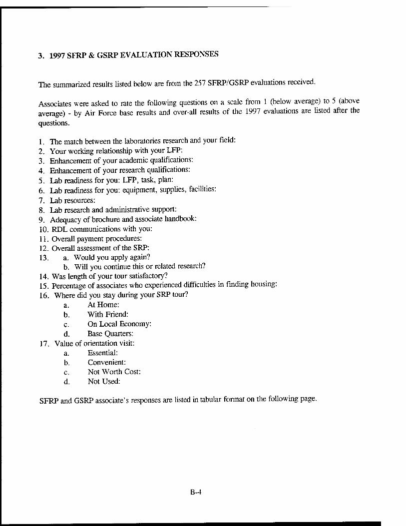
3. 1997 SFRP & GSRP EVALUATION RESPONSES

The summarized results Usted below are from the 257 SFRP/GSRP evaluations received.

Associates were asked to rate the following questions on a scale from 1 (below average) to 5 (above average) - by Air Force base results and over-all results of the 1997 evaluations are Usted after the

questions.

1. The match between the laboratories research and your field: 2. Your working relationship with your LFP: 3. Enhancement of your academic qualifications: 4. Enhancement of your research qualifications: 5. Lab readiness for you: LFP, task, plan: 6. Lab readiness for you: equipment, supplies, facilities: 7. Lab resources: 8. Lab research and administrative support: 9. Adequacy of brochure and associate handbook: 10. RDL communications with you: 11. Overall payment procedures: 12. Overall assessment of the SRP: 13. a. Would you apply again?

b. Will you continue this or related research? 14. Was length of your tour satisfactory? 15. Percentage of associates who experienced difficulties in finding housing: 16. Where did you stay during your SRP tour?

a. At Home: b. With Friend: c. On Local Economy: d. Base Quarters:

17. Value of orientation visit: a. Essential: b. Convenient: c. Not Worth Cost: d. Not Used:

SFRP and GSRP associate's responses are Usted in tabular format on the foUowing page.

B-4

Table B-4. 1997 SFRP & GSRP Associate Responses to SRP Evaluation

Arnold Brook.«* Edwards E^liii Griffi* Hanseoiu Kelly Kirtlaud Lacklnud Rubins Tyndull WI'AFH average

# res

6 48 6 14 31 19 3 32 1 2 1(1 85 257

1 4.8 4.4 4.6 4.7 4.4 4.9 4.6 4.6 5.0 5.0 4.0 4.7 4.6 2 5.0 4.6 4.1 4.9 4.7 4.7 5.0 4.7 5.0 5.0 4.6 4.8 4.7 3 4.5 4.4 4.0 4.6 4.3 4.2 4.3 4.4 5.0 5.0 4.5 4.3 4.4 4 4.3 4.5 3.8 4.6 4.4 4.4 4.3 4.6 5.0 4.0 4.4 4.5 4.5 5 4.5 4.3 3.3 4.8 4.4 4.5 4.3 4.2 5.0 5.0 3.9 4.4 4.4 6 4.3 4.3 3.7 4.7 4.4 4.5 4.0 3.8 5.0 5.0 3.8 4.2 4.2 7 4.5 4.4 4.2 4.8 4.5 4.3 4.3 4.1 5.0 5.0 4.3 4.3 4.4 8 4.5 4.6 3.0 4.9 4.4 4.3 4.3 4.5 5.0 5.0 4.7 4.5 4.5 9 4.7 4.5 4.7 4.5 4.3 4.5 4.7 4.3 5.0 5.0 4.1 4.5 4.5 10 4.2 4.4 4.7 4.4 4.1 4.1 4.0 4.2 5.0 4.5 3.6 4.4 4.3 11 3.8 4.1 4.5 4.0 3.9 4.1 4.0 4.0 3.0 4.0 3.7 4.0 4.0 12 5.7 4.7 4.3 4.9 4.5 4.9 4.7 4.6 5.0 4.5 4.6 4.5 4.6

Numbers below are percentages 13a 83 90 83 93 87 75 100 81 100 100 100 86 87 13b 100 89 83 100 94 98 100 94 100 100 100 94 93 14 83 96 100 90 87 80 100 92 100 100 70 84 88 15 17 6 0 33 20 76 33 25 0 100 20 8 39 16a . 26 17 9 38 23 33 4 - - - 30 16b 100 33 - 40 - 8 - - - - 36 2 16c _ 41 83 40 62 69 67 96 100 100 64 68 I6d . . - - - - - - - - - 0 17a . 33 100 17 50 14 67 39 - 50 40 31 35 17b . 21 . 17 10 14 - 24 - 50 20 16 16 17c . . . - 10 7 - - - - - 2 3 17d 100 46 - 66 30 69 33 37 100 - 40 51 46

B-5

4. 1997 USAF LABORATORY HSAP MENTOR EVALUATION RESPONSES

Not enough evaluations received (5 total) from Mentors to do useful summary.

B-6

5. 1997 HSAP EVALUATION RESPONSES

The summarized results listed below are from the 113 HSAP evaluations received.

HSAP apprentices were asked to rate the following questions on a scale from 1 (below average) to 5 (above average)

1. Your influence on selection of topic/type of work. 2. Working relationship with mentor, other lab scientists. 3. Enhancement of your academic qualifications. 4. Technically challenging work. 5. Lab readiness for you: mentor, task, work plan, equipment. 6. Influence on your career. 7. Increased interest in math/science. 8. Lab research & administrative support. 9. Adequacy of RDL's Apprentice Handbook and administrative materials. 10. Responsiveness of RDL communications. 11. Overall payment procedures. 12. Overall assessment of SRP value to you. 13. Would you apply again next year? Yes (92 %) 14. Will you pursue future studies related to this research? Yes (68 %) 15. Was Tour length satisfactory? Yes (82%)

Arnold Brooks Edwards Eglin Griffiss Hanscom Kirtland Tvndal] WPAFB Totals

resp 5 19 7 15 13 2 7 5 40 113

1 2

2.8 4.4

3.3 4.6

3.4 4.5

3.5 4.8

3.4 4.6

4.0 4.0

3.2 4.4

3.6 4.0

3.6 4.6

3.4 4.6

3 4

4.0 3.6

4.2 3.9

4.1 4.0

4.3 4.5

4.5 4.2

5.0 5.0

4.3 4.6

4.6 3.8

4.4 4.3

4.4 4.2

5 6

4.4 3.2

4.1 3.6

3.7 3.6

4.5 4.1

4.1 3.8

3.0 5.0

3.9 3.3

3.6 3.8

3.9 3.6

4.0 3.7

7 8

2.8 3.8

4.1 4.1

4.0 4.0

3.9 4.3

3.9 4.0

5.0 4.0

3.6 4.3

4.0 3.8

4.0 4.3

3.9 4.2

9 10

4.4 4.0

3.6 3.8

4.1 4.1

4.1 3.7

3.5 4.1

4.0 4.0

3.9 3.9

4.0 2.4

3.7 3.8

3.8 3.8

11 12

4.2 4.0

4.2 4.5

3.7 4.9

3.9 4.6

3.8 4.6

3.0 5.0

3.7 4.6

2.6 4.2

3.7 4.3

3.8 4.5

Numbers below are percenta ges

13 14

60% 20%

95% 80%

100% 71%

100% 80%

85% 54%

100% 100%

100% 71%

100% 80%

90% 65%

92% 68%

15 100% 70% 71% 100% 100% 50% 86% 60% 80% 82%

B-7

ENGINEERING ASSISTANT

Emily Blundell

Rosamond High School 2925 Rosamond Blvd. Rosamond, CA 93560

Final Report for: High School Office of Scientific Research

Boiling Air Force Base, DC

and

Phillips Laboratory

August 1997

1-1


Emily Blundell Rosamond High School

Abstract

As an Engineering Assistant, I did three types of work. All involved working with

drawings. I revised two drawings for an Engineer at the Satellite Engine Operations

Complex, designed drawings for a Technical Library, and made an excel spreadsheet of

data collected from drawings at the Space Environmental Propulsion Complex.

1-2


Emily Blundell

As an Engineering Assistant, I worked with drawings done by or needed by

Engineers. I worked in different parts of Phillips Laboratory, such as Experimental

Support Division, Satellite Engine Operations Complex, and Space Environmental

Propulsion Complex. Working in different areas gave me an opportunity to learn new

things.

When working at the Experimental Support Division, I designed floor plans for

three different room that are going to be part of a Technical Library. I measured and

mapped out the rooms. I also needed to find exactly how many filing cabinets and

bookcases would fit into each room. Bookcases and filing cabinets needed to be found to

be put into the rooms. So I went over to the supply building and found bookcases.

I took the bookcases from supply and put them in one of the rooms and started to

fill them up with book and binders. These books and binders will eventually be looked

through be another Engineer.

At the Satellite Engine Operations Complex, I revised two drawings of an engine

that is going to be tested. I did this by using Claris Cad Drafting. Drafting is something

new to me, so I had to learn by watching a video about the basics of Claris Cad. Using

Cad is a more accurate way of drawing.

1-3

After revising the drawings, I took the drawings out to the test cell, where the

engine will eventually be tested, and followed each different system, such as liquid

oxygen, gaseous nitrogen, water, and propane systems. I checked each individual valve,

filter, gage, etc., for part numbers, manufacturer name, and other details. This was quite

exciting, because I was able to climb all over different areas to find what I needed.

Next, after I was done searching, I put all the information into a spreadsheet and

found which valves, filters, etc. did not have any information besides a manufacturer's

name. So I looked in the Thomas Register Catalogs to find other information about the

parts, but if there was not any information, I copied down the manufacturer's name and

number, so that a catalog can be ordered.

My job at the Space Environmental Propulsion Complex was to figure out which

drawings were there and were needed at the complex. There were three different

buildings that contained drawings I needed to look at. I went through drawings and made

a rough list of drawing titles, numbers, and dates. Using this information, I went over to

General Physics, which is an on-site contractor hired to maintain area drawings, and

looked in the Drawing Archives to see what drawings are there from the Space

Environmental Propulsion Complex.

I found which drawings are at General Physics which are not at the Space

Environmental Propulsion Complex and vise versa. Then, using Microsoft Excel, I made

up a more complete list of all drawings that are at the Space Environmental Propulsion

Complex. Drawings that have neither titles nor drawing numbers were put on two

1-4

separate spreadsheet so that titles or drawing numbers can be found later on.

I also printed out a copy of the drawing list and saved all the information on a disk so

that, in the future, more drawings can be added to the list. General Physics and the Space

Environmental Propulsion Complex will have to get together and print out which

drawings that they each need.

I conclude that as an Engineering Assistant, I have learned what to expect when

becoming an Engineer and different things I can do as an Engineer. As an Engineer, I

would like to design things and what I have done this year at Phillips Laboratory has

helped to give me a head start.

1-5

EXPERIMENTAL VALIDATION OF THREE-DIMENSIONAL RECONSTRUCTION OF INHOMOGENEITY IMAGES IN TURBID MEDIA

Lauren Ferguson Moriarty Higli School

Moriarty, New Mexico 87035

Hanli Liu Assi stani Professor

Joint Program in Biomedical Engineering

Kelly Lau (iraduatc Student

Joini Program in Biomedical Engineering

University of Texas at Arlington P.O. Box 19138

Arlington, TX 76019

Final Rqxirt for: High School Summer Research Program

Sponsored by: Phillips Laboratory KirtlandAFB. NM

and Air Force Office of Scientific Research

Boiling AFB, Washington D.C.

August 1997

2-1

EXPERIMENTAL VALIDATION OF THREE-DIMENSIONAL RECONSTRUCTION OF INHOMOGENE1TY IMAGES IN TURBID MEDIA

Lauren Ferguson Moriarty High School Moriarty, New Mexico

Abstract

Near infrared radiation for imaging tumors in tissue has been recently explored and investigated.

In particular, to validate a novel FFT imaging reconstruction algorithm, we have performed experiments

on tissue phantoms using a frequency-domain photon migration system. The system includes an

amplitude-modulated laser diode, two radio frequency (RF) signal generators, an avalanche photo

detector, and a lock-in amplifier. The tissue phantoms were made with inhomogeneities imbedded and

were then scanned with the system at various RF frequencies. The data from the amplitude and phase

measurements were analyzed using the FFT reconstruction algorithm. The reconstructed data show clear

validation of the FFT algorithm and afford to localize inhomogeneities hidden in turbid media in three

dimensions. In addition, based on the results, we present preliminary analysis on optimization of

experimental parameters to obtain good-quality, reconstructed images with best experimental efficiency.

2-2

EXPERIMENTAL VALIDATION OF THREE-DIMENSIONAL RECONSTRUCTION OF INHOMOGENEITY IMAGES IN TURBID MEDIA

Lauren Ferguson

1. Introduction

In the last few years, numerous research efforts and technology developments have been made

towards using near infrared (NIR) radiation for human tissue quantification and imaging. Three forms of

light used in the field include short-pulsed light in time-domain (TD), intensity-modulated light in

frequency-domain(FD), and a continuous wave form (CW). Among them, the frequency-domain system

has its advantages over the other two: a FD system can acquire data almost in real time in an order of ms,

much faster than a TD system, which utilizes a single photon counting method and requires much longer

data acquisition time (in multi seconds). In addition, with the help of diffusion theory, the FD system

allows us to extract the optical properties of tissues/organs under study and to image inhomogeneities

hidden in tissues/organs. In comparison, CW method is in lack of quantification unless close-distanced

(2-5 mm) measurements are performed.

The light source used for a FD system is intensity modulated at a radio frequency (RF) ransing

from several MHz up to GHz at the wavelength range from 650 nm to 900 nm. In principle, NIR light

illuminating tissues becomes very much scattered about 1 mm after the light travels in tissue. In the FD

case, the intensity-modulated light travelling in tissue will form diffuse photon density waves (DPDW's),

and the amplitude and phase of DPDW's carry information on the optical properties of the tissue. By

extracting amplitude, phase, or optical properties of thick tissue, we can reconstruct tissue images that

show inhomogeneities imbedded inside the thick tissue. This provides a new methodology for tumor

imaging in medical applications.

Over last few years, common geometries used for imaging studies are 1) source(s)-detector pairs

scanning horizontally or 2) circularly.1 In both cases, mechanical movement is required, and it provides

only two-dimensional images. Recently, Matson et al proposed a new approach to three-dimensional

tumor localization in turbid media with the use of FD measurements in a single plane.2 The theoretical

basis of this novel reconstruction algorithm stems from Fourier Optics: applying Fast Fourier Transform

(FFT) to the diffusion equation that DPDW's obey, and then extending the solution of Fourier Optics to

DPDW's. This FFT reconstruction algorithm has several advantages, such as, 1) the light source does not

need to move mechanically, 2) it has a potential to avoid mechanical movement, which has been shown to

produce significant errors in imaging reconstruction. The theory has yet to be verified by experiments,

although it was supported by computer simulations at one RF frequency of 1 GHz with selected scanning

parameters.

2-3

The goal of this summer research project is to experimentally validate and optimize this three-

dimensional reconstruction algorithm to image inhomogeneities in turbid media. In this report, we will

first introduce the theoretical foundation for the FFT reconstruction algorithm, followed by a brief

description on experimental setups, materials and methods. Then we will show experimental results and

reconstructed images, and then investigate the correlation among experimental parameters that affect the

quality of the reconstructed images. Furthermore, computer simulations are performed to confirm the

findings that a larger scanning area is more crucial than smaller scanning pixels to obtain a higher

resolution image. Finally, we will draw conclusions from this study and indicate future work.

2. Theoretical Background

Based on Fourier Optics3, we define the following relations:

Az(fx,fy)=\\U(x,y,z)e-i2,t(f^f>y)dxdy, (1)

U(x,y,z)=llAz(Jxjy-^+fyy)^xcfy, (2)

where U(x, y, z) is the complex field of a monochromatic wave across the plane at z, and Az is a two-

dimensional Fourier transform of the function U(x, y, z). It can be shown that a free-space solution to the

source-free Helmholtz equation exists in the form of spatial frequency spectrum across a plane parallel to

the xy plane but at a distance z from it.3

In addition, it has been proved4 that the diffusion equation adequately represents photon

propagation in tissue, and the source-free diffusion equation in FD can be written as

V2U(x,y,z) + k2U(x,y,z) = 0, (3)

where U(x, y, z) is the spatial distribution of a DPDW in a scattering medium, and k2=(-vHa+ico)/D

-3uY(-|vt-ia>/v), v is the speed of light travelling in tissue, CO is the modulation frequency of the light

multiplied by 2iz, and u^ and uV are absorption and reduced scattering coefficients of the scattering

medium, respectively.

Now inserting the inverse Fourier transform definition, eq. (2), into the diffusion equation, eq.

(3), results in:

d2

J2Az(fxJy) +

az k2-(27fxf-(27fy)

2 A(/x,/,)=0. (4)

In analogy to the solution obtained in Fourier Optics for regular plane waves, we can find a solution to eq.

(4) using the Fourier transform definition:

\[f,j,)=^f,jy$*^. (5)

2-4

where Az=zo-Zi, is the distance between the detection plane at ZQ and the reconstruction plane z,.

Furthermore, we can define a transfer function, H^fc, fy), describing how a DPDW propagates in a

homogeneous medium,

Ml^7^ V<WJ2-W,): D (6)

It is worthwhile to notice several important points:

1) in using diffusion theory, we neglect boundary effects and assume the medium to be homogeneous

with spherical inhomogeneities;

2) in applying Fourier Optics to obtain equation (5), we extend the wave vector, k, from a real number to

a complex number to include scattering effects, as the diffusion equation does;

3) eq. (6) describes the change in the Fourier transform of the photon density wave as it propagates, and

thus eq. (6) can be used to invert the propagation and to reconstruct the photon density wave behind

the detection plane.

3. Necessity of Experiments

The primary goal of this summer research project is to experimentally validate the FFT reconstruction

algorithm, as introduced above. Taking experiments is necessary because

1) experiments permit studying boundary effects on the reconstructed images by using finite sizes of

tissue phantoms;

2) we can study instrument detectability and sensitivity in locating hidden objects with different

sizes and optical properties;

3) we can optimize scan parameters by performing experiments with various scan dimensions, pixel

sizes, and modulation frequencies;

4) measurement on homogeneous samples provide feasibility of obtaining correct background

information for the reconstruction and demonstrate the importance of such information.

4. Experimental Setup

As shown in Figure 1, the electronic components of our FD system include two RF signal generators,

(Rhode & Schwarz, SMY01) ranging from 9 kHz to 1.04 GHz, two 50% power splitters (Mini-Circuits,

ZFSC-2-1), two RF amplifiers (Mini-Circuits, ZFL-1000H), a NIR laser diode (LaserMax Inc, LSX-

3500) modulatable up to 100 MHz at 780 nm and 680 nm with laser powers of 3 mW (at 116 mA) at 9

mW, an Avalanche Photo Diode (APD) (Hamamatsu, C5331), two frequency mixers (Mini-Circuits,

ZLW-2), two low pass filters with the corner frequency at 1 MHz(Mini-Circuits, SLP-1.9), a lock-in

amplifier (Stanford Research Systems, SR850), and a computer-controlled, two-dimensional positioning

stage (Aerotech, Inc. ATS 100).

2-5

■^

Reference Generator f + Af (10-100 MHz)

■> 50% Power Splitter

■£ Signal Generator f (10-100 MHz)

-> 50% Power Splitter

f + Af

ik Reference

Mixer 1 ref:sig=7:l

A

->

Low Pass Filter (1MHz)

Amplitude

±M_ A

Lock-In Amplifier

V

Amplifier 1

A

\/f+M

Mixer 2

V /\<

Laser Diode

AL

-^

Af

Low Pass Filter (1MHz)

A

V

Phase

(GPIB)

Phantom

->

< frequency

Amplifier 2

Z2EZ Avalanche Photo Diode on a XY translation stage ^

Signal

movement

Computer (control and data P*

acquisition)

control (GPIB)

control (GPIB)

Figure 1. Experimental Setup of a FD system

The frequencies of the two signal generators were chosen from 10 to 100 MHz with an offset

Af=25 kHz for the reference signal with respect to the measurement signal in order to achieve a

heterodyne system. Both RF signals for the reference at f+Af and for the measurement at f were 50%

power split, and a branch from each the two RF signal generator was mixed by Mixer 1 to generate a

reference signal for a lock-in amplifier. The output levels of the two signal generators were set up with a

ratio of 7 to 1 between the reference and measurement signals to optimize the mixing efficiency. The

second branch of the measurement signal at f was amplified to gain enough power to modulate the

intensity of a NIR laser diode at 780 nm. Then the intensity-modulated, manufacture-collimated laser

light illuminated a tissue phantom and then was detected by a movable APD to convert the optical signal

to electrical signal. A second amplifier amplified the output of APD before the electrical signal was

mixed with the second branch of the reference signal at f+Af using Mixer 2. The output frequencies of

Mixer 1 and Mixer 2 consisted of 2f+Af, f+Af, f, Af, and higher harmonic components. By utilizing two

low pass filters with a comer frequency of 1 MHz, only the signal with frequency of Af at 25 kHz passes

to the lock-in amplifier. The corresponding readings for amplitude and phase were recorded

2-6

automatically by a computer; in turn, feedback from the computer controlled the sensitivity and time

constant settings for the lock-in amplifier based on the readings. In addition, through a GPIB interface,

the computer set the RF frequencies for the two signal generators and controlled a XY positioning stage,

which held the APD for 2-dimensional imaging scans.

5. Materials and Methods

Tissue phantoms were made out of plastic resin that hardens in molds by adding catalyst. The resin is

combined with Ti02 powder for scattering property and sometimes with NIR dye for absorption

property.5 The optical properties of homogeneous phantoms were determined using the slope algorithm6

in transmission geometry. Since the algorithm requires the information on the homogeneous background

medium that contains an object/objects, multiple samples were made as a set at the same time to ensure

that the samples of the set have the same background optical properties. In general, a set of phantoms

included a homogeneous sample, and two others with different objects implanted inside. The phantom

sizes were typically 14cm x 14cm x 5cm, and absorption and scattering coefficients of background media

were within a range of 0.01 to 0.1 cm"1 and 3 to 17 cm1, respectively. The objects used as

inhomogeneities were plastic black, white, and clear beads with various diameters and shapes, as shown

and listed in Figure 2.

LB (large black) 13 mm

O SW (small white)

4 mm

SB (small black) 9 mm

LC (large clear) 12 mm

LW (large white) 8 mm

MC (medium clear) 6 mm

o MW (medium white)

6 mm

CB (cylindrical black) 19 mm x 6 mm

Figure 2. Beads used as tumor objects imbedded in tissue phantoms

We will use a XYZ coordinate system, shown in Figure 3, in this report to refer to the positions of

hidden objects in the phantoms. The XY plane is in parallel with the detection plane, the origin is at the

center of the detection plane, and the Z axis is pointing from the detection plane into the phantom.

Normally, a bead was placed at the center of a phantom with a coordinate of (0, 0, d/2 cm), where d is the

thickness of the phantom. For multiple hidden tumors, two beads (the same or different kinds) were

placed at (0, -2 cm, -d/2 cm) and (0, 2 cm, -d/2 cm) inside of a phantom. In making inhomogeneous

phantoms, we positioned the object(s) on top of a semi-dried, background material which has been cast

earlier, and then added equal amount of ready-to-cast resin on top of the first part to complete the

2-7

phantom. In this way, we implanted the objects inside the phantoms with good 3-dimensional coordinate

references, and X-ray measurements have confirmed the positions of imbedded objects.

Figure 3. the xyz coordinate system used to label locations of hidden objects inside a phantom.

detection plane

All of the scans used for this report were performed on areas of 8 cm x 8 cm having 64x64,

32x32, or 16x16 pixels with pixel spacing of 0.125 cm, 0.25 cm, and 0.5 cm, respectively. The

modulation frequencies were scanned from 10 MHz to 100 MHz in various steps in actual experiments,

but all the data shown in this report were taken mainly at 20 or 40 MHz. An average measurement time

was about 2.5 hours for a 32x32 scan with two modulation frequencies (20 and 40 MHz). The

experiments were performed in transmission geometry with the light source fixed at one side of the

sample and the movable detector located on the other side of the sample. The software package

Interactive Data Language (IDL) was used to process the measured data and to perform the reconstruction

algorithm. In addition, the PMI simulation code was used to predict and confirm the experimental data.

Because the transfer function contains an exponential decay term, the reconstructed DPDW's are

hot stable, containing ringing patterns. A better understanding for this artifact is under investigation.

However, at present stage, to stabilize the reconstructed data or eliminate ringing patterns, we utilized a

low-pass filter (pillbox) to cut off high spatial frequency components. Specifically, the cutoff frequency

was ranged from only a few pixels, such as 1-4, in the spatial frequency domain. We multiplied the

Fourier spectra by this cutoff filter before inverse Fourier transforming the spatial frequency spectra to

reconstruct the DPDW's. For convenience, in the rest of the report, we will use "filter" as a short notation

to represent the pixel number in Fourier domain of cutoff spatial frequencies.

After the amplitude, A, and phase, 0, were measured as a function of positions in a XY plane at

z=zo, we followed the procedures given below to reconstruct three-dimensional images:

1) based on A and 0, calculate complex photon density waves Uh(x,y,Zo) and Uinh(x,y,Zo),

respectively, for both homogeneous sample and the sample containing objects;

2) subtract the homogeneous wave from the inhomogeneous wave, U(x,y,zo)=Uin(x,y,Zo)-

Uh(x,y,Zo);

2-8

3) EFT U(x,y,zo) to obtain its Fourier transform A(fx, fy, zo);

4) multiply A(fx, fy, Zo) by the transfer function to execute the reconstruction process at z,;

5) multiply A(fx, fy, z,) by a low-pass filter with a selected filter number (cutoff pixels);

6) inverse FFT A(fx, fy, z,) to the spatial domain for the reconstructed image at z,;

7) repeat steps 4) to 6) for different values of z, to back propagate the reconstruction;

8) determine the x, y coordinates of the hidden object at the detection plane, and then plot

amplitude versus z to localize the tumor in Z direction.

6. Experimental Results and Image Reconstructions

Figure 4 shows an example of amplitude images of DPDWs measured at the detection plane

using a 680 nm laser scanned with 32x32 pixels on a 8 cm x 8 cm area of a phantom containing one black

object. The phantom was 4.7 cm thick, and the black bead had a diameter of 9 mm imbedded at (0, 0, 2.3

cm). The illumination spot on the phantom was located at (-1.5 cm, 0, 2.3 cm), 1.5 cm off-centered in x

axis with respect to the center of the phantom. The modulation frequency used for this set of

measurements was 20 MHz, and the filter used for the reconstruction was 2. The absorption and reduced

scattering coefficients of the background medium were 0.14±0.06 and 3.1±1.4 era'1, respectively, which

were determined using a homogeneous sample. Three amplitude plots of the complex DPDWs in Figure

4 are obtained at the detection plane for a homogeneous field [4(a)] measured from the homogeneous

sample, perturbed field [4(b)] from the inhomogeneous sample, and the deviation between the two fields

[4(c)], i.e., perturbed field (pfield) - homogeneous field (hfield). Notice that in obtaining the image of

4(c), we first subtracted the two complex fields (pfield-hfield), which were calculated from amplitude and

phase measurements of the two samples, and then plotted the amplitude of the subtracted field.

Figure 4. Amplitude images of the DPDWs measured at the detection plane from a phantom with one hidden high-absorbing object, scanned at 20 MHz with an array size of 32 x 32. a) homogeneous field=hfield, b) perturbed field=pfield, c) pfield- hfield.

Figure 5 uses the same set of data as those for Figure 4. In the case of Figure 5, the FFT

reconstruction algorithm was utilized to obtain the images at different depths behind the detection plane.

The filter used here was 2. Let's first look at Figures 5(c) to 5(e), which are amplitude images at the

2-9

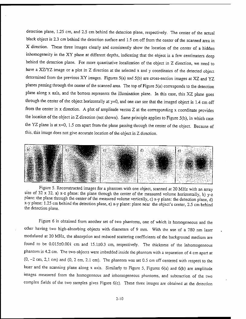
detection plane, 1.25 cm, and 2.5 cm behind the detection plane, respectively. The center of the actual

black object is 2.3 cm behind the detection surface and 1.5 cm off from the center of the scanned area in

X direction. These three images clearly and consistently show the location of the center of a hidden

inhomogeneity in the XY plane at different depths, indicating that the object is a few centimeters deep

behind the detection plane. For more quantitative localization of the object in Z direction, we need to

have a XZ/YZ image or a plot in Z direction at the selected x and y coordinates of the detected object

determined from the previous XY images. Figures 5(a) and 5(b) are cross-section images at XZ and YZ

planes passing through the center of the scanned area. The top of Figure 5(a) corresponds to the detection

plane along x axis, and the bottom represents the illumination plane. In this case, this XZ plane goes

through the center of the object horizontally at y=0, and one can see that the imaged object is 1.4 cm off

from the center in x direction. A plot of amplitude versus Z at the corresponding x coordinate provides

the location of the object in Z direction (not shown). Same principle applies to Figure 5(b), in which case

the YZ plane is at x=0, 1.5 cm apart from the plane passing through the center of the object. Because of

this, this image does not give accurate location of the object in Z direction.

Figure 5. Reconstructed images for a phantom with one object, scanned at 20 MHz with an array size of 32 x 32. a) x-z plane: the plane through the center of the measured volume horizontally, b) y-z plane: the plane through the center of the measured volume vertically, c) x-y plane: the detection plane, d) x-y plane: 1.25 cm behind the detection plane, e) x-y plane: plane near the object's center, 2.5 cm behind the detection plane.

Figure 6 is obtained from another set of two phantoms, one of which is homogeneous and the

other having two high-absorbing objects with diameters of 9 mm. With the use of a 780 nm laser

modulated at 20 MHz, the absorption and reduced scattering coefficients of the background medium are

found to be 0.015±0.001 cm and 15.1±0.3 cm, respectively. The thickness of the inhomogeneous

phantom is 4.2 cm. The two objects were imbedded inside the phantom with a separation of 4 cm apart at

(0, -2 cm, 2,1 cm) and (0, 2 cm, 2.1 cm). The phantom was set 0.5 cm off centered with respect to the

laser and the scanning plane along x axis. Similarly to Figure 5, Figures 6(a) and 6(b) are amplitude

images measured from the homogeneous and inhomogeneous phantoms, and subtraction of the two

complex fields of the two samples gives Figure 6(c). These three images are obtained at the detection

2-10

plane and show clearly two hidden objects after the simple subtraction. Furthermore, if the FFT

reconstruction algorithm is applied, we can obtain the reconstructed amplitude images of DPDW's at

different depths behind the detection plane. Figures 7(c) to 7(f) show such amplitude images

reconstructed at the detection plane, 1 cm, and 2 cm behind the detection plane, respectively. All three

images indicate consistently and unambiguously two hidden objects at about (0.5 cm, 2cm) and (0.5 cm, -

2 cm) in the XY plane at different depths. As the reconstructed plane goes deeper and closer to the center

of the hidden objects, the resolution for the imaged objects becomes better. In this case, a YZ image,

shown in Figure 7(b), supports the findings from the XY images, and it also provides locations of the two

objects in depth, which occur at the peaks of the two dark, cylindrical spots. Since the image plane for

Figure 7(a) is in between the two objects, not passing through either center of the hidden objects, this XZ

image does not give us very useful information in locating objects.

Figure 6. Amplitude images of the DPDW's measured from a phantom with two hi*h- absorbing objects, scanned at 20 MHz with an array size of 32 x 32. a) hfield b) pfield and c) pfield-hfield.

Jgure 7 Reconstructed images for a phantom with two objects, scanned at 20 MHz with an array size of 1 X I u r a SCan *"* of 8 cm x 8cm with Filter 2 used for the reconstruction, a) x-z plane- the plane through the center of the measured volume horizontally, b) y-z plane: the plane through the center of the measured volume vertically, c) x-y plane: at the detection plane, d) x-y plane: 1 cm behind the detection plane, and e) x-y plane: plane near the object's center, 2 cm behind the detection plane.

Notice that there are multiple bright, ringing patterns/loops in Figure 7(b); they are artifacts due

to Fourier transform. Higher filters used in the Fourier domain for the reconstruction algorithm give more

ringing patterns. This limits the bandwidth of the spatial frequency components in the reconstruction and

2-11

thus limits the spatial resolution of the reconstructed images. If higher spatial frequency components are

included, we have to be careful to differentiate the real hidden objects from FFT reconstruction artifacts.

In the next section, we will discuss how to select filter numbers, or cutoff spatial frequencies, to optimize

the reconstructed images. Further studies and understanding of the cause of ringing patterns are

underway.

The phantom used to obtain Figure 8 contains two objects, one black marble having 13 mm

diameter and one white bead of 8 mm diameter. They were implanted at the middle of a 4.5 cm thick

phantom in Z direction and about 2.5 cm apart vertically (or horizontally) symmetric to the center of the

phantom. Similarly, 32x32 pixels were chosen to scan a 8cm x 8cm area with a modulation frequency of

20 MHz. The absorption and reduced scattering coefficients of the background are 0.017±0.001 cm"1 and

15.9±0.6 cm"1, respectively. Figures 8(a) and 8(b) are amplitude plots, respectively, at the detection plane

and 2 cm behind the detection plane near the centers of the objects. It is seen that at the detection plane,

the image for the white object does not appear very well, whereas the image for the black object is very

obvious and clear. The reconstructed image on the XY plane near the centers of the objects (Figure 8(b)),

however, displays two clear imaging spots with different magnitudes. The big, dark spot is corresponding

to the black marble, and the small, light spot stems from the white bead. We can easily obtain the

separation distance of 2.7 cm between the spots from Figure 8(b). To confirm the result, we turned the

phantom 90° around the Z axis (the axis perpendicular to the detection plane) and rescanned the phantom.

The reconstructed images for this case are shown in Figures 8(c) and 8(d), and the results are very

consistent with those observed in Figures 8(a) and 8(b).

Detection plane Tumor plane (8cm x 8 cm) (2 cm behind)

Figure 8. Amplitude images of a phantom with two objects, a 13 mm black marble and a 8 mm white bead, scanned at 20 MHz with an array size of 32 x 32. a) and c): at the detection (x-y) plane, b) and d): near the center of the samples, 2 cm behind the detection plane. Filter of 2 was used for this reconstruction. y&Zzt-JS.

the white bead on top of the black marble

the white bead and the black marble are in parallel

2-12

In order to know how different wavelengths and powers of the laser affect the quality of the

reconstructed images, we performed two measurements on the same phantom using a 780 nm, 3 mW and

a 680 nm, 9 mW laser diode. In this case, the phantom contained two objects, one 12 mm black marble

and 12 mm clear bead. These two objects were imbedded in the middle of a 5 cm thick phantom, and

other parameters were the same as those used for Figure 8. The background medium has absorption and

reduced scattering coefficients of 0.016±0.00 cm"1 and 10.0±0.7 cm"1 at 780 nm, and 0.01510.001 cm"1

and 13.710.3 cm"1 at 680 nm. With a 3 mW laser at 780 nm, we reconstructed amplitude images of the

phantom, shown in Figures 9(a) and 9(b), at the detection plane and at the plane passing the centers of the

objects, 2.5 cm behind the detection plane. It is seen that the clear bead does not give a very

distinguished, resolvable feature in either case. Furthermore, after we switched to a higher (9 mW) power

laser at 680 nm, the reconstructed images (Figures 9(c) and 9(d)) look similar to those with the 780 nm

laser, except that the 680 nm, higher power laser gives a little better spatial resolution than the other case.

This may be because a higher power laser gives a better signal-to-noise ratio. But overall, there is no

significant difference between these two lasers in imaging large-mismatched objects in our phantoms.

Detection plane (8cm x 8 cm)

Tumor plane (2 cm behind)

Figure 9. Amplitude images of a phantom with two objects, scanned at 20 MHz with an array size of 32 x 32. Filter is 2. a) and c): at the detection (x-y) plane; b) and d): at the plane passing through the center of the objects.

with a 780 nm, 3 mW laser

with a 680 nm, 20 mW laser

To study the relationship between the quality of the reconstructed images and pixel spacing, we

also performed a series of scans on the same phantom with array sizes of 64 x 64, 32 x 32, and 16 x 16

having pixel spacing of 0.125 cm/pixel, 0.25 cm/pixel, and 0.5 cm/pixel, respectively. In this case, the

phantom was 4.4 cm thick and contained a 8 mm black and a 9 mm white bead. They were located at the

middle depth of the sample and about 4 cm apart along Y axis with the white bead on top of the black

bead. Figure 10 presents a set of reconstructed amplitude images at both the detection plane and at the

2-13

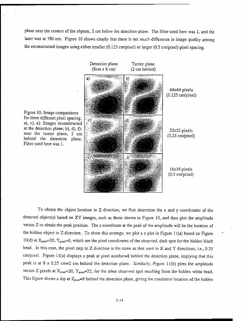
plane near the centers of the objects, 2 cm below the detection plane. The filter used here was 1, and the

laser was at 780 nm. Figure 10 shows clearly that there is not much difference in image quality among

the reconstructed images using either smaller (0.125 cm/pixel) or larger (0.5 cm/pixel) pixel spacing.

Figure 10. Image comparisons for three different pixel spacing, a), c), e): Images reconstructed at the detection plane; b), d), f): near the tumor plane, 2 cm behind the detection plane. Filter used here was 1.

Detection plane (8cm x 8 cm)

Tumor plane (2 cm behind)

^ÄWJ^K^^^Vmv

64x64 pixels (0.125 cm/pixel)



To obtain the object location in Z direction, we first determine the x and y coordinates of the

detected object(s) based on XY images, such as those shown in Figure 10, and then plot the amplitude

versus Z to obtain the peak position. The z coordinate at the peak of the amplitude will be the location of

the hidden object in Z direction. To show this strategy, we plot a z plot in Figure 11(a) based on Figure

10(d) at XpiMl=20, Ypi«i=6, which are the pixel coordinates of the observed, dark spot for the hidden black

bead. In this case, the pixel step in Z direction is the same as that used in X and Y directions, i.e., 0.25

cm/pixel. Figure 11(a) displays a peak at pixel number=8 behind the detection plane, implying that this

peak is at 8 x 0.25 cm=2 cm behind the detection plane. Similarly, Figure 11(b) plots the amplitude

versus Z pixels at Xpixci=20, Ypi«i=22, for the other observed spot resulting from the hidden white bead.

This Figure shows a dip at Zpixe|=8 behind the detection plane, giving the consistent location of the hidden

2-14

object in Z direction. A dip, rather than a peak, in amplitude might stem from a possible fact that the

absorption of the white bead is lower than the background material.

0.006O I

0.0050

0.0040

0.0 03O

0.0020

0.0010

0.0000

O O O (a)

L O

(20,6,z)

Pixel numbers in Z from the illumination Diane

0.0014 ■

0.0012 i o

o.ooiot"

0.0 008

0.0006

0.0004

0.0002

0.0 OOO

(b) 1

<o. o o

o o (20,22,z)

o 10 15 20

Figure 11. Z plots along the lines perpendicular to the detection plane and containing the black bead (a) and white bead (b). The pixel spacing in Z direction is 0.25 cm/pixel, corresponding to that shown in Figures 10(c) and 10(d). The filter used here was 2.

To confirm the object location in depth obtained from Figure 11, we plot two Z plots for the data

with 16 x 16 array sizes, as shown in Figures 10(e) and 10(f), at the corresponding x and y coordinates of

the two implanted objects. These two Z plots are given in Figures 12(a) and 12(b), respectively, for the

black and white bead. In this case, the pixel spacing in Z is 0.5 cm/pixel. One can see that a peak and a

dip appear at Z pixel number=4 behind the detection plane, i.e., 4 x 0.5 cm = 2 cm behind the detection

plane. Thus, the object location in Z direction given in figure 11 is in good agreement with that in figure

11.

2-15

0.020 .

0.015

0.01O

0.005

0.00O

0.0040

0.0 030

0.0 02O

0.001O :

0.000O

Pixel numbers in Z from the source

Figure 12. Z plots along the lines perpendicular to the detection plane and containing the black bead (a) and white bead (b). The pixel size in Z direction is 0.5 cm/pixel° corresponding to that shown in Figures 9(e) and 9(f). The filter used here was 2.

7. Data Analysis

Parameters used to scan and reconstruct images are as follows: 1) scanning dimensions/areas,

such as 8x8 or 4x4 cm2, 2) pixel spacing, such as 0.125, 0.25, or 0.5 cm/pixel, 3) modulation frequencies

at 20, 40, or 100 MHz, and 4) filters numbers or cutoff spatial frequencies. What is the relationship

among those parameters, and how do they affect the resolution of the reconstructed images? The answer

to these questions may be helpful to optimize the scanning and reconstruction parameters for good-quality

reconstructed images with best efficiency.

When a FFT of a 2-dimensional spatial domain function is performed, the number of pixels (or

elements) in the spatial frequency domain is equal to the same number of pixels in the spatial domain.

The 2-d spatial frequencies, fx and fy, will be multiple increments of Afx and Afy. Thus, we can rewrite the

transfer function (TF) as follows:

"Z(fXJy) ^7^=expp/(- Vßa+i(0 2 2 -)-{27Jfx) -{2ltfyy

D

2-16

= exp LAz^^-) + (27mAfx)2+(27mAfy)

2-i^\, (7)

where Az is the distance from the detection plane to the reconstructed plane behind the detection plane,

and Az is a positive number, n is an integer, ranging from 0 to n™, where nmx is equal to one half of the

number of pixels in a row in the spatial domain. In the reconstruction algorithm, n corresponds to the

filter number for the cutoff spatial frequency. It is known that the increments in the 2-d spatial frequency

domain, Afx and Afy, are related to the dimension of the spatial domain as:

y--7-T '• ,^-T~:T—* Lx dimension(x) 7 Ly dimension(y) . (g)

Therefore, the TF becomes

r, / r , x , 8 8 -Aißcos(-) /AzBsin(-) #*(/*./y) = exp{-Azfl[cos(-) + /sin(-)]} = e *e 2, (9)

l

where B is a real number and B = W/z/+(—)2 + (—)2]2 + (—)2 T ,

8 = tan"1

Lx Ly D

CO/ /D

(10)

(11)

Eqs. (9) to (11) show quantitative dependence of the TF on the spatial dimension, Lx and Ly, modulation

frequency, co, and cutoff pixels, n, for spatial frequencies. It is seen from eq. (9) that the TF, Hz, has an

9 0

decaying amplitude of e 2 with a phasor of e 2 . For a given phantom or tissue with fixed

values of absorption and reduced scattering coefficients, p, and (X,' having typical values of 0.1 and 10

cm" , B and 6, and thus HZ) are functions of co and n, if the scan dimensions, Lx and Ly, are selected.

Figure 13 demonstrates that 6/2 is relatively small with a range of modulation frequencies less than 100

MHz. This means that the transfer function is approximately a pure attenuation function with the phasor

equal to 1 when the modulation frequencies are within 100 MHz. Using the same parameters as those for g

_. -AiScos(—) Mgure 13, we plot the amplitude of e 2 with e=0j as shown in Figure 14 ft is se£n that at ]ower

modulation frequencies, such as 20 MHz, the amplitude of the transfer function decays much faster than

that at higher modulation frequencies, such as 1 GHz. This plot also shows that to obtain the same

2-17

magnitude of the normalized amplitude of TF, the number of pixels for Af would be much smaller at 20

MHz than that at 1GHz. This makes the cutoff filter in the spatial frequency domain to be more limited at

lower modulation frequencies than at higher modulation frequencies, i.e., only to be 1 or 2 pixels at 20

MHz but to be up to 5 more pixels at 1GHz. In addition, based on eq. (10), the cutoff filters can be

equivalently improved by increasing the scanning dimensions, Lx and Ly.

40

20 MHz

100 MHz

1000 MHz

3=* 4 8 12 16

Number of Pixels for delta f 20

Figure 13. Dependence of 0/2 in degrees on the number of pixels for Af in the spatial frequency domain. The parameters used for this plot are: ua=0.1 cm"1, u.s'=10 cm"1, Lx=Ly=8 cm.

1.2

"o X3 3

E < ■a

"S E

20 MHz, 8 cm

1000 MHz, 8 cm

2 4 6 8 10 12

Number of Pixels for Delta F (Filter #)

Figure 14. Dependence of normalized amplitude of transfer function on the number of pixels for Af in the spatial frequency domain. The parameters used for this plot are: ^=0.1 cm"1, |i.s'=10 cm'1, LX=LV=8 cm.

14

Thus, to improve the resolution of the reconstructed images, we can use higher modulation

frequencies or increase the sizes (dimensions) of the detection plane. Decrease in pixel spacing would not

be a crucial factor at this point, as long as the sampling frequency (number of pixels per unit length) is

larger than the spatial frequency of the imbedded object, i.e., l/(2*diameter of the object), according to

Nyquist's law.

To confirm the findings mentioned above, we have also conducted theoretical simulations using

similar parameters. The results are very consistent with the experimental data.

2- If

In the case of biomedical imaging, let us discuss two extreme cases as follows: the first case is

where the medium is highly absorbing in comparison to the modulation frequency. For example, at 20

MHz, we have u^ (typically 0.1-0.3 cm'1) »co/v (=0.006 cm'1 for 20 MHz signal), and the TF becomes a

purely exponential decay function. We can approximately use the following relationship to optimize the

parameters for the cutoff filter and the scanning dimension, n, Lx and Ly.

(2TCn/Lx)2+(27in/Ly)

2=3u4V~3cm-2, or n/Lx~0.2 cm'1.

In the second case, where the modulation frequency is comparable to or higher than the absorption factor

of the medium, we will have ^ (typically 0.04-0.1 cm"1) «co/v (=0.3 cm"1 for 1 GHz signal). The TF

has an exponential decay term and phase shift. In this case, we will use the following relationship to

estimate the parameters for the cutoff filter and the scanning dimension, n, Lx and Ly.

(2nnAfx)2+(2KnMy)

2=3\is,(0~3K cm"2, or nAfx~0.6 cm"1.

8. Conclusions and Future Work

What we have learned from this summer research project is as follows:

1) the FFT reconstruction algorithm works in imaging and positioning inhomogeneities 3-

dimensionally with good accuracy;

2) background information is necessary and important for accurate reconstruction;

3) At present stage, for high sensitivity, the imbedded object should be off-centered with respect to

the light source and the detection plane. Further studies are underway to improve the

reconstruction algorithm in order to eliminate this requirement.

4) large scanning dimension/area is more important than small scanning pixel size to achieve better

resolution;

5) high modulation frequencies (>500 MHz) may be helpful to achieve better resolution; low

modulation frequencies can provide adequate information for tumor screening;

6) this summer project has demonstrated that the experimental set-up works and the results

generated from it are in good agreement with the theoretical simulations. Inhomogeneities can be

detected and located in three-dimensions. However, we are not able to characterize the optical

properties of the inhomogeneities at this point. This remains for further study.

Our future work includes:

1) make phantoms containing objects which are small, purely absorptive, perturbations from the

background medium;

2) take measurements on the new phantoms;

2-19

3) complete a diffraction tomographic model for quantitative reconstruction of optical property

imaging;

4) apply the diffraction tomographic model to the data taken from the new phantoms for u^,, u^'

image reconstruction;

5) extend the modulation frequencies to KHz range, and explore the possibility at using CCD

cameras for image capture;

6) extend the system to clinical tests.

9. Acknowledgement

The authors are grateful to Dr. Chuck Matson for providing adequate laboratory equipment and the

bulk of the reconstruction programs, as well as for his theoretical insight and useful discussions. In

addition, the authors also wish to thank Grant Denton and Scott Newey for all of their helpful

technical support. Without all of them, this research project would not have been possible.

10. References

M. A. O'Leary, D. A. Boas, B. Chance, and A. G. Yodh, "Simultaneous Scattering and Absorption Images of Heterogeneous Media Using Diffusive Waves within the Rytov Approximation," SPIE 2389 p.328-339 (1995). Brain W. Pogue, Michael S. Patterson, and Tom J. Farrell, "Forward and Inverse Calculations for 3-D Frequency-Domain Diffuse Optical Tomography," SPIE, 2389, p.328-339 (1995).

C. L. Matson, N. Clark, L. McMackin, and J. S. Fender, "Three-dimensional tumor localization in thick tissue with the use of diffuse photon-density waves," Appl. Opt. 36, 214-220 (1997).

.- Joseph W. Goodman, Introduction to Fourier Optics, (San Francisco, McGraw-Hill Book Company 1968). P J'

4 M. S. Patterson, B. Chance, and B. C. Wilson, "Time resolved reflectance and transmittance for the non- invasive measurement of tissue optical properties," Appl. Opt. 28, 2331-2336 (1989).

5 M. Firbank, M. Hiraoka, and D. T. Delpy, "Development of a stable and reproducible tissue equivalent phantom for use in infrared spectroscopy and imaging," SPIE, 1888, 264-274 (1993).

J. B. Fishkin and E. Gratton, "Propagation of photon-density waves in strongly scattering media containing an absorbing semi-infinite plane bounded by a straight edge," J. Opt. Soc Am A 10 P7-140 (1993).

See the PMI (Photon Migration Imaging) Code Home Page: http://www.osa.org/homes /BIOOPTIC/Resource/softwar.htm

2-20

Chaotic Dynamics in a Nd:YAG laser

Erica S. Gerken

Manzano High School 12200 Lomas Blvd. NE

Albuquerque, NM 87112

Final Report for: High School Apprentice Program

Phillips Laboratory

Sponsored by: Air Force Office of Scientific Research


and

Phillips Laboratory

August 1997

3-1

Chaotic Dynamics in a Nd:YAG laser

Erica S. Gerken Manzano High School

Abstract A diode pumped Nd: YAG laser was constructed. The pump beam was modulated in

order to stimulate nonlinear dynamics. Bifurcation processes were investigated. Data was

acquired using a 16 bit vertical resolution digitizer card and signal processor.

3-2

Chaotic Dynamics in a Nd: YAG laser

Erica S. Gerken

Introduction Chaos was studied in an optical system using a custom built Nd: YAG laser. This laser can

be modeled using two ordinary differential equations and hence is a class B laser. The

pump beam was modulated to stimulate chaotic dynamics. A period doubling route into

chaos has been predicted to exist for a Nd: YAG laser but has never been observed in a

published experiment.

Construction Figure 1 shows the experimental apparatus. A laser diode emitting at 810nm with up to

lOOmW power pumps the Nd:YAG crystal. The highly divergent light is collimated using

an antireflection coated Newport FL-10 collimating lens. We may observe the pump using

a beam splitter. The pump light can be modulated using one of two methods. The easiest

way is to modulate the current of the laser diode. However, we found this introduces a

substantial amount of noise in the pump beam. Also, the modulation is limited to 50kHz

due to the limitations of the current driver. An alternative manner of modulation is to

modulate the intensity of the pump beam using an acousto-optic modulator. An iris is

used to control the intensity. The pump beam is focused on the crystal with a medium

focal length bi-convex lens. The dimensions of the Nd:YAG crystal are 5mm by 2mm.

One face of the crystal is coated for high transmission of 810nm and high reflection at the

YAG wavelength of 1064nm. An output coupling mirror with 98% reflectivity is placed a

short distance from the crystal. Thus, the cavity length is approximately 7mm. This

makes the free spectral range of the cavity approximately 4GHz (FSR = c/2nl.) With this

large FSR, the laser operates in a single longitudinal mode for low powers of pumping.

Furthermore, the laser can be made to operate in the Gaussian 00 mode. Finally, by

careful alignment and proper pumping levels, the laser operates in 1 polarization

eigenstate.

3-3

Fig. 1

Beam splitter Focusing lens

Diode r©/

CoBimating

lens

A. Oil

Detector

YAG crystal _ ' Output

coupling lens

T Iris

Data Acquisition One of the major impediments between theory and experiment is the resolution of the

experimentally acquired data. While theorists routinely work with double precision

machine data, experimentalists are limited to the vertical resolution of the digitizer. This is

typically 8 to 10 bits. We have employed a state of the art data acquisition system that

samples data at up to a 3 MHz rate with vertical resolution of 16 bits. The digitizer card

is installed on a PC and the incoming data is processed by a Bittware Gamma Digital

Signal Processor. It is necessary to program both the digitizer card and the DSP in order

to synchronize the two.

Problems Due to their high gain and nonlinear characteristics, laser diodes are extremely sensitive to

optical feedback. The consequences are that the laser will mode hop and its intensity will

oscillate in an erratic manner. The resulting oscillations will trigger relaxation oscillations

in the Nd: YAG laser. Undesired feedback into the laser diode existed due to many

sources. We found that reflections from poor collimating lenses are sufficient to induce

3-4

erratic behavior. We also found that reflections from the YAG crystal will stimulate this

behavior. This, in fact, is our most daunting problem. The solution is to place optical

isolators in the beam's path. Even this did not solve the problem completely.

Characterization of the Nd.YAG laser

Figure 2 is a plot of the square of the relaxation oscillation frequency versus the pump

intensity. This relationship obeys the following equation

CO

where co is the relaxation oscillation, P is the pump, P0is the pump at threshold, x is the

fluorescence lifetime, 240ns, and xp is the photon lifetime.

400000

300000

M 200000 s

-

100000

0 %s

1 l „„

85 90 95 100 105 110

Current (mA)

From this graph we find that xpis 3.28 ns.

Below, we looked at the relaxation oscillation as a function of the crystal temperature.

However, we did not observe a clear trend in the data.

3-5

Temperature (°C) Relaxation Oscillation (kHz) 10 22.89 11 17.40 12 10.08 13 10.14 14 10.14 15 10.14 16 17.46 17 27.23 18 25.40 19 18.07

Figure 3 is a time series of the pump modulated YAG. The modulated pump destabilizes

the normally constant output. The result is a wavetrain of spiky pulses. Here the laser is

operating in a chaotic state.

sooo 4000

3000

2000

1000

£-1000

|-2000

"-3000

-4000

-5000

-6000

-7000 -

1 U U u VJ

_j i i i_

100 200 300 400

Tim e

500 600 700

Conclusions Our initial search was to observe a period doubling route into chaos. While we observed a

limit cycle and a period two bifurcation, we saw no higher period doubling bifurcations.

Instead, chaos was reached by an explosive type of bifurcation in which the period two

orbit is suddenly replaced by the chaotic waveform seen in figure 3. We also observed

3-6

evidence of coexisting attractors. Here, the output jumped from low intensity oscillations

to very large amplitude oscillations.

Acknowledgements To Timothy C. Newell for his guidance throughout the experiment and for the help he

gave me while I wrote this paper.

3-7

Associate did not participate in the program.

4-1

A STUDY ON OPTICAL PATTERNATION

Paul G. Loftsgard

Quartz Hill High School 6040 W. Ave. L

Quartz Hill, Ca 93593

Final Report for: High School Apprenice Program

Phillips Laboratory


Boiling Air Force Bace, DC

and

Phillips Laboratory

August 1997

5-1

Abstract

Optical patternation was studied in an attempt to create a three dimensional image of a

liquid cone, created by a nozzle, of a specific angle, and composed of fluorescent water. The

image is created through the use of Planar Liquid Laser-Induced Fluorescence(PLLIF). PLLIF is

done by taking pictures, using CCD camera, of a laser sent through a spray containing a

fluorescent dye. With the use of a fluorescent filter the camera is able to take accurate pictures

of the spray and it's intensity. This type of picture is taken at successive heights and combined

to form a three dimensional model of the spray.

5-2

Introduction

The use of high density sprays in many industrial fields has generated the need to have

the sprays accurately diagrammed. The older method of attaining these diagrams, using a

system of pipes and test tubes, was tedious and inaccurate. A spray would be activated over a

field of holes connected to pipes, the liquid from the spray traveled down the pipes and into the

test tubes. The amount in each test tube was then measured manually, consuming excessive

amounts of time, for every picture taken anywhere from 576 to 221184 test tubes would need to

be measured.. Through the use of PLLIF in the same sprays a much more accurate and time

saving method was developed.

Approach

In order to establish the basic method of creating the three dimensional models a test

spray was used. The nozzle formed a 45 degree symmetrical spray. The spray was water with

fluorescent dye dissolved into it. The dye had a small concentration of approximately 0.00001 to

0.0001 molar. In order to induce flourescence an Argon laser was, through the use of cylindrical

lenses, turned into a sheet and sent through the spray.(Pic 1)

Experimentation

After taking several pictures of the spray at various heights, exposure times,

directions(of the laser), gains, and accumulations, two main problems arose: the spray seemed

to deplete from one side to the other, and particles out side of the laser sheet were being

illuminated by scattered light.

The first problem was found to be caused by the depletion of the laser sheet when put

through the spray, it was solved by sending a second laser sheet from the opposite side of the

spray(Pic 2).

5-3

The second problem required a new method of taking pictures to minimize the scattered

light. By sending just a single laser beam through the spray the amount of scattered light was

greatly reduced. An aperture creating a focused laser approximately 1/16 of an inch wide was

used. Pictures taken with just a beam though do not illuminate the entire spray(Pic 3). Only two

main points are shown, the spots where the beam passes through the cone of the spray. A new

method of taking pictures had to be used. It was determined to create a full sheet, pictures one

pixel wide had to be taken and combined(Pic 4, Pic 5). This new method reduced the amount of

light scattering and made the pictures more accurate. It also, however, made it much more time

consuming to take the pictures of a full spray. For every one picture taken previously thirty to

fifty now have to be taken, this method is still much less time consuming than the test tubes

though, and was used.

Combining the pictures was done through a program created using FORTRAN. The

rows of pictures are placed one on top of the other. Because of one pixel equaling just under

one millimeterrthe distance between pictures) the pictures of combined pixels are not to exact

scale.

The first problem encountered after starting one pixel wide pictures was a reversal of

peaks in the spray. When the laser was coming from the left the peak intensity would be on the

right. When coming from the right, the right side would be extremely intense. The factor causing

this was narrowed down to either the camera, the filter, or the spray nozzle.

The fluorescent filter was the first to be tested. The intensities remained on the wrong

sides. After taking out the filter. Several other filters were also tried with the same results. The

fluorescent filter was not the cause of the distorted pictures.

The nozzle to the spray was then taken off and cleaned. The pictures continued to be

distorted. It was then taken off and looked at under a low powered microscope. Several large

scratches and marks were found on the nozzle. The pictures returned to their expected

5-4

intensities after replacing it.

Just a few days later the same problem occurred once again. The nozzle was the first

object looked at. Once again the nozzle developed scratches from an unknown source. Two

filters were used(2 microns, 400 microns) to cleanse the water before it was put through the

nozzle. Another assumed source of the problem was also taken out, this was how the nozzle

was cleansed. To clean the nozzle, approximately once each day, it was put in a glass beaker

and run through a sonic cleaner. It is believed that the glass beaker may have scratched the

nozzle, it is now only put in plastic containers to be washed. Since the incident the spray has

remained relatively symmetric.

As a result of the filters the pressure decreased to the nozzle disrupting the spray yet

again. The 2 micron filter was taken out and the pressure was returned to normal. Throughout

the day as the filter clogged the pressure slowly decreased, lowering the intensities on all

pictures taken. The 2 micron filter was taken out leaving only the 400 micron filter to clean the

water, this has not had any noticeable effect on the spray.

The next problem was the result of the laser. It's intensity ,for an unknown reason,

decreased throughout the day. The intensity started at approximately .270 watts and decreased

to approximately .250. The effect on pictures was minimal at best. It did not create any

noticeable change in the pictures or the intensities within the pictures.

The laser was also the cause of another problem. After noticing that, on the pictures, the

beam seemed to be heading not right through the middle but at an angle. This caused the

pictures to appear lopsided. This was overcome by straightening the beam with the mirrors

directing it. The laser from the left and the right, however, are not going through the exact same

spot. This was taken care of by taking pictures at separate center pixels. The right was taken at

the pixel 190 versus the left which was taken at 193. The completed sheets look correct.

After eliminating all noticeable problems with the method of taking the pictures, full

5-5

scans were taken. This involved taking 30 scans, from the left and right containing 30 to 50

pictures each, varying distances from the nozzle. The number of pictures in each scan differed

depending on the width of the spray at the particular height of the scan. Each scan of pictures

was then combined, resulting in thirty pictures of full sheets.

5-6

References

Talley, D.G., Verdieck, J.F., Lee, S.W., McDonell, V.G., and Samuelsen, G.S.

'Accounting for Laser Sheet Extinction in Applying PLLIF to Sprays"

Verdieck, J.F. "Experimental Investigation of Atomization and Droplet Processes at High

Pressures"

5-7

PICTURE #1

TWO LASER SHEET DIAGNOSTIC for CORRECTION of EXTINCTION in DENSE SPRAYS : TOP VIEW

Liquid Catch Basin and Vapor Exhaust Collimating Lens

CCD Camera

-V'

Cylindrical Lenses

MVl^-h^

M

Argon Ion Laser 488 nm

Beamsplitter

5-8

Picture #2

0) Cß (D

8

o 3

3>

(/> (D

8 3 3 (Q

O 3 CO

5-9

PICTURE #4

METHOD OFF CREATING FULL SHEET PICTURES

t 30 to 50 one pixel pictures combined to form one M sheet picture

30 full sheet pictures combined to form three dimensional cone

5-11

PICTURE #5

PICTURES CREATED BY COMBINING PICTURES 1MM WIDE FROM LEFT(TOP) AND RIGHT(BOTTOM)

dswinviw. .. - . .-.-aiigUsi De ß* Mew .4«M*aw ß«*V,. Erocess |fecro Setup ;Qpbons Help . . .. -jiiijjilj:

5-12

A STUDY OF

SPACE STRUCTURE'S

ISOLATION

Fawn R. Miller

Manzano High School

12200 Lomas Blvd. NE


Final Report for:

High School Apprentice Program

Phillips Laboratory

Sponsored by:

Air Force Office of Scientific Research

Kirtland Air Force Base, NM

and

Phillips Laboratory

July 1997

6-1

A STUDY OF

SPACE STRUCTURE'S

ISOLATION

Fawn R. Miller

Manzano High School

Abstract

Tests on the Taurus-2 mass-payload for the GFO Mission were completed. The

tests utilized a 45,000 lb. shaker to provide controlled base motion. The first test was run

without any isolation techniques, and then isolators designed by CSA Engineering were

installed, and the test was run again. The isolators damp the satellite vibration during

launch. These tests were performed to demonstrate the system performance under launch-

like conditions.

6-2

A STUDY OF

SPACE STRUCTURE'S

ISOLATION

Fawn R. Miller

Introduction

As long as space craft have been in existence, their structures had to be tested to determine

whether the materials were strong enough to withstand take-off conditions. When a rocket

carrying a space vehicle takes off for space, high loads can damage such lightweight and

delicate structures. Space vehicles and rockets have to be strong enough to withstand all

these forces. These space craft cost thousands, even millions of dollars; thus, the

companies that built them, don't want them to fall apart before they leave the earth. Long

before a space craft even arrives at the launch pad, many tests are run on it to see if it can

survive in this highly-strenuous launch situation. This summer's research was dedicated to

the testing of one of these space structures; the Taurus-2 / GFO Mission satellite.

Methodology

This unique testing process required many preparatory steps for the protection of the

satellite. The equipment required the use of a class 100,000 Clean-Room, so the satellite

had to be handled carefully; more specifically, with protective gloves and clothing. The

structure was moved with slow movements on a large crane. Since this equipment is very

valuable, any drop could have resulted in thousands or more dollars in repairs or even a

termination of the project.

A mass simulator was fabricated for this system-level isolation system test series,

due to the highly abrasive program schedule. When the test article arrived in our High-bay,

6-3

(Fig. 1) The Taurus-2 / GFO Mission test setup.

the 900 lb. structure was removed from the large shipping crate, and placed on padded

blocks, so the setup process could begin. Twenty-two accelerometers were placed around

the structure to test its movement at specific spots. These accelerometers measured the

structure's acceleration along the X, Y, and Z directions. Each of the accelerometers had

one corresponding cable that lead to a signal analyzer and shaker controller, which then

measured the linear movement of each area.

The structure was placed on an adapter plate, which was in turn attached to the

shaker table. When all this was performed, the accelerometer cables had to be attached and

taped down so the moving cables did not create noise during the tests.

6-4

The structure consisted of an 800 lb. mass simulator of the actual payload, a

separation ring, used to disconnect the satellite from the launch vehicle, and an avionics

structure that was created from composite material. This complete structure was shaken in

a thrust axis (vertical direction) and in a lateral direction, both unisolated. Then after the

isolators were attached, the same thrust axis and the lateral directions were tested on the

shaker table.

Results

When the structure was completely assembled for the unisolated tests, a low level sine test

was run on the structure at 10 to 80 Hz, at O.lg, for 0.2 Hz/second sweep. Then a random

test using low level random input at 5 to 300 Hz, at 0.5g was run. These same tests were

run for the lateral configuration, and then again for the thrust axial and lateral isolated tests

at a higher level.

30.000

Log Rmp

100.00m

1 1 ■

Unisolated configuration

■

Isolated configuration

i ml

-

( /

/

1 / ^ 1 \ / \ "

\ y' \ J _y-^S \ if 1

' ^J^ / s^s*

Tt S -

.. X - J N

.1 i

*. " i — N.

l "/. i l 4

1

1 1 1 1

I/" 1

0.0000 Hz 100.00

(Fig. 2) This shows how effective the isolators were when compared to

the unisolated configuration at 0 to 100 Hz.

6-5

The isolators used for these tests worked well. The isolators showed a 5% in the

axial (plunge) direction. The isolators created a reduction in the vibration from the whole

structure, thus creating a safer environment for the satellite and its payload. When the

isolators were attached, the structure was shaken harder, and the payload's movement was

significantly less than when it was not isolated. Figure 3 shows measured acceleration

transmissibility functions from thrust-axis tests, in both unisolated and isolated

configurations. The isolators create a plunge mode at 38 Hz., producing isolation above 50

Hz. The unisolated resonance near 70 Hz. would cause damage to the satellite, as indicated

by the composite models. The response in this frequency range is reduced by a factor of

26 dB.

/l No A (4-\Ä

i |1\ i V \l l\\ , \

\' :\' \ \ \\ ' \

\ Jäbü Y\U/ ' rv/7

Freq : 2S.4a Hz Zeta : 2.38 * (% Critical damping)

(Fig. 3) The mode bending in the X direction at 26 Hz.

The dotted line is the undeformed geometry; the solid line depicts the test article

characteristic shape when mounted on the shaker expander head. A mode shape is the

characteristic response of a structure at a particular resonant frequency. This bonding mode

is of interest to the launch vehicle contractor, as it determines the amount of so-called rattle

6-6

Space required around the satellite to accommodate its motion.

Conclusion

There are many satellites that are launched and are destroyed because they do not have any

isolation system. These tests of the Taurus-2 / GFO satellite have shown that the isolation

system will damp the payload a significant amount, thereby protecting the satellite from

high launch loads.

Through the AFOSR Research Program, I gained hands on experience and learned

valuable information on a product that may excel in protection of future spacecraft during

their launches. Also to those who helped me out during this tour, a special thanks to these

PL/VTV Employees and Contractors. Mainly: Jim Goodding, Rory Ninneman, and Dino

Sciulli.

References

Ewins, D. J.; Modal Testing: Theory and Practice. Research Studies Press LTD.,

Letchworth, Hertfordshire, England; 1984.

Netscape Technology Pages: Vibration Isolation, Accelerometers, Signal Analyzers, and

CS A Engineering

6-7

A STUDY OF THE EFFECT OF FUEL SULFUR CONTENT ON THE PRODUCTION OF AEROSOLS IN AIRCRAFT EXHAUST FLUMES

Amy W. Mok

Newton North High School 360 Lowell Avenue

Newtonville, MA 02160


Phillips Laboratory


Hanscom Air Force Base, Massachusetts

and

Phillips Laboratory

August 1997

7-1

A STUDY OF THE EFFECT OF FUEL SULFUR CONTENT ON THE PRODUCTION OF AIRCRAFT EXHAUST PLUMES

Amy W. Mok Newton North High School

Abstract

In an attempt to discover the effect of fuel sulfur content on the production of contrail, several

flights were conducted in which F-16 aircraft burned different types of sulfur fuels. A T39 collected and

studied samples of the contrail and separated the sample with use of a mass spectrometer. This

instrument revealed what was contained in the sample and how much of each was present. The results

indicated that amounts of each of the masses did change due to the variation of the fuel sulfur content.

More in-depth studies were necessary to prove and explain the differences.

7-2

A STUDY OF THE EFFECT OF FUEL SULFUR CONTENT ON THE PRODUCTION OF AIRCRAFT EXHAUST PLUMES

Amy W. Mok

Introduction

Two groups have recently been interested in the type of fuel being burned by their aircraft. Each of the

groups had its own intention. One of the groups, the Air Force, was interested in learning how the

contrail produced by its aircraft could be predicted. In doing so, at times of war, the nation's aircraft

would be less visible to enemy fire and be in less danger. The second group, National Aeronautics and

Space Administration, NASA was interested in the atmospheric chemistry portion of this research.

NASA believed that contrail affected cloud formation and therefore caused alterations in weather. It

wanted to know if fuels of varying sulfur content would have different effects on the troposphere and

stratosphere. In both cases, the purpose was to find the type of fuel that would benefit both security and

environmental impact of the aircraft.

Methodology

In a span of three days, several scientists from the Hanscom Air Force Base in Massachusetts along with

several others conducted a total of six flights. The scientists flew inside of a T39 while chasing F-16

aircraft. On each of the three days the F-16 being chased would burn a different type of sulfur fuel. Each

type of fuel was tested twice; once at an altitude of 30,000 feet and once at 35,000 feet. The T39 collected

samples of the contrail left behind by the F-16 through a flow tube that was connected to a mass

spectrometer set up inside of the T39. The mass spectrometer, operated by the occupants of the T39,

separated the sample and showed what the contents of the sample were by indicating each of the contents'

mass and quantity on a graph. All data collected were stored in a program on the computer which was

also linked to the mass spectrometer. The purpose of this experiment was to see if fuel sulfur content had

an effect on contrail production. To answer this question, it was necessary to analyze all the collected data

on the computer with the assistance of a program created by the scientists and a graphing program called

AXUM. The computer program was designed by the scientists particularly for data analysis of this

experiment. AXUM is a "technical graphics and data analysis package" produced by Trimetrix for

Windows.

7-3

Collecting Samples and Data

Three special sulfur fuels were tested in addition to a control, or regular, fuel. On the first day, a flight

with high sulfur fuel was conducted at an altitude of 30,000 feet. A flight with high sulfur fuel at 35,000

feet was also done that same day. On the second day, two more flights were done at the same two

altitudes except this time with medium sulfur fuel. The third day was committed to low sulfur fuel.

Regular fuel was tested during all six flights for comparison to the special fuel results.

During each flight an F-16 aircraft would burn a special fuel and produce an exhaust plume. Scientists in

a T39 along with a mass spectrometer, computer, and a flow tube would follow chasing after the F16 to

collect samples of the exhaust plume for studying. Several samples were collected for each special fuel.

After collecting an adequate number of samples the T39 would chase another F-16 which burned the

regular fuel. More samples were collected from this aircraft. The mass spectrometer separated each

sample into its different ions. The ions were represented by only their mass and a count of each was

calculated. All data including the exact hour and minute of the day during which flight occurred was

transferred to and stored inside the computer while the T39 was still in flight. The program in the

computer performed many useful tasks. Mainly, it graphed the amount of each mass present throughout

the flight against the actual time of the flight. The program also averaged counts during specified blocks

of time, "block average", showed amounts of S02 and C02, displayed with markers periods where a

calibration occurred, and many other helpful skills. All these features assisted with the study of the data.

The Analysis

While the T39 was chasing F-16s and the computer was busy storing data, the scientists were busy

recording time and events by hand. Their logs included times when calibrations occurred, plume

crossings, altitude of aircraft, power settings of the machines, flow rates, and other significant details of

the flight. The first step of my analysis of the data was to compare the information on the computer with

that of the written logs. Did the times match? After all, the written logs were based on times from a wrist

watch. Did the graphs which the computer program produced agree with what was happening during the

flight at the same times? In order to make the graphs more comprehensible, I printed them out and wrote

the details of the events were written directly on the graphs. Comparison was repeated for all six flights.

This process was to ensure the validity and accuracy of both sets of data.

During one of the flights, an extensive calibration experiment was done. This experiment was to test how

much of each of five masses (60,78, 96, 112, 114) were present in the emission when the S02 flow dial

setting was varied. These five masses were chosen because they were presumed to be products of the

7-4

burning of the sulfur fuel used. There was a total of twelve settings: 50, 100, 150, 200, 300, 400, 500,

600, 700, 800, 900 & 1000. Viewing the graph of this calibration on the computer program indicated a

fluctuation in the amounts of the five masses present with the varying settings. To find out exactly how

they were changing, block averages were done on the five masses for each of the dial settings. The counts

obtained for each mass and flow were recorded for later entry into AXUM. Counts for each mass were

entered on to an AXUM data sheet along with their respective flow settings. AXUM then produced a

graph of count versus S02 flow for all five masses. The only one of the five curves that appeared to be a

straight line was that for mass 112. Another graph devoted just to mass 112 was made and indeed proved

to be a straight line. This result meant that mass 112 increased consistently with the increase of S02.

This conclusion was believed to be correct for mass 112 represented S05" which is produced from the

reaction of S02. The other four masses did not have consistent trends in their counts which may mean

that with different S02 flows different reactions involving the masses are occurring. These reactions may

be the cause of the varying amounts of the other four masses. Depending on which reactions took place at

which settings, the amount of a certain mass present could increase or decrease.

An exact simulation of this comprehensive calibration experiment was performed in the laboratory on

base. The same twelve S02 flow dial settings were used and block averages were done again on the

computer program. Once again, a graph of count versus S02 flow indicated an expected straight line

with mass 112^ The data from flight and from the laboratory were agreed with each other which assured

that the data obtained on flight was legitimate for use to make conclusions.

In addition to the extended calibration, short ones were also dispersed throughout the flights. At many

times the valves of S02 and HN03 were turned on and then shut off after a minute or two ending the

calibration. The valve for the S02 was turned on to a certain flow setting each time and the setting was

recorded on the logs. Block averages were performed again for each calibration of the six flights. After

average counts for the five masses were obtained, they were entered on to an AXUM data sheet. A graph

of mass count versus S02 flow was produced to check whether the mass counts were consistent for each

flow during all flights. In other words, all the counts for mass 112 should be the same for a dial setting of

600. More or less, the data was reasonably close to one another.

The following step in the study involved the use of newly obtained data. The new data consisted of the

time of flight given in seconds and the concentration of C02 in parts per million (ppm). This new data

will be described as "SN data" while the former data already in the computer program will be called "Jems

data." Unlike the SN data, Jems data had the time given in hours and minutes and the C02 in counts.

7-5

For the SN data to be of any use the Jems data was converted to the same units as the SN data.

Converting hours & minutes to seconds was a fairly simple process, but, as for the C02, the conversion

required a longer process. First, the SN data was imported to an AXUM data sheet and a graph was made

of C02 ppm versus time in seconds. This graph was then used to compare with the Jems data for

conversion. The AXUM graph was matched with the similar shape of the Jems graph from the scientists'

computer program by locating the peaks of the curve. In the computer program values of the count at the

peaks were found. These values were then compared with the values in ppm in the SN data that were

recorded at the same time. At this point, C02 counts were matched with C02 concentration. By using

AXUM again, a graph of C02 (ppm) to C02 (counts) was produced and an equation was obtained to

convert one to the other. The equations for the six flights were, more or less, identical which was what

was looked for. These equations were recorded for later use.

The next step in the analysis was very important. This was when S02 concentration was compared with

C02 concentration. The scientists were especially interested in knowing the ratio of the concentration of

these two products in determining the effect of different fuel sulfur contents. To start, calibrations (S02

valve is turned on so count is up) where plume crossings (C02 is up) were nearby in time were chosen for

analysis. Details of each of these calibrations had to be found including start and end time of calibration,

and mass 112 count during and just before/after the calibration. This information was then entered into

the program to change the graph's units for S02 from counts to concentration. The graph then displayed

the counts of C02 and the concentration of S02 versus time. By matching the two graphs for the same

times pairs of S02 (ppb) and C02 (counts) were found. This newly recorded data was entered into

AXUM and along with the equation that converted counts of C02 to concentration found earlier produced

matching sets of S02 (ppb) and C02 (ppm). Graphs of S02 versus C02 concentration were then made;

all of which produced lines. The ratio of S02 to C02 was found by calculating the slope of these lines

through regression. The slopes represented the ratio of S02 to C02 present in the emission for the type of

fuel used. It was found that with the higher sulfur content the slopes were greater. The slopes for the

regular fuel lay between the values for medium sulfur fuel and low sulfur fuel. What this trend meant was

that with more sulfur in the fuel the amount of S02 produced compared with the amount of C02 produced

becomes greater. In other words, with more sulfur in the fuel, either S02 production increased or C02

production decreased or both. The slopes were also compared with the different altitudes and power.

However, there wasn't enough information on these two factors to make any legitimate conclusions. All

that could be deduced was a general trend of higher slopes with increasing altitude and power.

7-6

The research continued with a detailed analysis of every calibration in all six flights. Counts for the

masses were found once again during and before/after the calibration. S02 flow dial settings were once

again noted and entered with the counts for the computer program to produce a list of new information.

The list included values for the absolute pressure, differential pressure, flow tube temperature, flow tube

velocity, tube flow, S02 flow (seem), S02 concentration, and the S02 calibration factor. Earlier in the

analysis, the mass 112 was noticed to not have been constant throughout a calibration. With the new list

of information, a search for trends was started by comparing graphs of each of the new factors versus

time. After a long examination of the numerous graphs, several conjectures were made on why mass 112

counts were changing as they were. It seemed that mass 112 counts either increased or stayed steady

throughout the calibration. The only decreases were very slight. After studying the graphs for the

calibrations whose mass 112 counts increased with time, it appeared that some factors may be pressure,

S02 concentration and tube flow. The calibrations with increases seem to have displayed high pressure

with high velocity, low S02 concentration and high tube flow. As for the ones with somewhat steady

mass 112 counts, low velocity with either high or low pressure, high concentration of S02 and low tube

flow seemed to be the deciding factors. These results are assumed to only be conjectures because they

weren't what was expected and the graphs were also not always accurate.

Further analysis was done concerning this experiment. Unfortunately, at the time of my departure from

the program, there was more data which needed to be investigated in the computer. The scientists at

Hanscom Air Force Base continued with the research and will hopefully discover new useful information

in the near future which will benefit the Air Force, NASA and many other people in the world.

7-7

THE SEPARATIONS AND REACTIONS OF CYCLOHEXYL POSS COMPOUNDS

Martin Morales

Palmdale High School 2137 E. Ave. R

Palmdale, CA 93550


Phillips Laboratory



and

Edwards Air Force Base, CA

August 1997

8-1

THE SEPARATIONS AND REACTIONS OF CYCLOHEXYL POSS COMPOUNDS

Martin Morales Palmdale High School

Abstract

Cyclohexyl POSS compounds are very useful in polymer chemistry. The

collection and separation are vital steps taken in order to apply these compounds to

rocket propulsion systems. The collection of cyclohexyl Poss compounds is long and

tedious. The separation requires large amounts of solvent. Therefore, new methods for

decreasing the amount of starting material were studied. Once isolated, functionality

was added to them through corner capping reactions.

8-2

SEPARATIONS AND REACTIONS OF

CYCLOHEXYL POSS COMPOUNDS

Martin Morales

Polyhedral oligomeric silsesquioxane (POSS) compounds are unique in

composition. They are polyhedral caged compounds made up of oligomers of

silsesquioxanes (RSiOi.5). The composition of a POSS unit is intermediate between

the mineral silica (Si02) and silicones (R2SiO). Thus, they bridge the property space

between sand and silicones. These POSS structures are building blocks to present and

future applications as polymeric units for aircraft and rocket propulsion systems.

POSS building blocks can be used for numerous purposes. They can be

chemically or physically incorporated into polymers, or used alone in applications

ranging from catalyst support to medical agents. Their unique 3-D structures and

tailorable chemical composition provide novel chemical starting materials for many

useful polymeric compounds.

One promising class of POSS compounds is made from the hydrolysis of

cyclohexyltrichlorosilane. Their synthesis yields a mixture of products with the following

structures: Cy °v Cv OH

Cy \ OH V \ ^°H

o-l «'\ s'o ^ —so7 sC°o -^r-^ ? / \ \ Cy/0H I \ \ C7 9~Cy V P '. ° Cy V 9 / ° Cy V ° ! \fa—ormA>» \,°:s^°-rf^cy \o-s^o-H-

Cy Cy °y Cy Cy Cy

Cy6T6 Cy7T7(OH)3 Cy8T8(OH)2

'Cy

8-3

These compounds must be isolated and separated for further use.

A fundamental application of the T7 compound is that of corner capping this triol

with silane coupling agents to create a fully condensed POSS system. In one case, T7,

or triol, is reacted with allyl trichlorosilane in anhydrous THF, to yield a fully caged

POSS allyl.

/"

/ Cy Cy \ OH V^0^ .

/\ \°»j" 3NEt3 /\ \i o Q, \ o / i_^ o Cv \ o /

s_ _~a-° -3HNEt3Cl L' ^s~° °y Cy CV Cy

POSS structures are produced through a hydrolysis reaction consisting of 121 of

Acetone, 3.21 DDI H20, and 650g CySiCI3. The solution is placed in a five gallon

carboy, stoppered, and set aside for an extended amount of time. Periodically, these

carboys are harvested by filtration to collect the precipitated products and washing with

acetone to remove resinous by-products. It is at this stage where the separation is

done. For results from the third harvest see Appendix A.

The synthesis and separation of the POSS structures was first performed in 1960

by John Brown and Lester Vogt, Jr1. Cyclohexyl T6 was separated by either fractional

crystallization from acetone or by extraction of the triol with cold pyridine. The T7 was

separated from the T6 by fractional crystallization or extraction with pyridine and

recrystallized from benzene-acetone. At that time, Cyclohexyl T8 was undetected.

A similar method of separation was used by Feher2. Feher isolated T6 by stirring

8-4

the crude mixture in 5 times its weight with pyridine, and filtering the insoluble material

from chloroform. The pyridine solution of T7 and T8 was crashed into aqueous HCI and

washed thoroughly with water. T7 and T8 were then separated by a series of ether and

chloroform fractional crystallization.

At Phillips Lab, the separation of T6, T7l and T8 was once exclusively performed

via the prep-HPLC method. However, this method consumes large amounts of solvent.

Therefore, recrystallization of crude cyclohexyl POSS in hexane is done, removing forty

percent of the starting material. This method crystallizes the T7, while the T6 and T8 are

left in solution. The solution, or mother liquor, is rotovapped and the material is

collected. The prep-HPLC system then separates the remaining T6, T7, and T8. In

order to further decrease the amount of starting material, triethylamine washings are

performed. This method is similar to the pyridine washings of Feher although the

removal of T6 is not quantitative.

The total collection from the third harvest of the hydrolysis reaction was 332g.

This total is quite low in comparison to previous harvests. This crude material along

with other crude was recrystallized in the hexane solution. In five separate

crystallizations, 348g of material was produced. Ofthat, 291g was usable T7 material.

The remaining 57g contained all three structures. The mother liquor also contained all

three structures. Further recrystallizations of this remaining material proved to be

ineffective as pure T7 was never collected.

Additional work is yet to be done for optimizing the separation of these

compounds. It appears as though the recrystallization and triethylamine washings are a

useful first step to the ultimate separation using preparative HPLC.

Another reaction performed involved the T2 compound. This reaction was setup

8-5

similar to the hydrolysis of the previous three POSS compounds, ony the ratio of water

to acetone was different. A reactor was placed in an ice water bath. 1.21 of water was

stirred in the reactor. 100ml of acetone and 32ml of cyclohexyltrichlorosilane was

slowly added to the stirring water. The length of the reaction is about four days. At that

time, the work-up requires filtration and and acetone washing. Theoretically, 15.3g is

expected, however, given the impurities, yields were well below average. The following

is a picture of the T2 compound:

OH OH

I I Cy Si O Si Cy

OH OH

Cy2T2(OH)4

In terms of the future, one consideration may be to research the triethylamine

washes and its advantages. Alone, it separates a large amount of T6, while leaving

behind only small amounts of T7 and T8. In combination with another solvent, it could

be possible to completely isolate the T6. It also may be possible to do this by optimizing

the amount of triethylamine in the washing procedure.

8-6

REFERENCES

1. J. Brown, Jr., L. Vogt, Jr., Polycondensation of Cyclohexylsilanetriol, 1965

2. F. J. Feher, D. A. Newman, J. F. Walzer, Journal of American Society, 1989, 1747

8-7

APPENDIX A

CYCLOHEXYLTRICHLOROSILANE HYDROLYSIS DATA

% %

2nd Harvest 3rd Harvest Amt T6 T7 T8 T6 T7 T8 2nd 3rd

Carboys

1 3% 93% 3% 14% 35% 20% 46g normal setup 650g CysiCI3 121 tech acetone 3.21 DDI water

2 1% 93% 6% 12% 39% 26% 23g normal setup

3 2% 90% 8% 18% 35% 24% 23g normal setup

4 1% 91% 8% 16% 8% 47% 19g normal setup

5 <1% 87% 8% 17% 4% 52% 13g normal setup

6 <1% 86% 13% 15% 5% 39% 23g normal setup

7 <1% 99% 1% 15% 8% 34% 11g normal setup

8 <1% 97% 3% 13% 8% 45% 11g normal setup

8-8

9 2% 92% 7% normal setup

20% 12% 44% 7g

10 21% 77% 2% 650g CysiCI3 121 tech acetone 3.21 DDI water added in reverse fashion

8% 46% 16% 21 Og 20g

11 20% 76% 4% 650g CySiCI3 121 acetone 3.21 DDI water CySiCI3 was added last

12% 57% 12% 140g 38g

12 13% 80% 7% same setup as #11

12% 54% 21% 158g 49g

13 17% 75% 8% 650g CySiCI3 118gNaCI 121 acetone 3.21 Dl water

10% 42% 26% 250g 8g

14 22% 74% 4% 650g CySiCI3 210g NaBr 121 acetone 3.21 Dl water

22% 48% 17% 21 Og 3g

15 23% 71% 6% 650g CySiCI3 121 acetone 3.21 Tap water

14% 62% 15% 230g 18g

16 16% 81% 3% 650g CySiCI3 (clear) 121 acetone 3.21 Dl water

14% 41% 26% ig

17 16% 82% 2% 17% 53% 17% normal setup

5g

18 13% 77% 10% same setup as #16

23% 53% 19%

8-9

2g

19 16% 79% 5% 13% 54% 19% 250g 10g 650g CySiCI3 and trace acetone 121 acetone 3.21 DI water

20 17% 79% 4% 13% 33% 35% 2g same setup as #16

21 22% 39% 21% 2g 650g CySiCI3 151 black liquid from carboys #4 and #10 5.5ml DDI water

8-10

INTRANET WEB PAGE, DESIGN AND DEVELOPMENT

David D. Parker

Boron High School 26831 Prospect St. Boron, CA 93516


Phillips Laboratory



and

Phillips Laboratory

July 1997

9-1


David D. Parker Boron High School

Abstract

We attempted to create an attractive Intranet Web Page for Phillips lab through

the process of trial and error as we attempted to use different forms of web page creating

techniques. In the past few years there has been a drastic increase in the use of the

Internet. This increase of usage has resulted in many new uses that often times include

household and business uses that normally would not be considered in everyday

discussions. On the business aspect, there are ways to create an intricate web page

system for a business that is only available to that business. Other businesses can also

receive permission to access the system by the operating center. The use of this type of

business owned Internet system is often times referred to as Intranets. With this new

capability of using Intranets, a business is able to communicate and broadcast all forms of

information to their employees via a network system. This ability makes it possible for

the businesses to save money on costs that would normally originate from memos and

other forms of communication that is now much less economically sound..

9-2


David D. Parker Introduction

The methods of creating web pages have expanded to a much larger scale today,

then what it was years ago. The original techniques of web page creators consisted

strictly of HTML and the use of a typing program permitting the creators to design and

save their web pages to their computer. In the recent years there has been many advances

in the field of web page creation that has permitted the pages to be more and more

interesting and fun to view. These advances consist mainly of Java, Javascript, and Web

Page Editors. Although Web Authorizing Tools make use of HTML, the creator never

has to look at the programming language if they do not want. Web Page Authorizing

Tools permit the creator to cut and past objects into and out of the page making it much

easier and quicker to create a web page. The main drawback of web page authorizing

tools, is that they do not allow you to have as much control as what you do while using

strictly HTML. Java and Javascript, although two completely different languages, are an

enhancement to HTML. Through the use of these languages the creator is now able to

insert many things into their pages that had only been a dream a few years back. With

these languages the creator can insert movies, songs, film strips, colored buttons, and

many more items that are too numerous to list. Now that all of these advancements have

become available to the general public there has been a huge increase in private parties

that have created and operate their own web page.

9-3

Methodology

When creating anything the first step is planning and Naturally it is the same

when creating web pages. We had to first develop a basic design, format, and outline for

the system that you are going to create. After we finished that crucial step we began the

ever lasting process of information collecting. When we had finished collecting

information you we began to edit through it and pick out the most important sections that

we would insert into the pages. After we had finished this step we had the task of

learning HTML and inserting the information into the document that we had already

decided what the basic format would look like. When we had inserted all the information

we began to make the document more pleasing to the viewer. This consisted of anything

from graphics to different text styles and colors or back ground colors. At the time when

we had created all of the necessary pages we got to the step in which we put them onto a

remote server and inserted and tested the links. This process can often times be very time

consuming or flat out confusing, depending on whether or not the pages are incorporated

into the same file. After we had gone through and checked to make sure all links were

working, we gave it one last look over to check and see if everything was working and

looked good. Finally we uploaded the web pages to a server making it possible for the

intended audiences to view the finished product (In our case we used a Macintosh OS 7.5,

with the server program MacHTTP.).

9-4

Conclusions

Through the research and study that I completed during the term of my internship

I was able to develop opinions about web pages and the methods used to create them. For

example, when using a program for creating a web page, that does not make you use the

HTML tags, the creator has very little control. This forces placement of items to often

times look nothing like what they had originally hoped for the finished product to look

like. A Tag is a short description enclosed by less than and greater than signs. The

opening tag for example, <B> (creating bold text), then after you finish typing what you

would like bold you end the phrase with a closing tag, </B>. On the other hand though,

with the use of strictly HTML and Notepad (a program on all windows based PC's), the

creator is able to create a more precise and extravagant web page. For instance, you

cannot insert sound clips into a web page with a web page creating program. With the

use of the HTML Embed Tag you can insert a sound clip (MIDI File), that has a graphic

with an active stop, play, pause, and volume Control. The only advantage that I could

find for web page creating programs is that they have a built in program to upload the

page to the Internet. They also allow you to change color without having to know the six

digit codes for the color. Other than those two small items, using HTML is a much better

and more time efficient way of creating dynamic web pages.

9-5

TJÄTTTTTTCTTTl—TTTTr

THAT WAS CREATED ,Ä- Operational Support Division (RKD) JE

BACK TO PLE MAIN PAGE

JgSnrp um gSftcfcg

^ I Double Click Here to Hear Test Music

•RKD SUBDIVISIONS** Mission: The mission of RKD is to provide support that enhances the completion of the Propulsion Directorate Mission in the areas of Safety, Health and

RKDI

information Technology Branch (RKDD Environmental quality. Logistics, Human services. Security and Information Technology. RKDL

Logistics Support Branch (RKDL)

RKDS Click Here to View RKD Org.

Saferv and Environmental Operations Branch (RKDS)

Chart

RKD^

Technical Services Branch fiUCDT)

E-MAIL

Please e-mail us here:

Paae Maintained Bv RKDI This Paae Was Last Modified On July 25, 1997

9-6

WHAT THE WEB PAGE LOOKS LIKE BEHIND THE BROWSER WINDOW

<HTML> <BODY BGCOLOR="#FFFFFF"> <HEAD>

<META HTTP-EQUIV="Conter.t-Type" CONTENT="text/html; charset=iso-8859

<META NAME="GENERATOR" C0NTENT="Mozilla/4.01 [en] (Win95; I) [Netsca

pe]»>

</HEAD>

SENTERXIMG SRC--PL_LOGO.GIF" ALT="PLE logo" HSPACE="5" HEIGHT--40» WI DT«="40" ALIGN="CENTER">Operational Support Division (RKDXIMG SRC="AFRL.GIF" ALT="AFRL logo" HSPACE="5" ha TGKT="40" WIDTH="40" ALIGN="CENTER"X/CENTER> <CENTERXTABLE BORDER WIDTH="100%" HEIGHT="5%" BGCOLOR="#80FF80"> <TTR aT TGM="CENTER" VALIGN="TOP"> <ll ALIGL"CEN?ER" VALIGN="TOP" WIDTH="25%"XBXFONT SIZE="-2"XA HREF=

"http://pie.af.mil">BACK TO PLE MAIN PAGE</AX/FONTX/BX/TD>

</TR> </TABLEX/CENTER>

<ESBED SRC="SMPUMP.MID" AUTOSTART=FALSE LOOP=FALSE WIDTH=145 KEIGHT=55

ATTGN="CENTER">Double Click Here to Hear Test Music</EMBED> <CENTERXTABLE CELLSPACING="0" CELLPADDING="0" WIDTH="100%">

<TR> <TD> <CENTER>< ! —LEFT COLUMN—></CENTER> </TD> <TD ALIGN="CENTER" VALIGN="TOP" WIDTH="24%" BGCOLOR="#FFFFFF"> <'T,^BLE CELLPADDING="0"> , , _„ <TRXCENTERXBXFONT COLOR=#000000>**RKD SOBDIVISIONS**</FONT></B></C=.N

TERX/TR> <rT'RXTD> <CENTERXBRXFORM METHOD="LINK" ACTION="/RKDI/RKDI. HTM"XINPUT TY?E="SU

3MTT" VALUE="RKDI"X/CSNTER> </FORMXCENTERXFONT COLOR=#000000><FONT SIZE="-2">Information Tecnnoio gy Branch (RKDI) </FONTX/CENTERX/FONT> </mD>< /TRXTRXTD> <CENTERXFORM METHOD="LINK" ACTION="/RKD/RKDL . HTM"XINPUT TY?E="SUBMIT"

VALUE="RKDL"X/CENTER> . . „ fc „ </FORMXCENTERXFONT COLOR=#000000XFONT SIZE="-2">Logistics Support =r anch (RKDL) </FONTX/CENTERX/FONT> < /TDX /TRXTR>^TD> <CENTERXFORM METHOD="LINK" ACTION="/RKDS/RKDS . HTM"XINPUT TYPE="SUBMIT

" VALUE="RKDS"X/CSNTER> </*ORMXCENTERXFONT COLOR=#000000XFONT SIZE="-2">Safety and Environme ntal Operations Branch (RKDS)</FONTX/CENTERX/FONT>

<c /TH>< /TR><CTR!>"<CTD^>

<CENTERXFORM METHOD="LINK" ACTION="/RKD/RKDT . HTM"XINPUT TY?E="SUBMIT"

VALUE = "RKDT"X/CENTER> . , . </FORMXCENTERXFONT COLOR=#000000XFONT SIZE="-2">Techmca. Services B ranch (RKDT) </FONTX/CENTERX/FONT>

9-7

</TDX/TRXTRXTD> „„„^ ..r—, <CENTERXFORM METHOD="LINK" ACTION="/RKD/mailf orm. htm"XINPUT TYPE= Su3 MIT" VALUE = "E-MAIL"X/CENTER> </FORMXCENTERXFONT COLOR=#000000><FONT SIZE="-2">Please e-mail us her e ! </FONTX/CENTERX/FONT> </TDX/TRX/TA3LEX/TD> <TD><!~CENTER COLUMN—></TD> <TD ALIGN="LEFT" VALIGN="TOP" WIDTH="50%" CELLPADDING="0" CELLSPACING»" 0" BGCOLOR="#FFFFFF"> <TABLE CELLSPACING="0" CELLPADDING="0">

<TR> <TDXBXFONT COLOR="#000000">Mission:</FONTXBX/TDX/TR>

<TR> . . , . , . . <TD> <FONT COLOR="#000000">The mission of RKD is to provide support t..= t enhances the completion of the Propulsion Directorate Mission in the areas of Safety, Health and Environmental quality, Logistics, Human ser vices, Security and Information Technology.</FONTx/TD> </TR> <TRXTDXHRX/TDX/TR> <TR> <TDXA HREF="RKDORG.GIF"XlMG HEIGHT=50 WIDTH=50 SRC="RKDORG. GIF" BORCE R=''0"x/AXFONT COLOR="#000000"> Click Here to View RKD Org. Charr</FCN

T></TD> </TRXTR> <TDXHRX/TD> </TRXTR> <TDXBRXCENTERXIMG SRC="rocketl. gif "X/CSNTERX/TD> </TRX/TABLEX/TDX/FONT> <TD><!~RIGHT COLUMN—X/TD> <TD VALIGN="CENTER" WIDTH="33%" CELLPADDING="0" CELLSPACING="0"> <TABLE CELLSPACING="0" CELLPADDING="0"> <TRXTDXIMG SRC="TSTIMG. jpg" usemap="#TSTIMG"x/TDX/TR> </TABLEX/TDX/TRX/TABLEX/CENTER>

<HR> Page Maintained By <A HREF="RKDI .HTM">RKDK/AXbr> This Page Was Last Modified On July 25, 1397 </BODY> </HTML>

9-8

References

I. Internet References

[mage Mapping Mapedit

FUNCTION

Sound

Frame Graphics

Forms

TOOLS USED/ LANGUAGE

http://www.boutell.com/mapedit

Internet Libraries HTML

HTML GIF Libraries

Graphic Conversion

LOCATION

http://www.aisp.net/mid.html-ssi http://www.midi-hits.com http ://www.htmlgoodies.com http://www.htmlgoodies.com

http://he.net/~notasoul/animate.html http ://geocities.com/SoHo/l 085

HTML http://http://www.htmlgoodies.com

Paint Shop Pro 4 http://www.visitorinfo.com/software/paint.html

II. Book References

A. HTML 3.2 & CGI Professional Reference Edition UNLEASHED By: John December and Mark Ginsburg

B. JAVA 1.1 No Experience Required, Will Train By: Steven Holzner

III. Software Used

A. Netscape Navigator 3.0 B. Netscape Navigator Gold C. Netscape Communicator 4.01 D. Notepad for Windows 95

9-9

SCIENTIFIC VISUALIZATION METHODS AT THE

CENTER FOR PLASMA THEORY AND COMPUTATION

Kimberly Robinson

Sandia Preparatory School 532 Osuna Rd. NE



Phillips Laboratory



And

Phillips Laboratory

August 1997

10-1



Kimberly Robinson Sandia Preparatory School

Abstract

Work in the field of scientific visualization allows computationalists to provide much depended

upon support to experimentalists. Within this field, the World Wide Web and various graphics programs

can be valuable tools for sharing information. The web enables computationalists to simulate a situation

and put graphical representations of the results on a page that can be restricted by IP address or server

domain, so that the experimentalist can see it the next day, without fear for security. This increases

efficiency and gives experimentalists a tool by which to judge their results. As a demonstration, the results

(charged particle positions and electromagnetic field values) of a Particle-In-Cell code simulation of a High

Power Microwave device have been presented in the form of QuickTime animation. This animation was

then placed within an outline set of web pages for the Center for Plasma Theory and Computation at the Air

Force Research Lab. The individual frames of the animation were prepared with the Visualization Edition

of Applications Visualization System/Express (AVS/Express).

10-2



Kimberly Robinson

Introduction

The field of data visualization has recently become important to scientists, both experimental and

computational. Experimentalists often perform measurements that require the accumulation and

interpretation of large volumes of data. Graphical representations of the data may be used to allow a very

fast comprehension of potentially complex data sets. Computer simulations are also used both to

understand physical phenomena and to aid in understanding experiments. These too generate large

amounts of data which are often most easily understood through some form of graphical representation.

The Center for Plasma Theory and Computation has three computer codes that are used to

simulate High Power Microwave devices, among other things. In such devices, microwaves are produced

by the interaction of three parts: a source of pulsed power, a beam/cavity interaction region, and an

antenna. The pulsed power device is used to create a high voltage pulse (200-500 kV) with a duration of

about 1 microsecond. This pulse is used to create a beam of electrons that are accelerated through the

cavity. The beam is caused to bunch through some feature of the cavity (which is unique to each device),

and this acceleration of the electron beam creates microwaves. The antenna is used to focus the

microwaves in a desired direction.

Figure 1: Mach3 was used to perform the first 3D simulated implosion of a cold-core gas puff. Shown in the picture are cut planes and isosurfaces of mass density (in kg/m 3) of radially-compressing plasma at 50 nsec.

10-3

Many pulsed power devices may be simulated using magnetohydrodynamic (MHD) calculations.

High-density problems where the behavior is fluid-like lend themselves to the MHD technique. The

MACH2 and MACH3 computer codes are examples of MHD codes that are used at the Air Force research

Lab (AFRL). The beam/cavity interaction region contains a lower density beam and is more appropriately

simulated with a particle-in-cell (PIC) code. The 3D parallel PIC code, ICEPIC, is used to simulate the

cavity. There should be no particles in the antenna so this region may be simulated with a computational

electromagnetics (CEM) code. The frequency domain code, PARANA, is used at AFRL to perform

antenna simulations. Figure 2 is a PARANA simulation of a Vlasov antenna.

Figure 2

Methods

Visualizing data can serve many different purposes, depending on what the researcher,

experimentalist or computationalist, wants to know. Making plots of everything from electric fields to

densities at thousands of different points can be a very useful tool. There are many different plots that can

be useful. As examples, ICEPIC computes electromagnetic field propagation; MACH computes density

and magnetic fields; and PARANA computes modes (frequencies) in cavities and waveguides.

In order to start work in this field one needs to have a specialized tool. Applications Visualization

System software (AVS) is one such tool. It is a powerful, object oriented program that allows the user to

create specific sets of modules that can be used to visualize data in many different ways, depending on

what is needed. In learning AVS, as with many other programs, it is best to begin by creating a simple

example that may be extended later to more complex applications. For this example, it is useful to create a

10-4

data set that is simple enough to allow quick and easy debugging but that has features similar to the more

complex data sets of interest. One such simulation that can be easily programmed, and then experimented

with on AVS is the Earth orbiting the Sun. Its results are similar to the electron positions in ICEPIC in that

the data is mostly position information that may be looped through time in order to create a movie. This

problem is well known and the only difficulty lies in creating the module interface to make the

visualization correct.

First, a program had to be written in order to create the data. The language that was chosen was C.

That involved learning enough C to write the program. Once that was finished, the data had to be read into

AVS, which, due to the complexity of the software and some bugs can be a difficult task. The easiest way

is to create a "File_Import_Module", which can be specially designed to suit the specific file that is to be

read in. Once this is done, the three coordinates for each point that is to be plotted are interleaved into

triplets. These can be run through a module to create a "field" (the basic AVS data structure that can

include node positions, cell connectivity, node data, and cell data), and then outputted to the viewer. If all

of the Earth-Sun data is read in at once, this creates a circle of dots around a single dot for the Sun.

Eventually, a kind of "back door" method was discovered that would show only one dot for the Earth and

one for the Sun at a time, and then cycle through them, giving the appearance that the Earth was orbiting

the Sun. This works because of a Loop module within AVS. The arrays of data can be indexed so that

only the values indexed at the current loop count will be shown, and as the loop cycles the points change.

One must also create some kind of reference boundary to prevent the window form rescaling at each step.

The easiest way of doing this is to build a big box that that encloses all the data and has a set relationship to

the maximum data value at each time step.

Working primarily with ICEPIC data, creating a template for making a QuickTime movie was an

interesting process. There were more problems involving data, and how to render it, than in the simpler

program. In order to make a movie, it was necessary to create a loop that would read through sets of

numbered files, taking pictures of each one once the information had been processed. The size of each data

set was over 10 MB and there were about 500 data sets, so this could often take several hours, sometimes

days. In order to make a movie out of the newly outputted files it was necessary to have other software that

10-5

Figure 3

could render a QuickTime movie. This work was performed on a Silicon Graphics High Impact

workstation which comes with simple tools to turn a series of numbered GIF files into an animation.

In creating the individual frames to be made into the movie, there were three parts, each requiring

a different visualization technique: the device geometry, the particles, and the fields. For each time step,

there was new particle information as well as new fields while the geometry stayed the same throughout.

The geometry was built from a set of quadrilaterals strung together to create a 3D boundary of the device.

Figure 3 shows the geometry without the particles

overlaid. More and more particles are created as the

electric field continues to propagate through MILO.

As time passes, they move around within the device

so that all of them need to be replotted at each time

step. The electric field values are specified on a

mesh lying in the x=0 plane. This plane divides the

device in half and is a plane of symmetry. Because

the mesh is not complete (there are places in the

device where the electric fields cannot penetrate)

the electric field values are not read in as a

structural mesh, but as a point mesh which was later converted into a standard field format. Each of the

points in the mesh was then colored according to the magnitude of the electric field. A second set of

electric field values in the plane y=150 at the downstream end of the device (past the antenna) was also

used to give an indication of the fields in 3D. These field plots were placed at the top of the screen by

adding 100 to all of the "y" values for that plot before interleaving the three coordinate arrays. The two

pictures (particles and fields) used the same loop so that the information on both always corresponded.

Figures 4 and 5 show different frames from the MILO movie. Figure 4 is from the very beginning at time

= 0.5 nsec. Figure 5 is at time = 150 nsec. The particles are the dots that group around the core of the

device.

An object, or set of objects, can be mapped to a specific color to allow better visualization. Nodes,

cells, or regions of the screen may also be mapped to a color based on data (such as the electric field here)

10-6

Figure 4

Time: 0.5 nsec

Figure 5

Time: 150 nsec

that is located at each of the nodes. Node data can be assigned by using the "File_Import_Module" and

routing the results through a module that will change arrays of numbers into node data. One problem that

arose within the electric fields was that the magnitude at some points was considerably higher than the

magnitude at other points, so that important data was being obscured when using the default datamap. The

datamap module in AVS is not particularly user friendly, but there is a way of creating multiple ranges

within the map, so that for a specific range of values, an essentially separate datamap is defined. The

drawback to the approach of creating new colormaps that repeat colors in other colormaps is that some

colors will be the same, even though the field magnitude that they represent might be very different. There

should be a way around that problem, too, with an option called sub-ranges. However, we were not able to

make these work correctly.

Related to the field of data visualization is the necessity of a way of sharing the information that

can be found in pictures of experiments. One way that this can be done is through the World Wide Web.

This vast network of computers can be very useful for telling other people what goes on inside the labs. It

can also be a way of sharing information with co-workers no matter where they are.

A set of general web pages was designed to share information about the Center for Plasma Theory

and Computation codes and projects. They are filled with pictures from all three of the codes, as well as

information and explanations of the projects. Examples of the information available are detailed

descriptions of the codes and algorithms, user's manuals, publication lists, sample input files, and

instructions for obtaining the codes. The pages are an easily accessible place for people to find those

descriptions.

Graphics are well known to be a "first sight" way of judging a web page, and the graphics

produced by AVS can be a way of interesting people in the web page, as well as a method of explaining the

experiments. The MILO movie is a good example of this. By putting it on a web page, it is easier to

understand what happens within the experiment than by having it explained.

Another vision of the Center is to be able to maintain their own web site that will have pages that

are open to the public as well as pages that can be locked. These closed pages can be limited by password,

server domain, or IP address so that specific people who are allowed in can see new results or images that

10-8

have not yet been cleared by Public Affairs. This would enable the personnel on base to share information

more quickly.

The idea of putting un-cleared information on the web is a security concern, but it can be now

implemented safely with the help of new server technology. The Microsoft NT Server allows certain

directories' visibility to be limited to or from certain computers. This is the slightly more difficult way of

doing things, but it does work. A more desirable way to do it, which is being investigated currently, is to

limit entry to the pages based on server domain. Ideally, these pages would be accessible only to people on

computers based within the plk.af.mil domain (at the Phillips Lab).

Results

Through this project several things have been accomplished. There is now a template for creating

movies with AVS. Other members of the group should be able to apply this template to their own data and

with a small investment of time produce high quality movies. It should only be a matter of replacing the

"File_Import_Module" to suit the new data, and possibly some new plot modules, if a different kind of plot

is needed.

In addition to that, there is a set of web page outlines that can simply be added to until they are

ready to be published. They were written in HTML in the frame format, but with new browser/editors, they

can be edited one frame at a time so that it is not necessary to leam HTML or Java to add to the pages.

The MHO movie should be on the web soon. Once the site has been completed and has cleared

Public Affairs, it can be seen at http://oblivion.plk.af.mil/wsq/wsq.htm.

Conclusion

The web pages will provide the Center with higher visibility as well as simplifying the distribution

of software. They can also make the sharing of results of simulations more efficient between the

computationalists and the experimentalists, allowing the computationalists to serve their basic function. If

the server idea is instituted, it will also be a safe medium, without fear of releasing sensitive information.

Visualization of scientific data is a very powerful and important tool. Animations such as the

MILO movie are an example of this. With the combination of the electric field propagation and the

movement of the particles, the relationships become more obvious to the viewer.

10-9

With the creation of the AVS movie template, the technique that was used is an example for

further visualization of other problems. This saves other people's time and energy because the way to

make the movies is already there. It simply needs to be customized for the data.

Scientific Visualization is beneficial in many ways. The experimentalists may be given a better

idea of what to look for in their measurements; the computationalists' results are often impossible to

understand without pictures; and people who do not know what exactly they are looking at can understand

because the pictures help to explain things, which is the main function of the Center for Plasma Theory and

Computation.

10-10

A STUDY OF THE EFFECT OF HEAT FLOW ON THE PERFORMANCE OF AN ALKALI METAL THERMAL-to-ELECTRIC CONVERTER

Michael P. Schoenfeld

New Mexico Military Institute 101 West College Boulevard Roswell,NM 88201-5173


Phillips Laboratory


Kirtland Air Force Base, NM

and

Phillips Laboratory

August 1997

11-1


Michael P. Schoenfeld New Mexico Military Institute

Abstract

The concentration of heat flow into an Alkali Metal Thermal-to-Electric Converter (AMTEC) was studied

to determine if the efficiency of the Thermally Regenerative Electrochemical System (TRES) would increase when

heat flow is concentrated into the Beta-Alumina Solid Electrolyte (BASE) tubes and evaporator by insulation

techniques. Two experimental insulation techniques were used to see which one could direct and use the heat in the

most efficient manner. Min-K was used as a standard insulator. Two experimental insulations, alumina powder and

multi-layer foil, were used in two different set ups in conjunction with the Min-K. Based on results, it was

hypothesized that alumina powder tended to sinter, thus increasing its thermal-conductivity which allows a larger

fraction of the heat to move through the powder instead of into the cell top. The multi-layer foil was found to direct

a larger fraction of the heat into the top, reducing the amount of heat lost by conduction through the alumina

powder.

11-2


Michael P. Schoenfeld

Introduction

The AMTEC cell directly converts heat to electrical energy using Beta-Alumina Solid Electrolyte (BASE) tubes

and sodium ions. These BASE tubes are composed of Na5/3 Li1/3 Al32/3017 and have crystal structure such that

spacing of the O2" ions above and below the Na+ planes have a low activation energy barrier that allows for rapid

diffusional motion of sodium ions. The reaction Na° ► Na+ + e" occurs at the high pressure side of the BASE.

At open circuit, Na+ ions move through BASE because of a pressure differential across the BASE. The differential

is caused by a temperature differential. An electric field builds up in the BASE until it is strong enough to stop the

flow of Na+ ions. The open circuit voltage is given from the Nernst equation Voc=RT2F"' ln(P2/P4) where R is the

gas constant, F is the Faraday, P2 is the vapor pressure of sodium at T2, and P4 is the sodium at the BASE-porous

electrode interface. When the circuit is complete, electrons flow through the external load and return to the low

pressure side of the BASE where they recombine with the sodium ions. This causes the reaction, Na + e" *■

Na°, to complete. Sodium atoms in their vapor state, leave the porous electrode, and release their heat of

condensation on the condenser. The heat input creates a pressure differential that creates a voltage across the BASE

tubes. This voltage drives electrons along current collectors producing electrical work. The sodium is then

"wicked" along the condenser, through the artery, and to the evaporator by capillary forces. When it reaches the

evaporator it becomes vapor, travels to the BASE tubes and cycles through the process again (See figure 1).

11-3

Figure 1

AMTEC

t...r,.l l"* Clrc.lt wv _^3

Voc =

Governing Equations

RTi, Pi In—

F PA

V(i) = Voc — /^internal

•2 P = iVoc~i Sintemal

TJ = Pout

Qin Vi

TJ = i{v^+<*T,-r,)iyQ

11-4

Figure 2

Multi-Foils Shielding for Electric Heater (for Cell PX-4B)

interface ofMin-K pieces

(52#)

(8#)

heater

Boron Nitride powder (conductive coupling)

(30#)

(20#)

(30#)^^"^ j] interface of Min-K pieces

All dimensions are in inches.

Molybdenum foils: 8 = 7.62 um spacer: Zirconia powder, Dp = 0.23 urn the thickness of multi-foils: 0.0055'71ayer

11-5

Methodology

The process of converting heat to electricity using an AMTEC cell is achieved by supplying heat to an evaporator

and BASE tubes. Heat can be supplied by concentrated solar energy, radioisotope decay or other nuclear sources,

fossil fuels, or I2R heating. Since efficiency of the system is a function of parasitic heat loss and internal resistance,

it is important to keep the heat flow concentrated into the BASE tubes and evaporator (cell top). Experiments were

conducted with two different insulation configurations to determine which design would keep the heat as

concentrated as possible. One experiment was designed with alumina powder and the other with multi-layer foil

(both in conjunction with Min-K). In one experiment the cell was placed in a circular cut out in the middle of the

Min-K. Then the gap between the Min-k and the cell was filled with alumina powder. The other experiment was

set up similarly, but the top of the cell and heater were shielded with multi-layer foil. The space below the foil was

filled with the alumina powder. The multi-layer foil was placed with spacing in between each other to keep the

emissivity very low (as in the equation Q=eaA»(Th4-Tc

4) for radiation heat transfer). Small beads of zirconium

oxide were placed on the foil to prevent direct contact between layers of foil. Not only would this lower the amount

of heat lost by radiation, but would also increase the reflectivity. Therefore, most of the heat is concentrated to the

BASE tubes and evaporator. Results showed that over time (1512 hours) the alumina powder sintered which

increased the amount of heat lost from the BASE tubes and evaporator by conduction. Then at 1700 hours the

multi-layer foil was set up and the power output increased because more heat was concentrated into the cell. Then,

at 1800 hours, new unsintered alumina powder was used to replace the multi-foil insulation. Results indicate that

the initial power curve (1512 hours) had suffered degradation caused by the A1203 partially sintering. Recovery of

this power was shown in the 1800 hour case where fresh A1203 powder was used with no multi-layer foil. The 1700

hour power curve shows that multi-layer foil significantly increase the ratio of heat input which goes directly into

the top of the cell (versus the heat lost by conduction down the side walls) (See figure 3).

11-6

Figure 3

2.50

2.00

1.50

a

1.00

0.50

0.00 0.00

PX-4B Power Nominal Tbeta=975/Tcond=550, CQ Multi-layer foil

T"

Power 4-17-97

-K-Power 5-21-97

Power 6-26-97

3.50

11-7

A STUDY OF THE CHARACTERIZATION OF REDUCED TOXICITY MONOPROPELLANTS

Thomas Jonathan Shea

Tehachapi High School 711 Anita Drive

Tehachapi. CA 93561


Phillips Laboratory


Boiling Air Force Base. DC

and

Phillips Laboratory

August 1997

12-1


Abstract

Selected characteristics of RK-124A. RK-124B and HAN-based monopropellants were investigated.

Literature data on safety precautions and effects of hydrazine along with the different monopropellants

were collected before the laboratory work was begun. Each liquid monopropellant was characterized

including their kinematic viscosity in relation to temperature, performance (Isp. Density, Combustion

Temperature), density at four different temperatures. Department of Transportation (DOT) Thermal

Stability, and heat capacity. All observations were recorded in the duration of an eight week period. A

desktop computer was used to calculate the theoretical performance and the Isp, Density, and Combustion

Temperature were recorded. A viscosity and density measurement was made for each sample at 0°C.

20°C 25°C, and 40° C, and the resulting calculations were recorded and graphed. However, RK-124A

was not evaluated at 0Ü because of its melting limitations but it was used in the thermal stability test. In

the DSC Heat Capacity test all monopropellants produced accurate results. Unstabilized NASA HAN was

made to help in comparison with the newly developed stabilized HAN. and was included in all safety

and performance tests. The goal of the experiment was to evaluate the physical properties of the four

monopropellants and to test their capabilities as a possible substitute to hydrazine in the future.

12-2


Introduction

In the vast world of monopropellant propulsion, there are three basic types of liquid

monopropellants. (1) Single substances (molecular compounds) that contain an oxidizing agent and

combustible matter in the same molecule, such as nitromethane. (2) Intimate mixtures of compounds that

are stable under normal conditions, such as HAN. and (3) Thermodynamically unstable chemicals, such

as hydrazine. Upon ignition, the first two types of monopropellants will undergo combustion much

like a bipropellant combination. The first is an oxidizer and a fuel in one molecule, which allows it to

burn very easilv. The components in the second type must be compatible at normal temperatures, but

react when ignited or heated under pressure to give hot combustion gases. It is an "intimate mixture"

because it combines the efforts of two or more molecules for oxidizing and fueling purposes. The third

type decomposes to produce hot gases by means of a catalyst or a thermal source. In hydrazine. there is no

real combustion. The compound is unstable in the presence of a catalyst, and when it decomposes it

makes ammonia, hydrogen, and nitrogen. The monopropellants under these three main categories,

specifically monopropellants with hydrazine. have been the most acceptable and useful in a wide variety

of systems to date.

Hydrazine's ease of catalytic decomposition has led to its becoming the principal fuel for low-

thrust satellite propulsion. It has replaced hydrogen peroxide in almost all monopropellant applications

because of its better storability and higher performance. Various alternative propellant compositions

have been evaluated as a mean of improving monopropellant performance compared to hydrazine. The

four samples (RK-124-A. RK-124B. Unstabilized NASA HAN, and Stabilized NASA HAN) have been

made with the desired outcome to improve the overall performance and reduce the toxicity of the current

monopropellants that are in use. Some key monopropellant characteristics were tested in the following

experiments to see if they have potential as a suitable replacement to hydrazine. An equal or better

12-3

performance than that of hydrazine itself will indicate the substances feasibility' as a replacement and

ability to increase the energy capacity of the existing and future satellites in orbit.

Methodology

Safety Standards on Dangerous Materials

Hydrazine- Anhydrous or aqueous solutions of hydrazine are toxic by ingestion. Inhalation of

vapors or contact with the skin causes systematic effects of physical breakdown. It can affect the nervous

system resulting in hernia, convulsions, and death. Some of the diseases hydrazine can cause is

pulmonary edema, irritation upon the eyes and respiratory tract, fatty necrosis if there is liver damage, and

interstitial nephritis if there is damage to the kidneys.

Hydroxyammonium Nitrate. Glycine (HAN)- HAN can cause abnormalities of the lungs and

liver. Animal data indicates it would be a sensitizer. Some of the diseases it could cause include

dermatitis and allergic dermatitis. Lethargy, atakia. coma, alopecia hyperactivity, brown staining of the

nose and mouth, soiling and wetness in the anogenital area, and alopecia were all observed in lab

experimentation of various animals. The exposure limit in humans is about 300 mg/cuM for 15 minutes.

In small animals like rats, the fatal limit is 250 mg.

Acid protective gloves, laboratory coat, skin and eye protection, and foot protection are essential

when handling these hazardous materials. TLV (Threshold Limit Value), PEL(Permissible Exposure

Limit), and LDL (Legal Dose Limit) are three of the many safety standards looked at when various

substances are tested.

Theoretical Calculations

Theoretical Isp, density, and combustion temperature all are essential in the initial formulating

stages of a monopropellant because they usually give accurate predictions of how the substance will

perform. The achieved number in each of these categories must meet a certain standard in

monopropellant performance, density, combustion temperature, and hopefully, a product that has

reduced toxicity. A thermodynamic equilibrium calculation program using an imputed ingredient library

is used to obtain theoretical monopropellant formulation numbers. The optimized performance

12-4

calculations of unstabilized NASA HAN. stabilized NASA HAN, RK-124A and RK-124B will be shown

in the results portion of this presentation.

Viscosity and Density

To determine the viscosity of each of the four monopropellants, many elements need to be

fulfilled before the actual testing of the material take place. The first step is to calibrate

the glass kinematic viscometer that is going to be used in the experiment.

A Cannon-Fenske Viscometer was used at sizes 50 and 100 (See Figure 1). The theoretical

approximate constant for serial tube A-37 (50) was found to be 0.004 and the approximate constant for

serial tube B-45 (100) was found to be 0.015. A liquid standard having a flow time of at least 200 seconds

and no more than 1000 seconds is the ASTM standard used in the experimentation process. To calculate

the viscosity constant (VJ, a standard must be used along with the following equation:

Vc = Cs/t {1}

In the equation. C, stands for the number at centistokes in a given temperature, and t stands for

the time it takes to go through the viscometer test. Once the viscosity constant for the viscometer is

obtained, experimentation on the monopropellants can begin. Once the constant is found, it can be

multiplied by the time to obtain the number of centistokes of the various monopropellants.

Cs=Vc*t {2}

To obtain the centipoise (Cp), the density of the product was determined using a pyncnometer..

A standard must be used to find the volume of the pyncnometer. which can be calculated from

the following equation.

V = g/D {3}

Once the volume is obtained from the standard being used, it becomes the constant for the

monopropellants that are to be tested in the pyncnometer. Once the weight of each propellant is obtained,

it can be divided by the volume of the standard to achieve the density.

D = wt/V {4}

Once the density is determined from each product, the centipoise (Cp) of each monopropellant

12-5

can be calculated. The equation to get the centipoise is as follows:

Cp = Cs/D{5}

The numbers achieved are explained in the results portion under density. The complete viscosity

spreadsheet can be seen on tables 2 and 3 and the viscosity vs. the temperature along with the density vs.

the temperature can be observed on figures 3 and 4 respectively.

Heat Capacity and DOT Thermal Stability Test

Heat capacity is the amount of heat required to raise the temperature of one gram of material one

degree centigrade. Specific heat capacity is the heat capacity of a sample divided by the heat capacity of

water. The heat capacity of a material changes with its temperature. Historically, it has been measured at

25° C and assumed not to change with temperature. The DSC Heat Capacity software however, calculates

the actual heat capacity at any temperature in the DSC scan. The heat capacity calculations require three

DSC scans: baseline, reference, and sample. The baseline scan is used for baseline subtraction from the

reference and sample data. The subtraction removes all systematic instrument effects from the heat

capacity results. The reference scan, usually done with sapphire, is used to calibrate the calorimetric

response of the DSC versus temperature. The sample scan can be used to calculate the heat capacity of the

sample at any temperature. The heat capacity of a material undergoing a constant heating or cooling

ramp is proportional to the heat flow at any temperature:

C, = E,*Q,IHr*M {6}

In this equation Cpis the specific heat capacity, E, is the cell constant, 0, is the heat flow due to

the actual sample at a temperature, Hr is the heating or cooling rate, and M is the mass of the sample.

The DSC Heat Capacity program should correct the measured heat flow for all files by subtracting the

contribution due to the sample pans, correct the measured beat flow in the reference and sample files for

the corrected baseline signal, and calculate the actual heating / cooling rate at each point from the sample

temperature data. It should also calculate the heat capacity of the sample at each point, integrate the total

heat transferred to or from the sample across the analysis region, and allow the user to exclude

contributions due to reactions or transitions within the analysis range. Finally, the DSC machine should

12-6

analvze sample heat capacities from increasing or decreasing temperature scans.

In the DOT thermal stability test, a sample is tested to see if ignition, explosion, color change,

and weight loss occur. A sample up to 50 grams is placed into a beaker, covered with a watch glass, and

weighed. The beaker is then placed into an oven at 75 °C for 48 hours. If an explosion occurs during

this time period, the sample has failed. After the two day period, the sample is taken out of the oven, re-

weighed, and determined if any of the sample has been lost based on the weight of the sample before and

after the test excluding moisture and volatiles. A 0 % error is desirable, but a sample re-weighing

anywhere between 0% to 3% error is considered passing in the experiment.

Results

Safety Standards on Dangerous Materials

The rules provided in the GenCorp Aerojet safe handling of HAN materials, the A3L Saftey

Update, and AF form 55 (EF-V1) helped develop precautionary measures with the hydrazine salts that

were used. The potential splashes of hazardous liquids, working near hot equipment, working in an area

where explosives are stored, chemical exposure, and the handling of the monopropellants were all taken

into account in the lab area. The experimentation resulted in no injuries or broken equipment because of

the careful consideration of the potential hazards.

Theoretical Calculations

In each of the four monopropellants, the theoretical Isp. combustion temperature, and density was

taken and compared with the numbers achieved in hydrazine. In unstabilized NASA HAN. the theoretical

Isp was at 208.703 seconds, the combustion temperature was 1300.78 °K. and the density was recorded at

1.330 g / cc. In stabilized NASA HAN, the Isp was taken at 209.618, the combustion temperature was at

1306.00 °K, and the density- is 1.332 g / cc. There is no real significant change from the two compounds

other than the use of stabilizers. The data from both monopropellants coincide with each other. PL

candidate RK-124A had an Isp of 264.267 seconds, a throat temperature of 1991.48 °K. and a density of

1.398 g / cc. With RK-124B. the Isp was recorded at 252.126 seconds, the throat temperature at 1808.00

°K. and the density- at 1.370 g / cc. much lower than that of RK-124A. The densities of ingredients in the

12-7

RK-124 monopropellants were estimated An overview of each of the monopropellants anticipated

performance in density, combustion temperature and Isp / Density can be seen on Table 1 and Figure 2.

Viscosity and Density

Before the viscosity experiment began two viscometer tubes were calibrated. Using viscosity

standard S6. Tube A-23 (50) was found to have a viscosity constant of 0.004376 {1}, very close to the

0.004 reading of the theoretical constant However, due to the small capillary in the viscometer of the A-

23 tube, all four monopropellants exceeded the 1000 second limit. The Cannon-Finske B-45 (100)

viscometer did meet the needs of ASTM time requirements of the standard S6 and the monopropellants.

It had an average viscosity constant at temperatures of 20°, 25°, and 40° of 0.014329 {1}, compared to the

theoretical constant of 0.015.

The monopropellants viscosity in centistokes was determined using equation {2} and the

number ranged as high as 11.7835 for unstabilized HAN at 0° C to as low as 3.1710 at 40° C on RK-

124B. The exact calculations may be observed on the viscosity tables.

In order to calculate the pyncnometer volume {3}, the standard that was used for the

pyncnometer was distilled H20. The water was found to have a volume that equaled 9.2356 at 25°C. The

units of the monopropellants in the pyncnometer at 0° C, 20° C, 25° C, and 40° C were divided by the

calculated volume of the distilled H:0 {4} to get the density of the monopropellant at that specific

temperature.

Once the density was obtained, the centipoise {5} could be calculated. The centipoise ranged as

low as 2.2051 at 40° with RK-124B to as high as 10.8481 at 20° with RK-124A. The results can be seen

with all of the monopropellants on Tables 2, 3, 4 and Figures 3 and 4.

Heat Capacity and DOT Thermal Stability Test

A reference file for the DSC Heat Capacity machine was used to help determine the achieved

data taken from the monopropellants. 35.56 mg of sapphire was used in a pan weighing 23.36 mg as a

standard in the experiment. Distilled H:0 was tested twice in a hermetically sealed pan, both weighing in

at 7.90 mg. The heat capacity in the test was found to be lower than the actual heat capacity of water

12-8

(4.184 J / g °C and 1.000 cal / g °C). The actual number achieved was 4.019 J / g °C and 0.959 cal / g °C

which gave about a 4.0% error in the monopropellant work.

Using equation {6} in the TA DSC Heat Capacity machine, the data recorded in all of the

monopropellants produced consistent numbers. RK-124A had 7.9 mg of solution in the pan and had an

average of 1.789 J / g °C (0.427 cal / g °C) and RK-124B had 6.4 mg of solution in the pan and had an

average of 1.836 J / g °C (0.438 cal / g °C). The unstabilized NASA HAN had 6.4 mg of solution and

averaged 2.191 J / g °C (0.523 cal / g °C) while the stabilized HAN had 7.9 mg of solution with a heat

capacity of 2.495 J / g °C (0.595 cal / g °C). Each of the monopropellants showed fluctuations in the

graphs, but relatively stayed constant during the experimentation. The heat capacity graphs of each of the

monopropellants can be observed on Tables 5 and Figure 5.

In the DOT Thermal Stability Test RK-124A was used in the experiment. The monopropellant

was weighed in a beaker and had a total mass of 41.3811 g, close enough to the 50 g needed for

experimentation. The monopropellant was placed in an oven over a two day period at 75 °C. When it

was taken out, it was re-weighed and found to have a new mass of 41.3808. The 0.0003 g difference

could be the result of either human error or vaporization of the H:0 in the water based material. The

monopropellant had a 99.9992 % of the material left with a suprisingly small 0.0008 % error. The

RK14A monopropellant did well during the 48 hour period and passed the thermal stability test.

Conclusion

The results that were gathered for each of the monopropellants have shown consistency with

literature data and of each other. In the theoretical calculations, the end result in the Isp, density, and

combustion temperature and the information obtained on the monopropellants have produced distinct

similarities and differences with each other and with hydrazine. Unfortunately, the monopropellants

have a much higher throat temperature than hydrazine. but the density is high which helps increase its

energy capacity and possibility of a stronger and longer life in satellite propulsion. The viscosity

decreases with temperature, and the time for the solution to run through the viscometer tube increases

with lower temperatures. In the viscosity vs. temperature graph (Figure 3). stabilized and unstabilized

12-9

NASA HAN have virtually the same points with stabilized HAN being slightly more viscous than the

unstabilized.

Another interesting point is the fact that RK-124B is less viscous than the two HAN products,

and RK-124A has the highest viscosity than all three. The theoretical densities of the products are

accurate based on the comparison of the achieved densities on Figure 4. The heat capacity of the

monopropellants show consistency in the data (Table 5) and relatively stable line graphs in the plots

(Figure 5).

All monopropellants have distinct advantages over each other and can be very beneficial

propulsion industry someday. They all have potential for use in satellites in the future. Stabilized HAN,

in particular, has stabilizers included in the compound and is more thermally stable than unstabilized

NASA HAN. The goal to develop a monopropellant that can run longer, cost relatively cheap, and have a

lower toxicity will someday become a reality based on the positive data achieved on the four different

monopropellants worked on in this lab work.

Acknowledgments

1. Brand Adam. General Information, Report and Presentation Assistance, Theoretical Calculations.' and Lab Assistance, 1997.

2. McKay, Milton (Mac). General Information, DOT Thermal Stability Test 1997.

3. Jones. Paul. Density, Viscosity, and Heat Capacity lab and report assistance. 1997.

4. Wilson. Angelica. Viscosity Lab Assistance. 1997.

5. LaRue, JoAnne. Viscosity Lab Assistance, 1997.

4. Ismail, Ismail. Heat Capacity Plotting and Graphing, 1997.

5. Schwartz. Daniel. Theoretical Calculation, Viscosity, and Density plotting and graphing, 1997.

6. Bach. Duyen. Theoretical Calculations. 1997.

7. Hawkins. Tom. Literature Data, Report and Presentation Assistance. 1997.

12-10

References

1. P. Ander and A.J. Sonnessa, Principles of Chemistry: An Introduction to Theoretical Concepts . The Macmillan Company, 1965.

2. N.I. Sax. Dangerous Properties of Industrial Materials . Van Nostrand Reinhold Company. 1984.

3. P.A. Smith. Derivatives of Hvdrazine and other Hvdronitrogens Having N-N Bonds The Benjamin / Cummings Publishing Company, 1983.

4. F.S. Forbes. Liquid Rocket Propellants. Academic Frontier. 1987

5. G. P Sutton and D.M. Ross. Rocket Propulsion Elements: An Introduction to the Engineering of Rockets. Wiley-lnterscience. 1976.

6. A Kat7akian Safe Handling of HAN Materials . GenCorp Aerojet 1991.

7. J.W. Beckmann and W.M. Kalliomaa, Rocket Propulsion Experimental Facilities at the Phillips Laboratory. Edwards Air Force Base. California . SAE international. 1993.

8. G.M. Clark. A3L Safety Update . GenCorp Aerojet. 1992.

9. n„ Pnm inurnment«; DSC Heat Capacity Data Analysis Program. TA Instruments. 1991

10. The Defense Logistics A^ncv Department of Defense Explosives Hazard Classification Procedures. iiA-1-47 Air Force. 1989

12-11

Figure 1 Viscosity and Density Instruments

Pyncnometer

Cannon-Fenske Viscometer

Table 1 Theoretical Calculations

RK-124A SubiBni NASA HAN UmubiIi2od NASA HAN RK-I24B ttydruwo Isp 264.627 209.618 208.703 252.126 232.796 Density Isp 369.948546 279.211176 277.5749 345.41262 235.12396 CT 1991.48 1306 1300.78 1808 756.79

12-12

n-ri

u 5

c o « 3 O (0 O o u c (0 E

0) Q.

« "3 a o a o c o

n-z\

s

o

>

(S I

a:

C

<

. ■: ;,.;„;

< z i 1 I

i I s 1 ̂ ä' V

1| ! B C

'■•

.'■ :i^y 3 •

Sgtejgl

i e 3 a

3 3 Q

1 5

s 5

1 i

5 St i £

1 1

5

i I a 8

5

I 5 s I

i a w "• « ▼

B

■>

f ■v

a

.'. ■

C - s

0 5 S R a

e a 3 'S 5 e 5

§ *

s « o ♦ • ■♦ ■» * <o « ■« «©

'<$'%& £ I«

??/£?&& **

3« «*sf

la £ < ft ft A *: ft a R R R ft ft ft ft ft jfc

$ *» ; -■ e e o e e e o o o o o o ©

3 e o e o O o e © o o e © e O o

'£«& «*&% M S» *2pp ».«=& JiiSSi

*fcSS

a* « 2 S a 8

S q

3 S

i S I i | a s 3

s a

H1-S&, ö'S Z:«!S •^^>»

S ^vjJiJ« l^r

£ ^JJ- fa tie a R a 8 8 a s a S a S 9 9 9 9

rü-c

5 < 2

"•-vi= 7 2

-■•-■; <

-■;■.•-

ÄHÄ

< s

1 V P .'•;

5jS 1 - ^3 I

9 ^ - 2

«Si :• ;: 1 8

n BÄSWisr- ^o> ' :*<:- <Ä" :■■$■:■ ***

ttll ■fa

'a M

a

5 -i | 1 S

3 5

s i

■Ä

• | 5

3 0t

i a 3

3 S a

1 i 1 ft

i s ft

3 S c ft

n r* « fill [j

•"".". > E

8 9 § 9 9 e « f 1 § S s I a n n s 2

— — — — — _ — .— — — .— — — — — — — — .— — . ;'*• .'

Zi2 y .

!— £

::..';-._i-: S o 'S r s 3 ft = s 3 s 3 s s 5 i s 73 5 s v £ 3 5

^^rfÄ. b - O o O O •* * ^ ■* * •* « -• « -•*• £ .: '::;.;.■ .

:::.»:•;:-. Ö ^^S

:;•..—" ;..-.-:' tZf.4 < ft ?i % ft R » "« R R R R R R ft ft ft ft R R R :3tÜ^Ä 6 e 0 o o o o o o o o O o o o o

«) O o O e e o o « o o e -o o o ^ o O o o o e

as^s

mm * Se^^

55.7.:' ©:«* ^*jftS ■iöwi

M ^ « St A — a 5 *, « 8 5 « 5 5 2 S K 5 » « s a.. p r- ^ s m -^ <y m m n m n n n a n rt

m~^> EC c :©:*:s ZS»i S3 2

:",'0"' :fa

e e o © e a A a R a S a a a a 9 9 9 8 9

$$$mi$ ^:^ /."t^-'ir

^^^ M

i B

•.Tn-;;.-,: fa IS jgSgsgg ^^.-"rT

^-.•~^- "*—*"»*

si-n

z <

< < Z

***'. ~ o Zi ~* X ~ *? ~

Z '2 < 3

< > v. < Z

u N"

re <A

3&3&C&3 5 M S

5&

1 i i l

9 C E 3 ■ i l

■c* *8

1 I if

1 -

B

': If

1 r i

I 1 1

£ a a

1 1

w!

a

flSSSSSsi **■

HI 3

S

i a 3 3 1

8

I i * i

5

8

§ c

| 1 i

X i s o

a B

Ä o | | | i |

ässäSsl 5 H ■ v "» » •w ^ ▼ ■v * ■^ *• « w " <■( •* ffi$»

«rfglS: S ~ - - ~ = — — ;5 — ^ ? ? ■» * ^ a S s ^

fall B a

* X * 5 x

SHi,*:*';i

«■^J. „

I«p|t y,

*TS?££Ä * O R 1 3

ft 1 I s a

a 3 2 i e s E 9 n 2 •t j «■

- *:>' t ^ .r r X r * * -« ^ « *» •* ■•» r* "' 1* " " « « £2$p 5= %•«£%?

teK X^fe :<ft^ iföss £ ■lacäix »i R ft R R R ft R R ft R R i« R R R » R OiS 1

-9 ^ V v 7

£H — — p o e o a o o o o e o o © o o o o © e e o o o Q o e o o e o o

H«5 U

SÄ O' '

«Ä

3Ä

»-■:.'

■<eÜ2&r'

'mfe a-p M p <* K » s * — 2 C - ft e 7 7 9 <• 2 M » X

«Ä X a g a JJ g ? 3t I 1 % ä ä S s s a » Ä a a

£-A <Ä Z"-:" ©S$

§iP^* *% .*■■ ". •■

.2 M e e e « a a R a R s a a a a a 9 9 8 8 9

sife. Bä^-R^

X H£S£ M

5 5«; <

1 M

::„•.»:•; •<

Ällj

■ i>^- .., .,-. .--', *^5;;f«

£ •■»

■X.T

'$>' ;^i\ s ::'• JA ;? E

i ";:

:;

V • :"■>, ! y? :? * i

••^JäSäT

hi s ::';■; ^?- s :-ir?

:% i I " ~ :'^

:'^*! « .;* ;& ^ ■?: '.*>; ** •4

,x?.:-.','ii .;!::.-_';:

-■■ :.:-■•

y, M

i 1 I i I 3

i 5 5

1 i s 1 1 i

8 s

5 2 8

| a 5 i i

s 5 8

i g

*

i ? « m • w M * w ^ "« ^ ^ * M

M r* M ri

— •; —"s B

. —^ äÄI s § g § S R ! | | 1 5 1 ^ 5 | I | 1 « I ?

' ÄS § ...:........ ffl s-i**r

O f * j fc ; « 9 8 o — B 5 a 8

<N 'S a a s 3 ■«■s ^ ~ ™ ™ ~ m ^» *o <» « ■•o ■*> tn *i "* ^ •^ n ~>

•-'.. 1

mO$z Ü

WrBM ......_. .

IS;!« ? « ft ft R ft » ft R ft R ft R ft R ft ft ft » ft s UJ

!P o D o o o o o © e Q o o o o © o o o O o ö>»3- o o O e e e e e © e -e e o © o o O e e e «

aS

£m ;

>iä* -ad a B 2 r s z R 2 9 ^ * 51 1! .« •e B T! M R 3 &:.. ; S g . ä . a » _» » » p; g ^ ^ 5 a a a 3 i^^s mi r

0:~ ■z:mi

•~> ■■:.''

a.

Sit1» .o e o o e H B R R R A a a a a « s s 9 »

"iv?

M

i 1 < 3

a.

5 J 5

/

Si •» i *. ~-rT 1 : 1 1 1

9T-n

Z z <

< X

T < < CO <

CO < z

z T3 CD

< .N CD

.N J3 CD CN

i J2 CO

i

0) L. 3

IS Q. E v h- w > >»

"55 o u (0

c re

"3 a o i_ a o c o

cc w D or

£ 3 « V a 0J

Viscosity (Cp)

Ll-Zl

B

3 O

•S3 £ o

D.

Ö 13 u a:

CD ICJ CO CM CM 00 T- Tf CO CM CO h» CM N CO Tf Tf r^- CO Cn „, • :<

cnlm CD CM T— Tf co en Tf CO o N cn o in Tf r*- co Tf

S«' in CM 05 CM in in o CM CM co Tf cn CO co o ^ Tf CO Tf CM Tf in en Tf h- in CO CO o o Tf ^r— o I*- co CO

;z raicoico Tf Tf CO CO CO Tf CO CO CO CO Tf Tf CO ■<*• Tf co CO ■* ^ B jCO i T d Tf Tf Tf Tf d ■* Tj" Tf Tf Tf Tf Tf Tf Tf Tf 2» OC u °!° d d d d d d d d d d d d d d

< CM CO CO m CO CM T- t^lTf ,^ N CO CO r~- CO CO CO Tf CO

U O CO CO OiCO en o Tf cn N CO ^ Tf 00 CO in CO 2 K ao CM

1

CM CO CD 00 cn CM r- Tf 1^ CO CO o cn Tf r^ CM T- CM o

OX CO CO en 0> a> CM CM CO in CO t^ CM in CM o r*. Tf h- ~SiCM CM CO CM CM CO Tf ■* CM CM CM co CM Tf CM ^ d •^ ^- i5*= 5 S CO Tf TT Tf Tf Tf d d Tt TT Tf Tf Tf d Tf Tf Tf

oP «» d d d d d d d d d d d d d d

_ ICO T— y— CO oo CMICM in CO CO CO Tf CM T— CM in Tf T— in -,!S. Z <*$ O) in m in CM in CO CO ■"3- co cn h- in o r*- CO < X

CO CM i-~ Tf r- CM o T— cn o Tf en r*. cn o CO O>|C0 Tf in CO CO r-. in CO CM Tf CO CO r^ in cn ^* oo — IIs* co CM CM CM CM co CM in CM CM T- l™ T- ^ CM T— T- U>i

c/> 3

B CO

üjö d in

d in

d m d

in

d in

d in

d in

d d in

d in

d in

d in

d in

d in

d in

d in

d

t CM j ■>*• O) CD CO h~ CO T- en Tf T— CO Tf T™ CO N co r- co^N

Z üim'co ■ lco:i-

T— i— O) en in co Tf N 00 T— cn Tf CM CM r- in 5* CM J»: o ^— o CO in o Tf cn oo in Tf O T— Tf o cn

< mr-.lt-» CO o O) CO co cn 00 CO cn CO cn N co cn CM ^ I ito.in r^ 00 r-> CO CO in 00 CO 00 o m o cn o CM ■r— r- tO;

• B j Tf i in w O d d

in

d in

6

in

6

in

d in

d d in

d in

d in

d CO

d d CO

d in

d CD

d CO

d CO

d

ii-jh» r*- CDICO T— CM CM cn co CO in r*. Tf CO cn Tf O) CO #>

<

< a

• coiO CO mico CO in

,^- o o o CO in Is* cn CO CM 00

Si»; o CO l^iO in r-> CO CO CM CO CO cn o cn m T— CO oicoiTf r» oolm in in CO in in Tf 1- ^ r«. CO CO CM r-»

CM rsicnlo co coico Tf Tf h- in in in f~ CO en in f- 00 cn co <m X BicOlO)

o d|d CD

d 0)jO)

djd en d

en d

en d

cn d

cn d

cn d

en d

cn d

d cn d

cn d

en d

d cn _;

Ü i i i Sm

> a T- CO in N-icn T— CO m r- cn ,_ CO in N cn ,_ co in CO Ä E

.2 coico CO COlCO Tf Tf rr Tf Tf in in in m in CO CD CO

• ■IB j 1 *U>:

o CO

j 1 1*

CD i „00 l(N en oolm m

CM 00

en "* CM CO 00

in co cn Tf ^ cn 1— CO cn en ~to-

TT UitO O) CM mien •^ in CO CO CO N m cn CO Tf CM «2 :co co-«5:

CM ^iO'CM in in|T- Tf TJ- CMICO CM Tf Tf T"* Tf Tf CO

CO a a!

r-j^Tf ;<X>

C! ! ;

CO 00 100

i

co oo OOJCO CO 00 CO 00 00 00 00

• !,. icOiin <D CM co'in Tf CO CO

CO CO

■* CO CM Tf in 00 ,_ 1 -|S:

in i CM eft ^■iücn;cD Tf i— i 00 co CO CM coicn CM i—

CO h- Tf r- CM cb

0 CM rJliCD^ <*J 0!0> T- f- CO 00 CO CO CO en Tf 00 Tf

T- coir» 00 r- h- h>; r^ h- i*- r-: N; r-;

X rr ■ • 1~ 1~ ,~ ,~ T" T— 1~ T— '"S 5» i i f=!„!00lCO r*-

i coico en cn CO

CM CM

co in CO

i^ Tf o CM

CO •>* co cn Tf ;>»-i:. <lO|inm CM * Nr en CM ■* cn Tf o CO co CO CO Tj _i; CO i in Tf

CM o o CMICM

o CM

o CM

o CM

cn CO f- h* CO r-

1 i ! CM CMJCM

! CM CM CM cvi CM CM CM' CM CM CM CM CM CM CMLCM;

ZI, JcOiCO

^ I M CO ! CO X ! .§* O) i CO

cn r- Tf T*- T" ■* CO CO CO CO CO in CM in in T_ Is- W

OICO en in CO in h- ^ CM CO in CO CO Tf ti -.'O» CM COICM in Tf r*- co CO N Tf en Tf 00 in o CO co Sf

in ;^5: Tf Tf |Tf Tf Tf •t Tj" T Tf in Tf in Tf in CO in

(/> I---;CM ! 1

CM CMICM CM cvi cvi CM CM CM CM CM CM CM CM CM CM CM CM

i Li f- Tf 00 en (*- TJ"

O q

CO CO CM CO Tf CO f- Y— CD ? -'A 00 CO r- ■^ CM o CM en CM O i^ en T" LO o h- ..Zm: CM CO T— CO CO CO o cn 1^ CO CO o cn T— 00 S;o: O) O) en en cn o o en o o o o o T— o

^jcvij" 1 1

CO co CO CO co TT Tj"

■^ CO Tf Tf Tf Tf Tf Tf Tf Tf :*T-

ü d CO in N- en CO in N en CO in i*» cn co in

E CO CO co CO CO 5 Tf TT Tf Tf in in in m in CD CO CO co ;S

£

81-31

o CM

X

CO

"3 a o Q. o c o

c

z < X

o CM

X

Ü CO Q. as a a> X

LO o in CT>

CO

O +

CO

o CD

X

X to O LO o T"™"

O CM o X

LO 1 o CO X

CO o LU

o + o CO

o X 1^ + o

CO X LU

CD LO O

II LU CM

z < I

I T> V N

2 CO

CM CM CO CD

+ CO

o o

CM X

o LÜ

CO X

o 111 CD

lh-

< X

i ■a

CO

M to c 3

CD i

[M

it

II"

i:

i ►

[

"3- CM

cc

LO 00 d

LO LO LO 1^ CO LO

odd 0 -ß/|B0 'dQ

LO

o o CD

d + X O) O) o o

CM X

CM o o o

CO X

CD O

LU

LO CO

o

LO CO

o CO

LO LO

o o Q- LO £

CD

LO <3"

o

LO CO

o CO

LO CM

A STUDY OF THE INTERRELATION OF CLOUD THICKNESS AND CLOUD LIQUID WATER CONTENT IN MARITIME STRATOCUMULUS

Carl W. Steinbach

Lincoln-Sudbury Regional High School 390 Lincoln Road

Sudbury, MA 01776-1012


Phillips Laboratory



and

Phillips Laboratory

August 1997

13-1

A STUDY OF THE INTERRELATION OF CLOUD THICKNESS AND CLOUD LIQUID WATER CONTENT IN MARITIME STRATOCUMULUS

Carl W. Steinbach Lincoln-Sudbury Regional High School

Abstract

A statistics software package was used to evaluate data collected from a vertically pointing

millimeter-wave cloud radar and from a vertically pointing two-channel microwave radiometer. Descriptive statistics

were produced for pertinent variables as well as a regression analysis of cloud thickness in relation to cloud liquid

water content. The results of these tests indicate that cloud thickness and cloud liquid water content are highly

correlated, and that a straight line model describes this relationship.

13-2

A STUDY OF THE INTERRELATION OF CLOUD THICKNESS

AND CLOUD LIQUID WATER CONTENT IN MARITIME STRATOCUMULUS

Carl W. Steinbach

Introduction

Nascent attempts have been made, such as those of the Defense Meteorological Satellite Program (DMSP), to sense

integrated cloud liquid water using the Special Sensor Microwave/Imager (SSM/I) instrument aboard the current

generation of DMSP satellites. Greenwald et al. [1993] conducted an analysis of SSM/I-retrieved liquid water

values, comparing them against ground based radiometer retrievals and found a theoretical average error between

25% and 40%, dependent on atmospheric/surface conditions and the amount of liquid water present in the cloud.

Techniques are also being devised to sense cloud layer thickness using orbiting radars. Uttal [1997] points

out that despite the fact that most clouds are thin, less than 1.5 km, and the range resolution of 0.5 km of these

proposed satellite radars would leave most clouds undersampled. Furthermore, studies have found that the cloudy

atmosphere will have clouds present at more than one level roughly 50% of the time [Uttal 1997].

Existing ground based vertically pointing millimeter-wave radars, however, already provide detailed

information about cloud layers and thicknesses and also exhibit a high sensitivity to hydrometeors and relative

insensitivity to ground clutter. For example, the 8.7-mm wavelength NOAA/K Doppler radar is able to attain

resolutions of 37.5m over 328 range gates. Used in conjunction with satellites and other atmospheric data collection

devices, ground based millimeter-wave radars are playing a valuable role in weather prediction and research efforts.

Current experiments with such radars, besides testing the effectiveness of this technique, have also resulted

in data which can be used to gauge correlations between cloud thickness, liquid water content and ice water content.

These studies reaffirm the value of radars in an integrated data collection system by evidencing the frequency of

multiple cloud layers.

The purpose of my project was to find a correlation between cloud thickness and cloud water content

through a statistical analysis of data gathered in the Atlantic Stratocumulus Transition Experiment (ASTEX)

[Albrecht et al. 1995]. A high correlation between these two variables would allow analysis systems to infer one

from the other. It would also indicate that cloud water content values retrieved with SSM/I equipped satellites could

be used to estimate cloud thicknesses. The accuracy of such estimates can be approximated by combining the

standard error of the LWP/cloud thickness regression analysis with the standard error of the LWP retrieval. The

accuracy that is achievable with this approach can then be compared with the accuracy of another method, under

development at Phillips Laboratory, for retrieval of cloud thicknesses.

Methodology

As part of ASTEX, the NOAA/K field system was deployed to Portugal's Puerto Santos Island in 1992. Located in

the subtropical Atlantic Ocean, Puerto Santos is positioned under a portion of the atmosphere where marine

13-3

stratocumulus cloud cover is predominant. This type of cloud covers large parts of the ocean's surface, and

consequently plays a great role in the global climate. Data used in this paper results from a 27 day period of

consecutive observations made in June using the NOAA/K millimeter-wave radar and a two-channel microwave

radiometer.

Cloud layer and liquid water path data collected, respectively, by the NOAA/K radar and microwave

radiometer, were archived at the National Oceanic and Atmospheric Administration's Environment Technology

Laboratory (NOAA/ETL). Later, the cloud layer data were processed using CLDSTATS, a cloud boundary

detection algorithm for vertically pointing radar data [Uttal etal. 1993]. CLDSTATS objectively determined cloud

base and cloud top heights using user defined thresholds and distinguished between different cloud layers. Data

from both sources were combined into data records. These records were provided at 3 s intervals with a separate

record for each cloud layer.

Data records were filtered. Records with liquid water path values less than zero were deemed instances of

insignificant cloud layer and were removed. Information entries contained in the output which were not pertinent to

this investigation were also removed. An initial analysis of the processed data indicated that there were many

records representing high altitude cirrus clouds. Figure 1 shows the original cloud top height frequency histogram

which clearly indicates the presence of two distinct cloud layers representing different cloud types. As my study was '

only concerned with the lower altitude stratocumulus layers, the decision was made to remove all data points with

cloud top heights above 3 km. This had the effect of eliminating the statistical outliers, i.e. the records representing

cirrus cloud layers.

Analysis software constraints forced a further reduction in the size of the filtered dataset. 75% of the

processed records were discarded using an algorithm that saved every fourth entry. This sampling method avoided

making the data subset biased chronologically. Though only one data subset was used for detailed study, a total of

four were created, each with different values. This allowed statistical comparisons to be made between the four

subsets to assure that they were statistically identical. Each subset contained 13,046 records and had an

observational interval of 12 s. Values such as the mean and median of the data subsets were computed for individual

variables and then compared. These values differed by less than 0.01% between the different subsets.

The data subset was analyzed using the Microsoft Excel statistical software package. The analysis included

the computation of descriptive statistics for variables including cloud base and top height, cloud thickness, and cloud

liquid water content. The statistics software was also used to conduct a regression analysis of the dataset to find

qualitative links between computed cloud thicknesses and corresponding recorded cloud liquid water path (LWP)

values. To this end an analysis of variance (ANOVA) test was performed and regression statistics were calculated

to assess the validity of the straight line model found through regression analysis. Values for the correlation constant

r and square of the correlation constant r2 were given by: 2 _ SSY-SSE

' SSY

where

13-4

J

Cloud Height

3500

3000

2500 - ■

c 0) 3

£ 1500 + u.

1000-

500-

j h*h Ml H111! 1111M! 0 lllllllff OCDCMCO^tCOCOCM

Ö -r- t— C\i CO *5"

rr CD co in CD

Height (km)

CM CO <«■ r^ K cci

wminini CJ CO Tj- CM d d T^ '"

□ Frequency

Fig. 1. Original cloud top height frequency histogram.

Cloud Thickness Cloud Base

Mean Standard Error Median Standard Deviation Sample Variance Range Minimum Maximum Count Confidence Levei(95.0%)

0.481144412 0.002417327

0.41 0.276104842 0.076233884

2.34 0.07 2.41

13046 0.004738317

Mean Standard Error Median Standard Deviation Sample Variance Range Minimum Maximum Count Confidence Level(95.0%)

1.446543002 0.00313966

1.41 0.358609094 0.128600482

2.44 0.48 2.92

13046 0.006154197

Fig. 2. Descriptive statistics summaries for cloud thickness, cloud base height, and cloud top height.

Cloud Top Mean Standard Error Median Standard Deviation Sample Variance Range Minimum Maximum Count Confidence Level(95.0%)

1.446543002 0.00313966

1.41 0.358609094 0.128600482

2.44 0.48 2.92

13046 0.006154197

13-5

and

where the summation is carried out over all data records i. Yt is a cloud thickness value, and SSE and SSY are the

Error Sum of Squares and Y Sum of Squares respectively. 7,- is the sample mean for the 7/s and Y; denotes the

estimated response at X, (a LWP value) based on the fitted regression line.

Results

Descriptive statistics results for cloud thickness, cloud base height, and cloud top height are summarized in Figure 2.

The mean cloud thickness value of 0.48 km agrees with other studies [Uttal].

Frequency distribution histograms of cloud thickness, cloud top height, and cloud base height (Figures 3, 4,

and 5 respectively) illustrate the distributions of these variables. These histograms also illustrate the cumulative

frequency of the variables. From Figure 3 it can be determined that 95% of the sampled clouds were less than 1.0

km thick. Similarly, it can also be determined that 95% of the sampled clouds had tops below 2.0 km and bases

below 1.5 km.

Regression statistics and ANOVA test results are listed in Figure 6. The value of the correlation coefficient

(r) for the regression analysis, 0.745, indicates that there is a high degree of linear association between the cloud

thickness variable and liquid water content variable. The value of the square of the correlation coefficient (r2), 0.55,

indicates that 55% of the variation in the cloud thickness variable can be explained by variations in the cloud liquid

water path variable. Collectively, the values of the correlation coefficient and its-square indicate that it was valid to

use a straight line model to approximate this relationship.

The equation for the line, of the form

;y = ßo + ßiX

had a y intercept value, ßo, of 0.305, and an x coefficient value, ßi, of 0.00338. These results and other related

values are summarized in Figs. 6 and 7.

Conclusion

My analysis of the cloud data made it clear that the millimeter-wave cloud radars are valuable research tools. Their

ability to provide a highly detailed picture of the vertical structure of cloud masses is a great asset. This situation

will not likely change. Proposed satellite radars with resolutions of 0.5 km would be ineffective at gauging vertical

cloud structure as 95% of clouds sampled were found to have thicknesses of less than 1 km.

One concern that should be considered is that the datasets upon which this study is based are relatively

small and restricted in terms of geography and season. More observations with vertically pointing millimeter-wave

radars in different parts of the world at different times of the year need to be made before any greater significance

can be drawn from these limited results.

13-6

Cloud Thickness

3500

3000

2500 +

c 2000 + 3

g 1500

1000 +

500

H^i

-aagaaBaaaaaaB

/

1 PI, n, n, —, o CM

d CO

d CM

CM

100.00%

90.00%

80.00%

70.00%

60.00%

50.00%

40.00%

30.00%

20.00%

10.00%

.00%

Cloud Thickness (km) Frequency

-Cumulative %

Fig. 3. Combination frequency distribution/cumulative frequency histogram of cloud thickness.

Cloud Top

2500 -

2000 -

_a^-g-«-3HHH ■■«

1/^ o 1500 J n c

a- _ n £ iooo ■ ■' •/

.. ■ i

nn7 -- >' 1 '

500 - ' '\ ' . -•

0 - Til lillillillil ii iii ii riii Li. I ,n.„,n - CM

d CO

d CO

d CO

CM

100.00%

90.00%

80.00%

70.00%

60.00%

50.00%

40.00%

30.00%

20.00%

10.00%

.00%

Top (km) Frequency

Cumulative %

Fig. 4. Combination frequency distribution/cumulative frequency histogram of cloud top height.

13-7

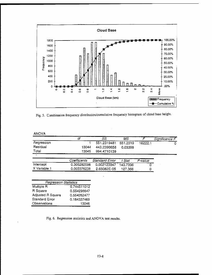
Cloud Base

low -

1600 - r n „^a-*-*"^"^ ■ 90.00%

1400 - ! i X"'*^ • 80.00%

>. 120° " S 1000-

f" 800-

"" 600 ■

■ i .

1 ; /I

• 70.00%

• 60.00%

• 50.00%

■ 40.00%

- 30.00%

400 - / - 20.00%

200 - <_, », _! «_L^K r J.FI.n.fi.n n i i-i i _, _ i

- 10.00% . nno/_ U 1IIIJIII «i '

OC\i^"<OCO'-C\l,*rCOCOC\l evi ■* o OOOO ■r- -r- i- i-

Cloud Base (km)

CM C\J o 2

'-■—-' Frequency

—■—Cumulative %

Fig. 5. Combination frequency distribution/cumulative frequency histogram of cloud base height.

ANOVA df SS MS F Significance F

Regression Residual Total

1 13044 13045

551.2319481 443.2390658 994.4710139

551.2319 0.03398

16222.1 0

Coefficients Standard Error tStat P-value Intercept X Variable 1

0.305282598 0.003376238

0.002123947 2.65082E-05

143.7336 127.366

0 0

Regression Statistics Multiple R R Square Adjusted R Square Standard Error Observations

0.744511012 0.554296647 0.554262477 0.184337469

13046

Fig. 6. Regression statistics and ANOVA test results.

13-8

CJoud Thickness (km)

-»■ in

O o E. H

en

<

c

S3

2

=3

Fig. 7. Cloud thickness vs. LWP scatter plot with regression iir

13-9

Finally, it shouid be noted that in addition to all of the advantages of millimeter-wave vertically pointing

radars, there are some disadvantages as well. Of these problems the most serious is the inability of millimeter-wave

radars to function appropriately during rainstorms, hurricanes, etc. This factor significantly reduces the number of

possible applications of this instrument.

Acknowledgments

This study is based upon data collected by the National Oceanographic and Atmospheric Agency's Environment

Technology Laboratory and posted on the World Wide Web at http://www6.etl.noaa.g0v/data/#astex.

References

Greenwald, T. I, G. L. Stephens, T. H. Vonder Haar, and D. L. Jackson, 1993:

A physical retrieval of cloud liquid water over the global oceans using Special Sensor Microwave/Imager (SSM/I)

observations. J. Geophys. Res., 98, 18471-18488.

Albrecht, B. A., C. S. Bretherton, D. Johnson, W. H. Schubert, and A. S. Frisch, 1995:

The Atlantic stratocumulus transition experiment-ASTEX. Bull. Am. Meteorol. Soc, 76, 889-904.

Hogg, D. C, F. O. Guiraud, J. B. Snider, M. T. Decker, and E. R. Westwater. 1983:

A steerable dual-channel microwave radiometer for measurement of water vapor and liquid in the troposphere, J.

Climate Appl. Meteor., 22, 789-806.

Uttal, T, 1997:

Detection of cloud boundaries with 8 millimeter-wave radar. Http://www6.etl.noaa.gov/review/tav.

Uttal, T., L. I. Church. B. E. Manner, and J. S. Gibson, 1993:

A cloud boundary detection algorithm for vertically pointing radar data. NOAA Tech. Memo. ERL WPL-233,

NOAA Environmental Research Laboratories, Boulder, CO, 28 pp. [Available from the National Technical

Information Service, 5285 Port Road, Springfield, VA 22161]

13-10

OPTICALLY ADDRESSED SPATIAL LIGHT MODULATORS AS REAL-TIME HOLOGRAPHIC MEDIA

NhiT. Tran

Manzano High School 12200 Lomas Blvd. NE



Phillips Laboratory



and

Phillips Laboratory

August 1997

14-1


NhiT. Tran Manzano High School

Abstract

An optically addressed spatial light modulator (OASLM) and its effects on a compensated imaging

process using real-time holography were studied. Use of a spatial light modulator to improve efficiency of real-

time adaptive optical corrective techniques for telescope and atmospheric-induced path aberrations is significant

because it makes the development of large, lightweight, low-optical-quality primary mirrors possible.

14-2


NhiT. Tran

Introduction

In recent years, the usage of an optically addressed spatial light modulator (OASLM) for works related to real-time

adaptive optical correction for telescope and atmospheric induced path aberrations have come forth with new

technology. Traditional telescope imaging can have defects due to atmospheric disturbance, misalignment of

telescope optics and primary mirror distortion. In addition to the construction problems arise the problem of

transporting heavy, high-optical primary mirrors into space. However, compensated imaging techniques have been

studied as possible solutions to the problem by correcting the usage of low-optical-quality primary mirrors for

imaging.

Background:

Spatial light modulators (SLM) are optical modulators constructed so as to spatially modulate, to a

prescribed input, a readout optical beam where the input can be either optical or electrical{ 1}. The overall function

of the SLM is to use optical techniques in processing the two-D information in which the input data is processed.

SLMs are used in a variety of different fields such as fiber-optics communication systems, imaging,

communicating data, and delivering optical power through an aberrated optical media.

Methodology: Experimental Setup{2}

Using the output from a helium neon laser operating at 543 nm, an object point source at infinity is simulated by

illuminating a 20mm pinhole and collimating the transmitted light with a six-inch diameter f/6 parabolic reflector.

The collimated light is then directed towards the membrane mirror telescope. Next, the output from the 5mW

green helium neon laser is used as the local beacon wavefront for the membrane mirror telescope. The output is

then expanded and guided through a null corrector, with positive and negative lens, and onto the primary mirror

surface. From the null corrector, a f/6 parabolic wavefront is produced and coincides with the normal center of

curvature of the membrane primary mirror. After generating through the focus and illuminating the membrane

14-3

mirror, the beacon wavefront is retroreflected and recollimated by the null corrector. In the pupil plane produced

by the null corrector, the beacon wavefront optical path difference relative to a planar wavefront is equal to twice

the membrane mirror surface optical path difference from the ideal parabolic surface. The pupil plane is then

directed to the "write" side of the OASLM where it interferes with a mutually coherent plane wave derived from

the same laser to record the phase aberration information in the hologram. In this demonstration, near diffraction

limited imaging was achieved using a membrane primary mirror with more than 200 waves of aberration.

local beacon laser dstorted merrfcrare ninor

vacumline

Figure 1. Experimental setup along with a two-dimensional photograph and three-dimensional intensity contours of aberrated and corrected images of a point source imaged by a low-optical-quality membrane optics using a real-time holographic phase subtraction technique. SLM, spatial light modulator; hwp, half-wave plate; qwp, quarter-wave plate; PBS, polarizing beam splitter.

14-4

Membrane mirror{2}:

The membrane mirror consists of a six-inch diameter, high-reflectivity-coated, four-micron-thick, nitrocellulose

membrane attached to a vacuum flange and held under partial vacuum to approximate an f/6 primary mirror. The

surface is characterized using an f/6 parabolic wavefront at one-micron wavelength in an interferometer setup to

write the hologram in Figure 1.

SLM{2}:

A Displaytech ferroelectric OASLM operating at 300Hz acts as the real- time hologram. The aberrated image-

bearing light is directed to the "read" side of the SLM that lies in the pupil plane for the image light. Due to the

internal reflection, the OASLM generates diffracted light in the backward direction. The reflected light is

propagated to a camera located in an image plane for the pinhole.

Problem

The purpose of the experiment was to transmit the image through distorting media using a SLM as a means of

compensating for path distortions. However, to accomplish this mean, the diffraction efficiency of the SLM must

be maximized. Commercially available parallel aligned nematic devices produce analog diffraction hologram

with demonst-ated efficiencies in excess of 30%{3}. For that purpose, the Hamamatsu parallel aligned nematic

liquid-crystal spatial light modulator (PAL SLM), model number X5641, was tested to show the greatest amount

of diffraction efficiency.

In Figure 2. the PAL nematic OASLM was tested using a green helium-neon laser at 543nm. The SLM is

placed on a rotating stage where the resolution can be observed. The line spacing on the SLM is dependent on the

angle of the two beams using the equation

p=8(in radians').

X

The SLM needs a certain angle to achieve a certain amount of line spacing. In order to achieve this, the SLM is

lined up perpendicular to one beam. Using the rotating stage, a certain degree changes the surface on the SLM to

14-5

get the second beam to retroreflect where the angle between the two beams is equivalent to the angle on the

rotating stage. From there, the diffraction efficiency is recorded.

XJ2

m Spatial Filt

i Heliun-Neon Lner

543mn

Polin zing Beam Splitter

I ui m m. Coffimanng Lorn

Ml

►

"mirror \

■r,

::(P==::^ moving tmrror 5CV50

Figure 2. Experimental setup for the PAL nematic OASLM and the diffraction efficiency data recording. X/2, half-wave plate: SLM, spatial light modulator.

Results

Working with various situations such as changing the resolution or the crossing-angle of the two beams, the

diffraction efficiency never achieved the set amount of 30% according to the Hamamatsu handbook{3}. In Figure

3., the diffraction efficiency was at its highest level reaching about 23% with the spatial frequency at 10 lines/mm.

Figure 4. shows different spatial frequency recorded and the diffraction efficiency that was generated.

i o 0. ■D (0 •G (0 t b

-- 20 #

Diffracted Power

Diffraction Efficiency

25

u

15 £ LU

10 § is CO

5 I

50 100

Writing Power (nW)

150 200

Figure 3. The highest level for diffraction efficiency of the Hamamatsu SLM. Crossing angle: 0.310 degrees; spatial frequency: 10 lines/mm; scaling information: 0.727953; readout power: 82.3)xm; reference beam: 254nm; input beam (both): 184.9|im; input beam (first): 93.3um; input beam (second): 91.9nm.

14-6

25

g20

|l5 e LU

|10

s Q 5

—ff-'f- -4f—i—

! f.***C -> : ; i»

t-1 4 : i"

■—i—i i i

»f ■ i t- j : :«: ■■ -t : *-^.

—i t i <—

—I—i—i—\—

; i t i

—t—i—i—(—

-f i i , ;

n ■i i k L

MM -Slines/nwn

-10 linesfmm

-16 lines/mm

20 40 60 80 100 120 VWting Power (fiW)

140 160 180 200

Figure 4. Diffraction efficiency comparison for different resolution.

Conclusion

The low net efficiency may be caused through variable problems associated with the use of the SLM. First, the

interface of the SLM is amorphous-silicon resulting in the loss of diffraction of the image light upon reflection.

Also, the SLM could also absorb light causing the efficiency to decrease.

Due to the low net diffraction efficiency of the SLM the severity of the aberration that can be corrected in

the application to the low- optical-quality primary mirror is limited. Improving the resolution to greater than 100

1/mm while maximizing the diffraction efficiency would make the SLM adequate for this application.

Acknowledgments

Special thanks to Mark Gruneisen, Chris Clayton, Roger Ramsey, and Mike Woods for their guidance in writing this paper.

References

1. Efron, Uzi "Spatial Light Modulator Technology: Material, Devices, and Applications". Marcel Dekker, Inc. NewYork,1995.. 2.M.T. Gruneisen and J.M. Wilkes, "compensated Imaging By Real-Time Holography with Optically Addressed Spatial Light Modulators," Spring Topical Meeting on Spatial Light Modulators, Lake Tahoe, NV, March 17-19, 1997, Paper STuB5. 3.Hamamatsu technical data sheets for model X5641 PAL-SLM parallel aligned nematic liquid-crystals spatial light modulator.

14-7

Constructing a Computer Model of the Space Shuttle and

The Effects of Lasers on Materials in Space

Jeremy L. White

Sandia Preparatory School 532 0sunaRdNE



Phillips Laboratory



and

Phillips Laboratory

August 1997

15-1



Jeremy White Sandia Preparatory School

Abstract

The possibility of a space based war is ever increasing due to the advantages of

carrying out certain tasks in space. It is important to have an accurate assessment of the

situation in any war because it helps you to make important decisions during the battle,

and these decisions can either help you win or loose the war. There is only one problem

with using conventional methods of gathering intelligence information, and that is that

they will not work. These methods will not work because they involve traveling to the

target and observing the area, and that is not possible in space because it is so

inaccessible. Satellites can be used to monitor the situation but visual information is

still limited. That is why three dimensional modeling is being used, because there is

always a visual representation that can be updated. Since the original is still available,

the two images can be compared to more accurately assess the status of the target.

Another thing that has to be considered is the use of lasers. Since they are such a new

weapon, the effects are still being researched, but that information is needed in the case

of a war, because if you don't know what a laser can do to an orbiting spacecraft, then

you can't accurately judge the status of a target that has been under laser attack. It also

helps one to know what you can do to an enemy spacecraft.

15-2'



Jeremy L. White

Introduction

With the growing interest in the exploitation of space, there is also an increasing

risk of war activities being conducted in space. One of the most important things that

one can have in a war is accurate intelligence. A computer program called IDASS,

which stands for Intelligence Data Analysis System for Spacecraft, is being developed in

order to improve our intelligence capabilities in the possible case of a space based war.

One technique that has been used in this program is the exploitation of computer

generated three dimensional models of orbiting spacecraft. This allows for the use of

visual intelligence information, which is sometimes the most helpful form of

information. One other important thing that has come up is the possible use of lasers as

weapons. Since lasers have never been used as weapons before, research is being done in

order to find out how a laser can affect a target This research will most likely play an

important part in the gathering of intelligence data.

Discussion of the Problem

There really was no problem involved with the work I did on modeling the space

shuttle. There were attempts to do it by other people working at the lab, but there just

15-3

was not enough time to construct a model quite as detailed as the one that I made. In

other words, this project was just something mat needed to be done. The problem with

the advent of high powered laser technology, is mat they will likely be the weapon of

choice if a space based war ever breaks out This causes difficulty in being able to

anticipate possible damage from enemy weapons, because we still do not know exactly

what a laser could do to a spacecraft. We do know mat a laser could bum a hole into the

craft, but there could be other things that might be a direct result of the hum Hamagp

There is a possibility that the laser bum would not completely cripple a satellite, or

spacecraft, but the things that we do not yet know about could finish the job. When

damage is being inflicted upon anything, there will always be some debris resulting from

that damage. We do know how to predict what the weapon will do in terms of debris,

and also what that debris will do. A major difference between the environment in space,

and the environment on earth is that there is no air in space. Space is a vacuum, so

therefore any debris, especially small debris, will behave differently due to the lack of

resistance. This fact makes it impossible to predict what will happen with that debris,

because we have never seen little debris affect anything because the particles in our

atmosphere put a stop to their movement before the can get anywhere. The other thing

mat prohibits the anticipation of debris damage to spacecraft is the fact that there is an

absence of gravity in space. This will also change the way that all debris will behave,

because the particles will not fall to the ground, but they will go in every direction,

uninhibited, unless they hit something else floating around in space. One other thing,

which has not been found to really affect the flow of debris, is the extreme low

15-4

temperatures which are found in space. The only thing that these low temperatures have

been proven to affect, is the effectiveness of the laser. A laser does damage by heating,

melting and weakening the material. The low temperature will prolong the hearing

process, because it has to start from a lower temperature than those encountered on earth.

We can replicate the lack of air in space, by using vacuum chambers, and by also using

liquid cooling processes, we can simulate the low temperatures of the space environment

The biggest problem with trying to simulate the space environment is that we do not yet

have an effective way of simulating a zero gravity environment So research done on

earth will not be totally accurate.

Methodology

As part of my summer research program I was privileged to be able to construct a

three dimensional model of the space shuttle for use with IDASS, using a program called

SMT, or Satellite Modeling TooL The first step in this process was to find a detailed

representation to base my model on. The most important part about this representation

was that it include measurements for the shuttle, because my model needed to be made to

scale accurately. The next thing to do was to then test the different scales in the

modeling program with the space shuttle measurements in order to find a scale that will

allow the space shuttle to fit on the screen, and that scale turned out to be meters. Once

that was done,! began to fabricate parts of the shuttle. I measuredeach component on

the picture, and then converted those into the scale within the program Within the

modeling program there is a set of predetermined shape formats with which you must

15-5

construct your model with. They range from cones, to cubes, to cylinders. To make a

shape with these formats, you must input the points, on a three dimensional coordinate

plane, which the computer uses to build the shapes. This is how every piece of. the model

is formed The name for the basic part of a model is called an element, which can have

multiple shapes inside them Creating the elements is one of the most difficult and time

consuming parts of the process because there are so many of them involved Once that

was complete, then came the difficult task of assembling all of those pieces, correctly,

into the form of the shuttle. In order to do this, the elements must be combined into

assemblies. The angles and positions of the elements must be manipulated within the

assemblies to form the correct shape. Then the assemblies must be joined together into

larger assemblies, until the last assembly, which forms the entire model of the shuttle.

This was a very difficult and time consuming part of the modeling process. The reason

that this was so difficult was that in order to place the shapes into the correct positions, I

had to manipulate each aspect of every shape within the three dimensional coordinate

plane. I wasforced to make changeson each axisof every shape, x,y,andfcaxes. This

included manipulating the angles of each shape according to each axis, and also I Ijad to

specify the distance from the center of the axis that each shape was placed Assoonas

the shuttle was completely assembled I then proceeded in designating which parts of the

model could be moveable. In order to do this I put the coordinates of the point on the

grid where the axis of rotation would begin for each moving part After that was

complete I set the limitationsof movement for the part on each three hundred and sixty

degree axis. In order to check and make sure that the rotation parameters were set

15-6

correctly I brought up that shape into the dynamics tool to animate the movement Then,

if it wasn't moving the way that I had wished it to, I would modify the rotation

parameters. I would then animate that shape again, and this, cycle was repeated until the

correct settings were found. This did get easier, however, as I became more familiar with

the way that each input into the rotation settings affected the movement of the part. The

next and final part of the modeling process was to assign the correct material properties

for each part of the space shuttle. TMs was simple, as there was, a list of properties to

pick from, but because I had to go and set this for some individual elements, it took a

Long time to complete. Since there are special coatings and paint and other such things

that can be put on the outside of the parts, the material of the bulk of the part, and the

surface of the part, both had to be individually assigned, whether it he an assembly or an

element With the completion of that, the task of modeling the shuttle was complete.

The next part of the modeling, was to mate the shuttle with another, previously

constructed model of the Mir Space Station, which was of an equal scale. The only thing

I had to do to accomplish this was to again find a detailed picture ofthe two while the

shuttle was docked. I constructed a docking module for the two and attached the two

pieces of it in their correct places. Then, using the picture, I aligned the shuttle up with

the space station, and joined the two spacecraft, and that completed my task of modeling

the space shuttle.

The next project that I was involved with was studying the effects of lasers on

different materials in space. The process for setting up these tests were not terribly

complicated. The first triing to do is to go around ard turn on all of the rnachines. The

15-7

list of machineswas incredihly long, but il consisted mostly of vartous caloriineters, and

computers and cameras. Once the computers had booted up, the other lab personnel

would bring up the proper programs to he used during the test I never learned how do

this, or to really learn how to use the programs, except for the slide scanning software-

Then we would uncover all of the optics and ready the laser for a test shot Before firing

the laser we would line up the optics, so that the laser beam would be in the right

position. WithtrMcoirqdete^wewaddseiagrar^

chamber so that the laser would not damage anything inside the chamber, and we always

put on protective goggles, which block out the wavelength of light that the lasen operates

in, which is a wavelength of 1.315»xm The other safety precaution that was taken was

the use of lenses that have an AR, ox anti-reflective coating for that same wavelength.

This prevented any unwanted stray laser beams in the lab. On the test shot, or shots,

depending on whether all of the equipment was functioning properly or not, we would

use an infrared light detector card which would show where the laser beam bit, to see that

the laser waslined up in the right place withall of the various instruments. Then we

would mount the target on an aluminum plate which was bolted to a fixed stand within

the vacuum chamber. For the next test, shot after that, the graphite block was removed,

and the alignment of the laser beam with the target was checked using that same infrared

light detector card During this test, there would be an attenuator lens in front of the

laser, which would only transmit some of the lasers full power through to the target The

rest of the light was directed towards another, larger graphite block behind the laser- The

reason that graphite blocks were used to stop the laser beam, is that they have almost zero

15-8

reflectance, which kept the beam from going else where, and because they can withstand

high amounts of heat. We would then adjust the position of the target according to where

the laser beam hit it, unless the beam was much higher than it should he, then we would

adjust the last lens before the vacuum chamber to compensate. Once the target was

aligned, the sensors inside the chamber would be checked to make sure they were in the

right place, and making contact A slide would also be mounted perpendicular, and right

next to the target in order to collect the debris from the burn. We used several kinds of

these: a glass slide, a polished copper slide, and a high index of refraction piece of glass.

These varied as the people on the analyzation part of the test series ran into problems

detecting the data, or debris, collected with their instruments. Once everything was

found to he correctly positioned and setup, the vacuum chamber would be sealed up and

pumped down. A roughing pump took care of most of the pressure, and then, a

molecular pump would bring it the rest of the way down. We would let the molecular

pump bring the pressure down to around 3 * 10"5 torr for every test, in order to simulate

the conditions in space. This measurement was recorded, as it was important to know

this in the case of any problems that might be run into, ox other unexpected things that

happened, which needed explaining. This would usually take about an hour or so to

pump it down, and consequently, this limited.the number of tests which could.be done in

a day. For some of the tests, we would also cool off the target using a cold finger, which

we would use to take the target down to about -70 degrees centigrade, and this number

would also be recorded When the cold finger was used, the number of tests was limited

even more, because if you broke vacuum before the target was back up to room

15-9

temperature, frost would, form on. the debris collection slide and ruin the collected data.

The warming process would take all night, until the heat tape was installed to help it

along. The heat tape, both inside, and outside of the vacuum chamber, was wrapped,

around the cold finger. This heat tape was able to bring it up to a temperature that would

prevent the formation of frost on the data collection slide, in about one hour. Although

the heating process was sped up considerably, the use of the cold finger stopped, because

it appeared, to have no effect upon the test results. While the vacuum chamber was

pumping down, we would do a pre-test scan of the date collection slide( except not with

high index of refraction glass due to different shape). This was done by computer control,

using a laser, and voltage detector mounted inside the chamber on a motor driven

platform. Depending on which type of slide was used, the voltage reading from the

photoelectric detector would be one of transmission (glass slideX or one of reflectivity

(copper slide). Tliis reading would.be input onto a graph on one of the computers. As

the motor moved the laser/detector assembly along the length of the slide, the voltage

would change, which would, show how much debris was on the slide. After this test, the

computers would be reset, and everything would be readied for the final shot Once the

chamber was completely pumped, down, we would all put on our protective goggles, and

fire the laser. There would be no attenuator for this shot, and the test would last only a

matter of seconds, anywhere from 3 - 25. Once all of the instruments had timed out, and

stopped collecting data, we recorded the calorimeter data This data included the

runtime of the laser and most importantly, the average irradiance of the laser on the

target This was the measure of power put on a square centimeter. We proceeded in

15-10

doing a post-test scan of the slide with the same setup as the pre-test scan. Thishelpsto

see if the data is useable or not,,but it still has to pass a scan using the other instrument

with the group of analysts. Then the target is taken out after the warm up, and.

preparations for another test are made.

One more thing which L was able to do, wasto use a laser profilometer. This

piece of equipment is a.laser triangulation gauge used to determine the surface structure

of what ever object you choose to put underneath it This laser proiilometer consists of

two servo motors, a motor power supply and control box, and a computer. A program on

the computer, called. 3<Lpro runs the laser triangulation gauge. It tells the motors what to

do, according to the scale and grid dimensions that you input into the program It then

collects the data points and stores them in either an ASCII or binary file format for

further processing This program runs the gauge on a Cartesian coordinate plane, but

there is also another program which does the same thing called RT pro, only it runs on a

polar coordinate plane. Then the file can be run in the surfer program, where a grid file

is produced, which can be viewed, as a three dimansinnfll pirtnfp on the monitor which

can be manipulated. This piece of equipment is used to determine how evenly the laser

burned the target. The reason that this equipment is used, rather than visually checking

it, is because the profilometer has a much higher resolution. It has a resolution of about

3& microns, but the size of the object is limited, because it can only handle a maximum

of 14,400 points. This level of resolution makes for a much more accurate picture of the

surface of the burned object

15-11

Results

The only results which I can show you, are the picturesof the model of the space

shuttle. I have no results from the laser tests, because the part of the experiment which I

helped with, was not with analyzing the data and detenrüning the results of the tests, but

actually performing the tests, or the laser profflometer, because that was only busy work

until I could start on the lab work.

I have chosen two pictures of the space shuttle model which I feel represent all the

aspects of the model I have also included a picture of the space shuttle while docked

15-12

with the Mir Space Station, because I helped with the finishing touches ofthat model,

and with the joining the two spacecraft.

15-13

Conclusion

This has been one of the best learning experiences that I have had in my life, and

to make it better it was also very enjoyable. I was able to see and work on real

experiments and projects, where the results would actually be used, not just some husy

work that was given to me so that I would have something to do. One very important

thing which happened to me during the time I spent working at Phillips Laboratory, is

that ä influenced my decision on what kind of a career I would like to pursue in the

future. I learned how to use a computer to make a three dimensional model of areal

15-14

object, which is a skill that I think will come in very handy with the growing use of

computers to aid in designing various objects. I also experienced what it was like to

work in a laboratory environment, which is something that I think I would enjoy being i

part of my job.

15-15

References

Hicks, Kerry, Major USAF. Chief, Systems Analysis and Integration's Branch.

Interview. June. 1997.

Joels, Kerry Mark, and David Larkin. The Space Shuttle Operators Manual.

New York: Ballantine Books, 1982.

Phillipson, Darrell, Lieutenant USAF. Satellite Systems Engineer.

Interview. June. 1997.

Roberts, John. PL/WSAE employee.

Interview. July. 1997.

Rudder, Ralph, Dr. PL/WSAE employee.


Shell, Jim, Captain USAF. Chief, Laser Effects Test Facility.


15-16

DEVELOPMENT OF ALGORITHMS TO OBJECTIVELY FORECAST

PRESENT WEATHER AND SURFACE VISIBILITY BY MEANS OF A REGIONAL

NUMERICAL MODEL- INDECISIVE APPROACHES

Joanne Wu

Newton North High School

360 Lowell Avenue

Newton, MA 02166

Final Report for:

High School Apprentice Program

Phillips Laboratory

Sponsored by:

Air Force Office of Scientific Research


and

Phillips Laboratory

Hanscom Air Force Base, MA

August 1997

16-1




Joanne Wu

Newton North High School

Abstract

Three distinct statistical approaches to probabilistically weather forecast precipitation were

studied: Perfect Prog, Model Output Statistics, and Modified Perfect Prog. Each of their respective

advantages and disadvantages were weighed in terms of their effectiveness in the Present Weather/Surface

Visibility algorithm development. The results of the study indicated that, although far from perfect, the

Modified Prog approach was the most appropriate technique for the given application

16-2




Joanne Wu

Introduction

One of the principle functions of the United States Air Force (USAF) is to complete missions by means of

traveling in the air. Such a job requires the Air Force Global Weather Center (AFGWC) to provide

precise forecasts of weather conditions to facilitate smooth missions. Currently, the Air Force lacks

accuracy in its forecasts for specific weather elements that could be potential obstacles in any mission.

Consequently, due to the implicit nature of current operational numerical models, the Air Force is in need

of an improved form of weather diagnosis that is able to predict sensible weather conditions with greater

precision. The main objective of the Air Force Global Theater Battle Management (TBM) Program is to

provide AFGWC with an enhanced forecasting technique for a wide selection of parameters. This will be

accomplished by means of producing algorithms which can use standard numerical model output to make

efficient and reliable probabilistic forecasts. The project is currently being carried out in the Atmospheric

Sciences Division (ASD) of the Geophysics Department of Phillips Laboratory (PL) at Hanscom Air Force

Base, MA. Work done on TBM will be applied on the Theater (Regional) and Global scales. Forecast

parameters of interest specified by AFGWC include: Present Weather/Surface Visibility, Clouds (e.g.,

ceiling height, thickness,) icing, turbulence and thunderstorms. Since each of these parameters presents a

unique type of aviation hazard during the course of any flight mission, individual algorithmic research is

needed for this project. Each group within the ASD starts out with common goals of successful algorithm

development: a) to determine statistical correlation between output from selected models and observed

weather parameter values, b) to develop algorithms from established relationships, c) to make forecasts on

future parameter values using algorithms, and d) to determine accuracy of the algorithms through testing

with an independent data set With these set objectives in mind, different working groups within the ASD

at PL are charged with independent algorithm development for distinct parameters. For instance, the

purpose of this paper is to describe the study design of the research headed by Ken Heideman and Capt.

Brian P. Newton at PL on Present Weather/Surface Visibility algorithm development. Towards the

completion of the TBM Program, the final product will be assembled by linking the work of all the groups

and creating a unified set of algorithms that act like a black box; the input of analyzed and observed

parameter values will result in forecasts for future respective values at various intervals. However, for

now, the overall discussion will be focused on the methodology of and the problems encountered by

Heideman and Newton during their ongoing Present Weather/Surface Visibility algorithm development.

16-3

Methodology

To begin the research on theater scale algorithm development in Present Weather/Surface Visibility, the

continental United States is divided into 12 regions (see Map 1.) The region assignments are based on

similar weather characteristics. For example, land along geographic features like the Gulf Coast, the

Rockies, the Appalachians, the Great Lakes, the Pacific and the Atlantic Oceans are all grouped

independently because their distinct locale subjects these regions to unique weather patterns. Following

the region establishments, data of present weather observations are requested at an average of 10 stations

(most of which are located at or near Air Force Bases) in each region for the years of 1992-1993 at

specified times of 0:00 and 12:00 GMT (Greenwich Mean Time.) Since the Nested Grid Model (NGM)

was the chosen model for development, for reasons which will be discussed, the stations located on grid

points would be ideal. Unfortunately, stations which satisfy that requirement are sparse (see Map 2.) In

order to compensate the error caused by the distances between the actual station and the NGM grid points,

the data from each station is interpolated (see Diagram 1.) The results from the calculation through

weighted bilinear interpolation are the basic data given to Heideman and Newton to begin Present

Weather/Surface Visibility algorithm development.

To understand the use of the given raw data, one must first know the AFGWC requirements of Present

Weather/Surface Visibility algorithm development (see Chart 1.) The AFGWC first wants to know which

of the two general weather categories present weather conditions fall in: Precipitation or No Precipitation

(see Chart 1) Cases where no Precipitation occurs yet is a hindrance to surface visibility, like fog and

haze, are placed into the Miscellaneous category. Precipitation events must again be sorted into stratiform

(e.g. stable snow, rain) or convective weather (e.g., thunderstorms, showers.) For further specifications,

AFGWC requires the Present Weather/Surface Visibility algorithms to probabilistically forecast the exact

type of weather or weather combination. The final product would then be an additional Probability of

Precipitation (PoP) guidance for meteorologists in forecasting, except with more detail and, hopefully,

with greater accuracy.

The raw data from each region is first separated into 2 seasons: warm (April-September) and cold

(October-March.) This split is required since weather patterns during the warm season vary dramatically

from those of the cold season. Then, development of predictive equations begin with a comparison of

potential predictors (the independent variable, x) and the predictands (the dependent variable, y.)

Predictors are essential to the development of algorithms. Think of the predictors being clues like sound,

pattern, and smell that help one guess what is inside a mysterious black box. Thus, no matter how

16-4

insignificant most of them might be, the higher the number of initial predictors, the better the chance of

finding solid statistical relationships between some of the predictors and the predictands. However, the

total number of the model-generated predictors at the two designated times being used in Present

Weather/Surface Visibility algorithm development is limited (see Chart 2). To expand on the number of

potential predictors, other parameters such as the dewpoint and divergence at various pressure levels (see

Chart 2) are derived from the predictors generated by the model and those given by the observations.

Further experimentation on parameters requires slight variations such as combining given and derived

parameters through simple mathematical calculations (e.g., multiplication by constants). Thus, the pool

of predictors is increased from the original 38 given parameters. However, the number and the type of

predictors that the project begin with and eventually end with will not be the same among all 12 regions.

For example, most of the current work is being completed on region 6 (the Gulf Coast) and the number of

possible predictors stands at around 170. These 170 or so predictors from region 6 will not be identical to

those from another region (e.g., region 10, the Great Lakes, for which there are approximately 150).

Then, in order to begin algorithm development, observed present weather data is again sorted into specific

categories. Initially, all kinds of present weather (e.g., no weather, thunderstorms, rain, snow) are

arbitrarily given a number. Then, the data is further categorized in their respective groups: No weather,

Miscellaneous, Stratiform, and Convective. Each category assigned a number (0,10,20, 30) to prepare

the observed and forecasted data for the next phase: Logistic Regression. Statistical Logistic Regression is

then applied to the four categories and distinct equations are derived. The result is four equations that

produce probability of the corresponding category of weather occurring at the valid times of 0:00 and

12:00 GMT. By observing the calculated Probability of Detection (POD) and False Alarm Rate (FAR), it

is determined whether some mathematical variation is needed to increase the accuracy of the derived

equations. Other pre-existing algorithms (see Ivens, 1987) and empirically derived algorithms are then

used as assistance in determining which specific type of precipitation, if any, has the highest probability of

occurring at a specified future time and location. To formally evaluate the Present Weather/Surface

Visibility algorithms, a series of testing is done through use of an independent database, which consists of

every fourth observation in the two-year database. The observations in the independent database were not

included when the forecast equations were first developed.

Types of Approaches

Due to the uncertainty of which specific type of operational regional model would be implemented by

AFGWC in 1997, the first task was to determine which regional numerical model would be most feasible

to use in developing the Present Weather/Surface Visibility algorithms. Two criteria were essential in

16-5

choosing the model: 1.) a long and reliable archived data set must be made available, and 2) the archived

data set must contain enough model-generated variables to present a sufficient amount of potential

predictors to the developmental database. The final selection of the NGM for development of the

algorithms was based largely on the fulfillment of these two criteria. Ideally, the ultimate Present

Weather/Surface Visibility algorithms would need not to be dependent on the NGM or any other

operational numerical model.

The Model Output Statistics (MOS) approach (Glahn and Lowry, 1972) is a PoP forecasting technique

used by many in the field of Meteorology as highly reliable forecast guidance. The MOS approach relates

weather observations (predictands) to variables forecast by numerical models (predictors) and calculates a

set of equations that fit with the chosen model for development. Typically, separate equations are created

for each forecast projection, independent of whether the projection range is short or long. An advantage of

the MOS approach is that it takes into account climatic frequencies for particular regions and adjusts the

numerical forecast equations so that errors are reduced in future forecasts. Thus, it is not very likely that

in longer range forecasts, MOS equations would result in forecasts that deviate dramatically from what

that particular region had experienced at the same time in the past. Another advantage is that MOS

partially compensates for error bias in the numerical forecasts made by the model it is developed on.

However, the constant compensation can also be a disadvantage in situations where no error is present in

the numerical forecasts. Thus, any adjustment made by MOS would create a biased forecast. Another

disadvantage of this technique is that its accuracy depends on the length of the data archives. Since MOS

examines climatic frequencies and takes past observations into account, this approach requires at least two

or three years of data sample to be effective. In addition, there must be no changes to the model during

the period of development Equations derived from this approach are only accurate with the chosen model

of development. Attempts to apply resulting MOS equations to other operational numerical models could

yield undesirable results.

In contrast to the MOS technique, the Perfect Prog approach (Klein et. al., 1959) develops relationships

through use of simple regression techniques between predictors and predictands. Equations between

numerical model analyses and observations are valid only at designated times of development. In

addition, the Perfect Prog approach is based on numerical models such as the NGM and other gridded

graphs. The equations are derived by means of plotting numerical data points and drawing the most

feasible line to represent the data. The line is drawn such that standard deviation is minimized. Through

use of this method, distinct equations are derived for each potential predictor. Only predictors whose

relationships with the predictands in both the forecasted and observation data are considered. One

advantage of this technique, on the contrary to MOS, is that

16-6

equations developed do not completely depend on the operational numerical model chosen. Equations are

flexible enough so that they are able to evolve through time. Also, in contrast with MOS, a robust

database is not necessary for equation development However, Perfect Prog is not flawless. A

disadvantage of Perfect Prog is that the resulting forecasts are made with an implicit assumption that the

numerical model data used as inputs are "perfect." As discussed above, error is almost always embedded

in any operational numerical model. Moreover, if a small database is used, rare events such as

precipitation (particularly in some regions) will be underrepresented in the development of the equations.

Thus, resulting Perfect Prog forecasts will be less accurate.

In addition to MOS and Perfect Prog, a third approach called the Modified Perfect Prog approach has

shown effectiveness in producing statistical forecasts. In contrast with the two techniques above, Modified

Perfect Prog uses short-ranged numerical forecasts (0:00-12:00 GMT) as predictors as opposed to

observations. However, Modified Perfect Prog also bears similarities to certain aspects of MOS and

standard Perfect Prog approaches. A common advantage of standard and Modified Perfect Prog is, while

still valid at any projection, only one equation needs to be derived for each time of the day. This advantage

remains true provided that the obvious changes in the projection of predictors occur similar to standard

technique. However, like one disadvantage of Perfect Prog, "Perfection" of the numerical model data used

as inputs for Modified Prog statistical analysis is implicitly assumed. Thus, although very short ranged

MOS equations are developed in actuality, forecasts with the use of Modified Prog do not account for the

potential error in the chosen numerical model like with the use of MOS. Fortunately, as with one

advantage of MOS, the Modified Perfect Prog approach does not pose any limitations on the type of

variables needed to be used for development. In addition to the observed variables at 0:00 and 12:00

GMT, other variables such as vertical velocity made available by most numerical models, can also be

utilized. Overall, due to the fact short-ranged numerical model output has a consistently high reliability

and the approach itself is not model-dependent, Modified Perfect Prog is a preferred guidance for most

forecasters in making short-ranged forecasts.

Results

After careful scrutiny of MOS, standard and Modified Perfect Prog approaches, it was concluded that the

most reasonable technique for Present Weather/Surface Visibility algorithm development is Modified

Prog. Given the initial vacillation in model decision-making on the part of the AFGWC, MOS was

eliminated because of the lack of available numerical data. If AFGWC had known precisely which

operational regional model would be desirable beginning in the year of 1996, a complete 3-5 year archive

of the model's output would be available for use of the MOS approach. Algorithm development with the

16-7

MOS approach would yield results that would specifically accommodate Air Force needs. Due to the fact

that this information was inaccessible, the choice was between standard and Modified Perfect Prog

approaches. Advantages to both techniques are that the resulting equations would not be model-

dependent and an immense data archive was not needed for development. However, the primary

disadvantage is the implicit assumption of the "perfection" in numerical model output. With these facts in

mind, the final choice was the Modified Perfect Prog approach by reason of its greater flexibility in

choosing potential predictors. Furthermore, Modified Prog allows assistance from pre-existing algorithms

in the prediction of the exact type of Precipitation when Precipitation occurs.

Concluding Remarks

Although the objectives of the Theater Battle Management (TBM) at Phillips Lab are the same among all

weather application components, each group has to create a study design that is specifically tailored to its

respective needs. The above discussion pertains to the ongoing work in Present Weather/Surface

Visibility algorithm development With the Modified Prog approach as the chosen course of action,

current algorithm development is being carried out in the Gulf Coast region (see Map 1; Region 6).

Given the initial uncertainty of the model chosen by AFGWC, the selection of Modified Perfect Prog

approach is most reasonable when compared with the MOS and Perfect Prog techniques. However, even

with use of the Modified Perfect Prog approach, it is discovered that the short length of the data archive

had a tremendous affect on the resulting equations. Due to the lack of sufficiently frequent observations

(0:00 and 12:00 GMT in 1992-1993 only), rare weather events such as precipitation in particular regions

are under-represented. Thus, accurate predictions of those events is difficult even with the application of

the Modified Perfect Prog approach. In spite of inherent problems and limitations, work on this TBM

project reinforces the value of statistical approaches to weather forecasting in supplementing numerical

model forecasts.

Acknowledgments

Due to a personal lack of full meteorological understanding, this paper could not have been written

without the unyielding support and patience of my mentor, Ken Heideman of PL/GPOF. It was with his

aid that I was able to piece together all the basic meteorological concepts to give the work on the Present

Weather/Surface Visibility algorithm development that I had accomplished this past summer a more

tangible feel. Also, without the constant support and humor of Bob d'Entremont and Captain Brian P.

Newton of PL, this paper would not be complete due to the high stress level it occasionally generated.

16-8

References

H. R. Glahn, and Lowry, D. A., 1972b: The use of Model Output Statistics (MOS) in objectively weather

forecasting. Journal of Applications in Meteorology. 11, pp. 1203-1211

Julian, P.R., and A. H. Murphy, 1972: Probability and statistics in meteorology: A review of some recent

developments. Bulletin of the American Meteorological Society. 53, pp 957-

965

H. R. Glahn, 1969a: An operational method for objectively forecasting probability of precipitation.

Abstract in Bulletin of American Meteorological Society, 50, p. 458

H. R Glahn, and Lowry, D. A., 1976: An operational method for forecasting probability of precipitation -

PEATMOS PoP. Monthly Weather Review. 104, pp. 221-232

H. R. Glahn and Lowry, D. A., 1969b: Relationships between integrated atmospheric moisture and surface

weather. Journal of Applications in Meteorology. 8, pp. 762-768

16-9

Map 1

Regions Used For Algorithm Development v|

Map 2

16-10

Diagram 1

Horizontal Interpolation

300IJ*

400mb

SOOmb

700mb

BSOntb

NGM

Weighted Bilinear

Interpolation

300mb 400mb SOOmb 700mb eSOmb W5mb WOmb

400mb-~~1 °S 500rob^7~ roomuNGM

850K<b 30Omb ^ - ^S^iiib

400mb C^J_^)

::ryoBs v -asomb

I^25mb

\ N.

V

SOOmb

— 400mb

SOOmb

700mb

BSOmb 925mb

NGM CD

NGM

HCfNIimi »*H

Chiiri 1

No Weather

Present Weather Categories

Other Hue

Fog

Sand (Blowing)

Duct (Blowing)

Blowing

Snow

Stratiform

Freezing Rain (LgttMooTHvy)

Freezing Drizzle

Freezing Fog Ice Pellets

Snow (LgVMooTHvy)

Rain (LgVMod/Kvy)

Drizzle

Convectl ve Thunderstorm«

Rain Shower» (LgtfMooTHvy)

Snow Shower«

(LgVHooVHvy)

Ice Pettet Shower«

16-11

Chart!

Predictors M54)

A. Mödftf Generated/Observed

(36) (5)

UWlnd

VWInd -"" o o 0

Tempera lure RH

{

B. Derived

(tfi)

Vort Vort Advectlon

Divergence

o o

o

Vapor Pressure Mixing Ratio

Various Combinations MOO)

^ Vort x Divergence o

o o

o

K Index Wind Dir x Terrain Grad

IVENS LEGEND

TW*fc Maximum We« Bulb-Temperature in the warm Laver (>0C> y

TWG: Wet Buib Temperatur« at the surface

R: forecasted amount of Precipitation

RC: Critical Precipitation for Snow

= .055 * Vertical Mean Temperature • Thickness of the Layer

RCM: Critical Precipitation for Merang Snow

Hl*2.42*fl\e*+1.50*B*.34+.23

16-12

IDASS ADDITIONS

Aaron Zimmerman

Sandia High School 7801 Candelaria Road NE Albuquerque, NM 87110

Final Report For: High School Apprentice Program

Phillips Laboratory

Sponsored By: Air Force Office of Scientific Research


and

Phillips Laboratory

August 1997

I7-1

IDASS ADDITIONS

Aaron Zimmerman Sandra High School

Abstract

To create a user friendly, efficient, and overall more productive program,

additions to Phillips Laboratory's Intelligence Data Analysis System for Spacecraft

(IDASS) core program are needed. Two additions added during the 1997 summer are

the ability to communicate and share data with Satellite Tool Kit (STK), by Analytical

Graphics Inc., and the ability to receive data from telescope images of deep space

satellites. These two additions allow the user a broader range of choices to complete

the task desired. With the two additions to IDASS, the user, who may be in the

intelligence field, who may be in charge of satellite development and tracking, or a

casual or serious observer, will benefit greatly in productivity and efficiency.

17-2

IDASS ADDITIONS

Aaron Zimmerman

Introduction:

With the ever increasing number of satellites being launched in the closing

years of this century, it is no surprise that software companies have realized the profits

that would accompany satellite tracking programs. Although many companies realize

the income potential, some cannot or have not spent the time and money necessary to

create a satellite identification and tracking program. One reason for this may be the

high graphical and processing power required to render three-dimensional models and

perform orbital calculations. This restraint allows only users working on expensive

power computers the ability to run these programs. As personal computers are

becoming increasingly powerful, at least one company, Analytical Graphics Inc., has

created spacecraft tracking software for the PC. Many companies are sure to follow.

In the near future, two satellite programs might be in use by interested companies.

These companies include the Air Force and any other company dealing with the

manufacturing, launching, or tracking of

satellites.

Phillips Laboratory wrote a satellite

identification program called Intelligence Data

Analysis System for Spacecraft (IDASS),

see Figure 1, which allows a user to identify

a satellite using a variety of means. Image

ran urnoAL usr.oMw

Intelligence Data Analysis System. for Spacecraft

Comparison (IC) allows a three-dimensional Figure 1. IDASS screen splash

1-7-3

model to be super-imposed over a telescopic photograph of a satellite. The three-

dimensional model is created by laboratory workers using Satellite Modeling Tool (SMT)

another program written by Phillips Laboratory. Being able to see both a three-

dimensional model and a satellite image laid on top of each other allows the user to

identify the satellite based on tie points. Tie points are distinct features present on both

the satellite model and the satellite image. After identifying the satellite, the user is

then abie to diagnose the satellites functions. Using Motion Estimation (ME), the user

is able to see if a spacecraft is alive and functioning or dead and drifting about in

space. Along with an Orbital Visuafizer (OV), IDASS is indispensable tool for anyone

needing to identify a satellite.

Where IDASS can be used for both identification and visualization of satellites,

Analytical Graphic's Satellite Tool Kit (STK), see Figure 2, is primarily used for

visualizing spacecraft and their

orbits (See Figure 4 and 5 to see a

side by side comparison of IDASS

and STK user interfaces). STK core

program comes with a two-

dimensional viewer that allows

vehicles, facilities, and sensors to be

seen. With the purchase of a

SATELUTE TOOLKIT ANALYTICAL GRAPHICS

Figure 2. STK screen splash-

Visualization Option Module (VO) the user is able to see the satellites and orbits in a

simulated three-dimensional space. The VO Module allows STK to use three-

dimensional models much like IDASS does in its Orbital Visualizer (OV) (See Figures 5

and 6 for a comparison of IDASS OV and STK VO). STK also has another add-on

module called the Interprocess Module (IPC) which allows STK program commands to

17-4

be sent from outside the program. Program commands can be sent from other

programs or can be read off a text file. This extends the usability of the program.

I DASS implements the I PC Module from within its Orbital Visualizer. These two high-

power programs working together create unbeatable interface for anyone dealing with

spacecraft.

In addition to the power gained from the fPC Module and the IdaSTKInterface

class, IDASS may also receive additional power from another Phillips Laboratory

project. The Multi-Spectral project headed by Captain Conrad Poelman and Stephanie

Meltzerwill allow a deep space satellite to be identified. These satellites are beyond

visual range, so IDASS Image Comparison will not work. An idea was introduced that

telescopes are still able to receive photons from the satellites, and that if each satellite

has a specific photon pattern it can be identified. Using simulated data, a neural

network, and patience the results being returned are near one hundred percent correct

identification. The ability to correctly identify deep space satellites wHI be another

addition to IDASS impressive identification suite.

With IDASS leading the way in satellite identification and tracking, program

code must be written to keep up with new advancements like the multi-spectral project.

Code to allow the communication between IDASS and STK was needed as was code

to incorporate filter files into the output of the multi-spectral project.

17-5

■" -'"* ■*•"■■ -~—-■—--<--" ■■_-~.:...x:-;-.; L^V."'-^^ : : ^^... -i:,j-.a_^n:«art

Notebook Pages Edit Database Analysis Windows Help:

Summary :.- •■ - • 'im'a;-.önii Models? MEResylts i (SResults: 'ICResuUsi » Motes s mêry h MuaBi:» >■ . - :■ .. ■. > . •--.■*

rtotebooK Name ChuckSÄT

■i' ; '"■:.!:"■'-' Srajecl j Demor:h'slratr9n HdteBööl<f •;

!':-. :...-. . Owne*\ tiitttertt ":~;:; ir\J:.::..l.... ....

"!.''•" ::--6â9OT;Date\TTi«.^r;*'f(9H2*Z:t99?':'':'

! Last Mmhficafion Date Thu Juir 6 Ü9~t2:82 199E

| Read Permissiierr Scope | v 0^^frar-i»,- Group1 y- Warlri ;

Write Permisssott Scope 1#- Owuner^-draiip \/ Htortd }

$

HI Summary:

-1 'i\

Figure 3 and 4. The IDASS (above) and STK (below) user interfaces.

1 ^ÎfSfsg^gSsfiya?^^ ■ «■ ■»■-.. •—*■■— ■■»■JI, ■ ■» -. • y.« L*>*.- » ■_^^-.iJ.-»^».a.-^»-.—-^'-^JJ

*SSS?J'.' j^ "Mv*i .'™J-§:V-f.

| Saft3 affip iJg| ij|S|ÖiÄä -iäiiyä JÄöS}JÄ& ffiljgpfpMBtt

•i;! ^Z^^^;E^£ffi||M^

2 r: = wi-sps^^^Lygiffltftfllip sSlpBt^S^^^lp;:

(»i.iri C-C'.»-l *■>■:'- •'. ■;-. ; Pitr 'i i -.. :■.-.:: ..-.- . :;.y..in Öl et ; . ... ." .:;...■

'■—ftrAl. ' = BHpääSMiiÄîiffiÖpiBppÄ HSgî|M|ä?Ö^^î?M|feiitHiä^

qigtâggttlB(tesis?j

: ^TäjigMiiösBfläi^

- -. JLJMpJif e|- EsifittofäfÄäStji! ' ^;;<,t --■*- ->■','

;T^JÄf-"fJ>_Ti-Äpjj|f\":tr -r^SlSSi^Jtr^tW^-^'^;:

'■•ffnirfli'iit^-ürii

17-6

Figure 5 and 6. A side by side comparison of IDASS OV (above) and STK VO (below).

17-7

Methodology:

The program written to aflow IDASS and STK to communicate is called the

IdaSTKInterface. This code is actually just a C++ class that contains a list of public

methods that IDASS can call from its OV page. A class was selected due to its

efficiency and its ability to be added without rewriting the program. The class contains

all the methods required to setup the communication socket, send the data to STK via

the IPC Module, handle errors, and disconnect communication from STK. The

communication takes place through a UNIX socket. This program was added after

IDASS had been written so the class made it easy for the Phillips programmers to

implement IdaSTKInterface without disturbing previously written code.

The first step in creating a class was to create the socket and test the ability of

both programs to communicate. The test included basic commands that STK would

recognize including "New / /Scenario IDASS" which creates a scenario called IDASS.

A scenario is the basic building block when dealing with vehicles and facilities. The

scenario contains the objects and events that take place during an allotted amount of

time. Only one scenario in STK can be loaded at a time. After receiving a success

upon receiving the data, communication between the two programs was proven

successful.

After proving it is possible to send data between programs, it is necessary to

code a method for every command that IDASS will use. The bulk of the

IdaSTKInterface program contained these methods. The IPC Module provided an

excellent link between the two programs. Some example of commands that would be

sent from IDASS to STK are: "New / /Scenario/IDASS/Vehicle NewVehicle",

"Articulation /Scenario/IDASS/Vehicle/lMewVehicle 1920 30 Cargo Rotate 0 -160",

17-8

and "Point /Scenario/IDASS/Vehicle/NewVehicle/Sensor/NewSensor Relative 0 -90".

The first example will create a new vehicle (satellite) called "NewVehicle". The second

example will rotate the cargo hatch on

NewVehilcle from 0 to -160 degrees,

see Figure 7. The final example will

point NewVehicle's sensor at the

Earth. An example of a sensor can be

seen in Figure 6. The sensor is the

cone going from the satellite to the

Earth. Of course, the user will not

have to type in these commands,

rather press an interface button, and IDASS will pass the correct data to

IdaSTKInterface and then IdaSTKInterface will pass the data to the IPC Module.

The third step in creating the IdaSTKInterface program was to test all the

commands from IdaSTKInterface. Since the class was not implemented into IDASS

yet, a local method called Run() was used to call the public methods simulating calls

IDASS would make. Problems in reading information, receiving the wrong data, and

typographical errors had to be corrected. This third step will ensure that the user will be

able to use IdaSTKInterface will crashing STK and/or IDASS. After testing was

completed, the program was left for the Phillips programmers to incorporate it into

Figure 7. A sample 3-D shuttle model with cargo bay articulation.

From within IDASS, the buttons that will send data to STK will probably be

located on the Orbital Visualizer page, see Figure 5. It is not definite where they will go

since the class has not been implemented yet. The ability to send data to STK will

17-9

allow the user another choice in how they may wish to visualize the satellite and its

orbit. The combination of IDASS ability to identify spacecraft along with STK ability to

display the spacecraft on two-dimensional and three-dimensional planes, will provide

the best satellite watching program available. The programs will save both time and

man power, precious commodities in any business.

The Phillips Laboratory Mulit-Spectral project uses many different programs,

some commercial, some written at Phillips, to identify a deep space vehicle. One of

these programs needed to be rewritten to allow for filter files to be integrated into the

final output. The filter files specifies a set of values that correspond to the wavelengths

at which a filter allows light to pass. These filters are placed in a filter wheel and

positioned between the object and the instrument used to capture the data. To

simulate real life data that the telescope would receive the filter files had to be part of

the output. This program that reads in data, changes the data, and prints out the data

to a file is called convert.c.

3.4fl0fl~

1.8DU0-

.» i

MtlOtt™

To start the program, the input file

format and the output file format had to be

determined before any coding could take

place. The input files were created by

TASAT, and the output files needed to be in :w

the correct format that the PDP++, the

neural network, needs.

After deciding on the format, it was

necessary to brainstorm the fastest way to

1 ,nnnr>— ->l

CtSUOU- ---jjf

»BtKin-- -4-

&*)*-'-- 4J aaon- ^^7 :anonfi - •

■ : %W& , . &6Q8B . .. tUitlOG s: l.«8CiB \ • iMXir ■ X'

Figure 8. The output in Xgraph before data is run through converts.

17-10

read in the input file and write the data to the output file. This is accomplished using for

and while loops. Convert.c also creates output files for a graphing program called

Xgraph, see Figures 8 and 9. The output files for Xgraph also had to be determined

and created.

After planning convert.c, it was time to ZM.0Ü0O- -rk

- '• ! • .- \ ■ ? ■ "A -

\ ■' ~ -L

noMoo ■-■;-.

start coding. The data that needed to be »M» -| ■- \ !-..^-^|i.-~-.|--.~..--4:-~:i «M.DflOS i ! : ■A'X!r—-\ I"'-' ■■';■■'-'■-. ' ■■•■ | • >•" ■' - ' '■■■! ■■• .. -|--: -

stored in data and the functions to manipulate 5sa.om» ; rf| r |, | SUimuif -—4- -•

the data was unclear and messy in the C «u»» -|

programming language so another C++ class sMixumu--—--I—,

was implemented for the Xgraph program. The TOu»«» --]---- ÜUU.WJUO- -:"t~

class was not explicitly for the Xgraph program, Km?,:.:/..;...... I -I | -,.: j.: ;!: iiuumii»-- - ■'-'- -!-'• -—-!•- —' - '— : '

... . , _, , ... «IX)«» «0.0000 500.0000 5500(00 B0I1D0OO «50.00» 70O000 but for all of convert.c to use. The class will

Figure 9. Data in Xgraph format after provide an ordered and clearer approach to the bein9 run through convert.c.

use of files. ReadlnFile(), WriteToFile(), WriteToScreen(), and lnterpolate() are just a

few of the methods the class will have. The classes data members will hold two list of

numbers, files, and other miscellaneous variables that the class will use.

After testing the output files with previously complied files, error in coding and

output had to be corrected. Many times the file was not as expected so the program

had to be debugged to find out why the output file was wrong. Many debug sessions

later, the program was working, and was given to the project creators to test their data.

At this time using three satellites, the program is showing near one hundred

percent correct identification. Being able to identify deep space satellites based solely

upon the photons they emit is a great advantage to anyone looking for deep space

identification. Testing is still being performed on more satellites at this time. The data

17-11

and input files that are being used are produced by a simulation and are not real data.

Real data will be available soon, and real results will be determined soon. Hopefully,

the results will be near the simulated data results.

Adding the ability to identify deep space satellites will provide the IDASS user

one more way to make their work more productive. Anyone who deals with deep space

vehicles will be able to work more efficiently with the Multi-Spectral addition to IDASS.

With the two additional programs added to IDASS, IdaSTKInterface and

convert.c, the user will have more methods to get the results desired. Creating these

programs took hours of coding and debugging, but the payoff is the increased

productivity and efficiency of the IDASS and STK user.

Results:

The results from each program are promising. The IdaSTKInterface program

allows the user to successfully give STK commands from within IDASS. These are

simulated commands because the IdaSTKInterface class has not been included in the

IDASS program. Even with the simulated commands, every call to STK was performed

successfully. Results from the multi-spectral project and the convert.c program have

also been promising. With the simulated data for three satellites, one hundred percent

correct identification was produced. With the real satellite data coming in the future,

the results will, hopefully, be one hundred percent also. The ability to identify deep

space satellites will be a great addition to IDASS along with the ability to communicate

with STK.

Conclusion:

17-12

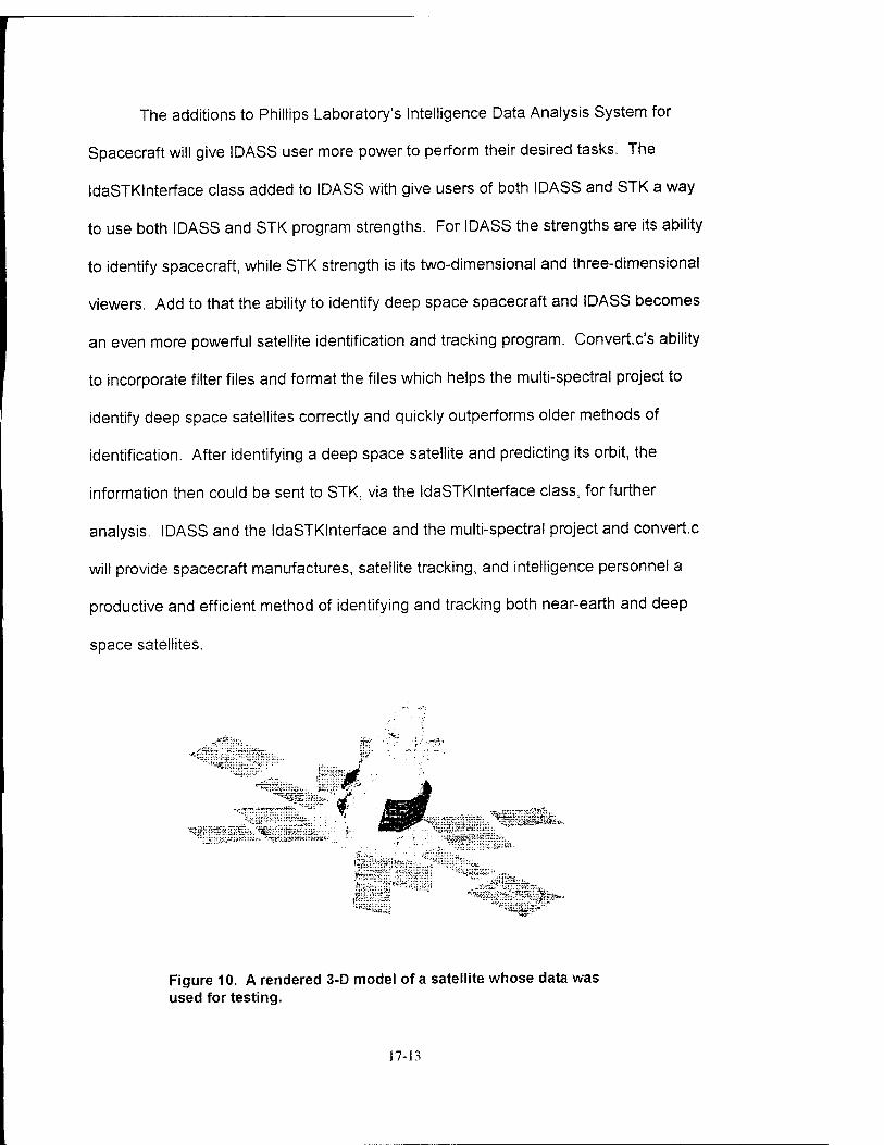
The additions to Phillips Laboratory's Intelligence Data Analysis System for

Spacecraft will give IDASS user more power to perform their desired tasks. The

IdaSTKInterface class added to IDASS with give users of both IDASS and STK a way

to use both IDASS and STK program strengths. For IDASS the strengths are its ability

to identify spacecraft, while STK strength is its two-dimensional and three-dimensional

viewers. Add to that the ability to identify deep space spacecraft and IDASS becomes

an even more powerful satellite identification and tracking program. Convertc's ability

to incorporate filter files and format the files which helps the multi-spectral project to

identify deep space satellites correctly and quickly outperforms older methods of

identification. After identifying a deep space satellite and predicting its orbit, the

information then could be sent to STK, via the IdaSTKInterface class, for further

analysis. IDASS and the IdaSTKInterface and the multi-spectral project and convert.c

will provide spacecraft manufactures, satellite tracking, and intelligence personnel a

productive and efficient method of identifying and tracking both near-earth and deep

space satellites.

-,v-y- ",>- ?:"*f!:':f^;:-... $?' ■ :

t.-' .-■^'rV

""^bl-J^'"" SBs;-:-r ..^ .t?r .,..,^p

:-=■£> :. ;:.:'*!-■ '

V ■' Tjwi.***.-™«-:-! "^r~ f&HBj TTi

^Kijjr^Tnr.rsirriE^v ': HP^J^^^'ii^:^Hil.;. -i^^l^*^'-^-^ '^: ^^-iS^.----..^""^"7^^^ ■ :: *-..-.

•" '■ ;Hi^'?#^. •z^:-''i'^-ii>''-'^~- *T£fc££äl*5pfK;?***«'*

$--\\[- ,-^"::;i::::.-_.

tv-- -. ' .. 2v? J,: ^Ty!^:':,

JJH:'wi? • !- *r^gß:®fJ$&-- ■■^^äi ̂ ■Sitö''

Figure 10. A rendered 3-D model of a satellite whose data was used for testing.

17-13

^ßt^vö t- DO-U^o - DTIC

Documents

Transcript of ^ßt^vö t- DO-U^o - DTIC