
SpringerBriefs in Computer Science Series Editors
102
-
Upload
independent -
Category
Documents
-
view
1 -
download
0
Transcript of SpringerBriefs in Computer Science Series Editors


SpringerBriefs in Computer Science
Series Editors
Stan ZdonikPeng NingShashi ShekharJonathan KatzXindong WuLakhmi C. JainDavid PaduaXuemin ShenBorko FurhtV. S. SubrahmanianMartial HebertKatsushi IkeuchiBruno Siciliano
For further volumes:http://www.springer.com/series/10028

Miles Hansard • Seungkyu LeeOuk Choi • Radu Horaud
Time-of-Flight Cameras
Principles, Methods and Applications
123

Miles HansardElectronic Engineering
and Computer ScienceQueen Mary, University of LondonLondonUK
Seungkyu LeeSamsung Advanced Institute
of TechnologyYongin-siKyonggi-doRepublic of South Korea
Ouk ChoiSamsung Advanced Institute
of TechnologyYongin-siKyonggi-doRepublic of South Korea
Radu HoraudINRIA Grenoble Rhône-AlpesMontbonnot Saint-MartinFrance
ISSN 2191-5768 ISSN 2191-5776 (electronic)ISBN 978-1-4471-4657-5 ISBN 978-1-4471-4658-2 (eBook)DOI 10.1007/978-1-4471-4658-2Springer London Heidelberg New York Dordrecht
Library of Congress Control Number: 2012950373
� Miles Hansard 2013This work is subject to copyright. All rights are reserved by the Publisher, whether the whole or part ofthe material is concerned, specifically the rights of translation, reprinting, reuse of illustrations,recitation, broadcasting, reproduction on microfilms or in any other physical way, and transmission orinformation storage and retrieval, electronic adaptation, computer software, or by similar or dissimilarmethodology now known or hereafter developed. Exempted from this legal reservation are briefexcerpts in connection with reviews or scholarly analysis or material supplied specifically for thepurpose of being entered and executed on a computer system, for exclusive use by the purchaser of thework. Duplication of this publication or parts thereof is permitted only under the provisions ofthe Copyright Law of the Publisher’s location, in its current version, and permission for use must alwaysbe obtained from Springer. Permissions for use may be obtained through RightsLink at the CopyrightClearance Center. Violations are liable to prosecution under the respective Copyright Law.The use of general descriptive names, registered names, trademarks, service marks, etc. in thispublication does not imply, even in the absence of a specific statement, that such names are exemptfrom the relevant protective laws and regulations and therefore free for general use.While the advice and information in this book are believed to be true and accurate at the date ofpublication, neither the authors nor the editors nor the publisher can accept any legal responsibility forany errors or omissions that may be made. The publisher makes no warranty, express or implied, withrespect to the material contained herein.
Printed on acid-free paper
Springer is part of Springer Science+Business Media (www.springer.com)

Preface
This book describes a variety of recent research into time-of-flight imaging.Time-of-flight cameras are used to estimate 3D scene structure directly, in a waythat complements traditional multiple-view reconstruction methods. The first twochapters of the book explain the underlying measurement principle, and examinethe associated sources of error and ambiguity. Chapters 3 and 4 are concerned withthe geometric calibration of time-of-flight cameras, particularly when used incombination with ordinary color cameras. The final chapter shows how to usetime-of-flight data in conjunction with traditional stereo matching techniques.The five chapters, together, describe a complete depth and color 3D reconstructionpipeline. This book will be useful to new researchers in the field of depth imaging,as well as to those who are working on systems that combine color and time-of-flight cameras.
v

Acknowledgments
The work presented in this book has been partially supported by a co-operativeresearch project between the 3D Mixed Reality Group at the Samsung AdvancedInstitute of Technology in Seoul, South Korea and the Perception group at INRIAGrenoble Rhône-Alpes in Montbonnot Saint-Martin, France.
The authors would like to thank Michel Amat for his contributions to Chaps. 3and 4, as well as Jan Cech and Vineet Gandhi for their contributions to Chap. 5.
vii

Contents
1 Characterization of Time-of-Flight Data . . . . . . . . . . . . . . . . . . . . 11.1 Introduction . . . . . . . . . . . . . . . . . . . . . . . . . . . . . . . . . . . . . 11.2 Principles of Depth Measurement . . . . . . . . . . . . . . . . . . . . . . 21.3 Depth-Image Enhancement . . . . . . . . . . . . . . . . . . . . . . . . . . . 3
1.3.1 Systematic Depth Error . . . . . . . . . . . . . . . . . . . . . . . . 41.3.2 Nonsystematic Depth Error . . . . . . . . . . . . . . . . . . . . . 51.3.3 Motion Blur . . . . . . . . . . . . . . . . . . . . . . . . . . . . . . . . 5
1.4 Evaluation of Time-of-Flight and Structured-Light Data. . . . . . . 121.4.1 Depth Sensors. . . . . . . . . . . . . . . . . . . . . . . . . . . . . . . 131.4.2 Standard Depth Data Set . . . . . . . . . . . . . . . . . . . . . . . 141.4.3 Experiments and Analysis . . . . . . . . . . . . . . . . . . . . . . 181.4.4 Enhancement . . . . . . . . . . . . . . . . . . . . . . . . . . . . . . . 22
1.5 Conclusions . . . . . . . . . . . . . . . . . . . . . . . . . . . . . . . . . . . . . 25References . . . . . . . . . . . . . . . . . . . . . . . . . . . . . . . . . . . . . . . . . . 26
2 Disambiguation of Time-of-Flight Data . . . . . . . . . . . . . . . . . . . . . 292.1 Introduction . . . . . . . . . . . . . . . . . . . . . . . . . . . . . . . . . . . . . 292.2 Phase Unwrapping from a Single Depth Map . . . . . . . . . . . . . . 30
2.2.1 Deterministic Methods. . . . . . . . . . . . . . . . . . . . . . . . . 352.2.2 Probabilistic Methods . . . . . . . . . . . . . . . . . . . . . . . . . 362.2.3 Discussion . . . . . . . . . . . . . . . . . . . . . . . . . . . . . . . . . 38
2.3 Phase Unwrapping from Multiple Depth Maps . . . . . . . . . . . . . 382.3.1 Single-Camera Methods . . . . . . . . . . . . . . . . . . . . . . . . 392.3.2 Multicamera Methods . . . . . . . . . . . . . . . . . . . . . . . . . 402.3.3 Discussion . . . . . . . . . . . . . . . . . . . . . . . . . . . . . . . . . 42
2.4 Conclusions . . . . . . . . . . . . . . . . . . . . . . . . . . . . . . . . . . . . . 42References . . . . . . . . . . . . . . . . . . . . . . . . . . . . . . . . . . . . . . . . . . 43
ix

3 Calibration of Time-of-Flight Cameras . . . . . . . . . . . . . . . . . . . . . 453.1 Introduction . . . . . . . . . . . . . . . . . . . . . . . . . . . . . . . . . . . . . 453.2 Camera Model . . . . . . . . . . . . . . . . . . . . . . . . . . . . . . . . . . . 463.3 Board Detection . . . . . . . . . . . . . . . . . . . . . . . . . . . . . . . . . . 46
3.3.1 Overview . . . . . . . . . . . . . . . . . . . . . . . . . . . . . . . . . . 483.3.2 Preprocessing . . . . . . . . . . . . . . . . . . . . . . . . . . . . . . . 493.3.3 Gradient Clustering . . . . . . . . . . . . . . . . . . . . . . . . . . . 493.3.4 Local Coordinates . . . . . . . . . . . . . . . . . . . . . . . . . . . . 513.3.5 Hough Transform . . . . . . . . . . . . . . . . . . . . . . . . . . . . 513.3.6 Hough Analysis . . . . . . . . . . . . . . . . . . . . . . . . . . . . . 533.3.7 Example Results . . . . . . . . . . . . . . . . . . . . . . . . . . . . . 55
3.4 Conclusions . . . . . . . . . . . . . . . . . . . . . . . . . . . . . . . . . . . . . 56References . . . . . . . . . . . . . . . . . . . . . . . . . . . . . . . . . . . . . . . . . . 58
4 Alignment of Time-of-Flight and Stereoscopic Data. . . . . . . . . . . . 594.1 Introduction . . . . . . . . . . . . . . . . . . . . . . . . . . . . . . . . . . . . . 594.2 Methods . . . . . . . . . . . . . . . . . . . . . . . . . . . . . . . . . . . . . . . . 62
4.2.1 Projective Reconstruction. . . . . . . . . . . . . . . . . . . . . . . 634.2.2 Range Fitting . . . . . . . . . . . . . . . . . . . . . . . . . . . . . . . 634.2.3 Point-Based Alignment . . . . . . . . . . . . . . . . . . . . . . . . 644.2.4 Plane-Based Alignment . . . . . . . . . . . . . . . . . . . . . . . . 664.2.5 Multisystem Alignment . . . . . . . . . . . . . . . . . . . . . . . . 68
4.3 Evaluation . . . . . . . . . . . . . . . . . . . . . . . . . . . . . . . . . . . . . . 694.3.1 Calibration Error. . . . . . . . . . . . . . . . . . . . . . . . . . . . . 704.3.2 Total Error . . . . . . . . . . . . . . . . . . . . . . . . . . . . . . . . . 70
4.4 Conclusions . . . . . . . . . . . . . . . . . . . . . . . . . . . . . . . . . . . . . 72References . . . . . . . . . . . . . . . . . . . . . . . . . . . . . . . . . . . . . . . . . . 74
5 A Mixed Time-of-Flight and Stereoscopic Camera System. . . . . . . 775.1 Introduction . . . . . . . . . . . . . . . . . . . . . . . . . . . . . . . . . . . . . 77
5.1.1 Related Work . . . . . . . . . . . . . . . . . . . . . . . . . . . . . . . 785.1.2 Chapter Contributions . . . . . . . . . . . . . . . . . . . . . . . . . 81
5.2 The Proposed ToF-Stereo Algorithm . . . . . . . . . . . . . . . . . . . . 825.2.1 The Growing Procedure . . . . . . . . . . . . . . . . . . . . . . . . 825.2.2 ToF Seeds and Their Refinement . . . . . . . . . . . . . . . . . 835.2.3 Similarity Statistic Based on Sensor Fusion . . . . . . . . . . 86
5.3 Experiments . . . . . . . . . . . . . . . . . . . . . . . . . . . . . . . . . . . . . 885.3.1 Real-Data Experiments . . . . . . . . . . . . . . . . . . . . . . . . 885.3.2 Comparison Between ToF Map and Estimated
Disparity Map . . . . . . . . . . . . . . . . . . . . . . . . . . . . . . 905.3.3 Ground-Truth Evaluation . . . . . . . . . . . . . . . . . . . . . . . 915.3.4 Computational Costs . . . . . . . . . . . . . . . . . . . . . . . . . . 92
5.4 Conclusions . . . . . . . . . . . . . . . . . . . . . . . . . . . . . . . . . . . . . 94References . . . . . . . . . . . . . . . . . . . . . . . . . . . . . . . . . . . . . . . . . . 94
x Contents

Chapter 1Characterization of Time-of-Flight Data
Abstract This chapter introduces the principles and difficulties of time-of-flightdepth measurement. The depth images that are produced by time-of-flight cam-eras suffer from characteristic problems, which are divided into the following twoclasses. First, there are systematic errors, such as noise and ambiguity, which aredirectly related to the sensor. Second, there are nonsystematic errors, such as scat-tering and motion blur, which are more strongly related to the scene content. It isshown that these errors are often quite different from those observed in ordinary colorimages. The case of motion blur, which is particularly problematic, is examined indetail. A practical methodology for investigating the performance of depth camerasis presented. Time-of-flight devices are compared to structured-light systems, andthe problems posed by specular and translucent materials are investigated.
Keywords Depth-cameras · Time-of-Flight principle ·Motion blur · Depth errors
1.1 Introduction
Time-of-Flight (tof) cameras produce a depth image, each pixel of which encodesthe distance to the corresponding point in the scene. These cameras can be usedto estimate 3D structure directly, without the help of traditional computer-visionalgorithms. There are many practical applications for this new sensing modality,including robot navigation [31, 37, 50], 3D reconstruction [17], and human–machineinteraction [9, 45]. Tof cameras work by measuring the phase delay of reflectedinfrared (IR) light. This is not the only way to estimate depth; for example, anIR structured-light pattern can be projected onto the scene, in order to facilitatevisual triangulation [44]. Devices of this type, such as the Kinect [12], share manyapplications with tof cameras [8, 33, 34, 36, 43].
M. Hansard et al., Time-of-Flight Cameras, SpringerBriefs in Computer Science, 1DOI: 10.1007/978-1-4471-4658-2_1, © Miles Hansard 2013
2 1 Characterization of Time-of-Flight Data
The unique sensing architecture of the tof camera means that a raw depth imagecontains both systematic and nonsystematic bias that has to be resolved for robustdepth imaging [11]. Specifically, there are problems of low depth precision and lowspatial resolution, as well as errors caused by radiometric, geometric, and illumina-tion variations. For example, measurement accuracy is limited by the power of theemitted IR signal, which is usually rather low compared to daylight, such that thelatter contaminates the reflected signal. The amplitude of the reflected IR also variesaccording to the material and color of the object surface.
Another critical problem with tof depth images is motion blur, caused by eithercamera or object motion. The motion blur of tof data shows unique characteristics,compared to that of conventional color cameras. Both the depth accuracy and theframe rate are limited by the required integration time of the depth camera. Longerintegration time usually allows higher accuracy of depth measurement. For staticobjects, we may therefore want to decrease the frame rate in order to obtain highermeasurement accuracies from longer integration times. On the other hand, capturinga moving object at fixed frame rate imposes a limit on the integration time.
In this chapter, we discuss depth-image noise and error sources, and performa comparative analysis of tof and structured-light systems. First, the tof depth-measurement principle will be reviewed.
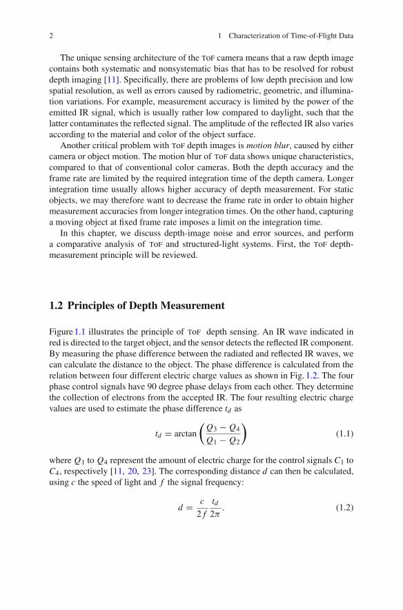
1.2 Principles of Depth Measurement
Figure 1.1 illustrates the principle of tof depth sensing. An IR wave indicated inred is directed to the target object, and the sensor detects the reflected IR component.By measuring the phase difference between the radiated and reflected IR waves, wecan calculate the distance to the object. The phase difference is calculated from therelation between four different electric charge values as shown in Fig. 1.2. The fourphase control signals have 90 degree phase delays from each other. They determinethe collection of electrons from the accepted IR. The four resulting electric chargevalues are used to estimate the phase difference td as
td = arctan
(Q3 − Q4
Q1 − Q2
)(1.1)
where Q1 to Q4 represent the amount of electric charge for the control signals C1 toC4, respectively [11, 20, 23]. The corresponding distance d can then be calculated,using c the speed of light and f the signal frequency:
d = c
2 f
td2π
. (1.2)

1.2 Principles of Depth Measurement 3
Fig. 1.1 The principle of tof depth camera [11, 20, 23]: the phase delay between emitted andreflected IR signals are measured to calculate the distance from each sensor pixel to target objects
Fig. 1.2 Depth can be calculated by measuring the phase delay between radiated and reflected IRsignals. The quantities Q1 to Q4 represent the amount of electric charge for control signals C1 toC4 respectively
Here, the quantity c/(2 f ) is the maximum distance that can be measured withoutambiguity, as will be explained in Chap. 2.
1.3 Depth-Image Enhancement
This section describes the characteristic sources of error in tof imaging. Some meth-ods for reducing these errors are discussed. The case of motion blur, which is partic-ularly problematic, is considered in detail.

4 1 Characterization of Time-of-Flight Data
Fig. 1.3 Systematic noise and error: these errors come from the tof principle of depth measurement.a Integration time error: longer integration time shows higher depth accuracy (right) than shorterintegration time (left). b IR amplitude error: 3D points of the same depth (chessboard on theleft) show different IR amplitudes (chessboard on the right) according to the color of the targetobject
1.3.1 Systematic Depth Error
From the principle and architecture of tof sensing, depth cameras suffer from severalsystematic errors such as IR demodulation error, integration time error, amplitudeambiguity, and temperature error [11]. As shown in Fig. 1.3a, longer integrationincreases signal-to-noise ratio, which, however, is also related to the frame rate.Figure 1.3b shows that the amplitude of the reflected IR signal varies according tothe color of the target object as well as the distance from the camera. The ambiguityof IR amplitude introduces noise into the depth calculation.

1.3 Depth-Image Enhancement 5
1.3.2 Nonsystematic Depth Error
Light scattering [32] gives rise to artifacts in the depth image, due to the low sensitivityof the device. As shown in Fig. 1.4a, close objects (causing IR saturation) in the lowerright part of the depth image introduce depth distortion in other regions, as indicatedby dashed circles. Multipath error [13] occurs when a depth calculation in a sensorpixel is an superposition of multiple reflected IR signals. This effect becomes seriousaround the concave corner region as shown in Fig. 1.4b. Object boundary ambiguity[35] becomes serious when we want to reconstruct a 3D scene based on the depthimage. Depth pixels near boundaries fall in between foreground and background,giving rise to 3D structure distortion.
1.3.3 Motion Blur
Motion blur, caused by camera or target object motions, is a critical error sourcefor online 3D capturing and reconstruction with tof cameras. Because the 3D depthmeasurement is used to reconstruct the 3D geometry of scene, blurred regions ina depth image lead to serious distortions in the subsequent 3D reconstruction. Inthis section, we study the theory of tof depth sensors and analyze how motion bluroccurs, and what it looks like. Due the its unique sensing architecture, motion blurin the tof depth camera is quite different from that of color cameras, which meansthat existing deblurring methods are inapplicable.
The motion blur observed in a depth image has a different appearance from thatin a color image. Color motion blur shows smooth color transitions between fore-ground and background regions [46, 47, 51]. On the other hand, depth motion blurtends to present overshoot or undershoot in depth-transition regions. This is due tothe different sensing architecture in tof cameras, as opposed to conventional colorcameras. The tof depth camera emits an IR signal of a specific frequency, and mea-sures the phase difference between the emitted and reflected IR signals to obtainthe depth from the camera to objects. While calculating the depth value from theIR measurements, we need to perform a nonlinear transformation. Due to this archi-tectural difference, the smooth error in phase measurement can cause uneven errorterms, such as overshoot or undershoot. As a result, such an architectural differ-ence between depth and color cameras makes the previous color image deblurringalgorithms inapplicable to depth images.
Special cases of this problem have been studied elsewhere. Hussmann et al. [19]introduce a motion blur detection technique on a conveyor belt, in the presence ofa single directional motion. Lottner et al. [28] propose an internal sensor controlsignal based blur detection method that is inappropriate in general settings. Lindneret al. [26] model the tof motion blur in the depth image, to compensate for theartifact. However, they introduce a simple blur case without considering the tof

6 1 Characterization of Time-of-Flight Data
Fig. 1.4 Nonsystematic noise and error: based on the depth-sensing principle, scene structure maycause characteristic errors. a Light scattering: IR saturation in the lower right part of the depthimage causes depth distortion in other parts, as indicated by dashed circles. b Multipath error: theregion inside the concave corner is affected, and shows distorted depth measurements. c Objectboundary ambiguity: several depth points on an object boundary are located in between foregroundand background, resulting in 3D structure distortion

1.3 Depth-Image Enhancement 7
Fig. 1.5 tof depth motion-blur due to movement of the target object
principle of depth sensing. Lee et al. [24, 25] examine the principle of tof depthblur artifacts, and propose systematic blur detection and deblurring methods.
Based on the depth-sensing principle, we will investigate how motion blur occurs,and what are its characteristics. Let us assume that any motion from camera or objectoccurs during the integration time, which changes the phase difference of the reflectedIR as indicated by the gray color in Fig. 1.2. In order to collect enough electric chargeQ1 to Q4 to calculate depth (1.1), we have to maintain a sufficient integration time.According to the architecture type, integration time can vary, but the integration timeis the major portion of the processing time. Suppose that n cycles are used for thedepth calculation. In general, we repeat the calculation n times during the integrationtime to increase the signal-to-noise ratio, and so
td = arctan
(nQ3 − nQ4
nQ1 − nQ2
)(1.3)
where Q1 to Q4 represent the amount of electric charge for the control signals C1to C4, respectively (cf. Eq. 1.1 and Fig. 1.2). The depth calculation formulation (1.3)expects that the reflected IR during the integration time comes from a single 3D pointof the scene. However, if there is any camera or object motion during the integrationtime, the calculated depth will be corrupted. Figure 1.5 shows an example of thissituation. The red dot represents a sensor pixel of the same location. Due the motionof the chair, the red dot sees both foreground and background sequentially withinits integration time, causing a false depth calculation as shown in the third imagein Fig. 1.5. The spatial collection of these false-depth points looks like blur aroundmoving object boundaries, where significant depth changes are present.
Figure 1.6 illustrates what occurs at motion blur pixels in the ‘2-tab’ architecture,where only two electric charge values are available. In other words, only Q1 − Q2and Q3 − Q4 values are stored, instead of all separate Q values. Figure 1.6a is thecase where no motion blur occurs. In the plot of Q1 − Q2 versus Q3 − Q4 in thethird column, all possible regular depth values are indicated by blue points, making adiamond shape. If there is a point deviating from it, as an example shown in Fig. 1.6b,it means that their is a problem in between the charge values Q1 to Q4. As we alreadyexplained in Fig. 1.2, this happens when there exist multiple reflected signals withdifferent phase values. Let us assume that a new reflected signal, of a different phasevalue, comes in from the mth cycle out of a total of n cycles during the first half orsecond half of the integration time. A new depth is then obtained as

8 1 Characterization of Time-of-Flight Data
(a)
(b)
Fig. 1.6 tof depth-sensing and temporal integration
td(m) = arctan
(nQ3 − nQ4
(m Q1 + (n − m)Q1)− (m Q2 + (n − m)Q2)
)(1.4)
td(m) = arctan
((m Q3 + (n − m)Q3)− (m Q4 + (n − m)Q4)
nQ1 − nQ2
)(1.5)
in the first or second half of the integration time, respectively. Using the depth calcula-tion formulation Eq. (1.1), we simulate all possible blur models. Figure 1.7 illustratesseveral examples of depth images taken by tof cameras, having depth value tran-sitions in motion blur regions. Actual depth values along the blue and red cuts ineach image are presented in the following plots. The motion blurs of depth images inthe middle show unusual peaks (blue cut) which cannot be observed in conventionalcolor motion blur. Figure 1.8 shows how motion blur appears in 2-tap case. In thesecond phase where control signals C3 and C4 collect electric charges, the reflectedIR signal is a mixture of background and foreground. Unlike color motion blurs,depth motion blurs often show overshoot or undershoot in their transition betweenforeground and background regions. This means that motion blurs result in higheror lower calculated depth than all near foreground and background depth values, asdemonstrated in Fig. 1.9.
In order to verify this characteristic situation, we further investigate the depthcalculation formulation in Eq. 1.5. First, we re-express Eq. 1.4 as

1.3 Depth-Image Enhancement 9
Fig. 1.7 Sample depth value transitions from depth motion blur images captured by an SR4000tof camera
Fig. 1.8 Depth motion blur in 2-tap case
td(m) = arctan
(nQ3 − nQ4
m(Q1 − Q1 − Q2 + Q2)+ n(Q1 − Q2)
)(1.6)
The first derivative of the Eq. 1.6 is zero, meaning local maxima or local minima,under the following conditions:

10 1 Characterization of Time-of-Flight Data
Fig. 1.9 tof depth motion blur simulation results
t ′d(m) = 1
1+(
nQ3−nQ4
m(Q1−Q1−Q2+Q2)+n(Q1−Q2)
)2 (1.7)
= (m(Q1 − Q1 − Q2 + Q2)+ n(Q1 − Q2))2
(nQ3 − nQ4)2 + (m(Q1 − Q1 − Q2 + Q2)+ n(Q1 − Q2))2= 0
m = nQ2 − Q1
Q1 − Q1 − Q2 + Q2= n
1− 2Q1
2Q1 − 2Q1(1.8)
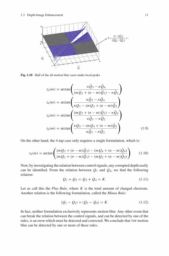
Figure 1.10 shows that statistically half of all cases have overshoots or under-shoots. In a similar manner, the motion blur model of 1-tap (Eq. 1.9) and 4-tap(Eq. 1.10) cases can be derived. Because a single memory is assigned for recordingthe electric charge value of four control signals, the 1-tap case has four differentformulations upon each phase transition:
1.3 Depth-Image Enhancement 11
Fig. 1.10 Half of the all motion blur cases make local peaks
td(m) = arctan
(nQ3 − nQ4
(m Q1 + (n − m)Q1)− nQ2
)
td(m) = arctan
(nQ3 − nQ4
nQ1 − (m Q2 + (n − m)Q2
)
td(m) = arctan
((m Q3 + (n − m)Q3)− nQ4
nQ1 − nQ2
)
td(m) = arctan
(nQ3 − (m Q4 + (n − m)Q4
nQ1 − nQ2
)(1.9)
On the other hand, the 4-tap case only requires a single formulation, which is:
td(m) = arctan
((m Q3 + (n − m)Q3)− (m Q4 + (n − m)Q4)
(m Q1 + (n − m)Q1)− (m Q2 + (n − m)Q2)
)(1.10)
Now, by investigating the relation between control signals, any corrupted depth easilycan be identified. From the relation between Q1 and Q4, we find the followingrelation:
Q1 + Q2 = Q3 + Q4 = K . (1.11)
Let us call this the Plus Rule, where K is the total amount of charged electrons.Another relation is the following formulation, called the Minus Rule:
|Q1 − Q2| + |Q3 − Q4| = K . (1.12)
In fact, neither formulation exclusively represents motion blur. Any other event thatcan break the relation between the control signals, and can be detected by one of therules, is an error which must be detected and corrected. We conclude that tof motionblur can be detected by one or more of these rules.

12 1 Characterization of Time-of-Flight Data
(a)
(b)
Fig. 1.11 Depth-image motion blur detection results by the proposed method. a Depth images withmotion blur. b Intensity images with detected motion blur regions (indicated by white color)
Figure 1.11a shows depth-image samples with motion blur artifacts due to variousobject motions such as rigid body, multiple body, and deforming body motions,respectively. Motion blur occurs not just around object boundaries; inside an object,any depth differences that are observed within the integration time will also causemotion blur. Figure 1.11b shows detected motion blur regions indicated by whitecolor on respective depth and intensity images, by the method proposed in [24].This is very straightforward but effective and fast method, which is fit for hardwareimplementation without any additional frame memory or processing time.
1.4 Evaluation of Time-of-Flight and Structured-Light Data
The enhancement of tof and structured-light (e.g., Kinect [44]) data is an importanttopic, owing to the physical limitations of these devices (as described in Sect. 1.3).The characterization of depth noise, in relation to the particular sensing architecture,is a major issue. This can be addressed using bilateral [49] or nonlocal [18] filters,or in wavelet space [10], using prior knowledge of the spatial noise distribution.Temporal filtering [30] and video-based [8] methods have also been proposed.

1.4 Evaluation of Time-of-Flight and Structured-Light Data 13
The upsampling of low-resolution depth images is another critical issue. Oneapproach is to apply color super-resolution methods on tof depth images directly[40]. Alternatively, a high-resolution color image can be used as a reference fordepth super resolution [1, 48]. The denoising and upsampling problems can also beaddressed together [2], and in conjunction with high-resolution monocular [34] orbinocular [7] color images.
It is also important to consider the motion artifacts [28] and multipath [13] prob-lems which are characteristic of tof sensors. The related problem of tof depthconfidence has been addressed using random-forest methods [35]. Other issues withtof sensors include internal and external calibration [14, 16, 27], as well as rangeambiguity [4]. In the case of Kinect, a unified framework of dense depth data extrac-tion and 3D reconstruction has been proposed [33].
Despite the increasing interest in active depth sensors, there are many unresolvedissues regarding the data produced by these devices, as outlined above. Furthermore,the lack of any standardized data sets, with ground truth, makes it difficult to makequantitative comparisons between different algorithms.
The Middlebury stereo [38], multiview [41], and Stanford 3D scan [6] data sethave been used for the evaluation of depth-image denoising, upsampling, and 3Dreconstruction methods. However, these data sets do not provide real depth imagestaken by either tof or structured-light depth sensors, and consist of illumination con-trolled diffuse material objects. While previous depth accuracy enhancement methodsdemonstrate their experimental results on their own data set, our understanding of theperformance and limitations of existing algorithms will remain partial without anyquantitative evaluation against a standard data set. This situation hinders the wideradoption and evolution of depth-sensor systems.
In this section, we propose a performance evaluation framework for both tofand structured-light depth images, based on carefully collected depth maps and theirground truth images. First, we build a standard depth data set; calibrated depth imagescaptured by a tof depth camera and a structured-light system. Ground truth depth isacquired from a commercial 3D scanner. The data set spans a wide range of objects,organized according to geometric complexity (from smooth to rough), as well asradiometric complexity (diffuse, specular, translucent, and subsurface scattering).We analyze systematic and nonsystematic error sources, including the accuracy andsensitivity with respect to material properties. We also compare the characteristicsand performance of the two different types of depth sensors, based on extensiveexperiments and evaluations. Finally, to justify the usefulness of the data set, we useit to evaluate simple denoising, super resolution, and inpainting algorithms.
1.4.1 Depth Sensors
As described in Sect. 1.2, the tof depth sensor emits IR waves to target objects, andmeasures the phase delay of reflected IR waves at each sensor pixel, to calculate thedistance traveled. According to the color, reflectivity, and geometric structure of the
14 1 Characterization of Time-of-Flight Data
target object, the reflected IR light shows amplitude and phase variations, causingdepth errors. Moreover, the amount of IR is limited by the power consumption of thedevice, and therefore the reflected IR suffers from low signal-to-noise ratio (SNR).To increase the SNR, tof sensors bind multiple sensor pixels to calculate a singledepth pixel value, which decreases the effective image size. Structured-light depthsensors project an IR pattern onto target objects, which provides a unique illuminationcode for each surface point observed at by a calibrated IR imaging sensor. Once thecorrespondence between IR projector and IR sensor is identified by stereo matchingmethods, the 3D position of each surface point can be calculated by triangulation.
In both sensor types, reflected IR is not a reliable cue for all surface materials. Forexample, specular materials cause mirror reflection, while translucent materials causeIR refraction. Global illumination also interferes with the IR sensing mechanism,because multiple reflections cannot be handled by either sensor type.
1.4.2 Standard Depth Data Set
A range of commercial tof depth cameras have been launched in the market, suchas PMD, PrimeSense, Fotonic, ZCam, SwissRanger, 3D MLI, and others. Kinectis the first widely successful commercial product to adopt the IR structured-lightprinciple. Among many possibilities, we specifically investigate two depth cameras:a tof type SR4000 from MESA Imaging [29], and a structured-light type MicrosoftKinect [43]. We select these two cameras to represent each sensor since they are themost popular depth cameras in the research community, accessible in the market andreliable in performance.
Heterogeneous Camera Set
We collect the depth maps of various real objects using the SR4000 and Kinectsensors. To obtain the ground truth depth information, we use a commercial 3Dscanning device. As shown in Fig. 1.12, we place the camera set approximately1.2 m away from the object of interest. The wall behind the object is located about1.5 m away from the camera set. The specification of each device is as follows.
Mesa SR4000. This is a tof type depth sensor producing a depth map and amplitudeimage at the resolution of 176× 144 with 16 bit floating-point precision. The ampli-tude image contains the reflected IR light corresponding to the depth map. In additionto the depth map, it provides {x, y, z} coordinates, which correspond to each pixel inthe depth map. The operating range of the SR4000 is 0.8–10.0 m, depending on themodulation frequency. The field of view (FOV) of this device is 43× 34 degrees.
Kinect. This is a structured IR light type depth sensor, composed of an IR emitter, IRsensor, and color sensor, providing the IR amplitude image, the depth map, and thecolor image at the resolution of 640× 480 (maximum resolution for amplitude and

1.4 Evaluation of Time-of-Flight and Structured-Light Data 15
Fig. 1.12 Heterogeneous camera setup for depth sensing
depth image) or 1600× 1200 (maximum resolution for RGB image). The operatingrange is between 0.8 and 3.5 m, the spatial resolution is 3 mm at 2 m distance, andthe depth resolution is 10 mm at 2 m distance. The FOV is 57× 43 degrees.
FlexScan3D. We use a structured-light 3D scanning system for obtaining groundtruth depth. It consists of an LCD projector and two color cameras. The LCD projectorilluminates coded pattern at 1024 × 768 resolution, and each color camera recordsthe illuminated object at 2560× 1920 resolution.
Capturing Procedure for Test Images
The important property of the data set is that the measured depth data is aligned withground truth information, and with that of the other sensor. Each depth sensor has tobe fully calibrated internally and externally. We employ a conventional camera cali-bration method [52] for both depth sensors and the 3D scanner. Intrinsic calibrationparameters for the tof sensors are known. Given the calibration parameters, we cantransform ground truth depth maps onto each depth sensor space. Once the system iscalibrated, we proceed to capture the objects of interest. For each object, we recorddepth (ToFD) and intensity (ToFI) images from the SR4000, plus depth (SLD) andcolor (SLC) from the Kinect. Depth captured by the FlexScan3D is used as groundtruth (GTD), as explained in more detail below (Fig. 1.13).
Data Set
We select objects that show radiometric variations (diffuse, specular, and translucent),as well as geometric variations (smooth or rough). The total 36-item test set is divided

16 1 Characterization of Time-of-Flight Data
Fig. 1.13 Sample raw image set of depth and ground truth. a GTD, b ToFD, c SLD, d Object,e ToFI, f SLC
into three subcategories: diffuse material objects (class A), specular material objects(class B), and translucent objects with subsurface scattering (class C), as in Fig. 1.15.Each class demonstrates geometric variation from smooth to rough surfaces (a smallerlabel number means a smoother surface).
From diffuse, through specular to translucent materials, the radiometric represen-tation becomes more complex, requiring a high-dimensional model to predict theappearance. In fact, the radiometric complexity also increases the level of challengesin recovering its depth map. This is because the complex illumination interferes withthe sensing mechanism of most depth devices. Hence, we categorize the radiometriccomplexity by three classes, representing the level of challenges posed by materialvariation. From smooth to rough surfaces, the geometric complexity is increased,especially due to mesostructure scale variation.
Ground Truth
We use a 3D scanner for ground truth depth acquisition. The principle of this sys-tem is similar to [39]; using illumination patterns and solving correspondences andtriangulating between matching points to compute the 3D position of each surfacepoint. Simple gray illumination patterns are used, which gives robust performancein practice. However, the patterns cannot be seen clearly enough to provide corre-spondences for non-Lambertian objects [3]. Recent approaches [15] suggest newhigh-frequency patterns, and present improvement in recovering depth in the pres-

1.4 Evaluation of Time-of-Flight and Structured-Light Data 17
Original objects After matt spray
Fig. 1.14 We apply white matt spray on top of non-Lambertian objects for ground truth depthacquisition. Original objects after matt spray
Fig. 1.15 Test images categorized by their radiometric and geometric characteristics: class A diffusematerial objects (13 images), class B specular material objects (11 images), and class C translucentobjects with subsurface scattering (12 images)
ence of global illumination. Among all surfaces, the performance of structured-lightscanning systems is best for Lambertian materials.
The data set includes non-Lambertian materials presenting various illuminationeffects; specular, translucent, and subsurface scattering. To employ the 3D scannersystem for ground truth depth acquisition of the data set, we apply white matt sprayon top of each object surface, so that we can give each object a Lambertian surface

18 1 Characterization of Time-of-Flight Data
while we take ground truth depth Fig. 1.14. To make it clear that the spray particlesdo not change the surface geometry, we have compared the depth maps captured bythe 3D scanner before and after the spray on a Lambertian object. We observe thatthe thickness of spray particles is below the level of the depth-sensing precision,meaning that the spray particles do not affect on the accuracy of the depth map inpractice. Using this methodology, we are able to obtain ground truth depth for non-Lambertian objects. To ensure the level of ground truth depth, we capture the depthmap of a white board. Then, we apply RANSAC to fit a plane to the depth map andmeasure the variation of scan data from the plane. We observe that the variation isless than 200µm, which is negligible compared to depth sensor errors. Finally, weadopt the depth map from the 3D scanner as the ground truth depth, for quantitativeevaluation and analysis.
1.4.3 Experiments and Analysis
In this section, we investigate the depth accuracy, the sensitivity to various differentmaterials, and the characteristics of the two types of sensors.
Depth Accuracy and Sensitivity
Given the calibration parameters, we project the ground truth depth map onto eachsensor space, in order to achieve viewpoint alignment (Fig. 1.12). Due to the res-olution difference, multiple pixels of the ground truth depth fall into each sensorpixel. We perform a bilinear interpolation to find corresponding ground truth depthfor each sensor pixel. Due to the difference of field of view and occluded regions,not all sensor pixels get corresponding ground truth depth. We exclude these pixelsand occlusion boundaries from the evaluation.
According to previous work [21, 42] and manufacturer reports on the accuracyof depth sensors, the root-mean-square error (RMSE) of depth measurements isapproximately 5–20 mm at the distance of 1.5 m. These figures cannot be generalizedfor all materials, illumination effects, complex geometry, and other factors. The useof more general objects and environmental conditions invariably results in higherRMSE of depth measurement than reported numbers. When we tested with a whitewall, which is similar to the calibration object used in previous work [42], we obtainapproximately 10.15 mm at the distance of 1.5 m. This is comparable to the previousempirical study and reported numbers.
Because only foreground objects are controlled, the white background is seg-mented out for the evaluation. The foreground segmentation is straightforwardbecause the background depth is clearly separated from that of foreground. InFigs. 1.16, 1.17 and 1.18, we plot depth errors (RMSE) and show difference maps(8 bit) between the ground truth and depth measurement. In the difference maps,gray indicates zero difference, whereas a darker (or brighter) value indicates that the

1.4 Evaluation of Time-of-Flight and Structured-Light Data 19
Fig. 1.16 Tof depth accuracy in RMSE (root mean square) for class A. The RMSE values and theircorresponding difference maps are illustrated. 128 in difference map represents zero differencewhile 129 represents the ground truth is 1 mm larger than the measurement. Likewise, 127 indicatesthat the ground truth is 1 mm smaller than the measurement
ground truth is smaller (or larger) than the estimated depth. The range of differencemap, [0, 255], spans [−128 mm, 128 mm] in RMSE.
Several interesting observations can be made from the experiments. First, weobserve that the accuracy of depth values varies substantially according to the mate-rial property. As shown in Fig. 1.16, the average RMSE of class A is 26.80 mmwith 12.81 mm of standard deviation, which is significantly smaller than the overallRMSE. This is expected, because class A has relatively simple properties, whichare well approximated by the Lambertian model. From Fig. 1.17 for class B, we areunable to obtain the depth measurements on specular highlights. These highlightseither prevent the IR reflection back to the sensor, or cause the reflected IR to satu-rate the sensor. As a result, the measured depth map shows holes, introducing a largeamount of errors. The RMSE for class B is 110.79 mm with 89.07 mm of standarddeviation. Class C is the most challenging subset, since it presents the subsurfacescattering and translucency. As expected, upon the increase in the level of translu-cency, the measurement error is dramatically elevated as illustrated in Fig. 1.18.

20 1 Characterization of Time-of-Flight Data
Fig. 1.17 Tof depth accuracy in RMSE (root mean square) for class B. The RMSE values and theircorresponding difference maps are illustrated
One thing to note is that the error associated with translucent materials differsfrom that associated with specular materials. We still observe some depth valuesfor translucent materials, whereas the specular materials show holes in the depthmap. The measurement on translucent materials is incorrect, often producing largerdepth than the ground truth. Such a drift appears because the depth measurementson translucent materials are the result of both translucent foreground surface and thebackground behind. As a result, the corresponding measurement points lie some-where between the foreground and the background surfaces.
Finally, the RMSE for class C is 148.51 mm with 72.19 mm of standard devia-tion. These experimental results are summarized in Table 1.1. Interestingly, the accu-racy is not so much dependent on the geometric complexity of the object. Focusingon class A, although A-11, A-12, and A-13 possess complicated and uneven sur-face geometry, the actual accuracy is relatively good. Instead, we find that the errorincreases as the surface normal deviates from the optical axis of the sensor. In fact,a similar problem has been addressed by [22], in that the orientation is the source

1.4 Evaluation of Time-of-Flight and Structured-Light Data 21
Fig. 1.18 Tof depth accuracy in RMSE (root mean square) for class C. The RMSE values and theircorresponding difference maps are illustrated
of systematic error in sensor measurement. In addition, surfaces where the globalillumination occurs due to multipath IR transport (such as the concave surfaces onA-5, A-6, A-10 of Class A) exhibit erroneous measurements.
Due to its popular application in games and human computer interaction, manyresearchers have tested and reported the result of Kinect applications. One of commonobservation is that the Kinect presents some systematic error with respect to distance.However, there has been no in-depth study on how the Kinect works on varioussurface materials. We measure the depth accuracy of Kinect using the data set, andillustrate the results in Figs. 1.16, 1.17 and 1.18.
Overall RMSE is 191.69 mm, with 262.19 mm of standard deviation. Although theoverall performance is worse than that of tof sensor, it provides quite accurate resultsfor class A. From the experiments, it is clear that material properties are stronglycorrelated with depth accuracy. The RMSE for class A is 13.67 mm with 9.25 mmof standard deviation. This is much smaller than the overall RMSE, 212.56 mm.However, the error dramatically increases in class B (303.58 mm with 249.26 mm ofdeviation). This is because the depth values for specular materials cause holes in thedepth map, similar to the behavior of the tof sensor.
From the experiments on class C, we observe that the depth accuracy drops sig-nificantly upon increasing the level of translucency, especially starting at the objectC-8. In the graph shown in Fig. 1.18, one can observe that the RMSE is reduced witha completely transparent object (C-12, a pure water). It is because caustic effects

22 1 Characterization of Time-of-Flight Data
Table 1.1 Depth accuracy upon material properties. Class A: diffuse, Class B: specular, Class C:translucent. See Fig. 1.15 for illustration
Overall Class A Class B Class C
ToF 83.10 29.68 93.91 131.07(76.25) (10.95) (87.41) (73.65)
Kinect 170.153 13.67 235.30 279.96(282.25) (9.25) (346.44) (312.97)
Root-mean-square error (standard deviation) in mm
Table 1.2 Depth accuracy before/after bilateral filtering and superresolution for class A. SeeFig. 1.19 for illustration
Original RMSE Bilateral filtering Bilinear interpolation
ToF 29.68 27.78 31.93(10.95) (10.37) (23.34)
Kinect 13.67 13.30 15.02(9.25) (9.05) (12.61)
Root-mean-square error (standard deviation) in mm
appear along the object, sending back unexpected IR signals to the sensor. Since thesensor receives the reflected IR, RMSE improves in this case. However, this doesnot always stand for a qualitative improvement. The overall RMSE for class C is279.96 mm with 312.97 mm of standard deviation. For comparison, see Table 1.1.
ToF Versus Kinect Depth
In previous sections, we have demonstrated the performance of tof and structured-light sensors. We now characterize the error patterns of each sensor, based on theexperimental results. For both sensors, we observe two major errors; data drift anddata loss. It is hard to state which kind of error is most serious, but it is clear that bothmust be addressed. In general, the tof sensor tends to show data drift, whereas thestructured-light sensor suffers from data loss. In particular, the tof sensor producesa large offset in depth values along boundary pixels and transparent pixels, whichcorrespond to data drift. Under the same conditions, the structured-light sensor tendsto produce holes, in which the depth cannot be estimated. For both sensors, specularhighlights lead to data loss.
1.4.4 Enhancement
In this section, we apply simple denoising, super resolution and inpainting algorithmson the data set, and report their performance. For denoising and super resolution, we

1.4 Evaluation of Time-of-Flight and Structured-Light Data 23
Table 1.3 Depth accuracy before/after inpainting for class B. See Fig. 1.20 for illustration
Original RMSE Example-based inpainting
ToF 93.91 71.62(87.41) (71.80)
Kinect 235.30 125.73(346.44) (208.66)
Root-mean-square error (standard deviation) in mm
test only on class A, because class B and C often suffer from significant data drift ordata loss, which neither denoising nor super resolution alone can address.
By excluding class B and C, it is possible to precisely evaluate the quality gaindue to each algorithm. On the other hand, we adopt the image inpainting algorithmon class B, because in this case the typical errors are holes, regardless of sensor type.Although the characteristics of depth images differ from those of color images, weapply color inpainting algorithms on depth images, to compensate for the data lossin class B. We then report the accuracy gain, after filling in the depth holes. Notethat the aim of this study is not to claim any state-of-the art technique, but to providebaseline test results on the data set.
We choose a bilateral filter for denoising the depth measurements. The bilateralfilter size is set to 3 × 3 (for tof, 174 × 144 resolution) or 10 × 10 (for Kinect,640 × 480 resolution). The standard deviation of the filter is set to 2 in both cases.We compute the RMSE after denoising and obtain 27.78 mm using tof, and 13.30 mmusing Kinect as demonstrated in Tables 1.2 and 1.3. On average, the bilateral filterprovides an improvement in depth accuracy; 1.98 mm gain for tof and 0.37 mm forKinect. Figure 1.19 shows the noise-removed results, with input depth.
We perform bilinear interpolation for super resolution, increasing the resolutiontwice per dimension (upsampling by a factor of four). We compute the RMSE beforeand after the super resolution process from the identical ground truth depth map.The depth accuracy is decreased after super resolution by 2.25 mm (tof) or 1.35 mm(Kinect). The loss of depth accuracy is expected, because the recovery of surfacedetails from a single low-resolution image is an ill-posed problem. The quantitativeevaluation results for denoising and super resolution are summarized in Tables 1.2and 1.3.
For inpainting, we employ an exemplar-based algorithm [5]. Criminisi et al.designed a fill order to retain the linear structure of scene, and so their methodis well suited for depth images. For hole filling, we set the patch size to 3×3 for tofand to 9×9 for Kinect, in order to account for the difference in resolution. Finally, wecompute the RMSE after inpainting, which is 75.71 mm for tof and 125.73 mm forKinect. The overall accuracy has been improved by 22.30 mm for tof and 109.57 mmfor Kinect. The improvement for Kinect is more significant than tof, because thedata loss appears more frequently in Kinect than tof. After the inpainting process,we obtain a reasonable quality improvement for class B.
24 1 Characterization of Time-of-Flight Data
.
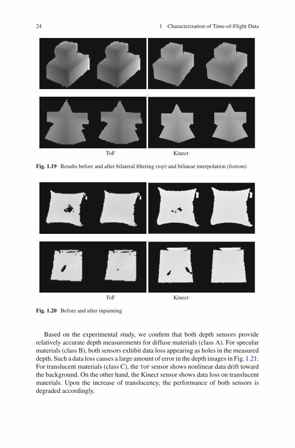
ToF Kinect
Fig. 1.19 Results before and after bilateral filtering (top) and bilinear interpolation (bottom)
.
ToF Kinect
Fig. 1.20 Before and after inpainting
Based on the experimental study, we confirm that both depth sensors providerelatively accurate depth measurements for diffuse materials (class A). For specularmaterials (class B), both sensors exhibit data loss appearing as holes in the measureddepth. Such a data loss causes a large amount of error in the depth images in Fig. 1.21.For translucent materials (class C), the tof sensor shows nonlinear data drift towardthe background. On the other hand, the Kinect sensor shows data loss on translucentmaterials. Upon the increase of translucency, the performance of both sensors isdegraded accordingly.

1.5 Conclusions 25
Fig. 1.21 Sample depth images and difference maps from the test image set
1.5 Conclusions
This chapter has reported both quantitative and qualitative experimental results forthe evaluation of each sensor type. Moreover, we provide a well-structured standarddata set of depth images from real world objects, with accompanying ground truthdepth. The data set spans a wide variety of radiometric and geometric complexity,which is well suited to the evaluation of depth processing algorithms. The analysishas revealed important problems in depth acquisition and processing, especiallymeasurement errors due to material properties. The data set will provide a standardframework for the evaluation of other denoising, super resolution, interpolation, andrelated depth-processing algorithms.
26 1 Characterization of Time-of-Flight Data
References
1. Bartczak, B., Koch, R.: Dense depth maps from low resolution time-of-flight depth and highresolution color views. In: Proceedings of the International Symposium on Visual Computing(ISVC), pp. 228–239. Las Vegas (2009)
2. Chan, D., Buisman, H., Theobalt, C., Thrun, S.: A noise-aware filter for real-time depth upsam-pling. In: ECCV Workshop on Multi-camera and Multi-modal Sensor Fusion Algorithms andApplications (2008)
3. Chen, T., Lensch, H.P.A., Fuchs, C., Seidel H.P.: Polarization and phase-shifting for 3D scan-ning of translucent objects. In: Proceedings of the Computet Vision and, Pattern Recognition,pp. 1–8 (2007)
4. Choi, O., Lim, H., Kang, B., Kim, Y., Lee, K., Kim, J., Kim, C.: Range unfolding for time-of-flight depth cameras. In: Proceedings of the International Conference on Image Processing.pp. 4189–4192 (2010)
5. Criminisi, A., Perez, P., Toyama, K.: Region filling and object removal by exemplar-basedimage inpainting. IEEE Trans. Image Process. 13(9), 1200–1212 (2004)
6. Curless, B., Levoy, M.: A volumetric method for building complex models from range images.In: Proceedings of ACM SIGGRAPH ’96, pp. 303–312 (1996)
7. Dolson, J., Baek, J., Plagemann, C., Thrun, S.: Fusion of time-of-flight depth and stereo forhigh accuracy depth maps. In: Proceedings of the Computer Vision and Pattern Pecognition(CVPR), pp. 1–8 (2008)
8. Dolson, J., Baek, J., Plagemann, C., Thrun, S.: Upsampling range data in dynamic environ-ments. In: Proceedings of the Computer Vision and Pattern Recognition (CVPR), pp. 1141–1148 (2010)
9. Du, H., Oggier, T., Lustenberger, F., Charbon, E.: A virtual keyboard based on true-3d opticalranging. In: Proceedings of the British Machine Vision Conference (BMVC’05), pp. 220–229(2005)
10. Edeler, T., Ohliger, K., Hussmann, S. Mertins, A.: Time-of-flight depth image denoising usingprior noise information. In: Proceedings of the IEEE 10th International Conference on SignalProcessing (ICSP), pp. 119–122 (2010)
11. Foix, S., Alenya, G., Torras, C.: Lock-in time-of-flight (ToF) cameras: a survey. IEEE Sens. J.11(9), 1917–1926 (2011)
12. Freedman, B., Shpunt, A., Machline, M., Arieli, Y.: Depth Mapping Using Projected Patterns.US Patent No. 8150412 (2012)
13. Fuchs, S.: Multipath interference compensation in time-of-flight camera images. In: Proceed-ings of the 2010 20th International Conference on, Pattern Recognition (ICPR). pp. 3583–3586(2010)
14. Fuchs, S., Hirzinger, G.: Extrinsic and depth calibration of ToF-cameras. In: Proceedings ofthe Computer Vision and Pattern Recognition (CVPR), pp. 1–6 (2008)
15. Gupta, M., Agrawal, A., Veeraraghavan, A., Narasimhan, S.G.: Structured light 3D scanningunder global illumination. In: Proceedings of the Computer Vision and Pattern Recognition(CVPR) (2011)
16. Hansard, M., Horaud, R., Amat, M., Lee, S.: Projective alignment of range and parallax data.In: Proceedings of the Computer Vision and Pattern Recognition (CVPR), pp. 3089–3096(2011)
17. Henry, P., Krainin, M., Herbst, E., Ren, X., Fox, D.: RGB-D mapping: using depth camerasfor dense 3d modeling of indoor environments. In: RGB-D: Advanced Reasoning with DepthCameras Workshop in Conjunction with RSS (2010)
18. Huhle, B., Schairer, T., Jenke, P., Strasser. W.: Robust non-local denoising of colored depthdata. In: Proceedings of the Computer Vision and Pattern Recognition (CVPR) Workshops,pp. 1–7 (2008)
19. Hussmann, S., Hermanski, A., Edeler, T.: Real-time motion artifact suppression in Tof camerasystems. IEEE Trans. Instrum. Meas. 60(5), 1682–1690 (2011)

References 27
20. Kang, B., Kim, S., Lee, S., Lee, K., Kim, J., Kim, C.: Harmonic distortion free distanceestimation in Tof camera. In: SPIE Electronic Imaging (2011)
21. Khoshelham, K.: Accuracy analysis of kinect depth data. In: Proceedings of the ISPRS Work-shop on Laser Scanning (2011)
22. Kim, Y., Chan, D., Theobalt, C., Thrun, S.: Design and calibration of a multi-view TOF sensorfusion system. In: Proceedings of the IEEE CVPR Workshop on Time-of-Flight Camera BasedComputer Vision (2008)
23. Kolb, A., Barth, E., Koch, R., Larsen, R.: Time-of-flight cameras in computer graphics. Comput.Graph Forum 29(1), 141–159 (2010)
24. Lee, S., Kang, B., Kim, J.D.K., Kim, C.-Y.: Motion blur-free time-of-flight range sensor.In: Proceedings of the SPIE Electronic Imaging (2012)
25. Lee, S., Shim, H., Kim, J.D.K., Kim, C.-Y.: Tof depth image motion blur detection using 3Dblur shape models. In: Proceedings of the SPIE Electronic Imaging (2012)
26. Lindner, M., Kolb, A.: Compensation of motion artifacts for time-of-flight cameras.In: Kolb, A., Koch, R. (eds.) Dynamic 3D Imaging, Lecture Notes in Computer Science,vol. 5742, pp. 16–27. Springer, Berlin (2009)
27. Lindner, M., Kolb, A., Ringbeck, T.: New insights into the calibration of tof-sensors. In:Proceedings on Computer Vision and Pattern Recognition Workshops, pp. 1–5 (2008)
28. Lottner, O., Sluiter, A., Hartmann, K., Weihs, W.: Movement artefacts in range images of time-of-flight cameras. In: International Symposium on Signals, Circuits and Systems (ISSCS),vol. 1, pp. 1–4 (2007)
29. Mesa Imaging AG. http://www.mesa-imaging.ch30. Matyunin, S., Vatolin, D., Berdnikov, Y., Smirnov, M.: Temporal filtering for depth maps
generated by kinect depth camera. In: Proceedings of the 3DTV, pp. 1–4 (2011)31. May, S., Werner, B., Surmann, H., Pervolz, K.: 3D Time-of-flight cameras for mobile robotics.
In: Proceedings of IEEE/RSJ International Conference on Intelligent Robots and Systems,pp. 790–795 (2006)
32. Mure-Dubois, J., Hugli, H.: Real-time scattering compensation for time-of-flight camera.In: Proceedings of Workshop on Camera Calibration Methods for Computer Vision Systems(CCMVS2007) (2007)
33. Newcombe, R.A., Izadi, S., Hilliges, O., Molyneaux, D., Kim, D., Davison, A.J., Kohli, P.,Shotton, J., Hodges, S., Fitzgibbon, A.: Kinectfusion: real-time dense surface mapping andtracking. IEEE International Symposium on Mixed and Augmented Reality (ISMAR), pp. 1–8(2011)
34. Park, J., Kim, H., Tai, Y.-W., Brown, M.-S., Kweon, I.S.: High quality depth map upsamplingfor 3D-TOF cameras. In: Proceedings of IEEE International Conference on Computer Vision(ICCV) (2011)
35. Reynolds, M., Dobos, J., Peel, L., Weyrich, T., Brostow, G.: Capturing time-of-flight datawith confidence. In: Proceedings of the Computer Vision and Pattern Recognition (CVPR),pp. 945–952 (2011)
36. Ryden, F., Chizeck, H., Kosari, S.N., King, H., Hannaford, B.: Using kinect and a hapticinterface for implementation of real-time virtual fixtures. In: RGB-D: Advanced Reasoningwith Depth Cameras Workshop in Conjunction with RSS (2010)
37. Schamm, T., Strand, M., Gumpp, T., Kohlhaas, R., Zollner, J., Dillmann, R.: Vision and Tof-based driving assistance for a personal transporter. In: Proceedings of the International Con-ference on Advanced Robotics (ICAR), pp. 1–6 (2009)
38. Scharstein, D., Szeliski, R.: A taxonomy and evaluation of dense two-frame stereo correspon-dence algorithms. Int. J. Comput. Vision 47, 7–42 (2002)
39. Scharstein, D., Szeliski, R.: High-accuracy stereo depth maps using structured light. In:Proceedings of the Computer Vision and Pattern Recognition (CVPR) (2003)
40. Schuon, S., Theobalt, C., Davis, J., Thrun, S.: High-quality scanning using time-of-flight depthsuperresolution. In: Proceedings of the Computer Vision and Pattern Recognition Workshops,pp. 1–7 (2008)

28 1 Characterization of Time-of-Flight Data
41. Seitz, S., Curless, B., Diebel, J., Scharstein, D., Szeliski, R.: A comparison and evaluationof multi-view stereo reconstruction algorithms. In: Proceedings of the Computer Vision andPattern Recognition (CVPR), pp. 519–528 (2006)
42. Shim, H., Adels, R., Kim, J., Rhee, S., Rhee, T., Kim, C., Sim, J., Gross, M.: Time-of-flightsensor and color camera calibration for multi-view acquisition. In: The Visual Computer (2011)
43. Shotton, J., Fitzgibbon, A., Cook, M., Blake, A.: Real-time human pose recognition in partsfrom single depth images. In: Proceedings of the Computer Vision and Pattern Recognition(CVPR) (2011)
44. Smisek, J., Jancosek, M., Pajdla, T.: 3D with kinect. In: Proceedings of International Conferenceon Computer Vision Workshops, pp. 1154–1160 (2011)
45. Soutschek, S., Penne, J., Hornegger, J., Kornhuber, J.: 3-D Gesture-based scene navigation inmedical imaging applications using time-of-flight cameras. In: Proceedings of the ComputerVision and Pattern Recognition Workshops, pp. 1–6 (2008)
46. Tai, Y.-W., Kong, N., Lin, S., Shin, S.Y.: Coded exposure imaging for projective motion deblur-ring. In: Proceedings of the Computer Vision and Pattern Recognition (CVPR), pp. 2408–2415(2010)
47. Whyte, O., Sivic, J., Zisserman, A., Ponce, J.: Non-uniform deblurring for shaken images.In: Proceedings of the Computer Vision and Pattern Recognition (CVPR), pp. 491–498 (2010)
48. Yang, Q., Yang, R., Davis, J., Nister, D.: Spatial-depth super resolution for range images.In: Proceedings of the Computer Vision and Pattern Recognition (CVPR), pp. 1–8 (2007)
49. Yeo, D., ul Haq, E., Kim, J., Baig, M., Shin, H.: Adaptive bilateral filtering for noise removalin depth upsampling. In: International SoC Design Conference (ISOCC), pp. 36–39 (2011)
50. Yuan, F., Swadzba, A., Philippsen, R., Engin, O., Hanheide, M., Wachsmuth, S.: Laser-basednavigation enhanced with 3D time-of-flight data. In: Proceedings of the International Confer-ence on Robotics and Automation (ICRA’09), pp. 2844–2850 (2009)
51. Zhang, L., Deshpande, A., Chen, X.: Denoising vs. deblurring: hdr imaging techniques usingmoving cameras. In: Proceedings of the Computer Vision and Pattern Recognition (CVPR),pp. 522–529 (2010)
52. Zhang, Z.: Flexible camera calibration by viewing a plane from unknown orientations.In: Proceedings of the International Conference on Computer Vision (ICCV) (1999)

Chapter 2Disambiguation of Time-of-Flight Data
Abstract The maximum range of a time-of-flight camera is limited by the peri-odicity of the measured signal. Beyond a certain range, which is determined bythe signal frequency, the measurements are confounded by phase wrapping. Thiseffect is demonstrated in real examples. Several phase-unwrapping methods, whichcan be used to extend the range of time-of-flight cameras, are discussed. Simplemethods can be based on the measured amplitude of the reflected signal, which isitself related to the depth of objects in the scene. More sophisticated unwrappingmethods are based on zero-curl constraints, which enforce spatial consistency on thephase measurements. Alternatively, if more than one depth camera is used, then thedata can be unwrapped by enforcing consistency among different views of the samescene point. The relative merits and shortcomings of these methods are evaluated,and the prospects for hardware-based approaches, involving frequency modulationare discussed.
Keywords Time-of-Flight principle · Depth ambiguity · Phase unwrapping ·Multiple depth cameras
2.1 Introduction
Time-of-Flight cameras emit modulated infrared light and detect its reflection fromthe illuminated scene points. According to the tof principle described in Chap. 1, thedetected signal is gated and integrated using internal reference signals, to form thetangent of the phase φ of the detected signal. Since the tangent of φ is a periodicfunction with a period of 2π , the value φ+2nπ gives exactly the same tangent valuefor any nonnegative integer n.
Commercially available tof cameras compute φ on the assumption that φ is withinthe range of [0, 2π). For this reason, each modulation frequency f has its maximumrange dmax corresponding to 2π , encoded without ambiguity:
M. Hansard et al., Time-of-Flight Cameras, SpringerBriefs in Computer Science, 29DOI: 10.1007/978-1-4471-4658-2_2, © Miles Hansard 2013

30 2 Disambiguation of Time-of-Flight Data
dmax = c
2 f, (2.1)
where c is the speed of light. For any scene points farther than dmax, the measureddistance d is much shorter than its actual distance d + ndmax. This phenomenon iscalled phase wrapping, and estimating the unknown number of wrappings n is calledphase unwrapping.
For example, the Mesa SR4000 [16] camera records a 3D point Xp at each pixel p,where the measured distance dp equals ‖Xp‖. In this case, the unwrapped 3D pointXp(n p) with number of wrappings n p can be written as
Xp(n p) = dp + n pdmax
dpXp. (2.2)
Figure 2.1a shows a typical depth map acquired by the SR4000 [16], and Fig. 2.1bshows its unwrapped depth map. As shown in Fig. 2.1e, phase unwrapping is crucialfor recovering large-scale scene structure.
To increase the usable range of tof cameras, it is also possible to extend themaximum range dmax by decreasing the modulation frequency f . In this case, theintegration time should also be extended, to acquire a high quality depth map,since the depth noise is inversely proportional to f . With extended integration time,moving objects are more likely to result in motion artifacts. In addition, we do notknow at which modulation frequency phase wrapping does not occur, without exactknowledge regarding the scale of the scene.
If we can accurately unwrap a depth map acquired at a high modulation frequency,then the unwrapped depth map will suffer less from noise than a depth map acquiredat a lower modulation frequency, integrated for the same time. Also, if a phase-unwrapping method does not require exact knowledge on the scale of the scene, thenthe method will be applicable in more large-scale environments.
There exist a number of phase-unwrapping methods [4–8, 14, 17, 21] that havebeen developed for tof cameras. According to the number of input depth maps, themethods are categorized into two groups: those using a single depth map [5, 7, 14,17, 21] and those using multiple depth maps [4, 6, 8, 20]. The following subsectionsintroduce their principles, advantages and limitations.
2.2 Phase Unwrapping from a Single Depth Map
tof cameras such as the SR4000 [16] provide an amplitude image along with itscorresponding depth map. The amplitude image is encoded with the strength of thedetected signal, which is inversely proportional to the squared distance. To obtaincorrected amplitude A′ [19], which is proportional to the reflectivity of a scene surfacewith respect to the infrared light, we can multiply amplitude A and its correspondingsquared distance d2:

2.2 Phase Unwrapping from a Single Depth Map 31
Fig. 2.1 Structure recovery through phase unwrapping. a Wrapped tof depth map. b Unwrappeddepth map corresponding to (a). Only the distance values are displayed in (a) and (b), to aid visibility.The intensity is proportional to the distance. c Amplitude image associated with (a). d and e displaythe 3D points corresponding to (a) and (b), respectively. d The wrapped points are displayed inred. e Their unwrapped points are displayed in blue. The remaining points are textured using theoriginal amplitude image (c)
A′ = Ad2. (2.3)
Figure 2.2 shows an example of amplitude correction. It can be observed fromFig. 2.2c that the corrected amplitude is low in the wrapped region. Based on theassumption that the reflectivity is constant over the scene, the corrected amplitudevalues can play an important role in detecting wrapped regions [5, 17, 21].
Poppinga and Birk [21] use the following inequality for testing if the depth ofpixel p has been wrapped:
A′p ≤ Arefp T, (2.4)
where T is a manually chosen threshold, and Arefp is the reference amplitude of
pixel p when viewing a white wall at 1 m, approximated by

32 2 Disambiguation of Time-of-Flight Data
Fig. 2.2 Amplitude correction example. a Amplitude image. b tof depth map. c Corrected ampli-tude image. The intensity in (b) is proportional to the distance. The lower left part of (b) has beenwrapped. Images courtesy of Choi et al. [5]
Arefp = B − (
(x p − cx )2 + (yp − cy)
2), (2.5)
where B is a constant. The image coordinates of p are (x p, yp), and (cx , cy) is approx-imately the image center, which is usually better illuminated than the periphery. Aref
p
compensates this effect by decreasing Arefp T if pixel p is in the periphery.
After the detection of wrapped pixels, it is possible to directly obtain an unwrappeddepth map by setting the number of wrappings of the wrapped pixels to one on theassumption that the maximum number of wrappings is 1.
The assumption on the constant reflectivity tends to be broken when the sceneis composed of different objects with varying reflectivity. This assumption cannotbe fully relaxed without detailed knowledge of scene reflectivity, which is hard toobtain in practice. To robustly handle varying reflectivity, it is possible to adaptivelyset the threshold for each image and to enforce spatial smoothness on the detectionresults.
Choi et al. [5] model the distribution of corrected amplitude values in an imageusing a mixture of Gaussians with two components, and apply expectation maxi-mization [1] to learn the model:
p(A′p) = αH p(A′p|μH , σ 2H )+ αL p(A′p|μL , σ 2
L), (2.6)
where p(A′p|μ, σ 2) denotes a Gaussian distribution with mean μ and variance σ 2,and α is the coefficient for each distribution. The components p(A′p|μH , σ 2
H ) andp(A′p|μL , σ 2
L) describe the distributions of high and low corrected amplitude values,respectively. Similarly, the subscripts H and L denote labels high and low, respec-tively. Using the learned distribution, it is possible to write a probabilistic version ofEq. (2.4) as
P(H |A′p) < 0.5, (2.7)
where P(H |A′p) = αH p(A′p|μH , σ 2H )/p(A′p).
To enforce spatial smoothness on the detection results, Choi et al. [5] use a seg-mentation method [22] based on Markov random fields (MRFs). The method findsthe binary labels n ∈ {H, L} or {0, 1} that minimize the following energy:

2.2 Phase Unwrapping from a Single Depth Map 33
Fig. 2.3 Detection of wrapped regions. a Result obtained by expectation maximization. b Resultobtained by MRF optimization. The pixels with labels L and H are colored in black and white,respectively. The red pixels are those with extremely high or low amplitude values, which arenot processed during the classification. c Unwrapped depth map corresponding to Fig. 2.2(b). Theintensity is proportional to the distance. Images courtesy of Choi et al. [5]
E =∑
p
Dp(n p)+∑(p,q)
V (n p, nq), (2.8)
where Dp(n p) is a data cost that is defined as 1 − P(n p|A′p), and V (n p, nq) is adiscontinuity cost that penalizes a pair of adjacent pixels p and q if their labels n p
and nq are different. V (n p, nq) is defined in a manner of increasing the penalty if apair of adjacent pixels have similar corrected amplitude values:
V (n p, nq) = λ exp(−β(A′p − A′q)2) δ(n p �= nq), (2.9)
where λ and β are constants, which are either manually chosen or adaptively deter-mined. δ(x) is a function that evaluates to 1 if its argument is true and evaluates tozero otherwise.
Figure 2.3 shows the classification results obtained by Choi et al. [5] Because ofvarying reflectivity of the scene, the result in Fig. 2.3a exhibits misclassified pixels inthe lower left part. The misclassification is reduced by applying the MRF optimizationas shown in Fig. 2.3b. Figure 2.3c shows the unwrapped depth map obtained by Choiet al. [5], corresponding to Fig. 2.2b.
McClure et al. [17] also use a segmentation-based approach, in which the depthmap is segmented into regions by applying the watershed transform [18]. In theirmethod, wrapped regions are detected by checking the average corrected amplitudeof each region.
On the other hand, depth values tend to be highly discontinuous across the wrap-ping boundaries, where there are transitions in the number of wrappings. For exam-ple, the depth maps in Figs. 2.1a, 2.2b shows such discontinuities. On the assumptionthat the illuminated surface is smooth, the depth difference between adjacent pixelsshould be small. If the difference between measured distances is greater than 0.5dmaxfor any adjacent pixels, say dp − dq > 0.5dmax, we can set the number of relativewrappings, or, briefly, the shift nq − n p to 1 so that the unwrapped difference willsatisfy −0.5dmax ≤ dp − dq − (nq − n p)dmax < 0, minimizing the discontinuity.

34 2 Disambiguation of Time-of-Flight Data
Fig. 2.4 One-dimensional phase-unwrapping example. a Measured phase image. b Unwrappedphase image where the phase difference between p and q is now less than 0.5. In (a) and (b), all thephase values have been divided by 2π . For example, the displayed value 0.1 corresponds to 0.2π
Fig. 2.5 Two-dimensionalphase-unwrapping example. aMeasured phase image. (b–d)Sequentially unwrapped phaseimages where the phase differ-ence across the red dotted linehas been minimized. Froma to d, all the phase valueshave been divided by 2π . Forexample, the displayed value0.1 corresponds to 0.2π
Figure 2.4 shows a one-dimensional phase-unwrapping example. In Fig. 2.4a, thephase difference between pixels p and q is greater than 0.5 (or π ). The shifts thatminimize the difference between adjacent pixels are 1 (or, nq −n p = 1) for p and q,and 0 for the other pairs of adjacent pixels. On the assumption that n p equals 0, wecan integrate the shifts from left to right to obtain the unwrapped phase image inFig. 2.4b.
Figure 2.5 shows a two-dimensional phase-unwrapping example. From Fig. 2.5ato d, the phase values are unwrapped in a manner of minimizing the phase differenceacross the red dotted line. In this two-dimensional case, the phase differences greaterthan 0.5 never vanish, and the red dotted line cycles around the image center infinitely.This is because of the local phase error that causes the violation of the zero-curlconstraint [9, 12].
Figure 2.6 illustrates the zero-curl constraint. Given four neighboring pixel loca-tions (x, y), (x + 1, y), (x, y+ 1), and (x + 1, y+ 1), let a(x, y) and b(x, y) denotethe shifts n(x+1, y)−n(x, y) and n(x, y+1)−n(x, y), respectively, where n(x, y)
denotes the number of wrappings at (x, y). Then, the shift n(x+1, y+1)−n(x, y) canbe calculated in two different ways: either a(x, y)+b(x+1, y) or b(x, y)+a(x, y+1)

2.2 Phase Unwrapping from a Single Depth Map 35
Fig. 2.6 Zero-curl constraint: a(x, y) + b(x + 1, y) = b(x, y) + a(x, y + 1). a The number ofrelative wrappings between (x+1, y+1) and (x, y) should be consistent regardless of its integratingpaths. For example, two different paths (red and blue) are shown. b shows an example in which theconstraint is not satisfied. The four pixels correspond to the four pixels in the middle of Fig. 2.5a
following one of the two different paths shown in Fig. 2.6a. For any phase-unwrappingresults to be consistent, the two values should be the same, satisfying the followingequality:
a(x, y)+ b(x + 1, y) = b(x, y)+ a(x, y + 1). (2.10)
Because of noise or discontinuities in the scene, the zero-curl constraint may notbe satisfied locally, and the local error is propagated to the entire image duringthe integration. There exist classical phase-unwrapping methods [9, 12] applied inmagnetic resonance imaging [15] and interferometric synthetic aperture radar (SAR)[13], which rely on detecting [12] or fixing [9] broken zero-curl constraints. Indeed,these classical methods [9, 12] have been applied to phase unwrapping for tofcameras [7, 14].
2.2.1 Deterministic Methods
Goldstein et al. [12] assume that the shift is either 1 or -1 between adjacent pixels iftheir phase difference is greater than π , and assume that it is 0 otherwise. They detectcycles of four neighboring pixels, referred to as plus and minus residues, which donot satisfy the zero-curl constraint.
If any integration path encloses an unequal number of plus and minus residue,the integrated phase values on the path suffer from global errors. In contrast, if anyintegration path encloses an equal number of plus and minus residues, the global erroris balanced out. To prevent global errors from being generated, Goldstein et al. [12]connect nearby plus and minus residues with cuts, which interdict the integrationpaths, such that no net residues can be encircled.
After constructing the cuts, the integration starts from a pixel p, and each neigh-boring pixel q is unwrapped relatively to p in a greedy and sequential manner if qhas not been unwrapped and if p and q are on the same side of the cuts.

36 2 Disambiguation of Time-of-Flight Data
Fig. 2.7 Graphical model that describes the zero-curl constraints (black discs) between neighboringshift variables (white discs). 3-element probability vectors (μ’s) on the shifts between adjacent nodes(−1, 0, or 1) are propagated across the network. The x marks denote pixels [9]
2.2.2 Probabilistic Methods
Frey et al. [9] propose a very loopy belief propagation method for estimating theshift that satisfies the zero-curl constraints. Let the set of shifts, and a measuredphase image, be denoted by
S ={
a(x, y), b(x, y) : x = 1, . . . , N − 1; y = 1, . . . , M − 1}
and
Φ ={φ(x, y) : 0 ≤ φ(x, y) < 1, x = 1, . . . , N ; y = 1, . . . , M
},
respectively, where the phase values have been divided by 2π . The estimation is thenrecast as finding the solution that maximizes the following joint distribution:
p(S, Φ) ∝N−1∏x=1
M−1∏y=1
δ(a(x, y)+ b(x + 1, y)− a(x, y + 1)− b(x, y))
×N−1∏x=1
M∏y=1
e− (φ(x + 1,y)−φ(x,y)+ a(x,y))2/2σ 2
×N∏
x=1
M−1∏y=1
e−(φ(x,y+1)−φ(x,y)+b(x,y))2/2σ 2
where δ(x) evaluates to 1 if x = 0 and to 0 otherwise. The variance σ 2 is estimateddirectly from the wrapped phase image [9].

2.2 Phase Unwrapping from a Single Depth Map 37
Fig. 2.8 a Constraint-to-shift vectors are computed from incoming shift-to-constraint vectors.b Shift-to-constraint vectors are computed from incoming constraint-to-shift vectors. c Estimatesof the marginal probabilities of the shifts given the data are computed by combining incomingconstraint-to-shift vectors [9]
Frey et al. [9] construct a graphical model describing the factorization of p(S, Φ),as shown in Fig. 2.7. In the graph, each shift node (white disc) is located betweentwo pixels, and corresponds to either an x-directional shift (a’s) or a y-directionalshift (b’s). Each constraint node (black disc) corresponds to a zero-curl constraint,and is connected to its four neighboring shift nodes. Every node passes a message toits neighboring node, and each message is a 3-vector denoted by μ, whose elementscorrespond to the allowed values of shifts, −1, 0, and 1. Each element of μ can beconsidered as a probability distribution over the three possible values [9].
Figure 2.8a illustrates the computation of a message μ4 from a constraint node toone of its neighboring shift nodes. The constraint node receives messages μ1, μ2,and μ3 from the rest of its neighboring shift nodes, and filters out the joint messageelements that do not satisfy the zero-curl constraint:
μ4i =1∑
j=−1
1∑k=−1
1∑l=−1
δ(k + l − i − j)μ1 jμ2kμ3l , (2.11)
where μ4i denotes the element of μ4, corresponding to shift value i ∈ {−1, 0, 1}.Figure 2.8b illustrates the computation of a message μ2 from a shift node to one
of its neighboring constraint node. Among the elements of the message μ1 from theother neighboring constraint node, the element, which is consistent with the measuredshift φ(x, y)− φ(x + 1, y), is amplified:
μ2i = μ1i exp(−(
φ(x + 1, y)− φ(x, y)+ i)2/2σ 2
). (2.12)
After the messages converge (or, after a fixed number of iterations), an estimate ofthe marginal probability of a shift is computed by using the messages passed into itscorresponding shift node, as illustrated in Fig. 2.8c:

38 2 Disambiguation of Time-of-Flight Data
P(a(x, y) = i |Φ) = μ1iμ2i∑
jμ1 jμ2 j
. (2.13)
Given the estimates of the marginal probabilities, the most probable value of each shiftnode is selected. If some zero-curl constraints remain violated, a robust integrationtechnique, such as least-squares integration [10] should be used [9].
2.2.3 Discussion
The aforementioned phase-unwrapping methods using a single depth map [5, 7, 14,17, 21] have an advantage that the acquisition time is not extended, keeping themotion artifacts at a minimum. The methods, however, rely on strong assumptionsthat are fragile in real world situations. For example, the reflectivity of the scenesurface may vary in a wide range. In this case, it is hard to detect wrapped regionsbased on the corrected amplitude values. In addition, the scene may be discontinuousif it contains multiple objects that occlude one another. In this case, the wrappingboundaries tend to coincide with object boundaries, and it is often hard to observelarge depth discontinuities across the boundaries, which play an important role indetermining the number of relative wrappings.
The assumptions can be relaxed by using multiple depth maps at a possible exten-sion of acquisition time. The next subsection introduces phase-unwrapping methodsusing multiple depth maps.
2.3 Phase Unwrapping from Multiple Depth Maps
Suppose that a pair of depth maps M1 and M2 of a static scene are given, which havebeen taken at different modulation frequencies f1 and f2 from the same viewpoint.In this case, pixel p in M1 corresponds to pixel p in M2, since the correspondingregion of the scene is projected onto the same location of M1 and M2. Thus, theunwrapped distances at those corresponding pixels should be consistent within thenoise level.
Without prior knowledge, the noise in the unwrapped distance can be assumedto follow a zero-mean distribution. Under this assumption, the maximum likelihoodestimates of the numbers of wrappings at the corresponding pixels should minimizethe difference between their unwrapped distances. Let m p and n p be the numbers ofwrappings at pixel p in M1 and M2, respectively. Then, we can choose m p and n p
that minimize g(m p, n p) such that
g(m p, n p) =∣∣dp( f1)+ m pdmax( f1)− dp( f2)− n pdmax( f2)
∣∣, (2.14)

2.3 Phase Unwrapping from Multiple Depth Maps 39
Fig. 2.9 Frequency modu-lation within an integrationperiod. The first half is modu-lated at f1, and the other halfis modulated at f2
where dp( f1) and dp( f2) denote the measured distances at pixel p in M1 and M2respectively, and dmax( f ) denotes the maximum range of f .
The depth consistency constraint has been mentioned by Göktürk et al. [11] andused by Falie and Buzuloiu [8] for phase unwrapping of tof cameras. The illuminat-ing power of tof cameras is, however, limited due to the eye-safety problem, and thereflectivity of the scene may be very low. In this situation, the amount of noise maybe too large for accurate numbers of wrappings to minimize g(m p, n p). For robustestimation against noise, Droeschel et al. [6] incorporate the depth consistency con-straint into their earlier work [7] for a single depth map, using an auxiliary depthmap of a different modulation frequency.
If we acquire a pair of depth maps of a dynamic scene sequentially and indepen-dently, the pixels at the same location may not correspond to each other. To deal withsuch dynamic situations, several approaches [4, 20] acquire a pair of depth mapssimultaneously. These can be divided into single-camera and multicamera methods,as described below.
2.3.1 Single-Camera Methods
For obtaining a pair of depth maps sequentially, four samples of integrated electriccharge are required per each integration period, resulting in eight samples within apair of two different integration periods. Payne et al. [20] propose a special hardwaresystem that enables simultaneous acquisition of a pair of depth maps at different fre-quencies by dividing the integration period into two, switching between frequenciesf1 and f2, as shown in Fig. 2.9.
Payne et al. [20] also shows that it is possible to obtain a pair of depth maps withonly five or six samples within a combined integration period, using their system.By using fewer samples, the total readout time is reduced and the integration periodfor each sample can be extended, resulting in an improved signal-to-noise ratio.

40 2 Disambiguation of Time-of-Flight Data
Fig. 2.10 a Stereo tof camera system. (b, c) Depth maps acquired by the system. d Amplitudeimage corresponding to (b). (e, f) Unwrapped depth maps, corresponding to (b) and (c), respectively.The intensity in (b, c, e, f) is proportional to the depth. The maximum intensity (255) in (b, c) and(e, f) correspond to 5.2 and 15.6 m, respectively. Images courtesy of Choi and Lee [4]
2.3.2 Multicamera Methods
Choi and Lee [4] use a pair of commercially available tof cameras to simultaneouslyacquire a pair of depth maps from different viewpoints. The two cameras C1 and C2are fixed to each other, and the mapping of a 3D point X from C1 to its correspondingpoint X′ from C2 is given by (R, T), where R is a 3 × 3 rotation matrix, and T isa 3 × 1 translation vector. In [4], the extrinsic parameters R and T are assumed tohave been estimated. Figure 2.10a shows the stereo tof camera system.
Denoting by M1 and M2 a pair of depth maps acquired by the system, a pixel pin M1 and its corresponding pixel q in M2 should satisfy:
X′q(nq) = RXp(m p)+ T, (2.15)
where Xp(m p) and X′q(nq) denote the unwrapped 3D points of p and q with theirnumbers of wrappings m p and nq , respectively.
Based on the relation in Eq. (2.15), Choi and Lee [4] generalize the depth con-sistency constraint in Eq. (2.14) for a single camera to those for the stereo camerasystem:
Dp(m p) = minnq∈{0,...,N }
(∥∥X′q (nq )− RXp(m p)− T∥∥)
, (2.16)
Dq(nq) = minm p∈{0,...,N }
(∥∥Xp (m p )− RT (X′q(nq)− T)∥∥)
,

2.3 Phase Unwrapping from Multiple Depth Maps 41
Table 2.1 Summary of phase-unwrapping methods
Methods # Depth maps Cues Approach Maximum range
Poppinga and Birk [21] 1 CAa Thresholding 2dmax
Choi et al. [5] 1 CA, DDb Segmentation, MRF (N d + 1)dmax
McClure et al. [17] 1 CA Segmentation, thresholding 2dmax
Jutzi [14] 1 DD Branch cuts, integration ∞Droeschel et al. [7] 1 DD MRF, integration ∞Droeschel et al. [6] 2 (Multi-freq.) DD, DCc MRF, integration ∞Payne et al. [20] 2 (Multi-freq.) DC Hardware c
2| f1− f2|Choi and Lee [4] 2 (Stereo) DC Stereo ToF, MRF (N + 1)dmaxa Corrected amplitude. b Depth discontinuity. c Depth consistency. d The maximum number ofwrappings determined by the user.
where pixels q and p are the projections of RXp(m p)+ T and RT (X′q(nq)− T)
onto M2 and M1, respectively. The integer N is the maximum number of wrappings,determined by approximate knowledge on the scale of the scene.
To robustly handle with noise and occlusion, Choi and Lee [4] minimize thefollowing MRF energy functions E1 and E2, instead of independently minimizingDp(m p) and Dq(mq) at each pixel:
E1 =∑
p∈M1
Dp(m p)+∑(p,u)
V (m p, mu), (2.17)
E2 =∑
q∈M2
Dq(nq)+∑(q,v)
V (nq , nv),
where Dp(m p) and Dq(nq) are the data cost of assigning m p and nq to pixels p andq, respectively. Functions V (m p, mu) and V (nq , nv) determine the discontinuitycost of assigning (m p,mu) and (nq ,nv) to pairs of adjacent pixels (p,u) and (q,v),respectively.
The data costs Dp(m p) and Dq(nq) are defined by truncating Dp(m p) and Dq(nq)
to prevent their values from becoming too large, due to noise and occlusion:
Dp(m p) = τε
(Dp(m p)
), Dq(nq) = τε
(Dq(nq)
), (2.18)
τε(x) ={
x, if x < ε,
ε, otherwise,(2.19)
where ε is a threshold proportional to the extrinsic calibration error of the system.The function V (m p, mu) is defined in a manner that preserves depth continuity
between adjacent pixels. Choi and Lee [4] assume a pair of measured 3D points Xp
and Xu to have been projected from close surface points if they are close to eachother and have similar corrected amplitude values. The proximity is preserved bypenalizing the pair of pixels if they have different numbers of wrappings:

42 2 Disambiguation of Time-of-Flight Data
V (m p, mu) =
⎧⎪⎨⎪⎩
λrpu
exp(−ΔX2
pu
2σ 2X
)exp
(−ΔA′2pu
2σ 2A′
)if
{m p �= mu andΔXpu < 0.5 dmax( f1)
0 otherwise.
where λ is a constant, ΔX2pu = ‖Xp − Xu‖2, and ΔA′2pu = ‖A′p − A′u‖2. The
variances σ 2X and σ 2
A′ are adaptively determined. The positive scalar rpu is the imagecoordinate distance between p and u for attenuation of the effect of less adjacentpixels. The function V (nq , nv) is defined by analogy with V (m p, mu).
Choi and Lee [4] minimize the MRF energies via the α-expansion algorithm [2],obtaining a pair of unwrapped depth maps. To enforce further consistency betweenthe unwrapped depth maps, they iteratively update the MRF energy correspondingto a depth map, using the unwrapped depth of the other map, and perform the min-imization until the consistency no longer increases. Figure 2.10e, f shows examplesof unwrapped depth maps, as obtained by the iterative optimizations. An alternativemethod for improving the depth accuracy using two tof cameras is described in [3].
2.3.3 Discussion
Table 2.1 summarizes the phase-unwrapping methods [4–7, 14, 17, 20, 21] for tofcameras. The last column of the table shows the extended maximum range, whichcan be theoretically achieved by the methods. The methods [6, 7, 14] based onthe classical phase-unwrapping methods [9, 12] deliver the widest maximum range.In [4, 5], the maximum number of wrappings can be determined by the user. Itfollows that the maximum range of the methods can also become sufficiently wide,by setting N to a large value. In practice, however, the limited illuminating powerof commercially available tof cameras prevents distant objects from being preciselymeasured. This means that the phase values may be invalid, even if they can beunwrapped. In addition, the working environment may be physically confined. Forthe latter reason, Droeschel et al. [6, 7] limit the maximum range to 2dmax.
2.4 Conclusions
Although the hardware system in [20] has not yet been established in commerciallyavailable tof cameras, we believe that future tof cameras will use such a frequencymodulation technique for accurate and precise depth measurement. In addition, thephase-unwrapping methods in [4, 6] are ready to be applied to a pair of depth mapsacquired by such future tof cameras, for robust estimation of the unwrapped depthvalues. We believe that a suitable combination of hardware and software systemswill extend the maximum tof range, up to a limit imposed by the illuminating powerof the device.

References 43
References
1. Bilmes, J.: A gentle tutorial of the EM algorithm and its application to parameter estimationfor gaussian mixture and hidden Markov models. Technical Report TR-97-021, University ofCalifornia. Berkeley (1998)
2. Boykov, Y., Veksler, O., Zabih, R.: Fast approximate energy minimization via graph cuts. IEEETrans. Pattern Anal. Mach. Intell 23(11), 1222–1239 (2001)
3. Castañeda, V., Mateus, D., Navab, N.: Stereo time-of-flight. In: Proceedings of the InternationalConference on Computer Vision (ICCV), pp. 1684–1691 (2011)
4. Choi, O., Lee, S.: Wide range stereo time-of-flight camera. In: Proceedings of InternationalConference on Image Processing (ICIP) (2012)
5. Choi, O., Lim, H., Kang, B., Kim, Y., Lee, K., Kim, J., Kim, C.: Range unfolding for time-of-flight depth cameras. In: Proceedings of International Conference on Image Processing (ICIP),pp. 4189–4192 (2010)
6. Droeschel, D., Holz, D., Behnke, S.: Multifrequency phase unwrapping for time-of-flight cam-eras. In: Proceedings of IEEE/RSJ International Conference on Intelligent Robots and Systems(IROS), Taipei (2010)
7. Droeschel, D., Holz, D., Behnke, S.: Probabilistic phase unwrapping for time-of-flight cameras.In: Joint 41st International Symposium on Robotics and 6th German Conference on Robotics(2010)
8. Falie, D., Buzuloiu, V.: Wide range time of flight camera for outdoor surveillance. In:Microwaves, Radar and Remote Sensing Symposium, pp. 79–82 (2008)
9. Frey, B.J., Koetter, R., Petrovic, N.: Very loopy belief propagation for unwrapping phase images.In: Advances in Neural Information Processing Systems (2001)
10. Ghiglia, D.C., Romero, L.A.: Robust two-dimensional weighted and unweighted phase unwrap-ping that uses fast transforms and iterative methods. J.Opt. Soc. Am. A 11(1), 107–117 (1994)
11. Göktürk, S.B., Yalcin, H., Bamji, C.: A time-of-flight depth sensor–system description, issuesand solutions. In: Proceedings of the Computer Vision and Parallel Recognition (CVPR) Work-shops (2004)
12. Goldstein, R.M., Zebker, H.A., Werner, C.L.: Satellite radar interferometry: two-dimensionalphase unwrapping. Radio Sci. 23, 713–720 (1988)
13. Jakowatz Jr, C., Wahl, D., Eichel, P., Ghiglia, D., Thompson, P.: Spotlight-mode SyntheticAperture Radar: A Signal Processing Approach. Kluwer Academic Publishers, Boston (1996)
14. Jutzi, B.: Investigation on ambiguity unwrapping of range images. In: International Archivesof Photogrammetry and Remote Sensing Workshop on Laserscanning (2009)
15. Liang, V., Lauterbur, P.: Principles of Magnetic Resonance Imaging: A Signal ProcessingPerspective. Wiley-IEEE Press, New York (1999)
16. Mesa Imaging AG. http://www.mesa-imaging.ch17. McClure, S.H., Cree, M.J., Dorrington, A.A., Payne, A.D.: Resolving depth-measurement
ambiguity with commercially available range imaging cameras. In: Image Processing: MachineVision Applications III (2010)
18. Meyer, F.: Topographic distance and watershed lines. Signal Process. 38(1), 113–125 (1994)19. Oprisescu, S., Falie, D., Ciuc, M., Buzuloiu, V.: Measurements with ToF cameras and their nec-
essary corrections. In: IEEE International Symposium on Signals, Circuits & Systems (2007)20. Payne, A.D., Jongenelen, A.P.P., Dorrington, A.A., Cree, M.J., Carnegie, D.A.: Multiple fre-
quency range imaging to remove measurment ambiguity. In: 9th Conference on Optical 3-D,Measurement Techniques (2009)
21. Poppinga, J., Birk, A.: A novel approach to efficient error correction for the swissranger time-of-flight 3D camera. In: RoboCup 2008: Robot Soccer World Cup XII (2008)
22. Rother, C., Kolmogorov, V., Blake, A.: “GrabCut”—interactive foreground extraction usingiterated graph cuts. In: International Conference and Exhibition on Computer Graphics andInteractive Techniques (2004)

Chapter 3Calibration of Time-of-Flight Cameras
Abstract This chapter describes the metric calibration of a time-of-flight cameraincluding the internal parameters, and lens distortion. Once the camera has beencalibrated, the 2D depth image can be transformed into a range map, which encodesthe distance to the scene along each optical ray. It is convenient to use establishedcalibration methods, which are based on images of a chequerboard pattern. Thelow resolution of the amplitude image, however, makes it difficult to detect theboard reliably. Heuristic detection methods, based on connected image compo-nents, perform very poorly on this data. An alternative, geometrically principledmethod is introduced here, based on the Hough transform. The Hough method iscompared to the standard OpenCV board-detection routine, by application to severalhundred time-of-flight images. It is shown that the new method detects significantlymore calibration boards, over a greater variety of poses, without any significant lossof accuracy.
Keywords Time-of-Flight cameras · Low-resolution camera calibration · Houghtransform · Chessboard detection
3.1 Introduction
Time-of-Flight (tof) cameras can, in principle, be modeled and calibrated as pinholedevices. For example, if a known chequerboard pattern is detected in a sufficientvariety of poses, then the internal and external camera parameters can be estimated bystandard routines [10, 19]. This chapter will briefly review the underlying calibrationmodel, before addressing the problem of chequerboard detection in detail. The latteris the chief obstacle to the use of existing calibration software, owing to the lowresolution of the tof images.
M. Hansard et al., Time-of-Flight Cameras, SpringerBriefs in Computer Science, 45DOI: 10.1007/978-1-4471-4658-2_3, © Miles Hansard 2013

46 3 Calibration of Time-of-Flight Cameras
3.2 Camera Model
If the scene coordinates of a point are (X, Y, Z)�, then the pinhole projection canbe expressed as (x p, yp, 1)� � R(X, Y, Z)�+ T where the rotation matrix R andtranslation T account for the pose of the camera. The observed pixel coordinates ofthe point are then modeled as
⎛⎝ x
y1
⎞⎠ =
⎛⎝ f sx f sθ x0
0 f sy y00 0 1
⎞⎠
⎛⎝ xd
yd
1
⎞⎠ (3.1)
where (xd , yd)� results from lens distortion of (x p, yp)�. The parameter f is the
focal length, (sx , sy) are the pixel scales, and sθ is the skew factor [10], which isassumed to be zero here. The lens distortion may be modeled by a radial part d1 andtangential part d2, so that
(xd
yd
)= d1(r)
(x p
yp
)+ d2
(x p, yp
)where r =
√x2
p + y2p (3.2)
is the radial coordinate. The actual distortion functions are polynomials of the form
d1(r) = 1+ a1r2 + a2r4 and d2(x, y) =(
2xy r2 + 2x2
r2 + 2y2 2xy
) (a3a4
). (3.3)
The coefficients (a1, a2, a3, a4) must be estimated along with the other internal para-meters ( f, sx , sy) and (x0, y0) in (3.1). The standard estimation procedure is based onthe projection of a known chequerboard pattern, which is viewed in many differentpositions and orientations. The external parameters (R, T), as well as the internalparameters can then be estimated as described by Zhang [1, 19], for example.
3.3 Board Detection
It is possible to find the chequerboard vertices, in ordinary images, by first detectingimage corners [9], and subsequently imposing global constraints on their arrangement[1, 14, 18]. This approach, however, is not reliable for low-resolution images (e.g.,in the range 100–500px2) because the local image structure is disrupted by samplingartifacts, as shown in Fig. 3.1. Furthermore, these artifacts become worse as theboard is viewed in distant and slanted positions, which are essential for high-qualitycalibration [2]. This is a serious obstacle for the application of existing calibrationmethods to new types of camera. For example, the amplitude signal from a typicaltof camera [15] resembles an ordinary grayscale image, but is of very low spatialresolution (e.g., 176×144), as well as being noisy. It is, nonetheless, necessary to

3.3 Board Detection 47
Fig. 3.1 Left Example chequers from a tof amplitude image. Note the variable appearance of thefour junctions at this resolution, e.g., ‘×’ at lower-left versus ‘+’ at top-right. Middle A perspectiveimage of a calibration grid is represented by line pencils L and M , which intersect at the �×m = 20internal vertices of this board. Strong image gradients are detected along the dashed lines. RightThe Hough transform H of the image points associated with M . Each high-gradient point mapsto a line, such that there is a pencil in H for each set of edge points. The line L �, which passesthrough the � = 4 Hough vertices, is the Hough representation of the image pencil L
calibrate these devices, in order to combine them with ordinary color cameras, for3-D modeling and rendering [4, 7, 8, 12, 13, 16, 20].
The method described here is based on the Hough transform [11], and effectivelyfits a global model to the lines in the chequerboard pattern. This process is much lesssensitive to the resolution of the data, for two reasons. First, information is integratedacross the source image, because each vertex is obtained from the intersection of twofitted lines. Second, the structure of a straight edge is inherently simpler than that ofa corner feature. However, for this approach to be viable, it is assumed that any lensdistortion has been precalibrated, so that the images of the pattern contain straightlines. This is not a serious restriction, for two reasons. First, it is relatively easy to findenough boards (by any heuristic method) to get adequate estimates of the internal andlens parameters. Indeed, this can be done from a single image, in principle [5]. Theharder problems of reconstruction and relative orientation can then be addressed afteradding the newly detected boards, ending with a bundle adjustment that also refinesthe initial internal parameters. Second, the tof devices used here have fixed lenses,which are sealed inside the camera body. This means that the internal parametersfrom previous calibrations can be reused.
Another Hough method for chequerboard detection has been presented by de laEscalera and Armingol [3]. Their algorithm involves a polar Hough transform of allhigh-gradient points in the image. This results in an array that contains a peak foreach line in the pattern. It is not, however, straightforward to extract these peaks,because their location depends strongly on the unknown orientation of the imagelines. Hence, all local maxima are detected by morphological operations, and asecond Hough transform is applied to the resulting data in [3]. The true peaks willform two collinear sets in the first transform (cf. Sect. 3.3.5), and so the final task isto detect two peaks in the second Hough transform [17].

48 3 Calibration of Time-of-Flight Cameras
The method described in this chapter is quite different. It makes use of the gradientorientation as well as magnitude at each point, in order to establish an axis-alignedcoordinate system for each image of the pattern. Separate Hough transforms are thenperformed in the x- and y-directions of the local coordinate system. By construction,the slope coordinate of any line is close to zero in the corresponding Cartesian Houghtransform. This means that, on average, the peaks occur along a fixed axis of eachtransform, and can be detected by a simple sweep-line procedure. Furthermore, theknown �×m structure of the grid makes it easy to identify the optimal sweep line ineach transform. Finally, the two optimal sweep lines map directly back to pencils of� and m lines in the original image, owing to the Cartesian nature of the transform.The principle of the method is shown in Fig. 3.1.
It should be noted that the method presented here was designed specifically foruse with tof cameras. For this reason, the range, as well as intensity data is used tohelp segment the image in Sect. 3.3.2. However, this step could easily be replacedwith an appropriate background subtraction procedure [1], in which case the newmethod could be applied to ordinary rgb images. Camera calibration is typicallyperformed under controlled illumination conditions, and so there would be no needfor a dynamic background model.
3.3.1 Overview
The new method is described in Sect. 3.3; preprocessing and segmentation areexplained in Sects. 3.3.2 and 3.3.3, respectively, while Sect. 3.3.4 describes the geo-metric representation of the data. The necessary Hough transforms are defined inSect. 3.3.5, and analyzed in Sect. 3.3.6.
Matrices and vectors will be written in bold, e.g., M, v, and the Euclidean lengthof v will be written |v|. Equality up to an overall nonzero scaling will be writtenv � u. Image points and lines will be represented in homogeneous coordinates [10],with p � (x, y, 1)� and l � (α, β, γ ), such that lp = 0 if l passes through p. Theintersection point of two lines can be obtained from the cross-product (l × m)�.An assignment from variable a to variable b will be written b ← a. It will beconvenient, for consistency with the pseudocode listings, to use the notation (m : n)
for the sequence of integers from m to n inclusive. The ‘null’ symbol ∅ will be usedto denote undefined or unused variables.
The method described here refers to a chequerboard of (�+1)× (m+1) squares,with � < m. It follows that the internal vertices of the pattern are imaged as the �mintersection points
vij = li ×m j where li ∈ L for i = 1 : � and m j ∈M for j = 1 : m.
(3.4)

3.3 Board Detection 49
The sets L and M are pencils, meaning that li all intersect at a point p, while m j
all intersect at a point q. Note that p and q are the vanishing points of the gridlines,which may be at infinity in the images.
It is assumed that the imaging device, such as a tof camera, provides a rangemap Dij, containing distances from the optical center, as well as a luminance-likeamplitude map Aij. The images D and A are both of size I × J . All images must beundistorted, as described in the Sect. 3.3.
3.3.2 Preprocessing
The amplitude image A is roughly segmented, by discarding all pixels that correspondto very near or far points. This gives a new image B, which typically contains theboard, plus the person holding it:
Bij ← Aij if d0 < Dij < d1, Bij ← ∅ otherwise. (3.5)
The near-limit d0 is determined by the closest position for which the board remainsfully inside the field-of-view of the camera. The far-limit d1 is typically set to avalue just closer than the far wall of the scene. These parameters need only to be setapproximately, provided that the interval d1−d0 covers the possible positions of thecalibration board.
It is useful to perform a morphologic erosion operation at this stage, in order topartially remove the perimeter of the board. In particular, if the physical edge of theboard is not white, then it will give rise to irrelevant image gradients. The erosionradius need only be set approximately, assuming that there is a reasonable amount ofwhite space around the chessboard pattern. The gradient of the remaining amplitudeimage is now computed, using the simple kernel Δ = (−1/2, 0, 1/2). The horizontaland vertical components are
ξij ← (Δ � B)ij
= ρ cos θand
ηij ← (Δ�� B)ij
= ρ sin θ(3.6)
where � indicates convolution. No presmoothing of the image is performed, owingto the low spatial resolution of the data.
3.3.3 Gradient Clustering
The objective of this section is to assign each gradient vector (ξij, ηij) to one of threeclasses, with labels κij ∈ {λ, μ, ∅}. If κij = λ then pixel (i, j) is on one of the lines in

50 3 Calibration of Time-of-Flight Cameras
ξ
η
σ
τ
−0.4 −0.2 0.0 0.2 0.4−0.4 −0.2 0.0 0.2 0.4
−0.
4−
0.2
0.0
0.2
0.4
−0.
4−
0.2
0.0
0.2
0.4
Fig. 3.2 Left the cruciform distribution of image gradients, due to black/white and white/blacktransitions at each orientation, would be difficult to segment in terms of horizontal and verticalcomponents (ξ, η). Right the same distribution is easily segmented, by eigenanalysis, in the double-angle representation (3.7). The red and green labels are applied to the corresponding points in theoriginal distribution, on the left
L , and (ξij, ηij) is perpendicular to that line. If κij = μ, then the analogous relationshold with respect to M . If κij = ∅ then pixel (i, j) does not lie on any of the lines.
The gradient distribution, after the initial segmentation, will contain two elongatedclusters through the origin, which will be approximately orthogonal. Each clustercorresponds to a gradient orientation (mod π ), while each end of a cluster correspondsto a gradient polarity (black/white vs. white/black). The distribution is best analyzedafter a double-angle mapping [6], which will be expressed as (ξ, η) �→ (σ, τ ). Thismapping results in a single elongated cluster, each end of which corresponds to agradient orientation (mod π ), as shown in Fig. 3.2. The double-angle coordinatesare obtained by applying the trigonometric identities cos(2θ) = cos2 θ − sin2 θ andsin(2θ) = 2 sin θ cos θ to the gradients (3.6), so that
σij ← 1
ρij
(ξ2
ij − η2ij
)and τij ← 2
ρijξijηij where ρij =
√ξ2
ij + η2ij (3.7)
for all points at which the magnitude ρij is above machine precision. Let the first uniteigenvector of the (σ, τ ) covariance matrix be
(cos(2φ), sin(2φ)
), which is written
in this way so that the angle φ can be interpreted in the original image. The clustermembership is now defined by the projection
πij =(σij, τij
) · (cos(2φ), sin(2φ))
(3.8)
of the data onto this axis. The gradient vectors (ξij, ηij) that project to either end ofthe axis are labeled as follows:

3.3 Board Detection 51
κij ←
⎧⎪⎨⎪⎩
λ if πij ≥ ρmin
μ if πij ≤ −ρmin
∅ otherwise.
(3.9)
Strong gradients that are not aligned with either axis of the board are assigned to ∅,as are all weak gradients. It should be noted that the respective identity of classes λ
and μ has not yet been determined; the correspondence {λ,μ} ⇔ {L ,M } betweenlabels and pencils will be resolved in Sect. 3.3.6.
3.3.4 Local Coordinates
A coordinate system will now be constructed for each image of the board. The verylow amplitudes Bij ≈ 0 of the black squares tend to be characteristic of the board(i.e., Bij � 0 for both the white squares and for the rest of B). Hence, a good estimateof the center can be obtained by normalizing the amplitude image to the range [0, 1]and then computing a centroid using weights (1− Bij). The centroid, together withthe angle φ from (3.8) defines the Euclidean transformation (x, y, 1)� = E ( j, i, 1)�
into local coordinates, centered on and aligned with the board.Let (xκ , yκ , 1)� be the coordinates of point (i, j), after transformation by E, with
the label κ inherited from κij, and let L ′ and M ′ correspond to L and M in thenew coordinate system. Now, by construction, any labeled point is hypothesized tobe part of L ′ or M ′, such that l′(xλ, yλ, 1)� = 0 or m′(xμ, yμ, 1)� = 0, where l′and m′ are the local coordinates of the relevant lines l and m, respectively. Theselines can be expressed as
l′ � (−1, βλ, αλ) and m′ � (βμ, −1, αμ) (3.10)
with inhomogeneous forms xλ = αλ + βλyλ and yμ = αμ + βμxμ, such that theslopes |βκ | � 1 are bounded. In other words, the board is axis aligned in localcoordinates, and the perspective-induced deviation of any line is less than 45◦.
3.3.5 Hough Transform
The Hough transform, in the form used here, maps points from the image to lines inthe transform. In particular, points along a line are mapped to lines through a point.This duality between collinearity and concurrency suggests that a pencil of n imagelines will be mapped to a line of n transform points, as in Fig. 3.1.
The transform is implemented as a 2-D histogram H(u, v), with horizontal andvertical coordinates u ∈ [0, u1] and v ∈ [0, v1]. The point (u0, v0) = 1
2 (u1, v1) isthe center of the transform array. Two transforms, Hλ and Hμ, will be performed, for

52 3 Calibration of Time-of-Flight Cameras
Fig. 3.3 Hough transform. Each gradient pixel (x, y) labeledκ ∈ {λ,μ}maps to a line uκ (x, y, v) intransform Hκ . The operators H⊕p and interpα(p, q) perform accumulation and linear interpolation,respectively. See Sect. 3.3.5 for details
points labeled λ and μ, respectively. The Hough variables are related to the imagecoordinates in the following way:
uκ(x, y, v) ={
u(x, y, v) if κ = λ
u(y, x, v) if κ = μwhere u(x, y, v) = u0 + x − y(v − v0).
(3.11)
Here, u(x, y, v) is the u-coordinate of a line (parameterized by v), which is the Houghtransform of an image point (x, y). The Hough intersection point (u�
κ , v�κ ) is found
by taking two points (x, y) and (x ′, y′), and solving uλ(x, y, v) = uλ(x ′, y′, v), withxλ and x ′λ substituted according to (3.10). The same coordinates are obtained bysolving uμ(x, y, v) = uμ(x ′, y′, v), and so the result can be expressed as
u�κ = u0 + ακ and v�
κ = v0 + βκ (3.12)
with labels κ ∈ {λ,μ} as usual. A peak at (u�κ , v�
κ ) evidently maps to a line of interceptu�
κ − u0 and slope v�κ − v0. Note that if the perspective distortion in the images is
small, then βκ ≈ 0, and all intersection points lie along the horizontal midline (u, v0)
of the corresponding transform. The Hough intersection point (u�κ , v�
κ ) can be usedto construct an image line l′ or m′, by combining (3.12) with (3.10), resulting in
l′ ← (−1, v�λ − v0, u�
λ − u0)
and m′ ← (v�μ − v0, −1, u�
μ − u0). (3.13)
The transformation of these line vectors, back to the original image coordinates, isgiven by the inverse transpose of the matrix E, described in Sect. 3.3.4.
The two Hough transforms are computed by the procedure in Fig. 3.3. Let Hκ
refer to Hλ or Hμ, according to the label κ of the ij-th point (x, y). For each accepted
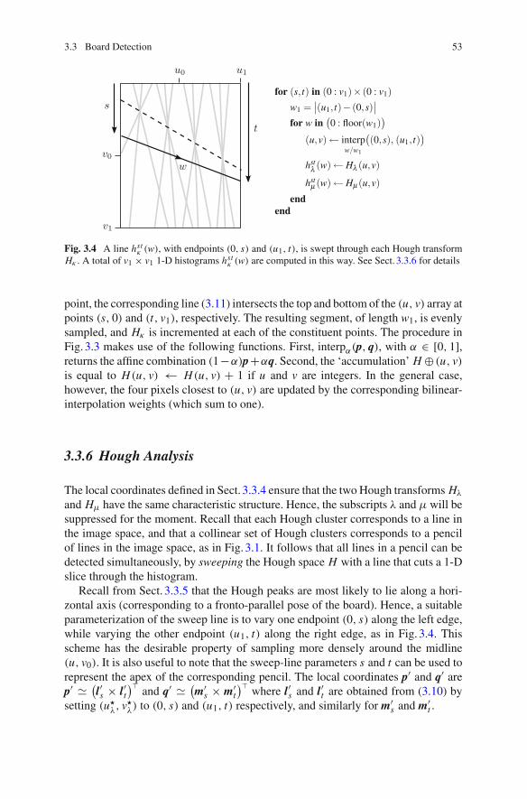
3.3 Board Detection 53
Fig. 3.4 A line hstκ (w), with endpoints (0, s) and (u1, t), is swept through each Hough transform
Hκ . A total of v1 × v1 1-D histograms hstκ (w) are computed in this way. See Sect. 3.3.6 for details
point, the corresponding line (3.11) intersects the top and bottom of the (u, v) array atpoints (s, 0) and (t, v1), respectively. The resulting segment, of length w1, is evenlysampled, and Hκ is incremented at each of the constituent points. The procedure inFig. 3.3 makes use of the following functions. First, interpα(p, q), with α ∈ [0, 1],returns the affine combination (1−α)p+αq. Second, the ‘accumulation’ H⊕ (u, v)is equal to H(u, v) ← H(u, v) + 1 if u and v are integers. In the general case,however, the four pixels closest to (u, v) are updated by the corresponding bilinear-interpolation weights (which sum to one).
3.3.6 Hough Analysis
The local coordinates defined in Sect. 3.3.4 ensure that the two Hough transforms Hλ
and Hμ have the same characteristic structure. Hence, the subscripts λ and μ will besuppressed for the moment. Recall that each Hough cluster corresponds to a line inthe image space, and that a collinear set of Hough clusters corresponds to a pencilof lines in the image space, as in Fig. 3.1. It follows that all lines in a pencil can bedetected simultaneously, by sweeping the Hough space H with a line that cuts a 1-Dslice through the histogram.
Recall from Sect. 3.3.5 that the Hough peaks are most likely to lie along a hori-zontal axis (corresponding to a fronto-parallel pose of the board). Hence, a suitableparameterization of the sweep line is to vary one endpoint (0, s) along the left edge,while varying the other endpoint (u1, t) along the right edge, as in Fig. 3.4. Thisscheme has the desirable property of sampling more densely around the midline(u, v0). It is also useful to note that the sweep-line parameters s and t can be used torepresent the apex of the corresponding pencil. The local coordinates p′ and q′ arep′ � (
l′s × l′t)� and q′ � (
m′s × m′t)� where l′s and l′t are obtained from (3.10) by
setting (u�λ, v�
λ) to (0, s) and (u1, t) respectively, and similarly for m′s and m′t .

54 3 Calibration of Time-of-Flight Cameras
The procedure shown in Fig. 3.4 is used to analyze the Hough transform. Thesweep line with parameters s and t has the form of a 1-D histogram hst
κ (w). Theinteger index w ∈ (0 : w1) is equal to the Euclidean distance |(u, v)− (0, s)| alongthe sweep line. The procedure shown in Fig. 3.4 makes further use of the interpolationoperator that was defined in Sect. 3.3.5. Each sweep line hst
κ (w), constructed by theabove process, will contain a number of isolated clusters: count(hst
κ ) ≥ 1. Theclusters are simply defined as runs of nonzero values in hst
κ (w). The existence ofseparating zeros is, in practice, highly reliable when the sweep line is close to thetrue solution. This is simply because the Hough data was thresholded in (3.9), andstrong gradients are not found inside the chessboard squares. The representation ofthe clusters, and subsequent evaluation of each sweep line, will now be described.
The label κ and endpoint parameters s and t will be suppressed, in the followinganalysis of a single sweep line, for clarity. Hence, let w ∈ (ac : bc) be the interval thatcontains the c-th cluster in h(w). The score and location of this cluster are definedas the mean value and centroid, respectively:
scorec
(h) =∑bc
w=ach(w)
1+ bc − acand wc = ac +
∑bcw=ac
h(w)w∑bcw=ac
h(w)(3.14)
More sophisticated definitions are possible, based on quadratic interpolation aroundeach peak. However, the mean and centroid give similar results in practice. A totalscore must now be assigned to the sweep line, based on the scores of the constituentclusters. If n peaks are sought, then the total score is the sum of the highest n clusterscores. But if there are fewer than n clusters in h(w), then this cannot be a solution,and the score is zero:
�n(h) =⎧⎨⎩
∑ni=1score
c(i)(h) if n ≤ count(h)
0 otherwise(3.15)
where c(i) is the index of the i-th highest-scoring cluster. The optimal clusters arethose in the sweep line that maximizes (3.15). Now, restoring the full notation, thescore of the optimal sweep line in the transform Hκ is
�nκ ← max
s, tscore
n(hst
κ ). (3.16)
One problem remains: it is not known in advance whether there should be � peaksin Hλ and m in Hμ, or vice versa. Hence all four combinations, ��
λ, �mμ , ��
μ, �mλ
are computed. The ambiguity between pencils (L ,M ) and labels (λ, μ) can thenbe resolved, by picking the solution with the highest total score:
(L ,M
)⇔{
(λ, μ) if ��λ +�m
μ > ��μ +�m
λ
(μ, λ) otherwise.(3.17)

3.3 Board Detection 55
Here, for example,(L ,M
)⇔ (λ, μ) means that there is a pencil of � lines in Hλ
and a pencil of m lines in Hμ. The procedure in (3.17) is based on the fact that thecomplete solution must consist of � + m clusters. Suppose, for example, that thereare � good clusters in Hλ, and m good clusters in Hμ. Of course, there are also �
good clusters in Hμ, because � < m by definition. However, if only � clusters aretaken from Hμ, then an additional m− � weak or nonexistent clusters must be foundin Hλ, and so the total score ��
μ +�mλ would not be maximal.
It is straightforward, for each centroid wc in the optimal sweep line hstκ , to compute
the 2-D Hough coordinates
(u�
κ , v�κ
)← interpwc/w1
((0, s), (u1, t)
)(3.18)
where w1 is the length of the sweep line, as in Fig. 3.4. Each of the resulting �mpoints are mapped to image lines, according to (3.13). The vertices vij are then becomputed from (3.4). The order of intersections along each line is preserved by theHough transform, and so the ij indexing is automatically consistent.
The final decision function is based on the observation that cross-ratios of dis-tances between consecutive vertices should be near unity (because the images areprojectively related to a regular grid). In practice, it suffices to consider simple ratios,taken along the first and last edge of each pencil. If all ratios are below a given thresh-old, then the estimate is accepted. This threshold was fixed once and for all, such thatno false-positive detections (which are unacceptable for calibration purposes) weremade, across all data sets.
3.3.7 Example Results
The method was tested on five multicamera data sets, and compared to the standardOpenCV detector. Both the OpenCV and Hough detections were refined by theOpenCV subpixel routine, which adjusts the given point to minimize the discrepancywith the image gradient around the chequerboard corner [1, 2]. Table 3.1 showsthe number of true-positive detections by each method, as well as the number ofdetections common to both methods. The geometric error is the discrepancy fromthe ‘ideal’ board, after fitting the latter by the optimal (DLT+LM) homography [10].This is by far the most useful measure, as it is directly related to the role of the detectedvertices in subsequent calibration algorithms (and also has a simple interpretation inpixel units). The photometric error is the gradient residual, as described in Sect. 3.3.6.This measure is worth considering, because it is the criterion minimized by thesubpixel optimization, but it is less interesting than the geometric error.
The Hough method detects 35 % more boards than the OpenCV method, on aver-age. There is also a slight reduction in average geometric error, even though the addi-tional boards were more problematic to detect. The results should not be surprising,because the new method uses a very strong model of the global board geometry(in fairness, it also benefits from the depth thresholding in 3.3.2). There were zero

56 3 Calibration of Time-of-Flight Cameras
Table 3.1 Results over six multi-tof camera setups
Number detected Geometric error Photometric errorSet / Camera OCV HT Both OCV HT OCV HT
1 / 1 19 34 13 0.2263 0.1506 0.0610 0.07821 / 2 22 34 14 0.1819 0.1448 0.0294 0.03601 / 3 46 33 20 0.1016 0.0968 0.0578 0.06951 / 4 26 42 20 0.2044 0.1593 0.0583 0.07052 / 1 15 27 09 0.0681 0.0800 0.0422 0.03722 / 2 26 21 16 0.0939 0.0979 0.0579 0.05232 / 3 25 37 20 0.0874 0.0882 0.0271 0.02543 / 1 14 26 11 0.1003 0.0983 0.0525 0.09563 / 2 10 38 10 0.0832 0.1011 0.0952 0.10573 / 3 25 41 21 0.1345 0.1366 0.0569 0.04543 / 4 18 23 10 0.1071 0.1053 0.0532 0.06564 / 1 16 21 14 0.0841 0.0874 0.0458 0.05264 / 2 45 53 29 0.0748 0.0750 0.0729 0.07434 / 3 26 42 15 0.0954 0.0988 0.0528 0.09185 / 1 25 37 18 0.0903 0.0876 0.0391 0.05675 / 2 20 20 08 0.2125 0.1666 0.0472 0.07595 / 3 39 36 24 0.0699 0.0771 0.0713 0.07855 / 4 34 35 19 0.1057 0.1015 0.0519 0.05286 / 1 29 36 20 0.1130 0.1203 0.0421 0.04726 / 2 35 60 26 0.0798 0.0803 0.0785 0.1067Mean: 25.75 34.8 16.85 0.1157 0.1077 0.0547 0.0659
Total detections for the OpenCV (515) versus Hough Transform (696) method are shown, as wellas the accuracy of the estimates. Geometric error is in pixels. The chief conclusion is that the HTmethod detects 35 % more boards, and slightly reduces the average geometric error
false-positive detections (100 % precision), as explained in Sect. 3.3.6. The numberof true negatives is not useful here, because it depends largely on the configura-tion of the cameras (i.e., how many images show the back of the board). The falsenegatives do not provide a very useful measure either, because they depend on anarbitrary judgement about which of the very foreshortened boards ‘ought’ to havebeen detected (i.e., whether an edge-on board is ‘in’ the image or not). Some exampledetections are shown in Figs. 3.5–3.7, including some difficult cases.
3.4 Conclusions
A new method for the automatic detection of calibration grids in tof images hasbeen described. The method is based on careful reasoning about the global geomet-ric structure of the board, before and after perspective projection. The method detectsmany more boards than existing heuristic approaches, which results in a larger andmore complete data set for subsequent calibration algorithms. Future work will inves-tigate the possibility of making a global refinement of the pencils, in the geometricparameterization, by minimizing a photometric cost function.

3.4 Conclusions 57
Fig. 3.5 Example detections in 176×144 tof amplitude images. The yellow dot (1-pixel radius) isthe estimated centroid of the board, and the attached thick translucent lines are the estimated axes.The board on the right, which is relatively distant and slanted, was not detected by OpenCV
Fig. 3.6 Example detections (cf. Fig. 3.5) showing significant perspective effects
Fig. 3.7 Example detections (cf. Fig. 3.5) showing significant scale changes. The board on theright, which is in an image that shows background clutter and lens distortion, was not detected byOpenCV
58 3 Calibration of Time-of-Flight Cameras
References
1. Bradski, G., Kaehler, A.: Learning OpenCV. O’Reilly, Sebastopol (2008)2. Datta, A., Jun-Sik, K., Kanade, T.: Accurate camera calibration using iterative refinement
of control points. In: Workshop on Visual Surveillance, Proceedings of IEEE InternationalConference on Computer Vision (ICCV), pp. 1201–1208 (2009)
3. de la Escalera, A., Armingol, J.: Automatic chessboard detection for intrinsic and extrinsiccamera parameter calibration. Sensors 10, 2027–2044 (2010)
4. Dubois, J.M., Hügli, H.: Fusion of time-of-flight camera point clouds. In: European Conferenceon Computer Vision (ECCV) Workshop on Multi-Camera and Multi-modal Sensor FusionAlgorithms and Applications (2008)
5. Gonzalez-Aguilera, D., Gomez-Lahoz, J., Rodriguez-Gonzalvez, P.: An automatic approachfor radial lens distortion correction from a single image. IEEE Sens. 11(4), 956–965 (2011)
6. Granlund, G.: In search of a general picture processing operator. Comput. Graph. Image Process.8, 155–173 (1978)
7. Hahne, U., Alexa, M.: Depth imaging by combining time-of-flight and on-demand stereo. In:Proceedings of DAGM Workshop on Dynamic 3D Imaging, pp. 70–83 (2009)
8. Hansard, M., Horaud, R., Amat, M., Lee, S.: Projective alignment of range and parallax Data.In: Proceedings of Computer Vision and Parallel Recognition (CVPR), pp. 3089–3096 (2011)
9. Harris, C., Stephens, M.: A combined corner and edge detector. In: Proceedings of the 4thAlvey Vision Conference, pp. 147–151 (1988)
10. Hartley, R., Zisserman, A.: Multiple View Geometry in Computer Vision. CambridgeUniversity Press, Cambridge (2000)
11. Illingworth, J., Kittler, J.: A survey of the hough transform. Comput. Vis. Graph. Image Process.44, 87–116 (1988)
12. Koch, R., Schiller, I., Bartczak, B., Kellner, F., Köser, K.: MixIn3D: 3D mixed reality withToF-camera. In: Proceedings of the DAGM Workshop on Dynamic 3D Imaging, pp. 126–141(2009)
13. Kolb, A., Barth, E., Koch, R., Larsen, R.: Time-of-flight cameras in computer graphics. Comput.Graph. Forum 29(1), 141–159 (2010)
14. Krüger, L., Wöhler, C., Würz-Wessel, A., Stein, F.: In-factory calibration of multiocular camerasystems. In: Proceedings of the SPIE Photonics Europe, pp. 126–137 (2004)
15. Mesa Imaging AG. http://www.mesa-imaging.ch16. Schiller, I., Beder, C., Koch, R.: Calibration of a PMD camera using a planar calibration object
together with a multi-camera setup. In: International Archieves of Photogrammetry, RemoteSensing and Spatial Information Sciences, XXI, pp. 297–302 (2008)
17. Tuytelaars, T., Proesmans, M., Gool, L.V.: The cascaded hough transform as support for group-ing and finding vanishing points and lines. In: Proceedings of International Workshop on Alge-braic Frames for the Perception-Action Cycle, pp. 278–289 (1997)
18. Wang, Z., Wu, W., Xu, X., Xue, D.: Recognition and location of the internal corners of planarcheckerboard calibration pattern image. Appl. Math. Comput. 185(2), 894–906 (2007)
19. Zhang, Z.: A flexible new technique for camera calibration. IEEE Trans. Pattern Anal. Mach.Intell. 22(11), 1330–1334 (2000)
20. Zhu, J., Wang, L., Yang, R.G., Davis, J.: Fusion of time-of-flight depth and stereo for highaccuracy depth maps. In: Proceedings of IEEE Conference on Computer Vision and ParallalRecognition (CVPR), pp. 1–8 (2008)

Chapter 4Alignment of Time-of-Flight and StereoscopicData
Abstract An approximately Euclidean representation of the visible scene can beobtained directly from a time-of-flight camera. An uncalibrated binocular system,in contrast, gives only a projective reconstruction of the scene. This chapter ana-lyzes the geometric mapping between the two representations, without requiringan intermediate calibration of the binocular system. The mapping can be found byeither of two new methods, one of which requires point correspondences betweenthe range and color cameras, and one of which does not. It is shown that thesemethods can be used to reproject the range data into the binocular images, whichmakes it possible to associate high-resolution color and texture with each point in theEuclidean representation. The extension of these methods to multiple time-of-flightsystem is demonstrated, and the associated problems are examined. An evaluationmetric, which distinguishes calibration error from combined calibration and deptherror, is developed. This metric is used to evaluate a system that is based on threetime-of-flight cameras.
Keywords Depth and color combination · Projective alignment · Time-of-Flightcamera calibration ·Multicamera systems
4.1 Introduction
It was shown in the preceding chapter that time-of-flight (tof) cameras can be geo-metrically calibrated by standard methods. This means that each pixel records anestimate of the scene distance (range) along the corresponding ray, according to theprinciples described in Chap. 1. The 3-D structure of a scene can also be recon-structed from two or more ordinary images, via the parallax between correspondingimage points. There are many advantages to be gained by combining the range andparallax data. Most obviously, each point in a parallax-based reconstruction can bemapped back into the original images, from which color and texture can be obtained.
M. Hansard et al., Time-of-Flight Cameras, SpringerBriefs in Computer Science, 59DOI: 10.1007/978-1-4471-4658-2_4, © Miles Hansard 2013

60 4 Alignment of Time-of-Flight and Stereoscopic Data
Fig. 4.1 The central panel shows a range image, color-coded according to depth (the blue region isbeyond the far limit of the device). The left and right cameras were aligned to the tof system, usingthe methods described here. Each 3-D range pixel is reprojected into the high-resolution left andright images (untinted regions were occluded, or otherwise missing, from the range images). Notethe large difference between the binocular views, which would be problematic for dense stereo-matching algorithms. It can also be seen that the tof information is noisy, and of low resolution
Parallax-based reconstructions are, however, difficult to obtain, owing to the difficultyof putting the image points into correspondence. Indeed, it may be impossible to findany correspondences in untextured regions. Furthermore, if a Euclidean reconstruc-tion is required, then the cameras must be calibrated. The accuracy of the resultingreconstruction will also tend to decrease with the distance of the scene from thecameras [23].
The range data, on the other hand, are often very noisy (and, for very scatteringsurfaces, incomplete), as described in Chap. 1. The spatial resolution of current tofsensors is relatively low, the depth range is limited, and the luminance signal may beunusable for rendering. It should also be recalled that tof cameras of the type usedhere [19] cannot be used in outdoor lighting conditions. These considerations leadto the idea of a mixed color and tof system [18] as shown in Figs. 4.1 and 4.2. Sucha system could, in principle, be used to make high-resolution Euclidean reconstruc-tions, with full photometric information [17]. The task of camera calibration wouldbe simplified by the tof camera, while the visual quality of the reconstruction wouldbe ensured by the color cameras.
In order to make full use of a mixed range/parallax system, it is necessary tofind the exact geometric relationship between the different devices. In particular, thereprojection of the tof data, into the color images, must be obtained. This chapteris concerned with the estimation of these geometric relationships. Specifically, theaim is to align the range and parallax reconstructions, by a suitable 3-D transforma-tion. The alignment problem has been addressed previously, by fully calibrating thebinocular system, and then aligning the two reconstructions by a rigid transformation[6, 12, 27, 28]. This approach can be extended in two ways. First, it is possible tooptimize over an explicit parameterization of the camera matrices, as in the work ofBeder et al. [3] and Koch et al. [16]. The relative position and orientation of all cam-eras can be estimated by this method. Second, it is possible to minimize an intensitycost between the images and the luminance signal of the tof camera. This methodestimates the photometric, as well as geometric, relationships between the different

4.1 Introduction 61
Fig. 4.2 A single tof+2rgb system, as used in this chapter, with the tof camera in the center ofthe rail
cameras [13, 22, 25]. A complete calibration method, which incorporates all of theseconsiderations, is described by Lindner et al. [18].
The approaches described above, while capable of producing good results, havesome limitations. First, there may be residual distortions in the range data, that makea rigid alignment impossible [15]. Second, these approaches require the binocularsystem to be fully calibrated, and recalibrated after any movement of the cameras.This requires, for best results, many views of a known calibration object. Typicalview-synthesis applications, in contrast, require only a weak calibration of the cam-eras. One way to remove the calibration requirement is to perform an essentially2-D registration of the different images [1, 4]. This, however, can only provide aninstantaneous solution, because changes in the scene structure produce correspond-ing changes in the image-to-image mapping.
An alternative approach is proposed here. It is hypothesized that the tof recon-struction is approximately Euclidean. This means that an uncalibrated binocularreconstruction can be mapped directly into the Euclidean frame, by a suitable 3-Dprojective transformation. This is a great advantage for many applications, becauseautomatic uncalibrated reconstruction is relatively easy. Furthermore, although theprojective model is much more general than the rigid model, it preserves manyimportant relationships between the images and the scene (e.g., epipolar geometryand incidence of points on planes). Finally, if required, the projective alignment canbe upgraded to a fully calibrated solution, as in the methods described above.
It is emphasized that the goal of this work is not to achieve the best possiblephotogrammetric reconstruction of the scene. Rather, the goal is to develop a practicalway to associate color and texture information to each range point, as in Fig. 4.1. Thisoutput is intended to use in view-synthesis applications.
This chapter is organized as follows. Section 4.2.1 briefly reviews some standardmaterial on projective reconstruction, while Sect. 4.2.2 describes the representation

62 4 Alignment of Time-of-Flight and Stereoscopic Data
of range data in the present work. The chief contributions of the subsequent sectionsare as follows: Sect. 4.2.3 describes a point-based method that maps an ordinaryprojective reconstruction of the scene onto the corresponding range representation.This does not require the color cameras to be calibrated (although it may be necessaryto correct for lens distortion). Any planar object can be used to find the alignment,provided that image features can be matched across all views (including that of thetof camera). Section 4.2.4 describes a dual plane-based method, which performsthe same projective alignment, but that does not require any point matches betweenthe views. Any planar object can be used, provided that it has a simple polygonalboundary that can be segmented in the color and range data. This is a great advantage,owing to the very low resolution of the luminance data provided by the tof camera(176 × 144 here). This makes it difficult to automatically extract and match pointdescriptors from these images, as described in Chap. 3. Furthermore, there are tofdevices that do not provide a luminance signal at all. Section 4.2.5 addresses theproblem of multisystem alignment. Finally, Sect. 4.3 describes the accuracy than canbe achieved with a three tof+2rgb system, including a new error metric for tof datain Sect. 4.3.2. Conclusions and future directions are discussed in Sect. 4.4.
4.2 Methods
This section describes the theory of projective alignment, using the following nota-tion. Bold type will be used for vectors and matrices. In particular, points P , Q andplanes U ,V in the 3-D scene will be represented by column vectors of homogeneouscoordinates, e.g.,
P =(
P�P4
)and U =
(U�U4
)(4.1)
where P� = (P1, P2, P3)� and U� = (U1, U2, U3)
�. The homogeneous coordi-nates are defined up to a nonzero scaling; for example, P � (P�/P4, 1)�. In par-ticular, if P4 = 1, then P� contains the ordinary space coordinates of the point P .Furthermore, if |U�| = 1, then U4 is the signed perpendicular distance of the planeU from the origin, and U� is the unit normal. The point P is on the plane U ifU�P = 0. The cross-product u × v is often expressed as (u)×v, where (u)× is a3× 3 antisymmetric matrix. The column vector of N zeros is written 0N .
Projective cameras are represented by 3 × 4 matrices. For example, the rangeprojection is
q � CQ where C = (A3×3 | b3×1
). (4.2)
The left and right color cameras C� and Cr are similarly defined, e.g., p� � C� P .Table 4.1 summarizes the geometric objects that will be aligned.
Points and planes in the two systems are related by the unknown 4 × 4 spacehomography H , so that

4.2 Methods 63
Table 4.1 Summary ofnotations in the left, right, andrange systems
Observed ReconstructedPoints Points Planes
Binocular C�,Cr p�, pr P URange C (q, ρ) Q V
Q � HP and V � H−�U . (4.3)
This model encompasses all rigid, similarity, and affine transformations in 3-D. Itpreserves collinearity and flatness, and is linear in homogeneous coordinates. Notethat, in the reprojection process, H can be interpreted as a modification of the cameramatrices, e.g., p� �
(C� H−1
)Q, where H−1 Q � P .
4.2.1 Projective Reconstruction
A projective reconstruction of the scene can be obtained from matched points p�k andprk , together with the fundamental matrix F, where p�rk Fp�k = 0. The fundamentalmatrix can be estimated automatically, using the well-established ransac method.The camera matrices can then be determined, up to a four-parameter projectiveambiguity [10]. In particular, from F and the epipole er , the cameras can be defined as
C� �(I | 03) and Cr �
((er )×F + er g�
∣∣ γ er). (4.4)
where γ �= 0 and g = (g1, g2, g3)� can be used to bring the cameras into a
plausible form. This makes it easier to visualize the projective reconstruction and,more importantly, can improve the numerical conditioning of subsequent procedures.
4.2.2 Range Fitting
The tof camera C provides the distance ρ of each scene point from the cameracenter, as well as its image coordinates q = (x, y, 1). The back projection of thispoint into the scene is
Q� = A−1((ρ/α) q − b)
where α = ∣∣A−1 q∣∣. (4.5)
Hence, the point ( Q�, 1)� is at distance ρ from the optical center −A−1b, in thedirection A−1q. The scalar α serves to normalize the direction vector. This is thestandard pinhole model, as used in [2].
64 4 Alignment of Time-of-Flight and Stereoscopic Data
The range data are noisy and incomplete, owing to illumination and scatteringeffects. This means that, given a sparse set of features in the intensity image (of thetof device), it is not advisable to use the back-projected point (4.5) directly. A betterapproach is to segment the image of the plane in each tof camera (using the rangeand/or intensity data). It is then possible to back project all of the enclosed points,and to robustly fit a plane V j to the enclosed points Qi j , so that V�j Qi j ≈ 0 ifpoint i lies on plane j . Now, the back projection Qπ of each sparse feature point qcan be obtained by intersecting the corresponding ray with the plane V , so that thenew range estimate ρπ is
ρπ = V�� A−1b− V4
(1/α) V�� A−1q(4.6)
where |V4| is the distance of the plane to the camera center, and V� is the unit normalof the range plane. The new point Qπ is obtained by substituting ρπ into (4.5).
The choice of plane-fitting method is affected by two issues. First, there may bevery severe outliers in the data, due to the photometric and geometric errors describedin Chap. 1. Second, the noise-model should be based on the pinhole model, whichmeans that perturbations occur radially along visual directions, which are not (ingeneral) perpendicular to the observed plane [11, 24]. Several plane-fitting methods,both iterative [14] and noniterative [20], have been proposed for the pinhole model.The outlier problem, however, is often more significant. Hence, in practice, a ransac-based method is often the most effective.
4.2.3 Point-Based Alignment
It is straightforward to show that the transformation H in (4.3) could be estimatedfrom five binocular points Pk , together with the corresponding range points Qk .This would provide 5 × 3 equations, which determine the 4 × 4 entries of H , sub-ject to an overall projective scaling. It is better, however, to use the ‘Direct LinearTransformation’ method [10], which fits H to all of the data. This method is basedon the fact that if
P ′ = HP (4.7)
is a perfect match for Q, then μ Q = λP ′, and the scalars λ and μ can be eliminatedbetween pairs of the four implied equations [5]. This results in
(42
) = 6 interdependentconstraints per point. It is convenient to write these homogeneous equations as
(Q4 P ′� − P ′4 Q�
Q� × P ′�
)= 06. (4.8)
Note that if P ′ and Q are normalized so that P ′4 = 1 and Q4 = 1, then themagnitude of the top half of (4.8) is simply the distance between the points.
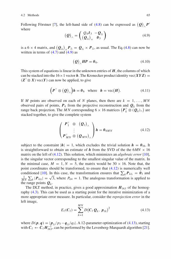
4.2 Methods 65
Following Förstner [7], the left-hand side of (4.8) can be expressed as(
Q)∧P ′
where (Q
)∧ =
(Q4 I3 −Q�(Q�
)× 03
)(4.9)
is a 6 × 4 matrix, and(
Q�)×P� = Q� × P�, as usual. The Eq. (4.8) can now be
written in terms of (4.7) and (4.9) as
(Q
)∧HP = 06. (4.10)
This system of equations is linear in the unknown entries of H , the columns of whichcan be stacked into the 16×1 vector h. The Kronecker product identity vec(XY Z) =(Z�⊗ X) vec(Y) can now be applied, to give
(P� ⊗ (
Q)∧)
h = 06 where h = vec(H
). (4.11)
If M points are observed on each of N planes, then there are k = 1, . . . , M Nobserved pairs of points, Pk from the projective reconstruction and Qk from therange back projection. The M N corresponding 6× 16 matrices
(P�k ⊗ ( Qk)∧
)are
stacked together, to give the complete system
⎛⎜⎝
P�1 ⊗(
Q1)∧
...
P�M N ⊗(
QM N
)∧
⎞⎟⎠ h = 06M N (4.12)
subject to the constraint |h| = 1, which excludes the trivial solution h = 016. Itis straightforward to obtain an estimate of h from the SVD of the the 6MN × 16matrix on the left of (4.12). This solution, which minimizes an algebraic error [10],is the singular vector corresponding to the smallest singular value of the matrix. Inthe minimal case, M = 1, N = 5, the matrix would be 30 × 16. Note that, thepoint coordinates should be transformed, to ensure that (4.12) is numerically wellconditioned [10]. In this case, the transformation ensures that
∑k Pk� = 03 and
1M N
∑k |Pk�| =
√3, where Pk4 = 1. The analogous transformation is applied to
the range points Qk .The DLT method, in practice, gives a good approximation HDLT of the homog-
raphy (4.3). This can be used as a starting point for the iterative minimization of amore appropriate error measure. In particular, consider the reprojection error in theleft image,
E�(C�) =M N∑k=1
D(C� Qk, p�k
)2 (4.13)
where D( p, q) = | p�/p3−q�/q3|. A 12-parameter optimization of (4.13), startingwith C�← C� H−1
DLT, can be performed by the Levenberg-Marquardt algorithm [21].

66 4 Alignment of Time-of-Flight and Stereoscopic Data
The result will be the camera matrix C�� that best reprojects the range data into the left
image (C�r is similarly obtained). The solution, provided that the calibration points
adequately covered the scene volume, will remain valid for subsequent depth andrange data.
Alternatively, it is possible to minimize the joint reprojection error, defined as thesum of left and right contributions,
E(H−1) = E�
(C� H−1)+ Er
(Cr H−1) (4.14)
over the (inverse) homography H−1. The 16 parameters are again minimized by theLevenberg-Marquardt algorithm, starting from the DLT solution H−1
DLT.The difference between the separate (4.13) and joint (4.14) minimizations is that
the latter preserves the original epipolar geometry, whereas the former does not.Recall that C� Cr , H and F are all defined up to scale, and that F satisfies anadditional rank-two constraint [10]. Hence, the underlying parameters can be countedas (12− 1)+ (12− 1) = 22 in the separate minimizations, and as (16− 1) = 15in the joint minimization. The fixed epipolar geometry accounts for the (9 − 2)
missing parameters in the joint minimization. If F is known to be very accurate (ormust be preserved) then the joint minimization (4.14) should be performed. This willalso preserve the original binocular triangulation, provided that a projective-invariantmethod was used [9]. However, if minimal reprojection error is the objective, thenthe cameras should be treated separately. This will lead to a new fundamental matrixF� = (e�
r )×C�r (C�
�)+, where (C�
�)+ is the generalized inverse. The right epipole is
obtained from e�r = C�
r d��, where d�
� represents the nullspace C��d�
� = 03.
4.2.4 Plane-Based Alignment
The DLT algorithm of Sect. 4.2.3 can also be used to recover H from matched planes,rather than matched points. Equation (4.10) becomes
(V )∧ H−�U = 06 (4.15)
where U and V represent the estimated coordinates of the same plane in the parallaxand range reconstructions, respectively. The estimation procedure is identical to thatin Sect. 4.2.3, but with vec(H−�) as the vector of unknowns.
This method, in practice, produces very poor results. The chief reason thatobliquely viewed planes are foreshortened, and therefore hard to detect/estimate,in the low-resolution tof images. It follows that the calibration data set is biasedtowards fronto-parallel planes.1 This bias allows the registration to slip sideways,perpendicular to the primary direction of the tof camera. The situation is greatly
1 The point-based algorithm is unaffected by this bias, because the scene is ultimately ‘filled’ withpoints, regardless of the contributing planes.

4.2 Methods 67
improved by assuming that the boundaries of the planes can be detected. For example,if the calibration object is rectangular, then the range projection of the plane V isbounded by four edges vi , where i = 1, . . . 4. Note that, these are detected as depthedges, and so no luminance data are required. The edges, represented as lines vi ,back project as the faces of a pyramid,
Vi = C�vi =(
Vi�0
), i = 1, . . . , L (4.16)
where L = 4 in the case of a quadrilateral projection. These planes are linearlydependent, because they pass through the center of projection; hence, the fourthcoordinates are all zero if, as here, the tof camera is at the origin. Next, if thecorresponding edges u�i and uri can be detected in the binocular system, using bothcolor and parallax information, then the planes Ui can easily be constructed. Eachcalibration plane now contributes an additional 6L equations
(Vi )∧ H−�Ui = 06 (4.17)
to the DLT system (4.12). Although these equations are quite redundant (any twoplanes span all possibilities), they lead to a much better DLT estimate. This is becausethey represent exactly those planes that are most likely to be missed in the calibrationdata, owing to the difficulty of feature detection over surfaces that are extremelyforeshortened in the image.
As in the point-based method, the plane coordinates should be suitably trans-formed, in order to make the numerical system (4.12) well conditioned. The trans-formed coordinates satisfy the location constraint
∑k Uk� = 03, as well as the scale
constraint∑
k |Uk�|2 = 3∑
k U 2k4, where Uk� = (Uk1, Uk2, Uk3)
�, as usual. A finalrenormalization |Uk | = 1 is also performed. This procedure, which is also appliedto the V k , is analogous to the treatment of line coordinates in DLT methods [26].
The remaining problem is that the original reprojection error (4.13) cannot be usedto optimize the solution, because no luminance features q have been detected in therange images (and so no 3-D points Q have been distinguished). This can be solvedby reprojecting the physical edges of the calibration planes, after reconstructingthem as follows. Each edge plane V i intersects the range plane V in a space-line,represented by the 4× 4 Plücker matrix
W i = V V �i − Vi V�. (4.18)
The line W i reprojects to a 3× 3 antisymmetric matrix [10]; for example
W�i � C�Wi C�� (4.19)
in the left image, and similarly in the right. Note that W �i p� = 0 if the point p� ison the reprojected line [10]. The line-reprojection error can therefore be written as

68 4 Alignment of Time-of-Flight and Stereoscopic Data
E×� (C�) =L∑
i=1
N∑j=1
D×(C�Wi C�� , u�i j
)2. (4.20)
The function D×(M, n
)compares image lines, by computing the sine of the angle
between the two coordinate vectors,
D×(M, n) =√
2∣∣Mn
∣∣|M| |n| =
|m × n||m| |n| , (4.21)
where M = (m)×, and |M| is the Frobenius norm. It is emphasized that the coor-dinates must be normalized by a suitable transformations G� and Gr , as in the caseof the DLT. For example, the line n should be fitted to points of the form Gp, andthen M should be transformed as G−�M, before computing (4.21). The reprojectionerror (4.20) is numerically unreliable without this normalization.
The line reprojection (4.21) can either be minimized separately for each camera,or jointly as
E×(H−1) = E×�
(C� H−1)+ E×r
(Cr H−1) (4.22)
by analogy with (4.14). Finally, it should be noted that although (4.21) is defined inthe image, it is an algebraic error. However, because the errors in question are small,this measure behaves predictably (see Fig. 4.2).
4.2.5 Multisystem Alignment
The point-based and plane-based procedures, described in Sects. 4.2.3 and 4.2.4respectively, can be used to calibrate a single tof+2rgb system. Related methodscan be used for the joint calibration of several such systems, as will now be explained,using the point-based representation. In this section, the notation P i will be usedfor the binocular coordinates (with respect to the left camera) of a point in the i-thsystem, and likewise Qi for the tof coordinates of a point in the same system. Hence,the i-th tof, left and right rgb cameras have the form
C i � (Ai | 03), C�i � (A�i | 03) and Cri � (Ari | bri ) (4.23)
where Ai and A�i contain only intrinsic parameters, whereas Ari also encodes therelative orientation of Cri with respect to C�i . Each system has a transformationH−1
i that maps tof points Qi into the corresponding rgb coordinate system of C�i .Furthermore, let the 4×4 matrix Gi j be the transformation from system j , mappingback to system i . This matrix, in the calibrated case, would be a rigid 3-D transfor-mation. However, by analogy with the tof-to-rgb matrices, each Gi j is generalizedhere to a projective transformation, thereby allowing for spatial distortions in thedata. The left and right cameras that project a scene point P j in coordinate system j

4.2 Methods 69
Fig. 4.3 Example of a three tof+2rgb setup, with tof cameras labeled 1,2,3. Each ellipse representsa separate system, with system 2 chosen as the reference. The arrows (with camera-labels) showsome possible tof-to-rgb projections. For example, a point P2 � H−1
2 Q2 in the center projectsdirectly to rgb view �2 via C�2, whereas the same point projects to �3 via C�32 = C�3G32
to image points p�i and pri in system i are
C�i j = C�i Gi j and Cri j = Cri Gi j . (4.24)
Note that if a single global coordinate system is chosen to coincide with the k-thrgb system, then a point Pk projects via C�ik and Crik . These two cameras arerespectively equal to C�i and Cri in (4.23) only when i = k, such that Gi j = Iin (4.24). A typical three-system configuration is shown in Fig. 4.3.
The transformation Gi j can only be estimated directly if there is a region ofcommon visibility between systems i and j . If this is not the case (as when the systemsface each other, such that the front of the calibration board is not simultaneouslyvisible), then Gi j can be computed indirectly. For example, G02 = G01 G12 whereP2 = G−1
12 G−101 P0. Note that, the stereo-reconstructed points P are used to estimate
these transformations, as they are more reliable than the tof points Q.
4.3 Evaluation
The following sections will describe the accuracy of a nine-camera setup, calibratedby the methods described above. Section 4.3.1 will evaluate calibration error, whereasSect. 4.3.2 will evaluate total error. The former is essentially a fixed function of theestimated camera matrices, for a given scene. The latter also includes the range noisefrom the tof cameras, which varies from moment to moment. The importance ofthis distinction will be discussed.

70 4 Alignment of Time-of-Flight and Stereoscopic Data
The setup consists of three rail-mounted tof+2rgb systems, i = 1 . . . 3, as inFig. 4.3. The stereo baselines are 17 cm on average, and the tof cameras are sepa-rated by 107 cm on average. The rgb images are 1624 × 1224, whereas the MesaImaging SR4000 tof images are 176×144, with a depth range of 500 cm. The threestereo systems are first calibrated by standard methods, returning a full Euclideandecomposition of C�i and Cri , as well as the associated lens parameters. It was estab-lished in [8] that projective alignment is generally superior to similarity alignment,and so the transformations Gi j and H−1
j will be 4 × 4 homographies. These trans-formations were estimated by the DLT method, and refined by LM-minimization ofthe joint geometric error, as in (4.14).
4.3.1 Calibration Error
The calibration error is measured by first taking tof points Qπj corresponding to ver-
tices on the reconstructed calibration plane π j in system j , as described in Sect. 4.2.2.These can then be projected into a pair of rgb images in system i , so that the errorEcal
i j = 12
(Ecal
�i j + Ecalri j
)can be computed, where
Ecal�i j =
1
|π |∑Qπ
j
D(
C�i j H−1j Qπ
j , p�i
)(4.25)
and Ecalri j is similarly defined. The function D(·, ·) computes the image distance
between inhomogenized points, as in (4.13), and the denominator corresponds tothe number of vertices on the board, with |π | = 35 in the present experiments. Themeasure (4.25) can of course be averaged over all images in which the board isvisible. The calibration procedure has an accuracy of around 1 pixel, as shown inFig. 4.4.
4.3.2 Total Error
The calibration error, as reported in the preceding section, is the natural way to eval-uate the estimated cameras and homographies. It is not, however, truly representativeof the ‘live’ performance of the complete setup. This is because the calibration erroruses each estimated plane π j to replace all vertices Q j with the fitted versions Qπ
j .In general, however, no surface model is available, and so the raw points Q j mustbe used as input for meshing and rendering processes.
The total error, which combines the calibration and range errors, can be measuredas follows. The i-th rgb views of plane π j must be related to the tof image pointsqj by the 2-D transfer homographies T �i j and T ri j , where

4.3 Evaluation 71
0.0 0.5 1.0 1.5 2.0
1 → 1, r1
pixel error0.0 0.5 1.0 1.5 2.0
2 → 2, r2
pixel error0.0 0.5 1.0 1.5 2.0
3 → 3, r3
pixel error
Fig. 4.4 Calibration error (4.25), measured by projecting the fitted tof points Qπ to the left andright rgb images (1624×1224) in three separate systems. Each histogram combines left-camera andright-camera measurements from 15 views of the calibration board. Subpixel accuracy is obtained
p�i � T �i j q j and pri � T ri j q j . (4.26)
These 3 × 3 matrices can be estimated accurately, because the range data itselfis not required. Furthermore, let Π j be the hull (i.e., bounding polygon) of planeπ j as it appears in the tof image. Any pixel q j in the hull (including the originalcalibration vertices) can now be reprojected to the i-th rgb views via the 3-D pointQ j , or transferred directly by T �i j and T ri j in (4.26). The total error is the average
difference between the reprojections and the transfers, E toti j = 1
2
(E tot
�i j+E totri j
), where
E tot�i j =
1
|Π j |∑
q j∈Π j
D(
C�i j H−1j Q j , T �i j q j
)(4.27)
and E totri j is similarly defined. The view-dependent denominator |Π j | � |π | is the
number of pixels in the hull Π j . Hence, E toti j is the total error, including range noise,
of tof plane π j as it appears in the i-th rgb cameras.If the rgb cameras are not too far from the tof camera, then the range errors
tend to be canceled in the reprojection. This is evident in Fig. 4.5, although it is clearthat the tail of each distribution is increased by the range error. However, if the rgbcameras belong to another system, with a substantially different location, then therange errors can be very large in the reprojection. This is clear from Fig. 4.6, whichshows that a substantial proportion of the tof points reproject to the other systemswith a total error in excess of 10 pixels.
It is possible to understand these results more fully by examining the distributionof the total error across individual boards. Figure 4.7 shows the distribution for aboard reprojected to the same system (i.e., part of the data from Fig. 4.5). There is arelatively smooth gradient of error across the board, which is attributable to errorsin the fitting of plane π j , and in the estimation of the camera parameters. The pixels

72 4 Alignment of Time-of-Flight and Stereoscopic Data
0.0 1.0 2.0 3.0
1 → 1, r1
pixel error0.0 1.0 2.0 3.0
2 → 2, r2
pixel error0.0 1.0 2.0 3.0
3 → 3, r3
pixel error
Fig. 4.5 Total error (4.27), measured by projecting the raw tof points Q to the left and right rgbimages (1624× 1224) in three separate systems. These distributions have longer and heavier tailsthan those of the corresponding calibration errors, shown in Fig. 4.4
0 5 10 15 20
2 → 1, r1
pixel error0 5 10 15 20
2 → 3, r3
pixel error
Fig. 4.6 Total error when reprojecting raw tof points from system 2 to rgb cameras in systems 1and 3 (left and right, respectively). The range errors are emphasized by the difference in viewpointsbetween the two systems. Average error is now around 5 pixels in the 1624× 1224 images, and thenoisiest tof points reproject with tens of pixels of error
can be divided into sets from the black and white squares, using the known boardgeometry and detected vertices. It can be seen in Fig. 4.7 (right) that the total error foreach set is comparable. However, when reprojecting to a different system, Fig. 4.8shows that the total error is correlated with the black and white squares on the board.This is due to significant absorption of the infrared signal by the black squares.
4.4 Conclusions
It has been shown that there is a projective relationship between the data provided bya tof camera, and an uncalibrated binocular reconstruction. Two practical methodsfor computing the projective transformation have been introduced; one that requiresluminance point correspondences between the tof and color cameras, and one that
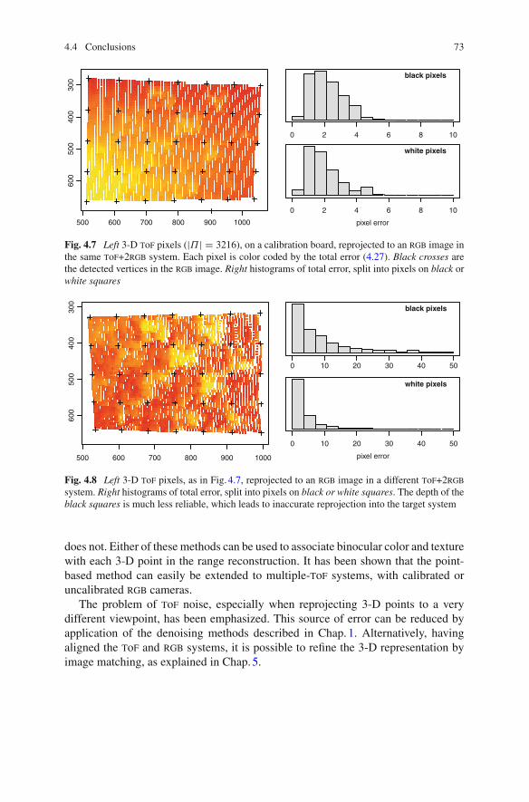
4.4 Conclusions 73
Fig. 4.7 Left 3-D tof pixels (|Π | = 3216), on a calibration board, reprojected to an rgb image inthe same tof+2rgb system. Each pixel is color coded by the total error (4.27). Black crosses arethe detected vertices in the rgb image. Right histograms of total error, split into pixels on black orwhite squares
500 600 700 800 900 1000
600
500
400
300
0 10 20 30 40 50
black pixels
0 10 20 30 40 50
pixel error
white pixels
Fig. 4.8 Left 3-D tof pixels, as in Fig. 4.7, reprojected to an rgb image in a different tof+2rgbsystem. Right histograms of total error, split into pixels on black or white squares. The depth of theblack squares is much less reliable, which leads to inaccurate reprojection into the target system
does not. Either of these methods can be used to associate binocular color and texturewith each 3-D point in the range reconstruction. It has been shown that the point-based method can easily be extended to multiple-tof systems, with calibrated oruncalibrated rgb cameras.
The problem of tof noise, especially when reprojecting 3-D points to a verydifferent viewpoint, has been emphasized. This source of error can be reduced byapplication of the denoising methods described in Chap. 1. Alternatively, havingaligned the tof and rgb systems, it is possible to refine the 3-D representation byimage matching, as explained in Chap. 5.
74 4 Alignment of Time-of-Flight and Stereoscopic Data
References
1. Bartczak, B., Koch, R.: Dense depth maps from low resolution time-of-flight depth and highresolution color views. In: Proceedings of International Symposium on Visual Computing(ISVC), pp. 228–239 (2009)
2. Beder, C., Bartczak, B., Koch, R.: A comparison of PMD-cameras and stereo-vision for thetask of surface reconstruction using patchlets. In: Proceedings of Computer Vision and ParallelRecognition (CVPR), pp. 1–8 (2007)
3. Beder, C., Schiller, I., Koch, R.: Photoconsistent relative pose estimation between a PMD2D3D-camera and multiple intensity cameras. In: Proceedings of Symposium of the GermanAssociation for Pattern Recognition (DAGM), pp. 264–273 (2008)
4. Bleiweiss, A., Werman, M.: Fusing time-of-flight depth and color for real-time segmentationand tracking. In: Proceedings of the Dynamic 3D Imaging: DAGM 2009 Workshop, pp. 58–69(2009)
5. Csurka, G., Demirdjian, D., Horaud, R.: Finding the collineation between two projective recon-structions. Comput. Vis. Image Underst. 75(3), 260–268 (1999)
6. Dubois, J.M., Hügli, H.: Fusion of time-of-flight camera point clouds. In: Proceedings ofEuropean Conference on Computer Vision (ECCV) Workshop on Multi-Camera and Multi-modal Sensor Fusion Algorithms and Applications, Marseille (2008)
7. Förstner, W.: Uncertainty and projective geometry. In: Bayro-Corrochano, E. (ed.) Handbookof Geometric Computing, pp. 493–534. Springer, New York (2005)
8. Hansard, M., Horaud, R., Amat, M., Lee, S.: Projective alignment of range and parallax data.In: Proceedings of Computer Vision and Parallel Recognition (CVPR), pp. 3089–3096 (2011)
9. Hartley, R., Sturm, P.: Triangulation. Comput. Vis. Image Underst. 68(2), 146–157 (1997)10. Hartley, R., Zisserman, A.: Multiple View Geometry in Computer Vision. Cambridge Univer-
sity Press, Cambridge (2000)11. Hebert, M., Krotkov, E.: 3D measurements from imaging laser radars: how good are they?
Image Vis. Comput. 10(3), 170–178 (1992)12. Horn, B., Hilden, H., Negahdaripour, S.: Closed-form solution of absolute orientation using
orthonormal matrices. J. Opt. Soc. Am. A 5(7), 1127–1135 (1988)13. Huhle, B., Fleck, S., Schilling, A.: Integrating 3D time-of-flight camera data and high resolution
images for 3DTV applications. In: Proceedings of 3DTV Conference, pp. 1–4 (2007)14. Kanazawa, Y., Kanatani, K.: Reliability of plane fitting by range sensing. In: International
Conference on Robotics and Automation (ICRA), pp. 2037–2042 (1995)15. Kim, Y., Chan, D., Theobalt, C., Thrun, S.: Design and calibration of a multi-view TOF sensor
fusion system. In: Proceedings of Computer Vision and Parallel Recognition (CVPR) Workshopon Time-of-Flight Camera based Computer Vision (2008)
16. Koch, R., Schiller, I., Bartczak, B., Kellner, F., Köser, K.: MixIn3D: 3D mixed reality withToF-camera. In: Proceedings of DAGM Workshop on Dynamic 3D Imaging, pp. 126–141(2009)
17. Kolb, A., Barth, E., Koch, R., Larsen, R.: Time-of-flight cameras in computer graphics. Comput.Graphics Forum 29(1), 141–159 (2010)
18. Lindner, M., Schiller, I., Kolb, A., Koch, R.: Time-of-flight sensor calibration for accuraterange sensing. Comput. Vis. Image Underst. 114(12), 1318–1328 (2010)
19. Mesa Imaging AG. http://www.mesa-imaging.ch20. Pathak, K., Vaskevicius, N., Birk, A.: Revisiting uncertainty analysis for optimum planes
extracted from 3D range sensor point-clouds. In: Proceedings of IEEE International Conferenceon Robotics and Automation (ICRA), pp. 1631–1636 (2009)
21. Press, W.H., Teukolsky, S.A., Vetterling, W.T., Flannery, B.P.: Numerical Recipes in C. Cam-bridge University Press, 2nd edition (1992)
22. Schiller, I., Beder, C., Koch, R.: Calibration of a PMD camera using a planar calibration objecttogether with a multi-camera setup. In: International Archives of Photogrammetry, RemoteSensing and Spatial Information Sciences XXI, pp. 297–302 (2008)

References 75
23. Verri, A., Torre, V.: Absolute depth estimate in stereopsis. J. Opt. Soc. Am. A 3(3), 297–299(1986)
24. Wang, C., Tanahasi, H., Hirayu, H., Niwa, Y., Yamamoto, K.: Comparison of local plane fittingmethods for range data. In: Proceedings of Computer Vision and Parallel Recognition (CVPR),pp. 663–669 (2001)
25. Wu, J., Zhou, Y., Yu, H., Zhang, Z.: Improved 3D depth image estimation algorithm for visualcamera. In: Proceedings of International Congress on Image and Signal Processing (2009)
26. Zeng, H., Deng, X., Hu, Z.: A new normalized method on line-based homography estimation.Pattern Recogn. Lett. 29, 1236–1244 (2008)
27. Zhang Q., Pless, R.: Extrinsic calibration of a camera and laser range finder (improves cameracalibration). In: Proceedings of Intenational Conference on Intelligent Robots and Systems,pp. 2301–2306 (2004)
28. Zhu, J., Wang, L., Yang, R.G., Davis, J.: Fusion of time-of-flight depth and stereo for highaccuracy depth maps. In: Proceedings of Computer Vision and Parallel Recognition (CVPR),pp. 1–8 (2008)

Chapter 5A Mixed Time-of-Flight and StereoscopicCamera System
Abstract Several methods that combine range and color data have been investigatedand successfully used in various applications. Most of these systems suffer from theproblems of noise in the range data and resolution mismatch between the range sen-sor and the color cameras. High-resolution depth maps can be obtained using stereomatching, but this often fails to construct accurate depth maps of weakly/repetitivelytextured scenes. Range sensors provide coarse depth information regardless of pres-ence/absence of texture. We propose a novel tof-stereo fusion method based on anefficient seed-growing algorithm which uses the tof data projected onto the stereoimage pair as an initial set of correspondences. These initial “seeds” are then prop-agated to nearby pixels using a matching score that combines an image similaritycriterion with rough depth priors computed from the low-resolution range data. Theoverall result is a dense and accurate depth map at the resolution of the color camerasat hand. We show that the proposed algorithm outperforms 2D image-based stereoalgorithms and that the results are of higher resolution than off-the-shelf RGB-Dsensors, e.g., Kinect.
Keywords Mixed-camera systems · Stereo seed-growing · Time-of-Flight sensorfusion · Depth and color combination
5.1 Introduction
Advanced computer vision applications require both depth and color information.Hence, a system composed of tof and color cameras should be able to provideaccurate color and depth information for each pixel and at high resolution. Sucha mixed system can be very useful for a large variety of vision problems, e.g., forbuilding dense 3D maps of indoor environments.
The 3D structure of a scene can be reconstructed from two or more 2D viewsvia a parallax between corresponding image points. However, it is difficult to obtainaccurate pixel-to-pixel matches for scenes of objects without textured surfaces, withrepetitive patterns, or in the presence of occlusions. The main drawback is that
M. Hansard et al., Time-of-Flight Cameras, SpringerBriefs in Computer Science, 77DOI: 10.1007/978-1-4471-4658-2_5, © Miles Hansard 2013

78 5 Time-of-flight and stereoscopic cameras
stereo matching algorithms frequently fail to reconstruct indoor scenes composed ofuntextured surfaces, e.g., walls, repetitive patterns and surface discontinuities, whichare typical in man-made environments.
Alternatively, active-light range sensors, such as time-of-flight (tof) or structured-light cameras (see Chap. 1), can be used to directly measure the 3D structure of ascene at video frame rates. However, the spatial resolution of currently availablerange sensors is lower than high-definition (HD) color cameras, the luminance sen-sitivity is poorer and the depth range is limited. The range-sensor data are often noisyand incomplete over extremely scattering parts of the scene, e.g., non-Lambertiansurfaces. Therefore, it is not judicious to rely solely on range-sensor estimates forobtaining 3D maps of complete scenes. Nevertheless, range cameras provide goodinitial estimates independently of whether the scene is textured or not, which is notthe case with stereo matching algorithms. These considerations show that it is usefulto combine the active-range and the passive-parallax approaches, in a mixed system.Such a system can overcome the limitations of both the active- and passive-range(stereo) approaches, when considered separately, and provides accurate and fast 3Dreconstruction of a scene at high resolution, e.g., 1200× 1600 pixels, as in Fig. 5.1.
5.1.1 Related Work
The combination of a depth sensor with a color camera has been exploited in sev-eral applications such as object recognition [2, 15, 24], person awareness, gesturerecognition [11], simultaneous localization and mapping (SLAM) [3, 17], robotizedplant-growth measurement [1], etc. These methods mainly deal with the problemof noise in depth measurement, as examined in Chap. 1, as well as with the lowresolution of range data as compared to the color data. Also, most of these meth-ods are limited to RGB-D, i.e., a single color image combined with a range sensor.Interestingly enough, the recently commercialized Kinect [13] camera falls in theRGB-D family of sensors. We believe that extending the RGB-D sensor model toRGB-D-RGB sensors is extremely promising and advantageous because, unlike theformer type of sensor, the latter type can combine active depth measurement withstereoscopic matching and hence better deal with the problems mentioned above.
Stereo matching has been one of the most studied paradigms in computer vision.There are several papers, e.g., [22, 23] that overview existing techniques and thathighlight recent progress in stereo matching and stereo reconstruction. While adetailed description of existing techniques is beyond the scope of this section, wenote that algorithms based on greedy local search techniques are typically fastbut frequently fail to reconstruct the poorly textured regions or ambiguous sur-faces. Alternatively, global methods formulate the matching task as an optimizationproblem which leads the minimization of a Markov random field (MRF) energyfunction of the image similarity likelihood and a prior on the surface smoothness.

5.1 Introduction 79
(a)
(b)
(c)
Fig. 5.1 a Two high-resolution color cameras (2.0 MP at 30 FPS) are combined with a single low-resolution tof camera (0.03 MP at 30 FPS). b The 144×177 tof image (upper left corner) and two1224× 1624 color images are shown at the true scale. c The depth map obtained with our method.The technology used by both these camera types allows simultaneous range and photometric dataacquisition with an extremely accurate temporal synchronization, which may not be the case withother types of range cameras such as the current version of Kinect

80 5 Time-of-flight and stereoscopic cameras
These algorithms solve some of the aforementioned problems of local methods butare very complex and computationally expensive since optimizing an MRF-basedenergy function is an NP-hard problem in the general case.
A practical tradeoff between the local and the global methods in stereo is the seed-growing class of algorithms [4–6]. The correspondences are grown from a small set ofinitial correspondence seeds. Interestingly, they are not particularly sensitive to badinput seeds. They are significantly faster than the global approaches, but they havedifficulties in presence of nontextured surfaces; Moreover, in these cases they yielddepth maps which are relatively sparse. Denser maps can be obtained by relaxing thematching threshold but this leads to erroneous growth, so there is a natural tradeoffbetween the accuracy and density of the solution. Some form of regularization isnecessary in order to take full advantage of these methods.
Recently, external prior-based generative probabilistic models for stereo matchingwere proposed [14, 20] for reducing the matching ambiguities. The priors used werebased on surface triangulation obtained from an initially matched distinctive interestpoints in the two color images. Again, in the absence of textured regions, such supportpoints are only sparsely available, and are not reliable enough or are not available atall in some image regions, hence the priors are erroneous. Consequently, such prior-based methods produce artifacts where the priors win over the data, and the solutionis biased toward such incorrect priors. This clearly shows the need for more accurateprior models. Wang et al. [25] integrate a regularization term based on the depthvalues of initially matched ground control points in a global energy minimizationframework. The ground control points are gathered using an accurate laser scanner.The use of a laser scanner is tedious because it is difficult to operate and because itcannot provide depth measurements fast enough such that it can be used in a practicalcomputer vision application.
Tof cameras are based on an active sensor principle1 that allows 3D data acqui-sition at video frame rates, e.g., 30 FPS as well as accurate synchronization with anynumber of color cameras.2 A modulated infrared light is emitted from the camera’sinternal lighting source, is reflected by objects in the scene and eventually travelsback to the sensor, where the time of flight between sensor and object is measuredindependently at each of the sensor’s pixel by calculating the precise phase delaybetween the emitted and the detected waves. A complete depth map of the scenecan thus be obtained using this sensor at the cost of very low spatial resolution andcoarse depth accuracy (see Chap. 1 for details).
The fusion of tof data with stereo data has been recently studied. For example,[8] obtained a higher quality depth map, by a probabilistic ad hoc fusion of tof andstereo data. Work in [26] merges the depth probability distribution function obtainedfrom tof and stereo. However, both these methods are meant for improvement overthe initial data gathered with the tof camera and the final depth-map result is stilllimited to the resolution of the tof sensor. The method proposed in this chapter
1 All experiments described in this chapter use the Mesa SR4000 camera [18].2 http://www.4dviews.com

5.1 Introduction 81
increases the resolution from 0.03 MP to the full resolution of the color camerasbeing used, e.g., 2 MP.
The problem of depth-map upsampling has been also addressed in the recent past.In [7] a noise-aware filter for adaptive multilateral upsampling of tof depth mapsis presented. The work described in [15, 21] extends the model of [9], and [15]demonstrates that the object detection accuracy can be significantly improved bycombining a state-of-the-art 2D object detector with 3D depth cues. The approachdeals with the problem of resolution mismatch between range and color data using anMRF-based superresolution technique in order to infer the depth at every pixel. Theproposed method is slow: It takes around 10 s to produce a 320× 240 depth image.All of these methods are limited to depth-map upsampling using only a single colorimage and do not exploit the added advantage offered by stereo matching, whichcan highly enhance the depth map both qualitatively and quantitatively. Recently,[12] proposed a method which combines tof estimates with stereo in a semiglobalmatching framework. However, at pixels where tof disparity estimates are available,the image similarity term is ignored. This make the method quite susceptible to errorsin regions where tof estimates are not precise, especially in textured regions wherestereo itself is reliable.
5.1.2 Chapter Contributions
In this chapter, we propose a novel method for incorporating range data within arobust seed-growing algorithm for stereoscopic matching [4]. A calibrated systemcomposed of an active-range sensor and a stereoscopic color camera pair, as describedin Chap. 4 and [16], allows the range data to be aligned and then projected onto eachone of the two images, thus providing an initial sparse set of point-to-point correspon-dences (seeds) between the two images. This initial seed set is used in conjunctionwith the seed-growing algorithm proposed in [4]. The projected tof points are usedas the vertices of a mesh-based surface representation which, in turn, is used asa prior to regularize the image-based matching procedure. The novel probabilisticfusion model proposed here (between the mesh-based surface initialized from thesparse tof data and the seed-growing stereo matching algorithm itself) combines themerits of the two 3D sensing methods (active and passive) and overcomes some ofthe limitations outlined above. Notice that the proposed fusion model can be incor-porated within virtually any stereo algorithm that is based on energy minimizationand which requires some form initialization. It is, however, particularly efficient andaccurate when used in combination with match-propagation methods.
The remainder of this chapter is structured as follows: Sect. 5.2 describes theproposed range-stereo fusion algorithm. The growing algorithm is summarizedin Sect. 5.2.1. The processing of the tof correspondence seeds is explained inSect. 5.2.2, and the sensor fusion based similarity statistic is described in Sect. 5.2.3.Experimental results on a real data set and evaluation of the method, are presentedin Sect. 5.3. Finally, Sect. 5.4 draws some conclusions.

82 5 Time-of-flight and stereoscopic cameras
5.2 The Proposed ToF-Stereo Algorithm
As outlined above, the tof camera provides a low-resolution depth map of a scene.This map can be projected onto the left and right images associated with thestereoscopic pair, using the projection matrices estimated by the calibration methoddescribed in Chap. 4. Projecting a single 3D point (x, y, z) gathered by the tof cam-era onto the rectified images provides us with a pair of corresponding points (u, v)and (u′, v′) with v′ = v in the respective images. Each element (u, u′, v) denotes apoint in the disparity space.3 Hence, projecting all the points obtained with the tofcamera gives us a sparse set of 2D point correspondences. This set is termed as theset of initial support points or tof seeds.
These initial support points are used in a variant of the seed-growing stereo algo-rithm [4, 6] which further grows them into a denser and higher resolution disparitymap. The seed-growing stereo algorithms propagate the correspondences by search-ing in the small neighborhoods of the seed correspondences. Notice that this growingprocess limits the disparity space to be visited to only a small fraction, which makesthe algorithm extremely efficient from a computational point-of-view. The limitedneighborhood also gives a kind of implicit regularization, nevertheless the solutioncan be arbitrarily complex, since multiple seeds are provided.
The integration of range data within the seed-growing algorithm requires twomajor modifications: (1) The algorithm is using tof seeds instead of the seedsobtained by matching distinctive image features, such as interest points, betweenthe two images, and (2) the growing procedure is regularized using a similaritystatistic which takes into account the photometric consistency as well as the depthlikelihood based on disparity estimate by interpolating the rough triangulated tofsurface. This can be viewed as a prior cast over the disparity space.
5.2.1 The Growing Procedure
The growing algorithm is sketched in pseudocode as Algorithm 1. The input is a pairof rectified images (IL , IR), a set of refined tof seeds S (see below), and a parameterτ which directly controls a tradeoff between matching accuracy and matching den-sity. The output is a disparity map D which relates pixel correspondences betweenthe input images.
First, the algorithm computes the prior disparity map Dp by interpolating tofseeds. Map Dp is of the same size as the input images and the output disparity map,Step 1. Then, a similarity statistic simil (s|IL , IR, Dp) of the correspondence, whichmeasures both the photometric consistency of the potential correspondence as well asits consistency with the prior, is computed for all seeds s = (u, u′, v) ∈ S , Step 2.Recall that the seed s stands for a pixel-to-pixel correspondence (u, v) ↔ (u′, v)
3 The disparity space is a space of all potential correspondences [22].

5.2 The Proposed Tof-Stereo Algorithm 83
Algorithm 1 Growing algorithm for tof-stereo fusionRequire: Rectified images (IL , IR),
initial correspondence seeds S ,image similarity threshold τ .
1: Compute the prior disparity map Dp by interpolating seeds S .2: Compute simil(s|IL , IR, Dp) for every seed s ∈ S .3: Initialize an empty disparity map D of size IL (and Dp).4: repeat5: Draw seed s ∈ S of the best simil(s|IL , IR, Dp) value.6: for each of the four best neighbors i ∈{1, 2, 3, 4}
q∗i = (u, u′, v) = argmaxq∈Ni (s)
simil(q|IL , IR, Dp)
do7: c := simil(q∗i |IL , IR, Dp)
8: if c ≥ τ and pixels not matched yet then9: Update the seed queue S := S ∪ {q∗i }.10: Update the output map D(u, v) = u − u′.11: end if12: end for13: until S is empty14: return disparity map D.
between the left and the right images. For each seed, the algorithm searches othercorrespondences in the surroundings of the seeds by maximizing the similarity statis-tic. This is done in a 4-neighborhood {N1,N2,N3,N4} of the pixel correspondence,such that in each respective direction (left, right, up, down) the algorithm searches thedisparity in a range of±1 pixel from the disparity of the seed, Step 6. If the similaritystatistic of a candidate exceeds the threshold value τ , then a new correspondence isfound, Step 8. This new correspondence becomes itself a new seed, and the outputdisparity map D is updated accordingly. The process repeats until there are no moreseeds to be grown.
The algorithm is robust to a fair percentage of wrong initial seeds. Indeed, sincethe seeds compete to be matched based on a best-first strategy, the wrong seedstypically have low score simil(s) associated with them and therefore when they areevaluated in Step 5, it is likely that the involved pixels been already matched. Formore details on the growing algorithm, we refer the reader to [4, 6].
5.2.2 ToF Seeds and Their Refinement
The original version of the seed-growing stereo algorithm [6] uses an initial set ofseeds S obtained by detecting interest points in both images and matching them.Here, we propose to use tof seeds. As already outlined, these seeds are obtainedby projecting the low-resolution depth map associated with the tof camera onto thehigh-resolution images. Likewise the case of interest points, this yields a sparse setof seeds, e.g., approximately 25,000 seeds in the case of the tof camera used in

84 5 Time-of-flight and stereoscopic cameras
Fig. 5.2 This figure shows an example of the projection of the tof points onto the left and rightimages. The projected points are color coded such that the color represents the disparity: coldcolors correspond to large disparity values. Notice that there are many wrong correspondences onthe computer monitor due to the screen reflectance and to artifacts along the occlusion boundaries
Fig. 5.3 The effect of occlusions. A tof point P that belongs to a background (BG) objects is onlyobserved in the left image (IL), while it is occluded by a foreground object (FG), and hence notseen in the right image (IR). When the tof point P is projected onto the left and right images, anincorrect correspondence (PI L ↔ P ′I R) is established
our experiments. Nevertheless, one of the main advantages of the tof seeds overthe interest points is that they are regularly distributed across the images regardlessof the presence/absence of texture. This is not the case with interest points whosedistribution strongly depends on texture as well as lighting conditions, etc. Regularlydistributed seeds will provide a better coverage of the observed scene, i.e., even inthe absence of textured areas.
However, tof seeds are not always reliable. Some of the depth values associatedwith the tof sensor are inaccurate. Moreover, whenever a tof point is projected ontothe left and onto the right images, it does not always yield a valid stereo match.There may be several sources of error which make the tof seeds less reliable thanone would have expected, as in Figs. 5.2 and 5.3. In detail:
1. Imprecision due to the calibration process. The transformations allowing toproject the 3D tof points onto the 2D images are obtained via a complex sensorcalibration process, i.e., Chap. 4. This introduces localization errors in the imageplanes of up to 2 pixels.

5.2 The Proposed Tof-Stereo Algorithm 85
Fig. 5.4 An example of the effect of correcting the set of seeds on the basis that they should beregularly distributed. a Original set of seeds. b Refined set of seeds
2. Outliers due to the physical/geometric properties of the scene. Range sensors arebased on active light and on the assumption that the light beams travel from thesensor and back to it. There are a number of situations where the beam is lost, suchas specular surfaces, absorbing surfaces (such as fabric), scattering surfaces (suchas hair), slanted surfaces, bright surfaces (computer monitors), faraway surfaces(limited range), or when the beam travels in an unpredictable way, such a multiplereflections.
3. The tof camera and the 2D cameras observe the scene from slightly differentpoints of view. Therefore, it may occur that a 3D point that is present in the tofdata is only seen into the left or right image, as in Fig. 5.3, or is not seen at all.
Therefore, a fair percentage of the tof seeds are outliers. Although the seed-growing stereo matching algorithm is robust to the presence of outliers in the initialset of seeds, as already explained in Sect. 5.2.1, we implemented a straightforwardrefinement step in order to detect and eliminate incorrect seed data, prior to applyingAlgorithm 1. First, the seeds that lie in low-intensity (very dark) regions are discardedsince the tof data are not reliable in these cases. Second, in order to handle thebackground-to-foreground occlusion effect just outlined, we detect seeds which arenot uniformly distributed across image regions. Indeed, projected 3D points lyingon smooth fronto-parallel surfaces form a regular image pattern of seeds, whileprojected 3D points that belong to a background surface and which project onto aforeground image region do not form a regular pattern, e.g., occlusion boundaries inFig. 5.4a.
Nonregular seed patterns are detected by counting the seed occupancy within small5×5 pixel windows around every seed point in both images. If there is more than oneseed point in a window, the seeds are classified as belonging to the background andhence they are discarded. A refined set of seeds is shown in Fig. 5.4b. The refinementprocedure typically filters 10–15 % of all seed points.

86 5 Time-of-flight and stereoscopic cameras
5.2.3 Similarity Statistic Based on Sensor Fusion
The original seed-growing matching algorithm [6] uses Moravec’s normalized cross-correlation [19] (MNCC),
simil(s) = MNCC(wL , wR) = 2cov(wL , wR)
var(wL)+ var(wR)+ ε(5.1)
as the similarity statistic to measure the photometric consistency of a correspondences : (u, v) ↔ (u′, v). We denote by wL and wR the feature vectors which collectimage intensities in small windows of size n × n pixels centered at (u, v) and (u′v)in the left and right image, respectively. The parameter ε prevents instability of thestatistic in cases of low-intensity variance. This is set as the machine floating pointepsilon. The statistic has low response in textureless regions and therefore the growingalgorithm does not propagate the correspondences across these regions. Since thetof sensor can provide seeds without the presence of any texture, we propose a novelsimilarity statistic, simil(s|IL , IR, Dp). This similarity measure uses a different scorefor photometric consistency as well as an initial high-resolution disparity map Dp,both incorporated into the Bayesian model explained in detail below.
The initial disparity map Dp is computed as follows. A 3D meshed surface is builtfrom a 2D triangulation applied to the tof image. The disparity map Dp is obtainedvia interpolation from this surface such that it has the same (high) resolution as ofthe left and right images. Figure 5.5a, b show the meshed surface projected ontothe left high-resolution image and built from the tof data, before and after the seedrefinement step, which makes the Dp map more precise.
Let us now consider the task of finding an optimal high-resolution disparity map.For each correspondence (u, v) ↔ (u′, v) and associated disparity d = u − u′ weseek an optimal disparity d∗ such that:
d∗ = argmaxd
P(d|IL , IR, Dp). (5.2)
By applying the Bayes’ rule, neglecting constant terms, assuming that the distributionP(d) is uniform in a local neighborhood where it is sought (Step. 6), and consideringconditional independence P(Il , Ir , D|d) = P(IL , IR |d)P(Dp|d), we obtain:
d∗ = argmaxd
P(IL , IR |d)P(Dp|d), (5.3)
where the first term is the color-image likelihood and the second term is the range-sensor likelihood. We define the color-image and range-sensor likelihoods as:
P(IL , IR |d) ∝ EXPSSD(wL , wR)
= exp
(−
∑n×ni=1 (wL(i)− wR(i))2
σ 2s
∑n×ni=1 (wL(i)2 + wR(i)2)
), (5.4)

5.2 The Proposed Tof-Stereo Algorithm 87
Fig. 5.5 Triangulation and prior disparity map Dp . These are shown using both raw seeds a, c andrefined seeds b, d. A positive impact of the refinement procedure is clearly visible
and as:
P(Dp|d) ∝ exp
(− (d − dp)
2
2σ 2p
)(5.5)
respectively, where σs are σp two normalization parameters. Therefore, the newsimilarity statistic becomes:
simil(s|IL , IR, Dp) = EPC(wL , wR, Dp)
= exp
(−
∑n×ni=1 (wL(i)− wR(i))2
σ 2s
∑n×ni=1 (wL(i)2 + wR(i)2)
− (d − dp)2
2σ 2p
). (5.6)
Notice that the proposed image likelihood has a high response for correspondencesassociated with textureless regions. However, in such regions, all possible matcheshave similar image likelihoods. The proposed range-sensor likelihood regularizes thesolution and forces it toward the one closest to the prior disparity map Dp. A tradeoffbetween these two terms can be obtained by tuning the parameters σs and σp. Werefer to this similarity statistic as the exponential prior correlation (EPC) score.
88 5 Time-of-flight and stereoscopic cameras
5.3 Experiments
Our experimental setup comprises one Mesa Imaging SR4000 tof camera [18] and apair of high-resolution Point Grey4 color cameras, as shown in Fig. 5.1. The two colorcameras are mounted on a rail with a baseline of about 49 cm and the tof camerais approximately midway between them. All three optical axes are approximatelyparallel. The resolution of the tof image is of 144×176 pixels and the color camerashave a resolution of 1224×1624 pixels. Recall that Fig. 5.1b highlights the resolutiondifferences between the tof and color images. This camera system was calibratedusing the alignment method of Chap. 4.
In all our experiments, we set the parameters of the method as follows: Windowsof 5×5 pixels were used for matching (n = 5), the matching threshold in Algorithm 1is set to τ = 0.5, the balance between the photometric and range-sensor likelihoods isgoverned by two parameters in (5.6), which were set to σ 2
s = 0.1 and to σ 2p = 0.001.
We show both qualitatively and quantitatively (using data sets with ground truth)the benefits of the range sensor and an impact of particular variants of the proposedfusion model integrated in the growing algorithm. Namely, we compare results of(i) the original stereo algorithm [6] with MNCC correlation and Harris seeds (MNCC-Harris), (ii) the same algorithm with tof seeds (MNCC-TOF), (iii) the algorithmwhich uses EXPSSD similarity statistic instead with both Harris (EXPSSD-Harris)and tof seeds (EXPSSD-TOF), and (iv) the full sensor fusion model of the regu-larized growth (EPC). Finally, small gaps of unassigned disparity in the disparitymaps were filled by a primitive procedure which assigns median disparity in the5 × 5 window around the gap (EPC—gaps filled). These small gaps usually occurin slanted surfaces, since Algorithm 1 in Step. 8 enforces one-to-one pixel matching.Nevertheless this way, they can be filled easily, if needed.
5.3.1 Real-Data Experiments
We captured two real-world data sets using the camera setup described above, SET-1in Fig. 5.6 and SET-2 in Fig. 5.7. Notice that in both of these examples the scene sur-faces are weakly textured. Results shown as disparity maps are color coded, such thatwarmer colors are further away from the cameras and unmatched pixels are dark blue.
In Fig. 5.6d, we can see that the original algorithm [6] has difficulties in weaklytextured regions which results in large unmatched regions due to the MNCC statistic(5.1), and it produces several mismatches over repetitive structures on the back-ground curtain, due to erroneous (mismatched) Harris seeds. In Fig. 5.6e, we can seethat after replacing the sparse and somehow erratic Harris seeds with uniformly dis-tributed (mostly correct) tof seeds, the results have significantly been improved.There are no more mismatches on the background, but unmatched regions arestill large. In Fig. 5.6f, the EXPSSD statistic (5.4) was used instead of MNCC which
4 http://www.ptgrey.com/
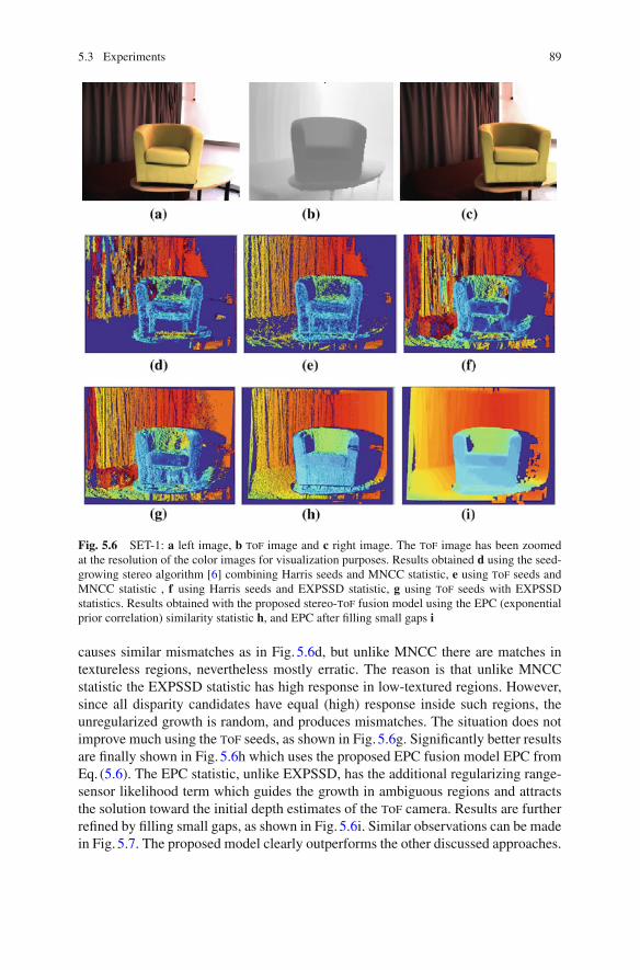
5.3 Experiments 89
Fig. 5.6 SET-1: a left image, b tof image and c right image. The tof image has been zoomedat the resolution of the color images for visualization purposes. Results obtained d using the seed-growing stereo algorithm [6] combining Harris seeds and MNCC statistic, e using tof seeds andMNCC statistic , f using Harris seeds and EXPSSD statistic, g using tof seeds with EXPSSDstatistics. Results obtained with the proposed stereo-tof fusion model using the EPC (exponentialprior correlation) similarity statistic h, and EPC after filling small gaps i
causes similar mismatches as in Fig. 5.6d, but unlike MNCC there are matches intextureless regions, nevertheless mostly erratic. The reason is that unlike MNCCstatistic the EXPSSD statistic has high response in low-textured regions. However,since all disparity candidates have equal (high) response inside such regions, theunregularized growth is random, and produces mismatches. The situation does notimprove much using the tof seeds, as shown in Fig. 5.6g. Significantly better resultsare finally shown in Fig. 5.6h which uses the proposed EPC fusion model EPC fromEq. (5.6). The EPC statistic, unlike EXPSSD, has the additional regularizing range-sensor likelihood term which guides the growth in ambiguous regions and attractsthe solution toward the initial depth estimates of the tof camera. Results are furtherrefined by filling small gaps, as shown in Fig. 5.6i. Similar observations can be madein Fig. 5.7. The proposed model clearly outperforms the other discussed approaches.

90 5 Time-of-flight and stereoscopic cameras
Fig. 5.7 SET-2. Please refer to the caption of Fig. 5.6 for explanations. a Left image. b tof image(zoomed). c Right image. d MNCC-Harris. e MNCC-TOF. f EXPSSD-Harris. g EXPSSD-TOF.h EPC (proposed). i EPC (gaps filled)
5.3.2 Comparison Between ToF Map and EstimatedDisparity Map
For the proper analysis of a stereo matching algorithm, it is important to inspect thereconstructed 3D surfaces. Indeed, the visualization of the disparity/depth maps cansometimes be misleading. Surface reconstruction reveals fine details in the qualityof the results. This is in order to qualitatively show the gain of the high-resolutiondepth map produced by the proposed algorithm with respect to the low-resolutiondepth map of the tof sensor.
In order to provide a fair comparison, we show the reconstructed surfaces associ-ated with the dense disparity maps Dp obtained after 2D triangulation of the tof datapoints, Fig. 5.8a, as well as the reconstructed surfaces associated with the disparitymap obtained with the proposed method, Fig. 5.8b. Clearly, much more of the sur-

5.3 Experiments 91
Fig. 5.8 The reconstructed surfaces are shown as relighted 3D meshes for a the prior disparitymap Dp (2D triangulation on projected and refined tof seeds), and b for the disparity map obtainedusing the proposed algorithm. Notice the fine surface details which were recovered by the proposedmethod
face details are recovered by the proposed method. Notice precise object boundariesand fine details, like the cushion on the sofa chair and a collar of the T-shirt, whichappear in Fig. 5.8b. This qualitatively corroborates the precision of the proposedmethod compared to the tof data.
5.3.3 Ground-Truth Evaluation
To quantitatively demonstrate the validity of the proposed algorithm, we carried outan experiment on data sets with associated ground-truth results. Similarly to [8] weused the Middlebury data set [22] and simulated the tof camera by sampling theground-truth disparity map.
The following results are based on the Middlebury-2006 data set.5 On purpose,we selected three challenging scenes with weakly textured surfaces: Lampshade-1,Monopoly, Plastic. The input images are of size 1330× 1110 pixels. We took every10th pixel in a regular grid to simulate the tof camera. This gives us about 14k oftof points, which is roughly the same ratio to color images as for the real sensors.We are aware that simulation tof sensor this way is naive, since we do not simulate
5 http://vision.middlebury.edu/stereo/data/scenes2006/

92 5 Time-of-flight and stereoscopic cameras
any noise or artifacts, but we believe that for validating the proposed method this issatisfactory.
Results are shown in Fig. 5.9 and Table 5.1. We show the left input image, results ofthe same algorithms as in the previous section with the real sensor, and the ground-truth disparity map. For each disparity, we compute the percentage of correctlymatched pixels in nonoccluded regions. This error statistic is computed as the numberof pixels for which the estimated disparity differs from the ground-truth disparity byless than one pixel, divided by number of all pixels in nonoccluded regions. Noticethat, unmatched pixels are considered as errors of the same kind as mismatches. Thisis in order to allow a strict but fair comparison between algorithms which deliversolutions of different densities. The quantitative evaluation confirms the previousobservations regarding the real-world setup. The proposed algorithm, which uses thefull sensor fusion model, significantly outperforms all other tested variants.
For the sake of completeness, we also report error statistics for the prior disparitymap Dp which is computed by interpolating tof seeds, see step 1 of Algorithm 1.These are 92.9, 92.1, 96.0 % for Lampshade-1, Monopoly, Plastic scene, respec-tively. These results are already quite good, which means the interpolation we useto construct the prior disparity map is appropriate. These scenes are mostly piece-wise planar, which the interpolation captures well. On the other hand, recall that inthe real case, not all the seeds are correct due to various artifacts of the range data.Nevertheless in all three scenes, the proposed algorithm (EPC with gaps filled) wasable to further improve the precision up to 96.4, 95.3, 98.2 % for the respectivescenes. This is again consistent with the experiments with the real tof sensor, wherehigher surface details were recovered, see Fig. 5.8.
5.3.4 Computational Costs
The original growing algorithm [6] has low computational complexity due to intrinsicsearch space reduction. Assuming the input stereo images are of size n × n pixels,the algorithm has the complexity of O(n2), while any exhaustive algorithm hasthe complexity at least O(n3) as noted in [5]. The factor n3 is the size of the searchspace in which the correspondences are sought, i.e., the disparity space. The growingalgorithm does not compute similarity statistics of all possible correspondences, butefficiently traces out components of high similarity score around the seeds. This lowcomplexity is beneficial especially for high-resolution imagery, which allows precisesurface reconstruction.
The proposed algorithm with all presented modifications does not representany significant extra cost. Triangulation of tof seeds and the prior disparity mapcomputation is not very costly, and nor is computation of the new EPC statistic(instead of MNCC).
For our experiments, we use an “academic”, i.e., a combined Matlab/C imple-mentation which takes approximately 5 s on two million pixel color images. Anefficient implementation of the seed-growing algorithm [6] which runs in real time

5.3 Experiments 93
Lampshade 1 MNCC-Harris MNCC-TOF EXPSSD-Harris
EXPSSD-TOF EPC EPC (gaps filled) Ground-truth
Monopoly MNCC-Harris MNCC-TOF EXPSSD-Harris
EXPSSD-TOF EPC EPC (gaps filled) Ground-truth
Plastic MNCC-Harris MNCC-TOF EXPSSD-Harris
EXPSSD-TOF EPC EPC (gaps filled) Ground-truth
Fig. 5.9 Middlebury data set. Left-right and top-bottom: the left images, results obtained with thesame algorithms as in Figs. 5.6 and 5.7, and the ground-truth disparity maps. This evaluation showsthat the combination of the proposed seed-growing stereo algorithm with a prior disparity map,obtained from a sparse and regularly distributed set of 3D points, yields excellent dense matchingresults

94 5 Time-of-flight and stereoscopic cameras
Table 5.1 The error statistics (percentage of correctly matched pixels) associated with the testedalgorithms and for three test image pairs from the Middlebury data set
Left image MNCC- MNCC- EXPSSD- EXPSSD- EPC (%) EPCHarris (%) TOF (%) Harris (%) TOF (%) (gaps filled) (%)
Lampshade-1 61.5 64.3 44.9 49.5 88.8 96.4Monopoly 51.2 53.4 29.4 32.1 85.2 95.3Plastic 25.2 28.2 13.5 20.6 88.7 98.2
on a standard CPU was recently proposed [10]. This indicates that a real-time imple-mentation of the proposed algorithm is feasible. Indeed, the modification of thegrowing algorithm and integration with the tof data does not bring any significantextra computational costs. The algorithmic complexity remains the same, since wehave only slightly modified the similarity score used inside the growing procedure.It is true that prior to the growing process, the tof data must be triangulated. Nev-ertheless, this can be done extremely efficiently using computer graphics techniquesand associated software libraries.
5.4 Conclusions
We have proposed a novel correspondence growing algorithm, performing fusionof a range sensor and a pair of passive color cameras, to obtain an accurate anddense 3D reconstruction of a given scene. The proposed algorithm is robust, andperforms well on both textured and textureless surfaces, as well as on ambiguousrepetitive patterns. The algorithm exploits the strengths of the tof sensor and those ofstereo matching between color cameras, in order to compensate for their individualweaknesses. The algorithm has shown promising results on difficult real-world data,as well as on challenging standard data sets which quantitatively corroborates itsfavorable properties. Together with the strong potential for real-time performancethat has been discussed, the algorithm would be practically very useful in manycomputer vision and robotic applications.
References
1. Alenyà, G., Dellen, B., Torras, C.: 3D Modelling of leaves from color and tof data for robo-tized plant measuring. In: Proceedings of IEEE International Conference on Robotics andAutomation (ICRA), pp. 3408–3414 (2011)
2. Attamimi, M., Mizutani, A., Nakamura, T., Nagai, T., Funakoshi, K., Nakano, M.: Real-time3D visual sensor for robust object recognition. In: Proceedings of IEEE/RSJ InternationalConference on Intelligent Robots and Systems (IROS), pp. 4560–4565 (2010)
3. Castañeda, V., Mateus, D., Navab, N.: SLAM combining ToF and high-resolution cameras.In: IEEE Workshkop on Motion and Video Computing (2011)

References 95
4. Cech, J., Matas, J., Perdoch, M.: Efficient sequential correspondence selection by cosegmen-tation. IEEE Trans. Pattern Anal. Mach. Intell. 32(9), 1568–1581 (2010)
5. Cech, J., Sanchez-Riera, J., Horaud, R.: Scene flow estimation by growing correspondenceseeds. In: Proceedings of the IEEE Conference on Computer Vision and Pattern Recognition(CVPR), pp. 3129–3136 (2011)
6. Cech, J., Šára, R.: Efficient sampling of disparity space for fast and accurate matching. In: Pro-ceedings of BenCOS Workshop CVPR (2007)
7. Chan, D., Buisman, H., Theobalt, C., Thrun, S.: A noise-aware filter for real-time depth upsam-pling. In: ECCV Workshop on Multi-camera and Multi-modal Sensor Fusion Algorithms andApplications (2008)
8. Dal Mutto, C., Zanuttigh, P., Cortelazzo, G.M.: A probabilistic approach to ToF and stereo datafusion. In: Proceedings of 3D Data Processing, Visualization and Transmission, Paris (2010)
9. Diebel, J., Thrun, S.: An application of Markov random fields to range sensing. In: Proceedingson Neural Information Processing Systems (NIPS) (2005)
10. Dobias, M., Sára, R.: Real-time global prediction for temporally stable stereo. In: Proceedingsof IEEE International Conference on Computer Vision Workshops, pp. 704–707 (2011)
11. Droeschel, D., Stückler, J., Holz, D., Behnke, S.: Towards joint attention for a domestic servicerobot—person awareness and gesture recognition using time-of-flight cameras. In: Proceedingsof International Conference on Robotic and Animation (ICRA), Shanghai, pp. 1205–1210(2011)
12. Fischer, J., Arbeiter, G., Verl, A.: Combination of time-of-flight depth and stereo usingsemiglobal optimization. In: Proceedings of IEEE International Conference on Robotics andAutomation (ICRA), pp. 3548–3553 (2011)
13. Freedman, B., Shpunt, A., Machline, M., Arieli, Y.: Depth Mapping Using Projected Patterns.US Patent No. 8150412 (2012)
14. Geiger, A., Roser, M., Urtasun, R.: Efficient large-scale stereo matching. In: Proceedings ofthe Asian Conference on Computer Vision (ACCV), pp. 25–38 (2010)
15. Gould, S., Baumstarck, P., Quigley, M., Ng, A.Y., Koller, D.: Integrating visual and range datafor robotic object detection. In: Proceedings of European Conference on Computer VisionWorkshops (2008)
16. Hansard, M., Horaud, R., Amat, M., Lee, S.: Projective alignment of range and parallax data.In: Proceedings of IEEE Conference on Computer Vision and Pattern Recognition (CVPR),pp. 3089–3096 (2011)
17. Jebari, I., Bazeille, S., Battesti, E., Tekaya, H., Klein, M., Tapus, A., Filliat, D., Meyer, C., Sio-Hoi, I., Benosman, R., Cizeron, E., Mamanna, J.-C., Pothier, B.: Multi-sensor semantic mappingand exploration of indoor environments. In: Technologies for Practical Robot Applications(TePRA), pp. 151–156 (2011)
18. Mesa Imaging AG. http://www.mesa-imaging.ch19. Moravec, H.P.: Toward automatic visual obstacle avoidance. In: 5th International Conference
Artificial Intelligence (ICAI), pp. 584–594 (1977)20. Newcombe, R.A., Davison, A.J.: Live dense reconstruction with a single moving camera.
In: Proceedings of IEEE Conference on Computer Vision and Pattern Recognition (CVPR),pp. 1498–1505 (2010)
21. Park, J., Kim, H., Tai, Y.-W., Brown, M.-S., Kweon, I.S.: High quality depth map upsamplingfor 3D-TOF cameras. In: Proceedings of IEEE International Conference on Computer Vision(ICCV) (2011)
22. Scharstein, D., Szeliski, R.: A taxonomy and evaluation of dense two-frame stereo correspon-dence algorithms. Int. J. Comput. Vision 47, 7–42 (2002)
23. Seitz, S., Curless, B., Diebel, J., Scharstein, D., Szeliski, R.: A comparison and evaluation ofmulti-view stereo reconstruction algorithms. In: Proceedings of Computer Vision and PatternRecognition (CVPR), pp. 519–528 (2006)
24. Stückler J., Behnke, S.: Combining depth and color cues for scale- and viewpoint-invariantobject segmentation and recognition using random forests. In: Proceedings of IEEE/ RSJ Inter-national Conference on Robots and Systems (IROS), pp. 4566–4571 (2010)

96 5 Time-of-flight and stereoscopic cameras
25. Wang, L., Yang, R.: Global stereo matching leveraged by sparse ground control points.In: Proceedings of IEEE Conference on Computer Vision and Pattern Recognition (CVPR),pp. 3033–3040 (2011)
26. Zhu, J., Wang, L., Yang, R.G., Davis, J.: Fusion of time-of-flight depth and stereo for highaccuracy depth maps. In: Proceedings of IEEE Conference on Computer Vision and PatternRecognition (CVPR), pp. 1–8 (2008)