Spring 2020 - 控制系統
18
Spring 2020 控制系統 Control Systems Unit 6E The Nyquist Stability Criterion Feng-Li Lian & Ming-Li Chiang NTU-EE Mar 2020 – Jul 2020
-
Upload
khangminh22 -
Category
Documents
-
view
1 -
download
0
Transcript of Spring 2020 - 控制系統
Spring 2020
控制系統Control Systems
Unit 6E
The Nyquist Stability Criterion
Feng-Li Lian & Ming-Li Chiang
NTU-EE
Mar 2020 – Jul 2020
CS6E-NyquistCriterion- 2
Feng-Li Lian © 2020Nyquist Stability Criterion
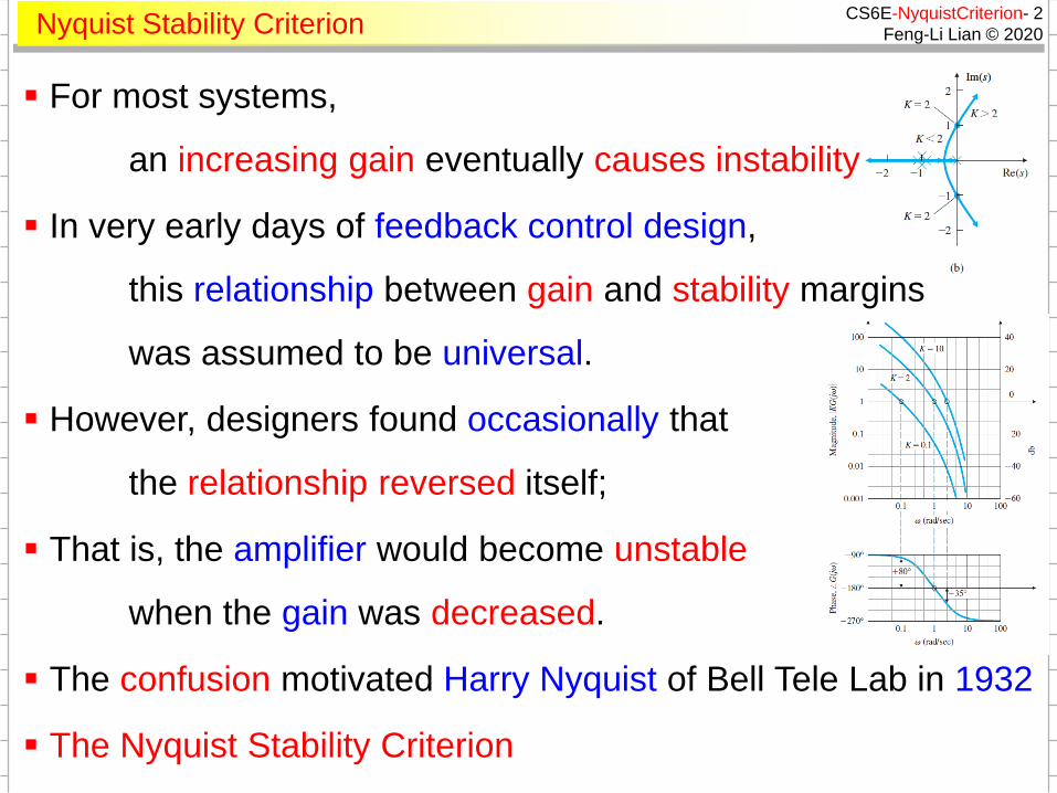
For most systems,
an increasing gain eventually causes instability
In very early days of feedback control design,
this relationship between gain and stability margins
was assumed to be universal.
However, designers found occasionally that
the relationship reversed itself;
That is, the amplifier would become unstable
when the gain was decreased.
The confusion motivated Harry Nyquist of Bell Tele Lab in 1932
The Nyquist Stability Criterion
CS6E-NyquistCriterion- 3
Feng-Li Lian © 2020Nyquist Stability Criterion
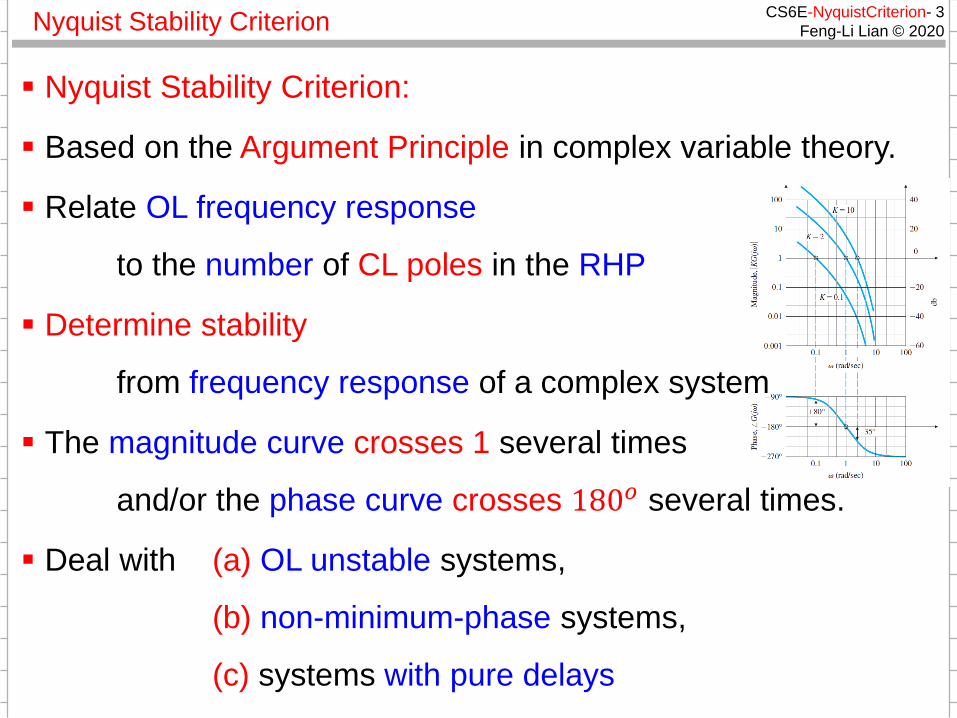
Nyquist Stability Criterion:
Based on the Argument Principle in complex variable theory.
Relate OL frequency response
to the number of CL poles in the RHP
Determine stability
from frequency response of a complex system
The magnitude curve crosses 1 several times
and/or the phase curve crosses 180𝑜 several times.
Deal with (a) OL unstable systems,
(b) non-minimum-phase systems,
(c) systems with pure delays
CS6E-NyquistCriterion- 4
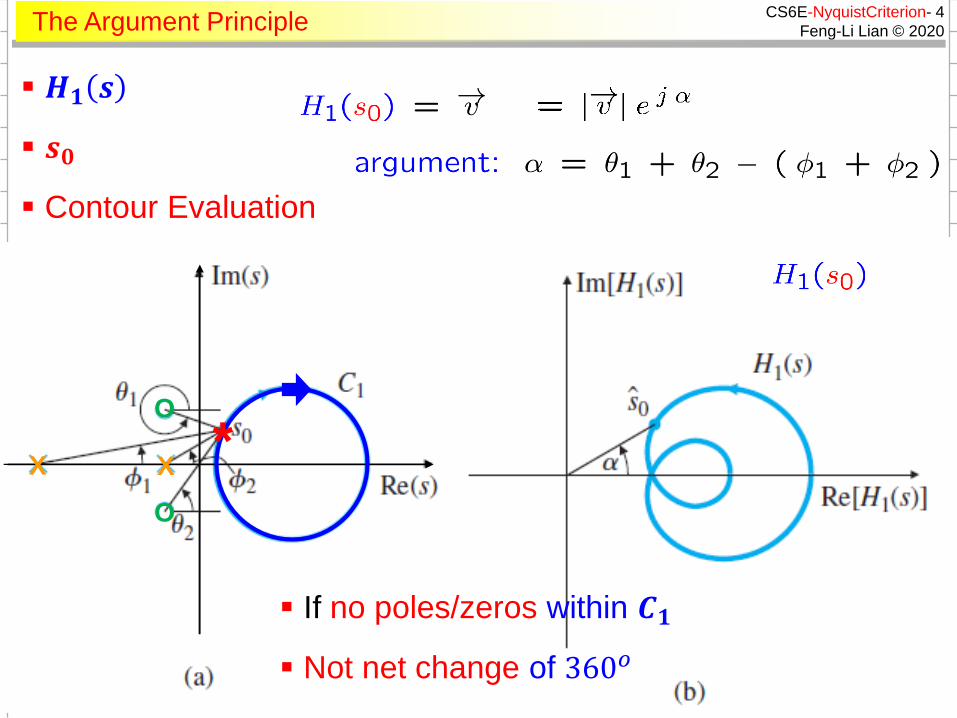
Feng-Li Lian © 2020The Argument Principle
X
O
O
X
𝑯𝟏 𝒔
𝒔𝟎
Contour Evaluation
*
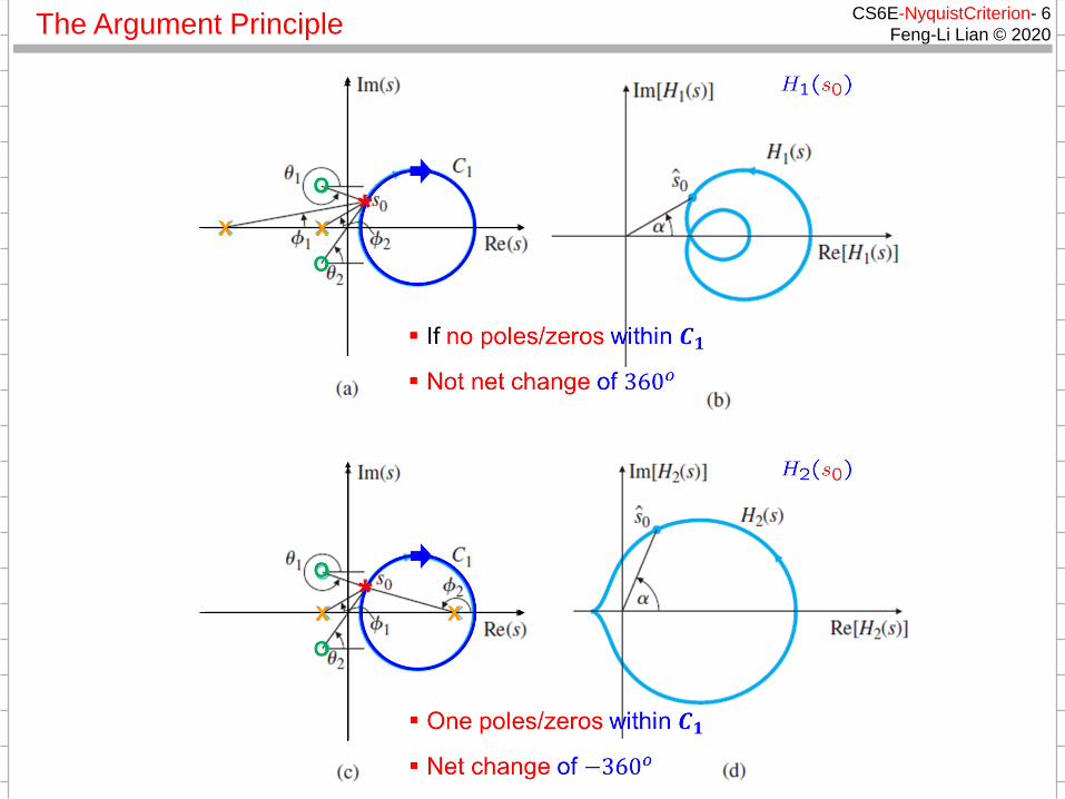
If no poles/zeros within 𝑪𝟏
Not net change of 360𝑜
CS6E-NyquistCriterion- 5
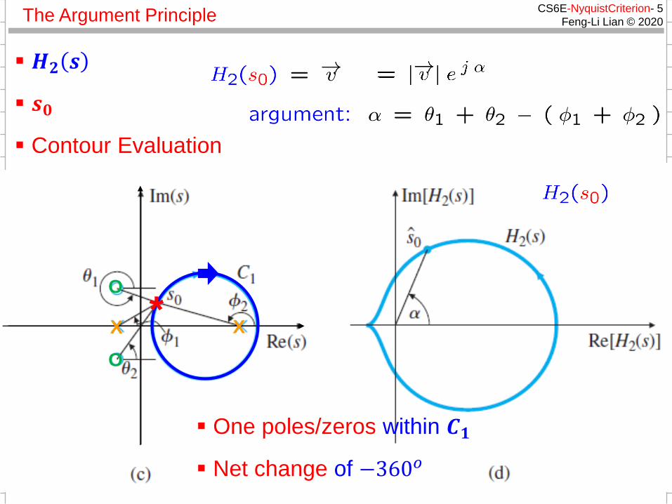
Feng-Li Lian © 2020The Argument Principle
𝑯𝟐 𝒔
𝒔𝟎
Contour Evaluation
X
O
O
X*
One poles/zeros within 𝑪𝟏
Net change of −360𝑜
CS6E-NyquistCriterion- 6
Feng-Li Lian © 2020The Argument Principle
CS6E-NyquistCriterion- 7
Feng-Li Lian © 2020The Argument Principle
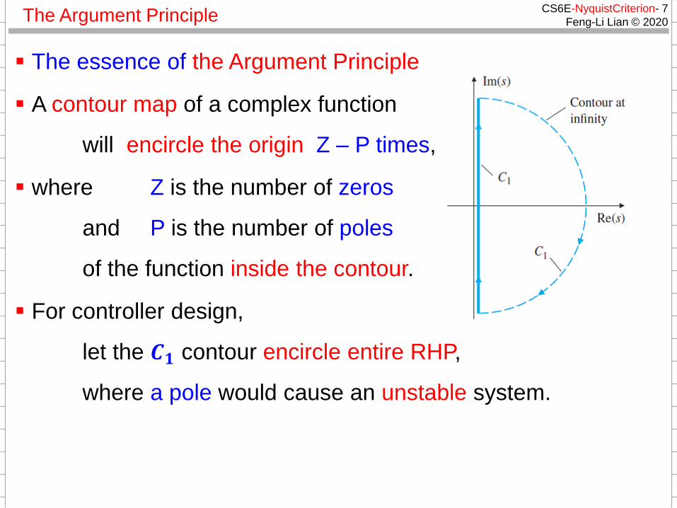
The essence of the Argument Principle
A contour map of a complex function
will encircle the origin Z – P times,
where Z is the number of zeros
and P is the number of poles
of the function inside the contour.
For controller design,
let the 𝑪𝟏 contour encircle entire RHP,
where a pole would cause an unstable system.
CS6E-NyquistCriterion- 8
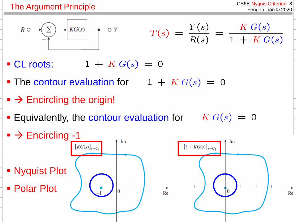
Feng-Li Lian © 2020The Argument Principle
CL roots:
The contour evaluation for
Encircling the origin!
Equivalently, the contour evaluation for
Encircling -1
Nyquist Plot
Polar Plot
CS6E-NyquistCriterion- 9
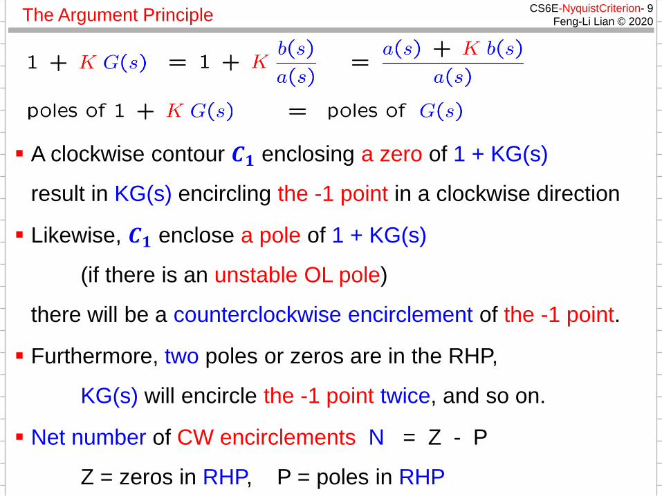
Feng-Li Lian © 2020The Argument Principle
A clockwise contour 𝑪𝟏 enclosing a zero of 1 + KG(s)
result in KG(s) encircling the -1 point in a clockwise direction
Likewise, 𝑪𝟏 enclose a pole of 1 + KG(s)
(if there is an unstable OL pole)
there will be a counterclockwise encirclement of the -1 point.
Furthermore, two poles or zeros are in the RHP,
KG(s) will encircle the -1 point twice, and so on.
Net number of CW encirclements N = Z - P
Z = zeros in RHP, P = poles in RHP
CS6E-NyquistCriterion- 10
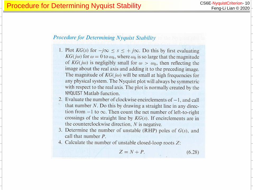
Feng-Li Lian © 2020Procedure for Determining Nyquist Stability
CS6E-NyquistCriterion- 11
Feng-Li Lian © 2020Examples
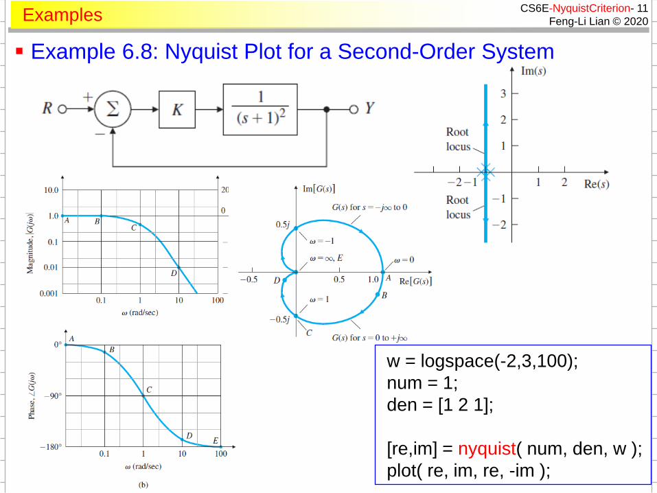
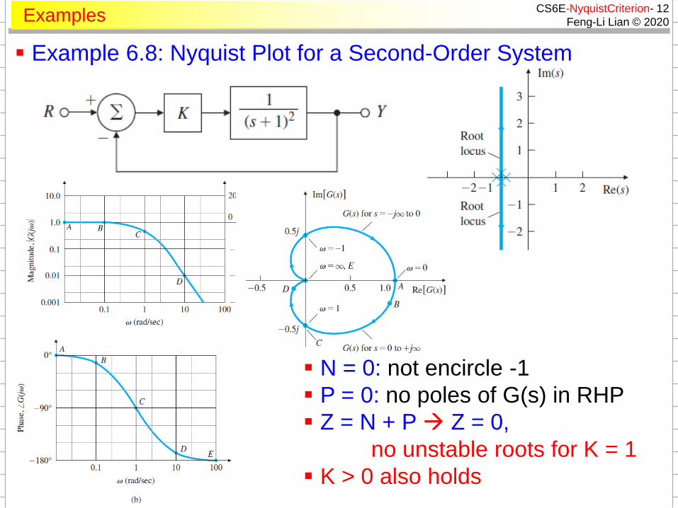
Example 6.8: Nyquist Plot for a Second-Order System
w = logspace(-2,3,100);
num = 1;
den = [1 2 1];
[re,im] = nyquist( num, den, w );
plot( re, im, re, -im );
CS6E-NyquistCriterion- 12
Feng-Li Lian © 2020Examples
Example 6.8: Nyquist Plot for a Second-Order System
N = 0: not encircle -1
P = 0: no poles of G(s) in RHP
Z = N + P Z = 0,
no unstable roots for K = 1
K > 0 also holds
CS6E-NyquistCriterion- 13
Feng-Li Lian © 2020Examples
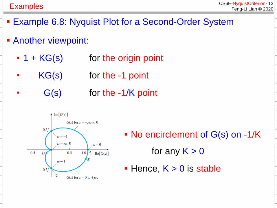
Example 6.8: Nyquist Plot for a Second-Order System
Another viewpoint:
• 1 + KG(s) for the origin point
• KG(s) for the -1 point
• G(s) for the -1/K point
No encirclement of G(s) on -1/K
for any K > 0
Hence, K > 0 is stable
CS6E-NyquistCriterion- 14
Feng-Li Lian © 2020Examples
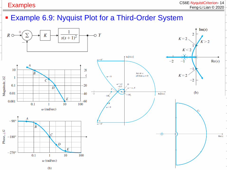
Example 6.9: Nyquist Plot for a Third-Order System
CS6E-NyquistCriterion- 15
Feng-Li Lian © 2020Examples
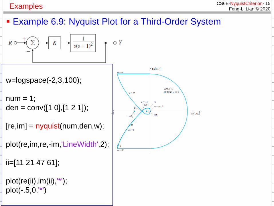
Example 6.9: Nyquist Plot for a Third-Order System
w=logspace(-2,3,100);
num = 1;
den = conv([1 0],[1 2 1]);
[re,im] = nyquist(num,den,w);
plot(re,im,re,-im,'LineWidth',2);
ii=[11 21 47 61];
plot(re(ii),im(ii),'*');
plot(-.5,0,'*')
CS6E-NyquistCriterion- 16
Feng-Li Lian © 2020Examples
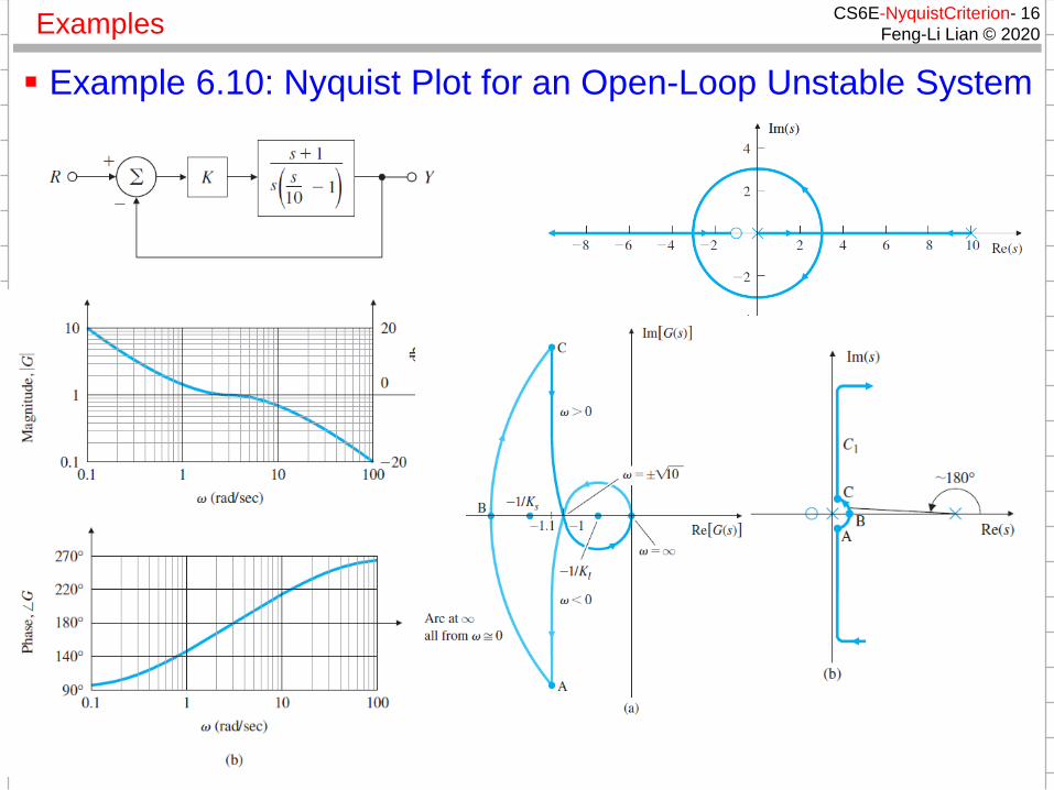
Example 6.10: Nyquist Plot for an Open-Loop Unstable System
CS6E-NyquistCriterion- 17
Feng-Li Lian © 2020Examples
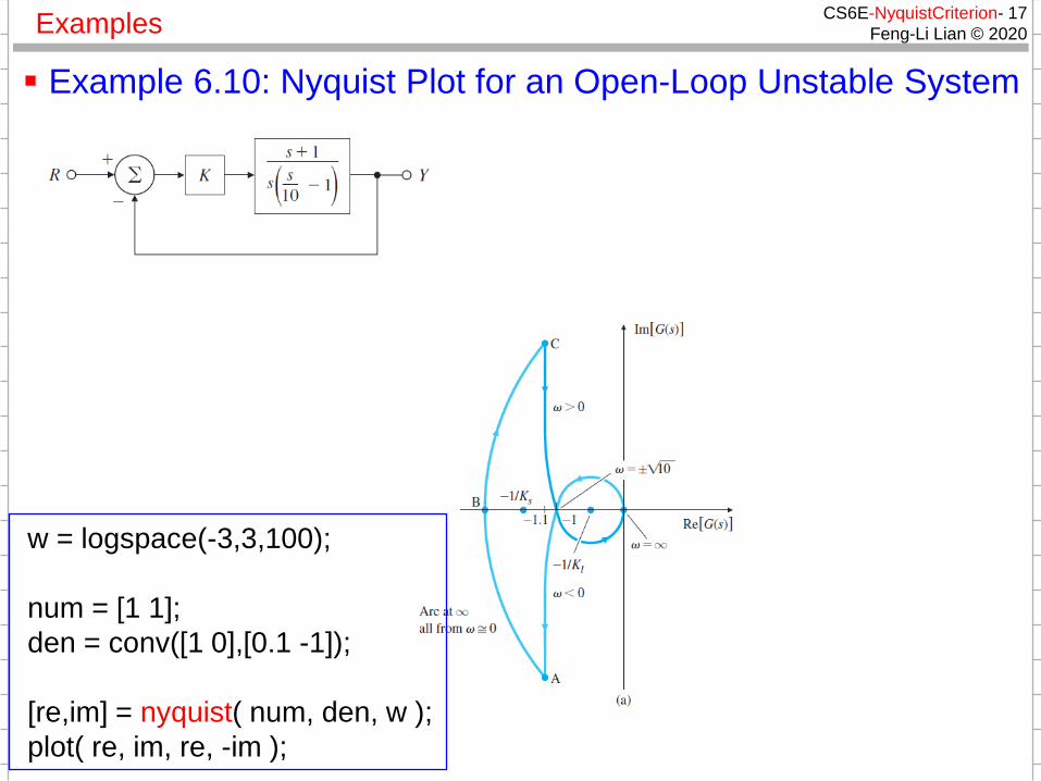
Example 6.10: Nyquist Plot for an Open-Loop Unstable System
w = logspace(-3,3,100);
num = [1 1];
den = conv([1 0],[0.1 -1]);
[re,im] = nyquist( num, den, w );
plot( re, im, re, -im );
CS6E-NyquistCriterion- 18
Feng-Li Lian © 2020Examples
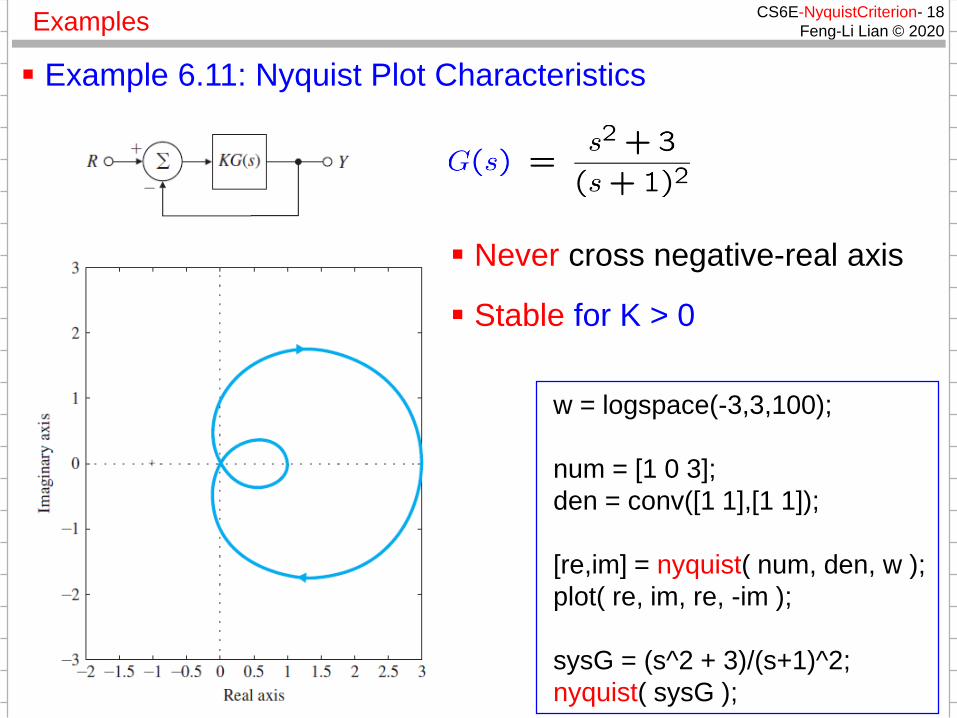
Example 6.11: Nyquist Plot Characteristics
w = logspace(-3,3,100);
num = [1 0 3];
den = conv([1 1],[1 1]);
[re,im] = nyquist( num, den, w );
plot( re, im, re, -im );
sysG = (s^2 + 3)/(s+1)^2;
nyquist( sysG );
Never cross negative-real axis
Stable for K > 0