Spillover Effects of the U.S. Financial Crisis on Financial Markets in Emerging Asian Countries

Auburn University

Department of Economics

Working Paper Series

Spillover Effects of the US Financial Crisis on

Financial Markets in Emerging Asian Countries

Bong-Han Kima and Hyeongwoo Kimb

aKongju National University; bAuburn University

AUWP 2011-04

This paper can be downloaded without charge from:

http://media.cla.auburn.edu/economics/workingpapers/

http://econpapers.repec.org/paper/abnwpaper/

http://media.cla.auburn.edu/economics/workingpapers/

http://econpapers.repec.org/paper/abnwpaper/

Spillover Effects of the US Financial Crisis on Financial Markets

in Emerging Asian Countries

Bong-Han Kim∗ and Hyeongwoo Kim†

Kongju National University and Auburn University

April 2011

Abstract

We estimate dynamic conditional correlations of financial asset returns across countries by an

array of multivariate GARCHmodels and analyze spillover effects of the recent US financial crisis

on 5 emerging Asian countries. We find a symptom of financial contagion around the collapse

of Lehman Brothers in September 2008. There appears to be a regime shift to substantially

higher conditional correlations that persisted for a fairly short-period of time. We also propose

a novel approach that allows simultaneous estimations of the conditional correlation coefficient

and the effects of its determining factors over time, which can be used to identify channels of

spillovers. We find the dominant role of foreign investment for the conditional correlations in

international equity markets. The dollar Libor-OIS spread, the sovereign CDS premium, and

foreign investment are found to play significant roles in foreign exchange markets.

Keywords: Financial Crisis, Spillover Effects, Contagion, Emerging Asian Countries, Dynamic

Conditional Correlation, DCCX-MGARCH

JEL Classification: C32, F31, G15

∗Department of International Economics, Kongju National University, Gongju, Chungnam, South Korea. Tel:82-41-850-8391. Fax: 82-41-850-8390. Email: [email protected].

†Department of Economics, Auburn University, Auburn, AL 36849. Tel: 1-334-844-2928. Fax: 1-334-844-4615.Email: [email protected].

1

1 Introduction

The collapse of the US housing market and the ensuing sub-prime mortgage market crash in the

Summer of 2007 triggered a global financial crisis, which is considered the first global crisis since

the Great Depression (Claessens et al. 2010). As Dooley and Hutchison (2009) point out, financial

reforms in emerging economies made it possible to temporarily insulate themselves from adverse

shocks originating from the US until the Summer of 2008. This relatively tranquil period of time,

however, was ended by a direct shock in the form of the Lehman failure in September 2008. The

equity price in Taiwan, for instance, dropped by 38.5% in 3 months following September 15, 2008.

During the same period, the Korean Won depreciated against the US dollar by 19.2% as global risk

aversion spurred demand for a safe asset (ironically, US dollars), which led to strong deteriorating

spillover effects on real sectors.

Even though understanding the nature of contagion in financial markets is of fundamental im-

portance, the economic profession has failed to reach a consensus even on the existence of contagion

during earlier financial crises. Forbes and Rigobon (2002), for example, argue that virtually all pre-

vious evidence of contagion (see, among others, King and Wadhwani, 1990, Lee and Kim, 1993,

Calvo and Reinhart, 1996) disappears when unconditional cross-market correlation coefficients are

corrected for bias. Corsetti et al. (2005), however, point out Forbes and Rigobon’s test is biased

towards the null hypothesis of no contagion, and report stronger evidence of contagion with an

alternative test.

In this paper, we investigate the transmission of the recent US crisis to financial markets in

five emerging Asian economies: Indonesia, Korea, the Philippines, Thailand, and Taiwan. We are

particularly interested in the following questions. Is there empirical evidence of contagion from the

US to emerging Asian financial markets? If so, when did it occur and for how long did it last?

More importantly, through what channels did the contagion spread to those markets? We employ an

array of multivariate generalized autoregressive conditional heteroskedasticity (MGARCH) models

to seek answers to these questions.

To answer the first two questions, we employ Engle’s (2002) dynamic conditional correlation

2

(DCC) model and a nonlinear conditional correlation MGARCH (NLCC-MGARCH) models, the

exponential smooth transition (EST) model. Throughout the paper, we focus on time-varying

dynamic conditional correlations during the recent crisis instead of unconditional correlation coef-

ficients as in our view the latter lacks practical usefulness from a policy perspective. Our NLCC-

MGARCH model estimations for the equity and foreign exchange markets in the US and 5 emerging

Asian economies identified two substantially different conditional correlations around the Lehman

episode. Overall, transitions from the tranquil period to the contagion period occurred very quickly

and lasted for fairly short period of time. This implies that these countries can experience a sudden

acceleration of systemic risk when exogenous shocks occur. We do not claim, however, that the

conditional correlation was the highest during the crisis in the entire sample period. Instead, we

demonstrate that the correlation of asset returns of the source and the victim countries tends to

increase rapidly during the crisis.

To answer the third question, we propose a novel DCC-MGARCH-type model with exogenous

variables (DCCX-MGARCH). To the best of our knowledge, this method is the first that estimates

both the dynamic conditional correlation and the effects of explanatory variables simultaneously

in a unified framework. The DCCX-MGARCH method can be quite useful to see what economic

fundamental variables affect the cross-country correlations in order to identify the channels of

contagion.

A number of variables can be considered for the factors that determine time-varying conditional

correlations. We consider the following three channels of contagion. The first one is the factors that

proxy the vulnerability of the US financial markets. We consider the VIX index for this purpose.

The TED spread and the daily 3-month US dollar Libor-overnight index swap (OIS) spread are also

considered as liquidity availability measures. Secondly, we use the sovereign credit default swap

(CDS) premium as a proxy for weakness of emerging Asian markets. The last factor is the amount

of foreign order flow (foreign investment) to quantitatively measure the role of foreign capital.

Our estimation reveals a dominant role of foreign capital for the conditional correlations in

international equity markets. In foreign exchange markets, the Libor-OIS spread, the sovereign

3

CDS premium, and the market share of foreign investors are found to play important roles. These

findings provide valuable policy implications. The importance of foreign capital, for instance, calls

for institutional arrangements such as currency swap agreements.

The remainder of the present paper is organized as follows. Section 2 provides a brief literature

review. In Section 3, we present our empirical models and discuss estimation techniques employed.

Section 4 describes the data and presents the empirical results. Some concluding remarks and

policy implications are reported in the last section.

2 Literature review

The empirical literature on spillover/contagion is extensive. There are at least two important but

unsettled issues: 1) whether contagion actually occurred between countries/markets during financial

crises in the past; 2) if contagion occurred, through what channels adverse shocks propagated to

other countries/markets from the source.

To deal with the first issue, researchers typically employ a sub-sample analysis for a structural

break (with a known structural break date) in unconditional cross-market correlation coefficients

in the pre- and post-crisis period. If the correlation coefficient increases significantly during the

crisis, this may imply statistically higher degree cross-market linkages, in other words, contagion.

Examples of studies that employ such methods include: King and Wadhwani (1990), Lee and Kim

(1993), Calvo and Reinhart (1996), and Baig and Goldfajn (1999), among others. Many of these

papers find sizable differences in correlation coefficients and conclude contagion occurred during

the crises they investigated.1

Forbes and Rigobon (2002) point out, however, that these tests based on sub-sample compar-

isons of correlation coefficients may suffer from severe bias due to heteroskedasticity.2 Correcting

1King and Wadhwani (1990) investigate stock return correlations between the US, the UK, and Japan and report a

significant increase in the cross-country correlation coefficients of stock returns after the 1987 US stock market crash.

Lee and Kim (1993) find similar evidence from an extended data set with 12 major markets. Calvo and Reinhart

(1996) find contagion between stock prices and bond prices after the 1994 Mexican crisis. Baig and Goldfajn (1999)

also report evidence of cross-country contagion in the currency and equity markets during the East Asian crisis.2Boyer et al. (1999) and Loretan and English (2000) made the same point and derive similar bias correction

methods independently.

4

for the bias, Forbes and Rigobon report virtually no evidence of contagion during crises in the

past, including the 1997 East Asian crisis, the 1994 Mexican Peso (devaluation) crisis, and the

1987 US market crash. Instead, they find a high level of correlation in all periods, which they call

interdependence. Corsetti et al. (2005), however, point out that the tests by Boyer et al. (1999)

and Forbes and Rigobon (2002) are biased towards the null hypothesis of no contagion.3 Using a

standard factor model, they report strong evidence of contagion during the 1997 Hong Kong stock

market crisis.

An array of research uses GARCH-type models focusing on price-volatility spillover effects. For

instance, Hamao et al. (1990) use a GARCH-M (GARCH in mean) model and report some spillover

effects on the conditional mean and variance in stock markets after the 1987 US stock market crash.

Edwards (1998) find similar evidence in international bonds markets after the 1994 Mexican Peso

crisis. Bekaert et al. (2005) find no evidence of increases in "excess" stock market correlations

(above the expected correlations based on economic fundamentals), contagion, after the 1994 Peso

crisis, while finding some evidence of contagion after the 1997 Asian crisis. It should be noted,

however, that these analysis do not provide direct evidence against those of Forbes and Rigobon

(2002), because Forbes and Rigobon focus on permanent changes in unconditional moments rather

than conditional ones.

Another group of researchers, including the present one, employ the dynamic conditional corre-

lation (DCC) MGARCH model by Engle (2002) to estimate time-varying conditional correlations.

This approach does not require knowledge of the exact date when the contagion occurs. Put dif-

ferently, we do not make an arbitrary assumption on the timing of turmoil periods, since it does

not rely on sub-sample analyses. See, among others, Chiang et al. (2007), Frank and Hesse (2009),

and Hwang et al. (2010).

The second issue, though we view more important than the first one from policy perspectives,

has drawn relatively less attention. Rose and Spiegel (2009), in their recent study for a cross-

section of 85 countries, consider a real linkage (trade channel) and a financial linkage (foreign asset

3Bekaert et al. (2005) also point out that Forbes and Rigobon’s method is not valid in the presence of common

shocks.

5

exposure) that may have allowed the recent US crisis to spread to other countries. They find little

evidence that these channels are closely related with the incidence of the crisis.4 Contagion due to

financial channels seem highly plausible, though, because a high exposure to foreign assets can lead

to a rapid deterioration in a country’s balance sheet when exogenous foreign adverse shocks occur

(see Davis, 2008).

One way to investigate the role of financial linkages for exacerbating contagious effects is to

compare dynamic conditional correlations across countries and across markets (see Frank and Hesse,

2009, for example). Our DCCX-MGARCH model is different from such models in that ours directly

estimates the effects of exogenous variables on the time-varying conditional correlations in a unified

MGARCH framework. To the best of our knowledge, this is a novel aspect of our model. Since it

provides information on what variables play dominant roles for channelling adverse shocks from the

source country to the recipient countries, it is possible to make more suitable policy suggestions.

3 The Econometric Model

3.1 The Dynamic Conditional Correlation Model

We first employ the dynamic conditional correlation (DCC) estimator (Engle, 2002) for multi-

variate generalized autoregressive conditional heteroskedasticity (MGARCH) models to estimate

time-varying conditional correlations of international asset returns. DCC-MGARCH can be viewed

as a generalization of the constant conditional correlation (CCC) estimator (Bollerslev, 1990).

Let y = [1 2 · · · ]0be a ×1 vector of asset returns that obeys the following stochastic

process.

y = Γ()y−1 + e (1)

where Γ() is the lag polynomial matrix. The conditional distribution of asset returns is assumed

4For articles that investigate trade linkages, see Eichengreen et al. (1996), Glick and Rose (1999), Eichengreen

and Rose (1998), and Forbes and Chinn (2004), among others.

6

to be joint normal,

e|Ω−1 ∼ N (0H) (2)

where Ω−1 is the adaptive information set at time − 1. The conditional covariance matrix H is

defined as,

H = DRD (3)

whereD is the diagonal matrix with the conditional variances along the diagonal,D = ³12

´and R is the time-varying correlation matrix.

5

The equation (3) can be re-parameterized as follows with standardized returns, = D−1 e,

E−10 = D

−1 HD

−1 = R = [] (4)

Engle proposes the following mean-reverting conditional correlations with the GARCH(1 1) speci-

fication.

=√

(5)

where

= (1− − ) + −1−1 + −1 (6)

and is the unconditional correlation between and . and are non-negative scalars that

satisfy + 1.6 In matrix form,

Q = Q (1− − )+−10−1 + Q−1 (7)

where Q is the unconditional correlation matrix of . R is obtained by

R = (Q∗ )−12

Q (Q∗ )−12 (8)

5Bollerslev’s CCC model assumes H = DRD, where R is a × time-invariant (symmetric) correlation matrix.6When + = 1, is nonstationary and the exponential smoothing estimator can apply.

7

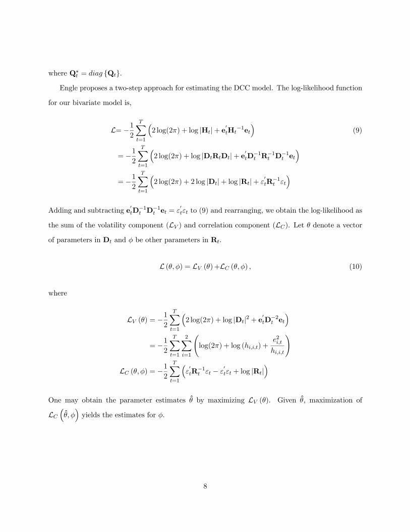
where Q∗ = Q.Engle proposes a two-step approach for estimating the DCC model. The log-likelihood function

for our bivariate model is,

L= −12

X=1

³2 log(2) + log |H|+ e0H

−1e´

(9)

= −12

X=1

³2 log(2) + log |DRD|+ e0D−1 R−1 D−1 e

´= −1

2

X=1

³2 log(2) + 2 log |D|+ log |R|+

0R−1

´

Adding and subtracting e0D−1 D

−1 e =

0 to (9) and rearranging, we obtain the log-likelihood as

the sum of the volatility component (L ) and correlation component (L). Let denote a vectorof parameters in D and be other parameters in R.

L ( ) = L ()+L ( ) (10)

where

L () = −12

X=1

³2 log(2) + log |D|2 + e0D−2 e

´= −1

2

X=1

2X=1

Ãlog(2) + log () +

2

!

L ( ) = −12

X=1

³0R−1 −

0 + log |R|

´

One may obtain the parameter estimates by maximizing L (). Given , maximization of

L³

´yields the estimates for .

8

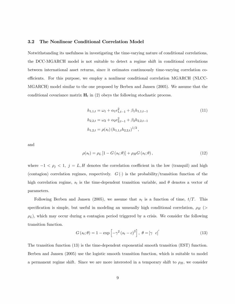
3.2 The Nonlinear Conditional Correlation Model

Notwithstanding its usefulness in investigating the time-varying nature of conditional correlations,

the DCC-MGARCH model is not suitable to detect a regime shift in conditional correlations

between international asset returns, since it estimates continuously time-varying correlation co-

efficients. For this purpose, we employ a nonlinear conditional correlation MGARCH (NLCC-

MGARCH) model similar to the one proposed by Berben and Jansen (2005). We assume that the

conditional covariance matrix H in (2) obeys the following stochastic process.

11 = 1 + 121−1 + 111−1 (11)

22 = 2 + 222−1 + 222−1

12 = () (1122)12

and

() = [1− (; )] + (; ) (12)

where −1 1 = denotes the correlation coefficient in the low (tranquil) and high

(contagion) correlation regimes, respectively. (·) is the probability/transition function of thehigh correlation regime, is the time-dependent transition variable, and denotes a vector of

parameters.

Following Berben and Jansen (2005), we assume that is a function of time, . This

specification is simple, but useful in modeling an unusually high conditional correlation, (

), which may occur during a contagion period triggered by a crisis. We consider the following

transition function.

(; ) = 1− exph−2 ( − )2

i = [ ]

0(13)

The transition function (13) is the time-dependent exponential smooth transition (EST) function.

Berben and Jansen (2005) use the logistic smooth transition function, which is suitable to model

a permanent regime shift. Since we are more interested in a temporary shift to , we consider

9

an exponential type transition function. determines how quickly transitions occur (smoothness)

and is a location parameter. We can estimate the unknown parameters of the EST NLCC-

MGARCH model by maximizing the following log-likelihood function with respect to all parameters

simultaneously.

L= −12

X=1

³2 log(2) + log |H|+ e0H

−1e´

3.3 The DCCX-MGARCH Model

We now propose a novel DCC-MGARCH model where the conditional correlation coefficient is

determined by exogenous variables (DCCX-MGARCH). We assume the following.

12 = (x) (1122)12 (14)

where −1 (x) 1 is an monotonic increasing function of x, a × 1 vector of economicfundamental variables that affect the size of the conditional correlation. This approach is useful for

identifying propagation channels of potentially harmful effects of crises.

We propose the following parameterization for such a conditional correlation function.

(x) = 2

⎡⎣ exp³0x

´1 + exp (

0x)

⎤⎦− 1 (15)

where = [1 2 · · · ]0and x = [1 2 · · · ]

0.

4 Empirical Results

4.1 Data and Summary Statistics

We utilize daily observations of stock indices and foreign exchange rates obtained from Bloomberg.

The sample period is April 2, 2007 to August 31, 2009. Exchange rates are national currency

prices of the US dollar. Asset returns are calculated by taking two-day differentials of natural

10

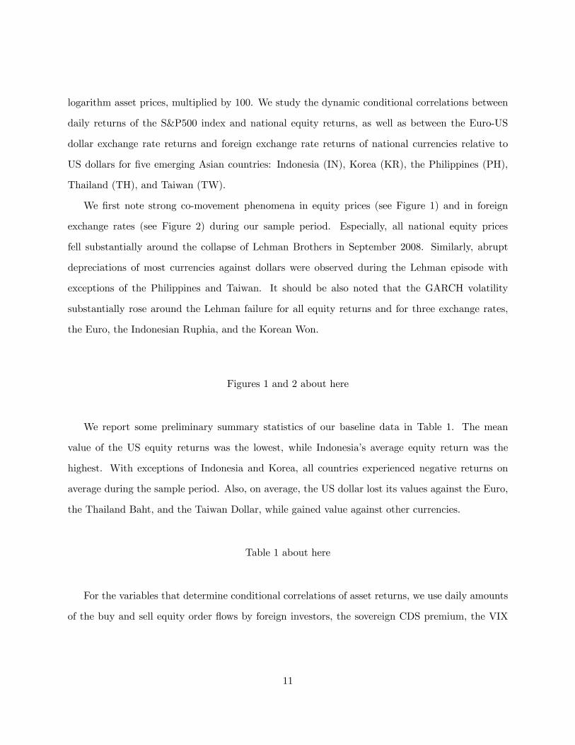
logarithm asset prices, multiplied by 100. We study the dynamic conditional correlations between

daily returns of the S&P500 index and national equity returns, as well as between the Euro-US

dollar exchange rate returns and foreign exchange rate returns of national currencies relative to

US dollars for five emerging Asian countries: Indonesia (IN), Korea (KR), the Philippines (PH),

Thailand (TH), and Taiwan (TW).

We first note strong co-movement phenomena in equity prices (see Figure 1) and in foreign

exchange rates (see Figure 2) during our sample period. Especially, all national equity prices

fell substantially around the collapse of Lehman Brothers in September 2008. Similarly, abrupt

depreciations of most currencies against dollars were observed during the Lehman episode with

exceptions of the Philippines and Taiwan. It should be also noted that the GARCH volatility

substantially rose around the Lehman failure for all equity returns and for three exchange rates,

the Euro, the Indonesian Ruphia, and the Korean Won.

Figures 1 and 2 about here

We report some preliminary summary statistics of our baseline data in Table 1. The mean

value of the US equity returns was the lowest, while Indonesia’s average equity return was the

highest. With exceptions of Indonesia and Korea, all countries experienced negative returns on

average during the sample period. Also, on average, the US dollar lost its values against the Euro,

the Thailand Baht, and the Taiwan Dollar, while gained value against other currencies.

Table 1 about here

For the variables that determine conditional correlations of asset returns, we use daily amounts

of the buy and sell equity order flows by foreign investors, the sovereign CDS premium, the VIX

11

index, the TED spread, and the Libor-overnight index swap (OIS) spread.7 The fundamental

variables that determine the size of DCC are briefly discussed below.

One motivation of using the amount of foreign order flows in local stock markets is an observation

of high dependence of local stock markets in the emerging Asian countries on the trade patterns of

foreign investors. We use the total amount of the buy- and sell-order by foreign investors instead of

their net order flows, because the total amount should better proxy the degree of financial linkages

between countries.

We also employ the sovereign CDS premium, costs of insuring against a sovereign default, as

a measure of country risk of emerging Asian economies. The sovereign CDS premium of these 5

countries soared beginning in September 2008.

The VIX index, the Chicago Board Options Exchange (CBOE) volatility index, is used as a

proxy for market uncertainty. It is a widely used barometer of investor fear.8 The TED spread

is used as a measure for the level of financial stress in the interbank market. The TED spread is

the difference between the three-month LIBOR and the yield on the US Treasury bills with same

maturity.9

The Libor-OIS spread is a measure of the market-wide liquidity risk. Adrian and Shin (2008)

point out that aggregate liquidity can be understood as the rate of growth of the aggregate financial-

sector balance sheet. A fall of asset prices during the crisis makes banks reluctant to lend in the

interbank market. This would reduce market liquidity and require a higher risk premium for

longer maturity loans. The spread between the term and overnight interbank lending, then, would

rise reflecting banks’ reluctance to extend longer maturity loans. The Libor-OIS spreads increased

7Similarly, Eichengreen et al. (2009) use the VIX index, the TED spread, and the dlloar LIBOR-OIS spread.

Frank and Hesse (2009) use the Libor-OIS spread as a measure for bank funding liquidity and for a general stress

level in the interbank money market. Gonzalez-Hermosillo and Hesse (2009) use the VIX index and the TED spread

as proxy variables for global financial market condition. Melvin and Taylor (2009) employ the TED spread to measure

the credit risk of the banking sector.8The VIX index is a volatility index implied by the current prices of options on the S&P 500 index. It represents

expected future stock market volatility over the next 30 days.9Eichengreen et al. (2009) point out that the TED spread reflects not just banking sector credit risk but also

includes liquidity or flight-to-quality risk since it can be decomposed into the banking sector credit risk premium

(LIBOR-OIS) and liquidity or flight-to-quality premium (OIS-T-Bill). The TED spread rose sharply in the post-

Lehman crash period due to a substantial increase in credit risk (the LIBOR-OIS spread) instead of the rise in the

liquidity premium (the OIS-T-Bill differential).

12

substantially after the collapse of Lehman Brothers in September 2008. We omit summary statistics

for these variables to save space.

4.2 Estimation Results

We first present a conventional diagonal BEKK-MGARCH (Engle and Kroner, 1995) estimation re-

sults in Table 2 as a benchmark. We also implement DCC-MGARCH along with CCC-MGARCH

estimations (Tables 3 and 4) and compare the estimated dynamic conditional correlations with

those from the BEKK-MGARCH model. See Figures 3 through 5. The dashed vertical line indi-

cates September 15, 2008 when financial market instability culminated after the failure of Lehman

Brothers.

Estimated conditional correlations by the DCC-MGARCH and the BEKK-MGARCH are overall

similar. However, the BEKK estimates tend to exhibit higher variability covering a wider range

of estimates. For instance, the conditional correlation of the equity returns between Indonesia and

the US ranges between about -0.2 to 0.8 when the BEKK method is applied, while about 0.2 to

0.55 when we use the DCC-MGARCH method. Overall, the estimates from both models strongly

imply that the notion of possible de-coupling has been misplaced in the case of emerging Asian

financial markets (Dooley and Hutchison, 2009).

One notable finding is the following. For the equity returns, the correlation coefficient estimates

rose substantially around the Lehman episode with an exception of Thailand. However, unusually

high correlations were short-lived as they quickly moved back to previous lower levels in around

October 2008. Similar movements around the Lehman episode were observed for the exchange rate

changes. Spikes in the correlation of exchange rates are more pronounced than in the case of stock

prices. We also observe similar spikes across local markets.

Naturally, the CCC estimates are about the mean values of the DCC estimates. We implement

a test for the null hypothesis of the CCC against the DCC alternative (Engle and Sheppard, 2001).

The results overall accept the null hypothesis with 47.5% and 20.2% p-values for the stock market

and the foreign exchange market, respectively. One shouldn’t be surprised to see this because our

13

observations cover only 29 months and sudden elevation of the conditional correlations persist only

for a month. Under such circumstances, it is not an easy task to find statistical evidence of such

sudden changes in conditional correlations. Put different, the power of such tests may not be good.

Tables 2, 3, and 4 about here

Figures 3, 4, and 5 about here

These findings suggest a possibility of nonlinear movements of correlation coefficients. To empir-

ically investigate this possibility, we implement NLCC-MGARCH estimations with the exponential

smooth transition function between the tranquil period correlation () and the contagion period

correlation (). The parameter estimates are reported in Tables 5 and 6. See Figure 6 for the

conditional correlation estimates of these models.

The results are overall consistent with our previous findings. With an exception of Thailand

equity returns, estimated conditional correlations rapidly rise to the contagion regime around the

Lehman episode period. It should be noted that the estimates are substantially different from

the estimates. In the case of Indonesia, for example, the equity correlation estimate increased

from about 0.363 to 0.836 and the exchange rate correlation moved from 0.137 to 0.536. Similar

findings were observed for the rest of the countries with an exception of Thailand equity returns.

We also note that smoothness parameter estimates of the EST model are quite large, implying

regime shifts occur fairly abruptly. This provides additional evidence for the existence of contagion

triggered by unexpected news shocks. We also note that estimated durations of the contagion

period are fairly short.

In a nutshell, our results imply that the US financial crisis had a strong spillover effect on

financial asset returns in most emerging Asian countries when the news of Lehman Brothers failure

was revealed in September 2008.

Tables 5 and 6 about here

14

Figure 6 about here

Next, we turn to analysis on determinant factors of the conditional correlation coefficient by

the DCCX-MGARCH model. A number of variables can be considered for the factors that play

important roles for determining the size of the dynamic conditional correlation. We first choose the

factors that are related to the financial condition of the source country where the crisis originated.

We consider the VIX index as a US financial market stability measure, and the TED spread and

the dollar Libor-OIS spread as the US risk premium or liquidity availability measures. We expect

these financial instability/fragility measures of the source country to have positive effects on the

conditional correlation. Second, we consider the sovereign CDS premium as a measure of potential

financial fragility in emerging Asian countries, which may increase likelihood of spillover effects.

Thirdly, we also consider the amount of foreign buy- and sell-order flows as an exogenous factor in

local stock markets. Sudden drainage of foreign capital (flight to safety) may cause severe liquidity

crunch, which may increase odds of contagion.

We report our parameter estimation results in Tables 9 and 10. Conditional correlation estimates

appear in Figure 7. Our major findings are as follows.

First, for the equity returns, foreign capital has a significantly positive effect on conditional

correlations in all five countries. The Libor-OIS spread has an insignificant effect for all countries.

The sovereign CDS premium has a significant effect on the correlations in Indonesia and Philippines,

though with a negative sign. For those two countries, the VIX index has a significantly positive

effect, implying that uncertainty in the US stock market may spread to those countries. Based on

these findings, we believe that the spillover effect of the US stock market shocks is mainly due to

surges in foreign capital and propagations of US uncertainty to some emerging Asian countries.

Global liquidity conditions seem to have an insignificant effect. Given the interconnectedness of

global financial markets, investors’ increase in global risk aversion triggered by problems in advanced

economies rapidly spilled over into emerging countries, as funds were pulled out from the latter and

subsequently invested into the safest and most liquid assets such as mature market fixed income

securities (Frank and Hesse, 2009).

15

Our findings on stock markets are similar to those of Didier et al. (2010). In their study

that analyzes the driving factors of the co-movement between US stock returns and returns in 83

countries, they also find that a larger share of US investors’ asset holdings in foreign markets is

associated with a more pronounced reaction to the US crisis.10

Second, the Libor-OIS spread, the sovereign CDS premium, and foreign capital appear to have

overall positive effects on conditional correlations with an exception of Korea for the CDS premium.

Especially, the amount of foreign buy- and sell-trades has a significantly positive effect on 3 out of 5

countries. Although the TED spread appears to have a significant effect on Korea, the Philippines,

and Taiwan, it comes with a negative sign for all five countries, which lacks economically meaningful

interpretations. Overall, it seems that the Libor-OIS spread, the sovereign CDS premium, and

foreign capital play important roles for determining conditional correlations in international foreign

exchange markets.11 The results on exchange rates seem consistent with arguments that the current

global crisis spreads quickly to other countries, first through lack of available liquidity and then

through concerns on solvency and loss of confidence.

These findings are consistent with Fratzscher’s (2009) explanations on exchange rate movements

during financial crises. He points out that a sharp reversal in the pattern of global capital flows

played a seminal role for global foreign exchange rate movements. He concludes that a repatriation

of capital to the US by US investors, a flight-to-safety phenomenon by US and non-US investors,

an increased need for US dollar liquidity and an unwinding of carry trade positions may all have

played a role in the sharp appreciation trend of the US dollar.

Third, Figure 7 clearly illustrate substantial and abrupt changes in dynamic conditional corre-

lations during the Lehman Brothers episode, which, we believe, imply our DCCX-MGARCH model

is a useful tool in studying spillover effects of financial crises.

10Didier et al. (2010) point out that their finding is consistent with a “margin calls” story. Facing large capital

losses at home, US investors withdrew money from foreign investments, which leads to a substantial effect especially

on countries where the share of foreign investments by the US is larger.11Frank and Hesse (2009) also report the important role of the dollar Libor-OIS spread for channelling adverse

shocks to other countries. They find that correlations between the US Libor-OIS spread and the EMBI+ sovereign

bonds spreads of Asia sharply increase following the onset of the subprime crisis.

16

Tables 7 and 8 about here

Figure 7 about here

5 Concluding Remarks

The present paper uses an array of MGARCH models to estimate dynamic conditional correlations

of financial asset returns between the US and five emerging Asian countries. Our major findings

imply that the recent US financial crisis, triggered by the collapse of Lehman Brothers in September

2008, has a substantial spillover effect on emerging Asian countries. Our analysis shows that the

conditional correlation, overall, abruptly rose to a much higher level around the Lehman Brothers

failure period and such a high correlation has persisted for a fairly short period of time. Put

differently, we find short-lived but non-negligible financial contagion from the US to emerging

Asian countries.

We also investigate major factors that determine the size of conditional correlations using a

novel DCCX-MGARCH model. Especially, we find a substantial role of the foreign investors for co-

movements across international equity markets. In the foreign exchange markets, the dollar Libor-

OIS spread, the sovereign CDS premium, and the amount of foreign order flows have significant

effects on determining dynamic conditional correlations.

Our analysis provides the following policy implications. Our NLCC-MGARCH model estima-

tions imply that spillover effects of the US financial crisis occurred abruptly. Though financial

contagion seems to persist for a fairly short period of time, its impacts can be substantial and po-

tentially harmful to these countries. This implies that emerging Asian countries are quite vulnerable

to external shocks and can experience a sudden acceleration of systemic risk through deterioration

in both the capital and the foreign exchange markets. This possibility calls for a need to construct

a financial stabilization mechanism against contagion originating from other countries.

It also appears that foreign investors play a potentially important role in channeling foreign

crises to domestic economies. Therefore, emerging countries should make an effort to lessen this

17

effect, possibly by supporting the role of domestic institutional investors in terms of total transaction

volumes in these financial markets.

Lastly, we find a stronger spillover effect in the foreign exchange market than the equity market.

Given the importance of trade accounts in these emerging Asian economies, foreign exchange market

instability caused by external shocks may lead to a serious dollar liquidity problem even when their

economic fundamentals are healthy. Therefore, it is advised for these countries to equip institutional

arrangements to enhance international cooperation, such as currency swap agreements.

18

Reference

1. Adrian, T. and H.S. Shin. 2008. “Liquidity and Leverage,” Journal of Financial Intermedi-

ation, forthcoming.

2. Ang, A. and G. Bekaert. 2002. “International Asset Allocation with Regime Shifts,” Review

of Financial Studies 15, pp. 1137-1187.

3. Ang, A. and J. Chen. 2002. “Asymmetric Correlations of Equity Portfolios,” Journal of

Financial Economics 63, pp. 443-494.

4. Bae, K., G. Karolyi, and R. Stulz. 2003. “A New Approach to Measuring Financial Conta-

gion,” Review of Financial Studies 16, pp. 717-763.

5. Baig, T. and I. Goldfajn. 1999. “Financial Market Contagion in the Asian Crisis,” IMF Staff

Papers 46, pp.167-195.

6. Bekaert, G., C.R. Harvey, and A. Ng. 2005, “Market Integration and Contagion,” Journal of

Business 78, pp. 39-69.

7. Berben, R.P. and W.J. Jansen, 2005, “Comovement in International Equity Markets: A

Sectoral View,” Journal of International Money and Finance 24, pp. 832-857.

8. Bollerslev, T. 1990. "Modelling the Coherence in Short-run Nominal Exchange Rates: A

Multivariate Generalized ARCH Model," Review of Economics and Statistics 72, pp 498-505.

9. Boyer, B.H., M.S. Gibson, and M. Loretan. 1999, “Pitfalls in Tests for Changes in Correla-

tions,” International Finance Discussion Papers No. 597R, Board of Governors of Federal

Reserve System.

10. Calvo, S. and C. Reinhart. 1996. "Capital Flows to Latin America: Is there Evidence of

Contagion Effects?" In G. Calvo, M. Goldstein, and E. Hochreiter (eds.), Private Capital

Flows to Emerging Markets after the Mexican Crisis, Institute for International Economics.

19

11. Cappiello, L., R. Engle, and K. Sheppard. 2006. “Asymmetric Dynamics in the Correlations

of Global Equity and Bond Returns,” Journal of Financial Econometrics 4, pp. 537-572.

12. Chiang, T., B. Jeon, and H. Li. 2007. “Dynamic Correlation Analysis of Financial Contagion:

Evidence from Asian Markets,” Journal of International Money and Finance 26, pp.1206-

1228.

13. Claessens. S., G. Dell’Ariccia, D. Igan, and L. Laeven. 2010, “Lessons and Policy Implications

from the Global Financial Crisis,” IMF Working Paper No. 10/44

14. Corsetti, G., M. Pericoli, and M. Sbracia. 2005. “Some Contagion, Some Interdependence:

More Pitfalls in Tests of Financial Contagion,” Journal of International Money and Finance

24, pp.1177-1199.

15. Davis, E.P. 2008. “Liquidity, Financial Crises and the Lender of Last Resort — How Much

of a Departure is the Sub-Prime Crisis?” in Bloxham P. and Kent C. Eds., Lessons from the

Financial Turmoil of 2007 and 2008, Reserve Bank of Australia Conference, H.C. Coombs

Centre for Financial Studies.

16. Didier, T., I. Love and M.S.M. Pería. 2010. “What Explains Stock Markets’ Vulnerability to

the 2007-2008 Crisis?” Word Bank Policy Research Working Paper No. 5224.

17. Dooley, M. and M. Hutchison. 2009. “Transmission of the U.S. Subprime Crisis to Emerg-

ing Markets: Evidence on the Decoupling-Recoupling Hypothesis,” Journal of International

Money and Finance 28, pp. 1331-1349.

18. Eichengreen, B., A. Mody, M. Nedeljkovic, and L. Sarno. 2009. “How the Subprime Crisis

Went Global: Evidence from Bank Credit Default SWAP Spreads,” NBER Working Paper

No. 14904.

19. Eichengreen, B. and A.K. Rose. 1998. “Contagious Currency Crises: Channels of Con-

veyance” in T. Ito and A. Krueger, eds., Changes in Exchange Rates in Rapidly Developing

Countries, University of Chicago Press.

20

20. Engle, R.F. 2002. “Dynamic Conditional Correlation: A Simple Class of Multivariate Gener-

alized Autoregressive Conditional Heteroskedasticity Models,” Journal of Business and Eco-

nomic Statistics 20, pp. 339-350.

21. Engle, R.F. & Kevin Sheppard, 2001. “Theoretical and Empirical properties of Dynamic

Conditional Correlation Multivariate GARCH,” NBER Working Papers No. 8554.

22. Engle, R.F. and K.F., Kroner. 1995. “Multivariate Simultaneous Generalized ARCH,” Econo-

metric Theory 11, pp. 122—150.

23. Forbes, K.J. and M.D. Chinn. 2004. “A Decomposition of Global Linkages in Financial

Markets Over Time,” Review of Economics and Statistics 86, pp. 705-722.

24. Forbes, K. and R. Rigobon. 2002. “No Contagion, Only Interdependence: Measuring Stock

Markets Comovements,” Journal of Finance 57, pp. 2223-2261.

25. Frank, N. and H. Hesse. 2009. “Financial Spillovers to Emerging Markets During the Global

Financial Crisis,” IMF Working Paper No. 09/104.

26. Fratzscher, M. 2009. “What Explains Global Exchange Rate Movements During the Financial

Crisis,” Journal of International Money and Finance 28, pp. 1390-1407.

27. Glick, R. and A.K. Rose. 1999. “Contagion and Trade: Why Are Currency Crises Regional?”

Journal of International Money and Finance 18, pp. 603-617.

28. Gonzalez-Hermosillo, B. and H. Hesse. 2009. “Global Market Condition and Systemic Risk,”

IMF Working Paper No. 09/230.

29. Hamao, Y., R.W. Masulis, and V. Ng, 1990. “Correlations in Price Changes and Volatility

Across International Stock Markets,” Review of Financial Studies 3, pp. 281-307.

30. Hartman, P., S. Straetmans, and C. de Vries. 2001. “Asset Market Linkages in Crisis Periods,”

ECB Working Paper No. 71.

21

31. Horta, P., C. Mendes, and I. Vieira. 2008. "Contagion Effects of the U.S. Subprime Crisis on

Developed Countries." Working Paper, University of Evora.

32. Hwang, I., F.H. In, and T. Kim., 2010, “Contagion Effects of the U.S. Subprime Crisis on

International Stock Markets,” Mimeo.

33. King, M., and S. Wadhwani. 1990. “Transmission of Volatility between Stock Markets,”

Review of Financial Studies 3, pp. 5-33.

34. Lee, S. and K. Kim. 1993. “Does the October 1987 Crash Strengthen the Co-movements

Among National Stock Markets?” Review of Financial Economics 3, pp. 89-102.

35. Longin, F. and B. Solnik. 2001. “Extreme Correlations of International Equity Markets,”

Journal of Finance 56, pp. 649-676.

36. Loretan, M. and W.B. English. 2000. “Evaluating ‘Correlation Breakdowns’ During Periods

of Market Volatility,” International Finance Discussion Papers No. 658, Board of Governors

of Federal Reserve System.

37. Melvin, M. and M.P. Taylor. 2009. “The Crisis in the Foreign Exchange Market,” Journal of

International Money and Finance 28, pp. 1317-1330.

38. Rodriguez, J.C. 2007. “Measuring Financial Contagion: A Copula Approach,” Journal of

Empirical Finance 14, pp. 401-423.

39. Rose, A.K. and M.M. Spiegel. 2009. “Cross-Country Causes and Consequences of the 2008

Crisis: International Linkages and American Exposure,” NBER Working Paper No. 15358.

22

Table 1. Summary Statistics

Stock Price Returns

USA IN KR PH TH TW

Mean −000055 000040 000015 −000020 −000025 −000007Median 000080 000177 000190 000056 000116 000015

Maximum 010246 007623 011284 007056 008054 007549

Minimum −009470 −010954 −011172 −013089 −006735 −011090Std. Dev. 001980 002053 002038 001809 001880 001717

Skewness −032679 −052421 −049231 −097701 −005700 −052263Kurtosis 727123 717861 788882 917514 481961 804300

Foreign Exchange Rate Returns

Euro IN KR PH TH TW

Mean −000012 000017 000049 000002 −000001 −000005Median −000031 −000005 000022 −000002 000008 000000

Maximum 006261 005356 010693 001703 001648 001237

Minimum −004607 −005557 −013594 −002057 −001721 −001097Std. Dev. 000817 000998 001493 000518 000339 000271

Skewness 034312 036868 −101083 −003472 −010003 009355

Kurtosis 122979 111303 255979 350013 806536 592453

23

Table 2. Diagonal BEKK-MGARCH Model

H =M+A0e0−1e−1A+BH−1B

0

M =

"1 2

2 3

# A =

"1 0

0 2

# B =

"1 0

0 2

#

Stock Price Returns

IN KR PH TH TW

1 01963∗(00000)

02158(00000)

∗ 02136(00000)

∗ 02204(00000)

∗ 01939(00000)

∗

2 03184∗(00000)

01463(00000)

∗ 03084(00000)

∗ 01154(00000)

∗ 01102(00000)

∗

3 03486∗(00000)

02658(00000)

∗ 03718(00000)

∗ 02067(00000)

∗ 02631∗(00000)

1 03027∗(00000)

03023(00000)

∗ 02882(00000)

∗ 03323(00000)

∗ 02904(00000)

∗

2 04042∗(00000)

03053(00000)

∗ 02996(00000)

∗ 02253(00000)

∗ 03136(00000)

∗

1 09500∗(00000)

09468(00000)

∗ 09495(00000)

∗ 09378(00000)

∗ 09524(00000)

∗

2 08909∗(00000)

09417(00000)

∗ 09101∗(00000)

09673(00000)

∗ 09374(00000)

∗

− ln 22072 21822 20855 21930 21295

Foreign Exchange Rate Returns

IN KR PH TH TW

1 00350∗(00000)

00658∗(00000)

00468∗(00000)

00457∗(00000)

00435∗(00000)

2 00314∗(00000)

01230∗(00000)

00585∗(00000)

00033∗(00000)

−00003∗(00015)

3 01010∗(00000)

00000(09940)

01195∗(00000)

00330∗(00000)

00228∗(00000)

1 02438∗(00000)

02678∗(00000)

02568∗(00000)

02694∗(00000)

02793∗(00000)

2 04229∗(00000)

07023∗(00000)

02244∗(00000)

03221∗(00000)

03872∗(00000)

1 09729∗(00000)

09631∗(00000)

09678∗(00000)

09661∗(00000)

09651∗(00000)

2 09097∗(00000)

07861∗(00000)

09403∗(00000)

09468∗(00000)

09297∗(00000)

− ln 12202 12495 10174 68334 53564

Note: i) p-values are reported in parentheses. ii) * indicates statistical significance at the 5% level.

24

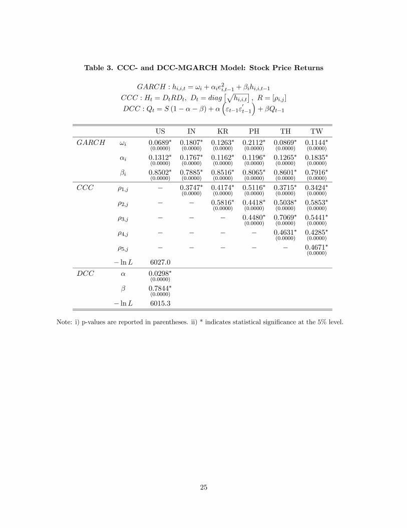
Table 3. CCC- and DCC-MGARCH Model: Stock Price Returns

: = + 2−1 + −1

: = = £p

¤ = [ ]

: = (1− − ) + ³−1

0−1´+ −1

US IN KR PH TH TW

00689∗(00000)

01807∗(00000)

01263∗(00000)

02112∗(00000)

00869∗(00000)

01144∗(00000)

01312∗(00000)

01767∗(00000)

01162∗(00000)

01196∗(00000)

01265∗(00000)

01835∗(00000)

08502∗(00000)

07885∗(00000)

08516∗(00000)

08065∗(00000)

08601∗(00000)

07916∗(00000)

1 − 03747∗(00000)

04174∗(00000)

05116∗(00000)

03715∗(00000)

03424∗(00000)

2 − − 05816∗(00000)

04418∗(00000)

05038∗(00000)

05853∗(00000)

3 − − − 04480∗(00000)

07069∗(00000)

05441∗(00000)

4 − − − − 04631∗(00000)

04285∗(00000)

5 − − − − − 04671∗(00000)

− ln 60270

00298∗(00000)

07844∗(00000)

− ln 60153


25

Table 4. CCC- and DCC-MGARCH Model: Foreign Exchange Rate Returns

: = + 2−1 + −1

: = = £p

¤ = [ ]

: = (1− − ) + ³−1

0−1´+ −1

Euro IN KR PH TH TW

00024∗(00000)

00103∗(00000)

00121∗(00000)

00072∗(00000)

00007∗(00000)

00009∗(00000)

00651∗(00000)

01704∗(00000)

02737∗(00000)

00399∗(00000)

00846∗(00000)

01714∗(00000)

09349∗(00000)

08296∗(00000)

07263∗(00000)

09338∗(00000)

09150∗(00000)

08286∗(00000)

1 − 01674∗(00000)

03023∗(00000)

02842∗(00000)

02968∗(00000)

03144∗(00000)

2 − − 03452∗(00000)

03816∗(00000)

02219∗(00000)

01771∗(00000)

3 − − − 03865∗(00000)

03649∗(00000)

02286∗(00000)

4 − − − − 03038∗(00000)

02520∗(00000)

5 − − − − − 01947∗(00000)

− ln 21231

00217∗(00000)

08543∗(00000)

− ln 21137


26

Table 5. EST NLCC-MGARCH Model: Stock Price Returns

11 = 1 + 121−1 + 111−1

22 = 2 + 222−1 + 222−1

12 = () (1122)12

() = [1− (; )] + (; )

(; ) = 1− exph−2 ( − )2

i = [ ]

0

Variance Equation

IN KR PH TH TW

1 00397∗(0037)

00342∗(0032)

00322∗(0045)

00389∗(0030)

003319(0077)

2 01799∗(0005)

00774∗(0023)

03282∗(0002)

00668∗(0036)

00568(0053)

1 01148∗(0000)

01055∗(0000)

00986∗(0000)

01057∗(0000)

01048∗(0000)

2 01823∗(0000)

00913∗(0000)

01645∗(0000)

01409∗(0000)

00970∗(0000)

1 08741∗(0000)

08880∗(0000)

08933∗(0000)

08847∗(0000)

08891∗(0000)

2 07867∗(0000)

08895∗(0000)

07283∗(0000)

08449∗(0000)

08945∗(0000)

Correlation Coefficient Equation

IN KR PH TH TW

03625∗(0000)

04386∗(0000)

05587∗(0000)

03494∗(0000)

03993∗(0000)

08364∗(0000)

07585∗(0000)

08723∗(0000)

04414∗(0002)

06002∗(0000)

17520∗(0024)

16309(0193)

62462∗(0022)

23834(0253)

50000(0852)

06277∗(0000)

06278∗(0000)

06779∗(0000)

05823∗(0000)

06348∗(0001)

− log 220104 216889 207943 210727 219225


27

Table 6. EST NLCC-MGARCH Model: Foreign Exchange Rate Returns

11 = 1 + 121−1 + 111−1

22 = 2 + 222−1 + 222−1

12 = () (1122)12

() = [1− (; )] + (; )

(; ) = 1− exph−2 ( − )2

i = [ ]

0

Variance Equation

IN KR PH TH TW

1 00020(0267)

00019(0235)

00016(0317)

00017(0201)

00018(0164)

2 00083∗(0011)

00055∗(0039)

00096(0199)

00014∗(0025)

00008∗(0046)

1 00726∗(0000)

00694∗(0000)

00754∗(0000)

00745∗(0000)

00732∗(0000)

2 02777∗(0000)

02513∗(0000)

00510∗(0031)

03178∗(0000)

00959∗(0000)

1 09233∗(0000)

09345∗(0000)

09304∗(0000)

09210∗(0000)

09303∗(0000)

2 07675∗(0000)

07442∗(0000)

09136∗(0000)

06849∗(0000)

09044∗(0000)


IN KR PH TH TW

01365∗(0005)

03081∗(0000)

02362∗(0000)

02996∗(0000)

02879∗(0000)

05358∗(0000)

08249∗(0000)

04906∗(0000)

05536∗(0000)

09002∗(0000)

22898∗(0025)

49200∗(0001)

11676∗(0008)

31786∗(0021)

18596(0170)

05620∗(0000)

06250∗(0000)

06936∗(0000)

06278∗(0000)

06435∗(0000)

− log 119028 123409 101708 52582 67752


28

Table 7. DCCX-MGARCH Model: Stock Price Returns

11 = 1 + 121−1 + 111−1

22 = 2 + 222−1 + 222−1

12 = (x) (1122)12

(x) = 2

"exp

³0x

´1+exp(0x)

#− 1 = [1 2 · · · ]

0

Variance Equation

IN KR PH TH TW

1 00392∗(0032)

00445∗(0018)

00346∗(0045)

00439∗(0025)

00357(0060)

2 01943∗(0004)

00931∗(0019)

03518∗(0001)

00805∗(0025)

00648∗(0045)

1 01247∗(0000)

01039∗(0000)

01010∗(0000)

01016∗(0000)

01057∗(0000)

2 01857∗(0000)

00903∗(0000)

01601∗(0000)

01410∗(0000)

00966∗(0000)

1 08682∗(0000)

08835∗(0000)

08902∗(0000)

08861∗(0000)

08864∗(0000)

2 07787∗(0000)

08853∗(0000)

07233∗(0000)

08390∗(0000)

08914∗(0000)


IN KR PH TH TW

1 01055∗(0045)

01299∗(0000)

01815∗(0003)

01875∗(0008)

01671∗(0023)

2 −08744∗(0014)

−01357(0281)

−04560∗(0014)

01316(0708)

−00871(0405)

3 12683∗(0027)

−01086(0361)

07900∗(0006)

−04824(0388)

−00296(0889)

4 −00331(0799)

00646(0502)

−00583(0559)

00790(0694)

01466(0370)

− log 220135 216806 207890 210588 219267

Note: i) x1, x2, x3, x4 are the foreign investment, the sovereign CDS premium, the VIX index, and

the dollar Libor-OIS spread, respectively. ii) p-values are reported in parentheses. iii) * indicates

statistical significance at the 5% level.

29

Table 8. DCCX-MGARCH Model: Foreign Exchange Rate Returns

11 = 1 + 121−1 + 111−1

22 = 2 + 222−1 + 222−1

12 = (x) (1122)12

(x) = 2

"exp

³0x

´1+exp(0x)

#− 1 = [1 2 · · · ]

0

Variance Equation

IN KR PH TH TW

1 00020(0256)

00027(0132)

00013(0382)

00018(0296)

00019(0273)

2 00079∗(0015)

00078∗(0018)

00113(0232)

00014∗(0031)

00008(0068)

1 00805∗(0000)

00657∗(0000)

00684∗(0000)

00764∗(0000)

00739∗(0000)

2 02843∗(0000)

02474∗(0000)

00494∗(0000)

03064∗(0000)

00986∗(0000)

1 09249∗(0000)

09356∗(0000)

09375∗(0000)

09291∗(0000)

09310∗(0000)

2 07654∗(0000)

07195∗(0000)

09093∗(0000)

06959∗(0000)

09019∗(0000)


IN KR PH TH TW

1 00584(0231)

03180∗(0000)

00950(0533)

00392(0794)

02624∗(0039)

2 02915(0292)

−02913∗(0010)

04338∗(0002)

03725∗(0010)

02729∗(0003)

3 −07009(0350)

−07527∗(0002)

−05273∗(0015)

−03638(0208)

−06347∗(0004)

4 02338∗(0039)

10111∗(0000)

03834∗(0034)

03057(0470)

05569∗(0038)

− log 119233 123180 101554 52293 67164

Note: i) x1, x2, x3, x4 are the foreign investment, the sovereign CDS premium, the TED spread, and

the dollar Libor-OIS spread, respectively. ii) p-values are reported in parentheses. iii) * indicates

statistical significance at the 5% level.

30

Figure 1. Stock Price Data and GARCH Volatility Estimates

(a) Stock Price

(b) GARCH Volatility Estimate

Note: The dashed vertical line indicates the Lehman failure on September 15, 2008.

31

Figure 2. Foreign Exchange Rate Data and GARCH Volatility Estimates

(a) Foreign Exchange Rate

(b) GARCH Volatility Estimate


32

Figure 3. BEKK Conditional Correlation Estimates

(a) Stock Price Returns

(b) Foreign Exchange Rate Returns


33

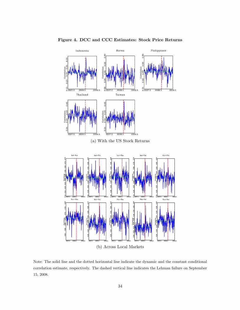
Figure 4. DCC and CCC Estimates: Stock Price Returns

(a) With the US Stock Returns

(b) Across Local Markets

Note: The solid line and the dotted horizontal line indicate the dynamic and the constant conditional

correlation estimate, respectively. The dashed vertical line indicates the Lehman failure on September

15, 2008.

34

Figure 5. DCC and CCC Estimates: Foreign Exchange Rate Returns

(a) With the Euro/US$

(b) Across Local Markets

Note: The solid line and the dotted horizontal line indicate the dynamic and the constant conditional

correlation estimate, respectively. The dashed vertical line indicates the Lehman failure on September

15, 2008.

35

Figure 6. Nonlinear Conditional Correlation Estimates



Note: The solid and the dotted lines indicate the ESTAR and the threshold conditional correlation

estimates, respectively. The dashed vertical line indicates the Lehman failure on September 15, 2008.

36

Figure 7. DCCX Estimates by NLCC-MGARCH Models




37

Spillover Effects of the U.S. Financial Crisis on Financial Markets in Emerging Asian Countries

Documents

Transcript of Spillover Effects of the U.S. Financial Crisis on Financial Markets in Emerging Asian Countries