Spectra of a shallow sea—unmixing for class identification and monitoring of coastal waters
170
”Dense Water” and “Fluid Sand” ”Dense water” and “Fluid Sand” Annelies Hommersom - IVM- Cover : Background: MERIS image May 4 2006 provided by the European Space Agency Left: TriOS sensors Center: reseach vessel Navicula (NIOZ) Right: AC9 instrument in turbid water Optical properties and methods for remote sensing of the extremely turbid Wadden Sea.
Transcript of Spectra of a shallow sea—unmixing for class identification and monitoring of coastal waters

”Dense W
ater” and “Fluid Sand”
”Dense water” and “Fluid Sand”
Annelies Hommersom - IVM-
Cover :Background: MERIS image May 4 2006provided by the European Space Agency Left: TriOS sensorsCenter: reseach vessel Navicula (NIOZ)Right: AC9 instrument in turbid water
Optical properties and methods for remote sensing of the extremely turbid Wadden Sea.
De Aula is 10 min lopen vanaf station Amsterdam Zuid uitgang VU/Parnassusweg. Komen met de auto is niet aan te raden.
The Aula is 10 min walk from station Amsterdam Zuid exit
VU/Parnassusweg. Coming by car is not recommended.
Annelies Hommersom
Sumatrastraat 16707 EE Wageningen
Uitnodiging - Invitation
Optical properties and methods for remote sensing of the extremely
turbid Wadden Sea.
voor het bijwonen van de openbare verdediging van
mijn proefschrift:to attend the public defence
of my thesis:
”Dense Water”and
“Fluid Sand”
Maandag 28 juni - Monday June 28
om - at 15.45in de - in the
Aula Vrije Universiteit
De Boelelaan 1105, Amsterdam
En de receptie na afloop.And the reception afterwards.
“Dense Water” and “Fluid Sand”
Optical properties and methods for remote sensing of the extremely turbid Wadden Sea
Annelies Hommersom

“Dense Wat
Optical prop
Ph.D. thesis
In Dutch:
“Dik Water”
Optische eig
Proefschrift
ISBN: 97890
© 2010 Ann
This work w
and at the R
This work w
Printed on F
ter” and “Flu
perties and m
s, Vrije Unive
” en “Vloeiba
genschappen
t, Vrije Unive
086594610
nelies Homm
was carried o
Royal Nether
was financed
FSC paper by
uid Sand”
methods for
ersiteit, Amst
aar Zand”
n en method
ersiteit, Amst
mersom
ut at the Ins
rlands Institu
by NWO/SR
y PrintPartne
remote sens
terdam
den van remo
terdam
titute for En
ute for Sea R
RON Program
ers Ipskamp,
sing of the e
ote sensing v
vironmental
Research (NIO
mme Bureau
Enschede, T
xtremely tur
voor de extre
l Studies (IVM
OZ), Texel.
Space Resea
The Netherla
rbid Wadden
eem troebel
M), Vrije Uni
arch.
ands
n Sea
e Waddenze
versiteit, Am
ee
msterdam

VRIJE UNIVERSITEIT
“Dense Water” and “Fluid Sand”
Optical properties and methods for remote sensing of the extremely turbid Wadden Sea
ACADEMISCH PROEFSCHRIFT
ter verkrijging van de graad Doctor aan
de Vrije Universiteit Amsterdam,
op gezag van de rector magnificus
prof.dr. L.M. Bouter,
in het openbaar te verdedigen
ten overstaan van de promotiecommissie
van de faculteit de Aard‐ en Levenswetenschappen
op maandag 28 juni 2010 om 15.45 uur
in de aula van de universiteit,
De Boelelaan 1105
door
Annelies Hommersom
geboren te Hengelo (ov)

promotor: prof.dr. J. de Boer
copromotor: dr. S.W.M. Peters

Table of contents
Chapter 1 Introduction 7
Chapter 2 A review on substances and processes relevant for optical remote sensing 17
of extremely turbid marine areas, with a focus on the Wadden Sea
Chapter 3 Spatial and temporal variability in bio‐optical properties of the Wadden Sea 39
Chapter 4 Performance of the regionally and locally calibrated algorithm HYDROPT in a 57
heterogeneous coastal area
Chapter 5 Tracing Wadden Sea water masses with an inverse bio‐optical and an
endmember model 85
Chapter 6 Spectra of a shallow sea: unmixing for coastal water class identification and 97
monitoring
Chapter 7 Synthesis and outlook 115
References 123
Summary and samenvatting 141
Acknowledgements and dankbetuiging 155
Annex 1 Glossary of terms and descriptions used in remote sensing of water quality 159
Annex 2 Abbreviations, acronyms, and symbols 163
Publications 167


Chapter 1
Introduction
Chapter 1
8
1 Introduction
1.1 Optical remote sensing of water quality
Remote sensing means “detecting from a distance”. A sensor used for detection can be hand‐held,
employed from an airplane (air‐borne remote sensing) or be part of a satellite (space‐born remote
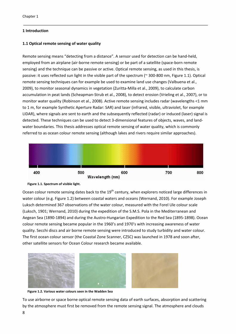
sensing) and the technique can be passive or active. Optical remote sensing, as used in this thesis, is
passive: it uses reflected sun light in the visible part of the spectrum (~ 300‐800 nm, Figure 1.1). Optical
remote sensing techniques can for example be used to examine land use changes (Valbuena et al.,
2009), to monitor seasonal dynamics in vegetation (Zuritta‐Milla et al., 2009), to calculate carbon
accumulation in peat lands (Scheapman‐Strub et al., 2008), to detect erosion (Vrieling et al., 2007), or to
monitor water quality (Robinson et al., 2008). Active remote sensing includes radar (wavelengths <1 mm
to 1 m, for example Synthetic Aperture Radar: SAR) and laser (infrared, visible, ultraviolet, for example
LIDAR), where signals are sent to earth and the subsequently reflected (radar) or induced (laser) signal is
detected. These techniques can be used to detect 3‐dimensional features of objects, waves, and land‐
water boundaries. This thesis addresses optical remote sensing of water quality, which is commonly
referred to as ocean colour remote sensing (although lakes and rivers require similar approaches).
Figure 1.1. Spectrum of visible light.
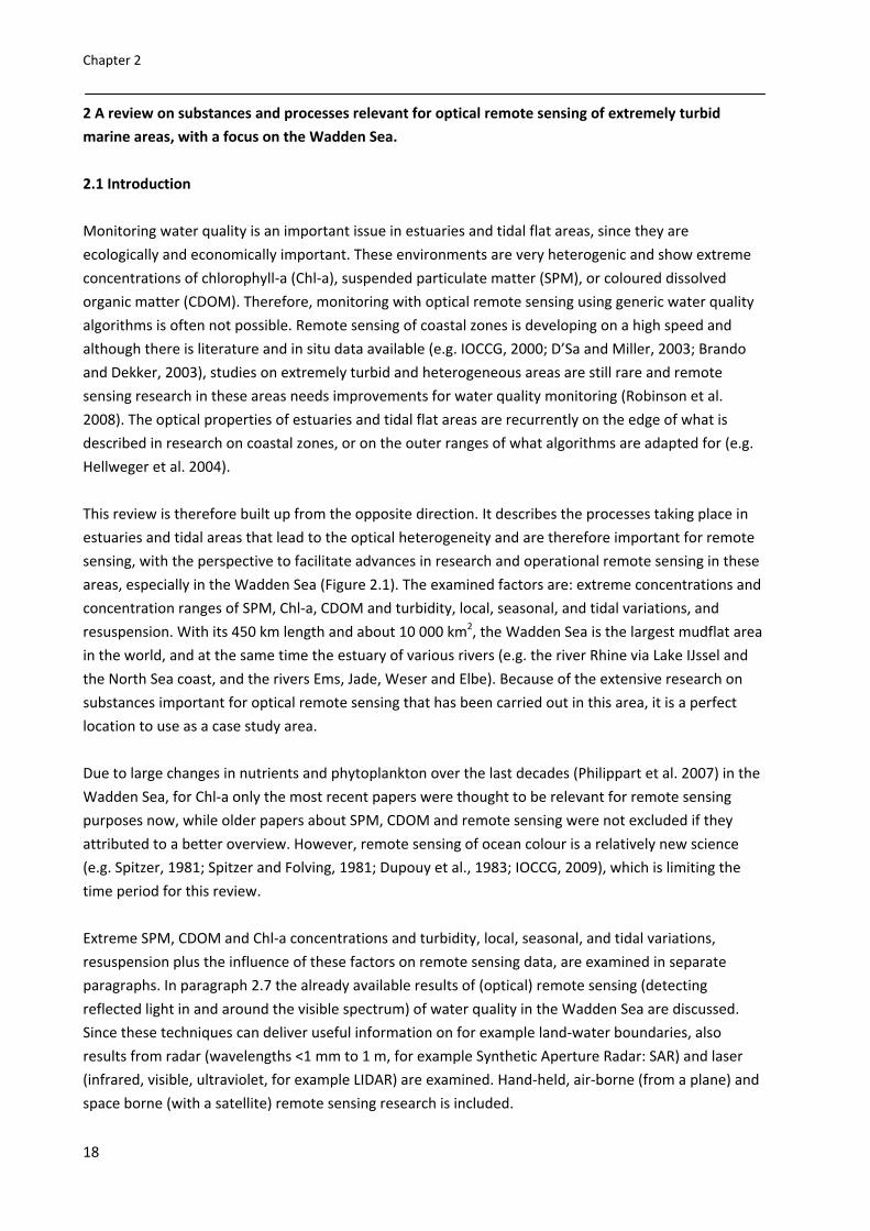
Ocean colour remote sensing dates back to the 19th century, when explorers noticed large differences in
water colour (e.g. Figure 1.2) between coastal waters and oceans (Wernand, 2010). For example Joseph
Luksch determined 367 observations of the water colour, measured with the Forel Ule colour scale
(Luksch, 1901; Wernand, 2010) during the expedition of the S.M.S. Pola in the Mediterranean and
Aegean Sea (1890‐1894) and during the Austro‐Hungarian Expedition to the Red Sea (1895‐1898). Ocean
colour remote sensing became popular in the 1960’s and 1970’s with increasing awareness of water
quality. Secchi discs and air borne remote sensing were introduced to study turbidity and water colour.
The first ocean colour sensor (the Coastal Zone Scanner, CZSC) was launched in 1978 and soon after,
other satellite sensors for Ocean Colour research became available.
Figure 1.2. Various water colours seen in the Wadden Sea
To use airborne or space borne optical remote sensing data of earth surfaces, absorption and scattering
by the atmosphere must first be removed from the remote sensing signal. The atmosphere and clouds

Introduction
9
reduce the sunlight penetration to the earth surface to ~55% (Pidwirny, 2006). A large portion of
reflected light is again absorbed and scattered on the way back to the satellite. Correcting signals for
this atmospheric influence is a research field of its own. In remote sensing of land, the light reflected by
the (land) surface is the variable that tells something about this surface. In ocean colour remote sensing,
interest lies with substances in the water column (ray 5 in Figure 1.3); reflectance from the (water)
surface (ray 6 in Figure 1.3) obscures this signal. Also the water itself can influence the reflected signal
and, at shallow or clear enough locations, so can the bottom (Figure 1.3). Consequently, only a small
portion of the light received by the sensor contains information on the content of the water and can be
used for water quality monitoring. Therefore, remote sensing of water requires different techniques
than remote sensing of land.
Figure 1.3. The most common routes of sunlight on its way to a satellite above the sea. Ray 1 is absorbed by the
atmosphere and never reaches the water surface and the sensor. Rays 2 and 3 are respectively absorbed and
scattered by the water or its contents and so never reach the sensor. Rays 4, 5, 6 and 7 reach the sensor. However,
only ray 5 is interesting for water quality monitoring. This ray is partly absorbed by water or its contents, but enough
is scattered over an angle > 90˚ (backscattered) to reach the sensor. Rays 4, 6, and 7 are, respectively, reflected by
the sea floor, by the water surface and scattered by the atmosphere. Combinations of these routes can also occur.
Substances in the water column that can be detected from optical remote sensing are: the water itself,
pigments, suspended particulate matter (SPM), and coloured dissolved organic matter (CDOM). The
pigment most abundant in marine phytoplankton, chlorophyll‐a (Chl‐a), is usually taken to represent the
pigments. SPM, Chl‐a and CDOM are (indirect) indicators for other water quality parameters such as
nutrient concentration, river runoff, resuspension or decay. As SPM, Chl‐a and CDOM have a significant
influence on the water colour, these three substances are called optically active substances in this
thesis. In the absence of optically active substances, water mainly absorbs red light, while the size of the
water molecules leads to scattering of blue light. The colour of pure water is therefore blue. Water
absorbs more than it scatters, and so very deep water bodies look dark from above. Chl‐a absorbs blue

Chapter 1
10
and red light, turning water green in high concentration (e.g. the central picture in Figure 1.3). Inorganic
SPM scatters light efficiently and can therefore lead to a high reflectance. This high reflection in
combination with absorption of organic SPM, mostly in the blue wavelengths, results in bright water
with often high red reflectance. CDOM absorption spectra are similar to those of organic particles, but
CDOM does not scatter. Therefore water with high CDOM concentrations, for example the Baltic Sea,
looks yellow‐brownish or even blackish (Berthon et al., 2008). The left picture in Figure 1.2 contains
some Chl‐a, SPM and CDOM, leading to greyish water; the picture on the right contains much SPM and
CDOM, which makes the water look brown‐red.
Figure 1.4. Reflectance spectra (Rrs) of different water colours that can be found in the Wadden Sea.
The colour of water is quantified by means of reflectance spectra, usually given per wavelength (λ) over
the range of visible light (Figure 1.4). Reflectance can be measured with hand‐held spectrometers, from
an air plane, or by satellite. When the distinct absorption and scattering properties of Chl‐a, SPM and
CDOM (Figure 1.5) are known, their abundances can theoretically be calculated from the reflectance.
Various types of algorithms (for example ratio algorithms, neural networks and inverse bio‐optical
models) are available to derive high quality results from remote sensing data of the open ocean.
Especially in coastal zones, Chl‐a, SPM and CDOM occur in mixtures, which complicates the derivation of
their concentrations from reflectances. The local specific absorption and scattering properties of these
substances (the specific inherent optical properties, SIOPs) (Figure 1.5) may also vary. For example, SPM
primarily scatters when it consists of sand, but might have a strong absorption when it mainly consists of
organic particles or clay. Pigment absorption varies for different phytoplankton species, while the water
source (e.g. North Sea water, river discharge, land‐runoff) determines the absorption properties of
CDOM. The levels of scattering and absorption, as well as the spectral shape of the SIOPs can vary.
Deriving concentrations from remote sensing data is therefore more complex in coastal areas than in
the open ocean and the results are often not yet precise enough for water quality monitoring.
High SPM concentrations, caused by resuspension, can mask the effects of Chl‐a and CDOM in shallow
coastal areas. Another problem is that reflectance of the bottom can influence the derived signal at
clear and shallow locations, while pixels at the coastline often contain a mixture of land and water. In
airborne and space‐born remote sensing high reflection of vegetation at the coast can (due to the height
of the sensor) lead to noise in the near‐by water reflectances, which is called the adjacency effect
(Santer and Schmechtig, 2000).
0
0.005
0.01
0.015
0.02
0.025
0.03
0.035
350 450 550 650 750
Rrs
λ (nm)

Introduction
11
Despite the difficulties mentioned above, remote sensing is an interesting possibility for water quality
monitoring of coastal zones. The Water Framework Directive regulations from the European Union force
member states to monitor all their coastal areas (Environment Directorate‐General of the European
Commission, 2000). Monitoring is an important means to support maintenance of ecological and
economic values of coastal zones, which are often highly populated areas (Robinson et al., 2008).
Monitoring of all coastal waters by ship poses severe logistic problems, apart from being costly and time
consuming. Remote sensing offers an attractive alternative because of its high spatial resolution (e.g.
the image at the cover). While remote sensing cannot detect all properties for water quality assessment
recommended by water authorities, such as concentrations of PCB’s ‐the substances held responsible
for the in decline in seal populations in the Wadden Sea in the late 1980’s (Reijnders, 1986)‐ it provides
information on transparency (Kd), Chl‐a, SPM (important for the visual acuity of the seal (Weiffen et al.,
2006)) and CDOM. These properties are highly relevant for the Water Framework Directive (Peeters et
al., 2009), while manual monitoring can always augment remote sensing in the case of unexpected
changes. Remote sensing only derives information from the upper layers of a water body, but, when
space borne remote sensing is used, a high temporal resolution (Fanton d’Andon et al., 2005) is
obtained.
Figure 1.5. Example spectral shapes of the specific absorption (a) and scattering (b) by water (m‐1), chlorophyll‐a (m2
mg‐1), SPM (m2 g‐1) and CDOM (‐) at MERIS wavelengths (Table 1.1). Black lines are related to the vertical axis on the
left, gray lines to the vertical axis on the right.
0
0.02
0.04
0.06
0.08
0.1
0
0.1
0.2
0.3
0.4
400 450 500 550 600 650 700
absorption or scattering
absorption or scattering
λ (nm)
aWater a*CDOM b*SPM a*Phytoplankton a*SPM bWater

Chapter 1
12
1.2 Research questions
This thesis studies the possibilities for water quality and water mass monitoring in an optically complex
coastal area, using two promising modelling techniques. The case study area is the Wadden Sea, an area
with clear ecological and economic values, which has recently been added to the UNSECO World
Heritage List (UNESCO, 2009). The Wadden Sea is also extremely turbid and optically heterogeneous,
and therefore very pertinent to the study of remote sensing in optically complex coastal areas. The
following research questions are addressed in this thesis:
What are the ranges in concentrations and the spatial and temporal variations in optically active
substances and (specific) optical properties in the Wadden Sea? Which processes are
responsible for variations in these concentrations and (specific) optical properties? How does
this affect (the accuracy of) ocean colour data of the area?
To what extent is water quality and/or water mass monitoring based on (MERIS) satellite data
and using a regionally calibrated inverse bio‐optical model or an end‐member approach
possible, in an extremely turbid and heterogeneous area such as the Wadden Sea?
1.3 Approach and outline
To identify gaps in knowledge in remote sensing research in extremely turbid areas, a review with a
focus on the Wadden Sea was made. This review, in Chapter 2, examines the concentration ranges of
optically active substances that occur in the Wadden Sea and the most important processes influencing
them. Gaps in the knowledge are identified, namely: little research was done on algorithms for
extremely turbid areas to simultaneously derive various substances, and there is a lack of information
on SIOPs and on the apparent optical properties (AOP’s) of the area. Information on SIOPs is essential to
calibrate algorithms and information on AOPs is essential for validation of these algorithms.
Sampling campaigns were conducted to fill the gaps in the knowledge needed for remote sensing.
Results of measurements on SIOPs and AOPs, measured simultaneously with the concentrations of
optically active substances are described in Chapter 3. This chapter also examines the processes
influencing variations in these parameters in time and space.
Two promising approaches are applied to predict concentrations of optically active substances and
model water masses from in situ reflectance measurements and MERIS data. The first approach,
described in Chapter 4, is an inverse bio‐optical model (called HYDROPT) which is calibrated with local
SIOPs derived from samples of the Wadden Sea. Inverse bio‐optical models, based on inherent optical
properties, will theoretically lead to the best retrievals, because the connection between IOPs and water
leaving radiance is direct and physical. Only atmospheric correction will influence the derived properties
(IOCCG, 2006). For greater precision and to avoid ambiguity various researchers argue for regionally
calibrated models (Defoin‐Platel and Chami, 2007, IOCCG, 2000, Lutz et al., 1996). Chapter 4 also shows
the retrieval of concentrations with HYDROPT with in situ spectra and with MERIS data as input, and
addresses the ambiguity of the input spectra and possible solutions for the lack of quality control
encountered. Chapter 4 concludes by comparing “water types” (water masses having similar SIOPs)

Introduction
13
derived from satellite images using the inverse‐bio optical model, with general knowledge on water
sources and currents in the Wadden Sea.
A second approach to identify water masses is presented in Chapter 5. This approach is an endmember
model, based on unmixing reflectance spectra in percentages of pre‐defined endmembers. Endmember
techniques are often applied in land remote sensing but have not been used before for water mass
modelling. Chapter 5 compares the water masses derived from the inverse bio‐optical model (“water
types”) with the “water classes” derived from the endmember technique.
The endmember model was applied to several MERIS images. Results of the model derived from images
acquired in different four seasons, with either high and low wind situations and on various moments
during the tidal cycle are compared in Chapter 6. This Chapter examines the extent to which the model
is able to visualise variations in optical properties as described in Chapter 2 and 3. Although no exact
concentrations can be obtained with the endmember technique, the results are promising.
In the last chapter (Chapter 7), a synthesis of the results and conclusions of this thesis is presented. This
chapter provides recommendations for future research and on application of optical remote sensing of
extremely turbid coastal waters.
To accommodate non‐expert readers a glossary of terms and descriptions used in ocean colour remote
sensing is provided (Annex 1). A list of abbreviations, acronyms, and symbols can be found in Annex 2.
1.4 Satellite data: MERIS
The satellite data used in this thesis originates from the MEdium Resolution Imaging Spectrometer
(MERIS), aboard the Envisat satellite (ESA, 2009a), deployed by the European Space Institute (ESA).
MERIS is specially developed for monitoring coastal waters, with a relatively small ground resolution of
~300 x 300 m and nine spectral bands in the visible part of the light spectrum (Table 1.1). These nine
bands enable the distinction of the spectral shapes of the absorptions by SPM, Chl‐a and CDOM.
Table 1.1. MERIS bands
Band number Wavelength (λ) Description Bandwidth (λ)
1 412.5 Visible 10
2 442.5 Visible 10
3 490 Visible 10
4 510 Visible 10
5 560 Visible 10
6 620 Visible 10
7 665 Visible 10
8 681.25 Visible 7.5
9 708.75 NIR 10
10 753.75 NIR 7.5
11 760.625 NIR 3.75
12 778.75 NIR 15
13 865 NIR 20
14 885 NIR 10
15 900 NIR 10

Chapter 1
14
1.5 Study area: the Wadden Sea
The Wadden Sea is located to the north of The Netherlands, northwest of Germany and west of
Denmark (Figure 1.6). It is a shallow sea and comprises large areas of tidal flats, and is sheltered from
the North Sea by a series of islands. North Sea water enters via tidal inlets (“channels”) around the
islands and fresh water enters via river discharges. With a length of almost 500 km and an area of about
8 000 km2, it is the largest mudflat area in the world and provides breeding, feeding and roosting
grounds for migratory birds. It is also an important breeding and nursery ground for (commercial) fish
and shellfish.
Large parts of the mudflats are tidal, emerging when the water retreats. Water in small basins almost
completely disappears with low tide, in large basins the disappearing and remaining water volumes at
low tide are about equal (Reise and De Jong, 1999). Mudflats can cover a very high percentage of the
surface area in some areas: for example intertidal flats in the Dollard account for 85 % of the surface (De
Jonge, 1995).High tide brings about 15 km3 saline water into the Wadden Sea twice a day. The islands in
the Dutch and East Frisian (German) Wadden Sea are oriented west to east, while the islands in the
North Frisian Wadden Sea are oriented north to south (Figure 1.6). The rivers and Lake IJssel together
discharge about 60 km3 freshwater yearly (Van Beusekom et al., 2001). Residence times of 11‐12 tidal
cycles, or about one week, are typical for most of the Wadden Sea (Postma, 1982). The water column is
well mixed (Postma, 1982; Tillmann et al., 2000) although salinity differences can cause weak
stratification and density differences near river mouths (Postma, 1982).
Large dikes were built in the past. In Denmark, the islands Mandø, Rømø and Sylt were connected to the
mainland and in The Netherlands a dike was built closing off the former “Zuiderzee”, now called Lake
IJssel. The dikes changed local currents and increased the tidal range in the Wadden Sea (Misdorp et al.
1989). A comprehensive overview on the (historical) human transformations of the Wadden Sea is given
by Lotze et al. (2005).
Contents of the saltwater inflow can change drastically in only a few years due to changes in the oceanic
climate, inducing large changes in the Wadden Sea phytoplankton community and ecosystem
(Lindeboom et al., 1995; Edwards et al., 2002). A complete overview of the geomorphology and the
hydrography of the Wadden Sea is given in the report series of the Wadden Sea Working Group edited
by respectively Dijkema et al. (1980) and Postma (1982). For ecological articles, interested readers are
referred to the overview of historical ecological changes in the Wadden Sea given by Lotze (2005).

Introduction
15
Figure 1.6. The Wadden Sea. Taken from Hommersom, A., Peters, S., Van der Woerd, H.J., Eleveld, M.A., De Boer, J.
Tracing Wadden Sea water masses with an inverse bio‐optical and an endmember model (Chapter 5 of this thesis).
EARSeL e‐Proceedings Vol 9, 1: 1‐12.
The three bordering countries manage the Wadden Sea as a nature reserve. It has officially been
declared a Particularly Sensitive Area (IMO, 2005), large parts are included in the convention on
wetlands of international importance (RAMSAR, 2010) and in the network of nature reserves
Natura2000 (European Commission, 2010). In June 2009, most of the Dutch and German Wadden Sea
was placed on the UNSECO World Heritage List (UNESCO, 2009); although small areas near large
German harbours are excluded for economic reasons. The economic activities in and around the
Wadden Sea vary. Fishing and shellfish culturing are traditional activities in the Wadden Sea, although
these are becoming quite strictly regulated. As can be expected from a nature reserve, the islands
attract many tourists. Camping, walking, biking, swimming, sailing, surfing, but also bird watching, and
“mudflat hiking” from the mainland to the islands are popular tourist activities. Large ships must cross
the Wadden Sea to reach harbours such as Eemshaven, Delfzijl, Hamburg, Bremerhaven, and Esbjerg. A
large natural gas reservoir has been detected under the Wadden Sea. Dutch companies have been
extracting gas from four locations on shore and from one location offshore since the 1980’s. In 2007
drilling at three additional on shore locations was begun.
Human activities, although far removed from the Wadden Sea, can influence the area. Problems
associated with eutrophication had, and still have, a large influence on the Wadden Sea (Lotze et al.,
2005). Rotterdam is creating a large new harbour located in the North Sea itself. Northward currents
may be affected by the new dike and the building and dredging activities may affect the Wadden Sea,
for example by increasing its turbidity. The combination of various economic activities and protection
makes monitoring of water quality very important. Governments should be able to detect changes in
the ecosystem promptly so that they can react to them in time. The European Union Water Framework
Directive (Environment Directorate‐General of the European Commission, 2000) made monitoring
obligatory for coastal zones. Remote sensing can probably contribute to the required monitoring with
highly scaled and frequent monitoring data.


Chapter 2
A review on substances and processes relevant for optical
remote sensing of extremely turbid marine areas, with a focus
on the Wadden Sea
Authors:
Annelies Hommersom, Marcel R. Wernand, Steef Peters, Jacob de Boer
Published in Helgoland Marine Research, online 7 February 2010.
DOI: 10.1007/s10152‐010‐0191‐6
Abstract
The interpretation of optical remote sensing data of estuaries and tidal flat areas is hampered by optical
complexity and often extreme turbidity. Extremely high concentrations of suspended matter,
chlorophyll and dissolved organic matter, local differences, seasonal and tidal variations, and
resuspension are important factors influencing the optical properties in such areas. This review gives an
overview of the processes in estuaries and tidal flat areas and the implications of these for remote
sensing in such areas, using the Wadden Sea as a case study area. Results show that remote sensing
research in extremely turbid estuaries and tidal areas is possible. However, this requires sensors with a
large ground resolution, algorithms tuned for high concentrations of various substances and the local
specific optical properties of these substances, a simultaneous detection of water colour and land‐water
boundaries, a very short time lag between acquisition of remote sensing and in situ data used for
validation, and sufficient geophysical and ecological knowledge of the area.
Chapter 2
18
2 A review on substances and processes relevant for optical remote sensing of extremely turbid
marine areas, with a focus on the Wadden Sea.
2.1 Introduction
Monitoring water quality is an important issue in estuaries and tidal flat areas, since they are
ecologically and economically important. These environments are very heterogenic and show extreme
concentrations of chlorophyll‐a (Chl‐a), suspended particulate matter (SPM), or coloured dissolved
organic matter (CDOM). Therefore, monitoring with optical remote sensing using generic water quality
algorithms is often not possible. Remote sensing of coastal zones is developing on a high speed and
although there is literature and in situ data available (e.g. IOCCG, 2000; D’Sa and Miller, 2003; Brando
and Dekker, 2003), studies on extremely turbid and heterogeneous areas are still rare and remote
sensing research in these areas needs improvements for water quality monitoring (Robinson et al.
2008). The optical properties of estuaries and tidal flat areas are recurrently on the edge of what is
described in research on coastal zones, or on the outer ranges of what algorithms are adapted for (e.g.
Hellweger et al. 2004).
This review is therefore built up from the opposite direction. It describes the processes taking place in
estuaries and tidal areas that lead to the optical heterogeneity and are therefore important for remote
sensing, with the perspective to facilitate advances in research and operational remote sensing in these
areas, especially in the Wadden Sea (Figure 2.1). The examined factors are: extreme concentrations and
concentration ranges of SPM, Chl‐a, CDOM and turbidity, local, seasonal, and tidal variations, and
resuspension. With its 450 km length and about 10 000 km2, the Wadden Sea is the largest mudflat area
in the world, and at the same time the estuary of various rivers (e.g. the river Rhine via Lake IJssel and
the North Sea coast, and the rivers Ems, Jade, Weser and Elbe). Because of the extensive research on
substances important for optical remote sensing that has been carried out in this area, it is a perfect
location to use as a case study area.
Due to large changes in nutrients and phytoplankton over the last decades (Philippart et al. 2007) in the
Wadden Sea, for Chl‐a only the most recent papers were thought to be relevant for remote sensing
purposes now, while older papers about SPM, CDOM and remote sensing were not excluded if they
attributed to a better overview. However, remote sensing of ocean colour is a relatively new science
(e.g. Spitzer, 1981; Spitzer and Folving, 1981; Dupouy et al., 1983; IOCCG, 2009), which is limiting the
time period for this review.
Extreme SPM, CDOM and Chl‐a concentrations and turbidity, local, seasonal, and tidal variations,
resuspension plus the influence of these factors on remote sensing data, are examined in separate
paragraphs. In paragraph 2.7 the already available results of (optical) remote sensing (detecting
reflected light in and around the visible spectrum) of water quality in the Wadden Sea are discussed.
Since these techniques can deliver useful information on for example land‐water boundaries, also
results from radar (wavelengths <1 mm to 1 m, for example Synthetic Aperture Radar: SAR) and laser
(infrared, visible, ultraviolet, for example LIDAR) are examined. Hand‐held, air‐borne (from a plane) and
space borne (with a satellite) remote sensing research is included.

A review
Figure 2.1
land and t
The main
in optica
from oth
develop
2.2 Extre
Estuarie
(substan
elevated
river out
fluxes of
range fo
and nea
(Rijkswa
nm. rang
extreme
pronoun
with spe
properti
(Wolans
locations
w on substance
. The Wadden
the barrier islan
n focus of th
al remote sen
her extremel
ment of rem
eme concent
s and tidal fl
nces having a
d due to nutr
tflow, while t
f these subst
or example <
r the Dollard
terstaat 200
ged 0.5 ‐ 2.5
e SPM concen
nced layer of
ecific propert
es of liquids
ki et al., 198
s in the worl
es and proces
Sea. For the pu
nds, indicated i
his review is o
nsing and alg
ly turbid area
mote sensing
trations and
at areas ofte
an important
rient input fr
the exchang
tances (Table
1 ‐ 90 mg m
d where at so
08, including
m‐1 in one m
ntrations (>
f “fluid mud”
ties, floccula
with a buoy
88; Winterwe
d (Winterwe
ses relevant f
urpose of this C
in grey.
on optical re
gorithm deve
as. The last p
in estuaries
d turbidity
en show extr
t influence o
rom rivers an
es between
e 2.1). Conce‐3 for Chl‐a a
ome occasion
over 20 000
measurement
1000 g m‐3) c
” (Van Leusse
tion and cer
yancy effect,
erp, 1999). T
erp and Van
for optical rem
Chapter the Wa
emote sensin
elopment in
paragraph (2
and tidal fla
remely high c
n the optica
nd land‐runo
estuarine an
entration ran
and < 1 ‐ 122
ns SPM was
stations bet
t campaign (
cited above w
en and van V
tain mixing p
while the lay
he resulting
Kesteren, 20
mote sensing o
adden Sea is de
ng for water q
the Wadden
2.8) provides
t areas.
concentratio
l properties
off, SPM due
nd sea water
nges found in
5 g m‐3 for S
found at con
tween 1976
(Spitzer, 198
were possibl
Velsen, 1989)
processes, th
yers keep th
fluid mud la
004), includin
of extremely t
efined as the ar
quality moni
n Sea are fille
recommend
ons of optica
in the water
to resuspen
r have a majo
n the Dutch p
PM, excludin
ncentrations
and 2008). C
1; Dupouy e
ly measured
). Due to the
hese turbid la
e mass of su
yers were fo
ng the Ems e
turbid marinefocus on the
rea between th
itoring; there
ed with infor
dations for fu
lly active sub
r column). Ch
sion and CDO
or influence
part of the W
ng the extrem
of up to 400
CDOM absor
t al., 1983). T
in a not very
e combinatio
ayers posses
uspended sed
ound at vario
estuary (Van
e areas, with ae Wadden Sea
19
he main
efore, gaps
rmation
urther
bstances
hl‐a is
OM due to
on the
Wadden Sea
me values in
00 g m‐3
ption at 375
The most
y
n of mud
ss the
diment
ous
Leussen
a a
9
Chapter 2
20
and Van Velsen, 1989), reaching concentrations of several tens to hundreds of kilograms per m3
(Winterwerp and Van Kesteren, 2004).
The high concentrations of optically active substances lead to a low penetration depth of sunlight.
Measures for this penetration depth are the diffuse attenuation coefficient for downwelling light (Kd (λ))
and the traditional Secchi depth. Because the underwater light field is an important factor for
autotrophic organisms (Van Duin et al., 2001) both Kd and Secchi depth are often reported (Marees and
Wernand, 1990; De Lange, 2000; Tillmann et al., 2000; Cadée and Hegeman, 2002). Kd values for
photosythethically available light are around 1.4 m‐1 in the Marsdiep inlet of the Wadden Sea (De Lange,
2000). Secchi depths measured by Rijkswaterstaat (2008) between 1982 and 2008 ranged < 0.1 to 4.60
m with a 0.95 percentile of 1.70 for almost 5 000 measurements spread over the Dutch Wadden Sea.
The last decade the water became clearer: the 0.95 percentile of the Secchi depths increased to 2.00 m
for data collected between 2000 and 2008 (Rijkswaterstaat, 2008).
Water quality algorithms should be adapted to these extreme concentrations, concentration ranges,
and attenuations occurring in estuaries and tidal flat areas. High concentrations of SPM lead to
detectable water leaving reflectances and absorption in the near‐infrared, so that atmospheric
correction methods for satellite data based on (near) infra‐red bands cannot be applied. High SPM
concentrations might saturate the spectrum (as shown in the reflectance spectra presented by Lodhi et
al., 1997), while the similarity in absorption properties by SPM and CDOM, and to a minor extent by Chl‐
a (in the blue wavelengths: 400‐500 nm), complicates the separation of individual components. A
positive side effect of the extremely high concentrations is that, even in these shallow waters, bottom
influence is greatly reduced due to the high attenuation of light. Højerslev (2002) concluded that the
influence of the bottom on remote sensing reflectance is reduced to negligible levels at 2.2 times the
Secchi depth. This would lead to negligible optical influence of the bottom in the Wadden Sea, where
the minimum Secchi depths reported were usually reported for stations near or in the (shallow) Dollard,
and stations with Secchi depts of 2 meters or more were all measured in (deep) channels
(Rijkswaterstaat, 2008).
2.3 Spatial variation
The dominant spatial structure of the Wadden Sea is formed by tidal channels and flats, fed by North
Sea and river water. Deep inlets between the Wadden islands bring in saline North Sea water and
accordingly split into several channels and branches, becoming shallower at the more protected places
behind the islands where most tidal flats are found. From the main land the rivers enter the Wadden
Sea contributing very distinctive water types. For instance, River Rhine water enters via Lake IJssel
which, in spring and summer, contains high concentrations of cyanobacteria (Simis, 2006), while the
Ems River is very turbid due to high SPM (Jonge, 1992) and (C)DOM (Laane and Kramer, 1990)
concentrations. The Elbe estuary is relatively clear, as the small organic particles stay in the deepened
freshwater part of the estuary (Kerner, 2007).
The tidal flats have a high reflection compared to the surrounding water and pixels with complete flat
coverage can therefore easily be detected by remote sensing. It is difficult to discriminate pixels at the
land‐water boundary with partly flat coverage or that are influenced by surrounding flats. Tidal flats,

A review on substances and processes relevant for optical remote sensing of extremely turbid marine areas, with a focus on the Wadden Sea
21
although generally located at the protected places behind the islands, constantly change in shape and
place, with a speed of several centimetres a day (Roelse, 2002, Niedermeier et al., 2005). At high water,
without surfacing flats, the water surface between the islands and the mainland has generally a width of
a few kilometres but depending on the location this width various between 2~20 km. This means that
the spatial resolution of current ocean colour sensors (e.g. ~1 km. for MODIS, ~300 m for MERIS, IOCCG,
2009), should be appropriate for water quality monitoring of the Wadden Sea during high water.
Surfacing tidal flats can have sizes of tens of meters square, to some kilometres square, so that during
low water at many locations only small channels between flats with widths ranging from smaller than
one to several tens of meters remain. However, the deep tidal inlets between the islands are still there
with low water. These inlets are one to three kilometres wide, and, although winding, some kilometres
long. Monitoring water quality during low tide with the current ocean sensors is reduced to these deep
channels, because the sensors resolution is not sufficient to monitor most of the small channels. Only
SPOT (SPOTimage, 2009) has a higher resolution, but has limited spectral bands (2 for 10 m resolution, 3
for 20 m.) which hinders water quality monitoring.
The flats vary in their optical properties and Chl‐a content, related to the algae living on the flat. A
distinction can be made between relatively stable sand flats and easier erodible mudflats. Mudflats with
fine particles have larger quantities of benthic organisms and Chl‐a content (10‐50 g m‐3 in the upper 5
cm) than the sand flats (2‐20 g m‐3 in the upper 5 cm) (Colijn and Dijkema, 1981; Billerbeck, 2005),
although the sand flats are net autotrophic and have 2‐3 times more light availability than the net
heterotrophic mudflats (Billerbeck, 2005). The crests of the flats generally show larger benthic growth
rates and higher stability than troughs, due to excretion products of benthic organisms (Lanuru et al.,
2007; De Jonge, 1992). This is supposed to be due to the extended emersion times of the crests and,
therefore, more effective irradiance (Colijn and Dijkema, 1981; De Jonge, 1992) or higher temperatures
(Rasmussen et al., 1983). At flats emerging for long periods, high salinities and pHs have a negative
influence on primary production (Rasmussen et al. 1983). Such flats are stabilised by physical processes
such as drying and compaction (Lanuru et al., 2007). Also, the protection of flats from waves is
important for their stability and Chl‐a content, since storms might destroy the surface layer of benthic
organisms. Via versa, the benthic algae help stabilising the flats (paragraph 2.6). Colijn and Dijkema
(1981) found Chl‐a concentrations of 20 mg m‐2 (yearly averages) in the upper 2 cm of sediment at not
protected locations, while protected stations had values of 100 mg m‐2, with extremes > 200 mg m‐2,
again for the upper two centimetres. Due to the growth of benthic organisms, tidal flats add significantly
to the primary production and the Chl‐a concentration in the Wadden Sea. For example, Cadée and
Hegeman (1974) found a production of 100 g C m‐2 yr‐1 for the microflora on the tidal flats and only 20 g
C m‐2 yr‐1 for the water over these flats. Poremba et al. (1999) concluded that high tide results in a
supply of primary production from the autotrophic intertidal flats to the heterotrophic channels. Benthic
red algae occur in the Wadden Sea in the subtidal zone, but their amount decreased largely the last
century (Reise et al., 1989). The species were found to have a distinguishable reflectance spectrum
(Kromkamp et al., 2006) and were mapped in an area around the island of Sylt by Reise et al. (1989).
Sea grass and macroalgae attribute to the total Chl‐a in the water seen in reflectance spectra, but their
spectral shapes are difficult to distinguish (Kromkamp et al., 2006). The sea grass species Zostera marina
L., or Eelgrass, used to cover large areas of the Wadden Sea, however, it almost completely disappeared
in the last century (Bos et al., 2005). The few sea grass fields (~ 60 km2) that left are for 90 % located at

Chapter 2
22
wave‐protected areas in the North Frisian Wadden Sea (Flöser, 2004) and consist of Zostera noltii (dwarf
Eelgrass). Macroalgae typically grow attached to hard substrates, which can in the environment of the
Wadden Sea only be found in the form of mussel banks (Dankers and Zuidema, 1995), oyster banks, and
other (empty) shells. However, they only maintain dense vegetations at sheltered locations (Cadée,
1980) since storms remove the macroalgae from more exposed flats. Floating macroalgae can continue
growing, but their contribution to primary production at places other than the sheltered flats with
enough substrate is low (Cadée, 1980).
In the water column of the Wadden Sea, spatial variation due to the mixing of water from various
sources was studied (Brasse et al., 1999; Dick and Schönveld, 1996; Zimmerman and Rommets, 1974).
Major currents between North Sea, Wadden Sea and rivers partly determine the concentrations of Chl‐a
and SPM (Grossart et al., 2004) and some researchers could optically distinguish water types and fronts
(Hoge and Swift, 1982; Reuter et al., 1993).
The spatial distribution of Chl‐a over the Wadden Sea is only partly related to the discharges of the
rivers. Although Chl‐a concentrations and primary production have been subject to much research in the
Wadden Sea for a long time (Postma, 1954; Cadée, 1986; De Jonge et al., 1996; Cadée and Hegeman,
2002), the system remains complex and is still not completely understood. Top‐down control by
predators for example makes the response of phytoplankton to nutrient reduction unpredictable
(Philippart et al., 2007). However, it is now known that phytoplankton is mainly light limited (Colijn and
Cadée, 2003). Evidence for light limitation was found at different stations in the Marsdiep inlet, the Ems‐
Dollard estuary, and near Norderney and Büsum, Germany (Tillmann et al., 2000; Colijn and Cadée,
2003). Only at the end of the spring bloom, in June, a few hours per day nutrients (silicon, phosphorus
and in some cases nitrogen) were found to be limiting (Tillmann et al., 2000).
SPM distribution is, due to resuspension, related to water depth (paragraph 2.6). Therefore, and
because of the accumulation of sediment at sheltered locations, the deeper channels contain generally
less suspended matter in most of their water column than the more shallow waters at protected places
behind the islands. Local differences in SPM transport occur due to local differences between flow
velocities of the ebb and flood current, the dominance of one of the tides or the settling times for
particles. Postma (1960) found much higher SPM contributions from the fresh water than in the salt
water to the Dollard estuary, while the sediment particles suggested a marine decent and therefore an
upstream transport of heavy particles. According to De Jonge (1992) large and small particles are
transported upstream in the Ems estuary. However, formation of large size flocs from small particles
(Van Leussen, 1994) and the turbidity maximum around the upper limit of the brackish water complicate
the distribution of small and large particles in this area (Postma, 1954, 1960). A net landward transport
of all suspended sediment was found in the Danish Wadden Sea (Austen et al., 1999), while in the Dutch
Wadden Sea an inward transport of fine particles (silt) was observed (Postma, 1954, 1961). Chang et al.
(2007) concludes that generally higher ratios of small to large particles can be found at flats at sheltered
locations in the Wadden Sea. However, there is no one‐dimensional landward gradient of SPM
concentrations or particles sizes, for example, Vinther et al. (2005) found zig‐zagging SPM transport in
the spit Skallingen, Chang et al. (2007) found lower ratios of small to large particles close to the main
land in years with stronger wind conditions than usual.

A review on substances and processes relevant for optical remote sensing of extremely turbid marine areas, with a focus on the Wadden Sea
23
Starting with the measurements of Spitzer (1981) and Dupouy et al (1983), studies of the spatial
distribution of CDOM have a long history in the Wadden Sea. Dissolved Organic Matter (DOM, which is
CDOM plus their uncoloured cousins), Dissolved Organic Carbon (DOC) and yellow substances (another
name for CDOM) were found to correlate with freshwater from the rivers (Zimmerman and Rommets,
1974; Laane, 1980; Warnock et al., 1999; Laane and Koole, 1982), leading to a general decrease in
CDOM concentration in seaward direction (Lübben et al., 2009). This is a well‐known phenomenon.
Most DOM in the Ems‐Dollard was found to originate from rivers, only a minor part has its origin in
phytoplankton production in sea (Laane, 1982). However, the situation in the Wadden Sea is complex
since it is the estuary of various rivers with different water types. As shown by Laane and Kramer (1990),
the rivers Ems, Elbe, Weser and Rhine have different fluorescence rates. CDOM in the Ems (at 440 nm)
was found to absorb over 2 m‐1, while the median absorption over the Wadden Sea area in spring,
summer and autumn was 0.64 m‐1 (Table 2.1) (Hommersom et al., 2009). In the shallow Wadden Sea
pore water adds to the CDOM concentration (Laane and Kramer, 1990; Boss et al., 2001; Lübben et al.,
2009), while sand beds were found to work as a sink for organic matter that can filter the entire water
body of the Wadden Sea within 3‐10 days (De Beer et al., 2005). Still, maps of CDOM concentrations
over the entire Wadden Sea area as in Hommersom et al. (2009) are sparse.
To conclude, for remote sensing purposes it is important to be able to distinguish (moving) tidal flats
from surrounding water. Using few year‐old maps to mask mudflats might not be sufficient due to their
migration. Detection of tidal flats will further be discussed in paragraph 2.7. The flats attribute to a high
degree to the Chl‐a concentrations. Red algae attribute to the reflectance signal but only occur in the
Wadden Sea at a few shallow locations (Reise et al., 1989) and are therefore less important for most
remote sensing purposes. Sea grass is important at shallow protected locations in the Danish Wadden
Sea while macroalgae, with a similar reflectance spectrum, will also only be found at sheltered tidal
flats, especially at those with mussel or oyster beds. SPM concentrations are generally larger at shallow
location but can follow complex patterns, which are, however, well documented. It is important to
recognise that wave‐protected locations in the Wadden Sea work as a trap for fine particles, leading to
sediment and SPM compositions that differ from that found in the North Sea. The use of optical remote
sensing will add to a better understanding of the processes responsible for the distribution of Chl‐a and
to the, until this moment, not well‐examined CDOM distribution in the Wadden Sea. With high tide and
in the deep inlets between the islands, remote sensing of water quality should be possible with the
current available optical sensors.
2.4 Seasonal variation
Chl‐a concentrations show a large variability over the year. Winter concentrations (average just above 0
mg m‐3) are much lower than summer concentrations (between 5 and 20 mg m‐3), while in spring
(between ~ week 10 and 20) a phytoplankton bloom with peak concentrations occurs (Table 2.1)
(Tillmann et al., 2000). Although the yearly patterns are similar (Cadée, 1980), the overall inter‐annul
variability is large (Cadée and Hegeman, 2002) as well as the maxima measured during spring bloom. For
example, Chl‐a concentrations during the bloom reported by Tillmann et al. (2000) in 1995 reached just
over 30 mg m‐3, while one year later concentrations were over 70 mg m‐3. A large contributor to Chl‐a
abundance in the Wadden Sea is Pheaocystis globosa (Peperzak, 2002). After the spring bloom the
decay of this species leads to the appearance of white reflecting foam at the sea surface, which leads to

Chapter 2
24
an increase in the remote sensing reflectance. Anoxia caused by decay of primary producers at the sea
bottom (Cadée, 1996), is, due to the lower chlorophyll concentrations, nowadays a rare phenomenon in
the Wadden Sea. However, it can lead to “black spots” (Michaelis et al., 1992) due to the high
concentrations of ferrous sulphide that colour the bottom black at places where anoxia occurs and was
in 1996 found to cover surfaces up to 50 m2 in the German Wadden Sea (Böttcher et al., 1998). Black
spots with such dimensions (1/36th of a MERIS Full Resolution pixel) will influence the measured remote
sensing reflectance.
SPM concentrations in autumn and winter were found to be higher (November 1999, 30‐120 g m‐3,
average about 70 g m‐3) than in spring and summer (May 2000, 25‐85 g m‐3, average about 40 g m‐3) by
Grossart et al. (2004), Lemke et al. (2009) and Andersen and Pejrup (2001). However, Bartholomä et al.
(2009) did not find this seasonal pattern. Higher winter concentrations might be mainly due to
resuspension by wind induced waves (paragraph 2.6) that occur more often in winter than in summer.
The positive relation between SPM concentrations and higher wind speeds was found by several
researchers (e.g. Badewien et al. 2009; Bartholomä et al. 2009; Lettman et al. 2009; Stanev et al. 2009).
However, even when weather conditions were similar, winter SPM concentrations were higher (Grossart
et al., 2004). These generally higher winter SPM concentrations are probably due to the absence of the
stabilising effect of benthic organisms that prevents the soil from (tidal) resuspension in summer
(paragraph 2.6). Organic matter accounts for a higher percentage of the dry weight in spring than in
winter (Grossart et al., 2004). This is due to spring phytoplankton blooms and floc formation. Flocs are
formed in the calm estuarine waters and account for a large percentage of the total SPM concentration
(Van Leussen, 1994). Calm weather in combination with high concentrations of organic matter and
phytoplankton, and high microbial activity, situations usually occurring in summer, stimulate floc
formation (Chang et al., 2006), leading to larger flocs and high settling times of SPM in summer. Floc size
increases to current velocities of 0.1 m s‐1 (Chang et al., 2006). Floc sizes are difficult to measure, since
flocs easily break down during handling. In the German Wadden Sea maximum sizes around 300‐400
µm were found (Bartholomä et al., 2009), while in the Elbe much larger flocs, (with all instruments > 400
µm, with some instruments even > 1000 µm) were found (Eisma et al., 1996). At higher (tidal) current
velocities floc size decreases with current speed (Bartholomä et al., 2009), large flocs break down,
releasing their contents (Chang et al., 2006) to a constant minimum mean size around 250 µm
(Bartholomä et al., 2009). Such situations with high currents occur more often in winter so that in
winter the concentration and average size of flocs are generally lower. As a result, a net inward
transport of organic particles is found in spring and summer, while with the generally higher turbulence
in winter a net transport of these particles from the Wadden Sea to the North Sea takes place (Cadée,
1980; Chang et al., 2006; paragraph 2.3).
CDOM and DOC were found to peak in winter, when the CDOM and DOC flow from rivers and land
runoff is high (Laane 1982; Lübben et al., 2009). An increase of DOC in summer, in the outer Ems estuary
and the Marsdiep inlet just after the phytoplankton bloom, was supposed to be the result of
degradation of phytoplankton (Cadée 1982; Laane, 1982). CDOM fluorescence was less influenced by
these degradation products, also because the fluorescence of marine CDOM is lower, and showed lower
values over the entire spring and summer period (Lübben et al., 2009).

A review on substances and processes relevant for optical remote sensing of extremely turbid marine areas, with a focus on the Wadden Sea
25
As a result of the higher SPM and CDOM concentrations in winter than in summer, turbidity in the
Wadden Sea is higher in winter (Secchi depths between approximately 0.3 and 1.5 m) than in summer
(Secchi depths between approximately 0.7 and 2.1 m) (Cadée and Hegeman, 2002). Total attenuation
values show that in summer the complete Wadden Sea falls within the area where 1 % of light
penetrates to a maximum of 15 meter deep, while in winter 1 % light penetrates to a maximum of only
to 5 m deep in the complete Wadden Sea (Visser, 1970). However, these patterns can vary in per year
(Tillmann et al., 2000).
The seasonal cycles described above will be reflected in remote sensing data. For monitoring purposes it
is important to realise that Chl‐a peak concentrations occur only during a short time and can even be
missed with weekly sampling (Cadée, 1980), so that cloudy periods may cause problems for monitoring
by remote sensing. The formation of flocs is supposed to be a serious difficulty for remote sensing. Flocs
have a size and structure that is very different from the SPM particles they consist of, leading to another
optical signature of SPM. However, due to the fragility of flocs their optical properties are difficult to
measure. General remote sensing algorithms might therefore perform less well in the Wadden Sea or
other shallow areas, especially with calm weather, in summer and at slack tide when the largest flocs
occur.
2.5 Tidal variation
Tides influence the water depth and therefore, determine which tidal flats surface and which are
submerged. The variation in tidal level depends on the location: the highest tidal ranges in the Wadden
Sea are found in the corner of the German Bight (> 3 m) and the least differences are found near the
islands Texel and Fanø (~ 1.5 m) (Postma, 1982; Dijkema et al., 1980). Storm events alter the water level
and thus also the water depth in the tidal area (Lettmann et al. 2009; Stanev et al., 2009). While most
South‐westerly storms will elevate the water level, strong easterly wind will lower the water level
significantly.
Tide causes strong tidal currents in the Wadden Sea, which lead to high mixing. Residence time is
typically 11‐12 tidal cycles (one week) (Postma, 1982) in the Wadden Sea but much shorter at areas
directly connected with the North Sea (Dick and Schönfeld, 1996). Therefore, the water column is
usually well mixed (Postma, 1982; Tillmann et al., 2000,). However, salinity differences can cause weak
stratification near rivers inputs (Postma et al., 1982). The residence time of the water is not enough to
develop autochthonous phytoplankton, which implies that the Wadden Sea species are similar to those
found in the North Sea.
Via resuspension, tidal currents have large effects on the SPM concentrations (Poremba et al., 1999;
Hommersom et al., 2009). Resuspension will be discussed in more detail in paragraph 2.6. The formation
and break down of flocs shows a tidal pattern (Eisma and Kalf, 1996; Van der Lee, 2000). Larger flocs are
formed in the calm moments of slack tide and, due to a higher collision frequency, at moments with
high SPM concentrations around mid‐tide. Depending on the location one of these processes can be
dominant (Eisma and Kalf, 1996; Van der Lee, 2000).

Chapter 2
26
For Chl‐a not always a correlation with tide was found (Poremba et al., 1999; Hommersom et al. 2009).
DOM was found to correlate with tides (5 % difference between ebb and flood) and salinity, indicating a
freshwater source as main contributor (Cadée, 1982). Lübben et al. (2009) report tidal fluxes of CDOM in
the German Wadden Sea, with maxima when freshwater and pore water mixed with water from the
open sea. During periods with significant release of fresh water (February), CDOM fluorescence at an
near‐shore location during low tide was found to be four times higher than during high tide (Lübben et
al., 2009). However, at the station in the tidal inlet, CDOM showed a better correlation with the tidal
cycle than at a near‐shore station, because at the inland location release of fresh water via flood‐gates
directly influenced the concentrations (Lübben et al., 2009).
For remote sensing purposes, the tidal influence on depth and surfacing mudflats is important. In the
Wadden Sea the time‐lag in tidal change is 6 hours between far north‐east and south‐west (Postma,
1982). Therefore, one satellite image can contain both locations where tide is high and locations where
tide is low. The variations in tidal range and the tidal time lag between areas are important to take into
account when a digital elevation model (DEM) is used in combination with satellite data to calculate
which tidal flats surface. Tidal variations in Chl‐a, SPM and CDOM lead to the necessity to shorten the
time difference between remote sensing data acquisition and in situ sampling for calibration.
2.6 Variation due to resuspension
Resuspension is caused by (tidal) currents, wind induced waves, human activity such as dredging (De
Jonge, 1992), and boating, and by activity of macroinvertebrates such as Hydrobia ulvae (Austen et al.,
1999; Andersen and Pejrup, 2002) or Arenicola marina (Cadée, 1976). The latter can, for example,
rework the upper 6‐7 cm sediment of the whole Wadden Sea every year (Cadée, 1976). Resuspension is
the main contributor to the concentration of SPM (Table 2.1). However, it also elevates the
concentrations of Chl‐a, due to resuspension of microphytobenthos (algae attached to particles) and
CDOM, due to the release of CDOM from pore water (Lübben et al., 2009). The opposite of
resuspension, settling, occurs to SPM and microphytobenthos in calm water, for example during slack
tide, and is stimulated by structures that protect areas from currents and waves, such as sea grass. Also
macroinvertebrates as mussels and cockles may remove large quantities of Chl‐a (Dame and Dankers,
1988; Dame et al., 1991) and SPM (Cadée and Hegeman 1974; Dankers and Koelemaij, 1989; Beukema
and Cadée, 1996) from the water column by filter‐feeding.
Tides have the largest influence on the occurrence of resuspension (Figure 2.2) (Poremba et al., 1999;
Stanev et al., 2009). In the Wadden Sea the time lag between the strongest current and high or low
water (slack tide) is 1 to 2 hours (Postma, 1982), which is clearly visible in time series where the water
level and concentration of SPM is plotted (Figure 2.2). In the Dutch Wadden Sea, the flood current has a
higher velocity than the ebb current, while at most other places in the Wadden Sea behind the barrier
islands the ebb current is stronger (Postma, 1982). The ebb current and tidal induced resuspension are
larger with spring tide than with neap tide, while flood currents are not significantly influenced by the
moon (Bartholomä et al., 2009). The highest current velocities, up to 2 m s‐1, occur near the rivers Elbe
and Weser.

A review on substances and processes relevant for optical remote sensing of extremely turbid marine areas, with a focus on the Wadden Sea
27
Figure 2.2. Data of May 1994. Variations in A: water depth (dotted line) and current velocity (solid line), B: Chl‐a (μg l‐1),
C: Seston or SPM (mg l‐1), D: Bacterial cell numbers. For B, C and D solid lines are surface samples, dotted lines are
bottom samples. Figures with kind permission from Springer Science+Business Media: Helgoland Marine Research, Tidal
impact on planktonic primary and bacterial production in the German Wadden Sea, 53, 1999, Pages 19‐27, K. Poremba,
U. Tillmann, K.‐J. Hesse, Figure 2 A, C, E, and F, © Springer‐Verlag and AWI 1999. Used with kind permission of the
authors.
Currents change with the available space: when at low water only small streams are left between the
mudflats, all water moves through these small streams causing relatively fast currents (up to 0.5 m s‐1).
At high tide, when the mudflats are covered with water, the area for water movements is much larger
and the currents are less strong (Postma, 1982). All these variations in current velocities influence the
resuspension rate. Spring tide increases the tidal dynamics that lead to resuspension (Stanev et al.,
2009).
If the dynamics in the water column are corrected for tide, wind force was found to be the most
important factor for dynamics (Stanev et al., 2009), and therefore for resuspension. At wind speeds of 2
m s‐1 resuspension already takes place (De Jonge, 1992). In the Ems estuary, which is relatively
protected from the sea, SPM concentrations are mainly influenced by wind generated waves and only to
a minor extent by (tidal) currents (De Jonge, 1992). SPM concentrations were found to strongly increase
after storms (Badewien et al., 2009). Andersen and Pejrup (2001) found SPM concentrations in channels
ranging <100‐500 g m‐3 for a period with little wind in July, while during a storm in December values of
<100 ‐ almost 1 000 g m‐3 were found. (Concentrations measured by Andersen and Pejrup were
relatively high because sampling was carried out near the bottom.) Not only wind speed, also the
direction of the wind influences the amount of resuspension: onshore winds cause less total
resuspension than offshore winds (Andersen and Pejrup, 2001; Badewien et al., 2009,). Furthermore,
the bottom material, benthic diatom content and invertebrates influence the rate of resuspension. In
tidal flats with low mud content (< 20 % by weight) mainly sand eroded with an erosion rate 6‐10‐fold
higher than at places with a high mud content, where mud and sand both eroded (Houwing, 1999).
Benthic diatoms stabilise the mudflat (Lanuru et al., 2007; Austen et al., 1999) with their extracellular
polymeric substances (excretion products of algae) (correlation Chl‐a content‐erosion threshold: r =
0.99) (Austen et al., 1999). Wind can damage the film of benthic diatoms on a tidal flat, making the flat
more vulnerable to erosion and causing resuspension of the benthic cells (Colijn and Dijkema, 1981;

Chapter 2
28
Hommersom et al., 2009). Therefore, also the Chl‐a concentration increased when the wind speed in the
period before sampling had been higher (De Jonge, 1992). Deposit feeders were found to destabilise
tidal flats (Austen et al., 1999).
Tidal variation in SPM is higher than its seasonal variation (Cadée, 1982), but nevertheless, most
researchers found resuspension to be more profound in winter than in summer (paragraph 2.4). In the
results of Grossart et al. (2004) maxima of Chl‐a and SPM occurred one hour before slack tide, with
higher maxima before high tide than before low tide, which agrees with the moments of maximum tidal
currents. The measured Chl‐a concentrations in May (6 ‐ 27 mg m‐3) were mainly due to planktonic
species, while in November (concentrations 3 ‐ 10 mg m‐3) benthic diatoms were dominant, which also
points at resuspension. Due to a generally lower current velocity and higher organic matter content, a
muddy drape‐coverage on the tidal flats can occur in summer, reducing resuspension in summer even
more (Chang et al., 2006).
Resuspension leads to higher concentrations of suspended material near the bottom than at the
surface. Concentrations and also the variation over a tidal cycle are higher near the bottom, as shown by
Poremba et al. (1999). In bottom water Chl‐a ranged in one tidal cycle 10‐100 mg m‐3 in May and 0‐20
mg m‐3 in July, while at the surface concentrations ranged 0‐30 mg m‐3 in May and 0‐15 mg m‐3 in July
(Poremba et al., 1999). For SPM the same pattern was seen: near the bottom at a calm station the range
over a tidal cycle was 9 ‐ 50 g m‐3 and at a station with high tidal influence < 22 ‐ 220 g m‐3. At the
surface concentrations at a calm station ranged 5 ‐ 20 g m‐3 (in July) and at a station with high tidal
influence 14 ‐ 88 g m‐3 (in May) (Poremba et al., 1999).
Bentic algae (microphytobenthos) account for a substantial part of the primary production in the
Wadden Sea (Cadée and Hegeman, 1974; De Jonge, 1992). Cadée (1980) calculates that the total
primary production at deep and shallow locations is similar, because the reduced production due to a
short water column at a shallow location is compensated by large production on the tidal flat. In the
Ems estuary 30 % of the primary production was due to microphytobenthos in the lower regions, up to
85 % in the Dollard (De Jonge, 1992). The microphytobenthos on tidal flats accounted for 22 %, the
resuspended microphytobenthos for 25 % and the phytoplankton for 53 % of the primary production in
the estuary. The resuspended microphytobenthos so accounts for a significant part of the production,
and, consequently, the Chl‐a concentration, in the water column. Generally, microphytobenthos cells
are bound to the mud coatings of coarser particles. Cells are present in the same numbers on these
aggregates on the intertidal flats as in the channels (De Jonge, 1992). Except of these bound
microphytobenthos, there are benthic cells living between the sediment particles. These free living cells
account generally for a smaller part (~30 %) of the benthic primary production (Cadée and Hegeman,
1974).
CDOM in pore water is high compared to CDOM in the water column (Spitzer, 1981; Lübben et al., 2009;
Dupouy et al., 1983). CDOM absorption (375 nm) ranges < 1 – 17 m‐1 for pore water, much higher than
in the water column (maximum ~2.5 m‐1) (Dupouy et al., 1983; Spitzer, 1981). Lübben et al. (2009)
present profiles of CDOM fluorescence for these pore waters, with 25 times higher values (2.5 Raman
fluorescence units –nm) at samples at 5 m deep than at the bottom surface (where values were just over
0 Raman fluorescence units –nm). Due to these high concentrations in pore water release during
A review on substances and processes relevant for optical remote sensing of extremely turbid marine areas, with a focus on the Wadden Sea
29
resuspension of sediment or seepage from sediment (Billerbeck et al., 2006) possibly attributes
significantly to the CDOM concentration in the water column (Lübben et al., 2009).
Models of SPM variation in the Wadden Sea including the effect of location, tide, and wind (Van Ledden
2003; Stanev et al. 2006, 2007, 2009; Lettmann et al., 2009) can be used to predict SPM patterns, which
can be compared with satellite data. Gayer et al. (2006) showed good agreement between their model,
in situ data and satellite data in the German Bight, derived with the modelling technique of
Pleskachevsky et al. (2005).
For remote sensing purposes it should be taken in account that the largest concentrations of SPM, and
often also Chl‐a and CDOM, are found near the bottom, and are therefore in such turbid areas not
visible in remote sensing data. The simultaneous resuspension of Chl‐a and SPM, and the release of
CDOM from sediment is interesting. In oceanic remote sensing it is common to assume SPM and Chl‐a
concentrations to be correlated because the SPM consists of algae and algorithms are built on this
assumption. In coastal water these parameters are assumed to be independent because of resuspension
of bottom material is independent from phytoplankton blooms. But the oceanic correlation between
SPM, Chl‐a and CDOM concentrations might partly be true again in very shallow areas like the Wadden
Sea due to the simultaneous resuspension of autotrophic organisms with sediment particles. These
correlations can be expected at locations that are heavily influenced by tidal currents and during periods
with high wind. Resuspension should be visible on satellite data because, due to differences in cell
properties (packaging effect) and in pigment content, benthic algae have another spectral shape than
pelagic algae. The fast changes due to resuspension with tidal change require almost simultaneous
acquisition of remote sensing data and in situ data for validation.
2.7 Achieved results of remote sensing
This paragraph (2.7) focuses on hand held, airborne and space borne remote sensing research in the
Wadden Sea. Already available results of optical remote sensing of the Wadden Sea are discussed.
Results obtained with radar and laser on for example land‐water boundaries are included. Where optical
remote sensing research or algorithm development for water quality monitoring in the Wadden Sea
shows large gaps, we refer to literature data from other extremely turbid areas.
2.7.1 Distinction between land and water
In a tidal flat area the distinction between land and water is obviously highly relevant. Landsat Thematic
Mapper (TM) data (NASA, 2009) was used to distinguish tidal flats (64 %) and water (36 %) (Bartholdy
and Folving, 1986) and land, water, foreland and clouds (Doerffer and Murphy, 1989). Radar and laser
have more recently led to good results. Wimmer et al. (2000), Niedermeier et al. (2005) and Wang
(1997) detected the land‐water line at several moments in the tidal cycle with SAR data and created
digital elevation models (DEMs) of it. Wimmer et al. (2000) used air‐born SAR (DEM height accuracies in
the order of 5 cm for vegetation‐free terrains as the Wadden Sea), while Wang (1997) (DEM height
accuracies 5 cm off compared to DEM created with echo sounding) and Niedermeier et al. (2005) (DEM
created from SAR data of few years, height accuracies in the order of 30 cm), used space‐born SAR data
of the ERS‐1 and ‐2 satellites (ESA, 2009b). The SAR technique is limited to application in relatively flat

Chapter 2
30
terrain without much vegetation. This is typical for tidal flat areas as the Wadden Sea, but it may exclude
use in some other estuaries. An advantage of using SAR to create DEM’s is that SAR also works with
clouds and during night. Brzank and Heipke (2007) and Brzank et al. (2008) presented a method to
classify areas as water or mudflat with LIDAR data and to create DEMs of the emerged area. Usually, this
classification worked well (90 % correct classification), but in case of slowly increasing heights at the
water‐land boundary the distinction became less precise. This technique can therefore be especially
useful in areas where SAR does not work.
Summarising, remote sensing research in the Wadden Sea had led to a proper distinction between land
and water. In a flat area where 1.5 m of tidal change causes complete areas to emerge or submerge,
even 1 meter spatial accuracy is very precise. The challenge now is to combine the knowledge to
distinguish land and water with optical remote sensing of water quality.
2.7.2 Classification of tidal flats
Tidal flats can be classified depending on their characteristics, their coverage and sediment type.
Moisture, porosity, organic content, and high (> 4 %) or low silt and clay content could be detected with
Landsat TM (Bartholdy and Folving, 1986). These data could be classified in mud flats (11 %), muddy or
mixed flats (20 %), wet or moist sand flat (30 %), dry sand (25 %) and high sand (14 %). Doerffer and
Murphy (1989) distinguished sea grass and macroalgae on the flats using aerial photography. The tidal
flats’ sensitivity to erosion was studied with hand‐held spectrometers by Hakvoort et al. (1998), who
concluded that the Chl‐a concentration in the upper layer of the sediment is the most important factor
for increasing stability, with the proportion of fine particles (< 63 μm) as the second most important
factor. However, the correlation between stability and Chl‐a changes depending on the fraction of fine
sediment and even disappears in sandy sediments. Twenty years after Bartholdy and Folving (1986), it
was possible to map all major properties on tidal flats. Bare sand flats, tidal flats covered with diatoms,
green macro‐algae, red algae and sea grass (Kromkamp et al., 2006), or flats with the properties of
macrophytes, several sediment types and mussel beds could be distinguished (Brockmann and Stelzer,
2008) with data from Landsat TM images. SAR data was used for classification of tidal flats sediment
types by Gade et al. (2008), who used a technique based on assumptions of sand ripples. Tidal flats in
almost the entire Wadden Sea were mapped (Brockmann and Stelzer, 2008).
2.7.3 Remote sensing of Chl‐a
Photosynthetically available radiation has a direct influence on primary production and therefore on
Chl‐a concentrations. Schiller (2006) derived photosynthetically available radiation in the German Bight
with a neural net and a physical model. They used surface reflecting light derived from METEOSAT
satellite (EUMETSAT 2009) data and found the neural net to perform best.
The only published Chl‐a algorithm based on reflectance spectra measured in the Wadden Sea, mainly
the Marsdiep inlet, was constructed by Wernand et al. (2006). This fluorescence algorithm is based on a
2‐band difference (670 and 685 nm) and can detect Chl‐a between concentrations of 3‐300 mg m‐3. In
lakes Chl‐a concentrations often reach very high values Therefore, in estuaries algorithms for lakes
might be useful. For the extremely turbid Chinese Lake Taihu (Chl‐a 4 ‐ > 400 mg m‐3, SPM < 10 – 280 g

A review on substances and processes relevant for optical remote sensing of extremely turbid marine areas, with a focus on the Wadden Sea
31
m‐3, and CDOM 0.27 ‐ > 2 m‐1) a three‐band ratio algorithm was developed to derive Chl‐a
concentrations (Zhang et al., 2009), while the Chl‐a algorithm of Gons (1999) and Gons et al. (2005), was
calibrated for several lakes. This algorithm was later tested in the Belgian coastal zone where high SPM
concentrations (< 10 ‐ > 500 g m‐3, Ruddick et al., 2004) occur. It performed for Chl‐a concentrations > 7
mg m‐3 better than the standard algorithms of MERIS, MODIS and SeaWiFS (De Cauwer et al., 2004;
instrument information: IOCCG 2009), although results were still not satisfactory (Ruddick et al., 2004).
2.7.4 Remote sensing of SPM
Satellite SPM detection in the German Bight and Elbe estuary was carried out by Doerffer et al. (1989a,
1989b) and later by Lehner et al. (2004). Doerffer et al. (1989a, 1989b) examined which parameters
could be identified by using Landsat TM data. They found that this sensor was only able to identify the
turbidity or SPM, water temperature and atmospheric scattering from seawater. But the SPM could be
determined with a high spatial resolution of at least 120 x 120 m. Lehner et al. (2004) used a
combination of data from two satellite imaging spectrometers: MOS (IOCCG, 2009) for its high spectral
resolution (13 bands), and SPOT, which has only 3 bands, for its high spatial resolution (10‐20 m). In situ
measurements were used to derive a semi‐empirical Wadden Sea SPM algorithm and to validate it. SPM
calculated with this algorithm from SPOT images was compared to two numerical models for SPM in the
Wadden Sea. The authors concluded that the SPOT data can be used to detect errors in SPM models.
The error for the SPOT derived data was 40 %. Doerffer et al. (2003) were one of the first working on
ESA’s Medium Resolution Imaging Spectrometer (MERIS) (IOCCG, 2009) validation for water
constituents. They validated MERIS bottom reflection from atmospheric reflectance for coastal waters
(L2) in the German Bight for reflectances measured from a ship. A problem in the atmospheric
correction of MERIS was found, resulting in abnormal spectra. Their own atmospheric correction based
on a neural network, performed better (Doerffer et al., 2003). Later this neural net became the standard
MERIS algorithm (Doerffer and Schiller, 2007). Gemein et al. (2006) used MERIS data to derive SPM in
the East Frisian Wadden Sea. Their results were in good comparison with the numerical model of Stanev
et al. (2006).
Waves and tidal currents, which are important for resuspension and therefore for SPM (and Chl‐a)
concentrations, can also be detected by remote sensing. Current velocities were measured with a
technique called along‐track interferometry (ATI) with an accuracy < 0.1 m s‐1 (Romeisner, 2007;
Romeisner and Runge, 2008). This accuracy is good for locations near the large German rivers (currents
up to 2 m s‐1, Postma, 1982) but less useful for intertidal places where currents are much smaller.
Horstmann and Koch (2008) used SAR data from ASAR and processed these with an algorithm called
WiSAR. They calculated wind directions (bias of ‐1.7°) and wind speeds (bias of ‐1.1 m s‐1) that showed a
good correlation with results from the numerical atmospheric model of the German Weather Service.
More precise results were obtained with radar employed from a ship. In a scanned area of about 500 m
wide, accuracies were 0.03 m s‐1 which was verified with a vertical Acoustic Doppler Current Profiler
(Ziemer, 2008). Disadvantage of the technique is the low spatial resolution; an advantage is the
opportunity to study local phenomena that can occur in the shallow areas between islands.
Although the MERIS algorithm was partly based on data from the North Sea, the extreme concentrations
from the Wadden Sea were not taken in account. Algorithms to derive SPM at locations with such
extreme high SPM concentrations are the one‐band algorithm tuned for the Belgian coast (Nechad et

Chapter 2
32
al., 2003; Ruddick et al., 2004), the ratio algorithms for the Gironde and Loire estuaries in France (Chl‐a <
5 µg l‐1, SPM < 30 ‐ > 2000 mg l‐1, CDOM 0.05 ‐ 0.26) (Doxaran et al., 2003), and the regression algorithm
for the Malaysian coastal waters around Penang (SPM maximum > 250 mg l‐1), which takes the specific
optical properties of Chl‐a and CDOM in account (Lim et al., 2008). Miller and McKee (2004) used Modis
Terra (IOCCG, 2009) with a ground resolution of 250 x 250 m to develop their SPM ratio algorithm in the
complex waters of the northern Gulf of Mexico (US), which is especially useful in narrow water bodies of
estuaries or the channels between tidal flats.
2.7.5 Remote sensing of CDOM
Hoge and Swift (1982) remotely measured CDOM in the German Bight, from a plane. They used a
nitrogen‐laser transmitter (337 nm) pointed at the sea surface to stimulate in situ fluorescence and
were able to detected the fronts of the salt and freshwater masses. Most mixing occurred north‐west of
the Weser and Elbe rivers over a large area, up to the island of Helgoland. Later, similar research with
the newest laser techniques was carried out by Reuter et al. (1993). Chl‐a fluorescence (induced with a
beam of 500 nm), CDOM fluorescence (induced with a beam of 450 nm) and attenuation (a combination
of the two lasers) were measured. Their water type maps, based on CDOM and salinity, showed
different patterns in the two investigated seasons (October and May). A linear correlation between
salinity and CDOM was found, which makes it theoretically possible to measure salinity by remote
sensing (Reuter et al., 1993). Algorithms for CDOM were not developed or validated in the Wadden Sea.
An algorithm to derive CDOM in the turbid Conwy estuary (UK) (Chl‐a < 10 mg m‐3, SPM < 10 – > 50 g m‐
3, and CDOM 0.73 ‐ > 2 m‐1) was developed by Bowers et al. (2004). The authors show that the algorithm
largely depends on the absorption properties of SPM and propose a three‐band algorithm to derive
CDOM (and SPM) in other estuaries where the shape of the absorption of CDOM and two ratios of the
absorption by particles are known.
2.7.6 Simultaneous acquisition of various substances and bio‐optical modelling
Remote sensing research on various substances in the Wadden Sea water column at the same time
dates back to the 1980’s. Optical measurements on water quality in the Wadden Sea were done with a
spectral irradiance meter by Spitzer and Wernand (1981), who recognised that particulate matter and
dissolved organic matter had a large influence on the measured absorption in the blue part of the
spectrum (400‐500 nm). Three internal reports of The Netherlands Institute of Sea Research (Spitzer,
1981; Spitzer and Folving, 1981; Dupouy et al., 1983) describe measurements of upwelling radiance and
downwelling irradiance in a shallow area (Balgzand) near the inlet Marsdiep with an Optical
Multichannel Analyser (Wernand and Spitzer, 1987) from a plane, and an 11‐channel radiometer at a
measurement tower. At the same time in situ measurements were carried out for Chl‐a and
pheopigments, SPM and the fluorescence of CDOM (Spitzer, 1981). The investigators used a band ratio
algorithm and were able to retrieve total and mineral suspended matter, pigment and Chl‐a from the
measured spectra. From data obtained from a plane also the fluorescence of Chl‐a could be detected.
Another ratio algorithm (green/blue) was used to determine the brown‐green pigment of
microphytobenthos (Dupouy et al., 1983). Their conclusion was that remote sensing of the Wadden Sea
seemed possible, despite the large SPM concentrations (Dupouy et al., 1983).

A review on substances and processes relevant for optical remote sensing of extremely turbid marine areas, with a focus on the Wadden Sea
33
Since then, the only attempt to create a model to retrieve concentrations of Chl‐a, SPM and CDOM in
the Wadden Sea simultaneously was carried out by Peters et al. (2000). They report a complete set of
specific inherent optical properties (SIOPs) for Chl‐a, SPM and CDOM measured in the Wadden Sea. Bio‐
optical models use SIOPs to relate concentrations of (usually) SPM, Chl‐a, and CDOM to reflectance
spectra. Inversed bio‐optical models can be applied as remote sensing algorithms. Peters et al. (2000)
modelled a reflectance spectrum with a bio‐optical model according to Gordon et al. (1975). The shapes
of their modelled and measured spectrum were similar but the intensity was different. SIOPs can show
high variability (Babin et al., 2003a, 2003b), while use of SIOPs that are not suitable for a specific area
can lead to large errors (e.g. Astoreca et al., 2006). The data of Peters et al. (2000) were all measured at
one location (the Marsdiep inlet) at two days in May 2000. The dataset of Babin et al. (2003a, 2003b)
included data from the Wadden Sea, but merged it with data from the North Sea. Due to the short
residence time in the Wadden Sea (Postma, 1982) phytoplankton species specific phytoplankton
absorption and will be similar to that in the coastal North Sea. However, due to the inward transport of
fine sediment, the formation of flocs and the CDOM from rivers, the SIOPs of SPM and CDOM are
supposed to be different for the Wadden Sea than for the North Sea. Data of Hommersom et al. (2009)
are measured over the entire Wadden Sea area, and indeed higher specific SPM absorption values were
found than the North Sea. This database lacks the seasonal information on the SIOPs of SPM and Chl‐a
though. Hence, there is currently not much information on SIOPs to be the basis for an inverse bio‐
optical algorithm for the Wadden Sea (Stelzer and Brockmann, 2006). An instrument to measure optical
properties in the shallow Wadden Sea with a drifter was developed by Puncken et al. (2006). The
instrument is called MOSES and floats with the currents at the water surface, measuring fluorescence.
Test results show that the technique works for detecting CDOM fluorescence (Puncken et al., 2006). This
technique will possibly increase the databases for the Wadden Sea. Another project that will add new
information to the longer term optical databases of the Wadden Sea is the measurement pole run by
the university of Oldenburg (Reuter et al., 2009).
For the extremely turbid estuaries of the Rhode River (US) and the Huon River (Australia) more optical
research on various water column substances was carried out. In the estuary of Rhode River the
concentrations of Chl‐a are very high (~ 50 mg m‐3, with a spring peak > 250 mg m‐3), but SPM (< 30 g m‐
3) and CDOM (< 2 m‐1) are not so extreme (Gallegos et al., 2005), while in the Huon estuary CDOM, with
absorption values at 440 nm up to 14 m‐1, is the extreme property (Clementson et al., 2004). SIOPs and
reflectance spectra were studied in the turbid estuaries of the rivers Gironde (France), Loire (France)
and Tamar (UK) (Doxaran et al., 2005, 2006) and in the turbid tidal flat area of the Belgian coast
(Astoreca et al. 2006). The extreme SPM concentrations of the Gironde, Loire and Belgian coast were
mentioned in paragraph 2.7.4; the Tamar River has concentrations similar to those in the Wadden Sea:
Chl‐a < 1 ‐ 48 mg m‐3, SPM 2 – 800 g m‐3, and CDOM 0.04 ‐ > 3 m‐1 (Doxaran et al., 2006). For the Tamar
ratio algorithms were presented to simultaneous derive SPM, CDOM and Chl‐a (Doxaran et al., 2005,
2006). The SIOPs from the Tamar River and the Belgian coast can be used for bio‐optical modelling,
although the SIOPs of these estuaries show large variation between the estuaries. Therefore, SIOPs
cannot be used for modelling in other estuaries without validation. About the even more extreme Lake
Taihu (China) mentioned above (paragraph 2.7.3) also much optical information was collected, which
was used for optical modelling (Zhang et al., 2009).

Chapter 2
34
Lately, two neural nets, especially for lakes and (extreme) coastal waters were trained. These
algorithms, the Case‐2 regional (C2R) processor and a lake processor (Doerffer and Schiller, 2008) derive
Chl‐a, SPM and CDOM from satellite data and are available in the “Basis ERS and ENVISAT (A)ATSR and
MERIS” Toolbox (BEAM) software. C2R was trained with maximum concentrations of 112 mg m‐3 for Chl‐
a‐a, ~ 50 g m‐3 for SPM, and 5.0 m‐1 for aCDOM at 442 nm (Doerffer and Schiller, 2008). The lake
processor consists of a boreal and a eutrophic lake processor. Since the eutrophic lake processor was
trained for SPM concentrations similar to that of C2R, a Chl‐a range of 0 ‐ ~30 mg m‐3 and the CDOM
component split in a humic and a fulvic acid component for which both separately the training range
was 0‐3 m‐1 (Doerffer and Schiller, 2008), it is also interesting for turbid waters. Another newly
developed plug‐in for BEAM is meant to reduce the adjacency effect, the effect of highly reflecting
vegetation or land on nearby water pixels, and is called ICOL (“improve contrast between ocean and
land”) (Santer and Zagolski, 2009). The lake processors and ICOL processor were validated with in situ
data from lakes (Koponen et al., 2008). No validation was carried out yet in estuarine waters. Although
C2R processor was partly trained with German Bight waters, just outside the Wadden Sea, no extensive
validation results from this area or elsewhere were found.
Table 2.1. Known variability of Chl‐a, SPM and CDOM over the Wadden Sea. For each listed type of variability, the columns
“Minimum” and “Maximum” represent either the locations or the times at which the minimum and maximum
concentrations of Chl‐a, SPM and CDOM occur for that type of variability. The example values for one component and one
type of variability are taken from publications that list both the minimum and the maximum value. Therefore, the minimum
and maximum example values for one type of variability can be compared very well since other causes of variability are
mostly constant. The values are considered to be representative for average conditions, and do probably not represent the
absolute minima or maxima. Type of variability
Sub‐stance
Minimum Example value
Maximum
Example value
unit Reference
Overall variability
Chl‐a Winter, no wind 1 Spring, in blooms 90 mg m‐3 Rijkswaterstaat 2008
SPM Summer, deep channel, slack tide, no wind
1 Winter, 1‐2 h before slack tide, windy
4000 g m‐3 Rijkswaterstaat 2008
CDOM North Sea side, spring or autumn
0.5 Ems river, winter 2.5 absorption (375) m
‐1
Spitzer 1981, Dupouy et al. 1983
Spatial variation
Chl‐a Depends on location blooms, rivers
Depends on location blooms, rivers
‐
SPM Deep channels 1 Shallows 4000 g m‐3 Rijkswaterstaat 2008
CDOM North Sea side 0.15 Ems river > 2 absorption(400) m
‐1
Hommersom et al. 2009
Seasonal variation
Chl‐a Winter Just over 0
Spring 30‐70 mg m‐3 Tillmann et al. 2000
SPM Spring/summer ~ 40 Winter ~ 70 g m‐3 Grossart et al. 2004
However: floc formation and high organic matter content in summer
However: less flocs and organic matter content in winter
Chang et al. 2006, Grossart et al. 2004
CDOM Spring/summer ~ 0.03‐0.08 Winter ~ 0.08‐0.22 Raman (308→ 420) nm
‐1
Lübben et al. 2009, Laane 1982
Tidal variation (incl. tidal resuspension)
Chl‐a Depends on blooms, rivers, location, wind
Depends on blooms, rivers, location, wind
SPM Slack tide 5 ‐ 20 1‐2 h before slack tide 14 ‐ 88 g m‐3 Poremba et al. 1999
CDOM High tide 0.06 (July)0.9 (Jan.)
Low tide 0.1 (July) 0.15 (Jan.)
Raman (308→ 420) nm
‐1
Lübben et al. 2009 Values North Sea inlet
Variation in depth (due to resuspension and seepage)
Chl‐a Equal, but with resuspension min. at surface
0‐30 (May) 0‐15 (July)
Equal, but with resuspension max at bottom
10‐100 (May)
0‐20 (July)
mg m‐3 Values Poremba et al.
1999, equal: Lemke et al 2009
SPM Surface 5 ‐ 20 Bottom 9 ‐ 50 g m‐3 Poremba et al. 1999
CDOM Possibly release at the bottom
Lübben et al. 2009

A review on substances and processes relevant for optical remote sensing of extremely turbid marine areas, with a focus on the Wadden Sea
35
2.8 Conclusions and recommendations
A schematic overview of the substances and processes interesting for optical remote sensing in an
estuary – tidal flat area as the Wadden Sea is given in Figure 2.3. Spatial variation, such as the inflow of
river water, calm areas where fine particles are trapped and flocs are formed, versus deep channels
dominated by North Sea water and strong currents, and for example the typical locations of sea grass
and macroalgae, are important for the optical heterogeneity in the area (paragraph 2.3). Seasonal
variation is mainly found in the phytoplankton blooms and the formation of flocs of suspended matter
(paragraph 2.4), while tidal currents (paragraph 2.5) regulate the salt water inflow from the North Sea
and determine which tidal flats emerge and where sand and mud are located. Tidal currents have a large
influence on the resuspension (paragraph 2.6) of SPM and Chl‐a (from microphytobenthos) too.
Figure 2.3. Schematic overview of substances and processes in the Wadden Sea that influence the colour of the water as detected by optical remote sensing.
Remote sensing of these extreme heterogeneous and turbid areas is developing. General requirements
for coastal remote sensing include e.g. atmospheric correction adapted to coastal areas (with high
concentrations of reflecting substances in the near infrared) (Robinson et al., 2008) and satellites with a
high ground resolution. With high water and in the deep inlets between the islands remote sensing of
water quality in the Wadden Sea should be possible with the current available optical sensors
(paragraph 2.3). To be able to monitor during low water in the whole area, sensors with the resolution
of SPOT (10 m) combined with high spectral resolution should become available.

Chapter 2
36
The extreme turbidity and heterogeneity in tidal flat areas and estuaries puts extra requirements to
remote sensing:
Algorithms tuned for the extremely high concentrations of various substances (paragraphs 2.2
and 2.7.2‐2.7.6).
A simultaneous detection of water colour and land‐water boundaries or a model based on a
DEM, tidal and weather (wind) information to distinguish land and water (paragraphs 2.3 and
2.7.1)
Enough local knowledge to interpret the results. Additional information can for example be
needed to distinguish locations with macroalgae cover from that with sea grass (paragraph 2.3),
to understand the distribution of certain sediments or CDOM (paragraph 2.3)
Simultaneous acquisition of remote sensing data and in situ data for validation because of the
fast changes as a result of resuspension due to tidal currents (paragraphs 2.5 and 2.6)
Local knowledge of optical properties to tune the algorithm (paragraph 2.7.6). Especially the
formation of flocs, with difficult to determine specific absorption properties, might cause
problems in optical remote sensing (paragraph 2.4)
Mapping of tidal flats, their coverage and sediment types is developed by various researchers
(paragraph 2.7.2), and also the detection of land‐water boundaries with a high accuracy is possible
(paragraph 2.7.1). However, combinations of optical remote sensing algorithms and precise models to
distinguish land and water are not known to the authors. A practical way should be found to combine
radar measurements with optical measurements, for example by combining data from two ENVISAT
instruments: ASAR (SAR) and MERIS (optical).
Waves have a negative influence on the measurements of reflected light (Mobely 1999). To correct for
the effect of waves, simultaneous detection of waves (paragraph 2.7.4) and optical remote sensing
would be very useful.
For the Wadden Sea, but also for many other estuaries and tidal flat areas, knowledge of local inherent
optical properties to locally calibrate algorithms is lacking and needs more research (paragraph 2.7.6,
Robinson et al. 2008). However, existing ratio algorithms developed for areas with extremely high
concentrations showed good results (e.g. Chl‐a algorithms for the Wadden Sea and Lake Taihu (China),
SPM algorithms for the Gironde (France), Loire (France) and Tamar (UK) estuaries and Belgian coast, and
CDOM algorithms for the Conwy (UK) and Tamar estuaries (paragraphs 2.7.3‐2.7.6)). The possibilities of
these algorithms should be tested and probably calibrated in other areas. Algorithms should specially be
validated in areas with similar concentration ranges as the areas they were developed for, such as for
the Wadden Sea, the Belgian coast, the Tamar estuary, and to a minor extent the Conwy estuary. Also
the C2R and boreal lake algorithms could, after validation, probably be used in these areas (paragraphs
2.7.3‐2.7.6). All these algorithms are already tuned for extremely high concentrations. If the other four
requirements listed above are taken in account water quality monitoring in the Wadden Sea and other
extremely turbid tidal and estuarine areas with optical remote sensing should be possible.

A review on substances and processes relevant for optical remote sensing of extremely turbid marine areas, with a focus on the Wadden Sea
37
Acknowledgements
Dr. Cadée is thanked gratefully for proofreading the manuscript. Rijkswaterstaat is acknowledged for
making their in situ archive available. Dr. Cadée and Dr. Vermaat are thanked gratefully for making their
personal libraries on the Wadden Sea available. Figure2.2 of this Chapter was taken with kind
permission from Springer Science+Business Media: Helgoland Marine Research, Tidal impact on
planktonic primary and bacterial production in the German Wadden Sea, 53, 1999, Pages 19‐27, K.
Poremba, U. Tillmann, K.‐J. Hesse, Figure 2 A, C, E, and F, © Springer‐Verlag and AWI 1999. Used with
kind permission of the authors. This project was financed by NWO/SRON Programme Bureau Space
Research.

Chapter 3
Spatial and temporal variability in bio‐optical properties of
the Wadden Sea
Authors:
Annelies Hommersom, Steef Peters, Marcel R. Wernand, Jacob de Boer
Reprinted from: Estuarine, Coastal and Shelf Sciences, Vol. 83, Annelies Hommersom, Steef Peters,
Marcel R. Wernand, Jacob de Boer, Spatial and temporal variability in bio‐optical properties of the
Wadden Sea, Pages 360‐370, Copyright (2009), with permission from Elsevier.
DOI: 10.1016/j.ecss.2009.03.042
Abstract
The Wadden Sea, a shallow coastal area bordering the North Sea, is an optically complex area due to its
shallowness, high turbidity and fast changes in concentrations of optically active substances. This study
gathers information on concentrations of suspended particulate matter (SPM), Chlorophyll‐a (Chl‐a),
and Coloured Dissolved Organic Matter (CDOM), on total absorption and beam attenuation, and on
reflectances from the whole area. It examines the processes responsible for variations in these
substances. Sampling took place at 156 stations in 2006 and 2007. At 37 locations also the specific
inherent optical properties (SIOPs) were determined. Results showed large concentration ranges of 2 to
450 mg l‐1 for SPM, 2 to 67 mg‐1 for Chl‐a and 0‐2.5 m‐1 for CDOM(440) absorption. Tides had a large
influence on the SPM concentration, while Chl‐a had a mainly seasonal pattern, with SPM and Chl‐a
showing a correlation during resuspension events. The absorption of CDOM had a spatial variability with
extremely high values in the Dollard, while the slope of the CDOM absorption spectra was similar to the
slopes of CDOM absorption found in the North Sea. The Chl‐a specific pigment absorption proved to be
influenced by phytoplankton species and specific absorption of non‐algal particles at 440 nm was
correlated with the mud content of the soil at the sample locations. SPM specific absorption did not
correlate with any measured factor. As the concentrations of optically active substances changed in time
due to tide, wind, season, or in space, we also found temporal and spatial variability in the absorption,
beam attenuation and reflectances. Reflectance spectra categorized in groups with decreasing station
water depths and with extreme CDOM and SPM concentrations showed distinguishable shapes.

Chapter 3
40
3 Spatial an
3.1 Introdu
The Wadde
Netherland
mixes with
Elbe. The ar
German Wa
define as su
such as chlo
and time, a
The variatio
Sea, leading
3.1b. With t
large spatia
available op
a specific ar
local optica
Figure 3.1. a: T
Elbe. Water o
and the series
2006.
This researc
most impor
(CDOM)), th
properties (
area of the
nd temporal
ction
n Sea intern
s, Germany a
discharges fr
rea is shallow
adden Sea) a
ubstances th
orophyll‐a (C
nd can occur
on in water s
g to large dif
the appropri
l coverage to
ptical inform
rea (Gemein
l properties
The Wadden Se
f the river Rhin
s of islands. Bla
ch was carrie
rtant opticall
he inherent o
(SIOPs), and
Wadden Sea
variability in
ational natu
and Denmar
rom the rive
w, leading to
and resuspen
at have an im
Chl‐a) and sus
r in very high
ources and i
ferences in c
ate supporti
o the existin
ation for the
et al., 2005)
(Robinson et
ea and its most
ne enters via th
ack dots indicat
ed out to stu
ly active subs
optical prope
the diversity
a. We examin
n bio‐optica
re reserve (F
rk, and the N
rs Rhine (via
o surfacing m
nsion due to
mportant inf
spended par
h concentrat
in concentra
colour in sate
ing informat
g governmen
e Wadden Se
). Therefore,
t al., 2008).
t important wa
he North Sea an
te the sampling
dy the range
stances (i.e.
erties (i.e. ab
y of reflectan
ne the facto
l properties
Figure 3.1) is
North Sea. W
a Lake IJssel a
mudflats with
tidal current
fluence on th
rticulate mat
tions (Porem
tions influen
ellite data, a
ion, of remo
ntal water q
ea is limited t
fieldwork is
ater sources (N
nd Lake IJssel).
g station. b: ME
e and the var
SPM, Chl‐a a
bsorption an
nce spectra (
rs or process
of the Wadd
s a coastal se
ater from tid
and the Nort
low tide (vis
ts. Optically
he optical pro
terial (SPM),
ba et al., 199
nces the opti
s observed i
ote sensing ca
uality monito
to one single
required to
orth Sea, Lake
The Wadden S
ERIS true colou
riation in the
and Coloured
d beam atte
apparent op
ses that are r
den Sea
ea between t
dal inlets from
th Sea), Ems,
sible in Figur
active substa
operties of t
show a grea
99; Table 3.2
cal propertie
n the MERIS
an add a hig
oring progra
e substance (
achieve mo
IJssel, rivers Em
Sea is the area
ur image of the
e concentrat
d Dissolved O
nuation), the
ptical propert
responsible f
the mainland
m the North
, Jade, Wese
re 3.1b in the
ances, that w
he water col
at variation in
2 of this chap
es of the Wa
image in Fig
h frequency
ams, howeve
(Wernand, 2
re knowledg
ms, Jade, Wese
between the m
Wadden Sea, M
ions of the t
Organic Matt
e specific op
ties) in the w
for variability
d of
Sea
er and
e
we
lumn,
n space
pter).
adden
gure
and
er, the
2006) or
ge on the
er and
mainland
May 4th
hree
ter
ptical
whole
y in the

Spatial and temporal variability in bio‐optical properties of the Wadden Sea
41
concentrations and the SIOPs, and therefore in the inherent and apparent optical properties in this area.
The site specific optical properties can be used for development of a regional algorithm suitable for the
Wadden Sea, while the knowledge on the processes responsible for variation in concentration and
optical properties is a necessary basis for understanding remote sensing data from the area.
3.2 Methods
Surface water samples to measure the concentrations of optically active substances and inherent optical
properties were taken at a total of 156 stations (Figure 3.1a) in the Wadden Sea, during eight sampling
campaigns in 2006 and 2007. Reflectance was measured at the same in situ stations and some
additional (i.e. meteorological) measurements were conducted. In May 2007, specific inherent optical
properties (SIOPs) of SPM and Chl‐a as well as phytoplankton cell numbers were derived at 37 of these
stations (Table 3.1).
Table 3.1. Measured and derived properties
3.2.1 Suspended particulate matter
Surface water samples for SPM concentration ([SPM]) measurements were collected with a bucket and
concentrated on pre‐weighted 47 mm, 0.4 μm polycarbonate filters (Mueller et al., 2003) and pre‐
filtered, pre‐dried, pre‐weighted 47 mm GF/F filters (Tilstone et al., 2003). Polycarbonate filters were
used to determine [SPM]. GF/F filters, from which it is more difficult to rinse the salt but that can stand
550 °C, were used to determine the fractions of organic and inorganic SPM. To prevent the filters from
clogging and slowing down the filtration, the filtered volumes varied between 100 and 750 ml for the
polycarbonate filters and 200 and 2500 ml for the GF/F filters. After filtration filters were rinsed with
MilliQ water and air‐dried before storage and transport to the lab. In the lab all filters were placed in a
Property Symbol/abbreviation Unit Method/equipment
Concentration Suspended Particulate Matter (inorganic and organic)
as substance: SPM as concentration: [SPM]
mg l‐1 Filtration, oven, weighting
Concentration Chlorophyll‐a as substance: Chl‐a as concentration: [Chl‐a ]
mg m‐3 Filtration, HPLC
Beam attenuation c (λ) m‐1 AC9 and Spectrophotometer, cuvette
Total absorption a (λ) m‐1 AC9
Absorption by Coloured Dissolved Organic Matter
aCDOM (λ) m‐1 Spectrophotometer, cuvette
Particle absorption ap (λ) m‐1 Spectrophotometer, filter pad Pigment absorption and Specific chlorophyll absorption
apig (λ) and a*Chl (λ) = apig (λ) / [Chl‐a]
m‐1
m2 mg‐1 Spectrophotometer, filter pad
Absorption by non‐algal particles and SPM specific absorption
anap (λ) and a*SPM (λ) = anap (λ) / [SPM]
m‐1
m2 g‐1 Spectrophotometer, filter pad
Scattering by particles and SPM specific scattering
bp (λ) and b*SPM (λ) = bp (λ) / [SPM]
m‐1
m2 g‐1 Calculated
Reflectance Rrs (λ) = (Lfsc(λ) – ρ * Ls(λ)) / Es. ‐ Calculated from TriOS Lfsc, Ls and Es measurements
Salinity ‐ ‐ Sensor Temperature ‐ °C Sensor pH ‐ ‐ Sensor Wind speed ‐ Bf Sensor Wave height ‐ cm Judged onboard Secchi depth ‐ m Secchi disk

Chapter 3
42
75 °C oven for one hour after which they were weighed, [SPM] was calculated as dry‐weight minus pre‐
weight divided by filtered volume. The GF/F filters were then placed in a 550 °C oven for at least 5 h for
ignition of organic substances and weighed again. The concentration of the inorganic part was
calculated as after‐ignition‐weight minus pre‐weight divided by filtered volume, the concentration of
the organic component as [SPM] minus the concentration of the inorganic part. The relative fractions of
these concentrations were used to calculate the percentages of inorganic and organic matter relative to
the [SPM] measured on polycarbonate. During the first cruises [SPM] was determined as the average
over a duplo, with strong correlations between the two samples (r2 March 0.90, May: 0.97 both
excluding one outlier, June 0.96).
3.2.2 Chlorophyll‐a
Surface water samples for Chl‐a concentration ([Chl‐a]) measurements were collected with a bucket and
concentrated on GF/F filters. Filters were frozen on deck at ‐20 °C and transferred to ‐80 °C in the lab
within few weeks of taking the first sample. The storage temperature of minus 80 °C is lower than the
eutectic temperature of seawater (Marion et al., 1999) and leads to good recovery results (> 96 %)
(Jeffrey et al., 1997). The storage time at ‐20 °C was for some samples longer than the recommended
week (Jeffery et al., 1997), but this was not expected to influence the results adversely because after
storage for one week at ‐20 °C the recovery is still > 95 % (Jeffrey et al., 1997). Chl‐a samples were
analysed on a Varian HPLC. The Ocean Optics protocol (Mueller et al., 2003) was used for HPLC analysis,
except for the solvent gradient program, which was modified to improve separation: 0.0’(100 % A),
2.0’(100 % B), 2.6’(90 % B, 10 % C), 13,6’(65 % B, 35 % C), 18,0’(31 % B, 69 % C), 23.0’(31 % B, 69 % C),
25,0’(100 %B), 26.0’(100 % A), 34’(100 % A). A reversed phase C 18 column (4.2 × 250 mm) was used;
peak areas were measured relatively to the peak areas of a Chl‐a standard in fresh water.
Concentrations of the standard were determined in acetone with a spectrophotometer. [Chl‐a] was
calculated as relative peak area multiplied by the concentration of the standard divided by volume
filtered. A correction was applied for the amount of water that remained in a filter following Mueller et
al (2003), in our own experiment the average amount of water retaining in a 47 mm GF/F filter was
found to be 0.58 ml. During the cruises in 2006 [Chl‐a] was determined as the average over a duplo, with
strong correlations between the two samples (r2 May: 0.91, August 0.94, September 0.87 excluding one
outlier) except of March 2006 when only 7 samples were taken and concentrations were almost similar.
3.2.3 Coloured dissolved organic matter and beam attenuation ex situ
Surface water samples were used to measure the beam attenuation (ex situ) and the absorption by
CDOM (aCDOM) with a spectrophotometer (Ocean Optics), in a 10 cm quartz cuvette. The water sample
for beam attenuation measurement was gently shaken before measuring. The water sample for the
aCDOM measurement was filtered over a 0.2 μm polycarbonate filter according to Mueller et al. (2003).
Both the CDOM and the beam attenuation measurements were corrected for a blank measurement on
MilliQ water.

Spatial and temporal variability in bio‐optical properties of the Wadden Sea
43
The raw beam attenuation or CDOM absorption was calculated from the measured absorbance using:
craw or aCDOM raw (λ) = ln(10) * absorbance (λ) / L (3.1)
L is the cuvette length in meters.
The best exponential fit for the beam attenuation and CDOM absorption between 400 and 750 nm was
taken using:
c (λ) or aCDOM (λ) = offset + (craw or aCDOM raw (W)) * e (‐S * (λ‐W)) (3.2)
S is the slope, W a reference wavelength
W was 550 nm for the beam attenuation, and 440 nm for CDOM. The CDOM absorption was corrected
for scattering; but as the absorption can be higher than zero at 750 nm in turbid waters (Laanen, 2007),
only the offset was subtracted as correction. With the exception of a few (7 out of 103 2006‐samples)
where the difference was higher, at the majority of the samples the difference at 440 nm between the
two correction methods was between 0 and 10 %. If measurements showed much noise around 400 nm,
the range to fit was adjusted to longer wavelengths, so that the average standard deviation was less
than 5 % of the value of the measurement at W. The slope was determined in the fitting process; the
slope of the CDOM curve is a specific optical property of the CDOM absorption.
The CDOM absorption measurements in 2007 were hindered by equipment failure. Due to this problem
the associated blank measurements were lost and simulated afterwards. The error associated with this
simulation affected the accuracy of some of the results, particularly the slope determination.
3.2.4 Inherent optical properties in situ
For in situ absorption and beam attenuation, the AC9 (WET Labs, 25 cm cuvette, linearity range 0.001‐30
m‐1) was lowered in the water down to two meters, or shallower if depth was less than two meters. At
the required depth the pump was started to purge bubbles out of the instrument. It is recommended to
do this at 10 m depth (Mueller et al., 2003) which was impossible in the shallow Wadden Sea, but
experiments showed changing values in the first few seconds and then stable measurements, which
suggested that bubbles were purged out completely. Then, the AC9 was lifted to just below the surface
(inlet ~ ‐0.5 m) for the measurement. Data was recorded continuously for about 5 minutes. Visible
outliers in the data were taken out and values were averaged over the measured period. The data was
corrected for temperature and salinity according to Pegau et al. (1997) and corrected with a
measurement on MilliQ. The absorption measurement was corrected for scattering according to the
proportional method from Zaneveld et al. (1994). Finally, the total scattering was calculated as the beam
attenuation minus the absorption.
We choose the proportional method of Zaneveld et al (1994) for scattering correction because of its
general use, also in turbid waters (Babin et al., 2003; McKee and Cunningham, 2006; Oubelkheir, 2006,).
It should be noted that with this method absorption measurements could be over‐corrected, especially
at the blue side of the spectrum (McKee and Cunningham, 2005). But McKee and Cunningham’s (2005)

Chapter 3
44
also showed that that their station with high values for all three inherent optical properties, which
would be characteristic for the Wadden Sea, least needed a wavelength dependent correction.
3.2.5 Specific inherent optical properties
Absorption by particles and pigments was measured in May 2007 with a spectrophotometer (Ocean
Optics), using the filter pad method based on Yentsch (1962). Protocol developments from Tassan and
Ferrari (1995, 1998) were applied, except no integrating sphere was available. Because losses due to
scattering are recorded as absorption, this can lead to overestimation of the absorption. As we show
later, we correct for part of this problem. Samples were filtered through 47 mm GF/F filters. Absorbance
was measured on a blank soaked filter, on the filter with filtrand and on the same filter with filtrand
after bleaching. Bleaching was conducted following Tassan en Ferrari (1998) with NaClO, but with a
concentration of 0.1 % active chlorine (Mueller et al., 2003), for 15 minutes. Particle absorption on the
filter (apf (λ)) was calculated using:
apf (λ) = ln(10) * (absorbancesample(λ) – absorbance blank(λ)) * filter area / volume filtered (3.3)
Particle absorption in suspension (ap (λ)) was calculated with the equation for the amplification factor
(which correlates absorption in water to that on a filter) found by Ferrari and Tassan (1996):
ap (λ) = 0.408 * apf (λ) + 0.512 * apf2 (λ) (3.4)
Absorption by non‐algal particles (anap (λ)) was also calculated with equations 3.3 and 3.4, except that
non‐algal particle absorbance was calculated from the difference absorbancebleached (λ) minus
absorbanceblank (λ). A similar fitting procedure as for the beam attenuation (Equation 3.2) was applied to
anap, with a W of 550. Pigment absorption (apig (λ)) finally was calculated as ap (λ) minus anap (λ). A
correction for scattering was applied to the spectra of ap, anap and apig, by subtracting the absorbance
value at 750 nm from the absorbance at all wavelengths, assuming absorbance by pigments and non‐
pigmented substances to be zero at 750 nm. This reduces the problem of overestimation of absorption
due to the absence of an integrating sphere, for that part of the scattering that is wavelength
independent. From the beam attenuation and the total of the absorptions the scattering by suspended
matter was calculated:
bSPM (λ) = c (λ) – (aCDOM (λ) + ap (λ) ) (3.5)
Finally, the specific absorptions for SPM, pigments, and CDOM and the specific scattering by SPM were
calculated respectively with equations 3.6‐3.9. The factor referred to as a*Chl is more precisely the Chl‐a
specific pigment absorption.
a*SPM (λ) = anap (λ) / [SPM] (m2 g‐1) (3.6)
a*Chl (λ) = apig (λ) / [Chl‐a] (m2 mg‐1) (3.7)
a*CDOM (λ) = aCDOM (λ) / aCDOM(440) (3.8)
b*SPM (λ) = bSPM (λ) / [SPM] (m2 g‐1) (3.9)

Spatial and temporal variability in bio‐optical properties of the Wadden Sea
45
Filter pad measurements were carried out on GF/F filters (with a nominal pore size of 0.7 μ and an
effective pore size of 0.45 μm) to be able to compare the results with other datasets that are commonly
measured on GF/F filters. So part of the fraction 0.45 μm – 0.7 μ and the smaller particles are not
included in the particle absorption measurements, while this fraction could add weight in [SPM]. The
mismatch between pore sizes used to determine particle absorption and particle weight (0.4 µm)
influences the calculated backscattering (Stramski and Boss, 2004). Because the ratio of large to small
particles is much higher in the Wadden Sea than in the open ocean research of Stramski and Boss
(2004), the relative effect of the mismatch is thought to be negligible here.
3.2.6 Reflectance spectra
Reflectance spectra were determined at the in situ stations to study the effect of the concentrations and
inherent optical properties on the reflected light, or apparent optical properties. Measurements were
conducted according to the Ocean Optics protocols (Mueller, 2003), taken only when the sun was at
least 30 ° above the horizon, and at stations where the actual depth was higher than the Secchi depth,
so that bottom reflectance was assumed to be negligible. Three multi‐spectral radiometric sensors
(TriOS) were used. Two radiance sensors (RAMSES ARC, FOV = 7 o) were employed at the front of the
ship in ~135 º azimuth angle away from the sun: one sensor measured light that entered the water at an
angle of 41 º relative to zenith direction (sky radiance, Ls), the other sensor measured light that escaped
the water at 41 º relative to nadir direction (surface radiance, Lsfc). If necessary, the azimuth angle was
adjusted, but still between 90 ° and 180 °. The third sensor (RAMSES ACC, cosine) was employed on top
of the ship and was used to measure downwelling irradiance (Ed). At each station a number of
measurements were taken within a few minutes. Visible outliers were omitted because foam, wave
angle and reflectance from the ship, although avoided, could easily influence the measurements. The
other station results were averaged. The station average water‐leaving radiance (Lw) was calculated
using:
)λ( L * ρ ‐ )λ(L =)λ( L ssfcw (3.10)
ρ is a correction factor for the light directly reflected by the water surface.
The values for ρ were estimated from the wind speed according to the information from Mobley (1999).
The remote sensing reflectance (Rrs) was then calculated using:
)λ( E /)λ( L = )λ( Rrs sw (3.11)
3.2.7 Phytoplankton determination
The most dominant algae species were determined at 15 stations in May 2007. Care was taken to cover
the whole Wadden Sea. Water samples for algal counts were collected with a bucket, preserved with
lugol (2 % v/v) and stored at ~ 4 ºC until analysis with reverse phase microscopy on an Olympus CK 30
microscope.

Chapter 3
46
3.2.8 Supplementary in situ measurements
Some additional measurements of wind speed (m s‐1, sensor on top of the ship), water temperature (˚C,
sensor (Temp Pro), water sample from bucket), pH (‐, sensor (HANNA), water sample from bucket),
salinity (‐ (Practical Salinity Scale), sensor (PINPOINT), water sample from bucket), and Secchi depth (m,
Secchi disk) were carried out. Wave height was estimated by visual inspection.
3.2.9 Supplementary data
Sediment properties of the sampling area were defined from soil maps (Dijkema, 1989). A grid of 5 × 5
km was placed on the map with the sampling station in the middle. Squares of 1 × 1 km that were at
least for 50 % indicated as mud (> 8 % clay) or muddy sand (5 – 8 % clay) were counted. The value for
sediment properties used in the analysis was calculated as percentage squares with mud + 0.5 ×
percentage squares with muddy sand. Local changes, for example the movements of a tidal flat or a
channel, since the time the maps were produced were thought to be negligible due to the coarse
method used: even if a flat moved a few hundred meters since 1989 it will in most cases still be in the
same grid.
3.2.10 Statistics
Campbell et al., (1995) predicted a model of lognormal distribution for optical properties and
concentrations in coastal waters, so the measured concentrations, absorption and optical properties
were log‐transformed and then checked for normality with the Kolmogorov‐Smirnov test.
3.3 Results
[SPM] over 50 g m‐3 were not unusual (12 % of the stations) (Table 3.2 and Figure 3.2a), and very high
concentrations (maximum 452 mg l‐1) were found at shallow stations or in the cases with high wind
speeds in May 2007. [SPM] also shows a strong tidal pattern (Figure 3.3), indicating that higher [SPM]
are driven by resuspension during periods with high wind speeds and due to tidal currents. Inorganic
content was 4 to 70 % (w/w) of total [SPM], with a median of 31 %. The percentage of the organic
matter decreased when total [SPM] increased (Figure 3.2b).
Chl‐a has a strong seasonal pattern (Table 3.2). During spring bloom in May 2007 the values were
highest (with maxima close to 70 mg m‐3); in May 2006 the spring bloom took place just after the cruise,
therefore [Chl‐a] values were lower (maxima around 40 mg m‐3, median 9 mg m‐3) and comparable with
August that year (maximum 45 mg m‐3, median 11 mg m‐3). In September 2006 values were lower
(maximum 17 mg m‐3, median 9 mg m‐3) than in May, but higher than in March (median around 5 mg m‐
3). Samples of June and July 2006 were lost due to a problem with the freezer.

Spatial and temporal variability in bio‐optical properties of the Wadden Sea
47
Table 3.2. Measured minimum, maximum and median values per cruise.
* Note: the number of stations in the cruise. Not for all parameters all measurements were good, so number of measurements
included in max, min, median calculation is to be lower in some cases.
At higher [SPM] concentrations, mainly measured in May 2007, a positive correlation between [Chl‐a]
and [SPM] was found (Figure 3.2c), which could be due to resuspension of benthic algae attached to
sediment.
Figure 3.2 a: [SPM] as a function of wind (Bf). b: percentage organic matter as a function of [SPM]. c: [Chl‐a] as a function of
[SPM].
0
100
200
300
400
500
0 5 10
[SP
M] (
mg/
l)
Wind (Bf)
01020304050607080
1 10 100 1000
% o
rgan
ic m
atte
r
[SPM] (mg/l)
01020304050607080
1 10 100 1000
[Chl
-a] (
ug/l)
[SPM] (mg/l)
Cruise no. and period
Location # Wind (Bf)
Depth station rel. to NAP (m)
[SPM] (g m‐3)
[Chl‐a] (mg m‐3)
aCDOM (m‐1)
Slope CDOM (nm‐1)
organic matter (%)
Secchi depth (m)
1 / 2 March 7‐9 ‘06
Marsdiep 7 * MIN 2.0 5.2 12.3 3.6 1.07 ‐0.009 3.65 0.90
MAX 6.0 11.2 25.8 7.2 1.07 ‐0.009 17.86 1.40
MEDIAN 4.0 11.2 14.5 4.8 1.07 ‐0.009 6.72 1.40
3 May 1‐9 ‘06
Whole Wadden Sea
40 * MIN 2.0 ‐0.8 2.0 2.0 0.20 ‐0.018 12.68 0.05
MAX 6.0 21.2 243.5 41.2 2.53 0.003 61.90 6.50
MEDIAN 4.0 6.6 6.1 9.0 0.76 ‐0.011 35.19 2.50
4 June 13‐15 ‘06
Marsdiep 10 * MIN 3.0 5.2 6.4 0.20 ‐0.016 22.49 0.60
MAX 4.0 5.2 35.6 0.91 ‐0.008 70.00 2.80
MEDIAN 3.0 5.2 13.2 0.61 ‐0.011 35.50 0.90
5 July 15‐19 ‘06
Marsdiep 10 * MIN 3.0 5.2 4.4 0.37 ‐0.017 19.33 0.50
MAX 4.0 5.2 52.4 0.68 ‐0.008 47.46 2.55
MEDIAN 4.0 5.2 13.2 0.55 ‐0.011 33.82 1.18
6 Aug. 21‐31 ‘06
Dutch Wadden Sea
30 * MIN 0.0 ‐0.8 6.6 3.9 0.00 ‐0.033 18.52 0.15
MAX 6.5 18.2 151.3 45.2 1.16 ‐0.008 52.17 3.50
MEDIAN 4.0 0.2 21.0 11.4 0.59 ‐0.014 29.79 1.10
7 Sept. 18‐21 ‘06
Dutch Wadden Sea
22 * MIN 2.0 1.2 2.3 4.0 0.01 ‐0.027 19.21 0.50
MAX 5.0 18.2 53.6 16.7 0.89 ‐0.017 40.00 2.50
MEDIAN 4.0 8.7 22.2 8.8 0.49 ‐0.016 29.20 1.00
8 May 7‐9 ‘07
Whole Wadden Sea
37 * MIN 2.0 ‐0.3 3.6 8.0 0.15 9.65 0.05
MAX 7.0 12.2 452.0 66.9 3.07 50.00 2.00
MEDIAN 5.0 3.2 29.2 20.6 0.76 25.93 0.80
a
b c

Chapter 3
48
Fig. 3.3 [SPM] (g m‐3), [Chl‐a] (mg m‐3), aCDOM(440), organic matter (%), Secchi depth (1/(Secchi depth m‐1)), beam attenuation
(550) (m‐1), and waves (m) at a station near the Dutch island Rottumerplaat, September 21, 2006, 6.00–15.15 h UTC. High tide
was 9.00 h, low tide was 15.15 h.
aCDOM(440) values varied between 0 and just over 3.0 m‐1, with a median over all stations of 0.64 m‐1 (s.d.
0.42). CDOM was found to have clear spatial variations, influenced by mixing of water from the North
Sea with fresh water sources (Figure 3.4). Especially in the Ems estuary aCDOM(440) was very high (> 2 m‐
1). One other station with aCDOM(440) higher than 1 m‐1 was found near Kornwerderzand, where water
from the Dutch Lake IJssel enters the Wadden Sea. A salinity of 19.2 suggests the lock gates were open
at the time of sampling. With the exception of these two cases, CDOM and salinity were not significantly
correlated (for all samples R2 = 0.28). The slope of the CDOM absorption did not correlate with any
parameter, nor did it deviate much from its median of ‐0.013 m‐1 (Table 3.2).
Figure 3.4. Distribution of CDOM absorption (m‐1) at 440 nm over all seasons in 2006.

Spatial and temporal variability in bio‐optical properties of the Wadden Sea
49
Log transformed [SPM] and [Chl‐a] showed two‐tailed significance values for the Kolmogorov‐Smirnov
test > 0.05, so these distributions are lognormal. ACDOM (440) was normally distributed.
Beam attenuation at 550 nm was found to correlate well between the spectrophotometer and the AC9
measurements (Figure 3.5c). For absorption measurements at various wavelengths the correlation
showed more scatter (Figure 3.5c), especially for 676 nm, but the correlation was still around the 1:1
line. The used path length amplification factor for the spectrophotometer measurements is therefore
thought to be suitable for this area: if the amplification factor would not be appropriate, systematic
positive or negative differences are expected between the total of the specific absorptions measured
with the spectrophotometer and the in situ absorption measured with the AC9, which is not the case. At
some stations the total absorption coefficients from the two methods were not at a similar level (Figure
3.5c). At the highest [SPM] (~ [SPM] > 150 g m‐3), only when c > 30 m‐1, non‐linear effects were seen in
the AC9 data at the blue wavelengths, causing scatter at the highest coefficients. Occasional much
higher absorption measurements for the AC9 could be due to bubbles in the instrument during periods
with high wind speeds in May 2007 (Table 2), the year in which the filter pad measurements were
carried out, while the total absorption measured with the spectrophotometers is vulnerable for errors
because it is the sum of two measurements and therefore also includes the sum of the associated
errors. For examining the inherent optical properties we use data from both instruments.
Figure 3.5. Seasonal changes in a: absorption and b: beam attenuation. c: correlation between the beam attenuation at 550
nm, (black crosses), absorption measured at 440 (gray triangles), 550 (black squares), and 676 nm (gray circles), measured
with spectrophotometer and AC9. Obvious erroneous measurements excluded.
Inherent optical properties showed large variation over the sampling stations (Table 3.2). Changing
values for the parameters over a tidal cycle (Figure 3.3) show that with high tide the water was relatively
clear, with low [SPM] (10.8 g m‐3), aCDOM (~ 0.5 m‐1) and beam attenuation (2.9 m‐1). The turbidity
increased in the period between high tide and low tide (Figure 3.6a, b) when tidal currents were strong
to values of 10.2 m‐1 for the beam attenuation, 53.6 g m‐3 for [SPM], and 0.69 m‐1 for aCDOM. Just after low
tide sediments sank to the bottom and [SPM] had low values again (~ 8 g m‐3), leading the beam
attenuation to decrease to 5 m‐1. The beam attenuation at low tide was higher than with high tide
because aCDOM only decreased gradually (Figure 3.3).

Chapter 3
50
Figure 3.6. Influence of tide on inherent optical properties and reflectance. Sampled at a station near the Dutch island
Rottumerplaat, September 21st 2006, 6.00‐15.15 h UTC. High tide was 9.00 h, low tide was 15.15 h.
Indications of seasonality can be found in the total absorption as well as in the beam attenuation. We
determined the median of c(550) for each season and choose the beam attenuation measurement with
that c(550) to present the a and c spectra (Figure 3.5, AC9 data). March and May 2006, both sampled
before the spring phytoplankton bloom, had the lowest absorption values. In contrast, the
phytoplankton bloom in the period with high wind speeds in May 2007, showed both the highest
absorption and the highest beam attenuation. The high absorption in May 2007 was due to
phytoplankton absorption because the wavelengths where aPig is the most important absorbent (< 500
nm and at 676 nm) were elevated in the absorption spectrum. In spite of the high absorption by
phytoplankton, the beam attenuation in this period was mainly elevated due to scattering, because this
spectrum was overall elevated and no special elevation was seen around 676 nm. High scattering, due
to the high [SPM] (Table 3.2) in that month, masks the phytoplankton absorption. In March 2006 a
relatively high beam attenuation was found in combination with a relatively low total absorption, so
scattering was also important in this period. Due to the tidal and seasonal variations, the spatial
distributions of absorption and beam attenuation changed rapidly over time and could not easily be
mapped.
anap and aPig were the most difficult determinations, because a minimum for a representative amount of
water should be filtered, while at higher volumes the high [SPM] rapidly reduced the attenuation of
light, decreasing the measurement to noise ratio. Therefore only 25 out of the 37 measurements of aPig
lead to reasonable spectra (Table 3.3). anap(440) (May 2007) was found to have a significant correlation
with the mud content of the sampling area (P = 0.02): higher mud correlated with higher anap values. No
correlation was found between the specific absorption of SPM or its slope and any other parameter.
Chl‐a specific absorption was related to phytoplankton species. The counted algae during the cruise in
May 2007 (Figure 3.7a) show that sampling took place after the Phaeoeocystis globosa bloom, which
usually takes place in the Wadden Sea in May (Peperzak, 2002). Foam at the water surface indicated
that these algae had indeed died already and counts showed a dominance of diatoms at the time with
Pseudo‐nitzschia delicatissima and Chaetoceros sp. as the dominant species over the whole area. No
large regional differences were found; most species occurred at almost all stations, only their relative
abundance varied. With a high mixing rate and a short residence time (Postma, 1982) for water in the
Wadden Sea (less than one week) this could be expected. The ratio between the cell numbers of P.
delicatissima: Chaetoceros sp at stations where both algae species were present had a significant
correlation (R2 = 0.77) with the ratio a*Chl(672) : a*Chl(443), as a power function (Figure 3.7b). Another

finding w
was the
assumpt
during o
two at th
Figure 3.7. R
delicatissima
Chaetoceros
samples wer
Almost a
the Secc
slopes o
distribut
Table 3.3.
SIOP chara
aPig(672) m
a*Chl(672)
aPig(443) m(average o
a*Chl(443) (average o
anap(440) m
a*SPM(440
Slope nap
aCDOM(440
Slope CDO
bSPM(550)
b*SPM(55
Remote
extent (m
was that at tw
most domin
tion that resu
or before the
he stations w
Results of algal
a, b: The relatio
s sp counts (y‐a
re taken, these
all tested SIO
chi depth, we
f aCDOM and a
tion.
Measured min
acteristic
m‐1
m2 mg‐1
m‐1 over 5 nm)
m2 mg‐1 over 5 nm)
m‐1
) m2 g‐1
nm‐1
0) m‐1
OM nm‐1
m‐1
50) m2 g‐1
sensing refle
mainly aroun
wo stations w
ant species.
uspension of
sampling, in
with high [SP
identifications
onship betwee
axis) at stations
e two algae spe
OPs (apig(672)
ere log‐norm
anap were rela
nimum, maxim
#
25
25
25
25
37
35
36
138
111
37
37
ectance was
nd 670 nm) d
Spatial an
with high [Ch
This species
f bottom ma
ncreasing [Ch
PM].
s. a: Dominant
en the ratio a*C
s where both a
ecies were dom
), a*Chl(672),
mally distribu
atively const
um and media
MIN
0.146
0.009
‐0.034
‐0.004
0.138
0.006
‐0.015
0.148
‐0.033
0.790
0.067
found to be
during spring
nd temporal v
hl‐a] (> 50 m
s is considere
aterial, includ
hl‐a] and [SP
algae species a
Chl (672): a*Chl (4
lgae species we
minant.
anap(440), a*
ted accordin
tant and did
n values of SIO
MAX
6 0.
9 0.
4 1.
4 0.
8 57.
6 0.
5 ‐0.
8 3.
3 ‐0.
0 131.
7 0.
primary infl
g bloom to C
variability in b
mg m‐3) and [S
ed a benthic
ding sand an
M] and lead
at 15 stations. P
443) (x‐axis) an
ere present. At
*SPM(440), bp
ng to the Kol
not show a s
OPs
MEDIAN
.568
.029
.067
.057
.530
.200
.008
.073
.003
.844
.857
uenced by [S
hl‐a. In Figur
io‐optical pro
SPM] (> 90 g
diatom, whi
d benthic or
ing to a corr
Pseudo‐nitzschi
nd the ratio P. d
t the time of th
p(550), b*SPM(
mogorov‐Sm
significant no
N
0.297
0.017
0.434
0.030
1.429
0.036
‐0.011
0.641
‐0.013
7.862
0.282
SPM] and aC
re 3.8 spectr
operties of the
g m‐3) Plagiog
ich supports
ganisms, too
elation betw
ia is Pseudo‐ni
delicatissima co
he cruise at whi
(550) and c(5
mirnov test. O
ormal or logn
DOM, only to
a are catego
e Wadden Sea
51
gramma sp.
the
ok place
ween these
tzschia
ounts :
ich these
550)) and
Only the
normal
a minor
orised: first
a
1

Chapter 3
52
stations in the North Sea (just out of the Wadden Sea), in the Dollard (aCDOM > 2 m‐1 and [SPM] > 50 g m‐
3), and with high resuspension ([SPM] > 90 g m‐3 while station depth > 8 m NAP) were selected. The
other spectra were grouped in station depth < 0.5 m NAP, station depth > 8 m NAP and a rest category
(“intermediate depth”). In the North Sea spectra were found with low reflectances over the whole
visible range, spectra from deep Wadden Sea stations have a similar shape but reflect more. Shallow
places in the Wadden Sea (< 0.5 m NAP) show reflectance spectra with higher values in the red
wavelengths than those from the deep stations. In the Dollard spectra were overall high with a peak
around 700 nm due to high aCDOM at the blue wavelengths. The highest reflectances were seen at the
high resuspension stations which were relatively flat between 550 and 700 nm. Reflectance at
intermediate depth stations can be very similar to those of the other depth categories, but some show a
lower reflectance in the green wavelengths than at deeper or shallower stations. In these spectra
probably a higher aCDOM causes a lower reflectance in the blue wavelengths than at the stations in the
deep channels, while less scattering by SPM compared to the reflectance at shallow stations reduces the
overall reflectance. We will continue on this subject and work on a more quantitative or statistical
analysis of spectral water types.
Due to tidal influence many different spectra can be found at one location. These spectra vary mainly in
height (due to bSPM) but not much in shape (Figure 3.8c). The changes in aCDOM at different stages of tide
are somewhat visible: the 12.15 h and 13.15 h spectra are less steep in the blue and green wavelengths,
due to a lower aCDOM.
Figure 3.8. Remote sensing reflectance spectra (Rrs). Different water types, with same scaling on the y‐axis. a: North Sea,
just out of the Wadden Sea. b: Wadden Sea stations depth > 8 m NAP. c: Wadden Sea stations “intermediate depth” d:
Wadden Sea stations depth < 0.5 m NAP). e: [SPM] > 90 mg l‐1. f: Dollard, with aCDOM > 2, [SPM] > 50 mg l‐1.

Spatial and temporal variability in bio‐optical properties of the Wadden Sea
53
3.4 Discussion
In this discussion we compare the ranges of the studied parameters with data from various researchers
on the Wadden Sea or the North Sea, and discuss the processes and parameters responsible for
variations in the optical active substances and optical properties in the Wadden Sea.
Both [SPM] and [Chl‐a] were within the range of results in the Wadden Sea reported by other
researchers (Poremba et al., 1999; Grossart et al., 2004). Seasonal variations in [Chl‐a] are a result of
spring blooms that are commonly found (for example Tillmann et al., 2000). Also the influence of tidal
currents and resuspension due to high wind speeds on [SPM] is a known process in the Wadden Sea
(Poremba et al., 1999). Our results showed that resuspension also influenced [Chl‐a], leading to a
correlation between [SPM] and [Chl‐a]. De Jonge (1992) already reported that resuspension in the
Wadden Sea adds to primary production in the water column. The aCDOM(440) in the Wadden Sea (0.63 ±
0.43 m‐1) is much higher than the values of aCDOM at 443 nm found by Babin et al. (2003) in the North
Sea. The CDOM absorption values as well as the variation in the Wadden Sea are also very high when
compared with the aCDOM (442) values found in the southern North Sea by Astoreca et al. (2006) (0.15‐
0.45 m‐1, mean around 0.30 m‐1 over two seasons) and by Blondeau‐Patissier et al. (2004) (0.02‐0.30 m‐
1). In the current study high aCDOM values were found in the inner Ems estuary (Dollard), and in the area
where Lake IJssel water enters the Wadden Sea. Although a clear spatial pattern of aCDOM was found with
higher values near shore and lower values near the North Sea, this distribution did not lead to a
significant correlation between aCDOM and salinity such as those found for the southern North Sea
(Astoreca et al., 2006) or the English Channel (Vantrepotte et al., 2007). The correlation between CDOM
and salinity in the Wadden Sea is influenced by particulate organic carbon, which is trapped in the
Wadden Sea (Postma, 1982), and releases CDOM with sediment resuspension (Buridge and Homstead,
1994; Boss et al., 2001) and possibly by biological activity (Bricaud et al., 1981). Compared with the
studies of Stedmon et al. (2000) and Foden et al. (2008), who also sampled in waters with high organic
sediment and still found a correlation between salinity and CDOM, our salinity range was small with
most samples (92 %) having a salinity between 25 and 30 due to the large tidal influence in the Wadden
Sea.
The median slope of aCDOM found in this study (0.013 nm‐1) is in the same range as the values found by
Babin et al. (2003) (0.01 nm‐1 ‐ 0.019 nm‐1) and Astoreca et al. (2006) (0.0093 nm‐1 ‐ 0.0155 nm‐1), and
only slightly lower than those of Vantrepotte et al. (2007) (median 0.0015 m‐1). But the variation found
in aCDOM slope values in the Wadden Sea was much larger than those found in these studies in the North
Sea.
The total absorption by non‐algal particles in the Wadden Sea (median 1.429 m‐1) was high compared to
results from Babin et al. (2003) for coastal zones of the North Sea (0.01 ‐ 1 m‐1), Astoreca et al. (2006) for
the southern North Sea (median 0.32 m‐1), and Vantrepotte et al. (2007) for English Channel (0.047 m‐1)
because [SPM] was higher in the Wadden Sea. Also fine particles influence anap, as expressed by the
correlation found between anap(440) and the mud content of the sampling area. Fine particles deposit at
the protected sites of the Wadden Sea due to lack of high wave action (Chang et al., 2007). In calm
water also flocs can be formed (Chang et al., 2006), which might influence anap. The slope of anap found in
the Wadden Sea (mean 0.011 nm‐1) is comparable with the data reported by Babin et al. (2003) (0.0116

Chapter 3
54
nm‐1), Astoreca et al. (2006) (0.0121 nm‐1 in May 2004) and Vantrepotte et al. (2007) (0.0115 nm‐1). The
first statement also goes for apig: medians found in the Wadden Sea (0.43 m‐1 at 440 nm, 0.30 m‐1 at 676
nm) are in the highest range of what was found by Babin et al. (2003) in the North Sea, because [Chl‐a]
was high compared to the data from the North Sea.
In SIOPs absorption and scattering properties are corrected for the high concentrations; these values for
the Wadden Sea were indeed more comparable with those found in the North Sea. The median a*SPM in
the Wadden Sea (0.036 ± 0.04 m2 g‐1) is similar to the (average) value found by Babin et al. (2003) (0.033
± 0.016 m2 g‐1). Although the organic content is usually high in the Wadden Sea, it was low during the
cruise (May 2007) in which a*SPM was measured (Table 3.2). Therefore values similar to the North Sea
could be expected. The standard deviation of a*SPM in the Wadden Sea was twice as high as in the North
Sea though. The median a*Chl spectrum found in the Wadden Sea lies in between those of March and
May 2000 measured by Vantrepotte et al. (2007). These a*Chl values were higher than those found by
Babin et al. (2003) in the North Sea. With mean values of a*Chl (672) = 0.017 ± 0.005 m2 mg‐1 and a*Chl
(443) = 0.030 ± 0.014 m2 mg‐1, the specific Chl‐a absorption spectrum in the Wadden Sea is, according to
Babin et al. (2003), most comparable to that of the Adriatic. Astoreca et al. (2006) found an average
value for a*Chl (443) of 0.022 ± 0.015 m2 mg‐1 for the southern North Sea in May, which is comparable to
the value found in the Wadden Sea in the present study. Astoreca does not report values for a*Chl (672).
The most reasonable explanation for the high a*Chl values is that algae species were different in the
Wadden Sea than in the North Sea. An influence of algae species on a*Chl in situ was examined by
Hoepffner and Sathyendranath (1992). They found changes between communities and in depths, due to
the packaging effect and changing pigment contents. Differences in pigments between the plankton
species in this study can be a reason for the variations in a*Chl. The packaging effect is the effect of
“flattening” of the absorption spectrum due to larger cell sizes or relatively lower [Chl‐a] per cell.
Pseudo‐nitzschia delicatissima cells are larger than of Chaetoceros sp. cells, therefore the “packaging
effect” can also attribute to the relationship found in the Wadden Sea (Figure 3.7b). A third factor that
may influence the phytoplankton absorption is light intensity (Schlüter et al., 2000), which can vary
greatly in the Wadden Sea due to turbidity, leading to variations in photosynthetic efficiency and affect
a*Chl.
The variations in concentrations and (specific) optical properties influence the reflected light and most
of the reflectance spectra as categorised in Figure 3.8 can be seen in the MERIS image of Figure 3.1b.
North Sea water has low concentrations of optically active substances, the lowest reflectances, and one
of the darkest colours in the MERIS image. As it enters the Wadden Sea through the inlets, this water
mixes with the water from shallow locations, containing more CDOM and SPM and showing higher
yellow reflectance, while blue light is partly absorbed by CDOM. At locations with high [SPM] and
extreme CDOM (> 2 m‐1) the water looks brown, while high resuspension ([SPM] > 90 g m‐3) (not visible
in this image) causes very high red reflectance. Tidal changes can rapidly change the reflectance.

Spatial and temporal variability in bio‐optical properties of the Wadden Sea
55
3.5 Conclusions
Our results show the concentration ranges and the dynamics that can be found in the optical active
substances as well as in the optical properties in the Wadden Sea. The processes influencing variations
in these were analysed. SPM, Chl‐a and CDOM concentrations, and therefore also the particle and
pigment absorption are much higher than in the bordering North Sea. On the other hand, the specific
inherent optical properties of SPM and the slope of the CDOM absorption are in the same range as in
the North Sea, they only show a larger variation. The specific phytoplankton absorption was found to be
higher in the Wadden Sea. For CDOM mainly spatial differences were found, while [SPM] showed large
short term variations due to tides and wind. [Chl‐a] had a clear seasonal pattern, but also increased due
to resuspension of soil material with benthic algae, leading to a correlation between [SPM] and [Chl‐a].
Phytoplankton species were found to influence a*Chl, the mud content correlated with anap. Because of
the changes in concentrations of SPM and Chl‐a, the absorption and beam attenuation also show tidal
and seasonal variation, as well as spatial differences due to the distribution of CDOM. On their turn the
inherent optical properties determine the reflected light, leading to changes in reflectance spectra.
Concentrations as well as the (specific) optical properties (except aCDOM and the slopes of aCDOM and anap)
have a log‐normal distribution, in agreement with Campbell’s (1995) model for optical variability in sea.
In spite of all dynamics, reflectance spectra grouped according to depth or extreme [SPM] or aCDOM show
similarity in shapes. The results of this study will be used for algorithm development to determine the
concentration of the optically active substances from satellite data in the Wadden Sea area and for
better understanding of remote sensing data from the area.
Acknowledgements
The captain and crew of the Navicula are thanked for their help during the fieldwork. Kristi Uudeberg‐
Valdmets did a lot of work on the cruise in May 2006, Hamza El Abida did a lot of work on the cruise in
May 2007: thanks to both of you! Thanks also to the IVM lab, especially Gerda Hopman, Kees Swart and
Peter Cenijn: your assistance was very valuable. Frans Kouwets and Ton Joosten of RIZA, thank you for
the help with algal identifications. Thanks also to an anonymous reviewer, for his/her important and
helpful comments on an earlier version of this paper. This project was financed by NWO/SRON
Programme Bureau Space Research. MERIS data were provided by the European Space Agency.


Chapter 4
Performance of the regionally and locally calibrated algorithm
HYDROPT in a heterogeneous coastal area
Authors:
Annelies Hommersom, Steef Peters, Hendrik Jan van de Woerd, Marieke A. Eleveld, Jacob de Boer
Submitted to the Canadian Journal of Remote Sensing
Abstract
In this Chapter, the inverse bio‐optical model HYDROPT was calibrated with regional Specific Inherent
Optical Properties (SIOPs) and various local SIOPs, to examine the effect of these calibrations on the
retrievals. The study area, the Wadden Sea, is an estuary and tidal flat area with very high
concentrations of Chl‐a, SPM and CDOM. HYDROPT could derive concentrations of chlorophyll‐a (Chl‐a),
Suspended Particulate Matter (SPM) and Coloured Dissolved Organic Matter (CDOM) with a reasonable
degree of accuracy when in situ above water reflectances were used as input (root mean squared error
of 0.15‐0.52 mg m‐3 for Chl‐a, 0.27‐0.46 mg m‐3 for SPM, and 0.17‐0.34 g m‐3 for aCDOM).
However, quality control showed that 70 % of the in situ input reflectance spectra were ambiguous ‐
these spectra could be modelled with various sets of SIOPs. Therefore, automatic local calibration based
on the χ2 value of the algorithm’s fitting procedure did not necessarily lead to the best results. When
MERIS data were used as input, the concentration maps showed distributions according to the
expectations, although tidal flats and nearby land affected the results at the locations that matched with
in situ stations. Water types (water with similar SIOPs) could also be detected based on MERIS data.

Chapter 4
58
4 Performance of the regionally and locally calibrated algorithm HYDROPT in a heterogeneous coastal
area.
4.1 Introduction
4.1.1 Algorithms for coastal zones
Optically complex shallow and coastal areas (Case‐2 waters) are currently the subject of many studies
regarding the remote sensing of water quality (IOCCG, 2000, e.g. Li et al., 2003; Blondeau‐Patissier et al.
2004; Darecki and Stramski, 2004; Brando et al., 2008). Case‐2 waters are characterized by high
concentrations of suspended particulate matter (SPM) and coloured dissolved organic matter (CDOM).
SPM and CDOM in Case‐2 waters do not correlate with chlorophyll‐a (Chl‐a) concentrations as they do in
the open ocean. At the same time, high SPM concentrations may “saturate” the spectrum and the
presence of near‐infrared (NIR) reflecting SPM effectively prevents the use of the black‐pixel method for
atmospheric correction, which assumes that all light in the NIR is absorbed (Moore et al., 1999; IOCCG,
2000). Satellite observed reflectances can also be influenced by bottom reflectance, the adjacency effect
(the influence of land and vegetation reflectances on nearby water pixels) (e.g. Santer and Schmechtig,
2000). Ambiguity in reflectance spectra ‐an spectrum can be modelled by various combinations of
Inherent Optical Properties (IOPs) and models (Sydor et al., 2004)‐ may lead to uncertainty in derived
parameters (e.g. concentrations).
A large range of empirical and semi‐empirical algorithms is available for deriving concentrations of
optically active substances from reflectance spectra: single band algorithms (the model for SPM of
Binding et al., 2005; the POWERS algorithm for SPM, Eleveld et al., 2008), algorithms based on band
ratios (the SeaWiFS Chl‐a algorithm, O’Reilly at al., 1998; the Chl‐a algorithms of Gons, 1999; the SPM
algorithm of Doxaran et al., 2003).
Another group of algorithms use IOPs, where absorption (a) and scattering (b) are calculated from the
reflectance and converted to concentrations via a second step. Lee et al. (in IOCCG, 2006) show that
these IOP‐based models theoretically lead to the best results as the correlation between the total IOPs
and water leaving radiance is direct and based on known physical laws. If the radiances determined by
the sensor are assumed to be correct, only atmospheric correction might influence the derived
properties. The IOPs calculated in an IOP model can be converted to concentrations with a neural
network (NN) such as the standard MERIS algorithm (Doerffer and Schiller, 2007), or with inverse bio‐
optical models. Both NN and inverse bio‐optical models were shown to lead to good results in coastal
waters (Cipollini et al., 2001; Blondeau‐Patissier et al., 2004; Schroeder et al., 2008; Brando et al., 2008).
Inverse bio‐optical models can easily be calibrated with regional or local Specific Inherent Optical
Properties (SIOPs); such a model was therefore chosen for this study.

Performance of the regionally and locally calibrated algorithm HYDROPT in a heterogeneous coastal area
59
4.1.2 Inverse bio‐optical models
Remote sensing reflectance (Rrs) is a function (f) of the total absorption (a) and backscattering (b), the
viewing angle and the water‐sky interface (Equation 1).
Rrs (λ) = f (a, b, θs, θv, φs, φv, fresnell coefficientwater‐air) (4.1)
In equation 4.1, θs is the solar zenith angle, φs the solar azimuth angle, θv the viewing zenith angle and
φv the viewing azimuth angle. In bio‐optical models equations 4.2 and 4.3 are used to describe the
correlation between the total absorption and scattering and concentrations.
a (λ) = aw (λ) + a*Chl (λ) x [Chl‐a] + a*SPM (λ) x [SPM] + a*CDOM (λ) x aCDOM(440) (4.2)
b (λ) = bw (λ) + b*SPM (λ) x [SPM] = bw + SPM
B x [SPM] (λ) (4.3)
In equations 4.2 and 4.3, aw is the absorption of water; a*Chl, a*SPM and a*CDOM are the specific absorption
coefficients for pigments, particles other than plankton, and CDOM, respectively; [Chl‐a] and [SPM] are
the concentrations of Chl‐a and SPM, respectively; aCDOM is the absorption of CDOM normalised by the
absorption value at 440 nm; bw is the scattering coefficient for water; b*SPM and bb*SPM are the specific
scattering and the specific backscattering coefficients for SPM, respectively; and B is the backscattering
to scattering ratio.
It is important to consider the difference between IOPs (the total absorption and scattering values a and
b, or the single substance absorption and scattering values) and the SIOPs (aw, a*Chl, a*SPM, a*CDOM, bw,
and b*SPM). IOPs yield information on the total influence of substances on the (underwater) light field.
IOPs enable the simulation of Rrs without knowing the concentrations of optically active substances.
When the concentrations need to be derived, knowing the SIOPs is a prerequisite, as SIOPs yield
information on the amount of absorption or scattering per unit of the substances. At the SIOPs level we
find the effect of the local phytoplankton species composition, suspended sediment and CDOM types.
SIOPs can therefore also be used to distinguish “water types” (defined here as water masses of which
the contents have different SIOPs). Water types have been studied by various researchers, using their
own definitions of water types (Oliver and Irwin, 2008; Martin Traykovski and Sosik, 2003; Reinart et al.,
2003), however, not many studies on water type detection with inverse bio‐optical models are available
(Hoge and Lyon, 2005; Schofield et al., 2004).
Both analytical models (i.e. Gordon et al., 1975) and radiative transfer models (i.e. HydroLight, Mobley,
1994) can be used to describe Equation 4.1, the relation between Rrs and equations 4.2 and 4.3 in a bio‐
optical model. Fast inversion of the reflectances requires methods such as a Matrix‐Inversion‐Method
(MIM) (Hoogenboom et al., 1998; Hoge and Lyon, 1996; Brando and Dekker, 2003) or an optimisation
technique (HYDROPT, Van Der Woerd and Pasterkamp, 2008). The HYDORPT model can be calibrated
with regional and local SIOP sets to derive concentrations and water types and was therefore chosen for
this study.

Chapter 4
60
4.1.3 Regional and local calibration
One of the challenges associated with applying remote sensing to Case‐2 waters is that the SIOPs vary
per region (e.g. Blondeau‐Patissier et al., 2009) and even within a region (locally) and over time. These
variations are due to numerous factors, including changes in water source, in sediment type, in
phytoplankton species composition and in CDOM source. Therefore it is necessary to use always the
best possible (or representative) SIOP set to derive concentrations from inversion of reflectances (Lutz
et al., 1996; IOCCG, 2000). For remote sensing purposes usually a regional calibration is used (one set of
representative SIOPs that are valid for a large area for longer time frames). This choice is usually based
on the unavailability of sufficiently large SIOP datasets. Positive results of regional calibration were
found for band‐ratio algorithms (Darecki and Stramski, 2004; Doxaran et al., 2006) and for a bio‐optical
model for the relatively clear Lake Garda (Giardino et al., 2007).
When a number of local SIOP sets are available for a region, one can try to determine which of these
SIOP sets provides the best optical closure per pixel, and use this SIOP set for local calibration at that
pixel. In this study the inverse bio‐optical model HYDROPT (Van Der Woerd and Pasterkamp, 2008), is
calibrated with two regional SIOP sets (median SIOPs determined in the North Sea‐Wadden Sea region),
various local SIOP sets (SIOPs derived as specific in situ stations) and an artificial (optimised) SIOP set.
Pasterkamp et al. (2005) show that HYDROPT tends to predict concentrations reasonably accurate in the
North Sea on a monthly basis, when it is calibrated with a regional SIOP set. The model has a function to
automatically select the best suitable local SIOP set from a provided list of SIOP sets, which will be
explained in more detail in the method section. Therefore, HYDROPT is also able to detect water types
(Van Der Woerd et al, 2004). In this study the algorithm was applied in the turbid and tide‐dominated
Wadden Sea.
4.1.5 Study area: the Wadden Sea
Figure 4.1. The study area – the Wadden Sea ‐ is the area between the mainland and the barrier islands. In situ stations are
marked with dots and MERIS matchup stations with arrows.

Performance of the regionally and locally calibrated algorithm HYDROPT in a heterogeneous coastal area
61
The study area, the Wadden Sea (Figure 4.1), is a typical Case‐2 water. It is a shallow tidal basin,
sheltered by barrier islands, which receives water from the North Sea, various rivers (Rhine, Ems, Elbe,
Jade), and is locally influenced by direct land runoff. Semidiurnal tides cause the water to mix at high
frequency. Local mixing is further driven by residual currents around islands and tidal flats (Dijkema et
al., 1980). Tidal currents and wave activity also lead to resuspension of bottom material, which varies in
size fraction depending on the specific location (Chang et al., 2007). Due to the heterogeneity in water
sources, rapid local changes and high concentrations of optically active substances (Table 4.1, Poremba
et al., 1999), the Wadden Sea is optically very heterogeneous (Hommersom et al., 2010). Thus, the
Wadden Sea is a suitable study site to examine the potential of a locally calibrated algorithm so that the
results obtained can provide an example of the application of regionally and locally calibrated models
for coastal areas.
Table 4.1. Ranges in concentrations and optical properties of the Wadden Sea as found during the fieldwork campaigns in
May, June, July, August and September 2006 and May 2007 (Hommersom et al., 2009).
Parameter Minimum Maximum Median
[Chl‐a] (mg m‐3) 2 67 11 [SPM] (g m‐3) 2 452 18 aCDOM(440) (m
‐1) 0.15 3.07 0.64 Beam attenuation (550) (m‐1) 0.05 138.63 5.21 Salinity (Practical Salinity Scale) 11 38 32
4.1.6 Objective: concentrations, quality control, water types
In this study the HYDROPT model was locally and regionally calibrated to examine its abilities to:
1) Derive concentrations of optically active substances from reflectance spectra (TriOS and MERIS
Full Resolution (FR) data) with various calibrations, including automatic per‐pixel calibration.
2) Control the quality of the output data. Important issues are the potential for ambiguity and the
fit between the measured and modelled spectrum in relation to the quality of the modelled
concentrations.
3) Identify various water types based on reflectance spectra (TriOS and MERIS FR data). We
assume that if a water mass can be characterized by certain SIOPs, the best fit with the
measured reflectance spectra of that water mass will be found with spectra modelled using that
set of SIOPs. Automatic selection of the SIOP set leading to the best fit is used for this section.
Additionally, in Annex 4.A the quality of the in situ measurements was discussed, to ensure that errors
in the validation measurements did not dominate the modelling results.

Chapter 4
62
4.2 Methods
4.2.1 HYDROPT algorithm
HYDROPT is an inverse bio‐optical model: it calculates the total IOPs from a given reflectance spectrum.
In a next step the concentrations of Chl‐a, SPM and CDOM are derived from the IOPs (Van Der Woerd
and Pasterkamp, 2008) using a set of SIOP values. To find the IOPs HYDROPT uses a lookup table (LUT)
based on HydroLight (Mobley, 1994) simulations. The LUT includes total IOPs and simulated reflectance
spectra per MERIS wavelength band over a large range of IOP values. Fluorescence in the MERIS band at
681 nm (Morel and Prieur, 1977) was not included in the forward HydroLight simulations to generate
the LUT. Therefore, this band is omitted from the analyses. The range of the LUT for this study was
expanded to accommodate for the large range in optical properties of the Wadden Sea (as compared to
the original version which was designed for the North Sea). To derive concentrations from IOPs,
HYDROPT has to be calibrated with a set of SIOP values over the MERIS wavelength bands in the visible
and NIR range. For each input (measured) reflectance spectrum, HYDROPT finds (by optimization) a
matching reflectance spectrum from the LUT together with its constituting IOPs. Based on the IOPs,
equations 4.2 and 4.3 and a pre‐selected SIOP set, HYDROPT derives values for [Chl‐a], [SPM] and aCDOM.
A modified least‐squares criterion (χ2) based on Garver and Siegel (1997) is used to fit the modelled
spectrum to the measured spectrum. Multiple runs per pixel, with HYDROPT using each time a different
set of SIOP values, results in a number of χ2 values. The SIOP set that provides the lowest χ2 is selected as
the most appropriate SIOP set for the pixel. In this study it is tested if this method, which is assumed to
be useful in areas with high spatial heterogeneity, is useful.
HYDROPT calculates χ2 over band differences to compensate for errors in the standard MERIS
atmospheric correction for turbid waters (Equation 4.4).
2mi
1i
i1)(ii1)(i2
σ
modelled) Rrs ‐ modelled (Rrs ‐ situ) in R ‐ situ in(Rrs = χ
(4.4)
In Equation 4.4, Rrs is the remote sensing reflectance, i is number of the bands in the analysis, m is i
minus 1, and σ is the estimated standard error in the band differences that was arbitrarily assumed to
be 3E‐4 (partly based on Rast et al., 1999), since for MERIS the standard error of the bands is not
available. In this study TriOS and MERIS data were given the same σ value. With 8 bands (7 band
differences) and three unknown independent concentration values (four degrees of freedom), a
modelled spectrum with χ2 values ≤ 9.49 is not significantly different (at the 0.05 level) than the
measured spectrum and is defined as a good spectral fit.
Outputs of HYDROPT are: the spectrum chosen from the LUT, χ2, the best fitting SIOP set, the
concentrations, and confidence intervals of these concentrations. In this study, χ2 is tested on its
suitability for quality control on the results.

Performance of the regionally and locally calibrated algorithm HYDROPT in a heterogeneous coastal area
63
4.2.2 In situ data for calibration and validation
In situ measurements were carried out in May, June, July, August and September 2006 (120 stations)
and in May 2007 (37 stations) (Figure 4.1 and Table 4.1) (Hommersom et al., 2009). During the
measurement campaigns, SIOPs to calibrate HYDROPT, remote sensing reflectances (Rrs) to use as
model input and concentrations of Chl‐a, SPM, and CDOM as to use for validation were determined. The
SIOPs a*Chl and a*nap were determined only in May 2007.
Water samples to measure the concentrations and derive the SIOPs were taken from the surface
(Hommersom et al., 2009). [Chl‐a] was determined with HPLC (Mueller, 2003) with the timing of the
solvent gradient program slightly adjusted to improve separation. [SPM] was determined gravimetrically
on 47 mm, 0.4 µm polycarbonate filters, as the difference between the weight of an empty filter and
that of the weight of the filter plus sample, dried at 75 ˚C (Mueller, 2003). CDOM was measured in a 10
cm quartz cuvette with an Ocean Optics spectrophotometer, after which an exponential function with
slope (S) was fitted through the data with equation 4.4.
aCDOM (λ) = offset + aCDOM (440)) * e (‐S * (λ‐440)) (4.4)
The derived spectrum was corrected for the offset, which is recommended for water with high
absorption (Laanen, 2007).
Specific CDOM absorption was determined by normalising the full CDOM absorption spectrum to the
absorption at 440 nm. Total particle absorption was determined at the 37 stations of May 2007, with
the filter pad method (Yentsch, 1962; Tassan and Ferrari, 1995 and 1998). This was unfortunately done
without an integrating sphere. In Annex 4.A a short discussion on the potential errors in the in situ
measurements will consider the impact of this method modification. The amplification factor from
Ferrari and Tassan (1996) was used to derive the absorption of the particles in solution. To determine
a*SPM, the filter with particles was bleached with 0.1 % active chlorine (Mueller et al., 2003) and the
retrieved bleached absorption, anap, was divided by [SPM]. Finally, a*Chl was calculated as the
phytoplankton absorption (apig), which is the difference between the total particle absorption and anap,
divided by [Chl‐a]. Beam attenuation was also determined in the 10 cm cuvette. Total scattering was
calculated as the difference between the beam attenuation and the sum of the absorptions. For b*SPM
this spectrum was divided by [SPM].
To derive Rrs, two radiance TriOS sensors (RAMSES) and one irradiance TriOS sensor were employed
according to the Ocean Optics protocols (Mueller, 2003). Rrs (λ) was calculated via equations 4.5 and
4.6, in which Ls is the measured sky radiance (41˚), Lsfc the measured surface radiance (41˚), and Es, the
measured downwelling irradiance.
)λ( E /)λ( L = )λ( Rrs sw (4.5)
)λ( L * ρ ‐ )λ(L =)λ( L ssfcw (4.6)

Chapter 4
64
The surface reflectance factor (ρ), depending on wind speed, was taken from Mobley (1999). Our
experience was that the spectra measured within a few minutes had very similar shapes, but usually
varied somewhat in height due to waves. If there were one or two obvious outliers these spectra were
removed before averaging. Such outliers could appear when for example foam or a floating macrophyte
passed by the sensor. At four stations the measured spectra had significant variations in shape or height.
These could have been caused by resuspension of bottom material by the ship, which leads to
continuously changing concentrations. These stations were excluded. The TriOS data was sub‐sampled
at MERIS wavelengths by taking the average Rrs over the MERIS band‐widths (ESA, 2009a).
4.2.3 Calibration of the algorithm
As described in section 4.2.1, HYDROPT should be calibrated with at least one SIOP set. Based on the in
situ data described in section 4.2.2 and theory, the SIOP sets used for calibration were:
Regional SIOP sets:
‐ The median SIOP set as determined from in situ data of the Wadden Sea: the “Wadden Sea
median” SIOP set (Figure 4.2 and Table 4.2). The 22 best quality SIOPs were used to calculate
the median a*Chl and a*SPM; the median a*CDOM was calculated over all 2006 stations. Medians for
each SIOP were calculated per wavelength (e.g. a*Chl was the spectrum found when for all
subsequent wavelengths the median of a*Chl(λ) at all in situ stations was taken).
‐ The median SIOP set determined in the project REVAMP (Peters et al., 2005; Brockmann
Consult, 2009): the “REVAMP” SIOP set (Figure 4.2 and Table 4.2). This median was calculated
from 437 North Sea stations and therefore thought to have a high quality. The SIOP set was
applied in the Wadden Sea because the North Sea is one of the major water sources of the
Wadden Sea.
‐ The SIOP set as described in Van Der Woerd and Pasterkamp (2008). This SIOP set was similar to
the REVAMP SIOP set, but includes an estimate of scattering caused by phytoplankton.
Local SIOP sets:
‐ The 22 best SIOP sets per station as measured at in situ stations in the Wadden Sea (section
4.2.2): the “Station‐Specific” SIOP sets. Due to equipment failure the accuracy of the CDOM
measurements in 2007 was lost. Instead, CDOM measured in 2006 at almost the same locations
was used. The local SIOP sets were first manually applied to the reflectances as measured at
their in situ stations and later listed for automatic local calibration by HYDROPT.
‐ A subset of four SIOP sets (Wad SIOP, North Sea SIOP, Mix SIOP and Extra SIOP), selected in the
section on water type detection from the 22 SIOP sets per station. These SIOP sets together
gave on 80% of the in situ reflectances the lowest χ2 values.
Artificial SIOP sets:
‐ The “Artificial” SIOP set (Figure 4.2 and Table 4.2). This set was optimised with in situ TriOS
measurements as input in HYDROPT, to derive concentrations that were most similar to the
concentrations at the same stations. The optimisation was done with the Levenberg‐Marquardt
method (Press et al., 1992), with the restriction that the absorption spectra of CDOM and non‐
algal particles should be exponential, and an optimisation based on the root mean square error
(RMSE, Equation 8) between the log of the measured and log of the modelled concentrations.

Performance of the regionally and locally calibrated algorithm HYDROPT in a heterogeneous coastal area
65
‐ The “CDOM uncorrected” SIOP set (Figure 4.2c). This is the Wadden Sea Median SIOP set with
modified a*CDOM. This SIOP set was included because a*CDOM in the Artificial SIOP appeared to
have a very flat spectral shape (Figure 4.2c and Table 4.2). Usually, CDOM absorption is
corrected for scattering by small particles that can pass through the filter of 0.2 µ (Mueller et al.,
2003) by subtracting the absorption at 750 nm or the offset of the exponential fit. If CDOM is
subsequently normalised by the value of the absorption at 440 nm to derive a*CDOM, a sharply
curved spectrum is found (Figure 4.2c). If CDOM is not corrected for scattering before the
normalisation, the a*CDOM spectrum has higher values for the red wavelengths and is more flat
(Figure 4.2c). In the “CDOM uncorrected” SIOP set the a*CDOM of the median Wadden Sea SIOP
set was replaced with the median of the uncorrected a*CDOM over all Wadden Sea stations.
Figure 4.2. Seven sets of specific optical properties (SIOPs) used to calibrate HYDROPT. a: a*Chl b: a*SPM c: a*CDOM d: b*SPM. The
Median Wadden Sea, REVAMP and Artificial SIOP sets were used to model concentrations, the Wad, North Sea, Mix, and
Extra SIOP sets were used to model water types.
HYDROPT needs a value for B per SIOP set. B was not measured in this study, neither was equipment
available to measure the backscattering directly. B values in turbid water range 0.02‐0.03 (Dekker et al.,
2001; Oubelkheir et al., 2006; Brando et al., 2006), and in the North Sea between 0.0024 and 0.0417,
with the highest values at locations with highly scattering material (Loisel et al., 2007). Therefore, the B
value was set at 0.03 for all SIOP sets. Because of the calculation of χ2 over the band differences
(Equation 4.4), the results of HYDROPT are almost insensitive to B.
4.2.4 MERIS data for validation
MERIS data from processor version IPF 5.05/MEGS7.4 was used (ESA, 2009a). The reflectance data at
the water surface (L2) for this processing version (MERIS L2 product, further referred to as “Standard
MERIS”) showed negative reflectance values in the blue wavelengths for almost the whole Wadden Sea.
This indicates problems in the atmospheric correction, probably due to poor aerosol model selection.
0
0.02
0.04
0.06
0.08
400 500 600 700
a*Chl(m
2mg‐
1)
λ
0
0.02
0.04
0.06
0.08
400 500 600 700
a*SPM(m
2g‐
1)
λ
0
0.5
1
1.5
400 500 600 700
a*CDOM(‐)
λ
0
0.2
0.4
0.6
0.8
400 500 600 700
b* S
PM(m
2g‐
1)
λ
a b
c d

Chapter 4
66
Therefore, we examined which alternative L2 processor version gave spectra that were most similar to
the observed TriOS spectra. Best results were obtained when L1 FR reflectance spectra were pre‐
processed with the “improve contrast between ocean and land” (ICOL) processor (Santer and Zagolski,
2009) to reduce the adjacency effect, and atmospherically corrected to L2 data with the Case‐2 regional
(C2R) processor (Doerffer and Schiller, 2008) in the Basis ERS and ENVISAT (A)ATSR and MERIS (BEAM)
Toolbox. The obtained L2 data was subsequently used as input for HYDROPT. An additional advantage to
use C2R data is that this NN was partly trained with data from the German Bight, just outside the
Wadden Sea.
Table 4.2 Information on the slopes of the absorption curves of CDOM and SPM of the SIOP sets presented in Figure 4.2
SIOP set Slope a*CDOM Slope a*SPM
Wadden Sea Median 0.0128 0.0110 REVAMP 0.0090 0.0074 Artificial 0.0024 0.0150 CDOM uncorrected * 0.0110 Wad 0.0163 0.0100 Mix 0.0163 0.0148 North Sea 0.0103 0.0083 Extra 0.0162 0.0112
* For the CDOM uncorrected SIOP equation 4.6 does not lead to a well fitting spectrum
Flags are added to the MERIS L2 and ICOL processed L1 data during the processing to add extra
information on the quality and validity to the reflectance data. Non‐water pixels such as land and clouds
are flagged, but also pixels that do not fulfil certain quality criteria. Standard MERIS l2 (ESA, 2009a) and
C2R L2 (Doerffer and Peters, 2006) use different flag names, different methods to define a pixel as land,
water, or cloud, and different algorithm‐depending quality flags. The C2R has a standard land detection
flag, which we reduced to “toa_reflec_10 > toa_reflec_6”. This narrowed expression flagged more
potential land or tidal flat pixels at shallow locations than the original expression, probably including
pixels influenced by bottom reflectance of submerged tidal flats. This C2R L2 land flag is more accurate
than the Standard MERIS L1 land flag which is based on an a priori atlas and does not include tidal flats.
Indeed C2R flagged for tidal flats at locations where they were expected, while many of these were not
visible in the L1 land flag. On the other hand, clouds were sometimes misinterpreted as “land” by C2R.
Therefore we applied a L1 masking for clouds, followed by a L2 mask for land. The C2R modelling failure
flags (RAD_ERR, TOSA_OOR, WLR_OOR and ATC_OOR) were applied to mask “flagged input” data. The
“white caps” flag was not included in the mask because white caps increase the reflectances over the
whole spectrum, a problem that is reduced by calculating χ2 over band differences.
4.2.5 Adapt to ambiguity
For the purpose of this study, an ambiguous reflectance spectrum is defined as a spectrum for which the
inversion has different solutions, based on the definitions of (Sydor et al., 2004) and Defoin‐Platel and
Chami (2007). Defoin‐Platel and Chami (2007) examined ambiguity in detail: their calculations showed
that approximately 92 % of the reflectance spectra are ambiguous. Defoin‐Platel and Chami (2007)
propose strategies to increase the accuracy of the results from inversion: adapting the model to local
situations; and using knowledge from local in situ measurements. Similarly, Sydor et al. (2004) proposed
to impose realistic limits on the derived IOPs. In this paper, local SIOP sets in HYDROPT were used to
follow the strategies proposed by Defoin‐Platel and Chami (2007) to adapt to ambiguity. This approach

Performance of the regionally and locally calibrated algorithm HYDROPT in a heterogeneous coastal area
67
differed from that of Sydor et al. (2004) in the sense that the absorption and scattering were not
independent in the current study: the SIOP sets that were used included both the specific scattering and
absorption by sediment, which are related via the sediment concentration.
4.2.6 Experimental setup
First, analyses were performed with TriOS reflectances instead of MERIS data as input (Figure 4.3). The
TriOS data were used to select the best SIOP sets to calibrate HYDROPT. By using TriOS data, one avoids
the comparison of point in situ data with satellite data encompassing a light measurement over 300×300
m, while additionally the atmospheric radiance was directly measured instead of inverted from radiance
data. Also, the dataset was large: 135 TriOS spectra with simultaneously measured concentrations were
available. In 99 cases the concentration measurements were complete ([Chl‐a], [SPM] and aCDOM
available), in 35 cases one and in 1 case two concentrations of optically active substances were missing.
The missing numbers were mainly caused by missing [Chl‐a] data for the cruises in June and July 2006.
All 135 TriOS spectra were used in the modelling, however, some RMSE values were calculated over less
than 135 stations.
Figure 4.3. Diagram of the experimental setup. The left side (left of the vertical black line) represents the calibration, the
right side the concentration and water type modelling with HYDROPT.

Chapter 4
68
HYDROPT runs on TriOS spectra were carried out with all SIOP sets listed in section 4.2.3, and with
combinations of the Station‐Specific SIOP sets. Similar runs on HYDROPT were carried out without the
band at 412 nm, because this band is known to be the most error prone in TriOS data (e.g. Mobley,
1999) and subject to noise in MERIS data (e.g. Zibordi et al., 2006). In this experimental stage with one
band less, spectra for which the χ2 value was ≤ 7.81 (= 3 degrees of freedom) were defined to be not
significantly different (at the 0.05 level).
The accuracy of the concentrations modelled by HYDROPT was evaluated by comparing the modelled
concentrations with the in situ concentrations using the root mean square error (RMSE) (Equation 4.8).
The RMSE was calculated per substance, for all (n) TriOS spectra; the lower the RMSE, the better the
modelled concentrations and the better the calibration of HYDROPT. The log values of the
concentrations were taken before calculating the RMSE. This was done to compensate for larger
absolute errors at higher concentrations, and for the log‐normal distribution of the data, including
relatively more low concentrations.
n
1
21010
n
conc)] (modelledlog ‐ conc) situ (in[log = RMSE (4.8)
After determining the best calibration of HYDROPT with TriOS reflectance data as input, ICOL‐C2R‐MERIS
data were fed to the model. At six stations we had matchups (in situ measurements simultaneous with
satellite overpass) with MERIS (Figure 4.1). At May 8th the station was located at very short distance to
the coast and all MERIS data for this station was flagged, while the pixel bordering the pixel of the in situ
station at the sea side was not flagged. This pixel south of the station was therefore also used in the
analysis. Modelled concentrations were now compared to the in situ concentrations at the matchup
stations. To examine the added value of a regionally and locally calibrated model, concentrations and
spectra were also compared to Standard MERIS products, to C2R products, and to Standard MERIS and
C2R products pre‐processed with ICOL. For the Standard MERIS product aCDOM values could only be
calculated from the YEL (aCDOM + anap) product, which was done using the median a*SPM measured in the
Wadden Sea multiplied by [SPM] and subtracting that value from the total YEL product.
After concentration modelling with TriOS and MERIS data as input, the value of χ2 as quality control on
concentration modelling was examined. Also, ambiguity of the reflectance spectra was considered.
For water type calculations the same approach was followed. First TriOS reflectances were used to
select the SIOP sets leading to good water type detection. The water types were validated with
knowledge on (tidal) distributions of water masses. Next, the ICOL‐C2R processed MERIS images were
used as input.
Finally, an error analysis on the in situ measurements was carried out to examine if some results could
be explained by errors in the in situ measurements. The possible sources of errors, their magnitude and
effects on the modelling results are discussed.

Performance of the regionally and locally calibrated algorithm HYDROPT in a heterogeneous coastal area
69
4.3 Results and discussion
4.3.1 HYDROPT concentrations modelling
4.3.1.1 Calibration of HYDROPT to model concentrations with a low RMSE
With the TriOS spectra as input, the Station‐Specific SIOP sets, applied to the reflectances obtained at
their own in situ stations, led to good results for [Chl‐a], [SPM] and aCDOM (Table 4.3). Modelled
concentrations were on average within a range of the in situ concentrations +/‐ 50 %. The Wadden Sea
Median SIOP set systematically underestimated [SPM] and [Chl‐a], however, modelled [Chl‐a] and aCDOM
were on average within a range of the in situ values +/‐ 50 % (Figure 4.4). Although the Wadden Sea
median and REVAMP SIOP set had similar spectra shapes, the REVAMP SIOP set led to lower RMSE for
all three concentrations (Table 4.3), while also for this SIOP set the modelled concentrations were on
average within a range of the in situ concentrations +/‐ 50 %. High sensitivity to small changes in SIOPs
was already found by Peters et al. (2002). The RMSE values found with the so far examined natural SIOP
sets (RMSEs of 0.15‐0.52 mg m‐3 for Chl‐a, 0.27‐0.46 mg m‐3 for SPM, and 0.17‐0.34 g m‐3 for aCDOM) were
in the same range as RMSEs found by various other researchers (IOCCG, 2006) for modelled versus in
situ apig, anap and aCDOM (~ 0.20 ‐ 0.47 m‐1) data. IOCCG (2006) researchers found lower RMSE values for
bSPM (~ 0.04 ‐ 0.08 m‐1) (IOCCG, 2006). The RMSE equation used by IOCCG (2006) was slightly different:
as in equation 4.7, but with n‐2 as denominator. However, this equation would result in only ~0.005
higher values in Table 4.3.
The introduction of scattering by phytoplankton as in the Van Der Woerd and Pasterkamp SIOP set led
to acceptable results for [Chl‐a] and aCDOM, but calculated [SPM] was consistent between 10 and 20 mg l‐
1, leading to a high average RMSE (Table 4.3). The Artificial SIOP set was optimised to minimise the
differences between the modelled and the in situ concentrations and had, therefore, the lowest RMSE
for all three concentrations (Table 4.3 and Figure 4.4). The shape of a*CDOM in the Artificial SIOP set had a
very low slope and high values at the red wavelengths, which made it resemble an uncorrected CDOM
absorption spectrum (Figure 4.2c).
Figure 4.4. Modelled concentrations derived with three SIOP sets (vertical axis) versus in situ measured concentrations
(horizontal axis). Median Wadden Sea SIOP in black, REVAMP SIOP in gray, Artificial SIOP as stars. a: [Chl‐a] (mg m‐3 <70) , b:
[SPM] (g m‐3 < 100), c: aCDOM(440) (m
‐1).
When in the Wadden Sea median SIOP set the CDOM absorption spectrum was replaced by the
uncorrected CDOM absorption spectrum (section 2.3), the modelled aCDOM was far underestimated,
leading to a high RMSE, however, the RMSE values for [SPM] and [Chl‐a] improved (Table 4.3).
0
20
40
60
0 20 40 60
Mod
elle
d [C
hl-a
] (m
g m
-3)
In-situ [Chl-a] (mg m-3)
0
20
40
60
80
100
0 20 40 60 80 100
Mod
elle
d [S
PM
] (g
m-3
)
In-situ [SPM] (g m-3)
0.0
1.0
2.0
3.0
0.0 1.0 2.0 3.0
mod
elle
d a C
DO
M(m
-1)
In-situ aCDOM (m-1)
a b c

Chapter 4
70
Next we tested if listing various SIOP sets and letting HYDROPT select the set leading to the best χ2
would lead to automatic calibration with the best suitable local SIOP set and, consequently, the best
modelled concentrations. However, although χ2 decreased, this option in HYDROPT did not lead to
better modelled concentrations (lower RMSE values). Three SIOP sets together were selected for > 80 %
of the stations for their low χ2 values (Figure 4.5a). When only these three SIOP sets were listed and
HYDROPT was allowed to choose between these three local SIOP sets, RMSE values of 0.20 for [Chl‐a],
0.42 for [SPM] and 0.40 for aCDOM (Table 4.3) were obtained.
Table 4.3. SIOP, number of stations (# St), RMSE for the three optically active substances and average RMSE, χ2 values from
HYDROPT between the modelled and measured spectrum.
SIOP # St. RMSE RMSE RMSE Average χ2 % St. with [Chl‐a] [SPM] aCDOM χ 2 ≤ 9.49
Median Wadden Sea 135 (*13) 0.523 0.455 (*1) 0.223 15.9 65 REVAMP 135 0.191 0.279 (*1) 0.197 11.2 72 Van Der Woerd and Pasterkamp 135 (*2) 0.269 0.498 0.257 53.3 21 Station‐Specific 13 0.449 0.273 0.336 8.1 62 Artificial 135 0.152 0.268 0.174 20.4 17 CDOM uncorrected 135 0.193 0.266 (*1) 0.416 6.8 80 3 SIOP sets 135 0.201 0.418 (*2) 0.395 6.6 83
Values marked with * in the brackets give the amount of stations for which HYDROPT had modelled a concentration of zero,
which were excluded before calculating RMSE.
Values of the SIOP with uncorrected CDOM are compared to uncorrected values of in situ CDOM.
When the same experiments were repeated omitting band 412 nm, the RMSE improved only for [Chl‐a]
with the median Wadden Sea SIOP set and for [Chl‐a] and aCDOM with the Station‐Specific SIOP sets
(Table 4.4). In all other cases RMSE values were similar as with band 412 nm, or worse. Apparently, in
TriOS reflectances potential errors in band 412 nm were generally not a problem in concentration
derivation. The improvements for Wadden Sea median and the Station‐Specific SIOP sets indicate errors
in these SIOP sets at the blue wavelengths, because omitting band 412 nm was expected to complicate
the distinction between phytoplankton, CDOM and suspended matter absorption.

Performance of the regionally and locally calibrated algorithm HYDROPT in a heterogeneous coastal area
71
Table 4.4. Same as in Table 4.2, but omitting band 412 nm in the model fit.
SIOP # St. RMSE RMSE RMSE Average χ2 % St. with [Chl‐a] [SPM] aCDOM χ 2 ≤ 7.81
Median Wadden Sea 135 (*11) 0.346 0.461 (*1) 0.226 11.9 66 REVAMP 135 0.224 0.285 (*1) 0.208 9.7 73 Van Der Woerd and Pasterkamp 135 (*1) 0.319 0.497 (*1) 0.247 45.9 23 Station‐Specific 13 0.445 0.276 0.322 6.7 69 Artificial 135 0.233 0.306 (*1) 0.288 4.7 87 CDOM uncorrected 135 0.214 0.268 (*1) 0.460 4.9 85 4 SIOP sets 135 0.319 0.497 (*1) 0.247 4.7 83
Without band 412 nm, four instead of three SIOP sets selected by Hydropt accounted for > 80 % of the
stations. RMSE values for this list of four SIOPs were good for [Chl‐a], and aCDOM, but high for [SPM]
(Table 4.4). For all SIOP sets the percentage stations with χ2 values lower than the threshold value
increased without band 412 nm. This also indicates noise at this wavelength in the SIOP sets, or in some
of the input spectra.
Figure 4.5. Selection of the SIOP sets for water type detection including band 412 nm. a: Frequency of the SIOP sets chosen
by HYDROPT, with all TriOS spectra as input. b: scatter plot of salinity and beam attenuation of the in situ stations with three
most occurring water types, presented by the North Sea (light grey dots), Wad (black dots) and Mix (dark grey dots) SIOP
sets.
High [SPM] negatively influenced the modelling of concentrations and corresponded with high RMSE
values. For [SPM] below 50 mg l‐1 the modelled [SPM] linearly correlated with the measured
concentration, above this value, modelled [SPM] was systematically lower than measured [SPM] (Figure
4.4). This was the case for all SIOP sets, and could be due to saturation of the reflectance spectrum or to
the fact that HYDROPT resolves the difference spectrum instead of the normal spectrum. Modelled [Chl‐
a] showed a linear correlation with in situ [Chl‐a], except for the highest concentrations, co‐occurring
with the highest [SPM], where [Chl‐a] tended to be underestimated. This could also be due to the
saturation of the spectrum by high [SPM], or to underestimation of [SPM], which is compensated by
lower absorption values and therefore lower [Chl‐a]. Evidence of saturation of the spectrum with high
[SPM] could also be found in the confidence intervals for modelled concentrations given by HYDROPT.
The confidence intervals increased logarithmically with higher [SPM], for all SIOP sets. Most scatter
between modelled and in situ concentrations occurred for aCDOM (Figure 4.4). For all SIOP sets the
differences between in situ and modelled concentrations ([Chl‐a], [SPM] and aCDOM) were higher for
higher [SPM].
0
10
20
30
40
50
60
70
80
1 3 5 7 9 11 13 15 17 19 21
Freq
uen
cy
SIOP
# Stations = 135
0.1
1
10
100
10.00 20.00 30.00 40.00Bea
m a
tenu
atio
n a
t 550
nm
(m
-1)
Salinity
a b

Chapter 4
72
Concluding from the examinations on concentration modelling with TriOS reflectances as input,
HYDROPT, calibrated with the Station‐Specific, the Wadden Sea median, and especially the REVAMP
SIOP sets, performed as well in modelling concentrations of SPM, Chl‐a and CDOM as other inverse‐bio
optical models (IOCCG, 2006) did in modelling the absorption by these substances. Listing various SIOP
sets and letting HYDROPT select the set leading to the best χ2 did not lead to lower RMSE values. High
SPM concentrations negatively influenced the results. The best calibrations of HYDROPT to model [Chl‐
a], [SPM] and aCDOM with a low RMSE were the Artificial SIOP set and the REVAMP SIOP set.
4.3.1.2 Concentration modelling with MERIS data as input
Following the conclusions of last section, HYDROPT was calibrated with the Artificial SIOP set and in next
runs with the REVAMP SIOP set to model concentrations from ICOL‐C2R processed MERIS data. ICOL‐
C2R spectra were thought to be the most suitable input for HYDROPT, because the reflectance spectra
of these products were most comparable to in situ TriOS spectra (Figure 4.6) at the matchup stations
and did not show negative reflectances such as in the Standard MERIS product. Pre‐processing with ICOL
had improved the reflectance spectra of the Standard MERIS reflectance spectra, however, then half of
the stations showed too high reflectances in the blue wavelengths (Figure 4.6).
Figure 4.6. Reflectance spectra derived from TriOS and MERIS with various processing versions at the matchup stations.
a: March 7, b: May 4, c: May 7, d: May 8, e: Sept 20, f: Sept 21; all in 2006.
0
0.005
0.01
0.015
0.02
410 510 610 710
Rrs
λ0
0.01
0.02
0.03
410 510 610 710
Rrs
λ
0
0.002
0.004
0.006
0.008
0.01
410 510 610 710
Rrs
λ
0
0.004
0.008
0.012
410 510 610 710
Rrs
λ
0
0.01
0.02
0.03
0.04
410 510 610 710
Rrs
λ
0
0.005
0.01
0.015
0.02
410 510 610 710
Rrs
λ
Standaard MERIS ICOL + standard MERIS C2R ICOL + C2R TriOS Non‐flagged pixel
ba c
d e f

Performance of the regionally and locally calibrated algorithm HYDROPT in a heterogeneous coastal area
73
Figure 4.7. Distribution of [SPM] derived with HYDROPT from the MERIS image of June 8, 2006, modelled with the Artificial
SIOP set.
With ICOL‐C2R data as input concentration distribution maps could be produced (Figure 4.7), with
higher concentrations in the Wadden Sea than in the North Sea. The spatial distribution was within the
expectations, with higher concentrations in the Wadden Sea than in the North Sea and most extreme
values in the Dollard (Hommersom et al., 2010). However, HYDROPT generally failed in modelling
concentrations at most of the matchup stations (Table 4.5). Only at May 7th [Chl‐a] and aCDOM, at the not‐
flagged pixel at May 8th [Chl‐a], [SPM], and at both September stations aCDOM were close to the in situ
concentrations. When band 412 nm was excluded from the modelling, [SPM] with the Artificial SIOP set,
and aCDOM obtained with the REVAMP SIOP set were better at some stations (Table 4.5). In most cases,
the quality of the results was similar to those of the experiments including band 412 nm. However, the
HYDROPT concentration modelling results were comparable to (ICOL)‐C2R concentration products.
Results were worse than the (ICOL)‐Standard MERIS products for [Chl‐a] and [SPM], but much better
than the (ICOL)‐Standard MERIS products for aCDOM (Table 4.5). C2R concentration products showed
barely any differences due to ICOL processing. The ICOL‐ Standard MERIS concentration products were
different than the Standard MERIS products, however, on average similar for [Chl‐a] and [SPM], and still
bad for aCDOM compared to the in situ concentrations (Table 4.5). A reason for the low quality of the
concentration products of the various MERIS processors and HYDROPT could be that most of the
matchup pixels were flagged (Table 4.4). Since flagged data is suspect and should normally not be used,
we did not calculate a RMSE for the concentrations at the matchup stations.

Chapter 4
74
Table 4.5. Concentrations of the (ICOL)‐MERIS Standard product, (ICOL)‐C2R product, and concentrations modelled with
HYDROPT from TriOS and ICOL‐C2R data with and without (w.o.) band 412 nm at the matchup stations. If not mentioned,
modelling was done including the band at 412 nm.
[Chl‐a] (mg m‐3)
[SPM] (g m‐3)
aCDOM (m‐1)
MERIS*, ICOL* or C2R flags Χ2 HYDROPT
March 7 ‘06
In situ 5.9 25.8 n.a.
MERIS standard 4.6 5.7 0.15** PCD_16,17, OOADB ICOL + MERIS standard 2.5 13.1 0.15** PCD_15,16,17, OOADB C2R 11.9 3.6 0.20 ATC_OOR C2R + ICOL 12.4 3.2 0.20 ATC_OOR HYDROPT on TriOS Artificial SIOP 6.5 16.5 0.49 3.2 HYDROPT on C2R + ICOL Artificial SIOP 16.8 7.8 0.7 13.2 HYDROPT on C2R + ICOL REVAMP SIOP 24.2 5.5 0.6 1.7 HYDROPT on C2R + ICOL Artificial SIOP w.o. 412 24.5 5.1 0.4 0.6 HYDROPT on C2R + ICOL REVAMP SIOP w.o. 412 23.1 6.3 0.7 0.9
May 4 ‘06
In situ 9.5 30.3 1.77 MERIS standard 17.5 29.1 5.88** Medium_glint ICOL + MERIS standard 0.7 22.6 5.10** PCD_15, Medium_glint C2R 23.2 42.2 1.52 C2R + ICOL 22.2 40.3 1.22 HYDROPT on TriOS Artificial SIOP 9.2 42.6 0.83 24.2 HYDROPT on C2R + ICOL Artificial SIOP 43.1 49.2 0.4 104.9 HYDROPT on C2R + ICOL REVAMP SIOP 49.7 49.5 0.0 290.5 HYDROPT on C2R + ICOL Artificial SIOP w.o. 412 37.9 35.1 0.7 19.8 HYDROPT on C2R + ICOL REVAMP SIOP w.o. 412 40.5 55.2 0.4 145.4
May 7 ‘06
In situ 15.8 2.4 0.62 MERIS standard 18.2 5.5 ‐0.08** PCD_16,17,18,19, Ice_haze, Medium_glint ICOL + MERIS standard
15.7 12.2 ‐0.08** PCD_1_13, PCD_14,15,16,17,18,19, Ice_haze,
Medium_glint C2R 13.5 5.5 0.25 ATC_OOR C2R + ICOL 13.7 5.7 0.26 ATC_OOR HYDROPT on TriOS Artificial SIOP 14.3 3.7 0.75 8.1 HYDROPT on C2R + ICOL Artificial SIOP 16.0 9.2 0.5 28.5 HYDROPT on C2R + ICOL REVAMP SIOP 24.9 7.5 0.4 3.9 HYDROPT on C2R + ICOL Artificial SIOP w.o. 412 23.2 5.7 0.3 0.6 HYDROPT on C2R + ICOL REVAMP SIOP w.o. 412 23.3 8.2 0.5 1.9
May 8 ‘06***
In situ 8.4 4.1 0.61 MERIS standard 21.0 7.9 1.32** ICOL + MERIS standard 16.9 10.2 0.01** PCD_15 C2R 18.2 12.0 0.62 ATC_OOR C2R + ICOL 18.2 12.1 0.60 ATC_OOR, duplicated C2R + ICOL non‐flagged 6.2 2.2 0.10 duplicated HYDROPT on TriOS Artificial SIOP 5.8 3.9 0.34 11.3 HYDROPT on C2R + ICOL non flagged Artificial SIOP 5.2 3.0 0.3 14.5 HYDROPT on C2R + ICOL non‐flagged REVAMP SIOP 11.9 2.4 0.1 0.3 HYDROPT on C2R + ICOL Artificial SIOP w.o. 412 10.9 2.1 0.1 1.3 HYDROPT on C2R + ICOL REVAMP SIOP w.o. 412 10.8 2.8 0.2 0.2
Sept 20 ‘06
In situ 24.0 8.3 0.40 MERIS standard 24.3 8.1 ‐0.11** PCD_16,17,18,19, Anom, Ice_haze, Medium_glint ICOL + MERIS standard
21.8 45.0 ‐1.30** PCD_1_13, PCD_15,16,17,18,19, Ice_haze,
Medium_glint C2R 20.2 21.9 0.83 ATC_OOR C2R + ICOL 18.8 17.7 0.51 ATC_OOR HYDROPT on TriOS Artificial SIOP n.a. n.a. n.a. n.a. HYDROPT on C2R + ICOL Artificial SIOP 36.4 38.1 0.4 77.1 HYDROPT on C2R + ICOL REVAMP SIOP 45.5 37.2 0.0 151.2 HYDROPT on C2R + ICOL Artificial SIOP w.o. 412 36.1 25.0 0.6 0.5 HYDROPT on C2R + ICOL REVAMP SIOP w.o. 412 38.4 43.5 0.4 54.1
Sept 21 ‘06
In situ 6.3 12.0 0.48 MERIS standard 11.4 10.6 2.66** ICOL + MERIS standard 6.4 13.6 1.65** PCD15,19 C2R 19.0 15.7 0.52 C2R + ICOL 18.7 15.2 0.48 HYDROPT on TriOS Artificial SIOP 24.6 21.4 0.5 60.3 HYDROPT on C2R + ICOL Artificial SIOP 34.4 23.3 0.2 32.3 HYDROPT on C2R + ICOL Artificial SIOP w.o. 412 29.1 13.6 0.4 0.4 HYDROPT on C2R + ICOL REVAMP SIOP w.o. 412 31.0 22.6 0.5 13.8
* All stations were for MERIS Standard, were flagged with water and the flags PCD_1_13, PCD_15, Case2_S, BPAC_ON. All stations were for ICOL‐MERIS Standard products flagged with water and the flags Case2_anom, Case2_S, BPAC_ON. All stations were for the ICOL products flagged with the suspect flag; this flag is adapted in ICOL indicating that the pixel was corrected for adjacency effect **aCDOM of MERIS standard products were calculated from YEL products with the median a*SPM (= 0.036 m
2 g
‐1) as measured in the Wadden Sea
and the [SPM] of MERIS standard product. *** This station was located on small distance to the coast and flagged. For C2R‐ICOL data the pixel bordering the in situ pixel at the not‐land side was not flagged and therefore used in the analysis.

Performance of the regionally and locally calibrated algorithm HYDROPT in a heterogeneous coastal area
75
4.3.2 Ambiguity and quality control
When the results were checked for ambiguity, it appeared that of the 135 TriOS spectra 117 (87 %)
could be modelled with a χ2 value ≤ 9.49 with the Wadden Sea Median, the REVAMP or the CDOM
uncorrected SIOP set. 57 (42 %) of the spectra could be modelled with each of these three SIOP sets,
and 37 (27 %) with two of the SIOP sets, keeping the χ2 values ≤ 9.49. So for these three SIOP sets, a total
of 94 (70 %) of the spectra were ambiguous. To select the best solution out of the possible ones, χ2 was
proposed. However, the solution with the lowest χ2 values did not necessarily lead to the best results for
the concentration modelling. For example, calibrated with the Artificial SIOP set HYDROPT had led to the
best concentration results, although this SIOP set gave only at 17 % of the stations a χ2 ≤ 9.49. This
percentage was low compared to the respectively 65 %, 72 % and 62 % of the stations when the model
was calibrated with the Station‐Specific, the Wadden Sea median, and the REVAMP SIOP sets, for which
the concentrations had been derived less well (Table 4.3). The opposite was seen with the CDOM
uncorrected SIOP or when HYDROPT was allowed to choose SIOP sets from a list including all Station‐
Specific SIOP sets: χ2 values became small, but the RMSEs were much higher than with the Artificial or
REVAMP SIOP sets (Table 4.3). A better overall fit might reduce the influence of for example the
chlorophyll absorption peak, which has a relatively large influence on the retrieval of [Chl‐a], but just a
small influence on the total χ2 value. Defoin‐Platel and Chami (2007) have shown that minimising χ2 (of
absolute differences) in inversion tends to lead to the mean of the possible solutions. This is a problem
in ambiguous non‐convex situations, where this mean does not occur. In a convex system all situations
situated linearly between possible extremes occur as well. In the Wadden Sea horizontal mixing takes
place continuously; the area is therefore supposed to be optically convex. However, also in convex
situations where ambiguity occurs the mean solution can be wrong (Defoin‐Platel and Chami, 2007).
Reducing ambiguity would be the best option. However, general suggestions to reduce ambiguity, e.g.
to use regions in the Rrs spectrum where effects that are only due to b*SPM and aw can be isolated (Sydor
et al., 2004), to set realistic ranges to the derived IOPs (Sydor et al., 2004), or to reduce the solutions to
the most plausible ones (Defoin‐Platel and Chami, 2007) cannot easily be applied in turbid areas. The
absorption in the red wavelengths is too large to be neglected to use the first option, while
concentrations can be too high and changes too rapid to set ranges to the derived IOPs or determine
what would be the most plausible concentrations. Such selections would disqualify many situations with
extreme concentrations. Local calibration (Defoin‐Platel and Chami, 2007) was incorporated in
HYDROPT, while, as mentioned, in HYDROPT absorption and scattering are coupled via the scattering
and absorption of SPM in an SIOP set, which reduces ambiguity. Modelling with the difference spectrum
reduces the ambiguity introduced due to the uncertainty in the backscattering to scattering ratio
(Defoin‐Platel and Chami, 2007). However, when the spectral shape of the (back)scattering is almost
horizontal, as in the artificial SIOP set, the spectral shape of the difference spectrum depends on
absorption values only and makes the solution more vulnerable for ambiguity. For most other SIOP sets
the similarity in shape of a*CDOM and a*SPM probably remains an important source of ambiguity (Sydor et
al., 2004).
In the Artificial SIOP sets and to a lesser extend the REVAMP SIOP set the shape of a*CDOM and a*SPM
were not similar (Figure 4.2c); the artificial and REVAMP SIOP sets lead to low RMSE. Specific for
Artificial SIOP set were high χ2 values at the blue side of the modelled spectrum (Figure 4.8). The

Chapter 4
76
modelled reflectances were too high for the 412 nm band, which was confirmed by improved χ2 values
when band 412 nm was excluded from the analysis, seen with TriOS (Table 4.4) as well as with ICOL‐C2R
MERIS data (Table 4.5) as input. The high χ2 values at 412 nm for the Artificial SIOP set could be due to
its relatively low CDOM absorption at that wavelength. As CDOM is the almost single absorbent around
700 nm and has a very low specific absorption in these wavelengths for most SIOP sets, a small change
in reflectance in the red wavelengths causes an exponential change in the blue region of the spectrum.
This can make CDOM a difficult SIOP to fit in the blue wavelengths. The artificial a*CDOM had a shape
most similar to an uncorrected aCDOM spectrum. To check if these apparent effects were true, the CDOM
absorption in the Wadden Sea median set was replaced with the uncorrected a*CDOM absorption
spectrum. χ2 indeed improved (Table 4.3), while also the RMSE of [SPM] and [Chl‐a] decreased. Only the
RMSE of CDOM increased.
Figure 4.8. Modelled and measured reflectance spectra. a: Typical Wadden Sea station, b: Typical “North Sea” station (just
out of the Wadden Sea). Because HYDROPT fits the differences between reflectance spectra, HYDROPT is not sensitive for
height. Therefore, to compare the shapes of the reflectance spectra, the raw HYDROPT spectra were corrected for their value
at 715 nm to the same height as the TriOS spectra. In these graphs the raw output for the spectra modelled with the Median
Wadden Sea SIOP set is shown. χ2 values were a: Wadden Sea median 20, REVAMP 10, Artificial 28, b: Wadden Sea median 2,
REVAMP 6, Artificial 19.
As ambiguity cannot be excluded, other parameters instead of the χ2 value can be suggested for quality
control on the modelled concentrations. For the Artificial SIOP set the confidence interval given by
HYDROPT (equations 10, 11 and 12 in Van der Woerd and Pasterkamp, 2008) for CDOM was generally
smaller than for the other SIOP sets (Figure 4.9), so that the gradient of the solution space was steep
and the best solution became rapidly fixed. Because the SIOP set was optimised, this fixed solution was
automatically at the right place. However, the confidence intervals per concentration could not be used
as standard quality product since for any of the SIOP sets there were only for [SPM] weak positive
correlations between the confidence intervals (steepness of the solution space) and the squared error
per station (Figure 4.9). For [Chl‐a] and aCDOM no correlations between the confidence intervals and the
squared errors were found. Confidence intervals and squared errors per substance do not need to
correlate, because confidence intervals only cover the effects of single substance changes, while it is
possible that a modelled spectrum remains the same if two or three concentrations of substances are
changed simultaneously, compensating each other. Changing only one concentration will always give an
effect in the modelled reflectance. Therefore, small confidence intervals do not necessarily indicate
much confidence on the overall solution: the variation of two or more substances at the same time
might make solutions over a larger range possible and the possibilities for the total solution broad.
0.000
0.005
0.010
0.015
0.020
400 500 600 700
Rrs
λ
0.000
0.005
0.010
0.015
400 500 600 700
Rrs
λ
TriOS Median Wadden Sea SIOP Hydropt raw output aritificial SIOP REVAMP SIOP
a b

Performance of the regionally and locally calibrated algorithm HYDROPT in a heterogeneous coastal area
77
Figure 4.9. Absolute differences between in situ measured concentrations and modelled concentrations (vertical axis) versus
confidence intervals derived from HYDROPT with three SIOP sets (horizontal axis) (as in Figure 4.4). Median Wadden Sea SIOP
in black, REVAMP SIOP in gray, Artificial SIOP as stars. a: [Chl‐a] (mg m‐3) , b: [SPM] (g m‐3), c: aCDOM(440) (m
‐1).
With MERIS images as input of HYDROPT it was found a good quality check was necessary. Here likely
the input spectrum was a problem, since the results from TriOS data at the matchup stations were much
better (Table 4.5). Only with the REVAMP SIOP set at three stations (March 7th, May 7th and the non‐
flagged pixel at May 8th) the HYDROPT and ICOL‐C2R spectra were similar (χ2 value ≤ 9.49) when band
412 nm was included in the analysis. At two of these stations (May 7th and May 8th) the modelled
concentrations were comparable to the in situ data. These stations were located in open water without
mudflats or islands nearby. It is likely that the pixels at the other four matchup stations were influenced
by land or tidal flats causing the ICOL‐C2R spectra to deviate from the TriOS spectra and leading to badly
modelled concentrations. Land and tidal flats would lead to unrealistic high reflectance spectra that can
easily be flagged, but mixed pixels will lead to spectral shapes similar to situations with high [SPM] and
[Chl‐a], which is indeed seen in the results (Table 5). Setting reasonable ranges to the output solution
(Sydor et al., 2004; Defoin‐Platel and Chami, 2007) to overcome problems due to ambiguity will exclude
pixels that partly consist of tidal flats, but also exclude many water pixels with real high [SPM]. Flagging
by high χ2 values was not reasonable for the Artificial SIOP set, because this SIOP set had shown high χ2
values when the concentrations were modelled well. Additionally, the MERIS data of March 7th
processed with the REVAMP median SIOP set would have been accepted because of its low χ2 value,
while the concentrations were not modelled well. The C2R flags could neither flag the all influenced
pixels: the data of September 21st was not flagged, but did not lead to well modelled concentrations.
With the few matchup stations in open water we have now, it is not possible to carry out a proper
validation and it cannot be stated that the pixels located further off land in the concentration maps
(Figure 8.7) can be trusted. Therefore, more matchup data is needed, or additional external criteria
need to be introduced to separate land influenced pixels from high SPM pixels, such as bathymetric
maps in combination with tidal models.
0
10
20
30
40
0 10 20
Abs
olut
e er
ror
Chl
-a
Confidence interval Chl-a
0
20
40
60
80
0 5 10
Abs
olut
e er
ror
SP
M
Confidence interval SPM
0.0
0.5
1.0
1.5
2.0
2.5
0.00 0.50 1.00
Abs
olut
e er
ror
aC
DO
M
Confidence interval aCDOM
ba c

Chapter 4
78
4.3.3 Water type modelling
4.3.3.1 Calibration of HYDROPT to model water types
When all Station‐Specific SIOP sets were listed and HYDROPT was allowed to select the SIOP set with the
lowest χ2 value for each TriOS spectrum, three Station‐Specific SIOPs together accounted for > 80 % of
the spectra (Figure 4.5a). The predominant SIOP set was measured in the Dutch Wadden Sea (“Wad
SIOP”, 1 in Figure 4.5a). The second SIOP set was measured in the mouth of the river Ems at high tide
(“Mix SIOP”, 2 in Figure 4.5a), and the third SIOP set was measured in a North Sea inlet of the Wadden
Sea (“North Sea SIOP”, 3 in Figure 4.5a) (Table 4.6, Figure 4.2). When band 412 nm was not taken into
account, a fourth SIOP set, sampled at another location in the Dutch Wadden Sea (“Extra SIOP”) (Table
4.6, Figure 4.2) gave a low χ2 value for many stations. These SIOP sets were used to detect water types.
Table 4.6. Information on in situ stations of SIOP sets used to determine water types.
SIOP set Wad SIOP Mix SIOP North Sea SIOP Extra SIOP
Location Dutch Wadden Sea near Terschelling
Ems estuary North of Langeoog Dutch Wadden Sea near Schiemonnikoog
Date* May 9 2007 May 11 2007 May 12 2007 May 9 2007 May 2 2006 May 5 2006 May 5 2006 May 3 2006 Depth* (m) relative to NAP**
1 8 7 0
1 8 12 4 Tide * ~2.25 h after LW ~0.5 h before HW ~0.75 before HW ~1.5 h before LW ~0.25 h before HW ~0.75 h after HW ~0.5 h after HW ~2h after HW Salinity* 32 24 32 33 32 11 35 31 Beam attenuation (m
‐1)* 22 2 11 9
*Two dates, depths, tides and salinity values are given: the first value corresponds to the data of the in situ station at which
a*Chl, a*SPM and b*SPM were determined, the second value corresponds with the in situ station at which a*CDOM was determined.
**Depth was not measured in situ, it was taken from a bathymetric map presenting data at low tide.
With TriOS data as input and including band 412, the Wad, North Sea and Mix SIOP sets were listed, and
HYDROPT was allowed to select an SIOP for each TriOS spectrum. The chosen SIOP sets could logically be
explained (Figure 4.5b and Figure 4.10).
Figure 4.10. Map with locations of TriOS measurements and their water type. Blue dots are stations for which the
Wadden Sea SIOP led to the best results, red for the North Sea SIOP and green for the Mix SIOP. a: data acquired during
ingoing tide and b: data acquired during outgoing tide.

Performance of the regionally and locally calibrated algorithm HYDROPT in a heterogeneous coastal area
79
The North Sea SIOP set gave to the best fits at locations with high salinity and low turbidity (Figure 4.5b):
in deep channels or with high tide (Figure 4.10). The Wad SIOP set was found all throughout the
Wadden Sea (Figure 4.10): at locations with high turbidity (Figure 4.5b). The SIOP set measured in the
Ems estuary (Mix SIOP set) gave the best fits in the North German and Danish Wadden Sea (Figure 4.10):
at stations with relatively low salinities combined with relatively low aCDOM and [SPM] and a high beam
attenuation (Figure 4.5c). Omitting band 412 nm from in this exercise and including the Extra SIOP set
showed that the Extra SIOP set, although measured at a location with a high [SPM], was selected for
many of the stations classified as North Sea before, and at some of the previous Mix and Wad stations at
locations with low turbidity. For this SIOP set, as for the North Sea SIOP set, a*SPM was low.
4.3.3.2 Water type modelling with MERIS data as input
When the water type detection was performed on MERIS data, first all pixels were modelled preferably
with the Wad SIOP set. When band 412 nm, the band with the largest differences between TriOS and
MERIS data (Figure 4.6), was omitted, water types could be detected in MERIS images (Figure 4.11). Two
images were processed to analyse water types. Both images were acquired at a very clear day when the
complete Wadden Sea was visible, one at high tide in the south‐east corner of the German Bight (June
8th), one at low tide in the south‐east corner of the German Bight (May 10th). For (ICOL‐C2R) MERIS data,
the North Sea SIOP set (3 in Figure 4.5a) did only lead to the lowest χ2 values at few locations. Instead,
the Extra SIOP set fitted best for most pixels located in the North Sea. At June 8th, North Sea water type
was found at some of the inlets of the Wadden Sea. The Wad SIOP was found in the Wadden Sea, but
also north of the Dutch islands. However, scattered pixels classified with the Extra SIOP set indicate that
in this area (<6˚ E and < 54˚ N) the χ2 values of the Wad and the Extra SIOP sets were almost similar. At
May 10th mostly Wad and no North Sea water type was found in the Wadden Sea. Wadden Sea water
type was also found outside the tidal inlets of the Dutch and German west‐east located islands. This is
consistent with the low tide situation, when Wadden Sea water flows into the North Sea. Further away
from the inlets pixels were classified with the Extra SIOP set. For both images Wadden Sea water was
found in a much broader zone around the northern German and the Danish islands. This pattern might
be caused by the water from the rivers Elbe, Jade and Weser, entering the North Sea in the German
Bight and moving with the residual current in northern direction. With high tide we found the Mix SIOP
in the estuaries of the large German rivers and to the north, similar to the results found with TriOS
measurements as input. This makes sense, since in the estuaries of the German rivers low salinities and
a low turbidity co‐occur near Cuxhaven, because the turbid zone of the Elbe is more upstream (Petersen
et al., 2008). In the image acquired at low tide near the larger German rivers the Mix SIOP was found at
some boundaries of flagged areas, indicating that these pixels were slightly affected by something that
also led to the flagging of their neighbouring pixels. Flagging was caused by land/tidal flats, and
concentrations or reflectances out of the training range of the C2R processor.
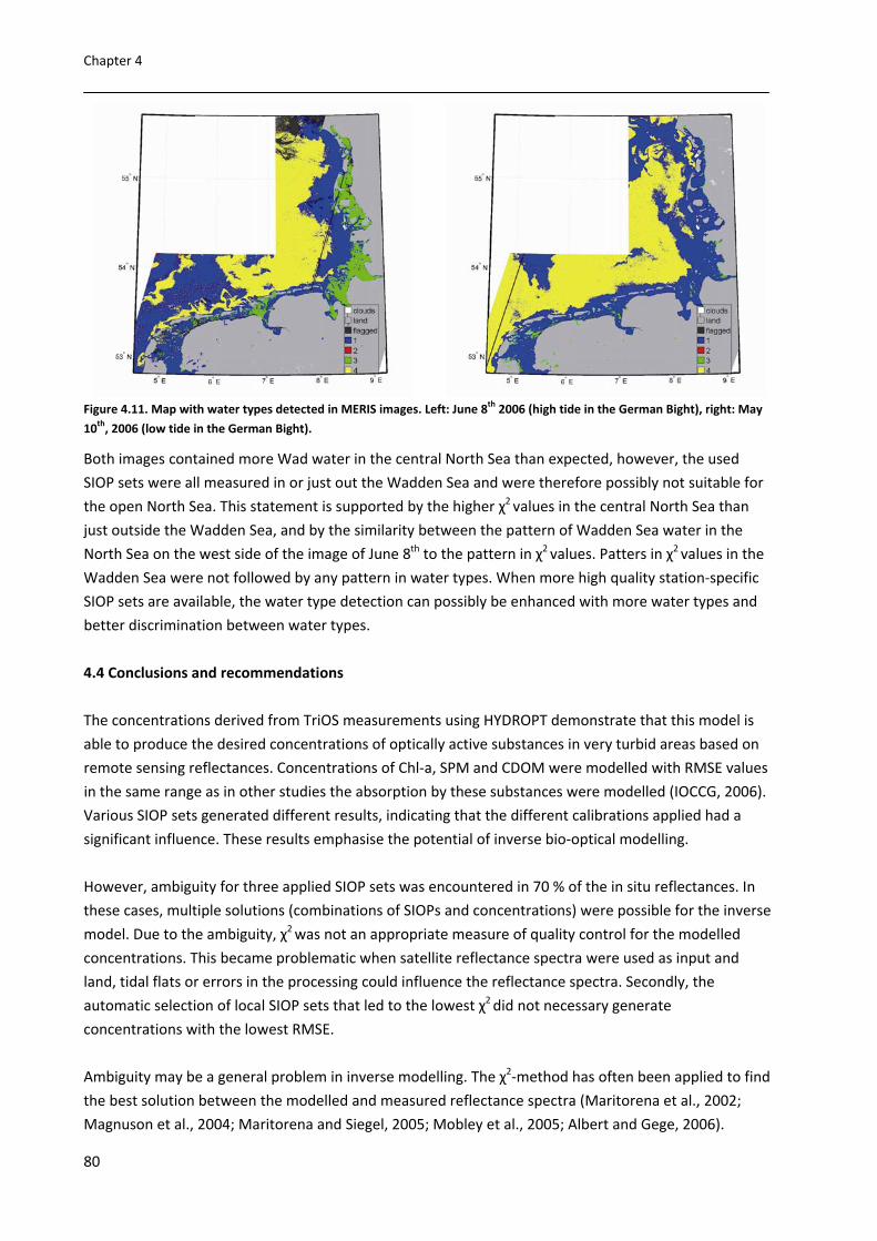
Chapter 4
80
Figure 4.11. Map with water types detected in MERIS images. Left: June 8th 2006 (high tide in the German Bight), right: May
10th, 2006 (low tide in the German Bight).
Both images contained more Wad water in the central North Sea than expected, however, the used
SIOP sets were all measured in or just out the Wadden Sea and were therefore possibly not suitable for
the open North Sea. This statement is supported by the higher χ2 values in the central North Sea than
just outside the Wadden Sea, and by the similarity between the pattern of Wadden Sea water in the
North Sea on the west side of the image of June 8th to the pattern in χ2 values. Patters in χ2 values in the
Wadden Sea were not followed by any pattern in water types. When more high quality station‐specific
SIOP sets are available, the water type detection can possibly be enhanced with more water types and
better discrimination between water types.
4.4 Conclusions and recommendations
The concentrations derived from TriOS measurements using HYDROPT demonstrate that this model is
able to produce the desired concentrations of optically active substances in very turbid areas based on
remote sensing reflectances. Concentrations of Chl‐a, SPM and CDOM were modelled with RMSE values
in the same range as in other studies the absorption by these substances were modelled (IOCCG, 2006).
Various SIOP sets generated different results, indicating that the different calibrations applied had a
significant influence. These results emphasise the potential of inverse bio‐optical modelling.
However, ambiguity for three applied SIOP sets was encountered in 70 % of the in situ reflectances. In
these cases, multiple solutions (combinations of SIOPs and concentrations) were possible for the inverse
model. Due to the ambiguity, χ2 was not an appropriate measure of quality control for the modelled
concentrations. This became problematic when satellite reflectance spectra were used as input and
land, tidal flats or errors in the processing could influence the reflectance spectra. Secondly, the
automatic selection of local SIOP sets that led to the lowest χ2 did not necessary generate
concentrations with the lowest RMSE.
Ambiguity may be a general problem in inverse modelling. The χ2‐method has often been applied to find
the best solution between the modelled and measured reflectance spectra (Maritorena et al., 2002;
Magnuson et al., 2004; Maritorena and Siegel, 2005; Mobley et al., 2005; Albert and Gege, 2006).

Performance of the regionally and locally calibrated algorithm HYDROPT in a heterogeneous coastal area
81
Brando et al. (2009) employed a variation on this method by multiplying χ2 by the spectral angle. The
spectral angle is sensitive only to the shape of the function and was calculated with a function called
Spectral Angle Mapper. Furthermore, χ2 was proposed as quality criterion by IOCCG (2006: Chapter 3);
Doerffer and Schiller (2007) used χ2 for this purpose. Generating exact solutions for concentrations
without an optimisation such as χ2 in the inversion is possible when a function such as the Gordon model
(Rrs = f*bb / a + bb, Gordon et al., 1975; Jerlov, 1976) is assumed to accurately describe the light field in
the water column. However, such models need assumptions about the spectral shape of (S)IOPs or the
necessity to disqualify spectral bands from the model to derive a square matrix for the MIM method.
In a heterogeneous area, such as the Wadden Sea, it is not appropriate to deal with ambiguity by setting
tight limits on the concentrations in the solution since this would disqualify pixels with extreme
concentrations. To improve quality control on modelled concentration maps, there is a need for further
validation with matchup data. This would best be approached by comparing concentration data from a
series of stations located progressively more distantly from tidal flats and islands with modelling results.
This type of comparison would lead to greater insight regarding the minimum distance required from
land features in order to have obtained useable reflectance data. If the input spectra don’t require much
quality control, results from HYDROPT on MERIS spectra are supposed to give results that are as good as
those derived from HYDROPT with TriOS reflectances as input.
Manual selection (expert knowledge) of areas where certain SIOP sets can be applied to reduce
ambiguity and obtain better concentration results (TriOS or MERIS) from the local calibration HYDROPT.
When multiple samples are taken at each location and SIOPs are determined as averages the obtained
“Location specific” local SIOP sets will be more robust (Annex 4A) and lead to better results than the
currently used “Station‐specific” local SIOP sets.
HYDROPT water type detection leads to positive results that can be explained with general knowledge
on the behaviour of water masses in the Wadden Sea. The ability to detect water types is an important
contribution of the locally calibrated model HYDROPT to existing algorithms.
Acknowledgements
Victoria Renner is thanked gratefully for English editing. Reinold Pasterkamp provided the HYDROPT
software libraries. Brockmann Consult is thanked for their help on ICOL processing. ACRI is thanked for
the MEGS 7.4 processing of ICOL processed L1 data. Marcel Wernand is thanked for making TriOS
sensors available to us. The captain and crew of the Royal Netherlands Institute for Sea Research R.V.
Navicula, Kristi Uudeberg‐Valdmets and Hamza el Abida are thanked for their help during the fieldwork
and the Institute for Environmental Studies laboratory for sharing their expertise on chlorophyll analysis.
MERIS data was provided by the European Space Agency. This project was financed by NWO/SRON
Programme Bureau Space Research, The Netherlands.

Chapter 4
82
Annex 4.A Discussion on the quality of the in situ measurements
TriOS measurements are most error prone in the blue part of the spectrum due to direct surface
reflectance. This effect is reduced by using viewing angles of ~135˚ azimuth away from the sun and 41˚
relative to the zenith and the nadir directions (Mobely, 1999) for the radiance detection, and by running
HYDROPT also without the band at 412 nm. Waves are small in the Wadden Sea, so that various sides of
waves are easily recorded and averaged, reducing the error due to direct surface reflectance. [SPM] was
during the first cruises determined as the average of a duplo, with strong correlations between the two
samples (in March the determination coefficient (r2) was 0.90, in May 0.97 both excluding one outlier,
and in June 0.96). During the cruises in 2006 [Chl‐a] was also determined as the average of a duplo, with
strong correlations between the two samples (in May r2 was 0.91, in August 0.94, and in September
0.87, excluding one outlier). In March 2006 there was no correlation calculated because only at 7
stations samples were taken and all concentrations were similar. The problems in the CDOM
measurements in 2007 (affecting 37 stations out of the total of 135, giving 27 % less‐accurate CDOM
measurements) are thought to add to random errors in the data. The errors in all in situ measurements
will mainly be random errors, because standard protocols were used. Assuming a Gaussian distribution
of errors would therefore be reasonable. However, systematic errors can occur (Sørensen et al., 2007)
and are difficult to determine. Random errors lead to more scatter in the measured‐modelled
concentration plots and higher RMSEs, but could not change the conclusions.
The single station SIOP sets are most vulnerable for measurement errors. Firstly, the concentrations of
the three optically active substances and their associated errors at that location have a significant
impact on the SIOPs. The random errors in concentration measurements create a systematic error on a
single SIOP. Secondly, SIOPs depend on several measurements, while an SIOP set consists of four SIOPs,
so that errors accumulate in the SIOP sets. Thirdly, lack of an integrating sphere led possibly to a
systematic overestimation of absorption in the filter pad measurements, as backscattering could partly
be recorded as absorption. Tassan and Ferrary (1995 ‐ Table 4.3) show that for cases with high
scattering and low absorption (like in the Wadden Sea), subtracting the value at 750 nm reduces this
error in the filter pad method to a range between 7 % at 440 nm and 23 % at 675 nm, against 3.5 % and
8 % respectively with use of an integrating sphere. Fourthly, there are many different equations for the
path length amplification factor, which is still not well understood and attributes to the uncertainty in
the specific absorption measurements (results of various researchers are summarised by Laurion et al.,
2003). However, the path length amplification factor used in this study (Ferrari and Tassan, 1996) was
probably suitable for the Wadden Sea (Hommersom et al., 2009), while Ferrari and Tassan (1996) state
that their equation is applicable to various phytoplankton cells, and mineral and organic suspended
sediment. Last, a*CDOM was not derived simultaneous with a*SPM and a*Chl, although it was measured
exactly one year earlier at almost the same locations. However, theoretically it is possible that the
obtained SIOP combination would not naturally occur. Assuming there are substantial errors in some of
the Station‐Specific SIOP sets might explain the rejection of many of these sets when HYDROPT was
allowed to select SIOP sets leading to the lowest χ2. This could also be the reason that on average the
Station‐Specific SIOP sets did not lead to the best RMSE for the modelled concentrations, or the lowest
χ2’s.

Performance of the regionally and locally calibrated algorithm HYDROPT in a heterogeneous coastal area
83
In the median SIOP set the effect of random errors in concentrations and the random errors in SIOPs are
averaged out. Therefore, the Wadden Sea median SIOP set showed values similar to those of the
REVAMP SIOP set and in the same range as the values of Babin et al. (2003) and Astoreca et al., (2006).
The higher RMSE values for the Wadden Sea median SIOP set were partly due to the systematic
underestimation of [Chl‐a] and [SPM](Figure 4.4). Using r2 values instead of RMSE values would show
that this SIOP set was able to model the distribution of [Chl‐a] and [SPM], only fail for the absolute
values. The lower RMSE values of the REVAMP SIOP set are thought to indicate the higher quality and
robustness of this SIOPs set, which was based on a much large database and carefully defined by a
group of researchers.


Chapter 5
Tracing Wadden Sea water masses with an inverse bio‐optical
and an endmember model
Authors:
Annelies Hommersom, Steef Peters, Hendrik Jan van de Woerd, Marieke A. Eleveld, Marcel R. Wernand,
Jacob de Boer
Published in EARSeL Proceedings Vol 9, 1: 1‐12.
Abstract
With its 500 km length the Wadden Sea is the largest mudflat area in the world. Discharges from various
rivers mix here with water from the North Sea. Due to surfacing tidal flats during low tide, the variation
in source water, resuspension and extremely high concentrations of Chlorophyll‐a (Chl‐a), Suspended
Particulate Matter (SPM), and Coloured Dissolved Organic Matter (CDOM), large temporal and spatial
differences in watercolour can be seen.
To visualise the horizontal mixing of water masses with different colours from MERIS images, two
approaches were followed. The first approach was an inverse bio‐optical model called HYDROPT, in
which the absorption and scattering properties of the water constituents (Specific Inherent Optical
Properties or SIOPs) can be adapted to regional values. This approach can be used to determine “water
types”: water masses in which the SIOPs of the constituents are similar. The second approach was an
endmember model, based on spectral reflectance shapes. This approach can be used to determine
“water classes”: water masses in which certain constituents are predominant. The predicted water types
and water classes were compared with knowledge on (tidal) distributions of water masses in the
Wadden Sea.
In the data of March ’07 (winter) and May ’06 (summer) differences in water types between the North
Sea, the Wadden Sea and water originating from the large rivers were seen in the German Bight. The
endmember approach was able to visualise mixing between water classes. Results of this method
showed dominance by SPM in winter and much higher concentrations of Chl‐a and CDOM in summer.
Combination of the two methods would probably lead to the best tracing water masses.

Chapter 5
86
5 Tracing Wadden Sea water masses with an inverse bio‐optical and an endmember model
5.1 Introduction
Remote sensing of estuaries and tidal flat areas is complex due to the often extreme turbidity and
heterogeneity, and explores therefore the upper limits of knowledge on remote sensing of coastal
zones. Remote sensing in these areas requires algorithms tuned for the extremely high concentrations
of various substances, almost simultaneous acquisition of remote sensing data and in situ data for
validation because of the fast changes as a result of resuspension due to tidal currents, and local
knowledge of optical properties to tune the algorithm. Apart of these problems, remote sensing of
coastal zones is an interesting possibility to water quality monitoring programs. The new Water
Framework Directive regulations from the European Union expect the member states to monitor all
their coastal areas (Environment Directorate‐General of the European Commission, 2000). Monitoring is
important to maintain the ecological and economical values of coastal zones, which are at the same
time the most densely populated areas in the world. Monitoring these coastal waters by ship is, as far as
possible, a costly and time consuming activity, where remote sensing can offer an alternative. The great
advantage of space borne remote sensing data is its high spatial resolution combined with a relatively
high temporal resolution. Drawback is that some, but not all substances important for water quality can
directly be monitored with space borne remote sensing data (Zielinski et al., 2009). However, many
water quality parameters (such as nutrients) can indirectly be related to parameters that can be
detected with remote sensing (Peeters et al., 2009; Zielinski et al., 2009).
The Wadden Sea is a very turbid and optically heterogeneous area. It is an embayment where the
estuary of various rivers (Rhine via Lake IJssel, Ems, Jade, Weser) and North Sea water confluence
(Figure 1.6, in the Introduction). The Wadden Sea is the largest tidal flat area in the world. The extreme
near‐surface concentrations of Particulate Suspended Matter (SPM: 5‐ 450 g m‐3), chlorophyll‐a (Chl‐a:
1‐50 mg m‐3), Coloured Dissolved Organic Matter (CDOM: 0.1‐3 m‐1), and the spatial, tidal and seasonal
variations (Hommersom et al., 2009) make the Wadden Sea optically very complex and a good case
study area for remote sensing in extremely turbid areas. The objectives of this study are therefore to
examine to what extent detection of water masses is possible in the Wadden Sea using MERIS data. The
possibilities of optical water mass detection based on ternary plots (in which the total absorption was
distributed over the relative absorption by Chl‐a, SPM and CDOM) was proven by Arnone, Gould and
others (e.g. Arnone et al., 2004a, 2004b). In this study we compare a regionally calibrated inverse bio‐
optical model and an endmember model.
The inverse bio‐optical model, called HYDROPT (Van Der Woerd and Pasterkamp, 2008) facilitates the
input of different (regional) sets of Specific Inherent Optical Properties of water constituents (SIOPs).
The model can automatically select a set of SIOPs from a given list that leads to the best modelled
reflectance spectrum compared to the measured spectrum. Its output includes the used SIOP set. This
approach can therefore be used to determine water masses in which the SIOPs of the constituents are
similar (Pasterkamp et al., 2005), called “water types” here. The second approach was an endmember
model, based on spectral reflectance shapes. The model unmixes the measured spectrum in a
combination of predefined extreme spectra, called endmembers. This approach can therefore be used
to determine water masses in which certain constituents are predominant, called “water classes” here.

Tracing Wadden Sea water masses with an inverse bio‐optical and an endmember model
87
The predicted water types and water classes are compared with knowledge on (tidal) distributions of
water masses in the Wadden Sea.
5.2 Methods
5.2.1 Satellite data
MERIS data L1 FR reflectance spectra (IPF 5.05/MEGS7.4, ESA, 2009a) were pre‐processed in the Basis
ERS and ENVISAT (A)ATSR and MERIS (BEAM) Toolbox. Adjacency effects were reduced with the
“improve contrast between ocean and land” (ICOL) processor (Santer and Zagolski, 2009). Next, the data
was atmospherically corrected with the Case‐2 regional (C2R) processor (Doerffer and Schiller, 2008).
The ICOL and C2R algorithms have their own land, cloud and quality flags (Doerffer and Peters 2006,
Santer and Zagolski, 2009). To be sure only water pixels were processed, the standard C2R land flag was
reduced to “toa_reflec_10 > toa_reflec_6”, flagging more pixels at shallow locations than the original
expression. Since clouds were sometimes flagged as “land” by C2R, the L1 flag for clouds was applied.
Data flagged with the C2R flags (RAD_ERR, TOSA_OOR, WLR_OOR and ATC_OOR) were flagged as
“flagged input” and not processed with HYDROPT or the endmember model.
Data of two acquisitions were chosen to trace water types and water classes: the data of March 12th
2007, representing a “winter” or before‐bloom situation, and the data of July 4th 2006, representing a
summer situation. The open North Sea is masked, because the SIOP sets used in HYDROPT were all
measured in or just outside the Wadden Sea and were therefore not supposed to be suitable for the
open North Sea.
5.2.2 Inverse bio‐optical model HYDROPT
HYDROPT is an inverse bio‐optical model: it calculates the IOPs, absorption (a) and scattering (b), from a
given reflectance spectrum. HYDROPT includes a lookup table (LUT) based on HydroLight (Mobely, 1994)
simulations of reflectances as a function of IOPs. Reflectances per wavelength over a large range of a
and b are included. The model was calibrated for each run with one or more sets of Specific Optical
Properties (SIOPs) at MERIS wavelengths. The absorption and scattering values at the correct solar angle
and viewing geometry in the LUT can be constructed from these SIOP sets plus concentrations of Chl‐a,
SPM, and CDOM via equations 5.1 and 5.2.
a (λ) = aw (λ) + a*Chl (λ) x [Chl‐a] + a*SPM (λ) x [SPM] + a*CDOM (λ) x aCDOM(440) (5.1)
b (λ) = bw (λ) + b*SPM (λ) x [SPM] = bw + SPM
B x [SPM] (λ) (5.2)
aw is the total absorption of water, a*Chl, a*SPM and a*CDOM are the specific absorption coefficients for
respectively pigments, particles other than phytoplankton, and CDOM. [Chl‐a] and [SPM] are the
concentrations of Chl‐a and SPM. For CDOM, the value at 440 nm is taken to normalize the attenuation
(aCDOM). bw is the scattering coefficient for water, b*SPM is the specific scattering coefficient and bb*SPM
the specific backscattering coefficient for SPM. B is the backscattering to scattering ratio, which was

Chapter 5
88
assumed to be spectrally neutral 0.03 (Dekker et al. 2001; Oubelkheir et al. 2006; Loisel et al., 2007;
Brando et al. 2008). For each given reflectance spectrum, HYDROPT finds a reflectance spectrum from
the LUT based on the entered SIOP sets and values for [Chl‐a], [SPM] and aCDOM. In the optimisation, the
modelled spectrum is compared to the measured spectrum with a least‐squares criterion of the band
differences (Equation 5.3). In Equation 5.3 Rrs is the remote sensing reflectance, i is the band number
and σ is the estimated standard error in the band differences, which was arbitrarily set to 3E‐4 and m is i‐
1. In this study σ was given the same value for TriOS and MERIS data.
2m
1
i1)(ii1)(i2
σ
modelled) Rrs ‐ modelled (Rrs ‐ situ) in R ‐ situ in(Rrs = χ
(5.3)
HYDROPT optimises the spectral fit by varying [Chl‐a], [SPM] and aCDOM and the SIOP sets. Subsequently
the outputs are: the spectrum that was chosen from the LUT, χ2, [Chl‐a], [SPM], aCDOM, confidence
intervals of these concentrations and the used SIOP set. Water for which the same SIOP set leads to the
best fitting spectrum is defined as one water type. Therefore, the maximum possible number of traced
water types is the number of SIOP sets the model is calibrated with.
At in situ campaigns in 2006 and 2007 [Chl‐a], [SPM] and aCDOM were measured, a*Chl, a*SPM were derived
directly from filter pad measurements in 2007, while b*SPM was calculated from the measured beam
attenuation and the measured absorptions (Hommersom et al., 2009). In situ reflectance was calculated
from above‐water radiance and irradiance measurements measured with TriOS sensors (Hommersom et
al., 2009). Due to equipment failure the accuracy of the CDOM measurements in 2007 was lost, instead,
a*CDOM derived from measurements at almost the same locations in 2006 was used in the SIOP sets.
Figure 5.1. Diagram of the water type detection with HYDROPT
Initial runs showed that water type detection in MERIS data was only possible when band 412 nm was
omitted from the analysis, probably due to the relatively large noise level in this band (Zibordi et al.,
2006). Using 7 bands, χ2 values ≤ 7.81 (3 degrees of freedom, P=0.05) were defined as a good spectral
fit. The most representative SIOP sets were selected by providing HYDROPT with a list of 22 SIOP sets as
measured at in situ stations (Hommersom et al., 2009) and performing runs with 135 TriOS spectra as
input (Figure 5.1). HYDROPT selected four SIOP sets for > 80 % of the TriOS measurements (Table 5.1).
These SIOP sets were considered to be most representative and were used for water type detection on
MERIS data (Figure 5.1). For each pixel HYDROPT selects one of the four SIOP sets to model the

Tracing Wadden Sea water masses with an inverse bio‐optical and an endmember model
89
spectrum. The pixels for which the same SIOP set was chosen are mapped to show the distribution of
water types.
Table 5.1. SIOP sets selected for water type detection. Absorption of CDOM was not measured simultaneously with a*Chl and
a*SPM, other properties are given as measured simultaneous with a*Chl and a*SPM.
SIOP set 1 2 3 4
in situ location Wadden Sea North Sea Ems estuary Wadden Sea
tide ingoing almost high almost high outgoing
salinity (Practical Salinity Scale) 32 32 25 33
organic content (%) 15.7 27.1 26.2 not available
a*Chl (681 nm) (m‐2 mg‐1) 0.80E‐2 0.83E‐2 1.65E‐2 18.4E‐2
a*SPM (442 nm) (m‐2 g‐1) 1.81E‐2 2.89E‐2 14.14E‐2 1.91E‐2
aCDOM(442 nm) (m‐1) 0.978 0.972 0.953 0.961
5.2.3 Endmember model
Endmember methods are common in land‐remote sensing, but almost new to water remote sensing
(Dowell et al., 2008), where endmember abundances have been used by few researchers, for deriving
Chl‐a concentrations (Tyler et al., 2006; Jianguang et al., 2005) and local calibration (Moore et al., 2001),
not yet for tracing of water masses. For land cover applications these methods are often used to
determine abundances of ground coverage of certain types within a pixel, in cases where typical ground
coverages are well known, while their spatial distribution contains too many entities smaller than the
pixel size. An example is grassland with asphalted roads through it. Generally, the roads will be too small
to be separately seen in the satellite data, while all pixels contain a mixture of light reflected by grass
and asphalt. Endmember methods use spectra of the most extreme situations occurring, e.g. pure grass
reflectance and pure asphalt reflectance, called “endmembers”, to unmix a measured spectrum. Linear
unmixing uses equation 4, in which R1 to Rn are the endmembers and a‐i the coefficients, or abundances
of the endmembers, determined in the unmixing process. Following the example, the calculated
abundances will provide the percentage coverage by grass and road per pixel. As will be explained later,
in our model n =9.
Rmeasured = aR1 + bR2 + cR3 + …iRn (5.4)
There are several ways to define the spectra to be used as endmembers for example:
Knowledge based manual selection. This method is fast and easy, however, not objective.
Pure pixel approach. In this approach spectra of all pixels are placed in a coordinate system with
on both axes a wavelength. This is repeated with other wavelengths and the spectra that occur
most often at the outer places of the scatter plots are selected as endmembers. This method is
objective, however, in sea (almost) no pure spectra can be found and endmembers will due to
variation in optical properties over the season vary per acquisition.

Chapter 5
90
Statistical classification, for example with K‐means, selecting the class means. This method is
objective; however, although these endmembers will represent water types, they will not
represent the extremes.
Simulation of “pure” spectra. This method is fairly objective, however, simulations require a
model and modelling always implies prepositions about for example inherent optical properties
of an area, or shapes of apparent optical properties. Endmembers generated for a certain region
can therefore be less suitable in other regions.
In this experiment endmembers were generated via the last approach. The Gordon (Gordon et al., 1975;
Jerlov, 1976) model (equation 5.5), was used in combination with equations 5.2 and 5.3, the assumption
f=0.33 (Morel and Prieur, 1977) and the median SIOP values as measured in the Wadden Sea needed for
equations 5.2 and 5.3.
Rrs = π x 1.332 x (f*bb / a + bb) (5.5)
Endmembers were not generated using the maximum [Chl‐a], [SPM] and aCDOM in the water, firstly
because concentrations higher than realistic in the area would deform the spectrum to a great extent.
Secondly, creating endmembers based on the “highest” concentration is not possible: ultimately
reflectance of a pure substance will remain, which is not the wanted endmember. On the other hand,
there is no problem if a pixel has reflectances somewhat higher than the highest SPM endmember, since
this pixel would be unmixed with this high‐SPM endmember anyhow. The situation would only increase
the modelling error. Therefore high, but not too high concentrations were chosen to generate the
endmembers. Endmembers were generated for pure water, for water with low concentrations (SPM 1 g
m3, Chl‐a 1 mg m3, CDOM 0.2 m‐1), high concentrations (SPM 100 g m3, Chl‐a 60 mg m3, CDOM 3 m‐1),
and mixtures between low and high concentrations (so one substance low and two high, or two low and
one high) for the thee substances, leading to a total of 9 endmembers (n=9). Endmembers simulated
with one or two high concentrations (for example high [Chl‐a]) were referred to as endmembers
dominated by that substance(s) (e.g.: the Chl‐dominated endmember); the endmembers simulated with
low respectively high concentrations for all the three substances were referred to as the low‐
concentrations respectively the high‐concentrations endmember. Data from Pope and Fry (1997) and
Morel et al. (2007) were used for absorption properties of pure water (aw) and data from Buiteveld
(1994) were used for the scattering properties of pure water (bw).
In an unconstrained unmixing method the abundances can have any value, while in a constrained
method the abundances are non‐negative (6) and in a fully constrained method also the sum of the
abundances is one (7).
a ≥ 0, b ≥ 0, c ≥ 0, …. i ≥ 0 (5.6)
a + b + c + …i = 1 (5.7)
In land remote sensing often the fully constrained method is used, because the total land‐cover (e.g. in
the example the total of grass and asphalt in a pixel) should be 100 %. To detect water types the same
unmixing method should be used. Negative abundances should not be possible, since always at least
pure (sea) water is present. Measured [SPM] higher than the one endmembers were based on are
possible, so that reflectances higher than the highest endmember could occur, abundances should also

Tracing Wadden Sea water masses with an inverse bio‐optical and an endmember model
91
sum to one. However, allowing sums higher than one would lead to for example 5 times a low‐SPM
endmember instead of 1 time the high‐SPM endmember, which implies that more water with low [SPM]
would have a similar reflectance as water with high [SPM], which is clearly not true. Also for CDOM and
Chl‐a that absorb light and therefore decrease the reflectance in higher concentrations this would lead
to problems. Higher abundances of for example the CDOM dominated endmember lead to higher total
reflectances, while more CDOM dominated water should lead to lower reflectances. Equation 5.4 is
therefore enhanced with constraints 5.6 and 5.7.
5.3 Results and discussion
5.3.1 Water type modelling with HYDROPT
Three of the four SIOP sets listed for HYDROPT were found to lead to the lowest χ2 values at most
locations in the MERIS acquisitions (Figure 5.2). Water type 2, which SIOP set was measured in the North
Sea, was only detected at a small spot in the data of July 4th. Apparently this SIOP set was less suitable
for the data in these two acquisitions, or subtle differences between MERIS and TriOS data made the
SIOP set more suitable for TriOS than for MERIS data.
In the Wadden Sea mainly water of type 1 was found, of which the SIOP set was measured at a location
in the Dutch Wadden Sea. In the winter acquisition this water type was also found in a large area around
the Wadden Sea and at some locations in the North Sea. This similarity between water in the Wadden
Sea and water in large areas in the North Sea was thought to be due to resuspension. Both March 12th
2007 and July 4th had a moderate breeze that could cause resuspension, however, in March 11th had
been a windier day, while July 3rd also had just a moderate breeze. At March 12th the water could
therefore contain more resuspended material than at July 4th. Also due to a lack of microphytobenthos
binding the sediment, resuspension is more prevalent in winter (Colijn and Dijkema, 1981). Water type 3
was detected in the estuaries of the large rivers and Lake IJssel, which could logically be explained since
the SIOP set of this water type had been measured in the outer estuary of the river Ems. Water type 4
was predominantly found in the North Sea. Although its SIOP set had been measured at a location in the
Wadden Sea, it apparently contained material that was similar to material usually found in the North
Sea. A relatively high salinity of 33 (Practical Salinity Scale) during sampling might explain the origin of
the water of which the data of SIOP set 4 was obtained.

Chapter 5
92
Figure 5.2: Water types modelled with HYDROPT. a: March 12th 2007, b: July 4th 2006. The colours indicate different SIOP
sets.
The dominant currents in the Wadden Sea are caused by the tide, moving in or out of the Wadden Sea
through the channels between the islands, and by the rivers discharging water. The overall rest current
in the Wadden Sea and German Bight is south‐west to north‐east. This pattern explains the pattern in
water types seen: Wadden Sea water (type 1) flowing through the tidal channels to the North Sea and
northward along the Danish coast, with a broader band of Wadden Sea water north of the Rivers Jade
and Weser in the data of March 12th, which was acquired at low tide near the estuaries of these rivers.
In the data of July 4th, which was acquired halfway outgoing tide near the estuaries of the large rivers,
their discharge was less visible.
5.3.2 Water class modelling with endmembers
Water class modelling with endmembers showed clear distribution results (Figure 5.3). In both
acquisitions, the endmember based on pure water was only in found offshore in low abundances (not
shown). The low‐concentrations endmember was found in the relatively coastal areas of the North Sea,
although in March more offshore (Figure 5.3a) than in July (Figure 5.3f). The other two end‐members
that were profound in the North Sea were the Chl‐dominated and the Chl‐CDOM‐dominated
endmembers. Note that high abundances of these endmembers provide information on the similarity
between spectral shapes between these endmembers and the reflectance spectra in the North Sea, not
on absolute concentrations. Chl‐a, and CDOM as its degradation product, are likely more dominant in
the North Sea than suspended matter, which settles out, while the shown area of the North Sea
contains too much sediment for much similarity with the pure‐water endmember.

Tracing Wadden Sea water masses with an inverse bio‐optical and an endmember model
93
Figure 5.3: Water classes modelled with endmembers. Left panel (a‐e): March 12th 2007, right panel (f‐j): July 4th 2006. The
colours represent the abundances of the endmembers: dark blue is low (0 %) abundance, red is high (100 %) abundance.
Shown endmembers are: a+f: low‐concentrations endmember, b+g: Chl‐dominant, c+h: Chl‐CDOM‐dominant, d+i: Chl‐SPM‐
dominant, e+j: SPM‐dominant.

Chapter 5
94
In March the Chl‐dominated endmember was found in one patch north of the Dutch islands (Figure
5.3b), in July, when phytoplankton concentrations are higher, it covered a larger area along the islands
and in the discharge of the Weser and Elbe rivers (Figure 5.3g). The Chl‐CDOM‐dominated endmember
was in March only found in the same area as the Chl‐dominated endmember (Figure 5.3c), while it
covered a large area in the German Bight in July (Figure 5.3h).
In most of the Wadden Sea the Chl‐SPM‐dominated endmember gave the highest abundances.
However, in March the abundances of this endmember were much higher than in July (Figure 5.3d and
5.3i). The SPM‐dominated endmember gave, only in March, high abundances in the inner estuaries of
the Jade and Dollard, as well as at few locations in the Wadden Sea and at the north side of some Dutch
and German islands (Figure 5.3e and 5.3j). In inland lakes and the River Weser the Chl‐dominated
endmember was profound. The CDOM‐dominated, SPM‐CDOM‐dominated and high‐concentrations
endmembers were in these acquisitions only found with abundances lower than 0.1 (not shown). The
water classification with the endmember method visualises the higher influence of high (SPM)
concentrations in March compared to July and the higher influence of chlorophyll, especially in the
North Sea, in July.
5.3.3 Comparison of the two approaches
The water type detection with the inverse bio‐optical model is a hard classifier, in that it showed strict
boundaries between water types, while horizontal mixing is surely taking place. This is partly inherent to
the method of selecting one SIOP set and therefore one water type per pixel, however, areas with
altering pixels would be possible. The water class detection with endmembers is fuzzy, and was able to
visualise the horizontal mixing between classes with decreasing versus increasing abundances. The
derived water classes relate to concentrations, giving information on dominance and on “high” or “low”
concentrations, and are useful for monitoring purposes. The method could also detect small patchiness
in the Wadden Sea. On the other hand, the endmembers approach cannot provide precise information
on concentrations of substances in the water, neither on the types of sediment, pigments of CDOM in
the water column. This is a consequence of applying a linear method to a non‐linear system. Methods to
circumvent this problem are use of difference spectra as input (Jianguang et al., 2005) or unconstrained
unmixing (Tyler et al., 2006). However, these models are adapted for one substance and therefore lose
their general application for water mass modelling. The bio‐optical model gives information on the
SIOPs and therefore on the type of pigments, SPM or CDOM present, while it can derive the
concentrations simultaneously with the water types (based on the total absorption and scattering from
the LUT).
5.3.4 Conclusions and outlook
Both methods lead to results that could be explained with general knowledge on the water masses in
the Wadden Sea and German Bight. The HYDROPT method shows water type in the Wadden Sea that is
different than the type in the German Bight. However, in a windy period in winter this Wadden Sea
water type extends into the German Bight. This is thought to be caused by resuspension of bottom
material, which is common in the Wadden Sea and extends to the German Bight after storm. Indeed, the
SPM‐dominated endmember has higher abundances in the same acquisition of March than in the

Tracing Wadden Sea water masses with an inverse bio‐optical and an endmember model
95
acquisition of July. Generally, Chl‐a and SPM is more dominant in the Wadden Sea than in the North Sea,
where low concentrations prevail, according to the endmember method. Discharge from the large
German rivers is visible in the results of HYDROPT, which finds another water type in the estuaries and
northwards.
Meanwhile, the techniques are different, leading to different but complimentary patterns. For example,
the patch north of the Dutch islands classified with endmembers as Chl‐dominated is not visible in the
water type detection with HYDROPT. Apparently there is relatively more chlorophyll in that patch than
in the surrounding water, while the phytoplankton is not of a different type. Similarities can strengthen
the results of the two methods. The apparent influence of resuspension leading to water type 1 in the
North Sea in March is visible with a low abundance for the SPM‐dominated endmember. Also the patch
west of the Danish islands (~55˚N, 8˚E) in the data of June is visible with both methods: the water is
classified as type 1 while also this patch is influenced by the SPM‐dominated endmember.
Although both methods lead to interesting results, the best tracing of water masses probably needs the
combination of the two methods. For example, abundances of endmembers can be used to determine
areas where certain SIOP sets of the bio‐optical model would be most applicable, as in Moore et al.
(2001). However, this method assumes the SIOP to vary with the water classes. Combination of the
results of the two methods assuming them to be complimentary can be interesting as well. The inverse
bio‐optical model misses the mixing, while the endmember model loses track of a water mass when for
example CDOM degrades, or SPM sinks, while the water still moves in a horizontal direction. However,
the water types of the inverse bio‐optical model contain information on the type of material and
therefore, in most cases, on the source, while the endmembers visualises the total influence of the
substances in the water column on the colour of the water and therefore the horizontal mixing,
degradation and sedimentation. With their specific possibilities the methods can supplement each
other.
Acknowledgements
The captain and crew of the Royal Netherlands Institute for Sea Research R.V. Navicula, Kristi Uudeberg‐
Valdmets and Hamza el Abida are thanked for their help during the in situ campaigns. Raul Zurita‐Milla is
thanked for his advice on the programming of the unmixing model. Dr. Rainer Reuter was thanked for
his suggestions on the endmember method at the EARSel workshop. Reinold Pasterkamp provided the
HYDROPT software libraries. MERIS data was provided by the European Space Agency. This project was
financed by NWO/SRON Programme Bureau Space Research, The Netherlands.


Chapter 6
Spectra of a shallow sea: unmixing for coastal water class
identification and monitoring
Authors:
Annelies Hommersom, Marcel R. Wernand, Steef Peters, Marieke A. Eleveld, Hendrik Jan van de Woerd,
Jacob de Boer
Submitted to Ocean Dynamics
Abstract
In heterogeneous coastal areas, monitoring water masses is a promising alternative for monitoring
concentrations. Fuzzy methods, such as spectral unmixing, are especially well suited for unmixing
reflectances of water masses. However, such models have not yet been applied for water classification
and monitoring. In this study a fully constrained endmember model with simulated endmembers was
developed for water class identification. Its performance was examined on in situ measured reflectances
and on MERIS satellite data. Water classification by means of unmixing reflectance spectra proved to be
successful. When the endmember model was applied to MERIS data it was able to visualise well known
spatial, tidal, seasonal, and wind related variations in optical properties in the heterogeneous Wadden
Sea. As the endmember model is insensitive to small variations in SIOPs, it can be applied in similar
turbid coastal areas. For use in open ocean situations or coastal or inland waters with other specific
inherent optical properties (SIOPs) re‐simulation of the endmembers with local optical properties is
required. However, such an adaptation requires only few local in situ measurements.

Chapter 6
98
6 Spectra of a shallow sea: unmixing for coastal water class identification and monitoring.
6.1 Introduction
Coastal waters are often very heterogeneous due to river discharge, land runoff, oceanic influence, and
human activities. Due to extreme concentrations of sediment in these waters, retrieval of precise
concentrations of chlorophyll‐a (Chl‐a), suspended particulate matter (SPM) and coloured dissolved
organic matter (CDOM) from remote sensing data can be problematic. Instead of monitoring
concentrations, water masses can be mapped and followed.
Tomczak (1999) defines water masses as: “a body of water with a common formation history, having its
origin in a particular region of the ocean”. This water mass formation “can be seasonal or intermittent in
time” (Tomczak, 1999). When monitoring water masses it is important to consider that some properties,
such as salinity, are conservative; that is they are stable in time. Changing values can only be attributed
to mixing (Tomczak, 1999). Non‐conservative properties change over time (Tomczak, 1999), due to for
example degradation or sinking. In papers on optical water mass monitoring (e.g. Van der Woerd et al.,
2004; Oliver and Irving 2008), the definition of a water mass differs depending on the method used. The
main difference in definitions can be found in the handling of non‐conservative properties.
In this study, waters with similar colours, expressed by similar total absorption and scattering properties
(the inherent optical properties or IOPs) are assigned the same water “class”. In these waters the
specific inherent optical properties (SIOPs) might still be different and therefore also the concentrations
of Chl‐a, SPM and CDOM do not have to be similar within one water class. However, there is a scaled
correlation between total absorption and scattering and total concentrations. In this study, waters with
similar SIOPs are assigned the same water “type”, even when the present concentrations (and thereby
reflectances) change.
Both water classes and water types can show large variability in time and space (e.g. Blondeau‐Patissier
et al., 2004; Doxaran et al., 2006, 2005) and have been used successfully for water mass identification.
Water types were identified with an inverse bio‐optical model called HYDROPT by Van der Woerd et al.
(2004). Inverse bio‐optical models were also used to define water classes, as in Hoge and Lyon (2005)
and Schofield et al. (2004). However, for water classification, clustering is a more general technique.
Various components, such as Chl‐a concentration, reflectances and Secchi depths can be used as
clustering properties (e.g. Reinart et al., 2003). Clustering based on reflectance spectra, combined with
salinity or temperature, has led to good classification results in various oceanic areas. For example
Oliver and Irwin (2008) were able to monitor the effect of El Nino events, and Lubac and Loisel (2007)
could determine the presence of Phaeocystis globosa based on spectral shapes. Improvements of the
clustering technique were studied by Oliver et al. (2004). Combining two theories, Feng et al (2005)
created a clustering technique to determine three water classes. In a next step they assumed the water
types in these water classes to be different. Then, they derived concentrations with three separately
calibrated bio‐optical models. Indeed, their results improved compared to the original bio‐optical
model. A sophisticated version of this method was developed by Moore et al. (2001), who used
unconstrained unmixing to determine water classes and subsequently derive concentrations with

Spectra of a shallow sea: unmixing for coastal water identification and classification
99
algorithms calibrated for the various water classes. This suggests that water types can vary with water
classes.
Another important point on water mass identification is the distinction between hard classification, in
which a pixel is classified as belonging to one or another water mass, and fuzzy classifications, in which
boundaries are gradual and pixels can be classified as a mixture of water masses. Water is subject to
local mixing, while non‐conservative properties gradually disappear from or appear in water masses.
Therefore, fuzzy methods are better suited for water mass monitoring (Dowell et al., 2008). Most
classifications based on clustering and inverse bio‐optical models give hard classifications. Only Oliver et
al. (2004) pays attention to the boundaries in their model.
Endmember models lead per definition to fuzzy classifications. These models are based on spectral
shapes: the model unmixes a given pixel in percentages, or abundances, of given endmembers and are
therefore also referred to as unmixing techniques. Unmixing is generally used in land remote sensing
(e.g. Asner et al., 2002) and for tidal flat identification (e.g. Doerffer and Murphy, 1989). However, only
few studies are available that apply unmixing to water reflectances (Dowell et al., 2008; Tyler et al.,
2006; Jianguang et al., 2005; Moore et al., 2001). Moore et al. (2001) base their approach on the fuzzy
property of endmember models to blend algorithms and retrieve concentration maps without
discontinuities. This approach still requires algorithms calibrated with the appropriate local SIOPs for
monitoring concentrations in extremely turbid coastal waters. To avoid this problem, our approach is to
monitor water classes instead of concentrations. This requires a fully constrained instead of an
unconstrained endmember model, as the total percentages of water masses should be positive and sum
to one. Only Jianguang et al. (2005) and Dowell et al. (2008) have successfully applied this type of model
to reflectances of water. Jianguan et al. (2005) used the derived abundances to calculate concentrations
and Dowell et al. (2008) presented promising primarily global results. Studies in which an endmember
model is used for monitoring (e.g. comparing images of various days) of water classes are not available.
The objective of this study was therefore to develop an endmember model for water classification and
examine its ability for monitoring water classes in the heterogeneous Wadden Sea. After generation of
the endmembers their performance was examined: firstly on in situ measured reflectance spectra;
subsequently, the model was applied to MEdium Resolution Imaging Spectrometer (MERIS) data. The
performance of the endmember model with MERIS data as input was evaluated by examining its
abilities to visualise well known spatial, seasonal, tidal and weather related variations in optical
properties (spatial, seasonal, tidal and weather related changes, Hommersom et al., 2010) in the
Wadden Sea.
6.2 Material and methods
6.2.1 In situ data
In situ remote sensing reflectance was derived from two radiance and one irradiance sensors (TriOS,
RAMSES (Heuermann, 1999)), according to equations 6.1 and 6.2. Measurements were carried out in
March, May, June, July, August and September 2006 (120 stations) and in May 2007 (37 stations)
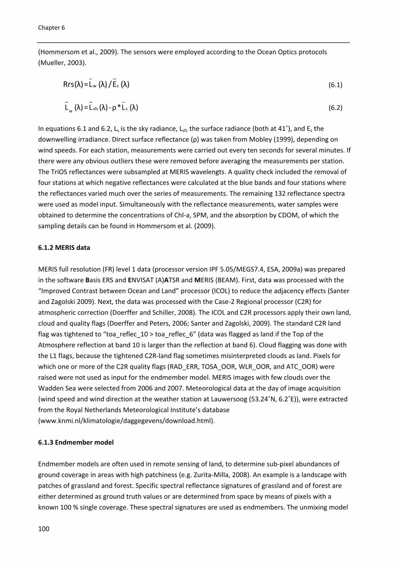
Chapter 6
100
(Hommersom et al., 2009). The sensors were employed according to the Ocean Optics protocols
(Mueller, 2003).
)λ( E /)λ( L = )λ( Rrs sw (6.1)
)λ( L * ρ ‐ )λ(L =)λ( L ssfcw (6.2)
In equations 6.1 and 6.2, Ls is the sky radiance, Lsfc the surface radiance (both at 41˚), and Es the
downwelling irradiance. Direct surface reflectance (ρ) was taken from Mobley (1999), depending on
wind speeds. For each station, measurements were carried out every ten seconds for several minutes. If
there were any obvious outliers these were removed before averaging the measurements per station.
The TriOS reflectances were subsampled at MERIS wavelengts. A quality check included the removal of
four stations at which negative reflectances were calculated at the blue bands and four stations where
the reflectances varied much over the series of measurements. The remaining 132 reflectance spectra
were used as model input. Simultaneously with the reflectance measurements, water samples were
obtained to determine the concentrations of Chl‐a, SPM, and the absorption by CDOM, of which the
sampling details can be found in Hommersom et al. (2009).
6.1.2 MERIS data
MERIS full resolution (FR) level 1 data (processor version IPF 5.05/MEGS7.4, ESA, 2009a) was prepared
in the software Basis ERS and ENVISAT (A)ATSR and MERIS (BEAM). First, data was processed with the
“Improved Contrast between Ocean and Land” processor (ICOL) to reduce the adjacency effects (Santer
and Zagolski 2009). Next, the data was processed with the Case‐2 Regional processor (C2R) for
atmospheric correction (Doerffer and Schiller, 2008). The ICOL and C2R processors apply their own land,
cloud and quality flags (Doerffer and Peters, 2006; Santer and Zagolski, 2009). The standard C2R land
flag was tightened to “toa_reflec_10 > toa_reflec_6” (data was flagged as land if the Top of the
Atmosphere reflection at band 10 is larger than the reflection at band 6). Cloud flagging was done with
the L1 flags, because the tightened C2R‐land flag sometimes misinterpreted clouds as land. Pixels for
which one or more of the C2R quality flags (RAD_ERR, TOSA_OOR, WLR_OOR, and ATC_OOR) were
raised were not used as input for the endmember model. MERIS images with few clouds over the
Wadden Sea were selected from 2006 and 2007. Meteorological data at the day of image acquisition
(wind speed and wind direction at the weather station at Lauwersoog (53.24˚N, 6.2˚E)), were extracted
from the Royal Netherlands Meteorological Institute’s database
(www.knmi.nl/klimatologie/daggegevens/download.html).
6.1.3 Endmember model
Endmember models are often used in remote sensing of land, to determine sub‐pixel abundances of
ground coverage in areas with high patchiness (e.g. Zurita‐Milla, 2008). An example is a landscape with
patches of grassland and forest. Specific spectral reflectance signatures of grassland and of forest are
either determined as ground truth values or are determined from space by means of pixels with a
known 100 % single coverage. These spectral signatures are used as endmembers. The unmixing model

Spectra of a shallow sea: unmixing for coastal water identification and classification
101
is subsequently used to determine the percentages coverage of both grass and forest per pixel and in
the entire area.
Linear models use equation 6.3, in which reflectances R1 to Rn are the endmember spectra, and a‐i the
abundances of the endmembers that will be determined in the unmixing process. (Reflectances are a
function of wavelength (λ), but λ was excluded for readability.)
Rmeasured = aR1 + bR2 + cR3 + …iRn (6.3)
In an unconstrained unmixing model the abundances can have any value, while in a constrained method
the abundances are non‐negative (equation 6.4) and in a fully constrained method additionally the sum
of the abundances is one (equation 6.5). On land‐reflectances generally the fully constrained method is
used, because the total coverage (e.g. in the example the total coverage by grass and forest in a pixel)
should be 100 %.
a ≥ 0, b ≥ 0, c ≥ 0, …. i ≥ 0 (6.4)
a + b + c + …i = 1 (6.5)
Compared to land, there will be less hard or fixed (“crisp”) boundaries in water, due to local mixing
between water masses, so that mixed pixels are more sparce. On the other hand, one geophysical
location can contain a mixture of two water masses, which never happens over land. Unless the
differences are large between land and water, a similar endmember model can be used. For unmixing
water reflectances in water classes, negative abundances are avoided, as there is always at least pure
(sea)water present. Abundances should sum to one, as the total mixture of water classes should lead to
100 % of the present water. Allowing abundances higher than one would tolerate high‐absorption
endmembers to sum to an – in total – high reflectance, which is incorrect. For example, a reflectance
spectrum with a high reflection could then be unmixed by taking 1x an SPM‐dominated endmember, or
5x a CDOM‐dominated endmember, while more CDOM dominated water should lead to lower
reflectances. To avoid such problems, a linear fully constrained method, based on equations 6.3, 6.4 and
6.5 was applied. The unmixing model was written within MATLAB software.
6.1.4 Endmember generation
Endmembers can be derived from in situ ground truth measurements or from images, and with several
methods, for example:
– Manual selection, based on expert knowledge. This method is fast and easy, however, not
objective. Another problem is that all endmembers should be available in the database. The
study of Martin Traykovski and Sosik (2003) used expert knowledge to define their classes,
although these were not used for endmember modelling.
– Pure pixel method. All pixels of an image are placed in a scatter plot with on both axes a
wavelength. This is repeated while varying the wavelengths. Spectra that occur most often at
the outer places of the scatter plots are selected as endmembers. This method is objective,
however, in the sea (almost) no pure spectra can be found, and endmembers defined with this
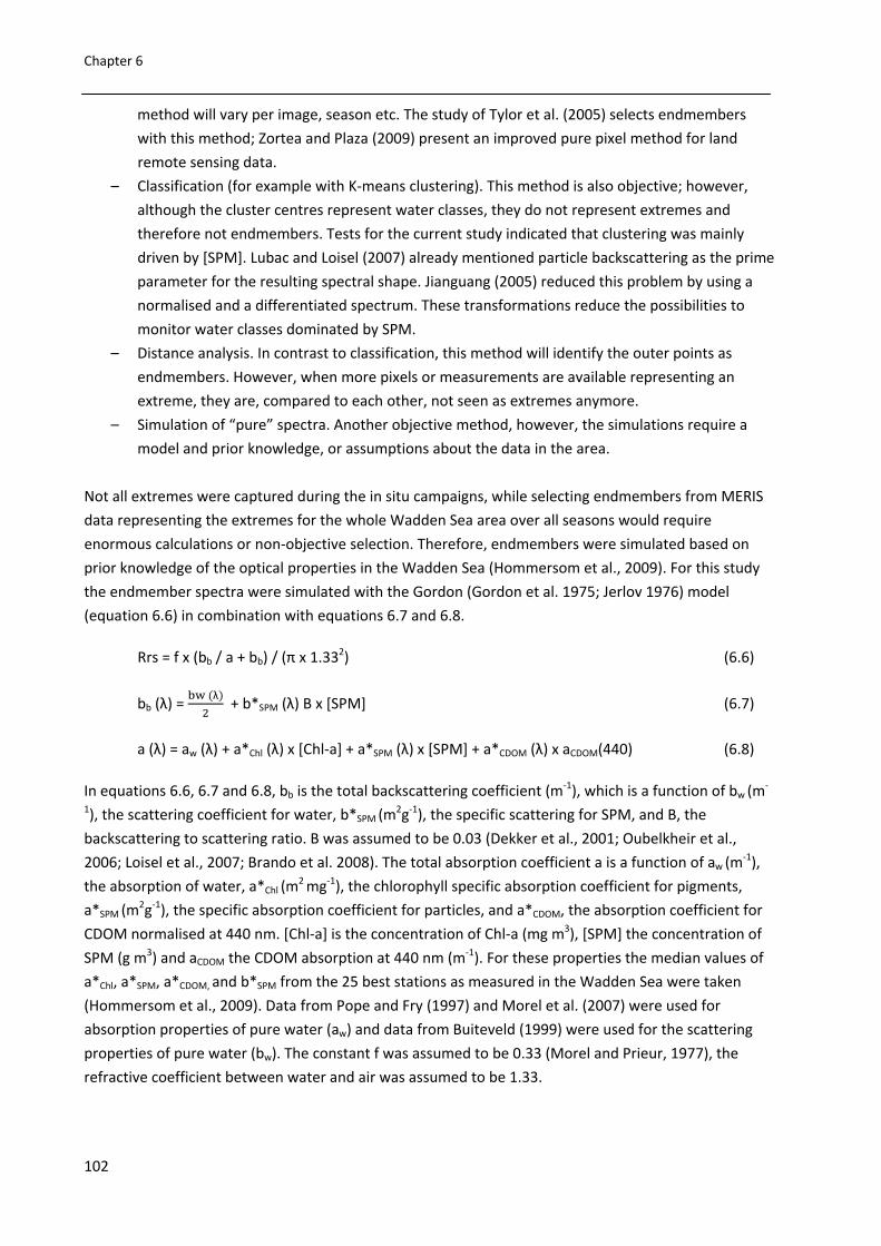
Chapter 6
102
method will vary per image, season etc. The study of Tylor et al. (2005) selects endmembers
with this method; Zortea and Plaza (2009) present an improved pure pixel method for land
remote sensing data.
– Classification (for example with K‐means clustering). This method is also objective; however,
although the cluster centres represent water classes, they do not represent extremes and
therefore not endmembers. Tests for the current study indicated that clustering was mainly
driven by [SPM]. Lubac and Loisel (2007) already mentioned particle backscattering as the prime
parameter for the resulting spectral shape. Jianguang (2005) reduced this problem by using a
normalised and a differentiated spectrum. These transformations reduce the possibilities to
monitor water classes dominated by SPM.
– Distance analysis. In contrast to classification, this method will identify the outer points as
endmembers. However, when more pixels or measurements are available representing an
extreme, they are, compared to each other, not seen as extremes anymore.
– Simulation of “pure” spectra. Another objective method, however, the simulations require a
model and prior knowledge, or assumptions about the data in the area.
Not all extremes were captured during the in situ campaigns, while selecting endmembers from MERIS
data representing the extremes for the whole Wadden Sea area over all seasons would require
enormous calculations or non‐objective selection. Therefore, endmembers were simulated based on
prior knowledge of the optical properties in the Wadden Sea (Hommersom et al., 2009). For this study
the endmember spectra were simulated with the Gordon (Gordon et al. 1975; Jerlov 1976) model
(equation 6.6) in combination with equations 6.7 and 6.8.
Rrs = f x (bb / a + bb) / (π x 1.332) (6.6)
bb (λ) = λ
+ b*SPM (λ) B x [SPM] (6.7)
a (λ) = aw (λ) + a*Chl (λ) x [Chl‐a] + a*SPM (λ) x [SPM] + a*CDOM (λ) x aCDOM(440) (6.8)
In equations 6.6, 6.7 and 6.8, bb is the total backscattering coefficient (m‐1), which is a function of bw (m
‐
1), the scattering coefficient for water, b*SPM (m2g‐1), the specific scattering for SPM, and B, the
backscattering to scattering ratio. B was assumed to be 0.03 (Dekker et al., 2001; Oubelkheir et al.,
2006; Loisel et al., 2007; Brando et al. 2008). The total absorption coefficient a is a function of aw (m‐1),
the absorption of water, a*Chl (m2 mg‐1), the chlorophyll specific absorption coefficient for pigments,
a*SPM (m2g‐1), the specific absorption coefficient for particles, and a*CDOM, the absorption coefficient for
CDOM normalised at 440 nm. [Chl‐a] is the concentration of Chl‐a (mg m3), [SPM] the concentration of
SPM (g m3) and aCDOM the CDOM absorption at 440 nm (m‐1). For these properties the median values of
a*Chl, a*SPM, a*CDOM, and b*SPM from the 25 best stations as measured in the Wadden Sea were taken
(Hommersom et al., 2009). Data from Pope and Fry (1997) and Morel et al. (2007) were used for
absorption properties of pure water (aw) and data from Buiteveld (1999) were used for the scattering
properties of pure water (bw). The constant f was assumed to be 0.33 (Morel and Prieur, 1977), the
refractive coefficient between water and air was assumed to be 1.33.

Spectra of a shallow sea: unmixing for coastal water identification and classification
103
Figure 6.1. Endmembers. Note the scale difference between figures a and b. The low‐concentrations endmember is shown
in both graphs for comparison.
Endmembers were not generated using maximum [Chl‐a], [SPM] and aCDOM in the water, because very
high concentrations would deform the spectrum to a great extent. Meanwhile, creating endmembers
based on the “highest” concentration is not possible: ultimately reflectances of a pure substance will
remain. Also, endmembers based on concentrations much higher than realistic in the area are not
needed: if a pixel has reflectances somewhat higher or lower than the most extreme endmember, since
this pixel would be classified as 100 % of this endmember anyhow. Such a situation would only increase
the modelling error. The same will happen when the shapes of the SIOPs (a*Chl, a*SPM, a*CDOM, and b*SPM)
used in the Gordon model are very different from the properties used to generate the endmembers, or
when high chlorophyll fluorescence occurs ‐which was not included in the model‐ or when the Gordon
model was not fully applicable. An input spectrum with a spectral shape different than can be
constructed with the endmembers will increase the modelling error, however, when the discrepancies
are not too large such a spectrum will still be unmixed with the most suitable endmembers and the
abundance results will be minimally influenced.
Table 6.1. Concentrations used in the Gordon model to generate the endmembers.
Endmember [Chl] [SPM] aCDOM (440)
pure water 0 0 0 low‐concentrations 1 1 0.2 CDOM‐dominated 1 1 3 CDOM‐Chl‐dominated 60 1 3 Chl‐dominated 60 1 0.2 SPM‐dominated 1 100 0.2 SPM‐CDOM‐dominated 1 100 3 SPM‐Chl‐dominated 60 100 0.2 high‐concentrations 60 100 3
Endmembers were generated for pure water, for water with low (SPM 1 g m3, Chl‐a 1 mg m3, CDOM 0.2
m‐1), and high (SPM 100 g m3, Chl‐a 60 mg m3, aCDOM 3 m‐1) concentrations, and mixtures between low
and high concentrations for the three substances (so one substance with a low and two with a high
concentration, or two with a low and one with a high concentration), leading to a total of 9
endmembers (Table 6.1, Figure 6.1). The endmember model can also be run with more or with less
endmembers than spectral bands, however, with more endmembers the model is over determined;
there is not one unique solution and the vulnerability for ambiguity increases. The modelling error is
0
0.01
0.02
0.03
0.04
400 500 600 700
Rrs
λpure water low-concentrationsSPM-dominated SPM-CDOM-dominatedSPM-Chl-dominated high-concentrations
0
0.001
0.002
0.003
0.004
0.005
400 500 600 700
Rrs
λlow-concentrations CDOM-dominated
CDOM-Chl-dominated Chl-dominated
a b

Chapter 6
104
calculated with the root mean squared error (RMSE), according to equation 6.9, in which n = 9 and a‐i
the abundances determined in the unmixing model. The RMSE was used to flag pixels for which the
unmixing process failed (artificially set to RMSE ≥ 0.01).
RMSE = R – R R R … R
(6.9)
6.1.5 Testing the endmember model
The endmember model was evaluated, first by unmixing in situ measured reflectance data and
comparing the obtained endmembers with the simultaneously measured concentrations of Chl‐a, SPM
and CDOM. Second, various MERIS images were used as model input. The ability of the model to
visualise well known spatial, seasonal, tidal and weather related changes in the Wadden Sea was tested
in many well known situations (Hommersom et al., 2010). The derived endmember abundances over the
gradients in the area, including the estuaries were examined, and the endmember abundances derived
in images acquired of various seasons, during different moments in the tidal cycle and during different
weather conditions were compared.
We anticipated for:
1) Spatial variation. Lower IOP values in the Wadden Sea than in the North Sea (Hommersom et al.,
2009); and an IOP gradient in the estuaries.
2) Seasonal variation. IOPs dominated by Chl‐a in spring because of phytoplankton blooms (e.g. Cadée
1980); IOPs dominated by SPM in winter (e.g. Grossart et al., 2004; Lemke et al., 2009) due to the
more windy weather, but also because of a lack of benthic organisms that stabilise the sediment
(Austen et al. 1999).
3) Tidal variation. High absorption and scattering by SPM and possibly absorption by Chl‐a at the
moment of the tidal cycle with the highest tidal currents (Poremba et al., 1999; Hommersom et al.,
2009), that occur about two hours before slack tide (Postma 1982).
4) Weather related variation. High IOPs during storm (Badewien et al., 2009; Stanev et al., 2009), due
to resuspension of SPM, Chl‐a and, to a lesser extent, CDOM from pore water (Lübben et al., 2009).
Differences in IOPs depending on wind direction (Badewien et al., 2009).
5) If reflectances that cannot be modelled with the current endmembers are encountered high
modelling errors are expected. These errors would indicate novelty spectra (Schiller et al., 2007).
6.2 Results and discussion
6.2.1 Validation of the endmembers and the model
A comparison was made between endmembers and the in situ reflectances. The generated
endmembers with the lowest reflectances were lower than any of the measured spectra (Figure 6.2).
This was necessary, because all in situ stations were located in the Wadden Sea or in the North Sea just
outside the island arc (Hommersom et al., 2009), while the reflectances in the open area of the German
Bight and North Sea were expected to be lower. The endmembers with the highest reflectances were
higher than almost all in situ measured spectra (Figure 6.2), although these endmembers showed a

Spectra of a shallow sea: unmixing for coastal water identification and classification
105
somewhat different spectral shape in the first two bands (412 and 440 nm) or in the last band (708 nm)
than the in situ spectra with the highest reflectances. This could be due to other SIOPs for SPM at these
in situ stations than the median value that was used to generate the endmembers. However, these
small spectral differences should not be a problem for the unmixing as these endmembers with the
highest reflectance will still remain the best suitable to unmix the high‐reflective measurements.
Figure 6.2. In situ measured Rrs (TriOS) (black lines) and coverage of the endmembers (grey shading).
To evaluate the model, first the in situ measured reflectance spectra were used as input. When the
abundances of the nine endmembers were compared with the in situ data of [Chl‐a], [SPM], and aCDOM,
the applicability of the endmembers could be validated (Table 6.2). In this validation it is assumed that,
in spite of variability in SIOPs, IOPs and concentrations have a positive correlation. It seems that the low‐
concentrations endmember functioned as a basis, as it was present with significant abundances in
almost all unmixing results. This endmember was usually found in combination with one and sometimes
two other endmembers at higher abundances (> 0.25) and two endmembers at low abundances (<
0.25). Indeed, spectra measured at locations with low [Chl‐a], [SPM], and aCDOM were unmixed with a
high abundance of the low‐concentrations endmember, while mostly the substance with a relatively
high concentration related with the end‐member dominated by that substance. Only in the spectrum
collected at May 2nd at 14.25 h., absorption by CDOM and Chl‐a (present in the in situ data) seemed to
be mistaken for pure water absorption by the model. The SPM‐dominated and the SPM‐Chl‐dominated
endmembers often occurred in higher abundances. The results indicate that the substance with the
largest influence on the reflectance spectrum is the substance with the relatively highest concentration.
At stations where concentrations are (relatively) comparable, SPM dominates the spectral shape of the
reflectance spectrum. The last remark is in agreement with general knowledge of the influence of SPM
and its spectral signature (e.g. Lubac and Loisel, 2007).

Chapter 6
106
Table 6.2. Results of unmixing in situ measured reflectance data. The table presents in situ concentrations and derived
endmember abundances. Due to space restraints, the data for not all of the 132 spectra were presented. Data were listed in
order of sampling time and data of every 3rd station is presented. Gray shading for abundances > 0, dark gray shading for
abundances > 0.25.
Date Time GPS N GPS E In situ data Endmember abundances RMSE
decimals
decimals
Chl‐a (mg m
‐3)
SPM (g m
‐3)
CDOM(m
‐1)
P
ure water
Low con.
CDOM
CDOM‐Chl
Chl
SPM
SPM‐CDOM
SPM‐Chl
High Conc.
7‐Mar‐06 14:20 52.9882 4.7880 4.0 12.3 n.a 0.07 0.66 0.00 0.00 0.00 0.28 0.00 0.00 0.00 3.97E‐039‐Mar‐06 17:05 53.0010 4.7868 7.2 13.1 n.a 0.05 0.72 0.00 0.00 0.00 0.24 0.00 0.00 0.00 3.59E‐032‐May‐06 9:36 53.3015 5.2652 6.2 6.0 0.8 0.00 0.75 0.00 0.00 0.21 0.03 0.00 0.01 0.00 2.69E‐042‐May‐06 16:25 53.4232 5.7993 15.7 62.4 1.0 0.28 0.08 0.00 0.00 0.00 0.51 0.00 0.13 0.00 2.40E‐033‐May‐06 10:36 53.4468 6.1698 10.5 25.9 0.9 0.00 0.62 0.00 0.00 0.00 0.22 0.00 0.15 0.00 9.42E‐043‐May‐06 15:42 53.4833 6.4708 6.3 7.5 1.0 0.00 0.68 0.00 0.00 0.25 0.07 0.00 0.00 0.00 7.48E‐044‐May‐06 10:14 53.3818 6.9580 9.5 30.3 1.8 0.00 0.44 0.00 0.00 0.00 0.52 0.00 0.04 0.00 1.41E‐035‐May‐06 8:40 53.5268 6.7540 12.6 6.7 1.1 0.00 0.45 0.00 0.00 0.44 0.00 0.05 0.06 0.00 1.02E‐035‐May‐06 16:34 53.7885 7.5155 2.0 2.6 0.6 0.04 0.81 0.13 0.00 0.00 0.02 0.00 0.00 0.00 5.87E‐056‐May‐06 10:51 54.0528 8.2733 10.5 2.1 0.5 0.00 0.62 0.00 0.00 0.34 0.00 0.02 0.02 0.00 4.53E‐047‐May‐06 10:19 54.8610 8.2167 15.7 2.4 0.6 0.00 0.28 0.00 0.00 0.70 0.00 0.02 0.00 0.00 1.69E‐048‐May‐06 6:27 55.0950 8.3375 4.3 2.5 0.2 0.00 0.51 0.00 0.00 0.49 0.00 0.00 0.00 0.00 9.18E‐049‐May‐06 6:02 54.5912 8.4035 6.6 7.2 0.9 0.00 0.89 0.00 0.00 0.00 0.07 0.00 0.03 0.00 1.09E‐039‐May‐06 12:08 54.1417 8.7235 41.2 23.2 0.8 0.00 0.53 0.00 0.00 0.00 0.11 0.00 0.36 0.00 8.23E‐0413‐Jun‐’06 10:57 53.0010 4.7870 n.a 30.0 0.9 0.00 0.70 0.00 0.00 0.00 0.28 0.00 0.03 0.00 1.08E‐0314‐Jun‐’06 7:55 53.0010 4.7870 n.a 22.0 0.7 0.00 0.60 0.00 0.00 0.00 0.33 0.00 0.06 0.00 1.22E‐0315‐Jun‐’06 11:05 53.0010 4.7870 n.a 24.0 0.5 0.00 0.79 0.00 0.00 0.00 0.19 0.00 0.01 0.00 1.34E‐0315‐Jul‐’06 10:45 53.0010 4.7870 n.a 25.2 0.7 0.00 0.70 0.00 0.00 0.00 0.12 0.00 0.18 0.00 8.25E‐0415‐Jul‐’06 17:45 53.0010 4.7870 n.a 52.4 0.4 0.00 0.65 0.00 0.00 0.00 0.26 0.00 0.09 0.00 9.99E‐0419‐Jul‐’06 8:10 53.0010 4.7870 n.a 4.4 0.5 0.00 0.75 0.00 0.00 0.00 0.23 0.00 0.02 0.00 1.47E‐0321‐Aug‐’06 13:00 53.2360 5.2585 25.4 20.8 0.5 0.10 0.33 0.00 0.00 0.00 0.37 0.00 0.20 0.00 2.54E‐0322‐Aug‐’06 10:50 53.4968 6.0128 12.1 63.6 0.5 0.00 0.46 0.00 0.00 0.00 0.40 0.00 0.14 0.00 1.93E‐0323‐Aug‐’06 10:25 53.4963 6.4028 5.1 16.8 0.3 0.15 0.41 0.00 0.00 0.00 0.44 0.00 0.00 0.00 3.96E‐0323‐Aug‐’06 18:00 53.4960 6.4023 13.2 38.4 0.7 0.00 0.52 0.00 0.00 0.00 0.34 0.00 0.14 0.00 1.77E‐0325‐Aug‐’06 4:55 53.4963 6.4032 7.8 20.8 0.8 0.01 0.71 0.00 0.00 0.00 0.24 0.00 0.05 0.00 1.55E‐0326‐Aug‐’06 17:05 53.4963 6.4032 14.6 19.6 0.8 0.00 0.71 0.00 0.00 0.00 0.16 0.00 0.13 0.00 1.27E‐0329‐Aug‐’06 10:37 53.4172 6.2135 20.8 65.2 0.7 0.00 0.56 0.00 0.00 0.00 0.25 0.00 0.19 0.00 6.08E‐0430‐Aug‐’06 10:05 53.4262 6.0572 24.7 46.4 0.6 0.10 0.23 0.00 0.00 0.00 0.47 0.00 0.20 0.00 2.19E‐0331‐Aug‐’06 7:45 53.2337 5.2943 22.3 15.6 0.6 0.00 0.71 0.00 0.00 0.00 0.19 0.00 0.10 0.00 2.52E‐0318‐Sep‐’06 10:08 53.0945 5.0645 8.4 5.4 0.9 0.00 0.84 0.00 0.00 0.13 0.00 0.02 0.01 0.00 8.63E‐0418‐Sep‐’06 16:30 53.3967 5.5738 4.7 3.2 n.a 0.18 0.56 0.00 0.00 0.00 0.26 0.00 0.00 0.00 2.19E‐0320‐Sep‐’06 14:45 53.4957 6.4020 15.8 25.6 0.5 0.02 0.68 0.00 0.00 0.00 0.23 0.00 0.06 0.00 1.33E‐0321‐Sep‐’06 8:15 53.4953 6.4013 8.6 13.2 n.a 0.01 0.75 0.00 0.00 0.00 0.23 0.00 0.00 0.00 1.68E‐0321‐Sep‐’06 11:15 53.4957 6.4022 11.8 53.6 0.7 0.00 0.65 0.00 0.00 0.00 0.33 0.00 0.03 0.00 1.75E‐0321‐Sep‐’06 14:15 53.4957 6.4020 4.0 27.6 0.6 0.00 0.65 0.00 0.00 0.00 0.29 0.00 0.06 0.00 1.47E‐037‐May‐’07 10:55 53.2215 4.9523 14.0 3.6 0.7 0.00 0.69 0.00 0.00 0.25 0.03 0.01 0.01 0.00 5.59E‐048‐May‐’07 8:25 53.1600 5.1993 11.0 41.2 0.7 0.09 0.44 0.00 0.00 0.00 0.43 0.00 0.03 0.00 2.54E‐038‐May‐’07 11:27 53.3067 5.4045 10.4 32.0 0.9 0.05 0.46 0.00 0.00 0.00 0.46 0.00 0.03 0.00 2.23E‐039‐May‐’07 9:45 53.3088 5.5455 64.5 452.0 n.a 0.17 0.00 0.00 0.00 0.00 0.50 0.00 0.34 0.00 1.50E‐0311‐May‐’07 13:40 53.3152 7.1600 32.0 290.0 1.5 0.00 0.21 0.00 0.00 0.00 0.05 0.35 0.00 0.40 5.39E‐0411‐May‐’07 17:20 53.3878 6.9672 27.2 14.4 1.5 0.04 0.39 0.00 0.00 0.00 0.31 0.00 0.26 0.00 1.43E‐0313‐May‐’07 9:25 53.9133 8.0730 24.9 9.2 0.6 0.00 0.33 0.00 0.00 0.65 0.02 0.00 0.00 0.00 3.05E‐0414‐May‐’07 10:30 54.1092 8.8662 38.5 30.0 0.7 0.06 0.42 0.00 0.00 0.00 0.26 0.00 0.26 0.00 1.21E‐0314‐May‐’07 14:15 54.1133 8.8663 > 60 154.0 0.5 0.00 0.10 0.33 0.00 0.00 0.00 0.04 0.00 0.54 1.29E‐03
6.2.2 Water class monitoring with unmixed MERIS data
In the unmixed MERIS images, spatial variation in the obtained water classes became clearly visible, as
shown in Figures 6.3 to 6.8. High abundances (0.5 to 0.9) of the SPM‐Chl‐dominated endmember were
found at the innermost locations of the Wadden Sea and in sheltered areas behind the islands (Figure
6.3). The basic low‐concentrations endmember showed its highest abundances in the North Sea, in
winter covering most of the German Bight (Figure 6.4a), while in spring and summer its area was
reduced (Figure 6.4b) in favour of the CDOM‐dominated, CDOM‐Chl‐dominated and Chl‐dominated

Spectra of a shallow sea: unmixing for coastal water identification and classification
107
endmembers (e.g. Figure 6.5). The pure water endmember had low abundances (maximum 0.5,
generally 0.2 or 0.3) at the most offshore locations (~ > 53.5˚N, < 5.5˚ E) in almost every image (not
shown). Only in winter this endmember was spread over the German Bight in abundances of maximum
0.2.
The most extreme spatial differences were found in the Ems‐Dollard estuary (Figure 6.6), the other
rivers did not show such extreme gradients. The Ems‐Dollard showed a trend with SPM‐dominated
water in the Dollard (6.6a), via SPM‐Chl‐dominated water in the inner estuary (6.6b) to high abundances
for the low‐concentrations endmember in the outer estuary (6.6c). In spring, outside the estuary the
Chl‐dominated endmember was found (6.6d). This spatial trend in IOPs with high b/a values, via lower
b/a values at high total a and b, and again lower b/a values at low total a and b, to finally low b/a values
at low a and b is similar to the trend found by Magnuson (2004) in the upper, mid and lower Chesapeake
Bay and the inshore Middle Atlantic Bight.
Figure 6.4. Abundance of the low‐concentrations endmember at days with comparable wind speeds, a: in winter, illustrated
with the image of January 16th 2006 (daily average south‐easterly wind 6.8 m s‐1, highest hourly average wind 8.0 m s‐1),
which could not be processed with the ICOL processor, b: in summer, illustrated with the image of June 30th 2006 (daily
average north easterly wind 6.1 m s‐1, highest hourly average wind 9.0 m s‐1). The flagged line is an error caused by the first
version of the ICOL processor.
Figure 6.3. Abundance of the SPM‐Chl‐dominated endmember with calm weather, illustrated with the image of May 10th
2006, when the daily average wind speed was 4.7 m s‐1 and the highest hourly average wind speed 6.0 m s‐1. The flagged
line in the west is an error caused by the first version of the ICOL processor.

Chapter 6
108
Analyses of variations over the tidal cycle required MERIS images acquired at various moments in the
tidal cycle. As the overpass of MERIS is each day at approximately the same time, images of several
weeks were needed, while other conditions (weather, season) should be similar. Four images, acquired
in June and July 2006, with calm weather (average daily wind conditions over the days of acquisition of
the four images ranging 2.9‐6.1 m s‐1, wind direction north‐east to south‐east) were selected. With these
four images half of the tidal cycle was covered. As the tide varies over the area, the part of the cycle that
was covered depends on the location (e.g. for the area near Den Helder the images cover high water
(HW) to low water (LW)). Figure 6.6 (a‐d) shows the abundances of the SPM‐Chl‐dominated
endmember, which was the most representative endmember in the Wadden Sea in the four selected
images. Other endmembers were absent in the Wadden Sea, except for the SPM‐dominated
endmember, which had high abundances in the Dollard in every image, and low abundances (<0.2) at
various locations in the Wadden Sea in the image of June 30th ’06. Over the examined part of the tidal
cycle the following trends in the abundances of the SPM‐Chl‐dominated endmember were visible
(Figure 6.6a‐d):
– The lowest abundances occurred just after HW, when relatively clear North Sea water had entered
the Wadden Sea and SPM and benthic algae have had the time to settle out (Den Helder, 6.6b; the
East Frisian Wadden Sea, 6.6c).
– Abundances increased during ebb (Den Helder, 6.6c; Eastern Dutch Wadden Sea, 6.6d; Ems
estuary/area near island Borkum, 6.6d; East Frisian Wadden Sea, 6.6d).
– At LW and the first hour(s) after, large percentages of the surface were covered with surfacing tidal
flats. Abundances in the surrounding water were similar to or lower than during ebb (East Frisian
Wadden Sea, 6.6a; near Den Helder, 6.6d). This makes sense, as SPM and benthic algae will be
subject to sedimentation in the calm water.
– The highest abundances were seen during flood, about 2.5 hours before HW (Eastern Dutch
Wadden Sea 6.6a and 6.6b; Ems estuary/area near island Borkum, 6.6b).
Figure 6.5. Development of the spring bloom in 2007, illustrated with abundances of the Chl‐dominated endmember. Images
of: a: March 12th, b: March 25th, c: March 28th, d: April 16th, e: April 29th, f: May 1st.

Spectra of a shallow sea: unmixing for coastal water identification and classification
109
Figure 6.6. General trend in the Ems‐Dollard estuary, illustrated with the unmixed image of April 16th, 2007. a: SPM‐
dominated endmember, b: SPM‐Chl‐dominated endmember, c: low‐concentrations endmember, d: Chl‐dominated
endmember.
Figure 6.7. Images showing the influence of tidal variation with the abundances of the SPM‐Chl‐dominated endmember.
a‐c respectively: July 3rd (10.29 UTC), June 30th (10.23 UTC), July 11th (10.20 UTC), June 8th (10.14 UTC), all 2006. The
circles represent the areas of red: Den Helder (DH, the narrow channel), green: the eastern Dutch Wadden Sea (EDWS),
yellow; Ems estuary/area near island Borkum (EB), blue: the East‐Frysian Wadden Sea (EFWS, Germany). Tides were
(HW = high water, LW = low water):
a: DH ~HW, EDWS: ~2.5 h after LW, EB: ~2 h after LW, EFWS: ~1.5 h after LW.
b: DH ~just after HW, EDWS: ~1.5 h before HW, EB: ~2.5 h before HW, EFWS: ~3 h before HW.
c: DH ~1.5 h before LW, EDWS: ~1 h after HW, EB: ~0.5 h after LW, EFWS: ~just after HW.
d: DH ~LW, EDWS: ~2 h before LW, EB: ~3 h before LW, EFWS: ~2.5 h after HW.

Chapter 6
110
Seasonal changes became visible in the abundances as well. In winter the abundances of the CDOM‐
dominated, CDOM‐Chl‐dominated and Chl‐dominated endmember were reduced to zero, while the
abundances of the SPM‐dominated endmember were relatively high compared to summer (Figure 6.8).
Because of many days with clear weather in (early) spring 2007, results could show the appearance,
development and movement of the spring bloom of phytoplankton in March‐May 2007 (Figure 6.5). The
bloom drifted in the direction of the residual current in the German Bight (Postma, 1982).
Unfortunately, May 2007 was very cloudy so that this bloom could not further be followed.
Figure 6.8. Abundance of the SPM dominated endmember, a: in winter, illustrated with the image of January 16th 2006
(daily average south easterly wind 6.8 m s‐1, highest hourly average wind 8.0 m s‐1), which could not be processed with
the ICOL processor, b: in summer, illustrated with the image of June 30th 2006 (daily average north‐easterly wind 6.1 m s‐
1, highest hourly average wind 9.0 m s‐1).
Wind induced resuspension became visible with high abundance of the SPM‐Chl‐dominated endmember
(Figure 6.9a and b) and the SPM‐dominated endmember (Figure 6.10a and b) in the Wadden Sea and on
the outer side of the islands. Abundances of these endmembers were much lower with calm weather
(Figure 6.3). The south‐westerly wind at December 10th 2006 had apparently blown relatively clear
North Sea water into the western Dutch Wadden Sea (low abundances of the SPM‐Chl‐dominated
endmember), while resuspension caused relatively high abundances of the SPM‐Chl‐dominated and
SPM‐dominated endmembers in the rest of the Wadden Sea, and north of the Dutch and western
German islands (Figure 6.9a and 6.10a). The north‐north‐easterly wind of late March 2007 caused much
higher resuspension than the south‐westerly wind early December 2006, visible as very high abundances
of the SPM‐Chl‐dominated endmember and relatively high abundances of the SPM‐dominated
endmember along the Northern German and Danish islands in the German Bight (Figure 6.9b). In
December, the high abundances of the SPM‐Chl‐dominated as well as the SPM‐dominated endmembers
could partly be due to extra resuspension caused by tide against wind, since the areas where the highest
abundances occurred, the Dutch and western German islands, were subject to ingoing tide at the time
of the image acquisition. This was not the case in March, when the highest abundances occurred around
the islands located 54˚44’ N, where tide was outgoing and the current moved more or less in the same
direction as the easterly wind. The wind‐wave induced mixing kept the sediment in the East‐Anglian
plume (Doerffer and Fischer, 1994; Eleveld et al., 2008) in suspension, which is visible as high
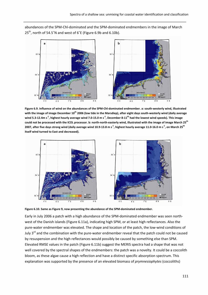
Spectra of a shallow sea: unmixing for coastal water identification and classification
111
abundances of the SPM‐Chl‐dominated and the SPM‐dominated endmembers in the image of March
25th, north of 54.5˚N and west of 6˚E (Figure 6.9b and 6.10b).
Figure 6.9. Influence of wind on the abundances of the SPM‐Chl‐dominated endmember. a: south‐westerly wind, illustrated
with the image of image December 10th 2006 (low tide in the Marsdiep), after eight days south‐westerly wind (daily average
wind 5.3‐12.4m s‐1, highest hourly average wind 7.0‐15.0 m s‐1, December 8‐11th had the lowest wind speeds). This image
could not be processed with the ICOL processor. b: north‐north‐easterly wind, illustrated with the image of image March 25th
2007, after five days strong wind (daily average wind 10.9‐13.8 m s‐1, highest hourly average 11.0‐16.0 m s‐1, on March 25th
itself wind turned to East and decreased).
Figure 6.10. Same as Figure 9, now presenting the abundance of the SPM‐dominated endmember.
Early in July 2006 a patch with a high abundance of the SPM‐dominated endmember was seen north‐
west of the Danish islands (Figure 6.11a), indicating high SPM, or at least high reflectances. Also the
pure‐water endmember was elevated. The shape and location of the patch, the low‐wind conditions of
July 3rd and the combination with the pure‐water endmember reveal that the patch could not be caused
by resuspension and the high reflectances would possibly be caused by something else than SPM.
Elevated RMSE values in the patch (Figure 6.11b) suggest the MERIS spectra had a shape that was not
well covered by the spectral shapes of the endmembers: the patch was a novelty. It could be a coccolith
bloom, as these algae cause a high reflection and have a distinct specific absorption spectrum. This
explanation was supported by the presence of an elevated biomass of prymnesiophytes (coccoliths)

Chapter 6
112
found by the Danish National Environmental Monitoring Institute (NERI:
www.dmu.dk/International/Water/MarineMonitoring/MADS) at the nearest in situ station in the first
two weeks of July 2006. The spectral shape of the reflectances in the patch showed high similarities with
the bloom found by Schiller et al. (2007); the high blue‐green rations explains why the pure‐water
endmember had high abundances.
Figure 6.11. Abundance of the SPM‐dominated endmember, July 3rd 2006.
Tidal flat detection would in principle be possible as well with the presented unmixing method.
Therefore, an endmember set including a “tidal flat”‐endmember should be used. However, this could
not be proven by unmixing level‐2 MERIS data. The neural network of the C2R processor was not trained
for land or tidal flat data and all pixels at land or tidal flat are flagged with the RAD_ERR flag, which
means that the reflection at the top of the atmosphere was invalid and reflectances should not be
trusted. The C2R level‐2 product used in this study indeed showed unrealistically low values at tidal flats
and land, so that unmixing did not give high abundances for a tidal flat endmember for these pixels.
Standard MERIS level‐2 data had often negative values in the blue wavelengths or showed unrealistic
spectral shapes in coastal water, probably due to incorrect atmospheric correction. Therefore, this data
has not been used as modelling input.
6.3 Conclusions
Water classification and monitoring by means of fully constrained unmixing of (MERIS) reflectance
spectra proved to be possible. The advantage of this type of model over other classification models is its
fuzziness, which is better suited to visualise degradation, sinking and mixing of (substances in) water
masses than other classification models.
The disadvantage of the presented model compared to retrieving concentrations is that abundances are
only scaled with absolute concentrations. Because the applied unmixing technique was linear, while the
effect of concentrations of Chl‐a, SPM and CDOM on reflectance spectra is not linear, derivation of
concentrations from the endmember abundances is not possible. The endmembers and therefore the
abundances in the current model are based on, but do not have a linear correlation with IOPs. As IOPs
are a function of SIOPs and concentrations, and as SIOPs show natural variability, neither IOPs nor

Spectra of a shallow sea: unmixing for coastal water identification and classification
113
endmembers are direct functions of concentrations. Tyler et al. (2006) were able to derive Chl‐a in Lake
Balaton by using an unconstrained unmixing method. However, this model cannot be used for
monitoring water masses since the abundances of the endmembers might have any value (including
negative values). Jianguang et al. (2005) minimised the effect of SPM, the most non‐linear component,
by normalising or differentiating the spectrum before unmixing. The derived endmembers could be used
to derive the concentration of Chl‐a, but the model loses its sensitivity to monitor water classes
influenced by SPM. Monitoring of water mass (movements) mainly requires an objective and
standardised technique, which allows comparison of data of one image to that of next day, or to that of
another situation. These objectives were achieved with the presented endmember model. The
advantage of the current model is its in‐vulnerability for variability in SIOPs and does not have to be
recalibrated with seasonal specific or local SIOPs when it is applied to images of other seasons or a
relatively similar turbid coastal area.
The results discussed above showed variation in water classes that were in agreement with expected
spatial, tidal, seasonal, and wind related variations. A coccolith bloom was identified as a novelty by a
combination of high reflectance values and a high RMSE at a location where this was not expected. An
extra “coccolith” endmember can be generated to directly identify such blooms. Because the method is
based on general shapes of reflectance spectra, and the endmembers were generated for an area with a
wide range of concentrations of SPM, Chl‐a, and CDOM, the presented model will be suitable for similar
turbid areas. It is insensitive to small variations is SIOPs, although for use in open ocean situations or
coastal areas with other specific properties (such as another colour sediment, specific dominant
phytoplankton species or water with a typical CDOM source) the endmember set needs to be re‐
simulated. Especially when spectral shapes of the input spectra are not covered by the endmembers, as
shown in Figure 4, re‐simulation is recommended. Also for application to other ocean colour sensors
(with enough spectral bands to distinguish Chl‐a and SPM absorption) the endmembers need to be re‐
simulated. Simulation of a new set of endmembers is easier than acquiring local SIOP sets or re‐
calibrating semi‐empirical models as it requires only few in situ measurements.
Acknowledgements
Scott Gillespie is thanked gratefully for English editing. Raul Zurita‐Milla is thanked for his advice on the
programming of the unmixing model. The captain and crew of the Royal Netherlands Institute for Sea
Research R.V. Navicula, Kristi Valdmets and Hamza el Abida are thanked for their help during the
fieldwork. The Institute for Environmental Studies laboratory is thanked for their expertise on
chlorophyll analysis. Wind data was provided by the Royal Netherlands Meteorological Institute, MERIS
data was provided by the European Space Agency, phytoplankton data off the Danish coast was
provided by the Danish National Environmental Monitoring Institute. This project is financed by
NWO/SRON Programme Bureau Space Research The Netherlands.


Chapter 7
Synthesis and outlook

Chapter 7
116
7 Synthesis and outlook
Optical remote sensing algorithms for monitoring water quality are under development for turbid
coastal zones. Their performances are improving; however, their products are still of limited accuracy
compared products derived from satellite data of the open oceans. There remains uncertainty regarding
the quality of the data acquired in turbid areas. This study is conducted to determine the possibilities of
the MERIS sensor for monitoring water quality or water masses by means of remote sensing in
extremely turbid areas. The Wadden Sea was taken as case study area, and is representative for other
estuaries and tidal flat areas. Furthermore, monitoring of this sea is mandatory because of its nature
reserve status and its July 2009 inclusion on the UNESCO World Heritage List.
7.1 Answers to the first research question. The ranges and the spatial and temporal variations in
concentrations of optically active substances and (specific) optical properties in the Wadden Sea,
processes responsible for these variations and their impact on remote sensing of the area (Chapters 2
and 3).
The second chapter of this thesis reviews the literature on optically active substances, optical
properties, remote sensing data and remote sensing algorithms for the Wadden Sea. A schematic
overview of the substances and processes interesting for optical remote sensing in an estuary and tidal
flat area such as the Wadden Sea is given in Figure 2.3. Concentrations of Chlorophyll‐a (Chl‐a),
Suspended Particulate Matter (SPM) and Coloured Dissolved Organic Matter (CDOM) are extremely
high. Spatial variation in optical properties is influenced by the inflow of CDOM‐containing river water in
the estuaries, the inflow of relatively clear North Sea water through channels between the islands, and
shallow areas with (emergent) tidal flats. The flats are generally located at sheltered locations behind
the islands. They form a substratum for microphytobenthos and, occasionally, are covered by macro
algae. In sheltered locations, SPM forms flocs and, in the calmest areas, sea grass can be found.
Flats, flocs, sea grass and macroalgae have their own specific optical properties and influence the
remote sensing reflectances seen in satellite data. Tidal currents cause resuspension of SPM, Chl‐a (from
microphytobenthos) and the breakdown of flocs. Due to asymmetric tidal currents, small particles
generally move in the direction of the mainland and accumulate in the Wadden Sea. Wind also causes
resuspension, so that high concentrations of SPM can be found in the water column during windy
periods. Resuspension is greater in winter because there are fewer benthic organisms to stabilise the
sediment. During large resuspension events, significant amounts of CDOM from pore water may be
released (Chapter 2).
In spring the optical properties are dominated by Chl‐a due to phytoplankton blooms. Concentrations of
phytoplankton are lower in summer and autumn and decrease to almost nothing in winter. CDOM,
being an excretion and degradation product, is found in higher concentrations during phytoplankton
blooms. Variability in optically active substances affects the inherent and apparent optical properties of
the area. The tidal flats have been subject to extensive mapping studies and detection of the flats with
radar and laser also showed good results. However, in the Wadden Sea only a few studies have been
carried out on optical properties, remote sensing algorithm development and the use of satellite remote
sensing data.

Synthesis and outlook
117
To apply optical remote sensing in an extremely turbid tidal flat area it is necessary to have: a satellite
with a high spectral and ground resolution (maximally a few hundred meters pixel size for the wider
channels and during high tide, some tens of metres pixel size for the whole area during low tide); an
atmospheric correction adapted to coastal areas (with high concentrations of reflecting substances in
the near infrared); algorithms tuned for the extremely high concentrations of various substances; a
simultaneous detection of water colour and land‐water boundaries or a model based on a Digital
Elevation Model (DEM), tidal and weather (wind) information to distinguish flats from water; enough
local knowledge to interpret the results; simultaneous acquisition of remote sensing data and in situ
data for validation because of the rapid changes that tidal currents can cause via resuspension; and
knowledge on local optical properties to tune the algorithm. The formation of flocs, with specific
absorption properties that are difficult to determine, might cause problems in calibration of optical
remote sensing algorithms (Chapter 2).
Conclusions of the literature review (Chapter 2) were that especially knowledge of local inherent optical
properties of the Wadden Sea, needed to locally calibrate algorithms, was lacking and needed more
research. It was proposed to test and probably re‐calibrate algorithms developed for other extremely
turbid areas (for instance the C2R algorithm) on the Wadden Sea.
Chapter 3 describes the results of in situ measurements carried out in May, June, July, August and
September 2006, and May 2007 (see also Figure 7.1). Concentrations of Chl‐a and SPM and the
absorption of CDOM at 440 nm (respectively [Chl‐a], [SPM] and aCDOM), the Specific Inherent Optical
Properties (SIOPs) of these substances, the total absorption and beam attenuation, and the
simultaneously acquired reflectances in the Wadden Sea were measured. The general trends in [Chl‐a],
[SPM] and aCDOM described in Chapter 2 were seen in the in situ data. Indeed, the concentration ranges
were extremely large: 2‐67 mg m‐3 for [Chl‐a], 2‐254 g m‐3 for [SPM] and 0.15‐3.07 m‐1 for aCDOM, much
higher than in the bordering North Sea. [Chl‐a] had a clear seasonal pattern, but also increased due to
resuspension, leading to a correlation between [SPM] and [Chl‐a]. [SPM] showed large short term
variations due to tidal currents and wind‐caused resuspension, while aCDOM mainly showed spatial
variation.
New was the information on optical properties. Due to the high concentrations of Chl‐a and SPM, also
the particle absorption (anap), the pigment absorption, the total absorption and beam attenuation were
generally very high. However, also the Chl‐a specific pigment absorption (a*Chl) appeared to be higher
than that in the North Sea as mentioned in literature. This property correlated with the two most
dominant phytoplankton species at the time of sampling (Pseudo‐nitzschia delicatissima and
Chaetoceros sp.). The specific sediment absorption (a*SPM) and the slope of the CDOM absorption were
in the same range as literature values on the North Sea, only with a larger variation. The mud content in
the area of the sampling stations correlated with anap; no parameter (including salinity) was found to
correlate with the slope of the CDOM absorption. Logically, the total absorption, beam attenuation and
subsequently the reflectances followed the spatial, tidal, seasonal, and wind‐related variations in Chl‐a,
SPM and CDOM. Reflectance spectra, grouped according to depth and at locations with extreme [SPM]
or aCDOM, showed similarity in shapes. Concentrations and (specific) optical properties (except aCDOM and
the slopes of aCDOM and anap) had a log‐normal distribution. The in situ measured (S)IOPs and the large
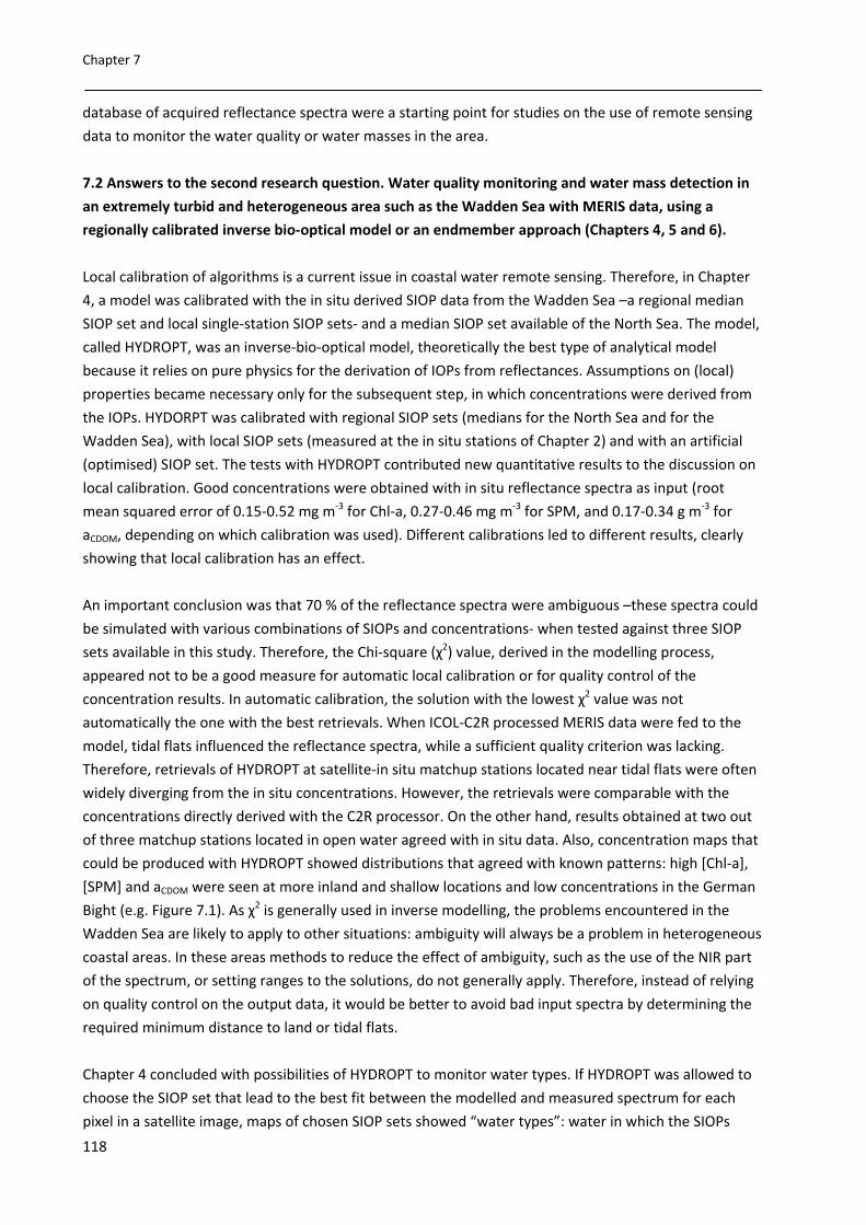
Chapter 7
118
database of acquired reflectance spectra were a starting point for studies on the use of remote sensing
data to monitor the water quality or water masses in the area.
7.2 Answers to the second research question. Water quality monitoring and water mass detection in
an extremely turbid and heterogeneous area such as the Wadden Sea with MERIS data, using a
regionally calibrated inverse bio‐optical model or an endmember approach (Chapters 4, 5 and 6).
Local calibration of algorithms is a current issue in coastal water remote sensing. Therefore, in Chapter
4, a model was calibrated with the in situ derived SIOP data from the Wadden Sea –a regional median
SIOP set and local single‐station SIOP sets‐ and a median SIOP set available of the North Sea. The model,
called HYDROPT, was an inverse‐bio‐optical model, theoretically the best type of analytical model
because it relies on pure physics for the derivation of IOPs from reflectances. Assumptions on (local)
properties became necessary only for the subsequent step, in which concentrations were derived from
the IOPs. HYDORPT was calibrated with regional SIOP sets (medians for the North Sea and for the
Wadden Sea), with local SIOP sets (measured at the in situ stations of Chapter 2) and with an artificial
(optimised) SIOP set. The tests with HYDROPT contributed new quantitative results to the discussion on
local calibration. Good concentrations were obtained with in situ reflectance spectra as input (root
mean squared error of 0.15‐0.52 mg m‐3 for Chl‐a, 0.27‐0.46 mg m‐3 for SPM, and 0.17‐0.34 g m‐3 for
aCDOM, depending on which calibration was used). Different calibrations led to different results, clearly
showing that local calibration has an effect.
An important conclusion was that 70 % of the reflectance spectra were ambiguous –these spectra could
be simulated with various combinations of SIOPs and concentrations‐ when tested against three SIOP
sets available in this study. Therefore, the Chi‐square (χ2) value, derived in the modelling process,
appeared not to be a good measure for automatic local calibration or for quality control of the
concentration results. In automatic calibration, the solution with the lowest χ2 value was not
automatically the one with the best retrievals. When ICOL‐C2R processed MERIS data were fed to the
model, tidal flats influenced the reflectance spectra, while a sufficient quality criterion was lacking.
Therefore, retrievals of HYDROPT at satellite‐in situ matchup stations located near tidal flats were often
widely diverging from the in situ concentrations. However, the retrievals were comparable with the
concentrations directly derived with the C2R processor. On the other hand, results obtained at two out
of three matchup stations located in open water agreed with in situ data. Also, concentration maps that
could be produced with HYDROPT showed distributions that agreed with known patterns: high [Chl‐a],
[SPM] and aCDOM were seen at more inland and shallow locations and low concentrations in the German
Bight (e.g. Figure 7.1). As χ2 is generally used in inverse modelling, the problems encountered in the
Wadden Sea are likely to apply to other situations: ambiguity will always be a problem in heterogeneous
coastal areas. In these areas methods to reduce the effect of ambiguity, such as the use of the NIR part
of the spectrum, or setting ranges to the solutions, do not generally apply. Therefore, instead of relying
on quality control on the output data, it would be better to avoid bad input spectra by determining the
required minimum distance to land or tidal flats.
Chapter 4 concluded with possibilities of HYDROPT to monitor water types. If HYDROPT was allowed to
choose the SIOP set that lead to the best fit between the modelled and measured spectrum for each
pixel in a satellite image, maps of chosen SIOP sets showed “water types”: water in which the SIOPs

Synthesis and outlook
119
were similar (e.g. Figure 7.1). Three major water types were identified: Wadden Sea water, North Sea
water and water influenced by river discharges. The last was only seen during low tide.
Chapter 5 gives a detailed discussion on monitoring of water masses. Water masses can be defined as
waters with distinct SIOPs, or as waters with distinct IOPs, concentrations or reflectances. Chapter 5
provides the definitions in which water with distinct SIOPs are called “water types”, while water in
which the totals of the optical properties vary are called “water classes”. Water types can be traced with
an inverse bio‐optical model, as is done with HYDROPT in Chapter 4. Water classes can be obtained with
an unmixing or endmember model. Such a model unmixes reflectance spectra in percentages of pre‐
defined extreme (endmember) spectra. Chapter 5 introduces an endmember model and compares the
differences in water masses obtained with this model and HYDROPT. A clear difference in the results of
the two models was seen in the North Sea. The German Bight was modelled as one water type with
HYDROPT, but classified with the low‐concentration endmember and the Chl‐dominated endmember
with the endmember model. It seemed logical that a mixture of the same phytoplankton species
occurred in the whole area, leading to a similar water type, while at the location classified with the Chl‐
dominated endmember the Chl‐a concentration was higher due to the presence of a bloom. The
endmember technique was best for visualising horizontal water mass mixing, degradation or sinking of
SPM, while the inverse bio‐optical model was able to follow a water mass in a horizontal direction even
when for example a bloom appears. For a real water mass detection it would be the best to combine the
results of the two methods. Another possibility would be the use of the endmember model to
determine areas where certain SIOP sets would be most applicable to calibrate the inverse bio‐optical
model.
In Chapter 6 the practical application of the endmember model is examined. This type of model is new
to monitoring water masses with remote sensing. An evaluation of the model could be carried out with
in situ reflectance data as input. Using MERIS images from four seasons, high and low wind situations,
and obtained at different stages in the tidal cycle as model input, it was assessed whether variability
could be monitored with this model. Although the endmember model did not deliver precise
concentrations, it gave quantitative information on the presence of IOPs and on the dominance of a
substance on the reflectance spectrum. The findings of Chapter 6 were in agreement with the variation
in optically active substances and optical properties presented in Chapters 2 and 3. Low concentrations
were mainly seen in the North Sea and during calm weather at deeper locations in the Wadden Sea.
Spectra dominated by Chl‐a were primarily seen in spring in the North Sea, co‐occurring with Chl‐CDOM
dominated spectra, while spectra dominated by SPM were primarily found in the Dollard. The
endmember dominated by SPM and Chl‐a was generally abundant in the Wadden Sea, but abundances
were greater during high tidal currents and with strong wind (e.g. Figure 7.1). Strong wind increased the
area of this endmember into the German Bight and increased abundances of the SPM‐dominated
endmember over the whole Wadden Sea and German Bight, as could be expected due to resuspension.
These were positive results for water class monitoring, and further exploration of the possibilities of
endmember models for monitoring water masses was therefore recommended. New studies can
include the examination of alternative endmember sets and application of the method in other
extremely turbid and optically heterogeneous areas. Validation of the results obtained from satellite
data can be achieved by comparing trends in concentrations and in abundances of certain endmembers
at matchup locations.

Chapter 7
120
Digital photo
acquired at the in situ station
HYDROPT Chl‐a
concentration (mg m3)
Chl‐dominated endmember
abundances
Reflectance obtained in situ and with various
processors
HYDROPT SPM
concentration (g m3)
Chl‐SPM dominated endmember
abundances
HYDROPT water type map.
(yellow = North Sea water (Extra SIOP),
blue = Wadden Sea water)
HYDROPT aCDOM
at 440 nm (m‐1).
Chl‐SPM dominated endmember
abundances at another, windy day.
Figure 7.1. An example of optical information and model results for a matchup station in the Danish Wadden Sea, at
55˚18’38’’N, 8˚27’27’’E (red arrows) at May 8th 2006, 9.48 UTC, ~20 minutes before high water with calm weather. In
situ obtained concentrations were: [Chl‐a] = 8.4 mg m3, [SPM] = 4.1 g m3, aCDOM = 0.6 m
‐1. The figure in the lower
right corner was added for comparison. It shows results for March 12th 2007, when the abundances of the Chl‐SPM
dominated end‐member were elevated due to resuspension.
7.3 Outlook
There are many issues that need to be taken in account (Chapter 2) when applying remote sensing in an
extremely turbid estuary or tidal flat area. Firstly, a satellite with a high ground resolution (few hundred
of meters for the channels and during high tide, few tens of meters for the whole area and during low
tide) is needed to retrieve valid data in the presence of tidal flats, and a method is needed to distinguish
flats from water. The sensors should have enough and correctly designed spectral bands to distinguish
Chl‐a, SPM and CDOM. The MERIS instrument (which data has been used in this thesis) has 300 x 300 m
pixels in 9 dedicated spectral bands in the visible wavelengths and could therefore be applied to the
whole area during high tide, but only in the wider channels during low tide. The successors of MERIS,
Sentinel 3A (300 x 300 m) and 3B (260 x 260 m) (IOCCG, 2009) have similar pixel sizes as MERIS.

Synthesis and outlook
121
However, the new WorldView2 satellite, launched October 2009, has 6 spectral bands in the visible and
two in the NIR, with a pixel size of 1.8 x 1.8 m (Worldview2, 2009) and can therefore be utilised in the
whole Wadden Sea area, independent of tide. In this thesis, flats and land were separated with a band
ratio applied in the C2R algorithm. Probably more precise methods are the combination of optical data
with simultaneously acquired SAR data, for example from two ENVISAT instruments ‐ ASAR (SAR) and
MERIS‐, or a model based on a DEM combined with information on tide and wind.
The second issue to be taken into account is the need for improvements in atmospheric correction
adapted to coastal areas, as the bright pixel method is still too vulnerable for scattering in the NIR and
the adjacency effect. In this thesis a first version of the ICOL algorithm (Santer and Zagolski, 2009) was
applied for adjacency effect correction, followed by the C2R algorithm (Doerffer and Schiller, 2008) to
derive L2 MERIS data that could be used as model input. The derived reflectance spectra are much more
realistic than those of the standard MERIS algorithm. However, even with ICOL‐C2R data as model input,
a criterion is needed on the distance from tidal flats and land required to obtain unaffected data. This
minimum distance should be determined with matchups of in situ validation data, located on increasing
distance from flats and land, and acquired simultaneously with satellite data. This minimum distance is
expected to vary per satellite instrument as it depends on pixel size, instrument orientation, viewing
angle and precision of corrections, and should therefore be obtained with matchups for each sensor to
be applied.
Thirdly, sufficient local knowledge is needed for calibration, validation and interpretation of the results.
Knowledge on local optical properties and variations in properties in space and time was collected in
Chapters 2 and 3. Therefore, algorithms for optical remote sensing could be calibrated and validated for
the Wadden Sea. However, more in situ data (especially on SIOPs) is still necessary for calibration, while
more in situ measured IOPs (e.g. AC9 data) and reflectances are relevant to increase the knowledge on
the spatial and temporal differences in optical properties. The optical properties of flocs are still missing
and should be determined to enhance the accuracy of the modelling results.
Fourthly, matchup in situ and remote sensing data should be acquired simultaneously in heterogeneous,
tidal influenced areas because of the fast (tidal) change in concentrations of optically active substances
(Chapters 2, 3 and 6). If there is a time lag between in situ data and satellite overpass, this is not a real
matchup for such areas and data cannot be used for validation purposes. The matchup database
acquired in the study was small (6 matchups) due to weather conditions. More matchup data is
therefore needed. Matchup data needed to determine the required distance from tidal flats can only be
determined by ship. However, to increase the general matchup database, measuring poles, buoys and
drift instruments equipped with instruments measuring reflectance, absorption and scattering or SIOPs,
and concentrations of Chl‐a, SPM and CDOM are recommended, as these instruments greatly increase
the chance of obtaining matchups. Time series of measurement poles, drift instruments and buoys can
also be used to validate the results of the endmember model, by comparing trends in concentrations
and abundances. Possibilities to obtain more insight in temporal differences and their effect on remote
sensing data on a higher spatial scale are to employ a geostationary satellite, a helicopter or a plane
with a frequent overpass.

Chapter 7
122
Finally, algorithms should be tuned for the extremely high concentrations of various substances. This
was achieved with the two models applied in this thesis (Chapters 4, 5 and 6) and is important to take
into account in other research as well.
When these issues are taken in account, remote sensing of water quality and water masses in extremely
turbid areas should, in principle, be possible (Chapter 2). Good quality control and validation of the
results are necessary. Concentrations derived with the regionally and locally calibrated inverse bio‐
optical model HYDROPT (Chapter 4) were good when in situ measured reflectance spectra were given as
input. Concentration maps showed distributions that could be expected with the information obtained
in Chapters 2 and 3. However, automatic selection of SIOP sets trough the χ2 value of the algorithms
fitting procedure did not automatically lead to the best concentrations due to a combination of
ambiguity and heterogeneity. Also quality control on modelled concentrations derived from MERIS data
was difficult. As the quality control on the output did not yet work properly, a better quality control on
the input spectra is needed. This can probably be achieved by determining the required distance from
tidal flats, as mentioned above.
Water mass modeling showed promising results, both with the HYDROPT model, and especially with the
newly developed endmember or unmixing model. As discussed in Chapter 4, the HYDROPT water type
detection can probably be improved by including more water types (SIOP sets) and with the use of
higher quality SIOP sets. These can be obtained by taking multiple samples per location and determining
the SIOPs as averages. This procedure reduces the influence of random errors that accumulate in the
SIOP sets based on single measurements.
The endmember model seems the most promising for direct monitoring application (Chapter 6), as it is
able to visualise the well‐known variations in optical properties in the Wadden Sea presented in Chapter
2. Although the results do not give precise concentrations, it classifies water as water with “high” or
“low” concentrations and indicates domination by one or two substances. These results could be
compared with independent pattern detection algorithms, such as the Forel Ule algorithm developed by
Wernand et al., (submitted). Interesting is that results of the Forel Ule algorithm can be compared with
historical Forel Ule determinations. By evaluation of several sets of endmembers and addition of extra
endmembers, such as one generated for a coccolith bloom, the endmember model can be improved and
extended. Endmember models can easily be adapted to new satellites, as endmembers can be
generated for other wavelengths. They can also be adapted to L1 satellite data, for example by
identifying the endmembers in TOA‐reflectances for new satellites (such as WorldView2) that have no
quality checked atmospheric correction available yet.
Combination of the two water mass detection methods examined in this thesis is recommended
(Chapter 5). An inverse‐bio‐optical model, such as HYDROPT, delivers water types ‐it provides
information on differences in type of phytoplankton, sediment or CDOM available in a water mass‐
while an endmember model contributes information on the quantities of the available substances and
can visualise processes such as mixing, degradation and sinking. Together, these two models will lead to
the best water mass monitoring.

References

124
References
– Albert, A., Gege, P., 2006. Inversion of irradiance and remote sensing reflectance in shallow water
between 400 and 800 nm for calculations of water and bottom properties. Applied Optics 45: 2331‐
2343
– Andersen, T. J., Pejrup, M., 2001. Suspended sediment transport on a temporate, microtidal
mudflat, the Danish Wadden Sea. Marine Geology 173: 69‐85.
– Andersen, T. J., Pejrup, M., 2002. Biological mediation of the settling velocity of bed material eroded
from an intertidal mudflat, the Danish Wadden Sea. Estuarine, Coastal and Shelf Science 54: 737‐
745.
– Arnone, R. A., Wood, A.M., Gould, R.W., 2004a. The evolution of optical water mass classification.
Oceanography 17: 14‐15.
– Arnone, R., A., Gould, R., Bissett, W.P., Moline, M., Schofield, O., Chang, G., Davis, C., 2004b. Optical
Classification of Watermasses Using Spectroscopy from Space, Ocean Optics Conference XVII,
Fremantle, Australia, CDROM, abstract 208, 1pp.
– Asner, G.P., Heidebrecht, K.B., 2002. Spectral unmixing of vegetation, soil and dry carbon cover in
arid regions: comparing multispectral and hyperspectral observations. International Journal of
Remote Sensing 23: 3939‐3958.
– Astoreca, R., Ruddick, K.G, Rousseau, V., Van Mol, B., Parent J.‐Y., Lancelot, C., 2006. Variability of
the inherent and apparent optical properties in a highly turbid coastal area: Impact on the
calibration of remote sensing algorithms. European Association of Remote Sensing Laboratories
eProceedings 5: 1‐17.
– Austen, I., Andersen, T.J., Edelvang, K., 1999. The influence of benthic diatoms and invertebrates on
the erodibility of an intertidal mudflat, the Danish Wadden Sea. Estuarine, Coastal and Shelf Science
49: 99‐111.
– Babin, M. Morel, A., Fournier‐Sicre, V., Fell, F., Stramski, D., 2003a. Light scattering properties of
marine particles in coastal and open ocean waters as related to the particle mass concentration.
Limnology and Oceanography 48: 843‐859.
– Babin, M., Stramski, D., Ferrari, G.M., Claustre, H., Bricaud, A., Obolensky, G., Hoepffner, N., 2003.
Variations in the light absorption coefficients of phytoplankton, nonalgal particles, and dissolved
organic matter in coastal waters around Europe. Journal of Geophysical Research‐Oceans 108: 1‐20
– Badewien, T.H., Zimmer, E., Bartholomä, A., Reuter, R., 2009. Towards continuous long‐term
measurements of suspended particulate matter (SPM) in turbid coastal waters. Ocean Dynamics 59:
227‐238.
– Bartholdy, J., Folving, S., 1986. Sediment classification and surface type mapping in the Danish
Wadden Sea by remote sensing. Netherlands Journal of Sea Research 20: 337‐345.
– Bartholomä, A., Kubicki, A., Badewien, T.H., Flemming, B.W., 2009. Suspended sediment transport in
the German Wadden Sea ‐ seasonal variations and extreme events. Ocean Dynamics 59:213‐225.
– Berthon, J.‐F, Zibordi, G., Canuti, E., Kaitala, S., Seppälä, J., Ylöstalo, P., 2008. Are the Northern Baltic
Sea waters even blacker? Proceedings of the Ocean Optics Conference XIX, Italy, 1pp.
– Beukema, J.J., Cadée, G.C., 1996. Consequences of the sudden removal of nearly all mussels and
cockles from the Dutch Wadden Sea. In: P.C Dworschak, M. Stachowitsch, J.A. Ott (editors)
Influences of Organisms on their Environment, the Role of Episodic Events: Proceedings of the 29th
European Marine Biology Symposium Vienna 1994. PSZN I: Marine Ecology, 17: 279‐289.

References
125
– Billerbeck, M., 2005. Pore water transport and microbial activity in intertidal Wadden Sea
sediments. Dissertation, Bremen University, Germany, 189 pp.
– Billerbeck, M., Werner, U., Polerecky, L., Walpersdorf, E., De Beer, D., Huettel., M., 2006. Surficial
and deep pore water circulation governs spatial and temporal scales of nutrient recycling in
intertidal sand flat sediment. Marine Ecology Progress Series 326: 61‐77.
– Binding, C.E., Bowers, D.G., Mitchelson‐Jacob, E.G., 2005. Estimating suspended sediment
concentrations from ocean colour measurements in moderately turbid waters; the impact of
variable particle scattering properties. Remote Sensing of Environment 94: 373–383.
– Blondeau‐Patissier, Brando, V.E., Oubelkheir, K., Dekker, A.G., Clementsson, L.A., Daniel, P., 2009.
Bio‐optical variability of the absorption and scattering properties of the Queensland inshore and
reef waters, Australia. Journal of Geophysical Research‐Oceans: C05003,
DOI:10.1029/2008JC005039.
– Blondeau‐Patissier, D., Tilstone, G.H., Martinez‐Vicente, V., Moore, G.F., 2004. Comparison of bio‐
physical marine products from SeaWiFS, MODIS and a bio‐optical model with in situ measurements
from Northern European waters. Journal of Optics A: Pure Applied Optics 6: 875–889.
– Bos, A. R., Dankers, N., Groeneweg, A.H., Hermus, D.C.R., Jager, Z., De Jong, D.J., Smit, T., De Vlas, J.,
Van Wieringen, M., Van Katwijk, M.M., 2005. Eelgrass (Zostera marina L.) in the western Wadden
Sea: monitoring, habitat suitability model, transplantations and communication. In: Mees, H.J‐L. J.,
Salman, A., Seys, J., Van Nieuwenhuyse, H., Dobbelaere, I. (Eds). 2005., pp. 95‐109. Proceedings
‘Dunes and Estuaries 2005’ ‐ International Conference on Nature Restoration, Practices in European
Coastal Habitats, Belgium 2005. VLIZ Special Publication 19, xiv + 685 pp.
– Boss, E., Pegau, W.S., Ron, J., Zaneveld, V., Barnard, A.H., 2001. Spatial and temporal variability of
absorption by dissolved material at a continental shelf. Journal of Geophysical Research 106: 9499–
9507.
– Böttcher, M., Oelschläger, B., Höepner, T., Brumsack, H.‐J., Rullköter, J., 1998. Sulfate reduction
related to the early diagenetic degradation of organic matter and “black spot” formation in tidal
sandflats of the German Wadden Sea (southern North Sea): stable isotope (13C, 34S, 18O) and other
geochemical results. Organic Geochemistry 29, pp. 15171530.
– Bowers, D.G., Evans, D., Thomas, D.N., Ellis, K., Williams, P.J. le B., 2004. Interpreting the colour of
an estuary. Estuarine, Coastal and Shelf Science 59: 13‐20.
– Brando, V.E., Anstee, J.M., Wettle, M, Dekker, A.G., Stuart R. Phinn, S.R., Roelfsema, C., 2009. A
physics based retrieval and quality assessment of bathymetry from suboptimal hyperspectral data.
Remote Sensing of Environment 113: 755–770.
– Brando, V.E., Blondeau‐Patissier, D. Dekker, A.G., Daniel, P.J., Wettle, M., Oubelkheir, K.,
Clementson, L., 2006. Bio‐optical variability of Queensland coastal waters for parameterisation of
coastal‐reef algorithms. Proceedings of the Ocean Optics conference XVIII, Montreal, Canada.
CDROM, 13 pp.
– Brando, V.E., Dekker, A.G., 2003. Satellite hyperspectral remote sensing for estimating estuarine and
coastal water quality. IEEE Transactions on Geoscience and Remote Sensing 41: 1378‐1387.
– Brando, V.E., Dekker, A.G., Schroeder, Th., Park, Y.J., Clementson, L.A., Steven, A., Blondeau‐
Patissier, D., 2008. Satellite retrieval of chlorophyll CDOM and NAP in optically complex waters using
a semi‐analytical inversion based on specific inherent optical properties. A case study for Great
Barrier Reef coastal waters. Proceedings of the Ocean Optics conference XIV, Castelvecchio Pascoli,
Italy. CDROM. 10 pp.
126
– Brasse, S., Reimer, A., Seifert, R., Michaelis, W., 1999. The influence of intertidal mudflats on the
dissolved inorganic carbon and total alkalinity distribution in the German Bight, southeastern North
Sea, Journal of Sea Research 42: 93‐103.
– Bricaud, A., Morel, A., Prieur, L., 1981. Absorption by dissolved organic matter of the sea (yellow
substance) in the UV and visible domains. Limnology and Oceanography 26: 43‐53.
– Brockmann Consult, 2009. WWW page: www.brockmann‐consult.de/revamp
– Brockmann, C., Stelzer, K., 2008. Optical Remote Sensing of Intertidal Flats. In: V. Barale, M. Gade,
M., Remote Sensing of the European Seas (pp 117‐128). Springer, Berlin, Germany.
– Brzank, A., Heipke, C., 2007. Supervised classification of water regions from lidar data in the Wadden
Sea using a fuzzy logic concept. In Proceedings of the ISPRS Workshop on Laser Scanning and
SilviLaser, Espoo 2007, Finland; International Archives of Photogrammetry, Remote Sensing, and
Spatial Information Sciences 36, Part 3/W52, 90‐95.
– Brzank, A., Heipke, C., Goepfert, J., Soergel, U., 2008. Aspects of generating precise digital terrain
models in the Wadden Sea from lidar–water classification and structure line extraction. ISPRS
Journal of Photogrammetry, Remote Sensing 63: 510‐528.
– Buiteveld, H., Hakvoort, J.H.M., Donze, M., 1994. The optical properties of pure water. Proceedings
of the SPIE: 2258, pp. 174‐183.
– Buridge, D.J., Homstead, J., 1994. Fluxes of dissolved organic carbon from Chesapeake Bay
sediments. Geochimica et Cosmochimica Acta 58: 3407‐3424.
– Cadée, G.C., 1976. Sediment reworking by Arenicola marina on tidal flats in the Dutch Wadden Sea.
Netherlands Journal of Sea Research 10, No 4: 440‐460.
– Cadée, G.C., 1980. Reappraisal of the production and import of organic carbon in the Western
Wadden Sea. Netherlands Journal of Sea Research 14: 305‐322.
– Cadée, G.C., 1982. Tidal and seasonal variation in particulate and dissolved organic matter in the
western Dutch Wadden Sea and the Marsdiep tidal inlet. Netherlands Journal of Sea Research 15:
220‐249.
– Cadée, G.C., 1986. Increased phytoplankton primary production in the Marsdiep area (western
Dutch Wadden Sea). Netherlands Journal of Sea Research 20, No 2‐3: 285‐290.
– Cadée, G.C., 1996. Accumulation and sedimentation of Phaeocystis globosa Wadden Sea. Journal of
Sea Research 36: 321‐327.
– Cadée, G.C., Hegeman, J., 1974. Primary production of the benthic microflora living on tidal flats in
the Dutch Wadden Sea. Netherlands Journal of Sea Research 8, No 2‐3: 260‐291.
– Cadée, G.C., Hegeman, J., 2002. Phytoplankton in the Marsdiep at the end of the 20th century; 30
years monitoring biomass, primary production, and Phaeocystis blooms. Journal of Sea Research 48:
97‐110.
– Campbell, J.W., 1995. The lognormal distribution as a model for bio‐optical variability in the sea.
Journal of Geophysical Research 100: 13,237–13,254.
– Chang, T.S., Flemming, B.W., Bartholomä, A., 2007. Distinction between sortable silts and
aggregated particles in muddy intertidal sediments of the East Frisian Wadden Sea, southern North
Sea. Sedimentary Geology 202: 453‐463.
– Chang, T.S., Joerdel, O., Flemming, B.W., Bartholomä, A., 2006. The role of particle
aggregation/disaggregation in muddy sediment dynamics and seasonal sediment turnover in a back‐
barrier tidal basin, East Frisian Wadden Sea, southern North Sea. Marine Geology 235: 49‐61.

References
127
– Cipollini, P., Corsini, G., Diani, M., Grasso, R., 2001. Retrieval of sea water optically active parameters
from hyperspectral data by means of generalized radial basis function neural networks. IEEE
Transactions on Geoscience and Remote Sensing 39: 1508‐1524.
– Clementson, L.A., Parslow, J.S., Turnbull, A.R., Bonham, P.I., 2004. Properties of light absorption in a
highly coloured estuarine system in south‐east Australia which is prone to blooms of the toxic
dinoflagellate Gymnodinium catenatum. Estuarine, Coastal and Shelf Science 60: 101‐112.
– Colijn, F., Cadée, G.C., 2003. Is phytoplankton growth in the Wadden Sea light or nitrogen limited?
Journal of Sea Research 49: 83‐93.
– Colijn, F., Dijkema, K.S., 1981. Species composition of benthic diatoms and distribution of chlorophyll
a on an intertidal flat in the Dutch Wadden Sea. Marine Ecology‐Progress series 4: 9‐21.
– D’Sa, E.D, Miller, R.L., 2003. Bio‐optical properties in waters influenced by the Mississippi River
during low flow conditions. Remote Sensing of Environment 84, 538‐549.
– Dame, R.F., Dankers, N., 1988. Uptake and Release of Materials by a Wadden Sea Mussel Bed.
Journal of Experimental Marine Biology and Ecology 118: 207‐216.
– Dame, R.F., Dankers, N., Prins, T., Jongsma, H., Smaal, A., 1991. The influence of mussel beds on
nutrients in the Western Wadden Sea and Eastern Scheldt estuaries. The influence of mussel beds
on nutrients in the Western Wadden Sea and Eastern Scheldt estuaries. Estuaries and Coasts, 4: 130‐
138.
– Dankers, N., Koelemaij, K., 1989. Variations in the mussel population of the Dutch Wadden Sea in
relation to monitoring of other ecological parameters. Helgoländer Meeresuntersuchungen
[Helgoland Marine Research] 43: 529‐535.
– Dankers, N., Zuidema, D.R., 1995. The Role of the Mussel (Mytilus edulis L.) and Mussel Culture in
the Dutch Wadden Sea. Estuaries 18: 71‐80.
– Darecki, M., Stramski, D., 2004. An evaluation of MODIS and SeaWiFS bio‐optical algorithms in the
Baltic Sea. Remote Sensing of Environment 89: 326–350.
– De Beer, D., Wenzhöfer, F., Ferdelman, T.G., Boehme, S.E., Huettel, M., Van Beusekom, J.E.E.,
Böttcher, M.E., Musat, N., Dubilier, N., 2005. Transport and mineralization rates in North Sea sandy
intertidal sediments, Sylt‐Rømø Basin, Wadden Sea. Limnology and Oceanography 50: 113‐127.
– De Cauwer, V., Ruddick, K., Park, Y.‐J., Nechad, B., Kyramarios, M., 2004. Optical remote sensing in
support of eutrophication monitoring in the southern North Sea. EARSeL eProceedings 3: 208‐224.
– De Jonge, V., 1995. The Ems estuary. Chapter 7. In : A.J. McComb (editors), Eutrophic Shallow
Estuaries and Lagoons: 181‐108. CRC Press Baton Rouge, Louisiana, USA.
– De Jonge, V.N, Bakker, J.F., Van Stralen, M., 1996. Recent changes in the contributions of river Rhine
and North Sea to the eutrophication of the Western Dutch Wadden Sea. Netherlands Journal of
Aquatic Ecology 30: 27‐39.
– De Jonge, V.N., 1992. Physical processes and dynamics of microphytobenthos in the Ems estuary
(The Netherlands), Ph.D. thesis, 176 pp. State Universiteit Groningen. The Netherlands.
– De Lange, H.J., 2000. The attenuation of ultraviolet and visible radiation in Dutch inland waters.
Aquatic Ecology 34: 215–226.
– Defoin‐Platel, M.,, Chami, M., 2007. How ambiguous is the inverse problem of ocean color in coastal
waters? Journal of Geophysical Research‐Oceans 112: DOI:10.1029/2006JC003847.
– Dekker, A., Brando, V.E., Anstee, J.M., Pinnel, T., Kuster, H., Hoogenboom H., Pasterkamp, R., Peters,
S., Vos, O., Malthus, T., 2001. Imaging spectrometry of water. Chapter 11, pages 307‐359. In: van der
Meer, F., and de Jong, S. (editors), Imaging Spectrometry: Basic principles and prospective

128
applications: Remote Sensing and Digital Image Processing, Kluwer Academic Publishers, Dordrecht,
The Netherlands.
– Dick, S., Schönfeld, W., 1996. Transport and Mixing in the North Frisian Wadden Sea‐ Results of
Numerical Investigations. Deutsche Hydrographische Zeitschrift [German Journal of Hydrography]
48, Number 1, 22 pp.
– Dijkema, K.S., 1989. Habitats of The Netherlands, German and Danish Wadden Sea. Research
Institute for Nature Management, Veth Foundation, Leiden, The Netherlands, 30 pp.
– Dijkema, K.S., Reijneck, H.‐E., Wolff, W.J., (editors), 1980. Geomorphology of the Wadden Sea area.
Report 1. Final report of the section ‘Geomorphology’ of the Wadden Sea Working Group, Leiden,
The Netherlands, 135 pp.
– Doerffer, R., Fischer J., 1994. Concentrations of chlorophyll, suspended matter, and gelbstoff in case
II waters derived from satellite coastal zone color scanner data with inverse modeling methods.
Journal of Geophysical Research‐Oceans 99: 7457‐7466.
– Doerffer, R., Fischer, J. Stössel, M., Brockmann, C., Grassl, H., 1989a. Analysis of Thematic Mapper
Data for Studying the Suspended Matter Distribution in the Coastal Area of the German Bight (North
Sea). Remote Sensing of Environment 28: 61‐73.
– Doerffer, R., Fischer, J. Stössel, M., Brockmann, C., Grassl, H., 1989b. Small scale patches of
suspended matter and phytoplankton in the Elbe River estuary, German Bight and tidal flats.
Advanced Space Research 9: (1)191‐(1)200.
– Doerffer, R., Murphy, D., 1989. Factor analysis and classification of remotely sensed data for
monitoring tidal flats. Helgoländer Meeresuntersuchungen [Helgoland Marine Research] 43: 275‐
293.
– Doerffer, R., Peters, M., 2006. Algorithm Theoretical Basis Document MERIS Case II ATBD‐ATMO ‐
MERIS Regional Case 2 Water BEAM Extension. Flags ATBD. Version 1.1 16, November 2006,
accessible via www.brockmann‐consult.de/beam‐wiki/display/LAKES/ATBDs, 5 pp.
– Doerffer R., Schiller, H., Krasemann H., Heymann K., Cordes, W., Schönfeld, W., Röttgers, R., Behner,
I., Kipp, P. 2003. MERIS Case 2 Water Validation Early Results North Sea / Helgoland /German Bight.
Proceedings of the ESA ENVISAT Validation Workshop 2002, ESA Special publications SP‐531 2003.
– Doerffer, R., Schiller, H., 2007. The MERIS Case 2 water algorithm. International Journal of Remote
Sensing 28: 517 ‐ 535.
– Doerffer, R. and Schiller, H., 2008. Algorithm Theoretical Basis Document MERIS Case II ATBD‐ATMO
MERIS Regional Case 2 Water BEAM Extension Atmospheric Correction ATBD Issue 1, June 2008,
accessible via www.brockmann‐consult.de/beam‐wiki/display/LAKES/ATBDs, 42 pp.
– Dowell, M., Berthon, J,‐F., Zibordi, G. 2008. The identification of optically distinct water types at
global and regional scales: implications for algorithm development and validation. Proceedings of
the Ocean Optics conference XIV, Castelvecchio Pascoli, Italy. CDROM. 1 pp.
– Doxaran, D., Cherukuru, R.C.N., Lavender, S.J., 2005. Use of reflectance band ratios to estimate
suspended and dissolved matter concentrations in estuarine waters. International Journal of
Remote Sensing 26: 1763–1769.
– Doxaran, D., Cherukuru, R.C.N., Lavender, S.J., 2006. Apparent and inherent optical properties of
turbid estuarine waters: measurements, empirical quantification relationships, and modeling.
Applied Optics 45, 2310‐2324.

References
129
– Doxaran, D., Froidefond, J‐.M., Castaing, P., 2003. Remote‐sensing reflectance of turbid sediment‐
dominated waters. Reduction of sediment type variations and changing illumination conditions
effects by use of reflectance ratios. Applied Optics 42: 2624‐2630.
– Dupouy, C., Arief, D., Spitzer, D., (editors), 1983. Optical remote sensing of waters and tidal flats in
western Wadden Sea. Internal Reports Royal Netherlands Institute for Sea Research (NIOZ) 2. NIOZ.
Texel. The Netherlands. 45 pp.
– Edwards, M., Beaugrand, G., Reid, P.C, Rowden., A.A., Jones, M.B., 2002. Ocean climate anomalies
and the ecology of the North Sea. Marine ecology progress series. 239: 1‐10.
– Eisma, D., Bale, A.J., Dearneley, M.P., Fennessy, M.J., Van Leussen, W., Maldiney, M.A., Pfeiffer, A.,
Wells, J.T., 1996. Intercomparison of in situ suspended matter (floc) size measurements. Journal of
Sea Research 36: 3‐14.
– Eisma, D., Kalf, J., 1996. In situ particle (floc) size measurement with the NIOZ in situ camera system.
Journal of Sea Research 36: 49‐53.
– Eleveld, M.A., Pasterkamp, R., Van der Woerd, H.‐J., Pietrzak, J.D., 2008. Remotely sensed
seasonality in the spatial distribution of sea‐surface suspended particulate matter in the southern
North Sea. Estuarine, Coastal and Shelf Science 80: 103–113.
– Environment Directorate‐General of the European Commission, 2000. Official Journal of the
European Communities, OJ L 327. PDF file, 688 KB. http://ec.europa.eu/environment/water/water‐
framework/index_en.html.
– ESA, 2009a. Website with information on the MERIS instrument and the processing versions.
http://earth.esa.int/pcs/envisat/meris/documentation. Checked at August 21st 2009.
– ESA, 2009b. Technical information on satellite missions. Accessible via http://earth.esa.int/missions.
Accessed 5 June 2009.
– EUMETSAT, 2009. Technical information on the METEOSAT satellites. Accessible via
www.eumetsat.int. Accessed 5 June 2009.
– European Commission, 2010. Www page on the Natura2000 network. Accessible via
http://ec.europa.eu/environment/nature. Accessed 16 January 2010.
– Fanton D'Andon, O., Mangin, A., Ganzin, N., Sauzade, D., Garnesson, Ph., Morel, A., 2005. Use of
Ocean Colour Observations to Support the Water Framework Directive Implementation. In H.
Lacosta. Proceedings of the MERIS (A)ATSR Workshop 2005 (ESA SP‐597). ESRIN. Frascati. Italy.
CDROM, pp 23.1
– Feng, H. Campbell, J.W., Dowell, M.D., Moore, T.S., 2005. Modeling spectral reflectance of optically
complex waters using bio‐optical measurements from Tokyo Bay. Remote Sensing of Environment
99: 232‐243.
– Ferrari, G.M., Tassan, S., 1996. Use of the 0.22‐micron Millipore membrane for light‐transmission
measurements of aquatic particles. Journal of Plankton Research 18: 1261‐1267.
– Flöser, G., 2004. Wadden Sea Newsletter 2004, no 1. Common Wadden Sea Secretariat (pp 8‐10).
Wilhelmshaven, Germany. ISSN 0922‐7989.
– Foden, J., Sivyer, D.B., Mills, D.K., Devlin M.J., 2008. Spatial and temporal distribution of
chromophoric dissolved organic matter (CDOM) fluorescence and its contribution to light
attenuation in UK waterbodies. Estuarine, Coastal and Shelf Science 79: 707–717.
– Gade, M., Alpers, W., Melsheimer, C., Tanck, G., 2008. Classification of sediments on exposed tidal
flats in the German Bight using multi‐frequency radar data. Remote Sensing of Environment 112:
1603‐1613.

130
– Gallegos, C.L., Jordan, T.E., Hines, A.H., Weller, D.E., 2005. Temporal variability of optical properties
in a shallow, eutrophic estuary: Seasonal and interannual variability. Estuarine, Coastal and Shelf
Science 64: 156‐170.
– Garver, S. A., Siegel, D. A., 1997. Inherent optical property inversion of ocean color spectra and its
biogeochemical interpretation. 1. Time series from the Sargasso Sea. Journal of Geophysical
Research‐Oceans, 102: 18607−18625.
– Gayer, G., Dick, S., Pleskachevsky, A., Rosenthal, W., 2006. Numerical modeling of suspended matter
transport in the North Sea. Ocean Dynamics 56: 62‐77.
– Gemein, N., Stanev, E., Brink‐Spalink, G., Wolff, J.‐O., Reuter, R., 2006. Patterns of suspended
matter in the East Frisian Wadden Sea: comparison of numerical simulations with MERIS
observitions. EARSeL eProceedings 5: 180‐198.
– Giardino, C, Brando, V.E., Dekker, A.G., Strömbeck, N., Candiani, G., 2007. Assessment of water
quality in Lake Garda (Italy) using Hyperion. Remote Sensing of Environment 109 : 183–195
– Gons, H.J., 1999. Optical Teledetection of Chlorophyll a in Turbid Inland Waters. Environmental
Science and Technology 33: 1127‐1132.
– Gons, H.J., Rijkeboer, M., Ruddick, K.G., 2005. Effect of a waveband shift on chlorophyll retrieval
from MERIS imagery of inland and coastal waters. Journal of Plankton research, 27: 125‐127.
– Gordon, H.R., Brown, O.B., Jacobs, M.M., 1975. Computed relationships between the inherent and
apparent optical properties of a flat homogeneous ocean. Applied Optics 14: 417‐427.
– Grossart, H.‐P., Brinkhoff, T., Martens, T., Duerselen, C., Liebezeit, G., Simon, M., 2004. Tidal
dynamics of dissolved and particulate matter and bacteria in a tidal flat ecosystem in spring and fall.
Limnology and Oceanography 49: 2212‐2222.
– Hakvoort, J.H.M., Heineke, M., Heymann, K., Kühl, H., Riethmüller, R., Witte, G., 1998. A basis for
mapping the erodibility of tidal flats by optical remote sensing. Marine and Freshwater Research 49:
867‐873.
– Hellweger, F.L., Schlosser, P., Lall, U., Weissel J.K., 2004. Use of atellite imagery for water quality
studies in New York Harbor. Estuarine, Coastal and Shelf Science 61: 437‐448.
– Heuermann, R., Reuter, R., Willkomm R., 1999. RAMSES, A modular multispectral radiometer for
light measurements in the UV and VIS. SPIE proceedings series, Environmental sensing and
applications. Conference proceedings, Munich, Germany, 3821: 279‐285.
– Hoepffner, N., Sathyendranath, S., 1992. Bio‐optical characteristics of coastal waters: absorption
spectra of phytoplankton and pigment distribution in the western North Atlantic. Limnology and
Oceanography 37: 1660‐1679.
– Hoge, F.E., Lyon, P.E., 1996. Satellite retrieval of inherent optical properties by linear matrix
inversion of oceanic radiance models: An analysis of model and radiance measurement errors.
Journal of Geophysical Research‐Oceans 101: 16,631–16,648.
– Hoge, F.E., Lyon, P.E., 2005. New tools for the study of oceanic eddies: Satellite derived inherent
optical properties. Remote Sensing of Environment 95: 444–452.
– Hoge, F.G., Swift, R.N., 1982. Delineation of estuarine fronts in the German Bight using airborne
laser‐induced water Raman backscatter and fluorescence of water column constituents.
International Journal of Remote Sensing 3: 475‐495.
– Højerslev, N. K., 2002. On the Small Potential of Color Remote Sensing of the Sea Waters Between
Norway, Sweden, Denmark, Germany and Poland. Ocean Optics XVI, Santa Fe. CDROM, abstract 122.
11 pp.

References
131
– Hommersom, A., Peters, S, Wernand, M.R., De Boer, J., 2009. Spatial and temporal variability in bio‐
optical properties of the Wadden Sea (Chapter 3 of this thesis). Estuarine, Coastal and Shelf Sciences
83: 360‐370.
– Hommersom, A., Wernand, M.R., Peters, S., De Boer, J., 2010. Substances and processes relevant for
optical remote sensing of extremely turbid marine areas – a review with a focus on the Wadden Sea
(Chapter 2 of this thesis). Helgoland Marine Research. doi: 10.1007/s10152‐010‐0191‐6.
– Hoogenboom, H.J., Dekker, A.G., de Haan, J.F., 1998. Retrieval of chlorophyll and suspended matter
from imaging spectrometry data by matrix inversion. Canadian Journal of Remote Sensing 24: 144‐
151.
– Horstmann, J., Koch, W., 2008. High resolution wind field retrieval from synthetic aperture radar:
North Sea examples. In: V. Barale, M. Gade, M., Remote Sensing of the European Seas (pp 331‐342).
Springer, Berlin, Germany.
– Houwing, E.‐J., 1999. Determination of the Critical Erosion Threshold of Cohesive Sediments on
Intertidal Mudflats Along the Dutch Wadden Sea Coast. Estuarine, Coastal and Shelf Science 49: 545‐
555.
– IMO, International Maritime Organisation, 2005. Resolution A.982(24): Revised guidelines for the
identification and designation of particulate sensitive areas. PDF‐file, 172 KB.
– IOCCG, 2000. Remote sensing of ocean colour in coastal, and other optically‐complex, waters.
Sathyendranath, S. (editor), Reports of the International Ocean‐Colour Coordinating Group, No. 3,
IOCCG, Dartmouth, Canada.
– IOCCG, 2006. Remote Sensing of Inherent Optical Properties: Fundamentals, Tests of Algorithms,
and Applications. Lee, Z.‐P. (editors), Reports of the International Ocean‐Colour Coordinating Group,
No. 5, IOCCG, Dartmouth, Canada, 126 pp.
– IOCCG, 2009. Technical information on ocean colour satellite missions. Accessible via:
www.ioccg.org/sensors_ioccg.html. Accessed 5 June 2009.
– Jeffrey, S.W., Mantoura, R.F.C., Wright, S.W., 1997. UNESCO, Paris, France, 661 pp.
– Jerlov, N.G., 1976. Marine optics. Elsevier, Amsterdam, The Netherlands, 231 pp.
– Jianguang, W., Qing, X., Qinhuo, L., Yi, Z., 2005. Extraction of chlorophyll‐a concentration based on
spectral unmixing model using field hyperspectral data in Taihu Lake. Defence technical information
Centre, OMB No. 0704‐0188, 3 pp, 2003. Published in Chinese in Scientia Geographica 27: 92‐97.
– Kerner, M., 2007. Effects of deepening the Elbe Estuary on sediment regime and water quality.
Estuarine, Coastal and Shelf Science 75: 492‐500.
– Koponen, S., Ruiz‐Verdu, A., Heege, T., Heblinski, J., Sorensen, K., Kallio, K., Pyhälahti, T., Doerffer,
R., Brockmann, C., Peters, M., 2008. Validation Report. Development of MERIS lake water
algorithms. Online, 65 pp.
– Kromkamp, J.C., Morris, E.P., Forster, R.M., Honeywill, C., Hagerthey, S., PatersonD.M., 2006.
Relationship of Intertidal Surface Sediment Chlorophyll Concentration to Hyperspectral Reflectance
and Chlorophyll Fluorescence. Estuaries and Coasts 29: 183‐196.
– Laane, R.W.P.M., 1980. Coservative behaviour of dissolved organic carbon in the Ems‐Dollart estuary
western Wadden Sea. Netherlands Journal of Sea Research 14: 192‐199.
– Laane, R.W.P.M., 1982. Source of dissolved organic carbon in the Ems‐Dollart estuary: the rivers and
phytoplankton. Netherlands Journal of Sea Research 15: 331‐339.

132
– Laane, R.W.P.M., Koole, L., 1982. The relation between fluorescence and dissolved organic carbon in
the Ems‐Dollart estuary and the Western Wadden Sea. Netherlands Journal of Sea Research 15: 217‐
227.
– Laane, R.W.P.M., Kramer, 1990. Natural fluorecence in the North Sea and its major estuaries.
Netherlands Journal of Sea Research 26: 1‐9.
– Laanen, M.L., 2007. Yellow Matters Improving the remote sensing of Coloured Dissolved Organic
Matter in inland freshwaters. Ph.D. thesis, VU University, Amsterdam, 267 pp:
http://hdl.handle.net/1871/10799
– Lanuru, M., Riethmüller, R, Van Bernem, C., Heymann, K., 2007. The effect of bedforms (crest and
trough systems) on sediment erodibility on a back‐barrier tidal flat of the East Frisian Wadden Sea,
Germany. Estuarine, Coastal and Shelf Science 72: 603‐614.
– Laurion, I., Blouin, F., Roy, S., 2003. The quantitative filter technique for measuring phytoplankton
absorption: Interference by MAAs in the UV waveband. Limnology and Oceanography: Methods 1,
2003, 1‐9.
– Lehner,S., Anders, I., Gayer, G., 2004. High resolution maps of the suspended particulate matter
concentration in the German Bight. EARSeL eProceedings 3, 1/2004: 118‐126.
– Lemke, A., Lunau, M., Stone, J., Dellwig, O., Simon M., 2009. Spatio‐temporal dynamics of
suspended matter properties and bacterial communities in the back‐barrier tidal flat system of
Spiekeroog Island. Ocean Dynamics 59: 277‐290.
– Lettmann, K.A., Wolff, J.O., Badewien, T.H., 2009. Modeling the impact of wind and waves on
suspended particulate matter fluxes in the East Frisian Wadden Sea (southern North Sea). Ocean
Dynamics 59: 239‐262.
– Li, R.‐R., Kaufman,Y.J., Gao, B.‐C., Davis, C.O., 2003. Remote sensing of suspended sediments and
shallow coastal waters. IEEE Transactions on Geoscience and Remote Sensing 41: 559‐566.
– Lim, H. S., MatJafri, M. Z., Abdullah, K., Alias, A. N., Rajab, J. M., Mohd. Saleh N., 2008. Algorithm for
TSS Mapping Using Satellite Data for Penang Island, Malaysia. In: Fifth International Conference on
Computer Graphics, Imaging and Visualisation 2008. CGIV: 376‐379. doi: 10.1109/CGIV.2008.18
– Lindeboom, H., Van Raaphorst, W., Beukema, J., Cadée, G.C., Swennen, C., 1995. (Sudden) changes
in the North Sea and Wadden Sea: Oceanic influences underestimated? Deutsche Hydrographische
Zeitschrift [German Hydrographical Journal]. Supplement 2, 87‐100. Hamburg. Germany.
– Lodhi, M.A., Rundquist, D.C., Han, L., Kuzila, M.S., 1997. The potential for remote sensing of loes
soils suspended in surface waters. Journal of the American Water Resources Association 33: 111‐
117.
– Loisel, H, Mériaux, X., Berthon, J‐F., Poteau A., 2007. Investigation of the optical backscattering to
scattering ratio of marine particles in relation to their biogeochemical composition in the eastern
English Channel and southern North Sea. Limnology and Oceanography 52: 739‐752.
– Lotze, H.K., 2005. Radical changes in the Wadden Sea fauna and flora over the last 2,000 years.
Helgoland Marine Research 59: 71‐83.
– Lotze, H.K., Reise, K., Worm, B., Van Beusekom, J., Busch, M., Ehlers, A., Heinrich, D., Hoffmann, R.C.,
Holm, P., Jensen, C., Knottnerus, O.S., Langhanki, N., Prummel, W., Vollmer, M., Wolff , W.J., 2005.
Human transformations of the Wadden Sea ecosystem through time: a synthesis. Helgoland Marine
Research 59: 84‐95.
– Lubac. B., Loisel, H., 2007. Variability and classification of remote sensing reflectance spectra in the
eastern English Channel and southern North Sea. Remote Sensing of Environment 110: 45–58.

References
133
– Lübben, A, Dellwig, O., Koch, S., Beck, M., Badewien, T.H., Fischer, S., Reuter, R., 2009. Distributions
and characteristics of dissolved organic matter in temperate coastal waters (Southern North Sea).
Ocean Dynamics 59: 263‐275.
– Luksch, J., 1901. Expeditionen S.M. Schiff "Pola" im Mittelländischen, Ägäischen und Rothen Meere
in den Jahren 1890‐1898. Wissenschaftliche Ergebnisse XIX. Untersuchungen über die Transparenz
und Farbe de Seewassers. Berichte der Commission für Oceanographische Foeschungen. Collectiv‐
Ausgabe aus dem LXIX Bande der Denkschriften Kaiserlichen Akademie der Wissenschafte. A.
Forschungen im Rothen Meere. B. Forschungen im Östlichen Mittelmeere, 400‐485. Hof‐ und
Staatsdruckerei, Wien.
– Lutz, V.A., Sathyendranath, S., Head, E.J.H., 1996. Absorption coefficient of phytoplankton: regional
variations in the North Atlantic. Marine Ecology Progress Series 135: 197‐213.
– Magnuson, A., Harding Jr. L.W., Mallonee, M.E., Adolf, J.E., 2004. Bio‐optical model for Chesapeake
Bay and the Middle Atlantic Bight. Estuarine, Coastal and Shelf Science 61: 403‐424.
– Marees, G., Wernand, M.R., 1990. Optical data from the Dutch coastal waters, with reference to
remote sensing applications. Internal reports Netherlands Institute for Sea Research (NIOZ) 1990‐1.
NIOZ, Texel, The Netherlands, 150 pp.
– Marion, G.M., Farren, R.E., Komrowski, A.J., 1999. Alternative pathways for seawater freezing Cold
Regions Science and Technology 29: 259–266.
– Maritorena, S., Siegel, D.A., 2005. Consistent merging of satellite ocean color data sets using a bio‐
optical model. Remote Sensing of Environment 94: 429‐440.
– Maritorena, S., Siegel, D.A., Peterson, A.R., 2002. Optimization of a semianalytical ocean color model
for global‐scale applications. Applied Optics 41: 2705‐2714.
– Martin Traykovski, L.V., Sosik, H.M., 2003. Feature‐based classification of optical water types in the
Northwest Atlantic based on satellite ocean color data. Journal of Geophysical Research – Oceans
108, C5, 3150, DOI:10.1029/2001JC001172.
– McKee, D, Cunningham, A. Evidence for wavelength dependence of the scattering phase function
and its implication for modeling radiance transfer in shelf seas, 2005. Applied Optics 44: 126‐135.
– McKee, D, Cunningham, A., 2006. Identification and characterisation of two optical water types in
the Irish Sea from in situ inherent optical properties and seawater constituents. Estuarine, Coastal
and Shelf Science 68: 305‐316.
– Michaelis, H., Kolbe K., Thiessen, A., 1992. The “black spot disease” (anaerobic surface sediments) of
the Wadden Sea. Contr. ICES Statutory Meeting, Rostock, Code Nr. E.: 36, 11 S. ICES. C.M. E: 36. 1‐
11. ICES Marine Environment Quality, Copenhagen. Denmark.
– Miller, R.L., McKee, B.A., 2004. Using MODIS Terra 250 m imagery to map concentrations of total
suspended matter in coastal waters. Remote Sensing of Environment 93: 259‐266.
– Misdorp, R., Steyaert, F., De Ronde J., Hallie, F., 1989. Monitoring in the western part of the Dutch
Wadden Sea ‐ sea level and morphology. Helgoländer Meeresuntersuchungen [Helgoland Marine
Research] 43: 333‐345.
– Mobley, C.D., 1994. Light and Water: Radiative Transfer in Natural Waters. Academic Press, New
York, 592 pp.
– Mobley, C.D., 1999. Estimation of the remote‐sensing reflectance from above‐surface
measurements. Applied Optics 38: 7442‐7455.
– Mobley, C.D., Sundman, L.K., Davis, C.O., Bowles, J.H., Downes, T.V., Leathers, R.A., Montes, M.J.,
Bissett, W.P., Kohler, D.D.R., Reid, R.P., Louchard, E.M., Gleason, A., 2005. Interpretation of

134
hyperspectral remote‐sensing imagery by spectrum matching and look‐up tables. Applied Optics 44:
3576‐3592
– Moore, G.F., Aiken, J., Lavender, S.J., 1999. The atmospheric correction of water colour and the
quantitative retrieval of suspended particulate matter in Case II waters: application to MERIS.
International Journal of Remote Sensing 20: 1713‐1733.
– Moore, T.S., Campbell, J.W., Feng, H., 2001. A fuzzy logic classification scheme for selecting and
blending satellite ocean color algorithms. IEEE Tranasactions on Geoscience and Remote Sensing 39
1764‐1776.
– Morel, A., Gentili, B., Claustre, H., Babin, M., Bricaud, A., Ras, J. Tièche, F., 2007. Optical properties
of the ‘‘clearest’’ natural waters. Limnology and Oceanography 52: 217–22.
– Morel, A., Prieur, L., 1977. Analysis of variations in ocean color. Limnology and Oceanography 22:
709‐222.
– Mueller, J.L., Fargion, G.S., McClain, C.R. 2003. Ocean optics protocols for satellite ocean color
sensor validation, Revision 4, volumes I‐VII. NASA, Goddard Space Flight Space Center, Greenbelt,
Maryland, USA, 141 pp.
– NASA, 2009. Technical information on satellite missions. Accessible via:
http://www.nasascience.nasa.gov/missions. Accessed 5 June 2009.
– Nechad, B., De Cauwer, V., Park, Y., Ruddick, K., 2003. Suspended Particulate Matter (SPM) mapping
from MERIS imagery. Calibration of a regional algorithm for the Belgian coastal waters, in MERIS
user workshop, November 2003, Frascati. European Space Agency 200, 6 pp.
– Niedermeier, A., Hoja, D., Lehner, S., 2005. Topography and morphodynamics in the German Bight
using SAR and optical remote sensing data. Ocean Dynamics 55: 100‐109.
– Oliver, M. J., Glenn, S., Kohut, J.T., Irwin, A. J., Schofield, O.M., 2004. Bioinformatic approaches for
objective detection of water masses on continental shelves. Journal of Geophysical Research‐Oceans
109, C07S04, DOI:10.1029/2003JC002072.
– Oliver, M.J., Irwin, A.J., 2008. Objective global ocean biogeographic provinces. Geophysical Research
Letters 35, L15601, DOI:10.1029/2008GL034238.
– O'Reilly, J.E., Maritorena, S. Mitchell, B.G. Siegel, D.A. Carder, K. L. Garver, S. A. Kahru, M., McClain
C., 1998. Ocean color chlorophyll algorithms for SeaWiFS. Journal of Geophysical Research‐Oceans,
103: 24,937‐24,954.
– Oubelkheir, K., Clementson, L.A., Webster,I.T., Ford, P.W., Dekker, A.G., Radke, L.C., Daniel, P., 2006.
Using inherent optical properties to investigate biogeochemical dynamics in a tropical macrotidal
coastal system. Journal of Geophysical Research 111: 15 pp.
– Pasterkamp, R., Van Der Woerd, H.J., Peters, S.W.M., Eleveld, M.A., Roberti, J.R., 2005.
Simultaneous determination of suspended sediment and chlorophyll‐a: validation for the North Sea
in 2003. Proceedings of the Eighth International Conference on Remote Sensing for Marine and
Coastal Environments, 17‐19 May 2005, Halifax, Nova Scotia, Canada, 8 pp.
– Peeters, E.T.H.M., Franken, R.J.M., Jeppesen, E., Moss, B., Bécares, E., Hansson, L‐A., Romo, S.,
Kairesalo, T., Gross, E.M., van Donk, E., Nõges, T., Irvine, K., Kornijów, R., Scheffer, M., 2009.
Assessing ecological quality of shallow lakes: Does knowledge of transparency suffice? Basic and
Applied Ecology 10: 89–96.
– Pegau, W. S., Gray, D., Zaneveld, J. R. V., 1997. Absorption and attenuation of visible and
nearinfrared light in water: dependence on temperature and salinity. Applied Optics 36: 6035 6046.

References
135
– Peperzak, L., 2002. The wax and wane of Phaeocystis globosa blooms. Ph.D. thesis. University of
Groningen. The Netherlands. 254 pp.
– Peters, S.W.M, Pasterkamp, R., Van Der Woerd, H.J., 2002. A sensitivity analysis of analytical
inversion methods to derive CHL from MERIS spectra in Case‐II waters. Proceedings of the Ocean
Optics Conference XVI, Santa Fe, USA, 9 pp.
– Peters, S.W.M., Eleveld, M., Pasterkamp, R., Van der Woerd, H. Devolder, M., Jans, S., Park, Y.,
Ruddick, K., Block, T., Brockmann, C., Doerffer, R., Krasemann, H., Röttgers, R., Schönfeld, W.,
Jørgensen, P.V., Tilstone, G., Martinez‐Vicente, V., Moore, G., Sørensen, K., Høkedal, J., Johnsen,
T.M., Lømsland, E.R., Aas E., 2005. Atlas of Chlorophyll‐a concentration for the North Sea based on
MERIS imagery of 2003. Vrije University, Amsterdam, 129 pp.
– Peters, S.W.M., Vos, R.J., Hoogenboom, E.J., Hakvoort, H., Van der Woerd, H., Rijkeboer, M.,
Pasterkamp, R., 2000. MERIMON‐2000. MERIS for water quality monitoring in the Belgian‐Dutch‐
German coastal zone. UPS‐2 report 01‐25. ISBN 90 54 11 370 7. The Netherlands Remote Sensing
board. Rijkswaterstaat Survey Department. Delft, The Netherlands, 122 pp.
– Philippart, C.J.M, Beukema, J.J., Cadée, G.C., Dekker, R., Goedhart, P.W., Van Iperen, J.M., Leopold,
M.F., Herman, P.M.J. , 2007. Impacts of nutrient reduction on coastal communities. Ecosystems. doi:
10.1007/s10021‐006‐9006‐7.
– Pidwirny, M., 2006. Fundamentals of Physical Geography. 2nd edition, e‐book.
www.physicalgeography.net. Accessed 9 December 2009.
– Pleskachevsky, A., Gayer, G., Horstmann, J., Rosenthal, W., 2005. Synergy of satellite remote sensing
and numerical modelling for monitoring of suspended particulate matter. Ocean Dynamics: 55: 2–9.
– Pope, R.M., Fry, E.S., 1997. Absorption spectrum (380–700 nm) of pure water. II. Integrating cavity
measurements. Applied Optics 36: 8710‐8722.
– Poremba, K., Tillmann, U., Hesse, K.‐J., 1999. Tidal impact on planktonic primary and bacterial
production in the German Wadden Sea. Helgololand Marine Research 53: 19–27.
– Postma, H. (editor), 1982. Hydrography of the Wadden Sea: Movements and properties of water
and particulate matter. Report 2. Final report of the section ‘Hydrography of the Wadden Sea
Working Group. Leiden, The Netherlands, 75 pp.
– Postma, H., 1954. Hydrography of the Dutch Wadden Sea. Dissertation, Groningen University, 106
pp.
– Postma, H., 1960. Einige Bemerkungen über den Sinkstoffentranspor im Ems‐Dollart Gebiet. [Some
findings on the suspended matter transport in the Ems‐Dollart area]. Verhangelingen K.N.G.M.G.
Deel XIX [Essays K.N.G.M.G. Part XIX]: 103‐110.
– Postma, H., 1961. Transport and accumulation of suspended matter in the Dutch Wadden Sea.
Netherlands Journal of Sea Research 1: 148‐190.
– Press, W. H., Flannery, B. P., Teukolsky, S. A.,, Vetterling, W. T., 1992. Numerical recipes: the art of
scientific computing in Fortran. Second edition. Cambridge University Press, Cambridge, UK, 992 pp.
– Puncken, O., Badewien, T., Reuter, R., 2006. MOSES (Measuring system for the observation of sea
surfaces): Lagrangian drift experiments in the East Frisian Wadden Sea. In: Marcal A. (editor).
EARSeL Symposium Proceedings, Global Developments in Environmental Earth Observation from
Space. Millpress, Rotterdam, The Netherlands. 697‐705.
– RAMSAR, 2010. WWW page with information on the RAMSAR convention. Accessible via
www.ramsar.org. Accessed 16 January 2010.

136
– Rasmussen, M.B., Henriksen, K., Jensen, A., 1983. Possible causes of temporal fluctuations in
primary production of the microphytobenthos in the Danish Wadden Sea. Marine Biology 73, 109‐
114.
– Rast, M., Bezy, J. L., Bruzzi, S., 1999. The ESA Medium Resolution Imaging Spectrometer MERIS—a
review of the instrument and its mission. International Journal of Remote Sensing, 20, 1681−1702.
– Reijnders, P.J., 1986. Reproductive failure in common seals feeding on fish from polluted coastal
waters. Nature 324: 456‐457.
– Reinart, A., Herlevi, A., Arst, H. Sipelgas, L., 2003. Preliminary optical classification of lakes and
coastal waters in Estonia and south Finland. Journal of Sea Research 49: 357‐ 366.
– Reise, K., De Jong, F., 1999. The tidal area. Chapter 5, Biology. In De Jong, F., Bakker, J.F., van Berkel,
C.J.M., Dankers, N.M.J.A., Dahl, K., Gätje, C., Marencic, H. and Potel, P., Wadden Sea Quality Status
Report. Wadden Sea Ecosystem No. 9. Common Wadden Sea Secretariat, Trilateral Monitoring and
Assessment Group, Quality Status Report Group. Wilhelmshaven, Germany.
– Reise, K., Herre, E., Sturm. M., 1989. Helgoländer Meeresuntersuchungen [Helgoland Marine
Research] 43: 417‐433.
– Reuter, R., Badewien, T.H., Bartholomä, A., Braun, A., Lübben, A., Rullkötter, J, 2009. A hydrographic
time series station in the Wadden Sea (southern North Sea). Ocean Dynamics 59:195‐211.
– Reuter, R., Diebel, D., Hengstermann, T., 1993. Oceanographic laser remote sensing: measurement
of hydrographic fronts in the German Bight and in the Northern Adriatic Sea. International Journal of
Remote Sensing, 14: 823 ‐ 848.
– Rijkswaterstaat, 2008. Water Base. Database with in situ measurements. Accessible via
http://www.waterbase.nl. Accessed 19 June 2008.
– Robinson, I.S., Antoine, D., Darecki, M, Gorringe, P, Pettersson, L., Ruddick, K., Santoleri, R, Siegel,
H.B., Vincent, P., Wernand, M.R., Westbrook,G., Zibordi, G., 2008. Remote sensing of shelf sea
ecosystems: state of the art and perspectives. ESF Marine Board Position Paper, 12. European
Science Foundation. ESF Marine Board: Strasbourg, 60 pp.
– Robinson, I.S., Antoine, D., Darecki, M., Gorringe, P., Pettersson, L., Ruddick, K., Santoleri, R., Siegel,
H.B., Vincent, P., Wernand, M.R., Westbrook, G., Zibordi, G., 2008. Remote sensing of shelf sea
ecosystems: state of the art and perspectives. ESF Marine Board Position Paper, 12. European
Science Foundation, ESF Marine Board, Strasbourg, 60 pp.
– Roelse, P., 2002. Water en zand in balans. Evaluatie zandsuppleties na 1990; een morfologische
beschouwing [Water and sand into balance. Evaluation zandsuppleties after 1990, a morphological
consideration]. Rapport RIKZ/2002.003. Rijksinstituut voor Kust en Zee/RIKZ [State Intitute for Coast
and Sea/RIKZ]. LnO drukkerij uitgeverij, Zierikzee, The Netherlands. ISBN 90‐36‐369‐3426‐5.108 pp.
– Romeisner, R., 2007. Latest radar technology permits current measurements in coastal waters and
rivers at sub‐kilometer resolution. Sea Technology 48: 44‐46.
– Romeisner, R., Runge, H., 2008. Current measurements in European Coastal waters and rivers by
along‐track InSAR. In V. Barale, M. Gade, M., Remote Sensing of the European Seas, pp 411‐422,
Springer, Berlin, Germany.
– Ruddick, K., Park, Y., Nechad, B., MERIS imagery of Beldian coastal waters: mapping of suspended
particulate matter and chlorophyll‐a., 2004. Proceedings of the MERIS User Workshop, Frascati,
Italy, November 2003. ESA SP‐549, 10 pp.
– Santer, R., Schmechtig, C., 2000. Adjacency effects on water surfaces: primary scattering
approximation and sensitivity study. Applied Optics 39: 361‐375.

References
137
– Santer, R., Zagolski, F., 2009. Algorithm Theoretical Basis Document ATBD ‐ The MERIS level 1c. Issue
1, rev. 1, 6 Jan 2009, accessible via www.brockmann‐consult.de/beam‐wiki/, 15 pp, 280 kB Pdf.
– Schaepman‐Strub, G., Limpens, J., Menken, M., Bartholomeus, H.M., Schaepman, M.E., 2008.
Towards spatial assessment of carbon sequestration in peatlands: spectroscopy based estimation of
fractional cover of three plant functional types. Biogeosciences Discussions 5: 1293–1317.
– Schiller, H., Schönfeld, W., Krasemann, H.L., Schiller, K., 2007. Novelty detection – recognition and
evaluation of exceptional water reflectance spectra. Environmental Moniroting and Assessment
132: 339‐350.
– Schiller, K., 2006. Derivation of photosynthetically available radiation from METEOSAT data in the
German Bight with neural nets. Ocean Dynamics 56: 79‐85.
– Schlüter, L., Møhlenberg, F., Havskum, H., Larsen, S., 2000. The use of phytoplankton pigments for
identifying and quantifying phytoplankton groups in coastal areas: testing the influence of light and
nutrients on pigment/chlorophyll a ratios. Marine ecology progress series 192: 49‐63.
– Schofield, O., Bergmann, T., Oliver, M.J., Irwin, A., Kirkpatrick, G., Bissett, W.P., Moline, M.A., Orrico,
C., 2004. Inversion of spectral absorption in the optically complex coastal waters of the Mid‐Atlantic
Bight. Journal of Geophysical Research‐Oceans 109, doi: 10.1029/2003JC002071.
– Schroeder, Th., Brando V. E., Cherukuru, N.C., Clementson, L.A., Blondeau‐Patissier, D. Dekker, A.G.,
Schaale, M., Fischer, J., 2008. Remote sensing of apparent and inherent optical properties of
Tasmanian coastal waters: application to MODIS data. Proceedings of the Ocean Optics conference
XIV, Castelvecchio Pascoli, Italy. CDROM. 11 pp.
– Simis, S.G.H, 2006. Blue‐green catastophe: remote sensing of mass viral lysis of cyanobacteria.
Dissertation, Vrije University Amsterdam, 144 pp. Accessible via http://hdl.handle.net/1871/10641.
– Sørensen, K., Grung, M. and Röttgers, R., 2007. An intercomparison of in vitro chlorophyll a
determinations for MERIS level 2 data validation. International Journal of Remote Sensing 28: 3,537‐
554.
– Spitzer, D. (editor.), 1981. Balgzandproject 1981: optische remote‐sensing van het water en het
wadoppervlak: methoden en resultaten [Balgzandproject 1981: optic remote‐sensing of the water
and the mudflat surface: methods and results]. Internal Reports Royal Netherlands Institute for Sea
Research (NIOZ) 7. NIOZ: Texel. The Netherlands. 130 pp.
– Spitzer, D., and Wernand, M.R., 1981. In situ measurements of absorption spectra in the sea. Deep‐
Sea Research 28A: 165‐174.
– Spitzer, D., Folving, S., 1981. Remote optical measurements above the Danish Wadden area. Internal
Reports Royal Netherlands Institute for Sea Research (NIOZ). Nederlands 8. NIOZ. Texel. The
Netherlands. 85 pp.
– SPOTimage, 2009. Webpage with technical information on the SPOT satellites
– Stanev, E.V., Brink‐Spalink, G., Wolff, J.‐O., 2007. Sediment dynamics in tidally dominated
environments controlled by transport and turbulence: A case study for the East Frisian Wadden Sea.
Journal of Geophysical Research 112. C04018, doi: 10.1029/2005JC003045.
– Stanev, E.V., Grayek, S. Staneva, J., 2009. Temporal and spatial circulation patterns in the East Frisian
Wadden Sea. Ocean Dynamics 59: 167‐181.
– Stanev, E.V., Wolff, J.‐O., Brink‐Spalink, G., 2006. On the sensitivity of the sedimentary system in the
East Frisian Wadden Sea to sea‐level rise and wave‐induced bed shear stress. Ocean Dynamics 56:
266–283.

138
– Stedmon, C.A., Markagerc, S., Kaasc, H., 2000. Optical properties and signatures of chromophoric
dissolved organic matter (CDOM) in Danish coastal waters. Estuarine, Coastal and Shelf Science 51:
267–278.
– Stelzer, K., Brockmann, C., 2006. Optische Fernerkundung für die Küstenzone [Optical remote
sensing for coastal zone]. In K.P. Traub, J. Kohlus, GIS im Küstenzonen Management. Grundlagen
und Anwendungen [GIS in the coastal zone management. Fundamentals and Applications] (pp 53‐
64). Wichmann Herbert. Heidelberg.
– Stramski, D., Boss, E., Bogucki, D., Voss, K.J., 2004. The role of seawater constituents in light
backscattering in the ocean. Progress in Oceanography 61: 27–56.
– Sydor, M., Gould, R.W., Arnone, R.A., Haltrin, V.L., Goode, W., 2004. Uniqueness in remote sensing
of the inherent optical properties of ocean water. Applied Optics 43: 2156‐2162.
– Tassan, S., Ferrari, G.M., 1995. An alternative approach to absorption measurements of aquatic
particles retained on filters. Limnology and Oceanography 40: 1358‐1368.
– Tassan, S., Ferrari, G.M., 1998. Measurement of light absorption by aquatic particles retained on
filters: determination of the optical pathlength amplification by the 'transmittance‐reflectance'
method. Journal of Plankton Research. 20: 1699‐1709.
– Tillmann, U., Hesse, K‐J., Colijn, F., 2000. Planktonic primary production in the German Wadden Sea.
Journal of Plankton Research 22: 1253–1276.
– Tilstone, G.H., Moore, G.F., Sørensen, K., Doerffer, R., Røtthers, R., Ruddick, K.G., Pasterkamp R.,
Jørgensen, P.V., 2003. REVAMP protocols document. In: Proceedings of the MAVT meeting 20‐24
October 2003, Frascati, Italy. ESA‐ESTEC Publications Division, Noordwijk, The Netherlands: 1‐77.
– Tomczak, M., 1999. Some historical, theoretical and applied aspects of quantitative water mass
analysis. Journal of Marine Research 57: 275–303.
– Tyler, A. N., Svab, E., Preston, T., Présing, M., Kovács, W.A., 2006. Remote sensing of the water
quality of shallow lakes: A mixture modelling approach to quantifying phytoplankton in water
characterized by high‐suspended sediment. International Journal of Remote Sensing 27: 1521‐1537.
– UNESCO, 2009. Website with information on the World Heritage Site, the Wadden Sea
http://whc.unesco.org/en/list/1314, checked at 31st August 2009.
– Valbuena, D., Verburg, P.H., Bregt, A.K., Ligtenberg, A., 2009. An agent‐based approach to model
land‐use change at a regional scale. Landscape Ecology. 15 pp. doi: 10.1007/s10980‐009‐9380‐6.
– Van Beusekom, J.E.E., Fock, H., De Jong, F., Diel‐Christiansen, S., Christiansen B., 2001. Wadden Sea
Specific Eutrophication Criteria. Wadden Sea Ecosystem No. 14. Common Wadden Sea Secretariat.
Wilhelmshaven. Germany.
– Van der Lee, W.T.B., 2000. The settling of mud flocs in the Dollard estuary, The Netherlands.
Dissertation, Utrecht University, The Netherlands, 133 pp.
– Van Der Woerd, H.J., Pasterkamp, R., 2008. HYDROPT: A fast and flexible method to retrieve
chlorophyll‐a from multispectral satellite observations of optically complex coastal waters. Remote
Sensing of Environment 112: 1795–1807.
– Van Der Woerd, H.J., Pasterkamp, R., Peters, S.W.M., Eleveld, M.A., 2004. How to deal with spatial
variability in bio‐optical properties in coastal waters: a case study of CHL‐retrieval for the North Sea.
Proceedings Ocean Optics XVII, 25‐29 Oct. 2004, Fremantle, Austria, 10 pp.
– Van Duin, E.H.S., Blom, G., Los, F.J., Maffione, R., Zimmerman, R., Cerco, C.F., Dortch, M., Best,
E.P.H., 2001. Modeling underwater light climate in relation to sedimentation, resuspension, water
quality and autotrophic growth. Hydrobiologia 444: 25‐42.

References
139
– Van Ledden, M., 2003. Sand‐mud segregation in estuaries and tidal basins. Dissertation, Technical
University Delft, The Netherlands, 248 pp.
– Van Leussen, W., 1994. Estuarine macroflocs and their role in fine‐grained sediment transport.
Dissertation, University of Utrecht, The Netherlands, 488 pp.
– Van Leussen, W., Van Velzen, E., 1989. High concentration suspensions: their origin and importance
in Dutch estuaries and Coastal Waters. Journal of Coastal Research, Special Issue no 5: 1‐22.
– Vantrepotte, V., Brunet, C., Mériaux, X., Lécuyer, E., Vellucci, V., Santer, R., 2007. Bio‐optical
properties of coastal waters in the Eastern English Channel. Estuarine, Coastal and Shelf Science 72:
201‐212
– Vinther, N., Aagaard, T., Nielsen, J., 2005. Complex sediment transport pattern on a spit‐platform in
the Danish Wadden Sea. Journal of Coastal Research 21: 710‐719.
– Visser, M.P., 1970. The Turbidity of the Southern North Sea. Deutsche Hydrographische Zeitschrift
23 [German Hydrographical Journal 23]: 98‐119.
– Vrieling, A., Rodrigues, S.C., Bartholomeus, H., Sterk, G., 2007. Automatic identification of erosion
gullies with ASTER imagery in the Brazilian Cerrados. International Journal of Remote Sensing 28:
2723–2738.
– Wang, Y., 1997. Satellite SAR imagery for topographic mapping of the tidal flat areas in the Dutch
Wadden Sea. Dissertation, Vrije University Amsterdam, ITC Publication number 47, Enschede, The
Netherlands, 172 pp.
– Warnock, R.E., Gieskes, W.W.C., Van Laar, S., 1999. Regional and seasonal differences in light
absorption by yellow substance in the Southern Bight of the North Sea. Journal of Sea Research 42:
169‐178.
– Weiffen, M, Möller, B., Mauck, B., Dehnhardt, G., 2006. Effect of water turbidity on the visual acuity
of harbor seals (Phoca vitulina). Vision Research 46: 1777–1783.
– Wernand, M.R., 2010. Ocean Optics from 1600 (Hudson) to 1930 (RAMAN). Shift in interpretation of
natural water colouring. Accepted for published as a book (January 2010) by L'union des
océanographes de France (UOF). l'Institut Océanographique, Paris, France.
– Wernand, M.R., Hommersom, A., Van de Woerd, H.J., submitted. MERIS satellite Forel Ule colour
mapping. Submitted to Optics Express.
– Wernand, M.R., D. Spitzer, 1987. Processing of airborne CORSAIR data. Proceedings of the joint
DFVLRLAPAN‐ NIOZ workshop on remote sensing of the sea. Participation in the Snellius II
expedition 1984. Reference Publication, TKH 8705 (pp 153‐159). Indonesian National Institute of
Aeronautics and Space (LAPAN), Jakarta, Timur, Indonesia.
– Wernand, M.R., Veldhuis, M.J.W., H.‐J. Van der Woerd, 2006. Abstract 60020. Proceedings of the
Ocean Optics OOXII Conference, Montreal, Canada. CDROM, 156 MB.
– Wimmer, C., Siegmund, R., Schwäbisch, M., Moreira, J., 2000. Generation of High‐Precision DEMs of
the Wadden Sea with Airborne Interferometric SAR. IEEE Transactions on Geoscience and Remote
Sensing, 38, 25 pp.
– Winterwerp, J.C., 1999. On the dynamics of high‐concentrated mud suspensions. Dissertation,
Technical University Delft, The Netherlands, 204 pp.
– Winterwerp, J.C., Van Kesteren, W.G.M., 2004. Introduction to the physics of cohesive sediment
transport in the marine environment. Elsevier, The Netherlands, 576 pp.
– Wolanski, E., Chappell, J., Ridd, P., Vertessy, R., 1988. Fluidization of mud in estuaries. Journal of
geophysical research 93: pp 2351‐2361.

140
– Worldview2, 2009. Webpage with thechnical information on the Worldview mission.
http://worldview2.digitalglobe.com. Accessed December 7th 2009.
– Yentsch,.C.S., 1962. Measurement of visible light absorption by particulate matter in the ocean.
Limnology and Oceanography 7: 207‐217.
– Zaneveld J. R. V., Kitchen J. C., Moore C., 1994. The scattering error correction of reflecting‐tube
absorption meters, in Ocean Optics XII, J.S. Jaffe, ed. (SPIE ‐ International Society for Optical
Engineering Vol. 2258, 1994): 44‐55.
– Zhang, Y., Liu, M., Qin, B., Van der Woerd, H. J., Li, J., Li, Y., 2009. Modeling remote‐sensing
reflectance and retrieving chlorophyll‐a concentration in extremely turbid Case‐2 waters (Lake
Taihu, China). IEEE Transactions on Geoscience and Remote Sensing 47, 1937‐1948.
Doi:10.1109/TGRS.2008.2011892.
– Zibordi, G., Mélin, F., Berthon, J,‐F., 2006. Comparison of SeaWiFS, MODIS and MERIS radiometric
products at a coastal site. Geophysical Research Letters 33, L06617, DOI:10.1029/2006GL025778,
4pp.
– Zielinski, O., Busch, J. A., Cembella, A. D., Daly, K. L., Engelbrektsson, J., Hannides, A. K., Schmidt, H.,
2009. Detecting marine hazardous substances and organisms: sensors for pollutants, toxins, and
pathogens, Ocean Science 5, 329‐349.
– Ziemer, F., 2008. Wave and current observations in European waters by ground‐based X‐band radar.
In: V. Barale, M. Gade, M., Remote Sensing of the European Seas (pp 423‐434). Springer, Berlin,
Germany. The Netherlands.
– Zimmerman, J.T.F., Rommets, J.W., 1974. Natural fluorescence as a tracer in the Dutch Wadden Sea
and the adjacent North Sea. Netherlands Journal of Sea Research 8: 117‐125.
– Zortea, M., Plaza, A., 2009. Spatial Preprocessing for Endmember Extraction. IEEE Transactions on
Geoscience and Remote Sensing 47: 2679‐2693.
– Zurita‐Milla, R., 2008. Mapping and monitoring heterogeneous landscapes: spatial, spectral and
temporal unmixing of MERIS data. PhD Thesis, Wageningen University, Wageningen, The
Netherlands, 149 pp.
– Zurita‐Milla, R., Kaiser, G., Clevers J.G.P.W., Schneider, W., Schaepman, M.E., 2009. Remote Sensing
of Environment 113: 1874–1885.

Summary and samenvatting

142
Summary This thesis, entitled: ‘“Dense Water” and “Fluid Sand" Optical properties and methods for remote
sensing of the extremely turbid Wadden Sea’ examines to what extent data of the satellite‐instrument
MERIS can be used to monitor water quality in the Wadden Sea.
Remote sensing literarily means “detecting from a distance”. This thesis is on measurements and
models for optical remote sensing of water quality by means of satellite data (space borne remote
sensing). The first chapter describes the principles of optical remote sensing and how sunlight is
influenced by the atmosphere and water before it is detected by a remote sensing instrument. Only a
small part of the detected light contains information on the substances in the water column. Remote
sensing was already applied in the 19th century by comparing the water colour with a colour scale, but
grew only in the 1960s and 1970s, when water quality gained more attention. The Coastal Zone Scanner
was the first water‐observation satellite, launched in 1978.
The four substances that have the largest influence on the colour of water are: 1) water itself; 2)
phytoplankton, that mostly shows the colour of their main pigment, chlorophyll‐a (Chl‐a); 3) suspended
particulate matter (SPM); and 4) coloured dissolved organic matter (CDOM). As these substances all
have their own specific absorption and reflection spectra, their concentrations can in principle be
derived from a reflection spectrum (i.e. the colour of the water). This is more difficult in coastal zones,
where the specific inherent optical properties (SIOPs) of the various substances can vary substantially,
while other factors (e.g. high concentrations, a mixture of substances that are difficult to distinguish,
bottom reflection and adjacency effect) also influence the derivation of concentrations from reflection
spectra to a great extent.
Nevertheless, remote sensing of coastal water is interesting for several reasons. Firstly, because
monitoring of water quality is necessary to maintain the ecological and economical values of coastal
zones. Secondly, because remote sensing can add a high frequency and spatial coverage compared to
the conventional monitoring methods. This thesis explores two promising models for water quality
monitoring with optical remote sensing. The Wadden Sea, an extremely turbid coastal area, was taken
as case‐study area. The research questions are on the variability of concentrations of optically active
substances and the optical properties in the Wadden Sea, and on the two examined models: an inverse
bio‐optical model and an endmember model.
The Wadden Sea is a heterogeneous area, where tidal flats surface at low tide, and rivers discharge (e.g.
the Ems, Jade, Weser, and also the Rhine via the North Sea coast and River IJssel) and their waters mix
with the water from the North Sea. Additionally, the Wadden Sea is a nature reserve and has been on
the UNESCO World Heritage List since July 2009, making the monitoring of water quality important. At
the end of Chapter 1, information on the satellite data used and on the hydrology of the Wadden Sea is
given.
Chapter 2 gives an overview of the known information about chlorophyll, SPM, CDOM optical
properties, and remote sensing of the area to collect information on which processes influence the
optical properties of the Wadden Sea, and to identify what should be taken into account when using

Summary and samenvatting
143
remote sensing data of this area. Also, algorithms for the Wadden Sea and other extremely turbid areas
are examined.
An overview of all processes influencing the optical properties of the Wadden Sea is given in Figure 2.3.
There is spatial variability due to the influence of CDOM from various rivers, mixing with relatively clear
North Sea water entering via the channels between the islands, and due to the occurrence of shallow
areas with tidal flats (on which benthic algae and sometimes macro algae can be found) at the protected
locations between the islands and the mainland. On locations where the water is calm, SPM can form
flocs, which changes the optical properties of SPM. Sea grass grows at the most sheltered locations in
the Wadden Sea. Tidal currents cause resuspension of soil material, which leads to increasing
concentrations of SPM, Chl‐a (due to the benthic algae) and CDOM (from pore water). The wind also
causes resuspension; this effect is stronger in winter, when there are fewer benthic algae that stabilise
the sediment with their excretion products. Another important yearly variation is the phytoplankton
bloom in spring, during which high concentrations of Chl‐a can occur. Such an algae bloom is often
followed by elevated CDOM concentrations, as CDOM is an excretion product of algae and is also
released as a degradation product after a bloom.
In the Wadden Sea, remote sensing has often been applied to create maps of tidal flats, for example to
map sediment types or locations with sea grass. The Wadden Sea has also been used for studies
applying radar and laser to detect coastlines. However, there are only a few studies available on optical
properties and on remote sensing algorithms that can be applied in the Wadden Sea. Therefore, Chapter
2 also refers to algorithms developed for other extremely turbid areas, such as the Tamar estuary in the
United Kingdom and the C2R algorithm which was mainly developed in the German Bight and could
therefore probably be applied in the Wadden Sea. Additionally, a list of conditions that should allow
remote sensing in areas like the Wadden Sea is given. The required conditions are: a satellite with a high
spatial resolution; an atmospheric correction suitable for coastal waters; algorithms tuned for the
extremely high concentrations of various substances; a simultaneous detection of water colour and the
land‐water boundaries or another model that predicts where surfacing tidal flats will be located at the
time of image acquisition; enough knowledge on the local circumstances to interpret the results;
simultaneous acquisition of satellite data and in situ measurements for validation because of the fast
changes; and knowledge of the local optical properties to calibrate an algorithm.
Chapter 3 describes in situ measurements that were carried out to gain more knowledge on optical
properties of the Wadden Sea. In May, June, July, August, and September 2006, and May 2007,
measurements were carried out on Chl‐a, SPM and the inorganic part of SPM, and on CDOM. The total
absorption and the beam attenuation were measured with an AC9, and reflection spectra were
determined with a TriOS sensor system. Additionally, in May 2007, the specific absorption of the
sediments and pigments were determined with the filter pad method. The specific scattering of SPM
was derived from the other measurements. The concentrations Chl‐a, SPM, and CDOM were indeed
very high: 2‐67 mg m‐3 for Chl‐a; 2‐254 g m‐3 for SPM; and 0.15‐3.07 m‐1 for CDOM. Variations in these
concentrations were seen according to those described in Chapter 2: seasonal variations with
particularly high concentrations of Chl‐a in spring; tidal variations with the highest concentrations about
two hours before high and low tide (during the highest currents); and also with strong wind much

144
resuspension and therefore high concentrations of SPM and Chl‐a. CDOM concentrations were
especially high in the Ems estuary and near Lake IJssel when the locks were open.
It was not yet known that the specific absorption and scattering of SPM in the Wadden Sea were
comparable with values of the North Sea, while the specific pigment absorption in the Wadden Sea was
found to be much higher. The specific pigment absorption appeared to correlate with the two most
dominant phytoplankton species that were present. The spectral slope of the CDOM absorption can be
an indication of the type of CDOM. However, no correlations were found between this spectral slope
and any other parameter. The specific absorption of SPM also showed no correlation with any other
parameter, although the total absorption of SPM correlated with the percentage of mud in the sediment
at the measurement location. The total absorption and beam attenuation logically followed the
variations in the concentrations of Chl‐a, SPM, and CDOM, and therefore also the reflection spectra
showed these variations. The reflection spectra could roughly be grouped in classes according to the
depth of the sampling location and local extremes in SPM and CDOM concentrations. This data of the in
situ measurements can be used to calibrate algorithms for water quality monitoring in the Wadden Sea
and to validate the results.
Local calibration is a current topic in the research on remote sensing of coastal zones. Chapter 4
therefore examines a model that can be calibrated with regional (medians) and local (station‐specific)
SIOPs. The model used is called HYDROPT; it is an inverse bio‐optical model as it derives concentrations
from a reflectance spectrum (inverse) based on bio‐optical properties (the optical properties of
pigments, SPM, and CDOM). In a first step the total absorption (a) and scattering (b) are calculated, and
in a second step the concentrations of Chl‐a, SPM, and CDOM are derived from these properties.
Because the derivation of the total absorption and scattering from a reflection spectrum is completely
based on physics, several researchers state that these are theoretically the most precise type of optical
models for water quality. Chapter 4 pays much attention to the theory of the HYDROPT model and how
it was calibrated. The model contains a lookup‐table with possible reflection spectra and the related a
and b. When a reflectance spectrum is given as input to the model (the input spectrum) the model first
chooses the most similar spectrum from the table and what a and b belong to this spectrum.
Subsequently, it attempts to model this a and b, with the SIOPs it is calibrated with and variable
concentrations (the sum of the SIOPs x concentrations = a and b). When this is achieved, the presented
results include: the concentrations, the modelled reflectance spectrum (the one belonging to the
modelled a and b), and a measure for the similarity between the modelled spectrum and the input
spectrum. This measure is Chi‐square (χ2); the lower the value of χ2, the better the modelling of the
spectrum was. An extra option in the HYDROPT model is automatic local calibration. For this option, the
model needs to be calibrated with several SIOP sets, after which the model can choose which set leads
to the best modelled spectrum. It is examined if this method is valid and if χ2 can be used for quality
control on the modelled concentrations.
The concentrations modelled by HYDROPT were good when manually measured reflection spectra were
used as input. Differences between modelled and in situ concentrations were given as the root mean
squared error (RMSE), and these values were 0.15‐0.52 mg m‐3 for Chl‐a, 0.27‐0.46 mg m‐3 for SPM, and
0.17‐0.34 g m‐3 for CDOM. The results varied per calibration, from which it can be concluded that local
calibration influenced the results. However, 70 % of the reflection spectra appeared to be ambiguous:

Summary and samenvatting
145
these spectra could be modelled well with different combinations of SIOPs and concentrations. Hence,
the calibration leading to the best χ2 did not necessarily give the best solutions. Therefore, the
automatic calibration and the quality control did not function well. This became problematic when
satellite data were used as model input. Maps of modelled concentrations resulting from these input
data appeared to be correct (Figure 4.7). However, when the concentrations were compared with
simultaneous in situ measurements the results were poor, although not worse than those of other
satellite processors. As χ2 could be used for quality control it was unclear for which pixels the results
were good and for which they were not. It seemed that the satellite results were mainly poor for the
stations near to tidal flats or land. It was likely that the flats of the land influenced the reflectance.
However, the database with simultaneous satellite and in situ measurements (matchups) was too small
to give confidence to this assumption. More research is needed on what is the minimal distance
required from land or tidal flats in order to be able to trust the results of the model.
The last part of Chapter 4 is on the modelling of water types. When HYDROPT chooses which SIOP set
leads to the lowest χ2, it gives as output not only the concentrations and χ2, but also which SIOP set was
chosen. When the chosen SIOP sets per pixel are plotted, maps like those in Figure 4.11 are the output
(each colour stands for an SIOP set). The water at locations for which the model chooses one SIOP set
apparently had similar optical properties; probably the same type of phytoplankton was present, or the
SPM or CDOM was similar. Waters with similar SIOPs are here defined as “water type”. The water types
modelled with HYDROPT could logically be explained with knowledge on water currents in the Wadden
Sea and the German Bight. For example, a different water type could be seen in the North Sea than in
the Wadden Sea (Figure 4.11). With low tide (Figure 11.4a), a third water type was visible in (and to the
north of) the large German rivers; this was probably river water following the residual current. With high
tide (Figure 4.11b) this river water apparently had less influence; the North Sea water was seen much
closer to the coast. We believe that the results of the water type detection can be enhanced with more
and better SIOP sets. SIOP are difficult to determine because they comprise of a series of
measurements, and the errors of these accumulate in an SIOP set. However, the results showed that
water type modelling with an inverse bio‐optical model, such as HYDROPT, is possible.
Chapter 5 continues on the subject of water masses. Monitoring water masses can be interesting in
areas where monitoring of precise concentrations with remote sensing data is difficult. It should be
taken in account that some substances in a water mass disappear (for example SPM finally sinks to the
bottom and CDOM degrades), while other substances, such as salt, are “conservative” and stay in the
water mass. Therefore, it matters whether a water mass is defined as water in which the SIOPs are
similar while the concentrations might change, or whether the water mass is defined as water in which
the total optical properties are similar, so that it becomes another water mass when the concentrations
change. Therefore, we define water in which the SIOPs are similar as the same “water type”, and water
in which the total optical properties are similar as a “water class”.
Subsequently, two methods to identify water masses are compared: one based on water types
(HYDROPT, as in Chapter 4) and another based on water classes (with an endmember method). The
endmember method is new for monitoring water masses. The method is often used in remote sensing
of land to assign percentages of typical land cover to pixels. Water masses do not have such crisp
boundaries as land coverages; however, water at one location can be a mixture of different water

146
masses. That is why a similar endmember model as on land can be applied on water. Various ways to
determine the necessary endmembers were listed. The Gordon model, combined with the SIOPs of the
Wadden Sea, as described in Chapter 3, was used for the generation. In total, there were 9
endmembers: one for pure water; one generated with low concentrations of SPM, Chl‐a, and CDOM;
one with high concentrations for the three substances; and subsequently one for each option with high
concentrations for one or two of the substances, and low concentrations for the others.
The advantage of the endmember model is that transitions and mixing of water classes is clearly visible;
most other classification methods lead to crisp boundaries. A disadvantage of such a model occurs with
changing concentrations. For example, when SPM sinks to the bottom while the water mass is moving
horizontally forward, the water will be classified as another water class, which makes it impossible to
monitor the water mass. In the results derived from the two methods, a clear difference was seen in the
North Sea. Almost the whole area outside the Wadden Islands was labelled as one water type with
HYDROPT, while the water in the same area was classified with the endmember model with both the
low‐concentrations endmember and the Chl‐dominated endmember. Probably the same phytoplankton
species were common in the whole German Bight, while the total concentrations changed drastically.
This explained the differences between the results using the two methods. The best water mass
monitoring will be obtained by combining the two methods. Another possibility is to use the
endmember model to determine the locations in which calibration of the inverse bio‐optical model
would be the best choice to achieve a local calibration and to derive concentrations. Some researchers
have already obtained positive results with comparable methods.
Chapter 6 describes the practical application of the endmember method introduced in Chapter 5. First,
the in situ measured reflectance spectra were used as model input. The percentages (“abundances”) for
each endmember derived from the model were compared with the concentrations of Chl‐a, SPM, and
CDOM measured at the stations. The low‐concentrations endmember was seen in relatively high
abundances in almost every result. Additionally, in each reflection spectrum one or two other
endmembers with relatively high abundances were found, showing the dominance of one or two
substances on the shape of the reflectance spectrum. When the concentrations were relatively similar,
SPM had the highest influence on the reflectance spectrum; this finding agreed with earlier knowledge.
Because the endmember model seemed to work well, it was applied to satellite images. The
reflectances in images of various seasons, various moments in the tidal cycle, and situations with and
without wind, as well as with differences in wind direction, were unmixed in abundances of
endmembers in order to examine whether the model could visualise expected variations (as described
in Chapter 2). The processes influencing the concentrations of Chl‐a, SPM, and CDOM ‐ examined in
Chapter 2 ‐ became visible in the results of the endmember model. Variations over the area with
relatively clear North Sea water in the deep channels between the islands, and very turbid water in the
Dollard near the Ems, were visible in the abundances of the low‐concentrations endmember, the SPM
dominated endmember, and the SPM‐chlorophyll dominated endmember (for example in Figure 6.6).
The SPM‐Chl‐dominated endmember was least abundant at high tide (Figure 6.7), when a lot of clear
North Sea water was present, while it was most abundant two hours before high tide, when the tidal
currents were strongest and there was most resuspension. During low tide, many tidal flats were visible.
However, the abundances of the SPM‐Chl‐dominated endmember were relatively low during low tide,

Summary and samenvatting
147
probably because the sediment sinks to the bottom in the shallow, calm water. With the use of images
of spring 2007, the appearance and movement of an algae bloom could be followed (Figure 6.5). Finally,
Figures 6.9 and 6.10 show the effect of strong wind with high abundances of the SPM‐Chl dominated
endmember and the SPM‐dominated endmember, compared to the abundances during calm periods
(Figures 6.3 and 8b). The wind‐direction influenced where the highest abundances could be found.
“Novelty spectra”, which are exceptional spectra outside the limits of the endmembers, could also be
detected with the endmember method. In one image a patch was seen with a much higher error than in
the surrounding pixels. From in situ data and the shape of the patch it was concluded that this was most
probably a bloom of coccoliths, a certain phytoplankton species with high scattering effect. A special
endmember should be generated to directly detect such blooms. A disadvantage of the endmember
method is that it does not directly deliver values for concentrations, but information on high or low
concentrations and the dominance of several optically active substances on the reflectance spectrum.
However, the results for the monitoring of water classes are positive. Therefore, more research to
examine the possibilities of this method is recommended.
Chapter 7 gives the synthesis of the results in the preceding chapters as well as recommendations for
application of optical remote sensing in the Wadden Sea and other extremely turbid areas. Referring to
the necessary issues that should be taken in account for optical remote sensing of these areas (Chapter
2), Chapter 7 discusses which issues were dealt with in this thesis, and which issues need further
research or other materials or techniques.
The new WorldView2 satellite is expected to give better results for the entire Wadden Sea area,
especially during low tide, than MERIS due to its smaller pixel size. Determining land‐water boundaries,
with or in combination with optical remote sensing, will remain to be an important issue and needs
more research. The C2R algorithm applied to MERIS data gave much better reflectance spectra than the
standard MERIS algorithm. However, also with this algorithm more research is needed on the required
distance from land or tidal flats that leads to high‐quality reflectance data. Although this thesis largely
increased the amount of optical data available for the Wadden Sea, more matchup (simultaneously
measured) in situ data for calibration and validation is needed, and more data will increase the accuracy
of algorithms. Measurement poles can attribute significant amounts of this type of data, which should
be gathered simultaneously (without a time lag) with the satellite overpass. The algorithms examined in
the thesis were tuned for the extreme concentrations in the Wadden Sea and the modelled
concentrations on in situ reflectances were good. However, for HYDROPT concentration data a valid
quality control was lacking when MERIS data were used as input.
Water mass identification shows promising results in this thesis. Water type results from HYDROPT can
be improved by determining more SIOP sets and improving their quality, for example by measuring
multiple times at each location and using the median SIOP set per location. Monitoring water classes
with the endmember model is new and gives good preliminary results. Therefore, more research on the
use of this method is recommended, for example on specific endmembers to detect, for example,
coccoliths. The best water mass tracing is expected by a combination of both models.

148
Samenvatting
Dit proefschrift, met als titel ‘“Dik Water” en “Vloeibaar Zand” Optische eigenschappen en methoden
van remote sensing voor de extreem troebele Waddenzee’ onderzoekt in hoeverre data van het
satelliet‐instrument MERIS gebruikt kunnen worden om waterkwaliteit te monitoren in de Waddenzee.
Remote sensing betekent letterlijk “op afstand bestuderen”. In dit proefschrift gaat het over metingen
en modellen ten behoeve van optische remote sensing van waterkwaliteit met behulp van satellietdata
(space borne remote sensing). Het eerste hoofdstuk beschrijft de principes van optische remote sensing
en hoe het zonlicht beïnvloed wordt door atmosfeer en water voor het wordt opgevangen door een
remote sensing instrument. Uiteindelijk bevat maar een klein deel van het gedetecteerde licht
informatie over de stoffen in de waterkolom. Remote sensing werd al in de 19e eeuw bedreven door de
waterkleur te bepalen met een kleurenschaal, maar kwam pas echt op gang in de jaren 60 en 70 van de
vorige eeuw, toen waterkwaliteit in de belangstelling kwam. De Coastal Zone Scanner, gelanceerd in
1978, was de eerste water‐observatie satelliet.
De vier stoffen die de kleur van het water het meest bepalen zijn: 1) water zelf; 2) fytoplankton, dat
vooral de kleur heeft van het belangrijkste pigment chlorofyl‐a (Chl‐a); 3) zwevend stof (SPM); en 4)
gekleurde opgeloste organische stoffen (CDOM). Omdat deze stoffen alle vier specifieke absorptie‐ en
verstrooiïngsspectra hebben, kunnen de concentraties hiervan in principe afgeleid worden uit een
reflectiespectrum (oftewel: uit de kleur van het water). Dat is lastiger in kustzones, waar de specifieke
inherente optische eigenschappen (SIOPs) van de verschillende stoffen sterk kunnen variëren, terwijl
ook andere factoren (hoge concentraties, een mix van stoffen die lastig te onderscheiden zijn,
bodemreflectie en aangrenzend effect) het afleiden van concentraties uit reflectiespectra sterk
beïnvloeden.
Om verschillende redenen is remote sensing van waterkwaliteit in kustzones toch interessant. Ten
eerste omdat monitoring noodzakelijk is om de ecologische en economische waarden van kustzones op
peil te houden. Ten tweede omdat remote sensing een hoge frequentie en een grote hoeveelheid
ruimtelijke informatie kan toevoegen ten opzichte van de conventionele monitoringsmethoden. Dit
proefschrift onderzoekt daarom twee veelbelovende modellen voor waterkwaliteitsmonitoring met
behulp van optische remote sensing. De Waddenzee, een extreem troebel kustgebied, wordt gebruikt
als praktijkvoorbeeld. De onderzoeksvragen gaan in op de variabiliteit in concentraties van optisch
actieve substanties en de optische eigenschappen in de Waddenzee en twee modellen: een invers bio‐
optisch model en een endmember‐model.
De Waddenzee is een heterogeen gebied waar met laag water wadplaten droogvallen, waar
verschillende rivieren uitmonden (o.a. de Eems, Jade en Weser en ook de Rijn via de Noordzeekust en
de IJssel) en mengen met water uit de Noordzee. De Waddenzee is bovendien een natuurgebied en
staat sinds juli 2009 op de UNESCO Werelderfgoedlijst, zodat het monitoren van waterkwaliteit
belangrijk is. Aan het eind van Hoofdstuk 1 wordt informatie over de gebruikte satellietdata en de
hydrologie van de Waddenzee gegeven.
Summary and samenvatting
149
Om te weten te komen welke processen er van invloed zijn op de optische eigenschappen van de
Waddenzee en om er achter te komen waar rekening mee gehouden moet worden bij gebruik van
remote sensing data in dit gebied, wordt in Hoofdstuk 2 een overzicht gegeven van de bestaande
informatie over Chl‐a, SPM, CDOM, optische eigenschappen en remote sensing van de Waddenzee. Ook
wordt gekeken naar remote sensing algoritmen voor de Waddenzee en andere extreem troebele
gebieden.
Een overzicht van alle processen die de optische eigenschappen van de Waddenzee bepalen wordt
gegeven in Figuur 2.3. Er is variabiliteit over het gebied door de invloed van CDOM uit verschillende
rivieren, dat mengt met relatief helder Noordzeewater dat binnenkomt door de geulen tussen de
eilanden en door het voorkomen van ondiepe delen met wadplaten (waarop bentische algen en soms
macroalgen voorkomen) op de beschutte plaatsen tussen de eilanden en het vasteland. Op plaatsen
waar het water kalm is kan het SPM vlokken vormen, waarbij de optische eigenschappen van het SPM
veranderen. Op de meest beschutte plaatsen in de Waddenzee groeit zeegras. Getijdestromingen
zorgen voor opwerveling (resuspensie) van bodemmateriaal, wat leidt tot verhoogde concentraties
SPM, Chl‐a (vanwege bentische algen) en CDOM (uit poriewater). Ook wind zorgt voor opwerveling; dit
effect is sterker in de winter, omdat er dan minder bodemalgen zijn die het sediment met hun
excretieproducten stabiliseren. Een ander belangrijke jaarlijkse variatie is de algenbloei in het voorjaar,
waarbij hoge concentraties Chl‐a voorkomen. Een algenbloei wordt vaak gevolgd door verhoogde
concentraties CDOM, omdat CDOM kan worden uitgescheiden door algen en ook ontstaat als een
afbraakproduct na een bloei.
Remote sensing is in de Waddenzee veel gebruikt om kaarten te maken van wadplaten, die bijvoorbeeld
sedimentsoorten en gebieden met zeegras aangeven. Ook is de Waddenzee veel gebruikt voor studies
die gebruik maken van laser en radar om kustlijnen te detecteren. Over de optische eigenschappen van
de stoffen in het water is echter weinig bekend; er is ook maar door enkelen onderzoek gedaan naar
remote sensing algoritmen die bruikbaar zijn in de Waddenzee. Hoofdstuk 2 refereert daarom ook naar
algoritmen die ontwikkeld zijn voor andere extreem troebele gebieden, zoals het estuarium van de
Tamar in Groot Brittannië, en het C2R‐algoritme dat voornamelijk is ontwikkeld voor de Duitse Bocht en
daarom mogelijk ook bruikbaar is in de Waddenzee. Verder wordt er een lijst gegeven met voorwaarden
die remote sensing in een gebied als de Waddenzee mogelijk moeten maken. Dit zijn: een satelliet met
hoge ruimtelijke resolutie, een atmosferische correctie die geschikt is voor kustwateren, algoritmen die
zijn afgesteld op de extreem hoge concentraties van de verschillende stoffen, een gelijktijdige detectie
van waterkleur en de land‐water grenzen of een ander model dat aangeeft waar op moment van
accuisitie drooggevallen wadplaten zijn, genoeg kennis van de lokale omstandigheden om de resultaten
te kunnen interpreteren, gelijktijdige satellietopnamen en in situ metingen voor validatie omdat
veranderingen snel kunnen optreden, en kennis van de lokale optische eigenschappen om een algoritme
te kunnen calibreren.
Hoofdstuk 3 gaat over de in situ metingen die gedaan zijn om meer te weten te komen over de optische
eigenschappen van de Waddenzee. In mei, juni, juli, augustus en september 2006 en mei 2007 werden
metingen gedaan naar chlorofyl, SPM en het anorganische deel daarvan en naar CDOM. De totale
absorptie en uitdoving van het licht werden gemeten met een AC9 en reflectiespectra werden bepaald
met behulp van een TriOS sensoren systeem. In mei 2007 werden bovendien met behulp van de “filter

150
pad” methode de specifieke absorptie van het aanwezige sediment en pigmenten gemeten. Uit de
andere metingen werd de specifieke verstrooiïng van SPM afgeleid. De concentraties Chl‐a, SPM en
CDOM waren inderdaad erg hoog: 2‐67 mg m‐3 voor Chl‐a, 2‐254 g m‐3 voor SPM en 0.15‐3.07 m‐1 voor
CDOM. In deze concentraties werden de variaties gevonden die al in Hoofdstuk 2 werden genoemd:
seisoensvariaties met vooral in het voorjaar veel Chl‐a, getijde variaties met met korte tijd voor hoog en
laag tij (wanneer de sterkste stroming staat) een hoge concentratie SPM en ook bij harde wind veel
opwerveling en dus hoge concentraties SPM en Chl‐a. CDOM concentraties waren vooral hoog in de
monding van de Eems en ‐ als de sluizen open stonden ‐ vlakbij het IJsselmeer.
Het was eerder nog niet bekend dat de specifieke absorptie en verstrooiïng van SPM in de Waddenzee
vergelijkbaar waren met die in de Noordzee, terwijl de specifieke absorptie van pigmenten in de
Waddenzee veel hoger bleek te zijn. De specifieke pigmentabsorptie bleek te correleren met de twee
meest dominante algensoorten die aanwezig waren. De spectrale helling van de CDOM‐absorptie kan
een aanwijzing zijn voor wat voor soort CDOM aanwezig is, maar er werden geen correlaties gevonden
tussen de spectrale helling van CDOM en enig andere parameter. De specifieke absorptie van SPM had
ook geen correlatie met een andere parameter, maar de totale absorptie van SPM correleerde met het
percentage modder in de bodem op de plaats van de meting. De totale absorptie en uitdoving volgden
logischerwijs de variaties in de concentraties Chl‐a, SPM en CDOM, zodat ook in de gemeten
reflectiespectra deze variaties zichtbaar waren. De reflectiespectra konden grofweg in klassen worden
ingedeeld naar gelang de diepte van het meetstation en locale extreme waarden van SPM en CDOM.
Deze gegevens van de in situ metingen kunnen gebruikt worden om algoritmen voor
waterkwaliteitsmonitoring in de Waddenzee te calibreren en de resultaten te valideren.
Lokale calibratie is een actueel onderwerp in remote sensing van kustwateren. Hoofdstuk 4 gaat daarom
over een model dat gecalibreerd kan worden met regionale (mediane) en locale (station‐specifieke)
SIOP sets. Het gebruikte model heet HYDROPT; het is een invers bio‐optisch model, wat wil zeggen dat
het uit een reflectiespectrum de concentraties afleidt (invers) en gebaseerd is op biologisch‐optische
grootheden (de optische eigenschappen van de pigmenten, SPM en CDOM). In een eerste stap worden
uit het reflectiespectrum de totale absorptie (a) en de verstrooiïng (b) berekend en in een tweede stap
worden de concentraties Chl‐a, SPM en CDOM hieruit afgeleid. Omdat de afleiding van de totale
absorptie en verstrooiïng uit het reflectiespectrum in dit soort modellen helemaal fysisch is, wordt door
verschillende wetenschappers gesteld dat dit in theorie de meest precieze optische modellen voor
waterkwaliteit zijn. Hoofdstuk 4 besteedt uitgebreid aandacht aan de theorie van het HYDROPT‐model
en aan hoe het gecalibeerd wordt. In het model zit een opzoek‐tabel met mogelijke reflectiespectra en
bijhorende totale a en b. Als een reflectiespectrum in het model wordt gestopt (het input‐spectrum)
kijkt het model eerst op welk spectrum in de tabel het input‐spectrum het meest lijkt en welke a en b
daarbij horen. Vervolgens gaat het met de SIOPs waarmee het model is gecalibeerd en variabele
concentraties proberen deze a en b te modelleren (de som van de SIOPs x concentraties = a en b). Als
dat is gelukt geeft het als uitkomst onder andere de concentraties, het gemodelleerde reflectiespectrum
(dat hoort bij de gemodelleerde a en b) en een maat voor hoeveel het gemodelleerde spectrum lijkt op
het input‐spectrum. Die maat is Chi‐kwadraat (χ2), hoe lager χ2, hoe beter het modelleren van het
spectrum is gelukt. Een extra optie in het HYDROPT model is automatische locale calibratie. Voor deze
optie moet het gecalibeerd worden met verschillende sets SIOPs, het model kan vervolgens bepalen
Summary and samenvatting
151
welke set tot het beste gemodelleerde reflectiespectrum leidt. Er wordt gekeken of deze methode werkt
en of χ2 gebruikt kan worden voor kwaliteitscontrole op de gemodelleerde concentraties.
De door HYDROPT gemodelleerde concentraties waren goed wanneer handgemeten reflectiespectra
werden gebruikt als input. Verschillen tussen gemodelleerde en in situ gemeten concentraties werden
gegeven als de wortel van de gemiddelde fout in het kwadraat (RMSE) en deze getallen waren 0.15‐0.52
mg m‐3 voor Chl‐a, 0.27‐0.46 mg m‐3 voor SPM, en 0.17‐0.34 g m‐3 voor CDOM. Per calibratie verschilden
de uitkomsten, waaruit geconcludeerd kon worden dat de locale calibratie inderdaad invloed heeft op
de uitkomsten. Het bleek echter ook, dat 70 % van de reflectiespectra ambigu zijn: deze kunnen met
verschillende combinaties van SIOPs en concentrations goed gemodelleerd worden. Ook was het niet zo
dat de calibratie die tot de laagste waarde van χ2 leidde ook automatisch de beste concentraties gaf. De
automatische calibratie en de kwaliteitscontrole op de uitkomsten werkten om deze redenen niet goed.
Dat werd een probleem toen reflectiespectra van satellietbeelden als input gebruikt werden. Kaartjes
met gemodelleerde concentraties die hier uit kwamen zagen er goed uit (Figuur 4.7). Maar toen de
concentraties vergeleken werden met gelijktijdige in situ metingen waren de resultaten slecht, alhoewel
niet slechter dan voor andere satellietprocessoren. Omdat χ2 niet voor de kwaliteitscontrole op de
concentraties gebruikt kon worden was onduidelijk voor welke pixels de resultaten wel goed zijn en
voor welke niet. Het leek er op dat de satelliet‐resultaten vooral slecht waren voor de meetstations
vlakbij wadplaten of bij land. Het was erg waarschijnlijk dat de platen of het land de reflectie van de
pixels in het satellietbeeld daar beïnvloed hadden. De database met gelijktijdige satellietbeelden en in
situ metingen (matchups) was echter te klein om hier zekerheid over te kunnen geven. Er zal eerst meer
onderzoek gedaan moeten worden naar hoe ver de afstand tot wadplaat of land minimaal moet zijn om
de uitkomsten van het model te kunnen vertrouwen.
Het laatste deel van Hoofdstuk 4 gaat over het modelleren van watertypen. Als HYDROPT kiest welke set
SIOPs leidt tot de laagste χ2, geeft het als uitkomsten niet alleen de concentraties en χ2, maar ook welke
SIOP‐set het gebruikt heeft. Als de gekozen SIOP‐sets per pixel in een kaartje worden weergegeven
komen er de kaartjes zoals Figuur 4.11 uit (elke kleur staat voor een SIOP‐set). Het water op plaatsen
waarvoor het model één SIOP‐set heeft uitgekozen, heeft blijkbaar vergelijkbare optische
eigenschappen, mogelijk omdat het zelfde soort algen er voorkwam, of het SPM of CDOM vergelijkbaar
was. Water met vergelijkbare SIOPs wordt hier een “watertype” genoemd. De watertypen uit HYDROPT
konden logisch verklaard worden met wat bekend is over waterstromingen in de Waddenzee en de
Duitse Bocht. Er was bijvoorbeeld te zien dat er een ander watertype in de Noordzee was dan in de
Waddenzee (Figuur 4.11). Bij laag tij (Figuur 4.11a) was in de monding van de grote Duitse rivieren en
vanaf daar naar het noorden (met de reststroming mee) een derde watertype te zien: waarschijnlijk
rivierwater. Bij hoog tij (Figuur 4.11b) had dit rivierwater blijkbaar minder invloed en kwam het
Noordzeewater tot veel dichter bij de kust. Waarschijnlijk kunnen de resultaten van de watertype‐
analyse verbeterd worden met meer goede SIOP‐sets. SIOPs zijn erg lastig te meten: ze bestaan uit een
hele serie metingen. Alle fouten in de SIOPs komen samen in de SIOP‐sets, die daarom erg foutgevoelig
zijn. Deze resultaten gaven echter wel aan dat watertypen modelleren met een invers bio‐optisch model
zoals HYDROPT goed mogelijk is.
Hoofdstuk 5 gaat verder in op het onderwerp van watermassa’s. Watermassa’s monitoren kan
interessant zijn in gebieden waar het monitoren van precieze concentraties met remote sensing data

152
lastig is. Daarbij moet rekening worden gehouden met het feit dat sommige stoffen die in een
watermassa aanwezig zijn langzaamaan verdwijnen (bijvoorbeeld SPM zinkt uiteindelijk naar de bodem
en CDOM wordt afgebroken), terwijl andere stoffen, zoals zout, wel langdurig aanwezig blijven
(conservatief zijn). Het maakt daarom verschil of een watermassa wordt gedefinieerd als water waarin
de SIOPs gelijk zijn terwijl de concentraties misschien wel veranderen, of dat een watermassa wordt
gedefinieerd als water waarin de totale optische eigenschappen gelijk zijn, zodat het dus een andere
watermassa wordt wanneer de concentraties veranderen. In dit proefschrift noemen we daarom water
waarvan de SIOPs hetzelfde zijn een “watertype” en water waarvan de concentraties of de totale
optische eigenschappen vergelijkbaar zijn een “waterklasse”.
Vervolgens worden twee methoden van watermassa identificatie vergeleken: één gebasseerd op
watertypen (HYDROPT, zoals in Hoofdstuk 4) en één op waterklassen (met een endmember methode).
De endmember‐methode is nieuw voor het monitoren van watermassa’s. De methode wordt vaak
gebruikt in remote sensing van land om percentages van een bepaalde bodembedekking aan pixels toe
te kennen. Grenzen tussen watermassa’s zijn niet zo scherp als tussen bodembedekkers; daarentegen
kan water op één plek bestaan uit een mix van verschillende watermassa’s. Daarom kan zowel op land
als op water eenzelfde endmember‐ methode gebruikt worden. Verschillende manieren om de
benodigde endmembers te bepalen komen aan de orde. Voor het genereren van endmembers werd het
Gordon‐model gebruikt, met de in de Waddenzee gemeten SIOPs zoals beschreven in Hoofdstuk 3. Er
waren in totaal 9 endmembers: één voor puur water, één gegenereerd met lage concentraties Chl‐a,
SPM en CDOM, één gegenereerd met hoge concentraties voor de drie de stoffen en vervolgens steeds
één voor alle combinaties, waarbij één of twee stoffen een hoge concentratie hebben en de rest een
lage.
Het voordeel van de endmember‐methode is dat de overgangen en het mixen van waterklassen
duidelijk zichtbaar wordt; de meeste andere klassificatiemethoden leiden tot strikte grenzen. Een
nadeel van de endmember‐methode ontstaat met veranderende concentraties. Bijvoorbeeld, als SPM
bezinkt terwijl het water horizontaal verder beweegt, wordt het water als een andere klasse
geklassificieerd, zodat de watermassa niet meer te volgen is. In de resultaten van de twee methoden
werd een duidelijk verschil gezien in de Noordzee. Bijna het hele gebied buiten de Waddeneilanden
werd getypeerd als één watertype met HYDROPT, terwijl het water in hetzelfde gebied met de
endmembermethode op sommige plaatsen geclassificeerd werd met de lage‐concentraties endmember
en op andere plaatsen met de Chl‐gedomineerde endmember. Vermoedelijk waren in de hele Duitse
Bocht dezelfde soorten fytoplankton algemeen aanwezig, terwijl de totale concentraties sterk
verschilden. Dit zou de verschillen tussen de resultaten van de twee methoden verklaren. Voor de beste
watermassa‐monitoring zouden de twee methoden daarom gecombineerd moeten worden. Een andere
mogelijkheid is om het endmember‐model te gebruiken om te bepalen waar welke calibratie van het
inverse bio‐optische model het beste is om zo tot een locale calibratie te komen om concentraties te
modelleren. Enkele onderzoekers hebben vergelijkbare methoden al met positief resultaat toegepast.
Hoofdstuk 6 beschrijft de praktische toepassingen van de endmember‐methode zoals die is
geïntroduceerd in Hoofdstuk 5. Eerst werden de in situ gemeten reflectiespectra als input voor het
model gebruikt. De percentages (“abundances”) voor elke endmember die uit het model kwamen
werden vergeleken met de concentraties Chl‐a, SPM en CDOM die op de stations gemeten waren. De

Summary and samenvatting
153
lage‐concentratie endmember werd in bijna elke uitkomst in relatief hoge abundances gezien, daarnaast
werden in elk reflectiespectrum één of twee andere endmembers gevonden die de dominantie van één
of twee stoffen op de vorm van het reflectiespectrum aangaven. Als de concentraties (relatief)
vergelijkbaar waren had het SPM de grootste invloed op het spectrum. Dit is in overeenstemming met
eerdere bevindingen.
Omdat het endmember‐model goed leek te werken werd het op satellietbeelden toegepast. De
reflecties in beelden van verschillende seizoenen, van verschillende momenten in de getijdecyclus, van
situaties met en zonder wind en met verschillende windrichtingen werden met het endmember model
gescheiden in abundances van de endmembers om te zien of het model de verwachtte variaties (zoals
beschreven in Hoofdstuk 2) zichtbaar kon maken. Het bleek dat de processen die de variaties in de
concentraties van Chl‐a, SPM en CDOM beïnvloeden ‐ die in Hoofdstuk 2 aan de orde zijn gekomen ‐
terug te zien waren in de resultaten van het endmember‐model. Variatie over het gebied met relatief
helder Noordzeewater in de diepe geulen tussen de eilanden en erg troebel water in de Dollard bij de
Eems waren te zien in de abundances van de lage‐concentratie endmember, de SPM‐gedomineerde
endmember en de SPM‐Chl‐gedomineerde endmember (bijvoorbeeld Figuur 6.6). In Figuur 6.7 was te
zien dat de SPM‐Chl‐gedomineerde endmember met hoog tij, wanneer er veel helder Noordzee water
is, het minst aanwezig was en ongeveer twee uur voor hoog tij, wanneer de getijdestroming het hoogst
is en de meeste opwerveling plaats vindt, het meest. Met laag tij waren veel wadplaten te zien, maar
waren de abundances van de SPM‐Chl‐gedomineerde endmember relatief laag, waarschijnlijk omdat in
het ondiepe kalme water sediment weer naar de bodem zinkt. Met de beelden van het voorjaar van
2007 kon het ontstaan en de verplaatsing van een algenbloei gevolgd worden (Figuur 6.5). De Figuren
6.9 en 6.10 tenslotte laten zien dat er met veel wind erg hoge abundances van de SPM‐Chl‐
gedomineerde endmember en de SPM‐gedomineerde endmember ontstonden, in vergelijking met
rustige omstandigheden (Figuur 6.3 en 8b). De windrichting had invloed op waar de hoogste
abundances aangetroffen konden worden.
Ook “novelty spectra”, oftewel uitzonderlijke spectra die niet binnen het bereik van de endmembers
liggen, bleken gedetecteerd te kunnen worden met de endmember methode. In een beeld werd een
vlek waargenomen met een veel hogere fout dan in de omliggende pixels. Uit in situ data en de vorm
van de spectra bleek dat het hier waarschijnlijk ging om de bloei van coccholiten, een type fytoplankton
met een hoge verstrooiïng. Om deze direct te kunnen detecteren zou een speciaal gegenereerde
endmember toegevoegd kunnen worden. De endmember‐methode levert niet direct getallen voor
concentraties, maar informatie over hoge of lage concentraties en dominantie van de verschillende
optisch actieve stoffen op het reflectiespectrum. De resultaten voor het monitoren van waterklassen
zijn positief. De verdere mogelijkheden van deze methode onderzoeken is daarom aan te bevelen.
Hoofdstuk 7 geeft de synthese van de resultaten in de voorgaande hoofdstukken alsmede
aanbevelingen voor toepassing van optische remote sensing in de Waddenzee en andere extreem
troebele gebieden. Refererend naar de voorwaarden waar aan voldaan moet worden om remote
sensing in deze gebieden mogelijk te maken (Hoofdstuk 2), geeft Hoofdstuk 7 aan aan welke
voorwaarden door middel van dit proefschrift is voldaan en voor welke onderwerpen meer onderzoek
of andere methoden of materialen nodig zijn.
154
De nieuwe WorldView2‐satelliet zal naar verwachting vooral gedurende laag tij, betere resultaten
opleveren voor de gehele Waddenzee dan MERIS, vanwege een kleine pixelgrootte. Het bepalen van
land‐water grenzen, met of in combinatie met optische remote sensing, zal een belangrijk onderwerp
blijven, meer onderzoek naar dit onderwerp is nodig. Het C2R‐algoritme, toegepast op MERIS data, gaf
veel betere reflectiespectra dan het standaard MERIS‐algoritme. Toch is ook met dit algoritme meer
onderzoek nodig naar de afstand die minimaal in acht moet worden genomen om reflectiespectra van
een hoge kwaliteit te krijgen. Hoewel met dit proefschrift de beschikbare optische informatie van de
Waddenzee sterk is vergroot, zijn er meer matchups (gelijktijdig gemeten in situ en satelliet metingen)
nodig voor calibratie en validatie en zullen meer data leiden tot een grotere precisie van de algoritmes.
Meetpalen kunnen een grote bijdrage leveren aan het genereren van dit soort data, die simultaan
(zonder tijdsverschil) met de overkomst van de satelliet gemeten dient te worden. De algoritmen die in
dit proefschrift zijn gebruikt hadden een bereik dat groot genoeg was voor de extreme concentraties in
de Waddenzee, en de gemodelleerde concentraties met in situ gemeten reflecties als input waren goed.
Echter, de HYDROPT concentratie‐data gemodelleerd met MERIS data als input misten een geldige
kwaliteitscontrole.
Watermassa‐identificatie laat positieve resultaten zien in dit proefschrift. De watertype‐modellering met
HYDROPT kan verbeterd worden door meer SIOP‐sets te bepalen en de kwaliteit van deze te verbeteren,
bijvoorbeeld door op elke locatie meerdere metingen te doen en de mediaan te gebruiken. De
monitoring van variaties in waterklassen met het endmembermodel was nieuw en lijkt tot goede eerste
resultaten te leiden. Meer onderzoek naar het gebruik van deze methode is daarom aan te bevelen,
bijvoorbeeld naar het gebruik van specifieke endmembers, zoals voor het detecteren van coccolieten.
De beste watermassa‐monitoring wordt verwacht wanneer beide modellen gecombineerd worden.

Acknowledgements and dankbetuiging

156
Acknowledgements
The following persons are gratefully thanked for their help during this project. First, Steef Peters, Marcel
Wernand and Jacob de Boer, my supervisors during the last 4 ½ years: thank you very much for all the
help, shared knowledge, ideas, etc!
Also everyone who helped during the field campaigns and with the lab work is gratefully acknowledged:
the captain and crew of the Navicula, Kees van der Star, Tony van der Vis, Hein de Vries, Piet van der Vis
(for all their help during the campaigns and the nice time onboard); the cruise organisers Maarten
Buisman, Henk van der Veer en Bernard Spaans (for providing me, Kristi and Hamza a place onboard);
Marnix Laanen (for explaining the Ocean Optics and PR650) Novi Susetyo Adi (for his help starting the
fieldwork campaigns); Kristi Uudeberg‐Valdmets and Hamza El Abida (who both did a lot of work during
the fieldwork campaigns, respectively in May 2006 and 2007 and for the nice co‐operation); the IVM lab,
especially Gerda Hopman, Kees Swart and Peter Cenijn (for sharing their knowledge on Chl‐a analysis
and microscopic work and their hospitality, I had a good time working in the lab), Jolanda van Iperen of
NIOZ and Frans Kouwets and Ton Joosten of RIZA (for their help with algae identification), the Aquatic
Ecology and Water Quality group of WUR (for use of their microscope) and Jordie Netten (for creating
this opportunity).
During modelling and writing also many people were very helpful, thanks to all of you: Marieke Eleveld,
Hans van de Woerd, Jan Vermaat and Alison Gilbert (for their useful comments during the whole
project). Dr. Cadée (for proofreading Chapter 2 and providing essential references), Reinold Pasterkamp
(for the HYDROPT software); Claudia Giardino (for her advice on C2R processing), Carsten Brockmann,
Brockmann Consult (for his help on ICOL processing); Constant Mazeran , ACRI (for the MEGS 7.4
processing of ICOL processed L1 data); Victoria Renner (for her English editing Chapter 4), Rainer Reuter
(for his suggestions on the endmember method); Raul Zurita‐Milla (for his advice on the programming of
the endmember method); Scott Gillespie (for English editing Chapter 6); Alison Gilbert (for English
editing the Introduction and the Synthesis); Philip Ward and Joost Kuijper (for editing respectively the
summary and the samenvatting); Ad van Dommelen (for his help in organising the seminar on remote
sensing); anonymous reviewers of some journals (for their valuable comments).
The Institute of Environmental Studies (IVM), Amsterdam, and the Royal Netherlands Institute for Sea
Research (NIOZ), Texel, and my the co‐workers at both of these institutes, especially Pauline Fransen,
Merijn Sligting, Fritz Hellman, Alison Gilbert, Mieke Tromp‐Meesters, and Jan Vermaat, are thanked
gratefully for their hospitality and the nice time I spent in these institutes. Petra Schillhorn van Veen and
Pauline Fransen are thanked for being my paranymphs. The more personal acknowledgements can be
found below in Dutch.
Necessary data was provided by various institutions: MERIS data was provided by the European Space
Agency; in situ data (referred to in Chapter 3) was provided by Rijkswaterstaat; weather information
(referred to in Chapter 6), was provided by KNMI; phytoplankton data off the Danish coast (referred to
in Chapter 6) was provided by the Danish National Environmental Monitoring Institute. Chapter 1 was
reprinted from: Estuarine, Coastal and Shelf Sciences, Vol. 83, Annelies Hommersom, Steef Peters,
Marcel R. Wernand, Jacob de Boer, Spatial and temporal variability in bio‐optical properties of the

Acknowledgements and dankbetuiging
157
Wadden Sea, Pages 360‐370, Copyright (2009), with permission from Elsevier. Figure2.2 of this thesis
was taken with kind permission from Springer Science+Business Media: Helgoland Marine Reseach, Tidal
impact on planktonic primary and bacterial production in the German Wadden Sea, 53, 1999, Pages 19‐
27, K. Poremba, U. Tillmann, K.‐J. Hesse, Figure 2 A, C, E, and F, © Springer‐Verlag and AWI 1999. Used
with kind permission of the authors.
This project was financed by NWO/SRON Programme Bureau Space Research, The Netherlands, and the
last four months by IVM.
Dankbetuiging
Er zijn een heleboel mensen die geholpen hebben om dit project te laten slagen. In de Engelse
dankbetuiging hierboven bedank ik de mensen die hebben meegeholpen, nuttige adviezen gaven,
stukken tekst voor me hebben doorgelezen, de organisaties waarvan ik data mocht gebruiken, de
drukkers die me copyright verleenden en de instanties die dit project hebben gefinancierd. Ik wil er hier
een aantal herhalen en uitlichten, aan wie ik de meeste dank verschuldigd ben en ook een paar
toevoegen, die niet direct inhoudelijk hebben bijgedragen, maar wier hulp voor mij wel onmisbaar was.
Deze dankbetuiging heeft een persoonlijkere noot dan de acknowledgements hierboven.
Ten eerste wil ik mijn supervisors, Steef Peters van het IVM, Marcel Wernand van het NIOZ en Jacob de
Boer, ook van het IVM, bedanken. Zij hebben mij het hele project door geholpen met van alles en nog
wat. Met alles wat je kan verzinnen dat fout gaat gedurende ruim vier jaar onderzoek en wat ik niet één‐
twee‐drie alleen op wist te lossen ging ik naar een van hen toe om het over mogelijke oplossingen te
hebben. Vooral Steef heeft erg vaak een klop‐klop van mij aan zijn deur gehad, of een mailtje, met de
info dat de metingen niet goed waren, de software niet werkte, de paper niet was geaccepteerd (“wat
nu?!”), of de vraag om een tekst door te lezen. Ik wil hen alle drie heel erg bedanken voor het geduld,
alle uitleg, de ideeën, de geïnvesteerde tijd en alles wat ik nu vergeet.
Veldwerk en labwerk is best intensief, bovendien had ik weinig ervaring met metingen vanaf een schip
en had ik nog nooit met een HPLC‐instrument gewerkt om chlorofyl te meten. De kapitein en
bemanning van de Navicula (Kees van der Star, Tony van der Vis, Hein de Vries, Piet van der Vis) en
iedereen die in het IVM‐lab werkt, vooral Gerda Hopman, Kees Swart en Peter Cenijn (in zijn
samenwerking met Hamza El Habida) hebben mij hierbij erg veel geholpen, van alles uitgelegd en
meegedacht. Stagaires Kristi Uudeberg‐Valdmets en Hamza El Abida hebben heel veel werk verricht op
de twee tochten naar Denemarken, en Hamza ook met het tellen en determineren van algen. Kristi and
Hamza, thanks a lot for the work you did during the fieldwork and with the microscope!
Bij het modelleren en schrijven kwamen weer heel andere vragen naar boven. Collega’s Marieke
Eleveld, Hans van de Woerd, Jan Vermaat en Alison Gilbert hebben toen op allerlei manieren
bijgedragen aan het slagen van dit project. Dank jullie wel! Dr. Cadée heeft hoofdstuk 2 gelezen voor het
naar het tijdschrift ging en het met zijn aanwijzingen sterk verbeterd. Als een manuscript eenmaal naar
een tijdschrift is gestuurd wordt het, vaak anoniem, gelezen door mede‐onderzoekers met kennis van
het vakgebied. Zij geven dan ook commentaar en aan de hand daarvan wordt het, meestal nadat je het
commentaar verwerkt hebt, al dan niet gepubliceerd. Enkele van deze anonieme lezers (reviewers)
158
hebben erg goede aanwijzingen gegeven en daarmee mijn teksten erg verbeterd. Victoria Renner, Scott
Gillespie, Alison Gilbert, Philip Ward and Joost Kuijper en hebben de teksten van respectievelijk
hoofdstuk 4 en 6, de Introductie + Synthese, de Engelse en de Nederlandse samenvatting gecontroleerd:
thank you very much!
Erg belangrijk voor het project waren natuurlijk de financiers. Het overgrote deel is betaald door
NWO/SRON Programme Bureau Space Research. Toen alles niet op tijd af dreigde te komen (doordat ik
tijdens mijn veldwerk raar viel en een whiplash opliep) schoot het IVM te hulp met vier maanden extra
tijd. Geweldig!
Sowieso heb ik op het IVM een fijne tijd gehad met gezellige collega’s. Een vast onderdeel was de 12 uur
lunch met Pauline, Fritz, Alison, Jan en Mieke. Mijn werkplek op het IVM deelde ik eerst met Merijn
Sligting. Behalve dat dat gezellig was, kwam zij met het ultieme idee voor een therapie tegen whiplash.
Zo kwam ik bij Mariëtte Frits terecht, die mij eerst wist gerust te stellen en mij ten tweede inderdaad
weer snel redelijk opgekalefaterde. Hartstikke bedankt!
Dezelfde kamer A567 deelde ik het grootste deel van de tijd met Pauline Fransen. Ik denk dat we met z’n
tween alle PhD comics wel hebben meegemaakt. Gelukkig was er bij alles wat mis ging die kamergenote
om tegen aan te zeuren en drop mee te eten om weer verder te kunnen. Soortgelijke gesprekken gingen
ook over de mail, in de zogenaamde schaapdraad met Marieke Heinrichs, Saskia Bakker en Mariëtte
Lenselink. De laatste maanden dat ik op het IVM werkte zaten Hanna Schlösler en Annick de Wit aan de
eerdere bureaus van Pauline en Merijn. Ook jullie wil ik bedanken voor de gezelligheid.
Een stukje moet ik misschien wijden aan de spitsreizigers, met wie ik talloze uren in de trein heb
gezeten. Ik ontdekte dat er de meest rare kennis ontwikkeld wordt, zoals: altijd weten waar op de
perronrand te wachten om precies voor de deur te staan als de trein stopt, welke kant je op moet lopen
of hoe je het beste om kan rijden bij welk type vertraging, onafhankelijk van wat het omroepbericht
daar over zegt. Vooral in de ochtend, wanneer de spitsreizigers nog niet verdund zijn met toevallige
dagjesmensen blijkt dat dit type mens een rustige reisgenoot: krantje, koffie, eventueel kleine
voorbereiding op werk en stilte, hoe vol de trein ook is. ’t Is gezellig met een soort wij‐gevoel. Gezellig
was het ook tijdens alle reizen die ik met Mieke samen maakte van en tot Utrecht.
Er zijn veel familieleden en vriend(inn)en die ik wel ergens voor wil bedanken, maar dat past niet
allemaal in zo’n stukje. Een paar mensen wil ik hier speciaal noemen. Ten eerste Albert, die me de avond
voor het sollicitatiegesprek heeft uitgelegd waar de vacature over ging en me als ex‐AIO nog veel vaker
nuttige tips heeft gegeven. Ook Conny en Dave, die de wekelijkse beslommeringen meekregen op onze
etentjes en nuttige adviezen gaven, danwel zorgden dat ik mijn werk vergat voor het zaterdag was. Mijn
ouders, die almaar geïnteresseerd bleven luisteren en met een hele rij onderwijzers hebben gezorgd dat
ik zover kwam dat ik dit project af kon ronden. Petra en Pauline (alweer) omdat ze mijn paranimfen
willen zijn en ik ze daar natuurlijk niet zomaar voor gevraagd heb. En natuurlijk Joost, sinds halverwege
dit project mijn echtgenoot. Hij heeft me al die tijd geholpen en gesteund, heeft weken alleen gegeten
als ik weer eens veldwerk deed of naar een conferentie was en nooit geklaagd. Hij heeft alle verhalen
aangehoord, de positieve en het gemopper, elke keer weer meegedacht. Joost, aan jou een dikke kus als
afsluiting van dit stukje.

Annex 1
General definitions used in remote sensing of water quality

Annex 1
160
Annex 1. Glossary of terms and descriptions used in remote sensing of water quality
Some general descriptions on remote sensing of water quality are assumed to be known by everyone in
the field and are therefore used without any explanation. A non‐specialised reader might need an
explanation of the following definitions.
Optically active substances: chlorophyll‐a, SPM and CDOM.
- The three most important substances for optical remote sensing of coastal water are algae
pigments, suspended particulate matter (SPM) and coloured dissolved organic matter (CDOM).
These substances are indicators for ecological water quality and have a relatively large influence
on the colour of the water. Pigments, SPM and CDOM are called optically active substances in
this thesis.
- The most common pigment for phytoplankton in sea water, chlorophyll‐a (Chl‐a), was chosen
to represent the pigments.
- Ideally SPM should contain only sediment particles since phytoplankton was already
represented by the pigments. However, phytoplankton, dead organic particles and inorganic
particles are difficult to separate, since ignition will also remove the dead organic particles.
Therefore, SPM is defined as the weight of all particles (that remain on a filter) in the water
column.
- For remote sensing purposes, only the coloured fraction of the dissolved degradation or
excretion products are interesting, and therefore used instead of dissolved organic particles
(DOM). Other words for CDOM are yellow substances and gelbstoff.
Reflection, absorption and (back)scattering
- (Specular) Reflection is direct reflection (what occurs in a mirror), an example is sun glint on the
water surface. This process is different than reflectance, which is defined later.
- Absorption (a) is the process in which light disappears when it hits a particle, because its
energy is for example transferred into heat.
- If a particle changes the direction in which the light moves the process is called scattering (b).
Often the angle over which light scatters is wavelength dependent. If light scatters over an
angle higher than 90˚ the process is called backscattering.
Optical properties, (specific) inherent optical properties and apparent optical properties
- Optical properties encompasses inherent and apparent optical properties.
- The total inherent optical properties (IOPs) of a water column are the optical properties of the
water including all dissolved and suspended substances. These properties include absorption
and scattering. Reflectance is angle dependent and therefore no IOP. Sometimes IOPs are given
in separate values for substances, e.g. the total absorption by pigments. Such substance‐specific
optical properties can also be defined as IOPs, but will always be introduced separately in this
thesis, to avoid confusion with the SIOPs that are defined next.
- Specific inherent optical properties (SIOPs) are the inherent optical properties that can be
attributed to quantities of a single substance, for example the absorption per mg chlorophyll.
- If a water column with certain optical properties is observed from the sky, the angles trough
which the satellite detects the light (looking angle) and the angles from which the sun is shining

Glossary of terms and descriptions used in remote sensing of water quality
161
at the water (solar angle) influence the detected light. For example, a low solar angle might give
a reddish colour to the water in the evening, although it was not red during daytime. When
optical properties are measured from such a location that they are influenced by solar and
viewing angles, these properties are called the apparent optical properties. Optical properties
measured from a satellite are therefore apparent, optical properties measured with a cuvette
are not apparent.
Radiance, irradiance (Figure A.1)
- Radiance (L (λ)) is light moving at a certain direction at one solid angle, as a ray.
- Irradiance (E (λ)) is all light moving in a certain direction, for example all the sunlight that
reaches the ocean, under various angles. If direct sunlight is blocked in the shadow still things
are visible due to the diffuse light, which is also included in the irradiance.
Figure A.1. Downwelling irradiance (Es) and radiance (Ld) from the sky and upwelling radiance (Lu) escaping the
water at a location in the Wadden Sea. Es is projected on the left vertical‐axis, Ld and Lu on the right vertical axis.
Downwelling or upwelling light and (remote sensing) reflectance
- Downwelling light is the total amount of light, mostly from the sun, that travels in the direction
of the sea floor. On its way down it can be absorbed or scattered by particles or molecules. The
bottom can do the same. Downwelling light therefore varies with depth.
- Light backscattered by particles or reflected by the bottom becomes upwelling light when it
moves towards the surface. Similar processes occur with light in the atmosphere. Finally, parts
of this upwelling light can be catched by a satellite.
- Reflectance is defined as a ratio between upwelling and downwelling light. This ratio is
important, because in the incoming light varies and the only way to tell something about how
much light is lost by absorption of scattering in the water column, is to give it as a percentage of
the incoming light. Major influences on the downwelling light, except of the atmosphere, are
the height of the sun above the horizon and the amount of clouds. Reflectance (R (λ)) is the
upwelling irradiance divided by the downwelling irradiance, which can be calculated for the
light above or below the water surface. Remote sensing reflectance (Rrs (λ)) is the upwelling
radiance divided by the downwelling irradiance.
0
10
20
30
40
50
60
70
0
200
400
600
800
1000
1200
350 450 550 650 750 850 950λ (nm)
Es Ld (sky) Lu (water)

Annex 1
162
In situ and matchup
- In situ samples are samples taken at the target location, in contrast to, for example, samples of
an experiment in a laboratory. In this thesis in situ data were taken from a ship at various
locations in the Wadden Sea, or from a jetty at the island Texel.
- Matchup data means data for comparison between a satellite image and in situ measurements
taken of the same location at the same time.
Forward and inverse modelling
- In forward modelling the inputs are inherent optical properties, or concentrations and specific
optical properties, and required angles. The output is the water leaving radiance.
- Inverse modelling works the other way around: reflectances are converted to (S)IOPs and/or
concentrations.

Annex 2
Abbreviations, acronyms, and symbols

Annex 2
164
Annex 2. Abbreviations, acronyms and symbols
a Total absorption
aCDOM CDOM absorption, usually aCDOM at 440 nm is taken for representation
a*CDOM Specific absorption coefficient for CDOM
a*Chl Specific absorption coefficient for pigments
AC9 A sensor measuring the absorption (a) and beam attenuation (c) at nine channels
anap Absorption by particles
AOP Apparent Optical Properties
apig Absorption by pigments
a*SPM Specific absorption coefficient for particles
aw, Absorption of pure (sea)water
b Total scattering
B Backscattering to scattering ratio
bb Total backscattering
bb*SPM Specific backscattering for SPM
BEAM Basis ERS and ENVISAT (A)ATSR and MERIS (BEAM) Toolbox; a satellite data viewing and
processing software, developed by Brockmann Consult
b*SPM Specific scattering for SPM
bw Scattering coefficient of pure (sea)water
c Beam attenuation
C Celsius
Case‐1 Ocean waters where only phytoplankton and phytoplankton related substances
influence the light field, except for the seawater itself
Case‐2 Coastal waters where various substances such as phytoplankton, SPM and CDOM
influence the light field, while these are not correlated
CDOM Coloured Dissolved Organic Matter
Chl Chlorophyll
Chl‐a Chlorophyll‐a
[Chl‐a] Concentration of Chl‐a
C2R Case‐2 regional processor; a software tool for satellite data processing developed by Dr.
Doerffer and Dr. Schiller
E East
Ed Downwelling irradiance
Eu Upwelling irradiance
ESA European Space Agency
FR Full Resolution
GPS Global Positioning System
GF/F Glass fibre filters
h Hour
HPLC High performance liquid chromatography
HW High water
HYDROPT An inverse bio‐optical model, developed by the Institute of Environmental Studies (IVM)
HydroLight A radiative transfer model, developed by Dr. Mobley

Abbreviations, acronyms and symbols
165
ICOL Improve Contrast between Ocean and Land processor; a software tool for satellite data
processing developed by Dr. Santer Dr. and Zagolski
IOP Inherent Optical Properties
IPF Instrument Processing Facility; the direct processor for MERIS data
IR Infrared
l Litre
λ Wavelength
Lsfc Upwelling radiance measured above the water surface (not corrected for surface
reflection)
Ls Downwelling radiance (from the sky)
LUT Lookup table
Lw Water leaving radiance (above water corrected for surface reflection)
LW Low water
L1 Level 1; the satellite data on top of the atmosphere
L2 Level 2; the satellite data extrapolated to ground level, so corrected for the atmosphere
m Meter
MATLAB A programming software
MEGS MERIS Ground Segment data processing prototype; offline processor for MERIS data
MERIS Medium Resolution Imaging Spectrometer Instrument; a satellite sensor
MODIS Moderate Resolution Imaging Spectroradiometer; a satellite sensor
N North
NIR Near infrared
nm Nanometer
φs Solar azimuth angle
φv Viewing azimuth angle, the angle of the satellite viewing direction with the azimuth
R Reflectance
ρ Surface reflectance factor
RR Reduced Resolution
Rrs Remote sensing reflectance
R0+ Above water reflectance
R0‐ Below water reflectance
r2 Determination coefficient
s Second
S Slope of an exponential function
σ Standard error
SeaWifS Sea Viewing Wide Field of View Sensor; a satellite sensor
SIOP Specific Inherent Optical Properties
RMSE Root mean squared error
SPM Suspended particulate matter
[SPM] Concentration SPM
θs Solar zenith angle
θv Viewing zenith angle, the angle of the satellite viewing direction with the zenith
TOA Top of the atmosphere

Annex 2
166
TriOS Name of a company producing sensors: commonly “TriOS” refers to their sensors. In this
thesis an optical irradiance sensor and two radiance sensors were used.
UTC Coordinated Universal Time
χ2 Chi‐square

Publications
167
Publications
Published in peer reviewed journals
‐ Hommersom, A., Peters, S., Wernand, M.R., De Boer, J., 2009. Spatial and temporal variability in
bio‐optical properties of the Wadden Sea (Chapter 3 of this thesis). Estuarine, Coastal and Shelf
Sciences 83: 360‐370, DOI:10.1016/j.ecss.2009.03.042.
‐ Hommersom, A., Wernand, M.R., Peters, S., De Boer, J., 2010. Substances and processes
relevant for optical remote sensing of extremely turbid marine areas – a review with a focus on
the Wadden Sea (Chapter 2 of this thesis). Helgoland Marine Research. doi: 10.1007/s10152‐
010‐0191‐6.
‐ Hommersom, A., Peters, S., Van der Woerd, H.J., Eleveld, M.A., De Boer, J. Tracing Wadden Sea
water masses with an inverse bio‐optical and an endmember model (Chapter 5 of this thesis).
EARSeL e‐Proceedings Vol 9, 1: 1‐12.
Submitted to peer reviewed journals
‐ Hommersom, A., Peters, S., Van der Woerd, H.J., Eleveld, M.A., De Boer, J. Performance of the
regionally and locally calibrated algorithm HYDROPT in a heterogeneous coastal area (Chapter 4
of this thesis). Submitted to the Canadian Journal of Remote Sensing.
‐ Hommersom, A., Wernand, M.R., Peters, S., Eleveld, M.A., Van der Woerd, H.J., De Boer, J.
Spectra of a shallow sea: unmixing for coastal water class identification and monitoring (Chapter
6 of this thesis). Submitted to Ocean Dynamics.
‐ Wernand, M.R., Hommersom, A., Van der Woerd, H.J. MERIS satellite Forel Ule colour mapping.
Submitted to Optics Express.
Conference / workshop proceedings
‐ Hommersom, A., Valdmets, K., Peters, S., Wernand, M.R., 2006. Measuring optical
heterogeneity in the Wadden Sea. Proceedings of the International Ocean Optics conference, (9
‐ 13 October), Montreal, Canada, CDROM, 7 pp.
‐ Hommersom, A., Peters, S., 2008. A case study on the use of HYDROPT in the Wadden Sea. 2nd
MERIS–(A)ATSR Workshop (22‐26 September), Fransciti, Italy, 7 pp.
‐ Hommersom, A., Peters, S., Wernand, M.R., 2008. Looking at “dense water” and “fluid sand”.
Proceedings of the International Ocean Optics conference (6‐10 October), Castelvecchio, Italy,
CDROM, 13 pp.
‐ Hommersom, A., Peters, S., Wernand, M.R., Van der Woerd, H.J., Eleveld, M.A., De Boer, J. ,
2009. Use of MERIS data in the Wadden Sea. 4th EARSeL Workshop on Remote Sensing of the
Coastal Zone, (17‐20 June), Chania, Crete, Greece, online, 11 pp.
Presentations without proceedings
‐ Use of ICOL in the Wadden Sea. MERIS Validation Team (MVT) Meeting, University of Faro,
Portugal (2‐5 March 2009).
‐ Remote Sensing of the extremely turbid Wadden Sea. SENSE Research School Seminar on
Remote Sensing (14 May), Amsterdam, The Netherlands.

168

Addition to the digital version:
Chapter 4 is used with the permission of the Canadian Aeronautics and Space Institute