Geophys. J , R. astr. Soc. (1984) 19, 363 -383

Spatial variations of P residuals and deep structure of the European lithosphere

v. BabuSka and J. Plomerova Geophysical Institute, Czechoslovakian Academy o f Science, 141 31 Praha 4, Czechoslovakia

J. SileIlY Institute of Geology and Georechnics. Czechoslovakian Academy of Science, 182 09 Praha 8, Czechoslovakia

Acceptcd, in revised form. 1984 January 16

Summary. Relative travel-time residuals of 224 earthquakes and nuclear explosions at distances from 20" t o 100" were calculated for 100 European seismic stations using the Jeffreys-Bullen tables. The P residuals were corrected for the Earth's ellipticity, altitude of the stations, as well as the thickness of sediments and crust, taking into consideration the velocities and Moho relief determined by DSS measurements. Other effects than those arising from deep-seated structures in the uppermost mantle beneath the stations were minimized by subtracting the average delays calculated for each event at 15 basic stations, uniformly covering the investigated territory. Spatial variations of these normalized residuals, as large as 2 s, were derived from events in different focal regions. An average residual at each station was calculated from 23 selected groups, compiled from 181 events evenly distri- buted as to their azimuths and distances. The 3-D inversion o f the residuals yielded very much the same picture of the relatively high- and low-velocity provinces for the upper layer o f the mantle as compared with the map of average residuals.

The map of average residuals mainly reflects variations in the thickness of the lithosphere and its thermal state. Regions of low velocities include the Pannonian Basin and Central Carpathians, the Northern Apennines and the Po Plain, as well as the Rhine Graben, the Rhenish Massif and the North German-Polish Platform. High velocities are observed in the south-western margin o f the East European Platform and in three well-defined zones situated in the inner part of the Western Alps, in the eastern part of the Austrian Alps and in the Eastern Carpathians. Besides the effects o f inhomo- geneities, also anisotropic effects are anticipated. From the spatial diagrams of the residuals, which show a similar pattern within large tectonic provinces,

r . . * * . . . . . . . 1. . .

364 V. BabuSka, J. Plomerova and J. jileny

over several hundred kilometres. They provide new structural information about the geodynaniic development of deep continental tectonics.

1 Introduction

One of t h e seismological methods of determining the deep structure o f continents consists in comparing the observed P-wave travel times with the travel times calculated for a standard earth model. The observed differences, P residuals, cleared to a large extent of the effects o f various source regions and deep mantle paths, reflect the composition and physical state of the crust and upper mantle beneath an array of seismic stations. The residuals show world- wide regional variations (Herrin & Taggart 1965; Cleary & Hales 1966; Poupinet 1979) and an azimuthal dependence (Ritsenia 1959; Bolt & Nuttli 1966; Rakes 1980: Baer 1980). Both phenomena are mostly explained by lateral velocity inhomogeneities and low-velocity layers (e.g. Scarpa 1983).

In this study, we present a method and some results of a detailed analysis of spatial variations of P residuals at Central European seismic stations, in order t o obtain information about variations of relative P velocities within the uppermost mantle in dependence on azimuth and angle o f incidence of waves arriving at the Mohorovicic' discontinuity. Some authors attribute variations in P residuals mainly to different crustal thicknesses and to effects o f sediments. The residual variations we observed both for the spatially averaged residuals and for residuals corresponding to different directions, are so large that their causes have to be looked for in the upper mantle. In our approach, we remove the effects of the crust in order to extract structural information from the uppermost mantle. This paper describes the processing of the data and brings a brief summary of the observations and the 3-D inversion of the residuals; their analysis and consequent tectonic implications are presented elsewhere ( B a b u k i , Plomerova & Sileny 1984).

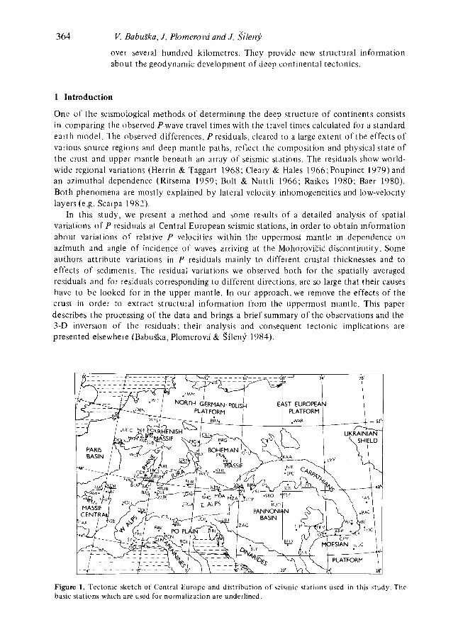
Figure 1. Tectonic sketch o f Central Europe and distribution of seismic stations used in this study. The basic stations which are used for normalization are underlined.

Spatial variatioris of P residuals 365

2 Material

The investigated territory is shown in a tectonic sketch map (Fig. I). It ranges t-rom the Massif Central t o the Ukrainian Shield in the W-E direction and from the Baltic Sea to the northern parts of the Apennines and Dinarides. About 100 stations were operating in this part of Europe between 1973 and 1979, and sending their data regularly to the International Seismological Centre. Except for two stations (GFU and MZA), the P arrivals published in the ISC Bulletins were used as the source of the data. Although the stations are not evenly distributed over the whole territory, especially over its eastern parts, they cover most of the tectonic units fairly well.

A set of 224 earthquakes and nuclear explosions at epicentral distance of 20" (with respect to the approximate centre of the array at PRA) to 100" (calculated for each station) provided 1 1 750 P arrivals for this study. A good azimuthal coverage and relatively even distribution of events as t o their epicentral distances were the main criteria for selecting these events (Fig. 2). The data set includes shallow, intermediate and deep earthquakes. The majority of events used had an ISC body wave magnitude of 5.5 or greater and I S per cent of them had mb > 6.0.

The quality of each event was tested by the number of stations of the array which recorded an event, b y the classification of the reported P-wave onsets (e, i) and by the

90°

Figure 2. Distribution of epicentres of earthquakes (dots) and nuclear explosions (dots in circles) in the distance range 20-100". The polar projection is centred at station P R A (50.1"N, 14.4" t ) .

366 Table 1. Detectability of seismic stations; 1 - number of observations, 2 - percentage of total number o f events. 3 - percentage o f f arrivals with classification better thane .

V. Rabuska, J. Plomerova arid J. &len$

(1)

ARR 12 AVT 72 BAC 28

BAS 8 BLO 128 BHG 138 BIZ 31 BLY 27 RNS I00 BOL 6 BRA 147 BRG 218 BRN 64

BUR 52 BUC 67 BUD 156 BUH 143 CAI 64 CDI 196 CLL 221 CMI' 143 D B N 136 D f V 173 DIX 132 DOU 224 ECH 145 I O C 42 I U R 206 GAP 127 G E N 41

G R r 201

m r 169

B s r 202

Gru 192

(2)

5 32 13 75

4 57 62 14 12 45

3 66 97 29 90 23 3 0 70 64 29 88 99 64 61 17 59

100 65 19 92 57 18 86 90

(3)

25 54

4 99 25 95 93 I 0 93 89

100 19 97 h l 85 96 I6 56 70 I 2 84 88 20 64 28 99 97 65 20 86 95

100 54 81

H A M HAU HEE HOI HOK IAS I so J 0s KHC KLL. K M R KRA K R L LBl,. LJU LOR LO I' LVV MEM M L R MOA MOX MZA M Z I ' NIP.. OGA PAV PCN PNI PRA PRU PSZ ROB

(1)

21 199 212 I55

18 78 26 97

220 21 8 0

203 30

21 1 182 214

23 I25 94

182 160 224

84 90

145 71 28 13 35 52

217 48 79

(2)

9 89 95 69

8 35 12 43 98

9 36 91 13 94 81 96 10 56 42 81 83

100 38 40 65 32 13 6

16 23 97 21 35

(3)

62 84 48 75 94 10 73 63 99 95 86 57 63 86 84 86 13 63 92 22 79 75

I 0(I 81 66 87

I00 100 I 00 67 98 65

100

SMI 97 43 SOP 181 81 SPC 152 6 8 SRO 118 53 SSB 85 38 SSI 214 96 SSR 25 I I STB 19 8 STR 137 h l S I U 100 45 STV 72 32 TCI 201 90 TIM 19 8 TNS 44 20 TRI 153 6 8 UCC 175 78 UDI 36 16 UZH 169 75 V I € 164 73 VKA 216 96

VRI 163 73 W A R 40 18 WET 149 67 W I 1 199 88 WLI- 65 29 WLS 217 97 W I S 159 71 ZAG 125 56 ZST 146 65 ZUL 208 93 ZUR 4 2

vou 10 4

79 66 72 57 86 86 20

100 61 79 97 87 42 68 92 43

100 71 13 87 90 17 53 95 4 0

8 99 63 90 65 98 50

accuracy o f origin times. It was found that 61 of the events (27 per cent) were reported by more than 60 stations of the array and 1'91 events (85 per cent) by more than 40 stations. The quality of their onseis is expressed by the 147 events (66 per cent) for which less than 30 per cent of the stations denoted P a s emergent (e).

The quality of a single station of the array was tested by the number o f P-wave obser- vations and by their classification (Table 1 ) . We have 48 stations which have reported the P arrivals for more than 60 per cent o f the events and only 25 stations which have classified P a s emergent for more than 40 per cent of their observations.

3 Method

A calculation flow-chart of the P residuals relative to a standard earth model and their further processing is shown in Fig. 3. By correcting for the sediment thickness and the crust. the I-esiduals were reduced to the Mohorovirid discontinuity and the relative (normalized) average residuals for various source regions were calculated. The spatial distribution o f the residuals provides information about the uppermost mantle structures and their orientations.

Spatial variations of P residuals 367

I I 23

t 0 t i r T l o ~ s a t r r l s t > v . h i g h a n d l o r v . l o r ? f i . i

Figure 3. I:low chart ot 'data processing.

3.1 C A L C U L A T I O N A N D P R O C E S S I N G O F R E S I D U A L S

The P residuals relative to the Jeffreys-Bullen earth model were calculated as the difference between the observed travel time (0) and the travel time calculated (C) according to the Jeffreys-Bullen tables (1 940). The corrections for the Earth's ellipticity and the station elevation were made first. The residuals at the individual stations were tested as t o their time stability throughout the investigated time intervals, and their frequency distributions at each station were constructed.

Various examples of the frequency distributions of P residuals are given in Fig. 4. The distributions were calculated for the residual intervals of 0.2 s from -5 to 5 s, where zero is the centre of the interval from -0.1 t o 0.1 s. Different shapes of the frequency distributions and the average residuals mainly reflect the accuracy with which the stations measured the P arrivals, and the azimuthal variations of residuals due to the effects o f different geological structures beneath the stations, as well as effects originating in sources regions and in the deep mantle.

The stations with the highest accuracy of onset times and the smallest azimuthal varia- tions of residuals have a narrow frequency distribution (e.g. station H A U in Fig. 4) and their average residuals usually correspond to the maximum of the distribution. Some of the stations have the whole pattern shifted to positive or negative values (e.g. DIX). An oriented structure beneath a station, an inhomogeneity in the mantle, as well as effects arising in various source regions can cause the distribution to split into two or more peaks (e.g. SAL),

368 V. Babufka, J . Plomerova and J. S'ilenj,

(4 -1 -1 0 1 (%,l -3 -1 -1 0 1 1 ($ -1 -1 0 1 2 (r) -5 - 4 -3 -1 -1 0 1 2 3 4 ( 9 5 - 4 - 3 - 2 -1 0 1

Figure 4. Examples ot frequency distribution of P residuals at five seismic stations: HAU (average 0.27 i 0.05 s , total number of P arrivals N = 199), SAL (average 0.01 t 0.12s, N = 131), LOR (average -0.52 k 0.05 s , N = 214), CMP (average 0.76 t 0.16 s, N = 134), DIX (average -0.87 + 0.09 s, N = 129). Nr is the relative number o f residuals in the individual intervals.

o r an asymmetry of its shape ( e g . LOR). In such cases the average residual does not correspond t o the maximum of the distribution and can even lie in its minimum (e.g. SAL). The lower accuracy of the first onset times contributes to broadening the frequency distri- bution (e.g. CMP).

As the structure of the uppermost mantle is the main objective of this study, it is necessary t o minimize all other components of the residuals. Therefore, corrections for the structure o f the crust 6, beneath each station were introduced. To derive these corrections mainly published DSS data were used (Giese, Prodehl & Stein 1976; Beranek & Zatopek 198 1 ; Sollogub, Chekunov & Guterch 1980). The thickness of the crust h M , average velocity U p and relief of the M-discontinuity, described by its dip (Y and strike rc/ (Table 21, were considered in calculating the d,-corrections in dependence on the P-wave incidence angle i and azimuth 8. A complicated shape o f the M-discontinuity beneath stations PNI and UDI is also considered (Table 2 ; parameters of PNIl are used for waves arriving from azimuths o f 36-216", parameters of UDI, are used for azimuths of 271-91"). By correcting for the crust, all the residuals were reduced t o the M-discontinuity at a reference depth of 33 km. The residuals of the stations, where a greater depth of the M-discontinuity was observed, had positive 6,-corrections (&Fax = 1.3 s for station LVV) and, o n the contrary, a shallower depth of the M-discontinuity implies a negative &,-correction (Spin = - 0.6 s for station BAS).

An additional correction for sediments was introduced at 20 stations situated in sedi- mentary basins. The thickness of the sediments hs (Ziegler 1982; Shatsky 1962) and the average velocity Up, used to calculate tiS(i, e) , are given in Table 3. Maximum corrections for sediments were applied at stations VKA and VIE (6rax = 0.5 s).

3.2 N O R M A L I Z A T I O N O F R E S I D U A L S

The effects arising from structural variations in the deep mantle between a station and a source region, and the effects originating in the source regions themselves, in their tectonics, namely in subduction zones, and originating in mislocations and in errors in determining the origin time, are largely eliminated by normalizing each event and then grouping them by source region,

Two methods o f normalization are usually used to calculate the relative (normalized) residuals. In the first method, a reference station of a seismic array is determined and its

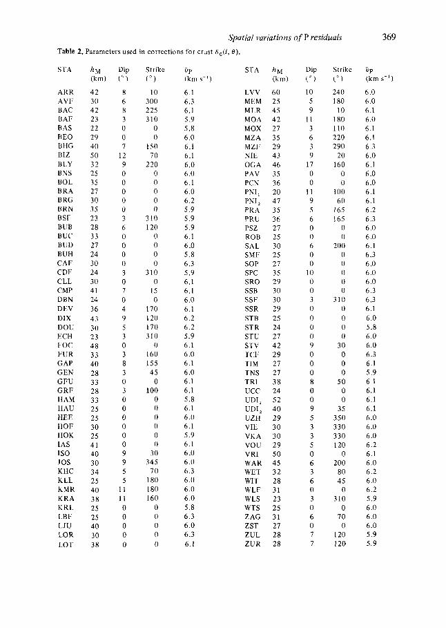
Spatial variations of P residuals Table 2. Parameters used in corrections for crust f jC(i , 6').

STA

ARR AVI: B AC BAF BAS B E 0 BHG BIZ B LY BNS BOL BRA B RG BRN BSF BUB BUC BUD BUH CAF CDF CLL CMP DBN DEV DIX DOU ECH FOC FUR GAP GEN C F U G R F HAM HAU HEE HOF HOK [AS I so JOS KHC KLL KMR KRA KRL LBF LJU LOR LOT

h M (km)

42 30 42 23 22 29 40 50 32 25 35 27 30 35 23 28 33 27 24 30 24 30 41 24 36 43 30 23 48 33 40 28 33 28 33 25 25 30 25 41 40 30 34 25 40 38 25 25 40 30 38

Dip ( " ?

8 6 8 3 0 0 I

12 9 0 0 0 0 0 3 6 0 0 0 0 3 0 7 0 4 9 5 3 0 3 8 3 0 3 0 0 0 0 0 0 9 9 5 5

11 11 0 0 0 0 0

Strike ( " )

10 300 225 310

0 0

150 70

220 0 0 0 0 0

3 10 120

0 0 0 0

3 10 0

15 0

170 120 170 310

0 160 155 45 0

100 0 0 0 0 0 0

30 345

70 180 180 160

0 0 0 0 0

6.1 6.3 6.1 5.9 5.8 6 .O 6.1 6.1 6.0 6 .O 6.1 6 .O 6.2 5.9 5.9 5.9 6.1 6 .O 5.8 6.3 5.9 6.1 6.1 6 .O 6.1 6.2 6.2 5.9 6.1 6 .O 6.1 6.0 6.1 6.1 5.8 6.1 6.0 6.1 5.9 6.1 6 .O 6 .O 6.3 6 .O 6 .O 6.0 5.8 6.3 6 .O 6.3 6.1

LVV 60 MEM 25 MLR 45 MOA 42 MOX 27 MZA 35 MZF 29 NIE 43 OGA 46 PAV 35 PCN 36 PNI, 20 PNI, 47 PRA 35 PRU 36 PSZ 27 ROB 25 SAL 30 SMF 25 SOP 27 SPC 35 SRO 29 SSB 30 SSF 30 SSR 29 STB 25 STR 24 STU 27 STV 42 TCF 29 TIM 27 TNS 21 TRI 3 8 UCC 24 UDI, 52 UDI, 40 UZH 29 VIE 30 VKA 30 VOU 29 VRI 50 WAR 45 WET 32 WIT 28 WLF 31 WLS 23 WTS 25 ZAG 31 ZST 27 ZUL 28 ZUR 28

Dip ! "? 10

5 9

11 3 6 3 9

17 0 0

11 9 5 6 0 0 6 0 0

10 0 0 3 0 0 0 0 9 0 0 0 8 0 0 9 5 3 3 5 0 6 3 6 0 3 0 6 0 7 7

Strike (" 1 240 180

10 180 110 220 290

20 160

0 0

100 60

165 165

0 0

200 0 0 0 0 0

3 10 0 0 0 0

30 0 0 0

50 0 0

35 350 330 330 120

0 200

80 45

0 310

0 70

0 120 120

369

bP (km s - ' )

6 .O 6 .O 6.1 6 .O 6.1 6.1 6.3 6 .O 6.1 6 .O 6 .O 6.1 6.1 6.2 6.3 6 .O 6.0 6.1 6.3 6 .O 6 .O 6 .O 6.3 6.3 6.1 6 .O 5.8 6 .O 6.0 6.3 6.1 5.9 6.1 6.1 6.1 6.1 6.0 6 .O 6 .O 6.2 6.1 6.0 6.2 6 .O 6.2 5.9 6.0 6 .O 6.0 5.9 5.9

370 Table 3. Parameters used in corrections for sediments b&. 0 )

S'I'A h,( k 111 Cp(kn1 a - l ) S I 'A h,(kni) Gp(kn1 S - ' )

BAC I31 0 1% K N BUC HIID D B N 1 OC I U R f i A M LVV

0.5 0 .7 2.5 1 .0 4 .O 2 .o 1 .5 2.5 5 .o 3.5

4.0 4 .O 4.5 3.5 4.5 4 .O 3.5 3.5 4 .o 4.5

PAV S KO T I M VIE VKA W A K WIT WTS Z l J L Z U K

5 .O 3 .0 I .O 3.2 3.2 0.8 1.5 1 .O 1 .o 1.0

4.5 4.0 4 .o 3.5 3.5 4.5 4 .O 4 .o 3.5 3.5

residual is subtracted as the normalized value from the residuals o f other stations (e.g. Raikes & Hadley 1979). The second method uses a normalization value obtained as the average residual over the whole array (Aki & Richards 1980).

The former method can negatively influence the distribution of the relative residuals, if a large tectonic inhomogeneity or a conspicuous anisotropy of the P-wave velocity exists below the reference station. On the other hand, the normalization procedure of the latter method suffers from the fact that not all stations report the P arrivals for each event and. therefore, the normalization value, obtained as an average residual, is calculated for different events from P onset times at different stations. This non-uniformity is incorrect especially when the events are grouped by source region, which is our case. and an average relative t-esidual is calculated for a group of events for each source region.

In this paper, we have modified the second method. A system of 15 basic stations was introduced and the normalization value calculated as an average of the residuals at these stations: BEO, CLL, DIX, DOU, FUR, GRF, KHC, WU, LOR, PRU, SAL, TCF, UZH, VKA, WLS (Fig. I ) . The basic stations, which belong to the best o f the array, were selected to obtain a fairly good coverage of the whole area. The stations with the largest number of time-stable observations and with a narrow frequency distribution gained priority. Moreover, a uniform representation o f the main tectonic provinces was kept in mind. A residual at a station o f the basic system must not differ by more than f 1 s from the average residual of this station, calculated from all events within a particular source region which will then be used to calculate the normalized value.

Besides the normalization in which we have used the system o f 15 basic stations, we made an attempt at calculating the relative residuals for nuclear explosions from Nevada. and East and West Kazakhstan, using the three-station normalization (DOU, LOR, KHC - Fig. 1). For all three source regions, the pattern of contour maps o f relative residuals is independent o f the system o f the normalization stations. The average differences calculated over the whole array between the residuals normalized with respect to 15 stations and those to three stations are as follows: Nevada region (A = 83", 0 = 332") 0.08 f 0.01 s (number o f stations used N = 63), East of Kazakhstan (A = 40°, 0 = 64") -0.20 f 0.00 s ( N = 7Y), West Kazakhstan (A = 22", 0 = 83") -0.01 f 0.01 s ( N = 8s). Moreover, the relative residuals for West Kazakhstan were calculated relative to a single reference station: if DOU is used, these residuals are 0.23 f 0.01 s smaller, o n average, than the residuals normalized with respect t o 15 stations. If KHC is used as the reference station, the West Kazakhstan residuals are 0.3 s smaller than the residuals normalized with respect to 15 stations, whereas for LOR they are 0.8 s larger. These examples show that normalization by an average residual calculated from a system of 15 stations is more stable and less dependent on residual variations due t o variable azimuths and incidence angles than the normalization with respect to three stations

Spatial i~zri~ztions 0.f' P residuals 37 1

or t o a single reference station. In the last case, moreover. the effect of the geology beneath the normalizing station may he eliminated and imprinted on all the other stations o f the array.

In order to obtain representative residuals for various azimuths and incidence angles of waves. besides the normalization, we grouped all events by source regions (Fig. 3). The average relative residuals R,,(k = 1, . . . , 43) were then calculated at each station (i) for the k t h source region. The residuals, which differed by moi-e than 5 2 s from the weighted i-esi- duals averaged over all events within a particular source region. were omitted. The residuals were weighted according to the quality of the P arrivals. The maps of average relative resi- duals Ri, for various source regions ?xpi-ess the directional dependence of i-esiduals on azimuths and incidence angles of waves propagating through the uppermost tnantle near the stations. These average residuals provide data for the 3-D inversion, the results of which are discussed in detail elsewhere ( B a b u h et al. 1084).

The uppermost mantle beneath each station. regardless of the direction of arriving waves. is characterized by a single value, RY)tr (Fig. 3). This residual was calculated a s the average o f the relative residuals K i , k for selected regions ( k = 1 , . . . , 2 3 ) , evenly distributed as t o their azimuths and distances in order to have a uniform representation of all directions of wave propagation.

On the other hand, the residuals RBtS (Fig. 3), calculated as the difference between the residuals R i k for the k t h source region and the representative residual !?p'tr o f the i t h station of the array, emphasizes their directional dependence. This dependence is expressed by the polar diagrams of RY$ (Figs 7 and 8) constructed for almost all station. In these diagrams, the R T f residuals are plotted in dependence on the azimuth and incidence angle o f P-waves.

3 . 3 T H R E E - D I M E N S I O N A L IN V E K S I O N

A method o f seismic residual inversion, giving the 3-D velocity structure beneath a seismic array, was presented by Mi, Christofferson & Husebye ( I 977). The structure in the region under study is parameterized by dividing it into rectangular blocks, lying in several layers with an assumed average velocity. The velocity fluctuations in each block are determined from the travel-time data observed in the array for many teleseismic events. The size of the blocks is determined by the density of the seismic network and by the wavelength of seismic waves, because the ray theory is used for computing the travel time. The wavefront is assumed to be a plane wave incident upon the base o f the flat layered structure, and raypaths are traced through the initially homogeneous layers assuming the validity of the Ferniat principle. The simplifying assumption was made that the entire raypath crossing a layer is assigned t o the block in this layer, in which the ray spends the majority of its time. I t was shown (Aki et al. 1977) that this problem reduces to solving a set o f linear equations in matrix form expressed by

F T = A m ,

where FT is the vector containing the travel-time residuals, A is the calculated travel path matrix and m is the vector containing the unknown velocity perturbations 6u/u. Since only relative residuals are used, this problem cannot be solved by classifical least-square techniques. but the method of generalized or stochastic inverse has to be employed (Backus & Gilbert 1968; Jackson 1973). The stochastic inverse (Franklin 1970), used in our calcu- lations, is given by

m = (A'A + 021) - ' A"6T,

372

where 8' is the damping parameter expressed by the ratio of the data and velocity flucua- tion variances a:/&.

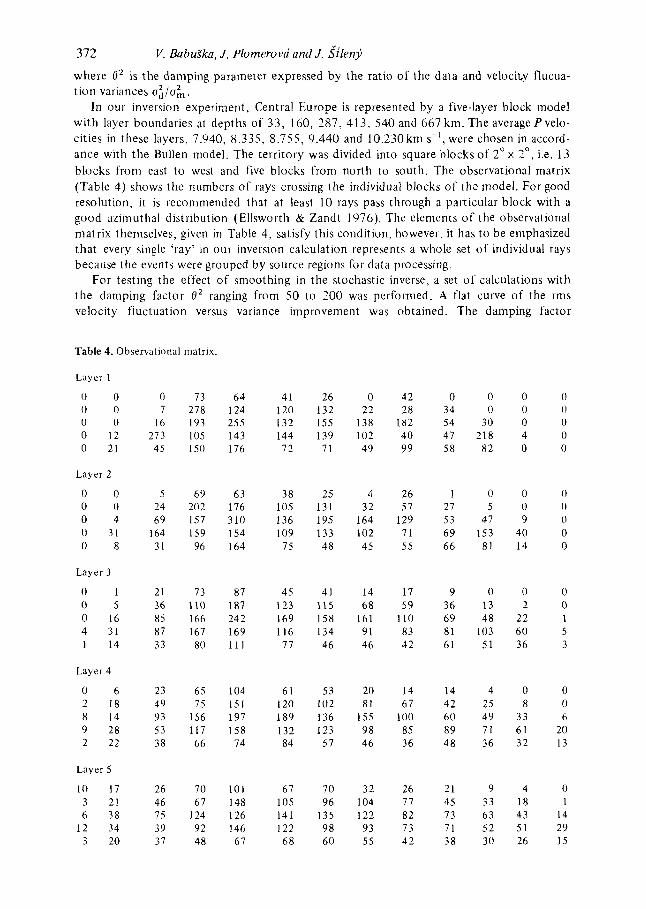
In our inversion experiment, Central Europe is represented by a five-layer block model with layer boundaries at depths of 33, 160, 2 8 7 , 413, 540 and 667 km. The average Pvelo- cities in these layers, 7.940, 8.335, 8.755, 9.440 and 10.230 km s-' , were chosen in accord- ance with the Bullen model. The territory was divided into square blocks o f 2" x 2"> i.e. 13 blocks from east to west and five blocks from north to south. The observational matrix (Table 4) shows the numbers of rays crossing the individual blocks o f thc model. For good resolution, it is recommended that at least 10 rays pass through a particular block with a good azimuthal distribution (Ellsworth & Zandt 1976). The elements o f the observational matrix themselves, given in Table 4, satisfy this condition, however, it has t o be emphasized that every single 'ray' in our inversion calculation represents a whole set of individual rays because the events were grouped by source regions for data processing.

For testing the effect of smoothing in the stochastic inverse, a set of calculations with the damping factor 19' ranging from 50 to 200 was performed. A flat curve o f the rms velocity fluctuation versus variance improvement was obtained. The damping factor

V. BabuSka, J. Plomerova and J. S'ileni

Table 4. Observational matrix.

Laycr 1

0 0 0 73 64 41 26 0 42 0 0 0 0 0 0 7 278 124 120 132 22 28 34 0 0 0 0 0 16 I93 255 132 155 138 182 54 30 0 0 0 12 273 105 143 144 139 102 40 47 218 4 0 0 21 45 150 176 72 71 49 99 58 82 0 0

Layer 2

0 0 5 69 63 38 25 4 26 1 0 0 0 0 0 24 202 176 105 131 32 57 27 5 0 0 0 4 69 157 310 136 195 164 129 53 47 9 0 0 31 164 159 I54 109 133 102 71 69 153 40 0 0 8 31 96 164 75 48 45 55 66 81 14 0

Layer 3

0 1 21 73 87 45 41 14 17 9 0 0 0 0 5 36 110 187 123 115 68 59 36 13 2 0 0 16 85 166 242 169 158 161 110 69 48 22 1 4 31 87 167 169 116 134 91 83 81 103 60 5 1 14 33 80 111 77 46 46 42 61 51 36 3

Layer 4

0 6 23 65 104 61 53 20 14 14 4 0 0 2 18 49 75 151 120 102 81 67 42 25 8 0 8 14 93 156 197 189 136 155 100 60 49 33 6 9 28 53 117 158 132 123 98 85 89 71 61 20 2 22 38 66 74 84 57 46 36 48 36 32 13

Layer 5

10 17 26 70 101 67 70 32 26 21 9 4 0 3 21 46 67 148 105 96 104 77 45 33 18 1 6 38 75 124 126 141 135 122 82 73 63 43 14

12 34 39 92 146 122 98 93 73 71 52 51 29 3 20 37 48 67 68 60 55 42 38 30 26 15

Tab

le 5. D

iago

nal e

lem

ents

of

reso

luti

on a

nd c

ovar

ianc

e m

atri

xes o

f th

e fi

rst

laye

r.

0.92

7 (1

.96)

0.96

5 (1

.41)

0.94

8 0.

989

(1.6

9)

(0.7

7)

0.96

2 0.

982

(1.4

3)

(1.0

1)

0.98

6 (0

.88)

0.99

0 (0

.74)

0.99

1 (0

.68)

0.99

0 (0

.72)

0.99

3 (0

.63)

0.98

5 (0

.93)

0.99

0 (0

.75)

0.99

2 (0

.66)

0.99

1 (0

.68)

0.99

3 (0

.62)

0.98

3 (1

.01)

0.99

0 (0

.74)

0.99

1 (0

.70)

0.99

2 (0

.66)

0.99

0 (0

.75)

0.96

0 (1

SO)

0.98

7 (0

.82)

0.98

9 (0

.76)

0.99

1 (0

.71)

0.98

6 (0

.88)

0.97

3 (1

.22)

0.98

9 (0

.76)

0.98

9 (0

.76)

0.98

3 (0

.98)

0.96

5 11

.36)

0.97

5 (1

.15)

0.98

7 (0

.79)

0.98

2 (1

.OO)

0.98

6 (0

.86)

0 96

8 (1

30)

0 97

7 0

965

(1 0

9)

(1 3

6)

0.98

1 0

982

(1 0

1)

(0 9

5)

0 98

3 0

981

to 9

5)

(1 0

0)

W

4

W

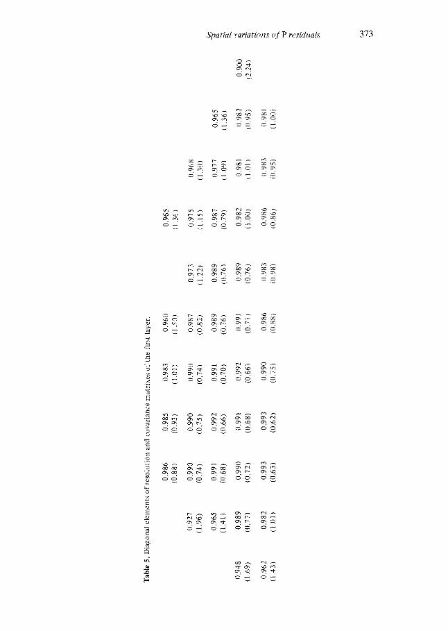
374 O 2 = 100 was adopted for further calculations, giving ;i variance improvement o f 24.2 per cent and a r i m velocity fluctuation equal to 1.4.

The resolution of the blocks o f the model and the standard error of determining the velo- city perturbations was tested by computing the resolution and covariance matrices. Diagonal elements of these matrices of the first layer are given in Table 5. All the elements are close to unity and, therefore, the resolution is very good. A similar pattern was obtained for deeper layers. as well, with the smallest element reaching a value of about 0.7. The numbers in brackets in Table 5 show the diagonal elements of the covariance matrix. The standard error of the velocity fluctuation foi- the well-resolved blocks in the centre of the first layer of the model was determined at a b o u t 0.7.

V. Babufka, J . Plomerova and J. .$ile@

3.4 S O U R C E S 01. i:KnoH

The main sources of eri-or, affecting the deterniination of the relative residuals. were discussed by Engdahl. Sinndorf & Eppley (1977) and Raikes (1980). Reading errors with unambiguous first arrivals at the seismograph network in Southern California were estimated by Raikes (1080) at 0.1 s . In case of the ISC Biillefin d a t a , this error probably does not exceed the value of 0.1 -0.2 s for most o f the stations we have used (Table 1). With some of the less sensitive stations, the error is reduced by weighted averaging.

Origin time and mislocat ion effects seems to be critical for- the deterniination of residuals. Since a suite of raypaths from each teleseismic event is almost common to stations o f a parti- cuI;ir part o f the network and the system of 15 high-quality stations was used for the mi-malization, this procedure eliminates most o f the origin time and mislocation effects, as well as most of the effects arising from the structure of source regions and inhomogeneities within the deep mantle. The grouping o f events within the individual soul-ce regions further helps in reducing the errors originating in the structure o f focal zones, in determining the time origin and location events.

Effects o f variable depths of events on the residuals were studied foi- four source regions: Alaska-Aleutians, the Kuriles, Japan and Ryuku-Philippines. It was found that the nornialization with respect to 15 basic stations completely removes the differences in distri- butions of residuals o f deep, intermediate-depth and shallow events.

Another group o f possible errors is related to corrections which we introduced t o elimi- nate the effects of different station elevations, crustal thickness arid, at some stations, also the occurrence of unconsolidated sediments, The station elevation correction is based on the assumption that the near-surface velocity is 5 km s- ' . The actual velocity below the stations cannot differ much from this value because special corrections are introduced for stations underlain by unconsolidated sediments (Table 3). Therefore, for most stations the error arising from the station elevation corrections does not exceed 0. I s, as also stated by Raikes (1Y80) for southern California.

The corrections f o r sediments were applied at 20 stations. The thickness of sedimentary layers ranges from 0.5 to 5 km and the velocity estimates from 3.5 to 4.5 kni s- ' (Table 3). However, any error in these estimates does not affect the applied corrections substantially, for example, a change in velocity from 3.5 t o 4.0 km s-' over a path of 5 km creates a difference o f less than 0.2 s, and error of 1 kni over a 5 km path results in a difference of 0.1 s.

The important corrections are related to the thickness of the crust and P velocities determined by DSS measurements. The residuals were reduced to the M-discontinuity at the standard depth hM = 33 km by subtracting the travel time corresponding to a raypath within the actual crust beneath a station, assuming varying crustal P velocity and undulations of the M-discontinuity. The average crustal velocity beneath the stations ranged from 5.8 to

Spatial variatioris of P residuals 375 6.3 kni s-', the depth of the M-discontinuity from 20 to 6 0 k m and its dip from 0" to 17". However, any error arising from incorrect velocity values and the listed geometrical parameters of the M-discontinuity (Table 2) is not essential: for example. a change in velocity from 6.0 to 6.3 km s-l (i.e. 5 per cent) causes an error in determining this correction o f less than 0.3 s, and a variation in depth of the M-discontinuity of 3 km is reflected in this correction only by a change of about 0.1 s.

Travel-time residuals were also calculated for all events by comparison with the Herrin tables (Herrin & Taggart 1968). The observed differences between the residuals averaged over the whole space and calculated according to the Jeffreys--Bullen (1940) and Herrin (1068) tables can be neglected as they do not exceed the error o f the avei-age residual at a single station.

By reducing the residuals fi-om the Earth's surface to the M-discontinuity along a i-aypath. the position of a point, to which the reduced value of the residual is assigned. is laterally shifted from the vertical projection of a station on to the M-discontinuity. The greater it$ depth and the smaller the epicentral distance, the larger the shift. In our configuration. the values of the shifts for the nearest focal regions. e.g. for Western Kazakhstan, are as large as 40 kni. In this type o f study, the error arising from neglecting this effect is n o t essential because of' the reiatively large distances between stations of the array. However, foi- further, more detailed studies in areas with a denser network of stations. this shift has to be considered.

As will be seen later on, the magnitudes of the residuals were found to be systematically higher in most cases than any error in the applied corrections and, therefore, the observed residuals should have a physical meaning, reflecting the actual variations in the structure of the upper mantle.

4 Results

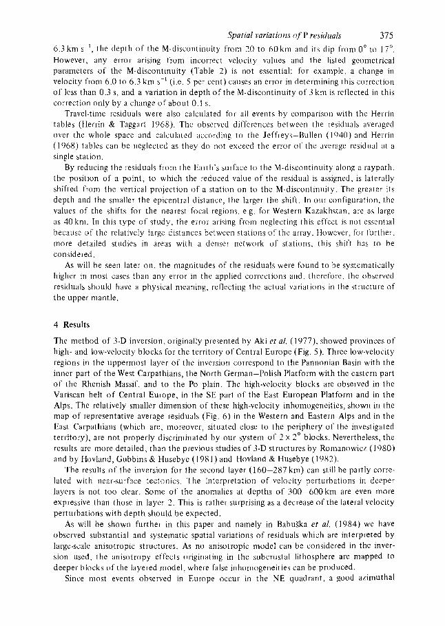
The method of 3-D inversion, originally presented by Aki et al. (1977), showed provinces o f high- and low-velocity blocks for the territory of Central Europe (Fig. 5). Three low-velocity regions in the uppermost layer of the inversion correspond to the Pannonian Basin with the inner part of the West Carpathians, the North German-Polish Platform with the eastern part o f the Rhenish Massif, and t o the Po plain. The high-velocity blocks are observed in the Variscan belt o f Central Europe, in the SE part of the East European Platform and in the Alps. The relatively smaller dimension of these high-velocity inhomogeneities, shown in the map of representative average residuals (Fig. 6) in the Western and Eastern Alps and in the East Carpathians (which are, moreover, situated close to the periphery of the investigated territory), are not properly discriminated by our system o f 2 x 2' blocks. Nevertheless, the results are niore detailed, than the previous studies of 3-D structures by Rornanowicz (1980) and by Hovland, Gubbins & Husebye (1 98 1 ) and Hovland & Husebye ( 1 982).

The results of the inversion for the second layer (160-287 km) can still be partly corre- lated with near-surface tectonics. The interpretation of velocity pel-turbations in deeper layers is not too clear. Some o f the anomalies at depths of 300-600km are even more expressive than those in layer 7,. This is rather surprising as a decrease of the lateral velocity perturbations with depth should be expected.

As will be shown further in this paper and namely in Babu5ka et al. (1984) we have observed substantial and systematic spatial variations of residuals which are interpreted by large-scale anisotropic structures. As no anisotropic model can be considered in the inver- sion used, the anisotropy effects originating in the subcrustal lithosphere are mapped t o deeper blocks of the layered model, where false inhomogeneities can be produced.

Since most events observed in Europe occur in the NE quadrant, a good azimuthal

376 V. Babufka, .J. Plomerova and J . s'i1erz.l;

Figure 5. 1:ive-layer model obtained by 3-D inversion of telescismic travel-time data. Each sheet represents a layer. placed at its median depth. The numbers in the 2 X 2" blocks express the velocity perturbations in tenths of a per cent with respect to the Hullen model, and the contours arc zmo isolines.

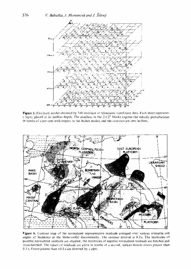
Figure 6 . Contour map of the normalized representative residuals averaged over various azimuths and angles of incidence at the MohoroviEic' discontinuity. The contour interval is 0.2 s. The territories of positive norrnalized residuals are stippled. the territories of negative normalized residuals are hatched and cross-hatched. 'The value< of residuals are given in tenths o f a second, indices denote errors greater than 0.1 s. Errors greater than t0.5 s are denoted by t sign.

Spatial variations of' P residuals 377 and distance coverage of source regions is critical for calculating the average residual a i a particular station. I n this study, we used data of 23 source regions which uniformly cover various azimuths and incidence angles of arriving wave fronts. Fig. 6 shows the map of representative average P residuals (in tenths o f a second) where errors higher than 0.1 s are denoted by indices. In spite o f the corrections for sediments, the regions of subsidence. the Po Plain, the Pannonian Basin and the North German-Polish Platform, are characterized by late arrivals, which implies relatively low velocities in the upper mantle. This is also valid for the Rhenish Massif, most of the Rhine Graben and the inner part of the Western Carpathians. The late arrivals, in general, correspond well to regions of thinner lithosphere as deterniined by Panza ef a f . (1980).

Early arrivals (relatively high P velocities) are observed at the south-western margin of the East European Platforni and in three zones several hundred kilometres long in the inner part of the Western Alps, in the eastern part o f the Austrian Alps and in the Eastern Carpathians at the north-western rim of the Moessian Platform. These deep-seated inhoniogeneities, the depth of which is estimated at 200-250 kni in the Western Alps and Eastern Carpathians, and at 150-200km in the Eastern Alps (Babufia et al. 1984), have been preliminarily inter- preted as remnants of the cold subducted lithosphere from the past.

A consistency of the average residuals within tectonic provinces and large differences in the relative residuals for various provinces, which often amount t o about 1.5 s, imply an upper-niantle source of the observed velocity variations. The variation of the lithosphere thickness (Panza et at. 1980) and partly the lateral changes o f temperature within it have a dominant effect on the averaged residuals. Some areas, where we observed relatively low velocities in the uppermost mantle col-respond t o regions of high heat flow, e.g. the Pannonian Basin and the Rhine Graben, other low-velocity areas, like the western part o f the North German-Polish Platforni and the Po Plain, display rather low heat flow near the surface (C'erniak & Hurtig 1979).

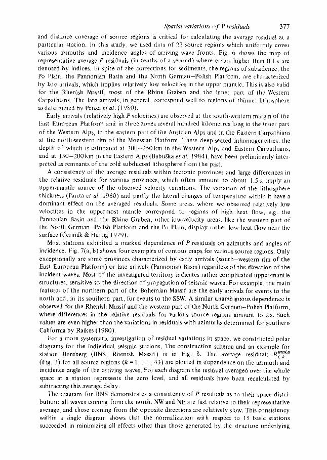
Most stations exhibited a marked dependence of P residuals on azimuths and angles o f incidence. Fig. 7(a, b ) shows four examples of contour maps for various source regions. Only exceptionally are some provinces characterized by early arrivals (south-western rim of the East European Platform) or late arrivals (Pannonian Basin) regardless o f the direction of the incident waves. Most of the investigated territory indicates rather complicated upper-mantle structures, sensitive t o the direction o f propagation of seismic waves. For example, the main features of the northern part of the Bohemian Massif are the early arrivals for events to the north and, in its sourhern part, for events to the SSW. A similar unambiguous dependence is observed for the Rhenish Massif and the western part of the North German-Polish Platform, where differences in the relative residuals for various source regions amount to 2s . Such values are even higher than the variations in residuals with azimuths determined for southern California by Raikes ( 1 980).

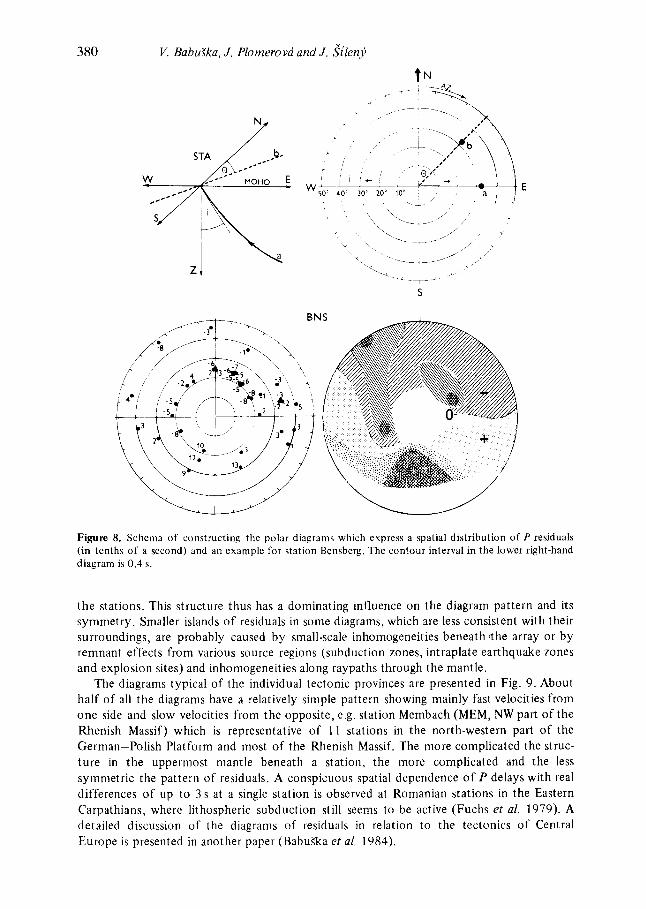
For a more systematic investigation of residual variations in space, we constructed polar diagrams for the individual seismic stations. The construction schema and an example for station Bensberg (BNS, Rhenish Massif) is in Fig. 8. The average residuals RF;IS (Fig. 3 ) for all source regions (k = 1 , . . . ,43) are plotted in dependence on the azimuth and incidence angle of the arriving waves. For each diagram the residual averaged over the whole space at a station represents the zero level, and all residuals have been recalculated by subtracting this average delay.

The diagram for BNS demonstrates a consistency o f P residuals as to their space distri- bution: all waves coming from the north, NW and NE are fast relative t o their representative average, and those coming from the opposite directions are relatively slow. This consistency within a single diagram shows that the normalization with respect to 15 basic stations succeeded in minimizing all effects other than those generated by the structure underlying

378 V. Babufka, J . Plomerovu and J . i i leny

Figure 7. ( a , b ) t w n p l e s of contour maps of P residuals for various source regions. the contour interval is 0.4 \. The territories of positive normalized residuals are \tippled. the territories characterized by negative nornializcd residuals are cross-liatclicd. The upper right-hand diagranls sliow a/iniuths 0 and inci- dence angles i at the MohoroviFiL' discontinuity for the centre of the map.

Spatial variations 01' P residuals 379

I

Figure 7 - continued

380 V. Babufka, J. Plomerova and J . s’ilen$

S

Figure 8. Schema of constructing the polar diagrams which express a spatial distribution of P residuals (in tenths of a second) and an example for station Bensberg. The contour interval in the lower right-hand diagram is 0.4 s.

t h e stations. This structure thus has a dominating influence on the diagram pattern and its symmetry. Smaller islands o f residuals in some diagrams, which are less consistent with their surroundings, are probably caused b y small-scale inhomogeneities beneath ithe array or b y remnant effects from various source regions (subduction zones, intraplate earthquake zones and explosion sites) and inhomogeneities along raypaths through the mantle.

The diagrams typical of the individual tectonic provinces are presented in Fig. 9. About half of all the diagrams have a relatively simple pattern showing mainly fast velocities from one side and slow velocities from the opposite, e.g. station Membach (MEM, NW part of the Rhenish Massif) which is representative of 1 1 stations in the north-western part of the German-Polish Platform and most of the Rhenish Massif. The more complicated the struc- ture in the uppermost mantle beneath a station, the more complicated and the less symmetric the pattern of residuals. A conspicuous spatial dependence o f P delays with real differences of up to 3 s at a single station is observed at Romanian stations in the Eastern Carpathians, where lithospheric subduction still seems to be active (Fuchs er al. 1979). A detailed discussion of the diagrams of residuals in relation to the tectonics o f Central Europe is presented in another paper (Babu&a el al. 1984).

Spatial variations of P residuals 381

Figure 9. Typical diagrams of spatial distribution of P residuals for various tectonic provinces.

The directions of relatively high and low velocities for all stations, which provided fairly good data for the diagrams, are schematically shown in Fig. 10. Comparing these directions with the map of representative average residuals (Fig. 6), we can see that , in areas which are characterized, on average, either by slow or high velocities, the diagrams of residuals reveal upper-mantle structures which are distinctly directionally dependent as t o P velocities. Lateral extension of the areas with a similar pattern of this directional dependence, like the Moldanubian part of the Bohemian Massif, the Alpine fordeep and the northern part o f the

Figure 10. Map of simplified patterns of relatively high-velocity (solid lines) and low-velocity (dashed lines) directions at various seismic stations. Territories with similar patterns are hatched.

382

Alps (vertically hatched in Fig. lo), o r the NW of the German-Polish Platform and most o f the Rhenish Massif (oblique hatching in Fig. lo), suggests the existence of large-scale, probably anisotropic structures in the uppermost mantle, which are consistent in their dips and orientations over several hundred kilonietres.

V. Babufka, J . Plomerova and J . i i l e n y

5 Conclusions

After carefully processing the ISC Bullefirz P arrivals from events relatively evenly distributed as to their azimuths and distances with respect to Central European seismic stations, we observed three types of consistency in relative P residuals reduced to the M-discontinuity: ( 1 ) lateral consistency of spatially average residuals reflecting large-scale inhomogeneities and thickness variation of the lithosphere: ( 2 ) consistency of the residuals as to their space distribution at a single station reflecting orientations and complexity o f the upper-mantle structure beneath stations; (3) consistency of patterns of the residual diagrams for groups o f stations within tectonic provinces reflecting a systematic orientation and probably also a large-scale anisotropy of the uppermost mantle structure.

The combined effects of inhomogeneities and anisotropic structure show up in the spatial variations of residuals. Recognizing the anisotropy patterns can yield a new insight into the geodynamic evolution of continents.

Acknowledgments

We would like to thank Dr S. Raikes for providing the list of events she used in her previous study, for punched J-B tables and for her program which we modified for residual compu- tations. Sincere thanks are also due t o the staft' of the Computer Centre of'the Geophysical Institute, Czechoslovakian Academy of Science, namely to Mrs E. Silena, for their helpful assistance and understanding with our extensive computations. Dr K . Aric o f the Institut fur Meteorologie und Geophysik der Universitst Wien kindly provided seismograms of station MZA and Dr Cicha of the Geological Survey in Prague was good enough t o discuss the sediment thicknesses beneath some of the seismic stations. This work was partly supported by Unesco contract SC/RP 560992.

References

Aki, K . , Christofferson, A. & Huscbye, E. S., 1977. Iktermination of the three-dimensional seismic

Aki, K . & Richards, P. G., 1980;Quantitative Seismology, W. H. Freeman, San Francisco. RabuSka. V.. Plomcrovd, J . & Silen);, J . , 1984. Largc-scale oriented structures in the uppermost mantle

of the Central Europe,Annls Gtophys., in press. Backus, G. E. & Gilbert, J . F., 1968. The resolving power of gross Earth data , Geophys. J. R. (Istr. SoC.,

16, 169--205. Raer, M., 1980. Kelative travel-time residuals lor teleseismic events at the new Swiss seismic station

network, Annls Ge'ophys., 36, 119-126. Berrlnek, H. & Zdtopek, A,, 1981. Earth's crust structure in Czechoslovakia and in Central Europe by

methods of explosion seismology, in Geophysical Syntheses in Czechoslovakia, pp. 243 -264, Publ. House Veda, Bratislava.

Bolt, B. A . & Nuttli, 0. W., 1966. P wave residuals as a function of azimuth, J. geophys. Rcs., 71, 5 9 1 I --5 9 85.

?ermdkJ V. & tiurtig, 1<.. 1979. Heat flow map of Europe, in Terrestrial Heat Flow in Europe, eds Cermdk, V. & Kybach. L.. Springer-Verlag, Berlin.

Clcary, J . & Ilales, A., 1966. An analy.;is of the travel tiines o f f ' waves t o North American stations in the distance range 32" to 100",Bull. seism. SOC. Am., 56, 467--489.

structure of the lithosphere, J. geophys. R e x , 82, 277-296.

Spatial variations of P residuals 383 Ellsworth. W. & Zandt, G., 1976. Program THREED, not published. Tingdahl, E. K., Sinndorf, J . G. 6; Eppley, R. A,, 1977. Interpretation o f relative telcseismic P-wave

residuals, J. geophys. Res., 82, 567 1-5682. b’ranklin, J . N . , 1970. Well posed stochastic extrusions of ill posed linear problems. J. math. Analysis

Applic., 31,682 -716. l~uchs , K., Bonjer, K . P., Bock, G., Cornea, I . , Radu, C., Enescu. D., Jianu, D., Nourescu. A., Merkler,

G., Moldoveanu. T. & Tudorache, G., 1979. The Romanian earthquake of March I . 1977. After- shocks and migration of seismic activity, Tectonophys., 53, 225 247.

Giese, P , , Prodehl, C. & Stein, A,, 1976. Explosion Seismology in Central Europe, Springer-Verlag. Berlin.

Herrin, E. 6; Taggart. J . . 1968. Regional variations in P travel times, B d . seism. Soc. A m . , 58, 1325 - 1337.

Hovland, J . , Gubbins, D. & Husebye, E. S., 1981. Upper mantle heterogeneities beneath central Europe. Geophys. J. R. astr. Soc., 66, 261 - 284.

Hovland, J. & Husebye, E. S., 1982. Upper mantle heterogeneities beneath eastern Europe, Tectonophys., 90, 137-151.

Jackson, D. D., 1973. Interpretation of inaccurate, insufficient and inconsistent data. Ceophys. J. R. astr. Soc., 28, 97 - 109,

Jeffreys. H. & Bullen, K . E., 1940. Seismological Tables, British Association for the Advancement of Science. London.

I’anza, G. I , . . Calcagnile, G., Scandonc, 1’. 62 Mueller, S., 1980. La struttura profonda dell’area mediter- ranea, Scienze, 24, 60-69.

Poupinet. G. , 1979. On the relation between P-wave travel time residuals and the age of continental platcs,Earth planet. Sci. Lett . , 43, 149 ~ 161.

Raikes, S. A,, 1980. Regional variations in upper mantle structure beneath Southern California, Geophys. J . R. astr. Soc., 63, 187 -2 16.

Raikes, S. & Hadley, D. M., 1979. The azimuthal variation o f teleseismicP-residualsin Southern C’alitornia: implications for upper-mantle structure, Tectonophys.. 56, 89-96.

Ritscma, A., 1959. Note on the azimuth deviations of P-waves recorded at Djakarta station, Geophis. pure appl., 43, 159--166.

Ronianowicz, €3. A., 1980. A study of large-scale lateral variations of P velocity in the upper mantle beneath western Europe, Geophys. J. R. astr. Soc., 63, 217-232.

Scarpa, R., 1982. Travel-time residuals and three-dimensional velocity structure of Italy, Pure appl. Geophys., 120,583-606.

Shatsky, N., 1962. Tectonic Map of Europe, Subcommission for world tectonic map, International Geology Congress, Moscow.

Sollogub, V. B., Chekunov, A. V. & Guterch, A,, 1980. Structure of the Earth’s crust in East-European Platform from data of explosion seismology, in The Structure o f t h e Earth’s Crust in Centraland Eastern Europe According to Geophysical investigations, Publ. House Naukova Dumka, Kiev (in Kussian).

Ziegler, P. A, , 1982. Geological Atlas of Western and Central Europe, Shell International Petroleum MaatschappQ BV, The Hague.