Spatial Patterns of Biodiversity–Assessing Vegetation Using Hexagonal Grids

SPATIAL PATTERNS OF

BIODIVERSITY-ASSESSING VEGETATION

USING HEXAGONAL GRIDS

Gerald Jurasinski and Carl Beierkuhnlein

ABSTRACT

We still lack quantitative and comprehensive methods to assess spatio-temporal changes inbiodiversity of landscapes. Even more, we need methods to determine the amounts of changeespecially in the light of the current acceleration in the loss of biodiversity.

We have developed a widely applicable method to reveal spatio-temporal changes in vegetationpatterns and relate them to ecosystem processes. We use a systematic grid of hexagonal plots in aspatially nested design (three spatial scales and levels) to examine these patterns. The hexagonal grid,as well as the hexagonal plot, provides several advantages compared to other methods. Mostimportant in the context of evaluating patterns is the equidistant nature of the grid. This facilitatesdata analysis and circumvents statistical and logical problems (compared to squared or circular plots).Correlation is very strong (r�/0.88**) between structural data assessed with the line-interceptmethod and that gathered from field sketches. This indicates that the lines used to mark out the plotsprovide an easy and feasible method to assess quantitative data on structure and disturbance.We showthat frequency data does not perform better than presence� absence data regarding correlation withother variables. We conclude that the hexagonal grid provides an efficient method to assess patternsof biodiversity.

INTRODUCTION

Land use and land-use changes are among the maindrivers of biodiversity loss (e.g. Austrheim et al .1999; Crist et al . 2000; Sala et al . 2000; Allan et al .2002). However, changes are often difficult to mea-sure; individuals of a species may still be foundflowering although the population has been indecline for decades and has only survived witha few over-aged specimens on a small remnantarea. Furthermore, populations often change theirgeographic occurrence or their density in a givenregion. There are hardly any reliable methods toassess and track such changes.

In general, recent literature on the influence ofglobal change on biodiversity focuses either on thehuman� environmental system (very large scale andmeta data analysis, e.g. Ayres and Lombardero2000; Hannah et al . 2002; de Vries et al . 2003) oron specific organisms or even organic responses toclimate change (very small scale and mostlyexperimental, e.g. Constable et al . 1999; Bermejoet al . 2002; Hattenschwiler and Korner 2003;Korner 2003). Information about shifts in com-munity composition at a medium scale (landscape,ecosystem, habitat) is scarce (e.g. Gottfried et al .1998). Hence, we need spatially and temporarilyexplicit and widely applicable methods givingcomparable results to widen our understanding of

these processes as well as to monitor changes inbiodiversity on a medium scale to predict long-termresponses of ecosystems to environmental change.

Even though a comprehensive concept ofbiodiversity encompasses more than just speciesdiversity, a lot of research is still based on speciesrichness (alpha diversity) as a measure of diversity(e.g. Tilman and Elhaddi 1992; Schulze andMooney 1993; Krishnamani et al . 2004). Even thelarge body of literature that deals with theimplications of biodiversity for ecosystem function(e.g. Grime 1998; Bednekoff 2001; Hart et al . 2001)focuses largely on alpha diversity. The same holdstrue for literature on emerging patterns of vege-tation (Richerson and Lum 1980; Addicott et al .1987; Olsvig-Whittaker 1988; Cracraft 1992;Araujo 1999; Lister et al . 2000). There are only afew studies which actually apply parts of acomprehensive concept of biodiversity (includingsimilarity/dissimilarity and functional diversity) inecological field studies (e.g. van der Maarel 1976;Pitkanen 1998; De’ath 1999; Kluth and Bruelheide2004). The concentration just on species numbersmay, inter alia , indicate a lack of methodologicalapplications of an extended biodiversity concept.

Our aim is to develop a spatially explicit,widely applicable method to assess phytodiversityencompassing species richness, spatial and temporalheterogeneity and functional diversity and to relate

Gerald Jurasinski(correspondingauthor e-mail:[email protected]) andCarl Beierkuhnlein,Department ofBiogeography,University ofBayreuth, 95440Bayreuth, Germany.

BIOLOGY AND ENVIRONMENT: PROCEEDINGS OF THE ROYAL IRISH ACADEMY, VOL. 106B, NO. 3, 401� 411 (2006). # ROYAL IRISH ACADEMY 401

it to environmental conditions (including siteconditions and disturbance regime). There is anurgent need for standardised and comparable data inorder to detect changes of biodiversity. Suchmethods are required to be representative as wellas pragmatic due to the simple fact that there isinsufficient time to obtain complete data sets relat-ing to temporal trends. If biodiversity is lost rapidlyat the landscape level, frequent re-investigationshave to be done in order to detect and analyse suchchanges. Thus, our objective is to provide a methodthat allows for the tracking of changes inbiodiversity at the landscape scale. In this commu-nication we focus on methodological aspectsof our work. We will answer the followingquestions on the basis of field data recorded in arecent study in north-eastern Morocco: 1) is thehexagonal plot suitable for an easy and efficientassessment of structural variables? 2) is there anybenefit in assessing frequency values (compared topresence absence data)?

MATERIALS AND METHODS

SITE DESCRIPTION

The investigation area is situated at 348N and 38Wat the edge of the north-eastern Moroccan highplateau (Plateau du Rekkam) about 100km fromboth the Algerian border and the MediterraneanSea. It lies at an altitude of between 1550m and1670m a.s.l. The Gaada de Debdou, which marksthe brim of the Plateau du Rekkam, is situated in anexceptional orographic position. It receives about500mm of precipitation a year, which is far morethan the Plateau itself (which receives about200mm a year). This allows evergreen forests togrow. On the edge of the plateau these forestsconsist mainly of Quercus rotundifolia L (stone oak).The nomenclature of the plant species followsValdes et al . (2002). On the slopes Pinus halepensisMill. (Aleppo pine) and Tetraclinis articulata (Vahl)Masters (gum juniper) are the main species. On theplateau, where most of the sampling was done, onlyJuniperus oxycedrus L. ssp oxycedrus (prickly juniper)occurs with the stone oak.

The principal anthropogenic influence isgrazing with sheep and goats by semi-nomadicfamilies. Because of the favourable climaticconditions the herds can graze over a long periodeven when food becomes scarce in regions furthereast on the plateau (Dhara) or in the western plains(Moulouya Valley). Consequently, the nomadsremain longer at the Gaada than elsewhere in theregion as long as conditions are favourable forgrazing.

SAMPLING DESIGN

We implemented a spatially nested hexagonalsampling grid that provides several advantagescompared to other methods. Systematic samplingmeans that sampling locations are objectivelychosen, thus minimising the influence ofsubjective decisions (Traxler 1998) that might bea problem with preferential and even randomsampling (Colbach et al . 2000). Compared tosystematic sampling, random sampling was oftenfound to be less efficient (e.g. Austin 1981;Kipfmueller and Baker 1998; Singer et al . 2002;Higgins and Ruokolainen 2004). Additionallysystematic sampling is the best choice whenlooking for spatial patterns (Cole et al . 2001).

In the hexagonal grid all adjacent plots are thesame distance from each other and there is nooverlap when comparing neighbouring samplingunits (see Fig. 1). These are important prerequisiteswhen using similarity indices to calculate spatialpatterns to avoid problems with spatial auto-correction. Moreover, we decided to usehexagonal plots for reasons of consistency and tominimise perimeter:area ratio. Circles would beideal in this regard, but they need more effort andare more complicated to set up in the field,especially when working in woody vegetation.

The proposed hexagonal sampling grid consistsof three nested scale levels. With data recorded atdifferent levels we can detect the scale at whichdisturbance-driven patterns emerge in vegetation.The hierarchical, spatially nested design is shown inFig. 2. The arrangement of the grid is the same at alllevels and consists of nineteen equidistant sample cells.To investigate the influence of distance on spatialpatterns of plant diversity the top level is replicated atthree distance levels. Some of the plots belong tomore than one level, thus providing an efficientmethod to evaluate the influence of grain and extenton spatial patterns of biodiversity (see Nekola andWhite (1999) for a comprehensive review on theimportance of scale in ecological analyses). It alsofacilitates the investigation of the different drivers thatdetermine the patterns at the various scales.

The sample plot is the main level of inves-tigation. Data from the sample plots are scaled up toprovide information on the plot. It is not possible tosample all sampling locations because this wouldresult in 15,523 sampling points. Therefore, onlyparts of the grid have been sampled completely at alllevels, (i.e. all sample plots in a plot and all sub-plotsin a sample plot) to enable the analysis of spatialpatterns at these scales, while elsewhere onlyrandomly chosen plots inside the bigger unitshave been sampled.

Spatial patterns of beta-diversity are calculatedthrough the computing of similarity measures(such as Sørensen-Index (Sørensen 1948) or

402

BIOLOGY AND ENVIRONMENT

Jaccard-Index (Jaccard 1912)) and distance mea-sures (e.g. Bray�Curtis distance (Bray and Curtis1957)) depending on data properties. For thecharacterisation and evaluation of spatial patternsvalues between neighbouring cells have beencomputed. For information regarding the generalspatial structure of the area investigated (e.g. viasemi-variograms, or correlograms) the values bet-ween all recorded sample plots were calculated.

DATA RECORDING

At the sample locations, data on vegetation, siteconditions, structure and disturbance were recordedto different extents, depending on the scale level.Here we will focus on data used to answermethodological questions. These were recorded atsample plot scale. Navigation to the sample plots

was done using GPS-Devices (Leica GS20 for exactmarking of the sample plots; a Garmin gpsmap 76awas used later when revisiting sites). The centre ofthe sample plot was marked initially with a magnetto facilitate repetitions at exactly the same place.Starting with a north-facing triangle the sample plotis marked out in the field using twelve ropes of 8mlength so that all the sample plots are oriented to thenorth.

To begin, a comprehensive description of thesample plot was made. The severity of disturbancewas categorised based on hoof marks, faeces of goatsand sheep, grazing signs and the distance to tracksand tents (using GIS). Aspect, slope, elevation andrelief were recorded to characterise the sites. Thesoil was classified in the field using the German SoilClassification System (Bodenkundliche Kartieran-leitung 4, A.G. Boden 1996), and a soil sample wastaken for later analysis of pH, C/N ratio, and con-ductivity in the laboratory of the University inBayreuth. The depth of the A horizon, soil type,stone and gravel content, presence of roots andhumus, bulk density and topsoil texture were alsorecorded.

The presence of higher plant species wasrecorded, unknown species being collected forfurther determination in Bayreuth. For efficiencyand in order to simplify the process, speciesabundance was not recorded. This means less butmore reliable information because the estimation ofabundance might be vulnerable to subjective errors(Tuxen 1972; Leps 1992). More exact approaches,such as the point quadrat method, are too time-consuming, especially for species with lowabundance (Goodall 1952; Everson et al . 1990),which make up the majority of the species in oursamples.

ASSESSING STRUCTURES

To evaluate the possibility of assessing quantitativedata on vegetation structure using the line-interceptmethod (e.g. Mueller-Dombois and Ellenberg1974), detailed sketches of the sample plots,including the shape and cover of bushes and trees,the location of fire-sites, rocks and several otherfeatures were made in 125 sample plots duringthe 2003 field season. The quality and precision ofthe sketches is very high because they weredrawn on a copied template (scale 1:100) of thehexagonal plot, which formed part of the fieldchecklist. Furthermore, the ropes provided a meansfor a projection of recorded features on points alongthe line, thus increasing the accuracy of thesketches.

The proportions of bare soil and stones as wellas the cover of trees, bushes and Asphodelusmicrocarpa DC were recorded using the line-intercept method. Asphodelus was recorded

a

b

Fig. 1* (a) In a square grid the adjacent plots are not

equidistant. Furthermore similarities calculated between

different plots occur in one place (crossing diagonals). To

calculate a mean of those is not acceptable. (b) In a

hexagonal (or triangular) grid all adjacent neighbours are

equidistant. All calculated similarity (or dissimilarity)

values are unique.

403

VEGETATION ASSESSMENT WITH HEXAGONAL GRIDS

because of its importance as a structural elementof the field layer. It is one of the few speciesin the study area that can be found with covervalues (after Braun-Blanquet, 1964) other than ‘�/’or ‘r’. It is a perennial member of theAsphodelaceae with straight, succulent leaves andconsiderable clonal growth. Due to its growth habitit provides shade and strongly influences micro-climatic conditions for other plants. In general,animals avoid this plant, resulting in Asphodeluscarpets. These do not form a closed canopy, thusallowing ephemerals and annuals to grow wherethey are protected from grazing, direct sunlight anddrought.

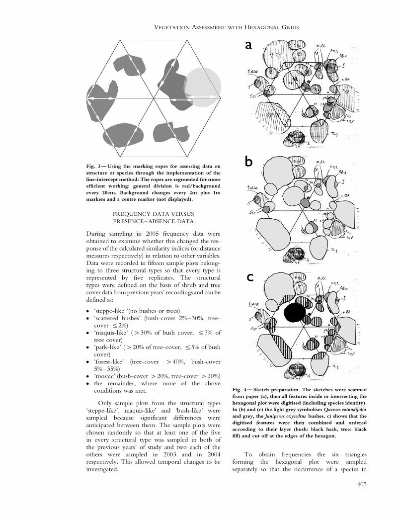
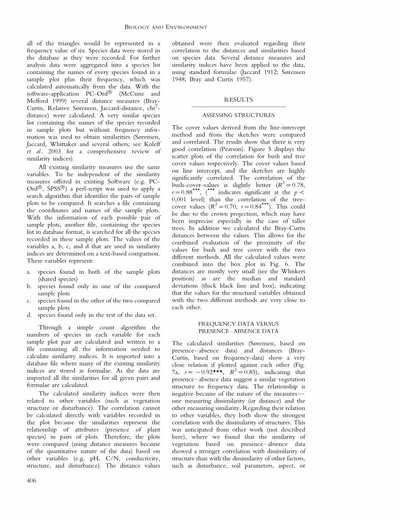
The ropes that were used to mark out the plotsare segmented (alternating red and white every20cm with additional marks at every meter andevery two meters) to facilitate recording. For eachrope the proportion covered by a certain featurewas assessed and recorded in a checklist (Fig. 3).The cover value for a certain feature on the sampleplot was later calculated automatically inside thedatabase by summing up the proportions on thetwelve lines. For analysis regarding the quality ofthe line-intercept method we only used the covervalues of the bushes and trees because thesematched the sketched features. The sketching ofthe proportion of open soil, open stones and

Asphodelus microcarpa would have been very timeconsuming and too elaborate to undertake.

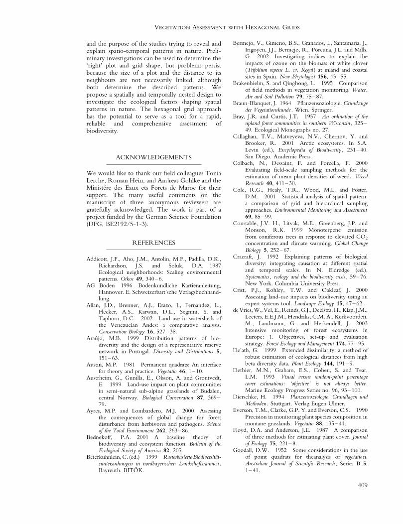
Figure 4 shows the steps in the preparation ofthe sketches. These were scanned and geo-referenced in ArcMAP† (part of the ArcGIS†

package from ESRI, which was also used for thefollowing procedures). The elements recorded weredigitised separately for each species and sample plot.All features occurring fully or partly inside a plotwere mapped. In the data-table belonging to thecreated shape-file (.shp) further information(vegetation layer, height, etc.) was assigned to thedigitised features to enable later queries. The shapefiles were then merged into a single file. Due to theimplementation of a global identifier, it is stillpossible to separate the shapes by their sample plotcode, vegetation layer, height and species.

All parts of the shapes outside the hexagonalplot were cut off at the edges so that only thoseparts inside were included in further analysis. As wewere interested in the cover of bushes and treesregardless of species identity we combined thespecies and ordered them in relation to theirpresence in the vegetation layers. Based on this,the polygons of a sample plot were combined intoone single shape, which allowed the calculation of asingle value per sample plot for the area covered bya certain feature (bush or tree).

a

b

c

Fig. 2* Nested sampling design. Inside the investigation area (a: side length 3000m, area 23.38km2) plots are arranged in

a regular hexagonal grid. Inside each plot (b: side length 120m, area 3.74ha), sample plots are located, and each of these

contains sub-plots (c). The sample plots have a side length of 8m (area 166m2). One side of the sub-plot measures 0.6m,

area is about 0.94m2). One of the sub-plots is filled black.

404


FREQUENCY DATA VERSUS

PRESENCE�ABSENCE DATA

During sampling in 2005 frequency data wereobtained to examine whether this changed the res-ponse of the calculated similarity indices (or distancemeasures respectively) in relation to other variables.Data were recorded in fifteen sample plots belong-ing to three structural types so that every type isrepresented by five replicates. The structuraltypes were defined on the basis of shrub and treecover data from previous years’ recordings and can bedefined as:

. ‘steppe-like ‘(no bushes or trees)

. ‘scattered bushes’ (bush-cover 2%�30%, tree-cover 5/2%)

. ‘maquis-like’ (�/30% of bush cover, 5/7% oftree cover)

. ‘park-like’ (�/20% of tree-cover, 5/5% of bushcover)

. ‘forest-like’ (tree-cover �/40%, bush-cover5%�35%)

. ‘mosaic’ (bush-cover �/20%, tree-cover �/20%)

. the remainder, where none of the aboveconditions was met.

Only sample plots from the structural types‘steppe-like’, maquis-like’ and ‘bush-like’ weresampled because significant differences wereanticipated between them. The sample plots werechosen randomly so that at least one of the fivein every structural type was sampled in both ofthe previous years’ of study and two each of theothers were sampled in 2003 and in 2004respectively. This allowed temporal changes to beinvestigated.

To obtain frequencies the six trianglesforming the hexagonal plot were sampledseparately so that the occurrence of a species in

Fig. 3* Using the marking ropes for assessing data on

structure or species through the implementation of the

line-intercept method: The ropes are segmented for more

efficient working: general division is red/background

every 20cm. Background changes every 2m plus 1m

markers and a centre marker (not displayed).

Fig. 4* Sketch preparation. The sketches were scanned

from paper (a), then all features inside or intersecting the

hexagonal plot were digitised (including species identity).

In (b) and (c) the light grey symbolises Quercus rotundifolia

and grey, the Juniperus oxycedrus bushes. c) shows that the

digitised features were then combined and ordered

according to their layer (bush: black hash, tree: black

fill) and cut off at the edges of the hexagon.

405


all of the triangles would be represented in afrequency value of six. Species data were stored inthe database as they were recorded. For furtheranalysis data were aggregated into a species listcontaining the names of every species found in asample plot plus their frequency, which wascalculated automatically from the data. With thesoftware-application PC-Ord† (McCune andMefford 1999) several distance measures (Bray-Curtis, Relative Sørensen, Jaccard-distance, chi2-distance) were calculated. A very similar specieslist containing the names of the species recordedin sample plots but without frequency infor-mation was used to obtain similarities (Sørensen,Jaccard, Whittaker and several others; see Koleffet al . 2003 for a comprehensive review ofsimilarity indices).

All existing similarity measures use the samevariables. To be independent of the similaritymeasures offered in existing Software (e.g. PC-Ord†, SPSS†) a perl-script was used to apply asearch algorithm that identifies the pairs of sampleplots to be compared. It searches a file containingthe coordinates and names of the sample plots.With the information of each possible pair ofsample plots, another file, containing the specieslist in database format, is searched for all the speciesrecorded in these sample plots. The values of thevariables a, b, c, and d that are used in similarityindices are determined on a text-based comparison.These variables represent:

a. species found in both of the sample plots(shared species)

b. species found only in one of the comparedsample plots

c. species found in the other of the two comparedsample plots

d. species found only in the rest of the data set.

Through a simple count algorithm thenumbers of species in each variable for eachsample plot pair are calculated and written to afile containing all the information needed tocalculate similarity indices. It is imported into adatabase file where many of the existing similarityindices are stored as formulae. As the data areimported all the similarities for all given pairs andformulae are calculated.

The calculated similarity indices were thenrelated to other variables (such as vegetationstructure or disturbance). The correlation cannotbe calculated directly with variables recorded inthe plot because the similarities represent therelationship of attributes (presence of plantspecies) in pairs of plots. Therefore, the plotswere compared (using distance measures becauseof the quantitative nature of the data) based onother variables (e.g. pH, C/N, conductivity,structure, and disturbance). The distance values

obtained were then evaluated regarding theircorrelation to the distances and similarities basedon species data. Several distance measures andsimilarity indices have been applied to the data,using standard formulae (Jaccard 1912; Sørensen1948; Bray and Curtis 1957).

RESULTS


The cover values derived from the line-interceptmethod and from the sketches were comparedand correlated. The results show that there is verygood correlation (Pearson). Figure 5 displays thescatter plots of the correlation for bush and treecover values respectively. The cover values basedon line intercept, and the sketches are highlysignificantly correlated. The correlation of thebush-cover-values is slightly better (R2�/0.78,r�/0.88***, (*** indicates significant at the p B/

0,001 level) than the correlation of the tree-cover values (R2�/0.70, r�/0.84***). This couldbe due to the crown projection, which may havebeen imprecise especially in the case of tallertrees. In addition we calculated the Bray-Curtisdistances between the values. This allows for thecombined evaluation of the proximity of thevalues for bush and tree cover with the twodifferent methods. All the calculated values werecombined into the box plot in Fig. 6. Thedistances are mostly very small (see the Whiskersposition) as are the median and standarddeviations (thick black line and box), indicatingthat the values for the structural variables obtainedwith the two different methods are very close toeach other.

FREQUENCY DATA VERSUS

PRESENCE� ABSENCE DATA

The calculated similarities (Sørensen, based onpresence� absence data) and distances (Bray-Curtis, based on frequency-data) show a veryclose relation if plotted against each other (Fig.7a, r�/�/0.92***, R2�/0.85), indicating thatpresence� absence data suggest a similar vegetationstructure to frequency data. The relationship isnegative because of the nature of the measures*one measuring dissimilarity (or distance) and theother measuring similarity. Regarding their relationto other variables, they both show the strongestcorrelation with the dissimilarity of structures. Thiswas anticipated from other work (not describedhere), where we found that the similarity ofvegetation based on presence� absence datashowed a stronger correlation with dissimilarity ofstructure than with the dissimilarity of other factors,such as disturbance, soil parameters, aspect, or

406


slope. The Bray-Curtis distances (R2�/0.35, r�/

0.59***) perform moderately better in this regardthan the Sørensen similarities (R2�/0.26, r�/

�/0.51***, see Fig. 7b and 7c), suggesting aslightly better relationship with frequency datacompared to presence� absence data. Overall,these analyses suggest that recording presence�absence results in only a slight reduction in usefulinformation compared to the more time consumingmeasurements of frequency.

DISCUSSION


The comparison of the structural variablesrecorded with the line-intercept method andwith the sketches reveals a very close relationshipbetween the respective values. This is trueregardless of the technique used to compare thetwo methods. This indicates that the recording of

structural features in the hexagonal plot withthe line-intercept method is a very reliable andefficient method to quantitatively characterisevegetation structure. It can be completed in just20% of the time needed for the sketches (allworking steps summarised), which makes it arealistic and labour-saving alternative. It alsoprovides possibilities elsewhere. In a recent studyin a Tundra-ecosystem, where micro-relief hasan important ecological function (e.g. Matveyeva1988; Walker 1995; Callaghan et al . 2001),Rettenmaier (2004) showed that it is also possi-ble to assess surface roughness using a slightlyadapted hexagonal plot sampling methodology.The ratio between the length of a ropefollowing all the surface bumps and hollows tothe direct distance was successfully used toquantify surface roughness. In this case themethodology also allowed for the assessment ofthe proportions of bare fine substrate, open stones,vegetation-covered stones, small ponds and boggydepressions.

As the ropes cross the plot through the centreand at the perimeter, the structural variables areassessed systematically and exactly. They are valid atthe sampling location on which they were recordedeven though there might be some auto-correlationbecause of the geographical proximity of the lines(which may be considered as short transects). Thesketches that were made during the first field seasonprovide a more exact basis for structural data butrequire much more work both in the field and inthe lab. As we wanted to provide a methodologythat minimises effort while giving sufficiently

Bra

y-C

urtis

-Dis

tanc

e

1.0

.9

.8

.7

.6

.5

.4

.3

.2

.1

0.0

Fig. 6* Distances (dissimilarity) between the values for

the cover of trees and bushes combined derived with line-

intercept method and from the sketches (n�/57). The

thick line represents the median, the box represents the

interquartile range. Whiskers are extremes. The ‘x’ is an

outlier.

0

0,1

0,2

0,3

0,4

0,5

0,6

bush

cov

er (

sket

ch)

0 0,1 0,2 0,3 0,4 0,5tree cover (line-intercept)

Rsqr = 0,70r = 0,84***n = 57

0

0,1

0,2

0,3

0,4

0,5

0,6

tree

cov

er (

sket

ch)

0 0,1 0,2 0,3 0,4 0,5 0,6 0,7bush cover (line-intercept)

Rsqr = 0,78r = 0,88***n = 83

Fig. 5* Correlation between the values derived from the

assessment of structures via the line-intercept method and

the sketches based on bush and tree cover values

respectively. ‘r ’ is the Pearson correlation coefficient;

the line is the regression line. ‘n ’ is less for tree cover

values because not all plots incorporated in the analysis

actually had trees.

407


accurate data on biodiversity and environment, theline-intercept approach on the hexagonal plotseems to be a very efficient and easily appliedmethod.

FREQUENCY VERSUS PRESENCE�ABSENCE

DATA

We have shown that the results obtained on thebasis of frequency data and presence� absence datarespectively differ only slightly regarding thecorrelation between similarity (or dissimilarity) ofvegetation and distance values based on otherenvironmental variables. However, additionalinformation is obtained if quantitative data onspecies are used. Furthermore we have to admitthat the six-triangle method produces very coarsefrequency values. It is very likely that even moreinformation could be obtained through a finerresolution of frequency values, although thiswould increase the effort required. We also foundthat for the methodology presented here theadditional information obtained using frequencyvalues at a finer resolution does not reflect theincrease in effort required for data recording(Beierkuhnlein 1999; Neßhover 1999; Retzer1999), which is much greater compared to theassessment of presence� absence data.

Similar arguments apply in regard to covervalues. Since one of our major objectives is thedevelopment of a comprehensive and reproduciblemethod to assess spatial patterns of biodiversity, weavoided using cover values because they are oftenfound to be highly variable. This is because theydepend on the recorder, time of day, vegetationheight and other factors (Dierschke 1994; Mueller-Dombois and Ellenberg 1974). Even thoughsubjective methods might be as precise asobjective methods under certain circumstances(Floyd and Anderson 1987; Dethier et al . 1993;Kent and Coker 1994; Brakenhielm and Qinghong1995) we think that it is more appropriate to usevery simple methods, especially whenimplementing long term monitoring. If a lot ofsampling must be done in as short a time aspossible* as is often the case with systematicsampling grids* it is better to use presence�absence data instead, particularly if they comparewell with other, much more elaborate and time-consuming approaches.

CONCLUSIONS

The systematic sampling on a hexagonal grid is agood way to reveal patterns of biodiversity and torelate them to other environmental variables. Herewe presented results showing that hexagonal plotsprovide several advantages. However, it is mostimportant to state that the patterns that emerge-are dependent on the scale of observation. Bydeciding on the sampling design we, as scientists,predetermine which patterns are found. Conse-quently, it is crucial to accurately define the scope

0,25

0,3

0,35

0,4

0,45

0,5

0,55

0,6

0,65

0,7

0,75

0,8

0 0,1 0,2 0,3 0,4 0,5 0,6 0,7 0,8 0,9Bray-Curtis Structure

Sør

ense

n V

eget

atio

n

RSqr = 0,26r (Pearson) = -0,51***

0,25

0,3

0,35

0,4

0,45

0,5

0,55

0,6

0,65

0,7

0,75

0,8

0 0,1 0,2 0,3 0,4 0,5 0,6 0,7 0,8 0,9Bray-Curtis Structure

Bra

y-C

urtis

Veg

etat

ion

RSqr = 0,35r (Pearson) = 0,59***

0,25

0,3

0,35

0,4

0,45

0,5

0,55

0,6

0,65

0,7

0,4

a

b

c

0,45 0,5 0,55 0,6 0,65 0,7 0,75 0,8Sørensen Vegetation

Bra

y-C

urtis

Veg

etat

ion

RSqr = 0,85r (Pearson) = -0,92***

Fig. 7* Frequency versus presence� absence data: (a)

The distance values (Bray-Curtis) plotted against the

similarity values (Sørensen) reveals close relation

between these different methods; (b) Bray-Curtis

distance on structural variables plotted against Bray-

Curtis distance based on frequency species data; (c) the

Bray-Curtis distances based on structural variables plotted

against Sørensen similarity based on presence� absence

species data.

408


and the purpose of the studies trying to reveal andexplain spatio-temporal patterns in nature. Preli-minary investigations can be used to determine the‘right’ plot and grid shape, but problems persistbecause the size of a plot and the distance to itsneighbours are not necessarily linked, althoughboth determine the described patterns. Wepropose a spatially and temporally nested design toinvestigate the ecological factors shaping spatialpatterns in nature. The hexagonal grid approachhas the potential to serve as a tool for a rapid,reliable and comprehensive assessment ofbiodiversity.

ACKNOWLEDGEMENTS

We would like to thank our field colleagues ToniaLerche, Roman Hein, and Andreas Gohlke and theMinistere des Eaux ets Forets de Maroc for theirsupport. The many useful comments on themanuscript of three anonymous reviewers aregratefully acknowledged. The work is part of aproject funded by the German Science Foundation(DFG, BE2192/5-1-3).

REFERENCES

Addicott, J.F., Aho, J.M., Antolin, M.F., Padilla, D.K.,Richardson, J.S. and Soluk, D.A. 1987Ecological neighborhoods: Scaling environmentalpatterns. Oikos 49, 340� 6.

AG Boden 1996 Bodenkundliche Kartieranleitung,Hannover. E. Schweizerbart’sche Verlagsbuchhand-lung.

Allan, J.D., Brenner, A.J., Erazo, J., Fernandez, L.,Flecker, A.S., Karwan, D.L., Segnini, S. andTaphorn, D.C. 2002 Land use in watersheds ofthe Venezuelan Andes: a comparative analysis.Conservation Biology 16, 527� 38.

Araujo, M.B. 1999 Distribution patterns of bio-diversity and the design of a representative reservenetwork in Portugal. Diversity and Distributions 5,151� 63.

Austin, M.P. 1981 Permanent quadrats: An interfacefor theory and practice. Vegetatio 46, 1� 10.

Austrheim, G., Gunilla, E., Olsson, A. and Grontvedt,E. 1999 Land-use impact on plant communitiesin semi-natural sub-alpine grasslands of Budalen,central Norway. Biological Conservation 87, 369�79.

Ayres, M.P. and Lombardero, M.J. 2000 Assessingthe consequences of global change for forestdisturbance from herbivores and pathogens. Scienceof the Total Environment 262, 263� 86.

Bednekoff, P.A. 2001 A baseline theory ofbiodiversity and ecosystem function. Bulletin of theEcological Society of America 82, 205.

Beierkuhnlein, C. (ed.) 1999 Rasterbasierte Biodiversitat-suntersuchungen in nordbayerischen Landschaftsraumen .Bayreuth. BITOK.

Bermejo, V., Gimeno, B.S., Granados, I., Santamaria, J.,Irigoyen, J.J., Bermejo, R., Porcuna, J.L. and Mills,G. 2002 Investigating indices to explain theimpacts of ozone on the biomass of white clover(Trifolium repens L. cv. Regal ) at inland and coastalsites in Spain. New Phytologist 156, 43� 55.

Brakenhielm, S. and Qinghong, L. 1995 Comparisonof field methods in vegetation monitoring. Water ,Air and Soil Pollution 79, 75� 87.

Braun-Blanquet, J. 1964 Pflanzensoziologie. Grundzugeder Vegetationskunde . Wien. Springer.

Bray, J.R. and Curtis, J.T. 1957 An ordination of theupland forest communities in southern Wisconsin , 325�49. Ecological Monographs no. 27.

Callaghan, T.V., Matveyeva, N.V., Chernov, Y. andBrooker, R. 2001 Arctic ecosystems. In S.A.Levin (ed.), Encyclopedia of Biodiversity , 231� 40.San Diego. Academic Press.

Colbach, N., Dessaint, F. and Forcella, F. 2000Evaluating field-scale sampling methods for theestimation of mean plant densities of weeds. WeedResearch 40, 411� 30.

Cole, R.G., Healy, T.R., Wood, M.L. and Foster,D.M. 2001 Statistical analysis of spatial pattern:a comparison of grid and hierarchical samplingapproaches. Environmental Monitoring and Assessment69, 85� 99.

Constable, J.V. H., Litvak, M.E., Greenberg, J.P. andMonson, R.K. 1999 Monoterpene emissionfrom coniferous trees in response to elevated CO2

concentration and climate warming. Global ChangeBiology 5, 252� 67.

Cracraft, J. 1992 Explaining patterns of biologicaldiversity: integrating causation at different spatialand temporal scales. In N. Eldredge (ed.),Systematics , ecology and the biodiversity crisis , 59� 76.New York. Columbia University Press.

Crist, P.J., Kohley, T.W. and Oakleaf, J. 2000Assessing land-use impacts on biodiversity using anexpert systems tool. Landscape Ecology 15, 47� 62.

de Vries, W., Vel, E.,Reinds, G.J., Deelstra, H., Klap, J.M.,Leeters, E.E.J.M., Hendriks, C.M. A., Kerkvoorden,M., Landmann, G. and Herkendell, J. 2003Intensive monitoring of forest ecosystems inEurope: 1. Objectives, set-up and evaluationstrategy. Forest Ecology and Management 174, 77� 95.

De’ath, G. 1999 Extended dissimilarity: a method ofrobust estimation of ecological distances from highbeta diversity data. Plant Ecology 144, 191� 9.

Dethier, M.N., Graham, E.S., Cohen, S. and Tear,L.M. 1993 Visual versus random-point percentagecover estimations: ‘objective’ is not always better .Marine Ecology Progress Series no. 96, 93� 100.

Dierschke, H. 1994 Planzensoziologie. Grundlagen undMethoden . Stuttgart. Verlag Eugen Ulmer.

Everson, T.M., Clarke, G.P. Y. and Everson, C.S. 1990Precision in monitoring plant species composition inmontane grasslands. Vegetatio 88, 135� 41.

Floyd, D.A. and Anderson, J.E. 1987 A comparisonof three methods for estimating plant cover. Journalof Ecology 75, 221� 8.

Goodall, D.W. 1952 Some considerations in the useof point quadrats for theanalysis of vegetation.Australian Journal of Scientific Research , Series B 5,1� 41.

409


Gottfried, M., Pauli, H. and Grabherr, G. 1998

Prediction of vegetation patterns at the limits of

plant life: A new view of the alpine-nival ecotone.

Arctic and Alpine Research 30, 207� 21.Grime, J.P. 1998 Benefits of plant diversity to eco-

systems: immediate, filter and founder effects. Journal

of Ecology 86, 902� 10.Hannah, L., Midgley, G.F. and Millar, D. 2002

Climate change-integrated conservation strategies.

Global Ecology and Biogeography 11, 485� 95.Hart, M.M., Reader, R.J. and Klironomos,

J.N. 2001 Biodiversity and ecosystem function:

alternate hypotheses or a single theory? Bulletin of the

Ecological Society of America 82, 88� 90.Hattenschwiler, S. and Korner, C. 2003 Does

elevated CO2 facilitate naturalization of the non-

indigenous Prunus laurocerasus in Swiss temperate

forests? Functional Ecology 17, 778� 85.Higgins, M.A. and Ruokolainen, K. 2004 Rapid

tropical forest inventory: a comparison of

techniques based on inventory data from western

Amazonia. Conservation Biology 18, 799� 811.Jaccard, P. 1912 The distribution of the flora of the

alpine zone. New Phytologist 11, 37� 50.Kent, M. and Coker, P. 1994 Vegetation description and

analysis: a practical approach . London. Publisher.Kipfmueller, K.F. and Baker, W.L. 1998 A

comparison of three techniques to date stand-

replacing fires in lodgepole pine forests. Forest

Ecology and Management 104, 171� 7.Kluth, C. and Bruelheide, H. 2004 Using standar-

dized sampling designs from population ecology

to assess biodiversity patterns of therophyte

vegetation across scales. Journal of Biogeography 31,

363� 77.Koleff, P., Gaston, K.J. and Lennon, J.J. 2003

Measuring beta diversity for presence� absence

data. Journal of Animal Ecology 72, 367� 82.Korner, C. 2003 Carbon limitation in trees. Functional

Ecology 91, 4� 17.Krishnamani, R., Kumar, A. and Harte, J. 2004

Estimating species richness at large spatial scales

using data from small discrete plots. Ecography 27,

637� 42.Leps, J. 1992 How reliable are our vegetation

analyses. Journal of Vegetation Science 3, 119� 24.Lister, A.J., Mou, P.P., Jones, R.H. and Mitchell,

R.J. 2000 Spatial patterns of soil and vegetation

in a 40-year-old slash pine (Pinus elliottii ) forest in

the Costal Plain of South Carolina, U.S.A. Canadian

Journal of Forest Research-Revue Canadienne de

Recherche Forestiere 30, 145� 55.Matveyeva, N.V. 1988 The horizontal structure of

tundra communities. In H.J. During, H.J.A. Werger

and H.J. Williams (eds), Diversity and pattern in

plant communities, 59� 66. Den Haag. SPB

Academic Publishing.McCune, B. and Mefford, M.J. 1999 Multivariate

analysis of ecological data. Glenedon Beach, Oregon.

MjM Software.Mueller-Dombois, D. and Ellenberg, H. 1974 Aims

and methods of vegetation ecology . New York. Wiley.

Nekola, J.C. and White, P.S. 1999 The distancedecay of similarity in biogeography and ecology.Journal of Biogeography 26, 867� 78.

Neßhover, C. 1999 Charakterisierung der Vegetatio-nsdiversitat durch funktionelle Attribute vonPflanzen* am Beispiel eines Landschaftsausschnittesder Nordlichen Frankenalb. In C. Beierkuhnlein(ed.), Rasterbasierte Biodiversitatsuntersuchungen innordbayerischen Landschaftsraumen , 1� 114. Bayreuth.BITOK*Bayreuther Institut fur terrestrischeOkosystemforschung.

Olsvig-Whittaker, L. 1988 Relating small-scalevegetation patterns to the environment. In H.J.During, H.J.A. Werger and H.J. Williams (eds)Diversity and pattern in plant communities, 87� 94.Den Haag. SPB.

Pitkanen, S. 1998 The use of diversity indices toassess the diversity of vegetation in managed borealforests. Forest Ecology and Management 112, 121� 37.

Rettenmaier, N. 2004 Raumliche Muster derBiodiversitat in der skandinavischen Tundra.Unpublished diploma thesis, Universitat Bayreuth,Lehrstuhl fur Biogeografie.

Retzer, V. 1999 Charakterisierung und Vergleich derVegetationsdiversitat zweier Kulturlandschaften*Untersuchungen anhand einer systematischenRastermethode in Frankenalb und Fichtelge-birge. In C. Beierkuhnlein (ed.), RasterbasierteBiodiversitatsuntersuchungen in nordbayerischen Land-schaftsraumen , 117� 206 S. Bayreuth. BITOK*Bayreuther Institut fur terrestrische Okosystem-forschung.

Richerson, P.J. and Lum, K.-L. 1980 Patterns ofplant species diversity in California: relation toweather and topography. The American Naturalist116, 504� 36.

Sala, O.E., Chapin, F.S., Armesto, J.J., Berlow, E.,Bloomfield, J., Dirzo, R., Huber-Sanwald, E.,Huenneke, L.F., Jackson, R.B., Kinzig, A.,Leemans, R., Lodge, D.M., Mooney, H.A.,Oesterheld, M., Poff, N.L., Sykes, M.T., Walker,B.H., Walker, M. and Wall, D.H. 2000Biodiversity* global biodiversity scenarios for theyear 2100. Science 287, 1770� 4.

Schulze, E.-D. and Mooney, H.A. (eds) 1993Biodiversity and ecosystem function . Berlin, Heidel-berg. Springer.

Singer, M.C., Stefanescu, C. and Pen, I. 2002 Whenrandom sampling does not work: standard designfalsely indicates maladaptive host preferences in abutterfly. Ecology Letters 5, 1� 6.

Sørensen, T. 1948 A method of establishing groups ofequal amplitude in plant sociology based onsimilarity of species content. Biologiske Skrifter 5,1� 34.

Tilman, D. and Elhaddi, A. 1992 Drought andbiodiversity in grasslands. Oecologia 89, 257� 64.

Traxler, A. 1998 Handbuch des vegetationsokologis-chen Monitorings. Methoden, Praxis, angewandteProjekte. Teil A � Methoden. Wien. Umwelt-bundesamt.

Tuxen, R. 1972 Kritische Bemerkungen zurInterpretation pflanzensoziologischer Tabellen. InE. van der Maarel and R. Tuxen (eds), Grundfragen

410


und Methoden in der Pflanzensoziologie , 168� 82. DenHaag. Junk.

Valdes, B., Rejdali, M., Achhal EL Kadmiri, A., Jury, J.L.and Montserrat, J.M. (eds) 2002 Checklist ofvascular plants of N Morocco with identificationkeys. Madrid. Consejo Superior de InvestigacionesCientificas.

van der Maarel, E. 1976 On the establishment ofplant community boundaries. Berichte der DeutschenBotanischen Gesellschaft 89, 415� 43.

Walker, M.D. 1995 Patterns and causes of arctic plantcommunity diversity. In F.S. Chapin and C. Korner(eds), Arctic and Alpine biodiversity: patterns , causes andecosystem consequences , 3� 20. Berlin. Springer.

411


Spatial Patterns of Biodiversity–Assessing Vegetation Using Hexagonal Grids

Documents

Transcript of Spatial Patterns of Biodiversity–Assessing Vegetation Using Hexagonal Grids