
Applying Constructionist Design Methodology to Agent-Based Simulation Systems
Upload
khangminh22Category
view
0download
0
Stefan Kern BSc.
Spatial enabled Agent-based Modeling and Simulation of a Production Environment
Master's degree programme: Geomatics Science
Ass.Prof. Dipl.-Ing (FH) Dr.techn. Johannes Scholz
Institute of Geodesy
Master of Science
Graz, September, 2018
EIDESSTATTLICHE ERKLÄRUNG
AFFIDAVIT
Ich erkläre an Eides statt, dass ich die vorliegende Arbeit selbstständig verfasst,
andere als die angegebenen Quellen/Hilfsmittel nicht benutzt, und die den benutzten
Quellen wörtlich und inhaltlich entnommenen Stellen als solche kenntlich gemacht
habe. Das in TUGRAZonline hochgeladene Textdokument ist mit der vorliegenden
Masterarbeit identisch.
I declare that I have authored this thesis independently, that I have not used other
than the declared sources/resources, and that I have explicitly indicated all material
which has been quoted either literally or by content from the sources used. The text
document uploaded to TUGRAZonline is identical to the present master‘s thesis.
Datum / Date Unterschrift / Signature
ii
Abstract
Industry 4.0 and digitization are terms that have become increasingly im-portant in recent years. These terms also include ideas and concepts toincrease the efficiency of production plants. This thesis deals with Industry4.0 in particular with the term Smart Factory, with the goal of being ableto simulate a semiconductor production process virtually. This modeling isagent-based since this approach is suitable for implementing the idea of asmart factory, taking into account the conditions of semiconductor produc-tion. For this purpose, a modeling concept is presented which combines theaspects of Industry 4.0 and agent-based modeling. This approach is furtherimplemented and analyzed in the form of a prototype. With this model, wetry to create an efficient production environment in which the workers coveras short distances as possible and the available machines and interim storagefacilities are used as efficiently as possible. On the one hand, the work showshow such an environment is modulated, but also how data can be obtainedfrom it. By the captured data it is analyzed whether the chosen approachbrings advantages for the production but also how the received informationcan be used to improve the production process.
iii
Zusammenfassung
Industrie 4.0 und Digitalisierung sind Begriffe, die in den letzten Jahrenimmer mehr an Bedeutung gewonnen haben. Unter anderem beschaftigensie sich mit Ideen und Konzepten, welche die Effizienz von Produktionsan-lagen erhohen. Diese Masterarbeit beschaftigt sich mit Industrie 4.0 - imSpeziellen mit dem Konzept Smart Factory - um einen Halbleiterproduktion-sprozess virtuell nachzubilden und simulieren zu konnen. Diese Modellierungerfolgt agentenbasiert, da sich dieser Ansatz dazu eignet, die Idee von einerSmart Factory unter Berucksichtigung der Gegebenheiten einer Halbleiter-produktion umzusetzen. Zu diesem Zweck wird ein Modellierungskonzeptvorgestellt, welches die Aspekte von Industrie 4.0 und agentenbasierter Mod-ellierung miteinander vereint. Dieser Ansatz wird in weiter Folge in Formeines Prototyps umgesetzt und analysiert. Mit diesem Prototyp wird ver-sucht, eine effiziente Produktionsumgebung zu schaffen, in der die Arbeit-er/innen moglichst kurze Strecken zurucklegen und die zur Verfugung ste-henden Maschinen und Zwischenlager effizient genutzt werden konnen. DieMasterarbeit zeigt einerseits, wie eine solche Umgebung moduliert wird, aberauch, wie daraus Daten gewonnen werden konnen. Anhand der erhobenenDaten wird in weiter Folge analysiert, ob der gewahlte Ansatz Vorteile furdie Produktion bringt und wie die gewonnen Informationen dazu genutztwerden konnen, den Produktionsprozess zu verbessern.
iv
Acknowledgements
I would like to take this opportunity to thank all those who, through theirprofessional and personal support for the success of this thesis. First I wouldlike to meet my supervisor Ass.Prof. Dipl.-Ing. (FH) Dr.techn. JohannesScholz, who enabled me to work on this topic. I appreciate that he alwaystook the time to answer my questions and help me with constructive sug-gestions. A big thank you goes to my family and friends who have alwayssupported me and are therefore an important part of this work. Finally, Iwould like to thank my fellow students and the scientific staff of the GrazUniversity of Technology for making these years of study a wonderful andunforgettable time.
v
Contents
List of Abbreviations xi
1 Introduction 11.1 Motivation . . . . . . . . . . . . . . . . . . . . . . . . . . . . 11.2 Goals . . . . . . . . . . . . . . . . . . . . . . . . . . . . . . . 31.3 Approach . . . . . . . . . . . . . . . . . . . . . . . . . . . . . 31.4 Literature . . . . . . . . . . . . . . . . . . . . . . . . . . . . . 4
2 Theory 62.1 Industry 4.0 . . . . . . . . . . . . . . . . . . . . . . . . . . . . 6
2.1.1 Definition . . . . . . . . . . . . . . . . . . . . . . . . . 62.1.2 Internet of Things and Cyber-physical systems . . . . 82.1.3 Smart factory . . . . . . . . . . . . . . . . . . . . . . . 9
2.2 Agent-based modeling and simulation . . . . . . . . . . . . . 112.2.1 Areas of Application . . . . . . . . . . . . . . . . . . . 122.2.2 Advantages of agent-based modeling. . . . . . . . . . . 122.2.3 Limitation of agent-based models . . . . . . . . . . . . 152.2.4 Structure of an agent-based model . . . . . . . . . . . 152.2.5 Agents . . . . . . . . . . . . . . . . . . . . . . . . . . . 162.2.6 Agent behavior and relationships . . . . . . . . . . . . 182.2.7 Environment . . . . . . . . . . . . . . . . . . . . . . . 212.2.8 Design an agent-based model . . . . . . . . . . . . . . 212.2.9 Software and Toolkits . . . . . . . . . . . . . . . . . . 242.2.10 ABMS in GIScience . . . . . . . . . . . . . . . . . . . 26
3 Approach 293.1 Basic knowledge for the concept . . . . . . . . . . . . . . . . . 293.2 Agents and functions . . . . . . . . . . . . . . . . . . . . . . . 303.3 Manufacturing control . . . . . . . . . . . . . . . . . . . . . . 313.4 Model concept . . . . . . . . . . . . . . . . . . . . . . . . . . 333.5 Implementation and testing . . . . . . . . . . . . . . . . . . . 35
4 Modeling and implementation 364.1 Structure of the model . . . . . . . . . . . . . . . . . . . . . . 364.2 Agents, attributes and other important parts . . . . . . . . . 37
4.2.1 Worker . . . . . . . . . . . . . . . . . . . . . . . . . . 394.2.2 Tools . . . . . . . . . . . . . . . . . . . . . . . . . . . 414.2.3 Products . . . . . . . . . . . . . . . . . . . . . . . . . 43
vi

Contents vii
4.2.4 Stocks . . . . . . . . . . . . . . . . . . . . . . . . . . . 444.2.5 Environment . . . . . . . . . . . . . . . . . . . . . . . 454.2.6 Manufacturing control . . . . . . . . . . . . . . . . . . 45
4.3 Implementation in Repast Simphony . . . . . . . . . . . . . . 514.4 Process overview . . . . . . . . . . . . . . . . . . . . . . . . . 524.5 Initialization . . . . . . . . . . . . . . . . . . . . . . . . . . . 54
4.5.1 Date base . . . . . . . . . . . . . . . . . . . . . . . . . 554.6 Manufacturing control . . . . . . . . . . . . . . . . . . . . . . 594.7 Transport . . . . . . . . . . . . . . . . . . . . . . . . . . . . . 60
4.7.1 Movement model . . . . . . . . . . . . . . . . . . . . . 604.8 Manufacture . . . . . . . . . . . . . . . . . . . . . . . . . . . 624.9 Model output . . . . . . . . . . . . . . . . . . . . . . . . . . . 63
4.9.1 Characteristics of the model . . . . . . . . . . . . . . . 634.9.2 Heatmap . . . . . . . . . . . . . . . . . . . . . . . . . 654.9.3 Time series . . . . . . . . . . . . . . . . . . . . . . . . 67
5 Generation of test data 685.1 Test data . . . . . . . . . . . . . . . . . . . . . . . . . . . . . 685.2 Verification, calibration and validation . . . . . . . . . . . . . 70
6 Results 756.1 General Scenario . . . . . . . . . . . . . . . . . . . . . . . . . 756.2 Effect of additional information on simulation . . . . . . . . . 816.3 Improvement of the simulation scenario based on the results . 86
7 Summary and outlook 887.1 Summary . . . . . . . . . . . . . . . . . . . . . . . . . . . . . 887.2 Outlook . . . . . . . . . . . . . . . . . . . . . . . . . . . . . . 89
Bibliography 90

List of Figures
2.1 The four stages of industrial revolutions. (modified from(Spath, Gerlach, Hammerle, Krause, & Schlund, 2013)) . . . 7
2.2 Industry 4.0 framework (PwC, 2016) . . . . . . . . . . . . . . 72.3 Schematic structure of an element in the Internet of Things
(IoT) (modified from Albach, Meffert, Pinkwart, and Ralf(2015). . . . . . . . . . . . . . . . . . . . . . . . . . . . . . . . 9
2.4 Reference architecture for a smart factory (modified fromShrouf, Ordieres, and Miragliotta (2014) . . . . . . . . . . . . 10
2.5 Illustration of an agent (modified from (Macal & North, 2010)) 182.6 Example of interaction between agents. Each agent uses de-
fined rules to interact (Heppenstall & Crooks, 2016). . . . . . 192.7 Basic forms of environment and topology in ABM (modified
from Macal and North (2009b)) . . . . . . . . . . . . . . . . . 202.8 ABM applications with different spatial and temporal scale
(Crooks, 2009) . . . . . . . . . . . . . . . . . . . . . . . . . . 262.9 Schematic representation of common Agent-based modeling
(ABM) problems (O’Sullivan, Millington, Perry, & Wain-wright, 2012) . . . . . . . . . . . . . . . . . . . . . . . . . . . 27
3.1 Agents in manufacturing control (Leitao, 2009) . . . . . . . . 323.2 Process control overview . . . . . . . . . . . . . . . . . . . . . 333.3 Schematic model process . . . . . . . . . . . . . . . . . . . . . 34
4.1 Class diagram of the model with the most important functionsand attributes of each agent class. . . . . . . . . . . . . . . . 38
4.2 Schematic overview of the agent class worker . . . . . . . . . 404.3 Schematic overview of the agent class Tool . . . . . . . . . . . 424.4 Flowchart of the class Process Control, when calling the get-
work function . . . . . . . . . . . . . . . . . . . . . . . . . . 464.5 Process overview of the function Transport to stock . . . . . 504.6 The schematic flow diagram of the model. Shown are the
processes (yellow), the classes / agents (blue) and the database / output (gray). . . . . . . . . . . . . . . . . . . . . . . . 53
4.7 Schematic sequence of data initialization. The input datamust be processed in order. . . . . . . . . . . . . . . . . . . . 54
4.8 Example of navigation using waypoints . . . . . . . . . . . . . 614.9 Concept for avoiding obstacles . . . . . . . . . . . . . . . . . 62
viii
List of Figures ix
4.10 Example of heatmap . . . . . . . . . . . . . . . . . . . . . . . 66
5.1 Test environment for the model . . . . . . . . . . . . . . . . . 695.2 Presentation of the modeling process (Crooks, Heppenstall,
& Malleson, 2018) . . . . . . . . . . . . . . . . . . . . . . . . 705.3 Test environment for model verification . . . . . . . . . . . . 71
6.1 Distance travelled by workers . . . . . . . . . . . . . . . . . . 766.2 Density of product movement . . . . . . . . . . . . . . . . . . 776.3 Status of the tools during simulation . . . . . . . . . . . . . . 786.4 Time series of machines and stocks . . . . . . . . . . . . . . 796.5 Production time of the products . . . . . . . . . . . . . . . . 806.6 Status of products during simulation . . . . . . . . . . . . . . 816.7 Comparison of runtime of simulation scenarios . . . . . . . . 836.8 Comparison of product data from four test runs . . . . . . . . 846.9 Comparison of worker behavior . . . . . . . . . . . . . . . . . 856.10 Comparison of tool data from four test runs . . . . . . . . . . 856.11 Comparison of tool data . . . . . . . . . . . . . . . . . . . . . 86
List of Tables
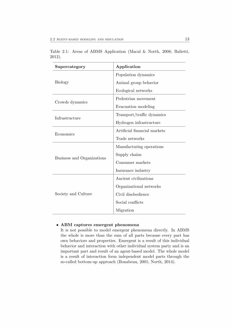
2.1 Areas of Agent-based modeling and simulation (ABMS) Ap-plication (Macal & North, 2008; Balietti, 2012). . . . . . . . . 13
2.2 The elements of the Overview, Design concepts, Details (ODD)protocol (Grimm & Railsback, 2012) . . . . . . . . . . . . . . 23
2.3 Five ABM toolkits in comparison (De Smith, Goodchild, &Longley, 2015; Crooks & Heppenstall, 2012) . . . . . . . . . . 25
3.1 Comparison of traditional and agent-based approach (Leitao,2009) . . . . . . . . . . . . . . . . . . . . . . . . . . . . . . . . 32
4.1 Description of the agent classes and their task . . . . . . . . . 394.2 Description of the attribute myStatus of the class tools. . . . 424.3 Description of the attribute myStatus of the class product.
Status with position information. . . . . . . . . . . . . . . . . 434.4 Description of the attribute myStatus of the class product.
Status with transport information with loaded worker. . . . . 444.5 Description of the attribute myStatus of the class product.
Status for transport information with unloaded worker. . . . 444.6 Overview of the weighting options of the simulation. . . . . . 484.7 Tabular process overview of the model. . . . . . . . . . . . . . 524.8 Structure and description of the input grid. . . . . . . . . . . 554.9 Description of the user input . . . . . . . . . . . . . . . . . . 584.10 Description of the user input for model testing . . . . . . . . 59
5.1 Settings of runs with extreme values . . . . . . . . . . . . . . 72
6.1 Simulation settings . . . . . . . . . . . . . . . . . . . . . . . . 766.2 Simulation settings . . . . . . . . . . . . . . . . . . . . . . . . 826.3 Comparison of number of machines and simulation time . . . 86
x
List of Abbreviations
ABM Agent-based modeling
ABMS Agent-based modeling and simulation
ABS Agent-based simulation
AI Artificial intelligence
GIS Geographical information system
IBM Individual-based modeling
ODD Overview, Design concepts, Details
OOP Object oriented programming
UML Unified Modeling Language
ID Identifier
GIScience Geographic information science
API Application Programming Interface
CPS Cyber-Physical Systems
IoT Internet of Things
PGM Portable Gray Map
GUI Graphical user interface
xi
Chapter 1
Introduction
1.1 Motivation
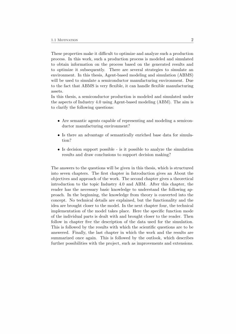
In modern industry, production time is an important cost factor. Therefore,it is important to optimize the production process. Additionally, there isa need for higher efficiency in manufacturing processes. In order to do so,modeling and simulation of the production environment is a possible option.This topic is part of the field Industry 4.0. The term defines the convergenceof communication, information and industrial production (Hermann, Pentek,& Otto, 2016). In Industry 4.0 humans, production assets and products com-municate and cooperate with each other to optimize the production process.These types of production environments are called “Smart Factories” (“Plat-tform Industrie 4.0,” 2018). The arrival of the Internet of Things (IoT)inproduction marks the beginning of the fourth industrial revolution. Ma-chines and production plants have intelligence and communicate with eachother and with people. They are able to make autonomous decisions andcontrol themselves and each other. This allows them to act flexibly fromchanges in production and to choose alternative ways to achieve their goalsindependently. In addition, all data is available in real time. Industry 4.0brings, and intelligent factories bring great potential into production (Hen-ning, Wolfgang, & Johannes, 2013).A special form of production is semiconductor production. The semicon-ductor manufacturing is very flexible due to the following reasons (Scholz &Schabus, 2014a):
• Depending on the product, the overall processing time can vary fromseveral days to a couple of weeks.
• For one product to be produced, several hundred production steps arenecessary.
• For the same production step, several different tools can be used.These tools can also vary in processing time and quality.
• There are many production assets for the different degrees of comple-tion.
1
1.1 Motivation 2
These properties make it difficult to optimize and analyze such a productionprocess. In this work, such a production process is modeled and simulatedto obtain information on the process based on the generated results andto optimize it subsequently. There are several strategies to simulate anenvironment. In this thesis, Agent-based modeling and simulation (ABMS)will be used to simulate a semiconductor manufacturing environment. Dueto the fact that ABMS is very flexible, it can handle flexible manufacturingassets.In this thesis, a semiconductor production is modeled and simulated underthe aspects of Industry 4.0 using Agent-based modeling (ABM). The aim isto clarify the following questions:
• Are semantic agents capable of representing and modeling a semicon-ductor manufacturing environment?
• Is there an advantage of semantically enriched base data for simula-tion?
• Is decision support possible - is it possible to analyze the simulationresults and draw conclusions to support decision making?
The answers to the questions will be given in this thesis, which is structuredinto seven chapters. The first chapter in Introduction gives an About theobjectives and approach of the work. The second chapter gives a theoreticalintroduction to the topic Industry 4.0 and ABM. After this chapter, thereader has the necessary basic knowledge to understand the following ap-proach. In the beginning, the knowledge from theory is converted into theconcept. No technical details are explained, but the functionality and theidea are brought closer to the model. In the next chapter four, the technicalimplementation of the model takes place. Here the specific function modeof the individual parts is dealt with and brought closer to the reader. Thenfollow in chapter five the description of the data used for the simulation.This is followed by the results with which the scientific questions are to beanswered. Finally, the last chapter in which the work and the results aresummarized once again. This is followed by the outlook, which describesfurther possibilities with the project, such as improvements and extensions.
1.2 Goals 3
1.2 Goals
The main goal of this thesis is the modeling and simulation of a semiconduc-tor production environment. This model is based on the aspects of industry4.0 and smart factory. The modeling is agent-based, which means, amongother things, the control of the production process is decentralized. In thisworker, three central questions are to be clarified.
• The first question is about the model and the process of modeling itself.It should clarify whether agents are able to represent a semiconductorproduction environment. This is a central question because it containsthe complete thesis. The clarification of this question begins with theliterature study and thus has a decisive influence on the concept of themodel. Finally, this question is answered by validating the model withreal data.
• The second question is about the model. The aim is to clarify whetherit is advantageous if semantically enriched data is available for thesimulation. These can be data about the intermediate storage work-ers, machinery, products or the environment. The influence of suchadditional information will be clarified in the context of this work.
• The last question is to clarify which data can be generated from themodel and how it can be used. Is it possible to analyze the simulationresults and draw conclusions to support decision making? The decisionmaking concerns the planning of production. This should optimizethe production process and thus also increase production. The actualoptimization is not the goal of these workers. However, it should beshown that the model provides data to perform an optimization.
1.3 Approach
The following items will point out, how the answers to the scientific questionscan be found. They will also be the approach to reach the desired results:
Basic knowledge for the concept. Here the goal is to collect the neces-sary basic knowledge. The focus is on the knowledge about industry4.0, smart factory and ABM. This includes the literature but also thechoice of a suitable software environment for the implementation. Themost important literature for the work is mentioned in Section 1.4.Also, the components of the model are worked out at this point. Thedescription is still conceptual and will be elaborated in the followingsteps.
1.4 Literature 4
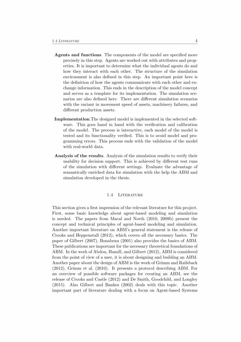
Agents and functions. The components of the model are specified moreprecisely in this step. Agents are worked out with attributes and prop-erties. It is important to determine what the individual agents do andhow they interact with each other. The structure of the simulationenvironment is also defined in this step. An important point here isthe definition of how the agents communicate with each other and ex-change information. This ends in the description of the model conceptand serves as a template for its implementation. The simulation sce-narios are also defined here. There are different simulation scenarioswith the variant in movement speed of assets, machinery failures, anddifferent production assets.
Implementation.The designed model is implemented in the selected soft-ware. This goes hand in hand with the verification and calibrationof the model. The process is interactive, each model of the model istested and its functionality verified. This is to avoid model and pro-gramming errors. This process ends with the validation of the modelwith real-world data.
Analysis of the results. Analysis of the simulation results to verify theirusability for decision support. This is achieved by different test runsof the simulation with different settings. Evaluate the advantage ofsemantically enriched data for simulation with the help the ABM andsimulation developed in the thesis.
1.4 Literature
This section gives a first impression of the relevant literature for this project.First, some basic knowledge about agent-based modeling and simulationis needed. The papers from Macal and North (2010, 2009b) present theconcept and technical principles of agent-based modeling and simulation.Another important literature on ABM’s general statement is the release ofCrooks and Heppenstall (2012), which covers all the necessary basics. Thepaper of Gilbert (2007), Bonabeau (2001) also provides the basics of ABM.These publications are important for the necessary theoretical foundations ofABM. In the work of Abdou, Hamill, and Gilbert (2012), ABM is consideredfrom the point of view of a user, it is about designing and building an ABM.Another paper about the design of ABM is the work of Grimm and Railsback(2012), Grimm et al. (2010). It presents a protocol describing ABM. Foran overview of possible software packages for creating an ABM, see therelease of Crooks and Castle (2012) and De Smith, Goodchild, and Longley(2015). Also Gilbert and Bankes (2002) deals with this topic. Anotherimportant part of literature dealing with a focus on Agent-based Systems
1.4 Literature 5
for manufacturing Monostori, Kumara, and Vancza (2006), Negmeldin andEltawil (2015) and Leitao (2009). This work is important for the conceptionof the model, which is created in the context of this thesis.The second important part of the thesis and an essential part of the projectis Industry 4.0. The article by Drath and Horch (2014) and Albach, Meffert,Pinkwart, and Ralf (2015) contains an overview of digitization and industry4.0. Another basis for the work is provided by the paper of Hermann etal. (2016), in which the basic principles and the structure of an industry4.0 scenario are presented. The basic structure of a Smart factory and anexample are also presented. Another important term is IoT this topic iscovered in the work of Mattern and Floerkemeier (2010). Another veryimportant literature is the publication of Shrouf, Ordieres, and Miragliotta(2014). It explains the topic of industry 4.0 but above all the term smartfactory.
Chapter 2
Theory
This chapter provides the theoretical overview of Industry 4.0 and Agent-based modeling (ABM). An introduction to the Industry 4.0 and Smartfactory can be found in Section 2.1. An introduction and description of thebasic features of ABM can be found in Section 2.2.This is followed 2.2.4 byan overview of the most important basic elements of this modeling approach.Section 2.2.8 shows a method for correctly describing an ABM. Section 2.2.9provides an overview and comparison of the current ABM platforms. Toconclude this chapter, ABM is considered in section 2.2.10 in the context ofGeographic information science (GIScience) and a Geographical informationsystem (GIS).
2.1 Industry 4.0
This chapter deals with the term industry 4.0, followed by an introductionto the basic topics covered in the thesis.
2.1.1 Definition
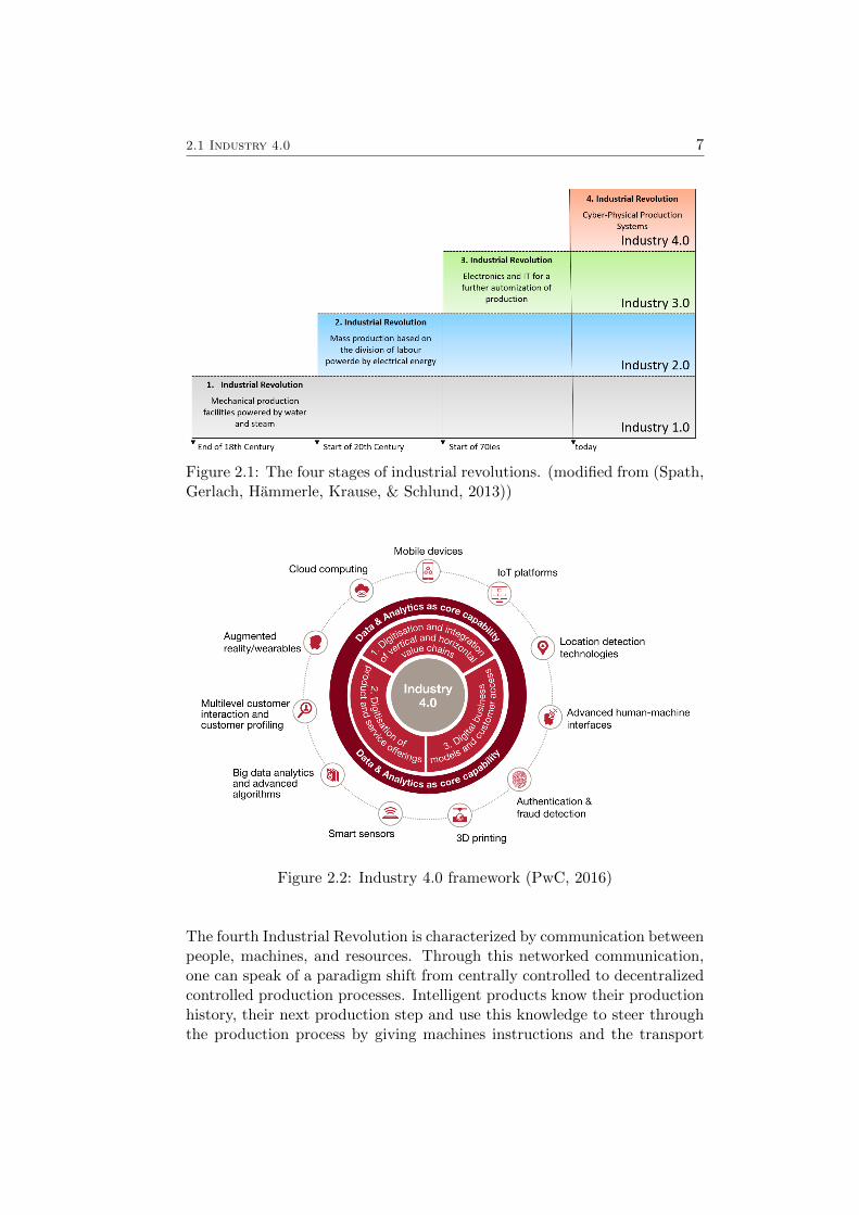
The term Industry 4.0 stands for the fourth industrial revolution. Figure2.1 shows the development of the industry after the introduction of mechan-ical production plants using the water and steam power (first revolution),the introduction of mass production by means of electric energy (secondrevolution), the use of electronics and IT for automation (third revolution),The fourth revolution is characterized by networking and communicatingsystems using the latest internet technology (Roth, 2016). Figure ?? showsa framework for Industry 4.0 as defined by PwC (2016), but it can be seenthat a variety of technologies are involved in building an Industry 4.0 envi-ronment. The most important basis is the data analysis. The data comesfrom different technologies, such as sensors, mobile devices and many more.The interaction takes place through the digitization of services, products,production and the entire value chain (PwC, 2016).
6
2.1 Industry 4.0 7
Figure 2.1: The four stages of industrial revolutions. (modified from (Spath,Gerlach, Hammerle, Krause, & Schlund, 2013))
Figure 2.2: Industry 4.0 framework (PwC, 2016)
The fourth Industrial Revolution is characterized by communication betweenpeople, machines, and resources. Through this networked communication,one can speak of a paradigm shift from centrally controlled to decentralizedcontrolled production processes. Intelligent products know their productionhistory, their next production step and use this knowledge to steer throughthe production process by giving machines instructions and the transport
2.1 Industry 4.0 8
system the goal for the next work step (Albach et al., 2015). There havebeen many publications on the term Industry 4.0, in the work of Hermann etal. (2016), Internet of Things (IoT), Cyber-Physical Systems (CPS), CloudComputing and Smart Factories have been defined as the most importantcomponents. These terms are treated below to better understand the ideabehind the term Industry 4.0.
2.1.2 Internet of Things and Cyber-physical systems
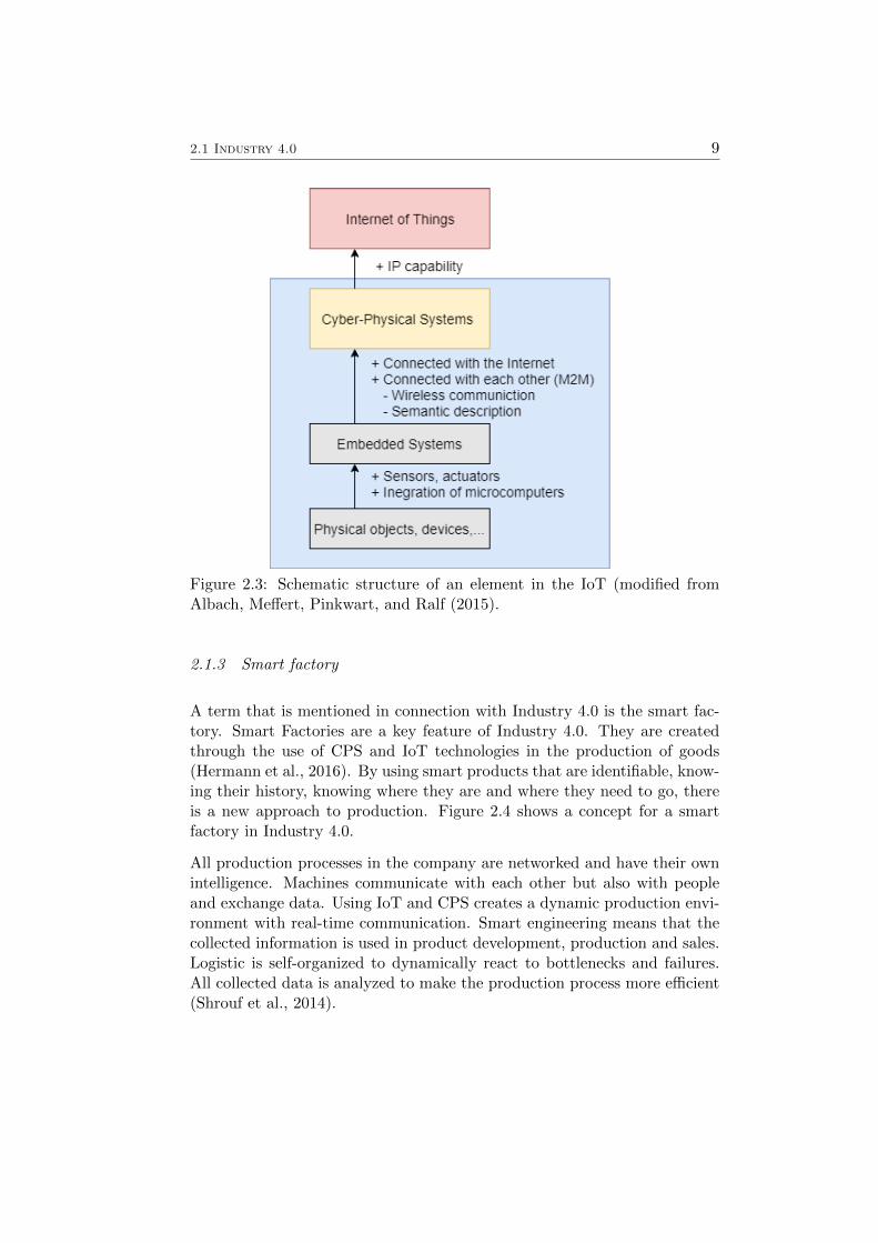
The IoT is the key to the Fourth Industrial Revolution (Henning et al.,2013). There are several definitions for the term IoT, (van Kranenburg &Dodson, 2008) defines the IoT as a global, dynamic network structure withself-configuring capabilities, in which physical and virtual ”things”have iden-tities, physical attributes, and virtual personalities, and intelligent interfacesare integrated into an information network. That means, things use the in-ternet to communicate and share information. These things exchange dataand create opportunities for more direct integration of the physical worldinto computerized systems. This should lead to efficiency improvements,economic benefits, and reduced human intervention (Mattern & Floerke-meier, 2010). Figure 2.3 shows the parts of an object in IoT. These areobjects that are equipped with sensors and actuators. The resulting systemis able to collect, process, and store data to affect itself or the environment.This turns objects into smart objects and environments into smart envi-ronments. If one connects such an embedded system to each other or theInternet and makes its data and capabilities available as online services, theresult is a digital revaluation of an object. By expanding with digital fea-tures, a physical object turns into a CPS. Such a CPS automatically collectsdata about their real environment and digital processes As the number ofdata increases; cloud computing can help. The data is then stored in a cen-tral location. This large amount of data can then be analyzed to gain newinformation (Albach et al., 2015). Thus, a CPS can communicate as com-ponents with mechanical and electronic parts that communicate over a datainfrastructure, such as the internet. In a manufacturing environment, suchcyber-physical systems may be, for example, intelligent machines, storagesystems, and manufacturing facilities that can exchange information, initi-ate actions, and control each other. This results in an improvement of thecomplete industrial process of a company. This includes areas such as man-ufacturing, supply and lifecycle management, and materials management(Henning et al., 2013). In the Internet of Things, Data, and Services, eachdevice can exchange information with any other device or person anywherein the world.
2.1 Industry 4.0 9
Figure 2.3: Schematic structure of an element in the IoT (modified fromAlbach, Meffert, Pinkwart, and Ralf (2015).
2.1.3 Smart factory
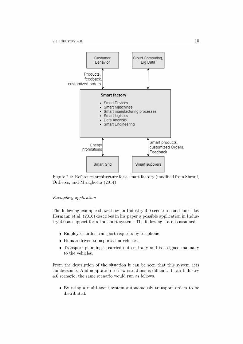
A term that is mentioned in connection with Industry 4.0 is the smart fac-tory. Smart Factories are a key feature of Industry 4.0. They are createdthrough the use of CPS and IoT technologies in the production of goods(Hermann et al., 2016). By using smart products that are identifiable, know-ing their history, knowing where they are and where they need to go, thereis a new approach to production. Figure 2.4 shows a concept for a smartfactory in Industry 4.0.
All production processes in the company are networked and have their ownintelligence. Machines communicate with each other but also with peopleand exchange data. Using IoT and CPS creates a dynamic production envi-ronment with real-time communication. Smart engineering means that thecollected information is used in product development, production and sales.Logistic is self-organized to dynamically react to bottlenecks and failures.All collected data is analyzed to make the production process more efficient(Shrouf et al., 2014).
2.1 Industry 4.0 10
Figure 2.4: Reference architecture for a smart factory (modified from Shrouf,Ordieres, and Miragliotta (2014)
Exemplary application
The following example shows how an Industry 4.0 scenario could look like.Hermann et al. (2016) describes in his paper a possible application in Indus-try 4.0 as support for a transport system. The following state is assumed:
• Employees order transport requests by telephone
• Human-driven transportation vehicles.
• Transport planning is carried out centrally and is assigned manuallyto the vehicles.
From the description of the situation it can be seen that this system actscumbersome. And adaptation to new situations is difficult. In an Industry4.0 scenario, the same scenario would run as follows.
• By using a multi-agent system autonomously transport orders to bedistributed.
2.2 Agent-based modeling and simulation 11
• Self-optimization leads to efficient use of resources.
• Use the smart phone for transport orders
• Vehicles are Autonomous guided.
• Structure as a modular system.
To improve the situation, a multi-agent system is used. Multi-agent sys-tems are computer systems in which autonomous agents to achieve commongoals. Each agent makes its own decisions. This is a decentralized control.Agent systems are discussed in detail in the following chapter 2.2. An im-portant prerequisite for this scenario is the communication flow. Automatedvehicles can easily be connected via communication technologies. However,humans need a user interface for communication. An important basis for theimplementation of such a scenario is the ability of all actors to share and re-ceive information. Such as the position and the order of each vehicle. Sinceeach vehicle knows the other vehicles about others and also knows the openorders, it can independently carry out open work. Thus, a decentralizedsystem is created.
2.2 Agent-based modeling and simulation
Agent-based modeling and simulation (ABMS) is an approach to simulatecomplex processes. It is a quite novel approach with increasing attentionover the past decade. In publications ABMS is also known as Agent-basedsimulation (ABS), ABM or Individual-based modeling (IBM). ABMS isconnected to fields like computer science, system dynamics, management,science, social science, Artificial intelligence (AI), robotics and many more.The most common use of ABMS is to model and simulate human behaviorswith individual decision-making, to represent social interactions, group be-havior, and collaboration (Macal & North, 2010, 2009b).Agent-based modeling and simulation is a computational approach, to modeland simulate dynamic processes with one or more autonomous agents. Insuch a model, agents are interacting among themselves and with a simulationenvironment. Agents can represent humans, vehicles, tools, geographical en-tities like an area or other abstract entities (Macal & North, 2013). ABMSis a bottom-up approach, this means that individual agent decisions andactions affect the resulting system (Crooks, Castle, & Batty, 2008). Withthis approach, it is possible to model the dynamic behaviors of multiple in-dividual agents in an artificial world. Each agent has behavior rules. Agentsmay influence other agents and change the environment by their behavior.(Crooks & Heppenstall, 2012).
2.2 Agent-based modeling and simulation 12
To model and simulate complex behaviors are just one part for ABMS an-other is to capture the emergence. Emergence is an important behaviorwhich is not explicitly modeled. It appears because of agent interactionsin the running model. This output is essential for further research of themodel (Macal & North, 2013). ABMS simulations are depending on time.The simulation is continued until a termination condition, or a final condi-tion is met. The simulation is often a process over a timeline, activity-based,steps over time or a discrete-event simulation (Macal & North, 2010, 2013).
2.2.1 Areas of Application
Agent-based models are used for a wide variety of topics and specialist work.However, all models have in common that self-acting objects are modeled.These objects all have their behavior and rules. Among other things, themodels themselves can be different in the modeling of physical or social space(Crooks & Heppenstall, 2012). According to Macal and North (2008) andBalietti (2012), the application of ABM is based on various topics. Table2.1 lists some of these areas. The list is not complete and shows only a cutof possible applications.
2.2.2 Advantages of agent-based modeling.
In literature, there are two different types of ABM, either with own ad-vantages and disadvantages. De Smith et al. (2015) separates ABM in anexploratory and a predictive model. In the exploratory modeling approach,the ABM is used to understand the observations, phenomena, and processes.The focus is on a specific part of the system. This will create conditions tounderstand individual phenomena better. Important to mention, in thisapproach, it is not intended to simulate future conditions, but the focusis on the understanding of observation. The potential disadvantage of thisapproach is the lack of analytical methods for empirically evaluating ABMresults. The second is the predictive modeling approach. Prediction modelsare used to extrapolate trends, predict future conditions and evaluate differ-ent simulation scenarios. These models are designed to mimic the real worldor systems. Due to changes in the rules of behavior and/or initial states,effects are observed and evaluated.In literature, there are three advantages of ABM over other modeling tech-niques (Bonabeau, 2001; De Smith et al., 2015).
2.2 Agent-based modeling and simulation 13
Table 2.1: Areas of ABMS Application (Macal & North, 2008; Balietti,2012).
Supercategory Application
Biology
Population dynamics
Animal group behavior
Ecological networks
Crowds dynamicsPedestrian movement
Evacuation modeling
InfrastructureTransport/traffic dynamics
Hydrogen infrastructure
EconomicsArtificial financial markets
Trade networks
Business and Organizations
Manufacturing operations
Supply chains
Consumer markets
Insurance industry
Society and Culture
Ancient civilizations
Organizational networks
Civil disobedience
Social conflicts
Migration
• ABM captures emergent phenomenaIt is not possible to model emergent phenomena directly. In ABMSthe whole is more than the sum of all parts because every part hasown behaviors and properties. Emergent is a result of this individualbehavior and interaction with other individual system party and is animportant part and result of an agent-based model. The whole modelis a result of interaction form independent model parts through theso-called bottom-up approach (Bonabeau, 2001; North, 2014).
2.2 Agent-based modeling and simulation 14
• ABM provides a natural description of a systemABM is usually the most natural approach to describe and simulate asystem of discrete entities, because there is a correspondence betweenthe real world and the agent-based model. Objects of the real world aredescribed as ontologically appropriate agents in the form of programcode. This property is called ontological correspondence With ABMobjects will be observed instead of variables(Gilbert, 2007). The be-havior of the subjects to be modeled and facts are usually complicated.Such a nonlinear discontinuous behavior is difficult to describe withconventional methods such as differential equation systems. The ABMapproach makes it easier to describe complex structures. (Bonabeau,2001), (De Smith et al., 2015). With ABM complex systems are mod-eled form bottom up in the form of individual objects with their ownattributes, behavior, relations, and properties. The individuals withtheir activities are at the center of this approach, and this is a morenatural way than describing system processes (Bonabeau, 2001). ABMis a natural way of describing the simulation environment. The envi-ronment again consists of entities that can represent the real world.Therefore, ABM is well-behaved to simulate people and their envi-ronment (De Smith et al., 2015), since the environment can also beimplemented with physical barriers or resources, which can affect agentbehavior (Gilbert, 2007). Furthermore, agents can have the ability tolearn about other agents and their environment (Abdou et al., 2012).The ability to present moving agents makes behaviors easier to under-stand for the viewer. To model such complex ABM systems, Objectoriented programming (OOP) is used, because it is are crucial to agent-based modeling. In OOP languages, objects with their own attributesand methods are used, like agents in ABM. Therefore, almost all ABSmodels are programmed in OOP languages, and ABM software toolk-its are built on such a programming language (Abdou et al., 2012).
• ABM is flexibleWith ABM, it’s easy to add more agents or change attributes. It’salso easy to get the agents into a different environment. All of thiscan change the behavior of the system. As a result, small changes canchange the behavior and complexity of the entire model. This featureof ABM makes this model approach very flexible (Bonabeau, 2001),(De Smith et al., 2015). Another possibility, which the model simplychanges is to change the behavior of the agents or to experiment withthe agents in groups. Thus completely new points of view on a topiccan be realized (De Smith et al., 2015).
2.2 Agent-based modeling and simulation 15
2.2.3 Limitation of agent-based models
ABM offers the possibility to model and simulate complex systems, but alsohas some limitations. An important point to note is the purpose of themodel. The model is only as useful as the purpose for which it was created(De Smith et al., 2015). As with other modeling techniques, it is importantto choose the right level of detail for the desired purpose. (Couclelis, 2000).Another difficulty is the modeling of systems themselves. So it is oftendifficult to implement the behavior, attributes, and interactions because thisinformation is often difficult to quantify from the real world. Therefore, themodeling behavior is often difficult to calibrate and to verify (De Smith etal., 2015). With ABM complex systems and conditions can be modeled. Asa result, the validation and verification of the model are similarly complexand requires a lot of time (Cooley & Solano, 2011). In addition, agent-based models can be harder to analyze, understand, and communicate thantraditional analytic/mathematical models. Another factor is the computingpower, the high computational effort of ABM remains a limitation in themodeling of large systems (Grimm, 1999) (De Smith et al., 2015). Anotherfactor is the emergence. As mentioned, this is not modeled directly but arisesfrom the system behavior of the model. The emergence and the resultingbehavior is often difficult to understand and convey. That’s because it’s notbased on a mathematical/analytic model. Agent-based models can be verysensitive to initial conditions and changes in the interaction rules. Thereforeit is necessary to carry out several simulations runs with different initial data.To evaluate the robustness of the results (De Smith et al., 2015).
2.2.4 Structure of an agent-based model
A typical agent-based model consists of the following three elements (Macal& North, 2010):
• A set of agents with attributes and behaviors
• Agent relationships and rules, which define how other agents and theenvironment behave with the agents
• An environment with which the agents can interact
Another important part of an ABMS is a scheduler. The scheduler brings atime component into the simulation. It is responsible for the chronologicalsuccession in the simulation. The time counter of the simulation usuallyincreases of one unit each step. In each step, the scheduler calls all agents
2.2 Agent-based modeling and simulation 16
in a consistent or randomized order. The agents can also be called by internrules to interact of discrete events (North, 2014).
2.2.5 Agents
There is no precise definition in the literature for the term “agent”. The ex-act definition of an agent does not go far beyond the property of autonomy.Therefore, some authors refer to any form of one autonomously acting com-ponent as agents (Macal & North, 2010). An agent can be any actor whocan influence himself, other agents, or the environment (North, 2014). Mostagents are defined by their properties. So sign (Gilbert, 2007), (Bonabeau,2001) Agents as actors with the following behaviors, they can share in-formation and make actions and decisions dependent on this information.In addition, agents can reproduce, adapt and learn their abilities (Gilbert,2007), (Bonabeau, 2001). Another definition comes from Wooldridge andJennings (1995). He define the agent by using a list of properties. Muchof these properties are found in agents in a variety of ABM models. Thisapproach was picked up and extended by De Smith et al. (2015), Crooks andHeppenstall (2012), and Macal and North (2009b). These defined propertiesare explained in the following list.
• Autonomy: Agents are autonomous units, meaning they do not needcentralized control. They can independently process information andexchange this information with other agents. With this information,they can make independent decisions. You can communicate and in-teract with other agents. Their behavior can influence the simulationand other agents.
• Heterogeneity: This means that the agent represents a single-objectwith its own properties and attributes. Thus, for example, no averageagent must be defined. Each agent is a separate autonomous indi-vidual. However, there may be groups of agents, but these groupsarise due to the bottom-up approach through the union of similar au-tonomous individuals.
• Active: Agents are active and can influence the simulation. Activityis a key factor in ABM and an agent can have the following character-istics
– Pro-active/goal-directed: Agents have goals that they pursue.The agent tries to reach this goal or goals with his behavior.
– Reactive/perceptive: An agent can be designed to perceiveits environment. In this context, it is also possible that an agent

2.2 Agent-based modeling and simulation 17
has prior knowledge of its environment. This may be reflectedin the form of boundaries, obstacles and destination, or in theperception of other agents. This knowledge can be implementedin the form of a map. This allows the agent to avoid obstaclesand find goals. Furthermore, this knowledge can also reflect theperception of other agents.
– Bounded rationality: Agents can have a kind of ”limited” ra-tionality, which is a consequence of their heterogeneity. By doingso, the agents are able to make independently adaptive decisionsabout their goals based on their attributes and goals. This formof ABM model is often found in the context of social sciencesrelated to rational-choice paradigm.
– Interactive/communicative: Agents have the ability to shareinformation with other agents in their neighborhood.
– Mobility: Agents can move the space (environment), in withthey are situated, of a model. But agents can also be stationary.It is thus possible to model any form of moving objects or dynamicbehaviors.
– Adaptation/learning: Agents can be defined to have memoryover old states. As a result, it is possible that the previous stateaffects the current state of the agent. This gives the agent theability to learn. Agents can also be equipped with the ability todevelop their own functionality.
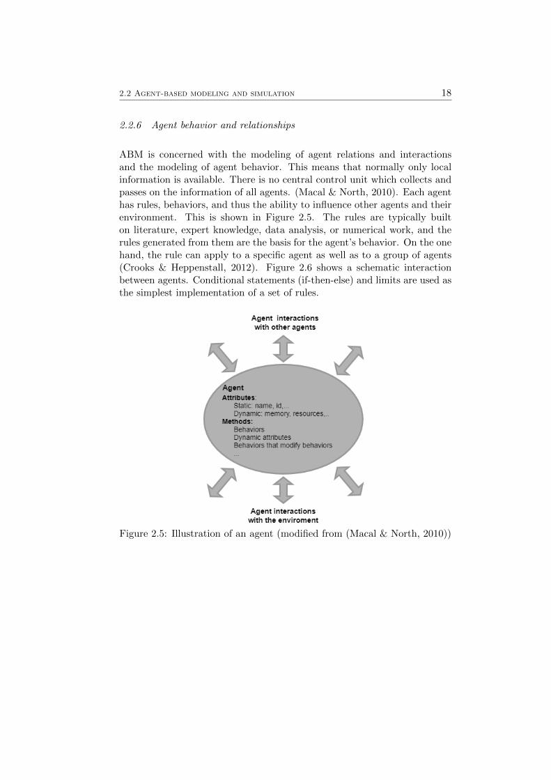
Not all of these properties apply to each agent. It is, therefore, possible foran agent to have only a few of these listed properties. The importance of theindividual properties also varies depending on the application. There canalso be different agents within a model, which differ in their characteristics.The agent can represent any kind of entity. (Crooks & Heppenstall, 2012;Macal & North, 2009a). Figure 2.5 shows an illustration of an agent. Itcontains the basic elements of an agent, which are attributes and methods.Attributes can be fixed static or dynamic, which means that they changeduring the simulation. Through behavioral rules, the agent interacts withother agents or with the environment, which in turn can affect attributes aswell as behavior.
2.2 Agent-based modeling and simulation 18
2.2.6 Agent behavior and relationships
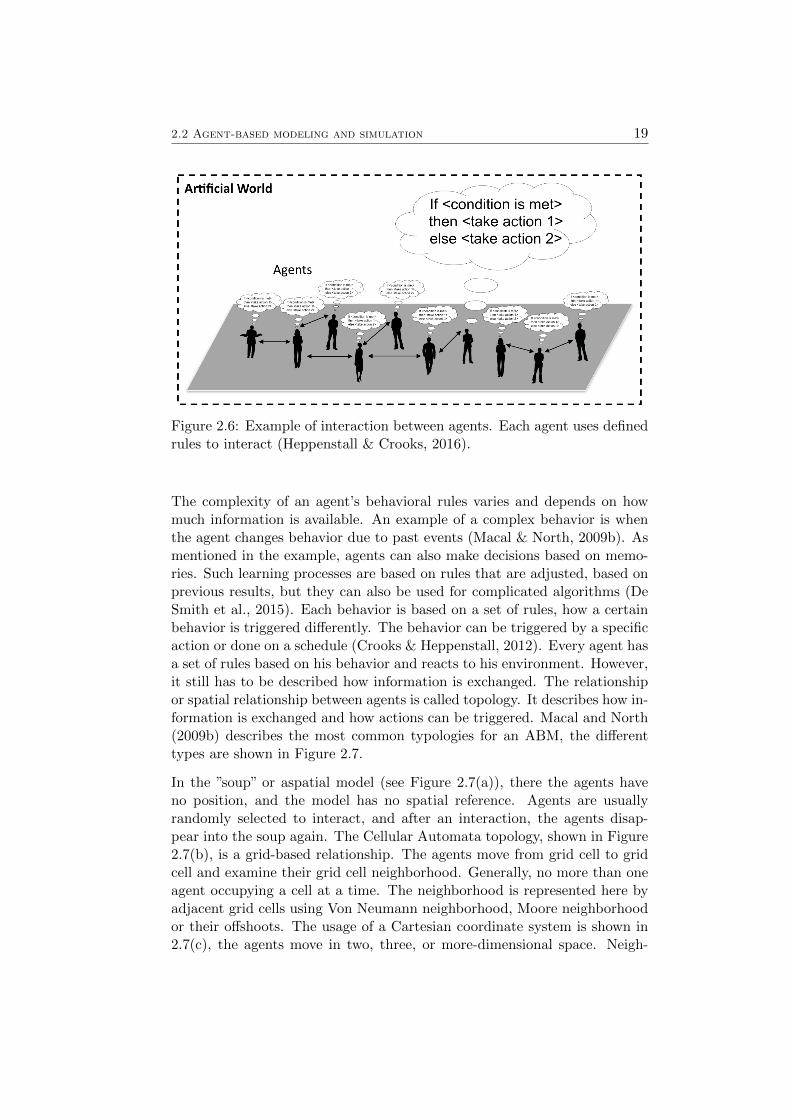
ABM is concerned with the modeling of agent relations and interactionsand the modeling of agent behavior. This means that normally only localinformation is available. There is no central control unit which collects andpasses on the information of all agents. (Macal & North, 2010). Each agenthas rules, behaviors, and thus the ability to influence other agents and theirenvironment. This is shown in Figure 2.5. The rules are typically builton literature, expert knowledge, data analysis, or numerical work, and therules generated from them are the basis for the agent’s behavior. On the onehand, the rule can apply to a specific agent as well as to a group of agents(Crooks & Heppenstall, 2012). Figure 2.6 shows a schematic interactionbetween agents. Conditional statements (if-then-else) and limits are used asthe simplest implementation of a set of rules.
Figure 2.5: Illustration of an agent (modified from (Macal & North, 2010))
2.2 Agent-based modeling and simulation 19
Figure 2.6: Example of interaction between agents. Each agent uses definedrules to interact (Heppenstall & Crooks, 2016).
The complexity of an agent’s behavioral rules varies and depends on howmuch information is available. An example of a complex behavior is whenthe agent changes behavior due to past events (Macal & North, 2009b). Asmentioned in the example, agents can also make decisions based on memo-ries. Such learning processes are based on rules that are adjusted, based onprevious results, but they can also be used for complicated algorithms (DeSmith et al., 2015). Each behavior is based on a set of rules, how a certainbehavior is triggered differently. The behavior can be triggered by a specificaction or done on a schedule (Crooks & Heppenstall, 2012). Every agent hasa set of rules based on his behavior and reacts to his environment. However,it still has to be described how information is exchanged. The relationshipor spatial relationship between agents is called topology. It describes how in-formation is exchanged and how actions can be triggered. Macal and North(2009b) describes the most common typologies for an ABM, the differenttypes are shown in Figure 2.7.
In the ”soup” or aspatial model (see Figure 2.7(a)), there the agents haveno position, and the model has no spatial reference. Agents are usuallyrandomly selected to interact, and after an interaction, the agents disap-pear into the soup again. The Cellular Automata topology, shown in Figure2.7(b), is a grid-based relationship. The agents move from grid cell to gridcell and examine their grid cell neighborhood. Generally, no more than oneagent occupying a cell at a time. The neighborhood is represented here byadjacent grid cells using Von Neumann neighborhood, Moore neighborhoodor their offshoots. The usage of a Cartesian coordinate system is shown in2.7(c), the agents move in two, three, or more-dimensional space. Neigh-

2.2 Agent-based modeling and simulation 20
(a) “Soup” Model, agentswithout spatial referencel
(b) Cellular Automata withgrid cell environment usingthe Von Neumann neighbor-hood as an example.
(c) Euclidean topology in a 2-, 3- or more-dimensional Eu-clidean space.
(d) GIS-topology with a geo-referenced environment allowsspatial relationships .
(e) Network topology: The nodesrepresent the agents and the edgesrepresent the relationships. Thenodes can exist with or withoutspatial reference.
Figure 2.7: Basic forms of environment and topology in ABM (modifiedfrom Macal and North (2009b))
borhood relations here refer to the Euclidean distance between the agents.In the Geographic Information System GIS topology, agents move over ageo-spatial landscape 2.7(d). Relationships can be described via the topo-logical operators like touch, inside, disjoint, etc.. Networks make it possibleto define the environment of an agent more generally and sometimes moreprecisely. In a network topology 2.7(e), networks can be static or dynamic.For static networks, links and nods are predefined and will not change inthe model. For dynamic networks, links and nods can arise and disappearaccording to the mechanisms contained in the model. Regardless of whichtopology is used in an agent-based model, for connecting the agents, the keyidea is local interaction and local information transfer between the agents(Macal & North, 2009b).
2.2 Agent-based modeling and simulation 21
2.2.7 Environment
Gilbert (2007) defines the environment of an agent as the virtual world inwhich he acts. Crooks and Heppenstall (2012) and Macal and North (2010)describe the environment as a space that forms the basis for an agent to actor interact with other agents. The environment can be designed much likean agent, with the difference, that it does not require the ability to interactwith the environment (Abdou et al., 2012). Depending on the model, agentscan change the environment through their behavior (O’Sullivan, Millington,Perry, & Wainwright, 2012). The environment can, in the simplest case, beused to provide the agent with information about his neighborhood. How-ever, as in any GIS, extensive geographic information may be provided tothe agents. The environment can restrict their actions through their designactions. Thus, depending on the position of the agents, or other rules couldbe used. For example, speed restrictions or hints may appear (Macal &North, 2010). In general, the environment is a geographic space with phys-ical features. Such models are considered spatially explicit. But there arealso models in which an abstract environment is used, such as modeling aknowledge space (Gilbert, 2007).
Figure 2.7 shows different types of an ABM environment: An Environmentwithout spatial reference is shown in 2.7(a), this environment is mostly usedfor abstract models. The grid-based environment 2.7(b), defines the posi-tion of agents in a grid. In Euclidean space 2.7(c), the agents act in a twoor more dimensional coordinate coordinate system. Geo-referenced data(2.7(d)) may also be used for the environment. It is also possible to linkABM with a GIS. Another possibility is to create the environment as anetwork (2.7(e)). It will differentiate between networks with and withoutcoordinately known nodes. The choice of suitable topology for the environ-ment is dependent on the model. The topology is important, and thus theenvironment defines how agents interact locally and exchange information.The different types can also be combined as desired (Macal & North, 2009b).
2.2.8 Design an agent-based model
Agent-based models usually consist of different agents. Each agent has itsattributes, rules, and behavior in the environment. Due to this fact the de-scription and communication of an ABM is difficult. A detailed descriptionof an ABM is usually incomplete. Therefore, Grimm and Railsback (2012)have developed a standardized format for describing ABM, the so-calledOverview, Design concepts, Details (ODD) protocol. The ODD protocolattempts to create a generic format and structure to describe and document
2.2 Agent-based modeling and simulation 22
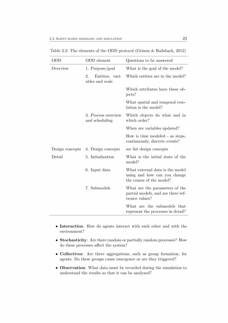
an ABM. The aim of the ODD protocol is to fully describe an ABM as wellas to simplify the writing and reading of a model description (Grimm et al.,2010). In ODD, an ABM is displayed hierarchically. First, an overview ofmodel structure and processes. Then follows a checklist in which the mod-eler shows his design decisions. Due to this, the design should become betterunderstandable. Details and processes are described at the end of the ODDprotocol (Grimm & Railsback, 2012). Table 2.2 shows the structure of theODD protocol.As mentioned above the first part gives an overview of the basic modelstructure. Each model is based on a question, a problem or a hypothe-sis. Therefore, the first point of the ODD protocol is a summary of themodel’s goal. It is important not to describe how it works, but what it isused for. This is followed by the description of entities, state variables, andscales. This includes all agents with their attributes and main variables aswell as the environment. The scale provides information about the spatialand temporal resolution of the model. In the process overview, the basicprocesses are described. This takes the form of keywords such as ”work”,”wait”, ”transport”. The detailed description of this process will follow laterin detail. Here only the expiry of the model is described. The process of themodel is controlled by the scheduler as described in chapter 2.2.4. The order,in which the scheduler calls the agents, performs the process and updatesthe variables, is described in this section (Grimm et al., 2010). The secondpart of the ODD protocol is the design concepts. It will use a checklist tounderstand why the ABM was designed in this way. The design concept isdefined by the following ten points (Grimm & Railsback, 2012):
• Emergence: Which results of the model are caused by the adaptivebehavior of agents. Are these results based on rules and are thereforepredictable?
• Adaptation: Can the agent adjust his behavior over and how arethese actions triggered? Is this behavior influenced by your own actionor by the environment?
• Objectives: Does the agent have a goal which he wants to reach?If an agent has one goal, how to determine whether the objective isachieved?
• Learning: Does the agent change his behavior based on experienceand how does it work?
• Prediction: Can the agent predict future scenarios to make decisions?Which rules or models are available for this?
• Sensing: What information can agents perceive and collect? Will thisinformation be considered for their adaptive behavior and how?
2.2 Agent-based modeling and simulation 23
Table 2.2: The elements of the ODD protocol (Grimm & Railsback, 2012)
ODD ODD element Questions to be answered
Overview 1. Purpose/goal What is the goal of the model?
2. Entities, vari-ables and scale
Which entities are in the model?
Which attributes have these ob-jects?
What spatial and temporal reso-lution is the model?
3. Process overviewand scheduling
Which objects do what and inwhich order?
When are variables updated?
How is time modeled - as steps,continuously, discrete events?
Design concepts 4. Design concepts see list design concepts
Detail 5. Initialization What is the initial state of themodel?
6. Input data What external data is the modelusing and how can you changethe course of the model?
7. Submodels What are the parameters of thepartial models, and are there ref-erence values?
What are the submodels thatrepresent the processes in detail?
• Interaction: How do agents interact with each other and with theenvironment?
• Stochasticity: Are there random or partially random processes? Howdo these processes affect the system?
• Collectives: Are there aggregations, such as group formation, foragents. Do these groups cause emergence or are they triggered?
• Observation: What data must be recorded during the simulation tounderstand the results so that it can be analyzed?
2.2 Agent-based modeling and simulation 24
Describing a model does not always require all of the listed concepts. Partsthat are not needed for the description can be omitted. However, conceptssuch as: emergence, interaction, randomness, and perception are emerging inevery model (Grimm & Railsback, 2012). The last part of the ODD proto-col contains a detailed description of the model. It first describes the initialstatus of the model. As mentioned in the description of ABM, small changesin the initial state can have an impact on the simulation results. Therefore,it is important to define the initial state. The next item is the descriptionof external data sources which will be used during the simulation or initial-ization, as well as a description of how the data will be exchanged. In thelast part, the section ”Process overview and scheduling” describes in detailwhich processes exist and how they are tested. The detailed description ofthe ODD protocol can be found in the paper Grimm et al. (2010) or Grimmand Railsback (2012).
2.2.9 Software and Toolkits
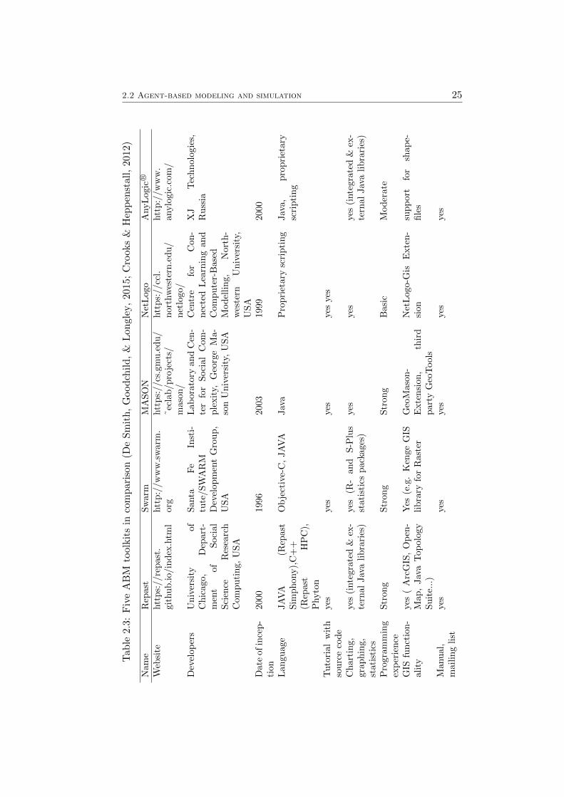
There are a lot of toolkits related to ABM (“Wikipedia- Comparison of agent-based modeling software,” 2018). Nikolai and Madey (2009) give their workan overview of the existing toolkits and organize them according to variouscriteria. Multi-platform support (Microsoft Windows, Mac OSX, and Linux)is common, and much of it uses the Java and C++ programming languagesto implement the models. The other toolkits use proprietary logo dialectsas well as visual programming languages, similar to, e.g., Unified ModelingLanguage (UML) diagrams. Therefore, all toolkits require a basic knowledgeof programming. Mainly object-oriented programming languages are usedOOP. Thus, the required level of modularity for implementing agent-basedsimulation can also be achieved (Crooks & Castle, 2012), (Nikolai & Madey,2009). There are free tools as well as commercially distributed solutions.The intended purpose can range from multifunction tools to specific appli-cations (Nikolai & Madey, 2009). The most notable representatives are:Repast, Swarm, NetLogo, AnyLogic and MASON (Macal & North, 2009b),(De Smith et al., 2015), (Crooks & Heppenstall, 2012). Table 2.3 comparesthe five toolkits. These are discussed in the following sections.
2.2 Agent-based modeling and simulation 25
Tab
le2.3
:F
ive
AB
Mto
olk
its
inco
mpar
ison
(De
Sm
ith,
Goodch
ild
,&
Lon
gley
,20
15;
Cro
oks
&H
epp
enst
all,
2012)
Nam
eR
epas
tSw
arm
MA
SO
NN
etL
ogo
AnyL
ogic
R ©
Web
site
htt
ps:
//re
pas
t.gi
thub
.io/
ind
ex.h
tml
htt
p:/
/w
ww
.sw
arm
.or
ghtt
ps:
//cs
.gm
u.e
du
/˜ec
lab
/pro
ject
s/m
aso
n/
htt
ps:
//cc
l.nor
thw
este
rn.e
du/
net
logo/
htt
p:/
/w
ww
.anylo
gic
.com
/
Dev
elop
ers
Univ
ersi
tyof
Chic
ago,
Dep
art-
men
tof
Soci
alSci
ence
Res
earc
hC
omputi
ng,
US
A
San
taF
eIn
sti-
tute
/SW
AR
MD
evel
opm
ent
Gro
up,
USA
Lab
ora
tory
and
Cen
-te
rfo
rSoci
al
Com
-ple
xit
y,G
eorg
eM
a-
son
Univ
ersi
ty,
USA
Cen
tre
for
Con
-nec
ted
Lea
rnin
gan
dC
om
pute
r-B
ase
dM
od
elling,
Nort
h-
wes
tern
Un
iver
sity
,U
SA
XJ
Tec
hn
olo
gie
s,R
uss
ia
Dat
eof
ince
p-
tion
2000
1996
2003
1999
2000
Lan
guag
eJA
VA
(Rep
ast
Sim
phon
y),
C+
+(R
epas
tH
PC
),P
hyto
n
Ob
ject
ive-
C,
JA
VA
Jav
aP
ropri
etary
scri
pti
ng
Jav
a,
pro
pri
etary
scri
pti
ng
Tuto
rial
wit
hso
urc
eco
de
yes
yes
yes
yes
yes
Char
ting,
grap
hin
g,st
atis
tics
yes
(inte
grat
ed&
ex-
tern
alJav
alib
rari
es)
yes
(R-
and
S-P
lus
stat
isti
cspack
ages
)ye
sye
sye
s(i
nte
gra
ted
&ex
-te
rnal
Jav
alib
rari
es)
Pro
gram
min
gex
per
ience
Str
ong
Str
ong
Str
ong
Basi
cM
oder
ate
GIS
funct
ion-
alit
yye
s(
Arc
GIS
,O
pen
-M
ap,
Jav
aT
opol
ogy
Su
ite.
..)
Yes
(e.g
.K
enge
GIS
lib
rary
for
Rast
erG
eoM
aso
n-
Exte
nsi
on
,th
ird
part
yG
eoT
ools
Net
Logo-G
isE
xte
n-
sion
supp
ort
for
shap
e-file
s
Man
ual
,m
ailin
glist
yes
yes
yes
yes
yes
2.2 Agent-based modeling and simulation 26
2.2.10 ABMS in GIScience
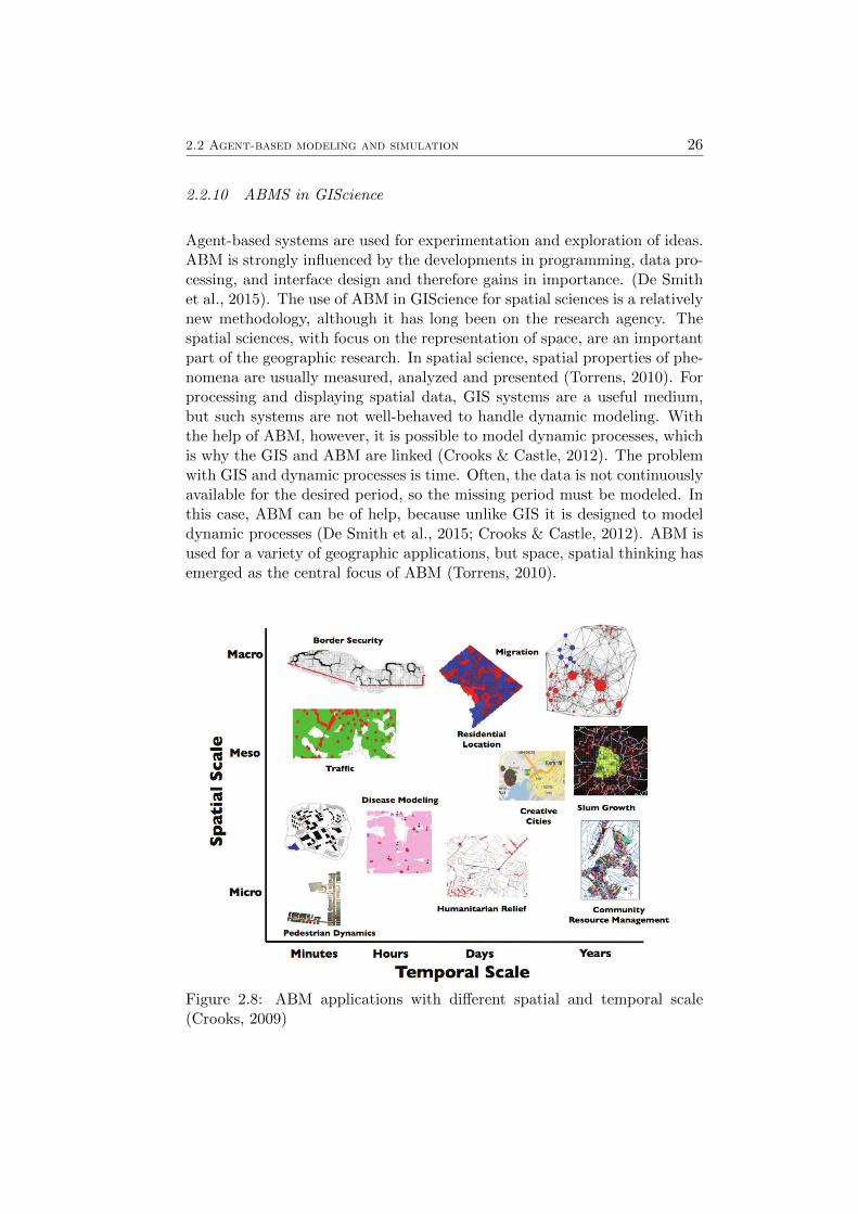
Agent-based systems are used for experimentation and exploration of ideas.ABM is strongly influenced by the developments in programming, data pro-cessing, and interface design and therefore gains in importance. (De Smithet al., 2015). The use of ABM in GIScience for spatial sciences is a relativelynew methodology, although it has long been on the research agency. Thespatial sciences, with focus on the representation of space, are an importantpart of the geographic research. In spatial science, spatial properties of phe-nomena are usually measured, analyzed and presented (Torrens, 2010). Forprocessing and displaying spatial data, GIS systems are a useful medium,but such systems are not well-behaved to handle dynamic modeling. Withthe help of ABM, however, it is possible to model dynamic processes, whichis why the GIS and ABM are linked (Crooks & Castle, 2012). The problemwith GIS and dynamic processes is time. Often, the data is not continuouslyavailable for the desired period, so the missing period must be modeled. Inthis case, ABM can be of help, because unlike GIS it is designed to modeldynamic processes (De Smith et al., 2015; Crooks & Castle, 2012). ABM isused for a variety of geographic applications, but space, spatial thinking hasemerged as the central focus of ABM (Torrens, 2010).
Figure 2.8: ABM applications with different spatial and temporal scale(Crooks, 2009)
2.2 Agent-based modeling and simulation 27
(a) Pedestrian/mobile agents (b) Residential agents
(c) Hunter-gatherer agents (d) Farmer/land-use change agents
(e) Property developer agents
Figure 2.9: Schematic representation of common ABM problems(O’Sullivan, Millington, Perry, & Wainwright, 2012)
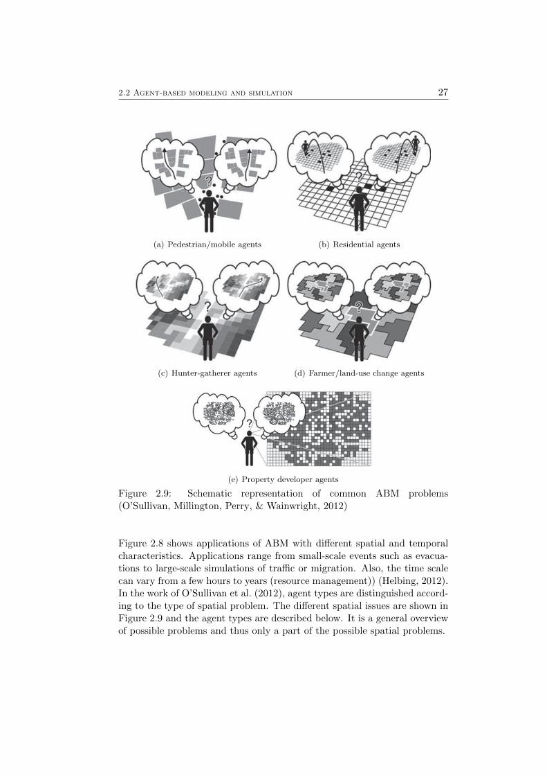
Figure 2.8 shows applications of ABM with different spatial and temporalcharacteristics. Applications range from small-scale events such as evacua-tions to large-scale simulations of traffic or migration. Also, the time scalecan vary from a few hours to years (resource management)) (Helbing, 2012).In the work of O’Sullivan et al. (2012), agent types are distinguished accord-ing to the type of spatial problem. The different spatial issues are shown inFigure 2.9 and the agent types are described below. It is a general overviewof possible problems and thus only a part of the possible spatial problems.
2.2 Agent-based modeling and simulation 28
Pedestrian/mobile agent (figure 2.9(a)): This mobile agent can reach aspecific destination. To do this, he interacts with his environment and withother agents. For example, the environment may be represented in the formof a road network or a building geometry. The position and the resultantenvironment of the agent is the most important reason for the demerit forhis next step.
Residential agent (figure 2.9(b)): Also this model is about the movementof the agent. The agent is looking for a new location, which, he prefers to thecurrent one, due to his rules. However, the movement is not continuous asin the case of the pedestrian-agent, but it simply moves to the new position.In this model, the nature of the environment does not affect the movement,but other agents influence the decision.
Hunter-gatherer agent (figure 2.9(c)): In this model they combined twoprevious types. The agent is trying to tap resources based on informationfrom the environment. Whether the agent moves on, is dependent on howmany resources are available. The movement is the same as with the pedes-trian agent. The target search as in the residential agent. In this model, theactions of the agent have a direct impact on the environment.
Farmer agent (figure 2.9(d)): This agent type has an impact on its envi-ronment. He interacts with his environment and can, therefore, change hisrelationship with the spatial environment. This relationship change takesplace in which he or she manages resources, such as harvesting, selling orexpanding land, with the aim of gaining many resources. It is unlikely thatthe agent moves.
Property developer agent (figure 2.9(e)): As with the former farmeragent, this agent gives the environment and other spatial objects a voice.However, this agent can evaluate complex spatial relationships to make deci-sions. This form of an agent is used, for example, to simulate the real estatemarket or to simulate urban growth.
Chapter 3
Approach
In order to answer the scientific questions, which have been defined in sec-tion 1.1, an experiment is done. The experiment is realized by an agent-based model. The property and capabilities of the model are examined ina test environment. The chosen approach for the model is explained in thischapter. The approach is inspired by the ideas of industry 4.0 and smartfactories, which were presented in section 2.1. Furthermore, the ideas of anagent-based manufacturing control described in the work of Leitao (2009)are included in the approach. Since the model simulates a semi-conductorproduction, for the creations, the conception of the model, as well as the testscenarios, are inspected by the work of Scholz and Schabus (2014b, 2015).
3.1 Basic knowledge for the concept
The first step is to set the framework for the model to implement. In theprocess, basic assumptions are made for the model from the initial situationand the task. We know that a semiconductor production is to be simulated.From the work of Scholz and Schabus (2014b), the following basic structuresare extracted.
• On a product, many work steps are carried out on different machines.The machines for the work steps can be distributed in the factory.
• The structure of the production environment can change dependingon the product. The construction is mostly in the form of corridors.The production halls/areas are separated by the airlock.
• There are machines, interim storage facilities, corridors, and airlock.
• The products are brought from worker to machine
From this information, the following functions for the model can be derived.:
• The structure of the environment is in the form of a factory hall withaisles and machines as well as intermediate storage. From this, it can
29
3.2 Agents and functions 30
be deduced that there are machines and intermediate storage. Thesethings can be considered as important elements.
• Workers transport the products. Mobile agents, which can indepen-dently navigate through the factory to handle transport orders.
• The simulation environment should be changeable.
• Products arrive and leave via airlocks in the individual productionsections. There are an input and an output in each area. Such an areacan be simulated independently.
3.2 Agents and functions
From the elaborated properties of the model components such as agents andbasic functions can now be determined. This is done under the point ofview of industry 4.0 and Agent-based modeling (ABM). The purpose of theindividual elements is now described and serves as a starting point for theimplementation of the model. The collected basic components of the modelare now shown.
• Products: Products are clearly identifiable, know their own positionand their work steps.
• Workers: These must be able to move through the production hall.They transport the products. The navigation of the workers takesplace independently. They receive the transport orders from otheragents or functions.
• Machines/Tools: The tools process the product and perform a specificwork step. You have a fixed position in the factory. Machines knowhow much work they have and share this information. Besides, theycan be broken.
• Stocks: Intermediate storage serves as an intermediate step if there isno free machine. They have a certain capacity, which can be queried.
• Simulation environment: A room in which the model works. Thisbrings the spatial component into the simulation. The structure ofthe factory with corridors and machines and stocks is determined as aresult of this.
An important part is the form of process or manufacturing control. This isan essential part of the model and will be covered in the next section.
3.3 Manufacturing control 31
3.3 Manufacturing control
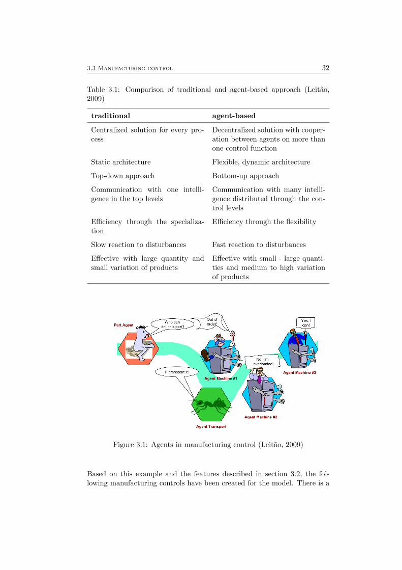
The most important element in the thesis is the implementation of the modelfrom the point of view of Industry 4.0. This means, considering the extractedbasic elements of the model, which all elements communicate with each otherand the control in the factory is decentralized (Shrouf et al., 2014). The coreelement in a production process is the manufacturing control. The manu-facturing control checks the processes in the factory. The progress of theproduct is monitored while it moves through the various steps in the fac-tory. Many decisions have to be made, such as: which product is producedon which machine, when will it be released for onward transport and inwhich order should the products be made? Traditionally, such processesare hierarchically and centrally controlled (Leitao, 2009). With the num-ber of required work steps as well as the number of interactions betweendeparting components, the complexity of scheduling increases. And the sys-tem is becoming slower to adapt to new situations (Cantamessa, 1997). Inwork, Leitao (2009) provides a manufacturing control based on agents. Thisapproach is based on the fact that all components of manufacturing are de-fined as agents. This means they work autonomously, are intelligent andwork together. Thus, a product which is executed as an agent knows itspast, knows which work step is next and can independently request furthertransport. These properties are also used in the description of an industry4.0 scenario (Albach et al., 2015). This example shows the difference be-tween hierarchical systems, which are listed in table 3.1. Figure 3.1 showsa simple example of how production control could be done with the help ofagents. The part-agent asks the available machine agents who free resourcesto perform the drilling step on the part. Upon this request, it receives thefollowing answers from the machines:
• Machine #1 replies: I am out of order, I cannot execute this operation.
• Machine #2 replies: I am overloaded.
• Machine #3 replies: I have free capacity for the request.
The job is carried out by machine #3, and the transport from the currentposition of the part to the machine is done using a transport agent.
3.3 Manufacturing control 32
Table 3.1: Comparison of traditional and agent-based approach (Leitao,2009)
traditional agent-based
Centralized solution for every pro-cess
Decentralized solution with cooper-ation between agents on more thanone control function
Static architecture Flexible, dynamic architecture
Top-down approach Bottom-up approach
Communication with one intelli-gence in the top levels
Communication with many intelli-gence distributed through the con-trol levels
Efficiency through the specializa-tion
Efficiency through the flexibility
Slow reaction to disturbances Fast reaction to disturbances
Effective with large quantity andsmall variation of products
Effective with small - large quanti-ties and medium to high variationof products
Figure 3.1: Agents in manufacturing control (Leitao, 2009)
Based on this example and the features described in section 3.2, the fol-lowing manufacturing controls have been created for the model. There is a
3.4 Model concept 33
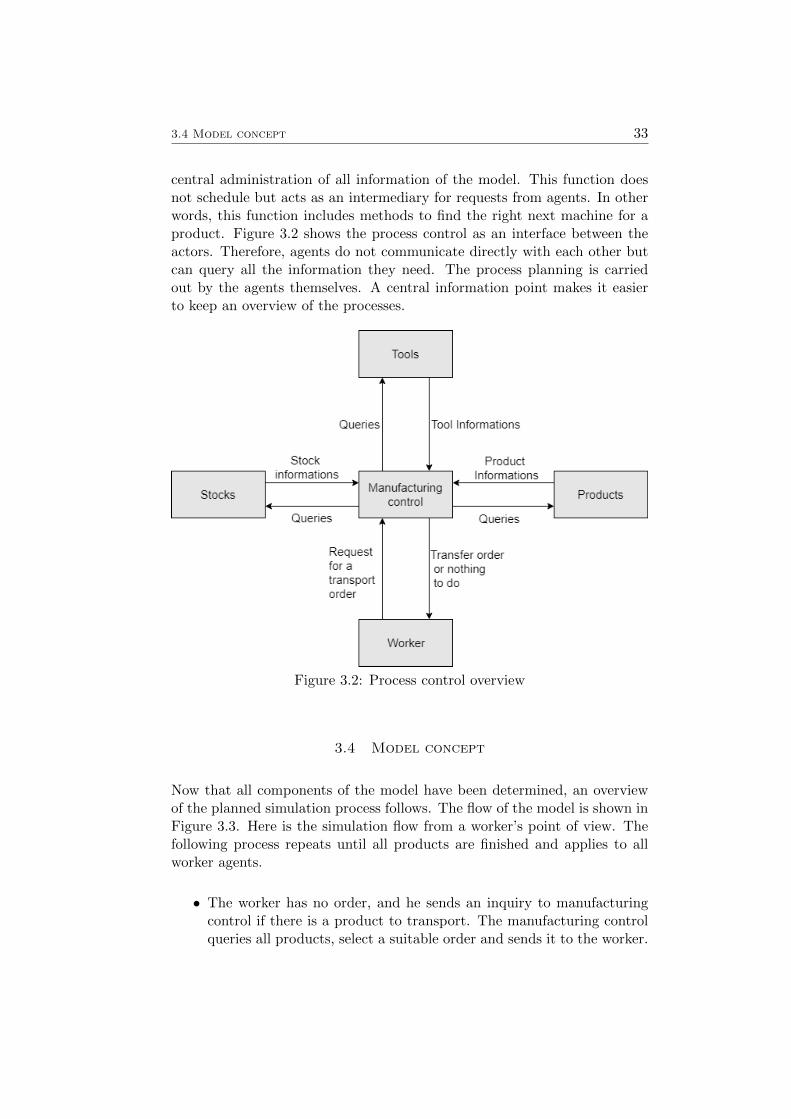
central administration of all information of the model. This function doesnot schedule but acts as an intermediary for requests from agents. In otherwords, this function includes methods to find the right next machine for aproduct. Figure 3.2 shows the process control as an interface between theactors. Therefore, agents do not communicate directly with each other butcan query all the information they need. The process planning is carriedout by the agents themselves. A central information point makes it easierto keep an overview of the processes.
Figure 3.2: Process control overview
3.4 Model concept
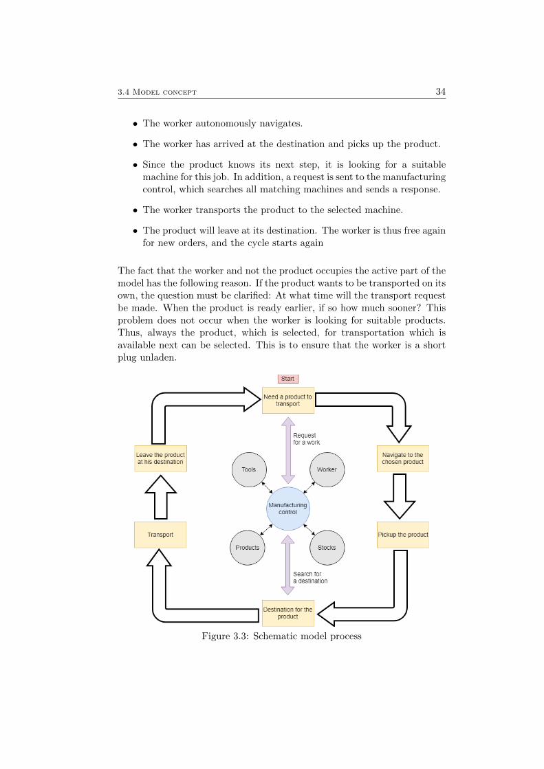
Now that all components of the model have been determined, an overviewof the planned simulation process follows. The flow of the model is shown inFigure 3.3. Here is the simulation flow from a worker’s point of view. Thefollowing process repeats until all products are finished and applies to allworker agents.
• The worker has no order, and he sends an inquiry to manufacturingcontrol if there is a product to transport. The manufacturing controlqueries all products, select a suitable order and sends it to the worker.
3.4 Model concept 34
• The worker autonomously navigates.
• The worker has arrived at the destination and picks up the product.
• Since the product knows its next step, it is looking for a suitablemachine for this job. In addition, a request is sent to the manufacturingcontrol, which searches all matching machines and sends a response.
• The worker transports the product to the selected machine.
• The product will leave at its destination. The worker is thus free againfor new orders, and the cycle starts again
The fact that the worker and not the product occupies the active part of themodel has the following reason. If the product wants to be transported on itsown, the question must be clarified: At what time will the transport requestbe made. When the product is ready earlier, if so how much sooner? Thisproblem does not occur when the worker is looking for suitable products.Thus, always the product, which is selected, for transportation which isavailable next can be selected. This is to ensure that the worker is a shortplug unladen.
Figure 3.3: Schematic model process
3.5 Implementation and testing 35
3.5 Implementation and testing
The implementation of the model takes place in a software/toolkit for ABM.Section 2.2.9 shows an overview of some software options. The selection ofthe appropriate toolkit was made according to the following criteria.
• It should be freely available.
• There must be documentation about the functionality.
• All functions for the model must be given, or it must be possible toimplement functions or to use them from external software libraries.
• There should be a tutorial and sample programs.
• It should run both Windows or Linux system.
The choice of software fell on Repast Simphony 1, since all conditions aremet here.
In order to answer the scientific questions, a testing environment has to becreated. The following data are required for this:
• Environment layout: where are paths and machines located.
• Wafer types with the associated production steps.
• Average production time at the machines.
• Comparison results: Average production time traveled distance pertype, transport density.
For this purpose, an attempt is made to obtain real data from the industry.If this does not work your own test data will be created and the functionsof the model shown.
1Repast Simphony https://repast.github.io/

Chapter 4
Modeling and implementation
This chapter deals with the description of the model used in this thesis.The model is built according to the approach outlined in Chapter 3. First,Section 4.1 describes the structure of the model. Followed by a detaileddescription of the agents and functions used in Section 4.2. Section 4.3 is abrief description of the key points for implementation in Repast SimphonyAfter that, in Section 4.4, a description of the most important processes inthe simulation comes in the form of process overview and process planning.Finally, in sections 4.5 to 4.9 an insight into the implemented processes isgiven.
4.1 Structure of the model
The model is the basis for the implementation of a prototype applicationand simulates production processes of products, in particular, the semicon-ductor production, or productions, in which people transport goods betweendifferent production assets or stocks. The model attempts to simulate sucha production process, in order to be able to infer a real production chain.The focus, of the model, is placed on the transportation of goods betweenthe production elements. The structure of the model is based on the workof Scholz and Schabus (2014b). In this work, an ontology for indoor semi-conductor production is described. As a simplification, however, only acompleted production area is considered, doors and air locks are not mod-eled. This would only be an extension of the environment but would nothave any influence on the basic functionality. The products come and leavethe model on a grid cell that can be considered as a link to other productionareas. The model consists of the following elements:
• Production hall: The production hall is the spatial environment ofthe simulation. These form the framework for the simulation.
• Tools (production unit): The machines have a fixed position in theproduction hall. They carry out work steps to manufacture a product.
• Workers: The workers carry (transport) products through the pro-
36
4.2 Agents, attributes and other important parts 37
duction hall. They must, therefore, be able to navigate through thespatial environment.
• Stocks: Stocks are optional for the production process. They serveas a stopover during transport between machines and have a fixedposition in the environment.
• Manufacturing control: The Manufacturing control is the dispatcherfor the workers. It assigns orders to the workers.
How these elements are related and how they are implemented in the modelis explained in the following sections. The implementation of the ABM isdone in the software Repast Simphony (“Repast - The Repast Suite,” 2018).
4.2 Agents, attributes and other important parts
The description of this section will be related to the basic elements of anABM from Section 2.2.4.The described model uses the following agents,relations, and the environment. Another important part of this section isthe conception of the product and the central process control.
• Agents: The main actors are workers, machinery, and stocks. Aboveall, the workers, as the only mobile agents. They have great impor-tance to the model. Each worker can carry a production item. Themachines are supplied by the workers and can each perform a spe-cific work step on the product. The stocks are another part of themodel and these as intermediate points to keep the production flowgoing. The decision, which product is to be transported, is made by aseparate manufacturing control.
• Relations:
– A worker transports a production item, to and from machinesand stocks;
– The machines process the product when a worker supplies themachine;
– The manufacturing controllers regulate the sequence of the ordersfor the workers;
– Stock can store product and are filled and emptied by the workers;
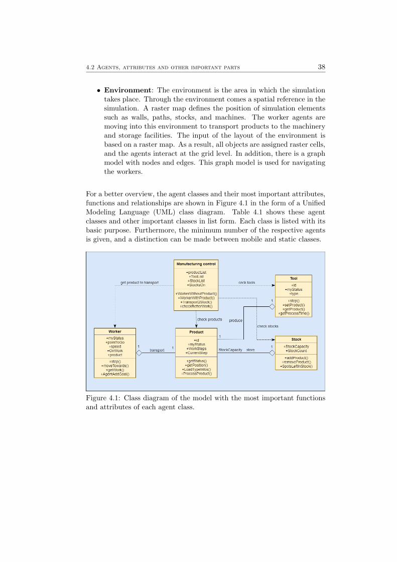
4.2 Agents, attributes and other important parts 38
• Environment: The environment is the area in which the simulationtakes place. Through the environment comes a spatial reference in thesimulation. A raster map defines the position of simulation elementssuch as walls, paths, stocks, and machines. The worker agents aremoving into this environment to transport products to the machineryand storage facilities. The input of the layout of the environment isbased on a raster map. As a result, all objects are assigned raster cells,and the agents interact at the grid level. In addition, there is a graphmodel with nodes and edges. This graph model is used for navigatingthe workers.
For a better overview, the agent classes and their most important attributes,functions and relationships are shown in Figure 4.1 in the form of a UnifiedModeling Language (UML) class diagram. Table 4.1 shows these agentclasses and other important classes in list form. Each class is listed with itsbasic purpose. Furthermore, the minimum number of the respective agentsis given, and a distinction can be made between mobile and static classes.
Figure 4.1: Class diagram of the model with the most important functionsand attributes of each agent class.
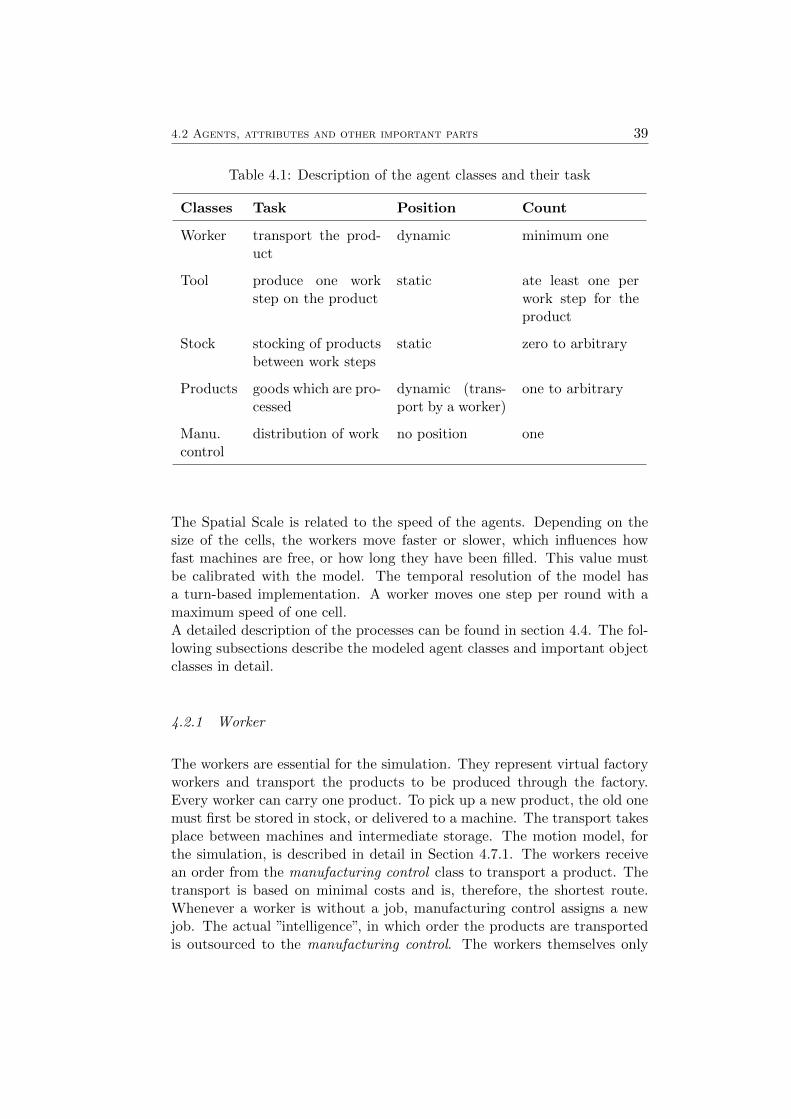
4.2 Agents, attributes and other important parts 39
Table 4.1: Description of the agent classes and their task
Classes Task Position Count
Worker transport the prod-uct
dynamic minimum one
Tool produce one workstep on the product
static ate least one perwork step for theproduct
Stock stocking of productsbetween work steps
static zero to arbitrary
Products goods which are pro-cessed
dynamic (trans-port by a worker)
one to arbitrary
Manu.control
distribution of work no position one
The Spatial Scale is related to the speed of the agents. Depending on thesize of the cells, the workers move faster or slower, which influences howfast machines are free, or how long they have been filled. This value mustbe calibrated with the model. The temporal resolution of the model hasa turn-based implementation. A worker moves one step per round with amaximum speed of one cell.A detailed description of the processes can be found in section 4.4. The fol-lowing subsections describe the modeled agent classes and important objectclasses in detail.
4.2.1 Worker
The workers are essential for the simulation. They represent virtual factoryworkers and transport the products to be produced through the factory.Every worker can carry one product. To pick up a new product, the old onemust first be stored in stock, or delivered to a machine. The transport takesplace between machines and intermediate storage. The motion model, forthe simulation, is described in detail in Section 4.7.1. The workers receivean order from the manufacturing control class to transport a product. Thetransport is based on minimal costs and is, therefore, the shortest route.Whenever a worker is without a job, manufacturing control assigns a newjob. The actual ”intelligence”, in which order the products are transportedis outsourced to the manufacturing control. The workers themselves only
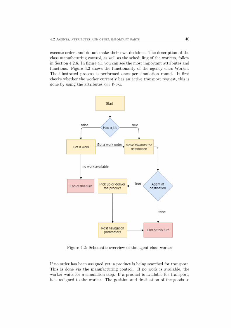
4.2 Agents, attributes and other important parts 40
execute orders and do not make their own decisions. The description of theclass manufacturing control, as well as the scheduling of the workers, followin Section 4.2.6. In figure 4.1 you can see the most important attributes andfunctions. Figure 4.2 shows the functionality of the agency class Worker.The illustrated process is performed once per simulation round. It firstchecks whether the worker currently has an active transport request, this isdone by using the attributes On Work.
Figure 4.2: Schematic overview of the agent class worker
If no order has been assigned yet, a product is being searched for transport.This is done via the manufacturing control. If no work is available, theworker waits for a simulation step. If a product is available for transport,it is assigned to the worker. The position and destination of the goods to
4.2 Agents, attributes and other important parts 41
be transported can be read from the assigned product. If the worker hasan order, he moves along way points to his destination. The way pointsare expressed by the variable pointToGo. If the transport target is notreached with this step, this simulation step ends. The goal is reached whenthe distance to the target is less than the movement speed of the agent.The movement speed differs depending on whether the agent is loaded ornot. The speed of how fast a worker is allowed to move can be inquiredabout the product to be transported. When the target point is reached, theaddGoal function is called. Depending on the order, a product is picked upor delivered. Finally, the navigation parameters are reset so that the workeris ready for a new job in the next round.
4.2.2 Tools
The machines are the second important part of the model because the prod-ucts are produced on them. Machines have a fixed location in the factory.Each Tool has a type, depending on the type of machine other work stepscan be performed. The production time, the time how long a product isprocessed depends on the type of machine. The machine type is determinedwhen creating the production environment - this is explained in detail insection 4.5.1 The machines can break while processing a product. This fea-ture is optional and must be activated. Because of a failure, the productiontime of the machine is increased by a random value. However, this machineis longer occupied. These random events may change the simulation result.Figure 4.3 shows the functionality of the agency class Tools. The illustratedprocess is performed once per simulation round. First, it checks if the ma-chine is working on a product. If there is no product in the machine, thefunction is ended. If, on the other hand, a work step is being executed,it is checked whether machine failures are activated in the settings. Withthe break down enabled, failures are simulated by a random number gener-ator. The size of the random pool, as well as the impact area, can be set inthe simulation settings. In case of failure, the production time is increased.As a result, the machine takes longer to work. In addition, it is no longerconsidered for job scheduling during the time of the failure. Furthermore,each round is carried out one working tick. Once all work steps have beencompleted on this machine, the product can be picked up from the machineagain. A machine can take different statuses. This status is importantfor the order assignment of the process control function. The states of thevariable myStatus are listed in the following table 4.2. In addition to thedescription, the color is also indicated with which the status is displayed inthe graphical simulation environment. The effects of these states are dealtwith in detail in section process control 4.2.6.

4.2 Agents, attributes and other important parts 42
Table 4.2: Description of the attribute myStatus of the class tools.
Status Description Color
Free The machine is free and ready for a product Green
Work The machine is currently producing a product Orange
Wait A worker is on his way to the machine. Duringthis period, the machine is not available for otherjobs
Yellow
Wait forexchange
A product is in the machine. A worker comes upwith a new product for the machine and takes thefinished one with him.
Cyan
BreakDown
The machine is broken. It is not available for neworders
Gray
Finished The product in the machine is ready and must bepicked up
Red
Figure 4.3: Schematic overview of the agent class Tool
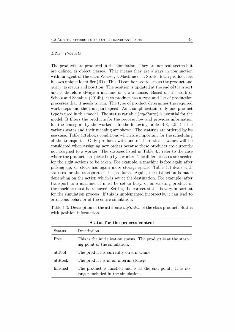
4.2 Agents, attributes and other important parts 43
4.2.3 Products
The products are produced in the simulation. They are not real agents butare defined as object classes. That means they are always in conjunctionwith an agent of the class Worker, a Machine or a Stock. Each product hasits own unique Identifier (ID). This ID can be used to access the product andquery its status and position. The position is updated at the end of transportand is therefore always a machine or a warehouse. Based on the work ofScholz and Schabus (2014b), each product has a type and list of productionprocesses that it needs to run. The type of product determines the requiredwork steps and the transport speed. As a simplification, only one producttype is used in this model. The status variable (myStatus) is essential for themodel. It filters the products for the process flow and provides informationfor the transport by the workers. In the following tables 4.3, 4.5, 4.4 thevarious states and their meaning are shown. The statuses are ordered by itsuse case. Table 4.3 shows conditions which are important for the schedulingof the transports. Only products with one of these status values will beconsidered when assigning new orders because these products are currentlynot assigned to a worker. The statuses listed in Table 4.5 refer to the casewhere the products are picked up by a worker. The different cases are neededfor the right actions to be taken. For example, a machine is free again afterpicking up, or stock has again more storage space. Table 4.4 deals withstatuses for the transport of the products. Again, the distinction is madedepending on the action which is set at the destination. For example, aftertransport to a machine, it must be set to busy, or an existing product inthe machine must be removed. Setting the correct status is very importantfor the simulation process. If this is implemented incorrectly, it can lead toerroneous behavior of the entire simulation.
Table 4.3: Description of the attribute myStatus of the class product. Statuswith position information.
Status for the process control
Status Description
Free This is the initialization status. The product is at the start-ing point of the simulation.
atTool The product is currently on a machine.
atStock The product is in an interim storage.
finished The product is finished and is at the end point. It is nolonger included in the simulation.
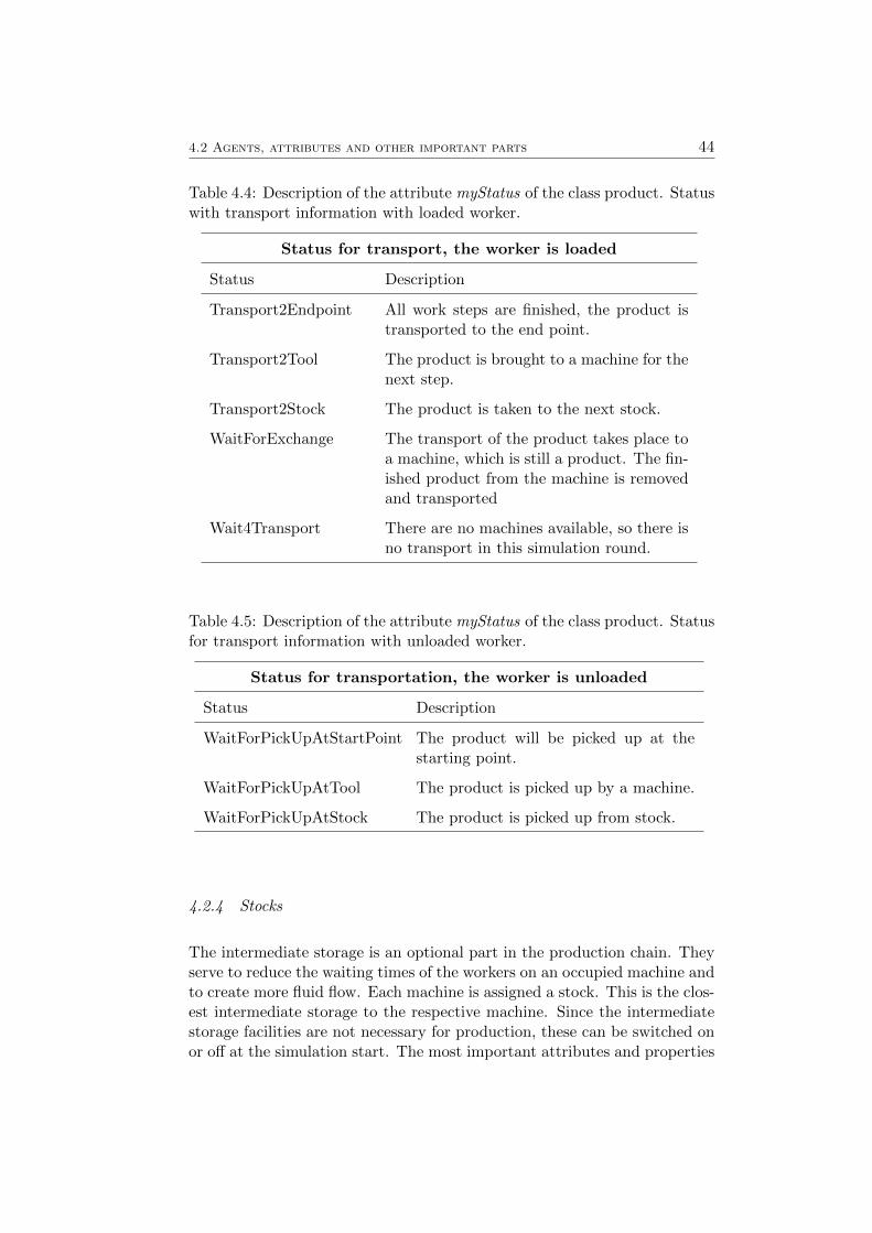
4.2 Agents, attributes and other important parts 44
Table 4.4: Description of the attribute myStatus of the class product. Statuswith transport information with loaded worker.
Status for transport, the worker is loaded
Status Description
Transport2Endpoint All work steps are finished, the product istransported to the end point.
Transport2Tool The product is brought to a machine for thenext step.
Transport2Stock The product is taken to the next stock.
WaitForExchange The transport of the product takes place toa machine, which is still a product. The fin-ished product from the machine is removedand transported
Wait4Transport There are no machines available, so there isno transport in this simulation round.
Table 4.5: Description of the attribute myStatus of the class product. Statusfor transport information with unloaded worker.
Status for transportation, the worker is unloaded
Status Description
WaitForPickUpAtStartPoint The product will be picked up at thestarting point.
WaitForPickUpAtTool The product is picked up by a machine.
WaitForPickUpAtStock The product is picked up from stock.
4.2.4 Stocks
The intermediate storage is an optional part in the production chain. Theyserve to reduce the waiting times of the workers on an occupied machine andto create more fluid flow. Each machine is assigned a stock. This is the clos-est intermediate storage to the respective machine. Since the intermediatestorage facilities are not necessary for production, these can be switched onor off at the simulation start. The most important attributes and properties
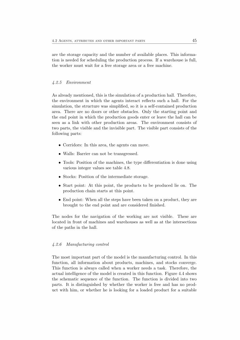
4.2 Agents, attributes and other important parts 45
are the storage capacity and the number of available places. This informa-tion is needed for scheduling the production process. If a warehouse is full,the worker must wait for a free storage area or a free machine.
4.2.5 Environment
As already mentioned, this is the simulation of a production hall. Therefore,the environment in which the agents interact reflects such a hall. For thesimulation, the structure was simplified, so it is a self-contained productionarea. There are no doors or other obstacles. Only the starting point andthe end point in which the production goods enter or leave the hall can beseen as a link with other production areas. The environment consists oftwo parts, the visible and the invisible part. The visible part consists of thefollowing parts:
• Corridors: In this area, the agents can move.
• Walls: Barrier can not be transgressed.
• Tools: Position of the machines, the type differentiation is done usingvarious integer values see table 4.8.
• Stocks: Position of the intermediate storage.
• Start point: At this point, the products to be produced lie on. Theproduction chain starts at this point.
• End point: When all the steps have been taken on a product, they arebrought to the end point and are considered finished.
The nodes for the navigation of the working are not visible. These arelocated in front of machines and warehouses as well as at the intersectionsof the paths in the hall.
4.2.6 Manufacturing control
The most important part of the model is the manufacturing control. In thisfunction, all information about products, machines, and stocks converge.This function is always called when a worker needs a task. Therefore, theactual intelligence of the model is created in this function. Figure 4.4 showsthe schematic sequence of the function. The function is divided into twoparts. It is distinguished by whether the worker is free and has no prod-uct with him, or whether he is looking for a loaded product for a suitable
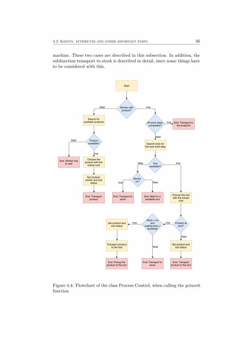
4.2 Agents, attributes and other important parts 46
machine. These two cases are described in this subsection. In addition, thesubfunction transport to stock is described in detail, since some things haveto be considered with this.
Start
Worker with product?
Search foravailable products
Productavailable?
End: Worker hasto wait
Choose theproduct with the
lowest cost
Set produkt,worker and tool
status
End: Transportproduct
All work stepscompleted?
End: Transport tothe endpoint
Search tools forthe next work step
Tool available?
Stocks on?
Choose the toolwith the lowest
costEnd: Transport to
stockEnd: Wait for aavailable tool
Product at tool?
Stock = on and
waiting time <threshold
Set product andtool status
End: Transportproduct to the tool
End: Transport tostock
Set product andtool status
Transport productto the tool
End: Pickup theproduct at the tool
false true
true
false
true
false
false true
true false
truetrue
false
false
Figure 4.4: Flowchart of the class Process Control, when calling the getworkfunction
4.2 Agents, attributes and other important parts 47
Worker without product
If the worker is not loaded, a free product is searched for transport. First, itchecks if there are currently any products that need to be transported nowor in the near future. Products with the following status are included in theselection.
• Free: The product is at the starting point of the simulation.
• at tool: The product is currently on a machine, and it is not distin-guished whether the production process is already completed or not.
• at stock: The product is in interim storage.
If no product is available for transport, the worker waits for a simulationround. An accessibility value is calculated for all eligible products. Thisvalue is composed of the distance to the product, the remaining produc-tion time at the machine and a weighting.
accessibility value =distance
speed+ remaining production time + weighting
The distance is calculated by a node edge structure using the Dijkstra’s algo-rithm. Since the accessibility value is given in simulation ticks, the distancemust still be divided by the speed of the workers. If the product is beingprocessed on a machine, remaining working time is added to accessibility.Also, a weighting value can be added. This additional value can be used tocontrol the simulation behavior. The next product is selected via the acces-sibility value, the product with the lowest value is selected for the transport.This means that the sum of travel time and waiting time is the smallest forthis product. In order to influence this selection, the weighting comes intoplay. This is determined at simulation start and applies to the entire run.Depending on the place where the free product is located, a factor can beapplied. For example, products that are in finished machines can be treatedpreferentially. An overview of the weighting options can be found in Table4.6. By varying these values, priorities can be set in the simulation. Theunit of weighting, as well as the accessibility, are simulation ticks.
Once the product to be transported has been selected, it is given to theworker and is excluded until the end of transport for other orders. Thisis done by setting a status variable. An overview of the respective statusvariables can be found in Table 4.5. The worker is now assigned the product,and it can complete the job and pick up the product at its location. A specialrule when selecting a product applies when the product is in a temporarystorage facility. Since it may happen that for several workers the closest
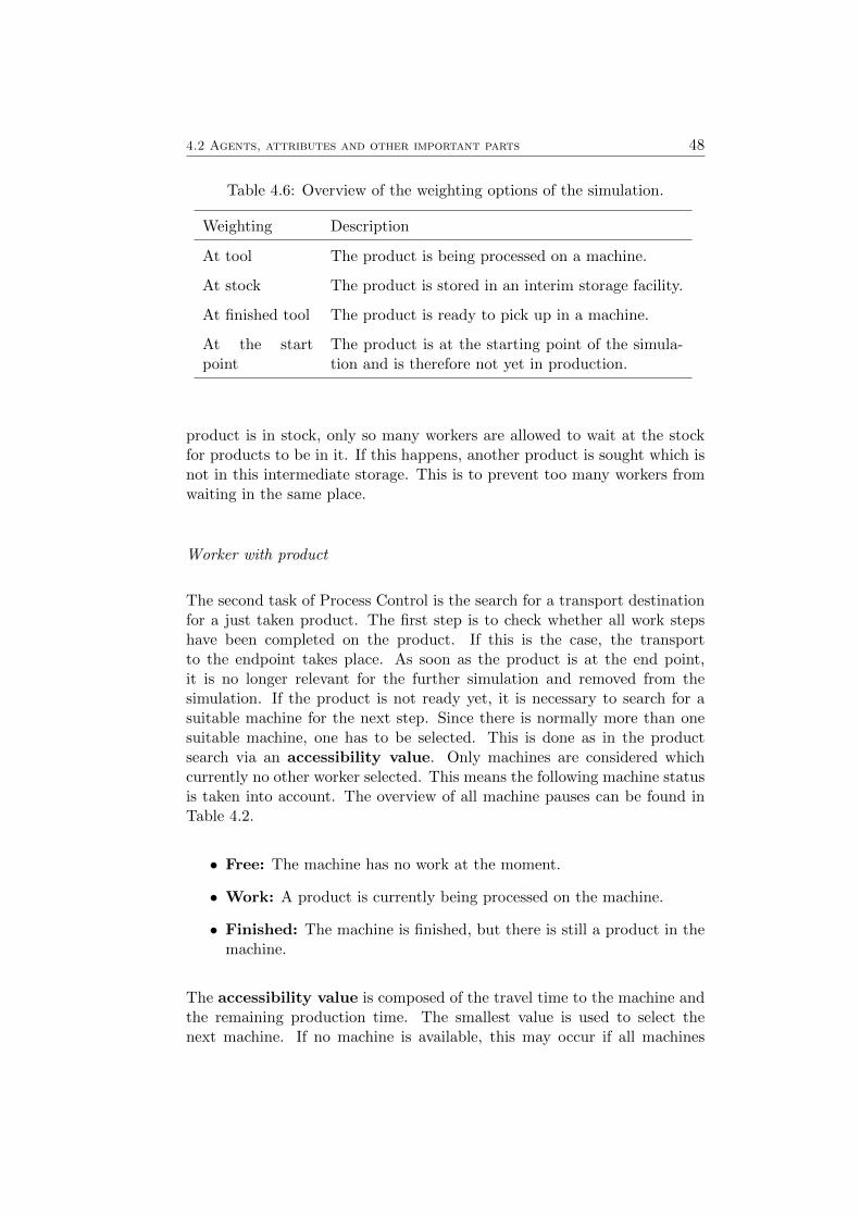
4.2 Agents, attributes and other important parts 48
Table 4.6: Overview of the weighting options of the simulation.
Weighting Description
At tool The product is being processed on a machine.
At stock The product is stored in an interim storage facility.
At finished tool The product is ready to pick up in a machine.
At the startpoint
The product is at the starting point of the simula-tion and is therefore not yet in production.
product is in stock, only so many workers are allowed to wait at the stockfor products to be in it. If this happens, another product is sought which isnot in this intermediate storage. This is to prevent too many workers fromwaiting in the same place.
Worker with product
The second task of Process Control is the search for a transport destinationfor a just taken product. The first step is to check whether all work stepshave been completed on the product. If this is the case, the transportto the endpoint takes place. As soon as the product is at the end point,it is no longer relevant for the further simulation and removed from thesimulation. If the product is not ready yet, it is necessary to search for asuitable machine for the next step. Since there is normally more than onesuitable machine, one has to be selected. This is done as in the productsearch via an accessibility value. Only machines are considered whichcurrently no other worker selected. This means the following machine statusis taken into account. The overview of all machine pauses can be found inTable 4.2.
• Free: The machine has no work at the moment.
• Work: A product is currently being processed on the machine.
• Finished: The machine is finished, but there is still a product in themachine.
The accessibility value is composed of the travel time to the machine andthe remaining production time. The smallest value is used to select thenext machine. If no machine is available, this may occur if all machines
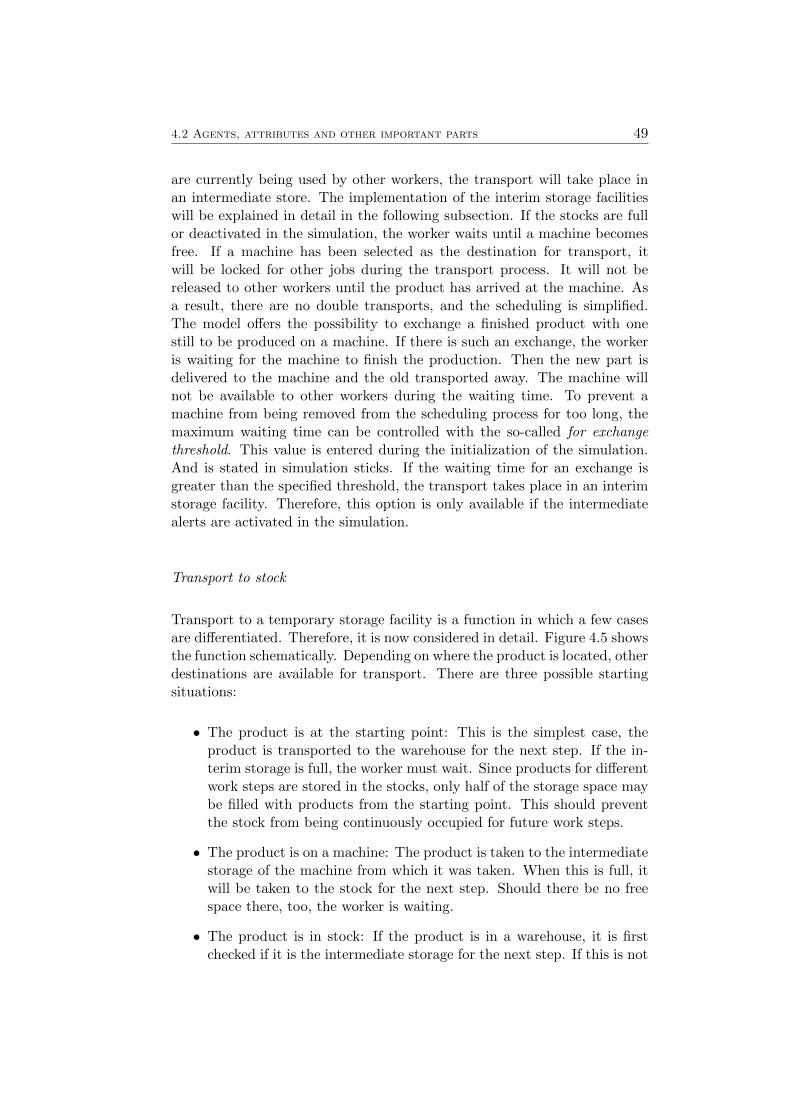
4.2 Agents, attributes and other important parts 49
are currently being used by other workers, the transport will take place inan intermediate store. The implementation of the interim storage facilitieswill be explained in detail in the following subsection. If the stocks are fullor deactivated in the simulation, the worker waits until a machine becomesfree. If a machine has been selected as the destination for transport, itwill be locked for other jobs during the transport process. It will not bereleased to other workers until the product has arrived at the machine. Asa result, there are no double transports, and the scheduling is simplified.The model offers the possibility to exchange a finished product with onestill to be produced on a machine. If there is such an exchange, the workeris waiting for the machine to finish the production. Then the new part isdelivered to the machine and the old transported away. The machine willnot be available to other workers during the waiting time. To prevent amachine from being removed from the scheduling process for too long, themaximum waiting time can be controlled with the so-called for exchangethreshold. This value is entered during the initialization of the simulation.And is stated in simulation sticks. If the waiting time for an exchange isgreater than the specified threshold, the transport takes place in an interimstorage facility. Therefore, this option is only available if the intermediatealerts are activated in the simulation.
Transport to stock
Transport to a temporary storage facility is a function in which a few casesare differentiated. Therefore, it is now considered in detail. Figure 4.5 showsthe function schematically. Depending on where the product is located, otherdestinations are available for transport. There are three possible startingsituations:
• The product is at the starting point: This is the simplest case, theproduct is transported to the warehouse for the next step. If the in-terim storage is full, the worker must wait. Since products for differentwork steps are stored in the stocks, only half of the storage space maybe filled with products from the starting point. This should preventthe stock from being continuously occupied for future work steps.
• The product is on a machine: The product is taken to the intermediatestorage of the machine from which it was taken. When this is full, itwill be taken to the stock for the next step. Should there be no freespace there, too, the worker is waiting.
• The product is in stock: If the product is in a warehouse, it is firstchecked if it is the intermediate storage for the next step. If this is not
4.2 Agents, attributes and other important parts 50
the case, the transport takes place in the next intermediate storage.The second option is the product is already in stock for the next step.To keep the times short in which the workers wait for free machines,they are looking for a better job. This function is explained in thefollowing subsection.
Transport between two interim storage facilities is also possible. This isintended to shorten the transport routes and increase the dynamics of thesystem. Of course, this functionality is only used if the intermediate storageis activated in the simulation.
Figure 4.5: Process overview of the function Transport to stock
4.3 Implementation in Repast Simphony 51
Find better work
The idea behind this function is to keep the waiting times at the intermediatestorage facilities for a free machine small. Without this feature, the workerwaits as long at stock until the next machine is free. As to be seen inFigure 4.5, this function is called if the product to be transported is in theinterim storage area for the next work step but no machine is available. Thefunction works in the same way as the search for a free product 4.2.6. Withthe difference that products which need the occupied machines as the nextwork step are excluded in the search. If the availability value of the newproduct is less than the waiting time at the machines, this is selected as thenew transport order. The other product remains in the stock
4.3 Implementation in Repast Simphony
The model is implemented with Repast Simphony version 2.51. Since RepastSimphony uses Java as the programming language, you also need the JavaRuntime Environment. Recommended for Repast Simphony 2.5 of the latestversion of Java 8. Here, Java SE 82 is used. The development environmentis Eclipse oxygen 1a3, as it is also installed with Repast Simphony on Win-dows. The introduction of Collier and North (2013) explains both the basicsof Eclipse and Repast Simpohny and was used as the basis for this modeling.Repast Simphony 2.5 provides the basic features for agent-based modeling.This includes a programming library as well as a graphical user interface.This user interface can be expanded with diagrams and setting options.According to the documentation of the Application Programming Inter-face (API) “Repast Simphony 2.5 API” (2018) the central feature in RepastSimphony is the Context class. In this context, all agents and parts of thesimulation are loaded. Therefore, the context represents the entire model.The Context can also be divided into different areas by means of SubContext.The Context acts as a container for agents and model elements. For yourspatial connection to come about, every context can be define one or more”projections”. This ”Projection” creates a space in which the agents can act.The space can be in the form of a grid, Euclidean space, physical space, net-works or geographic space (Geographical information system (GIS) data)The functionality of the individual objects has already been described insection 4.2.1 to 4.2.5. These must now be implemented as object-orientedJava classes. How the functional processes of the whole model look and workare described in the following chapter 4.4.
1Repast Simphony 2.5: https://repast.github.io/download.html2Java SE 8 download https://www.java.com/en/3Eclipse https://www.eclipse.org/
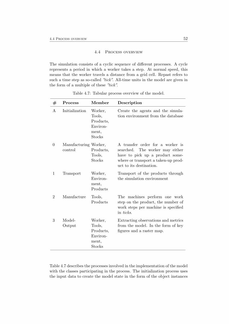
4.4 Process overview 52
4.4 Process overview
The simulation consists of a cyclic sequence of different processes. A cyclerepresents a period in which a worker takes a step. At normal speed, thismeans that the worker travels a distance from a grid cell. Repast refers tosuch a time step as so-called ”tick”. All-time units in the model are given inthe form of a multiple of these ”tick”.
Table 4.7: Tabular process overview of the model.
# Process Member Description
A Initialization Worker,Tools,Products,Environ-ment,Stocks
Create the agents and the simula-tion environment from the database
0 Manufacturingcontrol
Worker,Products,Tools,Stocks
A transfer order for a worker issearched. The worker may eitherhave to pick up a product some-where or transport a taken-up prod-uct to its destination.
1 Transport Worker,Environ-ment,Products
Transport of the products throughthe simulation environment
2 Manufacture Tools,Products
The machines perform one workstep on the product, the number ofwork steps per machine is specifiedin ticks.
3 Model-Output
Worker,Tools,Products,Environ-ment,Stocks
Extracting observations and metricsfrom the model. In the form of keyfigures and a raster map.
Table 4.7 describes the processes involved in the implementation of the modelwith the classes participating in the process. The initialization process usesthe input data to create the model state in the form of the object instances
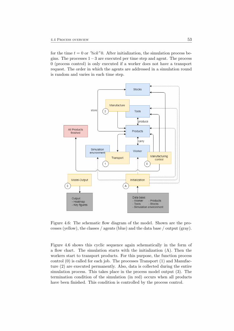
4.4 Process overview 53
for the time t = 0 or ”tick” 0. After initialization, the simulation process be-gins. The processes 1−3 are executed per time step and agent. The process0 (process control) is only executed if a worker does not have a transportrequest. The order in which the agents are addressed in a simulation roundis random and varies in each time step.
Figure 4.6: The schematic flow diagram of the model. Shown are the pro-cesses (yellow), the classes / agents (blue) and the data base / output (gray).
Figure 4.6 shows this cyclic sequence again schematically in the form ofa flow chart. The simulation starts with the initialization (A). Then theworkers start to transport products. For this purpose, the function processcontrol (0) is called for each job. The processes Transport (1) and Manufac-ture (2) are executed permanently. Also, data is collected during the entiresimulation process. This takes place in the process model output (3). Thetermination condition of the simulation (in red) occurs when all productshave been finished. This condition is controlled by the process control.
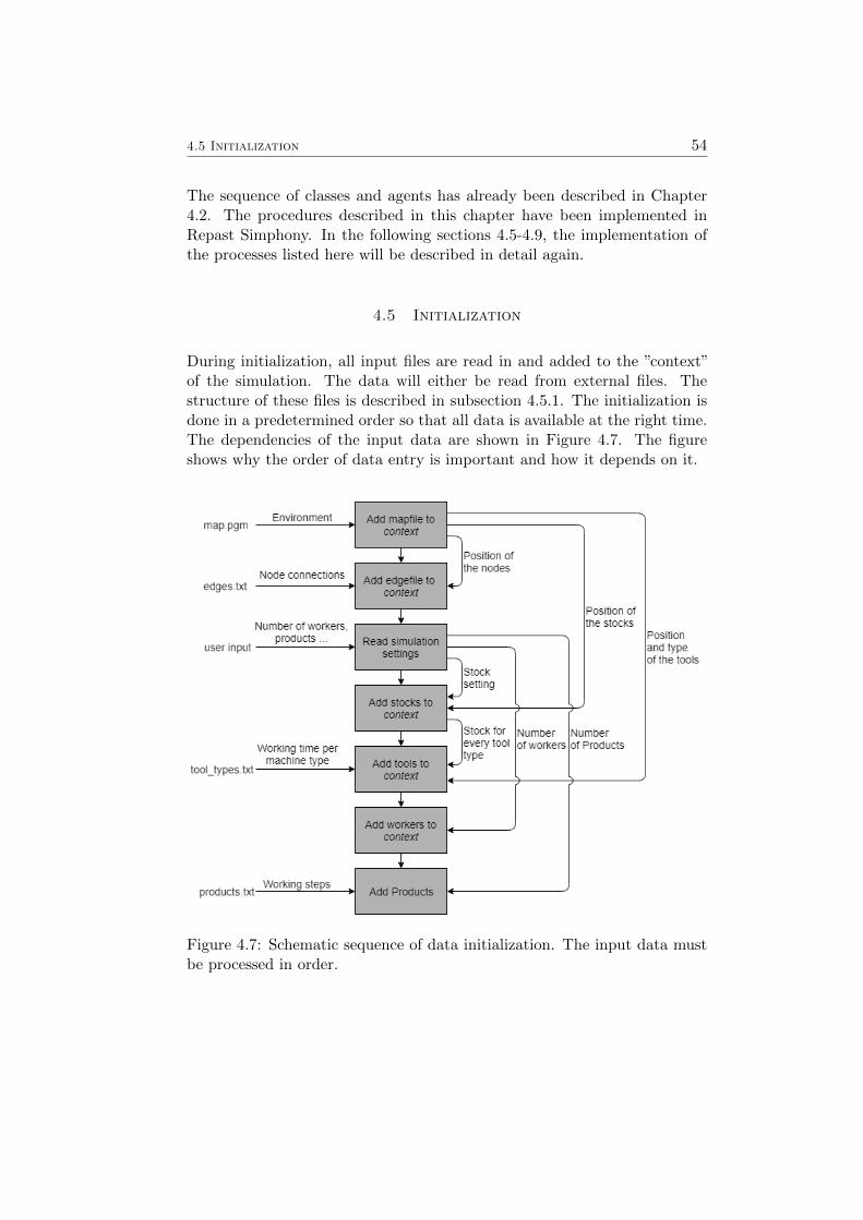
4.5 Initialization 54
The sequence of classes and agents has already been described in Chapter4.2. The procedures described in this chapter have been implemented inRepast Simphony. In the following sections 4.5-4.9, the implementation ofthe processes listed here will be described in detail again.
4.5 Initialization
During initialization, all input files are read in and added to the ”context”of the simulation. The data will either be read from external files. Thestructure of these files is described in subsection 4.5.1. The initialization isdone in a predetermined order so that all data is available at the right time.The dependencies of the input data are shown in Figure 4.7. The figureshows why the order of data entry is important and how it depends on it.
Figure 4.7: Schematic sequence of data initialization. The input data mustbe processed in order.
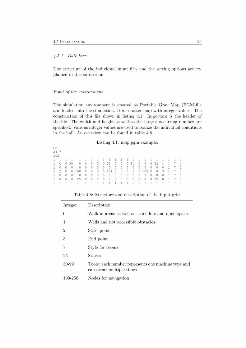
4.5 Initialization 55
4.5.1 Date base
The structure of the individual input files and the setting options are ex-plained in this subsection.
Input of the environment
The simulation environment is created as Portable Gray Map (PGM)fileand loaded into the simulation. It is a raster map with integer values. Theconstruction of this file shown in listing 4.1. Important is the header ofthe file. The width and height as well as the largest occurring number arespecified. Various integer values are used to realize the individual conditionsin the hall. An overview can be found in table 4.8.
Listing 4.1: map.pgm example.P224 71021 1 1 1 1 1 1 1 1 1 1 1 1 1 1 1 1 1 1 1 1 11 0 0 30 0 0 0 0 0 31 0 0 0 31 0 0 0 32 1 1 7 11 0 0 0 0 0 0 0 0 0 0 0 0 0 0 0 0 0 0 1 7 11 2 0 0 100 0 0 0 0 101 0 0 0 0 0 102 0 0 3 1 7 11 0 0 0 0 0 0 0 0 0 0 0 0 0 0 0 0 0 0 1 7 11 0 0 0 25 0 0 0 0 0 0 0 0 0 0 0 0 25 0 1 7 11 1 1 1 1 1 1 1 1 1 1 1 1 1 1 1 1 1 1 1 1 1
Table 4.8: Structure and description of the input grid.
Integer Description
0 Walk-in areas as well as: corridors and open spaces
1 Walls and not accessible obstacles
2 Start point
3 End point
7 Style for rooms
25 Stocks
30-99 Tools: each number represents one machine type andcan occur multiple times
100-250 Nodes for navigation
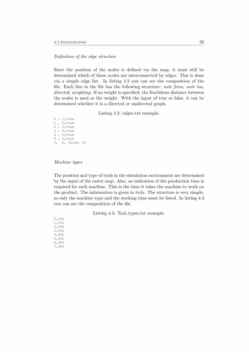
4.5 Initialization 56
Definition of the edge structure
Since the position of the nodes is defined via the map, it must still bedetermined which of these nodes are interconnected by edges. This is donevia a simple edge list. In listing 4.2 you can see the composition of thefile. Each line in the file has the following structure: note from, note too,directed, weighting. If no weight is specified, the Euclidean distance betweenthe nodes is used as the weight. With the input of true or false, it can bedetermined whether it is a directed or undirected graph.
Listing 4.2: edges.txt example.0 , 1,true1 , 2,true2 , 3,true3 , 4,true4 , 5,true5 , 6,true3, 6, false, 50
Machine types
The position and type of tools in the simulation environment are determinedby the input of the raster map. Also, an indication of the production time isrequired for each machine. This is the time it takes the machine to work onthe product. The information is given in ticks. The structure is very simple,so only the machine type and the working time must be listed. In listing 4.3you can see the composition of the file
Listing 4.3: Tool types.txt example.0,3001,1502,2003,1004,8005,2006,4007,380
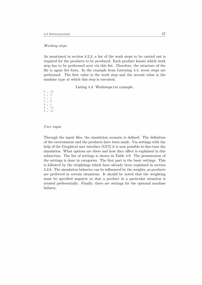
4.5 Initialization 57
Working steps
As mentioned in section 4.2.3, a list of the work steps to be carried out isrequired for the products to be produced. Each product knows which workstep has to be performed next via this list. Therefore, the structure of thefile is again list form. In the example from Listening 4.4, seven steps areperformed. The first value is the work step and the second value is themachine type at which this step is executed.
Listing 4.4: Worksteps.txt example.0 , 101 , 02 , 13 , 84 , 15 , 136 , 12
User input
Through the input files, the simulation scenario is defined. The definitionof the environment and the products have been made. Via settings with thehelp of the Graphical user interface (GUI) it is now possible to fine-tune thesimulation. What options are there and how they affect is explained in thissubsection. The list of settings is shown in Table 4.9. The presentation ofthe settings is done in categories. The first part is the basic settings. Thisis followed by the weightings which have already been explained in section4.2.6. The simulation behavior can be influenced by the weights, as productsare preferred in certain situations. It should be noted that the weightingmust be specified negative so that a product in a particular situation istreated preferentially. Finally, there are settings for the optional machinefailures.
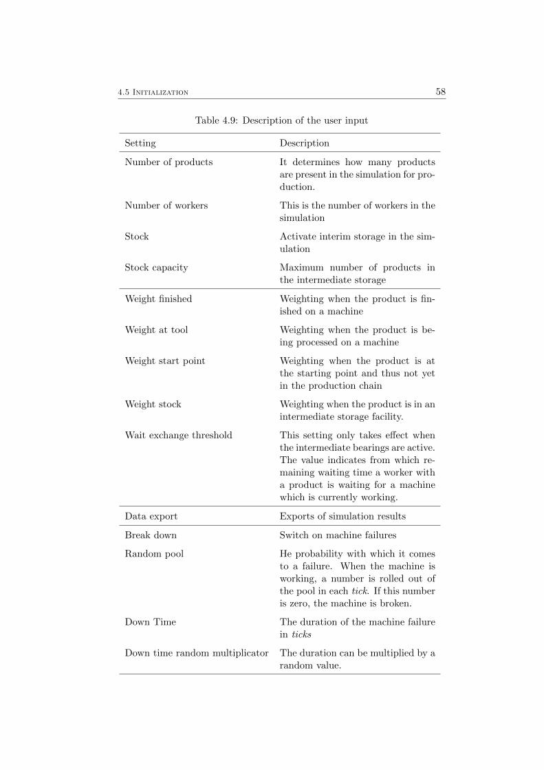
4.5 Initialization 58
Table 4.9: Description of the user input
Setting Description
Number of products It determines how many productsare present in the simulation for pro-duction.
Number of workers This is the number of workers in thesimulation
Stock Activate interim storage in the sim-ulation
Stock capacity Maximum number of products inthe intermediate storage
Weight finished Weighting when the product is fin-ished on a machine
Weight at tool Weighting when the product is be-ing processed on a machine
Weight start point Weighting when the product is atthe starting point and thus not yetin the production chain
Weight stock Weighting when the product is in anintermediate storage facility.
Wait exchange threshold This setting only takes effect whenthe intermediate bearings are active.The value indicates from which re-maining waiting time a worker witha product is waiting for a machinewhich is currently working.
Data export Exports of simulation results
Break down Switch on machine failures
Random pool He probability with which it comesto a failure. When the machine isworking, a number is rolled out ofthe pool in each tick. If this numberis zero, the machine is broken.
Down Time The duration of the machine failurein ticks
Down time random multiplicator The duration can be multiplied by arandom value.
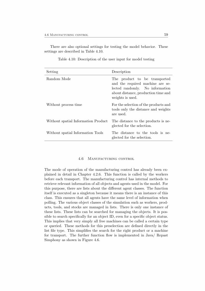
4.6 Manufacturing control 59
There are also optional settings for testing the model behavior. Thesesettings are described in Table 4.10.
Table 4.10: Description of the user input for model testing
Setting Description
Random Mode The product to be transportedand the required machine are se-lected randomly. No informationabout distance, production time andweights is used.
Without process time For the selection of the products andtools only the distance and weightsare used.
Without spatial Information Product The distance to the products is ne-glected for the selection.
Without spatial Information Tools The distance to the tools is ne-glected for the selection.
4.6 Manufacturing control
The mode of operation of the manufacturing control has already been ex-plained in detail in Chapter 4.2.6. This function is called by the workersbefore each transport. The manufacturing control has internal methods toretrieve relevant information of all objects and agents used in the model. Forthis purpose, there are lists about the different agent classes. The functionitself is executed as a singleton because it means there is an instance of thisclass. This ensures that all agents have the same level of information whenpolling. The various object classes of the simulation such as workers, prod-ucts, tools, and stocks are managed in lists. There is only one instance ofthese lists. These lists can be searched for managing the objects. It is pos-sible to search specifically for an object ID, even for a specific object status.This implies that very simply all free machines can be called a certain typeor queried. These methods for this preselection are defined directly in thelist file type. This simplifies the search for the right product or a machinefor transport. The further function flow is implemented in Java/ RepastSimphony as shown in Figure 4.6.
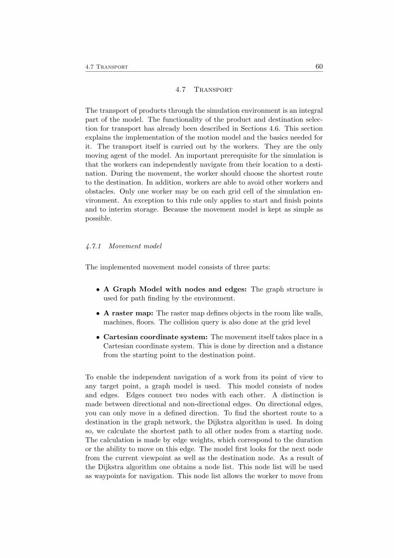
4.7 Transport 60
4.7 Transport
The transport of products through the simulation environment is an integralpart of the model. The functionality of the product and destination selec-tion for transport has already been described in Sections 4.6. This sectionexplains the implementation of the motion model and the basics needed forit. The transport itself is carried out by the workers. They are the onlymoving agent of the model. An important prerequisite for the simulation isthat the workers can independently navigate from their location to a desti-nation. During the movement, the worker should choose the shortest routeto the destination. In addition, workers are able to avoid other workers andobstacles. Only one worker may be on each grid cell of the simulation en-vironment. An exception to this rule only applies to start and finish pointsand to interim storage. Because the movement model is kept as simple aspossible.
4.7.1 Movement model
The implemented movement model consists of three parts:
• A Graph Model with nodes and edges: The graph structure isused for path finding by the environment.
• A raster map: The raster map defines objects in the room like walls,machines, floors. The collision query is also done at the grid level
• Cartesian coordinate system: The movement itself takes place in aCartesian coordinate system. This is done by direction and a distancefrom the starting point to the destination point.
To enable the independent navigation of a work from its point of view toany target point, a graph model is used. This model consists of nodesand edges. Edges connect two nodes with each other. A distinction ismade between directional and non-directional edges. On directional edges,you can only move in a defined direction. To find the shortest route to adestination in the graph network, the Dijkstra algorithm is used. In doingso, we calculate the shortest path to all other nodes from a starting node.The calculation is made by edge weights, which correspond to the durationor the ability to move on this edge. The model first looks for the next nodefrom the current viewpoint as well as the destination node. As a result ofthe Dijkstra algorithm one obtains a node list. This node list will be usedas waypoints for navigation. This node list allows the worker to move from
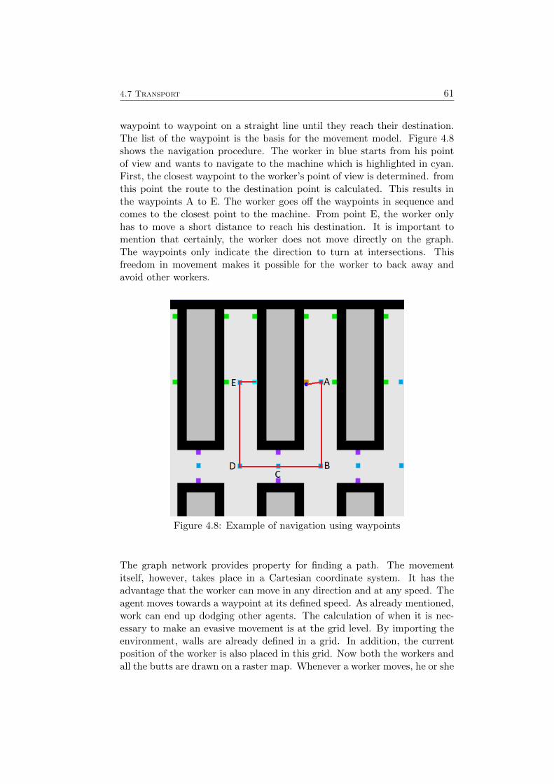
4.7 Transport 61
waypoint to waypoint on a straight line until they reach their destination.The list of the waypoint is the basis for the movement model. Figure 4.8shows the navigation procedure. The worker in blue starts from his pointof view and wants to navigate to the machine which is highlighted in cyan.First, the closest waypoint to the worker’s point of view is determined. fromthis point the route to the destination point is calculated. This results inthe waypoints A to E. The worker goes off the waypoints in sequence andcomes to the closest point to the machine. From point E, the worker onlyhas to move a short distance to reach his destination. It is important tomention that certainly, the worker does not move directly on the graph.The waypoints only indicate the direction to turn at intersections. Thisfreedom in movement makes it possible for the worker to back away andavoid other workers.
Figure 4.8: Example of navigation using waypoints
The graph network provides property for finding a path. The movementitself, however, takes place in a Cartesian coordinate system. It has theadvantage that the worker can move in any direction and at any speed. Theagent moves towards a waypoint at its defined speed. As already mentioned,work can end up dodging other agents. The calculation of when it is nec-essary to make an evasive movement is at the grid level. By importing theenvironment, walls are already defined in a grid. In addition, the currentposition of the worker is also placed in this grid. Now both the workers andall the butts are drawn on a raster map. Whenever a worker moves, he or she
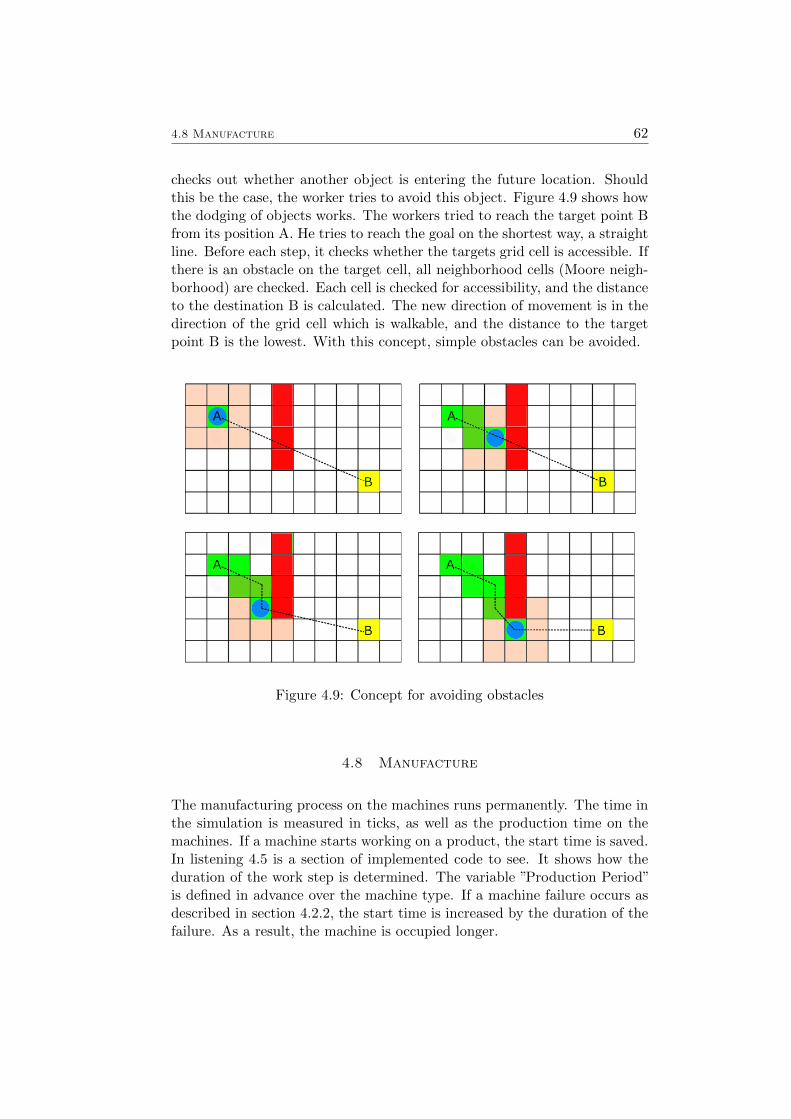
4.8 Manufacture 62
checks out whether another object is entering the future location. Shouldthis be the case, the worker tries to avoid this object. Figure 4.9 shows howthe dodging of objects works. The workers tried to reach the target point Bfrom its position A. He tries to reach the goal on the shortest way, a straightline. Before each step, it checks whether the targets grid cell is accessible. Ifthere is an obstacle on the target cell, all neighborhood cells (Moore neigh-borhood) are checked. Each cell is checked for accessibility, and the distanceto the destination B is calculated. The new direction of movement is in thedirection of the grid cell which is walkable, and the distance to the targetpoint B is the lowest. With this concept, simple obstacles can be avoided.
Figure 4.9: Concept for avoiding obstacles
4.8 Manufacture
The manufacturing process on the machines runs permanently. The time inthe simulation is measured in ticks, as well as the production time on themachines. If a machine starts working on a product, the start time is saved.In listening 4.5 is a section of implemented code to see. It shows how theduration of the work step is determined. The variable ”Production Period”is defined in advance over the machine type. If a machine failure occurs asdescribed in section 4.2.2, the start time is increased by the duration of thefailure. As a result, the machine is occupied longer.
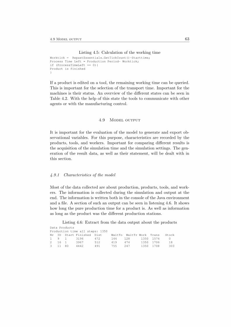
4.9 Model output 63
Listing 4.5: Calculation of the working timeWorktick = RepastEssentials.GetTickCount()-Starttime;Process Time Left = Production Period- Worktick;if (ProcessTimeLeft == 0){Product is finished}
If a product is edited on a tool, the remaining working time can be queried.This is important for the selection of the transport time. Important for themachines is their status. An overview of the different states can be seen inTable 4.2. With the help of this state the tools to communicate with otheragents or with the manufacturing control.
4.9 Model output
It is important for the evaluation of the model to generate and export ob-servational variables. For this purpose, characteristics are recorded by theproducts, tools, and workers. Important for comparing different results isthe acquisition of the simulation time and the simulation settings. The gen-eration of the result data, as well as their statement, will be dealt with inthis section.
4.9.1 Characteristics of the model
Most of the data collected are about production, products, tools, and work-ers. The information is collected during the simulation and output at theend. The information is written both in the console of the Java environmentand a file. A section of such an output can be seen in listening 4.6. It showshow long the pure production time for a product is. As well as informationas long as the product was the different production stations.
Listing 4.6: Extract from the data output about the productsData ProductsProduction time all steps: 1350Nr ID Start Finished Dist WaitTo WaitTr Work Trans Stock1 9 1 3196 472 144 128 1350 1574 02 16 1 3967 512 419 474 1350 1706 183 11 80 4442 491 755 247 1350 1708 303
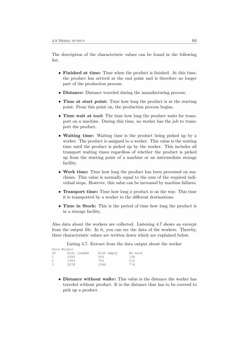
4.9 Model output 64
The description of the characteristic values can be found in the followinglist.
• Finished at time: Time when the product is finished. At this time,the product has arrived at the end point and is therefore no longerpart of the production process.
• Distance: Distance traveled during the manufacturing process.
• Time at start point: Time how long the product is at the startingpoint. From this point on, the production process begins.
• Time wait at tool: The time how long the product waits for trans-port on a machine. During this time, no worker has the job to trans-port the product.
• Waiting time: Waiting time is the product being picked up by aworker. The product is assigned to a worker. This value is the waitingtime until the product is picked up by the worker. This includes alltransport waiting times regardless of whether the product is pickedup from the starting point of a machine or an intermediate storagefacility.
• Work time: Time how long the product has been processed on ma-chines. This value is normally equal to the sum of the required indi-vidual steps. However, this value can be increased by machine failures.
• Transport time: Time how long a product is on the way. This timeit is transported by a worker to the different destinations.
• Time in Stock: This is the period of time how long the product isin a storage facility.
Also data about the workers are collected. Listening 4.7 shows an excerptfrom the output file. In it, you can see the data of the workers. Thereby,three characteristic values are written down which are explained below.
Listing 4.7: Extract from the data output about the workerData WorkerID Dist loaded Dist empty No work1 2058 543 1382 1904 702 2103 2078 1048 774
• Distance without wafer: This value is the distance the worker hastraveled without product. It is the distance that has to be covered topick up a product.
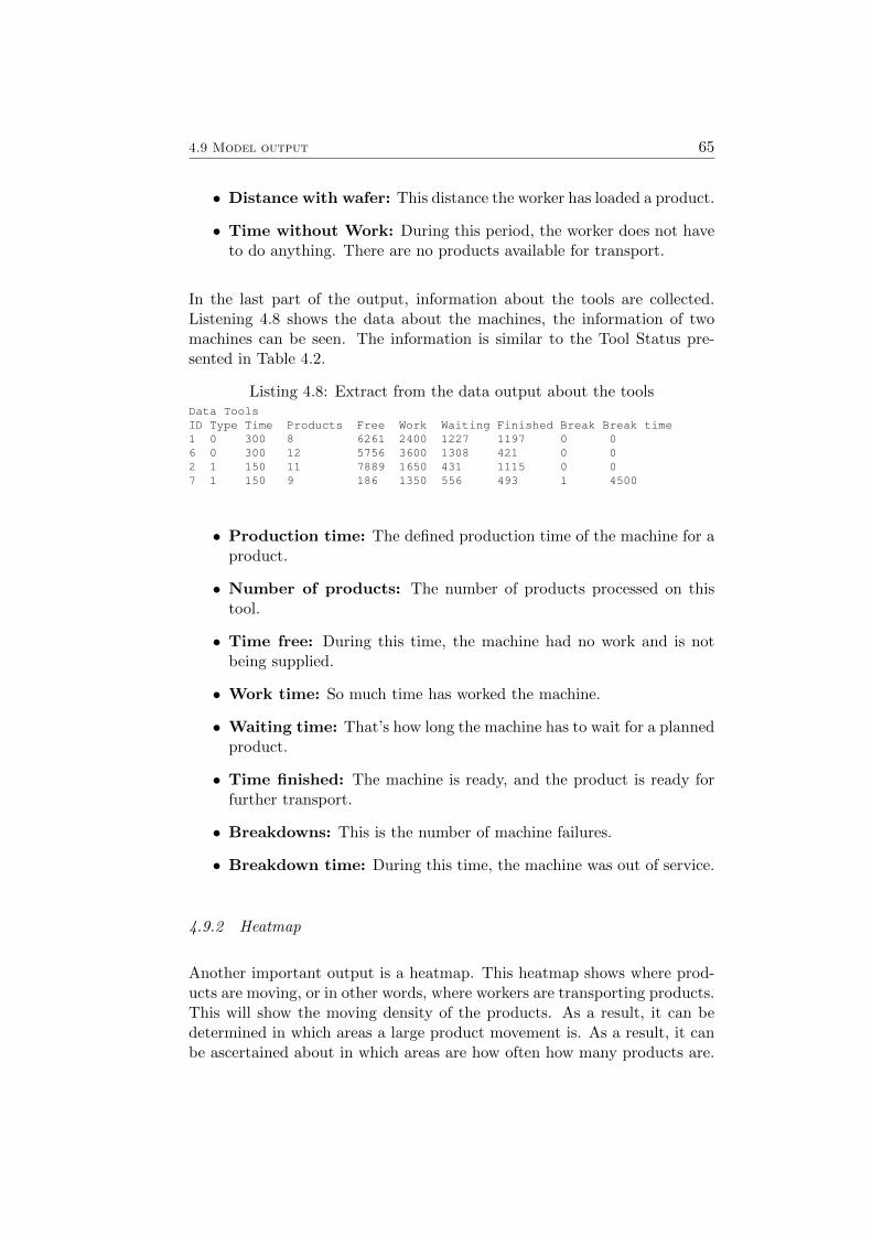
4.9 Model output 65
• Distance with wafer: This distance the worker has loaded a product.
• Time without Work: During this period, the worker does not haveto do anything. There are no products available for transport.
In the last part of the output, information about the tools are collected.Listening 4.8 shows the data about the machines, the information of twomachines can be seen. The information is similar to the Tool Status pre-sented in Table 4.2.
Listing 4.8: Extract from the data output about the toolsData ToolsID Type Time Products Free Work Waiting Finished Break Break time1 0 300 8 6261 2400 1227 1197 0 06 0 300 12 5756 3600 1308 421 0 02 1 150 11 7889 1650 431 1115 0 07 1 150 9 186 1350 556 493 1 4500
• Production time: The defined production time of the machine for aproduct.
• Number of products: The number of products processed on thistool.
• Time free: During this time, the machine had no work and is notbeing supplied.
• Work time: So much time has worked the machine.
• Waiting time: That’s how long the machine has to wait for a plannedproduct.
• Time finished: The machine is ready, and the product is ready forfurther transport.
• Breakdowns: This is the number of machine failures.
• Breakdown time: During this time, the machine was out of service.
4.9.2 Heatmap
Another important output is a heatmap. This heatmap shows where prod-ucts are moving, or in other words, where workers are transporting products.This will show the moving density of the products. As a result, it can bedetermined in which areas a large product movement is. As a result, it canbe ascertained about in which areas are how often how many products are.
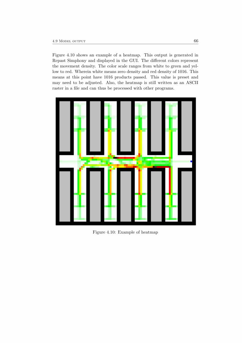
4.9 Model output 66
Figure 4.10 shows an example of a heatmap. This output is generated inRepast Simphony and displayed in the GUI. The different colors representthe movement density. The color scale ranges from white to green and yel-low to red. Wherein white means zero density and red density of 1016. Thismeans at this point have 1016 products passed. This value is preset andmay need to be adjusted. Also, the heatmap is still written as an ASCIIraster in a file and can thus be processed with other programs.
Figure 4.10: Example of heatmap
4.9 Model output 67
4.9.3 Time series
With Repast Simphony it is possible to create a time series during the sim-ulation. This can be done in the GUI. The following time series has beencreated for the model. Or performance reasons, the time series are not dis-played live, but are first created in post-processing. For further processing,the data can be exported as a csv file. With the help of all exported data,the results can be better visualized and analyzed with external programs.
• Number of products in the stock in the course of the simulation.
• Number of free machines in the simulation process.
• Number of finished tools during the simulation process
• Number of broken machines
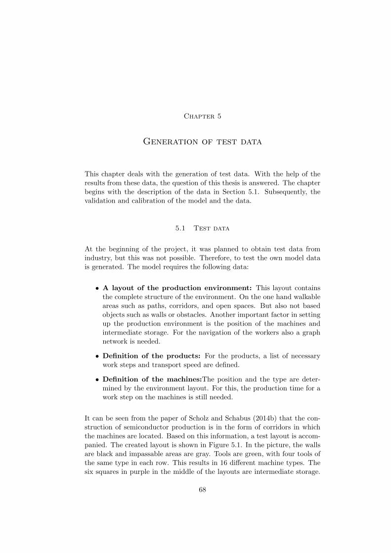
Chapter 5
Generation of test data
This chapter deals with the generation of test data. With the help of theresults from these data, the question of this thesis is answered. The chapterbegins with the description of the data in Section 5.1. Subsequently, thevalidation and calibration of the model and the data.
5.1 Test data
At the beginning of the project, it was planned to obtain test data fromindustry, but this was not possible. Therefore, to test the own model datais generated. The model requires the following data:
• A layout of the production environment: This layout containsthe complete structure of the environment. On the one hand walkableareas such as paths, corridors, and open spaces. But also not basedobjects such as walls or obstacles. Another important factor in settingup the production environment is the position of the machines andintermediate storage. For the navigation of the workers also a graphnetwork is needed.
• Definition of the products: For the products, a list of necessarywork steps and transport speed are defined.
• Definition of the machines:The position and the type are deter-mined by the environment layout. For this, the production time for awork step on the machines is still needed.
It can be seen from the paper of Scholz and Schabus (2014b) that the con-struction of semiconductor production is in the form of corridors in whichthe machines are located. Based on this information, a test layout is accom-panied. The created layout is shown in Figure 5.1. In the picture, the wallsare black and impassable areas are gray. Tools are green, with four tools ofthe same type in each row. This results in 16 different machine types. Thesix squares in purple in the middle of the layouts are intermediate storage.
68
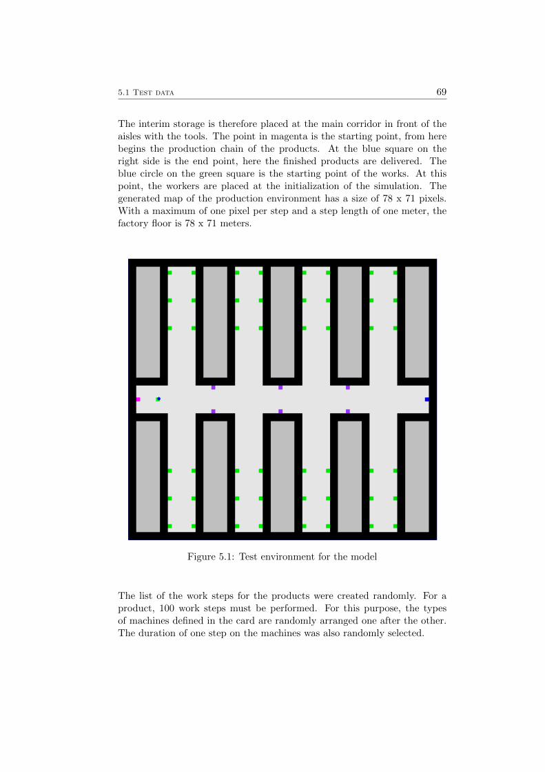
5.1 Test data 69
The interim storage is therefore placed at the main corridor in front of theaisles with the tools. The point in magenta is the starting point, from herebegins the production chain of the products. At the blue square on theright side is the end point, here the finished products are delivered. Theblue circle on the green square is the starting point of the works. At thispoint, the workers are placed at the initialization of the simulation. Thegenerated map of the production environment has a size of 78 x 71 pixels.With a maximum of one pixel per step and a step length of one meter, thefactory floor is 78 x 71 meters.
Figure 5.1: Test environment for the model
The list of the work steps for the products were created randomly. For aproduct, 100 work steps must be performed. For this purpose, the typesof machines defined in the card are randomly arranged one after the other.The duration of one step on the machines was also randomly selected.
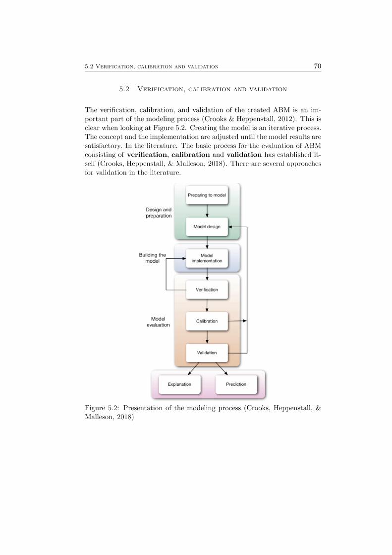
5.2 Verification, calibration and validation 70
5.2 Verification, calibration and validation
The verification, calibration, and validation of the created ABM is an im-portant part of the modeling process (Crooks & Heppenstall, 2012). This isclear when looking at Figure 5.2. Creating the model is an iterative process.The concept and the implementation are adjusted until the model results aresatisfactory. In the literature. The basic process for the evaluation of ABMconsisting of verification, calibration and validation has established it-self (Crooks, Heppenstall, & Malleson, 2018). There are several approachesfor validation in the literature.
Figure 5.2: Presentation of the modeling process (Crooks, Heppenstall, &Malleson, 2018)
5.2 Verification, calibration and validation 71
Verification
Verification is the process that ensures that the implemented model corres-ponds to the model design or that the model has been correctly programmed(Crooks & Heppenstall, 2012). Checking whether the model behaves as ex-pected is called internal validation. The internal validation is more difficultto perform because it must be evaluated why the model comes to a result.However, it is often difficult to say whether the unexpected result is a pro-gramming error or a logical error in the model. One way to overload thesystem is to bring the model in extreme situations where the results can bepredicted more easily (De Smith et al., 2015). An additional difficulty isthat the simulations are mostly based on random numbers. Thus, repeatedsimulation runs can lead to different results. Therefore, the model will betested component by component to check the function of each function. Theverification of the model can take more time than the actual modeling andprogramming (De Smith et al., 2015; Crooks et al., 2018). The validation ofthe model created in this project was traced back to a simple test environ-ment in which the actions of the agents can be easily tracked and controlled.The test environment for verifying the model is shown in Figure 5.3. Theenvironment has five different machine types and three intermediate stor-age. At each machine type, a work step is performed. Also, a bottleneck isintegrated into the layout. The two machines on the right-hand side havea much longer working time than the rest, followed by a single but fastmachine. Due to this structure, the workflow is heavily influenced, and theintermediate storage facilities must be used.
Figure 5.3: Test environment for model verification
Table 5.1 shows some settings for testing the system. In this case, the weight-ings are tested. In all test runs In all runs, 20 products are manufacturedwith five workers. There is room for five products in the interim storage
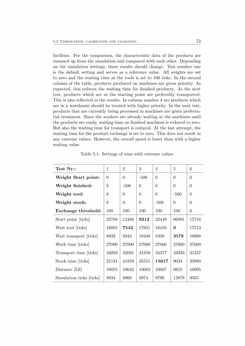
5.2 Verification, calibration and validation 72
facilities. For the comparison, the characteristic data of the products aresummed up from the simulation and compared with each other. Dependingon the simulation settings, these results should change. Test number oneis the default setting and serves as a reference value. All weights are setto zero and the waiting time at the tools is set to 100 ticks. In the secondcolumn of the table, products produced on machines are given priority. Asexpected, this reduces the waiting time for finished products. As the nexttest, products which are at the starting point are preferably transported.This is also reflected in the results. In column number 4 are products whichare in a warehouse should be treated with higher priority. In the next test,products that are currently being processed in machines are given preferen-tial treatment. Since the workers are already waiting at the machines untilthe products are ready, waiting time on finished machines is reduced to zero.But also the waiting time for transport is reduced. At the last attempt, thewaiting time for the product exchange is set to zero. This does not result inany extreme values. However, the overall speed is lower than with a higherwaiting value.
Table 5.1: Settings of runs with extreme values
Test Nr.: 1 2 3 4 5 6
Weight Start point: 0 0 -500 0 0 0
Weight finished: 0 -500 0 0 0 0
Weight tool: 0 0 0 0 -500 0
Weight stock: 0 0 0 -500 0 0
Exchange threshold: 100 100 100 100 100 0
Start point [ticks] 25788 12488 9312 32449 86991 15716
Wait tool [ticks] 16805 7542 17951 16416 0 17513
Wait transport [ticks] 6932 9343 10448 8338 3578 10668
Work time [ticks] 27000 27000 27000 27000 27000 27000
Transport time [ticks] 34093 32085 31859 34377 33033 31437
Stock time [ticks] 21131 41859 35551 15017 9034 33980
Distance [LE] 10055 10042 10083 10087 9855 10095
Simulation ticks [ticks] 8934 8960 8974 9790 13878 9565
5.2 Verification, calibration and validation 73
This is one way to verify the entire model. Other functions, such as themotion model or the correct sequence of work steps, were tested during theimplementation of the individual program parts.
Calibration
During calibration, the model parameters are set so that they correspondto the real system to be depicted. This process requires data on whichthe model is based (De Smith et al., 2015). The model adjusted using thecalibration observed data. This process is necessary because the theoreticalassumptions for the general structure of the model are not precise enoughand therefore still need to be adjusted (Crooks et al., 2018). The calibrationprocess is usually iterative and is usually repeated until the results of themodel correspond to the real collected data. If the result of the modelcannot be adapted to the real values, it is necessary to redesign and programaspects of the model. Thus the calibration can be seen as verification ofthe model. How a model corresponds to the real world depends on thepurpose of the model (De Smith et al., 2015). Calibration is not yet avalidation, but it can be seen as a fine-tuning in which the optimal modelparameters are found (Crooks & Heppenstall, 2012). Typically, there are twoapproaches to calibration, either quantitative or qualitative. Quantitativecalibration calculates the difference between the simulation output and thereal data. In qualitative calibration, the model results are evaluated usinghuman intuition. This method is used in spatial models with GIS and spatialdata visualization (Crooks et al., 2018). Since no real data are available forthe model created in this work, the calibration is performed only on theplausibility of the results.
Validation
The validation of a model concludes the evaluation of the model. The goalof validation is to prove that the model is sufficiently accurate. The tradi-tional approach for validation is based on the calibration approach (Guerini& Moneta, 2017). Since there is a risk that the model will be adapted to thedata during calibration, validation is performed with a new or different dataset. This condition is achieved when the model can reliably replicate realconditions without further calibration. Validation is carried out according tothe same qualitative and quantitative methods as calibration (Crooks et al.,2018). In the work of Guerini and Moneta (2017), however, this validationmethod is seen only as a first step. Despite the use of different data for cal-
5.2 Verification, calibration and validation 74
ibration and validation, the model may be adapted to the data. Therefore,this process is improved to prove that the modeled data generation mecha-nism corresponds to the real data generation mechanism. In the approachof Guerini and Moneta (2017), the causal structures are estimated by themodel or the real world and then compared with each other. This allowsthe ABM to be compared with empirical data as well as different models.Brown, Page, Riolo, Zellner, and Rand (2005) presents a further approachfor the validation and spatial in particular land use models. Measurementsof the spatial similarity of model results and reference data provide infor-mation about the accuracy and variability of the model.
Chapter 6
Results
In this chapter, the results of the experiment and the answers to the scientificquestion that are asked in the introduction will be given. The questions ofthe work are answered on the basis of the results from the model. For thispurpose, the simulation is executed in different settings, and the results aredisplayed. The following subjects are covered in this chapter.
• General scenario: The data obtained and the analysis possibilities ofthis data are shown here.
• Effect of additional information on simulation: This section explainshow storage and spatial information affect the simulation.
• Improvement of the simulation scenario based on the results: This sec-tion discusses how to improve the simulation result from the simulationdata.
6.1 General Scenario
In this section, the question is to be clarified whether ABM is able to re-produce a semiconductor production. Therefore, settings corresponding tothose of a semiconductor production are selected for this simulation. Asstated in the paper of Scholz and Schabus (2014a), several hundred worksteps on different machines can be required to finish a product. The envi-ronment described in Section 5.1 is used for the simulation. The simulationsettings are listed in Table 6.1. On the basis of this setup, the data obtainedand thus possible analyses of the model are shown.
75
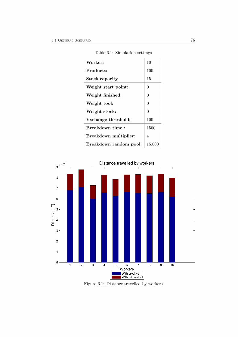
6.1 General Scenario 76
Table 6.1: Simulation settings
Worker: 10
Products: 100
Stock capacity 15
Weight start point: 0
Weight finished: 0
Weight tool: 0
Weight stock: 0
Exchange threshold: 100
Breakdown time : 1500
Breakdown multiplier: 4
Breakdown random pool: 15.000
Figure 6.1: Distance travelled by workers
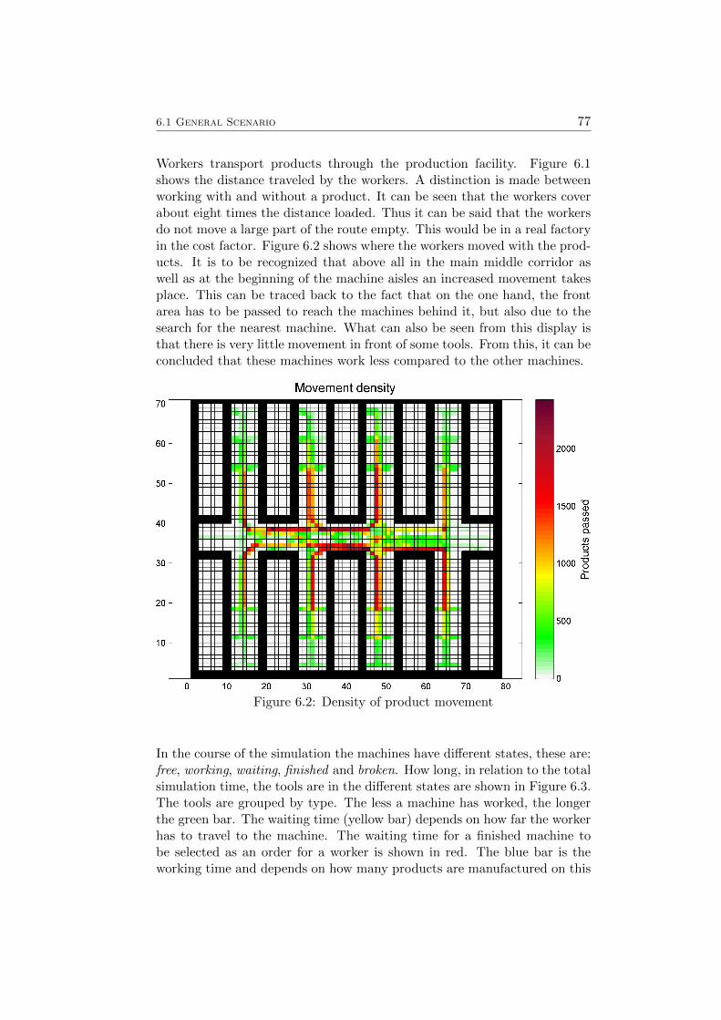
6.1 General Scenario 77
Workers transport products through the production facility. Figure 6.1shows the distance traveled by the workers. A distinction is made betweenworking with and without a product. It can be seen that the workers coverabout eight times the distance loaded. Thus it can be said that the workersdo not move a large part of the route empty. This would be in a real factoryin the cost factor. Figure 6.2 shows where the workers moved with the prod-ucts. It is to be recognized that above all in the main middle corridor aswell as at the beginning of the machine aisles an increased movement takesplace. This can be traced back to the fact that on the one hand, the frontarea has to be passed to reach the machines behind it, but also due to thesearch for the nearest machine. What can also be seen from this display isthat there is very little movement in front of some tools. From this, it can beconcluded that these machines work less compared to the other machines.
Figure 6.2: Density of product movement
In the course of the simulation the machines have different states, these are:free, working, waiting, finished and broken. How long, in relation to the totalsimulation time, the tools are in the different states are shown in Figure 6.3.The tools are grouped by type. The less a machine has worked, the longerthe green bar. The waiting time (yellow bar) depends on how far the workerhas to travel to the machine. The waiting time for a finished machine tobe selected as an order for a worker is shown in red. The blue bar is theworking time and depends on how many products are manufactured on this
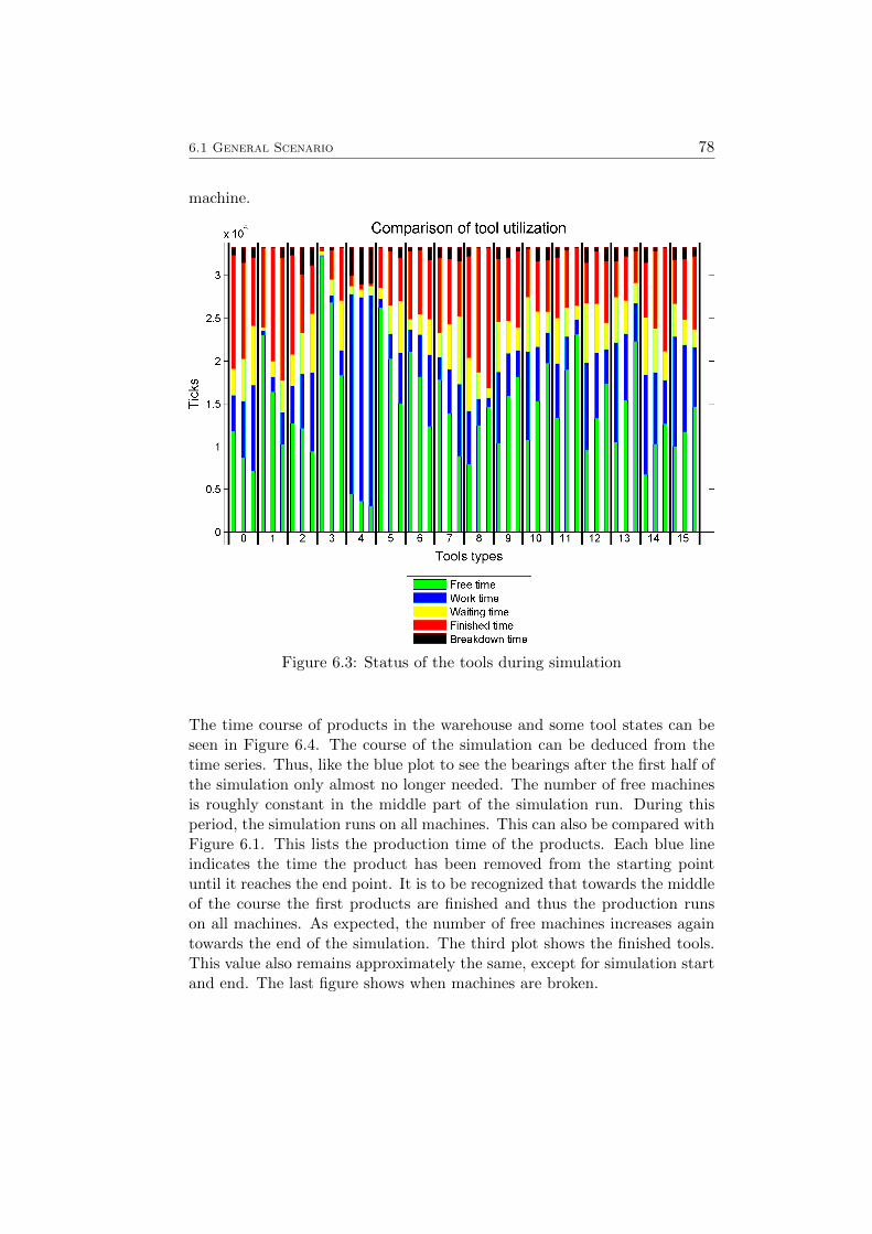
6.1 General Scenario 78
machine.
Figure 6.3: Status of the tools during simulation
The time course of products in the warehouse and some tool states can beseen in Figure 6.4. The course of the simulation can be deduced from thetime series. Thus, like the blue plot to see the bearings after the first half ofthe simulation only almost no longer needed. The number of free machinesis roughly constant in the middle part of the simulation run. During thisperiod, the simulation runs on all machines. This can also be compared withFigure 6.1. This lists the production time of the products. Each blue lineindicates the time the product has been removed from the starting pointuntil it reaches the end point. It is to be recognized that towards the middleof the course the first products are finished and thus the production runson all machines. As expected, the number of free machines increases againtowards the end of the simulation. The third plot shows the finished tools.This value also remains approximately the same, except for simulation startand end. The last figure shows when machines are broken.
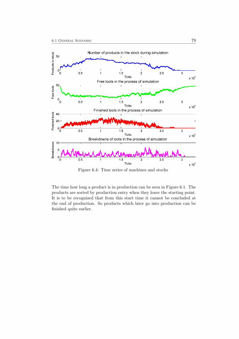
6.1 General Scenario 79
Figure 6.4: Time series of machines and stocks
The time how long a product is in production can be seen in Figure 6.1. Theproducts are sorted by production entry when they leave the starting point.It is to be recognized that from this start time it cannot be concluded atthe end of production. So products which later go into production can befinished quite earlier.
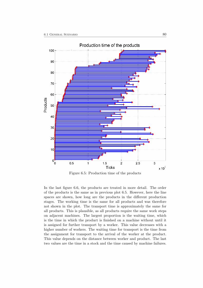
6.1 General Scenario 80
Figure 6.5: Production time of the products
In the last figure 6.6, the products are treated in more detail. The orderof the products is the same as in previous plot 6.5. However, here the linespaces are shown, how long are the products in the different productionstages. The working time is the same for all products and was thereforenot shown in the plot. The transport time is approximately the same forall products. This is plausible, as all products require the same work stepson adjacent machines. The largest proportion is the waiting time, whichis the time in which the product is finished on a machine without until itis assigned for further transport by a worker. This value decreases with ahigher number of workers. The waiting time for transport is the time fromthe assignment for transport to the arrival of the worker at the product.This value depends on the distance between worker and product. The lasttwo values are the time in a stock and the time caused by machine failures.

6.2 Effect of additional information on simulation 81
Figure 6.6: Status of products during simulation
6.2 Effect of additional information on simulation
In the model, the simulated production process is accelerated using distanceinformation and production time data on the machines. The following resultsare intended to clarify how this data affects the simulation and whetherit has an advantage. To be able to compare the results of the individualtests better, the random machine failures are deactivated. 50 products aremanufactured with the same settings as shown in Table 6.1. The simulationis made with the following settings.
• Normal: During this run, workers, have spatial information aboutproducts and tools at their disposal. Also, the running times of themachines can also be queried and included in the planning. Interimstorage facilities are also available. This represents the developed op-timal case.
• Without stocks: The same information is available to the workersas in the normal case, but the stocks must not be used.
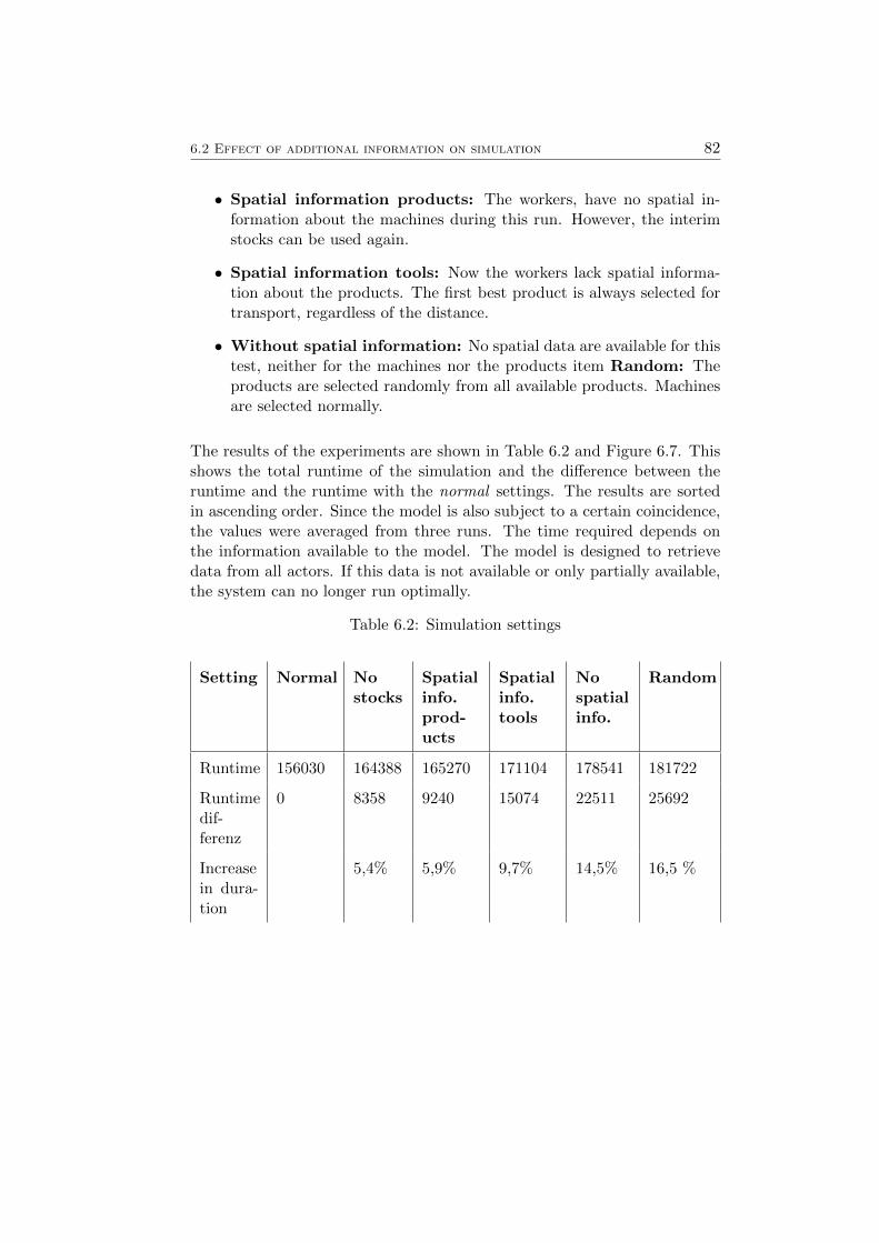
6.2 Effect of additional information on simulation 82
• Spatial information products: The workers, have no spatial in-formation about the machines during this run. However, the interimstocks can be used again.
• Spatial information tools: Now the workers lack spatial informa-tion about the products. The first best product is always selected fortransport, regardless of the distance.
• Without spatial information: No spatial data are available for thistest, neither for the machines nor the products item Random: Theproducts are selected randomly from all available products. Machinesare selected normally.
The results of the experiments are shown in Table 6.2 and Figure 6.7. Thisshows the total runtime of the simulation and the difference between theruntime and the runtime with the normal settings. The results are sortedin ascending order. Since the model is also subject to a certain coincidence,the values were averaged from three runs. The time required depends onthe information available to the model. The model is designed to retrievedata from all actors. If this data is not available or only partially available,the system can no longer run optimally.
Table 6.2: Simulation settings
Setting Normal Nostocks
Spatialinfo.prod-ucts
Spatialinfo.tools
Nospatialinfo.
Random
Runtime 156030 164388 165270 171104 178541 181722
Runtimedif-ferenz
0 8358 9240 15074 22511 25692
Increasein dura-tion
5,4% 5,9% 9,7% 14,5% 16,5 %
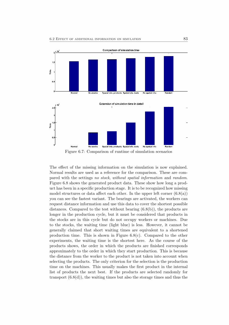
6.2 Effect of additional information on simulation 83
Figure 6.7: Comparison of runtime of simulation scenarios
The effect of the missing information on the simulation is now explained.Normal results are used as a reference for the comparison. These are com-pared with the settings no stock, without spatial information and random.Figure 6.8 shows the generated product data. These show how long a prod-uct has been in a specific production stage. It is to be recognized how missingmodel structures or data affect each other. In the upper left corner (6.8(a))you can see the fastest variant. The bearings are activated, the workers canrequest distance information and use this data to cover the shortest possibledistances. Compared to the test without bearing (6.8(b)), the products arelonger in the production cycle, but it must be considered that products inthe stocks are in this cycle but do not occupy workers or machines. Dueto the stocks, the waiting time (light blue) is less. However, it cannot begenerally claimed that short waiting times are equivalent to a shortenedproduction time. This is shown in Figure 6.8(c). Compared to the otherexperiments, the waiting time is the shortest here. As the course of theproducts shows, the order in which the products are finished correspondsapproximately to the order in which they start production. This is becausethe distance from the worker to the product is not taken into account whenselecting the products. The only criterion for the selection is the productiontime on the machines. This usually makes the first product in the internallist of products the next best. If the products are selected randomly fortransport (6.8(d)), the waiting times but also the storage times and thus the
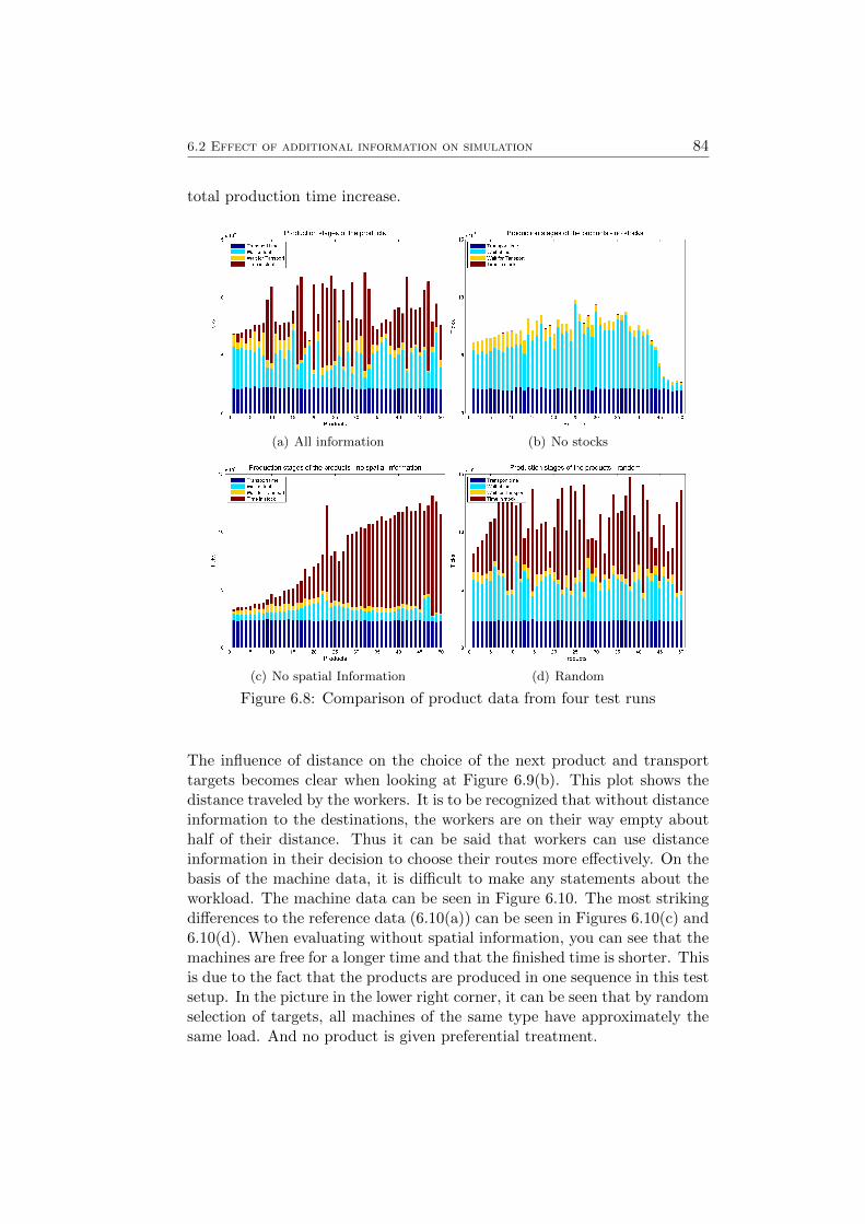
6.2 Effect of additional information on simulation 84
total production time increase.
(a) All information (b) No stocks
(c) No spatial Information (d) Random
Figure 6.8: Comparison of product data from four test runs
The influence of distance on the choice of the next product and transporttargets becomes clear when looking at Figure 6.9(b). This plot shows thedistance traveled by the workers. It is to be recognized that without distanceinformation to the destinations, the workers are on their way empty abouthalf of their distance. Thus it can be said that workers can use distanceinformation in their decision to choose their routes more effectively. On thebasis of the machine data, it is difficult to make any statements about theworkload. The machine data can be seen in Figure 6.10. The most strikingdifferences to the reference data (6.10(a)) can be seen in Figures 6.10(c) and6.10(d). When evaluating without spatial information, you can see that themachines are free for a longer time and that the finished time is shorter. Thisis due to the fact that the products are produced in one sequence in this testsetup. In the picture in the lower right corner, it can be seen that by randomselection of targets, all machines of the same type have approximately thesame load. And no product is given preferential treatment.
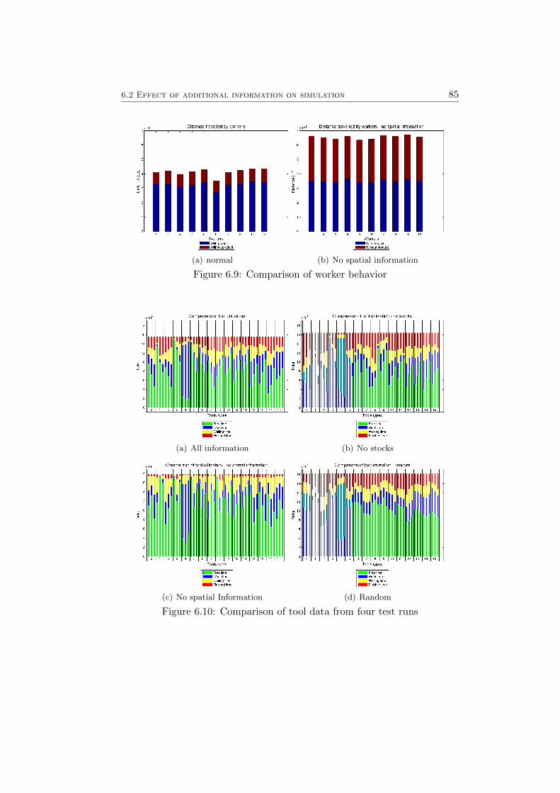
6.2 Effect of additional information on simulation 85
(a) normal (b) No spatial information
Figure 6.9: Comparison of worker behavior
(a) All information (b) No stocks
(c) No spatial Information (d) Random
Figure 6.10: Comparison of tool data from four test runs
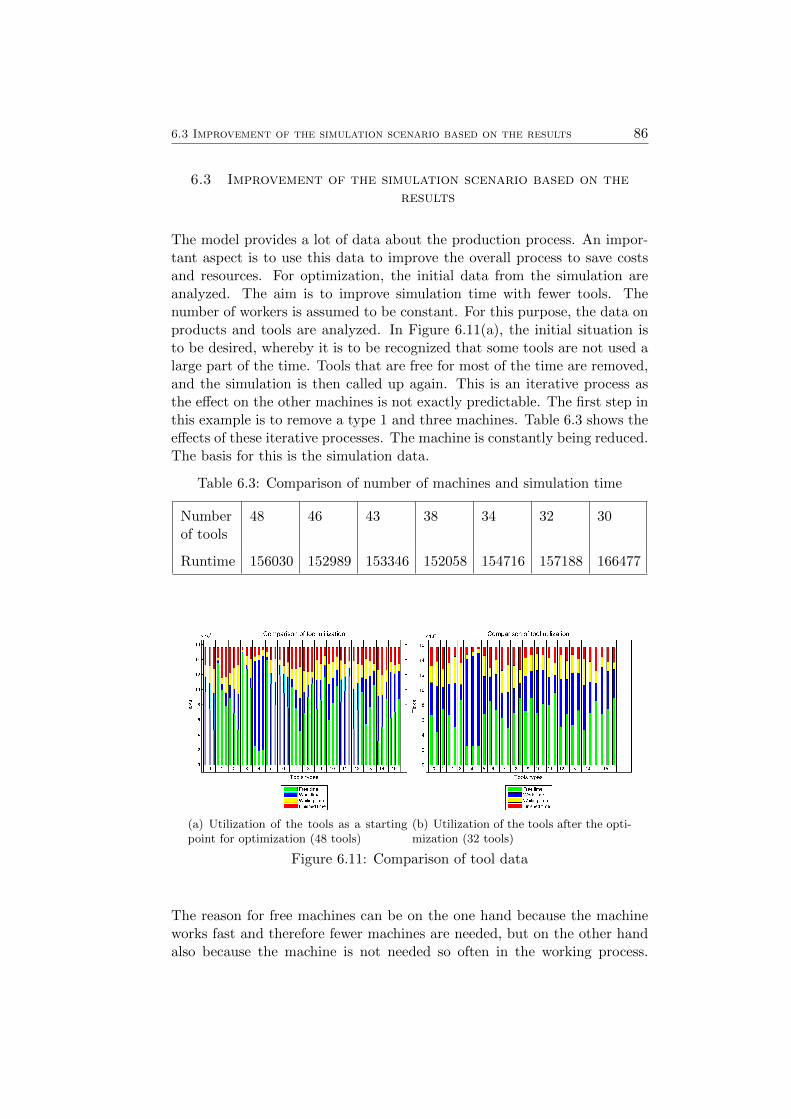
6.3 Improvement of the simulation scenario based on the results 86
6.3 Improvement of the simulation scenario based on theresults
The model provides a lot of data about the production process. An impor-tant aspect is to use this data to improve the overall process to save costsand resources. For optimization, the initial data from the simulation areanalyzed. The aim is to improve simulation time with fewer tools. Thenumber of workers is assumed to be constant. For this purpose, the data onproducts and tools are analyzed. In Figure 6.11(a), the initial situation isto be desired, whereby it is to be recognized that some tools are not used alarge part of the time. Tools that are free for most of the time are removed,and the simulation is then called up again. This is an iterative process asthe effect on the other machines is not exactly predictable. The first step inthis example is to remove a type 1 and three machines. Table 6.3 shows theeffects of these iterative processes. The machine is constantly being reduced.The basis for this is the simulation data.
Table 6.3: Comparison of number of machines and simulation time
Numberof tools
48 46 43 38 34 32 30
Runtime 156030 152989 153346 152058 154716 157188 166477
(a) Utilization of the tools as a startingpoint for optimization (48 tools)
(b) Utilization of the tools after the opti-mization (32 tools)
Figure 6.11: Comparison of tool data
The reason for free machines can be on the one hand because the machineworks fast and therefore fewer machines are needed, but on the other handalso because the machine is not needed so often in the working process.
6.3 Improvement of the simulation scenario based on the results 87
Furthermore, this type of machine can only be required at the beginning orend of the production chain. The absence of such a machine then affectsthe operating time. In the course of the experiment, the number of tools isreduced from 48 to 32, while the runtime remains approximately the same.Figure 6.11(b) shows the utilization of the tools after the reduction. Itis to be recognized that the working time has increased and the idle timeis reduced. The model provides other data to optimize the system. Forexample, the number of workers can be varied, or settings can be madeusing the weightings. Another possibility would be to position the machinedifferently in the factory hall. Due to the object based construction of themodel other data can also be extracted from the model, so every machine,every warehouse, every worker or every product can be observed individually.Thus the ABM offers enough data to optimize a production process.
Chapter 7
Summary and outlook
In this chapter, a summary of this thesis and an outlook for possible ex-tensions or tasks according to this thesis and the resulting Agent-basedmodeling and simulation (ABMS) is given.
7.1 Summary
The goal of the thesis was to create an agent-based model of a semicon-ductor production to simulate a production process. The approaches fromindustry 4.0 and Smart factory were to be combined with the propertiesof ABM. To achieve this goal, the necessary literature on this topic wasfirst prepared and presented. The similarities between the idea of a smartfactory and an ABM have converged. Based on the theory, a concept formodeling a semiconductor production environment using ABM was devel-oped. In the concept shown, the production process takes place without acentral control unit. This decentralized approach is an essential part of thiswork, as it weeps away the concepts of ABM and Industry 4.0. The deci-sions of which product is to be transported and where it is to be taken areadapted to the respective situation. With the aim of keeping the distanceand waiting times short. In the chosen approach, all actors involved areexecuted as agents or as objects, allowing each actor to act independentlyon the basis of defined rules. Workers can query machines and products andmake decisions based on a set of rules. Thus, empty distances can be re-duced. In addition, machine data and information about the stocks can alsobe retrieved. Products also know where they are and what their next stepis, as this corresponds to the idea of a smart factory. The created model hasall important components of production, workers, machines, warehouse, anda production environment. The structure makes it easy to add additionalrules or tests other scenarios. Subsequently, it was shown that the com-plicated model can simulate a production process. The model is equippedwith many adjustment possibilities, which should allow versatile use. It wasshown that the model is designed in such a way that the production processruns as effectively as possible. With the help of the generated data fromthe simulation, it is possible to optimize the initial situation. Unnecessary
88

7.2 Outlook 89
production components can be identified from the data. Furthermore, byanalyzing the movement of the workers and the machines, the productionballast can be further optimized. The ABM model based on object-orientedprogramming offers the possibility to extend the model as desired and toimprove the model or to generate other output data.
7.2 Outlook
The development of the approach chosen in this thesis is by no means com-plete. It is primarily a prototype, improvements and extensions are thereforepossible and also necessary. The most important point here is the referencedata from practice. The model created lacks calibration and validation. Val-idation is a central point in the modeling of a system. Without it, it can beshown that the model does not work, however, whether it corresponds to thereal system. Therefore, comparative data is the most important point forfurther improvements to the model. Based on the findings of a correct vali-dation, the model can be further improved. With the help of this improvedmodel, production processes from the real world can then be simulated andimproved. In further consequence, the production process could be furtherimproved. In the prototypes implanted in this thesis, the machines performa specific work step, which takes a specified amount of time. This imple-mentation could also be refined. To better adapt the amount of work to theindividual machines to the real conditions, depending on the production pro-cess. Another extension would be the implementation of different products.The products can differ not only between different work steps but also bydifferent transport speeds. Also, the implemented movement model couldbe further improved so that it corresponds to that of a real man. Anotherapproach is to see the agents who give the property into the future. Thiscould take the form of workers communicating with each other, exchang-ing information about when they arrive at their destination and what theyhave planned next. The production environment could also be expanded tocover a larger area of production. Doors could be integrated with air locksand staircases. Different areas with different movement speeds or rules ofbehavior would also be conceivable. However, the most important exten-sion in the sense of Geographic information science (GIScience) would be aspatial optimization, based on the validated model. To finally improve thereal production process with the help of the model or the simulation. Thisallows the process to be simulated and optimized even before the start ofproduction. With such an approach, problems in the production process canbe detected at an early stage before a real product is produced.
Bibliography
Abdou, M., Hamill, L., & Gilbert, N. (2012). Designing and building anagent-based model. Agent-Based Models of Geographical Systems, 141–165.
Albach, H., Meffert, H., Pinkwart, A., & Ralf, R. (2015). Management ofpermanent change. Management of Permanent Change, 1–240. doi:10.1007/978-3-658-05014-6. arXiv: arXiv:1011.1669v3
Balietti, S. (2012). Social Self-Organization. doi:10.1007/978-3-642-24004-1.eprint: arXiv:1011.1669v3
Bonabeau, E. (2001). Agent-based modeling: methods and techniques forsimulating human systems. Proceedings of the National Academy ofSciences, 99 (suppl. 3), 7280–7287. Retrieved from http://www.ncbi.nlm.nih.gov/pubmed/12011407
Brown, D. G., Page, S., Riolo, R., Zellner, M., & Rand, W. (2005). Pathdependence and the validation of agent-based spatial models of landuse. International Journal of Geographical Information Science, 19 (2),153–174. doi:10.1080/13658810410001713399
Cantamessa, M. (1997). Agent-balsed modeling and management of man-ufacturing systems. Computers in Industry, 34 (97), 173–186. doi:10.1016/S0166-3615(97)00053-5
Collier, N. & North, M. (2013). Repast java getting started, 1–36. Retrievedfrom http://repast.sourceforge.net/docs/RepastJavaGettingStarted.pdf
Cooley, P. & Solano, E. (2011). Agent-Based Model (ABM) Validation Con-siderations. SIMUL 2011, The Third International Conference on Ad-vances in System Simulation, (100), 134–139.
Couclelis, H. (2000). Chapter 2 : Modeling frameworks , paradigms , andapproaches, 1–15.
Crooks, A. (2009). Agent-Based Modeling and Geographical InformationSystems. A Practical Primer on Geostatistics, 348. Retrieved fromhttp://pubs.usgs.gov/of/2009/1103/
Crooks, A. & Castle, C. (2012, January). The integration of agent-basedmodelling and geographical information for geospatial simulation, 219–251.
Crooks, A., Castle, C., & Batty, M. (2008). Key challenges in agent-basedmodelling for geo-spatial simulation. Computers, Environment and Ur-ban Systems, 32 (6), 417–430.
90
Bibliography 91
Crooks, A. & Heppenstall, A. (2012). Introduction to Agent-Based Mod-elling. Agent-Based Models of Geographical Systems, 85–96.
Crooks, A., Heppenstall, A., & Malleson, N. (2018). Agent-Based Mod-eling. Comprehensive Geographic Information Systems, (December),218–243. doi:10.1016/B978-0-12-409548-9.09704-9
De Smith, J. M., Goodchild, M. F., & Longley, P. (2015). Geospatial anal-ysis: a comprehensive guide to principles, techniques and softwaretools - 5th edition. Retrieved December 31, 2017, from http://www.spatialanalysisonline.com/HTML/
Drath, R. & Horch, A. (2014). Industrie 4.0: hit or hype? [industry forum].IEEE Industrial Electronics Magazine, 8, 56–58.
Gilbert, N. (2007). Agent-Based Models, 1–20.Gilbert, N. & Bankes, S. (2002). Platforms and methods for agent-based
modeling. Proceedings of the National Academy of Sciences, 99 (Supplement3), 7197–7198. doi:10.1073/pnas.072079499
Grimm, V. (1999). Ten years of individual-based modelling in ecology: whathave we learned and what could we learn in the future? EcologicalModelling, 115 (2), 129–148. doi:https : / / doi . org / 10 . 1016 / S0304 -3800(98)00188-4
Grimm, V., Berger, U., DeAngelis, D. L., Polhill, J. G., Giske, J., & Rails-back, S. F. (2010). The ODD protocol: A review and first update.Ecological Modelling, 221 (23), 2760–2768. doi:10 .1016/j .ecolmodel .2010.08.019
Grimm, V. & Railsback, S. S. (2012). Designing, Formulating, and Com-municating Agent-Based Models. Agent-Based Models of GeographicalSystems, 361–377.
Guerini, M. & Moneta, A. (2017). A method for agent-based models val-idation. Journal of Economic Dynamics and Control, 82, 125–141.doi:10.1016/j.jedc.2017.06.001
Helbing, D. (2012). Agent-based modeling. Social self-organization, 25–70.Henning, K., Wolfgang, W., & Johannes, H. (2013). Recommendations for
implementing the strategic initiative INDUSTRIE 4.0. Final report ofthe Industrie 4.0 WG, (April), 82. doi:10.13140/RG.2.1.1205.8966
Heppenstall, A. & Crooks, A. (2016). Agent-based modeling in geographi-cal systems -AccessScience from McGraw-Hill Education Agent-basedmodeling in geographical systems, 1–9. doi:10.1036/1097-8542
Hermann, M., Pentek, T., & Otto, B. (2016). Design principles for industrie4.0 scenarios. Proceedings of the Annual Hawaii International Confer-ence on System Sciences, 2016-March, 3928–3937. doi:10.1109/HICSS.2016.488. arXiv: arXiv:1011.1669v3
Leitao, P. (2009). Agent-based distributed manufacturing control: A state-of-the-art survey. Engineering Applications of Artificial Intelligence,22 (7), 979–991. doi:10.1016/j.engappai.2008.09.005. arXiv: arXiv:1406.0223v1
Bibliography 92
Macal, C. M. & North, M. J. [Michael J.]. (2008). Agent-Based Modelingand Simulation: AMBS Examples. 2008 Winter Simulation Conference(WSC), 101–112. doi:10.1109/WSC.2008.4736060
Macal, C. M. & North, M. J. [Michael J.]. (2009a). Agent-based modelingand simulation. In Winter simulation conference (pp. 86–98). WSC’09. Austin, Texas: Winter Simulation Conference.
Macal, C. M. & North, M. J. [Michael J.]. (2009b). Agent-based modelingand simulation, 86–98.
Macal, C. M. & North, M. J. [Michael J.]. (2010). Tutorial on agent-basedmodelling and simulation, 151–162. Retrieved from https : / / link .springer.com/article/10.1057%2Fjos.2010.3
Macal, C. M. & North, M. J. [Michael J.]. (2013). Introductory tutorial:agent-based modeling and simulation, 362–376.
Mattern, F. & Floerkemeier, C. (2010). From the internet of computers tothe internet of things. Lecture Notes in Computer Science (includingsubseries Lecture Notes in Artificial Intelligence and Lecture Notes inBioinformatics), 6462 LNCS, 242–259. doi:10.1007/978-3-642-17226-7 15. eprint: 9780201398298
Monostori, L., Kumara, S., & Vancza, J. (2006). Agent-Based Systems forManufacturing. CIRP Annals - Manufacturing Technology, 55 (2), 697–720. doi:10.1016/j.cirp.2006.10.004
Negmeldin, M. A. & Eltawil, A. (2015). Agent Based Modeling in FactoryPlanning and Process Control. Industrial Engineering and EngineeringManagement (IEEM), 2015 IEEE International Conference on, 1810–1814.
Nikolai, C. & Madey, G. (2009). Tools of the trade: a survey of variousagent based modeling platforms. Journal of Artificial Societies andSocial Simulation, 12 (2), 2. Retrieved from http://jasss.soc.surrey.ac.uk/12/2/2.html
North, M. J. [Michael J]. (2014). A theoretical formalism for analyzing agent-based models. Complex Adaptive Systems Modeling, 2 (1), 3. Retrievedfrom http://casmodeling.springeropen.com/articles/10.1186/2194-3206-2-3
Plattform Industrie 4.0. (2018). Retrieved January 6, 2018, from http://www.plattform-i40.de/I40/Navigation/DE/Home/home.html
Repast Simphony 2.5 API. (2018). Retrieved May 15, 2018, from https ://repast.github.io/docs/api/repast simphony/index.html
Repast - The Repast Suite. (2018). Retrieved January 21, 2018, from https://repast.github.io/
Wikipedia- Comparison of agent-based modeling software. (2018). RetrievedJanuary 21, 2018, from https://en.wikipedia.org/wiki/Comparisonof agent-based modeling software
O’Sullivan, D., Millington, J., Perry, G., & Wainwright, J. (2012). Agent-based models – because they’re worth it? In A. J. Heppenstall, A. T.
Bibliography 93
Crooks, L. M. See, & M. Batty (Eds.), Agent-based models of ge-ographical systems (pp. 109–123). Dordrecht: Springer Netherlands.doi:10.1007/978-90-481-8927-4 6
PwC. (2016). Industry 4 . 0 : Building the digital enterprise, 1–36. doi:10.1080/01969722.2015.1007734
Roth, A. (2016). Einfuhrung und umsetzung von industrie 4.0. SpringerGabler.
Scholz, J. & Schabus, S. (2014a). An Indoor Navigation Ontology for Pro-duction Assets. Proceedings of the 8th International Conference, GI-Science 2014, Vienna, Austria, September 24-26, 2014. 204–220. doi:10.1007/978-3-319-11593-1 14
Scholz, J. & Schabus, S. (2014b). An Indoor Navigation Ontology for Pro-duction Assets. Proceedings of the 8th International Conference, GI-Science 2014, Vienna, Austria, September 24-26, 2014. 204–220. doi:10.1007/978-3-319-11593-1 14
Scholz, J. & Schabus, S. (2015). Geographic Information Science and Tech-nology as Key Approach to unveil the Potential of Industry 4.0. inProceedings of ICINCO 2015 Vol.2, 12th International Conference onInformatics in Control, Automation and Robotic, (2008), 463–470.
Shrouf, F., Ordieres, J., & Miragliotta, G. (2014). Smart factories in Indus-try 4.0: A review of the concept and of energy management approachedin production based on the Internet of Things paradigm. IEEE Inter-national Conference on Industrial Engineering and Engineering Man-agement, 2015-January, 697–701. doi:10.1109/IEEM.2014.7058728
Spath, D., Gerlach, S., Hammerle, M., Krause, T., & Schlund, S. (2013).Industrie 4.0 – Produktionsarbeit der Zukunft *. Werkstattstechnik,103, 130–134. doi:10 . 1007 / 978 - 3 - 658 - 04682 - 8. eprint: 9809069v1(arXiv:gr-qc)
Torrens, P. M. (2010). Agent-based Models and the Spatial Sciences. Geog-raphy Compass, 4 (5), 428–448. doi:10.1111/j.1749-8198.2009.00311.x
van Kranenburg, R. & Dodson, S. (2008). The internet of things: a cri-tique of ambient technology and the all-seeing network of rfid. Net-work notebooks. Institute of Network Cultures. Retrieved from https://books.google.at/books?id=PilgkgEACAAJ
Wooldridge, M. & Jennings, N. R. (1995). Intelligent agents: theory andpractice. Knowledge Engineering Review, 10, 115–152.
Copyright © 2022 FDOKUMEN