Spatial competition with endogenous location choices: An application to discount retailing
35
Quant Mark Econ (2009) 7:1–35 DOI 10.1007/s11129-008-9048-6 Spatial competition with endogenous location choices: An application to discount retailing Ting Zhu · Vishal Singh Received: 6 July 2007 / Accepted: 1 December 2008 / Published online: 31 January 2009 © Springer Science + Business Media, LLC 2009 Abstract This paper examines the importance of geographical differentiation in store location decisions of firms in the retail discount industry. Using a novel data set that includes the store locations and accompanying market conditions for all stores belonging to the Wal-Mart, Kmart, and Target chains, we study the factors that influence the entry and location decisions of these firms. The model involves an incomplete information game between the three players where each firm has private information about its own profitability. A key feature of our modeling approach is that it permits asymmetries across firms in the impact of exogenous market characteristics and competitive interaction effects. Variations in the exogenous firm specific characteristics, such as the distances from the market to firms’ headquarters and the nearest distribution centers, serve as exclusion restrictions and provide the source for model identification. Parameter estimates of the payoff functions are used to predict the equilibrium market structure under a variety of market conditions that provide insights into the competitive landscape of the industry. Results show that all firms exert a strong negative impact on competitors when they are in close proximity, but the effect decreases with distance to rivals suggesting The paper is based on Ting Zhu’s thesis at Carnegie Mellon University. T. Zhu (B ) · V. Singh University of Chicago Booth School of Business, 5807 S. Woodlawn Ave., Chicago, IL 60637 USA e-mail: [email protected] T. Zhu · V. Singh Leonard N Stern School of Business, Marketing Department, New York University, New York, NY, USA V. Singh e-mail: [email protected]
-
Upload
independent -
Category
Documents
-
view
0 -
download
0
Transcript of Spatial competition with endogenous location choices: An application to discount retailing

Quant Mark Econ (2009) 7:1–35DOI 10.1007/s11129-008-9048-6
Spatial competition with endogenous location choices:An application to discount retailing
Ting Zhu · Vishal Singh
Received: 6 July 2007 / Accepted: 1 December 2008 / Published online: 31 January 2009© Springer Science + Business Media, LLC 2009
Abstract This paper examines the importance of geographical differentiationin store location decisions of firms in the retail discount industry. Using a noveldata set that includes the store locations and accompanying market conditionsfor all stores belonging to the Wal-Mart, Kmart, and Target chains, we studythe factors that influence the entry and location decisions of these firms. Themodel involves an incomplete information game between the three playerswhere each firm has private information about its own profitability. A keyfeature of our modeling approach is that it permits asymmetries across firmsin the impact of exogenous market characteristics and competitive interactioneffects. Variations in the exogenous firm specific characteristics, such as thedistances from the market to firms’ headquarters and the nearest distributioncenters, serve as exclusion restrictions and provide the source for modelidentification. Parameter estimates of the payoff functions are used to predictthe equilibrium market structure under a variety of market conditions thatprovide insights into the competitive landscape of the industry. Results showthat all firms exert a strong negative impact on competitors when they arein close proximity, but the effect decreases with distance to rivals suggesting
The paper is based on Ting Zhu’s thesis at Carnegie Mellon University.
T. Zhu (B) · V. SinghUniversity of Chicago Booth School of Business,5807 S. Woodlawn Ave., Chicago, IL 60637 USAe-mail: [email protected]
T. Zhu · V. SinghLeonard N Stern School of Business, Marketing Department,New York University, New York, NY, USA
V. Singhe-mail: [email protected]

2 T. Zhu, V. Singh
strong returns to spatial differentiation in this industry. Target stores farewell under competition except when these competitors are in close proximity.Wal-Mart’s supercenter format is found to be the most formidable player asit substantially impacts competitors even at a large distance. We also findsignificant asymmetries across players in their response to market conditionsand competition interactions.
Keywords Entry · Discrete games · Location choice ·Retail competition · Discount stores
JEL Classifications L1 · L2 · L81 · R3
1 Introduction
Firms employ a variety of strategies to differentiate their product offeringsfrom competition. In the retailing sector, these strategies include the breadthand depth of product assortment, price, promotions, merchandise quality,customer service, and so forth. However, as a well known aphorism states, thethree most important decisions in retailing are location, location, and location.Store location decisions are particularly important since, unlike other market-ing mix elements, they are less adjustable in the short-run without incurringsignificant costs. When deciding whether to enter a particular local marketand where to locate within that market, firms consider a variety of factorsincluding demand and cost conditions, logistical issues, and proximity to andsize of their consumer base. In addition, firms must account for the actual andpotential presence of competitors. While favorable market conditions suchas large population base and low cost labor encourage entry, such marketsare also likely to attract competitors. In the long-run, the interaction of thesedifferent factors determines the observed entry patterns by firms.
We study the strategic entry and location choice decisions in the retaildiscount industry. For all practical purposes, the industry involves an oligopolycomprised of three dominant firms: Wal-Mart, Kmart, and Target. We as-semble a novel data set that includes store locations and associated marketconditions for all stores belonging to these three chains and study the factorsthat determine firm’s entry and location choices. Our primary objective inthe paper is to provide insights into the competitive landscape facing thesediscount retailers. In particular, we seek to answer the following questions: (1)How important is geographical differentiation in this industry? (2) Do notabledifferences exist in the types of locations that these firms find attractive? (3)How important are competitive effects across these retailers? (4) How dothese competitive effects vary depending on the identities and formats of thecompeting firms?
Ideally, answers to these questions would involve a model in which weexplicitly consider the demand impact of market characteristics as wellas substitution across retailers. With such information, one could evaluate

Spatial competition with endogenous location choices 3
competitive issues across the firms by evaluating the features of demand. Whileintuitively appealing, this approach is difficult to operationalize since accessto the necessary data at the level required for our analysis is problematic.Instead, we seek to answer these questions indirectly through an analysis of theobserved location choices by these retailers. The basic endeavor in our exerciseis to infer features of the firms’ payoffs and the competitive interactionsbetween firms even when one has no access to price, cost or quantity data. Theintuition behind the approach is to invoke revealed preference arguments: thefact that we observe a certain market structure (no entry, monopoly, duopoly,and oligopoly) reveals something about the underlying economic profits atthose locations. Our approach involves setting the decisions of the firms asan outcome of a game of location choices where distance to rivals servesas a form of product differentiation. The empirical analysis then relates thepredictions of the model to the observed behavior of the three chains. Theanalysis provides insights into a fundamental tension faced by these firms,namely the desire to be in attractive locations while also obtaining insulationfrom competition through spatial differentiation.
To model firm’s entry and location choice decisions, we build on theliterature on static discrete games advanced by Bresnahan and Reiss (1987,1990, 1991a, b) and Berry (1992). This literature endogenizes the competitivestructure in a market by implicitly analyzing the first stage of a two-stage gamein which firms first decide whether or not to enter followed by price or quantitycompetition. Mazzeo (2002a, b) extends this literature by incorporating prod-uct differentiation where a firm’s payoff asymmetrically depends on whether acompetitor is more or less similar to the firm. However, in Mazzeo’s frameworkfirms are restricted to choose from a few possible product “types” as a largerchoice set becomes computationally cumbersome due to the large number ofprofit constraints that need to be satisfied in equilibrium. Seim (2001, 2006)solves this dimensionality problem by allowing firms to possess private infor-mation about their own profitability. Her incomplete information approachcircumvents the need for checking a large number of entry configurations tofind the equilibria and allows for a considerably larger dimensional set ofproduct types than is feasible in games of complete information. In a recentpaper, Jia (2008) analyzes the impact of the discount stores on small retailers.An interesting feature of her model is that she allows for spill over effectswithin the same chain across markets. Nishida (2008) extends Jia’s frameworkto study the strategic store network choices by two chains in Japan. However,both authors do not model spatial differentiation across players. In particular,firms in Jia’s framework choose whether to enter a particular market, while inour model each firm decides entry as well as location such that the competitioneffect varies with the distance within a market.
We follow Seim (2001, 2006) by setting up the model as an incompleteinformation game where players privately observe their own location-specificpotential profits, but observe only the distribution of their rivals’ profitability.A firm’s payoff from entering a market and choosing a particular locationdepends on its expectation of the optimal location choices of its competitors

4 T. Zhu, V. Singh
and exogenous market characteristics. These market conditions include de-mand and cost factors such as population and retail wages. In addition to theobserved variables, all firms’ profits also depend on market components thatare unobserved by the analyst, but are observed by all firms. For example,positive or negative market wide shocks such as the availability of commercialland or the restrictiveness of zoning laws are difficult to measure and quantify,but are likely to play an important role in the entry decisions of all firms.Finally, a firm’s payoff in each location includes a component specific to thatfirm and location which could represent idiosyncratic operational costs ormanagerial talent that are unobserved by both the analyst and other players.
A unique feature of our modeling approach is that we explicitly allow forasymmetries related to the identity of the firms. The previous literature hasassumed that firms are symmetric in terms of their sensitivity to exogenousmarket conditions and in their impact on other competitors. In other words,a firm’s profits are assumed to depend on the total number of other firms inthe market rather than their actual identities beyond simple type differencesas in Mazzeo (2002a, b). In reality, firms care about the actual identities oftheir competitors rather than simply the total number of competitors. Forinstance, entry by firms such as Exxon-Mobil, Microsoft, Home Depot, orCitigroup into a geographical or product market may be viewed by competingfirms as a greater threat to profits than entry by smaller independent firms.1
In the current context of discount stores, such asymmetries may be crucial.For instance, Kmart’s profit may be different when it faces a Wal-Mart ratherthan a Target or when it faces a Wal-Mart supercenter rather than a Wal-Martdiscount store. Similarly, the impact of market demand and cost conditionsmay vary across firms as well as store formats. As such, it is paramount toallow such asymmetries in an analysis of this industry.
Our modeling approach allows for both competitive effects and preferencesover exogenous market conditions to be firm-specific. However, allowing forsuch firm asymmetries is not without cost since it leads to a significantly largernumber of parameters to be estimated. More importantly, it raises questionsabout model identification since, as discussed in Bajari et al. (2005a, b), onewould need exclusion restrictions in firm’s payoff functions. In particular, topin down the form of strategic interaction we would need variables that impacta firm’s profit but not impact its rival’s profits directly. In our application,we compute the distance of each market from firm’s headquarters and thenearest distribution center and use them as exclusion restrictions. Since moststates have only one or two distribution centers that cater to all stores inthe region, we take the location of distribution centers as given and focus oncompetition between firms at the retail outlet level. Given this assumption, theincomplete information model provides a tractable framework for studyingthe complex interactions of optimal site selection in which a trade-off exists
1Kyle (2006) makes similar arguments in the context of entry in pharmaceutical drugs.
Spatial competition with endogenous location choices 5
between proximity to competitors and the desirability of certain locationcharacteristics. The model translates the discrete actions of competitors intosmooth location choice probabilities that represent the likelihood of competi-tor entry into a location rather than actual realizations, thus allowing for alarger set of locations (or product types) than is generally feasible in gamesof complete information. The resulting Bayesian Nash equilibrium (BNE) isderived using a nested fixed-point algorithm which is then embedded in asimulated maximum likelihood procedure to estimate the model parameters.
To implement the model, we assembled an original data set that includesall store locations for the three largest players in the discount store industry:Wal-Mart, Kmart, and Target. The data includes the exact location (latitude/longitude) of all stores in operation as of 2003 across the United States. Wepartition the United States into a series of smaller markets and further divideeach market into smaller neighborhoods. Each store can then be mapped toone of these neighborhood locations. In addition, we collected information onthe location of firm’s headquarters and their distribution centers. As discussedabove, distances from the distribution centers to each market location areused as exclusion restrictions and serve as proxies to capture logistical issuesin firm’s location choice decisions. Finally, we supplement the data withdetailed information collected from the US Census Bureau and the Bureau ofLabor Statistics to capture demand and cost conditions at every geographicallocation.
The results show that population in closer distance bands to a locationcontribute more to profitability than population in distant bands. Interestingly,the parameters for distant population are significantly larger for Wal-Mart,especially for its supercenter format, suggesting that Wal-Mart’s trading areais larger than those of its rivals. All firms are found to prefer markets with lowerretail wages, markets where a larger proportion of families have children andvehicles, and markets that are closer to their respective headquarters. We alsofind significant differences across firms in certain demand characteristics. Forinstance, Target is found to prefer markets with higher income and educationlevels compared with its rivals, which is consistent with the common percep-tions of these stores. Wal-Mart, particularly for its supercenter format, givesmore weight to locations that are closer to its distribution center, reflectingits logistical efficiencies. In terms of competitive interactions, we find thatproximity to competitors is an important determinant of profitability. All firmsare found to exert negative impact on competitors when they are in close prox-imity, but the effect decreases with distance to rivals suggesting strong returnsto spatial differentiation in this industry. Looking at the competitive effectsacross firms, we find significant asymmetries in the competitive interactionparameters. For example, while a nearby Kmart strongly impacts Wal-Mart,the effect is significantly lower than the corresponding impact of a Wal-Mart onKmart’s payoffs. Target stores are found to fare well under competition fromother discount stores except when these competitors are in particularly closeproximity. Wal-Mart’s supercenter format is found to be the most formidableplayer as it substantially impacts competitors even at a large distance.

6 T. Zhu, V. Singh
We use the parameter estimates from the latent payoff functions to predictequilibrium market structures under a variety of market conditions that yield anumber of insights into the competitive structure of the industry. For example,as market population and income vary with all other variables held constant,we find that Wal-Mart is able to operate as a monopolist under a wide rangeof market conditions. Target is able to enter as monopolist in certain extremeconditions, such as a relatively small population and very high income, whichgenerally is not attractive to its rivals. Conversely, Kmart is rarely able to findlocations that are not attractive to at least one other player. Similarly, we findthat when entry involves only discount store formats, multiple firms are ableto enter the market under moderately good demand conditions by choosingdifferent locations within a market. On the other hand, Wal-Mart supercentertends to deter entry by competitors altogether unless a market becomes veryattractive. This effect arises since the supercenter format hurts even thosecompetitors that are located far away implying that the opportunities to mutecompetition through geographical differentiation are limited. However, as amarket becomes more and more attractive, good demand conditions overcomethe competition effect.
The rest of the paper is organized as follows. In the next section, we describeour modeling approach. The data used in the study are described in Section 3.Section 4 outlines the estimation strategy and presents the results. Section 5concludes with a discussion of limitations of the current study and directionsfor future research.
2 Model
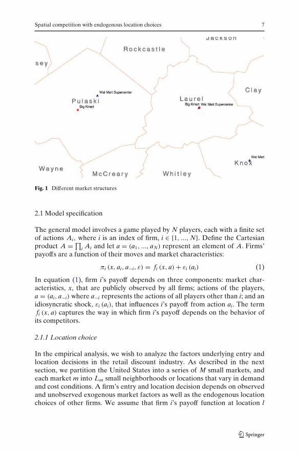
In this section we describe a model of the store location choices of firms in theretail discount industry. The model is structured as an incomplete informationgame following the framework originally developed in Seim (2006). However,as noted above, we allow for competitive effects and preferences overexogenous market conditions to be firm-specific. To illustrate, consider thetwo markets in Fig. 1 each with a Wal-Mart supercenter and Kmart. In the ap-proach of Bresnahan and Reiss (1991a, b) and Berry (1992), both marketswould have the same market structure as their models consider only thetotal number of undifferentiated competitors (besides the non-strategicfixed costs in Berry’s model.) Seim’s framework would categorize these twomarket structures differently due to the presence of geographic differentiation.However, if a Wal-Mart discount store or a Target store replaced the Wal-Martsupercenter, the market structure would not change as Seim (2006) does notconsider identities of the players. In the model presented below, we explicitlyaccount for firm identities and allow for firm-specific effects that are related tocompetitive interactions and the impact of exogenous market characteristics.
Spatial competition with endogenous location choices 7
Fig. 1 Different market structures
2.1 Model specification
The general model involves a game played by N players, each with a finite setof actions Ai, where i is an index of firm, i ∈ {1, ..., N}. Define the Cartesianproduct A = ∏
i Ai and let a = (a1, ..., aN) represent an element of A. Firms’payoffs are a function of their moves and market characteristics:
πi (x, ai, a−i, ε) = fi (x, a) + εi (ai) (1)
In equation (1), firm i’s payoff depends on three components: market char-acteristics, x, that are publicly observed by all firms; actions of the players,a = (ai, a−i) where a−i represents the actions of all players other than i; and anidiosyncratic shock, εi (ai), that influences i’s payoff from action ai. The termfi (x, a) captures the way in which firm i’s payoff depends on the behavior ofits competitors.
2.1.1 Location choice
In the empirical analysis, we wish to analyze the factors underlying entry andlocation decisions in the retail discount industry. As described in the nextsection, we partition the United States into a series of M small markets, andeach market m into Lm small neighborhoods or locations that vary in demandand cost conditions. A firm’s entry and location decision depends on observedand unobserved exogenous market factors as well as the endogenous locationchoices of other firms. We assume that firm i’s payoff function at location l
8 T. Zhu, V. Singh
in market m is a linear function of market and location characteristics andcompetition effects:
πiml = ximlβi −∑
i′ �=i
Lm∑
k=1
δii′klai′mk + ξm + εiml (2)
i, i′ = 1, 2, ...N (firms),
m = 1, 2, ...M (markets),
l, k = 1, 2, ..., Lm (locations),
where ximl are the observed exogenous variables that vary across differentlocations and markets. In addition, these exogenous characteristics includefirm-specific variables such as distance to the firm’s headquarters or the nearestdistribution center. The indicator variables am = (aim, a−im)N×Lm
denote firms’location choices such that aiml = 1 when firm i chooses location l and aiml = 0otherwise. The dimension of am is N × Lm, where N is the number of players,and Lm is the number of possible locations in market m.
Besides the observed variables, profits also depend on unobserved factors.Of these, ξm are market characteristics that are unobserved by the analyst,but are observed by all firms.2 We assume that ξm is normally distributed withmean 0 and variance σ 2. For example, market-specific shocks related to theoverall availability of commercial land or the stringency of zoning restrictionsare likely to play an important role in the entry decisions of all firms, but aredifficult to measure and quantify. Finally, εiml are firm-specific unobservablesrepresenting the private information of firm i’s profitability in location l. Thesefactors could include idiosyncratic operational costs or managerial talent thatare unobserved by both the analyst and other players. If firm i does not enterthe market so that aiml = 0 for all l = 1, ..., Lm, we normalize the payoff as
πim0 = εim0. (3)
The unknown parameters are (βi, δii′kl, σ ) where βi represents firm ı́’spreference for various market characteristics and δii′kl reflect the competitiveeffect that player i′ exerts on player i when they respectively operate stores inlocations k and l. As discussed earlier, we allow all the model parameters to befirm-specific. Thus, the model permits different firms (i) to impact competitorsdifferently and (ii) to put different weight on market conditions.3
Since εiml is private information, a firm cannot predict its competitors’responses (a−im) with certainty. Instead, a firm’s actions is based on its
2In principle, the unobserved market characteristics can impact firms differently. In the empiricalapplication we allowed for this possibility by estimating an additional model which allows for theunobserved market factor to vary across firms and found no substantial differences in results.3As discussed below in the context of format choices, it is also possible for the parameters to becontingent on the actions taken by firms.
Spatial competition with endogenous location choices 9
conjectures or expectation of its competitors’ responses. Thus, firm i’s expectedpayoff of choosing location l in market m is
π̂iml = ximlβi −∑
i′ �=i
Lm∑
k=1
δii′kl E (ai′mk) + ξm + εiml (4)
where E (ai′mk) denotes the expectation of firm i′ choosing location k. Firm ichooses the location that maximizes its expected payoff:
aiml ={
1 if π̂iml ≥ π̂imk, ∀ k = 0, 1, ..., Lm
0 otherwise
If firm’s private information εim (aim) is independently and identically distrib-uted across firms and locations with a type 1 extreme value distribution, theequilibrium probability of firm i choosing location l in market m conditionalon its beliefs of other firms’ behavior is given by
Piml =exp
(ximlβi − ∑
i′ �=i
∑Lmk=1 δii′kl Pi′mk + ξm
)
1 + ∑Lml′=1 exp
(ximl′βi − ∑
i′ �=i
∑Lmk=1 δii′kl′ Pi′mk + ξm
) . (5)
The probability of no entry in the market is then Pim0 = 1 − ∑Lml=1 Piml. Other
firms similarly construct their beliefs and choose their best responses based onthe expected payoffs. Since firms are asymmetric in terms of their preferencesof market conditions and competition, each firm may have different probabilityof choosing a given location. Define Pm = (Pim, P−im)(Lm×N) as a vector withLm × N elements that describes the conjectures of each location being chosenby each individual firm. In the ensuing Bayesian Nash equilibrium, firms’choices are consistent with their conjectures yielding a fixed-point mapping
Pm = F (Xm, ξm, Pm; δ, β) (6)
from the probability space of firms’ beliefs to their own strategies. The equilib-rium location conjectures is a vector with Lm × N probabilities resulting fromthe system of Lm × N equations defined in Eq. (5).
2.1.2 Location and format choice
As discussed in the data section below, the players in this industry operate twostore formats: discount stores and supercenters. The supercenter format com-bines the general merchandize aspect of the discount stores with a full-servicegrocery store. The model described above can be extended to allow the firms tochoose a store format. With Lm available locations in a market and a choice ofstore format, the total number of options available to firms are 2Lm + 1,wherethere are Lm possible locations for the discount store format, Lm possiblelocations for a supercenter, and one “no entry” option. To capture differencesin the impact of competition and exogenous characteristics across formats, the

10 T. Zhu, V. Singh
latent payoff of player i with store format f ∈ {Discount store, Supercenter
}
at location l in market m can be reformulated as
πiml f = ximlβi f −∑
f ′
∑
i′ �=i
Lm∑
k=1
δii′k f ′ l f ai′mkf ′ + ξm + εiml f , (7)
where εiml f is known to Wal-Mart but unobserved by other firms. As before,firms choose action that maximizes their expected latent payoff where theynow choose a format in addition to a location. In the current application, sinceKmart and Target have significantly fewer supercenters than discount stores,we restrict the format choice to Wal-Mart.
2.2 Identification
Bajari et al. (2005a, b) discuss identification in models of incomplete infor-mation game. They establish the sufficient conditions for model identificationwhen the unobservables in firms’ payoff functions are distributed i.i.d. acrossactions ai and agent i. In particular, these authors point out the role ofexclusion restrictions as a source of model identification. Suppose that thereis some variable xi that enters the firm i’s payoff but does not enter thepayoff of other firms directly. This exogenous variation in xi can pin downthe form of strategic interaction. For instance, in the current application,distances from the local market to firm i’s nearest distribution center andheadquarter are productivity shocks that only affect firm i’s entry decisionsdirectly but don’t affect other firms’ payoffs. Consider two market A andB that have similar market characteristics except that market A is closer toWal-Mart’s distribution center than B. The probability of Wal-Mart havinga store in market A is likely to be greater due to the logistical efficiency.In addition, suppose we observe fewer Kmart stores in market A, then wecan infer the intensity of competition by comparing the difference of Kmart’sentry decisions in market A and B. The intuition is the difference of Kmart’sdecisions between the two markets is only driven by its expectation on Wal-Mart’s choices rather than any other market characteristics.
2.3 Illustration of asymmetric competition effects
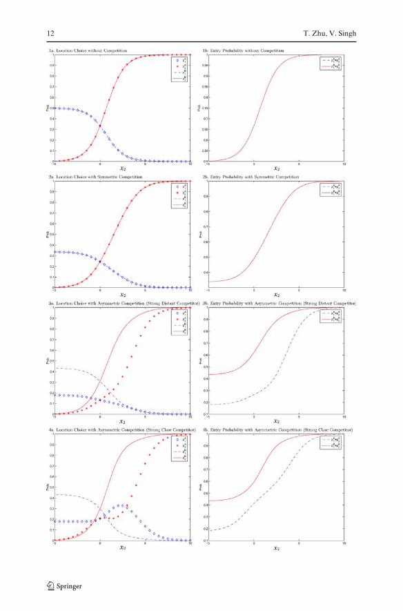
The model presented above is quite flexible in the asymmetries that it allowsin the model parameters. In order to understand how the primitives of themodel affect firms’ choices, we conducted a series of simulations to explorehow the probability of market entry and location choice depends on thestrength of competition among players. For this exercise, we consider asimplified version the model (Eq. (4)) discussed above and assume that thereare two players—firm A and firm B− and two possible locations—location 1and location 2. We further assume that the characteristics of locations xl
is unidimensional and βi = 1 so that firms are not heterogeneous in their

Spatial competition with endogenous location choices 11
sensitivity to the exogenous variable.4 In the exercise below, we normalizedx1 = 0 for location 1 and change market characteristics of location 2, x2, tostudy how firms’ location choices change as the attractiveness of location 2changes.
The focus of the simulation exercise is to investigate how competitionbetween firms influences their decisions and how firms’ locations choices differwhen they have different competitive positions in the market (i.e., strongplayers vs. weak players). Define the competition parameters δi
lk as the impacton firm i if it chooses location l and the competitor chooses location k. Weconsider four cases that involve different competitive interactions.5 In Case 1,there is no competition between players. In Case 2, firms are symmetric intheir competition effects. Further, the competition effect is stronger whenplayers are in the same location implying returns to differentiation. This case issimilar to the model considered in Seim (2006). The next two cases incorporateasymmetry in terms of competition where Firm B is a stronger player in themarket as it exerts a larger negative impact on Firm A. The difference betweenthe two scenarios is that in Case 3, Firm B can significantly impact A even at adistance whereas spatial differentiation can shield A from B in Case 4.
Parametersx1 = 0, βA = βB = 1
Case 1 δill = 0, δi
lk = 0
Case 2 δill = −2, δi
lk = −1
Case 3 δAll = −3.5, δA
lk = −2, δBll = −1.5, δB
lk = 0
Case 4 δAll = −3.5, δA
lk = 0, δBll = −1.5, δB
lk = 0
i = A, B, l, k = 1, 2 and l �= k
In Fig. 2, we plot the probability of location choice and market entryas the attractiveness of location 2 varies. The left panel depicts the choiceprobabilities of each firm with respect to the two locations. The diamond lineand the star line represent the probability that firm A chooses location 1 andlocation 2, respectively. The probability of location 1 and 2 being chosen byfirm B are plotted as dashed lines and dotted lines, respectively. The rightpanels summarize the overall probability of entry for two firms with the dashedline representing firm A’s entry probability and dotted lines firm B’s.
Case 1: With no competition between firms, the model degenerates to astandard single agent model, and both firms act identically. Thechoice probabilities and entry probabilities are monotonic functionsof location 2’s attractiveness.
4The marketwide random component is ignored as it does not provide any additional insight intothe importance of asymmetric effects.5The scenarios and parameter values are partly motivated by our empirical results.
12 T. Zhu, V. Singh

Spatial competition with endogenous location choices 13
�Fig. 2 Competition effects
Case 2: When firms are symmetric and the strength of competition decreaseswith distance, both firms have the same probability of choosingeach of the two locations. The choice probability of location 2 isagain a monotonic function of its attractiveness as is the overallprobability of entry. However, if we contrast this case to Case 1,we observe that entry probabilities and the probability of choosinga more attractive location are lower in this case where competitiveeffects exist. This observation indicates that each player makes atrade-off between the attractiveness of location and the intensifiedcompetition. Competition makes the “good” locations less attractivedue to concerns about entry by rivals.
Case 3: When firm B is a stronger player and can impact firm A significantlyat different distances, firm A is much less likely to enter the marketrelative to firm B and is correspondingly less likely to enter either ofthe two individual locations. In this scenario, firm B deters firm Afrom entering at all unless location 2 becomes sufficiently attractiveat which point A’s desire to avail itself to the attractive locationovercomes its wariness about competing with B.
Case 4: When firm B is a stronger player, but competitive effects are local,the choice patterns over the two locations differ dramatically acrossthe two firms. The stronger player (firm B) continues to be moreinclined to choose location 2 as location 2 becomes more attractive.The behavior of the weaker player (firm A) is more interesting.Unlike in all other cases, its choice probability of location 1 is notmonotonically decreasing in the attractiveness of location 2. Thebell-shaped function reveals that the weak firm will sacrifice a goodlocation in order to avoid competition when location 2 is moderatelyattractive. In this situation, firm A believes that firm B is sufficientlylikely to enter the relatively attractive location 2 that A is willingto enter the less attractive location in order to insulate itself fromcompetition with B. However, as location 2 becomes more attractive,the attractive market conditions eventually dominate the desire todifferentiate implying that firm A will also be more likely to choosethe good location. Comparing cases 3 and 4, location differentiationwill be more attractive when the relative competitive position changeswith distance. In case 3, firm A cannot shield itself from competitionby differentiation and thus is unlikely to enter at all for moderatelyattractive markets. This case would thus be associated with a domi-nant firm monopoly in moderately attractive markets and agglomer-ation to good locations in very attractive markets. Conversely, case 4would be more likely to yield a spatially differentiated duopoly inmoderately attractive markets with agglomeration again occurringwhen one location becomes sufficiently attractive.

14 T. Zhu, V. Singh
These simulations indicate the potential impact of asymmetries in com-petitive effects across locations as well as heterogeneity across firms. Addi-tionally, they indicate the way in which the parameters capturing the effectof spatial differentiation in the payoff functions are empirically identifiedfrom firms’location choice patterns. As market characteristics vary, differentscenarios will yield different entry patterns. Intuitively, the empirical analysiswill then attempt to identify the relevant “case” and associated parametervalues that make observed entry patterns as close as possible to those predictedby the model.
3 Data description
We apply the model to the discount store industry. Discount stores originatedin the late 1950s to offer general merchandise items at a substantial discountrelative to conventional department stores. For the most part, the industryis currently an oligopoly with three dominant firms: Wal-Mart, Kmart, andTarget. Interestingly, all three chains started in 1962 with Wal-Mart opening itsfirst store in Rogers, Arkansas, Kmart in Garden City, Michigan, and Targetin Roseville, Minnesota. Over the past few decades, these firms have obtaineddominant positions in the retail world while expanding their operations bothdomestically and internationally. They have also experimented with severalother retail formats, most prominently the supercenter which combines a full-service grocery store and a general merchandise outlet.
Besides physical store locations considered in this study, the firms havealso looked to differentiate themselves in other dimensions. For instance, withits EDLP strategy and the “Always Low Prices, Always” slogan, Wal-Marthas tried to establish itself as the low price leader in the industry. It hasalso emphasized the supercenter format more than Target and Kmart withapproximately half of its 3,000 stores selling grocery products. Similarly, Targethas looked to place itself in a niche as an “upscale” discounter with higher-end products. It has partnered with several designers to offer contemporarymerchandise, runs its own Target Guest credit card, and heavily promotes itsnationwide bridal and baby shower gift registries. Target’s panache is reflectedin the pop-culture use of a French-influenced pronunciation for its name(Tar-jay).6
We assemble a novel dataset that includes locations (street addresses andzip codes) of all stores in operation as of 2003 for Wal-Mart, Kmart, andTarget. In addition, we observe store format information, discount store versus
6For a detailed background on these firms, interested readers are referred to Zhu et al. (2008)and three recent books on each firm: The Wal-Mart Decade: How a New Generation of LeadersTurned Sam Walton’s Legacy into the World’s #1 Company (Robert Slater) Portfolio Hardcover(2003); On Target: How the World’s Hottest Retailer Hit a Bullseye ( Laura Rowley) Wiley (2003);Kmart’s Ten Deadly Sins: How Incompetence Tainted an American Icon, (Marcia Layton Turner)John Wiley & Sons (July 18, 2003).

Spatial competition with endogenous location choices 15
Table 1 Number ofstores in US
Store names Number of stores
Kmart discount store 1425Super Kmart center 59Target discount store 1133SuperTarget center 127Wal Mart store 1490Wal Mart supercenter 1442
supercenter. The total number of stores belonging to each chain is presentedin Table 1. We do not consider Sam’s Club as its main competitors are othermembership clubs such as Costco and BJ’s. Wal-Mart is the largest playerwith almost 3000 total stores and, as mentioned above, has stores equally splitbetween the two store formats. By contrast, Kmart and Target are relativelyminor players in the supercenter format. In Table 2, we show the distributionof stores for these three chains across the country. Not surprisingly, the highestnumber of stores are found in the two largest states, California and Texas. Thethree chains have the highest share (in terms of number of stores) in their statesof origin: Kmart in Michigan, Wal-Mart in Arkansas, and Target in Minnesota.The chains also tend to have a disproportionate share of stores in the statesneighboring their headquarters.
Our main objective in this paper is to analyze the factors underlying theentry and location choices of these firms and to infer competitive interactionparameters based on their revealed preferences. For the purpose, we need topartition the United States into small markets and each market into smallerneighborhoods. While various market definitions are possible, a practical con-sideration is the availability of data that capture demand and cost conditionsat each location. Our approach relies on census-delineated lines to define theindividual markets as well as the locations within markets. In particular, weuse counties as our definition of markets and census tracts within counties aslocations.7 Census tracts are small, relatively permanent geographic entitieswithin counties (or the statistical equivalents of counties) delineated by acommittee of local data users and tend to be fairly homogeneous with respectto population characteristics, economic status, and living conditions. In theempirical estimation, neighboring locations will be defined to be all locationswithin a given distance range which we specify below.
In Table 3, we present the competitive configurations across US countiesalong with some characteristics of those markets. The letters W, K, and Trepresent the presence of Wal-Mart, Kmart, and Target firms in the marketwhere, for the sake of brevity, we have omitted information associated with
7For very large urban counties (for example LA county), we use the first three digits of thetract number to create sub-markets. The complete census tract ID is defined as follows: SS-CCC-TTTTTT, where the first two digits “SS” represents State FIPS code, the next three digits “CCC”represents County FIPS Code, and the last six digits “TTTTTT” is the census tract number. Thisdefinition defines a market as the tracts within a county with the same first three digits in theirtract numbers and all six digit codes as locations.

16 T. Zhu, V. Singh
Table 2 Number of stores across states
State Kmart Target Wal-Mart Total
AK 5 0 9 14AL 29 10 87 126AR 6 4 86 96AZ 23 37 43 103CA 130 186 142 458CO 23 31 53 107CT 9 11 32 52DE 6 2 8 16FL 113 79 194 386GA 40 40 105 185HI 7 0 6 13IA 25 22 53 100ID 8 5 16 29IL 70 64 116 250IN 45 37 87 169KS 13 14 55 82KY 31 12 79 122LA 12 10 82 104MA 20 20 43 83MD 24 24 39 87ME 6 1 22 29MI 93 52 68 213MN 33 66 57 156MO 29 26 114 169MS 9 2 66 77MT 10 7 11 28NC 47 32 101 180ND 7 4 8 19NE 8 11 22 41NH 9 5 26 40NJ 43 29 35 107NM 15 8 26 49NV 11 14 20 45NY 62 37 78 177OH 90 44 105 239OK 10 10 94 114OR 14 16 28 58PA 106 31 104 241RI 1 2 8 11SC 29 15 60 104SD 10 4 10 24TN 39 23 96 158TX 20 110 310 440UT 18 9 27 54VA 46 31 77 154VT 3 0 4 7WA 21 29 35 85WI 39 29 71 139WV 17 3 29 49WY 9 2 10 21All 1493 1260 3057 5810a
aThe number of stores is larger than Table 1 because some neighborhood stores are included inTable 2

Spatial competition with endogenous location choices 17
Table 3 Marketconfigurations definedby county
Market structure CountyN Population Income
(0,0,0) 1356 15,029 31,260(W,0,0) 913 36,507 33,630(0,K,0) 70 93,493 38,582(0,0,T) 9 341,596 46,940(W,K,0) 339 78,374 36,657(W,0,T) 106 249,937 45,213(0,K,T) 17 395,953 44,314(W,K,T) 410 395,574 43,836
store format. For instance, (0,0,0) represents markets with no firms; (W,0,0)are Wal-Mart monopoly counties; (W,K,0) are duopoly counties of Wal-Martand Kmart, and so on. A few patterns are apparent from the numberspresented in Table 3. First, markets with no firms have significantly smallerpopulations compared to markets with at least one firm. Second, Wal-Martoperates as a monopolist in a larger number of counties than its rivals. Asthe associated market populations suggest, this reflects its ability to operate insmaller markets. Third, Target stores generally operate in markets with largerpopulation and significantly higher incomes compared to Wal-Mart and Kmartwhich is consistent with the anecdotal evidence discussed above. Finally, thepopulation numbers generally indicate that larger markets are required foradditional entry.
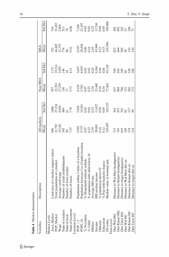
Table 4 lists the full set of variables used in the estimation where we separatethe variables that are observed at the market, location, and firm level. Wealso present the overall averages and means by MSA and rural Non-MSAmarkets. The average market size in our data is approximately 700 squaremiles although the rural markets tend to be larger in size than MSA markets.In terms of population we find the opposite as MSA markets have double thenumber of people reflecting that the urban areas are quite densely populatedcompared to rural markets. We can also see that MSA markets tend to havehigher retail wages and more retail establishments. The next row shows thenumber of census tracts within a market. The average number of locations ina market ranges from approximately six in the rural markets to over nine inMSA markets.
The next panel of the table describes the location-specific variables. Thefirst two rows are the populations within a two and a two-to-ten mile radiusof the location. We find a similar pattern to the market-level characteristics asMSA markets have significantly larger population numbers than the non-MSAmarkets. The next three variables %Novehicle, %Child, and HHsize are thepercent of population with no vehicles, percent of population with children inthe family, and household size respectively. These three variables do not differsubstantially across MSA and rural markets. However, MSA locations do tendto have higher levels of income and house values as well as a higher proportionof younger and educated population.
18 T. Zhu, V. Singh
Tab
le4
Mar
ketc
hara
cter
isti
cs
Var
iabl
esD
escr
ipti
onA
llm
arke
tsN
on-M
SAM
SAM
ean
Std
Dev
Mea
nSt
dD
evM
ean
Std
Dev
Mar
ket-
Lev
elA
rea_
Mar
ket
Lan
dar
eaof
am
arke
t(sq
uare
mile
s)69
610
6095
711
7533
273
4P
OP
_Mar
ket
Tot
alpo
pula
tion
ofa
mar
ket
31,7
9327
,234
22,7
6319
,214
44,4
0531
,455
Wag
eA
vera
gere
tail
wag
e19
,126
4,03
417
,270
3,69
521
,755
2,86
4N
umof
reta
ilers
Num
ber
ofre
tail
esta
blis
hmen
ts39
546
913
014
077
451
3N
umof
food
Num
ber
offo
odre
taile
r50
6117
1896
70N
umof
loca
tion
sN
umbe
rof
trac
ts7.
377.
705.
734.
119.
336.
06L
ocat
ion-
Lev
elP
OP
<2
Pop
ulat
ion
wit
hin
2m
iles
ofa
loca
tion
5,99
15,
826
4,15
83,
637
8,55
17,
186
PO
P2_
10P
opul
atio
nbe
twee
n2
to10
mile
slo
cati
on9,
737
19,3
615,
783
8,91
920
,836
21,1
07%
Nov
ehic
le%
Hou
seho
ldw
itho
utve
hicl
e0.
070.
030.
070.
030.
060.
03%
Chi
ld%
popu
lati
onw
ith
child
belo
w18
0.23
0.03
0.23
0.03
0.24
0.03
HH
size
Ave
rage
HH
size
2.59
0.23
2.56
0.20
2.63
0.25
Inco
me
HH
med
ian
inco
me
38,0
8111
,622
32,4
406,
264
45,9
6012
,744
Old
rati
o%
popu
lati
onab
ove
650.
140.
040.
160.
040.
120.
04E
duca
tion
%P
opw
ith
bach
elor
degr
ee0.
120.
050.
100.
040.
150.
05H
Uva
lue
Med
ian
valu
eof
hous
ing
unit
129,
497
103,
123
77,4
0243
,128
143,
590.
109,
888
Fir
m-L
evel
Dis
tWal
HQ
Dis
tanc
eto
Wal
-Mar
thea
dqua
rter
715
363
637
344
823
362
Dis
tKm
artH
QD
ista
nce
toK
mar
thea
dqua
rter
745
475
804
454
664
492
Dis
tTar
etH
QD
ista
nce
tota
rget
head
quar
ter
819
351
760
345
902
342
Dis
tWal
DC
Dis
tanc
eto
Wal
-Mar
tdis
tctr
109
8212
594
8553
Dis
tKm
artD
CD
ista
nce
toK
mar
tdis
tctr
174
117
202
120
133
100
Dis
tTar
etD
CD
ista
nce
tota
rget
dist
ctr
154
9917
210
812
977

Spatial competition with endogenous location choices 19
The last set of variables are firm-level variables that are specific to eachlocation. In particular, the data include distances from locations to the head-quarters and distribution centers of firms. These variables were created toproxy for logistical issues in a firm’s location decisions and, as we shall seebelow, tend to be quite important.
4 Empirical application
4.1 Estimation issues
The model described in (4) is very flexible as it allows for competition effectsto be asymmetric across firms and for the intensity of competition to dependon proximity. However, the general model has a large number of competitiveparameters (the δ’s) to be estimated. Without any constraints the number ofcompetitive interaction parameters is Lm × Lm × N × (N − 1) which growsquickly even with a small number of players and locations. For instance, withthree players and ten locations, the number of competition parameters is 600.Clearly, some restrictions on the number of parameters are required. To dealwith this difficulty, we create discrete distance bands and assume that thecompetitive intensity between players is the same as long as they are within thesame band.8 In the estimation, we categorize the distance between locationsinto three bands: less than 2 miles, 2 to 10 miles, and more than 10 miles.Note that this approach implies that if δii′0 is the competitive impact of firmi at location k1 that is within 2 miles from location l chosen by player i′,then the competitive effect is still δii′0 were firm i to choose another locationk2 that is also within 2 miles of l. In other words, in this framework theintensity of competition is determined by the distance between locations andnot the identities of those locations. The advantage of the approach is thatthe number of parameters reduces significantly. For instance, using the threedistance bands described above, the total number of parameters is reduced to3 × 3 × 2 = 18.
The model can be summarized as follows:
πiml = ximlβi −∑
i′ �=i
B−1∑
b=0
Lm∑
k=1
δii′b ai′mk1 (k ∈ bl) + ξm + εiml (8)
8We assume that firms are located at the centroid of the location, i.e., census tract. We calculate thedistance between locations using the Haversine Formula. Based on latitude-longitude coordinatedata, the distance between two points, a and b , is given by
da,b =2R arcsin
[
min
{((sin (0.5 (latb −lata)))2+cos (lata) cos (latb ) (sin (0.5 (lonb −lona)))
2)0.5
, 1
}]
where R = 3961 miles denotes the radius of the earth.
20 T. Zhu, V. Singh
where B is the total number of bands and 1 (k ∈ bl) is an indicator functionwith
1 (k ∈ bl) ={
1 if db ≤ dlk < db+1
0 otherwise, (9)
where db and db+1 denote cut-offs that define a distance band. In other words,1 (k ∈ bl) = 1 whenever location k is in distance band b relative to location l.
The parameters to be estimated are θ = {β, δ, σ } where β captures firms’preferences over the exogenous market conditions, δ reflects competitiveeffects across firms and locations, and σ measures the importance of themarket level random component. To estimate the model, we nest the fixedpoint algorithm in (5) into a maximum likelihood routine. For a given set ofvalues of the parameters and the market, location, and firm specific exogenousvariables, the system of equations in (5) is solved numerically for its fixedpoint for each market. The fixed point is a vector with
∑i Lim elements which
represent the probability of each location being chosen by each firm. Giventhose probabilities, P (ym) = ∏
i P (yim) is the probability of the equilibriumrealization that is consistent with the observed market outcome. The likelihoodfunction is given by
L (y, X, ξ ; θ) =M∏
m=1
P(ym|Xm, ξm; β, δ
). (10)
The unconditional likelihood then involves integrating over the distributionG (.) of the unobserved market component ξm, where ξm is assumed normallydistributed with variance σ in our application.
L (y, X; θ) =M∏
m=1
∫
P(ym|Xm, ξm; β, δ
)dG
(ξm|σ )
, (11)
where ym = (yWm, yKm, yTm) are observed actions taken by Wal-Mart, Kmartand Target.
Computationally, the model is quite complicated. To simplify the estima-tion, we employ a simulated maximum likelihood routine as follows.9 Given aset of parameter values and a vector of simulated draws with standard normaldistribution ς = (
ς1, ς2, ..., ς R)
for the unobserved market characteristic, webegin with an initial guess of the choice probability for each firm P0
m ∈[0, 1]
∑i Lim in each market. We then calculate each firm’s expected payoff for
each location conditional on its beliefs about its competitors’ location choiceprobability P0
−im. For each random draw ς r, we solve the fixed point problem(5) by successive approximation to obtain the Bayesian Nash equilibrium
9One problem of the likelihood approach is that there might be multiple equilibria in the incom-plete information game. Although we solved for the fixed point by using different starting values,uniqueness of the solution is not guaranteed. However, as long as the strength of competitioneffect is moderate, the equilibrium can be solved uniquely. We show analytical and simulationresults in the Appendix.

Spatial competition with endogenous location choices 21
probabilities Prm. We then repeat the procedure R times to find the Bayesian
Nash equilibrium for each random draw. The predicted probability of theobserved outcome is approximated by
∫
P(ym|Xm, ξm; β, δ
)dG
(ξm|σ ) = 1
R
R∑
r=1
Prm (ym) . (12)
We then use the simulated probabilities in a log-likelihood function:
θ̂ = arg maxθ
LL (y, X; θ) =M∑
m=1
ln
[1
R
R∑
r=1
Prm (ym)
]
. (13)
4.2 Results
We include a variety of variables that capture demand, cost, and logisticalfactors that could be important in a firm’s location decision. Since these factorsmight operate differently in large MSA markets compared to rural areas, wedivide the sample into MSA and non-MSA markets and estimate separatemodels for each.10 We also allow Wal-Mart to choose between its discountstore and supercenter formats. As noted in the data section above, the othertwo players mainly operate discount stores so we ignore the format choicedecisions for these players.
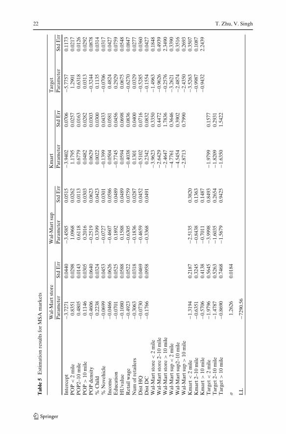
In Table 5, we report the parameter estimates for MSA markets. We willfocus on those estimates since similar results obtain for non-MSA marketsas displayed in Table 6. Not surprisingly, we find that closer populationcontributes more to profitability that more distant population as reflectedin the lower value of the coefficients for population in more distant bands.However, the parameters for distant population are significantly larger forWal-Mart, particularly for its supercenter format. This finding suggests thatthe trading area for Wal-Mart is larger than that of its rivals. The estimatedeffect of population density is negative for all players except Kmart. While thismay seem counterintuitive, note that population density is measured at thespecific location cell level, while the population measures include populationsfrom the immediate as well as neighboring locations that fall within therespective distance band. Since the discount stores tend be large in size, it is notnecessarily surprising that population density in the immediate location is low.In addition, a location with high population density may have high real estatecosts implying that the chains would prefer locations with lower immediatepopulation density, but higher overall surrounding population.
10A concern in our modeling framework is potential cannibalization across markets since eachmarket is treated independently. This is less likely to be an issue in the non-MSA markets wherethe distance between the adjacent stores is quite large. Note however that the travel time in MSAmarkets is likely to larger potentially mitigating cannibalization. Jia (2008) makes contribution tothe literature by incorporating the “spill over” effects across market within a firm. However theimplicit assumption in her approach is the externality between two close-by stores within the samechain is positive.
22 T. Zhu, V. Singh
Tab
le5
Est
imat
ion
resu
lts
for
MSA
mar
kets
Wal
-Mar
tsto
reW
al-M
arts
upK
mar
tT
arge
tP
aram
eter
Std
Err
Par
amet
erSt
dE
rrP
aram
eter
Std
Err
Par
amet
erSt
dE
rr
Inte
rcep
t−3
.727
10.
0440
−3.4
585
0.05
15−3
.940
20.
0706
−5.7
757
0.11
73P
OP
<2
mile
0.83
510.
0298
1.09
680.
0262
1.17
950.
0257
1.29
010.
0217
PO
P2–
10m
ile0.
4805
0.01
430.
6118
0.01
130.
6779
0.01
630.
6318
0.01
26P
OP
>10
mile
0.11
460.
0305
0.20
160.
0303
0.04
820.
0282
0.03
130.
0292
PO
Pde
nsit
y−0
.460
60.
0640
−0.2
519
0.06
230.
0629
0.03
03−0
.324
40.
0878
%C
hild
0.22
380.
0324
0.33
990.
0423
0.00
220.
0300
0.11
350.
0314
%N
oveh
icle
−0.0
699
0.04
53−0
.072
70.
0301
−0.1
399
0.04
33−0
.070
60.
0317
Inco
me
−0.0
466
0.06
26−0
.460
70.
0586
0.05
040.
0581
0.48
240.
0427
Edu
cati
on−0
.070
10.
0525
0.18
920.
0489
−0.7
745
0.04
560.
2929
0.07
59H
Uva
lue
−0.1
080
0.05
880.
1588
0.04
890.
0594
0.06
980.
0675
0.05
48R
etai
lwag
e−0
.492
30.
0522
−0.6
305
0.07
59−0
.403
80.
0836
−0.6
270
0.08
47N
umof
reta
ilers
−0.3
063
0.03
18−0
.183
60.
0287
0.13
010.
0400
0.03
290.
0277
Dis
tHQ
−0.0
730
0.04
69−0
.465
90.
0452
−0.5
102
0.07
16−0
.528
50.
0360
Dis
tDC
−0.1
766
0.09
58−0
.336
80.
0491
0.23
420.
0832
−0.1
554
0.04
27W
al-M
arts
tore
<2
mile
−3.9
623
0.33
50−1
.496
30.
1848
Wal
-Mar
tsto
re2–
10m
ile−2
.642
90.
4472
−0.9
626
0.49
39W
al-M
arts
tore
>10
mile
−2.4
647
1.78
36−0
.257
62.
3490
Wal
-Mar
tsup
<2
mile
−4.7
761
0.36
46−3
.262
10.
3390
Wal
-Mar
tsup
2–10
mile
−4.5
454
0.39
02−2
.487
40.
3516
Wal
-Mar
tsup
>10
mile
−2.8
713
0.79
90−2
.435
00.
2693
Km
art<
2m
ile−1
.319
40.
2187
−2.5
135
0.38
20−3
.526
30.
3507
Km
art2
–10
mile
−0.6
351
0.32
45−0
.843
80.
1363
−0.9
987
0.10
87K
mar
t>10
mile
−0.5
706
0.41
38−0
.701
10.
1487
−0.9
432
2.24
39T
arge
t<2
mile
−1.9
796
0.56
45−3
.999
80.
8493
−1.9
799
0.15
77T
arge
t2–1
0m
ile−1
.478
70.
5263
−1.6
035
0.26
54−1
.820
90.
2931
Tar
get>
10m
ile−0
.869
00.
7468
−1.5
679
0.94
25−1
.635
01.
5422
σ1.
2626
0.01
84
LL
−729
0.56

Spatial competition with endogenous location choices 23
Tab
le6
Est
imat
ion
resu
lts
for
non-
MSA
mar
kets
Wal
-Mar
tsto
reW
al-M
arts
upK
mar
tT
arge
tP
aram
eter
Std
Err
Par
amet
erSt
dE
rrP
aram
eter
Std
Err
Par
amet
erSt
dE
rr
Inte
rcep
t−3
.297
70.
2169
−3.4
794
0.16
11−3
.592
80.
2495
−6.4
059
0.43
48P
OP
<2
mile
2.14
010.
1202
1.02
890.
1284
1.67
240.
1833
2.10
040.
1759
PO
P2–
10m
ile0.
8925
0.08
110.
5954
0.08
560.
9375
0.08
640.
8084
0.17
29P
OP
>10
mile
0.04
850.
0967
0.20
690.
1021
0.04
210.
1107
0.07
360.
2234
PO
PD
ensi
ty−0
.348
50.
0937
−0.2
903
0.08
95−0
.172
50.
0998
−0.8
512
0.25
91%
Chi
ld0.
1469
0.09
980.
2552
0.10
040.
4373
0.11
780.
3662
0.25
88%
Nov
ehic
le−0
.221
60.
1070
−0.1
036
0.11
49−0
.275
50.
1515
0.04
130.
4817
Inco
me
0.30
440.
2321
−0.3
087
0.22
91−0
.566
70.
2706
0.80
650.
5457
Edu
cati
on0.
3539
0.14
22−0
.027
70.
1546
0.51
900.
1523
0.67
730.
2823
HU
valu
e−0
.057
60.
1001
0.13
320.
0595
0.22
310.
0724
−0.0
243
0.19
07R
etai
lwag
e0.
6232
0.13
62−0
.642
80.
1491
0.46
380.
1535
0.26
340.
3613
Num
ofre
taile
rs0.
1995
0.27
29−0
.239
80.
2205
1.74
930.
3029
2.40
260.
7522
Dis
tHQ
−0.4
644
0.09
49−0
.468
20.
1036
−0.6
043
0.10
61−0
.919
90.
2128
Dis
tDC
−0.3
610
0.10
33−0
.353
50.
1156
−0.0
306
0.06
68−0
.174
50.
2273
Wal
-Mar
tsto
re<
2m
ile−3
.395
71.
0625
−0.8
024
1.72
54W
al-M
arts
tore
2–10
mile
−2.9
987
0.95
24−0
.545
41.
9186
Wal
-Mar
tsto
re>
10m
ile−1
.966
91.
2111
−0.0
583
3.85
55W
al-M
arts
up<
2m
ile−4
.595
50.
9996
−3.6
291
2.23
09W
al-M
arts
up2–
10m
ile−3
.309
00.
9154
−2.7
650
0.96
55W
al-M
arts
up>
10m
ile−2
.950
01.
5134
−2.5
663
2.54
04K
mar
t<2
mile
−1.7
034
0.50
70−2
.508
10.
2337
−1.4
193
2.66
51K
mar
t2–1
0m
ile−1
.357
80.
7639
−1.6
668
0.63
62−1
.340
21.
2559
Km
art>
10m
ile−0
.459
71.
6763
−1.2
101
1.75
19−1
.019
44.
0983
Tar
get<
2m
ile−3
.510
51.
0283
−2.9
020
0.74
82−2
.250
71.
0300
Tar
get2
–10
mile
−2.6
986
1.16
95−1
.724
41.
0328
−1.8
001
0.67
65T
arge
t>10
mile
−0.9
601
1.75
60−1
.641
31.
6655
−0.7
464
1.52
87
σ1.
1052
0.13
45
LL
−524
2.78

24 T. Zhu, V. Singh
The next two variables, %Child and %Novehicle, represent the percentof population with children under the age of 18 and percent of populationwith no vehicles. The parameters for %Child are positive for Wal-Mart andTarget, but are insignificant for Kmart. Thus, both Wal-Mart and Target storesprefer markets where a larger proportion of families have kids. In relativeterms, the impact is larger for Wal-Mart, particularly for its supercenter format.The parameter for %Novehicle is significantly negative for all stores whichis intuitive as these stores are built with large parking lots that are generallyinaccessible without vehicles. The next two demographic variables are medianincome and education measured as the percentage of population with a collegedegree. These two variables reveal some interesting differences across firms.The income parameter is negative for both Wal-Mart formats, insignificant forKmart, and positive for Target. These results suggest that, all else equal, Wal-Mart enters markets with lower incomes while Target stores prefer high in-come areas. In addition, Target stores tend to have a more educated populationbase. These results are consistent with common perceptions of the positioningand target audiences of these stores. For example, as discussed above, Targethas historically attempted to position itself as an upscale discounter that catersto a higher income and more educated clientele than its competitors. Similarly,lower income levels in Wal-Mart locations are consistent with Wal-Mart’severy day low pricing and value positioning.
The next variable HouseValue is the median house value which ideally willcapture the impact of real estate prices. The coefficient is negative for Wal-Mart discount store, positive for its supercenter format, and insignificant forKmart and Target. However, the instability of these results appear to indicatethat residential house value is in fact an inaccurate proxy for commercial landvalue. The coefficients for retail wages are negative and significant indicatingthat all firms strongly prefer markets with lower wages. This is not surprisingsince labor tends to account for a significant proportion of operational costsin retailing. The variable “num of retailers” is the total number of otherretailers and captures the general business density at a location. Note thatthese retail stores are considered to be non-strategic players in our model eventhough some of them may actually compete with the three discount stores. Thecoefficient is negative for the two Wal-Mart stores and positive for Kmart andTarget. This suggests that Wal-Mart tends to prefer stand alone locations whileits competitors are more likely to be surrounded by other businesses.
The last two variables Dist HQ and Dist DC are the distance of differentmarket locations from the headquarters and nearest distribution center of afirm. Unlike all the variables discussed above, these distance measures arefirm-specific. The negative coefficients for distance to headquarters suggeststhat, all else equal, firms prefer markets that are closer to their respectiveheadquarters. This is consistent with the distribution of stores across statesreported in Table 2. Looking at the distance to distribution center, we findthat Wal-Mart, particularly for its supercenter format, prefers locations thatare closer to its distribution center. This is not surprising as Wal-Mart is well
Spatial competition with endogenous location choices 25
known for its efficiency in distribution, and a large part of its success as aretailer has been attributed to these logistical efficiencies.11
Looking at the competitive interaction parameters, some interesting pat-terns emerge. As expected, all parameters are negative indicating that pres-ence of rivals reduce a firm’s profits. However, proximity to competitors isan important determinant of profitability as the competition effect diminisheswith distance. For instance, the point estimates suggest that the impact ofKmart on a Wal-Mart’s discount store is approximately 45% lower when itis located more than ten miles away instead of being located in the immediateneighborhood. This decreasing relationship between distance and competitionis consistent across all firms and formats which suggests strong returns tospatial differentiation in this industry as firms can shield their profits by choos-ing sufficiently different locations. Looking at the competitive effects acrossfirms, we find strong asymmetries in the competitive interaction parameters.For example, looking at Kmart and the two Wal-Mart formats, we find thatwhile Kmart substantially impacts Wal-Mart when it is in close proximity, theeffect is significantly lower than the effect of Wal-Mart on Kmart. Similarly,when Kmart is located beyond ten miles, its effect on Wal-Mart’s discountstore and supercenter are approximately one-fourth of the impact that theWal-Mart stores have on Kmart at a similar distance. Target stores farewell in the face of competition from other discount stores except when thecompetitors are in close proximity. However, the chain appears vulnerable toWal-Mart’s supercenter format. Perhaps most interesting, the impact of Wal-Mart supercenter appears to decline less rapidly with distance when comparedto the effect of any of the other firms. This finding suggests that Wal-Mart’ssupercenter format yields a substantially larger market area relative to otherformats as even competitors which are relatively far from a supercenter are notinsulated from competition with it.
To better interpret the competition effects, one can calculate measures onthe demand reduction in terms of population when a competitor moves intoa location, holding all else constant. For example, moving a new Wal-Martdiscount store within 2 miles of Kmart is equivalent to reduction of 33,600in population for Kmart in the immediate neighborhood. The effect of a newKmart on a Wal-Mart discount store is only 15,800 which is less than half theimpact that Wal-Mart has on Kmart. If a new Wal-Mart supercenter moves in,even in a far away location (beyond 10 miles), it is equivalent to a reductionin population of 24,000 for Kmart and 18,900 for Target. The correspondingnumbers for a Wal-Mart discount store are 20,900 for Kmart and 2,000 forTarget. Thus, Kmart seems vulnerable to both formats of Wal-Mart even infar away locations, while Target fares well when faced with a distant Wal-Mart
11According to an independent study by McKinsey & Co., Wal-Mart’s efficiency gains were thesource of 25% of the entire U.S. economy’s productivity improvement from 1995 to 1999. “CanWal-Mart get any bigger” Time Magazine (Vol. 161, issue 2, 2003).

26 T. Zhu, V. Singh
discount store, but is still affected strongly by a Wal-Mart supercenter. In fact,the impact of Target is stronger on Kmart and Wal-Mart’s discount store whenlocated more than 10 miles away rather than the other way around.
4.3 Varying market conditions and equilibrium outcomes
The model parameters can be used to predict the equilibrium market struc-tures for different sets of market conditions and provide insights on howthese firms shield themselves from competition by spatial differentiation. Forinstance, consider a market with two possible locations that are 10 miles apart,and three potential competitors: Wal-Mart supercenter, Kmart, and Target.Further, suppose the population in location 1 is 30,000 and income is at themean level in the population which is normalized to zero. In addition, allother variables are set at their population mean levels. Figure 3 displays thepredicted market structures as population and income change in location2. Note that the parameter estimates of the latent payoff functions suggestthat the impact of the two variables may work differently for different firms.In particular, while all firms prefer increase in population especially in theimmediate location, Target is the only firm that prefers higher income levels.The darker shade represents choice of location 1, lighter shade the choice oflocation 2 (Red and Blue if viewed in color), and non-shaded areas representsituations where firms stay out of the market. The left panel shows the pre-dicted outcomes without considering competition, while the right panel showsthe equilibrium structures after taking competition into account. Figure 3ashows that when firms do not compete, no entry and monopoly outcomes arerare as all three firms are willing to enter the market with moderate increasesin population and income levels. Figure 3b shows that the region of no-entry and monopoly increase dramatically once we account for competition.Moreover, the occurrence of oligopoly is much less prevalent and only arisesat significantly high population and income levels.
In Fig. 3a to b, we show how the predicted entry and location choices varyby individual firms. Comparing individual firms under competition and no-competition, some interesting patterns emerge. Wal-Mart’s no-entry region,while larger under competition compared to the no-competition case, is rel-atively small compared to its rivals. The impact of competition is highest onKmart as it gives up the majority of the space that it would have occupied ifcompetitive concerns were irrelevant. Looking at Wal-Mart’s location choices,we observe that as the income in location 2 increase above a certain point,Wal-Mart is willing to enter the market by switching to location 1. On the otherhand, both Target and Kmart prefer not to enter the market altogether withmoderate market conditions and choose location 2 as it becomes sufficientlyattractive. These results are primarily driven by Wal-Mart supercenter’s abilityto enter markets with lower population levels, attract population from furtheraway locations, and its ability to impact competitors even when it is locatedfar away. Comparing the monopoly region in Fig. 3b with those of three firmsunder competition (Fig. 3), we can see that majority of the monopoly region

Spatial competition with endogenous location choices 27
is occupied by Wal-Mart with a small region (those with moderate populationand very high income) being Target’s monopoly. Kmart on the other handis rarely able to operate as a monopolist. Of course these predictions wouldchange at different values of the other market variables. For example, Kmartmay have monopoly markets in regions close enough to its headquarters.
Overall, the results show that all firms exert a strong negative impact on itscompetitors when they are in close proximity and that this effect decreases with
Fig. 3 Market structure predictions

28 T. Zhu, V. Singh
Fig. 3 (continued)
distance to rivals. Wal-Mart’s supercenter format is found to be the most formi-dable player as it strongly impacts competitors even from a distant location.Not surprisingly, in our empirical data we observe a large number of monopolymarkets for Wal-Mart supercenter. We also find asymmetries across players interms of exogenous market characteristics. In Table 7, we show the parameterestimates from a model that ignores player identities. With minor differences,this is the model used by Seim (2006) in her application to the video rentalstores. Several similarities exist in the parameter estimates with the full modelpresented above. For instance, payoffs are higher with population closer the
Table 7 Parameter estimates without firm asymmetry
Estimates from separate marketsMSA Non-MSAParameter Std Err Parameter Std Err
Intercept −4.0350 0.0281 −4.5098 0.1554POP < 2 mile 0.8470 0.0005 1.9706 0.0383POP2–10 mile 0.3934 0.0246 0.8453 0.0465POP > 10 mile 0.0175 0.0339 0.0668 0.0402POP density −0.2196 0.0396 −0.4390 0.0534% Child −0.0069 0.0454 0.3462 0.0746% Novehicle −0.2002 0.0341 −0.3261 0.0891Income 0.1104 0.0429 0.2915 0.0426Education −0.0451 0.0608 0.1988 0.1042HUvalue −0.3561 0.0534 0.1389 0.1086Retail wage −0.3056 0.0686 −0.8286 0.1826Num of retailers −0.0536 0.0534 1.6674 0.2280Dist HQ −0.5396 0.0341 −0.5453 0.0383Dist DC −0.0555 0.0386 −0.1186 0.0416Competition < 2 mile −1.3118 0.0919 −1.9736 0.0655Competition2–10 mile −0.8500 0.0965 −1.3723 0.0655Competition > 10 mile −0.5828 0.2376 −1.3522 0.1360
LL −5743.88 −3786.79

Spatial competition with endogenous location choices 29
firm’s location. Similarly, the competitive effect decreases with distance torivals suggesting returns to geographical differentiation. However, this modelcan not discern the differences across firms with regards to preference forexogenous variables as well as competition effects. While this model may bereasonable in industries with small local players who are reasonably homoge-neous in many respects, in our application the impact of income, education,business density, distance to distribution center, and competition is found tobe quite different based on the identities of individual players.
5 Conclusion
In this paper we study the strategic entry and location choice decisions in theretail discount industry. Using a novel data set that includes the store locationsand the accompanying market conditions for all stores belonging to Wal-Mart,Kmart, and Target chains, we study the factors determining firm’s entry andlocation choices. The model is set up as an incomplete information gamebetween the three players where firms are assumed to have private informationon their own profitability but observe only the distribution of their rivals’profitability. The model incorporates asymmetries related to the identity of thefirms by allowing the competitive effects and preference for exogenous marketconditions to be firm-specific. In addition, the variations in the exogenousfirm specific characteristics, such as the distances from the market to firms’headquarters and the distances to the nearest distribution centers provide thesource for model identification. The incomplete information setup provides atractable model for studying the complex interactions of optimal site selectionas a trade-off between proximity to good markets and increased competitionwith rivals in these prime locations.
Results show that population in closer distance bands to firm’s locationcontribute more to profitability than population in distant locations. All firmsare found to prefer markets with lower retail wages, markets where largerproportion of families have kids and vehicles, and markets that are closerto their respective headquarters. We also find significant differences acrossfirms in certain demand characteristics. For instance, Target prefers marketswith higher income and education levels compared to its rivals. We also findthat Wal-Mart, particularly for its supercenter format, gives strong weightto locations that are closer to its distribution center, reflecting its logisticalefficiencies. In terms of the competitive interaction parameters, we find that allfirms exert a strong negative impact on their competitors when they are in closeproximity, but the effect goes down with distance to rivals suggesting strongreturns to spatial differentiation in this industry. However, looking at thecompetitive effects across firms, we find strong asymmetries in the competitiveinteraction parameters. For example, while Kmart is able to impact Wal-Martstrongly when it is in close proximity, its effect is significantly lower than whatWal-Mart exerts on Kmart’s payoffs. Target stores are found to fare well undercompetition from other discount stores except when these competitors are
30 T. Zhu, V. Singh
in close proximity. Wal-Mart’s supercenter format is found to be the mostformidable player as it is able to impact the competitors strongly even whenit is located far away.
There are of course several caveats to this study and directions for futureresearch. First, the incomplete information assumption in a static game impliesthat players are allowed to have ex post regret about their decisions, whichnaturally leads to dynamic considerations (Aguirregabiria and Mira 2004;Pakes et al. 2004). While applications of multi-agent dynamic games posesignificant computational challenges, they may provide insights into the richdynamics inherent in strategic decisions like market entry and exit that are lostin a static setting. Similarly, in our application the only unobservables that arecorrelated across players are market specific that do not differentiate betweenlocations within a market. Location specific unobservables can obviously beincorporated in the model at the expense of additional computational burdenas in Orhun (2005). Although addressing many of these shortcomings posesignificant challenges in terms of data requirements and computations, withadvancements in computing power these hurdles can be overcome in thefuture.
Appendix: Equilibrium properties of incomplete information games
A well-known problem with multi-agent discrete games is that they have non-existence of pure strategy equilibria and multiple equilibria in which certainvalues of the underlying latent payoffs could simultaneously be consistentwith more than one equilibrium outcome. For existence, researchers generallyassume that the data is generated by a pure strategy equilibrium and thatthe model satisfies restrictions sufficient to guarantee the existence of at leastone such equilibrium. In the current application, since Eq. (6) is a continuousmapping from a probability space to itself, the existence of a solution of (6) canbe proved from Brouwer’s Fixed Point Theorem. However, the uniqueness ofsuch a solution is not guaranteed. The game will have multiple equilibria if,for given parameter θ , more than one value of P satisfies (6) in which casethe likelihood function is not well defined. Aradillas-Lopez (2005) discussesthe sufficient conditions for the uniqueness of equilibrium of incompleteinformation game and points out that the conditions for existence of a well-defined likelihood function are generally weaker in incomplete informationgame than in the complete information version of the game.
Heckman (1978) studies the general class of simultaneous equation qualita-tive response models and shows that if the distribution of the unobservablesis continuous with unbounded support, a necessary and sufficient conditionfor the model to have a unique equilibrium for any values of exogenousvariables is that the model is recursive. Though useful in some applications,this condition implies setting some strategic interactions parameters (whichare of main interest) to zero. Instead, researchers have generally adopted oneof the two approaches to deal with multiple equilibria problem. First, models

Spatial competition with endogenous location choices 31
sometimes yield a prediction for some outcome that is unique across allequilibria. For instance, Bresnahan and Reiss (1990, 1991a, b) and Berry (1992)ignore the identities of the players that enter a market and only considerthe total number of entrants, an outcome for which their models yield aunique prediction. Alternatively, some papers impose additional structure onthe model that guarantees equilibrium uniqueness. For example, Zhu et al.(2008) consider sequential move games that yields additional conditions for anoutcome to be a subgame perfect Nash equilibrium.
In this Appendix, we study the equilibrium properties for the model pro-posed in Section 2. We begin with a proof on the sufficient conditions ofuniqueness for the two player–two action game and then rely on simulationtechniques for a more complex game, i.e., when the action space or the numberof players becomes larger.
Consider a simple 2 × 2 game with two players and two possible actions: inor out. Firm i’s payoff of entry is
πi = xiβi − δi p−i + εi, i = 1, 2, (14)
where p−i is the entry probability of i’s competitor, and εi is the privateinformation held by firm i and is type 1 extreme value distributed. Similarto the discussion on Eq. (7), the BNE is obtained by solving the following twosimultaneous equations:
p1 = exp(x′
1β1 − δ1 p2)
1 + exp(x′
1β1 − δ1 p2) ,
and
p2 = exp(x′
2β2 − δ2 p1)
1 + exp(x′
2β2 − δ2 p1) .
Define f =(
f1
f2
)
, where
f1 = p1 − exp(x′
1β1 − δ1 p2)
1 + exp(x′
1β1 − δ1 p2) ,
f2 = p2 − exp(x′
2β2 − δ2 p1)
1 + exp(x′
2β2 − δ2 p1) ,
then taking the derivates of f1 with respect to p2 yields
∂ f1
∂p2= δ1 exp
(x′
1β1 − δ1 p2) [
1 + exp(x′
1β1 − δ1 p2)] − δ1 exp
(x′
1β1 − δ1 p2)
exp(x′
1β1 − δ1 p2)
[1 + exp
(x′
1β1 − δ1 p2)]2
= δ1 exp(x′
1β − δ1 p2)
[1 + exp
(x′
1β1 − δ1 p2)]2
,

32 T. Zhu, V. Singh
and similarly
∂ f2
∂p1= δ2 exp
(x′
2β2 − δ2 p1)
[1 + exp
(x′
2β2 − δ2 p1)]2 .
Hence the Jacobian matrix f ′ is⎛
⎜⎝
1δ1 exp(x′
1β1−δ1 p2)
[1+exp(x′1β1−δ1 p2)]2
δ2 exp(x′2β2−δ2 p1)
[1+exp(x′2β2−δ2 p1)]2 1
⎞
⎟⎠ .
From the Gale-Nikaido Theorem: Suppose f : Rn → R
n is continuouslydifferentiable function, and define � as the rectangle � = {x ∈ R
n, a ≤ x ≤ b} ,
where a and b are given vectors in Rn. Then f is one-to-one in � if for all
x ∈ �, Jacobian matrix f ′ (x) has only strictly positive principal minors. Thesufficient condition that (1) has unique solution for (p1, p2) is
1 −[
δ1 exp(x′
1β1 − δ1 p2)
[1 + exp
(x′
1β1 − δ1 p2)]2
][δ2 exp
(x′
2β2 − δ2 p1)
[1 + exp
(x′
2β2 − δ2 p1)]2
]
> 0,
or equivalently,
δ1δ2 <
[1 + exp
(x′
1β1 − δ1 p2)]2 [
1 + exp(x′
2β2 − δ2 p1)]2
exp(x′
1β1 − δ1 p2)
exp(x′
2β2 − δ2 p1)
= 4 + 2
exp(x′
1β1 − δ1 p2) + 2 exp
(x′
1β1 − δ1 p2) + 2
exp(x′
2β2 − δ2 p1)
+2 exp(x′
2β2 − δ2 p1) + exp
(x′
2β2 − δ2 p1)
exp(x′
1β1 − δ1 p2) + exp
(x′
1β1 − δ1 p2)
exp(x′
2β2 − δ2 p1)
+ 1
exp(x′
1β1 − δ1 p2 + x′2β2 − δ2 p1
) + exp(x′
1β1 − δ1 p2 + x′2β2 − δ2 p1
)
≥ 16
Hence as long as the interaction term of the competition intensity δ1δ2 is below16, the uniqueness of the Bayesian Nash equilibrium is ensured in this 2 × 2game.
The message from the simple example above is that as long as the strengthof strategic interaction is within a certain range, equilibrium is unique. As thegame becomes more complex, i.e., the action space or the number of playersgets larger, the matrix algebra becomes cumbersome. We rely on simulationtechnique to investigate the uniqueness property of incomplete informationgames. In the simulation, We are interested in how the equilibrium uniquenessproperty is related to (1) the variation of market characteristics acrosslocations (choice alternatives), (2) the heterogeneity across players, and (3)
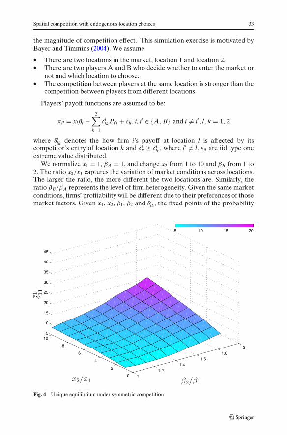
Spatial competition with endogenous location choices 33
the magnitude of competition effect. This simulation exercise is motivated byBayer and Timmins (2004). We assume
• There are two locations in the market, location 1 and location 2.• There are two players A and B who decide whether to enter the market or
not and which location to choose.• The competition between players at the same location is stronger than the
competition between players from different locations.
Players’ payoff functions are assumed to be:
πil = xlβi −2∑
k=1
δilk Pi′l + εil, i, i′ ∈ {A, B} and i �= i′, l, k = 1, 2
where δilk denotes the how firm i’s payoff at location l is affected by its
competitor’s entry of location k and δill ≥ δi
ll′ , where l′ �= l. εil are iid type oneextreme value distributed.
We normalize x1 = 1, βA = 1, and change x2 from 1 to 10 and βB from 1 to2. The ratio x2/x1 captures the variation of market conditions across locations.The larger the ratio, the more different the two locations are. Similarly, theratio βB/βA represents the level of firm heterogeneity. Given the same marketconditions, firms’ profitability will be different due to their preferences of thosemarket factors. Given x1, x2, β1, β2 and δi
lk, the fixed points of the probability
11.2
1.41.6
1.82
0
2
4
6
8
105
10
15
20
25
30
35
40
45
5 10 15 20
Fig. 4 Unique equilibrium under symmetric competition

34 T. Zhu, V. Singh
vector(P1A, P2A, P1B, P2B
)are solved from different starting values: (0 0 0 0)′,
(0 0 1 0)′, (0 0 0 1)′, (1 0 0 0)′, (1 0 1 0)′, (1 0 0 1)′, (0 1 0 0)′, (0 1 1 0)′, (0 1 0 1)′.The discussion on why one should choose those points as starting points totest equilibrium multiplicity can be found in Bayer and Timmins (2004). As wechange δA
11 from 0 to 100, and find δ̄ill, such that as δi
ll > δ̄ill, we start to observe
multiple fixed points for a particular combination of x1, x2, β1, β2. In Figs. 4and 5 we plot how δ̄i
ll changes as x2/x1 and β2/β1 changes under two scenarios:
Case 1: Symmetric competition , δAlk = δB
lk, δill′ = 1
2δill
Case 2: Asymmetric competition: δAlk = 2δB
ik, δill′ = 1
2δill
In the first case, firms are symmetric in terms of competition, while inthe second scenario Player B is stronger than player A in the sense that itexerts stronger negative impact on its competitor. The competition intensity isweaker if two players choose different locations. Comparing the plot for case2 and that for case 1, we can find that the threshold for case 2 is larger. Thereason is that the uniqueness conditions are determined by the interactionterms of the competition intensity. Hence the range for the competitionintensity of δ̄1
11 is larger if δAlk > δB
lk.The results from simulation can be summarized as follows. First, as long as
the strength of competition effect is moderate, there is a unique equilibrium inthe incomplete information game. Second, there exists a threshold δ̄A
lk such that
11.2
1.41.6
1.82
0
2
4
6
8
1010
15
20
25
30
35
40
45
15 20 25 30 35 40
Fig. 5 Unique equilibrium under asymmetric competition
Spatial competition with endogenous location choices 35
when δAlk > δ̄A
lk , one starts to observe multiple equilibrium given the locationcharacteristics and firms’ preference of those market characteristics. We findthat as the variation of market characteristics increases, the threshold δ̄A
lkincreases. Put another way, the multiple equilibria is less likely to be observedwhen there is larger variation across locations. This finding is consistent withSeim (2001). Finally, as the asymmetry between players increases both interms of their preference to market conditions (βB/βA) and the asymmetricof competition effect, the threshold δ̄A
lk becomes higher.
References
Aguirregabiria, V., & Mira, P. (2004). Sequential estimation of dynamic discrete games. WorkingPaper, Boston University.
Aradillas-Lopez, A. (2005). Semiparametric estimation of a simultaneous game with incompleteinformation. Working Paper, Berkeley.
Bajari P., Benkard, L., & Levin, J. (2005a). Estimating dynamic models of imperfect competition.Working Paper, Duke.
Bajari, P., Hong, H., Krainer, J., & Nekipelov, D. (2005b). Estimating static models of strategicinteractions. Working Paper, University of Michigan.
Bayer, P., & Timmins, C. (2004). On the equilibrium properties of locational sorting models.Working Paper, Yale University.
Berry, S. T. (1992). Estimation of a model of entry in the airline industry. Econometrica, 60(4),889–917.
Bresnahan, T. F., & Reiss, P. C. (1987). Do entry conditions vary across markets. Brookings Paperson Economic Activity, 1987(3), 833–881.
Bresnahan, T. F., & Reiss, P. C. (1990). Entry in monopoly markets. Review of Economic Studies,57(4), 531–553.
Bresnahan, T. F., & Reiss, P. C. (1991a). Entry and competition in concentrated markets. Journalof Political Economy, 99(5), 977–1009.
Bresnahan, T. F., & Reiss, P. C. (1991b). Empirical-models of discrete games. Journal of Econo-metrics, 48(1–2), 57–81.
Heckman, J. (1978). Dummy endogenous variables in a simultaneous equation system. Economet-rica, Econometric Society, 46(4), 931–959.
Jia, P. (2008). What happens when wal-mart comes to town: An empirical analysis of the discountindustry. Econometrica (in press).
Kyle, M. K. (2006). The role of firm characteristics in pharmaceutical product launches. RANDJournal of Economics, 37, 602–618.
Mazzeo, M. J. (2002a). Product choice and oligopoly market structure. Rand Journal ofEconomics, 33(2), 221–242.
Mazzeo, M. J. (2002b). Competitive outcomes in product-differentiated oligopoly. Review ofEconomics and Statistics, 84(4), 716–728.
Nishida, M. (2008). Estimating a model of strategic store network choice. Working Paper,University of Chicago.
Orhun, Y. (2005). Spatial differentiation in the supermarket industry. Working Paper, Berkeley.Pakes, A., Ostrovsky, M., & Berry, S. (2004). Simple estimators for the parameters of discrete
dynamic games with entry/exit examples. Working Paper, Harvard University.Seim, K. (2001). Spatial differentiation and market structure: The video retail industry. Yale
University Dissertation.Seim, K. (2006). An empirical model of firm entry with endogenous product-type choices. Rand
Journal of Economics, 37, 619–642.Zhu, T., Singh, V., & Manusazk, M. (2008). Market structure and competition in the retail discount
industry. Journal of Marketing Research (in press).