406 Int. J. Trade and Global Markets, Vol. 6, No. 4, 2013

Copyright © 2013 Inderscience Enterprises Ltd.

Source-differentiated analysis of exchange rate effects on US beef imports

Keithly G. Jones* Animal Products and Cost of Production Branch, Market and Trade Economics Division, Economic Research Service United States Department of Agriculture, Washington DC, USA Email: kjones@ers.usda.gov *Corresponding author

Andrew Muhammad International Demand and Trade, Market and Trade Economics Division, Economic Research Service United States Department of Agriculture, Washington DC, USA Email: amuhammad@ers.usda.gov

Kenneth Mathews Jr. Animal Products and Cost of Production Branch, Market and Trade Economics Division, Economic Research Service United States Department of Agriculture, Washington DC, USA Email: kmathews@ers.usda.gov

Abstract: The non-linear Inverse Almost Ideal Demand System is used in estimating the impact of exchange rates on source-differentiated import demand for beef in the USA. We estimate scale, own and cross-price flexibilities for six major beef suppliers and the rest of the world, incorporating exchange rates exogenously. Results indicate that beef imports from Canada and ROW were own-price flexible but, the remaining countries – Argentina, Brazil, Uruguay, Australia and New Zealand were own-price inflexible. Though exchange rate pass-through differs among sources, nearly all of the exporting countries had a near complete exchange rate pass-through. All own exchange-rate effects are negative and significant, except beef imported from Uruguay while nearly all cross exchange-rate effects are insignificant.

Keywords: beef; import demand; exchange rate fluctuation; inverse AIDS.

Reference to this paper should be made as follows: Jones, K.G., Muhammad, A. and Mathews Jr., K. (2013) ‘Source-differentiated analysis of exchange rate effects on US beef imports’, Int. J. Trade and Global Markets, Vol. 6, No. 4, pp.406–420.

Source-differentiated analysis of exchange rate 407

Biographical notes: Keithly G. Jones is a senior agricultural economist in the Animal Products and Cost of Production Branch in the Market and Trade Economics Division of the Economic Research Service, USDA.

Andrew Muhammad is the Chief, International Demand and Trade Branch in the Market and Trade Economics Division of the Economic Research Service, USDA.

Kenneth Mathews Jr. is a Senior Economist and Cross Commodity Analyst in the Animal Products and Cost of Production Branch in the Market and Trade Economics Division of the Economic Research Service, USDA.

1 Introduction

US beef imports have shown strong growth over the last several decades, increasing the interdependence between the US livestock sector and the livestock sectors of major US trading partners (Jones and Shane, 2009). According to the USDA Foreign Agriculture Service, the USA is both the largest producer and consumer of beef in the world. Most beef produced in the USA is grain-finished, high-value beef (Hahn et al., 2005). The USA domestic market is the largest taker of this high-end beef, consuming just under 95% of US domestic production in 2010. US beef exports also are for the most part, more expensive, choice-grade cuts to high income markets (Leuck, 2001). Furthermore, exports have increased steadily since the early 1980s accounting for about 5% of total US beef production in 2009 (Jones and Shane, 2009).

While the USA is both the largest producer and consumer of beef in the world, it is a net importer of beef (Jones and Shane, 2009). The USDA – Economic Research Service reports that as US high-value beef exports have increased, so have lower quality beef imports. The USA uses a large amount of lower grade beef for processed meat products (Castillo, 2003). Since US cow slaughter is insufficient to fully supply the market for processed meat, the USA imports processing-grade or manufacturing beef for blending with US beef trimmings (Castillo, 2003).

The USA and Canada have similar beef production systems and both countries produce high-quality, grain-fed beef (Hahn et al., 2005). The USDA Foreign Agricultural Service Foreign Trade Statistics data shows that a large portion of Canadian beef imports are primarily trimmings used by US beef processors. US beef imports from other countries are mainly from grass-fed cattle and are used primarily in hamburger production (Jones and Shane, 2009). US beef imports have grown steadily since the early 1980s and represented just over 10% of US beef consumption in 2009. Lean beef imports from Australia, New Zealand and Uruguay remain price-competitive with US products, partly explaining the increasing use of imported beef by US processors (Gordon, 2004). In 2009, beef imports came from 21 countries with over 90% of all beef imports coming from six countries – Australia, New Zealand, Canada, Brazil and Uruguay.

According to Jones and Shane (2009), fluctuations in the exchange rate of the US dollar have shaped the growth and direction of the US red meat trade. During the 1990s, a strong dollar relative to currencies of major red meat trading partners caused a

408 K.G. Jones, A. Muhammad and K. Mathews Jr.

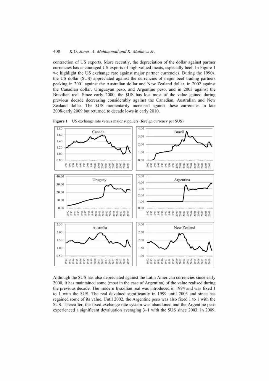
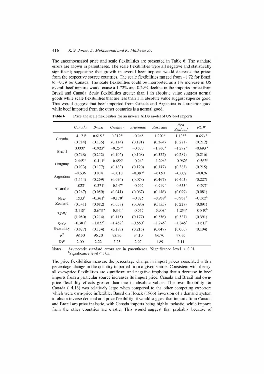
contraction of US exports. More recently, the depreciation of the dollar against partner currencies has encouraged US exports of high-valued meats, especially beef. In Figure 1 we highlight the US exchange rate against major partner currencies. During the 1990s, the US dollar ($US) appreciated against the currencies of major beef trading partners peaking in 2001 against the Australian dollar and New Zealand dollar, in 2002 against the Canadian dollar, Uruguayan peso, and Argentine peso, and in 2003 against the Brazilian real. Since early 2000, the $US has lost most of the value gained during previous decade decreasing considerably against the Canadian, Australian and New Zealand dollar. The $US momentarily increased against these currencies in late 2008/early 2009 but returned to decade lows in early 2010.

Figure 1 US exchange rate versus major suppliers (foreign currency per $US)

0.80

1.00

1.20

1.40

1.60

1.80

1992

1993

1994

1995

1996

1997

1998

1999

2000

2001

2002

2003

2004

2005

2006

2007

2008

2009

Canada

0.00

1.00

2.00

3.00

4.00

1992

1993

1994

1995

1996

1997

1998

1999

2000

2001

2002

2003

2004

2005

2006

2007

2008

2009

Brazil

0.00

10.00

20.00

30.00

40.00

1992

1993

1994

1995

1996

1997

1998

1999

2000

2001

2002

2003

2004

2005

2006

2007

2008

2009

Uruguay

0.00

1.00

2.00

3.00

4.00

5.00

1992

1993

1994

1995

1996

1997

1998

1999

2000

2001

2002

2003

2004

2005

2006

2007

2008

2009

Argentina

0.50

1.00

1.50

2.00

2.50

1992

1993

1994

1995

1996

1997

1998

1999

2000

2001

2002

2003

2004

2005

2006

2007

2008

2009

Australia

1.00

1.50

2.00

2.50

3.00

1992

1993

1994

1995

1996

1997

1998

1999

2000

2001

2002

2003

2004

2005

2006

2007

2008

2009

New Zealand

Although the $US has also depreciated against the Latin American currencies since early 2000, it has maintained some (most in the case of Argentina) of the value realised during the previous decade. The modern Brazilian real was introduced in 1994 and was fixed 1 to 1 with the $US. The real devalued significantly in 1999 until 2003 and since has regained some of its value. Until 2002, the Argentine peso was also fixed 1 to 1 with the $US. Thereafter, the fixed exchange rate system was abandoned and the Argentine peso experienced a significant devaluation averaging 3–1 with the $US since 2003. In 2009,

Source-differentiated analysis of exchange rate 409

the Argentine peso increased to about 3.8 to 1. In addition, until 2002 the Uruguayan peso gradually depreciated against the $US under a quasi fixed regime. Thereafter, the Uruguayan peso was allowed to float and lost half of its value until 2004 when it appreciated in nominal terms against the $US.

Such dramatic changes in the value of the $US relative to major beef trading partners currencies should have a significant effect on the value of US beef imports. It is important to note that while the pattern of $US appreciation in the 1990s then depreciation in the 2000s is relatively consistent across the beef supplying countries (Argentina is the exception), Figure 1 clearly show that the change in the relative value of the $US is by no means homogeneous across supplying countries. For instance, while the fluctuation in the $US relative to the New Zealand dollar is somewhat larger when compared to the Canadian dollar, the depreciation against the Canadian dollar was more extensive. The exchange rate differences across supplying countries suggest that not only should the own-country exchange rate have an impact on source-specific import values and hence prices, but cross-country exchange rate effects may also be important.

To date several studies have examined import demand for beef and other meats, but few studies have evaluated the possible impact of exchange rate fluctuation on import demand. The primary objective of this research is to examine the impact of changes in the exchange rate on the US import demand for source-differentiated beef. Specifically, we investigate: (a) US import demand for beef from its major suppliers; (b) the exchange rate pass-through effect in import prices and (c) and cross exporter effect of exchange rates on US beef imports.

Section 2 presents a brief overview of the literature on demand for meats and a discussion of exchange rate pass through in import prices. Section 3 presents the non-linear inverse AIDS model specification follows. After which in Section 4 a description of the data follows. Section 5 provides the empirical model results and Section 6 presents the discussion and Conclusions.

2 Previous research

There is a large body of literature on the demand for meats (Eales and Unnevehr, 1988; Brester and Wohlgenant, 1991; Eales and Unnevehr, 1993; Kesavan, et al., 1993; Yang and Koo, 1994; Hahn and Mathews, 2007; Muhammad et al., 2007). A number of studies have estimated inverse meat demand systems (Dahlgran, 1987; Eales and Unnevehr 1993; Kesavan and Buhr, 1995). The rationale for the inverse demand specification is that meat is perishable and quantities are predetermined in the short-run. Because of the lags associated with cattle production, short-run quantity adjustments are difficult, causing markets to clear based on price adjustments (Kesavan and Buhr, 1995). Further, an inverse demand system eliminates issues of multi-collinearity when evaluating the impacts of exchange rates exogenously.

The question often arises as to the impact of changes in exchange rates on imports of individual commodities. However, in many instances, a depreciation/appreciation in a given currency may not trigger immediate changes in imports of a particular commodity from that country. Knetter (1989) associates this low exchange rate pass-through with structural features of commodity markets, such as pricing-to-market by imperfectly

410 K.G. Jones, A. Muhammad and K. Mathews Jr.

competitive firms. Jabara and Schwartz (1987) analysed exchange rate pass-through for US agricultural exports to Japan and found evidence consistent with the pricing-to-market hypothesis in which exporters may practice third degree price discrimination across export markets in response to exchange rate movements. In such cases, a change in exchange rate does not necessarily result in price changes by the exporting firm, and in some instances, prices may be allowed to fall with the intent of gaining market share (Abbott et al., 1993).

Corsetti and Dedola (2005) argue that the domestic portion of total consumption as well as the role of substitution between goods plays an important role in determining exchange rate response. Given the traditional approach in which exchange rate pass-through models were developed (Abbott et al., 1993), low exchange rate pass through may be associated with sticky prices and the slow rate of adjustment of prices at the consumer level.

Jabara and Schwartz (1987) found that during the 1970s when the dollar depreciated against the yen, there was complete pass-through but, during the early 1980s when the dollar appreciated, pass-through was lower for corn, soybeans, and beef. They also observed asymmetric price and exchange rate movements where a short-term appreciation of the dollar would more likely be passed through to prices than would a short-term depreciation of the dollar. Xie et al. (2008) found that the prices of major exporting countries were as sensitive to changes in the relative currency values as to changes in the export volume.

Although there are many functional forms available for demand estimation, economic theory does not answer the question of which specification is best. Holt (2002) has shown that there are important differences in own-price and scale consumption flexibilities from a hybrid inverse demand system model, but stops short of endorsing any specific functional form. In this paper, the non-linear Inverse Almost Ideal Demand Systems (IAIDS) model is used to estimate US beef import demand because of the many attributes it confer: it is easily converted from a direct demand system; it is derived from a dual of cost function and has a well defined demand structure; and it is flexible and compatible over aggregation across consumers.

3 Model

The IAIDS introduced by Moschini and Vissa (1992) and Eales and Unnevehr (1993) and later followed by Goodwin et al. (2003) was employed for this analysis. The model differentiates a logarithmic distance function that corresponds to Deaton and Muellbauer’s (1980a) cost function. The distance function for a system of a differentiated product from k sources is given by:

ln ( , ) ln ( ) (1 ) ln( )d u q u b q u a q (1)

where similar to the AIDS model ln ( )a q is

*0

1 1 1

ln ( ) ln 0.5 ln lnk k k

i i ij i ji i j

a q q q q

(2)

Source-differentiated analysis of exchange rate 411

and ln ( )b q is

0 1ln ( ) ln ( )j

k

j iib q q a q

(3)

Substituting equations (2) and (3) into equation (1) results in

*0 0

1 1 1

ln ( , ) ln 0.5 ln ln j

k k k

j j ij i j ji i j

D u q q q q u q

(4)

Compensated share equations are derived from the differential logarithmic distance function. Following Deaton and Meullbauer (1980b) and Eales and Unnevehr (1993) these share equations can become uncompensated by inverting the distance function and solving for the utility index which is substituted into the share equation to yield:

01

ln lnk

i ij j ii

w q Q

(5)

where

* *( ) / 2ij ij ji and *0

1 1 1

ln ln 0.5 ln lnk k k

i i ij i ji i j

Q q q q

(6)

Equation (5) is referred to as the non-linear inverse AIDS model, and utility maximisation requires that the coefficients satisfy the following restrictions: Adding up is satisfied by 1; 0; 0i ij i

i i i

; homogeneity is satisfied if i 0;ijj

and

symmetry is satisfied if ij j i ij .

The price flexibilities in inverse demand models show the percentage changes in the prices associated with a 1% change in country i’s beef quantity supplied. This can be viewed as the inverse of the price elasticity in the direct demand system. The scale flexibility of beef from country i show the percentage change in the price of that good in response to a proportionate increase in the consumption of imported beef from all countries. Following Eales and Unnevehr (1993), the uncompensated price flexibility fij and scale flexibility fi are calculated as:

{ ( ln )}ij ij j jij ij

i

w Qf

w

(7)

and 1 ii

i

fw

(8)

We extend the standard non-linear inverse AIDS model for import demand to incorporate exchange rate effects. The full model is expressed as:

01 1

ln ln lnk k

i ij j i ij i ij ij ii i

w q Q X D T

(9)

where X is the exchange rate, D is a BSE dummy variable where 0 represents the pre-BSE period and 1 thereafter and T representing a time trend variable. We include the dummy variable to account for import disruptions due to the BSE outbreak.

, , , , and are parameters to be estimated and is a random disturbance term.

412 K.G. Jones, A. Muhammad and K. Mathews Jr.

The exchange rate coefficient in equation (9) obeys the classical restrictions on consumer demand (Xie et al., 2008). As such, adding up requires that 0ij j

i

and

homogeneity in exchange rate requires 0 .ij ij

and the Antonelli symmetry requires

ij ji .i j The exchange rate flexibilities ijc are calculated as:

[ ln ]jij ij i kj k

i

c qw

(10)

3.1 Test of endogeneity

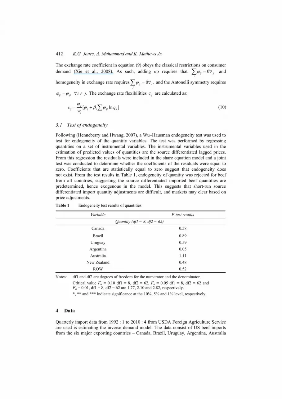
Following (Henneberry and Hwang, 2007), a Wu–Hausman endogeneity test was used to test for endogeneity of the quantity variables. The test was performed by regressing quantities on a set of instrumental variables. The instrumental variables used in the estimation of predicted values of quantities are the source differentiated lagged prices. From this regression the residuals were included in the share equation model and a joint test was conducted to determine whether the coefficients of the residuals were equal to zero. Coefficients that are statistically equal to zero suggest that endogeneity does not exist. From the test results in Table 1, endogeneity of quantity was rejected for beef from all countries, suggesting the source differentiated imported beef quantities are predetermined, hence exogenous in the model. This suggests that short-run source differentiated import quantity adjustments are difficult, and markets may clear based on price adjustments.

Table 1 Endogeneity test results of quantities

Variable F-test results

Quantity (df1 = 8, df2 = 62)

Canada 0.58

Brazil 0.89

Uruguay 0.59

Argentina 0.05

Australia 1.11

New Zealand 0.48

ROW 0.52

Notes: df1 and df2 are degrees of freedom for the numerator and the denominator.

Critical value Fα = 0.10 df1 = 8, df2 = 62, Fα = 0.05 df1 = 8, df2 = 62 and Fα = 0.01, df1 = 8, df2 = 62 are 1.77, 2.10 and 2.82, respectively.

*, ** and *** indicate significance at the 10%, 5% and 1% level, respectively.

4 Data

Quarterly import data from 1992 : 1 to 2010 : 4 from USDA Foreign Agriculture Service are used is estimating the inverse demand model. The data consist of US beef imports from the six major exporting countries – Canada, Brazil, Uruguay, Argentina, Australia

Source-differentiated analysis of exchange rate 413

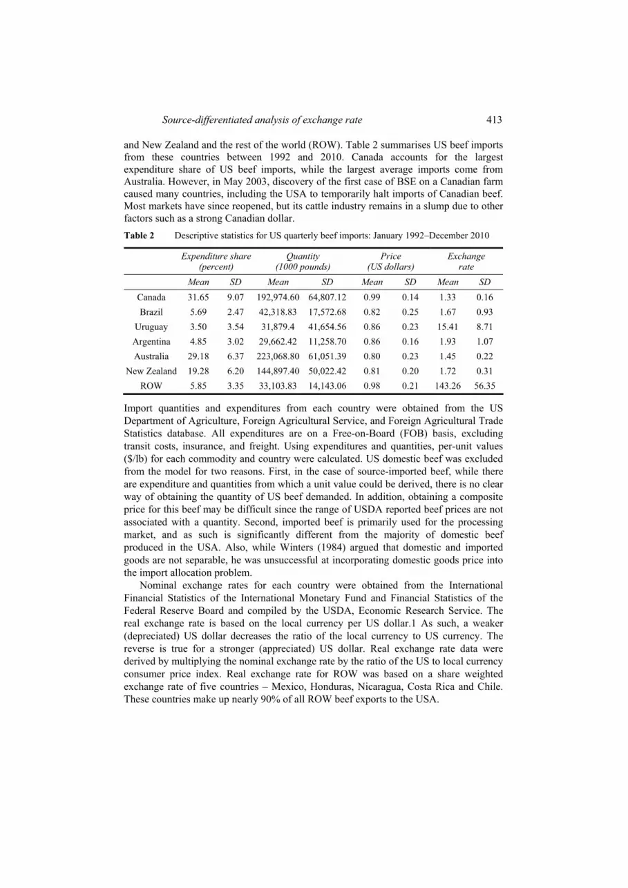
and New Zealand and the rest of the world (ROW). Table 2 summarises US beef imports from these countries between 1992 and 2010. Canada accounts for the largest expenditure share of US beef imports, while the largest average imports come from Australia. However, in May 2003, discovery of the first case of BSE on a Canadian farm caused many countries, including the USA to temporarily halt imports of Canadian beef. Most markets have since reopened, but its cattle industry remains in a slump due to other factors such as a strong Canadian dollar.

Table 2 Descriptive statistics for US quarterly beef imports: January 1992–December 2010

Expenditure share (percent)

Quantity (1000 pounds)

Price (US dollars)

Exchange rate

Mean SD Mean SD Mean SD Mean SD

Canada 31.65 9.07 192,974.60 64,807.12 0.99 0.14 1.33 0.16

Brazil 5.69 2.47 42,318.83 17,572.68 0.82 0.25 1.67 0.93

Uruguay 3.50 3.54 31,879.4 41,654.56 0.86 0.23 15.41 8.71

Argentina 4.85 3.02 29,662.42 11,258.70 0.86 0.16 1.93 1.07

Australia 29.18 6.37 223,068.80 61,051.39 0.80 0.23 1.45 0.22

New Zealand 19.28 6.20 144,897.40 50,022.42 0.81 0.20 1.72 0.31

ROW 5.85 3.35 33,103.83 14,143.06 0.98 0.21 143.26 56.35

Import quantities and expenditures from each country were obtained from the US Department of Agriculture, Foreign Agricultural Service, and Foreign Agricultural Trade Statistics database. All expenditures are on a Free-on-Board (FOB) basis, excluding transit costs, insurance, and freight. Using expenditures and quantities, per-unit values ($/lb) for each commodity and country were calculated. US domestic beef was excluded from the model for two reasons. First, in the case of source-imported beef, while there are expenditure and quantities from which a unit value could be derived, there is no clear way of obtaining the quantity of US beef demanded. In addition, obtaining a composite price for this beef may be difficult since the range of USDA reported beef prices are not associated with a quantity. Second, imported beef is primarily used for the processing market, and as such is significantly different from the majority of domestic beef produced in the USA. Also, while Winters (1984) argued that domestic and imported goods are not separable, he was unsuccessful at incorporating domestic goods price into the import allocation problem.

Nominal exchange rates for each country were obtained from the International Financial Statistics of the International Monetary Fund and Financial Statistics of the Federal Reserve Board and compiled by the USDA, Economic Research Service. The real exchange rate is based on the local currency per US dollar.1 As such, a weaker (depreciated) US dollar decreases the ratio of the local currency to US currency. The reverse is true for a stronger (appreciated) US dollar. Real exchange rate data were derived by multiplying the nominal exchange rate by the ratio of the US to local currency consumer price index. Real exchange rate for ROW was based on a share weighted exchange rate of five countries – Mexico, Honduras, Nicaragua, Costa Rica and Chile. These countries make up nearly 90% of all ROW beef exports to the USA.

414 K.G. Jones, A. Muhammad and K. Mathews Jr.

5 Results

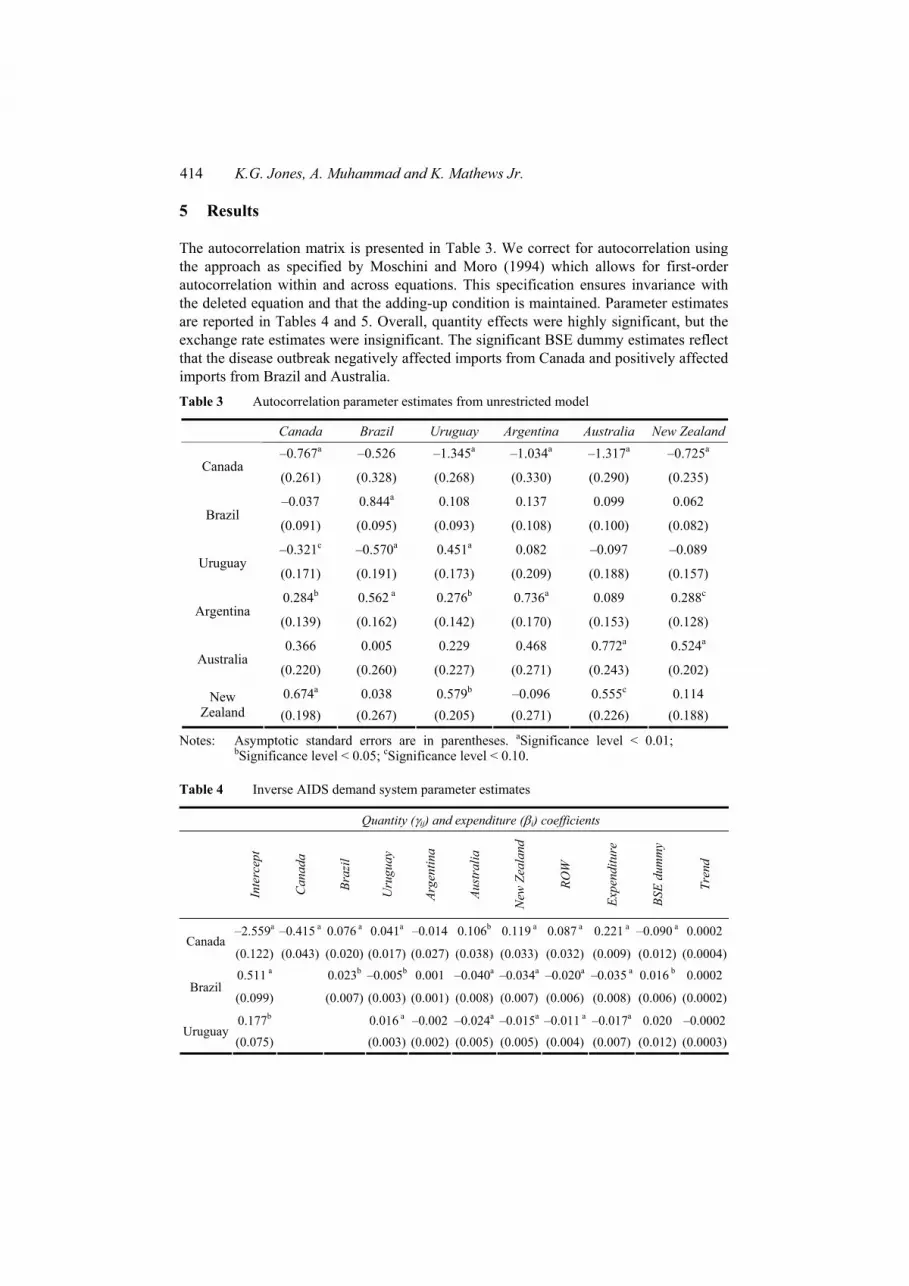
The autocorrelation matrix is presented in Table 3. We correct for autocorrelation using the approach as specified by Moschini and Moro (1994) which allows for first-order autocorrelation within and across equations. This specification ensures invariance with the deleted equation and that the adding-up condition is maintained. Parameter estimates are reported in Tables 4 and 5. Overall, quantity effects were highly significant, but the exchange rate estimates were insignificant. The significant BSE dummy estimates reflect that the disease outbreak negatively affected imports from Canada and positively affected imports from Brazil and Australia.

Table 3 Autocorrelation parameter estimates from unrestricted model

Canada Brazil Uruguay Argentina Australia New Zealand

–0.767a –0.526 –1.345a –1.034a –1.317a –0.725a Canada

(0.261) (0.328) (0.268) (0.330) (0.290) (0.235)

–0.037 0.844a 0.108 0.137 0.099 0.062 Brazil

(0.091) (0.095) (0.093) (0.108) (0.100) (0.082)

–0.321c –0.570a 0.451a 0.082 –0.097 –0.089 Uruguay

(0.171) (0.191) (0.173) (0.209) (0.188) (0.157)

0.284b 0.562 a 0.276b 0.736a 0.089 0.288c Argentina

(0.139) (0.162) (0.142) (0.170) (0.153) (0.128)

0.366 0.005 0.229 0.468 0.772a 0.524a Australia

(0.220) (0.260) (0.227) (0.271) (0.243) (0.202)

0.674a 0.038 0.579b –0.096 0.555c 0.114 New Zealand (0.198) (0.267) (0.205) (0.271) (0.226) (0.188)

Notes: Asymptotic standard errors are in parentheses. aSignificance level < 0.01; bSignificance level < 0.05; cSignificance level < 0.10.

Table 4 Inverse AIDS demand system parameter estimates

Quantity (ij) and expenditure (i) coefficients

Inte

rcep

t

Can

ada

Bra

zil

Uru

guay

Arg

enti

na

Aus

tral

ia

New

Zea

land

RO

W

Exp

endi

ture

BSE

dum

my

Tre

nd

–2.559a –0.415 a 0.076 a 0.041a –0.014 0.106b 0.119 a 0.087 a 0.221 a –0.090 a 0.0002 Canada

(0.122) (0.043) (0.020) (0.017) (0.027) (0.038) (0.033) (0.032) (0.009) (0.012) (0.0004)

0.511 a 0.023b –0.005b 0.001 –0.040a –0.034a –0.020a –0.035 a 0.016 b 0.0002 Brazil

(0.099) (0.007) (0.003) (0.001) (0.008) (0.007) (0.006) (0.008) (0.006) (0.0002)

0.177b 0.016 a –0.002 –0.024a –0.015a –0.011 a –0.017a 0.020 –0.0002 Uruguay

(0.075) (0.003) (0.002) (0.005) (0.005) (0.004) (0.007) (0.012) (0.0003)

Source-differentiated analysis of exchange rate 415

Table 4 Inverse AIDS demand system parameter estimates (continued)

Quantity (ij) and expenditure (i) coefficients

Inte

rcep

t

Can

ada

Bra

zil

Uru

guay

Arg

enti

na

Aus

tral

ia

New

Zea

land

RO

W

Exp

endi

ture

BSE

dum

my

Tre

nd

0.032 0.029 a –0.003 –0.007 –0.004 0.006 –0.007 –0.0008a Argentina

(0.127) (0.003) (0.009) (0.008) (0.006) (0.010) (0.011) (0.0027)

1.205 a 0.115 a –0.107 a –0.047 a –0.072 a 0.024 0.0007 Australia

(0.169) (0.024) (0.017) (0.012) (0.014) (0.015) (0.0036)

1.004 a 0.079a –0.034a 0.067a 0.018 –0.0002 New Zealand (0.145) (0.019) (0.008) (0.013) (0.012) (0.009)

0.629 a 0.030a ROW

(0.139) (0.012)

R2 98.00 95.77 91.71 92.44 95.82 96.83

DW 1.99 2.27 2.14 1.94 1.79 2.11

Notes: Asymptotic standard errors are in parentheses. aSignificance level < 0.01; bSignificance level < 0.05.

Table 5 Inverse AIDS exchange rate parameter estimates

Exchange rate (ij) coefficient

Canada Brazil Uruguay Argentina Australia New Zealand

ROW

0.083 0.003 –0.009 –0.007 –0.035 –0.005 –0.013 Canada

(0.044) (0.015) (0.021) (0.012) (0.038) (0.024) (0.009)

0.001 0.008 –0.007 0.017 –0.014 –0.001 Brazil

(0.007) (0.021) (0.006) (0.012) (0.012) (0.003)

0.026a –0.008 0.011 0.018b 0.004 Uruguay

(0.010) (0.008) (0.014) (0.009) (0.005)

0.007 0.004 0.007 –0.003 Argentina

(0.008) (0.012) (0.011) (0.004)

–0.010 –0.009 –0.002 Australia

(0.045) (0.029) (0.007)

0.025 0.011 New Zealand (0.021) (0.007)

Notes: Asymptotic standard errors are in parentheses. aSignificance level < 0.01; bSignificance level < 0.05.

416 K.G. Jones, A. Muhammad and K. Mathews Jr.

The uncompensated price and scale flexibilities are presented in Table 6. The standard errors are shown in parentheses. The scale flexibilities were all negative and statistically significant; suggesting that growth in overall beef imports would decrease the prices from the respective source countries. The scale flexibilities ranged from –1.72 for Brazil to –0.29 for Canada. The scale flexibilities could be interpreted as a 1% increase in US overall beef imports would cause a 1.72% and 0.29% decline in the imported price from Brazil and Canada. Scale flexibilities greater than 1 in absolute value suggest normal goods while scale flexibilities that are less than 1 in absolute value suggest superior good. This would suggest that beef imported from Canada and Argentina is a superior good while beef imported from the other countries is a normal good.

Table 6 Price and scale flexibilities for an inverse AIDS model of US beef imports

Canada Brazil Uruguay Argentina Australia New Zealand

ROW

–4.171a 0.615 a 0.312 a –0.065 1.220 a 1.135 a 0.653 a Canada

(0.284) (0.135) (0.114) (0.181) (0.264) (0.221) (0.212)

3.000a –0.923a –0.257a –0.027 –1.500 a –1.278 a –0.693 a Brazil

(0.768) (0.252) (0.105) (0.168) (0.322) (0.289) (0.216)

2.445 a –0.411a –0.655a –0.043 –1.294a –0.962a –0.563a Uruguay

(0.973) (0.177) (0.163) (0.120) (0.387) (0.363) (0.215)

–0.606 0.074 –0.010 –0.397a –0.093 –0.008 –0.026 Argentina

(1.114) (0.209) (0.094) (0.078) (0.467) (0.403) (0.227)

1.023a –0.271a –0.147a –0.002 –0.919 a –0.635 a –0.297a Australia

(0.267) (0.059) (0.041) (0.067) (0.186) (0.099) (0.081)

1.533a –0.361a –0.170a –0.025 –0.989a –0.968 a –0.365a New Zealand (0.341) (0.082) (0.058) (0.090) (0.155) (0.228) (0.091)

3.118a –0.673 a –0.341a –0.057 –0.908a –1.254a –0.819b ROW

(1.080) (0.214) (0.118) (0.177) (0.256) (0.327) (0.391)

–0.301a –1.623a –1.482 a –0.880 a –1.248a –1.345a –1.612a Scale flexibility (0.027) (0.134) (0.189) (0.213) (0.047) (0.066) (0.194)

R2 98.00 96.20 93.90 94.10 96.70 97.60

DW 2.00 2.22 2.23 2.07 1.89 2.11

Notes: Asymptotic standard errors are in parentheses. aSignificance level < 0.01; bSignificance level < 0.05.

The price flexibilities measure the percentage change in import prices associated with a percentage change in the quantity imported from a given source. Consistent with theory, all own-price flexibilities are significant and negative implying that a decrease in beef imports from a particular source increases its import price. Canada and Brazil had own-price flexibility effects greater than one in absolute values. The own flexibility for Canada (–4.16) was relatively large when compared to the other competing exporters which were own-price inflexible. Based on Houck (1966) inversion of a demand system to obtain inverse demand and price flexibility, it would suggest that imports from Canada and Brazil are price inelastic, with Canada imports being highly inelastic, while imports from the other countries are elastic. This would suggest that probably because of

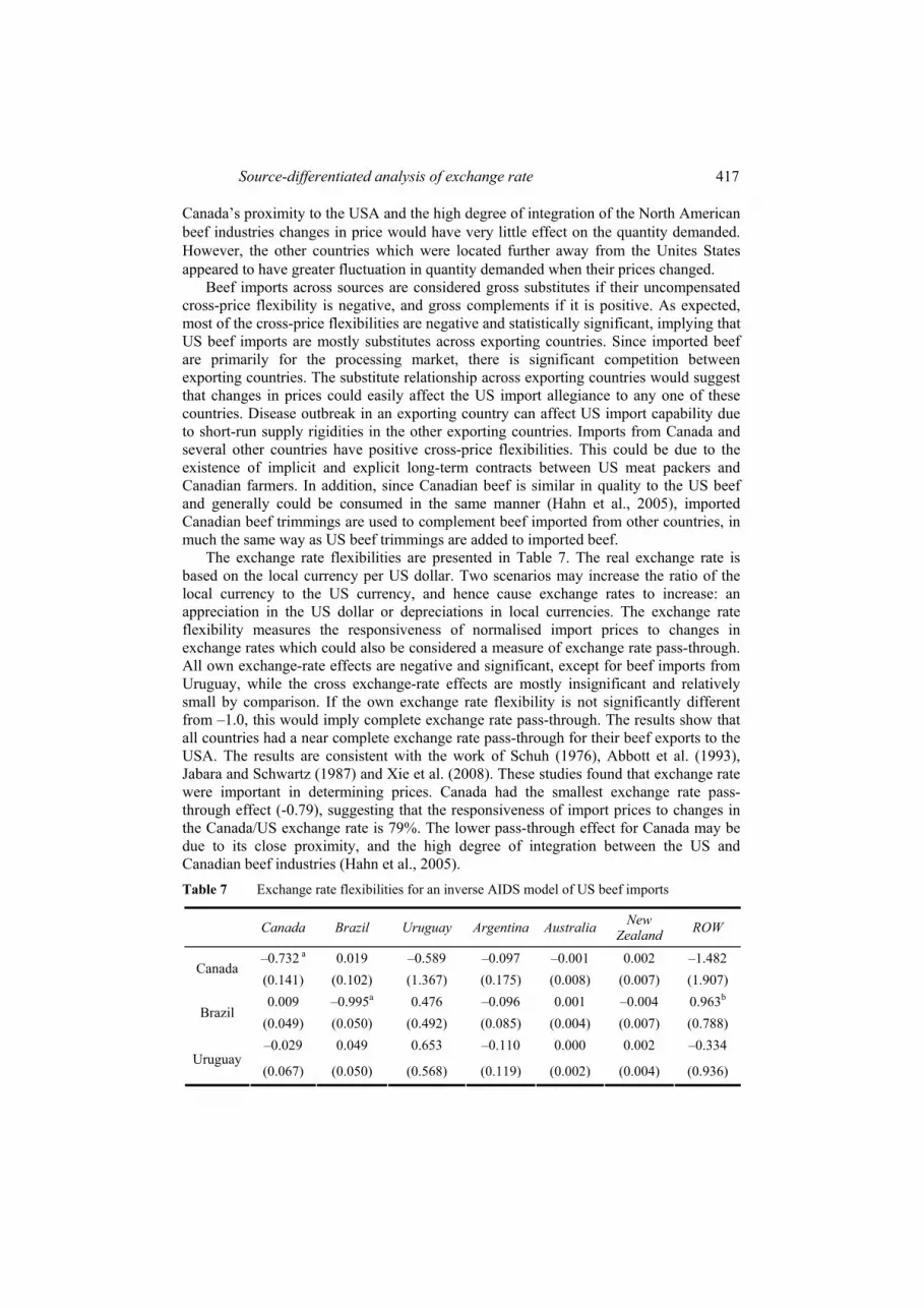
Source-differentiated analysis of exchange rate 417

Canada’s proximity to the USA and the high degree of integration of the North American beef industries changes in price would have very little effect on the quantity demanded. However, the other countries which were located further away from the Unites States appeared to have greater fluctuation in quantity demanded when their prices changed.

Beef imports across sources are considered gross substitutes if their uncompensated cross-price flexibility is negative, and gross complements if it is positive. As expected, most of the cross-price flexibilities are negative and statistically significant, implying that US beef imports are mostly substitutes across exporting countries. Since imported beef are primarily for the processing market, there is significant competition between exporting countries. The substitute relationship across exporting countries would suggest that changes in prices could easily affect the US import allegiance to any one of these countries. Disease outbreak in an exporting country can affect US import capability due to short-run supply rigidities in the other exporting countries. Imports from Canada and several other countries have positive cross-price flexibilities. This could be due to the existence of implicit and explicit long-term contracts between US meat packers and Canadian farmers. In addition, since Canadian beef is similar in quality to the US beef and generally could be consumed in the same manner (Hahn et al., 2005), imported Canadian beef trimmings are used to complement beef imported from other countries, in much the same way as US beef trimmings are added to imported beef.

The exchange rate flexibilities are presented in Table 7. The real exchange rate is based on the local currency per US dollar. Two scenarios may increase the ratio of the local currency to the US currency, and hence cause exchange rates to increase: an appreciation in the US dollar or depreciations in local currencies. The exchange rate flexibility measures the responsiveness of normalised import prices to changes in exchange rates which could also be considered a measure of exchange rate pass-through. All own exchange-rate effects are negative and significant, except for beef imports from Uruguay, while the cross exchange-rate effects are mostly insignificant and relatively small by comparison. If the own exchange rate flexibility is not significantly different from –1.0, this would imply complete exchange rate pass-through. The results show that all countries had a near complete exchange rate pass-through for their beef exports to the USA. The results are consistent with the work of Schuh (1976), Abbott et al. (1993), Jabara and Schwartz (1987) and Xie et al. (2008). These studies found that exchange rate were important in determining prices. Canada had the smallest exchange rate pass-through effect (-0.79), suggesting that the responsiveness of import prices to changes in the Canada/US exchange rate is 79%. The lower pass-through effect for Canada may be due to its close proximity, and the high degree of integration between the US and Canadian beef industries (Hahn et al., 2005).

Table 7 Exchange rate flexibilities for an inverse AIDS model of US beef imports

Canada Brazil Uruguay Argentina Australia New Zealand

ROW

–0.732 a 0.019 –0.589 –0.097 –0.001 0.002 –1.482 Canada

(0.141) (0.102) (1.367) (0.175) (0.008) (0.007) (1.907)

0.009 –0.995a 0.476 –0.096 0.001 –0.004 0.963b Brazil

(0.049) (0.050) (0.492) (0.085) (0.004) (0.007) (0.788)

–0.029 0.049 0.653 –0.110 0.000 0.002 –0.334 Uruguay

(0.067) (0.050) (0.568) (0.119) (0.002) (0.004) (0.936)

418 K.G. Jones, A. Muhammad and K. Mathews Jr.

Table 7 Exchange rate flexibilities for an inverse AIDS model of US beef imports (continued)

Canada Brazil Uruguay Argentina Australia New Zealand

ROW

–0.022 –0.039 –0.507 –0.900a –0.000 0.002 –0.690 Argentina

(0.040) (0.091) (0.534) (0.118) (0.001) (0.004) (0.799)

–0.089 0.112 0.693 –0.059 –1.000a –0.003 0.535 Australia

(0.090) (0.087) (0.949) (0.174) (0.003) (0.008) (2.223)

0.017 –0.093 0.563 0.091 –0.000 –0.993a –0.959 New Zealand (0.077) (0.064) (0.667) (0.127) (0.002) (0.012) (1.718)

–0.017 –0.046 –1.536b 0.083 0.019 –0.030 –0.832a ROW

(0.012) (0.071) (0.683) (0.065) (0.017) (0.026) (0.205)

Notes: Asymptotic standard errors are in parentheses. aSignificance level < 0.01; bSignificance level < 0.05.

Uruguay is the only country with insignificant exchange rate flexibility, implying that exchange rates play a limited role in determining the price of its beef exports to the USA. This may explain why there was still growth in beef imports from Uruguay even as the $US depreciated against the Uruguayan peso.

6 Summary and conclusion

This study contributes to the limited literature on the impact of exchange rates on import demand for source-different beef. An inverse almost ideal demand system was employed for this analysis and extended to incorporate exchange rate effects. The results of this study show almost complete exchange rates pass-through for beef imports from all countries except Uruguay, implying that exchange rates play a significant role in determining beef import prices. However, our results indicate a relatively higher rate of exchange rate pass-through for imported beef from outside North America. High rates of exchange rate pass-through imply that exchange rate changes are readily incorporated into US beef price changes. It also suggests that beef prices are market driven and may not be influenced by non-tariff distortions which may discriminate between domestic and imported beef.

The own flexibility for Canada (–4.16), the largest supplier of US imported beef was relatively large which implies a highly inelastic own price elasticity for beef. This suggests that with high rates of exchange rate pass-through, highly volatile exchange rates would have little impact on the import demand from Canada. Clearly, this would not be the case for the other competing exporters which were own-price inflexible. Fluctuations in their exchange rates would readily pass through to prices and influence the demand for their products imported beef products.

Acknowledgements

The views expressed here are those of the authors and may not be attributed to the Economic Research Service or the US Department of Agriculture.

Source-differentiated analysis of exchange rate 419

References

Abbott, P.C., Patterson, P.M. and Reca, A. (1993) ‘Imperfect competition and exchange rate pass-through in the food processing sector’, American Journal of Agricultural Economics, Vol. 75, No. 5, pp.1226–1230.

Brester, G.W. and Wohlgenant, M.K. (1991) ‘Examining interrelated demands for meats using new measures for ground and table cut beef’, American Journal of Agricultural Economics, Vol. 73, pp.1182–1194.

Castillo, M. (2003) A Look at Rising Cattle and Beef Trade in North America, FAS. Available online at: www.fas.usda.gov (accessed on 17 March 2012).

Corsetti, G. and Dedola, L. (2005) ‘Macroeconomics of international price discrimination’, Journal of International Economics, Vol. 67, No. 1, pp.129–156.

Dahlgran, R.A. (1987) ‘Complete flexibility systems and stationarity of us meat demands’, Western Journal of Agricultural Economics, Vol. 12, No. 2, pp.152–163

Deaton, A.S. and Muellbauer, J. (1980a) ‘An almost ideal demand system’, American Economic Review, Vol. 70, No. 3, pp.312–326.

Deaton, A.S. and Muellbauer, J. (1980b) Economics and Consumer Behavior, Cambridge University Press, Cambridge.

Eales, J.S. and Unnevehr, L.J. (1988) ‘Demand for beef and chicken products: separability and structural change’, American Journal of Agricultural Economics, Vol. 70, No. 3, pp.521–532.

Eales, J.S. and Unnevehr, L. (1993) ‘Simultaneity and structural change in us meat demand’, American Journal of Agricultural Economics, Vol. 75, No. 2, pp.259–268.

Goodwin, B.K., Harper, D. and Schnepf, R. (2003) ‘Short-run demand relationships in the U.S. fats and oils complex’, Journal of Agricultural and Applied Economics, Vol. 35, No. 1, pp.171–184.

Gordon, K. (2004) ‘Which countries will be competitive in supplying beef for the world’s needs in the next decade?’, Angus Journal, pp.188–189.

Hahn, W.F., Haley, M., Leuck, D., Miller, J.J., Perry, J., Taha, F. and Zahniser, S. (2005) Market Integration of the North American Animal Products Complex, Outlook Report LDP-M-131-01, U.S. Department of Agriculture, Economic Research Service.

Hahn, W.F. and Mathews Jr., K.H. (2007) ‘Characteristics and hedonic pricing of differentiated beef demands’, Agricultural Economics, Vol. 36, No. 3, pp.377–393.

Henneberry, S.R. and Hwang, S.H. (2007) ‘Meat demand in South Korea: an application of the restricted source-differentiated almost ideal demand system model’, Journal of Agricultural and Applied Economics, Vol. 39, No. 1, pp.47–60.

Holt, M.T. (2002) ‘Inverse demand systems and choice of functional form’, European Economic Review, Vol. 46, No. 1, pp.117–142.

Houck, J.P. (1966) ‘Relationship of direct price flexibilities to direct price elasticities’, Journal of Farm Economics, Vol. 47, No. 3, pp.789–792.

Jabara, C.L. and Schwartz, N.E. (1987) ‘Flexible exchange rates and commodity price changes: the case of Japan’, American Journal of Agricultural Economics, Vol. 69, No. 3, pp.580–590.

Jones, K. and Shane, M. (2009) Factors Shaping Expanding US Red Meat Trade, Livestock, Dairy, and Poultry Outlook, USDA, ERS, LDP-M-175-01.

Knetter, M.M. (1989) ‘Price discrimination by U.S. and German exporters’, American Economic Review, Vol. 79, No. 1, pp.198–210.

Kesavan, T. and Buhr, B. (1995) ‘Price determination and dynamic adjustments: an inverse demand system approach to meat products in the United States’, Empirical Economics, Vol. 20, No. 4, pp.681–698.

Kesavan, T., Hassan, Z.A., Jensen, H.H. and Johnson, S.R. (1993) ‘Dynamic and long-run structure in U.S. meat demand’, Canadian Journal of Agricultural Economics, Vol. 41, No. 2, pp.139–153.

420 K.G. Jones, A. Muhammad and K. Mathews Jr.

Leuck, D. (2001) The New Agricultural Trade Negotiations: Background and Issues for the U.S. Beef Sector, Outlook Report LDP-M-89-01, U.S. Department of Agriculture, Economic Research Service.

Moschini, G. and Moro, D. (1994) ‘Autocorrelation specification in singular equation systems’, Economic Letters, Vol. 46, No. 4, pp.303–309.

Moschini, G. and Vissa, A. (1993) ‘Flexible specification of mixed demand systems’, American Journal of Agricultural Economics, Vol. 75, No. 1, pp.1–9.

Muhammad, A., Jones, K.G. and Hahn, W.F. (2007) ‘The impact of domestic and import prices on U.S. lamb imports: a production system approach’, Agricultural and Resource Economics Review, Vol. 36, No. 2, pp.293–301.

Schuh, G.E. (1974) ‘The exchange rate and U.S. agriculture’, American Journal of Agricultural Economics, Vol. 56, No. 1, pp.1–13.

U.S. Department of Agriculture, Economic Research Service (ERS) Real and Nominal Country Exchange Rates, http://www.ers.usda.gov/Data/exchangerates/ (accessed on 2 May 2010).

U.S. Department of Agriculture, Foreign Agricultural Service (FAS) (2009) Livestock and Poultry: World Markets and Trade, Foreign Agricultural Service, USDA.

U.S. Department of Agriculture, Foreign Agricultural Service (FAS) Foreign Agricultural Trade of the United States (FATUS). Available online at: http://www.ers.usda.gov/Data/FATUS

Winters, L.A. (1984) ‘Separability and the specification of foreign trade function’, Journal of International Economics, Vol. 17, Nos. 3/4, pp.239–263.

Yang, S. and Koo, W.W. (1994) ‘Japanese meat import demand estimation with the source differentiated AIDS Model’, Journal of Agricultural and Resource Economics, Vol. 19, No. 2, pp.396–408.

Xie, J., Kinnucan, H.W. and Myrland, Ø. (2008) ‘The effects of exchange rates on export prices of farmed salmon’, Marine Resource Economics, Vol. 23, No. 4, pp.439–457.

Notes

1 Local currency applies to the exporting country.