Solubility of CO2 in 15, 30, 45 and 60 mass% MEA from 40 to 120 °C and model representation using...
14
Solubility of CO 2 in 15, 30, 45 and 60 mass% MEA from 40 to 120 1C and model representation using the extended UNIQUAC framework Ugochukwu E. Aronu a , Shahla Gondal a , Erik T. Hessen a , Tore Haug-Warberg a , Ardi Hartono a , Karl A. Hoff b , Hallvard F. Svendsen a,n a Department of Chemical Engineering, Norwegian University of Science and Technology, N-7491 Trondheim, Norway b SINTEF Materials and Chemistry, N-7465 Trondheim, Norway article info Article history: Received 23 January 2011 Received in revised form 20 August 2011 Accepted 27 August 2011 Available online 3 September 2011 Keywords: CO 2 absorption Separations Phase equilibria Thermodynamic process Extended UNIQUAC Monoethanolamine (MEA) abstract New experimental data for vapor–liquid equilibrium of CO 2 in aqueous monoethanolamine solutions are presented for 15, 30, 45 and 60 mass% MEA and from 40 to 120 1C. CO 2 partial pressures over loaded MEA solutions were measured using a low temperature equilibrium apparatus while total pressures were measured with a high temperature equilibrium apparatus. Experimental data are given as CO 2 partial pressure as function of loading in solution for temperatures from 40 to 80 1C and as total pressures for temperatures from 60 to 120 1C for the different MEA concentrations. The extended UNIQUAC model framework was applied and model parameters were fitted to the new experimental VLE data and physical CO 2 solubility data from the literature. The model gives a good representation of the experimental VLE data for CO 2 partial pressures and total pressures for all MEA concentrations with an average absolute relative deviation (AARD) of 24.3% and 11.7%, respectively, while the physical solubility data were represented with an AARD of 2.7%. Further, the model predicts well literature data on freezing point depression, excess enthalpy and liquid phase speciation determined by NMR. & 2011 Elsevier Ltd. All rights reserved. 1. Introduction Scrubbing effluent industrial fluid streams of acid gases such as CO 2 and H 2 S is an important industrial process operation. The technique has historically been applied for various reasons such as improving the calorific value of gas streams and avoiding corrosion on process lines and fittings. Recently, a more compel- ling reason for scrubbing of carbon dioxide from process streams has been the urgent need to reduce greenhouse gas emissions. CO 2 capture by absorption technology remains the most promis- ing and most mature technology for CO 2 removal from exhaust gas streams, and reducing the cost of this technology is of global interest. Amine-based CO 2 solvents have been the most studied absorbents for CO 2 capture by absorption. Several studies have been carried out on the solubility of CO 2 in aqueous MEA solution. Tables presenting summaries of pre- vious studies were presented by Jou et al. (1995), Kohl and Nielsen (1997) and Ma’mun et al. (2005). The experimental data of Jou et al. (1995) covers a wide range of temperatures, pressures and loadings, however it is available only for 30 mass% MEA. Of all the numerous work on MEA, only Mason and Dodge (1936) and Atadan (1954) measured CO 2 solubility in MEA at concentrations higher than 30 mass%. These data are old and quite few. Mason and Dodge (1936) measured only up to 75 1C and between 1.3 and 100 kPa while Atadan (1954) measured up to 70 1C and between 103 and 3447 kPa, thus not covering the temperature range for regeneration. There is also a strong need for more data in the very low loading and pressure regions for modeling purposes. Further MEA is often used as a base case solvent in comparative studies of new solvents for CO 2 absorption and new processes applying higher solvent concentrations are being developed. For e.g. Bouillon et al. (2011) have shown that use of MEA at higher concentrations can give improved CO 2 absorption results. Thus an up-to-date robust VLE data set for H 2 O–MEA–CO 2 system, spanning a large concen- tration range, is clearly needed. Accurate correlation of equilibrium behavior of CO 2 in aqueous MEA solutions will enable better process simulations towards cost reduction, better column design as well as improved plant opera- tion. Different thermodynamic models have been used to describe the equilibrium behavior of CO 2 in aqueous alkanolamine solu- tions, in particular, MEA. These models could be categorized into three (Hessen et al., 2010); the non-rigorous models, e.g. Kent- Eisenberg (1976) and the rigorous models with the two branches; activity models (excess Gibbs energy) and equation of state models (Helmholtz energy). Activity based models vary in complexity, ranging from the relatively simple Deshmukh and Mather (1981) to the more sophisticated ones, such as electrolyte–NRTL (Chen et al., 1982; Chen and Evans, 1986) and extended UNIQUAC models (Nicolaisen et al., 1993; Thomsen, 1997; Thomsen and Rasmussen, Contents lists available at SciVerse ScienceDirect journal homepage: www.elsevier.com/locate/ces Chemical Engineering Science 0009-2509/$ - see front matter & 2011 Elsevier Ltd. All rights reserved. doi:10.1016/j.ces.2011.08.042 n Corresponding author. Tel.: þ47 73594100; fax: þ47 73594080. E-mail addresses: [email protected] (U.E. Aronu), [email protected] (H.F. Svendsen). Chemical Engineering Science 66 (2011) 6393–6406
Transcript of Solubility of CO2 in 15, 30, 45 and 60 mass% MEA from 40 to 120 °C and model representation using...
Chemical Engineering Science 66 (2011) 6393–6406
Contents lists available at SciVerse ScienceDirect
Chemical Engineering Science
0009-25
doi:10.1
n Corr
E-m
hallvard
journal homepage: www.elsevier.com/locate/ces
Solubility of CO2 in 15, 30, 45 and 60 mass% MEA from 40 to 120 1C andmodel representation using the extended UNIQUAC framework
Ugochukwu E. Aronu a, Shahla Gondal a, Erik T. Hessen a, Tore Haug-Warberg a, Ardi Hartono a,Karl A. Hoff b, Hallvard F. Svendsen a,n
a Department of Chemical Engineering, Norwegian University of Science and Technology, N-7491 Trondheim, Norwayb SINTEF Materials and Chemistry, N-7465 Trondheim, Norway
a r t i c l e i n f o
Article history:
Received 23 January 2011
Received in revised form
20 August 2011
Accepted 27 August 2011Available online 3 September 2011
Keywords:
CO2 absorption
Separations
Phase equilibria
Thermodynamic process
Extended UNIQUAC
Monoethanolamine (MEA)
09/$ - see front matter & 2011 Elsevier Ltd. A
016/j.ces.2011.08.042
esponding author. Tel.: þ47 73594100; fax:
ail addresses: [email protected]
[email protected] (H.F. Svendsen)
a b s t r a c t
New experimental data for vapor–liquid equilibrium of CO2 in aqueous monoethanolamine solutions
are presented for 15, 30, 45 and 60 mass% MEA and from 40 to 120 1C. CO2 partial pressures over loaded
MEA solutions were measured using a low temperature equilibrium apparatus while total pressures
were measured with a high temperature equilibrium apparatus. Experimental data are given as CO2
partial pressure as function of loading in solution for temperatures from 40 to 80 1C and as total
pressures for temperatures from 60 to 120 1C for the different MEA concentrations. The extended
UNIQUAC model framework was applied and model parameters were fitted to the new experimental
VLE data and physical CO2 solubility data from the literature. The model gives a good representation of
the experimental VLE data for CO2 partial pressures and total pressures for all MEA concentrations with
an average absolute relative deviation (AARD) of 24.3% and 11.7%, respectively, while the physical
solubility data were represented with an AARD of 2.7%. Further, the model predicts well literature data
on freezing point depression, excess enthalpy and liquid phase speciation determined by NMR.
& 2011 Elsevier Ltd. All rights reserved.
1. Introduction
Scrubbing effluent industrial fluid streams of acid gases suchas CO2 and H2S is an important industrial process operation. Thetechnique has historically been applied for various reasons suchas improving the calorific value of gas streams and avoidingcorrosion on process lines and fittings. Recently, a more compel-ling reason for scrubbing of carbon dioxide from process streamshas been the urgent need to reduce greenhouse gas emissions.CO2 capture by absorption technology remains the most promis-ing and most mature technology for CO2 removal from exhaustgas streams, and reducing the cost of this technology is of globalinterest. Amine-based CO2 solvents have been the most studiedabsorbents for CO2 capture by absorption.
Several studies have been carried out on the solubility of CO2
in aqueous MEA solution. Tables presenting summaries of pre-vious studies were presented by Jou et al. (1995), Kohl andNielsen (1997) and Ma’mun et al. (2005). The experimental dataof Jou et al. (1995) covers a wide range of temperatures, pressuresand loadings, however it is available only for 30 mass% MEA. Of allthe numerous work on MEA, only Mason and Dodge (1936) andAtadan (1954) measured CO2 solubility in MEA at concentrations
ll rights reserved.
þ47 73594080.
nu.no (U.E. Aronu),
.
higher than 30 mass%. These data are old and quite few. Mason andDodge (1936) measured only up to 75 1C and between 1.3 and100 kPa while Atadan (1954) measured up to 70 1C and between103 and 3447 kPa, thus not covering the temperature range forregeneration. There is also a strong need for more data in the verylow loading and pressure regions for modeling purposes. FurtherMEA is often used as a base case solvent in comparative studies ofnew solvents for CO2 absorption and new processes applying highersolvent concentrations are being developed. For e.g. Bouillon et al.(2011) have shown that use of MEA at higher concentrations cangive improved CO2 absorption results. Thus an up-to-date robustVLE data set for H2O–MEA–CO2 system, spanning a large concen-tration range, is clearly needed.
Accurate correlation of equilibrium behavior of CO2 in aqueousMEA solutions will enable better process simulations towards costreduction, better column design as well as improved plant opera-tion. Different thermodynamic models have been used to describethe equilibrium behavior of CO2 in aqueous alkanolamine solu-tions, in particular, MEA. These models could be categorized intothree (Hessen et al., 2010); the non-rigorous models, e.g. Kent-Eisenberg (1976) and the rigorous models with the two branches;activity models (excess Gibbs energy) and equation of state models(Helmholtz energy). Activity based models vary in complexity,ranging from the relatively simple Deshmukh and Mather (1981) tothe more sophisticated ones, such as electrolyte–NRTL (Chen et al.,1982; Chen and Evans, 1986) and extended UNIQUAC models(Nicolaisen et al., 1993; Thomsen, 1997; Thomsen and Rasmussen,
U.E. Aronu et al. / Chemical Engineering Science 66 (2011) 6393–64066394
1999) models. The extended-UNIQUAC model was used in thiswork. Previous work such as Austgen et al. (1989), Faramarzi et al.(2009), Hessen et al. (2010), etc. have, respectively, implemented theoriginal electrolyte–NRTL, refined electrolyte–NRTL and extended-UNIQUAC models for the H2O–MEA–CO2 system. However, all theimplementations were based on experimental data of not more than30 mass% MEA concentration, except for Hessen et al. (2010) whoapplied the r-e-NRTL to predict experimental VLE results of 60mass% MEA up to 80 1C. None of the existing models have used thesolubility of N2O in MEA which by utilizing the so-called N2Oanalogy (originally proposed by Clarke (1964) and verified byLaddha et al. (1981)) gives a measure of the physical solubility, orHenry’s law constant, of CO2 in the aqueous MEA solution. Throughthe physical solubility of CO2, the activity coefficient of CO2 can becalculated. In Hessen (2010) it was shown that existing models giveCO2 activity coefficients which are far from the N2O analogy derivedvalues.
The objectives of this work are to present a consistent VLE dataset for MEA through experimental VLE measurements for 15, 30,45 and 60 mass% MEA in the low and high CO2 loading regionsfrom 40 to 120 1C, and to use these data together with CO2
solubility data based on the N2O analogy, to provide a rigorousequilibrium model based on the extended UNIQUAC modelframework.
Table 1Number of calibration points used for each CO2 IR analyzer range.
CO2 analyzer
concentration range
No. of calibration
points in range
0–200 ppm 2
0–1000 ppm 2
0–2000 5
0–1.0% 5
0–5.0% 6
0–20.0% 8
2. Equilibrium experiments
2-Aminoethanol (MEA) (purity Z99 mass%) was obtainedfrom Sigma-Aldrich. Sample solutions of 15, 30, 45 and 60 mass%MEA were prepared using deionized water. A total of about 5.0 Lsolution of each MEA concentration was prepared. Solutions wereprepared using a Sartorius GMBH Gottingen balance within70.1 g. The gases used; CO2, purity 499.99 mol% and calibrationgases, 2.5 mol% CO2 and 4.96 mol% CO2 were supplied by AGA GasGmbH while N2, purity 499.999 mol% and calibration gas100 ppm CO2 were supplied by Yara Praxair AS.
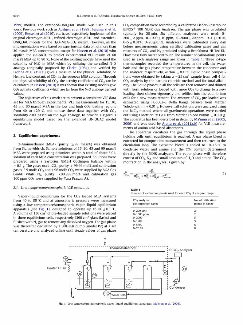
2.1. Low temperature/atmospheric VLE apparatus
Vapor–liquid equilibrium for the CO2 loaded MEA systemsfrom 40 to 80 1C and at atmospheric pressure were measuredusing a low temperature/atmospheric vapor–liquid equilibriumapparatus (see Fig. 1), designed to operate up to 8070.1 1C.A volume of 150 cm3 of pre-loaded sample solutions were placedin three equilibrium cells, respectively (360 cm3 glass flasks) andflushed with N2 gas to remove any dissolved oxygen. The gas phasewas thereafter circulated by a BUHLER pump (model P2) at a settemperature and analyzed online until steady values of gas phase
Water Ba
Heater + Fan
TI
Thermos
TI
TIC
TIC
34
Fig. 1. Low temperature/atmospheric vapor–liquid
CO2 composition were recorded by a calibrated Fisher–RosemountBINOSs 100 NDIR Gas Analyzer. The gas phase was circulatedtypically for 20 min. Six different analyzers were used; 0–20072 ppm, 0–1000710 ppm, 0–2000720 ppm, 0–170.01%,0–570.01%; 0–2070.1%. Analyzers were calibrated every daybefore measurements using certified calibration gases and gasmixtures of CO2 and N2 produced using a Bronkhorst Hi-Tec EL-Flow mass flow meter controller. The number of calibrations pointsused in each analyzer range are given in Table 1. Three K-typethermocouples recorded the temperatures in the cell, the waterbath and the gas phase temperature between the condenser andthe analyzer, respectively, within 70.1 1C. Liquid phase composi-tions were obtained by taking a �25 cm3 sample from cell 4 forCO2 analysis by the barium chloride method and for total alkali-nity. The liquid phases in all the cells are then removed and dilutedwith fresh solution or loaded with more CO2 to change to a newloading, then shaken vigorously and refilled into the equilibriumcells for a new measurement. The amount of CO2 pre-loaded wasestimated using PG5002-S Delta Range balance from MettlerToledo within 70.01 g. However, all solutions were analyzed usingthe BaCl2 method where all gravimetric operations were carriedout using a Mettler PM1200 from Mettler Toledo within 70.001 g.The apparatus has been described in detail by Ma’mun et al. (2005,2006) and was used by Aronu et al. (2011a,b) for VLE measure-ments of amino acid based absorbents.
The apparatus circulates the gas through the liquid phaseholding cells until equilibrium is reached. A gas phase bleed isextracted for composition measurement and then returned to thecirculation loop. The extracted bleed is cooled to 10–15 1C tocondense water and amine and the CO2 content determineddirectly by the NDIR analyzers. The vapor phase will thereforeconsist of CO2, N2, and small amounts of H2O and amine. The CO2
molfraction in the analyzer is given by
yIRCO2¼
nIRCO2
nIRCO2þnIR
N2þnIR
H2OþnIRamine
ð1Þ
IR CO2 Analyzer
Condenser
th
FI
tated box
12
equilibrium apparatus, Ma’mun et al. (2006).
U.E. Aronu et al. / Chemical Engineering Science 66 (2011) 6393–6406 6395
where n is the molar flow and the superscript IR is the vaporphase in the IR analyzer. As non-condensable gases, the flowsof CO2 and N2 before and after the condenser are assumed to bethe same. The amount and CO2 content in the condensate waschecked and was found to have a negligible influence on theresults even at low CO2 partial pressures. Eq. (1) together with amole balance gives the molar flow of CO2 in the system as
yIRCO2¼
nCO2
ntot�ðnH2O�nIRH2OÞ�ðnMEA�nIR
MEAÞð2Þ
where ntot , nH2O, and nMEA, respectively, denote the total molarflow and the molar flows of H2O and MEA in the circulationsystem. By dividing by the total pressure P, Eq.(2), the IR analyzerCO2 mole fraction can be expressed as
yIRCO2¼ pCO2
=½P�ðpH2O�pIRH2OÞ�ðpMEA�pIR
MEAÞ� ð3Þ
Due to the low vapor pressure of most amines at cooler tempera-
ture, pIRMEA is usually negligible. The partial pressures pH2O, pIR
H2O,
pMEA , pIRMEA are determined from the model but can with negligible
loss in precision also be determined using Raoult’s law.
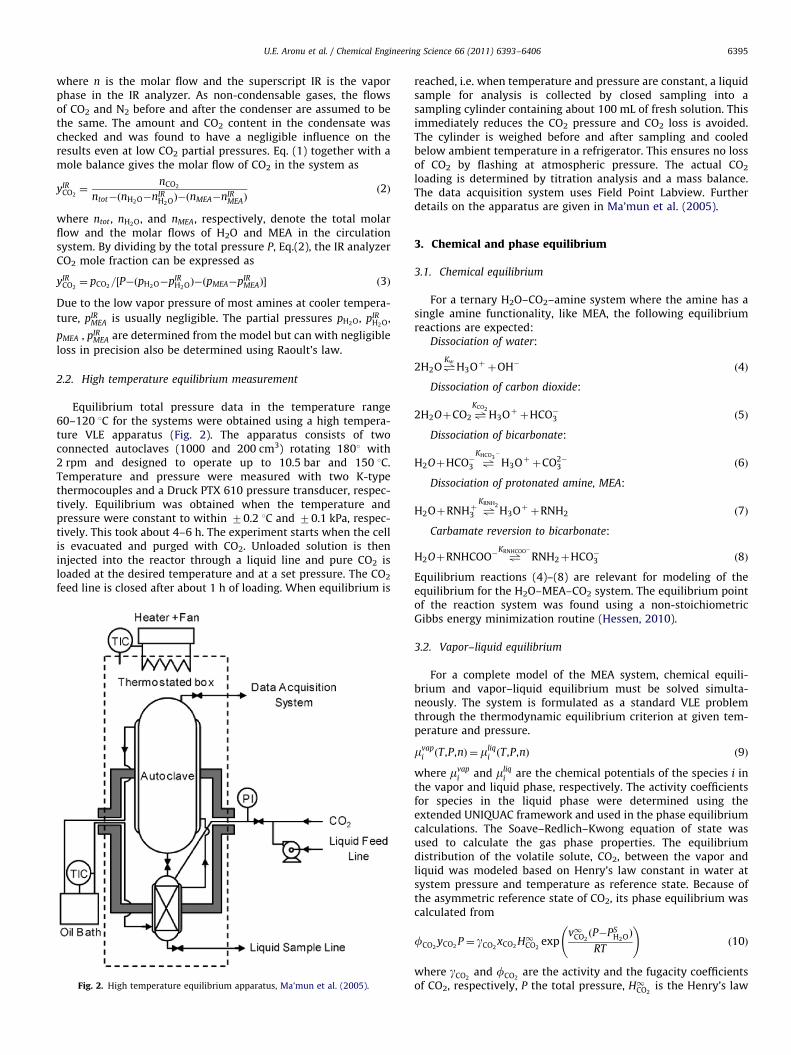
2.2. High temperature equilibrium measurement
Equilibrium total pressure data in the temperature range60–120 1C for the systems were obtained using a high tempera-ture VLE apparatus (Fig. 2). The apparatus consists of twoconnected autoclaves (1000 and 200 cm3) rotating 1801 with2 rpm and designed to operate up to 10.5 bar and 150 1C.Temperature and pressure were measured with two K-typethermocouples and a Druck PTX 610 pressure transducer, respec-tively. Equilibrium was obtained when the temperature andpressure were constant to within 70.2 1C and 70.1 kPa, respec-tively. This took about 4–6 h. The experiment starts when the cellis evacuated and purged with CO2. Unloaded solution is theninjected into the reactor through a liquid line and pure CO2 isloaded at the desired temperature and at a set pressure. The CO2
feed line is closed after about 1 h of loading. When equilibrium is
Fig. 2. High temperature equilibrium apparatus, Ma’mun et al. (2005).
reached, i.e. when temperature and pressure are constant, a liquidsample for analysis is collected by closed sampling into asampling cylinder containing about 100 mL of fresh solution. Thisimmediately reduces the CO2 pressure and CO2 loss is avoided.The cylinder is weighed before and after sampling and cooledbelow ambient temperature in a refrigerator. This ensures no lossof CO2 by flashing at atmospheric pressure. The actual CO2
loading is determined by titration analysis and a mass balance.The data acquisition system uses Field Point Labview. Furtherdetails on the apparatus are given in Ma’mun et al. (2005).
3. Chemical and phase equilibrium
3.1. Chemical equilibrium
For a ternary H2O–CO2–amine system where the amine has asingle amine functionality, like MEA, the following equilibriumreactions are expected:
Dissociation of water:
2H2O"Kw
H3Oþ þOH� ð4Þ
Dissociation of carbon dioxide:
2H2OþCO2"KCO2
H3Oþ þHCO�3 ð5Þ
Dissociation of bicarbonate:
H2OþHCO�3 "KHCO3
�
H3Oþ þCO2�3 ð6Þ
Dissociation of protonated amine, MEA:
H2OþRNHþ3 "KRNH2
H3Oþ þRNH2 ð7Þ
Carbamate reversion to bicarbonate:
H2OþRNHCOO� "KRNHCOO�
RNH2þHCO�3 ð8Þ
Equilibrium reactions (4)–(8) are relevant for modeling of theequilibrium for the H2O–MEA–CO2 system. The equilibrium pointof the reaction system was found using a non-stoichiometricGibbs energy minimization routine (Hessen, 2010).
3.2. Vapor–liquid equilibrium
For a complete model of the MEA system, chemical equili-brium and vapor–liquid equilibrium must be solved simulta-neously. The system is formulated as a standard VLE problemthrough the thermodynamic equilibrium criterion at given tem-perature and pressure.
mvapi ðT ,P,nÞ ¼ mliq
i ðT,P,nÞ ð9Þ
where mvapi and mliq
i are the chemical potentials of the species i inthe vapor and liquid phase, respectively. The activity coefficientsfor species in the liquid phase were determined using theextended UNIQUAC framework and used in the phase equilibriumcalculations. The Soave–Redlich–Kwong equation of state wasused to calculate the gas phase properties. The equilibriumdistribution of the volatile solute, CO2, between the vapor andliquid was modeled based on Henry’s law constant in water atsystem pressure and temperature as reference state. Because ofthe asymmetric reference state of CO2, its phase equilibrium wascalculated from
fCO2yCO2
P¼ gCO2xCO2
H1CO2exp
v1CO2ðP�PS
H2OÞ
RT
!ð10Þ
where gCO2and fCO2
are the activity and the fugacity coefficientsof CO2, respectively, P the total pressure, H1CO2
is the Henry’s law
U.E. Aronu et al. / Chemical Engineering Science 66 (2011) 6393–64066396
constant in water (Chen et al., 1979), v1CO2the infinite dilution
partial molar volume of CO2 (Brelvi and O’Connell, 1972) and T ðKÞis temperature. The reference states for water and amine were thepure components at system temperature and pressure. Thus thephase equilibrium was calculated from
fiyiP¼ gixiPifsi exp
viðP�Psi Þ
RT
� �ð11Þ
Here gi, fi, fsi are the activity coefficient, fugacity coefficients and
saturated vapor fugacity coefficients, respectively, while vi is thepartial molar volumes for the components (DIPPR, 2004).
The standard chemical potentials for most of the species in theCO2-amine system are not readily available in the literature.However, the equilibrium constant for the reaction j is relatedto the standard chemical potentials, mO
i , through Eq. (12)which allows for a calculation of the standard state chemicalpotentials.
RT lnKjðTÞ ¼�X
i
vijmOi ðTÞ ð12Þ
For the H2O–MEA–CO2 system there are nine species and fourreactions, hence Eq. (12) is underspecified. This was resolved bysetting four of the standard state chemical potentials to zero andthen solving for the remaining ones. This solution approach hasbeen described by Smith and Missen (1982), Solbraa (2002), andHessen et al. (2010).
3.3. Activity coefficient model
The activity coefficients for all species were calculated usingthe extended UNIQUAC thermodynamic model framework. Theoriginal non-electrolyte UNIQUAC equation by Abrams andPrausnitz (1975) was extended for electrolyte systems by addi-tion of an electrostatic term by Sanders et al. (1986) to a modifiedUNIQUAC equation. The model framework implemented in thiswork is as presented by Thomsen (1997) and Thomsen andRasmussen (1999). The model consists of three terms: a combi-natorial, entropic; a residual, enthalpic (short range terms) andthe electrostatic (long range) term of Debye–Huckel type, Eq. (13).The model requires volume, r and surface area, q parameters foreach species and adjustable binary interaction energy parameters,uki for each pair of species
gE
RT¼
gE
RT
� �Combinatorial
þgE
RT
� �Residual
þgE
RT
� �Debye�H €uckel
ð13Þ
The temperature, T ðKÞ, dependence of the interaction energyparameter (cki) of the residual term is given as
cki ¼ exp �uki�uii
T
� �ð14Þ
where
uki ¼ uOkiþuT
kiðT�298:15Þ ð15Þ
Table 2Mole fraction based temperature dependent equilibrium constants and Henry’s law co
Reaction Parameter C1 C2 C3
4 KH2 O 132.899 �13,445.90 �22.4
5 KCO2231.465 �12,092.10 �36.7
6 KHCO�3216.049 �12,431.70 �35.4
7 KMEA �4.9074 �6166.12 0
8 KMEACOO� 2.8898 �3635.09 0
HCO2170.7126 �8477.711 �21.9
3.4. Thermodynamic parameters
Thermodynamic parameters needed for each of the modelsare parameters in the activity coefficient model, equilibriumconstants and Henry’s law constant for CO2 in pure water. Theequilibrium constants are defined in terms of mole fractions, thusthey are dimensionless, while the Henry constant has the unit ofpascal. The temperature, T ðKÞ, dependencies of the equilibriumand Henry’s constant used in this work are given by
lnK or lnH ¼ C1þC2=TþC3 lnTþC4T ð16Þ
The coefficients C1–C4 are summarized in Table 2 for all reactionstogether with literature sources.
3.5. Model parameter regression
CO2 can be bound chemically by an absorbent or remain as freeCO2 (physical solubility) in an absorbent. Physical solubility of CO2 intoan absorbent at various concentrations and temperatures is necessaryin the development of kinetics and thermodynamic models for thesystem. The problem is that CO2 reacts with the absorbent. This reac-tive nature of CO2 with any absorbent does not allow direct measure-ment of the physical CO2 solubility in the solution. The physicalsolubility is thus measured indirectly using a similar non-reacting gas,N2O by an analogy, the N2O analogy. The N2O analogy was originallyproposed by Clarke (1964) and verified by Laddha et al. (1981). It givesa measure of the physical solubility of CO2 in the aqueous aminesolution. It has been applied on various amine systems; Haimour andSandall (1984), Versteeg and Van Swaaij (1988), Mandal et al. (2005),and Hartono et al. (2008). Previous works that have modeled CO2
equilibrium in aqueous MEA solutions have not incorporate experi-mentally determined physical (N2O) solubility of CO2 in MEA. The useof N2O solubility in the model calculations enables determination ofthe CO2 activity coefficient. Hessen (2010) showed results of CO2
activity coefficients calculated by refined-electrolyte–NRTL andextended UNIQUAC for N2O solubility and compared to experimentalvalues. Results from both models did not agree with experimentalresult. This work implements the Henry’s law constant of CO2 in MEA,as described by Eq. (19) as data from Hartono (2009) for solubility ofN2O into 30 mass% MEA solution at various CO2 loadings wereincluded in the parameter regression data set. Expressions for solubi-lity of CO2 and N2O in water have been correlated by Versteeg andVan Swaaij (1988) in form of Henry’s law constants; where Hw
CO2and
HwN2O are the Henry’s law constants of CO2 and N2O in water,
respectively, and T ðKÞ is temperature. The solubilities in the mixedMEA/water solvent are given as apparent Henry’s law coefficients
HwCO2¼ 2:82� 106 expð�2044=TÞ ð17Þ
HwN2O ¼ 8:55� 106 expð�2284=TÞ ð18Þ
Happ,MEACO2
¼Hw
CO2
HwN2O
Happ,MEAN2O
Happ,MEACO2
¼ gnCO2Hw
CO2ð19Þ
nstant for CO2.
C4 T (1C) Source
773 0 0–225 Edwards et al. (1978)
816 0 0–225 Edwards et al. (1978)
819 0 0–225 Edwards et al. (1978)
�0.00098482 0–50 Bates and Pinching (1951)
0 25–120 Austgen et al. (1989)
5743 0.005781 0–100 Chen et al. (1979)
U.E. Aronu et al. / Chemical Engineering Science 66 (2011) 6393–6406 6397
The model parameters that need to be evaluated are; volumeparameters, r, the surface area parameters, q, as well as theinteraction energy parameters uO
ki and uTki. The data set used for
regression of model parameters are; the experimental gas phase CO2
IR analyzer measurements, yIRCO2
expressed as CO2 partial pressures,pCO2
using Eq. (3), total pressure measurements from this work anddata for solubility of N2O into 30 mass% MEA from Hartono (2009).Regression of the e-UNIQUAC model parameters was tediousand not straight forward. The first step taken was to retain asmany literature parameters as possible from Thomsen andRasmussen (1999), Thomsen et al. (1996), and Faramarzi et al.(2009). Further, tests were carried out to identify sensitive para-meters. The sensitive parameters were grouped according to whatpressure region they affected the most i.e. low and high pressure
Table 4Equilibrium solubility of CO2 in aqueous 30 mass% MEA.
40 1C 60 1C 80 1C
pCO2
(kPa)aCO2
(mol/mol)pCO2
(kPa)aCO2
(mol/mol)pCO2
(kPa)aCO2
(mol/mol)
0.0016 0.102 0.0045 0.053 0.0056 0.017
0.0123 0.206 0.0154 0.105 0.0219 0.040
0.0246 0.250 0.0427 0.162 0.0557 0.075
0.0603 0.337 0.1348 0.244 0.1406 0.122
0.0851 0.353 0.3015 0.303 0.2485 0.155
0.1835 0.401 0.6436 0.360 0.6137 0.216
0.2928 0.417 1.0970 0.393 1.2538 0.271
0.3188 0.421 2.5014 0.428 3.7522 0.347
0.3809 0.433 13.558 0.491 7.9387 0.400
0.5702 0.447 8.3031 0.398
1.0662 0.464
1.8326 0.476
1.8278 0.477
2.3193 0.485
2.8577 0.489
8.5583 0.516
11.812 0.524
Table 3Equilibrium solubility of CO2 in aqueous 15 mass% MEA.
15% MEA
40 1C 60 1C 80 1C
pCO2 aCO2 Ptot pCO2 pCO2 model aCO2 Ptot pCO2 pCO2 m
(kPa) (mol/mol) (kPa) (kPa) (kPa) (mol/mol) (kPa) (kPa) (kPa)
0.0017 0.111 0.0042 0.048 0.0603
0.0035 0.148 0.0056 0.060 0.1315
0.0068 0.186 0.0068 0.075 0.3544
0.0170 0.220 0.0078 0.069 0.5250
0.0215 0.236 0.0094 0.098 3.6374
0.0427 0.295 0.0151 0.135 6.3092
0.0450 0.298 0.0234 0.144 138.3 101.53
0.0845 0.342 0.0417 0.175 194.7 208.89
0.2220 0.398 0.0965 0.230 288.2 248.88
0.6634 0.442 0.1462 0.253 412.5 358.88
0.7013 0.450 1.7998 0.415 495.4 455.12
4.8405 0.516 5.4090 0.480 598.5 505.15
7.8861 0.529 8.2297 0.492 689.0 539.09
16.0024 0.565 82.00 95.896 0.624 792.7 640.22
149.3 133.258 0.652 898.6 768.96
178.9 155.405 0.666
298.4 234.407 0.706
407.5 292.900 0.729
505.3 487.652 0.784
611.7 470.243 0.780
671.9 487.652 0.784
819.7 858.453 0.847
934.1 998.773 0.864
regions. Parameters that affected the low pressure region wereregressed to data with loading not greater than 0.3, while higherloading data were used to regress the parameters mainly affectingthe high pressure region. In the end all data sets were combined, andall the parameters were re-regressed simultaneously. The regressionanalysis was performed through a Levenberg–Marquardt mini-mization using the MATLAB based parameter estimation tool,Modfit (Hertzberg and Mejdell, 1998). The objective function usedis given
F ¼Xn
i ¼ 1
pexpCO2�pcalc
CO2
pexpCO2
!2
þXn
i ¼ 1
Pexptot �Pcalc
tot
Pexptot
� �2
þXn
i ¼ 1
Happ,expCO2
�Happ,calcCO2
Happ,expCO2
!2
ð20Þ
100 1C 120 1C
Ptot
(kPa)pCO2 model
(kPa)aCO2
(mol/mol)Ptot
(kPa)pCO2 model
(kPa)aCO2
(mol/mol)
103.0 14.464 0.344 214.8 38.534 0.311
130.0 42.199 0.409 254.3 81.379 0.364
170.2 79.197 0.443 351.9 228.102 0.432
174.6 114.232 0.462 469.9 374.623 0.464
254.6 181.397 0.486 556.8 429.659 0.473
308.8 272.872 0.508 662.7 529.618 0.487
338.8 277.827 0.509 691.7 578.233 0.493
407.5 361.398 0.524 767.7 630.539 0.499
525.5 478.990 0.541
100 1C 120 1C
odel aCO2 Ptot pCO2 model aCO2 Ptot pCO2 model aCO2
(mol/mol) (kPa) (kPa) (mol/mol) (kPa) (kPa) (mol/mol)
0.103 109.4 14.623 0.346 241.0 93.575 0.385
0.147 200.7 204.957 0.527 361.8 182.307 0.437
0.211 322.8 278.634 0.551 464.2 321.367 0.483
0.242 391.5 318.213 0.562 529.8 400.784 0.502
0.373 500.0 436.601 0.590 702.6 629.533 0.544
0.409 598.3 576.507 0.617 857.2 737.313 0.560
5 0.551 717.3 623.174 0.625 1050.2 929.845 0.585
1 0.605 717.6 647.446 0.629
1 0.620 799.9 697.913 0.637
2 0.654 917.5 757.845 0.646
6 0.678
0 0.689
8 0.696
9 0.715
9 0.736
U.E. Aronu et al. / Chemical Engineering Science 66 (2011) 6393–64066398
The deviations of the model results from the experimental data aregiven as absolute average relative deviations (AARD) according
AARD¼ 100%1
n
Xn
9xmodel�xexp
��xexp
ð21Þ
where x is partial pressure, total pressure or apparent Henry’s lawconstant.
4. Results and discussion
Vapor–liquid equilibrium experiment measurement results for15, 30, 45 and 60 mass% MEA are given in Tables 3–6, respec-tively, for 40–120 1C. Details of the estimated extended UNIQUACmodel volume, r and surface area, q parameters as well as thetemperature dependent interaction energy parameters uO
ki and uTki
regressed using experimentally determined CO2 partial pressures,total pressures and loadings as well as N2O solubility data ofHartono (2009) are given in Tables 7–9.
Table 6Equilibrium solubility of CO2 in aqueous 60 mass% MEA.
40 1C 60 1C 80 1C�
pCO2
(kPa)aCO2
(mol/mol)pCO2
(kPa)aCO2
(mol/mol)pCO2
(kPa)aCO2
(mol/mol)
0.0060 0.173 0.0007 0.046 0.0020 0.018
0.0127 0.242 0.0110 0.126 0.0170 0.056
0.0281 0.306 0.0341 0.172 0.0325 0.073
0.0526 0.344 0.1097 0.248 0.0777 0.124
0.1508 0.394 0.2933 0.316 0.1610 0.162
0.3824 0.427 0.8475 0.382 0.2513 0.191
0.9062 0.449 3.0267 0.424 0.5431 0.238
1.5153 0.468 8.2258 0.457 0.8699 0.264
3.7472 0.481 18.967 0.480 1.6522 0.308
12.472 0.500 3.4300 0.352
6.0947 0.387
9.0463 0.404
11.271 0.416
Table 5Equilibrium solubility of CO2 in aqueous 45 mass% MEA.
45% MEA
40 1C 60 1C 80 1C
pCO2
(kPa)aCO2
(mol/mol)Ptot
(kPa)pCO2
(kPa)pCO2 model
(kPa)aCO2
(mol/mol)Ptot
(kPa)pCO2
(kPa)pCO2 m
(kPa)
0.0035 0.141 0.0019 0.045 0.0008
0.0035 0.148 0.0059 0.087 0.0023
0.0077 0.195 0.0099 0.120 0.0056
0.0099 0.217 0.0205 0.169 0.0060
0.0123 0.234 0.0787 0.232 0.0099
0.0164 0.276 0.1284 0.269 0.0288
0.0178 0.271 0.4279 0.352 0.0529
0.0364 0.300 1.4259 0.392 0.1236
0.0598 0.354 4.6349 0.454 0.3981
0.1087 0.390 6.2928 0.460 4.5002
0.1781 0.404 8.2900 0.471 11.249
0.2787 0.428 56.3 36.099 0.503 97.0 59.190
0.9173 0.464 151.8 106.190 0.534 251.9 157.60
2.1609 0.475 322.2 264.384 0.567 342.5 279.46
5.4871 0.497 422.9 364.534 0.580 446.1 352.01
509.9 421.021 0.586 523.8 419.04
627.9 612.781 0.602 624.4 509.02
714.6 771.31 714.8 615.79
868.0 947.05 842.1 725.46
1030.4 1243.31 941.5 872.79
1039.8 1121.9
4.1. Binary H2O–MEA system
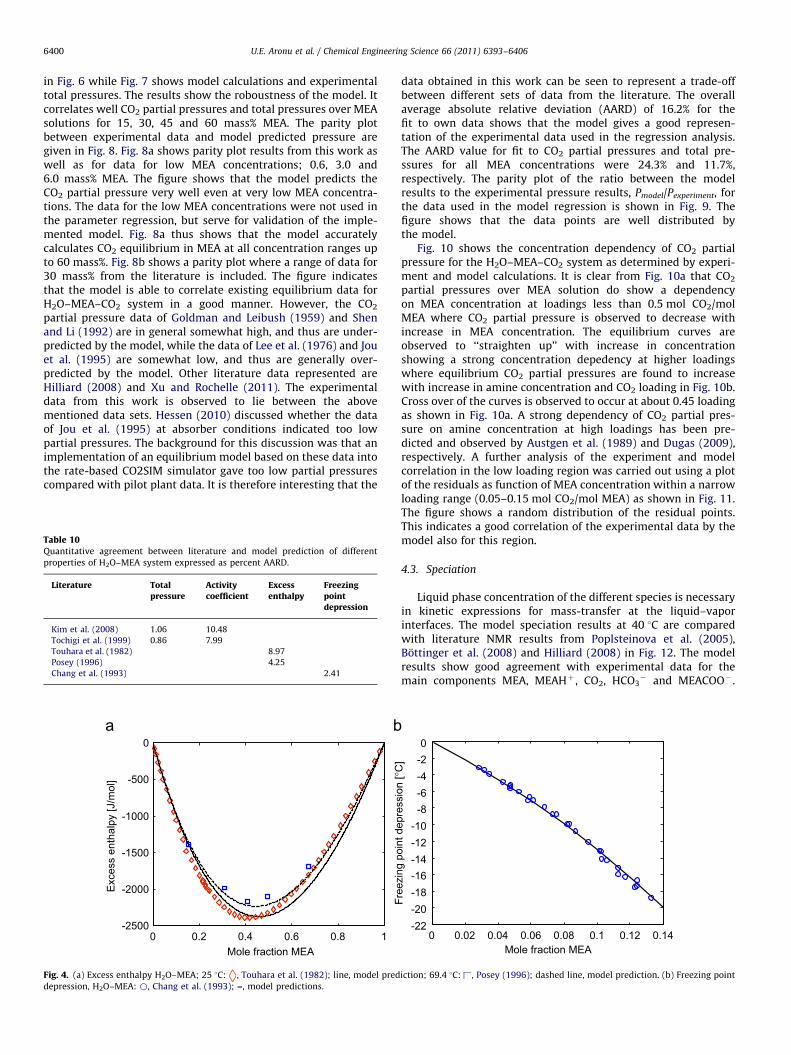
Vapor–liquid equilibrium for the binary H2O–MEA system wasnot measured in this work. However, sample model predictedresults for the binary H2O–MEA system are given as Pxy diagramsin Fig. 3a and compared with experimental results of Tochigi et al.(1999) and Belabbaci et al. (2009) while activity coefficients aregiven in Fig. 3b and compared with experimental results ofBelabbaci et al. (2009) and Kim et al. (2008). Fig. 4a shows resultsfor model prediction of excess enthalpy of MEA compared to datafrom Touhara et al. (1982) and Posey (1996). Freezing pointdepression predictions compared to data from Chang et al.(1993) are shown in Fig. 4b. These results confirm that thee-UNIQUAC implementation of this work is consistent with thework of Faramarzi et al. (2009) from which the interactionparameters for the binary H2O–MEA system were gathered.Quantitative agreement between literature and model predictionof different properties of H2O–MEA system expressed as percentAARD values are given in Table 10.
100 1C 120 1C
Ptot
(kPa)pCO2 model
(kPa)aCO2
(mol/mol)Ptot
(kPa)pCO2 model
(kPa)aCO2
(mol/mol)
106.3 30.942 0.386 196.9 77.117 0.346
204.9 78.602 0.430 306.0 185.399 0.398
308.6 126.628 0.450 412.3 306.435 0.426
414.6 226.909 0.473 537.0 395.997 0.440
518.3 279.632 0.481 700.0 551.896 0.458
618.4 438.671 0.498 963.3 845.133 0.481
705.0 529.194 0.505 1060.2 945.232 0.487
100 1C 120 1C
odel aCO2
(mol/mol)Ptot
(kPa)pCO2 model
(kPa)aCO2
(mol/mol)Ptot
(kPa)pCO2 model
(kPa)aCO2
(mol/mol)
0.017 86.6 4.708 0.270 165.1 3.560 0.145
0.027 201.7 96.884 0.445 241.5 106.177 0.374
0.038 319.4 208.127 0.479 361.5 250.646 0.426
0.025 433.3 238.500 0.485 443.7 335.793 0.443
0.061 539.0 341.539 0.501 538.7 490.925 0.465
0.086 625.4 389.847 0.507 653.1 592.662 0.476
0.109 747.2 434.768 0.512 752.2 667.434 0.483
0.135 879.5 574.312 0.525 852.7 750.925 0.490
0.236 974.6 611.783 0.528 928.9 887.076 0.500
0.389 1031.0 693.481 0.534 1039.6 979.386 0.506
0.435
0.479
4 0.512
8 0.533
2 0.542
5 0.549
9 0.557
6 0.565
6 0.572
7 0.580
6 0.591
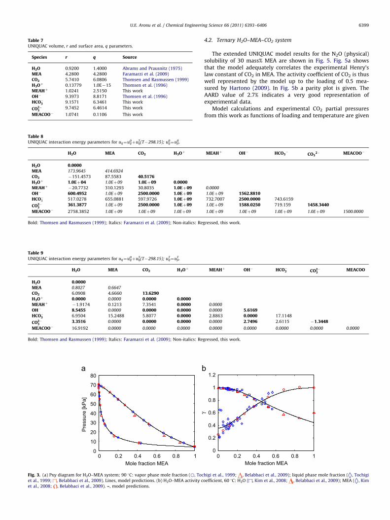
Table 8UNIQUAC interaction energy parameters for uij¼u0
ijþuTij(T�298.15); u0
ij¼u0ji.
H2O MEA CO2 H3Oþ
H2O 0.0000MEA 173.9645 414.6924
CO2 �151.4573 87.5583 40.5176H3Oþ 1.0Eþ04 1.0Eþ09 1.0Eþ09 0.0000MEAHþ �20.7732 310.1293 30.8035 1.0Eþ09OH� 600.4952 1.0Eþ09 2500.0000 1.0Eþ09HCO�3 517.0278 655.0881 597.9726 1.0Eþ09
CO2�3
361.3877 1.0Eþ09 2500.0000 1.0Eþ09
MEACOO� 2758.3852 1.0Eþ09 1.0Eþ09 1.0Eþ09
Bold: Thomsen and Rasmussen (1999); Italics: Faramarzi et al. (2009); Non-italics: Re
Table 9UNIQUAC interaction energy parameters for uij¼u0
ijþuTij(T�298.15); uT
ij¼uTji.
H2O MEA CO2 H3Oþ
H2O 0.0000MEA 0.8027 0.6647
CO2 6.0908 4.6660 13.6290H3Oþ 0.0000 0.0000 0.0000 0.0000MEAHþ �1.9174 0.1213 7.3541 0.0000OH� 8.5455 0.0000 0.0000 0.0000HCO�3 6.9504 15.2488 5.8077 0.0000
CO2�3
3.3516 0.0000 0.0000 0.0000
MEACOO� 16.9192 0.0000 0.0000 0.0000
Bold: Thomsen and Rasmussen (1999); Italics: Faramarzi et al. (2009); Non-italics: Re
Table 7UNIQUAC volume, r and surface area, q parameters.
Species r q Source
H2O 0.9200 1.4000 Abrams and Prausnitz (1975)
MEA 4.2800 4.2800 Faramarzi et al. (2009)
CO2 5.7410 6.0806 Thomsen and Rasmussen (1999)
H3Oþ 0.13779 1.0E�15 Thomsen et al. (1996)
MEAHþ 1.0241 2.5150 This work
OH� 9.3973 8.8171 Thomsen et al. (1996)
HCO�3 9.1571 6.3461 This work
CO2�3
9.7452 6.4614 This work
MEACOO� 1.0741 0.1106 This work
0 0.2 0.4 0.6 0.8 10
10
20
30
40
50
60
70
80
Mole fraction MEA
Pre
ssur
e [k
Pa]
Fig. 3. (a) Pxy diagram for H2O–MEA system; 90 1C: vapor phase mole fraction ( , Toc
et al., 1999; , Belabbaci et al., 2009). Lines, model predictions. (b) H2O–MEA activity c
et al., 2008; , Belabbaci et al., 2009). –, model predictions.
U.E. Aronu et al. / Chemical Engineering Science 66 (2011) 6393–6406 6399
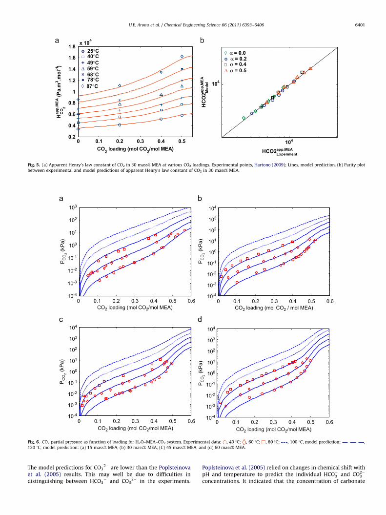
4.2. Ternary H2O–MEA–CO2 system
The extended UNIQUAC model results for the N2O (physical)solubility of 30 mass% MEA are shown in Fig. 5. Fig. 5a showsthat the model adequately correlates the experimental Henry’slaw constant of CO2 in MEA. The activity coefficient of CO2 is thuswell represented by the model up to the loading of 0.5 mea-sured by Hartono (2009). In Fig. 5b a parity plot is given. TheAARD value of 2.7% indicates a very good representation ofexperimental data.
Model calculations and experimental CO2 partial pressuresfrom this work as functions of loading and temperature are given
MEAHþ OH� HCO3�
CO32� MEACOO�
0.0000
1.0Eþ09 1562.8810732.7007 2500.0000 743.6159
1.0Eþ09 1588.0250 719.159 1458.3440
1.0Eþ09 1.0Eþ09 1.0Eþ09 1.0Eþ09 1500.0000
gressed, this work.
MEAHþ OH� HCO�3 CO2�3
MEACOO
0.0000
0.0000 5.61692.8863 0.0000 17.1148
0.0000 2.7496 2.6115 �1.3448
0.0000 0.0000 0.0000 0.0000 0.0000
gressed, this work.
0 0.2 0.4 0.6 0.8 10
0.2
0.4
0.6
0.8
1
1.2
Mole fraction MEA
γ
higi et al., 1999; , Belabbaci et al., 2009); liquid phase mole fraction ( , Tochigi
oefficient, 60 1C: H2O ( , Kim et al., 2008; , Belabbaci et al., 2009); MEA ( , Kim
U.E. Aronu et al. / Chemical Engineering Science 66 (2011) 6393–64066400
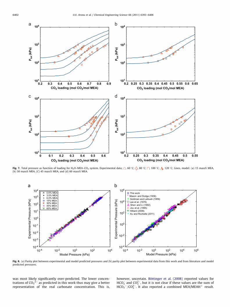
in Fig. 6 while Fig. 7 shows model calculations and experimentaltotal pressures. The results show the roboustness of the model. Itcorrelates well CO2 partial pressures and total pressures over MEAsolutions for 15, 30, 45 and 60 mass% MEA. The parity plotbetween experimental data and model predicted pressure aregiven in Fig. 8. Fig. 8a shows parity plot results from this work aswell as for data for low MEA concentrations; 0.6, 3.0 and6.0 mass% MEA. The figure shows that the model predicts theCO2 partial pressure very well even at very low MEA concentra-tions. The data for the low MEA concentrations were not used inthe parameter regression, but serve for validation of the imple-mented model. Fig. 8a thus shows that the model accuratelycalculates CO2 equilibrium in MEA at all concentration ranges upto 60 mass%. Fig. 8b shows a parity plot where a range of data for30 mass% from the literature is included. The figure indicatesthat the model is able to correlate existing equilibrium data forH2O–MEA–CO2 system in a good manner. However, the CO2
partial pressure data of Goldman and Leibush (1959) and Shenand Li (1992) are in general somewhat high, and thus are under-predicted by the model, while the data of Lee et al. (1976) and Jouet al. (1995) are somewhat low, and thus are generally over-predicted by the model. Other literature data represented areHilliard (2008) and Xu and Rochelle (2011). The experimentaldata from this work is observed to lie between the abovementioned data sets. Hessen (2010) discussed whether the dataof Jou et al. (1995) at absorber conditions indicated too lowpartial pressures. The background for this discussion was that animplementation of an equilibrium model based on these data intothe rate-based CO2SIM simulator gave too low partial pressurescompared with pilot plant data. It is therefore interesting that the
0 0.2 0.4 0.6 0.8 1-2500
-2000
-1500
-1000
-500
0
Mole fraction MEA
Exc
ess
enth
alpy
[J/m
ol]
Fig. 4. (a) Excess enthalpy H2O–MEA; 25 1C: , Touhara et al. (1982); line, model pred
depression, H2O–MEA: , Chang et al. (1993); –, model predictions.
Table 10Quantitative agreement between literature and model prediction of different
properties of H2O–MEA system expressed as percent AARD.
Literature Total
pressure
Activity
coefficient
Excess
enthalpy
Freezing
point
depression
Kim et al. (2008) 1.06 10.48
Tochigi et al. (1999) 0.86 7.99
Touhara et al. (1982) 8.97
Posey (1996) 4.25
Chang et al. (1993) 2.41
data obtained in this work can be seen to represent a trade-offbetween different sets of data from the literature. The overallaverage absolute relative deviation (AARD) of 16.2% for thefit to own data shows that the model gives a good represen-tation of the experimental data used in the regression analysis.The AARD value for fit to CO2 partial pressures and total pre-ssures for all MEA concentrations were 24.3% and 11.7%,respectively. The parity plot of the ratio between the modelresults to the experimental pressure results, Pmodel/Pexperiment, forthe data used in the model regression is shown in Fig. 9. Thefigure shows that the data points are well distributed bythe model.
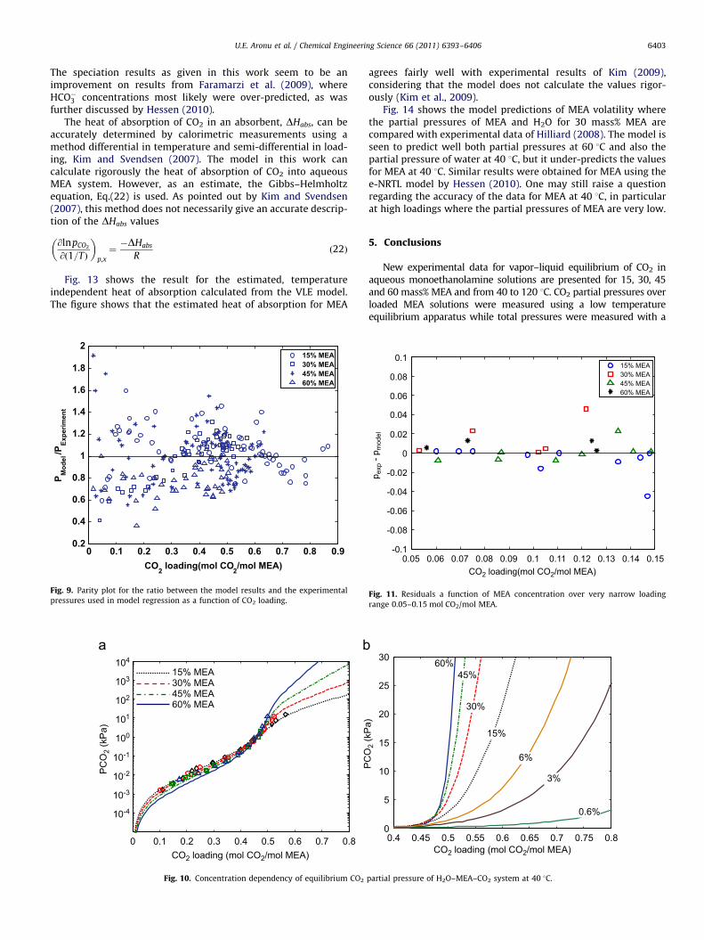
Fig. 10 shows the concentration dependency of CO2 partialpressure for the H2O–MEA–CO2 system as determined by experi-ment and model calculations. It is clear from Fig. 10a that CO2
partial pressures over MEA solution do show a dependencyon MEA concentration at loadings less than 0.5 mol CO2/molMEA where CO2 partial pressure is observed to decrease withincrease in MEA concentration. The equilibrium curves areobserved to ‘‘straighten up’’ with increase in concentrationshowing a strong concentration depedency at higher loadingswhere equilibrium CO2 partial pressures are found to increasewith increase in amine concentration and CO2 loading in Fig. 10b.Cross over of the curves is observed to occur at about 0.45 loadingas shown in Fig. 10a. A strong dependency of CO2 partial pres-sure on amine concentration at high loadings has been pre-dicted and observed by Austgen et al. (1989) and Dugas (2009),respectively. A further analysis of the experiment and modelcorrelation in the low loading region was carried out using a plotof the residuals as function of MEA concentration within a narrowloading range (0.05–0.15 mol CO2/mol MEA) as shown in Fig. 11.The figure shows a random distribution of the residual points.This indicates a good correlation of the experimental data by themodel also for this region.
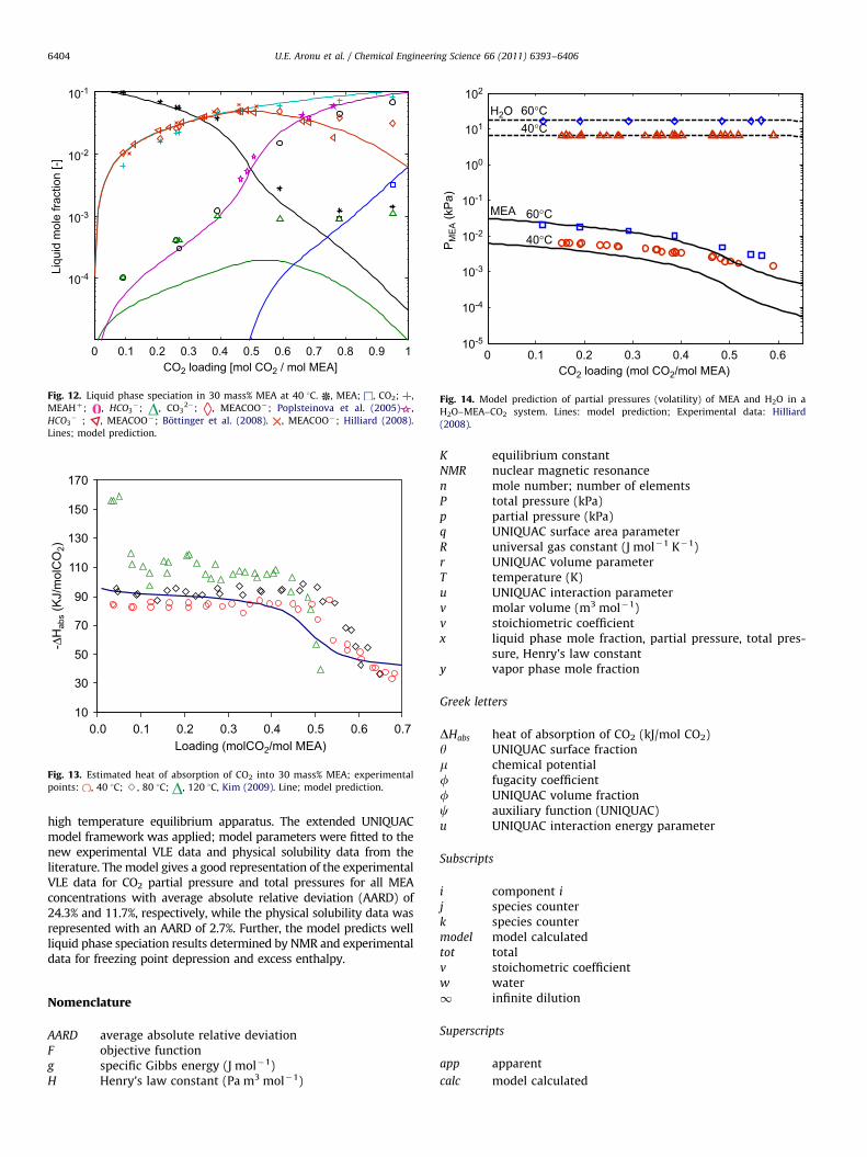
4.3. Speciation
Liquid phase concentration of the different species is necessaryin kinetic expressions for mass-transfer at the liquid–vaporinterfaces. The model speciation results at 40 1C are comparedwith literature NMR results from Poplsteinova et al. (2005),Bottinger et al. (2008) and Hilliard (2008) in Fig. 12. The modelresults show good agreement with experimental data for themain components MEA, MEAHþ , CO2, HCO3
� and MEACOO� .
0 0.02 0.04 0.06 0.08 0.1 0.12 0.14-22-20-18-16-14-12-10
-8-6-4-20
Mole fraction MEA
Free
zing
poi
nt d
epre
ssio
n [°
C]
iction; 69.4 1C: , Posey (1996); dashed line, model prediction. (b) Freezing point
0 0.1 0.2 0.3 0.4 0.5 0.610-4
10-3
10-2
10-1
100
101
102
103
CO2 loading (mol CO2/mol MEA)
PC
O2 (k
Pa)
0 0.1 0.2 0.3 0.4 0.5 0.610-4
10-3
10-2
10-1
100
101
102
103
104
CO2 loading (mol CO2/mol MEA)
PC
O2 (k
Pa)
0 0.1 0.2 0.3 0.4 0.5 0.610-4
10-3
10-2
10-1
100
101
102
103
104
CO2 loading (mol CO2/mol MEA)
PC
O2 (k
Pa)
0 0.1 0.2 0.3 0.4 0.5 0.610-4
10-3
10-2
10-1
100
101
102
103
104
CO2 loading (mol CO2 / mol MEA)
PC
O2 (k
Pa)
Fig. 6. CO2 partial pressure as function of loading for H2O–MEA–CO2 system. Experimental data; , 40 1C; , 60 1C; , 80 1C; , 100 1C, model prediction; ,
120 1C, model prediction: (a) 15 mass% MEA, (b) 30 mass% MEA, (C) 45 mass% MEA, and (d) 60 mass% MEA.
104
104
HCO2Experimentapp,MEA
HC
O2 M
odel
app,
MEA
0 0.1 0.2 0.3 0.4 0.50.2
0.4
0.6
0.8
1
1.2
1.4
1.6
1.8 x 10⁴
CO2 loading (mol CO2/mol MEA)
HC
O2
app,
MEA
(Pa.
m3 .m
ol-1)
o 25°C
+ 49°CΔ 59°C× 68°C
◊ 87°C
◊ α = 0.0o α = 0.2
Δ α = 0.5
□ 40°C
● 78°C
□ α = 0.4
Fig. 5. (a) Apparent Henry’s law constant of CO2 in 30 mass% MEA at various CO2 loadings. Experimental points, Hartono (2009); Lines, model prediction. (b) Parity plot
between experimental and model predictions of apparent Henry’s law constant of CO2 in 30 mass% MEA.
U.E. Aronu et al. / Chemical Engineering Science 66 (2011) 6393–6406 6401
The model predictions for CO32� are lower than the Poplsteinova
et al. (2005) results. This may well be due to difficulties indistinguishing between HCO3
� and CO32� in the experiments.
Poplsteinova et al. (2005) relied on changes in chemical shift withpH and temperature to predict the individual HCO�3 and CO2�
3
concentrations. It indicated that the concentration of carbonate
0.2 0.3 0.4 0.5 0.6 0.7 0.8 0.9101
102
103
104
CO2 loading (mol CO2/mol MEA)
P tot
(kPa
)
0.2 0.25 0.3 0.35 0.4 0.45 0.5 0.55 0.6 0.65101
102
103
104
CO2 loading (mol CO2/mol MEA)
P tot
(kPa
)
0.2 0.25 0.3 0.35 0.4 0.45 0.5 0.55101
102
103
104
CO2 loading (mol CO2/mol MEA)
P tot
(kPa
)
0 0.1 0.2 0.3 0.4 0.5 0.6101
102
103
104
CO2 loading (mol CO2/mol MEA)
P tot
(kPa
)
Fig. 7. Total pressure as function of loading for H2O–MEA–CO2 system. Experimental data; , 60 1C; , 80 1C; , 100 1C; , 120 1C; Lines, model: (a) 15 mass% MEA,
(b) 30 mass% MEA, (C) 45 mass% MEA, and (d) 60 mass% MEA.
10-4 10-2 100 102 10410-4
10-3
10-2
10-1
100
101
102
103
104
Exp
erim
enta
l Pre
ssur
e (k
Pa)
Model Pressure (kPa)
0.6% MEA3.0% MEA6.0% MEA15% MEA30% MEA45% MEA60% MEA
10-4 10-2 100 102 104 10610-4
10-2
100
102
104
106
Model Pressure (kPa)
Exp
erim
enta
l Pre
ssur
e (k
Pa)
o This work* Mason and Dodge (1936)+ Goldman and Leibush (1959)◊ Lee et al. (1976)Δ Shen and Li (1992) □ Jou et al. (1995)
Hilliard (2008)× Xu and Rochelle (2011)
Fig. 8. (a) Parity plot between experimental and model predicted pressures and (b) parity plot between experimental data from this work and from literature and model
predicted pressures.
U.E. Aronu et al. / Chemical Engineering Science 66 (2011) 6393–64066402
was most likely significantly over-predicted. The lower concen-trations of CO3
2� as predicted in this work thus may give a betterrepresentation of the real carbonate concentration. This is,
however, uncertain. Bottinger et al. (2008) reported values forHCO�3 and CO2�
3 , but it is not clear if these values are the sum ofHCO3
�=CO2�3 . It also reported a combined MEA/MEAHþ result.
U.E. Aronu et al. / Chemical Engineering Science 66 (2011) 6393–6406 6403
The speciation results as given in this work seem to be animprovement on results from Faramarzi et al. (2009), whereHCO�3 concentrations most likely were over-predicted, as wasfurther discussed by Hessen (2010).
The heat of absorption of CO2 in an absorbent, DHabs, can beaccurately determined by calorimetric measurements using amethod differential in temperature and semi-differential in load-ing, Kim and Svendsen (2007). The model in this work cancalculate rigorously the heat of absorption of CO2 into aqueousMEA system. However, as an estimate, the Gibbs–Helmholtzequation, Eq.(22) is used. As pointed out by Kim and Svendsen(2007), this method does not necessarily give an accurate descrip-tion of the DHabs values
@lnpCO2
@ð1=TÞ
� �p,x
¼�DHabs
Rð22Þ
Fig. 13 shows the result for the estimated, temperatureindependent heat of absorption calculated from the VLE model.The figure shows that the estimated heat of absorption for MEA
0 0.1 0.2 0.3 0.4 0.5 0.6 0.7 0.8 0.90.2
0.4
0.6
0.8
1
1.2
1.4
1.6
1.8
2
CO2 loading(mol CO2/mol MEA)
P Mod
el/P
Expe
rimen
t
15% MEA30% MEA45% MEA60% MEA
Fig. 9. Parity plot for the ratio between the model results and the experimental
pressures used in model regression as a function of CO2 loading.
0 0.1 0.2 0.3 0.4 0.5 0.6 0.7 0.8
10-4
10-3
10-2
10-1
100
101
102
103
104
PC
O2
(kP
a)
15% MEA30% MEA45% MEA60% MEA
CO2 loading (mol CO2/mol MEA)
Fig. 10. Concentration dependency of equilibrium CO2
agrees fairly well with experimental results of Kim (2009),considering that the model does not calculate the values rigor-ously (Kim et al., 2009).
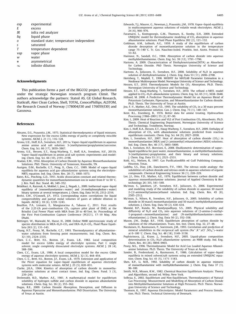
Fig. 14 shows the model predictions of MEA volatility wherethe partial pressures of MEA and H2O for 30 mass% MEA arecompared with experimental data of Hilliard (2008). The model isseen to predict well both partial pressures at 60 1C and also thepartial pressure of water at 40 1C, but it under-predicts the valuesfor MEA at 40 1C. Similar results were obtained for MEA using thee-NRTL model by Hessen (2010). One may still raise a questionregarding the accuracy of the data for MEA at 40 1C, in particularat high loadings where the partial pressures of MEA are very low.
5. Conclusions
New experimental data for vapor–liquid equilibrium of CO2 inaqueous monoethanolamine solutions are presented for 15, 30, 45and 60 mass% MEA and from 40 to 120 1C. CO2 partial pressures overloaded MEA solutions were measured using a low temperatureequilibrium apparatus while total pressures were measured with a
0.4 0.45 0.5 0.55 0.6 0.65 0.7 0.75 0.80
5
10
15
20
25
30
PC
O2
(kP
a)
6%
15%
30%
45%60%
3%
0.6%
CO2 loading (mol CO2/mol MEA)
partial pressure of H2O–MEA–CO2 system at 40 1C.
0.05 0.06 0.07 0.08 0.09 0.1 0.11 0.12 0.13 0.14 0.15-0.1
-0.08
-0.06
-0.04
-0.02
0
0.02
0.04
0.06
0.08
0.1
p exp
- p m
odel
15% MEA30% MEA45% MEA60% MEA
CO2 loading(mol CO2/mol MEA)
Fig. 11. Residuals a function of MEA concentration over very narrow loading
range 0.05–0.15 mol CO2/mol MEA.
10
30
50
70
90
110
130
150
170
0.0 0.1 0.2 0.3 0.4 0.5 0.6 0.7Loading (molCO2/mol MEA)
-ΔH
abs (
KJ/
mol
CO
2)
Fig. 13. Estimated heat of absorption of CO2 into 30 mass% MEA; experimental
points: , 40 1C; B, 80 1C; , 120 1C, Kim (2009). Line; model prediction.
0 0.1 0.2 0.3 0.4 0.5 0.610-5
10-4
10-3
10-2
10-1
100
101
102
CO2 loading (mol CO2/mol MEA)
PM
EA (k
Pa)
H2O
MEA
60°C40°C
60°C
40°C
Fig. 14. Model prediction of partial pressures (volatility) of MEA and H2O in a
H2O–MEA–CO2 system. Lines: model prediction; Experimental data: Hilliard
(2008).
0 0.1 0.2 0.3 0.4 0.5 0.6 0.7 0.8 0.9 1
10-4
10-3
10-2
10-1
Liqu
id m
ole
fract
ion
[-]
CO2 loading [mol CO2 / mol MEA]
Fig. 12. Liquid phase speciation in 30 mass% MEA at 40 1C. , MEA; , CO2; ,
MEAHþ; , HCO3�; , CO3
2�; , MEACOO�; Poplsteinova et al. (2005) ,
HCO3� ; , MEACOO�; Bottinger et al. (2008). , MEACOO�; Hilliard (2008).
Lines; model prediction.
U.E. Aronu et al. / Chemical Engineering Science 66 (2011) 6393–64066404
high temperature equilibrium apparatus. The extended UNIQUACmodel framework was applied; model parameters were fitted to thenew experimental VLE data and physical solubility data from theliterature. The model gives a good representation of the experimentalVLE data for CO2 partial pressure and total pressures for all MEAconcentrations with average absolute relative deviation (AARD) of24.3% and 11.7%, respectively, while the physical solubility data wasrepresented with an AARD of 2.7%. Further, the model predicts wellliquid phase speciation results determined by NMR and experimentaldata for freezing point depression and excess enthalpy.
Nomenclature
AARD average absolute relative deviationF objective functiong specific Gibbs energy (J mol�1)H Henry’s law constant (Pa m3 mol�1)
K equilibrium constantNMR nuclear magnetic resonancen mole number; number of elementsP total pressure (kPa)p partial pressure (kPa)q UNIQUAC surface area parameterR universal gas constant (J mol�1 K�1)r UNIQUAC volume parameterT temperature (K)u UNIQUAC interaction parameterv molar volume (m3 mol�1)v stoichiometric coefficientx liquid phase mole fraction, partial pressure, total pres-
sure, Henry’s law constanty vapor phase mole fraction
Greek letters
DHabs heat of absorption of CO2 (kJ/mol CO2)y UNIQUAC surface fractionm chemical potentialf fugacity coefficientf UNIQUAC volume fractionc auxiliary function (UNIQUAC)u UNIQUAC interaction energy parameter
Subscripts
i component i
j species counterk species countermodel model calculatedtot totalv stoichometric coefficientw water1 infinite dilution
Superscripts
app apparent
calc model calculated
U.E. Aronu et al. / Chemical Engineering Science 66 (2011) 6393–6406 6405
exp experimentalE excessIR infra red analyzerliq liquid phaseo standard state; temperature independents saturatedT temperature dependentvap vapor phasew watern asymmetrical1 infinite dilution
Acknowledgments
This publication forms a part of the BIGCO2 project, performedunder the strategic Norwegian research program Climit. Theauthors acknowledge the partners: Statoil AS, GE Global Research,Statkraft, Aker Clean Carbon, Shell, TOTAL, ConocoPhillips, ALSTOM,the Research Council of Norway (178004/I30 and 176059/I30) andGassnova.
References
Abrams, D.S., Prausnitz, J.M., 1975. Statistical thermodynamics of liquid mixtures.New expression for the excess Gibbs energy of partly or completely misciblesystems. AIChE J. 21 (1), 116–128.
Aronu, U.E., Hoff, K.A., Svendsen, H.F., 2011a. Vapor–liquid equilibrium in aqueousamine amino acid salt solution: 3-(methylamino)propylamine/sarcosine.Chem. Eng. Sci. 66 (17), 3859–3867.
Aronu, U.E., Hessen, E.T., Haug-Warberg, T., Hoff, K.A., Svendsen, H.F., 2011b.Vapor–liquid equilibrium in amino acid salt system: experiments and model-ing. Chem. Eng. Sci. 66 (10), 2191–2198.
Atadan, E.M., 1954. Absorption of Carbon Dioxide by Aqueous MonoethanolamineSolutions. PhD. Thesis. University of Tennessee, Knoxville, TN.
Austgen, D.M., Rochelle, G.T., Peng, X., Chen, C.C., 1989. Model of vapor–liquidequilibria for aqueous acid gas–alkanolamine systems using the electrolyte–NRTL equation. Ind. Eng. Chem. Res. 28 (7), 1060–1073.
Bates, R.G., Pinching, G.D., 1951. Acidic dissociation constant and related thermo-dynamic quantities for monoethanolammonium ion in water from 01 to 50 1C.J. Res. Natl. Bur. Stand. 46, 349–352.
Belabbaci, A., Razzouk, A., Mokbel, I., Jose, J., Negadi, L., 2009. Isothermal vapor–liquidequilibria of (monoethanolamineþwater) and (4-methylmorpholineþwater)binary systems at several temperatures. J. Chem. Eng. Data 54 (8), 2312–2316.
Brelvi, S.W., O’Connell, J.P., 1972. Corresponding states correlations for liquidcompressibility and partial molal volumes of gases at infinite dilution inliquids. AIChE J. 18 (6), 1239–1243.
Bouillon, P.A., Lemaire, E., Mangiaracina A., Tabasso C., 2011. First resultsof the 2.25 t/h post-combustion CO2 capture pilot plant of ENEL at theBrindisi Coal Power Plant with MEA from 20 to 40 %wt. In: Proceedings ofthe First Post-Combustion Capture Conference (PCCC1), 17–19 May, AbuDhabi.
Bottinger, W., Maiwald, M., Hasse, H., 2008. Online NMR spectroscopic study ofspecies distribution in MEA–H2O–CO2 and DEA–H2O–CO2. Fluid Phase Equili-bria 263 (2), 131–143.
Chang, H.T., Posey, M., Rochelle, G.T., 1993. Thermodynamics of alkanolamine–water solutions from freezing point measurements. Ind. Eng. Chem. Res.32 (10), 2324–2335.
Chen, C.-C., Britt, H.I., Boston, J.F., Evans, L.B., 1982. Local compositionmodel for excess Gibbs energy of electrolyte systems, Part I: singlesolvent, single completely dissociated electrolyte systems. AIChE J. 28 (4),588–596.
Chen, C.C., Evans, L.B., 1986. A local composition model for the excess Gibbsenergy of aqueous electrolyte systems. AIChE J. 32 (3), 444–454.
Chen, C.-C., Britt, H.I., Boston, J.F., Evans, L.B., 1979. Extension and application ofthe Pitzer equation for vapor–liquid equilibrium of aqueous electrolytesystems with molecular solutes. AIChE J. 25 (5), 820–831.
Clarke, J.K.A., 1964. Kinetics of absorption of carbon dioxide in monoetha-nolamine solutions at short contact times. Ind. Eng. Chem. Fund. 3 (3),239–245.
Deshmukh, R.D., Mather, A.E., 1981. A mathematical model for equilibriumsolubility of hydrogen sulfide and carbon dioxide in aqueous alkanolaminesolutions. Chem. Eng. Sci. 36 (2), 355–362.
Dugas, R.E., 2009. Carbon Dioxide Absorption, Desorption, and Diffusion inAqueous Piperazine and Monoethanolamine. PhD Dissertation. The Universityof Texas at Austin.
Edwards, T.J., Maurer, G., Newman, J., Prausnitz, J.M., 1978. Vapor–liquid equilibriain multicomponent aqueous solutions of volatile weak electrolytes. AIChE J.24 (6), 966–976.
Faramarzi, L., Kontogeorgis, G.M., Thomsen, K., Stenby, E.H., 2009. ExtendedUNIQUAC model for thermodynamic modeling of CO2 absorption in aqueousalkanolamine solutions. Fluid Phase Equilibria 282 (2), 121–132.
Goldman, A.M., Leibush, A.G., 1959. A study of the equilibrium of carbondioxide desorption of monoethanolamine solution in the temperaturerange 75–140 1C. Tr. Gos. Nauchno-Issled. Proektn. Inst. Azotn. Promsti 10,53–82.
Haimour, N., Sandall, O.C., 1984. Absorption of carbon dioxide into aqueousmethyldiethanolamine. Chem. Eng. Sci. 39 (12), 1791–1796.
Hartono, A. 2009. Characterization of Diethylenetriamine(DETA) as Absorbentfor Carbon Dioxide. PhD Thesis. Norwegian University of Science andTechnology.
Hartono, A., Juliussen, O., Svendsen, H.F., 2008. Solubility of N2O in aqueoussolution of diethylenetriamine. J. Chem. Eng. Data 53 (11), 2696–2700.
Hertzberg, T., Mejdell, T., 1998. MODFIT for MATLAB Parameter Estimation in aNonlinear Multiresponse Model. Norwegian University of Science and Technology.
Hessen, E.T.. 2010. Thermodynamic Models for CO2 Absorption. Ph.D. Thesis.Norwegian University of Science and Technology.
Hessen, E.T., Haug-Warberg, T., Svendsen, H.F., 2010. The refined e-NRTL modelapplied to CO2–H2O–alkanolamine systems. Chem. Eng. Sci. 65 (11), 3638–3648.
Hilliard, M. 2008. A Predictive Thermodynamic Model for an Aqueous Blend ofPotassium Carbonate, Piperazine, and Monoethanolamine for Carbon dioxide.Ph.D. Thesis. The University of Texas at Austin.
Jou, F.-Y., Mather, A.E., Otto, F.D., 1995. The solubility of CO2 in a 30 mass percentmonoethanolamine solution. Can. J. Chem. Eng. 73 (1), 140–147.
Kent, R.L., Eisenberg, B., 1976. Better data for amine treating. HydrocarbonProcessing (1966–2001) 55 (2), 87–90.
Kim, I., 2009. Heat of Reaction and VLE of Post Combustion CO2 Absorbents. Ph.D.Thesis. Chemical Engineering Department, Norwegian University of Scienceand Technology, Trondheim, Norway.
Kim, I., Hoff, K.A., Hessen, E.T., Haug-Warberg, T., Svendsen, H.F., 2009. Enthalpy ofabsorption of CO2 with alkanolamine solutions predicted from reactionequilibrium constants. Chem. Eng. Sci. 64 (9), 2027–2038.
Kim, I., Svendsen, H.F., 2007. Heat of absorption of carbon dioxide (CO2) inmonoethanolamine (MEA) and 2-(aminoethyl) ethanolamine (AEEA) solutions.Ind. Eng. Chem. Res. 46 (17), 5803–5809.
Kim, I., Svendsen, H.F., Borresen, E., 2008. Ebulliometric determination of vapor–liquid equilibria for pure water, monoethanolamine, n-methyldiethanolamine,3-(methylamino)-propylamine, and their binary and ternary solutions.J. Chem. Eng. Data 53 (11), 2521–2531.
Kohl, A.L., Nielsen, R., 1997. Gas Purificationfifth ed Gulf Publishing Company,Houston, Texas.
Laddha, S.S., Diaz, J.M., Danckwerts, P.V., 1981. The nitrous oxide analogy: thesolubilities of carbon dioxide and nitrous oxide in aqueous solutions of organiccompounds. Chemical Engineering Science 36 (1), 228–229.
Lee, J.I., Otto, F.D., Mather, A.E., 1976. Equilibrium between carbon dioxide andaqueous monoethanolamine solutions. Journal of Applied Chemistry & Bio-technology 26 (10), 541–549.
Ma’mun, S., Jakobsen, J.P., Svendsen, H.F., Juliussen, O., 2006. Experimentaland modeling study of the solubility of carbon dioxide in aqueous 30 mass%2-((2-aminoethyl)amino)ethanol solution. Ind. Eng. Chem. Res. 45 (8),2505–2512.
Ma’mun, S., Nilsen, R., Svendsen, H.F., Juliussen, O., 2005. Solubility of carbondioxide in 30 mass% monoethanolamine and 50 mass% methyldiethanolaminesolutions. J. Chem. Eng. Data 50 (2), 630–634.
Mandal, B.P., Kundu, M., Bandyopadhyay, S.S., 2005. Physical solubility anddiffusivity of N2O and CO2 into aqueous solutions of (2-amino-2-methyl-1-propanolþmonoethanolamine) and (N-methyldiethanolamineþmono-ethanolamine). J. Chem. Eng. Data 50 (2), 352–358.
Mason, J.W., Dodge, B.F., 1936. Equilibrium absorption of carbon dioxide bysolutions of the ethanolamines. Trans. Am. Inst. Chem. Eng. 32, 27–48.
Nicolaisen, H., Rasmussen, P., Soerensen, J.M., 1993. Correlation and prediction ofmineral solubilities in the reciprocal salt system ðNaþ ,Kþ ÞðCl� ,SOÞ4
2Þ–water
at 0–100 1C. Chem. Eng. Sci. 48 (18), 3149–3158.Poplsteinova, J.J., Krane, J., Svendsen, H.F., 2005. Liquid-phase composition
determination in CO2–H2O–alkanolamine systems: an NMR study. Ind. Eng.Chem. Res. 44 (26), 9894–9903.
Posey, M.L., 1996. Thermodynamic Model for Acid Gas Loaded Aqueous Alkanol-amine Solutions. Ph.D. Thesis. The University of Texas at Austin.
Sander, B., Fredenslund, A., Rasmussen, P., 1986. Calculation of vapor–liquidequilibria in mixed solvent/salt systems using an extended UNIQUAC equa-tion. Chem. Eng. Sci. 41 (5), 1171–1183.
Shen, K.P., Li, M.H., 1992. Solubility of carbon dioxide in aqueous mixturesof monoethanolamine with methyldiethanolamine. J. Chem. Eng. Data 37 (1),96–100.
Smith, W.R., Missen, R.W., 1982. Chemical Reaction Equilibrium Analysis: Theoryand Algorithms, second ed. Wiley, New York.
Solbraa, E., 2002. Equilibrium and Non-Equilibrium. Thermodynamics of NaturalGas Processing: Measurement and Modelling of Absorption of Carbon Dioxdeinto Methyldiethanolamine Solutions at High Pressures. Ph.D. Thesis. Norwe-gian University of Science and Technology.
Thomsen, K., 1997. Aqueous Electrolytes: Model Parameters and Process Simula-tion. Ph.D. Thesis. Technical University of Denmark.

U.E. Aronu et al. / Chemical Engineering Science 66 (2011) 6393–64066406
Thomsen, K., Rasmussen, P., 1999. Modeling of vapor–liquid–solid equilibrium ingas–aqueous electrolyte systems. Chem. Eng. Sci. 54 (12), 1787–1802.
Thomsen, K., Rasmussen, P., Gani, R., 1996. Correlation and prediction of thermalproperties and phase behavior for a class of aqueous electrolyte systems.Chem. Eng. Sci. 51 (14), 3675–3683.
Tochigi, K., Akimoto, K., Ochi, K., Liu, F., Kawase, Y., 1999. Isothermal vapor–liquidequilibria for waterþ2-aminoethanolþdimethyl sulfoxide and its constituentthree binary systems. J. Chem. Eng. Data 44 (3), 588–590.
Touhara, H., Okazaki, S., Okino, F., Tanaka, H., Ikari, K., Nakanishi, K., 1982. Thermo-dynamic properties of aqueous mixtures of hydrophilic compounds. 2. Ami-noethanol and its methyl derivatives. J. Chem. Thermodyn. 14 (2), 145–156.
Versteeg, G.F., Van Swaaij, W.P.M., 1988. Solubility and diffusivity of acid gases(carbon dioxide, nitrous oxide) in aqueous alkanolamine solutions. J. Chem.Eng. Data 33 (1), 29–34.
Xu, Q., Rochelle, G., 2011. Total pressure and CO2 solubility at high temperature inaqueous amines. Energy Procedia 4, 117–124.