SIAM J. APPL. MATH. c 1997 Society for Industrial and Applied MathematicsVol. 0, No. 0, pp. 1{100, May 1997 002SOLITARY-WAVE SOLUTIONS OF THE BENJAMIN EQUATION�JOHN P. ALBERTy JERRY L. BONAz and JUAN MARIO RESTREPO\Abstract. Considered here is a model equation put forward by Benjamin that governs ap-proximately the evolution of waves on the interface of a two- uid system in which surface tensione�ects cannot be ignored. Our principal focus is the traveling-wave solutions called solitary waves,and three aspects will be investigated. A constructive proof of the existence of these waves togetherwith a proof of their stability is developed. Continuation methods are used to generate a schemecapable of numerically approximating these solitary waves. The computer-generated approximationsreveal detailed aspects of the structure of these waves. They are symmetric about their crests, butunlike the classical Korteweg-de Vries solitary waves, they feature a �nite number of oscillations. Thederivation of the equation is also revisited to get an idea of whether or not these oscillatory wavesmight actually occur in a natural setting.Key words. Benjamin equation, solitary waves, oscillatory solitary waves, stability, continua-tion methodsAMS subject classi�cations. Primary 76B25; Secondary 35Q51, 35Q35, 65H20, 58G161 IntroductionThis paper was inspired by recent work of Benjamin ([7], [8]) concerning waves onthe interface of a two- uid system. Benjamin was concerned with an incompressiblesystem that, at rest, consists of a layer of depth h1 of light uid of density �1 boundedabove by a rigid plane and resting upon a layer of heavier uid of density �2 > �1 ofdepth h2, also resting on a rigid plane. Because of the density di�erence, waves canpropagate along the interface between the two uids. In Benjamin's theory, di�usiv-ity is ignored, but the parameters of the system are such that capillarity cannot bediscarded.Benjamin focused attention upon waves that do not vary with the coordinateperpendicular to the principal direction of propagation. The waves in question arethus assumed to propagate in only one direction, the positive x direction, say, and tohave long wavelength � and small amplitude a relative to h1. The small parameters� = ah1 and � = h1� are supposed to be of the same order of magnitude, so thatnonlinear and dispersive e�ects are balanced. Furthermore, the lower layer is assumedto be very deep relative to the upper layer, so that � = h2h1 is large.The coordinate system is chosen so that, at rest, the interface is located at z = 0.Thus, the upper bounding plane is located at z = h1 and the lower plane at z = �h2.Let �(x; t) denote the downward vertical displacement of the interface from its rest�Work supported in part by the Mathematical, Information, and Computational Sciences Di-vision subprogram of the O�ce of Computational and Technology Research, U.S. Department ofEnergy, under Contract W-31-109-Eng-38. JLB was supported by NSF and Keck Foundation grants.JMR was supported by an appointment to the Distinguished Postdoctoral Research Program spon-sored by the U.S. Department of Energy, O�ce of University and Science Education Programs, andadministered by the Oak Ridge Institute for Science and Education.yMathematics Department, University of Oklahoma Norman OK, 73019 U.S.A.(jalbert@uoknor.edu)zMathematics Department and Texas Institute for Computational and Applied Mathematics,University of Texas at Austin, Austin TX, 78712 U.S.A. (bona@math.utexas.edu)\Mathematics Department, University of California, Los AngelesLos Angeles, CA 90095 U.S.A. (restrepo@math.ucla.edu)1

2 john p. albert, jerry l. bona, and juan mario restrepoposition at the horizontal coordinate x at time t (so that positive values of � correspondto depressions of the interface). When the variables are suitably non-dimensionalized(see Section 2 below), the equation derived by Benjamin takes the form(1) �t + c0 (�x + 2r��x � �L�x � ��xxx) = 0;where the subscripts denote partial di�erentiation. The coe�cients in (1) are givenby c0 =r�2 � �1�1 ; r = 3a4h1 ;� = h1�22��1 ; � = T2g�2(�2 � �1) ;where T is the interfacial surface tension and g is the gravity constant. The operatorL = H@x is the composition of the Hilbert transform H and the spatial derivative. AFourier multiplier operator with symbol jkj, L �rst arose in the context of nonlinear,dispersive wave propagation in the studies [5] and [16] on internal waves in deep water(see also [24]).Benjamin pointed out that the functionalsF (�) = Z 1�1 12�2dx and G(�) = Z 1�1 �13r�3 � 12��L� + 12��2x� dxare constants of the motion for Eq. (1); that is, if � is a smooth solution of Eq. (1)that vanishes suitably at x = �1, then F (�) and G(�) are independent of t, beingdetermined by their initial values at t = 0, say. Note that F +G is a Hamiltonian forEq. (1).For � = 0, Eq. (1) has the form of the Korteweg-de Vries equation (KdV equationhenceforth), while for � = 0, the form is that of the Benjamin-Ono equation. In fact,the signs of the third and fourth terms on the left-hand side of Eq. (1) are such thatthe KdV-type dispersion relation arising from the fourth term competes against theBenjamin-Ono-type dispersion relation arising from the third term. To see this moreclearly, consider the linearized initial-value problem�t + c0 (�x � �L�x � ��xxx) = 0;�(x; 0) = f(x);(2)posed for x 2 R and t � 0. The formal solution of Eq. (2) is�(x; t) = 12� Z 1�1 eik(x�cB(k)t)f̂(k)dk;where f̂ denotes the Fourier transform of f and the function cB(k), known as thedispersion relation for Eq. (2), is given by(3) cB(k) = cB(k;�; �) = c0(1� �jkj+ �k2):The KdV dispersion term �k2 and the Benjamin-Ono dispersion term �jkj haveopposite signs in Eq. (3), and are comparable in size when jkj is near km = �=2�, thevalue of jkj at which cB takes its minimum cm = c0(1 � �2=4�). Figure 1 shows thebehavior of cB(k) near k = 0 for various values of � when � = 2 and c0 = 1.Notice that the dispersion relation has a discontinuous �rst derivative at k = 0for � > 0, and that the value of cm will be positive as long as �2=4� < 1. According

solitary-wave solutions of the benjamin equation 33

2.5

2

1.5

1

0.5

alpha

0

2

1.5

1

0.5

0

k0

1

0.5

0

-0.5

-1Figure 1. Dispersion relation cB(k;�;�) with � = 2:0.to Benjamin's commentary, Eq. (1) should be physically relevant when �2=4� is com-parable in size to �, so that (c0 � cm)=c0 is comparable to �, and km is comparableto �=� which is of order 1. It follows that for values of k near km the contributions ofthe KdV and Benjamin-Ono terms to the dispersion relation are of similar magnitudeand are oppositely directed. The question of the relative sizes of these two dispersiveterms will be discussed at more length in Section 2.In this paper, attention is focused on solitary-wave solutions of Eq. (1), which aresolutions of the form �(x; t) = �(x � c0(1�C)t);where �(X) and its derivatives tend to zero as the variable X = x � c0(1 � C)tapproaches �1. The dimensionless variable C represents the relative decrease in thespeed of the solitary wave from the speed c0 of very long-wavelength solutions of thelinearized Eq. (2). Substituting this form for � into Eq. (1) and integrating once withrespect to X yields the equationC�� �L�� ��00 + r�2 = 0;which, after transforming the dependent variable to(4) �(X) = �rC � r �CX! ;

4 john p. albert, jerry l. bona, and juan mario restrepocan be rewritten as(5) Q(�; ) � �� 2 L�� �00 � �2 = 0;where = �2p�C :Thus, possible solitary-wave solutions of Eq. (1) are solutions of the family of equationsEq. (5), indexed by the parameter . Since the assumptions underlying the derivationof Eq. (1) imply that C is a small number, of size comparable to (c0 � cm)=c0 �� � �2=4�, it follows that in the regime of physical parameters for which Benjamin'sequation is relevant, should be an order-one quantity.The questions of existence, asymptotics, and stability of solitary-wave solutionsof (1) were studied by Benjamin in [7] and [8]. Using the degree-theoretic approachof [9], he showed that for each value of in the range [0; 1), Eq. (5) has a solution� = � which is an even function of X with� (0) = maxX2R� (X) > 0:Notice that, according to the transformation in Eq. (4), such a � corresponds to awave motion for which the interface is de ected upwards at the point of maximumde ection. In this respect, the solitary-wave solutions of Eq. (5) di�er from Benjamin-Ono-type solitary waves, which in the uid system considered here would correspondto downward de ections of the interface. Also, the condition 0 < < 1 means that thedimensional wave speed of the solitary wave lies in the range �1 < c0(1� C) < cm.In particular, values of near zero correspond to large negative wave speeds, and thusto solutions of questionable physical relevance.Benjamin also provided some formal asymptotics suggesting that, for each �xedvalue of , there is a bounded range of values ofX in which the solitary wave � (X) willoscillate between positive and negative values, and that outside this bounded region,j� (X)j should decay monotonically like 1=jXj2. Finally, he sketched a perturbation-theoretic approach to a proof of existence of a branch of solutions of Eq. (5), de�nedfor near 0, which correspond to stable solutions of the initial-value problem forEq. (1).The plan of this paper is as follows. In Section 2 we determine more precisely therange of parameters for which Eq. (1) is a good approximation to the more generalequations from which it was derived. This aspect bears crucially on whether thesewaves are realizable in the laboratory or can be expected to occur in nature. InSection 3, we present a complete theory of existence and stability of solitary-wavesolutions corresponding to values of near 0; in fact this result will appear as aspecial case of a general result on perturbations of solitary-wave solutions of nonlineardispersive wave equations. Our argument is based on the Implicit Function Theorem,and yields an analytic dependence of solitary waves on the parameter . Section 4 isdevoted to explaining an algorithm for the approximation of solitary-wave solutions.The algorithm is a continuation method based on the Contraction Mapping Principlethat underlies the proof of existence made via the Implicit Function Theorem. Wethen present some numerical approximations of solitary-wave solutions of Benjamin'sequation using a computer code based on this algorithm. The output graphicallyreveals aspects of the structure of the solitary-wave solutions of Eq. (1). The paperconcludes with a summary and further discussion in Section 5.

solitary-wave solutions of the benjamin equation 52 Physical Regime of Validity of Benjamin's EquationIn this section we examine the conditions under which the dispersion relationappearing in Benjamin's equation is a valid approximation to the dispersion relationinduced by a more general system of equations for internal waves in a two- uid system.Some general conclusions are drawn as to the types of uids and con�gurations forwhich Benjamin's equation may be relevant as a model, and for which solitary wavesof the type considered in Sections 3 and 4 below might be observed.Consider two incompressible uids, each of constant density, contained betweenrigid horizontal planes, with the lighter of the two uids resting in a layer of nearlyuniform depth atop a layer of the heavier uid, also nearly uniform in depth. Ideally,the uids are non-dissipative, but for real uids we require that the Reynolds num-ber induced by the dynamics under consideration be large. We also ignore possibledi�usive e�ects across the interface that would lead to nonhomogeneous layers. It isassumed that the balance of pressure on either side of the interface is proportionalto the curvature of the interface. The only external force acting upon the system isthat of gravity. The ow is assumed to be irrotational (within each of the layers of uid) and is two-dimensional in the sense that the ow variables depend only on ahorizontal coordinate x, the vertical coordinate z, and the time variable t.The equations that govern the dynamics of the two- uid system just describedare well known (see [19] and references contained therein). In the interior of each uidlayer, the laws of conservation of mass and momentum imply the equations�ixx + �izz = 0 (i = 1; 2)and �i ��it + 12(�ix)2 + 12(�iz)2 + gz� = �pi (i = 1; 2):Here g is the gravitational acceleration; i = 1 connotes the upper layer and i = 2the lower layer; and the uid variables within each layer are the velocity potentials�i(x; z; t), the pressures pi(x; z; t), and the densities �i. The boundary planes, whichare located at z = h1 and z = �h2, are rigid and impermeable, so that�1z = 0 at z = h1and �2z = 0 at z = �h2.At the interface z = �(x; t) (which is located at z = 0 when the system is undisturbed),one has the kinematic conditions�t � �iz + �ix�x = 0 (i = 1; 2)and p2 � p1 = �T�xx;where T denotes the interfacial surface tension. In the latter equation, �xx is a goodapproximation to the curvature of the interface provided the slope �x is small.As in Section 1, we assume that � = a=h1 and � = h1=� are small, where a is atypical amplitude and � a typical wavelength of the interfacial waves being modeled.To make explicit the e�ects of this assumption, we non-dimensionalize the variablesin the above equations, so that the rescaled variables and their derivatives have values

6 john p. albert, jerry l. bona, and juan mario restrepoon the order of unity, and small terms will be identi�ed by the presence of factors of� or �. The rescaled independent variables (marked by tildes) are~x = x�; ~t = vt� ; ~z1 = zh1 ; ~z2 = zh2 ;where v denotes pgh1 and z is rescaled to ~z1 at points above the interface and to ~z2at points below the interface. The dependent variables are rescaled as~pi = pi�2v2 ; ~� = �a; ~�i = v�ig�a :In the non-dimensionalized variables (from which the tildes will henceforth bedropped for ease of reading), the equations of motion may be written as�2�1xx + �1z1z1 = 0 for z1 > ��;�2�2�2xx + �2z2z2 = 0 for z2 < ��=�;��1t + 12�2�21x + 12 �2�2�21z1 + z1 = �(1 + � )p1 for z1 > ��;��2t + 12�2�22x + 12 �2�2�2�22z2 + �z2 = �p2 for z2 < ��=�;�t + ��1x�x � 1�2�1z1 = 0 at z1 = ��;�t + ��2x�x � 1�2� �2z2 = 0 at z2 = ��=�;�(1 + � )(p2 � p1) + ����xx = 0 at z1 = �� and z2 = ��=�;�1z1 = 0 at z1 = 1;�2z2 = 0 at z2 = �1;where � = h2=h1, and � and � are dimensionless quantities de�ned by� = T(�2 � �1)g�2and � = (�2=�1) � 1:Note that � and � represent the only in uence of the physical properties of the uidson the system. (Since �2 > �1, both � and � must be positive.)If the preceding system is linearized by omitting terms of higher order in �, theresulting equations will have sinusoidal solutions of the form�i(x; zi; t) = Ai(k; zi)eik(x�ct) (i = 1; 2);pi(x; zi; t) = Bi(k; zi)eik(x�ct) (i = 1; 2);�(x; t) = C(k)eik(x�ct);where k is an arbitrary real number. The linearized equations determine not only theforms of the functions Ai, Bi, and C, but also the dispersion relationc2(k) = � (1 + k2�)(1 + � )�k coth(��k) + �k coth(�k) :

solitary-wave solutions of the benjamin equation 7To obtain conditions for the validity of Benjamin's equation, we now determine whenthe function c(k) may be approximated by a function of the form appearing in Eq. (3)above.When � � �� is large enough that coth(�) � 1, and jkj is not too small, thefunction c2(k) is approximately equal to(7) c2a(k) = � (1 + k2�)(1 + � )�jkj+ �k coth(�k) :An expansion of the right-hand side of Eq. (7) with respect to the small parameter �yieldsca(k) = p� �1 + �k2�1=2 �1� 12(1 + � )jkj�+�38(1 + � )2 � 16� k2�2 + O(�3)� :The approximation which results in the Benjamin equation now proceeds on the as-sumption that � is small. Indeed, � and � are related to the parameters � and �introduced in Section 1 by� = �(1 + � )2 and � = �2 ;and therefore, if � is not too large, Benjamin's assumption that �2=4� = O(�) corre-sponds to the assumption that � = O(�). For the moment, however, we simply treat� as a small parameter without comparing its size to that of �. Then an expansion ofca(k) through quadratic order in both � and � yields the expressionca(k) = p� �1� 12(1 + � )jkj�+ 12k2� +�38(1 + � )2 � 16� k2�2(8) �14(1 + � )k2jkj�� � 18k4�2 +O(�3; �2�; ��2; �3)� :(A minor error in Eq. (2.2) of [7] has been corrected here.)In the present scaling, the wavenumbers k of interest will have absolute valueson the order of unity. Therefore the terms on the right-hand side of Eq. (8) can beordered according to the size of the numbers (1 + � )� and �. One way to arrive at anapproximate dispersion relation of the form appearing in Eq. (3) is to assume that(9) (1 + � )2�2 � �:Then, to �rst order in (1 + � )�, the function ca(k) can be approximated bycb(k) = p� �1� 12(1 + � )jkj�+ 12k2�� ;which is the same form as that obtained by Benjamin.To verify the validity of the above formal arguments, and to obtain an idea of thesizes of the error terms in the approximations, the relative errorcb(k)� c(k)c(k)was plotted against k for various values of the parameters �, �, � and � . A typicalplot is shown in Figure 2a, where k and � vary over the ranges �1 � k � 1 and0 � � � 1:25, while � = 100, � = 0:5, and � = 0:05 are held constant. The relative

8 john p. albert, jerry l. bona, and juan mario restrepoerror is small for small values of �, and stays below 10% even for values of � up tounity. The ridge down the middle of the surface, which persists up to the point where� = 0 and k = 0, is due to the error of replacing coth(�k) by sgn k, which was madein passing from c(k) to the approximation ca(k) in Eq. (7). Here � = 5, and coth(�k)will not be close to sgn k for jkj less than about 0:5; yet the overall approximationremains accurate. As can be seen from Figure 2b, even reducing � to � = 1:5 onlyslightly magni�es the error. In Figure 2c, � varies over the range 0 � � � 0:5 while� = 0:01, � = 0:5, and � = 5 are held constant. Comparison with Figure 2a showsthat the relative error is more sensitive to � than it is to �, although it is within areasonable range for � between 0 and 0.25. Finally, Figure 2d (in which � = 100,� = 0:01, and � = 0:05 are held constant) shows that the relative error increases onlyslowly with � in the range 0 � � � 1 and beyond. In general, cb(k) will be a goodapproximation to c(k) over the range jkj � 1 provided � and � are small, � is not toosmall, and � is not too large. When � � 5 and � � 0:5, for example, the relative errorof the approximation is less than 1% for 0 � � � 0:5 and 0 � � � 0:25.The computations just described show that condition (9) is not necessary for thevalidity of Benjamin's approximation to the dispersion relation. However, when (9) isviolated, � is small enough that the contribution of the term 12k2� to the right-handside of cb(k) is no more signi�cant than the contribution of the O((1 + � )2�2) termin Eq. (8), so that the Benjamin dispersion relation is no better an approximation ofc(k) than is the Benjamin-Ono dispersion relationcBO(k) = p� �1� 12(1 + � )jkj�� :Furthermore, if (9) is violated, then the solitary-wave parameter = �2p�C = (1 + � )�p8�Cwill not be less than 1 unless C is on the order of unity or greater. The condition < 1 is necessary for the existence of the solitary waves studied below in Sections3 and 4. But, as mentioned in Section 1, solitary-wave solutions of physical interestshould correspond to values of C on the order of �, or in other words to values of Cmuch less than unity. Therefore (9) is a necessary condition for the physical relevanceof the solitary-wave solutions considered in Sections 3 and 4.To summarize the foregoing, cb is a good approximation to c when � � �0 � 2,� � �0 � 5, � � 1, and � � 1. Furthermore, if solitary waves of the type studiedbelow in Sections 3 and 4 are to exist and be consistent with the assumptions madein deriving the Benjamin equation, then condition (9) should also be satis�ed.The requirement that � � 1 means that h1=� � 1. In a laboratory settingthis could be achieved either by making the upper layer very thin or by creatingwaves with long length scales. If h1 is small, however, then the Reynolds numberR = vh1=� (in which v = pgh1 and � is a measure of a mechanism such as dynamicviscosity which attenuates the waves) will not be large. Hence attenuation will play asigni�cant role in the dynamics of the system, and the inviscid equation (1) will notbe an accurate model even on short time scales. Thus in a laboratory experiment fortesting the predictions of Eq. (1), the upper layer should not be made extremely thin,and disturbances with long wavelengths relative to the upper layer should be created.On the other hand, the requirements that � � 1 and � = �� � �0 combine to implythat h2h1 � �0=�� 1, so that the lower layer will have to be fairly deep.

solitary-wave solutions of the benjamin equation 90

0.08

0.06

0.04

0.02

0

k0

1

0.5

0

-0.5

-1

sigma

0

1.2

1

0.8

0.6

0.4

0.2

00

0.1

0.08

0.06

0.04

0.02

0

k0

1

0.5

0

-0.5

-1

sigma

0

1.2

1

0.8

0.6

0.4

0.2

0

0

0.05

0

-0.05

-0.1

-0.15

k0

1

0.5

0

-0.5

-1

mu

0

0.5

0.4

0.3

0.2

0.1

0

0

0.02

0.015

0.01

0.005

0

-0.005

-0.01

k0

1

0.5

0

-0.5

-1

tau

0

3

2.5

2

1.5

1

0.5

0Figure 2. The relative error cb�cc , for (a) � = 0:05, � = 0:5, � = 5; (b) � = 0:05, � = 0:5,� = 1:5; (c) � = 0:01, � = 0:5, � = 5; (d) � = 0:05, � = 0:01, � = 5.The requirement � � 1, or in other words,T(�2 � �1)g�2 � 1;is satis�ed in any con�guration of two uids if the waves under consideration are longenough so that � is su�ciently large. The requirement in condition (9), on the otherhand, strongly restricts the allowable con�gurations of the system. Writing (9) ash1 � ��1�2�s Tg(�2 � �1) ;we see that if the condition is to be satis�ed for uid depths h1 that are not too smallthen the density di�erence �2 � �1 must be small and the interfacial surface tensionT must be large. If for example T = 80 dyne/cm and h1 is to be greater than 1 cm,

10 john p. albert, jerry l. bona, and juan mario restrepothen (9) will hold only if �2 � �1 is signi�cantly less than 0:08.3 Existence and Stability of Solitary-Wave SolutionsAt issue in this section is the mathematical question of existence of solitary-wavesolutions �(x; t) = �(x � c0(1 � C)t) of Eq. (1) for small values of the parameter = �=(2p�C). If these waves exist, their physical relevance comes into question,and thus their stability is also within the purview of an initial inquiry. For = 0,existence is provided by the exact formula�(x; t) = �3Cr sech2 "12sC� (x� c0(1�C)t)# ;and stability was settled a�rmatively some time ago (see [3], [6], [11]). In [8], Ben-jamin presented a degree-theoretic proof of existence of solitary waves correspond-ing to all values of in the range 0 � < 1 (An alternative proof based on theConcentrated-Compactness Principle has been worked out in [15]). Benjamin alsooutlined an argument, based on the Implicit Function Theorem for proving existenceof solitary waves when is small. The aim of this section is to complete and generalizethe latter argument. Although limited to the case of small , it has several advantagesover the degree-theoretic approach. First, it is constructive in nature, and leads nat-urally to the method used below in Section 4 to compute solitary waves numericallyfor all values of in [0; 1). Secondly, the arguments used here yield not only theexistence of a branch of solitary waves for an interval of positive values of , but alsothe continuity and in fact the analyticity of this branch with respect to . This inturn makes it possible to establish such properties as the stability of the solitary waveswith regard to small perturbations of the wave pro�le, when considered as solutionsof the time-dependent equation. In what follows, let Hr(R) be the Sobolev space offunctions q which satisfykqk2r = ZR(1 + k2)rjbq(k)j2 dk <1:For any pair of Banach spaces X and Y , let B(X;Y ) be the space of bounded operatorsfrom X to Y with the operator norm.Consider a general class of equations of the form(10) ut + (f(u) + lg(u))x � (M + lS)ux = 0;where f : R! R, g : R! R, and M and S are Fourier multiplier operators de�nedby dMv(k) = �(k)bv(k)and cSv(k) = �(k)bv(k):We make the following assumptions.(A1) The functions �(k) and �(k) are measurable and even, and �(k) is non-negative.(A2) There exists a number s � 0 and positive constants B1, B2, and B3 suchthat, for all su�ciently large values of k, B1jkjs � �(k) � B2jkjs and j�(k)j �B3jkjs.(A3) The functions f and g are smooth, and f(0) = g(0) = 0.

solitary-wave solutions of the benjamin equation 11A solitary-wave solution of Eq. (10) is a solution of the form �u(x; t) = �(x�Ct),where C > 0 is the wave speed and � is a localized function, which is to say that�(y) ! 0 as y ! �1 at least at an algebraic rate. We say that such a solution is(orbitally) stable, with respect to a given norm, if the distance between a solutionu(x; t) of Eq. (10) and the orbit f�u(�; t) : t � 0g remains arbitrarily small in norm forall time, provided only that u(x; 0) is close enough in norm to �u(x; 0).The present-day theory of stability of solitary waves dates back to the paper ofBenjamin [6] as corrected in [11], and has undergone considerable development sincethen (cf. [3], [13], [18], [27]). Here we employ the criterion for stability set forth in[13]. De�ne the operator L : L2(R)! L2(R) by(11) L = C +M + lS � f 0(�) � lg0(�);where C, f 0(�), and g0(�), are viewed as multiplication operators. According toTheorem 4.1 and the proof of Lemma 5.1 of [13], the solitary wave �u(x; t) = �(x�Ct)will be stable with respect to the Hs=2-Sobolev norm provided that the following twoconditions on L are met:(C1) when viewed as an operator on L2(R) with domainHs, L is self-adjoint, withone simple negative eigenvalue, a simple eigenvalue at zero, and no other partof its spectrum on the non-positive real axis, and(C2) there exists � 2 L2(R) such that L(�) = � and R1�1 �(x)�(x) dx < 0.We now make a �nal assumption about Eq. (10).(A4) For l = 0, Eq. (10) has a solitary-wave solution u(x; t) = �0(x �Ct), whereC > 0 and �0(x) is a smooth, even function which belongs, together with allits derivatives, to the space L2(R). Moreover, the operator L0 associated to�0 via Eq. (11) satis�es conditions (C1) and (C2) above.It will now be shown that assumptions (A1) through (A4) imply the existenceof an analytic map l 7! �l, de�ned for l in a neighborhood of l = 0 and takingvalues in L2(R), such that for each l, the function u(x; t) = �l(x � Ct) is a stable,solitary-wave solution of Eq. (10). The proof of this assertion proceeds via the ImplicitFunction Theorem and relies on the classical perturbation theory of linear operatorsas expounded in Kato's book [21]. It is straightforward in outline, but not all thedetails are simple.For r > 0, let Hre denote the closed subspace of all even functions inHr(R). Fromassumption (A2) it follows that there exist positive constants l1, B4 and B5 such thatfor all l 2 (�l1; l1) and for jkj su�ciently large, one has(12) B4(1 + k2)s=2 � C + �(k) + l�(k) � B5(1 + k2)s=2:In consequence, the function C + �(k) + l�(k) de�nes a multiplication operator M onthe space fbq : q 2 H1eg whose maximal domain is the space fbq : q 2 H1+se g. Sincemaximal multiplication operators are self-adjoint, and the operator C +M + lS isunitarily equivalent to M via the Fourier transform, then C +M + lS is self-adjointon H1e with domainH1+se . It is straightforward to adduce that for small enough l, thespectrum of the operator M, and hence the operator C +M + lS, is a subset of aninterval of the form [b;+1), b > 0, and is comprised of continuous spectrum.Let � denote any function in H1e , and de�ne the multiplication operator Q on H1eby Q = (f 0(�) + lg0(�)) . Since f 0(�) 2 H1e , g0(�) 2 H1e , and H1e is an algebra, itfollows that Q is a bounded operator on H1e . Hence, by Theorem V{4.3 of [21], the

12 john p. albert, jerry l. bona, and juan mario restrepooperator C +M + lS � Q is self-adjoint on H1e with domain H1+se . Moreover, Q isrelatively compact with respect to C +M + lS (this may be veri�ed, for example, byusing the argument in the proof of Lemma 3.17 of [4] together with the fact thatZjxj�R jf 0(�) + lg0(�)j2 dx and Zjxj�R j((f 0(�))0 + lg0(�))0j2 dxtend to zero as R ! 1). Hence, as in Theorem V{5.7 of [21], it follows that thespectrum of L consists of a continuous spectrum, identical to that of C +M + lS,together with a �nite number of real eigenvalues of �nite multiplicity.Let I = (�l1; l1), and de�ne a map F : I �H1+se ! H1e byF (l; �) = (C +M + lS)(�) � f(�) � lg(�):A calculation shows that the Fr�echet derivative F� = �F�� exists on I � H1+se and isde�ned as a map from I �H1+se to B(H1+se ;H1e ) byF�(l; �) = C +M + lS � Q:From hypothesis (A4), it follows that F (0;�0) = 0 and that the operator L0 =F�(0;�0) has a one-dimensional nullspace N in L2(R). Upon substituting u(x; t) =�0(x � Ct) in Eq. (10) and di�erentiating once with respect to x, one �nds thatL0(�00) = 0, whence �00 2 N . Since �00 is odd, it is not a member of H1+se , and itfollows that L0 : H1+se ! H1e is invertible. Finally, since L and M map H1+se intoH1e boundedly and the maps � 7! f(�) + lg(�) and � 7! f 0(�) + lg0(�) are continuousmaps from H1e into itself, then F and F� are continuous maps from I � H1+se intotheir respective target spaces H1e and B(H1+se ;H1e ). Hence all the conditions of theImplicit Function Theorem (see [17], Theorem 15.1) are met, and it may be concludedthat there exist a number l2 > 0 and a continuous map l 7! �l from (�l2; l2) to H1+sesuch that F (l;�l) = 0 for all l 2 (�l2; l2). Indeed, since F (l;�) depends analyticallyon l, the map l 7! �l is analytic as well.The existence of the desired family of solitary-wave solutions of Eq. (10) has nowbeen demonstrated, and it remains to prove that these solitary waves are stable, atleast when l is su�ciently near zero. Consider the mapl 7! Ll = F�(l;�l);which is de�ned on the interval (�l2; l2) and takes values in the space C of closedoperators on L2(R). For l, l0 in (�l2; l2), it follows from Eq. (12) thatk(C +M + lS)�1�(C +M + l0S)�1kB(L2;L2) =supk2Rj(C + �(k) + l�(k))�1 � (C + �(k) + l0�(k))�1j� jl � l0j supk2R�(B5=l1)(1 + k2)s=2B4(1 + k2)s � :Hence (C +M + lS)�1 tends to (C+M + l0S)�1 in the norm of the space of boundedoperators on L2(R) as l approaches l0. Therefore, by Theorems IV{2.14 and IV{2.20of [21], Ll varies continuously with l in the topology of generalized convergence onC. Hence the results of section IV{4 of [21] imply that the eigenvalues of Ll dependcontinuously on l. In particular, since the function �0l is an eigenfunction of Ll witheigenvalue 0, one obtains that the condition (C1) holds for all l su�ciently near zero.Also, for these values of l, 0 is not an eigenvalue of Ll in H1e , and therefore by Theorem

solitary-wave solutions of the benjamin equation 13IV{2.25 of [21], the operator L�1l varies continuously with l in B(L2e; L2e). Hence themap l 7! L�1l (�l) is a continuous L2e-valued map for l in some neighborhood of zero,and so the condition (C2) holds for these values of l. This is enough to conclude, bythe theory put forward in [13], that the corresponding solitary waves �l are stable.To apply the above theory to the Benjamin equation, �rst make the change ofvariables u(x; t) = �(x� t;�t=c0), reducing Eq. (1) tout � 2ruux + �Lux + �uxxx = 0;which has the form of Eq. (10) with f(u) = �ru2, g(u) = 0, �(k) = �k2, �(k) = �jkj,and l = �. Assumptions (A1) through (A3) clearly hold in this case; and assumption(A4) becomes a well-known property of the Schr�odinger operator associated with theKdV-solitary wave (see [23]). Hence, from the general result just expounded, it followsthat for every C > 0 there exists a number �0 = �0(C) such that, for all � 2 (��0; �0),the above equation has a stable solitary-wave solution u(x; t) = �(x � Ct). Then�(x; t) = �(x � c0(1 � C)t) is a stable solitary-wave solution to Eq. (1). In fact,using the transformation in Eq. (4) one sees easily that the properties of existenceand stability of solitary-wave solutions of Eq. (1) depend only on = �=2p�C, inthe sense that if �1=2p�1C = �2=2p�2C, then the pro�le function �1 of a stablesolitary-wave solution corresponding to �1, �1, C1 is transformed via1C1�1(r �1C1X) = 1C2�2(r �2C2X)into the pro�le function �2 of a stable solitary-wave solution corresponding to �2, �2,C2. Hence the number �0 de�ned above can be taken as �0 = 2 0p�C, where 0 isindependent of C.It is also known (see [1], [10]) that assumptions (A1) through (A4) are valid ifone takes �(k) = jkj (so that Eq. (10) with l = 0 is the Benjamin-Ono equation) or if�(k) = k coth kh� (1=h), where h > 0 (in which case Eq. (10) with l = 0 is known asthe Intermediate Long-Wave equation). Therefore the above theory applies, and onemay conclude that existence and stability of solitary waves persists for perturbationsof these equations as well.4 Numerical Approximation of Solitary Waves4.1 Description of the Numerical Scheme.Solitary-wave solutions of Eq. (5), rescaled via the transformation X ! �X,where � is a spatial scaling factor, will be approximated by parameter-continuationmethods. The scaling factor is used to dilate or contract the support of the com-puted solution over a �xed computational interval. An increase in the value of thescaling factor makes the signi�cant support of the solution larger as compared to thecomputational interval. In the examples presented in this study, � = 0:051.A family of solutions to Eq. (5) for 2 [0; 1) onX 2 [0; 2�] was found numericallyby using a continuation-method strategy. Some of these calculated approximationsappear in Figures 3 and 4. These �gures indicate that the solitary-wave solutions aresymmetric waves which have prominent oscillatory tails when is close to 1, and,for a �xed value of the wave-speed c, whose maximum excursion from the rest statedecreases as the parameter approaches 1 (see Figure 5).To solve Eq. (5), the nonlinear di�erential equation is �rst recast as a system ofalgebraic equations using Fourier methods. For an even, positive integer N , denote

14 john p. albert, jerry l. bona, and juan mario restrepo-0.5 -0.4 -0.3 -0.2 -0.1 0.0 0.1 0.2 0.3 0.4 0.5

X

-0.5

-0.3

-0.1

0.1

0.3

0.5

0.7

0.9

1.1

1.3

1.5

γ=0.0

-0.5 -0.4 -0.3 -0.2 -0.1 0.0 0.1 0.2 0.3 0.4 0.5X

-0.5

-0.3

-0.1

0.1

0.3

0.5

0.7

0.9

1.1

1.3

1.5

γ=0.7

-0.5 -0.4 -0.3 -0.2 -0.1 0.0 0.1 0.2 0.3 0.4 0.5X

-0.5

-0.3

-0.1

0.1

0.3

0.5

0.7

0.9

1.1

1.3

1.5

γ=0.9

-0.5 -0.4 -0.3 -0.2 -0.1 0.0 0.1 0.2 0.3 0.4 0.5X

-0.5

-0.3

-0.1

0.1

0.3

0.5

0.7

0.9

1.1

1.3

1.5

γ=0.97

Figure 3. Solitary-wave solutions, scaled to the domain [�0:5;0:5]. (a) = 0:00, (b) =0:70, (c) = 0:90, (d) = 0:97. The vertical scale is the same in all �gures. N = 512.by SN the space of trigonometric polynomials of degree up to N=2, which is to saySN = spanfeikX j � N=2 � k < N=2g:Let PN : L2(T) ! SN be the orthogonal projection on SN in the standard innerproduct (�; �) of L2(T) where T= [0; 2�]. Thus, PN� is the truncated Fourier seriesPN " 1Xk=�1 �̂(k) (k)# = N=2�1Xk=�N=2 �̂(k) (k)of �, where (k) = eikX and �̂(k) denotes the kth Fourier coe�cient of �. Let

solitary-wave solutions of the benjamin equation 15-0.5 -0.4 -0.3 -0.2 -0.1 0.0 0.1 0.2 0.3 0.4 0.5

X

-0.20

-0.15

-0.10

-0.05

0.00

0.05

0.10

0.15

0.20

γ=0.99

Figure 4. Solitary-wave solution for = 0:99. The spatial domain has been scaled to unity.Note the vertical scale. N = 512.IN� 2 SN denote the trigonometric interpolant of the function � at the points Xj ,where Xj = j2�=N , 0 � j < N . That is, IN� is the unique element of SN thatagrees with � at X = Xj , 0 � j < N . Then, as is well-known [14], the bound on theinterpolation error is(13) k �� IN� kL2(T)� CI(N=2)�s k @s�@Xs kL2(T);where CI is a constant. The inequality in Eq. (13) is valid for all � 2 Hsp(T), theperiodic subspace of the Sobolev space of order s on [0; 2�], de�ned as the set of allf 2 L2(T) such that Pk2Zjkj2sjf̂(k)j2 <1.Demanding that the operator Q applied to the interpolation IN� have zero pro-jection in SN , which is to say (Q̂(IN�; ); (k))L2 = 0 for �N=2 � k < N=2, yieldsthe system of equations c(k; )�̂(k) � (�̂ � �̂)(k) = 0for the Fourier coe�cients of �. Here, c(k; ) = 1 � 2 jkj� + �2k2 and the discreteconvolution in the second term is de�ned as the sum (�̂ � �̂)(k) = Pl �̂(l)�̂(k � l),with �N=2 � l < N=2. The above nonlinear system may be written compactly as theone-parameter system(14) Y ( ; �̂(k)) = 0;where Y : [0; 1) � CN ! CN . For a �xed value of , the approximate solution � isgiven by the inverse discrete Fourier transform of the Fourier coe�cients f�̂gN=2�1k=�N=2which are the solution of Eq. (14). Assuming Eq. (14) has a branch of solutions thatis continuously di�erentiable with respect to the parameter , homotopy methods [25,pp. 127{129] present a potentially useful method for determining this branch. Themethod uses a known solution corresponding to a particular value of as an initial

16 john p. albert, jerry l. bona, and juan mario restrepo10

-210

-110

0

1−γ

0

1

10

log(

sup-

norm

)

Figure 5. Logarithm of the sup-norm of the computed solutions as a function of 1 � .N = 512.guess in an iterative procedure which seeks to compute a nearby solution on the branchwith a slightly di�erent value of . This strategy is bound to succeed if the branch ofsolutions does not feature bifurcations or folds. In the case of Eq. (14), a solution isknown for = 0, namely the projection onto SN of the solitary-wave solution to theKdV equation, and thus it is possible to initiate a parameter-continuation search ofapproximations to an entire branch of solutions to Eq. (5) for 0 � < 1. We proceednow to a description of the speci�c implementation of the general idea just enunciated.Numerically, Eq. (14) is approximated by elements �(�; ) 2 SN such that(15) kY ( ; �̂(k; ))kl2 < r;where l2 is the space of square-summable sequences and the residual r was taken to be10�13 for all cases reported in this study. Several values �j 2 [0; 1) are chosen for whichthe solutions �(X; �j ) are desired. The set is arranged so that �j+1 > �j and �0 = 0.The set f �j gJj=1 used in this report is listed in Table 1. Each segment [ �j ; �j+1] isdivided into Mm equal segments of size �m = 2�m�, where � is a number that ismuch smaller than the segment's length and is commensurate with it. The re�nementlevel is characterized by m = 0; 1; 2; � � �. The discrete values of the parameter in thesegment depend on the re�nement level and are given by n = �j + n�m; for n = 0; 1; � � � ;Mm:The Newton-Raphson method is used to �nd an approximation �̂(k; n+1) from�̂(k; n). This requires the solution of the system of equations(16) Jn�̂(k; n+1) = Jn�̂(k; n)�An( n+1 � n); �N=2 � k < N=2;for �̂(�; ), where Jn = @Y i=@�̂(k; n) and An = @Y i=@ n, �N=2 � i < N=2. Whenn = Mm, so that Mm = �j+1, the set of �̂ calculated with parameter step size �mis compared to the previously computed solution, obtained with parameter step size

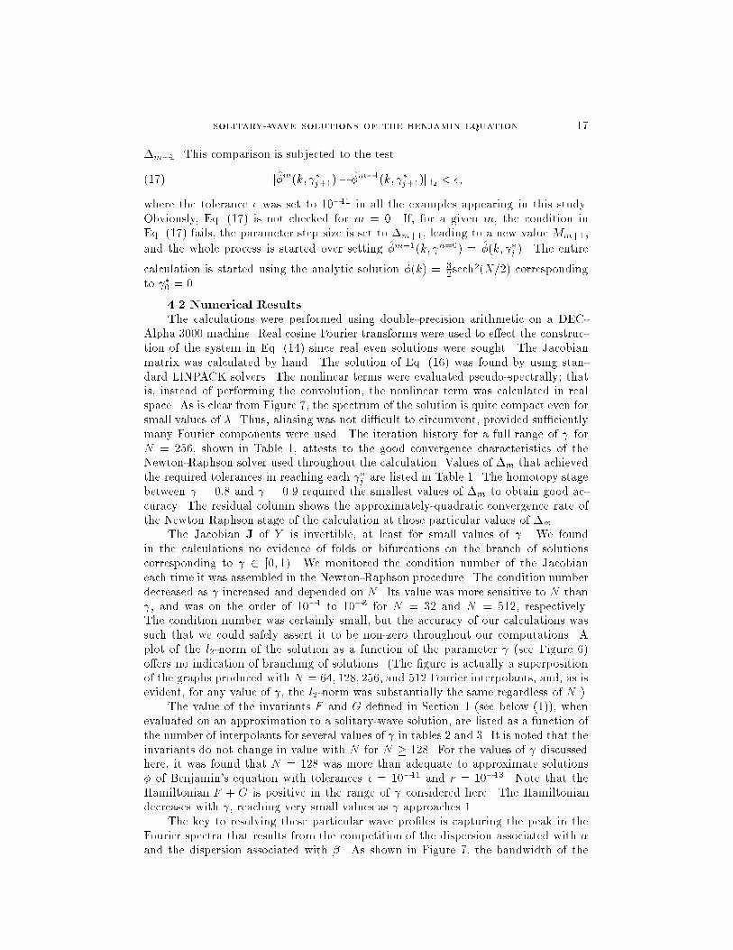
solitary-wave solutions of the benjamin equation 17�m�1. This comparison is subjected to the test(17) k�̂m(k; �j+1)� �̂m�1(k; �j+1)kl2 < �;where the tolerance � was set to 10�11 in all the examples appearing in this study.Obviously, Eq. (17) is not checked for m = 0. If, for a given m, the condition inEq. (17) fails, the parameter step size is set to �m+1, leading to a new value Mm+1,and the whole process is started over setting �̂m+1(k; n=0) = �̂(k; �j ). The entirecalculation is started using the analytic solution �̂(k) = \32sech2(X=2) correspondingto �0 = 0.4.2 Numerical Results.The calculations were performed using double-precision arithmetic on a DEC-Alpha 3000 machine. Real cosine Fourier transforms were used to e�ect the construc-tion of the system in Eq. (14) since real even solutions were sought. The Jacobianmatrix was calculated by hand. The solution of Eq. (16) was found by using stan-dard LINPACK solvers. The nonlinear terms were evaluated pseudo-spectrally; thatis, instead of performing the convolution, the nonlinear term was calculated in realspace. As is clear from Figure 7, the spectrum of the solution is quite compact even forsmall values of �. Thus, aliasing was not di�cult to circumvent, provided su�cientlymany Fourier components were used. The iteration history for a full range of forN = 256, shown in Table 1, attests to the good convergence characteristics of theNewton-Raphson solver used throughout the calculation. Values of �m that achievedthe required tolerances in reaching each �j are listed in Table 1. The homotopy stagebetween = 0:8 and = 0:9 required the smallest values of �m to obtain good ac-curacy. The residual column shows the approximately-quadratic convergence rate ofthe Newton Raphson stage of the calculation at those particular values of �m.The Jacobian J of Y is invertible, at least for small values of . We foundin the calculations no evidence of folds or bifurcations on the branch of solutionscorresponding to 2 [0; 1). We monitored the condition number of the Jacobianeach time it was assembled in the Newton-Raphson procedure. The condition numberdecreased as increased and depended on N . Its value was more sensitive to N than , and was on the order of 10�1 to 10�3 for N = 32 and N = 512, respectively.The condition number was certainly small, but the accuracy of our calculations wassuch that we could safely assert it to be non-zero throughout our computations. Aplot of the l2-norm of the solution as a function of the parameter (see Figure 6)o�ers no indication of branching of solutions. (The �gure is actually a superpositionof the graphs produced with N = 64; 128; 256, and 512 Fourier interpolants, and, as isevident, for any value of , the l2-norm was substantially the same regardless of N .)The value of the invariants F and G de�ned in Section 1 (see below (1)), whenevaluated on an approximation to a solitary-wave solution, are listed as a function ofthe number of interpolants for several values of in tables 2 and 3. It is noted that theinvariants do not change in value with N for N � 128. For the values of discussedhere, it was found that N = 128 was more than adequate to approximate solutions� of Benjamin's equation with tolerances � = 10�11 and r = 10�13. Note that theHamiltonian F + G is positive in the range of considered here. The Hamiltoniandecreases with , reaching very small values as approaches 1.The key to resolving these particular wave pro�les is capturing the peak in theFourier spectra that results from the competition of the dispersion associated with �and the dispersion associated with �. As shown in Figure 7, the bandwidth of the

18 john p. albert, jerry l. bona, and juan mario restrepo0.0 0.2 0.4 0.6 0.8 1.0

γ

0.00

0.05

0.10

0.15

0.20

0.25

0.30

l_2

Figure 6. The l2-norm of the solution versus . The superposition of the norms computedwith N = 64;128;256;512 Fourier interpolants are indistinguishable.spectra with signi�cant energy is approximately 0 � jkj � 60. Attempting to resolvethe wave with a smaller bandwidth yields a solution with a qualitatively di�erentshape. Figure 8 shows a portion of the spectrum �̂(k) computed using the algorithmoutlined in Section 4.1 with = 0:85. The upper curve is the superposition of thespectra computed with N = 64, N = 128, and N = 256, respectively. It was foundthat the spectra for N > 64 superimposes rather well on the N = 64 case. The lowercurve represents the spectrum as computed using N = 32 and clearly does not capturethe characteristic peak in the wave's spectrum. The example in this �gure correspondsto = 0:85. Not surprisingly, the N = 32 case did not meet the tolerance associatedwith the parameter �. To come to the approximation whose spectrum is displayed inFigure 8 using N = 32, this criteria had to be relaxed from � = 10�11 to � = 10�5.Figure 9 shows the energetic portion of the Fourier spectra �̂(k) for several valuesof , making it clear that the peak of the spectrum moves to higher modes as gets larger, and the morphology of the spectrum changes signi�cantly in the regionadjoining the peak for near 1. Furthermore, from the same �gure it is evident that,at k = 0, the spectrum �̂(k) has a non-zero right-hand derivative. Since �̂(k) is aneven function in k, it follows that there is a discontinuity in the spectrum at k = 0.Consideration of the symbol c(k) suggests that this should indeed be the case for all 6= 0. In this respect, the Fourier transform of the solitary waves discussed hereresembles the explicit spectral function �̂(k) = �e�jkj of the solitary-wave solution�(X) = 11+X2 of the Benjamin-Ono equation.In [8] Benjamin derived a formal asymptotic estimate for �(X) for large X. For near 1, he obtained(18) �(X) � �4K =X2 + 2�1� 2 jf(y1)j exp(�p1� 2X) cos[ X + arg(f(y1))]as X !1, where K is a constant and f is a function of the pole y1 = + ip1� 2

solitary-wave solutions of the benjamin equation 190.0 20.0 40.0 60.0 80.0 100.0

k

0.000

0.010

0.020

0.030

0.040

0.050

φ

γ=0.7

γ=0

γ=0.9

γ=0.97Figure 7. Portion of the Fourier spectra as a function of . N = 512.Table 1Residuals in reaching � in the Newton-Raphson stage ofthe N = 256 run. The �m's quoted in the table correspond to the size of the stepemployed to reach �j within the error tolerances. Tolerance on the residual was 10�13: � �m Residual � �m Residual0.10 3.125E-03 4.274742E-05 0.80 1.250E-02 1.353319E-055.171706E-08 7.966373E-081.806914E-13 7.479083E-125.877141E-25 5.099222E-200.20 5.000E-02 4.808639E-05 0.90 9.766E-05 1.689451E-057.438409E-08 3.287065E-074.198945E-13 4.811537E-104.044869E-24 1.057499E-150.30 2.500E-02 1.159375E-05 0.95 1.250E-02 3.065973E-225.338055E-09 1.236640E-342.623204E-150.40 2.500E-02 1.100423E-05 0.97 6.250E-03 1.286097E-276.216201E-09 4.376426E-354.582266E-150.50 2.500E-02 4.157460E-05 0.98 6.250E-03 1.645986E-311.100305E-07 7.247277E-361.945366E-122.833418E-220.70 2.500E-02 3.180455E-05 0.99 6.250E-03 3.356281E-151.664470E-07 1.798301E-241.296935E-115.133442E-20

20 john p. albert, jerry l. bona, and juan mario restrepoTable 2F as a function of the number of interpolants. 64 128 256 5120.00 2.435081E-02 2.435071E-02 2.435071E-02 2.435071E-020.10 2.102588E-02 2.103165E-02 2.103165E-02 2.103165E-020.50 9.506347E-03 9.521296E-03 9.521296E-03 9.521296E-030.70 5.015357E-03 5.029482E-03 5.029482E-03 5.029482E-030.90 1.578698E-03 1.583581E-03 1.583581E-03 1.583581E-030.99 4.785824E-04 4.790875E-04 4.790875E-04 4.790875E-04Table 3G as a function of the number of interpolants. 64 128 256 5120.00 2.435218E-02 2.435071E-02 2.435071E-02 2.435071E-020.10 1.944642E-02 1.944358E-02 1.944358E-02 1.944358E-020.50 4.398194E-03 4.391453E-03 4.391454E-03 4.391454E-030.70 4.140576E-04 4.068088E-04 4.068088E-04 4.068088E-040.90 -7.622961E-04 -7.658048E-04 -7.658048E-04 -7.658048E-040.99 -4.403099E-04 -4.407939E-04 -4.407939E-04 -4.407939E-040.0 10.0 20.0 30.0

k

0.000

0.005

0.010

0.015

φ

Ν=32

Ν>32

Figure 8. Fourier spectra of the solution for = 0:85. The lower curve corresponds to theN = 32 case, while the upper curve was computed using N = 64, N = 128, and N = 256. Dots showthe location of the calculated discrete spectral points.of 1=(1� 2 jkj+ k2). The second term on the right-hand side of the above expressiondecays exponentially as X ! 1, whereas the �rst term decays only algebraically,so that for very large values of X, the �rst term will dominate the second. As approaches 1, however, the coe�cient 2�=(1 � 2) of the second term will be muchlarger than the coe�cient of the �rst term, while the factor of p1� 2 within theexponential will become small, so that the second term will dominate the �rst term over

solitary-wave solutions of the benjamin equation 210.0 20.0 40.0 60.0 80.0 100.0

k

0.000

0.005

0.010

0.015

φ

Figure 9. Portion of the spectra as a function of , N = 512. Solid: = 0:99, dashed: = 0:98, dotted: = 0:97.an ever-increasing range of values of X. Within this range, according to Benjamin'sasymptotic expression (18), the zeros of �(X) will be near the zeros of cos( X), andhence will be spaced at intervals of length approximately �= .Our numerical approximations of �(X) conform to the above predictions. Figures3 and 4 show that the range of values of X over which �(X) exhibits oscillatorybehavior increases as approaches 1, and that within this range the zeros of �(X) arefairly evenly spaced. To compare the spacing between the zeros with the value �= predicted by Benjamin's estimate, we considered an approximate solution �(X) =�(X; ) with = 0:99, computed with N = 2048. A total of 17 zeros were foundon either side of the X = 0 axis. Since linear interpolation was used between the2048 data points, the location of these zeros carries an uncertainty of approximately�2:44 � 10�4. In the scaling used here, for = 0:99, Benjamin's estimate predicts aspacing between the zeros of z� = �=2 = 2:5758 � 10�2. Table 4 lists the location Zof the zeros and the intervals z between them for X > 0. The computed values of zshow adequate agreement with z�. Note that the deviation of z from z� for the largestvalues of Z is consistent with Benjamin's estimate. Since the largest values of Z occurin a region where the two terms in the estimate are nearly in balance, one would notexpect their spacing to be determined by the second term alone.It deserves remark that the formal asymptotic derived in [8] and displayed in (18)is di�erent from Benjamin's conclusion on the same topic in [7]. In the latter reference,Benjamin asserted the solitary-wave solutions of his equation decayed exponentiallyand oscillated in�nitely often. Certainly, solitary-wave solutions � of (1) cannot decayexponentially since then, by the Paley-Wiener Theorem, their Fourier transform �̂would be analytic, so in�nitely di�erentiable, and indeed all its derivatives would liein L2(R). This conclusion is not compatible with the singular aspect of the dispersioncB in (3). The matter has been rigorously settled in a recent paper of Chen and Bona

22 john p. albert, jerry l. bona, and juan mario restrepoTable 4Location of the zeros of �(X; ) with = 0:99, computedusing N = 2048, displayed consecutively from left to right and top to bottom. Theintervals between consecutive zeros, multiplied by 100, appear in parentheses.1.33E-02 (2.59) 3.92E-02 (2.56) 6.49E-02 (2.60)9.09E-02 (2.54) 1.164E-01 (2.61) 1.425E-01 (2.54)1.679E-01 (2.61) 1.94E-01 (2.53) 2.193E-01 (2.64)2.457E-01 (2.50) 2.707E-01 (2.60) 2.975E-01(2.43)3.218E-01 (2.78) 3.496E-01 (2.29) 3.725E-01 (3.05)4.028E-01 (1.91) 4.221E-01[15] using the decay results of Li and Bona [22], [12]. In [15], it is shown thatlimx!�1X2�(X) = D;where D is a non-zero constant. This is consistent with the formalism in (18) andimplies that � must feature at most �nitely many oscillations.5 Concluding RemarksIn this study, three themes were pursued in the context of Benjamin's equationfor the approximation of internal waves in certain two- uid systems where the e�ectsof surface tension cannot be ignored. First, a reappraisal of the derivation of theequation is given with an eye toward better understanding the circumstances underwhich the equation might be expected to provide physically relevant information. Sec-ond, an exact analysis of solitary-wave solutions is provided via the Implicit FunctionTheorem. The analysis is so organized that information about the stability is also ob-tained. Finally, the Contraction Mapping Principle underlying the proof of existenceof solitary waves is used as the basis of a continuation-type algorithm. This algorithmis implemented as a computer code which is used to obtain numerically generatedapproximations of these solitary waves.Analysis of the Benjamin equation in its context as a model for waves in cer-tain two- uid systems reveals there are ranges of the physical parameters for whichthe model's predictions might be relevant to waves seen in the laboratory or naturalsettings. It must be acknowledged, however, that the range in question is somewhatnarrow. As a next step, it would be useful to construct a reliable numerical schemefor the time-dependent problem (1)1. The outcome of an organized set of simulationsmight well suggest aspects to look for in an experimental situation.Previous experience with nonlinear, dispersive wave equations of the form de-picted in (10) (with l = 0, say) indicates that solitary-wave solutions may play animportant role in the long-time evolution of general disturbances. In consequence,we endeavored here to understand these traveling-wave solutions in some detail. Theform of these solitary waves varies with the parameter = 12�=pC�, where C is thedi�erence between the solitary-wave speed and the speed c0 of in�nitesimal waves ofextreme length, and � and � are measures of the strengths of the competing dispersivee�ects (the parameter � is related to �nite-depth e�ects whilst non-zero values of �are due to surface-tension e�ects). In a given setting, it is possible to cover the entire1 A time-dependent algorithm using a split-step method [20] based on Fourier projection forthe linear terms alternated with a conservative second-order approximation for the advective termsis being developed.

solitary-wave solutions of the benjamin equation 23range 0 < < 1 by appropriate choices of the speed c0(1 � C) of the solitary wave.Values of near 0 correspond to traveling waves with large, negative phase velocities,however, and these lie outside the range where the equation is expected to be a validmodel. Also, the results of Section 4 suggest that solitary waves corresponding tovalues of near 1 will have small amplitudes, making them hard to discern. When is order � or greater, and is not too close to 1, the corresponding solitary waves travelto the right, and are potentially observable.It is worth noting that the stability theory developed in Section 3 applies tothe Benjamin equation only for values of near 0. The general stability theory forsolitary-wave solutions of equations of the form depicted in (10) (cf. [2]) does not applydirectly to the Benjamin equation. The problem of extending the stability theoryto encompass the physically relevant regime is currently under study. In additionto an analytical approach, we expect to use the aforementioned computer code forapproximating solutions of the time-dependent problem (1) to investigate stability viaa coordinated set of numerical simulationswith initial data corresponding to perturbedsolitary waves.The continuation method developed in Section 4 for the approximation of solitary-wave solutions of the Benjamin equation appears capable of producing traveling wavesolutions over the entire range of . Another use of a time-dependent numerical inte-grator would be to check directly how closely the computed solitary waves correspondto traveling waves. Once this is settled satisfactorily, natural further questions includedetermining the outcome of interactions of solitary waves and whether or not generalinitial disturbances feature solitary waves in their long-time asymptotics. The resultsof Vanden-Broeck and Dias (cf. [26]) on a free-surface problem similar to the one con-sidered here suggest that other branches of solitary-wave solutions to the Benjaminequation may exist besides the one on which our computed solutions lie. Numericalexperiments like those described above may disclose whether such solutions exist andplay a role in general solutions of the initial-value problem for the Benjamin equation.References[1] J. P. ALBERT, \Positivity properties and stability of solitary-wave solutions ofmodel equations for long waves," Comm. P.D.E.17 (1992), 1{22.[2] J. P. ALBERT & J. L. BONA, \Total positivity and the stability of internal wavesin strati�ed uids of �nite depth," IMA J. App. Math.46 (1991), 1{19.[3] J. P. ALBERT, J. L. BONA & D. HENRY, \Su�cient conditions for stability ofsolitary-wave solutions of model equations for long waves," Phys. D 24 (1987), 343{366.[4] J. P. ALBERT, J. L. BONA & J. -C. SAUT, \Model equations for strati�ed uids,"Proc. Royal Soc. London, A (1997).[5] T. B. BENJAMIN, \Internal waves of permanent form in uids of great depth," J.Fluid Mech. 29 (1967), 559{592.[6] , \The stability of solitary waves," Proc. Royal Soc. London, A 328 (1972),153{183.[7] , \A new kind of solitary wave," J. Fluid Mechanics 245 (1992), 401{411.[8] , \Solitary and periodic waves of a new kind," Philos. Trans. Roy. Soc.LondonA 354 (1996), 1775{1806.

24 john p. albert, jerry l. bona, and juan mario restrepo[9] T. B. BENJAMIN, J. L. BONA & D. K. BOSE, \Solitary-wave solutions of nonlinearproblems," Phil. Trans. Royal Soc. London, A 340 (1990), 195{244.[10] D. P. BENNETT, R. W. BROWN, S. E. STANSFIELD, J. D. STROUGHAIR& J. L. BONA,\The stability of internal solitary waves," Math. Proc. Cambridge Philos. Soc. 94(1983), 351{379.[11] J. L. BONA, \On the stability theory of solitary waves," Proc. Royal Soc. London,A 344 (1975), 363{374.[12] J. L. BONA & Y. A. LI, \Decay and analyticity of solitary waves," J. Math. PuresAppliq. (1997).[13] J. L. BONA, P. E. SOUGANIDIS & W. A. STRAUSS, \Stability and instability ofsolitary waves of Korteweg{de Vries type," Proc. Royal Soc. London, A 411 (1987),395{412.[14] C. CANUTO, M. Y. HUSSAINI, A. QUARTERONI & T. A. ZANG, Spectral Methods inFluid Dynamics, Springer-Verlag, New York{Heidelberg{Berlin, 1988.[15] H. CHEN & J. L. BONA, \Existence and asymptotic properties of solitary-wavesolutions of Benjamin-type equations," submitted, 1997.[16] R. E. DAVIS & A. ACRIVOS, \Solitary internal waves in deep water," Journal ofFluid Mechanics 29 (1967), 593{616.[17] K. DEIMLING, Nonlinear Functional Analysis, Springer-Verlag, New York, 1985.[18] M. GRILLAKIS, J. SHATAH & W. STRAUSS, \Stability theory of solitary waves inthe presence of symmetry, I," J. Func. Anal.74 (1987), 160{197.[19] R. GRIMSHAW, \Evolution equations for long, nonlinear internal waves in strati�edshear ows ," Stud. Appl. Math.65 (1981), 159{188.[20] A. HASEGAWA & F. TAPPERT, \Transmision of stationary nonlinear optical pulsesin dispersive dielectric �bers. I. Anomalous dispersion," Applied Physics Letters23 (1973), 142{144.[21] T. KATO, Perturbation Theory of Linear Operators, Springer-Verlag, New York,1976.[22] Y. A. LI & J. L. BONA, \Analyticity of solitary-wave solutions of model equationsfor long waves ," SIAM J. Math. Anal.27 (1996), 725{737.[23] P. M. MORSE & H. FESHBACH, Methods of Theoretical Physics, Vol 1, McGraw-Hill, New York, 1953.[24] H. ONO, \Algebraic solitary waves in strati�ed uids," J. Phys. Soc. Japan 39(1975), 1082{1091.[25] R. SEYDEL, Practical Bifurcation and Stability Analysis, from Equilibrium toChaos, IAM Series, Springer-Verlag, New York{Heidelberg{Berlin, 1994.[26] J. M. VANDEN-BROECK & F. DIAS, \Gravity-capillary solitary waves in water of in-�nite depth and related free-surface ows," Journal of Fluid Mechanics 240 (1992),549{557.[27] M.WEINSTEIN, \Existence and dynamic stability of solitary-wave solutions of equa-tions arising in long-wave propagation," Comm. Partial Di�erential Equations 12(1987), 1133{1173.