SolisEnvironment for Numerical Computing

Sidi HAMADYFull Professor, Dr. habil. Eng.Université de Lorraine, France

LMOPS Lab., Université de Lorraine & CentraleSupélec, Francehttp://www.hamady.org

The latest Solis release (extracted size less than 10 MB) is freely available here:http://www.hamady.org/download/solis_windows_64bit.ziphttp://www.hamady.org/download/solis_linux_64bit.tgzThe latest version of this manual:http://www.hamady.org/download/solis_lua.pdf

Solis:Copyright(C) 2010-2022 Prof. Sidi HAMADYhttp://www.hamady.orgsidi@hamady.orgSolis is protected by copyright laws and international copyright treaties, as well as other intel-lectual property laws and treaties. Solis is free of charge only for non-commercial use. Sidi OuldSaad Hamady expressly disclaims any warranty for Solis. Solis is provided ‘As Is’ without anyexpress or implied warranty of any kind, including but not limited to any warranties of mer-chantability, noninfringement, or fitness of a particular purpose. Solis may not be redistributedwithout authorization of the author.

Solis Lua engine uses:the Lua programming language, (C) Lua.org, PUC-Rio.the Lua Just-In-Time Compiler, (C) Mike Pall.the LIS linear solvers, (C) The SSI Project, Kyushu University, Japan.the ODE solver developed by Scott D. Cohen and Alan C. Hindmarsh @ LLNL.

Solis device editor, code editor, data plotter and calculator use:the IUP GUI toolkit, (C) Tecgraf/PUC-Rio.the Scintilla Component, (C) Neil Hodgson.

Summary

Title Page i

Presentation 1

Solis Editor 3

Solis Modules 7Time functions . . . . . . . . . . . . . . . . . . . . . . . . . . . . . . . . . . . . . . . . 8Math functions . . . . . . . . . . . . . . . . . . . . . . . . . . . . . . . . . . . . . . . . 9Numerical Array Functions . . . . . . . . . . . . . . . . . . . . . . . . . . . . . . . . . 11Ordinary Differential Equations . . . . . . . . . . . . . . . . . . . . . . . . . . . . . . . 13Mathematical Optimization . . . . . . . . . . . . . . . . . . . . . . . . . . . . . . . . . 15Descriptive Statistics . . . . . . . . . . . . . . . . . . . . . . . . . . . . . . . . . . . . . 16Data Analysis . . . . . . . . . . . . . . . . . . . . . . . . . . . . . . . . . . . . . . . . . 17ASCII Data Files . . . . . . . . . . . . . . . . . . . . . . . . . . . . . . . . . . . . . . . 20XY Plotting . . . . . . . . . . . . . . . . . . . . . . . . . . . . . . . . . . . . . . . . . . 21BSD Socket . . . . . . . . . . . . . . . . . . . . . . . . . . . . . . . . . . . . . . . . . . 24C Modules . . . . . . . . . . . . . . . . . . . . . . . . . . . . . . . . . . . . . . . . . . . 28Instrumentation . . . . . . . . . . . . . . . . . . . . . . . . . . . . . . . . . . . . . . . . 33Math Parser . . . . . . . . . . . . . . . . . . . . . . . . . . . . . . . . . . . . . . . . . . 35Graphical User Interface using IUP . . . . . . . . . . . . . . . . . . . . . . . . . . . . . 39

Solis Calculator 41

Bibliography 45

iii

Presentation

Solis is a programming environment for numerical computing and data analysis using the Luascripting language [1, 2]. It is available for Linux and Windows with built-in Lua scriptingengine, integrated numerical, data plotting and analysis modules, full-featured editor with syntaxhighlighting, code completion, online documentation, code samples, etc.

The main goal of Solis is to provide an easy-to-use development environment for numericalcomputing using the Lua programming language on Linux and Windows. It integrates the Luascripting engine with all Lua functionalities, and a lot of specific Solis functionalities includingnumerical functions (differential equations, mathematical optimization, etc.), data plotting andanalysis modules and an extended mathematical library. In addition, it includes modules forinstrumentation using VISA and serial interfaces. Within the Solis environment, you can developalgorithms for science and engineering with one of the most elegant and fast scripting languages.

To learn the Lua programming language, you can read the reference book[1] and visit theLua official website:http://www.lua.orgExcellent tutorials, covering all Lua aspect from basics to advanced programming techniques,can be found here:http://lua-users.org/wiki/TutorialDirectoryThe Solis editor can also be used as a general purpose full-featured editor supporting C/C++,Bash/Text, Python, Octave, Fortran, LaTeX and Makefile with configurable tools (e.g. to run acompiler or a bash script).

To install Solis for Windows or Linux, download solis_windows_64bit.zip (Windows 64bit) orsolis_linux_64bit.tgz (Linux 64bit) from http://www.hamady.org, unzip/untar in any location(USB key or Memory stick for example) and run solisedit (Linux) or solisedit.exe (Windows) inthe bin directory.

The Solis distribution includes:

• An advanced code editor, solisedit under Linux or solisedit.exe under Windows, imple-mented in C. This editor offers all functionality found in modern editors such as syntaxhighlighting, autocompletion, markers, indentation control, find/replace, file explorer...and are fully customizable. It supports Lua, Python, C/C++, LATEX... and can be used asa general code editor. It can also be used to edit and run semiconductor device simulationsusing Solis Simulator.

• A data plotter, solisplot (Linux) or solisplot.exe (Windows), implemented in C andC++. This tool is used by Solis but could also be used as a standalone data plotter.

1

2 Presentation

• An advanced scientific calculator, soliscalc under Linux or soliscalc.exe under Windows,implemented in C.

• A semiconductor device simulator [3], driven by soliscomp under Linux or soliscomp.exeunder Windows, controlling the semiconductor simulator implementing the drift-diffusionmodel. The complete simulator documentation is located in solis_simulator.pdf. I starteddeveloping the simulator in 2009 and presented the first testing release in the 37th Inter-national Symposium on Compound Semiconductors (ISCS) in 2010 in Japan [4].

• A graphical device editor, solisdevice under Linux or solisdevice.exe under Windows,implemented in C. This tool gives an easy-to-use graphical frontend to the semiconductordevice simulator.

The whole Solis distribution size, including documentation and examples, is less that 10 MB.To know if a new version is available, click Menu/Help/Check for Update... or visit my

website: http://www.hamady.orgUnder Linux, Solis includes also an interactive terminal emulator (solisterm), a standalone ver-sion of the embedded terminal in SolisEdit.This terminal emulator is loaded and available to use if the VTE library is installed.

This Solis user manual is organized as follows:The first chapter contains the Solis editor.The second chapter gives an overview on how to use the Solis environment.The third chapter contains the description of the Solis built-in modules.The fourth chapter contains the description of the scientific calculator.

Solis Editor

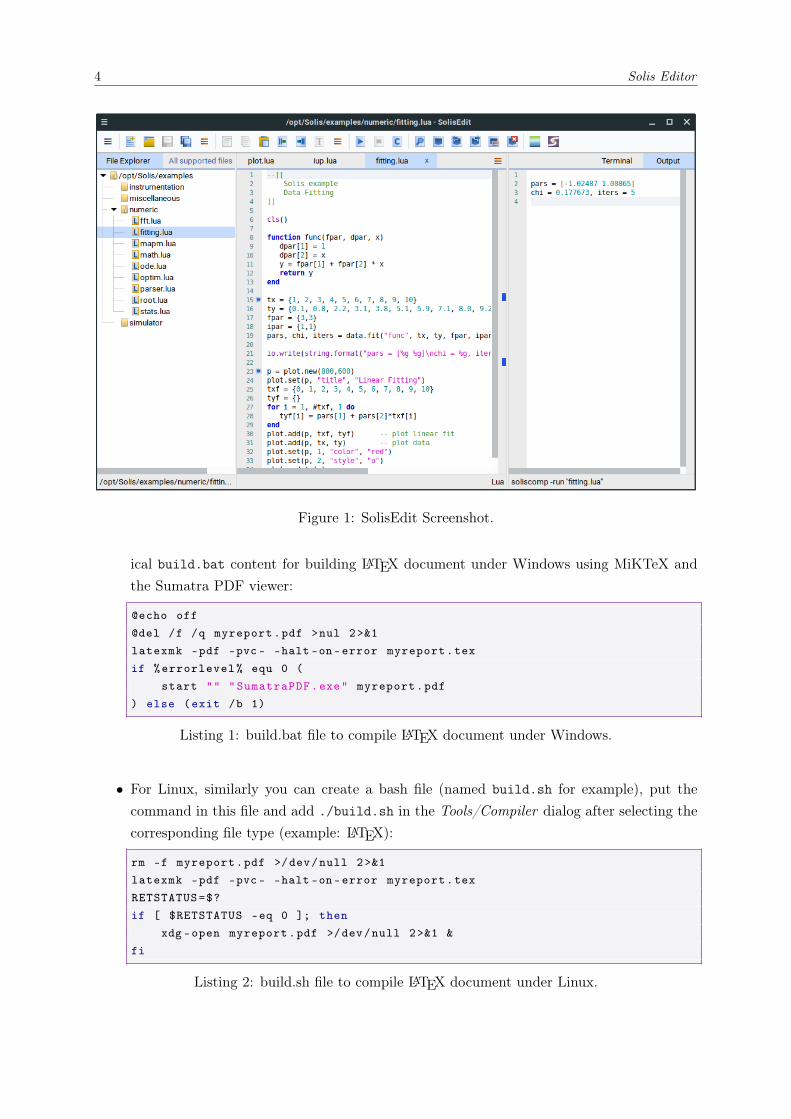
The Solis code editor, SolisEdit, offers all functionality found in modern editors such as syntaxhighlighting, autocompletion, markers, indentation control, find/replace, file explorer... and isfully customizable (screenshot in figure 1).

SolisEdit can be used to edit Lua files (with extension .lua) and, in addition, it supports aset of languages used by scientists and engineers such as C/C++, Bash, Python, Octave, Fortran,LATEX1 and Makefile. SolisEdit can also be used to edit the Solis Simulator input files (withextension .solis) and the physical models in Lua. The language is automatically selected basedon the file extension.

SolisEdit integrates a File Explorer to work easily with files, that can be set to show only(filter) some files based on their extension (right-click the root directory and select the corre-sponding filter).

SolisEdit includes a system of coloured Markers, shown in the margins, to show in realtimethe modified/saved sections of the current documents. The Markers can be reset at any time byselecting Edit/Remove Markers menu.One particular marker is the bookmark, used to mark a specific line in the code for easier navi-gation.

The classic Search/Replace functionality are included in SolisEdit: Search menu.Almost every aspect of the SolisEdit user interface can be customized: Options menu.

With SolisEdit, one can configure specific tool, such as a compiler or a bash script, to runfor a known file type (Lua of course, but also C, Python, LATEX, etc.). To configure a tool,select Tools/Compiler menu and type the command to use to build/compile the correspondingfile type. For example, for Lua, the command is soliscomp -run %s.solis where %s will bereplaced by the filename. It is useful to call a batch file (under Windows) or bash script (underLinux) to build a specific file. This can be done in the following way:

• For Windows, one can create a batch file (named build.bat for example), put the com-mand in this file and add the batch name build.bat in the Tools/Compiler dialog afterselecting the corresponding file type (example: LATEX). The following example gives a typ-

1This manual was composed in LATEX using SolisEdit.

3

4 Solis Editor

Figure 1: SolisEdit Screenshot.

ical build.bat content for building LATEX document under Windows using MiKTeX andthe Sumatra PDF viewer:

@echo off@del /f /q myreport.pdf >nul 2>&1latexmk -pdf -pvc - -halt -on-error myreport.texif %errorlevel% equ 0 (

start "" "SumatraPDF.exe" myreport.pdf) else (exit /b 1)

Listing 1: build.bat file to compile LATEX document under Windows.

• For Linux, similarly you can create a bash file (named build.sh for example), put thecommand in this file and add ./build.sh in the Tools/Compiler dialog after selecting thecorresponding file type (example: LATEX):

rm -f myreport.pdf >/dev/null 2>&1latexmk -pdf -pvc - -halt -on-error myreport.texRETSTATUS=$?if [ $RETSTATUS -eq 0 ]; then

xdg -open myreport.pdf >/dev/null 2>&1 &fi

Listing 2: build.sh file to compile LATEX document under Linux.

Solis Editor 5

• For Python (for both Windows or Linux), just put a command like this (replace with yourinstalled Python interpreter):python –u %s.py

In the Tools/Compiler dialog, one can check the Redirect standard output option to letSolisEdit to print out all the text generated by the tool to the Output Window. If this op-tion is unchecked, SolisEdit will launch a command window and run the tool inside it. In thislatter case, one can check the Close when restart option to close the previous command windowbefore starting a new one. For the Solis simulator it is better to check the Redirect standardoutput option (it is checked, by default) to benefit from functionality such as syntax coloring.

Under Linux, SolisEdit includes an embedded terminal emulator. This terminal emulator isloaded and available to use if the VTE library is installed.

Solis Modules

The Solis environment integrates the Lua scripting engine with all Lua functionalities, and a lotof specific Solis functionalities presented below.

7

8 Time functions

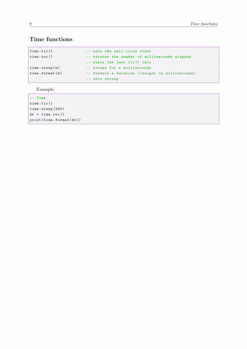
Time functions

time.tic () -- sets the wall -clock timertime.toc () -- returns the number of milliseconds elapsed

-- since the last tic() calltime.sleep(n) -- sleeps for n millisecondstime.format(n) -- formats a duration (integer in milliseconds)

-- into string

Example:

-- Timetime.tic ()time.sleep (200)dt = time.toc ()print(time.format(dt))

Math functions 9

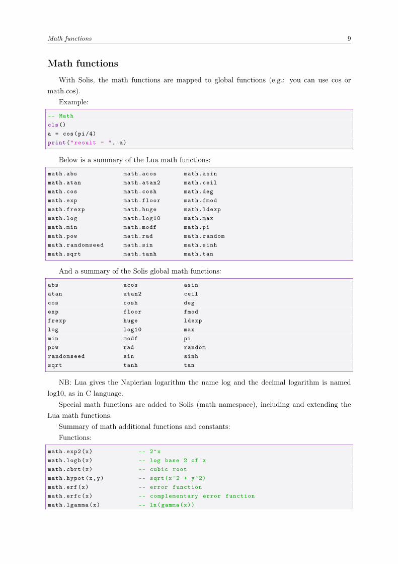
Math functions

With Solis, the math functions are mapped to global functions (e.g.: you can use cos ormath.cos).

Example:

-- Mathcls()a = cos(pi/4)print("result = ", a)

Below is a summary of the Lua math functions:

math.abs math.acos math.asinmath.atan math.atan2 math.ceilmath.cos math.cosh math.degmath.exp math.floor math.fmodmath.frexp math.huge math.ldexpmath.log math.log10 math.maxmath.min math.modf math.pimath.pow math.rad math.randommath.randomseed math.sin math.sinhmath.sqrt math.tanh math.tan

And a summary of the Solis global math functions:

abs acos asinatan atan2 ceilcos cosh degexp floor fmodfrexp huge ldexplog log10 maxmin modf pipow rad randomrandomseed sin sinhsqrt tanh tan

NB: Lua gives the Napierian logarithm the name log and the decimal logarithm is namedlog10, as in C language.

Special math functions are added to Solis (math namespace), including and extending theLua math functions.

Summary of math additional functions and constants:Functions:

math.exp2(x) -- 2^xmath.logb(x) -- log base 2 of xmath.cbrt(x) -- cubic rootmath.hypot(x,y) -- sqrt(x^2 + y^2)math.erf(x) -- error functionmath.erfc(x) -- complementary error functionmath.lgamma(x) -- ln(gamma(x))

10 Math functions

math.tgamma(x) -- gamma(x)math.trunc(x) -- nearest integermath.round(x) -- nearest integer , roundingmath.isinf(x) -- number is infinite?math.isnan(x) -- not a number?math.isnormal(x) -- number is normal?math.asinh(x)math.acosh(x)math.atanh(x)math.gauss(x,b,c) -- G(x) = exp(-(x - b)^2 / 2c^2)math.lorentz(x,b,c) -- L(x) = (c / ((x - b)^2 + c^2))

Constants (universal constants in international units (SI)):

math.q -- Electron charge (in C)math.me -- Electron mass (kg)math.kb -- Boltzmann constant (J/K)math.h -- Planck constant (Js)math.c -- Speed of Light in vacuum (m/s)math.na -- Avogadro constant (1/ mole)

Numerical Array Functions 11

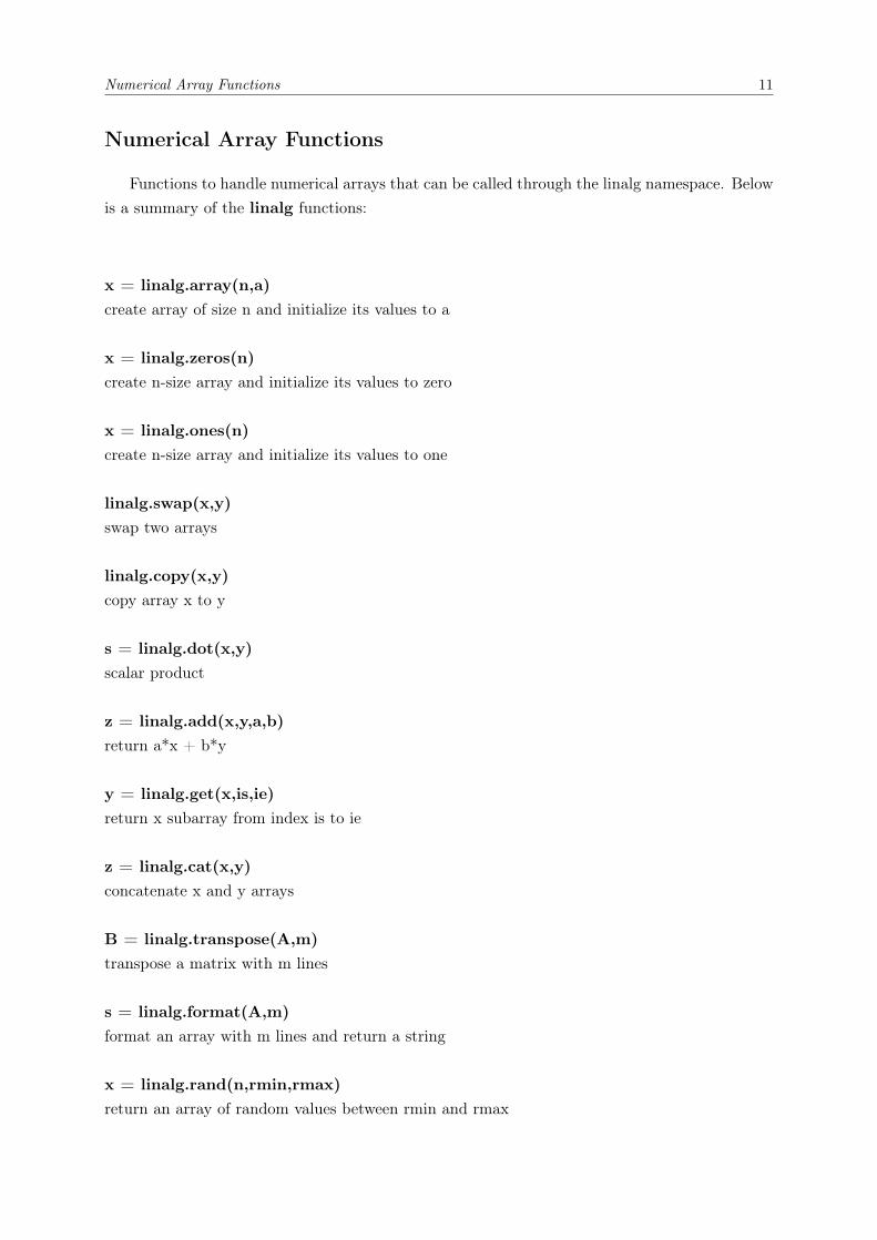
Numerical Array Functions

Functions to handle numerical arrays that can be called through the linalg namespace. Belowis a summary of the linalg functions:

x = linalg.array(n,a)create array of size n and initialize its values to a

x = linalg.zeros(n)create n-size array and initialize its values to zero

x = linalg.ones(n)create n-size array and initialize its values to one

linalg.swap(x,y)swap two arrays

linalg.copy(x,y)copy array x to y

s = linalg.dot(x,y)scalar product

z = linalg.add(x,y,a,b)return a*x + b*y

y = linalg.get(x,is,ie)return x subarray from index is to ie

z = linalg.cat(x,y)concatenate x and y arrays

B = linalg.transpose(A,m)transpose a matrix with m lines

s = linalg.format(A,m)format an array with m lines and return a string

x = linalg.rand(n,rmin,rmax)return an array of random values between rmin and rmax

12 Numerical Array Functions

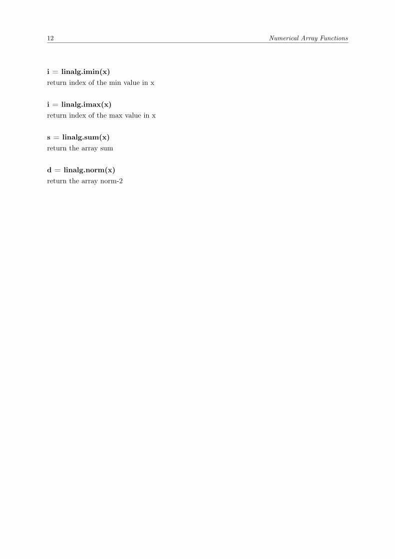
i = linalg.imin(x)return index of the min value in x

i = linalg.imax(x)return index of the max value in x

s = linalg.sum(x)return the array sum

d = linalg.norm(x)return the array norm-2

Ordinary Differential Equations 13

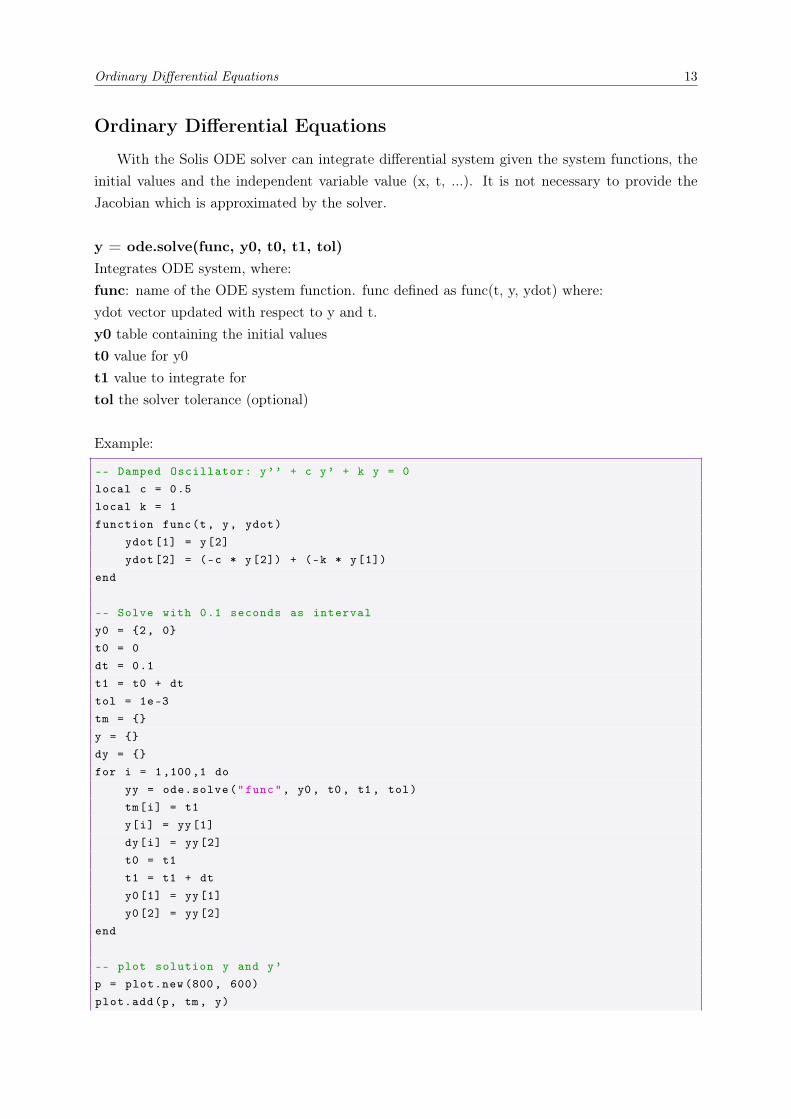
Ordinary Differential Equations

With the Solis ODE solver can integrate differential system given the system functions, theinitial values and the independent variable value (x, t, ...). It is not necessary to provide theJacobian which is approximated by the solver.

y = ode.solve(func, y0, t0, t1, tol)Integrates ODE system, where:func: name of the ODE system function. func defined as func(t, y, ydot) where:ydot vector updated with respect to y and t.y0 table containing the initial valuest0 value for y0t1 value to integrate fortol the solver tolerance (optional)

Example:

-- Damped Oscillator: y’’ + c y’ + k y = 0local c = 0.5local k = 1function func(t, y, ydot)

ydot [1] = y[2]ydot [2] = (-c * y[2]) + (-k * y[1])

end

-- Solve with 0.1 seconds as intervaly0 = {2, 0}t0 = 0dt = 0.1t1 = t0 + dttol = 1e-3tm = {}y = {}dy = {}for i = 1,100,1 do

yy = ode.solve("func", y0, t0 , t1, tol)tm[i] = t1y[i] = yy[1]dy[i] = yy[2]t0 = t1t1 = t1 + dty0[1] = yy[1]y0[2] = yy[2]

end

-- plot solution y and y’p = plot.new (800, 600)plot.add(p, tm, y)

14 Ordinary Differential Equations

plot.add(p, tm, dy)plot.set(p, "xlabel", "time (s)")plot.set(p, "ylabel", "amplitude")plot.set(p, 1, "legend", "y(t)")plot.set(p, 1, "color", "red")plot.set(p, 2, "legend", "y’(t)")plot.set(p, 2, "color", "blue")plot.update(p)

Mathematical Optimization 15

Mathematical Optimization

Solis integrates a mathematical optimization module including minimization of real functionof n variables. The Solis minimization function uses the Hooke and Jeeves algorithm which donot require the Jacobian to be evaluated.

iters = optim.minimize(func, pars, maxiters, tol, rho)func: name of the function of n variables to be minimized.func defined as func(x) where:x vector containing the variablespars table containing the initial values (will be updated to the calculated values)maxiters maximum number of iterations (optional)tol the algorithm tolerance (optional)rho the algorithm parameter, between 0 and 1 (optional). Decrease rho to improve speed andincrease it for better convergence.

xr = optim.root(func,a,b,iters,tol)– Finds the root of function in the [a,b] interval (optional), the given maximum number of iter-ations (optional) and.tolerance (optional).Returns the root value.

Example:

-- Optimizationfunction booth(x)

return (math.pow(x[1] + 2*x[2] - 4, 2) + math.pow (2*x[1] + x[2] - 5, 2))end

x = { -5, 5 }iters = optim.minimize("booth", x, 100, 1e-6)

cls()io.write(string.format("\n x = [%g %g] iters = %d \n", x[1], x[2], iters))

function func(x)return x^2 - x - 1

endx = optim.root("func" ,-5,5) -- expected: x ~ -0.618034print(x, func(x))

16 Descriptive Statistics

Descriptive Statistics

The data namespace includes functions to calculate the descriptive parameters of a list ofvalues:

Minimum: data.min(t)Maximum: data.max(t)Sum: data.sum(t)Mean: data.mean(t)Median: data.median(t)Variance: data.var(t)Standard Deviation: data.dev(t)Coefficient of Variation: data.coeff(t)Root Mean Square: data.rms(t)Skewness: data.skew(t)Kurtosis excess: data.kurt(t)

All the stats functions take a Lua table as argument, with 2048 maximum number of elements.

Example:

-- Statscls()t = {1,1,2,3,4,4,5}m = data.mean(t) -- expected: m = 2.8571428571429print(m)

Data Analysis 17

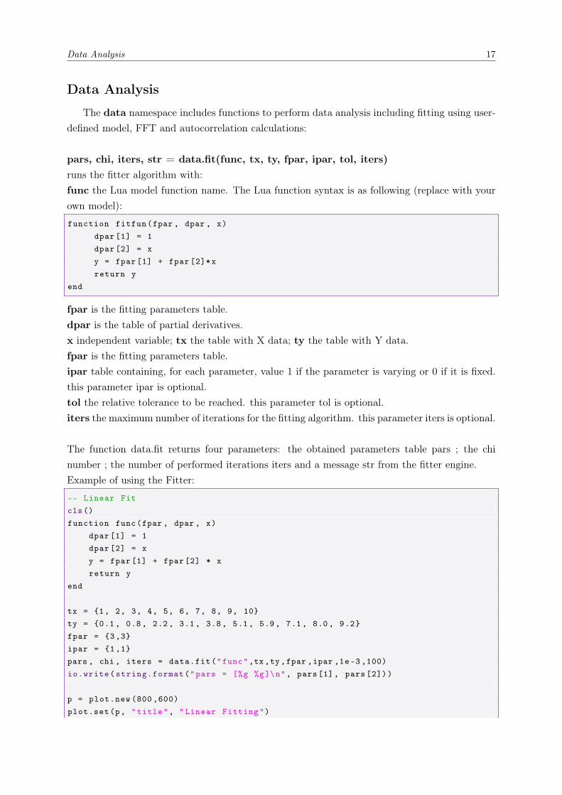
Data Analysis

The data namespace includes functions to perform data analysis including fitting using user-defined model, FFT and autocorrelation calculations:

pars, chi, iters, str = data.fit(func, tx, ty, fpar, ipar, tol, iters)runs the fitter algorithm with:func the Lua model function name. The Lua function syntax is as following (replace with yourown model):

function fitfun(fpar , dpar , x)dpar [1] = 1dpar [2] = xy = fpar [1] + fpar [2]*xreturn y

end

fpar is the fitting parameters table.dpar is the table of partial derivatives.x independent variable; tx the table with X data; ty the table with Y data.fpar is the fitting parameters table.ipar table containing, for each parameter, value 1 if the parameter is varying or 0 if it is fixed.this parameter ipar is optional.tol the relative tolerance to be reached. this parameter tol is optional.iters the maximum number of iterations for the fitting algorithm. this parameter iters is optional.

The function data.fit returns four parameters: the obtained parameters table pars ; the chinumber ; the number of performed iterations iters and a message str from the fitter engine.Example of using the Fitter:

-- Linear Fitcls()function func(fpar , dpar , x)

dpar [1] = 1dpar [2] = xy = fpar [1] + fpar [2] * xreturn y

end

tx = {1, 2, 3, 4, 5, 6, 7, 8, 9, 10}ty = {0.1 , 0.8, 2.2, 3.1 , 3.8, 5.1, 5.9 , 7.1, 8.0, 9.2}fpar = {3,3}ipar = {1,1}pars , chi , iters = data.fit("func",tx,ty,fpar ,ipar ,1e-3 ,100)io.write(string.format("pars = [%g %g]\n", pars[1], pars [2]))

p = plot.new (800 ,600)plot.set(p, "title", "Linear Fitting")

18 Data Analysis

txf = {0, 1, 2, 3, 4, 5, 6, 7, 8, 9, 10}tyf = {}for i = 1, #txf , 1 do

tyf[i] = pars [1] + pars [2]* txf[i]endplot.add(p, txf , tyf) -- plot linear fitplot.add(p, tx, ty) -- plot dataplot.set(p, 1, "color", "red")plot.set(p, 2, "style", "o")plot.update(p)

ft = data.fft(data, idir)calculates the FFT with:data the table with dataidir 1 for forward FFT and 0 for inverseThe function data.fft returns the obtained FFT table ft.NB: the FFT amplitude is scaled (divided) by the number of points.

Example of using data.fft:

-- FFTcls()

Fo = 50 -- signal frequency (Hz)To = 1/Fo -- signal period (seconds)A = 5 -- signal amplitudeAn = 1 -- noise amplitudeN = 256 -- number of points (power of 2)Ts = 4 * To/N -- sampling periodFs = 1/Ts -- sampling frequencyf = {}t = {}y = {}for i = 1, N, 1 do

f[i] = (i - 1) * Fs / (N - 1) -- frequencyt[i] = (i - 1) * Ts -- timey[i] = A*cos(2*pi*Fo*t[i]) + An*lmath.random ()

end

tfd = data.fft(y, 1)p = plot.new (800 ,600)plot.add(p, f, tfd)plot.update(p)

Data Analysis 19

ac = data.acorr(data)calculates the autocorrelation with data is the table with data.The function data.acorr returns the obtained autocorrelation table ac.

yf = data.filter(x, y, forder)Filters (smooths) x-y data using the Savitzky-Golay method, given the filter order. Returns thefiltered data yf.

20 ASCII Data Files

ASCII Data Files

c1,c2,... = data.load(filename, sep, skip, colcount, rowcount)Loads ASCII data with:filename source file name.sep separator , usually tab or semicolon (optional).skip number of rows to be skipped (optional).colcount number of columns to load (optional).rowcount number of rows to load (optional).The function data.load returns tables containing numeric data c1, c2, ...

rowcount = data.save(filename, sep, header, c1, c2, ...)Saves numeric data to ASCII file with:filename: destination file namesep: separator (usually tab or semicolon).header: file header (comment, labels, ...)c1, c2, ...: tables to saveThe function data.save returns the number of rows actually saved rowcount.

Example of using data.load and data.save:

-- ASCII

cls()

fname = "C:\\ Temp\\ ascii.txt"x = {1, 2, 3, 4, 5}y = {1, 2, 3, 4, 5}sep = "\t"skip = 0rc = data.save(fname , sep , "HEADER\n", x, y)print(rc ,"\n")

xt ,yt = data.load(fname , sep , skip)print(xt ,"\n")print(yt)

XY Plotting 21

XY Plotting

The plot namespace includes functions to plot data:

p = plot.new(width, height, template)creates plot.

plot.add(p, x, y)adds a curve with tables x,y.

plot.add(p, x, y, ey)adds a curve with tables x,y and error bar table ey.

plot.add(p, x, y, ex, ey)adds a curve with tables x,y and error bar tables ex,ey.

plot.add(p, curve, x, y)adds tables x,y to an existing curve.

plot.add(p, curve, x, y, ey)adds tables x,y to an existing curve, with error bar table ey.

plot.add(p, curve, x, y, ex, ey)adds tables x,y to an existing curve, with error bar tables ex,ey.

plot.add(p, expr, npoints, xstart, xend)adds a curve with expression (like "sin(x)", "1 - exp(-x)" ...).

plot.add(p, fname)adds a curve from data file (columns 1 and 2, TAB separated).

22 XY Plotting

plot.rem(p, curve)removes curve from plot.

plot.set(p, curve, prop, val)sets the curve properties. prop can be:"size" for curve line and symbol size. val is the size ("1", "2")"style" for curve. val is "o" for circle, "+" for plus sign, "s" for square, "d" for diamond, and"-" for line. Example: "-s" for line and squared markers."legend" for curve legend. val is the legend text."color" for curve color. val is color name like "red", "blue", ... or hex-value like "FF0000").

plot.set(p, prop, val)sets the plot properties. prop can be:"title" for the plot window title. val is the window title."xlabel" for the bottom axis label. val is the axis label."ylabel" for the left axis label. val is the axis label."xscale" for the bottom axis scale: val is "log" or "linear"."yscale" for the left axis scale: val is "log" or "linear"."xlim" for the bottom axis scale: val is "[min,max]" where min and max are the x-axis limits."ylim" for the left axis scale: val is "[min,max]" where min and max are the y-axis limits."maxpoints" set val as the maximum number of points per curve."autolim". val is "true": automatically set the axis limits.

plot.save(p, fname)saves plot to file (SVG or PDF).

plot.update(p)updates the plot window.

plot.close(p)closes the plot window.

XY Plotting 23

Example:

-- Plotx = {0,1,2,3,4,5}y = {0,1,2,3,4,5}p = plot.new (800, 600) --create a plotplot.set(p, "title", "Plot example")plot.add(p, x, y) --add curve to the new plotplot.set(p, 1, "size", 2) --set curve #1 line sizeplot.set(p, 1, "style", "-o") --set curve #1 style(line and marker)plot.set(p, 1, "color", "0000FF") --set curve #1 colorplot.update(p)

All the plot properties (curves options, scale, axis, colors . . . ) can be easily modified in theplot window. All these properties can be saved in a style template file to be used later. One cancreate a style template for a particular plot type and use it in the Lua code (plot.new function).You can also add text, lines, rectangles, ellipses . . . to the plot and save it as PDF or SVGdirectly from within the plot window.

24 BSD Socket

BSD Socket

The socket namespace includes BSD-like network functions:

s = socket.new(af,type,proto)creates socket where:af: family (socket.AF_INET by default)type: type (socket.SOCK_STREAM by default)proto: protocol (def: socket.IPPROTO_TCP)returns the socket identifier

ok = socket.bind(s, addr, port)binds socket s, where:s: socket identifieraddr: address (ex: socket.INADDR_ANY)port: port to bind toreturns true on success

ok = socket.listen(s, backlog)listens on socket, where:s: socket identifierbacklog: maximum queue lengthreturns true on success

ok = socket.connect(s, addr, port)connects socket, where:s: socket identifieraddr: addressport: port to connect toreturns true on success

sa = socket.accept(s, addr, port)accepts connection and create new socket:s: socket identifierreturns the new socket identifier sa

BSD Socket 25

ok = socket.timeout(s, to)sets the recv and send timeout, where:s: socket identifiertimeout in millisecondsreturns true on success

ok = socket.setsockopt(s, opt, val)sets socket option, where:s: socket identifieroption to set (ex: socket.SO_SNDTIMEO)val: option valuereturns true on success

ip = socket.getpeername(s)gets the socket s peer ip addresss: socket identifierreturns peer ip address

hn = socket.gethostbyaddr(s, addr)gets the host name for ip addresss: socket identifieraddr: ip addressreturns host name

ha = socket.gethostbyname(s, name)gets the ip address for host names: socket identifiername: host namereturns ip address

ha = socket.getsockname(s)gets the socket name, where:s: socket identifiername: host namereturns socket name

26 BSD Socket

ok = socket.send(s, data, flags)sends data, where:s: socket identifierdata: data to sendflags: optional flagsreturns true on success

ok = socket.sendto(s, addr, port, data, flags)sends data, where:s: socket identifieraddr: addressport: port to send todata: data to sendflags: optional flagsreturns true on success

data = socket.recv(s, datasize, flags)receives data, where:s: socket identifierdatasize: data size to be receivedflags: optional flagsreturns received data

data = socket.recvfrom(s, addr, port, datasize, flags)receives data from, where:s: socket identifieraddr: addressport: port to receive fromdatasize: data size to be receivedflags: optional flagsreturns received data

errf = socket.iserr(s)gets the error flag:s: socket identifier

BSD Socket 27

returns true if error flag set

errm = socket.geterr(s)gets the error message:s: socket identifierReturns the error message, if any

socket.shutdown(s)shutdowns socket, where:s: socket identifier

socket.delete(s)delete socket and free resources, where:s: socket identifier

Example:

-- BSD Socketcls()s = socket.new(socket.AF_INET , socket.SOCK_STREAM , socket.IPPROTO_TCP)ip = socket.gethostbyname(s, "www.debian.org")socket.connect(s, ip, 80)socket.send(s, "HEAD / HTTP/1.0\r\n\r\n")data = socket.recv(s, 1024)print(data)socket.delete(s)

28 C Modules

C Modules

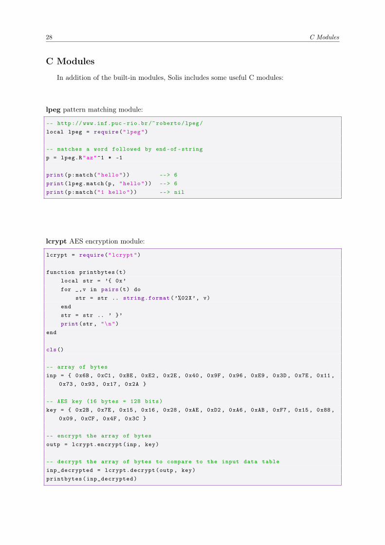
In addition of the built-in modules, Solis includes some useful C modules:

lpeg pattern matching module:

-- http :// www.inf.puc -rio.br /~ roberto/lpeg/local lpeg = require("lpeg")

-- matches a word followed by end -of-stringp = lpeg.R"az"^1 * -1

print(p:match("hello")) --> 6print(lpeg.match(p, "hello")) --> 6print(p:match("1 hello")) --> nil

lcrypt AES encryption module:

lcrypt = require("lcrypt")

function printbytes(t)local str = ’{ 0x’for _,v in pairs(t) do

str = str .. string.format (’%02X’, v)endstr = str .. ’ }’print(str , "\n")

end

cls()

-- array of bytesinp = { 0x6B , 0xC1 , 0xBE , 0xE2 , 0x2E , 0x40 , 0x9F , 0x96 , 0xE9 , 0x3D , 0x7E , 0x11 ,

0x73 , 0x93 , 0x17 , 0x2A }

-- AES key (16 bytes = 128 bits)key = { 0x2B , 0x7E , 0x15 , 0x16 , 0x28 , 0xAE , 0xD2 , 0xA6 , 0xAB , 0xF7 , 0x15 , 0x88 ,

0x09 , 0xCF , 0x4F , 0x3C }

-- encrypt the array of bytesoutp = lcrypt.encrypt(inp , key)

-- decrypt the array of bytes to compare to the input data tableinp_decrypted = lcrypt.decrypt(outp , key)printbytes(inp_decrypted)

C Modules 29

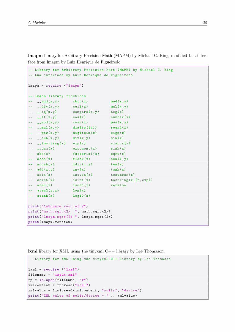
lmapm library for Arbitrary Precision Math (MAPM) by Michael C. Ring, modified Lua inter-face from lmapm by Luiz Henrique de Figueiredo.

-- Library for Arbitrary Precision Math (MAPM) by Michael C. Ring-- Lua interface by Luiz Henrique de Figueiredo

lmapm = require ("lmapm")

-- lmapm library functions:-- __add(x,y) cbrt(x) mod(x,y)-- __div(x,y) ceil(x) mul(x,y)-- __eq(x,y) compare(x,y) neg(x)-- __lt(x,y) cos(x) number(x)-- __mod(x,y) cosh(x) pow(x,y)-- __mul(x,y) digits ([n]) round(x)-- __pow(x,y) digitsin(x) sign(x)-- __sub(x,y) div(x,y) sin(x)-- __tostring(x) exp(x) sincos(x)-- __unm(x) exponent(x) sinh(x)-- abs(x) factorial(x) sqrt(x)-- acos(x) floor(x) sub(x,y)-- acosh(x) idiv(x,y) tan(x)-- add(x,y) inv(x) tanh(x)-- asin(x) iseven(x) tonumber(x)-- asinh(x) isint(x) tostring(x,[n,exp])-- atan(x) isodd(x) version-- atan2(y,x) log(x)-- atanh(x) log10(x)

print("\nSquare root of 2")print("math.sqrt (2) ", math.sqrt (2))print("lmapm.sqrt (2) ", lmapm.sqrt (2))print(lmapm.version)

lxml library for XML using the tinyxml C++ library by Lee Thomason.

-- Library for XML using the tinyxml C++ library by Lee Thomason

lxml = require ("lxml")filename = "input.xml"fp = io.open(filename , "r")xmlcontent = fp:read("*all")xmlvalue = lxml.read(xmlcontent , "solis", "device")print("XML value of solis/device = " .. xmlvalue)

30 C Modules

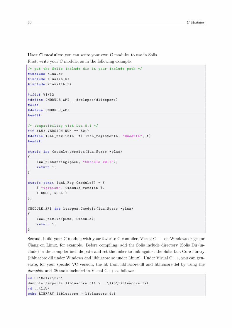
User C modules: you can write your own C modules to use in Solis.First, write your C module, as in the following example:

/* put the Solis include dir in your include path */#include <lua.h>#include <lualib.h>#include <lauxlib.h>

#ifdef WIN32#define CMODULE_API __declspec(dllexport)#else#define CMODULE_API#endif

/* compatibility with Lua 5.1 */#if (LUA_VERSION_NUM == 501)#define luaL_newlib(L, f) luaL_register(L, "Cmodule", f)#endif

static int Cmodule_version(lua_State *pLua){

lua_pushstring(pLua , "Cmodule v0.1");return 1;

}

static const luaL_Reg Cmodule [] = {{ "version", Cmodule_version },{ NULL , NULL }

};

CMODULE_API int luaopen_Cmodule(lua_State *pLua){

luaL_newlib(pLua , Cmodule);return 1;

}

Second, build your C module with your favorite C compiler, Visual C++ on Windows or gcc orClang on Linux, for example. Before compiling, add the Solis include directory (Solis Dir/in-clude) in the compiler include path and set the linker to link against the Solis Lua Core library(libluacore.dll under Windows and libluacore.so under Linux). Under Visual C++, you can gen-erate, for your specific VC version, the lib from libluacore.dll and libluacore.def by using thedumpbin and lib tools included in Visual C++ as follows:

cd C:\Solis\bin\dumpbin /exports libluacore.dll > ..\ lib\libluacore.txtcd ..\lib\echo LIBRARY libluacore > libluacore.def

C Modules 31

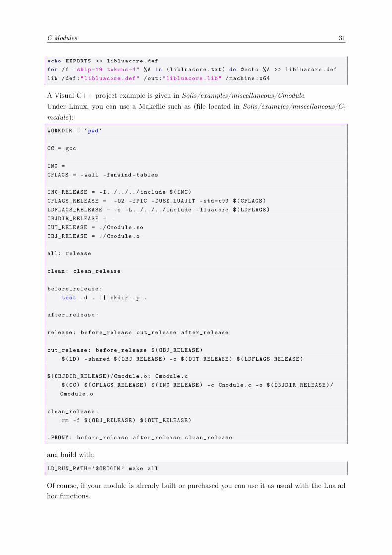
echo EXPORTS >> libluacore.deffor /f "skip =19 tokens =4" %A in (libluacore.txt) do @echo %A >> libluacore.deflib /def:"libluacore.def" /out:"libluacore.lib" /machine:x64

A Visual C++ project example is given in Solis/examples/miscellaneous/Cmodule.Under Linux, you can use a Makefile such as (file located in Solis/examples/miscellaneous/C-module):

WORKDIR = ‘pwd ‘

CC = gcc

INC =CFLAGS = -Wall -funwind -tables

INC_RELEASE = -I../../../ include $(INC)CFLAGS_RELEASE = -O2 -fPIC -DUSE_LUAJIT -std=c99 $(CFLAGS)LDFLAGS_RELEASE = -s -L../../../ include -lluacore $(LDFLAGS)OBJDIR_RELEASE = .OUT_RELEASE = ./ Cmodule.soOBJ_RELEASE = ./ Cmodule.o

all: release

clean: clean_release

before_release:test -d . || mkdir -p .

after_release:

release: before_release out_release after_release

out_release: before_release $(OBJ_RELEASE)$(LD) -shared $(OBJ_RELEASE) -o $(OUT_RELEASE) $(LDFLAGS_RELEASE)

$(OBJDIR_RELEASE)/Cmodule.o: Cmodule.c$(CC) $(CFLAGS_RELEASE) $(INC_RELEASE) -c Cmodule.c -o $(OBJDIR_RELEASE)/Cmodule.o

clean_release:rm -f $(OBJ_RELEASE) $(OUT_RELEASE)

.PHONY: before_release after_release clean_release

and build with:

LD_RUN_PATH=’$ORIGIN ’ make all

Of course, if your module is already built or purchased you can use it as usual with the Lua adhoc functions.

32 C Modules

Lastly, when your module was built as dll (under Windows) or so (under Linux), you can loadit and use it under Solis by using the standard Lua functions:

-- Load C module , the Lua standard waycls()local Cmodule = require("Cmodule")print(Cmodule.version ())

Instrumentation 33

Instrumentation

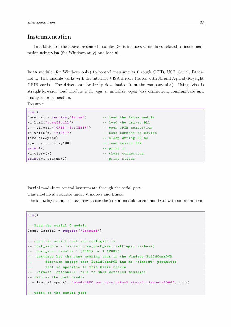
In addition of the above presented modules, Solis includes C modules related to instrumen-tation using visa (for Windows only) and lserial.

lvisa module (for Windows only) to control instruments through GPIB, USB, Serial, Ether-net ... This module works with the interface VISA drivers (tested with NI and Agilent/KeysightGPIB cards. The drivers can be freely downloaded from the company site). Using lvisa isstraightforward: load module with require, initialize, open visa connection, communicate andfinally close connection.Example:

cls()local vi = require("lvisa") -- load the lvisa modulevi.load("visa32.dll") -- load the driver DLLv = vi.open("GPIB ::8:: INSTR") -- open GPIB connectionvi.write(v, "*IDN?") -- send command to devicetime.sleep (50) -- sleep during 50 msr,n = vi.read(v ,100) -- read device IDNprint(r) -- print itvi.close(v) -- close connectionprint(vi.status ()) -- print status

lserial module to control instruments through the serial port.This module is available under Windows and Linux.The following example shows how to use the lserial module to communicate with an instrument:

cls()

-- load the serial C modulelocal lserial = require("lserial")

-- open the serial port and configure it-- port_handle = lserial.open(port_num , settings , verbose)-- port_num: usually 1 (COM1) or 2 (COM2)-- settings has the same meaning than in the Windows BuildCommDCB-- function except that BuildCommDCB has no ’timeout ’ parameter-- that is specific to this Solis module-- verbose (optional): true to show detailed messages-- returns the port handlep = lserial.open (1, "baud =4800 parity=n data=8 stop=2 timeout =1000", true)

-- write to the serial port

34 Instrumentation

-- lserial.write(port_handle , command)-- port_handle: the port handle , as returned by lserial.open-- command to send to the device-- returns the number of bytes writtenlserial.write(p, "*IDN?\n")

-- read from the serial port-- r,n = lserial.read(port_handle , bytes)-- port_handle: the port handle , as returned by lserial.open-- bytes: number of bytes to read-- returns the string read and the number of bytes readr,n = lserial.read(p, 128)io.write("\n recv = ", r, " ; bytes read = ", n)

-- close the serial port-- lserial.close(port_handle)-- port_handle: the port handle , as returned by lserial.openlserial.close(p)

Math Parser 35

Math Parser

The parser namespace includes functions to evaluate mathematical expressions:

p = parser.new()creates a new parser.

parser.set(p, name, value)sets variable.

val = parser.get(p, name)returns variable value.

val = parser.eval(p, expr)evaluates math expression.

val = parser.evalf(p, func, x)evaluates math function for x value.

val = parser.solve(p, eq, a, b)solves equation in [a,b] interval.

parser.delete(p)deletes a parser.

The math parser supports the following functions:

Exp(x)exponential

Ln(x)natural (Napierian) logarithm

Log(x)

36 Math Parser

decimal logarithm

Log2(x)base-2 logarithm

Sin(x)sine

Cos(x)cosine

Tan(x)tangent

Asin(x)arc sine

Acos(x)arc cosine

Atan(x)arc tangent

Sinh(x)hyperbolic sine

Cosh(x)hyperbolic cosine

Tanh(x)hyperbolic tangent

Abs(x)absolute value

Sqrt(x)square root

Cbrt(x)cubic root

Math Parser 37

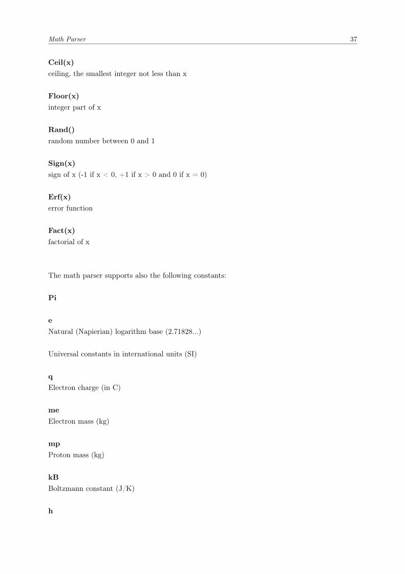
Ceil(x)ceiling, the smallest integer not less than x

Floor(x)integer part of x

Rand()random number between 0 and 1

Sign(x)sign of x (-1 if x < 0, +1 if x > 0 and 0 if x = 0)

Erf(x)error function

Fact(x)factorial of x

The math parser supports also the following constants:

Pi

eNatural (Napierian) logarithm base (2.71828...)

Universal constants in international units (SI)

qElectron charge (in C)

meElectron mass (kg)

mpProton mass (kg)

kBBoltzmann constant (J/K)

h

38 Math Parser

Planck constant (Js)

cSpeed of Light in vacuum (m/s)

eps0Electric constant (F/m)

mu0Magnetic constant (N/A2)

NAAvogadro constant (1/mole)

GConstant of gravitation (m3/kg/s2)

RiRydberg constant (1/m)

FFaraday constant (C/m)

RMolar gas constant (J/mole/K)

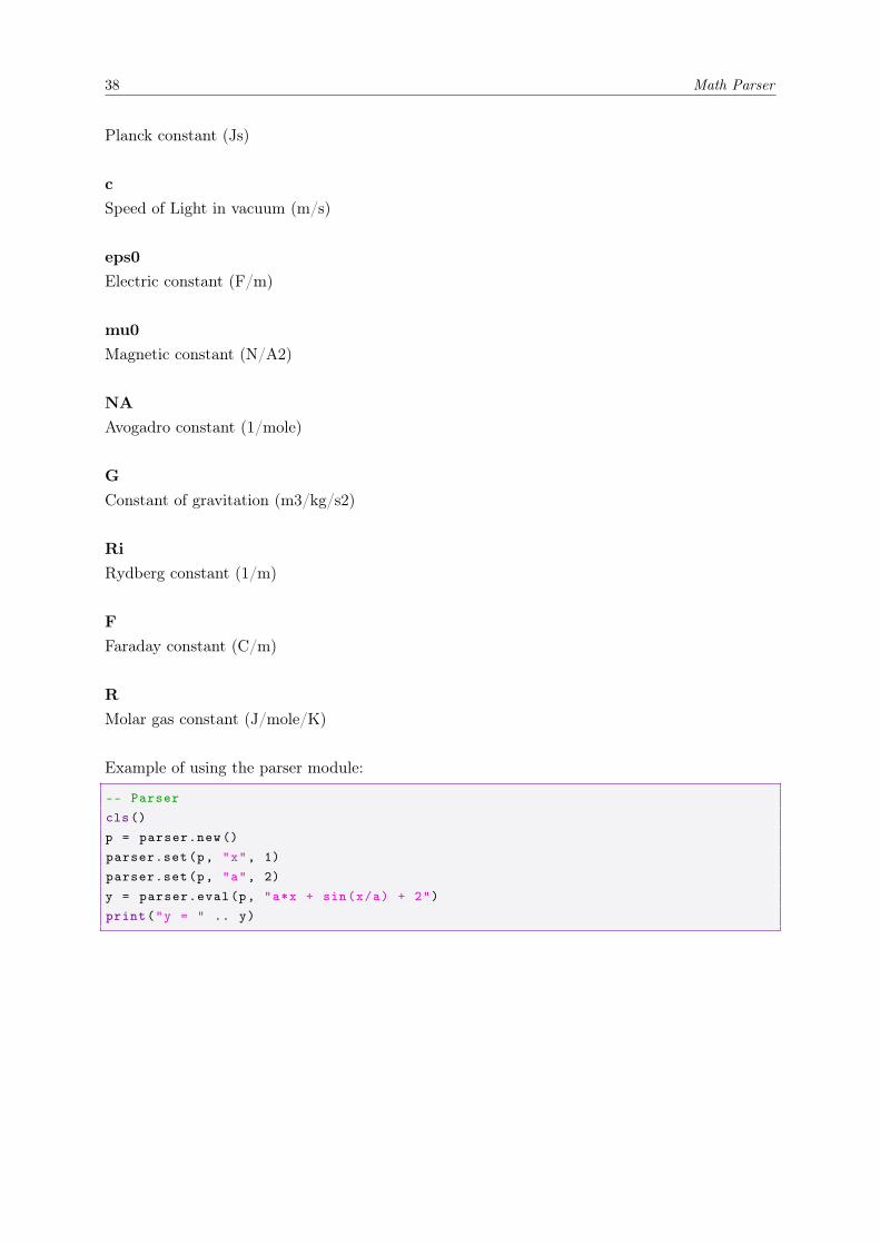
Example of using the parser module:

-- Parsercls()p = parser.new ()parser.set(p, "x", 1)parser.set(p, "a", 2)y = parser.eval(p, "a*x + sin(x/a) + 2")print("y = " .. y)

Graphical User Interface using IUP 39

Graphical User Interface using IUP

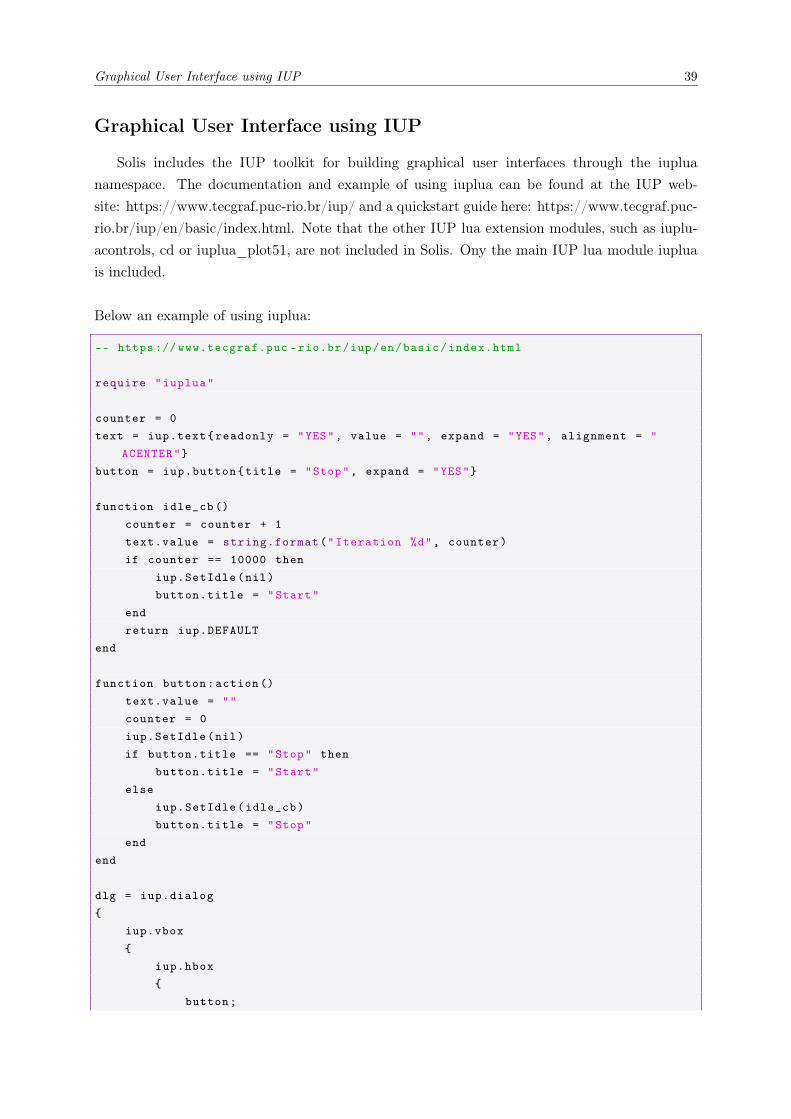
Solis includes the IUP toolkit for building graphical user interfaces through the iupluanamespace. The documentation and example of using iuplua can be found at the IUP web-site: https://www.tecgraf.puc-rio.br/iup/ and a quickstart guide here: https://www.tecgraf.puc-rio.br/iup/en/basic/index.html. Note that the other IUP lua extension modules, such as iuplu-acontrols, cd or iuplua_plot51, are not included in Solis. Ony the main IUP lua module iupluais included.

Below an example of using iuplua:

-- https :// www.tecgraf.puc -rio.br/iup/en/basic/index.html

require "iuplua"

counter = 0text = iup.text{readonly = "YES", value = "", expand = "YES", alignment = "

ACENTER"}button = iup.button{title = "Stop", expand = "YES"}

function idle_cb ()counter = counter + 1text.value = string.format("Iteration %d", counter)if counter == 10000 then

iup.SetIdle(nil)button.title = "Start"

endreturn iup.DEFAULT

end

function button:action ()text.value = ""counter = 0iup.SetIdle(nil)if button.title == "Stop" then

button.title = "Start"else

iup.SetIdle(idle_cb)button.title = "Stop"

endend

dlg = iup.dialog{

iup.vbox{

iup.hbox{

button;

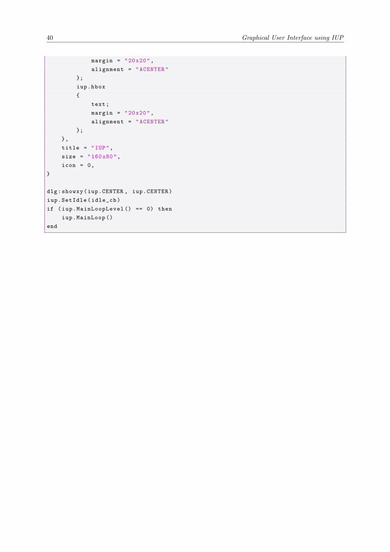
40 Graphical User Interface using IUP

margin = "20x20",alignment = "ACENTER"

};iup.hbox{

text;margin = "20x20",alignment = "ACENTER"

};},title = "IUP",size = "160x80",icon = 0,

}

dlg:showxy(iup.CENTER , iup.CENTER)iup.SetIdle(idle_cb)if (iup.MainLoopLevel () == 0) then

iup.MainLoop ()end

Solis Calculator

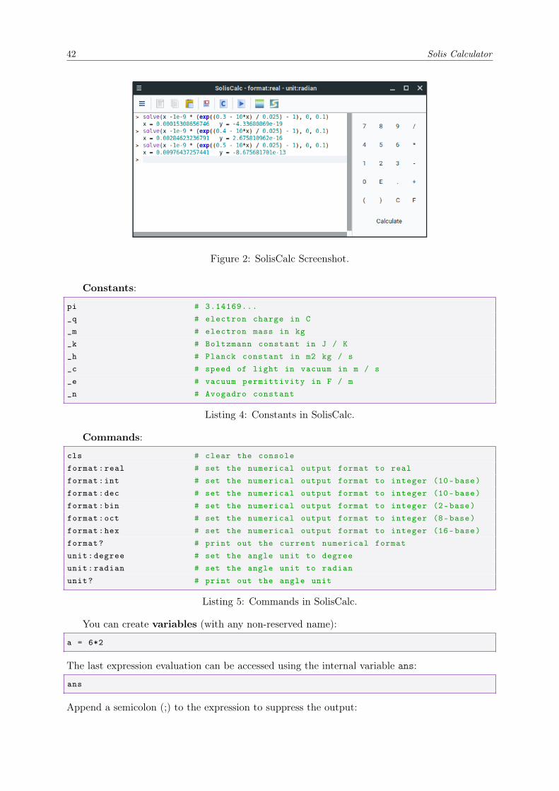
The Solis scientific calculator, SolisCalc, is an advanced mathematical expression-based calcu-lator (screenshot in figure 2). It supports the most common and useful functions. It’s easy to use:to evaluate an expression, simply write it, using operators ( + - * / ˆ ), parenthesis and math-ematical functions and press ENTER (or F12). One can also use the numeric keypad to enternumbers and operators. One can set variables (with any non-reserved name), using fundamentalconstants, etc. SolisCalc menu gives an easy way to use the software functionality.

The following mathematical functions are supported:

exp(x) # exponentialln(x) # natural logarithmlog(x) # decimal logarithmpow(x,n) # xnsin(x) # sinecos(x) # cosinetan(x) # tangentasin(x) # arc sineacos(x) # arc cosineatan(x) # arc tangentsinh(x) # hyperbolic sinecosh(x) # hyperbolic cosinetanh(x) # hyperbolic tangentabs(x) # absolute valuesqrt(x) # square rootceil(x) # ceiling , the smallest integer not less than xfloor(x) # floor , the largest integer not greater than xround(x) # nearest integer , roundingfmod(x,y) # x modulo yerf(x) # error functionjn(n,x) # Bessel function of x of the first kind of order nyn(n,x) # Bessel function of x of the second kind of order ngauss(x,m,s) # Gauss function: exp((x - m)^2 / 2s^2)lorentz(x,m,s) # Lorentz function: s / ((x - m)^2 + s^2)min(x,y) # smallest value of x and ymax(x,y) # largest value of x and yrand(x) # random number between 0 and 1time() # elapsed time in seconds since January 1, 1970sign(x) # sign of x (-1 if x < 0, +1 if x > 0 and 0 if x = 0)

Listing 3: Mathematical Functions in SolisCalc.

41

42 Solis Calculator

Figure 2: SolisCalc Screenshot.

Constants:

pi # 3.14169..._q # electron charge in C_m # electron mass in kg_k # Boltzmann constant in J / K_h # Planck constant in m2 kg / s_c # speed of light in vacuum in m / s_e # vacuum permittivity in F / m_n # Avogadro constant

Listing 4: Constants in SolisCalc.

Commands:

cls # clear the consoleformat:real # set the numerical output format to realformat:int # set the numerical output format to integer (10-base)format:dec # set the numerical output format to integer (10-base)format:bin # set the numerical output format to integer (2-base)format:oct # set the numerical output format to integer (8-base)format:hex # set the numerical output format to integer (16-base)format? # print out the current numerical formatunit:degree # set the angle unit to degreeunit:radian # set the angle unit to radianunit? # print out the angle unit

Listing 5: Commands in SolisCalc.

You can create variables (with any non-reserved name):

a = 6*2

The last expression evaluation can be accessed using the internal variable ans:

ans

Append a semicolon (;) to the expression to suppress the output:

Solis Calculator 43

a = 6*2;

A comment can be added at the end of an expression, using # :

y=sin(pi/4) # comment

Previous calculated expressions can be reused by pressing up or down arrows.

SolisCalc can be executed from the command line:

soliscalc -run input [-out outfile]

input may be a filename or a double-quoted expression and outfile is the output filename:

soliscalc -run "a=1;b=2;c=a*sin(b)"soliscalc -run calcin.txt -out calcout.txt

Integer arithmetic in binary, octal and hexadecimal bases:One can perform integer calculations in binary, octal, decimal and hexadecimal bases in 32 bitsunsigned format directly within the console, by prefixing the number with 0b for binary base, 0ofor octal base and 0x for hexadecimal base: just type the expression and press enter:

0xFFF7 + 12 + 0b111 + 0o547

To show result in hexadecimal, set accordingly the numerical output format (see listing 5):

format:hex

To solve a nonlinear equation f(x) = 0:

solve(x^2 - 2, 0, 10)

The syntax is solve(function, xl, xh) where function is the f(x) function expression (ex-ample: xˆ2 - 2 ), xl the x lower limit of the interval where the solution is to be found and xh

the x higher limit (xl and xh are optional).

A session (calculations history) can be saved in a text file (with extension .soliscalc) andretrieved later: menu File/Save and File/Open.

Bibliography

[1] S Ierusalimschy, L H Figueiredo, and Celes W. Lua 5.1 Reference Manual. Lua.org, 2006(cited p. 1).

[2] The IUP GUI toolkit, (C) 1994-2017 Tecgraf/PUC-Rio. 2017 (cited p. 1).

[3] S Ould Saad Hamady. “Solis: a modular, portable, and high-performance 1D semiconductordevice simulator”. In: Journal of Computational Electronics (2020), pp. 1–8 (cited p. 2).

[4] S Ould Saad Hamady. “SigmaSim: Enhanced One-Dimensional Simulator for SemiconductorDevices”. In: 37th International Symposium on Compound Semiconductors (ISCS), Taka-matsu, Japan. Oral. 2010 (cited p. 2).

45