Science of the Total Environment 479–480 (2014) 189–200

Contents lists available at ScienceDirect

Science of the Total Environment

j ourna l homepage: www.e lsev ie r .com/ locate /sc i totenv

Soil erodibility in Europe: A high-resolution dataset based on LUCAS

Panos Panagos a,⁎, Katrin Meusburger b, Cristiano Ballabio a, Pasqualle Borrelli a, Christine Alewell b

a European Commission, Joint Research Centre, Institute for Environment and Sustainability, Via E. Fermi 2749, I-21027 Ispra, VA, Italyb Environmental Geosciences, University of Basel, Bernoullistrasse 30, 4056 Basel, Switzerland

H I G H L I G H T S

• Soil erodibility in Europe is estimated at 0.032 t ha h ha−1 MJ−1 mm−1.• Stoniness has an important impact in Mediterranean countries.• High resolution (500 m grid cell) dataset of K-factor is available for modelling.• Coarse fragments, permeability and soil structure were considered in K-factor.• K-factor map has very good correspondence with regional data in literature studies.

⁎ Corresponding author. Tel.: +39 0332 785574; fax: +E-mail address: panos.panagos@jrc.ec.europa.eu (P. Pa

http://dx.doi.org/10.1016/j.scitotenv.2014.02.0100048-9697/© 2014 The Authors. Published by Elsevier B.V

a b s t r a c t

a r t i c l e i n f o

Article history:Received 25 September 2013Received in revised form 20 January 2014Accepted 2 February 2014Available online xxxx

Keywords:RUSLEK-factorStoninessModellingRegressionErosion

The greatest obstacle to soil erosion modelling at larger spatial scales is the lack of data on soil characteristics.One key parameter for modelling soil erosion is the soil erodibility, expressed as the K-factor in the widelyused soil erosion model, the Universal Soil Loss Equation (USLE) and its revised version (RUSLE). The K-factor,which expresses the susceptibility of a soil to erode, is related to soil properties such as organic matter content,soil texture, soil structure and permeability. With the Land Use/Cover Area frame Survey (LUCAS) soil surveyin 2009 a pan-European soil dataset is available for the first time, consisting of around 20,000 points across 25Member States of the European Union. The aim of this study is the generation of a harmonised high-resolutionsoil erodibility map (with a grid cell size of 500 m) for the 25 EU Member States. Soil erodibility was calculatedfor the LUCAS survey points using the nomograph of Wischmeier and Smith (1978). A Cubist regressionmodel was applied to correlate spatial data such as latitude, longitude, remotely sensed and terrain featuresin order to develop a high-resolution soil erodibility map. The mean K-factor for Europe was estimatedat 0.032 t ha h ha−1 MJ−1 mm−1 with a standard deviation of 0.009 t ha h ha−1 MJ−1 mm−1. The yielded soilerodibility dataset comparedwell with the published local and regional soil erodibility data. However, the incor-poration of the protective effect of surface stone cover, which is usually not considered for the soil erodibilitycalculations, resulted in an average 15% decrease of the K-factor. The exclusion of this effect in K-factor calcula-tions is likely to result in an overestimation of soil erosion, particularly for the Mediterranean countries, wherehighest percentages of surface stone cover were observed.

© 2014 The Authors. Published by Elsevier B.V. This is an open access article under the CC BY license(http://creativecommons.org/licenses/by/3.0/).

1. Introduction

Soil erosion is the most widespread form of soil degradation world-wide (Bridges andOldeman, 1999). Since soil erosion is difficult tomea-sure at large scales, soil erosion models are a crucial estimation tool atregional, national and European levels. The high heterogeneity of soilerosion causal factors, combined with often poor data availability is anobstacle for the application of complex soil erosion models. Thus, theempirical Revised Universal Soil Loss Equation (RUSLE) (Renard et al.,1997), which predicts the average annual soil loss resulting from rain-drop splash and runoff from field slopes, is still most frequently used

39 0332 786394.nagos).

. This is an open access article under

at large spatial scales (Renschler and Harbor, 2002; Panagos et al., inpress). The RUSLE is the simple multiplication of 5 soil erosion riskfactors, of which one is the soil erodibility also called K-factor. The K-factor is a lumped parameter that represents an integrated annualvalue of the soil profile reaction to the process of soil detachment andtransport by raindrops and surface flow (Renard et al., 1997). As suchsoil erodibility is best estimated by carrying out direct measurementson field plots (Kinnell, 2010). However, since field measurements areexpensive and often not easily transferable in space, researchers inves-tigated the relation between “classical” soil properties and soilerodibility.

A number of equations have been designed to predict soil erod-ibility, most famous is the soil erodibility nomograph of Wischmeieret al., 1971. Dangler and El-Swaify (1976) developed an equation for

the CC BY license (http://creativecommons.org/licenses/by/3.0/).

190 P. Panagos et al. / Science of the Total Environment 479–480 (2014) 189–200

Hawaiian soils. Other equations, such as that of Young and Mutcher(1977), require attributes that are not widely available to predictsoil erodibility (e.g. bulk density). During the 1990s, Römkens et al.(1997), Williams (1995) and Torri et al. (1997) developed simplerequations mainly based on soil texture.

At European level, Panagos et al. (2012a) estimated soil erodibilitybased on attributes (texture, organic carbon) which were availablefrom the Land Use/Cover Area frame Survey (LUCAS) topsoil data(Toth et al., 2013) using the original nomograph of Wischmeier et al.(1971). Inverse distance weighting (IDW) was used to interpolateerodibility to a map with a grid-cell resolution of 10 km. The dataset at-tracts great interest and it is available for download from the EuropeanSoil Data Centre (ESDAC); approximately 200 users have registered anddownloaded the data within two years. The greatmajority of these usedthe K-factor as an input for their USLE/RUSLE models, or for validationand comparison to their modelled or measured K-factor estimates.Past experience with the coarse-resolution soil erodibility datasetshowed that it is fairly difficult for soil erosion modellers to access soilprofile data in their area of interest.

However, a dataset with a resolution of 10-km grid cell can be con-sidered too rough for most applications especially as the vast majorityof users downloaded the K-factor for regional and local applications.Thus, the main objective of this paper is to produce a soil erodibilitydataset with a higher spatial resolution (500-m grid cell size). In orderto enable a better interpolation of the LUCAS point estimates Cubistregression-interpolation is applied. Besides the higher spatial resolutionachieved through the abovementioned interpolation technique, thisnew soil erodibility assessmentwill consider soil structure and the effectof stones both on the soil permeability and the shielding of rain splash.Moreover,Malta and Cyprus have been included in the analysis. Anothermajor improvement is that the estimated soil erodibility dataset will beverified against local, regional and national data found in the literature.

2. Materials and methods

2.1. Input data

The geographical extent of this study includes 25 Member States ofthe European Union (EU). Bulgaria, Romania and Croatia were not in-cluded as themain input dataset (LUCAS survey 2009) does not includedata for those countries.

2.1.1. LUCAS topsoil dataLUCAS (Land Use/Cover Area frame Survey) is an in-situ assessment,

whichmeans that the data is gathered through direct field observations.The aim of the LUCAS survey is to establish a fully harmonised databasewithin the EU on land use/cover and to document changes over time.A soil module was included in the LUCAS dataset for the first time in2009. Topsoil samples (0–30 cm, approximate weight of 0.5 kg) werecollected from 10% of the survey points, providing 19,969 soil samplesacross the 25 Member States. The density of LUCAS topsoil samplepoints is around 1 per 199 km2, corresponding to a grid cell size ofaround 14 km × 14 km (Panagos et al., 2013).

The objective of the soil module in the LUCAS dataset was to im-prove the availability of harmonised data on soil parameters inEurope. During the period 2010–2011, the 19,969 LUCAS soil sam-ples were analysed in a single ISO-certified laboratory to obtain a co-herent pan-European dataset. The significant advantage of thismethod is that discrepancies arising from inter-laboratory differ-ences (Cools et al., 2004) have been avoided. The results of the anal-ysis are stored in the LUCAS topsoil database (Toth et al., 2013),which includes (among others) the particle size distributionexpressed as percentages of clay (b0.002 mm), silt (0.002–0.05 mm), sand (0.05–2.0 mm) as well as organic carbon (%) andpercentage coarse material (N2.0 mm). Analysis of the soil parame-ters followed standard procedures (LUCAS, 2009a; ISO, 2013).

2.1.2. Stone cover percentageDuring the 2009 LUCAS data collection exercise, the surveyors

estimated the percentage of the surface that is covered with stones.Surveyors were given a chart (LUCAS, 2009b) to help them estimatethe percentage of stones present above the ground (Fig. 1). Accord-ing to the instruction guide (LUCAS, 2009b), the surveyors removedthe vegetation coverage and litters around the sampling point. Thesurveyors were trained to assign their estimation to one of the fiveclasses (LUCAS, 2009b) based on their visual assessment and thecharts provided in the instruction guide (Fig. 1). As surveyors inCyprus and Malta did not assess the percentage of stones, class =2 was assigned to their data as this is the predominant stonecover class in LUCAS for the southern parts of the Mediterraneancountries.

2.1.3. European Soil DatabaseThe European Soil Database (ESDB), at 1:1,000,000 resolution (King

et al., 1994), is a reference dataset for assessing the state of soils in theEU. The ESDB includes, among others, attributes such as texture andsoil types expressed as classes.

2.1.4. Covariates used for the Cubist regression modelCubist (Quinlan, 1992) is a rule based model tree where the ter-

minal leaves contain linear regression models. Prediction is obtainedusing the linear regressionmodel at the terminal node of the tree andsmoothed by taking into account the prediction from the linearmodel in the previous node of the tree. Various covariates were con-sidered for the Cubist model, but three main types were consideredto be significant:

1. Remotely sensed data derived from the Moderate ResolutionImaging Spectro-radiometer (MODIS), including vegetation indices(Normalized Difference Vegetation Index—NDVI, Enhanced Vegeta-tion Index — EVI) and raw band data which have been re-projectedusing Principal Component Analysis;

2. Terrain features, derived from the Shuttle Radar TopographyMission (SRTM) Digital Elevation Model, including commongeo-morphometric descriptors (elevation, slope, base level ofstreams, altitude above channel base level and multi-resolutionindex of valley bottom flatness);

3. Latitude and longitude.

TheMODIS data was acquired in 2009 during the same period as theLUCAS data, while the SRTM data refer to the year 2000.

2.2. Soil erodibility estimates for the LUCAS point dataset

As direct measurements of K-factor on field plots are not financiallysustainable at the regional or national levels, the soil erodibility nomo-graph (Wischmeier et al., 1971) is most commonly used and cited forsoil erodibility calculation. An algebraic approximation of the nomo-graph that includes five soil parameters (texture, organic matter, coarsefragments, structure, and permeability) is proposed byWischmeier andSmith (1978) and Renard et al. (1997) in Eq. (1):

K ¼ 2:1� 10−4 M1:14 12–OMð Þ þ 3:25 s−2ð Þ þ 2:5 p−3ð Þ� �

=100h i

� 0:1317ð1Þ

where:

M the textural factor with M = (msilt + mvfs) ∗ (100− mc);mc [%] clay fraction content (b0.002 mm);msilt [%] silt fraction content (0.002–0.05 mm);mvfs [%] very fine sand fraction content (0.05–0.1 mm);OM [%] the organic matter content;

Fig. 1.Methodology applied for the generation of a European K-factor (soil erodibility) map.

191P. Panagos et al. / Science of the Total Environment 479–480 (2014) 189–200

s the soil structure class (s = 1: very fine granular, s = 2: finegranular, s = 3, medium or coarse granular, s = 4: blocky,platy or massive; Table 1);

p the permeability class (p = 1: very rapid, …, p = 6: veryslow; Table 2).

The K-factor is expressed in the International System of units as t hah ha−1 MJ−1 mm−1. The proposed erodibility equation (Eq. (1)) canonly be recommended if organic matter content is known and silt con-tent is below 70%. If these criteria are met, this equation is more precisethan alternative equations (Declercq and Poesen, 1992). The

Table 1Classes of soil structure derived the European Soil Database.

Structure class (s) European Soil Database

1 (very fine granular: 1–2 mm) G (good)2 (fine granular: 2–5 mm) N (normal)3 (medium or coarse granular: 5–10 mm) P (poor)4 (blocky, platy or massive: N10 mm) H (humic or peaty top soil)

192 P. Panagos et al. / Science of the Total Environment 479–480 (2014) 189–200

methodology applied in this study (depicted in Fig. 1) was selectedbased on the availability of data to calculate input attributes at theEuropean level.

The combined application of the K-factor nomograph with theLUCAS dataset required three adaptions:

• According to Wischmeier and Smith (1978), Eq. (1) is restricted tosamples for which the silt fraction does not exceed 70%. A subset of718 soil samples collected in LUCAS 2009 had silt fractions in therange of 70%–80%. As these were mainly taken from northern France,southern Belgium and central Germany, it was considered essentialto be included in the calculation of the K-factor. An upper limit valueof 70% silt fractionwas assigned to those samples. The212 soil samplesthat exceeded the 80% silt fractionwere excluded from the calculation.

• In literature the sand fraction is categorised into five classes of sand:very fine, fine, medium, coarse, very coarse (Gee and Bauder, 1986;Gee and Or, 2002). The very fine sand structure (0.05–0.1 mm)as sub-factor (mvfs) in Eq. (1) is usually not subject of standard soilanalysis and was therefore estimated as 20% of the sand fraction(0.05–2.0 mm) which is available in the LUCAS topsoil database.

• For soil sampleswith organicmatter content above 4%, the upper limitof 4% has been applied (Wischmeier and Smith, 1978). The applicationof a 4% limit to soil organic matter intends to prohibit an underestima-tion of soil erodibility for soils that are rich in organic matter.

2.2.1. Estimation of structure classesGood soil structure and high aggregate stability are important for

improving soil fertility, enhancing porosity and decreasing erodibility(Bronick and Lal, 2005). In past studies (Bonilla and Johnson, 2012;Lopez-Vicente et al., 2008; Perez-Rodriguez et al., 2007), soil structurewas assigned based on soil types of the Food and Agriculture Organiza-tion (FAO). A pedotransfer rule for estimating soil structure when nodirect measurements are available has been developed by Van Ranstet al. (1995). In the European Soil Database, this pedotransfer rule clas-sifies the soil structure as humic, poor, normal or good (Table 1), usingpedological inputs such as the FAO soil name and soil texture (Joneset al., 2003). The latter dataset was used to derive the structure classvalues needed for K-factor calculation as given in Table 1.

2.2.2. Soil permeability estimationFor the estimation of the soil permeability, classes described in

the US Department of Agriculture's National Soils Handbook No. 430(USDA, 1983) were assigned according to soil texture classes (Table 2)(Rawls et al., 1982). These soil textural classes have also been employedfor the estimation of the range values of saturated hydraulic conduc-tivity, which are explained below (Table 2).

Table 2Soil permeability classes and saturated hydraulic conductivity ranges estimated frommajor soil textural classes.

Permeability class (p) Texture Saturated hydraulicconductivity, mm h−1

1 (fast and very fast) Sand N61.02 (moderate fast) Loamy sand, sandy loam 20.3–61.03 (moderate) Loam, silty loam 5.1–20.34 (moderate low) Sandy clay loam, clay loam 2.0–5.15 (slow) Silty clay loam, sand clay 1.0–2.06 (very slow) Silty clay, clay b1.0

Soil permeability is affected by the content of stones (N2 mm). TheAgriculture HandbookNo. 537 (Wischmeier and Smith, 1978) separatesthe influence of stone fragments into two components: a) surface rockfragments which can further reduce the splash detachment rate ina similar way to how vegetation protects soils from rainfall intensity;b) subsurface rock fragments that lead to increased soil loss due toreduced water infiltration.

The latter effect of coarse fragments is due to a reduction in theempty spaces (voids). As the LUCAS topsoil database includes coarsefragments (N2 mm), their effect on saturated hydraulic conductivityand soil erodibility can be calculated using the following equation(Brakensiek et al., 1986):

Kb=Kf ¼ 1−Rwð Þ ð2Þ

where Kb (mm day−1) is the modified saturated hydraulic conductivityafter accounting for the effect of rock fragments, and Kf is the saturatedhydraulic conductivity of thefine soil fraction (b2mm). Initial estimatesfor Kf were also assigned by classification of LUCAS texture informationinto the corresponding texture classes and associated saturated hydrau-lic conductivities of the US Department of Agriculture's National SoilsHandbook No. 430 (USDA, 1983). Rw is the percentage of coarse frag-ments greater than 2 mm. Rw reduces the saturated hydraulic conduc-tivity in the soil profile and can likely change the permeability class, asindicated in Table 2.

2.2.3. Adjustment of K-factor by inclusion of surface stone coverBesides the percentage of coarse fragments for the 0–30 cmsoil sam-

ples, LUCAS provides also a percentage estimate of the surface stonecover. Surface stone cover may have a negative effect on sedimentyield and thus, can be considered as natural soil-surface stabiliser.Rubio and Recatalá (2006) proposed stoniness to be included in thesoil erodibility index qualitative estimation. Poesen and Ingelmo-Sanchez (1992) carried out a review of the negative relationship be-tween stone cover and the relative interrill sediment yield. This negativerelationship is generally observed where stones are either partly em-bedded in the top layer or are on the surface of the soil.

Poesen et al. (1994) developed a soil erodibility reduction factorexpressed as an exponential decay function based on experimentalfield data:

St ¼ e−0:04 Rc−10ð Þ ð3Þ

where:

St is the correction factor for the relative decrease in sedimentyield;

Rc is the percentage of stones cover with 10% b Rc b 100%.

The mean rate of decay was calculated as 0.04. Similar equationswith different parameters that were proposed by other authors havegiven different rates of decay: 0.025 (Box, 1981), 0.044 (Simantonet al., 1986), 0.050 (Martin, 1988).

Table 3Classes of percentage surface stone cover of LUCAS database.

Class Percentage of stones Value (%) usedfor the Stcalculation

Number ofsamples andproportion (%)

St (correction factor)

0 0% 0.0% 95 (0.48%) 11 Stones ≤ 10% 5.0% 14,585 (73.37%) 12 10% b Stones b 25% 17.5% 3114 (15.66%) 0.7403 25% ≤ Stones b 50% 37.5% 1442 (7.25%) 0.3324 Stones ≥ 50 75.0% 643 (3.23%) 0.074

193P. Panagos et al. / Science of the Total Environment 479–480 (2014) 189–200

Surface stone cover was estimated by the LUCAS surveyor in fiveclasses (Table 3). The majority of the samples were found to have lessor equal to 10% of stones and a correction factor cannot be applied ac-cording to Eq. (3). For classes 2, 3 and 4 (Table 3), the mean value ofthe percentage class (Table 3 column 3) was applied in Eq. (3) resultingin three correction factors (St).

The updated soil erodibility value (Kst) incorporating surface stonecover was calculated according to Eq. (4):

Kst ¼ K � St: ð4Þ

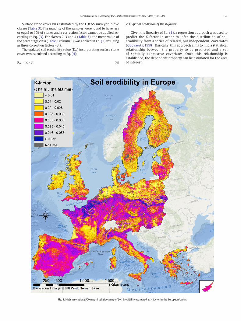
Fig. 2. High-resolution (500 m grid cell size) map of Soil Er

2.3. Spatial prediction of the K-factor

Given the linearity of Eq. (1), a regression approach was used topredict the K-factor in order to infer the distribution of soilerodibility from a series of related, but independent, covariates(Goovaerts, 1998). Basically, this approach aims to find a statisticalrelationship between the property to be predicted and a setof spatially exhaustive covariates. Once this relationship isestablished, the dependent property can be estimated for the areaof interest.

odibility estimated as K-factor in the European Union.

Fig. 3. K-factor compared to the European Soil Database (ESDB) soil surface textureclasses.

Table 4Summary of input soil property values used for the estimation of the K-factor.

Eq. (1) attributes Range Mean value Standarddeviation

Organic matter (OM) 0–4% 3.08% 1.05%Structure (S) 0, 1, 2, 3, 4 2a

Permeability incorporating coarsefragments (P)

1, 2, 3, 4, 5, 6 4a

Clay (mc) 0–100% 18.5% 13.4%Silt corrected (b70%) (msilt) 0–70% 35.5% 19.0%Very fine sand (mvfs) 0–20% 8.1% 5.5%K-factor (t ha h ha−1 MJ−1 mm−1) 0.004–0.076 0.0320 0.009

a Dominant value.

194 P. Panagos et al. / Science of the Total Environment 479–480 (2014) 189–200

2.3.1. Spatial analysisIn this study, the K-factor value of each LUCAS point sample was

interpolated using a series of spatially exhaustive environmental de-scriptors (covariates) in order to derive a continuous map for Europe.An alternative approachwould have been to apply the equation to inter-polated maps of all the soil properties needed in Eq. (1). However, thelatter approach has some critical drawbacks; first of all, every predictedproperty has its own error and (possibly) bias. This could lead to amisestimation of the K-factor which is not constant in the geographi-cal space. Moreover, it is inherently simpler to evaluate the effect ofcovariates on the value of K-factor if this is directly modelled as such,and not as the combination of the mapped variables upon which theK-factor is calculated.

The approach followed in this study made the calculation in twostages. Firstly, the regression model based on the Cubist rule (Quinlan,1992) was used to predict the value of the K-factor using a series ofcovariates. Cubist is a tree model where each terminal leaf contains alinear regression model. The prediction is made using the linear regres-sionmodel at the terminal nodes of the tree smoothed by taking into ac-count the predictions from previous nodes of the tree. Cubist makes anaverage of the sample value over a given neighbour (Quinlan, 1993).Once the first model is fitted, the nearest neighbours of a given instancecan be averaged and used as the proxy value for that instance. This pro-cedure avoids overfitting and makes the model more robust to outliers.

In the next stage, the residuals from the Cubist model were interpo-lated using Multilevel B-Splines (MBS) (Lee et al., 1997). In terms ofaccuracy and unbiasedness, MBS performs as well as kriging but itis computationally faster and allows an easy estimation of the interpo-lated field (K-factor).

Model performance was tested for both the fitting and a cross-validation dataset. In the bootstrapped cross-validation the randomsampling with replacement 1/10 of the original dataset (mutuallyexclusive with the training set) was used as a validation sample. Thebootstrap procedure was repeated 100 times to produce reliable esti-mates of the model predictive performance over LUCAS samples.

2.3.2. VerificationThe proposed high-resolution dataset was validated against local

and regional studies. An extensive review of published studies thatuse Eq. (1) was carried out. More than 100 soil erodibility assessmentswere found in the literature at local, regional or even national level(Hungary, Lithuania, Czech Republic and Slovakia). The authorscontacted the scientists who developed those assessments and receivedreplies and aggregated data of 21 published studies. The authorsattempted to ensure the maximum representativeness for the wholestudy area (with at least one study for each country).

3. Results and discussion

3.1. Soil erodibility in Europe

The mean K-factor for the 25 Member States was calculated as0.032 t ha h ha−1 MJ−1 mm−1 with a standard deviation of0.009 t ha h ha−1 MJ−1 mm−1 (Fig. 2). The range of values is0.004–0.076 t ha h ha−1 MJ−1 mm−1. The map (Fig. 2) does not in-clude lakes, bare rocks, glaciers and urban areas.

The Cubist regression model predicted the pan-European distribu-tion of the K-factor with a good performance as R2 = 0.4 and RMSE =0.0102 t ha h ha−1 MJ−1 mm−1 in k-fold cross validation. The interpo-lation using MBS further increased the prediction performance of theK-factor to an R2 of 0.94 for the fitting dataset. Cross-validation givesa less good performance (R2 of 0.74), given that part of the originalLUCAS points are left out for the prediction.

The spatial pattern of areas with high soil erodibility (Fig. 2) largelyfollows the Loess map of Europe 1:2,500,000 according to Haase et al.(2007). The mean K-factor value for the Loess areas of Europe was

estimated at 0.0419 t ha h ha−1 MJ−1 mm−1. A comparison betweenthe resulting K-factors and the textural classes of the European SoilDatabase shows that the highest mean values of the K-factor arein the medium–fine textural class (3), followed by the fine (4) and me-dium (2) classes, while the lowest mean values are recorded for coarse(1) and very fine (5) classes (Fig. 3). This follows the main rules of soilscience that coarse particles are relatively heavy and fine particleshave, due to their relatively large surface areas, high cohesion strengthand thus are less susceptible to soil detachment. Thus, the mediumsized texture classes are more prone to soil erosion. The organic soils(no mineral texture) have the lowest mean K-factor value.

Most of the soil samples belong to the Normal (N) soil structureclass of the ESDB corresponding to the fine granular (class: 2). The ma-jority of the samples had a moderate permeability class (3) whichwas corrected to moderate low (class: 4) with the incorporation ofcoarse fragments. A soil sample having as attributes the mean values(Table 4) of the input parameters of Eq. (1) will result in a K-factorequal to 0.032 t ha h ha−1 MJ−1 mm−1.

The aggregated country-level statistics present an overviewof the soil erodibility in Europe (Table 5). Organic matter has an im-portant impact on the soil erodibility pattern as countries with highconcentrations of organic matter have the lowest soil erodibility.Ireland, Estonia, Denmark, the Netherlands, the United Kingdom,Finland, Sweden and Latvia with high mean organic matter values(Jones et al., 2005) have mean soil erodibility values of less than0.030 t ha h ha−1 MJ−1 mm−1. On the other hand, the highest meanvalues (higher than 0.035 t ha h ha−1 MJ−1 mm−1) are observed in

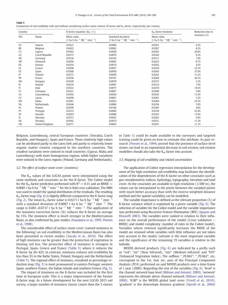
Table 5Comparison of soil erodibility with and without considering surface stone content (K-factor and Kst-factor, respectively) per country.

Country K-factor equation (Eq. (1)) Kst-factor stoniness Reduction due tostoniness (%)

ISO Name Mean value(t ha h ha−1 MJ−1 mm−1)

Standard deviation(t ha h ha−1 MJ−1 mm−1)

Mean value(t ha h ha−1 MJ−1 mm−1)

AT Austria 0.0321 0.0080 0.0291 9.5%BE Belgium 0.0422 0.0092 0.0387 8.2%CY Cyprus 0.0362 0.0028 0.0265 26.8%CZ Czech Republic 0.0373 0.0076 0.0342 8.3%DE Germany 0.0334 0.0102 0.0311 7.0%DK Denmark 0.0246 0.0065 0.0225 8.7%EE Estonia 0.0254 0.0074 0.0242 4.5%EL Greece 0.0298 0.0057 0.0229 23.3%ES Spain 0.0368 0.0058 0.0265 27.9%FI Finland 0.0273 0.0058 0.0242 11.2%FR France 0.0356 0.0101 0.0284 20.1%HU Hungary 0.0349 0.0078 0.0337 3.3%IE Ireland 0.0234 0.0047 0.0216 7.4%IT Italy 0.0322 0.0077 0.0276 14.5%LT Lithuania 0.0321 0.0067 0.0309 3.8%LU Luxembourg 0.0392 0.0036 0.0345 11.9%LV Latvia 0.0290 0.0067 0.0281 3.2%MT Malta 0.0381 0.0022 0.0284 25.5%NL Netherlands 0.0246 0.0084 0.0236 3.9%PL Poland 0.0299 0.0106 0.0285 4.8%PT Portugal 0.0333 0.0069 0.0194 41.8%SE Sweden 0.0293 0.0068 0.0252 13.9%SI Slovenia 0.0313 0.0052 0.0282 9.6%SK Slovakia 0.0362 0.0074 0.0321 11.3%UK United Kingdom 0.0271 0.0063 0.0241 11.1%

195P. Panagos et al. / Science of the Total Environment 479–480 (2014) 189–200

Belgium, Luxembourg, central European countries (Slovakia, CzechRepublic, and Hungary), Spain and France. Those relatively high valuescan be attributed partly to the Loess belt and partly to relatively lowerorganic matter content compared to the northern countries. Thesmallest variations were noticed in small countries (Cyprus, Malta andLuxembourg) with more homogenous regions, while higher variationswere noticed in the Loess regions (Poland, Germany and Netherlands).

3.2. The effect of surface stone cover (stoniness)

The Kst values of the LUCAS points were interpolated using thesame methods and covariates as for the K-factor. The Cubist modelfor the Kst-factor prediction performed with R2 = 0.31 and an RMSE =0.0081 t ha h ha−1 MJ−1 mm−1 for the k-fold cross validation. TheMBSwas used tomodel the spatial distribution of the residuals. The resultingKst-factor map (Fig. 4) is slightly different compared to the K-factor map(Fig. 2). The mean Kst-factor value is 0.0271 t ha h ha−1 MJ−1 mm−1

with a standard deviation of 0.0087 t ha h ha−1 MJ−1 mm−1. Therange is 0.001–0.0737 t ha h ha−1 MJ−1 mm−1. The application ofthe stoniness correction factor (St) reduces the K-factor on averageby 15%. The stoniness effect is much stronger in the MediterraneanBasin, as also confirmed by past studies (Danalatos et al., 1995; Poesenet al., 1998).

The considerable effect of surface stone cover (named stoniness inthe following) on soil erodibility in the Mediterranean Basin has alsobeen presented in recent studies (Zavala et al., 2010). The effectof high stoniness can be greater than the protection of vegetation inlimiting soil loss. The protective effect of stoniness is strongest inPortugal, Spain, Greece and France (Table 5) where it reduces theK-factor by 20–42%. In contrast, stoniness reduces soil erodibility byless than 5% in the Baltic States, Poland, Hungary and the Netherlands(Table 5). The regional effect of stoniness, visualised as percentage re-duction map (Fig. 5) is most pronounced in eastern Portugal, westernSpain, southern France, the Italian islands and southern Greece (Fig. 5).

The impact of stoniness on the K-factor was included for the firsttime at European scale. This is a major improvement of the formerK-factor map. As a future development for the next LUCAS 2015 soilsurvey, a larger number of stoniness classes (more than the 5 classes

in Table 3) could be made available to the surveyors and targetedtraining could be given on how to estimate this attribute. As past re-search (Poesen et al., 1994) proved that the presence of surface-levelstones can lead to an exponential decrease in soil erosion, soil erosionmodellers should also take the Kst-factor into account.

3.3. Mapping of soil erodibility and related uncertainties

The application of Cubist regression interpolation for the develop-ment of the high-resolution soil erodibility map facilitates the identifi-cation of the dependencies of the K-factor on other covariates such asgeo-morphometric indices, hydrology, topography, elevation and landcover. As the covariates are available in high resolution (≤500 m), thevalues can be interpolated to the pixels between the sampled pointswith much better accuracy than with the inverse weighted distancemethod and the spatial variability can be modelled.

The variable importance is defined as the relevant proportion (%) ofK-factor variance which is explained by a given variable (Fig. 6). Theselection of variables for the Cubist model and the variable importancewas performed using Recursive Feature Elimination (RFE) (Iguyon andElisseeff, 2003). The variables were ranked in relation to their influ-ence on the overall performance of the model (Cross validation —

RMSE) and model complexity (number of rules in the Cubist model).Variables whose removal significantly increases the RMSE of themodel are retained while variables with little influence are not takeninto account in the model. Latitude is the most important variableand the significance of the remaining 19 variables is relative to thelatitude.

MODIS derived products (Fig. 6) are indicated by a prefix suchas “red”, “nir” (Near Infrared), “mir” (Medium Infrared) and “EVI”(Enhanced Vegetation Index). The suffixes “_PCAb1”, “_PCAb2”, etc.correspond to the 1st, 2nd, etc. axes of the Principal ComponentAnalysis (PCA) performed on said MODIS products over a time frameof 1 year (2009). Regarding the rest of the variables (Fig. 6), ‘level’ isthe channel network base level (Böhner and Antonić, 2009), ‘network’represents the altitude above channel network (Böhner and Antonić,2009), ‘IGBP’ is the MODIS global land cover (Friedl et al., 2010),‘gradient’ is the downslope distance gradient (Hjerdt et al., 2004)

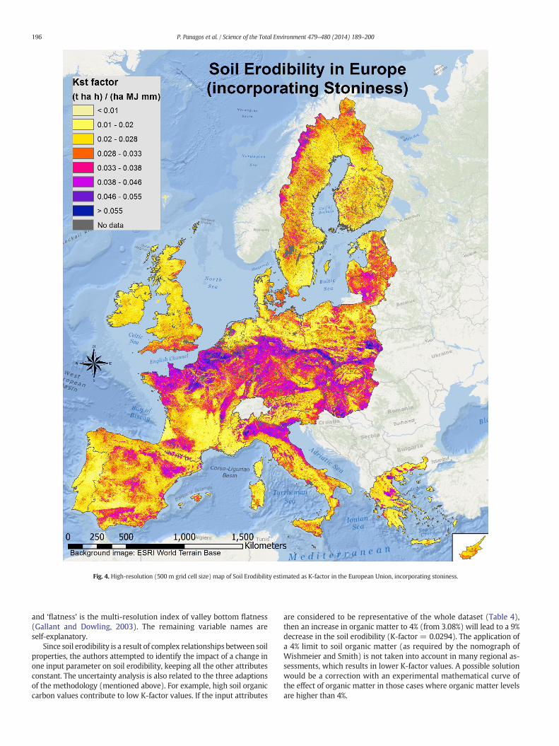
Fig. 4. High-resolution (500 m grid cell size) map of Soil Erodibility estimated as K-factor in the European Union, incorporating stoniness.

196 P. Panagos et al. / Science of the Total Environment 479–480 (2014) 189–200

and ‘flatness’ is the multi-resolution index of valley bottom flatness(Gallant and Dowling, 2003). The remaining variable names areself-explanatory.

Since soil erodibility is a result of complex relationships between soilproperties, the authors attempted to identify the impact of a change inone input parameter on soil erodibility, keeping all the other attributesconstant. The uncertainty analysis is also related to the three adaptionsof the methodology (mentioned above). For example, high soil organiccarbon values contribute to low K-factor values. If the input attributes

are considered to be representative of the whole dataset (Table 4),then an increase in organic matter to 4% (from 3.08%) will lead to a 9%decrease in the soil erodibility (K-factor = 0.0294). The application ofa 4% limit to soil organic matter (as required by the nomograph ofWishmeier and Smith) is not taken into account in many regional as-sessments, which results in lower K-factor values. A possible solutionwould be a correction with an experimental mathematical curve ofthe effect of organic matter in those cases where organic matter levelsare higher than 4%.

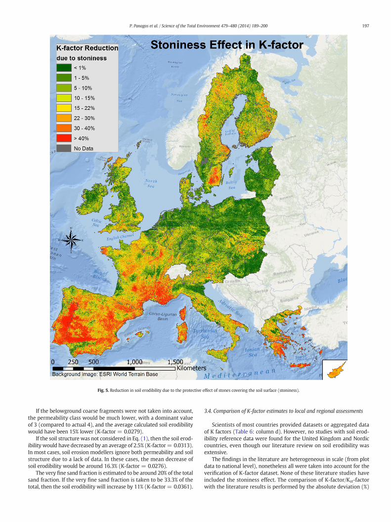
Fig. 5. Reduction in soil erodibility due to the protective effect of stones covering the soil surface (stoniness).

197P. Panagos et al. / Science of the Total Environment 479–480 (2014) 189–200

If the belowground coarse fragments were not taken into account,the permeability class would be much lower, with a dominant valueof 3 (compared to actual 4), and the average calculated soil erodibilitywould have been 15% lower (K-factor = 0.0279).

If the soil structure was not considered in Eq. (1), then the soil erod-ibility would have decreased by an average of 2.5% (K-factor= 0.0313).In most cases, soil erosion modellers ignore both permeability and soilstructure due to a lack of data. In these cases, the mean decrease ofsoil erodibility would be around 16.3% (K-factor = 0.0276).

The very fine sand fraction is estimated to be around 20% of the totalsand fraction. If the very fine sand fraction is taken to be 33.3% of thetotal, then the soil erodibility will increase by 11% (K-factor = 0.0361).

3.4. Comparison of K-factor estimates to local and regional assessments

Scientists of most countries provided datasets or aggregated dataof K factors (Table 6: column d). However, no studies with soil erod-ibility reference data were found for the United Kingdom and Nordiccountries, even though our literature review on soil erodibility wasextensive.

The findings in the literature are heterogeneous in scale (from plotdata to national level), nonetheless all were taken into account for theverification of K-factor dataset. None of these literature studies haveincluded the stoniness effect. The comparison of K-factor/Kst-factorwith the literature results is performed by the absolute deviation (%)

Fig. 6. The twenty most important covariates and their relative importance in the applica-tion of Cubist/MBS model for K-factor interpolation.

198 P. Panagos et al. / Science of the Total Environment 479–480 (2014) 189–200

(Table 6: columns g, h). The sign (−) is applied in case the aggregatedK-factor/Kst-factor data are lower than the ones found in the literature.

The comparison of our K-factor (Table 6: column e) against theregional studies (Table 6: column d) shows a deviation of about 14.3%in absolute terms (Table 6: column g). In most of the cases, K-factormean values are higher than those of the regional studies, with the ex-ception of the Lithuanian study, two local Polish studies and Frenchcatchment. At national and regional levels, the correspondence ofK-factor to the study area aggregated data was very positive with theexception of Brandenburg (Deumlich, 2009) where the permeabilityhad not been taken into consideration. The 14.3% average deviationcan be attributed to either the application of the 4% limit in organicmat-ter or to the incorporation of coarse fragments in the calculation of the

Table 6Comparison of K-factor estimates with local/regional/national studies.

Catchment/region(country) (a)

Coverage(no of points) (b)

Reference study (c)

Hungary (HU) National (2851) Centeri and Pataki (2000)Slovakia (SK) National Styk et al. (2008)Czech Republic (CZ) National Dostal et al. (2002)Lithuania (LT) National Mažvila et al. (2010)Hessen federal state (DE) Regional Tetzlaff et al. (2013)Bavaria federal state (DE) Regional (1051) Auerswald (1992)Nordrhein-Westfalen federalstate (DE)

Regional Elhaus (2013)

Brandenburg federal state (DE) Regional Deumlich (2009)Region of Sicily (IT) Regional (1813) Bagarello et al. (2012)Geul catchment (Maastricht, NL) Regional de Moor and Verstraeten (2008)Strymonas (GR) Regional Panagos et al. (2012b)Andalucia (ES) Regional (8) Ruiz-Sinoga and Diaz (2010)Sele Catchment, Basilicata (IT) Regional Diodato et al. (2011)Lautaret, Province Alps-Coted'Azur (FR)

Local Bakker et al. (2008)

Yialias River Catchment (CY) Local Alexakis et al. (2013)Gregos (PT) Local (97) Ferreira and Panagopoulos (2010Pico (PT) Local (25) Ferreira and Panagopoulos (2010Roncão (PT) Local (82) Ferreira and Panagopoulos (2010Bogucin, Poznan (PL) Local Rejman et al. (2008)Lazy, Carpathian foothill (PL) Local (7 plots) Swiechowicz (2010)Lublin, South Warsaw (PL) Local Wawer et al. (2005)Overall average 21 studies

permeability. However, the very good correspondence of K-factor withliterature data at local and regional scales shows how the soil erodibilityequation can be successfully applied at the European scale.

The relative agreement between the stoniness-corrected (Kst-factor)and the literature data is almost equally good. The Kst-factor (Table 6:column f) has an average deviation of 18.0% compared to the literaturestudies (Table 6: column h) and especially for the Mediterranean coun-tries the change towards smaller K-factor values is considerable. Thus,neglecting surface stone cover will likely result in an overestimation ofsoil erosion risk in these countries.

4. Conclusions

The presented soil erodibility map (Fig. 2) is an important contribu-tion to the estimation of soil erosion from local to European scales,as the K-factor is very crucial among the input factors used to esti-mate soil loss according to RUSLE and other models. In addition, theK-factor can usually not easily be determined or calculated by indi-vidual soil erosion modellers with no extensive data access. Withthe publication of this study, modellers and in general scientists willbe able to download the high-resolution datasets (K-factor, Kst-factor)from the European Soil Data Centre.

Compared with past attempts to predict soil erodibility at theEuropean level (Van der Knijff et al., 2000), the presented K-factordataset has the advantage of pan-European harmonised soil data. Inaddition, topsoil data was collected within one year (2009) all acrossEurope and analysed by the same ISO-certified laboratory. Furthermore,the past approach to map soil erodibility at European scale (Van derKnijff et al., 2000) was based on 5 estimated textural classes oflarge soil mapping units of the European Soil Database while the newK-factor dataset is based on measured values.

The proposed model provides a framework for the digital soil map-ping of the soil erodibility at continental scale. The Cubist regressionmodel successfully established the relation between the K-factorand environmental features with the advantage of explaining thespatial distribution of soil erodibility. This also improves the spatialaccuracy of the end product and allows establishing rules uponwhich the K-factor can be estimated from remotely sensed data.

K-factor of referencestudy (d)

K-factor(Fig. 2) (e)

Kst factor(Fig. 4) (f)

Deviation ofK-factor vs.study (g)

Deviation ofKst-factorvs. study (h)

Mean value (t ha h ha−1 MJ−1 mm−1) (%)

0.0293 0.0349 0.0337 16.0% 13.1%0.029 0.0362 0.0321 19.9% 9.7%0.0376 0.0373 0.0342 (−) 0.8% (−) 9.9%0.035 0.0321 0.0309 (−) 9.0% (−) 13.3%0.0400 0.0411 0.0382 2.6% (−) 4.8%0.0331 0.0367 0.0337 9.7% 1.8%0.033 0.0370 0.0337 10.7% 2.2%

0.0163 0.0232 0.0223 29.7% 27.0%0.0291 0.0300 0.0230 3.2% (−) 26.7%0.0420 0.0449 0.0383 6.5% (−) 9.6%0.0241 0.0292 0.0247 17.4% 2.3%0.0303 0.0379 0.0245 20.1% (−) 23.7%0.026 0.0269 0.0230 3.5% (−) 13.2%0.037 0.0344 0.0254 (−) 7.6% (−) 45.7%

0.0261 0.0378 0.0280 30.9% 6.6%) 0.0344 0.0383 0.0215 10.2% (−) 60.2%) 0.0290 0.0394 0.0192 26.4% (−) 50.9%) 0.0229 0.0382 0.0201 40.1% (−) 13.7%

0.0598 0.0623 0.0594 4.1% (−) 0.7%0.0738 0.0588 0.0552 (−) 25.6% (−) 33.8%0.0285 0.0267 0.0261 (−) 6.6% (−) 9.2%0.0344 0.0373 0.0308 14.3% 18.0.%

199P. Panagos et al. / Science of the Total Environment 479–480 (2014) 189–200

Another advantage is that the remote sensing products are con-stantly updated giving the possibility for dynamic prediction ofthe K-factor. On the contrary, the used remote sensing productsare not tailed for the prediction of soil properties and this possiblylimits the model accuracy.

The high-resolution soil erodibility map (Fig. 2) incorporates certainimprovements over the coarse-resolution map (Panagos et al., 2012a):

▪ Soil structure was for the first time included in the K-factorestimation.

▪ Coarse fragments were taken into account for the better estimationof soil permeability.

▪ Surface stone content, which acts as protection against soil erosionwas for the first time included in the K-factor estimation. This cor-rection is of great interest for the Mediterranean countries wherestoniness is an important regulating parameter of soil erosion.

Soil erodibility, together with management practices (P-factor) andvegetation cover (C-factor) can be influenced by agricultural practices.Therefore, the K-factor dataset can be a guide for applying better conser-vation practices (e.g., increase or preserve soil organic carbon in areasprone to high levels of soil erosion risk or adaption of soil managementat areas of high risk).

The K-factor dataset may also be proposed as an index for the vul-nerability of ecosystems. The soil erodibility maps (Figs. 2, 4) delineateareas where soil reaction to erosive rainfall events is considerablyhigh. Areas where the stoniness effect is relatively low (b10%) and soilerodibility is still high (Kst N 0.046 t ha h ha−1 MJ−1 mm−1) shouldbe treated with considerable care in terms of agricultural practicesand vegetation cover. For example, dependent on the force and timingof erosive rain events, local/regional policies can classify those areas asbeing ecologically vulnerable and propose the application of permanentcrops or permanent grasslands.

The study also identified possible future improvements that can bemade in the future LUCAS topsoil 2015 data collection process. Dataanalysis of the fraction of very fine sand and hydraulic conductivitywould certainly improve the textural and permeability calculation fac-tors, and lead to more precise estimations of soil erodibility.

Conflict of interest

The authors confirm and sign that there is no conflict of interestswith networks, organisations, and data centres referred in the paper.

Acknowledgements

The authors would like to thank Gráinne Mulhern for revision of thearticle from a linguistic point of view.

References

Alexakis DD, Hadjimitsis DG, Agapiou A. Integrated use of remote sensing, GIS and precip-itation data for the assessment of soil erosion rate in the catchment area of "Yialias" inCyprus. Atmos Res 2013;131:108–24.

Auerswald K. Predicted and measured sediment Loads of large watersheds in Bavaria.5th International Symposium of River sedimentation; 1992.

Bagarello V, Di Stefano V, Ferro V, Giordano G, Iovino M, Pampalone V. Estimating theUSLE soil erodibility factor in Sicily, South Italy. Appl Eng Agric 2012;28(2):199–206.

Bakker MM, Govers G, van Doorn A, Quetier F, Chouvardas D, Rounsevell M. The responseof soil erosion and sediment export to land-use change in four areas of Europe: theimportance of landscape pattern. Geomorphology 2008;98(3–4):213–26.

Böhner J, Antonić O. Chapter 8 Land-surface parameters specific to topo-climatology.In: Hengl Tomislav, Reuter Hannes I, editors. Developments in Soil Science, vol. 33.Elsevier; 2009. p. 195–226.

Bonilla CA, Johnson OI. Soil erodibility mapping and its correlation with soil properties inCentral Chile. Geoderma 2012;189–190:116–23.

Box J. The effects of surface slaty fragments on soil erosion by water. Soil Sci Soc Am J1981;45:111–6.

Brakensiek DL, Rawls WJ, Stephenson GR. Determining the saturated hydraulic conduc-tivity of a soil containing rock fragments. Soil Sci Soc Am J 1986;50(3):834–5.

Bridges EM, Oldeman LR. Global assessment of human-induced soil degradation. Arid SoilRes Rehabil 1999;13(4):319–25.

Bronick CJ, Lal R. Soil structure and management: a review. Geoderma 2005;124(1–2):3–22.

Centeri Cs, Pataki R. Erosion map of Hungary. Proceedings of the Conference on Environ-mental Management of the Rural Landscape in Central and Eastern Europe,Podbanske, Slovakia September 2–6, 2000 80-7137-940-9; 2000. p. 20–2.

Cools N, et al. Quality assurance in forest soil analyses: a comparison between Europeanlaboratories. Accred Qual Assur 2004;9:688–94.

Dangler EW, El-Swaify SA. Erosion of selected Hawaii soils by simulated rainfall. Soil SciSoc Am J 1976;40(5):769–73.

Danalatos NG, Kosmas CS, Moustakas NC, Yassoglou N. Rock fragments: II. Their impacton soil physical properties and biomass production under Mediterranean conditions.Soil Use Manage 1995;11:121–6.

de Moor JJW, Verstraeten G. Alluvial and colluvial sediment storage in the Geul Rivercatchment (The Netherlands) — combining field and modelling data to construct aLate Holocene sediment budget. Geomorphology 2008;95(3–4):487–503.

Declercq F, Poesen J. Evaluation of two models to calculate the soil erodibility factor K.Pedologie 1992;42(2):149–69.

Deumlich D. Map of the potential erosion risk in Brandenburg using DIN19708 (ABAG) inthe version of ZALF Müncheberg e.V; 2009.

Diodato N, Fagnano M, Alberico I, Chirico GB. Mapping soil erodibility from composeddata set in Sele River Basin, Italy. Nat Hazards 2011;58(1):445–57.

Dostal T, Krasa J, Vaska J, Vrana K. The map of soil erosion hazard and sediment transportin scale of the Czech Republic. Vodni Hospodarstvi 2002;2:46–50.

Elhaus D. Informationssystem Bodenkarte von NRW 1: 50,000; 2013 [Personalcommunication].

Ferreira V, Panagopoulos T. Soil erodibility assessment at the Alqueva Dam Watershed,Portugal. Advances in climate changes, global warming, biological problems andnatural hazards; 2010112–8.

Friedl MA, Sulla-Menashe D, Tan B, Schneider A, Ramankutty N, Sibley A, et al. MODISCollection 5 global land cover: algorithm refinements and characterization of newdatasets. Remote Sens Environ 2010;114:168–82.

Gallant JC, Dowling TI. A multiresolution index of valley bottom flatness for mappingdepositional areas. Water Resour Res 2003;39(12).

Gee GW, Bauder JW. Particle size analysis. In: Klute A, editor. Methods of soil analysis.Part 1. Physical and mineralogical methods; 1986. p. 383–411.

Gee GW, Or D. Methods of soil analysis; 2002255–79 [Part. Accessed from http://cprl.ars.usda.gov (July 2013)].

Goovaerts P. Geostatistical tools for characterizing the spatial variability of microbiologi-cal and physico-chemical soil properties. Biol Fertil Soils 1998;27(4):315–34.

Haase D, Fink J, Haase G, Ruske R, Pecsi M, Richter H, et al. Loess in Europe—its spatialdistribution based on a European Loess Map, scale 1:2,500,000. Quat Sci Rev2007;26(9–10):1301–12.

Hjerdt KN, McDonnell JJ, Seibert J, Rodhe A. A new topographic index to quantify down-slope controls on local drainage. Water Resour Res 2004;40.

Iguyon I, Elisseeff A. An introduction to variable and feature selection. J Mach Learn Res2003;3:1157–82.

ISO. International Organization for Standardization. ISO 10694 (1995), ISO 11277 (1998),ISO 11464 (2006). Accessed from http://www.iso.ch, 2013. [Dec 2013].

Jones RJA, Spoor G, Thomasson AJ. Vulnerability of subsoils in Europe to compaction:a preliminary analysis. Soil Tillage Res 2003;73(1–2):131–43.

Jones RJA, Hiederer R, Rusco E, Montanarella L. Estimating organic carbon in the soils ofEurope for policy support. Eur J Soil Sci 2005;56(5):655–71.

King D, Daroussin J, Tavernier R. Development of a soil geographic database from the SoilMap of the European Communities. Catena 1994;21(1):37–56.

Kinnell PIA. Event soil loss, runoff and the Universal Soil Loss Equation family of models:a review. J Hydrol 2010;385:384–97.

Lee S, Wolberg G, Shin SY. Scattered data interpolation with multilevel B-splines. IEEETrans Vis Comput Graph 1997;3(3):229–44.

Lopez-Vicente M, Navas A, Machin J. Identifying erosive periods by using RUSLE factors inmountain fields of the Central Spanish Pyrenees. Hydrol Earth Syst Sci 2008;12(2):523–35.

LUCAS. Service Provision for technical support in the LUCAS study, provision of centrallaboratory services for soil analysis. Accessed from http://web.jrc.ec.europa.eu/callsfortender/index.cfm?action=app.showdoc&id=2731, 2009. [Dec 2013].

LUCAS. Technical reference document C-1. Land Use/ Cover Area Frame Survey. Instruc-tions for surveyors. EUROSTATEUROSTAT; 2009b.

Martin W. Die Erodierbarkeit von B6den unter simulierten und natiirlichen Regen und ihreAbhaingigkeit von Bodeneigenschaften. Unpubl. Ph.D. thesis T.U. Munchen; 1988.

Mažvila J, Staugaitis G, Kutra G, Jankauskas BŽemės Ūkio Mokslai 2010;17(3–4):69–78.Panagos P, Meusburger K, Alewell C, Montanarella L. Soil erodibility estimation using

LUCAS point survey data of Europe. Environ Model Software 2012a;30:143–5.Panagos P, Karydas CG, Gitas IZ, Montanarella L. Monthly soil erosion monitoring

based on remotely sensed biophysical parameters: a case study in Strymonas riverbasin towards a functional pan-European service. Int J Digit Earth 2012b;5(6):461–87.

Panagos P, Ballabio C, Yigini Y, Dunbar M. Estimating the soil organic carbon content forEuropean NUTS2 regions based on LUCAS data collection. Sci Total Environ2013;442:235–46.

Panagos P, Meusburger K, van Liedekerke M, Alewell C, Hiederer R, Montanarella L.Assessing soil erosion in Europe based on data collected through a European net-work. Soil Sci Plant Nutr 2014. [in press].

Perez-Rodriguez R, Marques MJ, Bienes R. Spatial variability of the soil erodibility param-eters and their relation with the soil map at subgroup level. Sci Total Environ2007;378(1–2):166–73.

200 P. Panagos et al. / Science of the Total Environment 479–480 (2014) 189–200

Poesen J, Ingelmo-Sanchez F. Runoff and sediment yield from topsoils with differentporosity as affected by rock fragment cover and position. Catena 1992;19(5):451–74.

Poesen JW, Torri D, Bunte K. Effects of rock fragments on soil erosion by water at differentspatial scales: a review. Catena 1994;23(1–2):141–66.

Poesen JW, VanWesemael B, Bunte K, Benet AS. Variation of rock fragment cover and sizealong semiarid hillslopes: a case-study from southeast Spain. Geomorphology1998;23(2–4):323–35.

Quinlan. Learning with continuous classes. Proceedings of the 5th Australian Joint Confer-ence On Artificial Intelligence; 1992. p. 343–8.

Quinlan. Combining instance-based and model based learning. Proceedings of the TenthInternational Conference on Machine Learning; 1993. p. 236–43.

Rawls WJ, Brakensiek CL, Saxton KE, Transactions — American Society of AgriculturalEngineers. Estimation of soil water properties. Trans Am Soc Agric Eng 1982;25(5):1316–20. [1328].

Rejman J, Brodowski R, Iglik I. Annual variations of soil erodibility of silt loam developedfrom loess based on 10-years runoff plot studies. Annals of Warsaw University of LifeScienceAnnals of Warsaw University of Life Science; 200877–83 [Land ReclamationNo 39].

Renard KG, Foster GR, Weessies GA, McCool DK. Predicting soil erosion by water: a guideto conservation planning with the Revised Universal Soil Loss Equation (RUSLE). In:Yoder DC, editor. U.S. Department of Agriculture, Agriculture Handbook 703; 1997.

Renschler CS, Harbor J. Soil erosion assessment tools from point to regional scales —

the role of geomorphologists in land management research and implementation.Geomorphology 2002;47(2–4):189–209.

Römkens MJM, Young RA, Poesen JWA, McCool DK, El-Swaify SA, Bradford JM. Soilerodibility factor (K). (Compilers)In: Renard KG, Foster GR, Weesies GA, McCoolDK, Yoder DC, editors. Predicting soil erosion by water: a guide to conservationplanning with the Revised Universal Soil Loss Equation (RUSLE). Washington, DC,USA: Agric. HB No. 703, USDA; 1997. p. 65–99.

Rubio José L, Recatalá L. The relevance and consequences of Mediterranean desertificationincluding security aspects. Desertification in the Mediterranean Region. A SecurityIssue NATO Security Through Science Series, vol. 3; 2006133–65.

Ruiz-Sinoga JD, Diaz AR. Soil degradation factors along a Mediterranean pluviometricgradient in Southern Spain. Geomorphology 2010;118(3–4):359–68.

Simanton JR, Johnson CW, Nyhan JW, Romney EM. Rainfall simulation on rangeland ero-sion plots. In: Lane LJ, editor. Erosion on rangelands: emerging technology and database. Denver, CO: Society for Range Management; 1986. p. 11–7.

Styk J, Fulajtar E, Palka B, GranecM.Updated calculationof erodibility of soil factor (k-factor)for the purpose of detailed digital layer generation. Proceedings No. 30, 2008

Soil Science and Conservation Research Institute, Bratislava (Slovak Republic)978-80-89128-51-8; 2008. p. 139–46.

Swiechowicz J. Slopewash on agricultural foothill slopes in hydrological years 2007–2008in Lazy. Pace I Studia Geograficzne. T, 45; 2010243–63.

Tetzlaff B, Friedrich K, Vorderbrugge T, Vereecken H, Wendland F. Distributed modellingof mean annual soil erosion and sediment delivery rates to surface waters. Catena2013;102:13–20.

Torri D, Poesen J, Borselli L. Predictability and uncertainty of the soil erodibility factorusing a global dataset. Catena 1997;31(1–2):1–22.

Toth G, Jones A, Montanarella L. The LUCAS topsoil database and derived information onthe regional variability of cropland topsoil properties in the European Union. EnvironMonit Assess 2013;185(9):7409–25.

USDA. National Soil Survey Handbook (NSSH). Web address:http://www.nrcs.usda.gov/wps/portal/nrcs/detail/national/soils/?cid=nrcs142p2_054242, 1983. [accessedDecember 2013].

Van der Knijff JM, Jones RJA, Montanarella L. Soil erosion risk assessment in Europe.European Soil Bureau. European Commission, JRC Scientific and Technical Report,EUR 19044 EN; 2000 [34 pp.].

Van Ranst E, Thomasson AJ, Daroussin J, Hollis JM, Jones RJA, JamagneM, et al. Elaborationof an extended knowledge database to interpret the 1:1,000,000 EU Soil Map for en-vironmental purposes. In: King D, Jones RJA, Thomasson AJ, editors. European land in-formation systems for agro-environmental monitoring, EUR 16232 EN. Luxembourg:Office for Official Publications of the European Communities; 1995. p. 71–84.

Wawer R, Nowocien E, Podolski B. Real and calculated KUSLE erodibility factor for selectedPolish soils. Pol J Environ Stud 2005;14(5):655–8.

Williams JR. Chapter 25: the EPIC model. In: Singh VP, editor. Computer models of water-shed hydrology. Water Resources Publications; 1995. p. 909–1000.

Wischmeier W, Smith D. Predicting rainfall erosion losses: a guide to conservationplanning. Agricultural Handbook No. 537. Washington DC, USA: U.S. Departmentof Agriculture; 1978.

Wischmeier W, Johnson C, Cross B. A soil erodibility nomograph for farmland and con-struction sites. J Soil Water Conserv 1971;26(3):189–93.

Young R, Mutchler C. Erodibility of some Minnesota soils. J. Soil Water Conserv1977;32(3):180–2.

Zavala LM, Jordán A, Bellinfante N, Gil J. Relationships between rock fragment cover andsoil hydrological response in a Mediterranean environment. Soil Sci Plant Nutr2010;56:95–104.