ECOHYDROLOGYEcohydrol. (2014)Published online in Wiley Online Library(wileyonlinelibrary.com) DOI: 10.1002/eco.1472

Soil clay influences Acacia encroachment in a South Africangrassland

Séraphine Grellier,1* Nicolas Florsch,2 Jean-Louis Janeau,3 Pascal Podwojewski,4,5

Christian Camerlynck,6 Sébastien Barot,7 David Ward8 and Simon Lorentz51 University of Science and Technology of Hanoi (USTH), 18 Hoang Quoc Viet, Cau Giay, Hanoi, Vietnam

2 Sorbonne Universités, UPMC Univ Paris 06, UMI 209, UMMISCO, F-75005, Paris, France3 IRD-BIOEMCO c/o Soils and Fertilisers Research Institute (SFRI), Dong Ngac, Chem, Tu Liem District, Hanoi, Vietnam

4 IRD-BIOEMCO, 32, av. H. Varagnat, 93143, Bondy cedex, France5 Center for Water Resources Research, University of KwaZulu-Natal, Box X01, Scottsville 3209, South Africa

6 Sorbonne Universités, UPMC Univ Paris 06, UMR 7619 Metis, F-75005, Paris, France7 IRD-BIOEMCO, Ecole Normale Supérieure, 46 rue d’Ulm, 75230, Paris 05, France

8 School of Life Sciences, University of KwaZulu-Natal, Box X01, Scottsville 3209, South Africa

*CTecE-m

Co

ABSTRACT

Because of technical difficulties in measuring soil properties at a large scale, little is known about the effect of soil properties onthe spatial distribution of trees in grasslands. We were interested in the associations of soil properties with the phenomenon oftree encroachment, where trees increase in density at the expense of grasses. The spatial variation of soil properties and especiallysoil texture may modify the properties of hydraulic conductivity, and the availability of soil water and mineral nutrients, which inturn may affect the spatial distribution of encroaching trees. Through the development of a geophysical method (Slingram) usingan electromagnetic device EM38 and Bayesian inversion, we were able to accurately map soil electrical conductivity (EC) of aLuvisol in a grassland of South Africa. EC measured at the 0·8 to 2m depth on a 1·5 ha area is a proxy for clay content and wascorrelated with the spatial distribution of four size classes of the encroaching Acacia sieberiana. Tree location (all sizesconsidered) was significantly correlated with EC. Tall acacias (>3m height) were totally absent from patches with EC>24mSm�1. For all other size classes from medium trees to seedlings, tree density decreased with increasing EC. This suggeststhat high clay contents at depth associated with high EC values may prevent the establishment and/or survival of trees andinfluence the spatial distribution of A. sieberiana. This result also shows that geophysical tools may be useful for demonstratingimportant ecological processes. Copyright © 2014 John Wiley & Sons, Ltd.

KEY WORDS Acacia sieberiana; Bayesian inversion; conductivity; EM38; geophysics; Slingram method; soil horizon; woodyplant encroachment

Received 23 August 2013; Revised 7 January 2014; Accepted 7 January 2014

INTRODUCTION

Woody plant encroachment in grassland has been widelystudied (Archer, 1995; Brown and Archer, 1999; Sankaranet al., 2005; Ward, 2005; Sankaran et al., 2008;Van Auken, 2009). The main factors controlling thisphenomena are the availability of resources (water, nutrients),fires, herbivory (Sankaran et al., 2004) and possibly globalclimate changes (Bond and Midgley, 2000; Ward, 2010).Scientists have only recently started to explore the factorscontrolling the spatial pattern of encroaching tree populations(Wiegand et al., 2006; Halpern et al., 2010; Robinson et al.,2010). However, a better understanding of these patterns

orrespondence to: Séraphine Grellier, University of Science andhnology (USTH), 18 Hoang Quoc Viet, Cau Giay, Hanoi, Vietnam.ail: seraphine.grellier@usth.edu.vn

pyright © 2014 John Wiley & Sons, Ltd.

would give new insights into the complex issue of themechanisms leading to encroachment (Ward, 2005;Graz, 2008). Various models have been proposed, includingspatially explicit models (Wiegand et al., 2005; Wiegandet al., 2006; Meyer et al., 2007) where trees are aggregated inpatches whose dynamics are driven mainly by rainfall andinter-tree competition with a shift between facilitation andcompetition (Callaway andWalker, 1997; Halpern et al., 2010).Soil nutrient patches have also been highlighted as drivingspatial patterns of palm trees in tropical humid savanna ofLamto in the Ivory Coast (Barot et al., 1999). The oppositerelationship, i.e. herbaceous or woody vegetation modifyingsoil properties and ecosystem functioning, has also beendemonstrated (Lata et al., 2004; Grellier et al., 2013b; Verboomand Pate, 2013). If other studies mentioned the importance ofsoil properties on dynamics of woody vegetation (Britz andWard, 2007; Schleicher et al., 2011), few have tested the effects

S. GRELLIER et al.

of soil properties on vegetation spatial pattern in grasslands(Browning et al., 2008; Eggemeyer and Schwinning, 2009;Robinson et al., 2010; Colgan et al., 2012). Spatial variations insoil properties and especially soil texture may modify theavailability of soil moisture (Weng and Luo, 2008;Wang et al.,2012), the availability of mineral nutrients (Bechtold andNaiman, 2006) and hydraulic conductivity (Corwin and Lesch,2005). All these factors may affect the spatial distribution ofvegetation (Robinson et al., 2010).The lack of studies addressing this type of issue is probably

due to technical issues of measuring soil properties at thelandscape scale. The recent interdisciplinary links between soilscience, hydrology and ecology (Young et al., 2010) offeruseful possibilities for throwing new light on this issue by takinginto account more factors that could be missed otherwise.Within this framework, Robinson et al. (2008) consideredgeophysical methods for mapping soil properties at thewatershed scale and related them to vegetation spatial patterns.In this study, we explore the relationships between the

spatial pattern of trees and soil properties such as clay contentthrough geophysical measurements. As roots of adultand young trees reach different soil layers (Grellier, 2011)and because different processes affect their growth (Callawayand Walker, 1997; Grellier et al., 2012a), we may finddifferences between the spatial distributions of size classes oftrees. We focused on Acacia sieberiana, which encroachesgrasslands of KwaZulu-Natal in South Africa. The mainquestions that we aimed to answer are as follows:

1. Does the spatial pattern of acacias depend on soilproperties (particularly clay content) at different depths?

2. Does this pattern change with Acacia size?

We answer these two questions by studying the relation-ship between tree location according to tree size on a 1·5haarea and measured electrical conductivity (EC) of soil linkedto the clay content of a two-layered shallow soil, e.g. a topsoilat 0–0·8m (upper layer) and a subsoil at 0·8–2m (lowerlayer). We used the non-destructive Slingram method tocharacterize the EC of the first 2m of soil. This method hasoften been used to study interactions between plants and soils(Myers et al., 2007; Hossain et al., 2010). A previous study(Grellier et al., 2013a), dedicated to methodology, validatedthe geophysical method, which was used and was simplifiedin this study to assess our ecological questions regarding treeencroachment (cf. Discussion Section).

MATERIALS AND METHODS

Description of the study site

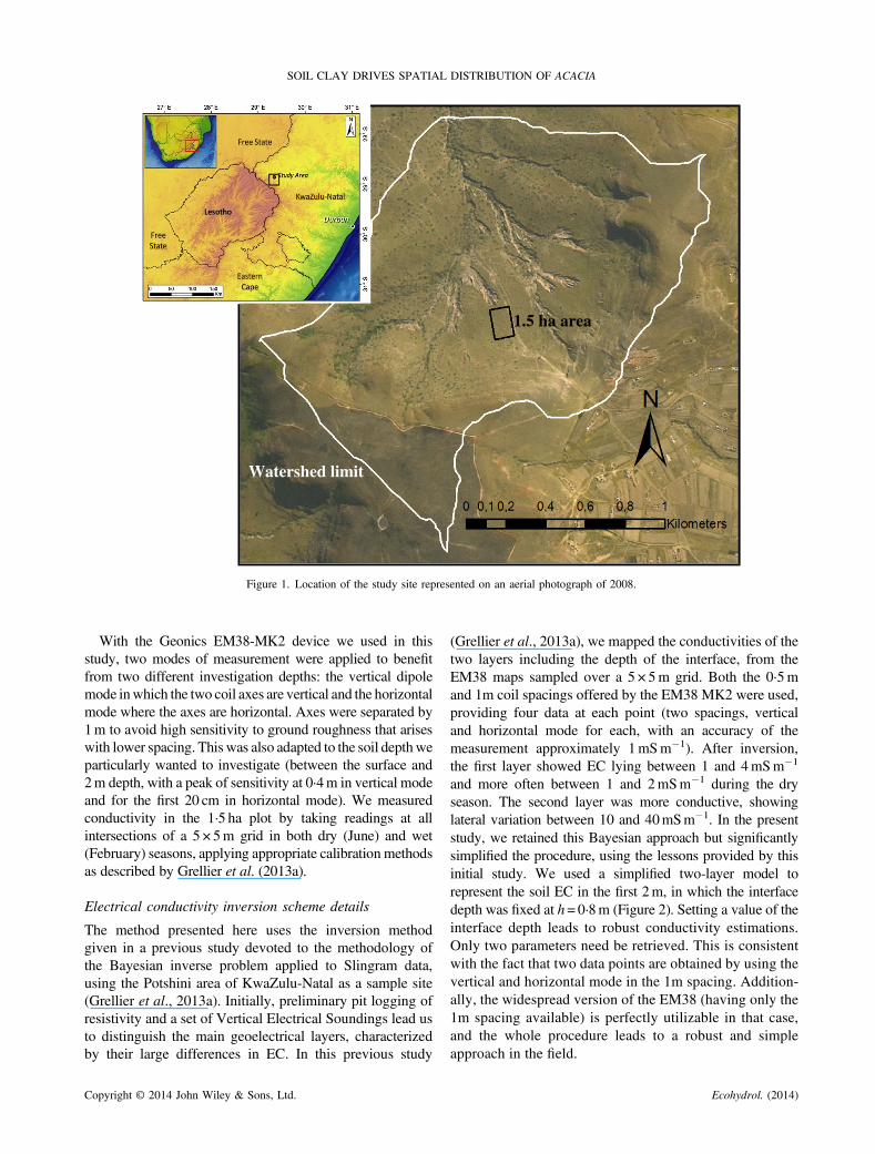
We conducted the study in a communal grassland of thePotshini village (28° 48′ 37″ S; 29° 21′ 19″ E), Kwazulu-Natal province, South Africa (Figure 1). The average

Copyright © 2014 John Wiley & Sons, Ltd.

altitude of the selected area of 1·5 ha (100m×150m) was1305m a.s.l. The climate is sub-humid sub-tropical withfour seasons, of which two are well marked: wet summer(October to April) and dry winter (May to September). Themean annual precipitation calculated from 1945 to 2009was 750mm (Grellier et al., 2012b). The mean annualtemperature in 2008 and 2009 was 16·3 °C. This sitebelongs to the Northern KwaZulu-Natal moist grasslandbiome (Mucina and Rutherford, 2006). Encroachment by asingle indigenous tree species, A. sieberiana var. woodii(Burtt Davy) Keay & Brenan, has occurred in the valley forthe last 30 years (Grellier et al., 2012b). The geology of thesite is characterized by fine-grained sandstones, shales,siltstone andmudstones that alternate in horizontal successionand belong to the Beaufort and Ecca Groups of the KarooSupergroup (King, 2002). Unconsolidated colluvial polycy-clic deposits up to 15m thick from the Pleistocene fill thevalleys and are very prone to linear gully erosion (Botha et al.,1994). The general soil type is Luvisol (FAO, 1998) withthree well-delimited main horizons. The A horizon (between0 and 40–50 cm) is coherent, loamy texture with browncolour (10 yr 4/1 to 10 yr 4/3). The BtHorizon (from 40–50 to70 cm) is dark brown (5–10 yr 4/2), clay-loamy, verycoherent and hard with a coarse blocky structure. The Chorizon below 80cm depth is a Pleistocenic colluvium 0·30–5m thick, brown (7·5 yr 4/6 to 5/6) sandy clay loam, notwell structured, prone to dispersion. This layer could beconsidered as a Paleosol. The clay mineralogy is exclusivelyIllite in the A and Bt horizon and an interstratified illite/illite-smectite in the C horizon. Evidence of lepidocrocite,mineral typical of temporary water-logging appear just abovethe Bt horizon (comm. pers. P. Podwojewski).

Topsoil and subsoil electrical conductivity measurementwith the Slingram EM38 device

The Slingram method for water and clay contentassessment has been applied by several authors (Cockxet al., 2007; Hezarjaribi and Sourell, 2007). The generalprinciple of the Slingram EM38 device is well described byMcNeill (1980). To summarize, one coil serves as atransmitter and produces an alternative magnetic field inthe ground (14·6 kHz for the EM38-MK2 used here). Thisprimary magnetic field induces an electric field E as statedby Maxwell–Faraday’s equation. The induced electric fieldleads to a current density →J according to Ohm’s law→J ¼ σ→E, where σ is the EC. These currents produce asecondary magnetic field following Maxwell–Ampere’sequation. The former is detected by the second coil(receiver) and is electronically separated from the primaryfield. This secondary field directly reflects a meanconductivity weighted in the medium under the coils.The depth of investigation mainly depends not only on thecoil separation but also on the direction of the coils’ axes.

Ecohydrol. (2014)

1.5 ha area

Watershed limit

Figure 1. Location of the study site represented on an aerial photograph of 2008.

SOIL CLAY DRIVES SPATIAL DISTRIBUTION OF ACACIA

With the Geonics EM38-MK2 device we used in thisstudy, two modes of measurement were applied to benefitfrom two different investigation depths: the vertical dipolemode inwhich the two coil axes are vertical and the horizontalmode where the axes are horizontal. Axes were separated by1m to avoid high sensitivity to ground roughness that ariseswith lower spacing. This was also adapted to the soil depthweparticularly wanted to investigate (between the surface and2m depth, with a peak of sensitivity at 0·4m in vertical modeand for the first 20 cm in horizontal mode). We measuredconductivity in the 1·5 ha plot by taking readings at allintersections of a 5 × 5m grid in both dry (June) and wet(February) seasons, applying appropriate calibration methodsas described by Grellier et al. (2013a).

Electrical conductivity inversion scheme details

The method presented here uses the inversion methodgiven in a previous study devoted to the methodology ofthe Bayesian inverse problem applied to Slingram data,using the Potshini area of KwaZulu-Natal as a sample site(Grellier et al., 2013a). Initially, preliminary pit logging ofresistivity and a set of Vertical Electrical Soundings lead usto distinguish the main geoelectrical layers, characterizedby their large differences in EC. In this previous study

Copyright © 2014 John Wiley & Sons, Ltd.

(Grellier et al., 2013a), we mapped the conductivities of thetwo layers including the depth of the interface, from theEM38 maps sampled over a 5 × 5m grid. Both the 0·5mand 1m coil spacings offered by the EM38 MK2 were used,providing four data at each point (two spacings, verticaland horizontal mode for each, with an accuracy of themeasurement approximately 1mSm�1). After inversion,the first layer showed EC lying between 1 and 4mSm�1

and more often between 1 and 2mSm�1 during the dryseason. The second layer was more conductive, showinglateral variation between 10 and 40mSm�1. In the presentstudy, we retained this Bayesian approach but significantlysimplified the procedure, using the lessons provided by thisinitial study. We used a simplified two-layer model torepresent the soil EC in the first 2m, in which the interfacedepth was fixed at h=0·8m (Figure 2). Setting a value of theinterface depth leads to robust conductivity estimations.Only two parameters need be retrieved. This is consistentwith the fact that two data points are obtained by using thevertical and horizontal mode in the 1m spacing. Addition-ally, the widespread version of the EM38 (having only the1m spacing available) is perfectly utilizable in that case,and the whole procedure leads to a robust and simpleapproach in the field.

Ecohydrol. (2014)

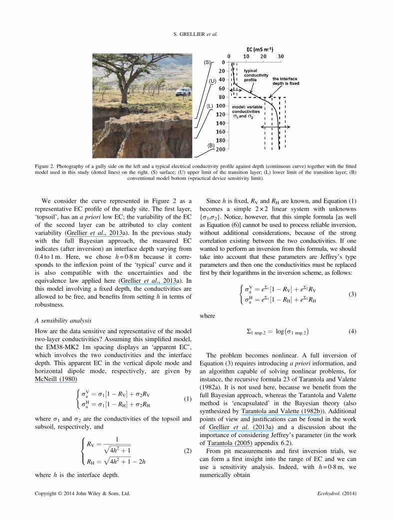
Figure 2. Photography of a gully side on the left and a typical electrical conductivity profile against depth (continuous curve) together with the fittedmodel used in this study (dotted lines) on the right. (S) surface; (U) upper limit of the transition layer; (L) lower limit of the transition layer; (B)

conventional model bottom (=practical device sensitivity limit).

S. GRELLIER et al.

We consider the curve represented in Figure 2 as arepresentative EC profile of the study site. The first layer,‘topsoil’, has an a priori low EC; the variability of the ECof the second layer can be attributed to clay contentvariability (Grellier et al., 2013a). In the previous studywith the full Bayesian approach, the measured ECindicates (after inversion) an interface depth varying from0.4 to 1m. Here, we chose h = 0·8m because it corre-sponds to the inflexion point of the ‘typical’ curve and itis also compatible with the uncertainties and theequivalence law applied here (Grellier et al., 2013a). Inthis model involving a fixed depth, the conductivities areallowed to be free, and benefits from setting h in terms ofrobustness.

A sensibility analysis

How are the data sensitive and representative of the modeltwo-layer conductivities? Assuming this simplified model,the EM38-MK2 1m spacing displays an ‘apparent EC’,which involves the two conductivities and the interfacedepth. This apparent EC in the vertical dipole mode andhorizontal dipole mode, respectively, are given byMcNeill (1980)

σVa ¼ σ1 1� RV½ � þ σ2RV

σHa ¼ σ1 1� RH½ � þ σ2RH

((1)

where σ1 and σ2 are the conductivities of the topsoil andsubsoil, respectively, and

RV ¼ 1ffiffiffiffiffiffiffiffiffiffiffiffiffiffiffi4h2 þ 1

pRH ¼

ffiffiffiffiffiffiffiffiffiffiffiffiffiffiffi4h2 þ 1

p� 2h

8><>: (2)

where h is the interface depth.

Copyright © 2014 John Wiley & Sons, Ltd.

Since h is fixed, RV and RH are known, and Equation (1)becomes a simple 2 × 2 linear system with unknowns{σ1,σ2}. Notice, however, that this simple formula [as wellas Equation (6)] cannot be used to process reliable inversion,without additional considerations, because of the strongcorrelation existing between the two conductivities. If onewanted to perform an inversion from this formula, we shouldtake into account that these parameters are Jeffrey’s typeparameters and then one the conductivities must be replacedfirst by their logarithms in the inversion scheme, as follows:

σVa ¼ eΣ1 1� RV½ � þ eΣ2RV

σHa ¼ eΣ1 1� RH½ � þ eΣ2RH

((3)

where

Σ1 resp:2 ¼ log σ1 resp:2� �

(4)

The problem becomes nonlinear. A full inversion ofEquation (3) requires introducing a priori information, andan algorithm capable of solving nonlinear problems, forinstance, the recursive formula 23 of Tarantola and Valette(1982a). It is not used here, because we benefit from thefull Bayesian approach, whereas the Tarantola and Valettemethod is ‘encapsulated’ in the Bayesian theory (alsosynthesized by Tarantola and Valette (1982b)). Additionalpoints of view and justifications can be found in the workof Grellier et al. (2013a) and a discussion about theimportance of considering Jeffrey’s parameter (in the workof Tarantola (2005) appendix 6.2).From pit measurements and first inversion trials, we

can form a first insight into the range of EC and we canuse a sensitivity analysis. Indeed, with h = 0·8m, wenumerically obtain

Ecohydrol. (2014)

SOIL CLAY DRIVES SPATIAL DISTRIBUTION OF ACACIA

RV ¼ 1ffiffiffiffiffiffiffiffiffiffiffiffiffiffiffi4h2 þ 1

p ¼ 1ffiffiffiffiffiffiffiffiffiffiffiffiffiffiffiffiffiffiffiffiffiffiffi4 0:8ð Þ2 þ 1

q ≅ 0:53

RH ¼ffiffiffiffiffiffiffiffiffiffiffiffiffiffiffi4h2 þ 1

p� 2h≅0:29

8>><>>: (5)

and

σVa ¼ 0:47σ1 þ 0:53σ2

σHa ¼ 0:71σ1 þ 0:29σ2

((6)

It shows that, for the vertical mode, 53% of the apparentEC results from σ2 and 47% from σ1. If we give typicalvalues of 2 and 20mSm�1 to the two conductivities σ1 andσ2, respectively, it shows that the contribution of thesecond layer is at least 10 times that of the first layer,whereas the ratio is about 4 in the horizontal mode. Thesensitivity of the measurement in the vertical dipole modeto the conductivities below 2 m is reduced toRV 2ð Þ ¼ 1ffiffiffiffi

17p ≅ 0:24%. In the rest of the study, we consider

that the inverted second layer EC is representative of theconductivity between 0·8 and approximately 2m.

Conversion of the electrical conductivity into clay content

Soil EC can be divided into two types, linked to the amount ofwater and clay content (Revil and Glover, 1997, 1998; Leroyand Revil, 2004). The first type is a bulk conductivity relatedto Archie’s law, and the second type is a surface conductivitylinked to thewater trapped by clay. Following this distinction,and according to Frohlich and Parke (1989), the effectiveconductivity (which is also the apparent conductivity asdetermined by the device) can be written as

σeff ¼ σwater

aΘk þ σsurface (7)

whereσwater is the EC of the water,Θ the (mobile) volumetricwater content, a is a factor reflecting the influence of mineralgrains on current flow and σsurface is the surface EC related tothe clay content. Mualem and Friedman (1991) propose asimilar relation, setting k=2·5 and involving the porosity ϕ:

σeff ¼ σwater

ϕΘ2:5 þ σsurface (8)

The volumetric water content is classically linked to thesaturation (Sw) and porosity (ϕ) through Archie’s lawwhere n is the saturation exponent and m is the cementationexponent of the rock:

Θk ¼ Snwϕm (9)

In the dry season, when the water content is very low,two cases may arise: (i) there is almost no clay, and the ECis residual and very low (below 5mSm�1); (ii) clays aresignificantly present, and we can assume the observedEC is due to the particles’ surface conductivity only. In

Copyright © 2014 John Wiley & Sons, Ltd.

formula (7) or (8), it is not certain whether the observedresidual is due to a residual amount of water or due to asmall amount of clay. However, when no mobile water isavailable, the residual conductivity is a surface conductiv-ity. This alternative issue has no major consequence in thepresent study.To convert the EC into clay content, we can use the

conversion formula given by Rhoades et al. (1989):

C ¼ σsurface þ 2:12:3

(10)

σsurface is given inmSm�1 (instead ofmS cm�1 in the originalformula), and clay content C in% (instead of decimals). Fromthis formula, the amount of clay of 5% (resp. 20%) leads to aconductivity of 10mSm�1 (resp. 40mSm�1).

Tree mapping

All acacias were mapped using a differential globalpositioning system giving an accurate position of 5 cm inall three coordinates X, Y and Z. Regular grids of 10 × 50m(allowing scanning of the area and mapping of the smallestseedlings) were delimited to map all acacias. Acacias wereseparated into different size classes according to Grellieret al. (2013b) and the following criteria used: the height of‘tall’ acacias was >3m. The height of ‘medium’ acaciasranged between 1 and 3m. The height of ‘small’ acaciaswas between 0·2 and 1m. Acacia seedlings were <0·2mhigh. Acacia density was calculated for each size class bycounting trees in 5 × 5m squares centred on each value ofEC using ArcGis 9.3 (ESRI, 2008).

Data analysis

We tested whether the location of Acacia trees is spatiallycorrelated with soil EC at 0·8- to 2m depth by using theSpatial Kolmogorov–Smirnov test of complete spatialrandomness included in the package Spatstat (Baddeley andTurner, 2005) in R software version 3.0.1 (R DevelopmentCore Team 2010, http://www.R-project.org). Soil ECwas logtransformed prior to statistical analyses.From the results we obtained, especially for medium-

sized acacias, we found that EC might affect localmaximum densities of acacias. Thus, we calculated themaximum Acacia density for all successive 1mS intervalsof EC values. Correlations between maximum Acaciadensity and EC were tested with general additive modelsin R.

RESULTS

Electrical conductivity map and clay content

In the dry season, the EC of the upper layer, σ1 (invertedby the Bayesian scheme), was 1·5 ± 0·5mSm�1. The low

Ecohydrol. (2014)

S. GRELLIER et al.

dispersion reveals the accuracy we have reached in theinversion, likely because of a special calibration proceduredescribed by Grellier et al. (2013a). Because the accuracywe expected from Slingram data was not better that1mSm�1, σ1 was on the order of the detection limit of theinstrument. The map of σ1 does not carry any othersignificant information and is not presented here.Electrical conductivity of the lower layer, σ2, lies

between 6 and 44mSm�1 (Figure 3). The wet seasoncase, represented in Figure 4, is provided for comparison.As previously stated, we consider that the most conductiveareas in the dry season (Figure 3) reflect the presence ofclay. Values of clay in the dry season, calculated withEquation (10), lie between 3 and 20% (Figure 3). We cansuppose that the amount of clay derived may be affected byuncertainties that are difficult to estimate, and suggestviewing this clay content as semi-quantitative.

Acacia spatial distribution according to size classes

The four size classes of acacias showed differentdistribution patterns (Figure 4). Tall acacias were mostlylocated in the south-eastern part and in the north-westernpart of the plot (Figure 4a). Medium acacias followed thesame pattern as tall acacias but with a higher density oftrees in the north-western and central parts (Figure 4b).Small acacias had also a high density in the north-westernpart and central part (Figure 4c). Seedlings were moreregularly dispersed on the plot with a high density in thenorth-eastern part of the plot, unlike other size classes(Figure 4d).

Figure 3. Electrical conductivity maps of the second layer, between 0·8m anand dry season on the 1·5 ha plot. Clay content (%) is represented on the

(North up

Copyright © 2014 John Wiley & Sons, Ltd.

Relationship between Acacia spatial distribution andelectrical conductivity (clay content) of the lower horizon

The results obtained with the complete spatial randomnesstest indicate that trees, independent of their size, showed asignificant negative correlation with the EC or clay contentof the lower horizon (Table I). All sizes, except tall acacias,had individually a significant negative correlation with EC(p-values lower than 0·05). However, tall acacias’ densitypresented a clear threshold, with an absence of tall trees forEC higher than 24mSm�1 or 12% of clay (Figures 5a and6a). The mean value of EC where tall acacias were presentwas 15·7 ±4mSm�1 (about 7% of clay). The EC valuesabove these thresholds were found in the north-eastern partof the plot where EC reflects a higher clay amount in thelower layer (personal observations, unpublished data).Medium acacias did not show as clear a threshold as tall

acacias but showed a decrease of the maximal density with anincrease of EC (Figure 6b). The general additivemodel used onthe maximal densities of medium acacias and EC values washighly significant (F=18·74, p< 0·0001) and explained82·7% of the deviance in maximum medium Acacia density(Figure 7). Small acacias showed a less clear threshold thantaller acacias, but their average densities dropped below 10trees 100m�2 for EC values above 24mSm�1 (Figure 6c). Nopattern could be clearly observed for seedlings (Figure 6b).

DISCUSSION

The map of soil EC showed spatial variations within our1·5ha plot. In our study, EC can be related mainly to soil

d 2m depths obtained with EM38-MK2, after Bayesian inversion in wetcolour scale for the dry season map. Coordinate system is UTM 35 Jward).

Ecohydrol. (2014)

Figure 4. Acacia density map for each size class. (a) tall acacias; (b) medium acacias; (c) small acacias; (d) seedlings. Crosses represent each Acacia.

Table I. Outputs from the Spatial Kolmogorov–Smirnov test ofComplete Spatial Randomness (D-value) and the associatedp-value on the spatial correlation between electrical conductivityvalues and tree locations.

Tree size D p

Seedling 0·09 0·0019 *Small 0·10 <0·0001 **Medium 0·11 0·0025 *Tall 0·15 0·0733 nsAll sizes 0·07 <0·0001 **

‘ns’ means not significant.Stars indicate significant p-values:*p< 0·01**p< 0·001

SOIL CLAY DRIVES SPATIAL DISTRIBUTION OF ACACIA

texture (clay content). This hypothesis, viz., that clay is themain factor that influences EC values during the dryseason, is ascribed to Corwin and Lesch (2005). It is validonly for non-saline soils. Using this approach, it has been

Copyright © 2014 John Wiley & Sons, Ltd.

shown that soil texture can vary spatially according totopography (Rosenbloom et al., 2001) and landscape(Robinson et al., 2010). It was also the case in ourstudy. In this grassland, clay content of the lower layer(0·8–2m) is highly variable. This layer is composed of amixture of Pleistocenic colluvium that is very heteroge-neous in thickness and grain-size composition. Thislayer overlays a weathered Permo-Triassic parentmaterial that is composed of a mixture of mudstoneand sandstone having very different grain-size contents.This layer is also mixed with the product of weatheringof metric intrusions of dolerite that is not visible at thesoil surface.The correlations between Acacia densities and conductiv-

ities are consistent with the study of Robinson et al. (2010)regarding oaks growing in semi-arid areas near Stanford(California, USA). They showed that oaks in this savannadeveloped preferentially on soils with lower EC in theuppermost 1m (~21mSm�1) associated with lower claycontent than areaswhere only grasswas present (~32mSm�1).

Ecohydrol. (2014)

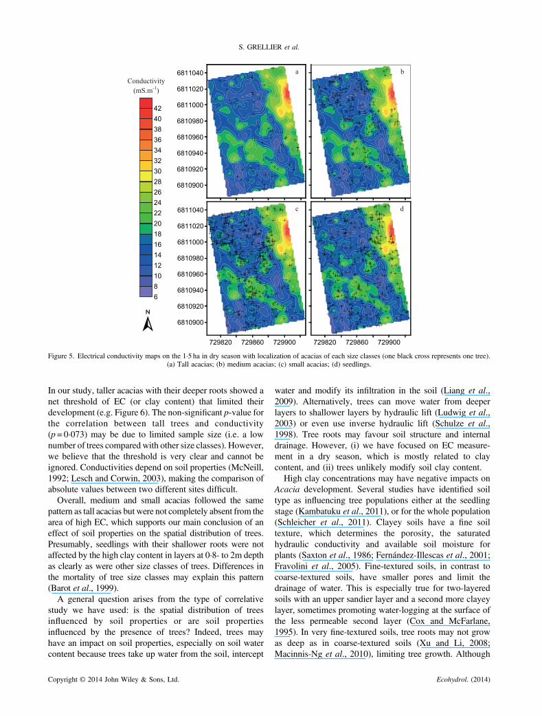
Figure 5. Electrical conductivity maps on the 1·5 ha in dry season with localization of acacias of each size classes (one black cross represents one tree).(a) Tall acacias; (b) medium acacias; (c) small acacias; (d) seedlings.

S. GRELLIER et al.

In our study, taller acacias with their deeper roots showed anet threshold of EC (or clay content) that limited theirdevelopment (e.g. Figure 6). The non-significant p-value forthe correlation between tall trees and conductivity(p = 0·073) may be due to limited sample size (i.e. a lownumber of trees compared with other size classes). However,we believe that the threshold is very clear and cannot beignored. Conductivities depend on soil properties (McNeill,1992; Lesch and Corwin, 2003), making the comparison ofabsolute values between two different sites difficult.Overall, medium and small acacias followed the same

pattern as tall acacias but were not completely absent from thearea of high EC, which supports our main conclusion of aneffect of soil properties on the spatial distribution of trees.Presumably, seedlings with their shallower roots were notaffected by the high clay content in layers at 0·8- to 2m depthas clearly as were other size classes of trees. Differences inthe mortality of tree size classes may explain this pattern(Barot et al., 1999).A general question arises from the type of correlative

study we have used: is the spatial distribution of treesinfluenced by soil properties or are soil propertiesinfluenced by the presence of trees? Indeed, trees mayhave an impact on soil properties, especially on soil watercontent because trees take up water from the soil, intercept

Copyright © 2014 John Wiley & Sons, Ltd.

water and modify its infiltration in the soil (Liang et al.,2009). Alternatively, trees can move water from deeperlayers to shallower layers by hydraulic lift (Ludwig et al.,2003) or even use inverse hydraulic lift (Schulze et al.,1998). Tree roots may favour soil structure and internaldrainage. However, (i) we have focused on EC measure-ment in a dry season, which is mostly related to claycontent, and (ii) trees unlikely modify soil clay content.High clay concentrations may have negative impacts on

Acacia development. Several studies have identified soiltype as influencing tree populations either at the seedlingstage (Kambatuku et al., 2011), or for the whole population(Schleicher et al., 2011). Clayey soils have a fine soiltexture, which determines the porosity, the saturatedhydraulic conductivity and available soil moisture forplants (Saxton et al., 1986; Fernández-Illescas et al., 2001;Fravolini et al., 2005). Fine-textured soils, in contrast tocoarse-textured soils, have smaller pores and limit thedrainage of water. This is especially true for two-layeredsoils with an upper sandier layer and a second more clayeylayer, sometimes promoting water-logging at the surface ofthe less permeable second layer (Cox and McFarlane,1995). In very fine-textured soils, tree roots may not growas deep as in coarse-textured soils (Xu and Li, 2008;Macinnis-Ng et al., 2010), limiting tree growth. Although

Ecohydrol. (2014)

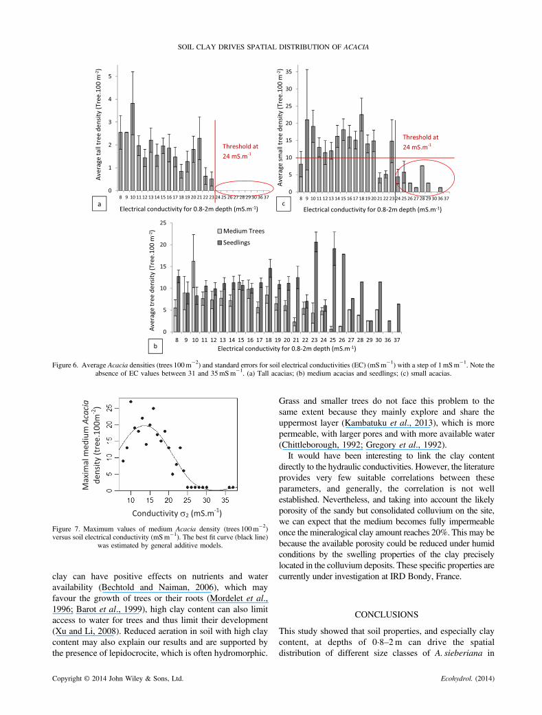
Figure 7. Maximum values of medium Acacia density (trees 100m�2)versus soil electrical conductivity (mSm�1). The best fit curve (black line)

was estimated by general additive models.

Figure 6. Average Acacia densities (trees 100m�2) and standard errors for soil electrical conductivities (EC) (mSm�1) with a step of 1mSm�1. Note theabsence of EC values between 31 and 35mSm�1. (a) Tall acacias; (b) medium acacias and seedlings; (c) small acacias.

SOIL CLAY DRIVES SPATIAL DISTRIBUTION OF ACACIA

clay can have positive effects on nutrients and wateravailability (Bechtold and Naiman, 2006), which mayfavour the growth of trees or their roots (Mordelet et al.,1996; Barot et al., 1999), high clay content can also limitaccess to water for trees and thus limit their development(Xu and Li, 2008). Reduced aeration in soil with high claycontent may also explain our results and are supported bythe presence of lepidocrocite, which is often hydromorphic.

Copyright © 2014 John Wiley & Sons, Ltd.

Grass and smaller trees do not face this problem to thesame extent because they mainly explore and share theuppermost layer (Kambatuku et al., 2013), which is morepermeable, with larger pores and with more available water(Chittleborough, 1992; Gregory et al., 1992).It would have been interesting to link the clay content

directly to the hydraulic conductivities. However, the literatureprovides very few suitable correlations between theseparameters, and generally, the correlation is not wellestablished. Nevertheless, and taking into account the likelyporosity of the sandy but consolidated colluvium on the site,we can expect that the medium becomes fully impermeableonce the mineralogical clay amount reaches 20%. This may bebecause the available porosity could be reduced under humidconditions by the swelling properties of the clay preciselylocated in the colluvium deposits. These specific properties arecurrently under investigation at IRD Bondy, France.

CONCLUSIONS

This study showed that soil properties, and especially claycontent, at depths of 0·8–2m can drive the spatialdistribution of different size classes of A. sieberiana in

Ecohydrol. (2014)

S. GRELLIER et al.

grasslands. Plot replication and/or studies at larger spatialscales with a focus on spatial relationships between sizeclasses of trees could be interesting to further support ourconclusions. This could also increase our capacity topredict tree encroachment. Together with fire, herbivoryand climate, soil properties will have to be taken intoaccount to elucidate the functioning of woody plantencroachment in grassland or savanna. Moreover, measuresto control encroachment could be more effective byfocusing specifically on areas that present favourableconditions for tree development. Finally, these resultsconfirm that developing and using geophysical tools inecology allows study at a large spatial scale withoutdisturbing the environment and, furthermore, revealimportant ecological processes.

ACKNOWLEDGEMENTS

We would like to acknowledge the NRF, SAFE Waterproject and the Institute of Research and Development(IRD) for funding this study. We also would like to thankPauline Ferry, Gonca Okay and Sibonelo Mabaso for theirhelp on the field. We further thank the Potshini Communityfor its support and the use of their land.

REFERENCES

Archer S. 1995. Tree-grass dynamics in aProsopis-thornscrub savanna parkland:reconstructing the past and predicting the future. Ecoscience 2: 83–99.

Baddeley A, Turner R. 2005. Spatstat: an R package for analyzing spatialpoint patterns. Journal of Statistical Software 12: 1–42.

Barot S, Gignoux J, Menaut J-C. 1999. Demography of a savanna palmtree: predictions from comprehensive spatial pattern analyses. Ecology80: 1987–2005.

Bechtold SJ, Naiman RJ. 2006. Soil texture and nitrogen mineralizationpotential across a riparian toposequence in a semi-arid savanna. SoilBiology and Biochemistry 38: 1325–1333.

Bond WJ, Midgley JJ. 2000. A proposed CO2-controlled mechanism ofwoody plant invasion in grasslands and savannas. Global ChangeBiology 6: 865–869.

Botha GA, Wintle AG, Vogel JC. 1994. Episodic late Quaternarypalaeogully erosion in northern KwaZulu-Natal, South Africa. Catena23: 327–340.

Britz M-L, Ward D. 2007. The effects of soil conditions and grazingstrategy on plant species composition in a semi-arid savanna. AfricanJournal of Range & Forage Science 24: 51–61.

Brown JR, Archer S. 1999. Shrub invasion of grassland: recruitment iscontinuous and not regulated by herbaceous biomass or density.Ecology 80: 2385–2396.

Browning DM, Archer SR, Asner GP, McClaran MP, Wessman CA.2008. Woody plants in grasslands: post-encroachment stand dynamics.Ecological Applications 18: 928–944.

Callaway RM, Walker LR. 1997. Competition and facilitation: a syntheticapproach to interactions in plant communities. Ecology 78: 1958–1965.

Chittleborough DJ. 1992. Formation and pedology of duplex soils.Australian Journal of Experimental Agriculture 32: 815–825.

CockxL,VanMeirvenneM,DeVosB. 2007.Using the EM38DD soil sensorto delineate clay lenses in a sandy forest soil. Soil Science Society ofAmerica Journal 71: 1314–1322. DOI: 10.2136/sssaj2006.0323

Colgan MS, Asner GP, Levick SR, Martin RE, Chadwick OA. 2012.Topo-edaphic controls over woody plant biomass in South African

Copyright © 2014 John Wiley & Sons, Ltd.

savannas. Biogeosciences 9: 1809–1821. DOI: 10.5194/bg-9-1809-2012

Corwin DL, Lesch SM. 2005. Apparent soil electrical conductivitymeasurements in agriculture. Computers and Electronics in Agriculture46: 11–43.

Cox JW, McFarlane DJ. 1995. The causes of waterlogging in shallow soils andtheir drainage in southwestern Australia. Journal of Hydrology 167: 175–194.

Eggemeyer KD, Schwinning S. 2009. Biogeography of woody encroachment:why is mesquite excluded from shallow soils? Ecohydrology 2: 81–87.

ESRI. 2008. ArcMap-ArcEditor version 9.3, Environmental SystemsResearch Institute, Inc.

FAO. 1998. World Reference Base for Soil Resources. World SoilResources Reports, FAO: Rome, Italy.

Fernández-Illescas CP, Porporato A, Laio F, Rodríguez-Iturbe I. 2001.The ecohydrological role of soil texture in a water-limited ecosystem.Water Resource Research 37: 2863–2872.

Fravolini A, Hultine KR, Brugnoli E, Gazal R, English NB, Williams DG.2005. Precipitation pulse use by an invasive woody legume: the role ofsoil texture and pulse size. Oecologia 144: 618–627.

Frohlich RK, Parke CD. 1989. The electrical resistivity of the vadose zone– field survey. Ground Water 27: 524–530.

Graz FP. 2008. The woody weed encroachment puzzle: gathering pieces.Ecohydrology 1: 340–348.

Gregory PJ, Tennant D, Hamplin AP, Eastham J. 1992. Components ofthe water-balance on duplex soils in western Australia. AustralianJournal of Experimental Agriculture 32: 845–855.

Grellier S. 2011. Hillslope Encroachment by Acacia Sieberiana in a Deep-Gullied Grassland of KwaZulu-Natal (South Africa). PhD thesis.University of Pierre and Marie Curie: Paris, France.

Grellier S, Janeau J-L, Barot S, Ward D. 2012a. Grass competition is moreimportant than seed ingestion by livestock for Acacia recruitment inSouth Africa. Plant Ecology 213: 899–908.

Grellier S, Kemp J, Florsch N, Janeau J-L, Ward D, Barot S, PodwojewskiP, Lorentz S, Valentin C. 2012b. The indirect impact of encroachingtrees on gully extension: a 64 year study in a sub-humid grassland ofSouth Africa. Catena 98: 110–119.

Grellier S, Florsch N, Camerlynck C, Janeau JL, Podwojewski P, LorentzS. 2013a. The use of Slingram EM38 data for topsoil and subsoilgeoelectrical characterization with a Bayesian inversion. Geoderma200-201: 140–155.

Grellier S, Ward D, Janeau J-L, Podwojewski P, Lorentz S, Abbadie L,Valentin C, Barot S. 2013b. Positive versus negative environmentalimpacts of tree encroachment in South Africa. Acta Oecologica 53: 1–10. http://dx.doi.org/10.1016/j.actao.2013.08.002

HalpernCB,Antos JA,Rice JM,HaugoRD,LangNL. 2010. Tree invasion ofa montane meadow complex: temporal trends, spatial patterns, and bioticinteractions. Journal of Vegetation Science 21: 717–732.

Hezarjaribi A, Sourell H. 2007. Feasibility study of monitoring the totalavailable water content using non-invasive electromagnetic induction-based and electrode-based soil electrical conductivity measurements.Irrigation and Drainage 56: 53–65.

Hossain MB, Lamb DW, Lockwood PV, Frazier P. 2010. EM38 forvolumetric soil water content estimation in the root-zone of deepvertosol soils. Computers and Electronics in Agriculture 74: 100–109.

Kambatuku JR, Cramer MD, Ward D. 2011. Savanna tree–grasscompetition is modified by substrate type and herbivory. Journal ofVegetation Science 22: 225–237.

Kambatuku JR, Cramer MD, Ward D. 2013. Overlap in soil water sourcesof savanna woody seedlings and grasses. Ecohydrology 6: 464–473.DOI: 10.1002/eco.1273

King GM. 2002. An Explanation of the 1:500 000 GeneralHydrogeological Map. Department of Water Affairs and Forestry:Pretoria, South Africa.

Lata JC, Degrange V, Raynaud X, Maron PA, Lensi R, Abbadie L. 2004.Grass populations control nitrification in savanna soils. FunctionalEcology 18: 605–611. DOI: 10.1111/j.0269-8463.2004.00880.x

Leroy P, Revil A. 2004. A triple-layer model of the surfaceelectrochemical properties of clay minerals. Journal of Colloid andInterface Science 270: 371–380. DOI: 10.1016/j.jcis.2003.08.007

Lesch SM, Corwin DL. 2003. Using the dual-pathway parallelconductance model to determine how different soil properties influenceconductivity survey data. Agronomy Journal 95: 365–379.

Ecohydrol. (2014)

SOIL CLAY DRIVES SPATIAL DISTRIBUTION OF ACACIA

Liang W-L, Kosugi K, Mizuyama T. 2009. A three-dimensional model ofthe effect of stemflow on soil water dynamics around a tree on ahillslope. Journal of Hydrology 366: 62–75.

Ludwig F, Dawson TE, de Kroon H, Berendse F, Prins HHT. 2003.Hydraulic lift in Acacia tortilis trees on an East African savanna.Oecologia 134: 293–300.

Macinnis-Ng CMO, Fuentes S, O’Grady AP, Palmer AR, Taylor D,Whitley RJ, Yunusa I, Zeppel MJB, Eamus D. 2010. Root biomassdistribution and soil properties of an open woodland on a duplex soil.Plant and Soil 327: 377–388.

McNeill JD. 1980. Electromagnetic Terrain Conductivity Measurement atLow Induction Numbers, Tech. Note TN-6. Geonics Ltd: Mississauga,Ontario. http://www.geonics.com/pdfs/technicalnotes/tn6.pdf

McNeill JD. 1992. Rapid, accurate mapping of soil salinity by electromag-netic ground conductivity meters. in Advances in Measurement of SoilPhysical Properties: Bringing Theory Into Practice, Specific Publication30, Soil Science Society of America, Madison, Wisconsin, 209–229.

Meyer KM, Wiegand K, Ward D, Moustakas A. 2007. SATCHMO: aspatial simulation model of growth, competition, and mortality incycling savanna patches. Ecological Modelling 209: 377–391.

Mordelet P, Barot S, Abbadie L. 1996. Root foraging strategies and soilpatchiness in a humid savanna. Plant and Soil 182: 171–176.

Mualem Y, Friedman S. 1991. Theoretical prediction of electricalconductivity in saturated and unsaturated soil. Water RessourcesResearch 27: 2771–2777. DOI: 10.1029/91WR01095

Mucina L, Rutherford MC. 2006. The Vegetation of South Africa, Lesothoand Swaziland. Strelitzia 19, South African National BiodiversityInstitute: Pretoria, South Africa.

Myers DB, Kitchen NR, Sudduth KA, Sharp RE, Miles RJ. 2007. Soybeanroot distribution related to claypan soil properties and apparent soilelectrical conductivity. Crop Science 47: 1498–1509. DOI: 10.2135/cropsci2006.07.0460

Revil A, Glover PWJ. 1997. Theory of ionic-surface electrical conductionin porous media. Physical Review B 55: 1757–1773. DOI: 10.1103/PhysRevB.55.1757

Revil A, Glover PWJ. 1998. Nature of surface electrical conductivity innatural sands, sandstones, and clays. Geophysical Research Letters 25:691–694. DOI: 10.1029/98gl00296

Rhoades J, Manteghi N, Shrouse P, Alves W. 1989. Soil electricalconductivity and soil salinity: new formulations and calibrations. SoilScience Society of America Journal 53: 433–439.

Robinson DA, Abdu H, Jones SB, Seyfried M, Lebron I, Knight R. 2008.Eco-geophysical imaging of watershed-scale soil patterns links withplant community spatial patterns. Vadose Zone Journal 7: 1132–1138.

Robinson DA, Lebron I, Querejeta JI. 2010. Determining soil–tree–grassrelationships in a california oak savanna using eco-geophysics. VadoseZone Journal 9: 1–8.

Rosenbloom NA, Doney SC, Schimel DS. 2001. Geomorphic evolution ofsoil texture and organic matter in eroding landscapes. GlobalBiogeochemistry Cycles 15: 365–381.

Sankaran M, Ratnam J, Hanan NP. 2004. Tree–grass coexistence insavannas revisited – insights from an examination of assumptions andmechanisms invoked in existing models. Ecology Letters 7: 480–490.

Sankaran M, Hanan NP, Scholes RJ, Ratnam J, Augustine DJ, Cade BS,Gignoux J, Higging SI, Roux XL, Ludwig F, Ardo J, Banyikwa F, BronnA, Bucini G, Caylor KK, Coughenour MB, Diouf A, Ekaya W, Feral CJ,February EC, Frost PGH, Hiernaux P, Hrabar H, Metzger KL, Prins HHT,

Copyright © 2014 John Wiley & Sons, Ltd.

Ringrose S, SeaW, Tews J, Worden J, Zambatis N. 2005. Determinants ofwoody cover in African savannas. Nature 438: 846–849.

Sankaran M, Ratnam J, Hanan N. 2008. Woody cover in Africansavannas: the role of resources, fire and herbivory. Global Ecology andBiogeography 17: 236–245.

Saxton K, Rawls WJ, Romberger JS, Ri P. 1986. Estimating generalizedsoil water characteristics from texture. Soil Science Society of AmericaJournal 50: 1031–1036.

Schleicher J, Wiegand K, Ward D. 2011. Changes of woody plantinteraction and spatial distribution between rocky and sandy soil areasin a semi-arid savanna, South Africa. Journal of Arid Environments 75:270–278.

Schulze E-D, Caldwell MM, Canadell J, Mooney HA, Jackson RB, ParsonD, Scholes R, Sala OE, Trimborn P. 1998. Downward flux of waterthrough roots (i.e. inverse hydraulic lift) in dry Lalahari sands.Oecologia 115: 460–462.

Tarantola A. 2005. Inverse Problem Theory and Methods for ModelParameter Estimation. Society for Industrial and Applied Mathematics:Philadelphia, PA, U.S.A.

Tarantola A, Valette B. 1982a. Generalized nonlinear inverse problemssolved using the least square criterion. Reviews of Geophysics andSpace Physics 20: 219–232.

Tarantola A, Valette B. 1982b. Inverse problems – quest for information.Journal of Geophysics 50: 159–170.

Van Auken OW. 2009. Causes and consequences of woody plantencroachment into western North American grasslands. Journal ofEnvironmental Management 90: 2931–2942.

Verboom WH, Pate JS. 2013. Exploring the biological dimension topedogenesis with emphasis on the ecosystems, soils and landscapes ofsouthwestern Australia. Geoderma 211: 154–183. DOI: 10.1016/j.geoderma.2012.03.030

Wang YQ, Shao MA, Liu ZP, Warrington DN. 2012. Regional spatialpattern of deep soil water content and its influencing factors.Hydrological Sciences Journal-Journal Des Sciences Hydrologiques57: 265–281. DOI: 10.1080/02626667.2011.644243

Ward D. 2005. Do we understand the causes of bush encroachment inAfrican savannas? African Journal of Range & Forage Science22: 101–105.

Ward D. 2010. A resource ratio model of the effects of changes in CO2 onwoody plant invasion. Plant Ecology 209: 147–152.

Weng ES, Luo YQ. 2008. Soil hydrological properties regulate grasslandecosystem responses to multifactor global change: a modeling analysis.Journal of Geophysical Research-Biogeosciences 113: DOI: 10.1029/2007jg000539

Wiegand K, Ward D, Saltz D. 2005. Multi-scale patterns and bushencroachment in an arid savanna with a shallow soil layer. Journal ofVegetation Science 16: 311–320.

Wiegand K, Saltz D, Ward D. 2006. A patch-dynamics approach tosavanna dynamics and woody plant encroachment – insights from anarid savanna. Perspectives in Plant Ecology, Evolution and Systematics7: 229–242.

Xu GQ, Li Y. 2008. Rooting depth and leaf hydraulic conductance in thexeric tree Haloxyolon ammodendron growing at sites of contrasting soiltexture. Functional Plant Biology 35: 1234–1242.

Young MH, Robinson DA, Ryel RJ. 2010. Introduction to coupling soilscience and hydrology with ecology: toward integrating landscapeprocesses. Vadose Zone Journal 9: 515–516.

Ecohydrol. (2014)