Software Package Supporting Ship Stability by using Catastrophe Theory

Damascus UNIV. Journal – V18 – Number (1) 2002 Ali - Yousif –Batiha

63

Software Package Supporting Ship Stability by using Catastrophe Theory

SEBAH A. Ali Basra University - Iraq

Jabar H. Yousif Department of Computer Irbid National University

Jordan

Khaldoun M. Batiha Department of Computer Irbid National University

Jordan

Abstract This study focuses on using the results of Catastrophe Theory and its

applications on ship stability in a form of software package. The package has guiding and warning aspects.

A software package has been designed and programmed using the Turbo Pascal Ver. (7) on an IBM-PC. The package deals with ship stability through a practical

method in terms of loading, unloading and the movement of free surfaces. The program also shows on the computer screen: The shape of

a catastrophic case of the ship, and the important points in ship stability and its movement as a result of those activities which take place on the board of the ship

and inside it.

Software Package Supporting Ship Stability by Using Catastrophe Theory

64

1. Introduction

The English scientist E. C. Zeeman has established a number of theories related to catastrophes science. These theories talk about and discuss ship stability.

However, his results have been purely mathematical in nature and not easy to be programmed and used. This study discusses the comparative research in order to

reveal difference and similarity points between the ship and Poston’s Gravitational Catastrophe Machine. The study has obtained results similar to

those found by Zeeman, but in a more simple method that is capable for programming and calculation.

This study considers the subject of using catastrophe theory and its results for the purpose of examining ship stability. The situation of a ship can be looked at

whether it is a turnover or crush due to the cargo rather than the clash as a catastrophe as such that often occurs as a result of miscalculating the tracks of

ship and its stability. Catastrophe Theory is a mathematical theory that has been initiated by the

French scientist Thom Rene in the early 1960’s. However, the English scientist Zeeman has developed the result of catastrophe theory in his attempts to

construct models of useful natural applications.[6] The catastrophe theory informally deals with continuous mathematical functions

that depend on a number of variables, which are called state variables. These variables are controlled by other variables named control variables. In some cases a small change in the values of control variables leads to discontinued

change and noncontinuity in the function value. This also leads to large jumps not calculated in the function values, these are called a catastrophe.

However, the subject of ship stability is considered as an important matter in the life of human society because ships represent one of the important transportation

vehicles (Oil tankers, Merchandise carriers). Therefore, the study of ship stability is considered an important and essential matter facing specialists.(1) The

operation of ship-stability process is carried out by designers and captains through an experimental method. Also, this process has developed by virtue of

experience and time to ultimately become a group of tables and facts for managing the ship, with reference to each ship as having its particular tables in

accordance with its basic design.


65

The aim of this study is to link between these two subjects to obtain a group of formulas and calculations, which can be programmed as software package. This

package is used to manage and calculate ship stability in a quick and accurate way that characterizes the computer in comparison with the human. The use of

the proposed package helps to obtain correct and accurate calculations by which the ship avoids the occurrence of catastrophe.

2. Background of Catastrophe Theory

Classical Mathematics has the ability to describe and study many continuous phenomena that occur in our world and to model them in programmable form. Since these models are basically based on the calculations, they are commonly

used as in physical sciences.(5) However, there are many useful natural phenomena which are included in the category of noncontinuity at some time as

in the social biological, and psychological sciences.[4,6] Therefore, there are no laws governing these phenomena.

Catastrophe Theory is a mathematical theory describing the systems whose behaviors are usually normal, but sometimes a noncontinuity case would occur. We will assume that the system at any time consists of n variables (x1, x2, x3, …,

xn). These variables are called state variables, where n is a finite number that can be very large as in the brain model.[5,6]

Assume that the system is controlled by m variables (u1, u2, u3, …, um). These variables are called control variables whose values determine the behavior of the

system. Accordingly, as the number of these variables increases, the system becomes disturbed and thus necessitates multiple solutions. Therefore, the

number of control variables must be relatively small to reduce the constraints imposed by such variables on the system, whereas, it is usual to leave the

calculation of any variables which do not cause significant effects on noncontinuity under consideration.

In order to explain the concept of state and control variables, we consider the quadratic function F(x)=ax2+bx+c, the variable x (state variable) that give the function parabola shape, while the variables a, b, c (control variables) give the

function movement on axis as shown in figure (1).


66

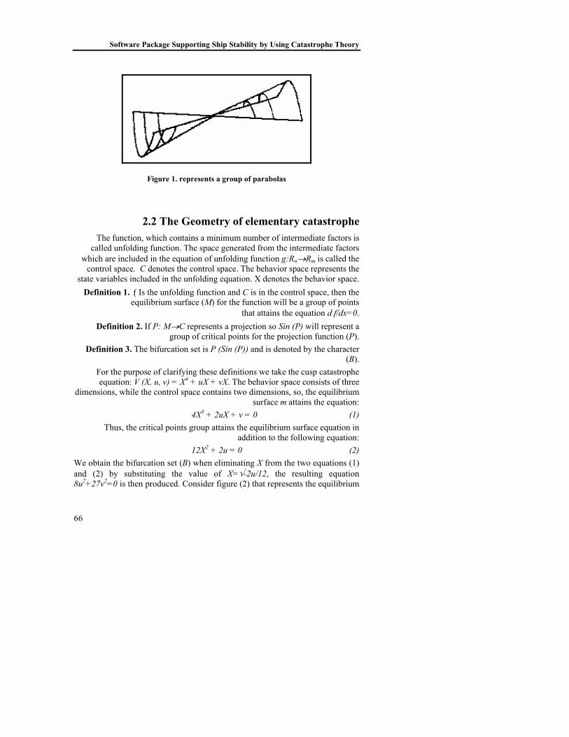
Figure 1. represents a group of parabolas

2.2 The Geometry of elementary catastrophe The function, which contains a minimum number of intermediate factors is

called unfolding function. The space generated from the intermediate factors which are included in the equation of unfolding function g:Rn→Rm is called the

control space. C denotes the control space. The behavior space represents the state variables included in the unfolding equation. X denotes the behavior space.

Definition 1. ƒ Is the unfolding function and C is in the control space, then the equilibrium surface (M) for the function will be a group of points

that attains the equation dƒ/dx=0. Definition 2. If P: M→C represents a projection so Sin (P) will represent a

group of critical points for the projection function (P). Definition 3. The bifurcation set is P (Sin (P)) and is denoted by the character

(B). For the purpose of clarifying these definitions we take the cusp catastrophe equation: V (X, u, v) = X4 + uX + vX. The behavior space consists of three

dimensions, while the control space contains two dimensions, so, the equilibrium surface m attains the equation:

4X3 + 2uX + v = 0 (1) Thus, the critical points group attains the equilibrium surface equation in

addition to the following equation: 12X2 + 2u = 0 (2)

We obtain the bifurcation set (B) when eliminating X from the two equations (1) and (2) by substituting the value of X=√-2u/12, the resulting equation 8u2+27v2=0 is then produced. Consider figure (2) that represents the equilibrium


67

surface and bifarction set for the cusp catastrophe.

Figure 2. represents equilibrium surface and bifraction set for the cusp catastrophe

2.3 Ship Stability: Basic Concepts: [1, 2, 7, 9] Ship stability depends on a number of basic physical concepts where a ship is a floating body on the surface of the water. Thus, there is a significant relationship between the ship’s gravity center and the water’s gravity center due to floating. Ship stability arises from studying the relationship between these two variables and their movements during loading and unloading a ship. It is difficult to say that there is a known and firm theory about these two points (G,B). The ship stability information can be obtained from a set of tables that describe the ship during the design stage. The basic concepts are as follows:

1. Gravity center of the ship. Gravity center of the ship is a point in the body of the ship representing the power of a downward vertical trend that is equal to the weight of the body. Furthermore, the gravity center of any symmetrical geometrical shape is its middle. G denotes the center gravity as shown in fig 3 .

2. The Buoyancy center. The buoyancy center is a point in the body of the ship representing the power of an upward vertical trend that is equal to displaced water. In addition, the buoyancy center for any symmetrical geometric shape is the middle of the geometric place that is sunk underneath the water. B denotes the buoyancy center as shown in fig 3.


68

Figure (3) represents the basic points in the ship

3. The Transverse metacenter. The transverse metacenter is a hypothetical point representing intersection of two lines of power of water impulsion to obliquity of the ship in two particular angles. This is denoted by (M) as shown in fig 3.

4. Keel of the ship. Keel of the ship is the lowest point at the ship. This is fixed and specified during the designing stage. K denotes keel point as shown in fig 3.

5. The Transverse metacenter height. This is the vertical distance between gravity center of the ship and its transverse metacenter. Gm denotes the transverse metacenter height as shown in fig 3.

6. The Water-plane coefficient. This is the percentage between the area of water for the ship to the area of a rectangular which has the same dimensions of a ship. Cw denotes Water-plane coefficient.

7. The Block Coefficient. This is the percentage of water volume displaced by the ship to the water volume displaced by a parallelogram segment that has similar measurements to a ship (length, beam, and depth). Cb denotes the block coefficient

8. The height of buoyancy center above the keel. This is the vertical distance between buoyancy center (B) and the keel (K). It is given the symbol (KB) as shows in fig 3.

9. The Draft. This is part of the ship immersed by water as a result of the weight of water downward. This is protected against the effects of water, and denoted by (D).

10. The tonnes per centimeter immersion. This is the amount of mass that must be added to (or lifted from) the ship in order to change the value of


69

ship draft by (1) centimeter. Tpc denotes it.

2.4 The stability [1, 7, 9] The stability is the ship resistance for all effects of the external forces, which try to founder the ship, and the ship’s attempt to maintain the stable position. The ship is to be stable floated. The float force that has an upward effect on the immersed part of the body must be equal to the whole weight of the ship. Since, these two forces balance each other, so their effect must be on the same line.

2.5 Effect of adding cargoes on the movement of ship’s gravity center

When a load is added on the board of the ship, its gravity center would move directly towards the gravity center of the added load, as shown by figure (4). Equation (3) is used to calculate the amount of distance (GG1), GG1 = (w*Dis)/W (3) where W is the new weight of the ship, i.e. (w+W)

Figure 4. represents the effect of adding cargoes on the movement of gravity center of the ship

Figure (4a) represents the movement of the ship’s gravity center (G) to (G1) as a result of placing a cargo under the gravity center (G) that leads to increasing the value of (GM). While, figure (4b) represents the movement of the ship’s gravity


70

center (G) to (G1) due to placing a cargo above the gravity center (G) that leads to reduce the value of (GM). Figure (4c) represents the movement of the ship’s gravity center (G) to (G1) because of placing a cargo on the left side of the gravity center (G) that leads to reduce the value of (GM). Finally figure (4d) represents the movement of the ship’s gravity center as a result of placing a cargo below the left side of the gravity center (G).

2.6 Effect of unloading cargoes on the movement of gravity center of the ship

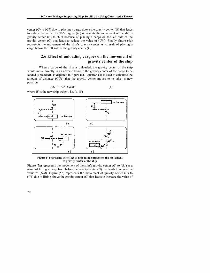
When a cargo of the ship is unloaded, the gravity center of the ship would move directly in an adverse trend to the gravity center of the cargo to be loaded (unloaded), as depicted in figure (5). Equation (4) is used to calculate the amount of distance (GG1) that the gravity center moves to to take its new position GG1 = (w*Dis)/W (4) where W is the new ship weight, i.e. (w-W)

Figure 5. represents the effect of unloading cargoes on the movement

of gravity center of the ship Figure (5a) represents the movement of the ship’s gravity center (G) to (G1) as a result of lifting a cargo from below the gravity center (G) that leads to reduce the value of (GM). Figure (5b) represents the movement of gravity center (G) to (G1) due to lifting above the gravity center (G) that leads to increase the value of


71

(GM). While, figure (5c) represents the movement of gravity center (G) to (G1) because of lifting a cargo placed at the right side of the gravity center (G). Finally figure (5d) represents the movement of gravity center (G) to (G1) as a result of lifting a cargo placed below the left side of the gravity center of the ship (G).

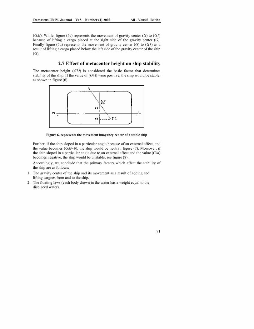
2.7 Effect of metacenter height on ship stability The metacenter height (GM) is considered the basic factor that determines stability of the ship. If the value of (GM) were positive, the ship would be stable, as shown in figure (6).

Figure 6. represents the movement buoyancy center of a stable ship

Further, if the ship sloped in a particular angle because of an external effect, and the value becomes (GM=0), the ship would be neutral, figure (7). Moreover, if the ship sloped in a particular angle due to an external effect and the value (GM) becomes negative, the ship would be unstable, see figure (8). Accordingly, we conclude that the primary factors which affect the stability of the ship are as follows:

1. The gravity center of the ship and its movement as a result of adding and lifting cargoes from and to the ship.

2. The floating laws (each body drown in the water has a weight equal to the displaced water).


72

Figure 7. represents the movement of a neutral ship

Figure 8. represents the movement of an unstable ship

2.8 Calculating the metacenter height GM The metacenter height (GM) is considered the basic factor that determines the ship stability. It is calculated from a group of equations [1], as follows:

GM = KM-KG (5) The value of (KM) is calculated from the equation

KM = KB+BM (6) While the value of (KB) for a container ship is calculated from equation (7),

KB = (½) d (7) where, d represents the ship draft. The diagonal metacenter height (BM) is calculated as follows:

BM = IB/V (8)


73

where (IB) represents the transverse inertia momentum of the ship, and (V) denotes the size of the ship. Further, the value of (IB) can be calculated from the equation:

IB = LB3/12 (9) where (L) represents the length of the ship, and (B) denotes its beam. Then, (BM) for the container ship is BM=B2/(12-D). The value of (KG) can be calculated as follows:

KG = Final displacement/Final momentum (10) The table (1) shows the values of (KB) and (KM) for drafts between 1m and 3m for a container ship whose length, beam and depth are 64m, 10m, and 6m respectively. The lowest draft and the highest draft for the ship are 1m and 5m respectively.

Table 1.

d KB = (½) d BM=B2/(12d) KM = KB+BM 1 0.5 8.33 8.83

1.5 0.75 5.66 6.31 2 1 4.17 5.17

2.5 1.25 3.33 4.58 3 1.5 2.78 4.28

The proposed work attempts to link and utilize the results of catastrophe theory and its application on the stability of ships. The significant problem in this respect is to find the mathematical function that controls the movement of the ship and its stability, and in turn studying catastrophes (turnovers) which a ship may encounter. The scientist Zeeman[6] studied ship stability and was able to establish and prove a number of theories and facts related to the basic points which affect ship stability. These points are: gravity center of the ship (G), metacenter height (GM), and buoyancy center height (KB). When these equations are used in an attempt to construct a software related to ship stability, it has been found out that these equations are difficult to be programmed on the one hand, and impractical on the other. This is because these theories relied on logic in their application rather than on reality. Zeeman has considered the ship (a container ship, for instance) similar to all ships which have the same dimensions, whereas the reality is that ships are not similar in their tables. Each ship has its different


74

tables. These are the same causes, which have led to exclude Zeeman’s theories in this respect. As a result, ship stability must practically be studied and compared with catastrophe theory. This comparative study depends on exploring points of similarity and dissimilarity, which can be observed in the ship movement and some catastrophic machines used as models to simplify catastrophe theory. In fact, Poston’s gravitational machine has taken our attention in this direction. Poston’s machine gives the characteristics upon which Zeeman has focused in his theories. These imply that the locus for this machine is parabola and the machine movement is resulted from the gravity center movement. The method of calculating the locus gives the impression that it is a ship.

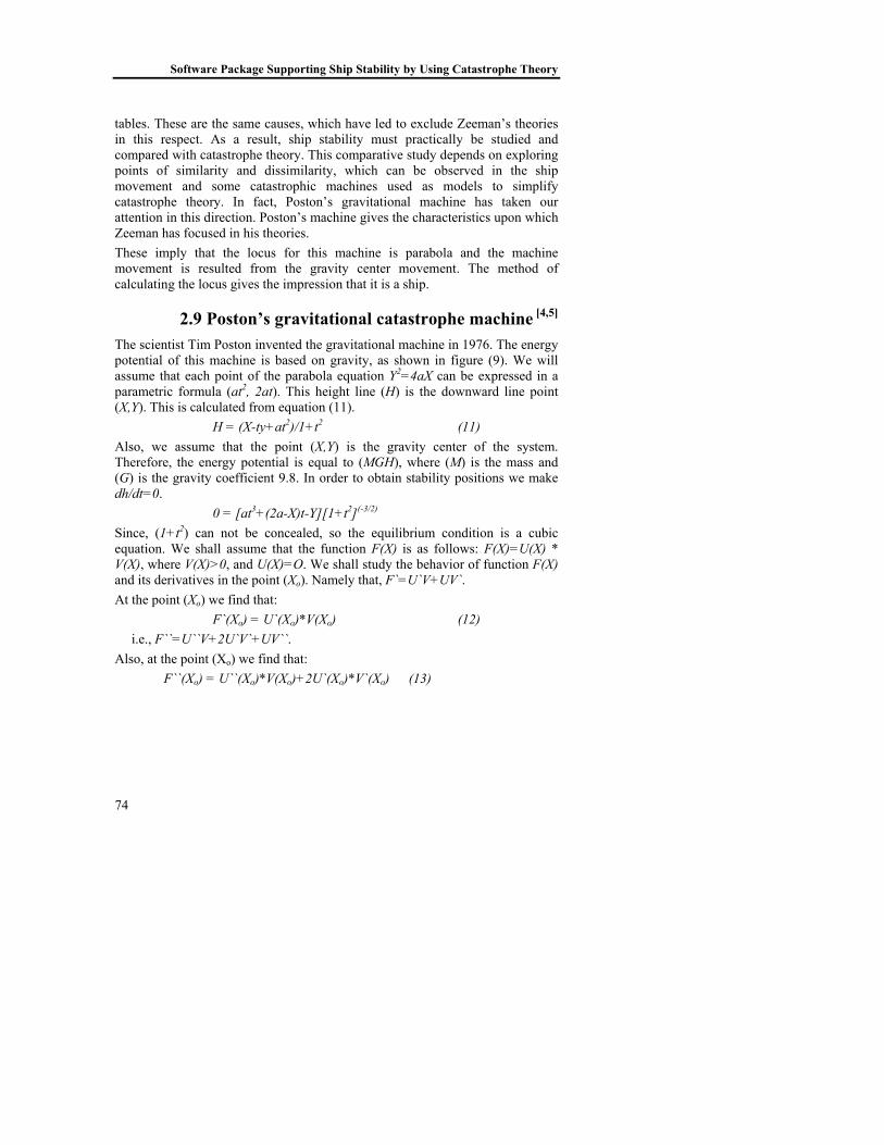
2.9 Poston’s gravitational catastrophe machine [4,5] The scientist Tim Poston invented the gravitational machine in 1976. The energy potential of this machine is based on gravity, as shown in figure (9). We will assume that each point of the parabola equation Y2=4aX can be expressed in a parametric formula (at2, 2at). This height line (H) is the downward line point (X,Y). This is calculated from equation (11). H = (X-ty+at2)/1+t2 (11)

Also, we assume that the point (X,Y) is the gravity center of the system. Therefore, the energy potential is equal to (MGH), where (M) is the mass and (G) is the gravity coefficient 9.8. In order to obtain stability positions we make dh/dt=0.

0 = [at3+(2a-X)t-Y][1+t2](-3/2) Since, (1+t2) can not be concealed, so the equilibrium condition is a cubic equation. We shall assume that the function F(X) is as follows: F(X)=U(X) * V(X), where V(X)>0, and U(X)=O. We shall study the behavior of function F(X) and its derivatives in the point (Xo). Namely that, F`=U`V+UV`. At the point (Xo) we find that:

F`(Xo) = U`(Xo)*V(Xo) (12) i.e., F``=U``V+2U`V`+UV``. Also, at the point (Xo) we find that:

F``(Xo) = U``(Xo)*V(Xo)+2U`(Xo)*V`(Xo) (13)


75

Figure 9. Poston machine

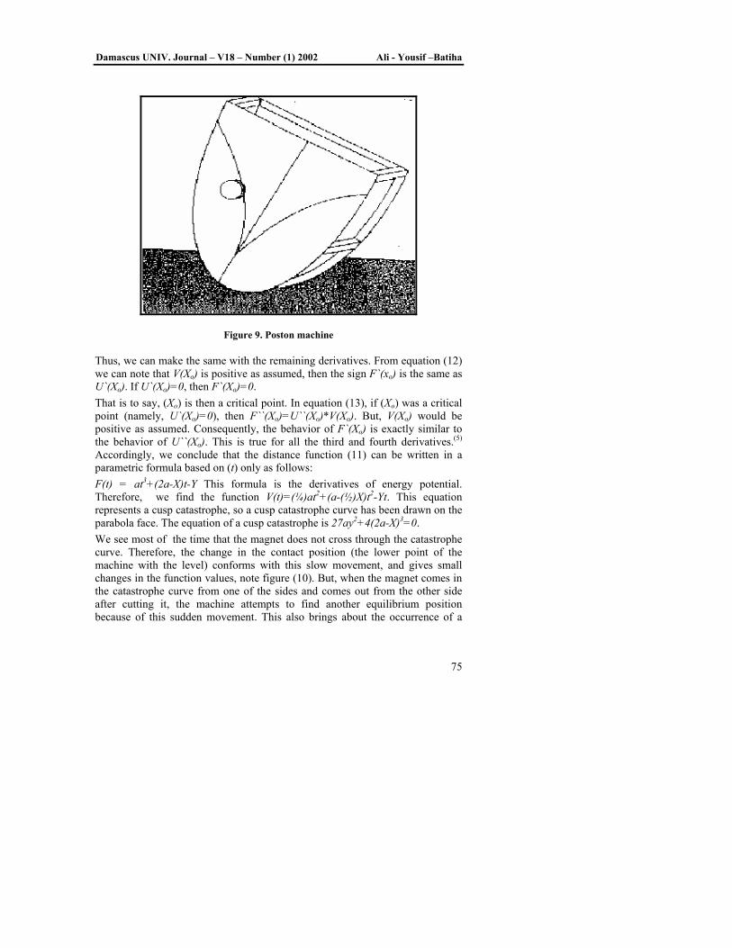
Thus, we can make the same with the remaining derivatives. From equation (12) we can note that V(Xo) is positive as assumed, then the sign F`(xo) is the same as U`(Xo). If U`(Xo)=0, then F`(Xo)=0. That is to say, (Xo) is then a critical point. In equation (13), if (Xo) was a critical point (namely, U`(Xo)=0), then F``(Xo)=U``(Xo)*V(Xo). But, V(Xo) would be positive as assumed. Consequently, the behavior of F`(Xo) is exactly similar to the behavior of U``(Xo). This is true for all the third and fourth derivatives.(5) Accordingly, we conclude that the distance function (11) can be written in a parametric formula based on (t) only as follows: F(t) = at3+(2a-X)t-Y This formula is the derivatives of energy potential. Therefore, we find the function V(t)=(¼)at2+(a-(½)X)t2-Yt. This equation represents a cusp catastrophe, so a cusp catastrophe curve has been drawn on the parabola face. The equation of a cusp catastrophe is 27ay2+4(2a-X)3=0. We see most of the time that the magnet does not cross through the catastrophe curve. Therefore, the change in the contact position (the lower point of the machine with the level) conforms with this slow movement, and gives small changes in the function values, note figure (10). But, when the magnet comes in the catastrophe curve from one of the sides and comes out from the other side after cutting it, the machine attempts to find another equilibrium position because of this sudden movement. This also brings about the occurrence of a


76

significant jump in the function values.

Figure 10. A group of movements of Poston’s machine

3. The comparative study between poston’s machine and the ship

Ship movement equation can be defined according to a comparative study of the ship and it’s movement during the work on the one hand, and the a known - of catastrophe machine on the other hand. The comparative study between the ship and Poston’s machine gives us the required answers. As a result of comparing the two figures, we find that:

1. Zeeman[6] proved that the geometric locus of buoyancy center movement (B) is a parabola and it has the same lower character representing the parabola of Poston’s machine (i.e., each ship has a matching Poston’s machine).

2. Gravity center of the ship (G) and its movement to (G1) when adding cargoes is the same as movement of Poston’s machine gravity center and its movement (G1) when placing a magnet.

3. The metacenter height (GM) is similar to the height line (H) of Poston’s line. Consequently, we conclude from the comparison that the ship movement is determined by Poston’s machine. Also, the function derived that determines movement of Poston’s machine conforms with the ship movement but with some complication. The stability in a ship depends on a number of factors such as movement of waves, loading cargoes, unloading cargoes, effect of free surface and other factors. On the other hand, the stability of Poston’s machine depends


77

on the magnet movement. The most difficult step is how the catastrophe projection can be selected on the control space. For this reason, the most important mathematical characteristic for parabola [8] has been utilized. That is, the curve determined by the intersection of poles (envelop) on the parabola tangency points gives us a locus similar to the required projection.

Figure 11. the lower point and height line

Figure 12. Movement (B) as proved by Zeeman

To illustrate this, we take an ellipse as in figure (13), and we take a group of points on it A0, A1, …, An. From each point of these points we raise a pole on the tangency of ellipse in that point, then we obtain the required curve, and upon this characteristic depends the programming of ship stability system.


78

Figure 13. represents an ellipse with tangent poles from the tangency point

4. The proposed program The proposed program is written by using Turbo Pascal (V.7). the program is designed to be interactive with user in order to be widely applicable . Guiding messages is used to ensure the accurate input and make the use of program easy. The program consists of three parts: The first part: The purpose of this part is to draw a projection catastrophe curve that would be used in the third part. This is to show the ship stability through looking at the chart of gravity center position of the ship (G) and the metacenter position (M). The buoyancy center movement (B) is first drawn, by using a parabola function, as proved by Zeeman.[6] Secondly, the metacenter position is derived. The second part. This part is related to the basic calculations of the ship, which are utilized to find out position (G) and (M). The aim of these calculations is to get the results and to compare them with actual results (collected from Iraqi Harbors, Sate Enterprise). However, the use of these calculations in the third part of the program is to reveal movement of (G) and (M). The third part. This is the most important part in the program because it transforms the calculations related to the ship to points, which move on the level of catastrophe projection. This becomes quite obvious from (G) and (M) on the


79

catastrophe projection. The dangerous areas have been determined by the movement of the points (M) and (G) as points around the projection of fold catastrophe. The ship can be stable as long as the two points (G) and (M) are moving within this projection. Also, the ship may be exposed to a turnover catastrophe if one of these points went out of the catastrophe projection curve.

5. The program during implementation The software package has been designed with a guiding interactive so that the personal responsible for the loading processes can operate this package before loading any cargo on the ship. The amount of cargo and other related information are entered to the program. Then, the new draft of the ship is calculated together with the height (GM). If the value of (GM) were negative, the ship would be unstable, and may be exposed to a turnover catastrophe. Therefore, the software package has given the required warning otherwise the ship would have neutral or positive stability. The results have been calculated for a hypothetical ship with the specifications shown in table (2). The primary data of an empty ship have been calculated and illustrated in table (3). Then, catastrophe projection is drawn on the screen, note figure (14) that shows the small rhombus forms representing the critical points for ship stability. The catastrophe (ship turnover) will take place when the ship crosses the critical points and the position (M) and (G). Now, we assume that there are a group of such successive processes as those shown in table (4). After entering the value of cargo whose specifications are indicated in table (5), the results of the program may be as depicted in table (6), considering the height (GM) after loading that cargo. Then, the program calls the Draw NGM procedure to reveal the catastrophe projection and the new points are illustrated on it. These points have been calculated after adding the required load, note figure (15). In this figure the symbol (OG) represents position of the primary gravity center of the ship.

Table 2. Represents the data of a hypothetical ship

The ship has the following data The ship: Length The ship: Beam The ship: Depth The block coefficient The coefficient of fineness

24.000 5.000 5.000 0.900 0.850


80

The water density 1.000

Table 3. Represents the primary metacenter height

The ship has the following data Displacement

Draft KB BM KM KG

216.000 2.000 1.000 1.042 2.024 1.500

The ship has positive GM 0.542

Table 4. Represents a group of cargoes and their specifications

The cargo node loading information No. Weight Distance Place 1 2 3 4 5 6

66 11 2 2 5 2

2 1 1 1 1 1

L L L L L L

Table 5. Represents the node loading

Input cargo (integer No.) 66 Load cargo (L / C / R) L Input cargo place 2

Table 6. represents the new calculations for the ship after adding 66 tons cargo


Draft KB BM KM KG

282.000 2.647 1.324 0.787 2.111 2.037


81

The ship has positive GM 0.074

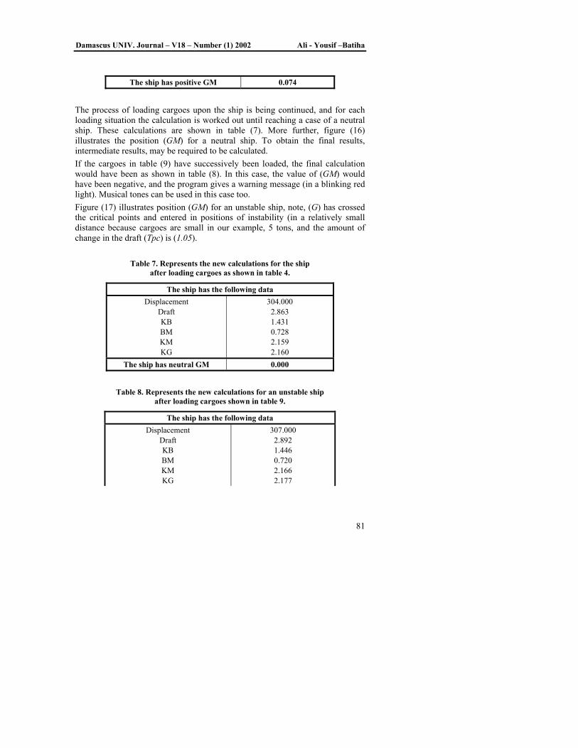
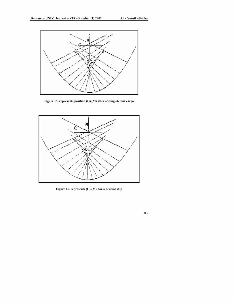
The process of loading cargoes upon the ship is being continued, and for each loading situation the calculation is worked out until reaching a case of a neutral ship. These calculations are shown in table (7). More further, figure (16) illustrates the position (GM) for a neutral ship. To obtain the final results, intermediate results, may be required to be calculated. If the cargoes in table (9) have successively been loaded, the final calculation would have been as shown in table (8). In this case, the value of (GM) would have been negative, and the program gives a warning message (in a blinking red light). Musical tones can be used in this case too. Figure (17) illustrates position (GM) for an unstable ship, note, (G) has crossed the critical points and entered in positions of instability (in a relatively small distance because cargoes are small in our example, 5 tons, and the amount of change in the draft (Tpc) is (1.05).

Table 7. Represents the new calculations for the ship after loading cargoes as shown in table 4.


Draft KB BM KM KG

304.000 2.863 1.431 0.728 2.159 2.160

The ship has neutral GM 0.000

Table 8. Represents the new calculations for an unstable ship after loading cargoes shown in table 9.


Draft KB BM KM KG

307.000 2.892 1.446 0.720 2.166 2.177


82

The ship has negative GM - 0.010

Table 9. Represents a group of cargoes and their specifications

The cargo node loading information No. Weight Distance Place 1 2 3 4 5 6

66 11 2 2 5 5

2 1 1 1 1 1

L L L L L L

Figure 14. represents the primary position (G),(M)


83

Figure 15. represents position (G),(M) after adding 66 tons cargo

Figure 16. represents (G),(M) for a neutral ship


84

Figure 17. represents position (G),(M) for an unstable ship

6. Discussion The general technique of this work in applying catastrophe theory to ship stability depends on two principles:

1. The theoretical principle is an analytical technique adopted by Zeeman in analyzing ships catastrophes and their stability. This principle consists of a group of theories, of which we have basically used the theory that says “The geometric place for points of the buoyancy center (B) is a parabola”.[6]

2. The practical principle is a structural constructional technique adopted by Poston to invent a catastrophic machine he called a gravitational catastrophe machine. It has been shown from the comparative study that the lower character of this machine is in fact a parabola. This parabola is the geometric place for points of the buoyancy center (B). Thus, Poston’s catastrophic equations have been programmed in order to be used as control and guiding equations which explain the ship catastrophes. It is very important to say that working with the second principle has not been Carried out on its own but it has been guided by the first principle as a means for examining the program’s results. Zeeman’s theoretical principle has been extensive since it has discussed all kinds of ships (rather than the container ships only whose equations have been programmed). This is what we see as a key for future research.


85

7. Conclusions This research examined Catastrophe Theory and how it deals with the cases of sudden changes in functions as a result of a small change in their independent variables. It also considered the possibility of applying the details of this theory and its analytical results as described by Tom Rene and Poston. The application of ships stability studied in this research has an economic and practical benefit. In particular, great numbers of oil tankers and commercial ships have become national and operated by local staff. The ship is a large body with three dimensions, and is subject to dynamic stresses due to the movement of changing cargoes. Also, effect of free surfaces gives the impression that there is a continuous danger over the ship. The proposed software package leads the management of cargo-loadiy loading and unloading and has the ability of distributing of cargoes. This package sends the warning message in the occurrence of catastrophe.


86

References

Is Is


87

1. Derret, D. R. (1972), “ Ship Stability for Master and Mates”, Standford

Maritime, London. 2. Eyres, D. J., (Second Edition), “Ship Construction”, William

Heinemann Ltd., 10 Tupper, Grosvenor Street, London. 3. Gilmore, R. (1981), “Catastrophe Theory for Scientists and Engineers”,

Wiley Interscience Publication. 4. Lu, Y. C. (1976), “Singularity Theory and an Introduction to

Catastrophe Theory”, Springer-verlag, New York Heidelberg, Berlin 5. James Croll (1976), “Is Catastrophe Theory Dangerous”, New Scientist

(17 June). 6. Obe, G. F. (1981), “ Brown’s Pocket-Book for Seaman”, Brown, Son,

& Ferguson Ltd., Glasgow, G41 2S G. 7. Owen, H. (1994), “Aids to Stability Displacement and Trim”, James

Brown & son, 5254 DARnley Street. 8. Poston, T. and Stewart I. (1978), “Catastrophe Theory and It’s

Applications”, Pitman London, San Francisco, Melbourne. 9. Rawson, K. J. and E. C. Tupper (1968), “Basic Ship Theory”,

Longmans, Green and Co Ltd., London and Harlow. 10. Saunders, P. T. (1980), “An Introduction to Catastrophe Theory”,

Cambridge University Press, Cambridge. 11. Stewart, I. (1975), “The Seven Elementary Catastrophes”, New

Scientist (20 November). 12. Stewart, I. (1983), “Nonelementary Catastrophe Theory”, IEEE

Transaction on Circuits and System, Vol. 20, No. 9, September. 13. Stewart, I. (1984), “Application of Nonelementary Catastrophe

Theory”, IEEE Transaction on Circuits and Systems, Vol. Cas-31, No. 2, February.

14. Taylor, L. G. (1977), “The Principles of Ship Stability”, Brown , Son, & Ferguson, Ltd., Glasgow, G41 2SG.

15. Thompson J. M. T., (1975), “Experiments in Catastrophe”, Articles Nature, Vol. 254 April.

16. Zeeman, E. C. (1980), “Bifurcation, Catastrophe, and Turbulence”, New Directions in Applied Mathematics, Springer-verlag, New York

Heidelberg Berlin. 17. Zeeman, E. C., “Catastrophe Theory”, (Delected Papers 1972-1977)”,


88

Addison-Wesley Publishing Company, Inc. ، الدار القومية للطباعة والنشر "الفن البحري العام ", )1965(حسن علي حسن ومحمد وسيم غالي .18

.965-949ص .، رسالة ماجستير، جامعة بغداد"تطبيقات نظریة الكوارث"، )1985(سعد ناجي العزاوي .19

Received, 17 December, 2000.

Software Package Supporting Ship Stability by using Catastrophe Theory

Documents

Transcript of Software Package Supporting Ship Stability by using Catastrophe Theory