Software Engineering: Principles

and Practice

Hans van Vliet

(c) Wiley, 2007

Contents

1 Introduction 1

Chapter 1 Introduction 1

1.1 What is Software Engineering? . . . . . . . . . . . . . . . . . . . . . 5

1.2 Phases in the Development of Software . . . . . . . . . . . . . . . . 10

1.3 Maintenance or Evolution . . . . . . . . . . . . . . . . . . . . . . . . 16

1.4 From the Trenches . . . . . . . . . . . . . . . . . . . . . . . . . . . 17

1.4.1 Ariane 5, Flight 501 . . . . . . . . . . . . . . . . . . . . . . . 18

1.4.2 Therac-25 . . . . . . . . . . . . . . . . . . . . . . . . . . . . 19

1.4.3 The London Ambulance Service . . . . . . . . . . . . . . . . 21

1.4.4 Who Counts the Votes? . . . . . . . . . . . . . . . . . . . . 23

1.5 Software Engineering Ethics . . . . . . . . . . . . . . . . . . . . . . 25

1.6 Quo Vadis? . . . . . . . . . . . . . . . . . . . . . . . . . . . . . . . 27

1.7 Summary . . . . . . . . . . . . . . . . . . . . . . . . . . . . . . . . 29

1.8 Further Reading . . . . . . . . . . . . . . . . . . . . . . . . . . . . . 29

Exercises . . . . . . . . . . . . . . . . . . . . . . . . . . . . . . . . . 30

I Software Management 33

2 Introduction to Software Engineering Management 34

Chapter 2 Introduction to Software Engineering Management 34

2.1 Planning a Software Development Project . . . . . . . . . . . . . . . 37

2.2 Controlling a Software Development Project . . . . . . . . . . . . . 40

2.3 Summary . . . . . . . . . . . . . . . . . . . . . . . . . . . . . . . . 42

Exercises . . . . . . . . . . . . . . . . . . . . . . . . . . . . . . . . . 43

3 The Software Life Cycle Revisited 45

Chapter 3 The Software Life Cycle Revisited 45

3.1 The Waterfall Model . . . . . . . . . . . . . . . . . . . . . . . . . . 48

3.2 Agile Methods . . . . . . . . . . . . . . . . . . . . . . . . . . . . . . 50

3.2.1 Prototyping . . . . . . . . . . . . . . . . . . . . . . . . . . . 51

3.2.2 Incremental Development . . . . . . . . . . . . . . . . . . . 56

3.2.3 Rapid Application Development and DSDM . . . . . . . . . 57

3.2.4 Extreme Programming . . . . . . . . . . . . . . . . . . . . . 61

3.3 The Rational Unified Process (RUP) . . . . . . . . . . . . . . . . . . 64

3.4 Intermezzo: Maintenance or Evolution . . . . . . . . . . . . . . . . . 66

3.5 Software Product Lines . . . . . . . . . . . . . . . . . . . . . . . . . 70

3.6 Process Modeling . . . . . . . . . . . . . . . . . . . . . . . . . . . . 71

3.7 Summary . . . . . . . . . . . . . . . . . . . . . . . . . . . . . . . . 75

3.8 Further Reading . . . . . . . . . . . . . . . . . . . . . . . . . . . . . 75

Exercises . . . . . . . . . . . . . . . . . . . . . . . . . . . . . . . . . 76

4 Configuration Management 78

Chapter 4 Configuration Management 78

4.1 Tasks and Responsibilities . . . . . . . . . . . . . . . . . . . . . . . . 80

4.2 Configuration Management Plan . . . . . . . . . . . . . . . . . . . . 85

4.3 Summary . . . . . . . . . . . . . . . . . . . . . . . . . . . . . . . . 86

4.4 Further Reading . . . . . . . . . . . . . . . . . . . . . . . . . . . . . 88

Exercises . . . . . . . . . . . . . . . . . . . . . . . . . . . . . . . . . 88

5 People Management and Team Organization 89

Chapter 5 People Management and Team Organization 89

5.1 People Management . . . . . . . . . . . . . . . . . . . . . . . . . . 91

5.1.1 Coordination Mechanisms . . . . . . . . . . . . . . . . . . . 93

5.1.2 Management Styles . . . . . . . . . . . . . . . . . . . . . . . 94

5.2 Team Organization . . . . . . . . . . . . . . . . . . . . . . . . . . . 96

5.2.1 Hierarchical Organization . . . . . . . . . . . . . . . . . . . 96

5.2.2 Matrix Organization . . . . . . . . . . . . . . . . . . . . . . 98

5.2.3 Chief Programmer Team . . . . . . . . . . . . . . . . . . . . 99

5.2.4 SWAT Team . . . . . . . . . . . . . . . . . . . . . . . . . . 100

5.2.5 Agile Team . . . . . . . . . . . . . . . . . . . . . . . . . . . 100

5.2.6 Open Source Software Development . . . . . . . . . . . . . 101

5.2.7 General Principles for Organizing a Team . . . . . . . . . . . 103

5.3 Summary . . . . . . . . . . . . . . . . . . . . . . . . . . . . . . . . 104

5.4 Further Reading . . . . . . . . . . . . . . . . . . . . . . . . . . . . . 105

Exercises . . . . . . . . . . . . . . . . . . . . . . . . . . . . . . . . . 105

6 On Managing Software Quality 107

Chapter 6 On Managing Software Quality 107

6.1 On Measures and Numbers . . . . . . . . . . . . . . . . . . . . . . . 110

6.2 A Taxonomy of Quality Attributes . . . . . . . . . . . . . . . . . . . 116

6.3 Perspectives on Quality . . . . . . . . . . . . . . . . . . . . . . . . . 123

6.4 The Quality System . . . . . . . . . . . . . . . . . . . . . . . . . . . 127

6.5 Software Quality Assurance . . . . . . . . . . . . . . . . . . . . . . . 128

6.6 The Capability Maturity Model (CMM) . . . . . . . . . . . . . . . . 130

6.7 Some Critical Notes . . . . . . . . . . . . . . . . . . . . . . . . . . . 136

6.8 Getting Started . . . . . . . . . . . . . . . . . . . . . . . . . . . . . 137

6.9 Summary . . . . . . . . . . . . . . . . . . . . . . . . . . . . . . . . 140

6.10 Further Reading . . . . . . . . . . . . . . . . . . . . . . . . . . . . . 140

Exercises . . . . . . . . . . . . . . . . . . . . . . . . . . . . . . . . . 141

7 Cost Estimation 144

Chapter 7 Cost Estimation 144

7.1 Algorithmic Models . . . . . . . . . . . . . . . . . . . . . . . . . . . 148

7.1.1 Walston--Felix . . . . . . . . . . . . . . . . . . . . . . . . . 151

7.1.2 COCOMO . . . . . . . . . . . . . . . . . . . . . . . . . . . 153

7.1.3 Putnam . . . . . . . . . . . . . . . . . . . . . . . . . . . . . 155

7.1.4 Function Point Analysis . . . . . . . . . . . . . . . . . . . . . 156

7.1.5 COCOMO 2: Variations on a Theme . . . . . . . . . . . . . 159

7.2 Guidelines for Estimating Cost . . . . . . . . . . . . . . . . . . . . . 166

7.3 Distribution of Manpower over Time . . . . . . . . . . . . . . . . . . 169

7.4 Summary . . . . . . . . . . . . . . . . . . . . . . . . . . . . . . . . 171

7.5 Further Reading . . . . . . . . . . . . . . . . . . . . . . . . . . . . . 174

Exercises . . . . . . . . . . . . . . . . . . . . . . . . . . . . . . . . . 174

8 Project Planning and Control 176

Chapter 8 Project Planning and Control 176

8.1 A Systems View of Project Control . . . . . . . . . . . . . . . . . . . 177

8.2 A Taxonomy of Software Development Projects . . . . . . . . . . . . 179

8.3 Risk Management . . . . . . . . . . . . . . . . . . . . . . . . . . . . 184

8.4 Techniques for Project Planning and Control . . . . . . . . . . . . . 189

8.5 Summary . . . . . . . . . . . . . . . . . . . . . . . . . . . . . . . . 194

8.6 Further Reading . . . . . . . . . . . . . . . . . . . . . . . . . . . . . 194

Exercises . . . . . . . . . . . . . . . . . . . . . . . . . . . . . . . . . 195

II The Software Life Cycle 197

9 Requirements Engineering 199

Chapter 9 Requirements Engineering 199

9.1 Requirements Elicitation . . . . . . . . . . . . . . . . . . . . . . . . 205

9.1.1 Requirements Engineering Paradigms . . . . . . . . . . . . . 210

9.1.2 Requirements Elicitation Techniques . . . . . . . . . . . . . . 212

9.1.3 Goals and Viewpoints . . . . . . . . . . . . . . . . . . . . . 220

9.1.4 Prioritizing Requirements . . . . . . . . . . . . . . . . . . . 223

9.1.5 COTS selection . . . . . . . . . . . . . . . . . . . . . . . . 224

9.2 Requirements Documentation and Management . . . . . . . . . . . . 227

9.2.1 Requirements Management . . . . . . . . . . . . . . . . . . . 234

9.3 Requirements Specification Techniques . . . . . . . . . . . . . . . . 236

9.3.1 Specifying Non-Functional Requirements . . . . . . . . . . . 238

9.4 Verification and Validation . . . . . . . . . . . . . . . . . . . . . . . 239

9.5 Summary . . . . . . . . . . . . . . . . . . . . . . . . . . . . . . . . 240

9.6 Further Reading . . . . . . . . . . . . . . . . . . . . . . . . . . . . . 242

Exercises . . . . . . . . . . . . . . . . . . . . . . . . . . . . . . . . . 243

10 Modeling 246

Chapter 10Modeling 246

10.1 Classic Modeling Techniques . . . . . . . . . . . . . . . . . . . . . . 248

10.1.1 Entity--Relationship Modeling . . . . . . . . . . . . . . . . . 248

10.1.2 Finite State Machines . . . . . . . . . . . . . . . . . . . . . . 250

10.1.3 Data Flow Diagrams (DFD) . . . . . . . . . . . . . . . . . . 252

10.1.4 CRC Cards . . . . . . . . . . . . . . . . . . . . . . . . . . . 252

10.2 On Objects and Related Stuff . . . . . . . . . . . . . . . . . . . . . . 254

10.3 The Unified Modeling Language . . . . . . . . . . . . . . . . . . . . 260

10.3.1 The Class Diagram . . . . . . . . . . . . . . . . . . . . . . . 260

10.3.2 The State Machine Diagram . . . . . . . . . . . . . . . . . . 265

10.3.3 The Sequence Diagram . . . . . . . . . . . . . . . . . . . . . 268

10.3.4 The Communication Diagram . . . . . . . . . . . . . . . . . 271

10.3.5 The Component Diagram . . . . . . . . . . . . . . . . . . . 272

10.3.6 The Use Case . . . . . . . . . . . . . . . . . . . . . . . . . . 273

10.4 Summary . . . . . . . . . . . . . . . . . . . . . . . . . . . . . . . . 274

10.5 Further Reading . . . . . . . . . . . . . . . . . . . . . . . . . . . . . 274

Exercises . . . . . . . . . . . . . . . . . . . . . . . . . . . . . . . . . 274

11 Software Architecture 276

Chapter 11Software Architecture 276

11.1 Software Architecture and the Software Life Cycle . . . . . . . . . . 280

11.2 Architecture design . . . . . . . . . . . . . . . . . . . . . . . . . . . 281

11.2.1 Architecture as a set of design decisions . . . . . . . . . . . . 284

11.3 Architectural views . . . . . . . . . . . . . . . . . . . . . . . . . . . 285

11.4 Architectural Styles . . . . . . . . . . . . . . . . . . . . . . . . . . . 291

11.5 Software Architecture Assessment . . . . . . . . . . . . . . . . . . . 306

11.6 Summary . . . . . . . . . . . . . . . . . . . . . . . . . . . . . . . . 309

11.7 Further Reading . . . . . . . . . . . . . . . . . . . . . . . . . . . . . 310

Exercises . . . . . . . . . . . . . . . . . . . . . . . . . . . . . . . . . 311

12 Software Design 313

Chapter 12Software Design 313

12.1 Design Considerations . . . . . . . . . . . . . . . . . . . . . . . . . 317

12.1.1 Abstraction . . . . . . . . . . . . . . . . . . . . . . . . . . . 318

12.1.2 Modularity . . . . . . . . . . . . . . . . . . . . . . . . . . . 321

12.1.3 Information Hiding . . . . . . . . . . . . . . . . . . . . . . . 325

12.1.4 Complexity . . . . . . . . . . . . . . . . . . . . . . . . . . . 325

12.1.5 System Structure . . . . . . . . . . . . . . . . . . . . . . . . 333

12.1.6 Object-Oriented Metrics . . . . . . . . . . . . . . . . . . . . 337

12.2 Classical Design Methods . . . . . . . . . . . . . . . . . . . . . . . . 340

12.2.1 Functional Decomposition . . . . . . . . . . . . . . . . . . . 342

12.2.2 Data Flow Design (SA/SD) . . . . . . . . . . . . . . . . . . . 346

12.2.3 Design based on Data Structures . . . . . . . . . . . . . . . . 351

12.3 Object-Oriented Analysis and Design Methods . . . . . . . . . . . . 359

12.3.1 The Booch Method . . . . . . . . . . . . . . . . . . . . . . . 366

12.3.2 Fusion . . . . . . . . . . . . . . . . . . . . . . . . . . . . . . 367

12.3.3 RUP Revisited . . . . . . . . . . . . . . . . . . . . . . . . . 369

12.4 How to Select a Design Method . . . . . . . . . . . . . . . . . . . . 370

12.4.1 Object Orientation: Hype or the Answer? . . . . . . . . . . . 373

12.5 Design Patterns . . . . . . . . . . . . . . . . . . . . . . . . . . . . . 375

12.6 Design Documentation . . . . . . . . . . . . . . . . . . . . . . . . . 380

12.7 Verification and Validation . . . . . . . . . . . . . . . . . . . . . . . 383

12.8 Summary . . . . . . . . . . . . . . . . . . . . . . . . . . . . . . . . 384

12.9 Further Reading . . . . . . . . . . . . . . . . . . . . . . . . . . . . . 388

Exercises . . . . . . . . . . . . . . . . . . . . . . . . . . . . . . . . . 389

13 Software Testing 394

Chapter 13Software Testing 394

13.1 Test Objectives . . . . . . . . . . . . . . . . . . . . . . . . . . . . . 398

13.1.1 Test Adequacy Criteria . . . . . . . . . . . . . . . . . . . . . 401

13.1.2 Fault Detection Versus Confidence Building . . . . . . . . . . 402

13.1.3 From Fault Detection to Fault Prevention . . . . . . . . . . . 403

13.2 Testing and the Software Life Cycle . . . . . . . . . . . . . . . . . . 406

13.2.1 Requirements Engineering . . . . . . . . . . . . . . . . . . . 407

13.2.2 Design . . . . . . . . . . . . . . . . . . . . . . . . . . . . . 408

13.2.3 Implementation . . . . . . . . . . . . . . . . . . . . . . . . . 409

13.2.4 Maintenance . . . . . . . . . . . . . . . . . . . . . . . . . . 409

13.2.5 Test-Driven Development (TDD) . . . . . . . . . . . . . . . 410

13.3 Verification and Validation Planning and Documentation . . . . . . . 411

13.4 Manual Test Techniques . . . . . . . . . . . . . . . . . . . . . . . . 413

13.4.1 Reading . . . . . . . . . . . . . . . . . . . . . . . . . . . . . 414

13.4.2 Walkthroughs and Inspections . . . . . . . . . . . . . . . . . 415

13.4.3 Correctness Proofs . . . . . . . . . . . . . . . . . . . . . . . 417

13.4.4 Stepwise Abstraction . . . . . . . . . . . . . . . . . . . . . . 418

13.5 Coverage-Based Test Techniques . . . . . . . . . . . . . . . . . . . . 419

13.5.1 Control-Flow Coverage . . . . . . . . . . . . . . . . . . . . 420

13.5.2 Dataflow Coverage . . . . . . . . . . . . . . . . . . . . . . . 423

13.5.3 Coverage-Based Testing of Requirements Specifications . . . 424

13.6 Fault-Based Test Techniques . . . . . . . . . . . . . . . . . . . . . . 425

13.6.1 Error Seeding . . . . . . . . . . . . . . . . . . . . . . . . . . 425

13.6.2 Mutation Testing . . . . . . . . . . . . . . . . . . . . . . . . 428

13.7 Error-Based Test Techniques . . . . . . . . . . . . . . . . . . . . . . 429

13.8 Comparison of Test Techniques . . . . . . . . . . . . . . . . . . . . 431

13.8.1 Comparison of Test Adequacy Criteria . . . . . . . . . . . . 432

13.8.2 Properties of Test Adequacy Criteria . . . . . . . . . . . . . . 434

13.8.3 Experimental Results . . . . . . . . . . . . . . . . . . . . . . 436

13.9 Different Test Stages . . . . . . . . . . . . . . . . . . . . . . . . . . 438

13.10Estimating Software Reliability . . . . . . . . . . . . . . . . . . . . . 439

13.11Summary . . . . . . . . . . . . . . . . . . . . . . . . . . . . . . . . 447

13.12Further Reading . . . . . . . . . . . . . . . . . . . . . . . . . . . . . 448

Exercises . . . . . . . . . . . . . . . . . . . . . . . . . . . . . . . . . 449

14 Software Maintenance 453

Chapter 14Software Maintenance 453

14.1 Maintenance Categories Revisited . . . . . . . . . . . . . . . . . . . 456

14.2 Major Causes of Maintenance Problems . . . . . . . . . . . . . . . . 459

14.3 Reverse Engineering and Refactoring . . . . . . . . . . . . . . . . . . 463

14.3.1 Refactoring . . . . . . . . . . . . . . . . . . . . . . . . . . . 466

14.3.2 Inherent Limitations . . . . . . . . . . . . . . . . . . . . . . 469

14.3.3 Tools . . . . . . . . . . . . . . . . . . . . . . . . . . . . . . 473

14.4 Software Evolution Revisited . . . . . . . . . . . . . . . . . . . . . . 474

14.5 Organizational and Managerial Issues . . . . . . . . . . . . . . . . . 476

14.5.1 Organization of Maintenance Activities . . . . . . . . . . . . 477

14.5.2 Software Maintenance from a Service Perspective . . . . . . . 480

14.5.3 Control of Maintenance Tasks . . . . . . . . . . . . . . . . . 486

14.5.4 Quality Issues . . . . . . . . . . . . . . . . . . . . . . . . . . 489

14.6 Summary . . . . . . . . . . . . . . . . . . . . . . . . . . . . . . . . 490

14.7 Further Reading . . . . . . . . . . . . . . . . . . . . . . . . . . . . . 491

Exercises . . . . . . . . . . . . . . . . . . . . . . . . . . . . . . . . . 492

15 Software Tools 494

Chapter 15Software Tools 494

15.1 Toolkits . . . . . . . . . . . . . . . . . . . . . . . . . . . . . . . . . 499

15.2 Language-Centered Environments . . . . . . . . . . . . . . . . . . . 500

15.3 Integrated Environments and Workbenches . . . . . . . . . . . . . . 501

15.3.1 Analyst WorkBenches . . . . . . . . . . . . . . . . . . . . . 501

15.3.2 Programmer Workbenches . . . . . . . . . . . . . . . . . . . 503

15.3.3 Management WorkBenches . . . . . . . . . . . . . . . . . . 507

15.3.4 Integrated Project Support Environments . . . . . . . . . . . 508

15.4 Process-Centered Environments . . . . . . . . . . . . . . . . . . . . 508

15.5 Summary . . . . . . . . . . . . . . . . . . . . . . . . . . . . . . . . 510

15.6 Further Reading . . . . . . . . . . . . . . . . . . . . . . . . . . . . . 511

Exercises . . . . . . . . . . . . . . . . . . . . . . . . . . . . . . . . . 512

Bibliography 514

1

Introduction

LEARNING OBJECTIVES� To understand the notion of software engineering and why it is important� To appreciate the technical (engineering), managerial, and psychological

aspects of software engineering� To understand the similarities and differences between software engineering

and other engineering disciplines� To know the major phases in a software development project� To appreciate ethical dimensions in software engineering� To be aware of the time frame and extent to which new developments impact

software engineering practice

2 INTRODUCTION

Software engineering concerns methods and techniques to develop large

software systems. The engineering metaphor is used to emphasize a systematic

approach to develop systems that satisfy organizational requirements and

constraints. This chapter gives a brief overview of the field and points at

emerging trends that influence the way software is developed.

Computer science is still a young field. The first computers were built in the mid

1940s, since when the field has developed tremendously.

Applications from the early years of computerization can be characterized as

follows: the programs were quite small, certainly when compared to those that are

currently being constructed; they were written by one person; they were written and

used by experts in the application area concerned. The problems to be solved were

mostly of a technical nature, and the emphasis was on expressing known algorithms

efficiently in some programming language. Input typically consisted of numerical

data, read from such media as punched tape or punched cards. The output, also

numeric, was printed on paper. Programs were run off-line. If the program contained

errors, the programmer studied an octal or hexadecimal dump of memory. Sometimes,

the execution of the program would be followed by binary reading machine registers

at the console.

Independent software development companies hardly existed in those days.

Software was mostly developed by hardware vendors and given away for free. These

vendors sometimes set up user groups to discuss requirements, and next incorporated

them into their software. This software development support was seen as a service to

their customers.

Present-day applications are rather different in many respects. Present-day pro-

grams are often very large and are being developed by teams that collaborate over

periods spanning several years. These teams may be scattered across the globe. The

programmers are not the future users of the system they develop and they have no

expert knowledge of the application area in question. The problems that are being

tackled increasingly concern everyday life: automatic bank tellers, airline reservation,

salary administration, electronic commerce, automotive systems, etc. Putting a man

on the moon was not conceivable without computers.

In the 1960s, people started to realize that programming techniques had lagged

behind the developments in software both in size and complexity. To many people,

programming was still an art and had never become a craft. An additional problem was

that many programmers had not been formally educated in the field. They had learned

by doing. On the organizational side, attempted solutions to problems often involved

adding more and more programmers to the project, the so-called ‘million-monkey’

approach.

As a result, software was often delivered too late, programs did not behave as the

user expected, programs were rarely adaptable to changed circumstances, and many

errors were detected only after the software had been delivered to the customer. This

3

became known as the ‘software crisis’.

This type of problem really became manifest in the 1960s. Under the auspices

of NATO, two conferences were devoted to the topic in 1968 and 1969 (Naur and

Randell, 1968), (Buxton and Randell, 1969). Here, the term ‘software engineering’ was

coined in a somewhat provocative sense. Shouldn’t it be possible to build software

in the way one builds bridges and houses, starting from a theoretical basis and using

sound and proven design and construction techniques, as in other engineering fields?

Software serves some organizational purpose. The reasons for embarking on

a software development project vary. Sometimes, a solution to a problem is not

feasible without the aid of computers, such as weather forecasting, or automated

bank telling. Sometimes, software can be used as a vehicle for new technologies, such

as typesetting, the production of chips, or manned space trips. In yet other cases

software may increase user service (library automation, e-commerce) or simply save

money (automated stock control).

In many cases, the expected economic gain will be a major driving force. It may

not, however, always be easy to prove that automation saves money (just think of

office automation) because apart from direct cost savings, the economic gain may

also manifest itself in such things as a more flexible production or a faster or better

user service. In either case, it is a value-creating activity.

Boehm (1981) estimated the total expenditure on software in the US to be $40

billion in 1980. This is approximately 2% of the GNP. In 1985, the total expenditure

had risen to $70 billion in the US and $140 billion worldwide. Boehm and Sullivan

(1999) estimated the annual expenditure on software development in 1998 to be

$300-400 billion in the US, and twice that amount worlwide.

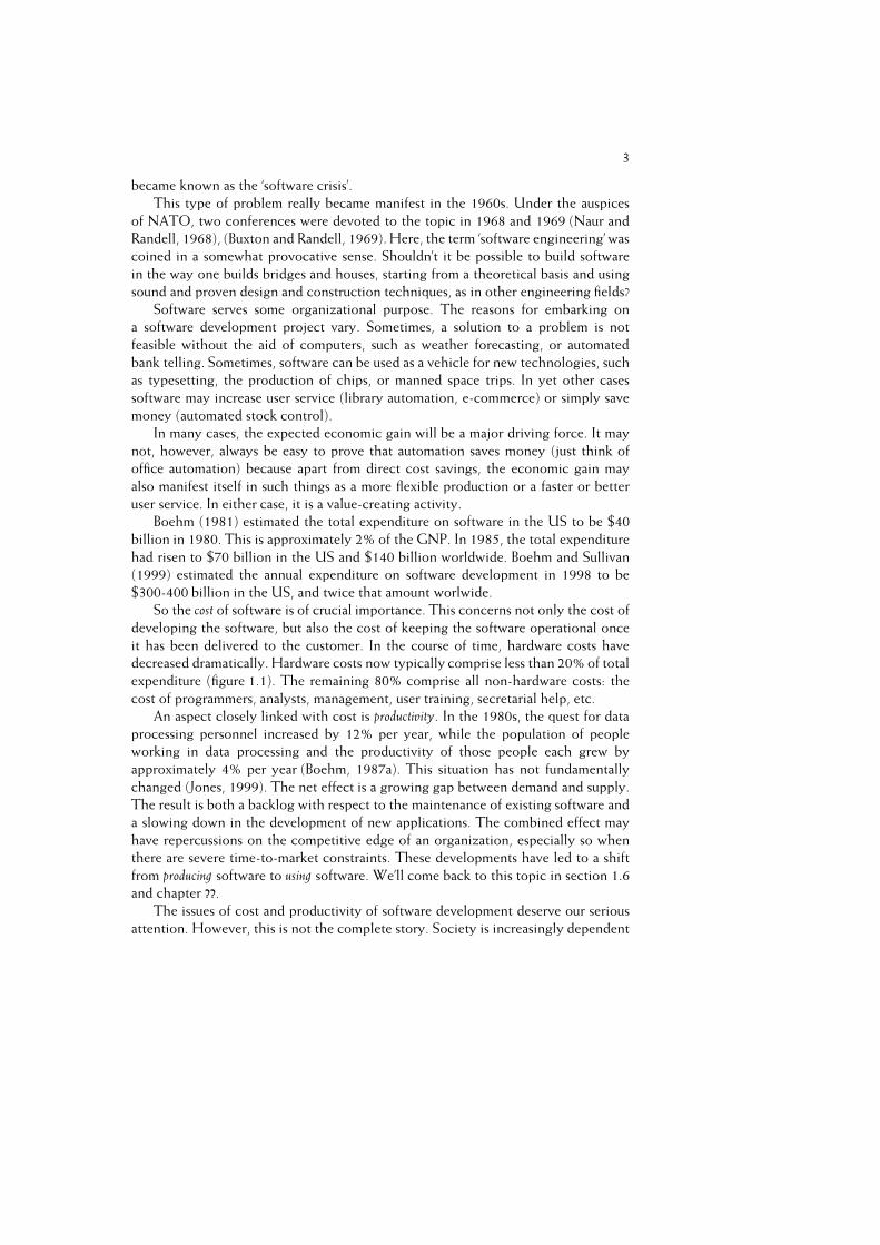
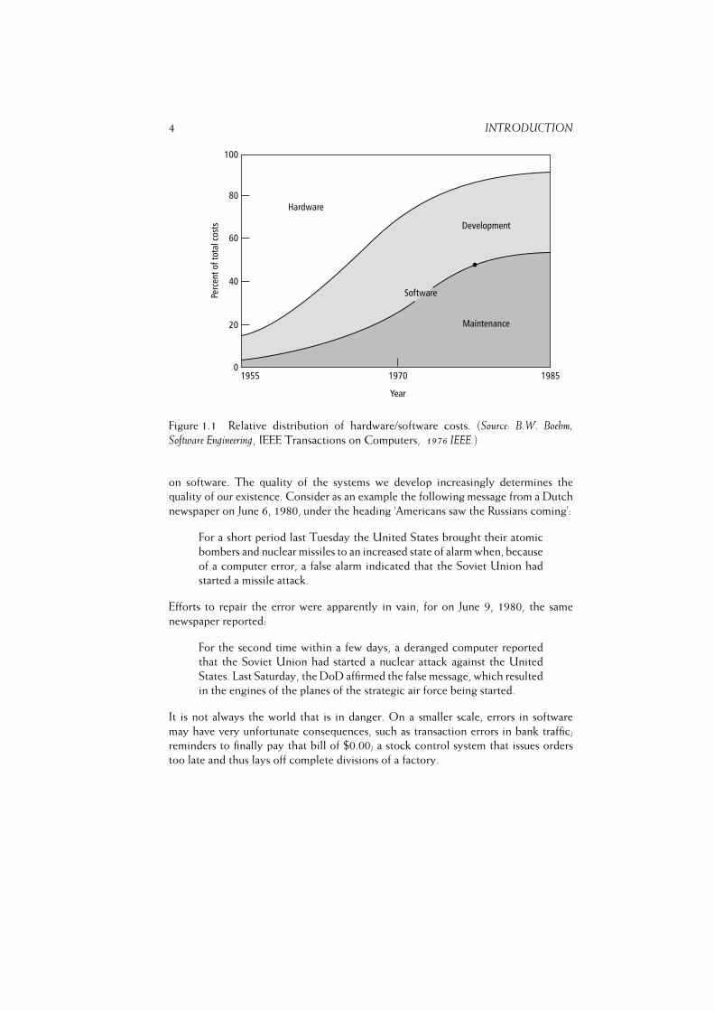
So the cost of software is of crucial importance. This concerns not only the cost of

developing the software, but also the cost of keeping the software operational once

it has been delivered to the customer. In the course of time, hardware costs have

decreased dramatically. Hardware costs now typically comprise less than 20% of total

expenditure (figure 1.1). The remaining 80% comprise all non-hardware costs: the

cost of programmers, analysts, management, user training, secretarial help, etc.

An aspect closely linked with cost is productivity. In the 1980s, the quest for data

processing personnel increased by 12% per year, while the population of people

working in data processing and the productivity of those people each grew by

approximately 4% per year (Boehm, 1987a). This situation has not fundamentally

changed (Jones, 1999). The net effect is a growing gap between demand and supply.

The result is both a backlog with respect to the maintenance of existing software and

a slowing down in the development of new applications. The combined effect may

have repercussions on the competitive edge of an organization, especially so when

there are severe time-to-market constraints. These developments have led to a shift

from producing software to using software. We’ll come back to this topic in section 1.6

and chapter ??.

The issues of cost and productivity of software development deserve our serious

attention. However, this is not the complete story. Society is increasingly dependent

4 INTRODUCTION

Figure 1.1 Relative distribution of hardware/software costs. (Source: B.W. Boehm,

Software Engineering, IEEE Transactions on Computers, 1976 IEEE.)

on software. The quality of the systems we develop increasingly determines the

quality of our existence. Consider as an example the following message from a Dutch

newspaper on June 6, 1980, under the heading ‘Americans saw the Russians coming’:

For a short period last Tuesday the United States brought their atomic

bombers and nuclear missiles to an increased state of alarm when, because

of a computer error, a false alarm indicated that the Soviet Union had

started a missile attack.

Efforts to repair the error were apparently in vain, for on June 9, 1980, the same

newspaper reported:

For the second time within a few days, a deranged computer reported

that the Soviet Union had started a nuclear attack against the United

States. Last Saturday, the DoD affirmed the false message, which resulted

in the engines of the planes of the strategic air force being started.

It is not always the world that is in danger. On a smaller scale, errors in software

may have very unfortunate consequences, such as transaction errors in bank traffic;

reminders to finally pay that bill of $0.00; a stock control system that issues orders

too late and thus lays off complete divisions of a factory.

1.1. WHAT IS SOFTWARE ENGINEERING? 5

The latter example indicates that errors in a software system may have serious

financial consequences for the organization using it. One example of such a financial

loss is the large US airline company that lost $50M because of an error in their

seat reservation system. The system erroneously reported that cheap seats were sold

out, while in fact there were plenty available. The problem was detected only after

quarterly results lagged considerably behind those of both their own previous periods

and those of their competitors.

Errors in automated systems may even have fatal effects. One computer science

weekly magazine contained the following message in April 1983:

The court in Dusseldorf has discharged a woman (54), who was on trial

for murdering her daughter. An erroneous message from a computerized

system made the insurance company inform her that she was seriously

ill. She was said to suffer from an incurable form of syphilis. Moreover,

she was said to have infected both her children. In panic, she strangled

her 15 year old daughter and tried to kill her 13 year old son and herself.

The boy escaped, and with some help he enlisted prevented the woman

from dying of an overdose. The judge blamed the computer error and

considered the woman not responsible for her actions.

This all marks the enormous importance of the field of software engineering.

Better methods and techniques for software development may result in large financial

savings, in more effective methods of software development, in systems that better fit

user needs, in more reliable software systems, and thus in a more reliable environment

in which those systems function. Quality and productivity are two central themes in

the field of software engineering.

On the positive side, it is imperative to point to the enormous progress that has

been made since the 1960s. Software is ubiquitous and scores of trustworthy systems

have been built. These range from small spreadsheet applications to typesetting

systems, banking systems, Web browsers and the Space Shuttle software. The

techniques and methods discussed in this book have contributed their mite to the

success of these and many other software development projects.

1.1 What is Software Engineering?

In various texts on this topic, one encounters a definition of the term software

engineering. An early definition was given at the first NATO conference (Naur and

Randell, 1968):

Software engineering is the establishment and use of sound engineering

principles in order to obtain economically software that is reliable and

works efficiently on real machines.

The definition given in the IEEE Standard Glossary of Software Engineering Terminol-

ogy (IEEE610, 1990) is as follows:

6 INTRODUCTION

Software engineering is the application of a systematic, disciplined,

quantifiable approach to the development, operation, and maintenance

of software; that is, the application of engineering to software.

These and other definitions of the term software engineering use rather different

words. However, the essential characteristics of the field are always, explicitly or

implicitly, present:� Software engineering concerns the development of large programs.(DeRemer and Kron, 1976) make a distinction between programming-in-the-

large and programming-in-the-small. The borderline between large and small

obviously is not sharp: a program of 100 lines is small, a program of 50 000 lines

of code certainly is not. Programming-in-the-small generally refers to programs

written by one person in a relatively short period of time. Programming-in-the-

large, then, refers to multi-person jobs that span, say, more than half a year.

For example:

– The NASA Space Shuttle software contains 40M lines of object code

(this is 30 times as much as the software for the Saturn V project from the

1960s) (Boehm, 1981);

– The IBM OS360 operating system took 5000 man years of development

effort (Brooks, 1995).

Traditional programming techniques and tools are primarily aimed at support-

ing programming-in-the-small.This not only holds for programming languages,

but also for the tools (like flowcharts) and methods (like structured program-

ming). These cannot be directly transferred to the development of large

programs.

In fact, the term program -- in the sense of a self-contained piece of software

that can be invoked by a user or some other system component -- is not

adequate here. Present-day software development projects result in systems

containing a large number of (interrelated) programs -- or components.� The central theme is mastering complexity.In general, the problems are such that they cannot be surveyed in their entirety.

One is forced to split the problem into parts such that each individual part can

be grasped, while the communication between the parts remains simple. The

total complexity does not decrease in this way, but it does become manageable.

In a stereo system there are components such as an amplifier, a receiver, and a

tuner, and communication via a thin wire. In software, we strive for a similar

separation of concerns. In a program for library automation, components such

as user interaction, search processes and data storage could for instance be

distinguished, with clearly given facilities for data exchange between those

components. Note that the complexity of many a piece of software is not

1.1. WHAT IS SOFTWARE ENGINEERING? 7

so much caused by the intrinsic complexity of the problem (as in the case

of compiler optimization algorithms or numerical algorithms to solve partial

differential equations), but rather by the vast number of details that must be

dealt with.� Software evolves.

Most software models a part of reality, such as processing requests in a library

or tracking money transfers in a bank. This reality evolves. If software is not to

become obsolete fairly quickly, it has to evolve with the reality that is being

modeled. This means that costs are incurred after delivery of the software

system and that we have to bear this evolution in mind during development.� The efficiency with which software is developed is of crucial importance.

Total cost and development time of software projects is high. This also holds

for the maintenance of software. The quest for new applications surpasses the

workforce resource. The gap between supply and demand is growing. Time-

to-market demands ask for quick delivery. Important themes within the field of

software engineering concern better and more efficient methods and tools for

the development and maintenance of software, especially methods and tools

enabling the use and reuse of components.� Regular cooperation between people is an integral part of programming-in-the-large.

Since the problems are large, many people have to work concurrently at solving

those problems. Increasingly often, teams at different geographic locations

work together in software development. There must be clear arrangements for

the distribution of work, methods of communication, responsibilities, and so

on. Arrangements alone are not sufficient, though; one also has to stick to

those arrangements. In order to enforce them, standards or procedures may

be employed. Those procedures and standards can often be supported by

tools. Discipline is one of the keys to the successful completion of a software

development project.� The software has to support its users effectively.Software is developed in order to support users at work. The functionality

offered should fit users’ tasks. Users that are not satisfied with the system will

try to circumvent it or, at best, voice new requirements immediately. It is not

sufficient to build the system in the right way, we also have to build the right

system. Effective user support means that we must carefully study users at work,

in order to determine the proper functional requirements, and we must address

usability and other quality aspects as well, such as reliability, responsiveness,

and user-friendliness. It also means that software development entails more

than delivering software. User manuals and training material may have to be

written, and attention must be given to developing the environment in which

the new system is going to be installed. For example, a new automated library

system will affect working procedures within the library.

8 INTRODUCTION� Software engineering is a field in which members of one culture create artifacts on behalf of

members of another culture.This aspect is closely linked to the previous two items. Software engineers are

expert in one or more areas such as programming in Java, software architecture,

testing, or the Unified Modeling Language. They are generally not experts in

library management, avionics, or banking. Yet they have to develop systems for

such domains. The thin spread of application domain knowledge is a common

source of problems in software development projects.

Not only do software engineers lack factual knowledge of the domain for

which they develop software, they lack knowledge of its culture as well. For

example, a software developer may discover the ‘official’ set of work practices

of a certain user community from interviews, written policies, and the like;

these work practices are then built into the software. A crucial question with

respect to system acceptance and success, however, is whether that community

actually follows those work practices. For an outside observer, this question is

much more difficult to answer.� Software engineering is a balancing act.In most realistic cases, it is illusive to assume that the collection of requirements

voiced at the start of the project is the only factor that counts. In fact, the

term requirement is a misnomer. It suggests something immutable, while in

fact most requirements are negotiable. There are numerous business, technical

and political constraints that may influence a software development project.

For example, one may decide to use database technology X rather than Y,

simply because of available expertise with that technology. In extreme cases,

characteristics of available components may determine functionality offered,

rather than the other way around.

The above list shows that software engineering has many facets. Software engineering

certainly is not the same as programming, although programming is an important

ingredient of software engineering. Mathematical aspects play a role since we

are concerned with the correctness of software. Sound engineering practices are

needed to get useful products. Psychological and sociological aspects play a role in

the communication between human and machine, organization and machine, and

between humans. Finally, the development process needs to be controlled, which is

a management issue.

The term ‘software engineering’ hints at possible resemblances between the

construction of programs and the construction of houses or bridges. These kinds of

resemblances do exist. In both cases we work from a set of desired functions, using

scientific and engineering techniques in a creative way. Techniques that have been

applied successfully in the construction of physical artifacts are also helpful when

applied to the construction of software systems: development of the product in a

number of phases, a careful planning of these phases, continuous audit of the whole

process, construction from a clear and complete design, etc.

1.1. WHAT IS SOFTWARE ENGINEERING? 9

Even in a mature engineering discipline, say bridge design, accidents do happen.

Bridges collapse once in a while. Most problems in bridge design occur when designers

extrapolate beyond their models and expertise. A famous example is the Tacoma

Narrows Bridge failure in 1940. The designers of that bridge extrapolated beyond

their experience to create more flexible stiffening girders for suspension bridges. They

did not think about aerodynamics and the response of the bridge to wind. As a result,

that bridge collapsed shortly after it was finished. This type of extrapolation seems to

be the rule rather than the exception in software development. We regularly embark

on software development projects that go far beyond our expertise.

There are additional reasons for considering the construction of software as

something quite different from the construction of physical products. The cost of

constructing software is incurred during development and not during production.

Copying software is almost free. Software is logical in nature rather than physical.

Physical products wear out in time and therefore have to be maintained. Software

does not wear out. The need to maintain software is caused by errors detected late

or by changing requirements of the user. Software reliability is determined by the

manifestation of errors already present, not by physical factors such as wear and tear.

We may even argue that software wears out because it is being maintained.

Viewing software engineering as a branch of engineering is problematic for

another reason as well. The engineering metaphor hints at disciplined work, proper

planning, good management, and the like. It suggests we deal with clearly defined

needs, that can be fulfilled if we follow all the right steps. Many software development

projects though involve the translation of some real world phenomenon into digital

form. The knowledge embedded in this real life phenomenon is tacit, undefined,

uncodified, and may have developed over a long period of time. The assumption that

we are dealing with a well-defined problem simply does not hold. Rather, the design

process is open ended, and the solution emerges as we go along. This dichotomy is

reflected in views of the field put in the forefront over time (Eischen, 2002). In the

early days, the field was seen as a craft. As a countermovement, the term software

engineering was coined, and many factory concepts got introduced. In the late 1990’s,

the pendulum swung back again and the craft aspect got emphasized anew, in the

agile movement (see chapter 3). Both engineering-like and craft-like aspects have

their place, and we will give a balanced treatment of both.

Two characteristics that make software development projects extra difficult to

manage are visibility and continuity. It is much more difficult to see progress in

software construction than it is to notice progress in building a bridge. One often

hears the phrase that a program ‘is almost finished’. One equally often underestimates

the time needed to finish up the last bits and pieces.

This ‘90% complete’ syndrome is very pervasive in software development. Not

knowing how to measure real progress, we often use a surrogate measure, the rate

of expenditure of resources. For example, a project that has a budget of 100 person-

days is perceived as being 50% complete after 50 person-days are expended. Strictly

speaking, we then confuse speed with progress. Because of the imprecise measurement

10 INTRODUCTION

of progress and the customary underestimation of total effort, problems accumulate

as time elapses.

Physical systems are often continuous in the sense that small changes in the

specification lead to small changes in the product. This is not true with software.

Small changes in the specification of software may lead to considerable changes in

the software itself. In a similar way, small errors in software may have considerable

effects. The Mariner space rocket to Venus for example got lost because of a typing

error in a FORTRAN program. In 1998, the Mars Climate Orbiter got lost, because

one development team used English units such as inches and feet, while another team

used metric units.

We may likewise draw a comparison between software engineering and computer

science. Computer science emerged as a separate discipline in the 1960s. It split

from mathematics and has been heavily influenced by mathematics. Topics studied in

computer science, such as algorithm complexity, formal languages, and the semantics

of programming languages, have a strong mathematical flavor. PhD theses in computer

science invariably contain theorems with accompanying proofs.

As the field of software engineering emerged from computer science, it had a

similar inclination to focus on clean aspects of software development that can be

formalized, in both teaching and research. We used to assume that requirements can

be fully stated before the project started, concentrated on systems built from scratch,

and ignored the reality of trading off quality aspects against the available budget. Not

to mention the trenches of software maintenance.

Software engineering and computer science do have a considerable overlap. The

practice of software engineering however also has to deal with such matters as

the management of huge development projects, human factors (regarding both the

development team and the prospective users of the system) and cost estimation and

control. Software engineers must engineer software.

Software engineering has many things in common both with other fields of

engineering and with computer science. It also has a face of its own in many ways.

1.2 Phases in the Development of Software

When building a house, the builder does not start with piling up bricks. Rather, the

requirements and possibilities of the client are analyzed first, taking into account such

factors as family structure, hobbies, finances and the like. The architect takes these

factors into consideration when designing a house. Only after the design has been

agreed upon is the actual construction started.

It is expedient to act in the same way when constructing software. First, the

problem to be solved is analyzed and the requirements are described in a very

precise way. Then a design is made based on these requirements. Finally, the

construction process, i.e. the actual programming of the solution, is started. There

are a distinguishable number of phases in the development of software. The phases

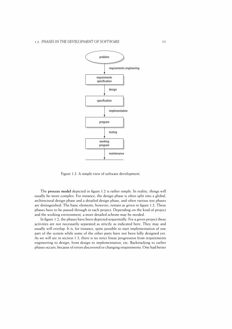
as discussed in this book are depicted in figure 1.2.

1.2. PHASES IN THE DEVELOPMENT OF SOFTWARE 11

Figure 1.2 A simple view of software development

The process model depicted in figure 1.2 is rather simple. In reality, things will

usually be more complex. For instance, the design phase is often split into a global,

architectural design phase and a detailed design phase, and often various test phases

are distinguished. The basic elements, however, remain as given in figure 1.2. These

phases have to be passed through in each project. Depending on the kind of project

and the working environment, a more detailed scheme may be needed.

In figure 1.2, the phases have been depicted sequentially. For a given project these

activities are not necessarily separated as strictly as indicated here. They may and

usually will overlap. It is, for instance, quite possible to start implementation of one

part of the system while some of the other parts have not been fully designed yet.

As we will see in section 1.3, there is no strict linear progression from requirements

engineering to design, from design to implementation, etc. Backtracking to earlier

phases occurs, because of errors discovered or changing requirements. One had better

12 INTRODUCTION

think of these phases as a series of workflows. Early on, most resources are spent on

the requirements engineering workflow. Later on, effort moves to the implementation

and testing workflows.

Below, a short description is given of each of the basic elements from figure 1.2.

Various alternative process models will be discussed in chapter 3. These alternative

models result from justifiable criticism of the simple-minded model depicted in

figure 1.2. The sole aim of our simple model is to provide an adequate structuring

of topics to be addressed. The maintenance phase is further discussed in section 1.3.

All elements of our process model will be treated much more elaborately in later

chapters.

Requirements engineering. The goal of the requirements engineering phase is to

get a complete description of the problem to be solved and the requirements posed

by and on the environment in which the system is going to function. Requirements

posed by the environment may include hardware and supporting software or the

number of prospective users of the system to be developed. Alternatively, analysis

of the requirements may lead to certain constraints imposed on hardware yet to be

acquired or to the organization in which the system is to function. A description of

the problem to be solved includes such things as:

– the functions of the software to be developed;

– possible future extensions to the system;

– the amount, and kind, of documentation required;

– response time and other performance requirements of the system.

Part of requirements engineering is a feasibility study. The purpose of the feasibility

study is to assess whether there is a solution to the problem which is both economically

and technically feasible.

The more careful we are during the requirements engineering phase, the larger is

the chance that the ultimate system will meet expectations. To this end, the various

people (among others, the customer, prospective users, designers, and programmers)

involved have to collaborate intensively. These people often have widely different

backgrounds, which does not ease communication.

The document in which the result of this activity is laid down is called the

requirements specification.

Design. During the design phase, a model of the whole system is developed which,

when encoded in some programming language, solves the problem for the user. To

this end, the problem is decomposed into manageable pieces called components; the

functions of these components and the interfaces between them are specified in a

very precise way. The design phase is crucial. Requirements engineering and design

are sometimes seen as an annoying introduction to programming, which is often seen

1.2. PHASES IN THE DEVELOPMENT OF SOFTWARE 13

as the real work. This attitude has a very negative influence on the quality of the

resulting software.

Early design decisions have a major impact on the quality of the final system.

These early design decisions may be captured in a global description of the system,

i.e. its architecture. The architecture may next be evaluated, serve as a template

for the development of a family of similar systems, or be used as a skeleton for

the development of reusable components. As such, the architectural description of

a system is an important milestone document in present-day software development

projects.

During the design phase we try to separate the what from the how. We concentrate

on the problem and should not let ourselves be distracted by implementation concerns.

The result of the design phase, the (technical) specification, serves as a starting

point for the implementation phase. If the specification is formal in nature, it can also

be used to derive correctness proofs.

Implementation. During the implementation phase, we concentrate on the individual

components. Our starting point is the component’s specification. It is often necessary

to introduce an extra ‘design’ phase, the step from component specification to

executable code often being too large. In such cases, we may take advantage of

some high-level, programming-language-like notation, such as a pseudocode. (A

pseudocode is a kind of programming language. Its syntax and semantics are in

general less strict, so that algorithms can be formulated at a higher, more abstract,

level.)

It is important to note that the first goal of a programmer should be the

development of a well-documented, reliable, easy to read, flexible, correct, program.

The goal is not to produce a very efficient program full of tricks. We will come back

to the many dimensions of software quality in chapter 6.

During the design phase, a global structure is imposed through the introduction

of components and their interfaces. In the more classic programming languages, much

of this structure tends to get lost in the transition from design to code. More recent

programming languages offer possibilities to retain this structure in the final code

through the concept of modules or classes.

The result of the implementation phase is an executable program.

Testing. Actually, it is wrong to say that testing is a phase following implementation.

This suggests that you need not bother about testing until implementation is finished.

This is not true. It is even fair to say that this is one of the biggest mistakes you can

make.

Attention has to be paid to testing even during the requirements engineering

phase. During the subsequent phases, testing is continued and refined. The earlier

that errors are detected, the cheaper it is to correct them.

Testing at phase boundaries comes in two flavors. We have to test that the

transition between subsequent phases is correct (this is known as verification). We

also have to check that we are still on the right track as regards fulfilling user

14 INTRODUCTION

requirements (validation). The result of adding verification and validation activities

to the linear model of figure 1.2 yields the so-called waterfall model of software

development (see also chapter 3).

Maintenance. After delivery of the software, there are often errors that have still

gone undetected. Obviously, these errors must be repaired. In addition, the actual

use of the system can lead to requests for changes and enhancements. All these types

of changes are denoted by the rather unfortunate term maintenance. Maintenance

thus concerns all activities needed to keep the system operational after it has been

delivered to the user.

An activity spanning all phases is project management. Like other projects, software

development projects must be managed properly in order to ensure that the product

is delivered on time and within budget. The visibility and continuity characteristics

of software development, as well as the fact that many software development

projects are undertaken with insufficient prior experience, seriously impede project

control. The many examples of software development projects that fail to meet their

schedule provide ample evidence of the fact that we have by no means satisfactorily

dealt with this issue yet. Chapters 2--8 deal with major aspects of software project

management, such as project planning, team organization, quality issues, cost and

schedule estimation.

An important activity not identified separately is documentation. A number of key

ingredients of the documentation of a software project will be elaborated upon

in the chapters to follow. Key components of system documentation include the

project plan, quality plan, requirements specification, architecture description, design

documentation and test plan. For larger projects, a considerable amount of effort will

have to be spent on properly documenting the project. The documentation effort

must start early on in the project. In practice, documentation is often seen as a

balancing item. Since many projects are pressed for time, the documentation tends

to get the worst of it. Software maintainers and developers know this, and adapt their

way of working accordingly. As a rule of thumb, Lethbridge et al. (2003) states that,

the closer one gets to the code, the more accurate the documentation must be for

software engineers to use it. Outdated requirements documents and other high-level

documentation may still give valuable clues. They are useful to people who have

to learn about a new system or have to develop test cases, for instance. Outdated

low-level documentation is worthless, and makes that programmers consult the code

rather than its documentation. Since the system will undergo changes after delivery,

because of errors that went undetected or changing user requirements, proper and

up-to-date documentation is of crucial importance during maintenance.

A particularly noteworthy element of documentation is the user documentation.

Software development should be task-oriented in the sense that the software to

be delivered should support users in their task environment. Likewise, the user

documentation should be task- oriented. User manuals should not just describe the

features of a system, they should help people to get things done (Rettig, 1991). We

1.2. PHASES IN THE DEVELOPMENT OF SOFTWARE 15

cannot simply rely on the structure of the interface to organize the user documentation

(just as a programming language reference manual is not an appropriate source for

learning how to program).

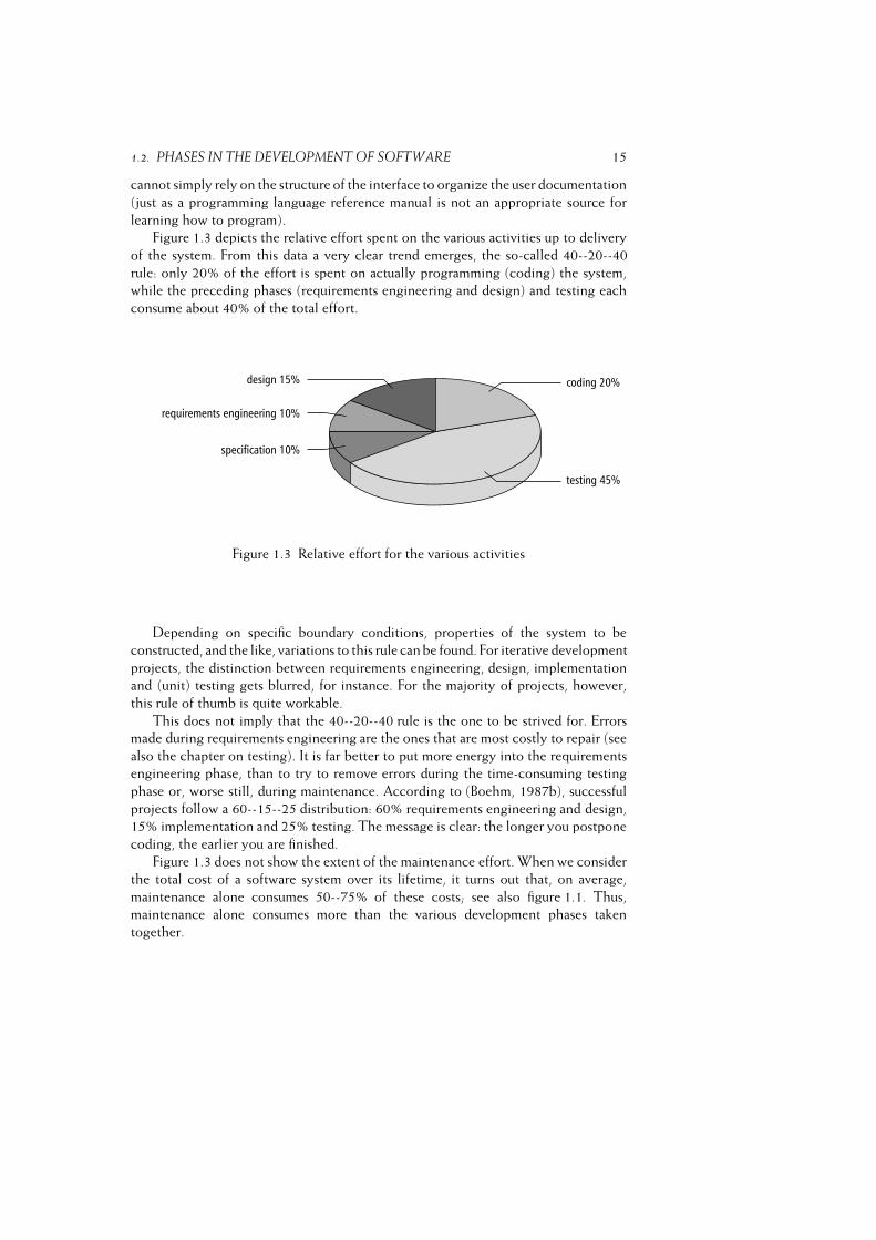
Figure 1.3 depicts the relative effort spent on the various activities up to delivery

of the system. From this data a very clear trend emerges, the so-called 40--20--40

rule: only 20% of the effort is spent on actually programming (coding) the system,

while the preceding phases (requirements engineering and design) and testing each

consume about 40% of the total effort.

Figure 1.3 Relative effort for the various activities

Depending on specific boundary conditions, properties of the system to be

constructed, and the like, variations to this rule can be found. For iterative development

projects, the distinction between requirements engineering, design, implementation

and (unit) testing gets blurred, for instance. For the majority of projects, however,

this rule of thumb is quite workable.

This does not imply that the 40--20--40 rule is the one to be strived for. Errors

made during requirements engineering are the ones that are most costly to repair (see

also the chapter on testing). It is far better to put more energy into the requirements

engineering phase, than to try to remove errors during the time-consuming testing

phase or, worse still, during maintenance. According to (Boehm, 1987b), successful

projects follow a 60--15--25 distribution: 60% requirements engineering and design,

15% implementation and 25% testing. The message is clear: the longer you postpone

coding, the earlier you are finished.

Figure 1.3 does not show the extent of the maintenance effort. When we consider

the total cost of a software system over its lifetime, it turns out that, on average,

maintenance alone consumes 50--75% of these costs; see also figure 1.1. Thus,

maintenance alone consumes more than the various development phases taken

together.

16 INTRODUCTION

1.3 Maintenance or Evolution

The only thing we maintain is user satisfaction(Lehman, 1980)

Once software has been delivered, it usually still contains errors which, upon

discovery, must be repaired. Note that this type of maintenance is not caused by

wearing. Rather, it concerns repair of hidden defects. This type of repair is comparable

to that encountered after a newly-built house is first occupied.

The story becomes quite different if we start talking about changes or enhance-

ments to the system. Repainting our office or repairing a leak in the roof of our house

is called maintenance. Adding a wing to our office is seldom called maintenance.

This is more than a trifling game with words. Over the total lifetime of a software

system, more money is spent on maintaining that system than on initial development.

If all these expenses merely concerned the repair of errors made during one of the

development phases, our business would be doing very badly indeed. Fortunately,

this is not the case.

We distinguish four kinds of maintenance activities:

– corrective maintenance -- the repair of actual errors;

– adaptive maintenance -- adapting the software to changes in the environment,

such as new hardware or the next release of an operating or database system;

– perfective maintenance -- adapting the software to new or changed user

requirements, such as extra functions to be provided by the system. Perfective

maintenance also includes work to increase the system’s performance or to

enhance its user interface;

– preventive maintenance -- increasing the system’s future maintainability.

Updating documentation, adding comments, or improving the modular struc-

ture of a system are examples of preventive maintenance activities.

Only the first category may rightfully be termed maintenance. This category, how-

ever, accounts only for about a quarter of the total maintenance effort. Approximately

another quarter of the maintenance effort concerns adapting software to environmen-

tal changes, while half of the maintenance cost is spent on changes to accommodate

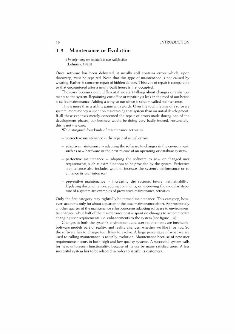
changing user requirements, i.e. enhancements to the system (see figure 1.4).

Changes in both the system’s environment and user requirements are inevitable.

Software models part of reality, and reality changes, whether we like it or not. So

the software has to change too. It has to evolve. A large percentage of what we are

used to calling maintenance is actually evolution. Maintenance because of new user

requirements occurs in both high and low quality systems. A successful system calls

for new, unforeseen functionality, because of its use by many satisfied users. A less

successful system has to be adapted in order to satisfy its customers.

1.4. FROM THE TRENCHES 17

Figure 1.4 Distribution of maintenance activities

The result is that the software development process becomes cyclic, hence the

phrase software life cycle. Backtracking to previous phases, alluded to above, does

not only occur during maintenance. During other phases, also, we will from time to

time iterate earlier phases. During design, it may be discovered that the requirements

specification is not complete or contains conflicting requirements. During testing,

errors introduced in the implementation or design phase may crop up. In these and

similar cases an iteration of earlier phases is needed. We will come back to this cyclic

nature of the software development process in chapter 3, when we discuss alternative

models of the software development process.

1.4 From the Trenches

And such is the way of all superstition, whether in astrology, dreams, omens, divine

judgments or the like; wherein men, having a delight in such vanities, mark the eventswhen they are fulfilled, but when they fail, though this happens much oftener, neglect and

pass them by. But with far more subtlety does this mischief insinuate itself into philosophy

and the sciences; in which the first conclusion colours and brings into conformity withitself all that come after, though far sounder and better. Besides, independently of that

delight and vanity which I have described, it is the peculiar and perpetual error of thehuman intellect to be more moved and excited by affirmatives than by negatives; whereas

it ought properly to hold itself indifferently disposed towards both alike. Indeed in the

establishment of any true axiom, the negative instance is the more forcible of the two.Sir Francis Bacon, The New Organon, Aphorisms XLVI (1611)

Historical case studies contain a wealth of wisdom about the nature of design and the

engineering method.

(Petroski, 1994)

In his wonderful book Design Paradigms, Case Histories of Error and Judgment in Engineering,

Henri Petroski tells us about some of the greatest engineering successes and, especially,

18 INTRODUCTION

failures of all time. Some such failure stories about our profession have appeared as

well. Four of them are discussed in this section.

These stories are interesting because they teach us that software engineering has

many facets. Failures in software development projects often are not one-dimensional.

They are not only caused by a technical slip in some routine. They are not only caused

by bad management. They are not only the result of human communication problems.

It is often a combination of many smaller slips, which accumulate over time, and

eventually result in a major failure. To paraphrase a famous saying of Fred Brooks

about projects getting late:

‘How does a project really get into trouble?’

‘One slip at a time.’

Each of the stories discussed below shows such a cumulative effect. Successes

in software development will not come about if we just employ the brightest

programmers. Or apply the newest design philosophy. Or have the most extensive

user consultation. Or even hire the best manager. You have to do all of that. And

even more.

1.4.1 Ariane 5, Flight 501

The maiden flight of the Ariane 5 launcher took place on June 4, 1996. After about 40

seconds, at an altitude of less than 4 kilometers, the launcher broke up and exploded.

This $500M loss was ultimately caused by an overflow in the conversion from a

64-bit floating point number to a 16-bit signed integer. From a software engineering

point of view, the Ariane 5 story is interesting because the failure can be attributed to

different causes, at different levels of understanding: inadequate testing, wrong type

of reuse, or a wrong design philosophy.

The altitude of the launcher and its movements in space are measured by

an Inertial Reference System (SRI -- Systeme de Reference Inertielle). There are

two SRIs operating in parallel. Their hardware and software is identical. Most of

the hardware and software for the SRI was retained from the Ariane 4. The fatal

conversion took place in a piece of software in the SRI which is only meaningful

before lift-off. Though this part of the software serves no purpose after the rocket

has been launched, it keeps running for an additional number of seconds. This

requirement was stated more than 10 years earlier for a somewhat peculiar reason. It

allows for a quick restart of the countdown, in the case that it is interrupted close to

lift-off. This requirement does not apply to the Ariane 5, but the software was left

unchanged -- after all, it worked. Since the Ariane 5 is much faster than the Ariane

4, the rocket reaches a much higher horizontal velocity within this short period

after lift-off, resulting in the above-mentioned overflow. Because of this overflow,

the first SRI ceased to function. The second SRI was then activated, but since the

hardware and software of both SRIs are identical, the second SRI failed as well. As a

consequence, wrong data were transmitted from the SRI to the on-board computer.

1.4. FROM THE TRENCHES 19

On the basis of these wrong data, full nozzle deflections were commanded. These

caused a very high aerodynamic load which led to the separation of the boosters from

the main rocket. And this in turn triggered the self-destruction of the launcher.

There are several levels at which the Ariane 5 failure can be understood and

explained:� It was a software failure, which could have been revealed with more extensive

testing. This is true: the committee investigating the event managed to expose

the failure using extensive simulations.� The failure was caused by reusing a flawed component. This is true as well but,

because of physical characteristics of the Ariane 4, this flaw had never become

apparent. There had been many successful Ariane 4 flights, using essentially

the same SRI subsystem. Apparently, reuse is not compositional: the successful

use of a component in one environment is no guarantee for successful reuse of

that component in another environment.� The failure was caused by a flaw in the design. The Ariane software follows a

typical hardware design philosophy: if a component breaks down, the cause

is assumed to be random and it is handled by shutting down that part and

invoking a backup component. In the case of a software failure, which is not

random, an identical backup is of little use. For the software part, a different

line might have been followed. For instance, the component could be asked to

give its best estimate of the required information.

1.4.2 Therac-25

The Therac-25 is a computer-controlled radiation machine. It has three modes:� field-light mode. This position merely facilitates the correct positioning of the

patient.� electron mode. In electron therapy, the computer controls the (variable) beam

energy and current, and magnets spread the beam to a safe concentration.� photon (X-ray) mode. In photon mode, the beam energy is fixed. A ‘beam

flattener’ is put between the accelerator and the patient to produce a uniform

treatment field. A very high current (some 100 times higher than in electron

mode) is required on one side of the beam flattener to produce a reasonable

treatment dose at the other side.

The machine has a turntable which rotates the necessary equipment into position.

The basic hazardous situation is obvious from the above: a photon beam is issued by

the accelerator, while the beam flattener is not in position. The patient is then treated

with a dose which is far too high. This happened several times. As a consequence,

several patients have died and others have been seriously injured.

20 INTRODUCTION

One of the malfunctions of the Therac-25 has become known as ‘Malfunction

54’. A patient was set up for treatment. The operator keyed in the necessary data on

the console in an adjacent room. While doing so, he made a mistake: he typed ‘x’ (for

X-ray mode) instead of ‘e’ (for electron mode). He corrected his mistake by moving

the cursor up to the appropriate field, typing in the correct code and pressing the

return key a number of times until the cursor was on the command line again. He then

pressed ‘B’ (beam on). The machine stopped and issued the message ‘Malfunction 54’.

This particular error message indicates a wrong dose, either too high or too low. The

console indicated a substantial underdose. The operator knew that the machine often

had quirks, and that these could usually be solved by simply pressing ‘P’ (proceed).

So he did. The same error message appeared again. Normally, the operator would

have audio and video contact with the patient in the treatment room. Not this time,

though: the audio was broken and the video had been turned off. It was later estimated

that the patient had received 16 000--25 000 rad on a very small surface, instead of

the intended dose of 180 rad. The patient became seriously ill and died five months

later.

The cause of this hazardous event was traced back to the software operating the

radiation machine. After the operator has finished data entry, the physical set up

of the machine may begin. The bending of the magnets takes about eight seconds.

After the magnets are put into position, it again checks if anything has changed. If

the operator manages to make changes and return the cursor to the command line

position within the eight seconds it takes to set the magnets, part of these changes

will result in changes in internal system parameters, but the system nevertheless

‘thinks’ that nothing has happened and simply continues. With the consequences as

described above.

Accidents like this get reported to the Federal Drugs Administration (FDA). The

FDA requested the manufacturer to take appropriate measures. The ‘fix’ suggested was

as follows:

Effective immediately, and until further notice, the key used for moving

the cursor back through the prescription sequence (i.e. cursor ‘UP’

inscribed with an upward pointing arrow) must not be used for editing

or any other purpose.

To avoid accidental use of this key, the key cap must be removed and the

switch contacts fixed in the open position with electrical tape or other

insulating material. . . .

Disabling this key means that if any prescription data entered is incorrect

then an ‘R’ reset command must be used and the whole prescription

reentered.

The FDA did not buy this remedy. In particular, they judged the tone of the notification

not commensurate with the urgency for doing so. The discussion between the FDA

and the manufacturer continued for quite some time before an adequate response was

given to this and other failures of the Therac-25.

1.4. FROM THE TRENCHES 21

The Therac-25 machine and its software evolved from earlier models that were

less sophisticated. In earlier versions of the software, for example, it was not possible

to move up and down the screen to change individual fields. Operators noticed that

different treatments often required almost the same data, which had to be keyed in all

over again. To enhance usability, the feature to move the cursor around and change

individual fields was added. Apparently, user friendliness may conflict with safety.

In earlier models also, the correct position of the turntable and other equipment

was ensured by simple electromechanical interlocks. These interlocks are a common

mechanism to ensure safety. For instance, they are used in lifts to make sure that

the doors cannot be opened if the lift is in between floors. In the Therac-25, these

mechanical safety devices were replaced by software. The software was thus made

into a single point of failure. This overconfidence in software contributed to the

Therac-25 accidents, together with inadequate software engineering practices and an

inadequate reaction of management to incidents.

1.4.3 The London Ambulance Service

The London Ambulance Service (LAS) handles the ambulance traffic in Greater

London. It covers an area of over 600 square miles and carries over 5000 patients per

day in 750 vehicles. The LAS receives over 2000 phone calls per day, including more

than 1300 emergency calls. The system we discuss here is a computer-aided dispatch

(CAD) system. Such a CAD system has the following functionality:� it handles call taking, accepts and verifies incident details including the location

of the incident;� it determines which ambulance to send;� it handles the mobilization of the ambulance and communicates the details of

the incident to the ambulance;� it takes care of ambulance resource management, in particular the positioning

of vehicles to minimize response times.

A fully-fledged CAD system is quite complex. In panic, someone might call and say

that an accident has happened in front of Foyle’s, assuming that everyone knows

where this bookshop is located. An extensive gazetteer component including a public

telephone identification helps in solving this type of problem. The CAD system also

contains a radio system, mobile terminals in the ambulances, and an automatic vehicle

location system.

The CAD project of the London Ambulance Service was started in the autumn

of 1990. The delivery was scheduled for January 1992. At that time, however, the

software was still far from complete. Over the first nine months of 1992, the system

was installed piecemeal across a number of different LAS divisions, but it was never

stable. On 26 and 27 October 1992, there were serious problems with the system and

22 INTRODUCTION

it was decided to revert to a semi-manual mode of operation. On 4 November 1992,

the system crashed. The Regional Health Authority established an Inquiry Team

to investigate the failures and the history that led to them. They came up with an

80-page report, which reads like a suspense novel. Below, we highlight some of the

issues raised in this report.

The envisaged CAD system would be a major undertaking. No other emergency

service had attempted to go as far. The plan was to move from a wholly manual

process -- in which forms were filled in and transported from one employee to the

next via a conveyor belt -- to complete automation, in one shot. The scheme was

very ambitious. The participants seem not to have fully realized the risks they were

taking.

Way before the project actually started, a management consultant firm had already

been asked for advice. They suggested that a packaged solution would cost $1.5M

and take 19 months. Their report also stated that if a package solution could not

be found, the estimates should be significantly increased. Eventually, a non-package

solution was chosen, but only the numbers from this report were remembered, or so

it seems.

The advertisement resulted in replies from 35 companies. The specification and

timetable were next discussed with these companies. The proposed timetable was

11 months (this is not a typo). Though many suppliers raised concerns about the

timetable, they were told that it was non-negotiable. Eventually, 17 suppliers provided

full proposals. The lowest tender, at approximately $1M, was selected. This tender was

about $700 000 cheaper than the next lowest bid. No one seems to have questioned

this huge difference. The proposal selected superficially suggests that the company

had experience in designing systems for emergency services. This was not a lie: they

had developed administrative systems for such services. The LAS system also was far

larger than anything they had previously handled.

The proposed system would impact quite significantly on the way ambulance

crews carried out their jobs. It would therefore be paramount to have their full

cooperation. If the crews did not press the right buttons at the right time and in the

right order, chaos could result. Yet, there was very little user involvement during the

requirements engineering process.

The intended CAD system would operate in an absolutely objective and impartial

way and would always mobilize the optimum resource to any incident. This would

overcome many of the then present working practices which management considered

outmoded and not in the interest of LAS. For instance, the new system would allocate

the nearest available resource regardless of the originating station. The following

scenario may result:� John’s crew has to go to an accident a few miles east of their home base.� Once there, they are directed to a hospital a few miles further east to deliver

the patient.

1.4. FROM THE TRENCHES 23� Another call comes in and John happens to be nearest. He is ordered to travel

yet a few miles further east.� And so on.

In this way, crews may have to operate further and further away from their home base,

and in unfamiliar territory. They lose time, because they take wrong turns, or may

even have to stop to ask for directions. They also have further to travel to reach their

home station at the end of a shift. Crews didn’t like this aspect of the new system.

The new system also took away the flexibility local emergency stations had in

deciding which resource to allocate. In the new scheme, resource management was

fully centralized and handled by the system. So, suppose John runs down to where

the ambulances are parked and the computer has ordered him to take car number 5.

John is in a hurry and maybe he cannot quickly spot car number 5, or maybe it is

parked behind some other cars. So John thinks about this patient waiting for him and

decides to take car number 4 instead. This means trouble.

The people responsible for those requirements were misguided or naive in

believing that computer systems in themselves can bring about such changes in

human practices. Computers are there to help people do their job, not vice versa.

Operational straitjackets are doomed to fail.

The eventual crash on 4 November 1992 was caused by a minor programming

error. Some three weeks earlier, a programmer had been working on part of the

system and forgot to remove a small piece of program text. The code in itself did

no harm. However, it did allocate a small amount of memory every time a vehicle

mobilization was generated by the system. This memory was not deallocated. After

three weeks, all memory was used up and the system crashed.

The LAS project as a whole did not fail because of this programmer mistake.

That was just the last straw. The project schedule was far too tight. Management of

both the London Ambulance Service and the contractor had little or no experience

with software development projects of this size and complexity. They were far too

optimistic in their assessment of risks. They assumed that all the people who would

interact with the system, would do so in exactly the right way, all of the time.

They assumed the hardware parts of the system would work exactly as specified.

Management decided on the functionality of the system, with hardly any consultation

with the people that would be its primary users. Any project with such characteristics

is doomed to fail. From the very first day.

1.4.4 Who Counts the Votes?

It’s not who votes that counts, it’s who counts the votes

Josef Stalin

Traditional, non-automated election systems leave a paper trail that can be used

for auditing purposes: have all votes been counted, have they been counted correctly.

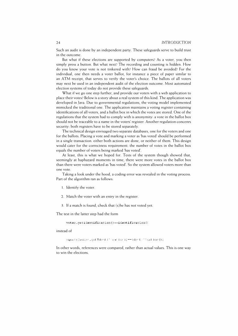
24 INTRODUCTION

Such an audit is done by an independent party. These safeguards serve to build trust

in the outcome.

But what if these elections are supported by computers? As a voter, you then

simply press a button. But what next? The recording and counting is hidden. How

do you know your vote is not tinkered with? How can fraud be avoided? For the

individual, one then needs a voter ballot, for instance a piece of paper similar to

an ATM receipt, that serves to verify the voter’s choice. The ballots of all voters

may next be used in an independent audit of the election outcome. Most automated

election systems of today do not provide these safeguards.

What if we go one step further, and provide our voters with a web application to

place their votes? Below is a story about a real system of this kind. The application was

developed in Java. Due to governmental regulations, the voting model implemented

mimicked the traditional one. The application maintains a voting register containing

identifications of all voters, and a ballot box in which the votes are stored. One of the

regulations that the system had to comply with is anonymity: a vote in the ballot box

should not be traceable to a name in the voters’ register. Another regulation concenrs

security: both registers have to be stored separately.

The technical design envisaged two separate databases, one for the voters and one

for the ballots. Placing a vote and marking a voter as ‘has voted’ should be performed

in a single transaction: either both actions are done, or neither of them. This design

would cater for the correctness requirement: the number of votes in the ballot box

equals the number of voters being marked ‘has voted’.

At least, this is what we hoped for. Tests of the system though showed that,

seemingly at haphazard moments in time, there were more votes in the ballot box

than there were voters marked as ‘has voted’. So the system allowed voters more than

one vote.

Taking a look under the hood, a coding error was revealed in the voting process.

Part of the algorithm ran as follows:

1. Identify the voter.

2. Match the voter with an entry in the register.

3. If a match is found, check that (s)he has not voted yet.

The test in the latter step had the formvoter.getIdentifi ation()==identifi ation()instead ofequals(voter.getIdentifi ation()==identifi ation())In other words, references were compared, rather than actual values. This is one way

to win the elections.

1.5. SOFTWARE ENGINEERING ETHICS 25

1.5 Software Engineering Ethics

Suppose you are testing part of a big software system. You find quite a few errors and

you’re certainly not ready to deliver. However, your manager is pressing you. The

schedule has already slipped by quite a few weeks. Your manager in turn is pressed

by his boss. The customer is eagerly awaiting delivery of the system. Your manager

suggests that you should deliver the system as is, continue testing, and replace the

system by a better version within the next month. How would you react to this

scheme? Would you simply give in? Argue with your manager? Go to his boss? Go to

the customer?

The development of complex software systems involves many people: software

developers, testers, technical managers, general managers, customers, etc. Within this

temporary organization, the relationship between individuals is often asymmetrical:

one person participating in the relationship has more knowledge about something

than the other. For example, a software developer has more knowledge about the

system under construction than his manager. Such an asymmetric relationship asks for

trust: if the developer says that development of some component is on schedule, his

manager cannot but believe this message. At least for a while. Such reliance provides

opportunities for unethical behavior, such as embezzlement. This is the more so if

there also is a power relationship between these individuals.

It is not surprising then that people within the software engineering community

have been discussing a software engineering code of ethics. Two large organizations

of professionals in our field, the IEEE Computer Society and ACM, have jointly

developed such a code. The short version of this code is given in figure 1.5.

In the long version of the code, each of the principles is further refined into a set

of clauses. Some of these clauses are statements of aspiration: for example, a software

engineer should strive to fully understand the specifications of the software on which

he works. Aspirations direct professional behavior. They require significant ethical

judgment. Other clauses express obligations of professionals in general: for example,

a software engineer should, like any other professional, provide service only in areas

of his competence. A third type of clause is directed at specific professional behavior

within software engineering: for example, a software engineer should ensure realistic

estimates of the cost and schedule of any project on which he works.

There are a number of clauses which bear upon the situation of the tester

mentioned above:� Approve software only if you have a well-founded belief that it is safe, meets

specifications, passes appropriate tests, and does not diminish quality of life or

privacy or harm the environment (clause 1.031).� Ensure adequate testing, debugging, and review of software and related docu-

ments on which you work (clause 3.10).

1Clause 1.03 denotes clause no 3 of principle no 1 (Public).

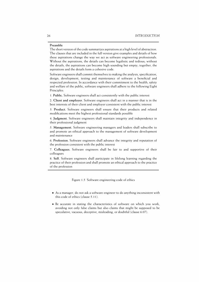
26 INTRODUCTION

Preamble

The short version of the code summarizes aspirations at a high level of abstraction.

The clauses that are included in the full version give examples and details of how

these aspirations change the way we act as software engineering professionals.

Without the aspirations, the details can become legalistic and tedious; without

the details, the aspirations can become high sounding but empty; together, the

aspirations and the details form a cohesive code.

Software engineers shall commit themselves to making the analysis, specification,

design, development, testing and maintenance of software a beneficial and

respected profession. In accordance with their commitment to the health, safety

and welfare of the public, software engineers shall adhere to the following Eight

Principles:

1. Public. Software engineers shall act consistently with the public interest

2. Client and employer. Software engineers shall act in a manner that is in the

best interests of their client and employer consistent with the public interest

3. Product. Software engineers shall ensure that their products and related

modifications meet the highest professional standards possible

4. Judgment. Software engineers shall maintain integrity and independence in

their professional judgment

5. Management. Software engineering managers and leaders shall subscribe to

and promote an ethical approach to the management of software development

and maintenance

6. Profession. Software engineers shall advance the integrity and reputation of

the profession consistent with the public interest

7. Colleagues. Software engineers shall be fair to and supportive of their

colleagues

8. Self. Software engineers shall participate in lifelong learning regarding the

practice of their profession and shall promote an ethical approach to the practice

of the profession

Figure 1.5 Software engineering code of ethics� As a manager, do not ask a software engineer to do anything inconsistent with

this code of ethics (clause 5.11).� Be accurate in stating the characteristics of software on which you work,

avoiding not only false claims but also claims that might be supposed to be

speculative, vacuous, deceptive, misleading, or doubtful (clause 6.07).

1.6. QUO VADIS? 27

The code is not a simple algorithm to discriminate between acceptable and unac-

ceptable behavior. Rather, the principles stated should influence you, as a software

engineer, to consider who is affected by your work. The software you develop affects

the public. The health, safety and welfare of the public is the primary concern of

this code of ethics. Adhering to this, or a similar, code of ethics is not something to

merely consider on a Friday afternoon. It should become a way of life.

The code not only addresses software engineers. It also addresses managers, in

that the code indicates what might reasonably be expected from professional software

engineers.

1.6 Quo Vadis?

A lot of progress has been made over the past 30 years. For each of the major

phases, numerous techniques and tools have been developed. A number of these have

found widespread use. In their assessment of design and coding practices for example,

DeMarco and Lister found that a number of widely acclaimed techniques (such as

the use of small units, strong component binding and structured programming) are

indeed applied in practice and pay off (DeMarco and Lister, 1989). However, the

short sketches in the preceding section (and the more elaborate discussion in the

following chapters) show that a lot of research is still needed to make software

engineering into a truly mature engineering discipline.

It takes some time before technology developed in research laboratories gets

applied in a routine way. This holds for physical products such as the transistor,

but also for methods, techniques, and tools in the area of software technology. The

first version of the UNIX operating system goes right back to 1971. Only since

the late 1980s, has interest in UNIX spread widely. In the early 1960s, studies of

the cost of software were first made. In the 1980s there was a growing interest in

quantitative models for estimating software costs (see also the later chapter on cost

estimation). Dijkstra’s article on programming as a human activity appeared in 1965.

In the late 1970s the first introductory textbooks on structured programming were

published. The term software engineering was introduced in 1968. In the 1980s large

national and international programs were initiated to foster the transition of this new

technology. The above list can be extended with many other examples (Redwine and

Riddle, 1985). This maturation process generally takes at least 10 to 15 years.

In a seminal article entitled ‘No silver bullet: essence and accidents of software

engineering’, Brooks (1987) discusses a number of potentially fruitful approaches to

dramatically increase software productivity. His main conclusion is: there is no silver

bullet. But we need not be afraid of the werewolf either. By a careful study of the

many innovations and an investigation of their true merits, a lot of improvements in

both quality and productivity can be achieved. The remainder of this text is devoted

to a critical assessment of these technological and non-technological developments.

Several relatively recent developments have a dramatic impact on the field:

28 INTRODUCTION� The rise of agile methods. As noted before in this chapter, the term software

engineering induces an orderly, factory-like approach to software development.

This ignores the fact that for many a project, it is impossible to state the

requirements upfront. They emerge as we go along. Armour (2001) compares

traditional software development with shooting down a Zeppelin, and agile

approaches with shooting down a supersonic plane. To shoot down a Zeppelin,

we collect information on altitude, distance, velocity and the like, relay this

information to the gun, aim, and shoot. This approach does not work for

supersonic planes. We do not know where the intercept will be, and the

missile will have to change direction while in the air. It is a challenge to

try to successfully combine engineering and craft-like approaches to software

development.� There is shift from producing software to using software. Time-to-market, cost,

and sheer complexity encourage organizations to assemble systems out of

existing components, rather than developing those components from scratch.

On one hand, builders build (pieces of) software, on the other hand integra-

tors integrate those pieces into end-user applications. As one consequence,

consumers of software often do not talk to developers anymore. Requirements

come from a variety of other sources, such as helpdesk call-log analysis or

market research (Sawyer, 2001). To the consumer, the software development

process is not interesting any more, only the resulting product counts. This shift

has given rise to new topics within software engineering, such as Component-

Based Software Development (CBSD), Commercial Off-The-Shelve (COTS)

components, Software Product Lines (SPL), and services.� Software development is becoming more heterogeneous. In the old days, a

software development organization had everything under control. Or so it

thought. Nowadays, software is being developed by teams scattered across

the globe. Part of it may be outsourced to a different organization. Software

incorporates components acquired from some other supplier, or services found

on the Web. As a consequence, one is not in control anymore.

To close this chapter is a list of important periodicals that contain material which is

relevant to the field of software engineering:

– Transactions on Software Engineering (IEEE), a monthly periodical in which research

results are reported;

– Software (IEEE), a bimonthly journal which is somewhat more general in scope;

– Software Engineering Notes, a bimonthly newsletter from the ACM Special Interest

Group on Software Engineering;

– Transactions on Software Engineering and Methodology (ACM), a quarterly journal

which reports research results.

1.7. SUMMARY 29

– The Journal of Systems and Software (Elsevier), a monthly journal covering both

research papers and reports of practical experiences;

– Proceedings of the International Conference on Software Engineering (ACM/IEEE), pro-

ceedings of the most important international conference in the field, organized

every year;

– Proceedings of the International Conference on Software Maintenance (IEEE), organized

yearly;

– Software Maintenance and Evolution: Research and Practice (Wiley), bimonthly journal

devoted to topics in software maintenance and evolution.

1.7 Summary

Software engineering is concerned with the problems that have to do with the

construction of large programs. When developing such programs, a phased approach is

followed. First, the problem is analyzed, and then the system is designed, implemented

and tested. This practice has a lot in common with the engineering of physical

products. Hence the term software engineering. Software engineering, however, also

differs from the engineering of physical products in some essential ways.

Software models part of the real world surrounding us, like banking or the reser-

vation of airline seats. This world around us changes over time. So the corresponding

software has to change too. It has to evolve together with the changing reality. Much

of what we call software maintenance, actually is concerned with ensuring that the

software keeps pace with the real world being modeled.

We thus get a process model in which we iterate earlier phases from time to time.

We speak about the software life cycle.

Agile methods, reuse of components, and globalisation are some of the relatively

recent trends that have a huge impact on the way we view the field. There is a shift

from producing software to using software. A major consequence hereof is that a

development organization looses control over what it delivers.

1.8 Further Reading

Johnson (1998) describes the early history of the software industry. The more recent

state of the practice is described in (Software, 2003).

For a more elaborate discussion of the differences and similarities between software

engineering and a mature engineering discipline, viz. bridge design, see (Spector and

Gifford, 1986). (Leveson, 1992) compares software engineering with the development

of high-pressure steam engines.

The four kinds of maintenance activities stem from (Lientz and Swanson, 1980).

30 INTRODUCTION

The Ariane failure is described in (Jezequel and Meyer, 1997). I found the report of

the Inquiry Team athttp://www. nes.fr/ARCHIVES/news/rapport 501.html.

An elaborate discussion of the Therac-25 accidents can be found in (Leveson and

Turner, 1993). The Inquiry into the London Ambulance Service is described in (Page

et al., 1993). (Neumann, 1995) is a book wholly devoted to computer-related risks.

The bimonthly ACM Software Engineering Notes contains a column ‘Risks to the public

in computer systems’, edited by Peter Neumann, which reports on large and small

catastrophes caused by automation. (Flowers, 1996) is a collection of stories about

information systems that failed, including the LAS system. (Kohno et al., 2004) and

(Raba, 2004) discuss problems with one specific electronic voting system. (Petroski,

1994) is a wonderful book on failures in engineering. (Software, 1999) is a special

issue with stories about successful IT projects.

The ACM/IEEE Software Engineering code of ethics is discussed in (Gotterbarn,

1999). The text of the code can also be found athttp:// omputer.org/tab/seprof/ ode.htm.

(Epstein, 1997) is a collection of (fictional) stories addressing the interaction between

ethics and software engineering. (Oz, 1994) discusses ethical questions of a real-life

project.

Exercises

1. Define the term software engineering.

2. What are the essential characteristics of software engineering?

3. What are the major phases in a software development project?

4. What is the difference between verification and validation?

5. Define four kinds of maintenance activity.

6. Why is the documentation of a software project important?

7. Explain the 40--20--40 rule of thumb in software engineering.

8. What is the difference between software development and software mainte-

nance?

9. ~ Do you think the linear model of software development is appropriate? In

which cases do you think an agile approach is more appropriate? You may

wish to reconsider this issue after having read the remainder of this text.

10. ~Discuss the major differences between software engineering and some other

engineering discipline, such as bridge design or house building. Would you

consider state-of-the-art software engineering as a true engineering discipline?

11. � Quality and productivity are major issues in software engineering. It is

1.8. FURTHER READING 31

often advocated that automated tools (CASE tools) will dramatically improve

both quality and productivity. Study a commercial CASE tool and assess

the extent to which it improves the software development process and its

outcome.

12. ~ Medical doctors have their Hippocratic oath. Could a similar ethical

commitment by software engineers be instrumental in increasing the quality

of software systems?

13. � Suppose you are involved in an office automation project in the printing

industry. The system to be developed is meant to support the work of journal

editors. The management objective for this project is to save labor cost; the

editors’ objective is to increase the quality of their work. Discuss possible

ramifications of these opposing objectives on the project. You may come

back to this question after having read chapter 9 or (Hirschheim and Klein,

1989).

14. ~ Discuss the difference between requirements-based software development

and market-driven software development (Sawyer, 2001).

15. ~ Discuss the impact of globalisation on software development.

16. � Study both the technical and user documentation of a system at your

disposal. Are you satisfied with them? Discuss their possible shortcomings

and give remedies to improve their quality.

17. � Take a piece of software you wrote more than a year ago. Is it documented

adequately? Does it have a user manual? Is the design rationale reflected in

the technical documentation? Can you build an understanding of the system

from its documentation that is sufficient for making non-trivial changes to it?

Repeat these questions for a system written by one of your colleagues.

18. � Try to gather quantitative data from your organization that reveals how

much effort is spent on various kinds of maintenance activity. Are these data

available at all? If so, is the pattern like that sketched in section 1.3? If not,

can you explain the differences?

19. � A 1999 Computer Society survey lists the following candidate fundamental

principles of software engineering:

A. Apply and use quantitative measurements in decision-making.

B. Build with and for reuse.

C. Control complexity with multiple perspectives and multiple levels of

abstraction.

D. Define software artifacts rigorously.

32 INTRODUCTION

E. Establish a software process that provides flexibility.

F. Implement a disciplined approach and improve it continuously.

G. Invest in the understanding of the problem.

H. Manage quality throughout the life cycle as formally as possible.

I. Minimize software components interaction.

J. Produce software in a stepwise fashion.

K. Set quality objectives for each deliverable product.

L. Since change is inherent to software, plan for it and manage it.

M. Since tradeoffs are inherent to software engineering, make them explicit

and document them.

N. To improve design, study previous solutions to similar problems.

O. Uncertainty is unavoidable in software engineering. Identify and manage

it.

For each of these principles, indicate whether you (strongly) agree or

(strongly) disagree, and why. You may wish to re-appraise these principles

after having studied the rest of this book.

Part I

Software Management

CONTENTS

Chapter 2 Introduction to Software Engineering Management 34

Chapter 3 The Software Life Cycle Revisited 45

Chapter 4 Configuration Management 78

Chapter 5 People Management and Team Organization 89

Chapter 6 On Managing Software Quality 107

Chapter 7 Cost Estimation 144

Chapter 8 Project Planning and Control 176

Software development projects often involve several people for a prolonged period

of time. Large projects may even range over several years and involve hundreds of

people. Such projects must be carefully planned and controlled. The main aspects

that deserve the continuous attention of project managers are introduced in chapter

2, and further dealt with in chapters 3--7: progress, information, people, quality,

cost and schedule. The management part ends with chapter 8 in which the various

approaches sketched in chapters 3--7 are reconciled.

2

Introduction to Software

Engineering Management

LEARNING OBJECTIVES� To be aware of the contents of a project plan� To understand the major dimensions along which a software development

project is controlled

35

Software development projects often involve several people for a prolonged

period of time. Large projects may even range over several years and involve

hundreds of people. Such projects must be carefully planned and controlled.

The main aspects that deserve the continuous attention of project managers

are introduced in this chapter.

It is not easy to complete successfully a software development project. This book

mainly deals with technical aspects of software development: design, specification,

implementation and testing of software systems. As we learn to control these aspects

better, we will also learn to satisfy our customer’s demands better. The organizational

and managerial aspects of software development projects are at least as important as

the technical aspects, though.

Before we embark on a discussion of these organizational and managerial aspects,

let us first pay some attention to the boundaries of a software development project as

they are drawn in this book.

A software development project is usually not started in complete isolation.

There are other projects within the organization that this particular project needs

to be tuned to, priorities between projects have to be decided upon, etc. The term

information planning is often used to refer to this meta-project planning process.

Also in a more technical sense, projects are not started in isolation. To increase

interoperability between systems, overall guidelines regarding, e.g., the use of certain

standards, data interchange formats, security policies, web page layout and the like

are laid down for the whole organization and imposed on every project. In product

line development, the architecture of the product line guides the development of

individual products.

These project exceeding rules result in a set of boundary conditions for each

project, much like the zoning regulations set the conditions for a building project.

Establishing these company-wide rules is a problem on its own, and will not be

addressed here. (We will, however, pay ample attention to some issues which

generally surpass the boundaries of individual software development projects, such as

configuration control, quality assurance and product line development.)

Also in a more technical sense, software is not generally developed in isolation.

In most cases, software is not written from scratch. It must interface with existing

software, extend existing software, use existing subroutine libraries, build upon an

existing framework, and so on.

In some sense, the notion of a ‘software development project’ is a misnomer.

We do not just develop software, we develop systems. Broadly speaking, a system

transforms inputs into outputs. Software is an important ingredient of the systems

we develop, but it is by no means the only ingredient. The technical and user

documentation, the hardware, the procedures that govern the use of the system, and

even the people using the software, may be considered as part of that same system.

Consider for example a system for library automation. The system will contain

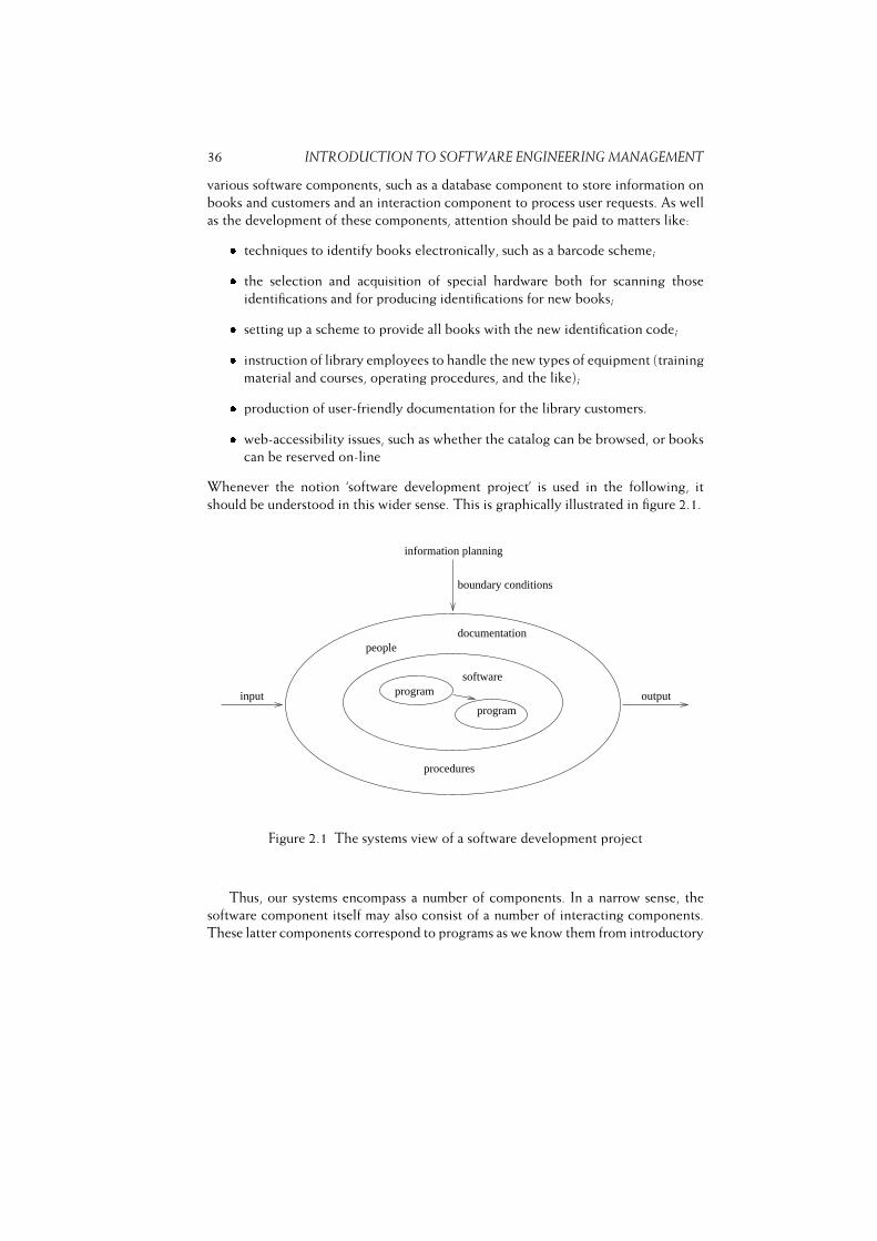
36 INTRODUCTION TO SOFTWARE ENGINEERING MANAGEMENT

various software components, such as a database component to store information on

books and customers and an interaction component to process user requests. As well

as the development of these components, attention should be paid to matters like:� techniques to identify books electronically, such as a barcode scheme;� the selection and acquisition of special hardware both for scanning those

identifications and for producing identifications for new books;� setting up a scheme to provide all books with the new identification code;� instruction of library employees to handle the new types of equipment (training

material and courses, operating procedures, and the like);� production of user-friendly documentation for the library customers.� web-accessibility issues, such as whether the catalog can be browsed, or books

can be reserved on-line

Whenever the notion ‘software development project’ is used in the following, it

should be understood in this wider sense. This is graphically illustrated in figure 2.1.

documentation

procedures

software

input output

information planning

boundary conditions

people

program

program

Figure 2.1 The systems view of a software development project

Thus, our systems encompass a number of components. In a narrow sense, the

software component itself may also consist of a number of interacting components.

These latter components correspond to programs as we know them from introductory

2.1. PLANNING A SOFTWARE DEVELOPMENT PROJECT 37

computer science textbooks. In general, a software development project results in a

set of components which collectively provide us with the desired functionality.

Given a project’s boundary conditions, a software development project may get

started. Planning the project is the very first step to be undertaken. Part of this

planning process is to identify the project characteristics and their impact on the

development process. The result of the planning phase is laid down in a document,

the project plan, which aims to provide a clear picture of the project to both the

customers and the development team. The contents of the project plan are discussed

in section 2.1.

During the execution of the project, a number of elements have to be managed:

time, information, organization, quality, and money (see section 2.2). Each of these

elements is further elaborated upon in a separate chapter.

2.1 Planning a Software Development Project

Before we embark on a software development project, it has to be carefully planned.

This entails, amongst other things, an assessment of project properties that may affect

the development process. A number of properties, however, will not be sufficiently

well understood until the requirements engineering phase has ended. Like many

other aspects of a software development project, planning is not a one-shot activity.

Rather, it is highly dynamic in nature. The project plan can serve as a guide during

the project.

The amount of upfront planning depends on characteristics of the problem at

hand. In highly explorative projects, where requirements are largely unknown at the

start, too rigorous early planning can be stifling and may increase the probability

of major failures. A strict ‘plan the work and work the plan’ attitude does not work

in these circumstances. Rather, such projects call for a nominal early planning and

a management style that encourages responding to change. This is reflected in the

contents and size of the project plan. Chapters 3 and 8 further discuss differences

between the so-called agile and planning-driven approaches to software development.

The major constituents of a project plan are:

1. Introduction In the introduction to the project plan, the background and

history of the project are given, together with its aims, the project deliverables,

the names of the persons responsible, and a summary of the project.

2. Process model In chapter 1, we introduced a simple life cycle model in order to

discuss the various activities to be dealt with in a software development project.

There exist many variations of this process model, some of which are discussed

in chapter 3. For each project, one has to decide upon the exact process model

to be followed: which activities are being undertaken, which milestones can

be identified, how do we ascertain whether those milestones are reached, and

which are the critical paths.

38 INTRODUCTION TO SOFTWARE ENGINEERING MANAGEMENT

Different types of projects have different characteristics, and so call for different

process models.

3. Organization of the project The relationship of the project to other entities

and the organization of the project itself are dealt with under this heading.

The project will have a relationship with the user organization, the parent

organization, and possibly with other organizations.

The prospective users will from time to time be involved in the project. The

project plan has to state which information, services, resources and facilities

are to be provided by the users and when these are to be provided.

Within the project team, various roles can be identified: project manager, tester,

programmer, analyst, etc. One has to clearly delineate these roles and identify

the responsibilities of each of them. If there are gaps in the knowledge required

to fulfill any of these roles, the training and education needed to fill these gaps

have to be identified. Different forms of team organization are discussed in

chapter 5.

4. Standards, guidelines, procedures Software projects are big projects. Usually,

a lot of people are involved. A strong working discipline is therefore needed, in

which each person involved follows the standards, guidelines and procedures

agreed upon. Besides being stated on paper, many of these can be supported

or enforced by tools. Of extreme importance are clear agreements about

documentation: when is documentation to be delivered, how is the quality of

the documentation to be assessed, how does one ensure that the documentation

is kept up-to-date?

To a large extent, these standards and procedures will be described in separate

documents, such as the Configuration Control Plan or the Quality Assurance

Plan.

5. Management activities Management activities are guided by goals and priorities

set for the project. For example, management will have to submit regular reports

on the status and progress of the project. It will also have to follow certain

priorities in balancing requirements, schedule and cost.

6. Risks Potential risks have to be identified as early as possible. There will always

be risks: hardware may not be delivered on time, qualified personnel may not

be available when required, critical information may be lacking when it is

needed, and so on. It is rather naive to suppose that a software development

project runs smoothly. Even in well-established fields like construction, there is

always something that goes wrong. One should diagnose the risks of a software

project early on, and provide measures to deal with them; see also chapter 8.

The more uncertain various aspects of the project are, the larger the risks.

2.1. PLANNING A SOFTWARE DEVELOPMENT PROJECT 39

7. Staffing At different points in time, the project will require different amounts

of personnel, with different skills. The start, duration, amount and expertise of

personnel categories are listed under this heading.

8. Methods and techniques Under this heading, the methods and techniques to

be used during requirements engineering, design, implementation and testing

are given. Typically, the way version and configuration control for software

components is dealt with is described here too. A large proportion of the

technical documentation will be produced during these phases. One thus has

to state how this documentation will be taken care of.

The necessary test environment and test equipment is described. During testing,

considerable pressure will normally be put on the test equipment. Therefore,

this activity has to be planned carefully. The order in which components are

integrated and tested has to be stated explicitly. Also, the procedures to be

followed during acceptance testing, i.e. the testing under user supervision, have

to be given. Testing will be discussed in chapter 13.

9. Quality assurance Which organization and procedures will be used to assure

that the software being developed meets the quality requirements stated? The

many aspects of a Quality Assurance Plan may also be dealt with in a separate

document. The topic of quality assurance is discussed in chapter 6.

10. Work packages Larger projects must be broken down into activities, manage-

able pieces that can be allocated to individual team members. Each of these

activities has to be identified in the project plan. The hierarchical decomposi-

tion of the project is depicted in a work breakdown structure (see also section

8.4).

11. Resources During the project, many resources are needed. The hardware,

CPU-cycles and tools needed to support the project are listed under this entry.

One should also indicate the personnel needed for the various process phases.

12. Budget and schedule The total budget for the project has to be allocated to the

various activities as indicated in the work breakdown structure. The activities

also have to be scheduled in time, e.g. using a PERT chart (see section 8.4). The

way in which resources and other expenditures are tracked is also indicated

under this heading. The topic of cost and time estimation will be dealt with

extensively in chapter 7.

13. Changes It has been stated before that changes are inevitable. One has to

ensure that these changes are dealt with in an orderly way. One thus needs

clear procedures on how proposed changes will be handled. If the process is

agile, every iteration involves changes, and these are dealt with in a lightweight

manner. In fact, they are not seen as changes anymore. In more heavyweight

processes, each proposed change must be registered and reviewed. When a

40 INTRODUCTION TO SOFTWARE ENGINEERING MANAGEMENT

change request has been approved, its impact (cost) has to be estimated. Finally,

the change has to be incorporated into the project. Changes that are entered

via the back door lead to badly structured code, insufficient documentation

and cost and time overruns. Since changes lead to different versions of both

documentation and code, the procedures to be followed in dealing with such

changes are often handled in the context of a Configuration Control Plan.

14. Delivery The procedures to be followed in handing over the system to the

customer must be stated.

The project plan aims to provide a clear picture of the project to both the customers

and the project team. If the objectives are not clear, they will not be achieved.

Despite careful planning, surprises will still crop up during the project. However,

careful planning early on leads to fewer surprises and makes one less vulnerable to

these surprises. The project plan addresses a number of questions which anticipate

possible future events. It gives orderly procedures for dealing with those events, so

that justifiable decisions can be reached.

2.2 Controlling a Software Development Project

After a project plan has been drawn up and approved, the execution of the project may

start. During the project, control has to be exerted along the following dimensions:

– time,

– information,

– organization,

– quality,

– money.

Progress of a software development project (the time aspect) is hard to measure.

Before the proposed system has been finished, there is only a (large) pile of paper.

Utterances such as ‘90% of the code has been written’ should be taken with a pinch

of salt. A much too rosy picture of the actual state of affairs is usually given. The

phased approach introduced in chapter 1, and its variants, aim at providing the

manager with an instrument to measure and control progress. The time needed to

build a system is obviously related to the size of the system, and thus to the total

manpower required. Larger systems require more time to develop, although we may

try to shorten development time by allocating more personnel. Part of the control

problem for software development projects is to trade off time against people. Adding

more people to shorten development time does not come for free. The more people

that are involved, the more time will be needed for coordination and communication.

After a certain point, adding more people actually lengthens the development time.

2.2. CONTROLLING A SOFTWARE DEVELOPMENT PROJECT 41

Part of the time control problem is phrased in Brooks’ Law: ‘Adding people to a late

project only makes it later’. We will come back to this issue in the chapter on cost

estimation.

The information that has to be managed, above all, is the documentation. Besides

technical and user documentation, this also entails documentation on the project

itself. Documentation concerning the project includes such things as: the current state

of affairs, changes that have been agreed upon, and decisions that have been made.

This type of documentation can best be handled in the context of configuration

management. In agile projects, less attention is given to documentation during

development. Necessary knowledge is tacit, it resides in the heads of the people

involved. But here too, once the system is ready and handed over to its customers,

documentation has to be provided.

All members of the development team must understand their role in the team and

what is expected of them. It is very important that these expectations are clear to

all people involved. Unspoken and unclear expectations lead to situations in which

individual team members set their own goals, either consciously or unconsciously.

These organizational aspects deserve the continuous attention of the project manager.

Secondly, the organization of a team and the coordination of the people involved

will, at least partly, depend upon characteristics of the project and its environment.

This dependence has to be recognized and taken into account when setting up a

project team.

The quality aspect is of paramount importance. Customers are not satisfied with

the purely technical solutions offered by computer specialists. They want systems that

fit their real needs. The quality requirements for software and its development often

conflict with one another. At architecture time, quality requirements are balanced in a

dialog with all stakeholders involved. During a project we will have to assess whether

or not the quality requirements are being met. This quality assessment has to occur

on a regular basis, so that timely actions can be undertaken. Quality is not an add-on

feature, it has to be built in.

Controlling expenses (the money aspect) largely means controlling labor costs.

Though the cost of hardware and tools cannot be ignored, these can usually be

estimated fairly precisely early in the project. Moreover, these are usually much less

of an issue than personnel costs.

Estimating the cost of software thus means that we must estimate the manpower

required to build the software. The manpower needed is very much dependent on

the size of the software, for instance measured as the amount of code to be delivered.

Many other factors, though, influence this cost or, alternatively, the productivity

with which the software can be produced. A well-balanced team with experienced

people will be much more productive than a newly-formed team with inexperienced

people. Extremely strict quality constraints, such as very high reliability or a very fast

response time, may also severely reduce productivity.

A number of models have been proposed that try to quantify the effect of

those different cost drivers on the manpower required (see chapter 7). Rather than

42 INTRODUCTION TO SOFTWARE ENGINEERING MANAGEMENT

estimating the size first, and then its cost, one may also set a cost threshold first, and

work incrementally, first on the most pressing user requirements and, if time allows,

on less pressing ones. Or one may agree on a first threshold, and decide whether more

money will be spent when this threshold is reached. These incremental approaches

to cost estimation fit in well with agile project development.

Software development is a very labor-intensive process. One of our hopes is

that better tools and the increased use of those tools will lead to a significant

increase in productivity and, consequently, a significant decrease in the cost involved

in developing software. A second way, to increase productivity dramatically, is to

use software rather than build it yourself. Both these topics will be discussed in

chapters to follow. As these trends continue, software development starts to become

a capital-intensive activity, rather than a labor-intensive one (Wegner, 1984).

Continuous assessment of the project with respect to these control aspects is

of the utmost importance and will from time to time lead to adjustments in time,

cost, organization, information, or quality, or some combination thereof. Project

management is a very dynamic activity.

In order to be able to adequately control a project, we need quantitative data

which is collected while the project is being executed. For instance, data about

errors discovered during unit testing may help us in estimating further test effort

needed. Data about the time and effort spent up to a specific point will guide us in

re-estimating the schedule and cost. To measure is to know.

These data are also valuable in a post-mortem evaluation of the project. In a post-

mortem evaluation we assess the present project in order to improve our performance

on projects yet to come: what have we done wrong, what have we learned, what

needs to be done differently on the next project?

Unfortunately, in practice very little hard data is ever gathered, let alone retained

for later use. Most software development organizations have little insight into what

they are doing. They tend to operate in a somewhat chaotic way, especially when

facing a crisis. By identifying key factors that affect the controllability of the software

development process, we may find ways to improve on it. This topic is further treated

in chapter 6, where we discuss the Software Capability Maturity Model.

2.3 Summary

This chapter provides an introduction to the management of software engineering

projects.

Before we embark on a software development project, it has to be carefully

planned. This planning process results in a document, the project plan, which

provides a clear picture of the project to both the customers and the project team.

Once the project plan has been drawn up and the project has started, its execution

must be controlled. We identified five entities that require our continuous attention

for project control:

2.3. SUMMARY 43� Time: How do we assess progress towards the project’s goals? Usually, some

phased approach is followed which aims to provide management with a means

to measure and control progress.� Information: How do we handle the documents that are produced in the course

of a project? In planning-based development, maintaining the integrity of the

set of documents and handling all change requests require careful procedures.� Organization: How do we organize the project team and coordinate the

activities of team members?� Quality: How do we define and assess quality requirements for both the

development process and the resulting product?� Money: How do we estimate the cost of a project? These costs are to a large

extent determined by the size of the software.

Each of these controlling aspects is further elaborated upon in a separate chapter

(chapters 3--7). The various dimensions of project control will then be reconciled in

chapter 8.

Exercises

1. In what sense is the phrase ‘software development project’ a misnomer?

2. What are the major constituents of a project plan?

3. List five dimensions along which a software development project has to be

controlled.

4. How may software development become a capital-intensive activity, rather

than a labor-intensive one?

5. � Consider a software development project you have been involved in. Did

the project have a project plan? Did the project plan address the issues listed

in section 2.1? If some of these issues were not addressed, do you think it

would have helped the project if they had been?

6. ~ Do you think quantitative project data are important? In what way can

they contribute to project planning?

7. ~ How would a project plan for an agile project differ from that of a

planning-driven project?

8. � Consider once again a software development project you have been

involved in. To what extent were any environmental issues such as user

training and working procedures adequately dealt with in the project?

44 INTRODUCTION TO SOFTWARE ENGINEERING MANAGEMENT

9. ~ A program written for personal use imposes rather less stringent require-

ments than a product that is also to be used by other people. According

to (Brooks, 1995), the latter may require three times as much effort. Discuss

possible reasons for this considerable increase in cost.

3

The Software Life Cycle

Revisited

LEARNING OBJECTIVES� To be aware of a number of generic models to structure the software develop-

ment process� To appreciate the pros and cons of these models, in particular those of the

classes of planning-driven and agile methods� To understand the similarities between software maintenance and software

evolution� To recognize that it is profitable to apply software product line engineering

when developing a series of similar systems� To be aware of process modeling as a way to describe software development

processes explicitly

46 THE SOFTWARE LIFE CYCLE REVISITED

To be able to assess progress during software development, one opts for a

phased approach with a number of well-defined milestone events. The linear

ordering of activities which underlies the traditional software development

model, the waterfall model, renders it an impossible idealization of reality

though. It assumes software development proceeds in an orderly, sequential

manner. Real projects proceed in far less rational ways. The waterfall model of

software development is not feasible, much like Escher’s Waterfall, reproduced

on the front cover, is unfeasible. This chapter discusses various alternative

models of the development process.

In chapter 1, we introduced a simple model of the software life cycle. We distinguished

several consecutive phases: requirements engineering, design, implementation, test-

ing, maintenance. It was stated that, in practice, one often uses more sophisticated

process models. In this chapter we continue this discussion. We introduce various

alternative models to structure the software development process.

Software development projects are often very large projects. A number of people

work on such a project for a long time and therefore the whole process needs to

be carefully planned and controlled: progress needs to be monitored, people and

resources need to be allocated at the right point in time, etc. Earlier on, it was pointed

out that progress of a software development project is particularly difficult to measure.

In order to control progress we use a phased development in which a number

of clearly identifiable milestones are established between the start and finish of the

project. We use a similar mechanism when constructing a house: foundations are laid,

the first floor is reached, the house is weatherproofed, and so on. Often, the payment

of installments is coupled to reaching those milestones.

In general, the milestones identified in a software development project correspond

to the points in time at which certain documents become available:

– after requirements engineering, there is a requirements specification;

– after the design phase there is a (technical) specification of the system;

– after implementation there is a set of programs;

– after testing has been completed there is a test report.

Traditional models for the phased development of software are, to a large extent,

‘document-driven’. The pile of paper that is produced in the course of the project

guides the development process. The development process is seen as a series of

transformations. It starts with a clear requirements document, and ends with running

code. In the next section we discuss the waterfall model, a well-known variation of

the process model introduced in chapter 1. In this variation, a check is performed

after each transformation, to determine whether we are still on the right track.

47

These document-driven methods are also known as planning-driven or heavyweight

methods. Planning-driven, because of the emphasis on an upfront plan for the whole

process. Heavyweight, because of the emphasis placed on the process.

In many a software development project, change is a fact of life. It may even be

the case that the client only has a vague idea of the requirements for the system he

asks for. In recent years, a number of lightweight, agile methods have been proposed that

purposedly deal with these rapidly changing circumstances. These methods advocate

to not ‘waste’ time on expensive planning and design activities early on, but to deliver

something valuable to the customer as quickly as possible. Based on feedback from

the user, next steps are then taken. Agile methods have evolved from approaches

such as prototyping and Rapid Application Development that try to dispose of some

or all of the drawbacks of the document-driven approach mentioned above. We will

discuss a number of lightweight approaches to software development in section 3.2.

Evolutionary models take into account that much of what is called maintenance is

really evolution. It would then seem natural to explicitly bear this anticipated evolution

in mind from the very start. This is usually not the case. In both heavyweight and

lightweight development approaches, the initial development of a software system

is in general strictly separated from the subsequent maintenance phase. The major

goal of a software development project then boils down to delivering a first version

of the system to the user. This may result in excessive maintenance costs later on.

In order to be able to properly assess costs and benefits, total life cycle cost rather

than just development cost should be our primary focus. Going one step further, we

may argue that management should concentrate on sets of similar products (so-called

product families) rather than individual products, thereby granting an incentive both

to the building of reusable parts and the reuse of (parts of) existing products when

developing new ones.

From all the possible life cycle models we have to choose a particular one for any

given project. By and large, heavyweight methods better fit (very) large projects, and

situations where the requirements can be decided upon at an early stage. Lightweight

methods fit situations of rapid change, and projects that do not involve more than,

say, 50 people. Different project characteristics, and appropriate ways to control

them effectively, are discussed in chapter 8.

The choice for a particular life cycle model also involves defining the individual

steps and phases, their possible interaction, their deliverables, etc. By using an

explicit process modeling language, which may be supported by tools, we may

increase our understanding of the software process, we are provided with a handle to

improve our control of software development, and we are given a baseline for process

improvement. This type of process modeling is discussed in section 3.6. Because

of the much larger emphasis on planning, this type of modeling fits in better with

heavyweight methods.

48 THE SOFTWARE LIFE CYCLE REVISITED

3.1 The Waterfall Model

The waterfall model is essentially a slight variation of the model introduced in

chapter 1. The waterfall model is generally attributed to Royce (1970). However,

a clearly phased approach to the development of software, including iteration and

feedback, could already be found in publications from the early 1960s.

The waterfall model particularly expresses the interaction between subsequent

phases. Testing software is not an activity which strictly follows the implementation

phase. In each phase of the software development process, we have to compare

the results obtained against those that are required. In all phases, quality has to be

assessed and controlled.

In figure 3.1, V & V stands for Verification and Validation. Verification asks if the

system meets its requirements (are we building the system right) and thus tries to

assess the correctness of the transition to the next phase. Validation asks if the system

meets the user’s requirements (are we building the right system).

Figure 3.1 The waterfall model

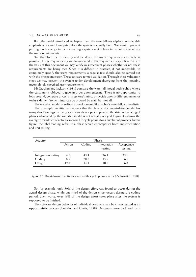
3.1. THE WATERFALL MODEL 49

Both the model introduced in chapter 1 and the waterfall model place considerable

emphasis on a careful analysis before the system is actually built. We want to prevent

putting much energy into constructing a system which later turns out not to satisfy

the user’s requirements.

We therefore try to identify and tie down the user’s requirements as early as

possible. These requirements are documented in the requirements specification. On

the basis of this document we may verify in subsequent phases whether or not these

requirements are being met. Since it is difficult in practice, if not impossible, to

completely specify the user’s requirements, a regular test should also be carried out

with the prospective user. These tests are termed validation. Through these validation

steps we may prevent the system under development diverging from the, possibly

incompletely specified, user requirements.

McCracken and Jackson (1981) compare the waterfall model with a shop where

the customer is obliged to give an order upon entering. There is no opportunity to

look around, compare prices, change one’s mind, or decide upon a different menu for

today’s dinner. Some things can be ordered by mail, but not all.

The waterfall model of software development, like Escher’s waterfall, is unrealistic.

There is ample quantitative evidence that the classical document-driven model has

many shortcomings. In many a software development project, the strict sequencing of

phases advocated by the waterfall model is not actually obeyed. Figure 3.2 shows the

average breakdown of activities across life cycle phases for a number of projects. In this

figure, the label ‘coding’ refers to a phase which encompasses both implementation

and unit testing.

Activity Phase

Design Coding Integration Acceptance

testing testing

Integration testing 4.7 43.4 26.1 25.8

Coding 6.9 70.3 15.9 6.9

Design 49.2 34.1 10.3 6.4

Figure 3.2 Breakdown of activities across life cycle phases, after (Zelkowitz, 1988)

So, for example, only 50% of the design effort was found to occur during the

actual design phase, while one-third of the design effort occurs during the coding

period. Even worse, over 16% of the design effort takes place after the system is

supposed to be finished.

The software design behavior of individual designers may be characterized as an

opportunistic process (Guindon and Curtis, 1988). Designers move back and forth

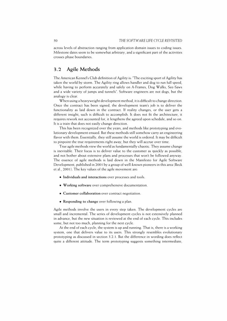
50 THE SOFTWARE LIFE CYCLE REVISITED

across levels of abstraction ranging from application domain issues to coding issues.

Milestone dates seem to be somewhat arbitrary, and a significant part of the activities

crosses phase boundaries.

3.2 Agile Methods

The American Kennel’s Club definition of Agility is: ”The exciting sport of Agility has

taken the world by storm. The Agility ring allows handler and dog to run full speed,

while having to perform accurately and safely on A-Frames, Dog Walks, See-Saws

and a wide variety of jumps and tunnels”. Software engineers are not dogs, but the

analogy is clear.

When using a heavyweight development method, it is difficult to change direction.

Once the contract has been signed, the development team’s job is to deliver the

functionality as laid down in the contract. If reality changes, or the user gets a

different insight, such is difficult to accomplish. It does not fit the architecture, it

requires rework not accounted for, it lengthens the agreed upon schedule, and so on.

It is a train that does not easily change direction.

This has been recognized over the years, and methods like prototyping and evo-

lutionary development ensued. But these methods still somehow carry an engineering

flavor with them. Essentially, they still assume the world is ordered. It may be difficult

to pinpoint the true requirements right away, but they will accrue over time.

True agile methods view the world as fundamentally chaotic. They assume change

is inevitable. Their focus is to deliver value to the customer as quickly as possible,

and not bother about extensive plans and processes that won’t be followed anyway.

The essence of agile methods is laid down in the Manifesto for Agile Software

Development, published in 2001 by a group of well-known pioneers in this area (Beck

et al., 2001). The key values of the agile movement are:� Individuals and interactions over processes and tools.� Working software over comprehensive documentation.� Customer collaboration over contract negotiation.� Responding to change over following a plan.

Agile methods involve the users in every step taken. The development cycles are

small and incremental. The series of development cycles is not extensively planned

in advance, but the new situation is reviewed at the end of each cycle. This includes

some, but not too much, planning for the next cycle.

At the end of each cycle, the system is up and running. That is, there is a working

system, one that delivers value to its users. This strongly resembles evolutionary

prototyping as discussed in section 3.2.1. But the difference in wording does reflect

quite a different attitude. The term prototyping suggests something intermediate,

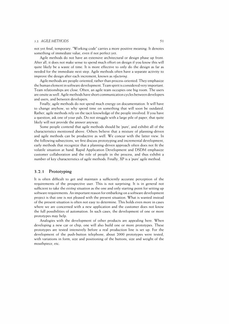
3.2. AGILE METHODS 51

not yet final, temporary. ”Working code” carries a more positive meaning. It denotes

something of immediate value, even if not perfect yet.

Agile methods do not have an extensive architectural or design phase up front.

After all, it does not make sense to spend much effort on design if you know this will

quite likely be a waste of time. It is more effective to only do the design as far as

needed for the immediate next step. Agile methods often have a separate activity to

improve the design after each increment, known as refactoring.

Agile methods are people-oriented, rather than process-oriented. They emphasize

the human element in software development. Team spirit is considered very important.

Team relationships are close. Often, an agile team occupies one big room. The users

are onsite as well. Agile methods have short communication cycles between developers

and users, and between developers.

Finally, agile methods do not spend much energy on documentation. It will have

to change anyhow, so why spend time on something that will soon be outdated.

Rather, agile methods rely on the tacit knowledge of the people involved. If you have

a question, ask one of your pals. Do not struggle with a large pile of paper, that quite

likely will not provide the answer anyway.

Some people contend that agile methods should be ‘pure’, and exhibit all of the

characteristics mentioned above. Others believe that a mixture of planning-driven

and agile methods can be productive as well. We concur with the latter view. In

the following subsections, we first discuss prototyping and incremental development,

early methods that recognize that a planning-driven approach often does not fit the

volatile situation at hand. Rapid Application Development and DSDM emphasize

customer collaboration and the role of people in the process, and thus exhibit a

number of key characteristics of agile methods. Finally, XP is a ‘pure’ agile method.

3.2.1 Prototyping

It is often difficult to get and maintain a sufficiently accurate perception of the

requirements of the prospective user. This is not surprising. It is in general not

sufficient to take the existing situation as the one and only starting point for setting up

software requirements. An important reason for embarking on a software development

project is that one is not pleased with the present situation. What is wanted instead

of the present situation is often not easy to determine. This holds even more in cases

where we are concerned with a new application and the customer does not know

the full possibilities of automation. In such cases, the development of one or more

prototypes may help.

Analogies with the development of other products are appealing here. When

developing a new car or chip, one will also build one or more prototypes. These

prototypes are tested intensively before a real production line is set up. For the

development of the push-button telephone, about 2000 prototypes were tested,

with variations in form, size and positioning of the buttons, size and weight of the

mouthpiece, etc.

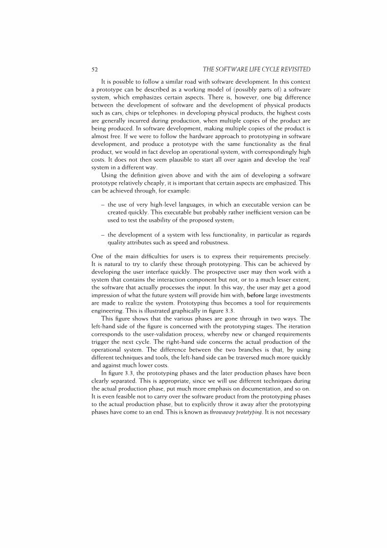
52 THE SOFTWARE LIFE CYCLE REVISITED

It is possible to follow a similar road with software development. In this context

a prototype can be described as a working model of (possibly parts of) a software

system, which emphasizes certain aspects. There is, however, one big difference

between the development of software and the development of physical products

such as cars, chips or telephones: in developing physical products, the highest costs

are generally incurred during production, when multiple copies of the product are

being produced. In software development, making multiple copies of the product is

almost free. If we were to follow the hardware approach to prototyping in software

development, and produce a prototype with the same functionality as the final

product, we would in fact develop an operational system, with correspondingly high

costs. It does not then seem plausible to start all over again and develop the ‘real’

system in a different way.

Using the definition given above and with the aim of developing a software

prototype relatively cheaply, it is important that certain aspects are emphasized. This

can be achieved through, for example:

– the use of very high-level languages, in which an executable version can be

created quickly. This executable but probably rather inefficient version can be

used to test the usability of the proposed system;

– the development of a system with less functionality, in particular as regards

quality attributes such as speed and robustness.

One of the main difficulties for users is to express their requirements precisely.

It is natural to try to clarify these through prototyping. This can be achieved by

developing the user interface quickly. The prospective user may then work with a

system that contains the interaction component but not, or to a much lesser extent,

the software that actually processes the input. In this way, the user may get a good

impression of what the future system will provide him with, before large investments

are made to realize the system. Prototyping thus becomes a tool for requirements

engineering. This is illustrated graphically in figure 3.3.

This figure shows that the various phases are gone through in two ways. The

left-hand side of the figure is concerned with the prototyping stages. The iteration

corresponds to the user-validation process, whereby new or changed requirements

trigger the next cycle. The right-hand side concerns the actual production of the

operational system. The difference between the two branches is that, by using

different techniques and tools, the left-hand side can be traversed much more quickly

and against much lower costs.

In figure 3.3, the prototyping phases and the later production phases have been

clearly separated. This is appropriate, since we will use different techniques during

the actual production phase, put much more emphasis on documentation, and so on.

It is even feasible not to carry over the software product from the prototyping phases

to the actual production phase, but to explicitly throw it away after the prototyping

phases have come to an end. This is known as throwaway prototyping. It is not necessary

3.2. AGILE METHODS 53

Figure 3.3 Prototyping as a tool for requirements engineering

to do so, though. The prototype may evolve to the final product. The user starts by

formulating the raw requirements, on the basis of which a first version of the system is

produced. The user starts to work with this system, which leads to new, or changed,

requirements. The next version is then developed. After a number of such iterations,

the user is satisfied and the last version developed is the product to be delivered. This

is known as evolutionary prototyping. In practice, evolutionary prototyping is used much

more often than throwaway prototyping. Discarding a (partly) working system is a

hurdle which is not easily taken. In agile methods, the phrase working code is often

used instead of evolutionary prototype.

Both throwaway and evolutionary prototyping entail advantages and disadvan-

tages. Figure 3.4 summarizes the pattern of pros and cons that emerges in case

studies that describe experiences of applying a prototyping approach. Note that

some properties can be influenced in both a positive and a negative way. Depending

on circumstances, either or both may occur in an actual project. For example, the

maintenance cost may go down because user needs are better satisfied. On the other

hand, the maintenance cost may go up because development has been done in a quick

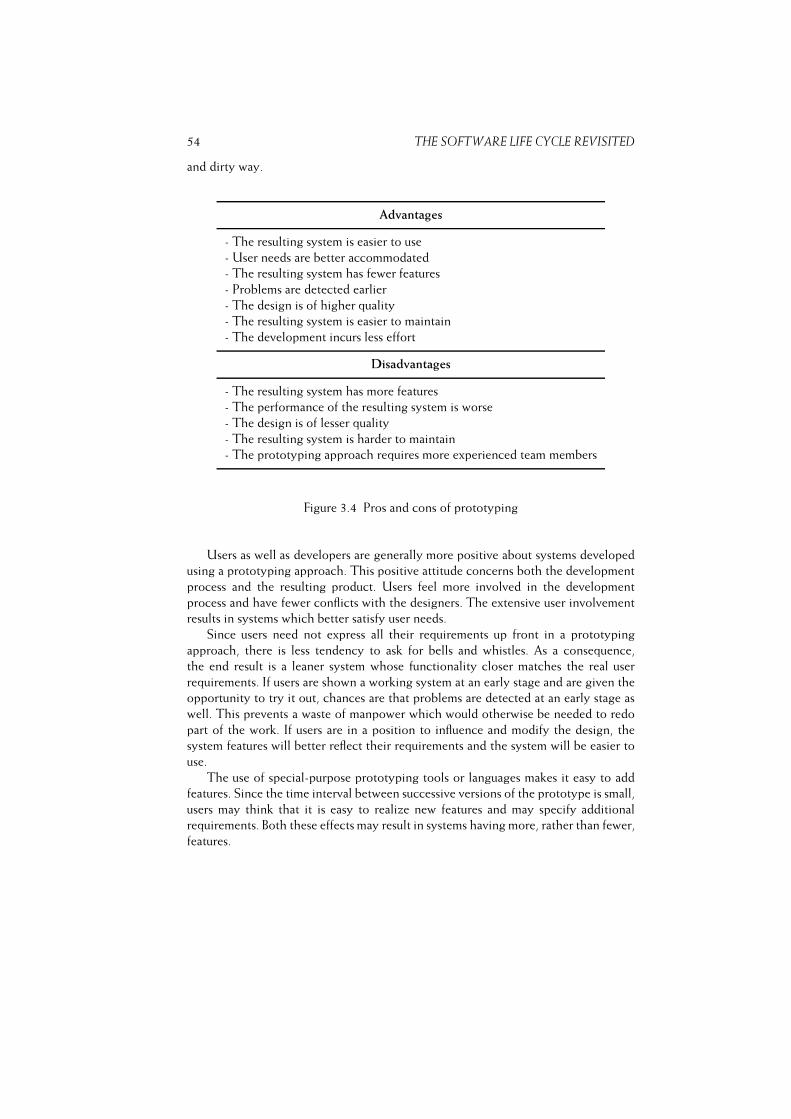
54 THE SOFTWARE LIFE CYCLE REVISITED

and dirty way.

Advantages

- The resulting system is easier to use

- User needs are better accommodated

- The resulting system has fewer features

- Problems are detected earlier

- The design is of higher quality

- The resulting system is easier to maintain

- The development incurs less effort

Disadvantages

- The resulting system has more features

- The performance of the resulting system is worse

- The design is of lesser quality

- The resulting system is harder to maintain

- The prototyping approach requires more experienced team members

Figure 3.4 Pros and cons of prototyping

Users as well as developers are generally more positive about systems developed

using a prototyping approach. This positive attitude concerns both the development

process and the resulting product. Users feel more involved in the development

process and have fewer conflicts with the designers. The extensive user involvement

results in systems which better satisfy user needs.

Since users need not express all their requirements up front in a prototyping

approach, there is less tendency to ask for bells and whistles. As a consequence,

the end result is a leaner system whose functionality closer matches the real user

requirements. If users are shown a working system at an early stage and are given the

opportunity to try it out, chances are that problems are detected at an early stage as

well. This prevents a waste of manpower which would otherwise be needed to redo

part of the work. If users are in a position to influence and modify the design, the

system features will better reflect their requirements and the system will be easier to

use.

The use of special-purpose prototyping tools or languages makes it easy to add

features. Since the time interval between successive versions of the prototype is small,

users may think that it is easy to realize new features and may specify additional

requirements. Both these effects may result in systems having more, rather than fewer,

features.

3.2. AGILE METHODS 55

Prototyping involves iterative design steps and, because of the repeated attention

to the design, its quality may increase. Since it is known a priori that the design

will evolve during subsequent prototyping steps, greater attention will be given to

quality factors such as flexibility and modularity and, as a result, design quality may

improve as well. In throwaway prototyping, the quality of the final design is often

higher because of the learning experience of the prototyping steps. Also, this final

design step is hardly, if at all, patched up because of rework actions. Because of these

aspects, the resulting systems are often found to be easier to maintain as well.

On the other hand, prototyping generally does not enforce strict design and

development standards. If we are concerned with a short development time, certain

necessary activities will receive less attention. The chances are that documentation

is sacrificed for speed. Because of additions resulting from frequent rework steps, the

design quality of an evolutionary prototype may deteriorate. For that reason too,

the resulting systems are less maintainable. Especially in evolutionary prototypes, the

robustness of the system will often be less than is customary with a more traditional

approach. In agile methods, refactoring is applied to counteract this phenomenon.

Finally, performance tends to be worse because attention is focused on functionality

and performance measures are either not taken at all or at a point in time at which

they have become too difficult to realize.

It is generally felt that prototyping projects require an experienced team. Prototyp-

ing involves making far-reaching design decisions, especially during early iterations.

In each iteration, user requests have to be weighed, both mutually and against the

ease and cost of their realization. Inexperienced team members are more likely to

make poor choices, thereby seriously threatening the success of a prototyping effort.

From this discussion, we may gather the following recommendations for the use

of prototyping techniques:

– prototyping is particularly useful in situations where the user requirements

are unclear or ambiguous. Prototyping seems a good way to clarify those

requirements;

– prototyping is also particularly useful for systems with a considerable emphasis

on the user interface and which show a high degree of user interaction;

– users and designers must be well aware of the prototyping approach and its

pitfalls. Users should realize that changing software is not all that easy. Users

should also realize that a prototype is a prototype and not a production-quality

system. Designers should be aware of the characteristics of prototyping projects

and not become frustrated by frequent changes in user requirements;

– prototyping must also be planned and controlled. We must impose limits on the

number of iterations. We must establish explicit procedures for documenting

and testing prototypes. The positive aspects of the traditional approach, which

make the process manageable and controllable, should also be applied in this

case.

56 THE SOFTWARE LIFE CYCLE REVISITED

By taking appropriate counter-measures, the potential disadvantages of prototyping

can be guarded against. Prototyping is then a viable alternative process model for

many a software development project.

3.2.2 Incremental Development

In the preceding section, we discussed a way of using prototypes for which the final

system is the last of a series of prototypes. Under careful management control in

order to ensure convergence, the next version is planned to accommodate new or

changed user requirements. There is another way to work towards the final system in

a number of iterations.

We proceed incrementally. The functionality of the system is produced and

delivered to the customer in small increments. Starting from the existing situation we

proceed towards the desired situation in a number of (small) steps. In each of these

steps, the phased approach that we know from the waterfall model, is employed.

Developing software this way avoids the ‘Big Bang’ effect, i.e. for a long time

nothing happens and then, suddenly, there is a completely new situation. Instead of

building software, the software grows. With this incremental approach, the user is

closely involved in planning the next step. Redirecting the project becomes easier

since we may incorporate changed circumstances more quickly.

Incremental development can also be used to fight the ‘overfunctionality’ syn-

drome. Since users find it difficult to formulate their real needs, they tend to demand

too much. Lacking the necessary knowledge of the malleability of software and its

development process, they may be inclined to think that everything can be achieved.

As a consequence, essential features appear next to bells and whistles in the list

of requirements. Analysts are not able to distinguish one from the other, nor are

they able to accurately estimate the effort required to implement individual features.

Chances then are that much effort is spent on realizing features that are not really

needed. As a result, many of today’s systems offer a rich functionality, yet are at the

same time ill-suited for the task at hand. For one thing, these systems are difficult to

use simply because of the complexity incurred by their rich functionality.

With the incremental approach, attention is first focused on the essential features.

Additional functionality is only included if and when it is needed. Systems thus

developed tend to be leaner and yet provide sufficient support to their users. With

the incremental approach, the most difficult parts are often tackled first, or the parts

that have the highest risks with respect to a successful completion of the project.

Following this line of thought, Boehm (1988) suggests a spiral model of the

software development process, in which each convolution of the spiral gives rise to

the following activities:

– identify the sub-problem which has the highest associated risk;

– find a solution for that problem;

3.2. AGILE METHODS 57

The various process models discussed before can be coupled with Boehm’s spiral

model in a natural way (see figure 3.5):

– If obtaining the proper set of user requirements is seen as the area with highest

risk, follow the spiral a few times around to solve this sub-problem (i.e.,

prototype).

– If, starting from a precise requirements specification, the main question is to

obtain a robust and well-documented system, follow the spiral once, using

the traditional process model with its phases and corresponding milestones as

intermediate steps.

– If developing software incrementally, track the spiral a number of times, once

for each increment.

– During maintenance, the reported errors or changing requirements are triggers

to track the spiral.

Viewed this way, the spiral model subsumes the other process models discussed so

far.

Incremental development is strongly advocated by Gilb (1988). It is doubtful

whether the time increment advocated by Gilb, up to a maximum of a few weeks,

is always reasonable. But the advantages of incremental development are consider-

able even with different time increments. Surprises that lurk within the traditional

approach and that pose considerable difficulties on the management side of software

development projects can be greatly diminished when software is developed and

delivered incrementally.

3.2.3 Rapid Application Development and DSDM

Rapid Application Development (RAD) has a lot in common with other iterative

development process models. It emphasizes user involvement, prototyping, reuse, the

use of automated tools, and small development teams. In addition to that, it employs

the notion of a time box, a fixed time frame within which activities are done. In most

development models, a set of requirements is fixed and then the project attempts to

fulfill these requirements within some estimated period of time. Within RAD, the

time frame is decided upon first and then the project tries to realize the requested

functionality within that time frame. If it turns out that not all of the functionality can

be realized within the time frame, some of the functionality is sacrificed. The agreed

deadline however is immovable.

The RAD life cycle consists of four phases:

– requirements planning,

– user design,

– construction,

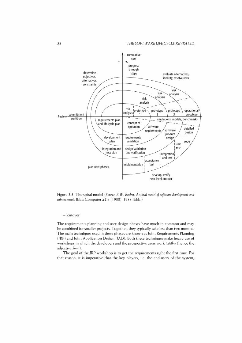
58 THE SOFTWARE LIFE CYCLE REVISITED

Figure 3.5 The spiral model (Source: B.W. Boehm, A spiral model of software development andenhancement, IEEE Computer 21:5 (1988) 1988 IEEE.)

– cutover.

The requirements planning and user design phases have much in common and may

be combined for smaller projects. Together, they typically take less than two months.

The main techniques used in these phases are known as Joint Requirements Planning

(JRP) and Joint Application Design (JAD). Both these techniques make heavy use of

workshops in which the developers and the prospective users work together (hence the

adjective Joint).The goal of the JRP workshop is to get the requirements right the first time. For

that reason, it is imperative that the key players, i.e. the end users of the system,

3.2. AGILE METHODS 59

be present. During the JRP workshop too, requirements are prioritized, since it is

likely that not all of them will be implemented in the first version of the system. This

requirement prioritization is known as triage. Triage usually means a process used on

the battlefield and in emergency rooms to sort injured people into groups based on

their need for or likely benefit from immediate medical treatment. In RAD, the triage

process is used to make sure that the most important requirements are addressed first.

The result of this process is often a prioritization denoted by the acronym MoSCoW:� Must haves are requirements that are definitely needed.� Should haves are requirements that are important, but not absolutely needed

for a usable system.� Could haves are requirements that are only implemented if time allows so.� Won’t haves are requirements that will be left for the next iteration.

As an example, consider the development of a Library Information System. The Must

have category would include the ability to borrow and return an item, and to enroll

as a member. The Should have category might include facilities to make a reservation

for an item. The ability to handle fines for items returned late might be considered a

Could have. Finally, functions to profile users and notify them of newly arrived items

might be classified as Won’t haves.

It is customary to have two JAD workshops during the design phase. Again, the

end users play an essential role in these workshops. The first JAD workshop yields

an initial design of the system. The developers then construct a prototype, to be

experimented with by the users. This prototype is evaluated during the second JAD

workshop, improvements are decided upon, and the design is finalized.

The system is constructed by a so-called SWAT team, a highly skilled team of

about four people. SWAT stands for Skilled With Advanced Tools (see also chapter

5). The SWAT team becomes involved after the first JAD workshop. The team

typically does its job in less than two months. In order to be able to do so, heavy

use is made of tools and existing components are reused whenever feasible. Within

the time allotted (the time box), the SWAT team constructs a series of evolutionary

prototypes. Developers and users work closely together during this process. Each

prototype is reviewed by the users and the review sessions result in requests for

enhanced or changed functionality. The agreed upon time frame is not exceeded. If

necessary, some of the functionality is sacrificed instead.

For a SWAT team to operate successfully, and deliver a good result in a very short

time span, it has to feel a definite ‘ownership’ of the problem to be addressed. In such

a situation, it is not very helpful if time estimates and deadlines are fixed by some

manager. Instead, the SWAT team itself estimates the time, the SWAT team decides

upon the number and length of the time boxes, and the SWAT team decides which

functionality to implement in each iteration.

During the cutover phase, the final testing of the system takes place, users are

trained, and the system is installed.

60 THE SOFTWARE LIFE CYCLE REVISITED

There are many variations on the RAD process model described above. For

example, it is possible to have explicit time boxes for the construction of each of

the intermediate prototypes as well. It is also possible to have JRP or JAD sessions

after each prototyping cycle. The main ingredients, however, remain: prototyping,

considerable user involvement, SWAT teams, and time boxes.

JRP and JAD have much in common with a design method known as Participatory

Design (PD), or the Scandinavian school of software development. Both emphasize

end-user involvement. They differ, however, in their goals. User involvement in JRP

and JAD is primarily intended to speed up the process of producing the right system.

User involvement in PD is motivated by a strong interest in the social context of the

work environment.

A well-known framework that builds on RAD is DSDM. DSDM stands for

Dynamic Systems Development Method. DSDM is based on the nine principles

depicted in Figure 3.6. DSDM is a non-profit framework, maintained by the DSDM

Consortium1. A high-level description of the framework is given in (Stapleton, 2003).

The complete set of DSDM practices is only available to members of the DSDM

Consortium. The DSDM process has five phases; see also figure 3.7:� In the feasibility study, the suitability of DSDM for the current project is

assessed. This is different from a more traditional feasibility study, where the

emphasis is whether a solution is feasible at all. So next to questions like

‘Can we build this system at all?’, the question ‘Is DSDM appropriate for this

project?’ has to be answered as well. Characteristics that make DSDM a feasible

approach reflect the principles of the method: it must be possible to identify the

users of the system, the system should not be too large, and not all requirements

are known upfront.� The business study results in a high-level description of the business processes

relevant for the system. These are determined using facilitated workshops

(like JRP), and result in a high-level baseline. In this phase, the high-level

architecture is determined as well.� The functional model iteration results in analysis models, prototypes, and

implementation of the major functional components. Iteration is done in time

boxes of typically two to six weeks. Each iteration consists of four activities:

(1) identify what you will do, (2) agree on how you will do it, (3) do it, and (4)

check that you have done it.� During the design and build iteration, the system is engineered to a sufficiently

high standard. Here too, work is done in time boxes of typically two to six

weeks, and the same four activities are performed. Though the emphasis of

functional model iterations is on deciding what to build, and that of design and

build iterations is on a properly engineered solution to that, the distinction

between those two types of iteration is not always clearcut.

1See www.dsdm.org

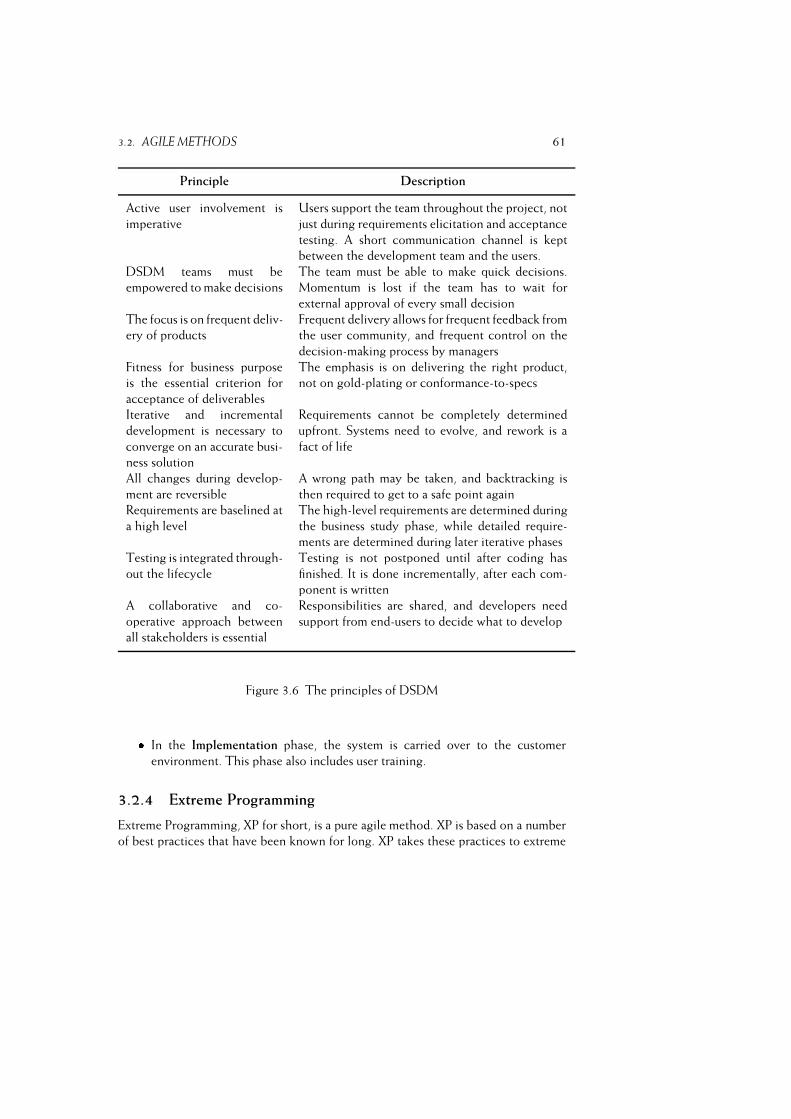
3.2. AGILE METHODS 61

Principle Description

Active user involvement is

imperative

Users support the team throughout the project, not

just during requirements elicitation and acceptance

testing. A short communication channel is kept

between the development team and the users.

DSDM teams must be

empowered to make decisions

The team must be able to make quick decisions.

Momentum is lost if the team has to wait for

external approval of every small decision

The focus is on frequent deliv-

ery of products

Frequent delivery allows for frequent feedback from

the user community, and frequent control on the

decision-making process by managers

Fitness for business purpose

is the essential criterion for

acceptance of deliverables

The emphasis is on delivering the right product,

not on gold-plating or conformance-to-specs

Iterative and incremental

development is necessary to

converge on an accurate busi-

ness solution

Requirements cannot be completely determined

upfront. Systems need to evolve, and rework is a

fact of life

All changes during develop-

ment are reversible

A wrong path may be taken, and backtracking is

then required to get to a safe point again

Requirements are baselined at

a high level

The high-level requirements are determined during

the business study phase, while detailed require-

ments are determined during later iterative phases

Testing is integrated through-

out the lifecycle

Testing is not postponed until after coding has

finished. It is done incrementally, after each com-

ponent is written

A collaborative and co-

operative approach between

all stakeholders is essential

Responsibilities are shared, and developers need

support from end-users to decide what to develop

Figure 3.6 The principles of DSDM� In the Implementation phase, the system is carried over to the customer

environment. This phase also includes user training.

3.2.4 Extreme Programming

Extreme Programming, XP for short, is a pure agile method. XP is based on a number

of best practices that have been known for long. XP takes these practices to extreme

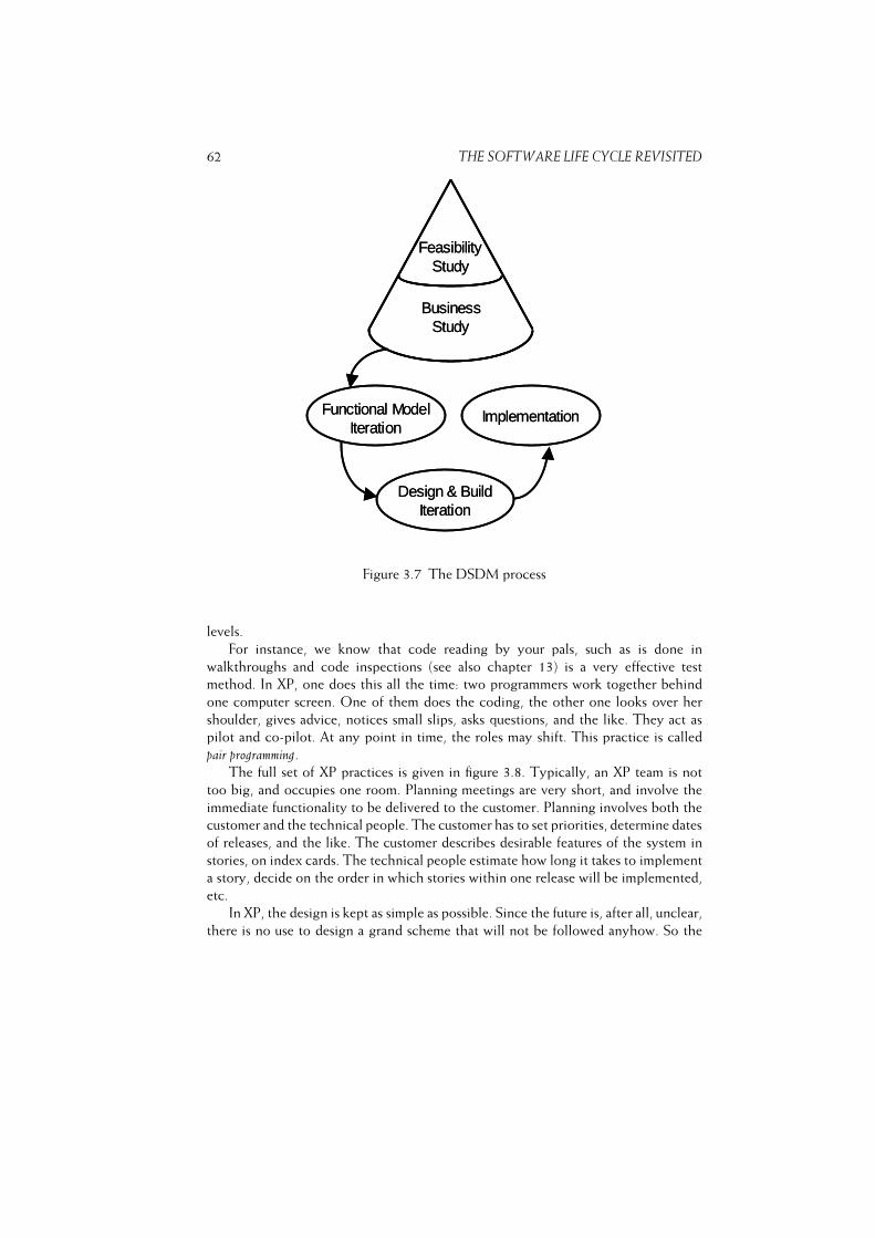
62 THE SOFTWARE LIFE CYCLE REVISITED

FeasibilityStudy

BusinessStudy

Functional ModelIteration

Design & BuildIteration

Implementation

FeasibilityStudy

BusinessStudy

Functional ModelIteration

Design & BuildIteration

Implementation

Figure 3.7 The DSDM process

levels.

For instance, we know that code reading by your pals, such as is done in

walkthroughs and code inspections (see also chapter 13) is a very effective test

method. In XP, one does this all the time: two programmers work together behind

one computer screen. One of them does the coding, the other one looks over her

shoulder, gives advice, notices small slips, asks questions, and the like. They act as

pilot and co-pilot. At any point in time, the roles may shift. This practice is called

pair programming.

The full set of XP practices is given in figure 3.8. Typically, an XP team is not

too big, and occupies one room. Planning meetings are very short, and involve the

immediate functionality to be delivered to the customer. Planning involves both the

customer and the technical people. The customer has to set priorities, determine dates

of releases, and the like. The customer describes desirable features of the system in

stories, on index cards. The technical people estimate how long it takes to implement

a story, decide on the order in which stories within one release will be implemented,

etc.

In XP, the design is kept as simple as possible. Since the future is, after all, unclear,

there is no use to design a grand scheme that will not be followed anyhow. So the

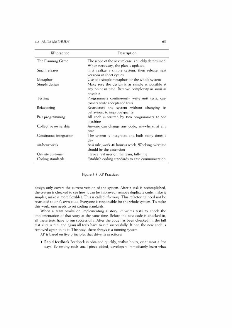
3.2. AGILE METHODS 63

XP practice Description

The Planning Game The scope of the next release is quickly determined.

When necessary, the plan is updated

Small releases First realize a simple system, then release next

versions in short cycles

Metaphor Use of a simple metaphor for the whole system

Simple design Make sure the design is as simple as possible at

any point in time. Remove complexity as soon as

possible

Testing Programmers continuously write unit tests, cus-

tomers write acceptance tests

Refactoring Restructure the system without changing its

behaviour, to improve quality

Pair programming All code is written by two programmers at one

machine

Collective ownership Anyone can change any code, anywhere, at any

time

Continuous integration The system is integrated and built many times a

day

40-hour week As a rule, work 40 hours a week. Working overtime

should be the exception

On-site customer Have a real user on the team, full-time

Coding standards Establish coding standards to ease communication

Figure 3.8 XP Practices

design only covers the current version of the system. After a task is accomplished,

the system is checked to see how it can be improved (remove duplicate code, make it

simpler, make it more flexible). This is called refactoring. This refactoring need not be

restricted to one’s own code. Everyone is responsible for the whole system. To make

this work, one needs to set coding standards.

When a team works on implementing a story, it writes tests to check the

implementation of that story at the same time. Before the new code is checked in,

all these tests have to run successfully. After the code has been checked in, the full

test suite is run, and again all tests have to run successfully. If not, the new code is

removed again to fix it. This way, there always is a running system.

XP is based on five principles that drive its practices:� Rapid feedback Feedback is obtained quickly, within hours, or at most a few

days. By testing each small piece added, developers immediately learn what

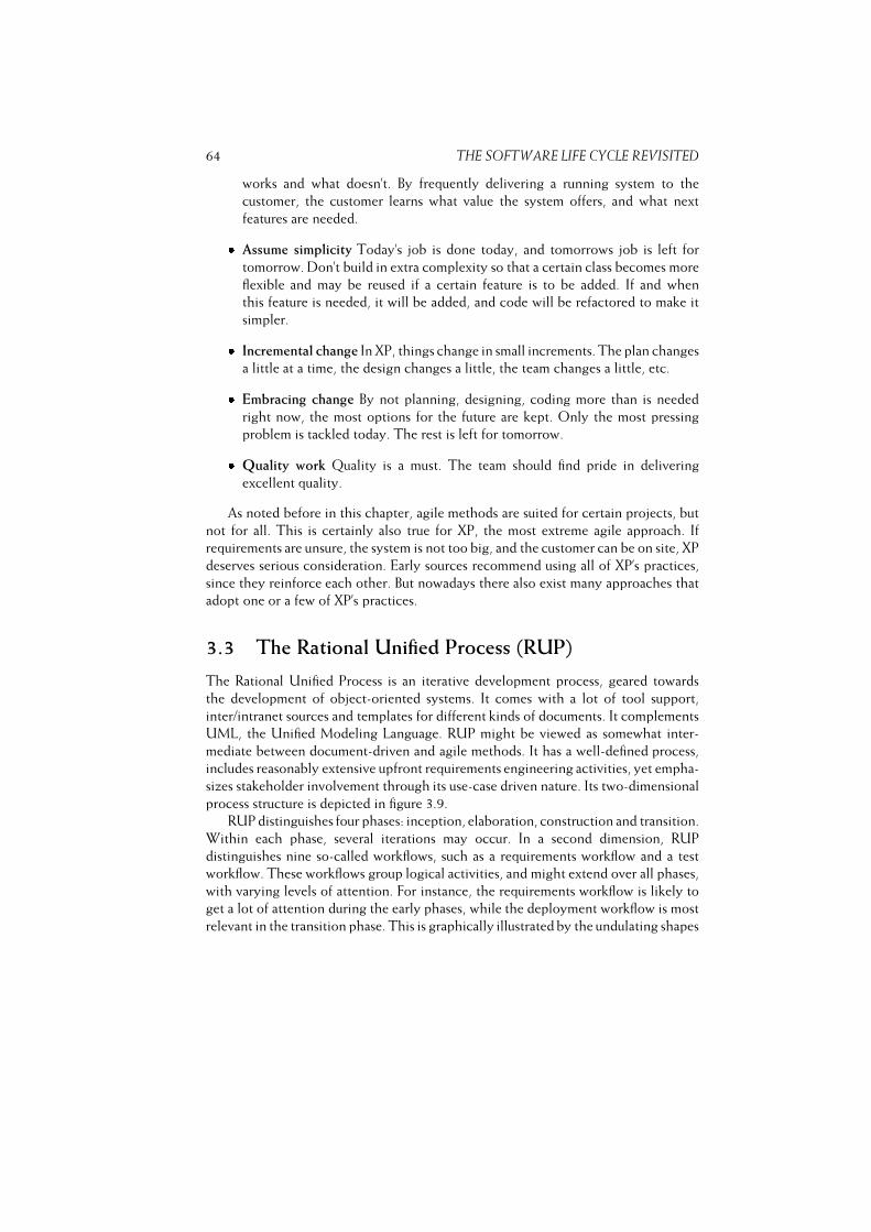
64 THE SOFTWARE LIFE CYCLE REVISITED

works and what doesn’t. By frequently delivering a running system to the

customer, the customer learns what value the system offers, and what next

features are needed.� Assume simplicity Today’s job is done today, and tomorrows job is left for

tomorrow. Don’t build in extra complexity so that a certain class becomes more

flexible and may be reused if a certain feature is to be added. If and when

this feature is needed, it will be added, and code will be refactored to make it

simpler.� Incremental change In XP, things change in small increments. The plan changes

a little at a time, the design changes a little, the team changes a little, etc.� Embracing change By not planning, designing, coding more than is needed

right now, the most options for the future are kept. Only the most pressing

problem is tackled today. The rest is left for tomorrow.� Quality work Quality is a must. The team should find pride in delivering

excellent quality.

As noted before in this chapter, agile methods are suited for certain projects, but

not for all. This is certainly also true for XP, the most extreme agile approach. If

requirements are unsure, the system is not too big, and the customer can be on site, XP

deserves serious consideration. Early sources recommend using all of XP’s practices,

since they reinforce each other. But nowadays there also exist many approaches that

adopt one or a few of XP’s practices.

3.3 The Rational Unified Process (RUP)

The Rational Unified Process is an iterative development process, geared towards

the development of object-oriented systems. It comes with a lot of tool support,

inter/intranet sources and templates for different kinds of documents. It complements

UML, the Unified Modeling Language. RUP might be viewed as somewhat inter-

mediate between document-driven and agile methods. It has a well-defined process,

includes reasonably extensive upfront requirements engineering activities, yet empha-

sizes stakeholder involvement through its use-case driven nature. Its two-dimensional

process structure is depicted in figure 3.9.

RUP distinguishes four phases: inception, elaboration, construction and transition.

Within each phase, several iterations may occur. In a second dimension, RUP

distinguishes nine so-called workflows, such as a requirements workflow and a test

workflow. These workflows group logical activities, and might extend over all phases,

with varying levels of attention. For instance, the requirements workflow is likely to

get a lot of attention during the early phases, while the deployment workflow is most

relevant in the transition phase. This is graphically illustrated by the undulating shapes

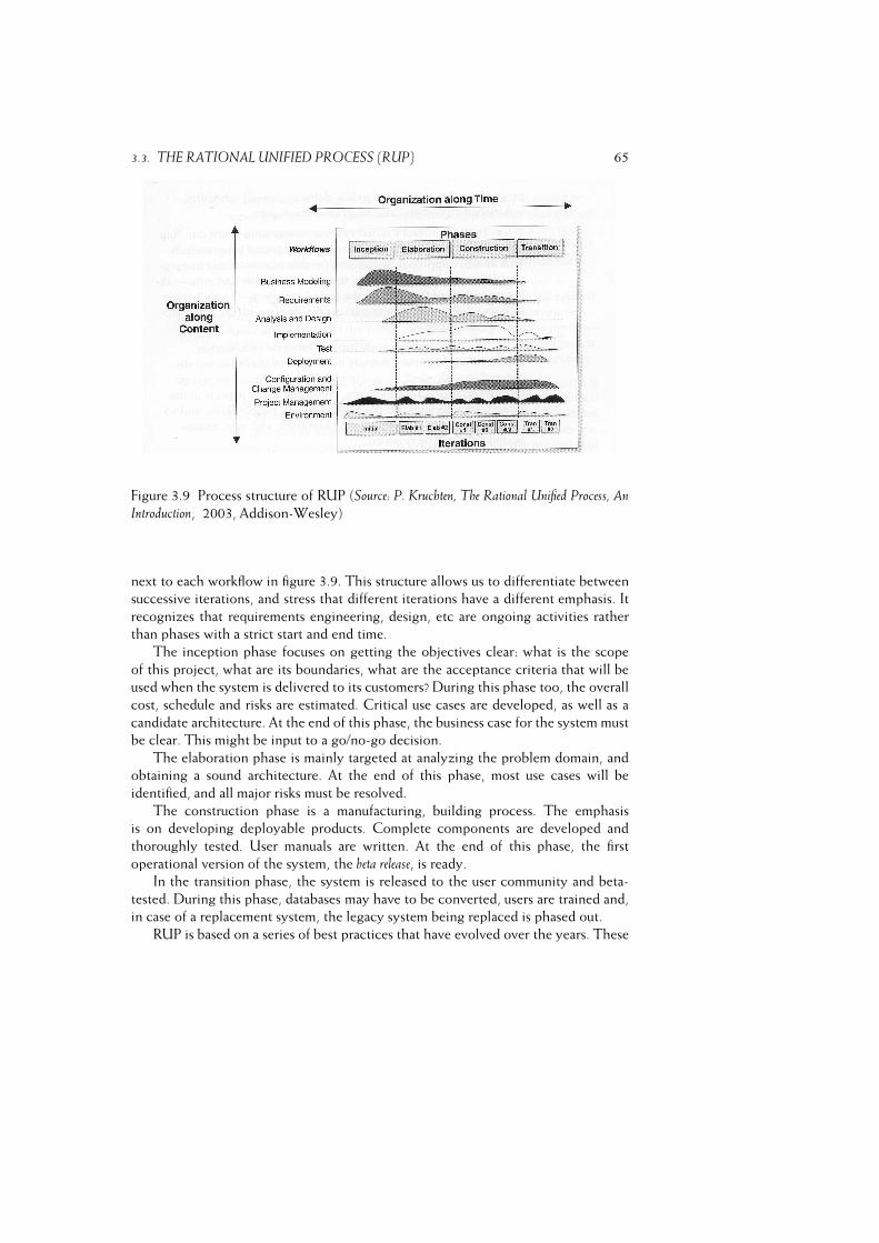
3.3. THE RATIONAL UNIFIED PROCESS (RUP) 65

Figure 3.9 Process structure of RUP (Source: P. Kruchten, The Rational Unified Process, An

Introduction, 2003, Addison-Wesley)

next to each workflow in figure 3.9. This structure allows us to differentiate between

successive iterations, and stress that different iterations have a different emphasis. It

recognizes that requirements engineering, design, etc are ongoing activities rather

than phases with a strict start and end time.

The inception phase focuses on getting the objectives clear: what is the scope

of this project, what are its boundaries, what are the acceptance criteria that will be

used when the system is delivered to its customers? During this phase too, the overall

cost, schedule and risks are estimated. Critical use cases are developed, as well as a

candidate architecture. At the end of this phase, the business case for the system must

be clear. This might be input to a go/no-go decision.

The elaboration phase is mainly targeted at analyzing the problem domain, and

obtaining a sound architecture. At the end of this phase, most use cases will be

identified, and all major risks must be resolved.

The construction phase is a manufacturing, building process. The emphasis

is on developing deployable products. Complete components are developed and

thoroughly tested. User manuals are written. At the end of this phase, the first

operational version of the system, the beta release, is ready.

In the transition phase, the system is released to the user community and beta-

tested. During this phase, databases may have to be converted, users are trained and,

in case of a replacement system, the legacy system being replaced is phased out.

RUP is based on a series of best practices that have evolved over the years. These

66 THE SOFTWARE LIFE CYCLE REVISITED

best practices are listed in Table 3.10. Many of these best practices of course are

also present in other development models. A strong point of RUP is that it provides

a balanced integration of them. Given its background, it is no surprise that RUP is

geared towards the development of object-oriented systems. But RUP is suited for

projects with widely different characteristics. The tuning of RUP to the situation at

hand though is left to the user of the method.

3.4 Intermezzo: Maintenance or Evolution

Old payroll programs never die;

they just get fat around the middleRobert Granholm (Datamation, 1971)

In chapter 1, it was pointed out that a considerable maintenance effort is inevitable.

Each maintenance task, whether it concerns repairing an error or adapting a system

to new user requirements, in principle entails all aspects of the initial development

cycle. During maintenance, we also have to analyze the problem and conceive a

design which is subsequently implemented and tested.

The first big difference is that these changes are being made to an existing product.

However, during initial development we often do not start from scratch either. If an

existing organization decides to automate its order administration, the system may

have to interface with already existing systems for, say, stock administration and

bookkeeping. Thus, maintenance activities differ in degrees from initial development,

rather than fundamentally. This relative difference is even more apparent when the

system is prototyped or developed incrementally.

The second main difference, time pressure, has a much larger impact. Time

pressure is most strongly felt when repairing errors, for then it is quite possible that

certain parts of the organization have to shut down because the software is not

operational. In such cases, we have to work against time to identify and repair the

errors. Often one patches the code and skips a thorough analysis and design step.

The structure of the system tends to suffer from such patches. The system’s entropy

increases, which hampers later maintenance activities. Worse still, the system’s

documentation may not be updated. Software and the corresponding documentation

then grow apart, which will again hamper future maintenance activities. A more

elaborate discussion of maintenance issues is given in chapter 14.

Lehman and his co-workers have extensively studied the dynamics of software

systems that need to be maintained and grow in size. Based on those quantitative

studies, they formulated the following laws of software evolution (explained below):

1. Law of continuing change A system that is being used undergoes continuous

change, until it is judged more cost-effective to restructure the system or replace

it by a completely new version.

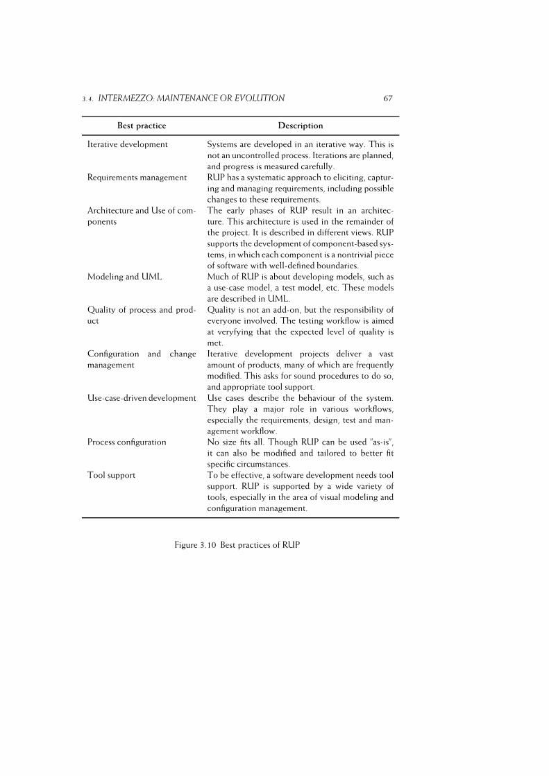
3.4. INTERMEZZO: MAINTENANCE OR EVOLUTION 67

Best practice Description

Iterative development Systems are developed in an iterative way. This is

not an uncontrolled process. Iterations are planned,

and progress is measured carefully.

Requirements management RUP has a systematic approach to eliciting, captur-

ing and managing requirements, including possible

changes to these requirements.

Architecture and Use of com-

ponents

The early phases of RUP result in an architec-

ture. This architecture is used in the remainder of

the project. It is described in different views. RUP

supports the development of component-based sys-

tems, in which each component is a nontrivial piece

of software with well-defined boundaries.

Modeling and UML Much of RUP is about developing models, such as

a use-case model, a test model, etc. These models

are described in UML.

Quality of process and prod-

uct

Quality is not an add-on, but the responsibility of

everyone involved. The testing workflow is aimed

at veryfying that the expected level of quality is

met.

Configuration and change

management

Iterative development projects deliver a vast

amount of products, many of which are frequently

modified. This asks for sound procedures to do so,

and appropriate tool support.

Use-case-driven development Use cases describe the behaviour of the system.

They play a major role in various workflows,

especially the requirements, design, test and man-

agement workflow.

Process configuration No size fits all. Though RUP can be used ”as-is”,

it can also be modified and tailored to better fit

specific circumstances.

Tool support To be effective, a software development needs tool

support. RUP is supported by a wide variety of

tools, especially in the area of visual modeling and

configuration management.

Figure 3.10 Best practices of RUP

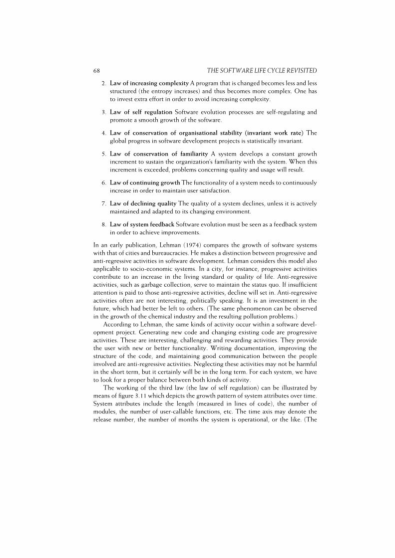
68 THE SOFTWARE LIFE CYCLE REVISITED

2. Law of increasing complexity A program that is changed becomes less and less

structured (the entropy increases) and thus becomes more complex. One has

to invest extra effort in order to avoid increasing complexity.

3. Law of self regulation Software evolution processes are self-regulating and

promote a smooth growth of the software.

4. Law of conservation of organisational stability (invariant work rate) The

global progress in software development projects is statistically invariant.

5. Law of conservation of familiarity A system develops a constant growth

increment to sustain the organization’s familiarity with the system. When this

increment is exceeded, problems concerning quality and usage will result.

6. Law of continuing growth The functionality of a system needs to continuously

increase in order to maintain user satisfaction.

7. Law of declining quality The quality of a system declines, unless it is actively

maintained and adapted to its changing environment.

8. Law of system feedback Software evolution must be seen as a feedback system

in order to achieve improvements.

In an early publication, Lehman (1974) compares the growth of software systems

with that of cities and bureaucracies. He makes a distinction between progressive and

anti-regressive activities in software development. Lehman considers this model also

applicable to socio-economic systems. In a city, for instance, progressive activities

contribute to an increase in the living standard or quality of life. Anti-regressive

activities, such as garbage collection, serve to maintain the status quo. If insufficient

attention is paid to those anti-regressive activities, decline will set in. Anti-regressive

activities often are not interesting, politically speaking. It is an investment in the

future, which had better be left to others. (The same phenomenon can be observed

in the growth of the chemical industry and the resulting pollution problems.)

According to Lehman, the same kinds of activity occur within a software devel-

opment project. Generating new code and changing existing code are progressive

activities. These are interesting, challenging and rewarding activities. They provide

the user with new or better functionality. Writing documentation, improving the

structure of the code, and maintaining good communication between the people

involved are anti-regressive activities. Neglecting these activities may not be harmful

in the short term, but it certainly will be in the long term. For each system, we have

to look for a proper balance between both kinds of activity.

The working of the third law (the law of self regulation) can be illustrated by

means of figure 3.11 which depicts the growth pattern of system attributes over time.

System attributes include the length (measured in lines of code), the number of

modules, the number of user-callable functions, etc. The time axis may denote the

release number, the number of months the system is operational, or the like. (The

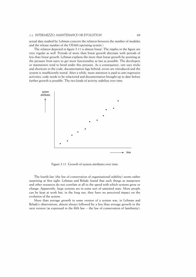
3.4. INTERMEZZO: MAINTENANCE OR EVOLUTION 69

actual data studied by Lehman concern the relation between the number of modules

and the release number of the OS360 operating system.)

The relation depicted in figure 3.11 is almost linear. The ripples in the figure are

very regular as well. Periods of more than linear growth alternate with periods of

less than linear growth. Lehman explains the more than linear growth by pointing at

the pressure from users to get more functionality as fast as possible. The developers

or maintainers tend to bend under this pressure. As a consequence, one uses tricks

and shortcuts in the code, documentation lags behind, errors are introduced and the

system is insufficiently tested. After a while, more attention is paid to anti-regressive

activities: code needs to be refactored and documentation brought up to date before

further growth is possible. The two kinds of activity stabilize over time.

Figure 3.11 Growth of system attributes over time

The fourth law (the law of conservation of organisational stability) seems rather

surprising at first sight. Lehman and Belady found that such things as manpower

and other resources do not correlate at all to the speed with which systems grow or

change. Apparently, large systems are in some sort of saturated state. More people

can be kept at work but, in the long run, they have no perceived impact on the

evolution of the system.

More than average growth in some version of a system was, in Lehman and

Belady’s observations, almost always followed by a less than average growth in the

next version (as expressed in the fifth law -- the law of conservation of familiarity).

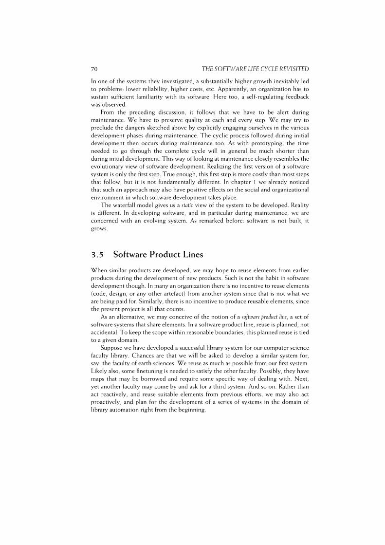
70 THE SOFTWARE LIFE CYCLE REVISITED

In one of the systems they investigated, a substantially higher growth inevitably led

to problems: lower reliability, higher costs, etc. Apparently, an organization has to

sustain sufficient familiarity with its software. Here too, a self-regulating feedback

was observed.

From the preceding discussion, it follows that we have to be alert during

maintenance. We have to preserve quality at each and every step. We may try to

preclude the dangers sketched above by explicitly engaging ourselves in the various

development phases during maintenance. The cyclic process followed during initial

development then occurs during maintenance too. As with prototyping, the time

needed to go through the complete cycle will in general be much shorter than

during initial development. This way of looking at maintenance closely resembles the

evolutionary view of software development. Realizing the first version of a software

system is only the first step. True enough, this first step is more costly than most steps

that follow, but it is not fundamentally different. In chapter 1 we already noticed

that such an approach may also have positive effects on the social and organizational

environment in which software development takes place.

The waterfall model gives us a static view of the system to be developed. Reality

is different. In developing software, and in particular during maintenance, we are

concerned with an evolving system. As remarked before: software is not built, it

grows.

3.5 Software Product Lines

When similar products are developed, we may hope to reuse elements from earlier

products during the development of new products. Such is not the habit in software

development though. In many an organization there is no incentive to reuse elements

(code, design, or any other artefact) from another system since that is not what we

are being paid for. Similarly, there is no incentive to produce reusable elements, since

the present project is all that counts.

As an alternative, we may conceive of the notion of a software product line, a set of

software systems that share elements. In a software product line, reuse is planned, not

accidental. To keep the scope within reasonable boundaries, this planned reuse is tied

to a given domain.

Suppose we have developed a successful library system for our computer science

faculty library. Chances are that we will be asked to develop a similar system for,

say, the faculty of earth sciences. We reuse as much as possible from our first system.

Likely also, some finetuning is needed to satisfy the other faculty. Possibly, they have

maps that may be borrowed and require some specific way of dealing with. Next,

yet another faculty may come by and ask for a third system. And so on. Rather than

act reactively, and reuse suitable elements from previous efforts, we may also act

proactively, and plan for the development of a series of systems in the domain of

library automation right from the beginning.

3.6. PROCESS MODELING 71

This way of doing involves two processes: domain engineering and application

engineering.

In domain engineering, we analyse the domain we are going to develop for. This

process has a life cycle of its own. It results in a set of reusable components that form

the basis for the products to be developed. Usually also, a reference architecture for

all products to be developed is produced as well. An important step in this process

is to decide on the scope of the product line. Are we going to develop a product

line for just university libraries, or for libraries in general? The former is simpler, but

has a more limited market. The latter potentially has a bigger market, but is likely to

result in a more complex overall architecture and more complex products. Scoping

for product lines is a difficult issue. It is influenced by the strategy of the organization

and requires insight into the likely evolution of the domain. Finally, the domain

engineering process yields a production plan, a guide of how to develop products

within the product family.

Application engineering concerns the development of individual products. It

usually follows a waterfall-like scheme. Its inputs are the outputs of the domain

engineering process: the reference architecture, the production plan, and the set of

reusable assets.

Product line organizations often separate domain engineering activities from

application engineering activities. Effectively, these activities then constitute separate

projects. The development of an individual product may result in new or adapted

components that lead to adaptations at the product family level, which in turn affects

the development of subsequent products. Consequently, there are feedback loops

from the application engineering process to the domain engineering process and vice

versa.

Software product lines are particularly suitable in domains where there is a lot of

variation in quite similar products, such as mobile phones, television sets, cameras.

Companies operating in these domains have pioneered the product line field.

A more elaborate discussion of software reuse and software product lines is given

in chapter ??. Software architectures are discussed in chapter 11.

3.6 Process Modeling

Without a repeatable process, the only repeatable results you are likely to produce are

errors.(Macala et al., 1996)

In the 1980s, Osterweil launched the idea of describing software development

processes as programs. These process programs are written in a process programming

language. Like other programming languages, process programming languages have a

rigorously defined syntax and semantics. As a simple example, consider the Pascal-like

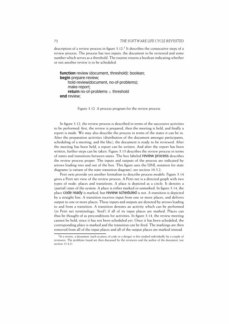
72 THE SOFTWARE LIFE CYCLE REVISITED

description of a review process in figure 3.12.2 It describes the consecutive steps of a

review process. The process has two inputs: the document to be reviewed and some

number which serves as a threshold. The routine returns a boolean indicating whether

or not another review is to be scheduled.

function review (document, threshold): boolean;begin prepare-review;

hold-review(document, no-of-problems);make-report;return no-of-problems < threshold

end review;

Figure 3.12 A process program for the review process

In figure 3.12, the review process is described in terms of the successive activities

to be performed: first, the review is prepared, then the meeting is held, and finally a

report is made. We may also describe the process in terms of the states it can be in.

After the preparation activities (distribution of the document amongst participants,

scheduling of a meeting, and the like), the document is ready to be reviewed. After

the meeting has been held, a report can be written. And after the report has been

written, further steps can be taken. Figure 3.13 describes the review process in terms

of states and transitions between states. The box labeled review process describes

the review process proper. The inputs and outputs of the process are indicated by

arrows leading into and out of the box. This figure uses the UML notation for state

diagrams (a variant of the state transition diagram); see section 10.3.2.

Petri nets provide yet another formalism to describe process models. Figure 3.14

gives a Petri net view of the review process. A Petri net is a directed graph with two

types of node: places and transitions. A place is depicted as a circle. It denotes a

(partial) state of the system. A place is either marked or unmarked. In figure 3.14, the

place code ready is marked, but review scheduled is not. A transition is depicted

by a straight line. A transition receives input from one or more places, and delivers

output to one or more places. These inputs and outputs are denoted by arrows leading

to and from a transition. A transition denotes an activity which can be performed

(in Petri net terminology, ‘fired’) if all of its input places are marked. Places can

thus be thought of as preconditions for activities. In figure 3.14, the review meeting

cannot be held, since it has not been scheduled yet. Once it has been scheduled, the

corresponding place is marked and the transition can be fired. The markings are then

removed from all of the input places and all of the output places are marked instead.

2In a review, a document (such as piece of code or a design) is first studied individually by a couple of

reviewers. The problems found are then discussed by the reviewers and the author of the document (see

section 13.4.2).

3.6. PROCESS MODELING 73

Figure 3.13 State transition diagram of the review process

Figure 3.14 Petri net view of the review process

Petri nets are an attractive modeling technique for processes, since they allow a

certain amount of nondeterminism and parallellism. For example, the process in figure

3.14 does not specify the order in which coding and scheduling activities are to be

performed. They may go on in parallel; synchronization takes place when both are

finished.

A precise description of the software process, be it in a programming-language

notation, a graphical notation, or otherwise, serves three main purposes:� It facilitates understanding and communication. In a software development

74 THE SOFTWARE LIFE CYCLE REVISITED

project, people have to work together. They thus need to have a shared view of

the processes to be carried out and the roles they are to play in those processes.

Either model of the review process given above can be used for this purpose.� It supports process management and improvement. A precise description of

activities to be performed can be used by project management to assign tasks

and to keep track of who is doing what. If the software development process is

to be improved, you first have to know what the current process is, i.e. it has

to be modeled.� It may serve as a basis for automated support. This automated support may

guide or enforce the order in which tasks are being carried out. For instance,

a reviewer may automatically be sent a message indicating that a certain piece

of code is ready for review as soon as its author releases that code. The

automated support may also be used to monitor and track progress, collect

process information and metrics, and so on.

The description of the review process in figure 3.12 is very deterministic. It can

be completely automated and executed without human intervention. In general, the

work that is being modeled will be carried out by both humans and machines. The

neutral term enactment is used to denote the execution of the process by either

humans or machines. Support for process enactment is often combined with support

for configuration management (see section 4.1).

Though the precise modeling of the software process has definite advantages, the

resulting process formality, or even rigidity, holds certain dangers and limitations as

well:� Many aspects of the software development process are heuristic or creative in

nature and do not lend themselves to an algorithmic description. For example,

the actual debugging or design processes will be quite difficult to capture in a

process model.� A process model is a model and, thus, a simplification of reality. For example,

the above models of the review process do not specify what to do if the minutes

of the meeting are not delivered or the review is not held because the author

of the code is on sick-leave, and so on.� Process models often focus on the transformation of artifacts, such as code, a

requirements specification, or a test plan. The progression of stages through

which the artifact evolves then gets confused with the organization of the

processes through which people actually develop those artifacts. This argument

was used earlier when we criticized the waterfall model. It is supported by the

studies of Zelkowitz and Guindon reported in section 3.1. Parnas and Clements

(1986) use similar arguments when they criticize the view that the software

design process is a rational one.

3.7. SUMMARY 75� Processes that do not directly transform artifacts tend to be ignored (for

example, learning the application domain, handling requirements that fluctuate

or conflict, and dealing with breakdowns in communication or coordina-

tion (Curtis et al., 1988).� Processes are treated as discrete rather than continuous in time (i.e. each

project invokes a separate process). This view inhibits the transfer of knowledge

between projects, as was discussed in the previous section.

Process modeling has received a lot of attention in the research literature. It is

indicative of the need for more formal approaches to the description of the software

process. The latest trend in process modeling research is aimed at providing developers

with computer guidance and assistance, rather than trying to fully automate the

process. Such precise descriptions provide a basis for a range of support functions,

ranging from the enactment of design steps to agenda management. This trend to

support people rather than take over fits in well with agile developments too.

3.7 Summary

In this chapter we have addressed the software life cycle again. There are quite a few

arguments against the strict sequential ordering of phases as discussed in chapter 1.

The traditional approach is, to a large extent, document-driven. On the way from

start to finish a number of milestones are identified. Reaching those milestones is

determined by the availability of certain documents. These documents then play a

key role in controlling the development process. It is a heavyweight process, and

planning-driven.

Daily practice hardly fits this model. Change is inevitable, and we had better

adopt a development method that accommodates change. In recent years, a number

of agile, lightweight methods have been proposed that consciously deal with change.

These have evolved from methods such as prototyping, incremental development,

and Rapid Application Development. A very influential agile method is eXtreme

Programming, or XP.

If a series of similar products is developed within a domain, it pays off to

plan reuse upfront, rather than leave it to individual projects to deliver reusable

components. This had led to the notion of software product lines, discussed in

section 3.5. In software product line engineering, the domain engineering part takes

care of developing reusable assets, while the application engineering part produces

individual products using those assets.

Finally, we introduced the notion of process modeling, which is aimed at

describing the software development process in a precise and unambiguous way. Such

descriptions are not intended to fully replace human activities, but rather to support

them.

76 THE SOFTWARE LIFE CYCLE REVISITED

3.8 Further Reading

The waterfall model is generally attributed to Royce (1970) and became well known

through Boehm (1976). However, a clearly phased approach to the development of

software, including iteration and feedback, can already be found in earlier publications:

(Benington, 1983) and (Hosier, 1961).

Advantages and disadvantages of prototyping, based on an analysis of 22 published

case studies and 17 first-hand accounts, are given in (Gordon and Bieman, 1994).

(Verner and Cerpa, 1997) address the different views held by analysts and managers

of the pros and cons of prototyping.

For a very elaborate discussion of RAD, see (Martin, 1991). DSDM is discussed

in (Stapleton, 2003). Participatory Design is described in (Floyd et al., 1989).

(CACM, 1993a) is a special issue on Participatory Design. It contains articles

describing experiences with Participatory Design, as well as a comparison of RAD

and Participatory Design. (Kruchten, 2003) provides a good introduction to RUP.

There are many books about agile methods. The standard book on XP is by its

inventor, Kent Beck (2000). A good companion volume is (Jeffries et al., 2001). Other

agile methods include Scrum (Schwaber and Beedle, 2002) and the Crystal family of

methodologies (Cockburn, 2002). For a comparison of a number of agile methods,

see (Abrahamsson et al., 2002). Boehm and Turner (2003) compare planning-driven

and agile methods, and give advice on when to use which kind of method.

Lehman and Belady (1985) give an overview of their early work on the laws of

software evolution. Lehman et al. (1997) and Cook et al. (2006) provide an updated

perspective. The formulation given in this chapter is based on (Lehman et al., 1997).

A factory-like view of software development was suggested at the very first

conference on Software Engineering (McIlroy, 1968). The term ‘software factory’

is also often associated with Japanese efforts to improve software development

productivity (Cusumano, 1989). The notion of software product lines emerged in the

80’s as a way to increase economy of scale. Clements and Northrop (2001) and Pohl

et al. (2005) provide an in-depth discussion of software product line engineering.

(Osterweil, 1987) launched the idea of describing software development processes

as programs. Critical appraisals of this view are given in (Lehman, 1987), (Curtis

et al., 1987) and (Curtis, 1989). The current trends in software process modeling are

described in (Fuggetta and Wolf, 1996).

Exercises

1. Describe the waterfall model of software development.

2. Describe the Rapid Application Development (RAD) approach to software

development.

3.8. FURTHER READING 77

3. Discuss the main differences between prototyping and incremental develop-

ment.

4. Discuss the main differences between incremental development and RUP.

5. Discuss the law of continuing change.

6. How does the spiral model subsume prototyping, incremental development,

and the waterfall model?

7. Explain the XP practices ‘pair programming’ and ‘refactoring’.

8. What is a software product line?

9. What is the main purpose of having an explicit description of the software

development process in a process model?

10. What is process enactment?

11. Discuss the key values of the agile movement.

12. � Suppose you are involved in a large project concerning the development of

a patient planning system for a hospital. You may opt for one of two strategies.

The first strategy is to start with a thorough analysis of user requirements,

after which the system is built according to these requirements. The second

strategy starts with a less complete requirements analysis phase, after which

a pilot version is developed. This pilot version is installed in a few small

departments. Further development of the system is guided by the experience

gained in working with the pilot version. Discuss the pros and cons of both

strategies. Which strategy do you favor?

13. ~ Consider the patient planning system project mentioned in the previous

exercise. Under what conditions would you opt for an agile approach for this

project?

14. Discuss the relative merits of throwaway prototyping as a means to elicit

the ‘true’ user requirements and prototyping as an evolutionary development

method.

15. In what ways may the notion of a software product line impact the structure

of the software development process?

16. ~ Software maintenance increases system entropy. Discuss possible ways to

counteract this effect.

17. ~ One of the reasons for using planning-driven approaches in software

development projects is that the plan provides some structure to measure

78 THE SOFTWARE LIFE CYCLE REVISITED

project progress. Do you think this measure is adequate? Can you think of

better ways to measure progress?

18. ~ Discuss the differences between RAD and Participatory Design (see also

(Carmel et al., 1993)).

19. � Describe the requirements engineering process depicted in figure 9.1 in a

notation like a programming language. Be as precise as possible. Discuss the

advantages and limitations of the resulting process description.

20. � Describe the requirements engineering process depicted in figure 9.1 in

a state transition diagram. Discuss the advantages and limitations of the

resulting process description.

4

Configuration Management

LEARNING OBJECTIVES� To understand the main tasks and responsibilities of software configuration

management� To be aware of the contents of a configuration management plan� To appreciate the interplay between the role of configuration management in

software development and the capabilities of supporting tools

80 CONFIGURATION MANAGEMENT

Careful procedures are needed to manage the vast number of elements (source

code components, documentation, change requests, etc.) that are created and

updated over the lifetime of a large software system. This is especially true in

distributed development projects. It is called configuration management.

In the course of a software development project, quite a few documents are

produced. These documents are also changed from time to time. Errors have to be

corrected, change requests have to be taken care of, etc. Thus, at each point in time

during a project, different versions of the same document may exist in parallel.

Often too, a software system itself is not monolithic. Software systems exist in

different versions or configurations. Different versions come about when changes are

implemented after the system has been delivered to the customer. From time to time,

the customer is then confronted with a new release. Different versions of components

of a system may also exist during development. For instance, if a change request has

been approved, a programmer may be implementing that change by rewriting one

or more components. Another programmer, however, may still be using the previous

version of those same components.

Different configurations also come about if a set of components may be assembled

into a system in more than one way. Take, for example, the system called ACK,

the Amsterdam Compiler Kit (Tanenbaum et al., 1983). ACK consists of a set of

programs to develop compilers for ALGOL-like languages. Important components of

ACK are:

– front ends for languages such as Pascal, C, or Modula-2. A front end for language

X will translate programs in that language into the universal intermediate code

EM;

– different EM-optimizers;

– back ends, which translate EM-code to assembler-code for a variety of real

machines.

A compiler is then obtained by selecting a front end for a specific language, a back

end for a specific machine and, optionally, one or more optimizers. Each compiler is

a configuration, a certain combination of elements from the ACK system. The ACK

system is an example of a product line, from an era before that notion was used.

The key tasks of configuration management are discussed in section 4.1. A

Configuration Management Plan lays down the procedures that describe how to

approach configuration management. The contents of this document are discussed in

section 4.2. Configuration management is often supported by tools. The discussion

of those tools is largely postponed until chapter 15.

4.1. TASKS AND RESPONSIBILITIES 81

4.1 Tasks and Responsibilities

Configuration management is concerned with the management of all artifacts pro-

duced in the course of a software development project. Though configuration

management also plays a role during the operational phase of a system, when dif-

ferent combinations of components can be assembled into one system and new

releases of a system are generated, the discussion below centers around the role of

configuration management during system development.

We will for the moment assume that, at any point in time, there is one official

version of the complete set of documents related to the project. This is called the

baseline. A baseline is ‘a specification or product that has been formally reviewed

and agreed upon, that thereafter serves as the basis for further development, and that

can be changed only through formal change control procedures’ (IEEE610, 1990).

Thus, the baseline is the shared project database, containing all approved items. The

baseline may or may not be stored in a real database and supported by tools to assist

in retrieving and updating its elements. The items contained in the baseline are the

configuration items. A configuration item is ‘an aggregation of hardware, software, or

both, that is designated for configuration management and treated as a single entity

in the configuration management process’ (IEEE610, 1990). Possible configuration

items are:

– source code components,

– the requirements specification,

– the design documentation,

– the test plan,

– test cases,

– test results,

– the user manual.

At some point in time, the baseline will contain a requirements specification. As time

goes on, elements will be added: design documents, source code components, test

reports, etc. A major task of configuration management is to maintain the integrity of

this set of artifacts.

This is especially important if changes are to be incorporated. Suppose that,

during testing, a major flaw in some component is discovered. We then have to

retrace our steps and correct not only that component but also the corresponding

design documents, and possibly even the requirements specification. This may affect

work being done by other people still using the old version. Worse still, someone

else may wish to make changes to the very same component at the same time.

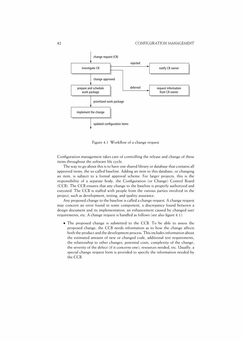
82 CONFIGURATION MANAGEMENT

Figure 4.1 Workflow of a change request

Configuration management takes care of controlling the release and change of these

items throughout the software life cycle.

The way to go about this is to have one shared library or database that contains all

approved items, the so-called baseline. Adding an item to this database, or changing

an item, is subject to a formal approval scheme. For larger projects, this is the

responsibility of a separate body, the Configuration (or Change) Control Board

(CCB). The CCB ensures that any change to the baseline is properly authorized and

executed. The CCB is staffed with people from the various parties involved in the

project, such as development, testing, and quality assurance.

Any proposed change to the baseline is called a change request. A change request

may concern an error found in some component, a discrepancy found between a

design document and its implementation, an enhancement caused by changed user

requirements, etc. A change request is handled as follows (see also figure 4.1):� The proposed change is submitted to the CCB. To be able to assess the

proposed change, the CCB needs information as to how the change affects

both the product and the development process. This includes information about

the estimated amount of new or changed code, additional test requirements,

the relationship to other changes, potential costs, complexity of the change,

the severity of the defect (if it concerns one), resources needed, etc. Usually, a

special change request form is provided to specify the information needed by

the CCB.

4.1. TASKS AND RESPONSIBILITIES 83� The CCB assesses the change request. The change request may be approved,

rejected, or deferred if further information is required. If the request is approved,

it eventually results in a work package which has to be scheduled.� The CCB makes sure that all configuration items affected will eventually be

updated accordingly. Configuration management provides a means to establish

the status of all items and, thereby, of the whole project.

Thus, configuration management is not only about keeping track of all the different

versions of elements of a system; it also encompasses workflow management tasks.

The process depicted in the state transition diagram in figure 4.1, for example,

describes what goes on in the life cycle of a change request. The process model thus

defined exemplifies how the workflow of change requests can be managed.

In a similar vein, the state transition diagram in figure 4.2 shows the workflow of

developer tasks during the development of a system component. It shows the possible

states of a system component and the transitions in between. For example, after a

component has been coded, it is unit tested. If bugs are found during unit testing,

further coding is necessary. Otherwise, the component enters the review stage. If the

review reveals problems, the coding stage is re-entered. Otherwise, the component is

submitted to the CCB for formal approval. Finally, if unit testing does not reveal any

errors, the review stage is skipped.

If components are kept under configuration control, configuration management

can be used to manage the workflow of development tasks as well. Changes in

the status of a component then trigger subsequent activities, as indicated in the

development workflow model.

We have to take care that the workflow schemes do not unnecessarily curtail the

day-to-day working of the people involved in the project. New items should not be

added to the baseline until they have been thoroughly reviewed and tested. Items

from the shared database may be used freely by the participants. If an item has to

be changed, the person responsible for implementing the change gets a copy of that

item and the item is temporarily locked, so that others can not simultaneously update

the same item. The person implementing the change is free to tinker with the copy.

After the change has been thoroughly tested, it is submitted back to the CCB. Once

the CCB has approved it, the revised item is included in the database, the change

itself is documented with the item, and the item is unlocked again. A sequence of

documented changes thus provides a revision history of that item.

When an item is changed, the old version is kept as well. The old version still

has to be used by others until they have adapted to the change. Also, we may wish

to go back to the old version if another change is requested. We thus have different

versions of one and the same item, and must be able to distinguish them. This can

be done through some numbering scheme, where each new version gets identified by

the next higher number. We then get, for a component X, versions X.0, X.1, X.2, and

so on.

84 CONFIGURATION MANAGEMENT

Figure 4.2 State transition diagram of development activities

In a more sophisticated environment, we may even create different branches of

revisions. Figure 4.3 gives an example of such a forked development. In the example,

component X.2.1. is, say, the result of fixing a bug in component X.2. Component X.3

may concern an enhancement to X.2. It should be noted that merging those parallel

development paths again can be difficult. Also, the numbering schemes soon tend to

become incomprehensible.

Configuration management is generally supported by powerful tools. Dart (1990)

classifies the functionalities of these software configuration management (SCM) tools

in eight categories:� Components. SCM tools support storing, retrieving, and accessing compo-

nents. Several versions of a component may be stored, baselines can be

established, and branches of revisions may be created.� Structure. SCM tools support support the representation and use of the

structure of a system made up of components and their interfaces. In terms of

architectural viewpoints, this is the implementation viewpoint; see section 11.3.

4.1. TASKS AND RESPONSIBILITIES 85

Figure 4.3 Parallel development paths� Construction. SCM tools support the construction of an executable version of

the system. By default, the latest version of all configuration elements is used,

but it is also possible to regenerate older versions of the system.� Auditing. SCM tools allow one to follow trails: which changes have been made

to this component, who did those changes, and why. This way, a searchable

archive of the system is maintained.� Accounting. The searchable archive allows one to gather statistics about

the system and the development process. We may for instance search for

components that are changed very often, and hypothesize about the quality of

those components.� Controlling. SCM tools may be used for traceability purposes. If sufficient

information is stored, we may trace defects to requirements, analyze the impact

of changes, and the like.� Process. SCM tools may support users in selecting tasks and performing those

tasks in the appropriate context. For instance, the tool may assist in assigning

the handling of a change request to a certain developer, and automatically

provide her with a workspace with the components that need to be changed.� Team. SCM tools may support collaboration, for example by generating

a workspace for a group of collaborating developers, by noticing conflicts

between developers, and the like.

Many SCM tools employ the version-oriented model of configurations. A physical

change in a component then results in a new version, and different versions are

thus characterized by their difference. Some tools use logical changes, rather than

physical ones, as a basic unit of work in configuration management. This so-called

change-oriented model gives a more intuitive way of working and may prevent a lot

of user errors when configuring a system. Rather than identifying a configuration by

86 CONFIGURATION MANAGEMENT

some arcane sequence of numbers, it is now identified by some baseline plus a set of

changes. The set of changes may be empty. We thus specify

baseline X plus ‘fix table size problem’

rather thanfX.3.1, Y.2.7, Z.1.4, . . . g.

As noted, SCM tools tools also offer help in constructing an executable version of the

system. One writes a ‘program’ that identifies the various components of the required

system and their mutual dependencies. The system in question is then generated

by executing this ‘program’: the components are retrieved automatically from the

database containing the source code components, and all components are translated

and linked together into an executable system. If the system is smart enough, only

those components that have been changed are translated anew.

Early SCM tools emphasized the product-oriented tasks of configuration manage-

ment. They provide functionality to lock and unlock elements, provide for automatic

numbering of revisions, and, by default, provide users with the latest version of an

item. If an item is changed, they prompt the user and ask him to document the change.

Present-day SCM tools increasingly provide the other functionalities as well, and

have become a key ingredient of managing modern, distributed and global, software

development. Tools for configuration and version management will be discussed more

extensively in chapter 15.

On one hand, configuration management entails procedures on how to handle

changes to and versions of documents. On the other hand, it consists of tool support

to maintain the version history and ensure an up to date version of the system. In

planning-driven development, both aspects are important. In agile projects, emphasis

is on the tool support part. Agile projects favor continuous integration, whereby

individual work of one developer is rapidly integrated with other parts of the system.

And then tests are run to make sure everything still works as expected. Such a

development cycle can take a few hours, and at most one day. At the end of the day,

one again has a running system that passes all tests. This process is known as the dailybuild.

4.2 Configuration Management Plan

The procedures for configuration management are laid down in a document, the

Configuration Management Plan. For the contents of this plan, we will follow the

corresponding IEEE Standard (IEEE828, 1990). This document describes methods to

identify configuration items, to control change requests, and to document the imple-

mentation of those change requests. A sample table of contents of the Configuration

Management Plan is given in figure 4.4. The main constituents of this plan are:

Management This section describes how the project is being organized. Particular

attention is paid to responsibilities which directly affect configuration management:

4.3. SUMMARY 87

how are change requests being handled, how are development phases closed, how

is the status of the system maintained, how are interfaces between components

identified? Also, the relationship with other functional organizations, such as software

development and quality assurance, is delineated.

Activities This section describes how a configuration will be identified and controlled

and how its status will be accounted and reported. A configuration is identified by a

baseline: a description of the constituents of that configuration. Such a configuration

must be formally approved by the parties involved.

Clear and precise procedures are needed with respect to the processing of change

requests if a software development project is to be controlled. A Configuration

Control Board (CCB) usually has the responsibility to evaluate and approve or reject

proposed changes. The authority, responsibility, and membership of the CCB have to

be stated. Since software components are usually incorporated in a library, procedures

for controlling this library have to be established as well.

In order to be able to control a software development project, data have to be

collected and processed. Information that is normally required includes: the present

status of components, versions and change requests, as well as reports of approved

changes and their implementation.

Changes to configuration items may affect items outside the scope of the plan,

such as hardware items. These external items have to be identified and their interfaces

controlled. In a similar vein, interfaces to items developed outside the project have to

be identified and controlled.

4.3 Summary

Configuration management is concerned with the management of all artifacts pro-

duced in the course of a software development project. It entails the following major

activities:� Configuration items must be identified and defined. A configuration item is a

collection of elements that is treated as one unit for the purpose of configuration

management. Examples of possible configuration items are the requirements

specification, a software component, a test report, and the user documentation.� The release and change of these items throughout the software life cycle must

be controlled. This means that orderly procedures must be established as to

whom is authorized to change or release configuration items.� The status of configuration items and change requests must be recorded and

reported. For example, the status of a change request may be: proposed,

approved, rejected, or incorporated.

For larger projects, a Configuration Control Board is usually established. The CCB

is responsible for evaluating all change requests and maintaining the integrity of

88 CONFIGURATION MANAGEMENT

1. Introductiona. Purpose

b. Scope

c. Definitions and acronyms

d. References

2. SCM managementa. Organization

b. SCM responsibilities

c. Applicable policies, directives and procedures

3. SCM activities

a. Configuration identification

b. Configuration control

c. Configuration status accounting

d. Configuration audits and reviews

e. Interface control

f. Subcontractor/vendor control

4. SCM schedules5. SCM resources

6. SCM plan maintenance

Figure 4.4 Sample structure of a software configuration management (SCM) plan

(Source: IEEE Standard for Software Configuration Management Plans, IEEE Std

828-1990. Reproduced by permission of IEEE.)

the complete set of documents that relate to a project. Its tasks and the further

procedures for configuration management are laid down in a separate document, the

Configuration Management Plan.

The history and development of configuration management is closely tied to

the history and development of configuration-management tools. In the early days,

these tools emphasized the logging of physical file changes. There was little support

for process aspects. Present-day configuration-management systems address process

aspects as well (workflow management) and many have adopted a change-oriented

next to or instead of a version-oriented view of configurations. More and more,

configuration-management tools function as document-management tools in that

they support cooperation among a group of people, possibly distributed over multiple

sites, working together on a collection of shared objects.

4.4. FURTHER READING 89

4.4 Further Reading

A readable introduction to the topic of configuration management is given in

(Babich, 1986). A more recent source is (Jonassen Hass, 2002). Estublier et al. (2005)

gives an excellent overview of the major developments in the field. Weber (1996)

and Wiborg-Weber (1997) describe the change-oriented configuration management

technology.

Further references on technical aspects of configuration management are given in

a later chapter, when tools for configuration and version control are discussed.

Exercises

1. What are the main tasks of configuration management?

2. Describe the role of the Configuration Control Board.

3. What is a configuration item?

4. What is a baseline?

5. Explain the difference between version-oriented and change-oriented config-

uration management.

6. Discuss the main contents of a configuration management plan.

7. ~ Discuss differences and similarities between configuration management

during development and maintenance.

8. ~ Discuss possible differences between configuration management in a

traditional waterfall development model and the evolutionary development

models (see also (Bersoff and Davis, 1991).

9. ~ Configuration management at the implementation level is often supported

by tools. Can you think of ways in which such tools can also support the

control of other artifacts (design documents, test reports, etc.)?

10. � Devise a configuration management scheme for a small project (say, less

than one person-year) and a large project (say, more than ten person-years).

Give a rationale for the possible differences between those schemes.

11. � To what extent could configuration-management tools support the gath-

ering of quantitative project data? To what extent could such tools support

project control?

5

People Management and Team

Organization

LEARNING OBJECTIVES� To be aware of the importance of people issues in software development� To know of different ways to organize work� To know of major types of management styles� To appreciate different ways to organize a software development team

91

Finding the right organizational framework and the right mix of skills for a

development team is a difficult matter. Little well-founded theory is available

for this. Yet, many stories of successful and less successful projects discern

some of the intricacies of project team issues. This chapter sketches the major

issues involved.

People are the organization’s most important asset

(Humphrey, 1997a)

In most organizations that develop software, programmers, analysts and other profes-

sionals work together in a team. An adequate team structure depends on many factors,

such as the number of people involved, their experience and involvement in the

project, the kind of project, individual differences and style. These factors also influ-

ence the way projects are to be managed. In this chapter, we discuss various aspects

of people management, as well as some of the more common team organizations for

software development projects.

The work to be done within the framework of a project, be it a software

development project, building a house, or the design of a new car, involves a number

of tasks. A critical part of management responsibility is to coordinate the tasks of all

participants.

This coordination can be carried out in a number of ways. There are both external

and internal influences on the coordination mechanism. Internal influences originate

from characteristics of the project. External influences originate from the project’s

organizational environment. If these influences ask for conflicting coordination

mechanisms, conflicts between the project and the environment are lurking around

the corner.

Consider as an example a highly innovative software development project, to

be carried out within a government agency. The characteristics of the project may

ask for a flexible, informal type of coordination mechanism, where the commitment

of specialized individuals, rather than a strict adherence to formal procedures, is a

critical success factor. On the other hand, the environment may be geared towards

a bureaucracy with centralized control, which tries to impose formal procedures

onto project management. These two mechanisms do not work harmoniously. As a

consequence, management may get crushed between those opposing forces.

Section 5.1 further elaborates the various internal and external factors that affect

the way projects are managed, and emphasizes the need to pay ample attention to

the human element in project management.

Software development involves teamwork. The members of the team have to

coordinate their work, communicate their decisions, etc. For a small project, the team

will consist of up to a few individuals. As the size of the project increases, so will

the team. Large teams are difficult to manage, though. Coordinating the work of

a large team is difficult. Communication between team members tends to increase

exponentially with the size of the team (see also chapter 7). Therefore, large teams

92 PEOPLE MANAGEMENT AND TEAM ORGANIZATION

are usually split into smaller teams in a way that confines most of the coordination

and communication within the sub-team.

Section 5.2 discusses several ways to organize a software development team.

Of these, the hierarchical and matrix organizations can be found in other types of

business too, while the chief programmer, SWAT and agile team are rather specific

to software development. Though open source projects have no means to impose

team structure, they usually converge to an onion-like organization as discussed in

section 5.2.6.

Because of outsourcing, networked companies and globalization, software devel-

opment has become a distributed activity. Teams in, say, Amsterdam, Boston and

Bangalore may have to cooperate on the development of the same system. How

should we split up the tasks between these groups? How to ensure that communi-

cation between these groups is effective? Cultural differences play a role as well in

multi-site development. For instance, people in Asia respect authority. In Northern

America, it is more customary that team members argue with their manager. Managers

as well as team members should be aware of those differences, and act accordingly.

People issues that affect multi-site software development are discussed in chapter ??.

5.1 People Management

A team is made up of individuals, each of whom has personal goals. It is the task of

project management to cast a team out of these individuals, whereby the individual

goals are reconciled into one goal for the project as a whole.

Though the individual goals of people may differ, it is important to identify

project goals at an early stage, and unambiguously communicate these to the project

members. Project members ought to know what is expected of them. If there is

any uncertainty in this respect, team members will determine their own goals: one

programmer may decide that efficiency has highest priority, another may choose

efficient use of memory, while yet a third will decide that writing a lot of code is what

counts. Such widely diverging goals may lead to severe problems.

Once project goals are established and the project is under way, performance of

project members with respect to the project goals is to be monitored and assessed.

This can be difficult, since much of what is being done is invisible and progress is

hard to measure.

Ideally, we would like to have an indication of the functionality delivered

and define productivity as the amount of functionality delivered per unit of time.

Productivity is mostly defined as the number of lines of code delivered per man-

month. Everyone will agree that this measure is not optimal, but nothing better

has been found. One of the big dangers of using this measure is that people tend

to produce as much code as possible. This has a very detrimental effect. The most

important cost driver in software development projects is the amount of code to be

delivered (see also the chapter on cost estimation). Writing less code is cheaper,

5.1. PEOPLE MANAGEMENT 93

therefore, and reuse of existing code is one way to save time and money. It should

therefore be strongly advocated. Using the amount of code delivered per man-month

as a productivity indicator offers no incentive for software reuse.

Another aspect of people assessment occurs in group processes like peer reviews,

inspections and walkthroughs. These techniques are used during verification and

validation activities, to discover errors or assess the quality of the code or documen-

tation. In order to make these processes effective it is necessary to clearly separate

the documents to be assessed from their authors. Weinberg Weinberg (1971) used

the term egoless programming in this Context. An assessment of the product of

someone’s work should not imply an assessment of that person.

One of the major problems in software development is the coordination of

activities of team members. As development projects grow bigger and become

more complex, coordination problems quickly accumulate. To counteract these

problems, management formalizes communication, for example by having formal

project meetings, strictly monitored inspections, and an official configuration control

board. However, informal and interpersonal communication is known to be a primary

way in which information flows into and through a development organization. It is

unwise to rule out this type of communication altogether.1 Informal, interpersonal

communication is most easily accomplished if people are physically at close quarters.

Even worse, people are inclined to trade the ease with which information can be

obtained against its quality. They will easily accept their neighbor’s advice, even if

they know that much better advice can be found on the next floor. To counteract

this tendency, it is wise to bring together diverse stakeholders in controlled ways, for

example by having domain experts in the design team, by having users involved in

the testing of software, or through participatory design approaches. The collocation

of all stakeholders is a main aspect of agile teams.

Successful software development teams exhibit a mix of qualities: technical

competence, end-user empathy, and organization awareness. Technical competency

of course is required to deliver a high-quality system in the first place. End-user

empathy and organizational awareness have to do with recognition of the individuals

and the organization that have to cope with the system. A blend of these orientations

in a team helps to ensure sufficient attention is given to each of these aspects (Klein

et al. (2002)).

Team management entails a great many aspects, not the least important of which

concern the care for the human element. Successes among software development

projects can often be traced to a strong focus on cultural and sociological concerns,

such as efforts to create a blame-free culture, or the solicitation of commitment and

partnership. This chapter touches upon only a few aspects thereof. (Brooks, 1995)

1One shining example hereof is the following anecdote from (Weinberg, 1971). The manager of a

university computing center got complaints about students and programmers chatting and laughing at thedepartment’s coffee machine. Being a real manager, and concerned about productivity, he removed the

coffee machine to some remote spot. Quickly thereafter, the load on the computing center consultants

increased considerably. The crowd near the coffee machine was in fact an effective, informal communication

channel, through which the majority of problems were solved.

94 PEOPLE MANAGEMENT AND TEAM ORGANIZATION

and (DeMarco and Lister, 1999) give many insightful observations regarding the

human element of software project management.

In the remainder of this section we will confine ourselves to two rather general

taxonomies for coordination mechanisms and management styles.

5.1.1 Coordination Mechanisms

In his classic text Structures in Fives: Designing Effective Organizations, Mintzberg dis-

tinguishes between five typical organizational configurations. These configurations

reflect typical, ideal environments. Each of these configurations is associated with a

specific coordination mechanism: a preferred mechanism for coordinating the tasks

to be carried out within that configuration type. Mintzberg’s configurations and

associated coordination mechanisms are as follows:� Simple structure In a simple structure there may be one or a few managers, and

a core of people who do the work. The corresponding coordination mechanism

is called direct supervision. This configuration is often found in new, relatively

small organizations. There is little specialization, training and formalization.

Coordination lies with separate people, who are responsible for the work of

others.� Machine bureaucracy When the content of the work is completely specified, it

becomes possible to execute and assess tasks on the basis of precise instructions.

Mass-production and assembly lines are typical examples of this configuration

type. There is little training and much specialization and formalization. The

coordination is achieved through standardization of work processes.� Divisionalized form In this type of configuration, each division (or project) is

granted considerable autonomy as to how the stated goals are to be reached.

The operating details are left to the division itself. Coordination is achieved

through standardization of work outputs. Control is executed by regularly measuring

the performance of the division. This coordination mechanism is possible only

when the end result is specified precisely.� Professional bureaucracy If it is not possible to specify either the end result or

the work contents, coordination can be achieved through standardization of workerskills. In a professional bureaucracy, skilled professionals are given considerable

freedom as to how they carry out their job. Hospitals are typical examples of

this type of configuration.� Adhocracy In projects that are big or innovative in nature, work is divided

amongst many specialists. We may not be able to tell exactly what each

specialist should do, or how they should carry out the tasks allocated to them.

The project’s success depends on the ability of the group as a whole to reach

a non-specified goal in a non-specified way. Coordination is achieved through

mutual adjustment.

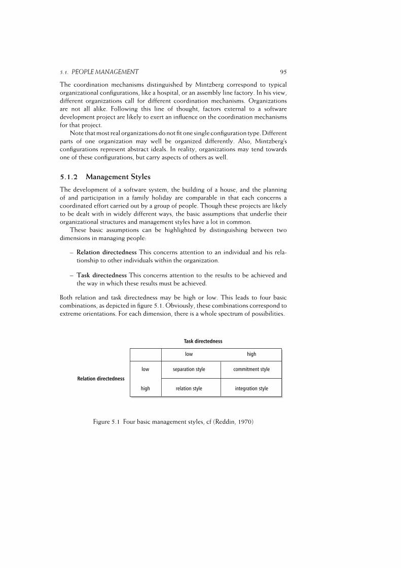
5.1. PEOPLE MANAGEMENT 95

The coordination mechanisms distinguished by Mintzberg correspond to typical

organizational configurations, like a hospital, or an assembly line factory. In his view,

different organizations call for different coordination mechanisms. Organizations

are not all alike. Following this line of thought, factors external to a software

development project are likely to exert an influence on the coordination mechanisms

for that project.

Note that most real organizations do not fit one single configuration type. Different

parts of one organization may well be organized differently. Also, Mintzberg’s

configurations represent abstract ideals. In reality, organizations may tend towards

one of these configurations, but carry aspects of others as well.

5.1.2 Management Styles

The development of a software system, the building of a house, and the planning

of and participation in a family holiday are comparable in that each concerns a

coordinated effort carried out by a group of people. Though these projects are likely

to be dealt with in widely different ways, the basic assumptions that underlie their

organizational structures and management styles have a lot in common.

These basic assumptions can be highlighted by distinguishing between two

dimensions in managing people:

– Relation directedness This concerns attention to an individual and his rela-

tionship to other individuals within the organization.

– Task directedness This concerns attention to the results to be achieved and

the way in which these results must be achieved.

Both relation and task directedness may be high or low. This leads to four basic

combinations, as depicted in figure 5.1. Obviously, these combinations correspond to

extreme orientations. For each dimension, there is a whole spectrum of possibilities.

Figure 5.1 Four basic management styles, cf (Reddin, 1970)

96 PEOPLE MANAGEMENT AND TEAM ORGANIZATION

The style that is most appropriate for a given situation depends on the type of

work to be done:� Separation style This management style is usually most effective for routine

work. Efficiency is the central theme. Management acts like a bureaucrat and

applies rules and procedures. Work is coordinated hierarchically. Decision-

making is top-down, formal, and based on authority. A major advantage of

this style is that it results in a stable project organization. On the other hand,

real innovations are difficult to accomplish. This style closely corresponds to

Mintzberg’s coordination through standardization of work processes.� Relation style This style is usually most effective in situations where people

have to be motivated, coordinated and trained. The tasks to be performed are

bound to individuals. The work is not of a routine character, but innovative,

complex, and specialized. Decision-making is a group process; it involves

negotiation and consensus building. An obvious weak spot of this style is that

it may result in endless chaotic meetings. The manager’s ability to moderate

efficient decision-making is a key success factor. This style best fits Mintzberg’s

mutual adjustment coordination mechanism.� Commitment style This is most effective if work is done under pressure. For

this style to be effective, the manager has to know how to achieve goals

without arousing resentment. Decision making is not done in meetings. Rather,

decisions are implied by the shared vision of the team as to the goals of the

project. A potential weak spot of this style is that, once this vision has been

agreed upon, the team is not responsive to changes in its environment, but

blindly stumbles on along the road mapped out. This style best fits Mintzberg’s

professional bureaucracy.� Integration style This fits situations where the result is uncertain. The work

is explorative in nature and the various tasks are highly interdependent. It

is the manager’s task to stimulate and motivate. Decision-making is informal,

bottom-up. This style promotes creativity, and individuals are challenged to get

the best out of themselves. A possible weak spot of this style is that the goals

of individual team members become disconnected to those of the project, and

that they start to compete with one another. Again, Mintzberg’s coordination

through mutual adjustment fits this situation well.

Each of the coordination mechanisms and management styles identified may be used

within software development projects. It is only reasonable to expect that projects

with widely different characteristics ask for different mechanisms. For an experienced

team asked to develop a well-specified application in a familiar domain, coordination

may be achieved through standardization of work processes. For a complex and

innovative application, this mechanism is not likely to work, though.

In chapter 8, we will identify various types of software development project and

indicate which type of coordination mechanism and management style best fits those

5.2. TEAM ORGANIZATION 97

projects. It should be noted that the coordination mechanisms suggested in chapter 8

stem from internal factors, i.e. characteristics of the project on hand. As noted before,

the project’s environment will also exert influence on its organization.

Notice that we looked from the manager to the team and its members in the above

discussion. Alternatively, we may look at the relation and task maturity of individual

team members. Relation maturity concerns the attitude of employees towards their

job and management. Task maturity is concerned with technical competence. It

is important that the manager aligns his dealings with team members with their

respective relation and task maturity. For example, a fresh graduate may have high

task maturity and low relation maturity, and so his introduction into a skilled team

may warrant some careful guidance.

5.2 Team Organization

Within a team, different roles can be distinguished. There are managers, testers,

designers, programmers, and so on. Depending on the size of the project, more than

one role may be carried out by one person, or different people may play the same

role. The responsibilities and tasks of each of these roles have to be precisely defined

in the project plan.

People cooperate within a team in order to achieve an optimal result. Yet it is

advisable to strictly separate certain roles. It is a good idea to create a test team

that is independent of the development team. Similarly, quality assurance should, in

principle, be conducted by people not directly involved in the development process.

Large teams are difficult to manage and are therefore often split up into smaller

teams. By clearly defining the tasks and responsibilities of the various sub-teams,

communication can be largely confined to communication between members of the

same sub-team. Quantifying the cost of interpersonal communication yields insights

into effects of team size on productivity and helps to structure large development

teams effectively. Some simple formulas for doing so are derived in chapter 7.

In the following subsections we discuss several organizational forms for software

development teams.

5.2.1 Hierarchical Organization

In an environment which is completely dedicated to the production of software,

we often encounter hierarchical team structures. Depending on the size of the

organization or project, different levels of management can be distinguished.

Figure 5.2 gives an example of a hierarchical organization. The rectangles denote

the various sub-teams in which the actual work is done. Circled nodes denote

managers. In this example, two levels of management can be distinguished. At

the lower level, different teams are responsible for different parts of the project.

The managers at this level have a primary responsibility in coordinating the work

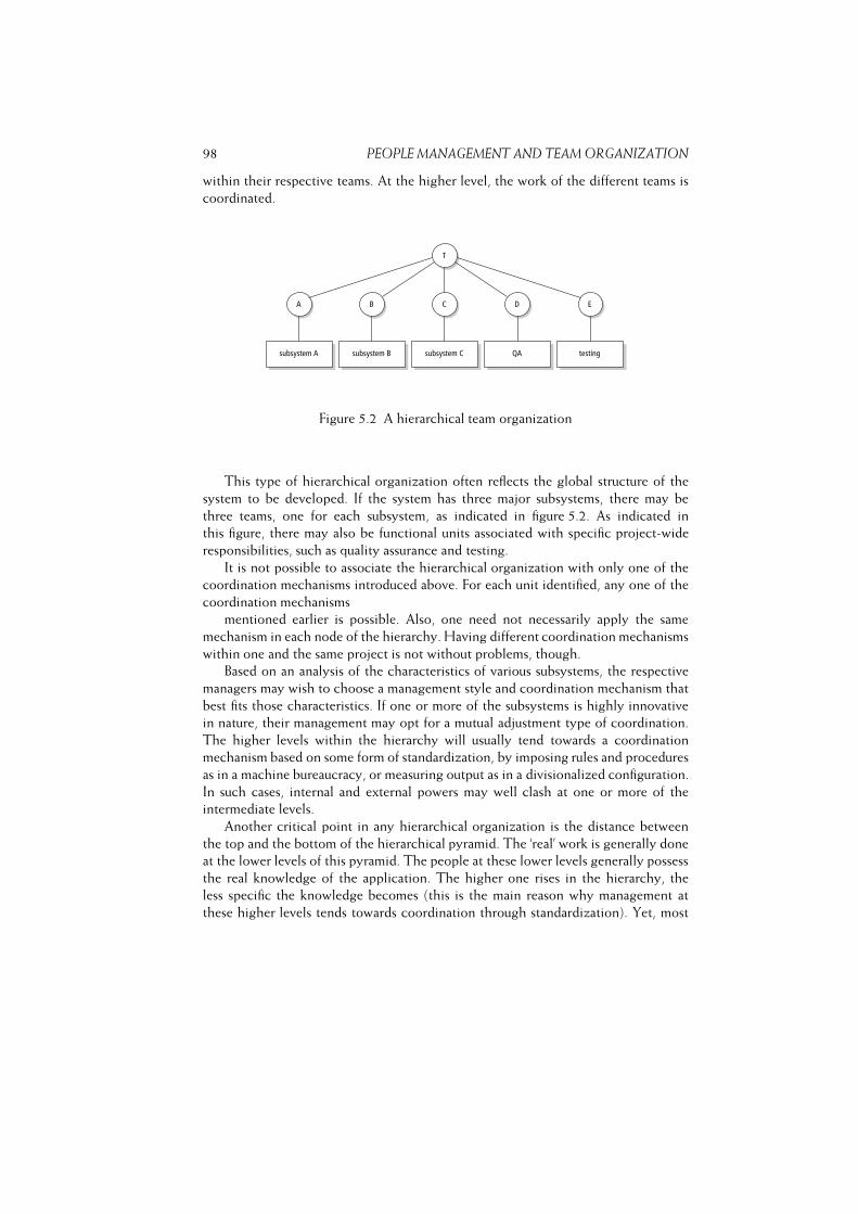
98 PEOPLE MANAGEMENT AND TEAM ORGANIZATION

within their respective teams. At the higher level, the work of the different teams is

coordinated.

Figure 5.2 A hierarchical team organization

This type of hierarchical organization often reflects the global structure of the

system to be developed. If the system has three major subsystems, there may be

three teams, one for each subsystem, as indicated in figure 5.2. As indicated in

this figure, there may also be functional units associated with specific project-wide

responsibilities, such as quality assurance and testing.

It is not possible to associate the hierarchical organization with only one of the

coordination mechanisms introduced above. For each unit identified, any one of the

coordination mechanisms

mentioned earlier is possible. Also, one need not necessarily apply the same

mechanism in each node of the hierarchy. Having different coordination mechanisms

within one and the same project is not without problems, though.

Based on an analysis of the characteristics of various subsystems, the respective

managers may wish to choose a management style and coordination mechanism that

best fits those characteristics. If one or more of the subsystems is highly innovative

in nature, their management may opt for a mutual adjustment type of coordination.

The higher levels within the hierarchy will usually tend towards a coordination

mechanism based on some form of standardization, by imposing rules and procedures

as in a machine bureaucracy, or measuring output as in a divisionalized configuration.

In such cases, internal and external powers may well clash at one or more of the

intermediate levels.

Another critical point in any hierarchical organization is the distance between

the top and the bottom of the hierarchical pyramid. The ‘real’ work is generally done

at the lower levels of this pyramid. The people at these lower levels generally possess

the real knowledge of the application. The higher one rises in the hierarchy, the

less specific the knowledge becomes (this is the main reason why management at

these higher levels tends towards coordination through standardization). Yet, most

5.2. TEAM ORGANIZATION 99

decisions are taken at a fairly high level. In many cases, signals from the lower level

somehow get subsumed at one of the intermediate levels.

If information seeps through the various levels in the hierarchy, it tends to become

more and more rose-colored. The following scenario is not entirely fictitious:

– bottom: we have severe troubles in implementing module X;

– level 1: there are some problems with module X;

– level 2: progress is steady, I do not foresee any real problems;

– top: everything proceeds according to our plan.

These kinds of distortion are difficult to circumvent altogether. They are, however,

reinforced by the fact that the organizational line along which progress is reported

is also the line along which the performance of team members is measured and

evaluated. Everyone is favored by a positive evaluation and is thus inclined to color

the reports accordingly. If data on a project’s progress is being collected and processed

by people not directly involved in the assessment of team members, you have a much

higher chance that the information collected is of sufficient reliability.

An equally problematic aspect of hierarchical organizations lies in the fact that

one is judged, both socially and financially, according to the level at which one stands

within the organization. It is thus natural to aspire to higher and higher levels within

the hierarchy. It is, however, not at all clear that this is desirable. The Peter Principle

says: in a hierarchical organization each employee in general rises until reaching a

level at which he is incompetent. A good programmer need not be a good manager.

Good programming requires certain skills. To be a good manager, different skills are

needed. In the long run, it seems wiser to maintain people at a level at which they

perform well, and reward them accordingly.

5.2.2 Matrix Organization

In an environment where software is a mere byproduct, we often encounter some

sort of matrix organization. People from different departments are then allocated to

a software development project, possibly part-time. In this type of organization it is

sometimes difficult to control progress. An employee has to satisfy several bosses and

may have the tendency to play off one boss against another.

We may also use a matrix organization in an environment completely dedicated

to software development. The basic unit, then, is a small, specialized group. There

may be more than one unit with the same specialization. Possible specializations are,

for instance, graphics programming, databases, user interfaces, quality control. The

units are organized according to their specialty. Projects, on the other hand, may

involve units with different specialties. Individuals are thus organized along two axes,

one representing the various specialist groups and one representing the projects to

which they are assigned. This type of matrix organization is depicted in figure 5.3.

100 PEOPLE MANAGEMENT AND TEAM ORGANIZATION

Figure 5.3 A matrix organization

In such a situation, the project manager is responsible for the successful completion

of the project. The manager in charge of one or more units with the same specialty has

a longer-term mission, such as maintaining or enlarging the knowledge and expertise

of the members of his team. Phrased in terms of the basic management dimensions

discussed earlier, the project manager is likely to emphasize task directedness, while

the unit manager will emphasize relation directedness. Such an organization can

be very effective, provided there is sufficient mutual trust and the willingness to

cooperate and pursue the project’s goals.

5.2.3 Chief Programmer Team

A team organization known as the chief programmer team was proposed by Harlan

Mills around 1970. The kernel of such a team consists of three people. The chief

programmer is team leader. He takes care of the design and implements key parts

of the system. The chief programmer has an assistant who can stand in for the

chief programmer, if needed. Thirdly, a librarian takes care of the administration and

documentation. Besides these three people, an additional (small) number of experts

may be added to the chief programmer team.

In this type of organization, fairly high demands are made upon the chief

programmer. The chief programmer has to be very competent in the technical area,

but he also has to have sufficient management capabilities. In other words, are there

enough chief programmers? Also, questions of competence may arise. The chief

programmer plays a very central role. He takes all the decisions. The other team

members may well challenge some of his qualities.

The early notion of a chief programmer team seems somewhat elitist. It resembles

a surgeon team in its emphasis on highly specialized tasks and charismatic leadership.

The benefits of a team consisting of a small group of peers over huge development

teams struggling to produce ever larger software systems may be regained in a

modified form of the chief programmer team though.

In this modified form, peer group aspects prevail. The development team then

consists of a small group of people collectively responsible for the task at hand. In

particular, jobs are not structured around life cycle stages. There are no analysts,

5.2. TEAM ORGANIZATION 101

designers, or programmers, though the role of tester may be assigned to a specific

person. Different levels of expertise may occur within the group. The most experienced

persons act as chief programmer and deputy chief programmer, respectively. At the

other end of the scale, one or two trainees can be assimilated and get the necessary

on-the-job training. A trainee may well act as the team’s librarian.

5.2.4 SWAT Team

In projects with an evolutionary or iterative process model such as RAD, a project

organization known as the SWAT team is sometimes used. SWAT stands for Skilled

With Advanced Tools. We may view the SWAT team as a software development

version of a project team in which both task and relation directedness are high.

A SWAT team is relatively small. It typically has four or five members. Preferably,

the team occupies one room. Communication channels are kept very short. The team

does not have lengthy formal meetings with formal minutes. Rather, it uses workshops

and brainstorming sessions of which little more than a snapshot of a white-board

drawing is retained.

A SWAT team typically builds incremental versions of a software system. In

order to do so effectively, it employs reusable components, very high-level languages,

and powerful software generators. The work of team members is supported and

coordinated through groupware or workflow management software.

As in the chief programmer team, the leader of a SWAT team is like a foreman

in the building industry: he is both a manager and a co-worker. The members of a

SWAT team are generalists. They may have certain specialties, but they must also be

able to do a variety of tasks, such as participate in a workshop with customers, build

a prototype, and test a piece of software.

Team motivation is very important in a SWAT team. A SWAT team often adopts

a catchy name, motto or logo. This label then expresses their vision. Individuals

derive pride and self-esteem from their membership of a SWAT team.

5.2.5 Agile Team

Agile approaches to software development grew out of, and have a lot in common

with, the various iterative development approaches. In the same vein, an agile team

has much in common with, e.g., a SWAT team: collocated, short communication

channels, a people-oriented attitude rather than a formalistic one. Often, people work

in pairs, with a pilot and co-pilot, but without a hierarchy.

Because agile processes have little discipline enforced on them from the outside,

they need discipline to come from within the team. Agile teams need self-discipline.

If a pair of programmers develops some code and subsequent tests fail, they must take

a step back and redo their work. After they have incorporated a piece of work, they

must consider the system as a whole and refactor if needed.

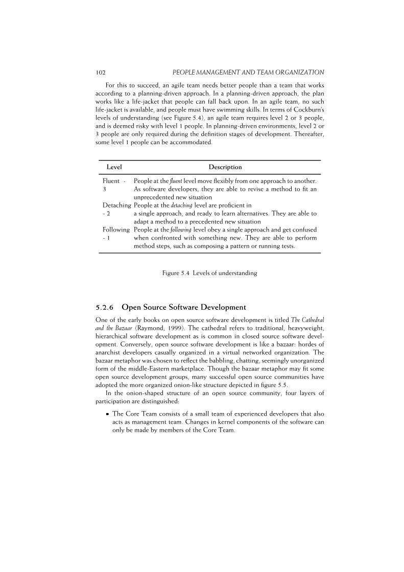
102 PEOPLE MANAGEMENT AND TEAM ORGANIZATION

For this to succeed, an agile team needs better people than a team that works

according to a planning-driven approach. In a planning-driven approach, the plan

works like a life-jacket that people can fall back upon. In an agile team, no such

life-jacket is available, and people must have swimming skills. In terms of Cockburn’s

levels of understanding (see Figure 5.4), an agile team requires level 2 or 3 people,

and is deemed risky with level 1 people. In planning-driven environments, level 2 or

3 people are only required during the definition stages of development. Thereafter,

some level 1 people can be accommodated.

Level Description

Fluent -

3

People at the fluent level move flexibly from one approach to another.

As software developers, they are able to revise a method to fit an

unprecedented new situation

Detaching

- 2

People at the detaching level are proficient in

a single approach, and ready to learn alternatives. They are able to

adapt a method to a precedented new situation

Following

- 1

People at the following level obey a single approach and get confused

when confronted with something new. They are able to perform

method steps, such as composing a pattern or running tests.

Figure 5.4 Levels of understanding

5.2.6 Open Source Software Development

One of the early books on open source software development is titled The Cathedraland the Bazaar (Raymond, 1999). The cathedral refers to traditional, heavyweight,

hierarchical software development as is common in closed source software devel-

opment. Conversely, open source software development is like a bazaar: hordes of

anarchist developers casually organized in a virtual networked organization. The

bazaar metaphor was chosen to reflect the babbling, chatting, seemingly unorganized

form of the middle-Eastern marketplace. Though the bazaar metaphor may fit some

open source development groups, many successful open source communities have

adopted the more organized onion-like structure depicted in figure 5.5.

In the onion-shaped structure of an open source community, four layers of

participation are distinguished:� The Core Team consists of a small team of experienced developers that also

acts as management team. Changes in kernel components of the software can

only be made by members of the Core Team.

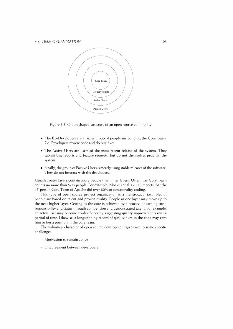
5.2. TEAM ORGANIZATION 103

Core Team

Co−Developers

Active Users

Passive Users

Figure 5.5 Onion shaped structure of an open source community� The Co-Developers are a larger group of people surrounding the Core Team.

Co-Developers review code and do bug fixes.� The Active Users are users of the most recent release of the system. They

submit bug reports and feature requests, but do not themselves program the

system.� Finally, the group of Passive Users is merely using stable releases of the software.

They do not interact with the developers.

Usually, outer layers contain more people than inner layers. Often, the Core Team

counts no more than 5-15 people. For example, Mockus et al. (2000) reports that the

15-person Core Team of Apache did over 80% of functionality coding.

This type of open source project organization is a meritrocacy; i.e., roles of

people are based on talent and proven quality. People in one layer may move up to

the next higher layer. Getting to the core is achieved by a process of earning trust,

responsibility and status through competition and demonstrated talent. For example,

an active user may become co-developer by suggesting quality improvements over a

period of time. Likewise, a longstanding record of quality fixes to the code may earn

him or her a position in the core team.

The voluntary character of open source development gives rise to some specific

challenges:

– Motivation to remain active

– Disagreement between developers

104 PEOPLE MANAGEMENT AND TEAM ORGANIZATION

– Communication between developers

An open source community is ”a company without walls” (Fang and Neufeld, 2006).

People may freely enter and leave the community. Developers participating in open

source projects rarely do so selflessly. They expect something in return, such as the

ability to learn new things, a higher status within their normal job, attention because

they are part of a successful project, and the like. This should come as no surprise.

Software professionals have high growth needs (Couger and Zawacki, 1980). Open

source projects that challenge developer skills, have a well-modularized code base,

and make use of advanced tools have a higher chance of attarcting a sustainable

community.

One of the worst things that may happen to an open source project is disagreement

between developers. A common obstacle in open source projects is disagreement

about development speed Godfrey and Tu (2000). Some developers may want to

issue new releases frequently, while others may take a more cautionary stand. Another

potential source of disagreement is when users start to feel uncomfortable by the

’undemocratic democracy’ of open source projects. Although many people may submit

bug fixes or feature requests, the power of what actually happens usually lies with one

or a few people in the Core Team. If submissions of a developer get rejected time and

again, he may get frustrated and leave the community or decide to create a fork: the

developer takes a copy of the source code and starts an independent development

track.

Communication between developers is an issue in every distributed team. But

in open source projects, the situation is worse because of the floating community

membership and the lack of formal documentation. A clear modularization of the

code is an important means to reduce the need for extensive communication. Open

source communities further tend to use configuration control tools and mailing lists

for communication.

5.2.7 General Principles for Organizing a Team

No matter how we try to organize a team, the key point is that it ought to be a team.

From many tests regarding productivity in software development projects, it turns out

again and again that factors concerning team capabilities have a far greater influence

than anything else. Factors such as morale, group norms and management style play

a more important role than such things as the use of high-level languages, product

complexity, and the like (see, for instance, (Lawrence, 1981)).

Some general principles for team organization are given in (Koontz and O’Donnell,

1972). In particular, these general principles also apply to the organization of software

development projects:� Use fewer, and better, people Highest productivity is achieved by a relatively

small group of people. This holds for novelists, soccer players and bricklayers.

There is no reason to believe that it does not equally apply to programmers

5.3. SUMMARY 105

and other people working in the software field. Also, large groups require more

communication, which has a negative effect on productivity and leads to more

errors.� Try to fit tasks to the capabilities and motivation of the people available In

other words: take care that the Peter Principle does not apply in your situation.

In many organizations, excellent programmers can be promoted only into

managerial positions. It is far better to also offer career possibilities in the more

technical areas of software development and maintenance.� In the long run, an organization is better off if it helps people to get the

most out of themselves So you should not pursue either of the following:

– The reverse Peter Principle: people rise within an organization to a level

at which they become indispensable. For instance, a programmer may

become the only expert in a certain system. If he does not get a chance

to work on anything else, it is not unlikely that this person, for want of

a more interesting and challenging task, will leave your organization. At

that point, you are in real trouble.

– The Paul Principle: people rise in an organization to a level at which

their expertise becomes obsolete within five years. Given the speed with

which new developments enter the market place in software engineering,

and computer science in general, it is very important that people get the

opportunity to grow and stay abreast of new developments.� It is wise to select people such that a well-balanced and harmonious team

results In general, this means that it is not sufficient only to have a few top

experts. A soccer team needs regular players as well as stars. Selecting the proper

mix of people is a complicated task. There are various good texts available that

specifically address this question (for example, (Weinberg, 1971), (Metzger,

1987)).� Someone who does not fit the team should be removed If it turns out that a

team does not function as a coherent unit, we are often inclined to wait a little

while, see how things develop, and hope for better times to come. In the long

run, this is detrimental.

5.3 Summary

Software is written by humans. Their productivity is partly determined by such

factors as the programming language used, machine speed, and available tools. The

organizational environment in which one is operating is equally important, though.

Good team management distinguishes itself from bad team management above all by

the degree to which attention is paid to these human factors. The human element in

106 PEOPLE MANAGEMENT AND TEAM ORGANIZATION

software project management was discussed in section 5.1, together with well-known

taxonomies of coordination mechanisms and management styles.

There are different ways to organize software developers in a team. These orga-

nizational forms and some of their caveats were discussed in section 5.2. Hierarchical

and matrix organizations are not specific to software development, while the chief

programmer, SWAT and agile teams originated in the software field. Each of the

latter somehow tries to reconcile the two types of management typically required in

software development projects: an individualistic, personal approach where one tries

to get the best out of team members, and a hierarchical, top-down management style

to get things done in time and within budget. Successful open source projects usually

have an onion-shaped organization.

5.4 Further Reading

A still very relevant source of information on psychological factors related to software

development is (Weinberg, 1971). (Brooks, 1995) and (DeMarco and Lister, 1999)

also contain a number of valuable observations. Coordination problems in software

development are discussed in (Kraut and Streeter, 1995). (Software, 1996a) and

(CACM, 1993b) are special journal issues on managing software projects.

(Mintzberg, 1983) is the classic text on the organization of management. The

basic management styles discussed in section 5.1.2 are based on (Reddin, 1970) and

(Constantine, 1993).

The chief programmer team is described in (Baker, 1972). Its modified form

is described in (Macro and Buxton, 1987). SWAT is discussed in (Martin, 1991).

Agile teams are described in, amongst others, (Highsmith, 2004). The three levels

of understanding are discussed in (Cockburn, 2002). (Software, 2005) contains a

number of articles on how to adopt agile methods.

(SPIP, 2006) contains a collection of articles on open source development

processes. Crowston and Howison (2006) discuss the health of open source com-

munities. Aberdour (2007) discusses ways to achieve quality in open source software

development.

Exercises

1. Explain Mintzberg’s classification of organizational configurations and their

associated coordination mechanisms.

2. Discuss Reddin’s basic management styles.

3. What are the critical issues in a hierarchical team organization?

4. Highlight the differences between a chief programmer team, a SWAT team

and an agile team.

5.4. FURTHER READING 107

5. Which of Reddin’s management styles fits in best with an agile team?

6. What is the Peter Principle? Where does it crop up in software development?

7. Why would an agile team need better people than a team following a

planning-based approach?

8. ~ Consider a software development project you have been involved in.

Which style of coordination mechanism or management style best fits this

project? Do you consider the management to have been adequate, or does

the discussion in section 5.1 point to possible improvements?

9. ~ From a management point of view, discuss possible pros and cons of having

a technical wizard on your development team.

10. �Write an essay on the role of people issues in software development. To do

so, you may consult some of the books that focus on people issues in software

development, such as (Brooks, 1995), (Weinberg, 1971) or (DeMarco and

Lister, 1999).

11. � Discuss the pros and cons of an organization in which the primary depart-

mentalization is vertical (i.e. by specialty, such as databases, human-computer

interfaces, or graphics programming) as opposed to one in which the primary

departmentalization is horizontal (for example, design, implementation, and

testing).

12. ~ Write an essay on how open source software development projects are

managed.

13. ~ Discuss the pros and cons of letting people rotate between projects from

different application domains as opposed to letting them become true experts

in one particular application domain.

6

On Managing Software Quality

LEARNING OBJECTIVES� To appreciate the need for sound measurements in determining software quality� To critically assess various taxonomies of quality attributes� To be able to contrast different views on software quality� To be aware of international standards pertaining to software quality� To know about the Capability Maturity Model� To understand how an organization may set up its own measurement program

109

Software quality is an important topic. With the increasing penetration of

automation in everyday life, more and more people are coming into contact

with software systems, and the quality of those systems is a major concern.

Quality cannot be added as an afterthought. It has to be built in from the very

beginning. This chapter discusses the many dimensions of quality of both the

software product and the software process.

In their landmark book In Search of Excellence, Peters and Waterman identify a

number of key factors that set the very successful companies of the world apart from

the less successful ones. One of those key factors is the commitment to quality of the

very successful companies. Apparently, quality pays off.

Long-term profitability is not the only reason why attention to quality is important

in software development. Because of the sheer complexity of software products and

the often frequent changes that have to be incorporated during the development of

software, continuous attention to, and assessment of, the quality of the product under

development is needed if we ever want to realize satisfactory products. This need is

aggravated by the increasing penetration of software technology into everyday life.

Low-quality products will leave customers dissatisfied, will make users neglect the

systems that are supposed to support their work, and may even cost lives.

One frightening example of what may happen if software contains bugs, has

become known as ‘Malfunction 54’. The Therac-25, a computerized radiation machine,

was blamed in incidents that caused the death of two people and serious injuries to

others. The deadly mystery was eventually traced back to a software bug, named

‘Malfunction 54’ after the message displayed at the console; see also section 1.4.2.

Commitment to quality in software development not only pays off, it is a sheer

necessity.

This commitment calls for careful development processes. This attention to the

development process is based on the premise that the quality of a product is largely

based on the quality of the process that leads to that product, and that this process

can indeed be defined, managed, measured, and improved.

Besides the product--process dichotomy, a conformance--improvement dichotomy

can be distinguished as well. If we impose certain quality requirements on the product

or process, we may devise techniques and procedures to ensure or test that the

product or process does indeed conform to these objectives. Alternatively, schemes may

be aimed at improving the quality of the product or process.

Figure 6.1 gives examples of these four different approaches to quality. Most

of software engineering is concerned with improving the quality of the products

we develop, and the label ‘best practices’ in this figure refers to all of the goodies

mentioned elsewhere in this book. The other three approaches are discussed in this

chapter.

Before we embark on a discussion of the different approaches to quality, we will

first elaborate on the notion of software quality itself, and how to measure it. When

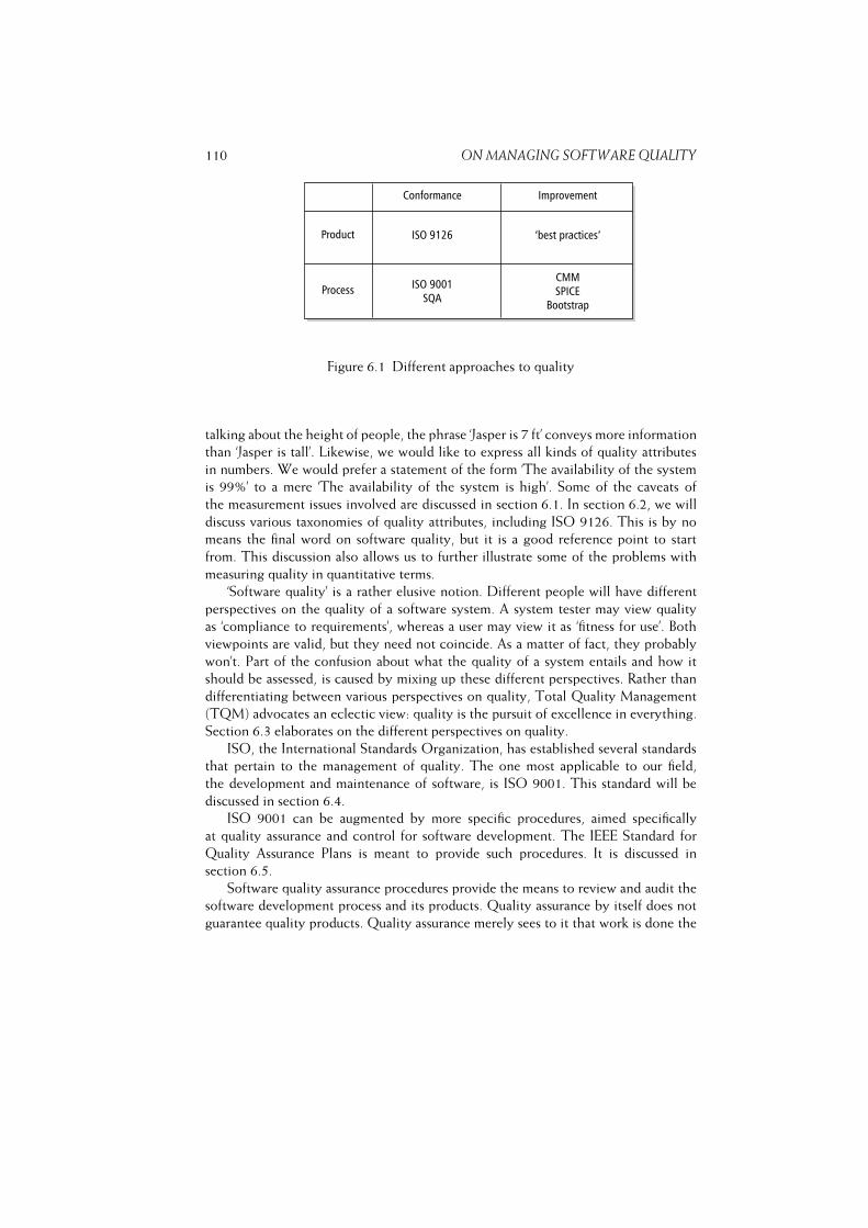
110 ON MANAGING SOFTWARE QUALITY

Figure 6.1 Different approaches to quality

talking about the height of people, the phrase ‘Jasper is 7 ft’ conveys more information

than ‘Jasper is tall’. Likewise, we would like to express all kinds of quality attributes

in numbers. We would prefer a statement of the form ‘The availability of the system

is 99%’ to a mere ‘The availability of the system is high’. Some of the caveats of

the measurement issues involved are discussed in section 6.1. In section 6.2, we will

discuss various taxonomies of quality attributes, including ISO 9126. This is by no

means the final word on software quality, but it is a good reference point to start

from. This discussion also allows us to further illustrate some of the problems with

measuring quality in quantitative terms.

‘Software quality’ is a rather elusive notion. Different people will have different

perspectives on the quality of a software system. A system tester may view quality

as ‘compliance to requirements’, whereas a user may view it as ‘fitness for use’. Both

viewpoints are valid, but they need not coincide. As a matter of fact, they probably

won’t. Part of the confusion about what the quality of a system entails and how it

should be assessed, is caused by mixing up these different perspectives. Rather than

differentiating between various perspectives on quality, Total Quality Management

(TQM) advocates an eclectic view: quality is the pursuit of excellence in everything.

Section 6.3 elaborates on the different perspectives on quality.

ISO, the International Standards Organization, has established several standards

that pertain to the management of quality. The one most applicable to our field,

the development and maintenance of software, is ISO 9001. This standard will be

discussed in section 6.4.

ISO 9001 can be augmented by more specific procedures, aimed specifically

at quality assurance and control for software development. The IEEE Standard for

Quality Assurance Plans is meant to provide such procedures. It is discussed in

section 6.5.

Software quality assurance procedures provide the means to review and audit the

software development process and its products. Quality assurance by itself does not

guarantee quality products. Quality assurance merely sees to it that work is done the

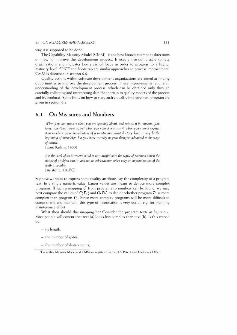
6.1. ON MEASURES AND NUMBERS 111

way it is supposed to be done.

The Capability Maturity Model (CMM)1 is the best known attempt at directions

on how to improve the development process. It uses a five-point scale to rate

organizations and indicates key areas of focus in order to progress to a higher

maturity level. SPICE and Bootstrap are similar approaches to process improvement.

CMM is discussed in section 6.6.

Quality actions within software development organizations are aimed at finding

opportunities to improve the development process. These improvements require an

understanding of the development process, which can be obtained only through

carefully collecting and interpreting data that pertain to quality aspects of the process

and its products. Some hints on how to start such a quality improvement program are

given in section 6.8.

6.1 On Measures and Numbers

When you can measure what you are speaking about, and express it in numbers, youknow something about it; but when you cannot measure it, when you cannot express

it in numbers, your knowledge is of a meagre and unsatisfactory kind; it may be the

beginning of knowledge, but you have scarcely in your thoughts advanced to the stageof science.

[Lord Kelvin, 1900]

It is the mark of an instructed mind to rest satisfied with the degree of precision which the

nature of a subject admits, and not to seek exactness when only an approximation of the

truth is possible.[Aristotle, 330 BC]

Suppose we want to express some quality attribute, say the complexity of a program

text, in a single numeric value. Larger values are meant to denote more complex

programs. If such a mapping C from programs to numbers can be found, we may

next compare the values of C(P1) and C(P2) to decide whether program P1 is more

complex than program P2. Since more complex programs will be more difficult to

comprehend and maintain, this type of information is very useful, e.g. for planning

maintenance effort.

What then should this mapping be? Consider the program texts in figure 6.2.

Most people will concur that text (a) looks less complex than text (b). Is this caused

by:

– its length,

– the number of gotos,

– the number of if-statements,

1Capability Maturity Model and CMM are registered in the U.S. Patent and Trademark Office.

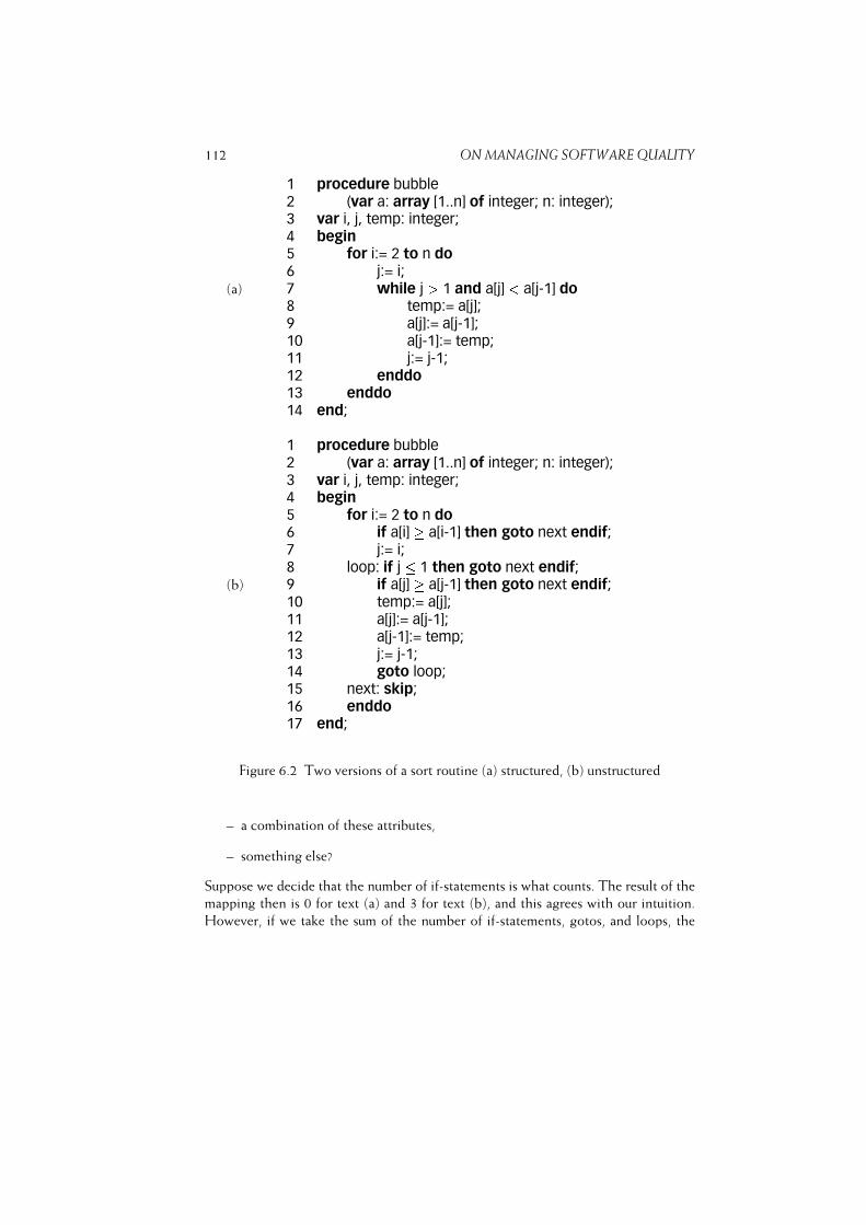
112 ON MANAGING SOFTWARE QUALITY

1 procedure bubble2 (var a: array [1..n] of integer; n: integer);3 var i, j, temp: integer;4 begin5 for i:= 2 to n do6 j:= i;

(a) 7 while j > 1 and a[j] < a[j-1] do8 temp:= a[j];9 a[j]:= a[j-1];10 a[j-1]:= temp;11 j:= j-1;12 enddo13 enddo14 end;

1 procedure bubble2 (var a: array [1..n] of integer; n: integer);3 var i, j, temp: integer;4 begin5 for i:= 2 to n do6 if a[i] � a[i-1] then goto next endif;7 j:= i;8 loop: if j � 1 then goto next endif;

(b) 9 if a[j] � a[j-1] then goto next endif;10 temp:= a[j];11 a[j]:= a[j-1];12 a[j-1]:= temp;13 j:= j-1;14 goto loop;15 next: skip;16 enddo17 end;

Figure 6.2 Two versions of a sort routine (a) structured, (b) unstructured

– a combination of these attributes,

– something else?

Suppose we decide that the number of if-statements is what counts. The result of the

mapping then is 0 for text (a) and 3 for text (b), and this agrees with our intuition.

However, if we take the sum of the number of if-statements, gotos, and loops, the

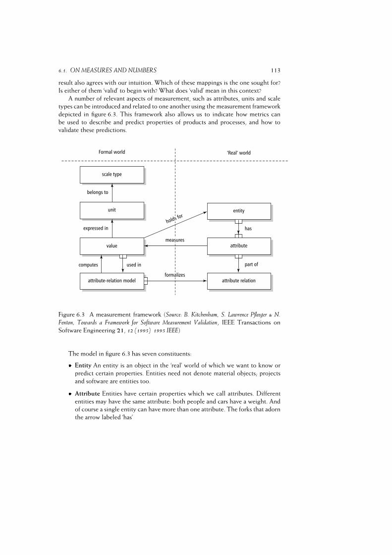
6.1. ON MEASURES AND NUMBERS 113

result also agrees with our intuition. Which of these mappings is the one sought for?

Is either of them ‘valid’ to begin with? What does ‘valid’ mean in this context?

A number of relevant aspects of measurement, such as attributes, units and scale

types can be introduced and related to one another using the measurement framework

depicted in figure 6.3. This framework also allows us to indicate how metrics can

be used to describe and predict properties of products and processes, and how to

validate these predictions.

Figure 6.3 A measurement framework (Source: B. Kitchenham, S. Lawrence Pfleeger & N.

Fenton, Towards a Framework for Software Measurement Validation, IEEE Transactions on

Software Engineering 21, 12 (1995) 1995 IEEE)

The model in figure 6.3 has seven constituents:� Entity An entity is an object in the ‘real’ world of which we want to know or

predict certain properties. Entities need not denote material objects; projects

and software are entities too.� Attribute Entities have certain properties which we call attributes. Different

entities may have the same attribute: both people and cars have a weight. And

of course a single entity can have more than one attribute. The forks that adorn

the arrow labeled ‘has’

114 ON MANAGING SOFTWARE QUALITY

in figure 6.3 indicate that this relationship is n-to-m.� Attribute relation Different attributes of one or more entities can be related.

For example, the attributes ‘length’ and ‘weight’ of an entity ‘snake’ are related.

Similarly, the number of man-months spent on a project is related to the cost

of that project. Also, an attribute of one entity can be related to an attribute of

another entity. For example, the experience of a programmer may be related to

the cost of a development project he is working on.� Value The former three constituents of the model reside in the ‘real’ world. We

want to formally characterize these objects by measuring attributes, i.e. assigning

values to them.� Unit Obviously, this value is expressed in a certain unit, such as meters, seconds

or lines of code.� Scale types This unit in turn belongs to a certain scale type. Some common

scale types are:

– Nominal Attributes are merely classified: the color of my hair is gray,

white or black.

– Ordinal There is a (linear) ordering in the possible values of an attribute:

one type of material is harder than another, one program is more complex

than another.

– Interval The same as ordinal, but the ‘distance’ between successive values

of an attribute is the same, as in a calendar, or the temperature measured

in degrees Fahrenheit.

– Ratio The same as interval, with the additional requirement that there

exists a value 0, as in the age of a software system, or the temperature

measured in degrees Kelvin.

– Absolute In this case we simply count the number of occurrences, as in

the number of errors detected in a program.

Note that we can sometimes measure an attribute in different units, where

these units lie on different scales. For example, we can measure temperature on

an ordinal scale: it either freezes, or it doesn’t. We can also measure it on an

interval scale: in degrees Fahrenheit or Celsius. Or we can measure it on a ratio

scale: in degrees Kelvin.� Attribute-relation model If there exists a relation between different attributes

of, possibly different, entities in the ‘real’ world, we may express that relation in

a formal model: the attribute-relation model. This model computes (predicts)

the value of an attribute in which we are interested from the values of one or

more other attributes from the model. The fork at the arrow labeled ‘formalizes’

6.1. ON MEASURES AND NUMBERS 115

in figure 6.3 indicates that we can have more than one model for the same

attribute relation.

Measurement is a mapping from the empirical, ‘real’ world to the formal, relational

world. A measure is the number or symbol assigned to an attribute of an entity by

this mapping. The value assigned obviously has a certain unit, e.g. lines of code. The

unit in turn belongs to a certain scale, such as the ratio scale for

lines of code, or the ordinal scale for the severity of a failure.

In mathematics, the term metric has a very specific meaning: it describes how far

apart two points are. In our field, the term is often used in a somewhat sloppy way.

Sometimes it denotes a measure, sometimes the unit of a measure. We will use the

term to denote the combination of:

– an attribute of an entity,

– the function which assigns a value to that attribute,

– the unit in which this value is expressed, and

– its scale type.

For each scale type, certain operations are allowed, while others are not. In particular,

we can not compute the average for an ordinal scale, but only its median (middle

value). Suppose we classify a system as either ‘very complex’, ‘complex’, ‘average’,

‘simple’ or ‘very simple’. The assignment of numbers to these values is rather arbitrary.

The only prerequisite is that a system that is classified as, say, ‘very complex’ is assigned

a larger value than a system classified as, say, ‘complex’. If we call this mappingW , the

only requirement thus is:W (very complex)> W (complex)> : : : > W (very simple).

Table 6.1 Example mappings for an ordinal scale

Very complex Complex Average Simple Very simple

5 4 3 2 1

100 10 5 2 1

Table 6.1 gives an example of two valid assignments of values to this attribute.

Suppose we have a system with three components, which are characterized as ‘very

complex’, ‘average’ and ‘simple’, respectively. By assigning the values from the first

row, the average would be 3, so the whole system would be classified to be of

average complexity. Using the values from the second row, the average would be 35,

something between ‘complex’ and ‘very complex’. The problem is caused by the fact

that, with an ordinal scale, we do not know whether successive values are equidistant.

When computing an average, we tacitly assume they are.

116 ON MANAGING SOFTWARE QUALITY

We often can not measure the value of an attribute directly. For example, the speed

of a car can be determined from the values of two other attributes: a distance and the

time it takes the car to travel that distance. The speed is then measured indirectly, by

taking the quotient of two direct measures. In this case, the attribute-relation model

formalizes the relation between the distance traveled, time, and speed.

We may distinguish between internal and external attributes. Internal attributes of

an entity can be measured purely in terms of that entity itself. Modularity, size,

defects encountered, and cost are typical examples of internal attributes. External

attributes of an entity are those which can be measured only with respect to how

that entity relates to its environment. Maintainability and usability are examples

of external attributes. Most quality factors we discuss in this chapter are external

attributes. External attributes can be measured only indirectly, since they involve the

measurement of other attributes.

Empirical relations between objects in the real world should be preserved in the

numerical relation system that we use. If we observe that car A drives faster than carB, then we would rather like our function S which maps the speed observed to some

number to be such that S(A) > S(B). This is called the representation condition.

If a measure satisfies the representation condition, it is said to be a valid measure.

The representation condition can sometimes be checked by a careful assessment

of the attribute-relation model. For example, we earlier proposed to measure the

complexity of a program text by counting the number of if-statements. For this

(indirect) measure to be valid we have to ascertain that:

– any two programs with the same number of if-statements are equally complex,

and

– if program A has more if-statements than program B, then A is more complex

than B.

Since neither of these statements is true in the real world, this complexity measure is

not valid.

The validity of more complex indirect measures is usually ascertained through

statistical means. Most of the cost estimation models discussed in chapter 7, for

example, are validated in this way.

Finally, the scale type of indirect measures merits some attention. If different

measures are combined into a new measure, the scale type of the combined measure

is the ‘weakest’ of the scale types of its constituents. Many cost estimation formulas

contain factors whose scale type is ordinal, such as the instability of the requirements

or the experience of the design team. Strictly speaking, different values that result from

applying such a cost estimation formula should then be interpreted as indicating that

certain projects require more effort than others. The intention though is to interpret

them on a ratio scale, i.e. actual effort in man-months. From a measurement-theory

point of view, this is not allowed.

6.2. A TAXONOMY OF QUALITY ATTRIBUTES 117

6.2 A Taxonomy of Quality Attributes

Some of the first elaborate studies on the notion of ‘software quality’ appeared in the

late 1970s (McCall et al., 1977), (Boehm et al., 1978). In these studies, a number of

aspects of software systems are investigated that somehow relate to the notion of

software quality. In the ensuing years, a large number of people have tried to tackle

this very same problem. Many taxonomies of quality factors have been published. The

fundamental problems have not been solved satisfactorily, though. The various factors

that relate to software quality are hard to define. It is even harder to measure them

quantitatively. On the other hand, real quality can often be identified surprisingly

easily.

In the IEEE Glossary of Software Engineering Terminology, quality is defined as ‘the

degree to which a system, component, or process meets customer or user needs or

expectations’. Applied to software, then, quality should be measured primarily against

the degree to which user requirements are met: correctness, reliability, usability,

and the like. Software lasts a long time and is adapted from time to time in order

to accommodate changed circumstances. It is important to the user that this is

possible within reasonable costs. The customer is therefore also interested in quality

factors which relate to the structure of the system rather than its use: maintainability,

testability, portability, etc.

We will start our discussion of quality attributes with McCall’s taxonomy. McCall

distinguishes between two levels of quality attributes. Higher-level quality attributes,

known as quality factors, are external attributes and can, therefore, be measured only

indirectly. McCall introduced a second level of quality attributes, termed quality

criteria. Quality criteria can be measured either subjectively or objectively. By

combining the ratings for the individual quality criteria that affect a given quality

factor, we obtain a measure for the extent to which that quality factor is being

satisfied. Users and managers tend to be interested in the higher-level, external

quality attributes.

For example, we can not directly measure the reliability of a software system. We

may however directly measure the number of defects encountered so far. This direct

measure can be used to obtain insight into the reliability of the system. This involves

a theory of how the number of defects encountered relates to reliability, which can be

ascertained on good grounds. For most other aspects of quality though, the relation

between the attributes that can be measured directly and the external attributes we

are interested in is less obvious, to say the least.

Table 6.2 lists the quality factors and their definitions, as they are used by McCall

et al.2 These quality factors can be broadly categorized into three classes. The first

class contains those factors that pertain to the use of the software after it has become

2This is a rather narrow definition of software reliability. A more complete definition is contained in the

IEEE Glossary of Software Engineering Terminology: ‘The ability of a system or component to perform

its required functions under stated conditions for a specified period of time.’ It is often expressed as a

probability.

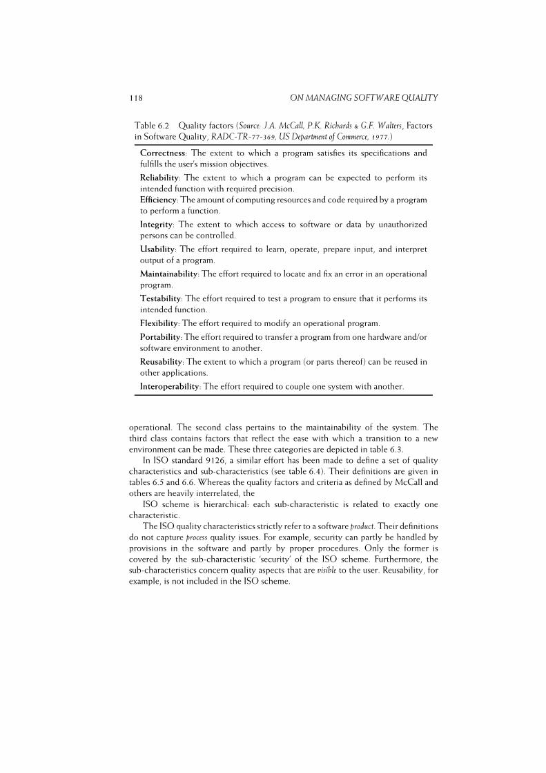
118 ON MANAGING SOFTWARE QUALITY

Table 6.2 Quality factors (Source: J.A. McCall, P.K. Richards & G.F. Walters, Factors

in Software Quality, RADC-TR-77-369, US Department of Commerce, 1977.)

Correctness: The extent to which a program satisfies its specifications and

fulfills the user’s mission objectives.

Reliability: The extent to which a program can be expected to perform its

intended function with required precision.

Efficiency: The amount of computing resources and code required by a program

to perform a function.

Integrity: The extent to which access to software or data by unauthorized

persons can be controlled.

Usability: The effort required to learn, operate, prepare input, and interpret

output of a program.

Maintainability: The effort required to locate and fix an error in an operational

program.

Testability: The effort required to test a program to ensure that it performs its

intended function.

Flexibility: The effort required to modify an operational program.

Portability: The effort required to transfer a program from one hardware and/or

software environment to another.

Reusability: The extent to which a program (or parts thereof) can be reused in

other applications.

Interoperability: The effort required to couple one system with another.

operational. The second class pertains to the maintainability of the system. The

third class contains factors that reflect the ease with which a transition to a new

environment can be made. These three categories are depicted in table 6.3.

In ISO standard 9126, a similar effort has been made to define a set of quality

characteristics and sub-characteristics (see table 6.4). Their definitions are given in

tables 6.5 and 6.6. Whereas the quality factors and criteria as defined by McCall and

others are heavily interrelated, the

ISO scheme is hierarchical: each sub-characteristic is related to exactly one

characteristic.

The ISO quality characteristics strictly refer to a software product. Their definitions

do not capture process quality issues. For example, security can partly be handled by

provisions in the software and partly by proper procedures. Only the former is

covered by the sub-characteristic ‘security’ of the ISO scheme. Furthermore, the

sub-characteristics concern quality aspects that are visible to the user. Reusability, for

example, is not included in the ISO scheme.

6.2. A TAXONOMY OF QUALITY ATTRIBUTES 119

Table 6.3 Three categories of software quality factors (Source: J.A. McCall,

P.K. Richards & G.F. Walters, Factors in Software Quality, RADC-TR-77-369,

US Department of Commerce, 1977.)

Product operation:

Correctness Does it do what I want?

Reliability Does it do it accurately all of the time?

Efficiency Will it run on my hardware as well as it can?

Integrity Is it secure?

Usability Can I run it?

Product revision:

Maintainability Can I fix it?

Testability Can I test it?

Flexibility Can I change it?

Product transition:

Portability Will I be able to use it on another machine?

Reusability Will I be able to reuse some of the software?

Interoperability Will I be able to interface it with another system?

The ISO characteristics and subcharacteristics, together with an extensive set of

measures, make up ISO˘s external and internal quality model. Internal quality refers to the

product itself, ultimately the source code. External quality refers to the quality when

the software is executed. For example, the average number of statements in a method

is a measure of internal quality, while the number of defects encountered during

testing is a measure of external quality.

Ultimately, the user is interested in the quality in use, defined in (ISO9126, 2001) as

”the user’s view of the quality of the software product when it is executed in a specific

environment and a specific context of use.” It measures the extent to which users can

achieve their goals, rather than mere properties of the software (see also section 6.3).

Quality in use is modeled in four characteristics: effectiveness, productivity, safety,

and satisfaction. The definitions for these quality in use characteristics are given in

table 6.7.

Theoretically, internal quality, external quality and quality in use are linked

together: internal quality indicates external quality, which in turn indicates quality in

use. In general, meeting criteria at one level is not sufficient for meeting criteria at

the next level. For instance, satisfaction is partly determined by internal and external

quality measures, but also includes the user’s attitude towards the product. The latter

has to be measured separately. Note that internal quality and external quality can be

measured directly. Quality in use can in general only be measured indirectly.

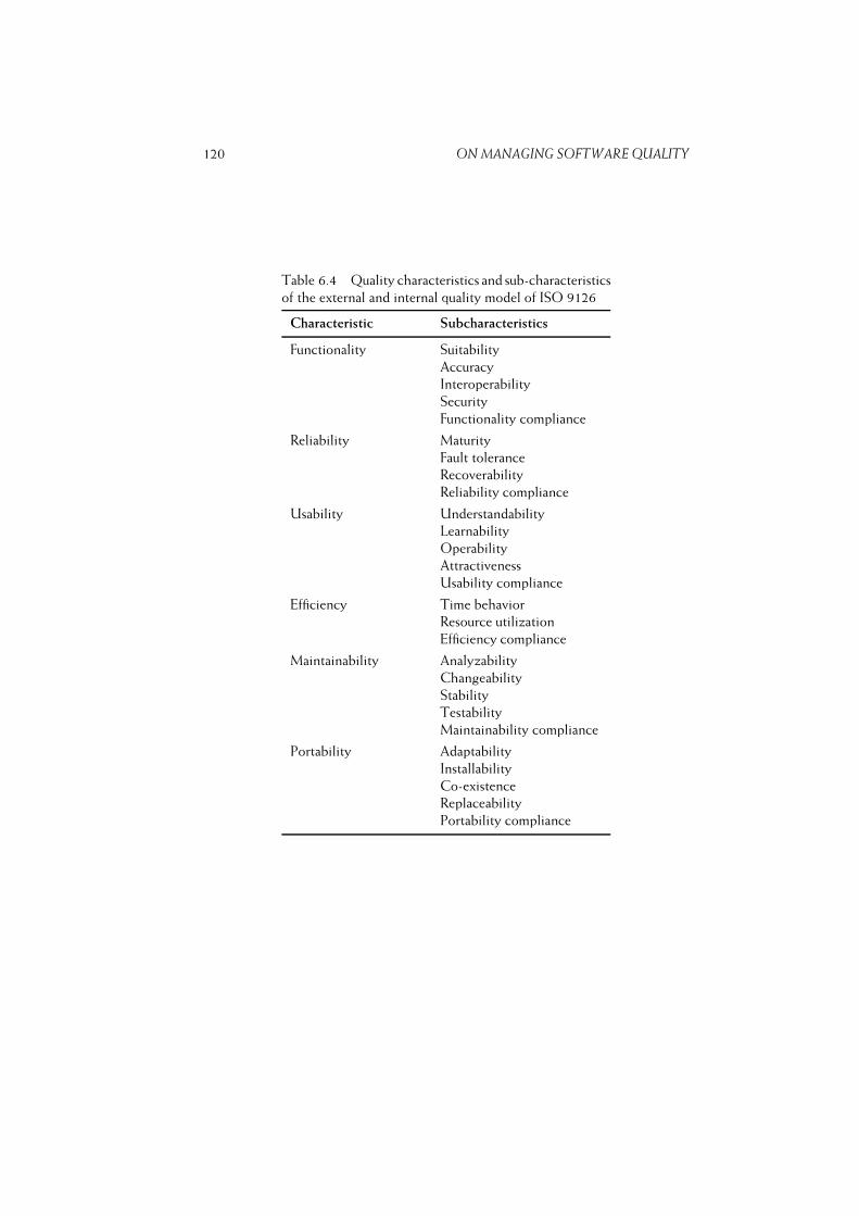
120 ON MANAGING SOFTWARE QUALITY

Table 6.4 Quality characteristics and sub-characteristics

of the external and internal quality model of ISO 9126

Characteristic Subcharacteristics

Functionality Suitability

Accuracy

Interoperability

Security

Functionality compliance

Reliability Maturity

Fault tolerance

Recoverability

Reliability compliance

Usability Understandability

Learnability

Operability

Attractiveness

Usability compliance

Efficiency Time behavior

Resource utilization

Efficiency compliance

Maintainability Analyzability

Changeability

Stability

Testability

Maintainability compliance

Portability Adaptability

Installability

Co-existence

Replaceability

Portability compliance

6.2. A TAXONOMY OF QUALITY ATTRIBUTES 121

Table 6.5 Quality characteristics of the external and internal quality model of

ISO 9126 (Source: ISO Standard 9126: Software Quality Characteristics and Metrics.

Reproduced by permission of ISO.)

Functionality: The capability of the software product to provide functions

which meet stated and implied needs when the software is used under specified

conditions.

Reliability: The capability of the software product to maintain a specified level

of performance when used under specified conditions.

Usability: The capability of the software product to be understood, learned,

used and be attractive to the user, when used under specified conditions.

Efficiency: The capability of the software product to provide appropriate

performance, relative to the amount of resources used, under stated conditions.

Maintainability: The capability of the software product to be modified. Modi-

fications may include corrections, improvements or adaptation of the software

to changes in environment, and in requirements and functional specifications.

Portability: The capability of the software product to be transferred from one

environment to another.

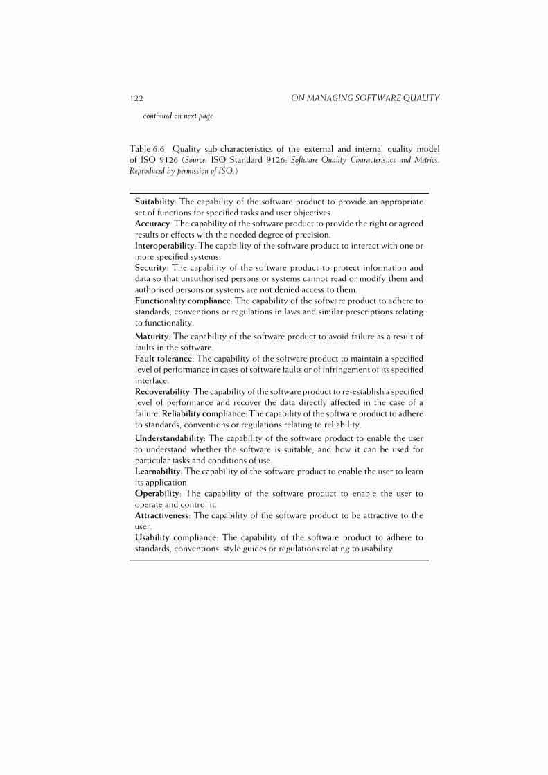
122 ON MANAGING SOFTWARE QUALITY

continued on next page

Table 6.6 Quality sub-characteristics of the external and internal quality model

of ISO 9126 (Source: ISO Standard 9126: Software Quality Characteristics and Metrics.

Reproduced by permission of ISO.)

Suitability: The capability of the software product to provide an appropriate

set of functions for specified tasks and user objectives.

Accuracy: The capability of the software product to provide the right or agreed

results or effects with the needed degree of precision.

Interoperability: The capability of the software product to interact with one or

more specified systems.

Security: The capability of the software product to protect information and

data so that unauthorised persons or systems cannot read or modify them and

authorised persons or systems are not denied access to them.

Functionality compliance: The capability of the software product to adhere to

standards, conventions or regulations in laws and similar prescriptions relating

to functionality.

Maturity: The capability of the software product to avoid failure as a result of

faults in the software.

Fault tolerance: The capability of the software product to maintain a specified

level of performance in cases of software faults or of infringement of its specified

interface.

Recoverability: The capability of the software product to re-establish a specified

level of performance and recover the data directly affected in the case of a

failure. Reliability compliance: The capability of the software product to adhere

to standards, conventions or regulations relating to reliability.

Understandability: The capability of the software product to enable the user

to understand whether the software is suitable, and how it can be used for

particular tasks and conditions of use.

Learnability: The capability of the software product to enable the user to learn

its application.

Operability: The capability of the software product to enable the user to

operate and control it.

Attractiveness: The capability of the software product to be attractive to the

user.

Usability compliance: The capability of the software product to adhere to

standards, conventions, style guides or regulations relating to usability

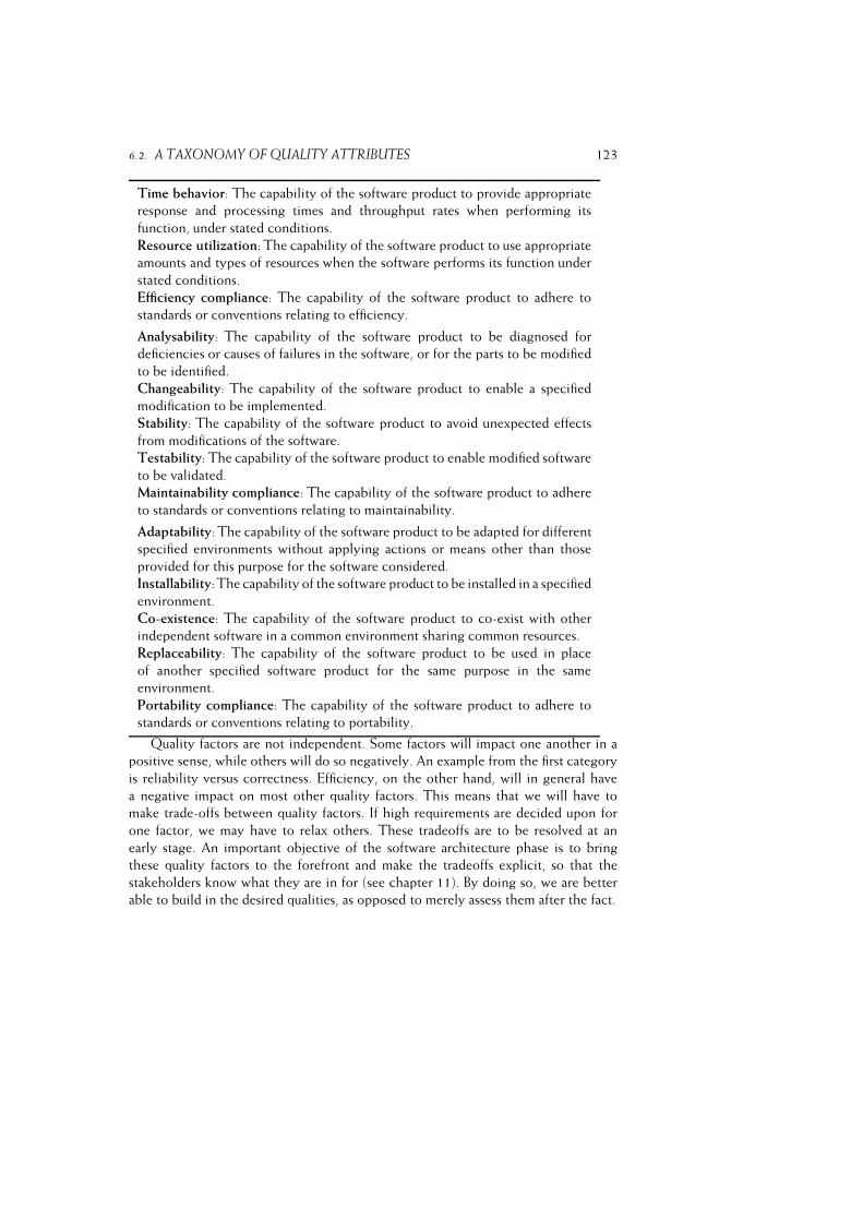
6.2. A TAXONOMY OF QUALITY ATTRIBUTES 123

Time behavior: The capability of the software product to provide appropriate

response and processing times and throughput rates when performing its

function, under stated conditions.

Resource utilization: The capability of the software product to use appropriate

amounts and types of resources when the software performs its function under

stated conditions.

Efficiency compliance: The capability of the software product to adhere to

standards or conventions relating to efficiency.

Analysability: The capability of the software product to be diagnosed for

deficiencies or causes of failures in the software, or for the parts to be modified

to be identified.

Changeability: The capability of the software product to enable a specified

modification to be implemented.

Stability: The capability of the software product to avoid unexpected effects

from modifications of the software.

Testability: The capability of the software product to enable modified software

to be validated.

Maintainability compliance: The capability of the software product to adhere

to standards or conventions relating to maintainability.

Adaptability: The capability of the software product to be adapted for different

specified environments without applying actions or means other than those

provided for this purpose for the software considered.

Installability:The capability of the software product to be installed in a specified

environment.

Co-existence: The capability of the software product to co-exist with other

independent software in a common environment sharing common resources.

Replaceability: The capability of the software product to be used in place

of another specified software product for the same purpose in the same

environment.

Portability compliance: The capability of the software product to adhere to

standards or conventions relating to portability.

Quality factors are not independent. Some factors will impact one another in a

positive sense, while others will do so negatively. An example from the first category

is reliability versus correctness. Efficiency, on the other hand, will in general have

a negative impact on most other quality factors. This means that we will have to

make trade-offs between quality factors. If high requirements are decided upon for

one factor, we may have to relax others. These tradeoffs are to be resolved at an

early stage. An important objective of the software architecture phase is to bring

these quality factors to the forefront and make the tradeoffs explicit, so that the

stakeholders know what they are in for (see chapter 11). By doing so, we are better

able to build in the desired qualities, as opposed to merely assess them after the fact.

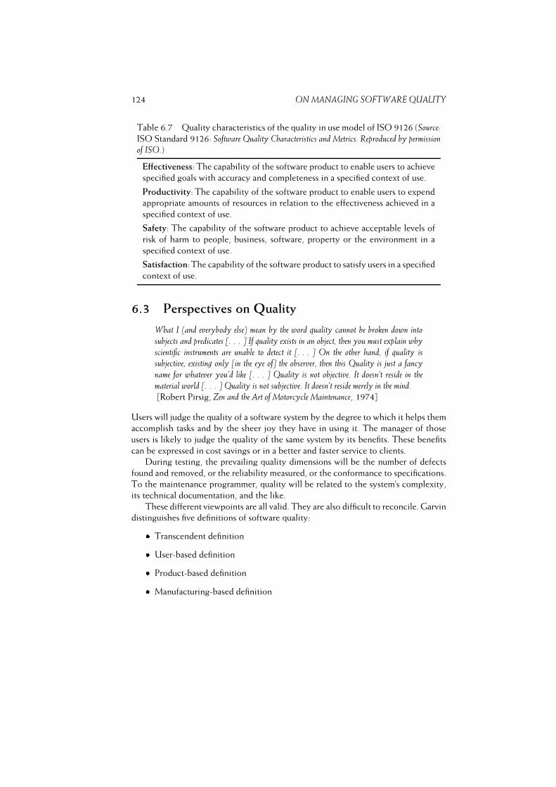
124 ON MANAGING SOFTWARE QUALITY

Table 6.7 Quality characteristics of the quality in use model of ISO 9126 (Source:

ISO Standard 9126: Software Quality Characteristics and Metrics. Reproduced by permissionof ISO.)

Effectiveness: The capability of the software product to enable users to achieve

specified goals with accuracy and completeness in a specified context of use.

Productivity: The capability of the software product to enable users to expend

appropriate amounts of resources in relation to the effectiveness achieved in a

specified context of use.

Safety: The capability of the software product to achieve acceptable levels of

risk of harm to people, business, software, property or the environment in a

specified context of use.

Satisfaction: The capability of the software product to satisfy users in a specified

context of use.

6.3 Perspectives on Quality

What I (and everybody else) mean by the word quality cannot be broken down into

subjects and predicates [. . . ] If quality exists in an object, then you must explain why

scientific instruments are unable to detect it [. . . ] On the other hand, if quality issubjective, existing only [in the eye of] the observer, then this Quality is just a fancy

name for whatever you’d like [. . . ] Quality is not objective. It doesn’t reside in the

material world [. . . ] Quality is not subjective. It doesn’t reside merely in the mind.[Robert Pirsig, Zen and the Art of Motorcycle Maintenance, 1974]

Users will judge the quality of a software system by the degree to which it helps them

accomplish tasks and by the sheer joy they have in using it. The manager of those

users is likely to judge the quality of the same system by its benefits. These benefits

can be expressed in cost savings or in a better and faster service to clients.

During testing, the prevailing quality dimensions will be the number of defects

found and removed, or the reliability measured, or the conformance to specifications.

To the maintenance programmer, quality will be related to the system’s complexity,

its technical documentation, and the like.

These different viewpoints are all valid. They are also difficult to reconcile. Garvin

distinguishes five definitions of software quality:� Transcendent definition� User-based definition� Product-based definition� Manufacturing-based definition

6.3. PERSPECTIVES ON QUALITY 125� Value-based definition.

Transcendent quality concerns innate excellence. It is the type of quality assessment

we usually apply to novels. We may consider Zen and the Art of Motorcycle Maintenance

an excellent book, we may try to give words to our admiration but these words are

usually inadequate. The practiced reader gradually develops a good feeling for this

type of quality. Likewise, the software engineering expert may have developed a good

feeling for the transcendent qualities of software systems.

The user-based definition of quality concerns ‘fitness for use’ and relates to the

degree in which a system addresses the user’s needs. It is a subjective notion. Since

different users may have different needs, they may assess a system’s quality rather

differently. The incidental user of a simple word-processing package may be quite

happy with its functionality and possibilities while a computer scientist may be rather

disappointed. The reverse situation may befall a complex system like LATEX.

In the product-based definition, quality relates to attributes of the software.

Differences in quality are caused by differences in the values of those attributes. Most

of the research into software quality concerns this type of quality. It also underlies

the various taxonomies of quality attributes discussed above.

The manufacturing-based definition concerns conformance to specifications. It

is the type of quality definition used during system testing, whereas the user-based

definition is prevalent during acceptance testing.

Finally, the value-based definition deals with costs and profits. It concerns

balancing time and cost on the one hand, and profit on the other hand. We may

distinguish various kinds of benefit, not all of which can be phrased easily in monetary

terms:� Increased efficiency Benefits are attributed to cost avoidance or reduction, and

their measures are economic.� Increased effectiveness This is primarily reflected through better information

for decision making. It can be measured in economic terms or through key

performance indicators, such as a reduced time to market.� Added value Benefits enhance the strategic position of the organization,

e.g. through an increased market share. The contribution of the information

technology component often can not be isolated.� Marketable product The system itself may be marketable, or a marketable

product may be identified as a by-product of system development.� Corporate IT infrastructure Communication networks, database environments

and the like provide little benefit by themselves, but serve as a foundation for

other systems.

Software developers tend to concentrate on the product-based and manufacturing-

based definitions of quality. The resulting quality requirements can be expressed in

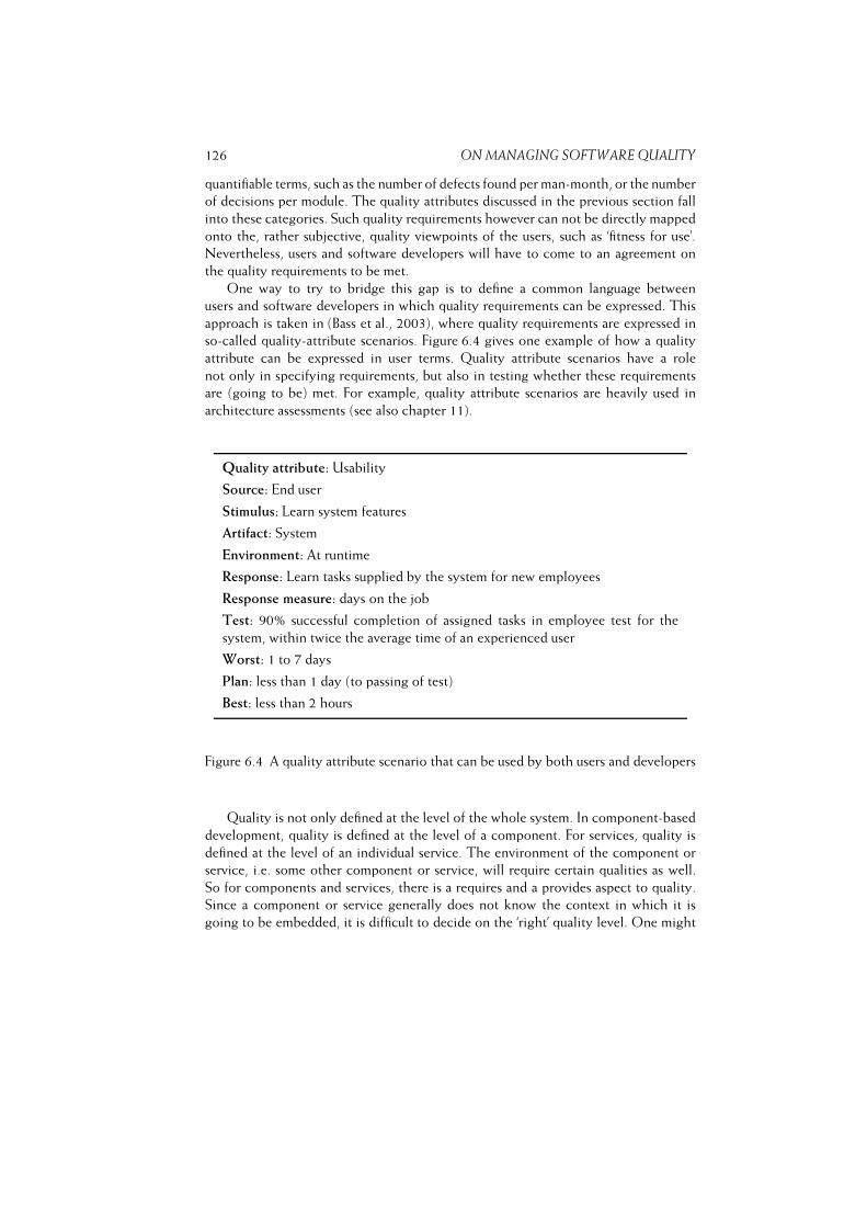
126 ON MANAGING SOFTWARE QUALITY

quantifiable terms, such as the number of defects found per man-month, or the number

of decisions per module. The quality attributes discussed in the previous section fall

into these categories. Such quality requirements however can not be directly mapped

onto the, rather subjective, quality viewpoints of the users, such as ‘fitness for use’.

Nevertheless, users and software developers will have to come to an agreement on

the quality requirements to be met.

One way to try to bridge this gap is to define a common language between

users and software developers in which quality requirements can be expressed. This

approach is taken in (Bass et al., 2003), where quality requirements are expressed in

so-called quality-attribute scenarios. Figure 6.4 gives one example of how a quality

attribute can be expressed in user terms. Quality attribute scenarios have a role

not only in specifying requirements, but also in testing whether these requirements

are (going to be) met. For example, quality attribute scenarios are heavily used in

architecture assessments (see also chapter 11).

Quality attribute: Usability

Source: End user

Stimulus: Learn system features

Artifact: System

Environment: At runtime

Response: Learn tasks supplied by the system for new employees

Response measure: days on the job

Test: 90% successful completion of assigned tasks in employee test for the

system, within twice the average time of an experienced user

Worst: 1 to 7 days

Plan: less than 1 day (to passing of test)

Best: less than 2 hours

Figure 6.4 A quality attribute scenario that can be used by both users and developers

Quality is not only defined at the level of the whole system. In component-based

development, quality is defined at the level of a component. For services, quality is

defined at the level of an individual service. The environment of the component or

service, i.e. some other component or service, will require certain qualities as well.

So for components and services, there is a requires and a provides aspect to quality.

Since a component or service generally does not know the context in which it is

going to be embedded, it is difficult to decide on the ‘right’ quality level. One might

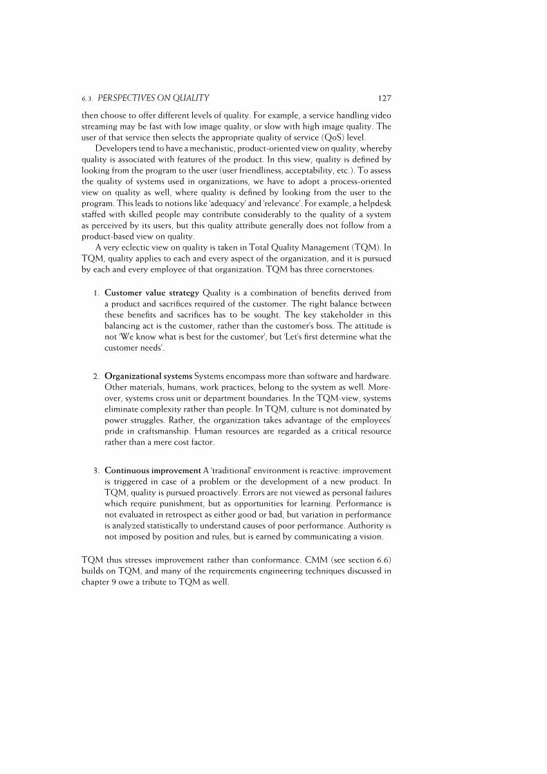
6.3. PERSPECTIVES ON QUALITY 127

then choose to offer different levels of quality. For example, a service handling video

streaming may be fast with low image quality, or slow with high image quality. The

user of that service then selects the appropriate quality of service (QoS) level.

Developers tend to have a mechanistic, product-oriented view on quality, whereby

quality is associated with features of the product. In this view, quality is defined by

looking from the program to the user (user friendliness, acceptability, etc.). To assess

the quality of systems used in organizations, we have to adopt a process-oriented

view on quality as well, where quality is defined by looking from the user to the

program. This leads to notions like ‘adequacy’ and ‘relevance’. For example, a helpdesk

staffed with skilled people may contribute considerably to the quality of a system

as perceived by its users, but this quality attribute generally does not follow from a

product-based view on quality.

A very eclectic view on quality is taken in Total Quality Management (TQM). In

TQM, quality applies to each and every aspect of the organization, and it is pursued

by each and every employee of that organization. TQM has three cornerstones:

1. Customer value strategy Quality is a combination of benefits derived from

a product and sacrifices required of the customer. The right balance between

these benefits and sacrifices has to be sought. The key stakeholder in this

balancing act is the customer, rather than the customer’s boss. The attitude is

not ‘We know what is best for the customer’, but ‘Let’s first determine what the

customer needs’.

2. Organizational systems Systems encompass more than software and hardware.

Other materials, humans, work practices, belong to the system as well. More-

over, systems cross unit or department boundaries. In the TQM-view, systems

eliminate complexity rather than people. In TQM, culture is not dominated by

power struggles. Rather, the organization takes advantage of the employees’

pride in craftsmanship. Human resources are regarded as a critical resource

rather than a mere cost factor.

3. Continuous improvement A ‘traditional’ environment is reactive: improvement

is triggered in case of a problem or the development of a new product. In

TQM, quality is pursued proactively. Errors are not viewed as personal failures

which require punishment, but as opportunities for learning. Performance is

not evaluated in retrospect as either good or bad, but variation in performance

is analyzed statistically to understand causes of poor performance. Authority is

not imposed by position and rules, but is earned by communicating a vision.

TQM thus stresses improvement rather than conformance. CMM (see section 6.6)

builds on TQM, and many of the requirements engineering techniques discussed in

chapter 9 owe a tribute to TQM as well.

128 ON MANAGING SOFTWARE QUALITY

6.4 The Quality System

ISO, the International Organization for Standardization, has developed ISO 9000, a

series of standards for quality management systems. The series consists of three parts:

ISO 9000:2000, ISO 9001:2000, and ISO 9004:2000. ISO 9000 gives fundamentals

and vocabulary of the series of standards on quality systems. ISO 9001 integrates

three earlier standards (labeled ISO 9001, ISO 9002 and ISO 9003). It specifies

requirements for a quality system for any organization that needs to demonstrate

its ability to deliver products that satisfy customer requirements. ISO 9004 contains

guidelines for performance improvement. It is applicable after implementation of ISO

9001.

ISO 9001 is a generic standard. It can be applied to any product. A useful

complement for software is ISO/IEC 90003:2004, containing guidelines for the

application of ISO 9001 to computer software. It is a joint standard of ISO and

IEC, the International Electrotechnical Committee. The scope of ISO/IEC 90003

is described as ”This International Standard specifies requirements for a quality

management system where an organization� needs to demonstrate its ability to consistently provide a product that meets

customer and applicable regulatory requirements, and� aims to enhance customer satisfaction through the effective application of the

system, including processes for continual improvement of the system and the

assurance of conformity to customer and applicable regulatory requirements.”

The standard is very comprehensive. It uses five perspectives from which the

management of quality in software engineering is addressed:� the systemic perspective, dealing with the establishment and documentation of

the quality system itself. The quality system consists of a number of processes,

such as those for software development, operation, and maintenance. These

processes, and the quality system itself, have to be documented properly.� the management perspective, dealing with the definition and management of

the policies to support quality. The quality management system itself has to be

developed, implemented, and regularly reviewed. This perspective describes

how this is done.� the resource perspective, dealing with the resources needed to implement and

improve the quality management system, as well as to meet customer and

regulatory requirements. The resources include both personnel, infrastructure,

and work environment.� the product perspective, dealing with the processes to actually create quality

products, such as those pertaining to requirements engineering, design, testing,

production and servicing. This perspective makes up over 60% of the standard.

6.5. SOFTWARE QUALITY ASSURANCE 129� the improvement perspective, dealing with monitoring, measuring and analysis

activities to maintain and improve quality.

Many organizations try, or have already tried, to obtain ISO 9000 registration. The

time and cost this takes depends on how much the current process deviates from the

ISO standards. If the current quality system is not already close to conforming, then

ISO registration may take at least one year. ISO registration is granted when a third-

party accredited body assesses the quality system and concludes that it does conform

to the ISO standard. Reregistration is required every three years and surveillance

audits are required every six months. ISO registration thus is a fairly drastic and costly

affair, after which you certainly cannot lean back, but have to keep the organization

alert.

Since software development projects have some rather peculiar characteristics

(frequent changes in requirements during the development process, the rather invisible

nature of the product during its development), there is a need for quality assurance

procedures which are tailored towards software development. This is the topic of the

next section.

6.5 Software Quality Assurance

The purpose of Software Quality Assurance (SQA) is to make sure that work gets done

the way it is supposed to be done. More specifically, the goals of SQA (Humphrey,

1989) are:� to improve software quality by appropriately monitoring the software and its

development process;� to ensure full compliance with the established standards and procedures for the

software and the development process;� to ensure that any inadequacies in the product, the process, or the standards

are brought to management’s attention so these inadequacies can be fixed.

Note that the SQA people themselves are not responsible for producing quality

products. Their job is to review and audit, and to provide the project and management

with the results of these reviews and audits.

There are potential conflicts of interest between the SQA organization and the

development organization. The development organization may be facing deadlines

and may want to ship a product, while the SQA people have revealed serious

quality problems and wish to defer shipment. In such cases, the opinion of the SQA

organization should prevail. For SQA to be effective, certain prerequisites must be

fulfilled:� It is essential that top management commitment is secured, so that suggestions

made by the SQA organization can be enforced. If this is not the case, SQA

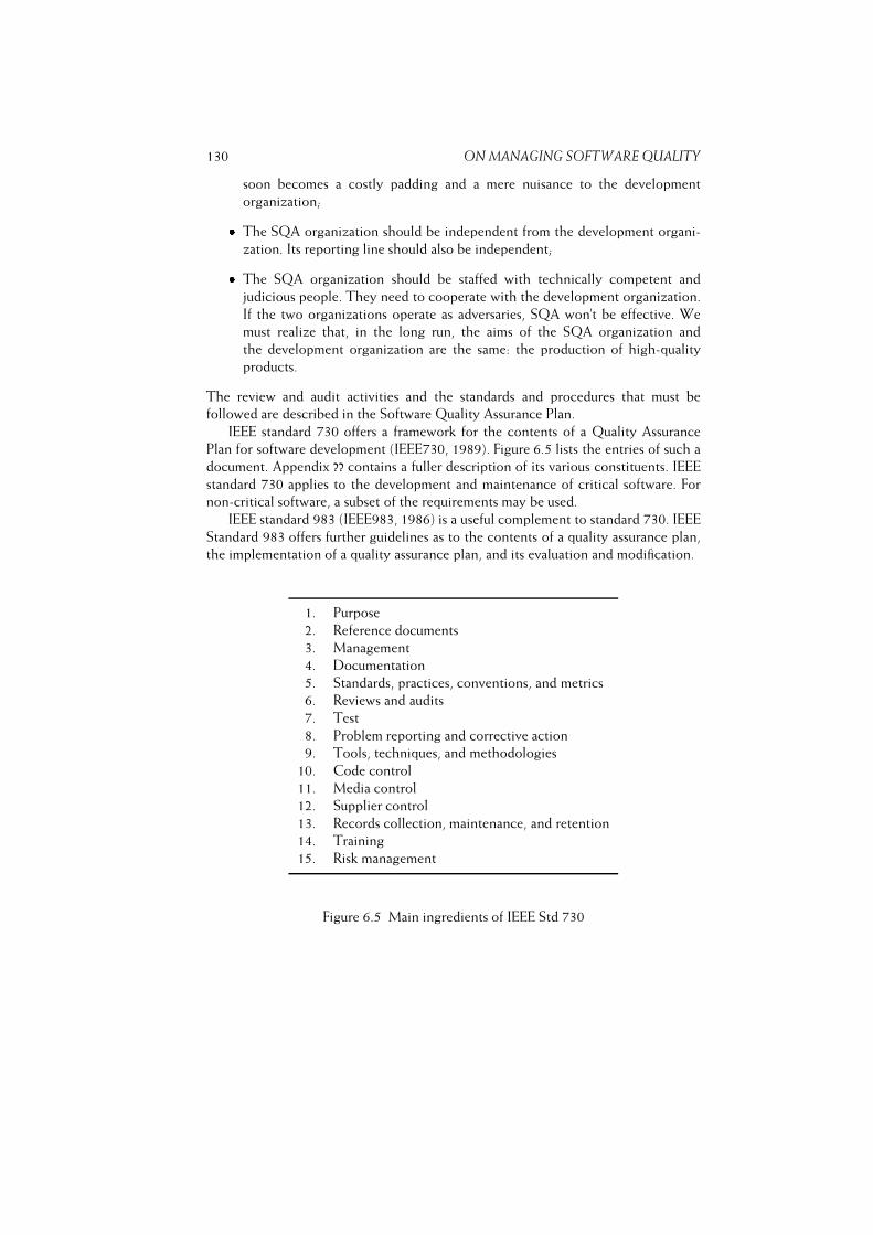
130 ON MANAGING SOFTWARE QUALITY

soon becomes a costly padding and a mere nuisance to the development

organization;� The SQA organization should be independent from the development organi-

zation. Its reporting line should also be independent;� The SQA organization should be staffed with technically competent and

judicious people. They need to cooperate with the development organization.

If the two organizations operate as adversaries, SQA won’t be effective. We

must realize that, in the long run, the aims of the SQA organization and

the development organization are the same: the production of high-quality

products.

The review and audit activities and the standards and procedures that must be

followed are described in the Software Quality Assurance Plan.

IEEE standard 730 offers a framework for the contents of a Quality Assurance

Plan for software development (IEEE730, 1989). Figure 6.5 lists the entries of such a

document. Appendix ?? contains a fuller description of its various constituents. IEEE

standard 730 applies to the development and maintenance of critical software. For

non-critical software, a subset of the requirements may be used.

IEEE standard 983 (IEEE983, 1986) is a useful complement to standard 730. IEEE

Standard 983 offers further guidelines as to the contents of a quality assurance plan,

the implementation of a quality assurance plan, and its evaluation and modification.

1. Purpose

2. Reference documents

3. Management

4. Documentation

5. Standards, practices, conventions, and metrics

6. Reviews and audits

7. Test

8. Problem reporting and corrective action

9. Tools, techniques, and methodologies

10. Code control

11. Media control

12. Supplier control

13. Records collection, maintenance, and retention

14. Training

15. Risk management

Figure 6.5 Main ingredients of IEEE Std 730

6.6. THE CAPABILITY MATURITY MODEL (CMM) 131

The Software Quality Assurance Plan describes how the quality of the software

is to be assessed. Some quality factors can be determined objectively. Most factors at

present can be determined only subjectively. Most often then, we will try to assess the

quality by reading documents, by inspections, by walkthroughs and by peer reviews.

In a number of cases, we may profitably employ tools during quality assurance, in

particular, for static and dynamic analysis of program code. The actual techniques to

be applied here will be discussed in the chapter on testing.

6.6 The Capability Maturity Model (CMM)

Consider the following course of events in a hypothetical software development

project. Some organization is to develop a distributed library automation system.

A centralized computer hosts both the software and the database. A number of

local libraries are connected to the central machine through a web-based interface.

The organization has some experience with library automation, albeit only with

stand-alone systems.

In the course of the project, a number of problems manifest themselves. At first

they seem to be disconnected and they do not alarm management. It turns out that

the requirements analysis has not been all that thorough. Local requirements turn out

to differ on some minor points. Though the first such deviations can be handled quite

easily, keeping track of all change requests becomes a real problem after a while.

When part of the system has been realized, the team starts to test the web-interface.

The interface turns out to be too complex and time-consuming.

The project gets into a crisis eventually. Management has no proper means to

handle the situation. It tries to cut back on both functionality and quality in a

somewhat haphazard way. In the end, a rather unsatisfactory system is delivered two

months late. During the subsequent maintenance phase, a number of problems are

solved, but the system never becomes a real success.

Though the above description is hypothetical, it is not all that unrealistic. Many

an organization has insufficient control over its software development process. If a

project gets into trouble, it is usually discovered quite late and the organization has

no other means but to react in a somewhat chaotic way. More often than not, speed

is confused with progress.

An important step in trying to address these problems is to realize that the

software development process can indeed be controlled, measured, and improved.

In order to gauge the process of improving the software development process,

Watts Humphrey developed a software maturity framework which has evolved into

the Capability Maturity Model (CMM). This framework owes tribute to Total Quality

Management (TQM), which in turn is based on principles of statistical quality control

as formulated by Walter Shewart in the 1930s and further developed by W. Edwards

Deming and Joseph Juran in the 1980s. Originally, there were separate CMM models

for software engineering, systems engineering, and several others. These have now

132 ON MANAGING SOFTWARE QUALITY

been integrated, and carry the label CMMI3. The version described here is CMMI

version 1.1 for software engineering and systems engineering (CMMI Product Team,

2002). CMM and CMMI were developed at the Software Engineering Institute (SEI)

of Carnegie Mellon University.

In CMM (and CMMI), the software process is characterized into one of five

maturity levels, evolutionary levels toward achieving a mature software process. To

achieve a certain maturity level, a number of process areas must be in place. These

process areas indicate important issues that have to be addressed in order to reach

that level. Taken together, the process areas of a level achieve the set of goals for that

level. Figure 6.6 lists the maturity levels and associated process areas of CMMI.

CMMI’s maturity levels can be characterized as follows:� Initial At the initial process level, the organization operates without formalized

procedures, project plans, or cost estimates. Tools are not adequately integrated.

Many problems are overlooked or forgotten, and maintenance poses real

problems. Software development at this level can be characterized as being

ad-hoc. Performance can be improved by instituting basic project management

controls:

– Requirements management involves establishing and maintaining an

agreement with the customer on the requirements of the system. Since

requirements inevitably change, controlling and documenting these

requirements is important.

– Project planning involves making plans for executing and managing the

project. To be able to do any planning, an approved statement of work to

be done is required. From this statement of work, estimates for the size of

the project, resources needed, and schedule are determined, and risks to

the project are identified. The results are documented in the project plan.

This plan is used to manage the project; it is updated when necessary.

– Project monitoring and control is concerned with the visibility of actual

progress. Intermediate results have to be reviewed and tracked with

respect to the project plan. When necessary, the project plan has to be

realigned with reality.

– Supplier agreement management. Where applicable, work done by

suppliers has to be managed: plans for their part of the work have to be

made, and progress of their part of the job has to be monitored.

– Measurement and analysis is concerned with making sure measurements

are made and their results used. First, objectives for measurement and the

way measures should be collected, stored and analyzed are established.

Next, the collection, storage, and analysis of data must be implemented.

Finally, the results are used for decision making, and corrective actions

are taken where needed.

3CMMI is a service mark of Carnegie Mellon University.

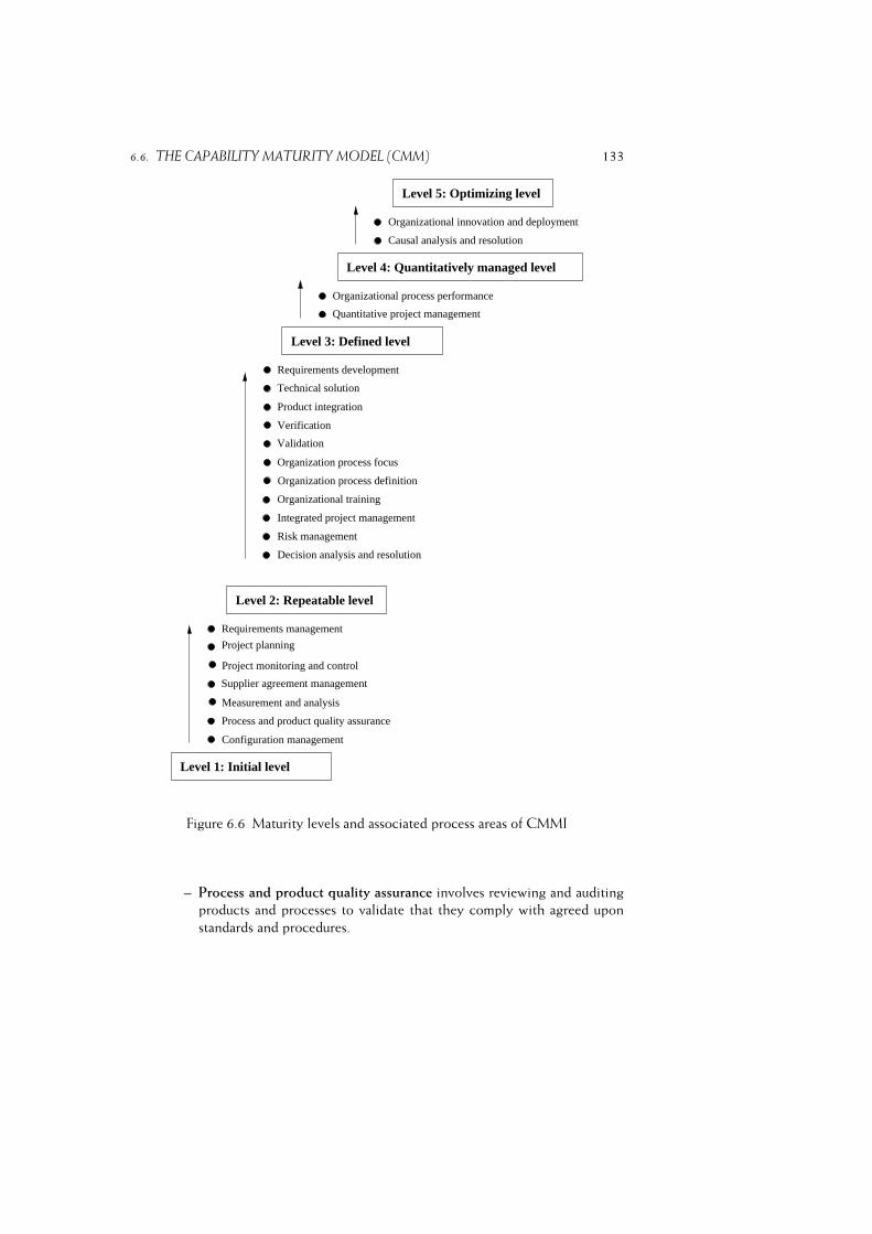
6.6. THE CAPABILITY MATURITY MODEL (CMM) 133

Level 5: Optimizing level

Organizational innovation and deployment

Causal analysis and resolution

Level 4: Quantitatively managed level

Organizational process performance

Quantitative project management

Level 3: Defined level

Requirements development

Technical solution

Product integration

Verification

Organization process definition

Level 1: Initial level

Decision analysis and resolution

Risk management

Integrated project management

Organizational training

Validation

Organization process focus

Measurement and analysis

Level 2: Repeatable level

Requirements management

Project planning

Project monitoring and control

Supplier agreement management

Process and product quality assurance

Configuration management

Figure 6.6 Maturity levels and associated process areas of CMMI

– Process and product quality assurance involves reviewing and auditing

products and processes to validate that they comply with agreed upon

standards and procedures.

134 ON MANAGING SOFTWARE QUALITY

– Configuration management is concerned with establishing and maintain-

ing the integrity of all work items during the entire project life cycle.

This involves identification of configuration items and baselines, and

procedures to control changes to them.� Repeatable The main difference between the initial process level and the

repeatable process level is that the repeatable level provides control over the

way plans and commitments are established. Through prior experience in doing

similar work, the organization has achieved control over costs, schedules, and

change requests, and earlier successes can be repeated. The introduction of

new tools, the development of a new type of product, and major organizational

changes however still represent major risks at this level. The process areas

needed to advance to the next level are aimed at standardizing the software

process across the projects of the organization:

– Requirements development involves the production and analysis of

requirements. Requirements have to be elicited, analyzed, validated, and

communicated to appropriate stakeholders. Requirements development

is not a one-shot activity. Rather, requirements are identified and refined

throughout the whole life cycle.

– Technical solution is about design and implementation. Decisions con-

cerning the architecture, custom development as opposed to an off the

shelf solution, and modularization issues are typical ingredienst of this

process area.

– Product integration concerns the assembling of a complete product out

of its components. This can be one stage after all components have been

developed, or it can proceed incrementally. An important element of

product integration is the management of interfaces, to make sure that

the components properly fit together.

– Verification is concerned with ensuring that the product meets its require-

ments. Peer reviews are an effective means for early defect detection and

removal. Peer reviews, such as walkthroughs and inspections, are practices

in which peers try to identify errors and areas where changes are needed.

– Validation is concerned with establishing that the product fulfills its

intended use. As far as possible, validation activities should be done in

the intended environment in which the product is going to be used.

– Organization process focus is concerned with organization process

improvement. Measurements, lessons learned, project postmortems, prod-

uct evaluation reports are typical sources of information to guide

improvement activities. The responsibility for guiding and implementing

these activities is typically assigned to a process group. In this way,

6.6. THE CAPABILITY MATURITY MODEL (CMM) 135

improvement of the organization’s process capabilities is made a respon-

sibility of the organization as a whole, rather than the individual project

manager.

– Organization process definition. The organization develops and main-

tains a set of software process assets, such as process elements, life cycle

models, guidelines for tailoring a process model. Each project uses a

process built out of these process assets.

– Organizational training. The purpose of the training program is to

develop the necessary skills and knowledge of individuals to perform

their roles. Training needs are identified at the level of the organization,

project and individual. The fulfillment of these needs is addressed as well.

– Integrated project management involves developing a project-specific

software process from the organization’s set of standard processes, as well

as the actual management of the project using the tailored process. Since

the software processes of different projects have a common ancestor,

projects may now share data and lessons learned.

– Risk management concerns the identification of potential problems, so

that timely actions can be taken to mitigate adverse effects.

– Decision analysis and resolution is concerned with establishing guide-

lines as to which issues should be subjected to formal evaluation processes,

and the application of those formal processes. The selection of COTS

components and architectural reviews are example arease where formal

evaluation processes might be applied.� Defined At the defined process level, a set of standard processes for the

development and maintenance of software is in place. The organization has

achieved a solid foundation, and may now start to examine their processes and

decide how to improve them. Major steps to advance to the next level are:

– Organizational process performance, whose purpose is to establish and

maintain a quantitative understanding of the performance of the set

of standard processes. Individual projects are measured, and compared

against expected results as documented in a baseline. The information is

not only used to assess a project, but also to quantitatively manage it.

– Quantitative project management, which involves the setting of per-

formance goals, measuring process performance, analyzing these mea-

surements, and making the appropriate adjustments to the process in

order to bring it in line with the defined limits. There is, therefore, an

organization-wide measurement program and the results of it are used

to continuously improve the process. An example process measure is the

number of lines of code reviewed per hour.

136 ON MANAGING SOFTWARE QUALITY� Quantitatively managed At the quantitatively managed process level, quan-

titative data is gathered and analyzed on a routine basis. Everything is under

control, and attention may therefore shift from being reactive -- what happens

to the present project? -- to being proactive -- what can we do to improve

future projects? The focus shifts to opportunities for continuous improvement:

– Organizational innovation and deployment is concerned with the iden-

tification and deployment of improvements. Technical improvements

relate to new technologies and their orderly transition into the organi-

zation. Process improvements relate to the process in order to improve

the quality of the products, the productivity of the software development

organization, and reduction of the time needed to develop products.

– Causal analysis and resolution is concerned with identifying common

causes of defects, and preventing them from recurring.� Optimizing At the final, optimizing, level, a stable base has been reached from

which further improvements can be made. The step to the optimizing process

level is a paradigm shift. Whereas attention at the other levels is focused on

ways to improve the product, emphasis at the optimizing level has shifted from

the product to the process. The data gathered can now be used to improve the

software development process itself.

In 1989, Humphrey investigated the state of software engineering practice with

respect to the CMM (Humphrey et al., 1989). Although this study concerned the

DoD software community, there is little reason to expect that the situation was

much rosier in another environment. According to his findings, software engineering

practice at that time was largely at the initial level. There were a few organizations

operating at the repeatable level, and a few projects operating at the defined level.

No organization or project operated at the managed or optimizing levels.

In the ensuing years, a lot has happened. Many organizations have initiated a

software process improvement program (SPI) to achieve a higher maturity level. Most

of these improvement programs concern a move to the repeatable or defined level.

The number of organizations at these levels has significantly increased since 1989.

There are still few organizations or projects at the managed or optimizing level.

Reports from practical experience show that it takes about two years to move up

a level. The cost ranges from $500 to $2000 per employee per year. The benefits,

however, seem to easily outweigh the cost. Several companies have reported a return

on investment of at least 5 to 1: every dollar invested in a process improvement

program resulted in cost savings of at least $5.

To address the needs of small companies and small project teams, the Soft-

ware Engineering Institute developed the Personal Software Process (PSP), a

self-improvement process designed to help individuals to improve the way they

work. Like the CMM, the PSP distinguishes between several maturity levels. The first

step in PSP is to establish some basic measurements, such as development time and

6.7. SOME CRITICAL NOTES 137

defects found, using simple forms to collect these data. At the next level, these data

are used to estimate time and quality. At still higher levels, the personal data are used

to improve the individual’s performance.

The basic principles of the CMM and the PSP are thus very similar: know thy

process, measure thy performance, and base thy improvement actions on an analysis

of the data gathered.

BOOTSTRAP and SPICE are two other CMM-like maturity models. BOOT-

STRAP uses a separate maturity rating for each of its practices. One of the interesting

features of BOOTSTRAP is that all assessment results are collected in a database,

thus allowing an organization to position itself by comparing its scores with those of

similar organizations.

SPICE is an international initiative and has become an international standard

(ISO/IEC 15504). SPICE stands for Software Process Improvement and Capability

dEtermination. SPICE distinguishes different process categories, such as the manage-

ment process, customer--supplier process and engineering process. The capability

(maturity) level is determined for each process category and each process. Like

BOOTSTRAP, SPICE thus results in a maturity profile. The SPICE methodology

places heavy emphasis on the way process assessments are performed.

6.7 Some Critical Notes

Software development organizations exist to develop software rather than processes.

(Fayad, 1997)

The massive attention of organizations to obtaining CMM or ISO 9000 certification

holds the danger that focus shifts from developing software to developing processes.

A certified organization, however, does not guarantee the quality of the software

developed under it. A mature development process is not a silver bullet. A framed

certificate definitely is not.

The SEI’s Capability Maturity Model seems most appropriate for the really big

companies. It is doubtful whether small companies can afford the time and money

required by a process improvement program as advocated by CMM. It is also

doubtful whether they can afford to implement some of the process areas, such

as the ‘organization process focus’ process area, which requires the setting up an

organization process group. Though the Personal Software Process may alleviate part

of this criticism, the PSP does not have the same status as the CMM.

CMM is focused on discipline: structured work processes, strict plans, standard-

ization. This fits bigger companies better than small ones. It also better fits activities

that lend themselves to a strict approach, such as configuration management and

testing. Requirements analysis and design ask for a certain amount of creativity, and

a pure CMM approach may have a stifling effect here. The dichotomy noted in

chapter 1 between factory-like and craft-like aspects of software engineering surfaces

here as well.

138 ON MANAGING SOFTWARE QUALITY

CMM’s original maturity levels constitute a rather crude five-point scale. If the

assessment of a level 2 organization reveals that it fails the level 3 criteria on just one

tiny issue, the verdict is rather harsh: the organization simply remains at level 2. This

may not improve morale after two years of hard labor and significant investment.

For one thing, this implication of maturity assessments places high demands on their

reliability.

The rather crude assessment of organizations on a five-point scale may have

other far-reaching consequences. The US government requires level 3 certification

to qualify for contracts. Will this imply that level 1 and level 2 organizations are

necessarily performing below standard? If level 3 certification is all that matters, is it

worthwhile to aim for level 4 or 5?

CMM’s original levels are like an instrument panel of an airplane with one gauge,

which moreover can display only a few discrete values and thus provides the pilot

with very little information. One may also envisage a software maturity ‘instrument

panel’ with many gauges, each of which shows a lot of detail. BOOTSTRAP and

SPICE are frameworks that result in a maturity profile rather than a single score. The

same holds for CMMI, which comes in two variants: a staged model which, like the

original CMM, just has five levels of maturity, and a continuous model in which

process improvement is done on a per process area basis.

6.8 Getting Started

In the preceding sections we discussed various ways to review the quality of a software

product and the associated development process. The development organization itself

should actively pursue the production of quality products, by setting quality goals,

assessing its own performance and taking actions to improve the development process.

This requires an understanding of possible inadequacies in the development

process and possible causes thereof. Such an understanding is to be obtained through

the collection of data on both the process and the resulting products, and a proper

interpretation of those numbers. It is rather easy to collect massive amounts of data

and apply various kinds of curve-fitting techniques to them. In order to be able to

properly interpret the trends observed, they should be backed by sound hypotheses.

An, admittedly ridiculous, example is given in figure 6.7. The numbers in this

table indicate that black cows produce more milk than white cows. A rather naive

interpretation is that productivity can be improved significantly by repainting all the

white cows.

Though the example itself is ridiculous, its counterpart in software engineering

is not all that far-fetched. Many studies, for example, have tried to determine a

relation between numbers indicating the complexity of software components and

the quality of those components. Quite a few of those studies found a positive

correlation between such complexity figures and, say, the number of defects found

during testing. A straightforward interpretation of those findings then is to impose

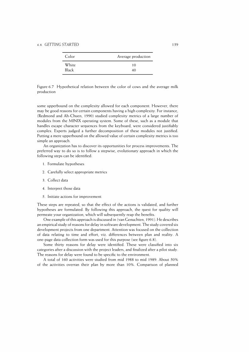
6.8. GETTING STARTED 139

Color Average production

White 10

Black 40

Figure 6.7 Hypothetical relation between the color of cows and the average milk

production

some upperbound on the complexity allowed for each component. However, there

may be good reasons for certain components having a high complexity. For instance,

(Redmond and Ah-Chuen, 1990) studied complexity metrics of a large number of

modules from the MINIX operating system. Some of these, such as a module that

handles escape character sequences from the keyboard, were considered justifiably

complex. Experts judged a further decomposition of these modules not justified.

Putting a mere upperbound on the allowed value of certain complexity metrics is too

simple an approach.

An organization has to discover its opportunities for process improvements. The

preferred way to do so is to follow a stepwise, evolutionary approach in which the

following steps can be identified:

1. Formulate hypotheses

2. Carefully select appropriate metrics

3. Collect data

4. Interpret those data

5. Initiate actions for improvement

These steps are repeated, so that the effect of the actions is validated, and further

hypotheses are formulated. By following this approach, the quest for quality will

permeate your organization, which will subsequently reap the benefits.

One example of this approach is discussed in (van Genuchten, 1991). He describes

an empirical study of reasons for delay in software development. The study covered six

development projects from one department. Attention was focused on the collection

of data relating to time and effort, viz. differences between plan and reality. A

one-page data collection form was used for this purpose (see figure 6.8).

Some thirty reasons for delay were identified. These were classified into six

categories after a discussion with the project leaders, and finalized after a pilot study.

The reasons for delay were found to be specific to the environment.

A total of 160 activities were studied from mid 1988 to mid 1989. About 50%

of the activities overran their plan by more than 10%. Comparison of planned

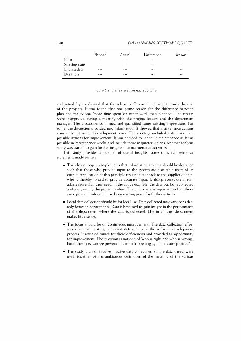
140 ON MANAGING SOFTWARE QUALITY

Planned Actual Difference Reason

Effort --- --- --- ---

Starting date --- --- --- ---

Ending date --- --- --- ---

Duration --- --- --- ---

Figure 6.8 Time sheet for each activity

and actual figures showed that the relative differences increased towards the end

of the projects. It was found that one prime reason for the difference between

plan and reality was ‘more time spent on other work than planned’. The results

were interpreted during a meeting with the project leaders and the department

manager. The discussion confirmed and quantified some existing impressions. For

some, the discussion provided new information. It showed that maintenance actions

constantly interrupted development work. The meeting included a discussion on

possible actions for improvement. It was decided to schedule maintenance as far as

possible in ‘maintenance weeks’ and include those in quarterly plans. Another analysis

study was started to gain further insights into maintenance activities.

This study provides a number of useful insights, some of which reinforce

statements made earlier:� The ‘closed loop’ principle states that information systems should be designed

such that those who provide input to the system are also main users of its

output. Application of this principle results in feedback to the supplier of data,

who is thereby forced to provide accurate input. It also prevents users from

asking more than they need. In the above example, the data was both collected

and analyzed by the project leaders. The outcome was reported back to those

same project leaders and used as a starting point for further actions.� Local data collection should be for local use. Data collected may vary consider-

ably between departments. Data is best used to gain insight in the performance

of the department where the data is collected. Use in another department

makes little sense.� The focus should be on continuous improvement. The data collection effort

was aimed at locating perceived deficiencies in the software development

process. It revealed causes for these deficiencies and provided an opportunity

for improvement. The question is not one of ‘who is right and who is wrong’,

but rather ‘how can we prevent this from happening again in future projects’.� The study did not involve massive data collection. Simple data sheets were

used, together with unambiguous definitions of the meaning of the various

6.9. SUMMARY 141

metrics. The approach is incremental, whereby the study gives an opportunity

for small improvements, and shows the way for the next study.

6.9 Summary

In this chapter, we paid ample attention to the notion of quality. Software quality

does not come for free. It has to be actively pursued. The use of a well-defined model

of the software development process and good analysis, design and implementation

techniques are a prerequisite. However, quality must also be controlled and managed.

To be able to do so, it has to be defined rigorously. This is not without problems,

as we have seen in sections 6.2 and 6.3. There exist numerous taxonomies of quality

attributes. For each of these attributes, we need a precise definition, together with a

metric that can be used to state quality goals, and to check that these quality goals are

indeed being satisfied. Most quality attributes relate to aspects that are primarily of

interest to the software developers. These engineer-oriented quality views are difficult

to reconcile with the user-oriented ‘fitness for use’ aspects.

For most quality attributes, the relation between what is actually measured

(module structure, defects encountered, etc.) and the attribute we are interested in is

insufficiently supported by a sound hypothesis. For example, though programs with a

large number of decisions are often complex, counterexamples exist which show that

the number of decisions (essentially McCabe’s cyclomatic complexity) is not a good

measure of program complexity. The issue of software metrics and the associated

problems is further dealt with in chapter 12.

Major standards for quality systems have been defined by ISO and IEEE. These

standards give detailed guidelines as regards the management of quality. Quality

assurance by itself does not guarantee quality products. It has to be supplemented

by a quality program within the development organization. Section 6.8 advocates an

evolutionary approach to establishing a quality program. Such an approach allows us

to gradually build up expertise in the use of quantitative data to find opportunities for

process improvements.

We finally sketched the software maturity framework developed by the Software

Engineering Institute. This framework offers a means to assess the state of software

engineering practice, as well as a number of steps to improve the software development

process. One of the major contributions of CMM and similar initiatives is their focus

on continuous improvement. This line of thought has subsequently been successfully

applied to other areas, resulting in, amongst others, a People-CMM, a Formal

specifications-CMM, and a Measurement-CMM.

6.10 Further Reading

Fenton and Pfleeger (1996) provide a very thorough overview of the field of

software metrics. The measurement framework discussed in section 6.1 is based

142 ON MANAGING SOFTWARE QUALITY

on (Kitchenham et al., 1995). Kaner and Bond (2004) also gives a framework for

evaluating metrics. (Software, 1997b) and (JSS, 1995) are special journal issues on

software metrics. Many of the articles in these issues deal with the application of

metrics in quality programs.

One of the first major publications on the topic of measurement programs

is (Grady and Caswell, 1987). Success factors for measurement programs can be

found in (Hall and Fenton, 1997) and (Gopal et al., 2002). Pfleeger (1995) elaborates

on the relation between metrics programs and maturity levels. Niessink and van Vliet

(1998b) give a CMM-like framework for the measurement capability of software

organizations.

The best known taxonomies of software quality attributes are given in (McCall

et al., 1977) and (Boehm et al., 1978). The ISO quality attributes are described

in (ISO9126, 2001) and (Cote et al., 2006). Critical discussions of these schemes are

given in (Kitchenham and Pfleeger, 1996) and (Fenton and Pfleeger, 1996). Suryn

et al. (2004) gives an overview of ISO/IEC 90003.

Garvin’s quality definitions are given in (Garvin, 1984). Different kinds of benefit

in a value-based definition of quality are discussed in (Simmons, 1996). For an elabo-

rate discussion of Total Quality Management, see (Bounds et al., 1994) or (Ishikawa,

1985).

The Capability Maturity Model is based on the seminal work of Watts

Humphrey (Humphrey, 1988, 1989). For a full description of the Capability Maturity

Model Integrated, see (CMMI Product Team, 2002). Practical experiences with soft-

ware process improvement programs are discussed in (Wohlwend and Rosenbaum,

1994), (Diaz and Sligo, 1997) and (Fitzgerald and O’Kane, 1999). Rainer and Hall

(2003) discuss success factors, and Baddoo and Hall (2003) discuss de-motivators

for SPI. A survey of benefits and costs of software process improvement programs is

given in (Herbsleb et al., 1997) and (Gartner, 2001). High-maturity, CMM level 5

organizations are discussed in (Software, 2000).

The Personal Software Process (PSP) is described in (Humphrey, 1996) and

(Humphrey, 1997a). BOOTSTRAP is described in (Kuvaja et al., 1994) and SPICE

in (El Emam et al., 1997).

Criticisms of CMM-like approaches are found in (Fayad, 1997), (Fayad and

Laitinen, 1997) and (Conradi and Fuggetta, 2002). El Emam and Madhavji (1995)

discuss the reliability of process assessments.

Process improvement is the topic of several special journal issues; see (CACM,

1997), (Software, 1994). The journal Software Process: Improvement and Practice is wholly

devoted to this topic.

Exercises

1. Define the following terms: measurement, measure, metric.

2. What is the difference between an internal and an external attribute?

6.10. FURTHER READING 143

3. Define the term representation condition. Why is it important that a measure

satisfies the representation condition?

4. What is the main difference between an ordinal scale and an interval scale?

And between an interval scale and a ratio scale?

5. What are the main differences between the user-based and product-based

definitions of quality?

6. Which are the three categories of software quality factors distinguished by

McCall?

7. Discuss the transcendent view of software quality.

8. Which of Garvin’s definitions of quality is mostly used by the software

developer? And which one is mostly used by the user?

9. Which quality viewpoint is stressed by ISO 9126?

10. Discuss the cornerstones of Total Quality Management.

11. What is the purpose of Software Quality Assurance?

12. Why should the Software Quality Assurance organization be independent of

the development organization?

13. Why should project members get feedback on the use of quality data they

submit to the Quality Assurance Group?

14. Describe the maturity levels of the Capability Maturity Model.

15. What is the major difference between level 2 and level 3 of the Capability

Maturity Model?

16. What is the difference between the staged and continuous versions of CMMI?

17. Why is it important to quantify quality requirements?

18. � Consider a software development project you have been involved in. How

was quality handled in this project? Were quality requirements defined at an

early stage? Were these requirements defined such that they could be tested

at a later stage?

19. ~ Define measurable properties of a software product that make up the

quality criteria Modularity and Operability. Do these properties constitute

an objective measure of these criteria? If not, in what ways is subjectivity

introduced?

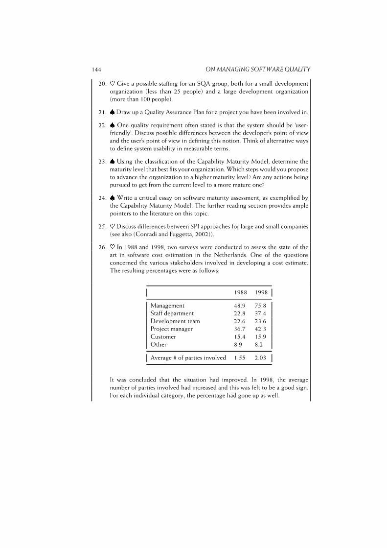
144 ON MANAGING SOFTWARE QUALITY

20. ~ Give a possible staffing for an SQA group, both for a small development

organization (less than 25 people) and a large development organization

(more than 100 people).

21. �Draw up a Quality Assurance Plan for a project you have been involved in.

22. � One quality requirement often stated is that the system should be ‘user-

friendly’. Discuss possible differences between the developer’s point of view

and the user’s point of view in defining this notion. Think of alternative ways

to define system usability in measurable terms.

23. � Using the classification of the Capability Maturity Model, determine the

maturity level that best fits your organization. Which steps would you propose

to advance the organization to a higher maturity level? Are any actions being

pursued to get from the current level to a more mature one?

24. � Write a critical essay on software maturity assessment, as exemplified by

the Capability Maturity Model. The further reading section provides ample

pointers to the literature on this topic.

25. ~ Discuss differences between SPI approaches for large and small companies

(see also (Conradi and Fuggetta, 2002)).

26. ~ In 1988 and 1998, two surveys were conducted to assess the state of the

art in software cost estimation in the Netherlands. One of the questions

concerned the various stakeholders involved in developing a cost estimate.

The resulting percentages were as follows:

1988 1998

Management 48.9 75.8

Staff department 22.8 37.4

Development team 22.6 23.6

Project manager 36.7 42.3

Customer 15.4 15.9

Other 8.9 8.2

Average # of parties involved 1.55 2.03

It was concluded that the situation had improved. In 1998, the average

number of parties involved had increased and this was felt to be a good sign.

For each individual category, the percentage had gone up as well.

6.10. FURTHER READING 145

Can you think of a possibly negative conclusion from this same set of data,

i.e. that the situation has become worse since 1988?

7

Cost Estimation

LEARNING OBJECTIVES� To appreciate the use of quantitative, objective approaches to software cost

estimation� To have insight in the factors that affect software development productivity� To understand well-known techniques for estimating software cost and effort� To understand techniques for relating effort to development time

147

Software development takes time and money. When commissioning a building

project, you expect a reliable estimate of the cost and development time up

front. Getting reliable cost and schedule estimates for software development

projects is still largely a dream. Software development cost is notoriously

difficult to estimate reliably at an early stage. Since progress is difficult to ‘see’

--just when is a piece of software 50% complete? --schedule slippages often go

undetected for quite a while, and schedule overruns are the rule, rather than

the exception. In this chapter, we look at various ways to estimate software

cost and schedule.

When commissioning a house construction, decorating the bathroom, or laying-

out a garden, we expect a precise estimate of the costs to be incurred before the

operation is started. A gardener is capable of giving a rough indication of the cost on

the basis of, say, the area of land, the desired size of the terrace or grass area, whether

or not a pond is required, and similar information. The estimate can be made more

precise in further dialog, before the first bit of earth is turned. If you expect a similar

accuracy as regards the cost estimate for a software development project, you are in

for a surprise.

Estimating the cost of a software development project is a rather unexplored field,

in which one all too often relies on mere guesstimates. There are exceptions to this

procedure, fortunately. There now exist a number of algorithmic models that allow us

to estimate total cost and development time of a software development project, based

on estimates for a limited number of relevant cost drivers. Some of the important

algorithmic cost estimation models are discussed in section 7.1.

In most cost estimation models, a simple relation between cost and effort is

assumed. The effort may be measured in man-months, for instance, and each man-

month is taken to incur a fixed amount, say, of $5000. The total estimated cost is

then obtained by simply multiplying the estimated number of man-months by this

constant factor. In this chapter, we freely use the terms cost and effort as if they are

synonymous.

The notion of total cost is usually taken to indicate the cost of the initial

software development effort, i.e. the cost of the requirements engineering, design,

implementation and testing phases. Thus, maintenance costs are not taken into

account. Unless explicitly stated otherwise, this notion of cost will also be used by

us. In the same vein, development time will be taken to mean: the time between the

start of the requirements engineering phase and the point in time when the software

is delivered to the customer. Lastly, the notion of cost as it is used here, does not

include possible hardware costs either. It concerns only personnel costs involved in

software development.

Research in the area of cost estimation is far from crystallized. Different models

use different measures and cost drivers, so that mutual comparisons are very difficult.

148 COST ESTIMATION

Suppose some model uses an equation of the form:E = 2:7KLOC 1:05This equation shows a certain relation between effort needed (E) and the size

of the product (KLOC = Kilo Lines Of Code = Lines Of Code=1000). The effort

measure could be the number of man-months needed. Several questions come to

mind immediately: What is a line of code? Do we count machine code, or the source

code in some high-level language? Do we count comment lines, or blank lines that

increase readability? Do we take into account holidays, sick-leave, and the like, in our

notion of the man-month, or does it concern a net measure? Different interpretations

of these notions may lead to widely different results. Unfortunately, different models

do use different definitions of these notions. Sometimes, it is not even known which

definitions were used in the derivation of the model.

To determine the equations of an algorithmic cost estimation model, we may

follow several approaches. Firstly, we may base our equations on the results of

experiments. In such an experiment, we in general vary one parameter, while the

other parameters are kept constant. In this way, we may try to determine the influence

of the parameter that is being varied. As a typical example, we may consider the

question of whether or not comments help to build up our understanding of a

program. Under careful control of the circumstances, we may pose a number of

questions about one and the same program text to two groups of programmers. The

first group gets program text without comments, the second group gets the same

program text, with comments. We may check our hypothesis using the results of the

two groups. The, probably realistic, assumption in this experiment is that a better and

faster understanding of the program text has a positive effect on the maintainability

of that program.

This type of laboratory experiment is often performed at universities, where stu-

dents play the role of programmers. It is not self-evident that the results thus obtained

also holds in industrial settings. In practice, there may be a rather complicated interac-

tion between different relevant factors. Also, the subjects need not be representative.

Finally, the generalization from laboratory experiments that are (of necessity) limited

in size to big software development projects with which professionals are confronted

is not possible. The general opinion is that results thus obtained have limited validity,

and certainly need further testing.

A second way to arrive at algorithmic cost estimation models is based on an

analysis of real project data, in combination with some theoretical underpinning. An

organization may collect data about a number of software systems that have been

developed. These data may concern the time spent on the various phases that are

being distinguished, the qualifications of the personnel involved, the points in time

at which errors occurred, both during testing and after installation, the complexity,

reliability and other relevant project factors, the size of the resulting code, etc.

Based on a sound hypothesis of the relations between the various entities involved

and a (statistical) analysis of these data we may derive equations that numerically

149

characterize these relations. An example of such a relation is the one given above,

which relatesE toKLOC . The usability and reliability of such equations is obviously

very much dependent upon the reliability of the data on which they are based. Also,

the hypothesis that underlies the form of the equation must be sound.

The findings obtained in this way reflect an average, a best possible approximation

based on available data. We therefore have to be very careful in applying the results

obtained. If the software to be developed in the course of a new project cannot be

compared with earlier products because of the degree of innovation involved, one is

in for a big surprise. For example, estimating the cost of the Space Shuttle project

cannot be done through a simple extrapolation from earlier projects. We may hope,

however, that the average software development project has a higher predictability

as regards effort needed and the corresponding cost.

The way in which we obtain quantitative relations implies further constraints on

the use of these models. The model used is based on an analysis of data from earlier

projects. Application of the model to new projects is possible only insofar as those

new projects resemble old projects, i.e. the projects on whose data the model is

based. If we have collected data on projects of a certain kind and within a particular

organization, a model based on these data cannot be used without amendment for

different projects in a possibly different organization. A model based on data about

administrative projects in a government environment has little predictive value for

the development of real-time software in the aerospace industry. This is one of the

reasons why the models of, for example, Walston and Felix (1977) and Boehm (1981)

(see section 7.1 for more detailed discussions of these models) yield such different

results for one and the same problem description.

The lesson to be learned is that blind application of the formulae from existing

models will not solve your cost estimation problem. Each model needs tuning to the

environment in which it is going to be used. This implies the need to continuously

collect your own project data, and to apply statistical techniques to calibrate model

parameters.

Other reasons for the discrepancies between existing models are:

– Most models give a relation between man-months needed and size (in lines

of code). As remarked before, widely different definitions of these notions are

used.

– The notion ‘effort’ does not always mean the same thing. Sometimes, one

only counts the activities starting from the design, i.e. after the requirements

specification has been fixed. Sometimes also, one includes maintenance effort.

Despite these discrepancies, the various cost estimation models do have a number of

characteristics in common. These common characteristics reflect important factors

that bear on development cost and effort. The increased understanding of software

costs allows us to identify strategies for improving software productivity, the most

important of which are:

150 COST ESTIMATION� Writing less code. System size is one of the main determinants of effort and

cost. Techniques that try to reduce size, such as software reuse and the use of

high-level languages, can obtain significant savings.� Getting the best from people. Individual and team capabilities have a large

impact on productivity. The best people are usually a bargain. Better incentives,

better work environments, training programs and the like provide further

productivity improvement opportunities.� Avoiding rework. Studies have shown that a considerable effort is spent redoing

earlier work. The application of prototyping or evolutionary development

process models and the use of modern programming practices (information

hiding) can yield considerable savings.� Developing and using integrated project support environments. Tools can help

us eliminate steps or make steps more efficient.

In the next section, we discuss and compare some of the well-known algorithmic

models for cost estimation. In many organizations, software cost is estimated by

human experts, who use their expertise and gut feeling, rather than a formula, to

arrive at a cost estimate. Some of the do’s and don’ts of expert-based cost estimation

are discussed in section 7.2.

Given an estimate of the size of a project, we will next be interested in the

development time needed. With a naive view, we may conjecture that a project with

an estimated effort of 100 man-months can be done in 1 year with a team of 8.5

people, but equally well in one month with a team of 100 people. This view is too

naive. A project of a certain size corresponds to a certain nominal physical time

period. If we try to shorten this nominal development time too much, we get into the

‘impossible region’ and the chance of failure sharply increases. This phenomenon is

further discussed in section 7.3.

The topics addressed in this chapter fit planning-driven development projects

more than they do agile projects. In agile projects, iterations are usually fairly small,

and do not warrant the effort required by the algorithmic models discussed in

section 7.1. In agile projects (see chapter 3, increments correspond to one or a few

user stories or scenarios. These user stories are estimated in terms of development

weeks, bucks, or some artificial unit, say Points. Next, it is determined which user

stories will be realized in the current increment, and development proceeds. Usually,

the time box agreed upon is sacred, i.e., if some of the user stories cannot be realized

within the agreed upon time frame, they are moved to a next iteration. Estimation

accuracy is assumed to improve in the course of the project.

7.1 Algorithmic Models

To be able to get reliable estimates, we need to extensively record historical data.

These historical data can be used to produce estimates for new projects. In doing

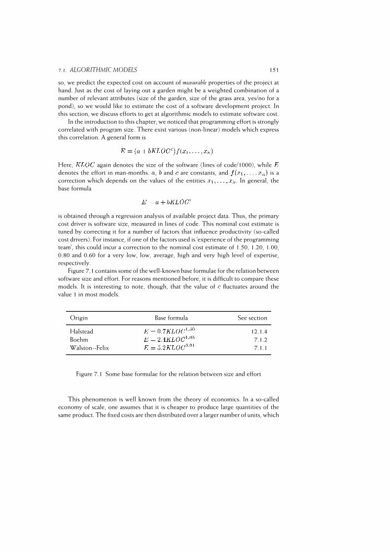
7.1. ALGORITHMIC MODELS 151

so, we predict the expected cost on account of measurable properties of the project at

hand. Just as the cost of laying out a garden might be a weighted combination of a

number of relevant attributes (size of the garden, size of the grass area, yes/no for a

pond), so we would like to estimate the cost of a software development project. In

this section, we discuss efforts to get at algorithmic models to estimate software cost.

In the introduction to this chapter, we noticed that programming effort is strongly

correlated with program size. There exist various (non-linear) models which express

this correlation. A general form isE = (a+ bKLOC )f(x1; : : : ; xn)Here, KLOC again denotes the size of the software (lines of code/1000), while Edenotes the effort in man-months. a, b and are constants, and f(x1; : : : ; xn) is a

correction which depends on the values of the entities x1; : : : ; xn. In general, the

base formula E = a+ bKLOC is obtained through a regression analysis of available project data. Thus, the primary

cost driver is software size, measured in lines of code. This nominal cost estimate is

tuned by correcting it for a number of factors that influence productivity (so-called

cost drivers). For instance, if one of the factors used is ‘experience of the programming

team’, this could incur a correction to the nominal cost estimate of 1.50, 1.20, 1.00,

0.80 and 0.60 for a very low, low, average, high and very high level of expertise,

respectively.

Figure 7.1 contains some of the well-known base formulae for the relation between

software size and effort. For reasons mentioned before, it is difficult to compare these

models. It is interesting to note, though, that the value of fluctuates around the

value 1 in most models.

Origin Base formula See section

Halstead E = 0:7KLOC 1:50 12.1.4

Boehm E = 2:4KLOC 1:05 7.1.2

Walston--Felix E = 5:2KLOC 0:91 7.1.1

Figure 7.1 Some base formulae for the relation between size and effort

This phenomenon is well known from the theory of economics. In a so-called

economy of scale, one assumes that it is cheaper to produce large quantities of the

same product. The fixed costs are then distributed over a larger number of units, which

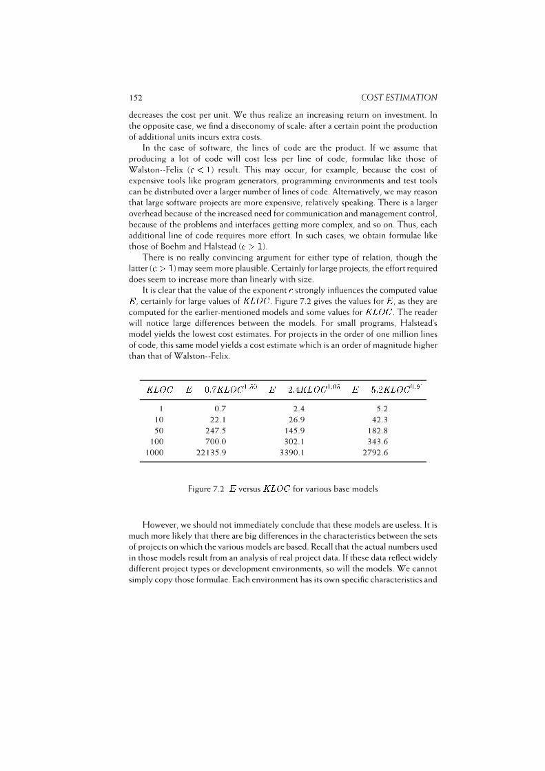
152 COST ESTIMATION

decreases the cost per unit. We thus realize an increasing return on investment. In

the opposite case, we find a diseconomy of scale: after a certain point the production

of additional units incurs extra costs.

In the case of software, the lines of code are the product. If we assume that

producing a lot of code will cost less per line of code, formulae like those of

Walston--Felix ( < 1) result. This may occur, for example, because the cost of

expensive tools like program generators, programming environments and test tools

can be distributed over a larger number of lines of code. Alternatively, we may reason

that large software projects are more expensive, relatively speaking. There is a larger

overhead because of the increased need for communication and management control,

because of the problems and interfaces getting more complex, and so on. Thus, each

additional line of code requires more effort. In such cases, we obtain formulae like

those of Boehm and Halstead ( > 1).

There is no really convincing argument for either type of relation, though the

latter ( > 1) may seem more plausible. Certainly for large projects, the effort required

does seem to increase more than linearly with size.

It is clear that the value of the exponent strongly influences the computed valueE, certainly for large values of KLOC . Figure 7.2 gives the values for E, as they are

computed for the earlier-mentioned models and some values for KLOC . The reader

will notice large differences between the models. For small programs, Halstead’s

model yields the lowest cost estimates. For projects in the order of one million lines

of code, this same model yields a cost estimate which is an order of magnitude higher

than that of Walston--Felix.KLOC E = 0:7KLOC 1:50 E = 2:4KLOC 1:05 E = 5:2KLOC 0:911 0.7 2.4 5.2

10 22.1 26.9 42.3

50 247.5 145.9 182.8

100 700.0 302.1 343.6

1000 22135.9 3390.1 2792.6

Figure 7.2 E versus KLOC for various base models

However, we should not immediately conclude that these models are useless. It is

much more likely that there are big differences in the characteristics between the sets

of projects on which the various models are based. Recall that the actual numbers used

in those models result from an analysis of real project data. If these data reflect widely

different project types or development environments, so will the models. We cannot

simply copy those formulae. Each environment has its own specific characteristics and

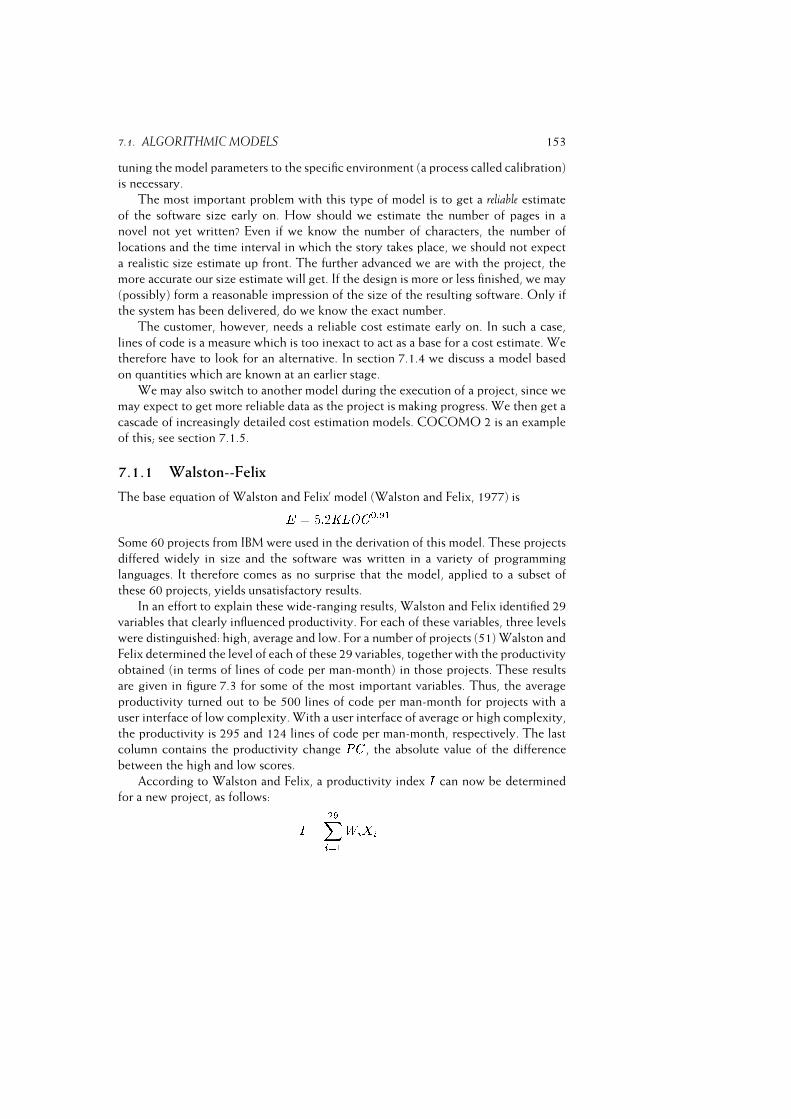
7.1. ALGORITHMIC MODELS 153

tuning the model parameters to the specific environment (a process called calibration)

is necessary.

The most important problem with this type of model is to get a reliable estimate

of the software size early on. How should we estimate the number of pages in a

novel not yet written? Even if we know the number of characters, the number of

locations and the time interval in which the story takes place, we should not expect

a realistic size estimate up front. The further advanced we are with the project, the

more accurate our size estimate will get. If the design is more or less finished, we may

(possibly) form a reasonable impression of the size of the resulting software. Only if

the system has been delivered, do we know the exact number.

The customer, however, needs a reliable cost estimate early on. In such a case,

lines of code is a measure which is too inexact to act as a base for a cost estimate. We

therefore have to look for an alternative. In section 7.1.4 we discuss a model based

on quantities which are known at an earlier stage.

We may also switch to another model during the execution of a project, since we

may expect to get more reliable data as the project is making progress. We then get a

cascade of increasingly detailed cost estimation models. COCOMO 2 is an example

of this; see section 7.1.5.

7.1.1 Walston--Felix

The base equation of Walston and Felix’ model (Walston and Felix, 1977) isE = 5:2KLOC 0:91Some 60 projects from IBM were used in the derivation of this model. These projects

differed widely in size and the software was written in a variety of programming

languages. It therefore comes as no surprise that the model, applied to a subset of

these 60 projects, yields unsatisfactory results.

In an effort to explain these wide-ranging results, Walston and Felix identified 29

variables that clearly influenced productivity. For each of these variables, three levels

were distinguished: high, average and low. For a number of projects (51) Walston and

Felix determined the level of each of these 29 variables, together with the productivity

obtained (in terms of lines of code per man-month) in those projects. These results

are given in figure 7.3 for some of the most important variables. Thus, the average

productivity turned out to be 500 lines of code per man-month for projects with a

user interface of low complexity. With a user interface of average or high complexity,

the productivity is 295 and 124 lines of code per man-month, respectively. The last

column contains the productivity change PC , the absolute value of the difference

between the high and low scores.

According to Walston and Felix, a productivity index I can now be determined

for a new project, as follows: I = 29Xi=1WiXi

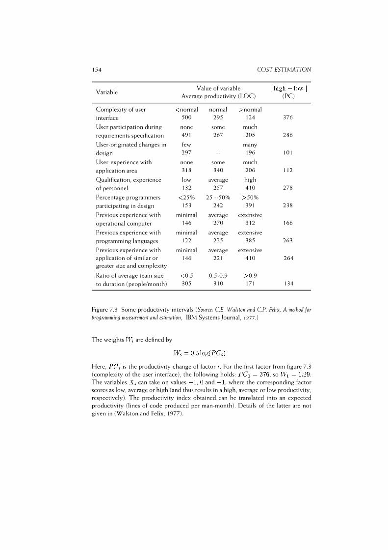
154 COST ESTIMATION

VariableValue of variable j high� low j

Average productivity (LOC) (PC)

Complexity of user

interface

<normal normal >normal

500 295 124 376

User participation during

requirements specification

none some much

491 267 205 286

User-originated changes in

design

few many

297 -- 196 101

User-experience with

application area

none some much

318 340 206 112

Qualification, experience

of personnel

low average high

132 257 410 278

Percentage programmers

participating in design

<25% 25 --50% >50%

153 242 391 238

Previous experience with

operational computer

minimal average extensive

146 270 312 166

Previous experience with

programming languages

minimal average extensive

122 225 385 263

Previous experience with

application of similar or

greater size and complexity

minimal average extensive

146 221 410 264

Ratio of average team size

to duration (people/month)

<0.5 0.5-0.9 >0.9

305 310 171 134

Figure 7.3 Some productivity intervals (Source: C.E. Walston and C.P. Felix, A method for

programming measurement and estimation, IBM Systems Journal, 1977.)

The weights Wi are defined byWi = 0:5 log(PC i)Here, PC i is the productivity change of factor i. For the first factor from figure 7.3

(complexity of the user interface), the following holds: PC 1 = 376, so W1 = 1:29.

The variables Xi can take on values +1, 0 and �1, where the corresponding factor

scores as low, average or high (and thus results in a high, average or low productivity,

respectively). The productivity index obtained can be translated into an expected

productivity (lines of code produced per man-month). Details of the latter are not

given in (Walston and Felix, 1977).

7.1. ALGORITHMIC MODELS 155

The number of factors considered in this model is rather high (29 factors out of

51 projects). Also it is not clear to what extent the various factors influence each

other. Finally, the number of alternatives per factor is only three, and does not seem

to offer enough choice in practical situations.

Nevertheless, the approach taken by Walston and Felix and their list of cost

drivers have played a very important role in directing later research in this area.

7.1.2 COCOMO

COCOMO (COnstructive COst MOdel) is one of the algorithmic cost estimation

models best documented. In its simplest form, called Basic COCOMO, the formula

that relates effort to software size, readsE = bKLOC Here, b and are constants that depend on the kind of project that is being executed.

COCOMO distinguishes three classes of project:� Organic A relatively small team develops software in a known environment.

The people involved generally have a lot of experience with similar projects

in their organization. They are thus able to contribute at an early stage, since

there is no initial overhead. Projects of this type will seldom be very large

projects.� Embedded The product will be embedded in an environment which is very

inflexible and poses severe constraints. An example of this type of project might

be air traffic control, or an embedded weapon system.� Semidetached This is an intermediate form. The team may show a mixture of

experienced and inexperienced people, the project may be fairly large, though

not excessively large, etc.

For the various classes, the parameters of Basic COCOMO take on the following

values:

organic: b = 2.4, = 1.05

semidetached: b = 3.0, = 1.12

embedded: b = 3.6, = 1.20

Figure 7.4 gives the estimated effort for projects of each of those three modes, for

different values of KLOC (though an ‘organic’ project of one million lines is not very

realistic). Amongst others, we may read from this figure that the constant soon

starts to have a major impact on the estimate obtained.

Basic COCOMO yields a simple, and hence a crude, cost estimate based on

a simple classification of projects into three classes. In his book Software Engineering

156 COST ESTIMATION

KLOC

Effort in man-months

organic semidetached embedded

(E = 2:4KLOC 1:05) (E = 3:0KLOC 1:12) (E = 3:6KLOC 1:20)

1 2.4 3.0 3.6

10 26.9 39.6 57.1

50 145.9 239.4 392.9

100 302.1 521.3 904.2

1000 3390.0 6872.0 14333.0

Figure 7.4 Size versus effort in Basic COCOMO

Economics, Boehm also discusses two other, more complicated, models, termed Inter-

mediate COCOMO and Detailed COCOMO, respectively. Both these models take

into account 15 cost drivers --attributes that affect productivity, and hence costs.

All these cost drivers yield a multiplicative correction factor to the nominal

estimate of the effort. (Both these models also use values for b which slightly differ

from that of Basic COCOMO.) Suppose we found a nominal effort estimate of 40

man-months for a certain project. If the complexity of the resulting software is low,

then the model tells us to correct this estimate by a factor of 0.85. A better estimate

then would be 34 man-months. On the other hand, if the complexity is high, we get

an estimate of 1:15� 40 = 46 man-months.

The nominal value of each cost driver in Intermediate COCOMO is 1.00 (see

also figure 7.11. So we may say that Basic COCOMO is based on nominal values for

each of the cost drivers.

On top of this set of cost drivers, the detailed model adds a further level of

refinement. First of all, this model is phase-sensitive, the idea being that not all cost

drivers influence each phase of the development cycle in the same way. So, rather

than having one table with effort multipliers as in Intermediate COCOMO, Detailed

COCOMO uses a set of such tables. These tables show, for each cost driver, a

separate effort multiplier for each major development phase. Furthermore, Detailed

COCOMO uses a hierarchy for the product to be developed, in which some cost

drivers have an impact on the estimate at the module level, while others have an

impact at the (sub)system level.

The COCOMO formulae are based on a combination of expert judgment, an

analysis of available project data, other models, etc. The basic model does not yield

very accurate results for the projects on which the model has been based. The

intermediate version yields good results and, if one extra cost driver (volatility of

the requirements specification) is added, it even yields very good results. Further

validation of the COCOMO models using other project data is not straightforward,

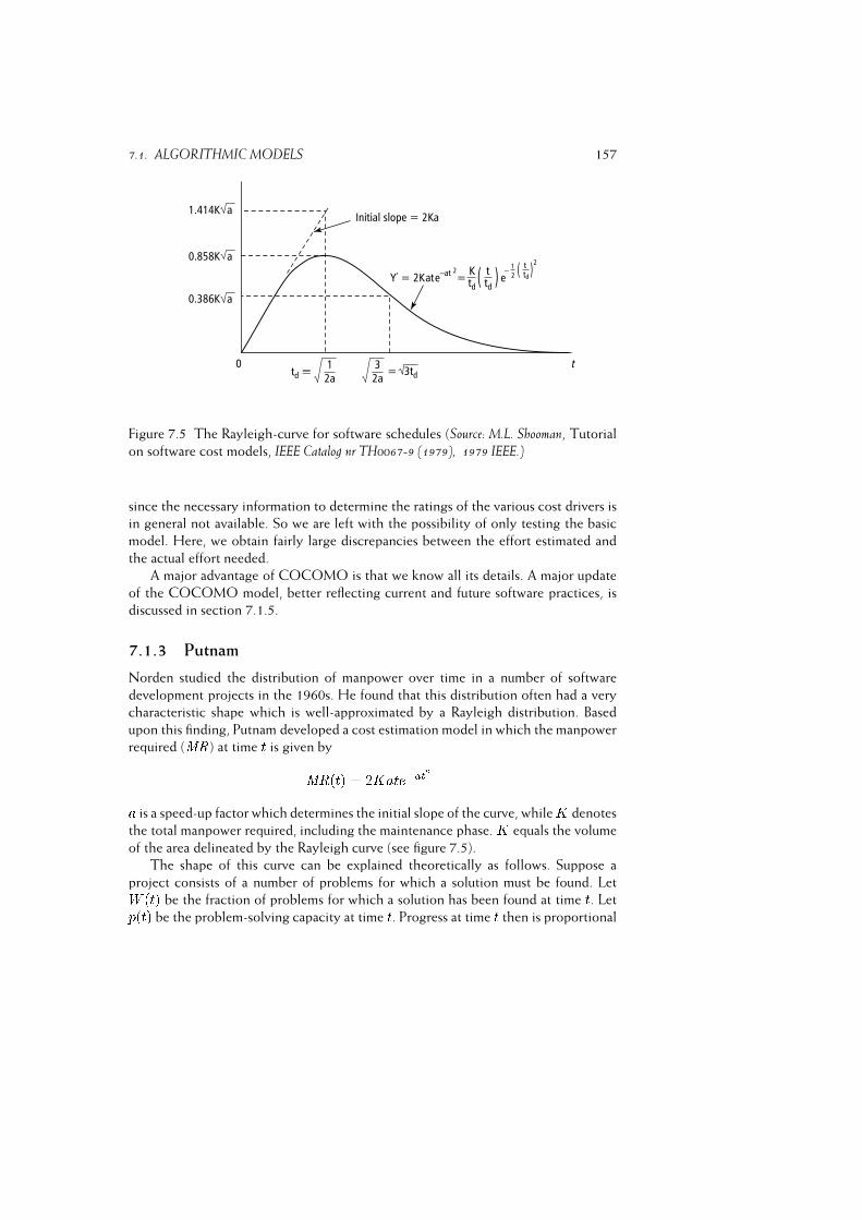
7.1. ALGORITHMIC MODELS 157

Figure 7.5 The Rayleigh-curve for software schedules (Source: M.L. Shooman, Tutorial

on software cost models, IEEE Catalog nr TH0067-9 (1979), 1979 IEEE.)

since the necessary information to determine the ratings of the various cost drivers is

in general not available. So we are left with the possibility of only testing the basic

model. Here, we obtain fairly large discrepancies between the effort estimated and

the actual effort needed.

A major advantage of COCOMO is that we know all its details. A major update

of the COCOMO model, better reflecting current and future software practices, is

discussed in section 7.1.5.

7.1.3 Putnam

Norden studied the distribution of manpower over time in a number of software

development projects in the 1960s. He found that this distribution often had a very

characteristic shape which is well-approximated by a Rayleigh distribution. Based

upon this finding, Putnam developed a cost estimation model in which the manpower

required (MR) at time t is given byMR(t) = 2Kate�at2a is a speed-up factor which determines the initial slope of the curve, whileK denotes

the total manpower required, including the maintenance phase. K equals the volume

of the area delineated by the Rayleigh curve (see figure 7.5).

The shape of this curve can be explained theoretically as follows. Suppose a

project consists of a number of problems for which a solution must be found. LetW (t) be the fraction of problems for which a solution has been found at time t. Letp(t) be the problem-solving capacity at time t. Progress at time t then is proportional

158 COST ESTIMATION

to the product of the available problem-solving capacity and the fraction of problems

yet unsolved. If the total amount of work to be done is set to 1, this yields:

dWdt = p(t)(1�W (t))

After integration, we get W (t) = 1� exp(� Z t p(�)d�)If we next assume that the problem-solving capacity is well approximated by an

equation of the form p(t) = at, i.e. the problem-solving capacity shows a linear

increase over time, the progress is given by a Rayleigh distribution:

dWdt = ate�(at2)=2

Integration of the equation for MR(t) that was given earlier yields the cumulative

effort I : I(t) = K(1� e�at2)In particular, we get I(1) = K. If we denote the point in time at which the Rayleigh-

curve assumes its maximum value by T , then a = 1=(2T 2). This point T will be close

to the point in time at which the software is being delivered to the customer. The

volume of the area delineated by the Rayleigh curve between points 0 and T then is

a good approximation of the initial development effort. For this, we getE = I(T ) = 0:3945KThis result is remarkably close to the often-used rule of thumb: 40% of the total effort

is spent on the actual development, while 60% is spent on maintenance.

Various studies indicate that Putnam’s model is well suited to estimating the cost

of very large software development projects (projects that involve more than 15

man-years). The model seems to be less suitable for small projects.

A serious objection to Putnam’s model, in our opinion, concerns the relation it

assumes between effort and development time if the schedule is compressed relative

to the nominal schedule estimate: E = =T 4. Compressing a project’s schedule in

this model entails an extraordinary large penalty (see also section 7.3).

7.1.4 Function Point Analysis

Function point analysis (FPA) is a method of estimating costs in which the problems

associated with determining the expected amount of code are circumvented. FPA

is based on counting the number of different data structures that are used. In the

FPA method, it is assumed that the number of different data structures is a good

7.1. ALGORITHMIC MODELS 159

size indicator. FPA is particularly suitable for projects aimed at realizing business

applications for, in these applications, the structure of the data plays a very dominant

role. The method is less suited to projects in which the structure of the data plays a

less prominent role, and the emphasis is on algorithms (such as compilers and most

real-time software).

The following five entities play a central role in the FPA-model:� Number of input types (I). The input types refer only to user input that results

in changes in data structures. It does not concern user input which is solely

concerned with controlling the program’s execution. Each input type that has

a different format, or is treated differently, is counted. So, though the records

of a master file and those of a mutation file may have the same format, they are

still counted separately.� Number of output types (O). For the output types, the same counting scheme

is used.� Number of inquiry types (E). Inquiry types concern input that controls the

execution of the program and does not change internal data structures. Examples

of inquiry types are: menu selection and query criteria.� Number of logical internal files (L). This concerns internal data generated by

the system, and used and maintained by the system, such as, for example, an

index file.� Number of interfaces (F ). This concerns data that is output to another

application, or is shared with some other application.

By trial and error, weights have been associated with each of these entities. The

number of (unadjusted) function points,UFP , is a weighted sum of these five entities:UFP = 4I + 5O + 4E + 10L+ 7FWith FPA too, a further refinement is possible, by applying corrections to reflect

differences in complexity of the data types. In that case, the constants used in the

above formula depend on the estimated complexity of the data type in question.

Figure 7.6 gives the counting rules when three levels of complexity are distinguished.

So, rather than having each input type count as four function points, we may count

three, four or six function points, based on an assessment of the complexity of each

input type.

Each input type has a number of data element types (attributes), and refers to zero

or more other file types. The complexity of an input type increases as the number of

its data element types or referenced file types increases. For input types, the mapping

of these numbers to complexity levels is given in figure 7.7. For the other file types,

these tables have the same format, with slightly different numbers along the axes.

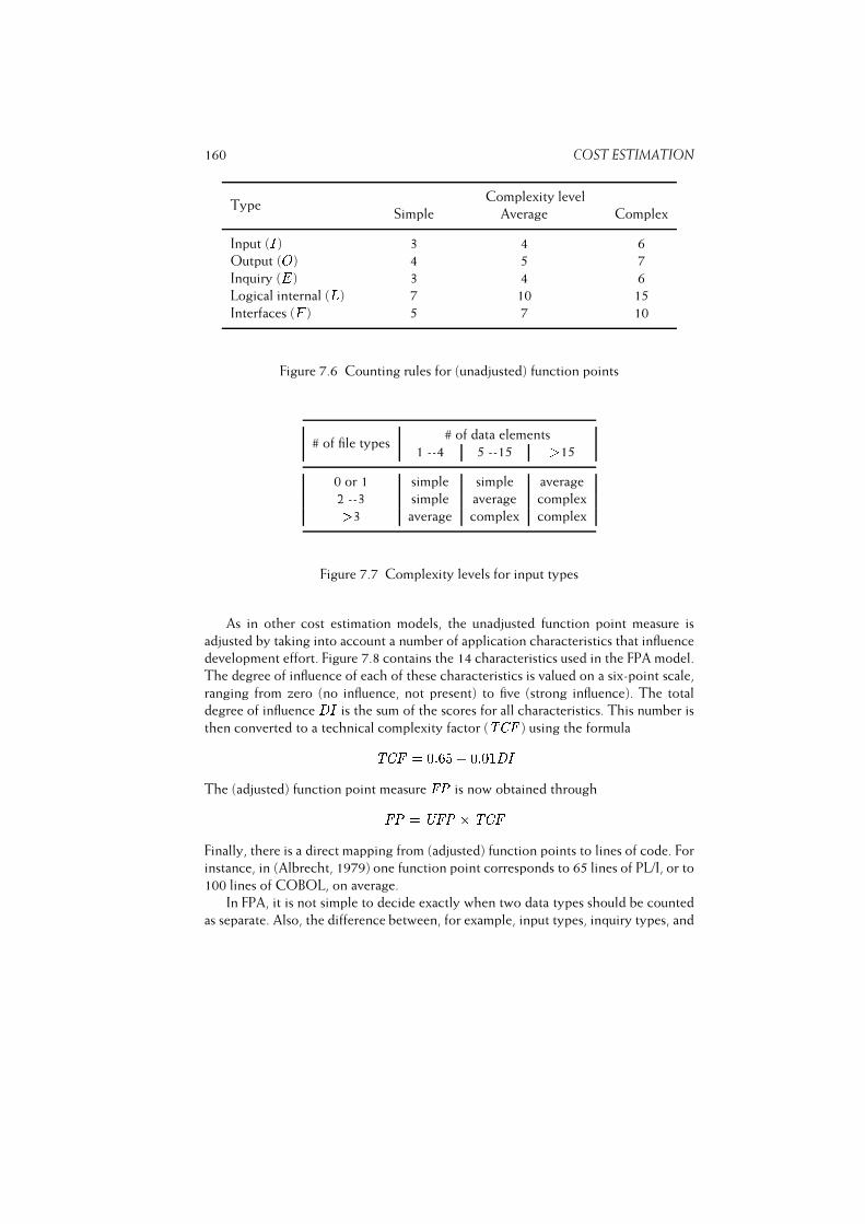
160 COST ESTIMATION

TypeComplexity level

Simple Average Complex

Input (I) 3 4 6

Output (O) 4 5 7

Inquiry (E) 3 4 6

Logical internal (L) 7 10 15

Interfaces (F ) 5 7 10

Figure 7.6 Counting rules for (unadjusted) function points

# of file types# of data elements

1 --4 5 --15 >15

0 or 1 simple simple average

2 --3 simple average complex>3 average complex complex

Figure 7.7 Complexity levels for input types

As in other cost estimation models, the unadjusted function point measure is

adjusted by taking into account a number of application characteristics that influence

development effort. Figure 7.8 contains the 14 characteristics used in the FPA model.

The degree of influence of each of these characteristics is valued on a six-point scale,

ranging from zero (no influence, not present) to five (strong influence). The total

degree of influence DI is the sum of the scores for all characteristics. This number is

then converted to a technical complexity factor (TCF ) using the formulaTCF = 0:65 + 0:01DIThe (adjusted) function point measure FP is now obtained throughFP = UFP � TCFFinally, there is a direct mapping from (adjusted) function points to lines of code. For

instance, in (Albrecht, 1979) one function point corresponds to 65 lines of PL/I, or to

100 lines of COBOL, on average.

In FPA, it is not simple to decide exactly when two data types should be counted

as separate. Also, the difference between, for example, input types, inquiry types, and

7.1. ALGORITHMIC MODELS 161

Data communications

Distributed functions

Performance

Heavily used configuration

Transaction rate

Online data entry

End-user efficiency

Online update

Complex processing

Re-usability

Installation ease

Operational ease

Multiple sites

Facilitate change

Figure 7.8 Application characteristics in FPA

interfaces remains somewhat vague. The International Function Point User Group

(IFPUG) has published extensive guidelines on how to classify and count the various

entities involved. This should overcome many of the difficulties that analysts have in

counting function points in a uniform way.

Further problems with FPA have to do with its use of ordinal scales and the way

complexity is handled. FPA distinguishes three levels of component complexity only.

A component with 100 elements thus gets at most twice the number of function points

of a component with one element. It has been suggested that a model which uses

the raw complexity data, i.e. the number of data elements and file types referenced,

might work as well as, or even better than, a model which uses an ordinal derivative

thereof. In a sense, complexity is counted twice: both through the complexity level of

the component and through one of the application characteristics. Yet it is felt that

highly complex systems are not adequately dealt with, since FPA is predominantly

concerned with counting externally visible inputs and outputs.

In applying the FPA cost estimation method, it still remains necessary to calibrate

the various entities to your own environment. This holds the more for the corrections

that reflect different application characteristics, and the transition from function

points to lines of code.

7.1.5 COCOMO 2: Variations on a Theme

COCOMO 2 is a revision of the 1981 COCOMO model, tuned to the life cycle

practices of the 1990s and 2000s. It reflects our cumulative experience with and

162 COST ESTIMATION

knowledge of cost estimation. By comparing its constituents with those of previous

cost estimation models, it also offers us a means to learn about significant changes in

our trade over the past decades.

COCOMO 2 provides three increasingly detailed cost estimation models. These

models can be used for different types of projects, as well as during different stages of

a single project:

– the Application Composition model, mainly intended for prototyping efforts,

for instance to resolve user interface issues (Its name suggests heavy use

of existing components, presumably in the context of a powerful CASE

environment.)

– the Early Design model, aimed at the architectural design stage

– the Post-Architecture model for the actual development stage of a software

product

The Post-Architecture model can be considered an update of the original COCOMO

model; the Early Design model is an FPA-like model; and the Application Composition

model is based on counting system components of a large granularity, such as screens

and reports.

The Application Composition model is based on counting Object Points. Object

Points have nothing to do with objects as in object-oriented development. In this

context, objects are screens, reports, and 3GL modules.

The roots of this type of model can be traced back to several variations on FPA-

type size measures. Function points as used in FPA are intended to be a user-oriented

measure of system function. The user functions measured are the inputs, outputs,

inquiries, etc. We may conjecture that these user-functions are technology-dependent,

and that FPA primarily reflects the batch-oriented world of the 1970s.

Present-day administrative systems are perhaps better characterized by their

number of menus or screens. This line of thought has been pursued in various studies.

Banker et al. (1991) compared Object Points with Function Points for a sample of

software projects, and found that Object Points did almost as well as Function Points.

Object Points, however, are easier to determine, and at an earlier point in time.

Total effort is estimated in the Application Composition model as follows:

1. Estimate the number of screens, reports, and 3GL components in the applica-

tion.

2. Determine the complexity level of each screen and report (simple, medium or

difficult). 3GL components are assumed to be always difficult. The complexity

of a screen depends on the number of views and tables it contains. The

complexity of a report depends on the number of sections and tables it

contains. A classification table similar to those in FPA (see figure 7.9 for an

example) is used to determine these complexity levels.

7.1. ALGORITHMIC MODELS 163

3. Use the numbers given in figure 7.10 to determine the relative effort (in Object

Points) to implement the object.

4. The sum of the Object Points for the individual objects yields the number of

Object Points for the whole system.

5. Estimate the reuse percentage, resulting in the number of New Object Points

(NOP) as follows: NOP = Obje tPoints � (100�%Reuse)=100.

6. Determine a productivity rate PROD = NOP=man-month. This productivity

rate depends on the experience and capability of both the developers and the

maturity of the CASE environment they use. It varies from 4 (very low) to 50

(very high).

7. Estimate the number of man-months needed for the project:E = NOP=PROD.

# of views

# and source of data tables

total < 4 total < 8 total � 8(< 2 on server (2� 3 on server (> 3 on server< 3 on client) 3� 5 on client) > 5 on client)< 3 simple simple medium3� 7 simple medium difficult> 8 medium difficult difficult

Figure 7.9 Complexity levels for screens

Object typeComplexity

simple medium difficult

Screen 1 2 3

Report 2 5 8

3GL component 10

Figure 7.10 Counting Object Points

164 COST ESTIMATION

The Early Design model uses unadjusted function points (UFPs) as its basic size

measure. These unadjusted function points are counted in the same way they are

counted in FPA. Next, the unadjusted function points are converted to Source Lines

Of Code (SLOC), using a ratio SLOC/UFP which depends on the programming

language used. In a typical environment, each UFP may correspond to, say, 91 lines of

Pascal, 128 lines of C, 29 lines of C++, or 320 lines of assembly language. Obviously,

these numbers are environment-specific.

The Early Design model does not use the FPA scheme to account for application

characteristics. Instead, it uses a set of seven cost drivers, which are a combination of

the full set of cost drivers of the Post-Architecture model. The intermediate, reduced

set of cost drivers is:� product reliability and complexity, which is a combination of the required

software reliability, database size, product complexity and documentation

needs cost drivers� required reuse, which is equivalent to its Post-Architecture counterpart� platform difficulty, which combines execution time, main storage constraints,

and platform volatility� personnel experience, which combines application, platform, and tool experi-

ence� personnel capability, which combines analyst and programmer capability and

personnel continuity.� facilities, which is a combination of the use of software tools and multi-site

development� schedule, which again equals its Post-Architecture counterpart

These cost drivers are rated on a seven-point scale, ranging from extra low to extra

high. The values assigned are similar to those in figure 7.11. Thus, the nominal values

are always 1.00, and the values become larger or smaller as the cost driver is estimated

to deviate further from the nominal rating. After the unadjusted function points have

been converted to Kilo Source Lines Of Code (KSLOC), the cumulative effect of

the cost drivers is accounted for by the formulaE = KSLOC �Yi cost driveriFinally, the Post-Architecture model is the most detailed model. Its basic effort

equation is very similar to that of the original COCOMO model:E = a�KSLOC b �Yi cost driveri

7.1. ALGORITHMIC MODELS 165

It differs from the original COCOMO model in its set of cost drivers, the use of lines

of code as its base measure, and the range of values of the exponent b.The differences between the COCOMO and COCOMO 2 set of cost drivers

reflect major changes in the field. The set of COCOMO 2 cost drivers and

the associated effort multipliers are given in figure 7.11. The values of the effort

multipliers in this figure are the result of calibration on a certain set of projects. The

changes are as follows:� Four new cost drivers have been introduced: required reusability, documentation

needs, personnel continuity, and multi-site development. They reflect the

growing influence of the corresponding aspects on development cost.� Two cost drivers have been dropped: computer turnaround time and use of

modern programming practices. Nowadays, developers use workstations and

(batch-processing) turnaround time is no longer an issue. Modern programming

practices have evolved into the broader notion of mature software engineering

practices, which are dealt with in the exponent b of the COCOMO 2 effort

equation.� The productivity influence, i.e. the ratio between the highest and lowest value,

of some cost drivers has been increased (analyst capability, platform experience,

language and tools experience) or decreased (programmer capability).

In COCOMO 2, the user may use both KSLOC and UFP as a base measure. It is

also possible to use UFP for part of the system. The UFP counts are converted toKSLOC counts as in the Early Design model, after which the effort equation applies.

Rather than having three ‘modes’, with slightly different values for the exponent bin the effort equation, COCOMO 2 has a much more elaborate scaling model. This

model uses five scale factors Wi, each of which is rated on a six-point scale from very

low (5) to extra high (0). The exponent b for the effort equation is then determined

by the formula: b = 1:01 + 0:01�Xi WiSo, b can take on values in the range 1.01 to 1.26, thus giving a more flexible rating

scheme than that used in the original COCOMO model.

The scale factors used in COCOMO 2 are:� precedentedness, indicating the novelty of the project to the development

organization. Aspects like the experience with similar systems, the need for

innovative architectures and algorithms, and the concurrent development of

hardware and software are reflected in this factor.� development flexibility, reflecting the need for conformance with pre-established

and external interface requirements, and a possible premium on early comple-

tion.

166 COST ESTIMATION� architecture/risk resolution, which reflects the percentage of significant risks

that have been eliminated. In many cases, this percentage will be correlated

with the percentage of significant module interfaces specified, i.e. architectural

choices made.� team cohesion, accounting for possible difficulties in stakeholder interactions.

This factor reflects aspects like the consistency of stakeholder objectives and

cultures, and the experience of the stakeholders in acting as a team.� process maturity, reflecting the maturity of the project organization according

to the Capability Maturity Model (see section 6.6).

Only the first two of these factors were, in a crude form, accounted for in the original

COCOMO model.

The original COCOMO model allows us to handle reuse in the following way.

The three main development phases, design, coding and integration, are estimated

to take 40%, 30% and 30% of the average effort, respectively. Reuse can be catered

for by separately considering the fractions of the system that require redesign (DM ),

recoding (CM ) and re-integration (IM ). An adjustment factor AAF is then given by

the formula AAF = 0:4DM + 0:3CM + 0:3IMAn adjusted value AKLOC , given byAKLOC = KLOC �AAF=100is next used in the COCOMO formulae, instead of the unadjusted value KLOC . In

this way a lower cost estimate is obtained if part of the system is reused.

By treating reuse this way, it is assumed that developing reusable components

does not require any extra effort. You may simply reap the benefits when part of a

system can be reused from an earlier effort. This assumption does not seem to be very

realistic. Reuse does not come for free (see also chapter ??).

COCOMO 2 uses a more elaborate scheme to handle reuse effects. This scheme

reflects two additional factors that impact the cost of reuse: the quality of the

code being reused and the amount of effort needed to test the applicability of the

component to be reused.

If the software to be reused is strongly modular, strongly matches the application

in which it is to be reused, and the code is well-organized and properly documented,

then the extra effort needed to reuse this code is relatively low, and estimated to

be 10%. This penalty may be as high as 50% if the software exhibits low coupling

and cohesion, is poorly documented, and so on. This extra effort is denoted by the

software understanding increment SU .

The degree of assessment and assimilation (AA) denotes the effort needed

to determine whether a component is appropriate for the present application. It

7.1. ALGORITHMIC MODELS 167

Rating

Cost drivers Very Low Nominal High Very Extra

low high high

Product factors

Reliability required 0.75 0.88 1.00 1.15 1.39

Database size 0.93 1.00 1.09 1.19

Product complexity 0.75 0.88 1.00 1.15 1.30 1.66

Required reusability 0.91 1.00 1.14 1.29 1.49

Documentation needs 0.89 0.95 1.00 1.06 1.13

Platform factors

Execution time constraints 1.00 1.11 1.31 1.67

Main storage constraints 1.00 1.06 1.21 1.57

Platform volatility 0.87 1.00 1.15 1.30

Personnel factors

Analyst capability 1.50 1.22 1.00 0.83 0.67

Programmer capability 1.37 1.16 1.00 0.87 0.74

Application experience 1.22 1.10 1.00 0.89 0.81

Platform experience 1.24 1.10 1.00 0.92 0.84

Language and tool experience 1.25 1.12 1.00 0.88 0.81

Personnel continuity 1.24 1.10 1.00 0.92 0.84

Project factors

Use of software tools 1.24 1.12 1.00 0.86 0.72

Multi-site development 1.25 1.10 1.00 0.92 0.84 0.78

Required development schedule 1.29 1.10 1.00 1.00 1.00

Figure 7.11 Cost drivers and associated effort multipliers in COCOMO 2 (Source: B.W.

Boehm et al., COCOMO II Model Definition Manual, University of Southern California,1997.)

ranges from 0% (no extra effort required) to 8% (extensive test, evaluation and

documentation required).

Both these percentages are added to the adjustment factor AAF , yielding the

equivalent kilo number of new lines of code, EKLOC :EKLOC = KLOC � (AAF + SU +AA)=100

168 COST ESTIMATION

7.2 Guidelines for Estimating Cost

The models discussed in the preceeding section are based on data about past projects.

One of the main problems in applying these models is the sheer lack of quantitative

data about past projects. There simply is not enough data available. Though the

importance of such a database is now widely recognized we still do not routinely

collect data on current projects. It seems as if we cannot spare the time to collect data;

we have to write software. DeMarco (1982) makes a comparison with the medieval

barber who also acted as a physician. He could have made the same objection: ‘We

cannot afford the time to take our patient’s temperature, since we have to cut his hair.’

We thus have to shift to other methods to estimate costs. These other methods

are based on the expertise of the estimators. In doing so, certain traps have to be

circumvented. It is particularly important to prevent political arguments from entering

the arena. Typical lines of reasoning that reflect political reasoning are:� We were given 12 months to do the job, so it will take 12 months. This might

be seen as a variation of Parkinson’s Law: work fills the time available.� We know that our competitor put in a bid of $1M, so we need to schedule a

bid of $0.9M. This is sometimes referred to as ‘price to win’.� We want to show our product at the trade show next year, so the software

needs to be written and tested within the next nine months, though we realize

that this is rather tight. This could be termed the ‘budget’ method of cost

estimation.� Actually, the project needs one year, but I can’t sell that to my boss. We know

that ten months is acceptable, so we settle for ten months.

Politically-colored estimates can have disastrous effects, as has been shown all too

often during the short history of our field. Political arguments almost always play a

role if estimates are being given by people directly involved in the project, such as

the project manager, or someone reporting to the project manager. Very soon, then,

estimates will influence, or be influenced by, the future assessment of those persons.

To quote DeMarco (1982): ”one chief villain is the policy that estimates shall be used

to create incentives.”

Jørgensen (2005) gives the following guidelines for expert-based effort estimation:

– Do not mix estimation, planning, and bidding,

– Combine estimation methods,

– Ask for justification,

– Select experts with experience from similar projects,

– Accept and assess uncertainty,

7.2. GUIDELINES FOR ESTIMATING COST 169

– Provide learning opportunities, and

– Consider postponing or avoiding effort estimation.

The politically-colored estimation methods mentioned above all mix up estimation,

planning and bidding. These have different goals, though. Estimation’s only goal is

accuracy. Planning involves risk assessment and schedule. Bidding is about winning a

contract. Though these activities have different goals, they are of course related. A

low bid for instance generally incurs a tight schedule and higher risks.

An interesting experiment on the effects of bidding on the remainder of a project

is described in (Jørgensen and Grimstad, 2004). In this experiment, the authors study

what is called the winner’s curse, a phenomenon known from auctions, where players are

uncertain of the value of a good when they bid. The highest bid wins, but the winner

may be left with an item that’s worth less than paid for. The term was first coined in

the 1950s, when oil industries had no accurate way to estimate the value of their oil

fields. In the software field, it has the following characteristics:

– Software providers differ in optimism in their estimates of most likely cost:

some are over-optimistic, some are realistic, and some are pessimistic.

– Software providers with over-optimistic estimates tend to have the lowest bids.

– Software clients require a fixed-price contract.

– Software clients tend to select a provider with a low bid.

The result often is a Pyrrhic victory, a contract that results in low or negative profits

to the bidder. But such a contract might also be risky for the client. Jørgensen and

Grimstad (2004) describe an experiment in which they actually asked 35 companies

for bids on a certain requirements specification. Next, four companies were asked to

implement the system. They found that the companies with the lowest bids incurred

the greatest risks.

Vacuuming a rug in two orthogonal directions is likely to pick up more dirt

than vacuum that rug twice in the same direction. Likewise, the combination of

sufficiently different estimation methods gives better estimates. So one may combine

a COCOMO estimate with that of an expert, or estimates from experts with a

different background. In this way, the bias that is inherent in a method or class of

experts is mitigated.

Estimators should be held accountable for their estimates. Lederer and Prasad

(2000) found that the use of estimates in performance evaluations of software

managers and professionals is the only practice that leads to better estimates. In a

slightly weaker form, one may at least ask for a justification of the estimate. Such a

justification could refer to a calibrated model used, or a work breakdown structure in

which cost estimates of components are derived from those in similar projects.

For lack of hard data, the cost of a software development project is often

estimated through a comparison with earlier projects. If the estimator is very

170 COST ESTIMATION

experienced, reasonable cost estimates may result. However, the learning effect of

earlier experiences may lead to estimates that are too pessimistic in this case. We may

expect that experience gained with a certain type of application leads to a higher

productivity for subsequent projects. Similar applications thus give rise to lower costs.

(McClure, 1968) describes a situation in which a team was asked to develop a

FORTRAN compiler for three different machines. The effort needed (in man-months)

for these three projects is given in figure 7.12.

Compiler Number of man-months needed

1 72

2 36

3 14

Figure 7.12 Learning effect in writing a FORTRAN compiler

On the other hand, peculiar circumstances and particular characteristics of a spe-

cific project tend to get insufficient attention if cost is estimated through comparison

with earlier projects. For example, a simple change of scale (automation of a local

library with 25 000 volumes as opposed to a university library with over 1 000 000

volumes), slightly harsher performance requirements, a compressed schedule (which

incurs a larger team and thus increases overhead because of communication) may

have a significant impact on the effort required in terms of man-months.

Careless application of the comparison method of cost estimation leads to

estimates like: the cost of this project is equal to the cost of the previous project.

We may also involve more than one expert in the estimation process. In doing

so, each expert gives an estimate based on his own experience and expertise. Factors

that are hard to quantify, such as personality characteristics and peculiar project

characteristics, may thus be taken into account. Here too, the quality of the estimate

cannot exceed the quality of the experts. The experts that participate in the estimate

then should have experience in simliar projects. It does not help all that much to ask

advice from an expert in office automation type systems to provide an estimate for an

air-traffic control system.

Estimates incur uncertainty. A cost estimate of, say, 100 man months might mean

that there is a 75% probability that the real cost of this project is between 80 and 120

manmonths. It is not a point estimate. One method that aims to get a more reliable

estimate is to have the expert produce more than one estimate. We all have the

tendency to conceive an optimistic estimate as being realistic. (Have you ever heard

of a software system that got delivered ahead of time?) To obviate this tendency,

we may employ a technique in which the expert is asked for three estimates: an

7.3. DISTRIBUTION OF MANPOWER OVER TIME 171

optimistic estimate a, a realistic estimate m, and a pessimistic estimate b. Using

a beta-distribution, the expected effort then is E = (a+ 4m+ b)=6. Though this

estimate will probably be better than the one simply based on the average of a and b,it seems justified to warn against too much optimism. Software has the tendency to

grow, and projects have the tendency to far exceed the estimated effort.

Training improves performance. This holds for skaters as well as software cost

estimators. Studies in other fields show that inexperienced people tend to overestimate

their abilities and performance. There is no reason to expect the software field to be

any different. The resulting cost and schedule overruns are all to common. Harrison

(2004) suggests that a prime reason for more mature organizations to have fewer

cost overruns is not so much higher productivity or better processes, but greater

self-knowledge. I concur the same is true for people estimating software cost.

While executing a task, people have to make a number of decisions. These

decisions are strongly influenced by requirements set or proposed. The cost estimate

is one such requirement which will have an impact on the end result. We may imagine

a hypothetical case in which model A estimates the cost at 300 man-months. Now

suppose the project actually takes 400 man-months. If model B would have estimated

the project at 450 man-months, is model B better than model A? It is quite possible

that, starting from the estimate given by model B, the eventual cost would have

been 600 man-months. The project’s behavior is also influenced by the cost estimate.

Choices made during the execution of a project are influenced by cost estimates

derived earlier on. If a cost estimate is not needed, it is wise not making one either.

7.3 Distribution of Manpower over Time

Having obtained an estimate of the total number of man-months needed for a given

project, we are still left with the question of how many calendar months it will take.

For a project estimated at 20 man-months, the kind of schedules you might think of,

include:

– 20 people work on the project for 1 month;

– 4 people work on the project for 5 months;

– 1 person works on the project for 20 months.

These are not realistic schedules. We noticed earlier that the manpower needed is not

evenly distributed over the time period of the project. From the shape of the Rayleigh

curve we find that we need a slowly increasing manpower during the development

stages of the project.

Cost estimation models generally provide us with an estimate of the development

time (schedule) T as well. Contrary to the effort equations, the various models show

a remarkable consistency when it comes to estimating the development time, as is

shown in figure 7.13.

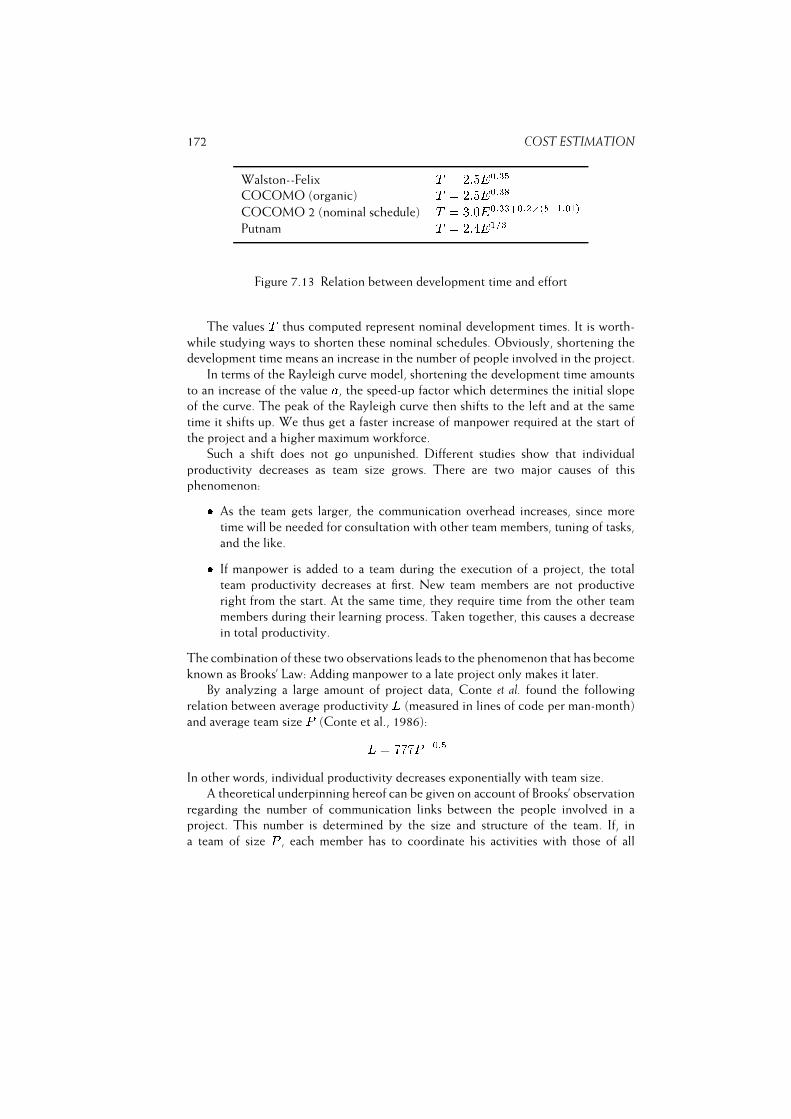
172 COST ESTIMATION

Walston--Felix T = 2:5E0:35COCOMO (organic) T = 2:5E0:38COCOMO 2 (nominal schedule) T = 3:0E0:33+0:2�(b�1:01)Putnam T = 2:4E1=3

Figure 7.13 Relation between development time and effort

The values T thus computed represent nominal development times. It is worth-

while studying ways to shorten these nominal schedules. Obviously, shortening the

development time means an increase in the number of people involved in the project.

In terms of the Rayleigh curve model, shortening the development time amounts

to an increase of the value a, the speed-up factor which determines the initial slope

of the curve. The peak of the Rayleigh curve then shifts to the left and at the same

time it shifts up. We thus get a faster increase of manpower required at the start of

the project and a higher maximum workforce.

Such a shift does not go unpunished. Different studies show that individual

productivity decreases as team size grows. There are two major causes of this

phenomenon:� As the team gets larger, the communication overhead increases, since more

time will be needed for consultation with other team members, tuning of tasks,

and the like.� If manpower is added to a team during the execution of a project, the total

team productivity decreases at first. New team members are not productive

right from the start. At the same time, they require time from the other team

members during their learning process. Taken together, this causes a decrease

in total productivity.

The combination of these two observations leads to the phenomenon that has become

known as Brooks’ Law: Adding manpower to a late project only makes it later.

By analyzing a large amount of project data, Conte et al. found the following

relation between average productivity L (measured in lines of code per man-month)

and average team size P (Conte et al., 1986):L = 777P�0:5In other words, individual productivity decreases exponentially with team size.

A theoretical underpinning hereof can be given on account of Brooks’ observation

regarding the number of communication links between the people involved in a

project. This number is determined by the size and structure of the team. If, in

a team of size P , each member has to coordinate his activities with those of all

7.4. SUMMARY 173

other members, the number of communication links is P (P � 1)=2. If each member

needs to communicate with one other member only, this number is P � 1. Less

communication than that seems unreasonable, since we would then have essentially

independent teams. (If we draw team members as nodes of a graph and communication

links as edges, we expect the graph to be connected.)

The number of communication links thus varies from roughlyP to roughlyP 2=2.

In a true hierarchical organization, this leads to P� communication paths, with1 < � < 2.

For an individual team member, the number of communication links varies from 1

to P � 1. If the maximum individual productivity is L and each communication link

results in a productivity loss l, the average productivity isL = L� l(P � 1) where , with 0 < � 1, is a measure of the number of communication links. (We

assume that there is at least one person who communicates with more than one other

person, so > 0.) For a team of size P , this leads to a total productivityLtot = P � L = P (L� l(P � 1) )For a given set of values for L, l and , this is a function which, for increasing

values of P , goes from 0 to some maximum and then decreases again. There thus is a

certain optimum team size Popt that leads to a maximum team productivity. The team

productivity for different values of the P is given in figure 7.14. Here, we assume that

individual productivity is 500 LOC=man-month (L = 500), and the productivity

loss is 10% per communication link (l = 50). With full interaction between team

members ( = 1) this results in an optimum team size of 5.5 persons.

Everything takes time. We can not shorten a software development project

indefinitely by exchanging time against people. Boehm sets the limit at 75% of the

nominal development time, on empirical grounds. A system that has to be delivered

too fast, gets into the ‘impossible region’. The chance of success becomes almost nil

if the schedule is pressed too far. See also figure 7.15.

In any case, a shorter development time induces higher costs. We may use the

following rule of thumb: compressing the development time by X% results in a cost

increase of X% relative to the nominal cost estimate (Boehm, 1984a).

7.4 Summary

It remains to be seen whether we will ever get one, general, cost estimation model.

The number of parameters that impact productivity simply seems to be too large.

Yet, each organization may develop a model which is well suited for projects to

be undertaken within that organization. An organization may, and should, build a

database with data on its own projects. Starting with a model like COCOMO 2,

the different parameters, i.e. applicable cost drivers and values for the associated

174 COST ESTIMATION

Team sizeIndividual Total

productivity productivity

1 500 500

2 450 900

3 400 1200

4 350 1400

5 300 1500

5.5 275 1512

6 250 1500

7 200 1400

8 150 1200

Figure 7.14 Impact of team size on productivity

effort multipliers, may then be determined. In the course of time, the model becomes

more closely tuned to the organizational environment, resulting in better and better

estimates. Reifer (2000) for example describes how COCOMO II can be adapted to

estimate Web-based software development projects.

Though we advocate the use of algorithmic cost estimation models, a word of

caution should be made. Present-day models of this kind are not all that good yet. At

best, they yield estimates which are at most 25% off, 75% of the time, for projects used toderive the model. For the time being, expert-based cost estimates are a viable alternative.

Even when a much better performance is realized, some problems remain when

using the type of cost estimation model obtained in this way:� Even though a model like COCOMO 2 looks objective, a fair amount of

subjectivity is introduced through the need to assign values to the various

levels of a number of cost drivers. Based on an analysis of historical project

data, (Jones, 1986) lists 20 factors which certainly influence productivity, and

another 25 for which it is probable. The set of COCOMO 2 cost drivers

already allows for a variation of 1:800. A much smaller number of relevant cost

drivers would reduce a model’s vulnerability to the subjective assessment of

project characteristics.� The models are based on data from old projects and reflect the technology of

those projects. In some cases, the project data are even fairly old. The impact

of more recent developments cannot easily be taken into account, since we do

not have sufficient data on projects which exhibit those characteristics.� Almost all models take into account attributes that impact the initial develop-

ment of software. Attributes which specifically relate to maintenance activities

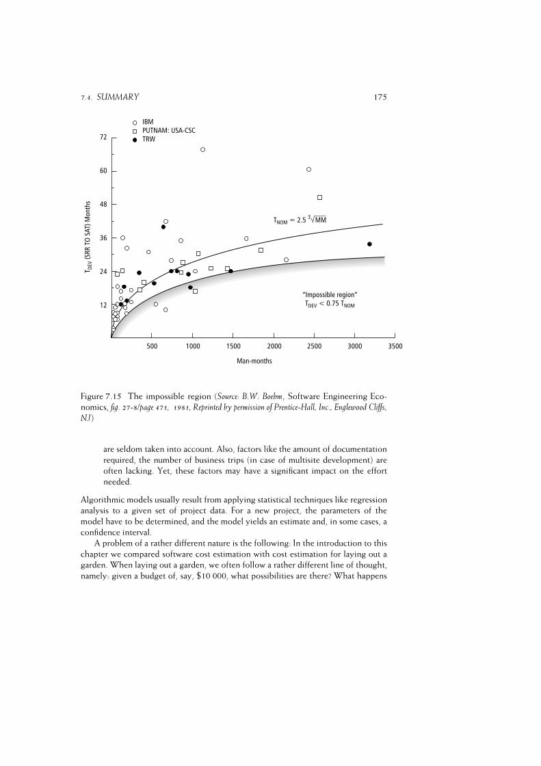
7.4. SUMMARY 175

Figure 7.15 The impossible region (Source: B.W. Boehm, Software Engineering Eco-

nomics, fig. 27-8/page 471, 1981, Reprinted by permission of Prentice-Hall, Inc., Englewood Cliffs,

NJ)

are seldom taken into account. Also, factors like the amount of documentation

required, the number of business trips (in case of multisite development) are

often lacking. Yet, these factors may have a significant impact on the effort

needed.

Algorithmic models usually result from applying statistical techniques like regression

analysis to a given set of project data. For a new project, the parameters of the

model have to be determined, and the model yields an estimate and, in some cases, a

confidence interval.

A problem of a rather different nature is the following: In the introduction to this

chapter we compared software cost estimation with cost estimation for laying out a

garden. When laying out a garden, we often follow a rather different line of thought,

namely: given a budget of, say, $10 000, what possibilities are there? What happens

176 COST ESTIMATION

if we trade off a pond against something else?

Something similar is also possible with software. Given a budget of $100 000 for

library automation, what possibilities are there? Which user interface can we expect,

what will the transaction speed be, how reliable will the system be? To be able to

answer this type of question, we need to be able to analyze the sensitivity of an

estimate to varying values of relevant attributes. Given the uncertainty about which

attributes are relevant to start with, this trade-off problem is still largely unsolved.

Finally, estimating the cost of a software development project is a highly dynamic

activity. Not only may we switch from one model to another during the course of a

project, estimates will also be adjusted on the basis of experiences gained. Switching

to another model during the execution of a project is possible, since we may expect

to get more reliable data while the project is making progress. We may, for instance,

imagine using the series of increasingly detailed COCOMO 2 models.

We cannot, and should not, rely on a one-shot statistical cost estimate. Controlling

a software development project implies a regular check of progress, a regular check of

estimates made, re-establishing priorities and weighing stakes, as the project is going

on.

7.5 Further Reading

Early cost estimation models are described in (Nelson, 1966) and (Wolverton, 1974).

The Walston--Felix model is described in (Walston and Felix, 1977). The model of

Putnam and Norden is described in (Norden, 1970), (Putnam, 1978). (Boehm, 1981)

is the definitive source on the original COCOMO model. COCOMO 2 is described

in (Boehm et al., 1995) and (Boehm et al., 1997).

Function point analysis (FPA) is developed by Albrecht (Albrecht, 1979; Albrecht

and Gaffney, 1983). Critical appraisals of FPA can be found in (Symons, 1988),

(Kemerer, 1993), (Kemerer and Porter, 1992), (Abran and Robillard, 1992) and

(Abran and Robillard, 1996). A detailed discussion of function points, its counting

process and some case studies, is provided by (Garmus and Herron, 1996).

The relation between project behavior and its cost estimate is discussed in

(Abdel-Hamid et al., 1993). Guidelines for cost estimation are given in (Boehm and

Sullivan, 1999), (Fairley, 2002) and (Jørgensen, 2005). (Software, 2000) is a special

issue devoted to software estimation.

Exercises

1. In which ways may political arguments influence cost estimates?

2. What does the Walston--Felix model look like?

3. How may the Rayleigh-curve be related to software cost estimation?

7.5. FURTHER READING 177

4. Give a sketch of Function Point Analysis (FPA).

5. Give a sketch of COCOMO 2.

6. Discuss the major differences between COCOMO 2 and FPA.

7. Give a rationale for Brooks’ Law.

8. In which sense does Function Point Analysis (FPA) reflect the batch-oriented

world of the 1970s?

9. How may early cost estimates influence the way in which a project is

executed?

10. Why is it difficult to compare different cost estimation models?

11. Suppose you are involved in a project which is estimated to take 100 man-

months. How would you estimate the nominal calendar time required for this

project? Suppose the project is to be finished within six calendar months. Do

you think such a schedule compression is feasible?

12. Why should software cost models be recalibrated from time to time?

13. �How would you calibrate the COCOMO 2 model to fit software develop-

ment in your organization?

14. ~ Suppose you are managing a project which is getting behind schedule.

Possible actions include: renegotiating the time schedule, adding people to

the project, and renegotiating quality requirements. In which ways can these

actions shorten the time schedule? Can you think of other ways to finish the

project on time?

15. ~ Suppose you have a LOC-based cost estimation model available whose

parameters are based on projects from your own organization that used

COBOL as the implementation language. Can you use this model to estimate

the cost of a project whose implementation language is Pascal? What if the

model is based on projects that used C?

16. ~ Can you give an intuitive rationale for the values of the COCOMO 2 cost

drivers (figure 7.11) that relate to project attributes?

8

Project Planning and Control

LEARNING OBJECTIVES� To appreciate looking at project control from a system point of view� To be aware of typical project situations, and ways in which projects can be

successfully dealt with in such situations� To understand how risks can be prevented from becoming problems� To know techniques for the day-to-day planning and control of software

development projects

8.1. A SYSTEMS VIEW OF PROJECT CONTROL 179

In this chapter I try to reconcile the various approaches sketched in chapters

3--7. A taxonomy of software development projects is given, together with

recommended management practices for dealing with such projects. The

chapter also deals with risk management and some well-known techniques for

project planning and control.

Software development projects differ widely. These differences are reflected in

the ways in which these projects are organized and managed. For some projects,

the budget is fixed and the goal of the project is to maximize the quality of

the end product. For others, quality constraints are fixed in advance, and the

goal is to produce effectively a system that meets those quality constraints. If the

developing organization has considerable experience with the application domain

and the requirements are fixed and stable, a tightly structured approach may yield

a satisfactory solution. In applications with fuzzy requirements and little previous

experience in the development team, a more agile approach may be desirable.

It is important to identify those project characteristics early on, because they

will influence the way a project is organized, planned and controlled. In section 8.1,

we will discuss project control from a systems point of view. This allows us to

identify the major dimensions along which software development projects differ.

These dimensions lead to a taxonomy of software development projects, which will

be discussed in section 8.2. For each of the project categories distinguished, we will

indicate how best to control the various entities identified in previous chapters. This

type of assessment is to be done at the project planning stage.

This assessment links global risk categories to preferred control situations. Daily

practice, however, is more complex. An actual project faces many risks, each of

which has to be handled in turn. Even risks for which we hoped to have found an

adequate solution, may turn into problems later on. Risk factors therefore have to

be monitored, and contingency plans have to be developed. The early identification

of risks and the development and carrying out of strategies to mitigate these risks is

known as risk management. Risk management is discussed in section 8.3.

Software development projects consist of a number of interrelated tasks. Some

of these will have to be handled sequentially (a module cannot be tested until it has

been implemented), while others may be handled in parallel (different modules can

be implemented concurrently). The dependencies between tasks can be depicted in

a network from which a project schedule can be derived. These and similar tools for

the micro-level planning and control of software development projects are discussed

in section 8.4.

8.1 A Systems View of Project Control

In the preceding chapters, we discussed several entities that need to be controlled.

During the execution of a software development project, each of these entities needs

180 PROJECT PLANNING AND CONTROL

to be monitored and assessed. From time to time, adjustments will have to be made.

To be able to do so, we must know which entities can be varied, how they can be

varied, and what the effect of adjustments is.

To this end, we will consider project control from a systems point of view. We

now consider the software development project itself as a system. Project control

may then be described in terms of:

– the system to be controlled, i.e. the software development project;

– the entity that controls the system, i.e. the project manager, his organization

and the decision rules he uses;

– information which is used to guide the decision process. This information may

come from two sources. It may either come from the system being controlled

(such as a notice of technical problems with a certain component) or it may

have a source outside the system (such as a request to shorten development

time).

The variables that play a role in controlling a system may be categorized into three

classes: irregular variables, goal variables, and control variables.

Irregular variables are those variables that are input to the system being controlled.

Irregular variables cannot be varied by the entity that controls the system. Their

values are determined by the system’s environment. Examples of irregular variables

are the computer experience of the user or the project staffing level.

An important precondition for effective control is knowledge of the project’s

goals. In developing software, various conflicting goals can be distinguished. One

possible goal is to minimize development time. Since time is often pressing, this goal is not

unusual. Another goal might be to maximize efficiency, i.e. development should be done

as cheaply as possible. Optimal use of resources (mostly manpower) is then needed.

Yet a third possible goal is to maximize quality. Each of these goals is possible, but

they can be achieved only if it is known which goals are being pursued. These goals

collectively make up the set of goal variables.

Finally, the decision process is guided by the set of control variables. Control

variables are entities which can be manipulated by the project manager in order to

achieve the goals set forth. Examples of possible control variables are the tools to be

used, project organization, efficiency of the resulting software.

It is not possible to make a rigid separation between the various sets of variables.

It depends on the situation at hand whether a particular variable should be taken as

an irregular variable, goal variable, or control variable. If the requirements are stable

and fixed, one may for instance try to control the project by employing adequate

personnel and using a proper set of tools. For another project, manpower may be

fixed and one may try to control the project by extending the delivery date, relaxing

quality constraints, etc.

However, in order to be able to control a project, the different sets of variables

must be known. It must be known where control is, and is not, possible. This is only

8.2. A TAXONOMY OF SOFTWARE DEVELOPMENT PROJECTS 181

one prerequisite, though. In systems theory, the following conditions for effective

control of a system are used:

– the controlling entity must know the goals of the system;

– the controlling entity must have sufficient control variety;

– the controlling entity must have information on the state, input and output of

the system;

– the controlling entity must have a conceptual control model. It must know how

and to what extent the different variables depend on and influence each other.

When all these conditions are met, control can be rational, in which case there is no

uncertainty, since the controlling entity is completely informed about every relevant

aspect. The control problem can then be structured and formalized. Daily practice of

software development is different, though. There is insufficient room for control or

the effect of control actions is not known. Control then becomes much more intuitive

or primitive. It is based on intuition, experience, and rules of thumb.

The degree to which a software development project can be controlled increases

as the control variety increases. This control variety is determined by the number of

control variables and the degree to which they can be varied. As noticed before, the

control variety is project dependent.

Controlling software development means that we must be able to measure both

the project and the product. Measuring a project means that we must we able to

assess progress. Measuring a product means that we must be able to determine the

degree to which quality and functional requirements are being met.

Controlling software development projects implies that effective control actions

are possible. Corrective actions may be required if progress is not sufficient or the

software does not comply with its requirements. Effective control means that we

know what the effect of control actions is. If progress is insufficient and we decide to

allocate extra manpower, we must understand the impact of this extra manpower on

the time schedule. If the quality of a certain component is less than required and we

decide to allocate extra test time, we must know how much test time is required in

order to achieve the desired quality.

In practice, controlling a software development project is not a rational process.

The ideal systems theory situation is not met. There are a number of uncertainties

which make managing such projects a challenging activity. Below, we will discuss a

few idealized situations, based on the uncertainty of various relevant aspects.

8.2 A Taxonomy of Software Development Projects

In the preceding section, we identified several conditions that need to be satisfied

in order to be able to control projects rationally. Since these conditions are often

not met, we will have to rely on a different control mechanism in most cases. The

182 PROJECT PLANNING AND CONTROL

control mechanism best suited to any given situation obviously depends on relevant

characteristics of the project at hand.

Based on an analysis of software development project characteristics that are

important for project control, we will distinguish several project situations, and

indicate how projects can successfully be controlled in these situations.

We will group project characteristics into three classes: product characteristics,

process characteristics, and resource characteristics. From the point of view of project

control, we are interested in the degree of certainty of those characteristics. For

example, if we have clear and stable user requirements, product certainty is high.

If part of the problem is to identify user requirements, or the user requirements

frequently change during the development project, product certainty is low.

If product certainty is high, control can be quite rational, insofar as it depends on

product characteristics. Since we know what the product is supposed to accomplish,

we may check compliance with the requirements and execute corrective actions if

needed. If product certainty is low, this is not feasible. We either do not know what

we are aiming at, or the target is constantly moving. It is only reasonable to expect

that control will be different in those cases.

For the present discussion, we are interested only in project characteristics that

may differ between projects. Characteristics common to most or all of software

development projects, such as the fact that they involve teamwork, will not lead to

different control paradigms.

We will furthermore combine the characteristics from each of the three categories

identified above, into one metric, the certainty of the corresponding category. This

leaves us with three dimensions along which software development projects may

differ:� Product certainty Product certainty is largely determined by two factors:

whether or not user requirements are clearly specified, as regards both func-

tionality and quality, and the volatility of those user requirements. Other

product characteristics are felt to have a lesser impact on our understanding of

what the end-product should accomplish.� Process certainty The degree of (development) process certainty is determined

by such factors as: the possibility of redirecting the development process, the

degree to which the process can be measured and the knowledge we have about

the effect of control actions, and the degree to which new, unknown tools are

being used.� Resource certainty The major determinant here is the availability of the

appropriate qualified personnel.

If we allow each of these certainty factors to take one of two values (high and low), we

get eight control situations, although some of them are not very realistic. If we have

little or no certainty about the software to be developed, we can hardly expect to be

certain about the process to be followed and the resources needed to accomplish our

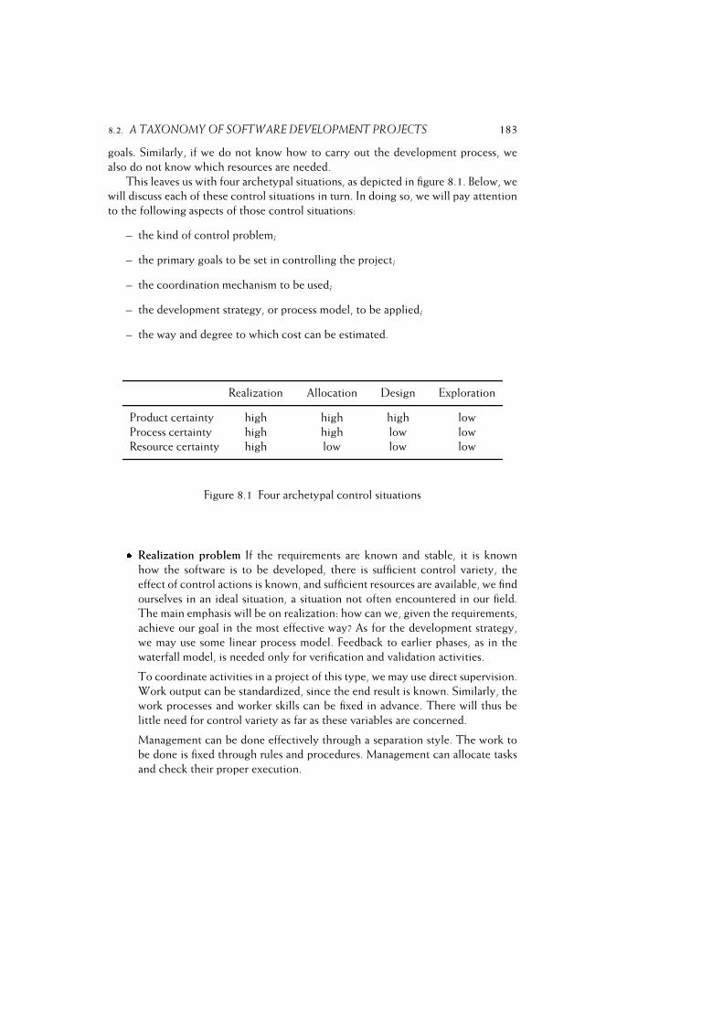
8.2. A TAXONOMY OF SOFTWARE DEVELOPMENT PROJECTS 183

goals. Similarly, if we do not know how to carry out the development process, we

also do not know which resources are needed.

This leaves us with four archetypal situations, as depicted in figure 8.1. Below, we

will discuss each of these control situations in turn. In doing so, we will pay attention

to the following aspects of those control situations:

– the kind of control problem;

– the primary goals to be set in controlling the project;

– the coordination mechanism to be used;

– the development strategy, or process model, to be applied;

– the way and degree to which cost can be estimated.

Realization Allocation Design Exploration

Product certainty high high high low

Process certainty high high low low

Resource certainty high low low low

Figure 8.1 Four archetypal control situations� Realization problem If the requirements are known and stable, it is known

how the software is to be developed, there is sufficient control variety, the

effect of control actions is known, and sufficient resources are available, we find

ourselves in an ideal situation, a situation not often encountered in our field.

The main emphasis will be on realization: how can we, given the requirements,

achieve our goal in the most effective way? As for the development strategy,

we may use some linear process model. Feedback to earlier phases, as in the

waterfall model, is needed only for verification and validation activities.

To coordinate activities in a project of this type, we may use direct supervision.

Work output can be standardized, since the end result is known. Similarly, the

work processes and worker skills can be fixed in advance. There will thus be

little need for control variety as far as these variables are concerned.

Management can be done effectively through a separation style. The work to

be done is fixed through rules and procedures. Management can allocate tasks

and check their proper execution.

184 PROJECT PLANNING AND CONTROL

As for cost estimation, we may successfully use one of the more formalized

cost models. Alternatively, experts in the domain may give a reliable estimate.

A cost estimation thus obtained can be used to guard the project’s progress and

yields a target to be achieved.� Allocation problem This situation differs from the previous one in that there is

uncertainty as regards the resources. The major problem then becomes one of

the availability of personnel. Controlling a project of this kind tends to become

one of controlling capacity. The crucial questions become: How do we get

the project staffed? How do we achieve the desired end-product with limited

means?

According to Mintzberg, one has to try to standardize the process as far as

possible in this case. This makes it easier to move personnel between tasks.

Guidelines and procedures may be used to describe how the various tasks have

to be carried out.

As regards the development strategy, we may again opt for the waterfall model.

We may either contract out the work to be done, or try to acquire the right

type and amount of qualified personnel.

As for cost estimation, either some cost estimation model or expert estimates

can be used. Since there is uncertainty as regards resources, there is a need for

sensitivity analyses in order to gain insight into such questions as: What will

happen to the total cost and development time if we allocate three designers

of level A rather than four designers of level B?� Design problem If the requirements are fixed and stable, but we do not know

how to carry out the process, nor which resources to employ, the problem is

one of design. Note that the adjective design refers to the design of the project,

not the design of the software. We have to answer such questions as: which

milestones are to be identified, which documents must be delivered and when,

what personnel must be allocated, how will responsibilities be assigned?

In this situation, we have insufficient knowledge of the effect of allocating extra

personnel, other tools, different methods and techniques. The main problem

then becomes one of controlling the development process.

In Mintzberg’s classification, this can best be pursued through standardization

of work outputs. Since the output is fixed, control should be done through the

process and the resources. The effect of such control actions is not sufficiently

known, however.

In order to make a project of this kind manageable, one needs overcapacity. As

far as the process is concerned, this necessitates margins in development time

and budget. Keeping extra personnel is not feasible, in general.

In these situations, we will need frequently to measure progress towards the

project’s goals in order to allow for timely adjustments. Therefore, we may want

8.2. A TAXONOMY OF SOFTWARE DEVELOPMENT PROJECTS 185

to go from a linear development model to an incremental one. This preference

will increase as the uncertainty increases.

Cost estimation will have to rely on past experience. We will usually not have

enough data to use one of the more formalized cost estimation models. In

this situation too, we will need sensitivity analyses. This need will be more

pressing than in the previous situation, since the uncertainty is greater. The

project manager will be interested in the sensitivity of cost estimates to certain

cost drivers. He might be interested in such questions as: what will happen to

the development schedule if two extra analysts are assigned to this project, or:

what will the effect be on the total cost if we shorten the development time byx days? By viewing cost estimation in this way, the manager will gain insight

to, and increase his feeling for, possible solution strategies.� Exploration problem If the product certainty, process certainty and resource

certainty are all low, we get the most difficult control situation.

Because of these uncertainties, the work will be exploratory in nature. This

situation does not fit a coordination mechanism based on standardization.

In a situation as complex and uncertain as this one, coordination can best be

achieved through mutual adjustment. The structure is one of adhocracy. Experts

from various disciplines work together to achieve some as yet unspecified goal.

A critical success factor in these cases is the commitment of all people involved.

Work cannot be split up into neat tasks. Flexibility in work patterns and work

contents is important. Adherence to a strict budget cannot be enforced upon

the team from above. The team members must commit themselves to the

project. Management has to place emphasis on their relations with the team

members.

Controlling a project of this kind is a difficult and challenging activity. To

make a project of this kind manageable, our goal will be to maximize output,

given the resources available to the project. This maximization may concern

the quality of the product, or its functionality, or both.

Since requirements are not precisely known, some agile approach is appropriate

as a process model. The larger the uncertainty, the more often we will have

to check whether we are still on the right track. Thus, some development

strategy involving many small steps and frequent user feedback is to be used.

Cost estimation using some formalized model clearly is not feasible in these

circumstances. The use of such models presupposes that we know enough of

the project at hand to be able to compare it with previous projects. Such is not

the case, though.

We may rely on expert judgments to achieve a rough cost estimate. Such a

cost estimate, however, cannot and should not be used as a fixed anchor point

as to when the project should be finished and how much it may cost. There

are simply too many uncertainties involved. Rather, it provides us with some

186 PROJECT PLANNING AND CONTROL

guidance as to the magnitude of the project. Based on this estimate, effort

and time can be allocated for the project, for instance to produce a certain

number of prototypes, a feasibility study, a pilot implementation of part of the

product, or to start a certain number of time boxes. The hope is that in time

the uncertainties will diminish sufficiently so that the project shifts to one of

the other situations.

The four control situations discussed above are once more depicted in figure 8.2,

together with a short characterization of the various control aspects discussed above.

For big projects, it may be effective to use different control mechanisms at the

macro and micro level, respectively (Karlstrom and Runeson, 2005). At the macro

level, management may have to coordinate the work of different teams, and report

to higher management. This may require an approach in which explicit stages and

corresponding milestones are distinguished. At the level of a small subteam though,

one may still apply agile methods to control the day-to-day work.

By taking the different control aspects into account during the planning stage of a

software development project, we can tailor the project’s management to the situation

at hand. In doing so, we recognize that software development projects are not all

alike. Neglecting those project-specific characteristics is likely to result in project

failures, failures that have often been reported upon in the literature, but equally often

remain hidden from the public at large.

8.3 Risk Management

Risk management is project management for adults

Tim Lister

In the previous section, we identified global risk categories and tied them to preferred

control situations. In this section, the emphasis is on individual risks and their

management during project execution. In some sense too, the discussion below takes

a more realistic point of view, in that we also consider adverse situations such as

unrealistically tight schedules and design gold plating.

Potential risks of a project must be identified as early as possible. It is rather naive

to suppose that a software project will run smoothly from start to finish. It won’t. We

should identify the risks of a software project early on and provide measures to deal

with them. Doing so is not a sign of unwarranted pessimism. Rather, it is a sign of

wisdom.

In software development, we tend to ignore risks. We assume an optimistic

scenario under all circumstances and we do not reserve funds for dealing with risks.

We rely on heroics when chaos sets in. If risks are identified at all, their severity

is often underestimated, especially by observers higher in the hierarchy. A designer

may have noticed that a certain subsystem poses serious performance problems. His

manager assumes that the problem can be solved. His manager’s manager assumes the

problem has been solved.

8.3. RISK MANAGEMENT 187

Problem type Realization Allocation Design Exploration

Product certainty high high high low

Process certainty high high low low

Resource certaintyhigh low low low

Primary goal Optimize Acquisition, Control of the Maximize

in control resource usage training of process result

Efficiency personnel Lower risks

and schedule

Coordination, Standardization Standardization Standardization Mutual

Management of product, of product and of process adjustment

style process, and process Commitment

resources Relation style

Hierarchy,

separation style

Development Waterfall Waterfall Incremental Incremental

strategy Prototyping

Agile

Cost estimation Models Models Expert estimate Expert estimate

Guard process Sensitivity Sensitivity Risk analysis

analysis analysis Provide

guidance

Figure 8.2 Four control situations (After: F.J. Heemstra, How much does software cost,

Kluwer Bedrijfswetenschappen, 1989.)

A risk is a possible future negative event that may affect the success of an effort.

So, a risk is not a problem, yet. It may become one, though, and risk management is

concerned with preventing risks from becoming problems. Some common examples of

risks and ways to deal with them, are:� Requirements may be unstable, immature, unrealistic, or excessive. If we merely

list the requirements and start to realize the system in a linear development

mode, it is likely that a lot of rework will be needed. This results in schedule

and budget overruns, since this rework was not planned. If the requirements

volatility is identified as a major risk, an evolutionary development strategy can

be chosen. This situation fits the exploration-problem category as identified in

the previous section.

188 PROJECT PLANNING AND CONTROL� If there is little or no user involvement during the early development stages, a

real danger is that the system will not meet user needs. If this is identified as a

risk, it can be mitigated, e.g. by having users participate in design reviews.� If the project involves different or complex domains, the spread of application

knowledge within the project team may be an issue. Recognizing this risk

may result in timely attention and resources for a training program for team

members.� If the project involves more than one development site, communication

problems may arise. A common way to deal with this is to pay attention to

socialization issues, for instance by scheduling site visits.

At the project planning stage, risks are identified and handled. A risk management

strategy involves the following steps:

1. Identify the risk factors. There are many possible risk factors. Each organization

may develop its own checklist of such factors. The top ten risk factors from

(Boehm, 1989) are listed in figure 8.3.

2. Determine the risk exposure. For each risk, we have to determine the probabilityp that it will actually occur and the effect E (e.g. in dollars or loss of man

months) that it will have on the project. The risk exposure then equals p�E.

3. Develop strategies to mitigate the risks. Usually, this will only be done for theN risks that have the highest risk exposure, or for those risks whose exposure

exceeds some threshold �.

There are three general strategies to mitigate risks: avoidance, transfer, and

acceptance. We may avoid risks by taking precautions so that they will not

occur: buy more memory, assign more people, provide for a training program

for team members, and the like. We may transfer risks by looking for another

solution, such as a prototyping approach to handle unstable requirements.

Finally, we may accept risks. In the latter case, we have to provide for a

contingency plan, to be invoked when the risk does become a problem.

4. Handle risks. Risk factors must be monitored. For some risks, the avoidance or

transfer actions may succeed, and those risks will never become a problem. We

may be less lucky for those risks that we decided up front not to handle. Also,

some of our actions may turn out to be less successful, and risks that we hoped

to have handled adequately may become a problem after all. Finally, project

characteristics will change over time, and so will the risks. Risk management

thus is a cyclic process, and occasionally risks must be handled by re-assessing

the project, invoking a contingency plan, or even a transfer to crisis mode.

Wallace and Keil (2004) give a useful categorization of risk factors. They distinguish

four types of risk (see also figure 8.4):

8.3. RISK MANAGEMENT 189

Risk Description

Personnel shortfall May manifest itself in a variety of ways, such

as inexperience with the domain, tools or

development techniques to be used, person-

nel turnover, loss of critical team members,

or the mere size of a team.

Unrealistic schedule/budget Estimates may be unrealistic with respect to

the requirements.

Wrong functionality May have a variety of causes, such as an

imperfect understanding of the customer

needs, the complexity of communication

with the client, insufficient domain knowl-

edge of the developers and designers.

Wrong user interface In certain situations, the user-friendliness of

the interface is critical to its success.

Gold plating Developers may wish to develop ‘nice’ fea-

tures not asked for by the customer.

Requirements volatility If many requirements change during devel-

opment, the amount of rework increases.

Bad external components The quality or functionality of externally

supplied components may be below what is

required for this project.

Bad external tasks Subcontractors may deliver inadequate prod-

ucts, or the skills obtained from outside the

team may be inadequate.

Real-time shortfalls The real-time performance of (parts of) the

system may be inadequate.

Capability shortfalls An unstable environment or new or untried

technology pose a risk to the development

schedule.

Figure 8.3 Top ten risk factors� C1: Risks related to customers and users. Examples include a lack of user

participation, conflicts between users, or a user organization resisting change.

Part of this can be mitigated through an agile approach. But equally often, such

risks are beyond the project manager’s control.

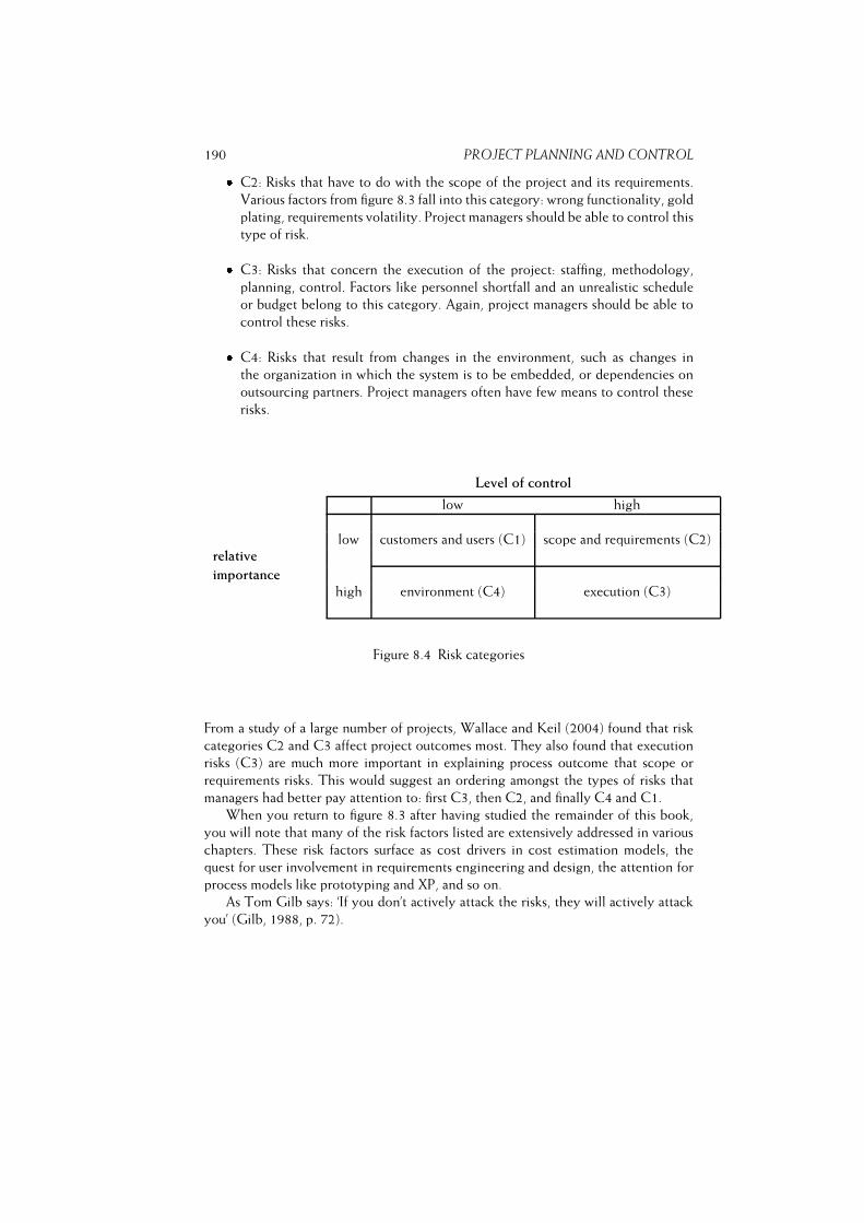
190 PROJECT PLANNING AND CONTROL� C2: Risks that have to do with the scope of the project and its requirements.

Various factors from figure 8.3 fall into this category: wrong functionality, gold

plating, requirements volatility. Project managers should be able to control this

type of risk.� C3: Risks that concern the execution of the project: staffing, methodology,

planning, control. Factors like personnel shortfall and an unrealistic schedule

or budget belong to this category. Again, project managers should be able to

control these risks.� C4: Risks that result from changes in the environment, such as changes in

the organization in which the system is to be embedded, or dependencies on

outsourcing partners. Project managers often have few means to control these

risks.

Level of control

low high

relative

importance

low customers and users (C1) scope and requirements (C2)

high environment (C4) execution (C3)

Figure 8.4 Risk categories

From a study of a large number of projects, Wallace and Keil (2004) found that risk

categories C2 and C3 affect project outcomes most. They also found that execution

risks (C3) are much more important in explaining process outcome that scope or

requirements risks. This would suggest an ordering amongst the types of risks that

managers had better pay attention to: first C3, then C2, and finally C4 and C1.

When you return to figure 8.3 after having studied the remainder of this book,

you will note that many of the risk factors listed are extensively addressed in various

chapters. These risk factors surface as cost drivers in cost estimation models, the

quest for user involvement in requirements engineering and design, the attention for

process models like prototyping and XP, and so on.

As Tom Gilb says: ‘If you don’t actively attack the risks, they will actively attack

you’ (Gilb, 1988, p. 72).

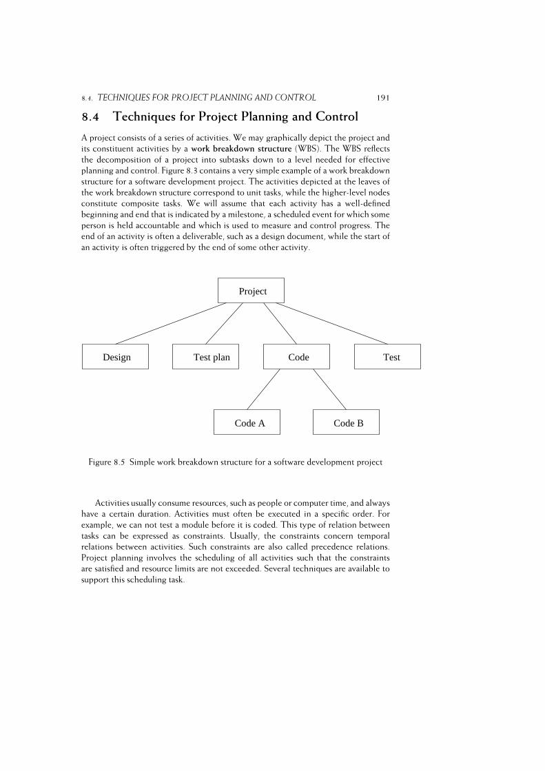
8.4. TECHNIQUES FOR PROJECT PLANNING AND CONTROL 191

8.4 Techniques for Project Planning and Control

A project consists of a series of activities. We may graphically depict the project and

its constituent activities by a work breakdown structure (WBS). The WBS reflects

the decomposition of a project into subtasks down to a level needed for effective

planning and control. Figure 8.3 contains a very simple example of a work breakdown

structure for a software development project. The activities depicted at the leaves of

the work breakdown structure correspond to unit tasks, while the higher-level nodes

constitute composite tasks. We will assume that each activity has a well-defined

beginning and end that is indicated by a milestone, a scheduled event for which some

person is held accountable and which is used to measure and control progress. The

end of an activity is often a deliverable, such as a design document, while the start of

an activity is often triggered by the end of some other activity.

Project

Design Test plan Code Test

Code A Code B

Figure 8.5 Simple work breakdown structure for a software development project

Activities usually consume resources, such as people or computer time, and always

have a certain duration. Activities must often be executed in a specific order. For

example, we can not test a module before it is coded. This type of relation between

tasks can be expressed as constraints. Usually, the constraints concern temporal

relations between activities. Such constraints are also called precedence relations.

Project planning involves the scheduling of all activities such that the constraints

are satisfied and resource limits are not exceeded. Several techniques are available to

support this scheduling task.

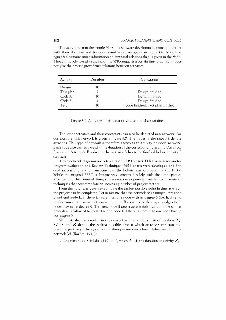
192 PROJECT PLANNING AND CONTROL

The activities from the simple WBS of a software development project, together

with their duration and temporal constraints, are given in figure 8.6. Note that

figure 8.6 contains more information on temporal relations than is given in the WBS.

Though the left-to-right reading of the WBS suggests a certain time ordering, it does

not give the precise precedence relations between activities.

Activity Duration Constraints

Design 10 --

Test plan 5 Design finished

Code A 10 Design finished

Code B 5 Design finished

Test 10 Code finished, Test plan finished

Figure 8.6 Activities, their duration and temporal constraints

The set of activities and their constraints can also be depicted in a network. For

our example, this network is given in figure 8.7. The nodes in the network denote

activities. This type of network is therefore known as an ‘activity-on-node’ network.

Each node also carries a weight, the duration of the corresponding activity. An arrow

from node A to node B indicates that activity A has to be finished before activity B

can start.

These network diagrams are often termed PERT charts. PERT is an acronym for

Program Evaluation and Review Technique. PERT charts were developed and first

used successfully in the management of the Polaris missile program in the 1950s.

While the original PERT technique was concerned solely with the time span of

activities and their interrelations, subsequent developments have led to a variety of

techniques that accommodate an increasing number of project factors.

From the PERT chart we may compute the earliest possible point in time at which

the project can be completed. Let us assume that the network has a unique start node

B and end node E. If there is more than one node with in-degree 0 (i.e. having no

predecessors in the network), a new start node B is created with outgoing edges to all

nodes having in-degree 0. This new node B gets a zero weight (duration). A similar

procedure is followed to create the end node E if there is more than one node having

out-degree 0.

We next label each node i in the network with an ordered pair of numbers (Si,Fi). Si and Fi denote the earliest possible time at which activity i can start and

finish, respectively. The algorithm for doing so involves a breadth-first search of the

network (cf. (Boehm, 1981)):

1. The start node B is labeled (0, DB), where DB is the duration of activity B;

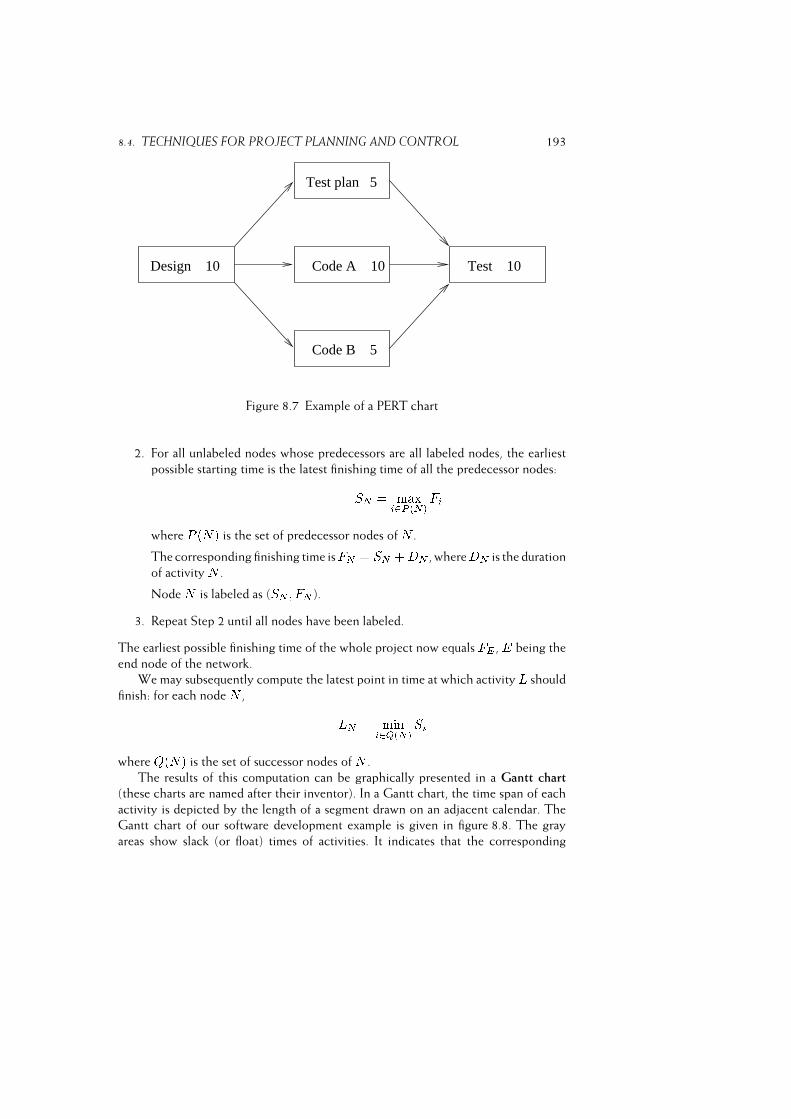
8.4. TECHNIQUES FOR PROJECT PLANNING AND CONTROL 193

Design 10

Test plan 5

Code A 10

Code B 5

Test 10

Figure 8.7 Example of a PERT chart

2. For all unlabeled nodes whose predecessors are all labeled nodes, the earliest

possible starting time is the latest finishing time of all the predecessor nodes:SN = maxi2P (N)Fiwhere P (N) is the set of predecessor nodes of N .

The corresponding finishing time isFN = SN +DN , whereDN is the duration

of activity N .

Node N is labeled as (SN ; FN ).

3. Repeat Step 2 until all nodes have been labeled.

The earliest possible finishing time of the whole project now equals FE , E being the

end node of the network.

We may subsequently compute the latest point in time at which activity L should

finish: for each node N , LN = mini2Q(N)Siwhere Q(N) is the set of successor nodes of N .

The results of this computation can be graphically presented in a Gantt chart

(these charts are named after their inventor). In a Gantt chart, the time span of each

activity is depicted by the length of a segment drawn on an adjacent calendar. The

Gantt chart of our software development example is given in figure 8.8. The gray

areas show slack (or float) times of activities. It indicates that the corresponding

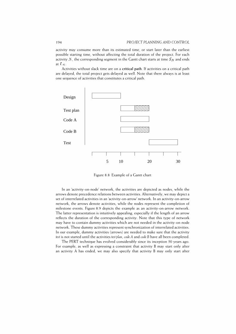
194 PROJECT PLANNING AND CONTROL

activity may consume more than its estimated time, or start later than the earliest

possible starting time, without affecting the total duration of the project. For each

activity N , the corresponding segment in the Gantt chart starts at time SN and ends

at LN .

Activities without slack time are on a critical path. If activities on a critical path

are delayed, the total project gets delayed as well. Note that there always is at least

one sequence of activities that constitutes a critical path.

������������

������������

������������

������������

Design

Test plan

Code A

Code B

Test

10 205 30

Figure 8.8 Example of a Gantt chart

In an ‘activity-on-node’ network, the activities are depicted as nodes, while the

arrows denote precedence relations between activities. Alternatively, we may depict a

set of interrelated activities in an ‘activity-on-arrow’ network. In an activity-on-arrow

network, the arrows denote activities, while the nodes represent the completion of

milestone events. Figure 8.9 depicts the example as an activity-on-arrow network.

The latter representation is intuitively appealing, especially if the length of an arrow

reflects the duration of the corresponding activity. Note that this type of network

may have to contain dummy activities which are not needed in the activity-on-node

network. These dummy activities represent synchronization of interrelated activities.

In our example, dummy activities (arrows) are needed to make sure that the activity

test is not started until the activities test plan, code A and code B have all been completed.

The PERT technique has evolved considerably since its inception 50 years ago.

For example, as well as expressing a constraint that activity B may start only after

an activity A has ended, we may also specify that activity B may only start after

8.4. TECHNIQUES FOR PROJECT PLANNING AND CONTROL 195

Design Code A

Code B

10

Test plan5

Test10

5

10

Figure 8.9 An activity-on-arrow network

activity A has started. We may also extend the technique so that it handles resource

constraints. For instance, if we have only one programmer available, the Gantt chart

of figure 8.6 would not work, since it assumes that coding of modules A and B is done

in parallel. The PERT technique may even be extended further to allow for sensitivity

analysis. By allowing so-called ‘what-if’ questions (‘what if we allocate three designers

rather than four’, ‘what if coding module A takes two months rather than one’) we

get a feeling for the sensitivity of a schedule to certain variations in resource levels,

schedule overruns, and the like.

Critical Path Method -- CPM -- is, as the name suggests, a technique very similar

to PERT and developed at around the same time.

In our discussion, we presented a Gantt chart as a graphical visualization of a

schedule that results from network analysis. Actually, we may use a Gantt chart as a

scheduling mechanism in its own right. We may simply list all activities and indicate

their earliest starting time and latest ending time on the calendar. Gantt charts by

themselves, however, do not carry information on dependencies between activities.

This makes it hard to adjust schedules, for instance when a certain activity slips. As far

as planning goes, we therefore prefer the use of Gantt charts as a means to visualize

the result of network analysis.

Using the information contained in the Gantt chart and knowledge of personnel

resources required for each activity, we may establish a personnel plan indicating how

many people are required in each unit of time. Since people costs are a major part

of project expenditures, this personnel plan provides a direct means to plan project

expenditures.

When the project is under way, its control is based on monitoring the project’s

progress and expenditures. Time spent per activity per project member can be

recorded on time cards. These time cards are the basis for determining cumulative

effort and expenditure. These cumulative data can be compared with the planned

levels of effort and expenditure. In order to properly judge whether the project is still

on track, management needs progress information as well. The most common way to

provide this is via milestone reports: activities cannot be considered completed until

196 PROJECT PLANNING AND CONTROL

a proper report has been produced and accepted.

The Gantt chart provides a very direct means to compare actual project status

with the project schedule. Schedule slippage shows itself immediately. Slippage of

activities on a critical path then necessitates prompt management action: renegotiation

of the schedule, the project’s deliverables, or both. Note that schedule slippage is a

sneaky affair; projects get behind one day at a time. Note also that project schedules

should at any point in time reflect the true project. An accepted change necessitates

reconsideration of the schedule.

8.5 Summary

In this chapter we looked at project control from a systems point of view and

gained insight into how different kinds of projects can be managed and controlled.

We identified four archetypal situations, which demand different process models,

coordination mechanisms and management styles.

Real projects face many risks, and it is a wise project manager who pays attention

to them early on. A risk is a possible future negative event that may affect success.

It is not a problem yet, but it may become one. Risk management is concerned with

preventing risks from becoming problems. It involves the following steps:

1. Identify the risk factors.

2. Determine the risk exposure, i.e. the probability that a risk will happen,

multiplied by its cost.

3. Develop strategies to mitigate risks, especially those with a high risk exposure.

Risks may be avoided (e.g. by hiring more people), transferred (e.g. by choosing

a different development strategy), or accepted.

4. Handle the risks: monitor risk factors and take action when needed.

In section 8.4, we focused on the planning and control of activities within a project.

By depicting the set of activities and their temporal relations in a graph, techniques

like PERT offer simple yet powerful means to schedule and control these activities

(see, for example, (Boehm, 1981)).

8.6 Further Reading

Some general software project management sources are: (Boehm, 1981), (Brooks,

1995), (Humphrey, 1997b) and (Royce, 1998). Highsmith (2004) focusses on agile

project management, while Boehm and Turner (2003) and Karlstrom and Runeson

(2005) discuss how to combine agile and plan-based approaches.

The discussion in section 8.2 is based on (Heemstra, 1989).

8.6. FURTHER READING 197

(Boehm, 1989) gives a good overview of software risk management. Risk manage-

ment experiences are reported on in (Software, 1997a). The risk categories discussed

in section 8.3 stem from (Wallace and Keil, 2004). Pfleeger (2000) compares software

risk management with risk management in other disciplines.

Exercises

1. List the conditions for effective systems control.

2. Is the waterfall approach suitable for a realization-type problem? If so, why?

3. Is the waterfall approach suitable for an exploration-type problem? If so, why?

4. What is risk management?

5. How can risks be mitigated?

6. Rephrase the cost drivers of the COCOMO cost estimation model as risk

factors.

7. What is a work breakdown structure?

8. What is a PERT chart?

9. What is a Gantt chart?

10. � Classify a project you have been involved in with respect to product

certainty, process certainty, and resource certainty. Which of the archetypal

situations sketched in section 8.2 best fits this project? In what ways did

actual project control differ from that suggested for the situation identified?

Can you explain possible differences?

11. ~ Consider the patient planning system mentioned in exercise 3.12. Sup-

pose the project team consists of several analysts and two members from

the hospital staff. The analysts have a lot of experience in the design of

planning systems, though not for hospitals. As a manager of this team, which

coordination mechanism and management style would you opt for?

12. ~ Discuss the pros and cons of a hierarchical as well as a matrix team

organization for the patient planning project.

13. � Consider a project you have been involved in. Identify the major irregular,

control, and goal variables for this project. In what ways did the control

variables influence project control?

14. ~ Suppose one of your team members is dissatisfied with his situation. He

has been involved in similar projects for several years now. You have assigned

198 PROJECT PLANNING AND CONTROL

him these jobs because he was performing so well. Discuss possible actions

to prevent this employee from leaving the organization.

15. ~ Why is planning (i.e., the activity) more important than the plan (the

document)?

16. ~ Suppose you are the manager of a project that is getting seriously behind

schedule. Your team is having severe problems with testing a particular

subsystem. Your client is pressing you to deliver the system on time. How

would you handle this situation? How would you handle the situation if

you were a member of the team and your manager was not paying serious

attention to your signals?

Part II

The Software Life Cycle

CONTENTS

Chapter 9 Requirements Engineering 199

Chapter 10Modeling 246

Chapter 11Software Architecture 276

Chapter 12Software Design 313

Chapter 13Software Testing 394

Chapter ?? Software Maintenance 453

Chapter ?? Software Tools 494

When designing a garden, you begin by formulating your requirements --

how large should the grass-area be, should you leave a corner to raise potatoes,

where should the sand-bin be put, do not the requirements interfere with future

maintenance work on the house (!), etc. After that, a design is drawn up which is

carefully documented in a blueprint. Only then will the gardener cut the first sod.

A similar approach is followed when developing software. In a number of phases

-- requirements engineering, design, implementation, testing -- the software system

will take shape. After the software is delivered to the client it must be maintained.

Reiteration of phases occurs because changes have to be incorporated and errors must

be corrected. The result is a highly cyclical process, the so-called software life cycle.

The various phases of the initial development cycle are the topics of chapters

9--13, and chapter 14 is devoted to software maintenance. In each phase, modeling

techniques are used to represent the results of that phase. A sample of well-known

200

modeling techniques is discussed in chapter 10. In each phase also, tools are employed.

The main classes of tools and their role in the software development process are

discussed in chapter 15.

9

Requirements Engineering

LEARNING OBJECTIVES� To understand that requirements engineering is a cyclical process involving

four types of activity: elicitation, specification, validation, and negotiation� To appreciate the role of social and cognitive issues in requirements engineering� To be able to distinguish a number of requirements elicitation techniques� To be aware of the contents of a requirements specification document� To know various techniques and notations for specifying requirements� To know different ways to structure a set of requirements

202 REQUIREMENTS ENGINEERING

This chapter covers requirements engineering, the first major phase in a

software development project. The most challenging and difficult aspect of

requirements engineering is to get a complete description of the problem

to be solved. We discuss a number of techniques for eliciting requirements

from the user. Following elicitation, these requirements must be negotiated,

validated, and documented.

The hardest single part of building a system is deciding what to build

(Brooks, 1987)

The requirements engineering phase is the first major step towards the solution of

a data processing problem. During this phase, the user’s requirements with respect

to the future system are carefully identified and documented. These requirements

concern both the functions to be provided and a number of additional requirements,

such as those regarding performance, reliability, user documentation, user training,

cost, and so on. During the requirements engineering phase we do not yet address the

question of how to achieve these user requirements in terms of system components

and their interaction. This is postponed until the design phase.

A requirement is ‘a condition or capability needed by a user to solve a problem

or achieve an objective’ (IEEE610, 1990). The ‘user’ alluded to in this definition may

be an end user of the system, a person behind the screen. However, it may also

denote several classes of indirect users, such as people who do not themselves turn

the knobs but rather use the information that the system delivers. It may also denote

the client (customer) who pays the bill. During requirements engineering, different

types of user may be the source of different types of requirements. Hopefully, the end

users will be the main source of information regarding the functional, task-related

requirements. Other requirements, e.g. those that relate to security issues, may well

be phrased by other stakeholders.

The word ‘requirement’ suggests that, once stated, it has to be met. In reality,

this hardly ever is the case. Most requirements are negotiable. Time to market, cost,

conflicting quality requirements, and conflicting needs of stakeholders all lead to a

situation where tradeoffs may have to be made.

The result of the requirements engineering phase is documented in the require-

ments specification. The requirements specification reflects the mutual understanding

of the problem to be solved between the analyst and the client. It is the basis for a

contract, be it formal or informal, between the client of the system and the devel-

opment organization. Eventually, the system delivered will be assessed by testing its

compliance with the requirements specification.

The requirements specification serves as a starting point for the next phase, the

design phase. In the design phase the architecture of the system is devised in terms

of system components and interfaces between those components. The design phase

results in a specification as well: a precise description -- preferably in some formal

language -- of the design architecture, its components, and its interfaces.

203

The notion ‘specification’ thus has several meanings. To prevent confusion, we

will always use the prefix ‘requirements’ if it denotes the result of the requirements

engineering phase.

To make matters worse, the phase in which the user’s requirements are analyzed

and documented is also sometimes called specification. We feel this to be somewhat

of a misnomer and will not use the term as such.

We use the term requirements engineering rather than the narrower notion of

requirements analysis to emphasize that it is an iterative and co-operative process

of analyzing a problem, documenting the resulting observations, and checking the

accuracy of the understanding gained. Requirements engineering not only involves

technical concerns of how to represent the requirements. Social and cognitive aspects

play a dominant role as well.

Requirements engineering and design generally cannot be strictly separated in

time. In some cases, the requirements specification is very formal and can be viewed

as a high-level design specification of the system to be built. Often, a preliminary

design is done after an initial set of requirements has been determined. Based on

the result of this design effort, the requirements specification may be changed and

refined. This type of iteration also occurs when prototyping techniques are being

used. In pure agile development projects, requirements emerge concurrently with an

up-and-running system. Well-known techniques such as data flow diagrams and UML

class diagrams are used to structure and document both requirements specifications

and designs.

It is only for ease of presentation that the requirements engineering and design

phases are strictly separated and treated consecutively in this book.

During requirements engineering, a number of quite different matters are being

addressed. Let us look at an example and consider the (hypothetical) case of a

university’s library automating its operation. We will start with the library containing

a number of cabinets. These cabinets hold a huge number of cards, one per book.

Each card contains the names of the authors, the book title, ISBN, publication year,

and other useful data. The cards are ordered alphabetically by the name of the first

author of each book.

This ordering system in fact presents major problems as it only works well if we

know the first author’s name. If we only know the title, or if we are interested in books

on a certain topic, the author catalog is of little or no help.

A software solution seems obvious. If we store the data for each book once in a

database, we may subsequently sort the entries in many different ways. Appropriate

tools can enable the user to search the database interactively. By providing internet

access to the database, service can be greatly enhanced.

During the requirements engineering phase, a number of user requirements will

be raised. Some of those requirements will concern updating the database, that is

adding, deleting and changing records. Others will concern functions to be provided

to ordinary members of the library, such as:

– Give a list of all books written by X;

204 REQUIREMENTS ENGINEERING

– Give a list of all books whose title contains Y;

– Give a list of all books on topic Z;

– Give a list of all books that arrived after date D.

It is expedient to try somehow to group user requirements into a few categories,

ranging from ‘essential requirements’ to ‘nice features’. As noted in chapter 3, users

tend to have difficulties in articulating their real needs. Chances are, then, that

much effort is spent on realizing features which later turn out to be mere bells and

whistles. By using a layered scheme in both the formulation of user requirements and

their subsequent realization, some of the problems that beset software development

projects can be circumvented. In our library system example, for instance, the

requirement ‘Give a list of all books that arrived after date D’ could be classified as a

nice feature. Service is not seriously degraded if this function is not provided, since

we may temporarily place the acquisitions on a dedicated shelf.

It is also possible to try to predict a number of future requirements, which will

not be implemented in the present project. It is, however, sensible to pay attention to

these matters at an early stage, so that they can be accommodated during the design

of the system. Possible future requirements of our library system could include such

things as:

– Storing information about books that have been ordered but have not been

received;

– Storing information about library members, such as their name and address,

and the dates on which books are lent to them, which can then be used to

generate a reminder notice for books not returned on time.

The above functions concern the use of the software by library members and

library personnel. There are other stakeholders as well, though. For example, library

management may wish to use the system to get information on member profiles in

order to improve the title acquisition process.

Besides these requirements, which directly relate to the functions of the software to

be delivered, a number of other matters should be addressed during the requirements

engineering phase. For our library example, as a minimum, the following points have

to be addressed:� On which machine will the system be implemented, and which operating

system will be used? If the data is to be stored in some DBMS, which (type of)

DBMS is to be used? What type of access is to be used and how many access

points will be supported?� Which classes of users can be distinguished? In our example, both library

personnel and library members will have to be served. What kind of knowledge

do these users have? Will certain functions of the system be restricted to certain

205

classes of user? Normal library members will probably not be allowed to update

the database or print the contents of the database.� What is the size of the database and how is it expected to grow in the course

of time? These factors influence both storage capacity needed and algorithms

to be used. For a database containing several thousands of books, some not

very efficient searching algorithm might suffice. For the Library of Congress,

the situation is quite different, though.� What response time should the system offer? A search request for a certain

book will have to be answered fairly quickly. If the user has to wait too long for

an answer, he will become dissatisfied and search the shelves directly. Related

questions concern the interaction between response time and the expected

number of question sessions per unit of time.� How much will a system of this kind cost? In our library example, we should

not only pay attention to the direct costs incurred by the software development

effort. The cost of converting the information contained in the present file

cabinets to a suitable database format should not be neglected. These, less

visible, indirect costs may well outweigh the direct cost of designing and

implementing the new system.

This relatively simple example already shows that it is not sufficient to merely list

the functional requirements of the new system. The system’s envisioned environment

and its interaction with that environment should be analyzed as well.

In our example, this concerns the library itself, to start with. The consequences

of introducing a system like this one can be much greater than it seems at first sight.

Working procedures may change, necessitating retraining of personnel, changes in

personnel functions and the overall organizational structure. Some members of staff

may even become redundant. Checking whether membership fees have been paid

might involve interfacing with the financial system, owned by another department.

In general, the setting up of an automated system may have more than just technical

repercussions. Often, not enough attention is paid to these other repercussions. The

lack of success of many software development projects can be traced back to a neglect

of non-technical aspects.

In practice, the requirements engineering process often is more complex than

sketched above:� Ordinary library automation is a relatively well-known domain, where we

may expect users to be able to articulate their requirements. But suppose our

library system also has to support elderly people in their dealings with the

world around them, including daily news, relevant government regulations,

information about healthcare, and the like. For the latter type of support, a

more agile approach seems more appropriate, where the requirements emerge

as we go along, rather than being elicited up front.

206 REQUIREMENTS ENGINEERING� Much software developed today however is market-driven rather than customer-

driven. For example, rather than developing a system for one specific library,

we could develop a ‘generic’ library application. Requirements for this generic

library application are created by exploring the library domain, while trade-offs

between requirements are based on market considerations, product fit, and the

like. We may decide that our system need not address the concerns of the

Library of Congress (too small a market), while it should definitely interface

with accounting system Y, since that system is widely used in university

departments, and this is perceived to be an important market for our library

application.� For different reasons (cost, time to market, quality) we may want to employ

commercial off the shelf (COTS) components in our library system. We then

have to tradeoff our requirements against the possibilities offered by those

COTS components.

Following Sommerville (2005), we distinguish four processes in requirements engi-

neering:� Requirements elicitation In general, the requirements analyst is not an expert in

the domain being modeled. Through interaction with domain specialists, such

as professional librarians, he has to build himself a sufficiently rich model of that

domain. Thus, requirements elicitation is about understanding the problem. The

fact that different disciplines are involved in this process complicates matters.

In many cases, the analyst is not a mere outside observer of the domain to

be modeled, simply eliciting facts from domain specialists. He may have to

take a stand in a power struggle or decide between conflicting requirements,

thereby actively participating in the construction of the domain of interest.

Section 9.1 discusses various issues related to, and a number of techniques used

in, requirements elicitation.� Requirements specification Once the problem is understood, it has to be

described. In section 9.2, we give guidelines for the contents of a requirements

specification document. This document describes the product to be delivered,

not the process of how it is developed. Project requirements are described in the

project plan, discussed in chapter 2. The collection of requirements not only

has to be documented, it also has to be managed during the course of a project.

Quite a number of techniques exist for specifying requirements, ranging from

very informal (natural language) to very formal (mathematical). Throughout

this book, a number of such modeling techniques are discussed, such as

object-oriented techniques in chapter 10, and techniques for specifying quality

requirements in chapter 6. The design techniques discussed in chapter 12

are often also used for specifying requirements. Section 9.3 is confined to a

discussion of some of the basic techniques for modeling requirements.

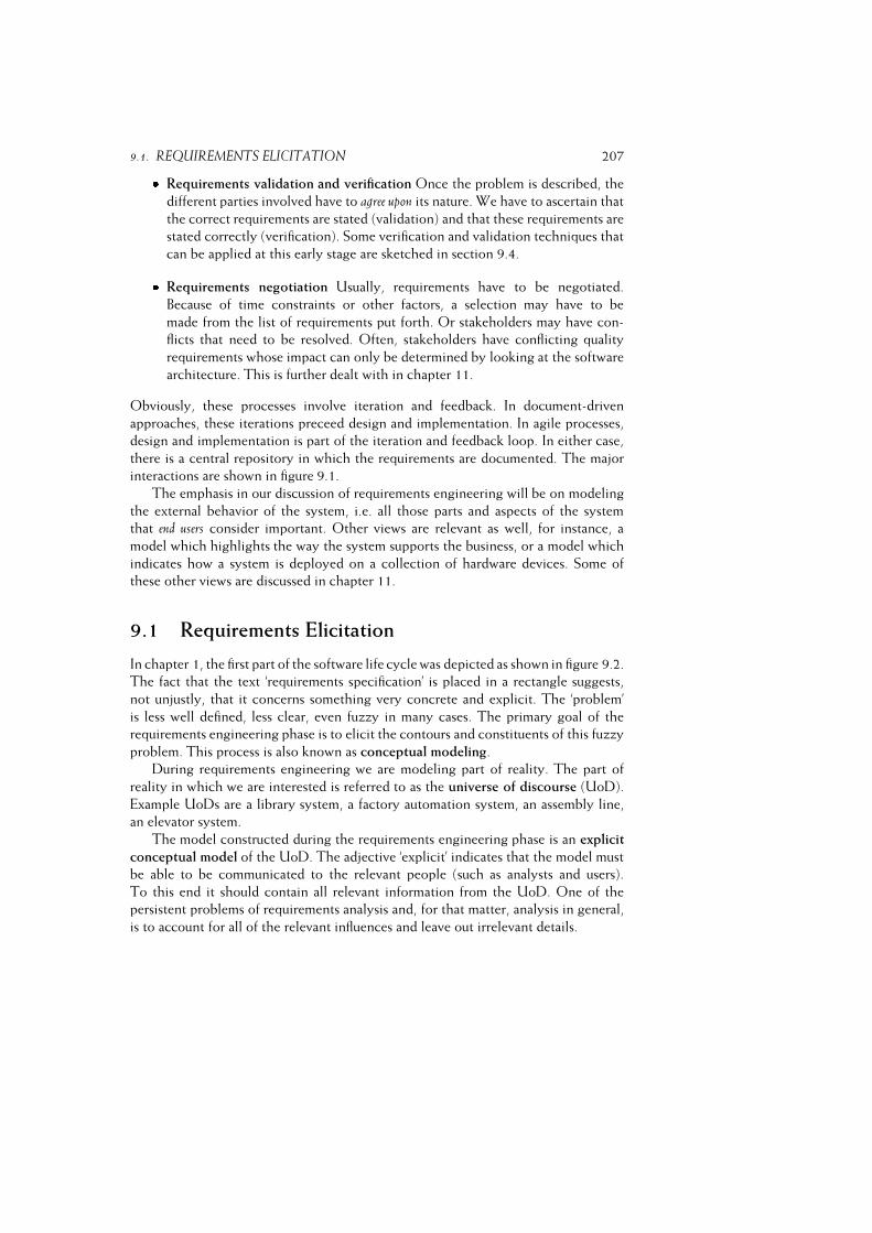
9.1. REQUIREMENTS ELICITATION 207� Requirements validation and verification Once the problem is described, the

different parties involved have to agree upon its nature. We have to ascertain that

the correct requirements are stated (validation) and that these requirements are

stated correctly (verification). Some verification and validation techniques that

can be applied at this early stage are sketched in section 9.4.� Requirements negotiation Usually, requirements have to be negotiated.

Because of time constraints or other factors, a selection may have to be

made from the list of requirements put forth. Or stakeholders may have con-

flicts that need to be resolved. Often, stakeholders have conflicting quality

requirements whose impact can only be determined by looking at the software

architecture. This is further dealt with in chapter 11.

Obviously, these processes involve iteration and feedback. In document-driven

approaches, these iterations preceed design and implementation. In agile processes,

design and implementation is part of the iteration and feedback loop. In either case,

there is a central repository in which the requirements are documented. The major

interactions are shown in figure 9.1.

The emphasis in our discussion of requirements engineering will be on modeling

the external behavior of the system, i.e. all those parts and aspects of the system

that end users consider important. Other views are relevant as well, for instance, a

model which highlights the way the system supports the business, or a model which

indicates how a system is deployed on a collection of hardware devices. Some of

these other views are discussed in chapter 11.

9.1 Requirements Elicitation

In chapter 1, the first part of the software life cycle was depicted as shown in figure 9.2.

The fact that the text ‘requirements specification’ is placed in a rectangle suggests,

not unjustly, that it concerns something very concrete and explicit. The ‘problem’

is less well defined, less clear, even fuzzy in many cases. The primary goal of the

requirements engineering phase is to elicit the contours and constituents of this fuzzy

problem. This process is also known as conceptual modeling.

During requirements engineering we are modeling part of reality. The part of

reality in which we are interested is referred to as the universe of discourse (UoD).

Example UoDs are a library system, a factory automation system, an assembly line,

an elevator system.

The model constructed during the requirements engineering phase is an explicit

conceptual model of the UoD. The adjective ‘explicit’ indicates that the model must

be able to be communicated to the relevant people (such as analysts and users).

To this end it should contain all relevant information from the UoD. One of the

persistent problems of requirements analysis and, for that matter, analysis in general,

is to account for all of the relevant influences and leave out irrelevant details.

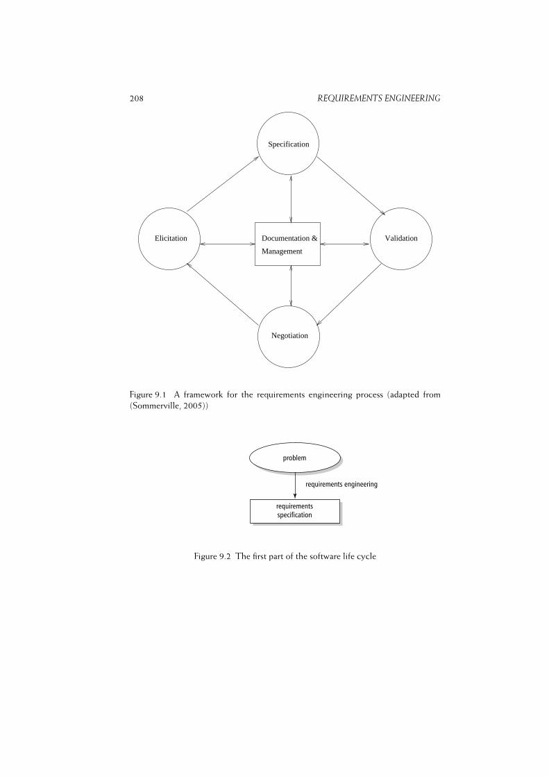
208 REQUIREMENTS ENGINEERING

Management

Documentation &

Negotiation

Elicitation Validation

Specification

Figure 9.1 A framework for the requirements engineering process (adapted from

(Sommerville, 2005))

Figure 9.2 The first part of the software life cycle

9.1. REQUIREMENTS ELICITATION 209

In our library example we could easily have overlooked the fact that in a number

of cases the author’s name as it appears on the cover of a book is not the ‘canonical’

author’s name. This phenomenon occurs in particular with authors from countries that

use non-Latin scripts. The transcription of the Russian name 4EXOB reads ‘Chekhov’

in English and ‘Tsjechow’ in Dutch. In such cases, librarians want to include the

author’s name twice: once the name is spelled as it appears on the book, and once the

name is spelled as it is used in the various search processes. An answer to a question

like ‘which books by Chekhov does our library possess?’ should also inform us about

the non-English titles.

Subtle mismatches between the analyst’s notion of terms and concepts and their

proper meaning within the domain being modeled can have profound effects. Such

mismatches can most easily occur in domains we already ‘know’, such as a library. An

illuminating discussion of potential problems in (formally) specifying requirements

of a library system can be found in (Wing, 1988). Problems noted include:� A library employee may also be a member of the library, so the two sets of

system users are not disjoint;� There is a difference between a book (identified by its ISBN) and the (physical)

copies of a book owned by the library;� It is not sufficient to simply denote the status of a book by a boolean value

present/not present (i.e. lent out). For instance, a book or, more properly, a

copy of a book, may be lost, stolen, or in repair.

People involved in a UoD have an implicit conceptual model of that UoD. An

implicit conceptual model consists of the background knowledge shared by people in

the UoD. The fact that this knowledge is shared gives rise to ‘of course’ statements by

people from within the UoD, because this knowledge is taken for granted. (‘Of course,

a copy of a book is not the same as a book.’) Part of the implicit conceptual model is

not verbalized. It contains tacit knowledge, knowledge that is skillfully applied and

functions in the background. Finally, an implicit conceptual model contains habits,

customs, prejudices and even inconsistencies.

During conceptual modeling, an implicit conceptual model is turned into an

explicit one. In doing so, the analyst is confronted with two types of problem: analysis

problems and negotiation problems. Analysis problems arise from the fact that part of

the implicit conceptual model is not verbalized, that the implicit conceptual model

evolves with time, that the user and analyst talk a different language, and that the

implicit conceptual model cannot be completely codified. Negotiation problems arise

because people in the UoD may counteract the analysis process, because the implicit

conceptual models of people in the UoD may differ, or because of opposing interests

of people involved (such as library personnel versus their managers). Both types of

problems are discussed below.

The problem to be addressed by the automated system arises from the user, a

human. This person must be able to describe this problem in both a correct and

210 REQUIREMENTS ENGINEERING

complete way. It must be communicated to a person who in general has a rather

different background. The analyst often lacks a sufficiently profound knowledge of

the application domain in which the problem originated. He has to learn the language

of the application domain and become acquainted with its terminology, concepts

and procedures. Especially in large projects, the application knowledge tends to be

thinly spread amongst the specialists involved, which easily leads to integration and

coordination difficulties.

In our earlier example, it is the librarian who has to express his wishes. It is

possible that the inclusion of two author names (‘Tsjechow’ and ‘Chekhov’) is seen as

an obvious detail which need not be brought forward explicitly. The analyst at the

other side of the table may still get the impression that he has a complete picture of

the system. This type of omission may have severe consequences.

A number of years back a large automated air defense system was being

developed in the US. During one of the final tests of this system, an alarm

signal was issued. One of the computers detected an unknown missile. It

turned out to be the moon. This possibility had not been thought of.

Eliciting correct and complete information is an important prerequisite for success.

This turns out to be rather problematic in practice. Asking the prospective user what

is wanted does not generally work. More often than not we get a rather incomplete

and inaccurate picture of the situation. Important reasons for this are the human

limitations for processing information, selecting information, and solving problems.

These limited human capabilities are yet aggravated by such factors as:

– the complexity and variation in requirements that can be imposed upon

software;

– the differences in background between the client, or user, and the software

specialist.

In research on human information processing one often uses a model in which human

memory consists of two components: a short-term memory in which information

is being processed, and a long-term memory in which the permanent knowledge is

stored. Short-term memory has a limited capacity: one often says that it has about

seven slots. Long-term memory on the other hand has a very large capacity.

So, information is processed in a relatively small part of human memory. Long-

term memory is thus accessed in an indirect way. In addition, humans also employ

external memories when information is being processed: a blackboard, a piece of

paper, etc.

If a person being interviewed during requirements engineering only uses his short-

term memory, the limitations thereof may have an impact on the results. This may

easily occur if no use is being made of external memories. Things can be forgotten,

simply because our short-term memory has limited capacity.

Humans are also inclined to be prejudiced about selecting and using information.

We are, in particular, inclined to let recent events prevail. In making up a requirements

9.1. REQUIREMENTS ELICITATION 211

specification, this leads to requirements bearing on the present situation, presently

available information, recent events, etc.

Humans are not very capable of rational thinking. They will simplify things and

use a model which does not really fit reality. Other limitations that influence our

model of reality are determined by such factors as education, prejudice, practice, etc.

This same kind of simplification occurs when software requirements are drawn up.

And the result will be limited by the same factors.

We cannot always expect the user to be able to precisely state his requirements at

an early stage. One reason for investigating the opportunities of automation is often

because of a certain dissatisfaction with the present situation. One is not satisfied with

the present situation and has the impression that automation will help. Whether this

is true or not -- many data processing problems are organizational problems -- simply

automating the present situation is not always the solution. Something different is

wanted, though it is not clear what. Only when insight into the possibilities of

automation is gained, will real requirements show themselves. This is one of the

reasons for the sheer size of the maintenance problem. About half of the maintenance

effort concerns adapting software to (new) requirements of the user. To counteract

this trend, software development process models that acknowledge this learning

process, such as prototyping, incremental development, and agile methodss are to be

preferred over those that don’t, i.e. the waterfall model and its variants.

Through a careful analysis, we may hope to build a sound perspective of user

requirements and anticipate future changes. However, no matter how much time is

spent in a dialog with the prospective users, future changes remain hard to foresee. We

may even go one step further and stipulate that requirements will never be complete. In

this respect, specifying requirements has much in common with weather-forecasting:

there is a limit to how far the future can be predicted.

In a situation where the goal of a software development project is to improve an

existing ‘system’, be it a manual process or a (partly) automated one, it is generally

helpful to explicitly distinguish two modeling steps. In the first step, the current

situation is modeled. Based on an analysis of the strengths and weaknesses of the

current situation, the situation-to-be is next modeled. Business Process Redesign, in

particular, stresses the distinction between these two modeling steps.

For the requirements engineering phase to be successful we need methods and

techniques that try to bypass the difficulties sketched above. The degree to which

powerful techniques are required depends on the experience of the people involved in

the requirements engineering phase (both users and analysts) and the expertise of the

analyst with the application domain. Section 9.1.2 discusses a number of techniques

for requirements elicitation.

But before we discuss these techniques, we first elaborate in section 9.1.1 how

different world views result in different approaches to requirements engineering.

In section 9.1.3 we discuss how requirements relate to higher level goals, and

how different viewpoints may result in different, and sometimes conflicting, sets of

requirements. Following section 9.1.3 we discuss how to prioritize requirements, and

212 REQUIREMENTS ENGINEERING

how requirements relate to the selection of COTS components.

9.1.1 Requirements Engineering Paradigms

Most requirements engineering methods, and software development methods in

general, are Taylorian in nature. Around the turn of this century, Taylor introduced

the notion of ‘scientific management’, in which tasks are recursively decomposed into

simpler tasks and each task has one ‘best way’ to accomplish it. By careful observations

and experiments this one best way can be found and formalized into procedures

and rules. Scientific management has been successfully applied in many a factory

operation. The equivalent in requirements engineering is to interview domain experts

and observe end users at work in order to obtain the ‘real’ user requirements. After

this, the experts go to work and implement these requirements. During the latter

process there is no further need to interact with the user community. This view of

software development is a functional, and rational, one. Its underlying assumption is

that there is one objective truth, which merely needs to be discovered during the

analysis process.

Though this view has its merits in drawing up requirements in purely technical

realms, many UoDs of interest involve people as well -- people whose model of the

world is incomplete, subjective, irrational, and may conflict with the world view of

others. In such cases, the analyst is not a passive outside observer of the UoD. Rather,

he actively participates in the shaping of the UoD.

It is increasingly being recognized that the Taylorian, functional, approach is

not the only, and need not be the most appropriate, approach to the requirements

engineering process.

Analysts have a set of assumptions about the nature of the subject of study. Such

a set of assumptions is commonly called a ‘paradigm’. In our field, these assumptions

concern the way in which analysts acquire knowledge (epistemological assumptions)

and their view of the social and technical world (ontological assumptions).

The assumptions about knowledge result in an objectivist--subjectivist dimension.

If the analyst takes the objectivist point of view, he applies models and methods

derived from the natural sciences to arrive at the one and only truth. In the subjectivist

position, his principal concern is to understand how the individual creates, modifies

and interprets the world he or she is in.

The assumptions about the world result in an order--conflict dimension. The

order point of view emphasizes order, stability, integration, and consensus. On the

other hand, the conflict view stresses change, conflict, and disintegration.

These two dimensions and their associated extreme positions yield four paradigms

for requirements engineering and, more generally, information systems development:

Functionalism (objective--order). In the functionalist paradigm, the developer is the

system expert who searches for measurable cause--effect relationships. An empirical

organizational reality is believed to exist, independent of the observer. Systems

are developed to support rational organizational operation. Their effectiveness and

9.1. REQUIREMENTS ELICITATION 213

efficiency can be tested objectively, by tests similar to those used in other engineering

disciplines.

Social-relativism (subjective--order). In this paradigm, the analyst operates as a

facilitator. Reality is not something immutable ‘out there’, but is constructed in the

human mind. The analyst is a change agent. He seeks to facilitate the learning of all

people involved.

Radical-structuralism (objective--conflict). In the radical paradigm the key assump-

tion is that system development intervenes in the conflict between two or more social

classes for power, prestige, and resources. Systems are often developed to support the

interests of the owners, at the expense of the interests of labor. In order to redress

the power balance, this paradigm suggests that the analyst should act as a labor

partisan. System requirements should evolve from a cooperation between labor and

the analyst. This approach is thought to lead to systems that enhance craftsmanship

and working conditions.

Neohumanism (subjective--conflict). The central theme in this paradigm is eman-

cipation. Systems are developed to remove distorting influences and other barriers

to rational discourse. The system developer acts as a social therapist in an attempt

to draw together, in an open discussion, a diverse group of individuals, including

customers, labor, and various levels of management.

Admittedly, these paradigms reflect extreme orientations. In practice, some mixture

of assumptions will usually guide the requirements engineering process. Yet it is fair to

say that the majority of system development techniques emphasizes the functionalist

view.

In the subjectivist--objectivist dimension, it is important to realize that a good

deal of subjectivism may be involved in the shaping of the UoD. If we have to

develop a system to, say, control a copying machine, we may safely take a functional

stand. We may expect such a machine to operate purely rationally. In the analysis

process, we list the functions of the machine, its internal signals, conditions, and so

on, in order to get a satisfactory picture of the system to be developed. Once these

requirements are identified, they can be frozen and some waterfall-like process model

can be employed to realize the system.

If, however, our task is to develop a system to support people in doing their

job, such as some office automation system, a purely functional view of the world

may easily lead to ill-conceived systems. In such cases, end-user participation in the

shaping of the UoD is of paramount importance. Through an open dialog with the

people concerned, we may encourage the prospective users to influence the system

to be developed. Part of the analyst’s job in this case is to reconcile the views

of the participants in the analysis process. Continuous feedback during the actual

construction phases with possibilities for redirection may further enhance the chance

of success. It is the future users who are going to work with the system. It is of no

avail to confront them with a system that does not satisfy their needs.

214 REQUIREMENTS ENGINEERING

Automation transforms organizations, and thus affects the organization’s employ-

ees. It may raise fears and other emotions with the employees affected. For instance,

our library system potentially gives people access to a lot more information than they

previously had. Some people though may prefer to have access only to information

related to their tasks and responsibilities. During requirements engineering, we have

to be conscious about these effects. The pure functionalist paradigm then is of no

avail.

A dissatisfied user will try to neglect the system or, at best, express additional

requirements immediately. The net result is that the envisaged gain in efficiency or

effectiveness is not reaped.

An illuminating and well-documented example of possible effects of following a

fairly radical paradigm is given in (Page et al., 1993); see also section 1.4.3. The system

concerns the Computer Aided Despatch System for the London Ambulance Service.

Though the system would significantly impact the way ambulance crews carried out

their jobs, there was little consultation with them. Some of the consequences of this

approach were the following (Page et al., 1993, pp 40--41):

– The system allocated the nearest available resource regardless of originating

station, so crews often had to operate further and further from their home base.

This resulted in them operating in unfamiliar territory with further to go to

reach their home station at the end of a shift.

– The new system took away the flexibility crews previously had for the station

to decide on which resource to allocate. This inevitably led to problems when

a different resource was used to the one that was allocated.

– The lack of voice contact made the whole process more impersonal and

exacerbated the ‘them and us’ situation.

If the conceptual models of the participants differ, we may either look for a

compromise, or opt for one of the views expressed. It is impossible to give general

guidelines on how to handle such cases. Looking for a compromise can be a tedious

affair and may lead to a system that no one is really happy with. Opting for one

particular view of the world will make one party happy, but may result in others

completely neglecting the system developed. Worse yet, they may decide to develop

a competing system.

9.1.2 Requirements Elicitation Techniques

The two main sources of information for the requirements elicitation process are

the users and the (application) domain. These sources both presuppose that there

exists something ‘out there’ to start with, and from which requirements can be

elicited. In market-driven software development though, this is often not the case,

and requirements elicitation in such projects is more like requirements invention or

problem-formulation, guided by marketing and sales considerations.

9.1. REQUIREMENTS ELICITATION 215

Figure 9.3 lists a number of elicitation techniques, which are elaborated upon

below. The figure also tells us that the user is the major source of information

in some techniques, while the domain is predominant in others. Furthermore, the

figure indicates whether each technique is particularly useful to model the current, as

opposed to the anticipated future, situation.

You should generally vacuum a rug in two directions rather than one; likewise,

you should use multiple requirements elicitation techniques.

Figure 9.3 A sample of requirements elicitation techniques

Asking We may simply ask the users what they expect from the system. A presup-

position then is that the user is able to bypass his own limitations and prejudices.

Asking may take the form of an interview, a brainstorm, or a questionnaire. In an

open-ended interview, the user freely talks about his tasks. This is the easiest form of

requirements elicitation, but it suffers from all of the drawbacks mentioned before.

In a structured interview, the analyst tries to overcome these by leading the user, for

example through closed or probing questions.

In discussion sessions with a group of users, we often find that some users are

far more articulate than others, and thus have a greater influence on the outcome.

The consensus thus reached need not be well-balanced. To overcome this problem, a

Delphi technique may be employed. The Delphi technique is an iterative technique

in which information is exchanged in a written form until a consensus is reached.

For example, participants may write down their requirements, sorted in order of

importance. The sets of requirements thus obtained are distributed to all participants,

216 REQUIREMENTS ENGINEERING

who reflect on them to obtain a revised set of requirements. This procedure is repeated

several times until sufficient consensus is reached.

For consumer products, such as word processing packages, antivirus software

or software for your personal administration, users often have the option to give

feedback, raise questions, report bugs, and the like, electronically. This type of

information is also regularly gathered and stored by sales and marketing people in

the course of their contacts with customers. These logs can be mined and in this way

provide a valuable source of information when looking for requirements for the next

release of that software.

Task analysis Employees working in some domain perform a number of tasks, such

as handling requests to borrow a book, cataloging new books, ordering books, etc.

Higher-level tasks may be decomposed into subtasks. For example, the task ‘handle

request to borrow a book’ may lead to the following subtasks:

– check member identification,

– check for limit on the number of books that may be borrowed,

– register book as being borrowed by the library member,

– issue a slip indicating the due back date.

Task analysis is a technique to obtain a hierarchy of tasks and subtasks to be carried

out by people working in the domain. Any of the other techniques discussed may be

used to get the necessary information to draw this hierarchy. There are no clear-cut

rules as to when to stop decomposing tasks. A major heuristic is that at some point

users tend to ‘refuse’ to decompose tasks any further. For instance, when being asked

how the member identification is checked, the library employee may say ‘Well, I

simply check his id.’ At this point, further decomposition is meaningless.

Task analysis is often applied at the stage when (details about) the human--

computer interaction component are being decided upon. This underestimates its

potency as a general requirements elicitation technique. It also gives the (wrong)

impression that users are only concerned with the ‘look and feel’ of the interface.

Scenario-based analysis Instead of looking for generic plans as in interviews or task

analysis, the analyst may study instances of tasks. A scenario is a story which tells

us how a specific task instance is executed. The scenario can be real or artificial. An

example of a real scenario is that the analyst observes how a library employee handles

an actual user request. We may ask the library employee to verbalize what he is doing

and make an audio or video recording thereof. This think aloud method is a fairly

unobtrusive technique to study people at work. It is often used to assess prototypes

or existing information systems.

Alternatively, we may construct artificial scenarios and discuss these with the user.

As a first shot, we may for example draw up the following scenario for returning a

book:

9.1. REQUIREMENTS ELICITATION 217

1. The due back date for the book is checked. If the book is overdue, the member

is asked to pay the appropriate fine.

2. The book is recorded as again being eligible for checking-out.

3. The book is put back in its proper place.

When this scenario is discussed with the library employee, a number of related issues

may crop up, either through probing questions from the analyst, or because the user

contrasts the scenario with daily practice. Example questions that could be raised

include such things as:

– What happens when the person returning the book is not a registered member

of the library?

– What happens when the book returned is damaged?

– What happens if the member returning this book has other books that are

overdue or an outstanding reservation for another book?

In essence, this type of story-telling provides the user with an artificial mock-up version

of the software eventually to be delivered. It serves as a paper-based prototype to

gain a better understanding of the requirements. If tied to a UML-type of modeling,

scenario-based analysis is often called use-case analysis; see section 10.3.6. Scenarios

and use cases are the elicitation methods most often used.

Scenario-based analysis is often done in a somewhat haphazard way. In that case,

there is no way of telling whether enough scenarios have been drawn up and a

sufficiently accurate and complete picture of the requirements is obtained. Writing

good scenarios is by no means easy. Though it may look trivial to ‘just record user

episodes’, a fair mount of domain expertise is needed to get a good and reliable set of

scenarios.

Scenarios can be looked at from different perspectives. In the above example

scenario for returning a book, the scenario lists a series of actions or events that

together make up some episode. The focus then is on the process aspect, showing

how the system proceeds through successive states. Alternatively, the same scenario

may be looked at from a user perspective: how will the user interact with the system,

what functionalities will she be offered? Yet another perspective is that the scenario

leads to discussions about alternatives from which a certain choice has to be made, as

in the questions that the example scenario above raised.

Ethnography A major disadvantage of eliciting requirements through, for example,

interviews is that the analyst imposes his view of how the world is ordered onto the

user. Such methods may fail if the analyst and user do not share a category system.

The analyst may, for example, ask the following:

‘If a member wants to borrow a book while he or she still has an outstanding fine, will

you:

218 REQUIREMENTS ENGINEERING

a) Refuse the request, or

b) Handle the request anyway’

This binary choice need not map actual practice. The library employee may, for

example, grant the request provided part of the outstanding fine is settled or if he

knows the member to be trustworthy.

Thinking aloud protocols are based on the idea that users have well-defined

goals and subgoals, and that they traverse such goal trees in a neat top-down

manner. People however often do not have preconceived plans, but rather proceed

in somewhat opportunistic ways.

A disadvantage of task analysis is that it considers individual tasks of individual

persons, without taking into account the social and organizational environment in

which these tasks are executed.

Ethnographic methods are claimed not to have such shortcomings. In ethnog-

raphy, groups of people are studied in their natural settings. It is well-known from

sociology, where for example Polynesian tribes are studied by living with them for an

extended period of time. Likewise, user requirements can be studied by participating

in their daily work for a period of time, for example by becoming a library employee.

The analyst becomes an apprentice, recognizing that the future users of the system

are the real experts in their work. Ethnographic methods are more likely to uncover

tacit knowledge than most other elicitation techniques.

Form analysis A lot of information about the domain being modeled can often

be found in various forms being used. For example, to request some conference

proceedings from another library, the user might have to fill in a form such as given

in figure 9.4.

Figure 9.4 A sample form

9.1. REQUIREMENTS ELICITATION 219

Forms provide us with information about the data objects of the domain, their

properties, and their interrelations. They are particularly useful as an input to modeling

the data aspect of the system; see also section 10.1.1.

Library users often have incomplete knowledge of the information sources they

are interested in. For example, someone might be looking for the proceedings of

the International Conference on Software Engineering that took place in Berlin. Only if the

various entries from the above form are used as entities in the underlying data model,

can such a query be answered easily. In this case, the form directly points at a useful

requirement which might otherwise go unnoticed.

Natural language descriptions Like forms, natural language descriptions provide a

lot of useful information about the domain to be modeled. The operating instructions

for library employees might for instance contain a paragraph like the one given in

figure 9.5. This text gives us such information as:

– There are (at least) two accounts that orders can be charged to;

– There is a list of staff members authorized to sign off such requests;

– There is the possibility of ordering multiple copies of titles, such as this book

on Software Engineering, on behalf of students.

Title acquisition

Before a request to acquire a title can be complied with, form B has to be filled in

completely. A request can not be handled if it is not signed by an authorized staff

member or the account to be charged (‘Student’ or ‘Staff’) is not indicated. A request

is not to be granted if the title requested is already present in the title catalog, unless

it is marked ‘Stolen’ or ‘Lost’, or the account is ‘Student’.

Figure 9.5 A sample instruction for library employees

Often, natural language descriptions (and forms) provide the analyst with background

information to be used in conjunction with other elicitation techniques such as

interviews. Natural language descriptions in particular tend to assume a lot of tacit

knowledge by the reader. For example, if form B contains an ISBN, this saves the

library employee some work, but the request will probably still be handled if this

information is not provided. A practical problem with natural language descriptions

is that they are often not kept up-to-date. Like software documentation, their validity

tends to deteriorate with time.

Natural language descriptions are often taken as a starting point in object-oriented

analysis techniques. This is further discussed in section 12.3.

220 REQUIREMENTS ENGINEERING

Derivation from an existing system Starting from an existing system, for instance a

similar system in some other organization or a description in a text book, we may

formulate the requirements of the new system. Obviously, we have to be careful and

take the peculiar circumstances of the present situation into account.

Rather than looking at one particular system, we may also study a number of

systems in some application domain. This meta-requirements analysis process is

known as domain analysis. Its goal generally is to identify reusable components,

concepts, structures, and the like. It is dangerous to look for reusable requirements

in immature domains. Requirements may then be reused simply because they are

available, not because they fit the situation at hand. They become ‘dead wood’. In

the context of requirements analysis, domain analysis can be viewed as a technique

for deriving a ‘reference’ model for systems within a given domain. Such a reference

model provides a skeleton (architecture) that can be augmented and adapted to fit

the specific situation at hand.

Domain analysis is further discussed in chapter ??, in the context of software reuse

and software product line development.

Business Process Redesign (BPR). In many software development projects, the

people involved jump to conclusions rather quickly: automation is the answer.

Even worse, their conclusion might be that automating the current situation is the

answer. In Business Process Redesign (or Business Process Reengineering), a rather

different strategy is followed. It is an organizational activity to radically redesign

business processes to achieve competitive breakthroughs in, e.g. quality, cost, or user

satisfaction. In BPR, we depart completely from the existing ways of doing things. In

BPR, the following steps are distinguished:

1. Identify processes for innovation. Two major approaches for doing so are the

exhaustive and high-impact approach. In the exhaustive approach, an attempt

is made to identify all processes, which are then prioritized for their redesign

urgency. The high-impact approach attempts to identify the most important

processes only, or the ones that conflict with the business vision.

2. Identify change levers. In this step, opportunities facilitating process improve-

ment are identified. Three types of lever can be recognized: organizational

enablers (such as empowering teams), human resource enablers (such as task

enrichment) and information technology enablers.

3. Develop process visions. For redesign to be successful, the organization needs

to know which goals it wants to reach. This is described in the process vision.

The main components of a process vision are: process objectives (measurable

targets of the future performance of the system), process attributes (qualitative

and descriptive properties of the future process), critical success factors and

constraints (organizational, cultural, and technological).

9.1. REQUIREMENTS ELICITATION 221

4. Understand the existing process. This includes documenting the existing

process, measuring it, and identifying problematic aspects. It allows us to assess

the health of the existing process, and brings problems to the surface.

5. Design and prototype the new process. This is the final step. Prototyping makes

it possible to try out new structures, thereby reducing the risk of failure.

BPR is not really a requirements elicitation technique proper. It is mentioned here

because it emphasizes an essential issue to be addressed during the requirements

engineering phase. Business processes should not be driven by information technol-

ogy. Rather, information technology should enable them. Though a complete BPR

effort is not necessary or feasible in many situations, rethinking the existing processes

and procedures is a step which is all too often thoughtlessly skipped in software

development projects.

As an example, consider our library automation project once again. Careful

inspection of the current situation might reveal that things aren’t all that bad.

However, the impression is that the number of requests that could not be granted has

steadily risen in the past years. This is perceived to be the main cause of the increasing

number of dissatisfied users. Since service to its customers has high priority, one of

the objectives is to decrease the number of requests that cannot be satisfied by 50%

within two years. For this to be possible, the library should be allowed to spend the

available budget at its own discretion, rather than being triggered by signals from

researchers only (this sounds radical, doesn’t it). It is therefore decided to augment

the existing automated system with modules to keep track of both successful and

unsuccessful requests. Based on the insights gained from this measurement process

during a period of three months, a decision will be taken as to how large a percentage

of the annual budget will be reallocated.

Prototyping Given the fact that it is difficult, if not impossible, to build the right

system from the start, we may decide to use prototypes. Starting from a first set of

requirements, a prototype of the system is constructed. This prototype is used for

experiments, which lead to new requirements and more insight into the possible uses

of the system. In one or more ensuing steps, a more definite set of requirements is

developed. Prototyping is discussed in section 3.2.1. Other agile processes follow a

similar strategy in which requirements are quickly translated into a running system to

be assessed by its users.

Of these requirements elicitation techniques, asking is the least certain strategy,

while prototyping is the least uncertain. Besides the experience of both users and

analysts, the uncertainty of the process is also influenced by the stability of the

environment, the complexity of the product to be developed and the familiarity with

the problem area in question. We may try to estimate the impact of those factors

on the vulnerability of the resulting requirements specification, and then decide on a

certain primary method for requirements elicitation based on this estimate.

222 REQUIREMENTS ENGINEERING

For a well-understood problem, with very experienced analysts, interviewing the

prospective users may suffice. However, if it concerns an advanced and ill-understood

problem from within a rapidly changing environment and the analysts have little or

no experience in the domain in question, it seems wise to follow an agile process.

Requirements uncertainty is not the only problem project managers have to

cope with, and a different process is not the only solution they opt for. Political

aspects (such as hidden agendas and conflicts between stakeholders) are often seen as

larger risks than mere requirements uncertainty (Moynihan, 2000). Of course, these

are related. In both cases chances are high that requirements will change. Project

managers often follow a formal route to handle disagreements between stakeholders,

and let the customers sign off the requirements document. Whether this is the answer

in the long run is questionable, though.

As the uncertainty decreases, the beneficial effects of user participation in

requirements engineering diminish. If the uncertainty increases, however, greater user

participation does have a positive effect on the quality of requirements engineering.

It is generally wise to have multiple customer--developer links in a software

development project, and during requirements engineering in particular. Keil and

Carmel (1995) studied the relation between project success and the number and

type of such customer--developer links. The authors observed a strong correlation

between the number of links and project success: more links implied more successful

projects. The relative contribution to project success diminishes as the number of

links grows; there is no need to have more than, say, half a dozen links. A further

interesting observation from this study is that links with direct users have more impact

on project success than links with indirect users such as user representatives or sales

people. Finally, it was noted that customer-driven development projects tend to

use and prefer different types of link to market-driven development projects. For

example, the favorite link for custom development -- facilitated teams -- was not used

by package developers, while the favorite link for package developers -- support lines

-- was seldom used for custom projects.

We should be very careful in our assessment of which requirements elicitation

technique to choose. It is all too common to be too optimistic about our ability to

properly assess software requirements.

As an example, consider the following anecdote from a Dutch newspaper. A firm

in the business of farm automation had developed a system in which microchips were

put in cows’ ears. Subsequently, each individual cow could be tracked: food and water

supply was regulated and adjusted, the amount and quality of the milk automatically

recorded and analyzed, etc. Quite naturally, this same technique was next successfully

applied to pigs. Thereafter, it was tried on goats. A million-dollar, fully automated

goat farm was built. But alas, things did not work out that well for goats. Contrary to

cows and pigs, goats eat everything, including their companions’ chips.

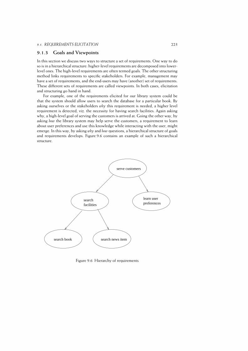
9.1. REQUIREMENTS ELICITATION 223

9.1.3 Goals and Viewpoints

In this section we discuss two ways to structure a set of requirements. One way to do

so is in a hierarchical structure: higher-level requirements are decomposed into lower-

level ones. The high-level requirements are often termed goals. The other structuring

method links requirements to specific stakeholders. For example, management may

have a set of requirements, and the end-users may have (another) set of requirements.

These different sets of requirements are called viewpoints. In both cases, elicitation

and structuring go hand in hand.

For example, one of the requirements elicited for our library system could be

that the system should allow users to search the database for a particular book. By

asking ourselves or the stakeholders why this requirement is needed, a higher level

requirement is detected, viz. the necessity for having search facilities. Again asking

why, a high-level goal of serving the customers is arrived at. Going the other way, by

asking how the library system may help serve the customers, a requirement to learn

about user preferences and use this knowledge while interacting with the user, might

emerge. In this way, by asking why and how questions, a hierarchical structure of goals

and requirements develops. Figure 9.6 contains an example of such a hierarchical

structure.

learn userpreferences

searchfacilities

search news itemsearch book

serve customers

Figure 9.6 Hierarchy of requirements

224 REQUIREMENTS ENGINEERING

Figure 9.6 depicts a refinement structure, in which each requirement is refined

(decomposed) into a set of subrequirements that together satisfy the parent require-

ment. The subrequirements are AND-related: ‘search book’ and ‘search news item’

together make up the ‘search facilities’ requirement.

We may also include other types of relationships. For instance, we may have

certain options for a particular requirement, and to that end have OR-relations next to

AND-relations. We may also include other types of link. If we have a requirement to

impose fines on customers who return items late, we may conceive this as conflicting

with our goal of serving customers, and connect these two requirements by a link of

type ‘conflicts with’.

This so-called goal-driven requirements engineering results in a graph connecting

high-level goals to lower-level requirements. This graph can be reasoned about, e.g.

to validate that certain goals are indeed reached, or to detect conflicts (Lamsweerde,

2001).

It is often useful to collect and organize requirements from different perspectives,

or viewpoints. Different stakeholders may have different sets of requirements.

Different quality concerns may also lead to different sets of requirements, leading

for instance to a security viewpoint. The latter type of perspective is usually dealt

with during software architecture design, and will be discussed in chapter 11. The

techniques discussed in section 9.3 implicitly denote different viewpoints as well, such

as a data viewpoint in the entity-relationship models. Here, we focus on different

viewpoints caused by different stakeholders. These different viewpoints may be in

conflict, and these conflicts need to be recognized and dealt with during requirements

engineering.

The Computer Aided Dispatch System for The London Ambulance Service

again provides a clear case of conflicting viewpoints: management wants an effective

system, crew members want to get home within a reasonable time after their shift has

ended (see also sections 1.4.3 and 9.1.1). For our library system, conflicts between

stakeholders may likewise occur.

Consider, for example, the following issue which may crop up during the

requirements elicitation phase for our library system. The system has to offer certain

features to register and handle fines. An item not returned in time incurs a fine of,

say, $0.25 per day. John, one of the library employees involved in the specification

process, takes the following position (denoted ‘Pos A’ in figure 9.7): members should

be warned about outstanding fines at the earliest possible moment. His argument (‘Arg

A’) is that service is degraded if a member cannot borrow an item because some other

member has not returned that item on time. Mary, the library manager, takes a rather

different position (‘Pos B’): members should not be warned about outstanding fines

until the due-back date has expired one month. Her argument (‘Arg B’) is that fines

are a most welcome addition to the library budget, which is under severe pressure

because of the continuing price increase of journal subscriptions.

This situation is graphically depicted in the graph in figure 9.7. The graph contains

nodes of types ‘issue’, ‘position’ and ‘argument’, and directed links of type ‘response-to’,

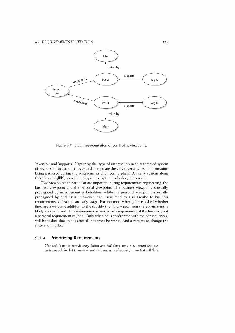
9.1. REQUIREMENTS ELICITATION 225

Figure 9.7 Graph representation of conflicting viewpoints

‘taken-by’ and ‘supports’. Capturing this type of information in an automated system

offers possibilities to store, trace and manipulate the very diverse types of information

being gathered during the requirements engineering phase. An early system along

these lines is gIBIS, a system designed to capture early design decisions.

Two viewpoints in particular are important during requirements engineering: the

business viewpoint and the personal viewpoint. The business viewpoint is usually

propagated by management stakeholders, while the personal viewpoint is usually

propagated by end users. However, end users tend to also ascribe to business

requirements, at least at an early stage. For instance, when John is asked whether

fines are a welcome addition to the subsidy the library gets from the government, a

likely answer is ‘yes’. This requirement is viewed as a requirement of the business, not

a personal requirement of John. Only when he is confronted with the consequences,

will he realize that this is after all not what he wants. And a request to change the

system will follow.

9.1.4 Prioritizing Requirements

Our task is not to provide every button and pull-down menu enhancement that our

customers ask for, but to invent a completely new way of working -- one that will thrill

226 REQUIREMENTS ENGINEERING

and amaze them.

(Robertson, 2002)

In most cases, not all requirements can be realized, so we have to make a selection.

In section 3.2.3 we mentioned a very simple form of requirements prioritization called

triage. A variant often used is known as MoSCoW (the o’s are just there to be able to

pronounce the word). Usinig MoSCoW, we distinguish four types of requirement:� Must haves: these are the top priority requirements, the ones that definitely

have to be realized in order to make the system acceptable to the customer.� Should haves: these requirements are not strictly mandatory, but they are

highly desirable.� Could haves: if time allows, these requirements will be realized as well. In

practice, they usually won’t.� Won’t haves: these requirements will not be realized in the present version.

They are recorded though. They will be considered again for a next version of

the system.

The MoSCoW scheme assumes that requirements can be ordered along a single axis,

and that realizing more requirements yields more satisfied customers. Reality often

is more complex. In the Kano model (Kano, 1993), user preferences are classified

into five categories, as listed in figure 9.8. The way customers value the Attractive,

Must-be and One-dimensional categories of requirements is depicted in figure 9.9.

This figure shows that offering attractive, so called killer features, is what will really

excite your customers. The above quote from Robertson (2002) points in the same

direction: amaze your customer by giving him something he never even dreamt of.

In market-driven software development, the product often has a series of releases.

The list of requirements for such products is usually derived from sales information,

user logs from earlier versions of the system, and other sources of indirect information.

One then has to decide which requirements to include in the current version, and

which ones to postpone to a next one. Business case analysis, return on investment

estimations, and similar economics-driven argumentations then are used to set

priorities. This priority setting is to be repeated for each version, since user preferences

may change, the market reacts, and the like.

Finally, the prioritization of requirements is related to the notion of scoping in

software product lines. If we want to develop a series of similar library systems, we

have to delimit the domain we intend to handle. A smaller domain, say only scientific

libraries, is easier to realize, but has a smaller market. A set of products covering

a larger domain is more difficult to realize, yet has the promise of larger sales and

profits. Scoping is further discussed in chapter ??, in the context of our discussion of

software product lines.

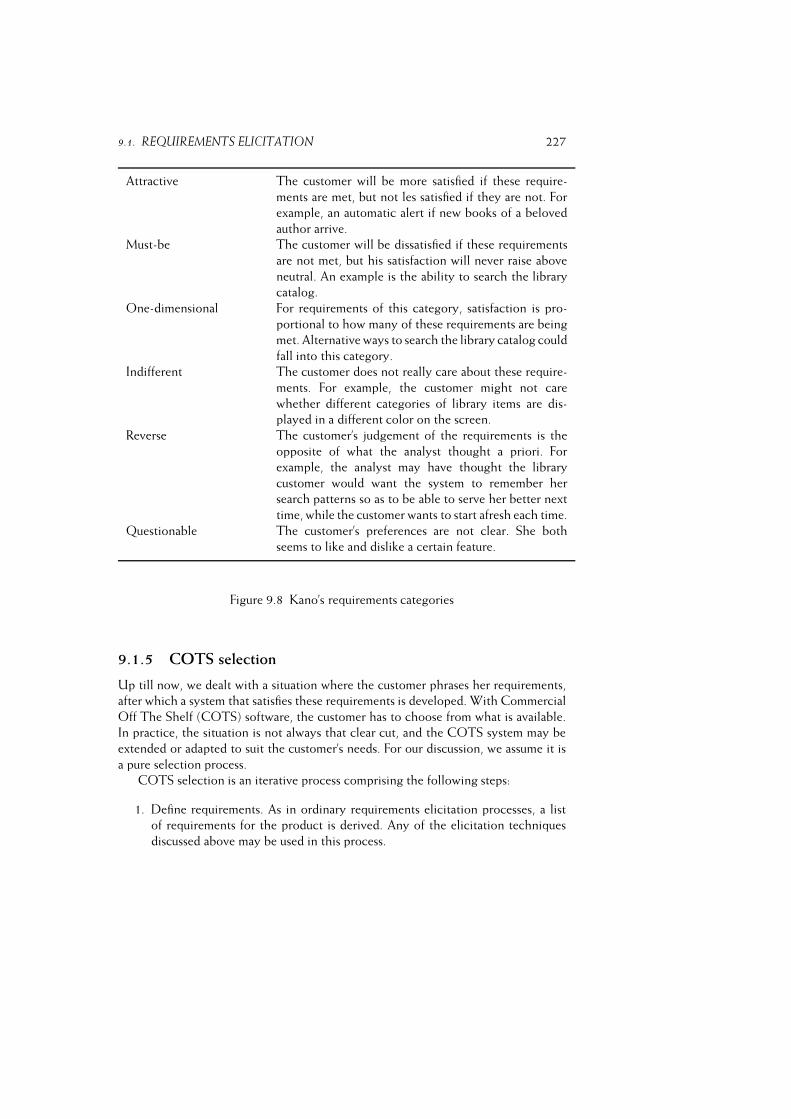
9.1. REQUIREMENTS ELICITATION 227

Attractive The customer will be more satisfied if these require-

ments are met, but not les satisfied if they are not. For

example, an automatic alert if new books of a beloved

author arrive.

Must-be The customer will be dissatisfied if these requirements

are not met, but his satisfaction will never raise above

neutral. An example is the ability to search the library

catalog.

One-dimensional For requirements of this category, satisfaction is pro-

portional to how many of these requirements are being

met. Alternative ways to search the library catalog could

fall into this category.

Indifferent The customer does not really care about these require-

ments. For example, the customer might not care

whether different categories of library items are dis-

played in a different color on the screen.

Reverse The customer’s judgement of the requirements is the

opposite of what the analyst thought a priori. For

example, the analyst may have thought the library

customer would want the system to remember her

search patterns so as to be able to serve her better next

time, while the customer wants to start afresh each time.

Questionable The customer’s preferences are not clear. She both

seems to like and dislike a certain feature.

Figure 9.8 Kano’s requirements categories

9.1.5 COTS selection

Up till now, we dealt with a situation where the customer phrases her requirements,

after which a system that satisfies these requirements is developed. With Commercial

Off The Shelf (COTS) software, the customer has to choose from what is available.

In practice, the situation is not always that clear cut, and the COTS system may be

extended or adapted to suit the customer’s needs. For our discussion, we assume it is

a pure selection process.

COTS selection is an iterative process comprising the following steps:

1. Define requirements. As in ordinary requirements elicitation processes, a list

of requirements for the product is derived. Any of the elicitation techniques

discussed above may be used in this process.

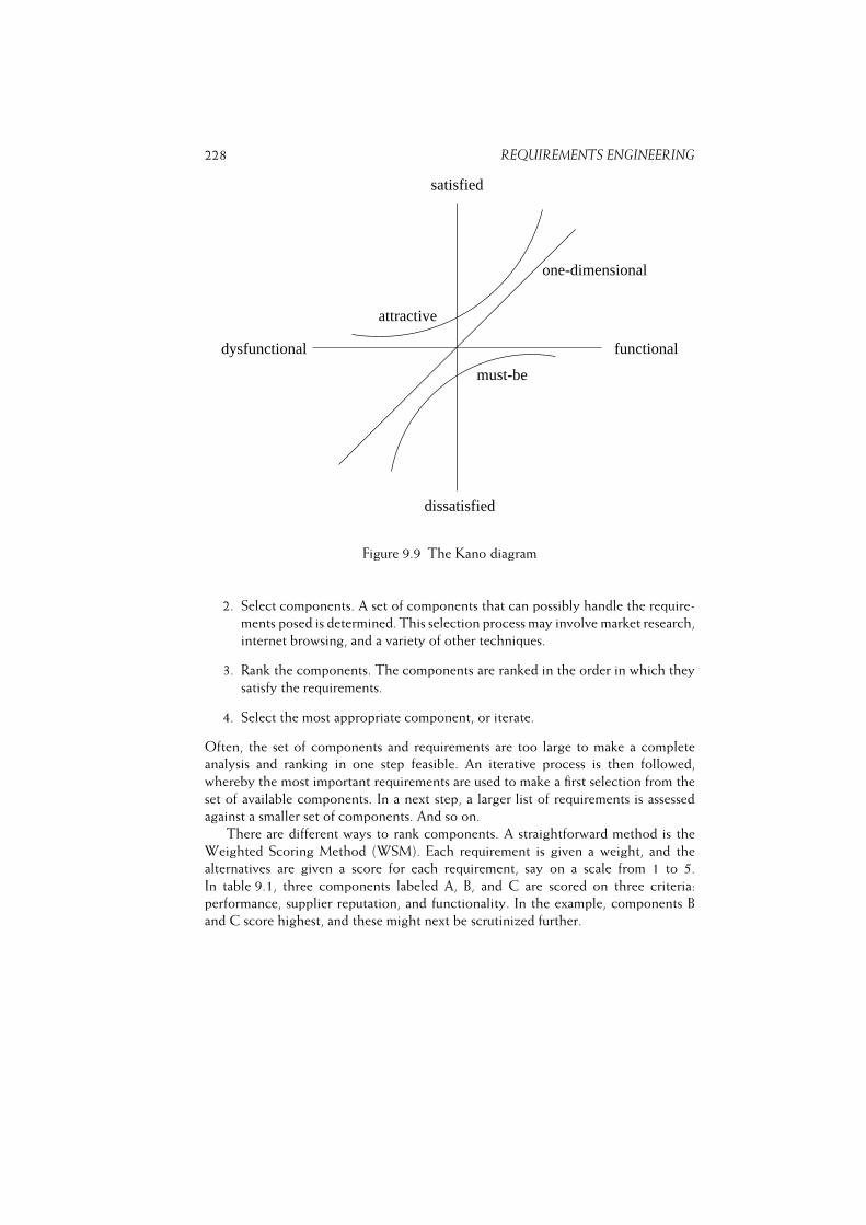
228 REQUIREMENTS ENGINEERING

functional

one-dimensional

must-be

dysfunctional

satisfied

dissatisfied

attractive

Figure 9.9 The Kano diagram

2. Select components. A set of components that can possibly handle the require-

ments posed is determined. This selection process may involve market research,

internet browsing, and a variety of other techniques.

3. Rank the components. The components are ranked in the order in which they

satisfy the requirements.

4. Select the most appropriate component, or iterate.

Often, the set of components and requirements are too large to make a complete

analysis and ranking in one step feasible. An iterative process is then followed,

whereby the most important requirements are used to make a first selection from the

set of available components. In a next step, a larger list of requirements is assessed

against a smaller set of components. And so on.

There are different ways to rank components. A straightforward method is the

Weighted Scoring Method (WSM). Each requirement is given a weight, and the

alternatives are given a score for each requirement, say on a scale from 1 to 5.

In table 9.1, three components labeled A, B, and C are scored on three criteria:

performance, supplier reputation, and functionality. In the example, components B

and C score highest, and these might next be scrutinized further.

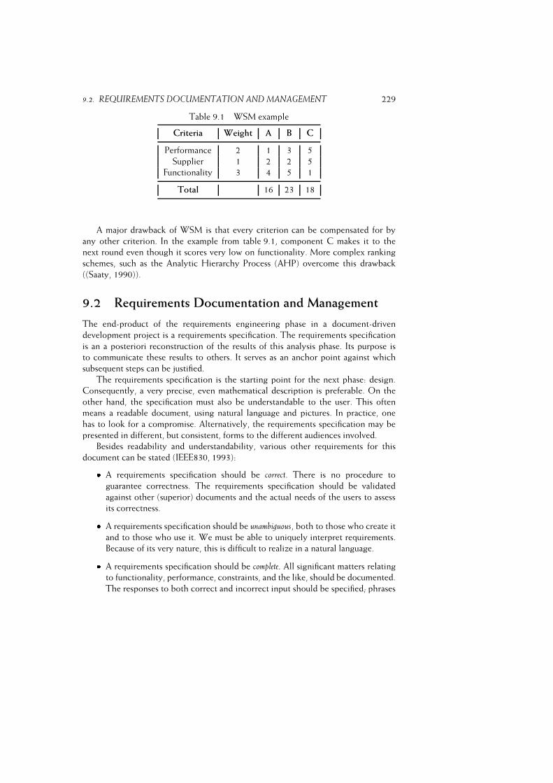
9.2. REQUIREMENTS DOCUMENTATION AND MANAGEMENT 229

Table 9.1 WSM example

Criteria Weight A B C

Performance 2 1 3 5

Supplier 1 2 2 5

Functionality 3 4 5 1

Total 16 23 18

A major drawback of WSM is that every criterion can be compensated for by

any other criterion. In the example from table 9.1, component C makes it to the

next round even though it scores very low on functionality. More complex ranking

schemes, such as the Analytic Hierarchy Process (AHP) overcome this drawback

((Saaty, 1990)).

9.2 Requirements Documentation and Management

The end-product of the requirements engineering phase in a document-driven

development project is a requirements specification. The requirements specification

is an a posteriori reconstruction of the results of this analysis phase. Its purpose is

to communicate these results to others. It serves as an anchor point against which

subsequent steps can be justified.

The requirements specification is the starting point for the next phase: design.

Consequently, a very precise, even mathematical description is preferable. On the

other hand, the specification must also be understandable to the user. This often

means a readable document, using natural language and pictures. In practice, one

has to look for a compromise. Alternatively, the requirements specification may be

presented in different, but consistent, forms to the different audiences involved.

Besides readability and understandability, various other requirements for this

document can be stated (IEEE830, 1993):� A requirements specification should be correct. There is no procedure to

guarantee correctness. The requirements specification should be validated

against other (superior) documents and the actual needs of the users to assess

its correctness.� A requirements specification should be unambiguous, both to those who create it

and to those who use it. We must be able to uniquely interpret requirements.

Because of its very nature, this is difficult to realize in a natural language.� A requirements specification should be complete. All significant matters relating

to functionality, performance, constraints, and the like, should be documented.

The responses to both correct and incorrect input should be specified; phrases

230 REQUIREMENTS ENGINEERING

like ‘to be determined’ are particularly insidious. Unfortunately, it is not always

feasible to complete the specification at an early stage. If certain requirements

can only be made specific at a later stage, the requirements specification

should at least document the ultimate point in time at which this should have

happened.� A requirements specification should be (internally) consistent, i.e. different parts

of it should not be in conflict with each other. Conflicting requirements can be

both logical and temporal. Using different terms for one and the same object

may also lead to conflicts.� Requirements should be ranked for importance or stability. Typically, some

requirements are more important than others. In some cases, a simple ranking

scheme like ‘essential’, ‘worthwhile’, and ‘optional’ will suffice; in other cases, a

more sophisticated classification scheme may be needed (see also section 9.1.4).

We may indicate the stability of requirements by indicating the likelihood,

or the expected number, of changes. Through the explicit incorporation of

this type of information in the requirements document, users are stimulated

to give more consideration to each requirement. It also gives developers the

opportunity to better direct their attention.� A requirements specification should be verifiable. This means that there must be

a finite process to determine whether or not the requirements have been met.

Phrases like ‘the system should be user-friendly’ are not verifiable. Likewise,

the use of quantities that cannot be measured, as in ‘the system’s response time

should usually be less than two seconds’, should be avoided. A requirement like

‘for requests of type X, the system’s response time is less than two seconds in

80% of cases, with a maximum machine load of Y’, is verifiable.� A requirements specification should be modifiable. Software models part of

reality. Therefore it changes. The corresponding requirements specification

has to evolve together with the reality being modeled. Thus, the document

must be organized in such a way that changes can be accommodated readily

(a tabular or database format, for example). Redundancy must be prevented

as much as possible, for otherwise there is the danger that changes lead to

inconsistencies.� A requirements specification should be traceable. The origin and rationale of each

and every requirement must be traceable. A clear and consistent numbering

scheme makes it possible that other documents can uniquely refer to parts of

the requirements specification.

As a guideline for the contents of a requirements specification we will follow

IEEE Standard 830. This standard does not give a rigid form for the requirements

specification. In our opinion, the precise ordering and contents of the elements of this

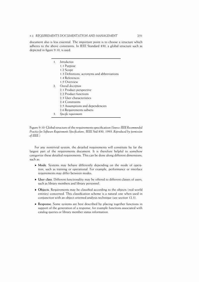
9.2. REQUIREMENTS DOCUMENTATION AND MANAGEMENT 231

document also is less essential. The important point is to choose a structure which

adheres to the above constraints. In IEEE Standard 830, a global structure such as

depicted in figure 9.10, is used.

1. Introduction

1.1 Purpose

1.2 Scope

1.3 Definitions, acronyms and abbreviations

1.4 References

1.5 Overview

2. Overall description2.1 Product perspective

2.2 Product functions

2.3 User characteristics

2.4 Constraints

2.5 Assumptions and dependencies

2.6 Requirements subsets

3. Specific requirements

Figure 9.10 Global structure of the requirements specification (Source: IEEE RecommendedPractice for Software Requirements Specifications, IEEE Std 830, 1993. Reproduced by permission

of IEEE.)

For any nontrivial system, the detailed requirements will constitute by far the

largest part of the requirements document. It is therefore helpful to somehow

categorize these detailed requirements. This can be done along different dimensions,

such as:� Mode. Systems may behave differently depending on the mode of opera-

tion, such as training or operational. For example, performance or interface

requirements may differ between modes.� User class. Different functionality may be offered to different classes of users,

such as library members and library personnel.� Objects. Requirements may be classified according to the objects (real-world

entities) concerned. This classification scheme is a natural one when used in

conjunction with an object-oriented analysis technique (see section 12.3).� Response. Some systems are best described by placing together functions in

support of the generation of a response, for example functions associated with

catalog queries or library member status information.

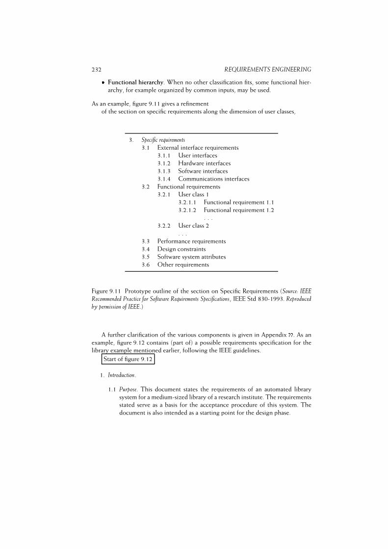
232 REQUIREMENTS ENGINEERING� Functional hierarchy. When no other classification fits, some functional hier-

archy, for example organized by common inputs, may be used.

As an example, figure 9.11 gives a refinement

of the section on specific requirements along the dimension of user classes,

3. Specific requirements

3.1 External interface requirements

3.1.1 User interfaces

3.1.2 Hardware interfaces

3.1.3 Software interfaces

3.1.4 Communications interfaces

3.2 Functional requirements

3.2.1 User class 1

3.2.1.1 Functional requirement 1.1

3.2.1.2 Functional requirement 1.2

. . .

3.2.2 User class 2

. . .

3.3 Performance requirements

3.4 Design constraints

3.5 Software system attributes

3.6 Other requirements

Figure 9.11 Prototype outline of the section on Specific Requirements (Source: IEEERecommended Practice for Software Requirements Specifications, IEEE Std 830-1993. Reproduced

by permission of IEEE.)

A further clarification of the various components is given in Appendix ??. As an

example, figure 9.12 contains (part of) a possible requirements specification for the

library example mentioned earlier, following the IEEE guidelines.

Start of figure 9.12

1. Introduction.

1.1 Purpose. This document states the requirements of an automated library

system for a medium-sized library of a research institute. The requirements

stated serve as a basis for the acceptance procedure of this system. The

document is also intended as a starting point for the design phase.

9.2. REQUIREMENTS DOCUMENTATION AND MANAGEMENT 233

1.2 Scope. The intended product automates the library functions described in

DOC1. Its purpose is to provide a more effective service to the library

users, in particular through the online search facilities offered. More details

of the performance requirements are given in section 3.3 of this document.

Once this system is installed, the incorporation of new titles will go from

an average of 15 minutes down to an average of 5 minutes.

1.3 Definitions, acronyms and abbreviations. Library member: . . . , Library personnel:

. . . , User: The term user may refer to both library members and library

personnel, and is used to denote either class of users. Title catalog: . . . ,

PICA: . . . , etc.

1.4 References. DOC1: . . . , DOC2: . . . , etc.

1.5 Overview. Section 2 of this document gives a general overview of the system.

Section 3 gives more specific requirements for functions offered. These

functions are categorized according to the class of users they support:

(external) members of the library and library personnel, respectively.

2. Overall description.

2.1 Product perspective. The already installed database system X will be used to

store the various catalogs as well as the library member administration.

There are no interfaces to other systems. The system will be realized on the

Y configuration. The maximum external storage capacity for the catalogs

of the system is 1500 MB. Library personnel will use a barcode reader to

enter member, book and journal identifications. The interface protocol to

the barcode reader is described in DOC4.

2.2 Product functions. The system provides two types of function:

– Functions by which users may search the catalogs of books and journal

articles. A list of these functions is given in DOC1. A more detailed

description is given in section 3.2.1.

– Functions by which library personnel may update the administration

of borrowed titles and the system’s catalogs; see section 3.2.2.

The user of the system selects one of the functions offered through the

main menu (section 3.2.1.1 and 3.2.2.1).

2.3 User characteristics. The library members are incidental users of the system

and have little knowledge of automated systems of this kind. The system

therefore has to be self-instructing. Specific requirements are formulated

in sections 3.1.1 and 3.3. The library personnel will be trained in the use

of the system; see section 3.1.1.

2.4 Constraints. Library members may only search the catalogs of books and

journal articles; they are not allowed to update a catalog or the user

administration. The latter functionality is to be offered through a dedicated,

password-protected interface only.

234 REQUIREMENTS ENGINEERING

2.5 Assumptions and dependencies. . . .

2.6 Requirements subsets. . . .

3. Specific requirements.

3.1 External interface requirements.

3.1.1 User interfaces. The screen formats for the different features are

specified in Appendix A. Appendix B lists the mapping of commands

to function keys. The user can get online help at any point by giving

the appropriate command. Appendix C contains a list of typical

usage scenarios. These usage scenarios will be used as acceptance

criteria: 80% of the users must be able to go through them within

ten minutes. An instruction session for library personnel should take

at most two hours.

3.1.2 Hardware interfaces. The user interface is screen-oriented. The system

uses up to ten function keys.

3.1.3 Software interfaces. The interface with database system X is described

in DOC2.

3.1.4 Communications interfaces. Not applicable.

3.2 Functional requirements.

3.2.1 Library member functions.

3.2.1.1 Select member feature. The user selects one of the options from

the main menu. Subsequent actions are described in sections

3.2.1.2 and 3.2.1.3.

At any point, the user has an option to return to the main

menu (see Appendix B).

3.2.1.2 Search book catalog. Given (part of) a book title or author

name, the user may search the book catalog for titles that

match the input given. The user is offered a screen with

two fill-in-the-blank areas (one for the title and one for the

author), one of which is to be filled in.

Input. The input may contain both upper and lower case

letters. Special symbols allowed are listed in DOC1. Any

other glyphs entered are discarded and are not shown on

the screen. The input is considered complete when the

processing command is issued.

Processing. All lower case letters are turned into upper case

letters. The string thus obtained is used when querying the

database. A database entry matches the title string given if

the transformed input is a substring of the title field of the

entry. The same holds for the author field if (part of) an

author name is input.

9.2. REQUIREMENTS DOCUMENTATION AND MANAGEMENT 235

Output. A list of titles that match the input is displayed. Up

to four titles are shown on the screen. The user may traverse

the list of titles found using the screen scrolling commands

provided. A warning is issued if no title matches the input

given.

3.2.1.3 Search article catalog. . . .

3.2.2 Library personnel functions.

3.2.2.1 Select personnel feature. Through a dedicated, password-protected

interface, library personnel are offered an extended main

menu, listing the options available to all users, as well as the

options available to library personnel only. The latter are

described in sections 3.2.2.2 and 3.2.2.3.

3.2.2.2 Borrow title. . . .

3.2.2.3 Modify catalog. . . .

3.3 Performance requirements. The system will initially support 32 concurrent access

points. Its maximum capacity is 128 concurrent access points.

The present database holds 25 000 book titles and 500 journal subscriptions.

The storage capacity needed for these data is 300 MB. On average 1000

books and 2000 journal issues enter the library per year. The average

journal issue has six articles. This requires a storage capacity of 15 MB per

year.

The system must be able to serve 20 users simultaneously. With this

maximum load and a database size of 450 MB, user queries as listed in

sections 3.2.1 and 3.2.2 must be answered within five seconds in 80% of

the cases.

3.4 Design constraints.

3.4.1 Standards compliance. Title descriptions must be stored in PICA-format.

This format is described in DOC3.

3.4.2 Hardware limitations. See section 2.1.

3.5 Software system attributes.

3.5.1 Availability. During normal office hours (9 am--5 pm) the system

must be available 95% of the time. A backup of the system is made

every day at 5 pm.

3.5.2 Security. The functions described in section 3.2.2 are restricted to

library employees and password-protected. . . .

3.5.3 Maintainability. . . .

3.6 Other requirements. . . .

The IEEE framework for the requirements specification is especially appropriate in

document-driven models for the software development process: the waterfall model

236 REQUIREMENTS ENGINEERING

Figure 9.12 Partly worked-out requirements specification for the library example

End figure 9.12

and its variants. When a prototyping technique is used to determine the user interface,

the IEEE framework can be used to describe the outcome of that prototyping process.

The framework assumes a model in which the result of the requirements engineering

process is unambiguous and complete. Though it is stated that requirements should

be ranked for importance, and requirements that may be delayed until future versions

may be included as subsets, this does not imply that a layered view of the system can

be readily derived from a requirements document drawn up this way.

Irrespective of the format chosen for representing requirements, the success of a

product strongly depends upon the degree to which the desired system is properly

described during the requirements engineering phase. Small slips in the requirements

specification may necessitate large changes in the final software. Software is not

continuous, as we noted earlier.

The importance of a solid requirements specification cannot be stressed often

enough. In some cases, up to 95% of the code of large systems has had to be rewritten

in order to adhere to the ultimate user requirements.

9.2.1 Requirements Management

A fundamental problem with the IEEE framework discussed above is that it describes

the end product only. Before this final stage is reached, the ‘current’ set of requirements

is in a constant state of flux. And even after the requirements phase is ended, require-

ments will change and new requirements will be put forth. The latter phenomenon is

known as requirements creep, and is the cause for many run-away projects.

Changes in requirements cannot be circumvented. In many cases, it is not wise to

aim for an early freeze of the requirements either. In general, the preferred situation

is as depicted in figure 9.13: in the course of time, the set of requirements becomes

more and more stable.

Obviously, this evolving set of requirements has to be managed. Requirements

management involves three activities:

– requirements identification,

– requirements change management, and

– requirements traceability.

Each requirement has to have a unique identification. The simplest form is to just

number them. If there is a hierarchical organization, as in a goal-hierarchy, such can

be reflected in the numbering scheme. Since requirements are often changed and

updated, it is expedient to include versioning information as well. Finally, we may

9.2. REQUIREMENTS DOCUMENTATION AND MANAGEMENT 237

time

requ

irem

ents

sta

bilit

y

requirementscreep

too earlyfreeze

Figure 9.13 Requirements stability over time

add some attributes to each requirement, such as its status, priority, main stakeholder

involved, and the like. Requirements engineering tools usually have means to store

requirements in a structured repository.

Changes to requirements have to be properly managed. By viewing each require-

ment as a configuration item, the rules and procedures from configuration management

(chapter 4) can be applied.

We may connect requirements to solution elements such as design elements or

even software components that realize those requirements. In this way, we establish

traceability from requirements to code and vice versa. This allows us to trace where

requirements are realized (forward traceability), and why certain solutions are chosen

(backward traceability). Traceability information is important in all development

phases. It can be used to answer a variety of questions, such as:

– where is this requirement implemented?

– do we need this requirement?

– are all requirements linked to solution elements?

– which requirement does this test case cover?

– what is the impact of this requirement?

238 REQUIREMENTS ENGINEERING

– do we need this design element (piece of code)?

This way of making the relation between requirements and solutions explicit

is closely related to design space analysis. In design space analysis, the aim is to

explicitly model all possible combinations of requirements and solutions. Design

space analysis originated in the field of human-computer interaction. A well-known

notation for Design Space Analysis is known as QOC (Questions, Options and

Criteria). Questions correspond to requirements, Options are the possible answers

to those requirements, and Criteria refer to the reasoning for choosing a particular

option. For instance, we may display the result of a news query of a library customer

(the question) either sorted by date of publication, or by author name (the options).

The criterion for using either order could be the source of the news item: sort

newspaper articles by date, and journal articles by author name.

On one hand, design space analysis results in a rich structure in which an extensive

record is built up of the rationale for a specific solution. Why is this system built the

way it is? Which alternatives did we consider but reject? Which requirements survived

the tradeoffs we had to make? On the other hand, capturing all this information is

expensive, and the immediate benefits are difficult to prove, if at all. This is a main

reason why design rationale by and large failed to transfer to practice.

9.3 Requirements Specification Techniques

The document that is produced during requirements engineering -- the requirements

specification -- serves two groups of people. For the user, the requirements specifica-

tion is a clear and precise description of the functionality that the system has to offer.

For the designer, it is the starting point for the design. It is not easy to serve both

groups with one and the same document.

The user is in general best served by a document which speaks his language, the

language that is used within the application domain. In the example used before, this

would result in using terms like ‘title description’ and ‘catalog’.

The designer on the other hand, is best served with a language in which concepts

from his world are used. In terms of the library example, he may prefer concepts

like records (an instance of which might be termed ‘title description’) or files. In one

sense, this boils down to a difference in language. However, this difference is of

fundamental importance with respect to the later use of the system’s description.

If the system is described in the user’s language, the requirements specification

is mostly phrased in some natural language. If we try to somewhat formalize this

description, we may end up with a technique in which certain forms have to be filled

in or certain drawing techniques have to be applied.

If, on the other hand, the expert language of the software engineer plays a central

role, we often use some formal language. A requirements specification phrased in such

a formal language may be checked using formal techniques, for instance with regard

to consistency and completeness.

9.3. REQUIREMENTS SPECIFICATION TECHNIQUES 239

In practice, an outspoken prevalence for the user’s expert language shows itself.

We may then use existing concepts from the environment in which the system is

going to be used. Admittedly, these concepts are not sharply defined, but in general

there are no misconceptions between the experts in the application domain as regards

the meaning of those concepts. A description in terms of those concepts can thus still

be very precise. Since the first goal of the requirements specification is to get a completedescription of the problem to be solved, the user’s expert language then would be the

best language for the requirements specification.

However, there are certain drawbacks attached to the use of natural language.

Meyer (1985) gives an example which illustrates very well what may go wrong when

natural language is used in a requirements specification. Meyer lists seven sins which

may beset the analyst when using natural language:� Noise This refers to the presence of text elements that do not contain

information relevant to the problem. Variants hereof are redundancy and

regret. Redundancy occurs when things are repeated. Since natural language

is very flexible, related matters can easily be phrased in completely different

ways. When this happens the cohesion between matters gets blurred. Regret

occurs when statements are reversed or shaded. In the library example, for

instance, we could have used the phrase ‘a list of all books written by author

D’ several times and only then realize that this list may be empty, necessitating

some special reaction from the system.� Silence Silence occurs when aspects that are of importance for a proper solution

of the problem, are not mentioned. An example of this was that the need for

two variants on an author’s name was not stated explicitly.� Over-specification This occurs when elements of a requirements specification

correspond to aspects of a possible solution, rather than to aspects of the

problem. As an example, we could have specified that books be kept sorted

by the first author’s name. Over-specification limits the solution space for the

designer.� Contradictions If the description of one and the same aspect is given more

than once, in different words, contradictions may occur. This risk is especially

threatening when one tries to be too literary. A requirements specification is

not meant to be a novel.� Ambiguity Natural language allows for more than one meaning for one and the

same phrase. Ambiguity can easily occur when terms are used that belong to

the jargon of one or both parties. A ‘book’ may both denote a physical object

and a more abstract entity of which several instantiations (copies) may exist.� Forward references References to aspects of the problem that are only defined

later on in the text. This especially occurs in large documents that lack a clear

structure. Natural language in itself does not enforce a clear structure.

240 REQUIREMENTS ENGINEERING� Wishful thinking A description of aspects of the system such that a realistic

solution will be hard to find.

A possible alternative given by Meyer is to first describe and analyze the problem

using some formal notation and then translate it back into natural language. The

natural language description thus obtained will in general represent a more precise

notion of the problem. And it is readable to the user. Obviously, both these models

must now be kept up-to-date.

Quite a number of techniques and accompanying notations have evolved to sup-

port the requirements engineering process. Most often, the representation generated

is a set of semantic networks. Each such representation has various types of nodes

and links between nodes, distinguished by visual clues such as their shape or natural

language labels. Nodes typically represent things like processes, stores, objects, and

attributes. Nodes are joined by arrows representing relationships such as data flow,

control flow, abstraction, part-whole, or is-part-of.

Typical examples of such techniques and their representations are discussed

in chapter 10. Entity--Relationship Modeling (section 10.1.1) is a widely-known

technique to model the data aspect of an information system. Finite State Machines

(section 10.1.2) can be viewed as a technique to model the functional aspect. They

have a much wider applicability though, and constitute a basic underlying mechanism

for many modeling techniques. In particular, the Unified Modeling Language (UML)

owes tribute to them. UML diagrams (section 10.3) are widely used to model the

result of both requirements engineering and design. Section 9.3.1 touches upon the

issue of how to specify non-functional requirements.

9.3.1 Specifying Non-Functional Requirements

The IEEE framework depicted in figure 9.11 lists four types of non-functional

requirements: external interface requirements, performance requirements, design

constraints and software system attributes. These non-functional requirements can

be viewed as constraints placed upon the development process or the products to be

delivered.

External interface requirements and design constraints are generally phrased in

terms of (non-negotiable) obligations to be met. They are dictated at the start of the

project and often concern matters which surpass an individual development project.

Examples of such requirements include:

– hardware, software and communications interfaces to be complied with;

– user interfaces that have to obey company standards;

– report formats to be adhered to;

– process constraints such as ISO 9000 compliance or a prescribed development

method;

9.4. VERIFICATION AND VALIDATION 241

– hardware limitations caused by the available infrastructure.

The remaining non-functional requirements are also known as quality requirements.

Quality requirements are notoriously difficult to specify and verify. This topic is dealt

with extensively in chapter 6. At this point, we merely wish to re-emphasize two

essential issues: quality requirements should be expressed in objective, measurable

terms and perfection incurs infinite cost.

Like all other requirements, quality requirements should be verifiable. Require-

ments such as ‘the system should be flexible’, ‘the system should be user-friendly’,

or ‘response times should be fast’, can never be verified and should not therefore

appear in the requirements specification. Other phraseology can be used such as ‘for

activities of type A the system should have a maximum response time of one second

in 80% of the cases, while a maximum response time of three seconds is allowed in

the remaining 20% of the cases’.

Conversely, extreme levels of quality requirements, such as zero defects or

response times of less than 1 second in 100% of the cases, generally incur extremely

high costs, or are not feasible at all. Given the fact that users find it difficult to

express their true requirements, they may be inclined to ask for too much where

quality requirements are concerned, just ‘to be on the safe side’. To the analyst and

developers, it is likewise difficult to assess the feasibility of those requirements. How

can we be sure about response times before even one line of code has been written?

Consider the following example of what may and may not be technically feasible.

Suppose we have an application in which two kinds of transactions may occur.

Those transactions are characterized by their frequency, CPU-time needed and the

number of physical I/O transports. The average I/O access time is also given. Using a

statistical distribution describing the dynamics of these systems, one may then answer

questions such as: ‘how much capacity should the CPU have in order to achieve a

response time of at most 2 seconds in X% of cases?’ Some given configuration may

satisfy the constraints for the case X = 80. A somewhat more stringent requirement

(X = 90) may require doubling the CPU-capacity. An even more severe requirement

(X = 95) might well not be achievable by the range of machines available.

At first sight, the differences between these requirements seem marginal. They

turn out to have a tremendous effect, though. An early and careful analysis of the

technical feasibility may yield surprising answers to a number of important questions.

Usually, this type of analysis is done at software architecture time. There are many

examples of projects in which lots of money was spent on software development

efforts which turned out to be not practically feasible (Baber, 1982).

9.4 Verification and Validation

In chapter 1, we argued that a careful study of the correctness of the decisions

made at each stage is a critical success factor. This means that during requirements

242 REQUIREMENTS ENGINEERING

engineering we should already start verifying and validating the decisions laid down

in the requirements specification.

The requirements specification should reflect the mutual understanding of the

problem to be solved by the prospective users and the development organization:

has everything been described, and has it been described properly. Validating the

requirements thus means checking them for properties like correctness, completeness,

ambiguity, and internal and external consistency. Of necessity, this involves user

participation in the validation process. They are the owners of the problem and

they are the only ones to decide whether the requirements specification adequately

describes their problem.

If the requirements specification itself is expressed in a formal language, the syntax

and semantics of that representation can be verified through formal means. However,

the requirements specification can never be completely validated in a formal way,

simply because the point of departure of requirements engineering is informal. Most

of the testing techniques applied at this stage are therefore informal as well. They are

meant to ascertain that the parties involved have the same, proper understanding of

the problem. A major stumbling block to this stage is ensuring the user understands

the contents of the requirements specification. The techniques applied at this stage

often resolve to a translation of the requirements into a form palatable to user

inspection: natural-language paraphrasing, the discussion of possible usage scenarios,

prototyping, and animation.

Besides testing the requirements specification itself, we also generate at this stage

the test plan to be used during system or acceptance testing. A test plan is a document

prescribing the scope, approach, resources, and schedule of the testing activities. It

identifies the items and features to be tested, the testing tasks to be performed, and

the personnel responsible for these tasks. We may at this point develop such a plan

for the system testing stage, i.e. the stage at which the development organization

tests the complete system against its requirements. Acceptance testing is similar, but

is performed under supervision of the user organization. Acceptance testing is meant

to determine whether or not the users accept the system.

A more elaborate treatment of the various verification and validation techniques

will be given in chapter 13.

9.5 Summary

During requirements engineering we try to get a complete and clear description of the

problem to be solved and the constraints that must be satisfied by any solution to that

problem. During this phase, we do not only consider the functions to be delivered, but

we also pay attention to requirements imposed by the environment. The requirements

engineering phase results in a series of models concentrating on different aspects of

the system (such as its functionality, user interface and communication structure)

and different perspectives (audiences). The result of this process is documented in a

requirements specification. A good framework for the contents of the requirements

9.5. SUMMARY 243

specification is given in (IEEE830, 1993). It should be kept in mind that this document

contains an a posteriori reconstruction of an as yet ill-understood iterative process.

This iterative process involves four types of activity:

– requirements elicitation, which is about understanding the problem,

– requirements specification, which is about describing the problem,

– requirements validation, which is about agreeing upon the problem, and

– requirements negotiation, which is about fitting the problem to the situation at

hand.

In many cases, fully completing requirements engineering before design and construc-

tion start is not feasible. In agile development processes, requirements engineering is

intertwined with design and construction.

During requirements engineering we are modeling part of reality. The part of

reality we are interested in is referred to as the universe of discourse (UoD). The

modeling process is termed conceptual modeling.

People involved in a UoD have an implicit conceptual model of that UoD.

During conceptual modeling, an implicit model is turned into an explicit one. The

explicit conceptual model is used to communicate with other people, such as users

and designers, and to assess the validity of the system under development during all

subsequent phases. During the modeling process, the analyst is confronted with two

types of problem: analysis problems and negotiation problems. Analysis problems

have to do with getting the requirements right. Negotiation problems arise because

different people involved may have different views on the UoD to be modeled,

opposing interests, and so on.

Existing approaches to requirements engineering are largely Taylorian in nature.

They fit a functional view of software development in which the requirements

engineering phase serves to elicit the ‘real’ user requirements. It is increasingly being

recognized that the Taylorian approach need not be the most appropriate approach

to requirements engineering. Many UoDs under consideration involve people whose

world model is incomplete, irrational, or in conflict with the world view of others.

In such cases, the analyst is not a passive outside observer of the UoD, but actively

participates in shaping the UoD. The analyst gets involved in negotiation problems

and has to choose the view of some party involved, or assist in obtaining some

compromise.

The following description techniques are often used for the requirements specifi-

cation:

– natural language,

– pictures, and

– formal language.

244 REQUIREMENTS ENGINEERING

An advantage of using natural language is that the specification is very readable and

understandable to the user and other non-professionals involved. Pictures may be put

to advantage in bringing across the functional architecture of the system. A formal

language allows us to use tools in analyzing the requirements. Because of its precision,

it is a good starting point for the design phase. We may also argue that both formal

and informal notations be used, since they augment and complement each other. For

each of the parties involved, a notation should be chosen that is appropriate to the

task at hand.

9.6 Further Reading

There are many text books fully devoted to requirements engineering. Davis (1993)

provides a fairly complete coverage of ‘classic’ requirements specification techniques.

Davis (2005) focuses on requirements engineering in the face of tight schedule con-

straints. Wieringa (1996) discusses a number of requirements specification techniques

in quite some depth. The distinction between implicit and explicit conceptual models

is made there too. Loucopoulos and Karakostas (1995) and Kotonya and Sommerville

(1997) have a stronger emphasis on the full requirements engineering process. Juristo

et al. (2002) discuss the state of the practice in requirements engineering. Hofman

and Lehner (2001) focus on successful requirements practices. Sommerville (2005)

discusses recent developments in the field.

Pohl (1993) and Goguen and Jirotka (1994) emphasize the role of social and

cognitive issues in requirements engineering. Ramos et al. (2005) argue that emotion

is relevant in requirements engineering. The thin spread of application knowledge

amongst the specialists involved is discussed in (Curtis et al., 1988). Difficulties of

requirements engineering for market-driven software development are addressed in

(Potts, 1993). Moynihan (2000) discusses how managers cope with requirements

uncertainty.

The objectivist--subjectivist and order--conflict dimensions and the resulting four

paradigms for requirements engineering are discussed in (Hirschheim and Klein,

1989). Various socio-technical, subjectivist, approaches to requirements elicitation

are discussed in (Atkinson, 2000).

Task analysis is discussed in (Sebillotte, 1988). Scenario-based requirements

engineering techniques are discussed in (Weidenhaupt et al., 1998) and (TrSE,

1998). Sutcliffe et al. (1998) describe how to create and document scenarios during

requirements engineering. Business Process Redesign is described in (Keen, 1991) and

(Tapscott and Caston, 1993). A framework for BPR is given in (Davenport, 1993).

Research in requirements elicitation is aimed at developing techniques which

overcome our limitations as humans in conveying information. An early overview

of this type of problem is given in (Davis, 1982). A more recent survey and

evaluation of elicitation techniques is given in (Goguen and Linde, 1993). Example

experience reports are given in (Sommerville et al., 1994) and (Coakes and Coakes,

9.6. FURTHER READING 245

2000) (ethnographic approach) and (Beyer and Holtzblatt, 1995) (the analyst as an

apprentice to the user).

Lamsweerde (2001) gives a very good overview of goal-oriented requirements

engineering. Mylopoulos et al. (2001) is another article by pioneers in this area. Darke

and Shanks (1996) and Sommerville and Sawyer (1997) provide a good overview of

viewpoints in the context of requirements engineering.

Leffingwell and Widrig (2000) is fully devoted to requirements management. One

of the first discussions of requirements traceability is (Gotel and Finkelstein, 1994).

Design space analysis is discussed in (Moran and Carroll, 1994). Questions, Options,

Criteria (QOC) stem from (MacLean et al., 1991). gIBIS, a hypertext system designed

to capture early design decisions, is described in (Conklin and Begeman, 1988).

Kano’s model is discussed in (Kano, 1993). The quest for creativity in requirements

engineering is further stressed in (Robertson, 2002), Austin and Devin (2003) and

(Maiden et al., 2004).

Morisio et al. (2002) gives a taxonomy of COTS products. COTS selection

procedures are discussed in (Maiden and Ncube, 1998).

Exercises

1. What are the four major types of activity in requirements engineering?

2. What is requirements elicitation?

3. What is the difference between an implicit and an explicit conceptual model?

4. In what sense are most requirements engineering techniques Taylorian in

nature?

5. Describe the requirements elicitation technique called task analysis.

6. Describe the requirements elicitation technique called scenario-based analy-

sis.

7. In which circumstances is ethnography a viable requirements elicitation

technique?

8. What is goal-oriented requirements engineering?

9. How can conflicting requirements be represented in viewpoints?

10. What does MoSCoW stand for?

11. Why is the distinction between ‘Attractive’, ‘Must-be’ and ‘One-dimensional’

categories of requirements in Kano’s model relevant?

246 REQUIREMENTS ENGINEERING

12. How does the presence of COTS components affect requirements engineer-

ing?

13. Why is requirements traceability important?

14. List and discuss the major quality requirements for a requirements document.

15. List and discuss major drawbacks of using natural language for specifying

requirements.

16. �Draw up a requirements specification for a system whose development you

have been involved with, following IEEE 830. Discuss the major differences

between the original specification and the one you wrote.

17. ~ What are major differences in the external environment of an office

automation system and that of an embedded system, like an elevator con-

trol system. What impact will these differences have on the requirements

elicitation techniques to be employed?

18. ~ For an office information system, identify different types of stakeholders.

Can you think of ways in which the requirements of these stakeholders might

conflict?

19. ~ Refine the framework in figure 9.1 such that it reflects the situation in which

we have to explicitly model both the current and the new work situation.

20. ~Discuss pros and cons of the following descriptive means for a requirements

specification: full natural language, constrained natural language, a pictorial

language like UML.

21. ~ Which of the descriptive means mentioned in the previous exercise would

you favor for describing the requirements of an office automation system?

And which one for an elevator control system?

22. � Take the requirements specification document from a project you have

been involved in and assess it with respect to the requirements for such a

document as listed in section 9.2 (unambiguity, completeness, etc.).

23. ~ How would you test the requirements stated in the document from the

previous exercise? Are the requirements testable to start with?

24. �How would you go about determining the requirements for a hypertext-like

browsing system for a technical library. Both users and staff of the library

only have experience with keyword-based retrieval systems.

25. ~ As an analyst involved in the development of this hypertext browsing

9.6. FURTHER READING 247

system, discuss possible stands in the subjectivist--objectivist and order--

conflict dimensions. What are the arguments for and against these stands?

26. � Write a requirements specification for a hypertext browsing system.

27. ~ Study the following specification for a simple line formatter:

The program’s input is a stream of characters whose end is signaled with a

special end-of-text character, ET. There is exactly one ET character in each

input stream. Characters are classified as:

– break characters -- BL (blank) and NL (new line);

– nonbreak characters -- all others except ET;

– the end-of-text indicator - ET.

A word is a non-empty sequence of nonbreak characters. A break is a sequence

of one or more break characters. Thus, the input can be viewed as a sequence

of words separated by breaks, with possible leading and trailing breaks, and

ending with ET.

The program’s output should be the same sequence of words as in the input,

with the exception that an oversize word (i.e. a word containing more than

MAXPOS characters, where MAXPOS is a positive integer) should cause an

error exit from the program (i.e. a variable, Alarm, should have the value

TRUE). Up to the point of an error, the program’s output should have the

following properties:

1 A new line should start only between words and at the beginning of the

output text, if any.

2 A break in the input is reduced to a single break character in the output.

3 As many words as possible should be placed on each line (i.e. between

successive NL characters).

4 No line may contain more than MAXPOS characters (words and BLs).

Identify as many trouble spots as you can in this specification. Compare your

findings with those in (Meyer, 1985).

28. ~ What are the major uses of a requirements specification. In what ways do

these different uses affect the style and contents of a requirements document?

10

Modeling

LEARNING OBJECTIVES� To know about various classic modeling techniques� To know about UML, the Unified Modeling Language, and its main diagram

types� To know the terminology of object orientation

249

In the course of a software development project, and most notably during

requirements engineering and design, many modeling notations are used.

These range from very informal sketches of system functions or screen layout,

to highly formal descriptions of system behaviour. The most common notations

used are box-and-line diagrams with semi-formal semantics. In this chapter we

discuss a number of these diagrammatic notations.

During software development, a lot of communication takes place. This commu-

nication is supported by all kinds of notations to convey its message. A sketch of

some screen layout may support the communication between a user and a require-

ments engineer. A much more formal description of class interfaces may support the

communication between a designer and a developer.

The most common notations used to support communication between the

various stakeholders involved in software development use some sort of box-and-line

diagrams. Sometimes, these diagrams have very informal semantics. For instance, the

boxes may denote parts of the system, where it is not clear what exactly a part is.

One box may denote a major subsystem, another box may denote the set of security

measures taken. Likewise, lines may denote a parts-of relation, a calling relation, a

uses relation, and so on. While being drawn, these loose semantics may not be a

problem. But the next day, confusion will arise.

An alternative is to use diagrams that do have a more precise semantics. If the

readers know these semantics, there need not be any confusion of what exactly is

meant. If the semantics are precise enough, the diagrams can be subjected to all kinds

of consistency checks. Tools may generate the diagrams, read them, and possibly

even generate executable code from the diagrams. And finally, we may link the

diagrams to the methods that generate them, thereby giving some operationalization

to their construction process. For instance, the steps in a design method can be linked

to the steps for generating the corresponding diagram. The latter kinds of diagrams

are discussed in chapter 12, together with a discussion of the corresponding design

methods.

In this chapter, we discuss a number of semi-formal modeling notations. Most of

them use some sort of box-and-line diagram. Some use a more textual layout. The

diagrams and schema are usually drawn during requirements engineering and design.

Some primarily serve requirements engineering. For instance, use case diagrams are

usually drawn during requirements engineering. Jackson structure diagrams on the

other hand are mostly used during design. Many modeling notations serve both.

Currently, the mainstream modeling notations stem from UML -- the Unified

Modeling Language. Many diagrams from UML, though, are based on or derived

from earlier ones. And, certainly in legacy applications, you may come across many

of these older notations. Therefore, a sample of both is provided in this chapter.

UML evolved from some of the mainstream object-oriented analysis and design

methods. The concept of object orientation in turn has its roots in the development

250 MODELING

of programming languages, most notably SIMULA-67 and Smalltalk. With respect

to analysis and design (and requirements analysis), object orientation is best viewed

by highlighting the differences with more traditional design methods such as func-

tional decomposition and dataflow design. Whereas traditional techniques focus on

identifying the functions that the system is to perform, object-oriented methods focus

on identifying and interrelating the objects that play a role in the system. Section 10.2

introduces a number of relevant concepts, such as object, attribute, class, relationship.

In one way or another, these concepts show up in many UML diagram types.

10.1 Classic Modeling Techniques

We discuss four classic modeling techniques that have been around for quite a while:� Entity--Relationship Modeling (ERM) is a data modeling technique, pioneered

by Chen in the seventies. UML class diagrams are based on ERM.� Finite State Machines (FSM) are used to model states and state transitions.

In the early days, certain types of formal languages, as for instance used in

compilers, were modeled as finite state machines. UML state machine diagrams

are based on finite state machines.� Data Flow Diagrams (DFD) model a system as a set of processes and data flows

that connect these processes. It is the notation used in data flow design. DFDs

resemble the UML sequence diagram.� CRC cards are a simple requirements elicitation tool. Much of the information

collected on CRC cards can also be represented in UML communication

diagrams.

Many other classic modeling notations exist. Many of these are tied to a certain

analysis or design method. We will discuss some of them in chapter 12 in the

context of a discussion of design methods. The ones discussed here are relatively

method-independent.

10.1.1 Entity--Relationship Modeling

In data-intensive systems, modeling the (structure of) the data is an important concern.

Until the 1970s, data modeling techniques very much mixed up implementation

concerns with concerns arising from the logical structure of the UoD. For example,

the book catalog would be modeled as a ‘table’ containing ‘tuples’ (‘records’) with

alphanumeric fields containing the title and author, and numeric fields containing the

publication year and number of pages.

Entity--relationship modeling (ERM), as pioneered by Chen, is directed at

modeling the logical, semantic structure of the UoD, rather than its realization in

some database system. Entity relationship models are depicted in entity--relationship

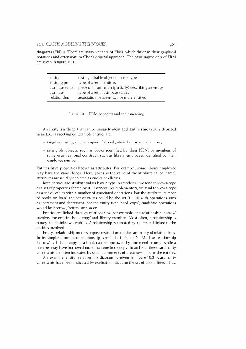
10.1. CLASSIC MODELING TECHNIQUES 251

diagrams (ERDs). There are many variants of ERM, which differ in their graphical

notations and extensions to Chen’s original approach. The basic ingredients of ERM

are given in figure 10.1.

entity distinguishable object of some type

entity type type of a set of entities

attribute value piece of information (partially) describing an entity

attribute type of a set of attribute values

relationship association between two or more entities

Figure 10.1 ERM concepts and their meaning

An entity is a ‘thing’ that can be uniquely identified. Entities are usually depicted

in an ERD as rectangles. Example entities are:

– tangible objects, such as copies of a book, identified by some number;

– intangible objects, such as books identified by their ISBN, or members of

some organizational construct, such as library employees identified by their

employee number.

Entities have properties known as attributes. For example, some library employee

may have the name ‘Jones’. Here, ‘Jones’ is the value of the attribute called ‘name’.

Attributes are usually depicted as circles or ellipses.

Both entities and attribute values have a type. As modelers, we tend to view a type

as a set of properties shared by its instances. As implementors, we tend to view a type

as a set of values with a number of associated operations. For the attribute ‘number

of books on loan’, the set of values could be the set 0 .. 10 with operations such

as increment and decrement. For the entity type ‘book copy’, candidate operations

would be ‘borrow’, ‘return’, and so on.

Entities are linked through relationships. For example, the relationship ‘borrow’

involves the entities ‘book copy’ and ‘library member’. Most often, a relationship is

binary, i.e. it links two entities. A relationship is denoted by a diamond linked to the

entities involved.

Entity--relationship models impose restrictions on the cardinality of relationships.

In its simplest form, the relationships are 1--1, 1--N, or N--M. The relationship

‘borrow’ is 1--N: a copy of a book can be borrowed by one member only, while a

member may have borrowed more than one book copy. In an ERD, these cardinality

constraints are often indicated by small adornments of the arrows linking the entities.

An example entity--relationship diagram is given in figure 10.2. Cardinality

constraints have been indicated by explicitly indicating the set of possibilities. Thus,

252 MODELING

this ERD states that a book copy can be borrowed by at most one member, and a

member may borrow up to 10 book copies.

Figure 10.2 An entity--relationship diagram

An entity--relationship model can be obtained using any of the elicitation

techniques discussed before. In particular, form analysis and analysis of natural

language descriptions are often used. Since ERMs tell only part of the story,

additional techniques have to be employed to model other aspects. Many Structured

Analysis techniques, for example, incorporate ERM to model the data aspect.

Entity--relationship modeling is a natural outgrowth of database modeling.

Originally, ERM was intended to model the logical structure of data, rather than

the logical structure of the UoD. In heuristics on how to obtain a ‘good’ entity--

relationship model, these roots are still visible. For example, some of these heuristics

resemble normalization constraints from database theory. This may explain why

some do not commend entity--relationship modeling as a requirements specification

technique (see, e.g. (Davis, 1993)).

Present-day ERM has a lot in common with object-oriented analysis techniques.

For example, subtype--supertype relations between entity types are included in many

ERM-techniques. Conversely, the class diagram of UML (see section 10.3.1) includes

many elements from ERM.

10.1.2 Finite State Machines

At any one point in time, our library is in one of a (vast) number of possible states.

The state of the library can be expressed in terms of things like:

– the collection of titles available,

10.1. CLASSIC MODELING TECHNIQUES 253

– the collection of titles ordered but not yet received,

– the collection of library members,

– the balance of the account from which acquisitions are paid.

Any action occurring in the library, be it the return of a book or the appointment of

a new employee, transforms the current state s into a new state s0.Requirements specification techniques which model a system in terms of states

and transitions between states are called state-based modeling techniques. A simple

yet powerful formalism for specifying states and state transitions is the Finite State

Machine (FSM). An FSM consists of a finite number of states and a set of transitions

from one state to another that occur on input signals from a finite set of possible

stimuli. The initial state is a specially designated state from which the machine

starts. Usually, one or more states are designated as final states. Pictorially, FSMs

are represented as state transition diagrams (STD). In a state transition diagram,

states are represented as bubbles with a label identifying the state, and transitions

are indicated as labeled arcs from one state to another, where the label denotes the

stimulus which triggers the transition. Figure 10.3 gives an FSM depicting the possible

states of a book copy and the transitions between those states. The final state is the

one labeled ‘written off’. Any of the others could be designated as the initial state.

Figure 10.3 A state transition diagram

Figure 10.3 models only a tiny part of the library system. It does not describe

the complete state of the system in any one bubble, nor does it depict all possible

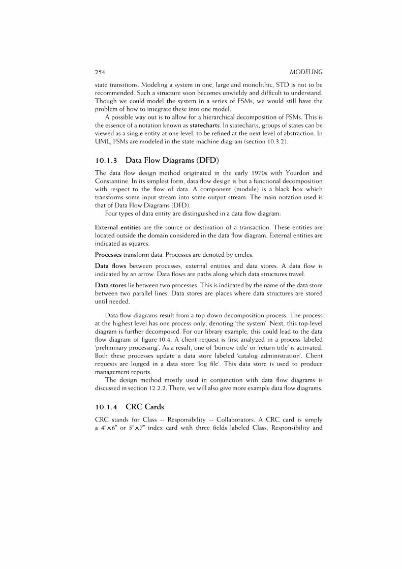
254 MODELING

state transitions. Modeling a system in one, large and monolithic, STD is not to be

recommended. Such a structure soon becomes unwieldy and difficult to understand.

Though we could model the system in a series of FSMs, we would still have the

problem of how to integrate these into one model.

A possible way out is to allow for a hierarchical decomposition of FSMs. This is

the essence of a notation known as statecharts. In statecharts, groups of states can be

viewed as a single entity at one level, to be refined at the next level of abstraction. In

UML, FSMs are modeled in the state machine diagram (section 10.3.2).

10.1.3 Data Flow Diagrams (DFD)

The data flow design method originated in the early 1970s with Yourdon and

Constantine. In its simplest form, data flow design is but a functional decomposition

with respect to the flow of data. A component (module) is a black box which

transforms some input stream into some output stream. The main notation used is

that of Data Flow Diagrams (DFD).

Four types of data entity are distinguished in a data flow diagram:

External entities are the source or destination of a transaction. These entities are

located outside the domain considered in the data flow diagram. External entities are

indicated as squares.

Processes transform data. Processes are denoted by circles.

Data flows between processes, external entities and data stores. A data flow is

indicated by an arrow. Data flows are paths along which data structures travel.

Data stores lie between two processes. This is indicated by the name of the data store

between two parallel lines. Data stores are places where data structures are stored

until needed.

Data flow diagrams result from a top-down decomposition process. The process

at the highest level has one process only, denoting ‘the system’. Next, this top-level

diagram is further decomposed. For our library example, this could lead to the data

flow diagram of figure 10.4. A client request is first analyzed in a process labeled

‘preliminary processing’. As a result, one of ‘borrow title’ or ‘return title’ is activated.

Both these processes update a data store labeled ‘catalog administration’. Client

requests are logged in a data store ‘log file’. This data store is used to produce

management reports.

The design method mostly used in conjunction with data flow diagrams is

discussed in section 12.2.2. There, we will also give more example data flow diagrams.

10.1.4 CRC Cards

CRC stands for Class -- Responsibility -- Collaborators. A CRC card is simply

a 4”�6” or 5”�7” index card with three fields labeled Class, Responsibility and

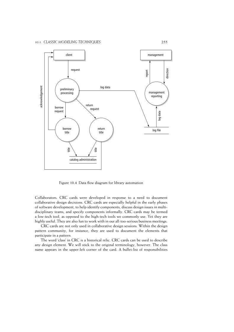
10.1. CLASSIC MODELING TECHNIQUES 255

Figure 10.4 Data flow diagram for library automation

Collaborators. CRC cards were developed in response to a need to document

collaborative design decisions. CRC cards are especially helpful in the early phases

of software development, to help identify components, discuss design issues in multi-

disciplinary teams, and specify components informally. CRC cards may be termed

a low-tech tool, as opposed to the high-tech tools we commonly use. Yet they are

highly useful. They are also fun to work with in our all-too-serious business meetings.

CRC cards are not only used in collaborative design sessions. Within the design

pattern community, for instance, they are used to document the elements that

participate in a pattern.

The word ‘class’ in CRC is a historical relic. CRC cards can be used to describe

any design element. We will stick to the original terminology, however. The class

name appears in the upper-left corner of the card. A bullet-list of responsibilities

256 MODELING

appears under the class name and a list of collaborators appears on the right part of

the card.

Figure 10.5 A CRC card

Figure 10.5 gives an example of a CRC card for a component Reservations in our

library system. The main responsibilities of this component are to keep an up-to-date

list of reservations and to handle reservations on a FIFO basis. Its collaborators are the

catalog component and the user session component. The types of interaction with

these components is shown in figure 10.16.

10.2 On Objects and Related Stuff

What matters is not how closely we model today’s reality but how extensible andreusable our software is.

(Meyer, 1996)

The world around us is full of objects, animate and inanimate, concrete and abstract:

trees and tables, cars and legal cases. According to some, analysis and design is about

modeling those real-world objects. By and large, this view has its origins in the

Scandinavian school of programming language design (SIMULA-67) and software

development. It may be termed the European view. According to others, analysis

and design is about identifying reusable components and building their inheritance

hierarchy. This latter view, which may be termed the American view, clearly shows

itself in the above citation.

What then is an object? As might be expected, there are different views of what

the notion of object entails. We may distinguish the following viewpoints:

10.2. ON OBJECTS AND RELATED STUFF 257� The modeling viewpoint: an object is a conceptual model of some part of a real

or imaginary world. This is termed the European view. From this point of view,

important characteristics are:

– each object has an identity, which distinguishes it from all other objects;

– objects have substance: properties that hold and can be discovered by

investigating an object.

From a practical point of view, object identity is an immutable tag, or an address,

which uniquely identifies that object. Different objects occupy different regions

of memory. Pragmatically also, objects may be regarded as implementations

of abstract data types (ADTs). An object then consists of a mutable state, i.e.

the set of variables of the ADT, and operations to modify or inspect the state.

Typically, the only way to access an object is through these operations. These

operations thus act as an interface to the object. An object then is a collection

of three aspects:

object = identity + variables + operations

or

object = identity + state + behavior� The philosophical viewpoint: objects are existential abstractions, as opposed

to universal abstractions. In some circles (notably Smalltalk), ‘everything

is an object’. In this view, objects act as a unifying notion underlying all

computation. However, one may also argue that there are two rather distinct

types of abstraction. Some kinds of entity have a natural beginning and end.

They are created at some point in time, exist for a while, and are ultimately

destroyed. The kinds of entities modeled as objects during analysis and design

typically belong to this class. Other kinds of entities, such as numbers, dates

and colors, have ‘eternal’ existence. They are not instantiated; they cannot be

changed; they ‘live’ forever. These entities are usually referred to as values.� The software engineering viewpoint: objects are data abstractions, encapsulat-

ing data as well as operations on those data. This viewpoint stresses locality

of information and representation independence; see also sections 12.1.1

and 12.1.3. However, not all programming languages enforce data abstrac-

tion, and objects need not always encapsulate an abstract data type. We might

claim that data abstraction and objects are somewhat orthogonal, independent

dimensions.

A programming language that merely allows us to encapsulate abstract data

types in modules is often termed object-based. The adjective object-oriented

then is reserved for languages that also support inheritance. Inheritance is

discussed below.

258 MODELING� The implementation viewpoint: an object is a contiguous structure in memory.

Technically, an object may be regarded as a record of data and code elements.

An object may be composite or aggregate, in which case it possesses other

objects. These sub-objects in turn may possess even ‘smaller’ sub-objects,

etcetera. The lowest-level objects in this hierarchy are atomic objects, typically

denoting things like integers, real numbers or Booleans.

The implementation of this ‘possessed-by’ relation appears to be intricate. On

the one hand, objects may be contained in other objects. In this representation,

all references are dispensed with. There is no concept of sharing. This scheme

is known as value semantics. Value semantics is inadequate for object-oriented

systems, since such systems require sharable objects. The opposite scheme is

reference semantics: data is represented as either an atomic object or as an

aggregate of references to other objects. Pure reference semantics is inefficient

in the case of primitive objects like integers or characters. A combination in

which aggregate objects may contain other objects, refer to other objects, or

do both at the same time, is commonly used as a storage scheme. The choice of

a particular storage model is to some extent reflected in the high-level language

semantics (for example, where it concerns copying or comparing objects).� The formal viewpoint: an object is a state machine with a finite set of states and

a finite set of state functions. These state functions map old states and inputs to

new states and outputs.

Formalization of the concepts and constructions of object-oriented languages is

difficult. Mathematical formalisms tend to be value-based. Imperative concepts,

such as state and sharing, that are central to object-oriented languages do not

fit easily within such schemes.

During analysis, the conceptual viewpoint is usually stressed. Those who are of the

opinion that analysis and design smoothly shade off into one another tend to keep

this view during design. Others however are of the opinion that analysis and design

are different, irrespective of whether they are object-oriented or not. They are likely

to stress other viewpoints during design. The definition of an object as given in (Coad

and Yourdon, 1991) also reflects the tension between a problem-oriented and a

solution-oriented viewpoint: an object is ‘an abstraction of something in a problem

domain, reflecting the capabilities of a system to keep information about it, interact

with it, or both; an encapsulation of Attribute values and their exclusive Services.’

We will come back to this dichotomy when discussing object-oriented methods in

section 12.3.

As noted above, objects are characterized by a set of attributes (properties).

A table has legs, a table top, size, color, etc. The attribute concept originates

with Entity--Relationship Modeling; see section 10.1.1. In ERM, attributes represent

intrinsic properties of entities, properties whose value does not depend on other entities.

Attributes denote identifying and descriptive properties, such as name or weight.

10.2. ON OBJECTS AND RELATED STUFF 259

Relationships on the other hand denote mutual properties, such as an employee being

assigned to a project or a book being borrowed by a member. In UML, these

relationships are called associations. In UML, the distinction between attributes and

relationships formally does not exist. Both are properties of a class. It is considered

good practice in UML though to model simple properties as attributes, and more

complex properties as associations.

In the context of object-oriented modeling, the term attribute is sometimes used

to denote any field in the underlying data structure. In that case, the object’s identity

is an attribute, the state denotes the set of ‘structural’ attributes, and the operations

denote the ‘behavioral’ attributes. We will use the term attribute to denote a structural

attribute. Collectively, this set of attributes of an object thus constitutes its state. It

includes the intrinsic properties, usually represented as values, as well as the mutual

properties, usually represented as references to other objects.

At the programming-language level, objects that have the same set of attributes

are said to belong to the same class. Individual objects of a class are called instances of

that class. So we may have a class Table, with instances MyTable and YourTable.

These instances have the same attributes, with possibly different values.

An object not only encapsulates its state, but also its behavior, i.e. the way in which

it acts upon other objects and is acted upon by other objects. The behavior of an

object is described in terms of services provided by that object. These services are

invoked by sending messages from the object that requests the service to the object that

is acted upon.

In order for a collection of objects to operate together as intended, each of the

objects must be able to rely on the proper operation of the objects with which it

interacts. In a client-server view, one object, the client, requests some service from

another object, the server. This mutual dependency may be viewed as a contract

between the objects involved. The client will not ask more than what is stated in the

contract, while the server promises to deliver what is stated in the contract. In this

perspective, services are also referred to as responsibilities.

The major behavioral aspect of an object concerns state changes. The state of an

object instance is not static, but changes over time: the object instance is created,

updated, and eventually destroyed. Also, certain information may be requested from

an object. This information may concern the state of the object instance, but it may

also involve a computation of some sort.

For example, a customer of a library may have attributes like Name, Address,

and BooksOnLoan. It must be possible to create an instance of the object type

Customer. When doing so, suitable values for its attributes must be provided. Once

the instance has been created, state changes are possible: books are loaned and

returned, the customer changes address, etc. Finally, the instance is destroyed when

the customer ceases to be a member. Information requested may concern such things

as a list of books on loan or the number of books on loan. The former is part of the

state that describes a particular customer and can be retrieved directly from that state.

NumberOfBooksOnLoan is a service that requires a computation of some sort, for

260 MODELING

example counting the number of elements in BooksOnLoan.

We will generally not be concerned with individual objects. Our goal is to identify

and relate the object types (i.e. classes). We will often use the term object to denote

an object type. One of our major concerns during analysis and design is to identify

this set of objects, together with their attributes (state) and services (behavior).

Relations between objects can be expressed in a classification structure. The major

types of relation depicted in such structures are listed in figure 10.6.

Relation Example

Specialization/Generalization, is-a Table is-a FurnitureWhole-part, has Table has TableTopMember-of, has Library has Member

Figure 10.6 Major types of relations between objects

If we have objects Table and Chair, we may also define a more general object

Furniture. Table and Chair are said to be specializations of Furniture, while Furnitureis a generalization of Table and Chair. These relations are also known as ‘is-a’ relations.

The is-a relation is a well-known concept from Entity--Relationship Modeling.

The generalization/specialization relations can be expressed in a hierarchical

structure like the one in figure 10.7. In its most general form the classification

structure is a directed acyclic graph (DAG). Many classification structures can be

depicted as a tree though, in which case each object is a direct descendant of exactly

one other object. At the programming-language level, single inheritance corresponds

to a tree structure, while multiple inheritance corresponds to a DAG.

Different objects may share some of their attributes. Both tables and chairs have

a height, for instance. Rather than defining the full set of attributes for each object,

we may define common attributes at a higher level in the object hierarchy and let

descendants inherit those attributes. We may therefore define the attribute Height at

the level of Furniture rather than at the level of each of its descendants. Obviously,

this is just another way of looking at the object hierarchy. The fact that Chair and

Table are both descendants of Furniture already suggests that they share certain

properties, properties that are common to the various types of furniture. The fact that

they are different descendants of Furniture also suggests that they each have unique

properties.

Alternatively, we may view the object hierarchy as a type hierarchy. Chair and

Table are subtypes of Furniture, just like Cardinal is a subtype of Integer. In this

view, an object is a restriction of the objects of which it is a specialization. Each chair

is a piece of furniture, but the reverse is not generally true.

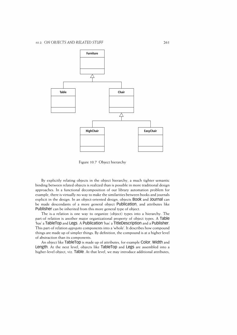
10.2. ON OBJECTS AND RELATED STUFF 261

Figure 10.7 Object hierarchy

By explicitly relating objects in the object hierarchy, a much tighter semantic

binding between related objects is realized than is possible in more traditional design

approaches. In a functional decomposition of our library automation problem for

example, there is virtually no way to make the similarities between books and journals

explicit in the design. In an object-oriented design, objects Book and Journal can

be made descendants of a more general object Publication, and attributes like

Publisher can be inherited from this more general type of object.

The is-a relation is one way to organize (object) types into a hierarchy. The

part-of relation is another major organizational property of object types. A Table‘has’ a TableTop and Legs. A Publication ‘has’ a TitleDescription and a Publisher.This part-of relation aggregates components into a ‘whole’. It describes how compound

things are made up of simpler things. By definition, the compound is at a higher level

of abstraction than its components.

An object like TableTop is made up of attributes, for example Color, Width and

Length. At the next level, objects like TableTop and Legs are assembled into a

higher-level object, viz. Table. At that level, we may introduce additional attributes,

262 MODELING

such as Size, so that Table may also be seen as an aggregate of the first kind. In

general, a compound object consists of a number of (references to) other objects and

a number of ‘simple’ attributes, i.e. values.

In the case of Table, the part-of relation is a real-world part-of relation. In the

case of Publication, Publisher does not correspond to some part of the underlying

real-world object. It merely is part of the representation of the object Publication.

Sometimes, an explicit distinction is made between the real-world part-of relation

and the representational part-of (or component-of) relation. In UML they are called

composition and aggregation, respectively.

In many modeling methods, the part-of relation subsumes the member-of relation.

The member-of relation is used to model the relationship between a set and its

members. It is, however, sometimes useful to be able to distinguish between these

organizational properties. For example, the part-of relation is generally considered to

be transitive, whereas the member-of relation is not. If Book is a member of Library,

and Library is a member of PublicInstitutions, we do not want to infer that Bookis a member of PublicInstitutions.

10.3 The Unified Modeling Language

The Unified Modeling Language has its roots in the object-oriented analysis and

design methods of the 1980s. Several key players in this field (Grady Booch, John

Rumbaugh and Ivar Jacobson) came to work for Rational, and started to unify their

methods and notations. This resulted in the first versions of UML. At a later stage,

OMG --- the Object Management Group, an open consortium of companies --- took

over. They now control the activities around UML, and adopted it as one of their

standards. The current version is known as UML 2. UML is by far the most widely

used notation for both requirements engineering and design.

The 13 diagrams of UML 2 are listed in figure 10.8. Some diagrams, such as the

class diagram and the state machine diagram, have been there since the beginning

of object orientation. Others are more recent. For example, the composite structure

diagram and the timing diagram were introduced in UML 2. Some of the diagrams

give a static view. For instance, a class diagram shows the static structure of a system.

Other diagrams give a dynamic, or behavioral view, i.e. they show what happens

when the system is executed. For instance, a sequence diagram shows which messages

are exchanged between instances of classes. In figure 10.8, static diagrams are marked

with an S, and dynamic diagrams are marked with a D. In the next subsections, we

discuss the most important UML diagrams.

10.3.1 The Class Diagram

Class diagrams depict the static structure of a system. A class diagram is a graph

in which the nodes are objects (classes) and the edges are relationships between

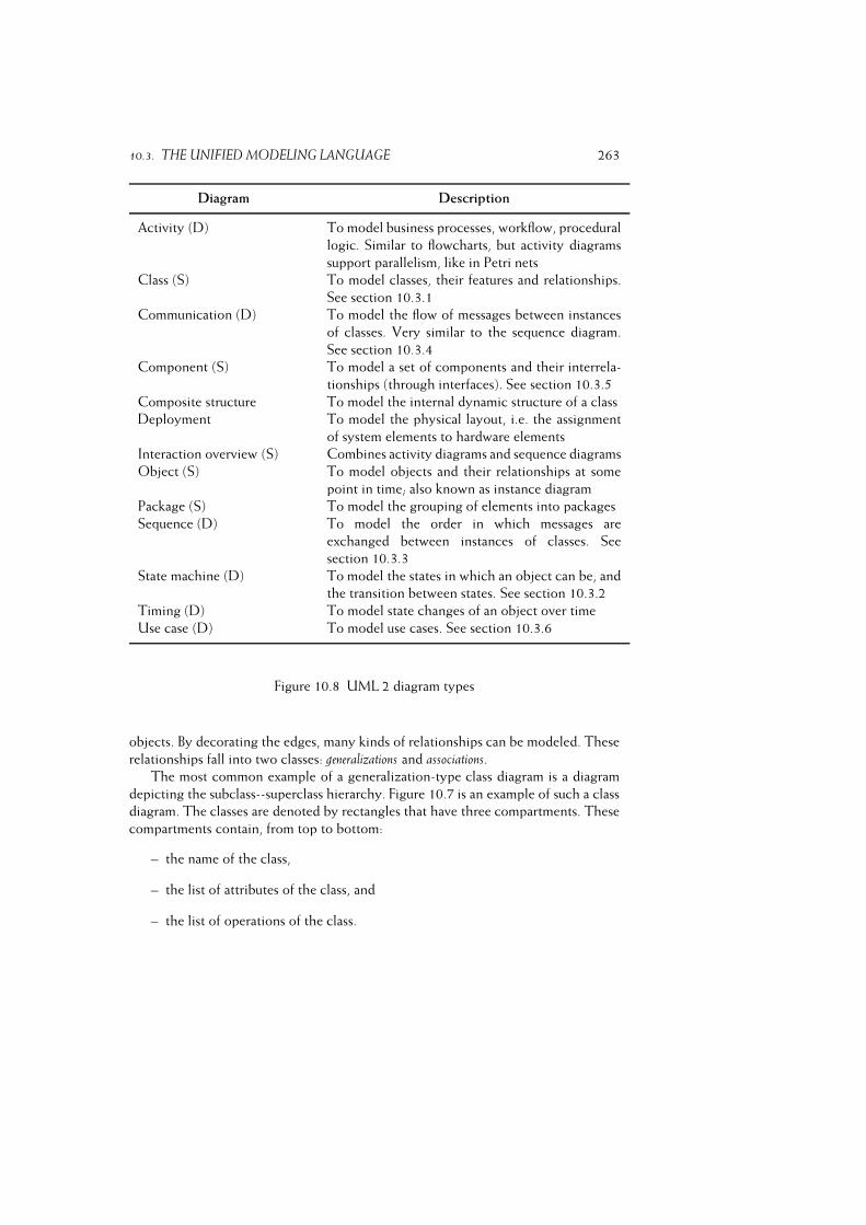
10.3. THE UNIFIED MODELING LANGUAGE 263

Diagram Description

Activity (D) To model business processes, workflow, procedural

logic. Similar to flowcharts, but activity diagrams

support parallelism, like in Petri nets

Class (S) To model classes, their features and relationships.

See section 10.3.1

Communication (D) To model the flow of messages between instances

of classes. Very similar to the sequence diagram.

See section 10.3.4

Component (S) To model a set of components and their interrela-

tionships (through interfaces). See section 10.3.5

Composite structure To model the internal dynamic structure of a class

Deployment To model the physical layout, i.e. the assignment

of system elements to hardware elements

Interaction overview (S) Combines activity diagrams and sequence diagrams

Object (S) To model objects and their relationships at some

point in time; also known as instance diagram

Package (S) To model the grouping of elements into packages

Sequence (D) To model the order in which messages are

exchanged between instances of classes. See

section 10.3.3

State machine (D) To model the states in which an object can be, and

the transition between states. See section 10.3.2

Timing (D) To model state changes of an object over time

Use case (D) To model use cases. See section 10.3.6

Figure 10.8 UML 2 diagram types

objects. By decorating the edges, many kinds of relationships can be modeled. These

relationships fall into two classes: generalizations and associations.The most common example of a generalization-type class diagram is a diagram

depicting the subclass--superclass hierarchy. Figure 10.7 is an example of such a class

diagram. The classes are denoted by rectangles that have three compartments. These

compartments contain, from top to bottom:

– the name of the class,

– the list of attributes of the class, and

– the list of operations of the class.

264 MODELING

UML allows for quite some variety in its notation. We may for instance depict

a class as a rectangle with one compartment only, just giving the name of the

class. Adding slightly more detail, we may depict a class as a rectangle having two

compartments, where the second one characterizes the responsibilities of that class,

i.e., what it is supposed to do, as kind of an inline comment. Figure 10.9 gives the

three-compartment representation in which a number of analysis-level details have

been added. We may even extend the notation further and add implementation-level

details, such as whether attributes and operations are public or private. We may think

of these different representations as different views of the same model element. We

may envision tool support that allows the user to switch from one representation to

another, suppressing or adding detail as the need arises.

archive()

publisher: Stringisbn: String

name: String

return()borrow(Client)

title: Stringauthor: String

Publication

JournalBook

Figure 10.9 UML class diagram: generalization

The hollow triangle in figure 10.9 indicates that the structure is a generaliza-

tion/specialization structure. Generalization is shown as a solid path from the more

specific element (such as Book) to the more general element (Publication), with a

large hollow triangle at the end of the path. A group of generalization paths may be

shown as a tree with a shared segment, as in figure 10.9.

10.3. THE UNIFIED MODELING LANGUAGE 265

The attributes of a class denote properties of that class. E.g., publisher is a property

of Publication. Next to attributes, UML has another way of denoting properties of

a class, viz. associations. A UML association is depicted as a solid line connecting two

classes. This line may be adorned with a variety of glyphs and textual information to

provide further specifics of the relationship. A simple association between a library

and its clients is depicted in figure 10.10a. The (optional) name of the association is

printed near the path. The solid triangle indicates the direction in which the verb is

to be read. Note that associations are bi-directional: a client is a member of a library,

and a library has members. Further adornments can be added to indicate properties of

the association. In figure 10.10a we have added multiplicity information: a client can

be a member of one or more libraries, while a library may have zero or more clients.

Strictly speaking, there is no difference between an attribute and an association.

In figure 10.10b, we have depicted Client as an attribute of Library. Usually, simple

properties such as numbers and dates are modeled as attributes, while more significant

concepts are modeled as associations.

An association such as Member-of also has class properties. For example, this

association has attributes, e.g. MemberId, and operations, such as BecomeMemberand CeaseToBeMember. Alternatively, we may say that class Membership has

association properties. In UML, this model element is termed association class. It

can be depicted as a class symbol attached by a dashed line to an association path,

as in figure 10.10c. We may even promote an association clas to a full class, as

in figuUML10.10d. Notice that the multiplicities have moved. A membership (of

a client) can be to one or more libraries, whereas the membership (of the library)

relates to zero or more clients.

The part-of relation is called aggregation or composition in UML. In an aggre-

gation, objects can be part of more than one other object. For example, if our library

maintains lists of required readings for certain courses, then a given book may be a

part of more than one required reading list. Aggregation is denoted with an open

filed diamond as association role adornment. Composition is a strong notion of

aggregation, in which the part object may belong to only one whole object. With

composition, the parts are expected to live and die with the whole. If a table is

composed of four legs and a tabletop, the table owns these parts. They cannot be part

of another table at the same time. Composition is denoted by a solid filled diamond as

an association role adornment, as in figure 10.11a. Figure 10.11a shows a Book with

parts title, author, and isbn. A book has one title and one ISBN, so these parts have

multiplicity 1. We assume here that a book may have up to three authors, so that part

has multiplicity of 1..3. At the whole end of composition, the multiplicity is either 1

or 0..1. This part-of relationship is a relationship between a class and the classes of

its attributes. An alternative notation for this part-of relation therefore consists of the

top two compartments of the diagram for a class, as in figure 10.11b.

Next to generalization and association, there are many other ways in which

elements of a class diagram may depend on each other. For example, one class may

call operations from another class, create instances of another class, and so on. Such

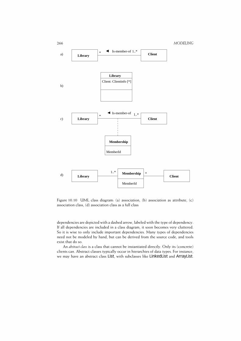
266 MODELING

Library

Client: Clientinfo [*]b)

Client1..** Is-member-of

Library

MemberId

Membership

d)

a)

Is-member-of

c)

LibraryMembership

MemberId

Client1..* *

ClientLibrary* 1..*

Figure 10.10 UML class diagram: (a) association, (b) association as attribute, (c)

association class, (d) association class as a full class

dependencies are depicted with a dashed arrow, labeled with the type of dependency.

If all dependencies are included in a class diagram, it soon becomes very cluttered.

So it is wise to only include important dependencies. Many types of dependencies

need not be modeled by hand, but can be derived from the source code, and tools

exist that do so.

An abstract class is a class that cannot be instantiated directly. Only its (concrete)

clients can. Abstract classes typically occur in hierarchies of data types. For instance,

we may have an abstract class List, with subclasses like LinkedList and ArrayList.

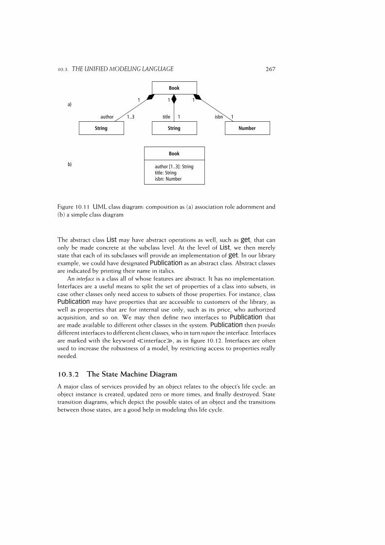
10.3. THE UNIFIED MODELING LANGUAGE 267

Figure 10.11 UML class diagram: composition as (a) association role adornment and

(b) a simple class diagram

The abstract class List may have abstract operations as well, such as get, that can

only be made concrete at the subclass level. At the level of List, we then merely

state that each of its subclasses will provide an implementation of get. In our library

example, we could have designated Publication as an abstract class. Abstract classes

are indicated by printing their name in italics.

An interface is a class all of whose features are abstract. It has no implementation.

Interfaces are a useful means to split the set of properties of a class into subsets, in

case other classes only need access to subsets of those properties. For instance, class

Publication may have properties that are accessible to customers of the library, as

well as properties that are for internal use only, such as its price, who authorized

acquisition, and so on. We may then define two interfaces to Publication that

are made available to different other classes in the system. Publication then providesdifferent interfaces to different client classes, who in turn require the interface. Interfaces

are marked with the keyword �interface�, as in figure 10.12. Interfaces are often

used to increase the robustness of a model, by restricting access to properties really

needed.

10.3.2 The State Machine Diagram

A major class of services provided by an object relates to the object’s life cycle: an

object instance is created, updated zero or more times, and finally destroyed. State

transition diagrams, which depict the possible states of an object and the transitions

between those states, are a good help in modeling this life cycle.

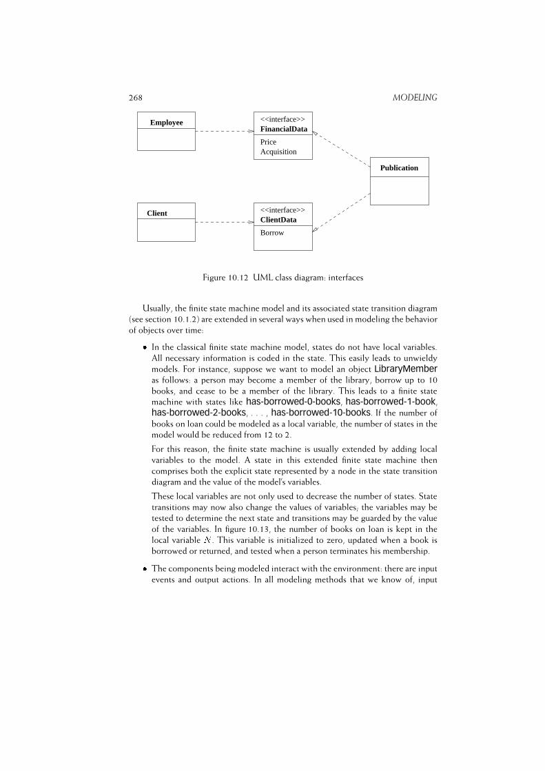
268 MODELING

Publication

Borrow

ClientData<<interface>>

Price

<<interface>>FinancialData

Acquisition

Employee

Client

Figure 10.12 UML class diagram: interfaces

Usually, the finite state machine model and its associated state transition diagram

(see section 10.1.2) are extended in several ways when used in modeling the behavior

of objects over time:� In the classical finite state machine model, states do not have local variables.

All necessary information is coded in the state. This easily leads to unwieldy

models. For instance, suppose we want to model an object LibraryMemberas follows: a person may become a member of the library, borrow up to 10

books, and cease to be a member of the library. This leads to a finite state

machine with states like has-borrowed-0-books, has-borrowed-1-book,

has-borrowed-2-books, . . . , has-borrowed-10-books. If the number of

books on loan could be modeled as a local variable, the number of states in the

model would be reduced from 12 to 2.

For this reason, the finite state machine is usually extended by adding local

variables to the model. A state in this extended finite state machine then

comprises both the explicit state represented by a node in the state transition

diagram and the value of the model’s variables.

These local variables are not only used to decrease the number of states. State

transitions may now also change the values of variables; the variables may be

tested to determine the next state and transitions may be guarded by the value

of the variables. In figure 10.13, the number of books on loan is kept in the

local variable N . This variable is initialized to zero, updated when a book is

borrowed or returned, and tested when a person terminates his membership.� The components being modeled interact with the environment: there are input

events and output actions. In all modeling methods that we know of, input

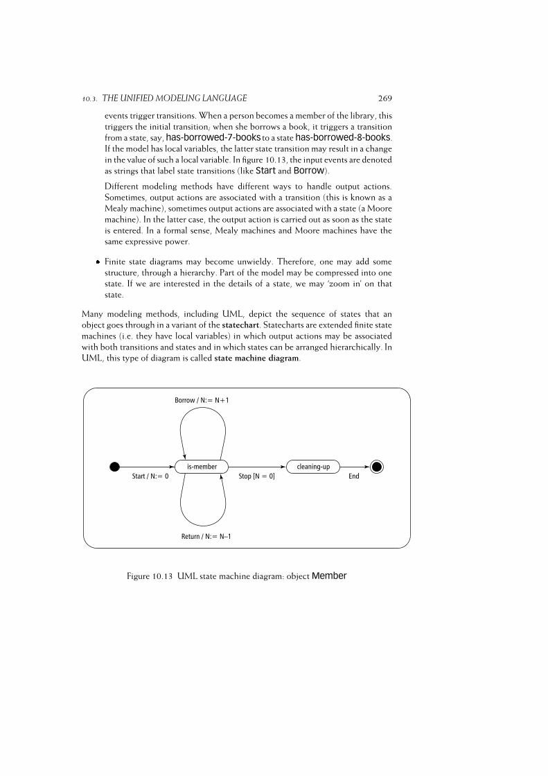
10.3. THE UNIFIED MODELING LANGUAGE 269

events trigger transitions. When a person becomes a member of the library, this

triggers the initial transition; when she borrows a book, it triggers a transition

from a state, say, has-borrowed-7-books to a state has-borrowed-8-books.

If the model has local variables, the latter state transition may result in a change

in the value of such a local variable. In figure 10.13, the input events are denoted

as strings that label state transitions (like Start and Borrow).

Different modeling methods have different ways to handle output actions.

Sometimes, output actions are associated with a transition (this is known as a

Mealy machine), sometimes output actions are associated with a state (a Moore

machine). In the latter case, the output action is carried out as soon as the state

is entered. In a formal sense, Mealy machines and Moore machines have the

same expressive power.� Finite state diagrams may become unwieldy. Therefore, one may add some

structure, through a hierarchy. Part of the model may be compressed into one

state. If we are interested in the details of a state, we may ‘zoom in’ on that

state.

Many modeling methods, including UML, depict the sequence of states that an

object goes through in a variant of the statechart. Statecharts are extended finite state

machines (i.e. they have local variables) in which output actions may be associated

with both transitions and states and in which states can be arranged hierarchically. In

UML, this type of diagram is called state machine diagram.

Figure 10.13 UML state machine diagram: object Member

270 MODELING

As with class diagrams, UML has a rich notation for state diagrams. We will

illustrate the major ingredients through a few examples; see also figures 10.13

and 10.14.

A state is some condition in the life of an object. It is shown as a rectangle with

rounded corners. An initial (pseudo) state is shown as a small filled circle. This initial

state is a mere notational device; an object can not be in such a state. It indicates

the transition to the first ‘real’ state. A final (pseudo) state is shown as a small circle

surrounding a small filled circle. This final state is also a notational device. A transition

is shown as a solid arrow from one state to another. When a change of state occurs,

that transition is said to ‘fire’. A transition has a label that comes in three parts. The

general form is trigger-signature [guard]/activity. All three parts are optional. The trigger-

signature denotes the event which triggers the transaction, such as the borrowing of a

book. The event may be guarded by a Boolean expression. For example, the transition

from state is-member to cleaning-up in figure 10.13 is guarded by the expression

‘N = 0’; it can only occur if the number of books on loan is zero. When an event

occurs, only one transition can be taken. So if multiple transitions occur with the

same event, the guards must be mutually exclusive. The transition label may include

a procedural expression after the symbol ‘/’. This procedural expression is executed

when the transition fires.

Figure 10.14 gives an example of nested states. Figure 10.14a gives a global view

of the life cycle of an object Book: a book is ordered, stays alive for a while, and is

eventually either disposed of or archived. In figure 10.14b, state alive is expanded to

show its finer structure. In this example, the state is refined into mutually exclusive

disjoint substates: a book is either available or borrowed1. The transition from state

ordered to state alive is drawn to the boundary of state alive. This is equivalent

to a transition to the initial state within the graphics region of alive. The transition

from the nested state available to states disposed and archived is made directly.

To indicate this transition from a suppressed internal state of alive to disposed and

archived in figure 10.14a, the transitions are not drawn from the boundary of alive,

but from a so-called stub, shown as a small vertical line drawn inside its boundary.

10.3.3 The Sequence Diagram

Objects communicate by sending messages. To carry out a certain task, a particular

sequence of messages may have to be exchanged between two or more objects. The

time ordering in which this sequence of messages has to occur may be depicted

in a sequence diagram. A sequence diagram is on type of interaction diagram.

A second type of interaction diagram is the communication diagram, discussed in

1UML also allows you to refine a state into concurrent substates. For example, when a book is returned,

several things have to be done. It has to be checked whether the book is returned within the fixed time.If not, some fine may be due. Possible outstanding reservations need to be checked as well and, if so, one

of these reservations must be handled. These subprocesses can be handled concurrently. There can be a

state returning book which, when refined, results in two or more concurrent, and-related substates. This

is shown by tiling the graphics region of the state using dashed lines to separate subregions.

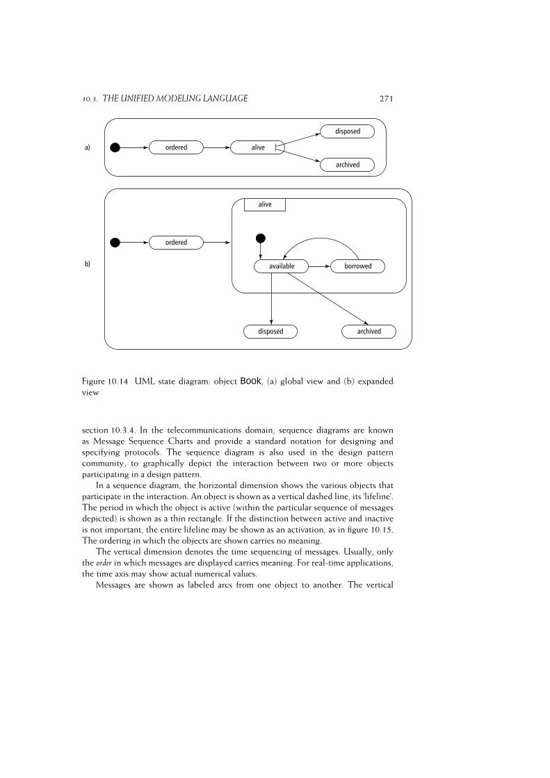
10.3. THE UNIFIED MODELING LANGUAGE 271

Figure 10.14 UML state diagram: object Book, (a) global view and (b) expanded

view

section 10.3.4. In the telecommunications domain, sequence diagrams are known

as Message Sequence Charts and provide a standard notation for designing and

specifying protocols. The sequence diagram is also used in the design pattern

community, to graphically depict the interaction between two or more objects

participating in a design pattern.

In a sequence diagram, the horizontal dimension shows the various objects that

participate in the interaction. An object is shown as a vertical dashed line, its ‘lifeline’.

The period in which the object is active (within the particular sequence of messages

depicted) is shown as a thin rectangle. If the distinction between active and inactive

is not important, the entire lifeline may be shown as an activation, as in figure 10.15.

The ordering in which the objects are shown carries no meaning.

The vertical dimension denotes the time sequencing of messages. Usually, only

the order in which messages are displayed carries meaning. For real-time applications,

the time axis may show actual numerical values.

Messages are shown as labeled arcs from one object to another. The vertical

272 MODELING

arrangement of messages indicates their order. The labels may also contain sequence

numbers, which are particularly useful to indicate concurrency. A message may also

be labeled with a guard, a boolean expression that states the condition which must

hold for the message to be sent.

start

user

6: remove reservation

6: borrow title

5: title available

5: hold title

4: title returned

3: [not available] reserve title

2: title data

1: look up

reservationscatalog

Figure 10.15 UML sequence diagram: reserving a title

Figure 10.15 shows a possible sequence of interactions between a user, a catalog

of available books, and an object which handles reservations. The first message comes

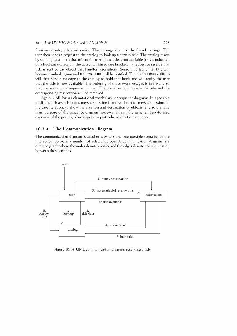
10.3. THE UNIFIED MODELING LANGUAGE 273

from an outside, unknown source. This message is called the found message. The

user then sends a request to the catalog to look up a certain title. The catalog reacts

by sending data about that title to the user. If the title is not available (this is indicated

by a boolean expression, the guard, within square brackets), a request to reserve that

title is sent to the object that handles reservations. Some time later, that title will

become available again and reservations will be notified. The object reservationswill then send a message to the catalog to hold that book and will notify the user

that the title is now available. The ordering of those two messages is irrelevant, so

they carry the same sequence number. The user may now borrow the title and the

corresponding reservation will be removed.

Again, UML has a rich notational vocabulary for sequence diagrams. It is possible

to distinguish asynchronous message-passing from synchronous message-passing, to

indicate iteration, to show the creation and destruction of objects, and so on. The

main purpose of the sequence diagram however remains the same: an easy-to-read

overview of the passing of messages in a particular interaction sequence.

10.3.4 The Communication Diagram

The communication diagram is another way to show one possible scenario for the

interaction between a number of related objects. A communication diagram is a

directed graph where the nodes denote entities and the edges denote communication

between those entities.

3: [not available] reserve title

5: title available

look up1:

title data2:

user

borrow6:

title

catalog

start

6: remove reservation

reservations

4: title returned

5: hold title

Figure 10.16 UML communication diagram: reserving a title

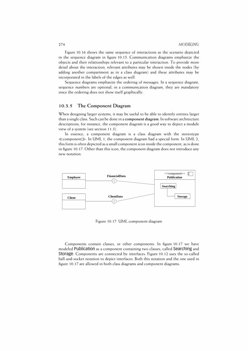
274 MODELING

Figure 10.16 shows the same sequence of interactions as the scenario depicted

in the sequence diagram in figure 10.15. Communication diagrams emphasize the

objects and their relationships relevant to a particular interaction. To provide more

detail about the interaction, relevant attributes may be shown inside the nodes (by

adding another compartment as in a class diagram) and these attributes may be

incorporated in the labels of the edges as well.

Sequence diagrams emphasize the ordering of messages. In a sequence diagram,

sequence numbers are optional; in a communication diagram, they are mandatory

since the ordering does not show itself graphically.

10.3.5 The Component Diagram

When designing larger systems, it may be useful to be able to identify entities larger

than a single class. Such can be done in a component diagram. In software architecture

descriptions, for instance, the component diagram is a good way to depict a module

view of a system (see section 11.3).

In essence, a component diagram is a class diagram with the stereotype�component�. In UML 1, the component diagram had a special form. In UML 2,

this form is often depicted as a small component icon inside the component, as is done

in figure 10.17. Other than this icon, the component diagram does not introduce any

new notation.

FinancialData

ClientData

<<component>>Publication

Searching

Storage

Employee

Client

Figure 10.17 UML component diagram

Components contain classes, or other components. In figure 10.17 we have

modeled Publication as a component containing two classes, called Searching and

Storage. Components are connected by interfaces. Figure 10.12 uses the so-called

ball-and-socket notation to depict interfaces. Both this notation and the one used in

figure 10.17 are allowed in both class diagrams and component diagrams.

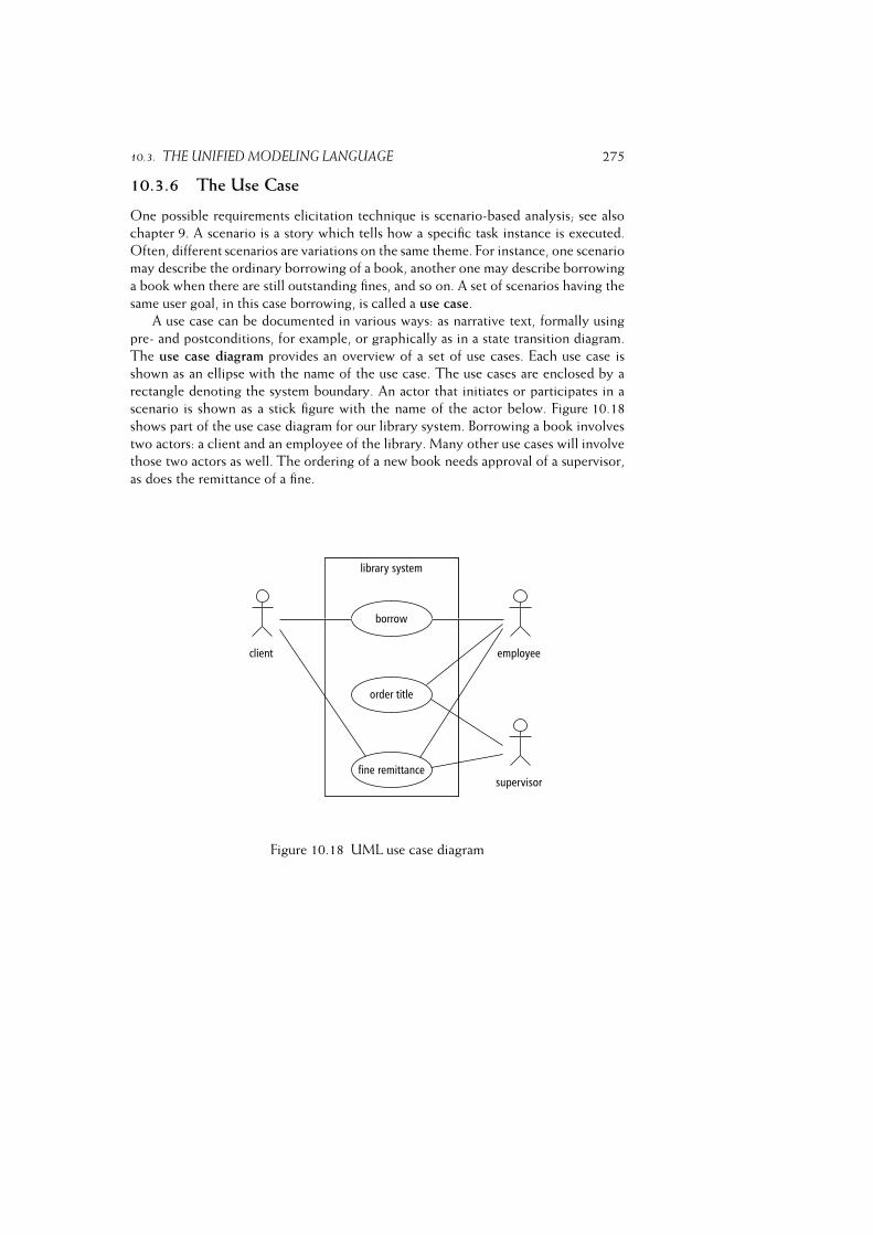
10.3. THE UNIFIED MODELING LANGUAGE 275

10.3.6 The Use Case

One possible requirements elicitation technique is scenario-based analysis; see also

chapter 9. A scenario is a story which tells how a specific task instance is executed.

Often, different scenarios are variations on the same theme. For instance, one scenario

may describe the ordinary borrowing of a book, another one may describe borrowing

a book when there are still outstanding fines, and so on. A set of scenarios having the

same user goal, in this case borrowing, is called a use case.

A use case can be documented in various ways: as narrative text, formally using

pre- and postconditions, for example, or graphically as in a state transition diagram.

The use case diagram provides an overview of a set of use cases. Each use case is

shown as an ellipse with the name of the use case. The use cases are enclosed by a

rectangle denoting the system boundary. An actor that initiates or participates in a

scenario is shown as a stick figure with the name of the actor below. Figure 10.18

shows part of the use case diagram for our library system. Borrowing a book involves

two actors: a client and an employee of the library. Many other use cases will involve

those two actors as well. The ordering of a new book needs approval of a supervisor,

as does the remittance of a fine.

Figure 10.18 UML use case diagram

276 MODELING

10.4 Summary

During requirements engineering and design, a variety of modeling notations are

being applied. Most of these use some sort of box-and-line diagram. The mainstream

modeling notations of today stem from UML --- the Unified Modeling Language.

Many UML diagrams in turn are based on or derived from earlier types of diagram. In

this chapter, we discuss a selection of classic modeling notations as well as the major

UML diagram types.

The classic modeling notations discussed are:� Entity-Relationship Modeling (ERM), used to model the structure of data.� Finite State Machines (FSM), to model states and state transitions of a system.� Data Flow Diagrams (DFD) to model functional decomposition with respect

to data.� CRC Cards, a simple notation to document collaborative design decisions.

UML evolved from earlier object-oriented analysis and design methods. Concepts

used in UML, such as object, attribute, class, relationship, originate in the field of

object orientation. UML 2 offers 13 diagram types. These fall into two classes. Some

diagrams give a static view of the system. For instance, a class diagram shows how a

system is statically organized into classes. Other diagrams give a dynamic view. For

instance, a sequence diagram shows the time ordering of message exchanges between

instance of classes.

10.5 Further Reading

Entity--relationship modeling was pioneered by Chen (Chen, 1976). Many texts on

database modeling include an elaborate discussion of ERM; see for example (Batini

et al., 1992). Statecharts are described in (Harel, 1988). CRC cards are described

in (Beck and Cunningham, 1989).

The different views of the notion of object are discussed in (Taivalsaari, 1993).

The various meanings of attribute and related notions such as aggregate, part and

member are discussed in (Motschnig-Pitrik, 1996). (Wegner, 1992) is a classic paper

on the various dimensions of object-oriented modeling.

Fowler (2004) provides a good introduction to UML. UML is extensively discussed

in two books by its creators: (Booch et al., 1999) and (Rumbaugh et al., 1999).

Exercises

1. Explain the following concepts from entity--relationship modeling: entity,

entity type, attribute value, attribute, relationship.

10.5. FURTHER READING 277

2. Define the following terms: object, state, attribute, message, and inheritance.

3. Explain the difference between the specialization--generalization relation and

the whole--part relation.

4. Explain the difference between a class diagram and a state machine diagram.

5. Explain the difference between a sequence diagram and a communication

diagram.

6. Explain the difference between a class diagram and a component diagram.

7. What are CRC cards and use-case scenarios used for in object-oriented

analysis and design?

8. In what respects does a UML state diagram differ from a state transition

diagram?

9. ~ In what sense can the interface to a class be considered a contract? What

are the repercussions of this for subtyping relations? (See (Meyer, 1992)).

11

Software Architecture

LEARNING OBJECTIVES� To appreciate the role of software architecture in software development� To understand the relation between software architecture and design decisions� To be able to document a software architecture in different views� To be able to characterize some important software architectural styles� To understand the role and purpose of software architecture assessments

279

Software architecture concerns the large-scale structure of software systems.

This large-scale structure reflects the early, essential design decisions. This

decision process involves negotiating and balancing of functional and quality

requirements on one hand, and possible solutions on the other hand. Software

architecture is not a phase strictly following requirements engineering, but

the two are intertwined. In this chapter, we discuss how to design, document

and evaluate software architectures.

A good design is the key to a successful product. Almost 2000 years ago, the

Roman architect Vitruvius recorded what makes a design good: durability (firmitas),utility (utilitas), and charm (venustas). These quality requirements still hold, for

buildings as well as software systems. A well-designed system is easy to implement, is

understandable and reliable, and allows for smooth evolution. Badly-designed systems

may work at first, but they are hard to maintain, difficult to test, and unreliable.

During the design phase, the system is decomposed into a number of interacting

components. The top-level decomposition of a system into major components

together with a characterization of how these components interact, is called its

software architecture. Viewed this way, software architecture is synonymous with

global design. There is, however, more to software architecture than mere global

design.

Software architecture serves three main purposes:� It is a vehicle for communication among stakeholders. A software architecture

is a global, often graphic, description that can be communicated with the

customers, end users, designers, and so on. By developing scenarios of antici-

pated use, relevant quality aspects can be analyzed and discussed with various

stakeholders. The software architecture also supports communication during

development. It can be used to develop a skeletal version of the system. This

skeletal version contains all of the architecture’s components in a rudimentary

form. The skeletal system can be used as an environment for the incremental

implementation of the system. It can also be used as an environment (test

harness) for testing the system.� It captures early design decisions. In a software architecture, the global

structure of the system has been decided upon, through the explicit assignment

of functionality to components of the architecture. These early design decisions

are important since their ramifications are felt in all subsequent phases. It is

therefore paramount to assess their quality at the earliest possible moment.

By evaluating the architecture, a first and global insight into important quality

aspects can be obtained. The global structure decided upon at this stage also

structures development: the work-breakdown structure may be based on the

decomposition chosen at this stage, testing may be organized around this same

decomposition, and so on.

280 SOFTWARE ARCHITECTURE� It is a transferable abstraction of a system. The architecture is a basis for

reuse. Design decisions are often ordered, from essential to nice features. The

essential decisions are captured in the architecture, while the nice features can

be decided upon at a later stage. The software architecture thus provides a basis

for a family of similar systems, a so-called product line; see also chapter ??.

The global description captured in the architecture may also serve as a basis

for training, e.g. to introduce new team members.

The traditional view holds that the requirements fully determine the structure of a

system. Traditional design methods as discussed in chapter 12 work that way. Their

aim is to systematically bridge the gap between the requirements and some blueprint

of an operational system in which all of the requirements are met. It is increasingly

being recognized that other forces influence the architecture (and, for that matter,

the design) as well:� Architecture is influenced by the development organization. In our library

example, for example, the hardware and software for reading bar codes

might be subcontracted to some organization having special expertise in that

area. There will then be one or more system components with externally-

dictated functionality and interfaces to deal with this part of the problem.

If an organization deploys one or more systems with a certain architecture,

(maintenance) expertise will be structured according to the decomposition

chosen in that architecture and there will be a pressure to have future systems

follow that same architecture.� Architecture is influenced by the background and expertise of the architect.

If an architect has positive experience with, say, a layered architecture, he is

likely to use that same approach on his next project.� Architecture is influenced by its technical and organizational environment.

In financial applications, for instance, government rules may require a certain

division of functionality between system components. In embedded systems,

the functionality of hardware components may influence the functionality of

and interaction between software components. Finally, the software engineering

techniques prevalent in the development organization will exert influence on

the architecture.

This mutual influencing between an architecture and its environment is a cyclical

process, known as the Architecture Business Cycle (ABC) (Bass et al., 2003). For

example, an architecture yields certain units of work, corresponding to the compo-

nents distinguished in the architecture. If the same components occur over and over

again, expertise will be organized according to the functionality embedded in these

components. The development organization may then become expert in certain areas.

This expertise then becomes an asset which may affect the goals of the development

organization. The organization may try to develop and market a series of similar

products in which this expertise is exploited.

281

Traditional design is inward-looking: given a set of requirements, how can we

derive a system that meets those requirements. Software architecture has an outward

focus as well: it takes into account how the system fits into its environment. Software

architecting includes negotiating and balancing of functional and quality requirements

on one hand, and possible solutions on the other hand. This is further elaborated

in section 11.1. Balancing requirements also requires that the candidate software

architecture is assessed. This is a form of testing, discussed in section 11.5.

One of the early definitions of software architecture is (Shaw et al., 1995):

The architecture of a software system defines that system in terms of

computational components and interactions among those components.

A more recent definition is (Bass et al., 2003):

The software architecture of a program or computing system is the

structure or structures of the system, which comprise software elements,

the externally visible properties of those elements, and the relationships

among them.

The latter definition reflects, among others, the insight that there may be more than

one structure that is of interest. In house construction, we also use different drawings:

one for the electrical wiring, one for the water supply, etc. These drawings reflect

different structures which are all part of the same overall architecture. We generally

observe the architecture through one of these more specific views. The same holds

for the software architecture. This is further elaborated in section 11.3.

In the software architecture, the global structure of the system has been decided

upon. This global structure captures the early, major design decisions. Whether a

design decision is major or not really can only be ascertained with hindsight, when

we try to change the system. Only then will it show which decisions were really

important. A priori, it is often not at all clear if and why one design decision is more

important than another (Fowler, 2003). For instance, we may decide to separate the

user interface from the processing part and store data about books in a flat file in our

library system. Both decisions could be important, but need not be. Separating the

user interface from the processing part is generally considered good design. If, at a

later stage, changes occur in either part, we will be glad to have made this decision. If

no such changes occur, the decision was not all that important, after all. Deciding to

use flat files to store data in our library system may turn out to have been important if

our library grows and we are forced to switch to database storage of data. But again,

if no such change occurs, the decision wasn’t that important either.

Viewed this way, the architectural design process is about making the important

design decisions. Next, these important design decisions need to be documented.

Both the process of making architectural decisions and their documentation for later

use are discussed in section 11.2.

A very active field of research these days is aimed at identifying and describing

components at a higher level of abstraction, i.e. above the level of a module or

282 SOFTWARE ARCHITECTURE

abstract data type. These higher-level abstractions are known as design patterns and

software architectural styles (or architectural patterns).

Part of the work in software architecture is aimed at characterizing and classifying

these software architectural styles, as well as developing appropriate notations and

supporting tools. The ultimate goal is that the resulting abstractions become part of

the vocabulary of software engineers, much like abstract data types are already part

of that vocabulary. Section 11.4 gives an overview of the major issues involved in

software architectural styles. Design patterns are further discussed in Chapter 12.

Today’s work in software architecture is broad in scope. Almost any topic in

software engineering is being rethought in architectural terms. The discussion in

this chapter is focused on how to design, name, Document, and assess software

architectures.

11.1 Software Architecture and the Software Life Cycle

If software architecture is just global design, we would be selling old wine in new

bottles. The design phase then is simply split into two subphases: architectural, global

design, and detailed design. The methods used in these two subphases might be

different, but both essentially boil down to a decomposition process, taking a set

of requirements as their starting point. Both design phases then are inward-looking:

starting from a set of requirements, derive a system that meets those requirements.

A ‘proper’ software architecture phase however has an outward focus as well. It

includes negotiating and balancing of functional and quality requirements on one

hand, and possible solutions on the other hand. This means requirements engineering

and software architecture are not subsequent phases that are more or less strictly

separated, but instead they are heavily intertwined. An initial set of functional and

quality requirements is the starting point for developing an initial architecture. This

initial architecture results in a number of issues that require further discussion with

stakeholders. For instance, the envisaged solution may be too costly, integration with

already existing systems may be complex, maintenance may be an issue because of a

lack of staff with certain expertise, or performance requirements cannot be met. These

insights lead to further discussions with stakeholders, a revised set of requirements,

and a revised architecture. This iterative process continues until an agreement is

reached. Only then will detailed design and implementation proceed. The difference

between these two paradigms is illustrated in figure 11.1.

We thus see important differences between the traditional process models without

specific attention to software architecture, and process models which do pay attention

to software architecture:� In traditional models, iteration only concerns functional requirements. Once

the functional requirements are agreed upon, design starts. In process models

that include a software architecture phase, iteration involves both functional

11.2. ARCHITECTURE DESIGN 283

agreement

stakeholders(few) (many)

stakeholders

requirements quality requirements quality

development

architecture

agreement

development)

(b)(a)

Figure 11.1 Software life cycle without (a) and with (b) explicit attention to software

architecture

and quality requirements. Only when the combined set of functional and

quality requirements is agreed upon, will development proceed.� Traditional models involve negotiation with a few stakeholders only. Usually,

only the client and end users are involved. Negotiations about architectural

solutions may involve a much larger variety of stakeholders, and include for

instance the future maintenance organization for the system to be developed,

or owners of other systems that this system has to interact with.� In traditional models there is no balancing of functional and quality require-

ments. Once the functional requirements are agreed upon, development

proceeds and it is assumed that quality requirements can be met. If it turns

out that the quality requirements cannot be met, the project gets into trouble.

Deadlines slip, functionality is skipped, more hardware is bought, etc. In pro-

cess models that include a software architecture phase, there is a balancing of

functional and quality requirements at an early stage.

11.2 Architecture design

Design is a problem-solving activity, and as such very much a matter of trial and

error. In the presentation of a mathematical proof, subsequent steps dovetail well into

each other and everything drops into place at the end. The actual discovery of the

284 SOFTWARE ARCHITECTURE

proof was probably quite different. The same holds for the design of software. We

should not confuse the outcome of the design process with the process itself. The

outcome of the design process is a ‘rational reconstruction’ of that process. (Note that

we made precisely the same remark with respect to the outcome of the requirements

engineering process.)

During design, the system is decomposed into parts that each have a lower

complexity than the system as a whole, while the parts together solve the user’s

problem. The design problem can now be formulated as follows: how to determine

this decomposition. There really is no universal method for this. The design process is

a creative one, and the quality and expertise of the designers is a critical determinant

for its success. Yet, during the course of the years, a number of ideas and guidelines

have emerged which may serve us in designing software. These have resulted in a

large number of design methods, which are the topic of chapter 12.

In a similar vein, architectural design methods have been developed. A good

example hereof is Attribute Driven Design (ADD), described in (Bass et al., 2003).

The input to the ADD process are the requirements, formulated as a set of prioritized

quality attribute scenarios. A quality attribute scenario is a scenario as known

from requirements engineering, but whose description explicitly captures quality

information; see also section 6.3.

ADD is described as a topdown decomposition process. In each iteration, one or

a few components are selected for further decomposition. In the first iteration, there

is only one component, ‘the system’. From the set of quality attribute scenarios, an

important quality attribute is selected that will be handled in the current refinement

step. For instance, in our library system, we may have decided on a first decomposition

of the system into three layers: a presentation layer, a business logic layer, and a

data layer. In a next ADD step, we may decide to decompose the presentation layer,

and select usability as the quality attribute that drives this decomposition. A pattern

is then selected that satisfies the quality attribute. For instance, a data validation

pattern (Folmer et al., 2003) may be applied to verify whether data items have been

entered correctly. Finally, the set of quality attribute scenarios is verified and refined,

to prepare for the next iteration.

ADD gives little guidance for the precise order and kind of refinement steps. This

is very much a matter of the architect’s expertise. The same rather global support is

given by other architecture design methods, as discussed by Hofmeister et al. (2007).

The global workflow common to these methods is depicted in figure 11.2. At the

centre, the backlog is depicted. The backlog contains a list of issues to be tackled,

open problems, ideas that still have to be investigated, and so on. The name derives

from Scrum, an agile method (Schwaber and Beedle, 2002). There, the backlog drives

the project. In (architecture) design projects, the notion of a backlog is usually not

represented explicitly. Yet, it is always there, if only in the head of the architect.

There are three inputs to the backlog: context, requirements, and evaluation results.

The context refers to such things as upfront ideas the architect may have, available

assets that can be used, constraints set, and the like. Obviously, the requirements

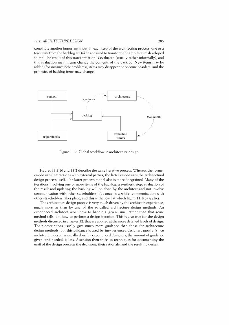
11.2. ARCHITECTURE DESIGN 285

constitute another important input. In each step of the architecting process, one or a

few items from the backlog are taken and used to transform the architecture developed

so far. The result of this transformation is evaluated (usually rather informally), and

this evaluation may in turn change the contents of the backlog. New items may be

added (for instance new problems), items may disappear or become obsolete, and the

priorities of backlog items may change.

evaluation

synthesiscontext

backlog

resultsevaluation

requirements

architecture

Figure 11.2 Global workflow in architecture design

Figures 11.1(b) and 11.2 describe the same iterative process. Whereas the former

emphasizes interactions with external parties, the latter emphasizes the architectural

design process itself. The latter process model also is more finegrained. Many of the

iterations involving one or more items of the backlog, a synthesis step, evaluation of

the result and updating the backlog will be done by the architect and not involve

communication with other stakeholders. But once in a while, communication with

other stakeholders takes place, and this is the level at which figure 11.1(b) applies.

The architecture design process is very much driven by the architect’s experience,

much more so than by any of the so-called architecture design methods. An

experienced architect knows how to handle a given issue, rather than that some

method tells him how to perform a design iteration. This is also true for the design

methods discussed in chapter 12, that are applied at the more detailed levels of design.

Their descriptions usually give much more guidance than those for architecture

design methods. But this guidance is used by inexperienced designers mostly. Since

architecture design is usually done by experienced designers, the amount of guidance

given, and needed, is less. Attention then shifts to techniques for documenting the

result of the design process: the decisions, their rationale, and the resulting design.

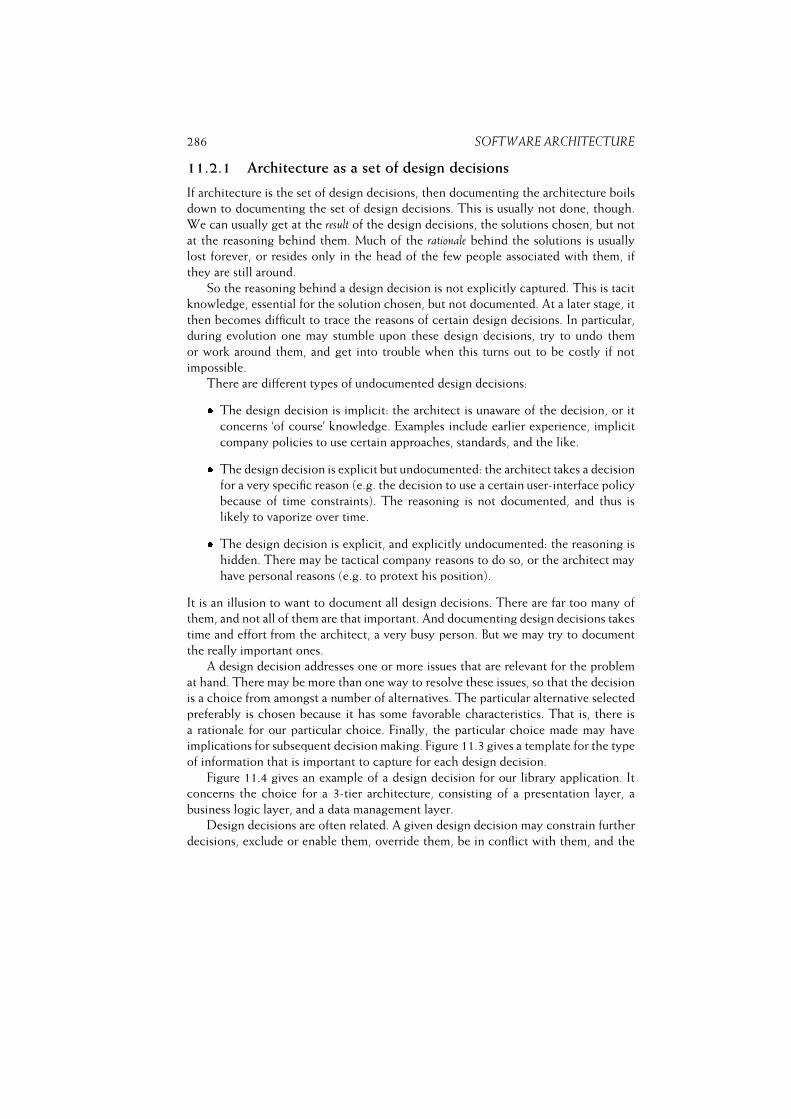
286 SOFTWARE ARCHITECTURE

11.2.1 Architecture as a set of design decisions

If architecture is the set of design decisions, then documenting the architecture boils

down to documenting the set of design decisions. This is usually not done, though.

We can usually get at the result of the design decisions, the solutions chosen, but not

at the reasoning behind them. Much of the rationale behind the solutions is usually

lost forever, or resides only in the head of the few people associated with them, if

they are still around.

So the reasoning behind a design decision is not explicitly captured. This is tacit

knowledge, essential for the solution chosen, but not documented. At a later stage, it

then becomes difficult to trace the reasons of certain design decisions. In particular,

during evolution one may stumble upon these design decisions, try to undo them

or work around them, and get into trouble when this turns out to be costly if not

impossible.

There are different types of undocumented design decisions:� The design decision is implicit: the architect is unaware of the decision, or it

concerns ‘of course’ knowledge. Examples include earlier experience, implicit

company policies to use certain approaches, standards, and the like.� The design decision is explicit but undocumented: the architect takes a decision

for a very specific reason (e.g. the decision to use a certain user-interface policy

because of time constraints). The reasoning is not documented, and thus is

likely to vaporize over time.� The design decision is explicit, and explicitly undocumented: the reasoning is

hidden. There may be tactical company reasons to do so, or the architect may

have personal reasons (e.g. to protext his position).

It is an illusion to want to document all design decisions. There are far too many of

them, and not all of them are that important. And documenting design decisions takes

time and effort from the architect, a very busy person. But we may try to document

the really important ones.

A design decision addresses one or more issues that are relevant for the problem

at hand. There may be more than one way to resolve these issues, so that the decision

is a choice from amongst a number of alternatives. The particular alternative selected

preferably is chosen because it has some favorable characteristics. That is, there is

a rationale for our particular choice. Finally, the particular choice made may have

implications for subsequent decision making. Figure 11.3 gives a template for the type

of information that is important to capture for each design decision.

Figure 11.4 gives an example of a design decision for our library application. It

concerns the choice for a 3-tier architecture, consisting of a presentation layer, a

business logic layer, and a data management layer.

Design decisions are often related. A given design decision may constrain further

decisions, exclude or enable them, override them, be in conflict with them, and the

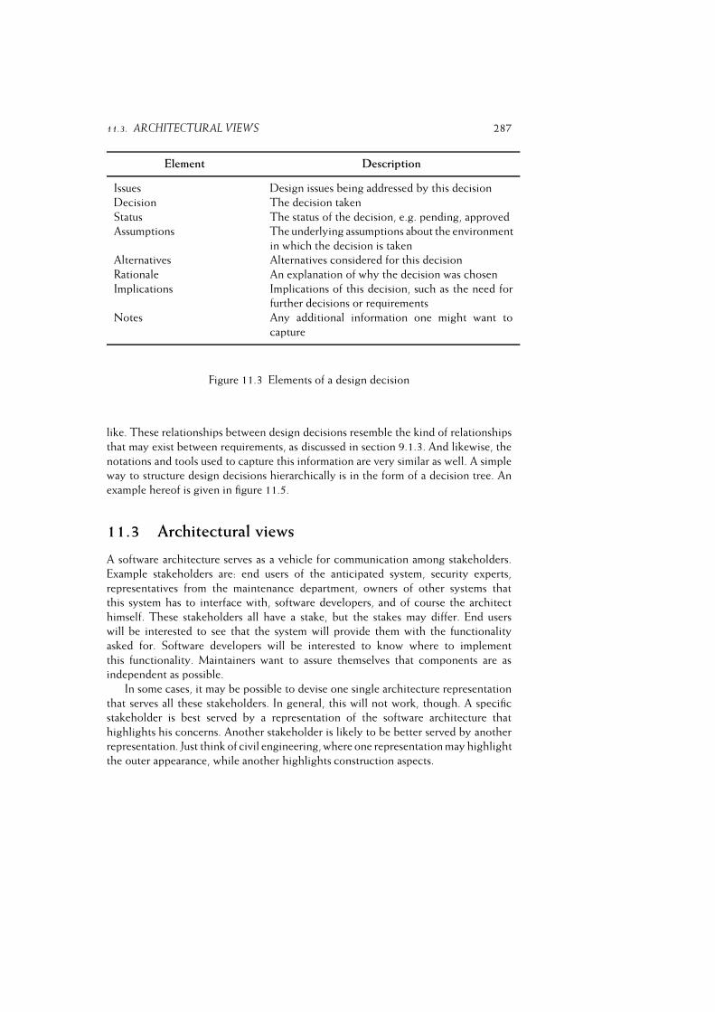
11.3. ARCHITECTURAL VIEWS 287

Element Description

Issues Design issues being addressed by this decision

Decision The decision taken

Status The status of the decision, e.g. pending, approved

Assumptions The underlying assumptions about the environment

in which the decision is taken

Alternatives Alternatives considered for this decision

Rationale An explanation of why the decision was chosen

Implications Implications of this decision, such as the need for

further decisions or requirements

Notes Any additional information one might want to

capture

Figure 11.3 Elements of a design decision

like. These relationships between design decisions resemble the kind of relationships

that may exist between requirements, as discussed in section 9.1.3. And likewise, the

notations and tools used to capture this information are very similar as well. A simple

way to structure design decisions hierarchically is in the form of a decision tree. An

example hereof is given in figure 11.5.

11.3 Architectural views

A software architecture serves as a vehicle for communication among stakeholders.

Example stakeholders are: end users of the anticipated system, security experts,

representatives from the maintenance department, owners of other systems that

this system has to interface with, software developers, and of course the architect

himself. These stakeholders all have a stake, but the stakes may differ. End users

will be interested to see that the system will provide them with the functionality

asked for. Software developers will be interested to know where to implement

this functionality. Maintainers want to assure themselves that components are as

independent as possible.

In some cases, it may be possible to devise one single architecture representation

that serves all these stakeholders. In general, this will not work, though. A specific

stakeholder is best served by a representation of the software architecture that

highlights his concerns. Another stakeholder is likely to be better served by another

representation. Just think of civil engineering, where one representation may highlight

the outer appearance, while another highlights construction aspects.

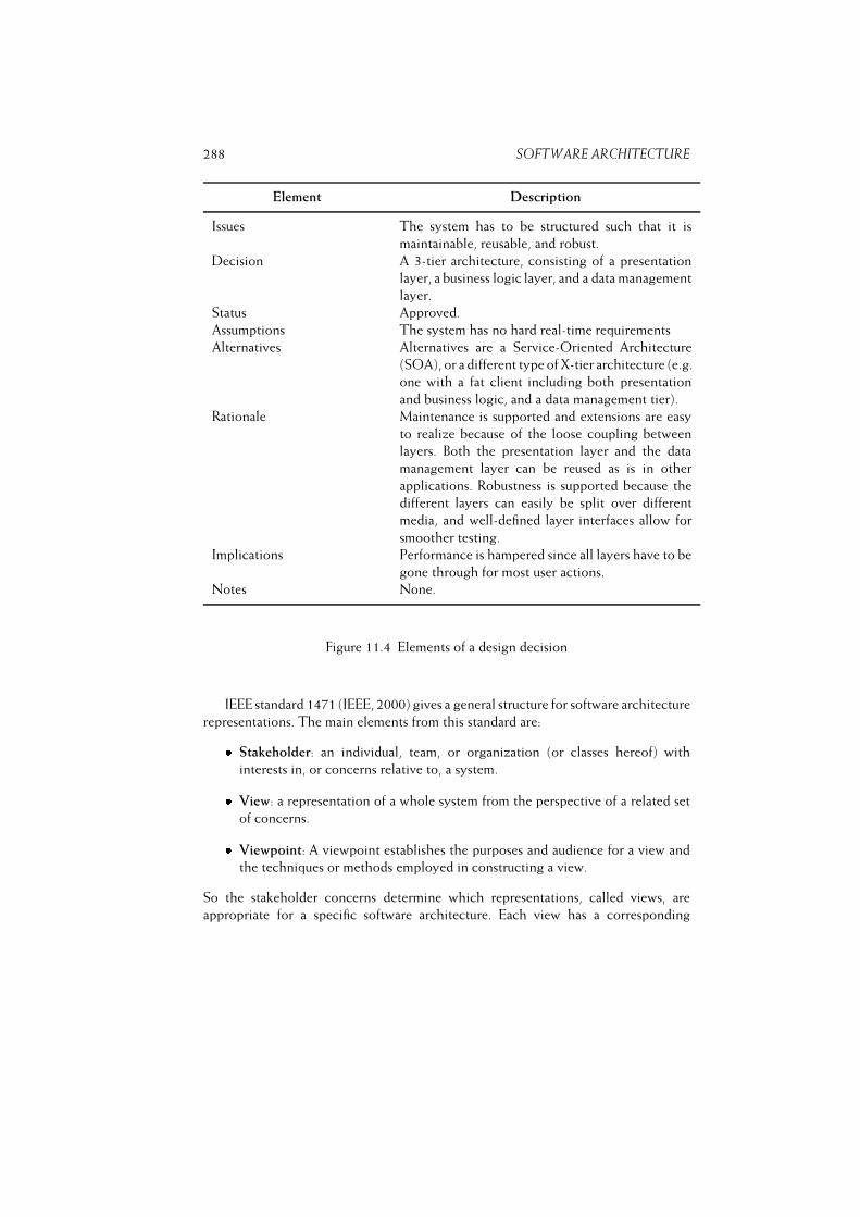
288 SOFTWARE ARCHITECTURE

Element Description

Issues The system has to be structured such that it is

maintainable, reusable, and robust.

Decision A 3-tier architecture, consisting of a presentation

layer, a business logic layer, and a data management

layer.

Status Approved.

Assumptions The system has no hard real-time requirements

Alternatives Alternatives are a Service-Oriented Architecture

(SOA), or a different type of X-tier architecture (e.g.

one with a fat client including both presentation

and business logic, and a data management tier).

Rationale Maintenance is supported and extensions are easy

to realize because of the loose coupling between

layers. Both the presentation layer and the data

management layer can be reused as is in other

applications. Robustness is supported because the

different layers can easily be split over different

media, and well-defined layer interfaces allow for

smoother testing.

Implications Performance is hampered since all layers have to be

gone through for most user actions.

Notes None.

Figure 11.4 Elements of a design decision

IEEE standard 1471 (IEEE, 2000) gives a general structure for software architecture

representations. The main elements from this standard are:� Stakeholder: an individual, team, or organization (or classes hereof) with

interests in, or concerns relative to, a system.� View: a representation of a whole system from the perspective of a related set

of concerns.� Viewpoint: A viewpoint establishes the purposes and audience for a view and

the techniques or methods employed in constructing a view.

So the stakeholder concerns determine which representations, called views, are

appropriate for a specific software architecture. Each view has a corresponding

11.3. ARCHITECTURAL VIEWS 289

MVC

observer

X-tier

SOA

3-tier

system structure

Figure 11.5 Tree of design decisions

viewpoint which gives the ‘syntax’ of the view, much like a construction drawing has

an accompanying description telling what all the glyphs in the drawing mean.

IEEE 1471 does not tell you which viewpoints to use. In essence, it suggests we

develop an appropriate set of viewpoints for each separate software architecture.

It does have the notion of a library viewpoint, though, a viewpoint that might

be useful across different software architectures. Bass et al. (2003) give a collection

of viewpoints that is useful across a wide variety of software architectures. These

viewpoints fall into three classes:� Module viewpoints give a static view of the system. They are usually depicted in

the form of box and line diagrams where the boxes denote system components

and the lines denote some relation between those components. Figure 11.6

describes typical module viewpoints.� Component and connector viewpoints give a dynamic view of the system, i.e.

they describe the system in execution. Again, they are usually depicted as

box and line diagrams. Figure 11.7 describes typical component and connector

viewpoints.� Allocation viewpoints give a relation the system and its environment, such as

who is responsible for which part of the system. Fig 11.8 gives typical allocation

viewpoints.

290 SOFTWARE ARCHITECTURE

Decomposition. In a decomposition viewpoint, elements are related by the ‘is

a submodule of’ relation. Larger elements are composed of smaller ones. It is

the result of a topdown refinement process. The decomposition viewpoint often

forms the basis for the project organization and the system’s documentation.

Uses. In a uses viewpoint, the relation between elements is ‘uses’ ( A calls B,

A passes information to B, etc). The uses relation goes back to Parnas (1972);

see also chapter 12. It is important when we want to assess modifiability: if an

element is changed, all elements it is used by potentially have to be changed as

well. It is also useful to determine incremental subsets of a system: if an element

is in a given subset, all elements it uses must also be in that subset.

Layered. The layered viewpoint is a special case of the uses viewpoint. It is useful

if we want to view the system as a series of layers, where elements from layer ncan only use elements from layers < n. Layers can often be interpreted as virtual

machines.

Class. The class viewpoint describes how certain elements are a generalization of

other elements. The relation between elements is ‘inherits from’. It is obviously

most applicable for object-oriented systems.

Figure 11.6 Module viewpoints

Of course, you are not going to use all these viewpoints for a single software

architecture. Usually, one from each category will suffice. You may for instance

choose the decomposition, deployment, and work assignment viewpoints. It is also

possible to combine viewpoints. In figure 11.9 we have combined the decomposition

viewpoint and the client-server viewpoint to create a view for our library system. In

specific cases, additional architectural views may be helpful or needed. In systems

for which the user interface is of critical importance, a separate user-interface view

may be developed. In electronic commerce applications, a view highlighting security

aspects may come in handy. And so on.

Many organizations have developed their own set of library viewpoints. A well-

known set of library viewpoints is known as the ‘4 + 1 model’ (Kruchten, 1995). It

consists of the following viewpoints:

– a conceptual, or logical viewpoint, which describes the system in terms of

major design elements and their interactions;

– an implementation viewpoint, which gives a view of the system in terms of

modules or packages and layers;

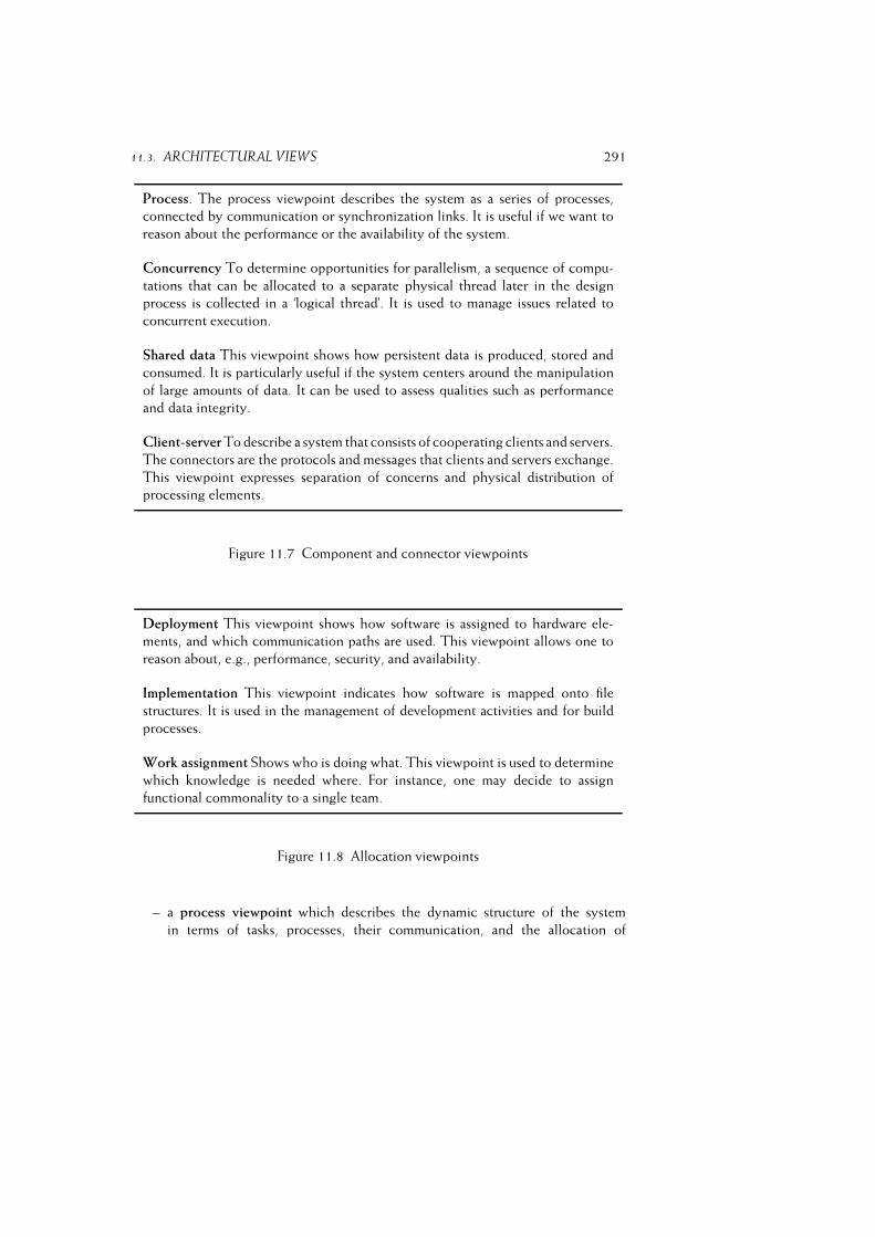
11.3. ARCHITECTURAL VIEWS 291

Process. The process viewpoint describes the system as a series of processes,

connected by communication or synchronization links. It is useful if we want to

reason about the performance or the availability of the system.

Concurrency To determine opportunities for parallelism, a sequence of compu-

tations that can be allocated to a separate physical thread later in the design

process is collected in a ‘logical thread’. It is used to manage issues related to

concurrent execution.

Shared data This viewpoint shows how persistent data is produced, stored and

consumed. It is particularly useful if the system centers around the manipulation

of large amounts of data. It can be used to assess qualities such as performance

and data integrity.

Client-server To describe a system that consists of cooperating clients and servers.

The connectors are the protocols and messages that clients and servers exchange.

This viewpoint expresses separation of concerns and physical distribution of

processing elements.

Figure 11.7 Component and connector viewpoints

Deployment This viewpoint shows how software is assigned to hardware ele-

ments, and which communication paths are used. This viewpoint allows one to

reason about, e.g., performance, security, and availability.

Implementation This viewpoint indicates how software is mapped onto file

structures. It is used in the management of development activities and for build

processes.

Work assignment Shows who is doing what. This viewpoint is used to determine

which knowledge is needed where. For instance, one may decide to assign

functional commonality to a single team.

Figure 11.8 Allocation viewpoints

– a process viewpoint which describes the dynamic structure of the system

in terms of tasks, processes, their communication, and the allocation of

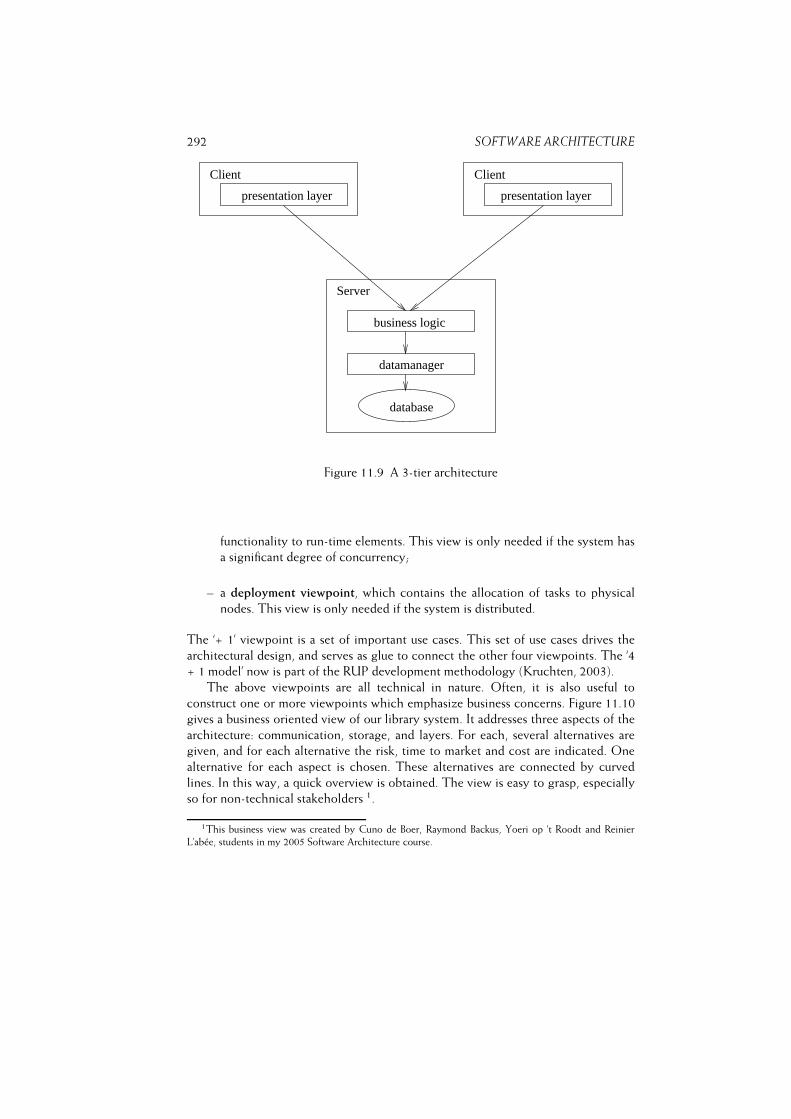
292 SOFTWARE ARCHITECTURE

Server

ClientClient

database

datamanager

business logic

presentation layerpresentation layer

Figure 11.9 A 3-tier architecture

functionality to run-time elements. This view is only needed if the system has

a significant degree of concurrency;

– a deployment viewpoint, which contains the allocation of tasks to physical

nodes. This view is only needed if the system is distributed.

The ‘+ 1’ viewpoint is a set of important use cases. This set of use cases drives the

architectural design, and serves as glue to connect the other four viewpoints. The ‘4

+ 1 model’ now is part of the RUP development methodology (Kruchten, 2003).

The above viewpoints are all technical in nature. Often, it is also useful to

construct one or more viewpoints which emphasize business concerns. Figure 11.10

gives a business oriented view of our library system. It addresses three aspects of the

architecture: communication, storage, and layers. For each, several alternatives are

given, and for each alternative the risk, time to market and cost are indicated. One

alternative for each aspect is chosen. These alternatives are connected by curved

lines. In this way, a quick overview is obtained. The view is easy to grasp, especially

so for non-technical stakeholders 1.

1This business view was created by Cuno de Boer, Raymond Backus, Yoeri op ’t Roodt and Reinier

L’abee, students in my 2005 Software Architecture course.

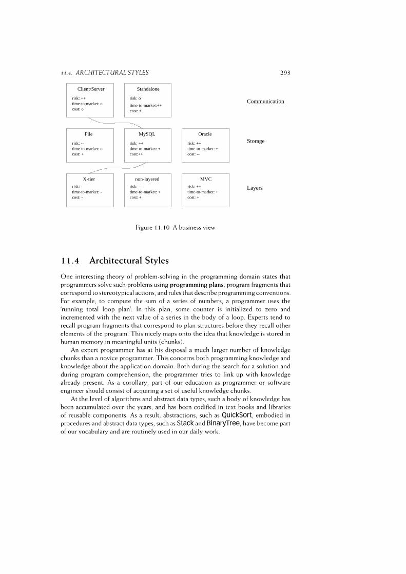
11.4. ARCHITECTURAL STYLES 293

risk: ++

risk: o

time-to-market:++cost: +

risk: --

cost: +time-to-market: +cost:++

time-to-market: +cost: --

risk: -time-to-market: -cost: -

risk: --time-to-market: +cost: +

risk: ++time-to-market: +cost: +

Communication

Layers

Storagerisk: ++

Client/Server Standalone

File MySQL Oracle

X-tier non-layered MVC

time-to-market: o

risk: ++time-to-market: ocost: o

Figure 11.10 A business view

11.4 Architectural Styles

One interesting theory of problem-solving in the programming domain states that

programmers solve such problems using programming plans, program fragments that

correspond to stereotypical actions, and rules that describe programming conventions.

For example, to compute the sum of a series of numbers, a programmer uses the

‘running total loop plan’. In this plan, some counter is initialized to zero and

incremented with the next value of a series in the body of a loop. Experts tend to

recall program fragments that correspond to plan structures before they recall other

elements of the program. This nicely maps onto the idea that knowledge is stored in

human memory in meaningful units (chunks).

An expert programmer has at his disposal a much larger number of knowledge

chunks than a novice programmer. This concerns both programming knowledge and

knowledge about the application domain. Both during the search for a solution and

during program comprehension, the programmer tries to link up with knowledge

already present. As a corollary, part of our education as programmer or software

engineer should consist of acquiring a set of useful knowledge chunks.

At the level of algorithms and abstract data types, such a body of knowledge has

been accumulated over the years, and has been codified in text books and libraries

of reusable components. As a result, abstractions, such as QuickSort, embodied in

procedures and abstract data types, such as Stack and BinaryTree, have become part

of our vocabulary and are routinely used in our daily work.

294 SOFTWARE ARCHITECTURE

The concepts embodied in these abstractions are useful during the design,

implementation and maintenance of software for the following reasons:� They can be used in a variety of settings and can be given unique names.

The names are used in communicating the concepts and serve as labels when

retrieving and storing them in human memory. The label QuickSort rings the

same bell for all people working in our field.� We have notations and mechanisms to support their use and reuse, such as

procedure calls and the module concept.� We have organized related concepts into (semantic) networks that can be

searched for an item that fits the problem at hand. For example, we know the

time and space tradeoffs between QuickSort and BubbleSort, or between a

standard binary search tree and an AVL-tree, and we know the grounds on

which to make a choice.

Design patterns are collections of a few modules (or, in object-oriented circles,

classes) which are often used in combination, and which together provide a useful

abstraction. A design pattern is a recurring solution to a standard problem. The

prototypical example of a pattern is the MVC (Model--View--Controller) pattern

known from Smalltalk. We may view design patterns as micro-architectures. Design

patterns are further discussed in section 12.5.

Two further notions often used in this context are (application) framework

and idiom. An application framework is a semi-finished system which needs to be

instantiated to obtain a complete system. It describes the architecture of a family

of similar systems. It is thus tied to a particular application domain. The best

known examples are frameworks for building user interfaces. An idiom is a low-level

pattern, specific to some programming language. For example, the Counted Pointer

idiom (Buschmann et al., 1996, pp 353--358) can be used to handle references to

objects created dynamically in C++. It keeps a reference counter which is incremented

or decremented when references to an object are added or removed. Memory occupied

by an object is freed if no references to that object remain, i.e. when the counter

becomes zero. Frameworks and idioms thus offer solutions that are more concrete and

language-specific than the architectural styles and design patterns we will discuss.

The work in the area of software architecture and design patterns has been strongly

influenced by the ideas of the architect Christopher Alexander, as formulated in his

books The Timeless Way of Building and A Pattern Language. The term ‘pattern’ derives

from Alexander’s work, and the format used to describe software architectural styles

and design patterns is shaped after the format Alexander used to describe his patterns,

like ‘alcove’, ‘office connection’ or ‘public outdoor room’. In software engineering, we

often draw a parallel with other engineering disciplines, in particular civil engineering.

This comparison is made to highlight both similarities, such as the virtues of a phased

approach, and differences, such as the observation that software is logical rather than

physical, which hampers the control of progress. The comparison with the field of

11.4. ARCHITECTURAL STYLES 295

architecture is often made to illustrate the role of different views, as expressed in the

different types of blueprint produced. Each of these blueprints emphasizes a particular

aspect.

The classical field of architecture provides some further interesting insights for

software architecture. These insights concern:

– the notion of architectural style,

– the relationship between style and engineering, and

– the relationship between style and materials.

Architecture is a (formal) arrangement of architectural elements. An architectural

style abstracts from the specifics of an architecture. The decomposition of our library

system might for instance result in an architecture consisting of one main program

and four subroutines, sharing three data stores. If we abstract from these specifics, we

obtain its architectural style, in which we concentrate on the types of its elements

and their interconnections.

Viewed in this way, an architectural style describes a certain codification of

elements and their arrangement. Conversely, an architectural style constrains both

the elements and their interrelationships. For example, the Tudor style describes how

a certain type of house looks and also prescribes how its design should look. In a

similar vein we may characterize a software architectural style such as, say, the

pipes-and-filter style.

Different engineering principles apply to different architectural styles. This often

goes hand in hand with the types of materials used. Cottage-style houses and high-

rise apartment-buildings differ in the materials used and the engineering principles

applied. A software design based on abstract data types (= material) emphasizes

separation of concerns by encapsulating secrets (= engineering principle). A design

based on pipes and filters emphasizes bundling of functionality in independent

processes.

When selecting a certain architectural style with its corresponding engineering

principles and materials, we are guided by the problem to be solved as well as

the larger context in which the problem occurs. We cannot build a skyscraper from

wooden posts. Environmental regulations may prohibit us erecting high-rise buildings

in rural areas. And, the narrow frontages of many houses on the Amsterdam canals

are partly due to the fact that local taxes were based on the number of street-facing

windows. Similar problem- and context-specific elements guide us in the selection of

a software architectural style.

These similarities between classical architecture and software architecture provide

us with clues as to what constitutes a software architectural style and what its

description should look like.

In his book A Pattern Language, the architect Christopher Alexander presents

253 ‘patterns’, ranging in scale from how a city should look down to rules for the

296 SOFTWARE ARCHITECTURE

construction of a porch. Perhaps his most famous pattern is about the height of

buildings:

‘There is abundant evidence to show that high buildings make people

crazy.

. . .

High buildings have no genuine advantage, except in speculative gains

to banks and land owners. They are not cheaper, they do not help create

open space, they make life difficult for children, they are expensive to

maintain, they wreck the open spaces near them, and they damage the

light and air and view. But quite apart from this, empirical evidence

shows that they can actually damage people’s minds and feelings.

. . .

In any urban area, no matter how dense, keep the majority of buildings

four stories high or less. It is possible that certain buildings should exceed

this limit, but they should never be buildings for human habitation.’

An Alexandrian pattern is not a cookbook, black-box recipe for architects, any more

than a dictionary is a toolkit for a novelist. Rather, a pattern is a flexible generic

scheme providing a solution to a problem in a given context. In a narrative form, its

application looks like this:

IF you find yourself in <context>, for example <examples>, with<problem>,

THEN for some <reasons>, apply <pattern> to construct a solution

leading to a <new context> and <other patterns>.

The above ‘Four-Story Limit’ pattern may for example be applied in a context where

one has to design a suburb. The citation gives some of the reasons for applying this

pattern. If it is followed, it will give rise to the application of other patterns, such

as those for planning parking lots, the layout of roads, or the design of individual

houses.2

Shaw (1996) characterizes a number of well-known software architectural styles

in a framework that resembles a popular way of describing design patterns. Both the

characterization and the framework are shaped after Alexander’s way of describing

2Here, we may note another similarity between classical architecture and software architecture. In the

1950s and 1960s, housing was a major problem in Western Europe and beyond. There were far too few

houses available, while those available were mostly of a bad quality (damp, no bathroom, too small). In

the post-war economic boom, many suburbs were constructed, with lots of spacious apartments, each one

a container made of steel and concrete. These new suburbs solved one problem -- the housing of a large

number of people -- but at the same time created other problems which only showed themselves much later,

e.g. lack of community feeling and social ties, high crime rates. As a result, massive renovation projectshave started and many a high-rise apartment building has been demolished. In software development, we

developed company-wide systems in the 1970s and 1980s, with an emphasis on performance, uniformity,

and standardized ways of working. Many of these systems are unable to cope satisfactorily with today’s

requirements of flexibility and adaptability, and are therefore being renovated.

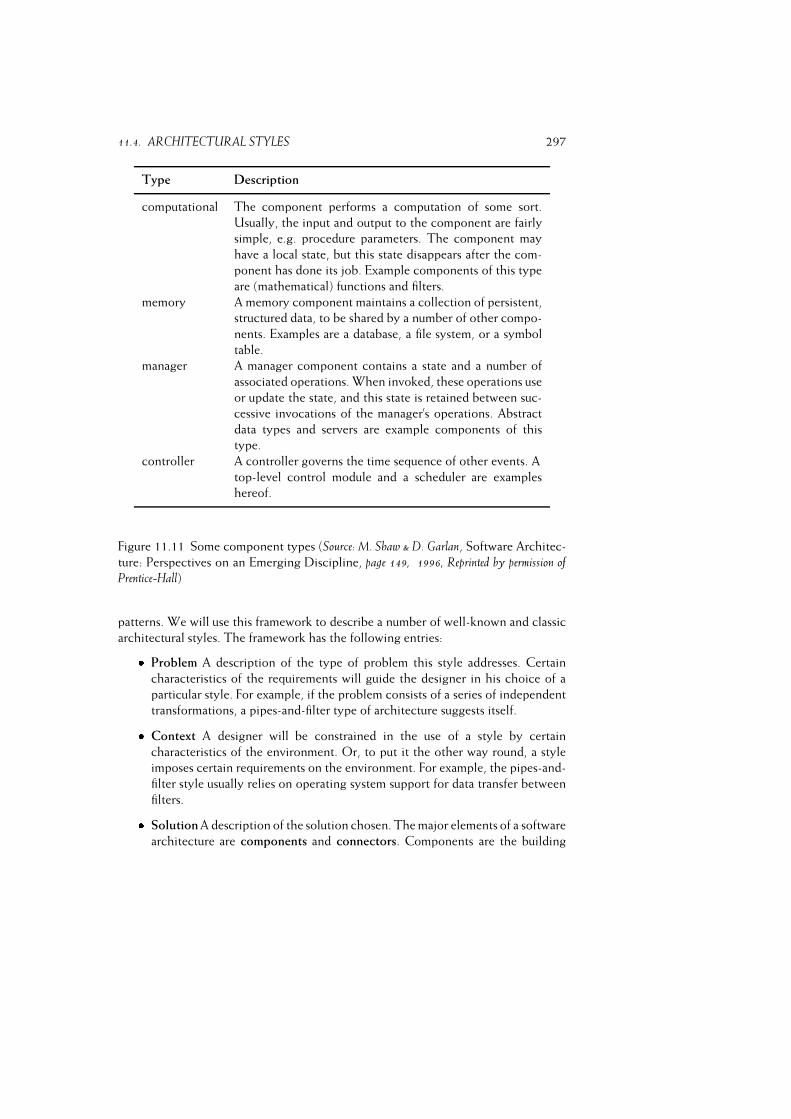
11.4. ARCHITECTURAL STYLES 297

Type Description

computational The component performs a computation of some sort.

Usually, the input and output to the component are fairly

simple, e.g. procedure parameters. The component may

have a local state, but this state disappears after the com-

ponent has done its job. Example components of this type

are (mathematical) functions and filters.

memory A memory component maintains a collection of persistent,

structured data, to be shared by a number of other compo-

nents. Examples are a database, a file system, or a symbol

table.

manager A manager component contains a state and a number of

associated operations. When invoked, these operations use

or update the state, and this state is retained between suc-

cessive invocations of the manager’s operations. Abstract

data types and servers are example components of this

type.

controller A controller governs the time sequence of other events. A

top-level control module and a scheduler are examples

hereof.

Figure 11.11 Some component types (Source: M. Shaw & D. Garlan, Software Architec-

ture: Perspectives on an Emerging Discipline, page 149, 1996, Reprinted by permission ofPrentice-Hall)

patterns. We will use this framework to describe a number of well-known and classic

architectural styles. The framework has the following entries:� Problem A description of the type of problem this style addresses. Certain

characteristics of the requirements will guide the designer in his choice of a

particular style. For example, if the problem consists of a series of independent

transformations, a pipes-and-filter type of architecture suggests itself.� Context A designer will be constrained in the use of a style by certain

characteristics of the environment. Or, to put it the other way round, a style

imposes certain requirements on the environment. For example, the pipes-and-

filter style usually relies on operating system support for data transfer between

filters.� Solution A description of the solution chosen. The major elements of a software

architecture are components and connectors. Components are the building

298 SOFTWARE ARCHITECTURE

blocks of a software architecture. They usually embody a computational

element of some sort (like a procedure), but a component can also be a data

store (such as a database). The connectors describe how components interact.3

Some typical types of component and connector are given in figures 11.11 and

11.12.

The order of execution of components is governed by the control structure.

The control structure captures how control is transferred during execution.

The choice of components and connectors is not independent. Usually, a

style is characterized by a combination of certain types of component and

connector, as well as a certain control structure. The system model captures

the intuition behind such a combination.

It describes the general flavor of the system.� Variants Architectural styles give a rather general description. Often, certain

variants or specializations may be identified, which differ from the general

style.� Examples One should include references to real examples of a style. Archi-

tectural styles do not stem from theoretical investigations, but result from

identifying and characterizing best practice.

Figures 11.13--11.18 contain descriptions of six well-known architectural styles:

the main program with subroutines, abstract data type, implicit invocation, pipes and

filters, repository and layered styles.

In the main-program-with-subroutines architectural style, the main tasks of the

system are allocated to different components which are called, in the appropriate

order, from a control component. The decomposition is strongly geared towards an

ordering of the various actions to be performed with respect to time. The top-level

component controls this ordering.

Components in the main-program-with-subroutines type of decomposition often

use shared data storage. Decisions abaout data representations then are in fact a

mutual property of the components that use those data. We may also try to make

those decisions locally rather than globally. In that case the user does not get direct

access to the data structures, but is offered an interface. The data can only be accessed

through appropriate procedure or method calls. This is the essence of the abstract

data type architectural style.

A major advantage of abstract data types over shared data is that changes in

data representation and algorithms can be accomplished relatively easily. Changes

in functionality, however, may be much harder to realize. This is because method

invocations are explicit, hard-coded in the implementation. An alternative is to use

the implicit invocation style. In implicit invocation, a component is not invoked

3These notions of component and connector are not related to the ‘component-and-connector’

viewpoints discussed in section 11.3.

11.4. ARCHITECTURAL STYLES 299

Type Description

procedure call With this type of connector, there is a single thread of

control between the caller and the called component.

Control is transferred to the component being called,

and this component remains in control until its work

has ended. Only then is control transferred back to

the calling component. The traditional procedure call

and the remote procedure call are examples of this

type of connector.

data flow With a data flow connector, processes interact through

a stream of data, as in pipes. The components

themselves are independent. Once input data to a

component is available, it may continue its work.

implicit invocation With implicit invocation, a computation is invoked

when a certain event occurs, rather than by explicit

interaction (as in a procedure call). Components rais-

ing events do not know which component is going

to react and invoked components do not know which

component raised the event to which they are reacting.

message passing Message passing occurs when we have independent

processes that interact through explicit, discrete trans-

fer of data, as in TCP/IP. Message passing can be

synchronous (in which case the sending/receiving pro-

cess is blocked until the message has been completely

sent/received) or asynchronous (in which case the

processes continue their work independently).

shared data When using shared data connectors, components

operate concurrently on the same data space, as in

blackboard systems or multiuser databases. Usually,

some blocking scheme prevents concurrent writes to

the same data.

instantiation With instantiation, one component (the instantia-

tor) provides space for the state required by another

component (the instantiated), as in abstract data types.

Figure 11.12 Some connector types (Source: M. Shaw & D. Garlan, Software Architecture:

Perspectives on an Emerging Discipline, page 149-150, 1996, Reprinted by permission of

Prentice-Hall)

300 SOFTWARE ARCHITECTURE

Style: Main program with subroutines

Problem The system can be described as a hierarchy of procedure definitions. This

style is a natural outcome of a functional decomposition of a system (see

chapter 12). The top-level module acts as the main program. Its main task is to

invoke the other modules in the right order. As a consequence, there is usually

a single thread of control.

Context This style naturally fits in with programming languages that allow for nested

definitions of procedures and modules.

Solution

System model Procedures and modules are defined in a hierarchy. Higher-

level modules call lower-level modules. The hierarchy may be strict, in

which case modules at level n can only call modules at level n� 1, or it

may be weak, in which case modules at level n may call modules at leveln� i, with i � 1. Procedures are grouped into modules following such

criteria as coupling and cohesion (see chapter 12).

Components (Groups of) procedures, which may have their own local data,

and global data which may be viewed as residing in the main program.

Connectors Procedure call and shared access to global data.

Control structure There is a single, centralized thread of control; the main

program pulls the strings.

Variants This style is usually applied to systems running on one CPU. Abstractly,

the model is preserved in systems running on multiple CPUs and using the

Remote Procedure Call (RPC) mechanism to invoke processes.

Examples (Parnas, 1972)

Figure 11.13 Main-program-with-subroutines architectural style (Source: M. Shaw,Some Patterns for Software Architectures, in J.M. Vlissides et al., Pattern Languages of Program

Design 2, Reproduced by permission of Addison-Wesley.)

explicitly. Instead, a so-called event is generated. Other components in the system

may express their interest in this event by associating a method with it; this method

is automatically invoked each time the event is raised. Functional changes can be

realized easily by changing the list of events components are interested in.

Some applications consist of a series of components in which component iproduces output which is next read and processed by component i+ 1, in the same

order in which it is written by component i. In such cases, we need not explicitly

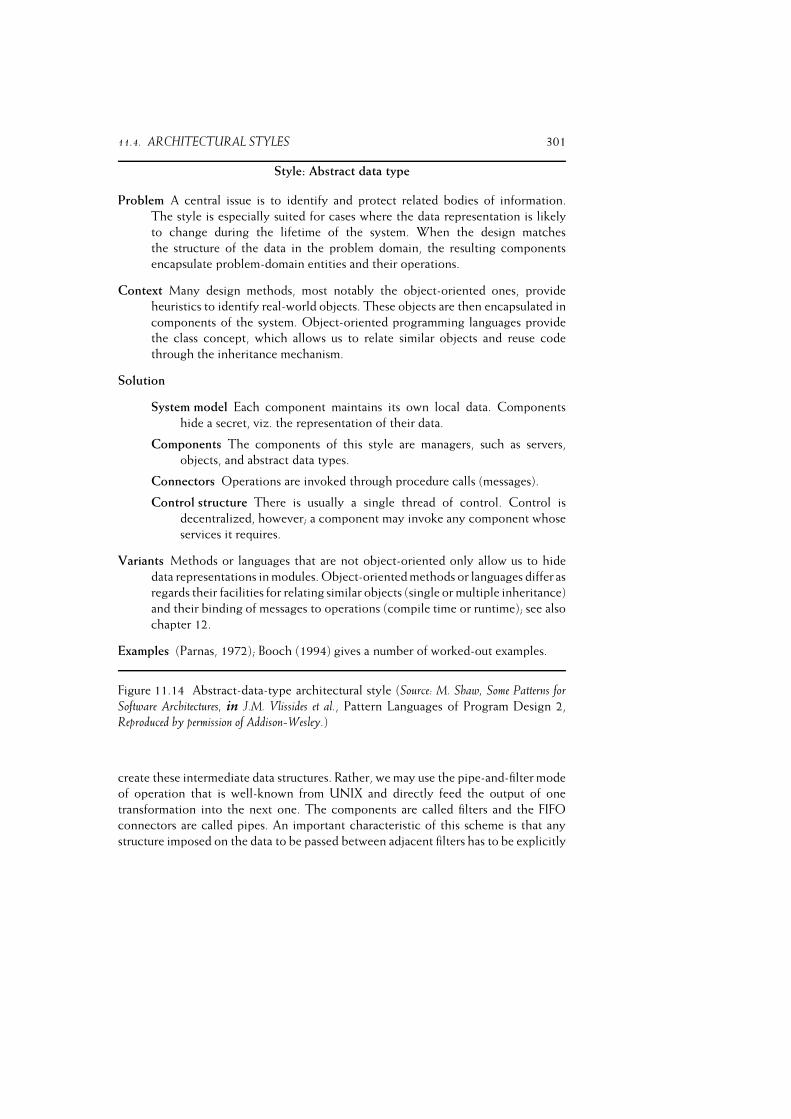
11.4. ARCHITECTURAL STYLES 301

Style: Abstract data type

Problem A central issue is to identify and protect related bodies of information.

The style is especially suited for cases where the data representation is likely

to change during the lifetime of the system. When the design matches

the structure of the data in the problem domain, the resulting components

encapsulate problem-domain entities and their operations.

Context Many design methods, most notably the object-oriented ones, provide

heuristics to identify real-world objects. These objects are then encapsulated in

components of the system. Object-oriented programming languages provide

the class concept, which allows us to relate similar objects and reuse code

through the inheritance mechanism.

Solution

System model Each component maintains its own local data. Components

hide a secret, viz. the representation of their data.

Components The components of this style are managers, such as servers,

objects, and abstract data types.

Connectors Operations are invoked through procedure calls (messages).

Control structure There is usually a single thread of control. Control is

decentralized, however; a component may invoke any component whose

services it requires.

Variants Methods or languages that are not object-oriented only allow us to hide

data representations in modules. Object-oriented methods or languages differ as

regards their facilities for relating similar objects (single or multiple inheritance)

and their binding of messages to operations (compile time or runtime); see also

chapter 12.

Examples (Parnas, 1972); Booch (1994) gives a number of worked-out examples.

Figure 11.14 Abstract-data-type architectural style (Source: M. Shaw, Some Patterns for

Software Architectures, in J.M. Vlissides et al., Pattern Languages of Program Design 2,

Reproduced by permission of Addison-Wesley.)

create these intermediate data structures. Rather, we may use the pipe-and-filter mode

of operation that is well-known from UNIX and directly feed the output of one

transformation into the next one. The components are called filters and the FIFO

connectors are called pipes. An important characteristic of this scheme is that any

structure imposed on the data to be passed between adjacent filters has to be explicitly

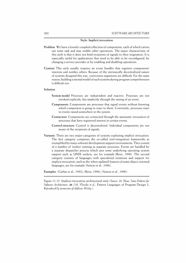
302 SOFTWARE ARCHITECTURE

Style: Implicit invocation

Problem We have a loosely-coupled collection of components, each of which carries

out some task and may enable other operations. The major characteristic of

this style is that it does not bind recipients of signals to their originators. It is

especially useful for applications that need to be able to be reconfigured, by

changing a service provider or by enabling and disabling operations.

Context This style usually requires an event handler that registers components’

interests and notifies others. Because of the intrinsically decentralized nature

of systems designed this way, correctness arguments are difficult. For the same

reason, building a mental model of such systems during program comprehension

is difficult too.

Solution

System model Processes are independent and reactive. Processes are not

invoked explicitly, but implicitly through the raising of an event.

Components Components are processes that signal events without knowing

which component is going to react to them. Conversely, processes react

to events raised somewhere in the system.

Connectors Components are connected through the automatic invocation of

processes that have registered interest in certain events.

Control structure Control is decentralized. Individual components are not

aware of the recipients of signals.

Variants There are two major categories of systems exploiting implicit invocation.

The first category comprises the so-called tool-integration frameworks as

exemplified by many software development support environments. They consist

of a number of ‘toolies’ running as separate processes. Events are handled by

a separate dispatcher process which uses some underlying operating system

support such as UNIX sockets; see for example (Reiss, 1990). The second

category consists of languages with specialized notations and support for

implicit invocation, such as the ‘when-updated’ features of some object-oriented

languages; see for example (Sutton et al., 1990).

Examples (Garlan et al., 1992); (Reiss, 1990); (Sutton et al., 1990).

Figure 11.15 Implicit-invocation architectural style (Source: M. Shaw, Some Patterns for

Software Architectures, in J.M. Vlissides et al., Pattern Languages of Program Design 2,

Reproduced by permission of Addison-Wesley.)

11.4. ARCHITECTURAL STYLES 303

Style: Pipes and filters

Problem A series of independent, sequential transformations on ordered data. Usu-

ally, the transformations are incremental. Often, the structure of the datastreams

is very simple: a sequence of ASCII characters. If the data has a rich structure,

this will imply quite some overhead for the parsing and unparsing of the data.

Context This style requires that the system can be decomposed into a series of

computations, filters, that incrementally transform one or more input streams.

It usually relies on operating system operations to transfer the data from one

process to another (pipes). Error handling is difficult to deal with uniformly in a

collection of filters.

Solution

System model The resulting systems are characterized by continuous data flow

between components, where the components incrementally transform

datastreams.

Components The components are filters that perform local processing; i.e.

they read part of their input data, transform the data, and produce part of

their output. They have little internal state.

Connectors Datastreams (usually plain ASCII, as in UNIX).

Control structure Data flow between components. Each component usually

has its own thread of control.

Variants Pure filters have little internal state and process their input locally. In the

degenerate case they consume all of their input before producing any output.

In that case, the result boils down to a batch-processing type of system.

Examples (Delisle and Garlan, 1990)

Figure 11.16 Pipes-and-filters architectural style (Source: M. Shaw, Some Patterns forSoftware Architectures, in J.M. Vlissides et al., Pattern Languages of Program Design 2,

Reproduced by permission of Addison-Wesley.)

encoded in the datastream that connects these filters. This encoding scheme involves

decisions which much be known to both filters. The data has to be unparsed by one

filter while the next filter must parse its input in order to rebuild that structure. The

Achilles’ heel of the pipes-and-filers scheme is error handling. If one filter detects

an error, it is cumbersome to pass the resulting error message through intermediate

filters all the way to the final output. Filters must also be able to resynchronize after

an error has been detected and filters further downstream must be able to tolerate

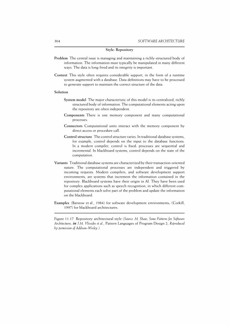
304 SOFTWARE ARCHITECTURE

Style: Repository

Problem The central issue is managing and maintaining a richly-structured body of

information. The information must typically be manipulated in many different

ways. The data is long-lived and its integrity is important.

Context This style often requires considerable support, in the form of a runtime

system augmented with a database. Data definitions may have to be processed

to generate support to maintain the correct structure of the data.

Solution

System model The major characteristic of this model is its centralized, richly

structured body of information. The computational elements acting upon

the repository are often independent.

Components There is one memory component and many computational

processes.

Connectors Computational units interact with the memory component by

direct access or procedure call.

Control structure The control structure varies. In traditional database systems,

for example, control depends on the input to the database functions.

In a modern compiler, control is fixed: processes are sequential and

incremental. In blackboard systems, control depends on the state of the

computation.

Variants Traditional database systems are characterized by their transaction-oriented

nature. The computational processes are independent and triggered by

incoming requests. Modern compilers, and software development support

environments, are systems that increment the information contained in the

repository. Blackboard systems have their origin in AI. They have been used

for complex applications such as speech recognition, in which different com-

putational elements each solve part of the problem and update the information

on the blackboard.

Examples (Barstow et al., 1984) for software development environments; (Corkill,

1997) for blackboard architectures.

Figure 11.17 Repository architectural style (Source: M. Shaw, Some Patterns for Software

Architectures, in J.M. Vlissides et al., Pattern Languages of Program Design 2, Reproduced

by permission of Addison-Wesley.)

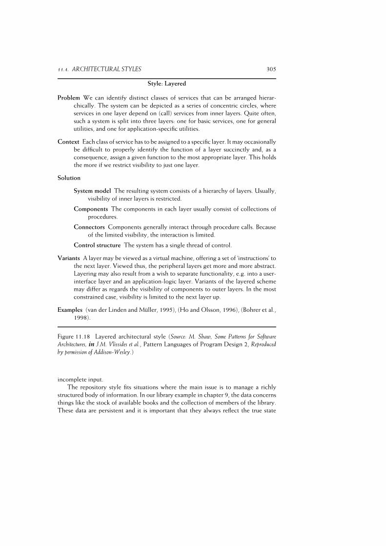
11.4. ARCHITECTURAL STYLES 305

Style: Layered

Problem We can identify distinct classes of services that can be arranged hierar-

chically. The system can be depicted as a series of concentric circles, where

services in one layer depend on (call) services from inner layers. Quite often,

such a system is split into three layers: one for basic services, one for general

utilities, and one for application-specific utilities.

Context Each class of service has to be assigned to a specific layer. It may occasionally

be difficult to properly identify the function of a layer succinctly and, as a

consequence, assign a given function to the most appropriate layer. This holds

the more if we restrict visibility to just one layer.

Solution

System model The resulting system consists of a hierarchy of layers. Usually,

visibility of inner layers is restricted.

Components The components in each layer usually consist of collections of

procedures.

Connectors Components generally interact through procedure calls. Because

of the limited visibility, the interaction is limited.

Control structure The system has a single thread of control.

Variants A layer may be viewed as a virtual machine, offering a set of ‘instructions’ to

the next layer. Viewed thus, the peripheral layers get more and more abstract.

Layering may also result from a wish to separate functionality, e.g. into a user-

interface layer and an application-logic layer. Variants of the layered scheme

may differ as regards the visibility of components to outer layers. In the most

constrained case, visibility is limited to the next layer up.

Examples (van der Linden and Muller, 1995), (Ho and Olsson, 1996), (Bohrer et al.,

1998).

Figure 11.18 Layered architectural style (Source: M. Shaw, Some Patterns for SoftwareArchitectures, in J.M. Vlissides et al., Pattern Languages of Program Design 2, Reproduced

by permission of Addison-Wesley.)

incomplete input.

The repository style fits situations where the main issue is to manage a richly

structured body of information. In our library example in chapter 9, the data concerns

things like the stock of available books and the collection of members of the library.

These data are persistent and it is important that they always reflect the true state

306 SOFTWARE ARCHITECTURE

of affairs. A natural approach to this problem is to devise database schemas for the

various types of data in the application (books, journals, library clients, reservations,

and so on) and store the data in one or more databases. The functionality of the system

is incorporated in a number of, relatively independent, computational elements. The

result is a repository architectural style.

Modern compilers are often structured in a similar way. Such a compiler maintains

a central representation of the program to be translated. A rudimentary version of

that representation results from the first, lexical, phase: a sequence of tokens rather

than a sequence of character glyphs. Subsequent phases, such as syntax and semantic

analysis, further enrich this structure into, for example, an abstract syntax tree. In

the end, code is generated from this representation. Other tools, such as symbolic

debuggers, pretty-printing programs, or static analysis tools, may also employ the

internal representation built by the compiler. The resulting architectural style again is

that of a repository: one memory component and a number of computational elements

that act on that repository. Unlike the database variant, the order of invocation of the

elements matters in the case of a compiler. Also, different computational elements

enrich the internal representation, rather than merely update it.

The repository architectural style can also be found in certain AI applications. In

computationally complex applications, such as speech recognition, an internal repre-

sentation is built and acted upon by different computational elements. For example,

one computational element may filter noise, another one builds up phonemes, etc.

The internal representation in this type of system is called a blackboard and the

architecture is sometimes referred to as a blackboard architecture. A major difference

with traditional database systems is that the invocation of computational elements in

a blackboard architecture is triggered by the current state of the blackboard, rather

than by (external) inputs. Elements from a blackboard architecture enrich and refine

the state representation until a solution to the problem is found.

Our final example of an architectural style is the layered architectural style.

A prototypical instance hereof is the ISO Open System Interconnection Model

for network communication. It has seven layers: physical, data, network, transport,

session, presentation, and application. The bottom layer provides basic functionality.

Higher layers use the functionality of lower layers. The different layers can be viewed

as virtual machines whose ‘instructions’ become more powerful and abstract as we go

from lower layers to higher layers.

In a layered scheme, by definition, lower levels cannot use the functionality offered

by higher levels. The other way round, the situation is more varied. We may choose

to allow layer n to use the functionality of each layer m, with m < n. We may also

choose to limit the visibility of functionality offered by each layer, and for example

restrict layer n to use only the functionality offered by layer n� 1. A design issue

in each case is how to assign functionality to the different layers of the architecture,

i.e. how to characterize the virtual machine it embodies. If visibility is not restricted,

some of the elegance of the layered architecture gets lost. This situation resembles

that of programming languages containing low-level bit manipulation operations

11.4. ARCHITECTURAL STYLES 307

alongside while statements and procedure calls. If visibility is restricted, we may end

up copying functionality to higher levels without increasing the level of abstraction.

van der Linden and Muller (1995) give an example of a layered architectural style

for use in telecommunications. In this example, layers do not correspond to different

levels of abstraction. Rather, the functionality of the system has been separated. Two

main guidelines drive the assignment of functionality to layers in this architecture:

– hardware-dependent functionality should be placed in lower-level layers than

application-dependent functionality.

– generic functionality should be placed in lower layers than specific functionality.

The resulting architecture has four layers:� Operating system This layer comprises the runtime system, database, memory

management, and so on.� Equipment maintenance This layer houses the control for peripheral devices and

its interconnection structure. It deals with such things as data distribution

and fault-handling of peripheral hardware. The bottom two layers together

constitute the distributed operating infrastructure upon which applications run.� Logical-resource management Logical resources come in two flavors. The first class

contains abstractions from hardware objects. The second class consists of

software-related logical objects, such as those for call-forwarding in telephony.� Service management This layer contains the application functionality.

A similar line of thought can be followed in other domains. For instance, it is hard to

predict how future household electronic equipment will be assembled into hardware

boxes. Will the PC and the television be in the same box? Will the television and

the DVD player be combined or will they remain as separate boxes? No one seems

to know. Since the half-life of many of these products is about six months, industry

is forced to use a building-block approach, emphasizing reuse and the development

of product families rather than products. A division of functionality into a hardware-

related inner layer, a generic signal processing layer, and a user-oriented service layer

suggests itself. The above architecture for telecommunications applications can be

understood along the same lines.

In practice, we will usually encounter a mixture of architectural styles. For example,

many software development environments can be characterized as a combination

of the repository and layered architectural styles; see also chapter 15. The core

of the system is a repository in which the various objects, ranging from program

texts to work-breakdown structures, reside. Access to these objects as well as basic

mechanisms for the execution and communication of tools are contained in a layer on

top of this repository. The tools themselves are configured in one or more layers on

top of these basic layers. Interaction between tools may yet follow another paradigm,

such as implicit invocation.

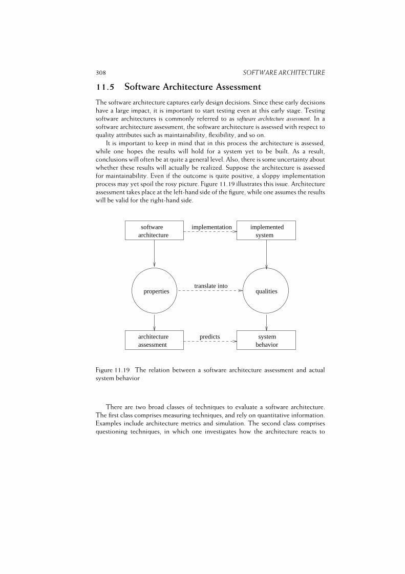
308 SOFTWARE ARCHITECTURE

11.5 Software Architecture Assessment

The software architecture captures early design decisions. Since these early decisions

have a large impact, it is important to start testing even at this early stage. Testing

software architectures is commonly referred to as software architecture assessment. In a

software architecture assessment, the software architecture is assessed with respect to

quality attributes such as maintainability, flexibility, and so on.

It is important to keep in mind that in this process the architecture is assessed,

while one hopes the results will hold for a system yet to be built. As a result,

conclusions will often be at quite a general level. Also, there is some uncertainty about

whether these results will actually be realized. Suppose the architecture is assessed

for maintainability. Even if the outcome is quite positive, a sloppy implementation

process may yet spoil the rosy picture. Figure 11.19 illustrates this issue. Architecture

assessment takes place at the left-hand side of the figure, while one assumes the results

will be valid for the right-hand side.

predictsbehaviorsystem

assessmentarchitecture

implementation

translate intoqualitiesproperties

systemimplemented

architecturesoftware

Figure 11.19 The relation between a software architecture assessment and actual

system behavior

There are two broad classes of techniques to evaluate a software architecture.

The first class comprises measuring techniques, and rely on quantitative information.

Examples include architecture metrics and simulation. The second class comprises

questioning techniques, in which one investigates how the architecture reacts to

11.5. SOFTWARE ARCHITECTURE ASSESSMENT 309

certain situations. This is often done with the help of scenarios. In the sequel, we

concentrate on the latter.

There are different types of scenarios one may use in architecture assessments.

Common types are:� Use cases: these often are already available, or can be derived from the

requirements.� Change cases: change cases describe possible or likely future situations. They

describe ”what-if” like situations, like ”what if our library has to be able to

handle dvd’s next to books and journals”.� Stress situations: these describe extreme conditions under which the system

still has to operate, such as limits with respect to performance or the number

of concurrent users of the system.� Far-into-the-future scenarios: these are like change cases, but farther away. For

instance, we may envision a future in which a library changes from a document

archive to a memory archive. We may want to retain how an old-fashioned

bakery smells, or the sound of a San Francisco tram.

One of the best known architecture assessment methods is ATAM: the Architecture

Tradeoff Analysis Method. As the name says, an important goal of ATAM is to

determine how quality attributes interact. If we decide to include an authorization

component to increase security, such is likely to degrade performance. By making

the consequences of design decisions explicit, it becomes possible for stakeholders to

trade off the different possibilities, and make informed decisions, with clear insight

into the consequences thereof.

1. Present method to stakeholders

2. Present business drivers (by project manager)

3. Present architecture (by lead architect)

4. Identify architectural approaches

5. Generate quality attribute tree

6. Analyze architectural approaches

7. Brainstorm and prioritize scenarios

8. Analyze architectural approaches

9. Present results

Figure 11.20 Steps of ATAM

The main steps of ATAM are listed in figure 11.20. There may be a preparatory

phase in which participants meet to discuss the whole exercise, and a follow-up phase

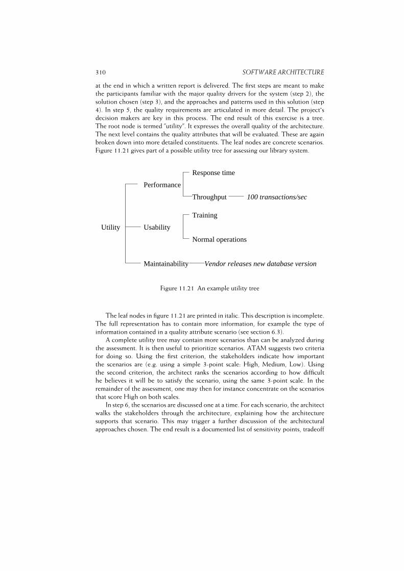
310 SOFTWARE ARCHITECTURE

at the end in which a written report is delivered. The first steps are meant to make

the participants familiar with the major quality drivers for the system (step 2), the

solution chosen (step 3), and the approaches and patterns used in this solution (step

4). In step 5, the quality requirements are articulated in more detail. The project˘s

decision makers are key in this process. The end result of this exercise is a tree.

The root node is termed ”utility”. It expresses the overall quality of the architecture.

The next level contains the quality attributes that will be evaluated. These are again

broken down into more detailed constituents. The leaf nodes are concrete scenarios.

Figure 11.21 gives part of a possible utility tree for assessing our library system.

Vendor releases new database version

100 transactions/sec

Maintainability

Normal operations

Training

Response time

Throughput

Performance

UsabilityUtility

Figure 11.21 An example utility tree

The leaf nodes in figure 11.21 are printed in italic. This description is incomplete.

The full representation has to contain more information, for example the type of

information contained in a quality attribute scenario (see section 6.3).

A complete utility tree may contain more scenarios than can be analyzed during

the assessment. It is then useful to prioritize scenarios. ATAM suggests two criteria

for doing so. Using the first criterion, the stakeholders indicate how important

the scenarios are (e.g. using a simple 3-point scale: High, Medium, Low). Using

the second criterion, the architect ranks the scenarios according to how difficult

he believes it will be to satisfy the scenario, using the same 3-point scale. In the

remainder of the assessment, one may then for instance concentrate on the scenarios

that score High on both scales.

In step 6, the scenarios are discussed one at a time. For each scenario, the architect

walks the stakeholders through the architecture, explaining how the architecture

supports that scenario. This may trigger a further discussion of the architectural

approaches chosen. The end result is a documented list of sensitivity points, tradeoff

11.6. SUMMARY 311

points, risks and nonrisks, relating the architectural decisions made to the relevant

quality attributes.

A sensitivity point is a property of the architecture that is critical for a certain

quality attribute. For example, the possibility to undo user actions critically affects

the usability of our library system, and this property therefore is a sensitivity point

with respect to usability. At the same time, this decision also is a sensitivity point

with respect to performance. If a decision is a sensitivity point for more than one

quality attribute, it is called a tradeoff point. If performance is of utmost importance, the

decision to include an undo facility may be a risk. If this decision is not critical, it is a

nonrisk.

The utility tree is based on the main drivers used during the design of the

architecture. Its construction is done in consultation with the main decision makers.

There are other stakeholders, such as a maintenance manager or security expert, that

can also be polled for additional scenarios. This is done in step 7. And similar to step

5, these scenarios are prioritized, and a selection is made for further study. Similar

to step 6, these additional scenarios are analyzed in step 8. Finally, the collected

information is summarized and presented to all stakeholders in step 9.

The result of an architecture assessment goes way beyond a list of sensitivity

points, tradeoff points, risks and nonrisks. Stakeholders, including the architect,

often construct a much deeper understanding of the architecture, its underlying

decisions, and the ramifications thereof. Also, a better documentation is often

delivered as a byproduct of the assessment. This is similar to the extra benefits

software inspections and walkthroughs have besides the identification of software

errors (see section 13.4.2).

In practice, organizations often perform software architecture assessments in a less

rigid sense than suggested by the above description of ATAM. Usually, a cafetaria-like

approach is followed, whereby those elements from ATAM and similar methods are

chosen that best fit the situation at hand (Kazman et al., 2006).

11.6 Summary

Software architecture is concerned with the description of elements from which

systems are built, the interaction among those elements, patterns that guide their

composition, and constraints on those patterns. The design of a software architecture

is driven by quality concerns. The resulting software architecture is described in

different views, each of which addresses specific concerns on behalf of specific

stakeholders. This resembles the way different drawings of a building emphasize

different aspects on behalf of its different stakeholders.

It is important to not only document the resulting solution, but also the decisions

that led to that solution, its rationale, and other information that is helpful to guide

its further evolution.

Software architecture is an important notion, for more than one reason:

312 SOFTWARE ARCHITECTURE� The comparison with traditional architecture reveals commonalities which help

us to get a better grip on the software design process and its products. Software

architecture is not only concerned with the blueprint that is the outcome of the

design process. The notion of an architectural style has merits of its own and

the relationship between style on the one hand and engineering and materials

on the other hand provide additional insights into what software design entails

(Perry and Wolf, 1992).� The field may eventually yield a repertoire of concepts that software architects

can use in their search for solutions. Expert designers in any field build on a

vast collection of reusable concepts. These concepts are given unique names,

which are used to communicate them, and serve as labels when retrieving

and storing them in human memory. Software architecture is concerned

with identifying, describing and categorizing components at a high level of

abstraction. The resulting abstractions are to become part of the vocabulary

of software engineers, much like abstract data types are already part of that

vocabulary.� Phrasing a software design in software architectural terms promotes consistency

during development and maintenance. Phrasing the global design in terms of

an architecture forces us to think about its general flavor, in terms of types of

component and connector, as well as a certain control structure. By making

this intuition explicit, it both describes and prescribes how the system should look

and how it may evolve over time.� A software architecture captures early design decisions. The architecture can

be used to evaluate those decisions. It also provides a way to discuss those

decisions and their ramifications with the various stakeholders.

11.7 Further Reading

Shaw and Garlan (1996) is an early influential source that discusses the emerging field

of software architecture, in particular software architectural styles. Bass et al. (2003)

give a broad overview of the field, including the various forces that influence software

architecture and the purposes of a software architecture, and ADD. It includes a

number of case studies to illustrate these issues. Clements et al. (2003) is wholly

devoted to architecture documentation and architectural views. The state of the art

in software architecture is reflected in (Software, 2006). A comparison between the

classical field of architecture and software architecture is made in (Perry and Wolf,

1992). Different architectural views on the same system are the topic of (Kruchten,

1995) and (Soni et al., 1995). Rozanski and Woods (2005) give a very good catalog

of useful architectural viewpoints. Architecture as a set of design decisions is the topic

of (Tyree and Akerman, 2005).

11.7. FURTHER READING 313

Software architecture and design patterns have been strongly influenced by the

works of the architect Christopher Alexander. It is certainly worthwhile to have a look

at them (Alexander et al., 1977), (Alexander, 1979). Lea (1994) gives an introduction

to his work for software engineers. Alexander (1999) explains the origins of pattern

theory. Buschmann et al. (1996) is an excellent source for architectural patterns. The

theory of programming plans stems from (Soloway, 1986).

Clements et al. (2002) discusses software architecture evaluation in great depth.

Maranzano et al. (2005) discuss experiences with architecture reviews. A survey of

architecture assessment methods is given in (Dobrica and Niemela, 2002).

Many issues related to software architecture have not been touched upon in this

chapter. These include efforts to classify software architectural styles along different

dimensions (Shaw and Clements, 1996), architecture description languages and

supporting tools (Shaw et al., 1995), architecture description languages (Medvidovic

and Taylor, 2000), architecture reconstruction (van Deursen et al., 2004), the role of

the software architect (Kruchten, 1999), (Mustapic et al., 2004).

Exercises

1. Give a definition of the term ‘software architecture’. Explain the different

elements in this definition.

2. What is the difference between software architecture and top-level design?

3. What is the main purpose of a software architecture?

4. What is the relation between design decisions and software architecture?

5. Explain the architecture design method ADD (Attribute Driven Design).

6. What is the role of the backlog in design?

7. What is the difference between the notions software architecture and design

pattern?

8. What is the difference between the conceptual or logical viewpoint and the

implementation viewpoint?

9. Explain the difference between module, component and connector, and

allocation viewpoints.

10. Describe in your own words the essence of the implicit-invocation architec-

tural style.

11. In what sense does the abstract-data-type architectural style constrain the

designer?

314 SOFTWARE ARCHITECTURE

12. Why is error-handling difficult in the pipes-and-filter architectural style?

13. Why is language so important in software design?

14. Define the following component types: computational, memory, manager.

15. Define the following connector types: data flow, message passing, shared

data.

16. In what sense may the layers in a layered architecture be viewed as virtual

machines?

17. What is a software architecture assessment?

18. Explain the steps of ATAM.

19. � To what extent may the development organization, background and

expertise of the designer, and the technical environment have influenced the

architecture of the World Wide Web? See also (Bass et al., 2003, chapter 13).

20. ~ Take a software system you have been involved in. Identify and document

three important design decisions for that system.

21. ~ For that same system, develop a module view. Indicate the concerns this

view addresses.

22. ~ For that same system, develop a business oriented view. Indicate the

concerns this view addresses.

23. ~ What are the possible roles of software architecture and design patterns

during software comprehension?

24. � Write an essay on the influence of social and organizational issues on

software architecture. See for example (Cockburn, 1996).

25. � Write an essay on the role of the software architect. See for example

(Kruchten, 1999)

12

Software Design

LEARNING OBJECTIVES� To be able to discern desirable properties of a software design� To understand different notions of complexity, at both the module and system

level� To be aware of some object-oriented metrics� To be aware of some widely-known classical design methods� To understand the general flavor of object-oriented analysis and design methods� To be aware of a global classification scheme for design methods� To understand the role of design patterns and be able to illustrate their

properties� To be aware of guidelines for the design documentation

316 SOFTWARE DESIGN

Software design concerns the decomposition of a system into its constituent

parts. A good design is the key to the successful implementation and evolution

of a system. A number of guiding principles for this decomposition help to

achieve quality designs. These guiding principles underlie the main design

methods discussed in this chapter. Unlike more classical design fields, there is

no visual link between the design representation of a software system and the

ultimate product. This complicates the communication of design knowledge

and raises the importance of proper design representations.

During software development, we should adhere to a planned approach. If we

want to travel from point A to point B, we will (probably) consult a map first.

According to some criterion, we will then plan our travel scheme. The time-loss

caused by the planning activity is bound to outweigh the misery that occurs if we do

not plan our trip at all but just take the first turn left, hoping that this will bring us

somewhat closer to our destination.

In designing a garden, we will also follow some plan. We will not start by planting

a few bulbs in one corner, an apple tree in another, and a poplar next to the front

door.

The above examples sound ridiculous. They are. Yet, many a software development

project is undertaken in this way. Somewhat exaggeratedly, we may call it the

‘programmer’s approach’ to software development. Far too much software is still being

developed without a clear design phase. The reasons for this ‘code first, design later’

attitude are many:� We do not want to, or are not allowed to, ‘waste our time’ on design activities.� We have to, or want to, quickly show something to our customer.� We are judged by the amount of code written per man-month.� We are, or expect to be, pressed for time.

Such an approach grossly underestimates the complexity of software and its devel-

opment. Just as with the furnishing of a house or the undertaking of a long trip, it is

paramount to put thought into a plan, resulting in a blueprint that is then followed

during actual construction. The outcome of this process (the blueprint) will be termed

the design or, if the emphasis is on its notation, the (technical) specification. The

process of making this blueprint is also called design. To a large extent, the quality

of the design determines the quality of the resulting product. Errors made during the

design phase often go undetected until the system is operational. At that time, they

can be repaired only by incurring very high costs.

Design is a problem-solving activity and, as such, very much a matter of trial and

error. In the presentation of a mathematical proof, subsequent steps dovetail well into

each other and everything drops into place at the end. The actual discovery of the

317

proof was probably quite different. The same holds for the design of software. We

should not confuse the outcome of the design process with the process itself. The

outcome of the design process is a ‘rational reconstruction’ of that process. (Note that

we made precisely the same remark with respect to the outcome of the requirements

engineering process.)

Software design is a ‘wicked problem’. The term originated in research into the

nature of design issues in social planning problems. Properties of wicked problems in

this area are remarkably similar to properties of software design:� There is no definite formulation of a wicked problem. The design process

can hardly be separated from either the preceding requirements engineering

phase or the subsequent documentation of the design in a specification. These

activities will, in practice, overlap and influence each other. At the more global

(architectural) stages of system design, the designer will interact with the user

to assess fitness-for-use aspects of the design. This may lead to adaptations in

the requirements specification. The more detailed stages of design often cannot

be separated from the specification method used.

One corollary of this is that the waterfall model does not fit the type of problem

it is meant to address.� Wicked problems have no stopping rule. There is no criterion that tells us

when the solution has been reached. Though we do have a number of quality

measures for software designs, there does not exist a single scale against which

to measure the quality of a design. There probably never will be such a scale.� Solutions to wicked problems are not true or false. At best, they are good

or bad. The software design process is not analytic. It does not consist of a

sequence of decisions each of which brings us somewhat closer to that one,

optimal solution. Software design involves making a large number of trade-offs,

such as those between speed and robustness. As a consequence, there is a

number of acceptable solutions, rather than one best solution.� Every wicked problem is a symptom of another problem. Resolving one problem

may very well result in an entirely different problem elsewhere. For example,

the choice of a particular dynamic data structure may solve the problem of

an unknown input size and at the same time introduce an efficiency problem.

A corollary of this is that small changes in requirements may have large

consequences in the design or implementation. Elsewhere, we described this

by saying that software is not continuous.

During design we may opt for a Taylorian, functionality-centered view and consider

the design problem as a purely technical issue. Alternatively, we may realize that

design involves user issues as well and therefore needs some form of user involvement.

The role of the user during design need not be restricted to that of a guinea-pig in

shaping the actual user interface. It may also involve much deeper issues.

318 SOFTWARE DESIGN

Rather than approaching system design from the point of view that human

weaknesses need to be compensated for, we may take a different stand and consider

computerized systems as a means to support human strengths. Likewise, systems

need not reflect the interests of system owners only. In a democratic world, systems

can be designed so that all those involved benefit. This less technocratic attitude

leads to extensive user involvement during all stages of system development. Agile

development methods advocate this type of approach.

Whereas traditional system development has a production view in which the

technical aspects are optimized, the ‘Scandinavian school’ pays equal attention to

the human system, and holds the view that technology must be compatible with

organizational and social needs. The various possible modes of interaction between

the designer or analyst on the one hand and the user on the other hand are also

discussed in section 9.1. In this chapter, we concentrate on the technical issues of

software design.

Pure agile approaches do suggest to start by just planting a few bulbs in one corner

of the garden. If we happen to move into our new house in late autumn and want

some color when spring sets in, this sounds like the best thing we can do. If we change

our mind at some later point in time, we can always move the bulbs and do some

additional garden design. It thus depends on the situation at hand how much upfront

design is feasible. In this chapter, we assume enough context and requirements are

known to warrant an explicit design step.

From the technical point of view, the design problem can be formulated as follows:

how can we decompose a system into parts such that each part has a lower complexity

than the system as a whole, while the parts together solve the user’s problem. Since

the complexity of the individual components should be reasonable, it is important

that the interaction between components not be too complicated.

Design has both a product aspect and a process aspect. The product aspect refers to

the result, while the process aspect is about how we get there. At the very global,

architectural levels of design, there is little process guidance, and the result is very

much determined by the experience of the designer. For that reason, chapter 11

largely focuses on the characterization of the result of the global design process, the

software architecture. In this chapter, we focus on the more detailed stages of design,

where more process guidance has been accumulated in a number of software design

methods. But for the more detailed stages of software design too, the representational

aspect is the more important one. This representation is the main communication

vehicle between the designer and the other stakeholders. Unlike more classical design

fields, there is no visual link between the design representations of a software system

and the ultimate product. The blueprint of a bridge gives us lots of visual clues as to

how that bridge will eventually look like. Such is not the case for software, and we

have to seek other ways to communicate design knowledge to our stakeholders.

There really is no universal design method. The design process is a creative one,

and the quality and expertise of the designers are a critical determinant for its success.

However, over the years a number of ideas and guidelines have emerged which may

12.1. DESIGN CONSIDERATIONS 319

serve us in designing software.

The single most important principle of software design is information hiding. It

exemplifies how to apply abstraction in software design. Abstraction means that we

concentrate on the essential issues and ignore, abstract from, details that are irrelevant

at this stage. Considering the complexity of the problems we are to solve, applying

some sort of abstraction is a sheer necessity. It is simply impossible to take in all the

details at once.

Section 12.1 discusses desirable design features that bear on quality issues, most

notably maintainability and reusability. Five issues are identified that have a strong

impact on the quality of a design: abstraction, modularity, information hiding,

complexity, and system structure. Assessment of a design with respect to these issues

allows us to get an impression of design quality, albeit not a very quantitative one yet.

Efforts to quantify such heuristics have resulted in a number of metrics specifically

aimed at object-oriented systems.

A vast number of design methods exist, many of which are strongly tied to a

certain notation. These methods give strategies and heuristics to guide the design

process. Most methods use a graphical notation to depict the design. Though the

details of those methods and notations differ widely, it is possible to provide broad

characterizations in a few classes. The essential characteristics of those classes are

elaborated upon in sections 12.2 and 12.3.

Design patterns are collections of a few modules (or, in object-oriented circles,

classes) which are often used in combination, and which together provide a useful

abstraction. A design pattern is a recurring solution to a standard problem. The

opposite of a pattern is an antipattern: a mistake often made. The prototypical

example of a pattern is the MVC (Model--View--Controller) pattern known from

Smalltalk. Design patterns are discussed in section 12.5.

During the design process too, quite a lot of documentation will be generated.

This documentation serves various users, such as project managers, designers, testers,

and programmers. Section 12.6 discusses IEEE Standard 1016. This standard contains

useful guidelines for describing software designs. The standard identifies a number of

roles and indicates, for each role, the type of design documentation needed.

Finally, section 12.7 discusses some verification and validation techniques that

may fruitfully be applied at the design stage.

12.1 Design Considerations

Up till now we have used the notion of ‘module’ in a rather intuitive way. It is not

easy to give an accurate definition of that notion. Obviously, a module does not

denote some random piece of software. We apply certain criteria when decomposing

a system into modules.

At the programming language level, a module usually refers to an identifiable unit

with respect to compilation. We will use a similar definition of the term ‘module’ with

respect to design: a module is an identifiable unit in the design. It may consist of a

320 SOFTWARE DESIGN

single procedure, or a class, or even a set of classes. It preferably has a clean interface

to the outside world, and the functionality of the module then is only approached

through that interface.

There are, in principle, many ways to decompose a system into modules.

Obviously, not every decomposition is equally desirable. In this section we are

interested in desirable features of a decomposition, irrespective of the type of system

or the design method used. These features can in some sense be used as a measure of

the quality of the design. Designs that have those features are considered superior to

those that do not have them.

The design features we are most interested in are those that facilitate maintenance

and reuse: simplicity, a clear separation of concepts into different modules, and

restricted visibility (i.e. locality) of information.1 Systems that have those properties

are easier to maintain since we may concentrate our attention on those parts that are

directly affected by a change. These properties also bear on reusability, because the

resulting modules tend to have a well-defined functionality that fits concepts from the

application domain. Such modules are likely candidates for inclusion in other systems

that address problems from the same domain.

In the following subsections we discuss five interrelated issues that have a strong

impact on the above features:

– abstraction,

– modularity,

– information hiding,

– complexity, and

– system structure.

For object-oriented systems, a specific set of quality heuristics and associ-

ated metrics has been defined. The main object-oriented metrics are discussed in

section 12.1.6.

12.1.1 Abstraction

Abstraction means that we concentrate on the essential features and ignore, abstract

from, details that are not relevant at the level we are currently working. Consider, for

example, a typical sorting module. From the outside we cannot (and need not be able

to) discern exactly how the sorting process takes place. We need only know that the

output is indeed sorted. At a later stage, when the details of the sorting module are

decided upon, then we can rack our brains about the most suitable sorting algorithm.

1Obviously, an even more important feature of a design is that the corresponding system should

perform the required tasks in the specified way. To this end, the design should be validated against the

requirements.

12.1. DESIGN CONSIDERATIONS 321

The complexity of most software problems makes applying abstraction a sheer

necessity. In the ensuing discussion, we distinguish two types of abstraction: procedural

abstraction and data abstraction.

The notion of procedural abstraction is fairly traditional. A programming lan-

guage offers if-constructs, loop-constructs, assignment statements, and the like. The

transition from a problem to be solved to these primitive language constructs is a

large one in many cases. To this end a problem is first decomposed into subproblems,

each of which is handled in turn. These subproblems correspond to major tasks to

be accomplished. They can be recognized by their description in which some verb

plays a central role (for example: read the input, sort all records, process the next user

request, compute the net salary). If needed, subproblems are further decomposed into

even simpler subproblems. Eventually we get at subproblems for which a standard

solution is available. This type of (top-down) decomposition is the essence of the

main-program-with-subroutines architectural style.

The result of this type of stepwise decomposition is a hierarchical structure. The

top node of the structure denotes the problem to be solved. The next level shows its

first decomposition into subproblems. The leaves denote primitive problems. This is

schematically depicted in figure 12.1.

The procedure concept offers us a notation for the subproblems that result from

this decomposition process. The application of this concept is known as procedural

abstraction. With procedural abstraction, the name of a procedure (or method, in

object oriented languages) is used to denote the corresponding sequence of actions.

When that name is used in a program, we need not bother ourselves about the exact

way in which its effect is realized. The important thing is that, after the call, certain

prestated requirements are fulfilled.

This way of going about the process closely matches the way in which humans

are inclined to solve problems. Humans too are inclined to the stepwise handling of

problems. Procedural abstraction thus offers an important means of tackling software

problems.

When designing software, we are inclined to decompose the problem so that

the result has a strong time orientation. A problem is decomposed into subproblems

that follow each other in time. In its simplest form, this approach results in input-

-process--output schemes: a program first has to read and store its data, next some

process computes the required output from these data, and the result finally is output.

Application of this technique may result in programs that are difficult to adapt and

hard to comprehend. Applying data abstraction results in a decomposition which

shows this affliction to a far lesser degree.

Procedural abstraction is aimed at finding a hierarchy in the program’s control

structure: which steps have to be executed and in which order. Data abstraction is

aimed at finding a hierarchy in the program’s data. Programming languages offer

primitive data structures for integers, real numbers, truth values, characters and

possibly a few more. Using these building blocks we may construct more complicated

data structures, such as stacks and binary trees. Such structures are of general use in

322 SOFTWARE DESIGN

Figure 12.1 The idea of procedural abstraction

application software. They occur at a fairly low level in the hierarchy of data structures.

Application-oriented objects, such as ‘paragraph’ in text processing software or ‘book’

in our library system, are found at higher levels of the data structure hierarchy. This

is schematically depicted in figure 12.2.

Figure 12.2 The idea of data abstraction

For the data, too, we wish to abstract from details that are not relevant at a certain

level. In fact, we already do so when using the primitive data structures offered by our

programming language. In using these, we abstract from details such as the internal

representation of numbers and the way in which the addition of two numbers is

realized. At the programming language level we may view the integers as a set of

objects (0, 1, -1, 2, -2, . . . ) and a set of operations on these objects (+, �, �, =,

. . . ). These two sets together determine the data type integer. To be able to use

this data type we need only name the set of objects and specify its operations.

We may proceed along the same lines for the data structures not directly supported

by the programming language. A data type binary-tree is characterized by a set of

12.1. DESIGN CONSIDERATIONS 323

objects (all conceivable binary trees) and a set of operations on those objects. When

using binary trees, their representation and the implementation of the corresponding

operations need not concern us. We need only ascertain the intended effect of the

operations.

Applying data abstraction during design is sometimes called object-oriented

design, since the type of object and the associated operations are encapsulated in one

module. The buzzword ‘object-oriented’ however also has a subtly different meaning.

We will further elaborate upon this notion in section 12.3.

Languages such as Ada, Java and C++ offer a language construct (called package,

class, and struct, respectively) that allows us to maintain a syntactic separation

between the implementation and specification of data types. Note that it is also

possible to apply data abstraction during design when the ultimate language does not

offer the concept. However, it then becomes more cumbersome to move from design

to code.

We noticed before that procedural abstraction fits in nicely with the way humans

tend to tackle problems. To most people, data abstraction is a bit more complicated.

When searching for a solution to a software problem we will find that the

solution needs certain data structures. At some point we will also have to choose a

representation for these data structures. Rather than making those decisions at an early

stage and imposing the result on all other components, you are better off if you create

a separate subproblem and make only the procedural, implementation-independent,

interfaces public. Data abstraction thus is a prime example of information hiding.

The development of these abstraction techniques went hand-in-hand with other

developments, particularly those in the realm of programming languages. Procedures

were originally introduced to avoid the repetition of instruction sequences. At a later

stage we viewed the name of a procedure as an abstraction of the corresponding

instruction sequence. Only then did the notion of procedural abstraction get its

present connotation. In a similar vein, developments in the field of formal data type

specifications and language notions for modules (starting with the class concept of

SIMULA-67) strongly contributed to our present notion of data abstraction.

As a final note we remark that we may identify yet a third type of abstraction,

control abstraction. In control abstraction we abstract from the precise order in which

a sequence of events is to be handled. Though control abstraction is often implicit

when procedural abstraction is used, it is sometimes convenient to be able to explicitly

model this type of nondeterminacy, for instance when specifying concurrent systems.

This topic falls outside the scope of this book.

12.1.2 Modularity

During design, the system is decomposed into a number of modules and the

relationships between those modules are indicated. In another design of the same

system, different modules may show up and there may be different relationships

between the modules. We may try to compare those designs by considering both a

324 SOFTWARE DESIGN

typology for the individual modules and the type of connections between them. This

leads us to two structural design criteria: cohesion and coupling.

Cohesion may be viewed as the glue that keeps the module together. It is a

measure of the mutual affinity of the elements of a module. In general we will wish

to make the cohesion as strong as possible. In their classic text on Structured Design,

Yourdon and Constantine identify the following seven levels of cohesion of increasing

strength:� Coincidental cohesion With coincidental cohesion, elements are grouped into

modules in a haphazard way. There is no significant relation between the

elements.� Logical cohesion With logical cohesion, the elements realize tasks that are

logically related. One example is a module that contains all input routines.

These routines do not call one another and they do not pass information to

each other. Their function is just very similar.� Temporal cohesion A typical example of this type of cohesion is an initialization

module. The various elements of it are independent but they are activated at

about the same point in time.� Procedural cohesion A module exhibits procedural cohesion if it consists of a

number of elements that have to be executed in some given order. For instance,

a module may have to first read some datum, then search a table, and finally

print a result.� Communicational cohesion This type of cohesion occurs if the elements of a

module operate on the same (external) data. For instance, a module may read

some data from a disk, perform certain computations on those data, and print

the result.� Sequential cohesion Sequential cohesion occurs if the module consists of a

sequence of elements where the output of one element serves as input to the

next element.� Functional cohesion In a module exhibiting functional cohesion all elements

contribute to the one single function of that module. Such a module often

transforms a single input datum into a single output datum. The well-known

mathematical subroutines are a typical example of this. Less trivial examples are

modules like ‘execute the next edit command’ and ‘translate the program given’.

In a classic paper on structured design, (Stevens et al., 1974) provide some simple

heuristics that may be of help in establishing the degree of cohesion of a module.

They suggest writing down a sentence that describes the function (purpose) of the

module and examining that sentence. Properties to look for include the following:

12.1. DESIGN CONSIDERATIONS 325� If the sentence is compound, has a connective (such as a comma or the word

‘and’), or contains more than one verb, then that module is probably performing

more than one function. It is likely to have sequential or communicational

cohesion.� If the sentence contains words that relate to time (such as ‘first’, ‘next’, ‘after’,

‘then’), then the module probably has sequential or temporal cohesion.� If the sentence contains words like ‘initialize’, the module probably has temporal

cohesion.

The levels of cohesion identified above reflect the cohesion between the functions

that a module provides. Abstract data types cannot easily be accommodated in this

scheme. (Macro and Buxton, 1987) therefore propose adding an extra level, data

cohesion, to identify modules that encapsulate an abstract data type. Data cohesion

is even stronger than functional cohesion.

It goes without saying that it is not always an easy task to obtain the strongest

possible cohesion between the elements of a module. Though functional cohesion

may be attainable at the top levels and data cohesion at the bottom levels, we will

often have to settle for less at the intermediate levels of the module hierarchy. The

trade-offs to be made here are what makes design such a difficult, and yet challenging,

activity.

The second structural criterion is coupling. Coupling is a measure of the strength

of the intermodule connections. A high degree of coupling indicates a strong

dependence between modules. A high degree of coupling between modules means

that we can only fully comprehend this set of modules as a whole and may result in

ripple effects when a module has to be changed, because such a change is likely to

incur changes in the dependent modules as well. Loosely-coupled modules, on the

other hand, are relatively independent and are easier to comprehend and adapt. Loose

coupling therefore is a desirable feature of a design (and its subsequent realization).

The following types of coupling can be identified (from tightest to loosest):� Content coupling With content coupling, one module directly affects the

working of another module. Content coupling occurs when a module changes

another module’s data or when control is passed from one module to the middle

of another (as in a jump). This type of coupling can, and should, always be

avoided.� Common coupling With common coupling, two modules have shared data.

The name originates from the use of COMMON blocks in FORTRAN. Its

equivalent in block-structured languages is the use of global variables.� External coupling With external coupling, modules communicate through an

external medium, such as a file.

326 SOFTWARE DESIGN� Control coupling With control coupling, one module directs the execution of

another module by passing the necessary control information. This is usually

accomplished by means of flags that are set by one module and reacted upon

by the dependent module.� Stamp coupling Stamp coupling occurs when complete data structures are

passed from one module to another. With stamp coupling, the precise format

of the data structures is a common property of those modules.� Data coupling With data coupling, only simple data is passed between modules.

The various types of coupling emerged in the 1970s and reflect the data type concepts

of programming languages in use at that time. For example, programming languages of

that time had simple scalar data types such as real and integer. They allowed arrays

of scalar values and records were used to store values of different types. Modules

were considered data-coupled if they passed scalars or arrays. They were considered

stamp-coupled if they passed record data. When two modules are control-coupled,

the assumption is that the control is passed through a scalar value.

Nowadays, programming languages have much more flexible means of passing

information from one module to another, and this requires a more detailed set of

coupling levels. For example, modules may pass control data through records (as

opposed to scalars only). Modules may allow some modules access to their data

and deny it to others. As a result, there are many levels of visibility between local

and global. Finally, the coupling between modules need not be commutative. When

module A passes a scalar value to B and B returns a value which is used to control

the further execution of A, then A is data-coupled to B, while B is control-coupled

to A. As a result, people have extended and refined the definitions of cohesion and

coupling levels.

Coupling and cohesion are dual characteristics. If the various modules exhibit

strong internal cohesion, the intermodule coupling tends to be minimal, and vice

versa.

Simple interfaces -- weak coupling between modules and strong cohesion between

a module’s elements -- are of crucial importance for a variety of reasons:� Communication between programmers becomes simpler. When different peo-

ple are working on one and the same system, it helps if decisions can be made

locally and do not interfere with the working of other modules.� Correctness proofs become easier to derive.� It is less likely that changes will propagate to other modules, which reduces

maintenance costs.� The reusability of modules is increased. The fewer assumptions that are made

about an element’s environment, the greater the chance of fitting another

environment.

12.1. DESIGN CONSIDERATIONS 327� The comprehensibility of modules is increased. Humans have limited memory

capacity for information processing. Simple module interfaces allow for an

understanding of a module independent of the context in which it is used.� Empirical studies show that interfaces exhibiting weak coupling and strong

cohesion are less error-prone than those that do not have these properties.

12.1.3 Information Hiding

The concept of information hiding originates from a seminal paper of David Par-

nas Parnas (1972). The principle of information hiding is that each module has a

secret which it hides to other modules. Its use as a guiding principle in design is aptly

illustrated in the KWIC-index example. In the second decomposition, for example,

module Store hides how lines are stored and module Sort hides how and when shifts

are sorted.

Design involves a sequence of decisions, such as how to represent certain

information, or in which order to accomplish tasks. For each such decision we should

ask ourselves which other parts of the system need to know about the decision and

how it should be hidden from parts that do not need to know.

Information hiding is closely related to the notions of abstraction, cohesion, and

coupling. If a module hides some design decision, the user of that module may abstract

from (ignore) the outcome of that decision. Since the outcome is hidden, it cannot

possibly interfere with the use of that module. If a module hides some secret, that

secret does not permeate the module’s boundary, thereby decreasing the coupling

between that module and its environment. Information hiding increases cohesion,

since the module’s secret is what binds the module’s constituents together. Note that,

in order to maximize its cohesion, a module should hide one secret only.

It depends on the programming language used whether the separation of concerns

obtained during the design stage will be identifiable in the ultimate code. To some

extent, this is of secondary concern. The design decomposition will be reflected, if only

implicitly, in the code and should be explicitly recorded (for traceability purposes) in

the technical documentation. It is of great importance for the later evolution of the

system. A confirmation of the impact of such techniques as information hiding on the

maintainability of software can be found in (Boehm, 1983).

12.1.4 Complexity

Like all good inventions, readability yardsticks can cause harm in misuse. They are

handy statistical tools to measure complexity in prose. They are useful to determinewhether writing is gauged to its audience. But they are not formulas for writing

. . . Writing remains an art governed by many principles. By no means all factors thatcreate interest and affect clarity can be measured objectively.

(Gunning, 1968)

328 SOFTWARE DESIGN

In a very general sense, the complexity of a problem refers to the amount of

resources required for its solution. We may try to determine complexity in this way

by measuring, say, the time needed to solve a problem. This is a so-called externalattribute: we are not looking at the entity itself (the problem), but at how it behaves.

In the present context, complexity refers to attributes of the software that affect

the effort needed to construct or change a piece of software. These are internalattributes: they can be measured purely in terms of the software itself. For example,

we need not execute the software to determine their values.

Both these notions are very different from the complexity of the computation

performed (with respect to time or memory needed). The latter is a well-established

field in which many results have been obtained. This is much less true for the type

of complexity in which we are interested. Software complexity in this sense is still a

rather elusive notion.

Serious efforts have been made to measure software complexity in quantitative

terms. The resulting metrics are intended to be used as anchor points for the

decomposition of a system, to assess the quality of a design or program, to guide

reengineering efforts, etc. We then measure certain attributes of a software system,

such as its length, the number of if-statements, or the information flow between

modules, and try to relate the numbers thus obtained to the system’s complexity. The

type of software attributes considered can be broadly categorized into two classes:

– intra-modular attributes are attributes of individual modules, and

– inter-modular attributes are attributes of a system viewed as a collection of

modules with dependencies.

In this subsection we are dealing with intra-modular attributes. Inter-modular

attributes are discussed in the next subsection. We may distinguish two classes

of complexity metrics:� Size-based complexity metrics. The size of a piece of software, such as the

number of lines of code, is fairly easy to measure. It also gives a fair indication

of the effort needed to develop that piece of software (see also chapter 7). As a

consequence, it could also be used as a complexity metric.� Structure-based complexity metrics. The structure of a piece of software is a

good indicator of its design quality, because a program that has a complicated

control structure or uses complicated data structures is likely to be difficult to

comprehend and maintain, and thus more complex.

The easiest way to measure software size is to count the number of lines of code. We

may then impose limits on the number of lines of code per module. In (Weinberg,

1971), for instance, the ideal size of a module is said to be 30 lines of code. In a variant

hereof, limits are imposed on the number of elements per module. Some people

claim that a module should contain at most seven elements. This number seven can

12.1. DESIGN CONSIDERATIONS 329

be traced back to research in psychology, which suggests that human memory is

hierarchically organized with a short-term memory of about seven slots, while there

is a more permanent memory of almost unlimited capacity. If there are more than

seven pieces of information, they cannot all be stored in short-term memory and

information gets lost.

There are serious objections to the direct use of the number of lines of code as

a complexity metric. Some programmers write more verbose programs than others.

We should at least normalize the counting to counteract these effects and be able to

compare different pieces of software. This can be achieved by using a prettyprinter,

a piece of software that reproduces programs in a given language in a uniform way.

A second objection is that this technique makes it hard to compare programs

written in different languages. If the same problem is solved in different languages,

the results may differ considerably in length. For example, APL is more compact than

COBOL.

Finally, some lines are more complex than others. An assignment like

a:= b

looks simpler than a loop

while p".next <> nil do p:= p".next

although they each occupy one line.

Halstead’s method, also known as ‘software science’, uses a refinement of counting

lines of code. This refinement is meant to overcome the problems associated with

metrics based on a direct count of lines of code.

Halstead’s method uses the number of operators and operands in a piece of

software. The set of operators includes the arithmetic and Boolean operators, as well

as separators (such as a semicolon

between adjacent instructions) and (pairs of) reserved words. The set of operands

contains the variables and constants used. Halstead then defines four basic entities:

– n1 is the number of unique (i.e. different) operators in the program;

– n2 is the number of unique (i.e. different) operands in the program;

– N1 is the total number of occurrences of operators;

– N2 is the total number of occurrences of operands.

Figure 12.3 contains a simple sorting program. Table 12.1 lists the operators and

operands of this program together with their frequency. Note that there is no

generally agreed definition of what exactly an operator or operand is. So the numbers

given have no absolute meaning. This is part of the criticism of this theory.

Using the primitive entities defined above, Halstead defines a number of derived

entities, such as:

330 SOFTWARE DESIGN

1 procedure sort(var x: array; n: integer);2 var i, j, save: integer;3 begin4 for i:= 2 to n do5 for j:= 1 to i do6 if x[i] < x[j] then7 begin save:= x[i];8 x[i]:= x[j];9 x[j]:= save10 end11 end;

Figure 12.3 A simple sorting routine

Table 12.1 Counting the number of operators and operands in the sortroutine

OperatorNumber of

OperandNumber of

occurrences occurrences

procedure 1 x 7

sort() 1 n 2

var 2 i 6

: 3 j 5

array 1 save 3

; 6 2 1

integer 2 1 1

, 2

begin . . . end 2

for . . . do 2

if . . . then 1

:= 5< 1

[ ] 6n1 = 14 N1 = 35 n2 = 7 N2 = 25– Size of the vocabulary: n = n1 + n2.

– Program length: N = N1 +N2.

– Program volume: V = N log2 n.

12.1. DESIGN CONSIDERATIONS 331

This is the minimal number of bits needed to store N elements from a set of

cardinality n.

– Program level: L = V �=V .

Here V � is the most compact representation of the algorithm in question. For

the example in figure 12.3 this is sort(x, n);, so n = N = 5, and V � = 5 log2 5.

From the formula it follows that L is at most 1. Halstead postulates that

the program level increases if the number of different operands increases,

while it decreases if the number of different operators or the total number

of operands increases. As an approximation of L, he therefore suggests:L = (2=n1)(n2=N2).– Programming effort: E = V=L.

The effort needed increases with volume and decreases as the program level

increases. E represents the number of mental discriminations (decisions) to be

taken while implementing the problem solution.

– Estimated programming time in seconds: T = E=18.

The constant 18 is determined empirically. Halstead explains this number

by referring to (Stroud, 1967), which discusses the speed with which human

memory processes sensory input. This speed is said to be 5--20 units per second.

In Halstead’s theory, the number 18 is chosen. This number is also referred to

as Stroud’s number.

The above entities can only be determined after the program has been written. It is,

however, possible to estimate a number of these entities. When doing so, the values

for n1 and n2 are assumed to be known. This may be the case, for instance, after the

detailed design step. Halstead then estimates program length as:N = n1 log2 n1 + n2 log2 n2An explanation for this formula can be given as follows. There are n12n1 � n22n2ways to combine the n given symbols such that operators and operands alternate.

However, the program is organized and organization generally gives a logarithmic

reduction in the number of possibilities. Doing so yields the above formula for N .

Table 12.2 lists the values for a number of entities from

Halstead’s theory for the example program in figure 12.3.

A number of empirical studies have addressed the predictive value of Halstead’s

formulae. These studies often give positive evidence of the validity of the theory.

The theory has also been heavily criticized. The underpinning of Halstead’s

formulas is not convincing. Results from cognitive psychology, like Stroud’s number,

are badly used, which weakens the theoretical foundation. Halstead concentrates on

the coding phase and assumes that programmers are 100% devoted to a programming

task for an uninterrupted period of time. Practice is likely to be quite different.

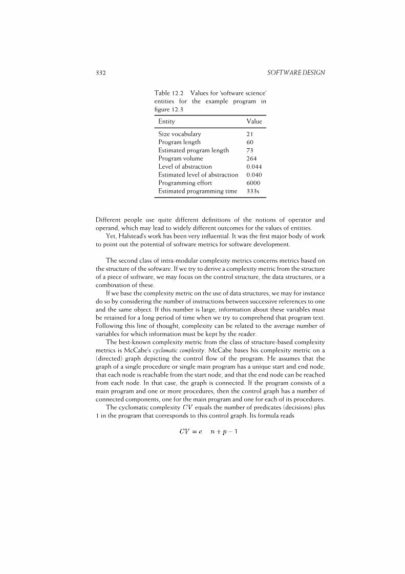
332 SOFTWARE DESIGN

Table 12.2 Values for ‘software science’

entities for the example program in

figure 12.3

Entity Value

Size vocabulary 21

Program length 60

Estimated program length 73

Program volume 264

Level of abstraction 0.044

Estimated level of abstraction 0.040

Programming effort 6000

Estimated programming time 333s

Different people use quite different definitions of the notions of operator and

operand, which may lead to widely different outcomes for the values of entities.

Yet, Halstead’s work has been very influential. It was the first major body of work

to point out the potential of software metrics for software development.

The second class of intra-modular complexity metrics concerns metrics based on

the structure of the software. If we try to derive a complexity metric from the structure

of a piece of software, we may focus on the control structure, the data structures, or a

combination of these.

If we base the complexity metric on the use of data structures, we may for instance

do so by considering the number of instructions between successive references to one

and the same object. If this number is large, information about these variables must

be retained for a long period of time when we try to comprehend that program text.

Following this line of thought, complexity can be related to the average number of

variables for which information must be kept by the reader.

The best-known complexity metric from the class of structure-based complexity

metrics is McCabe’s cyclomatic complexity. McCabe bases his complexity metric on a

(directed) graph depicting the control flow of the program. He assumes that the

graph of a single procedure or single main program has a unique start and end node,

that each node is reachable from the start node, and that the end node can be reached

from each node. In that case, the graph is connected. If the program consists of a

main program and one or more procedures, then the control graph has a number of

connected components, one for the main program and one for each of its procedures.

The cyclomatic complexity CV equals the number of predicates (decisions) plus

1 in the program that corresponds to this control graph. Its formula readsCV = e� n+ p+ 1

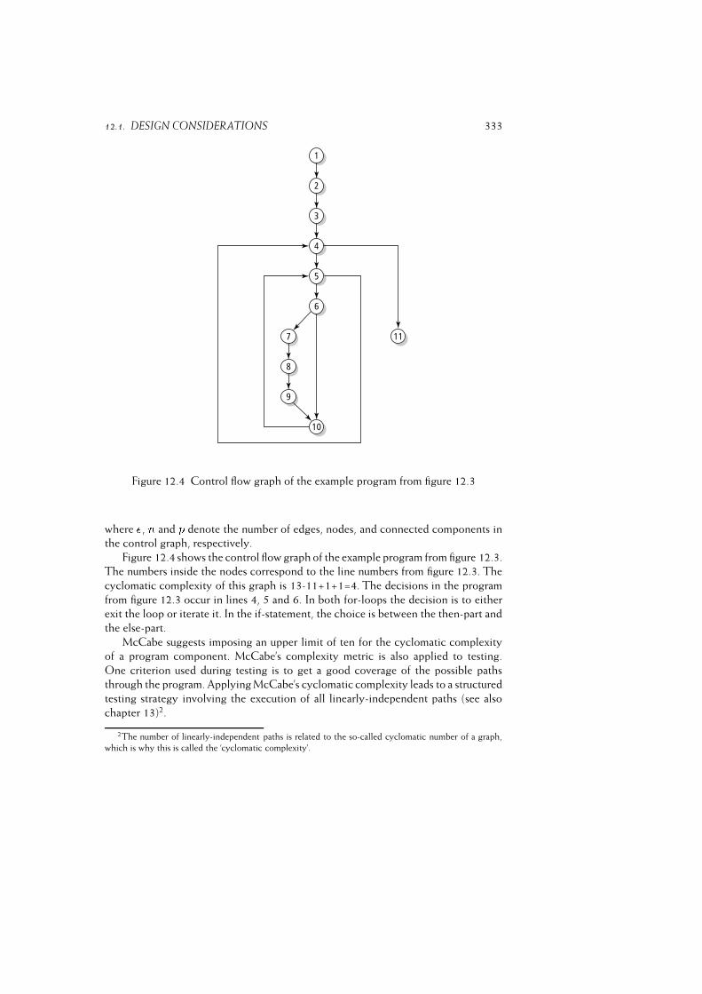
12.1. DESIGN CONSIDERATIONS 333

Figure 12.4 Control flow graph of the example program from figure 12.3

where e, n and p denote the number of edges, nodes, and connected components in

the control graph, respectively.

Figure 12.4 shows the control flow graph of the example program from figure 12.3.

The numbers inside the nodes correspond to the line numbers from figure 12.3. The

cyclomatic complexity of this graph is 13-11+1+1=4. The decisions in the program

from figure 12.3 occur in lines 4, 5 and 6. In both for-loops the decision is to either

exit the loop or iterate it. In the if-statement, the choice is between the then-part and

the else-part.

McCabe suggests imposing an upper limit of ten for the cyclomatic complexity

of a program component. McCabe’s complexity metric is also applied to testing.

One criterion used during testing is to get a good coverage of the possible paths

through the program. Applying McCabe’s cyclomatic complexity leads to a structured

testing strategy involving the execution of all linearly-independent paths (see also

chapter 13)2.

2The number of linearly-independent paths is related to the so-called cyclomatic number of a graph,

which is why this is called the ‘cyclomatic complexity’.

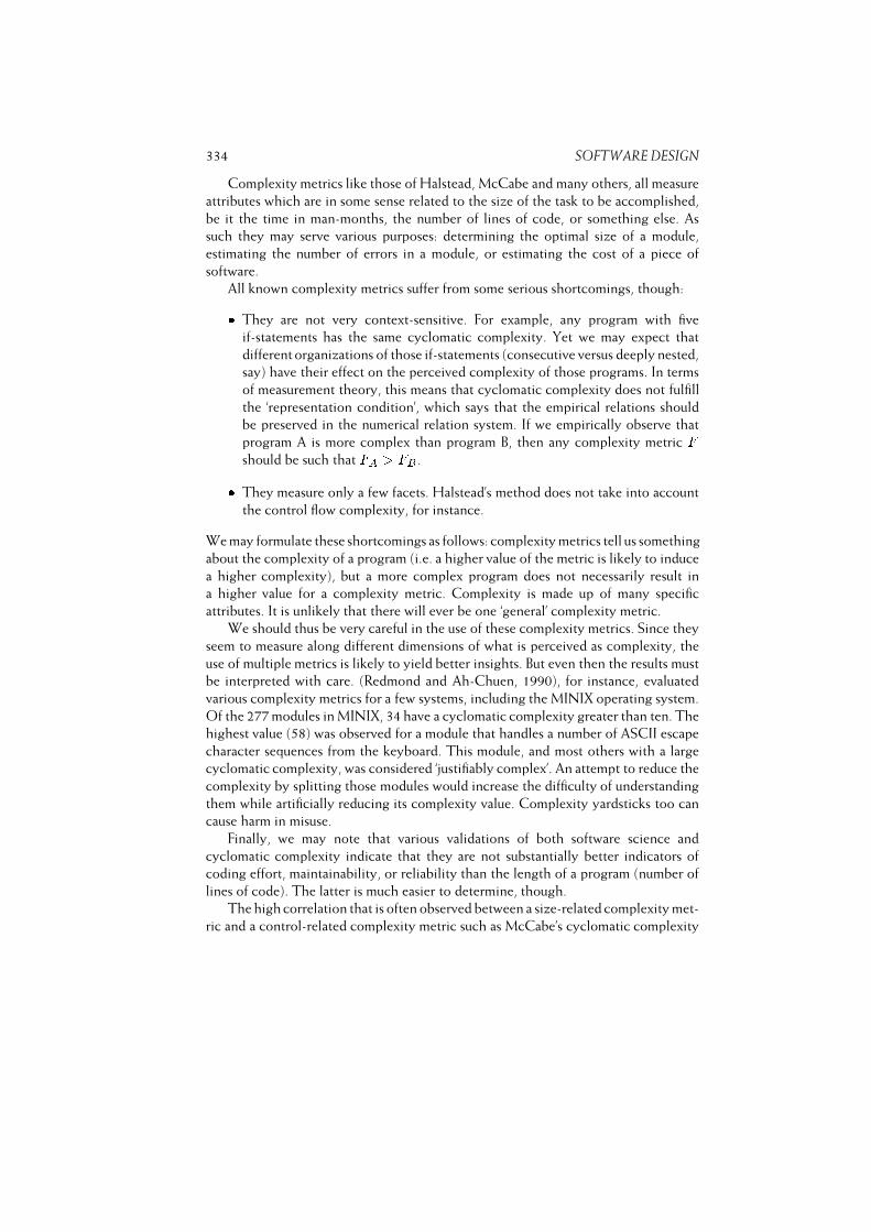
334 SOFTWARE DESIGN

Complexity metrics like those of Halstead, McCabe and many others, all measure

attributes which are in some sense related to the size of the task to be accomplished,

be it the time in man-months, the number of lines of code, or something else. As

such they may serve various purposes: determining the optimal size of a module,

estimating the number of errors in a module, or estimating the cost of a piece of

software.

All known complexity metrics suffer from some serious shortcomings, though:� They are not very context-sensitive. For example, any program with five

if-statements has the same cyclomatic complexity. Yet we may expect that

different organizations of those if-statements (consecutive versus deeply nested,

say) have their effect on the perceived complexity of those programs. In terms

of measurement theory, this means that cyclomatic complexity does not fulfill

the ‘representation condition’, which says that the empirical relations should

be preserved in the numerical relation system. If we empirically observe that

program A is more complex than program B, then any complexity metric Fshould be such that FA > FB .� They measure only a few facets. Halstead’s method does not take into account

the control flow complexity, for instance.

We may formulate these shortcomings as follows: complexity metrics tell us something

about the complexity of a program (i.e. a higher value of the metric is likely to induce

a higher complexity), but a more complex program does not necessarily result in

a higher value for a complexity metric. Complexity is made up of many specific

attributes. It is unlikely that there will ever be one ‘general’ complexity metric.

We should thus be very careful in the use of these complexity metrics. Since they

seem to measure along different dimensions of what is perceived as complexity, the

use of multiple metrics is likely to yield better insights. But even then the results must

be interpreted with care. (Redmond and Ah-Chuen, 1990), for instance, evaluated

various complexity metrics for a few systems, including the MINIX operating system.

Of the 277 modules in MINIX, 34 have a cyclomatic complexity greater than ten. The

highest value (58) was observed for a module that handles a number of ASCII escape

character sequences from the keyboard. This module, and most others with a large

cyclomatic complexity, was considered ‘justifiably complex’. An attempt to reduce the

complexity by splitting those modules would increase the difficulty of understanding

them while artificially reducing its complexity value. Complexity yardsticks too can

cause harm in misuse.

Finally, we may note that various validations of both software science and

cyclomatic complexity indicate that they are not substantially better indicators of

coding effort, maintainability, or reliability than the length of a program (number of

lines of code). The latter is much easier to determine, though.

The high correlation that is often observed between a size-related complexity met-

ric and a control-related complexity metric such as McCabe’s cyclomatic complexity

12.1. DESIGN CONSIDERATIONS 335

should not come as a surprise. Large programs tend to have more if-statements than

small programs. What counts, however, is the density with which those if-statements

occur. This suggests a complexity metric of the form CV =LOC rather than CV .

12.1.5 System Structure

We may depict the outcome of the design process, a set of modules and their mutual

dependencies, in a graph. The nodes of this graph correspond to modules and the

edges denote relations between modules. We may think of many types of intermodule

relations, such as:

– module A contains module B;

– module A follows module B;

– module A delivers data to module B;

– module A uses module B.

The type of dependencies we are interested in are those that determine the complexity

of the relations between modules. The amount of knowledge that modules have of

each other should be kept to a minimum. To be able to assess this, it is important

to know, for each module, which other modules it uses, since that tells us which

knowledge of each other they (potentially) use. In a proper design the information

flow between modules is restricted to flow that comes about through procedure calls.

The graph depicting the

uses-relation is therefore often termed a call graph.

The call graph may have different shapes. In its most general form it is a directed

graph (figure 12.5a).3 If the graph is acyclic, i.e. it does not contain a path of the formM1;M2; : : : ;Mn;M1, the uses-relation forms a hierarchy. We may then decompose

the graph into a number of distinct layers such that a module at one layer uses only

modules from lower layers (figure 12.5b). Going one step further, we get at a scheme

like the one in figure 12.5c, where modules from level i use only modules from leveli+ 1. Finally, if each module is used by only one other module, the graph reduces to

a tree (figure 12.5d).

There are various aspects of the call graph that can be measured. Directly

measurable attributes that relate to the ‘shape’ of the call graph include:� its size, measured in terms of the number of nodes, the number of edges, or the

sum of these;� its depth, the length of the longest path from the root to some leaf node (in an

acyclic directed graph);

3We assume that the graph is connected, i.e. that there is a path between each pair of nodes if we

ignore the direction of the arrows that link nodes. This assumption is reasonable, since otherwise the graph

can be split into two or more disjoint graphs between which there is no information flow. These disjoint

graphs then correspond to independent programs.

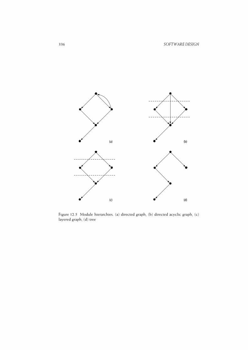
336 SOFTWARE DESIGN

Figure 12.5 Module hierarchies. (a) directed graph, (b) directed acyclic graph, (c)

layered graph, (d) tree

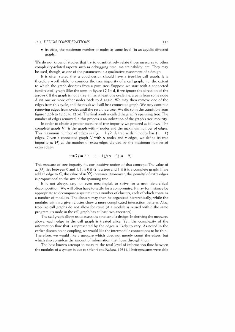
12.1. DESIGN CONSIDERATIONS 337� its width, the maximum number of nodes at some level (in an acyclic directed

graph).

We do not know of studies that try to quantitatively relate those measures to other

complexity-related aspects such as debugging time, maintainability, etc. They may

be used, though, as one of the parameters in a qualitative assessment of a design.

It is often stated that a good design should have a tree-like call graph. It is

therefore worthwhile to consider the tree impurity of a call graph, i.e. the extent

to which the graph deviates from a pure tree. Suppose we start with a connected

(undirected) graph (like the ones in figure 12.5b-d, if we ignore the direction of the

arrows). If the graph is not a tree, it has at least one cycle, i.e. a path from some node

A via one or more other nodes back to A again. We may then remove one of the

edges from this cycle, and the result will still be a connected graph. We may continue

removing edges from cycles until the result is a tree. We did so in the transition from

figure 12.5b to 12.5c to 12.5d. The final result is called the graph’s spanning tree. The

number of edges removed in this process is an indication of the graph’s tree impurity.

In order to obtain a proper measure of tree impurity we proceed as follows. The

complete graph Kn is the graph with n nodes and the maximum number of edges.

This maximum number of edges is n(n� 1)=2. A tree with n nodes has (n� 1)edges. Given a connected graph G with n nodes and e edges, we define its tree

impurity m(G) as the number of extra edges divided by the maximum number of

extra edges: m(G) = 2(e� n+ 1)=(n� 1)(n� 2)This measure of tree impurity fits our intuitive notion of that concept. The value ofm(G) lies between 0 and 1. It is 0 if G is a tree and 1 if it is a complete graph. If we

add an edge to G, the value of m(G) increases. Moreover, the ‘penalty’ of extra edges

is proportional to the size of the spanning tree.

It is not always easy, or even meaningful, to strive for a neat hierarchical

decomposition. We will often have to settle for a compromise. It may for instance be

appropriate to decompose a system into a number of clusters, each of which contains

a number of modules. The clusters may then be organized hierarchically, while the

modules within a given cluster show a more complicated interaction pattern. Also,

tree-like call graphs do not allow for reuse (if a module is reused within the same

program, its node in the call graph has at least two ancestors).

The call graph allows us to assess the structure of a design. In deriving the measures

above, each edge in the call graph is treated alike. Yet, the complexity of the

information flow that is represented by the edges is likely to vary. As noted in the

earlier discussion on coupling, we would like the intermodule connections to be ‘thin’.

Therefore, we would like a measure which does not merely count the edges, but

which also considers the amount of information that flows through them.

The best known attempt to measure the total level of information flow between

the modules of a system is due to (Henri and Kafura, 1981). Their measures were able

338 SOFTWARE DESIGN

to identify change-prone UNIX procedures and evaluate potential design changes.

(Shepperd, 1990) studied the information flow measure extensively and proposed

several refinements, thus obtaining a ‘purer’ metric. Using Shepperd’s definitions, the

information flow measure is based on the following notions of local and global data

flow:� A local flow from module A to module B exists if

(a) A invokes B and passes it a parameter, or

(b) B invokes A and A returns a value.� A global flow from module A to module B exists if A updates some global data

structure and B retrieves from that structure.

Using these notions of local and global data flow, Shepperd defines the ‘complexity’

of a module M as omplexity(M) = (fan-in(M)� fan-out(M))2where

– fan-in(M) is the number of (local and global) flows whose sink is M , and

– fan-out(M) is the number of (local and global) flows whose source is M .

A weak point of the information flow metric is that all flows have equal weight.

Passing one simple integer as parameter and invoking a complex global data structure

contribute equally to this measure of complexity. The abstract data type architectural

style easily results in modules with a high fan-in and fan-out. If the same system is

built using global data structures, its information flow metric is likely to have a smaller

value. Yet, the information flow both to and from the modules in the abstract data

type style generally concern simple scalar values only, and are therefore considered

simpler.

In a more qualitative sense, the information flow metric may indicate spots in the

design that deserve our attention. If some module has a high fan-in, this may indicate

that the module has little cohesion. Also, if we consider the information flow per

level in a layered architecture, an excessive increase from one level to the next might

indicate a missing level of abstraction.

During design, we (pre)tend to follow a top-down decomposition strategy. We

may also take a completely different stand and try to compose a hierarchical system

structure from a flat collection of system elements. Elements that are in some sense

‘closest’ to one another are grouped together. We then have to define some measure

for the distance between elements and a mathematical technique known as cluster

analysis can be used to do the actual grouping. Elements in the same group are more

like other elements within the same group and less like elements in other groups. If

the measure is based on the number of data types that elements have in common,

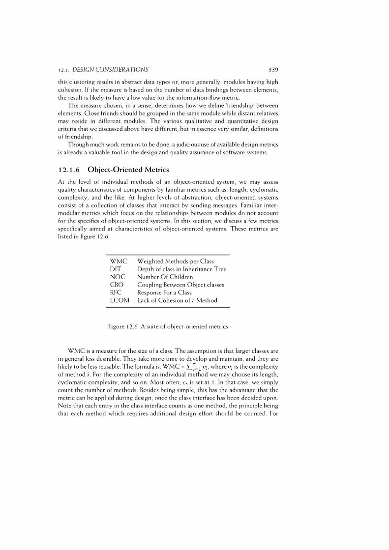
12.1. DESIGN CONSIDERATIONS 339

this clustering results in abstract data types or, more generally, modules having high

cohesion. If the measure is based on the number of data bindings between elements,

the result is likely to have a low value for the information-flow metric.

The measure chosen, in a sense, determines how we define ‘friendship’ between

elements. Close friends should be grouped in the same module while distant relatives

may reside in different modules. The various qualitative and quantitative design

criteria that we discussed above have different, but in essence very similar, definitions

of friendship.

Though much work remains to be done, a judicious use of available design metrics

is already a valuable tool in the design and quality assurance of software systems.

12.1.6 Object-Oriented Metrics

At the level of individual methods of an object-oriented system, we may assess

quality characteristics of components by familiar metrics such as: length, cyclomatic

complexity, and the like. At higher levels of abstraction, object-oriented systems

consist of a collection of classes that interact by sending messages. Familiar inter-

modular metrics which focus on the relationships between modules do not account

for the specifics of object-oriented systems. In this section, we discuss a few metrics

specifically aimed at characteristics of object-oriented systems. These metrics are

listed in figure 12.6.

WMC Weighted Methods per Class

DIT Depth of class in Inheritance Tree

NOC Number Of Children

CBO Coupling Between Object classes

RFC Response For a Class

LCOM Lack of Cohesion of a Method

Figure 12.6 A suite of object-oriented metrics

WMC is a measure for the size of a class. The assumption is that larger classes are

in general less desirable. They take more time to develop and maintain, and they are

likely to be less reusable. The formula is: WMC =Pni=1 i, where i is the complexity

of method i. For the complexity of an individual method we may choose its length,

cyclomatic complexity, and so on. Most often, i is set at 1. In that case, we simply

count the number of methods. Besides being simple, this has the advantage that the

metric can be applied during design, once the class interface has been decided upon.

Note that each entry in the class interface counts as one method, the principle being

that each method which requires additional design effort should be counted. For

340 SOFTWARE DESIGN

example, different constructors for one and the same operation, as is customary in

C++, count as different methods.

Classes in an object-oriented design are related through a subtype--supertype

hierarchy. If the class hierarchy is deep and narrow, a proper understanding of a

class may require knowledge of many of its superclasses. On the other hand, a wide

and shallow inheritance structure occurs when classes are more loosely coupled. The

latter situation may indicate that commonality between elements is not sufficiently

exploited. DIT is the distance of a class to the root of its inheritance tree. Note that

the value of DIT is somewhat language-dependent. In Smalltalk, for example, every

class is a subclass of Object, and this increases the value of DIT. A widely accepted

heuristic is to strive for a forest of classes, i.e. a collection of inheritance trees of

medium height.

NOC counts the number of immediate descendants of a class. If a class has a large

number of descendants, this may indicate an improper abstraction of the parent class.

A large number of descendants also suggests that the class is to be used in a variety

of settings, which will make it more error-prone. The idea thus is that higher values

of NOC suggest a higher complexity of the class.

CBO is the main coupling metric for object-oriented systems. Two classes are

coupled if a method of one class uses a method or state variable of the other class.

The CBO is a count of the number of other classes with which it is coupled. As with

the traditional coupling metric, high values of CBO suggest tight bindings with other

components, and this is undesirable.

In the definition of CBO, all couplings are considered equal. However, if we look

at the different ways in which classes may be coupled, it is reasonable to say that:

– access to state variables is worse than mere parameter passing;

– access to elements of a foreign class is worse than access to elements of a

superclass;

– passing many complex parameters is worse than passing a few simple parameters;

– messages that conform to Demeter’s Law4 are better than those which don’t.

If we view the methods as bubbles, and the couplings as connections between

bubbles, CBO simply counts the number of connections for each bubble. In reality,

we consider some types of couplings worse than others: some connections are ‘thicker’

than others, and some connections are to bubbles ‘further away’. For the representation

4The Law of Demeter is a generally-accepted design heuristic for object-oriented systems. It says that

the methods of a class should only depend on the top-level structure of their own class. More specifically,

in the context of a class C with method M, M should only send messages to:

– the parameters of C, or

– the state variables of C, or

– C itself.

12.1. DESIGN CONSIDERATIONS 341

condition of measurement theory to hold, these empirical relations should be reflected

in the numerical relation system.

Martin (2002) defines coupling measures at the package level:� The afferent coupling (Ca) of a package P is the number of other packages

that depend upon classes within P (through inheritance or associations). It

indicates the dependence of a package on its environment.� The efferent coupling (Ce) of a package P is the number of packages that

classes within P depend upon. It indicates the dependence of the environment

on a package.

Adding these numbers together results in a total coupling measure of a package P .

The ratio I = Ce=(Ce + Ca) indicates the relative dependence of the environment

to P with respect to the total number of dependencies between P and its environment.

If Ce equals zero, P does not depend at all on other packages. Then, I = 0 as well.

If on the other hand Ca equals zero, P only depends on other packages, and no

other package depends on P . In that case, I = 1. I thus can be seen as an instability

measure for P . Larger values of I denote a larger instability of the package.

RFC measures the ‘immediate surroundings’ of a class. Suppose a class C has a

collection of methodsM . Each method fromM may in turn call other methods, fromC or any other class. Let fRig be the set of methods called from method Mi. Then

the response set of this class is defined as: fMg [i fRig, i.e. the set of messages that

may potentially be executed if a message is sent to an object of classC. RFC is defined

as the number of elements in the response set. Note that we only count method calls

up to one level deep. Larger values of RFC means that the immediate surroundings of

a class is larger in size. There is, then, a lot of communication with other methods

or classes. This makes comprehension of a class more difficult and increases test time

and complexity.

The final object-oriented metric to be discussed is the lack of cohesion of a

method. The traditional levels of cohesion express the degree of mutual affinity of the

components of a module. It is a measure of the glue that keeps the module together.

If all methods of a class use the same state variables, these state variables serve as

the glue which ties the methods together. If some methods use a subset of the state

variables, while other methods use another subset of the state variables, the class lacks

cohesion. This may indicate a flaw in the design, and it may be better to split it into

two or more subclasses. LCOM is the number of disjoint sets of methods of a class.

Any two methods in the same set share at least one local state variable. The preferred

value for LCOM is 0.

There are obviously many more metrics that aim to address the specifics of

object-oriented systems. Most of these have not been validated extensively, though.

Several experiments have shown that the above set does have some merit. Overall,

WMC, CBO, RFC and LCOM have been found to be the more useful quality

indicators. These metrics for example were able to predict fault-proneness of classes

342 SOFTWARE DESIGN

during design, and were found to have a strong relationship with maintenance effort.

The merits of DIT and NCO remain somewhat unclear.

Note that many of these metrics are correlated with class size. One may expect

that larger classes have more methods, have more descendants, have more couplings

with other classes, etc. El Emam et al. (2001) indeed found that class size has a

confounding effect on the values of the above metrics. It thus remains questionable

whether these metrics tell more than a plain LOC count.

12.2 Classical Design Methods

Having discussed the properties of a good system decomposition, we now come to

a question which is at least as important: how do you get a good decomposition to

start with?

There exist a vast number of design methods, a sample of which is given in

table 12.3. These design methods generally consist of a set of guidelines, heuristics,

and procedures on how to go about designing a system. They also offer a notation to

express the result of the design process. Together these provide a systematic means for

organizing and structuring the design process and its products.

12.2. CLASSICAL DESIGN METHODS 343

continued on next page

Table 12.3 A sample of design methods

Decision tables Matrix representation of complex decision logic at the detailed

design level.

E--R Entity--Relationship Model. Family of graphical techniques for

expressing data-relationships; see also chapter 10.

Flowcharts Simple diagram technique to show control flow at the detailed

design level. Exists in many flavors; see (Tripp, 1988) for an

overview.

FSM Finite State Machine. A way to describe a system as a set of

states and possible transitions between those states; the resulting

diagrams are called state transition diagrams; see also chapter 10.

JSD Jackson System Development; see section 12.2.3. Successor to,

and more elaborate than, JSP; has an object-oriented flavor.

JSP Jackson Structured Programming. Data-structure-oriented

method; see section 12.2.3.

LCP Logical Construction of Programs, also known as the Warnier--

Orr method; data-structure-oriented, similar to JSP.

NoteCards Example hypertext system. Hypertext systems make it possible

to create and navigate through a complex organization of

unstructured pieces of text (Conklin, 1987).

OBJ Algebraic specification method; highly mathematical (Goguen,

1986).

OOD Object-oriented design; exists in many flavors; see section 12.3.

PDL Program Design Language; example of a constrained natural

language (‘structured English’) to describe designs at various

levels of abstraction. Offers the control constructs generally

found in programming languages. See (Pintelas and Kallistros,

1989) for an overview.

344 SOFTWARE DESIGN

Petri nets Graphical design representation, well-suited for concurrent sys-

tems. A system is described as a set of states and possible

transitions between those states. States are associated with

tokens and transitions are described by firing rules. In this way,

concurrent activities can be synchronized (Peterson, 1981).

SA/SD Structured Analysis/Structured Design. Data flow design tech-

nique; see also section 12.2.2.

SA/RT Extension to Structured Analysis so that real-time aspects can

be described (Hatley and Pirbhai, 1988).

SSADM Structured Systems Analysis and Design Method. A highly

prescriptive method for performing the analysis and design

stages; UK standard (Downs et al., 1992).

For some methods, such as FSM or Petri nets, emphasis is on the notation, while the

guidelines on how to tackle design are not very well developed. Methods like JSD,

on the other hand, offer extensive prescriptive guidelines as well. Most notations are

graphical and somewhat informal, but OBJ uses a very formal mathematical language.

Some methods concentrate on the design stage proper, while others are part of a

wider methodology covering other life cycle phases as well. Examples of the latter

are SSADM and JSD. Finally, some methods offer features that make them especially

useful for the design of certain types of application, such as SA/RT (real-time systems)

or Petri nets (concurrent systems).

In the following subsections we discuss three classical design methods:� Functional decomposition, which is a rather general approach to system

design. It is not tied to any specific method listed in table 12.3. Many different

notations can be used to depict the resulting design, ranging from flowcharts

or pseudocode to algebraic specifications.� Data flow design, as exemplified by SA/SD.� Design based on data structures, as is done in JSP, LCP and JSD.

A fourth design method, object-oriented design, is discussed in section 12.3. Whereas

the above three methods concentrate on identifying the functions of the system, object-

oriented design focuses on the data on which the system is to operate. Object-oriented

design is the most popular design approach today, not the least because of the

omnipresence of UML as a notational device for the outcome of both requirements

engineering and design.

12.2.1 Functional Decomposition

In a functional decomposition the intended function is decomposed into a number

of subfunctions that each solve part of the problem. These subfunctions themselves

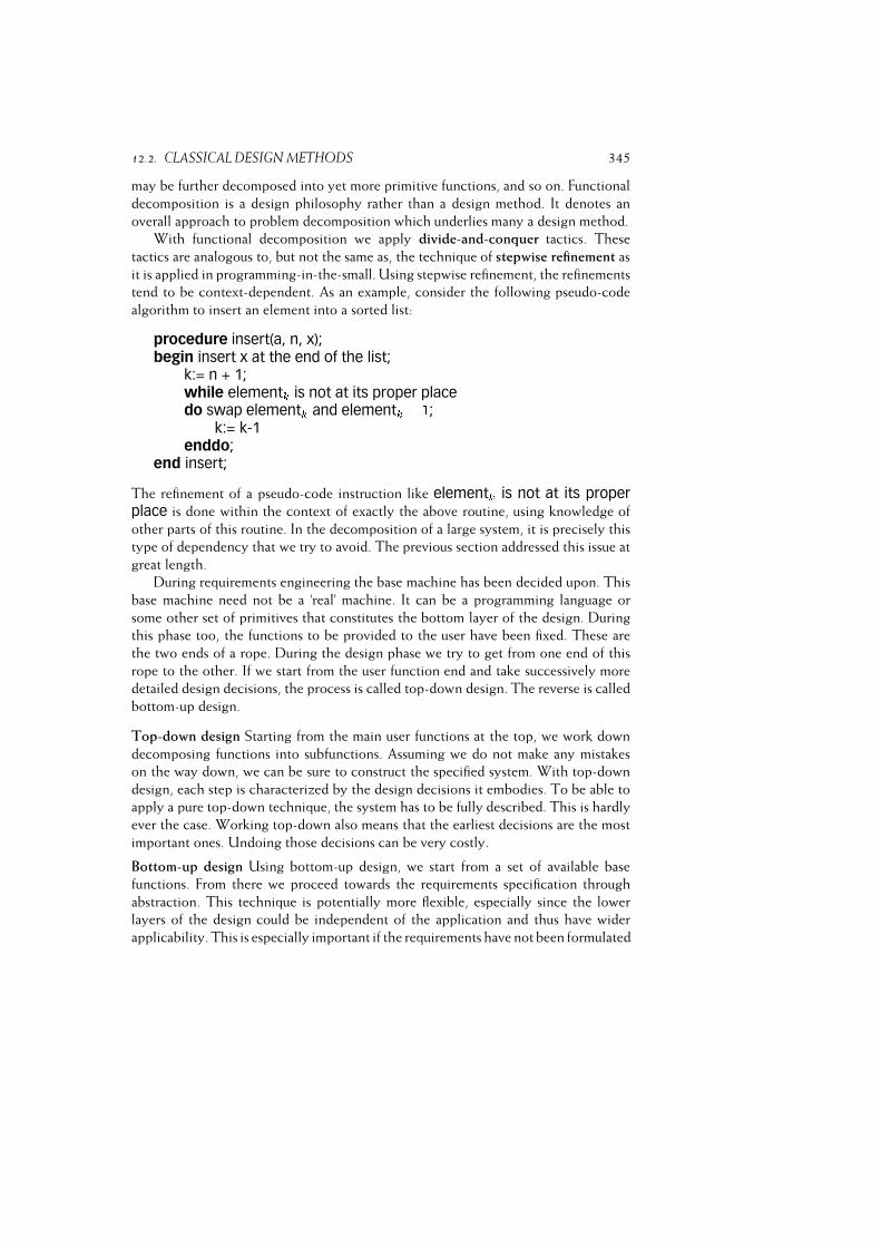
12.2. CLASSICAL DESIGN METHODS 345

may be further decomposed into yet more primitive functions, and so on. Functional

decomposition is a design philosophy rather than a design method. It denotes an

overall approach to problem decomposition which underlies many a design method.

With functional decomposition we apply divide-and-conquer tactics. These

tactics are analogous to, but not the same as, the technique of stepwise refinement as

it is applied in programming-in-the-small. Using stepwise refinement, the refinements

tend to be context-dependent. As an example, consider the following pseudo-code

algorithm to insert an element into a sorted list:

procedure insert(a, n, x);begin insert x at the end of the list;

k:= n + 1;while elementk is not at its proper placedo swap elementk and elementk � 1;

k:= k-1enddo;

end insert;

The refinement of a pseudo-code instruction like elementk is not at its properplace is done within the context of exactly the above routine, using knowledge of

other parts of this routine. In the decomposition of a large system, it is precisely this

type of dependency that we try to avoid. The previous section addressed this issue at

great length.

During requirements engineering the base machine has been decided upon. This

base machine need not be a ‘real’ machine. It can be a programming language or

some other set of primitives that constitutes the bottom layer of the design. During

this phase too, the functions to be provided to the user have been fixed. These are

the two ends of a rope. During the design phase we try to get from one end of this

rope to the other. If we start from the user function end and take successively more

detailed design decisions, the process is called top-down design. The reverse is called

bottom-up design.

Top-down design Starting from the main user functions at the top, we work down

decomposing functions into subfunctions. Assuming we do not make any mistakes

on the way down, we can be sure to construct the specified system. With top-down

design, each step is characterized by the design decisions it embodies. To be able to

apply a pure top-down technique, the system has to be fully described. This is hardly

ever the case. Working top-down also means that the earliest decisions are the most

important ones. Undoing those decisions can be very costly.

Bottom-up design Using bottom-up design, we start from a set of available base

functions. From there we proceed towards the requirements specification through

abstraction. This technique is potentially more flexible, especially since the lower

layers of the design could be independent of the application and thus have wider

applicability. This is especially important if the requirements have not been formulated

346 SOFTWARE DESIGN

very precisely yet, or if a family of systems has to be developed. A real danger of the

bottom-up technique is that we may miss the target.

In its pure form, neither the top-down nor the bottom-up technique is likely to be

used all that often. Both techniques are feasible only if the design process is a pure

and rational one. And this is an idealization of reality. There are many reasons why

the design process cannot be rational. Some of these have to do with the intangibles

of design processes per se, some originate from accidents that happen to befall many

a software project. Parnas and Clements (1986) list the following reasons, amongst

others:

– Mostly, users do not know exactly what they want and they are not able to tell

all they know.

– Even if the requirements are fully known, a lot of additional information is

needed. This information is discovered only when the project is under way.

– Almost all projects are subject to change. Changes influence earlier decisions.

– People make errors.

– During design, people use the knowledge they already have, experiences from

earlier projects, and the like.

– In many projects we do not start from scratch, but we build from existing

software.

Design exhibits a ‘yo-yo’ character: something is devised, tried, rejected again, new

ideas crop up, etc. Designers frequently go about in rather opportunistic ways. They

frequently switch from high-level application domain issues to coding and detailed

design matters, and use a variety of means to gather insight into the problem to be

solved. At most, we may present the result of the design process as if it came about

through a rational process.

A general problem with any form of functional decomposition is that it is often

not immediately clear along which dimension the system is decomposed. If we

decompose along the time-axis, the result is often a main program that controls the

order in which a number of subordinate modules is called. In Yourdon’s classification,

the resulting cohesion type is temporal. If we decompose with respect to the grouping

of data, we obtain the type of data cohesion exhibited in abstract data types. Both

these functional decompositions can be viewed as an instance of some architectural

style. Rather than worrying about which dimension to focus on during functional

decomposition, you had better opt for a particular architectural style and let that style

guide the decomposition.

At some intermediate level, the set of interrelated components comprises the

software architecture as discussed in chapter 11. This software architecture is a

product which serves various purposes: it can be used to discuss the design with

12.2. CLASSICAL DESIGN METHODS 347

different stakeholders; it can be used to evaluate the quality of the design; it can

be the basis for the work breakdown structure; it can be used to guide the testing

process, etc. If a software architecture is required, it necessitates a design approach in

which, at quite an early stage, each and every component and connection is present.

A bottom-up or top-down approach does not meet this requirement, since in both

these approaches only part of the solution is available at intermediate points in time.

Parnas (1978) offers the following useful guidelines for a sound functional

decomposition:

1. Try to identify subsystems. Start with a minimal subset and define minimal

extensions to this subset.

The idea behind this guideline is that it is extremely difficult, if not impossible,

to get a complete picture of the system during requirements engineering. People

ask too much or they ask the wrong things. Starting from a minimal subsystem,

we may add functionality incrementally, using the experience gained with the

actual use of the system. The idea is very similar to that of agile approaches,

discussed in chapter 3.

2. Apply the information hiding principle.

3. Try to define extensions to the base machine step by step. This holds for

both the minimal machine and its extensions. Such incremental extensions

lead to the concept of a virtual machine. Each layer in the system hierarchy

can be viewed as a machine. The primitive operations of this machine are

implemented by the lower layers of the hierarchy. This machine view of the

module hierarchy nicely maps onto a layered architectural style. It also adds a

further dimension to the system structuring guidelines offered in section 12.1.5.

4. Apply the uses-relation and try to place the dependencies thus obtained in a

hierarchical structure.

Obviously, the above guidelines are strongly interrelated. It has been said before

that a strictly hierarchical tree structure of system components is often not feasible.

A compromise that often is feasible is a layered system structure as depicted in

figure 12.7.

The arrows between the various nodes in the graph indicate the uses-relation.

Various levels can be distinguished in the structure depicted. Components at a given

level only use components from the same, or lower, levels. The layers distinguished

in this picture are not the same as those induced by the acyclicity of the graph

(as discussed in section 12.1.5) but are rather the result of viewing a distinct set of

modules as an abstract, virtual machine. Deciding how to group modules into layers

in this way involves considering the semantics of those modules. Lower levels in this

hierarchy bring us closer to the ‘real’ machine on which the system is going to be

executed. Higher levels are more application-oriented. The choice of the number of

levels in such an architecture is a, problem-dependent, design decision.

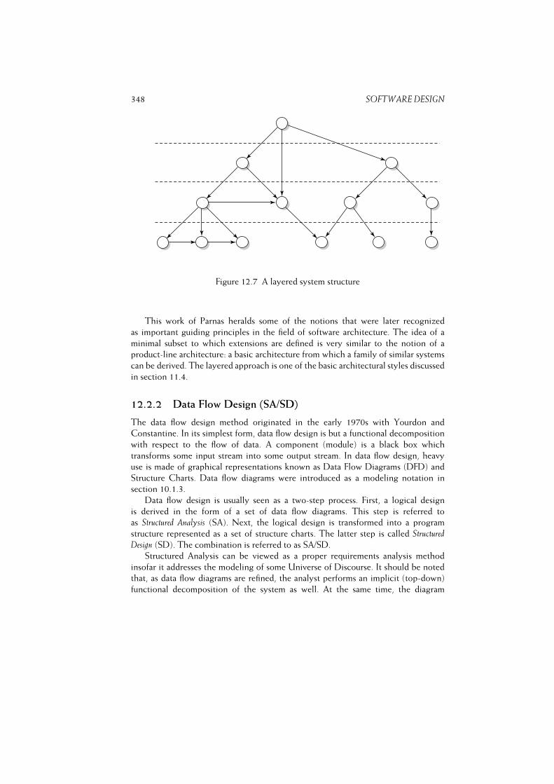
348 SOFTWARE DESIGN

Figure 12.7 A layered system structure

This work of Parnas heralds some of the notions that were later recognized

as important guiding principles in the field of software architecture. The idea of a

minimal subset to which extensions are defined is very similar to the notion of a

product-line architecture: a basic architecture from which a family of similar systems

can be derived. The layered approach is one of the basic architectural styles discussed

in section 11.4.

12.2.2 Data Flow Design (SA/SD)

The data flow design method originated in the early 1970s with Yourdon and

Constantine. In its simplest form, data flow design is but a functional decomposition

with respect to the flow of data. A component (module) is a black box which

transforms some input stream into some output stream. In data flow design, heavy

use is made of graphical representations known as Data Flow Diagrams (DFD) and

Structure Charts. Data flow diagrams were introduced as a modeling notation in

section 10.1.3.

Data flow design is usually seen as a two-step process. First, a logical design

is derived in the form of a set of data flow diagrams. This step is referred to

as Structured Analysis (SA). Next, the logical design is transformed into a program

structure represented as a set of structure charts. The latter step is called Structured

Design (SD). The combination is referred to as SA/SD.

Structured Analysis can be viewed as a proper requirements analysis method

insofar it addresses the modeling of some Universe of Discourse. It should be noted

that, as data flow diagrams are refined, the analyst performs an implicit (top-down)

functional decomposition of the system as well. At the same time, the diagram

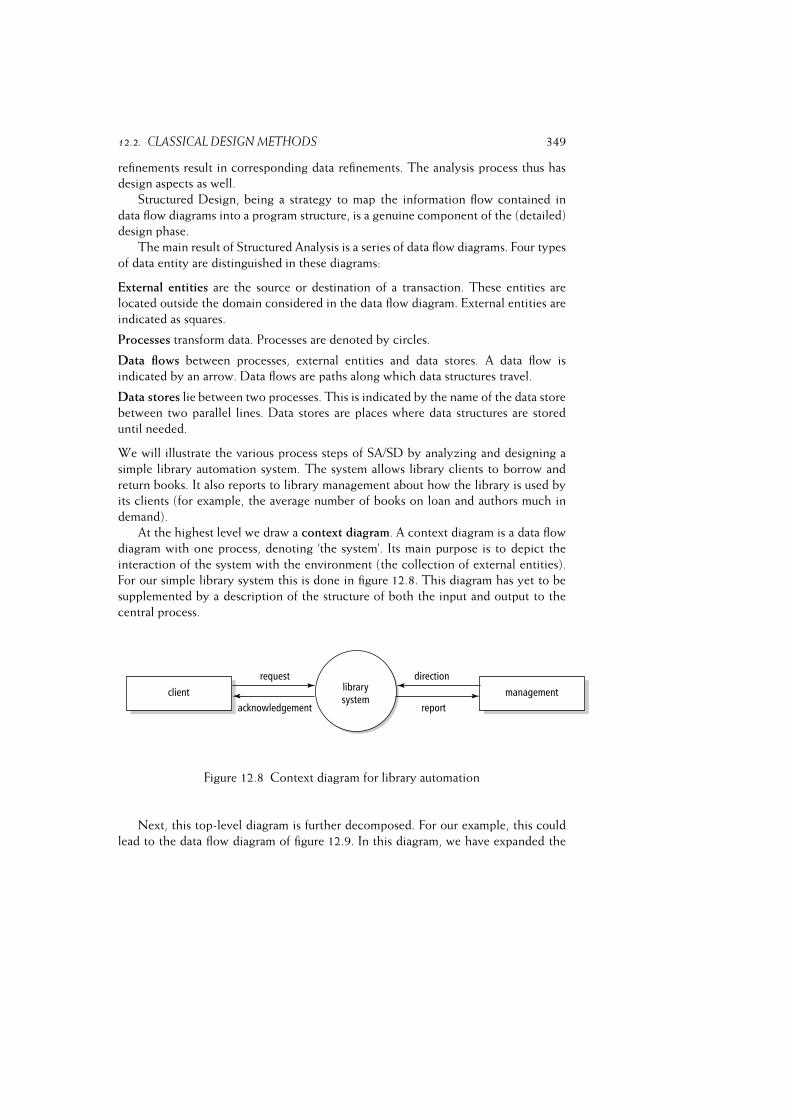
12.2. CLASSICAL DESIGN METHODS 349

refinements result in corresponding data refinements. The analysis process thus has

design aspects as well.

Structured Design, being a strategy to map the information flow contained in

data flow diagrams into a program structure, is a genuine component of the (detailed)

design phase.

The main result of Structured Analysis is a series of data flow diagrams. Four types

of data entity are distinguished in these diagrams:

External entities are the source or destination of a transaction. These entities are

located outside the domain considered in the data flow diagram. External entities are

indicated as squares.

Processes transform data. Processes are denoted by circles.

Data flows between processes, external entities and data stores. A data flow is

indicated by an arrow. Data flows are paths along which data structures travel.

Data stores lie between two processes. This is indicated by the name of the data store

between two parallel lines. Data stores are places where data structures are stored

until needed.

We will illustrate the various process steps of SA/SD by analyzing and designing a

simple library automation system. The system allows library clients to borrow and

return books. It also reports to library management about how the library is used by

its clients (for example, the average number of books on loan and authors much in

demand).

At the highest level we draw a context diagram. A context diagram is a data flow

diagram with one process, denoting ‘the system’. Its main purpose is to depict the

interaction of the system with the environment (the collection of external entities).

For our simple library system this is done in figure 12.8. This diagram has yet to be

supplemented by a description of the structure of both the input and output to the

central process.

Figure 12.8 Context diagram for library automation

Next, this top-level diagram is further decomposed. For our example, this could

lead to the data flow diagram of figure 12.9. In this diagram, we have expanded the

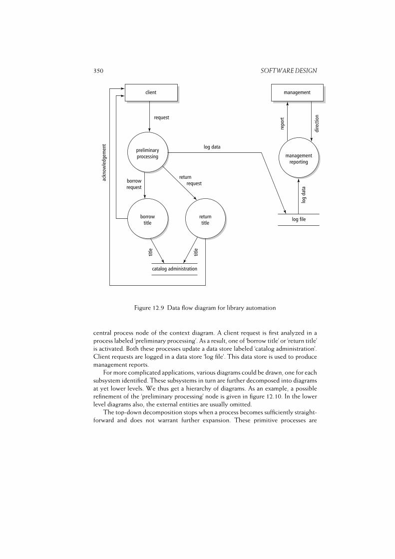
350 SOFTWARE DESIGN

Figure 12.9 Data flow diagram for library automation

central process node of the context diagram. A client request is first analyzed in a

process labeled ‘preliminary processing’. As a result, one of ‘borrow title’ or ‘return title’

is activated. Both these processes update a data store labeled ‘catalog administration’.

Client requests are logged in a data store ‘log file’. This data store is used to produce

management reports.

For more complicated applications, various diagrams could be drawn, one for each

subsystem identified. These subsystems in turn are further decomposed into diagrams

at yet lower levels. We thus get a hierarchy of diagrams. As an example, a possible

refinement of the ‘preliminary processing’ node is given in figure 12.10. In the lower

level diagrams also, the external entities are usually omitted.

The top-down decomposition stops when a process becomes sufficiently straight-

forward and does not warrant further expansion. These primitive processes are

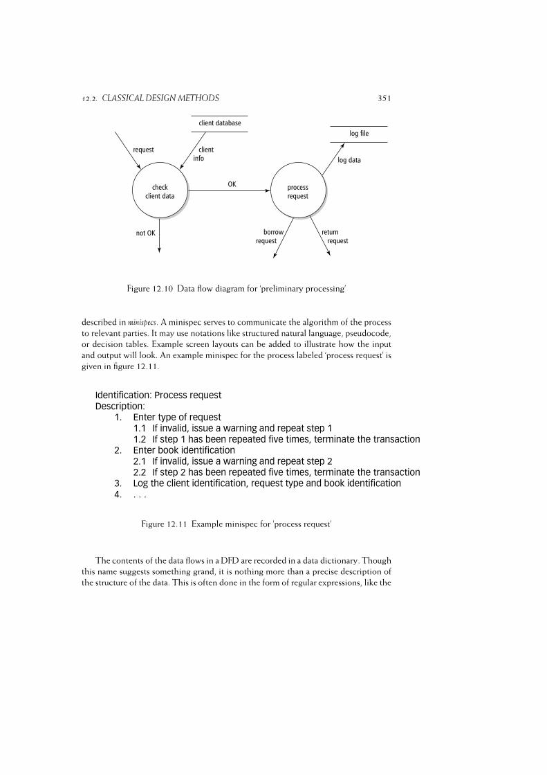
12.2. CLASSICAL DESIGN METHODS 351

Figure 12.10 Data flow diagram for ‘preliminary processing’

described in minispecs. A minispec serves to communicate the algorithm of the process

to relevant parties. It may use notations like structured natural language, pseudocode,

or decision tables. Example screen layouts can be added to illustrate how the input

and output will look. An example minispec for the process labeled ‘process request’ is

given in figure 12.11.

Identification: Process requestDescription:

1. Enter type of request1.1 If invalid, issue a warning and repeat step 11.2 If step 1 has been repeated five times, terminate the transaction

2. Enter book identification2.1 If invalid, issue a warning and repeat step 22.2 If step 2 has been repeated five times, terminate the transaction

3. Log the client identification, request type and book identification4. . . .

Figure 12.11 Example minispec for ’process request’

The contents of the data flows in a DFD are recorded in a data dictionary. Though

this name suggests something grand, it is nothing more than a precise description of

the structure of the data. This is often done in the form of regular expressions, like the

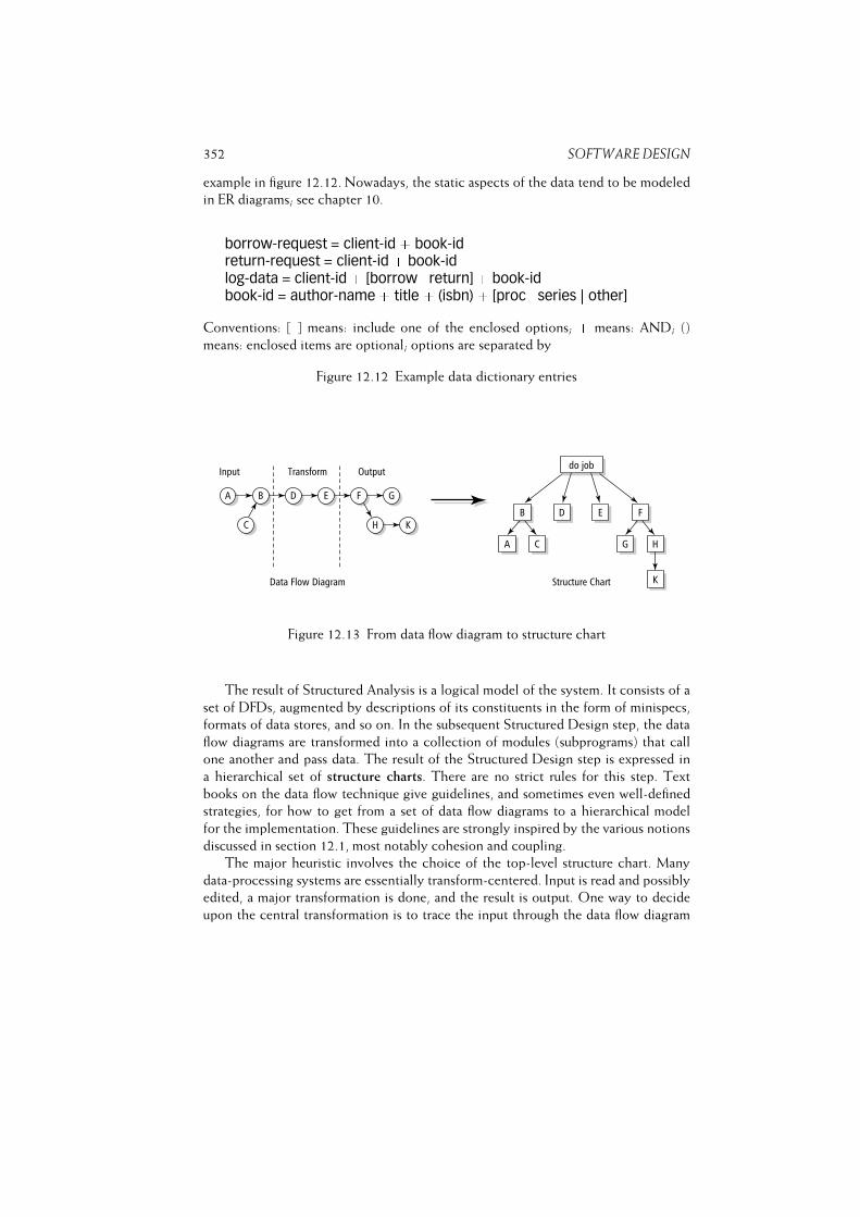
352 SOFTWARE DESIGN

example in figure 12.12. Nowadays, the static aspects of the data tend to be modeled

in ER diagrams; see chapter 10.

borrow-request = client-id + book-idreturn-request = client-id + book-idlog-data = client-id + [borrow j return] + book-idbook-id = author-name + title + (isbn) + [proc j series j other]

Conventions: [ ] means: include one of the enclosed options; + means: AND; ()

means: enclosed items are optional; options are separated by jFigure 12.12 Example data dictionary entries

Figure 12.13 From data flow diagram to structure chart

The result of Structured Analysis is a logical model of the system. It consists of a

set of DFDs, augmented by descriptions of its constituents in the form of minispecs,

formats of data stores, and so on. In the subsequent Structured Design step, the data

flow diagrams are transformed into a collection of modules (subprograms) that call

one another and pass data. The result of the Structured Design step is expressed in

a hierarchical set of structure charts. There are no strict rules for this step. Text

books on the data flow technique give guidelines, and sometimes even well-defined

strategies, for how to get from a set of data flow diagrams to a hierarchical model

for the implementation. These guidelines are strongly inspired by the various notions

discussed in section 12.1, most notably cohesion and coupling.

The major heuristic involves the choice of the top-level structure chart. Many

data-processing systems are essentially transform-centered. Input is read and possibly

edited, a major transformation is done, and the result is output. One way to decide

upon the central transformation is to trace the input through the data flow diagram

12.2. CLASSICAL DESIGN METHODS 353

until it can no longer be considered input. The same is done, in the other direction,

for the output. The bubble in between acts as the central transform. If we view the

bubbles in a DFD as beads, and the data flows as threads, we obtain the corresponding

structure chart by picking the bead that corresponds to the central transformation

and shaking the DFD.5 The processes in the data flow diagram become the modules

of the corresponding structure chart and the data flows become module calls. Note

that the arrows in a structure chart denote module calls, whereas the arrows in a data

flow diagram denote flows of data. These arrows often point in opposite directions;

a flow of data from A to B is often realized through a call of B to A. Sometimes it

is difficult to select one central transformation. In that case, a dummy root element

is added and the resulting Input--Process--Output scheme is of the form depicted in

figure 12.13.

Because of the transformation orientation of the structure chart, the relations

between modules in the graph have a producer--consumer character. One module

produces a stream of data which is then consumed by another module. The control

flow is one whereby modules call subordinate modules so as to realize the required

transformation. There is a potentially complex stream of information between

modules, corresponding to the data flow that is passed between producer and

consumer. The major contribution of Structured Design is found in the guidelines

that aim to reduce the complexity of the interaction between modules. These

guidelines concern the cohesion and coupling criteria discussed in section 12.1.

12.2.3 Design based on Data Structures

The best-known technique for design based on data structures originates with Michael

Jackson. The technique is known as Jackson Structured Programming (JSP). Essentials

of JSP have been carried over to Jackson System Development (JSD). JSP is a technique

for programming-in-the-small and JSD is a technique for programming-in-the-large.

We will discuss both techniques in turn.

The basic idea of JSP is that a good program reflects the structure of both the

input and the output in all its facets. Given a correct model of these data structures, we

may straightforwardly derive the corresponding program from the model. It is often

postulated that the structure of the data is much less volatile than the transformations

applied to the data. As a consequence, designs that take the data as their starting

point should be ‘better’ too. This same argument is also used in the context of

object-oriented analysis and design.

JSP distinguishes elementary and compound components. Elementary compo-

nents are not further decomposed. There are three types of compound component:

sequence, iteration and selection. Compound components are represented by dia-

grams (also called Jackson diagrams or structure diagrams) or some sort of pseudocode

(called structure text or schematic logic). The base forms of both are given in

5We do the same when turning a free tree into an oriented tree. A free tree has no root. By selecting

one node of the tree as the root, the parent--child relations are brought about.

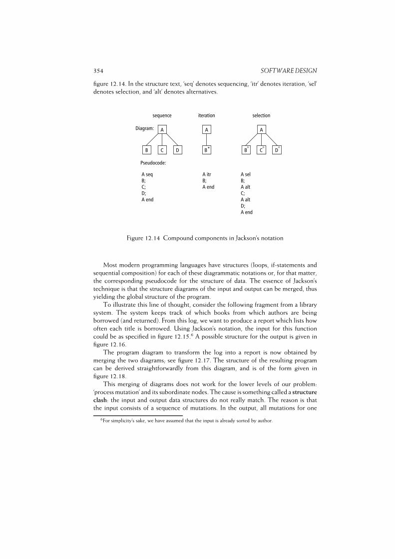
354 SOFTWARE DESIGN

figure 12.14. In the structure text, ‘seq’ denotes sequencing, ‘itr’ denotes iteration, ‘sel’

denotes selection, and ‘alt’ denotes alternatives.

Figure 12.14 Compound components in Jackson’s notation

Most modern programming languages have structures (loops, if-statements and

sequential composition) for each of these diagrammatic notations or, for that matter,

the corresponding pseudocode for the structure of data. The essence of Jackson’s

technique is that the structure diagrams of the input and output can be merged, thus

yielding the global structure of the program.

To illustrate this line of thought, consider the following fragment from a library

system. The system keeps track of which books from which authors are being

borrowed (and returned). From this log, we want to produce a report which lists how

often each title is borrowed. Using Jackson’s notation, the input for this function

could be as specified in figure 12.15.6 A possible structure for the output is given in

figure 12.16.

The program diagram to transform the log into a report is now obtained by

merging the two diagrams; see figure 12.17. The structure of the resulting program

can be derived straightforwardly from this diagram, and is of the form given in

figure 12.18.

This merging of diagrams does not work for the lower levels of our problem:

‘process mutation’ and its subordinate nodes. The cause is something called a structure

clash: the input and output data structures do not really match. The reason is that

the input consists of a sequence of mutations. In the output, all mutations for one

6For simplicity’s sake, we have assumed that the input is already sorted by author.

12.2. CLASSICAL DESIGN METHODS 355

Figure 12.15 Log of books borrowed and returned, in JSP notation

given book are taken together. So, the mutations have to be sorted first. We have to

restructure the system, for instance as depicted in figure 12.19.

A clear disadvantage of the structure thus obtained is that there is now an

intermediate file. Closer inspection shows that we do not really need this file. This is

immediately clear if we depict the structure as in figure 12.20.

Here, we may invert component A1 and code it such that it serves as a replacement

of component B2. Alternatively (and in this case more likely), we may invert B1

and substitute the result for component A2. In either case, the first-in-first-out type

of intermediate file between the two components is removed by making one of the

components a subordinate of the other.

This example shows the fundamental issues involved in the use of JSP:

1. Modeling input and output using structure diagrams,

2. Merging the diagrams to create the program structure, meanwhile

3. Resolving possible structure clashes, and finally

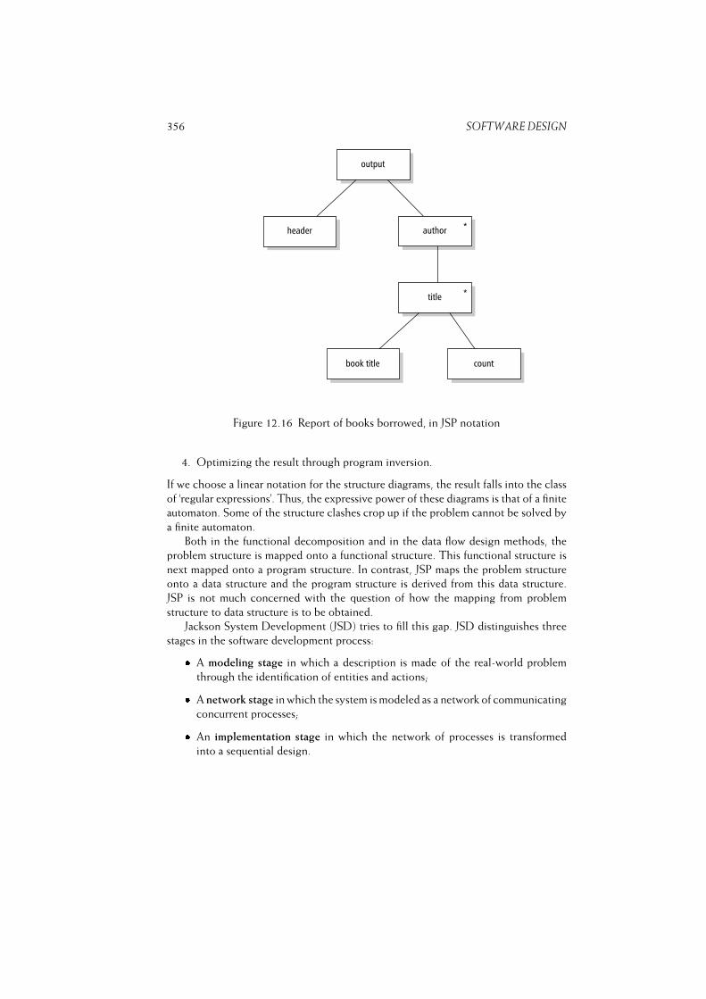
356 SOFTWARE DESIGN

Figure 12.16 Report of books borrowed, in JSP notation

4. Optimizing the result through program inversion.

If we choose a linear notation for the structure diagrams, the result falls into the class

of ‘regular expressions’. Thus, the expressive power of these diagrams is that of a finite

automaton. Some of the structure clashes crop up if the problem cannot be solved by

a finite automaton.

Both in the functional decomposition and in the data flow design methods, the

problem structure is mapped onto a functional structure. This functional structure is

next mapped onto a program structure. In contrast, JSP maps the problem structure

onto a data structure and the program structure is derived from this data structure.

JSP is not much concerned with the question of how the mapping from problem

structure to data structure is to be obtained.

Jackson System Development (JSD) tries to fill this gap. JSD distinguishes three

stages in the software development process:� A modeling stage in which a description is made of the real-world problem

through the identification of entities and actions;� A network stage in which the system is modeled as a network of communicating

concurrent processes;� An implementation stage in which the network of processes is transformed

into a sequential design.

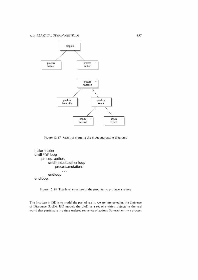
12.2. CLASSICAL DESIGN METHODS 357

Figure 12.17 Result of merging the input and output diagrams

make headeruntil EOF loop

process author:until end of author loop

process mutation:. . .

endloopendloop.

Figure 12.18 Top-level structure of the program to produce a report

The first step in JSD is to model the part of reality we are interested in, the Universe

of Discourse (UoD). JSD models the UoD as a set of entities, objects in the real

world that participate in a time-ordered sequence of actions. For each entity a process

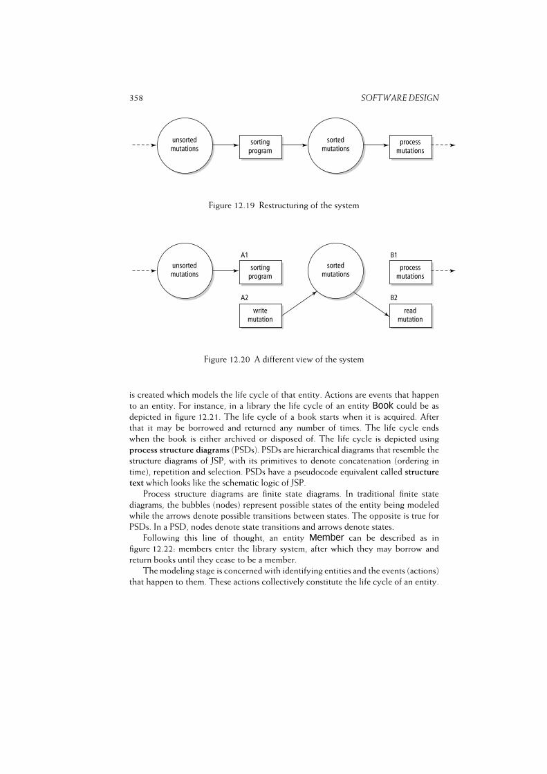
358 SOFTWARE DESIGN

Figure 12.19 Restructuring of the system

Figure 12.20 A different view of the system

is created which models the life cycle of that entity. Actions are events that happen

to an entity. For instance, in a library the life cycle of an entity Book could be as

depicted in figure 12.21. The life cycle of a book starts when it is acquired. After

that it may be borrowed and returned any number of times. The life cycle ends

when the book is either archived or disposed of. The life cycle is depicted using

process structure diagrams (PSDs). PSDs are hierarchical diagrams that resemble the

structure diagrams of JSP, with its primitives to denote concatenation (ordering in

time), repetition and selection. PSDs have a pseudocode equivalent called structure

text which looks like the schematic logic of JSP.

Process structure diagrams are finite state diagrams. In traditional finite state

diagrams, the bubbles (nodes) represent possible states of the entity being modeled

while the arrows denote possible transitions between states. The opposite is true for

PSDs. In a PSD, nodes denote state transitions and arrows denote states.

Following this line of thought, an entity Member can be described as in

figure 12.22: members enter the library system, after which they may borrow and

return books until they cease to be a member.

The modeling stage is concerned with identifying entities and the events (actions)

that happen to them. These actions collectively constitute the life cycle of an entity.

12.2. CLASSICAL DESIGN METHODS 359

Figure 12.21 Process structure diagram for the entity Book

As with other design methods, there is no simple recipe to determine the set of

entities and actions. The approach generally taken has a linguistic stance. From notes,

documentation, interviews and the like, we may draw up a preliminary list of actions

and entities. One heuristic is to look for real-world objects with which the system is to

interact. Since a library is all about books, an entity Book immediately suggests itself.

From statements like ‘members borrow books’ we may infer that an event Borrowoccurs in the life cycle of both books and members. Once such a preliminary list is

made up, further reflection should lead to a precisely demarcated life cycle of the

entities identified.

Entities are made up of actions. These actions are atomic, i.e. they cannot be

further decomposed into subactions. Actions respond to events in the real world. The

action Acquire that is part of the life cycle of the entity Book is triggered when a

real-world event, the actual acquisition of a book, takes place. In the process structure

diagram, actions show up as leaf nodes.

Events are communicated to the system through data messages, called attributes.

In a procedural sense these attributes constitute the parameters of the action. For the

action Acquire we may have such attributes as ISBN, date-of-acquisition, title and

authors.

Entities have attributes as well: local variables that keep information from the

past and collectively determine its state. The entity Book for example may retain

some or all of the information that was provided upon acquisition (ISBN, title, etc).

360 SOFTWARE DESIGN

Figure 12.22 Process structure diagram for the entity Member

Entities also have two special attributes. First, the identifier attribute uniquely identifies

the entity. Second, each entity has an attribute that indicates its status. This attribute

can be viewed as a pointer to some leaf node of the process structure diagram.

Each entity can be viewed as a separate, long-running, process. In the library

example, each book and each member has its own life cycle. The processes though are

not completely independent. During the network stage, the system is modeled as a net-

work of interconnected processes. This network is depicted in a system specification

diagram (SSD). JSD has two basic mechanisms for interprocess communication:� An entity may inspect the state vector of another entity. This state vector

describes the local state of an entity at some point in time.� An entity may asynchronously pass information to another entity through a

datastream.

Recall that the actions Borrow and Return occur in the life cycle of both Book and

Member (see figures 12.21 and 12.22). Such common actions create a link between

these entities. As a consequence, the life cycles of these entities will be synchronized

with respect to these events.

If a member wants to borrow a book, certain information about that book is

required. A Member entity may obtain that information by inspecting the state

vector of the appropriate Book entity. This type of communication is indicated by

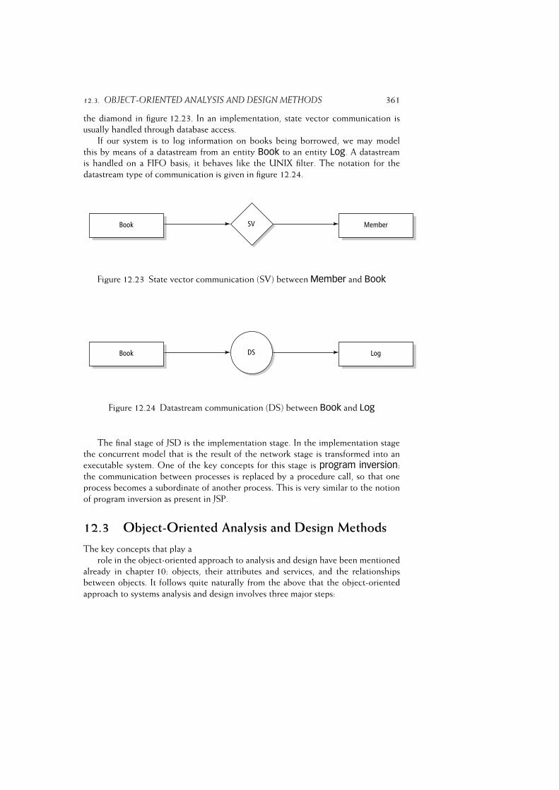
12.3. OBJECT-ORIENTED ANALYSIS AND DESIGN METHODS 361

the diamond in figure 12.23. In an implementation, state vector communication is

usually handled through database access.

If our system is to log information on books being borrowed, we may model

this by means of a datastream from an entity Book to an entity Log. A datastream

is handled on a FIFO basis; it behaves like the UNIX filter. The notation for the

datastream type of communication is given in figure 12.24.

Figure 12.23 State vector communication (SV) between Member and Book

Figure 12.24 Datastream communication (DS) between Book and Log

The final stage of JSD is the implementation stage. In the implementation stage

the concurrent model that is the result of the network stage is transformed into an

executable system. One of the key concepts for this stage is program inversion:

the communication between processes is replaced by a procedure call, so that one

process becomes a subordinate of another process. This is very similar to the notion

of program inversion as present in JSP.

12.3 Object-Oriented Analysis and Design Methods

The key concepts that play a

role in the object-oriented approach to analysis and design have been mentioned

already in chapter 10: objects, their attributes and services, and the relationships

between objects. It follows quite naturally from the above that the object-oriented

approach to systems analysis and design involves three major steps:

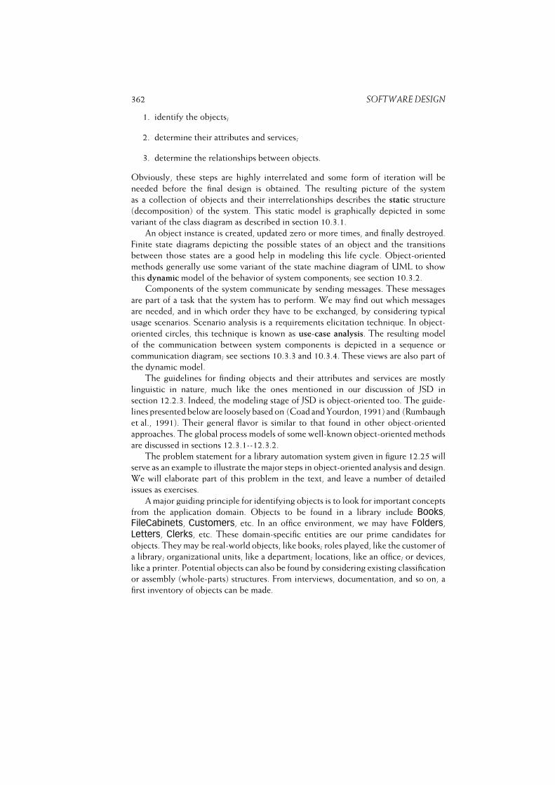
362 SOFTWARE DESIGN

1. identify the objects;

2. determine their attributes and services;

3. determine the relationships between objects.

Obviously, these steps are highly interrelated and some form of iteration will be

needed before the final design is obtained. The resulting picture of the system

as a collection of objects and their interrelationships describes the static structure

(decomposition) of the system. This static model is graphically depicted in some

variant of the class diagram as described in section 10.3.1.

An object instance is created, updated zero or more times, and finally destroyed.

Finite state diagrams depicting the possible states of an object and the transitions

between those states are a good help in modeling this life cycle. Object-oriented

methods generally use some variant of the state machine diagram of UML to show

this dynamic model of the behavior of system components; see section 10.3.2.

Components of the system communicate by sending messages. These messages

are part of a task that the system has to perform. We may find out which messages

are needed, and in which order they have to be exchanged, by considering typical

usage scenarios. Scenario analysis is a requirements elicitation technique. In object-

oriented circles, this technique is known as use-case analysis. The resulting model

of the communication between system components is depicted in a sequence or

communication diagram; see sections 10.3.3 and 10.3.4. These views are also part of

the dynamic model.

The guidelines for finding objects and their attributes and services are mostly

linguistic in nature, much like the ones mentioned in our discussion of JSD in

section 12.2.3. Indeed, the modeling stage of JSD is object-oriented too. The guide-

lines presented below are loosely based on (Coad and Yourdon, 1991) and (Rumbaugh

et al., 1991). Their general flavor is similar to that found in other object-oriented

approaches. The global process models of some well-known object-oriented methods

are discussed in sections 12.3.1--12.3.2.

The problem statement for a library automation system given in figure 12.25 will

serve as an example to illustrate the major steps in object-oriented analysis and design.

We will elaborate part of this problem in the text, and leave a number of detailed

issues as exercises.

A major guiding principle for identifying objects is to look for important concepts

from the application domain. Objects to be found in a library include Books,

FileCabinets, Customers, etc. In an office environment, we may have Folders,

Letters, Clerks, etc. These domain-specific entities are our prime candidates for

objects. They may be real-world objects, like books; roles played, like the customer of

a library; organizational units, like a department; locations, like an office; or devices,

like a printer. Potential objects can also be found by considering existing classification

or assembly (whole-parts) structures. From interviews, documentation, and so on, a

first inventory of objects can be made.

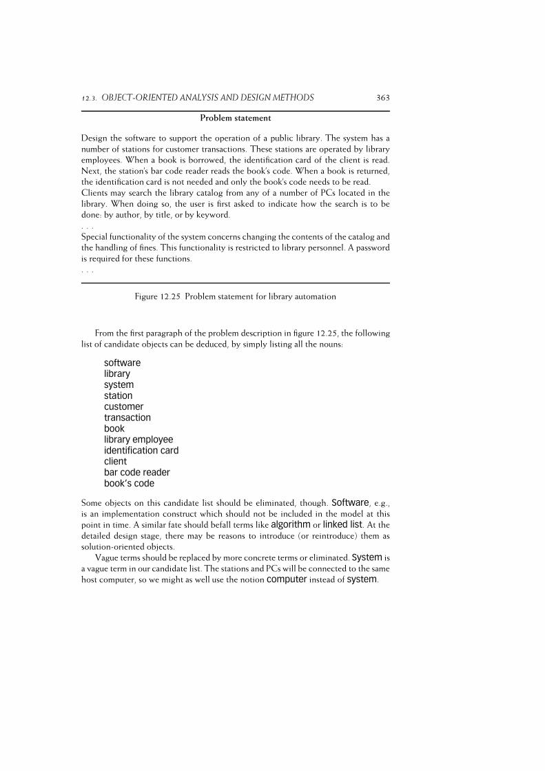
12.3. OBJECT-ORIENTED ANALYSIS AND DESIGN METHODS 363

Problem statement

Design the software to support the operation of a public library. The system has a

number of stations for customer transactions. These stations are operated by library

employees. When a book is borrowed, the identification card of the client is read.

Next, the station’s bar code reader reads the book’s code. When a book is returned,

the identification card is not needed and only the book’s code needs to be read.

Clients may search the library catalog from any of a number of PCs located in the

library. When doing so, the user is first asked to indicate how the search is to be

done: by author, by title, or by keyword.

. . .

Special functionality of the system concerns changing the contents of the catalog and

the handling of fines. This functionality is restricted to library personnel. A password

is required for these functions.

. . .

Figure 12.25 Problem statement for library automation

From the first paragraph of the problem description in figure 12.25, the following

list of candidate objects can be deduced, by simply listing all the nouns:

softwarelibrarysystemstationcustomertransactionbooklibrary employeeidentification cardclientbar code readerbook’s code

Some objects on this candidate list should be eliminated, though. Software, e.g.,

is an implementation construct which should not be included in the model at this

point in time. A similar fate should befall terms like algorithm or linked list. At the

detailed design stage, there may be reasons to introduce (or reintroduce) them as

solution-oriented objects.

Vague terms should be replaced by more concrete terms or eliminated. System is

a vague term in our candidate list. The stations and PCs will be connected to the same

host computer, so we might as well use the notion computer instead of system.

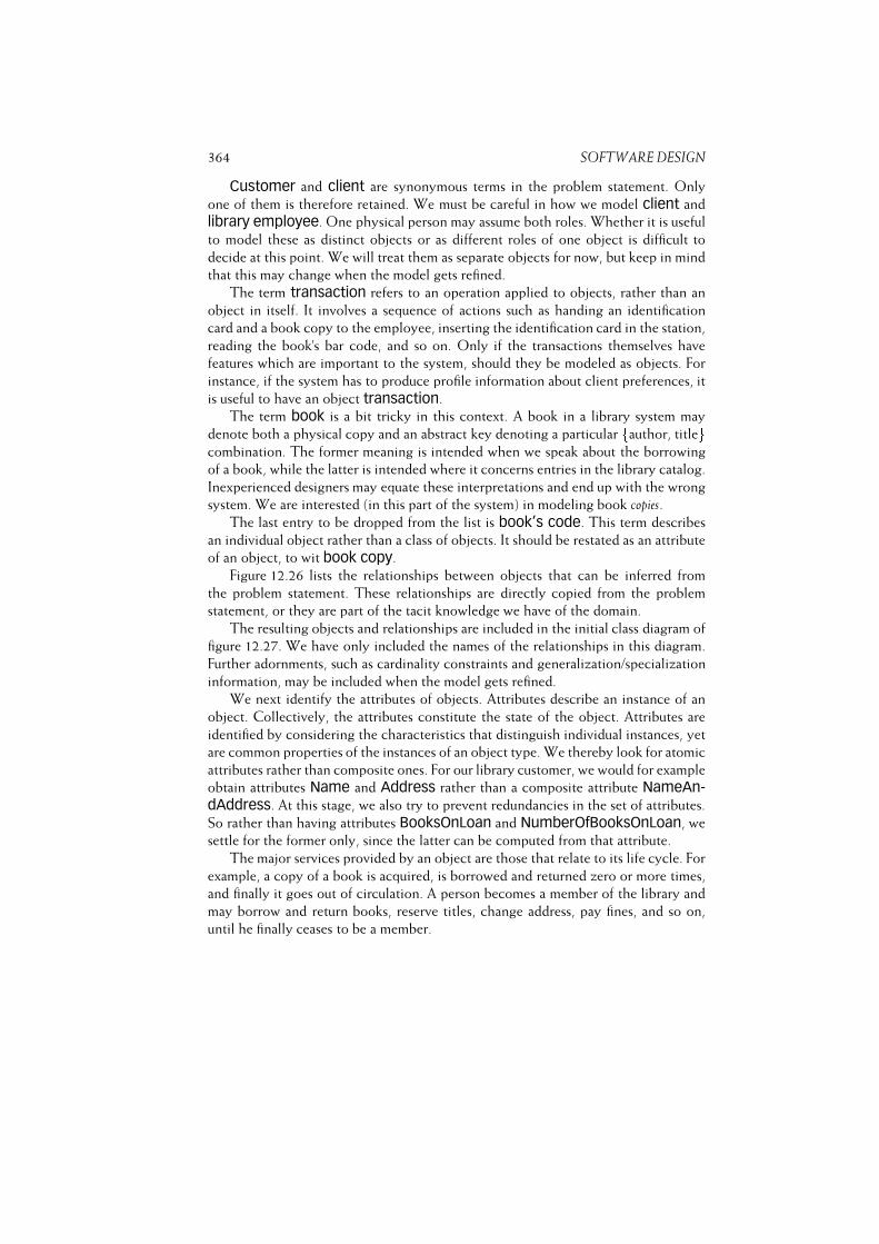
364 SOFTWARE DESIGN

Customer and client are synonymous terms in the problem statement. Only

one of them is therefore retained. We must be careful in how we model client and

library employee. One physical person may assume both roles. Whether it is useful

to model these as distinct objects or as different roles of one object is difficult to

decide at this point. We will treat them as separate objects for now, but keep in mind

that this may change when the model gets refined.

The term transaction refers to an operation applied to objects, rather than an

object in itself. It involves a sequence of actions such as handing an identification

card and a book copy to the employee, inserting the identification card in the station,

reading the book’s bar code, and so on. Only if the transactions themselves have

features which are important to the system, should they be modeled as objects. For

instance, if the system has to produce profile information about client preferences, it

is useful to have an object transaction.

The term book is a bit tricky in this context. A book in a library system may

denote both a physical copy and an abstract key denoting a particular fauthor, titlegcombination. The former meaning is intended when we speak about the borrowing

of a book, while the latter is intended where it concerns entries in the library catalog.

Inexperienced designers may equate these interpretations and end up with the wrong

system. We are interested (in this part of the system) in modeling book copies.

The last entry to be dropped from the list is book’s code. This term describes

an individual object rather than a class of objects. It should be restated as an attribute

of an object, to wit book copy.

Figure 12.26 lists the relationships between objects that can be inferred from

the problem statement. These relationships are directly copied from the problem

statement, or they are part of the tacit knowledge we have of the domain.

The resulting objects and relationships are included in the initial class diagram of

figure 12.27. We have only included the names of the relationships in this diagram.

Further adornments, such as cardinality constraints and generalization/specialization

information, may be included when the model gets refined.

We next identify the attributes of objects. Attributes describe an instance of an

object. Collectively, the attributes constitute the state of the object. Attributes are

identified by considering the characteristics that distinguish individual instances, yet

are common properties of the instances of an object type. We thereby look for atomic

attributes rather than composite ones. For our library customer, we would for example

obtain attributes Name and Address rather than a composite attribute NameAn-dAddress. At this stage, we also try to prevent redundancies in the set of attributes.

So rather than having attributes BooksOnLoan and NumberOfBooksOnLoan, we

settle for the former only, since the latter can be computed from that attribute.

The major services provided by an object are those that relate to its life cycle. For

example, a copy of a book is acquired, is borrowed and returned zero or more times,

and finally it goes out of circulation. A person becomes a member of the library and

may borrow and return books, reserve titles, change address, pay fines, and so on,

until he finally ceases to be a member.

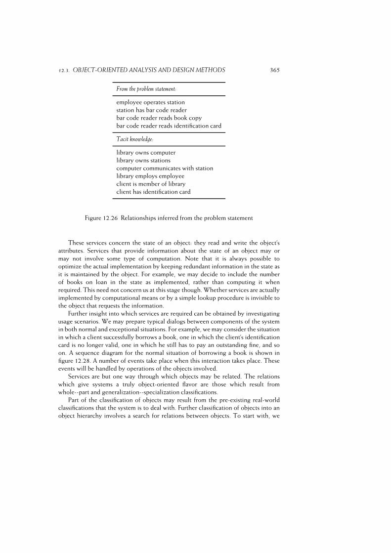
12.3. OBJECT-ORIENTED ANALYSIS AND DESIGN METHODS 365

From the problem statement:

employee operates station

station has bar code reader

bar code reader reads book copy

bar code reader reads identification card

Tacit knowledge:

library owns computer

library owns stations

computer communicates with station

library employs employee

client is member of library

client has identification card

Figure 12.26 Relationships inferred from the problem statement

These services concern the state of an object: they read and write the object’s

attributes. Services that provide information about the state of an object may or

may not involve some type of computation. Note that it is always possible to

optimize the actual implementation by keeping redundant information in the state as

it is maintained by the object. For example, we may decide to include the number

of books on loan in the state as implemented, rather than computing it when

required. This need not concern us at this stage though. Whether services are actually

implemented by computational means or by a simple lookup procedure is invisible to

the object that requests the information.

Further insight into which services are required can be obtained by investigating

usage scenarios. We may prepare typical dialogs between components of the system

in both normal and exceptional situations. For example, we may consider the situation

in which a client successfully borrows a book, one in which the client’s identification

card is no longer valid, one in which he still has to pay an outstanding fine, and so

on. A sequence diagram for the normal situation of borrowing a book is shown in

figure 12.28. A number of events take place when this interaction takes place. These

events will be handled by operations of the objects involved.

Services are but one way through which objects may be related. The relations

which give systems a truly object-oriented flavor are those which result from

whole--part and generalization--specialization classifications.

Part of the classification of objects may result from the pre-existing real-world

classifications that the system is to deal with. Further classification of objects into an

object hierarchy involves a search for relations between objects. To start with, we

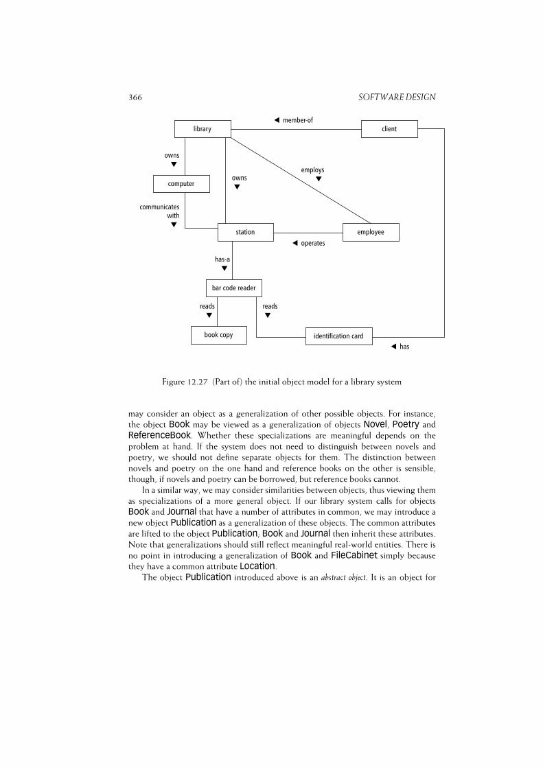
366 SOFTWARE DESIGN

Figure 12.27 (Part of) the initial object model for a library system

may consider an object as a generalization of other possible objects. For instance,

the object Book may be viewed as a generalization of objects Novel, Poetry and

ReferenceBook. Whether these specializations are meaningful depends on the

problem at hand. If the system does not need to distinguish between novels and

poetry, we should not define separate objects for them. The distinction between

novels and poetry on the one hand and reference books on the other is sensible,

though, if novels and poetry can be borrowed, but reference books cannot.

In a similar way, we may consider similarities between objects, thus viewing them

as specializations of a more general object. If our library system calls for objects

Book and Journal that have a number of attributes in common, we may introduce a

new object Publication as a generalization of these objects. The common attributes

are lifted to the object Publication; Book and Journal then inherit these attributes.

Note that generalizations should still reflect meaningful real-world entities. There is

no point in introducing a generalization of Book and FileCabinet simply because

they have a common attribute Location.

The object Publication introduced above is an abstract object. It is an object for

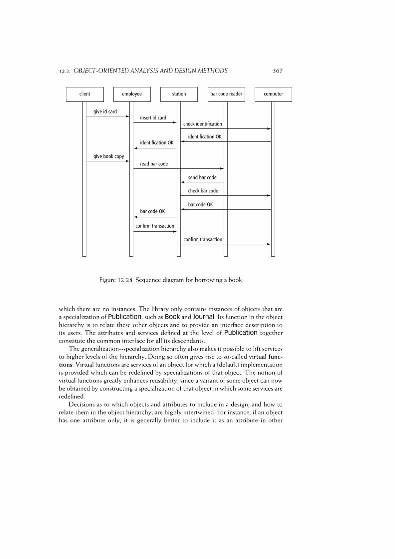
12.3. OBJECT-ORIENTED ANALYSIS AND DESIGN METHODS 367

Figure 12.28 Sequence diagram for borrowing a book

which there are no instances. The library only contains instances of objects that are

a specialization of Publication, such as Book and Journal. Its function in the object

hierarchy is to relate these other objects and to provide an interface description to

its users. The attributes and services defined at the level of Publication together

constitute the common interface for all its descendants.

The generalization--specialization hierarchy also makes it possible to lift services

to higher levels of the hierarchy. Doing so often gives rise to so-called virtual func-

tions. Virtual functions are services of an object for which a (default) implementation

is provided which can be redefined by specializations of that object. The notion of

virtual functions greatly enhances reusability, since a variant of some object can now

be obtained by constructing a specialization of that object in which some services are

redefined.

Decisions as to which objects and attributes to include in a design, and how to

relate them in the object hierarchy, are highly intertwined. For instance, if an object

has one attribute only, it is generally better to include it as an attribute in other

368 SOFTWARE DESIGN

objects. Also, the instances of an object should have common attributes. If some

attributes are only meaningful for a subset of all instances, then we really have a

classification structure. If some books can be borrowed, but others cannot, this is an

indication of a classification structure where the object Book has specializations such

as Novel and ReferenceBook.

Note also that, over time, the set of attributes of and services provided by an

object tends to evolve, while the object hierarchy remains relatively stable. If our

library decides to offer an extra service to its customers, say borrowing records, we

may simply adapt the set of attributes and extend the set of services for the object

Customer.Object-oriented design can be classified as a middle-out design method. The set

of objects identified during the first modeling stages constitutes the middle level of the

system. In order to implement these domain-specific entities, lower-level objects are

used. These lower-level objects can often be taken from a class library. For the various

object-oriented programming languages, quite extensive class libraries already exist.

The higher levels of the design constitute the application-dependent interaction of

the domain-specific entities.

In the following subsections, we discuss three design methods that typify the

evolution of object-oriented analysis and design:� The Booch method, an early object-oriented analysis and design method, with

an emphasis on employing a new and rich set of notations.� Fusion, developed at HP, with a much larger emphasis on the various process

steps of the method.� The Rational Unified Process (RUP), a full life cycle model associated with

UML.

12.3.1 The Booch Method

The global process model of the method described in (Booch, 1994) is shown in

figure 12.29. It consists of four steps, to be carried out in roughly the order specified.

The process is iterative, so each of the steps may have to be done more than once. The

first cycles are analysis-oriented, while later ones are design-oriented. The blurring

of activities in this process model is intentional. Analysis and design activities are

assumed to be under opportunistic control. It is therefore not deemed realistic to

prescribe a purely rational order for the activities to be carried out.

The first step is aimed at identifying classes and objects. The purpose of this step

is to establish the boundaries of the problem and to obtain a first decomposition.

During analysis, emphasis is on finding meaningful abstractions from the domain of

application. During design, objects from the solution domain may be added. The

major outcome of this step is a data dictionary containing a precise description of the

abstractions identified.

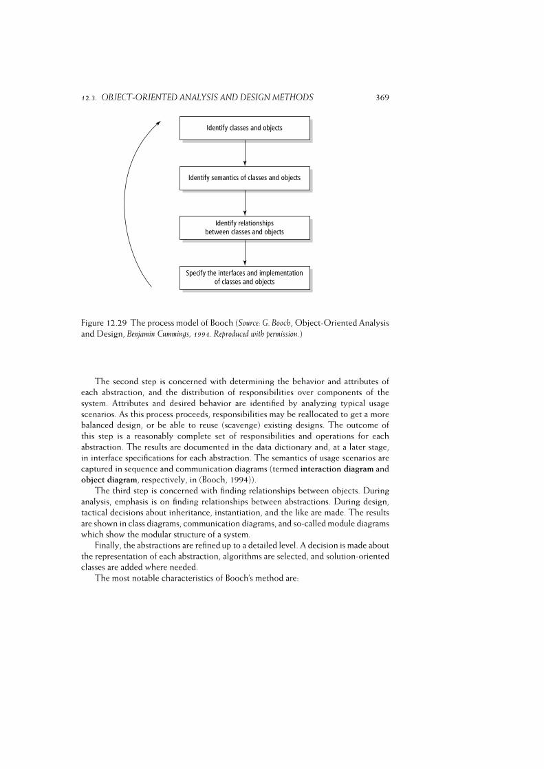
12.3. OBJECT-ORIENTED ANALYSIS AND DESIGN METHODS 369

Figure 12.29 The process model of Booch (Source: G. Booch, Object-Oriented Analysis

and Design, Benjamin Cummings, 1994. Reproduced with permission.)

The second step is concerned with determining the behavior and attributes of

each abstraction, and the distribution of responsibilities over components of the

system. Attributes and desired behavior are identified by analyzing typical usage

scenarios. As this process proceeds, responsibilities may be reallocated to get a more

balanced design, or be able to reuse (scavenge) existing designs. The outcome of

this step is a reasonably complete set of responsibilities and operations for each

abstraction. The results are documented in the data dictionary and, at a later stage,

in interface specifications for each abstraction. The semantics of usage scenarios are

captured in sequence and communication diagrams (termed interaction diagram and

object diagram, respectively, in (Booch, 1994)).

The third step is concerned with finding relationships between objects. During

analysis, emphasis is on finding relationships between abstractions. During design,

tactical decisions about inheritance, instantiation, and the like are made. The results

are shown in class diagrams, communication diagrams, and so-called module diagrams

which show the modular structure of a system.

Finally, the abstractions are refined up to a detailed level. A decision is made about

the representation of each abstraction, algorithms are selected, and solution-oriented

classes are added where needed.

The most notable characteristics of Booch’s method are:

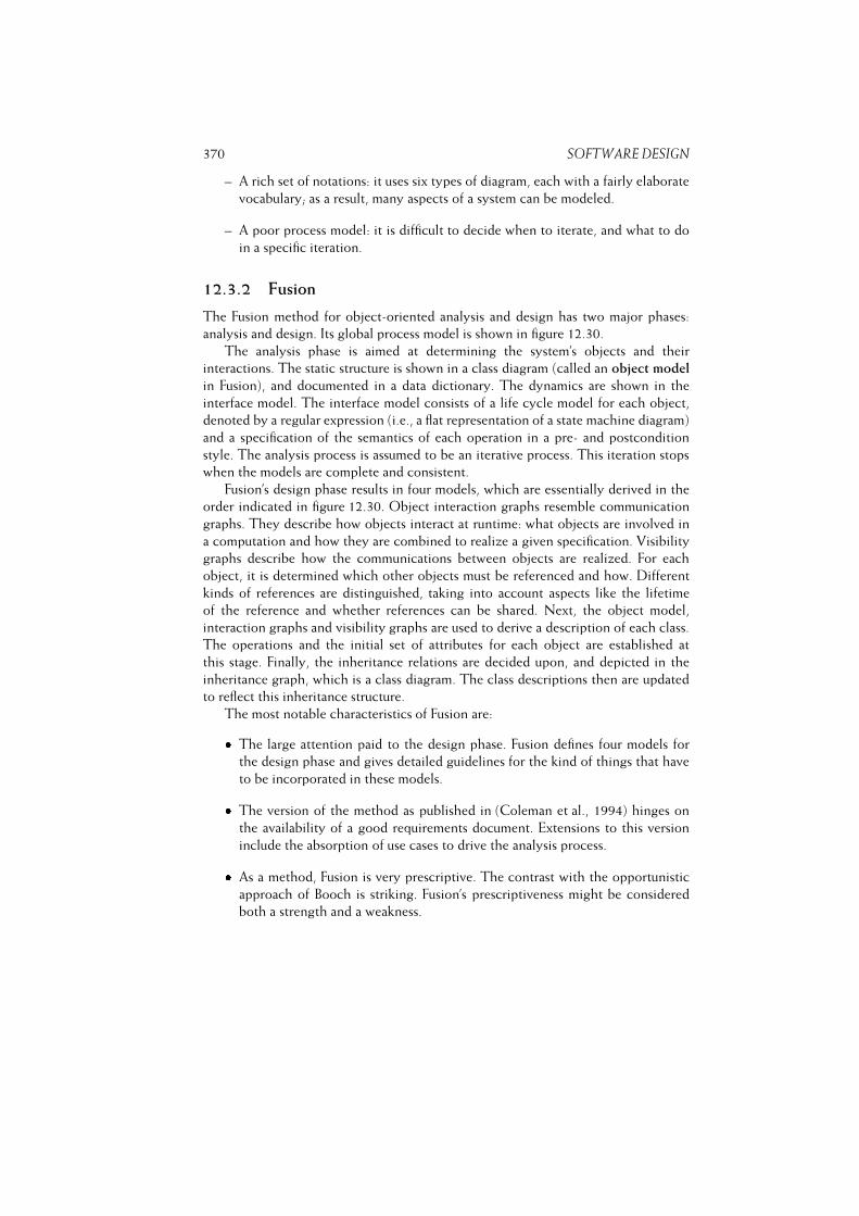
370 SOFTWARE DESIGN

– A rich set of notations: it uses six types of diagram, each with a fairly elaborate

vocabulary; as a result, many aspects of a system can be modeled.

– A poor process model: it is difficult to decide when to iterate, and what to do

in a specific iteration.

12.3.2 Fusion

The Fusion method for object-oriented analysis and design has two major phases:

analysis and design. Its global process model is shown in figure 12.30.

The analysis phase is aimed at determining the system’s objects and their

interactions. The static structure is shown in a class diagram (called an object model

in Fusion), and documented in a data dictionary. The dynamics are shown in the

interface model. The interface model consists of a life cycle model for each object,

denoted by a regular expression (i.e., a flat representation of a state machine diagram)

and a specification of the semantics of each operation in a pre- and postcondition

style. The analysis process is assumed to be an iterative process. This iteration stops

when the models are complete and consistent.

Fusion’s design phase results in four models, which are essentially derived in the

order indicated in figure 12.30. Object interaction graphs resemble communication

graphs. They describe how objects interact at runtime: what objects are involved in

a computation and how they are combined to realize a given specification. Visibility

graphs describe how the communications between objects are realized. For each

object, it is determined which other objects must be referenced and how. Different

kinds of references are distinguished, taking into account aspects like the lifetime

of the reference and whether references can be shared. Next, the object model,

interaction graphs and visibility graphs are used to derive a description of each class.

The operations and the initial set of attributes for each object are established at

this stage. Finally, the inheritance relations are decided upon, and depicted in the

inheritance graph, which is a class diagram. The class descriptions then are updated

to reflect this inheritance structure.

The most notable characteristics of Fusion are:� The large attention paid to the design phase. Fusion defines four models for

the design phase and gives detailed guidelines for the kind of things that have

to be incorporated in these models.� The version of the method as published in (Coleman et al., 1994) hinges on

the availability of a good requirements document. Extensions to this version

include the absorption of use cases to drive the analysis process.� As a method, Fusion is very prescriptive. The contrast with the opportunistic

approach of Booch is striking. Fusion’s prescriptiveness might be considered

both a strength and a weakness.

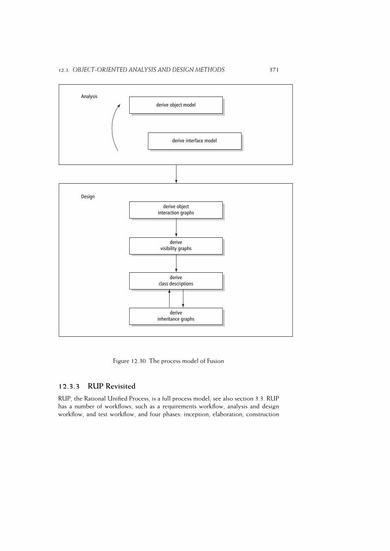
12.3. OBJECT-ORIENTED ANALYSIS AND DESIGN METHODS 371

Figure 12.30 The process model of Fusion

12.3.3 RUP Revisited

RUP, the Rational Unified Process, is a full process model; see also section 3.3. RUP

has a number of workflows, such as a requirements workflow, analysis and design

workflow, and test workflow, and four phases: inception, elaboration, construction

372 SOFTWARE DESIGN

and transition. Workflows describe the activities to be carried out, while the phases

indicate the organization along the time axis. Most workflows extend over most

phases.

Here, we discuss the analysis and design workflow, in which the requirements are

transformed into a design. RUP is an iterative process, so this transformation is carried

out in a number of iterations as well. The first iterations take place in the elaboration

phase of RUP. In that phase, the architecture of the system is determined. The RUP

way of doing architectural design reasonably fits the global workflow model discussed

in section 11.2. In subsequent iterations, concerning the lower-level design, the main

activities are termed Analyze behavior and Design components.

The purpose of the Analyze behavior step is to transform the use cases into a set

of design elements that together serve as a model of the problem domain. It is about

what the system is to deliver. It produces a black box model of the solution. The

purpose of the Design elements step is to refine the definitions of the design elements

into classes, relationships, interfaces and the like. In this activity, the black box whatmodel is turned into a white box how model.

During both activities, the resulting design is reviewed, and the results thereof

are fed back into the next iteration.

Notable characteristics of RUP are:� It is a very complete, iterative model that goes much further than mere analysis

and design.� It makes heavy use of the Unified Modeling Language to represent artifacts and

views.� Use cases play a central role. They provide thread information from one

workflow to another. For example, the analysis and design workflow produces

use case realizations, which describe how use cases are actually realized by a

collection of interacting objects and classes.

12.4 How to Select a Design Method

It is not easy to compare the many design methods that exist. They all have their pros

and cons. None of them gives us a straightforward recipe as to how to proceed from

a list of requirements to a successfully implemented system. We always need some

sort of magic in order to get a specific decomposition. The expertise and quality of

the people involved have a major impact on the end result of the design process.

Problem solving is based on experience. It is estimated that an expert has over 50

000 chunks of domain-specific knowledge at his disposal. When solving a problem,

we try to map the problem at hand onto the knowledge available. The greater this

knowledge is, and the more accessible it is, the more successful this process will be.

The prescriptiveness of the design methods differs considerably. The various

variants of functional decomposition and the object-oriented design methods rely

12.4. HOW TO SELECT A DESIGN METHOD 373

heavily on the heuristic knowledge of the designers. Jackson’s techniques seem to

suffer less from this need. Especially if structure clashes do not occur, JSP provides

a well-defined framework for how to tackle design. The prescriptive nature of JSP

possibly explains to some extent its success, especially in the realm of administrative

data-processing. JSD offers similar advantages. Its strict view of describing data

structures as a list of events may lead to problems, however, if the data structures do

not fit this model. JSP has a static view of the data. More importantly, it does not tell

us how to organize the data. As such, this technique seems most suited for problems

where the structure of the data has been fixed beforehand. JSD and object-oriented

methods offer better support as regards the structuring of data. Though these methods

give useful heuristics for the identification of objects, obtaining a well-balanced set

of objects is still very much dependent on the skills of the designer.

The data flow technique has a more dynamic view of the data streams that are the

base of the system to be constructed. We may often view the bubbles from a data flow

diagram as clerks that perform certain transformations on incoming data to produce

data for other clerks. The technique seems well-suited for circumstances where an

existing manual system is to be replaced by a computerized one. A real danger,

though, is that the existing system is just copied, while additional requirements are

overlooked.

If we take into account that a substantial part of the cost of software is spent in

maintaining that software, it is clear that such factors as flexibility, comprehensibility

and modularity should play a crucial role when selecting a specific design technique.

The ideas and guidelines of Parnas are particularly relevant in this respect. The

object-oriented philosophy incorporates these ideas and is well-matched to current

programming languages, which allow for a smoother transition between the different

development phases.

Quite a few attempts have been made to classify design methods along various

dimensions, such as the products they deliver, the kind of representations used, or

their level of formality. A simple but useful framework is proposed in (Blum, 1994). It

has two dimensions: an orientation dimension and a model dimension.

In the orientation dimension, a distinction is made between problem-oriented

techniques and product-oriented techniques. Problem-oriented techniques con-

centrate on producing a better understanding of the problem and its solution.

Problem-oriented techniques are human-oriented. Their aim is to describe, commu-

nicate, and document decisions. Problem-oriented techniques usually have one foot

in the requirements engineering domain. Conversely, product-oriented techniques

focus on a correct transformation from a specification to an implementation. The

second dimension relates to the products, i.e. models, that are the result of the design

process. In this dimension, a distinction is made between conceptual models and

formal models. Conceptual models are descriptive. They describe an external reality,

the Universe of Discourse. Their appropriateness is established through validation.

Formal models on the other hand are prescriptive. They prescribe the behavior of the

system to be developed. Formal models can be verified.

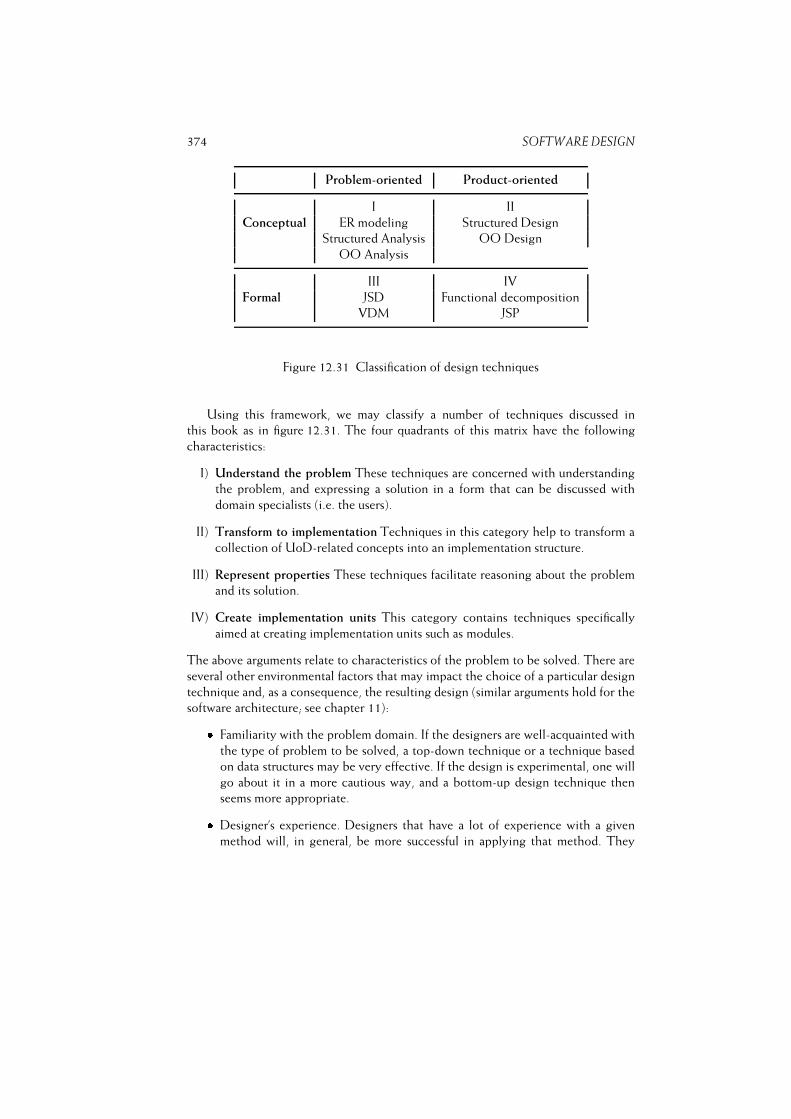
374 SOFTWARE DESIGN

Problem-oriented Product-oriented

I II

Conceptual ER modeling Structured Design

Structured Analysis OO Design

OO Analysis

III IV

Formal JSD Functional decomposition

VDM JSP

Figure 12.31 Classification of design techniques

Using this framework, we may classify a number of techniques discussed in

this book as in figure 12.31. The four quadrants of this matrix have the following

characteristics:

I) Understand the problem These techniques are concerned with understanding

the problem, and expressing a solution in a form that can be discussed with

domain specialists (i.e. the users).

II) Transform to implementation Techniques in this category help to transform a

collection of UoD-related concepts into an implementation structure.

III) Represent properties These techniques facilitate reasoning about the problem

and its solution.

IV) Create implementation units This category contains techniques specifically

aimed at creating implementation units such as modules.

The above arguments relate to characteristics of the problem to be solved. There are

several other environmental factors that may impact the choice of a particular design

technique and, as a consequence, the resulting design (similar arguments hold for the

software architecture; see chapter 11):� Familiarity with the problem domain. If the designers are well-acquainted with

the type of problem to be solved, a top-down technique or a technique based

on data structures may be very effective. If the design is experimental, one will

go about it in a more cautious way, and a bottom-up design technique then

seems more appropriate.� Designer’s experience. Designers that have a lot of experience with a given

method will, in general, be more successful in applying that method. They

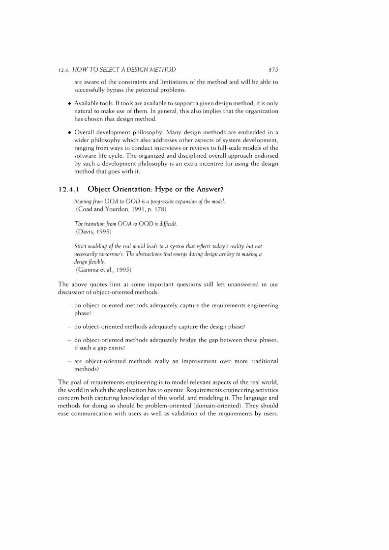
12.4. HOW TO SELECT A DESIGN METHOD 375

are aware of the constraints and limitations of the method and will be able to

successfully bypass the potential problems.� Available tools. If tools are available to support a given design method, it is only

natural to make use of them. In general, this also implies that the organization

has chosen that design method.� Overall development philosophy. Many design methods are embedded in a

wider philosophy which also addresses other aspects of system development,

ranging from ways to conduct interviews or reviews to full-scale models of the

software life cycle. The organized and disciplined overall approach endorsed

by such a development philosophy is an extra incentive for using the design

method that goes with it.

12.4.1 Object Orientation: Hype or the Answer?

Moving from OOA to OOD is a progressive expansion of the model.(Coad and Yourdon, 1991, p. 178)

The transition from OOA to OOD is difficult.(Davis, 1995)

Strict modeling of the real world leads to a system that reflects today’s reality but notnecessarily tomorrow’s. The abstractions that emerge during design are key to making a

design flexible.

(Gamma et al., 1995)

The above quotes hint at some important questions still left unanswered in our

discussion of object-oriented methods:

– do object-oriented methods adequately capture the requirements engineering

phase?

– do object-oriented methods adequately capture the design phase?

– do object-oriented methods adequately bridge the gap between these phases,

if such a gap exists?

– are object-oriented methods really an improvement over more traditional

methods?

The goal of requirements engineering is to model relevant aspects of the real world,

the world in which the application has to operate. Requirements engineering activities

concern both capturing knowledge of this world, and modeling it. The language and

methods for doing so should be problem-oriented (domain-oriented). They should

ease communication with users as well as validation of the requirements by users.

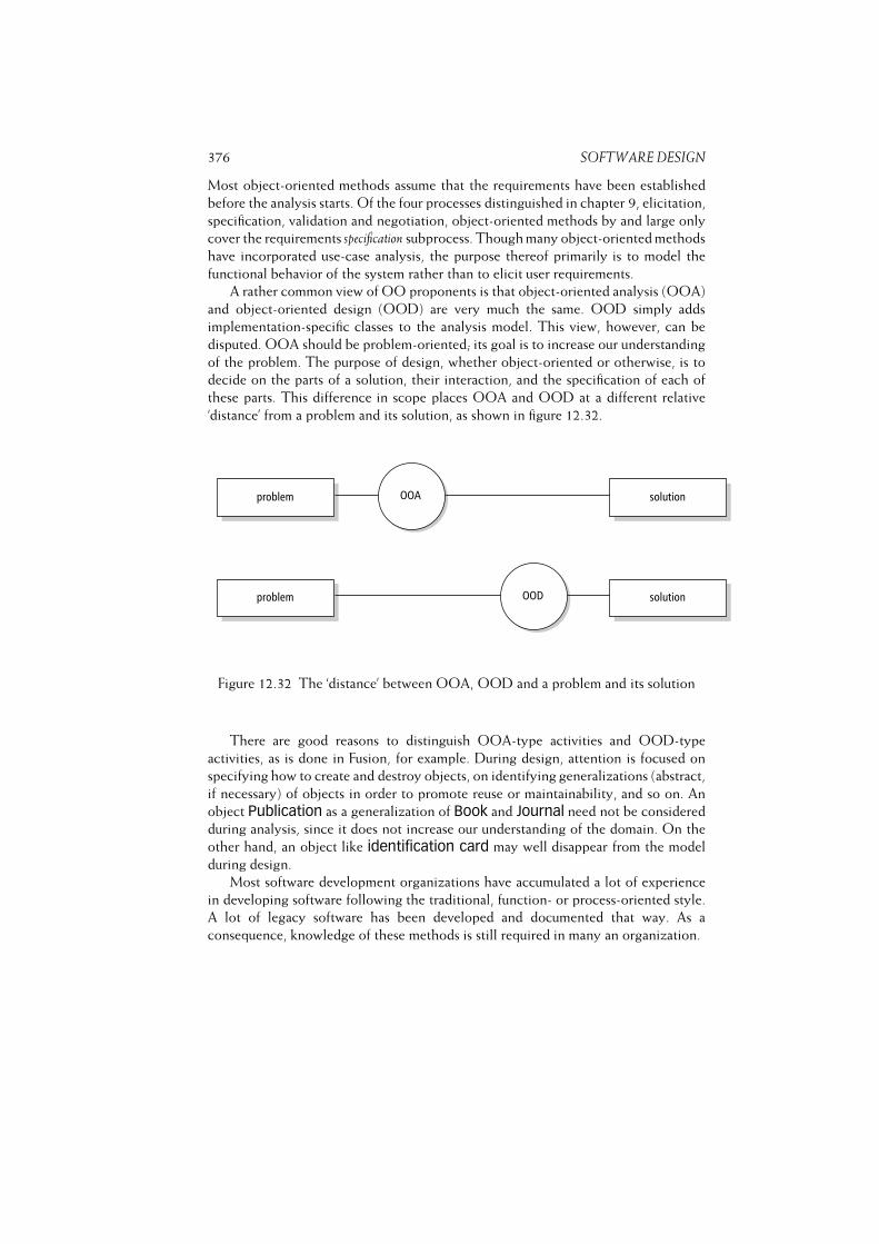
376 SOFTWARE DESIGN

Most object-oriented methods assume that the requirements have been established

before the analysis starts. Of the four processes distinguished in chapter 9, elicitation,

specification, validation and negotiation, object-oriented methods by and large only

cover the requirements specification subprocess. Though many object-oriented methods

have incorporated use-case analysis, the purpose thereof primarily is to model the

functional behavior of the system rather than to elicit user requirements.

A rather common view of OO proponents is that object-oriented analysis (OOA)

and object-oriented design (OOD) are very much the same. OOD simply adds

implementation-specific classes to the analysis model. This view, however, can be

disputed. OOA should be problem-oriented; its goal is to increase our understanding

of the problem. The purpose of design, whether object-oriented or otherwise, is to

decide on the parts of a solution, their interaction, and the specification of each of

these parts. This difference in scope places OOA and OOD at a different relative

‘distance’ from a problem and its solution, as shown in figure 12.32.

Figure 12.32 The ‘distance’ between OOA, OOD and a problem and its solution

There are good reasons to distinguish OOA-type activities and OOD-type

activities, as is done in Fusion, for example. During design, attention is focused on

specifying how to create and destroy objects, on identifying generalizations (abstract,

if necessary) of objects in order to promote reuse or maintainability, and so on. An

object Publication as a generalization of Book and Journal need not be considered

during analysis, since it does not increase our understanding of the domain. On the

other hand, an object like identification card may well disappear from the model

during design.

Most software development organizations have accumulated a lot of experience

in developing software following the traditional, function- or process-oriented style.

A lot of legacy software has been developed and documented that way. As a

consequence, knowledge of these methods is still required in many an organization.

12.5. DESIGN PATTERNS 377

Many organizations have switched to some kind of object-oriented analysis and

design approach. Hard evidence of increased productivity or quality has not been

determined, though. Several experiments have been done to test the effectiveness

of the OO paradigm, and the results do seem to indicate some deeper problems

too. For example, in one experiment it was tested how effective object-oriented

models are as the main vehicle of communication between the typical customer

and the developer (Moynihan, 1996). It was found that the traditional, functional

models were easier to understand, provoked more questions and comments, gave

a more holistic understanding of the business, and better helped to evaluate likely

implementations. In another experiment it was tested whether novice analysts are

able to develop requirements more easily with certain methods than with others,

and whether they learn to use certain methods more readily than others (Vessey

and Conger, 1994). And again, the results were negative for OO: novice analysts

were better able to apply the process-oriented method, and significant learning only

occurred for the process-oriented method.

In a similar vein, (Arisholm and Sjøberg, 2004) found that novice users have fewer

problems maintaining systems that have centralized control compared to systems

having delegated control. In a centralized control style, one or a few large classes

are in control. These large classes coordinate the work of a lot of smaller classes.

This resembles the hierarchical main-program-with-subroutines architectural style.

In a delegated style, responsibilities are distributed over a larger set of classes. OO

proponents usually advocate a delegated control style. It seems one needs a certain

maturity to be effective with this style.

The inheritance mechanism of object-orientation needs to be handled with care

too, as noted in section 12.1.6. Deep hierarchies require one to comprehend design

or implementation units that may be wide apart. Such designs tend to be error

prone (Bieman et al., 2001) and more difficult to inspect (Dunsmore et al., 2002),

because of the delocalized nature of information in them.

There may well be some truth in the observation that users do not think in

objects; they think in tasks. From that point of view, use-case analysis may be seen as

one way to introduce a functional view into an otherwise object-oriented approach.

12.5 Design Patterns

A design pattern is a recurring structure of communicating components that solves

a general design problem within a particular context. A design pattern differs from

an architectural style in that it does not address the structure of a complete system,

but only that of a few (interacting) components. Design patterns may thus be termed

micro-architectures. On the other hand, a design pattern encompasses more than a

single component, procedure or module.

The archetypical example of a design pattern is the Model--View--Controller

(MVC) pattern. Interactive systems consist of computational elements as well as

elements to display data and handle user input. It is considered good design practice

378 SOFTWARE DESIGN

to separate the computational elements from those that handle I/O. This separation

of concerns is achieved by the MVC pattern.

MVC involves three components: the Model, the View, and the Controller. The

model component encapsulates the system’s data as well as the operations on those

data. The model component is independent of how the data is represented or how

input is done. A view component displays the data that it obtains from the model

component. There can be more than one view component. Finally, each view has an

associated controller component. A controller handles input actions. Such an input

action may cause the controller to send a request to the model, for example to update

its data, or to its view, for example to scroll.

For any given situation, the above description has to be considerably refined and

made more precise. For instance, a controller may or may not depend on the state

of the model. If the controller does not depend on the state of the model, there is

a one-way flow of information: the controller signals an input event and notifies the

model. If the controller does depend on the state of the model, information flows in

the other direction as well. The latter type of dependence can be observed in most

word-processing systems for example, where menu entries are made active or inactive

depending on the state of the model.

MVC was first used in the Smalltalk environment. Since then it has been applied

in many applications. In various graphical user interface platforms, a variant has been

applied in which the distinction between the view and the controller has been relaxed.

This variant is called the Document--View pattern; see (Kruglinski, 1996).

Design patterns have a number of properties which explain what they offer, as

well as why and how they do so:� A pattern addresses a recurring design problem that arises in specific design

situations and presents a solution to it. Many software systems include compu-

tational elements as well as user-interface elements. For reasons of flexibility,

we may wish to separate these as much as possible. MVC offers a solution to

precisely this recurring problem.� A pattern must balance a set of opposing forces, i.e. characteristics of the

problem that have to be dealt with in its solution. For example, in interactive

applications we want to be able to present information in different ways,

changes to the data must be reflected immediately in all views affected by these

changes, and different ‘look and feel’ interfaces should not affect the application

code. MVC seeks to balance all these forces.� Patterns document existing, well-proven design experience. Patterns are not

invented; they evolve with experience. They reflect best practices. MVC, for

example, is used in various application frameworks as well as in scores of

interactive systems.� Patterns identify and specify abstractions above the level of single components.

MVC has three, interacting components which together solve a given problem.

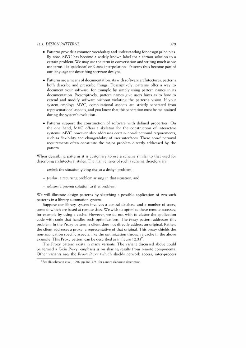
12.5. DESIGN PATTERNS 379� Patterns provide a common vocabulary and understanding for design principles.

By now, MVC has become a widely known label for a certain solution to a

certain problem. We may use the term in conversation and writing much as we

use terms like ‘quicksort’ or ‘Gauss interpolation’. Patterns thus become part of

our language for describing software designs.� Patterns are a means of documentation. As with software architectures, patterns

both describe and prescribe things. Descriptively, patterns offer a way to

document your software, for example by simply using pattern names in its

documentation. Prescriptively, pattern names give users hints as to how to

extend and modify software without violating the pattern’s vision. If your

system employs MVC, computational aspects are strictly separated from

representational aspects, and you know that this separation must be maintained

during the system’s evolution.� Patterns support the construction of software with defined properties. On

the one hand, MVC offers a skeleton for the construction of interactive

systems. MVC however also addresses certain non-functional requirements,

such as flexibility and changeability of user interfaces. These non-functional

requirements often constitute the major problem directly addressed by the

pattern.

When describing patterns it is customary to use a schema similar to that used for

describing architectural styles. The main entries of such a schema therefore are:

– context: the situation giving rise to a design problem,

– problem: a recurring problem arising in that situation, and

– solution: a proven solution to that problem.

We will illustrate design patterns by sketching a possible application of two such

patterns in a library automation system.

Suppose our library system involves a central database and a number of users,

some of which are based at remote sites. We wish to optimize these remote accesses,

for example by using a cache. However, we do not wish to clutter the application

code with code that handles such optimizations. The Proxy pattern addresses this

problem. In the Proxy pattern, a client does not directly address an original. Rather,

the client addresses a proxy, a representative of that original. This proxy shields the

non-application specific aspects, like the optimization through a cache in the above

example. This Proxy pattern can be described as in figure 12.337.

The Proxy pattern exists in many variants. The variant discussed above could

be termed a Cache Proxy: emphasis is on sharing results from remote components.

Other variants are: the Remote Proxy (which shields network access, inter-process

7See (Buschmann et al., 1996, pp 263-275) for a more elaborate description.

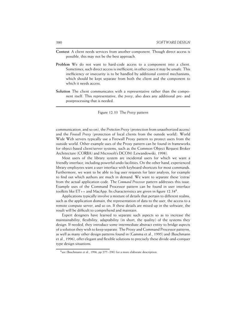
380 SOFTWARE DESIGN

Context A client needs services from another component. Though direct access is

possible, this may not be the best approach.

Problem We do not want to hard-code access to a component into a client.

Sometimes, such direct access is inefficient; in other cases it may be unsafe. This

inefficiency or insecurity is to be handled by additional control mechanisms,

which should be kept separate from both the client and the component to

which it needs access.

Solution The client communicates with a representative rather than the compo-

nent itself. This representative, the proxy, also does any additional pre- and

postprocessing that is needed.

Figure 12.33 The Proxy pattern

communication, and so on), the Protection Proxy (protection from unauthorized access)

and the Firewall Proxy (protection of local clients from the outside world). World

Wide Web servers typically use a Firewall Proxy pattern to protect users from the

outside world. Other example uses of the Proxy pattern can be found in frameworks

for object-based client/server systems, such as the Common Object Request Broker

Architecture (CORBA) and Microsoft’s DCOM (Lewandowski, 1998).

Most users of the library system are incidental users for which we want a

friendly interface, including powerful undo facilities. On the other hand, experienced

library employees want a user interface with keyboard shortcuts for most commands.

Furthermore, we want to be able to log user requests for later analysis, for example

to find out which authors are much in demand. We want to separate these ‘extras’

from the actual application code. The Command Processor pattern addresses this issue.

Example uses of the Command Processor pattern can be found in user interface

toolkits like ET++ and MacApp. Its characteristics are given in figure 12.348.

Applications typically involve a mixture of details that pertain to different realms,

such as the application domain, the representation of data to the user, the access to a

remote compute server, and so on. If these details are mixed up in the software, the

result will be difficult to comprehend and maintain.

Expert designers have learned to separate such aspects so as to increase the

maintainability, flexibility, adaptability (in short, the quality) of the systems they

design. If needed, they introduce some intermediate abstract entity to bridge aspects

of a solution they wish to keep separate. The Proxy and Command Processor patterns,

as well as many other design patterns found in (Gamma et al., 1995) and (Buschmann

et al., 1996), offer elegant and flexible solutions to precisely these divide-and-conquer

type design situations.

8see (Buschmann et al., 1996, pp 277--290) for a more elaborate description.

12.5. DESIGN PATTERNS 381

Context User interfaces which must be flexible or provide functionality that goes

beyond the direct handling of user functions. Examples are undo facilities or

logging functions.

Problem We want a well-structured solution for mapping an interface to the internal

functionality of a system. All ‘extras’ which have to do with the way user

commands are input, additional commands such as undo or redo, and any

non-application-specific processing of user commands, such as logging, should

be kept separate from the interface to the internal functionality.

Solution A separate component, the command processor, takes care of all commands.

The command processor component schedules the execution of commands,

stores them for later undo, logs them for later analysis, and so on. The actual

execution of the command is delegated to a supplier component within the

application.

Figure 12.34 The Command Processor pattern

Patterns describe common practices that have proven useful. Antipatterns describe

recurring practices that have proven to generate problems. Next to collections of

patterns, people have developed collections of mistakes often made, and described

them as antipatterns. Knowledge of antipatterns is useful during design to prevent

common pitfalls, and during evolution to improve an evolving design. In the latter

case, one actually searches for antipatterns and next applies a technique called

refactoring to improve the design; see also chapter 14. Descriptions of antipatterns

usually include the refactoring remedy. Some well-known antipatterns are:� The God Class. In this situation, there is one central class that is in control

and holds most responsibilities. It is linked to a lot of other classes that

execute relatively simple tasks. It is also known as The Blob. When such a

design is refactored, responsibilities are more evenly distributed. Note though

that we previously observed that centralized designs are often more easily

comprehended by novices.� Lava flow. At the code level, this amounts to dead code. Following the slogan

”If it ain’t broken, don’t touch it”, obsolete code and obsolete design elements

may be dragged along indefinitely.� Poltergeists. These are classes that have limited responsibilities and usually live

shortly. Their role often is to just start up other processes.� Golden Hammer. This occurs when an available solution is applied to a problem

that it does not really fit (”If the only available tool is a hammer, everything

else is a nail”). This antipattern is common practice when organizations feel

382 SOFTWARE DESIGN

they have to use database package X or interface toolkit Y, simply because

they have a license, or because their employees have deep knowledge of that

technology. At the level of an individual designer, it shows up as the obsessive

use of a small set of patterns.� Stovepipe. This phenomenon occurs if multiple systems are developed inde-

pendently, and each one uses its own set of technologies for the user interface,

database, platform, and the like. Integration and cooperation then becomes

difficult. Such a situation is often encountered when organizations merge or

different organizations link their information systems in a chain. At a more

local level it occurs if developers or design teams reinvent the wheel.� Swiss Army Knife. This is an excessively complex class interface. It occurs

when a designer wants to make a class as general and reusable as possible.

12.6 Design Documentation

A requirements specification is developed during requirements engineering. That

document serves a number of purposes. It specifies the users’ requirements and as such

it often has legal meaning. It is also the starting point for the design and thus serves

another class of user.

The same applies to the design documentation. The description of the design

serves different users, who have different needs. A proper organization of the design

documentation is therefore very important.

IEEE Standard 1016 discusses guidelines for the description of a design. This

standard mainly addresses the kind of information needed and its organization. For

the actual description of its constituent parts any existing design notation can be

used.

Barnard et al. (1986) distinguishes between seven user roles for the design

documentation:

1. The project manager needs information to plan, control and manage the

project. He must be able to identify each system component and understand

its purpose and function. He also needs information to make cost estimates and

define work packages.

2. The configuration manager needs information to be able to assemble the

various components into one system and to control changes.

3. The designer needs information about the function and use of each component

and its interfaces to other components.

4. The programmer must know about algorithms to be used, data structures, and

the kinds of interaction with other components.

12.6. DESIGN DOCUMENTATION 383

5. The unit tester must have detailed information about components, such as

algorithms used, required initialization, and data needed.

6. The integration tester must know about relations between components and

the function and use of the components involved.

7. The maintenance programmer must have an overview of the relations between

components. He must know how the user requirements are realized by the

various components. When changes are to be realized, he assumes the role of

the designer.

In IEEE Standard 1016, the project documentation is described as an information

model. The entities in this model are the components identified during the design

stage. We used the term ‘modules’ for these entities. Each of these modules has a

number of relevant attributes, such as its name, function, and dependencies. We may

now construct a matrix in which it is indicated which attributes are needed for which

user roles. This matrix is depicted in figure 12.35.

Attributes User roles

1 2 3 4 5 6 7

Identification � � � � � � �Type � � � �Purpose � � �Function � � �Subordinates �Dependencies � � �Interface � � � �Resources � � � �Processing � �Data � �

Figure 12.35 User roles and attributes (Source: H.J. Barnard et al, A recommended practice

for describing software designs: IEEE Standards Project 1016, IEEE Transactions on Software

Engineering SE-12, 2, Copyright 1986, IEEE.)

IEEE Standard 1016 distinguishes ten attributes. These attributes are minimally

required in each project. The documentation about the design process is strongly

related to the above design documentation. The design process documentation

includes information pertaining to, among others, the design status, alternatives that

have been rejected, and revisions that have been made. It is part of configuration

control, as discussed in chapter 4. The attributes from IEEE Standard 1016 are:

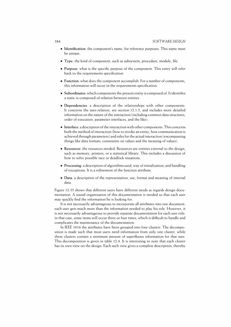
384 SOFTWARE DESIGN� Identification: the component’s name, for reference purposes. This name must

be unique.� Type: the kind of component, such as subsystem, procedure, module, file.� Purpose: what is the specific purpose of the component. This entry will refer

back to the requirements specification.� Function: what does the component accomplish. For a number of components,

this information will occur in the requirements specification.� Subordinates: which components the present entity is composed of. It identifies

a static is-composed-of relation between entities.� Dependencies: a description of the relationships with other components.

It concerns the uses-relation, see section 12.1.5, and includes more detailed

information on the nature of the interaction (including common data structures,

order of execution, parameter interfaces, and the like).� Interface: a description of the interaction with other components. This concerns

both the method of interaction (how to invoke an entity, how communication is

achieved through parameters) and rules for the actual interaction (encompassing

things like data formats, constraints on values and the meaning of values).� Resources: the resources needed. Resources are entities external to the design,

such as memory, printers, or a statistical library. This includes a discussion of

how to solve possible race or deadlock situations.� Processing: a description of algorithms used, way of initialization, and handling

of exceptions. It is a refinement of the function attribute.� Data: a description of the representation, use, format and meaning of internal

data.

Figure 12.35 shows that different users have different needs as regards design docu-

mentation. A sound organization of this documentation is needed so that each user

may quickly find the information he is looking for.

It is not necessarily advantageous to incorporate all attributes into one document:

each user gets much more than the information needed to play his role. However, it

is not necessarily advantageous to provide separate documentation for each user role:

in that case, some items will occur three or four times, which is difficult to handle and

complicates the maintenance of the documentation.

In IEEE 1016 the attributes have been grouped into four clusters. The decompo-

sition is made such that most users need information from only one cluster, while

these clusters contain a minimum amount of superfluous information for that user.

This decomposition is given in table 12.4. It is interesting to note that each cluster

has its own view on the design. Each such view gives a complete description, thereby

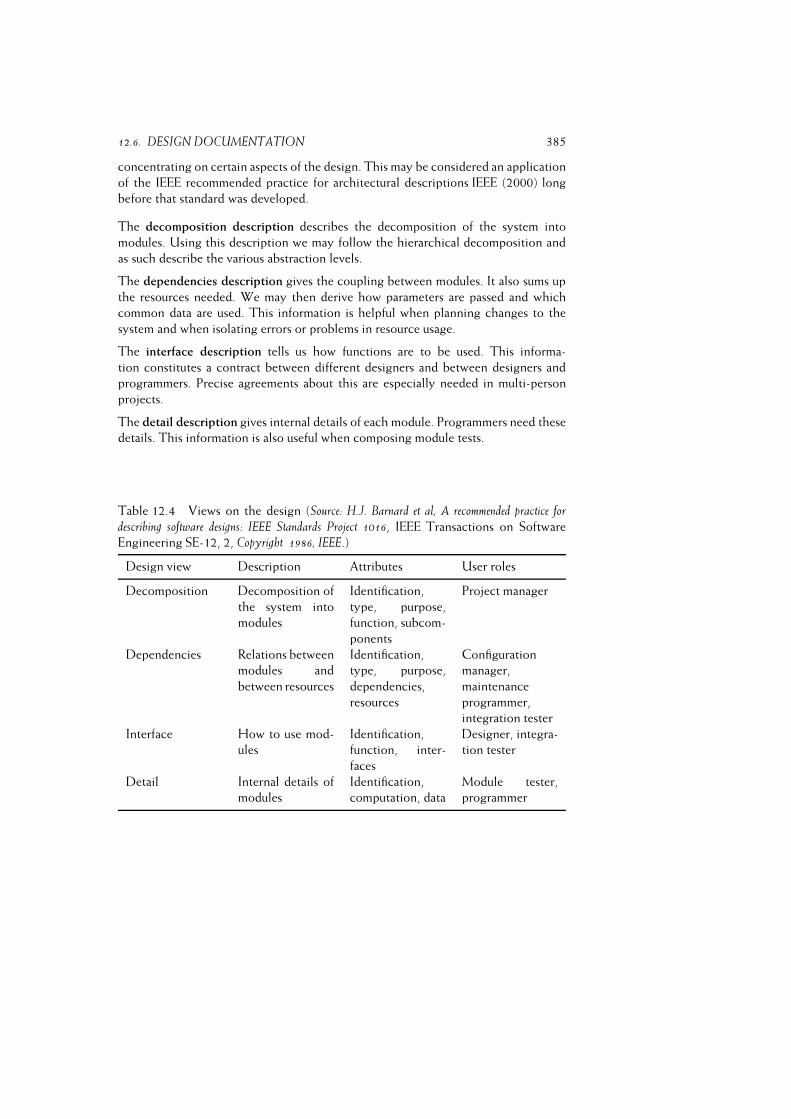
12.6. DESIGN DOCUMENTATION 385

concentrating on certain aspects of the design. This may be considered an application

of the IEEE recommended practice for architectural descriptions IEEE (2000) long

before that standard was developed.

The decomposition description describes the decomposition of the system into

modules. Using this description we may follow the hierarchical decomposition and

as such describe the various abstraction levels.

The dependencies description gives the coupling between modules. It also sums up

the resources needed. We may then derive how parameters are passed and which

common data are used. This information is helpful when planning changes to the

system and when isolating errors or problems in resource usage.

The interface description tells us how functions are to be used. This informa-

tion constitutes a contract between different designers and between designers and

programmers. Precise agreements about this are especially needed in multi-person

projects.

The detail description gives internal details of each module. Programmers need these

details. This information is also useful when composing module tests.

Table 12.4 Views on the design (Source: H.J. Barnard et al, A recommended practice for

describing software designs: IEEE Standards Project 1016, IEEE Transactions on Software

Engineering SE-12, 2, Copyright 1986, IEEE.)

Design view Description Attributes User roles

Decomposition Decomposition of

the system into

modules

Identification,

type, purpose,

function, subcom-

ponents

Project manager

Dependencies Relations between

modules and

between resources

Identification,

type, purpose,

dependencies,

resources

Configuration

manager,

maintenance

programmer,

integration tester

Interface How to use mod-

ules

Identification,

function, inter-

faces

Designer, integra-

tion tester

Detail Internal details of

modules

Identification,

computation, data

Module tester,

programmer

386 SOFTWARE DESIGN

12.7 Verification and Validation

Errors made at an early stage are difficult to repair and incur high costs if they are not

discovered until a late stage of development. It is therefore necessary to pay extensive

attention to testing and validation issues during the design stage.

The way in which the outcome of the design process can be subject to testing

strongly depends upon the way in which the design is recorded. If some formal

specification technique is used, the resulting specification can be tested formally.

It may also be possible to do static tests, such as checks for consistency. Formal

specifications may sometimes be executed, which offers additional ways to test the

system. Such prototypes are especially suited to test the user interface. Users often

have little idea of the possibilities to be expected and a specification-based prototype

offers good opportunities for aligning users’ requirements and designers’ ideas.

Often, the design is stated in less formal ways, limiting the possibilities for

testing to forms of reading and critiquing text, such as inspections and walkthroughs.

However, such design reviews provide an extremely powerful means for assessing

designs.

During the design process the system is decomposed into a number of modules.

We may develop test cases based on this process. These test cases may be used during

functional testing at a later stage. Conversely, the software architecture can be used

to guide the testing process. A set of scenarios of typical or anticipated future usage

can be used to test the quality of the software architecture.

A more comprehensive discussion of the various test techniques is given in

chapter 13.

12.8 Summary

Just like designing a house, designing software is an activity which demands creativity

and a fair dose of craftsmanship. The quality of the designer is of paramount

importance in this process. Mediocre designers will not deliver excellent designs.

The essence of the design process is that the system is decomposed into parts that

each have less complexity than the whole. Some form of abstraction is always used in

this process. We have identified several guiding principles for the decomposition of a

system into modules. These principles result in desirable properties for the outcome

of the design process, a set of modules with mutual dependencies:� Modules should be internally cohesive, i.e. the constituents of a module should

‘belong together’ and ‘be friends’. By identifying different levels of cohesion, a

qualitative notion of module cohesion is obtained.� The interfaces between modules should be as ‘thin’ as possible. Again, various

levels of module coupling have been identified, allowing for an assessment of

mutual dependencies between modules.

12.8. SUMMARY 387� Each module should hide one secret. Information hiding is a powerful design

principle, whereby each module is characterized by a secret which it hides

from its environment. Abstract data types are a prime example of the application

of this principle.� The structure of the system, depicted as a graph whose nodes and edges

denote modules and dependencies between modules, respectively, should have

a simple and regular shape. The most constrained form of this graph is a tree.

In a less constrained form the graph is acyclic, in which case the set of modules

can be split into a number of distinct layers of abstraction.

Abstraction is central to all of these features. In a properly-designed system we should

be able to concentrate on the relevant issues and ignore the irrelevant ones. This

is an essential prerequisite for comprehending a system, for implementing parts of

it successfully without having to consider design decisions made elsewhere, and for

implementing changes locally, thus allowing for a smooth evolution of the system.

The above features are highly interrelated and reinforce one another. Information

hiding results in modules with high cohesion and low coupling. Cohesion and

coupling are dual characteristics. A clear separation of concerns results in a neat

design structure.

We have discussed several measures to quantify properties of a design. The most

extensive research in this area concerns complexity metrics. These complexity metrics

concern both attributes of individual modules (called intra-modular attributes) and

attributes of a set of modules (called inter-module attributes).

A word of caution is needed, though. Software complexity is a very illusive notion,

which cannot be captured in a few simple numbers. Different complexity metrics

measure along different dimensions of what is perceived as complexity. Also, large

values for any such metric do not necessarily imply a bad design. There may be good

reasons to incorporate certain complex matters into one component.

A judicious and knowledgeable use of multiple design metrics is a powerful tool

in the hands of the craftsman. Thoughtless application, however, will not help. To

paraphrase Gunning, the inventor of the fog index (a popular readability measure for

natural language prose): design metrics can cause harm in misuse.

There exist a great many design methods. They consist of a number of guidelines,

heuristics and procedures on how to approach designing a system and notations to

express the result of that process. Design methods differ considerably in their pre-

scriptiveness, formality of notation, scope of application, and extent of incorporation

in a more general development paradigm. Several tentative efforts have been made to

compare design methods along different dimensions.

We discussed four design methods in this chapter:

– functional decomposition,

– data flow design,

388 SOFTWARE DESIGN

– data structure design, and

– object-oriented design.

The first three design methods have been around longest. Object-oriented analysis

and design came later, and this is now the most widely used approach, partly caused

also by the popularity of the notations of the Unified Modeling Language (UML), its

associated tools, and full-scale development methods like RUP.

Proponents of object-oriented methods have claimed a number of advantages of

the object-oriented approach over the more traditional, function-oriented, approaches

to design:� The object-oriented approach is more natural. It fits the way we view the world

around us. The concepts that show up in the analysis model have a direct

counterpart in the UoD being modeled, thus providing a direct link between

the model and the world being modeled. This makes it easier for the client to

comprehend the model and discuss it with the analyst.� The object-oriented approach focuses on structuring the problem rather than

any particular solution to it. This point is closely related to the previous one.

In designs based on the functional paradigm the modules tend to correspond

to parts of a solution to the problem. It may then not be easy to relate these

modules to the original problem. The result of an object-oriented analysis

and design is a hierarchy of objects with their associated attributes which still

resembles the structure of the problem space.� The object-oriented approach provides for a smoother transition from require-

ments analysis to design to code. In our discussion of the object-oriented

approach it is often difficult to strictly separate UoD modeling aspects from

design aspects. The object hierarchy that results from this process can be

directly mapped onto the class hierarchy of the implementation (provided

the implementation language is object-oriented too). The attributes of objects

become encapsulated by services provided by the objects in the implementation.� The object-oriented approach leads to more flexible systems that are easier to

adapt and change. Because the real-world objects have a direct counterpart in the

implementation, it becomes easy to link change requests to the corresponding

program modules. Through the inheritance mechanism, changes can often be

realized by adding another specialized object rather than through tinkering

with the code. For example, if we wish to extend our system dealing with

furniture by adding another type of chair, say armchair, we do so by defining

a new object ArmChair, together with its own set of attributes, as another

specialization of Chair.� The object-oriented approach promotes reuse by focusing on the identification

of real-world objects from the application domain. In contrast, more traditional

12.8. SUMMARY 389

approaches focus on identifying functions. In an evolving world, the objects

tend to be stable, while the functions tend to change. For instance, in an office

environment the functions performed are likely to change with time, but there

will always be letters, folders, and so on. Thus, an object-oriented design is less

susceptible to changes in the world being modeled.� The inheritance mechanism adds to reusability. New objects can be created

as specializations of existing objects, inheriting attributes from the existing

objects. At the implementation level, this kind of reuse is accomplished

through code sharing. The increasing availability of class libraries contributes

to this type of code reuse.� Objects in an object-oriented design encapsulate abstract data types. As such,

an object-oriented design potentially has all the right properties (information

hiding, abstraction, high cohesion, low coupling, etc).

The object-oriented approach, however, does not by definition result in a good

design. It is a bit too naive to expect that the identification of domain-specific entities

is all there is to good design. The following issues must be kept in mind:� There are other objects besides the ones induced by domain concepts. Objects

that have to do with system issues such as memory management or error

recovery do not naturally evolve from the modeling of the UoD. Likewise,

‘hypothetical’ objects that capture implicit knowledge from the application

domain may be difficult to identify.� The separation of concerns that results from the encapsulation of both state

and behavior into one component need not be the one that is most desirable.

For example, for many an object it might be necessary to be able to present

some image of that object to the user. In a straightforward application of the

object-oriented method, this would result in each object defining its own ways

for doing so. This, however, is against good practices of system design, where

we generally try to isolate the user interface from the computational parts. A

clearly identifiable user interface component adds to consistency and flexibility.� With objects too, we have to consider the uses relation. An object uses another

object if it requests a service from that other object. It does so by sending

a message. The bottom-up construction of a collection of objects may result

in a rather loosely-coupled set, in which objects freely send messages to

other objects. With a nod at the term spaghetti-code to denote overly complex

control patterns in programs, this is known as the ravioli problem (or antipatern).

If objects have a complicated usage pattern, it is difficult to view one object

without having to consider many others as well.

A design pattern is a recurring structure of communicating components that solves a

general design problem within a particular context. A design pattern thus encompasses

390 SOFTWARE DESIGN

more than a single component. It involves some, usually 2--5, communicating

components which together solve a problem. The problem that the pattern solves is a

general, recurring one, which can be characterized by the context in which it arises.

A design pattern differs from an architectural style in that it does not address the

structure of a complete system, but only that of a few (interacting) components.

Design patterns may thus be termed micro-architectures. Not surprisingly, the good

things about design patterns are essentially the same as those listed for software

architectures in chapter 11.

Design patterns describe best practices. They represent the collective experience

of some of the most experienced and successful software designers. Likewise, antipat-

terns describe widely shared bad experiences. The description of both patterns and

antipatterns, as found in textbooks, is the result of endless carving and smoothing.

Some are the outcome of writers’ workshops, a format commonly used to review

literature, suggesting that we should review software literature with a profoundness

like that used to review poetry (as a consequence, these writers’ workshops are also

known as workers’ write shops).

The distinction between the notions software architecture and design pattern is

by no means sharp. Some authors for example use the term ‘architectural pattern’ to

denote the architectural styles we discussed in section 11.4. The notions application

framework and idiom are generally used to denote a software architecture and design

pattern, respectively, at a more concrete, implementation-specific level. But again,

the distinction is not sharp.

Finally, the design itself must also be documented. IEEE Standard 1016 may

serve as a guideline for this documentation. It lists a number of attributes for each

component of the design. These attributes may be clustered into four groups, each

of which represents a certain view on the design. This resembles the way IEEE 1471

advocates to document a software architecture.

Unfortunately, the design documentation typically describes only the design result

and not the process that led to that particular result. Yet, information about choices

made, alternatives rejected, and deliberations on the design decisions is a valuable

additional source of information when a design is to be implemented, assessed, or

changed.

12.9 Further Reading

Budgen (2003) is a good textbook on software design. I found the ‘software as a

wicked problem’ analogy in that text. Bergland and Gordon (1981) and Freeman

and Wasserman (1983) are compilations of seminal articles on software design. For

an interesting discussion on the ‘Scandinavian’ approach to system development, see

(Floyd et al., 1989) or (CACM, 1993a). Wieringa (1998) provides an extensive survey

of both classical and object-oriented design methods and their notations.

The classic text on Structured Analysis and Design is (Yourdon and Constantine,

1975). Other names associated with the development of SA/SD are DeMarco

12.9. FURTHER READING 391

(DeMarco, 1979) and Gane and Sarson (Gane and Sarson, 1979).

For a full exposition of JSP, the reader is referred to (Jackson, 1975) or (King,

1988). JSP is very similar to a method developed by J.-D. Warnier in France at

about the same time (Warnier, 1974). The latter is known as Logical Construction of

Programs (LCP) or the Warnier--Orr method, after Ken Orr who was instrumental

in the translation of Warnier’s work. For a full exposition of JSD, see (Jackson, 1983),

(Cameron, 1989) or (Sutcliffe, 1988). The graphical notations used in this chapter

are those of (Sutcliffe, 1988).

Booch’ method for object-oriented analysis and design is discussed in (Booch,

1994). Fusion is described in (Coleman et al., 1994). Updates to this 1994 version

can be found in (Coleman, 1996). RUP is discussed in (Kruchten, 2003). A critical

discussion of the differences and similarities between object-oriented analysis and

object-oriented design is given in (Davis, 1995) and (Hødalsvik and Sindre, 1993).

Fenton and Pfleeger (1996) presents a rigorous approach to the topic of software

metrics. The authors explain the essentials of measurement theory and illustrate

these using a number of proposed metrics (including those for complexity, quality

assessment, and cost estimation).

Cohesion and coupling were introduced in (Yourdon and Constantine, 1975).

Efforts to objectify these notions can be found in (Offutt et al., 1993), (Patel et al.,

1992) and(Xia, 2000). Darcy (2005) describes empirical studies to validate the

importance of weak coupling and strong cohesion.

Halstead’s method, ‘software science’, is described in (Halstead, 1977) and

(Fitzsimmons and Love, 1978). Positive evidence of its validity is reported in (Curtis

et al., 1979) and (Elshoff, 1976). A good overview of the criticism of this method

(as well as McCabe’s cyclomatic complexity and Henri and Kafura’s information flow

metric) is given in (Shepperd and Ince, 1993). McCabe’s cyclomatic complexity is

introduced in (McCabe, 1976). In most discussions of this metric, the wrong formula

is used; see exercise 24 or (Henderson Sellers, 1992). Discussions in favor of using a

(cyclomatic) complexity density metric can be found in (Mata-Toledo and Gustafson,

1992) and (Hops and Sherif, 1995).

Definitions of the object-oriented metrics introduced in section 12.1.6 can be

found in (Chidamber and Kemerer, 1994). A critical assessment of these metrics is

given in (Hitz and Montazeri, 1996) and (Churcher and Shepperd, 1995). To meet

some of this criticism, we have adopted the definition of LCOM, as suggested in (Li

and Henry, 1993). Experiments to validate the Chidamber--Kemerer metrics suite

are reported in (Succi et al., 2003), (Darcy and Kemerer, 2005) and (Gyimothy et al.,

2005).

Design patterns have their origin in the work of Cunningham and Beck, who

developed patterns for user interfaces in Smalltalk, such as ‘no more than three panes

per window’ (Power and Weiss, 1987, p. 16). MVC was first used in the Smalltalk

environment (Krasner and Pope, 1988). Since that time, the topic has drawn a lot of

attention, especially in object-oriented circles. A major collection of design patterns

was published by the ‘Gang of Four’ in 1995 (Gamma et al., 1995). Another good

392 SOFTWARE DESIGN

collection of design patterns can be found in (Buschmann et al., 1996). The latter text

has a somewhat less object-oriented perspective than (Gamma et al., 1995). Brown

et al. (1998) describes a collection of well-known antipatterns. Since 1994, there

has been an annual conference on Pattern Languages of Programming (PLOP). The

format for describing patterns has not only been used for design patterns; there are

also collections of analysis patterns, process patterns, test patterns, etc.

Exercises

1. What is the difference between procedural abstraction and data abstraction?

2. List and explain Yourdon and Constantine’s seven levels of cohesion.

3. Explain the notions cohesion and coupling.

4. In what sense are the various notions of coupling technology-dependent?

5. What is the essence of information hiding?

6. Give an outline of Halstead’s software science.

7. Determine the cyclomatic complexity of the following program:

no 6:= true; sum:= 0;for i to no of courses do

if grade[i] < 7 then no 6:= false endif;sum:= sum + grade[i]

endfor;average:= sum / no of courses;if average � 8 and no 6

then print(”with distinction”)endif;

8. Would the cyclomatic complexity be any different if the last if-statement

were written as follows:

if average � 8 thenif no 6

then print(”with distinction”)endif

endif;

Does this concur with your own ideas of a control complexity measure, i.e.

does it fulfill the representation condition?

12.9. FURTHER READING 393

9. Give the formula and a rationale for the information flow complexity metric.

10. Is cyclomatic complexity a good indicator of system complexity?

11. Draw the call graphs for a non-trivial program you have written, and determine

its tree impurity. Does the number obtained agree with our intuitive idea

about the ‘quality’ of the decomposition?

12. Compute Henri and Kafura’s information flow metric for the design of two

systems you have been involved in. Do these numbers agree with our intuitive

understanding?

13. Why is DIT -- the depth of a class in the inheritance tree -- a useful metric to

consider when assessing the quality of an object-oriented system?

14. What does RFC -- Response For a Class -- measure?

15. How does the Law of Demeter relate to the maintainability of object-oriented

systems?

16. Discuss the relative merits and drawbacks of deep and narrow versus wide

and shallow inheritance trees.

17. What is functional decomposition?

18. Give a global sketch of the Data Flow Design method.

19. Explain what a structure clash is in JSP.

20. What is the main difference between problem-oriented and product-oriented

design methods?

21. Discuss the general flavor of RUP˘s Analysis and Design workflow.

22. What are the differences between object-oriented design and the simple

application of the information hiding principle?

23. What are the properties of a design pattern?

24. ~ Make it plausible that the formula for the cyclomatic complexity should

read CV = e� n+ p+ 1 rather than CV = e� n+ 2p. (Hint: consider

the following program:

beginif A then B else C endif;call P;print(”done”)

end;

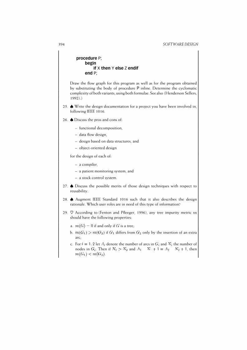
394 SOFTWARE DESIGN

procedure P;begin

if X then Y else Z endifend P;

Draw the flow graph for this program as well as for the program obtained

by substituting the body of procedure P inline. Determine the cyclomatic

complexity of both variants, using both formulae. See also (Henderson Sellers,

1992).)

25. � Write the design documentation for a project you have been involved in,

following IEEE 1016.

26. � Discuss the pros and cons of:

– functional decomposition,

– data flow design,

– design based on data structures, and

– object-oriented design

for the design of each of:

– a compiler,

– a patient monitoring system, and

– a stock control system.

27. � Discuss the possible merits of those design techniques with respect to

reusability.

28. � Augment IEEE Standard 1016 such that it also describes the design

rationale. Which user roles are in need of this type of information?

29. ~ According to (Fenton and Pfleeger, 1996), any tree impurity metric mshould have the following properties:

a. m(G) = 0 if and only if G is a tree;

b. m(G1) > m(G2) if G1 differs from G2 only by the insertion of an extra

arc;

c. For i = 1; 2 let Ai denote the number of arcs in Gi and Ni the number of

nodes in Gi. Then if N1 > N2 and A1 �N1 + 1 = A2 �N2 + 1, thenm(G1) < m(G2).

12.9. FURTHER READING 395

d. For all graphs G, m(G) � m(KN) = 1 where N = number of nodes of Gand KN is the (undirected) complete graph of N nodes.

Give an intuitive rationale for these properties. Show that the tree impurity

metric discussed in section 12.1.5 has these properties.

30. ~ Extend the object model of figure 12.27 such that it also models user

queries to the catalog.

31. ~ Extend the model from the previous exercise such that it also includes the

attributes and services of objects.

32. � Write an essay on the differences and similarities of analysis and design

activities in object-oriented analysis and design.

33. ~ Why would object-oriented design be more ‘natural’ than, say, data flow

design?

34. �Discuss the assertion ‘The view that object-oriented methods make change

easy is far too simplistic’. Consult (Lubars et al., 1992), who found that

changes to object models were fairly localized, whereas changes to behavior

models had more far-reaching consequences.

35. ~ The Document--View pattern relaxes the separation of view and controller

in MVC. Describe the Document--View pattern in terms of the context

in which it arises, the problem addressed, and its solution. Compare your

solution with the Observer pattern in (Gamma et al., 1995, p. 293).

36. ~ How do design patterns impact the quality of a design?

13

Software Testing

LEARNING OBJECTIVES� To be aware of the major software testing techniques� To see how different test objectives lead to the selection of different testing

techniques� To appreciate a classification of testing techniques, based on the objectives

they try to reach� To be able to compare testing techniques with respect to their theoretical

power as well as practical value� To understand the role and contents of testing activities in different life cycle

phases� To be aware of the contents and structure of the test documentation� To be able to distinguish different test stages� To be aware of some mathematical models to estimate the reliability of software

397

Testing should not be confined to merely executing a system to see whether

a given input yields the correct output. During earlier phases, intermediate

products can, and should, be tested as well. Good testing is difficult. It

requires careful planning and documentation. There exist a large number of

test technieques. We discuss the major classes of test techniques with their

characteristics.

Suppose you are asked to answer the kind of questions posed in (Baber, 1982):

– Would you trust a completely-automated nuclear power plant?

– Would you trust a completely-automated pilot whose software was written by

yourself? What if it was written by one of your colleagues?

– Would you dare to write an expert system to diagnose cancer? What if you are

personally held liable in a case where a patient dies because of a malfunction of

the software?

You will (probably) have difficulties answering all these questions in the affirmative.

Why? The hardware of an airplane probably is as complex as the software for an

automatic pilot. Yet, most of us board an airplane without any second thoughts.

As our society’s dependence on automation ever increases, the quality of the

systems we deliver increasingly determines the quality of our existence. We cannot

hide from this responsibility. The role of automation in critical applications and the

threats these applications pose should make us ponder. ACM Software Engineering Notesruns a column ‘Risks to the public in computer systems’ in which we are told of

numerous (near) accidents caused by software failures. The discussion on software

reliability provoked by the Strategic Defense Initiative is a case in point (Parnas,

1985; Myers, 1986; Parnas, 1987). Discussions, such as those about the Therac-25

accidents or the maiden flight of the Ariane 5 (see section 1.4), should be compulsory

reading for every software engineer.

Software engineering is engineering. Engineers aim for the perfect solution, but

know this goal is generally unattainable. During software construction, errors are

made. To locate and fix those errors through excessive testing is a laborious affair and

mostly not all the errors are found. Good testing is at least as difficult as good design.

With the current state of the art we are not able to deliver fault-free software.

Different studies indicate that 30--85 errors per 1000 lines of source code are made.

These figures seem not to improve over time. During testing, quite a few of those

errors are found and subsequently fixed. Yet, some errors do remain undetected.

Myers (1986) gives examples of extensively-tested software that still contains 0.5--3

errors per 1000 lines of code. A fault in the seat reservation system of a major airline

company incurred a loss of $50M in one quarter. The computerized system reported

that cheap seats were sold out while this was in fact not the case. As a consequence,

398 SOFTWARE TESTING

clients were referred to other companies. The problems were not discovered until

quarterly results were found to lag considerably behind those of their competitors.

Testing is often taken to mean executing a program to see whether it produces

the correct output for a given input. This involves testing the end-product, the

software itself. As a consequence, the testing activity often does not get the attention

it deserves. By the time the software has been written, we are often pressed for time,

which does not encourage thorough testing.

Postponing test activities for too long is one of the most severe mistakes often

made in software development projects. This postponement makes testing a rather

costly affair. Figure 13.1 shows the results of an early study by Boehm about the

cost of error correction relative to the phase in which the error is discovered. This

picture shows that errors which are not discovered until after the software has

become operational incur costs that are 10 to 90 times higher than those of errors

that are discovered during the design phase. This ratio still holds for big and critical

systems (Boehm and Basili, 2001). For small, noncritical systems the ratio may be

more like 1 to 5.

The development methods and techniques that are applied in the pre-implementation

phases are least developed, relatively. It is therefore not surprising that most of the

errors are made in those early phases. An early study by Boehm showed that over

60% of the errors were introduced during the design phase, as opposed to 40% during

implementation (Boehm, 1975). Worse still, two-thirds of the errors introduced at the

design phase were not discovered until after the software had become operational.

It is therefore incumbent on us to plan carefully our testing activities as early

as possible. We should also start the actual testing activities at an early stage. An

extreme form hereof is test-driven development, one of the practices of XP, in

which development starts with writing tests. If we do not start testing until after

the implementation stage, we are really far too late. The requirements specification,

design, and design specification may also be tested. The rigor hereof depends on the

form in which these documents are expressed. This has already been hinted at in

previous chapters. In section 13.2, we will again highlight the various verification and

validation activities that may be applied at the different phases of the software life

cycle. The planning and documentation of these activities is discussed in section 13.3.

Before we decide upon a certain approach to testing, we have to determine our

test objectives. If the objective is to find as many errors as possible, we will opt

for a strategy which is aimed at revealing errors. If the objective is to increase our

confidence in the proper functioning of the software we may well opt for a completely

different strategy. So the objective will have its impact on the test approach chosen,

since the results have to be interpreted with respect to the objectives set forth.

Different test objectives and the degree to which test approaches fit these objectives

are the topic of section 13.1.

Testing software shows only the presence of errors, not their absence. As such,

it yields a rather negative result: up to now, only n (n � 0) errors have been found.

Only when the software is tested exhaustively are we certain about its functioning

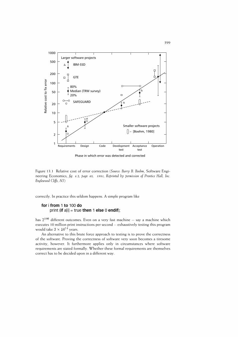
399

Figure 13.1 Relative cost of error correction (Source: Barry B. Boehm, Software Engi-

neering Economics, fig. 4.2, page 40, 1981, Reprinted by permission of Prentice Hall, Inc.Englewood Cliffs, NJ)

correctly. In practice this seldom happens. A simple program like

for i from 1 to 100 doprint (if a[i] = true then 1 else 0 endif);

has 2100 different outcomes. Even on a very fast machine -- say a machine which

executes 10 million print instructions per second -- exhaustively testing this program

would take 3� 1014 years.

An alternative to this brute force approach to testing is to prove the correctness

of the software. Proving the correctness of software very soon becomes a tiresome

activity, however. It furthermore applies only in circumstances where software

requirements are stated formally. Whether these formal requirements are themselves

correct has to be decided upon in a different way.

400 SOFTWARE TESTING

We are thus forced to make a choice. It is of paramount importance to choose

a sufficiently small, yet adequate, set of test cases. Test techniques may be classified

according to the criterion used to measure the adequacy of a set of test cases:

Coverage-based testing In coverage-based testing, testing requirements are specified

in terms of the coverage of the product (program, requirements document, etc.) to

be tested. For example, we may specify that all statements of the program should

be executed at least once if we run the complete test set, or that all elementary

requirements from the requirements specification should be exercised at least once.

Fault-based testing Fault-based techniques focus on detecting faults. The fault

detecting ability of the test set then determines its adequacy. For example, we may

artificially seed a number of faults in a program, and then require that a test set reveal

at least, say, 95% of these artificial faults.

Error-based testing Error-based techniques focus on error-prone points, based on

knowledge of the typical errors that people make. For example, off-by-1 errors are

often made at boundary values such as 0 or the maximum number of elements in a

list, and we may specifically aim our testing effort at these boundary points.

Alternatively, we may classify test techniques based on the source of information

used to derive test cases:

Black-box testing, also called functional or specification-based testing. In black-box

testing, test cases are derived from the specification of the software, i.e. we do not

consider implementation details.

White-box testing, also called structural or program-based testing. This is a com-

plementary approach, in which we do consider the internal logical structure of the

software in the derivation of test cases.

We will use the first classification, and discuss different techniques for coverage-based,

fault-based and error-based testing in sections 13.5--13.7. These techniques involve

the actual execution of a program. Manual techniques which do not involve program

execution, such as code reading and inspections, are discussed in section 13.4. In

section 13.8 we assess some empirical and theoretical studies that aim to put these

different test techniques in perspective.

The above techniques are applied mainly at the component level. This level of

testing is often done concurrently with the implementation phase. It is also called

unit testing. Besides the component level, we also have to test the integration of a

set of components into a system. Possibly also, the final system will be tested once

more under direct supervision of the prospective user. In section 13.9 we will sketch

these different test phases.

At the system level, the goal pursued often shifts from detecting faults to

building trust, by quantitatively assessing reliability. Software reliability is discussed

in section 13.10.

13.1. TEST OBJECTIVES 401

13.1 Test Objectives

Until now, we have not been very precise in our use of the notion of an ‘error’. In order

to appreciate the following discussion, it is important to make a careful distinction

between the notions error, fault and failure. An error is a human action that produces an

incorrect result. The consequence of an error is software containing a fault. A fault

thus is the manifestation of an error. If encountered, a fault may result in a failure.1

So, what we observe during testing are failures. These failures are caused by faults,

which are in turn the result of human errors. A failure may be caused by more than

one fault, and a fault may cause different failures. Similarly, the relation between

errors and faults need not be 1--1.

One possible aim of testing is to find faults in the software. Tests are then intended

to expose failures. It is not easy to give a precise, unique, definition of the notion

of failure. A programmer may take the system’s specification as reference point. In

this view, a failure occurs if the software does not meet the specifications. The user,

however, may consider the software erroneous if it does not match expectations.

‘Failure’ thus is a relative notion. If software fails, it does so with respect to something

else (a specification, user manual, etc). While testing software, we must always be

aware of what the software is being tested against.

In this respect a distinction is often made between ‘verification’ and ‘validation’.

The IEEE Glossary defines verification as the process of evaluating a system or

component to determine whether the products of a given development phase satisfy

the conditions imposed at the start of that phase. Verification thus tries to answer the

question: Have we built the system right?

The term ‘validation’ is defined in the IEEE Glossary as the process of evaluating a

system or component during or at the end of the development process to determine

whether it satisfies specified requirements. Validation then boils down to the question:

Have we built the right system?

Even with this subtle distinction in mind, the situation is not all that clear-cut.

Generally, a program is considered correct if it consistently produces the right output.

We may, though, easily conceive of situations where the programmer’s intention is not

properly reflected in the program but the errors simply do not manifest themselves.

An early empirical study showed that many faults are never activated during the

lifetime of a system (Adams, 1984). Is it worth fixing those faults? For example, some

entry in a case statement may be wrong, but this fault never shows up because it

happens to be subsumed by a previous entry. Is this program correct, or should it

rather be classified as a program with a ‘latent’ fault? Even if it is considered correct

1The IEEE Glossary of Software Engineering Terminology gives four definitions of the word ‘error’. To

distinguish between these definitions, the words ‘error’, ‘fault’, ‘failure’ and ‘mistake’ are used. The word‘error’ in the Glossary is used to denote a measurement error, while ‘mistake’ is used to denote a human

error. Though ‘mistake’ has the advantage of being less condemning, we follow the accepted software

engineering literature in this respect. Our definitions of ‘fault’ and ‘failure’ are the same as those in the

Glossary.

402 SOFTWARE TESTING

within the context at hand, chances are that we get into trouble if the program is

changed or parts of it are reused in a different environment.

As an example, consider the maiden flight of the Ariane 5. Within 40 seconds after

take-off, at an altitude of 3700 meters, the launcher exploded. This was ultimately

caused by an overflow in a conversion of a variable from a 64-bit floating point

number to a 16-bit signed integer. The piece of software containing this error was

reused from the Ariane 4 and had never caused a problem in any of the Ariane 4 flights.

This is explained by the fact that the Ariane 5 builds up speed much faster than the

Ariane 4, which in turn resulted in excessive values for the parameter in question; see

also section 1.4.1.

With the above definitions of error and fault, such programs must be considered

faulty, even if we cannot devise test cases that reveal the faults. This still leaves

open the question of how to define errors. Since we cannot but guess what the

programmer’s real intentions were, this can only be decided upon by an oracle.

Given the fact that exhaustive testing is not feasible, the test process can be

thought of as depicted in figure 13.2. The box labeled P denotes the object (program,

design document, etc.) to be tested. The test strategy involves the selection of a

subset of the input domain. For each element of this subset, P is used to ‘compute’ the

corresponding output. The expected output is determined by an oracle, something

outside the test activity. Finally, the two answers are compared.

Figure 13.2 Global view of the test process

The most crucial step in this process is the selection of the subset of the input

domain which will serve as the test set. This test set must be adequate with respect

to some chosen test criterion. In section 13.1.1 we elaborate upon the notion of test

adequacy.

Test techniques generally use some systematic means to derive test cases. These

test cases are meant to provoke failures. Thus, the main objective is fault detection.

Alternatively, our test objective could be to increase our confidence in failure-free

behavior. These quite different test objectives, and their impact on the test selection

problem, are the topic of section 13.1.2.

13.1. TEST OBJECTIVES 403

To test whether the objectives are reached, test cases are tried in order that faults

manifest themselves. A quite different approach is to view testing as fault prevention.

This leads us to another dimension of test objectives, which to a large extent parallels

the evolution of testing strategies over the years. This evolution is discussed in

section 13.1.3.

Finally, the picture so far considers each fault equally hazardous. In reality,

there are different types of fault, and some faults are more harmful than others. All

techniques to be discussed in this chapter can easily be generalized to cover multiple

classes of faults, each with its own acceptance criteria.

Some faults are critical and we will have to exert ourselves in order to find those

critical faults. Special techniques, such as fault tree analysis, have been developed

to this end. Using fault tree analysis, we try to derive a contradiction by reasoning

backwards from a given, undesirable, end situation. If such a contradiction can be

derived, we have shown that that particular situation can never be reached.

13.1.1 Test Adequacy Criteria

Consider the program text in figure 13.3 and a test set S containing just one test case:

n = 2, A[1] = 10, A[2] = 5

If we execute the program using S, then all statements are executed at least once.

If our criterion to judge the adequacy of a test set is that 100% of the statements

are executed, then S is adequate. If our criterion is that 100% of the branches are

executed, then S is not adequate, since the (empty) else-branch of the if-statement is

not executed by S.

A test adequacy criterion thus specifies requirements for testing. It can be used

in different ways: as stopping rule, as measurement, or as test case generator. If a test

adequacy criterion is used as a stopping rule, it tells us when sufficient testing has

been done. If statement coverage is the criterion, we may stop testing if all statements

have been executed by the tests done so far. In this view, a test set is either good

or bad; the criterion is either met, or it isn’t. If we relax this requirement a bit and

use, say, the percentage of statements executed as a test quality criterion, then the

test adequacy criterion is used as a measurement. Formally, it is a mapping from the

test set to the interval [0; 1℄. Note that the stopping rule view is in fact a special

case of the measurement view. Finally, the test adequacy criterion can be used in the

test selection process. If a 100% statement coverage has not been achieved yet, an

additional test case is selected that covers one or more statements yet untested. This

generative view is used in many test tools.

Test adequacy criteria are closely linked to test techniques. For example, coverage-

based test techniques keep track of which statements, branches, and so on, are

executed, and this gives us an easy handle to determine whether a coverage-based

adequacy criterion has been met or not. The same test technique, however, does not

help us in assessing whether all error-prone points in a program have been tested.

404 SOFTWARE TESTING

In a sense, a given test adequacy criterion and the corresponding test technique are

opposite sides of the same coin.

13.1.2 Fault Detection Versus Confidence Building

Failures are needles in the haystack of the input domain

(Hamlet and Taylor, 1990)

Suppose we wish to test some component P which sorts an array A[1..n] of integers,

1 � n �1000. Since exhaustive testing is not feasible, we are looking for a strategy

in which only a small number of tests are exercised. One possible set of test cases is

the following:

Let n assume values 0, 1, 17 and 1000. For each of n = 17 and n = 1000, choose three

values for the array A:

– A consists of randomly selected integers;

– A is sorted in ascending order;

– A is sorted in descending order.

In following this type of constructive approach, the input domain is partitioned

into a finite, small number of subdomains. The underlying assumption is that these

subdomains are equivalence classes, i.e. from a testing point of view each member

from a given subdomain is as good as any other. For example, we have tacitly assumed

that one random array of length 17 is as good a test as any other random array of

length i with 1 < i < 1000.

Suppose the actual sorting algorithm used is the one from figure 13.3. If the tests

use positive integers only, the output will be correct. The output will not be correct

if a test input happens to contain negative integers.

The test set using positive integers only does not reveal the fault because the

inputs in the subdomains are not really interchangeable (instead of comparing the

values of array entries, the algorithm compares their absolute values). Any form of

testing which partitions the input domain works perfectly if the right subdomains

are chosen. In practice however, we generally do not know where the needles are

hidden, and the partition of the input domain is likely to be imperfect.

Both functional and structural testing schemes use a systematic means to determine

subdomains. They often use peculiar inputs to test peculiar cases. Their intention is to

provoke failure behavior. Their success hinges on the assumption that we can indeed

identify subdomains with a high failure probability. Though this is a good strategy

for fault detection, it does not necessarily inspire confidence.

The user of a system is interested in the probability of failure-free behavior.

Following this line of thought, we are not so much interested in the faults themselves,

but rather in their manifestations. A fault which frequently manifests itself will in

13.1. TEST OBJECTIVES 405

procedure selection-sort (A, n);integer i, j, small, temp;begin

for i:= 1 to n-1 dosmall:= i;for j:= i+1 to n do

if abs(A[j]) < abs(A[small]) then small:= j endifenddo;temp:= A[i]; A[i]:= A[small]; A[small]:= temp

enddoend selection-sort;

Figure 13.3 Erroneous selection sort procedure

general cause more damage than a fault which seldom shows up. This is precisely

what we hinted at above when we discussed fault detection and confidence building

as possible test objectives.

If failures are more important than faults, the goal pursued during the test phase

may also change. In that case, we will not pursue the discovery of as many faults

as possible but will strive for a high reliability. Random testing does not work all

that well if we want to find as many faults as possible -- hence the development of

different test techniques. When pursuing a high reliability, however, it is possible to

use random input.

In order to obtain confidence in the daily operation of a software system, we have

to mimic that situation. This requires the execution of a large number of test cases

that represent typical usage scenarios. Random testing does at least as good a job in

this respect as any form of testing based on partitioning the input domain.

This approach has been applied in the Cleanroom development method. In this

method, the development of individual components is done by programmers who

are not allowed to actually execute their code. The programmer must then convince

himself of the correctness of his components using manual techniques such as stepwise

abstraction (see also section 13.4).

In the next step, these components are integrated and tested by someone else.

The input for this process is generated according to a distribution which follows the

expected operational use of the system. During this integration phase, one tries to

reach a certain required reliability level. Experiences with this approach are positive.

The quantitative assessment of failure probability brings us into the area of

software reliability. Section 13.10 is devoted to this topic.

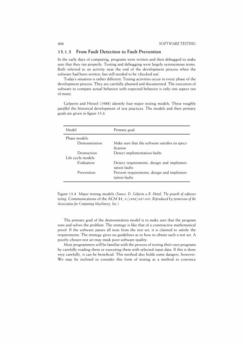
406 SOFTWARE TESTING

13.1.3 From Fault Detection to Fault Prevention

In the early days of computing, programs were written and then debugged to make

sure that they ran properly. Testing and debugging were largely synonymous terms.

Both referred to an activity near the end of the development process when the

software had been written, but still needed to be ‘checked out’.

Today’s situation is rather different. Testing activities occur in every phase of the

development process. They are carefully planned and documented. The execution of

software to compare actual behavior with expected behavior is only one aspect out

of many.

Gelperin and Hetzel (1988) identify four major testing models. These roughly

parallel the historical development of test practices. The models and their primary

goals are given in figure 13.4.

Model Primary goal

Phase models

Demonstration Make sure that the software satisfies its speci-

fication

Destruction Detect implementation faults

Life cycle models

Evaluation Detect requirements, design and implemen-

tation faults

Prevention Prevent requirements, design and implemen-

tation faults

Figure 13.4 Major testing models (Source: D. Gelperin & B. Hetzel, The growth of software

testing, Communications of the ACM 31, 6 (1988) 687-695. Reproduced by permission of the

Association for Computing Machinery, Inc.)

The primary goal of the demonstration model is to make sure that the program

runs and solves the problem. The strategy is like that of a constructive mathematical

proof. If the software passes all tests from the test set, it is claimed to satisfy the

requirements. The strategy gives no guidelines as to how to obtain such a test set. A

poorly-chosen test set may mask poor software quality.

Most programmers will be familiar with the process of testing their own programs

by carefully reading them or executing them with selected input data. If this is done

very carefully, it can be beneficial. This method also holds some dangers, however.

We may be inclined to consider this form of testing as a method to convince

13.1. TEST OBJECTIVES 407

ourselves or someone else that the software does not contain errors. We will then,

partly unconsciously, look for test cases which support this hypothesis. This type of

demonstration-oriented approach to testing is not to be advocated.

Proper testing is a very destructive process. A program should be tested with the

purpose of finding as many faults as possible. A test can only be considered successful

if it leads to the discovery of at least one fault. (In a similar way, a visit to your

physician is only successful if he finds a ‘fault’ and we will generally consider such a

visit unsatisfactory if we are sent home with the message that nothing wrong could

be found.)

In order to improve the chances of producing a high quality system, we should

reverse the strategy and start looking for test cases that do reveal faults. This may be

termed a proof by contradiction. The test set is then judged by its ability to detect

faults.

Since we do not know whether any residual faults are left, it is difficult to decide

when to stop testing in either of these models. In the demonstration-oriented model,

the criteria most often used to determine this point in time seem to be the following:

– stop if the test budget has run out;

– stop if all test cases have been executed without any failures occurring.

The first criterion is pointless, since it does not tell us anything about the quality

of the test effort. If there is no money at all, this criterion is most easily satisfied.

The second criterion is pointless as well, since it does not tell us anything about the

quality of the test cases.

The destruction-oriented model usually entails some systematic way of deriving

test cases. We may then base our stop criterion on the test adequacy criterion that

corresponds to the test technique used. An example of this might be: ‘We stop testing

if 100% of the branches are covered by the set of test cases, and all test cases yield

an unsuccessful result’.

Both these models view testing as one phase in the software development process.

As noted before, this is not a very good strategy. The life cycle testing models extend

testing activities to earlier phases. In the evaluation-oriented model, the emphasis

is on analysis and review techniques to detect faults in requirements and design

documents. In the prevention model, emphasis is on the careful planning and design

of test activities. For example, the early design of test cases may reveal that certain

requirements cannot be tested and thus such an activity helps to prevent errors from

being made in the first place. Test-driven development falls into this category as well.

We may observe a gradual shift of emphasis in test practice, from a demonstration-

like approach to prevention-oriented methods. Though many organizations still

concentrate their test effort late in the development life cycle, various organizations

have shown that upstream testing activities can be most effective. Quantitative

evidence hereof is provided in section 13.8.3.

Testing need not only result in software with fewer errors. Testing also results in

valuable knowledge (error-prone constructs and so on) which can be fed back into

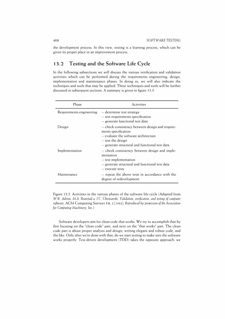
408 SOFTWARE TESTING

the development process. In this view, testing is a learning process, which can be

given its proper place in an improvement process.

13.2 Testing and the Software Life Cycle

In the following subsections we will discuss the various verification and validation

activities which can be performed during the requirements engineering, design,

implementation and maintenance phases. In doing so, we will also indicate the

techniques and tools that may be applied. These techniques and tools will be further

discussed in subsequent sections. A summary is given in figure 13.5.

Phase Activities

Requirements engineering -- determine test strategy

-- test requirements specification

-- generate functional test data

Design -- check consistency between design and require-

ments specification

-- evaluate the software architecture

-- test the design

-- generate structural and functional test data

Implementation -- check consistency between design and imple-

mentation

-- test implementation

-- generate structural and functional test data

-- execute tests

Maintenance -- repeat the above tests in accordance with the

degree of redevelopment

Figure 13.5 Activities in the various phases of the software life cycle (Adapted from

W.R. Adrion, M.A. Branstad & J.C. Cherniavski, Validation, verification, and testing of computersoftware, ACM Computing Surveys 14, 2 (1982), Reproduced by permission of the Association

for Computing Machinery, Inc.)

Software developers aim for clean code that works. We try to accomplish that by

first focusing on the ”clean code” part, and next on the ”that works” part. The clean

code part is about proper analysis and design, writing elegant and robust code, and

the like. Only after we’re done with that, do we start testing to make sure the software

works properly. Test-driven development (TDD) takes the opposite approach: we

13.2. TESTING AND THE SOFTWARE LIFE CYCLE 409

first make sure the software works, and then tackle the clean code part. We discuss

test-driven development in section 13.2.5.

13.2.1 Requirements Engineering

The verification and validation techniques applied during this phase are strongly

dependent upon the way in which the requirements specification has been laid down.

Something which should be done at the very least is to conduct a careful review or

inspection in order to check whether all aspects of the system have been properly

described. As we saw earlier, errors made at this stage are very costly to repair if

they go unnoticed until late in the development process. Boehm gives four essential

criteria for a requirements specification (Boehm, 1984b):

– completeness;

– consistency;

– feasibility;

– testability.

Testing a requirements specification should primarily be aimed at testing these

criteria.

The aim of testing the completeness criterion then is to determine whether all

components are present and described completely. A requirements specification is

incomplete if it contains such phrases as ‘to be determined’ or if it contains references

to undefined elements. We should also watch for the omission of functions or

products, such as back-up or restart procedures and test tools to be delivered to the

customer.

A requirements specification is consistent if its components do not contradict

each other and the specification does not conflict with external specifications. We

thus need both internal and external consistency. Moreover, each element in the

requirements specification must be traceable. It must, for instance, be possible to

decide whether a natural language interface is really needed.

According to Boehm, feasibility has to do with more than functional and

performance requirements. The benefits of a computerized system should outweigh

the associated costs. This must be established at an early stage and necessitates timely

attention to user requirements, maintainability, reliability, and so on. In some cases,

the project’s success is very sensitive to certain key factors, such as safety, speed,

availability of certain types of personnel; these risks must be analyzed at an early

stage.

Lastly, a requirements specification must be testable. In the end, we must be able

to decide whether or not a system fulfills its requirements. So requirements must

be specific, unambiguous, and quantitative. The quality-attribute scenario framework

from (Bass et al., 2003) is an example of how to specify such requirements; see also

section 6.3.

410 SOFTWARE TESTING

Many of these points are raised by Poston (1987). According to Poston, the

most likely errors in a requirements specification can be grouped into the following

categories:

– missing information (functions, interfaces, performance, constraints, reliability,

and so on);

– wrong information (not traceable, not testable, ambiguous, and so forth);

– extra information (bells and whistles).

Using a standard format for documenting the requirements specification, such as IEEE

Standard 830 discussed in chapter 9, may help enormously in preventing these types

of errors to occur in the first place.

Useful techniques for testing the degree to which criteria have been met, are

mostly manual (reading documents, inspections, reviews). Scenarios for the expected

use of the system can be devised with the prospective users of the system. If

requirements are already expressed in use cases, such scenarios are readily available.

In this way, a set of functional tests is generated.

At this stage also, a general test strategy for subsequent phases must be formulated.

It should encompass the choice of particular test techniques; evaluation criteria; a test

plan; a test scheme; and test documentation requirements. A test team may also be

formed at this stage. These planning activities are dealt with in section 13.3.

13.2.2 Design

The criteria mentioned in the previous subsection (completeness, consistency, feasi-

bility and testability) are also essential for the design. The most likely errors in design

resemble the kind of errors one is inclined to make in a requirements specification:

missing, wrong, and extraneous information. For the design too, a precise documen-

tation standard is of great help in preventing these types of errors. IEEE Standard

1016, discussed in chapter 12, is one such standard.

During the design phase, we decompose the total system into subsystems and

components, starting from the requirements specification. We may then develop tests

based on this decomposition process. Design is not a one-shot process. During the

design process a number of successive refinements will be made, resulting in layers

showing increasing detail. Following this design process, more detailed tests can be

developed as the lower layers of the design are decided upon.

During the architectural design phase, a high-level conceptual model of the

system is developed in terms of components and their interaction. This architecture

can be assessed, for example by generating scenarios which express quality concerns

such as maintainability and flexibility in very concrete terms, and next evaluating how

the architecture handles these scenarios; see also section 11.5.

During the design phase, we may also test the design itself. This includes tracing

elements from the requirements specification to the corresponding elements in the

13.2. TESTING AND THE SOFTWARE LIFE CYCLE 411

design description, and vice versa. Well-known techniques for doing so are, amongst

others, simulation, design walkthroughs, and design inspections.

At the requirements engineering phase, the possibilities for formally document-

ing the resulting specification are limited. Most requirements specifications make

excessive use of natural language descriptions. For the design phase, there are ample

opportunities to formally document the resulting specification. The more formally the

design is specified, the more possibilities we have for applying verification techniques,

as well as formal checks for consistency and completeness.

13.2.3 Implementation

During the implementation phase, we do the ‘real’ testing. One of the most effective

techniques to find errors in a program text is to carefully read that text, or have it read.

This technique has been successfully applied for a long time. Somewhat formalized

variants are known as code-inspection and code-walkthrough. We may also apply the

technique of stepwise abstraction. In stepwise abstraction, the function of the code is

determined in a number of abstraction steps, starting from the code itself. The various

manual test techniques will be discussed in section 13.4.

There are many tools to support the testing of code. We may distinguish between

tools for static analysis and tools for dynamic analysis. Static analysis tools inspect

the program code without executing it. They include tests like: have all variables

been declared and given a value before they are used?

Dynamic analysis tools are used in conjunction with the actual execution of the

code, for example tools that keep track of which portions of the code have been

covered by the tests so far.

We may try to prove the correctness of the code using formal verification

techniques.

All of the above techniques are aimed at evaluating the quality of the source code

as well as its compliance with design specifications and code documentation.

It is crucial to control the test information properly while testing the code. Tools

may help us in doing so, for example test drivers, test stubs and test data generators.

A test driver is a tool that generates the test environment for a component to be

tested. A test stub does the opposite: it simulates the function of a component not

yet available. In bottom-up testing, we will, in general, make much use of test drivers,

while top-down testing implies the use of test stubs. The test strategy (top-down

versus bottom-up) may be partly influenced by the design technique used. If the high

level, architectural design is implemented as a skeletal system whose holes yet have

to be filled in, that skeletal system can be used as a test driver.

Tools may also be profitable while executing the tests (test harnesses and test

systems). A simple and yet effective tool is one which compares test results with

expected results. The eye is a very unreliable medium. After a short time, all results

look OK. An additional advantage of this type of tool support is that it helps to

achieve a standard test format. This in turn helps with regression testing.

412 SOFTWARE TESTING

13.2.4 Maintenance

On average, more than 50% of total life-cycle costs is spent on maintenance. If we

modify the software after a system has become operational (because an error is found

late on, or because the system must be adapted to changed requirements), we will

have to test the system anew. This is called regression testing. To have this proceed

smoothly, the quality of the documentation and the possibilities for tool support, are

crucial factors.

In a retest-all approach, all tests are rerun. Since this may consume a lot of time and

effort, we may also opt for a selective retest, in which only some of the tests are rerun.

A regression test selection technique is then used to decide which subset should be

rerun. We would like this technique to include all tests in which the modified and

original program produce different results, while omitting tests that produce the same

results.

13.2.5 Test-Driven Development (TDD)

Suppose our library system needs to be able to block borrowing items to members that

are on a black list. We could start by redesigning part of the system and implementing

the necessary changes: a new table BlackList, and appropriate checks in method

Borrow. We also have to decide when members are put on the black list, and how

to get them off that list. After having done all the necessary analysis and design,

and implemented the changes accordingly, we devise test cases to test for the new

functionality.

This order of events is completely reversed in test-driven development (TDD).

In test-driven development, we first write a few tests for the new functionality. We

may start very simple, and add a test in the start-up method to ensure that the black

list is initially empty:

assertEquals(0, BlackList)

Of course, this test will fail. To make it succeed, we have to introduce BlackList,and set it equal to 0. At the same time, we make a list of things still to be done,

such as devising a proper type for BlackList, including operations to add and remove

members to that list, an update of Borrow to check whether a person borrowing an

item is on the black list, and the like. This list of things to be done is similar to the

backlog used by architects while architecting a system (see section 11.2).

After we have made the simple test to work, the new version of the system is

inspected to see whether it can be improved. And next another small change is

contemplated. We may for example decide to make BlackList into a proper list, and

write some simple tests to see that after adding some item to the list, that item is

indeed in the list. Again, the test will fail, and we update the system accordingly.

Possibly, improvements can be made now since the library system probably contains

other list-type classes that we can inherit from, and some duplicate code can be

removed. And so on.

13.3. VERIFICATION AND VALIDATION PLANNING AND DOCUMENTATION413

Test-driven development is one of the practices of eXtreme Programming (see

section 3.2.4). As such, it is part of the agile approach to system development which

favors small increments and redesign (refactoring) where needed over big design

efforts. The practice is usually supported by an automated unit testing framework,

such as JUnit for Java, that keeps track of the test set and reports back readable

error messages for tests that failed (Hunt and Thomas, 2003). The assertEqualmethod used above is one of the methods provided by the JUnit framework. The

framework allows for a smooth integration of coding and unit testing. On the fly, a

test set is built that forms a reusable asset during the further evolution of the system.

JUnit and similar frameworks have greatly contributed to the success of test-driven

development.

The way of working in each iteration of test-driven development consists of the

following steps:

1. Add a test

2. Run all tests, and observe that the one added will fail

3. Make a small change to the system to make the test work

4. Run al tests again, and observe that they run properly

5. Refactor the system to remove duplicate code and improve its design.

In pure eXtreme Programming, iterations are very small, and may take a few minutes

up to, say, an hour. But test-driven development can also be done in bigger leaps, and

be combined with more traditional approaches.

Test-driven development is much more than a test method. It is a different way of

developing software. The effort put into the upfront development of test cases forces

one to think more carefully of what it means for the current iteration to succeed or

fail. Writing down explicit test cases subsumes part of the analysis and design work.

Rather than producing UML diagrams during requirements analysis, we produce

tests. And these tests are used immediately, by the same person that implemented the

functionality that the test exercises. Testing then is not an afterthought, but becomes

an integral part of the development process. Another benefit is that we have a test

set and a test criterion to decide on the success of the iteration. Experiments with

test-driven development indicate that it increases productivity and reduces defect

rates.

13.3 Verification and Validation Planning and Docu-

mentation

Like the other phases and activities of the software development process, the testing

activities need to be carefully planned and documented. Since test activities start

414 SOFTWARE TESTING

early in the development life cycle and span all subsequent phases, timely attention

to the planning of these activities is of paramount importance. A precise description

of the various activities, responsibilities and procedures must be drawn up at an early

stage.

The planning of test activities is described in a document called the Software

Verification and Validation Plan. We will base our discussion of its contents on

the corresponding IEEE Standard 1012. Standard 1012 describes verification and

validation activities for a waterfall-like life cycle in which the following phases are

identified:� Concept phase� Requirements phase� Design phase� Implementation phase� Test phase� Installation and checkout phase� Operation and maintenance phase

The first of these, the concept phase, is not discussed in the present text. Its aim is

to describe and evaluate user needs. It produces documentation which contains, for

example, a statement of user needs, results of feasibility studies, and policies relevant

to the project. The verification and validation plan is also prepared during this phase.

In our approach, these activities are included in the requirements engineering phase.

The sections to be included in the Verification and Validation (V&V) Plan are

listed in figure 13.6. The structure of this plan resembles that of other standards

discussed earlier. The plan starts with an overview and gives detailed information on

every aspect of the topic being covered. The various constituents of the Verification

and Validation Plan are discussed in appendix ??.

More detailed information on the many V&V tasks covered by this plan can be

found in (IEEE1012, 1986). Following the organization proposed in this standard,

the bulk of the test documentation can be structured along the lines identified in

figure 13.7. The Test Plan is a document describing the scope, approach, resources,

and schedule of intended test activities. It can be viewed as a further refinement of

the Verification and Validation Plan and describes in detail the test items, features to

be tested, testing tasks, who will do each task, and any risks that require contingency

planning.

The Test Design documentation specifies, for each software feature or combina-

tion of such features, the details of the test approach and identifies the associated

tests. The Test Case documentation specifies inputs, predicted outputs and execu-

tion conditions for each test item. The Test Procedure documentation specifies the

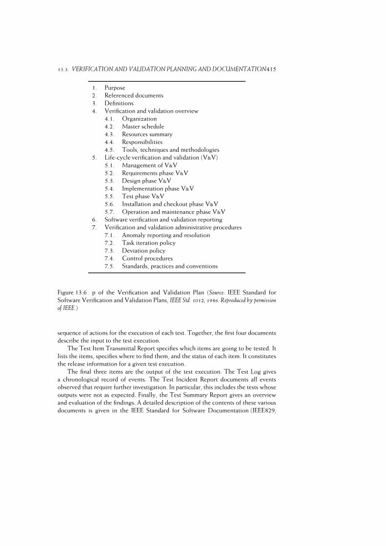
13.3. VERIFICATION AND VALIDATION PLANNING AND DOCUMENTATION415

1. Purpose

2. Referenced documents

3. Definitions

4. Verification and validation overview

4.1. Organization

4.2. Master schedule

4.3. Resources summary

4.4. Responsibilities

4.5. Tools, techniques and methodologies

5. Life-cycle verification and validation (V&V)

5.1. Management of V&V

5.2. Requirements phase V&V

5.3. Design phase V&V

5.4. Implementation phase V&V

5.5. Test phase V&V

5.6. Installation and checkout phase V&V

5.7. Operation and maintenance phase V&V

6. Software verification and validation reporting

7. Verification and validation administrative procedures

7.1. Anomaly reporting and resolution

7.2. Task iteration policy

7.3. Deviation policy

7.4. Control procedures

7.5. Standards, practices and conventions

Figure 13.6 p of the Verification and Validation Plan (Source: IEEE Standard for

Software Verification and Validation Plans, IEEE Std. 1012, 1986. Reproduced by permission

of IEEE.)

sequence of actions for the execution of each test. Together, the first four documents

describe the input to the test execution.

The Test Item Transmittal Report specifies which items are going to be tested. It

lists the items, specifies where to find them, and the status of each item. It constitutes

the release information for a given test execution.

The final three items are the output of the test execution. The Test Log gives

a chronological record of events. The Test Incident Report documents all events

observed that require further investigation. In particular, this includes the tests whose

outputs were not as expected. Finally, the Test Summary Report gives an overview

and evaluation of the findings. A detailed description of the contents of these various

documents is given in the IEEE Standard for Software Documentation (IEEE829,

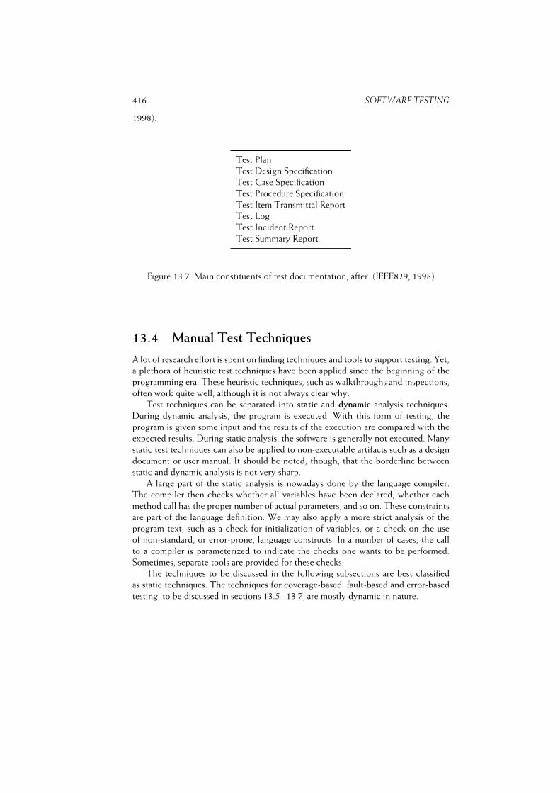
416 SOFTWARE TESTING

1998).

Test Plan

Test Design Specification

Test Case Specification

Test Procedure Specification

Test Item Transmittal Report

Test Log

Test Incident Report

Test Summary Report

Figure 13.7 Main constituents of test documentation, after (IEEE829, 1998)

13.4 Manual Test Techniques

A lot of research effort is spent on finding techniques and tools to support testing. Yet,

a plethora of heuristic test techniques have been applied since the beginning of the

programming era. These heuristic techniques, such as walkthroughs and inspections,

often work quite well, although it is not always clear why.

Test techniques can be separated into static and dynamic analysis techniques.

During dynamic analysis, the program is executed. With this form of testing, the

program is given some input and the results of the execution are compared with the

expected results. During static analysis, the software is generally not executed. Many

static test techniques can also be applied to non-executable artifacts such as a design

document or user manual. It should be noted, though, that the borderline between

static and dynamic analysis is not very sharp.

A large part of the static analysis is nowadays done by the language compiler.

The compiler then checks whether all variables have been declared, whether each

method call has the proper number of actual parameters, and so on. These constraints

are part of the language definition. We may also apply a more strict analysis of the

program text, such as a check for initialization of variables, or a check on the use

of non-standard, or error-prone, language constructs. In a number of cases, the call

to a compiler is parameterized to indicate the checks one wants to be performed.

Sometimes, separate tools are provided for these checks.

The techniques to be discussed in the following subsections are best classified

as static techniques. The techniques for coverage-based, fault-based and error-based

testing, to be discussed in sections 13.5--13.7, are mostly dynamic in nature.

13.4. MANUAL TEST TECHNIQUES 417

13.4.1 Reading

We all read, and reread, and reread, our program texts. It is the most traditional test

technique we know of. It is also a very successful technique to find faults in a program

text (or a specification, or a design).

In general, it is better to have someone else read your texts. The author of a

text knows all too well what the program (or any other type of document) ought to

convey. For this reason, the author may be inclined to overlook things, suffering from

some sort of trade blindness.

A second reason why reading by the author himself might be less fruitful, is that

it is difficult to adopt a destructive attitude towards one’s own work. Yet such an

attitude is needed for successful testing.

A somewhat institutionalized form of reading each other’s programs is known

as peer review. This is a technique for anonymously assessing programs as regards

quality, readability, usability, and so on.

Each person partaking in a peer review is asked to hand in two programs: a ‘best’

program and one of lesser quality. These programs are then randomly distributed

amongst the participants. Each participant assesses four programs: two ‘best’ programs

and two programs of lesser quality. After all results have been collected, each

participant gets the (anonymous) evaluations of their programs, as well as the

statistics of the whole test.

The primary goal of this test is to give the programmer insight into his own

capabilities. The practice of peer reviews shows that programmers are quite capable

of assessing the quality of their peers’ software.

A necessary precondition for successfully reading someone else’s code is a business-

like attitude. Weinberg (1971) coined the term egoless programming for this. Many

programmers view their code as something personal, like a diary. Derogatory remarks

(‘how could you be so stupid as to forget that initialization’) can disastrously impair

the effectiveness of such assessments. The opportunity for such an antisocial attitude

to occur seems to be somewhat smaller with the more formalized manual techniques.

13.4.2 Walkthroughs and Inspections

Walkthroughs and inspections are both manual techniques that spring from the

traditional desk-checking of program code. In both cases it concerns teamwork,

whereby the product to be inspected is evaluated in a formal session, following

precise procedures.

Inspections are sometimes called Fagan inspections, after their originator (Fagan,

1976, 1986). In an inspection, the code to be assessed is gone through statement

by statement. The members of the inspection team (usually four) get the code, its

specification, and the associated documents a few days before the session takes place.

Each member of the inspection team has a well-defined role. The moderator is

responsible for the organization of inspection meetings. He chairs the meeting

and ascertains that follow-up actions agreed upon during the meeting are indeed

418 SOFTWARE TESTING

performed. The moderator must ensure that the meeting is conducted in a businesslike,

constructive way and that the participants follow the correct procedures and act as

a team. The team usually has two inspectors or readers, knowledgeable peers that

paraphrase the code. Finally, the code author is a largely silent observer. He knows the

code to be inspected all too well and is easily inclined to express what he intended

rather than what is actually written down. He may, though, be consulted by the

inspectors.

During the formal session, the inspectors paraphrase the code, usually a few lines

at a time. They express the meaning of the text at a higher level of abstraction than

what is actually written down. This gives rise to questions and discussions which

may lead to the discovery of faults. At the same time, the code is analyzed using a

checklist of faults that often occur. Examples of possible entries in this checklist are:

– wrongful use of data: variables not initialized, array index out of bounds,

dangling pointers, etc.;

– faults in declarations: the use of undeclared variables or the declaration of the

same name in nested blocks, etc.;

– faults in computations: division by zero, overflow (possible in intermediate

results too), wrong use of variables of different types in the same expression,

faults caused by an erroneous understanding of operator priorities, etc.;

– faults in relational expressions: using an incorrect operator (> instead of �,= instead of ==) or an erroneous understanding of priorities of Boolean

operators, etc.;

– faults in control flow: infinite loops or a loop that gets executed n+ 1 or n� 1times rather than n times, etc.;

– faults in interfaces: an incorrect number of parameters, parameters of the wrong

type, or an inconsistent use of global variables, etc.

The result of the session is a list of problems identified.

These problems are not resolved during the formal session itself. This might easily

lead to quick fixes and distract the team from its primary goal. After the meeting,

the code author resolves all issues raised and the revised code is verified once again.

Depending on the number of problems identified and their severity, this second

inspection may be done by the moderator only or by the complete inspection team.

Since the goal of an inspection is to identify as many problems as possible in order

to improve the quality of the software to be developed, it is important to maintain

a constructive attitude towards the programmer whose code is being assessed.2 The

results of an inspection therefore are often marked confidential. These results should

certainly not play a role in the formal assessment of the programmer in question.

2One way of creating a non-threatening atmosphere is to always talk about ‘problems’ rather than

‘faults’.

13.4. MANUAL TEST TECHNIQUES 419

In a walkthrough, the team is guided through the code using test data. These test

data are mostly of a fairly simple kind. Otherwise, tracing the program logic soon

becomes too complicated. The test data serves as a means to start a discussion, rather

than as a serious test of the program. In each step of this process, the designer may

be questioned regarding the rationale of the decisions. In many cases, a walkthrough

boils down to some sort of manual simulation.

Both walkthroughs and inspections may profitably be applied at all stages of the

software life cycle. The only precondition is that there is a clear, testable document.

It is estimated that these review methods detect 50 to 90% of defects (Boehm and

Basili, 2001). Both techniques not only serve to find faults. If properly applied, these

techniques may help to promote team spirit and morale. At the technical level, the

people involved may learn from each other and enrich their knowledge of algorithms,

programming style, programming techniques, error-prone constructions, and so on.

Thus, these techniques also serve as a vehicle for process improvement. Under the

general umbrella of ‘peer reviews’, they are part of the CMM level 3 key process area

Verification (see section 6.6).

A potential danger of this type of review is that it remains too shallow. The

people involved become overwhelmed with information, they may have insufficient

knowledge of the problem domain, their responsibilities may not have been clearly

delineated. As a result, the review process does not pay off sufficiently.

Parnas and Weiss (1987) describe a type of review process in which the people

involved have to play a more active role. Parnas distinguishes between different types

of specialized design review. Each of these reviews concentrates on certain desirable

properties of the design. As a consequence, the responsibilities of the people involved

are clear. The reviewers have to answer a list of questions (‘under which conditions

may this function be called’, ‘what is the effect of this function on the behavior of

other functions’, and the like). In this way, the reviewers are forced to study carefully

the design information received. Problems with the questionnaire and documentation

can be posed to the designers, and the completed questionnaires are discussed by the

designers and reviewers. Experiments suggest that inspections with specialized review

roles are more effective than inspections in which review roles are not specialized.

A very important component of Fagan inspections is the meeting in which the

document is discussed. Since meetings may incur considerable costs or time-lags,

one may try to do without them. Experiments suggest that the added value of group

meetings, as far as the number of problems identified is concerned, is quite small.

13.4.3 Correctness Proofs

The most complete static analysis technique is the proof of correctness. In a proof

of correctness we try to prove that a program meets its specification. In order to be

able to do so, the specification must be expressed formally. We mostly do this by

expressing the specification in terms of two assertions which hold before and after

the program’s execution, respectively. Next, we prove that the program transforms

420 SOFTWARE TESTING

one assertion (the precondition) into the other (the postcondition). This is generally

denoted asfPg S fQgHere, S is the program, P is the precondition, and Q is the postcondition. Termination

of the program is usually proved separately. The above notation should thus be read

as: if P holds before the execution of S, and S terminates, then Q holds after the

execution of S.

Formally verifying the correctness of a not-too-trivial program is a very complex

affair. Some sort of tool support is helpful, therefore. Tools in this area are often

based on heuristics and proceed interactively.

Correctness proofs are very formal and, for that reason, they are often difficult

for the average programmer to construct. The value of formal correctness proofs is

sometimes disputed. We may state that the thrust in software is more important than

some formal correctness criterion. Also, we cannot formally prove every desirable

property of software. Whether we built the right system can only be decided upon

through testing (validation).

On the other hand, it seems justified to state that a thorough knowledge of this

type of formal technique will result in better software.

13.4.4 Stepwise Abstraction

In the top-down development of software components we often employ stepwise

refinement. At a certain level of abstraction the function to be executed will then

be denoted by a description of that function. At the next level, this description is

decomposed into more basic units.

Stepwise abstraction is just the opposite. Starting from the instructions of the

source code, the function of the component is built up in a number of steps. The

function thus derived should comply with the function as described in the design or

requirements specification.

Below, we will illustrate this technique with a small example. Consider the

search routine of figure 13.8. We know, from the accompanying documentation, for

instance, that the elements in array A are sorted when this routine is called.

We start the stepwise abstraction with the instructions at the innermost nesting

level, the if-statement on lines 7--10. In these lines, x is being compared with A[mid].Depending on the result of this comparison, one of high, low and found is given a

new value. If we take into account the initializations on lines 4 and 6, the function of

this if-statement can be summarized as

stop searching (found:= true) if x = A[mid], or

shorten the interval [low .. high] that might contain x, to an interval

[low’ .. high’], where high’ - low’ < high - low

Alternatively, this may be described as a postcondition to the if-statement:

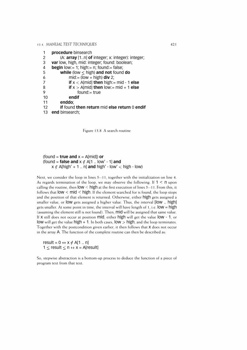
13.4. MANUAL TEST TECHNIQUES 421

1 procedure binsearch2 (A: array [1..n] of integer; x: integer): integer;3 var low, high, mid: integer; found: boolean;4 begin low:= 1; high:= n; found:= false;5 while (low � high) and not found do6 mid:= (low + high) div 2;7 if x < A[mid] then high:= mid - 1 else8 if x > A[mid] then low:= mid + 1 else9 found:= true10 endif11 enddo;12 if found then return mid else return 0 endif13 end binsearch;

Figure 13.8 A search routine

(found = true and x = A[mid]) or(found = false and x =2 A[1 .. low’ - 1] and

x =2 A[high’ + 1 .. n] and high’ - low’ < high - low)

Next, we consider the loop in lines 5--11, together with the initialization on line 4.

As regards termination of the loop, we may observe the following. If 1 � n upon

calling the routine, then low � high at the first execution of lines 5--11. From this, it

follows that low � mid � high. If the element searched for is found, the loop stops

and the position of that element is returned. Otherwise, either high gets assigned a

smaller value, or low gets assigned a higher value. Thus, the interval [low .. high]gets smaller. At some point in time, the interval will have length of 1, i.e. low = high(assuming the element still is not found). Then, mid will be assigned that same value.

If x still does not occur at position mid, either high will get the value low - 1, or

low will get the value high + 1. In both cases, low > high, and the loop terminates.

Together with the postcondition given earlier, it then follows that x does not occur

in the array A. The function of the complete routine can then be described as:

result = 0 $ x =2 A[1 .. n]1 � result � n $ x = A[result]

So, stepwise abstraction is a bottom-up process to deduce the function of a piece of

program text from that text.

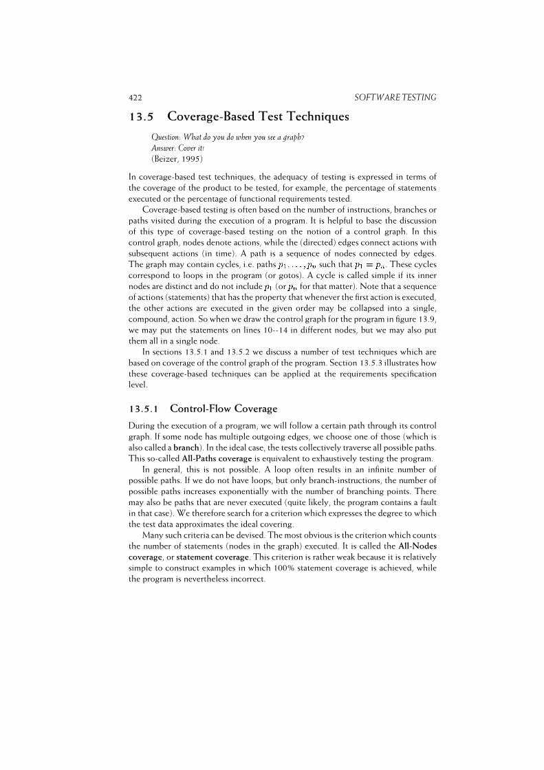
422 SOFTWARE TESTING

13.5 Coverage-Based Test Techniques

Question: What do you do when you see a graph?

Answer: Cover it!(Beizer, 1995)

In coverage-based test techniques, the adequacy of testing is expressed in terms of

the coverage of the product to be tested, for example, the percentage of statements

executed or the percentage of functional requirements tested.

Coverage-based testing is often based on the number of instructions, branches or

paths visited during the execution of a program. It is helpful to base the discussion

of this type of coverage-based testing on the notion of a control graph. In this

control graph, nodes denote actions, while the (directed) edges connect actions with

subsequent actions (in time). A path is a sequence of nodes connected by edges.

The graph may contain cycles, i.e. paths p1; : : : ; pn such that p1 = pn. These cycles

correspond to loops in the program (or gotos). A cycle is called simple if its inner

nodes are distinct and do not include p1 (or pn for that matter). Note that a sequence

of actions (statements) that has the property that whenever the first action is executed,

the other actions are executed in the given order may be collapsed into a single,

compound, action. So when we draw the control graph for the program in figure 13.9,

we may put the statements on lines 10--14 in different nodes, but we may also put

them all in a single node.

In sections 13.5.1 and 13.5.2 we discuss a number of test techniques which are

based on coverage of the control graph of the program. Section 13.5.3 illustrates how

these coverage-based techniques can be applied at the requirements specification

level.

13.5.1 Control-Flow Coverage

During the execution of a program, we will follow a certain path through its control

graph. If some node has multiple outgoing edges, we choose one of those (which is

also called a branch). In the ideal case, the tests collectively traverse all possible paths.

This so-called All-Paths coverage is equivalent to exhaustively testing the program.

In general, this is not possible. A loop often results in an infinite number of

possible paths. If we do not have loops, but only branch-instructions, the number of

possible paths increases exponentially with the number of branching points. There

may also be paths that are never executed (quite likely, the program contains a fault

in that case). We therefore search for a criterion which expresses the degree to which

the test data approximates the ideal covering.

Many such criteria can be devised. The most obvious is the criterion which counts

the number of statements (nodes in the graph) executed. It is called the All-Nodes

coverage, or statement coverage. This criterion is rather weak because it is relatively

simple to construct examples in which 100% statement coverage is achieved, while

the program is nevertheless incorrect.

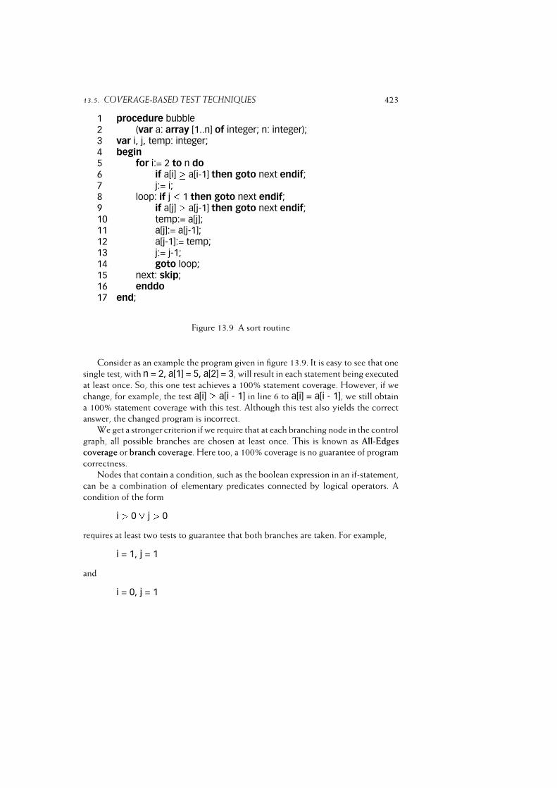
13.5. COVERAGE-BASED TEST TECHNIQUES 423

1 procedure bubble2 (var a: array [1..n] of integer; n: integer);3 var i, j, temp: integer;4 begin5 for i:= 2 to n do6 if a[i] � a[i-1] then goto next endif;7 j:= i;8 loop: if j � 1 then goto next endif;9 if a[j] � a[j-1] then goto next endif;10 temp:= a[j];11 a[j]:= a[j-1];12 a[j-1]:= temp;13 j:= j-1;14 goto loop;15 next: skip;16 enddo17 end;

Figure 13.9 A sort routine

Consider as an example the program given in figure 13.9. It is easy to see that one

single test, with n = 2, a[1] = 5, a[2] = 3, will result in each statement being executed

at least once. So, this one test achieves a 100% statement coverage. However, if we

change, for example, the test a[i] � a[i - 1] in line 6 to a[i] = a[i - 1], we still obtain

a 100% statement coverage with this test. Although this test also yields the correct

answer, the changed program is incorrect.

We get a stronger criterion if we require that at each branching node in the control

graph, all possible branches are chosen at least once. This is known as All-Edges

coverage or branch coverage. Here too, a 100% coverage is no guarantee of program

correctness.

Nodes that contain a condition, such as the boolean expression in an if-statement,

can be a combination of elementary predicates connected by logical operators. A

condition of the form

i > 0 _ j > 0

requires at least two tests to guarantee that both branches are taken. For example,

i = 1, j = 1

and

i = 0, j = 1

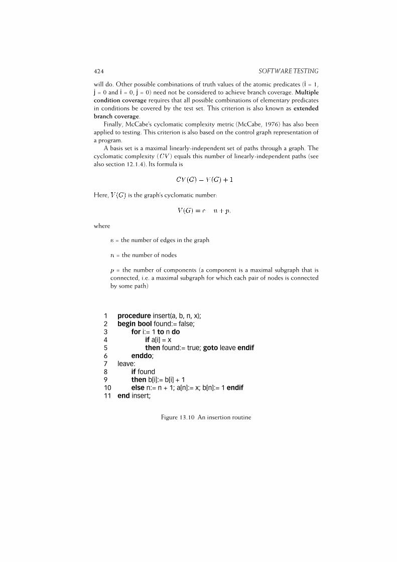
424 SOFTWARE TESTING

will do. Other possible combinations of truth values of the atomic predicates (i = 1,

j = 0 and i = 0, j = 0) need not be considered to achieve branch coverage. Multiple

condition coverage requires that all possible combinations of elementary predicates

in conditions be covered by the test set. This criterion is also known as extended

branch coverage.

Finally, McCabe’s cyclomatic complexity metric (McCabe, 1976) has also been

applied to testing. This criterion is also based on the control graph representation of

a program.

A basis set is a maximal linearly-independent set of paths through a graph. The

cyclomatic complexity (CV ) equals this number of linearly-independent paths (see

also section 12.1.4). Its formula isCV (G) = V (G) + 1Here, V (G) is the graph’s cyclomatic number:V (G) = e� n+ p;wheree = the number of edges in the graphn = the number of nodesp = the number of components (a component is a maximal subgraph that is

connected, i.e. a maximal subgraph for which each pair of nodes is connected

by some path)

1 procedure insert(a, b, n, x);2 begin bool found:= false;3 for i:= 1 to n do4 if a[i] = x5 then found:= true; goto leave endif6 enddo;7 leave:8 if found9 then b[i]:= b[i] + 110 else n:= n + 1; a[n]:= x; b[n]:= 1 endif11 end insert;

Figure 13.10 An insertion routine

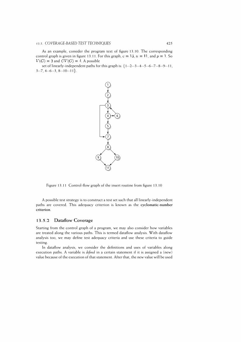
13.5. COVERAGE-BASED TEST TECHNIQUES 425

As an example, consider the program text of figure 13.10. The corresponding

control graph is given in figure 13.11. For this graph, e = 13, n = 11, and p = 1. SoV (G) = 3 and CV (G) = 4. A possible

set of linearly-independent paths for this graph is: f1--2--3--4--5--6--7--8--9--11,

3--7, 4--6--3, 8--10--11g.

Figure 13.11 Control-flow graph of the insert routine from figure 13.10

A possible test strategy is to construct a test set such that all linearly-independent

paths are covered. This adequacy criterion is known as the cyclomatic-number

criterion.

13.5.2 Dataflow Coverage

Starting from the control graph of a program, we may also consider how variables

are treated along the various paths. This is termed dataflow analysis. With dataflow

analysis too, we may define test adequacy criteria and use these criteria to guide

testing.

In dataflow analysis, we consider the definitions and uses of variables along

execution paths. A variable is defined in a certain statement if it is assigned a (new)

value because of the execution of that statement. After that, the new value will be used

426 SOFTWARE TESTING

in subsequent statements. A definition in statement X is alive in statement Y if there

exists a path from X to Y in which that variable does not get assigned a new value at

some intermediate node. In the example in figure 13.9, for instance, the definition of

j at line 7 is still alive at line 13 but not at line 14. A path such as the one from line 7

to 13 is called definition-clear (with respect to j). Algorithms to determine such facts

are commonly used in compilers in order to allocate variables optimally to machine

registers.

We distinguish between two types of variable use: P-uses and C-uses. P-uses are

predicate uses, like those in the conditional part of an if-statement. All other uses are

C-uses. Examples of the latter are uses in computations or I/O statements.

A possible test strategy is to construct tests which traverse a definition-clear path

between each definition of a variable to each (P- or C-) use of that definition and

each successor of that use. (We have to include each successor of a use to force

all branches following a P-use to be taken.) We are then sure that each possible

use of a definition is being tested. This strategy is known as All-Uses coverage. A

slightly stronger criterion requires that each definition-clear path is either cycle-free

or a simple cycle. This is known as All-DU-Paths coverage. Several weaker dataflow

criteria can be defined as well:

– All-defs coverage simply requires the test set to be such that each definition is

used at least once.

– All-C-uses/Some-P-uses coverage requires definition-clear paths from each

definition to each computational use. If a definition is used only in predicates,

at least one definition-clear path to a predicate use must be exercised.

– All-P-Uses/Some-C-uses coverage requires definition-clear paths from each

definition to each predicate use. If a definition is used only in computations, at

least one definition-clear path to a computational use must be exercised.

– All-P-Uses coverage requires definition-clear paths from each definition to

each predicate use.

13.5.3 Coverage-Based Testing of Requirements Specifications

Program code can be easily transformed into a graph model, thus allowing for all kinds

of test adequacy criteria based on graphs. Requirements specifications, however, may

also be transformed into a graph model. As a consequence, the various coverage-based

adequacy criteria can be used in both black-box and white-box testing techniques.

Consider the example fragment of a requirements specification document for our

library system in figure 13.12. We may rephrase these requirements a bit and present

them in the form of elementary requirements and relations between them. The result

can be depicted as a graph, where the nodes denote elementary requirements and the

edges denote relations between elementary requirements; see figure 13.13. We may

13.6. FAULT-BASED TEST TECHNIQUES 427

use this graph model to derive test cases and apply any of the control-flow coverage

criteria to assess their adequacy.

Function Order allows the user to order new books. The user is shown a fill-in-the-

blanks screen with fields like Author, Title, Publisher, Price and Department. The

Title, Price and Department fields are mandatory. The Department field is used

to check whether the department’s budget is large enough to purchase this book. If

so, the book is ordered and

the department’s budget is reduced accordingly.

Figure 13.12 A requirements specification fragment

A very similar route can be followed if the requirement is expressed in the form of

a use case. Figure 13.14 gives a possible rewording of the fragment from figure 13.12.

It uses the format from (Cockburn, 2001). The use case describes both the normal

case, called the Main Success Scenario, as well as extensions that cover situations

that branch off the normal path because of some condition. For each extension,

both the condition and the steps taken are listed. Note that figure 13.13 directly

mimics the use case description from 13.14. The use case description also allows us

to straightforwardly derive test cases and apply control-flow coverage criteria.

Generally speaking, a major problem in determining a set of test cases is to

partition the program domain into a (small) number of equivalence classes. We try to

do so in such a way that testing a representative element from a class suffices for the

whole class. Using control-flow coverage criteria, for example, we assume that any

test of some node or branch is as good as any other such test. In the above example,

for instance, we assume that any execution of the node labeled ‘check dept. budget’

will do.

The weak point in this procedure is the underlying assumption that the program

behaves equivalently on all data from a given class. If such assumption is true, the

partition is perfect and so is the test set.

Such assumption will in general not hold however (see also section 13.1.2).

13.6 Fault-Based Test Techniques

In coverage-based testing techniques, we consider the structure of the problem or

its solution, and the assumption is that a more comprehensive covering is better.

In fault-based testing strategies, we do not directly consider the artifact being tested

when assessing the test adequacy. We only take into account the test set. Fault-based

techniques are aimed at finding a test set with a high ability to detect faults.

We will discuss two fault-based testing techniques: error seeding and mutation

testing.

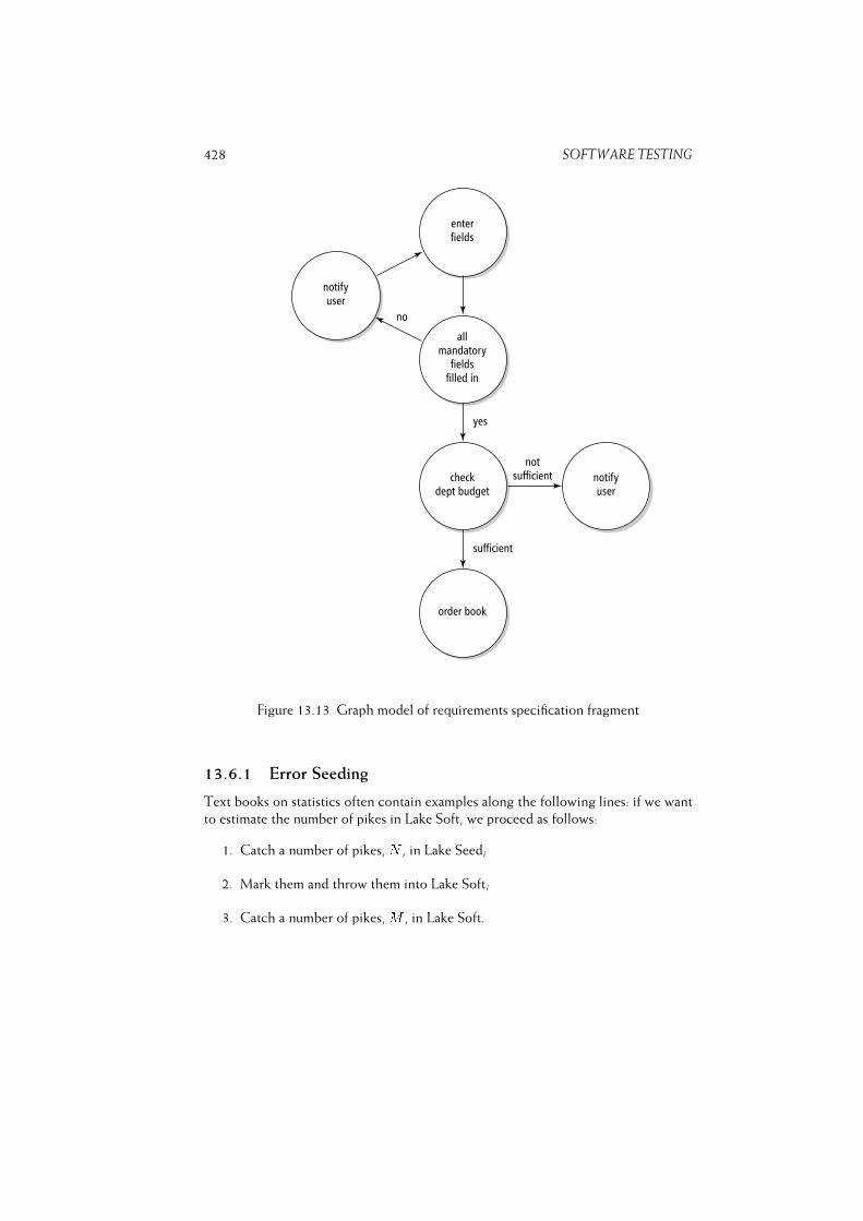
428 SOFTWARE TESTING

Figure 13.13 Graph model of requirements specification fragment

13.6.1 Error Seeding

Text books on statistics often contain examples along the following lines: if we want

to estimate the number of pikes in Lake Soft, we proceed as follows:

1. Catch a number of pikes, N , in Lake Seed;

2. Mark them and throw them into Lake Soft;

3. Catch a number of pikes, M , in Lake Soft.

13.6. FAULT-BASED TEST TECHNIQUES 429

Use Case: Order new Book

Primary Actor: Library user

Scope: Library

Level: User goal

Stakeholders and Interests:

User---wants to acquire new books

Department---wants to guard its budget

Precondition: User is logged on

Minimum Guarantee: User id has been validated

Success Guarantee: Order is accepted

Main Success Scenario:

1. User fills in form

2. Book information is checked

3. Department budget is checked

4. Order is placed

5. User is informed about placed order

Extensions:

2a. Book information is not valid

2a1. User is asked to correct information

3a. Department budget is inadequate

3a1. Order is rejected, user is notified

Figure 13.14 Requirement in the form of a use case

Supposing that M 0 out of the M pikes are found to be marked, the total number of

pikes originally present in Lake Soft is then estimated as (M �M 0)�N=M 0.A somewhat unsophisticated technique is to try to estimate the number of faults

in a program in a similar way. The easiest way to do this is to artificially seed a number

of faults in the program. When the program is tested, we will discover both seeded

faults and new ones. The total number of faults is then estimated from the ratio of

those two numbers.

We must be aware of the fact that a number of assumptions underlie this method

-- amongst others, the assumption that both real and seeded faults have the same

distribution.

There are various ways of determining which faults to seed in the program. A not

very satisfactory technique is to construct them by hand. It is unlikely that we will

be able to construct very realistic faults in this way. Faults thought up by one person

have a fair chance of having been thought up already by the person that wrote the

software.

430 SOFTWARE TESTING

Another technique is to have the program independently tested by two groups.

The faults found by the first group can then be considered seeded faults for the

second group. In using this technique, though, we must realize that there is a chance

that both groups will detect (the same type of) simple faults. As a result, the picture

might well get distorted.

A useful rule of thumb for this technique is the following: if we find many

seeded faults and relatively few others, the result can be trusted. The opposite is not

true. This phenomenon is more generally applicable: if, during testing of a certain

component, many faults are found, it should not be taken as a positive sign. Quite the

contrary, it is an indication that the component is probably of low quality. As Myers

observed: ‘The probability of the existence of more errors in a section of a program

is proportional to the number of errors already found in that section.’ (Myers, 1979).

The same phenomenon has been observed in some experiments, where a strong linear

relationship was found between the number of defects discovered during early phases

of development and the number of defects discovered later.

13.6.2 Mutation Testing

Suppose we have some program P which produces the correct results for some testsT1 and T2. We next generate some variant P 0 of P . P 0 differs from P in just one

place. For instance, a + is replaced by a �, or the value v1 in a loop of the form

for var:= v1 to v2 do

is changed into v1 + 1 or v1 � 1. Next, P 0 is tested using tests T1 and T2. Let us

assume that T1 produces the same result in both cases, whereas T2 produces different

results. Then T1 is the more interesting test case, since it does not discriminate

between two variants of a program, one of which is certainly wrong.

In mutation testing, a (large) number of variants of a program is generated.

Each of those variants, or mutants, slightly differs from the original version. Usually,

mutants are obtained by mechanically applying a set of simple transformations called

mutation operators. Figure 13.15 lists a number of such mutation operators.

Next, all these mutants are executed using a given test set. As soon as a test

produces a different result for one of the mutants, that mutant is said to be dead.

Mutants that produce the same results for all of the tests are said to be alive. As an

example, consider the erroneous sort procedure in figure 13.3 and the correct variant

thereof which compares array elements rather than their absolute values. Tests with

an array which happens to contain positive numbers only will leave both variants

alive. If a test set leaves us with many live mutants, then that test set is of low quality,

since it is not able to discriminate between all kinds of variants of a given program.

If we assume that the number of mutants that is equivalent to the original program

is 0 (normally, this number will certainly be very small), then the mutation adequacy

score of a test set equals D=M , whereD is the number of dead mutants and M is the

total number of mutants.

13.6. FAULT-BASED TEST TECHNIQUES 431

Replace a constant by another constant

Replace a variable by another variable

Replace a constant by a variable

Replace an arithmetic operator by another arithmetic operator

Replace a logical operator by another logical operator

Insert a unary operator

Delete a statement

Figure 13.15 A sample of mutation operators

There are two major variants of mutation testing: strong mutation testing and

weak mutation testing. Suppose we have a program P with a component T . In strong

mutation testing, we require that tests produce different results for program P and

a mutant P 0. In weak mutation testing, we only require that component T and its

mutant T 0 produce different results. At the level of P , this difference need not crop

up. Weak mutation adequacy is often easier to establish. Consider a component T of

the form

if x < 4.5 then . . .

We may then compute a series of mutants of T , such as

if x > 4.5 then . . .if x = 4.5 then . . .if x > 4.6 then . . .if x < 4.4 then . . .. . .

Next, we have to devise a test set that produces different results for the original

component T and at least one of its variants. This test set is then adequate for T .

Mutation testing is based on two assumptions: the Competent Programmer Hypothesisand the Coupling Effect Hypothesis. The Competent Programmer Hypothesis states that

competent programmers write programs that are ‘close’ to being correct. So the

program actually written may be incorrect, but it will differ from a correct version by

relatively minor faults. If this hypothesis is true, we should be able to detect these

faults by testing variants that differ slightly from the correct program, i.e. mutants.

The second hypothesis states that tests that can reveal simple faults can also reveal

complex faults. Experiments give some empirical evidence for these hypotheses.

432 SOFTWARE TESTING

13.7 Error-Based Test Techniques

Suppose our library system maintains a list of ‘hot’ books. Each newly-acquired book

is automatically added to the list. After six months, it is removed again. Also, if a book

is more than four months old and is being borrowed less than five times a month

or is more than two months old and is being borrowed at most twice a month, it is

removed from the list.

This rather complex requirement can be graphically depicted as in figure 13.16. It

shows that the two-dimensional (age, average number of loans) domain can be parti-

tioned into four subdomains. These subdomains directly relate to the requirements as

stated above. The subdomains are separated by borders such as the line age = 6. For

each border, it is indicated which of the adjacent subdomains is closed at that border

by placing a hachure at that side of the border. A subdomain S is closed at a border if

that border belongs to S; otherwise, it is open at that border.

Figure 13.16 Partitioning of the input space

An obvious test technique for this requirement is to use an input from each of

these subdomains. If the program follows the logic of the requirement, then test

adequacy for that requirement equals path coverage for the corresponding program.

However, in error-based testing, we focus on error prone points, and these are often

found near the borders of subdomains.

13.8. COMPARISON OF TEST TECHNIQUES 433

One such test strategy concentrates on ON and OFF points. An ON point is a

point on the border of a subdomain. If a subdomain is open with respect to some

border, then an OFF point of a border is a point just inside that border. If a subdomain

is closed with respect to some border, then an OFF point lies just outside that border.

Two adjacent subdomains share the same ON point; they may share the same OFF

point. In figure 13.16, the solid circle on the line age = 6 is an ON point of both Aand B, while the circle just off this line is an OFF point of both these subdomains.

Suppose we have subdomains Di; i = 1; : : : ; n. We may then construct a test set

which contains N test cases for ON points of each border B of each subdomain Di,and at least one test case for an OFF point of each border. The resulting test set is

called N � 1 domain adequate.

Above, we have illustrated this error-based technique in its black-box, specification-

based form. The same technique can be applied to program text, though. If a program

contains code of the form

if x > 6 then . . .elsif x > 4 and y < 5 then . . .elsif x > 2 and y � 2 then . . .else . . .

then we may identify the same four subdomains and use the same technique to test for

boundary cases. In fact, this technique is just a systematic way to do what experienced

programmers have done for a long time past: test for boundary values, such as 0, nil,

lists with 0 or 1 element, and so on.

13.8 Comparison of Test Techniques

Most test techniques are heuristic in nature and lack a sound theoretical basis. Manual

test techniques rely heavily on the qualities of the participants in the test process.

But even the systematic approaches taken in functional and structural test techniques

have a rather weak underpinning and are based on assumptions that are generally not

true.

Experiments show that it is sometimes deceptively simple to make a system

produce faults or even let it crash. Miller et al. (1990) describe one such experiment,

in which they were able to crash or hang approximately 30% of the UNIX utilities

on seven versions of the UNIX operating system. The utilities tested included

commonly-used text editors and text formatters.

Similar results have been obtained in mutation analysis experiments. In one

such experiment (Knight and Ammann, 1985), 17 programs developed by different

programmers from one and the same specification were used. These programs had all

been thoroughly tested. Some of them had successfully withstood one million tests.

For each of those programs, 24 mutants were created, each mutant containing one

seeded fault. The programs thus obtained were each tested 25 000 times. The results

can be summarized as follows:

434 SOFTWARE TESTING

– Some seeded faults were found quickly, some needed quite a few tests, and

some remained undetected even after 25 000 tests. This pattern was found for

each of the 17 programs;

– In some cases, the original program failed, while the modified program yielded

the right result.

In the past, several attempts have been made to obtain more insights into the

theoretical aspects of test techniques. An example is the research that is aimed at

relating different test adequacy criteria. Test adequacy criteria serve as rules used

to determine whether or not testing can be terminated. An important issue then is

to decide whether one such criterion is ‘better’ than another. In section 13.8.1, we

compare the strength of a number of test adequacy criteria discussed in previous

sections. In section 13.8.2 we investigate a number of fundamental properties of test

adequacy criteria. This type of research is aimed at gaining a deeper insight into

properties of different test techniques.

Several experiments have been done to compare different test techniques. Real

data from a number of projects are also available on the fault-detection capabilities

of test techniques used in those projects. In section 13.8.3 we discuss several of these

findings which may provide some practical insight into the virtues of a number of test

techniques.

13.8.1 Comparison of Test Adequacy Criteria

A question that may be raised is whether, say, the All-Uses adequacy criterion is

stronger or weaker than the All-Nodes or All-Edges adequacy criteria. We may

define the notion ‘stronger’ as follows: criterion X is stronger than criterion Y if, for

all programs P and all test sets T, X-adequacy implies Y-adequacy. In the testing

literature this relation is known as ‘subsume’. In this sense, the All-Edges criterion is

stronger than (subsumes) the All-Nodes criterion. The All-Uses criterion, however,

is not stronger than the All-Nodes criterion. This is caused by the fact that programs

may contain statements which only refer to constants. For the program

if a < bthen print(0)else print(1)

the All-Uses criterion will be satisfied by any non-empty test set, since this criterion

does not require that each statement be executed. If we ignore references to

constants, the All-Uses criterion is stronger than the All-Nodes criterion. With the

same exception, the All-Uses criterion is also stronger than the All-Edges criterion.

A problem with any graph-based adequacy criterion is that it can only deal

with paths that can be executed (feasible paths). Paths which cannot be executed are

known as ’infeasible paths’. Infeasible paths result if parts of the graph are unreachable,

as in

13.8. COMPARISON OF TEST TECHNIQUES 435

if truethen x:= 1else x:= 2

The else-branch is never executed, yet most adequacy criteria require this branch to

be taken. Paths that are infeasible also result from loops. If a loop is of the form

for i from 1 to 10 dobody

there will be no feasible paths that traverse the resulting cycle in the graph any other

than ten times.

There does not exist a simple linear scale along which the strength of all

program-based adequacy criteria can be depicted. For the criteria discussed in

sections 13.5--13.7, the subsume hierarchy is depicted in figure 13.17, as far as it is

known. An arrow A ! B indicates that A is stronger than (subsumes) B. In most

cases, the subsume relation holds for both the feasible and not feasible versions of

the criteria. Arrows adorned with an asterisk denote relations which hold only for the

not feasible version.

The subsume relation compares the thoroughness of test techniques, not their

ability to detect faults. Especially if an adequacy criterion is used in an a priori sense,

i.e. if it is used to generate the next test case, the subsume relations of figure 13.17 do

not necessarily imply better fault detection. However, if some other tool is used to

generate test cases, and the criterion is only used a posteriori to decide when to stop

testing, a stronger adequacy criterion implies better fault-detection ability as well.

The theoretical upper bounds for the number of test cases needed to satisfy

most of the coverage-based adequacy criteria are quadratic or exponential. Empirical

studies, however, show that, in practice, these criteria are usually linear in the number

of conditional statements.

13.8.2 Properties of Test Adequacy Criteria

A major problem with any test technique is to decide when to stop testing. As noted,

functional and structural test techniques provide only weak means for doing so.

Weyuker (1988) provides an interesting set of properties of test adequacy criteria.

Although it is intuitively clear that any test adequacy criterion should satisfy all of

the properties listed, it turns out that even some of the well-known test techniques

such as All-Nodes coverage and All-Edges coverage fail to satisfy several of them.

The characteristics identified relate to program-based adequacy criteria, i.e.

criteria that involve the program’s structure. The first four criteria, however, are fairly

general and should apply to any test adequacy criterion. The following 11 properties

are identified in (Weyuker, 1988)3:

3Reproduced by permission of the Association for Computing Machinery, Inc.

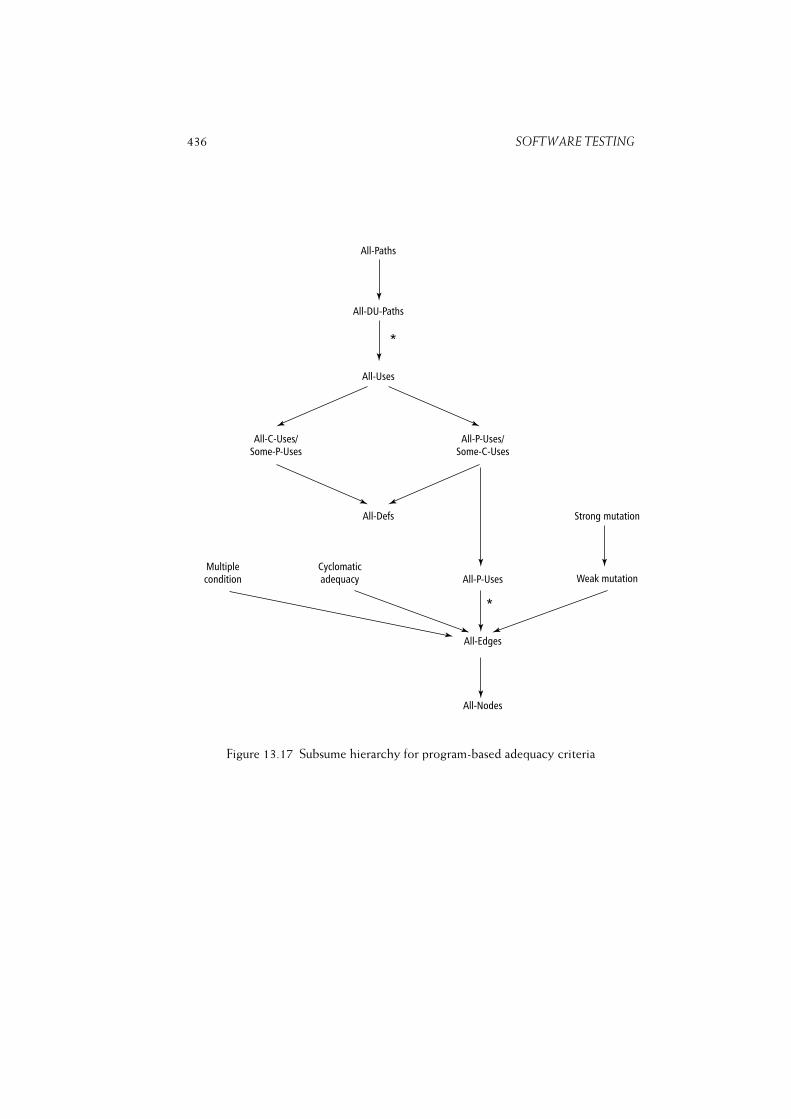
436 SOFTWARE TESTING

Figure 13.17 Subsume hierarchy for program-based adequacy criteria

13.8. COMPARISON OF TEST TECHNIQUES 437� Applicability property For every program, there exists an adequate test set.

Exhaustive testing obviously satisfies this criterion but, in general, we will look

for a reasonably-sized test set. Both All-Nodes and All-Edges coverage criteria

do not fulfill this property. If the program contains unexecutable code, there

simply are no tests to cover those parts of the program.� Non-exhaustive applicability property This property says that, even if exhaus-

tive testing may be required in some cases, a criterion should certainly not

require exhaustive testing in all circumstances.� Monotonicity property This property states that once a program has been

adequately tested, running some additional tests can do no harm. Obviously,

the additional tests may reveal further faults, but this does not deem the original

test set inadequate. It merely improves the quality of the test process.� Inadequate empty set property The empty test set is not an adequate test set

for any program. A test adequacy criterion should measure how well the testing

process has been conducted. If a program has not been tested at all, it certainly

has not been adequately tested.� Antiextensionality property This property states that semantic equivalence is

not sufficient to imply that the programs are to be tested in the same way.

For instance, routines BubbleSort and QuickSort are likely to require different

test sets. This property is specific for program-based adequacy criteria, which

depend on the implementation rather than the function being implemented. In

a specification-based approach this property need not hold.� General multiple change property Whereas the previous property states that

semantic ‘closeness’ is not sufficient to imply that two programs can be tested

in the same way, this property states that syntactic closeness is not sufficient

either. Programs are said to be syntactically close if they have the same structure

and the same dataflow characteristics. This is the case, for instance, when some

of the relational or arithmetic operators in those programs differ. Though the

shape of these programs is the same, testing them on the same data may well

cause different paths through the flow graph being executed.� Antidecomposition property This property states that if a component is

adequately tested in one environment, this does not imply that it is adequately

tested for some other environment. Put in other words: if some assembly

of components is adequately tested, this does not imply that the individual

components have been adequately tested as well. For example, a sorting routine

may well be adequately tested in an environment where the size of the array is

always less than ten. If we move that routine to an environment which requires

much larger arrays to be sorted, it must be tested anew in that environment.

438 SOFTWARE TESTING� Anticomposition property This property reflects just the opposite: even if

components have been adequately tested in isolation, we still have to test their

composition in order to ascertain that their interfaces and interactions work

properly.� Renaming property If two programs differ only in inessential ways, as is the

case when different variable names are used, then an adequate test set for one

of these programs also suffices for the other.� Complexity property Intuitively, more complex programs require more testing.

This property reflects this intuition by stating that for every program there

exists other programs that require more testing.� Statement coverage property One central property of program-based adequacy

criteria is that they should at least cause every executable statement of the

program to be executed.

As noted, the All-Nodes and All-Edges coverage metrics fail to satisfy the applicability

criterion. This is rather unsatisfactory, since it implies that we may not be able to

decide whether testing has been adequate. If a 50% coverage has been obtained using

either of these criteria, we do not know whether additional tests will help. It may be

that the other 50% of the statements or branches is not executed by any input.

Both the All-Nodes and All-edges criteria do not satisfy the antidecomposition

and anticomposition criteria either. For example, if all statements of individual

components are executed using some given test set, then this same test set is likely

to satisfy that criterion on their composition. Further research along these lines is

expected to deepen our insight into what test techniques may or may not accomplish.

13.8.3 Experimental Results

When one vacuums a rug in one direction only, one is likely to pick up less dirt than ifthe vacuuming occurs in two directions.

(Cha et al., 1988, p. 386)

The most common techniques for unit testing have been discussed in the previous

sections. The effectiveness of those techniques is discussed in (Basili and Selby,

1987). There, Basili and Selby describe an experiment in which both professional

programmers and students participated. Three techniques were compared:

– stepwise abstraction;

– functional testing based on equivalence classes and boundary value analysis

(see section 13.7);

– structural testing with 100% statement coverage.

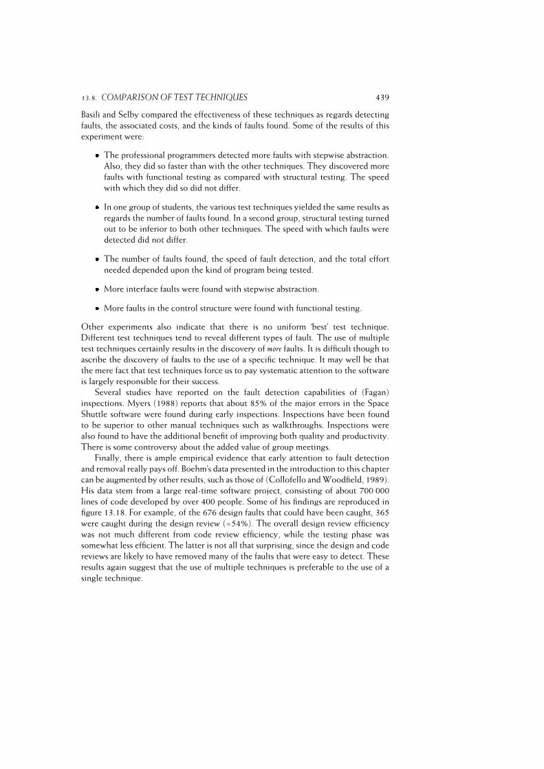
13.8. COMPARISON OF TEST TECHNIQUES 439

Basili and Selby compared the effectiveness of these techniques as regards detecting

faults, the associated costs, and the kinds of faults found. Some of the results of this

experiment were:� The professional programmers detected more faults with stepwise abstraction.

Also, they did so faster than with the other techniques. They discovered more

faults with functional testing as compared with structural testing. The speed

with which they did so did not differ.� In one group of students, the various test techniques yielded the same results as

regards the number of faults found. In a second group, structural testing turned

out to be inferior to both other techniques. The speed with which faults were

detected did not differ.� The number of faults found, the speed of fault detection, and the total effort

needed depended upon the kind of program being tested.� More interface faults were found with stepwise abstraction.� More faults in the control structure were found with functional testing.

Other experiments also indicate that there is no uniform ‘best’ test technique.

Different test techniques tend to reveal different types of fault. The use of multiple

test techniques certainly results in the discovery of more faults. It is difficult though to

ascribe the discovery of faults to the use of a specific technique. It may well be that

the mere fact that test techniques force us to pay systematic attention to the software

is largely responsible for their success.

Several studies have reported on the fault detection capabilities of (Fagan)

inspections. Myers (1988) reports that about 85% of the major errors in the Space

Shuttle software were found during early inspections. Inspections have been found

to be superior to other manual techniques such as walkthroughs. Inspections were

also found to have the additional benefit of improving both quality and productivity.

There is some controversy about the added value of group meetings.

Finally, there is ample empirical evidence that early attention to fault detection

and removal really pays off. Boehm’s data presented in the introduction to this chapter

can be augmented by other results, such as those of (Collofello and Woodfield, 1989).

His data stem from a large real-time software project, consisting of about 700 000

lines of code developed by over 400 people. Some of his findings are reproduced in

figure 13.18. For example, of the 676 design faults that could have been caught, 365

were caught during the design review (=54%). The overall design review efficiency

was not much different from code review efficiency, while the testing phase was

somewhat less efficient. The latter is not all that surprising, since the design and code

reviews are likely to have removed many of the faults that were easy to detect. These

results again suggest that the use of multiple techniques is preferable to the use of a

single technique.

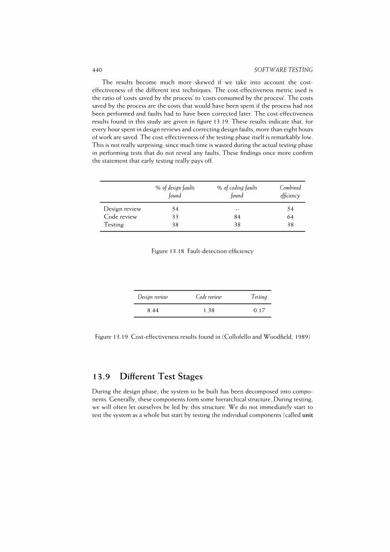
440 SOFTWARE TESTING

The results become much more skewed if we take into account the cost-

effectiveness of the different test techniques. The cost-effectiveness metric used is

the ratio of ‘costs saved by the process’ to ‘costs consumed by the process’. The costs

saved by the process are the costs that would have been spent if the process had not

been performed and faults had to have been corrected later. The cost-effectiveness

results found in this study are given in figure 13.19. These results indicate that, for

every hour spent in design reviews and correcting design faults, more than eight hours

of work are saved. The cost-effectiveness of the testing phase itself is remarkably low.

This is not really surprising, since much time is wasted during the actual testing phase

in performing tests that do not reveal any faults. These findings once more confirm

the statement that early testing really pays off.

% of design faults % of coding faults Combined

found found efficiency

Design review 54 -- 54

Code review 33 84 64

Testing 38 38 38

Figure 13.18 Fault-detection efficiency

Design review Code review Testing

8.44 1.38 0.17

Figure 13.19 Cost-effectiveness results found in (Collofello and Woodfield, 1989)

13.9 Different Test Stages

During the design phase, the system to be built has been decomposed into compo-

nents. Generally, these components form some hierarchical structure. During testing,

we will often let ourselves be led by this structure. We do not immediately start to

test the system as a whole but start by testing the individual components (called unit

13.9. DIFFERENT TEST STAGES 441

testing). Next, these components are incrementally integrated into a system. Testing

the composition of components is called integration testing.

In doing this, we may take one of two approaches. In the first approach, we

start by testing the low-level components which are then integrated and coupled

with components at the next higher level. The subsystem thus obtained is tested

next. Then gradually we move towards the highest-level components. This is known

as bottom-up testing. The alternative approach is top-down testing. In top-down

testing, the top-level components are tested first and are gradually integrated with

lower-level components.

In bottom-up testing, we often have to simulate the environment in which the

component being tested is to be integrated. This an environment is called a test

driver. In top-down testing the opposite is true: we have to simulate lower-level

components, through so-called test stubs.

Both methods have advantages and disadvantages. For instance, in bottom-up

testing it may be difficult to get a sound impression of the final system during the early

stages of testing because whilst the top-level components are not integrated, there is

no system, only bits and pieces. With top-down testing, on the other hand, writing

the stubs can be rather laborious. If the implementation strategy is one whereby a

skeletal system is built first and then populated with components, this skeletal system

can be used as a test driver and the test order then becomes much less of an issue.

In practice, it is often useful to combine both methods. It is not necessarily

the case that some given design or implementation technique drives us in selecting

a particular test technique. If the testing is to partly parallel the implementation,

ordering constraints induced by the order of implementation have to be obeyed,

though.

The program-based adequacy criteria make use of an underlying language model.

Subtle differences in this underlying model may lead to subtle differences in the

resulting flow graphs as used in coverage-based criteria, for instance. Roughly

speaking, the results reported hold at the level of a procedure or subroutine in

languages like FORTRAN, Pascal, and so on.

As a consequence, the corresponding test techniques apply at the level of indi-

vidual methods in object-oriented programs. Testing larger components of OO

programs, such as parameterized classes or classes that inherit part of their functional-

ity from other classes, resembles regression testing as done during maintenance. We

then have to decide how much retesting should be done if methods are redefined in

a subclass, or a class is instantiated with another type as a parameter.

Other forms of testing exist besides unit testing and integration testing. One

possibility is to test the whole system against the user documentation and requirements

specification after integration testing has finished. This is called the system test. A

similar type of testing is often performed under supervision of the user organization

and is then called acceptance testing. During acceptance testing, emphasis is on

testing the usability of the system, rather than compliance of the code against some

specification. Acceptance testing is a major criterion upon which the decision to

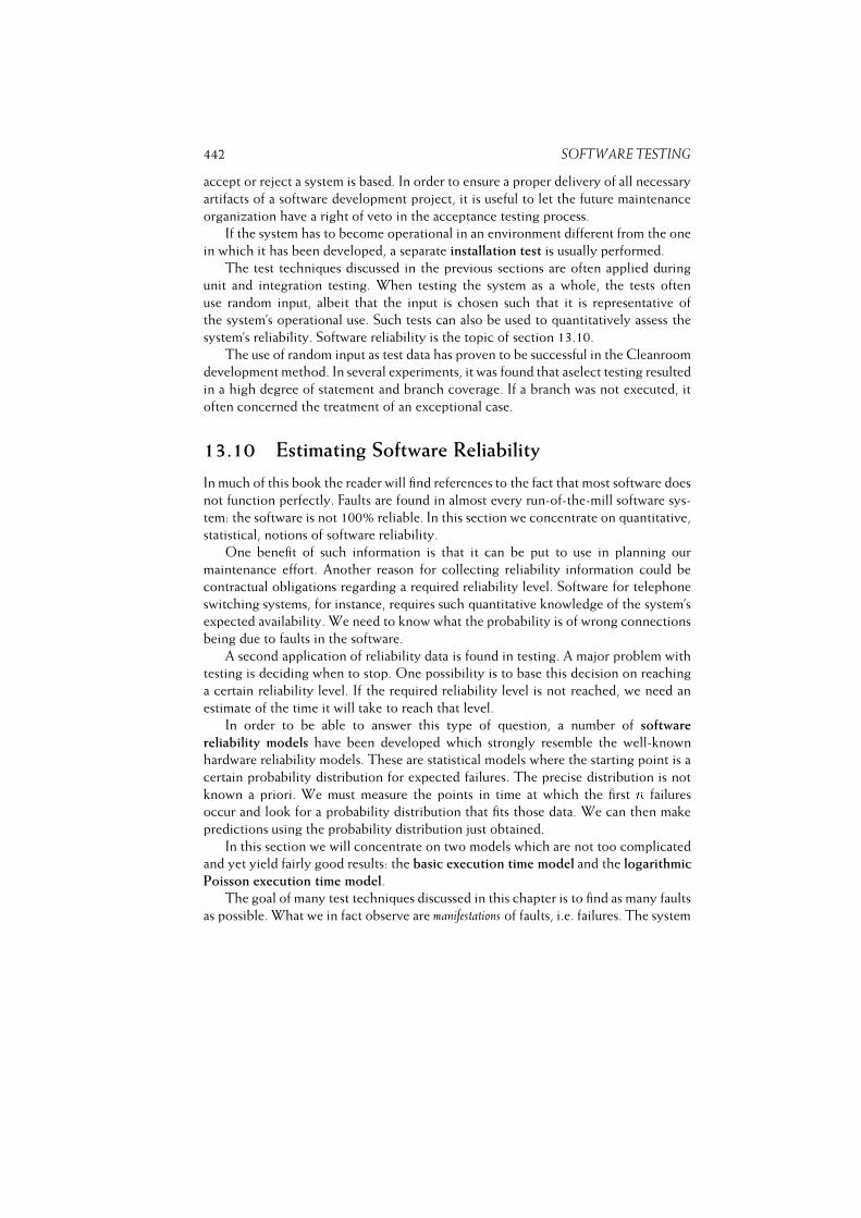
442 SOFTWARE TESTING

accept or reject a system is based. In order to ensure a proper delivery of all necessary

artifacts of a software development project, it is useful to let the future maintenance

organization have a right of veto in the acceptance testing process.

If the system has to become operational in an environment different from the one

in which it has been developed, a separate installation test is usually performed.

The test techniques discussed in the previous sections are often applied during

unit and integration testing. When testing the system as a whole, the tests often

use random input, albeit that the input is chosen such that it is representative of

the system’s operational use. Such tests can also be used to quantitatively assess the

system’s reliability. Software reliability is the topic of section 13.10.

The use of random input as test data has proven to be successful in the Cleanroom

development method. In several experiments, it was found that aselect testing resulted

in a high degree of statement and branch coverage. If a branch was not executed, it

often concerned the treatment of an exceptional case.

13.10 Estimating Software Reliability

In much of this book the reader will find references to the fact that most software does

not function perfectly. Faults are found in almost every run-of-the-mill software sys-

tem: the software is not 100% reliable. In this section we concentrate on quantitative,

statistical, notions of software reliability.

One benefit of such information is that it can be put to use in planning our

maintenance effort. Another reason for collecting reliability information could be

contractual obligations regarding a required reliability level. Software for telephone

switching systems, for instance, requires such quantitative knowledge of the system’s

expected availability. We need to know what the probability is of wrong connections

being due to faults in the software.

A second application of reliability data is found in testing. A major problem with

testing is deciding when to stop. One possibility is to base this decision on reaching

a certain reliability level. If the required reliability level is not reached, we need an

estimate of the time it will take to reach that level.

In order to be able to answer this type of question, a number of software

reliability models have been developed which strongly resemble the well-known

hardware reliability models. These are statistical models where the starting point is a

certain probability distribution for expected failures. The precise distribution is not

known a priori. We must measure the points in time at which the first n failures

occur and look for a probability distribution that fits those data. We can then make

predictions using the probability distribution just obtained.

In this section we will concentrate on two models which are not too complicated

and yet yield fairly good results: the basic execution time model and the logarithmic

Poisson execution time model.

The goal of many test techniques discussed in this chapter is to find as many faults

as possible. What we in fact observe are manifestations of faults, i.e. failures. The system

13.10. ESTIMATING SOFTWARE RELIABILITY 443

fails if the output does not meet the specification. Faults in a program are static in

nature, failures are dynamic. A program can fail only when it is executed. From the

user’s point of view, failures are much more important than faults. For example, a fault

in a piece of software that is never, or hardly ever, used is, in general, less important

than a fault which manifests itself frequently. Also, one and the same fault may show

up in different ways and a failure may be caused by more than one fault.

In the following discussion on reliability, we will not be concerned with the

expected number of faults in a program. Rather, the emphasis will be on the expected

number of failures. The notion of time plays an essential role. For the moment, we

will define reliability as: the probability that the program will not fail during a certain

period of time.

The notion of time deserves further attention. Ultimately, we are interested

in statements regarding calendar time. For example, we might want to know the

probability that a given system will not fail in a one-week time period, or we might

be interested in the number of weeks of system testing still needed to reach a certain

reliability level.

Both models discussed below use the notion of execution time. Execution time

is the time spent by the machine actually executing the software. Reliability models

based on execution time yield better results than those based on calendar time. In

many cases, an a posteriori translation of execution time to calendar time is possible.

To emphasize this distinction, execution time will be denoted by � and calendar time

by t.The failure behavior of a program depends on many factors: quality of the

designers, complexity of the system, development techniques used, etc. Most of these

cannot adequately be dealt with as variables in a reliability model and therefore are

assumed to be fixed. Reliability, when discussed in this section, will therefore always

concern one specific project.

Some factors affecting failure behavior can be dealt with, though. As noticed

before, the models discussed are based on the notion of execution time. This is

simple to measure if we run one application on a stand-alone computer. Translation

between machines that differ in speed can be taken care of relatively easily. Even if

the machine is used in multiprogramming mode, translation from the time measured

to proper execution time may be possible. This is the case, for instance, if time is

relatively uniformly distributed over the applications being executed.

The input to a program is also variable. Since we estimate the model’s parameters

on the basis of failures observed, the predictions made will only hold insofar as future

input resembles the input which led to the observed failure behavior. The future has to

resemble the past. In order to get reliable predictions, the tests must be representative

of the later operational use of the system. If we are able to allocate the possible inputs

to different equivalence classes, simple readjustments are possible here too.

We may summarize this discussion by including the environment in the definition

of our notion of software reliability. Reliability then is defined as the probability that

a system will not fail during a certain period of time in a certain environment.

444 SOFTWARE TESTING

Finally, software systems are not static entities. Software is often implemented

and tested incrementally. Reliability of an evolving system is difficult to express. In

the ensuing discussion, we therefore assume that our systems are stable over time.

We may characterize the failure behavior of software in different ways. For

example, we may consider the expected time to the next failure, the expected time

interval between successive failures, or the expected number of failures in a certain

time interval. In all cases, we are concerned with random variables, since we do not

know exactly when the software will fail. There are at least two reasons for this

uncertainty. Firstly, we do not know where the programmer made errors. Secondly,

the relation between a certain input and the order in which the corresponding set

of instructions is being executed is not usually known. We may therefore model

subsequent failures as a stochastic process. Such a stochastic process is characterized

by, amongst other things, the form and probability distribution of the random

variables.

When the software fails, we try to locate and repair the fault that caused this

failure. In particular, this situation arises during the test phase of the software life

cycle. Since we assume a stable situation, the application of reliability models is

particularly appropriate during system testing, when the individual components have

been integrated into one system. This system-test situation in particular will be

discussed below.

In this situation, the failure behavior will not follow a constant pattern but

will change over time, since faults detected are subsequently repaired. A stochastic

process whose probability distribution changes over time is called non-homogeneous. The

variation in time between successive failures can be described in terms of a function�(�) which denotes the average number of failures until time � . Alternatively, we

may consider the failure intensity function �(�), the average number of failures per

unit of time at time � . �(�) then is the derivative of �(�). If the reliability of a

program increases through fault correction, the failure intensity will decrease.

The relationship between �(�), �(�) and � is graphically depicted in figure 13.20.

The models to be discussed below, the basic execution time model (BM) and the

logarithmic Poisson execution time model (LPM), differ in the form of the failure

intensity function �(�).Both BM and LPM assume that failures occur according to a non-homogeneous

Poisson process. Poisson processes are often used to describe the stochastic behavior

of real-world events. Examples of Poisson processes are: the number of telephone

calls expected in a given period of time, or the expected number of car accidents in

a given period of time. In our case, the processes are non-homogeneous, since the

failure intensity changes as a function of time, assuming a (partly) successful effort to

repair the underlying errors.

In BM, the decrease in failure intensity, as a function of the number of failures

observed, is constant. The contribution to the decrease in failure intensity thus is the

same for each failure observed. In terms of the mean number of failures observed (�),

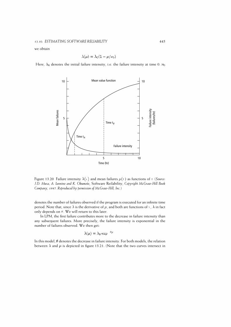
13.10. ESTIMATING SOFTWARE RELIABILITY 445

we obtain �(�) = �0(1� �=�0)Here, �0 denotes the initial failure intensity, i.e. the failure intensity at time 0. �0

Figure 13.20 Failure intensity �(�) and mean failures �(�) as functions of � (Source:J.D. Musa, A. Iannino and K. Okumoto, Software Reilability, Copyright McGraw-Hill Book

Company, 1987. Reproduced by permission of McGraw-Hill, Inc.)

denotes the number of failures observed if the program is executed for an infinite time

period. Note that, since � is the derivative of �, and both are functions of � , � in fact

only depends on � . We will return to this later.

In LPM, the first failure contributes more to the decrease in failure intensity than

any subsequent failures. More precisely, the failure intensity is exponential in the

number of failures observed. We then get:�(�) = �0 exp���In this model, � denotes the decrease in failure intensity. For both models, the relation

between � and � is depicted in figure 13.21. (Note that the two curves intersect in

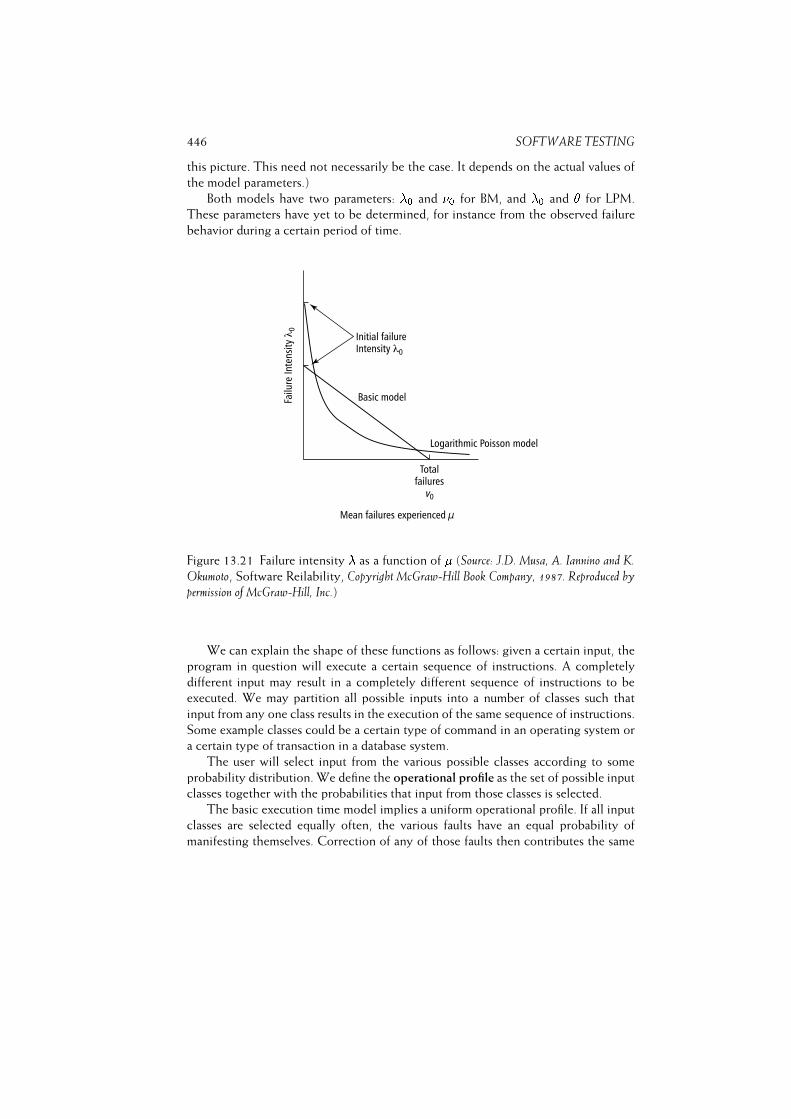
446 SOFTWARE TESTING

this picture. This need not necessarily be the case. It depends on the actual values of

the model parameters.)

Both models have two parameters: �0 and �0 for BM, and �0 and � for LPM.

These parameters have yet to be determined, for instance from the observed failure

behavior during a certain period of time.

Figure 13.21 Failure intensity � as a function of � (Source: J.D. Musa, A. Iannino and K.

Okumoto, Software Reilability, Copyright McGraw-Hill Book Company, 1987. Reproduced bypermission of McGraw-Hill, Inc.)

We can explain the shape of these functions as follows: given a certain input, the

program in question will execute a certain sequence of instructions. A completely

different input may result in a completely different sequence of instructions to be

executed. We may partition all possible inputs into a number of classes such that

input from any one class results in the execution of the same sequence of instructions.

Some example classes could be a certain type of command in an operating system or

a certain type of transaction in a database system.

The user will select input from the various possible classes according to some

probability distribution. We define the operational profile as the set of possible input

classes together with the probabilities that input from those classes is selected.

The basic execution time model implies a uniform operational profile. If all input

classes are selected equally often, the various faults have an equal probability of

manifesting themselves. Correction of any of those faults then contributes the same

13.10. ESTIMATING SOFTWARE RELIABILITY 447

amount to the decrease in failure intensity. It has been found that BM still models the

situation fairly well in the case of a fairly non-uniform operational profile.

With a strong non-uniform operational profile the failure intensity curve will have

a convex shape, as in LPM. Some input classes will then be selected relatively often.

As a consequence, certain faults will show up earlier and be corrected sooner. These

corrections will have a larger impact on the decrease in failure intensity.

In both models, � and � are functions of � (execution time). Furthermore, failure

intensity � is the derivative of mean failures �. For BM, we may therefore write�(�) = �0(1� �=�0)as d�(�)d� = �0(1� �(�)=�0)Solving this differential equation yields�(�) = �0(1� exp��0�=�0)and �(�) = �0 exp��0�=�0In a similar way, we obtain for LPM:�(�) = ln(�0�� + 1)=�and �(�) = �0=(�0�� + 1)For LPM, the expected number of failures in infinite time is infinite. Obviously, the

number of failures observed during testing is finite.

Both models allow that fault correction is not perfect. In BM the effectiveness of

fault correction is constant, though not necessarily 100%. This again shows up in the

linearity of the failure intensity function. In LPM, the effectiveness of fault correction

decreases with time. Possible reasons could be that it becomes increasingly more

difficult to locate the faults, for example because the software becomes less structured,

or the personnel less motivated.

If the software has become operational and faults are not being corrected any

more, the failure intensity will remain constant. Both models then reduce to a

homogeneous Poisson process with failure intensity � as the parameter. The number

of failures expected in a certain time period will then follow a Poisson-distribution.

The probability of exactly n failures being observed in a time period of length � is

then given by Pn(�) = (��)n � exp��� =n!

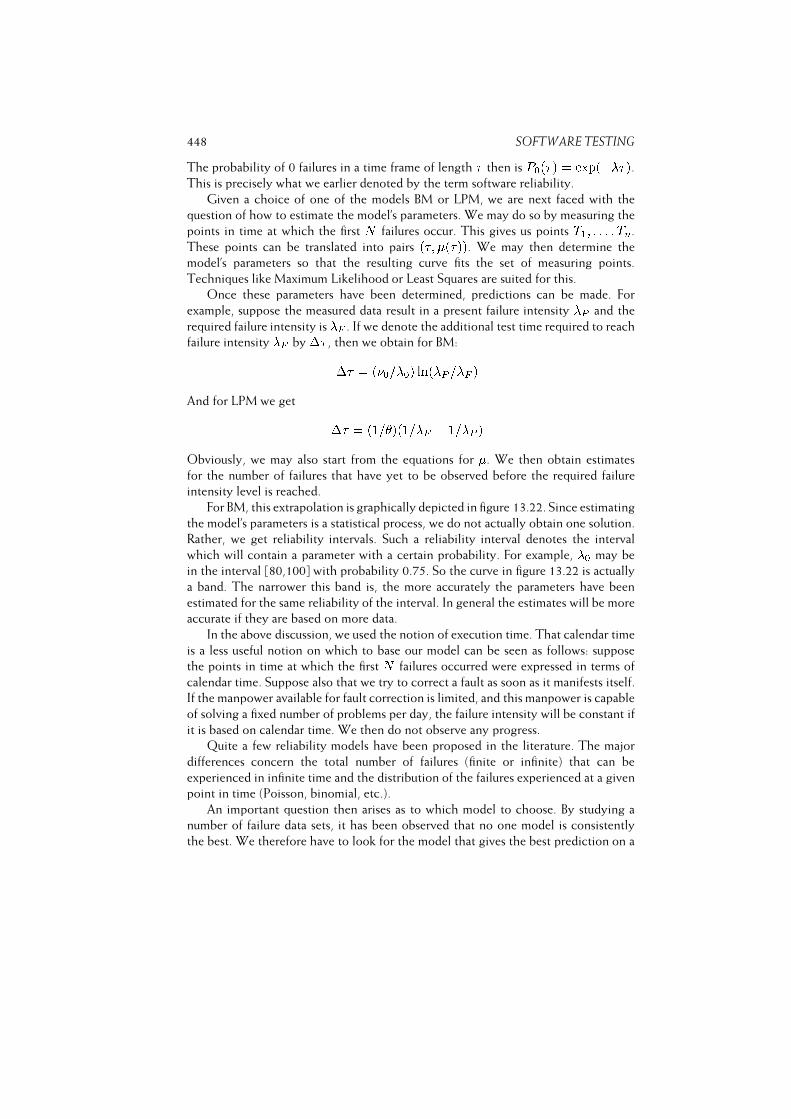
448 SOFTWARE TESTING

The probability of 0 failures in a time frame of length � then is P0(�) = exp(���).This is precisely what we earlier denoted by the term software reliability.

Given a choice of one of the models BM or LPM, we are next faced with the

question of how to estimate the model’s parameters. We may do so by measuring the

points in time at which the first N failures occur. This gives us points T1; : : : ; Tn.

These points can be translated into pairs (�; �(�)). We may then determine the

model’s parameters so that the resulting curve fits the set of measuring points.

Techniques like Maximum Likelihood or Least Squares are suited for this.

Once these parameters have been determined, predictions can be made. For

example, suppose the measured data result in a present failure intensity �P and the

required failure intensity is �F . If we denote the additional test time required to reach

failure intensity �F by �� , then we obtain for BM:�� = (�0=�0) ln(�P =�F )And for LPM we get �� = (1=�)(1=�F � 1=�P )Obviously, we may also start from the equations for �. We then obtain estimates

for the number of failures that have yet to be observed before the required failure

intensity level is reached.

For BM, this extrapolation is graphically depicted in figure 13.22. Since estimating

the model’s parameters is a statistical process, we do not actually obtain one solution.

Rather, we get reliability intervals. Such a reliability interval denotes the interval

which will contain a parameter with a certain probability. For example, �0 may be

in the interval [80,100] with probability 0.75. So the curve in figure 13.22 is actually

a band. The narrower this band is, the more accurately the parameters have been

estimated for the same reliability of the interval. In general the estimates will be more

accurate if they are based on more data.

In the above discussion, we used the notion of execution time. That calendar time

is a less useful notion on which to base our model can be seen as follows: suppose

the points in time at which the first N failures occurred were expressed in terms of

calendar time. Suppose also that we try to correct a fault as soon as it manifests itself.

If the manpower available for fault correction is limited, and this manpower is capable

of solving a fixed number of problems per day, the failure intensity will be constant if

it is based on calendar time. We then do not observe any progress.

Quite a few reliability models have been proposed in the literature. The major

differences concern the total number of failures (finite or infinite) that can be

experienced in infinite time and the distribution of the failures experienced at a given

point in time (Poisson, binomial, etc.).

An important question then arises as to which model to choose. By studying a

number of failure data sets, it has been observed that no one model is consistently

the best. We therefore have to look for the model that gives the best prediction on a

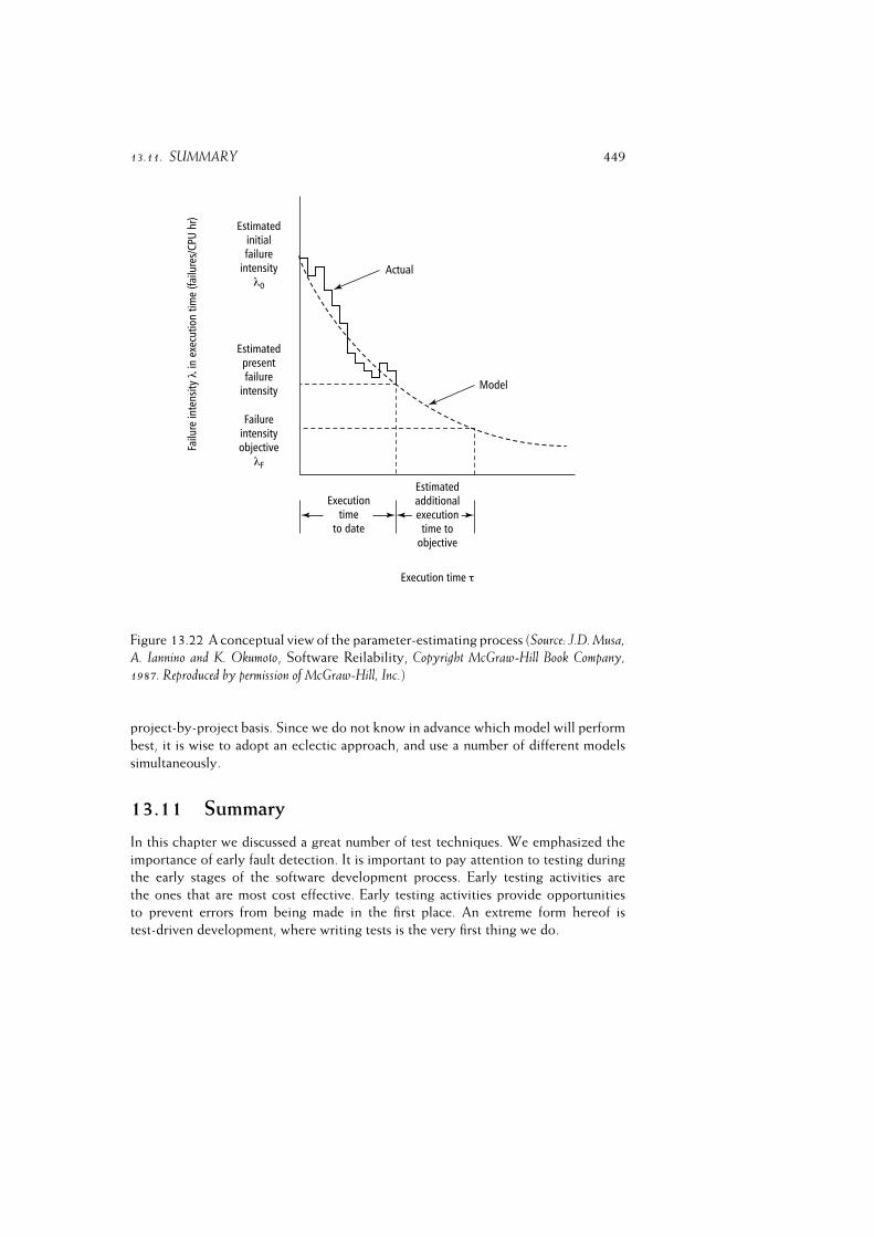
13.11. SUMMARY 449

Figure 13.22 A conceptual view of the parameter-estimating process (Source: J.D. Musa,A. Iannino and K. Okumoto, Software Reilability, Copyright McGraw-Hill Book Company,

1987. Reproduced by permission of McGraw-Hill, Inc.)

project-by-project basis. Since we do not know in advance which model will perform

best, it is wise to adopt an eclectic approach, and use a number of different models

simultaneously.

13.11 Summary

In this chapter we discussed a great number of test techniques. We emphasized the

importance of early fault detection. It is important to pay attention to testing during

the early stages of the software development process. Early testing activities are

the ones that are most cost effective. Early testing activities provide opportunities

to prevent errors from being made in the first place. An extreme form hereof is

test-driven development, where writing tests is the very first thing we do.

450 SOFTWARE TESTING

In practice, the various manual test techniques seem to be used most often. They

turn out to be at least as successful as the various structural and functional techniques.

Inspections in particular have been found to be a very cost-effective test technique.

Next to the test techniques used, a major element in software fault detection and

removal is the choice of personnel -- some people are significantly better at finding

and removing faults than others.

Since exhaustive testing is generally not feasible, we have to select an adequate

set of test cases. Test techniques can be classified according to the criterion used

to measure the adequacy of this a test set. Three broad categories of test adequacy

criteria can be distinguished:

– Coverage-based testing, in which testing requirements are specified in terms

of the coverage of the product to be tested, for example, the percentage of

statements executed.

– Fault-based testing, in which the focus is on detecting faults, for example, the

percentage of seeded faults detected.

– Error-based testing, which focuses on testing error-prone points, such as 0, 1,

or the upper bound of an array.

A test adequacy criterion can be used as stopping rule, as a measurement instrument,

or as a generator of test cases. Test adequacy criteria and the corresponding test

techniques can be viewed as two sides of the same coin. A coverage-based test

technique makes it easy to measure coverage-based criteria, but does not help us in

assessing whether all error-prone points have been tested.

Experimental evaluations show that there is no uniform best test technique.

Different techniques tend to reveal different types of error. It is therefore wise to

‘vacuum the carpet in more than one direction’.

One line of research addresses the relative power of test adequacy criteria. A

well-known measure to compare program-based test adequacy criteria is the subsume

relation: criterion X subsumes Y if, for all programs P and all test sets T, X-adequacy

implies Y-adequacy. Many of the well-known adequacy criteria have been related to

one another in a subsume hierarchy.

As with any other life cycle activity, testing has to be carefully planned, controlled,

and documented. Some of the IEEE Standards provide useful guidelines for doing

this (IEEE829, 1998; IEEE1012, 1986).

The last part of this chapter was devoted to a discussion of how to quantitatively

estimate the reliability of a piece of software. The currently-available software

reliability models are limited in their immediate practical value. In particular, no

model consistently performs best.

13.12. FURTHER READING 451

13.12 Further Reading

Well-known textbooks on testing are (Myers, 1979) (or its updated version (Myers,

2004)) and (Beizer, 1995). Whittaker (2000) gives a concise overview of the field.

For a further discussion of safety issues, see (Leveson, 1991). Fault-tree analysis is

discussed in (Leveson, 1986). Zhu et al. (1997) gives a very good overview of the

types of test strategy discussed in sections 13.5--13.7 and the associated adequacy

criteria. Rothermel and Harrold (1996) and Harrold (1999) give a very good overview

of regression test techniques. Testing object-oriented software is addressed in (Binder,

2000).

The first attempts at developing some theory on testing date back to the

1970s (Goodenough and Gerhart, 1975), (Howden, 1982), and (Howden, 1985).

Thereafter, much of that research has been directed towards finding and relating test

adequacy criteria (Weyuker, 1988), (Clarke et al., 1989), (Weyuker, 1990), (Frankl

and Weyuker, 1993a), (Frankl and Weyuker, 1993b), (Parrish and Zweben, 1995),

and (Zhu, 1996). Experimental evaluations of test adequacy criteria can be found in

(Frankl and Weiss, 1993), (Weyuker, 1993), (Offutt and Lee, 1994), (Harrold et al.,

1997), and (Frankl et al., 1997). Experiments that compare manual and functional or

structural test techniques are reported upon in (Basili and Selby, 1987), (Kamsties

and Lott, 1995), and (Wood et al., 1997). Juristo et al. (2004) give an overview of 25

years of testing technique experiments.

The Cleanroom development method is described in (Selby et al., 1987) and

(Mills et al., 1987). Experiences with Cleanroom are discussed in (Currit et al., 1986)

and (Trammell et al., 1992). Stepwise abstraction is described in (Linger et al., 1979).

Beck (2003) describes test-driven development. Janzen and Saiedian (2005) give

a somewhat wider perspective on its potential. Hunt and Thomas (2003) is one of the

many textbooks describing JUnit. Effects of test-driven development on productivity

and errors are reported in (Maximilien and Williams, 2003) and (Erdogmus et al.,

2005).

Inspections were introduced by Fagan in the 1970s (Fagan, 1976) and (Fagan,

1986). Gilb and Graham (1993) is a text book on inspections; Wiegers (2002) is

a text book on peer reviews. There have been many experimental evaluations of

inspections; see for instance (Knight and Myers, 1993), (Weller, 1993), (Grady and

van Slack, 1994), (Porter et al., 1995), (Porter et al., 1997), (Porter et al., 1998) and

(Biffl and Halling, 2002). Parnas and Lawford (2003a) and Parnas and Lawford (2003b)

are introductions to two companion special journal issues on software inspections.

Ciolkowski et al. (2003) discusses the state of the art in software reviews. The value

of formal correctness proofs is disputed in (DeMillo et al., 1979). Heated debates in

the literature show that this issue has by no means been resolv (Fetzer, 1988).

The basic execution time model and the logarithmic Poisson execution time model

are extensively discussed, and compared with a number of other models, in Musa

et al. (1987). Lyu (1995) is a very comprehensive source on software reliability.

Experiences with software reliability modeling are reported in (Jeske and Zhang,

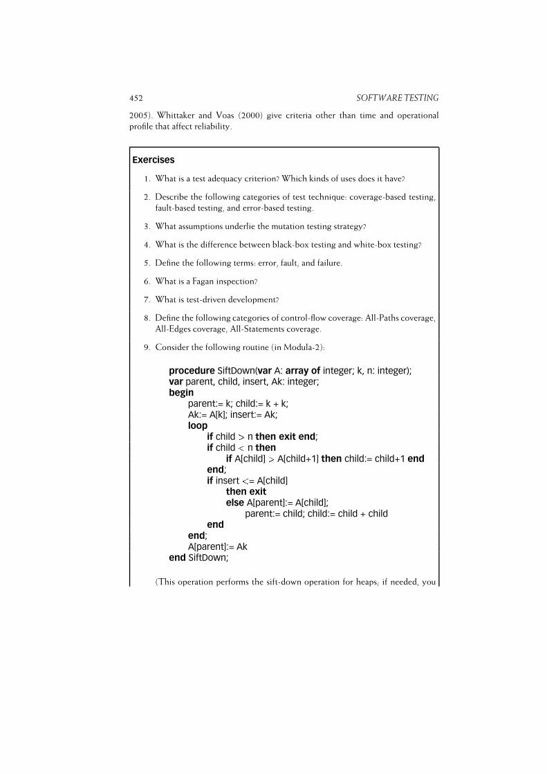
452 SOFTWARE TESTING

2005). Whittaker and Voas (2000) give criteria other than time and operational

profile that affect reliability.

Exercises

1. What is a test adequacy criterion? Which kinds of uses does it have?

2. Describe the following categories of test technique: coverage-based testing,

fault-based testing, and error-based testing.

3. What assumptions underlie the mutation testing strategy?

4. What is the difference between black-box testing and white-box testing?

5. Define the following terms: error, fault, and failure.

6. What is a Fagan inspection?

7. What is test-driven development?

8. Define the following categories of control-flow coverage: All-Paths coverage,

All-Edges coverage, All-Statements coverage.

9. Consider the following routine (in Modula-2):

procedure SiftDown(var A: array of integer; k, n: integer);var parent, child, insert, Ak: integer;begin

parent:= k; child:= k + k;Ak:= A[k]; insert:= Ak;loop

if child > n then exit end;if child < n then

if A[child] > A[child+1] then child:= child+1 endend;if insert <= A[child]

then exitelse A[parent]:= A[child];

parent:= child; child:= child + childend

end;A[parent]:= Ak

end SiftDown;

(This operation performs the sift-down operation for heaps; if needed, you

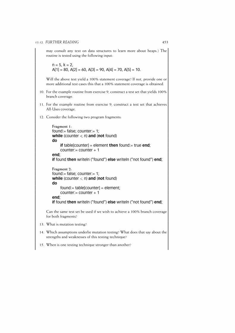
13.12. FURTHER READING 453

may consult any text on data structures to learn more about heaps.) The

routine is tested using the following input:

n = 5, k = 2,A[1] = 80, A[2] = 60, A[3] = 90, A[4] = 70, A[5] = 10.

Will the above test yield a 100% statement coverage? If not, provide one or

more additional test cases this that a 100% statement coverage is obtained.

10. For the example routine from exercise 9, construct a test set that yields 100%

branch coverage.

11. For the example routine from exercise 9, construct a test set that achieves

All-Uses coverage.

12. Consider the following two program fragments:

Fragment 1:

found:= false; counter:= 1;while (counter < n) and (not found)do

if table[counter] = element then found:= true end;counter:= counter + 1

end;if found then writeln (”found”) else writeln (”not found”) end;

Fragment 2:

found:= false; counter:= 1;while (counter < n) and (not found)do

found:= table[counter] = element;counter:= counter + 1

end;if found then writeln (”found”) else writeln (”not found”) end;

Can the same test set be used if we wish to achieve a 100% branch coverage

for both fragments?

13. What is mutation testing?

14. Which assumptions underlie mutation testing? What does that say about the

strengths and weaknesses of this testing technique?

15. When is one testing technique stronger than another?

454 SOFTWARE TESTING

16. What is the difference between a system test and an acceptance test?

17. Contrast top-down and bottom-up integration testing.

18. What is the major difference between the basic execution time model and

the logarithmic Poisson execution time model of software reliability?

19. Give a definition of software reliability. Give a rationale for the various parts

of this definition.

20. Why is it important to consider the operational profile of a system while

assessing its reliability?

21. Can you think of reasons why reliability models based on execution time

yield better results than those based on calendar time?

22. Can software reliability be determined objectively?

23. � Read (DeMillo et al., 1979) and both (Fetzer, 1988) and the reactions to

it (cited in the bibliography entry for that article). Write a position paper on

the role of correctness proofs in software development.

24. � For a (medium-sized) system you have developed, write a Software

Verification and Validation Plan (SVVP) following IEEE Standard 1012.

Which of the issues addressed by this standard were not dealt with during

the actual development? Could a more thorough SVVP have improved the

development and testing process?

25. ~ Consider the following sort routine:

procedure selectsort(var r: array [1 .. n] of integer);var j, k, small: integer;begin

if n > 1 thenfor k:= 1 to n - 1 do

small:= k;for j:= k + 1 to n do

if r[j] < r[small] then small:= j endend;swap(r[k], r[small])

endend

end selectsort;

13.12. FURTHER READING 455

Determine the function (by means of pre- and postconditions) of this routine

using stepwise abstraction.

26. ~ Generate ten mutants of the procedure in exercise 20. Next, test these

mutants using the following set of test cases:

– an empty array;

– an array of length 1;

– a sorted array of length 10;

– an array of 10 elements that all have the same value;

– an array of length 10 with random elements.

Which of these mutants stay alive? What does this tell you about the quality

of these tests?

27. ~Construct an example showing that the antidecomposition and anticompo-

sition axioms from section 13.8.2 do not hold for the All-Nodes and All-Edges

testing criteria. Why are these axioms important?

28. � With one or two fellow students or colleagues, inspect a requirements or

design document not produced by yourself. Is the documentation sufficient

to do a proper inspection? Discuss the findings of the process with the author

of the document. Repeat the process with a document of which you are the

author.

29. ~ Assess the strengths and weaknesses of:

– functional or structural testing,

– correctness proofs,

– random testing, and

– inspections

for fault finding and confidence building, respectively.

30. ~ One way of testing a high-level document such as a requirements specifi-

cation is to devise and discuss possible usage scenarios with prospective users

of the system to be developed. What additional merits can this a technique

have over other types of review?

31. ~ How do you personally feel about a Cleanroom-like approach to software

development?

456 SOFTWARE TESTING

32. ~ Discuss the following claim: ‘Reliability assessment is more important than

testing’. Can you think of reasons why both are needed?

14

Software Maintenance

LEARNING OBJECTIVES� To know about well-known categories of maintenance tasks and data on their

distribution� To be able to discern major causes of maintenance problems� To be aware of reverse engineering, its limitations, and tools to support it� To appreciate different ways in which maintenance activities can be organized� To understand major differences between development and maintenance and

the consequences thereof

458 SOFTWARE MAINTENANCE

Software maintenance is not limited to the correction of faults. A large part

of maintenance deals with accommodating new or changed user requirements

and adapting software to a changed environment. It is about evolution, rather

than just maintenance. We discuss the various types of maintenance tasks, and

how to organize them.

Like living organisms and most natural phenomena, software projects follow a life cycle

that starts from emptiness, is followed by rapid growth during infancy, enters a long

period of maturity, and then begins a cycle of decay that almost resembles senility.(Jones, 1989)

Software, unlike a child, does not grow smarter and more capable; unfortunately, it doesseem to grow old and cranky.

(Lyons, 1981)

Consider UBank, a multinational bank, a typical large organization that is heavily

dependent upon automation for its daily operation. UBank is the result of a number

of mergers and takeovers.

UBank has hundreds of offices spread all over the world. It has a number of

mainframes at a central site, as well as thousands of workstations and printers

connected. It has internet connectivity, all over the world, and strives for 24 � 7availability. The workload is an enormous number of transactions per hour. The bank

has hundreds of application systems averaging over 100 000 lines of code. Programs

are written in a variety of languages, most notably COBOL, various 4GLs and JCL.

The systems make use of huge databases implemented under IDMS, INGRES, and so

on. Some of the basic information is shared by many systems.

Quite likely, the bank has no complete overview of its application portfolio.

Because of the mergers and acquisitions, integration of applications is a big issue.

There are many wrappers, bridges, and other temporary means to glue systems

together. There are more people involved in maintaining UBank’s information

systems, than there are people involved in developing new systems for UBank.

There are many organizations like UBank, organizations whose portfolio of

information systems is vital for their day-to-day operation. At the same time, these

information systems are ageing and it becomes increasingly difficult to keep them ‘up

and running’. An increasing percentage of the annual budget of these organizations is

spent on keeping installed systems functioning properly.

It is estimated that there are more than 100 billion lines of code in production in

the world. As much as 80% of it is unstructured, patched, and badly documented. It is a

gargantuan task to keep these software systems operational: errors must be corrected,

and systems must be adapted to changing environments and user needs. This is what

software maintenance is about. Software maintenance is defined as (IEEE610, 1990):

459

The process of modifying a software system or component after delivery

to correct faults, improve performance or other attributes, or adapt to a

changed environment.

So software maintenance is, in particular, not limited to the correction of latent faults.

The distinction between development and maintenance is fuzzy, to say the least. This

makes it hard to very bold about percentages and types of maintenance categories.

In section 14.1, we revisit the discussion about types of maintenance activities from

chapter 1 and provide a more balanced view.

Changes in both the system’s environment and user requirements are inevitable.

Software models part of reality, and reality changes, whether we like it or not. So the

software has to change too. It has to evolve. A large percentage of what we are used

to calling maintenance, is actually evolution.

When looking for ways to reduce the maintenance problem, it is worth bearing in

mind the classification of maintenance activities given in chapter 1. Possible solutions

to be considered include:� Higher-quality code, better test procedures, better documentation and adher-

ence to standards and conventions may help to save on corrective maintenance;� By anticipating changes during requirements engineering and design and by

taking them into account during realization, future perfective and adaptive

maintenance can be realized more easily. In particular, the explicit evaluation

of a software architecture with respect to ease of change is to be recommended.

Through its inheritance and virtual typing capabilities, the object-oriented

development paradigm in particular offers opportunities for isolating parts that

are susceptible to changes from those that are less so. Many design patterns are

aimed at encapsulating change-prone elements;� Finer tuning to user needs may lead to savings in perfective maintenance.

This may, for example, be achieved through prototyping techniques or a more

intensive user participation during the requirements engineering and design

phase;� Less maintenance is needed when less code is written. The sheer length of

the source code is the main determinant of total cost, both during initial

development and during maintenance. In particular, a 10% change in a module

of 200 LOC is more expensive than a 20% change in a module of 100 LOC. The

reuse of existing software in particular has a very direct impact on maintenance

costs.

These possible actions are all concerned with initial software development. This is

not surprising, since the key to better maintainable software is to be found there. All

these issues have been discussed at great length in previous chapters.

Better initial development though will not automatically result in lower main-

tenance costs. Worse, Dekleva (1992) found exactly the opposite. He found that

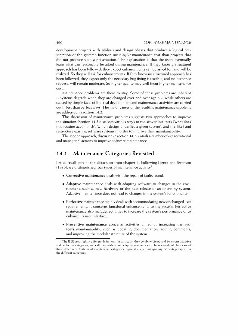
460 SOFTWARE MAINTENANCE

development projects with analysis and design phases that produce a logical pre-

sentation of the system’s function incur higher maintenance cost than projects that

did not produce such a presentation. The explanation is that the users eventually

learn what can reasonably be asked during maintenance. If they know a structured

approach has been followed, they expect enhancements can be asked for, and will be

realized. So they will ask for enhancements. If they know no structured approach has

been followed, they expect only the necessary bug fixing is feasible, and maintenance

requests will remain moderate. So higher quality may well incur higher maintenance

cost.

Maintenance problems are there to stay. Some of these problems are inherent

-- systems degrade when they are changed over and over again -- while others are

caused by simple facts of life: real development and maintenance activities are carried

out in less than perfect ways. The major causes of the resulting maintenance problems

are addressed in section 14.2.

This discussion of maintenance problems suggests two approaches to improve

the situation. Section 14.3 discusses various ways to rediscover lost facts (‘what does

this routine accomplish’, ‘which design underlies a given system’, and the like) and

restructure existing software systems in order to improve their maintainability.

The second approach, discussed in section 14.5, entails a number of organizational

and managerial actions to improve software maintenance.

14.1 Maintenance Categories Revisited

Let us recall part of the discussion from chapter 1. Following Lientz and Swanson

(1980), we distinguished four types of maintenance activity1:� Corrective maintenance deals with the repair of faults found.� Adaptive maintenance deals with adapting software to changes in the envi-

ronment, such as new hardware or the next release of an operating system.

Adaptive maintenance does not lead to changes in the system’s functionality.� Perfective maintenance mainly deals with accommodating new or changed user

requirements. It concerns functional enhancements to the system. Perfective

maintenance also includes activities to increase the system’s performance or to

enhance its user interface.� Preventive maintenance concerns activities aimed at increasing the sys-

tem’s maintainability, such as updating documentation, adding comments,

and improving the modular structure of the system.

1The IEEE uses slightly different definitions. In particular, they combine Lientz and Swanson’s adaptive

and perfective categories, and call the combination adaptive maintenance. The reader should be aware of

these different definitions of maintenance categories, especially when interpreting percentages spent on

the different categories.

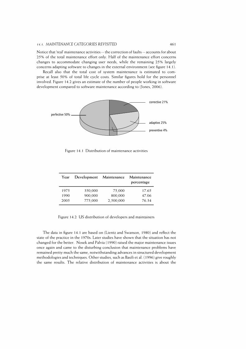
14.1. MAINTENANCE CATEGORIES REVISITED 461

Notice that ‘real’ maintenance activities -- the correction of faults -- accounts for about

25% of the total maintenance effort only. Half of the maintenance effort concerns

changes to accommodate changing user needs, while the remaining 25% largely

concerns adapting software to changes in the external environment (see figure 14.1).

Recall also that the total cost of system maintenance is estimated to com-

prise at least 50% of total life cycle costs. Similar figures hold for the personnel

involved. Figure 14.2 gives an estimate of the number of people working in software

development compared to software maintenance according to (Jones, 2006).

Figure 14.1 Distribution of maintenance activities

Year Development Maintenance Maintenance

percentage

1975 350,000 75,000 17.65

1990 900,000 800,000 47.06

2005 775,000 2,500,000 76.34

Figure 14.2 US distribution of developers and maintainers

The data in figure 14.1 are based on (Lientz and Swanson, 1980) and reflect the

state of the practice in the 1970s. Later studies have shown that the situation has not

changed for the better. Nosek and Palvia (1990) raised the major maintenance issues

once again and came to the disturbing conclusion that maintenance problems have

remained pretty much the same, notwithstanding advances in structured development

methodologies and techniques. Other studies, such as Basili et al. (1996) give roughly

the same results. The relative distribution of maintenance activities is about the

462 SOFTWARE MAINTENANCE

same as it was 20 years ago. Systems though have become larger, maintenance staff

has grown, there are more systems, and there is a definite trend to an increase in

maintenance effort relative to development effort.

Some studies give results that are quite different from the general picture sketched

above. Schach et al. (2003), for instance, investigated maintenance effort in three

systems and found corrective maintenance percentages of 50% and more, and very

low percentages for adaptive maintenance. There is no convincing argument for these

differences.

In many organizations, the definition of software maintenance does not follow

the IEEE definition. Some organizations for instance define change efforts larger than,

say, three months, as development rather than maintenance. This blurs the picture

even further. In practice also, people find it difficult to distinguish between adaptive

and perfective maintenance. What remains then is a distinction between correcting

fault and ’the rest’. The latter mostly caters for 75% or more of the maintenance effort.

The maintenance categories from (Lientz and Swanson, 1980) refer to the software

only. Keeping software alive incurs other costs too, though. For instance, new users

must be trained, and the helpdesk needs to be staffed. Nowadays, it is not uncommon

that these supporting costs account for around 25% of the cost of keeping a system

deployed.

Another way to look at the distribution of maintenance cost and prevailing types

of maintenance tasks is along the time dimension. We may distinguish the following

maintenance life cycle stages:� During the introductory stage of a new system, most of the effort is spent on

user support. Users have to be trained, and they will often contact the helpdesk

for clarification.� Next follows a growth stage in which more and more users start to explore the

system’s possibilities. As far as maintenance is concerned, emphasis during this

stage is on correcting faults.� The growth stage is followed by a period of maturity. Users know what the

system can and cannot do, and ask for enhancements.� Finally, a period of decline sets in. Technology replacement, such as another

platform or user interface kit, constitutes a major category of maintenance tasks

during this period.

Successful maintenance requires knowledge of the application. After initial delivery,

this knowledge usually is available. Either knowledge of the application is explicitly

transferred to the maintenance organization via documentation, training, and the like,

or the developers have become maintainers of the application they just developed.

But over time, this knowledge vaporizes, and at some point in time, it has become

scant. This point in time more or less coincides with the transition from the mature

stage to the declining stage. The ”if it ain’t broken don’t fix it” adagium then becomes

14.2. MAJOR CAUSES OF MAINTENANCE PROBLEMS 463

prevalent. Bennett and Rajlich (2000) use the terms evolution stage and servicing

stage to distinguish between the period in which the system can successfully evolve

and the subsequent period where this is no longer the case. In the latter stage, changes

become tactical. For example, necessary changes are realized through patches and

wrappers.

Finally, we may consider the distribution of effort over the activities of a single

maintenance task. For the code-related tasks, the main activities are:� Isolation The first activity is concerned with determining the part of the system

(modules, classes) that needs to be changed.� Modification This concerns the actual changes. One or more components are

adapted to accommodate the change.� Testing After the changes have been made, the system has to be tested anew

(regression testing).

As a rule of thumb, isolation takes about 40% of effort, while the other two activities

each take about 30%. This distribution is not the same for all types of maintenance.

For corrective maintenance, isolation often takes an even larger share, while for

adaptive maintenance tasks, the actual modification takes longer. During corrective

maintenance, the fault that caused the failure has to be found, and this may take a lot

of effort. Once it is found, the actual modification often is fairly small. For adaptive

maintenance tasks, the reverse holds.

14.2 Major Causes of Maintenance Problems

The following story reveals many of the problems that befall a typical software

maintenance organization. It is based on an anecdote once told by David Parnas and

concerns the re-engineering of software for fighter planes.

The plane in question has two altimeters. The onboard software tries to read either

meter and displays the result. The software for doing so is depicted in figure 14.3.

The code is unstructured and does not contain any comments. With a little effort

though its functioning can be discerned. A structured version of the same code is

given in figure 14.4. What puzzles us is the meaning of the default value 3000. Why

on earth does the system display the value 3000 (which, at first sight is not very

peculiar) when both altimeters cannot be read?

The rationale for the default value could not be discerned from the (scarce or

nonexistent) documentation. Eventually, the programmer who had written this code

was traced. He said that, when writing this piece of code, he did not know what

to display in case both altimeters were unreadable. So he asked one of the fighter

pilots what their average flying altitude was. The pilot made a back-of-the-envelope

calculation and came up with the above value: the average flying altitude is 3000 feet.

Hence this fragment.

464 SOFTWARE MAINTENANCE

IF not-read1 (V1) GOTO DEF1;display (V1);GOTO C;DEF1: IF not-read2 (V2) GOTO DEF2;display (V2);GOTO C;DEF2: display (3000);C:

Figure 14.3 Unstructured code to read altimeters

if read-meter1 (V1) then display (V1) elseif read-meter2 (V2) then display (V2) else

display (3000)endif;

Figure 14.4 Structured code to read altimeters

The person reengineering the software rightfully thought that this was not the

proper way to react to malfunctioning hardware. Fighter planes either fly at a very

high altitude or very close to the ground. They don’t fly in between. So he contacted

the officials in charge and asked permission to display a clear warning message instead,

such as a flashing ‘PULL UP’.

The permission to change the value displayed was denied. Generations of fighter

pilots were by now trained to react appropriately to the current default message. Their

training manual even stated a warning phrase like ‘If the altimeter reader displays the

value 3000 for more than a second, PULL UP’.

This story can’t be true. Or can it? It does illustrate some of the major causes of

maintenance problems:

– unstructured code,

– maintenance programmers having insufficient knowledge of the system or

application domain. Understanding the rationale behind code is one of the

most serious problems maintainers face.

– documentation being absent, out of date, or at best insufficient.

– software maintenance has a bad image (this is not illustrated by the anecdote

but is definitely a maintenance problem).

14.2. MAJOR CAUSES OF MAINTENANCE PROBLEMS 465

Unstructured code is used here as a generic term for systems that are badly designed

or coded. It manifests itself in a variety of ways: the use of gotos, long procedures,

poor and inconsistent naming, high module complexity, weak cohesion and strong

coupling, unreachable code, deeply-nested if statements, and so on.

Even if systems were originally designed and built well, they may have become

harder to maintain in the course of time. Much software that is to be maintained was

developed in the pre-structured programming era. Parts of it may still be written in

assembly language. It was designed and written for machines with limited processing

and memory capacities. It may have been moved to different hardware or software

platforms more than once without its basic structure having changed.

This is not the whole story either. The bad structure of many present-day systems

at both the design and code level is not solely caused by their age. As a result of

their studies of the dynamics of software systems, Lehman and Belady formulated a

series of Laws of Software Evolution (see also chapter 3). The ones that bear most on

software maintenance are:

Law of continuing change A system that is being used undergoes continuing change,

until it is judged more cost-effective to restructure the system or replace it by a

completely new version.

Law of increasing complexity A program that is changed, becomes less and less

structured (the entropy increases) and thus becomes more complex. One has to invest

extra effort in order to avoid increasing complexity.

Large software systems tend to stay in production for a long time. After being put into

production, enhancements are inevitable. As a consequence of the implementation of

these enhancements, the entropy of software systems increases over time. The initial

structure degrades and complexity increases. This in turn complicates future changes

to the system. Such software systems show signs of arthritis. Preventive maintenance

may delay the onset of entropy but, usually, only a limited amount of preventive

maintenance is carried out.

Eventually, systems cannot be properly maintained any more. In practice, it

is often impossible to completely replace old systems by new ones. Developing

completely new systems from scratch is either too expensive, or they will contain

too many residual errors to start with, or it is impossible to re-articulate the original

requirements. Usually, a combination of these factors applies. Increasing attention is

therefore given to ways to ‘rejuvenate’ or ‘recycle’ existing software systems, ways to

create structured versions of existing operational systems in order that they become

easier to maintain.

Entropy is not only caused by maintenance. In agile methods, such as XP, it is

an accepted intermediate stage. These methods have an explicit step to improve the

code. This is known as refactoring. Refactoring is based on identifying ‘bad smells’

and rework the code to improve its design (see also section 14.3.1).

466 SOFTWARE MAINTENANCE

At a low level the code improvement process can be supported by tools such

as code restructurers and reformatters. To get higher-level abstractions generally

requires human guidance and a sufficient understanding of the system.

This leads us to the second maintenance problem: the scant knowledge mainte-

nance programmers have of the system or application domain. Note that the lack of

application domain knowledge pertains to software development in general (Curtis

et al., 1988). The situation with respect to software maintenance is aggravated by

the fact that there are usually scarce sources that can be used to build such an

understanding. In many cases, the source code is the only reliable source. A major

issue in software maintenance then is to gain a sufficient understanding of a system

from its source code. The more spaghetti-like this code is, the less easy it becomes

to disentangle it. An insufficient understanding results in changes that may have

unforeseen ripple effects which in turn incurs further maintenance tasks.

Maintenance is also hampered if documentation is absent, insufficient, or out-of-

date. Experienced programmers have learnt to distrust documentation: a disappointing

observation in itself, albeit realistic. During initial development, documentation often

comes off badly because of deadlines and other time constraints. Maintenance

itself often occurs in a ‘quick-fix’ mode whereby the code is patched to accommodate

changes. Technical documentation and other higher-level descriptions of the software

then do not get updated. Maintenance programmers having to deal with these systems

have become part historian, part detective, and part clairvoyant (Corby, 1989).

Careful working procedures and management attention could prevent such a

situation from occurring. But even then we are not sure that the right type of

documentation will result. Two issues deserve our attention in this respect:� A design rationale is often missing. Programmers and designers tend to

document their final decisions, not the rationale for those decisions and

the alternatives rejected. Maintenance programmers have to reconstruct this

rationale and may easily make the wrong decisions.� In trying to comprehend a piece of software, programmers often operate in

an opportunistic mode. Based on their programming knowledge, in terms

of programming plans and other stereotyped solutions to problems, they

hypothesize a reasonable structure. Problems arise if the code does not meet

these assumptions.

Finally, the noun ‘maintenance’ in itself has a negative connotation. Maintaining

software is considered a second-rate job. Maintenance work is viewed as unchallenging

and unrewarding. Preferably, new and inexperienced programmers are assigned to the

maintenance group, possibly under the guidance of an experienced person. The more

experienced people are to be found working on initial software development. In the

structure of the organization, maintenance personnel ranks lower, both financially

and organizationally, than programmers working on the development of new systems.

This tends to affect morale. Maintenance programmers are often not happy with

their circumstances and try to change jobs as fast as possible. The high turnover of

14.3. REVERSE ENGINEERING AND REFACTORING 467

maintenance programmers precludes them from becoming sufficiently familiar with

the software to be maintained which in turn hampers future maintenance.

It would be far better to have a more positive attitude towards maintenance.

Maintaining software is a very difficult job. The job content of a maintenance

programmer is more demanding than the job content of a development programmer.

The programs are usually written by other people, people who can often not be

consulted because they have left the firm or are entangled in the development of

new systems. When making changes in an existing system, one is bound by the very

structure of that system. There is generally a strong time pressure on maintenance

personnel. Maintenance work requires more skills and knowledge than development

does. It is simply more difficult (Chapin, 1987).

The maintenance group is of vital importance. It is they who keep things going.

It is their job to ensure that the software keeps pace with the ever-changing reality.

Compared to software development, software maintenance has more impact on the

well-being of an organization.

14.3 Reverse Engineering and Refactoring

What we’re doing now with reverse engineering is Archeology. We’re trying to gain an

understanding of existing systems by examining ancient artifacts and piecing together the

software equivalent of broken clay pots. Then we look to restructuring and reengineeringto save the clay.

(Chikofsky, 1990)

It is fashionable in our trade to coin new terms once in a while and offer them as

a panacea to the software crisis. One of the magical terms is reverse engineering.

It comes under different guises and means altogether different things to different

people. In the discussion below we will use the terminology from (Chikofsky and

Cross II, 1990). The different terms are illustrated in figure 14.5.

Chikofsky defines reverse engineering as ’the process of analyzing a subject system

to

– identify the system’s components and their interrelationships and

– create representations of the system in another form or at a higher level of

abstraction.’

According to this definition, reverse engineering only concerns inspection of a

system. Adaptations of a system and any form of restructuring, such as changing

gotos into structured control constructs, do not fall within the strict definition of

reverse engineering. Reverse engineering is akin to the reconstruction of a lost

blueprint. Retiling the bathroom or the addition of a new bedroom is an altogether

different affair. If this distinction is not carefully made, the meaning of the term reverse

engineering dilutes too much and it reduces to a fancy synonym for maintenance.

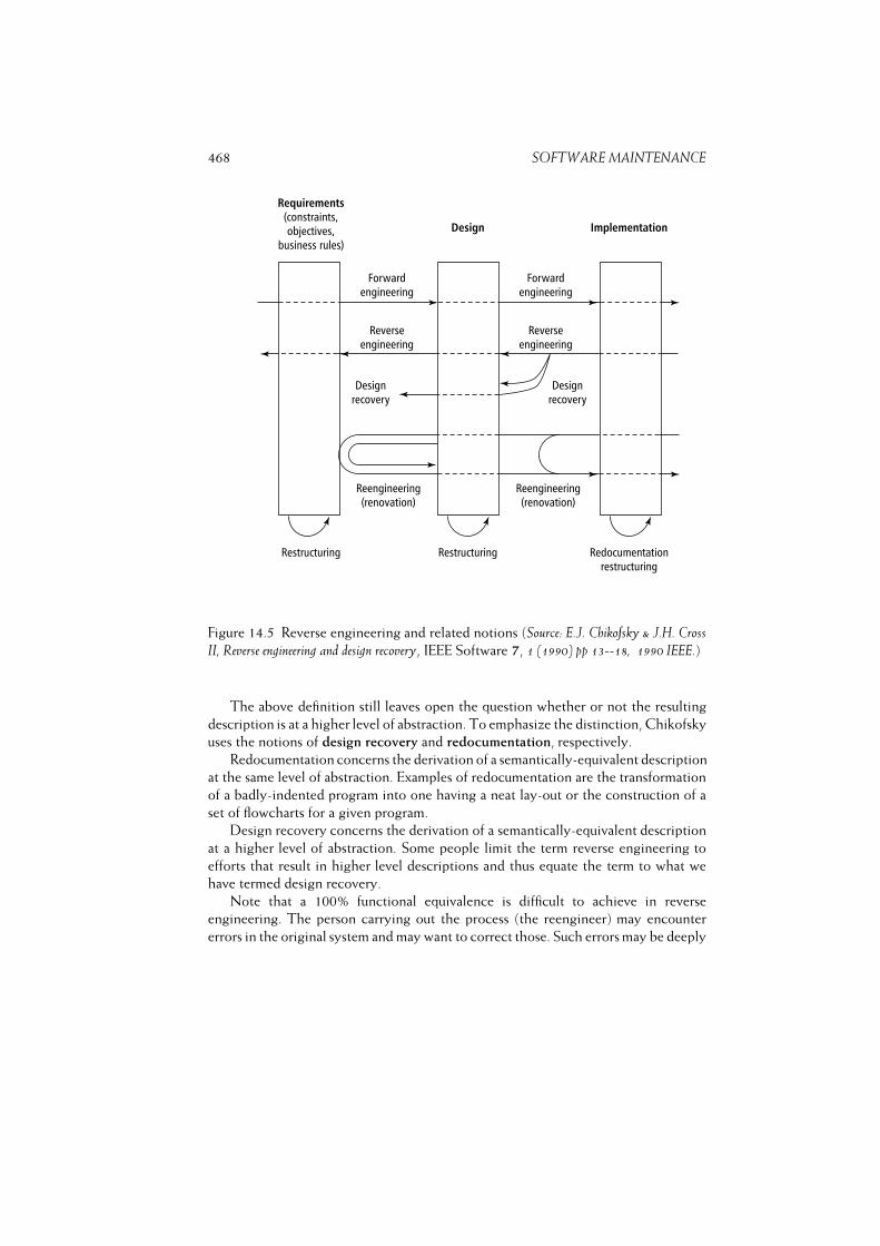
468 SOFTWARE MAINTENANCE

Figure 14.5 Reverse engineering and related notions (Source: E.J. Chikofsky & J.H. Cross

II, Reverse engineering and design recovery, IEEE Software 7, 1 (1990) pp 13--18, 1990 IEEE.)

The above definition still leaves open the question whether or not the resulting

description is at a higher level of abstraction. To emphasize the distinction, Chikofsky

uses the notions of design recovery and redocumentation, respectively.

Redocumentation concerns the derivation of a semantically-equivalent description

at the same level of abstraction. Examples of redocumentation are the transformation

of a badly-indented program into one having a neat lay-out or the construction of a

set of flowcharts for a given program.

Design recovery concerns the derivation of a semantically-equivalent description

at a higher level of abstraction. Some people limit the term reverse engineering to

efforts that result in higher level descriptions and thus equate the term to what we

have termed design recovery.

Note that a 100% functional equivalence is difficult to achieve in reverse

engineering. The person carrying out the process (the reengineer) may encounter

errors in the original system and may want to correct those. Such errors may be deeply

14.3. REVERSE ENGINEERING AND REFACTORING 469

hidden in the original system and become much more troublesome in the reverse

engineered system. The programming language may be incompletely defined and its

implementation may depend on certain machine characteristics. Data equivalence

may be difficult to achieve because of typing issues, approximations, data conversions,

etc. In practice, it seems sensible to solve this issue by agreeing on some acceptance

test for the reengineered system, thereby relaxing the 100% functional equivalence

requirement.

Obviously, reverse engineering is often done in circumstances where the tar-

get system is adapted as well. Two important subclasses are restructuring and

reengineering.

Restructuring concerns the transformation of a system from one representation

to another, at the same level of abstraction. The functionality of the system does

not change. The transformation of spaghetti-code to structured code is a form of

restructuring. The redesign of a system (possibly after a design recovery step) is

another example of restructuring. In agile methods, restructuring the code to improve

its design is an explicit process step. There, it is known as refactoring. Refactoring is

discussed in section 14.3.1.

Refactoring is a white-box method, in that it involves inspection of and changes

to the code. It is also possible to modernize a system without touching the code. For

example, a legacy system may be given a modern user interface. The old, text-based

interface is then wrapped to yield, for example, a graphical user interface or a client

running in a Web browser. This is a black box method. The code of the old system is

not inspected. The input and output are simply redirected to the wrapper. Usability

is increased, although the capabilities of the new type of interface are often not fully

exploited. A similar black box technique can be used to switch to another database, or

integrate systems through intermediate XML documents. A third black box wrapping

technique is applied at the level of components, where both business logic and data

are wrapped and next accessed through an interface as if it were, say, a JavaBean.

These wrapping techniques do not change the platform on which the software

is running. If a platform change is involved in the restructuring effort of a legacy

system, this is known as migration. Migration to another platform is often done

in conjunction with value-adding activities such as a change of interface, or code

improvements.

Restructuring is sometimes done in conjunction with efforts to convert existing

software into reusable building blocks. Such reclamation efforts may well have higher

(indirect) payoffs than the mere savings in maintenance expenditure for the particular

system being restructured, especially if the effort concerns a family of similar systems.

The latter is often done in combination with domain engineering and the development

of a (reusable) architecture or framework.

With reengineering, also called renovation, real changes are made to the system.

The reverse engineering step is followed by a traditional forward engineering step in

which the required changes are incorporated.

Each of the above transformations starts from a given description of the system

470 SOFTWARE MAINTENANCE

to be transformed. In most cases this will be the program code, which may or may

not be adequately documented. However, it is also possible to, say, restructure an

existing design or to reconstruct a requirements specification for a given design. For

these transformations too, the term reverse engineering applies.

Both reverse engineering and restructuring can be done manually, but it is a

rather tiresome affair. Quite a number of tools have been developed to support these

processes. These tools are discussed in section 14.3.3. There are, however, some

inherent limitations as to how much can be achieved automatically. These limitations

are discussed in section 14.3.2.

14.3.1 Refactoring

The modern name for restructuring is refactoring. Refactoring has become popular

as one of the practices from XP (see section 3.2.4). Of course, programmers have

applied the technique in some form since the beginning of programming.2. Quite

often, refactoring activities are not explicitly planned, and occur somewhat unnoticed

in the daily work of software developers. In XP and other agile methods, they are an

explicit method step.

There are both arguments for and against refactoring. The classic engineering

rule ”if it aint’t broken don’t fix it” is a compelling argument against refactoring. On

the other hand, the second law of software evolution tells us that software becomes

increasingly complex over time. So we are forced to apply refactoring to keep the

software maintainable. The arguments pro and con are both valid. It depends on the

phase the software is in which argument is the decisive one. During the evolution

stage, when knowledge about the system is still around, refactoring is a viable option.

During the servicing stage, knowledge will have vaporized to some extent, and

refactoring then may well introduce more problems than it solves. During that stage,

one may decide for example to add a wrapper, and not touch the software anymore.

Refactoring is applied when the structure of the software is of substandard quality.

Fowler (1999) used the term bad smells to indicate occurrences of substandard code

quality. Fowler (1999) lists the following 22 bad smells3:� Long Method A method that is too long.� Large Class A class that is too big, in terms of instance variables or methods.� Primitive Obsession The use of primitives, such as numbers, instead of small

classes such as Dollar.

2My earliest recall of a refactoring activity goes back to 1970. I was at that time fulfilling my

compulsory military service. I couldn’t properly fire a gun, so I got assigned to the army’s computer center

as a programmer. A couple of weeks before I got demobilized, I finished my last FORTRAN program. To

fill up the time, I decided to improve it a bit: improve the structure, remove redundant goto’s, and the like.Configuration control was unheard of at the time and I only retained the last copy of the source code. By

the time I left the army, I had introduced some faults, and I could not make the program work anymore.

They were probably glad I left, but not this way.3Fowler also gives detailed instructions on how to improve the bad code.

14.3. REVERSE ENGINEERING AND REFACTORING 471� Long Parameter List A parameter list that is too long.� Data Clumps Groups of data items that are often used together, such as the

height, width and color of a graphical object. If you remove one of the items,

the rest doesn’t make sense any more.� Switch Statements The use of type codes instead of polymorphism. This results

in case statements all over the code� Temporary Field A class has a variable which is only used in some circum-

stances.� Refused Bequest A subclass which does not support all of the methods or data

it inherits.� Alternative Classes with Different Interfaces Methods that do the same things

but have different interfaces. For example, methods DisplayRectangle next to

DisplayCircle.� Parallel Inheritance Hierarchies Two class hierarchies exist, and if one of them

has to be extended, so has the other.� Lazy Class A class that isn’t doing all that much. This might be the result of a

previous refactoring operation.� Data Class A class that holds data, but little else.� Duplicate Code According to Fowler (1999), this is ”number one in the stink

parade”.� Speculative Generality Code has been created for which you anticipate some

future need. But this future is unknown.� Message Chains An object asks for an object from another object, which in

turn asks for an object from yet another object, and so on.� Middle Man A class delegates most of its tasks to other classes. Delegation is

OK, but too much delegation is not.� Feature Envy A method is more tightly coupled to, i.e. interested in, other

classes than the class where it is located.� Inappropriate Intimacy Two classes are coupled too tightly.� Divergent Change The same class needs to be changed for different reasons,

e.g. each time a new database is added, and each time the user interface

changes.

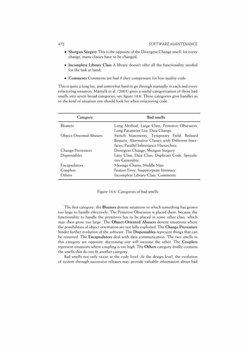
472 SOFTWARE MAINTENANCE� Shotgun Surgery This is the opposite of the Divergent Change smell: for every

change, many classes have to be changed.� Incomplete Library Class A library doesn’t offer all the functionality needed

for the task at hand.� Comments Comments are bad if they compensate for low-quality code.

This is quite a long list, and somewhat hard to go through manually in each and every

refactoring situation. Mantyla et al. (2003) gives a useful categorization of these bad

smells into seven broad categories; see figure 14.6. These categories give handles as

to the kind of situation one should look for when refactoring code.

Category Bad smells

Bloaters Long Method, Large Class, Primitive Obsession,

Long Parameter List, Data Clumps

Object-Oriented Abusers Switch Statements, Temporary Field, Refused

Bequest, Alternative Classes with Different Inter-

faces, Parallel Inheritance Hierarchies

Change Preventers Divergent Change, Shotgun Surgery

Dispensables Lazy Class, Data Class, Duplicate Code, Specula-

tive Generality

Encapsulators Message Chains, Middle Man

Couplers Feature Envy, Inapprorpiate Intimacy

Others Incomplete Library Class, Comments

Figure 14.6 Categories of bad smells

The first category, the Bloaters denote situations in which something has grown

too large to handle effectively. The Primitive Obsession is placed there, because the

functionality to handle the primitives has to be placed in some other class, which

may then grow too large. The Object-Oriented Abusers denote situations where

the possibilities of object orientation are not fully exploited. The Change Preventers

hinder further evolution of the software. The Dispensables represent things that can

be removed. The Encapsulators deal with data communication. The two smells in

this category are opposite: decreasing one will increase the other. The Couplers

represent situations where coupling is too high. The Others category finally contains

the smells that do not fit another category.

Bad smells not only occur at the code level. At the design level, the evolution

of system through successive releases may provide valuable information about bad

14.3. REVERSE ENGINEERING AND REFACTORING 473

smells. For example, if certain classes often change, or classes get introduced in one

version, disappear in the next, and then reappear again, such merits closer inspection.

Fowler (1999) states that ”no set of metrics rivals informed human intuition”. On

the other hand, several of the metrics defined in section 12.1 do relate to a number

of the bad smells listed above. For example, a high value for McCabe’s cyclomatic

complexity could indicate the Switch Statement bad smell, while a high value for the

Coupling Between Object Classes (CBO) metric could indicate a Feature Envy bad

smell. Metrics thus may augment human intuition in the search for bad smells.

14.3.2 Inherent Limitations

If you pass an unstructured, unmodular mess through one of these restructuring systems,

you end up with at best, a structured, unmodular mess.(Wendel, 1986)

Reverse engineering will mostly not be limited to redocumentation in a narrow sense.

We will often be inclined to ask why certain things are being done the way they are

done, what the meaning is of a certain code fragment, and the like. We must therefore

investigate how programmers go about studying program text. The relevance of these

issues shows from results of a study into maintenance activities (Fjelstad and Hamlen,

1979), confirmed by Yu and Chen (2006):� maintenance programmers study the original program code about one and a

half times as long as its documentation;� maintenance programmers spend as much time reading the code as they do

implementing a change.

Insights into the discovery process which takes place during maintenance activities

will give us the necessary insight to put various developments regarding reverse

engineering and refactoring into perspective.

In forward engineering activities we usually proceed from high-level abstractions

to low-level implementations. Information gets lost in the successive steps involved in

this process. If we want to reverse the route, this information must be reconstructed.

The object we start with, a piece of source code in general, usually offers insufficient

clues for a full reconstruction.

The programmer uses various sources of information in his discovery process.

For example, if the design documentation is available, that documentation will reveal

something about the structure of the system. A characteristic situation in practice is

that the source code is the only reliable source of information. So this source code

has to be studied in order to discover the underlying abstractions. The question is

how the programmer goes about doing this.

Several theories have been developed to describe this comprehension process.

Common to these theories is that expert programmers may draw on a vast number of

knowledge chunks. These knowledge chunks are called in when software is developed.

474 SOFTWARE MAINTENANCE

Within the realm of programming, it is postulated that experts know of program-

ming plans or beacons. A programming plan is a program fragment that corresponds

to a stereotypical action. For example, to compute the sum of a series of numbers, a

programmer uses the ‘running total loop plan’. In this plan, some counter is initialized

to zero and incremented with the next value of a series in the body of a loop. A

beacon is a key feature that typically indicates the presence of a particular structure

or operation. Beacons seem to be very diagnostic of program meaning. For example,

the kernel idea or central operation in a sorting program is a swap operation. If we

are presented with a program that contains a swap operation, our immediate reaction

would then be that it concerns some sorting program.

This type of program comprehension process occurs when studying existing

software. Meaningful units are isolated from the ‘flat’ source text. Knowledge from

human memory is called in during this process. The more knowledge the reader has

about programming or the application domain, the more successful this process will

be. The better the source code maps onto knowledge already available to the reader,

the more effective this process will be.

During the comprehension process, the reader forms hypotheses and checks these

hypotheses with the actual text. Well-structured programs and proper documentation

ease this process. If application domain concepts map onto well-delineated program

units then the program text will be more easily understood. If the structure of a

program shows no relation with the structure of the application domain, or the reader

cannot discern this structure, then understanding of the program text is seriously

hampered.

As a side remark we note that there are two extreme strategies for studying

program text:

– the as-needed strategy, and

– the systematic strategy.

In the as-needed strategy, program text is read from beginning to end like a piece of

prose and hypotheses are formulated on the basis of local information. Inexperienced

programmers in particular tend to fall back onto this strategy. In the systematic

strategy, an overall understanding of the system is formed by a systematic top-down

study of the program text. The systematic approach gives a better insight into causal

relations between program components.

These causal relations play an important role when implementing changes. So-

called delocalized plans, in which conceptually related pieces of code are located

in program parts that are physically wide apart, may seriously hamper maintenance

activities. Excessive use of inheritance increases the use of delocalized plans. If our

understanding is based on local clues only, modifications may easily result in so-

called ripple-effects, i.e. changes that are locally correct but lead to new problems at

different, unforeseen places. Use of the as-needed strategy increases the probability

of ripple effects.

14.3. REVERSE ENGINEERING AND REFACTORING 475

During the comprehension process the programmer uses knowledge that has its

origin outside the program text proper. To illustrate this phenomenon, consider the

program text from figure 14.7.

for i:= 1 to n dofor j:= 1 to n do

if A[j, i] thenfor k:= 1 to n do

if A[i, k] then A[j, k]:= true endifenddo

endifenddo

enddo

Figure 14.7 Warshall’s algorithm to compute the transitive closure of a graph

The program fragment of figure 14.7 manipulates a boolean matrix A. Before this

fragment is executed the matrix will have a certain value. The matrix is traversed in

a rather complicated way (potentially, each element is visited n times) and once in a

while an element of the array is set to true. But what does this fragment mean? What

does it do?

An expert will ‘recognize’ Warshall’s algorithm. Warshall’s algorithm computes

the transitive closure of a relation (graph). The notions ‘transitive closure’, ‘relation’

and ‘graph’ have a precise meaning within a certain knowledge domain. If you don’t

know the meaning of these notions, you haven’t made any progress in understanding

the algorithm either.

At yet another level of abstraction the meaning of this fragment could be described

as follows. Suppose we start with a collection of cities. The relation A states, for each

pair of cities i and j, whether there is a direct rail connection between cities i andj. The code fragment of figure 14.7 computes whether there is a connection at all

(either direct or indirect) between each pair of cities.

Warshall’s algorithm has many applications. If you know the algorithm, you will

recognize the fragment reproduced in figure 14.7. If you don’t know the algorithm,

you will not discover the meaning of this fragment either.

As a second example, consider the code fragment of figure 14.8, adapted from

(Biggerstaff, 1989). The fragment will not mean much to you. Procedure and variable

names are meaningless. A meaningful interpretation of this fragment is next to

impossible.

The same code fragment is given in figure 14.9, though with meaningful names.

From that version you may grasp that the routine has something to do with window

management. The border of the current window is depicted in a lighter shade while

476 SOFTWARE MAINTENANCE

procedure A(var x: w);begin b(y, n1);

b(x, n2);m(w[x]);y:= x;r(p[x])

end;

Figure 14.8 An incomprehensible code fragment

the border of another window gets highlighted. The cursor is positioned in the now

highlighted window and the process of that window is restarted. If we add a few

comments to the routine, its text becomes fairly easy to interpret. Meaningful names

and comments together provide for an informal semantics of this code which suffice

for a proper understanding.

This informal semantics goes much further than building local knowledge of the

meaning of a component. Developers use naming conventions also to find their way

around in a large system. Organizations often prescribe naming conventions precisely

for this reason. When design and architecture documentation is not updated, these

naming conventions serve as a proxy for that documentation.

procedure change window(var nw: window);begin border(current window, no highlight);

border(nw, highlight);move cursor(w[nw]);current window:= nw;resume(process[nw])

end;

Figure 14.9 Code fragment with meaningful names

Common to these two examples as well as the altimeter anecdote from section 14.2

is that we need outside information for a proper interpretation of the code fragments.

The outside information concerns concepts from a certain knowledge domain or

a design rationale that was only present in the head of the programmer.

The window management example is illustrative for yet another reason. Tools

manipulate sequences of symbols. In principle, tools do not have knowledge of

the (external) meaning of the symbols being manipulated. In particular, a reverse

engineering tool has no knowledge of ‘windows’, ‘cursor’ and the like. These notions

14.3. REVERSE ENGINEERING AND REFACTORING 477

derive their meaning from the application domain, not from the program text itself.

From the tool point of view, the texts of figures 14.8 and 14.9 are equally meaningful.

The above observations have repercussions for the degree to which tools can

support the reverse engineering and restructuring process. Such tools cannot turn a

badly-designed system into a good one. They cannot infer knowledge from a source

text which is not already contained in that text without calling in external knowledge

as an aid. In particular, completely automatic design recovery is not feasible. You

can’t make a pig out of a sausage.

14.3.3 Tools

During the reverse engineering process, the programmer builds an understanding of

what the software is trying to accomplish and why things are done the way they are

done. Several classes of tools may support the task of program understanding:� Tools to ease perceptual processes involved in program understanding (refor-

matters). Tools may for example produce a neat lay-out in which nested

instructions are indented and blank lines are put between successive methods.

More advanced tools print procedure names in a larger font or generate page

headers which contain the name of the component, its version number, creation

date, and the like.� Tools to gain insight into the static structure of programs. For example,

tools that generate tables of contents and cross-reference listings help to

trace the use of program elements. Browsers provide powerful interactive

capabilities for inspecting the static structure of programs. Hypertext systems

provide mechanisms to extend the traditional flat organization of text by their

capabilities for linking non-sequential chunks of information. If system-related

information is kept in a hypertext form, this opens up new possibilities for

interactive, dynamic inspection of that information. Code analyzers may be

used to identify potential trouble spots by computing software complexity

metrics, highlighting ‘dead code’, or indicating questionable coding practices

or bad smells. Finally, tools may generate a graphical image of a program text in

the form of a control graph or a calling hierarchy. Tools may analyze the surface

structure of large systems, e.g. by considering variable names, and cluster parts

that seem to be highly related. The result of this clustering provides a first guess

at a restructuring for the system.� Tools that inspect the version history of a system (see also section 14.4).

These tools may for example highlight components that have been changed

very often, indicating candidates for reengineering. Tools that identify pairs

of components that have often changed together but are not logically related

may indicate weak spots in the software architecture.

478 SOFTWARE MAINTENANCE� Tools to gain insight into the dynamic behavior of programs. Next to traditional

text-oriented debugging systems there are systems which provide graphical

capabilities to monitor program execution, e.g. to animate data structures or

the execution flow.

Note that these tools provide support for maintenance tasks in general (alongside

tools such as test coverage monitors, which keep track of program paths executed

by a given set of test data, and source comparators, which identify changes between

program versions). With respect to reverse engineering, the above tools may be

classified as redocumentation tools. By far the majority of reverse engineering tools

falls into this category.

Tools which result in a description at a higher level of abstraction (design recovery

tools) have some inherent limitations, as argued in the previous section. Tools for

design recovery need a model of the application domain in which the concepts from

that domain are modeled in an explicit way, together with their mutual dependencies

and interrelations. Completely automatic design recovery is not feasible for the

foreseeable future. Concepts from an application domain usually carry an informal

semantics. Tools for design recovery may, in a dialog with the human user, search for

patterns, make suggestions, indicate relations between components, etc. Such a tool

may be termed a ‘maintenance apprentice’.

Many tools exist for restructuring program code. The history of these restructuring

tools goes all the way back to the late 1960s. In 1966, Bohm and Jacopini (1966)

published a seminal paper in which it was shown that gotos are not necessary for

creating programs. The roots of restructuring tools like Recoder (Bush, 1985) can

be traced to the constructive proof given in Bohm and Jacopini’s paper. Recoder

structures the control flow of Cobol programs. There is a wide choice of such Cobol

restructuring tools.

Restructuring tools can be very valuable -- a well-structured program is usually

easier to read and understand. A study reported by Gibson and Senn (1989) provides

evidence that structural differences do affect maintenance performance. Specifically,

it was found that eliminating gotos and redundancy appears to decrease both the time

required to perform maintenance and the frequency of ripple effects.

Yet, the merit of restructuring tools is limited. They will not transform a flawed

design into a good one.

14.4 Software Evolution Revisited

Lehman and Belady studied the evolution of software systems and formulated their

well-known laws of software evolution. Empirical studies have given general support

for these laws.

Apparently, there is quite a bit of regularity in the evolution of software. We

can use this insight and try to predict the future evolution of a specific system by

looking at the actual evolution of that system till now. We then base our next action

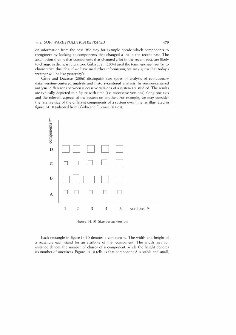
14.4. SOFTWARE EVOLUTION REVISITED 479

on information from the past. We may for example decide which components to

reengineer by looking at components that changed a lot in the recent past. The

assumption then is that components that changed a lot in the recent past, are likely

to change in the near future too. Gırba et al. (2004) used the term yesterday’s weather to

characterize this idea: if we have no further information, we may guess that today’s

weather will be like yesterday’s.

Gırba and Ducasse (2006) distinguish two types of analysis of evolutionary

data: version-centered analysis and history-centered analysis. In version-centered

analysis, differences between successive versions of a system are studied. The results

are typically depicted in a figure with time (i.e. successive versions) along one axis

and the relevant aspects of the system on another. For example, we may consider

the relative size of the different components of a system over time, as illustrated in

figure 14.10 (adapted from (Gırba and Ducasse, 2006)).

1 2 3 4 5 versions

B

C

D

A

com

pone

nts

Figure 14.10 Size versus version

Each rectangle in figure 14.10 denotes a component. The width and height of

a rectangle each stand for an attribute of that component. The width may for

instance denote the number of classes of a component, while the height denotes

its number of interfaces. Figure 14.10 tells us that component A is stable and small,

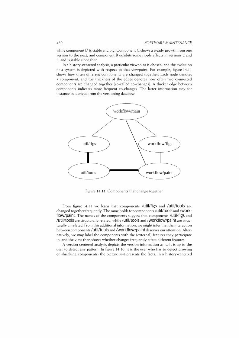
480 SOFTWARE MAINTENANCE

while component D is stable and big. Component C shows a steady growth from one

version to the next, and component B exhibits some ripple effects in versions 2 and

3, and is stable since then.

In a history-centered analysis, a particular viewpoint is chosen, and the evolution

of a system is depicted with respect to that viewpoint. For example, figure 14.11

shows how often different components are changed together. Each node denotes

a component, and the thickness of the edges denotes how often two connected

components are changed together (so-called co-changes). A thicker edge between

components indicates more frequent co-changes. The latter information may for

instance be derived from the versioning database.

workflow/paint

workflow/figs

util/tools

util/figs

workflow/main

Figure 14.11 Components that change together

From figure 14.11 we learn that components /util/figs and /util/tools are

changed together frequently. The same holds for components /util/tools and /work-flow/paint. The names of the components suggest that components /util/figs and

/util/tools are structurally related, while /util/tools and /workflow/paint are struc-

turally unrelated. From this additional information, we might infer that the interaction

between components /util/tools and /workflow/paint deserves our attention. Alter-

natively, we may label the components with the (external) features they participate

in, and the view then shows whether changes frequently affect different features.

A version-centered analysis depicts the version information as-is. It is up to the

user to detect any pattern. In figure 14.10, it is the user who has to detect growing

or shrinking components; the picture just presents the facts. In a history-centered

14.5. ORGANIZATIONAL AND MANAGERIAL ISSUES 481

analysis, some hypothesis guides the representation, and the patterns are then encoded

in the representation, as in figure 14.11.

14.5 Organizational and Managerial Issues

The duties of maintenance management are not different from those of other

organizational functions, and software development in particular. In chapter 2 we

identified five entities that require continuous attention of management:

– time, i.e. progress towards goals;

– information, in particular the integrity of the complete set of documents,

including change requests;

– organization of the team, including coordination of activities;

– quality of the product and process;

– money, i.e. cost of the project.

In this section we address these issues from a maintenance perspective. We pay

particular attention to issues that pose specific problems and challenges to mainte-

nance. These issues are: the organization of maintenance activities, major differences

between development and maintenance, the control of maintenance tasks, and quality

assessment.

14.5.1 Organization of Maintenance Activities

The primary question to be addressed here is whether or not software maintenance

should be assigned to a separate organizational unit. The following discussion is largely

based on an insightful study of different forms of systems staff departmentalization

presented in (Swanson and Beath, 1990). The authors of this article explore the

strengths and weaknesses of three alternative bases for staff departmentalization. The

three organizational forms with their focal strengths and weaknesses are listed in

figure 14.12. We will sketch the W- and A-Type organizations and discuss the L-type

organization with its pros and cons more elaborately.

Traditionally, departmentalization in software development tended to be accord-

ing to work type (a W-Type scheme). In such a scheme, people analyze user needs,

or design systems, or implement them, or test them, etc. Even though they cooperate

in a team, each team member has quite separate responsibilities and roles.

In a W-Type scheme, work assignments may originate from both development

and maintenance projects. For example, a designer may be involved in the design of a

(sub)system in the context of some development project or in the design of a change

to an existing system. Likewise, a programmer may implement an algorithm for a new

system or realize changes in an operational program.

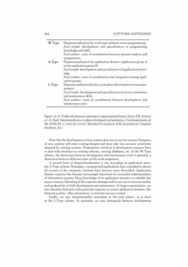
482 SOFTWARE MAINTENANCE

W-Type Departmentalization by work type (analysis versus programming)

Focal strength: development and specialization of programming

knowledge and skills

Focal weakness: costs of coordination between systems analysts and

programmers

A-Type Departmentalization by application domain (application group A

versus application group B)

Focal strength: development and specialization of application knowl-

edge

Focal weakness: costs of coordination and integration among appli-

cation groups

L-Type Departmentalization by life-cycle phase (development versus main-

tenance)

Focal strength: development and specialization of service orientation

and maintenance skills

Focal weakness: costs of coordination between development and

maintenance units

Figure 14.12 Trade-offs between alternative organizational forms (Source: E.B. Swanson

& C.M. Beath, Departmentalization in software development and maintenance, Communications of

the ACM 33, 6 (1990) pp 658-667. Reproduced by permission of the Association for Computing

Machinery, Inc.)

Note that the development of new systems does not occur in a vacuum. Designers

of new systems will reuse existing designs and must take into account constraints

imposed by existing systems. Programmers involved in development projects have

to deal with interfaces to existing software, existing databases, etc. In the W-Type

scheme, the distinction between development and maintenance work is primarily a

distinction between different origins of the work assignment.

A second form of departmentalization is one according to application areas,

the A-Type scheme. Nowadays, computerized applications have extended to almost

all corners of the enterprise. Systems have become more diversified. Application

domain expertise has become increasingly important for successful implementation

of information systems. Deep knowledge of an application domain is a valuable but

scarce resource. Nurturing of this expertise amongst staff is one way to increase quality

and productivity in both development and maintenance. In larger organizations, we

may therefore find units with particular expertise in certain application domains, like

financial systems, office automation, or real-time process control.

Finally, we may departmentalize according to life-cycle phases, as is done

in the L-Type scheme. In particular, we may distinguish between development

14.5. ORGANIZATIONAL AND MANAGERIAL ISSUES 483

and maintenance. With an increasing portfolio of systems to be maintained and

the increasing business need of keeping the growing base of information systems

working satisfactorily, the division of development and maintenance into separate

organizational units is found more often.

Separating development and maintenance has both advantages and disadvantages.

The major advantages are:� Clear accountability: we may clearly separate the cost and effort involved in

maintenance activities from investments in new developments. If personnel are

involved in both types of work, they have some freedom in charging their

time. It is then more difficult to measure and predict the ‘real’ cost of software

maintenance.� Intermittent demands of maintenance make it difficult to predict and control

progress of new system development. If people do both maintenance work and

development, some control can be exercised by specifically allocating certain

periods of time as maintenance periods. For instance, the first week of each

calendar month may be set aside for maintenance. But even then, maintenance

problems are rather unpredictable and some need immediate attention. Many

a schedule slippage is due to the maintenance drain.� A separation of maintenance and development facilitates and motivates the

maintenance organization to conduct a meaningful acceptance test before the

system is taken into production. If such an acceptance test is not conducted

explicitly, maintenance may be confronted with low-quality software or systems

which still need a ‘finishing touch’ which the development team has left undone

for lack of time.� By specializing on maintenance tasks, a higher quality of user service can

be realized. By their very nature, development groups are focused on system

delivery, whereas maintenance people are service-oriented and find pride in

satisfying user requests. We will further elaborate upon this issue in section

14.5.2.� By concentrating on the systems to be maintained, a higher level of productivity

is achieved. Maintenance work requires specific skills of which a more optimal

use can be made in a separate organization. If people are involved in both

development and maintenance, more staff have to be allocated to maintenance

and the familiarity with any particular system is spread more thinly.

On the other hand, the strict separation of development and maintenance has certain

disadvantages as well:� Demotivation of personnel because of status differences, with consequential

degradation of quality and productivity. Managerial attitudes and traditional

career paths are the main causes for these motivational problems. Conversely,

484 SOFTWARE MAINTENANCE

proper managerial attention to maintenance work goes a large way towards

alleviating the morale problem. For example, an organization may decide to

hire new people into development only and explicitly consider a transfer to

maintenance as a promotion. (Most organizations do exactly the opposite.)� Loss of knowledge about the system (with respect to both its design and the

application domain knowledge incorporated) when the system is transferred

from development to maintenance. Various strategies can mitigate against

this loss. For example, a future maintainer of a system may spend some time

with the development team, a developer may stay with maintenance until the

maintainers have become sufficiently acquainted with the system, or a designer

may instruct the maintainers about the design of a system.� Coordination costs between development and maintenance, especially when

the new system replaces an existing one.� Increased cost of system acceptance by the maintenance organization. If

the system is explicitly carried over from development, certain quality and

documentation criteria must be met. Within an A-type organization these

requirements can often be relaxed a bit, or their fulfillment is postponed. It

is by no means clear though that this really incurs an increase in cost. In the

long run it may well be cheaper to only accept systems which pass a proper

maintenance acceptance test.� Possible duplication of communication channels to the user organization.

Based on an analysis of existing departmentalizations and the resulting list of strengths

and weaknesses, Swanson and Beath express a slight preference for having develop-

ment and maintenance as separate organizational units. We concur with that. Careful

procedures could be devised that overcome some or all of the disadvantages listed.

We should stress that personnel demotivation is a real issue in many organizations. It

deserves serious management attention.

Combinations of departmentalization types are also possible. In particular, com-

binations of A-type and L-type departmentalizations are quite common. So, within

the maintenance organization, smaller groups may specialize in some application

domain, i.e. a specific collection of information systems. This may be termed the

L-A-scheme. Conversely, in an A-L-scheme a small maintenance unit is found within

a group that specializes in a certain application area. The L-A-scheme is more likely

to exhibit the advantages of the L-scheme than the A-L-scheme does.

Too much specialization is a lurking danger though. A system should never

become someone’s private property. A variation of the reverse Peter principle applies

here: people rise within an organization to a level at which they become indispensable.

Job rotation is one way to avoid people from becoming too much entrenched in the

peculiarities of a system. There is a trade-off though, since such a step also means

that in-depth knowledge of a system is sacrificed.

14.5. ORGANIZATIONAL AND MANAGERIAL ISSUES 485

14.5.2 Software Maintenance from a Service Perspective

Software maintenance organizations need to realize that they are in the customer service

business.(Pigoski, 1996)

Software development results in a product, a piece of software. Software maintenance

can be seen as providing a service. There are notable differences between products and

services, which mean that the quality of products and services is judged differently.

As a consequence, the quality of software development and software maintenance

is also judged differently and maintenance organizations should pay attention to

service-specific quality aspects.

Apparently, this is not widely recognized yet. Within the software maintenance

domain, the focus is still on product aspects. The final phases of software development

supposedly concern the delivery of an operations manual, installing the software,

handling change requests and fixing bugs. In practice, the role of an IT department is

much broader during the deployment stage, as is illustrated by the ubiquitous help

desk.

This is confirmed by Stalhane et al. (1997) who report on a survey to find those

aspects of software quality that customers consider most important. The main insight

to be gained from their study is the strong emphasis customers place on service

quality. The top five factors found in their study are: service responsiveness, service

capacity, product reliability, service efficiency, and product functionality. They also

quote an interesting result from a quality study in the telecommunications domain.

To the question ‘Would you recommend others to buy from this company?’, a

100% yes was obtained from the category of users that had complained and got a

satisfactory result. For the category that had not complained, this percentage was

87%. Apparently, it is more important to get a satisfactory service than to have no

problems at all.

The main differences between products and services are as follows:� Services are intangible, products are tangible. This is considered the most

basic difference between products and services. Services -- being benefits

or activities -- cannot be seen, felt, tasted, or touched, unlike products.

Consequently, services cannot be counted, stored, patented, readily displayed,

or communicated, and pricing is more difficult.� Because services are created by activities, and activities are performed by

humans, services tend to be more heterogeneous than products. Customer

satisfaction depends on employee actions during the service delivery. Service

quality depends on factors which are difficult to control, such as the ability of

customers to articulate their needs, the ability and willingness of personnel to

satisfy those needs, the presence or absence of other customers, and the level

of demand for the service. These complicating factors make it hard to know

whether the service was delivered according to plan or specification.

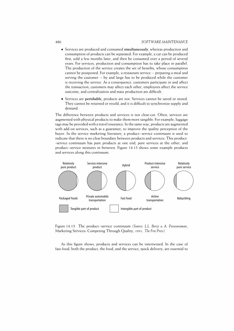
486 SOFTWARE MAINTENANCE� Services are produced and consumed simultaneously, whereas production and

consumption of products can be separated. For example, a car can be produced

first, sold a few months later, and then be consumed over a period of several

years. For services, production and consumption has to take place in parallel.

The production of the service creates the set of benefits, whose consumption

cannot be postponed. For example, a restaurant service -- preparing a meal and

serving the customer -- by and large has to be produced while the customer

is receiving the service. As a consequence, customers participate in and affect

the transaction, customers may affect each other, employees affect the service

outcome, and centralization and mass production are difficult.� Services are perishable, products are not. Services cannot be saved or stored.

They cannot be returned or resold, and it is difficult to synchronize supply and

demand.

The difference between products and services is not clear-cut. Often, services are

augmented with physical products to make them more tangible. For example, luggage

tags may be provided with a travel insurance. In the same way, products are augmented

with add-on services, such as a guarantee, to improve the quality perception of the

buyer. In the service marketing literature, a product--service continuum is used to

indicate that there is no clear boundary between products and services. This product-

-service continuum has pure products at one end, pure services at the other, and

product--service mixtures in between. Figure 14.13 shows some example products

and services along this continuum.

Figure 14.13 The product--service continuum (Source: L.L. Berry & A. Parasuraman,

Marketing Services: Competing Through Quality, 1991, The Free Press)

As this figure shows, products and services can be intertwined. In the case of

fast-food, both the product, the food, and the service, quick delivery, are essential to

14.5. ORGANIZATIONAL AND MANAGERIAL ISSUES 487

the customer. The quality of such a product--service mix is judged on both product

and service aspects: does the food taste good and is it served quickly.

Let us return to the software engineering domain. A major difference between

software development and software maintenance is the fact that software development

results in a product, whereas software maintenance results in a service being delivered

to the customer. Software maintenance has more service-like aspects than software

development, because the value of software maintenance lies in activities that result

in benefits for the customers, such as corrected faults and new features. Contrast

this with software development, where the development activities themselves do not

provide benefits to the customer. It is the resulting software system that provides

those benefits.

As noted, the difference between products and services is not clear-cut. Con-

sequently, this goes for software development and software maintenance as well.

Figure 14.14 shows the product--service continuum with examples from the software

engineering domain.

Figure 14.14 The product--service continuum for software development and mainte-

nance

Service marketeers often use the gap model to illustrate how differences between

perceived service delivery and expected service may come about. This gap model is

depicted in figure 14.15. Service quality is improved if those gaps are closed. The

difference between the perceived quality and the expected quality (gap 5) is caused

by four other gaps. These four gaps, and suggested solutions for bridging them, are:

Gap 1 The expected service as perceived by the service provider

differs from the service as expected by the customer. In the field of software

maintenance, this difference is often caused by an insufficient relationship

focus of the service provider. For example, a maintenance department may

aim to satisfy certain availability constraints such as 99% availability, while

the actual customer concern is with maximum downtime.

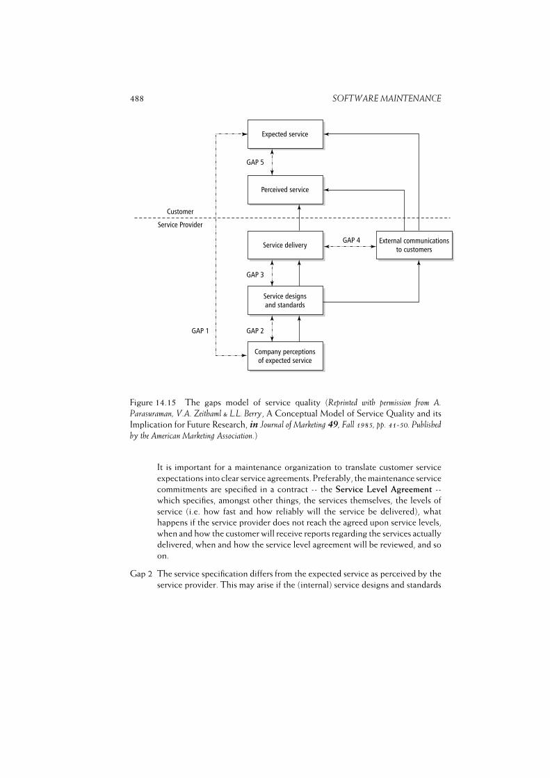
488 SOFTWARE MAINTENANCE

Figure 14.15 The gaps model of service quality (Reprinted with permission from A.Parasuraman, V.A. Zeithaml & L.L. Berry, A Conceptual Model of Service Quality and its

Implication for Future Research, in Journal of Marketing 49, Fall 1985, pp. 41-50. Published

by the American Marketing Association.)

It is important for a maintenance organization to translate customer service

expectations into clear service agreements. Preferably, the maintenance service

commitments are specified in a contract -- the Service Level Agreement --

which specifies, amongst other things, the services themselves, the levels of

service (i.e. how fast and how reliably will the service be delivered), what

happens if the service provider does not reach the agreed upon service levels,

when and how the customer will receive reports regarding the services actually

delivered, when and how the service level agreement will be reviewed, and so

on.

Gap 2 The service specification differs from the expected service as perceived by the

service provider. This may arise if the (internal) service designs and standards

14.5. ORGANIZATIONAL AND MANAGERIAL ISSUES 489

do not match the service requirements as perceived by the service provider.

For example, the customer expects a quick restart of the system, while the

standard procedure of the maintenance organization is focused on analyzing

the reason for the crash.

The maintenance activities as specified in the service level agreement have to be

planned. This includes the planning of the activities themselves, the transfer of

the results to the customer, the planning of releases, the estimation of resources

needed, the scheduling of maintenance activities, and the identification of

possible risks. Explicitly basing the planning of maintenance activities on the

commitments as agreed with the customer helps to close this gap.

Gap 3 The actual service delivery differs from the specified services. This is often

caused by deficiencies in human resource policies, failures to match demand

and supply, and customers not fulfilling their role. For example, customers

may bypass the helpdesk by phoning the maintainer of their system directly,

thereby hindering a proper incident management process.

The service level agreement states which maintenance activities are to be

carried out, and how fast, reliably, etc. this should be done. In order to be able

to report on the performance of the maintenance organization in this respect,

information about the actual maintenance activities must be gathered. This

information can be used to monitor maintenance activities and take corrective

actions if necessary.

For example, when the customer reports a bug, information about the bug

itself (originator, type, etc.) is recorded, as well as the reporting time, the

time when corrective action was started and ended, and the time when the

bug was reported as fixed. If these data indicate that the average downtime

of a system exceeds the level as specified in the service level agreement,

the maintenance organization might assign more maintenance staff to this

system, put maintenance staff on point-duty at the customer site, renegotiate

the agreed upon service level, or take other action to realign agreement and

reality.

By keeping a strict eye upon the performance of the maintenance organization

and adjusting the maintenance planning or renegotiating the commitments

with the customer when required, gap 3 is narrowed.

Gap 4 Communication about the service does not match the actual service delivery.

This may be caused by ineffective management of customer expectations,

promising too much, or ineffective horizontal communication. For example, a

customer is not informed about the repair of a bug he reported.

An important instrument to help close this gap is event management. Event

management concerns the management of events that cause or might cause

the maintenance activities carried out to deviate from the levels as promised

490 SOFTWARE MAINTENANCE

in the service level agreement. An event is either a change request, such as a

user request for a new feature, or an incident. Incidents are software bugs and

other hazards that the maintenance organization has promised to deal with,

such as, say, a server being down.

The main purpose of event management is to manage all those events. To do

so, an event management library system is employed, often in the form of

a ‘helpdesk system’. The event management library system provides for the

storage, update, and retrieval of event records, and the sharing and transfer

of event records between parties involved. This event management library

system supports the communication with the customer about maintenance

services delivered. It is also a highly valuable ‘memory’ for the maintainers:

they may use the event library to search for similar incidents, to see why

certain components were changed before, etc.4

Since the fifth gap is caused by the four other gaps, perceived service quality can be

improved by closing those first four gaps, thus bringing the perceived quality in line

with the expected quality. Since software maintenance organizations are essentially

service providers, they need to consider the above issues. They need to manage their

product -- software maintenance -- as a service in order to be able to deliver high

quality.

14.5.3 Control of Maintenance Tasks

Careful control of the product is necessary during software development. The vast

amount of information has to be kept under control. Documentation must be kept

consistent and up-to-date. An appropriate scheme for doing so is provided by the

set of procedures that make up configuration control; see chapter 4. Configuration

control pays particular attention to the handling of change requests. Since handling

change requests is what maintenance is all about, configuration control is of vital

importance during maintenance.

Effective maintenance depends on following a rigorous methodology, not only

with respect to the implementation of changes agreed upon, but also with respect to

the way change is controlled. Following IEEE Standard 1219, we suggest the following

orderly, well-documented process for controlling changes during maintenance:

1. Identify and classify change requests Each change request (CR) is given a

unique identification number and is classified into one of the maintenance

categories (corrective, adaptive, perfective, preventive). The CR is analyzed to

decide whether it will be accepted, rejected, or needs further evaluation. This

analysis also results in a first cost estimate. The CR is finally prioritized and

scheduled for implementation.

4Note that the focus of the event management library system differs somewhat from that of configuration

management as discussed in the next section. Configuration management emphasizes the internal use of

information about change requests and the like. Our description of event management focuses on the

external use of essentially the same information. In practice, the two processes may well be combined.

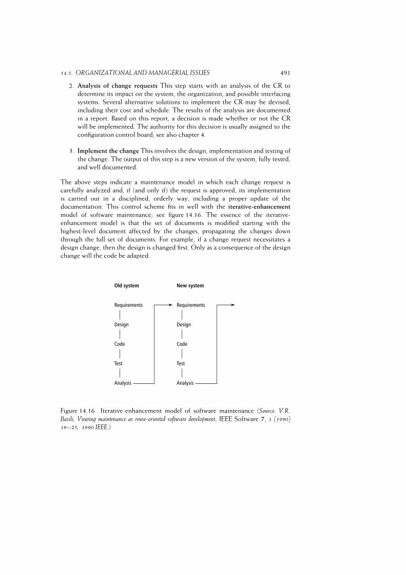
14.5. ORGANIZATIONAL AND MANAGERIAL ISSUES 491

2. Analysis of change requests This step starts with an analysis of the CR to

determine its impact on the system, the organization, and possible interfacing

systems. Several alternative solutions to implement the CR may be devised,

including their cost and schedule. The results of the analysis are documented

in a report. Based on this report, a decision is made whether or not the CR

will be implemented. The authority for this decision is usually assigned to the

configuration control board; see also chapter 4.

3. Implement the change This involves the design, implementation and testing of

the change. The output of this step is a new version of the system, fully tested,

and well documented.

The above steps indicate a maintenance model in which each change request is

carefully analyzed and, if (and only if) the request is approved, its implementation

is carried out in a disciplined, orderly way, including a proper update of the

documentation. This control scheme fits in well with the iterative-enhancement

model of software maintenance; see figure 14.16. The essence of the iterative-

enhancement model is that the set of documents is modified starting with the

highest-level document affected by the changes, propagating the changes down

through the full set of documents. For example, if a change request necessitates a

design change, then the design is changed first. Only as a consequence of the design

change will the code be adapted.

Figure 14.16 Iterative-enhancement model of software maintenance (Source: V.R.

Basili, Viewing maintenance as reuse-oriented software development, IEEE Software 7, 1 (1990)19--25, 1990 IEEE.)

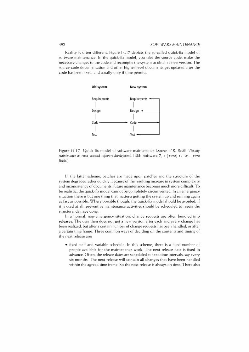
492 SOFTWARE MAINTENANCE

Reality is often different. Figure 14.17 depicts the so-called quick-fix model of

software maintenance. In the quick-fix model, you take the source code, make the

necessary changes to the code and recompile the system to obtain a new version. The

source-code documentation and other higher-level documents get updated after the

code has been fixed, and usually only if time permits.

Figure 14.17 Quick-fix model of software maintenance (Source: V.R. Basili, Viewingmaintenance as reuse-oriented software development, IEEE Software 7, 1 (1990) 19--25, 1990

IEEE.)

In the latter scheme, patches are made upon patches and the structure of the

system degrades rather quickly. Because of the resulting increase in system complexity

and inconsistency of documents, future maintenance becomes much more difficult. To

be realistic, the quick-fix model cannot be completely circumvented. In an emergency

situation there is but one thing that matters: getting the system up and running again

as fast as possible. Where possible though, the quick-fix model should be avoided. If

it is used at all, preventive maintenance activities should be scheduled to repair the

structural damage done.

In a normal, non-emergency situation, change requests are often bundled into

releases. The user then does not get a new version after each and every change has

been realized, but after a certain number of change requests has been handled, or after

a certain time frame. Three common ways of deciding on the contents and timing of

the next release are:� fixed staff and variable schedule. In this scheme, there is a fixed number of

people available for the maintenance work. The next release date is fixed in

advance. Often, the release dates are scheduled at fixed time intervals, say every

six months. The next release will contain all changes that have been handled

within the agreed time frame. So the next release is always on time. There also

14.5. ORGANIZATIONAL AND MANAGERIAL ISSUES 493

is some flexibility as to the contents of the next release, since the maintainers

and the customer do not fix the contents in advance.� variable staff and fixed schedule. Here, a release date is fixed in advance. The

portfolio of change requests to be handled in this release is also negotiated and

fixed in advance. Next, the number of people needed to implement the changes

within the fixed time frame is decided. On the way, some renegotiation of both

the contents and the schedule is possible. An advantage of this scheme is that

change requests are assigned clear priorities and that communication with the

customer about the contents of the next release is enforced.� variable staff and variable schedule. As in the previous scheme, the portfolio

of change requests to be handled in the next release is negotiated and fixed

in advance. Then, the cost and schedule for this release are negotiated, and

the number of maintainers required to achieve it is determined. This scheme

requires more planning and oversight than the other two schemes. It is also

likely to better accommodate the customer. As with ordinary development,

schedule slippages and contents renegotiation are not uncommon in this

scheme.

14.5.4 Quality Issues

Changing software impairs its structure. By a conscious application of software quality

assurance procedures during maintenance, we may limit the negative effects. If we

know the software quality factors that affect maintenance effort and cost, we may

measure those factors and take preventive actions accordingly. In particular, such

metrics can be used to guide decisions as to when to start a major overhaul of

components or complete systems.

Quality control issues get quite some attention during software development.

Software quality assurance however should broaden its scope to maintenance as

well. The implementation of changes during maintenance requires the same level of

quality assurance as development work. The ingredients of software quality assurance

procedures, as discussed in chapter 6, apply equally well to software maintenance.

Software quality assurance can be backed up by measurements that quantify

quality aspects. With respect to maintenance, we may focus on measures which

specifically relate to maintenance effort, such as counting defects reported, change

requests issued, effort spent on incorporating changes, complexity metrics, etc.

Relationships between such measures can then be sought. Observed trends can

be used to initiate actions, such as:� If maintenance efforts correlate well with complexity metrics like Henri and

Kafura’s Information Flow or McCabe’s cyclomatic complexity (see chapter 12),

then these complexity metrics may be used to trigger preventive maintenance.

Various studies have indeed found such correlations.

494 SOFTWARE MAINTENANCE� If certain modules require frequent changes or much effort to realize changes,

then a re-design of such modules should be given serious consideration.� Metrics can be used to spot bad smells, and initiate refactoring.

A particularly relevant issue during maintenance is to decide when to reengineer. At a

certain point in time, evolving an old system becomes next to impossible and a major

reengineering effort is required or the system enters the servicing stage. There are

no hard figures on which to decide this, but certain system characteristics certainly

indicate system degradation:� Frequent system failures;� Code over seven years old;� Overly-complex program structure and logic flow;� Code written for previous generation hardware;� Running in emulation mode;� Very large modules or subroutines;� Excessive resource requirements;� Hard-coded parameters that are subject to change;� Difficulty in keeping maintenance personnel;� Seriously deficient documentation;� Missing or incomplete design specifications.

The greater the number of such characteristics present, the greater the potential for

redesign.

Improvements in software maintenance requires insight into factors that determine

maintenance cost and effort. Software metrics provide such insight. To measure is to

know. By carefully collecting and interpreting maintenance data, we may discover

the major cost drivers of software maintenance and initiate actions to improve both

quality and productivity.

14.6 Summary

Software maintenance encompasses all modifications to a software product after

delivery. The following breakdown of maintenance activities is usually made:

Corrective maintenance concerns the correction of faults.

Adaptive maintenance deals with adapting software to changes in the environment.

14.7. FURTHER READING 495

Perfective maintenance mainly deals with accommodating new or changed user

requirements.

Preventive maintenance concerns activities aimed at increasing a system’s maintain-

ability.

‘Real’ maintenance, the correction of faults, consumes approximately 25% of mainte-

nance effort. By far the larger part of software maintenance concerns the evolution

of software. This evolution is inescapable. Software models part of reality. Reality

changes, and so does the software that models it.

Major causes of maintenance problems were discussed in section 14.2: the exis-

tence of a vast amount of unstructured code, insufficient knowledge about the

system or application domain on the part of maintenance programmers, insufficient

documentation, and the bad image of the software maintenance department.

Some of these problems are accidental and can be remedied by proper actions.

Through a better organization and management of software maintenance, substantial

quality and productivity improvements can be realized. These issues were discussed

in section 14.5. Obviously, improved maintenance should start with improved devel-

opment. Opportunities to improve the development process are a major topic in most

chapters of this book.

A particularly relevant issue for software maintenance is that of reverse engineer-

ing, the process of reconstructing a lost blueprint. Before changes can be realized, the

maintainer has to gain an understanding of the system. Since the majority of opera-

tional code is unstructured and undocumented, this is a major problem. Section 14.3

addresses reverse engineering, its limitations, and tools to support it.

The fundamental problem is that maintenance will remain a big issue. Because of

the changes made to software, its structure degrades. Specific attention to preventive

maintenance activities aimed at improving system structure are needed from time to

time to fight system entropy.

Software maintenance used to be a rather neglected topic in the software

engineering literature. Like programmers, researchers are more attracted to developing

new, fancy methods and tools for software development. This situation has changed.

Major journals regularly feature articles on software maintenance, there is an annual

IEEE Conference on Software Maintenance (since 1985), and the journal Software

Maintenance and Evolution: Research and Practice (launched 1989) is wholly devoted to it.

14.7 Further Reading

(Pigoski, 1996) is a text book wholly devoted to software maintenance. Lientz

and Swanson (1980) is a seminal booklet on software maintenance. It introduces the

widely-known categories of maintenance tasks and provides data on their distribution.

More recent data on the distribution of maintenance tasks are given in (Nosek and

Palvia, 1990), (Dekleva, 1992) and (Sousa and Mozeira, 1998). Chapin et al. (2001)

gives a new classification of maintenance categories, including a separate category

496 SOFTWARE MAINTENANCE

for user support. The maintenance life cycle stages are discussed in (Burch and

Kung, 1997) and (Kung and Hsu, 1998). The distinction between an evolution stage

and a servicing stage stems from (Bennett and Rajlich, 2000). The distribution of

code-related maintenance activities is discussed in (Yu and Chen, 2006). The practice

of software maintenance is discussed in (Singer, 1998) and (Tan and Gable, 1998).

The various types of reverse engineering are discussed in (Chikofsky and Cross II,

1990). The 100% functional equivalence issue in reverse engineering is discussed

in (Bennett, 1998). Reverse engineering tools are discussed in (Biggerstaff et al.,

1994), (Jarzabek and Wang, 1998) and (Bellay and Gall, 1998). Fowler (1999) is the

standard text for refactorinig. Mens and Tourwe (2004) provide a survey of software

refactoring. Migration is discussed in (Rahgozar and Oroumchian, 2003) and (Bisbal

et al., 1999). Programming plans and beacons were originally proposed in (Soloway

and Ehrlich, 1984) and (Brooks, 1983). Research addressing the role of these concepts

in program comprehension processes is described in (von Mayrhauser and Vans, 1995)

and (von Mayrhauser et al., 1997). LaToza et al. (2006) discusses developer work

habits, including code comprehension, during development and evolution. Example

tools to help software maintenance include (Singer et al., 2005) (support for browsing

through software), (Rysselberghe and Demeyer, 2004) (visualize change history) and

(Ducasse et al., 2006) (visualization of distribution of system properties).

Gırba and Ducasse (2006) provide an overview of types of software evolution

analysis. The distinction between version-centered and history-centered analysis is

made in that article. Gırba et al. (2004) discusses the ‘yesterday’s weather’ approach

to reverse engineering. Fischer and Gall (2004) and Greevy et al. (2006) discuss

history-centered analysis.

Possible organizations of maintenance activities as well as their major advantages

and disadvantages are discussed in (Swanson and Beath, 1990). Yeh and Jeng (2002)

discuss the influence of departmentalization on software maintenance. The service

perspective on software maintenance is discussed in (Niessink and van Vliet, 1999).

The translation hereof into a Capability Maturity Model aimed at maintenance

processes is described in (Niessink and van Vliet, 1998a).

The IEEE Process model for software maintenance is described in (IEEE1219,

1992). The iterative-enhancement and quick-fix models of software maintenance are

discussed in (Basili, 1990). Approaches to scheduling releases are the topic of (Stark

and Oman, 1997).

The cost of software maintenance, and empirical relations between quality aspects

and cost are the topic of (Banker et al., 1993), (Kemerer and Slaughter, 1997), (Henry

and Cain, 1997) and (Niessink and van Vliet, 1997). Indicators of system degradation

are given in (Martin and Osborne, 1983).

Exercises

1. Define the following terms: corrective maintenance, adaptive maintenance,

perfective maintenance, and preventive maintenance.

14.7. FURTHER READING 497

2. Discuss the major causes of software maintenance problems.

3. What is reverse engineering?

4. What is refactoring?

5. Characterize the evolution and servicing stage of software maintenance.

6. What is the difference between design recovery and redocumentation?

7. Characterize the version-oriented analysis and history-centered analysis of

software evolution data.

8. Why does corrective maintenance have more service-like aspects than

product-like aspects?

9. Discuss the iterative-enhancement and quick-fix models of software mainte-

nance.

10. Discuss the major impediments to fully-automated design recovery.

11. Discuss advantages of software configuration control support during software

maintenance.

12. Discuss the possible structure and role of an acceptance test by the mainte-

nance organization prior to the release of a system.

13. ~ An alternative classification of maintenance and development activities is

as follows:� Functional maintenance = corrective maintenance + adaptive mainte-

nance + non-functional perfective maintenance (i.e. improving quality)+ replacement of a system by a functional equivalent.� Functional development = functional perfective maintenance (i.e. adding

new features) + development of new systems.

Could this classification provide us with a better picture of the real maintenance

effort? See also (Krogstie, 1994).

14. ~Assess opportunities of knowledge-based support for software maintenance

(see (Devanbu et al., 1991) for a very interesting application of such ideas).

15. ~ Give a primary classification of your maintenance organization as W-, A-,

or L-Type (see figure 14.12). What are the major strengths and weaknesses

of your particular organization?

16. ~Does your organization collect quantitative data on maintenance activities?

If so, what type of data, and how are they used to guide and improve the

498 SOFTWARE MAINTENANCE

maintenance process? If not, how is maintenance planned and controlled?

17. � Study the technical documentation of a system whose development you

have been involved in. Does the documentation capture the design rationale?

In what ways does it support comprehension of the system? In hindsight,

can you suggest ways to improve the documentation for the purpose of

maintenance?

18. ~ Discuss the impact of component reuse on maintainability.

19. ~Discuss the possible contribution of object-oriented software development

to software maintenance.

20. ~ Can you think of reasons why a 10% change in a program of 200 LOC

would take more effort than a 20% change in a program of 100 LOC?

15

Software Tools

LEARNING OBJECTIVES� To be able to distinguish various dimensions along which tools can be classified� To be aware of the major trends in (collections of) software tools� To appreciate the role of tools in the software development process

500 SOFTWARE TOOLS

Software development is generally supported by tools, ranging from tools

supporting a single activity to integrated environments supporting a complete

development process. In this chapter we discuss the main classes of software

development tools and their role in the development process.

The demand for software grows faster than the increase in software development

productivity and available manpower. The result is an ever-increasing shortage of

personnel; we are less and less able to satisfy the quest for software. To turn the tide,

we must look for techniques that result in significant productivity gains.

One of the most obvious routes to pursue is automation itself. We may use the

computer as a tool in the production of software. In the past, all sorts of things were

automated, save software development itself. Programmers knew better than that.

We have long been accustomed to employ the computer as a tool for the

implementation of software. To this end, programmers have a vast array of tools at

their disposal, such as compilers, linkers and loaders. Also during testing, tools like

test drivers and test harnesses have been used for a long time. The development of

tools to support earlier phases of the software life cycle is more recent. One example

of the latter is software to aid the drawing and validation of UML diagrams.

The use of software tools may have a positive effect on both the productivity

of the people involved and the quality of the product being developed. Tools may

support checking conformance to standards. Tools may help to quantify the degree

of testing. Tools may support progress tracking. And so on.

The application of tools in the software development process is referred to

as Computer Aided Software Engineering (CASE). Apart from the traditional

implementation and test tools, CASE has a relatively short history. The first tools to

support design activities appeared in the early 1980s. Today, the number of CASE

products is overwhelming.

As the number of available CASE products proliferates, it becomes expedient

to classify them. One way of doing so is according to the breadth of support they

offer. Figure 15.1 gives a classification of CASE products along this dimension. Some

products support a specific task in the software development process. Others support

the entire software process. The former are called tools, the latter environments. In

between these two extremes it is useful to identify CASE products that support a

limited set of activities, such as those which comprise the analysis and design stages.

Such a coherent set of tools with a limited scope is referred to as a workbench.

Environments can be further classified according to the mechanism that ties

together the individual tools that make up the environment. In a toolkit, tools

are generally not well integrated. The support offered is independent of a specific

programming language or development paradigm. A toolkit merely offers a set of useful

building blocks. A language-centered environment contains tools specifically suited

for the support of software development in a specific programming language. Such

an environment may be hand-crafted or generated from a grammatical description of

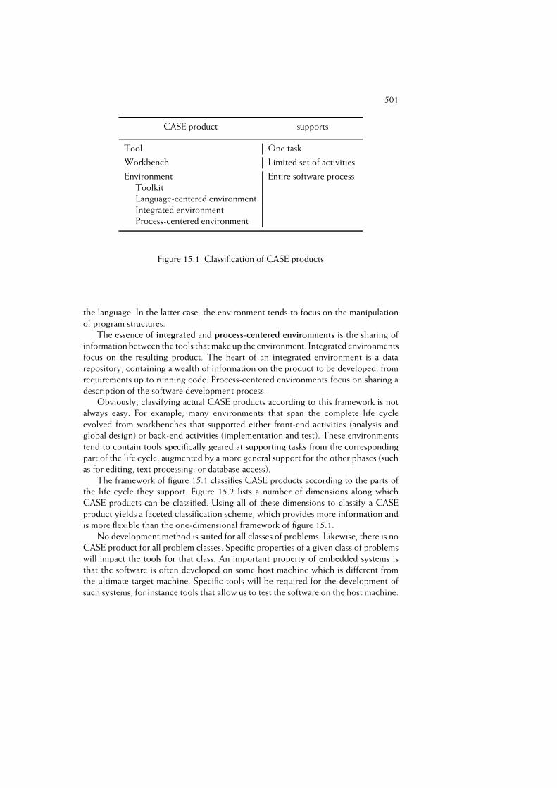
501

CASE product supports

Tool One task

Workbench Limited set of activities

Environment Entire software process

Toolkit

Language-centered environment

Integrated environment

Process-centered environment

Figure 15.1 Classification of CASE products

the language. In the latter case, the environment tends to focus on the manipulation

of program structures.

The essence of integrated and process-centered environments is the sharing of

information between the tools that make up the environment. Integrated environments

focus on the resulting product. The heart of an integrated environment is a data

repository, containing a wealth of information on the product to be developed, from

requirements up to running code. Process-centered environments focus on sharing a

description of the software development process.

Obviously, classifying actual CASE products according to this framework is not

always easy. For example, many environments that span the complete life cycle

evolved from workbenches that supported either front-end activities (analysis and

global design) or back-end activities (implementation and test). These environments

tend to contain tools specifically geared at supporting tasks from the corresponding

part of the life cycle, augmented by a more general support for the other phases (such

as for editing, text processing, or database access).

The framework of figure 15.1 classifies CASE products according to the parts of

the life cycle they support. Figure 15.2 lists a number of dimensions along which

CASE products can be classified. Using all of these dimensions to classify a CASE

product yields a faceted classification scheme, which provides more information and

is more flexible than the one-dimensional framework of figure 15.1.

No development method is suited for all classes of problems. Likewise, there is no

CASE product for all problem classes. Specific properties of a given class of problems

will impact the tools for that class. An important property of embedded systems is

that the software is often developed on some host machine which is different from

the ultimate target machine. Specific tools will be required for the development of

such systems, for instance tools that allow us to test the software on the host machine.

502 SOFTWARE TOOLS

Dimension Typical values

Breadth of support Tool, workbench, or environment

Class of problem Embedded, business, real-time, . . .

Size of system Small, medium, or large

User scale Individual, family, city, or state

Number of sites 1, > 1Process scale Product, people, or product-and-people

Process support None, fixed, or variable

Execution paradigm State machine, Petri net, production rules, procedures, . . .

Figure 15.2 Faceted classification structure for CASE products

For many business applications, the human--computer interaction plays a promi-

nent role, while the requirements analysis of such systems tends to be problematic.

A development environment for such systems had better contain tools that support

those aspects (analyst workbench, prototyping facilities, and facilities to generate

screen layouts).

As a final example, when developing real-time software, it would be preferable to

have tools that allow us to analyze system performance at an early stage.

A second dimension relates the set of tools to the size of the system to be

developed. In practice, it shows that tool usage increases with problem size. For a

small project, we may confine ourselves to a simple configuration control system,

simple test tools, and a shared database system to store documents. In a medium-sized

project, more advanced support could be used, such as a structured database with

objects like design documentation, test plans, or code components. Certain relations

between objects, such as A uses B, or A implements B, could be maintained. For a

medium-sized project, the toolset would also include tools to support management

tasks, for example to create CPM or PERT charts. For a large project, we may require

that the tools be mutually compatible. The toolset for a large project will generally

also impose more constraints on their users.

The user scale refers to the number of users the product supports. Not surprisingly,

the user-scale dimension is closely related to the system size dimension. Larger

systems require larger development teams, don’t they? Using a sociological paradigm,

possible values along the user-scale dimension are called individual, family, city

and state. Some products support the individual developer. These products are

dominated by issues of software construction. The emphasis is on tools that support

software construction: editors, debuggers, compilers, etc. CASE products that offer

configuration management and system build facilities can be classified as belonging

to the family model of software development environments. In the family model, a

503

great deal of freedom is left to the individual developer, while a number of rules are

agreed upon to regulate critical interactions between developers.

This model is not appropriate any more if projects get really big. Larger

populations require more complicated rules and restrictions on individual freedom.

Within my family, a few simple rules suffice (Jasper and Marieke take turns in washing

dishes), and adjustments and local deviations are easily established (Jasper has a party

today and asks Marieke to take over). Within a large company, policies have to be

more strictly obeyed and cooperation between individuals is enforced (like in a city).

Likewise, toolsets to support the development of large systems should enforce the

proper cooperation between individual developers.

A state may be viewed as a collection of cities. A company may be viewed as a

collection of projects. In the state model, the main concern is with commonality and

standardization, to allow developers to switch between projects, to be able to reuse

code, designs, test plans, etc.

If development is done at more than one site, we need tools to facilitate

collaboration and coordination. On one hand, tools like those for configuration

management and requirements management need to provide support to coordinate

development work at multiple sites. On the other hand, tools from the realm of

Computer-Supported Cooperative Work (CSCW) could be part of the tool suite.

This dimension is also closely related to the user-scale and system size dimension,

since larger projects tend to be distributed over multiple sites; see also chapter ??.

The process scale specifies whether the CASE product supports code production

activities, people activities, or both. CASE products focusing on code production

concentrate on support for the evolution of software. They contain tools to write,

compile, test, debug, and configure code. These are all activities done by a computer.

Other CASE products concentrate on personnel interactions, such as the scheduling

of review meetings. Still others do both. Values along this axis may be termed

product, people, and product-and-people.

CASE products may or may not support the development process. If the develop-

ment process is supported, some tools do so on the basis of a predefined model of the

process. Others allow the user to define his own process model. If the CASE product

supports the development process, it may employ various internal means to guide the

execution (or enactment) of the development process, such as state machines, Petri

nets, production rules, or procedures.

The various approaches to collections of software tools are addressed in sections

15.1 to 15.4, using the simple classification scheme of figure 15.1. Toolkits are

discussed in section 15.1. UNIX is a prime example from this category. Section 15.2

discusses language-centered environments. This encompasses both environments

created manually around some given programming language, and environments gen-

erated from a grammatical description of the program structures being manipulated. In

both cases, the support offered mostly concerns the individual programmer. Section

15.3 and 15.4 discuss integrated and process-centered environments, respectively.

Since most workbenches may be viewed as trimmed-down integrated environments,

504 SOFTWARE TOOLS

workbenches are discussed in section 15.3 as well.

The discussion below is fairly global in nature. We will skim over details of

individual tools. Our aim is to sketch discernible trends in this area and to have a

critical look at the possible role of tools in the software development process.

15.1 Toolkits

With a toolkit, developers are supported by a rather loosely-coupled collection of

tools, each of which serves a specific, well-defined, task. The analogy with a carpenter

is obvious. His toolkit contains hammers, screwdrivers, a saw, and the like. These

tools each serve a specific task. However, they are not ‘integrated’ in the way a drill

and its attachments are.

The prime example of a toolkit environment is UNIX. UNIX may be viewed as

a general support environment, not aimed at one specific programming language,

development method, or process model. UNIX offers a number of very convenient,

yet very simple, building blocks with which more complicated things can be

realized (Kernighan and Mashey, 1981):� The file system is a tree. The leafs of this tree are the files, while inner nodes

correspond to directories. A specific file can be addressed absolutely or relative

to the current directory. The addressing is through a pathname, analogous to

the selection of method names in Java. Directories are files too, though the user

cannot change their contents.� Files have a very simple structure. A file is but a sequence of characters (bytes).

So there are no physical or logical records, there is no distinction between

random access files and sequential access files, and there are no file types.

An I/O device is a file too; if it is opened, it automatically activates a program

which handles the traffic with that device. In this way, a user may write

programs without knowing (or, indeed, without having to know) where the

input comes from or where the output goes to.� All system programs (and most user programs) assume that input comes from

the user’s terminal, while the output is again written to that terminal. The user

can easily redirect both input and output. Through a call of the form

prog <in >out

input is read from file in, while output is written to file out. The program itself

need not be changed.� UNIX offers its users a very large set of small, useful, programs. To name but

a few: wc counts the number of lines, words and characters in files, lpr prints

files, grep does pattern matching.

15.2. LANGUAGE-CENTERED ENVIRONMENTS 505� UNIX programs can easily be combined to form larger programs. If the output

of one program is to serve as input to another program, they can be connected

through a pipe, denoted by ‘j’:ls j pr

makes a list of all file names and subsequently prints that list. There is no need

for an auxiliary file to store intermediate results.

In this way, users are led to try to reach their goals by gluing existing components

together, rather than writing a program from scratch. A disadvantage of UNIX is

that there is little consistency in interfaces and the choice of command names. For

different programs, the ‘-k’ option, say, may well mean something rather different.

To stop a dialogue, you may try kill, stop, quit, end, leave, and a few others. If you

get tired, CTRL-c is likely to work too.

The average UNIX user knows only a fairly limited subset of the available

commands and tools (Fischer, 1986). It is quite likely that, after a while, a workable

set of commands will be known and used, and then the learning process stops.

Inevitably, the facilities offered under UNIX are far from optimally used.

In UNIX, the different tools have minimal knowledge of the objects they

manipulate. Various integrated and process-centered environments have been built

on top of UNIX. They make use of the attractive features of UNIX, but try to

overcome its disadvantages by imposing more structure.

Besides tools that support the individual programmer, UNIX also offers support

for programming-in-the-large, through configuration management and system build

facilities like SCCS and Make. These will be discussed in section 15.3.2.

15.2 Language-Centered Environments

Nowadays, most software is developed interactively, changes are made interactively,

and programs are tested and executed interactively. Much research in the area of

language-centered environments is aimed at developing a collection of useful, user-

friendly, effective tools for this type of activity. Since most of these environments

focus on supporting programming tasks, this type of environment is often called a

programming environment. To emphasize their graphic capabilities to manipulate

program constructs, they are sometimes called visual programming environments.

Environments that are built around a specific programming language exploit the

fact that a program entails more than a mere sequence of characters. Programs have a

clear structure. This structure can be used to make the editing process more effective,

to handle debugging in a structured way, and the like. Knowledge of properties of the

objects to be manipulated can be built into the tools and subsequently used by these

tools. Well-known early examples of language-centered environments are Interlisp

and the Smalltalk-80 environment.

506 SOFTWARE TOOLS

Present-day language-centered environments generally come with a host of com-

ponents that considerably ease software development. Examples of such environments

include Microsoft Studio .NET and Eclipse. The support offered ranges from a set

of API’s for generating user interfaces (such as Swing), to facilities for handling

persistence (EJB) or create web applications (Ajax). The richness of features comes

with a price: a rather long learning curve.

15.3 Integrated Environments and Workbenches

This section is devoted to CASE products that support (parts of) the software

development process. Depending on the scope of the set of tools available, such

an environment is called an Analyst WorkBench (AWB), a Programmer WorkBench

(PWB), a Management WorkBench (MWB), or an Integrated Project Support Envi-

ronment (IPSE); see also figure 15.3. The acronym CASE (Computer-Aided Software

Engineering) is often used to indicate any type of tool support in the software devel-

opment process. The qualified terms Upper-CASE and Lower-CASE refer to tool

support during the analysis--design and implementation--test phases, respectively.

In the ideal case, the choice of a specific set of tools will be made as follows. First,

a certain approach to the software development process is selected. Next, techniques

are selected that support the various phases in that development process. As a last

step, tools are selected that support those techniques. Some steps in the development

process may not be supported by well-defined techniques. Some techniques may not

be supported by tools. Thus, a typical development environment will have a pyramid

shape as in figure 15.4.

In practice, we often find the reverse conical form: a barely-developed model of

the development process, few well-defined techniques, and a lot of tools. In this way,

the benefits of the tools will be limited at best. To paraphrase the situation: for many

a CASE, there is a lot of Computer-Aided, and precious little Software Engineering.

The different tool sets identified above are discussed in the subsections to follow.

15.3.1 Analyst WorkBenches

Analyst workbenches serve to support the activities in the early phases of software

development: requirements engineering and (global) design. In these phases, analysis

and design data is gathered. Often, a graphical image of the system is made,

for instance in the form of a set of UML diagrams. From a practical point of

view, important problems concern the drawing and redrawing of those diagrams

and guarding the consistency and completeness of the data gathered. AWB tools

specifically address these points.

The kernel of an AWB is a database in which the information gathered is stored.

The structure of the database can be rather free, or it can be derived from the

techniques supported. The AWB will also contain tools to support the following

types of activity:

15.3. INTEGRATED ENVIRONMENTS AND WORKBENCHES 507

Figure 15.3 Scope of tool sets

Figure 15.4 Support in a typical development environment

508 SOFTWARE TOOLS� Drawing, changing and manipulation of pictures. This may vary from simple

drawing programs that have no knowledge of the pictures’ semantics, to

programs that have an elaborate knowledge of the semantics of the drawing

technique in question. As far as the latter is concerned, we may think of

automatic generation of pointers to subpictures, the automatic reconfiguration

of pictures to circumvent intersecting lines, and the like. If the drawing

technique has been sufficiently formalized, the user support can be comparable

to that offered by a syntax-directed editor for programming languages.� Analysis of data produced, as regards consistency and completeness. The

possibilities of doing this are strongly dependent upon the degree to which the

drawing technique itself imposes strict rules. There is a choice as to when this

checking takes place. If the user is immediately notified when an error is made,

there is little chance for errors to cascade. On the other hand, the freedom

to ‘play’ during the exploratory development stages is also limited. If checking

is done at a later stage, the user may continue on the wrong track for quite

a while before detection, and it then becomes more difficult to identify the

proper error messages.� Managing information. A prime example is managing requirements. A simple

way is to store them in a plain text document. More advanced tools allow

for maintaining relations between requirements, tracing requirements to design

documents, detecting and handling conflicts, and the like.� Generating reports and documentation. It is important to be able to adapt

the precise form of reports and documentation to the requirements of the

user. For instance, internal standards of some organization may enforce certain

report formats. It should be possible to configure the tools to adhere to these

standards.

Further tools of an AWB may support, amongst others, prototyping, the generation

of user interfaces, or the generation of executable code. Post et al. (1998) found that

users perceive two types of (Upper-CASE) tool: those that are good at supporting

analysis and design tasks and those that are good at code generation and prototyping.

Apparently, the tools tend to emphasize one of these uses.

15.3.2 Programmer Workbenches

A programmer workbench consists of a set of tools to support the implementa-

tion and test phases of software development. The term originated in the UNIX

world (Dolotta et al., 1978). The support offered by UNIX mainly concerns these

types of activity. Many programming environments constructed around a certain

programming language also support these phases in particular. In a PWB, we find

tools to support, amongst others:

– editing and analysis of programs;

15.3. INTEGRATED ENVIRONMENTS AND WORKBENCHES 509

– debugging;

– generation of test data;

– simulation;

– test coverage determination.

The tools that support teamwork on large projects deserve our special attention. In a

typical environment, a group of programmers will be working on the same system.

The system will have many components, developed, tested, and changed by different

people. During the evolution of the system, different versions of components will

result. Automatic support for the control of such a set of components, both technically

and organizationally, is a sheer necessity.

One of the early systems for configuration control is the Source Code Control

System (SCCS), originally developed for IBM OS and best known from UNIX. SCCS

enables the user to keep track of modifications in files (which may contain such

diverse things as program code, documentation, or test sets). The system enables the

user to generate any version of the system. New versions can be generated without

old versions being lost. Important aspects of SCCS are:

– no separate copies of versions are kept: only the modifications (so-called deltas)

to previous versions are stored;

– access to files is protected: only authorized users can make changes;

– each file is identified by author, version number, and date and time of

modification;

– the system asks the user for information on the reason for a change, which

change is made, where, and by whom.

Figure 15.5 illustrates the main operations provided by SCCS. Within SCCS, all

information is kept in so-called s-files. The operation create creates the s-file for the

first time. If the original file is named prog, then the SCCS file is named s.prog.

The operation get yields a read-only copy of the file requested. This read-only copy

can be used for compiling, printing, and the like. It is not intended to be edited.

The operation edit retrieves a copy to be edited. SCCS takes care of protection in

the sense that only one person can be editing a file at one time. Finally, the deltaoperation stores the revised version of the file edited.

Versions of SCCS files are numbered, 1.1, 1.2, 1.3, 2.1, etc. The number to the

left of the period is the major version number (release number). The number to the

right of the period is the minor version number. The first version is numbered 1.1.

By default, get and edit retrieve the latest version of a file, while delta results in an

increase of the minor version number. If an older version is required or the major

version number is to be increased, this must be specified explicitly.

510 SOFTWARE TOOLS

Figure 15.5 Main operations of SCCS

The above scheme results in a linear sequence of versions. SCCS also provides

the possibility of creating branches (forks), as illustrated in figure 15.6. For example,

starting from version 1.2 we may create versions 1.3, 1.4, etc to represent normal

development of a system component, and versions 1.2.1.1, 1.2.1.2, etc to represent

bug fixes in version 1.2. In SCCS, the merging of development paths must be done

manually.

When different versions of the same system are maintained in this way, the need

to automate the construction of new executable versions arises. Make is a tool that

does this (Feldman, 1978). Make uses a description of the various components of a

system and their mutual dependencies. When generating a new executable system,

Make inspects the date and time of the latest changes to components and only

recompiles components when needed (i.e. components that have been changed since

the last compilation). A tool like Make not only saves machine time, but also ensures

that the most recent version of each component is used.

The basic functionality of configuration control systems has not fundamentally

changed since the development of SCCS in the early 1970s. Rather than keeping

a copy of each version, SCCS and similar systems only keep track of what has

changed from the previous version (the so-called deltas). Nowadays, disk storage is

not an issue anymore, and many software configuration systems use simple zip-like

compression instead of deltas. Additional features offered in present-day systems are

mainly directed at increasing the flexibility and usability of such systems:

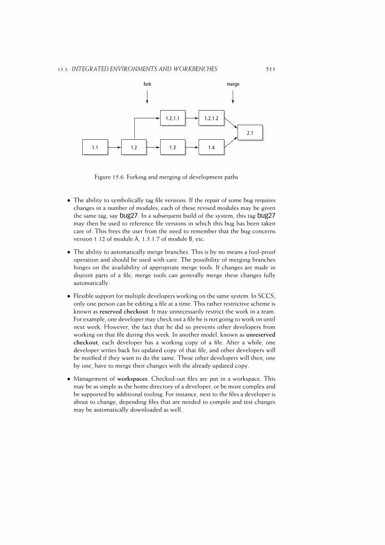
15.3. INTEGRATED ENVIRONMENTS AND WORKBENCHES 511

Figure 15.6 Forking and merging of development paths� The ability to symbolically tag file versions. If the repair of some bug requires

changes in a number of modules, each of these revised modules may be given

the same tag, say bug27. In a subsequent build of the system, this tag bug27may then be used to reference file versions in which this bug has been taken

care of. This frees the user from the need to remember that the bug concerns

version 1.12 of module A, 1.3.1.7 of module B, etc.� The ability to automatically merge branches. This is by no means a fool-proof

operation and should be used with care. The possibility of merging branches

hinges on the availability of appropriate merge tools. If changes are made in

disjoint parts of a file, merge tools can generally merge these changes fully

automatically.� Flexible support for multiple developers working on the same system. In SCCS,

only one person can be editing a file at a time. This rather restrictive scheme is

known as reserved checkout. It may unnecessarily restrict the work in a team.

For example, one developer may check out a file he is not going to work on until

next week. However, the fact that he did so prevents other developers from

working on that file during this week. In another model, known as unreserved

checkout, each developer has a working copy of a file. After a while, one

developer writes back his updated copy of that file, and other developers will

be notified if they want to do the same. These other developers will then, one

by one, have to merge their changes with the already updated copy.� Management of workspaces. Checked-out files are put in a workspace. This

may be as simple as the home directory of a developer, or be more complex and

be supported by additional tooling. For instance, next to the files a developer is

about to change, depending files that are needed to compile and test changes

may be automatically downloaded as well.

512 SOFTWARE TOOLS� Support for communication within a development team. For example, if one

developer checks out a file someone else is already working on, he may be given

a notification of this, so that the developers can start a dialog and coordinate

their activities. The latter type of support connects the pure archival function

of configuration control systems with the communication and coordination

functions of workflow management systems.

Language-centered environments as discussed in section 15.2 support the individual

developer. These environments are dominated by issues of software construction. The

emphasis is on tools that support software construction: editors, debuggers, compilers,

etc. Toolsets that offer configuration management and system build facilities like those

offered by SCCS and Make can be classified as belonging to the family model of

software development environments: a great deal of freedom is left to the individual

developers, while a number of rules are agreed upon to regulate critical interactions

between developers.

Most programmer workbenches offer this family type of support. For example,

Make assumes that files whose names end in .c are C source files. Members of the

development family follow this rule and may even have agreed upon further naming

conventions. The development environment however has no way of enforcing those

rules. It is up to management to make sure that the rules are followed.

15.3.3 Management WorkBenches

A management workbench contains tools that assist the manager during planning and

control of a software development project. Example tools in an MWB include:

Configuration control Besides the control of software components as discussed in

the previous section, we may also think of the control of other project-specific

information, like design and analysis data, or documentation. An essential aspect

of this type of configuration control concerns the control of change requests.

Changes are proposed, assessed, approved or rejected, given a priority and cost

estimate, planned, and executed. The corresponding procedures are described in a

configuration control plan. The administration and workflow of those change requests

may well be supported through a tool. See also chapter 4.

Work assignment Given a number of components, their mutual dependencies, and

resources needed (both people and hardware), tools can be used to determine critical

paths in the network of tasks, and work packages may be assigned accordingly. This

is a central feature of process-centered environments; see section 15.4.

Cost estimation Various quantitative cost-estimation models have been developed.

These models yield cost estimates, based on project characteristics. Tools have been

developed that assist in gathering quantitative project data, calibrating cost-estimation

models based on these data, and making cost estimates for new projects.

15.4. PROCESS-CENTERED ENVIRONMENTS 513

15.3.4 Integrated Project Support Environments

An Integrated Project Support Environment is meant to support all phases of the

software life cycle. Thus, such an environment has to contain the various tools as

discussed in the previous sections. Environments that span the complete life cycle

usually emphasize the support of either front-end activities (analysis and global design

-- Upper-CASE) or back-end activities (implementation and testing -- Lower-CASE).

They then contain tools specifically geared at supporting tasks from the corresponding

part of the life cycle, augmented by a more general support for the other phases (such

as for editing, text processing, or database access).

When developing an IPSE, we may strive for either a strong or a weak integration

of its tools. A strong integration, as realized in the language-centered environments

discussed in section 15.2, has both advantages (like better control capabilities) and

disadvantages. One disadvantage is that such an IPSE tends to be less flexible. If the

tools are not integrated, as in UNIX, there is more flexibility. On the other hand, a

more stringent management control is then needed.

We may also look for intermediate forms. For example, all objects may be stored

in the UNIX file system, controlled by SCCS, and the relationships between objects

may be represented using a relational database system.

The heart of an integrated environment is the data repository, containing the

information shared between the tools that make up the environment. The constraints

imposed on the structure of this repository mirror the degree to which the tools

are integrated. A stricter integration of tools allows for a stricter definition of the

structure of the data they share, and vice versa.

15.4 Process-Centered Environments

In a process-centered software engineering environment (PSEE), a description of the

software development process is shared by the tools that make up the environment.

Not surprisingly, developments in process-centered environments are closely tied

to developments in process modeling, and vice versa. For example, the kinds of

description used in process modeling (state transition diagrams, Petri nets, and the

like) are also the formalisms used in PSEEs. Process modeling is discussed in section

3.6.

Like an integrated environment, a process-centered environment may cover the

complete life cycle. Like an IPSE, a PSEE tends to be geared towards supporting tasks

from a specific part of the software development life cycle. Since back-end activities

(implementation and testing) are somewhat easier to structure and formalize, work in

process modeling and PSEEs has concentrated on modeling and supporting back-end

activities, consequently.

Figure 15.7 gives a model of the process of conducting a code review. The

notation is that of Petri nets. In section 3.6, this same figure was used to explain the

514 SOFTWARE TOOLS

role of different formalisms in process modeling. Here, we will use it to discuss its

role in a process-centered software engineering environment.

Figure 15.7 Petri net view of the review process

If the developer indicates that some piece of code is ready for review, the

environment is notified and comes into a state as indicated in figure 15.7. Parallel

to the coding activity, management schedules a review meeting. Once this is done,

the place1 labeled review scheduled is marked. The support environment then

‘knows’ that the review can be held and may offer support for doing so. In this way,

the environment guides the developers and other participants through the steps of

the review process, alerts them when certain actions are required, maintains status

information of code products and other pieces of information, etc. Thus, PSEEs

provide support for software development by automating routine tasks, invoking

appropriate development tools, and enforcing rules and practices.

Formal models of a software process are rigid. In practice, this rigidity is a

hindrance, since there will always be exceptions. For example, the minutes of a review

meeting might get lost, management may decide to skip a certain review meeting,

a review meeting may have to be rescheduled because some participant got ill, etc.

The Petri model of figure 15.7 can not cope with these situations. A number of them

can be accommodated by making the model more complex. But the model will never

cover all situations. There is thus a need to be able to intervene. Some PSEEs, for

example, offer means to update process models on the fly. A fully satisfactory solution

is difficult to find, and the rigidity of formal models is likely to continue to conflict

with the requirements of flexibility in process support.

This holds the more where it supports the early stages of software development.

A designer or requirements engineer is not helped by an environment that dictates

1See section 3.6 for the terminology of Petri nets.

15.5. SUMMARY 515

the detailed order of process steps to be taken. Broadly speaking, we may distin-

guish two types of activity: the unstructured, creative, and cooperative activities

that characterize the early stages of software development; and the repetitive and

structured activities that characterize the later stages. A similar dichotomy may be

observed in PSEEs. PSEEs focusing on the early stages have much in common with

groupware and Computer Supported Cooperative Work (CSCW) systems. These

PSEEs support coordination of activities, such as access to and sharing of information,

and cooperation activities, such as communication between people and scheduling

meetings. This type of support is becoming increasingly important in present-day

multisite development; see also chapter ??. PSEEs focusing on the later stages have

much in common with workflow management and configuration control systems.

Present-day configuration control systems not only offer the basic versioning and

access capabilities known from systems like SCCS (see section 15.3.2) but they also

offer ways to define and enact software configuration tasks and policies. Some even

claim that configuration management tools are the ‘real’ PSEEs (Conradi et al., 1998).

15.5 Summary

Developments in the area of (integrated) collections of tools move very fast. For

many a facet of the software development process, good tools are available. In

this chapter, we have discussed the major developments as regards computer-aided

software engineering (CASE). We have done so using a simple, one-dimensional

classification of CASE products, which expresses the parts of the life cycle they

support:� a tool supports one specific task;� a workbench supports a limited set of activities, such as those which comprise

the implementation and testing stages;� an environment supports the entire process.

We have further classified environments according to the mechanism that ties together

the tools that make up the environment:� In a toolkit, the tools are generally not so well integrated. A toolkit merely

offers a set of useful building blocks. UNIX is a prime example of this.� A language-centered environment contains tools specifically aimed at support-

ing software development in a specific programming language.� An integrated environment contains tools that share information about the

resulting product. This information is stored in a data repository, and the tools

read and write this repository.

516 SOFTWARE TOOLS� A process-centered environment contains tools that share a description of the

software-development process.

Though environments are supposed to cover the entire life cycle, they tend to

emphasize certain parts of the process. They then contain tools specifically geared at

supporting tasks from that part of the process, augmented by a more general, and often

limited, support for the other parts. For example, language-centered environments

tend to focus on the implementation and testing stages.

One of the major impediments to the widespread use of tools is their rigidity.

Software tools are driven by formal models of what can and can not be done. A tool

for requirements engineering is likely to enforce certain rules of well-formedness on

the diagrams it handles. A tool to support the testing process is likely to prescribe a

certain order of process steps. The requirements engineer, though, may well want to

play with ill-formed diagrams for a while. Likewise, the tester may want to deviate

from the pre-established order of steps if circumstances require this. The tension

between the demands for flexibility of tool users and those for formality of tool

builders is one of the major challenging research themes in this area.

In a retrospective of PSEE research, Cugola and Ghezzi (1998) refer to this tension

as the minimalist versus maximalist approach. In a maximalist approach, the goal is

to model all possible situations. A minimalist approach follows a more lightweight

approach, and acknowledges that humans play a decisive role in the decision process.

A further corollary is that tools should support cooperation rather than automation.

An interesting open question is whether tools really help. Studies of tool adoption

and usage show mixed results. Some conclude that tools offer real improvements,

while others conclude that users have not found tools to be helpful. There are

definitely certain impediments to tool adoption. Tools cost money, sometimes a lot

of money. There also is a learning curve for tool users. Finally, there is quite a gulf

between the state of the art as reported in this chapter and the state of the practice.

For many an organizational problem, automation seems to be the panacea.

Likewise, the use of tools is often seen as panacea for our problems in software

engineering: CASE as prosthesis. Tools, though, remain mere tools. Within the

software development process, other factors play a role as well. If the tools do not

fit the procedures used within your organization, they are likely to have a far from

optimal effect. Also, tools cannot make up for an ineffective development method or

badly-qualified personnel. Good people deliver good products and mediocre people

deliver mediocre products, irrespective of the tools they use.

15.6 Further Reading

An early taxonomy of CASE products is given in (Dart et al., 1987). Fuggetta (1993)

extended this framework with a category ’process-centered environments’. The latter

classification is used in this chapter. Additional dimensions for classifying CASE

15.6. FURTHER READING 517

products are given in (Lott, 1993). The sociological paradigm (individual, family,

etc.) for the user scale stems from (Perry and Kaiser, 1991).

Barstow et al. (1984) is a collection of seminal articles on programming envi-

ronments, including the UNIX toolkit approach and early language-centered envi-

ronments like Interlisp. The Source Code Control System (SCCS) is described in

(Rochkind, 1975). The state of the art in configuration management is reflected in

(Estublier et al., 2005). Building tools have not changed much since Make (Feldman,

1978). A recent development in this area in the Java world is Ant (Serrano and

Ciordia, 2004).

In the 1980s, tool research focused on creating integrated environments. (Tah-

vanainen and Smolander, 1990) is an annotated bibliography of articles on software

engineering environments from that period. Subsequent research in the area of tools

focused on PSEEs. The state of the art in this area is reflected in (Fuggetta and Wolf,

1996) and (Ambriola et al., 1997). The case for more flexibility in software engineer-

ing environments is made in (Jankowski, 1994), (Cugola et al., 1996), (Jarzabek and

Huang, 1998) and (Cugola and Ghezzi, 1998).

Tool integration issues are addressed in (Sharon and Bell, 1995). Tools assessment

is the topic of (Software, 1996b). Studies of tool adoption and usage can be found in

(Iivari, 1996) and (Post et al., 1998).

Exercises

1. What does the acronym CASE stand for?

2. Define the following terms:

– tool,

– workbench,

– environment.

3. What are the main distinguishing features of:

– a toolkit,

– a language-centered environment,

– an integrated environment, and

– a process-centered environment.

4. What is the difference between Upper-CASE and Lower-CASE?

5. What is the basic functionality of a tool for configuration management?

6. Discuss the fundamental tension between formality and informality in tools.

518 SOFTWARE TOOLS

7. Why is the user scale an important issue when considering the adoption of

tools?

8. ~ Defend the statement that configuration management tools are the only

‘real’ process-centered environments (see (Conradi et al., 1998)).

9. � For the development environment you are currently working in, prepare a

list of:

– utilities you use on a regular basis;

– utilities you use infrequently or vaguely know about.

Next compare these lists with the manuals describing the environment. What

percentage of the environment’s functionality do you really need?

10. � Select and evaluate some commercial UML modeling tool using the criteria

given in (Zucconi, 1989) or (Baram and Steinberg, 1989).

11. ~ Discuss the possible role of automatic support for configuration control in

the management of artifacts other than source code modules.

12. ~ One of the claims of CASE-tool providers is that CASE will dramatically

improve productivity. At the same time though, customers seem to be

disappointed with CASE and take a cautionary stand. Can you think of

reasons for this discrepancy?

13. ~ Why is tool integration such an important issue?

Bibliography

Abdel-Hamid, T., Sengupta, K., and Ronan, D. (1993). Software Project Control: An

Experimental Investigation of Judgment with Fallible Information. IEEE Transactionson Software Engineering, 19(6):603--612.

Aberdour, M. (2007). Achieving Quality in Open Source Software. IEEE Software,

24(1):58--64.

Abrahamsson, P., Salo, O., Ronkainen, J., and Warsta, J. (2002). Agile Software

Development Methods. Technical report, VTT Publications 478, VTT, Finland.

Abran, A. and Robillard, P. (1992). Function Points: A Study of Their Measurement

Processes and Scale Transformations. Journal of Systems and Software, 25(2):171--184.

Abran, A. and Robillard, P. (1996). Function Points Analysis: An Empirical Study of

Its Measurement Processes. IEEE Transactions on Software Engineering, 22(12):895--910.

Adams, E. (1984). Optimizing Preventive Service of Software Products. IBM Journal

of Research and Development, 28(1):2--14.

Albrecht, A. (1979). Measuring Applications Development Productivity. In Proceedings

Application Development Symposium, pages 83--92. SHARE/GUIDE.

Albrecht, A. and Gaffney, J. (1983). Software Function, Source Lines of Code, and

Development Effort Prediction: A Software Science Validation. IEEE Transactions on

Software Engineering, 9(6):639--648.

Alexander, C. (1979). The Timeless Way of Building. Oxford University Press.

Alexander, C. (1999). The Origins of Pattern Theory. IEEE Software, 16(5):71--82.

Alexander, C., Ishikawa, S., and Silverstein, M. (1977). A Pattern Language. Oxford

University Press.

Ambriola, V., Conradi, R., and Fuggetta, A. (1997). Assessing Process-Centered

Software Engineering Environments. ACM Transactions on Software Engineering and

Methodology, 6(3):283--328.

520 BIBLIOGRAPHY

Arisholm, A. and Sjøberg, D. (2004). Evaluating the Effect of a Delegated versus

Centralized Control Style on the Maintainability of Object-Oriented Software.

IEEE Transactions on Software Engineering, 30(8):521--534.

Armour, P. (2001). Zeppelins and Jet Planes: A Metaphor for Modern Software

Projects. Communications of the ACM, 44(10):13--15.

Atkinson, C. (2000). Socio-Technical and Soft Approaches to Information Require-

ments Elicitation in the Post-Methodology Era. Requirements Engineering Journal,

5(2):67--73.

Austin, R. and Devin, L. (2003). Beyond Requirements: Software Making as Art. IEEE

Software, 20(1):93--95.

Baber, R. (1982). Software Reflected. North-Holland Publishing Company.

Babich, W. (1986). Software Configuration Management. Addison-Wesley.

Baddoo, N. and Hall, T. (2003). De-motivators for software process improvement:

an anlysis of practitioners’ views. Journal of Systems and Software, 66(1):23--34.

Baker, F. (1972). Chief Programmer Team Management of Production Programming.

IBM Systems Journal, 11(1):56--73.

Banker, R., Datar, S., Kemerer, C., and Zweig, D. (1993). Software Complexity and

Maintenance Costs. Communications of the ACM, 36(11):81--94.

Banker, R., Kauffman, R., and Kumar, R. (1991). An Emperical Test of Object-Based

Output Measurement Metrics in a Computer Aided Software Engineering (CASE)

Environment. Journal of Management Information Systems, 8(3):127--150.

Baram, G. and Steinberg, G. (1989). Selection Criteria for Analysis and Design CASE

Tools. ACM Software Engineering Notes, 14(6):73--80.

Barnard, H., Metz, R., and Price, A. (1986). A Recommended Practice for Describing

Software Designs: IEEE Standards Project 1016. IEEE Transactions on Software

Engineering, 12(2):258--263.

Barstow, D., Shrobe, H., and Sandewall, E., editors (1984). Interactive ProgrammingEnvironments. McGraw-Hill.

Basili, V. (1990). Viewing Maintenance as Reuse-Oriented Software Development.

IEEE Software, 7(1):19--25.

Basili, V., Briand, L., Condon, S., Kim, Y.-M., Melo, W., and Valen, J. (1996).

Understanding and Predicting the Process of Software Maintenance Releases. In

Proceedings International Conference on Software Maintenance (ICSM’96), pages 464--474.

IEEE.

BIBLIOGRAPHY 521

Basili, V. and Selby, R. (1987). Comparing the Effectiveness of Software Testing

Strategies. IEEE Transactions on Software Engineering, 13(12):1278--1296.

Bass, L., Clements, P., and Kazman, R. (2003). Software Architecture in Practice. Addison

Wesley, second edition.

Batini, C., Ceri, S., and Navathe, S. (1992). Conceptual Database Design: An Entity--

Relationship Approach. Benjamin Cummings.

Beck, K. (2000). Extreme Programming Explained. Addison-Wesley.

Beck, K. (2003). Test-Driven Development. Addison-Wesley.

Beck, K. and Cunningham, W. (1989). A Laboratory For Teaching Object-Oriented

Thinking. In OOPSLA ’89 Proceedings, ACM SIGPLAN Notices 24(10), pages 1--6.

Beck, K. et al. (2001). Manifesto for Agile Software Development.

Beizer, B. (1995). Black Box Testing. John Wiley & Sons.

Bellay, B. and Gall, H. (1998). An Evaluation of Reverse Engineering Tool Capabilities.

Journal of Software Maintenance: Research and Practice, 10:305--331.

Benington, H. (1983). Production of Large Computer Programs. In Proceedings ONR

Symposium (1956), reprinted in Annals of the History of Computing 5(4), pages 350--361.

Bennett, K. (1998). Do Program Transformations Help Reverse Engineering? In

Proceedings International Conference on Software Maintenance (ICSM’98), pages 247--254.

IEEE.

Bennett, K. and Rajlich, V. (2000). Software Maintenance and Evolution: a Roadmap.

In Finkelstein, A., editor, The Future of Software Engineering, pages 73--87. ACM Press.

Bergland, G. and Gordon, R. (1981). Tutorial: Software Design Strategies. IEEE, EZ389.

Bersoff, E. and Davis, A. (1991). Impacts of Life Cycle Models on Software

Configuration Management. Communications of the ACM, 34(8):104--118.

Beyer, H. and Holtzblatt, K. (1995). Apprenticing with the Customer. Communicationsof the ACM, 38(5):45--52.

Bieman, J., Jain, D., and Yang, H. (2001). OO Design Patterns, Design Structure,

and Program Changes: An Industrial CaseStudy. In Proceedings International Conferenceon Software Maintenance (ICSM’01), pages 580--589. IEEE.

Biffl, S. and Halling, M. (2002). Investigating the Influence of Inspector Capability

Factors with Four Inspection Techniques on Inspection Performance. In Proceedings

8th IEEE International Software Metrics Symposium, pages 107--17. IEEE.

522 BIBLIOGRAPHY

Biggerstaff, J., Mitbander, B., and Webster, D. (1994). Program Understanding and

the Concept Assignment Problem. Communications of the ACM, 37(5):72--83.

Biggerstaff, T. (1989). Design Recovery for Maintenance and Reuse. IEEE Computer,

22(7):36--50.

Binder, R. (2000). Testing Object-Oriented Systems. Addison-Wesley.

Bisbal, J., Lawless, D., Wu, B., and Grimson, J. (1999). Legacy Information Systems:

Issues and Directions. IEEE Software, 16(5):103--111.

Blum, B. (1994). A Taxonomy of Software Development Methods. Communications of

the ACM, 37(11):82--94.

Boehm, B. (1975). Some Experience with Automated Aids to the Design of Large-

Scale Reliable Software. In Proceedings International Conference on Reliable Software, ACM

SIGPLAN Notices 10(6), pages 105--113. ACM.

Boehm, B. (1976). Software Engineering. IEEE Transactions on Computers, C-25(12):1226-

-1241.

Boehm, B. (1981). Software Engineering Economics. Prentice-Hall.

Boehm, B. (1983). The Economics of Software Maintenance. In Proceedings Software

Maintenance Workshop, pages 9--37. IEEE, 83CH1982-8.

Boehm, B. (1984a). Software Life Cycle Factors. In Vick, C. and Ramamoorthy, C.,

editors, Handbook of Software Engineering, pages 494--518. Van Nostrand Reinhold.

Boehm, B. (1984b). Verifying and Validating Software Requirements and Design

Specifications. IEEE Software, 1(1):75--88.

Boehm, B. (1987a). Improving Software Productivity. IEEE Computer, 20(9):43--57.

Boehm, B. (1987b). Industrial Software Metrics Top 10 List. IEEE Software, 4(5):84--85.

Boehm, B. (1988). A Spiral Model of Software Development and Enhancement. IEEEComputer, 21(5):61--72.

Boehm, B. (1989). Software Risk Management. IEEE.

Boehm, B. and Basili, V. (2001). Software Defect Reduction Top 10 List. IEEE

Computer, 34(1):135--137.

Boehm, B., Brown, J., Kaspar, H., Lipow, M., MacLeod, G., and Merrit, M. (1978).

Characteristics of Software Quality. Number 1 in TRW Series of Software Technology.

North-Holland.

BIBLIOGRAPHY 523

Boehm, B., Clark, B., Horowitz, E., Westland, C., Madachy, R., and Selby, R. (1995).

Cost Models for Future Software Life Cycle Processes: COCOMO 2.0. Annals of

Software Engineering, 1:57--94.

Boehm, B. and Sullivan, K. (1999). Software economics: status and prospects.

Information and Software Technology, 41(14):937--946.

Boehm, B. and Turner, R. (2003). Balancing Agility and Discipline. Addison-Wesley.

Boehm et al., B. (1997). COCOMO II Model Definition Manual. Technical report,

University of Southern California.

Bohm, C. and Jacopini, G. (1966). Flow Diagrams, Turing Machines, and Languages

With Only Two Formation Rules. Communications of the ACM, 9(5):366--371.

Bohrer, K., Johnson, V., Nilsson, A., and Rudin, B. (1998). Business Process

Components for Distributed Object Applications. Communications of the ACM,

41(6):43--48.

Booch, G. (1994). Object-Oriented Analysis and Design with Applications. Benjamin-

Cummings, second edition.

Booch, G., Rumbaugh, J., and Jacobson, I. (1999). UML User Guide. Addison Wesley.

Bounds, G., Yorks, L., Adams, M., and Ranney, G. (1994). Beyond Total Quality

Management. McGraw-Hill.

Brooks, F. (1995). The Mythical Man-Month. Addison-Wesley, second edition.

Brooks, Jr., F. (1987). No Silver Bullet: Essence and Accidents of Software Engineering.

IEEE Computer, 20(4):10--20.

Brooks, R. (1983). Towards a Theory of the Comprehension of Computer Programs.

International Journal of Man-Machine Studies, 18:543--554.

Brown, W., Malveau, R., III, H. M., and Mowbray, T. (1998). AntiPatterns: Refactoring

Software, Architectures, and Projects in Crisis. John Wiley & Sons.

Budgen, D. (2003). Software Design. Addison Wesley, second edition.

Burch, E. and Kung, H.-J. (1997). Modeling Software Maintenance Requests: A

CaseStudy. In Proceedings International Conference on Software Maintenance (ICSM’97),

pages 40--47.

Buschmann, F., Meunier, R., Rohnert, H., Sommerlad, P., and Stal, M. (1996). A

System of Patterns. John Wiley & Sons.

Bush, E. (1985). The Automatic Restructuring of COBOL. In Proceedings Conference on

Software Maintenance, pages 35--41. IEEE.

524 BIBLIOGRAPHY

Buxton, J. and Randell, B., editors (1969). Software Engineering Techniques, Report on a

Conference. NATO Scientific Affairs Division, Rome.

CACM (1993a). Special Issue on Participatory Design. Communications of the ACM,

36(6).

CACM (1993b). Special Issue on Project Organization and Management. Communi-cations of the ACM, 36(10).

CACM (1997). Special issue The Quality Approach: Is It Delivering. Communicationsof the ACM, 40(6).

Cameron, J. (1989). JSP & JSD, The Jackson Approach to Software Development. IEEE.

Carmel, E., Whitaker, R., and George, J. (1993). PD and Joint Application Design: A

Transatlantic Comparison. Communications of the ACM, 36(6):40--48.

Cha, S., Leveson, N., and Shimeall, T. (1988). Safety Verification in MURPHY using

Fault-Tree Analysis. In Proceedings 10th International Conference on Software Engineering(ICSE10), pages 377--386. IEEE.

Chapin, N. (1987). The Job of Software Maintenance. In Proceedings Conference on

Software Maintenance, pages 4--12. IEEE.

Chapin, N., Hale, J., Khan, K., amil, J., and Tan, W.-G. (2001). Types of software

evolution and software maintenance. Journal of Software Maintenance and Evolution:

Research and Practice, 13:3--30.

Chen, P. (1976). The Entity--Relationship Model: Toward a Unifying View of Data.

ACM Transactions on Data Base Systems, 1(1):9--36.

Chidamber, S. and Kemerer, C. (1994). A Metrics Suite for Object Oriented Design.

IEEE Transactions on Software Engineering, 20(6):476--493.

Chikofsky, E. (1990). CASE & Reengineering: From Archeology to Software Pere-

stroika. In Proceedings 12th International Conference on Software Engineering (ICSE12), page

122. IEEE.

Chikofsky, E. and Cross II, J. (1990). Reverse Engineering and Design Recovery: A

Taxonomy. IEEE Software, 7(1):13--18.

Churcher, N. and Shepperd, M. (1995). Comments on ‘A Metrics Suite for Object

Oriented Design’. IEEE Transactions on Software Engineering, 21(3):263--265.

Ciolkowski, M., Laitenberger, O., and Biffl, S. (2003). Software Reviews: The State

of the Practice. IEEE Software, 20(6):46--51.

BIBLIOGRAPHY 525

Clarke, L., Podgurski, A., Richardson, D., and Zeil, S. (1989). A Formal Evaluation

of Data Flow Path Selection Criteria. IEEE Transactions on Software Engineering,

15(11):1318--1332.

Clements, P., Bachman, F., Bass, L., Garlan, D., Ivers, J., Little, R., Nord, R., and

Stafford, J. (2003). Documenting Software Architectures: Views and Beyond. Addison

Wesley.

Clements, P., Kazman, R., and Klein, M. (2002). Evaluating Software Architectures: Methods

and Case Studies. Addison-Wesley.

Clements, P. and Northrop, L. (2001). Software Product Lines: Practices and Patterns.

Addison-Wesley.

CMMI Product Team (2002). CMMISM for Systems Engineering/Software

Engineering, Version 1.1, Staged Representation. Technical report, CMU/SEI-

2002-TR-002, Software Engineering Institute.

Coad, P. and Yourdon, E. (1991). Object-Oriented Analysis. Yourdon Press, second

edition.

Coakes, J. and Coakes, E. (2000). Specifications in Context: Stakeholders, Systems

and Modelling of Conflict. Requirements Engineering Journal, 5(2):103--113.

Cockburn, A. (1996). The Interaction of Social Issues and Software Architecture.

Communications of the ACM, 39(10):40--46.

Cockburn, A. (2001). Writing Effective Use Cases. Addison-Wesley.

Cockburn, A. (2002). Agile Software Development. Addison-Wesley.

Coleman, D. (1996). Fusion with Use Cases: Extending Fusion for

Requirements Modelling. Technical report, available through URL

http://www.hpl.hp.com/fusion/index.html.

Coleman, D., Arnold, P., Bodoff, S., Dollin, C., Gilchrist, H., Hayes, F., and Jeremaes,

P. (1994). Object-Oriented Development: The FUSION Method. Prentice-Hall.

Collofello, J. and Woodfield, S. (1989). Evaluating the Effectiveness of Reliability-

Assurance Techniques. Journal of Systems and Software, 9(3):191--195.

Conklin, J. (1987). Hypertext: An Introduction and Survey. IEEE Computer, 20(9):17-

-41.

Conklin, J. and Begeman, M. (1988). gIBIS: A Hypertext Tool for Exploratory Policy

Discussion. ACM Transactions on Office Information Systems, 6(4):303--331.

Conradi, R. and Fuggetta, A. (2002). Improving Software Process Improvement. IEEE

Software, 19(4):92--99.

526 BIBLIOGRAPHY

Conradi, R., Fuggetta, A., and Jaccheri, M. (1998). Six Theses on Software Process

Research. In Gruhn, V., editor, Software Process Technology, 6th European workshop,

EWSPT’98. Springer Verlag, LNCS 1487.

Constantine, L. (1993). Work Organization: Paradigms for Project Management and

Organization. Communications of the ACM, 36(10):34--43.

Conte, S., Dunsmore, H., and Shen, V. (1986). Software Engineering Metrics and Models.

Benjamin Cummings.

Cook, S., Harrison, R., Lehman, M., and Wernick, P. (2006). Evolution in software

systems: foundations for the SPE classification scheme. Journal of Software Maintenance

and Evolution: Research and Practice, 18(1):1--35.

Corby, T. (1989). Program Understanding: Challenge for the 1990s. IBM Systems

Journal, 28(2):294--306.

Corkill, D. (1997). Countdown to Success: Dynamic Objects, GBB, and RADARSET-

1. Communications of the ACM, 40(5):48--58.

Cote, M.-A., Suryn, W., and Georgiadou, E. (2006). Software Quality Model

Requirements for Software Quality Engineering. In Proceedings 14th International

Software Quality Management & INSPIRE Conference.

Couger, J. and Zawacki, R. (1980). Motivating and Managing Computer Personnel. Wiley.

Crowston, K. and Howison, J. (2006). Assesing the Health of Open Source

Communities. IEEE Computer, 39(5):89--91.

Cugola, G., di Nitto, E., Fuggetta, A., and Ghezzi, C. (1996). A framework for

Formalizing Inconsistencies and Deviations in Human-Centered Systems. ACMTransactions on Software Engineering and Methodology, 5(3):191--230.

Cugola, G. and Ghezzi, C. (1998). Software Processes: a Retrospective and a Path to

the Future. Software Process -- Improvement and Practice, 4(3):101--123.

Currit, P., Dyer, M., and Mills, H. (1986). Certifying the Reliability of Software.

IEEE Transactions on Software Engineering, 12(1):3--11.

Curtis, B. (1989). Three Problems Overcome with Behavioral Models of the Software

Development Process. In Proceedings 11th International Conference on Software Engineering(ICSE11), pages 398--399. IEEE.

Curtis, B., Krasner, H., and Iscoe, N. (1988). A Field Study of the Software Design

Process for Large Systems. Communications of the ACM, 31(11):1268--1287.

Curtis, B., Krasner, H., Shen, V., and Iscoe, N. (1987). On Building Software Process

Models Under the Lamppost. In Proceedings 9th International Conference on Software

Engineering (ICSE9), pages 96--103.

BIBLIOGRAPHY 527

Curtis, B., Sheppard, S., and Milliman, P. (1979). Third Time Charm: Stronger

Prediction of Programmer Performance by Software Complexity Metrics. In

Proceedings 4th International Conference on Software Engineering (ICSE4), pages 356--360.

IEEE.

Cusumano, M. (1989). The Software Factory: A Historical Interpretation. IEEESoftware, 6(2):23--30.

Darcy, D. (2005). The Structural Complexity of Software: An Experimental Test.

IEEE Transactions on Software Engineering, 31(11):982--995.

Darcy, D. and Kemerer, C. (2005). OO Metrics in Practice. IEEE Software, 22(6):17--

19.

Darke, P. and Shanks, G. (1996). Stakeholder Viewpoints in Requirements Definition:

A Framework for Understanding Viewpoint Development Approaches. RequirementsEngineering Journal, 1:88--105.

Dart, S. (1990). Spectrum of Functionality in Configuration Management Systems.

Technical report, CMU/SEI-90-TR-11, Software Engineering Institute.

Dart, S., Ellison, R., Feiller, P., and Habermann, A. (1987). Software Development

Environments. IEEE Computer, 20(11):18--28.

Davenport, T. (1993). Process Innovation: Reengineering Work through Information Technology.

Harvard Business School Press, Cambridge, MA.

Davis, A. (1993). Software Requirements: Objects, Functions and State. Prentice-Hall, second

edition.

Davis, A. (1995). Object-Oriented Requirements to Object-Oriented Design: An

Easy Transition? Journal of Systems and Software, 30(1 & 2):151--159.

Davis, A. (2005). Just Enough Requirements Management. Dorset House.

Davis, G. (1982). Strategies for Information Requirements Determination. IBM

Systems Journal, 21(1):4--30.

Dekleva, S. (1992). Delphi Study of Software Maintenance Problems. In ProceedingsInternational Conference on Software Maintenance (ICSM’92), pages 10--17. IEEE.

Delisle, N. and Garlan, D. (1990). Applying Formal Specification to Industrial

Problems: A Specification of an Oscilloscope. IEEE Software, 7(5):29--37.

DeMarco, T. (1979). Structured Analysis and System Specification. Prentice-Hall.

DeMarco, T. (1982). Controlling Software Projects. Yourdon Press.

528 BIBLIOGRAPHY

DeMarco, T. and Lister, T. (1989). Software Development: State of the Art vs.

State of the Practice. In Proceedings 11th International Conference on Software Engineering

(ICSE11), pages 271--275. IEEE.

DeMarco, T. and Lister, T. (1999). Peopleware: Productive Projects and Teams. Dorset

House, second edition.

DeMillo, R., Lipton, R., and Perlis, A. (1979). Social Processes and the Proofs of

Theorems and Programs. Communications of the ACM, 22(5):271--280.

DeRemer, F. and Kron, H. (1976). Programming-in-the-large Versus Programming-

in-the-small. IEEE Transactions on Software Engineering, 2(2):80--86.

Devanbu, P., Brachman, R., Selfridge, P., and Ballard, B. (1991). LASSIE: A

Knowledge-Based Software Information System. Communications of the ACM,

34(5):34--49.

Diaz, M. and Sligo, J. (1997). How Software Process Improvement Helped Motorola.

IEEE Software, 14(5):75--81.

Dobrica, L. and Niemela, E. (2002). A Survey of Software Architecture Analysis

Methods. IEEE Transactions on Software Engineering, 28(7):638--653.

Dolotta, T., Haight, R., and Mashey, J. (1978). UNIX Time-Sharing System: The

Programmer’s Workbench. The Bell System Technical Journal, 57(6):2177--2200.

Downs, E., Clare, P., and Coe, I. (1992). SSADM: Structured Systems Analysis and DesignMethod. Prentice-Hall, second edition.

Ducasse, S., Gırba, T., and Kuhn, A. (2006). Distribution Map. In Proceedings

International Conference on Software Maintenance (ICSM’06), pages 203--212. IEEE.

Dunsmore, A., Roper, M., and Wood, M. (2002). Further Investigations into the

Development and Evaluation of Reading Techniques for Object-Oriented Code

Inspection. In Proceedings 24th International Conference on Software Engineering (ICSE24),

pages 47--57. IEEE.

Eischen, K. (2002). Software Development: An Outsider’s View. IEEE Computer,

35(5):36--44.

El Emam, K., Benlarbi, S., Goel, N., and Rai, S. (2001). The Confounding Effect of

Class Size on the Validity of Object-Oriented Metrics. IEEE Transactions on Software

Engineering, 27(7):630--650.

El Emam, K., Drouin, J., and Melo, W. (1997). SPICE: The Theory and Practice of Software

Process Improvement and Capability Determination. IEEE.

El Emam, K. and Madhavji, N. (1995). The Reliability of Measuring Organizational

Maturity. Software Process -- Improvement and Practice, 1(1):3--25.

BIBLIOGRAPHY 529

Elshoff, J. (1976). Measuring Commercial PL-1 Programs Using Halstead’s Criteria.

ACM SIGPLAN Notices, 11(5):38--76.

Epstein, R. (1997). The Case of the Killer Robot. John Wiley & Sons.

Erdogmus, H., Morisio, M., and Torchiano, M. (2005). On the Effectiveness of

the Test-First Approach to Programming. IEEE Transactions on Software Engineering,

31(3):226--237.

Estublier, J., Leblang, D., van der Hoek, A., Conradi, R., Clemm, G., Tichy, W.,

and Wiborg-Weber, D. (2005). Impact of Software Engineering Research on

the Practice of Software Configuration Management. ACM Transactions on Software

Engineering and Methodology, 14(4):383--430.

Fagan, M. (1976). Design and Code Inspections to Reduce Errors in Program

Development. IBM Systems Journal, 15(3):182--211.

Fagan, M. (1986). Advances in Inspections. IEEE Transactions on Software Engineering,

12(7):744--751.

Fairley, D. (2002). Making Accurate Estimates. IEEE Software, 19(6):61--63.

Fang, Y. and Neufeld, D. (2006). Should I Stay or Should I Go? Worker Commitment

to Virtual Organizations. In Proceedings 39th Hawaii International Conference on InformationSciences (HICSS). IEEE.

Fayad, M. (1997). Software Development Process: A Necessary Evil. Communicationsof the ACM, 40(9):101--103.

Fayad, M. and Laitinen, M. (1997). Process Assessment Considered Wasteful.

Communications of the ACM, 40(11):125--128.

Feldman, S. (1978). Make: A Program for Maintaining Computer Programs. Technical

report, AT&T.

Fenton, N. and Pfleeger, S. L. (1996). Software Metrics: A Rigorous & Practical Approach.

Thomson Computer Press, second edition.

Fetzer, J. H. (1988). Program Verification: The Very Idea. Communications of the ACM,

31(9):1048--1063. See also ref: Communications of the ACM 32(3):374--381 (1989)

and 32(4):506--512 (1989).

Fischer, G. (1986). From Interactive to Intelligent Systems. In Skwirzynski, J., editor,

Software System Design Methods, volume 22 of NATO ASI Series F: Computer and SystemsSciences, pages 185--212. Springer Verlag.

Fischer, M. and Gall, H. (2004). Visualizing feature evolution of large-scale software

based on problem and modification report data. Journal of Software Maintenance and

Evolution: Research and Practice, pages 385--403.

530 BIBLIOGRAPHY

Fitzgerald, B. and O’Kane, T. (1999). A Longitudinal Study of Software Process

Improvement. IEEE Software, 16(3):37--51.

Fitzsimmons, A. and Love, T. (1978). A Review and Evaluation of Software Science.

ACM Computing Surveys, 10(1):3--18.

Fjelstad, R. and Hamlen, W. (1979). Application Program Maintenance Study: Report

to our Respondents. In Proceedings of GUIDE 48.

Flowers, S. (1996). Software Failure: Management Failure. John Wiley & Sons.

Floyd, C., Mehl, W.-M., Reisin, F.-M., Schmidt, G., and Wolf, G. (1989). Out of

Scandinavia: Alternative Approaches to Software Design and System Development.

Human-Computer Interaction, 4:253--350.

Folmer, E., van Gurp, J., and Bosch, J. (2003). A Framework for Capturing the Rela-

tionship between Usability and Software Architecture. Software Process Improvement

and Practice, 8(2):67--87.

Fowler, M. (1999). Refactoring: Improving the Design of Existing Code. Addison Wesley.

Fowler, M. (2003). Who Needs an Architect. IEEE Software, 20(5):11--13.

Fowler, M. (2004). UML Distilled. Addison Wesley, third edition.

Frankl, P. and Weiss, S. (1993). An Experimental Comparison of the Effectiveness

of Branch Testing and Data Flow Testing. IEEE Transactions on Software Engineering,

19(8):774--787.

Frankl, P., Weiss, S., and Hu, C. (1997). All-Uses vs Mutation Testing: An

Experimental Comparison of Effectiveness. Journal of Systems and Software, 38(3):235-

-253.

Frankl, P. and Weyuker, E. (1993a). A Formal Analysis of the Fault-Detection Ability

of Testing Methods. IEEE Transactions on Software Engineering, 19(3):202--213.

Frankl, P. and Weyuker, E. (1993b). Provable Improvements on Branch Testing. IEEE

Transactions on Software Engineering, 19(10):962--975.

Freeman, P. and Wasserman, A., editors (1983). Tutorial: Software Design Techniques.

IEEE EZ514.

Fuggetta, A. (1993). A Classification of CASE Technology. IEEE Computer, 26(12):25-

-38.

Fuggetta, A. and Wolf, A., editors (1996). Software Process -- Improvement and Practice.

John Wiley & Sons.

BIBLIOGRAPHY 531

Gamma, E., Helm, R., Johnson, R., and Vlissides, J. (1995). Design Patterns: Elements of

Reusable Object-Oriented Software. Addison-Wesley.

Gane, C. and Sarson, T. (1979). Structured Analysis and Systems Analysis: Tools andTechniques. Prentice-Hall.

Garlan, D., Kaiser, G., and Notkin, D. (1992). Using Tool Abstraction to Compose

Systems. IEEE Computer, 25(6):30--38.

Garmus, D. and Herron, D. (1996). Measuring the Software Process: A Practical Guide toFunctional Measurements. Prentice-Hall.

Gartner (2001). Describing the Capability Maturity Model. Measure IT.

Garvin, D. (1984). What does ‘Product Quality’ really mean? Sloan Management Review.

Gelperin, D. and Hetzel, B. (1988). The Growth of Software Testing. Communications

of the ACM, 31(6):687--695.

Gibson, V. and Senn, J. (1989). System Structure and Software Maintenance

Performance. Communications of the ACM, 32(3):347--358.

Gilb, T. (1988). Principles of Software Engineering Management. Addison-Wesley.

Gilb, T. and Graham, D. (1993). Software Inspection. Addison Wesley.

Gırba, T. and Ducasse, S. (2006). Modeling history to analyze software evolution.

Journal of Software Maintenance and Evolution: Research and Practice, 18:207--236.

Gırba, T., Ducasse, S., and Lanza, M. (2004). Yesterday’s Weather: Guiding early

reverse engineering efforts by summarizing the evolution of changes. In Proceedings

International Conference on Software Maintenance (ICSM’04), pages 40--49. IEEE.

Godfrey, M. and Tu, Q. (2000). Evolution in Open Source Software: A Case Study.

In Proceedings 2000 International Conference on Software Maintenance (ICSM’00), pages

131--142. IEEE.

Goguen, J. (1986). An Introduction to OBJ: A Language for Writing and Testing

Formal Algebraic Program Specifications. In Gehani, N. and McGettrick, A.,

editors, Software Specification Techniques, pages 391--419. Addison-Wesley.

Goguen, J. and Jirotka, M., editors (1994). Requirements Engineering: Social and Technical

Issues. Academic Press, Boston.

Goguen, J. and Linde, C. (1993). Techniques for Requirements Elicitation. In

Proceedings 1st International Symposium on Requirements Engineering (RE93), pages 152--164,

San Diego. IEEE.

532 BIBLIOGRAPHY

Goodenough, J. and Gerhart, S. (1975). Toward a Theory of Test Data Selection.

IEEE Transactions on Software Engineering, 1(2):156--173.

Gopal, A., Krishnan, M., Mukhopadhyay, T., and Goldenson, D. (2002). Mea-

surement Programs in Software Development: Determinants of Success. IEEE

Transactions on Software Engineering, 28(9):863--875.

Gordon, V. and Bieman, J. (1994). Rapid Prototyping: Lessons Learned. IEEE Software,

12(1):85--95.

Gotel, O. and Finkelstein, A. (1994). An Analysis of the Requirements Traceability

Problem. In Proceedings International Conference on Requirements Engineering, pages 94--101.

IEEE.

Gotterbarn, D. (1999). How the New Software Engineering Code of Ethics Affects

You. IEEE Software, 16(6):58--64.

Grady, R. and Caswell, D. (1987). Software Metrics: Establishing a Company-Wide Program.

Prentice-Hall.

Grady, R. and van Slack, T. (1994). Key Lessons in Achieving Widespread Inspection

Use. IEEE Software, 11(4):46--57.

Greevy, O., Ducasse, S., and Gırba, T. (2006). Analyzing software evolution through

feature views. Journal of Software Maintenance and Evolution: Research and Practice, pages

425--456.

Guindon, R. and Curtis, B. (1988). Control of Cognitive Processes during Design:

What Tools Would Support Software Designers? In Proceedings CHI’88, pages

263--268. ACM.

Gunning, R. (1968). The Technique of Clear Writing. McGraw-Hill.

Gyimothy, T., Ferenc, R., and Siket, I. (2005). Empirical Validation of Object-

Oriented Metrics on Open Source Software for Fault Prediction. IEEE Transactions

on Software Engineering, 31(10):897--910.

Hall, T. and Fenton, N. (1997). Implementing Effective Software Metrics Programs.

IEEE Software, 14(2):55--65.

Halstead, M. (1977). Elements of Software Science. North-Holland Publishing Company.

Hamlet, D. and Taylor, R. (1990). Partition Testing Does Not Inspire Confidence.

IEEE Transactions on Software Engineering, 16(12):1402--1411.

Harel, D. (1988). On Visual Formalisms. Communications of the ACM, 31(5):514--530.

Harrison, W. (2004). Clueless--and Oblivious. IEEE Software, 21(3):5--7.

BIBLIOGRAPHY 533

Harrold, M. (1999). Testing Evolving Software. Journal of Systems and Software,

47(2/3):173--181.

Harrold, M., Offutt, A., and Tewary, K. (1997). An Approach to Fault Modeling and

Fault Seeding Using the Program Dependence Graph. Journal of Systems and Software,36(3):273--295.

Hatley, D. and Pirbhai, I. (1988). Strategies for Real-Time System Specification. Dorset

House.

Heemstra, F. (1989). How Much Does Software Cost. PhD thesis, Technical University

of Eindhoven, The Netherlands. In Dutch.

Henderson Sellers, B. (1992). Modularization and McCabe’s Cyclomatic Complexity.

Communications of the ACM, 35(12):17--19.

Henri, S. and Kafura, D. (1981). Software Structure Metrics Based on Information

Flow. IEEE Transactions on Software Engineering, 7(5):510--518.

Henry, J. and Cain, J. (1997). Comparison of Perfective and Corrective Software

Maintenance. Journal of Software Maintenance: Research and Practice, 9:281--297.

Herbsleb, J., Zubrow, D., Goldenson, D., Hayes, W., and Paulk, M. (1997). Software

Quality and the Capability Maturity Model. Communications of the ACM, 40(6):30--40.

Highsmith, J. (2004). Agile Project Management. Addison-Wesley.

Hirschheim, R. and Klein, H. (1989). Four Paradigms of Information Systems

Development. Communications of the ACM, 32(10):1199--1216.

Hitz, M. and Montazeri, B. (1996). Chidamber and Kemerer’s Metrics Suite: A

Measurement Theory Perspective. IEEE Transactions on Software Engineering, 22(4):267-

-271.

Ho, W. and Olsson, R. (1996). A Layered Model for Building Debugging and

Monitoring Tools. Journal of Systems and Software, 34(3):211--222.

Hødalsvik, G. and Sindre, G. (1993). On the purpose of Object-Oriented Analysis.

In OOPSLA’93 Proceedings, ACM SIGPLAN Notices 28 (10), pages 240--255.

Hofman, H. and Lehner, F. (2001). Requirements Engineering as a Success Factor in

Software Projects. IEEE Software, 18(4):58--66.

Hofmeister, C., Kruchten, P., Nord, R., Obbink, H., Ran, A., and America, P. (2007).

A General Model of Software Architecture Design Derived from Five Industrial

Approaches. Journal of Systems and Software, 80(1):106--126.

534 BIBLIOGRAPHY

Hops, J. and Sherif, J. (1995). Development and Application of Composite Com-

plexity Models and a Relative Complexity Metric in a Software Maintenance

Environment. Journal of Systems and Software, 31(2):157--169.

Hosier, W. (1961). Pitfalls and Safeguards in Real-Time Digital Systems With

Emphasis on Programming. IRE Transactions on Engineering Management, pages 99--115.

Howden, W. (1982). Validation of Scientific Programs. ACM Computing Surveys,

14(2):193--227.

Howden, W. (1985). The Theory and Practice of Functional Testing. IEEE Software,2(5):6--17.

Humphrey, W. (1988). Characterizing the Software Process: A Maturity Framework.

IEEE Software, 5(2):73--79.

Humphrey, W. (1989). Managing the Software Process. SEI Series in Software Engineering.

Addison-Wesley.

Humphrey, W. (1996). Using a Defined and Measured Personal Software Process.

IEEE Software, 13(3):77--88.

Humphrey, W. (1997a). Introduction to the Personal Software Process. Addison-Wesley.

Humphrey, W. (1997b). Managing Technical People. Addison-Wesley.

Humphrey, W., Kitson, D., and Kasse, T. (1989). The State of Software Engineering

Practice: A Preliminary Report. In Proceedings 11th International Conference on SoftwareEngineering (ICSE11), pages 277--288. IEEE.

Hunt, A. and Thomas, D. (2003). Pragmatic Unit Testing. The Pragmatic Bookshelf.

IEEE (2000). IEEE Recommended Practice for Architectural Description of Software-

Intensive Systems. Technical report, IEEE.

IEEE1012 (1986). IEEE Standard for Software Verification and Validation Plans. IEEE Std

1012.

IEEE1219 (1992). IEEE Standard for Software Maintenance. IEEE Std 1219.

IEEE610 (1990). IEEE Standard Glossary of Software Engineering Terminology. IEEE Std

610.12.

IEEE730 (1989). IEEE Standard for Software Quality Assurance Plans. IEEE Std 730.

IEEE828 (1990). IEEE Standard for Software Configuration Management Plans. IEEE Std 828.

Revision of IEEE Std 828-1983.

IEEE829 (1998). IEEE Standard for Software Test Documentation. IEEE Std 829.

BIBLIOGRAPHY 535

IEEE830 (1993). IEEE Recommended Practice for Software Requirements Specifications. IEEE Std

830.

IEEE983 (1986). IEEE Standard on Software Quality Assurance planning. IEEE Std 983.

Iivari, J. (1996). Why are CASE tools not used? Communications of the ACM, 39(10):94-

-103.

Ishikawa, K. (1985). What Is Total Quality Control? The Japanese Way. Prentice-Hall.

ISO9126 (2001). ISO/IEC 9126-1: Software Engineering -- Product Quality -- Part 1: Quality

Model. ISO.

Jackson, M. (1975). Principles of Program Design. Academic Press.

Jackson, M. (1983). System Development. Prentice-Hall.

Jankowski, D. (1994). The Feasibility of CASE Structured Analysis Methodology

Support. ACM Software Engineering Notes, 19(2):72--82.

Janzen, D. and Saiedian, H. (2005). Test-Driven Development: Concepts, Taxonomy,

and Future Direction. IEEE Computer, 38(9):43--50.

Jarzabek, S. and Huang, R. (1998). The Case for User-Centered CASE Tools.

Communications of the ACM, 41(8):93--98.

Jarzabek, S. and Wang, G. (1998). Model-based Design of Reverse Engineering

Tools. Journal of Software Maintenance: Research and Practice, 10:353--380.

Jeffries, R., Anderson, A., and Hendrickson, C. (2001). Extreme Programming Installed.

Addison-Wesley.

Jeske, D. and Zhang, X. (2005). Some successful approaches to software reliability

modeling in industry. Journal of Systems and Software, 74(1):85--100.

Jezequel, J.-M. and Meyer, M. (1997). Design by Contract: The Lessons of Ariane.

IEEE Computer, 30(1):129--130.

Johnson, L. (1998). A View From the 1960s: How the Software Industry Began. IEEE

Annals of the History of Computing, 20(1):36--42.

Jonassen Hass, A. (2002). Configuration Management Principles and Practice. Addison-

Wesley.

Jones, C. (1986). Programming Productivity. McGraw-Hill.

Jones, C. (1989). Software Enhancement Modelling. Journal of Software Maintenance:

Research and Practice, 1(2):91--100.

536 BIBLIOGRAPHY

Jones, C. (1999). The Euro, Y2K, and the US Software Labor Sortage. IEEE Software,

16(3):55--61.

Jones, C. (2006). The Economics of Software Maintenance in the Twenty First

Century, Version 3, February 14, 2006. Technical report, http://www.spr.com.

Jørgensen, M. (2005). Practical Guidelines for Expert-Judgment-Based Software Effort

Estimation. IEEE Software, 22(3):57--63.

Jørgensen, M. and Grimstad, S. (2004). Over-optimism in Software Development

Projects: ”The winner’s curse”. Improve, Software Process Improvement Newsletter, (4).

JSS (1995). Special issue on Software Metrics. Journal of Systems and Software, 31(2).

Juristo, N., Moreno, A., and Silva, A. (2002). Is he European Industry Moving toward

Solving Requirements Engineering Problems? IEEE Software, 19(6):70--77.

Juristo, N., Moreno, A., and Vegas, S. (2004). Reviewing 25 Years of Testing

Technique Experiments. Empirical Software Engineering, 9:7--44.

Kamsties, E. and Lott, C. (1995). An Emperical Evaluation of Three Defect-Detection

Techniques. In Schafer, W. and Botella, P., editors, Software Engineering -- ESEC ’95,

LNCS 989, pages 362--383. Springer Verlag.

Kaner, C. and Bond, W. (2004). Software Engineering Metrics: What Do They

Measure and How Do We Know. In Proceedings 10th International Software MetricsSymposium (Metrics 2004), pages 1--12. IEEE.

Kano (1993). Kano’s Methods for Understanding Customer-defined Quality. Center

for Quality of Management Journal, 2(4):3--36.

Karlstrom, D. and Runeson, P. (2005). Combining Agile Methods with State-Gate

Project Management. IEEE Software, 22(3):43--49.

Kazman, R., Bass, L., and Klein, M. (2006). The essential components of software

architecture design and analysis. Journal of Systems and Software, 79(8):1207--1216.

Keen, P. (1991). Shaping the Future: Business Design through Information Technology. Harvard

Business School Press, Cambridge, MA.

Keil, M. and Carmel, E. (1995). Customer-Developer Links in Software Development.

Communications of the ACM, 38(5):33--44.

Kemerer, C. (1993). Reliability of Function Points Measurement. Communications of the

ACM, 36(2):85--97.

Kemerer, C. and Porter, B. (1992). Improving the Reliability of Function Point

Measurement: An Empirical Study. IEEE Transactions on Software Engineering,

18(11):1011--1024.

BIBLIOGRAPHY 537

Kemerer, C. and Slaughter, S. (1997). Determinants of Software Maintenance

Profiles: An Empirical Investigation. Journal of Software Maintenance: Research and

Practice, 9:235--251.

Kernighan, B. and Mashey, J. (1981). The UNIX Programming Environment. IEEE

Computer, 14(4):12--24.

King, D. (1988). Creating Effective Software: Computer Program Design Using the JacksonMethodology. Yourdon Press.

Kitchenham, B. and Pfleeger, S. (1996). Software Quality: The Elusive Target. IEEE

Software, 13(1):12--21.

Kitchenham, B., Pfleeger, S., and Fenton, N. (1995). Towards a Framework

for Software Measurement Validation. IEEE Transactions on Software Engineering,

21(12):929--943.

Klein, G., Jiang, J., and Tesch, D. (2002). Wanted: Project Teams with a Blend of IS

Professional Orientations. Communications of the ACM, 45(6):81--87.

Knight, J. and Ammann, P. (1985). An Experimental Evaluation of Simple Methods

for Seeding Program Errors. In Proceedings 8th International Conference on SoftwareEngineering (ICSE8), pages 337--342. IEEE.

Knight, J. and Myers, E. (1993). An Improved Inspection Technique. Communications

of the ACM, 36(11):50--61.

Kohno, T., Stubblefield, A., Rubin, A., and Wallach, D. (2004). Analysis of an

Electronic Voting System. In Proceedings IEEE Symposium on Security and Privacy, pages

27--42.

Koontz, H. and O’Donnell, C. (1972). Principles of Management: An Analysis of ManagerialFunctions. McGraw-Hill.

Kotonya, G. and Sommerville, I. (1997). Requirements Engineering, Processes and Techniques.

John Wiley & Sons.

Krasner, G. and Pope, S. (1988). A cookbook for using the Model--View--Controller

user interface paradigm in Smalltalk-80. Journal of Object Oriented Programming,

1(3):26--49.

Kraut, R. and Streeter, L. (1995). Coordination in Software Development. Communi-

cations of the ACM, 38(3):69--81.

Krogstie, J. (1994). On the Distinction between Functional Development and

Functional Maintenance. Journal of Software Maintenance: Research and Practice, 7:383--

403.

538 BIBLIOGRAPHY

Kruchten, P. (1995). The 4 + 1 View Model of Architecture. IEEE Software,

12(6):42--50.

Kruchten, P. (1999). The Software Architect. In Software Architecture (WICSA1), pages

563--583. Kluwer Academic Publishers.

Kruchten, P. (2003). The Rational Unified Process, An Introduction. Addison-Wesley, third

edition.

Kruglinski, D. (1996). Inside Visual C++. Microsoft Press.

Kung, H.-J. and Hsu, C. (1998). Software Maintenance Life Cycle Model. In

Proceedings International Conference on Software Maintenance (ICSM’98), pages 113--121.

Kuvaja, P., Simila, J., Krzanik, L., Bicego, A., Koch, G., and Saukonen, S. (1994). Soft-

ware Process Assessment and Improvement: the BOOTSTRAP aproach. Blackwell Publishers,

Oxford, UK.

Lamsweerde, A. v. (2001). Goal-Oriented Requirements Engineering: A Guided Tour.

In Proceedings 5th International Symposium on Requirements Engineering (RE’01), pages 1--13.

IEEE.

LaToza, T., Venolia, G., and DeLine, R. (2006). Maintaining Mental Models: A

Study of Developer Work Habits. In Proceedings 28th International Conference on SoftwareEngineering (ICSE28), pages 492--501. ACM.

Lawrence, M. (1981). Programming Methodology, Organizational Environment, and

Programming Productivity. Journal of Systems and Software, 2:257--269.

Lea, D. (1994). Christopher Alexander: An Introduction for Object-Oriented Design-

ers. ACM Software Engineering Notes, 19(1):39--46.

Lederer, A. and Prasad, J. (2000). Software management and cost estimating eroor.

Journal of Systems and Software, 50(1):33--42.

Leffingwell, D. and Widrig, D. (2000). Managing Software Requirements -- A Unified

Approach. Addison-Wesley.

Lehman, M. (1974). Programs, Cities and Students: Limits to Growth? Number 9 in Inaugural

Lecture Series. Imperial College, Londen.

Lehman, M. (1980). Programs, Life Cycles, and Laws of Software Evolution. Proceedings

of the IEEE, 68(9):1060--1076.

Lehman, M. (1987). Process Models, Process Programs, Programming Support. In

Proceedings 9th International Conference on Software Engineering (ICSE9), pages 14--16. IEEE.

Lehman, M. and Belady, L., editors (1985). Program Evolution. Number 27 in APIC

Studies in Data Processing. Academic Press.

BIBLIOGRAPHY 539

Lehman, M., Ramil, J., Wernick, P., Perry, D., and Turski, W. (1997). Metrics and

Laws of Software Evolution -- The Nineties View. In Proceedings 4th International

Symposium On Software Metrics (Metrics 97), pages 20--32. IEEE.

Lethbridge, T., Singer, J., and Forward, A. (2003). How Software Engineers Use

Documentation: The State of the Practice. IEEE Software, 20(6):35--39.

Leveson, N. (1986). Software Safety: What, Why, and How. ACM Computing Surveys,

18(2):125--164.

Leveson, N. (1991). Software Safety Issues in Embedded Computer Systems.

Communications of the ACM, 34(2):34--46.

Leveson, N. (1992). High-Pressure Steam Engines and Computer Software. In

Proceedings 14th International Conference on Software Engineering (ICSE14), pages 2--14.

IEEE.

Leveson, N. and Turner, C. (1993). An Invesigation of the Therac-25 Accidents.

IEEE Computer, 26(7):18--41.

Lewandowski, S. (1998). Frameworks for Component-Based Client/Server Comput-

ing. ACM Computing Surveys, 30(1):3--27.

Li, W. and Henry, S. (1993). Object-Oriented Metrics that Predict Maintainability.

Journal of Systems and Software, 23(2):111--122.

Lientz, B. and Swanson, E. (1980). Software Maintenance Management. Addison-Wesley.

Linger, R., Mills, H., and Witt, B. (1979). Structured Programming, Theory and Practice.

Addison-Wesley.

Lott, C. (1993). Process and Measurement Support in SEEs. ACM Software Engineering

Notes, 18(4):83--93.

Loucopoulos, P. and Karakostas, V. (1995). Systems Requirements Engineering. McGraw-

Hill.

Lubars, M., Meredith, G., Potts, C., and Richter, C. (1992). Object-Oriented Analysis

for Evolving Systems. In Proceedings 14th International Conference on Software Engineering(ICSE14), pages 173--185. IEEE.

Lyons, M. (1981). Salvaging Your Software Asset (Tools Based Maintenance). In

AFIPS Conference Proceedings, volume 50, pages 337--341.

Lyu, M., editor (1995). Handbook of Software Reliability Engineering. McGraw-Hill.

Macala, R., Stuckey, Jr., L., and Gross, D. (1996). Managing Domain-Specific,

Product-Line Development. IEEE Software, 13(3):57--68.

540 BIBLIOGRAPHY

MacLean, A., Young, R., Bellotti, V., and Moran, T. (1991). Questions, Options, and

Criteria: Elements of Design Space Analysis. Human-Computer Interaction, 6:201--250.

Macro, A. and Buxton, J. (1987). The Craft of Software Engineering. Addison-Wesley.

Maiden, N., Gizikis, A., and Robertson, S. (2004). Provoking Creativity: Imagine

What Your Requirements Could Be Like. IEEE Software, 21(5):68--75.

Maiden, N. and Ncube, C. (1998). Acquiring COTS Software Selection Requirements.

IEEE Software, 15(2):46--56.

Mantyla, M., Vanhanen, J., and Lassenius, C. (2003). A Taxonomy and an Initial

Empirical Study of Bad Smells in Code. In Proceedings International Conference on SoftwareMaintenance (ICSM’03), pages 381--384.

Maranzano, J., Rozsypal, S., Zimmerman, G., Warnken, G., Wirth, P., and Weiss, D.

(2005). Architecture Reviews: Practice and Experience. IEEE Software, 22(2):34--43.

Martin, J. (1991). Rapid Application Development. MacMillan.

Martin, R. (2002). Agile Software Development, Principles, Patterns and Practices. Prentice-Hall.

Martin, R. and Osborne, W. (1983). Guidance on Software Maintenance. National Bureau

of Standards, Washington. NBS Special Publication 500-106.

Mata-Toledo, R. and Gustafson, D. (1992). A Factor Analysis of Software Complexity

Measures. Journal of Systems and Software, 17(3):267--273.

Maximilien, E. and Williams, L. (2003). Assessing Test-Driven Development at

BM. In Proceedings 25th International Conference on Software Engineering (ICSE25), pages

564--569. IEEE.

McCabe, T. (1976). A Complexity Measure. IEEE Transactions on Software Engineering,

2(4):308--320.

McCall, J., Richards, P., and Walters, G. (1977). Factors in Software Quality.

Technical Report RADC-TR-77-369, US Department of Commerce.

McClure, R. (1968). Production-Management Aspects. In Naur and Randell (1968),

page 72.

McCracken, D. and Jackson, M. (1981). A Minority Dissenting Position. In et al.,W. C., editor, Systems Analysis and Design: A foundation for the 1980’s, pages 551--553.

North Holland.

McIlroy, M. (1968). Mass-Produced Software Components. In Naur and Randell

(1968), pages 88--98.

BIBLIOGRAPHY 541

Medvidovic, N. and Taylor, R. (2000). A Classification and Comparison Framework

for Software Architecture Description Languages. IEEE Transactions on Software

Engineering, 26(1):70--93.

Mens, T. and Tourwe, T. (2004). A Survey of Software Refactoring. IEEE Transactionson Software Engineering, 30(2):126--139.

Metzger, P. (1987). Managing Programming People. Prentice-Hall.

Meyer, B. (1985). On Formalism in Specifications. IEEE Software, 2(1):6--26.

Meyer, B. (1992). Design by Contract. IEEE Computer, 25(10):40--51.

Meyer, B. (1996). Reality: A cousin twice removed. IEEE Computer, 29(7):96--97.

Miller, B., Fredrikson, L., and So, B. (1990). An Experimental Study of the Reliability

of UNIX Facilities. Communications of the ACM, 33(12):32--44.

Mills, H., Dyer, M., and Linger, R. (1987). Cleanroom Software Engineering. IEEE

Software, 4(5):19--25.

Mintzberg, H. (1983). Structures in Fives: Designing Effective Organizations. Prentice-Hall.

Mockus, A., Fielding, R., and Herbsleb, J. (2000). A Case Study of Open Source

Software Development: The Apache Server. In Proceedings 22nd International Conferenceon Software Engineering (ICSE22), pages 263--272. IEEE.

Moran, T. and Carroll, J. (1994). Design Rationale: Concepts, Techniques, and Use. Lawrence

Erlbaum Associates.

Morisio, M., Seaman, C., Basili, V., Parra, A., Kraft, S., and Condon, S. (2002).

COTS-based software development: Processes and open issues. Journal of Systems

and Software, 61(3):189--199.

Motschnig-Pitrik, R. (1996). Analyzing the Notions of Attribute, Aggregate, Part and

Member in Data/Knowledge Modeling. Journal of Systems and Software, 33(2):113--

122.

Moynihan, T. (1996). An Experimental Comparison of Object-Orientation and

Functional-Decomposition as Paradigms for Communicating System Functionality

to Users. Journal of Systems and Software, 33(2):163--170.

Moynihan, T. (2000). Coping with ‘requirements-uncertainty’: the theories-of-

action of experienced IS/software project managers. Journal of Systems and Software,

53(2):99--109.

Musa, J., Iannino, A., and Okumoto, K. (1987). Software Reliability: Measurement,

Prediction, Application. McGraw-Hill.

542 BIBLIOGRAPHY

Mustapic, G., Wall, A., Norstrom, C., Crnkovic, I., Sandstrom, K., Froberg, J., and

Andersson, J. (2004). Real World Influences on Software Architecture -- Interviews

with Industrial System Experts. In Proceedings 4th Working IEEE/IFIP Conference on

Software Architecture (WICSA4), pages 101--111. IEEE.

Myers, G. (1979). The Art of Software Testing. John Wiley & Sons.

Myers, G. (2004). The Art of Software Testing. Wiley, second edition.

Myers, W. (1986). Can Software for the SDI ever be Error-Free? IEEE Computer,19(10):61--67.

Myers, W. (1988). Shuttle Code Achieves Very Low Error Rate. IEEE Software,5(5):93--95.

Mylopoulos, J., Chung, L., Liao, S., Wang, H., and Yu, E. (2001). Exploring

Alternatives during Requirements Analysis. IEEE Software, 18(1):92--96.

Naur, P. and Randell, B., editors (1968). Software Engineering, Report on a Conference.

NATO Scientific Affairs Division, Garmisch.

Nelson, E. (1966). Management Handbook for the Estimation of Computer Programming Costs.

Systems Development Corp. AD-A648750.

Neumann, P. (1995). Computer-Related Risks. Addison-Wesley.

Niessink, F. and van Vliet, H. (1997). Predicting Maintenance Effort with Function

Points. In Proceedings International Conference on Software Maintenance (ICSM’97), pages

32--39. IEEE.

Niessink, F. and van Vliet, H. (1998a). Towards Mature IT Services. Software Process-- Improvement and Practice, 4(2):55--71.

Niessink, F. and van Vliet, H. (1998b). Towards Mature Measurement Programs.

In Nesi, P. and Lehner, F., editors, Proceedings 2nd Euromicro Conference on SoftwareMaintenance and Reengineering, pages 82--88. IEEE.

Niessink, F. and van Vliet, H. (1999). Software Maintenance from a Service

Perspective. Technical report, Vrije Universiteit.

Norden, P. (1970). Useful Tools for Project Management. In Starr, M., editor,

Management of Production, pages 71--101. Penguin Books.

Nosek, J. and Palvia, P. (1990). Software Maintenance Management: Changes in the

Last Decade. Journal of Software Maintenance: Research and Practice, 2(3):157--174.

Offutt, A., Harrold, M., and Kolte, P. (1993). A Software Metric System for Module

Coupling. Journal of Systems and Software, 20(3):295--308.

BIBLIOGRAPHY 543

Offutt, A. and Lee, S. (1994). An Emperical Evaluation of Weak Mutation. IEEETransactions on Software Engineering, 20(5):337--344.

Osterweil, L. (1987). Software Processes Are Software Too. In Proceedings 9th

International Conference on Software Engineering (ICSE9), pages 2--13. IEEE.

Oz, E. (1994). When Professional Standards are Lax: The CONFIRM Failure and its

Lessons. Communications of the ACM, 37(10):29--36.

Page, D., Williams, P., and Boyd, D. (1993). Report of the Inquiry into the London Ambulance

Service. South West Thames Regional Health Authority.

Parnas, D. (1972). On the Criteria to be Used in Decomposing Systems Into Modules.

Communications of the ACM, 15(12):1053--1058.

Parnas, D. (1978). Designing Software for Ease of Extension and Contraction. In

Proceedings 3rd International Conference on Software Engineering (ICSE3), pages 264--277.

IEEE.

Parnas, D. (1985). Software Aspects of Strategic Defense Systems. ACM SoftwareEngineering Notes, 10(5):15--23.

Parnas, D. (1987). SDI ‘Red Herrings’ Miss the Boat. IEEE Computer, 20(2):6--7.

Parnas, D. and Clements, P. (1986). A Rational Design Process: How and Why to

Fake it. IEEE Transactions on Software Engineering, 12(2):251--257.

Parnas, D. and Lawford, M. (2003a). Inspection’s Role in Software Quality Insurance.

IEEE Software, 20(4):16--20.

Parnas, D. and Lawford, M. (2003b). The Role of Inspection in Software Quality

Assurance. IEEE Transactions on Software Engineering, 29(8):674--676.

Parnas, D. and Weiss, D. (1987). Active Design Reviews: Principles and Practices.

Journal of Systems and Software, 7(4):259--265.

Parrish, A. and Zweben, S. (1995). On the Relationships Among the All-Uses, All-

DU-Paths, and All-Edges Testing Criteria. IEEE Transactions on Software Engineering,

21(12):1006--1009.

Patel, S., Chu, W., and Baxter, R. (1992). A Measure for Composite Module Cohesion.

In Proceedings 14th International Conference on Software Engineering (ICSE14), pages 38--48.

IEEE, Melbourne.

Perry, D. and Kaiser, G. (1991). Models of Software Development Environments.

IEEE Transactions on Software Engineering, 17(3):283--295.

Perry, D. and Wolf, A. (1992). Foundations for the Study of Software Architecture.

ACM Software Engineering Notes, 17(4):40--52.

544 BIBLIOGRAPHY

Peterson, J. (1981). Petri Net Theory and the Modelling of Systems. Prentice-Hall.

Petroski, H. (1994). Design Paradigms: Case Histories of Error and Judgment in Engineering.

Cambridge University Press.

Pfleeger, S. (1995). Maturity, Models and Goals: How to Build a Metrics Plan. Journalof Systems and Software, 31(2):143--155.

Pfleeger, S. (2000). Risky business: what we have yet to learn about risk management.

Journal of Systems and Software, 53(3):265--273.

Pigoski, T. (1996). Practical Software Maintenance. John Wiley & Sons.

Pintelas, P. and Kallistros, V. (1989). An Overview of Some Software Design

Languages. Journal of Systems and Software, 10(2):125--138.

Pohl, K. (1993). The Three Dimensions of Requirements Engineering. In Rolland, C.,

Bodart, F., and Cauvet, C., editors, Proceedings Fifth International Conference on Advanced

Information Systems Engineering (CAiSE’93), pages 275--292. Springer Verlag.

Pohl, K., Bockle, G., and van der Linden, F. (2005). Software Product Line Engineering.

Springer Verlag.

Porter, A., Siy, H., Mockus, A., and Votta, L. (1998). Understanding the Sources

of Variation in Software Inspections. ACM Transactions on Software Engineering and

Methodology, 7(1):41--79.

Porter, A., Siy, H., Toman, C., and Votta, L. (1997). An Experiment to Assess the

Cost-Benefits of Code Inspections in Large Scale Software Developments. IEEE

Transactions on Software Engineering, 23(6):329--346.

Porter, A., Votta, Jr., L., and Basili, V. (1995). Comparing Detection Methods for

Software Requirements Inspections: A Replicated Experiment. IEEE Transactions on

Software Engineering, 21(6):563--575.

Post, G., Kagan, A., and Keim, R. (1998). A Comparative Evaluation of CASE Tools.

Journal of Systems and Software, 44(2):87--96.

Poston, R. (1987). Preventing Most-Probable Errors in Requirements. IEEE Software,4(5):81--83.

Potts, C. (1993). Software-Engineering Research Revisited. IEEE Software, 10(5):19--

28.

Power, L. and Weiss, Z., editors (1987). Addendum to the Proceedings of OOPSLA87.

ACM.

Putnam, L. (1978). A General Empirical Solution to the Macro Software Sizing and

Estimating Problem. IEEE Transactions on Software Engineering, 4(4):345--361.

BIBLIOGRAPHY 545

Raba (2004). Trusted Agent Report Diebold AccuVote-TS Voting System. RABA

Technologies.

Rahgozar, M. and Oroumchian, F. (2003). An effective strategy for legacy systems

evolution. Journal of Software Maintenance and Evolution: Research and Practice, 15:325--

344.

Rainer, A. and Hall, T. (2003). A quantitative and qualitative analysis of factors

affecting software processes. Journal of Systems and Software, 66(1):7--22.

Ramos, I., Berry, D., and Carvalho, J. (2005). Requirements engineering for organi-

zational transformation. Information and Software Technology, 47(5):479--495.

Raymond, E. (1999). The Cathedral and The Bazaar. O’Reilly.

Reddin, W. (1970). Managerial Effectiveness. McGraw-Hill.

Redmond, J. and Ah-Chuen, R. (1990). Software Metrics: A User’s Perspective.

Journal of Systems and Software, 13(2):97--110.

Redwine, S. and Riddle, W. (1985). Software Technology Maturation. In Proceedings

8th International Conference on Software Engineering (ICSE8), pages 189--200. IEEE.

Reifer, D. (2000). Web Development: Estimating Quick-to-Market Software. IEEE

Software, 17(6):57--64.

Reiss, S. (1990). Connecting Tools Using Message Passing in the Field Environment.

IEEE Software, 7(4):57--66.

Rettig, M. (1991). Nobody Reads Documentation. Communications of the ACM,

34(7):19--24.

Robertson, J. (2002). Eureka! Why Analysts Should Invent Requirements. IEEE

Software, 19(4):20--22.

Rochkind, M. (1975). The Source Code Control System. IEEE Transactions on SoftwareEngineering, 1(4):364--370.

Rothermel, G. and Harrold, M. (1996). Analyzing Regression Test Selection Tech-

niques. IEEE Transactions on Software Engineering, 22(8):529--551.

Royce, W. (1970). Managing the Development of Large Software Systems: Concepts

and Techniques. In Proceedings IEEE WESCON, pages 1--9. IEEE.

Royce, W. (1998). Software Project Management: A Unified Framework. Addison-Wesley.

Rozanski, N. and Woods, E. (2005). Software Systems Architecture: Working with Stakeholders

using Viewpoints and Perspectives. Addison-Wesley.

546 BIBLIOGRAPHY

Rumbaugh, J., Blaha, M., Premerlani, W., Eddy, F., and Lorensen, W. (1991).

Object-Oriented Modeling and Design. Prentice-Hall.

Rumbaugh, J., Jacobson, I., and Booch, G. (1999). The Unified Modeling Language ReferenceManual. Addison Wesley.

Rysselberghe, F. v. and Demeyer, S. (2004). Studying Software Evolution Informtion

By Visualizing the Change History. In Proceedings International Conference on SoftwareMaintenance (ICSM’04), pages 328--337. IEEE.

Saaty, T. (1990). Multicriteria Decision Making -- The Analytic Hierarchy Process. Volume I,

AHP Series, McGraw Hill.

Sawyer, S. (2001). A Market-Based Perspective on Information Systems Development.

Communications of the ACM, 44(11):97--102.

Schach, S., Jin, B., Yu, L., Heler, G., and Offutt, J. (2003). Determining the

Distribution of Maintenance Categories: Survey versus Measurement. EmpiricalSoftware Engineering, 8:351--365.

Schwaber, K. and Beedle, M. (2002). Agile Software Development with Scrum. Prentice-Hall.

Sebillotte, S. (1988). Hierarchical Planning as a Method for Task-Analysis: The

Example of Office Task Analysis. Behaviour and Information Technology, 7(3):275--293.

Selby, R., Basili, V., and Baker, F. (1987). Cleanroom Software Development. IEEE

Transactions on Software Engineering, 13(9):1027--1037.

Serrano, N. and Ciordia, I. (2004). Ant: Automating the Process of Building

Applications. IEEE Software, 21(6):89--91.

Sharon, D. and Bell, R. (1995). Tools That Bind: Creating Integrated Environments.

IEEE Software, 12(2):76--85.

Shaw, M. (1996). Some Patterns for Software Architectures. In Proceedings Second

Workshop on Pattern Languages for Programming. Addison-Wesley.

Shaw, M. and Clements, P. (1996). A Field Guide to Boxology: Preliminary

Classification of Architectural Styles for Software Systems. Technical report,

Carnegie Mellon University/Software Engineering Institute.

Shaw, M., DeLine, R., Klein, D., Ross, T., Young, D., and Zelesnik, G. (1995).

Abstractions for Software Architecture and Tools to Support Them. IEEE Transactions

on Software Engineering, 21(4):314--335.

Shaw, M. and Garlan, D. (1996). Software Architecture: Perspectives on an Emerging Discipline.

Prentice-Hall.

BIBLIOGRAPHY 547

Shepperd, M. (1990). Design Metrics: An Empirical Analysis. Software Engineering

Journal, 5(1):3--10.

Shepperd, M. and Ince, D. (1993). A Critique of Three Metrics. Journal of Systems andSoftware, 26(3):197--210.

Simmons, P. (1996). Quality Outcomes: Determining Business Value. IEEE Software,13(1):25--32.

Singer, J. (1998). Practices of Software Maintenance. In Proceedings International

Conference on Software Maintenance (ICSM’98), pages 139--145. IEEE.

Singer, J., Eles, R., and Storey, M.-A. (2005). NavTracks: Supporting Navigation in

Software Maintenance. In Proceedings International Conference on Software Maintenance(ICSM’05), pages 325--334. IEEE.

Software (1994). Special issue on Process Improvement. IEEE Software, 11(4).

Software (1996a). Special Issue on Managing Large Software Projects. IEEE Software,

13(4).

Software (1996b). Special Issue on Software Tools Assessment. IEEE Software, 13(5).

Software (1997a). Special issue on Managing Risk. IEEE Software, 14(3).

Software (1997b). Special issue on Measurement. IEEE Software, 14(2).

Software (1999). Special Issue on Critical Success Factors. IEEE Software, 16(3).

Software (2000). Special Issue: Software Estimation. IEEE Software, 17(6):22--70.

Software (2003). Special Issue: State of the Practice in Software Engineering. IEEESoftware, 20(6).

Software (2005). Special issue: Adapting Agility. IEEE Software, 22(3):17--49.

Software (2006). Special issue: Software Architecture. IEEE Software, 23(2):22--87.

Soloway, E. (1986). Learning to Program = Learning to Construct Mechanisms and

Explanations. Communications of the ACM, 29(9):850--858.

Soloway, E. and Ehrlich, K. (1984). Empirical Studies of Programming Knowledge.

IEEE Transactions on Software Engineering, 10(5):595--609.

Sommerville, I. (2005). Integrated Requirements Engineering: A Tutorial. IEEESoftware, 22(1):16--23.

Sommerville, I., Bentley, R., Rodden, T., and Sawyer, P. (1994). Cooperative System

Design. The Computer Journal, 37(5):357--366.

548 BIBLIOGRAPHY

Sommerville, I. and Sawyer, P. (1997). Viewpoints: principles, problems and a

practical approach to requirements engineering. Annals of Software Engineering,

3:101--130.

Soni, D., Nord, R., and Hofmeister, C. (1995). Software Architecture in Industial

Applications. In Proceedings 17th International Conference on Software Engineering (ICSE17),pages 196--207. IEEE.

Sousa, M. and Mozeira, H. (1998). A Survey on the Software Maintenance Process.

In Proceedings International Conference on Software Maintenance (ICSM’98), pages 265--274.

IEEE.

Spector, A. and Gifford, D. (1986). A Computer Science Perspective of Bridge

Design. Communications of the ACM, 29(4):267--283.

SPIP (2006). Special Issues: Understanding Free/Open Source Software Development

Processes. Software Process: Improvement and Practice, 11(2):93--211.

Stalhane, T., Borgersen, P., and Arnesen, K. (1997). In Search of the Customer’s

Quality View. Journal of Systems and Software, 38(1):85--94.

Stapleton, J., editor (2003). DSDM, Business Focused Development. Addison-Wesley,

second edition.

Stark, G. and Oman, P. (1997). Software Maintenance Management Strategies:

Observations from the Field. Journal of Software Maintenance: Research and Practice,

9:365--378.

Stevens, W., Myers, G., and Constantine, L. (1974). Structured Design. IBM Systems

Journal, 13(2):115--139.

Stroud, J. (1967). The Fine Structure of Psychological Time. Annals NY Academy ofSciences, 138:623--631.

Succi, G., Pedrycz, W., Stefanovic, M., and Miller, J. (2003). Practical assessment of

the models for identification of defect-prone classes in object-oriented commercial

systems using design metrics. Journal of Systems and Software, 65(1):1--12.

Suryn, W., Hailey, V., and Coster, A. (July/August 2004). Hoge potential user base

for ISO/IEC 90003. ISO Management Systems, pages 34--39.

Sutcliffe, A. (1988). Jackson System Development. Prentice-Hall.

Sutcliffe, A., Maiden, N., Minocha, S., and Manuel, D. (1998). Supporting

Scenario-Based Requirements Engineering. IEEE Transactions on Software Engineering,

24(12):1072--1088.

BIBLIOGRAPHY 549

Sutton, S., Heimbigner, D., and Osterweil, L. (1990). Language Constructs for

Managing Change in Process-centered Environments. In SIGSOFT’90, Proceedings of

the Fourth Symposium on Software Development Environments. ACM.

Swanson, E. and Beath, C. (1990). Departmentalization in Software Development

and Maintenance. Communications of the ACM, 33(6):658--667.

Symons, C. (1988). Function Point Analysis: Difficulties and Improvements. IEEETransactions on Software Engineering, 14(1):2--11.

Tahvanainen, V.-P. and Smolander, K. (1990). An annotated CASE Bibliography.

ACM Software Engineering Notes, 15(1):79--92.

Taivalsaari, A. (1993). On the Notion of Object. Journal of Systems and Software,

21(1):3--16.

Tan, W.-G. and Gable, G. (1998). Attitudes of Maintenance Personnel Towards

Maintenance Work: A Comparative Analysis. Journal of Software Maintenance: Research

and Practice, 10:59--74.

Tanenbaum, A., van Staveren, H., Keizer, E., and Stevenson, J. (1983). A Practical

Toolkit for Making Portable Compilers. Communications of the ACM, 26(9):654--662.

Tapscott, D. and Caston, A. (1993). Paradigm Shift: The New Promise of Information

Technology. McGraw-Hill.

Trammell, C., Binder, L., and Snyder, C. (1992). The Automated Production Control

Documentation System: A Case Study in Cleanroom Software Engineering. ACM

Transactions on Software Engineering and Methodology, 1(1):81--94.

Tripp, L. (1988). A Survey of Graphical Notations for Program Design -- An Update.

ACM Software Engineering Notes, 13(4):39--44.

TrSE (1998). Special Issue on Scenario Management. IEEE Transactions on SoftwareEngineering, 24(12).

Tyree, J. and Akerman, A. (2005). Architecture Decisions: Demystifying Architecture.

IEEE Software, 22(2):19--27.

van der Linden, F. and Muller, J. (1995). Creating Architectures with Building Blocks.

IEEE Software, 12(6):51--60.

van Deursen, A., Hofmeister, C., Koschke, R., Moonen, L., and Riva, C. (2004).

Symphony: View-Driven Software Architecture Reconstruction. In Proceedings 4th

Working IEEE/IFIP Conference on Software Architecture (WICSA4), pages 122--132. IEEE.

van Genuchten, M. (1991). Towards a Software Factory. PhD thesis, Technical University

of Eindhoven, The Netherlands.

550 BIBLIOGRAPHY

Verner, J. and Cerpa, N. (1997). Prototyping: Does Your View of its Advantages

Depend on Your Job. Journal of Systems and Software, 36(1):3--16.

Vessey, I. and Conger, S. (1994). Requirements Specification: Learning Object,

Process, and Data Methodologies. Communications of the ACM, 37(5):102--113.

von Mayrhauser, A. and Vans, A. (1995). Program Comprehension During Software

Maintenance and Evolution. IEEE Computer, 28(8):44--55.

von Mayrhauser, A., Vans, A., and Howe, A. (1997). Program Understanding

Behaviour during Enhancement of Large-scale Software. Journal of Software Mainte-

nance: Research and Practice, 9:299--327.

Wallace, L. and Keil, M. (2004). Software Project Risks and Their Effect on Project

Outcomes. Communications of the ACM, 47(4):68--73.

Walston, C. and Felix, C. (1977). A Method of Programming Measurement and

Estimation. IBM Systems Journal, 16(1):54--73.

Warnier, J.-D. (1974). Logical Construction of Programs. Stenfert Kroese.

Weber, D. (1996). Change Sets Versus Change Packages. In Sommerville, I.,

editor, Proceedings Workshop on Software Configuration Management (SCM6), pages 25--35.

Springer, LNCS1167.

Wegner, P. (1984). Capital-Intensive Software Technology. IEEE Software, 1(3):7--45.

Wegner, P. (1992). Dimensions of Object-Oriented Modeling. IEEE Computer,

25(10):12--21.

Weidenhaupt, K., Pohl, K., Jarke, M., and Haumer, P. (1998). Scenarios in System

Development: Current Practice. IEEE Software, 15(2):34--45.

Weinberg, G. (1971). The Psychology of Computer Programming. Van Nostrand Reinhold.

Weller, E. (1993). Lessons from Three Years of Inspection Data. IEEE Software,

10(5):38--45.

Wendel, I. (1986). Software Tools of the Pleistocene. Software Maintenance News,

4(10):20.

Weyuker, E. (1988). The Evaluation of Program-Based Software Test Data Adequacy

Criteria. Communications of the ACM, 31(6):668--675.

Weyuker, E. (1990). The Cost of Data Flow Testing: An Empirical Study. IEEE

Transactions on Software Engineering, 16(2):121--128.

Weyuker, E. (1993). More Experience with Data Flow Testing. IEEE Transactions on

Software Engineering, 19(9):912--919.

BIBLIOGRAPHY 551

Whittaker, J. (2000). What Is Software Testing? And Why Is It So Hard. IEEESoftware, 17(1):70--79.

Whittaker, J. and Voas, J. (2000). Toward a More Reliable Theory of Software

Reliability. IEEE Computer, 33(12):36--42.

Wiborg-Weber, D. (1997). Change Sets versus Change Packages: Comparing

Implementations of Change-Based SCM. In Proceedings 7th International Workshop on

Software Configuration Management (SCM’7), pages 25--35. Springer LNCS 1235.

Wiegers, K. (2002). Peer Reviews in Software --- A Practical Guide. Addison-Wesley.

Wieringa, R. (1996). Requirements Engineering: Frameworks for Understanding. John Wiley &

Sons.

Wieringa, R. (1998). A Survey of Structured and Object-Oriented Software Specifi-

cation Methods and Techniques. ACM Computing Surveys, 30(4):459--527.

Wing, J. (1988). A Study of 12 Specifications of the Library Problem. IEEE Software,5(4):66--76.

Wohlwend, H. and Rosenbaum, S. (1994). Schlumberger’s Software Improvement

Program. IEEE Transactions on Software Engineering, 20(11):833--839.

Wolverton, R. (1974). The Cost of Developing Large-Scale Software. IEEE Transactions

on Computers, pages 615--636.

Wood, M., Roper, M., Brooks, A., and Miller, J. (1997). Comparing and Combining

Software Defect Detection Techniques. In Jazayeri, M. and Schauer, H., editors,

Proceedings 6th European Software Engineering Conference, LNCS 1301, pages 262--277.

Springer Verlag.

Xia, F. (2000). On the Concept of Coupling, its Modeling and Measurement. Journal

of Systems and Software, 50(1):75--84.

Yeh, D. and Jeng, J.-H. (2002). An empirical study of the influence of departmen-

talization and organizational position on software maintenance. Journal of Software

Maintenance and Evolution: Research and Practice, 14:65--82.

Yourdon, E. and Constantine, L. (1975). Structured Design. Yourdon Press.

Yu, L. and Chen, K. (2006). An Empirical Study of the Maintenance Effort. In

Proceedings 8th International Conference on Software Engineering and Knowledge Engineering

(SEKE), pages 242--245.

Zelkowitz, M. (1988). Resource Utilization During Software Development. Journal

of Systems and Software, 8(4):331--336.

552 BIBLIOGRAPHY

Zhu, H. (1996). A Formal Analysis of the Subsume Relation Between Software Test

Adequacy Criteria. IEEE Transactions on Software Engineering, 22(4):248--255.

Zhu, H., Hall, P., and May, J. (1997). Software Unit Test Coverage and Adequacy.

ACM Computing Surveys, 29(4):366--427.

Zucconi, L. (1989). Selecting a CASE Tool. ACM Software Engineering Notes, 14(2):42-

-44.