Social Strain: an Empirical Study of Contextual Effects and Homicide Rates in Europe.

178

Social Strain: An Empirical Study of Contextual Effects and Homicide Rates in Europe

Luis David Ramírez-de GarayPurpose:

The objective of this work is to propose alternative strategies to assess the link between social context and violent crime through the use of quantitative analysis. For this purpose, I use Social Strain, a newly developed concept for the empirical assessment of contextual effects on violent crime. Design/Methods/Approach:

Social Strain has three components: Ascribed Economic Conditions, Opportunities Structure, and Institutional Support. Each component was identified with a Confirmatory Factor Analysis. Afterwards, the resulting components were tested using an exploratory application of Structural Equation Modelling to detect different articulations between the components and homicide rates. This work used the Eurostat database to measure the death rate in 193 European regions from 13 EU countries (2001–2006), and socio-economic statistics from different sources for the elaboration of the components.Findings:

The results of this work showed the relevance of the regional institutional structure for the variation of homicide rates at the cross-national level. Social strain turned out to be a useful instrument to detect the basic components linked with criminogenic contexts and, even more appealing, the differential articulations between the same components. Research Limitations/Implications:

The results of this research showed that more detailed data are needed in order to take full advantage of the techniques utilized here. However, the application of SEM modelling proved to be a promising route in empirically-based crime research. Originality/Value:

In comparison with other studies of violent crime in Western Europe, the present work is the first to incorporate a cross-national and longitudinal analysis of homicide rates to address particular theoretical questions at the meso-level. It is also the first attempt to use the Eurostat regional database as its empirical source.

UDC: 343.3/.7(4)

Keywords: homicide, social strain, contextual effects, quantitative, Europe

VARSTVOSLOVJE,Journal of CriminalJustice and Security,year 16no. 2pp. 178‒200

179

Družbeni pritisk: empirična raziskava vsebinskih učinkov in števila umorov v Evropi

Namen prispevka:Namen prispevka je s pomočjo kvantitativnih metod določiti alternativne

strategije ovrednotenja povezave med družbenim kontekstom in nasilnimi kaznivimi dejanji. V ta namen je uporabljen koncept »družbenega pritiska« kot novo razvitega koncepta za empirično ovrednotenje vsebinskih učinkov na nasilno kriminaliteto. Metode:

Družbeni pritisk vsebuje tri komponente: pripadajoče ekonomske pogoje, strukturne priložnosti in institucionalno podporo. S potrjevalno faktorsko analizo (CFA) dobljene komponente so bile v nadaljevanju preverjene še s pojasnjevalno aplikacijo modelov strukturnih enačb (SEM) za razpoznavo različnih povezav med komponentami in številom umorov. Podatki o številu umorov za 193 evropskih regij iz 13 držav Evropske unije v letih 2001–2006 so iz baze Eurostat, socio-ekonomske statistike (za komponente) pa iz različnih drugih virov. Ugotovitve:

Rezultati pokažejo, da ima regionalna institucionalna struktura vpliv na variiranje števila umorov na mednarodni ravni. Družbeno breme se pokaže kot učinkovit instrument za razpoznavo osnovnih komponent, povezanih s kriminogenimi konteksti oziroma, kar je še pomembneje, z različnimi povezavami med istimi komponentami. Omejitve/uporabnost raziskave:

Rezultati pokažejo, da so za popolni izkoristek uporabljenih metod potrebni še natančnejši podatki. Kljub vsemu se SEM izkaže za obetajočo pot pri empiričnem preiskovanju kriminalitete. Izvirnost/pomembnost prispevka:

V primerjavi z drugimi študijami nasilne kriminalitete v Zahodni Evropi je ta prispevek prvi, ki vključuje mednarodno in longitudinalno analizo števila umorov za odgovore na določena vprašanja na mezoravni. Je tudi prvi poskus uporabe regionalne baze Eurostat kot empiričnega vira.

UDK: 343.3/.7(4)

Ključne besede: umor, družbeni pritisk, vsebinski učinek, kvantitativno, Evropa

1 SOCIAL STRAIN

Social strain is a working concept for the explanation of violent crime at the aggregate level. It is the contextual configuration emerging from the operation of social mechanisms at the meso-level of observation and a connecting factor between macro and micro explanations. Social strain is based on the identification of its generating social mechanisms in a particular time and geographical area. I have identified three basic mechanisms needed for the emergence of social strain:

Luis David Ramírez-de Garay

180

the consolidation of Ascribed Economic Condition (AEC), the expansion and contraction of the Opportunities Structure (OS), and alterations in the framework of Institutional Support (INST). These mechanisms also entail a qualitative differentiation namely, that the effects of the AEC are regarded as the main effects while the opportunity and institutional mechanisms mediate the AEC.

The Ascribed Economic Condition (AEC) relies on the idea that economic variables are not a sufficient explanation for the formation of criminogenic contexts if the corresponding factors of ascription are not taken into account (Blau, 1977; Blau & Blau, 1982). These factors entail some characteristics of the stratification structure that, when combined with an economic aspect like income,acquire its criminogenic characteristics. A classic example is the combination of low income and ethnic-group membership. In a particular urban context, this combination results in a higher probability of crime because the AEC is directly connected with other social processes behind the emergence of criminogenic contexts (South & Messner, 2000).

One advantage of the AEC concept is that the connection between economic aspects and stratification is historically conditioned, meaning that one combination cannot be arbitrarily applied to social contexts where the processes of stratification have followed different historical paths. For example, in the United States, economic inequality and poverty have been largely linked with historical patterns of ethnic discrimination, resulting in a particular configuration of AEC connected with criminogenic contexts. However, countries with different historical paths of stratification will also have distinct pairs of AEC. In the European context, and specifically the countries included in my research, the AEC cannot be the same as in the USA because of differential historical patterns (Blau, 1986). To find the correct factor for the European countries, we need to look into other characteristics, such as: urbanization settings, migration trends, educational past, and welfare between others. An empirical study with the component AEC needs to include both economic elements and social stratification elements. For the identification of AEC, we need to find a group of at least two indicators grouped into two correlated factors: A Stratification Factor (SF) and an Economic Factor (EF). If two factors are identified but without a connection between them, then the indicators used are not appropriate for the concept of AEC.

The second component of social strain is the Opportunities Structure (OS) and is the first mediation component of social strain. OS comes from the latter reformulations of Merton to his anomie-strain theory of deviant behaviour (Merton, 1995, 1997). As a component of social strain, the OS reflects the distribution and availability of chances of economic success for the inhabitants of a particular area. Merton’s original concept of opportunities structure is based on the existence of contextual characteristics as factors determining the probability of achieving economic stability. In Merton’s formulation, the two most relevant aspects are related to employment conditions and educational chances. In the framework of social strain, the OS is a mediator of the effects coming from the AEC. The basic idea is that the probability of a criminogenic context is not exclusively limited to the conditions that emerge from the AEC. Similar to the AEC, the OS is a component is made up of two factors: Labour Conditions (LABC)


181

and Education (EDU). Each of these needs to be significantly associated with the proper indicators and there should be a connection between the factors.

The second mediation component of social strain is Institutional Support (INST). In general, this is conceived as the institutional framework of a region whose work helps to reduce the pervasive influence of the AEC in the formation of crime-prone contexts. Its theoretical basis is Institutional-Anomie theory (IAT) (Messner, 2003; Messner & Rosenfeld, 1997, 2009; Messner, Thome, & Rosenfeld, 2008), and focuses on the role of pro-social institutions to thwart the effects of adverse economic conditions in the formation of crime-prone contexts. Institutional-Anomie theory describes the institutional structure of Western-industrialized societies as a field where economic institutions and political institutions are in constant competition to impose their commanding values and orientations. A state of Institutional-Anomie will come forward when the actual configuration,or in IAT terminology: institutional balance of power, is dominated by economic institutions. Such misbalance is a proper condition for criminogenic contexts, because the social-institutions cannot lessen the effects of economic hardship through the institutional framework. There are various forms in which social-supportive institutions can be present in a social context. To identify the presence of supportive institutions, the proponents of the IAT have focused their attentions on welfare, political participation, and civic engagement, among others.

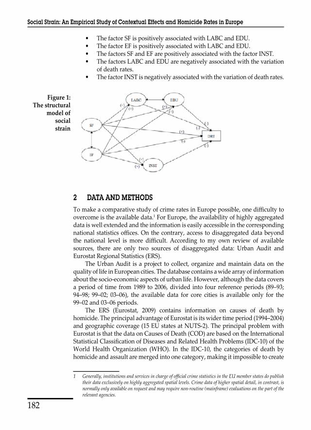
1.1 The Structural ModelAs already mentioned, the social strain model includes not only three components but also the relationship between them. The structural part of the model explains the connections between the input component, or exogenous independent variable (AEC), and the mediator components or endogenous independent variables (OS and INST). The underlying idea is that in a contextual configuration where the three components are present, there is substantive difference in the position each component occupies. The original formulation of social strain places the input sources on the side the AEC, while the mediators are represented by the corresponding factors of OS and INST (the complete model is depicted in Figure 1).

The first relationships to be acknowledged are the direct paths from the AEC to the dependent variable (homicide rates). For these relationships, we can derive two initial hypotheses:

• The SF factor is positively associated with death rates, meaning that intense conditions of social segregation are conducive to higher death rates.

• The EF factor is negatively related with death rates, where higher scores of income and wealth are linked with lower death rates.

A second group of paths is needed to include the mediators and their effects on the dependent variable. The effects of AEC on the mediators and their corresponding effects on the dependent variable are represented in the following hypotheses:


182

• The factor SF is positively associated with LABC and EDU.• The factor EF is positively associated with LABC and EDU.• The factors SF and EF are positively associated with the factor INST.• The factors LABC and EDU are negatively associated with the variation

of death rates.• The factor INST is negatively associated with the variation of death rates.

2 DATA AND METHODSTo make a comparative study of crime rates in Europe possible, one difficulty to overcome is the available data.1 For Europe, the availability of highly aggregated data is well extended and the information is easily accessible in the corresponding national statistics offices. On the contrary, access to disaggregated data beyond the national level is more difficult. According to my own review of available sources, there are only two sources of disaggregated data: Urban Audit and Eurostat Regional Statistics (ERS).

The Urban Audit is a project to collect, organize and maintain data on the quality of life in European cities. The database contains a wide array of information about the socio-economic aspects of urban life. However, although the data covers a period of time from 1989 to 2006, divided into four reference periods (89–93; 94–98; 99–02; 03–06), the available data for core cities is available only for the 99–02 and 03–06 periods.

The ERS (Eurostat, 2009) contains information on causes of death by homicide. The principal advantage of Eurostat is its wider time period (1994–2004) and geographic coverage (15 EU states at NUTS-2). The principal problem with Eurostat is that the data on Causes of Death (COD) are based on the International Statistical Classification of Diseases and Related Health Problems (IDC-10) of the World Health Organization (WHO). In the IDC-10, the categories of death by homicide and assault are merged into one category, making it impossible to create

1 Generally,institutionsandservicesinchargeofofficialcrimestatisticsintheEUmemberstatesdopublishtheir data exclusively on highly aggregated spatial levels. Crime data of higher spatial detail, in contrast, is normally only available on request and may require non-routine (mainframe) evaluations on the part of the relevant agencies.

As already mentioned, the social strain model includes not only three components but also the

relationship between them. The structural part of the model explains the connections between

the input component, or exogenous independent variable (AEC), and the mediator

components or endogenous independent variables (OS and INST). The underlying idea is that

in a contextual configuration where the three components are present, there is substantive

difference in the position each component occupies. The original formulation of social strain

places the input sources on the side the AEC, while the mediators are represented by the

corresponding factors of OS and INST (the complete model is depicted in Figure 1).

The first relationships to be acknowledged are the direct paths from the AEC to the dependent

variable (homicide rates). For these relationships, we can derive two initial hypotheses:

• The SF factor is positively associated with death rates, meaning that intense conditions

of social segregation are conducive to higher death rates.

• The EF factor is negatively related with death rates, where higher scores of income

and wealth are linked with lower death rates.

A second group of paths is needed to include the mediators and their effects on the dependent

variable. The effects of AEC on the mediators and their corresponding effects on the

dependent variable are represented in the following hypotheses:

• The factor SF is positively associated with LABC and EDU.

• The factor EF is positively associated with LABC and EDU.

• The factors SF and EF are positively associated with the factor INST.

• The factors LABC and EDU are negatively associated with the variation of death

rates.

• The factor INST is negatively associated with the variation of death rates.

Figure 1: The structural model of social strain

4

Figure 1:The structural

model ofsocialstrain


183

a differentiated indicator of homicide. However, this is a minor problem that did not diminish the possibilities of the database.

The ERS contains aggregated data at three different regional levels. Eurostat used a regional breakdown based on the existence of administrative boundaries and structures. In other words, the different regional levels reflect real and effective administrative divisions between regions (or regions as an administrative concept). The ERS data uses the 1970 classification Nomenclature of Statistical Territorial Units (NUTS, for the French nomenclature d‘unités territoriales statistiques) as a single, coherent system for dividing up the European Union’s territory (refer to tables 1 to 3 for some characteristics of the NUTS regions).

Average size of NUTS regions (in 1000 population) 2005

Level 1 Level 2 Level 3

Austria 2,755 918 236

Belgium 3,504 956 239

Finland 2,628 1,051 263

France 6,987 2,419 629

Germany 5,152 2,114 192

Greece 2,781 856 218

Ireland 4,159 2,105 526

Italy 11,750 2,798 549

Netherlands 4,084 1,361 408

Portugal 3,523 1,510 352

Spain 6,251 2,303 742

Sweden 3,016 1,131 431

United Kingdom 5,033 1,632 454

Table 2: Average size regions NUTS-2

Pop 99 Area km2 NUTS2 NUTS2 (study) Pop/#NUTS2 Area/#NUTS2

Austria 8,177,000 82,444 9 9 908,556 9,160

Belgium 10,152,000 30,278 11 11 922,909 2,753

Finland 5,165,474 304,473 6 5 860,912 50,746

France 59,099,433 640,053 26 22 2,273,055 24,617

Germany 82,087,000 349,223 40 34 2,052,175 8,731

Greece 10,626,000 130,800 13 13 817,385 10,062

Ireland 3,744,700 68,890 2 2 1,872,350 34,445

Italy 57,343,000 294,020 20 20 2,867,150 14,701

Netherlands 15,810,000 33,883 12 12 1,317,500 2,824

Portugal 9,988,520 91,951 7 7 1,426,931 13,136

Spain 39,418,017 499,452 18 18 2,189,890 27,747

Sweden, 8,857,361 410,934 8 8 1,107,170 51,367United Kingdom 58,744,000 241,590 36 32 1,631,778 6,711

Table 3: NUTS population thresholds

Population

Minimum Maximum

NUTS-1 3 million 7 million

NUTS-2 800,000 3 million

NUTS-3 150,000 800,000

6



Austria 2,755 918 236

Belgium 3,504 956 239

Finland 2,628 1,051 263

France 6,987 2,419 629

Germany 5,152 2,114 192

Greece 2,781 856 218

Ireland 4,159 2,105 526

Italy 11,750 2,798 549


Portugal 3,523 1,510 352

Spain 6,251 2,303 742

Sweden 3,016 1,131 431




Austria 8,177,000 82,444 9 9 908,556 9,160

Belgium 10,152,000 30,278 11 11 922,909 2,753

Finland 5,165,474 304,473 6 5 860,912 50,746

France 59,099,433 640,053 26 22 2,273,055 24,617

Germany 82,087,000 349,223 40 34 2,052,175 8,731

Greece 10,626,000 130,800 13 13 817,385 10,062

Ireland 3,744,700 68,890 2 2 1,872,350 34,445

Italy 57,343,000 294,020 20 20 2,867,150 14,701

Netherlands 15,810,000 33,883 12 12 1,317,500 2,824

Portugal 9,988,520 91,951 7 7 1,426,931 13,136

Spain 39,418,017 499,452 18 18 2,189,890 27,747



Population

Minimum Maximum



NUTS-3 150,000 800,000

6



Austria 2,755 918 236

Belgium 3,504 956 239

Finland 2,628 1,051 263

France 6,987 2,419 629

Germany 5,152 2,114 192

Greece 2,781 856 218

Ireland 4,159 2,105 526

Italy 11,750 2,798 549


Portugal 3,523 1,510 352

Spain 6,251 2,303 742

Sweden 3,016 1,131 431




Austria 8,177,000 82,444 9 9 908,556 9,160

Belgium 10,152,000 30,278 11 11 922,909 2,753

Finland 5,165,474 304,473 6 5 860,912 50,746

France 59,099,433 640,053 26 22 2,273,055 24,617

Germany 82,087,000 349,223 40 34 2,052,175 8,731

Greece 10,626,000 130,800 13 13 817,385 10,062

Ireland 3,744,700 68,890 2 2 1,872,350 34,445

Italy 57,343,000 294,020 20 20 2,867,150 14,701

Netherlands 15,810,000 33,883 12 12 1,317,500 2,824

Portugal 9,988,520 91,951 7 7 1,426,931 13,136

Spain 39,418,017 499,452 18 18 2,189,890 27,747



Population

Minimum Maximum



NUTS-3 150,000 800,000

6

Table 1: Average size of regions NUTS 1-3




184

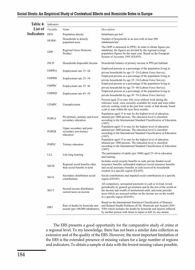
The ERS presents a good opportunity for the comparative study of crime at a regional level. To my knowledge, there has not been a similar data collection as extensive and of the quality of the ERS. However, the most important limitation of the ERS is the extended presence of missing values for a large number of regions and indicators. To obtain a sample of data with the fewest missing values possible,


Table 4: List of

Indicators

Table 4: List of Indicators

Indicators

Variable Name Description

DEN Population density Inhabitants per km2.

HURB1 Households in densely populated areas

Number of households in an area with at least 500 inhabitants/km2.

GDP Regional Gross Domestic Product

The GDP is measured in (PPS). In order to obtain figures per inhabitant, the figures are divided by the regional average population figures for the same year. Based on the European System of Accounts 1995 (ESA95).

INCD Households disposable Income Households balance of primary income in PPS per habitant.

EMPRA Employment rate 15–24Employed persons as a percentage of the population living in private households by age 15–24 (Labour Force Survey).

EMPRB Employment rate 25–34Employed persons as a percentage of the population living in private households by age 25–34 (Labour Force Survey).

EMPRC Employment rate 35–44Employed persons as a percentage of the population living in private households by age 35–44 (Labour Force Survey).

EMPRD Employment rate 45–54Employed persons as a percentage of the population living in private households by age 45–54 (Labour Force Survey).

UEMPC Unemployment

Persons aged 25 to max who were without work during the reference week, were currently available for work and were either actively seeking work in the past four weeks or had already found a job to start within the next three months.

POPEA Pre-primary, primary and lower secondary education

Population aged 15 to max by the highest level of education attained per 1000 persons. The education level is classified according to the International Standard Classification of Education (1997).

POPEBUpper secondary and post-secondary non-tertiary education


POPEC Tertiary education


LLL Life-long learning The participation of adults (per 1000) aged 25–64 in education and training.

SECB Regional social benefits other than social benefits in kind

Includes social security benefits in cash, private funded social insurance benefits, unfounded employee social insurance benefits and social assistance benefits in cash received by households resident in a specific region (ESA95).

SECS Secondary distribution social contributions

Social contributions and imputed social contributions in a specific region (ESA95).

SECT Second income distribution current taxes on income

All compulsory, unrequited payments in cash or in kind, levied periodically by general government and by the rest of the world on the income and wealth of institutional units, and some periodic taxes which are assessed neither on the income nor on the wealth in a specific region (ESA95).

DRT Rate of deaths by homicide and assault (per 100,000 inhabitants)

Based on the International Statistical Classification of Diseases and Related Health Problems (ICD). Homicide and Assault (X85-Y09) which includes the deaths by homicide and injuries inflicted by another person with intent to injure or kill, by any means.

7

185

I have applied some criteria to concentrate the size and the scope of the sample in the countries with better scores of complete data, and with relevant indicators for the theory.

First, I selected indicators that, according to the theoretical base of my hypotheses, could work as viable observable measures for the latent factors. The result was an initial selection of more than 200 indicators on demographic statistics, economic accounts, education, labour market, employment, unemployment, socio-demographic labour force, labour market disparities, migration, structural business and health.

During the first screenings of the data, it became evident that the missing cases were mainly clustered in the most recent Member States and in the older entries. There was also a disparity in the years in which the first entries were collected. For example, all the economic data from The European System of Accounts (ESA95) started in 1999, while the health statistics are available from 1994. In view of the missing values’ distribution, a second selection was made between the Member States with the highest rate of complete entries. From the initial 27 Member States, I reduced the sample to the 15 Member States of the EU’s fourth expansion. After this selection, I conducted more diagnostics of the distribution of missing cases and, although their number reduced, there were still cases and variables with more than 30 percent missing values.

For the next selection of data, I kept the years with the most complete entries. As a result, I initially chose the data from 1999 to 2006. The missing values decreased, but their total number was still too high for a reliable multivariate statistical analysis. Looking at the distribution of missing values, it became evident that a large percentage was concentrated in two years (1999 and 2000) and in some specific regions. Based on this, I made a third and final selection and the final sample was reduced to thirteen countries for the period 2001–2006.

After cleaning the data, the indicators from the original list still had a considerable number of incomplete data, and I finally deleted the indicators with more than 20 percent total missing values. The final number of indicators was reduced to 58, which ultimately constituted the independent variables plus the dependent variable.

To reduce the missing values to a minimum, I completed the missing entries with data from other sources. Of particular priority was the dependent variable, which still had various regions with missing cases. Table 5 illustrates the sources, the data, and the regions (countries) that were completed without Eurostat data.2 The most similar, accessible and reliable options for some regions were the regional database of the Organisation for Economic Co-operation and Development (OECD, 2009) and some national government agencies.3 Finally, the sample included 13 Member States for a total of 193 regions from 2001 to 2006.

2 The use of data from other sources carrieswith it the problem of different definitions of the dependentvariable.ThisisthecaseofthedatafromtheOECD,HomeOfficeandtheBelgianFederalPolicewheretheirdefinitionofhomicideisnotbasedontheICD-10.Itisbasedonmurdersreportedbythepolice.Thepolice data utilized did not include assault but only murder, and it may under-represent the real variation of violent crime in those areas.

3 ThehomiciderateforUKisself-calculatedbasedonHomeOfficedata.


186

Only nine nations kept their complete number of regions, and for France, the United Kingdom, Finland and Germany, some regions with a higher percentage of missing values were deleted from the database.

2.1 Describing the Data

Basically, the final sample has a high percentage of variables with complete information,4 and contains indicators on the following aspects: urban composition, income, wealth, tax income, public social benefits, various indicators of employment, and educational attainment (Table 4).

To identify the presence of multivariate outliers, I conducted a Hadi test.5 The presence of multivariate outliers is a good sign of a non-normal distribution, however, I have also conducted the Jarque-Bera tests for skewness and kurtosis for each variable. The results show that almost one-half of the indicators of the independent variables are non-normally distributed with variant scores of skewness and kurtosis. The other half of the indicators was at least moderately skewed (particularly the indicators of income and taxes).

The distribution of the dependent variable has high skewness and kurtosis scores for all years. This is a common characteristic of crime data (particularly homicide data) for two reasons: homicide is a very improbable event with a low frequency, and the distribution of high rates of homicide tends to be concentrated in a reduced number of cases who attract the whole variance of the variable. To improve the distribution of the data, I used a natural log transformation for all the remaining variables.6

4 There were only two exceptions: the independent variable households in densely populated areas (HURB1) with a missing value around 10 and 13 percent, and the dependent variable for Italy in 2004 with 10 percent.

5 The Hadi test consists in the usage of a measure of distance from an observation to a cluster of points. A base clusterofrpointsisselectedandthentheclusteriscontinuallyredefinedbytakingther+1pointsclosestasa new cluster. The procedure continues until some stopping rule is encountered. (In Appendix table for the listofregionsforeveryyear–availableuponrequestattheauthororeditors).

6 Iusedthetransformationln(x+100)becausethereweresomevariableswithzerosasvalues.

regions with missing cases. Table 5 illustrates the sources, the data, and the regions

(countries) that were completed without Eurostat data.2 The most similar, accessible and

reliable options for some regions were the regional database of the Organisation for Economic

Co-operation and Development (OECD, 2009) and some national government agencies.3

Finally, the sample included 13 Member States for a total of 193 regions from 2001 to 2006.

Only 9 nations kept their complete number of regions, and for France, the United Kingdom,

Finland and Germany, some regions with a higher percentage of missing values were deleted

from the database.

Table 5: No-ESR Data

Alternative Sources

Regions/years ICD-10 Police DataOECD AT21/01-06 IT (all)/05

*

Home Office UK(all)/02-06 *Belgian Federal Police BE (all) *

Austria National Statistics AT06/01-06 *French National Institute for

Statistics and Economic Studies

FR (all)/06*

2.1Describing the DataBasically, the final sample has a high percentage of variables with complete information,4 and

contains indicators on the following aspects: urban composition, income, wealth, tax income,

public social benefits, various indicators of employment, and educational attainment (Table

4).

To identify the presence of multivariate outliers, I conducted a Hadi test.5 The

presence of multivariate outliers is a good sign of a non-normal distribution, however, I have

2 The use of data from other sources carries with it the problem of different definitions of the dependent variable. This is the case of the data from the OECD, Home Office and the Belgian Federal Police where their definition of homicide is not based on the ICD-10. It is based on murders reported by the police. The police data utilized did not include assault but only murder, and it may under-represent the real variation of violent crime in those areas.3 The homicide rate for UK is self-calculated based on Home Office data.4 There were only two exceptions: the independent variable households in densely populated areas (HURB1) with a missing value around 10 and 13 percent, and the dependent variable for Italy in 2004 with 10 percent.5 The Hadi test consists in the usage of a measure of distance from an observation to a cluster of points. A base cluster of r points is selected and then the cluster is continually redefined by taking the r+1 points closest as a new cluster. The procedure continues until some stopping rule is encountered. (In Appendix table for the list of regions for every year – available upon request at the author or editors).

9


Table 5: No-ESR

Data

187

2.2 The Regional Death Rate

The dependent variable (homicides per 100,000 inhabitants) has a mean of 0.93 for the reference period. The year 2003 had the lower mean (0.85) while 2004 showed the highest score with a mean value of 1.06. For my group of 193 regions, 75% have a death rate value ranging under 1.1 to 1.3. The four regions with the lowest mean death rate in the six years are: Prov. Brabant Wallon (0.2) in Belgium; the Gloucestershire, Wiltshire and Bristol/Bath and the Herefordshire, Worcestershire and Warwick region (0.3) in United Kingdom; and The Border, Midland and Western region (0.3) of Ireland.

The distribution of death rates reflects the typical distribution of these kinds of variables. Because death by homicide and assault is an inherently improbable phenomenon, their distribution tends to be accumulated in the lower scores. In my sample, the distribution is positively skewed and with high kurtosis levels (particularly the year 2001), which means that the vast majority of cases are distributed around the lower death rates.

Other interesting characteristic is the concentration of higher values in a compact group of regions. Calculating the Interquartile Ranges of the dependent variable, the following regions qualified as severe outliers for different years: Corsica (France), Ceuta, Melilla (Spain), Pohjois-Suomi, Itä-Suomi (Finland), Algarve, Madeira (Portugal), and Calabria, (Italy).7 Of particular interest are the cases of Corsica in 2001, with an extraordinary rate of 9.9, and Ceuta in 2005, with a rate of 6.0. In the case of Finland, the two regions have also a lower population density: Itä-Suomi had the fourth lowest (9.5) and Pohjois-Suomi the sixth lowest (22.9).

Alone, these eight regions had a mean of 3.01 from 2001 to 2006, while the entire sample’s mean (without outliers) is 0.83 for the same years. In comparison with the sample average, these eight cases are more densely populated and have a lower GDP and income level than the sample, but they are not close to the mean of the poorer regions. Their employment and unemployment rates are very close to the ones of the sample. Concerning educational level, there is a relatively large difference between the sample and the outliers but they are still distant from the regions with the lowest scores. Finally, the level of levied taxes and received public monetary benefits are smaller in comparison with the sample, but not close to the regions with lower indicators.8

The descriptive statistics of the group of eight outliers have an interesting characteristic; namely, they do not comply with the expected or common characteristics of these types of outliers. It has been widely discussed in the empirical literature that units with unexpected rates of violent crime, are also among other low performers on economic development and education. However, in this case the eight regions have lower scores than the rest of the sample, but their socio-economic indicators are not those of the regions with the worst

7 The test also detected the region of Madrid (4.0) in 2004 and Inner London (3.1) in 2006, however these ratesarecountingtheterroristattacksof2004and2006anddonotreflectthe»normal« rate of those cities.

8 More descriptive data in Appendix (available upon request at the author or editors).


188

socio-economic conditions. Considering these reasons, I have decided to leave the eight regions with particular high rates of death in the sample, because their high scores are not related with extreme values on the independent variables.

3 FACTOR ANALYSIS AND STRUCTURAL EQUATION MODELLING

For the analysis of the proposed model, I have applied Structural Equation Modelling (SEM) techniques to test the empirical viability in a sample of European regions. The first part of the analysis determines the factors for the components of social strain. Having found the corresponding factors, I have used SEM9 to test the identified structural relations between the components. I first ran a confirmatory application of SEM to the original model of social strain, and then performed an exploratory usage of SEM modelling to find alternative structures for the regions under study. For both the factor analysis and structural equation modelling, I used the full information maximum likelihood estimation method to deal with the still present missing values in the sample.

3.1 Confirmatory Factor Analysis

The first part of the empirical study is based on the application of Confirmatory Factor Analysis (CFA) to find the best group of indicators for each component of social strain in all the regions from 2001 to 2006. From all the available variables in the final sample, the construction of the factors was first conducted by a pre-selection of the indicators according to their theoretical relevance or closeness to the components of social strain. This first classification was the starting point for the CFA. The general procedure was first to find a good fitting model for the year 2006 and if the model worked to test it on the remaining years. The final factors are the ones that showed good measures of fit for all the years. In other words, all the factors are empirically valid for the period 2001–2006. These are the results of the CFA and the best factors whose structure gave a better representation of the concepts postulated in the theory.10, 11

3.2 Factor AEC

The original formulation of AEC would have needed a second-order factor to capture the complete dimension of the concept. However, second-order factors need three first-order factors with at least four indicators. With the available data, it was impossible to find the required number of indicators, so I have stayed with a simpler first-order factor for the AEC.

9 I used the program Amos v.17 for the factor analysis and the structural equation modelling.10 The tables with the factor loadings are in the Appendix (available upon request at the author or editors). 11 Toachieveabettergoodnessoffit,Ihaveequalledsomeparametersaccordingwithananalysisofthecritical

ratiosfordifferencesbetweenparameters.


189

The final configuration of AEC included two factors: the Stratification Factor represented by Urbanism (URB) and the Economic Factor represented by Economic Wealth (EW) (see Table 6). According to the indicators qualified for the factor URB, the element of social stratification is the degree of urbanization, where highly urbanized regions are depicted through high levels of population density and of households in urbanized areas. The other factor is capturing the variation of two measures of regional economic wealth. The resulting AEC factor measures the regions ranging from highly urbanized and economically wealthy regions, to low urbanized regions with a lower economic performance.

3.3 Factor LABC and EDU

For the component OS, the ideal constitution of factors would have also been of the second order, however, again data insufficiency made this impossible. Nevertheless, I have managed to identify a structure with two factors for the OS component: Labour Conditions and Education. The factor Labour Conditions (LABC) was finally constructed with three measures of employment rate by age and one indicator of unemployment (see Table 7). The second factor, Education (EDU) had two indicators: achieved educational level and long-life learning (see Table 8). For the two factors of the OS component, no connection or link (correlation) could be identified. As a result, the presumed theoretical connection between the factors of the component Opportunities Structure does not have empirical support of the data. The OS component is represented with two non-correlated factors.

This empirical depiction of the component OS is based on the idea that regions with a good opportunities structure should also have high scores of employment

The first part of the empirical study is based on the application of Confirmatory Factor

Analysis (CFA) to find the best group of indicators for each component of social strain in all

the regions from 2001 to 2006. From all the available variables in the final sample, the

construction of the factors was first conducted by a pre-selection of the indicators according

to their theoretical relevance or closeness to the components of social strain. This first

classification was the starting point for the CFA. The general procedure was first to find a

good fitting model for the year 2006 and if the model worked to test it on the remaining years.

The final factors are the ones that showed good measures of fit for all the years. In other

words, all the factors are empirically valid for the period 2001–2006. These are the results of

the CFA and the best factors whose structure gave a better representation of the concepts

postulated in the theory.10 11

3.2 Factor AECThe original formulation of AEC would have needed a second-order factor to capture the

complete dimension of the concept. However, second-order factors need three first-order

factors with at least four indicators. With the available data, it was impossible to find the

required number of indicators, so I have stayed with a simpler first-order factor for the AEC.

The final configuration of AEC included two factors: the Stratification Factor

represented by Urbanism (URB) and the Economic Factor represented by Economic Wealth

(EW) (see Table 6). According to the indicators qualified for the factor URB, the element of

social stratification is the degree of urbanization, where highly urbanized regions are depicted

through high levels of population density and of households in urbanized areas. The other

factor is capturing the variation of two measures of regional economic wealth. The resulting

AEC factor measures the regions ranging from highly urbanized and economically wealthy

regions, to low urbanized regions with a lower economic performance.

Table 6: Factor AEC

Standardized Regression Weights

2006 2005 2004 2003 2002 2001

DEN <--- urb 0.761 0.762 0.760 0.761 0.761 0.760

HURB1 <--- urb 0.709 0.699 0.701 0.706 0.710 0.712

GDP <--- ew 0.879 0.881 0.882 0.881 0.885 0.889

INCD <--- ew 0.809 0.812 0.824 0.801 0.794 0.809

10 The tables with the factor loadings are in the Appendix (available upon request at the author or editors). 11 To achieve a better goodness of fit, I have equalled some parameters according with an analysis of the critical ratios for differences between parameters.

12

Table 6: FactorAEC

all sig p < .001

Correlations

2006 2005 2004 2003 2002 2001

ew <--> urb 0.644 0.657 0.653 0.652 0.643 0.638

all sig p < .001

Model Fit Summary

χ2 df p RMSEA CFI ECVI

27.631 28 0.484 0 1 0.121

3.3 Factor LABC and EDUFor the component OS, the ideal constitution of factors would have also been of the second

order, however, again data insufficiency made this impossible. Nevertheless, I have managed

to identify a structure with two factors for the OS component: Labour Conditions and

Education. The factor Labour Conditions (LABC) was finally constructed with three

measures of employment rate by age and one indicator of unemployment (see Table 7). The

second factor, Education (EDU) had two indicators: achieved educational level and long-life

learning (see Table 8). For the two factors of the OS component, no connection or link

(correlation) could be identified. As a result, the presumed theoretical connection between the

factors of the component Opportunities Structure does not have empirical support of the data.

The OS component is represented with two non-correlated factors.

This empirical depiction of the component OS is based on the idea that regions with a

good opportunities structure should also have high scores of employment and lower levels of

unemployment, as well as high levels of educational attainment in the three educational

sectors and for long-life learning.

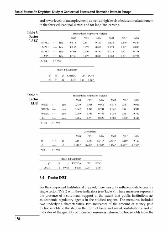
Table 7: Factor LABC


2006 2005 2004 2003 2002 2001

EMPRD <--- labc 0.814 0.811 0.819 0.836 0.840 0.844

EMPRB <--- labc 0.852 0.859 0.852 0.873 0.887 0.895

EMPRA <--- labc 0.708 0.740 0.730 0.756 0.777 0.778

UEMPC <--- labc -0.736 -0.749 -0.800 -0.788 -0.801 -0.794

all sig p < .001

Model Fit Summary

13


190

all sig p < .001

Correlations

2006 2005 2004 2003 2002 2001

ew <--> urb 0.644 0.657 0.653 0.652 0.643 0.638

all sig p < .001

Model Fit Summary


27.631 28 0.484 0 1 0.121

3.3 Factor LABC and EDUFor the component OS, the ideal constitution of factors would have also been of the second

order, however, again data insufficiency made this impossible. Nevertheless, I have managed

to identify a structure with two factors for the OS component: Labour Conditions and

Education. The factor Labour Conditions (LABC) was finally constructed with three

measures of employment rate by age and one indicator of unemployment (see Table 7). The

second factor, Education (EDU) had two indicators: achieved educational level and long-life

learning (see Table 8). For the two factors of the OS component, no connection or link

(correlation) could be identified. As a result, the presumed theoretical connection between the

factors of the component Opportunities Structure does not have empirical support of the data.

The OS component is represented with two non-correlated factors.

This empirical depiction of the component OS is based on the idea that regions with a

good opportunities structure should also have high scores of employment and lower levels of

unemployment, as well as high levels of educational attainment in the three educational

sectors and for long-life learning.

Table 7: Factor LABC


2006 2005 2004 2003 2002 2001

EMPRD <--- labc 0.814 0.811 0.819 0.836 0.840 0.844

EMPRB <--- labc 0.852 0.859 0.852 0.873 0.887 0.895

EMPRA <--- labc 0.708 0.740 0.730 0.756 0.777 0.778

UEMPC <--- labc -0.736 -0.749 -0.800 -0.788 -0.801 -0.794

all sig p < .001

Model Fit Summary

13χ2 df p RMSEA CFI ECVI

70 23 0 0.42 0.981 0.167

Table 8: Factor EDU


2006 2005 2004 2003 2002 2001

POPEC <--- edu 0.919 0.919 0.916 0.914 0.911 0.911

POPEB <--- edu 0.942 0.942 0.941 0.941 0.941 0.941

POPEA <--- edu 0.789 0.788 0.766 0.756 0.751 0.752

LLL <--- edu 0.786 0.761 0.829 0.708 0.580 0.544

all sig p < .001

Correlations

2006 2005 2004 2003 2002 2001

e8 <--> e9 -0.181 -0.181 -0.341* -0.314* -0.219 -0.127

e6 <--> e9 0.618* 0.609* 0.308* 0.466* 0.483* 0.538*

*sig p < .001

Model Fit Summary


20.33 11 0.983 0.027 0.997 0.144

3.4 Factor INSTFor the component Institutional Support, there was only sufficient data to create a single

factor (INST) with three indicators (see Table 9). These measures represent the presence of

institutional support to the extent that public institutions act as economic regulatory agents in

the studied regions. The measures included two underlying characteristics: two indicators of

the amount of money paid by households to the state in the form of taxes and social

14

and lower levels of unemployment, as well as high levels of educational attainment in the three educational sectors and for long-life learning.

3.4 Factor INST

For the component Institutional Support, there was only sufficient data to create a single factor (INST) with three indicators (see Table 9). These measures represent the presence of institutional support to the extent that public institutions act as economic regulatory agents in the studied regions. The measures included two underlying characteristics: two indicators of the amount of money paid by households to the state in the form of taxes and social contributions, and an indicator of the quantity of monetary resources returned to households from the

Table 8: Factor

EDU

Table 7: FactorLABC


70 23 0 0.42 0.981 0.167

Table 8: Factor EDU


2006 2005 2004 2003 2002 2001

POPEC <--- edu 0.919 0.919 0.916 0.914 0.911 0.911

POPEB <--- edu 0.942 0.942 0.941 0.941 0.941 0.941

POPEA <--- edu 0.789 0.788 0.766 0.756 0.751 0.752

LLL <--- edu 0.786 0.761 0.829 0.708 0.580 0.544

all sig p < .001

Correlations

2006 2005 2004 2003 2002 2001

e8 <--> e9 -0.181 -0.181 -0.341* -0.314* -0.219 -0.127

e6 <--> e9 0.618* 0.609* 0.308* 0.466* 0.483* 0.538*

*sig p < .001

Model Fit Summary


20.33 11 0.983 0.027 0.997 0.144

3.4 Factor INSTFor the component Institutional Support, there was only sufficient data to create a single

factor (INST) with three indicators (see Table 9). These measures represent the presence of

institutional support to the extent that public institutions act as economic regulatory agents in

the studied regions. The measures included two underlying characteristics: two indicators of

the amount of money paid by households to the state in the form of taxes and social

14


191

state in the form of social benefits. This factor accurately captures the regions with high scores of institutional intervention in the form of levied taxes and monetary returns from the state.

After the identification of the factors for the three social strain components, there are a total of +four factors to construct and test the structural model. As already mentioned, the results of the CFA are not the expected reflection of the theoretical construct. One concern is that for the components AEC and OS, it was not possible to create a second order factor. Another important shortcoming is that the four factors had a relatively small number of indicators, ranging from 2 to 5 observed variables. According to the statistical literature (Blunch, 2008; Bollen, 1989; Kaplan, 2004), the latent variables in CFA and SEM modelling should have the most indicators possible to assure an increased variance for the latent variables. Unfortunately in this case, the final factors have a small number of indicators. Nevertheless, with this limitation, the resulting factors showed very acceptable goodness of fit scores and they can be considered as reliable and suitable factors to test the structural model. Also problematic is that in the original formulation of social strain, the factors of the component OS, do not have the expected correlation. Finally, taking into account a two-step approach to model identification, I made a CFA with the five factors to assess probable identification problems of the measurement model. The CFA is identified with 571 degrees of freedom.

3.5 SEM Confirmatory

The second step of the study is to test the complete model of social strain. To do this, I have implemented Structural Equation Modelling (SEM) techniques in order to find the presence of social strain in the regions under study. I have used the resulting factors as measurement models of the complete model. According to

contributions, and an indicator of the quantity of monetary resources returned to households

from the state in the form of social benefits. This factor accurately captures the regions with

high scores of institutional intervention in the form of levied taxes and monetary returns from

the state.

Table 9: Factor INST


2006 2005 2004 2003 2002 2001

SECB <--- Inst 0.985 0.985 0.985 0.985 0.985 0.985

SECS <--- Inst 0.985 0.985 0.985 0.985 0.985 0.986

SECT <--- Inst 0.952 0.959 0.960 0.957 0.959 0.956

all sig p < .001

Correlations

2006 2005 2004 2003 2002 2001

e2 <--> e3 0.081 -0.153 -0.325 -0.39 -0.386 -0.368

Model Fit Summary


13.662 5 0.018 0.039 0.999 0.097

After the identification of the factors for the three social strain components, there are a total of

four factors to construct and test the structural model. As already mentioned, the results of the

CFA are not the expected reflection of the theoretical construct. One concern is that for the

components AEC and OS, it was not possible to create a second order factor. Another

important shortcoming is that the four factors had a relatively small number of indicators,

ranging from 2 to 5 observed variables. According to the statistical literature (Blunch, 2008;

Bollen, 1989; Kaplan, 2004), the latent variables in CFA and SEM modelling should have the

most indicators possible to assure an increased variance for the latent variables. Unfortunately

in this case, the final factors have a small number of indicators. Nevertheless, with this

limitation, the resulting factors showed very acceptable goodness of fit scores and they can be

considered as reliable and suitable factors to test the structural model. Also problematic is that

in the original formulation of social strain, the factors of the component OS, do not have the

expected correlation. Finally, taking into account a two-step approach to model identification,

I made a CFA with the five factors to assess probable identification problems of the

measurement model. The CFA is identified with 571 degrees of freedom.

15

Table 9: FactorINST


192

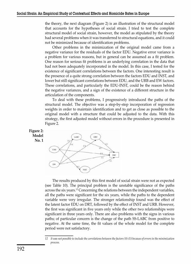
the theory, the next diagram (Figure 2) is an illustration of the structural model that accounts for the hypotheses of social strain. I tried to test the complete structural model of social strain, however, the model as stipulated by the theory had several problems when it was transferred to structural equations, and it could not be minimized because of identification problems.

Other problems in the minimization of the original model came from a negative variance for the residuals of the factor EDU. Negative error variance is a problem for various reasons, but in general can be assumed as a fit problem. One reason for serious fit problems is an underlying correlation in the data that had not been adequately incorporated in the model. In this case, I tested for the existence of significant correlations between the factors. One interesting result is the presence of a quite strong correlation between the factors EDU and INST, and lower but still significant correlations between EDU, and the URB and EW factors. These correlations, and particularly the EDU-INST, could be the reason behind the negative variances, and a sign of the existence of a different structure in the articulation of the components.

To deal with these problems, I progressively introduced the paths of the structural model. The objective was a step-by-step incorporation of regression weights in order to maintain identification and to get as close as possible to the original model with a structure that could be adjusted to the data. With this strategy, the first adjusted model without errors in the procedure is presented in Figure 2.

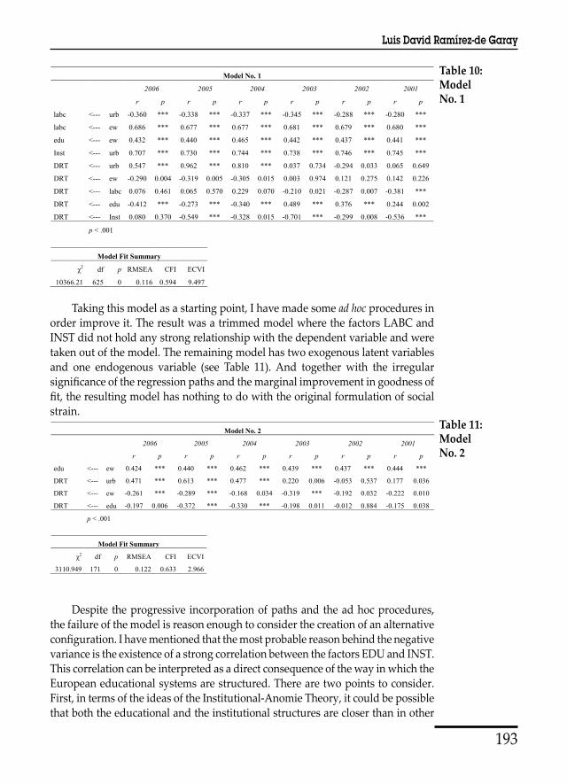
The results produced by this first model of social strain were not as expected (see Table 10). The principal problem is the unstable significance of the paths across the six years.12 Concerning the relations between the independent variables, all the paths were significant for the six years, while the paths to the dependent variable were very irregular. The stronger relationship found was the effect of the latent factor EDU on DRT, followed by the effect of INST and URB. However, the first was significant in five years only while the other two relationships were significant in three years only. There are also problems with the signs in various paths; of particular concern is the change of the path SS-LABC from positive to negative. At the same time, the fit values of the whole model for the complete period were not satisfactory.

12 It was not possible to include the correlations between the factors SS-ES because of errors in the minimization process.

3.5SEM ConfirmatoryThe second step of the study is to test the complete model of social strain. To do this, I have

implemented Structural Equation Modelling (SEM) techniques in order to find the presence of

social strain in the regions under study. I have used the resulting factors as measurement

models of the complete model. According to the theory, the next diagram (Figure 2) is an

illustration of the structural model that accounts for the hypotheses of social strain. I tried to

test the complete structural model of social strain, however, the model as stipulated by the

theory had several problems when it was transferred to structural equations, and it could not

be minimized because of identification problems.

Other problems in the minimization of the original model came from a negative

variance for the residuals of the factor EDU. Negative error variance is a problem for various

reasons, but in general can be assumed as a fit problem. One reason for serious fit problems is

an underlying correlation in the data that had not been adequately incorporated in the model.

In this case, I tested for the existence of significant correlations between the factors. One

interesting result is the presence of a quite strong correlation between the factors EDU and

INST, and lower but still significant correlations between EDU, and the URB and EW factors.

These correlations, and particularly the EDU-INST, could be the reason behind the negative

variances, and a sign of the existence of a different structure in the articulation of the

components.

To deal with these problems, I progressively introduced the paths of the structural

model. The objective was a step-by-step incorporation of regression weights in order to

maintain identification and to get as close as possible to the original model with a structure

that could be adjusted to the data. With this strategy, the first adjusted model without errors in

the procedure is presented in Figure 2.

Figure 2: Model No. 1

16

Figure 2: Model

No. 1


193

Taking this model as a starting point, I have made some ad hoc procedures in order improve it. The result was a trimmed model where the factors LABC and INST did not hold any strong relationship with the dependent variable and were taken out of the model. The remaining model has two exogenous latent variables and one endogenous variable (see Table 11). And together with the irregular significance of the regression paths and the marginal improvement in goodness of fit, the resulting model has nothing to do with the original formulation of social strain.

Despite the progressive incorporation of paths and the ad hoc procedures, the failure of the model is reason enough to consider the creation of an alternative configuration. I have mentioned that the most probable reason behind the negative variance is the existence of a strong correlation between the factors EDU and INST. This correlation can be interpreted as a direct consequence of the way in which the European educational systems are structured. There are two points to consider. First, in terms of the ideas of the Institutional-Anomie Theory, it could be possible that both the educational and the institutional structures are closer than in other

Table 10: ModelNo. 1


together with the irregular significance of the regression paths and the marginal improvement

in goodness of fit, the resulting model has nothing to do with the original formulation of

social strain.

Table 11: Model No. 2

Model No. 2

2006 2005 2004 2003 2002 2001

r p r p r p r p r p r p

edu <--- ew 0.424 *** 0.440 *** 0.462 *** 0.439 *** 0.437 *** 0.444 ***

DRT <--- urb 0.471 *** 0.613 *** 0.477 *** 0.220 0.006 -0.053 0.537 0.177 0.036

DRT <--- ew -0.261 *** -0.289 *** -0.168 0.034 -0.319 *** -0.192 0.032 -0.222 0.010

DRT <--- edu -0.197 0.006 -0.372 *** -0.330 *** -0.198 0.011 -0.012 0.884 -0.175 0.038

p < .001

Model Fit Summary


3110.949 171 0 0.122 0.633 2.966

Despite the progressive incorporation of paths and the ad hoc procedures, the failure of the

model is reason enough to consider the creation of an alternative configuration. I have

mentioned that the most probable reason behind the negative variance is the existence of a

strong correlation between the factors EDU and INST. This correlation can be interpreted as a

direct consequence of the way in which the European educational systems are structured.

There are two points to consider. First, in terms of the ideas of the Institutional-Anomie

Theory, it could be possible that both the educational and the institutional structures are closer

than in other countries,13 and consequentially are a more decisive factor on the availability of

opportunities than the employment dimension. Second, because of the size of the units of

analysis, it could also be possible that the link between education and institutional support is

stronger at the meso-level because of the prevalence of decentralized structures in most of the

countries represented in the data. A third probable reason points to the nature of the indicators

of the latent factor INST. The measures used for this variable are general measures of the

amount of taxes levied by the state and state financial support. In this case, it would not be

strange to find that in the regions where the levying of taxes is high, the local educational

level is consequentially elevated.

In view of these results, I decided to leave the confirmatory approach and go further

with an exploratory analysis of social strain with some alternative configurations. My

13 Apparently for the case of Europe it is not possible to find an opportunity structure like in the USA where education and labour opportunities are conceptually closer.

18


The results produced by this first model of social strain were not as expected (see Table 10).

The principal problem is the unstable significance of the paths across the six years.12

Concerning the relations between the independent variables, all the paths were significant for

the six years, while the paths to the dependent variable were very irregular. The stronger

relationship found was the effect of the latent factor EDU on DRT, followed by the effect of

INST and URB. However, the first was significant in five years only while the other two

relationships were significant in three years only. There are also problems with the signs in

various paths; of particular concern is the change of the path SS-LABC from positive to

negative. At the same time, the fit values of the whole model for the complete period were not

satisfactory.


Model No. 1

2006 2005 2004 2003 2002 2001


labc <--- urb -0.360 *** -0.338 *** -0.337 *** -0.345 *** -0.288 *** -0.280 ***

labc <--- ew 0.686 *** 0.677 *** 0.677 *** 0.681 *** 0.679 *** 0.680 ***

edu <--- ew 0.432 *** 0.440 *** 0.465 *** 0.442 *** 0.437 *** 0.441 ***

Inst <--- urb 0.707 *** 0.730 *** 0.744 *** 0.738 *** 0.746 *** 0.745 ***

DRT <--- urb 0.547 *** 0.962 *** 0.810 *** 0.037 0.734 -0.294 0.033 0.065 0.649

DRT <--- ew -0.290 0.004 -0.319 0.005 -0.305 0.015 0.003 0.974 0.121 0.275 0.142 0.226

DRT <--- labc 0.076 0.461 0.065 0.570 0.229 0.070 -0.210 0.021 -0.287 0.007 -0.381 ***

DRT <--- edu -0.412 *** -0.273 *** -0.340 *** 0.489 *** 0.376 *** 0.244 0.002

DRT <--- Inst 0.080 0.370 -0.549 *** -0.328 0.015 -0.701 *** -0.299 0.008 -0.536 ***

p < .001

Model Fit Summary


10366.21 625 0 0.116 0.594 9.497

Taking this model as a starting point, I have made some ad hoc procedures in order improve

it. The result was a trimmed model where the factors LABC and INST did not hold any strong

relationship with the dependent variable and were taken out of the model. The remaining

model has two exogenous latent variables and one endogenous variable (see Table 11). And

12 It was not possible to include the correlations between the factors SS-ES because of errors in the minimization process.

17

194

countries,13 and consequentially are a more decisive factor on the availability of opportunities than the employment dimension. Second, because of the size of the units of analysis, it could also be possible that the link between education and institutional support is stronger at the meso-level because of the prevalence of decentralized structures in most of the countries represented in the data. A third probable reason points to the nature of the indicators of the latent factor INST. The measures used for this variable are general measures of the amount of taxes levied by the state and state financial support. In this case, it would not be strange to find that in the regions where the levying of taxes is high, the local educational level is consequentially elevated.

In view of these results, I decided to leave the confirmatory approach and go further with an exploratory analysis of social strain with some alternative configurations. My objective is to find, perhaps with other combinations between the latent factors, a stable model that could give empirical support to social strain.

3.6 SEM Exploratory

As a starting point for the exploratory application of SEM, I have taken into consideration the problems of the original model. From the start, there are two problematic correlations: a weak link between EW and EDU, and a stronger one between EDU and INST. To see if these correlations correspond to an empirical structure in the regions, I tried two new factors.

The first factor was a reformulation of the exogenous variable of social strain. I incorporated the factor INST to the factors URB and EW, as three latent variables with the corresponding correlations. The factor INST-URB-EW did not work and could not be minimized. In a second attempt, I created the factor EDU-INST to capture the correlation between the two latent variables. The new latent factor was stable and significant in the six years (see Table 12).

13 ApparentlyforthecaseofEuropeitisnotpossibletofindanopportunitystructurelikeintheUSAwhereeducation and labour opportunities are conceptually closer.

objective is to find, perhaps with other combinations between the latent factors, a stable

model that could give empirical support to social strain.

3.6 SEM ExploratoryAs a starting point for the exploratory application of SEM, I have taken into consideration the

problems of the original model. From the start, there are two problematic correlations: a weak

link between EW and EDU, and a stronger one between EDU and INST. To see if these

correlations correspond to an empirical structure in the regions, I tried two new factors.

The first factor was a reformulation of the exogenous variable of social strain. I

incorporated the factor INST to the factors URB and EW, as three latent variables with the

corresponding correlations. The factor INST-URB-EW did not work and could not be

minimized. In a second attempt, I created the factor EDU-INST to capture the correlation

between the two latent variables. The new latent factor was stable and significant in the six

years (see Table 12).

Table 12: Factor INST-EDU


2006 2005 2004 2003 2002 2001

POPEC <--- edu 0.927 0.927 0.925 0.923 0.92 0.921

POPEB <--- edu 0.950 0.950 0.949 0.949 0.949 0.949

POPEA <--- edu 0.749 0.752 0.730 0.721 0.715 0.717

LLL <--- edu 0.817 0.790 0.832 0.743 0.650 0.632

SECS <--- Inst 0.986 0.986 0.986 0.986 0.986 0.986

SECT <--- Inst 0.949 0.949 0.946 0.941 0.943 0.941

SECB <--- Inst 0.986 0.986 0.986 0.986 0.986 0.986

all sig p < .001

Correlations

2006 2005 2004 2003 2002 2001

Inst <--> edu 0.991 0.991 0.993 0.999 0.994 0.987

e1 <--> e4 0.544 0.523 0.272 0.385 0.351 0.392

e4 <--> e7 0.501 0.551 0.525 0.498 0.515 0.527

e1 <--> e5 -0.486 -0.412 -0.486 -0.472 -0.462 -0.459

all sig p < .001

Model Fit Summary


530.927 82 0 0.069 0.966 0.683

19

Table 12:Factor

INST-EDU


195

I have incorporated this new factor in a CFA with all the latent variables to see if the measurement model can be identified. The measurement model is identified with 565 degrees of freedom.

With these latent variables, I propose an alternative model of social strain with one exogenous independent variable (URB-EW) and two endogenous independent variables or mediators (LABC and EDU-INST) (see Table 13). It was not possible to maintain the correlation linking the latent variables EDU and INST because of its function as an endogenous variable. However, I expect that the existent correlation can be assessed through the three covariances of the residuals. The following diagram (Figure 3) shows the resulting structural model followed by its corresponding tables.

As indicated in the model and in the corresponding tables, there are no direct links connecting the exogenous variable to the dependent variable. According to the model, all the probable effects of the latent factors representing the AEC go through the endogenous factors. The paths between exogenous variables and endogenous variables were significant for the six years and have a positive sign.

I have incorporated this new factor in a CFA with all the latent variables to see if the

measurement model can be identified. The measurement model is identified with 565 degrees

of freedom.

With these latent variables, I propose an alternative model of social strain with one

exogenous independent variable (URB-EW) and two endogenous independent variables or

mediators (LABC and EDU-INST) (see Table 13). It was not possible to maintain the

correlation linking the latent variables EDU and INST because of its function as an

endogenous variable. However, I expect that the existent correlation can be assessed through

the three covariances of the residuals. The following diagram (Figure 3) shows the resulting

structural model followed by its corresponding tables.



Model No. 3

2006 2005 2004 2003 2002 2001


labc <--- ew 0.507 *** 0.501 *** 0.510 *** 0.505 *** 0.534 *** 0.538 ***

edu <--- ew 0.442 *** 0.464 *** 0.465 *** 0.455 *** 0.455 *** 0.464 ***

DRT <--- labc -0.212 0.006 -0.152 0.013 0.014 0.823 -0.181 *** -0.199 0.005 -0.284 ***

DRT <--- Inst 0.125 0.069 -0.554 *** -0.524 *** -0.652 *** -0.360 *** -0.408 ***

DRT <--- edu -0.160 0.029 0.362 *** 0.385 *** 0.483 *** 0.249 *** 0.233 ***

p < .001

Model Fit Summary


10271.749 631 0 0.115 0.598 9.404

20

I have incorporated this new factor in a CFA with all the latent variables to see if the

measurement model can be identified. The measurement model is identified with 565 degrees

of freedom.

With these latent variables, I propose an alternative model of social strain with one

exogenous independent variable (URB-EW) and two endogenous independent variables or

mediators (LABC and EDU-INST) (see Table 13). It was not possible to maintain the

correlation linking the latent variables EDU and INST because of its function as an

endogenous variable. However, I expect that the existent correlation can be assessed through

the three covariances of the residuals. The following diagram (Figure 3) shows the resulting

structural model followed by its corresponding tables.



Model No. 3

2006 2005 2004 2003 2002 2001


labc <--- ew 0.507 *** 0.501 *** 0.510 *** 0.505 *** 0.534 *** 0.538 ***

edu <--- ew 0.442 *** 0.464 *** 0.465 *** 0.455 *** 0.455 *** 0.464 ***

DRT <--- labc -0.212 0.006 -0.152 0.013 0.014 0.823 -0.181 *** -0.199 0.005 -0.284 ***

DRT <--- Inst 0.125 0.069 -0.554 *** -0.524 *** -0.652 *** -0.360 *** -0.408 ***

DRT <--- edu -0.160 0.029 0.362 *** 0.385 *** 0.483 *** 0.249 *** 0.233 ***

p < .001

Model Fit Summary


10271.749 631 0 0.115 0.598 9.404

20

Figure 3: ModelNo. 3


Table 14: ModelsComparison

Table 14: Models Comparison

Model Fit Summary


Model No. 1 10366.205 625 0 0.116 0.594 9.497

Model No. 2 3110.949 171 0 0.122 0.633 2.966

Model No. 3 10271.749 631 0 0.115 0.598 9.404

As indicated in the model and in the corresponding tables, there are no direct links connecting

the exogenous variable to the dependent variable. According to the model, all the probable

effects of the latent factors representing the AEC go through the endogenous factors. The

paths between exogenous variables and endogenous variables were significant for the six

years and have a positive sign.

Concerning the endogenous variables and the dependent variable, the factor LABC has

a small negative effect on death rates and is only significant for 2001 and 2003.14 For the

factor INST, there are relatively strong significant negative effects for the five year-period,

2001–2005. In the case of EDU, there are modest positive and significant effects for the same

years. Finally, goodness of fit scores represent a very marginal improvement in comparison

with the original model of social strain (see Table 14).

4 DISCUSSIONThe first interesting result is related to the factors identified in the CFA or the measurement

model. The identification of five stable factors representing the core components of social

strain is a good indicator of the existence of such concepts as empirical structures in the

regions under study.

Although the original formulation of social strain did not work with SEM modelling,

two important ideas can be derived from the study. First, the fact that the original

configuration of social strain did not find support in the studied regions is an indicator of the

existence of differential institutional and structural arrangements related with the appearance

of criminological contexts. Second, the modest but still significant results of the last model

throw light on the presence of those different structures. Especially relevant is the

reformulation of the factors for the component Institutional Support through the incorporation

of EDU.

14 There is also a change of sign of the effects in 2004 but it is very small and not significant.21


196

Concerning the endogenous variables and the dependent variable, the factor LABC has a small negative effect on death rates and is only significant for 2001 and 2003.14 For the factor INST, there are relatively strong significant negative effects for the five year-period, 2001–2005. In the case of EDU, there are modest positive and significant effects for the same years. Finally, goodness of fit scores represent a very marginal improvement in comparison with the original model of social strain (see Table 14).

4 DISCUSSION

The first interesting result is related to the factors identified in the CFA or the measurement model. The identification of five stable factors representing the core components of social strain is a good indicator of the existence of such concepts as empirical structures in the regions under study.

Although the original formulation of social strain did not work with SEM modelling, two important ideas can be derived from the study. First, the fact that the original configuration of social strain did not find support in the studied regions is an indicator of the existence of differential institutional and structural arrangements related with the appearance of criminological contexts. Second, the modest but still significant results of the last model throw light on the presence of those different structures. Especially relevant is the reformulation of the factors for the component Institutional Support through the incorporation of EDU.

Together with the concept of social strain, another important objective of the study was the finding of mediators regulating the effects of the exogenous independent variables. Looking at the two complete models (No. 1 and No. 3), the direct effects of the factors from the component AEC were not supported in almost any regression path of the structural parts of the models. On the contrary, in the two models there were several significant regression paths from the mediators through the dependent variable. For the case of the last model (No. 3), the direct effects where not at all present in the final configuration, while the stronger effects on the dependent variable came from one mediator: the factor EDU-INST. A different case is the component OS and its latent factor LABC. In the two models and even after ad hoc procedures, LABC as a mediator has not had an effect on the dependent variable.

Finally, the most important finding of the application of CFA and SEM modelling to the studied regions is contained in the last model. The fact that the paths coming from the AEC factors are mediated through Institutional Support and have some influence on the variance of death rates is an appealing evidence for the role of institutional frameworks on the formation of criminogenic contexts.

One important problem of my empirical research is the absence of stronger scores for the goodness of fit measures in all the tested models. One probable reason for this could be a poorly specified model without equivalence in the data. However, before the pertinence of the theoretical model is rejected, there are also

14 Thereisalsoachangeofsignoftheeffectsin2004butitisverysmallandnotsignificant.


197

some important limitations related with the data that need to be appraised. The final size of the sample, although within the limits, is still far from the ideal size that a sample must have for a completely satisfactory use of the SEM models. At the same time, the absence of more indicators of violent crime also represents a considerable reduction of the explicable variance of the dependent variable. Finally, the impossibility of gathering more indicators for the latent variables could also have hindered the results of the model.

In comparison with other studies of violent crime in Western Europe, the present work is, to my knowledge, the first to incorporate a cross-national and longitudinal analysis of homicide rates to find an answer to particular theoretical questions at the meso-level. It is also the first attempt to use the Eurostat regional database (with disaggregation level NUTS-2) as its empirical source.15

This work is also the first attempt to find support for two appealing ideas: the existence of different contextual configurations related to criminogenic contexts; and the relevance of the institutional framework as a way of containing the pervasive effects of social stratification and economic hardship. The latter finding in particular has captured the attention of scholars in Europe (Aebi, 2004) and in the western world (LaFree, 1999; Pratt & Cullen, 2005).

A particularly appealing result not previously found in the literature, is related to the contra-intuitive effect found in the last model for the factor EDU-INST. According to the theory, EDU as a factor of the component OS has a negative influence on the variation of death rates, where better scores of educational attainment are related with smaller death rates. On the contrary, for the factor EDU-INST the direction of the relation has changed. The change of the sign implies higher death rates when the conditions of institutional support are lower and educational attainment is higher.

This effort to make an empirical evaluation of social strain with available regional socio-economic data from Western Europe has signalled interesting ways that need to be further developed, both theoretically and empirically.

Concerning the empirical work, the original formulation of social strain needs more specific data to adequately include the particularities behind each concept. An example is the contrast between the original theoretical formulation of Ascribed Economic Conditions and the factors (URB and EW) used in the models. As a concept largely based on the work of Blau and Blau (1982), the AEC tries to illustrate the conjunction between economic inequality (as lack of economic resources) and the position in the social structure (system of stratification). In the original formulation of Blau and Blau (1982), the concept was connected to the membership in ethnically differentiated groups in the United States. The application of this concept in Europe requires a different operationalization to give account of the particular historical patterns of the European context. However, there are not sufficient data to make cross-national and longitudinal comparisons. For this reason, the indicators used to measure the latent variables of the AEC need to be improved in future research.

15 A previous cross-national study of city-level homicide rates had been made by (McCall & Nieuwbeerta, 2007) using the Urban Audit database of Eurostat.


198

With reference to the theory, the resulting effects of Institutional Support as a mediator, point to an already present issue in the literature. Many studies affirm the negative effects of welfare structures and their provisions on the variation of crime rates (Albrecht, 2001; Oberwittler, 2007; Savage, Bennett, & Danner, 2008). There is also interesting evidence on differentiated effects of welfare on different types of crime (Chamlin, Cochran, & Lowenkamp, 2002), as well as recent theory that has incorporated these ideas into a more systematized conceptual framework (Chamlin & Cochran, 2007; Messner & Rosenfeld, 2009).

The results also have connections with a well-presented argument by Killias about the limits of USA-based theories, and the different conditions in which criminogenic contexts can appear (Killias & Aebi, 2000). In the last model, the observed variation of the components and their articulation could be generated by a particular institutional structure of the 13 European nations under study. For example, the high correlation between the factors INST and EDU (and the resulting factor) can be observed as a probable indicator of a differential institutional arrangement in some European regions. For some societies, education is closer to and more dependent on the institutional framework than on the opportunities structure. This may be possible because the concepts of AEC and Institutional Support strongly rely on the development of historical patterns.16 These differential trajectories could be the reason behind the last model. However, this possibility should be further tested with better data and in other contexts.

Finally, the general focus of this study could be of interest for other theories and research questions, particularly regarding the heuristic possibilities of cross-national and longitudinal studies at the meso-level. If the findings here can be supported with different data, then it would be appealing for future research to go further on the exploration of theories and methods based on the existence of mechanisms, structures or relations particular of the meso-level. These studies could provide opportunities to confront different theories, resolve theoretical or empirical problems, find an increased differentiation according to contexts, and improve the dialogue between theory and empirical work.

REFERENCES

Aebi, F. M. (2004). Crime trends in Western Europe from 1990 to 2000. European Journal on Criminal Policy and Research, 10(2–3), 163–186.

Albrecht, G. (2001). Soziale Ungleichheit, Deprivation und Gewaltkriminalität. In G. Albrecht, O. Backes, & W. Kühnel (Eds.), Gewaltkriminalität zwischen Mythos und Realität (pp. 195–235). Frankfurt am Main: Suhrkamp.

Blau, P. M. (1977). Inequality and heterogeneity. New York: Free Press. Blau, P. M. (1986). Metropolitan structure and criminal violence. Sociological Quar-

terly, 27(1), 15–26.Blau, J. R., & Blau, P. M. (1982). The cost of inequality: Metropolitan structure and

violent crime. American Sociological Review, 47(1), 114–129.

16 Forexample:thehistoricalpatternsofethnicaldiscriminationandinequality;theboundariesofthepoliticalinstitutions;andtheconnectionsbetweenmarketandpolity.


199

Blunch, J. N. (2008). Introduction to structural equation modelling using SPSS and AMOS. London: Sage.

Bollen, K. A. (1989). Structural equations with latent variables. New York: Wiley. Chamlin, B. M., & Cochran, J. K. (2007). An evaluation of the assumptions that

underlie institutional anomie theory. Theoretical Criminology, 11(1), 39–61.Chamlin, M. B., Cochran, J. K., & Lowenkamp, C. T. (2002). A longitudinal analy-

sis of the welfare-homicide relationship: Testing two (nonreductionist) mac-ro-level theories. Homicide Studies, 6(1), 39–60.

Eurostat. (2009). European regional and urban statistics reference guide. Luxembourg: Office for Official Publications of the European Communities.

Kaplan, D. (2004). Structural equation modeling: Foundations and extensions. New York: Sage.

Killias, M., & Aebi, F. M. (2000). Crime trends in Europe from 1990 to 1996: How Europe illustrates the limits of the American experience. European Journal on Criminal Policy and Research, 8(1), 43–63.

LaFree, G. (1999). A summary and review of cross-national comparative studies of homicide. In M. D. Smith, & A. M. Zahn (Eds.), Homicide: A sourcebook of social research (pp. 124–148). Thousand Oaks: Sage.

McCall, P. L., & Nieuwbeerta, P. (2007). Structural covariates of homicide rates: A European city cross-national comparative analysis. Homicide Studies, 11(3), 167–188.

Merton, R. K. (1995). Opportunity structure: The emergence, diffusion, and dif-ferentiation of a sociological concept 1930–1950. In F. Adler, & W. S. Laufer (Eds.), The legacy of anomie theory (pp. 3–78). New Brunswick: Transaction Publishers.

Merton, R. K. (1997). On the evolving synthesis of differential association and ano-mie theory: A perspective from the sociology of science. Criminology, 35(3), 517–525.

Messner, S. F. (2003). An institutional-anomie theory of crime: Continuities and elaborations in the study of social structure an anomie. Kölner Zeitschrift für Soziologie und Sozialpsychologie, 43, 93–109.

Messner, S. F., & Rosenfeld, R. (1997). Crime and the American dream (2nd ed.). Belmont: Wadsworth.

Messner, S. F., & Rosenfeld, R. (2009). The present and future of institutional-anomie theory. In F. T. Cullen (Ed.), Taking stock: The status of criminological theory (pp. 127–148). New Brunswick: Transaction.

Messner, S. F., Thome, H., & Rosenfeld, R. (2008). Institutions, anomie, and violent crime: Clarifying and elaborating institutional-anomie theory. International JournalofConflictandViolence,2(2), 163–181.

Oberwittler, D. (2007). Theeffectsofethnicandsocialsegregationonchildrenandado-lescents: Recent research and results from a German multilevel study. Berlin: Social Science Research Centre.

Organisation for Economic Co-operation and Development [OECD]. (2009). Re-gional statistics and indicators. Retrieved from http://www.oecd.org/gov/re-gional-policy/regionalstatisticsandindicators.htm

Pratt, T. C., & Cullen, F. T. (2005). Assessing macro-level predictors and theories of crime: A meta-analysis. In M. Tonry (Ed.), Crime and justice: A review of research (pp. 373–450). Chicago: University of Chicago Press.


200

Savage, J., Bennett, R. R., & Danner, M. (2008). Economic assistance and crime: A cross-national investigation. European Journal of Criminology, 5(2), 217–238.

South, S. J., & Messner, S. F. (2000). Crime and demography: Multiple linkages, reciprocal relations. Annual Review of Sociology, 26(1), 83–106.

About the Author:

Luis David Ramírez-de Garay, Ph.D., Professor of Sociology of Crime at The College of México, Centre for Sociological Studies, México. Email: [email protected]

Social Strain: an Empirical Study of Contextual Effects and Homicide Rates in Europe.

Documents

Transcript of Social Strain: an Empirical Study of Contextual Effects and Homicide Rates in Europe.