Small area estimation: its evolution in five decades
22
STATISTICS IN TRANSITION new series, Special Issue, August 2020 Vol. 21, No. 4, pp. 1–22, DOI 10.21307/stattrans-2020-022 Received – 31.01.2020; accepted – 30.06.2020 Small area estimation: its evolution in five decades Malay Ghosh 1 ABSTRACT The paper is an attempt to trace some of the early developments of small area esti- mation. The basic papers such as the ones by Fay and Herriott (1979) and Battese, Harter and Fuller (1988) and their follow-ups are discussed in some details. Some of the current topics are also discussed. Key words: template, article, journal. 1. Prologue Small area estimation is witnessing phenomenal growth in recent years. The vastness of the area makes it near impossible to cover each and every emerging topic. The review articles of Ghosh and Rao (1994), Pfeffermann (2002, 2013) and the classic text of Rao (2003) captured the contemporary research of that time very successfully. But the literature continued growing at a very rapid pace. The more recent treatise of Rao and Molina (2015) picked up many of the later developments. But then there came many other challenging issues, particularly with the advent of “big data”, which started moving the small area estimation machine faster and faster. It seems real difficult to cope up with this super-fast development. In this article, I take a very modest view towards the subject. I have tried to trace the early history of the subject up to some of the current research with which I am familiar. It is needless to say that the topics not covered in this article far outnumber those that are covered. Keeping in mind this limitation, I will make a feeble attempt to trace the evolution of small area estimation in the past five decades. 2. Introduction The first and foremost question that one may ask is “what is small area estimation”? Small area estimation is any of several statistical techniques involving estimation of pa- rameters in small ‘sub-populations’ of interest included in a larger ‘survey’. The term ‘small area’ in this context generally refers to a small geographical area such as a county, census tract or a school district. It can also refer to a ‘small domain’ cross-classified by 1 Department of Statistics, University of Florida, Gainesville, FL, USA. E-mail: [email protected]fl.edu. ORCID: https://orcid.org/0000-0002-8776-7713.
-
Upload
khangminh22 -
Category
Documents
-
view
0 -
download
0
Transcript of Small area estimation: its evolution in five decades
STATISTICS IN TRANSITION new series, Special Issue, August 2020Vol. 21, No. 4, pp. 1–22, DOI 10.21307/stattrans-2020-022Received – 31.01.2020; accepted – 30.06.2020
Small area estimation: its evolutionin five decades
Malay Ghosh1
ABSTRACT
The paper is an attempt to trace some of the early developments of small area esti-mation. The basic papers such as the ones by Fay and Herriott (1979) and Battese,Harter and Fuller (1988) and their follow-ups are discussed in some details. Some ofthe current topics are also discussed.
Key words: template, article, journal.
1. Prologue
Small area estimation is witnessing phenomenal growth in recent years. The vastness ofthe area makes it near impossible to cover each and every emerging topic. The reviewarticles of Ghosh and Rao (1994), Pfeffermann (2002, 2013) and the classic text ofRao (2003) captured the contemporary research of that time very successfully. But theliterature continued growing at a very rapid pace. The more recent treatise of Rao andMolina (2015) picked up many of the later developments. But then there came manyother challenging issues, particularly with the advent of “big data”, which started movingthe small area estimation machine faster and faster. It seems real difficult to cope upwith this super-fast development.
In this article, I take a very modest view towards the subject. I have tried to trace theearly history of the subject up to some of the current research with which I am familiar.It is needless to say that the topics not covered in this article far outnumber those thatare covered. Keeping in mind this limitation, I will make a feeble attempt to trace theevolution of small area estimation in the past five decades.
2. Introduction
The first and foremost question that one may ask is “what is small area estimation”?Small area estimation is any of several statistical techniques involving estimation of pa-rameters in small ‘sub-populations’ of interest included in a larger ‘survey’. The term‘small area’ in this context generally refers to a small geographical area such as a county,census tract or a school district. It can also refer to a ‘small domain’ cross-classified by
1Department of Statistics, University of Florida, Gainesville, FL, USA. E-mail: [email protected]: https://orcid.org/0000-0002-8776-7713.
2 M. Ghosh: Small area estimation: its evolution...
several demographic characteristics, such as age, sex, ethnicity, etc. I want to emphasizethat it is not just the area, but the ‘smallness’ of the targeted population within an areathat constitutes the basis for small area estimation. For example, if a survey is targetedtowards a population of interest with prescribed accuracy, the sample size in a particularsubpopulation may not be adequate to generate similar accuracy. This is because if asurvey is conducted with sample size determined to attain prescribed accuracy in a largearea, one may not have the resources available to conduct a second survey to achievesimilar accuracy for smaller areas.
A domain (area) specific estimator is ‘direct’ if it is based only on the domain-specificsample data. A domain is regarded as ‘small’ if domain-specific sample size is not largeenough to produce estimates of desired precision. Domain sample size often increaseswith population size of the domain, but that need not always be the case. This requiresuse of ‘additional’ data, be it either administrative data not used in the original survey,or data from other related areas. The resulting estimates are called ‘indirect’ estimatesthat ‘borrow strength’ for the variable of interest from related areas and/or time periodsto increase the ‘effective’ sample size. This is usually done through the use of models,mostly ‘explicit’, or at least ‘implicit’ that links the related areas and/or time periods.
Historically, small area statistics have long been used, albeit without the name “smallarea” attached to it. For example, such statistics existed in eleventh century Englandand seventeenth century Canada based on either census or on administrative records.Demographers have long been using a variety of indirect methods for small area estima-tion of population and other characteristics of interest in postcensal years. I may pointout here that the eminent role of administrative records for small area estimation cannotbut be underscored even today. A very comprehensive review article in this regard is dueto Erciulescu, Franco and Lahiri (2020).
In recent years, the demand for small area statistics has greatly increased worldwide. Theneed is felt for formulating policies and programs, in the allocation of government fundsand in regional planning. For instance, legislative acts by national governments havecreated a need for small area statistics. A good example is SAIPE (Small Area Incomeand Poverty Estimation) mandated by the US Legislature. Demand from the privatesector has also increased because business decisions, particularly those related to smallbusinesses, rely heavily on local socio-economic conditions. Small area estimation is ofparticular interest for the transition economics in central and eastern European countriesand the former Soviet Union countries. In the 1990’s these countries have moved awayfrom centralized decision making. As a result, sample surveys are now used to produceestimates for large areas as well as small areas.
3. Examples
Before tracing this early history, let me cite a few examples that illustrate the ever in-creasing current day importance of small area estimation. One important ongoing small

STATISTICS IN TRANSITION new series, Special Issue, August 2020 3
area estimation problem at the U.S. Bureau of the Census is the small area income andpoverty estimation (SAIPE) project. This is a result of a Bill passed by the US Houseof Representatives requiring the Secretary of Commerce to produce and publish at leastevery two years beginning in 1996, current data related to the incidence of poverty inthe United States. Specifically, the legislation states that “to the extent feasible”, thesecretary shall produce estimates of poverty for states, counties and local jurisdictionsof government and school districts. For school districts, estimates are to be made ofthe number of poor children aged 5-17 years. It also specifies production of state andcounty estimates of the number of poor persons aged 65 and over.
These small area statistics are used by a broad range of customers including policy mak-ers at the state and local levels as well as the private sector. This includes allocation ofFederal and state funds. Earlier the decennial census was the only source of income dis-tribution and poverty data for households, families and persons for such small geographicareas. Use of the recent decennial census data pertaining to the economic situation isunreliable especially as one moves further away from the census year. The first SAIPEestimates were issued in 1995 for states, 1997 for counties and 1999 for school districts.The SAIPE state and county estimates include median household income number of poorpeople, poor children under age 5 (for states only), poor children aged 5-17, and poorpeople under age 18. Also starting 1999, estimates of the number of poor school-agedchildren are provided for the 14,000 school districts in the US (Bell, Basel and Maples,2016).
Another example is the Federal-State Co-Operative Program (FSCP). It started in 1967.The goal was to provide high-quality consistent series of post-censal county populationestimates with comparability from area to area. In addition to the county estimates,several members of FSCP now produce subcounty estimates as well. Also, the US Cen-sus Bureau used to provide the Treasury Department with Per Capita Income (PCI)estimates and other statistics for state and local governments receiving funds under thegeneral revenue sharing program. Treasury Department used these statistics to determineallocations to local governments within the different states by dividing the correspond-ing state allocations. The total allocation by the Treasury Dept. was $675 billion in 2017.
United States Department of Agriculture (USDA) has long been interested in predictionof areas under corn and soybeans. Battese, Harter and Fuller (JASA, 1988) consideredthe problem of predicting areas under corn and soybeans for 12 counties in North-CentralIowa based on the 1978 June enumerative survey data as well as Landsat Satellite Data.The USDA statistical reporting Service field staff determined the area of corn and soy-beans in 37 sample segments of 12 counties in North Central Iowa by interviewing farmoperators. In conjunction with LANDSAT readings obtained during August and Septem-ber 1978, USDA procedures were used to classify the crop cover for all pixels in the 12counties.
4 M. Ghosh: Small area estimation: its evolution...
There are many more examples. An important current day example is small area “povertymapping” initiated by Elbers, Lanjouw and Lanjouw (2003). This was extended as wellas substantially refined by Molina and Rao (2010) and many others.
4. Synthetic Estimation
An estimator is called ‘Synthetic’ if a direct estimator for a large area covering a smallarea is used as an indirect estimator for that area. The terminology was first used by theU.S. National Center for Health Statistics. These estimators are based on a strong un-derlying assumption is that the small area bears the same characteristic for the large area.
For example, if y1, · · · ,ym are the direct estimates of average income for m areas withpopulation sizes N1, · · · ,Nm, we may use the overall estimate ys = ∑m
j=1 Njy j/N for aparticular area, say, i ,where N = ∑m
j=1 Nj. The idea is that this synthetic estimator hasless mean squared error (MSE) compared to the direct estimator yi if the bias ys− yi isnot too strong. On the other hand, a heavily biased estimator can affect the MSE as well.
One of the early use of synthetic estimation appears in Hansen, Hurwitz and Madow(1953, pp 483-486). They applied synthetic regression estimation in the context of radiolistening. The objective was to estimate the median number of radio stations heard dur-ing the day in each of more than 500 counties in the US. The direct estimate yi of thetrue (unknown) median Mi was obtained from a radio listening survey based on personalinterviews for 85 county areas. The selection was made by first stratifying the popula-tion county areas into 85 strata based on geographical region and available radio servicetype. Then one county was selected from each stratum with probability proportional tothe estimated number of families in the counties. A subsample of area segments wasselected from each of the sampled county areas and families within the selected areasegments were interviewed.
In addition to the direct estimates, an estimate xi of Mi, obtained from a mail survey wasused as a single covariate in the linear regression of yi on xi. The mail survey was firstconducted by sampling 1,000 families from each county area and mailing questionnaires.The xi were biased due to nonresponse (about 20% response rate) and incomplete cov-erage, but were anticipated to have high correlation with the Mi. Indeed, it turned outthat Corr(yi,xi) = .70. For nonsampled counties, regression synthetic estimates wereMi = .52+ .74xi.
Another example of Synthetic Estimation is due to Gonzalez and Hoza (JASA, 1978, pp7-15). Their objective was to develop intercensal estimates of various population char-acteristics for small areas. They discussed synthetic estimates of unemployment wherethe larger area is a geographic division and the small area is a county.
Specifically, let pi j denote the proportion of labor force in county i that correspondsto cell j ( j = 1, · · · ,G). Let u j denote the corresponding unemployment rate for cell j
STATISTICS IN TRANSITION new series, Special Issue, August 2020 5
based on the geographic division where county i belongs. Then, the synthetic estimateof the unemployment rate for county i is given by u∗i = ∑G
j=1 pi ju j. These authors alsosuggested synthetic regression estimate for unemployment rates.
While direct estimators suffer from large variances and coefficients of variation for smallareas, synthetic estimators suffer from bias, which often can be very severe. This ledto the development of composite estimators, which are weighted averages of direct andsynthetic estimators. The motivation is to balance the design bias of synthetic estima-tors and the large variability of direct estimators in a small area.
Let yi j denote the characteristic of interest for the jth unit in the ith area; j = 1, · · · ,Ni; i=1, · · · ,m. Let xi j denote some auxiliary characteristic for the jth unit in the ith local area.Note that the population means are Yi = ∑Ni
j=1 yi j/Ni and Xi = ∑Nij=1 xi j/Ni. We denote
the sampled observations as yi j, j = 1, · · · ,ni with corresponding auxiliary variables xi j,j = 1, · · · ,ni. Let xi = ∑ni
j=1 xi j/ni. xi is obtained from the sample. In addition, one needsto know Xi, the population average of auxiliary variables.
A Direct Estimator (Ratio Estimator) of Yi is yRi = (yi/xi)Xi. The corresponding Ratio
Synthetic Estimator of Yi is (ys/xs)Xi, where ys = ∑mi=1 Niyi/∑m
i=1 Ni andxs = ∑m
i=1 Nixi/∑mi=1 Ni. A Composite Estimator of Yi is
(ni/Ni)yi +(1−ni/Ni)(ys/xs)X ′i ,
where X ′i = (Ni−ni)−1 ∑Ni
j=ni+1 xi j/(Ni−ni). Note NiXi = nixi+(Ni−ni)X ′i . All one needsto know is the population average Xi in addition to the already known sample average xi
to find X ′i . Several other weights in forming a linear combination of direct and syntheticestimators have also been proposed in the literature.
The Composite Estimator proposed in the previous paragraph can be given a model-
based justification as well. Consider the model yi jind∼ (bxi j,σ2xi j). Best linear unbised
estimator of b is obtained by minimizing ∑mi=1 ∑ni
j=1(yi j − bxi j)2/xi j. The solution is
b= ys/xs. Now estimate Yi = (∑nij=1 yi j+∑Ni
j=ni+1 yi j)/Ni by ∑nij=1 yi j/Ni+ b∑Ni
j=ni+1 xi j/Ni.This simplifies to the expression given in the previous paragraph. Holt, Smith andTomberlin (1979) provided more general model-based estimators of this type.
5. Model-Based Small Area Estimation
Small area models link explicitly the sampling model with random area specific effects.The latter accounts for between area variation beyond that is explained by auxiliaryvariables. We classify small area models into two broad types. First, the “area level”models that relate small area direct estimators to area-specific covariates. Such modelsare necessary if unit (or element) level data are not available. Second, the “unit level”models that relate the unit values of a study variable to unit-specific covariates. Indirect
6 M. Ghosh: Small area estimation: its evolution...
estimators based on small area models will be called “model-based estimators”.
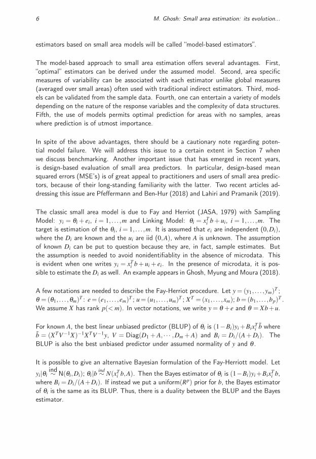
The model-based approach to small area estimation offers several advantages. First,“optimal” estimators can be derived under the assumed model. Second, area specificmeasures of variability can be associated with each estimator unlike global measures(averaged over small areas) often used with traditional indirect estimators. Third, mod-els can be validated from the sample data. Fourth, one can entertain a variety of modelsdepending on the nature of the response variables and the complexity of data structures.Fifth, the use of models permits optimal prediction for areas with no samples, areaswhere prediction is of utmost importance.
In spite of the above advantages, there should be a cautionary note regarding poten-tial model failure. We will address this issue to a certain extent in Section 7 whenwe discuss benchmarking. Another important issue that has emerged in recent years,is design-based evaluation of small area predictors. In particular, design-based meansquared errors (MSE’s) is of great appeal to practitioners and users of small area predic-tors, because of their long-standing familiarity with the latter. Two recent articles ad-dressing this issue are Pfeffermann and Ben-Hur (2018) and Lahiri and Pramanik (2019).
The classic small area model is due to Fay and Herriot (JASA, 1979) with SamplingModel: yi = θi + ei, i = 1, . . . ,m and Linking Model: θi = xT
i b+ ui, i = 1, . . . ,m. Thetarget is estimation of the θi, i = 1, . . . ,m. It is assumed that ei are independent (0,Di),where the Di are known and the ui are iid (0,A), where A is unknown. The assumptionof known Di can be put to question because they are, in fact, sample estimates. Butthe assumption is needed to avoid nonidentifiablity in the absence of microdata. Thisis evident when one writes yi = xT
i b+ ui + ei. In the presence of microdata, it is pos-sible to estimate the Di as well. An example appears in Ghosh, Myung and Moura (2018).
A few notations are needed to describe the Fay-Herriot procedure. Let y = (y1, . . . ,ym)T ;
θ =(θ1, . . . ,θm)T : e=(e1, . . . ,em)
T ; u=(u1, . . . ,um)T ; XT =(x1, . . . ,xm); b=(b1, . . . ,bp)
T .We assume X has rank p(< m). In vector notations, we write y = θ +e and θ = Xb+u.
For known A, the best linear unbiased predictor (BLUP) of θi is (1−Bi)yi+BixTi b where
b = (XTV−1X)−1XTV−1y, V = Diag(D1 +A, · · · ,Dm +A) and Bi = Di/(A+Di). TheBLUP is also the best unbiased predictor under assumed normality of y and θ .
It is possible to give an alternative Bayesian formulation of the Fay-Herriott model. Let
yi|θiind∼ N(θi,Di); θi|b ind∼ N(xT
i b,A). Then the Bayes estimator of θi is (1−Bi)yi+BixTi b,
where Bi = Di/(A+Di). If instead we put a uniform(Rp) prior for b, the Bayes estimatorof θi is the same as its BLUP. Thus, there is a duality between the BLUP and the Bayesestimator.
STATISTICS IN TRANSITION new series, Special Issue, August 2020 7
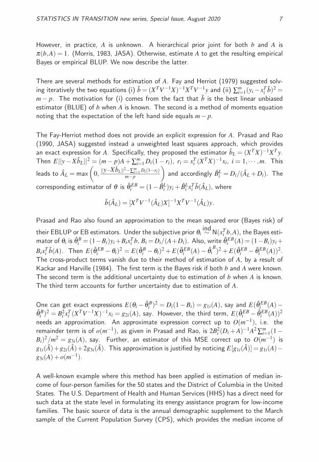
However, in practice, A is unknown. A hierarchical prior joint for both b and A isπ(b,A) = 1. (Morris, 1983, JASA). Otherwise, estimate A to get the resulting empiricalBayes or empirical BLUP. We now describe the latter.
There are several methods for estimation of A. Fay and Herriot (1979) suggested solv-ing iteratively the two equations (i) b = (XTV−1X)−1XTV−1y and (ii) ∑m
i=1(yi−xTi b)2 =
m− p. The motivation for (i) comes from the fact that b is the best linear unbiasedestimator (BLUE) of b when A is known. The second is a method of moments equationnoting that the expectation of the left hand side equals m− p.
The Fay-Herriot method does not provide an explicit expression for A. Prasad and Rao(1990, JASA) suggested instead a unweighted least squares approach, which providesan exact expression for A. Specifically, they proposed the estimator bL = (XT X)−1XT y.Then E||y−XbL||2 = (m− p)A+∑m
i=1 Di(1− ri), ri = xTi (X
T X)−1xi, i = 1, · · · ,m. This
leads to AL = max(
0, ||y−XbL||2−∑mi=1 Di(1−ri)
m−p
)and accordingly BL
i = Di/(AL +Di). The
corresponding estimator of θ is θ EBi = (1− BL
i )yi + BLi xT
i b(AL), where
b(AL) = [XTV−1(AL)X ]−1XTV−1(AL)y.
Prasad and Rao also found an approximation to the mean squared eror (Bayes risk) of
their EBLUP or EB estimators. Under the subjective prior θiind∼ N(xT
i b,A), the Bayes esti-mator of θi is θ B
i =(1−Bi)yi+BixTi b, Bi =Di/(A+Di). Also, write θ EB
i (A)= (1−Bi)yi+
BixTi b(A). Then E(θ EB
i − θi)2 = E(θ B
i − θi)2 +E(θ EB
i (A)− θiB)2 +E(θ EB
i − θ EBi (A))2.
The cross-product terms vanish due to their method of estimation of A, by a result ofKackar and Harville (1984). The first term is the Bayes risk if both b and A were known.The second term is the additional uncertainty due to estimation of b when A is known.The third term accounts for further uncertainty due to estimation of A.
One can get exact expressions E(θi− θ Bi )
2 = Di(1−Bi) = g1i(A), say and E(θ EBi (A)−
θ Bi )
2 = B2i xT
i (XTV−1X)−1xi = g2i(A), say. However, the third term, E(θ EB
i − θ EBi (A))2
needs an approximation. An approximate expression correct up to O(m−1), i.e. theremainder term is of o(m−1), as given in Prasad and Rao, is 2B2
i (Di +A)−1A2 ∑mi=1(1−
Bi)2/m2 = g3i(A), say. Further, an estimator of this MSE correct up to O(m−1) is
g1i(A)+g2i(A)+2g3i(A). This approximation is justified by noticing E[g1i(A)] = g1i(A)−g3i(A)+o(m−1).
A well-known example where this method has been applied is estimation of median in-come of four-person families for the 50 states and the District of Columbia in the UnitedStates. The U.S. Department of Health and Human Services (HHS) has a direct need forsuch data at the state level in formulating its energy assistance program for low-incomefamilies. The basic source of data is the annual demographic supplement to the Marchsample of the Current Population Survey (CPS), which provides the median income of

8 M. Ghosh: Small area estimation: its evolution...
four-person families for the preceding year. Direct use of CPS estimates is usually un-desirable because of large CV’s associated with them. More reliable results are obtainedthese days by using empirical and hierarchical Bayesian methods.
Here sample estimates of the state medians for the current year (c) as obtained from theCurrent Population Survey (CPS) were used as dependent variables. Adjusted censusmedian (c) defined as the base year (the recent most decennial census) census median(b) times the ratio of the BEA PCI (per capita income as provided by the Bureau ofEconomic Analysis of the United States Bureau of the Census) in year (c) to year (b) wasused as an independent variable. Following the suggestion of Fay (1987), Datta, Ghosh,Nangia and Natarajan (1996) used the census median from the recent most decennialcensus as a second independent variable. The resulting estimates were compared againsta different regression model employed earlier by the US Census Bureau.
The comparison was based on four criteria recommended by the panel on small areaestimates of population and income set up by the US committee on National Statistics.In the following, we use ei as a generic notation for the ith small area estimate, and ei.T R
the “truth”, i.e. the figure available from the recent most decennial census. The panelrecommended the following four criteria for comparison.Average Relative Absolute Bias = (51)−1 ∑51
i=1 |ei− ei,T R|/ei,T R.Average Squared Relative Bias = (51)−1 ∑51
i=1(ei− ei,T R)2/e2
i,T R.Average Absolute Bias = (51)−1 ∑51
i=1 |ei− ei,T R|.Average Squared Deviation = (51)−1 ∑51
i=1(ei− ei,T R)2.
Table 1 compares the Sample Median, the Bureau Estimate and the Empirical BLUPaccording to the four criteria as mentioned above.
Table 1. Average Relative Absolute Bias, Average Squared Relative Bias, AverageAbsolute Bias and Average Squared Deviation (in 100,000) of the Estimates.
Bureau Estimate Sample Median EBAver. rel. bias 0.325 0.498 0.204Aver. sq. rel bias 0.002 0.003 0.001Aver. abs. bias 722.8 1090.4 450.6Aver. sq. dev. 8.36 16.31 3.34
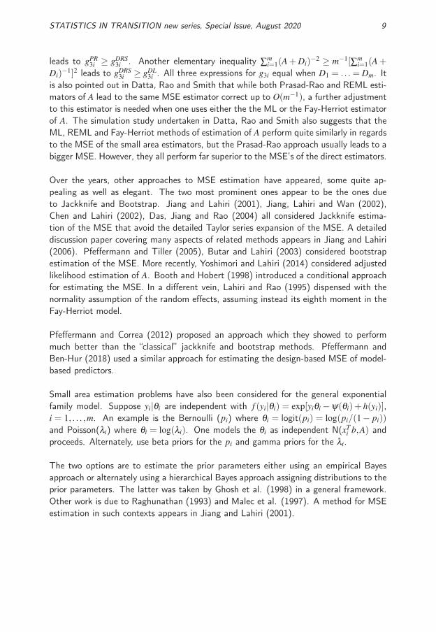
There are other options for estimation of A. One due to Datta and Lahiri (2000) usesthe MLE or the residual MLE (RMLE). With this estimator, gDL
3i is approximated by2D2
i (A+Di)−3[∑m
i=1(A+Di)−2]−1, while g1i and g2i remain unchanged. Finally, Datta,
Rao and Smith (2005), went back to the original Fay-Herriot method of estimation ofA, and obtained gDRS
3i = 2D2i (A+Di)
−3m[∑mi=1(A+Di)
−2]−1.
The string of inequalities
m−1m
∑i=1
(A+Di)2 ≥ [m−1
m
∑i=1
(A+Di)]2 ≥ m2[
m
∑i=1
(A+Di)−1]2
STATISTICS IN TRANSITION new series, Special Issue, August 2020 9
leads to gPR3i ≥ gDRS
3i . Another elementary inequality ∑mi=1(A+Di)
−2 ≥ m−1[∑mi=1(A+
Di)−1]2 leads to gDRS
3i ≥ gDL3i . All three expressions for g3i equal when D1 = . . .= Dm. It
is also pointed out in Datta, Rao and Smith that while both Prasad-Rao and REML esti-mators of A lead to the same MSE estimator correct up to O(m−1), a further adjustmentto this estimator is needed when one uses either the the ML or the Fay-Herriot estimatorof A. The simulation study undertaken in Datta, Rao and Smith also suggests that theML, REML and Fay-Herriot methods of estimation of A perform quite similarly in regardsto the MSE of the small area estimators, but the Prasad-Rao approach usually leads to abigger MSE. However, they all perform far superior to the MSE’s of the direct estimators.
Over the years, other approaches to MSE estimation have appeared, some quite ap-pealing as well as elegant. The two most prominent ones appear to be the ones dueto Jackknife and Bootstrap. Jiang and Lahiri (2001), Jiang, Lahiri and Wan (2002),Chen and Lahiri (2002), Das, Jiang and Rao (2004) all considered Jackknife estima-tion of the MSE that avoid the detailed Taylor series expansion of the MSE. A detaileddiscussion paper covering many aspects of related methods appears in Jiang and Lahiri(2006). Pfeffermann and Tiller (2005), Butar and Lahiri (2003) considered bootstrapestimation of the MSE. More recently, Yoshimori and Lahiri (2014) considered adjustedlikelihood estimation of A. Booth and Hobert (1998) introduced a conditional approachfor estimating the MSE. In a different vein, Lahiri and Rao (1995) dispensed with thenormality assumption of the random effects, assuming instead its eighth moment in theFay-Herriot model.
Pfeffermann and Correa (2012) proposed an approach which they showed to performmuch better than the “classical” jackknife and bootstrap methods. Pfeffermann andBen-Hur (2018) used a similar approach for estimating the design-based MSE of model-based predictors.
Small area estimation problems have also been considered for the general exponentialfamily model. Suppose yi|θi are independent with f (yi|θi) = exp[yiθi−ψ(θi)+ h(yi)],i = 1, . . . ,m. An example is the Bernoulli (pi) where θi = logit(pi) = log(pi/(1− pi))
and Poisson(λi) where θi = log(λi). One models the θi as independent N(xTi b,A) and
proceeds. Alternately, use beta priors for the pi and gamma priors for the λi.
The two options are to estimate the prior parameters either using an empirical Bayesapproach or alternately using a hierarchical Bayes approach assigning distributions to theprior parameters. The latter was taken by Ghosh et al. (1998) in a general framework.Other work is due to Raghunathan (1993) and Malec et al. (1997). A method for MSEestimation in such contexts appears in Jiang and Lahiri (2001).

10 M. Ghosh: Small area estimation: its evolution...
Jiang, Nguyen and Rao (2011) evaluated the performance of a BLUP or EBLUP using
only the sampling model yiind∼ (θi,Di). Recall Bi = Di/(A+Di). Then
E[{(1−Bi)yi +BixTi b−θi}2|θi] = (1−Bi)
2Di +B2i (θi− xT
i b)2.
Noting that E[(yi− xTi b)2|θi] = Di + (θi− xT
i b)2, an unbiased estimator of the aboveMSE is (1−Bi)
2Di−B2i Di +B2
i (yi−xTi b)2. When one minimizes the above with respect
to b and A, then the resulting estimators of of b and A are referred to as observedbest predictive estimators. The corresponding estimators of the θi are referred to as the“observed best predictors”. These authors suggested Fay-Herriot or Prasad-Rao methodfor estimation of b and A.
6. Model Based Small Area Estimation: Unit Specific Models
Unit Specific Models are those where observations are available for the sampled unitsin the local areas. In addition, unit-specific auxiliary information is available for thesesampled units, and possibly for the non-sampled units as well.
To be specific, consider m local areas where the ith local area has Ni units with a sampleof size ni. We denote the sampled observations by yi1, . . . ,yini , i = 1, . . . ,m. Consider themodel
yi j = xTi jb+ui + ei j, j = 1, . . . .Ni, i = 1, . . . ,m.
The ui’s and ei j’s are mutually independent with the ui iid (0,σ2u ), and the ei j independent
(0,σ2ψi j).
The above nested error regression model was considered by Battese, Harter and Fuller(BHF, 1988), where yi j is the area devoted to corn or soybean for the jth segment inthe ith county; xi j = (1,xi j1,xi j2)
T , where xi j1 denotes the no. of pixels classified ascorn for the jth segment in the ith county and xi j2 denotes the no. of pixels classifiedas soybean for the jth segment in the ith county; b = (b0,b1,b2)
T is the vector of re-gression coefficients. BHF took ψi j = 1. The primary goal of BHF was to estimate theYi = N−1
i ∑Nij=1 yi j, the population average of area under corn or soybean for the 12 areas
in North Central Iowa, Ni denoting the population size in area i.
A second example appears in Ghosh and Rao (1994). Here yi j denotes wages and salariespaid by the jth business firm in the ith census division in Canada and xi j = (1,xi j)
T ,where xi j is the gross business income of the jth business firm in the ith census division.In this application, ψi j = xi j was found more appropriate than the usual model involvinghomoscedasticity.
I consider in some detail the BHF model. Their ultimate goal was to estimate thepopulation means Yi = (Ni)
−1 ∑Nij=1 yi j, In matrix notation, we write yi = (yi1, . . . ,yini)
T ,
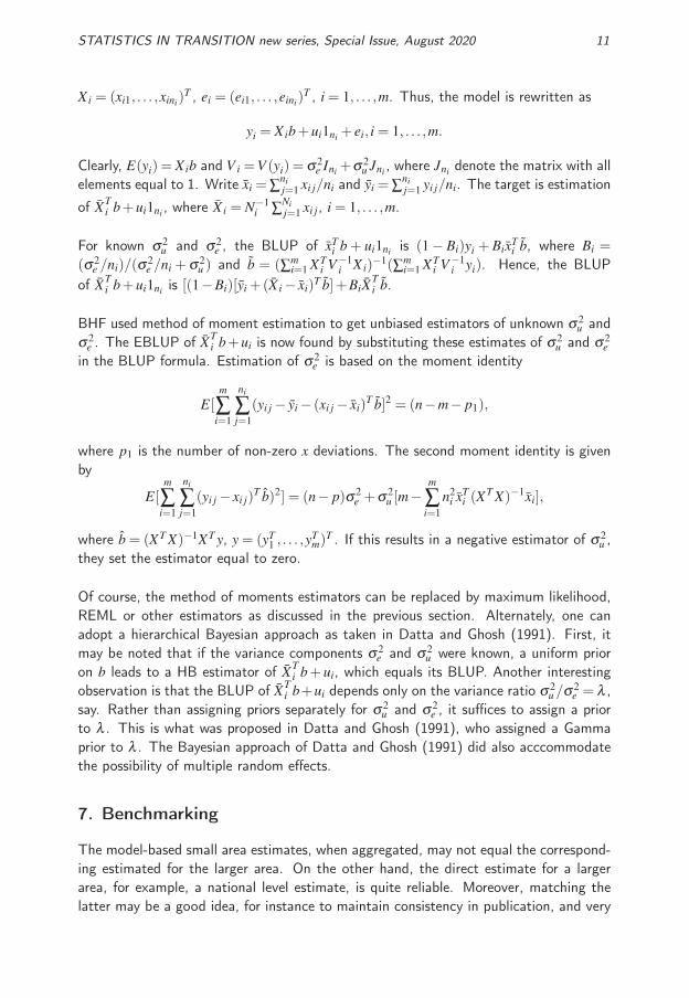
STATISTICS IN TRANSITION new series, Special Issue, August 2020 11
Xi = (xi1, . . . ,xini)T , ei = (ei1, . . . ,eini)
T , i = 1, . . . ,m. Thus, the model is rewritten as
yi = Xib+ui1ni + ei, i = 1, . . . ,m.
Clearly, E(yi) = Xib and V i =V (yi) = σ2e Ini +σ2
u Jni , where Jni denote the matrix with allelements equal to 1. Write xi = ∑ni
j=1 xi j/ni and yi = ∑nij=1 yi j/ni. The target is estimation
of XTi b+ui1ni , where X i = N−1
i ∑Nij=1 xi j, i = 1, . . . ,m.
For known σ2u and σ2
e , the BLUP of xTi b + ui1ni is (1− Bi)yi + BixT
i b, where Bi =
(σ2e /ni)/(σ2
e /ni + σ2u ) and b = (∑m
i=1 XTi V−1
i X i)−1(∑m
i=1 XTi V−1
i yi). Hence, the BLUPof XT
i b+ui1ni is [(1−Bi)[yi +(X i− xi)T b]+BiX
Ti b.
BHF used method of moment estimation to get unbiased estimators of unknown σ2u and
σ2e . The EBLUP of XT
i b+ui is now found by substituting these estimates of σ2u and σ2
ein the BLUP formula. Estimation of σ2
e is based on the moment identity
E[m
∑i=1
ni
∑j=1
(yi j− yi− (xi j− xi)T b]2 = (n−m− p1),
where p1 is the number of non-zero x deviations. The second moment identity is givenby
E[m
∑i=1
ni
∑j=1
(yi j− xi j)T b)2] = (n− p)σ2
e +σ2u [m−
m
∑i=1
n2i xT
i (XT X)−1xi],
where b = (XT X)−1XT y, y = (yT1 , . . . ,y
Tm)
T . If this results in a negative estimator of σ2u ,
they set the estimator equal to zero.
Of course, the method of moments estimators can be replaced by maximum likelihood,REML or other estimators as discussed in the previous section. Alternately, one canadopt a hierarchical Bayesian approach as taken in Datta and Ghosh (1991). First, itmay be noted that if the variance components σ2
e and σ2u were known, a uniform prior
on b leads to a HB estimator of XTi b+ ui, which equals its BLUP. Another interesting
observation is that the BLUP of XTi b+ui depends only on the variance ratio σ2
u /σ2e = λ ,
say. Rather than assigning priors separately for σ2u and σ2
e , it suffices to assign a priorto λ . This is what was proposed in Datta and Ghosh (1991), who assigned a Gammaprior to λ . The Bayesian approach of Datta and Ghosh (1991) did also acccommodatethe possibility of multiple random effects.
7. Benchmarking
The model-based small area estimates, when aggregated, may not equal the correspond-ing estimated for the larger area. On the other hand, the direct estimate for a largerarea, for example, a national level estimate, is quite reliable. Moreover, matching thelatter may be a good idea, for instance to maintain consistency in publication, and very
12 M. Ghosh: Small area estimation: its evolution...
often for protection against model failure. The latter may not always be achieved, forexample in time series models, as pointed out by Wang, Fuller and Qu (2008).
Specifically, suppose θi is the ith area mean and θT = ∑mi=1 wiθi is the overall mean,
where w j may be the known proportion of units in the jth area. The direct estimate forθT is ∑m
i=1 wiθi. Also, let θi denote an estimator of θi based on a certain model. Then∑m
i=1 wiθi is typically not equal to ∑mi=1 wiθi
In order to address this, people have suggested (i) ratio adjusted estimators
θ RAi = θ G
i (m
∑j=1
w jθ j)/(m
∑j=1
w jθ Gj )
and (ii) difference adjusted estimator θ DAi = θ G
i +∑mj=1 w jθ j−∑m
j=1 w jθ Gj , where θ G
j issome generic model-based estimator of θ j.
One criticism against such adjustments is that a common adjustment is used for all smallareas regardless of their precision. Wang, Fuller and Qu (2008) proposed instead mini-mizing ∑m
j=1 φ jE(e j−θ j)2 for some specified weights φ j(> 0) subject to the constraint
∑mj=1 w je j = θT . The resulting estimator of θi is
θWFQi = θ BLUP
i +λi(m
∑j=1
w jθ j−m
∑j=1
w jθ BLUPj ),
where λi = wiφ−1i /(∑m
j=1 w2jφ−1j ).
Datta, Ghosh, Steorts and Maples (2011) took instead a general Bayesian approach andminimized ∑m
j=1 φ j[E(e j − θ j)2|data] subject to ∑m
j=1 w je j = θT and obtained the esti-mator θ AB
i = θ Bi +λi(∑m
j=1 w jθ j−∑mj=1 w jθ B
j ), with the same λi. This development issimilar in spirit to those of Louis (1984) and Ghosh (1992) who proposed constrainedBayes and empirical Bayes estimators to prevent overshrinking. The approach of Datta,Ghosh, Steorts and Maples extends readily to multiple benchmarking constraints. In afrequentist context. Bell, Datta and Ghosh (2013) extended the work of Wang, Fullerand Qu (2008) to multiple benchmarking constraints.
There are situations also when one needs two-stage benchmarking. A current example isthe cash rent estimates of the Natural Agricultural Statistics Service (NASS), where oneneeds the dual control of matching the aggregate of county level cash rent estimates tothe corresponding agricultural district (comprising of several counties) level estimates,and the aggregate of the agricultural district level estimates to the final state level es-timate. Berg, Cecere and Ghosh (2014) adopted an approach of Ghosh and Steorts(2013) to address the NASS problem.
STATISTICS IN TRANSITION new series, Special Issue, August 2020 13
Second order unbiased MSE estimators are not typically available for ratio adjustedbenchmarked estimators. In contrast, second order unbiased MSE estimators are avail-able for difference adjusted benchmarked estimators, namely, θ DB
i = θ EBi +(∑m
j=1 w jθ j−∑m
j=1 w jθ EBj ). Steorts and Ghosh (2013) have shown that MSE(θ DB
i ) = MSE(θ EBi )+
g4(A) + o(m−1), where MSE(θ EBi ) is the same as the one given in Prasad and Rao
(1990), and
g4(A) =m
∑i=1
w2i B2
i (Di +A)−m
∑i=1
m
∑j=1
wiw jBiB jxTi (X
TV−1x j).
We may recall that Bi =Di/(A+Di), XT = (x1, . . . ,xm) and V =Diag(A+D1, . . . ,A+Dm)
in the Fay-Herriot model. A second order unbiased estimator of the benchmarked EBestimator is thus g1i(A)+g2i(A)+2g3i(A)+g4i(A).
There are two available approaches for self benchmarking that do not require any ad-justment to the EBLUP estimators. The first, proposed in You and Rao (2002) forthe Fay-Herriot model replaces the estimator b in the EBLUP by an estimator whichdepends both on b as well as the weights wi. This changes the MSE calculation. Re-call the Prasad-Rao MSE of the EBLUP given by MSE(θ EB
i ) = g1i + g2i + g3i, whereg1i =Di(1−Bi), g2i =B2
i xTi (X
TV−1X)−1xi and g3i = 2D2i (A+Di)
−3m−2{∑mj=1(A+D j)
2}.For the Benchmarked EBLUP, g2i changes.
The second approach is by Wang, Fuller and Qu (2008) and it uses an augmented modelwith new covariates (xi,wi,Di). This second approach was extended by Bell, Datta andGhosh (2013) to accommodate multiple benchmarking constraints.
8. Fixed versus Random Area Effects
A different but equally pertinent issue has recently surfaced in the small area literature.This concerns the need for random effects in all areas, or whether even fixed effectsmodels would be adequate for certain areas. Datta, Hall and Mandal (DHM, 2011) werethe first to address this problem. They suggested essentially a preliminary test-basedapproach, testing the null hypothesis that the common random effect variance was zero.Then they used a fixed or a random effects model for small area estimation based onacceptance or rejection of the null hypothesis. This amounted to use of synthetic orregression estimates of all small area means upon acceptance of the null hypothesis, andcomposite estimates which are weighted averages of direct and regression estimatorsotherwise. Further research in this area is due to Molina, Rao and Datta (2015).
The DHM procedure works well when the number of small areas is moderately large, butnot necessarily when the number of small areas is very large. In such situations, the nullhypothesis of no random effects is very likely to be rejected. This is primarily due to a

14 M. Ghosh: Small area estimation: its evolution...
few large residuals causing significant departure of direct estimates from the regressionestimates. To rectify this, Datta and Mandal (2015) proposed a Bayesian approach with“spike and slab” priors. Their approach amounts to taking δiui instead of ui for randomeffects where the δi and the ui are independent with δi iid Bernoulli(γ) and ui iid N(0,σ2
u ).
In contrast to the spike and slab priors of Datta and Mandal (2015), Tang, Ghosh, Haand Sedransk (2018) considered a different class of priors that meets the same objective.as the spike and slab priors, but uses instead absolutely continuous priors. These priorsallow different variance components for different small areas, in contrast to the priorsof Datta and Mandal, who considered prior variances to be either zero or else commonacross all small areas. This seems to be particularly useful when the number of smallareas is very large, for example, when one considers more than 3000 counties of the US,where one expects a wide variation in the county effects. The proposed class of priors, isusually referred to as “global-local shrinkage priors” (Carvalho, Polson and Scott (2010);Polson and Scott (2010)).
The global-local priors, essentially scale mixtures of normals, are intended to capturepotential “sparsity”, which means lack of significant contribution by many of the ran-dom effects, by assigning large probabilities to random effects close to zero, but alsoidentifying random effects which differ significantly from zero. This is achieved by em-ploying two levels of parameters to express prior variances of random effects. The first,the “local shrinkage parameters”, acts at individual levels, while the other, the “globalshrinkage parameter” is common for all random effects. This is in contrast to Fay andHerriot (1979) who considered only one global parameter. These priors also differ fromthose of Datta and Mandal (2015), where the variance of random effects is either zeroor common across all small areas.
Symbolically, the random effects ui have independent N(0,λ 2i A) priors. While the global
parameter A tries to cause an overall shrinking effect, the local shrinkage parameters λ 2i
are useful in controlling the degree of shrinkage at the local level. If the mixing den-sity corresponding to local shrinkage parameters is appropriately heavy-tailed, the largerandom effects are almost left unshrunk. The class of “global-local” shrinkage priorsincludes the three parameter beta normal (TPBN) priors (Armagon, Clyde and Dun-son, 2011) and Generalized Double Pareto priors (Armagon, Dunson and Lee, 2012).TPBN includes the now famous horseshoe (HS) priors (Scott and Berger, 2010) and thenormal-exponential-gamma priors (Griffin and Brown, 2005).
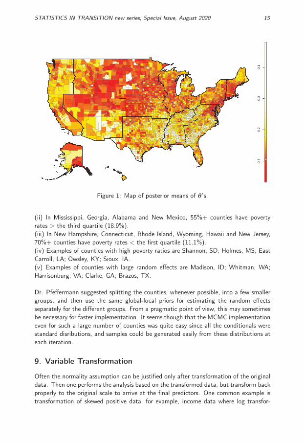
As an example, consider estimation of 5-year (2007–2011) county-level overall povertyratios in the US. There are 3,141 counties in the data set. The covariates are foodstampparticipation rates. The map given in Figure 1 gives the poverty ratios for all the coun-ties of US. Some salient findings from these calculations are given below.
(i) Estimated poverty ratios are between 3.3% (Borden County, TX) and 47.9% (Shan-non County, SD). The median is 14.7%.
STATISTICS IN TRANSITION new series, Special Issue, August 2020 15
0.1
0.2
0.3
0.4
Figure 1: Map of posterior means of θ ’s.
(ii) In Mississippi, Georgia, Alabama and New Mexico, 55%+ counties have povertyrates > the third quartile (18.9%).(iii) In New Hampshire, Connecticut, Rhode Island, Wyoming, Hawaii and New Jersey,70%+ counties have poverty rates < the first quartile (11.1%).(iv) Examples of counties with high poverty ratios are Shannon, SD; Holmes, MS; EastCarroll, LA; Owsley, KY; Sioux, IA.(v) Examples of counties with large random effects are Madison, ID; Whitman, WA;Harrisonburg, VA; Clarke, GA; Brazos, TX.
Dr. Pfeffermann suggested splitting the counties, whenever possible, into a few smallergroups, and then use the same global-local priors for estimating the random effectsseparately for the different groups. From a pragmatic point of view, this may sometimesbe necessary for faster implementation. It seems though that the MCMC implementationeven for such a large number of counties was quite easy since all the conditionals werestandard disributions, and samples could be generated easily from these distributions ateach iteration.
9. Variable Transformation
Often the normality assumption can be justified only after transformation of the originaldata. Then one performs the analysis based on the transformed data, but transform backproperly to the original scale to arrive at the final predictors. One common example istransformation of skewed positive data, for example, income data where log transfor-
16 M. Ghosh: Small area estimation: its evolution...
mation gets a closer normal approximation. Slud and Maiti (2006) and Ghosh andKubokawa (2015) took this approach, providing final results for the back-transformedoriginal data.
For example, consider a multiplicative model yi = φiηi with zi = log(yi), θi = log(φi)
and ei = log(ηi). Consider the Fay-Herriott (1979) model (i) zi|θiind∼ N(θi,Di) and (ii)
θiind∼ N(xT
i β ,A). θi has the N(θ Bi ,Di(1−Bi)) posterior with θ B
i = (1−Bi)zi +BixTi β ,
Bi = Di/(A+Di). Now E(φi|zi) = E[exp(θi)|zi] = exp[θ Bi +(1/2)Di(1−Bi)].
Another interesting example is the variance stabilizing transformation. For example,
suppose yiind∼ Bin(ni, pi). The arcsine transformation is given by pi = sin−1(2pi− 1).
The back transformation is pi = (1/2)[1+ sin(θi)].
A third example is the Poisson model for count data. There yiind∼ Poisson(λi). Then one
models zi = y1/2i as independent N(θi,1/4) where where θi = λ 1/2
i . An added advantagein the last two examples is that the assumption of known sampling variance, which isreally untrue, can be avoided.
10. Final Remarks
As acknowledged earlier, the present article leaves out a large number of useful currentday topics in small area estimation. I list below a few such topics which are not coveredat all here. But there are are many more. People interested in one or more of the topicslisted below and beyond should consult the book of Rao and Molina (2015) for theirdetailed coverage of small area estimation and an excellent set of references for thesetopics.
• Design consistency of small area estimators.
• Time series models.
• Spatial and space-time models.
• Variable Selection.
• Measurement errors in the covariates.
• Poverty counts for small areas.
• Empirical Bayes confidence intervals.
• Robust small area estimation.
• Misspecification of linking models.
STATISTICS IN TRANSITION new series, Special Issue, August 2020 17
• Informative sampling.
• Constrained small area estimation.
• Record Linkage.
• Disease Mapping.
• Etc, Etc., Etc.
Acknowledgements
I am indebted to Danny Pfeffermann for his line by line reading of the manuscript andmaking many helpful suggestions, which improved an earlier version of the paper. ParthaLahiri read the original and the revised versions of this paper very carefully, and caughtmany typos. A comment by J.N.K. Rao was helpful. The present article is based onthe Morris Hansen Lecture delivered by Malay Ghosh before the Washington StatisticalSociety on October 30, 2019. The author gratefully acknowledges the Hansen LectureCommittee for their selection.
REFERENCES
ARMAGAN, A., CLYDE, M., and DUNSON, D. B., (2013). Generalized double paretoshrinkage. Statistica Sinica, 23, pp. 119–143.
ARMAGAN, A., DUNSON, D. B., LEE, J., and BAJWA, W. U., (2013). Posterior con-sistency in linear models under shrinkage priors. Biometrika, 100, pp. 1011–1018.
BATTESE, G. E., HARTER, R. M., and FULLER, W. A., (1988). An error componentsmodel for prediction of county crop area using survey and satellite data. Journalof the American Statistical Association, 83, pp. 28–36.
BELL, W. R., DATTA, G, S., and GHOSH, M., (2013). Benchmarking small area esti-mators. Biometrika, 100, pp. 189–202.
BELL, W. R., BASEL, W. W., and MAPLES, J. J., (2016). An overview of U.S. Cen-sus Bureau’s Small Area Income and Poverty Estimation Program. In Analysis ofPoverty Data by Small Area Estimation. Ed. M. Pratesi. Wiley, UK, pp. 349–378.
BERG, E., CECERE, W., and GHOSH, M., (2014). Small area estimation of countylevel farmland cash rental rates. Journal of Survey Statistics and Methodology,2, pp. 1–37. Bivariate hierarchical Bayesian model for estimating cropland cashrental rates at the county level. Survey Methodology, in press.
18 M. Ghosh: Small area estimation: its evolution...
BOOTH, J. G., HOBERT, J., (1998). Standard errors of prediction in generalized linearmixed models. Journal of the American Statistical Association, 93, pp. 262–272.
BUTAR, F. B., LAHIRI, P., (2003). On measures of uncertainty of empirical Bayessmall area estimators. Journal of Statistical Planning and Inference, 112, pp.63–76.
CARVALHO, C. M., POLSON, N. G., SCOTT, J. G., (2010). The horseshoe estimatorfor sparse signals. Biometrika, 97, pp. 465–480.
CHEN, S., LAHIRI, P., (2003).A comparison of different MPSE estimators of EBLUPfor the Fay-Herriott model. In Proceedings of the Section on Survey ResearchMethods. Washington, D.C. American Statistical Association, pp. 903–911.
DAS, K., JIANG, J., RAO, J. N. K., ((2004). Mean squared error of empirical predictor.Annals of Statistics, 32, pp. 818–840.
DATTA, G. S., GHOSH, M., (1991). Bayesian prediction in linear models: applicationsto small area estimation. The Annals of Statistics, 19, pp. 1748–1770.
DATTA, G., GHOSH, M., NANGIA, N., and NATARAJAN, K., (1996). Estimation ofmedian income of four-person families: a Bayesian approach. In Bayesian Statis-tics and Econometrics: Essays in Honor of Arnold Zellner. Eds. D. Berry, K.Chaloner and J. Geweke. North Holland, pp. 129–140.
DATTA, G. S., LAHIRI. P., (2000). A unified measure of uncertainty of estimated bestlinear unbiased predictors in small area estimation problems. Statistica Sinica, 10,pp. 613–627.
DATTA, G. S., RAO, J. N. K., and SMITH, D. D., (2005). On measuring the variabil-ity of small area estimators under a basic area level model. Biometrika, 92, pp.183–196.
DATTA, G. S., GHOSH, M., STEORTS, R., and MAPLES, J. J., (2011). Bayesianbenchmarking with applications to small area estimation. TEST, 20, pp. 574–588.
DATTA, G. S., HALL, P., and MANDAL, A., (2011). Model selection and testing forthe presence of small area effects and application to area level data. Journal ofthe American Statistical Association, 106, pp. 362–374.
DATTA, G. S., MANDAL, A., (2015). Small area estimation with uncertain randomeffects. Journal of the American Statistical Association, 110, pp. 1735–1744.
STATISTICS IN TRANSITION new series, Special Issue, August 2020 19
ELBERS, C., LANJOUW, J. O., and LANJOUW, P., (2003). Micro-level estimation ofpoverty and inequality. Econometrica, 71. pp. 355–364.
ERCIULESCU, A. L., FRANCO, C., and LAHIRI, P., (2020). Use of administrativerecords in small area estimation. To appear in Administrative Records for SurveyMethodology. Eds. P. Chun and M. Larson. Wiley, New York.
FAY, R. E., (1987). Application of multivariate regression to small domain estimation.In Small Area Statistics. Eds. R. Platek, J.N.K. Rao, C-E Sarndal and M.P. Singh.Wiley New York, pp. 91–102.
FAY, R. E., HERRIOT, R. A., (1979). Estimates of income for small places: an applica-tion of James-Stein procedure to census data. Journal of the American StatisticalAssociation, 74, pp. 269–277.
GHOSH, M., (1992). Constrained Bayes estimation with applications. Journal of theAmerican Statistical Association, 87, pp. 533–540.
GHOSH, M., RAO, J. N. K., (1994). Small area estimation: an appraisal. StatisticalScience, pp. 55–93.
GHOSH, M., NATARAJAN, K., STROUD, T. M. F., and CARLIN, B. P., (1998).Generalized linear models for small area estimation. Journal of the AmericanStatistical Association, 93, pp. 273–282.
GHOSH, M., STEORTS, R., (2013). Two-stage Bayesian benchmarking as applied tosmall area estimation. TEST, 22, pp. 670–687.
GHOSH, M., KUBOKAWA, T., and KAWAKUBO, Y., (2015). Benchmarked empiricalBayes methods in multiplicative area-level models with risk evaluation. Biomerika,102, pp. 647–659.
GHOSH, M., MYUNG, J., and MOURA, F. A. S., (2018). Robust Bayesian small areaestimation. Survey Methodology, 44, pp. 101–115.
GONZALEZ, M. E., HOZA, C., (1978). Small area estimation with application tounemployment and housing estimates. Journal of the American Statistical Asso-ciation, 73, pp. 7–15.
GRIFFIN, J. E., BROWN, P. J., (2010). Inference with normal-gamma prior distribu-tions in regression problems. Bayesian Analysis, 5, pp. 171–188.
HANSEN, M. H., HURWITZ, W. N., and MADOW, W. G., (1953). Sample SurveyMethods and Theory. Wiley, New York.
20 M. Ghosh: Small area estimation: its evolution...
HOLT, D., SMITH, T. M. F., and TOMBERLIN, T. J., (1979). A model-based ap-proach for small subgroups of a population. Journal of the American StatisticalAssociation, 74, pp. 405–410.
JIANG, J., LAHIRI, P., (2001). Empirical best prediction of small area inference withbinary data. Annals of the Institute of Statistical Mathematics, 53, pp. 217–243.
JIANG, J., LAHIRI, P., and WAN, S-M., (2002). A unified jackknife theory. TheAnnals of Statistics, 30, pp. 1782–1810.
JIANG, J., LAHIRI, P., (2006). Mixed model prediction and small area estimation (withdiscussion). TEST, 15, pp. 1–96.
JIANG, J., NGUYEN, T., and RAO, J. S., (2011). Best predictive small area estimation.Journal of the American Statistical Association, 106, pp. 732–745.
KACKAR, R. N., HARVILLE, D. A., (1984). Approximations for standard errors ofestimators of fixed and random effects in mixed linear models. Journal of theAmerican Statistical Association, 79, pp. 853–862.
LAHIRI, P., RAO, J. N. K., (1995). Robust estimation of mean squared error of smallarea estimators. Journal of the American Statistical Association, 90, pp. 758–766.
LAHIRI, P., PRAMANIK, S., (2019). Evaluation of synthetic small area estimatorsusing design-based methods. Austrian Journal of Statistics, 48, pp. 43–57.
LOUIS, T. A., (1984). Estimating a population of parameter values using Bayes andempirical Bayes methods. Journal of the American Statistical Association, 79,pp. 393–398.
MALEC, D., DAVIS, W. W., and CAO, X., (1999). Model-based small area estimates ofoverweight prevalence using sample selection adjustment. Statistics and Medicine,18, pp. 3189–3200.
MOLINA, I., RAO, J. N. K., (2010). Small area estimation of poverty indicators.Canadian Journal of Statistics, 38, pp. 369–385.
MOLINA, I., RAO, J. N. K., and DATTA, G. S., (2015). Small area estimation undera Fay-Herriot model with preliminary testing for the presence of random effects.Survey Methodology.
PFEFFERMANN, D., TILLER, R. B., (2005). Bootstrap approximation of predictionMSE for state-space models with estimated parameters. Journal of Time SeriesAnalysis, 26, pp. 893–916.
STATISTICS IN TRANSITION new series, Special Issue, August 2020 21
MORRIS, C. N., (1983). Parametric empirical Bayes inference: theory and applications.Journal of the American Statistical Association, 78, pp. 47–55.
POLSON, N. G., SCOTT, J. G., (2010). Shrink globally, act locally: Sparse Bayesianregularization and prediction. Bayesian Statistics, 9, pp. 501–538.
PFEFFERMANN, D., (2002). Small area estimation: new developments and direction.International Statistical Review, 70, pp. 125–143.
PFEFFERMANN, D., (2013). New important developments in small area estimation.Statistical Science, 28, pp. 40–68.
PRASAD, N. G. N., RAO, J. N. K., (1990). The estimation of mean squared error ofsmall area estimators. Journal of the American Statistical Association, 85, pp.163–171.
RAGHUNATHAN, T. E., (1993). A quasi-empirical Bayes method for small area esti-mation. Journal of the American Statistical Association, 88, pp. 1444–1448.
RAO, J. N. K., (2003). Some new developments in small area estimation. Journal ofthe Iranian Statistical Society, 2, pp. 145–169.
RAO, J. N. K., (2006). Inferential issues in small area estimation: some new develop-ments. Statistics in Transition, 7, pp. 523–526.
RAO, J. N. K., Molina, I., (2015). Small Area Estimation, 2nd Edition. Wiley, NewJersey.
SCOTT, J. G., BERGER, J. O., (2010). Bayes and empirical-Bayes multiplicity ad-justment in the variable-selection problem. The Annals of Statistics, 38, pp.2587–2619.
SLUD, E. V., MAITI, T., (2006). Mean squared error estimation in transformed Fay-Herriot models. Journal of the Royal Statistical Society, B, 68, pp. 239–257.
TANG, X., GHOSH, M., Ha, N-S., and SEDRANSK, J., (2018). Modeling randomeffects using global-local shrinkage priors in small area estimation. Journal of theAmerican Statistical Association, 113, pp. 1476–1489.
WANG, J., FULLER, W. A., and QU, Y., (2008). Small area estimation under restric-tion. Survey Methodology, 34, pp. 29–36.

22 M. Ghosh: Small area estimation: its evolution...
YOSHIMORI, M., LAHIRI, P., (2014). A new adjusted maximum likelihood methodfor the Fay-Herriott small area model. Journal of Multivariate Analysis, 124, pp.281–294.
YOU, Y., RAO, J. N. K., and HIDIROGLOU, M. A., (2013). On the performance ofself-benchmarked small area estimators under the Fay-Herriott area level model.Survey Methodology, 39, pp. 217–229.